Variants of Deterministic and Stochastic Nonlinear ...

HAL Id: tel-01127048https://tel.archives-ouvertes.fr/tel-01127048

Submitted on 6 Mar 2015

HAL is a multi-disciplinary open accessarchive for the deposit and dissemination of sci-entific research documents, whether they are pub-lished or not. The documents may come fromteaching and research institutions in France orabroad, or from public or private research centers.

L’archive ouverte pluridisciplinaire HAL, estdestinée au dépôt et à la diffusion de documentsscientifiques de niveau recherche, publiés ou non,émanant des établissements d’enseignement et derecherche français ou étrangers, des laboratoirespublics ou privés.

Variants of Deterministic and Stochastic NonlinearOptimization Problems

Chen Wang

To cite this version:Chen Wang. Variants of Deterministic and Stochastic Nonlinear Optimization Problems. Data Struc-tures and Algorithms [cs.DS]. Université Paris Sud - Paris XI, 2014. English. NNT : 2014PA112294.tel-01127048

https://tel.archives-ouvertes.fr/tel-01127048

https://hal.archives-ouvertes.fr

UNIVERSITÉ PARIS-SUD

ECOLE DOCTORALE N:427INFORMATIQUE DE PARIS-SUD

Laboratoire: Laboratoire de Recherche en Informatique

Thèse de doctorat

par

Chen WANG

Variants of Deterministic and StochasticNonlinear Optimization Problems

Date de soutenance: 31/10/2014

Composition du jury:

Directeur de thèse : M. Abdel Lisser

Rapporteurs : Mme. Janny Leung

M. Alexandre Caminada

Examinateurs : M. Sylvain Conchon

M. Pablo Adasme

2

Acknowledgments

Foremost, I would like to thank my supervisor, Prof. Abdel Lisser for providing me

with the opportunity to complete my PhD thesis at the Paris Sud University. I am

very grateful for his patient guidance to my research and warm help in my daily life.

Special thanks to Prof. Janny Leung and Prof. Alexandre Caminada for agreeing

to review my thesis and their invaluable comments and suggestions. Thanks also to

Prof. Sylvain Conchon and Dr. Pablo Adasme for being part of my defense jury and

their precious suggestions.

I appreciate Dr. Pablo Adasme and Chuan Xu for our fruitful collaboration. I

would like to thank all colleagues in research group for their hospitality and help. I

also wish to express my appreciation to my friends Jianqiang Cheng, Weihua Yang,

Yandong Bai, Weihua He et al. for sharing the good time in the lab and this beautiful

city.

Finally, I am really grateful to my parents for their infinite love, encouragement

and support over the past three years in the foreign country.

3

4

Abstract

Combinatorial optimization problems are generally NP-hard problems, so they

can only rely on heuristic or approximation algorithms to find a local optimum or a

feasible solution. During the last decades, more general solving techniques have been

proposed, namely metaheuristics which can be applied to many types of combinato-

rial optimization problems. This PhD thesis proposed to solve the deterministic and

stochastic optimization problems with metaheuristics. We studied especially Vari-

able Neighborhood Search (VNS) and choose this algorithm to solve our optimization

problems since it is able to find satisfying approximated optimal solutions within a

reasonable computation time. Our thesis starts with a relatively simple determin-

istic combinatorial optimization problem: Bandwidth Minimization Problem. The

proposed VNS procedure offers an advantage in terms of CPU time compared to

the literature. Then, we focus on resource allocation problems in OFDMA systems,

and present two models. The first model aims at maximizing the total bandwidth

channel capacity of an uplink OFDMA-TDMA network subject to user power and

subcarrier assignment constraints while simultaneously scheduling users in time. For

this problem, VNS gives tight bounds. The second model is stochastic resource al-

location model for uplink wireless multi-cell OFDMA Networks. After transforming

the original model into a deterministic one, the proposed VNS is applied on the de-

terministic model, and find near optimal solutions. Subsequently, several problems

either in OFDMA systems or in many other topics in resource allocation can be mod-

eled as hierarchy problems, e.g., bi-level optimization problems. Thus, we also study

stochastic bi-level optimization problems, and use robust optimization framework to

deal with uncertainty. The distributionally robust approach can obtain slight conser-

vative solutions when the number of binary variables in the upper level is larger than

the number of variables in the lower level. Our numerical results for all the problems

studied in this thesis show the performance of our approaches.

Keyword: Variable Neighborhood Search, Bandwidth minimization problem,

Resource allocation problem of OFDMA network, Bi-level programming.

5

6

RésuméLes problèmes d’optimisation combinatoire sont généralement réputés NP-difficiles,

donc il n’y a pas d’algorithmes efficaces pour les résoudre. Afin de trouver des solu-

tions optimales locales ou réalisables, on utilise souvent des heuristiques ou des algo-

rithmes approchés. Les dernières décennies ont vu naitre des méthodes approchées

connues sous le nom de métaheuristiques, et qui permettent de trouver une solution

approchées. Cette thèse propose de résoudre des problèmes d’optimisation détermin-

iste et stochastique à l’aide de métaheuristiques. Nous avons particulièrement étudié

la méthode de voisinage variable connue sous le nom de VNS. Nous avons choisi cet al-

gorithme pour résoudre nos problèmes d’optimisation dans la mesure où VNS permet

de trouver des solutions de bonne qualité dans un temps CPU raisonnable. Le premier

problème que nous avons étudié dans le cadre de cette thèse est le problème déter-

ministe de largeur de bande de matrices creuses. Il s’agit d’un problème combinatoire

difficile, notre VNS a permis de trouver des solutions comparables à celles de la littéra-

ture en termes de qualité des résultats mais avec temps de calcul plus compétitif. Nous

nous sommes intéressés dans un deuxième temps aux problèmes de réseaux mobiles

appelés OFDMA-TDMA. Nous avons étudié le problème d’affectation de ressources

dans ce type de réseaux, nous avons proposé deux mod¨¨les : Le premier modèle est

un modèle déterministe qui permet de maximiser la bande passante du canal pour un

réseau OFDMA à débit monodirectionnel appelé Uplink sous contraintes d’énergie

utilisée par les utilisateurs et des contraintes d’affectation de porteuses. Pour ce

problème, VNS donne de très bons résultats et des bornes de bonne qualité. Le

deuxième modèle est un problème stochastique de réseaux OFDMA d’affectation de

ressources multi-cellules. Pour résoudre ce problème, on utilise le problème déter-

ministe équivalent auquel on applique la méthode VNS qui dans ce cas permet de

trouver des solutions avec un saut de dualité très faible. Les problèmes d’allocation

de ressources aussi bien dans les réseaux OFDMA ou dans d’autres domaines peuvent

aussi être modélisés sous forme de problèmes d’optimisation bi-niveaux appelés aussi

problèmes d’optimisation hiérarchique. Le dernier problème étudié dans le cadre de

cette thèse porte sur les problèmes bi-niveaux stochastiques. Pour résoudre le prob-

7

lème lié à l’incertitude dans ce problème, nous avons utilisé l’optimisation robuste

plus précisément l’approche appelée "distributionnellement robuste". Cette approche

donne de très bons résultats légèrement conservateurs notamment lorsque le nombre

de variables du leader est très supérieur à celui du suiveur. Nos expérimentations ont

confirmé l’efficacité de nos méthodes pour l’ensemble des problèmes étudiés.

Mots clés: Recherche à Voisinage Variable, problème de minimisation de la

largeur de bande de matrices, problème d’allocation de ressource dans les réseaux

OFDMA, problèmes bi-niveaux.

8

Contents

1 Introduction 17

2 Metaheuristics 25

2.1 Single solution based metaheuristics . . . . . . . . . . . . . . . . . . . 27

2.1.1 Simulated Annealing . . . . . . . . . . . . . . . . . . . . . . . 28

2.1.2 Tabu Search . . . . . . . . . . . . . . . . . . . . . . . . . . . . 33

2.1.3 Greedy Randomized Adaptive Search Procedure . . . . . . . . 41

2.1.4 Variable Neighborhood Search . . . . . . . . . . . . . . . . . . 44

2.2 Population based metaheuristics . . . . . . . . . . . . . . . . . . . . . 51

2.2.1 Genetic Algorithm . . . . . . . . . . . . . . . . . . . . . . . . 51

2.2.2 Scatter Search . . . . . . . . . . . . . . . . . . . . . . . . . . . 60

2.3 Improvement of metaheuristics . . . . . . . . . . . . . . . . . . . . . . 65

2.3.1 Algorithm Parameters . . . . . . . . . . . . . . . . . . . . . . 65

2.3.2 General Strategy . . . . . . . . . . . . . . . . . . . . . . . . . 67

2.4 Evaluation of metaheuristics . . . . . . . . . . . . . . . . . . . . . . . 68

2.5 Conclusions . . . . . . . . . . . . . . . . . . . . . . . . . . . . . . . . 69

3 Bandwidth Minimization Problem 71

3.1 Formulations . . . . . . . . . . . . . . . . . . . . . . . . . . . . . . . 72

3.1.1 Matrix bandwidth minimization problem . . . . . . . . . . . . 72

3.1.2 Graph bandwidth minimization problem . . . . . . . . . . . . 73

3.1.3 Equivalence between graph and matrix versions . . . . . . . . 73

3.2 Solution methods . . . . . . . . . . . . . . . . . . . . . . . . . . . . . 76

9

3.2.1 Exact algorithms . . . . . . . . . . . . . . . . . . . . . . . . . 76

3.2.2 Heuristic algorithms . . . . . . . . . . . . . . . . . . . . . . . 76

3.2.3 Metaheuristics . . . . . . . . . . . . . . . . . . . . . . . . . . . 77

3.3 The VNS approach for bandwidth minimization problem . . . . . . . 92

3.3.1 Initial solution . . . . . . . . . . . . . . . . . . . . . . . . . . 92

3.3.2 Shaking . . . . . . . . . . . . . . . . . . . . . . . . . . . . . . 93

3.3.3 Local search . . . . . . . . . . . . . . . . . . . . . . . . . . . . 94

3.3.4 Move or not . . . . . . . . . . . . . . . . . . . . . . . . . . . . 95

3.4 Numerical results . . . . . . . . . . . . . . . . . . . . . . . . . . . . . 96

3.5 Conclusions . . . . . . . . . . . . . . . . . . . . . . . . . . . . . . . . 98

4 Wireless Network 101

4.1 Orthogonal Frequency Division Multiplexing (OFDM) . . . . . . . . . 103

4.1.1 Development and application . . . . . . . . . . . . . . . . . . 103

4.1.2 OFDM characteristics . . . . . . . . . . . . . . . . . . . . . . 104

4.2 Orthogonal Frequency Division Multiplexing Access (OFDMA) . . . . 105

4.2.1 Background of OFDMA . . . . . . . . . . . . . . . . . . . . . 107

4.2.2 OFDMA resource allocation method . . . . . . . . . . . . . . 110

4.2.3 Research status of algorithms . . . . . . . . . . . . . . . . . . 120

4.3 Scheduling in wireless OFDMA-TDMA networks using variable neigh-

borhood search metaheuristic . . . . . . . . . . . . . . . . . . . . . . 123

4.3.1 Introduction . . . . . . . . . . . . . . . . . . . . . . . . . . . . 124

4.3.2 Problem formulation . . . . . . . . . . . . . . . . . . . . . . . 127

4.3.3 The VNS approach . . . . . . . . . . . . . . . . . . . . . . . . 128

4.3.4 Numerical results . . . . . . . . . . . . . . . . . . . . . . . . . 131

4.3.5 Conclusions . . . . . . . . . . . . . . . . . . . . . . . . . . . . 135

4.4 Stochastic resource allocation for uplink wireless multi-cell OFDMA

networks . . . . . . . . . . . . . . . . . . . . . . . . . . . . . . . . . . 136

4.4.1 Introduction . . . . . . . . . . . . . . . . . . . . . . . . . . . . 137

4.4.2 System description and problem formulation . . . . . . . . . . 140

10

4.4.3 Deterministic equivalent formulation . . . . . . . . . . . . . . 143

4.4.4 Variable neighborhood search procedure . . . . . . . . . . . . 145


4.4.6 Conclusions . . . . . . . . . . . . . . . . . . . . . . . . . . . . 152

4.5 Conclusions . . . . . . . . . . . . . . . . . . . . . . . . . . . . . . . . 154

5 Bi-level Programming Problem 155

5.1 Definition . . . . . . . . . . . . . . . . . . . . . . . . . . . . . . . . . 157

5.2 Formulation . . . . . . . . . . . . . . . . . . . . . . . . . . . . . . . . 158

5.3 Application . . . . . . . . . . . . . . . . . . . . . . . . . . . . . . . . 163

5.4 Characteristics . . . . . . . . . . . . . . . . . . . . . . . . . . . . . . 165

5.4.1 Complexity . . . . . . . . . . . . . . . . . . . . . . . . . . . . 165

5.4.2 Optimality condition . . . . . . . . . . . . . . . . . . . . . . . 165

5.5 Methods . . . . . . . . . . . . . . . . . . . . . . . . . . . . . . . . . . 167

5.5.1 Extreme-point approach . . . . . . . . . . . . . . . . . . . . . 167

5.5.2 Branch-and-bound algorithm . . . . . . . . . . . . . . . . . . . 168

5.5.3 Complementary pivoting approach . . . . . . . . . . . . . . . 169

5.5.4 Descent method . . . . . . . . . . . . . . . . . . . . . . . . . . 169

5.5.5 Penalty function method . . . . . . . . . . . . . . . . . . . . . 170

5.5.6 Metaheuristic method . . . . . . . . . . . . . . . . . . . . . . 171

5.5.7 Other methods . . . . . . . . . . . . . . . . . . . . . . . . . . 172

5.6 Distributionally robust formulation for stochastic quadratic bi-level

programming . . . . . . . . . . . . . . . . . . . . . . . . . . . . . . . 173

5.6.1 Introduction . . . . . . . . . . . . . . . . . . . . . . . . . . . . 174

5.6.2 Problem formulation . . . . . . . . . . . . . . . . . . . . . . . 176

5.6.3 The distributionally robust formulation . . . . . . . . . . . . . 178

5.6.4 Equivalent MILP formulation . . . . . . . . . . . . . . . . . . 181


5.6.6 Conclusions . . . . . . . . . . . . . . . . . . . . . . . . . . . . 190

5.7 Conclusions . . . . . . . . . . . . . . . . . . . . . . . . . . . . . . . . 191

11

6 Conclusions 193

12

List of Figures

3-1 Labeling f of graph G. . . . . . . . . . . . . . . . . . . . . . . . . . . 74

3-2 Labeling f ′ of graph G . . . . . . . . . . . . . . . . . . . . . . . . . . 75

3-3 v3 is the first label vertex . . . . . . . . . . . . . . . . . . . . . . . . 93

3-4 v2 is the first label vertex . . . . . . . . . . . . . . . . . . . . . . . . 93

4-1 Average bounds for instances 1-24 in Table 4.1 . . . . . . . . . . . . . 133

4-2 Average CPU times in seconds for instances in Table 4.1 . . . . . . . 134

4-3 System description . . . . . . . . . . . . . . . . . . . . . . . . . . . . 141

13

14

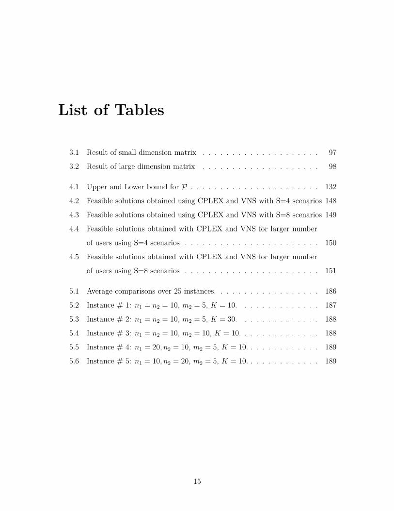
List of Tables

3.1 Result of small dimension matrix . . . . . . . . . . . . . . . . . . . . 97

3.2 Result of large dimension matrix . . . . . . . . . . . . . . . . . . . . 98

4.1 Upper and Lower bound for P . . . . . . . . . . . . . . . . . . . . . . 132

4.2 Feasible solutions obtained using CPLEX and VNS with S=4 scenarios 148

4.3 Feasible solutions obtained using CPLEX and VNS with S=8 scenarios 149

4.4 Feasible solutions obtained with CPLEX and VNS for larger number

of users using S=4 scenarios . . . . . . . . . . . . . . . . . . . . . . . 150

4.5 Feasible solutions obtained with CPLEX and VNS for larger number

of users using S=8 scenarios . . . . . . . . . . . . . . . . . . . . . . . 151

5.1 Average comparisons over 25 instances. . . . . . . . . . . . . . . . . . 186

5.2 Instance # 1: n1 = n2 = 10, m2 = 5, K = 10. . . . . . . . . . . . . . 187

5.3 Instance # 2: n1 = n2 = 10, m2 = 5, K = 30. . . . . . . . . . . . . . 188

5.4 Instance # 3: n1 = n2 = 10, m2 = 10, K = 10. . . . . . . . . . . . . . 188

5.5 Instance # 4: n1 = 20, n2 = 10, m2 = 5, K = 10. . . . . . . . . . . . . 189

5.6 Instance # 5: n1 = 10, n2 = 20, m2 = 5, K = 10. . . . . . . . . . . . . 189

15

16

Chapter 1

Introduction

Combinatorial optimization problem consists in, under given optimum conditions,

finding the optimal scheme among all the possible solutions. The general mathemat-

ical model can be described as:

min f(x)

s.t. g(x) ≤ 0

x ∈ D (1.1)

where x is the decision variable, f(x) is the objective function, g(x) is the constraint,

and D denotes the set consisting of a finite number of points.

A combinatorial optimization problem can be represented by three parameters

(D,F, f). D is the definition domain of decision variables. F represents the feasible

region: F = x|x ∈ D, g(x) ≤ 0, and the element in F is called a feasible solution for

the combinatorial optimization problem. f is the objective function, and the feasible

solution x∗ which meets f(x∗) = minf(x)|x ∈ F is called the optimal solution for

the problem.

The feature of combinatorial optimization consists in the feasible solution set is a

finite set. Therefore, as long as the finite points are determined one by one to check

whether they meet the constraints and compare with the objective function value, the

17

optimal solution of the problem must exist and can be obtained. Because in the real

life, most optimization problems consist in selecting the best integer solution among a

finite number of solutions, then many practical optimization problems are combinato-

rial optimization problems. The typical combinatorial optimization problem includes:

traveling salesman problem (TSP), scheduling problem (such as flow-shop, job-shop),

knapsack problem, bin packing problem, graph coloring problem, clustering problem

etc.

The definition of combinatorial optimization problem shows that every combina-

torial optimization problem can obtain the optimal solution by enumeration method.

The enumeration method takes time to find the optimal solution, some running time

can be accepted, but some can not. Thus, the analysis of the enumeration algorithm

needs to consider the space and time complexity of the problem.

The complexity of an algorithm or a problem is generally expressed as a func-

tion of the problem size n. The time complexity is denoted as T (n), and the space

complexity is denoted as S(n). In the analysis and design of algorithms, the key op-

erations of solving problem such as addition, subtraction, multiplication, comparison

are defined as basic operations. Thus, the number of the basic operation performed

in an algorithm is defined as the time complexity of algorithms, and the storage unit

which algorithm takes during the execution is the space complexity of the algorithm.

If the time complexity of an algorithm A is TA(n) = O(p(n)), and p(n) is the poly-

nomial function of n, thus the algorithm A is a polynomial algorithm. However, for

many problems, there is no polynomial function to solve them. These problems may

require exponential time to find the solution. When the problem size is large, the

required time of such problem is often unaccepted.

Because some combinatorial optimization problems have not been solved in poly-

nomial time to find the optimal solution, but these problems have the strong real

application background, thus researchers try to use some algorithms which may not

be able to get the optimal solution, refereed to as metaheuristics, to solve the combi-

natorial optimization problems.

Metaheuristic is proposed comparing with exact algorithms. The polynomial algo-

18

rithm of a problem is to find the optimal solution. Metaheuristic is a technique which

can find a sufficiently good solution even the optimal solution for optimization prob-

lems with less computational assumptions. Because in some cases, the running time

of optimal algorithms is not acceptable, or the difficulty of the problem makes the

running time increase exponentially with the size of the problem, then the problem

can only be solved by using metaheuristics to obtain a feasible solution.

The definition of metaheuristics shows that it is simple and fast. Although it can

not ensure to obtain the optimal solution, it can find a better acceptable feasible

solution in a reasonable computational time. Therefore, metaheuristics have been

developing rapidly and are widely used. The classic metaheuristic algorithms include:

simulated annealing (SA), tabu search (TS), genetic algorithm (GA), scatter search

(SS)...

Variable neighborhood search algorithm is a recent metaheuristic which includes

the dynamic neighborhood structure. This algorithm is more general and the freedom

is large which can be designed in various forms for particular problems.

The basic idea of VNS consists in systematically changing the neighborhood struc-

ture set to expand the search area in the search process and get local optimal solution,

then based on this local optimum, find another the local optimal solution by changing

the neighborhood structure to expand search range. Since the variable neighborhood

search is proposed, it has been one of the research focus in metaheuristic algorithms.

Its idea is simple and easy to implement, and the algorithm structure is independent

of the problem, so VNS is suitable for all kinds of optimization problems. Besides,

VNS can be embedded into other approximation algorithms, and it may also be

evolved other approximation algorithms through transferring or increasing the com-

ponent of algorithms. A large number of experiments and practical applications show

that variable neighborhood search and its variants are able to find a more satisfying

approximation optimal solution within a reasonable computation time.

Due to the efficiency of VNS, this algorithm is applied to solve the following two

optimization problems in this thesis: bandwidth minimization problem and resource

allocation problem of Orthogonal Frequency Division Multiple Access (OFDMA) sys-

19

tem.

Assume a symmetric matrix A = aij, the matrix bandwidth minimization problem

is to find a permutation of the rows and columns of matrix A in order to keep the

non-zero elements of A in a band that is as close as possible to the main diagonal,

which is defined as:

minmax|i− j| : aij 6= 0 (1.2)

The bandwidth minimization problem can also be described as a graph form: Let

G = (V,E) be a graph with n vertices, and f(v) is the labeling of vertex v, then the

graph bandwidth is defined as:

minmax|f(u)− f(v)| : ∀u,∀v, (u, v) ∈ E (1.3)

The graph bandwidth minimization problem can be transformed into the matrix

bandwidth minimization problem by considering the matrix as the incidence matrix

for the graph. The bandwidth minimization problem was proved to be NP-complete.

Orthogonal Frequency Division Multiplex (OFDM) is a multi-carrier modulation,

the frequency will be divided into a number of orthogonal subcarriers. OFDMA is a

multiple access technology based on OFDM. Because OFDMA can obtain a higher

data transfer rate, against frequency selective fading, overcome inter symbol interfer-

ence and have flexible resource allocation etc., it is seen as the key technology of 4G.

In OFDMA system, how to optimally allocate the wireless resource such as subcar-

rier, bit, time slot and power to the different users is becoming a research hotspot in

recent years. The dynamic resource allocation of OFDMA system is often seen as an

optimization problem, e.g., minimize total system power under the constraint of the

total number of bits, or maximize the system capacity with total power constrain-

t. Therefore, the research in this area can be divided into two categories: margin

adaptive resource allocation and rate adaptive resource allocation.

Several problems either in OFDMA systems or many other topics in resource

allocation can be modeled as hierarchy problems, e.g., bi-level optimization problems.

20

In this thesis, we also study bi-level optimization problems under uncertainty.

Bi-level programming is an optimization framework with two level hierarchical

structure. The general model of bi-level programming is denoted as:

minx∈X,y

F (x, y)

s.t. G(x, y) ≤ 0

miny

f(x, y)

s.t. g(x, y) ≤ 0 (1.4)

where x ∈ Rn1 , y ∈ Rn2 are the decision variables of upper level and lower level

problems respectively. F : Rn1 × Rn2 → R and f : Rn1 × Rn2 → R are the objective

functions for the upper and lower level problems respectively. The functions G :

Rn1 × Rn2 → Rm1 and g : Rn1 × Rn2 → Rm2 are called upper and lower level

constraints respectively.

From the above model we can see: the upper and lower level problems have their

own objective functions and constraints. The objective function and constraints of

upper level are not only related to the decision variables of the upper level, but also

depend on the optimal solution of the lower level. The optimal solution of the lower

level is affected by the decision variables of the upper level.

Generally, solving bi-level programming problems is difficult. Bi-level linear pro-

gramming is proved as a NP-hard problem, and finding the local optimal solution

of the bi-level linear programming is also a NP-hard problem. Even both the objec-

tive function and constraint of the upper and lower level are linear, it may also be

a non-convex problem. Non-convexity is another important reason which causes the

complexity of solving bi-level programming.

In this thesis, our research will focus on two parts: using metaheuristics to solve

combinatorial optimization problems, and solving bi-level programming problems.

For metaheuristics part, we especially use variable neighborhood search (VNS) al-

gorithm to solve two combinatorial optimization problems: bandwidth minimization

21

problem and resource allocation problem of OFDMA system. For bi-level program-

ming part, we use a robust optimization approach for bi-level programming problems.

The details of the work are presented in the following four chapters.

In chapter 2, we give a survey of metaheuristics including the generation back-

ground, the definition, the advantages and weaknesses. Then, we describe several

typical metaheuristics such as simulated annealing (SA), tabu search (TA), greedy

randomized adaptive search procedure (GRASP), variable neighborhood search (VN-

S), genetic algorithm (GA), scatter search (SS) in details. Besides, we also analyze

how to improve and evaluate the effectiveness of metaheuristics.

In chapter 3, we study the bandwidth minimization problem. We focus on the lit-

eratures which solve the bandwidth minimization problem with different metaheuris-

tics. According to the literature, we solve the bandwidth minimization problem with

three metaheuristic algorithms by using the graph formulation which can save run-

ning time compared with the matrix formulation. For VNS, we combine the local

search method with metaheuristics and change some key parameters to improve the

efficiency of the algorithm. By the experiment results of 47 benchmark instances, the

running time of the algorithm is reduced compared to the literature.

In chapter 4, we focus on another optimization problem: OFDMA resource allo-

cation problem. We describe a hybrid OFDMA-TDMA optimization problem firstly,

and then propose a simple VNS to solve this problem and compute tight bounds. The

key part of the proposed VNS approach is the decomposition structure of the problem

which allows solving a set of smaller integer linear programming subproblems within

each iteration of the VNS approach. The experiment results show that the linear

programming relaxations of these subproblems are very tight.

In chapter 5, We propose a distributionally robust model for a (0-1) stochastic

quadratic bi-level programming problem. To this purpose, we first transform the

stochastic bi-level problem into an equivalent deterministic formulation. Then, we

use this formulation to derive a bi-level distributionally robust model. The latter is

accomplished while taking into account the set of all possible distributions for the

input random parameters. Finally, we transform both, the deterministic and the

22

distributionally robust models into single level optimization problems. This allows

comparing the optimal solutions of the proposed models. Our preliminary numerical

results indicate that slight conservative solutions can be obtained when the number

of binary variables in the upper level problem is larger than the number of variables

in the follower.

23

24

Chapter 2

Metaheuristics

Combinatorial optimization is an important branch of operational research, it widely

exists in the area of economic management, industrial engineering, information tech-

nology, communications networks etc. Combinatorial optimization problem consists

in finding the optimal solutions from all the solutions under a given optimal con-

dition. The form of combinatorial optimization problems is diverse, but its general

mathematical model can be described as follow:

minf(x)

s.t. g(x) ≤ 0

x ∈ D (2.1)

where x is the decision variable, f(x) is the objective function, g(x) is the constraint,

and D denotes the domain of x. F = x|x ∈ D, g(x) ≤ 0 is feasible region. Any

element in F is a feasible solution of the problem, and F is a finite set. Usually D is

also a finite set. Therefore, as long as F is not an empty set, theoretically the optimal

solution can be obtained through exhaustive search for the elements of D.

There are many classic combinatorial optimization problems in operational re-

search, such as traveling salesman problem (TSP), knapsack problem, vehicle routing

problem (VRP), scheduling problem, bandwidth minimization problem (BMP) etc.

25

Theory shows that these problems are NP-hard problems, so they can only rely on

heuristic algorithms to find a local optimum or a feasible solution.

Heuristic algorithm is proposed with respect to the exact algorithm. The exact

algorithm is to obtain the optimal solution for problems, but its computing time

may be unacceptable. Especially in engineering applications, computing time is an

important indicator of the algorithm feasibility. Therefore, exact algorithms can only

be able to solve comparatively small size problems with a reasonable running time. In

order to balance the relationship between calculation costs and the quality of results,

heuristic algorithms began to be used to solve combinatorial optimization problems.

The heuristic algorithm is defined in several different descriptions with the lit-

erature. It is an intuitive or experienced construction algorithm. In an acceptable

cost (time, space, etc.), a feasible solution for each instance of the combinatorial opti-

mization problem is given, but the gap between the feasible solution and the optimal

solution can not be considered.

The heuristic algorithm has the following advantages:

(1) The heuristic is simple, intuitive, and the solving time is fast.

(2) Some heuristic algorithms can be used in the exact algorithm, such as in the

branch and bound algorithm, heuristic can be used to estimate the upper bound.

Meanwhile, there are some weaknesses of heuristic:

(1) It can not guarantee to obtain the optimal solution.

(2) The quality of the algorithm depends on the real problem, the designer’s

experience and technology.

However, before 1990s, most of the proposed heuristics for solving the combinato-

rial optimization problem were particular to a given problem [215]. Therefore, more

general techniques have been proposed, known as metaheuristic. Because the meta-

heuristic does not excessively rely on the structure information of problems, it can be

applied to many types of combinatorial optimization problems.

The term metaheuristic is first used by Glover in 1986 [128], which derives from

two Greek words: Heuristic comes from the verb "heuriskein", which means "to find",

and the prefix meta means "beyond, in an upper level" [49]. The term metaheuristic

26

was called modern heuristics before it was widely used [277].

So far there is no commonly accepted definition for metaheuristic, but there are

several representative definitions. Osman and Laporte [257] gave the definition: "A

metaheuristic is formally defined as an iterative generation process which guides a

subordinate heuristic by combining intelligently different concepts for exploring and

exploiting the search space, learning strategies are used to structure information in

order to find efficiently near-optimal solutions." Other definitions can be seen in [231,

302,322].

In summary, metaheuristic is the technique which is more general than heuristic.

Metaheuristic can find a sufficiently good solution even the optimal solution for the

optimization problem with less computational assumptions. Therefore, in the past

decades, many research have been focused on using metaheuristic for solving complex

optimization problems.

In the Section 2.1 and 2.2, we introduce a number of well-known metaheuristics

in details which can be divided into two kinds: single solution and population. Each

metaheuristic will be presented from three parts: basic idea, key parameters and

research status. Section 2.3 discusses two ways to improve the global search capability

of the metaheuristic algorithm. Section 2.4 introduces three types of evaluation for

metaheuristic performance. Section 2.5 concludes this chapter.

2.1 Single solution based metaheuristics

The single solution based metaheuristic (also called trajectory method) has only one

solution in the iterative process. The commonality of this kind of metaheuristic is,

there is always a mechanism to ensure that the inferior solution could be accepted

and become the next state, and not just greedily select the best state.

The core processes of the single solution based metaheuristic contains two steps:

select the candidate solutions, determine and accept the candidate solution. In first

step, the generation of candidate solutions is dependent on the solution expression and

selection of the neighborhood function, but this step is often associated with structure

27

of optimization problems. As in the TSP problem, random swap and k-swap are the

common methods to generate neighborhood solution.

The second step is the difference among these algorithms. For example, Tabu

search produces multiple candidate solutions, and deterministically chooses the best

state based on tabu list and aspiration criterion; Simulated annealing generates a

candidate solution, and accepts inferior solutions with a probability.

2.1.1 Simulated Annealing

Simulated Annealing (SA) is a probabilistic metaheuristic proposed in [181] for find-

ing the global solution. Simulated annealing algorithm is a random optimization

algorithm based on Monte Carlo iterative solution strategy, and the starting point is

based on the physical annealing process of solid matter. At a certain initial temper-

ature, while accompanying by the decline of temperature, SA is combined with the

sudden jump probability in the solution space to randomly search the global optimal

solution of the objective function, that is, SA can probabilistically jump out of the

local optimal solution, and eventually become a global optimal.

SA is a general optimization algorithm, which has been widely used in engineering,

such as production scheduling, control engineering, machine learning, image process-

ing and other areas.

Basic Scheme

SA was first proposed for the combinatorial optimization with the following aim:

(1) To provide an effective approximation algorithm for NP-hard problem.

(2) To overcome the optimization process falling into local optimum.

(3) To overcome the initial solution dependency.

The algorithm starts from a high initial temperature and uses Metropolis sampling

strategy with sudden jump probability to do the random search in the solution space.

SA repeats the sampling process accompanied with the decline of temperature, and

finally obtains the global optimal solution of the problem.

28

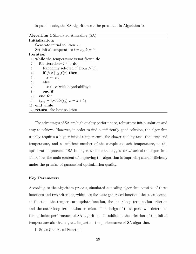
In pseudocode, the SA algorithm can be presented in Algorithm 1:

Algorithm 1 Simulated Annealing (SA)Initialization:

Generate initial solution x;Set initial temperature t = t0, k = 0;

Iteration:1: while the temperature is not frozen do2: for Iteration=2,3,... do3: Randomly selected x′ from N(x);4: if f(x′) ≤ f(x) then5: x← x

′ ;6: else7: x← x

′ with a probability;8: end if9: end for10: tk+1 = update(tk), k = k + 1;11: end while12: return the best solution

The advantages of SA are high quality performance, robustness initial solution and

easy to achieve. However, in order to find a sufficiently good solution, the algorithm

usually requires a higher initial temperature, the slower cooling rate, the lower end

temperature, and a sufficient number of the sample at each temperature, so the

optimization process of SA is longer, which is the biggest drawback of the algorithm.

Therefore, the main content of improving the algorithm is improving search efficiency

under the premise of guaranteed optimization quality.

Key Parameters

According to the algorithm process, simulated annealing algorithm consists of three

functions and two criterions, which are the state generated function, the state accept-

ed function, the temperature update function, the inner loop termination criterion

and the outer loop termination criterion. The design of these parts will determine

the optimize performance of SA algorithm. In addition, the selection of the initial

temperature also has a great impact on the performance of SA algorithm.

1. State Generated Function

29

The starting point of designing the state generated function (neighborhood func-

tion) should be to ensure that the generated candidate solutions are throughout the

entire solution space. Typically, the function consists of two parts: the way to gen-

erate candidate solutions and the probability distribution of generated candidate so-

lutions. The former determines the way to generate candidate solutions from the

current solution, and the latter determines the probability of selecting different states

in candidate solutions. The way of generating candidate solutions is determined by

the property of the problem, and usually solutions are produced in a certain probabili-

ty way in the neighborhood structure of the current state. The neighborhood function

and the probability way can be diversely designed, for example, the probability dis-

tribution can be the uniform distribution, the normal distribution, the exponential

distribution, the Cauchy distribution etc.

2. State Accepted Function

The state accepted function is generally given by the way of probability, and the

main difference among the different accepted function is the different form of the

accepted probability. In order to design the state accepted probability, the following

principles should be followed:

(1) Under a fixed temperature, the probability of accepting a candidate solution

which makes the objective function value decline is greater than which increases the

objective function value.

(2) With the drop of temperature, the probability of accepting the solution that

makes the objective function value solution rising should gradually decreases.

(3) When the temperature goes to zero, only the solution of reducing the objective

function value can be accepted.

The state accepted function is the most critical factor of SA algorithm to achieve

the global search, but experiments show that specific form of the function does not

have a significant impact on the performance of the algorithm. Therefore, SA algo-

rithm usually used min[1, exp(−∆C/t)] as the state accepted function, and ∆C =

f(x′)− f(x), where x′ is the new solution and x is the current solution respectively.

3. Initial Temperature

30

The initial temperature t0, the temperature update function, the inner loop termi-

nation criterion and the outer loop termination criterion are usually called annealing

schedule.

Experimental results show that, greater is the initial temperature, larger is the

probability of obtaining high quality solution, but the calculation time will increase.

Therefore, the initial temperature should be determined with considering both opti-

mization quality and efficiency. Commonly used methods include:

(1) Uniform sampling a set of states, and the variance of each state’s objective

value is used as the initial temperature.

(2) A set of states is randomly generated, and the maximum objective value d-

ifference between any two states is defined as |∆max|, and then based on the dif-

ference, using certain functions to determine the initial temperature. For example,

t0 = −∆max/ ln pt, where pt is the initial accepted probability.

(3) The initial temperature is given by the experience.

4. Temperature Update Function

The temperature update function is the drop way of temperature, which is used

to modify the temperature in the outer loop.

Currently, the most commonly used temperature update function is tk+1 = αtk,

where 0 < α < 1 and α can change.

5. Inner Loop Terminate Criterion

The inner loop termination criterion, or called Metropolis sample stability criteri-

on, is used to decide the number of generated candidate solutions at each temperature.

Commonly used criterions include:

(1) Checking whether the mean of objective function is stability.

(2) Small change of objective value in several steps.

(3) Sampling according to a certain number of steps.

6. Out Loop Terminate Criterion

The out loop terminate criterion is the stopping rule of the algorithm, which

determines the end time of the algorithm. Usually the criterion includes:

(1) Setting the threshold of termination temperature.

31

(2) Setting the iterations of the outer loop.

(3) The optimal value remains unchanged in consecutive several steps.

Research Status

In 1983 Kirkpatrick et al. [181] designed the large scale integrated circuit with using

SA. Szu [306] proposed a fast simulated annealing algorithm (FSA) that the anneal-

ing rate is inversely proportional to the time. In 1987 Laarhoven and Aarts published

the book ’Simulated Annealing’ [314], which systematically summarized the SA algo-

rithm, and promoted the development of theoretical study and practical application

of SA algorithm, this is a milestone in the history of SA algorithm. In 1990 Dueck

and Scheuer [100] studied the method for determining the critical value of the initial

temperature of the SA algorithm. Kirkpatrick et al. [165] used simulated anneal-

ing algorithm for optimization problems, and achieved very good results. Nabhan

et al. [245] studied in parallel computing to improve computational efficiency of SA

algorithm and can be used to solve complex scientific and engineering calculations.

So far, simulated annealing has been applied to several combinatorial optimiza-

tion problems. Connolly [80] proposed an improved simulated annealing to solve

the quadratic assignment problem. The experiment showed the effectiveness of this

algorithm. Laarhoven et al. [315] used simulated annealing for solving the job shop

scheduling problem. Al-khedhairi [8] solved p-median problem by using simulated an-

nealing in order to find the optimal or near-optimal solution of the p-median problem.

Liu et al. [212] proposed a heuristic simulated annealing algorithm for the circular

packing problem. Rodriguez-Tello et al. [281] proposed an improved simulated anneal-

ing algorithm for solving the bandwidth minimization problem, while comparing with

several literature algorithms under the benchmark instance experiment, the results

showed the improvement of the algorithm. Hao [151] proposed a heuristic algorith-

m for solving traveling salesman problem. The approach introduced the crossover

and mutation operator into SA in order to balance the running speed and accuracy.

Experiment verified the effectiveness of the proposed SA algorithm.

32

2.1.2 Tabu Search

Tabu Search (TS) is a metaheuristic originally proposed by Glover in 1989 [129,130].

By introducing a flexible storage structure and corresponding tabu criterion, TS can

avoid the repetition search, and the aspiration criterion is used to release some good

states which are banned, thereby TS ensures the diversification of effective search to

eventually achieve the global optimization.

So far, TS algorithm has achieved great success in combinatorial optimization,

production scheduling, machine learning, circuit design and other fields .

Basic Scheme

Tabu Search is a reflection of artificial intelligence, and an extension of the local

neighborhood search. The most important idea of Tabu Search is to mark the ob-

jects which are corresponding to the found local optimal solution, and try to avoid

these objects in further iterative search (not absolutely prohibit), thus can ensure an

effective search for different exploration ways.

Tabu search is starting from a given initial solution and some candidate solutions

in the neighborhood of current solution. If the objective value of the best candidate

solution is better than ’best so far’ state, the tabu property of the candidate solution

will be ignored, and it will replace the current solution and ’best so far’ state, and

is put into the tabu list. If such a candidate solution does not exist, the best and

no-tabu candidate solution will be chose as the new solution without considering the

quality.

The simple pseudocode of the Tabu Search is presented in Algorithm 2.

Compared with traditional optimization algorithm, the main features of TS are:

(1) The worse solution can be accepted in the search process, so TS has a strong

’climbing ability’.

(2) The new solution is not randomly generated in the neighborhood of the current

solution, but it is the solution which is better than the ’best so far’ state, or is the best

solution which is not in the tabu list, so the probability of selecting a good solution

33

Algorithm 2 Tabu Search (TS)Initialization:

Generate a random initial solution x;Tabu List ← ∅;

Iteration:1: while Stopping rule is not satisfied do2: Generate the neighborhood solution N(x) of x and candidate list;3: Judge aspiration criterion;4: if f(xbest) < f(x) then5: x← xbest, update Tabu List;6: else7: select the best solution x′ ∈ N(x) \ TabuList, update Tabu List;8: end if9: end while10: return the best solution

is much larger than choosing other solutions.

Thus, TS is a global iterative optimization algorithm with strong local search

capability. However, there are also some shortcomings of TS:

(1) TS has a strong dependence with the initial solution. A good initial solution

can make TS find a good solution in the solution space, but a bad initial solution will

reduce the convergence speed.

(2) The iterative search process is serial, which is only the moving of single state,

not a parallel search.

In order to further improve the performance of tabu search, on the one hand the

operations and parameters of the algorithm can be improved, on the other hand TS

can be combined with other algorithms.

Key Parameters

Generally, in order to design a tabu search algorithm, the algorithm needs to deter-

mine the following points:

1. Fitness Function

Fitness function of tabu search is used to evaluate the status of the search, and

then it is combined with tabu guideline and aspiration criteria to select a new state.

Clearly, it is relatively easy that the objective function value is used directly as fitness

34

function.

However, if the calculation of the objective function is difficult or time consuming,

some eigenvalues which reflect the problem goals can be used as the fitness function,

thereby can improve the time performance of the algorithm. Certainly, the selection

of the fitness function should be determined according to the specific problem, but it

must ensure optimality of both the eigenvalue and the optimality of objective function.

2. Tabu Object

The tabu object is a change element which will be put into the tabu list. The

purpose of tabu is to avoid the circuitous search and explore more effective search

ways. Usually, the tabu object can select the state itself, the state component or the

change of fitness value etc.

(1) The most simple easiest way is the state itself or its change is used to be the

tabu object. Specifically, when the state x changes to the state y, the state y (or the

change state x→ y) can be as the tabu object, thus the state y (or the change state

x→ y) can be prohibited to appears again under certain conditions.

(2) The change of state including the change of many state components, thus

using the change of state component as the tabu object will expand the range of

tabu, and reduce the corresponding calculation amount. For example, for flow shop

problem, the two points exchange caused by SWAP operation means the change of

state component, and it can be used as tabu object.

(3) The fitness value is used as tabu object. In other words, the states which have

same fitness value are considered as the same state. The change of a fitness value

implies the change of many states, so in this case, the tabu range will expand relative

to state change.

Therefore, if the state itself is chose as the tabu object, the tabu range is smaller

than the tabu object is the state component or fitness value, and the search range

is larger which is easy to cause the increase of computing time. However, under the

condition that the size of tabu length and candidate solution set are same and smaller,

choosing state component or fitness value as the tabu object will make the search into

local minimum because of the larger tabu range.

35

3. Tabu Length and Candidate Solution

The size of tabu length and candidate solution set are two key parameters that

affects the performance of the TS algorithm. Tabu length is the maximum number of

the tabu object which is not allowed to be selected without considering the aspiration

criteria (To put it simply, it is the term of tabu object in the tabu list), the tabu

object can be lifted only if the term is 0. The candidate solution set usually is a

subset of the current neighborhood solution set. When constructing the algorithm,

the computation and storage are required as little as possible, so the size of tabu

length and candidate solution set should be as small as possible. However, too short

tabu length will cause the circulation of search, and too small candidate solution set

is easy to fall into local minimum.

The selection of tabu length is related to the problems characteristics and the

researchers experience, which determines the computational complexity of the algo-

rithm.

On the one hand, the tabu length t can be steady constant. For example, the

tabu length is fixed at a number (such as t = 3 etc.), or fixed at an amount which is

associated with the problem size (such as t =√n, n is the dimension or size of the

problem).

On the other hand, the tabu length can be dynamic. For example, the change

interval [tmin, tmax] of tabu length can be set according to the search performance

and problems characteristic (such as [3, 10], [0.9√n, 1.1

√n]), and the tabu length can

vary within its interval according to certain principles or formulas. Of course, the

interval size of the tabu length may also change dynamically with the change of search

performance.

Generally, when the dynamic performance of the algorithm has a significant de-

crease, it indicates that the current search capability is strong, and may also the

minimal solution which near the current solution forms a deep ’trough’, so we can set

a large tabu length to continue the current search and avoid falling into local mini-

mum. Numerous studies show that the dynamic setting mode for the tabu length has

better performance and robustness than the static mode, but the more efficient and

36

rational setting manner needs further studied.

The candidate solutions are usually selected in the neighborhood of current solu-

tion which under the principle of merit-based. However, selecting too many candidate

solutions will cause excessive amount of computation, and selecting too few is easy

to fall into local minimum. Besides, the merit-based selection in the whole neighbor-

hood structure often requires a lot of calculations, for example, the SWAP operation

of TSP will generate C2n neighborhood solutions. Therefore, the candidate solution

can be chose deterministically or randomly in part of neighborhood solutions, and

the specific number of candidate solutions can be determined by the characteristics

of problem and the algorithm requirements.

4. Aspiration Criterion

In the tabu search algorithm, the situation that all the candidate solutions are in

the tabu list or a tabu candidate solution is better than the ’best so far’ state may

appear, then the aspiration criterion will allow some states to be lifted, in order to

achieve more efficient performance of optimization. Several common way of aspiration

criterion is described as follows.

(1) Based on the fitness value

The global mode (the most common mode): If the fitness value of a tabu candidate

solution is better than the ’best so far’ state, so this candidate solution will be lifted

and used as the current state and the new ’best so far’ state. The region mode: The

search space is divided into several subregions, if the fitness value of a tabu candidate

solution is better than the ’best so far’ state in its region, thus this candidate solution

will be used as the current solution and the new ’best so far’ state in corresponding

region. This criterion can be intuitively understood as the algorithm finds a better

solution.

(2) Based on the search direction

If a tabu object improved the fitness value when it was put in the tabu list last

time, and now the fitness value of corresponding candidate solution for this tabu

object is better than current solution, so this tabu object will be released. This

criterion means the algorithm is running according to an efficient search way.

37

(3) Based on the minimum error

If all the candidate solutions are banned, and there is not a candidate solution

which is better than ’best so far’ state, the best one in the candidate solutions will be

released to continue the search. This criterion is a simple treatment for the deadlock

of the algorithm.

(4) Based on the influence

In the search process, the change of different objects has a different influence on the

fitness value, and this influence can be used as a property to construct the aspiration

criterion with the tabu length and the fitness value. The intuitive understanding is,

releasing a high impact tabu object is helpful to get a better solution in the future

search. It is noted that, the influence is just a scalar index, which can be characterized

by a decrease of the fitness value, and can also represent the rise of the fitness value.

For instance, if all the candidate solutions are worse than the ’best so far’ state, but

the influence index of one tabu object is large, and it will be released soon, thus

this tabu object should be lifted immediately to expect a better state. Obviously,

this criterion is necessary to introduce a measure which describes the influence, and a

value which is associated with the tabu length, so it will increase the complexity of the

algorithm operation. Meanwhile, in order to adapt the change of the search process

and the algorithm performance, it would be better these indicators are dynamic.

5. Tabu Frequency

Recording the tabu frequency is a supplement of the tabu property. It can relax

the range of selecting the decision object. For example, if a fitness value occurs

frequently, it can be speculated that the algorithm falls into a kind of loop or a

minimum point, or the existing algorithm parameters are difficult to help to explore

better state, thus the structure or parameters of the algorithm should be modified.

When solve the problem, according to the need of the problem and algorithm, the

frequency of a state can be recorded. The information of some exchange objects or

fitness value can be also recorded, and such information can be static or dynamic.

The static frequency information mainly includes the frequency of the state, the

fitness value or the exchange object which appear in the optimization process, and its

38

calculation is relatively simple, such as the number of times that the objects appear

in the calculation, the radio between the appearance times and the total number

of iterations, and the number of circles between two states etc. Obviously, these

information help to understand the characteristics of some objects, and the number

of the corresponding cycle appears and so on.

The dynamic frequency information mainly records the variation trend of the

transfer from some states, fitness values or exchange objects to other ones, such as

the change of a state sequence. The record of the dynamic frequency information

is more complex, while the amount of the information is greater. Commonly used

methods are as follows:

(1) Recording the length of a sequence, that is the number of elements in the

sequence. When recording the sequence of some key points, the change of sequence

length of these key points can be calculated.

(2) Recording the iteration number of starting from a element in the sequence and

then back to this element.

(3) Recording the average fitness value of a sequence, or the fitness value change

of each corresponding element.

(4) Recoding the frequency of a sequence appears.

The frequency information helps to strengthen the capacity and efficiency of the

tabu search, and contributes to the control of the tabu search algorithm parameters.

Or based on the frequency information, the corresponding object will get punishment.

For instance, if a object appears frequently, increasing the tabu length can avoid the

loop; If the fitness value of a sequence changes less, the tabu length for all the objects

in this sequence can increase; If the best fitness value sustains for a long time, the

search process can be terminated and this fitness value can be considered as the best

solution.

In addition, in order to enhance the search quality and efficiency of the algo-

rithm, many improved tabu search algorithms add the intensification and diversifi-

cation mechanism in the algorithm based on the frequency and other information.

The intensification mechanism emphasizes that the algorithm focus on the search in

39

the good region. For instance, re-initializing or multi-step searching based on the

optimal or suboptimal state, and increasing the select probability of the algorithm

parameters which obtain the best state, etc.; The diversification mechanism under-

lined broaden the search range, especially those unexplored areas, which is similar

to the genetic algorithm with enhancing diversity of population. The intensification

and diversification mechanism is contradictory on some levels, but both mechanisms

have a significant impact on the performance of the algorithm. Therefore, as a good

tabu search algorithm, it should have a capability of reasonable balance between the

intensification and diversification mechanism.

6. Stopping Criterion

Tabu search requires a stopping criterion to end the algorithmic search process. If

strictly achieving the theoretical convergence condition, that is achieving the traversal

of the state space under the condition that the tabu length is sufficiently large, it is

obviously not practical. Thus, the approximate convergence criterion is usually used

for actually algorithm design. Common methods are as follows:

(1) Given the maximum number of iterations. This method is simple and easy to

operate, but it is difficult to ensure the optimization quality.

(2) Set the maximum frequency of a tabu object. In other words, if the tabu

frequency of a state, fitness value or exchange object exceeds a certain threshold,

then the algorithm is terminated, which also includes the situation that the best

fitness value remain unchangs for several consecutive steps.

(3) Set the deviation amplitude of the fitness value. That is, firstly there is a

estimated lower bound of the problem, once the deviation between the best fitness

value and the lower bound is smaller than a certain amplitude, then the algorithm

stops.

Research Status

In the theory research, the main concern research aspect includes the selection of algo-

rithm parameters, the algorithm operations and hybrid algorithm. Sexton et al. [291]

proposed a improved TS algorithm which the size of tabu list is variable, and used

40

for training the neural network. Jozefowska et al. [172] raised three tabu list man-

agement methods for discrete - continuous scheduling problem, and did a comparison

study on three methods. Glover [129,132] proposed a strategy oscillation approach to

strengthen the management of the tabu list, which is applied on the p-medium prob-

lem. In addition, in order to improve the optimization performance and efficiency of

the algorithm, two or more algorithms are combined together, while forming a new

hybrid algorithm which has become a trend. For example, the combination of TS and

GA, etc. [171], The studies show that the hybrid algorithm has a more substantial

upgrade on the performance and efficiency of the algorithm.

Because the TS algorithm has a strong versatility, and does not need special

information of problems, so it has a wide area of application. At present the main

application areas include scheduling problem [9, 191, 205, 264], quadratic assignment

problem [97,159,192], traveling salesman problem [122], vehicle routing problem [120],

knapsack problem [248], bandwidth problem [229]...

2.1.3 Greedy Randomized Adaptive Search Procedure

The basic local search algorithm is easy to fall into the local minimum. A simple

method to improve the quality of the solution is to start local search algorithm several

times, and each time the local search starts from a new randomly generated initial

solution. Although this method is able to improve the quality of the solution, the

efficiency of the algorithm is low because of the randomness of the initial solution.

Greedy Randomized Adaptive Search Procedure (GRASP) was first introduced in Feo

and Resende [106,107]. GRASP trying to improve the performance of the algorithm

by generating the high-quality initial solution with certain diversity. It is a heuristic

iterative method for solving stochastic optimal combination problems, which has been

widely used in many fields.

41

Basic Scheme

Greedy Randomized Adaptive Search Process refers to randomized the greedy con-

structive heuristic method to generate a large number of different initial solutions for

local search. Therefore, it is a kind of local search procedure which is multi-start,

and each iteration consists of two phases:

(1)To construct the initial solution by greedy randomized adaptive structure al-

gorithm.

(2)To optimize the constructed initial solution which generated in phase 1 through

a local search algorithm.

The description of GRASP is showed in Algorithm 3.

Algorithm 3 Greedy Randomized Adaptive Search Procedure (GRASP)1: while Stopping rule is not satisfied do2: Generate an initial feasible solution using a randomized greedy heuristic;3: Apply a local search starting from the initial solution;4: end while5: return the best solution

The construction process of the solution is as follows: Suppose that the solution

is composed of many solution elements, according to some heuristic criteria, an e-

valuation value is calculated for each solution element, which means the superior or

inferior degree of the solution element which will be added into the partial solution

under the current circumstances.

The restricted candidate list (RCL) is constructed by the partial solution element

with high evaluation value, and then a solution element is randomly selected from the

restricted candidate list to the partial solution. This process will be repeated until

the solution construction is completed.

Key Parameters

1. Construction

The construction phase is a process of generating the feasible solution by iteration,

and the restricted candidate list is a important part in this phase.

42

At each step of the construction phase, the solution element solution is sorted

according to the greedy function, some top elements will be put into the restricted

candidate list. The typical method of forming the restricted candidate includes two

kinds:

(1) Best Strategy: This strategy selects the best top λ% in the solution element.

(2) First Strategy: The first strategy chooses the top δ% solution element accord-

ing to sequence of the corresponding greedy value in the solution elements.

Besides, the length of RCL l has a great influence on the GRASP performance.

If the length is equal to 1, then each added solution element is the current best one,

which is actually a deterministic greedy algorithm, and the same initial solution will

be obtained each time. If the solution is equal to the number of all the elements, the

construction algorithm is a completely random process, and GRASP degenerates into

random multi-start local search algorithm. There are two different ways to determine

the parameter l:

(1) Based on base number: The length of RCL can be defined as a fixed value.

(2) Based on evaluation value: This way is based on the evaluation value of the

solution element. The element whose evaluation value is better than a certain critical

value will be put into the restrict candidate list, and its length is not fixed.

2. Local Search

The randomly generated feasible solution from the construction phase can not

guarantee the local optimum, so it is necessary to enter the local search phase. The

local search starts from the feasible solution which is obtained in the construction

phase, and find the local optimal solution in a certain neighborhood. The best local

optimum in all iteration is the global optimal solution.

The local search process can use a basic local search algorithm, or some more

advanced algorithms can be accepted such as simulated annealing, tabu search etc.

Research Status

Atkinson et al. [17] applied GRASP to solve the time constrained vehicle scheduling

problem, and two forms of adaptive search (local adaptation and global adaptation)

43

were illustrated. Fleurent et al. [108] applied GRASP on the quadratic assignmen-

t problem. Laguna et al. [193] combined GRASP with path relinking to improve

the algorithm performance. Prais et al. [271] used a reactive GRASP for a matrix

decomposition problem in TDMA traffic assignment. Binato et al. [47] proposed

a new metaheuristic approach named greedy randomized adaptive path relinking

(GRAPR). Pinana et al. [267] developed a greedy randomized adaptive search pro-

cedure (GRASP) combined with a path relinking strategy for solving the bandwidth

minimization problem. Hirsch et al. [160] presented a continuous GRASP (C-GRASP)

through extending GRASP from discrete optimization to continuous global optimiza-

tion. Andrade et al. [15] combined GRASP with an evolutionary path relinking to

solve the network migration problem. Moura and Scaraficci [242] combined GRASP

with a path relinking to solve the school timetabling problem. Marinakis [226] de-

veloped a Multiple Phase Neighborhood Search GRASP (MPNS-GRASP) for solving

vehicle routing problem.

2.1.4 Variable Neighborhood Search

Variable Neighborhood Search (VNS) is a metaheuristic that is firstly proposed by

Hansen and Mladenovic [236] in 1997. This metaheuristic has been proved to be

very useful for obtaining an approximate solution to optimization problems. Variable

neighborhood search includes dynamically changing neighborhood structures. The

algorithm is more general, the degree of freedom is large, and many variants can be

designed for specific problems.

Since variable neighborhood search algorithm has been proposed, because VNS

has the advantages such as the idea is simple, the algorithm is easy to achieve, the

algorithm structure is irrelevant to the problem and is suitable for all kinds of op-

timization problems, so VNS has been one of the key optimization algorithms are

studied.

44

Basic Scheme

The basic idea of variable neighborhood search is:

(1) The local optimal solution in a neighborhood structure is not necessarily the

one in another neighborhood.

(2) The local optimal solution in all possible neighborhood structure is the global

optimal solution.

Variable neighborhood search algorithm relies on the following three facts [150]:

Fact1. The local optimum of a neighborhood structure is not necessarily the local

optimal solution of another neighborhood structure.

Fact2. The global optimal solution is the local optimal solution for all possible

neighborhood structure.

Fact3. For a lot of problems, the local optimums of several neighborhood struc-

tures are close to each other.

The last fact is obtained from the experience, it means that the local optimal

solution can provide some information of the global optimal solution. Through the

study of the neighborhood structure, better feasible solutions can be found, and then

VNS keeps close to the global optimal solution.

When using neighborhood change to solve the problem, neighborhood transfor-

mation can be divided into three categories [150]: (1) deterministic; (2)stochastic;

(3)both deterministic and stochastic. Nk(k = 1, 2, ..., kmax) is defined as a finite set

of neighborhood structure, where Nk(x) is the solution set of k neighborhood for x.

The basic procedure of neighborhood change is, comparing the value between the

new solution f(x′) and the current solution f(x) in kth neighborhood Nk(x). If the

new solution has improved, then k = 1 and the current solution is updated (x← x′).

Otherwise, the next neighborhood will be considered (k = k + 1).

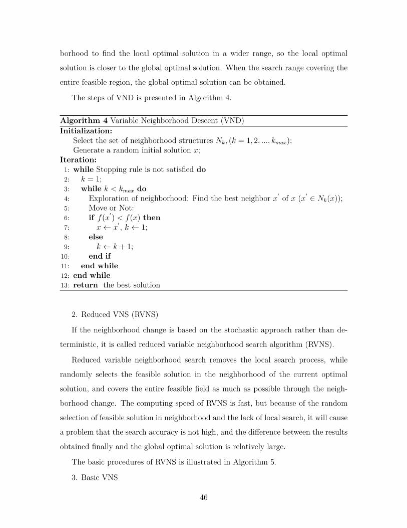
1. Variable Neighborhood Descent (VND)

If the neighborhood changes based on deterministic methods, it is called the vari-

able neighborhood descent search algorithm (VND).

Essentially, variable neighborhood descent is a algorithm by expanding the neigh-

45

borhood to find the local optimal solution in a wider range, so the local optimal

solution is closer to the global optimal solution. When the search range covering the

entire feasible region, the global optimal solution can be obtained.

The steps of VND is presented in Algorithm 4.

Algorithm 4 Variable Neighborhood Descent (VND)Initialization:

Select the set of neighborhood structures Nk, (k = 1, 2, ..., kmax);Generate a random initial solution x;

Iteration:1: while Stopping rule is not satisfied do2: k = 1;3: while k < kmax do4: Exploration of neighborhood: Find the best neighbor x′ of x (x′ ∈ Nk(x));5: Move or Not:6: if f(x′) < f(x) then7: x← x

′ , k ← 1;8: else9: k ← k + 1;10: end if11: end while12: end while13: return the best solution

2. Reduced VNS (RVNS)

If the neighborhood change is based on the stochastic approach rather than de-

terministic, it is called reduced variable neighborhood search algorithm (RVNS).

Reduced variable neighborhood search removes the local search process, while

randomly selects the feasible solution in the neighborhood of the current optimal

solution, and covers the entire feasible field as much as possible through the neigh-

borhood change. The computing speed of RVNS is fast, but because of the random

selection of feasible solution in neighborhood and the lack of local search, it will cause

a problem that the search accuracy is not high, and the difference between the results

obtained finally and the global optimal solution is relatively large.

The basic procedures of RVNS is illustrated in Algorithm 5.

3. Basic VNS

46

Algorithm 5 Reduced Variable Neighborhood Search (RVNS)Initialization:


Iteration:1: while Stopping rule is not satisfied do2: k = 1;3: while k < kmax do4: Shaking: One solution x

′(x′ ∈ Nk(x)) is generated randomly from the kthneighborhood structure of x;

5: Move or Not:6: if f(x′) < f(x) then7: x← x

′ , k ← 1;8: else9: k ← k + 1;10: end if11: end while12: end while13: return the best solution

The basic variable neighborhood search algorithm (Basic VNS) changes the neigh-

borhood by using both deterministic and stochastic methods.

The basic variable neighborhood search algorithms includes three processes: shak-

ing, local search and neighborhood change. Shaking is trying to jump out the current

local optimum and find a new local optimal solution, while making the local optimal

solution be closer to the global optimal solution. Local search is used to find the local

optimal solution in order to improve search accuracy. "Move or not" which means the

neighborhood change provides an iterative method and stopping criterion.

The pseudocode of the Variable Neighborhood Search is presented in Algorithm

6.

Comparing the three above algorithms, VND omits the random search which is

in basic VNS, and replaces two parts of VNS (random search and local search) by

exploration of neighborhood. RVNS is to simplify the VNS, while omitting local

search process of the VNS algorithm. The purpose is to save time-consuming local

search part, so it is suitable for large-scale computing local search problem.

47

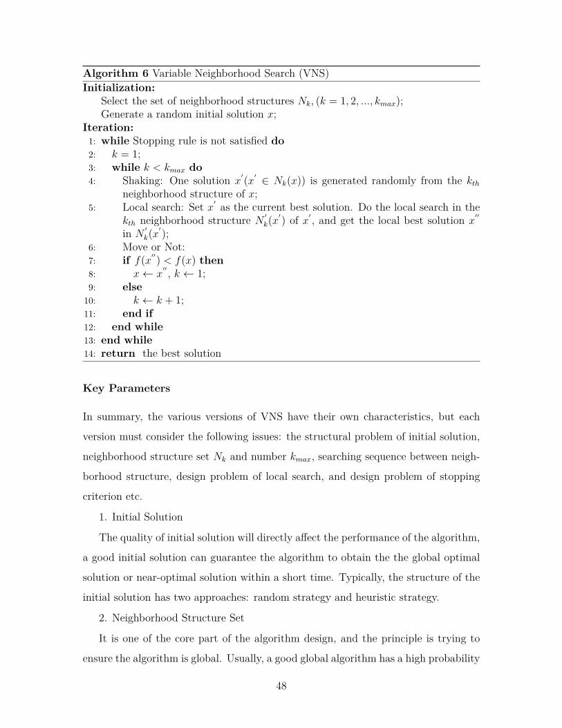
Algorithm 6 Variable Neighborhood Search (VNS)Initialization:


Iteration:1: while Stopping rule is not satisfied do2: k = 1;3: while k < kmax do4: Shaking: One solution x

′(x′ ∈ Nk(x)) is generated randomly from the kthneighborhood structure of x;

5: Local search: Set x′ as the current best solution. Do the local search in thekth neighborhood structure N ′

k(x′) of x′ , and get the local best solution x

′′

in N ′k(x

′);6: Move or Not:7: if f(x′′) < f(x) then8: x← x

′′ , k ← 1;9: else

10: k ← k + 1;11: end if12: end while13: end while14: return the best solution

Key Parameters

In summary, the various versions of VNS have their own characteristics, but each

version must consider the following issues: the structural problem of initial solution,

neighborhood structure set Nk and number kmax, searching sequence between neigh-

borhood structure, design problem of local search, and design problem of stopping

criterion etc.

1. Initial Solution

The quality of initial solution will directly affect the performance of the algorithm,

a good initial solution can guarantee the algorithm to obtain the the global optimal

solution or near-optimal solution within a short time. Typically, the structure of the

initial solution has two approaches: random strategy and heuristic strategy.

2. Neighborhood Structure Set

It is one of the core part of the algorithm design, and the principle is trying to

ensure the algorithm is global. Usually, a good global algorithm has a high probability

48

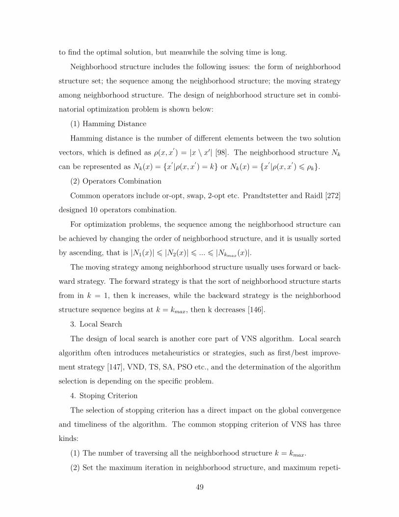
to find the optimal solution, but meanwhile the solving time is long.

Neighborhood structure includes the following issues: the form of neighborhood

structure set; the sequence among the neighborhood structure; the moving strategy

among neighborhood structure. The design of neighborhood structure set in combi-

natorial optimization problem is shown below:

(1) Hamming Distance

Hamming distance is the number of different elements between the two solution

vectors, which is defined as ρ(x, x′) = |x \ x′| [98]. The neighborhood structure Nk

can be represented as Nk(x) = x′|ρ(x, x′) = k or Nk(x) = x′ |ρ(x, x′) 6 ρk.

(2) Operators Combination

Common operators include or-opt, swap, 2-opt etc. Prandtstetter and Raidl [272]

designed 10 operators combination.

For optimization problems, the sequence among the neighborhood structure can

be achieved by changing the order of neighborhood structure, and it is usually sorted

by ascending, that is |N1(x)| 6 |N2(x)| 6 ... 6 |Nkmax(x)|.

The moving strategy among neighborhood structure usually uses forward or back-

ward strategy. The forward strategy is that the sort of neighborhood structure starts

from in k = 1, then k increases, while the backward strategy is the neighborhood

structure sequence begins at k = kmax, then k decreases [146].

3. Local Search

The design of local search is another core part of VNS algorithm. Local search

algorithm often introduces metaheuristics or strategies, such as first/best improve-

ment strategy [147], VND, TS, SA, PSO etc., and the determination of the algorithm

selection is depending on the specific problem.

4. Stoping Criterion

The selection of stopping criterion has a direct impact on the global convergence

and timeliness of the algorithm. The common stopping criterion of VNS has three

kinds:

(1) The number of traversing all the neighborhood structure k = kmax.

(2) Set the maximum iteration in neighborhood structure, and maximum repeti-

49

tion number of the optimal solution.

(3) The maximum allowable CPU time.

Research Status

Hansen and Mladenovic first proposed the variable neighborhood search algorithm in

1997, and then in the 2001 they published the invited review [145] in the European

Journal of Operational Research, which analyzed the improved version of VNS and

did the comparative analysis with the classical algorithm for specific problems. In

recent years, a large number of papers on VNS emerged in the International Journals.

Hansen and Mladenovis [145] used VNS and 2-opt algorithm to solve the TSP (the

problem size from 100 to 1000), and the results showed that the VNS obtains the aver-

age improvement in value of 2.73% and average save in solving time of 22.09s. Besides,

the 2-opt algorithm is embedded into the local search of VNS, and the simulation re-

sults showed that the algorithm is superior to VNS. Hansen et al. [149] using VNS,

FI, RVNS and VNDS solved TSP. Based on CROSS-exchange and iCROSS-exchange

operations, Polacek et al. [274] designed VNS algorithm with 8 neighborhood for

solving TSP.

Kytojoki et al. [190] designed guided VNS algorithm to solve 32 existing large scale

VPR problem, and the comparison with TS showed that the proposed algorithm

is better than TS in terms of timeliness, and solved the VRP problem whose size

is up to 20000 cities. Hemmelmayr et al. [156] constructed initial solution using

saving algorithm, and used 3-opt as the local search strategy. The results showed the

effectiveness of VNS comparing with previous research.

Avanthay et al. [21] first introduce VNS to solve the Graph Coloring Problem.

Ribeiro and Souza [280] adopted VND to solve this problem, and its neighborhood

design used k-edge exchange method, the experiments showed that VND is superior

to GA in timeliness.

Hansen and Mladenovic [144] designed VNS and compared with TS based on

ORLIB and TSPLIB, the effect is good. Crainic et al. [86] proposed a collaborative

neighborhood VNS, and tested in TSPLIB.

50

Mladenovic et al. [237] proposed a variable neighborhood search method which

combines several ideas from the literatures for minimizing the bandwidth. The ex-

periment results of 113 benchmark instances showed that the performance of the

proposed VNS approach was better than all previous methods.

In addition, there are many papers used improved VNS to solve combinatorial

optimization problems. For example, Gao et al. [115] solved jop shop scheduling

problem using VNS combined with GA. Lopez et al. [117] solved p-median problem

with parallel VNS. Burke et al. [54] presented a hybrid heuristic ordering and VNS for

solving the nurse roistering problem. Lazic et al [197] proposed variable neighborhood

decomposition search method for 0-1 mixed integer problem. Hu et al. [163] combined

VNS and integer linear programming to solve the generalized minimum spanning tree

problem. In these problems, the use of VNS have received good results.

2.2 Population based metaheuristics

In population based metaheuristics, each generation has multiple individuals with

parallel computing. The difference between these metaheuristics is the rule of gener-

ating adjacent states (i.e., the next state for the population). For example, genetic

algorithm does operation on certain selected chromosomes with genetic operators.

Scatter search constructs the subset from the reference set.

2.2.1 Genetic Algorithm

Genetic algorithm is proposed by Holland [161] inspired by biological evolution, and

it is a metaheuristic which is based on the idea of the survival of the fittest. This

algorithm represents the solving problem as the ’survival of the fittest’ process of the

chromosome. Through the population of chromosomes evolving generation by gen-

eration, while including selection, crossover and mutation operations, the algorithm

ultimately converges to the individual which is the best adapted to the environment,

and thus obtains the optimal solution or satisfactory solution.

GA is a general optimization algorithm. The encoding techniques and genetic

51

operations are relatively simple, and optimization is not restrained by the constraint

conditions, so it has a wide range of application value. Therefore, genetic algorithm is

widely used in automatic control, computer science, pattern recognition, engineering

design, management and social sciences and other fields.

Basic Scheme

Genetic algorithm is a kind of stochastic optimization algorithm, but it is not a

simply random comparison search. Through using the evaluation on chromosomes

and the role worked on chromosome genes, the existing information is effectively

used to guide the search which can explore the state which hopefully improves the

optimization quality.

The following pseudocode simply illustrates the genetic algorithm operation pro-

cess.

Algorithm 7 Genetic Algorithm (GA)Initialization:

Initialize populationCalculate the fitness value of initial population;

Iteration:1: while the stopping rule is not satisfied do2: According to the fitness value, execute the selection operation;3: if rand(0,1) ≤ crossover rate then4: Execute the crossover operation;5: end if6: if rand(0,1) ≤ mutation rate then7: Execute the mutation operation;8: end if9: Update population;10: Calculate the fitness value of new population11: end while12: return the best solution

Genetic algorithm uses the idea of biological evolution and heredity. Different from

traditional optimization methods, genetic algorithm has the following characteristics:

(1) Instead of the parameter itself, GA starts the evolution operation after the

problem parameters are encoded as the chromosome. It makes the function be not

52

restricted by function constraints, such as continuity, conductivity etc.

(2) The search process of GA is stating from a solution set of the problem, not a

single individual, so it has a implicit parallel search feature, thus can greatly reduce

the possible of falling into local minimum.

(3) All the genetic operation used in GA are random operations. Meanwhile, the

search of GA is according to the fitness value information of the individual without

other information.

(4) GA has the capability of global search.

The superiority of the genetic algorithm is mainly reflected in:

(1) The genetic algorithm can do the whole space parallel search, and the search

focuses on the high performance parts, which can improve the efficiency and avoid

local optimum.

(2) The algorithm has inherent parallelism. Through the genetic operation on the

population, it can handle a large number of states, and is easy to parallel implemen-

tation.

Key Parameters

Typically, the genetic algorithm is designed according to the following steps:

(1) Determine the encode scheme of the problem.

(2) Determine the fitness value function.

(3) Design the genetic operators.

(4) Select the algorithm parameters, including the number of population, the

probability of crossover and mutation, the number of generation etc.

(5) Determine the termination condition of the algorithm.

Following is the introduction of the design for the key parameters and operations.

1. Encode

Encode is to use a code to indicate the problem solution, thus the code space of

genetic algorithm which is corresponding to the state space of the problem will be

obtained. Encode is largely dependent on the property of the problem, and will affect

the design of genetic operations.

53

The optimization process of GA dose not directly work on the problem parameter

itself, but on the code space with corresponding encode scheme, so the selection of

encode is an important factor affecting the performance and efficiency of the algo-

rithm.

In the optimization function, the different code length and code system have a

great influence on the accuracy and efficiency of the solving problem. The binary

encoding describes the problem solution as a binary string, and the solution of the

problem in decimal encoding is represented by a decimal string. Apparently the code

length will affect the accuracy of the algorithm, and the algorithm should have a large

amount of storage.

The real number encoding uses a real number to represent the problem solution,

and it can solve the problem that the encode effect on the algorithm accuracy and the

amount of storage, and also facilitates the introduction of problem related information

in the optimization. Real number encoding has been widely used in high-dimensional

complex optimization problems.

In combinatorial optimization, due to the property of the problem itself, the en-

coding requires a special design. For example, the path encoding based on the re-

placement in TSP problem, the 0-1 matrix encoding etc.

2. Fitness Function

The fitness value function is used to evaluate the individual, and is also the basis

for the development of optimization process. When optimizing simple problems,

usually the objective function can be directly converted to be used as the fitness

value function. When optimizing complex problems, it often needs to construct an

appropriate fitness function to adapt GA optimization.

3. Algorithm Parameter

The number of population is one of the factors affecting the optimize performance

and efficiency of the algorithm. Typically, if the population is too small, it can not

provide enough sample points, which causes a poor performance of the algorithm,

and even can not obtain the feasible solution of the problem; When the population

number is too large, although the increasing optimization information can prevent to

54

fall into local optimum, but it will undoubtedly increase the amount of computation.

Of course, in the optimization process, the number of population is allowed to vary.

The crossover probability is used to control the frequency of crossover operation.

If the probability is too large, the strings in the population update soon, and then

the individuals with high fitness value are quickly destroyed; If the probability is too

small, rarely crossover operation will make the search stalled.

Mutation probability is an important factor to increase the diversity of population.

In GA which based on the binary encoding, usually a lower mutation rate is sufficient

to prevent the gene at any location from remain unchanging in the entire population.

However, if the probability is too small, it will not produce new individuals; and the

too large probability will make GA become a random search.

Thus, determining the optimal parameters is an extremely complex optimization

problem.

4. Genetic Operator

Survival of the fittest is the basic idea of genetic algorithm. The idea should be

embodied in the genetic operator such as selection, crossover, mutation, while taking

into account the impact on the algorithm efficiency and performance.

(1) Selection Operation

The selection operation is also called the copy operation. Copy operation is to

prevent the loss of effective gene to make high-performance individuals survival with

greater probability, thereby improving the global convergence and computational effi-

ciency. Potts et al. outlined 23 selection methods [270]. Common selection operations

are as follows:

Proportion Selection

The proportion selection is the most basic and common used selection method in

genetic algorithm. The larger the fitness value of individual, the higher the selected

probability. This method reflects the principle of natural selection which is ’survival

of the fittest’. The selected individuals are put into the paired library, and randomly

paired to perform the following crossover operation.

Sort Selection

55

There is no special requirements for the individual fitness value which taking

positive or negative value. All the individuals in the population are sorted according

to the corresponding fitness value, and selected probability for each individual is

assigned according to the sorting.

Best Individual Selection

The individual with the best fitness value in the population is directly copied

to the next generation without crossover operation. The benefit of doing so is to

ensure that the optimal solution in one generation do not destroyed by crossover and

mutation operations during the genetic process. This method is an essential condition

to ensure the convergence of the genetic algorithm. However, it is also easy to make

a local optimum individual can not be easily eliminated, while causing the algorithm

stagnation in the local optimal solution, that is, this approach affects the global search

ability of genetic algorithm. Therefore, it is usually not used alone.

Competition Selection

Two individuals are selected randomly, and the fitness value of them are compared.

The large one will be chose, and the small one is naturally eliminated. If the fitness

value of two individuals are same, then one of them is selected arbitrarily. Repeating

this process until the paired library contains N individuals. This approach not only

ensures the paired library individuals have better dispersion in the solution space, but

also ensures the individuals which are put into the library have larger fitness value.

(2) Crossover Operation

The crossover operation is used to assemble a new individual, and do effective

search in the solution space, while reducing the failure probability for effective models.

Potts et al. summarized 17 kinds of crossover method [270]. Several common crossover

operators applied to binary coding or real number coding are as follows:

Single Point Crossover

It is also referred to as the simple crossover. A cross point is randomly selected

in the individual string, and two individuals exchange part of genes with each other

before or after the point to generate a new individual.

Two Point Crossover

56

Two cross points are randomly set in a pair of two individual strings, and part of

genes exchange between these two points.

Uniform Crossover

Each position gene of two individuals are exchanged with the same probability,

thus two new individuals are generated.

Arithmetic Crossover

The new individual is generated by a linear combination of two individuals. That

is, x′1 = αx1 + (1− α)x2, x

′2 = αx2 + (1− α)x1, and α ∈ (0, 1), x1, x2 are the parent

chromosomes, x′1, x

′2 are the offspring chromosomes.

Besides, according to the different research objects, there are a variety of alter-

native crossover methods, such as partially mapped crossover, order crossover, cycle

crossover etc.

(3) Mutation Operation

The mutation operation randomly changes some genes’ value of the individual in

the population with a small probability Pm. The basic process of mutation is: for each

gene value of offspring individuals which obtained by crossover operation, a pseudo

random number rand ∈ (0, 1) is generated, if rand < Pm, then do the mutation

operation.

Mutation is random local search. If it is combined with the selection and crossover

operators, it will be able to avoid the permanent loss of some information which is

caused by the selection and crossover operations. Using the mutation operator in

genetic algorithm has two main purposes:

(1) It ensures the effectiveness of the genetic algorithm, and makes GA has the

capability of local random search;

(2) It ensures that GA maintains the diversity to prevent premature convergence.

Therefore, the mutation operation is a measure to avoid the algorithm falling into

local optimum. Here are some common mutation methods:

Basic Mutation

For individual string, doing the mutation operation on one or a few genes which

are assigned randomly with the mutation probability Pm.

57

Uniform Mutation

Respectively using the random number which is in accord with uniform distribu-

tion within a certain range, the original gene value of the individual string is replaced

with a small probability. Uniform mutation operation is particularly suitable for the

initial running phase of the genetic algorithm, which makes the search points can move

freely throughout the search space, and can increase the diversity of the population.

Binary Mutation

This method needs two chromosomes. After binary mutation operation, each gene

of two new generated individuals will be valued as the xnor or xor of the corresponding

gene value of original chromosomes. It changes the traditional way of mutation, while

effectively overcoming the premature convergence and improving optimize speed of

the genetic algorithm.

Gaussian Mutation

This method using the random number which is followed the normal distribution

with the mean value µ and the variance σ2 to replace the original gene value. Its

operation process is similar to the uniform mutation.

5. Termination Condition

Improving the convergence speed is relevant to the design of algorithm operation

and the selection of parameter. The algorithm can not go on running without stop-

ping, and the optimal solution of the problem is usually not known, thus a certain

condition is required to terminate the process of the algorithm. The most common

termination condition is that given a maximum number of generation, or checking

whether the optimal value has no significant change in several continuous steps etc.

Research Status

Genetic algorithm provides a common frame for solving complex system optimization

problems, which does not depend on the specific area problem, is widely used in a

variety of disciplines.

With the increasing scale of the problem, the search space of combinatorial opti-

mization problems have expanded dramatically, sometimes on the current computer

58

enumeration method it is difficult or even impossible to determine their exact optimal

solution. For such complex problems, the research should focus on finding satisfactory

solutions, and genetic algorithm is one of the best tools which seek such satisfacto-

ry solution. Practice has proved that the genetic algorithm has been successfully

applied on the NP-hard problem such as traveling salesman problem [52], knapsack

problem [77], bin packing [104], layout optimization [188], bandwidth minimization

problem [16,209] etc.

In many cases, the mathematical model created by conventional methods can not

accurately solve the production scheduling problem, even after some simplification

the problem can be solved, sometimes the result is far away from the actual target

because of too much simplification. Under normal circumstances, scheduling is mainly

relied on experience in real production. The study found that genetic algorithm has

become an effective tool for solving complex scheduling problems, in terms of job-

shop scheduling problem [72,92,137], flow shop scheduling problem [68,244], lot sizing

problem [337], genetic algorithms have been effectively applied.

The robot is a complex and difficult to accurately modeling artificial system. Since

the origin of the genetic algorithm if from the study of artificial adaptive system, cer-

tainly robotics becomes an important application field of genetic algorithms. Genetic

algorithms have researched and applied on several aspects including mobile robot

path planning [142,164], robot inverse kinematics [263] etc.

Image processing is an important research field of computer vision. In the image

processing, such as scanning, image segmentation, feature extraction, inevitably there

will be some error, and thus affect the image effect. How to minimize these errors is an

important requirement for practical use of computer vision. Genetic algorithm can be

used to optimize the calculation of image processing, and currently has been applied

in pattern recognition [261], image restoration [71], image feature extraction [53,285]

etc.

Data mining can extract hidden, unknown, potential application value knowledge

and rules from large database. Many data mining problems can be seen as a search

problem. The database can be seen as the search space, mining algorithms can be seen

59

as the search strategy. Applying genetic algorithm to search in the database, and the

evolution is used for a set of rules which randomly generated, until the database can

be covered by this set of rules, thus dig out hidden rules in the database [66,85,109].

2.2.2 Scatter Search

Scatter Search (SS) is introduced by Glover [127] in 1997 for solving the integer

programming problem. SS using global search strategy based on the population,

and the intelligence iterative mechanism of ’decentralized-convergence gathering’, to

obtain the solution with high quality and diversity in reference set. Besides, SS

applies the subset combination method and the reference set update method, to find

the global optimal solution or satisfactory solution.

Compared to other algorithms, due to the memory ability of the reference set,

scatter search can dynamically track the current search to adjust its search strategy,

thus the randomness of the search process can be reduced, and SS more focuses on

using some systematic way to build the new solution. In the meantime, scatter search

has a flexible frame wherein each mechanism can be implemented using a variety of

methods. SS algorithm incorporates a variety of effective mechanisms, including

diversification generation method, local search method and path relinking method

etc. [131], which make scatter search can quickly obtain the satisfactory solution,

while avoiding prematurely falling into local optimal solution. Therefore, scatter

search can effectively solve the optimization problems.

Currently, SS has been applied in many fields, such as logistics and supply chain,

production management, image processing, data mining, signal processing, operations

research and other fields.

Basic Scheme

As an evolutionary algorithm, scatter search rarely relies on the stochastic of search

process. It uses a series of systematic approaches which are in its frame to solve the

optimization problem. Glove [131] in 1998 defined the template of scatter search, and

60

proposed the implementation of the key part of the template.

The basic frame of SS consists of five parts: diversification generation, improve-

ment, reference set update, subset generation and solution combination. The main

steps of Scatter Search are presented in Algorithm 8:

Algorithm 8 Scatter Search (SS)1: while the good quality and diverse solutions are not produced do2: Diversification Generation;3: Improvement;4: Reference Set Update;5: end while6: while the stopping rule is not satisfied do7: Subset Generation;8: Solution Combination;9: Improvement;10: Reference Set Update;11: end while

Firstly, SS uses the diversification generation method to generate a series of diverse

initial solutions in the feasible solution space of the problem, and Np is the number

of initial solutions. After the improvement method, the local search is used to im-

prove initial solutions, and through the reference set update method, the reference

set RefSet = x1, x2, ..., xb is constructed with the initial solutions, which includes

b1 high quality solutions and b2 diverse solutions, and b1 + b2 = b. The amount of

solutions in reference set is small and satisfies 10× b 6 Np [133].

The subset of reference set is created by using the subset generation method, and

Ns is the number of subsets. The common subset generation approach is generating

all of the two-tuples in reference set, and each two-tuple is denoted as a subset,

thus there are (b2 − b)/2 subsets. The solution combination method combines the

subset to generate one or more new solutions. The purpose of combination is making

new solutions contain both the diverse solution and the high quality solution. The

common approach is weighted linear combination [228]. For example, generating two

random number λ1 and λ2, and λ1 +λ2 = 1, so the new solution set (Si) is generated

by the two-tuple (Sk, Sl) according to the following linear combination approach:

61

sin = [λ1ekn + λ2eln],

∀Si = (si1, si2, ..., siN), Ei = (ei1, ei2, ..., eiN) (2.2)

Then the improvement method is used again to improve new solutions and obtain

high quality solutions. This method can be also considered as the local search strategy

with new solutions as the start point. The reference set update method updates the

reference set according to the solution with high quality and diversity. The usual

reference set update approach is that firstly selecting b1 good solutions as the high

quality solution, then from the current population, a solution which has the minimal

sum of the distance with other solutions will be chose as a diverse solution, and this

process will be repeated until b2 diverse solutions are obtained.

The above algorithm is the basic processes of scatter search. Because SS has

the characteristics of the flexible frame, the five parts can use different achievement

methods for different problems. Meanwhile, the frame of scatter search is not fixed,

it can be modified to some extent. For example, when scatter search is running under

the real-time environment, the improvement method is not necessary to use, and it

will improve the speed to generate the satisfactory solution.

Key Parameters

On the basis of the basic processes of scatter search, there are a lot of research focus on

the important mechanism of the algorithm, which is to improve the speed of solving

the problem, and enhance the solution result of SS. The research on the important

mechanism in the algorithm frame are mainly summarized in the following aspects:

1. Reference Set Update

The reference set update method includes static method and dynamic method.

The static reference set update approach is putting the generated new solutions

in a buffer pool, then updating the reference set once until all of the new solutions

are generated or the buffer pool has been filled.

62

Valls et al. [313] proposed the dynamic reference set update approach. This

method cancels the buffer pool and the reference set can be updated immediate-

ly after creating a new solution which can update the reference set. The dynamic

method improves the generated speed of the new solutions, but also increases the

complexity of the algorithm.

Alvarez et al. [10] and Yamashita et al. [341] verified the effectiveness of the

dynamic reference set update method for solving the NP-hard problems.

Laguna et al. [194] presented a multi-reference set update approach. First, the

reference set is divided into three kinds: the solution set with good objective value,

the solution set with high diversity and the solution set which meets certain objective

value and diversity, then each solution set is updated according to the objective value,

the diversity or the function which considers both objective value and diversity, thus

the multi-reference set update method completes the update for the whole reference

set.

2. Solution Combination

The solution combination is the method which has the most flexible achievement

way in the scatter search frame. Due to the solution combination method is closely

correlated with the expression form of solutions, which often changes depending on

the different problem, so its achievement way is various.

Pardalos et al. [279] proposed the scoring combination method, by selecting the

solution in the subset and scoring its elements, the new solution is generated based

on the element score. Lopez et al. [216] raised through the operations of union,

intersection and subtract to combine the subset and generate the new solution. Gomes

et al. [136] introduced the detected subset into the solution combination method to

increase the diversity of the combination process. In addition, the crossover in genetic

algorithm is also often introduced to the solution combination method which is used

to combine the solutions in subset and create the new solution [83].

63

Research Status

In view of the superiority of scatter search, SS has been widely used in many areas

of the natural science and the engineering science, and shows a strong advantage and

potential.

SS is widely used in logistics and supply chain area including the problem of vehicle

routing, location, inventory etc. Russell et al. [283] applied SS algorithm, and used

TS as the improved method for SS solutions to solve vehicle routing problem with

time windows. Greistorfer [139] combined the SS and TS to solve arc routing problem.

Keskin et al. [179] used path relinking as the SS solution combination method, and the

applied SS to solve two-stage layout problem. Alvarez et al. [11] solved the commodity

network design problem with scatter search. Gutierrez et al. [140] compared SS with

RAND, and respectively solved the joint replenishment problem.

Because the optimization problem in the field of production and management

is often the large-scale combinatorial optimization problem, in recent years SS has

been widely used in this field. Nowicki et al. [253] combined the SS and PR to

solve the flow shop problem, and verified the performance of the algorithm. Alvarez-

Valdes et al. [12] solved the project scheduling problem under the situation of existing

both renewable resources and nonrenewable resources. Rahimi-Vahed et al. [275] ap-

plied multi-objective SS algorithm to solve the mixed model assembly line sequencing

problem, and compared with other multi-objective algorithms which also solved this

problem, finally verified the effectiveness of the algorithm.

Hamiez et al. [141] first introduced scatter search to the field of image processing,

to solve the graph coloring problem. Cordon et al. [81] applied SS in 3D image

registration problem, and compared with the classical algorithm to check the validity

of SS. Cordon et al. [82] solved point matching problem which is in the medical 3D

image registration process with SS. Cordon et al. [83] used SS to solve the 3D image

registration problem with considering the similarity transformation, and six different

images are used to verify the performance of scatter search.

In the field of data mining, Scheuerer et al. [289] proposed SS based on heuristic

64

to solve the clustering problem under the determinate capacity situations. Pacheco

et al. [260] combined TS, PR and SS to solve the non-hierarchical clustering problem.

Abdule-Wahab et al. [1] used SS to solve the automatic clustering problem. Lopez

et al. [216] solved the feature selection problem with parallel SS, and compared the

performance with the serial SS which according to the sequence combination method.

In the field of signal processing, Cotta [84] solved the design problem of error

correction code in the communication field, and compared with local optimization

algorithms based on population to verify the performance of scatter search. Garici

and Drias [119] solved the password replacement problem in cryptanalysis field.

In the field of operations research, SS has been widely applied and achieved good

results. Gomes et al. [135] applied scatter search to solve the bi-criteria 0-1 knapsack

problem. Liu [213] applied SA and approximate evaluation methods into the frame

of SS, to solve the heterogeneous probabilistic traveling salesman problem. Garcia-

Lopez et al. [118] proposed parallel scatter search algorithm which consists of three

parallel strategies, and used this algorithm on the p-medium problem. Campos et

al. [59] applied scatter search to solve the linear ordering problem, with plenty of

experiments, the effectiveness of the algorithm is proved. Campos et al. [60] used the

Scatter Search (SS) to solve the bandwidth minimization problem.

2.3 Improvement of metaheuristics

2.3.1 Algorithm Parameters

To improve the global search capability of the algorithm, there are many improved

methods based on single algorithm, the most common way is to do some adjustment

on the key parameters of the algorithm which is to guide the search process convert

between intensification and diversification. Experience has shown that the choice of

parameters has an important impact on algorithm performance.

Each metaheuristics has different core, and these key parameters can be divided

into two parts: the general parameters and particular parameters.

65

For general part, the main parameters which needs to be considered are:

1. Solution

Firstly, what kind of information from the problem can be used as the expression

of solution should be considered. Besides, the initial solutions are usually generated

randomly, but for some metaheuristics, a good quality initial solution is constructed

to saving the running time of algorithm. For example, [209, 237] used breadth-first-

search (BFS) to obtain the initial solution with good quality.

2. Evaluation function

The selection of evaluation function is very important in search procedure. First,

the evaluation should be simple to efficiently check each potential solution. Second,

it should be sensitive to catch even the smallest change during the searching process.

Finally, the evaluation function is consistent as the change of solutions, in other words,

a better solution must has a better value [281]. Mostly, the objective function is set

as the evaluation function which is easy to calculate. In [281], instead of the graph

bandwidth, a new evaluation function is proposed which can avoid the situation that

the bandwidth of graph dose not change after a move.

3. Neighborhood

The basic idea of neighborhood is guiding how to generate a new solution from

the current solution. The design of the neighborhood often relies on the property

of the problem and the expression of the solution. [281] generates a new labeling for

neighborhood solution by rotating the current labeling to improve the diversification

of solutions.

Different metaheuristics have different particular parameters. For example, for

TS, the control parameters are needed to be considered such as the structure and the

length of tabu list; for SA, the initial temperature, cooling ratio and the stopping

rule should be set; For GA, the algorithm should concerns on the rate of crossover,

the mutation method and the selection mechanism [169].

66

2.3.2 General Strategy

Because the mechanism of the existing metaheuristics have significant differences, the

research on global search capability is often associated with the specific algorithm and

problem Therefore, in addition to adjust key parameters of the algorithm, there are

also general strategies as follows:

1. Decomposition strategy

(1) Complex structure problem

The original problem with complex structure can be decomposed into simple struc-

ture subproblems. Each subproblem can use an optimization algorithm alone, and

the results of subproblems require further synthesis optimization.

(2) Large scale problem

The large scale original problem can be decomposed into a number of small-scale

subproblems, each subproblem can be solved using the same algorithm.

2. Elite Strategy

This strategy is to save multiple good states which have been found, then use local

search again on these states. Its purpose is to expand local search area, rather than

stay at a final solution which is found by the algorithm.

3. Diffusion Strategy

For the individuals in the algorithm based on population and the good states

based on elite strategy, it is necessary to keep the difference among individuals and

the ’distance’ among good status.

4. Hybrid Strategy

Hybrid algorithm is a research hot spot for mete-heuristics, which becomes an

effective strategy to expand the application scope of the algorithm and improve the

algorithm performance. Hybrid algorithm not only refers to the hybrid metaheuristic,

but also the fusion of classic optimization method and metaheuristic.

67

2.4 Evaluation of metaheuristics

The performance evaluation index of metaheuristic are mainly three types: optimizing

performance (effect), time performance (efficiency) and robustness. Metaheuristic

usually more concerned about the first two indexes, namely whether the algorithm is

able to improve the performance or running time.

1. Effect

The optimizing performance index includes absolute error and relative error. Ab-

solute error is the deviation of the optimal value and the best value, and the percentage

of this bias and the best value is the relative error.

The relative error Gap is defined as:

Gap = vopt − vbestvbest

× 100% (2.3)

where vopt is the optimal value, and vbest is the best value. Smaller gap means better

optimal solution.

There are also many studies directly use the optimal value as the index of per-

formance evaluation, which is usually used to compare the performance of multiple

algorithms, and this method is more convenient.

2. Efficiency

The time performance can check the CPU time, either directly examine the num-

ber of iterations. Time-consuming calculation is as follows:

E = IaT0

Imax× 100% (2.4)

where Ia is the average number of algorithm iterations after run several times over,

T0 is the average computational time for one step iteration, and Imax is the given

maximum number of iterations. E smaller, the converge of algorithm better.

3. Robustness

Robustness is used to measure the algorithm dependence on the initial value and

controllable parameters. Robust index can directly use the mean square error of

68

several experiment results, or use the following formula:

R = va − vbestvbest

× 100% (2.5)

where va is the average value of algorithm after several times run. Smaller is R, better

is the robustness .

2.5 Conclusions

The past 50 years, metaheuristic algorithm has been widely studied. Because meta-

heuristic is a effective procedure to solve optimization problem with few assumptions,

it provides a new idea for solving complex problems. This chapter mainly describes

two types of metaheuristic algorithm: the first category is single solution based meta-

heuristic including simulated annealing, tabu search, greedy randomized adaptive

search procedure and variable neighborhood search; the second category is popula-

tion based metaheuristic including genetic algorithm and scatter search. Besides,

in order to improve the global search capability of metaheuristic, we can consider

two points: key parameter for each algorithm and general strategy for metaheuristic.

Finally, three types of evaluation index are given.

69

70

Chapter 3

Bandwidth Minimization Problem

Matrix bandwidth minimization problem (MBMP) is a well-known problem. This

problem consists of finding a permutation of the rows and columns of a sparse matrix

in order to keep the non-zero elements in a band that is as close as possible to the

main diagonal [229,236,281].

The matrix bandwidth minimization problem originated in the 1950s when the

steel frameworks was firstly analyzed by computers: When we bring all the nonzero

entries into a narrow band around the main diagonal and get an reordering matrix,

the operations such as inversion and determinants will save time [74]. Meanwhile, the

graph bandwidth problem originated in 1962 at the Jet Propulsion Laboratory which

focus on the error of 6-bit picture code and minimizing the maximum and average

absolute error.

The main application of bandwidth minimization problem is to solve large size

linear systems. Gaussian elimination will take O(nb2) time with matrices of dimen-

sion n and bandwidth b, which is faster than the forward O(n3) algorithm when b

is smaller than n [208]. Besides, bandwidth minimization problem has a wide range

of other applications, e.g., data storage, network survivability, VLSI design, industri-

al electromagnetic [103], saving large hypertext media [41], finite element methods,

circuit design, large-scale power transmission systems, numerical geophysics [267].

Because of the wide range of applications, the bandwidth minimization problem

has generated a strong interest in developing algorithms for solving it since 1960s. Pa-

71

padimitriou [262] showed that the bandwidth minimization problem is NP-complete.

Garey et al. [116] proved that the bandwidth minimization problem is NP-complete

even though a given graph is a tree and the degree of all graph vertices is less than

3. Therefore, for the difficult cases, several heuristic algorithms have been proposed

in the literature to find good quality solutions with less running time [281]. Howev-

er, most of the proposed heuristic methods are particular to a given problem, then

recently more general algorithms are proposed which are called metaheuristics [215].

This chapter will focus on the use of meta-heuristics for solving bandwidth min-

imization problem and it consists of five sections. Section 3.1 concentrates on the

two formulations of bandwidth minimization problem: matrix bandwidth minimiza-

tion problem and graph bandwidth minimization problem, and an example shows the

formulation specifically and the equivalence between the matrix and graph version-

s. Section 3.2 discusses the literature for solving bandwidth minimization problem

including exact algorithm, heuristic, and especially meta-heuristic. Section 3.3 in-

troduces the basic VNS and describes the detail of each step of our VNS for solving

bandwidth minimization problem. Section 3.4 concentrates on the computational ex-

periments and compares the results of different three meta-heuristics which solve the

bandwidth minimization problem. Section 2.5 concludes the chapter.

3.1 Formulations

3.1.1 Matrix bandwidth minimization problem

The matrix bandwidth minimization problem (MBMP) is defined as follows: Given

a 0-1 sparse symmetric matrix A = aij, the bandwidth of matrix A is

B(A) = max|i− j| : aij 6= 0 (3.1)

Thus, the MBMP consists of permuting the rows and columns of matrix A to keep

the non-zeros elements in a band that is as close as possible to the main diagonal

[229,236,281], that is to minimize the bandwidth B(A).

72

3.1.2 Graph bandwidth minimization problem

The bandwidth minimization problem can be described in graph as follows: Let

G = (V,E) be a finite undirected graph, where V is the set of vertices and E is the

set of edges, and a one to one function f : V → 1, 2, ..., n is the labeling of its

nodes, then the bandwidth of vertex v is defined as

Bf (v) = maxi:(i,j)∈E

|f(i)− f(j)| (3.2)

and the bandwidth of G for f is defined as

Bf (G) = max|f(i)− f(j)| : (i, j) ∈ E (3.3)

The bandwidth minimization problem for graphs is to find a labeling f which

minimizes the graph bandwidth, that is the Bf (G) is minimum.

3.1.3 Equivalence between graph and matrix versions

The bandwidth minimization problem for graph and matrix versions are equivalent.

These two versions are interconvertible by transferring the given graph into an inci-

dence matrix A [207]. Following is an example we present to show this equivalence.

Example. Given an undirected graph G = (V,E) with |V | = 5 and the given

labeling f : f(v1) = 3, f(v2) = 1, f(v3) = 2, f(v4) = 5, f(v5) = 4. The original graph

is given in Figure 3-1.

Then the bandwidth of each vertex of the graph G under f is:

Bf (v1) = max|1− 3| = 2

Bf (v2) = max|3− 1|, |2− 1|, |5− 1| = 4

Bf (v3) = max|1− 2| = 1

Bf (v4) = max|1− 5|, |4− 5| = 4

Bf (v5) = max|5− 4| = 1

73

Figure 3-1: Labeling f of graph G.

The bandwidth of the graph G under f is:

Bf (G) = maxv∈V

Bf (v) = max2, 4, 1, 4, 1 = 4

The adjacency matrix of the graph under labeling f is:

A(f) =

1 1 1 0 1

1 1 0 0 0

1 0 1 0 0

0 0 0 1 1

1 0 0 1 1

If we exchange the label of node v1 with the label of node v2, the resulting graph

with new labeling f ′ is given in Figure 3-2.

Currently, the bandwidth of each vertex under labeling f ′ is as follows:

Bf ′ (v1) = max|3− 1| = 2

Bf ′ (v2) = max|1− 3|, |2− 3|, |5− 3| = 2

Bf′ (v3) = max|3− 2| = 1

Bf ′ (v4) = max|3− 5|, |4− 5| = 2

74

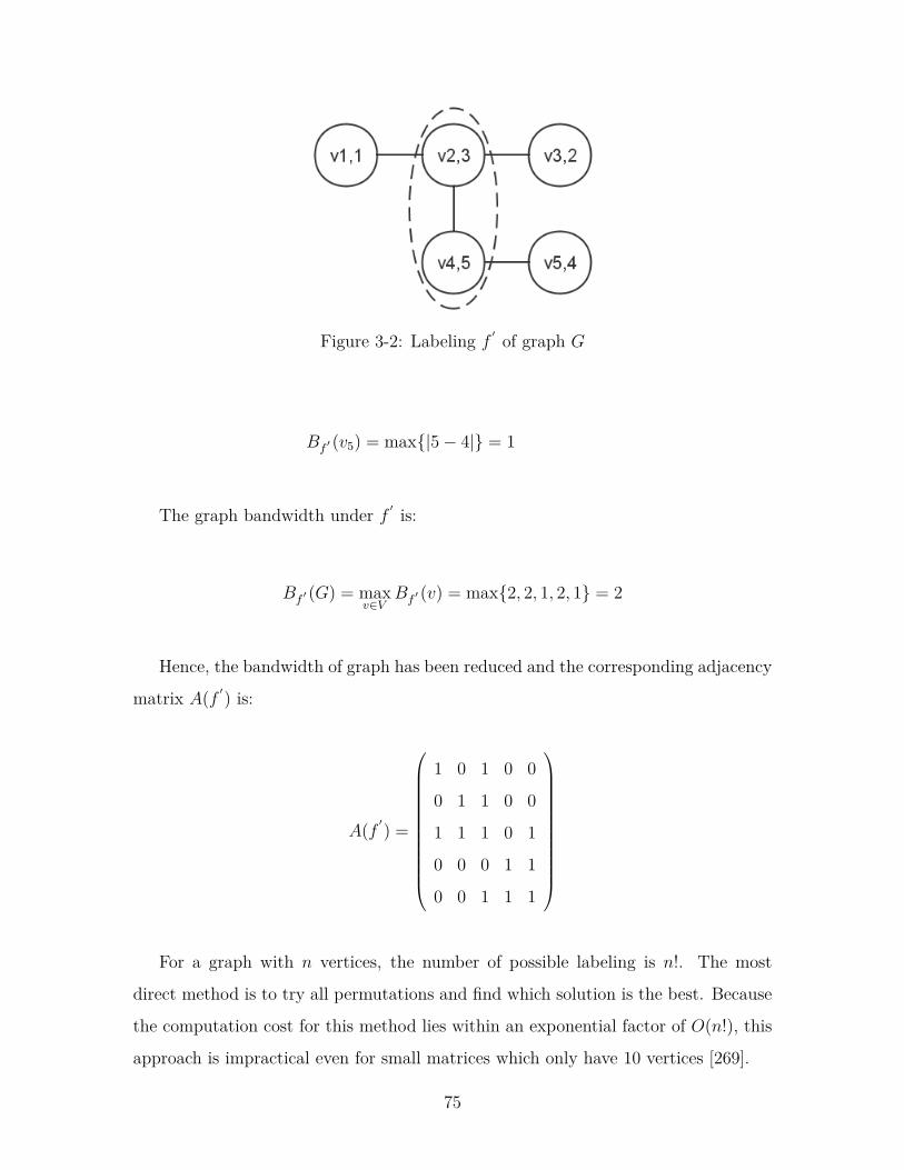
Figure 3-2: Labeling f ′ of graph G

Bf ′ (v5) = max|5− 4| = 1

The graph bandwidth under f ′ is:

Bf ′ (G) = maxv∈V

Bf ′ (v) = max2, 2, 1, 2, 1 = 2

Hence, the bandwidth of graph has been reduced and the corresponding adjacency

matrix A(f ′) is:

A(f ′) =

1 0 1 0 0

0 1 1 0 0

1 1 1 0 1

0 0 0 1 1

0 0 1 1 1

For a graph with n vertices, the number of possible labeling is n!. The most

direct method is to try all permutations and find which solution is the best. Because

the computation cost for this method lies within an exponential factor of O(n!), this

approach is impractical even for small matrices which only have 10 vertices [269].

75

3.2 Solution methods

Based on the literature, the algorithms of bandwidth minimization problem can be

divided into two classes. The first one is exact algorithms. The second one is heuristic

methods, and recently metaheuristics have been developed for this problem in order

to obtain high quality solutions.

3.2.1 Exact algorithms

For the optimal labeling of vertices in the graph and optimal permutation of rows

and columns in the matrix, the exact algorithms are mainly based on branch and

bound search. Del Corso and Manzini [90] proposed two exact branch and bound

methods: MB-ID and MB-PS to solve small and medium instances. MB-ID(Minimum

Bandwidth by Iterative Deepening) uses a depth first search, and MB-PS (Minimum

bandwidth by Perimeter Search) is based on perimeter search which is a developed

variant of depth first search. Caprara and Salazar [64] solved large size instances by

introducing tighter lower bounds. Martí et al. [227] proposed an algorithm which

combines the branch and bound search with some information based on a heuristic.

It used the solution obtained by GRASP algorithm from [267] as the initial upper

bound of branch and bound procedure.

For exact algorithms, the computational cost should be considered to obtain the

optimal solution. Therefore, these methods can only be able to solve comparatively

small size problems with a reasonable running time.

3.2.2 Heuristic algorithms

Heuristic refers to the technique which is based on experience, and it gives a solution

which is not guaranteed to be optimal. However, heuristics can quickly find a solution

which is good enough for combinatorial optimization problems.

In 1969, the well-known Cuthill-McKee algorithm [88] appeared, which uses breadth

first search to construct a level structure for graphs. The Cuthill-McKee algorithm

was the most widely used method for bandwidth minimization problem during the

76

1970s, but it has several disadvantages. For example, the time consuming, the actual

bandwidth might be less than the width of level structure [74]. George [124] proposed

a reverse ordering for this problem.

A few years later, Gibbs et al. [126] developed an algorithm known as GPS which

is still based on the level structure. The GPS has three phases [74]:

(1) Finding a diameter of G. Generally, increasing the number of levels will reduce

the vertices number in each level and the width of level structure. Thus, this

phase will have a maximal depth with small width.

(2) Minimizing level width. A new level structure is created by combination of two

previous level structures, and the width of new one usually smaller than the

original ones.

(3) Numbering a level structure. The vertices are labeled level-by-level, and for

each level, the labels are given to vertices starting from the the vertex with the

smallest degree.

The experiment results showed that the GPS algorithm is comparable with the

Cuthill-McKee algorithm while the time consuming is shorter [126].

In [74, 99,125], several other algorithms for bandwidth minimization problem are

mentioned.

3.2.3 Metaheuristics

Metaheuristic is a technique which is more general than heuristic,because the heuris-

tic method is usually specific for a given problem. Metaheuristic can find a sufficiently

good solution even optimal solution for the optimization problem with less computa-

tional assumptions. Therefore, in the past decades, many research papers focused on

using metaheurisitics for solving complex bandwidth minimization problem.

77

Tabu Search

Tabu Search (TS) is a metaheuristic originally proposed by Glover in 1989 [129] [130].

The process of the algorithm is getting a initial solution firstly, then searching a better

solution in neighborhood structure or moving to a worse area and searching the best

solution in it. In order to avoid falling into local optimal solution, the path which

has been searched should be recorded as the basis of the next search. This algorithm

establishes a tabu list, which can avoid the local optimum, to record the local optimum

points which have been searched, and uses the information of the tabu list in the next

search to search these points no longer or selectly. Therefore, the algorithm can jump

out of local optimum point and achieve global optimization.

The simple pseudocode of the Tabu Search is presented in Chapter 2, Algorithm

2.

According to the algorithm of TS, there are two important concepts: tabu list and

aspiration criterion.

1. Tabu list

Tabu list is the core of the tabu search algorithm. The main purpose of tabu list

is to prevent the circulation in search process and avoid falling into local optimum.

It is a circulate list which after each iteration, the latest move will be put in the

end of tabu list, and the earliest move will be released from tabu list. The length

of tabu list significantly influence search speed and quality of solution. If the length

is short, it will cause the circulation of the search, and fall into local optimum. On

the opposite, a tabu list with high length will increase the amount of calculation and

memory. Therefore, a good tabu list length should be as small as possible but also

avoid the algorithm into circulation.

2. Aspiration criterion

Aspiration criterion ensures that when all the candidate solutions or some candi-

date solutions which are better than current solution are banned, the specific solution

can be released, or to say, this solution can be accepted as new current solution.

In 2001, Martí et al. [229] used the tabu search to solve the bandwidth minimiza-

78

tion problem. Extensive experiments showed that their TS outperforms the previous

algorithms. In the following we describe the key parts of this TS algorithm in details.

1. Critical vertex set

In [229], the critical vertex set includes the critical and near critical vertices. A

near critical vertex v is belong to the set which Bf (v) ≥ αBf (G) and 0 < α < 1.

Although the near critical vertices can not influence the current value of bandwidth,

they will possibly become critical in following iterations. Therefore, the critical vertex

set is defined as

C(f) = v : Bf (v) ≥ αBf (G) (3.4)

2. Candidate list of moves

First, a set of suitable swapping vertices is constructed. They defined two quan-

tities for vertex v and current labeling f :

max(v) = maxf(u) : u ∈ N(v) (3.5)

min(v) = minf(u) : u ∈ N(v) (3.6)

and the best labeling for v is

mid(v) = [max(v) +min(v)2 ] (3.7)

Then the set of suitable swapping vertices for vertex v is defined as:

N′(v) = u : |mid(v)− f(u)| < |mid(v)− f(v)| (3.8)

Thus, the candidate list of moves for vertex v is as follows:

CL(v) = move(v, u) : u ∈ N ′(v) (3.9)

3. Move value

Most algorithms define the value of move as the change of objective function

79

value. However, in bandwidth minimization problem, sometimes the bandwidth will

not change after a move if there are more than one critical vertex in the current

labeling. Besides, calculating the bandwidth of graph after each execution of a move

is computationally expensive. Therefore, they defined the value of move(v,u) which

will be changed according to the following three cases:

(1) If (Bf ′ (u) > Bf (u) andBf ′ (u) > βBf (G)),movevalue(v, u) = movevalue(v, u)+

1

(2) For all w in N(v), if (|f ′(v)− f(w)| > Bf (w) and |f ′(v)− f(w)| > βBf (G)),

movevalue(v, u) = movevalue(v, u) + 1

(3) For all w in N(u), if (|f ′(u)− f(w)| > Bf (w) and |f ′(u)− f(w)| > βBf (G)),

movevalue(v, u) = movevalue(v, u) + 1

4. Tabu list

The tabu list is constructed by a one dimensional array, and set to zero initially.

Besides, they set "tenure" as the number of iterations that vertex v is not accepted

to change labels. Each time when vertex v changes labels, the tabu list updates the

tabu status of vertex v.

Greedy Randomized Adaptive Search Procedure

Greedy Randomized Adaptive Search Procedure (GRASP) which is a random and

iterative algorithm was first introduced in Feo and Resende [106,107]. Each iteration

of the GRASP algorithm is composed of two phases: construction and local search.

The description of GRASP is showed in Chapter 2, Algorithm 3.

1. Construction

The construction phase is a process of generating the feasible solution by itera-

tion. In each iteration the restricted candidate list (RCL) which consists of candidate

elements is formed by using greedy function values, and a random element is selected

to add to the solution. After choosing an element from the RCL, the remaining can-

didates need to be recalculated the greedy function value, and a new RCL is formed.

The method of randomly selecting element from RCL makes each construction phase

can produce different feasible solution. When the processing of all elements is com-

80

plete, the iteration is terminated, and returns the feasible solution.

2. Local search

The randomly generated feasible solution from the construction phase can not

ensure the local optimum, so it is necessary to enter the local search phase. The

local search starts from the feasible solution which is obtained in the construction

phase, and find the local optimal solution in a certain neighborhood. The best local

optimum in all iteration is the global optimal solution.

Rinana et al. [267] developed a greedy randomized adaptive search procedure

(GRASP) combined with a path relinking strategy for the bandwidth minimization

problem. The GRASP algorithm is made of two main phases: the construction phase

and the improvement phase.

1. Construction phase

Firstly, a level structure which is a partition of V into sets L1, L2, ..., Lk is con-

structed, and it has the following characteristics:

(1) vertices adjacent to a vertex in level L1 are either in L1 or L2;

(2) vertices adjacent to vertex in level Lk are either in Lk or Lk−1;

(3) vertices adjacent to vertex in level Li (for 1 < i < k) are either in Li−1, Li or

Li+1.

Then, a vertex from the vertices with low degree is randomly selected as the root

in L1, and from this starting vertex, the next level structure should begin with the

vertex of minimum degree in the last level. Next, the vertex will be labeled level-

by-level. In each iteration, the candidate list CL is formed with the vertices in the

current level. Thus, the initial CL is the starting vertex in L1, and after this vertex

has been labeled, CL=L2 and so on.

In order to construct the RCL, the two function are defined:

(1) LeftB(v, l): the difference between l and the minimum label of its adjacent

vertices in level Li−1;

(2) RightB(v, l): the difference between l and the maximum label of its adjacent

vertices in level Li+1.

l is the label will be assigned, and v is the vertex in level Li. If the vertices in

81

level Li+1 have not labeled, a lower bound of RightB(v, l) is defined as the number of

vertices which have not labeled (not including v) in Li plus the number of adjacent

vertices of v in Li+1. Therefore, the RCL is composed of the vertices in CL with a

minimum value of RightB(v, l)− LeftB(v, l).

2. Improvement phase

The local search of GRASP is based on the Tabu Search proposed by Martí et

al. [229]. They considered the set of critical vertices C(f) which do not include the

near critical vertices. Besides, the operator move(u, v) and the candidate list CL(v)

are also used in this algorithm. Meanwhile, a new move evaluation is presented as

the difference between the number of critical vertices which is before and after the

move:

movevalue(u, v) = ||C(f)| − |C(f ′)|| (3.10)

For the selection of vertex u in candidate list CL(v), there are two strategies are

used. The best strategy selects the move whose move(u, v) is the largest among all

moves with u in CL(v); The first strategy selects the first vertex u whose move(u, v)

is strictly positive.

Genetic Algorithm

Genetic algorithm was proposed by Holland [161] inspired by biological evolution,

and it is a metaheuristic which is based on the idea of the survival of the fittest. This

algorithm is a kind of random optimization method, but it is not a simply random

search. Through the evaluation of chromosome and the information of genes in the

chromosome, it efficiently use the existing information to guide the search for those

solution which can improve the optimization quality. Genetic algorithm solves the op-

timization problem as the survival of the fittest process of the chromosome. Through

the generation of chromosome evolution, including the selection, crossover and muta-

tion operation, it eventually find the individual which adapt to the environment, in

other words, obtain the optimal solution of the problem.

82

In Chapter 2, Algorithm 7 simply illustrates the genetic algorithm operation pro-

cess.

The core of genetic algorithm includes the following parts:

1. Fitness value

Fitness value is used to evaluate the individuals. For simply problems, GA usually

use the objective function as the fitness value directly. In optimizing the complex

problems, we need to construct an appropriate evaluation function.

2. Population

The number of population is one of the factors influencing the performance and

efficiency of the algorithm. The number which is too small can not provide enough

sample points, so the algorithm performance is poor, even can not get feasible solution

of the problem. Although large number of population can increase the optimization

information, the running time is too long. In the process of optimization, the number

of populations is allowed to change to adapt the requirement of the algorithm.

3. Selection

Selection operation is also called the copy operation. This operation selects the

individuals which adapt to the environment according to the fitness value. Generally,

the selection will make higher fitness individuals reproduce more next generation, but

for the individuals with smaller fitness, the number of breeding the next generation

is less or even be eliminated. The commonly used methods are proportion selection

and selection based on the ranking. The former selects the corresponding individuals

by the probability which is proportional to fitness value, and the latter is based on

the ranking of individuals in the population.

4. Crossover

Crossover operation is to cross the two selected individuals with a crossover rate,

so that two new individuals are generated. The crossover rate is used to control the

frequency of crossover operation. When the rate is large, the strings in the population

update soon, then the individuals with high fitness value will be destroyed quickly;

The small rate makes little crossover operation and can not generate enough new

individuals.

83

5. Mutation

When the fitness values of next generation which is generated by crossover oper-

ation have stopped evolving and not obtained the optimal, it means the premature

convergence of the algorithm. The root of this phenomenon is the loss of effective

gene, but mutation overcomes this kind of situation to some extent, and it is helpful

to increase the diversity of population. The rate of mutation is a important factor of

enhancing population diversity. The low rate can not generate new individual, but

high rate will make the algorithm as the random search.

In 2006, Lim et al. [209] presented a method combing the genetic algorithm and

improved hill climbing to solve the bandwidth minimization problem. First, based

on the set of suitable swapping vertices which is proposed by [229], they used a hill

climbing strategy to determine whether change the label of critical vertex, and the

condition is that the number of critical edges reduced. This hill climbing strategy

requires O(|V |2|E|) time for each iteration. Next, in order to reduce the required

checking amount, they defined the critical value C(V ) by:

C(V ) =

0 when Bf (v) < Bf (G)

1 when Bf (v) = Bf (G)(3.11)

Through using this definition in the check condition, the time complexity is re-

duced into O(|V |(|V |+ |E|)).

Then a genetic algorithm with this improved hill climbing is proposed. The

method used the label sequences as chromosomes, and the different chromosomes

are set as an initial set of solution. The crossover and mutation operations are ap-

plied on this set to generate new chromosomes. The next generation consists of the

fittest chromosomes and the algorithm stops after a certain generations. The features

of the GA algorithm are described as follows:

1. Initial population

The initial population is generated by a level structure procedure which using

breadth-first-search (BFS). A level structure of a graph is denoted by L(G), and

it is a partition of the vertices into levels L1, L2, ..., Lk which satisfy the following

84

conditions [16, 229]:




Li+1.

According to this, reasonable good solutions can be obtained. Therefore, initial

populations are generated by applying BFS with randomly selecting the start vertex,

and different start vertices will provide different initial solutions. According to the

experiment, the size of population is set to be 100 can balance the solution quality

and running time.

2. Crossover

The crossover operation used mid-point crossover scheme. The two parent chro-

mosomes are selected randomly, and split at the mid point of string. The genes to the

left half of the split from one chromosome are exchanged with genes to the right half

of the split from the other chromosome, and two new chromosomes are generated.

The experiment showed that when the crossover rate exceeds 0.95, the best solutions

can be obtained.

3. Mutation

This GA used a k swap mutation scheme. A parent chromosome is chosen ran-

domly at the beginning, then each time two labels are selected randomly in the parent

chromosome and exchanged, and such operation will be done k times. Through the

experiment, the best solutions are obtained when the mutation rate is between 0.002

to 0.005.

4. Selection

After generating the new chromosomes by crossover and mutation operation, and

using the improved hill climbing to the new chromosomes, the fitness value of the

new chromosomes will be calculated again, and the chromosomes which have largest

fitness value from the old and new chromosomes are selected as the new generations.

From the experiment results, the bandwidth decreased quickly before 30 generations.

Therefore, the GA set 60 generations for considering both solution quality and running

85

time.

Scatter Search

Scatter Search (SS) is introduced by Glover [127] in 1997. The purpose of this al-

gorithm is that obtain the better solution on the basis of original solution (parent

generation). The main operation of the algorithm focus on the reference set. The

new solutions are generated by the combination of reference subset, and the main

mechanism of combination is linear combination of two solutions from reference set.

The new solution must be improved, after that, it is likely to enter the reference set.

The main steps of Scatter Search are presented in Chapter 2, Algorithm 8, and

the five components are explained in the following:

1. Diversification Generation

It generates the diverse trial solutions from the arbitrary trial solutions as the

input of the algorithm.

2. Improvement

It transforms a trial solution into one or more enhanced trial solutions, and the

local search is usually used in this step.

3. Reference Set Update

It is used to establish and maintain the reference set. The reference set consists of

two subsets, one is composed of good quality solutions, the other one includes good

diversity solution. Therefore, the goal is to ensure the good quality and diversity of

the solutions.

4. Subset Generation

It creates the subset of reference set as a basis of creating combined solutions.


It is transformed the subset of solutions which is produced by Subset Generation

into one or more combined solutions.

Campos et al. [60] used the Scatter Search (SS) to solve the bandwidth mini-

mization problem. Because the Diversification Generation, the Improvement and the

Solution Combination are problem dependent, so these method should be designed

86

specifically. The SS presents the three methods as follows.

1. Diversification Generation

Pinana et al. [267] proposed five different constructive methods. C2 based on the

node assignment and C5 based on the level structure are used to obtain solutions

with different structures. Besides, a new method C6 is proposed to enhance the

diversity of solutions. Based on the level structure of C5, the difference between C5

and C6 is that C6 directly gives label l to the vertex v with the minimum value of

LeftB(v, l)−RightB(v, l) and do not generate candidate list.

2. Improvement

This local search is similar to the GRASP improvement phase [267]. For the

selection strategy which chooses a vertex to be considered for a move, [60] used the

first strategy.


Four different combination methods are presented to obtain a new solution.

(1) Comb1 is based on the "average label". Given two labeling f and g, the

"average label" for vertex v is

Avg(v) = (1/2)(f(v) + g(v)) (3.12)

Then the vertices are sorted according to their average values from lowest to

highest, and assigned the labels for them from 1 to n.

(2) Comb2 is based on the "convex combination label".

Conv(v) = f(v) + λ(g(v)− f(v)) (3.13)

and sorting and labeling vertices are same as Comb1.

(3) Comb3 considers that each labeling votes for its first label which has not been

included in the combine solution, and the vote decides the next label to the first

as the vertex which has not been labeled of the combined solution. Besides, before

combining two solutions with Comb3, one of the solution is rotated to maximize the

number of vertices with the same label in two solutions.

87

(4) Comb4 constructs two level structures. The first one starts from the vertex

which has label 1 in solution f , and the level structure as in GRASP is constructed.

The second one firstly focuses on the vertices in the last level of first level structure.

Then from those vertices, the vertex with largest label in solution g is selected and

set as the starting vertex for the second level structure. Finally, these two level

structures are combined, and in each level, the first label is given to the vertex with

lowest average value which defined in Comb1.

Simulated Annealing

Simulated Annealing (SA) is a probabilistic meta-heuristic proposed in [181]. The

algorithm generates an initial solution and temperature parameter T . Then, in each

iteration, a solution x′ is randomly selected in the neighborhood N(x) of the current

solution x. If x′ is better than x, x′ is accepted and x is replaced by x′ . Otherwise,

x′ can be accepted with a probability depending on the difference of value between

two solutions and the temperature parameter.

In pseudocode, the SA algorithm can be presented in Chapter 2, Algorithm 1:

The acceptance probability and cooling schedule are the important part in SA.

1. Acceptance Probability

The key fact of SA to achieve the global search is acceptance probability. SA

algorithms usually use min[1, exp(−∆C/t)] where ∆C is the value difference between

new and current solution (∆C = f(x′)− f(x))as the acceptance probability.

2. Cooling Schedule

In cooling schedule, the initial temperature can influence the solution. Experiment

results show that if the initial temperature is higher, the probability of getting good

solution is bigger, but the calculation time will increase. Therefore, the selection of

initial solution should consider both solution quality and running time. For updating

the temperature, the most common function is tk+1 = αtk (0 < α < 1). The update

function of temperature shows that the temperature decreases during the search pro-

cess, so the probability of accepting the worse solution is high at the beginning of

search, and it gradually decreases as the temperature drops.

88

Rodriguez-Tello et al. [281] proposed an improved simulated annealing algorithm

for bandwidth minimization problem. This method integrates three important fea-

tures which have a great influence on the heuristic search which described specifically

as follows:

1. Internal representation

For a given graph G = (V,E), a labeling f is defined as f : V → 1, 2, ..., n where

n = |V |. Then the labeling f is represented as an array l whose ith value l[i] denotes

the vertex with the label i. This representation has a key characteristic: because

of the intrinsical locality, an interchange of two adjacent vertices produces smooth

changes [281].

2. Neighborhood function

The neighborhood of the current labeling f in this algorithm is that f ′ is obtained

by rotating the labels from f . swap(f(i), f(j)) is the function of exchanging two labels

of f , and the rotation between two labels f(i) and f(j) is defined as:

rotation(f(i), f(j))

= swap(f(i), f(j)) ∗ swap(f(i), f(j − 1)) ∗

∗ swap(f(i), f(j − 2)) ∗ · · · ∗ swap(f(i), f(i+ 1)) (3.14)

where 0 ≤ f(i) ≤ n−1, 0 ≤ f(j) ≤ n−1 and f(i) < f(j). The rotation can construct

a compound move, and the compound moves can find better solution than those only

using the simply moves.

3. Evaluation function

The proposed evaluation function for a labeling f is defined as follows where dxis the number of absolute differences with value x between two adjacent vertices, and

β is the bandwidth of labeling f :

δ(f) = β +β∑x=1

(dx

(n+β−x+1)!n!

))

(3.15)

This new evaluation function is to decrease the impact of the absolute differences

89

dx with small values and increase the influence of those with values close to the

bandwidth β, so it is sensitive enough to catch the smallest improvement.

Variable Neighborhood Search

Variable Neighborhood Search (VNS) was firstly proposed by Hansen and Mladenovic

[236] in 1997. This meta-heuristic has been proved to be very useful for obtaining

an approximate solution to optimization problems. Variable neighborhood search

systematically changes the set of neighborhood structure to expand the search range

and obtain the local optimal solution until the best solution is found.

The pseudocode of the Variable Neighborhood Search is presented in Chapter 2,

Algorithm 6.

According to the approach, after generating the initial solution, the main cycle of

VNS begins. This cycle includes three steps: shaking, local search, move or not.

1. Shaking

The aim of shaking is jumping out current area of local optimal solution and

search new one to make local optimum near the global optimal solution.

2. Local search

Local search is used to find local optimal solution and improve search precision.

The result of local search is mainly dependent on the selection of the starting point and

neighborhood structure. Therefore, in order to obtain better solution, the different

neighborhood structure and starting point can be chosen in local search.

3. Move or not

Because a local optimal solution which is obtained in one neighborhood structure

may be not local optimal in another neighborhood structure, so the choice of accep-

tance criteria for move or not is very important. In literature [145,148], the problem

of what strategy should be used is considered, and several strategies of move or not

are discussed.

Mladenovic et al. [237] proposed a variable neighborhood search method which

combines several ideas from the literatures for minimizing the bandwidth problem.

The experiment results of 113 benchmark instances showed that the performance of

90

the proposed VNS approach was better than all previous methods. The detail of the

key parts is described as follows.

1. Initialization

The random initial solution replaced by a good quality one in this method. They

construct a good initial solution with depth-first-search manner. The idea is obvious:

In a good solution which means the small bandwidth, the adjacent vertices should

have close labels. The initial labeling of vertex is set in rows: There is only one

vertex v which is selected randomly in first row, and this vertex is given the label 1

(f(v)← 1); the second row contains the adjacent vertices of vertex v, and the label of

them is 2,3,...; the third row contains the adjacent vertices of the vertices in previous

row, but these adjacent vertices do not appear in second row and so on.

2. Shaking

Two shaking functions are proposed in [237]. The first one defined a distance

to show the number of different labels between any two solution f and f′ at the

beginning. The distance is given by

ρ(f, f ′) =n∑i=1

η(i)− 1, η(i)− 1 =

1 f(i) = f′(i)

0 otherwise(3.16)

Then a vertex u ∈ K (the set K is specially defined) is chose randomly, and the

its critical vertex v is found. Next a vertex w which satisfy the following condition

would be selected as the swap vertex with v: maxf(v) − fmin(w), fmax(w) − f(v)

is minimum, where fmin(u) ≤ f(w) ≤ fmax(u).

The second shaking function uses the transformation from f to π (or from π to

f) as follows: π(f(v)) = v,∀v (or f(π(v)) = v,∀v).

3. Local search

In local search of this VNS algorithm, the define of suitable swapping vertices

proposed by [229] and the hill climbing strategy proposed by [209] was applied to

construct the reduced swap neighborhood.

4. Move or not

Three acceptance criteria are used in [237]:

91

(1) If the new objective function value is better than current one: Bf ′ (G) < Bf (G)

(2) If Bf ′ (G) = Bf (G), the number of critical vertices of f ′ is smaller than f :

|Vc(f′)| < |Vc(f)|

(3) If Bf ′ (G) = Bf (G) and |Vc(f′)| = |Vc(f)|, the distance between f and f

′ is

far: ρ(f, f ′> α) (α = 10 is set in [237])

3.3 The VNS approach for bandwidth minimiza-

tion problem

The detail of our algorithm for solving bandwidth minimization problem is described

as follows.

3.3.1 Initial solution

A good initial solution can be generated by a level structure procedure which using

breadth first search (BFS). The idea is that adjacent vertices should have close labels.

A level structure of a graph is denoted by L(G), and it is a partition of the vertices

into levels L1, L2, ..., Lk which satisfy the following conditions [229]:




Li+1.

According to this, reasonable good solutions can be obtained. Therefore, initial

solutions are generated by applying BFS with random selection of the starting vertex,

and different starting vertices will provide different initial solutions. For example, for

the matrix A, if we start from the vertex v3, the bandwidth decreases to 3. If we

choose vertex v2 as the first label, the bandwidth is 2. Figure 3-3 and 3-4 show the

examples of initial solution. According to the level structure, all the initial solutions

92

are better than the original assignment. Obviously, the bandwidth obtained by this

method can not be worse than the maximum bandwidth of the graph, because the

adjacent vertices are assigned with sequential numbers. BFS method gives an upper

bound of good quality solution.

Figure 3-3: v3 is the first label vertex

Figure 3-4: v2 is the first label vertex

3.3.2 Shaking

A labeling f ′ is in the kth neighborhood of the labeling f , that is, there are k + 1

different labels between f and f ′. More precisely, the distance ρ between any two

solutions f and f ′ is defined as:

ρ(f, f ′) =n∑i=1

η(i)− 1, η(i) =

1 f(i) = f ′(i)

0 f(i) 6= f ′(i)(3.17)

93

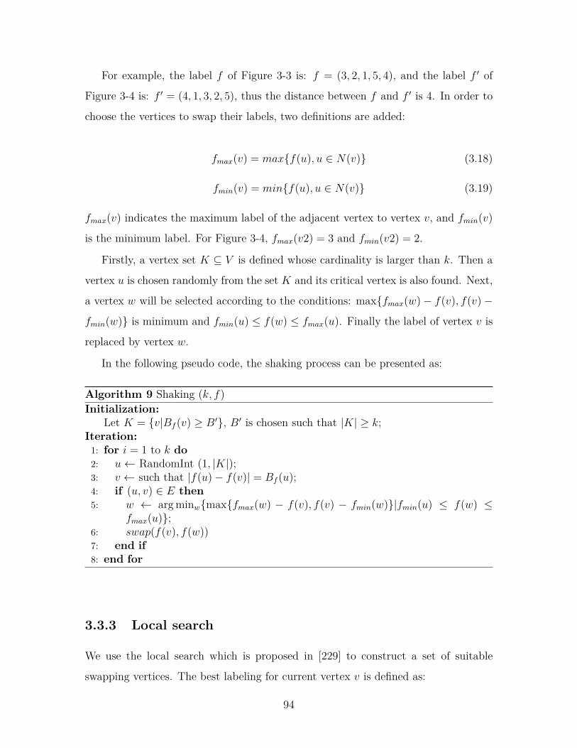
For example, the label f of Figure 3-3 is: f = (3, 2, 1, 5, 4), and the label f ′ of

Figure 3-4 is: f ′ = (4, 1, 3, 2, 5), thus the distance between f and f ′ is 4. In order to

choose the vertices to swap their labels, two definitions are added:

fmax(v) = maxf(u), u ∈ N(v) (3.18)

fmin(v) = minf(u), u ∈ N(v) (3.19)

fmax(v) indicates the maximum label of the adjacent vertex to vertex v, and fmin(v)

is the minimum label. For Figure 3-4, fmax(v2) = 3 and fmin(v2) = 2.

Firstly, a vertex set K ⊆ V is defined whose cardinality is larger than k. Then a

vertex u is chosen randomly from the set K and its critical vertex is also found. Next,

a vertex w will be selected according to the conditions: maxfmax(w)− f(v), f(v)−

fmin(w) is minimum and fmin(u) ≤ f(w) ≤ fmax(u). Finally the label of vertex v is

replaced by vertex w.

In the following pseudo code, the shaking process can be presented as:

Algorithm 9 Shaking (k, f)Initialization:

Let K = v|Bf (v) ≥ B′, B′ is chosen such that |K| ≥ k;Iteration:1: for i = 1 to k do2: u← RandomInt (1, |K|);3: v ← such that |f(u)− f(v)| = Bf (u);4: if (u, v) ∈ E then5: w ← arg minwmaxfmax(w) − f(v), f(v) − fmin(w)|fmin(u) ≤ f(w) ≤

fmax(u);6: swap(f(v), f(w))7: end if8: end for

3.3.3 Local search

We use the local search which is proposed in [229] to construct a set of suitable

swapping vertices. The best labeling for current vertex v is defined as:

94

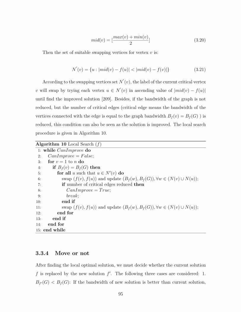
mid(v) = [max(v) +min(v)2 ] (3.20)

Then the set of suitable swapping vertices for vertex v is:

N′(v) = u : |mid(v)− f(u)| < |mid(v)− f(v)| (3.21)

According to the swapping vertices setN ′(v), the label of the current critical vertex

v will swap by trying each vertex u ∈ N′(v) in ascending value of |mid(v) − f(u)|

until find the improved solution [209]. Besides, if the bandwidth of the graph is not

reduced, but the number of critical edges (critical edge means the bandwidth of the

vertices connected with the edge is equal to the graph bandwidth Bf (v) = Bf (G) ) is

reduced, this condition can also be seen as the solution is improved. The local search

procedure is given in Algorithm 10.

Algorithm 10 Local Search (f)1: while CanImprove do2: CanImprove = False;3: for v = 1 to n do4: if Bf (v) = Bf (G) then5: for all u such that u ∈ N ′(v) do6: swap (f(v), f(u)) and update (Bf (w), Bf (G)),∀w ∈ (N(v) ∪N(u));7: if number of critical edges reduced then8: CanImprove = True;9: break;10: end if11: swap (f(v), f(u)) and update (Bf (w), Bf (G)),∀w ∈ (N(v) ∪N(u));12: end for13: end if14: end for15: end while

3.3.4 Move or not

After finding the local optimal solution, we must decide whether the current solution

f is replaced by the new solution f ′. The following three cases are considered: 1.

Bf ′(G) < Bf (G): If the bandwidth of new solution is better than current solution,

95

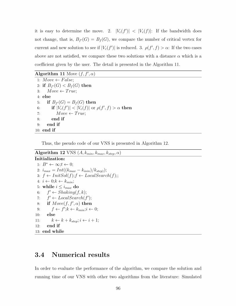
it is easy to determine the move. 2. |Vc(f ′)| < |Vc(f)|: If the bandwidth does

not change, that is, Bf ′(G) = Bf (G), we compare the number of critical vertex for

current and new solution to see if |Vc(f ′)| is reduced. 3. ρ(f ′, f) > α: If the two cases

above are not satisfied, we compare these two solutions with a distance α which is a

coefficient given by the user. The detail is presented in the Algorithm 11.

Algorithm 11 Move (f, f ′, α)1: Move← False;2: if Bf ′(G) < Bf (G) then3: Move← True;4: else5: if Bf ′(G) = Bf (G) then6: if |Vc(f ′)| < |Vc(f)| or ρ(f ′, f) > α then7: Move← True;8: end if9: end if10: end if

Thus, the pseudo code of our VNS is presented in Algorithm 12.

Algorithm 12 VNS (A, kmin, kmax, kstep, α)Initialization:1: B∗ ←∞;t← 0;2: imax = Int((kmax − kmin)/kstep));3: f ← InitSol(f);f ← LocalSearch(f);;4: i← 0;k ← kmin;5: while i ≤ imax do6: f ′ ← Shaking(f, k);7: f ′ ← LocalSearch(f ′);8: if Move(f, f ′, α) then9: f ← f ′;k ← kmin;i← 0;10: else11: k ← k + kstep; i← i+ 1;12: end if13: end while

3.4 Numerical results

In order to evaluate the performance of the algorithm, we compare the solution and

running time of our VNS with other two algorithms from the literature: Simulated

96

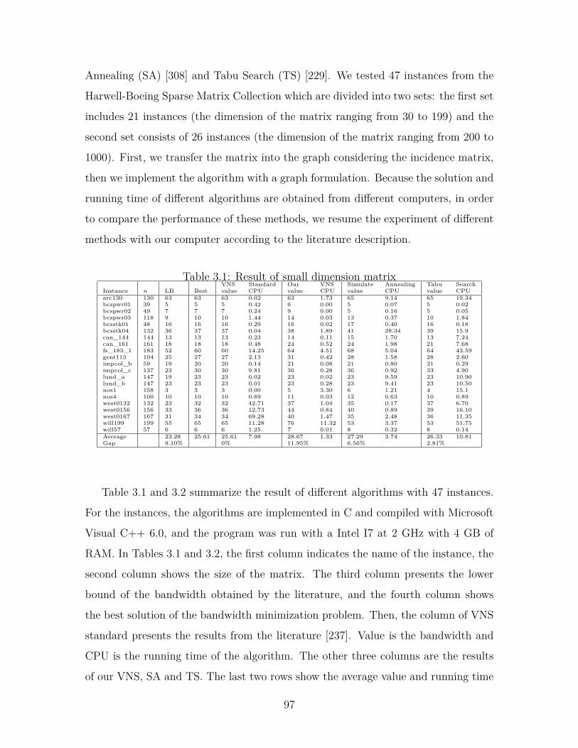
Annealing (SA) [308] and Tabu Search (TS) [229]. We tested 47 instances from the

Harwell-Boeing Sparse Matrix Collection which are divided into two sets: the first set

includes 21 instances (the dimension of the matrix ranging from 30 to 199) and the

second set consists of 26 instances (the dimension of the matrix ranging from 200 to

1000). First, we transfer the matrix into the graph considering the incidence matrix,

then we implement the algorithm with a graph formulation. Because the solution and

running time of different algorithms are obtained from different computers, in order

to compare the performance of these methods, we resume the experiment of different

methods with our computer according to the literature description.

Table 3.1: Result of small dimension matrixVNS Standard Our VNS Simulate Annealing Tabu Search

Instance n LB Best value CPU value CPU value CPU value CPUarc130 130 63 63 63 0.02 63 1.73 65 9.14 65 19.34bcspwr01 39 5 5 5 0.42 6 0.00 5 0.07 5 0.02bcspwr02 49 7 7 7 0.24 9 0.00 5 0.16 5 0.05bcspwr03 118 9 10 10 1.44 14 0.03 13 0.37 10 1.84bcsstk01 48 16 16 16 0.29 16 0.02 17 0.40 16 0.18bcsstk04 132 36 37 37 0.04 38 1.89 41 28.34 39 15.9can_144 144 13 13 13 0.23 14 0.11 15 1.70 13 7.24can_161 161 18 18 18 0.48 24 0.52 24 1.98 21 7.68fs_183_1 183 52 60 60 14.25 64 4.51 68 5.04 64 43.59gent113 104 25 27 27 2.13 31 0.42 28 1.58 28 2.60impcol_b 59 19 20 20 0.14 21 0.08 21 0.80 21 0.29impcol_c 137 23 30 30 9.81 36 0.28 36 0.92 33 4.90lund_a 147 19 23 23 0.02 23 0.02 23 9.59 23 10.90lund_b 147 23 23 23 0.01 23 0.28 23 9.41 23 10.50nos1 158 3 3 3 0.00 5 3.30 6 1.21 4 15.1nos4 100 10 10 10 0.89 11 0.03 12 0.63 10 0.89west0132 132 23 32 32 42.71 37 1.04 35 0.17 37 6.70west0156 156 33 36 36 12.73 44 0.84 40 0.89 39 16.10west0167 167 31 34 34 69.28 40 1.47 35 2.48 36 11.35will199 199 55 65 65 11.28 76 11.32 53 3.37 53 51.75will57 57 6 6 6 1.25 7 0.01 8 0.32 8 0.14Average 23.28 25.61 25.61 7.98 28.67 1.33 27.29 3.74 26.33 10.81Gap 9.10% 0% 11.95% 6.56% 2.81%

Table 3.1 and 3.2 summarize the result of different algorithms with 47 instances.

For the instances, the algorithms are implemented in C and compiled with Microsoft

Visual C++ 6.0, and the program was run with a Intel I7 at 2 GHz with 4 GB of

RAM. In Tables 3.1 and 3.2, the first column indicates the name of the instance, the

second column shows the size of the matrix. The third column presents the lower

bound of the bandwidth obtained by the literature, and the fourth column shows

the best solution of the bandwidth minimization problem. Then, the column of VNS

standard presents the results from the literature [237]. Value is the bandwidth and

CPU is the running time of the algorithm. The other three columns are the results

of our VNS, SA and TS. The last two rows show the average value and running time

97

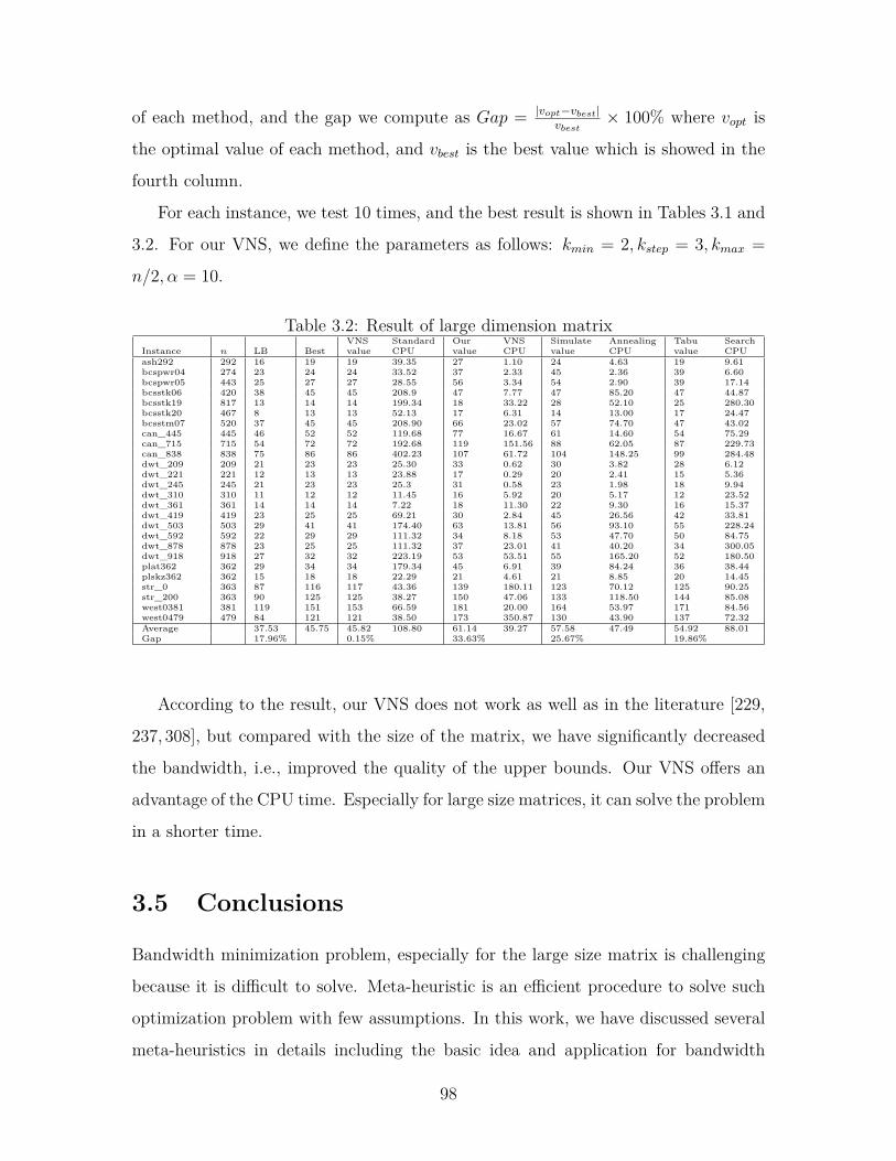
of each method, and the gap we compute as Gap = |vopt−vbest|vbest

× 100% where vopt is

the optimal value of each method, and vbest is the best value which is showed in the

fourth column.

For each instance, we test 10 times, and the best result is shown in Tables 3.1 and

3.2. For our VNS, we define the parameters as follows: kmin = 2, kstep = 3, kmax =

n/2, α = 10.

Table 3.2: Result of large dimension matrixVNS Standard Our VNS Simulate Annealing Tabu Search

Instance n LB Best value CPU value CPU value CPU value CPUash292 292 16 19 19 39.35 27 1.10 24 4.63 19 9.61bcspwr04 274 23 24 24 33.52 37 2.33 45 2.36 39 6.60bcspwr05 443 25 27 27 28.55 56 3.34 54 2.90 39 17.14bcsstk06 420 38 45 45 208.9 47 7.77 47 85.20 47 44.87bcsstk19 817 13 14 14 199.34 18 33.22 28 52.10 25 280.30bcsstk20 467 8 13 13 52.13 17 6.31 14 13.00 17 24.47bcsstm07 520 37 45 45 208.90 66 23.02 57 74.70 47 43.02can_445 445 46 52 52 119.68 77 16.67 61 14.60 54 75.29can_715 715 54 72 72 192.68 119 151.56 88 62.05 87 229.73can_838 838 75 86 86 402.23 107 61.72 104 148.25 99 284.48dwt_209 209 21 23 23 25.30 33 0.62 30 3.82 28 6.12dwt_221 221 12 13 13 23.88 17 0.29 20 2.41 15 5.36dwt_245 245 21 23 23 25.3 31 0.58 23 1.98 18 9.94dwt_310 310 11 12 12 11.45 16 5.92 20 5.17 12 23.52dwt_361 361 14 14 14 7.22 18 11.30 22 9.30 16 15.37dwt_419 419 23 25 25 69.21 30 2.84 45 26.56 42 33.81dwt_503 503 29 41 41 174.40 63 13.81 56 93.10 55 228.24dwt_592 592 22 29 29 111.32 34 8.18 53 47.70 50 84.75dwt_878 878 23 25 25 111.32 37 23.01 41 40.20 34 300.05dwt_918 918 27 32 32 223.19 53 53.51 55 165.20 52 180.50plat362 362 29 34 34 179.34 45 6.91 39 84.24 36 38.44plskz362 362 15 18 18 22.29 21 4.61 21 8.85 20 14.45str_0 363 87 116 117 43.36 139 180.11 123 70.12 125 90.25str_200 363 90 125 125 38.27 150 47.06 133 118.50 144 85.08west0381 381 119 151 153 66.59 181 20.00 164 53.97 171 84.56west0479 479 84 121 121 38.50 173 350.87 130 43.90 137 72.32Average 37.53 45.75 45.82 108.80 61.14 39.27 57.58 47.49 54.92 88.01Gap 17.96% 0.15% 33.63% 25.67% 19.86%

According to the result, our VNS does not work as well as in the literature [229,

237, 308], but compared with the size of the matrix, we have significantly decreased

the bandwidth, i.e., improved the quality of the upper bounds. Our VNS offers an

advantage of the CPU time. Especially for large size matrices, it can solve the problem

in a shorter time.

3.5 Conclusions

Bandwidth minimization problem, especially for the large size matrix is challenging

because it is difficult to solve. Meta-heuristic is an efficient procedure to solve such

optimization problem with few assumptions. In this work, we have discussed several

meta-heuristics in details including the basic idea and application for bandwidth

98

minimization problem. Besides, We transfer the matrix problem into a graph problem

and apply variable neighborhood search (VNS) to solve the bandwidth minimization

problem. By combining the improved local search with the basic VNS and defining

the parameters which influent the neighborhood change, the experiment results show

that our VNS is competitive with the state of art from the result quality point of

view, and both for the small and large instances, our VNS outperforms the state of

art from CPU time point of view. For the future work, on one hand, we could further

improve the result quality of our algorithm with considering to add a restart in the

program so that it does not end early and may gain better solution. On the other

hand, because of the reduced running time of our VNS, we can use this algorithm to

solve very large size instances, i.e., matrices with more than 10,000×10,000..

99

100

Chapter 4

Wireless Network

Mobile communication is an important component of modern communication sys-

tems. As the name suggests, mobile communication consists in at least one of the

communicating parties to transmit information in a state of motion.

The development of modern mobile communication technology began in the 1920s.

Mobile communication not only integrates the latest technological achievement of

wireless communication and wired communication, but also many achievements of

network reception and computer technology. Currently, mobile communication has

been developed from analog communication to digital communication stage, and to a

higher stage of fast and reliable individual communication. The goal of future mobile

communication is to be able to provide fast and reliable communication service to

anyone at any time and any place [273].

In the end of 1978, the United States Bell Labs successfully developed the ad-

vanced mobile phone system (AMPS) and built a cellular simulation mobile commu-

nication network which greatly improved the system capacity. At the same time, other

countries had also developed the public cellular mobile communication network. At

this stage, the cellular mobile communication network became a practical system, and

rapidly developed around the world. The reasons for the rapid development of mobile

communication are not only the main driving force of rapid increase in user demand,

but also the condition offered by several aspects of technological development. First,

micro-electronic technology had rapidly developed in this period which made the com-

101

munication device can realize miniaturization and microminiaturization. Second, the

concept of cellular network which is proposed by Bell Labs in the 1970s formed a new

system of mobile communication. The birth of the mobile communication system in

this stage is generally called the first generation mobile communication system.

In the early 1990s, the Qualcomm company proposed CDMA cellular mobile com-

munication system which is a milestone in the development of mobile communication

system. Since then, CDMA occupied the more important position in the field of

mobile communication. The digital mobile communication system which is currently

widely used is called the second generation mobile communication system. However,

with the increasing requirement of communication service range and business, the

second generation mobile communication system was difficult to meet new business

needs. In order to meet the market demands, the third generation mobile communi-

cation system (3G) which is mainly based on CDMA was proposed.

However, for the high speed data service, both the single carrier TDMA system

and the narrow band CDMA system are flawed, the research of fourth generation

mobile communication system (4G) emerged. The fourth genration mobile communi-

cation technology will have the function of intelligence, broadband, individualization

and mobilization. Orthogonal Frequency Division Multiplexing (OFDM) technology

is generally considered as the core technology in the fourth generation mobile com-

munication system because its network structure is highly scalable and it has good

anti-noise property and high utilization of the spectrum [276].

Section 4.1 introduces development, application and characteristic of OFDM. Sec-

tion 4.2 discusses the background of OFDMA system, the definition of resource alloca-

tion problem of OFDMA system and the solving method and their research states in

detail. Section 4.3 proposes a hybrid resource allocation model for OFDMA-TDMA

wireless networks and an algorithmic framework using a variable neighborhood search

metaheuristic approach (VNS for short) for solving the problem. Section 4.4 presentes

a (0-1) stochastic resource allocation model for uplink wireless multi-cell OFDMA

Networks and a simple reduced variable neighborhood search metaheuristic proce-

dure to solve this model. Section 4.5 concludes this chapter.

102

4.1 Orthogonal Frequency Division Multiplexing

(OFDM)

4.1.1 Development and application

Orthogonal Frequency Division Multiplexing (OFDM) originated in the mid 1950s,

and the concept of using parallel data transmission and frequency division multiplex-

ing had been formed in 1960s. The first practical application is the high frequency

wireless communication link for military. In 1971, Weinstein and Ebert applied the

discrete Fourier transform (DFT) to the modulation and demodulation of orthogonal

frequency division multiplexing system [330].

Because Orthogonal frequency division multiplexing multi-carrier transmission

technique can effectively solve the inter-symbol interference problem which is faced

by the broadband wireless communication system, it is suitable for the high speed da-

ta transmission in mobile environment. For this reason, OFDM technology received

more and more attention and began to be widely used in practical systems.

Application 1: High definition television (HDTV)

OFDM made a wide range of applications in digital broadcast television system.

Further, the modulation technique which is adopted by digital HDTV transmission

system includes OFDM. In the area of digital audio broadcasting and digital video

broadcasting (DVB), the main reason of selecting OFDM is: OFDM can effectively

solve the multipath delay spread problem.

Application 2: Wireless Local Area Network (WLAN)

The continuous development of technology triggers the fusion of technology. Some

key technologies of 3.5G and 4G such as OFDM, MIMO, smart antenna and software

defined radio start to be applied in the wireless local area network to enhance the

performance of WLAN. For example, 802.11a and 802.11g improves the transmission

rate and increases the network throughput by using OFDM modulation technique;

802.11n plans to use a combination of MIMO and OFDM to make transmission rate

doubled.

103

Application 3: Broadband Wireless Access (BWA)

Because OFDM technology is suitable for the high speed transmission in wireless

environment, it is applied in Broadband Wireless Access (BWA). In the field of BWA,

although the developed technologies of some companies are based on OFDM, they

have their own characteristics. For example, Vector OFDM (VOFDM) from Cisco

and Iospan company, Wideband OFDM (WOFDM) from Wi-LAN company and flash

OFDM from Flarion company.

Application 4: Wimax and IEEE 802.16

Another wireless data solution based on OFDM which has been widely recognized

is IEEE 802.16. The typical application of 802.16 includes mesh network, back-haul

and broadband mobile network.

4.1.2 OFDM characteristics

In recent years, OFDM system is more widely used because it has the following

advantages:

1. High spectral utilization

In the conventional frequency division multiplexing access, the frequency band is

divided into several disjoint subfrequency bands to transmit data in parallel, so the

utilization of the spectrum is low. In OFDM system, each subcarrier is orthogonal to

each other and spectrum overlap, thus the spectrum utilization of system is high.

2. The inherent frequency diversity ability

When the data is assigned in parallel on the unrelated subbands to send, the time

diversity and frequency diversity can be combined to improve the reliability of the

system transmission.

3. Different transmission rate

Generally, the amount of transmission data in the downlink is much greater than

in the uplink. For example, the web browsing in Internet business, FTP download,

etc. On the other hand, the power of the mobile terminal is generally small, and

the base station transmission power can be large. Therefore, considering from the

need of user data business and the requirement of mobile communication system, the

104

physical layer is supposed to support the asymmetric data transmission, and OFDM

system can easily achieve the different transmission rate in downlink and uplink by

using a different number of subchannels [350].

However, due to the orthogonal subcarriers in OFDM system, and a plurality of

subchannel signals are superimposed when OFDM outputs signals, so compared with

single carrier system, OFDM has the following drawback:

(1) As the subchannel spectrum covering each other, so the strict requirement of

orthogonality is requested. The basis of OFDM is the subcarrier must be orthogonal.

Otherwise, the performance of the whole system would seriously decline, and the

crosstalk would be generated among the subcarriers.

(2) Compared with single carrier system, the output of multi-carrier modulation

system is a superposition of a plurality of subchannel signals. If the phase of multiple

signals is consistent, the instantaneous power of superimposed OFDM signals will be

greater than the average power of signals. Thus a large peak to average power ratio

(PAR) is generated. How to reduce the PAR of signal is another difficulty in OFDM

technology [330].

4.2 Orthogonal Frequency Division Multiplexing

Access (OFDMA)

Orthogonal frequency division multiplexing access (OFDMA) technology is a key

technology in the fourth generation (4G) mobile communication, which is based on

the OFDM technology. As mentioned before, OFDM technology is a kind of multi-

carrier modulation technique, which uses hundreds or even thousands narrow band

subcarrier for high speed data transmission, wherein the subcarrier is orthogonal

to each other. Because subcarriers overlapping occupy the spectrum, OFDM can

provide high spectrum efficiency and high information transmission rate. Through

assigning different subcarriers to different users, OFDMA provides a natural multi-

access mode. Besides, because of occupying different subcarriers, the orthogonality is

105

satisfied between users and without inter-cell interference. The idea of this technology

is simple which is proposed as early as the 1950s-1960s, and currently it becomes the

key technology of 4G [50].

OFDMA can support fixed terminals and mobile terminals to access the wireless

metropolitan area networks (WMANs). Due to the mobile characteristic of terminals

and the "not line of sight" (NLOS) transmission, the channel fading will appear which

caused by path loss, shadow fading and multi-path effect etc. Thus, for the channel

fading, designing the effective and reliable resource allocation algorithm for OFDMA

technology is necessary. Because OFDMA divides the entire bandwidth into a set of

orthogonal subchannels, thereby increasing the coherence symbol length and making

the system enhance the ability of against inter-symbol interference and frequency

selective fading. For multi-users situation, OFDMA using each user in different time

slots and different subchannels with different channel responses provide a dynamic slot

allocation (DSA) scheme. Therefore, matched channel DSA scheme greatly improves

the system throughput. Meanwhile, the achieved rate of system is directly related to

the distribution power, so the adaptive power allocation (APA) can also improve the

system throughput [5].

OFDMA resource allocation problem can generally be classified as follows. Ac-

cording to the target, OFDMA resource allocation problem can be divided into rate

adaptive (RA) problem and margin adaptive (MA) problem. The RA problem is to

maximize the system throughput under the limited power condition, and the MA

problem is to minimize the power loss of the system subject to the throughput con-

straint [5].

Except the classification of OFDMA problem, generally, OFDMA resource can

be divided into a time slot, a frequency domain (subcarrier), coding (using different

coding techniques) and a space (combined with MIMO). In addition, OFDMA should

face the power limit of base station or mobile terminal, the limit on the number of

bits and the limit of quality of service (Qos) requested by users. Thus OFDMA

resource allocation problem is to optimize the user access under the limit of power,

hardware implementation, bit load and fairness among users and the various channel

106

conditions. The user access is assigning corresponding resource to users, and the

resource includes space, time and frequency. The target can be the purpose of saving

resource, or maximizing the rate of user terminals [202].

4.2.1 Background of OFDMA

OFDMA technology is proposed by Mosier and Clabaugh in 1957. Its principle is to

divide a wide frequency band into several narrow bands and transmit in parallel which

can be good for fighting against multi-path interference. This technology was mature

on theory, but due to the high complexity generated by discrete Flourier transform

which is used in the algorithm and the limitation of integrated circuit implementation,

it had been not put in an important position. Until 1966, Turkey proposed fast

Fourier transform which reduces the complexity from O(N2) to O(N/2 · log2(N/2)),

and integrated circuit rapidly developed, OFDMA technology received attention and

its application had been widely researched [182].

Combining OFDMmodulation technology with multiple access technique will con-

stitute different multi-user mobile communication system. The common multiple

access technique includes: TDMA, FDMA, CDMA, SDMA [276].

1. Time Division Multiple Access (TDMA)

TDMA scheme consists in the channel is divided into a number of time division

channels according to the time slot, then each user occupies one slot and only send

or receive signals within the specified time slot. The key part of TDMA is the user.

Each user is assigned to a time slot.

2. Frequency Division Multiple Access (FDMA)

The frequency division also refers to channelization sometimes. The assignable

spectrum is divided into a plurality of individual wireless channels, each channel can

transmit one voice or control information. Under the system control, any user can

access any one of these channels.

3. Code Division Multiple Access (CDMA)

Unlike FDMA and TDMA which separate the user information from the frequency

and time, CDMA can simultaneously transmit a plurality of user information in

107

one channel, i.e., the mutual interference between users is allowed. The key is the

information should be encoded specially before the transmission, and the original

information will not lost. So many mutually orthogonal code sequence, so many

users can simultaneously communicate on one carrier.

4. Space Division Multiple Access (SDMA)

SDMA is to constitute different channels by using space division. It is a satellite

communication mode, which uses the directivity of dish antenna to optimize the use of

wireless frequency and reduce system cost. For example, using a plurality of antennas

on the satellite, the beam of each antenna toward the different regions of the earth’s

surface. Even the earth stations which are on the ground in different regions work at

the same time with the same frequency, the interference will not be formed between

them.

About the subcarrier allocation scheme, OFDMA must consider the subcarrier

exclusivity. Assuming the number of user as K and the number of subcarrier as N , if

user k is assigned the power pk,n on the subcarrier n, so pk,n 6= 0,∀k ∈ 1, ..., K, n ∈

1, ..., N, and pk′ ,n = 0,∀k′ 6= k, k′ ∈ 1, ..., K, i.e., any subcarrier is used by one

and only one user.

Then, the uplink and downlink resource allocation problem of OFDMA system will

be described [186]. Downlink is one transmitter sending signals to many receiver, for

example, the radio and television broadcasting, the transmission access from a base

station to mobile terminals and the transmission access from a satellite to ground

stations. Uplink is many transmitter sending signals to one receiver, for example, the

laptop wireless LAN, the transmission link from mobile terminals to a base station

and the transmission link from ground stations to a satellite.

Margin adaptive (MA) problem

Assume the throughput of user k is rk. Generally, for the downlink channel, the

system has a limit of total link throughput R, and ∑Kk=1 rk ≥ R; for the uplink

channel, the throughput of each user is limited which can be represented as rk ≥ Rk

[73].

108

The objective of margin adaptive approach is to minimize the system power of

whole system subject to the downlink/uplink throughput constraint and the assigned

power constraint. Assume Pbs is the power constraint of base station, and Pk is the

power constraint of user k. Thus, for downlink, the margin adaptive problem can be

represented as:

minpk,n

k∑k=1

N∑n=1

pk,n

s.t.k∑k=1

N∑n=1

rk,n ≥ R

k∑k=1

N∑n=1

pk,n ≤ Pbs

pk′ ,n = 0,∀pk,n 6= 0;∀k′ 6= k;∀k, k′ ∈ 1, ..., K;∀n ∈ 1, ..., N (4.1)

For uplink, the margin adaptive problem can be represented as:

minpk,n

k∑k=1

N∑n=1

pk,n

s.t.N∑n=1

rk,n ≥ Rk,∀k ∈ 1, ..., K

N∑n=1

pk,n ≤ Pk,∀k ∈ 1, ..., K

pk′ ,n = 0,∀pk,n 6= 0;∀k′ 6= k;∀k, k′ ∈ 1, ..., K;∀n ∈ 1, ..., N (4.2)

Rate adaptive (RA) problem

The objective of rate adaptive approach is to maximize the system throughput with

the power constraint [73]. If the system can provide limited resources, and the channel

condition of some users are good, it is possible that other users can not be completely

assigned the resource. Therefore, for the downlink, the rate adaptive problem can be

written as:

109

maxrk,n

k∑k=1

N∑n=1

rk,n

s.t.N∑n=1

rk,n ≥ Rk,∀k ∈ 1, ..., K

k∑k=1

N∑n=1

pk,n ≤ Pbs

pk′ ,n = 0,∀pk,n 6= 0;∀k′ 6= k;∀k, k′ ∈ 1, ..., K;∀n ∈ 1, ..., N (4.3)

Similarly, for the uplink, the rate adaptive problem can be written as:

maxrk,n

k∑k=1

N∑n=1

rk,n

s.t.N∑n=1

rk,n ≥ Rk,∀k ∈ 1, ..., K

N∑n=1

pk,n ≤ Pk

pk′ ,n = 0,∀pk,n 6= 0;∀k′ 6= k;∀k, k′ ∈ 1, ..., K;∀n ∈ 1, ..., N (4.4)

4.2.2 OFDMA resource allocation method

Convex optimization

According to the optimization theory, the convex optimization problem is generally

denoted as [266]:

min f0(x)

s.t. fi(x) ≤ 0, i = 1, ..., K (4.5)

where x ∈ Rn is the optimal variable, f0, ..., fk are convex functions. Assume that the

dual variable for each constraint fi(x) ≤ 0 is λi. The Lagrange optimization problem

110

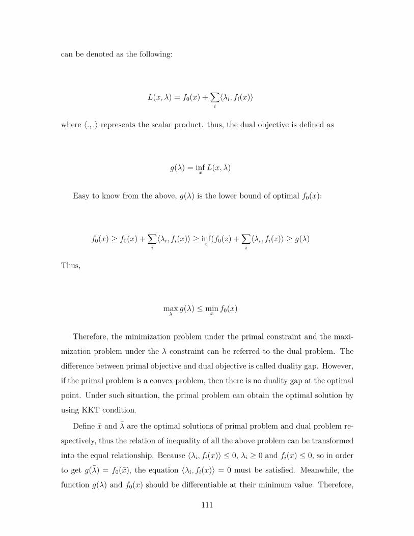
can be denoted as the following:

L(x, λ) = f0(x) +∑i

〈λi, fi(x)〉

where 〈., .〉 represents the scalar product. thus, the dual objective is defined as

g(λ) = infxL(x, λ)

Easy to know from the above, g(λ) is the lower bound of optimal f0(x):

f0(x) ≥ f0(x) +∑i

〈λi, fi(x)〉 ≥ infz

(f0(z) +∑i

〈λi, fi(z)〉 ≥ g(λ)

Thus,

maxλ

g(λ) ≤ minxf0(x)

Therefore, the minimization problem under the primal constraint and the maxi-

mization problem under the λ constraint can be referred to the dual problem. The

difference between primal objective and dual objective is called duality gap. However,

if the primal problem is a convex problem, then there is no duality gap at the optimal

point. Under such situation, the primal problem can obtain the optimal solution by

using KKT condition.

Define x and λ are the optimal solutions of primal problem and dual problem re-

spectively, thus the relation of inequality of all the above problem can be transformed

into the equal relationship. Because 〈λi, fi(x)〉 ≤ 0, λi ≥ 0 and fi(x) ≤ 0, so in order

to get g(λ) = f0(x), the equation 〈λi, fi(x)〉 = 0 must be satisfied. Meanwhile, the

function g(λ) and f0(x) should be differentiable at their minimum value. Therefore,

111

taking these conditions above, the following KKT condition can be obtained:

fi(x) ≤ 0

λi ≥ 0

∇f0(x) +∑i=1∇〈λi, fi(x)〉 = 0

〈λi, fi(x)〉 = 0 (4.6)

As long as the problem (4.5) is a convex optimization problem, then the optimal

value of this problem can be solved and obtained using the above conditions.

Integer programming

In mathematical programming, in addition to the objective function and constraint

function are linear function, the decision variable is the integer variable, such problem

is called linear programming [266]. Besides, if the decision variable is 0-1 variable,

that is 0-1 programming which denoted as:

min c · x

s.t. Ax = b

xj ∈ 0, 1, j = 1, 2, ..., n (4.7)

where c · x is the objective function, Ax = b is the constraint, A is a m× n matrix,

c is a n-dimensional column vector, b is a m-dimensional row vector, and x is a

n-dimensional row vector.

For solving such problem, there are several algorithms such as branch and bound,

cutting plane method and implicit enumeration etc.

1. Branch and Bound

Branch and bound is the classic method for solving 0-1 integer programming. Di-

rectly solving the integer programming problem is difficult, so the feasible region can

112

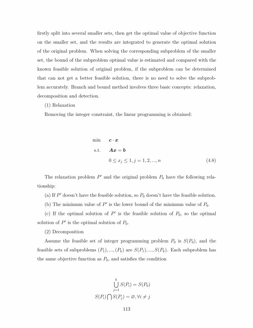
firstly split into several smaller sets, then get the optimal value of objective function

on the smaller set, and the results are integrated to generate the optimal solution

of the original problem. When solving the corresponding subproblem of the smaller

set, the bound of the subproblem optimal value is estimated and compared with the

known feasible solution of original problem, if the subproblem can be determined

that can not get a better feasible solution, there is no need to solve the subprob-

lem accurately. Branch and bound method involves three basic concepts: relaxation,

decomposition and detection.

(1) Relaxation

Removing the integer constraint, the linear programming is obtained:

min c · x

s.t. Ax = b

0 ≤ xj ≤ 1, j = 1, 2, ..., n (4.8)

The relaxation problem P ′ and the original problem P0 have the following rela-

tionship:

(a) If P ′ doesn’t have the feasible solution, so P0 doesn’t have the feasible solution.

(b) The minimum value of P ′ is the lower bound of the minimum value of P0.

(c) If the optimal solution of P ′ is the feasible solution of P0, so the optimal

solution of P ′ is the optimal solution of P0.

(2) Decomposition

Assume the feasible set of integer programming problem P0 is S(P0), and the

feasible sets of subproblems (P1), ..., (Pk) are S(P1), ..., S(Pk). Each subproblem has

the same objective function as P0, and satisfies the condition

k⋃j=1

S(Pi) = S(P0)

S(Pi)⋂S(Pj) = ∅, ∀i 6= j

113

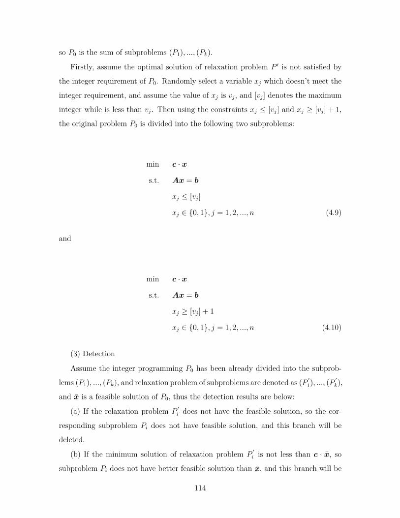
so P0 is the sum of subproblems (P1), ..., (Pk).

Firstly, assume the optimal solution of relaxation problem P ′ is not satisfied by

the integer requirement of P0. Randomly select a variable xj which doesn’t meet the

integer requirement, and assume the value of xj is vj, and [vj] denotes the maximum

integer while is less than vj. Then using the constraints xj ≤ [vj] and xj ≥ [vj] + 1,

the original problem P0 is divided into the following two subproblems:

min c · x

s.t. Ax = b

xj ≤ [vj]

xj ∈ 0, 1, j = 1, 2, ..., n (4.9)

and

min c · x

s.t. Ax = b

xj ≥ [vj] + 1

xj ∈ 0, 1, j = 1, 2, ..., n (4.10)

(3) Detection

Assume the integer programming P0 has been already divided into the subprob-

lems (P1), ..., (Pk), and relaxation problem of subproblems are denoted as (P ′1), ..., (P ′

k),

and x is a feasible solution of P0, thus the detection results are below:

(a) If the relaxation problem P′i does not have the feasible solution, so the cor-

responding subproblem Pi does not have feasible solution, and this branch will be

deleted.

(b) If the minimum solution of relaxation problem P′i is not less than c · x, so

subproblem Pi does not have better feasible solution than x, and this branch will be

114

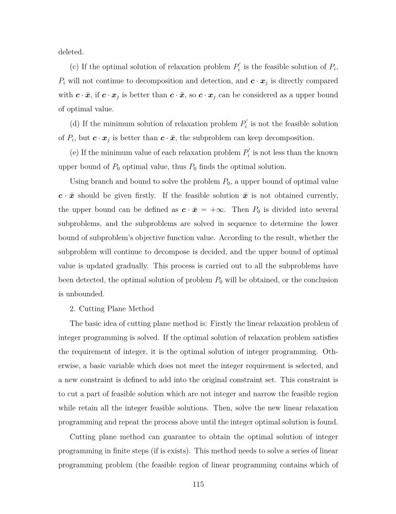
deleted.

(c) If the optimal solution of relaxation problem P′i is the feasible solution of Pi,

Pi will not continue to decomposition and detection, and c · xj is directly compared

with c · x, if c · xj is better than c · x, so c · xj can be considered as a upper bound

of optimal value.

(d) If the minimum solution of relaxation problem P′i is not the feasible solution

of Pi, but c · xj is better than c · x, the subproblem can keep decomposition.

(e) If the minimum value of each relaxation problem P′i is not less than the known

upper bound of P0 optimal value, thus P0 finds the optimal solution.

Using branch and bound to solve the problem P0, a upper bound of optimal value

c · x should be given firstly. If the feasible solution x is not obtained currently,

the upper bound can be defined as c · x = +∞. Then P0 is divided into several

subproblems, and the subproblems are solved in sequence to determine the lower

bound of subproblem’s objective function value. According to the result, whether the

subproblem will continue to decompose is decided, and the upper bound of optimal

value is updated gradually. This process is carried out to all the subproblems have

been detected, the optimal solution of problem P0 will be obtained, or the conclusion

is unbounded.

2. Cutting Plane Method

The basic idea of cutting plane method is: Firstly the linear relaxation problem of

integer programming is solved. If the optimal solution of relaxation problem satisfies

the requirement of integer, it is the optimal solution of integer programming. Oth-

erwise, a basic variable which does not meet the integer requirement is selected, and

a new constraint is defined to add into the original constraint set. This constraint is

to cut a part of feasible solution which are not integer and narrow the feasible region

while retain all the integer feasible solutions. Then, solve the new linear relaxation

programming and repeat the process above until the integer optimal solution is found.

Cutting plane method can guarantee to obtain the optimal solution of integer

programming in finite steps (if is exists). This method needs to solve a series of linear

programming problem (the feasible region of linear programming contains which of

115

integer programming), and use the optimal solution of linear programming problem to

gradually approximate the optimal solution of original integer programming problem.

Cutting plane method is also a relaxation method actually. For minimization form

of integer programming problem, the optimal solution of relaxation problem is the

lower bound of optimal solution of integer programming problem.

The key of cutting plane method is how to define the cutting constraint. Assume

a integer programming problem:

min c · x

s.t. Ax = b

xj ≥ 0, j = 1, 2, ..., n, xj ∈ Z (4.11)

and its relaxation problem is:

min c · x

s.t. Ax = b

xj ≥ 0, j = 1, 2, ..., n (4.12)

Assume the optimal variable of the relaxation problem is B, so the optimal solu-

tion is:

x∗ =

xBxN

=

B−1b

0

=

b0

≥ 0 (4.13)

If the components of x∗ are integer, so x∗ is the optimal solution of problem

(4.11). Otherwise, a basic variable which does not meet the integer requirement is

selected such as xBi , and the cutting constraint is defined by using a constraint which

contains this basic variable. Assume the constraint which contains xBi is:

116

xBi +∑j∈R

yijxj = bi (4.14)

where R is the subscript set of nonbasic variable, yij is the ith component of B−1pj,

and pj is the jth column of A. The variation coefficient and constant in (4.14) are

divided into two parts: integer and nonnegative true fraction, that is:

bi = [bi] + fi

yij = [yij] + fij, j ∈ R

Thus, equation (4.14) is rewritten as:

xBi +∑j∈R

[yij]xj − [bi] = fi −∑j∈R

fijxj (4.15)

Because 0 < fi < 1, 0 ≤ fij < 1, xj > 0, according to (4.15), the following

inequality can be obtained:

fi −∑j∈R

fijxj < 1

For any integer feasible solution, because the left side of equation (4.15) is integer,

so the right side is the integer which less than 1, thus the necessary condition of integer

solution is obtained as below:

fi −∑j∈R

fijxj ≤ 0 (4.16)

(4.16) is used as the cutting condition and added into the constraint of problem

117

(4.12) and a new linear programming problem is:

min c · x

s.t. Ax = b

fi −∑j∈R

fijxj ≤ 0

xj ≥ 0, j = 1, 2, ..., n (4.17)

and then the problem is solved again.

It is easy to know that the original non integer solution x∗ =

B−1b

0

is not the

feasible solution of problem (4.17). Otherwise, because xj = 0, ∀j ∈ R, and fi > 0, so

the left side of inequity (4.16) is more than 0 which is contradict with the constraint

(4.16).

3. Implicit Enumeration

The 0-1 programming P is denoted as:

min c · x

s.t. Aix = bi, i = 1, 2, ...,m

xj ∈ 0, 1, j = 1, 2, ..., n (4.18)

where c = (c1, c2, ..., cn), x = (x1, x2, ..., xn)T , A =

a11 a12 . . . a1n

a21 a22 . . . a2n... ... ...

am1 am2 . . . amn

=

A1

A2...

Am

, b =

b1

b2...

bm

, cj ≥ 0(j = 1, 2, ..., n).

118

There are two assumptions:

(1) If cj < 0, then do the variable substitution which defines x′j = 1− xj, and for

x′j, the coefficient must meet the condition −cj > 0.

(2) c1 ≤ c2 ≤ · · · ≤ cn. If this requirement is not met, then change the variable

subscript to make the hypothesis stand.

The basic idea of implicit enumeration algorithm is, the problem P is divided

into several subproblems, according to certain rules, each subproblem is detected

until the optimal solution is found [123]. Specifically, the problem P is divided

into P1 and P2 according to x1 taking 1 or 0, and P1 is denoted as +1 and

P2 is −1. x1 is called fixed variable, and x2, x3, ..., xn are called free variable.

Then decompose each subproblem according to x2 taking 1 or 0. Define x2 tak-

ing 1 as +2 and taking 0 as −2. If x1 and x2 are taken as fixed variables,

x3, x4, ..., xn are free variables, so 4 subproblems are obtained, and respectively de-

noted as +1,+2, +1,−2, −1,+2, −1,−2. Generally, if xi, xj, ..., xk are fixed

variables, and the value of them are 1, 0, ..., 1 respectively. σ is represented as the

corresponding subproblem which is denoted as σ = +i,−j, ...,+k, and the other

variables are free variable.

Implicit enumeration algorithm starts from problem P∅, along each branch,

each subproblem is detected from left to right until the optimal solution is found or

the conclusion of no solution is obtained.

In the process of detection, for each subproblem σ, take the point which the

free variables are equal to 0 as the detected point and denoted as σ0. For example,

for subproblem σ = +1,−2,+3, take σ0 = (1, 0, 1, 0, ..., 0)T as the detected point

of this subproblem. Obviously, because 0 ≤ c1 ≤ c2 ≤ · · · ≤ cn, if σ0 is the feasible

point, so it is the minimum point of subproblem σ.

Assume x is a feasible point of integer programming P , and its objective function

value is f = cx. Consider a subproblem σ of P , the corresponding detected point

is denoted as σ0. Assume xj is the free variable with minimum subscript in σ, so

the rule of detection is:

(1) If cσ0 ≥ f , so there is not better feasible solution than x in subproblem σ.

119

(2) If cσ0 < f , and σ0 is the feasible solution of P , so σ0 is better than the

original x, thus x = σ0 and f = cσ0.

(3) If cσ0 < f , but σ0 is not the feasible solution of P , and cσ0 + cj ≥ f , so there

is not a better feasible solution than x in σ.

(4) Assume the free variable includes xj1 , xj2 , ..., xjk , which satisfies the inequality

cσ0 + cj1 ≤ · · · ≤ cσ0 + cjr < f ≤ cσ0cjr+1 ≤ · · · ≤ cσ0 + cjk

and denoted as J = j1, j2, ...jr, J is called collection set.

Define si = Aiσ0−bi(i = 1, ...,m), si is the relaxation variable of the ith constraint.

If si ≥ 0,∀i, so σ0 is better than current solution x, thus x = σ0 and f = cσ0.

(5) If σ0 is not the feasible solution, defining I = i|si < 0 which is called against

constraint set, and

Ji = j|j ∈ J, aij > 0, i ∈ I

qi =∑j∈Ji

aij, i ∈ I

where aij is the element of matrix A in row i and column j.

Calculate si + qi,∀i ∈ I, if for one i(i ∈ I), there is si + qi < 0, so this subproblem

does not have better feasible solution.

4.2.3 Research status of algorithms

An important feature of the wireless communication is the communication channel

having a fast variability. The variability includes the path loss, frequency selective

fading, shadow fading and the impact of interference and noise received by the receiv-

er. For these channel weaknesses, the user admission control and resource allocation

algorithm related to the channel are presented in many studies. The resource al-

location algorithm of OFDMA system has many key points to consider, the main

considered factor includes channel influence, impact of inter-cell interference, relay

120

network model and multiple-input multiply-output model. The detail of these stud-

ies are listed below.

In [282], from two points of view of the service provider and access user of WiMax

system, two resource allocation algorithm are proposed which are adaptive power al-

location (APA) and call mission control (CAC). Adaptive power allocation algorithm

reasonably allocates the power in access users. Call mission control algorithm rea-

sonably allocates the bandwidth according to the service request. The joint APA and

CAC can effectively solve the resource allocation problem of PHY and MAC layers.

Finally the literature proposed an optimal strategy for balancing the profit of service

provider and user’s satisfaction for access rate.

In [5], the researchers focused on IEEE 802.16 wireless metropolitan area net-

work and discussed four interrelated resource allocation problems, including adaptive

subcarrier allocation, adaptive power allocation, admission control and capacity plan-

ning.

In [186], the resource allocation model of a single cell OFDMA system is proposed,

KKT condition is used to find the optimal solution of corresponding problem to the

model, and joint power allocation and subcarrier allocation scheme is presented.

In [238], the algorithm of maximizing the throughput under the power constraint

in order to ensure the fairness among the users is studied, and this algorithm reduced

the complexity of calculation.

In [152], a joint flow control and resource allocation algorithm of multi-service

multi-user OFDMA system is proposed. The flow control algorithm can determine

the output data rate requirement for each user according to the user channel state

information and user service request. Resource allocation algorithm allocates the

subcarrier and power to the user according to the data rate.

In [105], the research of optimal resource allocation which allow the delayed user

request is studied based on the traditional resource allocation problem, and a load

adaptive algorithm for the non-real time services is proposed to minimize the average

packet delay for all users.

Literature [4, 138, 221, 309] solved the resource allocation problem of OFDMA

121

system by using integer programming.

In [309], the integer modeling for solving the resource allocation problem with

limited rate and subcarrier of OFDMA system is proposed.

In [138], the integer modeling for the resource allocation problem with limited

rate, subcarrier, power and user admission fairness of OFDMA system is developed.

In [4], the integer modeling considered throughput constraint and delay constraint,

that is, in traditional resource modeling problem of OFDMA system, not only the

allocation of time and frequency are considered, but also the time slot allocation to

ensure the minimum delay is taken into account.

In [221], based on integer programming, a resource allocation algorithm using

branch and bound is developed. Two suboptimal algorithms including pre-allocation

and re-allocation are also proposed.

In [189], the multi-cell resource allocation problem is studied. Under consider-

ing the condition of the multi-cell interference, the model and solution of multi-cell

resource allocation are proposed.

In [335], a new frequency reuse architecture is proposed. Based on this new

frequency reuse architecture, a inter-cell interference coordination scheme is presented

to avoid allocating strong interference bit on subcarrier.

In [157], a new frequency reuse framework is developed, and the optimal power

allocation method is proposed by using water filling algorithm.

In [158], the proposed frequency reuse framework is different from [157], the re-

source allocation problem which is based on SINR link estimation is discussed.

In [50], various feasible interference coordination techniques for 4G OFDM sys-

tems are proposed including power control, adaptive fractional frequency reuse, intra

and inter-base station interference cancelation, spatial antenna techniques and op-

portunistic spectrum access etc.

In [203], a wide variety of frequency reuse frameworks are presented, and the

inter-cell interference under these frequency reuse frameworks are analyzed.

In [305], the fair resource allocation problem with inter-symbol interference in

Gaussian frequency division broadcast channel is considered, and an iterative method

122

which allocates the power and subcarrier respectively to solve the joint power and

subcarrier allocation problem.

In [299] and [200], different from that most studies of OFDMA resource allocation

problem are based on perfect channel information estimation, two resource allocation

problems with imperfect channel information are considered. The former is based

on partial channel state information, and the latter is based on delayed channel side

information. Both the proposed algorithms in two papers considered the balance

between the algorithm performance and computation complexity, and had a good

throughput performance.

In [87], the imperfect global channel state information is considered. The imperfect

global channel state information is mainly constrained by estimation noise and delay.

Based on imperfect CSI, a solution which considers the user admission rate fairness,

relay network, distributed subcarrier allocation power and rate control is proposed.

In [247], the impact of CSI and power allocation on relay channel capacity and

cooperation strategies is considered, including the receiver and the transmitter have

full CSI information, and only the receiver has full CSI information.

In [232], the energy utilization efficiency factor which is proportional to the achieved

rate and inversely proportional to the transmission power is proposed in order to

maximize energy efficiency. According to this factor, a link adaptation solution is

presented which has 15% improvement in energy utilization.

In [69], the resource waste problem is considered, and a strategy minimizing the

internal bandwidth wastage and external bandwidth wastage is proposed.

4.3 Scheduling in wireless OFDMA-TDMA net-

works using variable neighborhood search meta-

heuristic

In this section, we present our numerical results under the form of the paper published

in MISTA-Multidisciplinary International Scheduling Conference 2013, Belgium.

123

Scheduling in Wireless OFDMA-TDMA Networks using

Variable Neighborhood Search Metaheuristic

Pablo Adasme1, Abdel Lisser2, Chen Wang2, Ismael Soto1

1 Departamento de Ingeniería Eléctrica,

Universidad de Santiago de Chile, Avenida Ecuador 3519, Santiago, Chile.

[email protected]

[email protected] Laboratoire de Recherche en Informatique,

Université Paris-Sud XI, Batiment 650, 91190, Orsay Cedex, France.

[email protected]

[email protected]

Abstract. In this paper, we present a hybrid resource allocation model for OFDMA-

TDMA wireless networks and an algorithmic framework using a Variable Neighborhood

Search metaheuristic approach for solving the problem. The model is aimed at maximizing

the total bandwidth channel capacity of an uplink OFDMA-TDMA network subject to user

power and subcarrier assignment constraints while simultaneously scheduling users in time.

As such, the model is best suited for non-real time applications where subchannel multiuser

diversity can be further exploited simultaneously in frequency and in time domains. The

VNS approach is constructed upon a key aspect of the proposed model, namely its decom-

position structure. Our numerical results show tight bounds for the proposed algorithm,

e.g., less than 2% in most of the instances. Finally, the bounds are obtained at a very low

computational cost.

Keywords: OFDMA-TDMA networks, resource allocation, variable neighborhood search.

4.3.1 Introduction

Orthogonal frequency and time division multiple access (resp. OFDMA, TDMA)

are two wireless multi-carrier transmission schemes currently embedded into modern

technologies such as Wifi and Wimax [301]. In an OFDMA network, multiple access is

124

achieved by assigning different subsets of subcarriers (subchannels) to different users

while maintaining orthogonal frequencies among subcarriers. In theory, this means

that interference among subcarriers is completely minimized which allows simultane-

ous data rate transmissions from/to several users to/from the base station (BS). The

transmission direction from the BS to users is known as a downlink process while

the opposite is known as an uplink process. The TDMA transmission scheme, on the

other hand, has the property of scheduling users in time by assigning all bandwidth

channel capacity to only one user within a given time slot in order to transmit sig-

nals. Although, these transmission schemes work differently, the underlying purpose

in both of them is nearly the same, i.e., to make an efficient use of resource allocation

of power and bandwidth channel capacity of the network.

In this paper, we propose a hybrid resource allocation model for OFDMA-TDMA

wireless networks and an algorithmic framework using a variable neighborhood search

metaheuristic approach (VNS for short) for solving the problem [145]. More precisely,

we aim at maximizing the total bandwidth channel capacity of an uplink OFDMA-

TDMA network subject to user power and subcarrier assignment constraints while

simultaneously scheduling users in time. As such, the model is best suited for nonreal

time applications where signals can be transmitted at different time slots without fur-

ther restrictions [246]. The latter allows the fact that subchannel multiuser diversity

can be further exploited simultaneously in frequency and in time domains. As far as

we know, joint OFDMA-TDMA transmission schemes have not been investigated so

far. In [67], the authors compare the performance in support of real time multimedia

transmission schemes when using separately OFDMA-TDMA and OFDMA networks.

Their numerical results show that OFDMA outperforms OFDMA-TDMA in several

quality of service metrics for real-time applications. In a similar vein, the authors

in [178] consider resource allocation of an OFDM wireless network while mixing real-

time and non-realtime traffic patterns. They use a utility based framework to balance

efficiency and fairness among users. Thus, they propose a scheduler mechanism which

gives in one shot the subcarrier and power allocation plus the transmission schedul-

ing for each time slot. Their numerical results indicate that the proposed method

125

achieves a significant performance in terms of the overall throughput of the system.

Another related work is proposed in [246] where an hybrid transmission scheme for

non-realtime applications while using simultaneously code division and time division

multiple access (CDMA-TDMA) schemes is investigated. The authors use a utili-

ty based approach as well, and formulate the optimal downlink resource allocation

problem for a non-realtime CDMA-TDMA network. Their numerical results show a

significant improvement in the overall throughput of the system due to multi-access-

point diversity gain.

We propose a simple VNS based metaheuristic approach [145] to compute tight

bounds for our hybrid OFDMA-TDMA optimization problem. To this purpose, we

randomly partition the set of users into T disjoint subsets of users within each it-

eration of the VNS approach. By doing so, we must solve T smaller integer linear

programming (ILP) subproblems, one for each subset of users assigned to time slot

t ∈ T = 1, ..., T. Note that, in principle, each subproblem could be solved sequen-

tially or in parallel using any algorithmic procedure. As in our case each subproblem

is formulated as an ILP problem, so far now, we solve its linear programming (LP)

relaxation to compute the bounds. In fact, this is a key aspect in our proposed VNS

approach since the LP relaxations of the subproblems are very tight. Since each user

must be attended by the BS in only one time slot t ∈ T , the final solution of the

problem can be easily reconstructed for the original problem from the solutions of

each time slot t ∈ T . The decomposition of the problem allows us to apply the VNS

procedure in a straightforwardly manner and also to compute tight bounds easily. It

turns out that solving the problem to optimality becomes rapidly prohibitive from a

computationally point of view when the instances dimensions increase.

The paper is organized as follows. Section 4.3.2 briefly introduces the system

description and presents the OFDMA-TDMA formulation of the problem. Section

4.3.3 presents the VNS algorithmic procedure while Section 4.3.4 provides preliminary

numerical result. Finally, Section 4.3.5 gives the main conclusion of the paper and

provides some insights for future work.

126

4.3.2 Problem formulation

We consider a BS surrounded by several mobile users within a single cell area. The

BS has to assign a set of N = 1, .., N subcarriers (or subchannels) to a set of

K = 1, .., K users in different time slots T = 1, .., T in order to allow users to send

signals to the BS. The allocation process is performed by the BS dynamically in time

depending on the quality of the channels which are intrinsically stochastic. The latter

affects the amount of bandwidth channel capacity needed by users to transmit their

signals. Without loss of generality, we assume that the BS can fully and accurately

predict the channel state information for each t ∈ T . This is possible in OFDMA-

TDMA networks when using adaptive overlapping pilots in uplink applications [300].

A scheduling formulation for an uplink wireless OFDMA-TDMA network can thus

be written as follows:

P : maxx,ϕ

T∑t=1

K∑k=1

N∑n=1

ctk,nxtk,n (4.19)

s.t.N∑n=1

ptk,nxtk,n ≤ Pkϕk,t, ∀k, t (4.20)

T∑t=1

ϕk,t = 1, ∀k (4.21)

K∑k=1

xtk,n ≤ 1, ∀n, t (4.22)

xtk,n ∈ 0, 1;ϕk,t ∈ 0, 1, ∀k, n, t (4.23)

where xtk,n,∀k, n, t and ϕk,t,∀k, t are the decision variables. These variables are defined

as follows: xtk,n = 1 if user k is assigned subcarrier n at time slot t and zero otherwise.

Similarly, ϕk,t = 1 if user k is scheduled to be attended in time slot t and zero

otherwise. Matrices (ctk,n), (ptk,n) and (Pk) are input data matrices defined as follows.

The entries in (ctk,n) denote the capacity achieved by user k using subcarrier n in time

slot t while entries in (ptk,n) denote the power utilized by user k using subcarrier n

in time slot t. Finally, (Pk) denotes the maximum power allowed for each user k to

transmit their signals to the BS. The objective function in P is aimed at maximizing

127

the total bandwidth channel capacity of the network. Constraint (4.20) is a maximum

available power constraint imposed for each user k and for each time slot t to transmit

signals to the BS. This is the main constraint which makes the difference between

a downlink and an uplink process. In the former, there should be only one power

constraint imposed for the BS whereas in the latter, each user is constrained by its

own available maximum power (Pk), k ∈ K. Constraint (4.21) imposes the condition

that each user must be attended by the BS in a unique time slot t ∈ T . This constraint

is specifically related to the time domain which is basically the transmission scheme

of TDMA wireless networks. Whereas constraint (4.22) is realted to the OFDMA

scheme which imposes the condition that each subcarrier should be assigned to at

most one user at instant t ∈ T . Finally, constraint (4.23) are domain constraints for

the decision variables.

We note that P is an integer linear programming (ILP) formulation which is NP-

Hard and thus difficult to solve directly for medium and large scale instances. Instead,

we propose a VNS decomposition approach to compute tight bounds.

4.3.3 The VNS approach

In order to computer tight bounds for P using a VNS metaheuristic approach, we first

note that for any feasible assignment of ϕk,t = (ϕk,t), i.e., such that ∑Tt=1 ϕk,t = 1,∀k.

Problem P reduces to solving T subproblems of the following form:

P(t) : maxy

∑k∈Kt

N∑n=1

ctk,nytk,n (4.24)

s.t.N∑n=1

ptk,nytk,n ≤ Pkϕk,t, ∀k ∈ Kt (4.25)∑

k∈Ktytk,n ≤ 1, ∀n (4.26)

ytk,n ∈ 0, 1, ∀k ∈ Kt, n ∈ N (4.27)

where ⋃Tt=1Kt = K. Variables ytk,n for each k ∈ Kt, n ∈ N and t ∈ T are analogously

defined as for xtk,n, i.e., ytk,n = 1 if user k ∈ Kt ⊂ K is assigned subcarrier n in time

128

slot t and zero otherwise. Matrices (ctk,n), (ptk,n) and (Pk) are respectively submatrices

of (ctk,n), (ptk,n) and (Pk) we obtain from model P for each t ∈ T according to users

in Kt. Note that any solution xt′k,n of P in a particular time slot t′ ∈ T can be

reconstructed by simply mapping the values of variables yt′k,n,∀k ∈ Kt′ , n ∈ N into

each user position in xt′k,n,∀k ∈ Kt′ . All remaining values in xt

′k,n such that k /∈ Kt′

must be equal to zero. Therefore, for any feasible assignment ϕ = ϕ the optimal

solutions xt in P and optimal solutions yt in P(t), ∀t ∈ T , we have

T∑t=1

K∑k=1

N∑n=1

ctk,nxtk,n =

T∑t=1

∑k∈Kt

N∑n=1

ctk,nytk,n (4.28)

Note that there are TK feasible assignments for ϕk,t = (ϕk,t) and each subset Kthas a cardinality of ∑k∈K ϕk,t users. In case any subset Kt′ = ∅, it means that no

user is scheduled to be attended in time slot t′ ∈ T . Also notice that solving each

P(t), ∀t ∈ T such that Kt′ 6= ∅ is an NP-Hard problem as it is equivalent to solve a

multiple choice multiple knapsack problem [241].

VNS is a recently proposed metaheuristic approach [145] that uses the idea of

neighborhood change during the descent toward local optima and to scape from the

valleys that contain them. We define only one neighbor structure as Ngh(ϕ) for P

as the set of neighbor solutions ϕ′ in P at a distance "h" from ϕ where the distance

"h" corresponds to the number of users assigned in solutions ϕ′ and ϕ. The VNS

procedure we propose is depicted in Algorithm 13. As input receives an instance

of problem P and provides a tight solution for it. We denote by (x, ϕ, f) the final

solution obtained with the algorithm where f represents the objective value function.

The algorithm is simple and works as follows. First, it computes randomly a feasible

assignment of ϕ = (ϕk,t) and solve each subproblem P(t), ∀t ∈ T according to ϕ. This

allows obtaining an initial solution (x, ϕ, f) for P that we keep. Next, the algorithm

performs a variable neighborhood search by randomly scheduling H ≤ K users in

different time slots. Initially, H ← 1 while it is increased in one unit when there is

no improvement after new "η" solutions have been evaluated. On the other hand, if

129

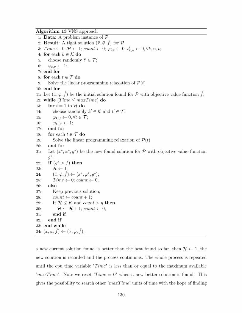
Algorithm 13 VNS approach1: Data: A problem instance of P2: Result: A tight solution (x, ϕ, f) for P3: Time← 0; H ← 1; count← 0; ϕk,t ← 0, xtk,n ← 0,∀k, n, t;4: for each k ∈ K do5: choose randomly t′ ∈ T ;6: ϕk,t′ ← 1;7: end for8: for each t ∈ T do9: Solve the linear programming relaxation of P(t)10: end for11: Let (x, ϕ, f) be the initial solution found for P with objective value function f ;12: while (Time ≤ maxTime) do13: for i = 1 to H do14: choose randomly k′ ∈ K and t′ ∈ T ;15: ϕk′,t ← 0,∀t ∈ T ;16: ϕk′,t′ ← 1;17: end for18: for each t ∈ T do19: Solve the linear programming relaxation of P(t)20: end for21: Let (x∗, ϕ∗, g∗) be the new found solution for P with objective value function

g∗;22: if (g∗ > f) then23: H ← 1;24: (x, ϕ, f)← (x∗, ϕ∗, g∗);25: Time← 0; count← 0;26: else27: Keep previous solution;28: count← count+ 1;29: if H ≤ K and count > η then30: H ← H + 1; count← 0;31: end if32: end if33: end while34: (x, ϕ, f)← (x, ϕ, f);

a new current solution found is better than the best found so far, then H ← 1, the

new solution is recorded and the process continuous. The whole process is repeated

until the cpu time variable "Time" is less than or equal to the maximum available

"maxTime". Note we reset "Time = 0" when a new better solution is found. This

gives the possibility to search other "maxTime" units of time with the hope of finding

130

better solutions.

As it can be observed, the VNS approach is constructed upon a key aspect of

problem P , namely its decomposition structure. On the other hand, the effectiveness

of the algorithm also relies on the fact that the linear programming relaxation of each

subproblem P(t), ∀t ∈ T is very tight.

4.3.4 Numerical results

We present preliminary numerical results for problem P using the proposed VNS

algorithm. We generate realistic power data using a wireless channel from [294]

while we set the capacities ctk,n = Mtk,n,∀k, n, t where Mt

k,n represents an integer

number of bits randomly and uniformly generated between 1, .., 10. These number

of bits are required in higher order M-PSK or M-QAM modulation transmission

schemes [2]. Specially for multimedia applications where the users bit rate demands

are significantly higher. So far, we assume that the bit rate demands are uniformly

distributed. In a larger version of this work, we will also consider other distribution

types. Finally, we set Pk = 0.4 ·∑n∈N p1k,n,∀k ∈ K and η = 500. A Matlab program is

implemented using CPLEX 12 to solve problem P while we use MOSEK solver [240]

to solve its linear programming relaxation we denote hereafter by LP and each linear

programming relaxation P(t),∀t ∈ T within each iteration of the VNS algorithm.

The numerical experiments have been carried out on a Pentium IV, 1 GHz with

2 GoBytes of RAM under windows XP. In Table 4.1, column 1 gives the instance

number and columns 2-4 give the instances dimensions. In columns 5-8, we provide

the optimal solutions of P , LP , and the cpu time in seconds CPLEX needs to solve

P and LP , respectively. Similarly, in columns 9-11, we present the initial solutions

found with the Algorithm 13, its best solution found and the cpu time in seconds the

algorithm needs to reach that solution. Notice that this cpu time considers all the

time spent when solving all the subproblems involved in the algorithm sequentially

and not in parallel as it could be improved. In all our tests we set the maximum time

available to maxTime = 50 seconds. We also mention that whenever the variable

Time reached this amount, it means the algorithm did not find any better solution

131

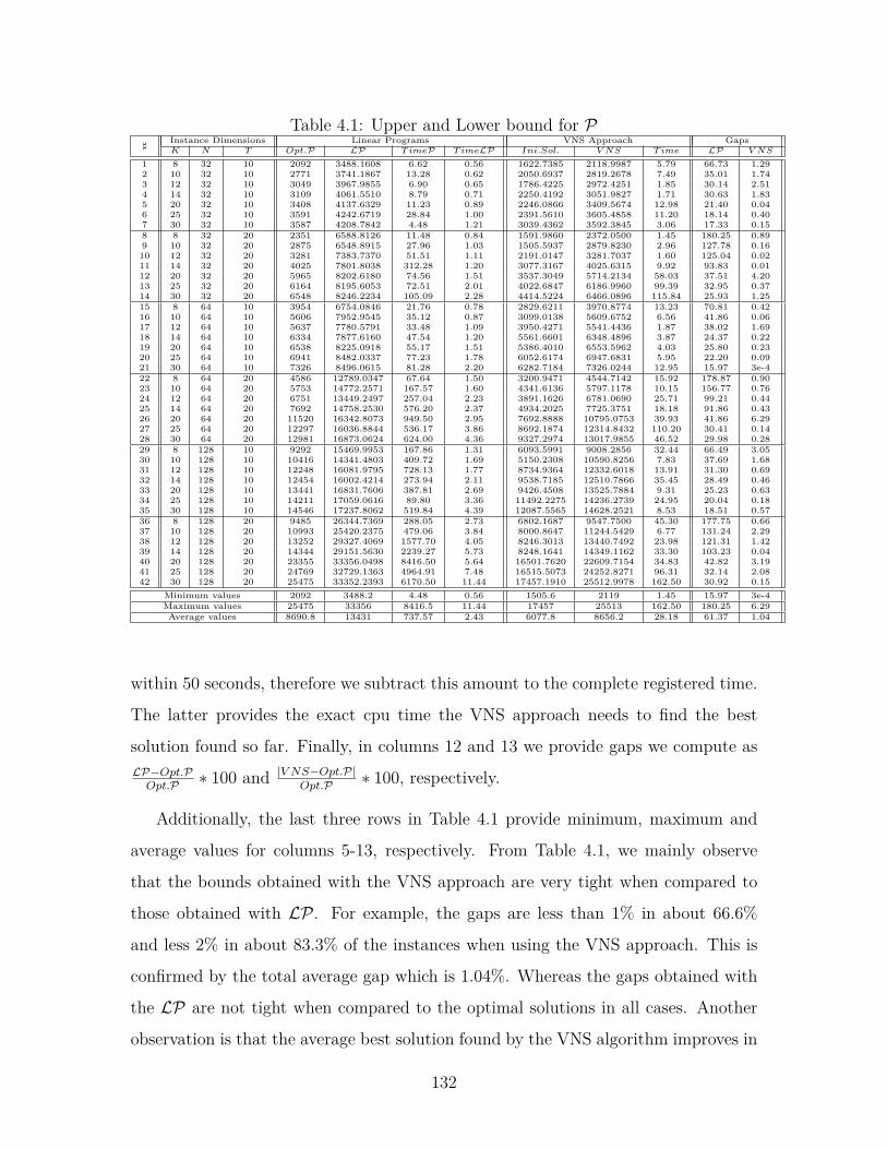
Table 4.1: Upper and Lower bound for P]

Instance Dimensions Linear Programs VNS Approach GapsK N T Opt.P LP TimeP TimeLP Ini.Sol. V NS Time LP V NS

1 8 32 10 2092 3488.1608 6.62 0.56 1622.7385 2118.9987 5.79 66.73 1.292 10 32 10 2771 3741.1867 13.28 0.62 2050.6937 2819.2678 7.49 35.01 1.743 12 32 10 3049 3967.9855 6.90 0.65 1786.4225 2972.4251 1.85 30.14 2.514 14 32 10 3109 4061.5510 8.79 0.71 2250.4192 3051.9827 1.71 30.63 1.835 20 32 10 3408 4137.6329 11.23 0.89 2246.0866 3409.5674 12.98 21.40 0.046 25 32 10 3591 4242.6719 28.84 1.00 2391.5610 3605.4858 11.20 18.14 0.407 30 32 10 3587 4208.7842 4.48 1.21 3039.4362 3592.3845 3.06 17.33 0.158 8 32 20 2351 6588.8126 11.48 0.84 1591.9860 2372.0500 1.45 180.25 0.899 10 32 20 2875 6548.8915 27.96 1.03 1505.5937 2879.8230 2.96 127.78 0.16

10 12 32 20 3281 7383.7370 51.51 1.11 2191.0147 3281.7037 1.60 125.04 0.0211 14 32 20 4025 7801.8038 312.28 1.20 3077.3167 4025.6315 9.92 93.83 0.0112 20 32 20 5965 8202.6180 74.56 1.51 3537.3049 5714.2134 58.03 37.51 4.2013 25 32 20 6164 8195.6053 72.51 2.01 4022.6847 6186.9960 99.39 32.95 0.3714 30 32 20 6548 8246.2234 105.09 2.28 4414.5224 6466.0896 115.84 25.93 1.2515 8 64 10 3954 6754.0846 21.76 0.78 2829.6211 3970.8774 13.23 70.81 0.4216 10 64 10 5606 7952.9545 35.12 0.87 3099.0138 5609.6752 6.56 41.86 0.0617 12 64 10 5637 7780.5791 33.48 1.09 3950.4271 5541.4436 1.87 38.02 1.6918 14 64 10 6334 7877.6160 47.54 1.20 5561.6601 6348.4896 3.87 24.37 0.2219 20 64 10 6538 8225.0918 55.17 1.51 5386.4010 6553.5962 4.03 25.80 0.2320 25 64 10 6941 8482.0337 77.23 1.78 6052.6174 6947.6831 5.95 22.20 0.0921 30 64 10 7326 8496.0615 81.28 2.20 6282.7184 7326.0244 12.95 15.97 3e-422 8 64 20 4586 12789.0347 67.64 1.50 3200.9471 4544.7142 15.92 178.87 0.9023 10 64 20 5753 14772.2571 167.57 1.60 4341.6136 5797.1178 10.15 156.77 0.7624 12 64 20 6751 13449.2497 257.04 2.23 3891.1626 6781.0690 25.71 99.21 0.4425 14 64 20 7692 14758.2530 576.20 2.37 4934.2025 7725.3751 18.18 91.86 0.4326 20 64 20 11520 16342.8073 949.50 2.95 7692.8888 10795.0753 39.93 41.86 6.2927 25 64 20 12297 16036.8844 536.17 3.86 8692.1874 12314.8432 110.20 30.41 0.1428 30 64 20 12981 16873.0624 624.00 4.36 9327.2974 13017.9855 46.52 29.98 0.2829 8 128 10 9292 15469.9953 167.86 1.31 6093.5991 9008.2856 32.44 66.49 3.0530 10 128 10 10416 14341.4803 409.72 1.69 5150.2308 10590.8256 7.83 37.69 1.6831 12 128 10 12248 16081.9795 728.13 1.77 8734.9364 12332.6018 13.91 31.30 0.6932 14 128 10 12454 16002.4214 273.94 2.11 9538.7185 12510.7866 35.45 28.49 0.4633 20 128 10 13441 16831.7606 387.81 2.69 9426.4508 13525.7884 9.31 25.23 0.6334 25 128 10 14211 17059.0616 89.80 3.36 11492.2275 14236.2739 24.95 20.04 0.1835 30 128 10 14546 17237.8062 519.84 4.39 12087.5565 14628.2521 8.53 18.51 0.5736 8 128 20 9485 26344.7369 288.05 2.73 6802.1687 9547.7500 45.30 177.75 0.6637 10 128 20 10993 25420.2375 479.06 3.84 8000.8647 11244.5429 6.77 131.24 2.2938 12 128 20 13252 29327.4069 1577.70 4.05 8246.3013 13440.7492 23.98 121.31 1.4239 14 128 20 14344 29151.5630 2239.27 5.73 8248.1641 14349.1162 33.30 103.23 0.0440 20 128 20 23355 33356.0498 8416.50 5.64 16501.7620 22609.7154 34.83 42.82 3.1941 25 128 20 24769 32729.1363 4964.91 7.48 16515.5073 24252.8271 96.31 32.14 2.0842 30 128 20 25475 33352.2393 6170.50 11.44 17457.1910 25512.9978 162.50 30.92 0.15

Minimum values 2092 3488.2 4.48 0.56 1505.6 2119 1.45 15.97 3e-4Maximum values 25475 33356 8416.5 11.44 17457 25513 162.50 180.25 6.29

Average values 8690.8 13431 737.57 2.43 6077.8 8656.2 28.18 61.37 1.04

within 50 seconds, therefore we subtract this amount to the complete registered time.

The latter provides the exact cpu time the VNS approach needs to find the best

solution found so far. Finally, in columns 12 and 13 we provide gaps we compute asLP−Opt.POpt.P ∗ 100 and |V NS−Opt.P|

Opt.P ∗ 100, respectively.

Additionally, the last three rows in Table 4.1 provide minimum, maximum and

average values for columns 5-13, respectively. From Table 4.1, we mainly observe

that the bounds obtained with the VNS approach are very tight when compared to

those obtained with LP . For example, the gaps are less than 1% in about 66.6%

and less 2% in about 83.3% of the instances when using the VNS approach. This is

confirmed by the total average gap which is 1.04%. Whereas the gaps obtained with

the LP are not tight when compared to the optimal solutions in all cases. Another

observation is that the average best solution found by the VNS algorithm improves in

132

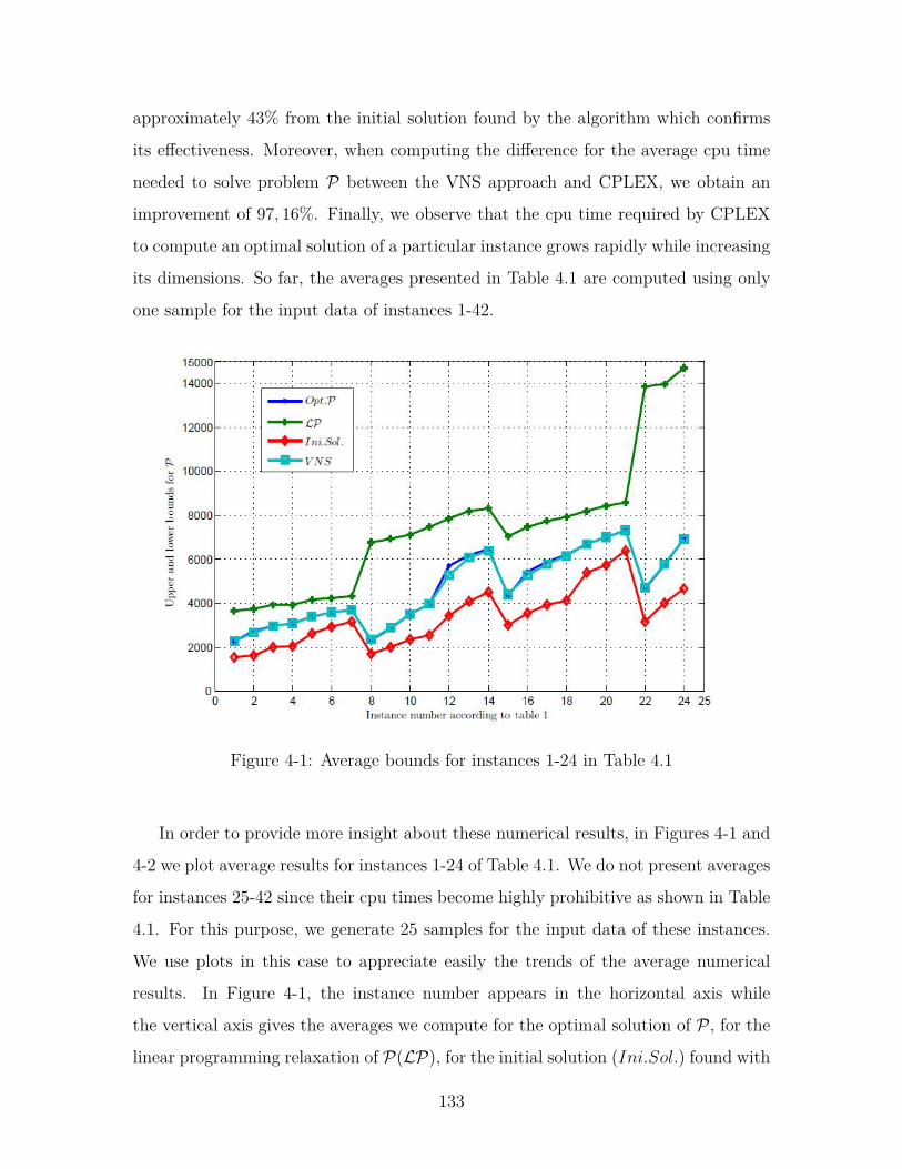
approximately 43% from the initial solution found by the algorithm which confirms

its effectiveness. Moreover, when computing the difference for the average cpu time

needed to solve problem P between the VNS approach and CPLEX, we obtain an

improvement of 97, 16%. Finally, we observe that the cpu time required by CPLEX

to compute an optimal solution of a particular instance grows rapidly while increasing

its dimensions. So far, the averages presented in Table 4.1 are computed using only

one sample for the input data of instances 1-42.

Figure 4-1: Average bounds for instances 1-24 in Table 4.1

In order to provide more insight about these numerical results, in Figures 4-1 and

4-2 we plot average results for instances 1-24 of Table 4.1. We do not present averages

for instances 25-42 since their cpu times become highly prohibitive as shown in Table

4.1. For this purpose, we generate 25 samples for the input data of these instances.

We use plots in this case to appreciate easily the trends of the average numerical

results. In Figure 4-1, the instance number appears in the horizontal axis while

the vertical axis gives the averages we compute for the optimal solution of P , for the

linear programming relaxation of P(LP), for the initial solution (Ini.Sol.) found with

133

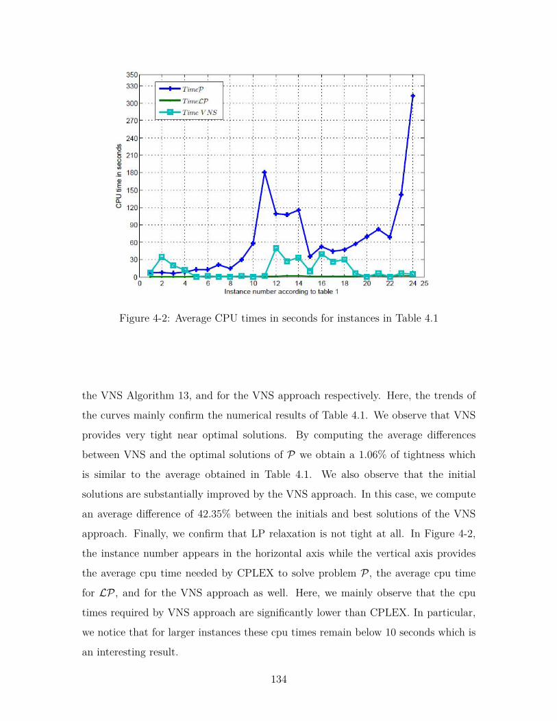
Figure 4-2: Average CPU times in seconds for instances in Table 4.1

the VNS Algorithm 13, and for the VNS approach respectively. Here, the trends of

the curves mainly confirm the numerical results of Table 4.1. We observe that VNS

provides very tight near optimal solutions. By computing the average differences

between VNS and the optimal solutions of P we obtain a 1.06% of tightness which

is similar to the average obtained in Table 4.1. We also observe that the initial

solutions are substantially improved by the VNS approach. In this case, we compute

an average difference of 42.35% between the initials and best solutions of the VNS

approach. Finally, we confirm that LP relaxation is not tight at all. In Figure 4-2,

the instance number appears in the horizontal axis while the vertical axis provides

the average cpu time needed by CPLEX to solve problem P , the average cpu time

for LP , and for the VNS approach as well. Here, we mainly observe that the cpu

times required by VNS approach are significantly lower than CPLEX. In particular,

we notice that for larger instances these cpu times remain below 10 seconds which is

an interesting result.

134

4.3.5 Conclusions

In this paper, we proposed a hybrid resource allocation model for OFDMA-TDMA

wireless networks and a VNS metaheuristic approach for solving the problem. The

model is aimed at maximizing the total bandwidth channel capacity of an uplink

OFDMA-TDMA network subject to user power and subcarrier assignment constraints

while simultaneously scheduling users in time. As such, the model is best suited

for non-real time applications where subchannel multiuser diversity can be further

exploited in frequency and in time domains, simultaneously. The effectiveness of the

proposed VNS approach relies on the decomposition structure of the problem which

allowed solving a set of smaller integer linear programming subproblems within each

iteration of the VNS approach. It turned out that the linear programming relaxations

of these subproblems were very tight. Our numerical results showed tight bounds for

the proposed algorithm, e.g., less than 2% in most of the instances. Besides, the

bounds were obtained at a very low computational cost.

Future research will be focussed on developing other algorithmic approaches for

solving each subproblem while considering other variants of the proposed model such

as minimizing power subject to capacity constraints for uplink and downlink applica-

tions.

135

4.4 Stochastic resource allocation for uplink wire-

less multi-cell OFDMA networks

In this section, we present our numerical result under the form of the paper published

in MobiWIS- Mobile Web Information Systems Conference 2014, Spain.

136

Stochastic Resource Allocation for Uplink Wireless

Multi-cell OFDMA Networks

Pablo Adasme1, Abdel Lisser2, Chen Wang2





[email protected] [email protected]

Abstract. In this paper, we propose a (0-1) stochastic resource allocation model for

uplink wireless multi-cell OFDMA Networks. The model maximizes the total signal to

interference noise ratio produced in a multi-cell OFDMA network subject to user power

and subcarrier assignment constraints. We transform the proposed stochastic model into a

deterministic equivalent binary nonlinear optimization problem having quadratic terms and

second order conic constraints. Subsequently, we use the deterministic model to derive an

equivalent mixed integer linear programming formulation. Since the problem is NP-Hard,

we propose a simple reduced variable neighborhood search (VNS for short) metaheuristic

procedure [145, 149]. Our preliminary numerical results indicate that VNS provides near

optimal solutions for small and medium size instances when compared to the optimal so-

lution of the problem. Moreover, it provides better feasible solutions than CPLEX when

the instances dimensions increase. Finally, these results are obtained at a significantly less

computational cost.

Keywords: Wireless multi-cell OFDMA networks, resource allocation, mixed integer

linear programming, variable neighborhood search.

4.4.1 Introduction

Orthogonal frequency division multiple access (OFDMA) is a wireless multi-carrier

transmission scheme currently embedded into modern technologies such as IEEE

137

802.11a/g WLAN and IEEE 802.16a. It has also been implemented in mobile WiMax

deployments ensuring high quality of service (QoS) [301,340]. In a wireless OFDMA

network, multiple access is achieved by assigning different subsets of subcarriers (sub-

channels) to different users using orthogonal frequencies. In theory, this means that

interference is completely minimized between subcarriers which allows simultaneous

data rate transmissions from/to several users to/from the base station (BS). We can

have an OFDMA system consisting of one or more BSs surrounded by several mobile

users within a given radial transmission area. The former is known as a single-cell

OFDMA network while the latter forms a multi-cell OFDMA network. The last one

is by far the highest complex scenario since it involves the interference generated

among different users [13]. Interference between the BSs is also possible as long as

their radial transmissions overlap each other. The interference phenomenon is main-

ly caused by the fact that different users and BSs use the same frequency bands

either for uplink and/or downlink transmissions. In the uplink case, the transmis-

sion of signals is performed from the users to the BS whereas in the downlink case,

this is done in the opposite direction. In this paper, we propose a (0-1) stochastic

resource allocation model for wireless uplink multi-cell OFDMA networks. The pro-

posed model maximizes the total signal to interference noise ratio (SINR) produced

in a multi-cell OFDMA network subject to user power and subcarrier assignment

constraints. The SINR is defined as the ratio between the power of a signal over the

sum of different powers caused by other interfering signals plus the absolute value

of the Additive White Gaussian Noise (AWGN). Maximizing SINR is relevant in a

multi-cell OFDMA network as it allows selecting the best subcarriers for the different

users while simultaneously exploiting multi-user diversity. The multi-user diversity

phenomena occurs since subcarriers perceive large variations in channel gains which

are different for each user and then each subcarrier can vary its own transmission

rate depending on the quality of the channel. The better the quality of the chan-

nel, the higher the number of bits that can be transmitted. On the other hand,

the interfering signals in a particular subcarrier can be efficiently detected using any

multi-user detection scheme [317]. We transform the proposed stochastic model into

138

a deterministic equivalent binary nonlinear optimization problem having quadratic

terms and second order conic constraints. Finally, we use the deterministic model

to derive an equivalent mixed integer linear programming formulation. This allows

computing optimal solutions and upper bounds directly using its linear programming

(LP) relaxation. Since the problem is NP-Hard, we propose a simple reduced vari-

able neighborhood search (VNS) metaheuristic procedure to come up with tight near

optimal solutions [145, 149]. We choose VNS mainly due to its simplicity and low

memory requirements [145]. Our numerical results indicate that VNS provides near

optimal solutions for most of the instances when compared to the optimal solution of

the problem. Moreover, it provides better feasible solutions than CPLEX when the

instances dimensions increase. Finally, these solutions are obtained at a significantly

less computational cost.

Several mathematical programming formulations for resource allocation in OFD-

MA networks have been proposed in the literature so far. In [13], the authors present

a table with 19 papers published until 2007 where only two of them deal with multi-

cell OFDMA networks either for uplink and downlink transmissions. More recent

works can be found in [158, 316, 353]. In [158], the authors address the problem of

inter-cell interference (ICI) management in the context of single frequency broad-

band OFDMA based networks. Whereas in [353], the problem of resource allocation

in multi-cell OFDMA networks under the cognitive radio network (CRN) paradigm

is considered. Finally, in [316] the problem of energy efficient communication in the

downlink of a multi-cell OFDMA network is considered where user scheduling and

power allocation are jointly optimized. As far as we know, stochastic programming

or VNS algorithmic procedures have not been investigated so far for resource allo-

cation in multi-cell OFDMA networks. In this section, we adopt a simple scenario

based approach to handle the expectation in the objective function of our stochastic

formulation [114]. This is a valid assumption in stochastic programming framework

as one may use historical data for instance [91, 114]. On the other hand, we use a

second order conic programming (SOCP) approach to deal with the probabilistic user

power constraints [214]. For this purpose, we assume that the entries in the input

139

power matrices are independent multivariate random variables normally distributed

with known means and covariance matrices. The normal distribution assumption is

motivated by its several theoretical characteristics amongst them the central limit

theorem.

This paper is organized as follows. Section 4.4.2 briefly introduces the system

description and presents the stochastic multi-cell OFDMA model. In Section 4.4.3,

we transform the stochastic model into a deterministic equivalent mixed integer linear

programming problem. Subsequently, in Section 4.4.4 we present our VNS algorithmic

procedure. In Section 4.4.5, we conduct numerical tests to compare the optimal

solution of the problem with those obtained with the LP relaxation and with the

VNS approach, respectively. Finally, in Section 4.4.6 we give the main conclusions of

the paper and provide some insights for future research.

4.4.2 System description and problem formulation

In this section, we give a brief system description of an uplink wireless multi-cell

OFDMA network and formulate a stochastic model for the problem.

System description

A general system description of an uplink wireless multi-cell OFDMA network is

shown in Figure 4-3. As it can be observed, within a given radial transmission area,

the BSs and users simultaneously transmit their signals. This generates interference

and degrades the quality of wireless channels. These type of networks may arise

in many difficult situations where infrastructure less approaches are mandatorily re-

quired. Mobile ad hoc networks (MANETS) or mesh type networks are examples

of them commonly used in emergency, war battlefield or natural disaster scenarios

where no strict planning of the network is possible due to short time constraints. In a

multi-cell OFDMA network, the interference phenomena is a major concern in order

to efficiently assign subcarriers to users. Each BS must perform the allocation process

over time in order to exploit the so-called multi-user diversity and hence increasing

140

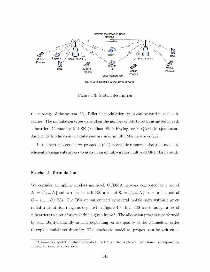
Figure 4-3: System description

the capacity of the system [63]. Different modulation types can be used in each sub-

carrier. The modulation types depend on the number of bits to be transmitted in each

subcarrier. Commonly, M-PSK (M-Phase Shift Keying) or M-QAM (M-Quadrature

Amplitude Modulation) modulations are used in OFDMA networks [332].

In the next subsection, we propose a (0-1) stochastic resource allocation model to

efficiently assign subcarriers to users in an uplink wireless multi-cell OFDMA network.

Stochastic formulation

We consider an uplink wireless multi-cell OFDMA network composed by a set of

N = 1, .., N subcarriers in each BS, a set of K = 1, .., K users and a set of

B = 1, .., B BSs. The BSs are surrounded by several mobile users within a given

radial transmission range as depicted in Figure 4-3. Each BS has to assign a set of

subcarriers to a set of users within a given frame1. The allocation process is performed

by each BS dynamically in time depending on the quality of the channels in order

to exploit multi-user diversity. The stochastic model we propose can be written as

1A frame is a packet in which the data to be transmitted is placed. Each frame is composed byT time slots and N subcarriers.

141

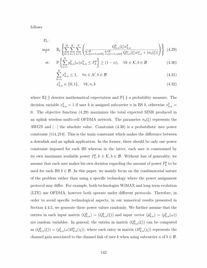
follows

P0 :

maxx

Eξ

B∑b=1

K∑k=1

N∑n=1

Qbk,n(ξ)xbk,n∑B

w=1,w 6=b∑Kv=1,v 6=kQ

wv,n(ξ)xwv,n + |σ0(ξ)|

(4.29)

st: P

N∑n=1

pbk,n(ω)xbk,n ≤ P bk

≥ (1− α), ∀k ∈ K, b ∈ B (4.30)

K∑k=1

xbk,n ≤ 1, ∀n ∈ N , b ∈ B (4.31)

xbk,n ∈ 0, 1, ∀k, n, b (4.32)

where E· denotes mathematical expectation and P· a probability measure. The

decision variable xbk,n = 1 if user k is assigned subcarrier n in BS b, otherwise xbk,n =

0. The objective function (4.29) maximizes the total expected SINR produced in

an uplink wireless multi-cell OFDMA network. The parameter σ0(ξ) represents the

AWGN and | · | the absolute value. Constraint (4.30) is a probabilistic user power

constraint [114,214]. This is the main constraint which makes the difference between

a downlink and an uplink application. In the former, there should be only one power

constraint imposed for each BS whereas in the latter, each user is constrained by

its own maximum available power P bk , k ∈ K, b ∈ B. Without loss of generality, we

assume that each user makes his own decision regarding the amount of power P bk to be

used for each BS b ∈ B. In this paper, we mainly focus on the combinatorial nature

of the problem rather than using a specific technology where the power assignment

protocol may differ. For example, both technologies WiMAX and long term evolution

(LTE) use OFDMA, however both operate under different protocols. Therefore, in

order to avoid specific technological aspects, in our numerical results presented in

Section 4.4.5, we generate these power values randomly. We further assume that the

entries in each input matrix (Qbk,n) = (Qb

k,n(ξ)) and input vector (pbk,n) = (pbk,n(ω))

are random variables. In general, the entries in matrix (Qbk,n(ξ)) can be computed

as (Qbk,n(ξ)) = (pbk,n(ω)Hb

k,n(χ)), where each entry in matrix (Hbk,n(χ)) represents the

channel gain associated to the channel link of user k when using subcarrier n of b ∈ B.

142

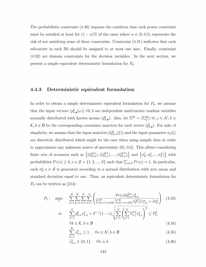
The probabilistic constraint (4.30) imposes the condition that each power constraint

must be satisfied at least for (1 − α)% of the cases where α ∈ [0, 0.5) represents the

risk of not satisfying some of these constraints. Constraint (4.31) indicates that each

subcarrier in each BS should be assigned to at most one user. Finally, constraint

(4.32) are domain constraints for the decision variables. In the next section, we

present a simple equivalent deterministic formulation for P0.

4.4.3 Deterministic equivalent formulation

In order to obtain a simple deterministic equivalent formulation for P0, we assume

that the input vectors (pbk,•(ω)) ∀k, b are independent multivariate random variables

normally distributed with known means (pbk,•). Also, let Σkb = (Σkbij ),∀i, j ∈ N , k ∈

K, b ∈ B be the corresponding covariance matrices for each vector (pbk,•). For sake of

simplicity, we assume that the input matrices (Qbk,n(ξ)) and the input parameter σ0(ξ)

are discretely distributed which might be the case when using sample data in order

to approximate any unknown source of uncertainty [91,114]. This allows considering

finite sets of scenarios such as

(Qb,1k,n), (Qb,2

k,n), ..., (Qb,Sk,n)

and

σ1

0, σ20, ..., σ

S0 )with

probabilities Pr(s) ≥ 0, s ∈ S = 1, 2, ..., S such that ∑s∈S Pr(s) = 1. In particular,

each σs0, s ∈ S is generated according to a normal distribution with zero mean and

standard deviation equal to one. Thus, an equivalent deterministic formulation for

P0 can be written as [214]:

P1 : maxx

B∑b=1

K∑k=1

N∑n=1

S∑s=1

Pr(s)Qb,sk,nx

bk,n∑B

w=1,w 6=b∑Kv=1,v 6=kQ

w,sv,nxwv,n + |σs0|

(4.33)

st:N∑n=1

pbk,nxbk,n + F−1(1− α)

√√√√√ N∑i=1

N∑j=1

Σk,bi,j x

bk,j

2

≤ P bk ,

∀k ∈ K, b ∈ B (4.34)K∑k=1

xbk,n ≤ 1, ∀n ∈ N , b ∈ B (4.35)

xbk,n ∈ 0, 1, ∀k, n, b (4.36)

143

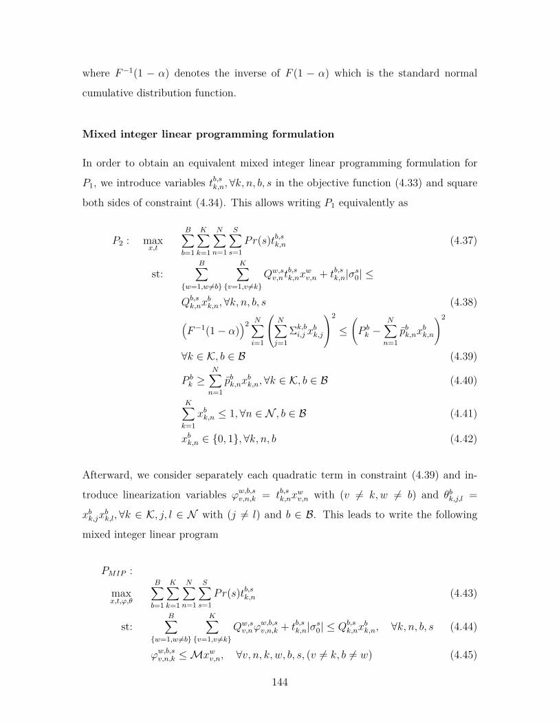
where F−1(1 − α) denotes the inverse of F (1 − α) which is the standard normal

cumulative distribution function.

Mixed integer linear programming formulation

In order to obtain an equivalent mixed integer linear programming formulation for

P1, we introduce variables tb,sk,n, ∀k, n, b, s in the objective function (4.33) and square

both sides of constraint (4.34). This allows writing P1 equivalently as

P2 : maxx,t

B∑b=1

K∑k=1

N∑n=1

S∑s=1

Pr(s)tb,sk,n (4.37)

st:B∑

w=1,w 6=b

K∑v=1,v 6=k

Qw,sv,nt

b,sk,nx

wv,n + tb,sk,n|σs0| ≤

Qb,sk,nx

bk,n,∀k, n, b, s (4.38)

(F−1(1− α)

)2 N∑i=1

N∑j=1

Σk,bi,j x

bk,j

2

≤(P bk −

N∑n=1

pbk,nxbk,n

)2

∀k ∈ K, b ∈ B (4.39)

P bk ≥

N∑n=1

pbk,nxbk,n,∀k ∈ K, b ∈ B (4.40)

K∑k=1

xbk,n ≤ 1,∀n ∈ N , b ∈ B (4.41)

xbk,n ∈ 0, 1,∀k, n, b (4.42)

Afterward, we consider separately each quadratic term in constraint (4.39) and in-

troduce linearization variables ϕw,b,sv,n,k = tb,sk,nxwv,n with (v 6= k, w 6= b) and θbk,j,l =

xbk,jxbk,l,∀k ∈ K, j, l ∈ N with (j 6= l) and b ∈ B. This leads to write the following

mixed integer linear program

PMIP :

maxx,t,ϕ,θ

B∑b=1

K∑k=1

N∑n=1

S∑s=1

Pr(s)tb,sk,n (4.43)

st:B∑

w=1,w 6=b

K∑v=1,v 6=k

Qw,sv,nϕ

w,b,sv,n,k + tb,sk,n|σs0| ≤ Qb,s

k,nxbk,n, ∀k, n, b, s (4.44)

ϕw,b,sv,n,k ≤Mxwv,n, ∀v, n, k, w, b, s, (v 6= k, b 6= w) (4.45)

144

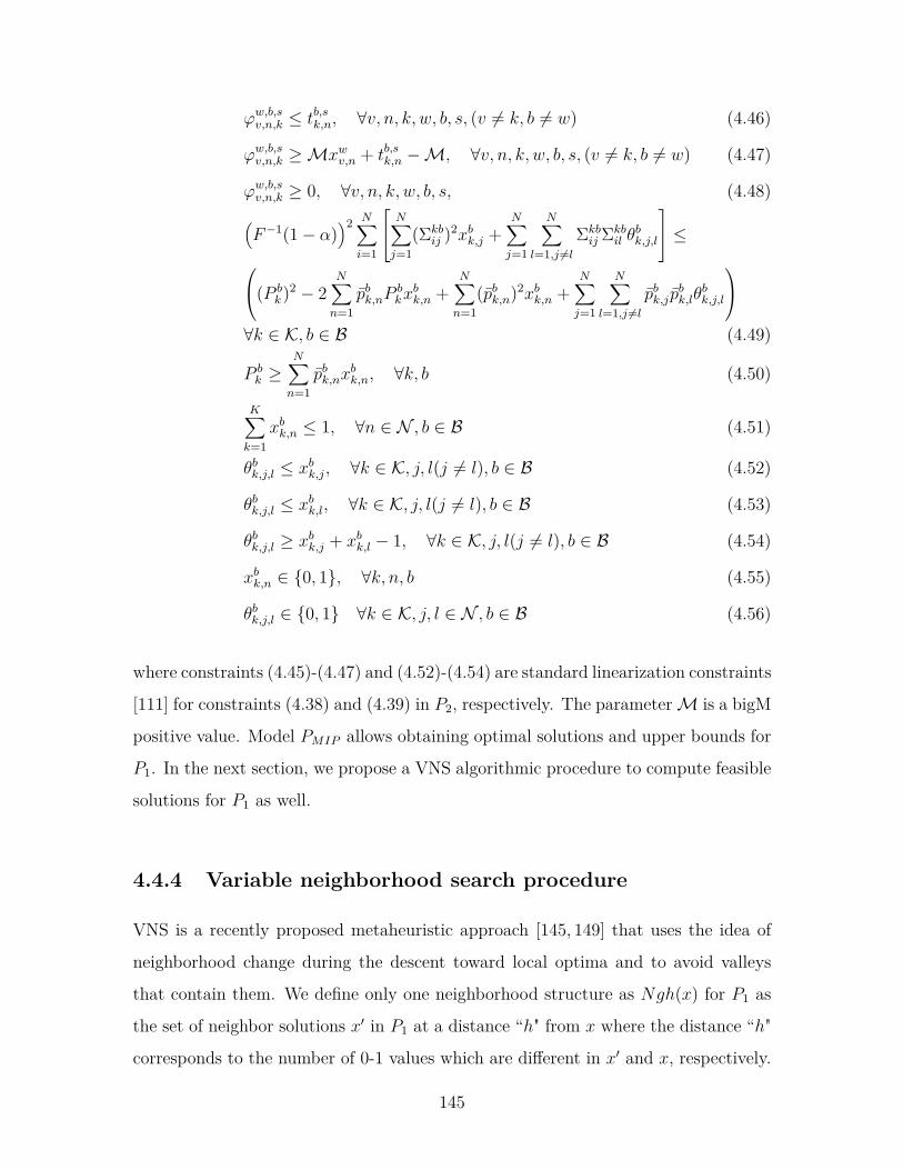
ϕw,b,sv,n,k ≤ tb,sk,n, ∀v, n, k, w, b, s, (v 6= k, b 6= w) (4.46)

ϕw,b,sv,n,k ≥Mxwv,n + tb,sk,n −M, ∀v, n, k, w, b, s, (v 6= k, b 6= w) (4.47)

ϕw,b,sv,n,k ≥ 0, ∀v, n, k, w, b, s, (4.48)(F−1(1− α)

)2 N∑i=1

N∑j=1

(Σkbij )2xbk,j +

N∑j=1

N∑l=1,j 6=l

Σkbij Σkb

il θbk,j,l

≤(P b

k)2 − 2N∑n=1

pbk,nPbkx

bk,n +

N∑n=1

(pbk,n)2xbk,n +N∑j=1

N∑l=1,j 6=l

pbk,j pbk,lθ

bk,j,l

∀k ∈ K, b ∈ B (4.49)

P bk ≥

N∑n=1

pbk,nxbk,n, ∀k, b (4.50)

K∑k=1

xbk,n ≤ 1, ∀n ∈ N , b ∈ B (4.51)

θbk,j,l ≤ xbk,j, ∀k ∈ K, j, l(j 6= l), b ∈ B (4.52)

θbk,j,l ≤ xbk,l, ∀k ∈ K, j, l(j 6= l), b ∈ B (4.53)

θbk,j,l ≥ xbk,j + xbk,l − 1, ∀k ∈ K, j, l(j 6= l), b ∈ B (4.54)

xbk,n ∈ 0, 1, ∀k, n, b (4.55)

θbk,j,l ∈ 0, 1 ∀k ∈ K, j, l ∈ N , b ∈ B (4.56)

where constraints (4.45)-(4.47) and (4.52)-(4.54) are standard linearization constraints

[111] for constraints (4.38) and (4.39) in P2, respectively. The parameterM is a bigM

positive value. Model PMIP allows obtaining optimal solutions and upper bounds for

P1. In the next section, we propose a VNS algorithmic procedure to compute feasible

solutions for P1 as well.

4.4.4 Variable neighborhood search procedure

VNS is a recently proposed metaheuristic approach [145, 149] that uses the idea of

neighborhood change during the descent toward local optima and to avoid valleys

that contain them. We define only one neighborhood structure as Ngh(x) for P1 as

the set of neighbor solutions x′ in P1 at a distance “h" from x where the distance “h"

corresponds to the number of 0-1 values which are different in x′ and x, respectively.

145

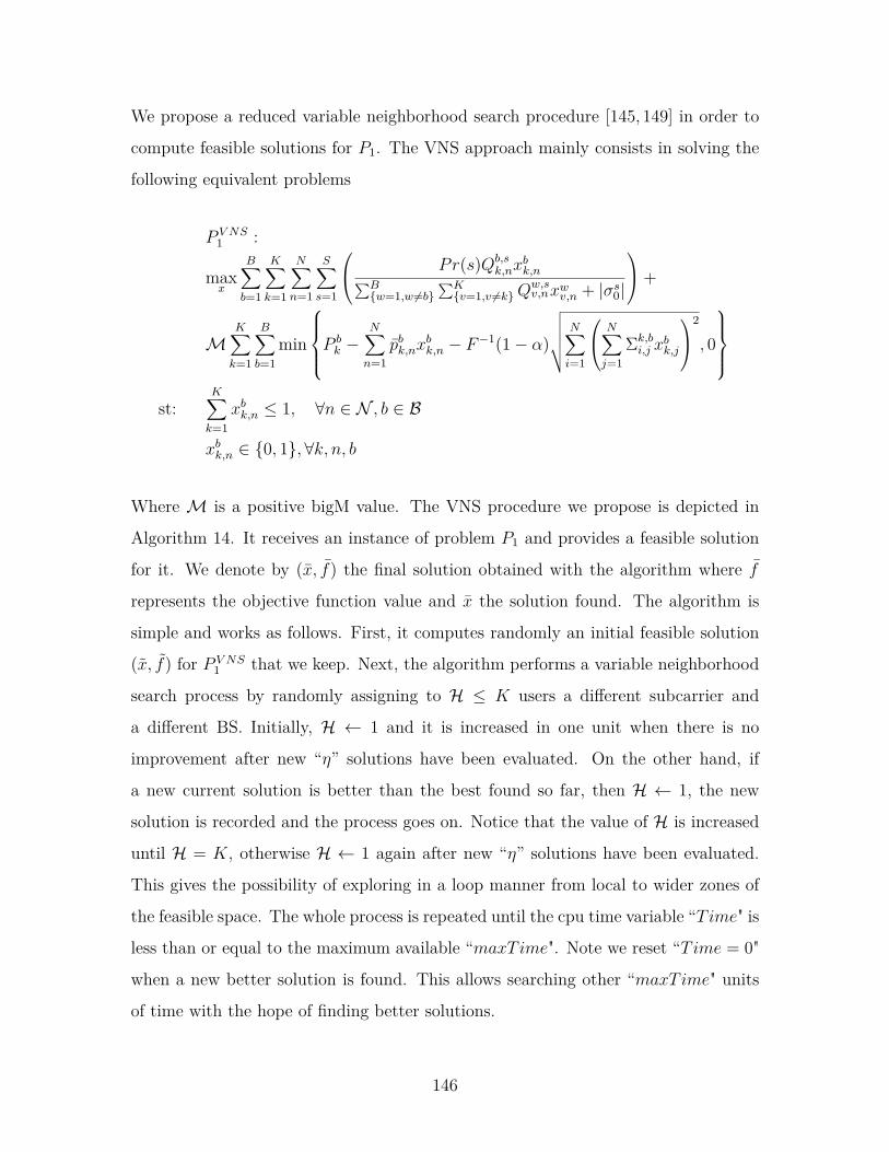
We propose a reduced variable neighborhood search procedure [145, 149] in order to

compute feasible solutions for P1. The VNS approach mainly consists in solving the

following equivalent problems

P V NS1 :

maxx

B∑b=1

K∑k=1

N∑n=1

S∑s=1

Pr(s)Qb,sk,nx

bk,n∑B

w=1,w 6=b∑Kv=1,v 6=kQ

w,sv,nxwv,n + |σs0|

+

MK∑k=1

B∑b=1

min

P bk −

N∑n=1

pbk,nxbk,n − F−1(1− α)

√√√√√ N∑i=1

N∑j=1

Σk,bi,j x

bk,j

2

, 0

st:

K∑k=1

xbk,n ≤ 1, ∀n ∈ N , b ∈ B

xbk,n ∈ 0, 1,∀k, n, b

Where M is a positive bigM value. The VNS procedure we propose is depicted in

Algorithm 14. It receives an instance of problem P1 and provides a feasible solution

for it. We denote by (x, f) the final solution obtained with the algorithm where f

represents the objective function value and x the solution found. The algorithm is

simple and works as follows. First, it computes randomly an initial feasible solution

(x, f) for P V NS1 that we keep. Next, the algorithm performs a variable neighborhood

search process by randomly assigning to H ≤ K users a different subcarrier and

a different BS. Initially, H ← 1 and it is increased in one unit when there is no

improvement after new “η” solutions have been evaluated. On the other hand, if

a new current solution is better than the best found so far, then H ← 1, the new

solution is recorded and the process goes on. Notice that the value of H is increased

until H = K, otherwise H ← 1 again after new “η” solutions have been evaluated.

This gives the possibility of exploring in a loop manner from local to wider zones of

the feasible space. The whole process is repeated until the cpu time variable “Time" is

less than or equal to the maximum available “maxTime". Note we reset “Time = 0"

when a new better solution is found. This allows searching other “maxTime" units

of time with the hope of finding better solutions.

146

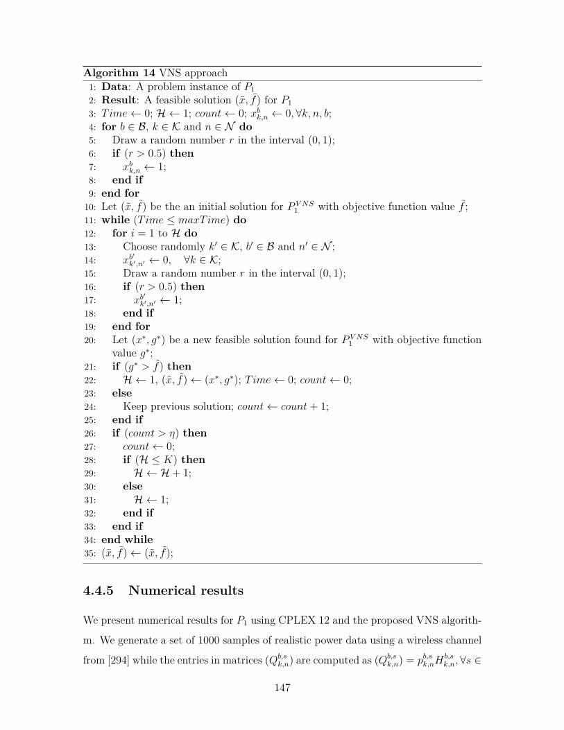
Algorithm 14 VNS approach1: Data: A problem instance of P12: Result: A feasible solution (x, f) for P13: Time← 0; H ← 1; count← 0; xbk,n ← 0,∀k, n, b;4: for b ∈ B, k ∈ K and n ∈ N do5: Draw a random number r in the interval (0, 1);6: if (r > 0.5) then7: xbk,n ← 1;8: end if9: end for10: Let (x, f) be the an initial solution for P V NS

1 with objective function value f ;11: while (Time ≤ maxTime) do12: for i = 1 to H do13: Choose randomly k′ ∈ K, b′ ∈ B and n′ ∈ N ;14: xb

′k′,n′ ← 0, ∀k ∈ K;

15: Draw a random number r in the interval (0, 1);16: if (r > 0.5) then17: xb

′k′,n′ ← 1;

18: end if19: end for20: Let (x∗, g∗) be a new feasible solution found for P V NS

1 with objective functionvalue g∗;

21: if (g∗ > f) then22: H ← 1, (x, f)← (x∗, g∗); Time← 0; count← 0;23: else24: Keep previous solution; count← count+ 1;25: end if26: if (count > η) then27: count← 0;28: if (H ≤ K) then29: H ← H + 1;30: else31: H ← 1;32: end if33: end if34: end while35: (x, f)← (x, f);


We present numerical results for P1 using CPLEX 12 and the proposed VNS algorith-

m. We generate a set of 1000 samples of realistic power data using a wireless channel

from [294] while the entries in matrices (Qb,sk,n) are computed as (Qb,s

k,n) = pb,sk,nHb,sk,n,∀s ∈

147

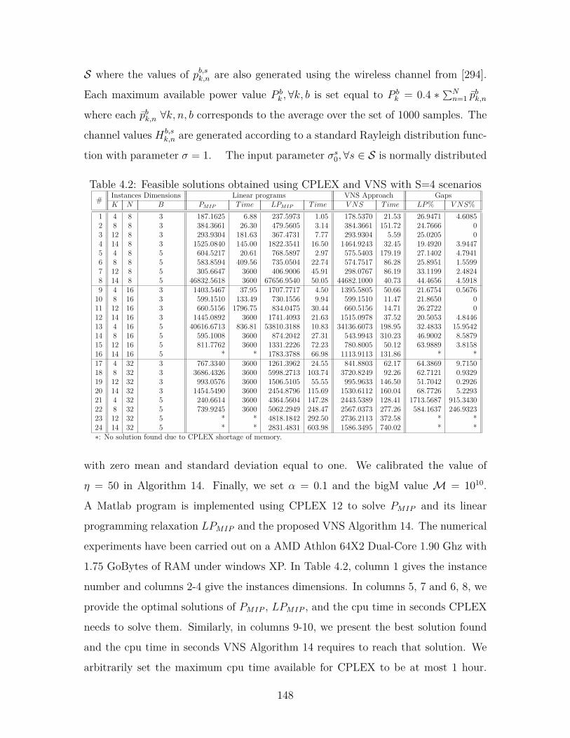
S where the values of pb,sk,n are also generated using the wireless channel from [294].

Each maximum available power value P bk ,∀k, b is set equal to P b

k = 0.4 ∗ ∑Nn=1 p

bk,n

where each pbk,n ∀k, n, b corresponds to the average over the set of 1000 samples. The

channel values Hb,sk,n are generated according to a standard Rayleigh distribution func-

tion with parameter σ = 1. The input parameter σs0,∀s ∈ S is normally distributed

Table 4.2: Feasible solutions obtained using CPLEX and VNS with S=4 scenarios# Instances Dimensions Linear programs VNS Approach Gaps

K N B PMIP Time LPMIP Time V NS Time LP% V NS%1 4 8 3 187.1625 6.88 237.5973 1.05 178.5370 21.53 26.9471 4.60852 8 8 3 384.3661 26.30 479.5605 3.14 384.3661 151.72 24.7666 03 12 8 3 293.9304 181.63 367.4731 7.77 293.9304 5.59 25.0205 04 14 8 3 1525.0840 145.00 1822.3541 16.50 1464.9243 32.45 19.4920 3.94475 4 8 5 604.5217 20.61 768.5897 2.97 575.5403 179.19 27.1402 4.79416 8 8 5 583.8594 409.56 735.0504 22.74 574.7517 86.28 25.8951 1.55997 12 8 5 305.6647 3600 406.9006 45.91 298.0767 86.19 33.1199 2.48248 14 8 5 46832.5618 3600 67656.9540 50.05 44682.1000 40.73 44.4656 4.59189 4 16 3 1403.5467 37.95 1707.7717 4.50 1395.5805 50.66 21.6754 0.567610 8 16 3 599.1510 133.49 730.1556 9.94 599.1510 11.47 21.8650 011 12 16 3 660.5156 1796.75 834.0475 30.44 660.5156 14.71 26.2722 012 14 16 3 1445.0892 3600 1741.4093 21.63 1515.0978 37.52 20.5053 4.844613 4 16 5 40616.6713 836.81 53810.3188 10.83 34136.6073 198.95 32.4833 15.954214 8 16 5 595.1008 3600 874.2042 27.31 543.9943 310.23 46.9002 8.587915 12 16 5 811.7762 3600 1331.2226 72.23 780.8005 50.12 63.9889 3.815816 14 16 5 * * 1783.3788 66.98 1113.9113 131.86 * *17 4 32 3 767.3340 3600 1261.3962 24.55 841.8803 62.17 64.3869 9.715018 8 32 3 3686.4326 3600 5998.2713 103.74 3720.8249 92.26 62.7121 0.932919 12 32 3 993.0576 3600 1506.5105 55.55 995.9633 146.50 51.7042 0.292620 14 32 3 1454.5490 3600 2454.8796 115.69 1530.6112 160.04 68.7726 5.229321 4 32 5 240.6614 3600 4364.5604 147.28 2443.5389 128.41 1713.5687 915.343022 8 32 5 739.9245 3600 5062.2949 248.47 2567.0373 277.26 584.1637 246.932323 12 32 5 * * 4818.1842 292.50 2736.2113 372.58 * *24 14 32 5 * * 2831.4831 603.98 1586.3495 740.02 * *∗: No solution found due to CPLEX shortage of memory.

with zero mean and standard deviation equal to one. We calibrated the value of

η = 50 in Algorithm 14. Finally, we set α = 0.1 and the bigM value M = 1010.

A Matlab program is implemented using CPLEX 12 to solve PMIP and its linear

programming relaxation LPMIP and the proposed VNS Algorithm 14. The numerical

experiments have been carried out on a AMD Athlon 64X2 Dual-Core 1.90 Ghz with

1.75 GoBytes of RAM under windows XP. In Table 4.2, column 1 gives the instance

number and columns 2-4 give the instances dimensions. In columns 5, 7 and 6, 8, we

provide the optimal solutions of PMIP , LPMIP , and the cpu time in seconds CPLEX

needs to solve them. Similarly, in columns 9-10, we present the best solution found

and the cpu time in seconds VNS Algorithm 14 requires to reach that solution. We

arbitrarily set the maximum cpu time available for CPLEX to be at most 1 hour.

148

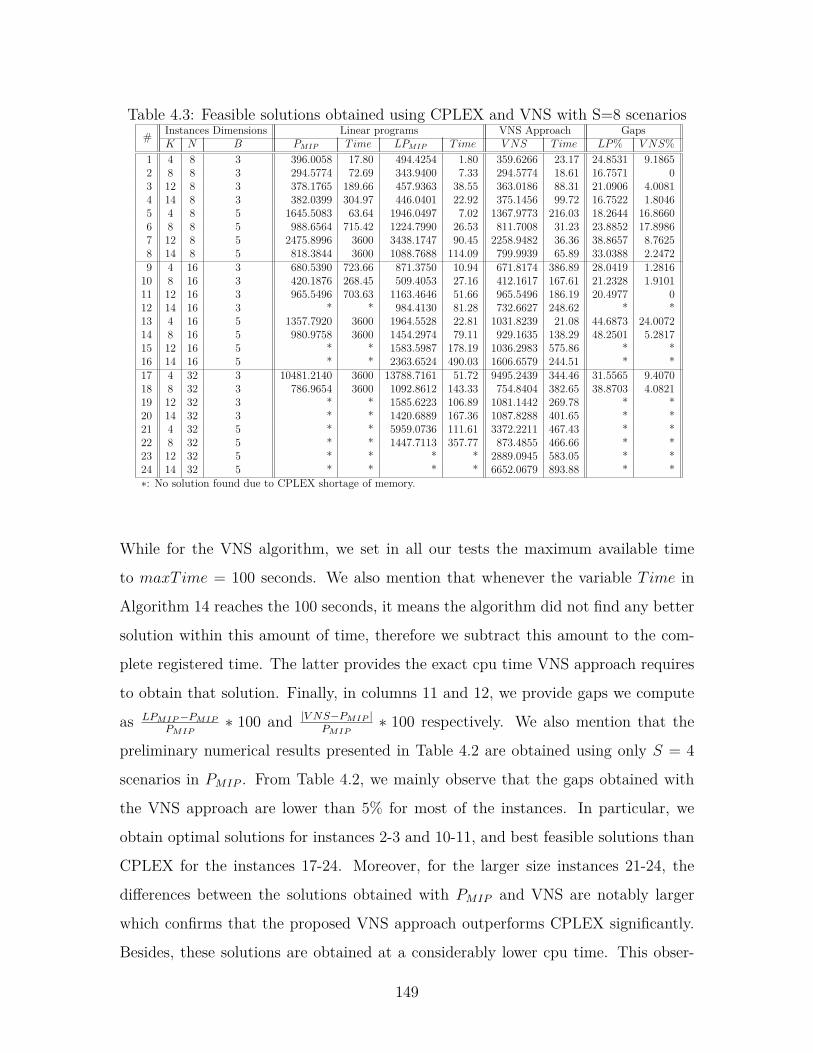
Table 4.3: Feasible solutions obtained using CPLEX and VNS with S=8 scenarios# Instances Dimensions Linear programs VNS Approach Gaps

K N B PMIP Time LPMIP Time V NS Time LP% V NS%1 4 8 3 396.0058 17.80 494.4254 1.80 359.6266 23.17 24.8531 9.18652 8 8 3 294.5774 72.69 343.9400 7.33 294.5774 18.61 16.7571 03 12 8 3 378.1765 189.66 457.9363 38.55 363.0186 88.31 21.0906 4.00814 14 8 3 382.0399 304.97 446.0401 22.92 375.1456 99.72 16.7522 1.80465 4 8 5 1645.5083 63.64 1946.0497 7.02 1367.9773 216.03 18.2644 16.86606 8 8 5 988.6564 715.42 1224.7990 26.53 811.7008 31.23 23.8852 17.89867 12 8 5 2475.8996 3600 3438.1747 90.45 2258.9482 36.36 38.8657 8.76258 14 8 5 818.3844 3600 1088.7688 114.09 799.9939 65.89 33.0388 2.24729 4 16 3 680.5390 723.66 871.3750 10.94 671.8174 386.89 28.0419 1.281610 8 16 3 420.1876 268.45 509.4053 27.16 412.1617 167.61 21.2328 1.910111 12 16 3 965.5496 703.63 1163.4646 51.66 965.5496 186.19 20.4977 012 14 16 3 * * 984.4130 81.28 732.6627 248.62 * *13 4 16 5 1357.7920 3600 1964.5528 22.81 1031.8239 21.08 44.6873 24.007214 8 16 5 980.9758 3600 1454.2974 79.11 929.1635 138.29 48.2501 5.281715 12 16 5 * * 1583.5987 178.19 1036.2983 575.86 * *16 14 16 5 * * 2363.6524 490.03 1606.6579 244.51 * *17 4 32 3 10481.2140 3600 13788.7161 51.72 9495.2439 344.46 31.5565 9.407018 8 32 3 786.9654 3600 1092.8612 143.33 754.8404 382.65 38.8703 4.082119 12 32 3 * * 1585.6223 106.89 1081.1442 269.78 * *20 14 32 3 * * 1420.6889 167.36 1087.8288 401.65 * *21 4 32 5 * * 5959.0736 111.61 3372.2211 467.43 * *22 8 32 5 * * 1447.7113 357.77 873.4855 466.66 * *23 12 32 5 * * * * 2889.0945 583.05 * *24 14 32 5 * * * * 6652.0679 893.88 * *∗: No solution found due to CPLEX shortage of memory.

While for the VNS algorithm, we set in all our tests the maximum available time

to maxTime = 100 seconds. We also mention that whenever the variable Time in

Algorithm 14 reaches the 100 seconds, it means the algorithm did not find any better

solution within this amount of time, therefore we subtract this amount to the com-

plete registered time. The latter provides the exact cpu time VNS approach requires

to obtain that solution. Finally, in columns 11 and 12, we provide gaps we compute

as LPMIP−PMIP

PMIP∗ 100 and |V NS−PMIP |

PMIP∗ 100 respectively. We also mention that the

preliminary numerical results presented in Table 4.2 are obtained using only S = 4

scenarios in PMIP . From Table 4.2, we mainly observe that the gaps obtained with

the VNS approach are lower than 5% for most of the instances. In particular, we

obtain optimal solutions for instances 2-3 and 10-11, and best feasible solutions than

CPLEX for the instances 17-24. Moreover, for the larger size instances 21-24, the

differences between the solutions obtained with PMIP and VNS are notably larger

which confirms that the proposed VNS approach outperforms CPLEX significantly.

Besides, these solutions are obtained at a considerably lower cpu time. This obser-

149

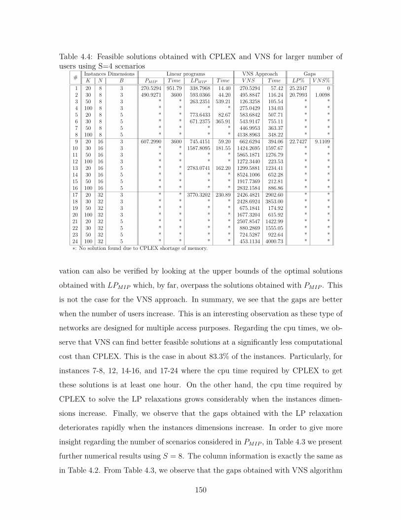
Table 4.4: Feasible solutions obtained with CPLEX and VNS for larger number ofusers using S=4 scenarios

# Instances Dimensions Linear programs VNS Approach GapsK N B PMIP Time LPMIP Time V NS Time LP% V NS%

1 20 8 3 270.5294 951.79 338.7968 14.40 270.5294 57.42 25.2347 02 30 8 3 490.9271 3600 593.0366 44.20 495.8847 116.24 20.7993 1.00983 50 8 3 * * 263.2351 539.21 126.3258 105.54 * *4 100 8 3 * * * * 275.0429 134.03 * *5 20 8 5 * * 773.6433 82.67 583.6842 507.71 * *6 30 8 5 * * 671.2375 365.91 543.9147 755.11 * *7 50 8 5 * * * * 446.9953 363.37 * *8 100 8 5 * * * * 4138.8963 348.22 * *9 20 16 3 607.2990 3600 745.4151 59.20 662.6294 394.06 22.7427 9.110910 30 16 3 * * 1587.8095 181.55 1424.2695 1597.67 * *11 50 16 3 * * * * 5865.1871 1276.79 * *12 100 16 3 * * * * 1272.3440 223.53 * *13 20 16 5 * * 2783.0741 162.20 1299.5881 1234.41 * *14 30 16 5 * * * * 8524.1006 652.28 * *15 50 16 5 * * * * 1917.7369 212.81 * *16 100 16 5 * * * * 2832.1584 886.86 * *17 20 32 3 * * 3770.3202 230.89 2426.4821 2902.60 * *18 30 32 3 * * * * 2428.6924 3853.00 * *19 50 32 3 * * * * 675.1841 174.92 * *20 100 32 3 * * * * 1677.3204 615.92 * *21 20 32 5 * * * * 2507.8547 1422.99 * *22 30 32 5 * * * * 880.2869 1555.05 * *23 50 32 5 * * * * 724.5287 922.64 * *24 100 32 5 * * * * 453.1134 4000.73 * *∗: No solution found due to CPLEX shortage of memory.

vation can also be verified by looking at the upper bounds of the optimal solutions

obtained with LPMIP which, by far, overpass the solutions obtained with PMIP . This

is not the case for the VNS approach. In summary, we see that the gaps are better

when the number of users increase. This is an interesting observation as these type of

networks are designed for multiple access purposes. Regarding the cpu times, we ob-

serve that VNS can find better feasible solutions at a significantly less computational

cost than CPLEX. This is the case in about 83.3% of the instances. Particularly, for

instances 7-8, 12, 14-16, and 17-24 where the cpu time required by CPLEX to get

these solutions is at least one hour. On the other hand, the cpu time required by

CPLEX to solve the LP relaxations grows considerably when the instances dimen-

sions increase. Finally, we observe that the gaps obtained with the LP relaxation

deteriorates rapidly when the instances dimensions increase. In order to give more

insight regarding the number of scenarios considered in PMIP , in Table 4.3 we present

further numerical results using S = 8. The column information is exactly the same as

in Table 4.2. From Table 4.3, we observe that the gaps obtained with VNS algorithm

150

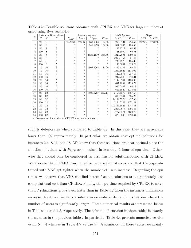
Table 4.5: Feasible solutions obtained with CPLEX and VNS for larger number ofusers using S=8 scenarios

# Instances Dimensions Linear programs VNS Approach GapsK N B PMIP Time LPMIP Time V NS Time LP% V NS%

1 20 8 3 304.9070 926.97 363.6304 62.98 250.3734 226.53 19.2594 17.88532 30 8 3 * * 346.1478 104.80 317.3865 155.50 * *3 50 8 3 * * * * 192.7712 402.53 * *4 100 8 3 * * * * 328.1000 60.58 * *5 20 8 5 * * 1929.2130 284.56 1220.2991 1099.84 * *6 30 8 5 * * * * 2063.0753 331.43 * *7 50 8 5 * * * * 736.4978 185.36 * *8 100 8 5 * * * * 140.0601 619.28 * *9 20 16 3 * * 4902.3964 144.20 4290.7134 492.44 * *10 30 16 3 * * * * 7289.1626 1133.05 * *11 50 16 3 * * * * 532.0673 737.55 * *12 100 16 3 * * * * 242.7288 478.31 * *13 20 16 5 * * * * 1142.8744 1158.90 * *14 30 16 5 * * * * 687.1994 1739.78 * *15 50 16 5 * * * * 990.0482 403.17 * *16 100 16 5 * * * * 615.1829 2235.63 * *17 20 32 3 * * 3926.1787 327.11 2156.4379 1687.58 * *18 30 32 3 * * * * 819.6241 585.23 * *19 50 32 3 * * * * 14159.5528 427.56 * *20 100 32 3 * * * * 2154.5143 1071.48 * *21 20 32 5 * * * * 100865.1824 3447.88 * *22 30 32 5 * * * * 2255.9878 1005.44 * *23 50 32 5 * * * * 1787.8574 2139.78 * *24 100 32 5 * * * * 828.8698 6320.64 * *∗: No solution found due to CPLEX shortage of memory.

slightly deteriorates when compared to Table 4.2. In this case, they are in average

lower than 7% approximately. In particular, we obtain near optimal solutions for

instances 2-4, 8-11, and 18. We know that these solutions are near optimal since the

solutions obtained with PMIP are obtained in less than 1 hour of cpu time. Other-

wise they should only be considered as best feasible solutions found with CPLEX.

We also see that CPLEX can not solve large scale instances and that the gaps ob-

tained with VNS get tighter when the number of users increase. Regarding the cpu

times, we observe that VNS can find better feasible solutions at a significantly less

computational cost than CPLEX. Finally, the cpu time required by CPLEX to solve

the LP relaxations grows even faster than in Table 4.2 when the instances dimensions

increase. Next, we further consider a more realistic demanding situation where the

number of users is significantly larger. These numerical results are presented below

in Tables 4.4 and 4.5, respectively. The column information in these tables is exactly

the same as in the previous tables. In particular Table 4.4 presents numerical results

using S = 4 whereas in Table 4.5 we use S = 8 scenarios. In these tables, we mainly

151

observe that finding optimal solutions with CPLEX becomes rapidly prohibitive. In

fact, we can only find feasible solutions for instances 1, 2 and 9 in Table 4.4 and for

instance number 1 in Table 4.5 using the linear programs. On the opposite, using

VNS approach still allows finding feasible solutions up to instances with K = 100

users. Although, the cpu times are considerably larger when compared to Tables

4.2 and 4.3, respectively. This confirms again that the proposed VNS approach is

competitive.

In general, when looking at the four tables presented, we observe that solving

PMIP and LPMIP is considerably harder than solving the proposed VNS approach.

However, the proposed linear programs still provide an alternative way to compute

optimal solutions and upper bounds for the multi-cell OFDMA problem. Also, we

observe that the VNS approach outperforms the solutions obtained with CPLEX in

most of the cases, especially when the instances dimensions increase. Additionally, we

observe that the number of scenarios s ∈ S directly affects the performance of CPLEX

when solving the linear programs. This can be explained by the fact that using more

scenarios implies using more variables in the linear programs. This is not the case

for the VNS approach where the number of variables in P V NS1 does not depend on

the number of scenarios. Finally, we observe that the linear programs can not be

solved efficiently when considering a larger number of users in the system. Hence, the

number of scenarios and the number of users can be considered as bottlenecks for the

proposed linear programs. On the other hand, the performance of the VNS approach

deteriorates when incrementing the number of users and the number of subcarriers

either separately or simultaneously.

4.4.6 Conclusions

In this paper, we propose a (0-1) stochastic resource allocation model for uplink wire-

less multi-cell OFDMA Networks. The model maximizes the total signal to interfer-

ence noise ratio produced in a multi-cell OFDMA network subject to user power and

subcarrier assignment constraints. We transformed the stochastic model into a de-

terministic equivalent binary nonlinear optimization problem having quadratic terms

152

and second order conic constraints. Subsequently, we use the deterministic model

to derive an equivalent mixed integer linear programming formulation. Finally, we

proposed a reduced variable neighborhood search metaheuristic procedure [145, 149]

to compute feasible solutions. Our preliminary numerical results provide near opti-

mal solutions for most of the instances when compared to the optimal solution of the

problem. Moreover, we find better feasible solutions than CPLEX when the instances

dimensions increase. Finally, we obtain these feasible solutions at a significantly less

computational cost.

As future research, we plan to study new stochastic and algorithmic approaches

for the problem.

153

4.5 Conclusions

This chapter mainly focused on the field of OFDMA system and resource allocation

and scheduling problem. Based on the introduction of OFDM system, the detailed

information of OFDMA system includes the background, modeling, basic algorithm,

especially the method for solving the OFDMA resource allocation problem with var-

ious conditions are described. In our two papers, we presented numerical results for

two OFDMA optimization problems.

154

Chapter 5

Bi-level Programming Problem

Hierarchy is one of the important characteristics of a given system. It is a main

characteristic for large and complicated systems. In the fields of socio-economic, en-

gineering, management and military, the system with the hierarchical relationships

can be found everywhere, for example, the superior and the subordinate relationship

in management institutions, the supply and marketing relationship in the economic

activity, the defense and counter-defense relationship in military system, the rela-

tionship between the company and the branch, the relationship between the control

variables and state variables in the engineering design etc. In these systems with

hierarchical structure, the upper level is the leader to consider the overall situation

which has coordinating and leading effect, and the goal is to make the whole system

cost minimum. The lower level is the follower which makes decisions depending on the

constraints of the upper level problem to make the cost minimum of the subsystem.

Therefore, the multilevel programming is proposed to study the system hierarchy.

Multilevel programming is a kind of mathematical programming which contains

the optimization problem in the constraints. It studies the interaction among multiple

objective functions which are according to the non-cooperative and orderly manner.

The behavior of each one affects the strategy selection and goal achievement of the

other ones, but neither can fully control the selection behavior of the other ones.

The hierarchy programming model was firstly proposed by H. Stackelberg. In

the 1950s, in order to better describe the economic model in reality, H. Stackelberg

155

first presented hierarchy programming in his monograph [321]. Although hierarchy

programming is similar to multilevel programming, for multilevel programming, the

decision makers in each level make decisions in sequence, and each strategy set can

be no longer separated. In 1960s, Dantzig and Wolfe proposed the decomposition

algorithm for large scale linear programming, which admitted a core decision maker

whose goal is above all else. However, there is a big difference between the decompo-

sition algorithm and multilevel programming. The latter admits the highest decision

maker but not absolutely, it allows the lower decision makers have different inter-

ests. The multi-objective programming which was developed in 1970s usually seek a

compromise solution for conflicting multiple objective function of a decision maker,

while the multilevel programming emphasizes the impact of the lower level decision

on the upper level decision, and the multilevel programming problem usually can not

be solved independently by levels.

Since the 1970s, in the study of the various reality optimization problems of dis-

tributed level systems such as production planning, resource allocation, government

regulation and engineering design, it was found that the above methods and tra-

ditional mathematical programming techniques can not better solve such problems,

thus in the process of finding a variety of specific methods which successfully solve

these problems, the concept and the method of multilevel programming is gradually

formed. The term "multilevel programming" is first proposed by Candler and Nor-

ton in the research report of the dairy industry model and the Mexico agricultural

model [61].

In the past few decades, the theory, method and application of multilevel pro-

gramming have a lot of development and become a new important branch in the

optimization theory. In the study of multilevel programming, the bi-level program-

ming is an important study object. The bi-level programming is a special case in

the multilevel programming, which can be seen as a complex of a series of bi-level

programming [40,45].

In this chapter, Section 5.1, 5.2, 5.3, 5.4, 5.5 present the definition, formulation,

application, property and method of bi-level programming in detail, respectively.

156

Section 5.6 proposes a distributionally robust model for a (0-1) stochastic quadratic

bi-level programming problem. Section 5.7 concludes this chapter.

5.1 Definition

Bi-level programming was first proposed in the research of unbalanced economy mar-

ket competition. In 1973, in the article of Bracken and Mcgill [51], the bi-level

programming model is presented. In 1977, in the scientific report of Candler and

Norton [61], the term of bi-level programming and multilevel programming officially

appeared. From the 1980s, bi-level programming attracted a lot of attention. The re-

search began to focus on bi-level programming problems and multilevel programming

problems.

Bi-level programming is a kind of system optimization problem with two level

hierarchical structures. The upper and lower level problems have their own decision

variables, constraints and objective functions. The objective function and constraint

of the upper level problem is not only related to the decision variable of upper level

problem, but also the optimal solution of lower level problem, while the optimal

solution of lower level problem is affected by the upper level decision variable.

According to the above definition, bilevel programming has the following main

features:

(1) Hierarchy. The system is a hierarchical management, decision makers in each

level make decisions orderly, and the lower obeys the upper.

(2) Conflict. Each decision maker has its different objective function, and these

objective functions are often contradictory.

(3) Priority. The upper decision maker makes priority decisions, while the lower

decision maker can not go against the upper decision when chooses the decision to

optimize its objective function.

(4) Conditionality. The lower decision will not only determine the achievement of

its own objective, but also affects the realization of the upper objective.

(5) Dependence. The allowed strategy set of each level decision maker are usually

157

inseparable, they tend to form an interconnected whole.

5.2 Formulation

In 1973, the bi-level programming model was appeared in Bracken and Mcgill’s article.

In bi-level programming model, different decision makers control the corresponding

decision variables and optimize their own objective function. Because the strategy set

selected by two levels is independent, the upper decision will affect the lower decision

selection and objective achievement, and vice versa.

The general formulation of a bi-level programming problem is

minx∈X,y

F (x, y)

s.t. G(x, y) ≤ 0

miny

f(x, y)

s.t. g(x, y) ≤ 0 (5.1)

where x ∈ Rn1 , y ∈ Rn2 are the decision variables of upper and lower level problems

respectively. Similarly, F : Rn1 × Rn2 → R and f : Rn1 × Rn2 → R are the objective

functions for the upper and lower level problems respectively. The functions G :

Rn1 × Rn2 → Rm1 and g : Rn1 × Rn2 → Rm2 are called upper and lower level

constraints respectively.

According to different reactions from lower level to upper level, the bi-level pro-

gramming model can be divided into the following two types:

(1) The optimal solution of lower level feedbacks to the upper level.

minx∈X,y

F (x, y)

s.t. G(x, y) ≤ 0

miny∈Y

f(x, y)

158

s.t. g(x, y) ≤ 0 (5.2)

(2) The optimal value of the objective function of lower level feedbacks to the

upper level.

minx∈X

F (x, v(x))

s.t. G(x, v(x)) ≤ 0

v(x) = miny∈Yf(x, y)|g(x, y) ≤ 0 (5.3)

Generally, the first model is a hot area of researches.

In order to study the characteristic, method and application of bi-level program-

ming problem, some further concepts of bi-level programming are introduced in the

following:

(1)Constraint region:

Ω = (x, y) ∈ Rn1 ×Rn2 : x ∈ X,G(x, y) ≤ 0 and g(x, y) ≤ 0

(2)For a given x, the lower level feasible set:

Ω(x) = y ∈ Rn2 : g(x, y) ≤ 0

(3)For a given x, the rational reaction set of lower level problem:

M(x) = y ∈ Rn2 : y ∈ argminf(x, y) : y ∈ Ω(x)

(4)For a given x and corresponding y ∈ M(x), the optimal value of lower level

problem:

v(x) = f(x, y)

(5)Induced region:

IR = (x, y) ∈ Rn1 ×Rn2 : x ∈ X,G(x, y) ≤ 0, y ∈M(x)

159

The induced region is the feasible solution set of bi-level programming problem.

For any decision variable x of upper level, when the rational reaction set M(x) is a

singleton, the solution of lower level is unique. In addition, in order to ensure that

bi-level programming problem has a solution, we assume that the constraint region

Ω and the induced region IR are nonempty and bounded. The definition of feasible

solution and optimal solution are given below.

Definition 1 If (x, y) ∈ IR, then (x, y) is the feasible solution of bi-level program-

ming problem.

Definition 2 If (x∗, y∗) ∈ IR and F (x∗, y∗) ≤ F (x, y),∀(x, y) ∈ IR, thus (x∗, y∗) is

the optimal solution of bi-level programming problem.

Assuming that x is selected in upper level, lower level will optimize its objective

function with parameter x. However, for the given x, lower level problem may have

an infinite number of optimal solutions. These solutions are undifferentiated to the

lower level, but are probably different for the objective function of upper level, thus

the difficulty of optimizing objective function of upper level increases. In other words,

the rational reaction set M(x) of lower level is not a singleton, the objective function

F (x, y)(y ∈ M(x)) of upper level problem is a multi-valued function.The following

example will illustrate this.

Example.

minx

F = x+ y1 − y2

s.t. 0 ≤ x ≤ 1

miny

f = −y1 − y2

s.t. x+ y1 + y2 = 1

y1, y2 ≥ 0

For the above problem, the upper level has only one decision variable x, and the

lower level has two decision variables y1 and y2. When 0 ≤ x ≤ 1, the objective

160

function of lower level can be obtained as f = x − 1 according to x + y1 + y2 = 1.

When x = 0.5 in upper level, the optimal value of objective function in lower level is

min f = x − 1 = −0.5, but the optimal solution of lower level is not unique. When

the solution of the lower level satisfies constraints x+ y1 + y2 = 1 and y1, y2 ≥ 0, the

objective function of the upper level F = x + y1 − y2 will be affected obviously. For

example, when (y1, y2) = (0.5, 0), F = 1; when (y1, y2) = (0, 0.5), F = 0. For this

example, the upper level can take any x ∈ [0, 1], and the optimal solution of lower

level is not unique, that is, there will be an infinite number of optimal solutions.

This example illustrates that when the upper level gives an allowable decision, if

the optimal solution of the lower level is not unique, i.e., the element in the rational

reaction set of the lower level is not unique, it will cause the complexity of solving

the entire bilevel programming problem, even not guarantee to obtain the optimal

solution of the problem [36].

In order to overcome the difficulty of multiple solutions, Bialas and Karnm [45]

proposed a method which replaces the objective function of the lower level f2 by

using f2 + εf1, where ε is an appropriate small positive number. The idea consists

in the upper level gives a part of the income to the lower level, thus the lower level

selects its solution which is beneficial for the upper level. In other application of bi-

level programming problem, f2 − εf1 can be used to represent a kind of "opposition"

relationship between the upper and lower objectives.

Generally, when the lower level of bi-level linear programming problem exists more

than one optimal solution, the bi-level linear programming can be solved twice. The

first time f2 + εf1 is used to replace f2 (optimistic case), the second time f2 − εf1

instead of f2 (pessimistic case). If a solution in both cases is the optimal solution,

then it is the optimal solution of the whole problem. Otherwise, the bi-level linear

programming problem is only able to get the lower and upper bounds for its optimal

solution, and the optimal solution doesn’t exist.

Dempe [94] pointed out that if the solution of the lower level problem is not

unique, the bi-level programming will be unstable. In order to overcome the difficulty,

two modeling approaches are proposed in the literature which are optimistic bilevel

161

programming and pessimistic bi-level programming.

In the optimistic bi-level programming, the follower will choose an optimal solution

which is the best one for the leader. The optimistic bi-level programming problem is

defined as following:

minx

ϕo(x)

miny

f(x, y)

s.t. g(x, y) ≤ 0 (5.4)

where

ϕo(x) = minyF (x, y) : G(x, y) ≤ 0, y ∈M(x) (5.5)

and a pair of points (x∗, y∗) is called a local optimistic solution of the bi-level pro-

gramming problem if y∗ ∈ M(x), F (x∗, y∗) = ϕo(x∗), and x∗ is the optimal solution

of upper level.

On the other hand, the pessimistic bi-level programming problem is:

minx

ϕp(x)

miny

f(x, y)

s.t. g(x, y) ≤ 0 (5.6)

where

ϕp(x) = maxyF (x, y) : G(x, y) ≤ 0, y ∈M(x) (5.7)

and a pair of points (x∗, y∗) is called a local pessimistic solution of the bi-level pro-

162

gramming problem if y∗ ∈ M(x), F (x∗, y∗) = ϕp(x∗), and x∗ is the optimal solution

of upper level.

However, both optimistic and pessimistic solution are not the good approximation

to the solution of the original bi-level programming in practice. A slight change in

the data of the problem will have a huge impact on the solution of the lower level.

Therefore, Dempe proposed not to select the optimal solution of bi-level programming

but select a small perturbation of the optimal solution to ensure that the lower level

has the unique and stable solution. In addition, Dempe gave some theories to assure

such solutions can be obtained, and also presented some algorithms for the bi-level

programming problem where the optimal solution of lower level is not unique [93,95].

5.3 Application

For general bi-level programming problem, the earliest application that appears in the

literature is the general problem of economic planning at the regional or national level

[233]. The early work of Candler and Nonton [61] mainly focused on the development

of agriculture in northern Mexico, which explained how to use bi-level programming to

analyze the adjustment of economy. Fortuny-Amat and McCarl [112] gave a regional

model for the competition of fertilizer supply among the farm. Aiyoushi, Shimizu [3]

and Bard [25] studied the energy distribution problem of the hierarchical organization.

The transportation is a major application area of bi-level programming. Currently

there is a wide literature which describes the urban transportation network design

problem (NDP) with the bi-level programming model. Leblance and Boyce [198] first

solved the NDP with the bi-level programming model, and gave a clear definition, but

their model assumed that the cost function increases linearly which has a certain gap

with the practical problem. Later, Ben-Aye et al. [39] gave a more general formulation

under the condition of allowing the cost function increases non-linearly. Bard [30] took

Tunisia for instance, according to the regional highway network planning problem

in developing country, discussed a more realistic bi-level programming model. In

addition, the study of NDP such as continuous NDP, balance NDP etc. can be seen

163

in [38, 113,222,223,304,310].

The application of bilevel programming on the transportation also includes esti-

mating Origin-Destination demands problem and traffic control problem. Migdalas et

al. [233] made a detailed description for estimating O-D demands problem, discussed

the significance and application of the problem, and derived the necessary optimality

condition. Moreover, how to control the signal to make the user have a reasonable re-

sponse and reduce the traffic congestion and delay can be also considered as a bi-level

programming problem, the related literature can be seen in [75,342,343].

Resource allocation is a kind of complex management problem. The upper depart-

ment allocates resources to multiple lower departments, and lower departments orga-

nize production to maximize their own benefits according to the allocated resources

and their existing resources. However, the resource of the upper level department is

limited, and the benefit of each lower department is different, so how to make limited

resources produce the greatest benefits is the biggest problem for the upper level.

Based on this contradiction, bi-level programming model can describe this kind of

problem well [34].

The price problem and the production planning problem are typical bilevel pro-

gramming problem. Baumol and Fabian [35] studied the pricing control problem with

bi-level programming, Lam and Zhou [195], Goel and Haghani [134] also focused on

such problem. Nicholls [249, 250] continuously published the articles about the pro-

duction planning problem of aluminum production company. Karlof and Wang [177]

studied the flow shop-scheduling problem.

Currently, with the rapid development of market globalization and the drastic

change of competition environment, more and more companies recognize the impor-

tance of supply chain management. Manufacturer working closely with its supplier to

achieve a win-win strategy becomes a hot research issue. Therefore, establishing the

bi-level programming model, while the lower level objective is to maximize the ben-

efit to each member and the upper level objective is the comprehensive performance

of the supply chain, has important application value and practical significance. In

addition, the bi-level programming is also applied in the field of engineering [185],

164

facility location [234,307], policy planing [184,256], etc.

5.4 Characteristics

5.4.1 Complexity

In general, solving bi-level programming problem is very difficult. For bi-level pro-

gramming problem, its objective function of upper level depends on the solution func-

tion of lower level, and this solution function is not linear and differentiable. There-

fore, even if the bi-level linear programming is also a non-convex programming [45]

and is non-differentiable everywhere.

Jeroslow [170] first pointed out that bi-level linear programming is a NP-hard

problem. Ben-Aye and Blair [37] turned a known NP-hard problem, Knapsack opti-

mization problem, into a bi-level linear programming problem through a polynomial

transformation, thus the bi-level linear programming problem is NP-hard. Later,

Bard [29] proved this conclusion. Besides, Hansen et al. [143] gave a rigorous proof

on bi-level linear programming is a strongly NP-hard problem. In 1994, Vicente [318]

pointed out that to find the local optimum for the bi-level linear programming is also a

NP-hard problem, and there is no polynomial algorithm. Deng [96] did a summarized

discussion to the complexity of bi-level linear programming.

5.4.2 Optimality condition

In the mathematical programming, the optimal solution should satisfy the optimality

condition. It is the theoretical basis to find the algorithm for solving mathematical

programming problems. Bard [27] first studied the optimality condition of bi-level

linear programming problem. He applied a single level programming with an infinite-

dimensional parametric constraint set which is equivalent to the original problem to

obtain some optimality conditions. On this basis, Bard [24, 25] and Unlu [312] gave

an algorithm for solving the linear bi-level programming. Clarke and Westerberg [78],

Haurie et al. [153] gave the counter example for these conditions.

165

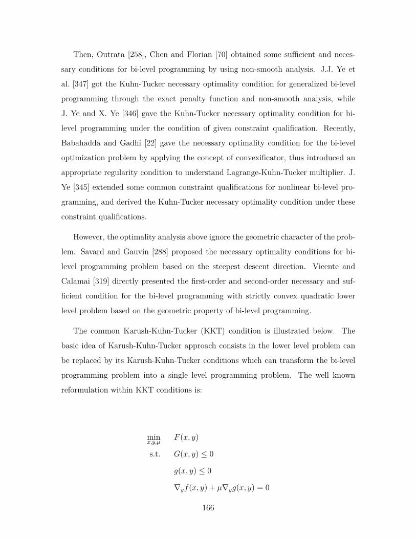
Then, Outrata [258], Chen and Florian [70] obtained some sufficient and neces-

sary conditions for bi-level programming by using non-smooth analysis. J.J. Ye et

al. [347] got the Kuhn-Tucker necessary optimality condition for generalized bi-level

programming through the exact penalty function and non-smooth analysis, while

J. Ye and X. Ye [346] gave the Kuhn-Tucker necessary optimality condition for bi-

level programming under the condition of given constraint qualification. Recently,

Babahadda and Gadhi [22] gave the necessary optimality condition for the bi-level

optimization problem by applying the concept of convexificator, thus introduced an

appropriate regularity condition to understand Lagrange-Kuhn-Tucker multiplier. J.

Ye [345] extended some common constraint qualifications for nonlinear bi-level pro-

gramming, and derived the Kuhn-Tucker necessary optimality condition under these

constraint qualifications.

However, the optimality analysis above ignore the geometric character of the prob-

lem. Savard and Gauvin [288] proposed the necessary optimality conditions for bi-

level programming problem based on the steepest descent direction. Vicente and

Calamai [319] directly presented the first-order and second-order necessary and suf-

ficient condition for the bi-level programming with strictly convex quadratic lower

level problem based on the geometric property of bi-level programming.

The common Karush-Kuhn-Tucker (KKT) condition is illustrated below. The

basic idea of Karush-Kuhn-Tucker approach consists in the lower level problem can

be replaced by its Karush-Kuhn-Tucker conditions which can transform the bi-level

programming problem into a single level programming problem. The well known

reformulation within KKT conditions is:

minx,y,µ

F (x, y)

s.t. G(x, y) ≤ 0

g(x, y) ≤ 0

∇yf(x, y) + µ∇yg(x, y) = 0

166

µTg(x, y) = 0, µ ≥ 0

(x, y) ∈ Rn1 ×Rn2 (5.8)

5.5 Methods

5.5.1 Extreme-point approach

The basic idea consists in any solution of linear bi-level programming problem appears

in the extreme point of lower level constraint set. Firstly, a variety of methods are

used to find the extreme point of constraint space, then the local optimal point or

global optimal point are found out from the extreme point. However, as the size of

the problem and the number of extreme point increase, the amount of computation

increases rapidly, thus the large scale problem is difficult to solve.

In the study of linear bi-level programming which has no constraint in upper level

and the unique solution in lower level, Candle and Townsley [62] got a property: if

the number of linear bi-level programming optimal solutions is finite, then at least

an extreme point is the optimal solution from the extreme point of the constraint

set. Later, Bard [26], Bialas and Karwan [45] proved that this property is a general

characteristic of linear bi-level programming under the assumption of the bounded

constraint set. Bialas and Karwan [44] firstly proposed Kth best approach which

obtains the optimal solution of linear bi-level programming problem through enumer-

ating all extreme points of linear bi-level programming constraint region. Bard [24]

proposed an algorithm using sensitivity analysis to solve linear bi-level programming

problem, and it was more efficient than Kth best. However, Haurie et al. [153] and

Ben-Ayed and Blair [37] pointed out that this algorithm may not find the optimal so-

lution, and the reason is that it can not provide the middle result, i.e., if the algorithm

stops when the termination condition is not satisfied, the algorithm can not even ob-

tain an approximatal solution. Even if a solution can be obtained, the algorithm can

not be sure that this solution is the global or local optimal solution [37].

Recently, based on the new definition of bilevel linear programming solution [296],

167

Shi et al. [295] not only proposed extended Kth best approach to solve linear bi-

level programming problem, but also the Kth best approach for the linear bi-level

programming with several decision makers in lower level [297].

5.5.2 Branch-and-bound algorithm

Branch and bound approach divides the solving problem into a series of sub-problems

according to the pre-selected branching criteria, and chooses a sub-problem and tests

to determine the choice. Branch and bound approach is widely used in the convex

bi-level programming problem.

Fortuny-Amat and McCarl [112] replaced the lower level problem of quadratic

bi-level programming by its Karush-Kuhn-Tucker conditions to get a single level pro-

gramming problem, then used two equation constraints with binary variable instead

of nonlinear complementarity condition to obtain a mixed integer bi-level program-

ming, thus the global solution of bi-level programming problem will be obtained.

Likewise, Bard and Moore [32] changed linear bi-level programming problem into s-

ingle level problem by using Karush-Kuhn-Tucker condition to replace the lower level

problem, then solved the linear programming after removing the complementary con-

dition, and checked whether the complementary condition is true in each iteration. If

true, the corresponding point is in the induced region, so a potential optimal solution

is obtained; Otherwise, all combinations of complementary slackness conditions are

checked by branch and bound method. Due to the general property of this branch

and bound algorithm, it can also be used to solve the nonlinear bi-level programming

problem. Later, Hansen et al. [143] proposed a new branch and bound algorithm to

solve linear bi-level programming, which explores or simplifies the sub-problem by

using the necessary optimality conditions which is represented by the tight constraint

of lower level, and the branch and punish operation are same as in the mixed integer

programming. This approach is particularly effective for medium size problems. In

addition, Bard and Falk [31] studied the branch and bound method to solve multi-

level programming. Bard [28], Edmunds and Bard [101] and Al-Khayyal et al. [7]

proposed the branch and bound approach for the quadratic bi-level programming.

168

Wen and Yang [326], Bard and Moore [33, 239] presented branch and bound algo-

rithm for solving the integer linear bi-level programming. Edmunds and Bard [102]

solved integer quadratic bi-level programming problem by using branch and bound

approach.

5.5.3 Complementary pivoting approach

This approach is proposed for linear bi-level programming problem, and the main

idea is to transfer the problem into parametric complementarity problem, then solve

the problem by using the complementary pivot algorithm. This method is a heuristic

algorithm.

Bialas et al. [46] first solved the linear bi-level programming with the complemen-

tary pivoting approach, and the algorithm can also be used to solve linear three-level

programming problem. However, Bialas and Karwan [45] pointed out that this al-

gorithm can not get the global optimal solution of linear bi-level programming, so

Judice and Faustino [173] improved the complementary pivoting approach to ensure

the global optimal solution. Later, Judice and Faustino [173–175] presented sequen-

tial linear complementary pivoting (SLCP) algorithm to get the ε global optimal

solution of linear quadratic bi-level programming, and this algorithm is effective for

medium size problems. The complementary pivoting algorithm which is proposed by

Onal [255] can be seen as an improved simplex method.

5.5.4 Descent method

This algorithm solves the problem based on some optimality conditions of the lower

level or by using the gradient information of lower level optimal solution about upper

level decision variable. Although the application scope of this method is wide, gen-

erally it can only obtain the local optimal solution of nonlinear bi-level programming

problem.

The first typical algorithm is the steepest descent approach. Savard and Gauvin

[288] used this algorithm to solve nonlinear bi-level programming problem. Vicente

169

et al. [318] proposed two descent methods for convex bi-level programming. One is

based on pivot steps, but it can not ensure the local optimum. The other one is a

modified steepest descent approach which overcomes this drawback. Then a hybrid

approach which combines these two strategies is discussed. Another typical approach

is the descent approach presented by Kolstad and Lasdon [187] using the gradient

information to solve nonlinear bi-level programming problem.

5.5.5 Penalty function method

This method mainly uses the principle of penalty function in the theory of nonlinear

programming which uses different forms of penalty terms to transform the lower level

problem into an unconstrained mathematical programming problem, then the penalty

term is added to the objective function of upper level, and the problem is changed into

a single level problem with the penalty parameter. After solving a series of nonlinear

programming problems, the optimal solution of bi-level programming is obtained.

This method not only appling to linear bi-level programming, but also for solving

nonlinear bi-level programming problem.

Based on the fact that the duality gap equals to zero when linear programming

is at its optimal solution, Anandalingam and White [14] proposed a penalty function

method using duality gap as penalty term. In this method, the duality gap of lower

level problem is taken as the penalty term of the upper level problem, then this

complex problem is decomposed into a series of linear programming problems, thus

the local optimal solution of original problem is obtained. Then they presented a

penalty function method for solving linear bi-level programming to get the global

optimal solution [329]. Ishizuka and Aiyoshi [167] constructed a penalty function

method through punishing both objective function of upper and lower level to solve

bi-level programming where the optimal solution of lower level is not unique. White

and Anandalingam [329], White [328] presented the exact penalty function method

for bi-level programming. Campelo et al. [56] pointed out that the original dual tight

assumption which is considered in the literature [329] is inaccurate, and the cut set

to remove the optimal solution in the algorithm is not defined clearly. They redefined

170

the cut set, thus the property of the penalty problem was good without the tight

assumption. Liu et al. [211] proposed a new constraint qualification for convex bi-

level programming, and gave a locally and globally first order exact penalty function

method under this constraint qualification, without considering whether the linear

independence and strict complementary condition in lower level are satisfied. Calvete

and Gale [55] presented a penalty function method for bi-level programming problem

which the upper level is linear fractional and the lower level is linear. Based on

considering the relationship between the lower level problem and its dual problem,

this method used the duality gap of lower level to construct a exact penalty method

to achieve the global optimum. Recently, Lv et al. [219] proposed a penalty function

method to solve the weak price control problem, and Lv et al. [220] also presented a

penalty function method based on Karush-Kuhn-Tucker condition for linear bi-level

programming.

5.5.6 Metaheuristic method

Mathieu et al. [230] proposed a genetic algorithm (GA) to solve linear bi-level pro-

gramming problem. In this algorithm, the decision variable of upper level is generated

randomly, and the reaction of lower level is obtained through solving a linear program-

ming, and only mutation operation is used in GA. However, because each individual

does not necessarily represent a extreme point, but represents a reachable solution,

such that the search space is greatly expanded. Hejazi et al. [155] presented a genetic

algorithm. Each feasible individual represents a vertex of the feasible region, thus the

search space is greatly reduced. In addition, Liu [210] proposed a genetic algorithm

to solve Stackerberg-Nash equilibrium for multilevel programming. Niwa et al. [251]

solved decentralized bi-level 0-1 programming problem by using genetic algorithm

with double strings. Yin [348] applied genetic algorithm on bi-level programming

model in transport planning and management. In this method, the decision variable

of upper level is encoded, and its fitness value is calculated through solving the lower

level problem, finally the optimal solution is obtained by using the selection, crossover

and mutation operations. Later, Oduguwa and Roy [254] presented a genetic algo-

171

rithm for bi-level programming which solves different types of bi-level programming

problems in a single framework through the finite asymmetrical cooperation between

two participants. Wang et al. [324] solved bi-level programming using an evolutionary

algorithm with a new constraint-handling scheme.

Gendreau et al. [121] proposed an adaptive search algorithm combined with tabu

search to solve linear bi-level programming problem. This algorithm determined the

initial solution and improved the current solution by using the concept of penalty

function, and also used tabu search algorithm to make search from a feasible point to

another feasible point. Wen and Huang [325] presented a simple tabu search algorithm

to solve mixed integer linear bi-level programming problem. Shih et al. [298] solved

multi-objective and multilevel programming problem with neural network algorithm.

Lan et al. [196] proposed a hybrid algorithm which combines the neural network and

tabu search to solve bi-level programming.

5.5.7 Other methods

Wu et al. [333] proposed a cutting plane method to solve linear bi-level programming

problem. Loridan and Morgan [217] gave an approximate algorithm for bi-level pro-

gramming. Weng and Wen [327] presented an improved primal-dual interior point

algorithm to solve linear bi-level programming. Marcotte et al. [224] proposed a trust

region algorithm for solving nonlinear bi-level programming. Dempe [93] presented

a bundle algorithm for bi-level programming with non-unique solution of lower level.

Onal [255] gave an improved simplex method for linear bi-level programming problem.

This method replaced the lower level problem by its Karush-Kuhn-Tucker conditions,

and took the complementary slackness conditions as the penalty term of upper level

problem, finally used the improved simplex algorithm to solve bi-level programming

problem and got the global optimum. However, Campelo and Scheimberg [57] pointed

out some problems which exist in the theoretical analysis, and the algorithm above

may not find the global optimum. Then, Campelo and Scheimberg [58] proposed a

simplex algorithm for finding local optimum of linear bi-level programming, and gave

the local optimality condition for linear bi-level programming problem.

172

5.6 Distributionally robust formulation for stochas-

tic quadratic bi-level programming

In this section, we present out numerical results under the form of the paper published

in ICORES-International Conference on Operations Research and Enterprise Systems

2013, Spain.

173

Distributionally Robust Formulation for Stochastic

Quadratic Bi-level Programming

Pablo Adasme1, Abdel Lisser2, Chen Wang2





[email protected]

[email protected]

Abstract. In this paper, we propose a distributionally robust model for a (0-1) s-

tochastic quadratic bi-level programming problem. To this purpose, we first transform the

stochastic bi-level problem into an equivalent deterministic formulation. Then, we use this

formulation to derive a bi-level distributionally robust model [204]. The latter is accom-

plished while taking into account the set of all possible distributions for the input random

parameters. Finally, we transform both, the deterministic and the distributionally robust

models into single level optimization problems [20]. This allows comparing the optimal

solutions of the proposed models. Our preliminary numerical results indicate that slight

conservative solutions can be obtained when the number of binary variables in the upper

level problem is larger than the number of variables in the follower.

Keywords: Distributionally robust optimization, Stochastic programming, binary quadrat-

ic bi-level Programming, Mixed integer Programming.

5.6.1 Introduction

Bi-level programming (BP) is a hierarchical optimization framework. It consists in

optimizing an objective function subject to a constrained set where another optimiza-

tion problem is embedded. The first level optimization problem is referred to as the

174

leader problem while the lower level, as the follower problem. Formally, a BP problem

can be written as follows

minx∈X,y

F (x, y)

s.t. G(x, y) ≤ 0

miny

f(x, y)

s.t. g(x, y) ≤ 0 (5.9)

where x ∈ Rn1 , y ∈ Rn2 , F : Rn1 × Rn2 → R and f : Rn1 × Rn2 → R are the

decision variables and the objective functions for the upper and lower level problems,

respectively. The functions G : Rn1 × Rn2 → Rm1 and g : Rn1 × Rn2 → Rm2 denote

upper and lower level constraints. The goal is to find an optimal point such that

the leader and the follower minimizes their respective objective functions subject to

their respective linking constraints [20]. Applications of BP include transportation,

network design, management and planning among others. For more application do-

mains, see for instance [110]. It has been shown that bi-level problems are strongly

NP-Hard, even for the simplest case where all the involved functions are affine [20].

As far as we know, robust optimization approaches have not yet been reported

in the literature for bi-level programming. Some preliminary works concerning pure

stochastic programming approaches can be found, for instance, in [18,65,176,259,334].

In [65], an application for retailer futures market trading is considered whereas a

natural gas cash-out problem is studied in [176].

Stochastic programming (SP) as well as robust optimization (RO) are well known

optimization techniques to deal with mathematical problems involving uncertainty in

the input parameters. In SP, it is usually assumed that the probability distributions

are discrete and known or that they can be estimated [293]. There are two well known

scenario approaches in SP, the recourse model and the probabilistic constrained ap-

proach. See for instance [48,290]. Different from the SP approach, the RO framework

assumes that the input random parameters lie within a convex uncertainty set and

175

that the robust solutions must remain feasible for all possible realizations of the input

parameters. Thus, the optimization is performed over the worst case realization of

the input parameters. In compensation, we obtain robust solutions which are pro-

tected from undesired fluctuations in the input parameters. In this case, the objective

function provides more conservative solutions. We refer the reader to [43] and [42]

for a more general understanding on RO.

In this paper, we propose a distributionally RO model for a (0-1) stochastic

quadratic bi-level problem with expectation in the objective and probabilistic knap-

sack constraints in the leader. To this purpose, we first transform the stochastic

problem into an equivalent deterministic problem [114]. Subsequently, we apply a

novel and simple distributionally robust approach proposed by [204] to derive a dis-

tributionally robust formulation for our stochastic bi-level problem. The latter allows

optimizing the objective function over the set of all possible distributions in the input

random parameters. Finally, we compute optimal solutions by transforming both

problems, the deterministic as well as the distributionally models into single level op-

timization problems [20]. Preliminary numerical comparisons are given. The paper

is organized as follows. Section 5.6.2, presents the stochastic model under study and

the equivalent deterministic formulation. In Section 5.6.3, we derive the distribution-

ally robust formulation. In Section 5.6.4, we transform the deterministic and robust

models into single level optimization problems. Then, in Section 5.6.5, we provide

preliminary numerical comparisons. Finally, Section 5.6.6 concludes the paper.

5.6.2 Problem formulation

We consider the following (0-1) stochastic quadratic bi-level problem we denote hereby

Q0 as follows:

maxx

E

n1∑i=1

n1∑j=1

Di,j(ξ)xixj

(5.10)

176

s.t. P

n1∑j=1

aj(ξ)xj +n2∑j=1

bj(ξ)yj ≤ c(ξ)

≥ (1− α) (5.11)

xj ∈ 0, 1, j = 1 : n1 (5.12)

y ∈ arg maxyn2∑j=1

djyj (5.13)

s.t.n1∑j=1

Fi,jxj +n2∑j=1

Gi,jyj ≤ hi, i = 1 : m2 (5.14)

0 ≤ yj ≤ 1, j = 1 : n2 (5.15)

where x ∈ 0, 1n1 and y ∈ [0, 1]n2 are the leader and the follower decision variables

respectively. The term E· denotes mathematical expectation while P· represents

a probability imposed on the upper level knapsack constraint. This probability should

be satisfied as least for (1−α)% of the cases where α ∈ (0, 0.5] represents the risk. The

matrices D,F,G and vectors a, b, d, h, c are input nonnegative real matrices/vectors

defined accordingly. We assume D = D(ξ), a = a(ξ), b = b(ξ) and c = c(ξ) are

random variables distributed according to a discrete probability distribution Ω. As

such, one may suppose that aj(ξ), bj(ξ) and c(ξ) are concentrated on a finite set of

scenarios as aj(ξ) = a1j , .., a

Kj , bj(ξ) = b1

j , .., bKj and c(ξ) = c1, .., cK respectively,

with probability vector qT = (q1, .., qK) such that ∑Kk=1 qk = 1 and qk ≥ 0. A

deterministic equivalent formulation proposed by [114] can be obtained by replacing

the probabilistic constraint with the following deterministic constraints:

n1∑j=1

akjxj +n2∑j=1

bkjyj ≤ ck +Mkzk, zk ∈ 0, 1∀k

K∑k=1

qkzk ≤ α (5.16)

where Mk is defined for each k = 1 : K by Mk = ∑n1j=1 a

kj +∑n2

j=1 bkj − ck. The variable

zk for each k is a binary variable used to decide whether a particular constraint is

discarded. This is handled by taking the risk α in constraint (5.16).

Analogously, Di,j(ξ) are discretely distributed, i.e., Di,j(ξ) = (D1i,j, ..., D

Ki,j),∀i, j

such that ∑Kk=1 ρk = 1 and ρk ≥ 0 where ρ is the probability vector. Thus, the

177

expectation in the objective function (5.10) can be written as

maxx,z

K∑k=1

ρk

n1∑i=1

n1∑j=1

Dki,jxixj

This yields the following deterministic equivalent problem we denote by QD as follows:

maxx,z

K∑k=1

ρk

n1∑i=1

n1∑j=1

Dki,jxixj

s.t.

n1∑j=1

akjxj +n2∑j=1

bkjyj ≤ ck +Mkzk, ∀k

K∑k=1

qkzk ≤ α

zk ∈ 0, 1∀k

xj ∈ 0, 1, j = 1 : n1


djyj

s.t.n1∑j=1

Fi,jxj +n2∑j=1

Gi,jyj ≤ hi, i = 1 : m2

0 ≤ yj ≤ 1, j = 1 : n2

This model is a deterministic equivalent formulation for Q0 provided the assump-

tion on the discrete probability space Ω holds.

5.6.3 The distributionally robust formulation

In this section, we derive a distributionally RO model for QD. We assume that the

probability distributions of the random vectors ρT = (ρ1, .., ρK) and qT = (q1, .., qK)

are not known and can be estimated by some statistical mean from some available

historical data. Thus, we consider the maximum likelihood estimator of the proba-

bility vectors ρT and qT to be the observed frequency vectors. In order to formulate

a robust model for QD, we write its objective function as follows

178

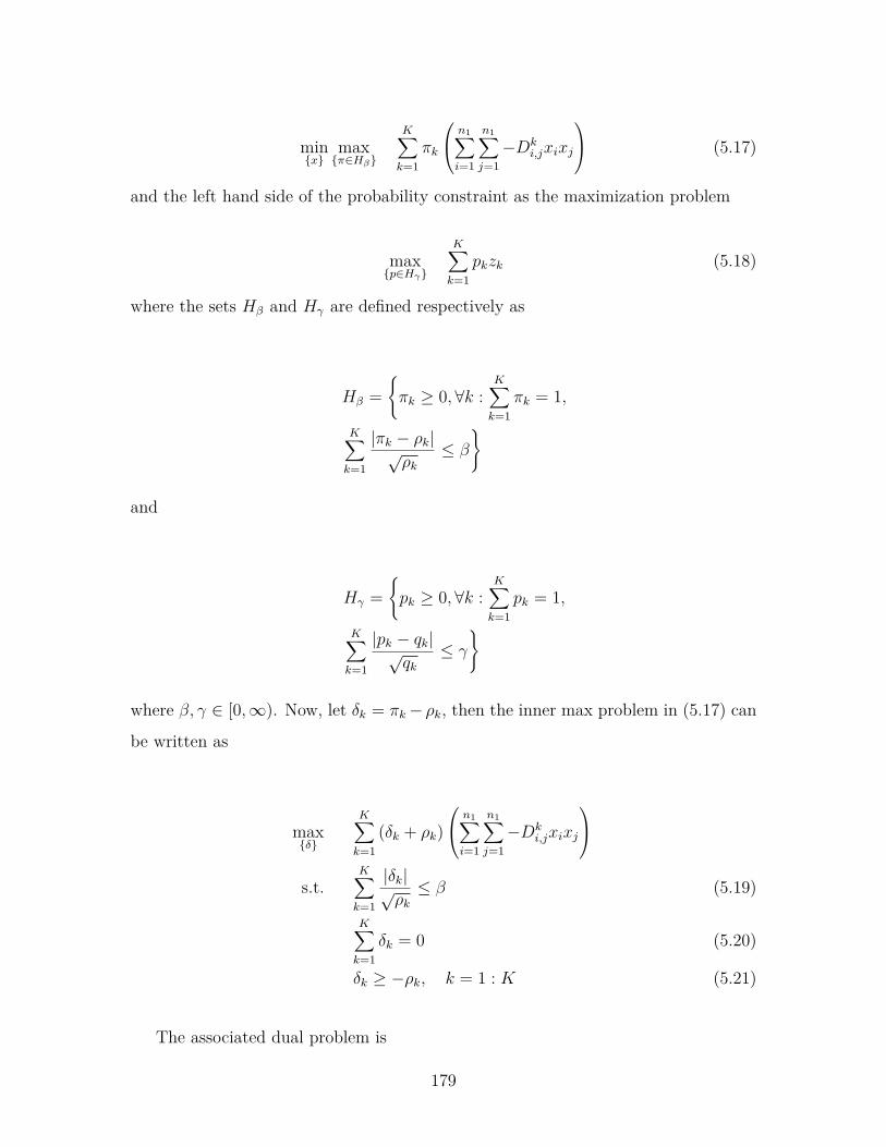
minx

maxπ∈Hβ

K∑k=1

πk

n1∑i=1

n1∑j=1−Dk

i,jxixj

(5.17)

and the left hand side of the probability constraint as the maximization problem

maxp∈Hγ

K∑k=1

pkzk (5.18)

where the sets Hβ and Hγ are defined respectively as

Hβ =πk ≥ 0,∀k :

K∑k=1

πk = 1,

K∑k=1

|πk − ρk|√ρk

≤ β

and

Hγ =pk ≥ 0,∀k :

K∑k=1

pk = 1,

K∑k=1

|pk − qk|√qk

≤ γ

where β, γ ∈ [0,∞). Now, let δk = πk− ρk, then the inner max problem in (5.17) can

be written as

maxδ

K∑k=1

(δk + ρk) n1∑i=1

n1∑j=1−Dk

i,jxixj

s.t.

K∑k=1

|δk|√ρk≤ β (5.19)

K∑k=1

δk = 0 (5.20)

δk ≥ −ρk, k = 1 : K (5.21)

The associated dual problem is

179

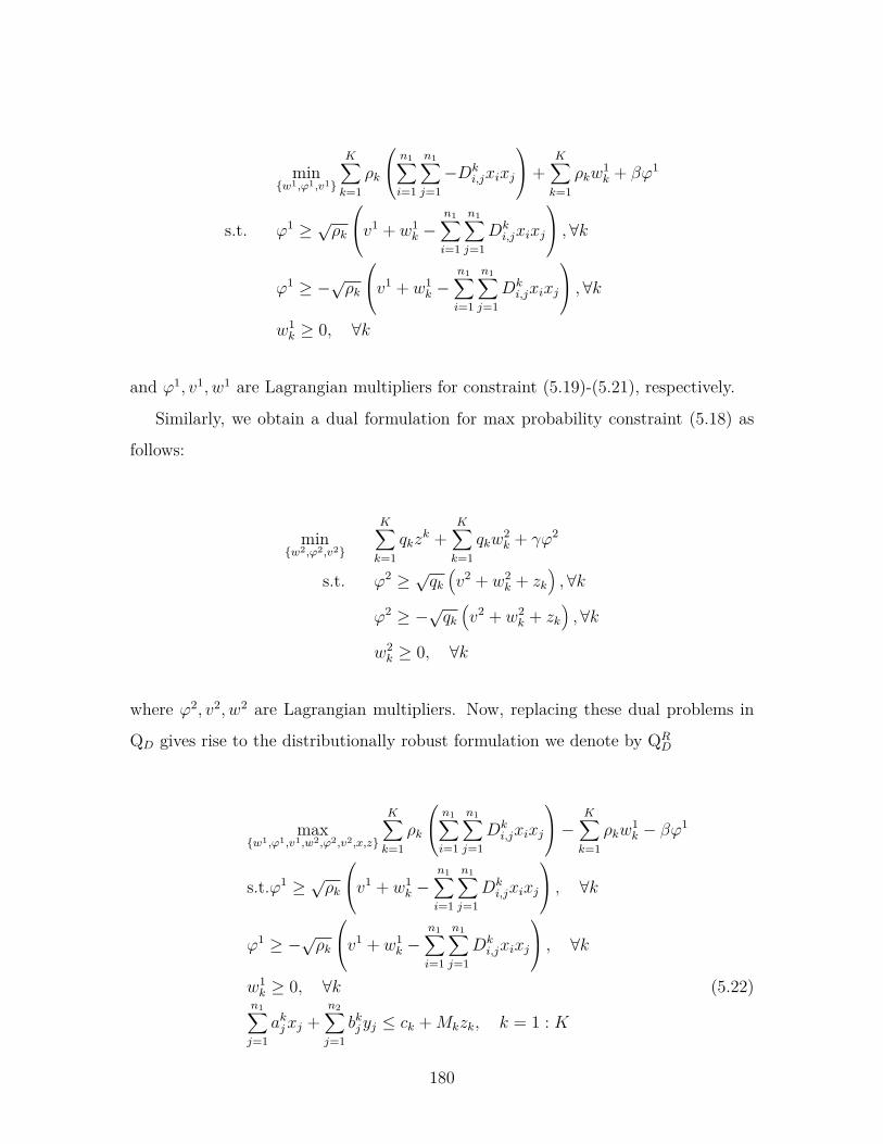
minw1,ϕ1,v1

K∑k=1

ρk

n1∑i=1

n1∑j=1−Dk

i,jxixj

+K∑k=1

ρkw1k + βϕ1

s.t. ϕ1 ≥ √ρk

v1 + w1k −

n1∑i=1

n1∑j=1

Dki,jxixj

, ∀kϕ1 ≥ −√ρk

v1 + w1k −

n1∑i=1

n1∑j=1

Dki,jxixj

,∀kw1k ≥ 0, ∀k

and ϕ1, v1, w1 are Lagrangian multipliers for constraint (5.19)-(5.21), respectively.

Similarly, we obtain a dual formulation for max probability constraint (5.18) as

follows:

minw2,ϕ2,v2

K∑k=1

qkzk +

K∑k=1

qkw2k + γϕ2

s.t. ϕ2 ≥ √qk(v2 + w2

k + zk), ∀k

ϕ2 ≥ −√qk(v2 + w2

k + zk),∀k

w2k ≥ 0, ∀k

where ϕ2, v2, w2 are Lagrangian multipliers. Now, replacing these dual problems in

QD gives rise to the distributionally robust formulation we denote by QRD

maxw1,ϕ1,v1,w2,ϕ2,v2,x,z

K∑k=1

ρk

n1∑i=1

n1∑j=1

Dki,jxixj

− K∑k=1

ρkw1k − βϕ1

s.t.ϕ1 ≥ √ρk

v1 + w1k −

n1∑i=1

n1∑j=1

Dki,jxixj

, ∀k

ϕ1 ≥ −√ρk

v1 + w1k −

n1∑i=1

n1∑j=1

Dki,jxixj

, ∀k

w1k ≥ 0, ∀k (5.22)

n1∑j=1

akjxj +n2∑j=1

bkjyj ≤ ck +Mkzk, k = 1 : K

180

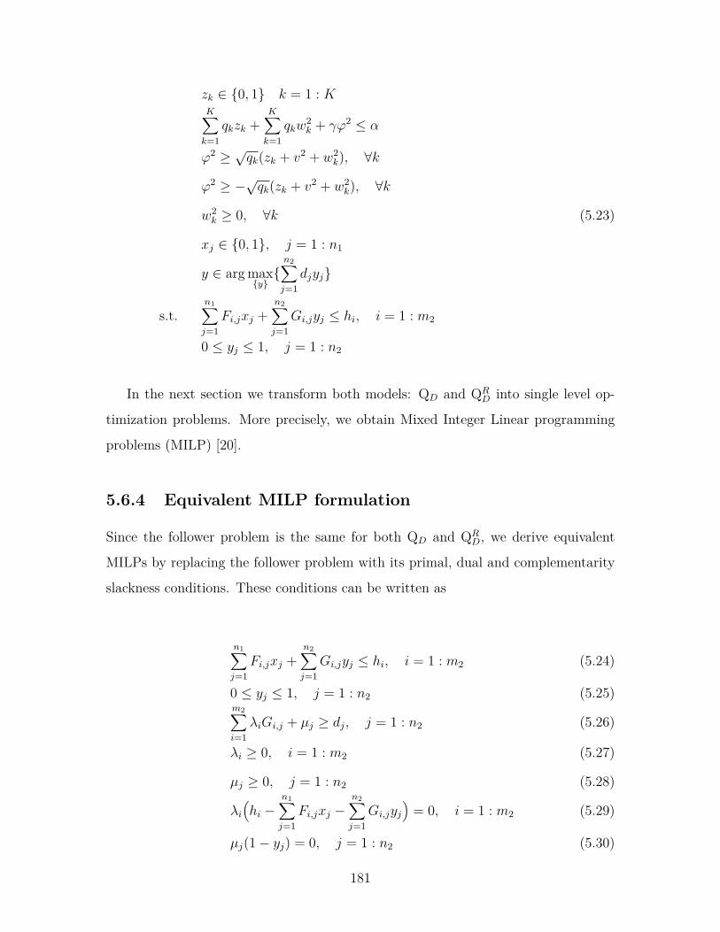
zk ∈ 0, 1 k = 1 : KK∑k=1

qkzk +K∑k=1

qkw2k + γϕ2 ≤ α

ϕ2 ≥ √qk(zk + v2 + w2k), ∀k

ϕ2 ≥ −√qk(zk + v2 + w2k), ∀k

w2k ≥ 0, ∀k (5.23)

xj ∈ 0, 1, j = 1 : n1


djyj

s.t.n1∑j=1

Fi,jxj +n2∑j=1

Gi,jyj ≤ hi, i = 1 : m2

0 ≤ yj ≤ 1, j = 1 : n2

In the next section we transform both models: QD and QRD into single level op-

timization problems. More precisely, we obtain Mixed Integer Linear programming

problems (MILP) [20].

5.6.4 Equivalent MILP formulation

Since the follower problem is the same for both QD and QRD, we derive equivalent

MILPs by replacing the follower problem with its primal, dual and complementarity

slackness conditions. These conditions can be written as

n1∑j=1

Fi,jxj +n2∑j=1

Gi,jyj ≤ hi, i = 1 : m2 (5.24)

0 ≤ yj ≤ 1, j = 1 : n2 (5.25)m2∑i=1

λiGi,j + µj ≥ dj, j = 1 : n2 (5.26)

λi ≥ 0, i = 1 : m2 (5.27)

µj ≥ 0, j = 1 : n2 (5.28)

λi(hi −

n1∑j=1

Fi,jxj −n2∑j=1

Gi,jyj)

= 0, i = 1 : m2 (5.29)

µj(1− yj) = 0, j = 1 : n2 (5.30)

181

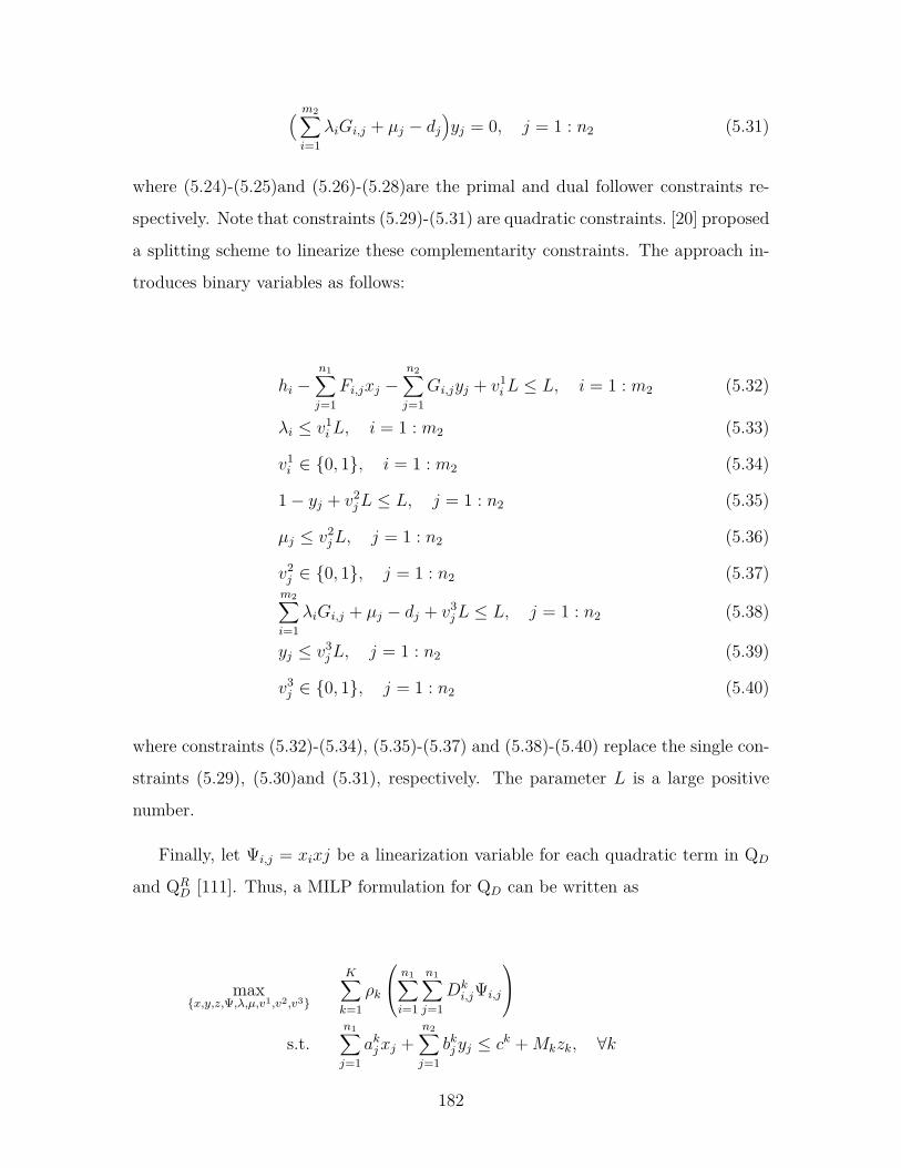
( m2∑i=1

λiGi,j + µj − dj)yj = 0, j = 1 : n2 (5.31)

where (5.24)-(5.25)and (5.26)-(5.28)are the primal and dual follower constraints re-

spectively. Note that constraints (5.29)-(5.31) are quadratic constraints. [20] proposed

a splitting scheme to linearize these complementarity constraints. The approach in-

troduces binary variables as follows:

hi −n1∑j=1

Fi,jxj −n2∑j=1

Gi,jyj + v1iL ≤ L, i = 1 : m2 (5.32)

λi ≤ v1iL, i = 1 : m2 (5.33)

v1i ∈ 0, 1, i = 1 : m2 (5.34)

1− yj + v2jL ≤ L, j = 1 : n2 (5.35)

µj ≤ v2jL, j = 1 : n2 (5.36)

v2j ∈ 0, 1, j = 1 : n2 (5.37)m2∑i=1

λiGi,j + µj − dj + v3jL ≤ L, j = 1 : n2 (5.38)

yj ≤ v3jL, j = 1 : n2 (5.39)

v3j ∈ 0, 1, j = 1 : n2 (5.40)

where constraints (5.32)-(5.34), (5.35)-(5.37) and (5.38)-(5.40) replace the single con-

straints (5.29), (5.30)and (5.31), respectively. The parameter L is a large positive

number.

Finally, let Ψi,j = xixj be a linearization variable for each quadratic term in QD

and QRD [111]. Thus, a MILP formulation for QD can be written as

maxx,y,z,Ψ,λ,µ,v1,v2,v3

K∑k=1

ρk

n1∑i=1

n1∑j=1

Dki,jΨi,j

s.t.

n1∑j=1

akjxj +n2∑j=1

bkjyj ≤ ck +Mkzk, ∀k

182

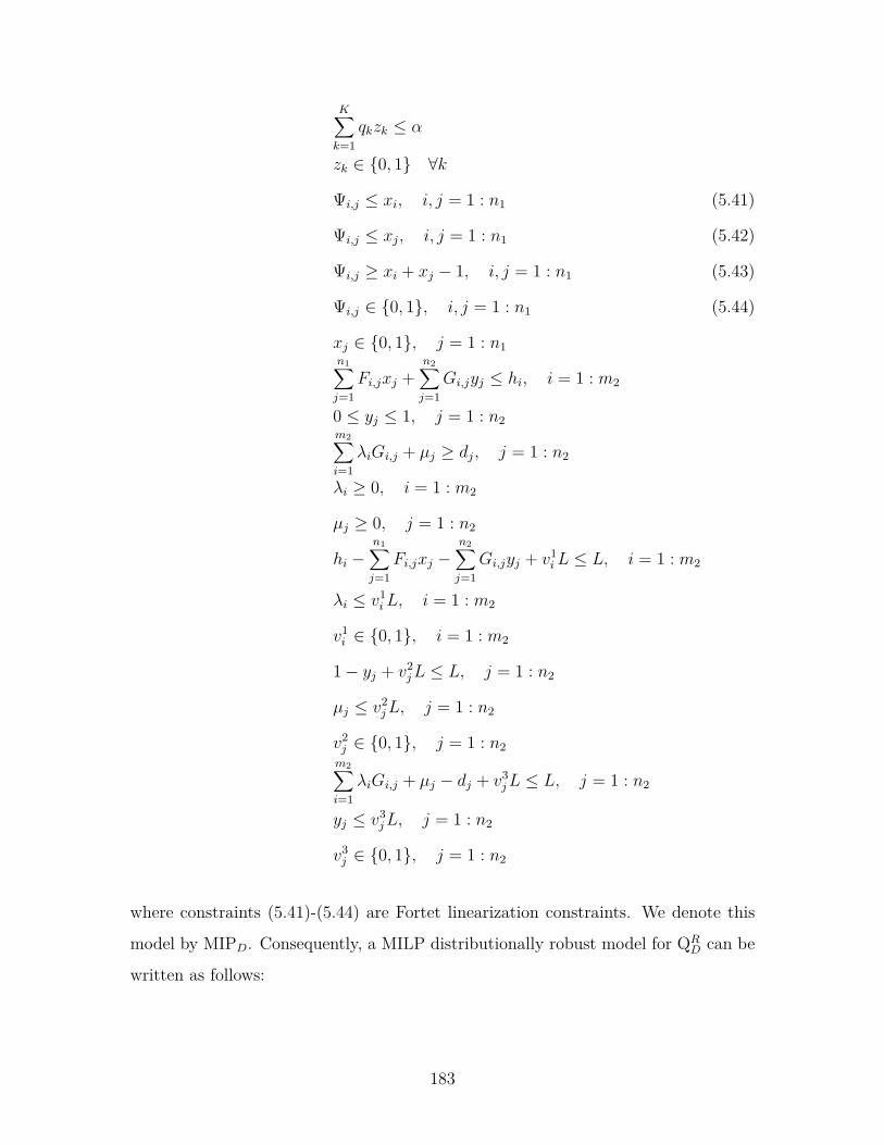
K∑k=1

qkzk ≤ α

zk ∈ 0, 1 ∀k

Ψi,j ≤ xi, i, j = 1 : n1 (5.41)

Ψi,j ≤ xj, i, j = 1 : n1 (5.42)

Ψi,j ≥ xi + xj − 1, i, j = 1 : n1 (5.43)

Ψi,j ∈ 0, 1, i, j = 1 : n1 (5.44)

xj ∈ 0, 1, j = 1 : n1n1∑j=1

Fi,jxj +n2∑j=1

Gi,jyj ≤ hi, i = 1 : m2

0 ≤ yj ≤ 1, j = 1 : n2m2∑i=1

λiGi,j + µj ≥ dj, j = 1 : n2

λi ≥ 0, i = 1 : m2

µj ≥ 0, j = 1 : n2

hi −n1∑j=1

Fi,jxj −n2∑j=1

Gi,jyj + v1iL ≤ L, i = 1 : m2

λi ≤ v1iL, i = 1 : m2

v1i ∈ 0, 1, i = 1 : m2

1− yj + v2jL ≤ L, j = 1 : n2

µj ≤ v2jL, j = 1 : n2

v2j ∈ 0, 1, j = 1 : n2m2∑i=1

λiGi,j + µj − dj + v3jL ≤ L, j = 1 : n2

yj ≤ v3jL, j = 1 : n2

v3j ∈ 0, 1, j = 1 : n2

where constraints (5.41)-(5.44) are Fortet linearization constraints. We denote this

model by MIPD. Consequently, a MILP distributionally robust model for QRD can be

written as follows:

183

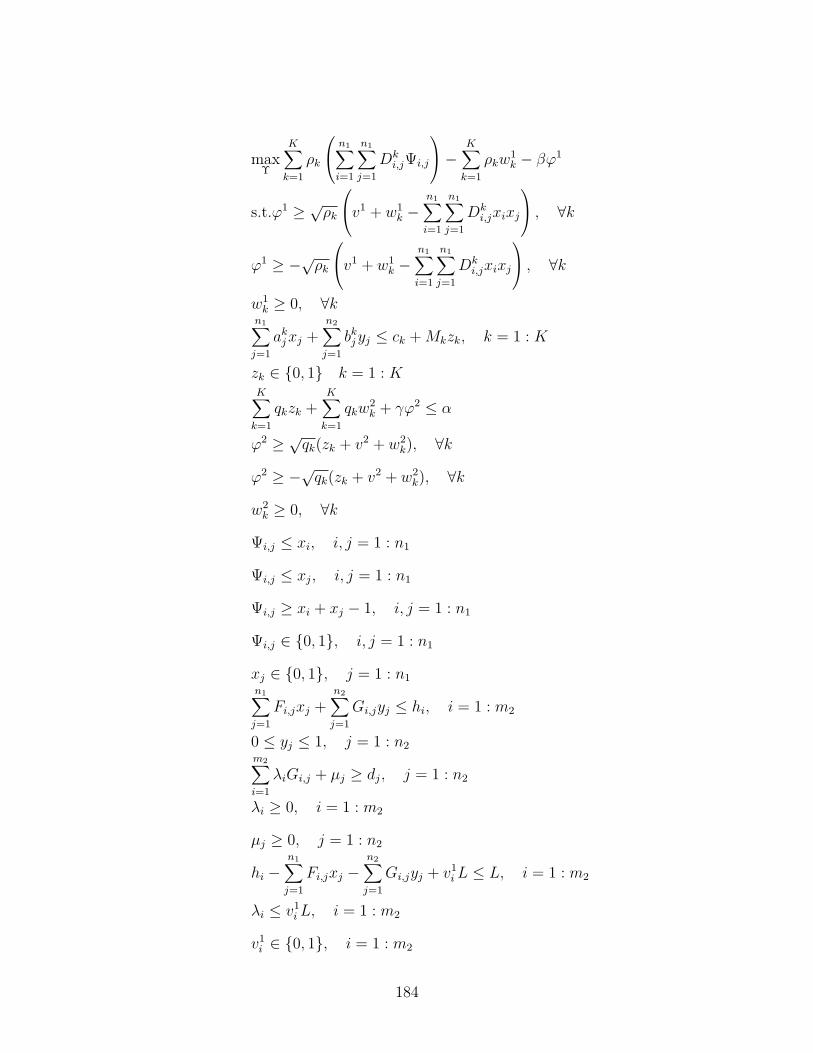
maxΥ

K∑k=1

ρk

n1∑i=1

n1∑j=1

Dki,jΨi,j

− K∑k=1

ρkw1k − βϕ1

s.t.ϕ1 ≥ √ρk

v1 + w1k −

n1∑i=1

n1∑j=1

Dki,jxixj

, ∀k

ϕ1 ≥ −√ρk

v1 + w1k −

n1∑i=1

n1∑j=1

Dki,jxixj

, ∀k

w1k ≥ 0, ∀k

n1∑j=1

akjxj +n2∑j=1

bkjyj ≤ ck +Mkzk, k = 1 : K

zk ∈ 0, 1 k = 1 : KK∑k=1

qkzk +K∑k=1

qkw2k + γϕ2 ≤ α

ϕ2 ≥ √qk(zk + v2 + w2k), ∀k

ϕ2 ≥ −√qk(zk + v2 + w2k), ∀k

w2k ≥ 0, ∀k

Ψi,j ≤ xi, i, j = 1 : n1

Ψi,j ≤ xj, i, j = 1 : n1

Ψi,j ≥ xi + xj − 1, i, j = 1 : n1

Ψi,j ∈ 0, 1, i, j = 1 : n1

xj ∈ 0, 1, j = 1 : n1n1∑j=1

Fi,jxj +n2∑j=1

Gi,jyj ≤ hi, i = 1 : m2

0 ≤ yj ≤ 1, j = 1 : n2m2∑i=1

λiGi,j + µj ≥ dj, j = 1 : n2

λi ≥ 0, i = 1 : m2

µj ≥ 0, j = 1 : n2

hi −n1∑j=1

Fi,jxj −n2∑j=1

Gi,jyj + v1iL ≤ L, i = 1 : m2

λi ≤ v1iL, i = 1 : m2

v1i ∈ 0, 1, i = 1 : m2

184

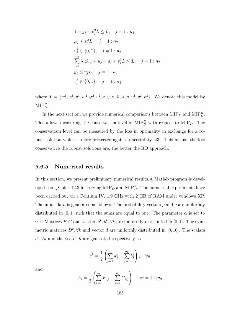
1− yj + v2jL ≤ L, j = 1 : n2

µj ≤ v2jL, j = 1 : n2

v2j ∈ 0, 1, j = 1 : n2m2∑i=1

λiGi,j + µj − dj + v3jL ≤ L, j = 1 : n2

yj ≤ v3jL, j = 1 : n2

v3j ∈ 0, 1, j = 1 : n2

where Υ = w1, ϕ1, v1, w2, ϕ2, v2, x, y, z,Ψ, λ, µ, v1, v2, v3. We denote this model by

MIPRD.

In the next section, we provide numerical comparisons between MIPD and MIPRD.

This allows measuring the conservatism level of MIPRD with respect to MIPD. The

conservatism level can be measured by the loss in optimality in exchange for a ro-

bust solution which is more protected against uncertainty [43]. This means, the less

conservative the robust solutions are, the better the RO approach.


In this section, we present preliminary numerical results.A Matlab program is devel-

oped using Cplex 12.3 for solving MIPD and MIPRD. The numerical experiments have

been carried out on a Pentium IV, 1.9 GHz with 2 GB of RAM under windows XP.

The input data is generated as follows. The probability vectors ρ and q are uniformly

distributed in [0, 1] such that the sums are equal to one. The parameter α is set to

0.1. Matrices F,G and vectors ak, bk,∀k are uniformly distributed in [0, 1]. The sym-

metric matrices Dk,∀k and vector d are uniformly distributed in [0, 10]. The scalars

ck,∀k and the vector h are generated respectively as

ck = 12

n1∑j=1

akj +n2∑j=1

bkj

, ∀k

and

hi = 12

n1∑j=1

Fi,j +n2∑j=1

Gi,j

, ∀i = 1 : m2

185

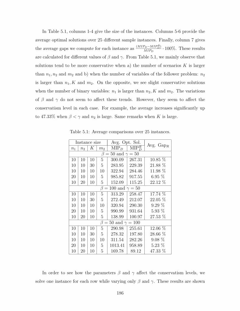
In Table 5.1, columns 1-4 give the size of the instances. Columns 5-6 provide the

average optimal solutions over 25 different sample instances. Finally, column 7 gives

the average gaps we compute for each instance as (MIPD−MIPRD )MIPD

· 100%. These results

are calculated for different values of β and γ. From Table 5.1, we mainly observe that

solutions tend to be more conservative when a) the number of scenarios K is larger

than n1, n2 and m2 and b) when the number of variables of the follower problem: n2

is larger than n1, K and m2. On the opposite, we see slight conservative solutions

when the number of binary variables: n1 is larger than n2, K and m2. The variations

of β and γ do not seem to affect these trends. However, they seem to affect the

conservatism level in each case. For example, the average increases significantly up

to 47.33% when β < γ and n2 is large. Same remarks when K is large.

Table 5.1: Average comparisons over 25 instances.

Instance size Avg. Opt. Sol. Avg. GapRn1 n2 K m2 MIPD MIPRDβ = 50 and γ = 50

10 10 10 5 300.09 267.31 10.85 %10 10 30 5 283.95 229.39 21.88 %10 10 10 10 322.94 284.46 11.98 %20 10 10 5 985.82 917.55 6.95 %10 20 10 5 152.09 115.25 22.12 %

β = 100 and γ = 5010 10 10 5 313.29 258.47 17.74 %10 10 30 5 272.49 212.07 22.05 %10 10 10 10 320.94 290.30 9.29 %20 10 10 5 990.99 931.64 5.93 %10 20 10 5 138.99 100.97 27.53 %

β = 50 and γ = 10010 10 10 5 290.98 255.61 12.06 %10 10 30 5 278.32 197.80 28.66 %10 10 10 10 311.54 282.26 9.08 %20 10 10 5 1013.41 958.89 5.23 %10 20 10 5 169.78 89.12 47.33 %

In order to see how the parameters β and γ affect the conservatism levels, we

solve one instance for each row while varying only β and γ. These results are shown

186

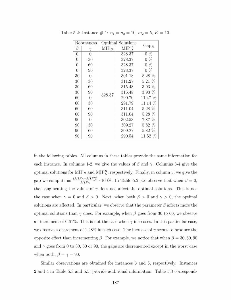
Table 5.2: Instance # 1: n1 = n2 = 10, m2 = 5, K = 10.

Robustness Optimal Solutions GapRβ γ MIPD MIPRD0 0

328.37

328.37 0 %0 30 328.37 0 %0 60 328.37 0 %0 90 328.37 0 %30 0 301.18 8.28 %30 30 311.27 5.21 %30 60 315.48 3.93 %30 90 315.48 3.93 %60 0 290.70 11.47 %60 30 291.79 11.14 %60 60 311.04 5.28 %60 90 311.04 5.28 %90 0 302.53 7.87 %90 30 309.27 5.82 %90 60 309.27 5.82 %90 90 290.54 11.52 %

in the following tables. All columns in these tables provide the same information for

each instance. In columns 1-2, we give the values of β and γ. Columns 3-4 give the

optimal solutions for MIPD and MIPRD, respectively. Finally, in column 5, we give the

gap we compute as (MIPD−MIPRD )MIPD

· 100%. In Table 5.2, we observe that when β = 0,

then augmenting the values of γ does not affect the optimal solutions. This is not

the case when γ = 0 and β > 0. Next, when both β > 0 and γ > 0, the optimal

solutions are affected. In particular, we observe that the parameter β affects more the

optimal solutions than γ does. For example, when β goes from 30 to 60, we observe

an increment of 0.61%. This is not the case when γ increases. In this particular case,

we observe a decrement of 1.28% in each case. The increase of γ seems to produce the

opposite effect than incrementing β. For example, we notice that when β = 30, 60, 90

and γ goes from 0 to 30, 60 or 90, the gaps are decremented except in the worst case

when both, β = γ = 90.

Similar observations are obtained for instances 3 and 5, respectively. Instances

2 and 4 in Table 5.3 and 5.5, provide additional information. Table 5.3 corresponds

187

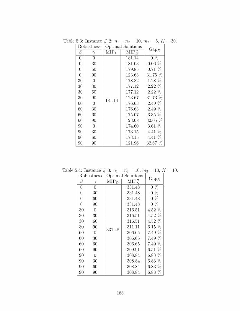
Table 5.3: Instance # 2: n1 = n2 = 10, m2 = 5, K = 30.Robustness Optimal Solutions GapRβ γ MIPD MIPRD0 0

181.14

181.14 0 %0 30 181.03 0.06 %0 60 179.85 0.71 %0 90 123.63 31.75 %30 0 178.82 1.28 %30 30 177.12 2.22 %30 60 177.12 2.22 %30 90 123.67 31.73 %60 0 176.63 2.49 %60 30 176.63 2.49 %60 60 175.07 3.35 %60 90 123.08 32.05 %90 0 174.60 3.61 %90 30 173.15 4.41 %90 60 173.15 4.41 %90 90 121.96 32.67 %

Table 5.4: Instance # 3: n1 = n2 = 10, m2 = 10, K = 10.Robustness Optimal Solutions GapRβ γ MIPD MIPRD0 0

331.48

331.48 0 %0 30 331.48 0 %0 60 331.48 0 %0 90 331.48 0 %30 0 316.51 4.52 %30 30 316.51 4.52 %30 60 316.51 4.52 %30 90 311.11 6.15 %60 0 306.65 7.49 %60 30 306.65 7.49 %60 60 306.65 7.49 %60 90 309.91 6.51 %90 0 308.84 6.83 %90 30 308.84 6.83 %90 60 308.84 6.83 %90 90 308.84 6.83 %

188

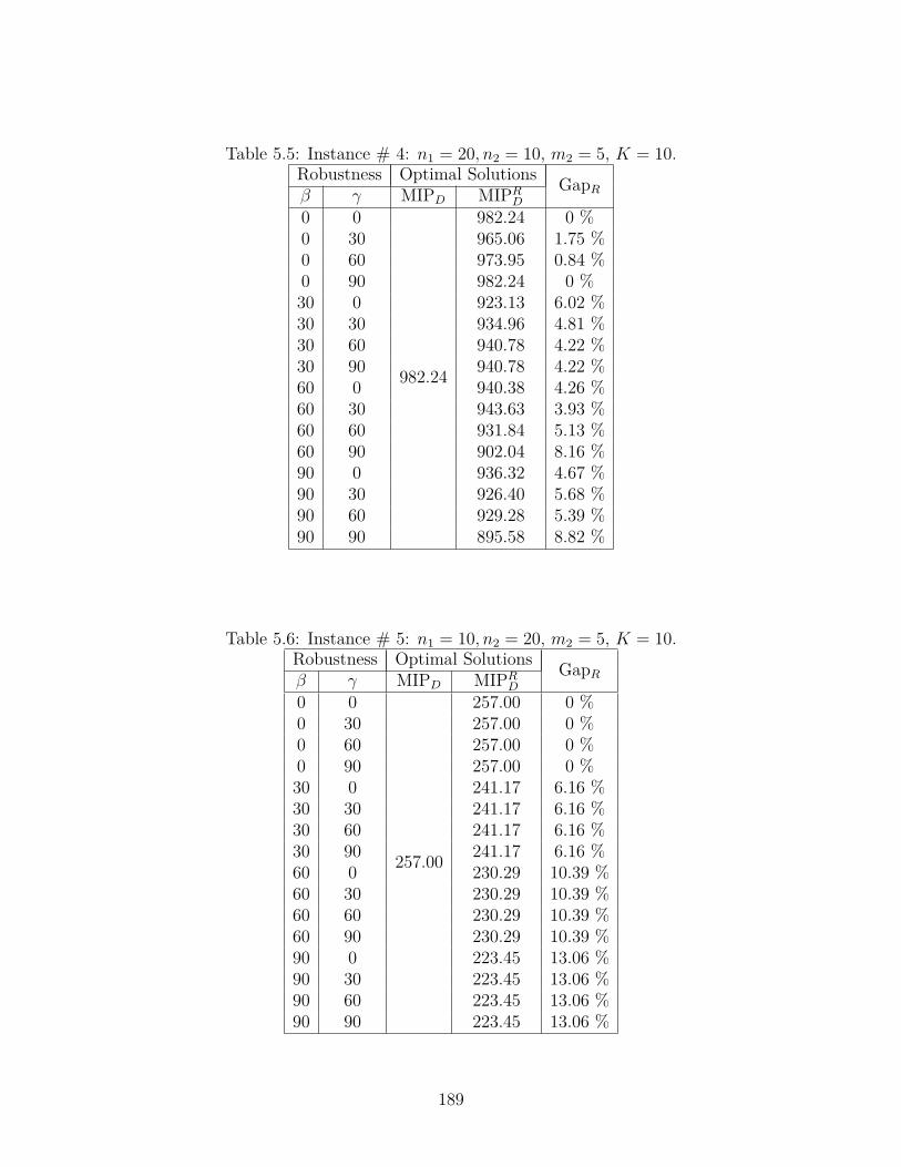
Table 5.5: Instance # 4: n1 = 20, n2 = 10, m2 = 5, K = 10.Robustness Optimal Solutions GapRβ γ MIPD MIPRD0 0

982.24

982.24 0 %0 30 965.06 1.75 %0 60 973.95 0.84 %0 90 982.24 0 %30 0 923.13 6.02 %30 30 934.96 4.81 %30 60 940.78 4.22 %30 90 940.78 4.22 %60 0 940.38 4.26 %60 30 943.63 3.93 %60 60 931.84 5.13 %60 90 902.04 8.16 %90 0 936.32 4.67 %90 30 926.40 5.68 %90 60 929.28 5.39 %90 90 895.58 8.82 %

Table 5.6: Instance # 5: n1 = 10, n2 = 20, m2 = 5, K = 10.Robustness Optimal Solutions GapRβ γ MIPD MIPRD0 0

257.00

257.00 0 %0 30 257.00 0 %0 60 257.00 0 %0 90 257.00 0 %30 0 241.17 6.16 %30 30 241.17 6.16 %30 60 241.17 6.16 %30 90 241.17 6.16 %60 0 230.29 10.39 %60 30 230.29 10.39 %60 60 230.29 10.39 %60 90 230.29 10.39 %90 0 223.45 13.06 %90 30 223.45 13.06 %90 60 223.45 13.06 %90 90 223.45 13.06 %

189

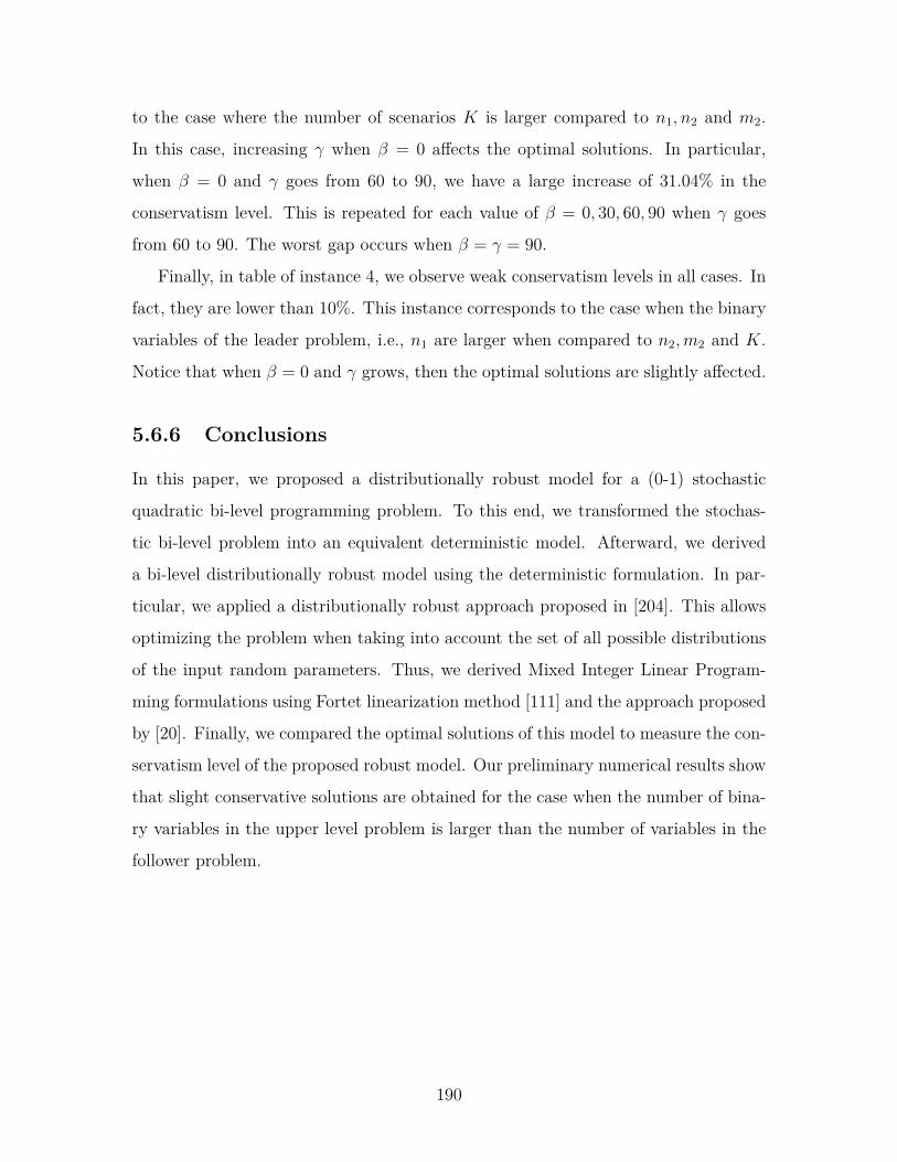
to the case where the number of scenarios K is larger compared to n1, n2 and m2.

In this case, increasing γ when β = 0 affects the optimal solutions. In particular,

when β = 0 and γ goes from 60 to 90, we have a large increase of 31.04% in the

conservatism level. This is repeated for each value of β = 0, 30, 60, 90 when γ goes

from 60 to 90. The worst gap occurs when β = γ = 90.

Finally, in table of instance 4, we observe weak conservatism levels in all cases. In

fact, they are lower than 10%. This instance corresponds to the case when the binary

variables of the leader problem, i.e., n1 are larger when compared to n2,m2 and K.

Notice that when β = 0 and γ grows, then the optimal solutions are slightly affected.

5.6.6 Conclusions

In this paper, we proposed a distributionally robust model for a (0-1) stochastic

quadratic bi-level programming problem. To this end, we transformed the stochas-

tic bi-level problem into an equivalent deterministic model. Afterward, we derived

a bi-level distributionally robust model using the deterministic formulation. In par-

ticular, we applied a distributionally robust approach proposed in [204]. This allows

optimizing the problem when taking into account the set of all possible distributions

of the input random parameters. Thus, we derived Mixed Integer Linear Program-

ming formulations using Fortet linearization method [111] and the approach proposed

by [20]. Finally, we compared the optimal solutions of this model to measure the con-

servatism level of the proposed robust model. Our preliminary numerical results show

that slight conservative solutions are obtained for the case when the number of bina-

ry variables in the upper level problem is larger than the number of variables in the

follower problem.

190

5.7 Conclusions

This chapter mainly focused on the bi-level programming model, property, application

and method. Since a variety of problems can be described as the bi-level programming

model in real life, so modeling bi-level programming to solve practical problems is

still one of the future development direction. However, due to the wide range of types

of practical problems, the study of all types of bi-level programming model is needed.

Besides, it is not only necessary to design the feasible and effective algorithm, but

also make further discussion on the basic property and optimality condition of bi-level

programming.

191

192

Chapter 6

Conclusions

In this thesis, our research considers three problems: bandwidth minimization prob-

lem, resource allocation problem of OFDMA system and bi-level programming prob-

lem. The parameters of the bandwidth minimization problem are deterministic, and

we use a metaheuristic-variable neighborhood search (VNS) to solve it. For the OFD-

MA system, we propose two models of the resource allocation problem. The first one

is a deterministic model. We obtain the relaxation of this model, and use linear pro-

gramming and VNS to solve it. The second one is a stochastic model. Firstly we use a

second order conic programming (SOCP) approach to transform the stochastic model

into a deterministic model. Then we apply mixed integer linear programming and

VNS for solving the problem respectively. About the stochastic bi-level programming

problem, we apply a distributionally robust approach to deal with the probabilistic

constraints in the problem, then it is solved by transforming the model into single

level optimization problem.

In practical application, due to many problems are proved to be NP-hard prob-

lems, it is difficult to find an efficient algorithm to solve such problems. A reasonable

approach is to find metaheuristic algorithms. After using metaheuristic algorithms,

under the condition of an acceptable computational complexity, the local optimal so-

lution or a feasible solution of such problems can be obtained. Because the optimizing

mechanism of the metaheuristic do not very depend on the structure information of

problems, it can be applied to many types of optimization problems. Metaheuristics

193

include simulated annealing, tabu search, genetic algorithm, variable neighborhood

search etc. Especially, variable neighborhood search has better ability of finding the

optimal solution, so this algorithm is used in this thesis for solving two optimization

problems: bandwidth minimization problem and the dynamic resource allocation

problem of OFDMA system.

Besides, for many practical problems, the hierarchy of systems needs to be con-

sidered, i.e., there are more than one decision makers in the entire system, and they

control the different decision variables and objective functions. This kind of problems

can not be solved with traditional mathematical programming techniques, so multi-

level programming has gradually attracted the attention. Bi-level programming is

the basic form of multi-level programming, thus bi-level programming has important

research values. Bi-level programming is a system optimization problem with two

level hierarchical structures. In the model of bi-level programming, the upper and

lower level have their own objective functions and constraints. The objective function

and constraint of upper level are not only relevant to the decision variables of the

upper level, but also relies on the optimal solution of the lower level. However, the

optimal solution of the lower level is affected by the decision variables of the upper

level. Because bi-level programming is a NP-hard problem, the effective and feasible

algorithm to solve bi-level programming should be studied. Thus we consider the

approach for bi-level programming in this thesis.

For bandwidth minimization problem, through introducing the different formula-

tions of bandwidth minimization problem and the relationship during these formula-

tion, we choose graph formulation and use three metaheuristics including simulated

annealing, tabu search and variable neighborhood search to solve bandwidth mini-

mization problem which can save CPU time compared with other formulations. Based

on VNS, by combining the local search with the metaheuristic and changing some

key parameters of the algorithm, the experiment results of running time is reduced

compared with the other two metaheuristic methods.

For the resource allocation problem of OFDMA system, we propose a hybrid re-

source allocation model for OFDMA-TDMA wireless networks and an algorithmic

194

framework using a Variable Neighborhood Search metaheuristic approach for solving

the problem. The model is aimed at maximizing the total bandwidth channel ca-

pacity of an uplink OFDMA-TDMA network subject to user power and subcarrier

assignment constraints while simultaneously scheduling users in time. As such, the

model is best suited for non-real time applications where subchannel multiuser diver-

sity can be further exploited simultaneously in frequency and in time domains. The

VNS approach is constructed upon a key aspect of the proposed model, namely its

decomposition structure. Our numerical results show tight bounds for the proposed

algorithm, and the bounds are obtained at a very low computational cost. Meanwhile,

we present a (0-1) stochastic resource allocation model for uplink wireless multi-cell

OFDMA Networks. The model maximizes the total signal to interference noise ra-

tio produced in a multi-cell OFDMA network subject to user power and subcarrier

assignment constraints. We transform the stochastic model into a deterministic e-

quivalent binary nonlinear optimization problem having quadratic terms and second

order conic constraints. Subsequently, we use the deterministic model to derive an e-

quivalent mixed integer linear programming formulation. Then, we propose a reduced

variable neighborhood search to compute feasible solutions. Our preliminary numeri-

cal results provide near optimal solutions for most of the instances when compared to

the optimal solution of the problem. Moreover, we find better feasible solutions than

CPLEX when the instances dimensions increase. Finally, we obtain these feasible

solutions at a significantly less computational cost.

For the part of bi-level programming, we propose a distributionally robust model

for a (0-1) stochastic quadratic bi-level programming problem. We first transform

the stochastic bi-level problem into an equivalent deterministic formulation. Then,

we use this formulation to derive a bi-level distributionally robust model. Finally, we

transform both the deterministic and the distributionally robust models into single

level optimization problems and compare the optimal solutions of the proposed mod-

els. Our preliminary numerical results indicate that slight conservative solutions can

be obtained when the number of binary variables in the upper level problem is larger

than the number of variables in the follower.

195

The future work of each problem is presented as follows.

For bandwidth minimization problem, we still consider use other metaheuristics

or hybrid algorithms (such as hybrid metaheuristics or the combination of classic

optimization methods and metaheuristics) to solve large size problems. Besides, we

consider applying semidefinite programming to come up with strong lower bound in

order to improve the metaheuristics performances. We also focus on proposing an

algorithm to obtain good quality initial solution which can save the running time of

the method.

For resource allocation problem of OFDMA system, we try to develop other meta-

heuristics for solving the two proposed models: the hybrid OFDMA-TDMA model

and the 0-1 stochastic model. In addition, we only focus on Rate Adaptive (RA)

problem which is to maximize the system capacity with total power constraint in

this thesis, and we will consider other variants of the proposed model such as Margin

Adaptive (MA) problem which is to minimize the power subject to capacity con-

straints.

For bi-level programming, we will continue studying on combining the distribu-

tionally robust model and variable neighborhood search (VNS) to solve large size

of 0-1 stochastic quadratic bi-level programming problems. Besides, we can con-

sider more complex bi-level programming models, such as using joint probabilistic

constraint to replace the individual probabilistic constraint, which will have more

application values.

196

Bibliography

[1] Abdule-Wahab, R. S., Monmarche, N., Slimane, M., Fahdil, M. A., Saleh, H. H.2006. A scatter search algorithm for the automatic clustering problem. Advancesin Data Mining. Applications in Medicine, Web Mining, Marketing, Image andSignal Mining. Springer Berlin Heidelberg, 350-364.

[2] Air Interface for Fixed Broadband Wireless Access Systems, MAC and AdditionalPHY Specifications for 2-11 GHz, IEEE Std. 802.16a, 2003.

[3] Aiyoshi, E., Shimizu, K. 1981. Hierarchical decentralized systems and its new solu-tion by a barrier method. IEEE Transactions on Systems, Man, and Cybernetics,11(6), 444-449.

[4] Alavi, S. M., Zhou, C., Cheng, Y. 2009. Low complexity resource allocation algo-rithm for IEEE 802.16 OFDMA system. Communications, 2009. ICC’09. IEEEInternational Conference on. IEEE, 1-5.

[5] Ali, S. H., Lee, K. D., Leung, V. C. 2007. Dynamic resource allocation in OFDMAwireless metropolitan area networks [Radio Resource Management and ProtocolEngineering for IEEE 802.16]. Wireless Communications, IEEE, 14(1), 6-13.

[6] Al-Khayyal, F. A. 1987. An implicit enumeration procedure for the general linearcomplementarity problem. Springer Berlin Heidelberg, 1-20.

[7] Al-Khayyal, F. A., Horst, R., Pardalos, P. M. 1992. Global optimization of concavefunctions subject to quadratic constraints: an application in nonlinear bilevelprogramming. Annals of Operations Research, 34(1), 125-147.

[8] Al-Khedhairi, A. 2008. Simulated annealing metaheuristic for solving p-medianproblem. International Journal of Contemporary Mathematical Sciences, 3(28),1357-1365.

[9] Al-Turki, U., Fedjki, C., Andijani, A. (2001). Tabu search for a class of single-machine scheduling problems. Computers & Operations Research, 28(12), 1223-1230.

[10] Alvarez, A. M., Gonzalez-Velarde, J. L., De-Alba, K. 2005. GRASP embeddedscatter search for the multicommodity capacitated network design problem. Jour-nal of Heuristics, 11(3), 233-257.

197

[11] Alvarez, A. M., Gonzalez-Velarde, J. L., De-Alba, K. 2005. Scatter search fornetwork design problem. Annals of Operations Research, 138(1), 159-178.

[12] Alvarez-Valdes, R., Crespo, E., Tamarit, J. M., Villa, F. 2006. A scatter searchalgorithm for project scheduling under partially renewable resources. Journal ofHeuristics, 12(1-2), 95-113.

[13] Amzallag, D., Armarnik, T., Livschitz, M., Raz, D. 2007. Multi-cell slots allo-cation in OFDMA systems. Mobile and Wireless Communications Summit, 2007.16th IST, IEEE, 1-5.

[14] Anandalingam, G., White, D. J. 1990. A solution method for the linear staticStackelberg problem using penalty functions. Automatic Control, IEEE Transac-tions on, 35(10), 1170-1173.

[15] Andrade, D. V., Resende, M. G. 2007. GRASP with evolutionary path-relinking.Proceedings of Seventh Metaheuristics International Conference.

[16] Arany, I., Smyth, W. F., Szoda L. 1972. An improve method for reducingthe band-width of sparse symmetric matrices. Proceedings of IFIP Congress 71,North-Holland, Amsterdam, 1246-1250.

[17] Atkinson, J. B. 1998. A greedy randomised search heuristic for time-constrainedvehicle scheduling and the incorporation of a learning strategy. Journal of theOperational Research Society, 700-708.

[18] Audestad, J. A., Gaivoronski, A. A., Werner, A. 2006. Extending the stochas-tic programming framework for the modeling of several decision makers: pricingand competition in the telecommunication sector. Annals of Operations Research,142(1), 19-39.

[19] Audet, C., Haddad, J., Savard, G. 2006. A note on the definition of a linear bilevelprogramming solution. Applied mathematics and computation, 181(1), 351-355.

[20] Audet, C., Hansen, P., Jaumard, B., Savard, G. 1997. Links between linearbilevel and mixed 0-1 programming problems. Journal of optimization theory andapplications, 93(2), 273-300.

[21] Avanthay, C., Hertz, A., Zufferey, N. 2003. A variable neighborhood search forgraph coloring. European Journal of Operational Research, 151(2), 379-388.

[22] Babahadda, H., Gadhi, N. 2006. Necessary optimality conditions for bilevel op-timization problems using convexificators. Journal of Global Optimization, 34(4),535-549.

[23] Badia, L., Baiocchi, A., Todini, A., Merlin, S., Pupolin, S., Zanella, A., Zorzi,M. 2007. On the impact of physical layer awareness on scheduling and resourceallocation in broadband multicellular IEEE 802.16 systems [Radio Resource Man-agement and Protocol Engineering for IEEE 802.16]. Wireless Communications,IEEE, 14(1), 36-43.

198

[24] Bard, J. F. 1983. An efficient point algorithm for a linear two-stage optimizationproblem. Operations Research, 31(4), 670-684.

[25] Bard, J. F. 1983. Coordination of a multidivisional organization through twolevels of management. Omega, 11(5), 457-468.

[26] Bard, J. F. 1984. An investigation of the linear three level programming problem.Systems, Man and Cybernetics, IEEE Transactions on, 14(5), 711-717.

[27] Bard, J. F. 1984. Optimality conditions for the bilevel programming problem.]emphNaval research logistics quarterly, 31(1), 13-26.

[28] Bard, J. F. 1988. Convex two-level optimization. Mathematical Programming,40(1-3), 15-27.

[29] Bard, J. F. 1991. Some properties of the bilevel programming problem. Journalof optimization theory and applications, 68(2), 371-378.

[30] Bard, J. F. 1998. Practical bilevel optimization: algorithms and applications.Springer.

[31] Bard, J. F., Falk, J. E. 1982. An explicit solution to the multi-level programmingproblem. Computers & Operations Research, 9(1), 77-100.

[32] Bard, J. F., Moore, J. T. 1990. A branch and bound algorithm for the bilevelprogramming problem. SIAM Journal on Scientific and Statistical Computing,11(2), 281-292.

[33] Bard, J. F., Moore, J. T. 1992. An algorithm for the discrete bilevel programmingproblem. Naval Research Logistics (NRL), 39(3), 419-435.

[34] Bard, J. F., Plummer, J., Claude Sourie, J. 2000. A bilevel programming ap-proach to determining tax credits for biofuel production. European Journal ofOperational Research, 120(1), 30-46.

[35] Baumol, W. J., Fabian, T. 1964. Decomposition, pricing for decentralization andexternal economies. Management Science, 11(1), 1-32.

[36] Ben-Ayed, O. 1993. Bilevel linear programming. Computers & operations re-search, 20(5), 485-501.

[37] Ben-Ayed, O., Blair, C. E. 1990. Computational difficulties of bilevel linear pro-gramming. Operations Research, 38(3), 556-560.

[38] Ben-Ayed, O., Blair, C. E., Boyce, D. E., LeBlanc, L. J. 1992. Constructionof a real-world bilevel linear programming model of the highway network designproblem. Annals of Operations Research, 34(1), 219-254.

199

[39] Ben-Ayed, O., Boyce, D. E., Blair, C. E. 1988. A general bilevel linear program-ming formulation of the network design problem. Transportation Research PartB: Methodological, 22(4), 311-318.

[40] Benson, H. P. 1989. On the structure and properties of a linear multilevel pro-gramming problem. Journal of operation Theory and Applications, 60(3), 353-373.

[41] Berry, M. W., Hendrickson, B., Raghavan, P. 1996. Sparse matrix reorder-ing schemes for browsing hypertext. Lectures in Applied Mathematics, AmericanMathematical Society, Providence, RI, 32, 99-123.

[42] Bertsimas, D., Brown, D. B., Caramanis, C. 2011. Theory and applications ofrobust optimization. SIAM review, 53(3), 464-501.

[43] Bertsimas, D., Sim, M. 2004. The price of robustness. Operations research, 52(1),35-53.

[44] Bialas, W. F., Karwan, M. H. 1982. On two-level optimization. Automatic Con-trol, IEEE Transactions on, 27(1), 211-214.

[45] Bialas, W. F., Karwan, M. H. 1984. Two-level linear programming. ManagementScience, 30(8), 1004-1020.

[46] Bialas, W. F., Karwan, M. H., Shaw, J. 1980. A parametric complementarypivot approach for two-level linear programming. State University of New York atBuffalo.

[47] Binato, S., Faria Jr, H., Resende, M. G. 2001. Greedy randomized adaptive pathrelinking. Proceedings of the IV Metaheuristics International Conference, 393-397.

[48] Birge, J. R., Louveaux, F. 2011. Introduction to stochastic programming.Springer.

[49] Blum, C., Roli, A. 2003. Metaheuristics in combinatorial optimization: Overviewand conceptual comparison. ACM Computing Surveys (CSUR), 35(3), 268-308.

[50] Boudreau, G., Panicker, J., Guo, N., Chang, R., Wang, N., Vrzic, S. 2009. In-terference coordination and cancellation for 4G networks. Communications Mag-azine, IEEE, 47(4), 74-81.

[51] Bracken, J., McGill, J. T. 1973. Mathematical programs with optimization prob-lems in the constraints. Operations Research, 21(1), 37-44.

[52] Braun, H. 1991. On solving travelling salesman problems by genetic algorithms.In Parallel problem solving from nature. Springer Berlin Heidelberg, 129-133.

[53] Brumby, S. P., Theiler, J. P., Perkins, S. J., Harvey, N. R., Szymanski, J. J.,Bloch, J. J., Mitchell, M. 1999. Investigation of image feature extraction by a ge-netic algorithm. SPIE’s International Symposium on Optical Science, Engineer-ing, and Instrumentation. International Society for Optics and Photonics, 24-31.

200

[54] Burke, E. K., Curtois, T., Post, G., Qu, R., Veltman, B. 2008. A hybrid heuris-tic ordering and variable neighbourhood search for the nurse rostering problem.European Journal of Operational Research, 188(2), 330-341.

[55] Calvete, H. I., Galé, C. 2004. A penalty method for solving bilevel linear fraction-al/linear programming problems. Asia-Pacific Journal of Operational Research,21(02), 207-224.

[56] Campelo, M., Dantas, S., Scheimberg, S. 2000. A note on a penalty functionapproach for solving bilevel linear programs. Journal of global optimization, 16(3),245-255.

[57] Campelo, M., Scheimberg, S. 2000. A note on a modified simplex approach forsolving bilevel linear programming problems. European Journal of OperationalResearch, 126(2), 454-458.

[58] Campelo, M., Scheimberg, S. 2005. A simplex approach for finding local solutionsof a linear bilevel program by equilibrium points. Annals of Operations Research,138(1), 143-157.

[59] Campos, V., Glover, F., Laguna, M., Martí, R. 2001. An experimental evaluationof a scatter search for the linear ordering problem. Journal of Global Optimization,21(4), 397-414.

[60] Campos, V., Piaana, E., Martí, R. 2011. Adaptive memory programming formatrix bandwidth minimization. Annals of Operations Research, 183(1), 7-23.

[61] Candler, W., Norton, R. 1977. Mutilevel Programming, Techinical Report 20.World Bank Development Research Center, Washington D.C..

[62] Candler, W., Townsley, R. 1982. A linear two-level programming problem. Com-puters & Operations Research, 9(1), 59-76.

[63] Cao, Z., Tureli, U., Liu, P. 2003. Optimum subcarrier assignment for OFDMAuplink. Signals, Systems and Computers, 2004. Conference Record of the Thirty-Seventh Asilomar Conference on. IEEE, 1, 708-712.

[64] Caprara, A., Salazar-González, J. J. 2005. Laying out sparse graphs with prov-ably minimum bandwidth. INFORMS Journal on Computing, 17(3), 356-373.

[65] Carrión, M., Arroyo, J. M., Conejo, A. J. 2009. A bilevel stochastic programmingapproach for retailer futures market trading. Power Systems, IEEE Transactionson, 24(3), 1446-1456.

[66] Carvalho, D. R., Freitas, A. A. 2004. A hybrid decision tree/genetic algorithmmethod for data mining. Information Sciences, 163(1), 13-35.

[67] Chang, Y. J., Chien, F. T., Kuo, C. C. 2007. Cross-layer QoS analysis of op-portunistic OFDM-TDMA and OFDMA networks. Selected Areas in Communi-cations, IEEE Journal on, 25(4), 657-666.

201

[68] Chen, C. L., Vempati, V. S., Aljaber, N. 1995. An application of genetic algo-rithms for flow shop problems. European Journal of Operational Research, 80(2),389-396.

[69] Chen, H. C., Shih, K. P., Wang, S. S., Chiang, C. T. 2010. An EfficientDownlink Bandwidth Allocation Scheme for Improving Subchannel Utilization inIEEE 802.16 e WiMAX Networks. Vehicular Technology Conference (VTC 2010-Spring), 2010 IEEE 71st. IEEE, 1-5.

[70] Chen, Y., Florian, M. 1995. The nonlinear bilevel programming problem: For-mulations, regularity and optimality conditions. Optimization, 32(3), 193-209.

[71] Chen, Y. W., Nakao, Z., Fang, X., Tamura, S. 1996. A parallel genetic algo-rithm for image restoration. Pattern Recognition, 1996., Proceedings of the 13thInternational Conference on. IEEE, 4, 694-698.

[72] Cheng, R., Gen, M., Tsujimura, Y. 1996. A tutorial survey of job-shop schedul-ing problems using genetic algorithms-I. Representation. Computers & IndustrialEngineering, 30(4), 983-997.

[73] Chieochan, S., Hossain, E. 2009. Adaptive radio resource allocation in OFDMAsystems: a survey of the state-of-the-art approaches. Wireless Communicationsand Mobile Computing, 9(4), 513-527.

[74] Chinn, P. Z., Chvatalova, J., Dewdney, A. K., Gibbs, N. E. 1982. The bandwidthproblem for graphs and matrices-a survey. Journal of Graph Theory, 6(3), 223-254.

[75] Chiou, S. W. 1999. Optimization of area traffic control for equilibrium networkflows. Transportatin Science, 33(3), 279-289.

[76] Chu, F., Labadi, N., Prins, C. 2006. A scatter search for the periodic capacitatedarc routing problem. European Journal of Operational Research, 169(2), 586-605.

[77] Chu, P. C., Beasley, J. E. 1998. A genetic algorithm for the multidimensionalknapsack problem. Journal of heuristics, 4(1), 63-86.

[78] Clark, P. A., Westerberg, A. W. 1988. A note on the optimality conditions for thebilevel programming problem. Naval Research Logistics (NRL), 35(5), 413-418.

[79] Colson, B., Marcotte, P., Savard, G. 2005. Bilevel programming: A survey. 4OR,3(2), 87-107.

[80] Connolly, D. T. 1990. An improved annealing scheme for the QAP. EuropeanJournal of Operational Research, 46(1), 93-100.

[81] Cordon, O., Damas, S., Santamaria, J. 2004. A scatter search algorithm for the3D image registration problem. Parallel Problem Solving from Nature-PPSN VIII.Springer Berlin Heidelberg, 471-480.

202

[82] Cordon, O., Damas, S., Santamaria, J. 2006. A fast and accurate approach for3D image registration using the scatter search evolutionary algorithm. PatternRecognition Letters, 27(11), 1191-1200.

[83] Cordon, O., Damas, S., Santamaria, J., Martí, R. 2005. 3D inter-subject med-ical image registration by scatter search. Hybrid Metaheuristics. Springer BerlinHeidelberg, 90-103.

[84] Cotta, C. 2004. Scatter search and memetic approaches to the error correct-ing code problem. Evolutionary Computation in Combinatorial Optimization.Springer Berlin Heidelberg, 51-61.

[85] Cox, E. 2005. Fuzzy modeling and genetic algorithms for data mining and ex-ploration. Academic Press.

[86] Crainic, T. G., Gendreau, M., Hansen, P., Mladenovic, N. 2004. Cooperativeparallel variable neighborhood search for the p-median. Journal of Heuristics,10(3), 293-314.

[87] Cui, Y., Lau, V. K., Wang, R. 2009. Distributive subband allocation, power andrate control for relay-assisted OFDMA cellular system with imperfect system stateknowledge. Wireless Communications, IEEE Transactions on, 8(10), 5096-5102.

[88] Cuthill, E., McKee, J. 1969. Reducing the bandwidth of sparse symmetric ma-trices. Proceedings of the 1969 24th national conference, ACM, 157-172.

[89] Danskin, J. M. 1966. The theory of max-min, with applications. SIAM Journalof Applied Mathematics, 14(4), 641-664.

[90] Del Corso, G. M., Manzini, G. 1999. Finding exact solutions to the bandwidthminimization problem. Computing, 62(3), 189-203.

[91] Delage, E., Ye, Y. 2010. Distributionally robust optimization under momentuncertainty with application to data-driven problems. Operations Research, 58(3),595-612.

[92] Della Croce, F., Tadei, R., Volta, G. 1995. A genetic algorithm for the job shopproblem. Computers & Operations Research, 22(1), 15-24.

[93] Dempe, S. 2000. A bundle algorithm applied to bilevel programming problemswith non-unique lower level solutions. Computational Optimization and Applica-tions, 15(2), 145-166.

[94] Dempe, S. 2002. Foundations of bilevel programming. Springer.

[95] Dempe, S., Schmidt, H. 1996. On an algorithm solving two-level programmingproblems with nonunique lower level solutions. Computational Optimization andApplications, 6(3), 227-249.

203

[96] Deng, X. 1998. Complexity issues in bilevel linear programming. Multilevel opti-mization: algorithms and applications, Springer US, 149-164.

[97] Diaz, J. A., Fernandez, E. 2001. A tabu search heuristic for the generalizedassignment problem. European Journal of Operational Research, 132(1), 22-38.

[98] Drazic, M., Lavor, C., Maculan, N., Mladenovic, N. 2008. A continuous variableneighborhood search heuristic for finding the three-dimensional structure of amolecule. European Journal of Operational Research, 185(3), 1265-1273.

[99] Dueck, G., Jeffs, J. 1995. A Heuristic Bandwidth Reduction Algorithm. Journalof Combinatorial Mathematics and Combinatorial Computing, 18, 97-108.

[100] Dueck, G., Scheuer, T. 1990. Threshold accepting: a general purpose optimiza-tion algorithm appearing superior to simulated annealing. Journal of computa-tional physics, 90(1), 161-175.

[101] Edmunds, T. A., Bard, J. F. 1991. Algorithms for nonlinear bilevel mathe-matical programs. Systems, Man and Cybernetics, IEEE Transactions on, 21(1),83-89.

[102] Edmunds, T. A., Bard, J. F. 1992. An algorithm for the mixed-integer nonlinearbilevel programming problem. Annals of Operations Research, 34(1), 149-162.

[103] Esposito, A., Catalano, M. S., Malucelli, F., Tarricone. L. 1998. Sparse ma-trix band-width reduction:Algorithms, Applications and real industrial cases inelectromagnetics, high performance algorithms for structured matrix problems.Advances in the theory of Computation and Computational Mathematics, 2, 27-45.

[104] Falkenauer, E. 1996. A hybrid grouping genetic algorithm for bin packing. Jour-nal of heuristics, 2(1), 5-30.

[105] Fattah, H., Alnuweiri, H. 2009. A load adaptive subcarrier and bit allocationalgorithm for non-real time services in an OFDMA system. Wireless Commu-nication Systems, 2009. ISWCS 2009. 6th International Symposium on. IEEE,642-646.

[106] Feo, T. A., Resende, M. G. 1989. A probabilistic heuristic for a computationallydifficult set covering problem. Operations Research Letters, 8(2), 67-71.

[107] Feo, T. A., Resende, M. G. 1995. Greedy randomized adaptive search proce-dures. Journal of Global Optimization, 6(2), 109-133.

[108] Fleurent, C., Glover, F. 1999. Improved constructive multistart strategies forthe quadratic assignment problem using adaptive memory. INFORMS Journal onComputing, 11(2), 198-204.

204

[109] Flockhart, I. W., Radcliffe, N. J., Simoudis, E., Han, J., Fayyad, U. 1996. AGenetic Algorithm-Based Approach to Data Mining. KDD, 299-302.

[110] Floudas, C. A., Pardalos, P. M. 2001. Encyclopedia of Optimization. KluwerAcademic Publishers, Dordrecht. The Netherlands.

[111] Fortet, R. 1960. Applications de l’algebre de boole en recherche operationelle.Revue Francaise de Recherche Operationelle, 4(14), 17-26.

[112] Fortuny-Amat, J., McCarl, B. 1981. A representation and economic interpre-tation of a two-level programming problem. Journal of the Operational ResearchSociety, 32(9), 783-792.

[113] Friesz, T. L., Anandalingam, G., Mehta, N. J., Nam, K., Shah, S. J., Tobin,R. L. 1993. The multiobjective equilibrium network design problem revisited: Asimulated annealing approach. European Journal of Operational Research, 65(1),44-57.

[114] Gaivoronski, A. A., Lisser, A., Lopez, R., Xu, H. 2011. Knapsack problem withprobability constraints. Journal of Global Optimization, 49(3), 397-413.

[115] Gao, J., Sun, L., Gen, M. 2008. A hybrid genetic and variable neighborhooddescent algorithm for flexible job shop scheduling problems. Computers & Oper-ations Research, 35(9), 2892-2907.

[116] Garey, M. R., Graham, R. L., Johnson, D. S., Knuth, D. E. 1978. Complex-ity results for bandwidth minimization. SIAM Journal on Applied Mathematics,34(3), 477-495.

[117] Garcia-Lopez, F., Melian-Batista, B., Moreno-Perez, J. A., Moreno-Vega, J.M. 2002. The parallel variable neighborhood search for the p-median problem.Journal of Heuristics, 8(3), 375-388.

[118] Garcia-Lopez, F., Melian-Batista, B., Moreno-Perez, J. A., Moreno-Vega, J.M. 2003. Parallelization of the scatter search for the p-median problem. ParallelComputing, 29(5), 575-589.

[119] Garici, M. A., Drias, H. 2005. Cryptanalysis of substitution ciphers using s-catter search. IArtificial Intelligence and Knowledge Engineering Applications: ABioinspired Approach. Springer Berlin Heidelberg, 31-40.

[120] Gendreau, M., Hertz, A., Laporte, G. 1994. A tabu search heuristic for thevehicle routing problem. Management science, 40(10), 1276-1290.

[121] Gendreau, M., Marcotte, P., Savard, G. 1996. A hybrid tabu-ascent algorithmfor the linear bilevel programming problem. Journal of Global Optimization, 8(3),217-233.

205

[122] Gendreau, M., Laporte, G., Semet, F. 1998. A tabu search heuristic for theundirected selective travelling salesman problem. European Journal of OperationalResearch, 106(2), 539-545.

[123] Geoffrion, A. M. 1967. Integer programming by implicit enumeration and Balas’method. Siam Review, 9(2), 178-190.

[124] George, J. A. 1971. Computer implementation of the finite element method.STANFORD UNIV CA DEPT OF COMPUTER SCIENCE.

[125] Gibbs, N. E., Poole Jr, W. G., Stockmeyer, P. K. 1976. A comparison of severalbandwidth and profile reduction algorithms. ACM Transactions on MathematicalSoftware, 2(4), 322-330.

[126] Gibbs, N. E., Poole Jr, W. G., Stockmeyer, P. K. 1976. An algorithm for re-ducing the bandwidth and profile of a sparse matrix. SIAM Journal on NumericalAnalysis, 13(2), 236-250.

[127] Glover, F. 1977. Heuristics for integer programming using surrogate constraints.Decision Science, 8(1), 156-166.

[128] Glover, F. 1986. Future paths for integer programming and links to artificialintelligence. Computers & Operations Research, 13(5), 533-549.

[129] Glover, F. 1989. Tabu search-part I. INFORMS Journal on Computing, 1(3),190-206.

[130] Glover, F. 1990. Tabu search-part II. ORSA Journal on Computing, 2(1), 4-32.

[131] Glover, F. 1998. A template for scatter search and path relinking. Artificialevolution, Springer, Berlin Heidelberg, 1-51.

[132] Glover, F. 2000. Multi-start and strategic oscillation methods-principles to ex-ploit adaptive memory. Computing Tools for Modeling, Optimization and Simu-lation, Springer US, 1-23.

[133] Glover, F., Laguna, M., Martí, R. 2000. Fundamentals of scatter search andpath relinking. Control and cybernetics, 39(3), 653-684.

[134] Goel, P., Haghani, A. 2000. Model for determining airline fares for meeting orconvention demand. Journal of transportation engineering, 126(2), 107-114.

[135] Gomes da Silva, C., Climaco, J., Figueira, J. 2006. A scatter search method forbi-criteria 0, 1-knapsack problems. European Journal of Operational Research,169(2), 373-391.

[136] Gomes da Silva, C., Figueira, J., Climaco, J. 2007. Integrating partial optimiza-tion with scatter search for solving bi-criteria 0, 1-knapsack problems. EuropeanJournal of Operational Research, 177(3), 1656-1677.

206

[137] Goncalves, J. F., de Magalhaes Mendes, J. J., Resende, M. G. 2005. A hy-brid genetic algorithm for the job shop scheduling problem. European journal ofoperational research, 167(1), 77-95.

[138] Gotsis, A. G., Komnakos, D., Constantinou, P. 2009. Linear modeling andperformance evaluation of resource allocation and user scheduling for LTE-likeOFDMA networks. Wireless Communication Systems, 2009. ISWCS 2009. 6thInternational Symposium on. IEEE, 196-200.

[139] Greistorfer, P. 2003. A tabu scatter search metaheuristic for the arc routingproblem. Computers & Industrial Engineering, 44(2), 249-266.

[140] Gutierrez, A., de-los-Cobos, S., Goddard, J. 2006. A comparison between scat-ter search and the RAND method for solving the joint replenishment problem.Artificial Intelligence, 2006. MICAI’06. Fifth Mexican International Conferenceon. IEEE, 287-295.

[141] Hamiez, J. P., Hao, J. K. 2002. Scatter search for graph coloring. ArtificialEvolution. Springer Berlin Heidelberg, 168-179.

[142] Han, W. G., Baek, S. M., Kuc, T. Y. 1997. Genetic algorithm based pathplanning and dynamic obstacle avoidance of mobile robots. Systems, Man, andCybernetics, 1997. Computational Cybernetics and Simulation., 1997 IEEE In-ternational Conference on. IEEE, 3, 2747-2751.

[143] Hansen, P., Jaumard, B., Savard, G. 1992. New branch-and-bound rules for lin-ear bilevel programming. SIAM Journal on Scientific and Statistical Computing,13(5), 1194-1217.

[144] Hansen, P., Mladenovic, N. 1997. Variable neighborhood search for the p-median. Location Science, 5(4), 207-226.

[145] Hansen, P., Mladenovic, N. 2001. Variable neighborhood search: Principles andapplications. European Journal of Operational Research, 130(3), 449-467.

[146] Hansen, P., Mladenovic, N. 2002. Developments of variable neighborhoodsearch. Springer US, 415-439.

[147] Hansen, P., Mladenovic, N. 2006. First vs. best improvement: An empiricalstudy. Discrete Applied Mathematics, 154(5), 802-817.

[148] Hansen, P., Mladenovic, N. 2009. Variable neighborhood search methods Vari-able Neighborhood Search Methods. Springer US, 3975-3989.

[149] Hansen, P., Mladenovic, N., Perez-Britos, D. 2001. Variable neighborhood de-composition search. Journal of Heuristics, 7(4), 335-350.

[150] Hansen, P., Mladenovic, N., Perez, J. A. M. 2010. Variable neighbourhoodsearch: methods and applications. Annals of Operations Research, 175(1), 367-407.

207

[151] Hao, X. 2010. Optimization Models and Heuristic Method Based on Simulat-ed Annealing Strategy for Traveling Salesman Problem. Applied Mechanics andMaterials, 34, 1180-1184.

[152] Hassan, N. U., Assaad, M. 2009. Joint flow control and physical resource al-location in multi-service multiuser downlink OFDMA system. Signal ProcessingAdvances in Wireless Communications, 2009. SPAWC’09. IEEE 10th Workshopon. IEEE, 389-393.

[153] Haurie, A., Savard, G., White, D. J. 1990. A note on: an efficient point al-gorithm for a linear two-stage optimization problem. Operations Research, 38(3),553-555.

[154] Hayashi, K., Fujii, T., Kaneko, M., Sakai, H., Okada, Y. 2009. Transmit beam-forming and power allocation for downlink OFDMA systems. Modeling and Op-timization in Mobile, Ad Hoc, and Wireless Networks, 2009. WiOPT 2009. 7thInternational Symposium on. IEEE, 1-7.

[155] Hejazi, S. R., Memariani, A., Jahanshahloo, G., Sepehri, M. M. 2002. Lin-ear bilevel programming solution by genetic algorithm. Computers & OperationsResearch, 29(13), 1913-1925.

[156] Hemmelmayr, V. C., Doerner, K. F., Hartl, R. F. 2009. A variable neighborhoodsearch heuristic for periodic routing problems. European Journal of OperationalResearch, 195(3), 791-802.

[157] Hernandez, A., Guío, I., Montero, V., Valdovinos, A. 2010. Impact of ICImanagement schemes on packet scheduling strategies in OFDMA systems. Wire-less Pervasive Computing (ISWPC), 2010 5th IEEE International Symposium on.IEEE, 395-400.

[158] Hernandez, A., Guío, I., Valdovinos, A. 2009. Interference management throughresource allocation in multi-cell OFDMA networks. Vehicular Technology Confer-ence, 2009. VTC Spring 2009. IEEE 69th. IEEE, 1-5.

[159] Higgins, A. J. 2001. A dynamic tabu search for large-scale generalised assign-ment problems. Computers & Operations Research, 28(10), 1039-1048.

[160] Hirsch, M. J., Meneses, C. N., Pardalos, P. M., Resende, M. G. 2007. Globaloptimization by continuous grasp. Optimization Letters, 1(2), 201-212.

[161] Holland, J. H. 1975. Adaptation in natural and artificial systems: An introduc-tory analysis with applications to biology, control, and artificial intelligence. UMichigan Press.

[162] Hong, Y. W., Huang, W. J., Chiu, F. H., Kuo, C. C. J. 2007. Cooperative com-munications in resource-constrained wireless networks. IEEE Signal ProcessingMagzine, 24(3), 47-57.

208

[163] Hu, B., Leitner, M., Raidl, G. R. 2008. Combining variable neighborhood searchwith integer linear programming for the generalized minimum spanning tree prob-lem. Journal of Heuristics, 14(5), 473-499.

[164] Hu, Y., Yang, S. X. 2004. A knowledge based genetic algorithm for path plan-ning of a mobile robot. Robotics and Automation, 2004. Proceedings. ICRA’04.2004 IEEE International Conference on. IEEE, 5, 4350-4355.

[165] Ingber, L., Rosen, B. 1992. Genetic algorithms and very fast simulated rean-nealing: A comparison. Mathematical and Computer Modelling, 16(11), 87-100.

[166] Inuiguchi, M., Higashitani, H., Tanino, T. 1999. On computation methods ofthe minimax regret solution for linear programming problems with uncertain ob-jective function coefficients. Systems, Man, and Cybernetics, 1999. IEEE SMC’99Conference Proceedings. 1999 IEEE International Conference on. IEEE, 3, 979-984.

[167] Ishizuka, Y., Aiyoshi, E. 1992. Double penalty method for bilevel optimizationproblems. Annals of Operations Research, 34(1), 73-88.

[168] Jang, J., Lee, K. B. 2003. Transmit power adaptation for multiuser OFDMsystems. Selected Areas in Communications, IEEE Journal on, 21(2), 171-178.

[169] Jans, R., Degraeve, Z. 2007. Meta-heuristics for dynamic lot sizing: A reviewand comparison of solution approaches. European Journal of Operational Research,177(3), 1855-1875.

[170] Jeroslow, R. G. 1985. The polynomial hierarchy and a simple model for com-petitive analysis. Mathematical programming, 32(2), 146-164.

[171] Jiang, T., Yang, F. 2002. An evolutionary tabu search for cell image segmen-tation. Systems, Man, and Cybernetics, Part B: Cybernetics, IEEE Transactions,32(5), 675-678.

[172] Jozefowska, J., Waligora, G., Weglarz, J. 2002. Tabu list management methodsfor a discrete¨Ccontinuous scheduling problem. European Journal of OperationalResearch, 137(2), 288-302.

[173] Júdice, J. J., Faustino, A. M. 1988. The solution of the linear bilevel pro-gramming problem by using the linear complementarity problem. InvestigacaoOperacional, 8, 77-95.

[174] Júdice, J. J., Faustino, A. M. 1992. A sequential LCP method for bilevel linearprogramming. Annals of Operations Research, 34(1), 89-106.

[175] Júdice, J. J., Faustino, A. M. 1994. The linear-quadratic bilevel programmingproblem. INFOR, 32(2), 87-98.

209

[176] Kalashnikov, V. V., Pérez-Valdés, G. A., Tomasgard, A., Kalashnykova, N. I.2010. Natural gas cash-out problem: Bilevel stochastic optimization approach.European Journal of Operational Research, 206(1), 18-33.

[177] Karlof, J. K., Wang, W. 1996. Bilevel programming applied to the flow shopscheduling problem. Computers & operations research, 23(5), 443-451.

[178] Katoozian, M., Navaie, K., Yanikomeroglu, H. 2008. Optimal utility-based re-source allocation for OFDM networks with multiple types of traffic. VehicularTechnology Conference, 2008. VTC Spring 2008. IEEE. IEEE, 2223-2227.

[179] Keskin, B. B., Uster, H. 2007. A scatter search-based heuristic to locate capaci-tated transshipment points. Computers & Operations Research, 34(10), 3112-3125.

[180] Kim, K., Han, Y., Kim, S. L. 2005. Joint subcarrier and power allocation inuplink OFDMA systems. Communications Letters, IEEE, 9(6), 526-528.

[181] Kirkpatrick, S., Vecchi, M. P. 1983. Optimization by simmulated annealing.science, 220(4598), 671-680.

[182] Kivanc, D., Li, G., Liu, H. 2003. Computationally efficient bandwidth allocationand power control for OFDMA.Wireless Communications, IEEE Transactions on,2(6), 1150-1158.

[183] Kocvara, M. 1997. Topology optimization with displacement constraints: abilevel programming approach. Structural Optimization, 14(4), 256-263.

[184] Kocvara, M., Outrata, J. V. 1992. A nondifferentiable approach to the solutionof optimum design problems with variational inequalities. System modelling andoptimization. Springer Berlin Heidelberg, 364-373.

[185] Kocvara, M., Outrata, J. V. 1993. A numerical solution of two selected shapeoptimization problems. Technical Report DFG (German Scientific Foundation)Research Report 464, University of Bayreuth.

[186] Kim, S. W., Kim, B. S., Fang, Y. (2005). Downlink and uplink resource allo-cation in IEEE 802.11 wireless LANs. Vehicular Technology, IEEE Transactionson, 54(1), 320-327.

[187] Kolstad, C. D., Lasdon, L. S. 1990. Derivative evaluation and computation-al experience with large bilevel mathematical programs. Journal of optimizationtheory and applications, 65(3), 485-499.

[188] Krishnakumar, K., Melkote, S. N. 2000. Machining fixture layout optimizationusing the genetic algorithm. International Journal of Machine Tools and Manu-facture, 40(4), 579-598.

[189] Ksairi, N., Bianchi, P., Ciblat, P., Hachem, W. 2010. Resource allocation fordownlink cellular OFDMA systems-part I: optimal allocation. Signal Processing,IEEE Transactions on, 58(2), 720-734.

210

[190] Kytojoki, J., Nuortio, T., Braysy, O., Gendreau, M. 2007. An efficient vari-able neighborhood search heuristic for very large scale vehicle routing problems.Computers & Operations Research, 34(9), 2743-2757.

[191] Laguna, M., Glover, F. 1993. Integrating target analysis and tabu search forimproved scheduling systems. Expert Systems with Applications, 6(3), 287-297.

[192] Laguna, M., Kelly, J. P., Gonzalez-Velarde, J., Glover, F. 1995. Tabu search forthe multilevel generalized assignment problem. European Journal of OperationalResearch, 82(1), 176-189.

[193] Laguna, M., Martí, R. 1999. GRASP and path relinking for 2-layer straight linecrossing minimization. INFORMS Journal on Computing, 11(1), 44-52.

[194] Laguna, M., Martí, R. 2003. Scatter search: methodology and implementationsin C. Springer.

[195] Lam, W. H., Zhou, J. 2000. Optimal fare structure for transit networks withelastic demand. Transportation Research Record: Journal of the TransportationResearch Board, 1733(1), 8-14.

[196] Lan, K. M., Wen, U. P., Shih, H. S., Lee, E. S. 2007. A hybrid neural networkapproach to bilevel programming problems. Applied Mathematics Letters, 20(8),880-884.

[197] Lazic, J., Hanafi, S., Mladenovic, N., Urosevic, D. 2010. Variable neighbourhooddecomposition search for 0-1 mixed integer programs. Computers & OperationsResearch, 37(6), 1055-1067.

[198] LeBlanc, L. J., Boyce, D. E. 1986. A bilevel programming algorithm for exactsolution of the network design problem with user-optimal flows. TransportationResearch Part B: Methodological, 20(3), 259-265.

[199] Li, H., Luo, H., Wang, X., Lin, C., Li, C. 2009. Fairness-aware resource allo-cation in OFDMA cooperative relaying network. Communications, 2009. ICC’09.IEEE International Conference on. IEEE, 1-5.

[200] Li, X., Cao, F., Wu, D. 2009. QoS-driven power allocation for multi-channelcommunication under delayed channel side information. Consumer Communica-tions and Networking Conference, 2009. CCNC 2009. 6th IEEE. IEEE : 1-5.

[201] Li, X., Tian, P., Min, X. 2006. A hierarchical particle swarm optimization forsolving bilevel programming problems. Artificial Intelligence and Soft Computing-ICAISC 2006. Springer Berlin Heidelberg, 1169-1178.

[202] Li, Y., Zhou, W., Song, J. 2003. An adaptive subcarrier, bit and power alloca-tion algorithm for multicell OFDM systems. Electrical and Computer Engineering,2003. IEEE CCECE 2003. Canadian Conference on. IEEE, 3, 1531-1534.

211

[203] Liang, D., Wang, W. 2009. A frequency reuse partitioning scheme with succes-sive interference cancellation for OFDM downlink transmission. Telecommunica-tions, 2009. ICT’09. International Conference on. IEEE, 377-381.

[204] Liao, S., Koole, G., Van Delft, C., Jouini, O. 2012. Staffing a call center withuncertain non-stationary arrival rate and flexibility. OR spectrum, 34(3), 691-721.

[205] Liaw, C. F. 1999. A tabu search algorithm for the open shop scheduling problem.Computers and Operations Research, 26(2), 109-126.

[206] Lignola, M. B., Morgan, J. 1995. Topological existence and stability for Stackel-berg problems. Journal of Optimization Theory and Applications, 84(1), 145-169.

[207] Lim, A., Lin, J., Rodrigues, B., Xiao, F. 2006. Ant colony optimization withhill climbing for the bandwidth minimization problem. Applied Soft Computing,6(2), 180-188.

[208] Lim, A., Rodrigues, B., Xiao, F. 2002. A genetic algorithm with hill climbingfor the bandwidth minimization problem. available from Citeseer-X.

[209] Lim, A., Rodrigues, B., Xiao, F. 2006. Heuristics for matrix bandwidth reduc-tion. European Journal of Operational Research, 174(1), 69-91.

[210] Liu, B. 1998. Stackelberg-Nash equilibrium for multilevel programming withmultiple followers using genetic algorithms. Computers & Mathematics with Ap-plications, 36(7), 79-89.

[211] Liu, G. S., Han, J. Y., Zhang, J. Z. 2001. Exact penalty functions for convexbilevel programming problems. Journal of Optimization Theory and Applications,110(3), 621-643.

[212] Liu, J., Zheng, Y., Liu, W. 2009. A heuristic simulated annealing algorithmfor the circular packing problem. Genetic and Evolutionary Computing, 2009.WGEC’09. 3rd International Conference on. IEEE, 802-805.

[213] Liu, Y. H. 2006. A scatter search based approach with approximate evalua-tion for the heterogeneous probabilistic traveling salesman problem. EvolutionaryComputation, 2006. CEC 2006. IEEE Congress on. IEEE, 1603-1609.

[214] Lobo, M. S., Vandenberghe, L., Boyd, S., Lebret, H. 1998. Applications ofsecond-order cone programming. Linear algebra and its applications, 284(1), 193-228.

[215] Loiola, E. M., de Abreu, N. M. M., Boaventura-Netto, P. O., Hahn, P., Querido,T. 2007. A survey for the quadratic assignment problem. European Journal ofOperational Research, 176(2), 657-690.

[216] Lopez, F. C. G., Torres, M. G., Perez, J. A. M., Vega, J. M. M. 2004. Scattersearch for the feature selection problem. Current Topics in Artificial Intelligence,Springer Berlin Heidelberg, 517-525.

212

[217] Loridan, P., Morgan, J. 1989. New results on approximate solution in two-leveloptimization. Optimization, 20(6), 819-836.

[218] Luo, Z. Q., Pang, J. S., Wu, S. 1993. Exact penalty functions for mathemat-ical programs and bilevel programs with analytic constraints. Preprint from theDepartment of Electrical and Computer Engineering, Mc-Master University.

[219] Lv, Y., Hu, T., Wan, Z. 2007. A penalty function method for solving weak pricecontrol problem. Applied mathematics and computation, 186(2), 1520-1525.

[220] Lv, Y., Hu, T., Wang, G., Wan, Z. 2007. A penalty function method basedon Kuhn-Tucker condition for solving linear bilevel programming. Applied Math-ematics and Computation, 188(1), 808-813.

[221] Mao, Z., Wang, X. 2008. Efficient optimal and suboptimal radio resource al-location in OFDMA system. Wireless Communications, IEEE Transactions on,7(2), 440-445.

[222] Marcotte, P. 1986. Network design problem with congestion effects: A case ofbilevel programming. Mathematical Programming, 34(2), 142-162.

[223] Marcotte, P., Marquis, G. 1992. Efficient implementation of heuristics for thecontinuous network design problem. Annals of Operations Research, 34(1), 163-176.

[224] Marcotte, P., Savard, G., Zhu, D. L. 2001. A trust region algorithm for nonlinearbilevel programming. Operations research letters, 29(4), 171-179.

[225] Marcotte, P. D. P., Savard, G. 1992. Novel approaches to the discriminationproblem. ZOR - Methods and Models of Operations Research, 36(6), 517-545.

[226] Marinakis, Y. 2012. Multiple phase neighborhood search-GRASP for the capaci-tated vehicle routing problem. Expert Systems with Applications, 39(8), 6807-6815.

[227] Martí, R., Campos, V., Pinana, E. 2008. A branch and bound algorithm forthe matrix bandwidth minimization. European Journal of Operational Research,186(2), 513-528.

[228] Martí, R., Laguna, M., Glover, F. 2006. Principles of scatter search. EuropeanJournal of Operational Research, 169(2), 359-372.

[229] Martí, R., Laguna, M., Glover, F., Campos, V. 2001. Reducing the bandwidthof a sparse matrix with tabu search. European Journal of Operational Research,135(2), 450-459.

[230] Mathieu, R., Pittard, L., Anandalingam, G. 1994. Genetic algorithm basedapproach to bi-level linear programming. RAIRO. Recherche opérationnelle, 28(1),1-21.

213

[231] METAHEURISTICS NETWORK WEBSITE 2000. http: // www. metaheuris-tics. net/ : Visited in January 2003.

[232] Miao, G., Himayat, N., Li, Y. 2008. Energy-efficient transmission in frequency-selective channels. Global Telecommunications Conference, 2008. IEEE GLOBE-COM 2008. IEEE. IEEE, 1-5.

[233] Migdalas, A., Pardalos, P. M., Varbrand, P. 1998. Multilevel optimization: al-gorithms and applications. Springer.

[234] Miller, T., Friesz, T. L., Tobin, R. L. 1992. Heuristic algorithms for deliveredprice spatially competitive network facility location problems. Annals of Opera-tions Research, 34(1), 177-202.

[235] Misevicius, A. 2003. A modified simulated annealing algorithm for the quadraticassignment problem. Informatica, 14(4), 497-514.

[236] Mladenovic, N., Hansen, P. 1997. Variable neighborhood search. Computers &Operations Research, 24(11), 1097-1100.

[237] Mladenovic, N., Urosevic, D., Pérez-Brito, D., García-González, C. G. 2010.Variable neighbourhood search for bandwidth reduction. European Journal of Op-erational Research, 200(1), 14-27.

[238] Mohanram, C., Bhashyam, S. 2005. A sub-optimal joint subcarrier and powerallocation algorithm for multiuser OFDM. Communications Letters, IEEE, 9(8),685-687.

[239] Moore, J. T., Bard, J. F. 1990. The mixed integer linear bilevel programmingproblem. Operations research, 38(5), 911-921.

[240] MOSEK is an optimization software designed to solve large-scale mathematicaloptimization problems. http://www.mosek.com/.

[241] Mostofa Akbar, M., Sohel Rahman, M., Kaykobad, M., Manning, E. G., Shoja,G. C. 2006. Solving the multidimensional multiple-choice knapsack problem byconstructing convex hulls. Computers & operations research, 33(5), 1259-1273.

[242] Moura, A. V., Scaraficci, R. A. 2010. A GRASP strategy for a more constrainedSchool Timetabling Problem. International Journal of Operational Research, 7(2),152-170.

[243] Muller, C., Klein, A., Wegner, F., Kuipers, M., Raaf, B. 2007. Dynamic sub-carrier, bit and power allocation in OFDMA-based relay networks. Proceeding of12th International OFDM-Workshop, Hamburg, Germany.

[244] Murata, T., Ishibuchi, H., Tanaka, H. 1996. Multi-objective genetic algorithmand its applications to flowshop scheduling. Computers & Industrial Engineering,30(4), 957-968.

214

[245] Nabhan, T. M., Zomaya, A. Y. 1995. A parallel simulated annealing algorith-m with low communication overhead. Parallel and Distributed Systems, IEEETransactions, 6(12), 1226-1233.

[246] Navaie, K., Yanikomeroglu, H. 2006. Optimal downlink resource allocation fornon-real time traffic in cellular CDMA/TDMA networks. Communications Let-ters, IEEE, 10(4), 278-280.

[247] Ng, C. T. K., Goldsmith, A. J. 2008. The impact of CSI and power allocationon relay channel capacity and cooperation strategies. Wireless Communications,IEEE Transactions on, 7(12), 5380-5389.

[248] Niar, S., Freville, A. 1997. A parallel tabu search algorithm for the 0-1 multidi-mensional knapsack problem. Parallel Processing Symposium, 1997. Proceedings.,11th International. IEEE, 512-516.

[249] Nicholls, M. G. 1995. Aluminum Production Modeling-A Nonlinear Bilevel Pro-gramming Approach. Operations research, 43(2), 208-218.

[250] Nicholls, M. G. 1997. Developing an integrated model of an aluminium smelterincorporating sub-models with different time bases and levels of aggregation. Eu-ropean journal of operational research, 99(2), 477-490.

[251] Niwa, K., Nishizaki, I., Sakawa, M. 1998. Decentralized two-level 0-1 program-ming through genetic algorithms with double strings. Knowledge-Based IntelligentElectronic Systems, 1998. Proceedings KES’98. 1998 Second International Con-ference on. IEEE, 2, 278-284.

[252] Niyato, D., Hossain, E. 2007. Radio resource management games in wirelessnetworks: an approach to bandwidth allocation and admission control for pollingservice in IEEE 802.16 [Radio Resource Management and Protocol Engineeringfor IEEE 802.16]. Wireless Communications, IEEE, 14(1), 27-35.

[253] Nowicki, E., Smutnicki, C. 2006. Some aspects of scatter search in the flow-shopproblem. European Journal of Operational Research, 169(2), 654-666.

[254] Oduguwa, V., Roy, R. 2002. Bi-level optimisation using genetic algorithm. Ar-tificial Intelligence Systems, 2002.(ICAIS 2002). 2002 IEEE International Con-ference on. IEEE, 322-327.

[255] Onal, H. 1993. A modified simplex approach for solving bilevel linear program-ming problems. European Journal of Operational Research, 67(1), 126-135.

[256] Onal, H., Darmawan, D. H., Johnson III, S. H. 1995. A multilevel analysis ofagricultural credit distribution in East Java, Indonesia. Computers & operationsresearch, 22(2), 227-236.

[257] Osman, I. H., Laporte, G. 1996. Metaheuristics: A bibliography. Annals ofOperations Research, 63(5), 511-623.

215

[258] Outrata, J. V. 1993. Necessary optimality conditions for Stackelberg problems.Journal of optimization theory and applications, 76(2), 305-320.

[259] Ozaltin, O. Y., Prokopyev, O. A., Schaefer, A. J. 2010. The bilevel knapsackproblem with stochastic right-hand sides. Operations Research Letters, 38(4), 328-333.

[260] Pacheco, J. A. 2005. A scatter search approach for the minimum sum-of-squaresclustering problem. Computers & operations research, 32(5), 1325-1335.

[261] Pal, S. K., Wang, P. P. 1996. Genetic algorithms for pattern recognition. CRCpress.

[262] Papadimitriou, C. H. 1976. The NP-completeness of the bandwidth minimiza-tion problem. Computing, 16(3), 263-270.

[263] Parker, J. K., Khoogar, A. R., Goldberg, D. E. 1989. Inverse kinematics ofredundant robots using genetic algorithms. Robotics and Automation, 1989. Pro-ceedings., 1989 IEEE International Conference on. IEEE, 271-276.

[264] Pezzella, F., Merelli, E. 2000. A tabu search method guided by shifting bot-tleneck for the job shop scheduling problem. European Journal of OperationalResearch, 120(2), 297-310.

[265] Phan, K. T., Le-Ngoc, T., Vorobyov, S. A., Tellambura, C. 2008. Power Allo-cation in Wireless Relay Networks: A Geometric Programming-Based Approach.GLOBECOM, 3237-3241.

[266] Pierre, D. A. 2012. Optimization theory with applications. Courier Dover Pub-lications.

[267] Pinana, E., Plana, I., Campos, V., Martí, R. 2004. GRASP and path relinkingfor the matrix bandwidth minimization. European Journal of Operational Re-search, 153(1), 200-210.

[268] Pischella, M., Belfiore, J. C. 2010. Weighted sum throughput maximization inmulticell OFDMA networks. Vehicular Technology, IEEE Transactions on, 59(2),896-905.

[269] Pop, P., Matei, O. 2011. Reducing the bandwidth of a sparse matrix with geneticprogramming. http://www.researchgate.net/publication /221053552 An ImprovedHeuristic for the Bandwidth Minimization Based on Genetic Programming/ file/79e41505af6aac067c. pdf.

[270] Potts, J. C., Giddens, T. D., Yadav, S. B. 1994. The development and evalua-tion of an improved genetic algorithm based on migration and artificial selection.Systems, Man and Cybernetics, IEEE Transactions on, 24(1), 73-86.

216

[271] Prais, M., Ribeiro, C. C. 2000. Reactive GRASP: An application to a ma-trix decomposition problem in TDMA traffic assignment. INFORMS Journal onComputing, 12(3), 164-176.

[272] Prandtstetter, M., Raidl, G. R. 2008. An integer linear programming approachand a hybrid variable neighborhood search for the car sequencing problem. Euro-pean Journal of Operational Research, 191(3), 1004-1022.

[273] Proakis, J. G., Salehi, M., Zhou, N., Li, X. 1994. Communication systemsengineering. Englewood Cliffs: Prentice-hall.

[274] Polacek, M., Doerner, K. F., Hartl, R. F., Kiechle, G., Reimann, M. 2007.Scheduling periodic customer visits for a traveling salesperson. European Journalof Operational Research, 179(3), 823-837.

[275] Rahimi-Vahed, A. R., Rabbani, M., Tavakkoli-Moghaddam, R., Torabi, S. A.,Jolai, F. 2007. A multi-objective scatter search for a mixed-model assembly linesequencing problem. Advanced Engineering Informatics, 21(1), 85-99.

[276] Rappaport, T. S. 1996. Wireless communications: principles and practice. NewJersey: prentice hall PTR.

[277] Reeves, C. R. 1993. Modern heuristic techniques for combinatorial problems.Blackwell Scientific Publishing, Oxford, England.

[278] Resende, M. G. C. 2008. Metaheuristic hybridization with greedy randomizedadaptive search procedures. Tutorials in Operations Research, 295-319.

[279] Resende, M. G. C., Pardalos, P. M. 2002. Handbook of applied optimization.Oxford: Oxford University Press.

[280] Ribeiro, C. C., Souza, M. C. 2002. Variable neighborhood search for thedegree-constrained minimum spanning tree problem. Discrete Applied Mathemat-ics, 118(1), 43-54.

[281] Rodriguez-Tello, E., Hao, J. K., Torres-Jimenez, J. 2008. An improved simulat-ed annealing algorithm for bandwidth minimization. European Journal of Opera-tional Research, 185(3), 1319-1335.

[282] Rong, B., Qian, Y., Chen, H. H. 2007. Adaptive power allocation and calladmission control in multiservice WiMAX access networks [Radio Resource Man-agement and Protocol Engineering for IEEE 802.16]. Wireless Communications,IEEE, 14(1), 14-19.

[283] Russell, R. A., Chiang, W. C. 2006. Scatter search for the vehicle routing prob-lem with time windows. European Journal of Operational Research, 169(2), 606-622.

217

[284] Sahin, K. H., Ciric, A. R. 1998. A dual temperature simulated annealing ap-proach for solving bilevel programming problems. Computers & chemical engi-neering, 23(1), 11-25.

[285] Sahiner, B., Chan, H. P., Wei, D., Petrick, N., Helvie, M. A., Adler, D. D.,Goodsitt, M. M. 1996. Image feature selection by a genetic algorithm: Applicationto classification of mass and normal breast tissue. Medical Physics, 23(10), 1671-1684.

[286] Salehipour, A., Sorensen, K., Goos, P., Braysy, O. 2011. Efficient GRASP +VND and GRASP + VNS metaheuristics for the traveling repairman problem.4OR, 9(2), 189-209.

[287] Savard, G. 1989. Contribution a la programmation mathematique a deuxniveaux. PhD thesis, Ecole Polytechnique, Universite de Montreal.

[288] Savard, G., Gauvin, J. 1994. The steepest descent direction for the nonlinearbilevel programming problem. Operations Research Letters, 15(5), 265-272.

[289] Scheuerer, S., Wendolsky, R. 2006. A scatter search heuristic for the capacitatedclustering problem. European Journal of Operational Research, 169(2), 533-547.

[290] Schultz, R., Stougie, L., Vlerk, M. V. D. 1996. Two-stage stochastic integerprogramming: a survey. Statistica Neerlandica, 50(3), 404-416.

[291] Sexton, R. S., Alidaee, B., Dorsey, R. E., Johnson, J. D. 1998. Global optimiza-tion for artificial neural networks: a tabu search application. European Journal ofOperational Research, 106(2), 570-584.

[292] Shan, H., Zhuang, W., Wang, Z. 2009. Distributed cooperative MAC for mul-tihop wireless networks. Communications Magazine, IEEE, 47(2), 126-133.

[293] Shapiro, A., Dentcheva, D., Ruszczyński, A. 2009. Lectures on stochastic pro-gramming: modeling and theory. SIAM.

[294] Shen, Z., Andrews, J. G., Evans, B. L. 2003. Short range wireless channel predic-tion using local information. Signals, Systems and Computers, 2004. ConferenceRecord of the Thirty-Seventh Asilomar Conference on. IEEE, 1, 1147-1151.

[295] Shi, C., Lu, J., Zhang, G. 2005. An extended Kth-best approach for linearbilevel programming. Applied Mathematics and computation, 164(3), 843-855.

[296] Shi, C., Zhang, G., Lu, J. 2005. On the definition of linear bilevel programmingsolution. Applied Mathematics and Computation, 160(1), 169-176.

[297] Shi, C., Zhang, G., Lu, J. 2005. The kth-best approach for linear bilevel multi-follower programming. Journal of Global Optimization, 33(4), 563-578.

218

[298] Shih, H. S., Wen, U. P., Lee, S., Lan, K. M., Hsiao, H. C. 2004. A neural networkapproach to multiobjective and multilevel programming problems. Computers &Mathematics with Applications, 48(1), 95-108.

[299] Stefanatos, S., Dimitriou, N. 2009. Downlink OFDMA resource allocation underpartial channel state information. Communications, 2009. ICC’09. IEEE Inter-national Conference on. IEEE, 1-5.

[300] Sternad, M., Aronsson, D. 2005. Channel estimation and prediction for adaptiveOFDMA/TDMA uplinks, based on overlapping pilots. Acoustics, Speech, and Sig-nal Processing, 2005. Proceedings.(ICASSP’05). IEEE International Conferenceon. IEEE, 3, 861-864.

[301] Sternad, M., Svensson, T., Ottosson, T., Ahlén, A., Svensson, A., Brunstrom,A. 2007. Towards systems beyond 3G based on adaptive OFDMA transmission.Proceedings of the IEEE, 95(12), 2432-2455.

[302] Stutzle, T. G. 1999. Local search algorithms for combinatorial problems: anal-ysis, improvements, and new applications. Sankt Augustin, Germany: Infix.

[303] Su, W., Sadek, A. K., Liu, K. R. 2005. SER performance analysis and optimumpower allocation for decode-and-forward cooperation protocol in wireless network-s. Wireless Communications and Networking Conference, 2005 IEEE. IEEE, 2,984-989.

[304] Suh, S., Kim, T. J. 1992. Solving nonlinear bilevel programming models of theequilibrium network design problem: a comparative review. Annals of OperationsResearch, 34(1), 203-218.

[305] Sung, C. W., Shum, K. W., Ng, C. Y. 2009. Fair resource allocation for theGaussian broadcast channel with ISI. Communications, IEEE Transactions on,57(5), 1381-1389.

[306] Szu, H., Hartley, R. 1987. Fast simulated annealing. Physics letters A, 122(3),157-162.

[307] Tobin, R. L., Friesz, T. L. 1986. Spatial competition facility location models:definition, formulation and solution approach. Annals of Operations Research,6(3), 47-74.

[308] Torres-Jimenez, J., Rodriguez-Tello, E. 2000. A new measure for the bandwidthminimization problem. In Advances in Artificial Intelligence. Springer Berlin Hei-delberg, 477-486.

[309] Turgu, C., Toker, C. 2009. A low complexity resource allocation algorithmfor OFDMA systems. Statistical Signal Processing, 2009. SSP’09. IEEE/SP 15thWorkshop on. IEEE, 689-692.

219

[310] Tzeng, G. H., Tsaur, S. H. 1997. Application of multiple criteria decision makingfor network improvement. Journal of Advanced Transportation, 31(1), 49-74.

[311] Ul Hassan, N., Assaad, M. 2009. Low complexity margin adaptive resourceallocation in downlink MIMO-OFDMA system. Wireless Communications, IEEETransactions on, 8(7), 3365-3371.

[312] Unlu, G. 1987. A linear bilevel programming algorithm based on bicriteria pro-gramming. Computers & operations research, 14(2), 173-179.

[313] Valls, V., Laguna, M., Lino, P., Perez, A., Quintanilla, S. 1999. Project schedul-ing with stochastic activity interruptions. Project Scheduling. Springer US, 333-353.

[314] Van Laarhoven, P. J., Aarts, E. H. 1987. Simulated annealing. Springer Nether-lands.

[315] Van Laarhoven, P. J., Aarts, E. H., Lenstra, J. K. 1992. Job shop schedulingby simulated annealing. Operations research, 40(1), 113-125.

[316] Venturino, L., Risi, C., Buzzi, S., Zappone, A. 2013. Energy-efficient coordinat-ed user scheduling and power control in downlink multi-cell OFDMA networks.Personal Indoor and Mobile Radio Communications (PIMRC), 2013 IEEE 24thInternational Symposium on. IEEE, 1655-1659.

[317] Verdu, S. 1998. Multiuser detection. Cambridge university press.

[318] Vicente, L., Savard, G., Júdice, J. 1994. Descent approaches for quadratic bilevelprogramming. Journal of Optimization Theory and Applications, 81(2), 379-399.

[319] Vicente, L. N., Calamai, P. H. 1995. Geometry and local optimality conditionsfor bilevel programs with quadratic strictly convex lower levels. Minimax andApplications. Springer US, 141-151.

[320] Villegas, J. G., Prins, C., Prodhon, C., Medaglia, A. L., Velasco, N. 2010.GRASP/VND and multi-start evolutionary local search for the single truck andtrailer routing problem with satellite depots. Engineering Applications of ArtificialIntelligence, 23(5), 780-794.

[321] Von Stackelberg, H. 1952. The theory of the market economy. William Hodge.

[322] Voss, S., Osman, I. H., Roucairol, C. 1999. Meta-heuristics: Advances andtrends in local search paradigms for optimization. Kluwer Academic Publishers.

[323] Wan, Z. P., Lv, Y. B., Wang, G. M. 2006. A Note on the Definition of Lin-ear Bilevel Programming Solution. Journal of Computational Mathematics andOptimization, 2(2), 99-109.

220

[324] Wang, Y., Jiao, Y. C., Li, H. 2005. An evolutionary algorithm for solving non-linear bilevel programming based on a new constraint-handling scheme. Systems,Man, and Cybernetics, Part C: Applications and Reviews, IEEE Transactions on,35(2), 221-232.

[325] Wen, U. P., Huang, A. D. 1996. A simple tabu search method to solve themixed-integer linear bilevel programming problem. European Journal of Opera-tional Research, 88(3), 563-571.

[326] Wen, U. P., Yang, Y. H. 1990. Algorithms for solving the mixed integer two-levellinear programming problem. Computers & Operations Research, 17(2), 133-142.

[327] Weng, W. T., Wen, U. P. 2000. A primal-dual interior point algorithm for solv-ing bilevel programming problem. Asia Pacific Journal of Operational Research,17(2), 213-231.

[328] White, D. J. 1996. Solving bi-level linear programmes. Journal of mathematicalanalysis and applications, 200(1), 254-258.

[329] White, D. J., Anandalingam, G. 1993. A penalty function approach for solvingbi-level linear programs. Journal of Global Optimization, 3(4), 397-419.

[330] Wong, C. Y., Cheng, R. S., Lataief, K. B., Murch, R. D. 1999. Multiuser OFDMwith adaptive subcarrier, bit, and power allocation. Selected Areas in Communi-cations, IEEE Journal on, 17(10), 1747-1758.

[331] Wong, I. C., Evans, B. L. 2008. Optimal downlink OFDMA resource alloca-tion with linear complexity to maximize ergodic rates. Wireless Communications,IEEE Transactions on, 7(3), 962-971.

[332] Wong, I. C., Shen, Z., Evans, B. L., Andrews, J. G. 2004. A low complexi-ty algorithm for proportional resource allocation in OFDMA systems. In SignalProcessing Systems, 2004. SIPS 2004. IEEE Workshop on. IEEE, 1-6.

[333] Wu, S., Marcotte, P., Chen, Y. 1998. A cutting plane method for linear bilevelprograms. Systems Science and Mathematical Sciences, 11, 125-133.

[334] Wynter, L. 2009. Encyclopedia of Optimization, chapter Stochastic Bilevel Pro-grams. Springer.

[335] Xiao, H., Feng, Z. 2010. A novel fractional frequency reuse architecture and in-terference coordination scheme for multi-cell OFDMA networks. Vehicular Tech-nology Conference (VTC 2010-Spring), 2010 IEEE 71st. IEEE, 1-5.

[336] Xiao, L., Zhang, T., Zhu, Y., Cuthbert, L. 2009. Two-hop subchannel schedulingand power allocation for fairness in OFDMA relay networks. Wireless and MobileCommunications, 2009. ICWMC’09. Fifth International Conference on. IEEE,267-271.

221

[337] Xie, J., Dong, J. 2002. Heuristic genetic algorithms for general capacitatedlot-sizing problems. Computers & Mathematics with Applications, 44(1), 263-276.

[338] Xu, Y., Chen, W., Cao, Z., Letaief, K. 2008. Game-theoretic analysis for pow-er allocation in frequency-selective unlicensed bands. Global TelecommunicationsConference, 2008. IEEE GLOBECOM 2008. IEEE. IEEE, 1-5.

[339] Xu, Z. K. 1999. Deriving the properties of linear bilevel programming viaa penalty function approach. Journal of optimization theory and applications,103(2), 441-456.

[340] Yaghoobi, H. 2004. Scalable OFDMA physical layer in IEEE 802.16 Wireless-MAN. Intel Technology Journal, 8, 201-212.

[341] Yamashita, D. S., Armentano, V. A., Laguna, M. 2006. Scatter search forproject scheduling with resource availability cost. European Journal of Opera-tional Research, 169(2), 623-637.

[342] Yang, H., Yagar, S. 1994. Traffic assignment and traffic control in generalfreeway-arterial corridor systems. Transprotation Research, Part B: Methodologi-cal, 28(6), 463-486.

[343] Yang, H., Yagar, S. 1995. Traffic assignment and signal control in saturated roadnetworks. Transportation Research, Part A: Policy and Practice, 29(2), 125-139.

[344] Ye, J. J. 1997. Optimal strategies for bilevel dynamic problems. SIAM journalon control and optimization, 35(2), 512-531.

[345] Ye, J. J. 2006. Constraint qualifications and KKT conditions for bilevel pro-gramming problems. Mathematics of Operations Research, 31(4), 811-824.

[346] Ye, J. J., Ye, X. Y. 1997. Necessary optimality conditions for optimization prob-lems with variational inequality constraints. Mathematics of Operations Research,22(4), 977-997.

[347] Ye, J. J., Zhu, D. L., Zhu, Q. J. 1997. Exact penalization and necessary op-timality conditions for generalized bilevel programming problems. SIAM Journalon Optimization, 7(2), 481-507.

[348] Yin, Y. 2000. Genetic-algorithms-based approach for bilevel programming mod-els. Journal of Transportation Engineering, 126(2), 115-120.

[349] Zhang, Z., He, Y., Chong, E. K. 2005. Opportunistic downlink scheduling formultiuser OFDM systems. Wireless Communications and Networking Conference,2005 IEEE. IEEE, 2, 1206-1212.

[350] Zhang, Y. J., Letaief, K. B. 2004. Multiuser adaptive subcarrier-and-bit alloca-tion with adaptive cell selection for OFDM systems. Wireless Communications,IEEE Transactions on, 3(5), 1566-1575.

222

[351] Zhang, J. M., Shao, C. J., Wang, Y., Zhang, P. 2004. Optimal power allo-cation for multiple-input-multiple-output relaying system. Vehicular TechnologyConference, 2004. VTC2004-Fall. 2004 IEEE 60th. IEEE, 2, 1405-1409.

[352] Zhou, W. A., Li, Z., Zhuge, Q., SONG, J. D. 2004. An optimal bit loadingalgo-rithm in multi-cell multi-user OFDM systems. Journal of Beijing Universityof Posts and Telecommunications, 27(2), 212-216.

[353] Zhou, Z., Zhu, J., Li, J., Li, W., Ren, Y. 2013. Resource Allocation Basedon Immune Algorithm in Multi-cell Cognitive Radio Networks with OFDMA.Computational and Information Sciences (ICCIS), 2013 Fifth International Con-ference on. IEEE, 1644-1647.

[354] Zhu, D., Xu, Q., Lin, Z. 2004. A homotopy method for solving bilevel pro-gramming problem. Nonlinear Analysis: Theory, Methods & Applications, 57(7),917-928.

223

Publication

1. P. Adasme, A. Lisser and C. Wang. A Distributionally Robust Formulation

for Stochastic Quadratic Bi-level Programming. Proceedings of the 2nd Inter-

national Conference on Operations Research and Enterprise Systems (ICORES

2013), 24-31, 2013, Barcelona, Spain. (Best student paper award)

2. P. Adasme, A. Lisser, C. Wang and I. Soto. Scheduling in Wireless OFDMA-

TDMA Networks using Variable Neighborhood Search MetaHeuristic. Proceed-

ings of the 6th Multidisciplinary International Scheduling Conference: Theory

and Applications (MISTA 2013), 27-30, 2013, Ghent, Belgium.

3. P. Adasme, A. Lisser and C. Wang. Stochastic Resource Allocation for Uplink

Wireless Multi-cell OFDMA Networks. Lecture Notes in Computer Science

(including subseries Lecture Notes in Artificial Intelligence and Lecture Notes

in Bioinformatics). 2014;8640 LNCS:100-113. (Second best paper award)

4. C. Wang, C. Xu and A. Lisser. Bandwidth Minimization Problem. 10th Inter-

national Conference on Modeling, Optimization and Simulation (MOSIM 2014),

2014, Nancy, France.

224

Variants of Deterministic and Stochastic Nonlinear ...

Documents