Variance Component Testing in Generalized Linear Mixed Models for Longitudinal/Clustered Data and Other Related Topics Daowen Zhang 1,* , Xihong Lin 2 1 Department of Statistics, North Carolina State University, Raleigh, NC 27695 2 Department of Biostatistics, Harvard School of Public Health, Boston, MA 02115 * email: [email protected] KEY WORDS: Boundary parameters; Likelihood ratio tests; Mixtures of chi-squares; Penalized splines, Score tests, Smoothing splines 1

Welcome message from author
This document is posted to help you gain knowledge. Please leave a comment to let me know what you think about it! Share it to your friends and learn new things together.
Transcript

Variance Component Testing in Generalized Linear Mixed Models
for Longitudinal/Clustered Data and Other Related Topics
Daowen Zhang1,∗, Xihong Lin2
1 Department of Statistics, North Carolina State University, Raleigh, NC 27695
2 Department of Biostatistics, Harvard School of Public Health, Boston, MA 02115
∗email: [email protected]
KEY WORDS: Boundary parameters; Likelihood ratio tests; Mixtures of chi-squares;
Penalized splines, Score tests, Smoothing splines
1

1 Introduction
Linear mixed models (Laird and Ware, 1982) and generalized linear mixed models (GLMMs)
(Breslow and Clayton, 1993) have been widely used in many research areas, especially in the
area of biomedical research, to analyze longitudinal and clustered data and multiple outcome
data. In a mixed effects model, subject-specific random effects are used to explicitly model
between-subject variation in the data and often assumed to follow a mean zero parametric
distribution, e.g., multivariate normal, that depends on some unknown variance components.
A large literature was developed in the last two decades for the estimation of regression
coefficients and variance components in mixed effects models. See Diggle, et al (2002),
Verbeke and Molenberghs (2000, 2005) for an overview.
In many situations, however, we are interested in testing whether or not some of the
between-subject variation is absent in a mixed effects model. This is equivalent to testing
some variance components equal to zero. However, such a null hypothesis places some
variance components on the boundary of the parameter space. Hence the commonly used
tests, such as the likelihood ratio, Wald and score tests, do not have the traditional chi-
squared distribution. In this chapter, we will review the likelihood ratio test and the score
test for testing variance components in generalized linear mixed models.
A closely related topic is testing whether or not a covariate effect in a GLMM can be
adequately represented by a polynomial of certain degree. Using a smoothing spline or
penalized spline approach, testing for a polynomial covariate effect is equivalent to testing a
zero variance component in an induced GLMM. We will review the likelihood ratio test and
the score test for testing a parametric polynomial model versus a smoothing spline model for
longitudinal data within the generalized additive mixed models framework (Lin and Zhang,
1999).
This chapter is organized as follows. In Section 2, we present the model specification
of a GLMM and briefly review model estimation and inference procedures. In Section 3,
2

we review the likelihood ratio test for variance components in GLMMs and illustrate such
tests in several common cases of interest. In Section 4, we review the score test for variance
components in GLMMs, and compare the performance of the likelihood ratio test with the
score test in a simple GLMM. In Section 6, we review the likelihood ratio test and the score
test for testing a polynomial covariate effect versus a nonparametric smoothing spline model
for longitudinal data. We illustrate these tests in Section 7 through application to data from
Indonesian children infectious disease study. The chapter ends in Section 8 with a discussion.
2 Generalized Linear Mixed Models for Longitudi-
nal/Clustered Data
Suppose there are m subjects in the sample. For the ith subject, denote by yij the response
measured for the jth observation, e.g., the jth time point for longitudinal data or the jth
outcome for multiple outcome data. Similarly denote by xij a p × 1 vector of covariates
associated with fixed effects and by zij a q × 1 vector of covariate values associated with
random effects. Given subject-specific random effects bi, the responses yij are assumed to be
conditionally independent and belong to an exponential family with the conditional mean
E(yij|bi) = µij and conditional variance var(yij|bi) = V (µij) = φω−1ij v(µij), where φ is a
positive dispersion parameter, ωij is a pre-specified weight such as the binomial denominator
when yij is the proportion of events in binomial sampling, and v(·) is the variance function.
A generalized linear mixed model (GLMM) relates the conditional mean µij to the covariates
xij and zij as follows
g(µij) = xTijβ + zTijbi, (1)
where g(·) is a strictly increasing link function, β is a p× 1 vector of fixed effects (regression
coefficients) of x, and bi is a q × 1 vector of subject-specific random effects of z. The model
specification is completed by the usual assumption that bi ∼ N0, D(ψ), where ψ is a c× 1
vector of variance components.
3

Model (1) includes many popular models for continuous and discrete data as special cases.
For example, if the yij are continuous outcome measurements assumed to have a normal
distribution given random effects bi and the link function is the identity link g(µ) = µ, then
model (1) reduces to the following linear mixed model (Laird and Ware, 1982)
yij = xTijβ + zTijbi + εij, (2)
where εijiid∼ N(0, φ) are residual errors. When the yij are binary responses, a common choice
of the link function is the logit link g(µ) = logµ/(1 − µ). In this case, model (1) reduces
to the following logistic-normal model
logitP(yij = 1|bi) = xTijβ + zTijbi. (3)
The log-likelihood function `(β, ψ; y) given outcome y under Model (1) is
exp`(β, ψ; y) ∝ |D(ψ)|−m/2m∏
i=1
∫exp
ni∑
j=1
`ij(β, ψ; yij|bi) −1
2bTi D
−1(ψ)bi
dbi, (4)
where
`ij(β, ψ; yij|bi) =∫ µij
yij
ωij(yij − u)
φv(u)du
is the conditional log-likelihood of yij given random effects bi.
Estimation and inference in Model (1) are often hampered by the intractable integrations
involved in evaluation of likelihood (4) and have been well developed in the past two decades.
Our main focus in this paper is on variance component testing in a GLMM. We hence list
here some representative work as references. Zeger and Karim (1991) used a Gibbs sampling
approach for model estimation and inference. Breslow and Clayton (1993) approximated the
likelihood (4) using Laplace approximation and conducted model estimation and inference
by maximizing a penalized quasi-likelihood (PQL). Breslow and Lin (1995) and Lin and
Breslow (1996) studied the bias in PQL estimators and developed bias-correction methods.
Booth and Hobert (1999) proposed an automated Monte Carlo EM algorithm to maximize
the integrated likelihood (4).
4
As usual, throughout this chapter, we will use X for the design matrix of β and Z the
design matrix of b. That is, X = (XT1 , X
T2 , ..., X
Tm)T where Xi = (xi1, xi2, ..., xini
)T , and
Z = diagZ1, Z2, ..., Zm where Zi = (zi1, zi2, ..., zini)T .
3 The Likelihood Ratio Test for Variance Components
in GLMMs
The specification of the subject-specific random effects bi in model (1) models the source
of between-subject variation in the covariate effects of z, which also determines the within-
subject correlation. The magnitude of this between-subject variation/within-subject corre-
lation is captured by the magnitude of the elements of D(ψ). In practice, investigators may
be interested to see if there is no between-subject variation in some covariate effects of z.
Statistically, it is equivalent to testing some or all of the elements of D(ψ) to be zero.
In a regular hypothesis testing setting, a likelihood ratio test (LRT) is the most commonly
used test due to its desirable theoretical properties and the fact that it is easy to construct.
Under very general regularity conditions, the LRT statistic asymptotically has a χ2 null
distribution with the degrees of freedom equal to the number of independent parameters
being tested under the null hypothesis. However, when the elements of D(ψ) are tested,
the null hypothesis usually places some or all of the components of ψ on the boundary of
the model parameter space, in which case the LRT statistic does not have the usual χ2 null
distribution.
Denote by θ = (βT , ψT )T , a combined vector of regression and variance-covariance pa-
rameters in the model. Self and Liang (1987) formulated the asymptotic null distribution of
the LRT statistic −2lnλm for testing
H0 : θ0 ∈ Ω0 vs. HA : θ0 ∈ Ω1 = Ω \ Ω0,
when the true value θ0 of θ is possibly on the boundary of the model parameter space Ω.
Assume that the parameter spaces Ω1 under HA and Ω0 under H0 can be approximated at
5

θ0 by cones CΩ1and CΩ0
, respectively, with vertex θ0. Self and Liang (1987) showed that
under some regularity conditions the LRT statistic −2lnλm asymptotically has the same
distribution as
infψ∈CΩ0
−θ0(U − θ)T I(θ0)(U − θ) − inf
ψ∈CΩ−θ0(U − θ)T I(θ0)(U − θ), (5)
where CΩ is the cone approximating Ω with vertex at θ0, CΩ−θ0 and CΩ0−θ0 are translated
cones of CΩ and CΩ0such that their vertices are the origin, I(θ0) is the (Fisher) information
matrix at θ0, and U is a random vector distributed as N0, I−1(θ0). Alternatively, Self and
Liang (1987) expressed (5) as
infψ∈C0
‖U − θ‖2 − infψ∈C
‖U − θ‖2, (6)
where C = θ : θ = Λ1/2QT θ for all θ ∈ CΩ − θ0, C0 = θ : θ = Λ1/2QT θ for all θ ∈ CΩ0− θ0,
U is a random vector from N(0, I) and QΛQT is the spectral decomposition of I(θ0); that
is, I(θ0) = QΛQT , QQT = I and Λ = diagλi. We can use either (5) or (6) to derive the
asymptotic null distribution for the LRT statistic depending on the structure of I(θ0).
Stram and Lee (1994) applied the above general results of Self and Liang (1987) to
investigate the asymptotic null distribution of LRT statistic −2lnλm for testing components
of D(θ) for linear mixed model (2). Since the results of Self and Liang (1987) are for a general
parametric model, they are also applicable to GLMM (1) as long as one can maximize the
likelihood (4) under the null and alternative hypotheses of interest. Here we list some cases
one commonly encounters in practice. For reviews on LRT for variance components in linear
mixed models, see the chapter “Likelihood ratio testing for zero variance components in
linear mixed models” by Crainiceanu.
Case 1: Assume the dimension q of the random effects is equal to one, that is, D = d11,
and we are testing H0 : d11 = 0 vs. HA : d11 > 0. For example, consider the random intercept
model Zijbi = bi and bi ∼ N(0, d11) in model (1).
6
In this case, θ = (βT , d11)T and CΩ0
= Rp × 0 and CΩ1= RP × (0,∞). Decompose
U and I(θ0) in (5) as U = (UT1 , U2)
T and I(θ0) = Ijk corresponding to β and d11. Some
algebra then shows that
infψ∈CΩ0
−θ0(U − θ)T I(θ0)(U − θ) = U2
2 ,
where U2 = (I22 − I21I−111 I12)
1/2U2, and
infψ∈CΩ−θ0
(U − θ)T I(θ0)(U − θ) = U22 I(U2 ≤ 0).
Therefore, (5) reduces to U22 I(U2 > 0). It is easy to see that U2 ∼ N(0, 1). The asymptotic
null distribution of −2lnλm (as m→ ∞) is then a 50:50 mixture of χ20 and χ2
1.
Denote the observed LRT statistic by Tobs. Then the level α likelihood ratio test will
reject H0 : d11 = 0 if Tobs ≥ χ22α,1, where χ2
2α,1 is the (1−2α)th quantile of the χ2 distribution
with one degree of freedom. The corresponding p-value is P [χ21 ≥ Tobs]/2, half of the p-value
if the regular but incorrect χ21 distribution were used.
Case 2: Assume q = 2 so D = dij2×2, and we test H0 : d11 > 0, d12 = d22 = 0 vs. HA :
D is positive definite. As an example, consider the random intercept and slope model
zTijbi = b0i + b1itij, where tij is time and b0i and b1i are subject-specific random intercept
and slope in longitudinal data assumed to follow (b0i, b1i) ∼ N0, D(ψ). The foregoing
hypothesis tests the random intercept model (H0) versus the random intercept and slope
model (H1).
In this case, θ = (θT1 , θ2, θ3)T where θ1 = (βT , d11)
T , θ2 = d12 and θ3 = d22. Under
H0 : d11 > 0, the translated approximating cone at θ0 is CΩ0− θ0 = Rp+1 × 0 × 0.
Under H0 ∪ HA, d11 > 0 and D is positive semidefinite. This is equivalent to d11 > 0
and d22 − d−111 d
212 ≥ 0. Since the boundary defined by d22 − d−1
11 d212 = 0 for any given
d11 > 0 is a smooth surface, the translated approximating cone at θ0 under H0 ∪ HA is
CΩ − θ0 = Rp+1 × R1 × [0,∞). Similar to Case 1, decompose U and I−1(θ0) in (5) as
U = (UT1 , U2, U3)
T and I−1(θ0) = Ijk corresponding to θ1, θ2 and θ3. We can then show
7
that
infψ∈CΩ0
−θ0(U − θ)T I(θ0)(U − θ) = [U2, U3]
[I22 I23
I32 I33
]−1 [U2
U3
], (7)
infψ∈CΩ−θ0
(U − θ)T I(θ0)(U − θ) = (I33)−1U23 I(U3 ≤ 0). (8)
Since (UT1 , U2, U3)
T ∼ N0, I−1(θ0), the distribution of the difference between (7) and (8)
is a 50:50 mixture of χ21 and χ2
2.
For a given significance level α, the critical value cα for the LRT can be solved by the
following equation using some statistical software
0.5P [χ21 ≥ c] + 0.5P [χ2
2 ≥ c] = α.
Alternatively, the significance level α can also be compared to the LRT p-value
p-value = 0.5P [χ21 ≥ Tobs] + 0.5P [χ2
2 ≥ Tobs],
where Tobs is the observed LRT statistic. This p-value is always smaller than the usual but
incorrect p-value P [χ22 ≥ Tobs] in this setting. The decision based on this classical p-value is
hence conservative.
Case 3: Assume q > 2 and we test the presence of the qth element of the random effects
bi in model (1). Denote D =
(D11 D12
D21 D22
), where the dimensions of D11, D12 and D21 are
s × s, s × 1 and 1 × s respectively (s = q − 1), and D22 is a scalar. Then statistically, we
test H0 : D11 is positive definite, D12 = 0, D22 = 0 vs. HA : D is positive definite.
Denote by θ1 the combined vector of β and the unique elements of D11, θ2 = D12 and θ3 =
D22. Under H0, the translated approximating cone at θ0 is CΩ0−θ0 = Rp+s(s+1)/2×0s×0.
Under H0 ∪ HA, D11 is positive definite and D is positive semidefinite. This is equivalent
to D11 being positive definite and D22 −DT12D
−111 D12 ≥ 0 (Stram and Lee, 1994, incorrectly
used q constraints). Again, since the boundary defined by D22 − DT12D
−111 D12 = 0 for any
given positive definite matrix D11 is a smooth surface, the translated approximating cone
at θ0 under H0 ∪HA is CΩ − θ0 = Rp+s(s+1)/2 × Rs × [0,∞). This case is similar to Case 2
8

except that U2 is an s×1 random vector. Therefore, the asymptotic null distribution of LRT
statistic is a 50:50 mixture of χ2s and χ2
s+1. The p-value of the LRT test for given observed
LRT statistic Tobs is equal to 0.5P [χ2s ≥ Tobs] + 0.5P [χ2
s+1 ≥ Tobs], which will be closer to the
usual but incorrect p-value P [χ2s+1 ≥ Tobs] as s becomes larger.
Case 4: Suppose the random effects part zTijbi in model (1) can be decomposed as zTijbi =
zT1ijb1i + zT2ijb2i, where b1i ∼ N0, D1(ψ1), b2i ∼ N(0, ψ2I) and we test H0 : ψ2 = 0 and D1 is
positive definite versus HA : ψ2 > 0 and D1 is positive definite. Denote by θ1 the combined
vector of β and the unique elements of D1, and θ2 = ψ2. Since the true values of the nuisance
parameters θ1 are interior points of the corresponding parameter space, we can apply the
result of Case 1 to this case. This implies that the asymptotic null distribution of the LRT
statistic is a 50:50 mixture of χ20 and χ2
1.
Case 5: Suppose D1(ψ1) in Case 4 takes the form ψ1I, and we test H0 : ψ1 = 0, ψ2 = 0
versus HA : either ψ1 > 0 or ψ2 > 0. Denote θ = (βT , ψ1, ψ2) with θ1 = β, θ2 = ψ1 and
θ3 = ψ2. Under H0, the translated approximating cone at θ0 is CΩ0− θ0 = Rp × 0 × 0.
Under H0 ∪HA, the translated approximating cone at θ0 is CΩ − θ0 = Rp × [0,∞)× [0,∞).
Decompose U and I(θ0) in (5) as (UT1 , U2, U3)
T and I(θ0) = Iij corresponding to θ1, θ2
and θ3, and define matrix I as follows:
I =
[I22 I23I32 I33
]=
[I22 I23I32 I33
]−
[I21I31
]I−111 [I12, I13].
Then (U2, U3)T ∼ N(0, I−1). Given θ2 and θ3, it can be easily shown that
infθ1∈Rp
(U − θ)T I(θ0)(U − θ) = [U2 − θ2, U3 − θ3]I
[U2 − θ2U3 − θ3
]= (U2 − θ2)
2 + (U3 − θ3)2,
where (U2, U3)T = Λ1/2QT (Z2, Z3)
T , (θ2, θ3)T = Λ1/2QT (θ2, θ3)
T , QΛQT is the spectral de-
composition of I. Therefore, under H0, we have
infθ∈CΩ0
−θ0(U − θ)T I(θ0)(U − θ) = U2
2 + U23 .
Denote by ϕ the angle in the radiant formed by the vectors Λ1/2Q(1, 0)T and Λ1/2Q(0, 1)T ,
that is, ϕ = cos−1
(I23/
√I22I33
)(Self and Liang, 1987, who incorrectly used Ijk), and set
9

ξ = ϕ/2π, then
infθ∈CΩ−θ0
(U − θ)T I(θ0)(U − θ) =
U22 + U2
3 with probability ξ
U22 with probability 0.25
U23 with probability 0.25
0 with probability 0.5 − ξ.
Therefore, the asymptotic null distribution of the LRT statistic is a mixture of χ20, χ
21 and χ2
2
with mixing probabilities ξ, 0.5 and 0.5 − ξ. Note that since I is a positive definite matrix,
the probability ξ satisfies 0 < ξ < 0.5. In particular, if I is diagonal, the mixing probabilities
are 0.25, 0.5 and 0.25.
The asymptotic null distribution of the LRT statistic is relatively easier to study for the
above cases. The structure of the information matrix I(θ0) and the approximating cones
CΩ − θ0 and CΩ0− θ0 play key roles in deriving the asymptotic null distribution. For more
complicated cases of testing variance components, although the asymptotic null distribution
of the LRT is generally still a mixture of some chi-squared distributions, it may be too
difficult to derive the mixing probabilities. In this case one may use simulation to calculate
the p-value.
4 The Score Test for Variance Components in GLMMs
Conceptually, the LRT test for variance components in GLMMs discussed in Section 3 is easy
to apply. However, the LRT involves fitting GLMM (1) under H0 and H0 ∪HA. For many
situations, it is relatively straightforward to fit model (1) under H0. However, one could
often encounter numerical difficulties in fitting the full model (1) under H0 ∪ HA. First,
fitting model (1) under H0 ∪ HA involves higher dimensional integration, thus increasing
computational burden. Second, if H0 is true or approximately true, it is often unstable
to fit a more complicated model under H0 ∪ HA as the parameters used to specify H0 are
estimated close to the boundary. For example, although the Laplace approximation used
by Breslow and Clayton (1993) and others is recommended for a GLMM with complex
10

parameter boundary, such approximation may work poorly in such cases (Hsiao, 1997). In
this section, we discuss score tests for variance components in model (1). One advantage of
using score tests is that we only need to fit model (1) under H0, often dramatically reducing
computational burden. Another advantage is that unlike likelihood ratio tests, score tests
only require the specification of the first two moments of random effects and are hence robust
to mis-specification of the distribution of random effects (Lin, 1997).
We first review the score test for Case 1 discussed in Section 3, that is, we assume there
is only one variance component in model (1) for which we would like to conduct hypothesis
testing. A one-sided score test is desirable in this case and can be found in Lin (1997),
Jacqmin-Gadda and Commenges (1995). Zhang (1997) discussed a one-sided score test for
testing H0 : ψ2 = 0 for Case 5 in Section 3 for a generalized additive mixed model, which
includes model (1) as a special case. Verbeke and Molenberghs (2003) discussed one-sided
score tests for linear mixed model (2). Lin (1997) derived score statistics for testing single or
multiple variance components in GLMMs and considered simpler two-sided tests. Parallel
to likelihood ratio tests, the one-sided score tests follow a mixture of chi-square distribution
whose weights could be difficult to calculate when multiple variance components are set to be
zero under H0 as illustrated in Case 5. The two-sided score tests assume the score statistic
follows a regular chi-square distribution and hence its p-value can be calculated more easily,
especially for multiple variance component tests. The two-sided score test has the correct
size under H0, while its power might be lower than the one-sided score and likelihood ratio
tests. See the simulation results for more details.
In Case 1, ψ = d11. Assume at the moment that β is known. One can show using
L’Hopital’s rule or the Taylor expansion (Lin, 1997) that the score for ψ is
Uψ =∂`(β, ψ; y)
∂ψ
∣∣∣∣∣ψ=0
=1
2
m∑
i=1
ni∑
j=1
zijwijδij(yij − µ0ij)
2
−ni∑
j=1
z2ijwij + eij(yij − µ0
ij)
, (9)
11
where wij = [V (µ0ij)g
′(µ0ij)
2]−1, δij = g′(µ0ij),
eij =V ′(µ0
ij)g′(µ0
ij) + V (µ0ij)g
′′(µ0ij)
V 2(µ0ij)g
′(µ0ij)
3,
which is zero for the canonical link function g(·), and µ0ij satisfies g(µ0
ij) = xTijβ.
It can be easily shown that the random variable Uψ defined by (9) has zero mean under
H0 : ψ = 0. As argued by Verbeke and Molenberghs (2003), the log-likelihood `(β, ψ; y) for
the linear mixed model (2) on average has a positive slope at ψ = 0 when in fact ψ > 0. The
same argument also applies to GLMM (1). This is because under HA : ψ > 0, the MLE ψ
of ψ will be close to ψ so that ψ > 0 when the sample size m gets large. If the log-likelihood
`(β, ψ; y) as a function of ψ only is smooth and has a unique MLE ψ, which is the case for
most GLMMs, the slope Uψ of `(β, ψ; y) at ψ = 0 will be positive. Indeed, E(Uψ) generally
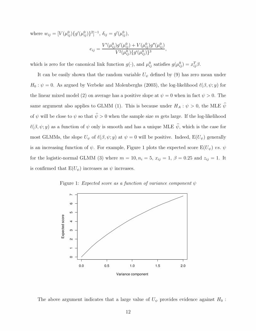
is an increasing function of ψ. For example, Figure 1 plots the expected score E(Uψ) vs. ψ
for the logistic-normal GLMM (3) where m = 10, ni = 5, xij = 1, β = 0.25 and zij = 1. It
is confirmed that E(Uψ) increases as ψ increases.
Figure 1: Expected score as a function of variance component ψ
0.0 0.5 1.0 1.5 2.0
01
23
45
67
Variance component
Expe
cted
sco
re
The above argument indicates that a large value of Uψ provides evidence against H0 :
12

ψ = 0 and we should reject H0 only if Uψ is large. Since Uψ is a sum of independent random
variables, classic results show that it will have an asymptotic normal distribution under
H0 : ψ = 0 with zero mean and variance equal to Iψψ = E(U2ψ), where the expectation is
taken at H0 : ψ = 0.
Denote by κrij the rth cumulant of yij under H0. By the properties of the distributions in
an exponential family, κ3ij and κ4ij are related to κ2ij via κ(r+1)ij = κ2ij∂κrij/∂µij (r = 2, 3),
where κ2ij = φω−1ij v(µij) and µij = µ0
ij. Specifically,
κ3ij = (φω−1ij )2v′(µij)v(µij), κ4ij = (φω−1
ij )3[v′′(µij)v(µij) + v′(µij)2]v(µij).
Then Iψψ can be shown to be (Lin, 1997)
Iψψ =1
4
m∑
i=1
ni∑
j=1
z2ijrii,
where rii = w4ijδ
4ijκ4ij + 2w2
ij + eijκ2ij − 2w2ijδ
2ijeijκ3ij . Therefore, a level α score test for
testing H0 : ψ = 0 vs. HA : ψ > 0 will reject H0 : ψ = 0 if Uψ ≥ zαI1/2ψψ .
In practice, however, β in Uψ and Iψψ is unknown and has to be estimated under H0. This
is straightforward since under H0 : ψ = 0, GLMM (1) reduces to the standard generalized
linear model for independent data g(µij) = XTijβ and existing software can be used to easily
calculate the MLE β of β under H0 : ψ = 0. In this case, Lin (1997) considered the bias-
corrected score statistic to account for the estimation of β under H0 as
U cψ =
∂`(β, ψ; y)
∂ψ
∣∣∣∣∣ψ=0,β=β
=1
2
m∑
i=1
ni∑
j=1
zijwijδij(yij − µ0ij)
2
−ni∑
j=1
z2ijw0ij
, (10)
where all quantities are obtained by replacing β by β, w0ij = (1−hij)wij + eij(yij− µ0ij), and
hij is the corresponding diagonal element of the hat matrix H = W 1/2X(XWX)−1XTW 1/2,
W = diagwij, and showed that U cψ has variance
Iψψ = Iψψ − ITψβI−1ββ Iψβ, (11)
13

where
Iψβ =1
2
m∑
i=1
ni∑
j=1
cijzijxij, Iββ = XTWX =m∑
i=1
ni∑
j=1
wijxijxTij (12)
with cij = w3ijδ
3ijκ3ij − wijδijeijκ2ij . Then the bias-corrected score test at level α would
reject H0 if Ts = U cψ ≥ zαI
1/2ψψ . The one-sided score test presented above is asymptotically
equivalent to the likelihood ratio test (Verbeke and Molenberghs, 2003). The two-sided score
test assumes the score statistic Ts = U cψ
2/Iψψ follows a χ2 distribution. Unlike the regular
likelihood ratio test, such a two-sided score test has the correct size under H0 but is subject
to some loss of power. As shown in our simulation studies for a single variance component,
the loss of power is minor to moderate for most alternatives. The highest power loss is about
10% when the magnitude of the variance component is moderate.
When the dimension of ψ is greater than 1, suppose we can partition ψ = (ψ1, ψ2) where
ψ1 is a c1 × 1 vector and ψ2 is a c2 × 1 vector. We are interested in testing H0 : ψ1 =
0 vs. HA : ψ1 ≥ 0. Here the inequality is interpreted element-wise. Lin (1997) considered
a simple two-sided score test for this multiple variance component test. Specifically, denote
by (β, ψ2) the MLE of (β, ψ2) under H0 : ψ1 = 0. We can similarly derive the (corrected)
score Sψ1= m−1/2∂`(β, ψ1; y)/∂ψ1|ψ1=0,β=β,ψ2=ψ2
. See Lin (1997) for the special case where
each element of ψ represents a variance of a random effect. Asymptotically, Sψ has a normal
distribution with zero mean and variance equal to the efficient information matrix Hψ1ψ1=
m−1Iψ1ψ1under H0, where Iψ1ψ1
is defined similarly to (11) except that Iφβ and Iββ are
replaced by Iψ1γ and Iγγ and γ = (ψ2, β). The simple two-sided score statistic is defined as
Ts = STψ1H−1ψ1ψ1
Sψ1, (13)
and the p-value is calculated by assuming Ts follows a chi-square distribution with c1 degrees
of freedom.
Silvapulle and Silvapulle (1995) proposed a one-sided score test for a general parametric
model and showed that the one-sided score test is asymptotically equivalent to the likelihood
14

ratio test. Verbeke and Molenberghs (2003) extended Silvapulle and Silvapulle’s (1995) one-
sided score test for testing variance components H0 : ψ1 = 0 vs. HA : ψ1 ∈ C for linear
mixed model (2) and showed similar asymptotic equivalence between the one-sided score
test and the likelihood ratio test. Hall and Praestgaard (2001) derived a one-sided score test
for GLMMs. Then the one-sided score statistic T ∗s is defined as
T ∗
s = STψ1H−1ψ1ψ1
Sψ1− inf
ψ1∈C(Sψ1
− ψ1)TH−1
ψ1ψ1(Sψ1
− ψ1). (14)
It is easy to see that T ∗s as defined in (14) has the same asymptotic null distribution of
the likelihood ratio test for testing H0 : ψ1 = 0 vs. HA : ψ1 ∈ C. Similarly to the case for
the likelihood ratio test, it is critical to determine Hψψ and the shape of C, and T ∗s generally
follows a mixture of chi-square distributions and we usually have to study the distribution of
T ∗s case by case. Both the two-sided test Ts and the one-sided test T ∗
s have the correct size
under H0. The two-sided test Ts is much easier to calculate, but is subject to some loss of
power. Hall and Praestgaard (2001) conducted extensive simulation studies comparing Lin’s
(1997) two-sided score test and their one-sided score test for GLMMs with two-dimensional
random effects and found similar power loss to the case of a single variance component (Table
4 in Hall and Praestgaard, 2001; the maximum power loss is about 9%).
5 Simulation Study to Compare the Likelihood Ratio
Test and the Score Test for Variance Components
We conducted a small simulation study to compare the size and the power of the one-sided
and two-sided score tests with the likelihood ratio test. We considered the logistic-normal
GLMM (3) by assuming binary responses yij (i = 1, 2, ..., m = 100, j = 1, 2, ..., ni = 5) were
generated from the following logistic-normal GLMM
logitP(yij = 1|bi) = β + bi, (15)
15

where β = 0.25 and bi ∼ N(0, ψ), with equal spaced ψ in [0,1] by 0.2. For each value of
ψ, 500 data sets were generated. The likelihood ratio test described in Section 3 and the
(corrected) one-sided and two-sided score tests were applied to test H0 : ψ = 0. We compare
the performance of the regular but conservative LRT, the appropriate LRT, one-sided and
two-sided score test for testing H0 : ψ = 0. The nominal level of all 4 tests were set at
α = 0.05.
Table 1: Size and Power comparisons of the likelihood ratio tests and score tests for a singlevariance component based on 500 simulations under the logistic model (15)
Size PowerMethod ψ = 0 ψ = 0.2 ψ = 0.4 ψ = 0.6 ψ = 0.8 ψ = 1.0LRT 0.034 0.370 0.790 0.922 0.990 1.000Regular LRT 0.020 0.280 0.672 0.882 0.968 0.992One-sided score test 0.054 0.416 0.834 0.938 0.996 1.000Two-sided score test 0.050 0.336 0.736 0.910 0.980 0.998
Table 5 presents the simulation results. The results show that the size of the (correct)
likelihood ratio test is little smaller than the nominal level. This is probably due to the
numerical instability caused by numerical difficulties in fitting model (15) when in fact there
is no random effect in the model, or the fact that the sample size (number of clusters
m = 100) may not be large enough for the asymptotic theory to take effect. As expected,
the regular LRT using χ21 is conservative and the size is too small. On the other hand,
both one-sided and two-sided score test have their sizes very close to the nominal level. The
powers of the likelihood ratio test and the one-sided score test are almost the same, although
the one-sided score test is slightly more powerful than the LRT, which may be due to the
numerical integration required to fit model (15). The two-sided score test has some loss of
power compared to the one-sided score test and the correct LRT. However the p-value of the
two-sided score test is much easier to calculate especially for testing for multiple variance
components.
16

6 Polynomial Test in Semiparametric Additive Mixed
Models
Lin and Zhang (1999) proposed generalized additive mixed models (GAMMs), an extension
of GLMMs where each parametric covariate effect in model (1) is replaced by a smooth but
arbitrary nonparametric function, and proposed to estimate each function by a smoothing
spline. Using a mixed model representation for a smoothing spline, they cast estimation and
inference of GAMMs in a unified framework through a working GLMM, where the inverse
of a smoothing parameter is treated as a variance component. A special case of GAMMs is
the semiparametric additive mixed models considered by Zhang and Lin (2003):
g(µij) = f(tij) + sTijα + zTijbi, (16)
where f(t) is an unknown smooth function, i.e., the covariate effect of t is assumed to be
nonparametric, sij is some covariate vector, and bi ∼ N0, D(ψ). For independent (normal)
data with the identity link, model (16) reduces to a partially linear model. We are interested
in developing a score testing for testing f(t) is a parametric polynomial function versus a
smooth nonparametric function. Specifically, we set H0: f(t) is a polynomial function of
degree K − 1 and H1: f(t) is a smoothing spline.
Following Zhang and Lin (2003), denote by t0 = (t01, t02, ..., t
0r)T a vector of ordered distinct
tij’s and by f a vector of f(t) evaluated at t0 (without loss of generality, assume 0 < t01 <
· · · < t0r <1). The Kth-order (K ≥ 1) smoothing spline estimator f(t) can be expressed as
f(t) =K∑
k=1
δkφk(t) +r∑
l=1
alR(t, t0l ), (17)
where φk(t) = tk−1/(k − 1)!Kk=1 is a basis for the space of polynomials of order K − 1 and
R(t, s) is defined as
R(t, s) =1
(K − 1)!2
∫ 1
0(s− u)K−1
+ (t− u)K−1+ du.
17

Then the smoothing spline estimator of f has the following mixed effect representation
f = Tδ + Σa, (18)
where T is an r×K matrix with the (l, k)th element equal to φk(t0l ), Σ is a positive matrix
with the (l, k)th element equal to R(t0l , t0k), δ = (δ1, ..., δK)T is a vector of fixed effects and
a = (a1, a2, ..., ar)T ∼ N(0, τΣ−1) is a vector of random effects with τ ≥ 0 being the inverse
of the smoothing parameter for the smoothing spline estimate f(t).
Let n =∑mi=1 ni be the total sample size and denote by N the n × r incidence matrix
that maps tij’s into t0. Further denote S = (si1, ..., sini)T, X = (NT, S), B = NΣ,
µb = (µb11, ..., µb1n1, ..., µbm1, ..., µ
bmnm
)T . Then under the mixed effect representation (18),
semiparametric additive mixed model (16) reduces to a generalized linear mixed model in
matrix notation
g(µ) = Xβ +Ba + Zb, (19)
where β = (δT , αT )T are new fixed effects and a and b = (bT1 , ..., bmm)T are independent new
random effects. Therefore, the smoothing spline estimator f(t) can be estimated using the
estimation procedure for a GLMM, such as maximum penalized quasi-likelihood procedure
of Breslow and Clayton (1993).
We are interested in using this spline and mixed model connection to test whether or not
the smoothing spline f(t) in semiparametric additive mixed model (16) can be adequately
modeled by a polynomial of order K − 1, i.e., H0: f(t) is a polynomial of order K − 1 and
HA : f(t) is a smoothing spline. From the smoothing spline expression (17), it is clear that
f(t) is a polynomial of order K − 1 if and only if a1 = a2 = · · · = ar = 0. By mixed effect
representation (18), this test is equivalent to the variance component test H0 : τ = 0 vs
HA : τ > 0. It is hence natural to consider using the variance component likelihood ratio
test or score test described in the previous sections to test H0 : τ = 0. However, the data
do not have independent cluster structure under the alternative HA : τ > 0. Therefore,
18
the asymptotic null distribution of the likelihood ratio test statistic for testing H0 : τ = 0
does not follow a 50:50 mixture of χ20 and χ2
1. In fact, for independent normal data with the
identity link, Crainiceanu et al. (2005) showed that, when f(t) is modeled by a penalized
spline (similar to a smoothing spline), the LRT statistic asymptotically has approximately
0.95 mass probability at zero. For this special case, Crainiceanu et al. (2005) derived the
exact null distribution of the LRT statistic. Their results, however, may not be applicable to
testing H0 : τ = 0 under a more general mixed model representation (19). Furthermore, it
could be computationally difficult to calculate this LRT statistic by fitting model (19) under
the alternative HA : τ > 0 as it usually requires high-dimensional numerical integrations.
Due to the special structure of the smoothing matrix Σ, the score statistic of τ evaluated
under H0 : τ = 0 does not have a normal distribution. Zhang and Lin (2003) showed that
the score statistic of τ can usually be expressed as a weighted sum of chi-squared random
variables with positive but rapidly decaying weights, and its distribution can be adequately
approximated by that of a scaled chi-squared random variable.
Under the mixed model representation (19), the marginal likelihood function LM (τ, ψ; y)
of (τ, ψ) is given by
LM(τ, ψ; y) ∝ |D|−m/2τ−r/2∫
exp
m∑
i=1
ni∑
j=1
`ij(β, ψ, bi; yij) −1
2
m∑
i=1
bTi D−1bi −
1
2τaTΣa
dadbdβ.(20)
Let `M(τ, ψ; y) = logLM (τ, ψ; y) be the log-marginal likelihood function of (τ, ψ). Zhang
and Lin (2003) showed that the score Uτ = ∂`M (τ, ψ; y)/∂τ |τ=0 can be approximated by
Uτ ≈1
2(Y −Xβ)TV −1NΣNTV −1(Y −Xβ) − tr(PNΣNT )
∣∣∣∣β,ψ
, (21)
where β is the MLE of β and ψ is the REML estimate of ψ from the null GLMM (22), and
Y is the working vector Y = Xβ + Zb + ∆(y − µ) under the null GLMM
g(µ) = Xβ + Zb, (22)
where ∆ = diagg′(µij), P = V −1 − V −1X(XTV −1X)−1XTV −1 and V = W−1 + ZDZT
19

with D = diagD, ..., D and W is defined similarly as in Section 4 except µ0ij is replaced by
µij. All these matrices are evaluated under the reduced model (22).
Write Uτ = Uτ− e, where Uτ and e are the first and second terms of Uτ in (21). Zhang and
Lin (2003) showed that the mean of Uτ is approximately equal to e under H0 : τ = 0. Similar
to the score test derived in Section 4, the mean of Uτ increases as τ increases. Therefore, we
will reject H0 : τ = 0 when Uτ is large, implying a one-sided test. The variance of Uτ under
H0 can be approximated by
Iττ = Iττ − ITτψI−1ψψIτψ, (23)
where
Iττ =1
2tr(PNΣNT )2, Iτψ =
1
2tr
(PNΣNTP
∂V
∂ψ
), Iψψ =
1
2tr
(P∂V
∂ψP∂V
∂ψ
). (24)
Define κ = Iττ/2e and ν = 2e2/Iττ . Then Sτ = Uτ/κ approximately has a χ2ν distribution,
and we will reject H0 : τ = 0 at the significance level α if Sτ ≥ χ2α;ν . The simulation
conducted by Zhang and Lin (2003) indicates that this modified score test for polynomial
covariate effect in the semiparametric additive mixed model (16) has approximately right
size and is powerful to detect alternatives.
7 Application
In this section, we illustrate the likelihood ratio testing and the score testing for variance
components in GLMMs discussed in Sections 3 and 4, as well as the score polynomial co-
variate effect testing in GAMMs discussed in Section 6 through application to the data from
Indonesian children infectious disease study (Zeger and Karim, 1991). Two hundred and
seventy-five Indonesian preschool children were examined for up to six quarters for the sign
of respiratory infection (0=no, 1=yes). Totally there are 2000 observation in the data set.
Available covariates include: age in years; Xerophthelmia status (sign for vitamin A defi-
ciency); gender; height for age; the presence of stunning and the seasonal sine and cosine.
20

The primary interest of the study is to see if vitamin A deficiency has an effect on the respi-
ratory infection adjusting for other covariates and taking into account the correlation in the
data.
Zeger and Karim (1991) used Gibbs’ sampling approach to fit the following logistic-normal
GLMM
logit(P [yij = 1|bi]) = xTijβ + bi, (25)
where yij is the respiratory infection indicator for the ith child at the jth interview, xij is
the 7 × 1 vector of the covariates described above with corresponding effects β, bi ∼ N(0, θ)
is the random effect modeling the between-child variation/between-child correlation. No
statistically significant effect of vitamin A deficiency on respiratory infection was found.
We can also conduct a likelihood inference for model (25) by evaluating the required
integrations using Gaussian quadrature technique. The MLE of θ is θ = 0.58 with SE(θ) =
0.31, which indicates that there may be between-child variation in the probability of getting
respiratory infection. An interesting question is whether or not we can reject H0 : θ = 0.
The likelihood ratio statistic for this data set is -2lnλm = 674.872 − 669.670 = 5.2. The
resulting p-value = 0.5P [χ21 ≥ 5.2] = 0.011, indicating strong evidence against H0 using the
LRT procedure.
Alternatively, we may apply the score tests to test H0. The (corrected) score statistic
for this data set is 2.678. The p-value from the one-sided score test is 0.0037, and the p-
value from the two-sided score test is 0.0074. Both tests provide strong evidence against
H0 : θ = 0.
Motivated by their earlier work, Zhang and Lin (2003) considered testing whether or not
f(age) in the following semiparametric additive mixed model can be adequately represented
by a quadratic function of age
logit(P [yij = 1|bi]) = sTijβ + f(ageij) + bi, (26)
21

where sij are the remaining covariates. The score test statistic described in Section 6 for
K = 3 is Sτ = 5.73 with 1.30 degrees of freedom, indicating a strong evidence against H0 :
f(age) is a quadratic function of age (p-value= 0.026). This may imply that nonparametric
modeling of f(age) in model (26) is preferred.
8 Discussion
In this chapter, we have reviewed the likelihood ratio test and the score test for testing
variance components in generalized linear mixed models. The central issue is that the null
hypothesis usually places some of the variance components on the boundary of the model
parameter space, and therefore the traditional null chi-squared distribution of the LRT
statistic no longer applies and the p-value based on traditional LR chi-square distribution
is often too conservative. Using the theory developed by Self and Liang (1987), we have
reviewed the LRT for some special cases and show the LRT generally follows a mixture of
chi-square distribution. In order to derive the right null distribution of the LRT statistic, one
needs to know the (Fisher) information matrix at the true parameter value (under the null
hypothesis) and the topological behavior of the neighborhood of the true parameter value.
However, as our simulation indicates, the LRT for the variance components in a GLMM
may suffer from numerical instability when the variance component is small and numerical
integration is high dimensional.
On the other hand, the score statistic only involves parameter estimates under the null
hypothesis and hence can be calculated much more straightforward and efficiently. We
discussed both the one-sided score test and the much simpler two-sided score test. Both
tests have the correct size. The one-sided score test has the same asymptotic distribution as
the correct likelihood ratio test. Hence, similar to the LRT, the calculation of the one-sided
score test requires the knowledge of the information matrix and the topological behavior of
the neighborhood of the true parameter value and also requires computing a mixture of chi-
22

square distributions. The two-sided score test is based on the regular chi-square distribution
and has the right size. It is much easier to calculate especially for testing multiple variance
components. The simulation studies presented here and in the statistical literature show
that the two-sided score test may suffer from some power loss compared to the (correct)
likelihood ratio test and the one-sided score test.
We have also reviewed the likelihood ratio test and the score test for testing whether or
not a nonparametric covariate effect in a GAMM can be adequately modeled by a polynomial
of certain degree compared to a smoothing spline or a penalized spline function. Although the
problem can be reduced to testing a variance component equal to zero using the mixed effects
representation of the smoothing (penalized) spline, the GLMM results for likelihood ratio
test and the score test for variance components do not apply because the data under mixed
effects representation of the spline do not have an independent cluster structure any more.
Since the LRT statistic will be prohibitive to calculate for a GLMM with potentially high
dimensional random effects, we have particularly reviewed the score test of Zhang and Lin
(2003) for testing the parametric covariate model versus the nonparametric covariate model
in the presence of a single nonparametric covariate function. Future research is needed to
develop simultaneous tests for multiple covariate effects.
References
Booth, J.G. and Hobert, J.P. (1999). Maximizing generalized linear mixed model likelihoods
with an automated Monte Carlo EM algorithm. Journal of the Royal Statistical Society,
Series B 61, 265–285.
Breslow, N.E. and Clayton, D.G. (1993). Approximate inference in generalized linear mixed
models. Journal of the American Statistical Association 88, 9–25.
Breslow, N.E. and Lin, X. (1995). Bias correction in generalized linear mixed models with
a single component of dispersion. Biometrika 82, 81–91.
23
Crainiceanu, C., Ruppert, D., Claeskens, G. and Wand, M.P. (2005). Exact likelihood ratio
tests for penalized splines. Biometrika 92, 91-103.
Diggle, Heagerty, Liang and Zeger (2002). Analysis of Longitudinal Data. Oxford University
Press.
Hall, D.B. and Praestgaard, J.T. (2001). Order-restricted score tests for homogeneity in
generalized linear and nonlinear mixed models. Biometrika 88, 739–751.
Hsiao, C.K. (1997). Approximate Bayes factors when a model occurs on the boundary.
Journal of the American Statistical Association 92, 656–663.
Jacqmin-Gadda, H. and Commenges, D. (1995). Tests of homogeneity for generalized linear
models. Journal of the American Statistical Association 90, 1237–46.
Laird, N.M. and Ware, J.H. (1982). Random effects models for longitudinal data. Biomet-
rics 38, 963–974.
Lin, X. (1997). Variance component testing in generalized linear models with random
effects. Biometrika 84, 309–326.
Lin, X. and Breslow, N.E. (1996). Bias correction in generalized linear mixed models with
multiple components of dispersion. Journal of the American Statistical Association 91,
1007–1016.
Lin, X. and Zhang, D. (1999). Inference in generalized additive mixed models using smooth-
ing splines. Journal of the Royal Statistical Society, Series B 61, 381–400.
Self, S.G. and Liang, K.Y. (1987). Asymptotic properties of maximum likelihood estimators
and likelihood ratio tests under nonstandard conditions. Journal of the American
Statistical Association 82, 605–610.
24

Silvapulle, M.J. and Silvapulle, P. (1995). A score test against one-sided alternatives.
Journal of the American Statistical Association 90, 342-349.
Stram, D.O. and Lee, J.W. (1994). Variance components testing in the longitudinal mixed
effects model. Biometrics, 50, 1171–1177.
Verbeke,G. and Molenberghs, G. (2000). Linear Mixed Models for Longitudinal Data.
Springer.
Verbeke, G. and Molenberghs, G. (2003). The use of score tests for inference on variance
components. Biometrics 59, 254–262.
Verbeke, G. and Molenberghs, G. (2005). Models for Discrete Longitudinal Data. Springer
Zeger, S.L. and Karim, M.R. (1991). Generalized linear models with random effects; a
Gibbs sampling approach. Journal of the American Statistical Association 86, 79–86.
Zhang, D. (1997). Generalized Additive Mixed Model, unpublished Ph.D. dissertation, De-
partment of Biostatistics, University of Michigan.
Zhang, D. and Lin, X. (2003). Hypothesis testing in semiparametric additive mixed models.
Biostatistics 4, 57–74.
25
Related Documents