Variable neighborhood search for the vertex separation problem

Variable Neighborhood Search for the Vertex Separation Problem

Abraham Duartea,1, Laureano F. Escuderob, Rafael Martíc, Nenad Mladenovicd, Juan José Pantrigoa,Jesús Sánchez-Oroa

aDpto. de Ciencias de la Computación, Universidad Rey Juan Carlos, Móstoles (Madrid), SpainbDpto. de Estadística e Investigación Operativa, Universidad Rey Juan Carlos, Móstoles (Madrid),Spain

cDpto. de Estadística e Investigación Operativa, Universidad de Valencia, Valencia, SpaindDept. of Mathematics, SISCM, London, United Kingdom

Abstract

The vertex separation problem belongs to a family of optimization problems in which the objective is tond the best separator of vertices or edges in a generic graph. This optimization problem is strongly relatedto other well-known graph problems; such as the Path-Width, the Node Search Number or the IntervalThickness, among others. All of these optimization problems are NP-hard and have practical applicationsin VLSI (Very Large Scale Integration), computer language compiler design or graph drawing. Up to know,they have been generally tackled with exact approaches, presenting polynomial-time algorithms to obtainthe optimal solution for specic types of graphs. However, in spite of their practical applications, theseproblems have been ignored from a heuristic perspective, as far as we know. In this paper we proposea pure 0-1 optimization model and a metaheuristic algorithm based on the variable neighborhood searchmethodology for the vertex separation problem on general graphs. Computational results show that smallinstances can be optimally solved with this optimization model and the proposed metaheuristic is able tond high-quality solutions with a moderate computing time for large-scale instances.

Key words: Combinatorial Optimization, Metaheuristics, Variable Neigborhood Search, Layout Problems.

1. Introduction

Let G(V,E) be an undirected graph where V (n = |V |) and E (m = |E|) are the sets of vertices andedges, respectively. A linear layout ϕ of the vertices of G is a bijection or mapping ϕ : V → 1, 2, . . . , n inwhich each vertex receives a unique and dierent integer between 1 and n. For vertex u, let ϕ(u) denote itsposition or label in layout ϕ. Let L(p, ϕ,G) be the set of vertices in V with a position in the layout ϕ lowerthan or equal to position p. Symmetrically, let R(p, ϕ,G) be the set of vertices with a position in the layoutϕ larger than position p. In mathematical terms,

L(p, ϕ,G) = v ∈ V : ϕ(v) ≤ p and R(p, ϕ,G) = v ∈ V : ϕ(v) > p.

Since layouts are usually represented in a straight line, where the vertex in position 1 comes rst,L(p, ϕ,G) can be simply called the set of left vertices with respect to position p and, R(p, ϕ,G) the set ofthe right vertices w.r.t. p.

The Cut-value at position p of layout ϕ, Cut(p, ϕ,G), is dened as the number of vertices in L(p, ϕ,G)with one or more adjacent vertices in R(p, ϕ,G), then,

Cut(p, ϕ,G) = |u ∈ L(p, ϕ,G) : ∃v ∈ R(p, ϕ,G) ∩N(u)|,

1Corresponding author. e-mail address: [email protected].

Preprint submitted to Elsevier March 28, 2012

where N(u) = v ∈ V : (u, v) ∈ E. The Vertex Separation value (VS) of layout ϕ is the maximum of theCut-value among all positions in layout ϕ: V S(ϕ,G) = maxp Cut(p, ϕ,G).

The Vertex Separation Problem (VSP) consists of nding a layout, say ϕ∗, minimizing the VS in graphG. Despite of its practical applications, there is no previous heuristic or metaheuristic algorithm to ndgood solutions in short computing times. We propose a variable neighborhood search (VNS) [18] approachwhose performance is assessed by a broad testbed of instances.

The remainder of this paper is organized as follows. Section 2 presents the Vertex Separation Problem,including its application domain. Section 3 formalizes the mathematical optimization model. Section 4presents our algorithmic approach based on the VNS metaheuristic framework. Section 5 reports on anextensive computational experience to validate the proposed algorithm by (1) comparing its performanceand computing time versus the optimization of the mathematical model for small instances, and (2) analysingits performance for large instances. Finally, Section 6 summarizes the main conclusions of our research.

2. Description, related problems and applications

The Vertex Separation Problem (VSP) in graph G consists of nding a layout, say ϕ∗, that minimizesV S(G,ϕ), where V S(G,ϕ) is the maximum Cut-value in graph G for layout ϕ, i.e., V S(G,ϕ) =maxpCut(p, ϕ,G). For the sake of simplicity, we denote the optimum value V S(G,ϕ∗) as V S∗.

Figure 1: (a) Graph illustrative example. (b) A layout ϕ for its VSP.

Figure 1.a shows an illustrative example of an undirected graph G with 7 vertices and 9 edges. Figure1.b depicts a solution (layout) ϕ of this graph and the Cut-value of each position p, Cut(p, ϕ,G). Forexample, Cut(1, ϕ,G) = 1 because L(1, ϕ,G) = D and R(1, ϕ,G) = A, F, G, E, B, C and there is onevertex in L having an adjacent vertex in R. Similarly, Cut(3, ϕ,G) = 2 where L(3, ϕ,G) = D, A, F andR(3, ϕ,G) = G, E, B, C. The objective function value, computed as the maximum of these cut values, isV S(G,ϕ) = 3 whose related position is p = 4.

The decisional version of the VSP was proved to be NP-complete for general graphs [26]. It is also knownthat the problem remains NP-complete for planar graphs with maximum degree of three [31], as well as forchordal graphs [15], bipartite graphs [16], grid graphs and unit disk graphs [6].

We can nd many dierent graph problems that, although stated in dierent terms, are equivalent tothe VSP in the sense that a solution to one problem provides a solution to the other one. Some of them arethe Path-Width problem [20], the Interval Thickness problem [22], the Node Search Number [23] and theGate Matrix Layout [21]. The equivalence between these problems is a consequence of the results presentedin [13, 20, 23]. For any graph G let V S(G), PW (G), IT (G), SN(G) and GML(G) be the objectivefunction value of the optimal solution for the Vertex Separation, Path-Width, Interval Thickness, NodeSearch Number and Gate Matrix Layout problems, respectively. These values verify the following relations:

V S(G) = PW (G) = IT (G) = SN(G)− 1 = GML(G) + 1.2

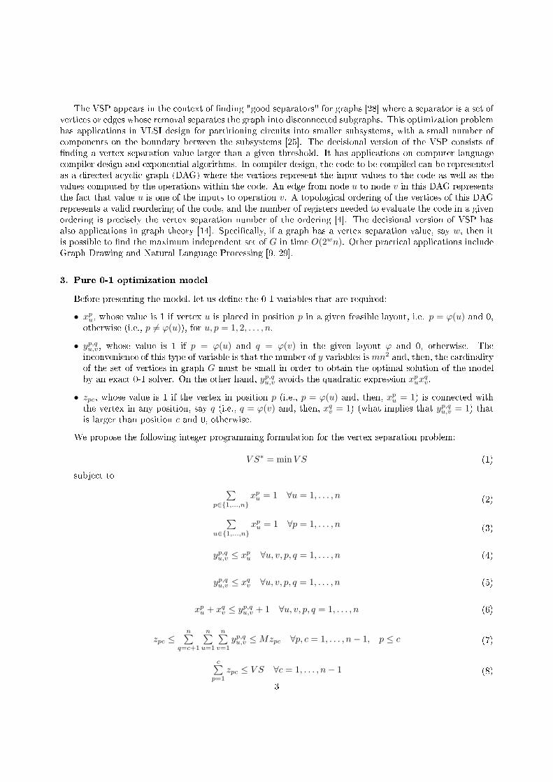
The VSP appears in the context of nding "good separators" for graphs [28] where a separator is a set ofvertices or edges whose removal separates the graph into disconnected subgraphs. This optimization problemhas applications in VLSI design for partitioning circuits into smaller subsystems, with a small number ofcomponents on the boundary between the subsystems [25]. The decisional version of the VSP consists ofnding a vertex separation value larger than a given threshold. It has applications on computer languagecompiler design and exponential algorithms. In compiler design, the code to be compiled can be representedas a directed acyclic graph (DAG) where the vertices represent the input values to the code as well as thevalues computed by the operations within the code. An edge from node u to node v in this DAG representsthe fact that value u is one of the inputs to operation v. A topological ordering of the vertices of this DAGrepresents a valid reordering of the code, and the number of registers needed to evaluate the code in a givenordering is precisely the vertex separation number of the ordering [4]. The decisional version of VSP hasalso applications in graph theory [14]. Specically, if a graph has a vertex separation value, say w, then itis possible to nd the maximum independent set of G in time O(2wn). Other practical applications includeGraph Drawing and Natural Language Processing [9, 29].

3. Pure 0-1 optimization model

Before presenting the model, let us dene the 0-1 variables that are required:

• xpu, whose value is 1 if vertex u is placed in position p in a given feasible layout, i.e. p = ϕ(u) and 0,

otherwise (i.e., p 6= ϕ(u)), for u, p = 1, 2, . . . , n.

• yp,qu,v, whose value is 1 if p = ϕ(u) and q = ϕ(v) in the given layout ϕ and 0, otherwise. Theinconvenience of this type of variable is that the number of y variables ismn2 and, then, the cardinalityof the set of vertices in graph G must be small in order to obtain the optimal solution of the modelby an exact 0-1 solver. On the other hand, yp,qu,v avoids the quadratic expression xp

uxqv.

• zpc, whose value is 1 if the vertex in position p (i.e., p = ϕ(u) and, then, xpu = 1) is connected with

the vertex in any position, say q (i.e., q = ϕ(v) and, then, xqv = 1) (what implies that yp,qu,v = 1) that

is larger than position c and 0, otherwise.

We propose the following integer programming formulation for the vertex separation problem:

V S∗ = minV S (1)

subject to ∑p∈1,...,n

xpu = 1 ∀u = 1, . . . , n (2)

∑u∈1,...,n

xpu = 1 ∀p = 1, . . . , n (3)

yp,qu,v ≤ xpu ∀u, v, p, q = 1, . . . , n (4)

yp,qu,v ≤ xqv ∀u, v, p, q = 1, . . . , n (5)

xpu + xq

v ≤ yp,qu,v + 1 ∀u, v, p, q = 1, . . . , n (6)

zpc ≤n∑

q=c+1

n∑u=1

n∑v=1

yp,qu,v ≤Mzpc ∀p, c = 1, . . . , n− 1, p ≤ c (7)

c∑p=1

zpc ≤ V S ∀c = 1, . . . , n− 1 (8)

3

xpu, y

p,qu,v, zpc ∈ 0, 1 ∀u, v, p, q = 1, . . . , n (9)

The assignment constraints (2) and (3) ensure that each vertex is only assigned to one position, andeach position is only assigned to one vertex, respectively. Subsystem (4)-(6) denes the variable yp,qu,v as theproduct of the variables xp

u and xqv in the traditional way. So, notice that for a position p,

∑nq=c+1 y

p,qu,v

computes the number of edges from the vertex in position p, say p = ϕ(u), to any vertex in a position q,say q = ϕ(v) (since xq

v = 1 for yp,qu,v = 1) that is bigger than c, for c = q + 1, . . . , n for a given layout ϕ.Constraints (7) compute the 0-1 value of the zpc variable from the yp,qu,v variables (since xp

u = 1 foryp,qu,v = 1), where M is the standard big-M parameter that should be computationally small enough to allowany feasible layout ϕ, in our case M = n− 1.

The left hand side (lhs) of constraints (8) gives the number of vertices in positions p that, in one hand,are lower than or equal to position c, in any feasible layout ϕ or equal to c and, in the other hand, they areconnected with vertices whose positions are larger than position c. So, there is a position c in layout ϕ thathas the greatest lhs in the constraints (8), which is V S∗. The objective function of the model (1) minimizesthat value, being V S∗ the optimal value.

We can observe that this model has O(mn2) 0-1 variables and O(mn3) constraints, what makes itimpractical for relatively large instances.

4. Algorithmic Approach: Variable Neighborhood Search

In spite of the diculty of the model presented above we can nd ecient exact approaches to solvethe VSP on special classes of graphs. A linear algorithm to compute the optimal vertex separation of atree is proposed in [10] as well as an O(n log n) algorithm for nding the corresponding optimal layout. Thealgorithm was improved in [36] with a linear time procedure to nd the optimal layout. In [33] an alternativemethod to compute the Vertex Separation of trees was proposed. [12] proposes an O(n log n) algorithm tocompute the Vertex Separation of unicyclic graphs (i.e., trees with an extra edge). A polynomial-timealgorithm to compute the Path-Width (what is identical to VSP) is proposed in [2]. However, the algorithmcannot be considered from a practical point of view, since the bound on its time complexity is Ω(n), see [12].[5] proposes a polynomial time algorithm for optimally solving the VSP for n-dimensional grids. Co-graphsand permutational graphs can also be optimally solved as it was proposed in [1] and [2], respectively.

Approximation algorithms have been also proposed for the VSP. Specically, [3] proposes a polynomialtime O(log2 n)-approximation algorithm for general graphs and a O(log n)-approximation algorithm forplanar graphs. Similar results for binomial random graphs are presented in [7].

VNS is a metaheuristic for solving optimization problems based on a systematic change of neighborhoodstructures, without guaranteeing the solution's optimality. In recent years, a large variety of VNS strategieshave been proposed. We can highlight the Variable Neighborhood Descent (VND), Reduced VNS (RVNS),Basic VNS (BVNS), Skewed VNS (SVNS), General VNS (GVNS), Variable Neighborhood DecompositionSearch (VNDS) and Reactive VNS, among others. We refer the reader to [18] for a complete review ofthis methodology and its dierent variants. In this paper, we focus on the Basic VNS variant, see [30] forthe details, which combines deterministic and stochastic changes of neighborhood as shown in the BVNSpseudo-code depicted in Algorithm 1.

The method starts by constructing a feasible solution (step 1), using one of the constructive proceduredescribed in Section 4.1. The BVNS implementation is executed for a predened computing time, tmax

(step 2 to 10). The search process starts with the rst neighborhood of the constructed solution, N1(ϕ)(step 3). Then, BVNS performs stochastic changes of neighborhood structures until reaching the largestpredened neighborhood kmax (steps 4 to 8). VNS has three main strategies within the main loop, namely,Shaking (step 5), Improvement (step 6) and Neighborhood change (step 7). In the shaking stage a solution,say ϕ′, is generated within Nk(ϕ), where k = 1, . . . , kmax identies a neighborhood structure within a set ofpredened neighborhoods (see Section 4.3 for additional details). Then, the improvement method (Section4.5) is applied to ϕ′ in order to nd a local optimum, say ϕ′′, in the corresponding neighborhood. Finally,the neighborhood change stage (Section 4.4), analyzes if ϕ′′ is better than ϕ (see in Section 4.5 the extended

4

Algorithm 1 BasicVNS(kmax, tmax)

1: ϕ← Construct()2: repeat

3: k ← 14: repeat

5: ϕ′ ← Shake(ϕ, k)6: ϕ′′ ← LocalSearch(ϕ′)7: NeighbourhoodChange(ϕ,ϕ′′, k)8: until (k = kmax)9: t← Time()10: until (t = tmax)

denition of the concept of improvement move). If so, ϕ is replaced with ϕ′′ and k is set to one. Otherwise,k is incremented by one unit. And, in any case, we repeat the procedure.

We now describe with more detail the main strategies of our BVNS approach for solving the VertexSeparation Problem.

4.1. Constructive procedures

We have designed two greedy constructive algorithms, say C1 and C2, for the VSP. The constructiveprocedure, C1, starts by creating a set of unlabeled vertices U (initially U = V ), and a set of labeled verticesL = V \U . The vertex with the minimum degree is selected as the rst node u (ties are broken at random).The vertex u is labeled with 1. Then, sets U and L are properly updated (i.e., U = U \u and L = L∪u).Once the rst label is assigned to vertex u, C1 evaluates the greedy function as follows

g(v) = |NL(v)| − |NU (v)| ∀v ∈ U,

where NL(v) is the set of vertices adjacent to v that has been already labeled, and NU (v) is the set ofvertices adjacent to v not labeled yet. The constructive procedure selects the vertex with the maximumg-value and assigns the next label to it. The procedure ends when all the vertices of the graph have a label(i.e., U = ∅).

The second constructive procedure, C2, is based on the creation of the so-called level structures [27]which means that the set of vertices V is partitioned into dierent sets L1, L2, . . . , Lλ called levels. Therst level, L1, contains only one vertex. The rest of levels Ll with l = 2, 3, . . . , λ (where λ indicates thenumber of levels) contain all the vertices adjacent to some vertex in Ll−1 that are not present in any Lj

with 1 ≤ j < l. The number of levels λ exclusively depends on the graph and the vertex placed in L1.The level structure created in this way guarantees that the vertices in alternative levels are not adjacent.

In order to construct this level structure we use a breadth rst search approach, performing the search oncefor each vertex of the graph. Therefore, if the graph has n vertices, we construct n dierent level structures.In the context of the VSP, it is desirable to obtain a level structure with λ as large as possible (i.e., astructure with the largest number of levels). Once we have identied the most suitable level structure, C2explores it performing a breadth-rst search and assigning levels in an incremental way, thus obtaining asolution for the VSP.

4.2. Updating the objective function

Let ϕp be a partial solution where p vertices have been placed in positions from 1 to p. For the sake ofsimplicity, we denote vp as the vertex placed in position p, i.e., p = ϕ(vp). We maintain this notation forthe rest of the paper. Given a graph G and a partial solution ϕp, the Cut-value of a position p, Cut(p, ϕ,G)can be computed from the Cut-value of the previous position p− 1 (except for p = 1 where, obviously, theCut-value is always 1) as follows,

Cut(p, ϕp, G) = Cut(p− 1, ϕp, G) + δ+(p)− δ−(p),5

where δ+(p) ∈ 0, 1 has the value 1 if vertex vp has, at least, one adjacent vertex in NU (vp), and 0,otherwise; and δ−(p) = |NL(vp)|.

This strategy can be extended to the incremental computation in complete solutions (i.e., solutionsϕ = ϕr with r = n). Specically, for any position p the set NU (vp) is replaced with the set of vertices placedin a position q with 1 ≤ q ≤ p. Symmetrically, the set NL(vp) is replaced with the set of vertices placed ina position q with p < q ≤ n. Figure 2 shows an example of the incremental objective function computation.Let us consider the third position in ϕ (i.e., vertex C). The Cut-value of this position can be computed byusing the Cut-value of the previous position, Cut(2, ϕ,G) = 2. The value of δ+(3) is 1 because vertex C hasone adjacent at least (specically, three adjacents) placed in a position greater than ϕ(C) = 3 (vertices B,F and E, with ϕ(B) = 4, ϕ(F) = 5 and ϕ(E) = 6, respectively). On the other hand, the value of δ−(3) is 2because C is the adjacent vertex with the largest label of vertices A and D, placed in positions ϕ(A) = 1 andϕ(D) = 2, respectively. The same reasoning can be applied to compute the rest of the Cut-values.

Figure 2: Incremental objective function computation. The symbol * means that the corresponding value is not dened for therst position.

4.3. Shake

In this section we propose a shake function for the VSP, called shake(ϕ, k). This procedure initiallyselects the vertices to be moved, based on their Cut-value. Specically, shake(ϕ, k) selects the k vertices inV with the largest Cut-value in ϕ. Then, each selected vertex is exchanged with another vertex determinedat random, obtaining a new ordering ϕ′. The rationale behind this procedure is that the k selected verticeshave Cut-values close or equal to the maximum Cut-value for ϕ in G and, therefore, the aim is to reducetheir Cut-value improving the objective function of ϕ′. Additionally, it is expected that the shaking stepwill contribute to the diversication of the search process. In other words, shaking will produce a solutionfar away from the current one, allowing to explore dierent regions of the solution space.

4.4. Neighborhood structures

A solution to the VSP can be represented as an ordering, where each vertex is located in the positiongiven by its label. For example, the labeling of the graph depicted in Figure 1 can be expressed by theordering ϕ = (D, A, F, G, E, B, C), where the rst vertex, D, in the ordering receives the label 1, the secondvertex, A, receives the label 2, and so on. We dene neighborhood structures based on the exchange ofvertices in a given ordering. Given a solution ϕ = (v1, . . . , vp, . . . , vq, . . . , vn), we dene Move(ϕ, p, q) asexchanging in ϕ the vertex in position p (i.e., vp) with the vertex in position q (i.e., vq) and, thus, producinga new solution ϕ′ = (v1, . . . , vq, . . . , vp, . . . , vn).

6

In a direct implementation, the complexity of evaluating ϕ′ is O(n2) in the worst case since it requires tovisit, for each position p in ϕ, all the vertices with labels p ≤ q. However, the Cut-value of some vertices doesnot change when we perform a move. Therefore, it is not required to compute them again. Specically, if weperform Move(ϕ, p, q), all vertices with label r for 1 ≤ r < p or q ≤ r ≤ n do not change their Cut-values.As a consequence, we only need to update vertices whose label s is such that p ≤ s < q. For example, Figure3.a shows a layout and Figure 3.b represents the layout resulting from performing Move(ϕ, 2, 5). This moveonly aects the Cut-value of positions 2 ≤ s < 5 (represented as a highlighted band in those gures).

Additionally, to compute the Cut-value of the vertices involved (i.e., the set of vertices D, C, B in Figure3.b) we can use the incremental objective function computation described above, but restricted to verticesin positions from p to q − 1. In the example shown in Figure 3.b we can observe that the update of theCut-values is only needed for the vertices in positions ϕ(D) = 2, ϕ(C) = 3 and ϕ(B) = 4.

Figure 3: Illustrative example of an interchange move: (a) layout before the move and (b) layout after the move.

Given a layout ϕ, its neighborhood N1(ϕ) is dened as all possible exchanges between each pair ofvertices. In other words, a solution ϕ′ belongs to N1(ϕ) if and only if ϕ and ϕ′ only dier in two labels. Ingeneral, we may say that a solution ϕ′ belongs to the kth neighborhood of solution ϕ (i.e., ϕ′ ∈ Nk(ϕ)) if ϕand ϕ′ dier in k + 1 labels.

4.5. Local search

VSP is a min-max problem [8, 32, 35] where the value of the objective function is usually reached inseveral positions of the permutation ϕ. This kind of problems present a at landscape, which turns outin a challenge for classical local search procedures as well as for 0-1 solvers to obtain the optimal layout.Typically, local search strategies do not perform well from a computational point of view, since most ofthe moves have associated a null value. Then, given a graph G, changing the label p of a particularvertex vp in ϕ (i.e., obtaining a new solution ϕ′) such that its Cut-value is decreased, does not necessarilyimply that V S(G,ϕ′) < V S(G,ϕ). However, it can be considered as an interesting move if the number ofvertices with a relative large Cut-value is reduced, regardless whether the objective function improves ornot. Considering this extended denition of improving we overcome the lack of information provided bythe objective function. Specically, we implement a candidate list strategy classifying the vertices of thegraph according to its Cut-value. For example, given the graph depicted in Figure 1 and the labeling ϕ, weobtain three dierent sets: S3(ϕ) = G, containing vertices with Cut-value equal to 3; S2(ϕ) = A, F, E,with Cut-value equal to 2; and nally S1(ϕ) = D, B with Cut-value equal to 1.

Given the denition of Si(ϕ) that has been introduced in the previous paragraph, we consider that amove improves the current solution if any node involved in the move is removed from Si(ϕ) and included inSj(ϕ) with j < i without increasing the cardinality of any set Sl(ϕ) for l > i. According to this denitionof improving, a move which removes a vertex from S2(ϕ) (for example, vertex A) including it in S1(ϕ) is

7

Figure 4: (a) improving move and (b) non-improving move over the layout depicted in Figure 3.a.

considered an improving move if the cardinality of S3(ϕ) remains unaltered. We have empirically foundthat this criterion allows the local search procedure to explore a larger number of solutions than a typicalimplementation that only performs moves when the objective function is improved. Figure 4.a shows animproving move for the labelling of Figure 3.a. The move consists of exchanging the labels of vertices C

and A and, thus, obtaining a new solution ϕ′. In the new labelling, vertex F is removed from set S2(ϕ) andincluded in set S1(ϕ

′). It means that the Cut-value of vertex F is decreased by 1 unit. This move doesnot reduce the VS value of the graph, but it reduces the number of vertices with large Cut-value. Observethat this move does not improve the incumbent solution, but it can allow further moves that, at the end,improves it. On the other hand, if we now exchange the labels of vertices B and C obtaining a new solutionϕ′′ (see Figure 4.b) then vertex C is removed from set S2(ϕ) and included in set S3(ϕ

′′) (i.e., its Cut-valueis increased by one unit). Therefore, although this move does not aect the VS value, it is not accepted.Algorithm 2 shows a pseudocode of the procedure, where the acceptance criterion has been implemented.This procedure starts by comparing the objective function of the previous ordering (ϕ) and the relatedfunction of the ordering after the corresponding movement (ϕ′). If the associated move reduces the valueof the objective function, then IsImprovementMove returns true (step 2). On the other hand, if themove deteriorates the objective function value then this procedure returns false (step 4). In case that thecorresponding move does not aect the value of the objective function (steps 6 to 13) IsImprovementMoveconsiders the extended denition of improvement move dened above.

Algorithm 2 IsImprovementMove(ϕ,ϕ′)

1: if V S(G,ϕ′) < V S(G,ϕ) then2: return true3: else if V S(G,ϕ′) > V S(G,ϕ) then4: return false5: else * V S(G,ϕ) = V S(G,ϕ′) *6: for i← V S(G,ϕ) downto 1 do7: if |Si(ϕ)| > |Si(ϕ

′)| then8: return true9: else if |Si(ϕ)| < |Si(ϕ

′)| then10: return false11: end if

12: end for

13: return false14: end if

The proposed Local Search strategy is presented in Algorithm 3. This method receives a layout ϕ andperform moves while an improve is produced (i.e., while-loop in step 2). Specically, the procedure startsby arranging the vertices in descending order of the Cut-value, obtaining the set posSet which contains

8

the position of such vertices (step 4). Then, the algorithm traverses this set (for-loop in step 5) trying tointerchange each vertex in posSet with the remaining vertices in ϕ (for-loop in step 6). In each iteration,the method proves to interchange the position of the two considered vertices (step 8) accepting the move ifthe new layout ϕ′ outperforms ϕ (steps 9 to 12). This procedure is repeated until no improvement in themove is found.

Algorithm 3 LocalSearch(ϕ)

1: improvement← true2: while improvement do3: improvement← false4: posSet← OrderByCutV alue(ϕ)5: for all p ∈ posSet do6: for q ← 1 to |ϕ| do7: if p 6= q then8: ϕ′ ← Interchange(ϕ, p, q)9: if IsImprovementMove(ϕ,ϕ′) then10: ϕ← ϕ′

11: improvement← true12: end if

13: end if

14: end for

15: end for

16: end while

17: return ϕ

5. Computational experience

This section reports the computational experiments that we have performed for testing the eciency ofour VNS procedure, so called BVNS, for solving the VSP. The algorithm has been implemented in Java SE6 and all the experiments were conducted on an Intel Core i7 2600 CPU (3.4 Ghz) and 2 Gb RAM. Wehave experimented with three sets of instances, totalizing 173 instances (All of the instances are availableat http://www.optsicom.es/vsp/).

5.1. Testbed description

• HB: We derived 73 instances from the Harwell-Boeing Sparse Matrix Collection. This collection consistsof a set of standard test matrices M = Muv arising from problems in linear systems, least squares,and eigenvalue calculations from a wide variety of scientic and engineering disciplines. The graphsare derived from these matrices by considering an edge (u, v) for every element Muv = 0. From theoriginal set we have selected the 73 graphs with n ≤ 1000. The number of vertices and edges rangefrom 24 to 960 and from 34 to 3721, respectively.

• Grids: This set consists of 50 matrices constructed as the Cartesian product of two paths [34]. Theyare also called two dimensional meshes and the optimal solution of the VSP for squared grids is knownby construction, see [7]. Specically, the vertex separation value of a square grid of size λ×λ is λ. Forthis set, the vertices are arranged on a square grid with a dimension λ×λ for 5 ≤ λ ≤ 54. The numberof vertices and edges range from 5× 5 = 25 to 54× 54 = 2916 and from 40 to 5724, respectively.

• Trees: Let T (λ) be set of trees with minimum number of nodes and vertex separation equal to λ.As it is stated in [11], there is just one tree in T (1), namely the tree with a single edge, and anotherone in T (2), the tree constructed with a new node acting as root of three subtrees that belong toT (1). In general, to construct a tree with vertex separation λ + 1 it is necessary to select any three

9

members from T (λ) and link any one node from each of these to a new node acting as the root of thenew tree. The number of nodes, n(λ), of a tree in T (λ) can be obtained using the recurrence relationn(λ) = 3n(λ − 1) + 1 where and n(1) = 2 (see [11] for additional details). We consider 50 dierenttrees: 15 trees in T (3), 15 trees in T (4) and 20 trees in T (5). The number of vertices and edges rangefrom 22 to 202 and from 21 to 201, respectively.

Eight experiments are performed for assessing the validation of the proposed procedure BVNS. We haveselected 32 HB representative instances, with dierent sizes and densities, to perform the experiments 1 to 5oriented to establish the best conguration of the BVNS procedure. Let us name this set of instances the HBsubset. Specically, we consider the instances ASH85, BCSPWR01, BCSPWR02, BCSPWR03, BCSSTK01, BCSSTK02,BCSSTK03, BCSSTK04, BCSSTK05, BCSSTK22, CAN_144, CAN_161, CAN_187, CAN_229, CAN_24, CAN_61, CAN_62,CAN_73, CAN_96, DWT_162, DWT_193, DWT_198, DWT_209, DWT_221, DWT_234, DWT_245, DWT_59, DWT_66,DWT_72, DWT_87, NOS1 and NOS4. Experiment 6 evaluates the performance of the optimization model (1)-(9).Experiment 7 evaluates the performance of BVNS on instances whose optimum is known and, nally, theperformance of the best conguration of the procedure BVNS is analyzed by using the full testbed of 173instances (experiment 8).

5.2. Experiment 1: constructive procedures performance

In our rst experiment we compare the performance of the two proposed constructive procedures for theVSP, namely C1 and C2, described in Section 4.1. We have conducted the experiment over the HB subset of32 instances presented above. We generate one solution with each constructive procedure. The statistics ofTable 1 are as follows: #Best, number of best solutions found in the experiment; Avg., average quality overall instances; Dev(%), average percent deviation with respect to the best solution found in the experiment;and Time, average computing time in seconds required by the procedure.

Table 1: Constructive procedures.

C1 C2#Best 19 18Avg. 17.50 17.65

Dev(%) 11.24 15.66Time 0.010 0.018

Table 1 shows that C1 obtains better results than C2 in all headings and using similar computing time.Specically, C1 reaches a smaller deviation (11.24%) than C2 (15.66%) and a larger number of best solutions(19 versus 18) in the set of instances experimented with.

5.3. Experiment 2: local search performance

We compare the two constructive procedures for the VSP (C1 and C2) coupled with the improvementprocedure (LS) presented in Section 4.5. Table 2 reports the results using the same headings as above.We can observe that the method C2 coupled with LS gets more best solutions than C1+LS (22 versus 19),smaller deviation (9.48% versus 9.86%) and requires 7% smaller computing time (26.25 sec versus 24.42 sec)than the method C1 + LS. Despite C1 alone has better performance than C2 (see Table 1), when couplingthe improvement strategy to the constructive procedures the behaviour completely changes and C2 + LSclearly outperforms C1 + LS. This behaviour may be partially explained by the fact that C2 is able toconstruct layouts with broader diversity than C1.

5.4. Experiment 3: objective function computation

We study the computing time of C2 + LS when (1) using a direct objective function computation (DOFC)and (2) using the incremental objective function computation (IOFC) presented in Section 4.2. Figure 5

10

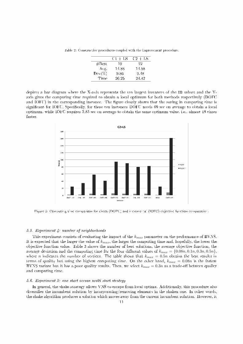
Table 2: Constructive procedures coupled with the improvement procedure.

C1 + LS C2 + LS#Best 19 22Avg. 14.88 14.88

Dev(%) 9.86 9.48Time 26.25 24.42

depicts a bar diagram where the X-axis represents the ten largest instances of the HB subset and the Y-axis gives the computing time required to obtain a local optimum for both methods respectively (DOFCand IOFC) in the corresponding instance. The gure clearly shows that the saving in computing time issignicant for IOFC. Specically, for these ten instances DOFC needs 69 sec on average to obtain a localoptimum, while IOFC requires 3.85 sec on average to obtain the same optimum value, i.e., almost 18 timesfaster.

Figure 5: Computing time comparison for direct (DOFC) and incremental (IOFC) objective function computation.

5.5. Experiment 4: number of neighborhoods

This experiment consists of evaluating the impact of the kmax parameter on the performance of BVNS.It is expected that the larger the value of kmax, the larger the computing time and, hopefully, the lower theobjective function value. Table 3 shows the number of best solutions, the average objective function, theaverage deviation and the computing time for the four dierent values of kmax = 0.08n, 0.1n, 0.3n, 0.5n,where n indicates the number of vertices. The table shows that kmax = 0.5n obtains the best results interms of quality but using the highest computing time. On the other hand, kmax = 0.08n is the fastestBVNS variant but it has a poor quality results. Then, we select kmax = 0.3n as a trade-o between qualityand computing time.

5.6. Experiment 5: one-start versus multi-start strategy

In general, the shake strategy allows VNS to escape from local optima. Additionally, this procedure alsodiversies the incumbent solution by incorporating/removing elements in the shaken one. In other words,the shake algorithm produces a solution which moves away from the current incumbent solution. However, it

11

Table 3: Comparison of dierent kmax values.

kmax

0.08n 0.1n 0.3n 0.5n#Best 27 28 31 32Avg. 13.34 13.31 12.91 12.87

Dev(%) 3.71 2.92 0.78 0.00Time 69.70 79.54 214.32 341.74

could be possible that the shake strategy is not powerful enough to be used alone (i.e., deep local optimum).Consequently, in order to analyze the potential improvement of diversication, we consider a multi-startstrategy which construct solutions in dierent positions of the search space and, then, execute the VNS.In this experiment we compare the performance of the best identied variant of BVNS (which includesC2, exchange-based LS and the parameter kmax set to 0.3n) with a multi-start BVNS. In order to have afair comparison, both methods use the same constructive and search strategies. The multi-start BVNS isexecuted starting from 10 dierent solutions. So, it is expected that its computing time is about 10 timesslower, and the kmax parameter is set to 0.03n, so it is 10 times lower than the kmax value in BVNS. Table4 show that the best variant of BVNS while using the one-start approach has better performance than themulti-start strategy in the same envronment. Specically, the former has more best solutions (30 versus25) and it reaches smaller average deviation (0.40%) than the latter (4.46%) in the set of 32 instances ofthe HB subset considered in the experimentation. Furthermore, the computing time for the one-start BVNS(214.32 sec.) is a 93% less than the time required by the multi-start strategy (3170.09 sec.) for BVNS. It isimportant to remark that in both variants, the BVNS algorithm is exactly the same.

Table 4: One-start Vs multi-start BVNS.

BVNS Multi-start BVNS#Best 30 25Avg. 12.91 13.41

Dev(%) 0.40 4.46Time 214.32 3170.09

5.7. Experiment 6: pure 0-1 optimization model

This experiment consists of evaluating the optimization of the mathematical model introduced in Section3, by using the state-of-the-art optimization engine CPLEX v12.1 [19].

The main results of the experiment are shown in Table 5, whose headings indicate the name of the instance(Instance), number of vertices (n), number of constraints (nc), number of 0-1 variables (n01), numberof constraint matrix non-zero elements (nel), number of CPLEX branch-and-cut required for obtainingthe incumbent vertex separation (nn), optimal vertex separation value for the corresponding instance G(V S∗ = V S(G)), LP lower bound of the optimal vertex separation value provided by CPLEX (V SCPLEX),optimality gap in percentage (GAP = (V S∗−V SCPLEX)/V SCPLEX), vertex separation value related to theincumbent vertex separation provided by CPLEX, computing time (secs) required by CPLEX (TimeCPLEX),vertex separation value provided by our metaheuristic procedure BVNS ( V SBVNS), and computing time(secs) required by the procedure (TimeBVNS).

12

Table5:CPLEXresults.

Modeldim

ensions,optimalsolution,CPLEXincumbentsolution,BVNSsolutionandcomputingtimes

(secs.)

Instance

nnc

n01

nel

nn

VS∗

VSCPLEX

GAP

(%)

VSCPLEX

Tim

e CPLEX

VSBVN

STim

e BVN

S

grid_3

95938

2062

19690

12636

33

0.00

32528

30.054

grid_4

1637166

12665

152318

902

41

300.00

55400

40.126

Tree_

22_3_

rot0_3

2261532

21044

2922994

533

31

200.00

45400

30.029

Tree_

22_3_

rot1_3

2261532

21044

2922994

543

31

200.00

55400

30.022

Tree_

22_3_

rot2_3

2261532

21044

2922994

604

31

200.00

45400

30.024

Tree_

22_3_

rot3_3

2261532

21044

2922994

557

31

200.00

45400

30.037

Tree_

22_3_

rot4_3

2261532

21044

2922994

553

31

200.00

35400

30.019

Tree_

22_3_

rot5_3

2261532

21044

2922994

572

31

200.00

45400

30.018

Tree_

22_3_

rot6_3

2261532

21044

2922994

593

31

200.00

45400

30.015

Tree_

22_3_

rot0_1

2261532

21044

2922994

595

31

200.00

45400

30.04

Tree_

22_3_

rot1_1

2261532

21044

2922994

597

31

200.00

45400

30.02

Tree_

22_3_

rot2_1

2261532

21044

2922994

572

31

200.00

45400

30.018

Tree_

22_3_

rot3_1

2261532

21044

2922994

577

31

200.00

45400

30.025

Tree_

22_3_

rot4_1

2261532

21044

2922994

590

31

200.00

45400

30.016

Tree_

22_3_

rot5_1

2261532

21044

2922994

566

31

200.00

45400

30.019

Tree_

22_3_

rot6_1

2261532

21044

2922994

646

31

200.00

55400

30.022

Tree_

22_3_

rot0_2

2261532

21044

2922994

625

31

200.00

55400

30.029

Tree_

22_3_

rot1_2

2261532

21044

2922994

590

31

200.00

55400

30.022

Tree_

22_3_

rot2_2

2261532

21044

2922994

547

31

200.00

45400

30.024

Tree_

22_3_

rot3_2

2261532

21044

2922994

588

31

200.00

45400

30.037

Tree_

22_3_

rot4_2

2261532

21044

2922994

591

31

200.00

45400

30.019

Tree_

22_3_

rot5_2

2261532

21044

2922994

543

31

200.00

45400

30.018

Tree_

22_3_

rot6_2

2261532

21044

2922994

636

31

200.00

45400

30.015

Note:

CPLEX

computingtimelimit:5400

secs.

13

Table 5 reports the main results of the following small instances: two instances from the grid set andthe 21 instances from the set that have 22 nodes. In total 23 out of 173 instances in the sets that we haveexperimented with. We selected those instances where CPLEX could be used for its optimization. It isimportant to remark that CPLEX could not execute the model for the rest of instances since there wasnot enough memory (in our computer) to allocate the model, due to its large dimensions. Notice that theoptimal vertex separation of the subset of instances in Table 5 is known by construction.

We can observe in Table 5 that the LP lower bound V SCPLEX is so small that is useless, in fact is 1, i.e.,the minimum possible value for connected graphs. Additionally, we can observe that CPLEX only obtains theoptimal vertex separation for the smallest instance, grid_3. On the other hand, the dierence between theCPLEX incumbent solution and the optimum (V S∗) is one or two units. Attending to the optimality gap, wecan observe the weakness of the 0-1 model. Finally, it is worth to mention that, although CPLEX obtains theoptimal value V S∗ = 3 for instance TREE_22_3_rot4, it can not guarantee its optimality in the computingtime limit, 5400 secs (taking into account the value of the lower bound V SCPLEX = 1 < V S∗ = 3).

Finally, we can observe in Table 5 that the procedure BVNS obtains the optimal vertex separation valuein all instances that we have used in the experiment, being impressive its computing time (much less than0.15 secs. for each instance). On the other hand, since our BVNS is heuristic in nature, it does not guaranteethe optimality of these solutions by itself.

5.8. Experiment 7: BVNS on instances with known optimum value

We evaluate in this experiment the performance of our best identied variant of BVNS on a larger setof instances than the set used in the previous experiment. In this other set the optimal vertex separationis known by construction. Specically, we use the 50 instances of the set Grids and 50 instances of the setTrees and test whether the BVNS is able to match the optimum or not. Table 6 has the same headingsas the other tables plus the computing time, say, Time_to_Opt, required by BVNS to reach the optimalsolution on average.

Table 6: Grids and Trees.

Grids Trees_22 Trees_67 Trees_202

#Opt 50 15 15 1Avg. 29.5 3.00 4.00 6.35

Dev(%) 0.00 0.00 0.00 27.00Time_to_Opt 0.36 0.002 0.58 *

Time 1422.76 0.02 3.37 314.28

Observe that BVNS is able to nd the optimum solution in all the instances of the set Grids, subset Trees_22and subset Trees_67. Therefore, BVNS is able to nd the optimum in the instances where CPLEX couldnot due to running out of memory while solving the model presented in Section 3. Indeed, BVNS nds theoptimum in subsets Trees_22 and Trees_67 in short computing time. It is worth to remark that althoughthe BVNS method requires a relative large computing time (1422.76 sec) for the whole procedure, it obtainsthe optimal solution in only 0.36 sec on average. In sight of these results we can conclude that grids instancesare easily solved by our procedure. Regarding the instances of the set Trees the algorithm is able to nd theoptimal solution for the small and medium instances (i.e., Trees_22 and Trees_67) in very small computingtime, 0.002 sec for nding the solution and 0.02 sec for proving it for trees with 22 nodes, and 0.58 sec and3.37 respectively, for trees with 67 nodes. Specically, BVNS only nds the optimal solution in one out of20 large instances included in the set Trees_202 and the average deviation is 27.0%. But, although thecomputing time, 314.28 sec, is large as compared to the other sets of instances, it is not too much eortconsidering that the instances have 202 vertices. Moreover, although it is not reported in Table 6, we canobserve analyzing each instance that, besides guaranteeing optimally in one instance, BVNS obtains in 11instances a quasi-optimal solution (the solution value is 6, i.e., one unit from the optimal one), and for theremaining 8 instances it obtains a solution value of 7 (i.e., two units from the optimal one). Notice that,

14

since BVNS does not match the optimal value in 19 instances, the corresponding Time_to_Opt value isnot reported (represented by an asterisk in the table).

5.9. Experiment 8: BVNS procedure versus C2 and C2 + LS

The VSP has been computationally observed to be optimally solved for particular graphs (trees, grids,co-graphs, etc.). Additionally, as it was presented in Section 2, VSP has relevant practical applications.However, as far as we know, there are no previous heuristic procedures to obtain high-quality solutions ongeneral graphs. In order to provide a nal comparison, our experiment consists of evaluating the performanceof BVNS versus the constructive approach C2, and the constructive C2 plus the local search procedure, C2+ LS, executed as stand-alone procedures. To provide a fair comparison, the three procedures are executedduring a similar computing time. Specically, C2 is run for 23000 independent iterations while C2 + LS isexecuted for 150 independent iterations. The target of this computational comparison is to experimentallyshow how a systematic change of neighborhood (VNS) is able to outperform more direct approaches (sayC2 and C2 + LS).

Table 7: Constructive Vs Constructive plus local search Vs BVNS

C2 C2 + LS BVNS#Best 16 38 73Avg. 30.70 26.68 24.25

Dev(%) 35.97 11.73 0.00Time 1417.05 1204.38 749.77

Finally, the results of the last experiment are shown in Table 7, where the performance of the proceduresC2, C2 + LS and BVNS are compared by executing them over the whole set of 73 HB instances, where theoptimum is not known. Taking into account that we are considering large instances (up to 1000 vertices),the computing time could not be eventually aordable. Therefore, the time limit for stopping the heuristicmethods was set to 1000 sec. We can observe that the inclusion of the local search procedure LS describedin Section 4.5 improves the solution obtained by the constructive approach C2 alone. Furthermore, BVNSclearly outperforms C2 and C2 + LS in all headings. Specically, BVNS is able to nd the best solution inthe 73 instances under consideration (in 749.77 sec), while C2 + LS nds it in only 38 instances (requiring1204.38 sec) and C2 only nds it in 16 instances (requiring 1417.05 sec).

6. Conclusions

In this paper we have proposed a pure 0-1 optimization model for the Vertex Separation Problem (VSP).This model has O(mn2) variables and O(mn3) constraints, which makes it impractical for relatively largeinstances, as we have reported in our experimentation. We therefore have also presented an approximationalgorithm. As far as we know, it is the rst heuristic procedure for gereral graphs for the VSP. Specically,we have introduced two constructive procedures based on dierent greedy strategies, so called C1 and C2.Experimental results show that C1 marginally improves the performance of C2. Additionally, we introducea novel scheme for calculating the objective function which substantially reduces the computing time (by afactor of 18) as compared with the direct implementation. We also propose a local search strategy, LS, basedon exchanges that incorporates a new denition of the improvement move. It allows the procedure to searchin at landscapes. Experimental results revealed that coupling constructives procedures with the local searchstrategy, improves the results of constructive methods by themselves in terms of quality although consumingmore computing time. We can observe in our extensive experimentation that the best combination is C2+ LS which means that although as a constructive procedure C1 obtains better results than C2, whencombined with the local search C2 becomes the best alternative. We also introduce a shake procedure whichselects vertices according to their contribution, performing an interchange in a stochastic way (in order tofavor diversication). Finally, we incorporate C2, LS and the shake procedure in a BVNS algorithm. The

15

proposed metaheuristic has been tested on a large benchmark consisting of 173 well-known instances inthe existing literature. Specically, the BVNS has been able to nd the optimal Vertex Separation in 81out of 100 instances (whose optimal solution is known by construction). In the rest of instances, where theoptimum value is unknown, the BVNS procedure clearly outperforms C2 and C2 + LS when executing all theprocedures with the same running time proving experimentally the superiority of the BVNS metaheuristic.

7. Acknowledgements

This research has been partially supported by the Spanish Ministry of Science and Innovation, grantsTIN2009-07516 and TIN2011-28151, and the Government of the Community of Madrid, grant S2009/TIC-1542.

References

[1] Bodlaender HL, Möhring RH. The pathwidth and treewidth of cographs. Proc. of the second Scandinavian workshop onAlgorithm theory, SWAT'90, 1990; 301309.

[2] Bodlaender HL, Kloks T, Kratsch D. Treewidth and Pathwidth of Permutation Graphs. SIAM Journal of DiscreteMathematics 1995; 8(4):606616.

[3] Bodlaender HL, Gilbert JR, Hafsteinsson H, Kloks T. Approximating treewidth, pathwidth, frontsize, and shortestelimination tree. Journal of Algorithms 1995; 18(2):238255.

[4] Bodlaender HL, Gustedt J, Telle JA. Linear-time register allocation for a xed number of registers. Proc. of teh Symposiumon Discrete Algorithms, 1998; 574583.

[5] Bollobás B, Leader I. Edge-isoperimetric inequalities in the grid. Combinatorica 1991; xxx:299314.[6] Díaz J, Penrose MD, Petit, Serna M. Approximating layout problems on random geometric graphs. Algorithms 2001;

39(1):78116.[7] Díaz J, Petit J, Serna M. A survey of graph layout problems. ACM Computing Survey 2002; 34(3):313356.[8] Duarte A, Martí R. Resende MGC, Silva RMA GRASP with path relinking heuristics for the antibandwidth problem.

Networks, 2011; 58(3):171189.[9] Dujmovi¢ V, Fellows MR, Kitching M, Liotta G, Mccartin K, Nishimura N, Ragde P, Rosamond FA, Whitesides S, Wood

DR. On the Parameterized Complexity of Layered Graph Drawing. Algorithmica 2008; 52(2):267292.[10] Ellis JA, Sudborough IH, Turner JS. The Vertex Separation And Search Number Of A Graph. Information and

Computation 1978; 113:5079.[11] Ellis JA, Sudborough IH, Turner JS. The vertex separation and search number of a graph Journal Information and

Computation, 1994; 113:5079.[12] Ellis JA, Markov M. Computing the vertex separation of unicyclic graphs. Informtion Computing 2004; 192(2):123161.[13] Fellows MR, Langston MA. On search, decision and the eciency of polynomial-time algorithms. Journal of Computing

Systems Sciences 1994; 49(3):769779[14] Fomin FV, Hie K. Pathwidth of cubic graphs and exact algorithms. Information Processing Letters 2006; 97:191196.[15] Gustedt J. On the pathwidth of chordal graphs. Discrete Applied Mathemastics 1993; 45(3):233248.[16] Goldberg PW, Golumbic MC, Kaplan H, Shamir R. Four strikes against physical mapping of DNA. Journal of Computing

Biology 1995; 12(1):139152.[17] Hansen P, Mladenovic N, Pérez-Brito D. A Variable Neighbourhood Decomposition Search. Journal of Heuristics 2001;

7(4):335350.[18] Hansen P, Mladenovic N, Moreno JA. Variable Neighbourhood Search: methods and applications. Annals of Operations

Research 2010; 175(1):367407.[19] IBM ILOG CPLEX User manual, 2009.[20] Kinnersley NG. The vertex separation number of a graph equals its path-width. Information Processing Letters 1992;

42(6):34550.[21] Kinnersley NG, Langston MA. Obstruction set isolation for the gate matrix layout problem. Discrete Applied Mathematics

1994; 54(2-3):169213.[22] Kirousis M, Papadimitriou CH. Interval graphs and searching. Discrete Mathematics 1985; 55(2):181184.[23] Kirousis M, Papadimitriou CH. Searching and pebbling. Theory of Computatiuon Sciences 1986; 47(2):205218.[24] Lazic J, Hani S, Mladenovic N, Krosevic D. Variable Neighbourhood Decomposition Search for 0-1 mixed programs.

Computers & Operations Research 2010; 37:10551067.[25] Leiserson CE. Area-Ecient Graph Layouts (for VLSI). Proc. of IEEE Symposium on Foundations of Computer Science,

1980; 270281.[26] Lengauer T. Black-White Pebbles and Graph Separation. Acta Informatica 1981; 16:465475.[27] Lewis JG. The Gibbs-Poole-Stockmeyer and Gibbs-King Algorithms for Reordering Sparse Matrices. ACM Trans. Math.

Softw. 1982; 8:190194.[28] Lipton RJ, Tarjan RE. A separator theorem for planar graphs. SIAM Journal of Applied Mathematics 1979; 36:177189.[29] Miller GA. The Magical Number Seven, Plus or Minus Two. SIAM Journal of Applied Mathematics 1956; 13:8197.

16

[30] Mladenovi¢, N., Hansen, P. Variable neighborhood search. Computers and Operations Research 1997; 24:10971100.[31] Monien B, Sudborough IH. Min Cut is NP-Complete for Edge Weighted Treees. Theory of Computatiuon Sciences 1988;

58:209229.[32] Pantrigo JJ, Martí R., Duarte A, Pardo EG Scatter Search for the Cutwidth Minimization Problem. Annals of Operations

Research. DOI: 10.1007/s10479-011-0907-2[33] Peng SL, Ho C-W, Hsu TS, Ko MT, Tang CY. A Linear-Time Algorithm for Constructing an Optimal Node-Search

Strategy of a Tree. Proc. of the 4th Annual International Conference on Computing and Combinatorics, COCOON '98,1998; 279288.

[34] A. Raspaud, H. Schröder, O. Sýkora, L. Török, and I. Vrt'o. Antibandwidth and cyclic antibandwidth of meshes andhypercubes. Discrete Mathematics, 2009; 309:35413552.

[35] Resende MGC, Martí R, Gallego M, Duarte A GRASP and Path Relinking for the Max-Min Diversity Problem Computersand Operations Research, 2010, 37:498508.

[36] Skodinis K. Computing optimal strategies for trees in linear time. Proc. of the 8th Annual European Symposium onAlgorithms, 2000; 403414.

17