Variability of visual responses of superior colliculus neurons depends on stimulus velocity

Behavioral/Systems/Cognitive

Variability of Visual Responses of Superior ColliculusNeurons Depends on Stimulus Velocity

Gabriela Mochol, Daniel K. Wojcik, Marek Wypych, Andrzej Wrobel, and Wioletta J. WaleszczykDepartment of Neurophysiology, Nencki Institute of Experimental Biology, 02-093 Warsaw, Poland

Visually responding neurons in the superficial, retinorecipient layers of the cat superior colliculus receive input from two primarilyparallel information processing channels, Y and W, which is reflected in their velocity response profiles. We quantified the time-dependent variability of responses of these neurons to stimuli moving with different velocities by Fano factor (FF) calculated in discretetime windows. The FF for cells responding to low-velocity stimuli, thus receiving W inputs, increased with the increase in the firing rate.In contrast, the dynamics of activity of the cells responding to fast moving stimuli, processed by Y pathway, correlated negativelywith FF whether the response was excitatory or suppressive. These observations were tested against several types of surrogate data.Whereas Poisson description failed to reproduce the variability of all collicular responses, the inclusion of secondary structure tothe generating point process recovered most of the observed features of responses to fast moving stimuli. Neither model couldreproduce the variability of low-velocity responses, which suggests that, in this case, more complex time dependencies need to betaken into account. Our results indicate that Y and W channels may differ in reliability of responses to visual stimulation. Apartfrom previously reported morphological and physiological differences of the cells belonging to Y and W channels, this is a newfeature distinguishing these two pathways.

IntroductionSensory systems transform external information of all modalitiesinto electrical signals. The reliability of this process depends onthe precision of coding at different stages of information process-ing. Variability of cell responses may originate at any level frommolecular to network (Paninski et al., 2007; Faisal et al., 2008).Several measures were proposed for quantification of neuralvariability (Perkel et al., 1967; Gabbiani and Koch, 1998;Dayan and Abbott, 2001; Shinomoto et al., 2009). Interspikeintervals variability is typically quantified with the coefficientof variation (Holt et al., 1996; Chelvanayagam and Vidyasagar,2006), whereas spike count distributions used in estimation oftrial-to-trial variability are quantified with the Fano factor(FF) (Fano, 1947).

In the visual system, variability was studied extensively in thegeniculate pathway, from the retina, through the dorsal lateralgeniculate nucleus to visual cortex (for review, see Lestienne,2001; Field and Chichilnisky, 2007). It was shown that, whenstepping up the levels of the hierarchy of the geniculate visualpathway, the variability of neuronal signal increases (Kara et al.,2000). To our knowledge, there are no available data on the vari-ability of spike trains in the superior colliculus, the first stage of

information processing in the extrageniculate visual pathway re-laying information through the second-order thalamic nuclei tothe higher-order visual areas.

Superior colliculus (SC), the main retinorecipient nucleus ofthe mammalian midbrain, is involved in visually guided behaviorand orientation response directing eyes and head toward the ob-ject of interest. SC neurons receive direct inputs from only twoclasses of retinal ganglion cells: Y and W, which innervate pre-dominantly distinct SC layers (for review, see Waleszczyk et al.,2004). These two inputs shape the characteristic properties of SCneurons, including their velocity preference (Hoffmann, 1973;Waleszczyk et al., 1999, 2007; Wang et al., 2001). The cat SC cellsreceiving principal input from the Y channel have relatively highbackground and evoked activity and respond to stimuli at lowspatial and high temporal frequencies. These last two featuresimply that cells driven exclusively by Y inputs respond only to faststimuli. On the other hand, collicular cells with W inputs respondwell to stimulation by slowly moving objects, whereas their“spontaneous” and evoked activities are lower.

The aim of our present study was to analyze how distinctpatterns of projection to the SC of the two channels (Y and W)influence the variability of responses of collicular neurons to vi-sual stimulation. To measure response variability, we calculatedthe FF, compared its changes along with the firing rate, and ver-ified hypothesis using stochastic modeling approach. One wouldexpect that, during the response, the variability would decrease,as the cell should then transmit maximum information about thestimulus. This expectation proved to be true for responses tofast-moving stimuli, when information is transmitted via the Ypathway, but not in the case of the activation by slowly movingstimuli, transmitted via the W channel.

Received July 8, 2009; revised Nov. 25, 2009; accepted Dec. 28, 2009.This work was supported by Polish State Committee for Scientific Research Grant 3 P04C 08222 and Polish

Ministry of Science and Higher Education Grants N401 146 31/3239, N N303 070234, and 46/N-COST/2007/0. Wethank Anaida Ghazarian for participation in some experiments. We also thank Liam Burke and Bogdan Dreher forvaluable discussion.

Correspondence should be addressed to Wioletta J. Waleszczyk, Department of Neurophysiology, Nencki Insti-tute of Experimental Biology, 3 Pasteur Street, 02-093 Warsaw, Poland. E-mail: [email protected].

DOI:10.1523/JNEUROSCI.3250-09.2010Copyright © 2010 the authors 0270-6474/10/303199-11$15.00/0

The Journal of Neuroscience, March 3, 2010 • 30(9):3199 –3209 • 3199

A preliminary report of these findings has been publishedpreviously in abstract form and conference materials (Mochol etal., 2008a,b).

Materials and MethodsSurgical proceduresAcute experiments were performed on anesthetized adult cats of eithersex. All experimental procedures were performed to minimize the num-ber and the suffering of the animals and followed the European Commu-nities Council Directive of November 24, 1986 (S6 609 EEC) andNational Institutes of Health guidelines for the care and use of animalsfor experimental procedures. The experimental protocol was approvedby the Local Ethics Committee at the Nencki Institute of ExperimentalBiology. Typically, experiments lasted 4 d, during which neuronal activ-ity from the superficial layers of the superior colliculus was recordedcontinuously with short breaks needed for track changes. On the daypreceding the experiment, cats were given dexamethasone phosphate(0.3 mg/kg, i.m.; Dexamethasone; Eurovet Animal Health BV) to reducethe possibility of brain edema. During the experiment, the animals wereinitially anesthetized with a mixture of xylazine (3 mg/kg, i.m.; Xylavet;ScanVet), propionylpromazine (1 mg/kg, i.m.; Combelen; Bayer), andketamine (20 mg/kg, i.m.; Ketanest; Biovet) injected intramuscularlywith atropine sulfate (0.1 mg/kg; Atropinum Sulfuricum; WarszawskieZakłady Farmaceutyczne Polfa). Tracheal and cephalic vein cannulationswere performed to allow, respectively, artificial ventilation and infusionof paralyzing drugs. Bilateral sympathectomy was performed to furtherminimize eye movements. During the recording session, anesthesia wasmaintained with a gaseous mixture of N2O/O2 (2:1) and isoflurane (0.5–1%). Antibiotic (enrofloxacin, 5 mg/kg; Baytril; Bayer), dexamethasonephosphate (0.3 mg/kg), and atropine sulfate (0.1 mg/kg, to reduce mu-cous secretion) were injected intramuscularly daily. Paralysis was in-duced with intravenously injection of 20 mg of gallamine triethiodide(Sigma) in 1 ml of sodium lactate solution and maintained with contin-uous infusion of gallamine triethiodide (7.5 mg � kg �1 � h �1, i.v.) in amixture of equal parts of 5% glucose and sodium lactate solutions. Ani-mals were artificially ventilated, and body temperature was automaticallymaintained at �37.5°C with an electric heating blanket. Expired CO2 wascontinuously monitored and maintained at 3.5– 4.5% by adjusting therate and/or stroke volume of the pulmonary pump. The electrocortico-gram (ECoG) from the occipital lobe and the heart rate were also moni-tored continuously. Slow-wave synchronized cortical activity and heartrate below 220 beats/min were maintained by adjusting the isofluranelevel in the gaseous mixture. Atropine sulfate (1–2 drops, 0.5% Atropi-num Sulfuricum; Warszawskie Zakłady Farmaceutyczne Polfa) andphenylephrine hydrochloride (1–2 drops, 10% Neo-Synephrine; Winthrop-Breon Laboratories) were applied daily on the cornea to dilate the pupils andretract the nictitating membranes. Air-permeable zero-power contact lenseswere used to protect the corneas.

A fiber optic light source was used to project the optic discs onto ascreen (Pettigrew et al., 1979). The positions of the areae centrales wereplotted by reference to the optic discs (Bishop et al., 1962).

Recording and visual stimulationExtracellular single-unit recordings were made from neurons located insuperficial, retinorecipient layers of the SC. For recordings, a plastic cyl-inder was mounted and glued around the craniotomy (Horsley–Clarkecoordinates P1–A5 and L0 –L5) above one of the SC. The cylinder wasfilled with 4% agar gel and sealed with warm wax. Action potentials ofsingle SC neurons were recorded extracellularly with a tungsten orstainless-steel microelectrode (6 –10 M�; FHC Inc.), conventionally am-plified, monitored via a loudspeaker, and visualized on oscilloscope. Re-corded signals were digitized and fed to a personal computer for onlinedisplay, analysis, and data storage with the use of CED 1401 Plus andSpike2 software (Cambridge Electronic Design). Signals containing spikewaveforms were bandpass filtered between 0.5 and 5 kHz and digitized ata sampling rate of 50 kHz. The ECoG was bandpass filtered between 0.1and 100 Hz and digitized at a sampling rate of 1 kHz. The responsivenessof a neuron to visual stimulation and origin of its input from ipsilateraland/or contralateral eye were determined with black or white hand-held

stimuli, and the excitatory contralateral and/or ipsilateral receptive fields(minimum discharge fields) of recorded neurons were plotted. The ocu-lar dominance was first determined by listening to neuronal responsesvia loudspeaker with spikes converted into standard pulses (transistor–transistor logic), and the dominant eye was chosen on this basis for visualstimulation (with the other eye covered). If conditions allowed, i.e., reg-istered signal was stable with well isolated single-unit activity, responseswere also recorded to stimulation of the second eye, and ocular dominanceclass was determined quantitatively following commonly used criteria (Dis-tler and Hoffmann, 1991; Waleszczyk et al., 1999; Hashemi-Nezhad et al.,2003).

To determine velocity response profiles and trial-to-trial variability,we recorded responses of single SC neurons to multiple sweeps of a lightrectangles of 1° � 2° or 0.5° � 1° (4 – 6 cd/m 2 luminance against 0.5–1cd/m 2 background) moving with constant velocity. A slide projectorunder computer control was used to project stimuli onto a sphericalconcave screen located at a distance of 0.75 m in front of the cat’s eyes andcovering an area of 70° in diameter of visual field. The center of the screenwas adjusted to overlap the receptive field center of the recorded neuron.The stimulus moved through the receptive field center along its horizon-tal or vertical axis with velocity ranging from 2 to 1000°/s, the chosenvalues being approximately uniformly distributed on the logarithmicscale. Movement of the stimulus on the screen was achieved by computercontrol of the mirror attached to the axle of galvanometer. Voltagechanges transferred to galvanometer were generated with Spike2 soft-ware and digital-to-analog converter CED 1401 Plus (Cambridge Elec-tronic Design). To ensure smoothness of the stimulus movement, singlesweep with full amplitude of 50° was achieved in 500 steps of voltagechanges for the fastest stimulus used (1000°/s) up to 5000 steps for theslowest stimulus (2°/s). One trial consisted of motion in one direction,followed by a 1 s waiting period, and then motion in the reverse directionwith the same velocity, also followed by 1 s waiting time. The number oftrials was proportional to stimulus velocity (from 10 for 2°/s to 100 for1000°/s).

Localization of recording sitesAt the end of recording sessions, small electrolytic lesions were made.The animals were killed with overdose of sodium pentobarbitone (intra-venously; Nembutal Sodium Solution, Abbott Laboratories). Brains wereremoved and immersed in 4% paraformaldehyde in 0.1 M phosphatebuffer, pH 7.4. The electrode tracks were reconstructed from 50 �mcoronal sections stained with cresyl violet.

Data analysisOf 140 recorded collicular cells for the study of variability, we chose 35neurons for which we were sure that every spike was correctly classifiedduring offline discrimination. Thus, for the analysis, we chose these re-cordings in which signal-to-noise ratio was at least 2. As signal-to-noiseratio, we took peak amplitude of the spike divided by the maximal am-plitude of background activity (e.g., spike amplitude of next unit). Spikesorting was based on waveform analysis and performed with Spike2 soft-ware (Fig. 1 A–C). In all cases, correctness of the single-unit discrimina-tion was confirmed by the presence of an absolute refractory period in theautocorrelogram or interspike interval histogram (Fig. 1C). In one case,two units were discriminated from a simultaneous recording by oneelectrode. Spike2 software was used to perform offline conversion ofsingle-unit activity waveforms into discrete times of spike occurrence.

For later numerical analysis, we used sets of single spike trains corre-sponding to the stimulus motion in one direction and backward sepa-rated by waiting periods (Fig. 1 A). After each sweep across the screen, thestimulus was outside the receptive field for 1 s. This waiting time wasneeded to observe delayed response components, especially in the case ofvery fast movements. The peristimulus time histograms (PSTHs) wereconstructed from the responses to all repetitions of a given stimuluswhose number varied from 10 for slow to 100 for fast stimuli (Fig. 1 D, E,black line). We made similar analysis in two paradigms. In the first case,the time base was divided into 200 bins regardless of the duration of thetrial. This approach resulted in different bin lengths depending on thestimulus velocity. In the second paradigm, we used a sliding window of

3200 • J. Neurosci., March 3, 2010 • 30(9):3199 –3209 Mochol et al. • Variability of Visual Responses in SC

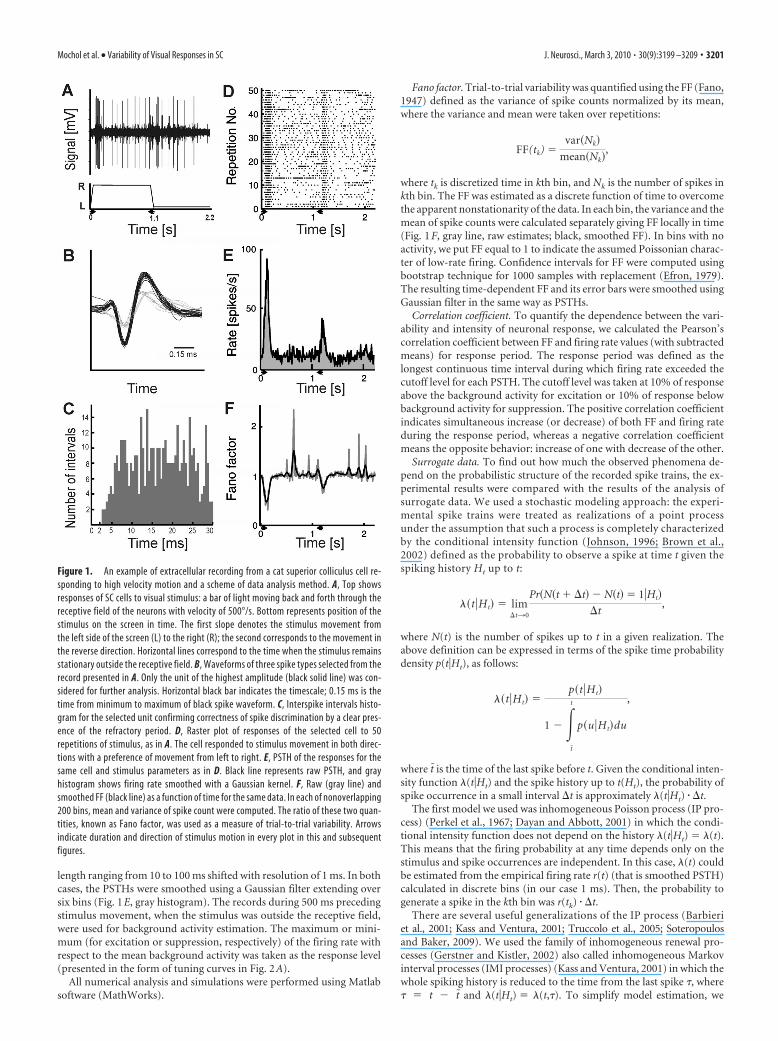
length ranging from 10 to 100 ms shifted with resolution of 1 ms. In bothcases, the PSTHs were smoothed using a Gaussian filter extending oversix bins (Fig. 1 E, gray histogram). The records during 500 ms precedingstimulus movement, when the stimulus was outside the receptive field,were used for background activity estimation. The maximum or mini-mum (for excitation or suppression, respectively) of the firing rate withrespect to the mean background activity was taken as the response level(presented in the form of tuning curves in Fig. 2 A).

All numerical analysis and simulations were performed using Matlabsoftware (MathWorks).

Fano factor. Trial-to-trial variability was quantified using the FF (Fano,1947) defined as the variance of spike counts normalized by its mean,where the variance and mean were taken over repetitions:

FF(tk) �var�Nk�

mean�Nk�,

where tk is discretized time in kth bin, and Nk is the number of spikes inkth bin. The FF was estimated as a discrete function of time to overcomethe apparent nonstationarity of the data. In each bin, the variance and themean of spike counts were calculated separately giving FF locally in time(Fig. 1 F, gray line, raw estimates; black, smoothed FF). In bins with noactivity, we put FF equal to 1 to indicate the assumed Poissonian charac-ter of low-rate firing. Confidence intervals for FF were computed usingbootstrap technique for 1000 samples with replacement (Efron, 1979).The resulting time-dependent FF and its error bars were smoothed usingGaussian filter in the same way as PSTHs.

Correlation coefficient. To quantify the dependence between the vari-ability and intensity of neuronal response, we calculated the Pearson’scorrelation coefficient between FF and firing rate values (with subtractedmeans) for response period. The response period was defined as thelongest continuous time interval during which firing rate exceeded thecutoff level for each PSTH. The cutoff level was taken at 10% of responseabove the background activity for excitation or 10% of response belowbackground activity for suppression. The positive correlation coefficientindicates simultaneous increase (or decrease) of both FF and firing rateduring the response period, whereas a negative correlation coefficientmeans the opposite behavior: increase of one with decrease of the other.

Surrogate data. To find out how much the observed phenomena de-pend on the probabilistic structure of the recorded spike trains, the ex-perimental results were compared with the results of the analysis ofsurrogate data. We used a stochastic modeling approach: the experi-mental spike trains were treated as realizations of a point processunder the assumption that such a process is completely characterizedby the conditional intensity function (Johnson, 1996; Brown et al.,2002) defined as the probability to observe a spike at time t given thespiking history Ht up to t:

��t�Ht� � lim�t30

Pr�N�t � �t� � N�t� � 1�Ht�

�t,

where N(t) is the number of spikes up to t in a given realization. Theabove definition can be expressed in terms of the spike time probabilitydensity p(t�Ht), as follows:

��t�Ht� �p�t�Ht�

1 � �t

t

p�u�Ht�du

,

where t is the time of the last spike before t. Given the conditional inten-sity function �(t�Ht) and the spike history up to t(Ht), the probability ofspike occurrence in a small interval �t is approximately �(t�Ht) � �t.

The first model we used was inhomogeneous Poisson process (IP pro-cess) (Perkel et al., 1967; Dayan and Abbott, 2001) in which the condi-tional intensity function does not depend on the history �(t�Ht) � �(t).This means that the firing probability at any time depends only on thestimulus and spike occurrences are independent. In this case, �(t) couldbe estimated from the empirical firing rate r(t) (that is smoothed PSTH)calculated in discrete bins (in our case 1 ms). Then, the probability togenerate a spike in the kth bin was r(tk) � �t.

There are several useful generalizations of the IP process (Barbieriet al., 2001; Kass and Ventura, 2001; Truccolo et al., 2005; Soteropoulosand Baker, 2009). We used the family of inhomogeneous renewal pro-cesses (Gerstner and Kistler, 2002) also called inhomogeneous Markovinterval processes (IMI processes) (Kass and Ventura, 2001) in which thewhole spiking history is reduced to the time from the last spike �, where� � t � t and �(t�Ht) � �(t,�). To simplify model estimation, we

Figure 1. An example of extracellular recording from a cat superior colliculus cell re-sponding to high velocity motion and a scheme of data analysis method. A, Top showsresponses of SC cells to visual stimulus: a bar of light moving back and forth through thereceptive field of the neurons with velocity of 500°/s. Bottom represents position of thestimulus on the screen in time. The first slope denotes the stimulus movement fromthe left side of the screen (L) to the right (R); the second corresponds to the movement inthe reverse direction. Horizontal lines correspond to the time when the stimulus remainsstationary outside the receptive field. B, Waveforms of three spike types selected from therecord presented in A. Only the unit of the highest amplitude (black solid line) was con-sidered for further analysis. Horizontal black bar indicates the timescale; 0.15 ms is thetime from minimum to maximum of black spike waveform. C, Interspike intervals histo-gram for the selected unit confirming correctness of spike discrimination by a clear pres-ence of the refractory period. D, Raster plot of responses of the selected cell to 50repetitions of stimulus, as in A. The cell responded to stimulus movement in both direc-tions with a preference of movement from left to right. E, PSTH of the responses for thesame cell and stimulus parameters as in D. Black line represents raw PSTH, and grayhistogram shows firing rate smoothed with a Gaussian kernel. F, Raw (gray line) andsmoothed FF (black line) as a function of time for the same data. In each of nonoverlapping200 bins, mean and variance of spike count were computed. The ratio of these two quan-tities, known as Fano factor, was used as a measure of trial-to-trial variability. Arrowsindicate duration and direction of stimulus motion in every plot in this and subsequentfigures.

Mochol et al. • Variability of Visual Responses in SC J. Neurosci., March 3, 2010 • 30(9):3199 –3209 • 3201

further assumed the multiplicative form of the conditional intensityfunction �(t�Ht) � �1(t) � �2(�).

In the multiplicative IMI process, the first component �1(t) describesthe time-dependent modulation of the spiking activity of the neuronreflecting its responsiveness to different stimuli (Berry and Meister, 1998;Brown et al., 2003; Schaette et al., 2005). The second component �2(�),which might be called “postimpulse probability” following Poggio andViernstein (1964), reflects the membrane properties of the neuron in-cluding its refractory periods.

We used two versions of the model in which �2(�) was obtainedthrough parametric (assuming gamma distribution) or nonparametric(kernel smoothing) fits to interspike interval distribution p(�) estimatedfrom the background activity. Under stationary condition, �1(t) is con-stant and can be set to unity. From p(�), the component �2(�) was com-puted as follows:

�2��� �p���

1 � �0

�

p�u�du

Given �2(�), we could calculate the modulatory factor �1(t). To do so, thetime of experiment was divided into bins of length �t short enough thatthere would be at most one spike per bin. Given N repetitions of stimulus,we estimated �1(tk) in kth bin as follows:

�1�tk� �N � rk

�j�1

N

�2��kj�

,

where rk was the rate in kth bin: rk �1

�t�

Nk

N; Nk was the number of

trials in which we observed a spike in the kth bin, and �kj was the interval

between current time and the time from the last spike in jth repetition.Details of the estimation technique have been presented previously(Wojcik et al., 2009).

Given conditional intensity function, surrogate data were generatedusing the thinning method (Dayan and Abbott, 2001; Press et al., 2007).Each set of surrogate data had the same structure (time duration and therepetition number) as the corresponding experimental dataset.

Goodness-of-fit between the proposed models and spike train dataseries was assessed on the basis of the time-rescaling theorem (Brown etal., 2002). If the assumed model is correct, then the experimental inter-

vals �k rescaled via conditional intensity function �k � �0

�k

��t,��d� are

independent exponential variables with the mean equal to unity. One canthen transform the rescaled intervals to uniform distribution throughz � 1 � exp��k� and use the Kolmogorov–Smirnov (K–S) test to quantifythe quality of estimation (Brown et al., 2002).

ResultsWe studied trial-to-trial response variability of neurons recordedfrom upper (retinorecipient) layers of SC (stratum zonale, stra-tum griseum superficiale, stratum opticum, and upper part ofstratum griseum intermediale). For each neuron, we recordedresponses to a visual stimulus moving at constant velocity in arange from 2 to 1000 o/s along a horizontal or vertical axis of thereceptive field. Responses of 35 neurons for which there was nodoubt that every spike was correctly sorted during offline dis-crimination (see Materials and Methods) were taken for analysis.The cells were recorded from the rostral half of the superior col-liculus, which contains binocular representation of the visualfield (Feldon and Kruger, 1970; Lane et al., 1974). All cells hadbinocular inputs. Assuming five classes of eye dominance, 54% ofcells (14 of 26 cells for which we could quantitatively determinerelative intensity of responses via both eyes) could be classified asbelonging to group 3 (equal magnitude of response recorded via

the contralateral and ipsilateral eye), 19% (5 of 26) showed con-tralateral eye dominance (group 2), and 27% (7 of 26) showedipsilateral eye dominance (group 4). Eye dominance of neuronsin our sample was similar to those recorded in previous studies(Bacon et al., 1998; Waleszczyk et al., 1999; Hashemi-Nezhad etal., 2003). In most cases, responses to stimulation of the dom-inant eye (usually contralateral) were analyzed, but for someneurons (n � 6), we also analyzed data obtained during stim-ulation of the other eye. No qualitative differences in the re-sponse properties of cells or results of later analysis ofvariability were observed between responses evoked via theipsilateral and contralateral eye.

On the basis of velocity tuning curves, cells were separatedinto four groups according to the criteria established in our pre-vious experiments (Waleszczyk et al., 1999). Thus, eight cells thatwere responsive only to slow stimulus movement (�200 o/s) con-stituted the low velocity excitatory (LVE) group, six neurons thatresponded exclusively to velocities above 10 o/s constituted thehigh velocity excitatory (HVE) group, and 13 cells that were ex-cited in a broad range of velocities constituted the LVE/HVEgroup. Finally, the activity of eight cells was increased at low andsuppressed at high velocity of stimulus movement (LVE/HVSgroup).

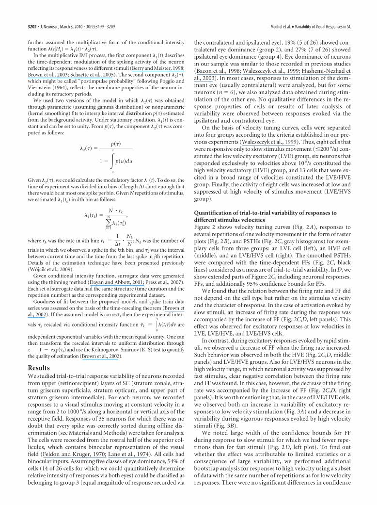
Quantification of trial-to-trial variability of responses todifferent stimulus velocitiesFigure 2 shows velocity tuning curves (Fig. 2A), responses toseveral repetitions of one velocity movement in the form of rasterplots (Fig. 2B), and PSTHs (Fig. 2C, gray histograms) for exem-plary cells from three groups: an LVE cell (left), an HVE cell(middle), and an LVE/HVS cell (right). The smoothed PSTHswere compared with the time-dependent FFs (Fig. 2C, blacklines) considered as a measure of trial-to-trial variability. In D, weshow extended parts of Figure 2C, including neuronal responses,FFs, and additionally 95% confidence bounds for FFs.

We found that the relation between the firing rate and FF didnot depend on the cell type but rather on the stimulus velocityand the character of response. In the case of activation evoked byslow stimuli, an increase of firing rate during the response wasaccompanied by the increase of FF (Fig. 2C,D, left panels). Thiseffect was observed for excitatory responses at low velocities inLVE, LVE/HVE, and LVE/HVS cells.

In contrast, during excitatory responses evoked by rapid stim-uli, we observed a decrease of FF when the firing rate increased.Such behavior was observed in both the HVE (Fig. 2C,D, middlepanels) and LVE/HVE groups. Also for LVE/HVS neurons in thehigh velocity range, in which neuronal activity was suppressed byfast stimulus, clear negative correlation between the firing rateand FF was found. In this case, however, the decrease of the firingrate was accompanied by the increase of FF (Fig. 2C,D, rightpanels). It is worth mentioning that, in the case of LVE/HVE cells,we observed both an increase in variability of excitatory re-sponses to low velocity stimulation (Fig. 3A) and a decrease invariability during vigorous responses evoked by high velocitystimuli (Fig. 3B).

We noted large width of the confidence bounds for FFduring response to slow stimuli for which we had fewer repe-titions than for fast stimuli (Fig. 2 D, left plot). To find outwhether the effect was attributable to limited statistics or aconsequence of large variability, we performed additionalbootstrap analysis for responses to high velocity using a subsetof data with the same number of repetitions as for low velocityresponses. There were no significant differences in confidence

3202 • J. Neurosci., March 3, 2010 • 30(9):3199 –3209 Mochol et al. • Variability of Visual Responses in SC

intervals calculated for the truncated and the original datasetof responses at high velocities. Thus, the broader range ofconfidence bounds for low velocity responses is a consequenceof the higher variability of data.

To quantify the observed effects, we calculated the Pearson’scorrelation coefficient between the FF and the firing rate duringthe response period (see Materials and Methods). Summary re-sults of dependence of the correlation between firing rate and FFon velocity for the whole set of experimental data are presented inFigure 4. For very slow stimuli, the correlation coefficients werefound to be almost exclusively positive (Fig. 4A, 2 and 5°/s).However, in a range of moderate velocities, we found both posi-tive and negative correlation coefficients with a negative trend forhigher velocities. For fast stimuli, most coefficients were negative.These observations are supported by the graph presented in Fig-

ure 4B, in which for each velocity themean correlation coefficient is shown.The crossover velocity for LVE/HVE orLVE/HVS cells (that is, a velocity at whichthe correlation coefficient changed sign)spans between 20 and 200°/s. For thewhole dataset, the mean correlation coef-ficients between rate and FF were positiveat low velocities of stimulus movement,up to 20°/s, and negative for velocitiesabove 50°/s.

Other factors potentially affectingcalculated trial-to-trial variabilityTwo factors in the above analysis couldpotentially affect variability measure andthereby give rise to opposite behavior ofFF in the case of low and high velocityresponses. One is the different bin sizeused for FF estimation (Teich et al., 1997).To test the putative influence of bin sizeon FF, we performed the whole analysisusing a fixed number of bins for every re-sponse (200) or using fixed size slidingwindows shifted with 1 ms resolution re-gardless of stimulus duration and velocity(see Materials and Methods) for the wholeset of collected responses. Regardless ofthe window size (10, 25, 50, or 100 ms), weobserved a monotonous decrease of thefiring rate � FF correlation coefficientwith increasing velocity (Fig. 5), similar tothe fixed-number-of-bins analysis.

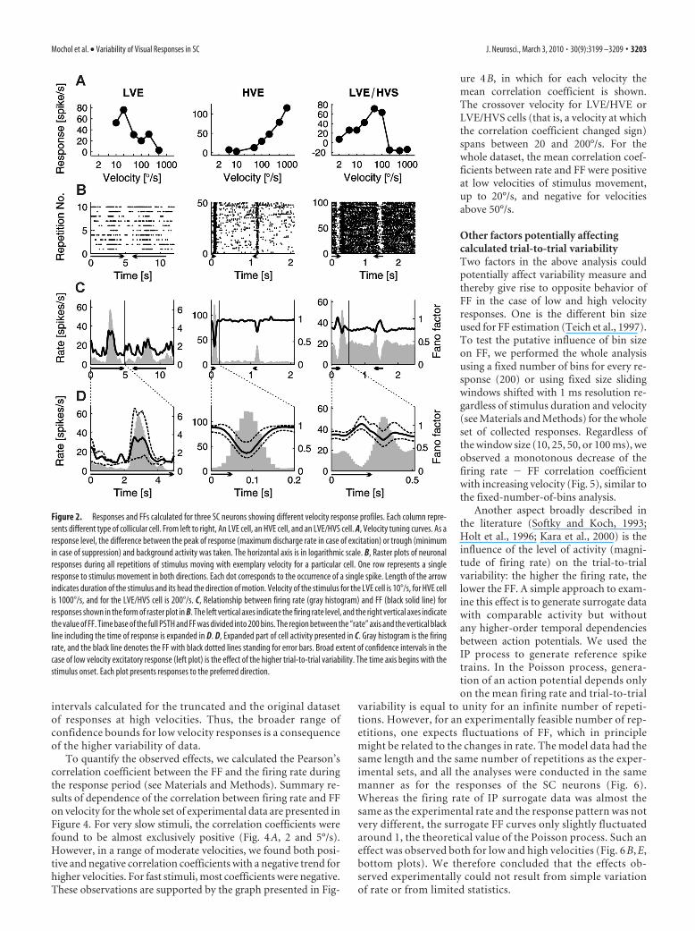
Another aspect broadly described inthe literature (Softky and Koch, 1993;Holt et al., 1996; Kara et al., 2000) is theinfluence of the level of activity (magni-tude of firing rate) on the trial-to-trialvariability: the higher the firing rate, thelower the FF. A simple approach to exam-ine this effect is to generate surrogate datawith comparable activity but withoutany higher-order temporal dependenciesbetween action potentials. We used theIP process to generate reference spiketrains. In the Poisson process, genera-tion of an action potential depends onlyon the mean firing rate and trial-to-trial

variability is equal to unity for an infinite number of repeti-tions. However, for an experimentally feasible number of rep-etitions, one expects fluctuations of FF, which in principlemight be related to the changes in rate. The model data had thesame length and the same number of repetitions as the exper-imental sets, and all the analyses were conducted in the samemanner as for the responses of the SC neurons (Fig. 6).Whereas the firing rate of IP surrogate data was almost thesame as the experimental rate and the response pattern was notvery different, the surrogate FF curves only slightly fluctuatedaround 1, the theoretical value of the Poisson process. Such aneffect was observed both for low and high velocities (Fig. 6 B, E,bottom plots). We therefore concluded that the effects ob-served experimentally could not result from simple variationof rate or from limited statistics.

Figure 2. Responses and FFs calculated for three SC neurons showing different velocity response profiles. Each column repre-sents different type of collicular cell. From left to right, An LVE cell, an HVE cell, and an LVE/HVS cell. A, Velocity tuning curves. As aresponse level, the difference between the peak of response (maximum discharge rate in case of excitation) or trough (minimumin case of suppression) and background activity was taken. The horizontal axis is in logarithmic scale. B, Raster plots of neuronalresponses during all repetitions of stimulus moving with exemplary velocity for a particular cell. One row represents a singleresponse to stimulus movement in both directions. Each dot corresponds to the occurrence of a single spike. Length of the arrowindicates duration of the stimulus and its head the direction of motion. Velocity of the stimulus for the LVE cell is 10°/s, for HVE cellis 1000°/s, and for the LVE/HVS cell is 200°/s. C, Relationship between firing rate (gray histogram) and FF (black solid line) forresponses shown in the form of raster plot in B. The left vertical axes indicate the firing rate level, and the right vertical axes indicatethe value of FF. Time base of the full PSTH and FF was divided into 200 bins. The region between the “rate” axis and the vertical blackline including the time of response is expanded in D. D, Expanded part of cell activity presented in C. Gray histogram is the firingrate, and the black line denotes the FF with black dotted lines standing for error bars. Broad extent of confidence intervals in thecase of low velocity excitatory response (left plot) is the effect of the higher trial-to-trial variability. The time axis begins with thestimulus onset. Each plot presents responses to the preferred direction.

Mochol et al. • Variability of Visual Responses in SC J. Neurosci., March 3, 2010 • 30(9):3199 –3209 • 3203

Inclusion of spiking history in simulations of neural spikingactivity in different groups of collicular cellsTo better understand stochastic properties of the experimentalresults, we went one step further in modeling the data and incor-porated first-order temporal dependencies between action po-tentials. Using the IMI model (Berry and Meister, 1998; Kass andVentura, 2001), in which the probability of generating a spike wasa product of two terms, stimulus-dependent and spike-historycomponents, we generated a second family of surrogate data (seeMaterials and Methods). As for the IP model, the resulting PSTHsfor IMI processes were very similar to experimental ones for bothlow and high stimulus velocities (Fig. 6, compare A, D with C, F,

bottom plots). The IMI model reproduced well the observeddependency of the FF and firing rates in the case of high ve-locity responses (Fig. 6 F, bottom plot) but did not mimic theexperimental results for low velocity responses (Fig. 6C,bottom plot).

Goodness-of-fit between the proposed model and the exper-imental data was assessed on the basis of time-rescaling theoremand Kolmogorov–Smirnov statistics (Brown et al., 2002; Truccolo etal., 2005; Czanner et al., 2008). For a good model of the data,experimental interspike intervals, rescaled and transformedusing the model conditional intensity, should be uniformly dis-tributed random variables on the interval [0,1]. Histograms ofrescaled times and the K–S plots for different models of exem-plary responses are presented in Figure 7. A and C show histo-grams of rescaled interspike intervals obtained for conditionalintensity functions estimated with the IP model or IMI models(parametric gamma and nonparametric) for low and high veloc-ity examples, respectively. For high velocity data, the most uni-form distribution of the rescaled interspike intervals is obtainedfor the nonparametric IMI model. In the case of the low velocityexample, however, neither model leads to a uniform distributionof the rescaled interspike intervals.

Similarly, the curves in the K–S plots (Fig. 7B,D) were ob-tained by appropriate rescaling of interspike intervals using con-ditional intensity functions estimated with either the IP model(gray curve) or IMI models (nonparametric, thick solid line;parametric gamma, dash– dotted line). Diagonal (thin solid line)corresponds to the perfect model of data for which rescaled in-terspike intervals are uniformly distributed. The distance fromthe diagonal can be used as a measure of the quality of the model.All models describe data obtained for high velocity responses(Fig. 7D) much better than those for low velocities (Fig. 7B). Inthe low velocity example (Fig. 7B), performance of the IP andparametric IMI models is worst in the range of medium intervals.The nonparametric IMI model seems most adequate except atshort intervals. All three models seem to account reasonably wellonly for the longest interspike intervals because all the K–S curvesin this range lie within the 95% confidence bounds (Fig. 7B,D,two parallel thin dashed lines). For the high velocity example, theIP model provides the worst description of the data. The IMImodels give a much better description, with K–S curve for thenonparametric IMI model lying entirely within the 95% confi-dence bounds.

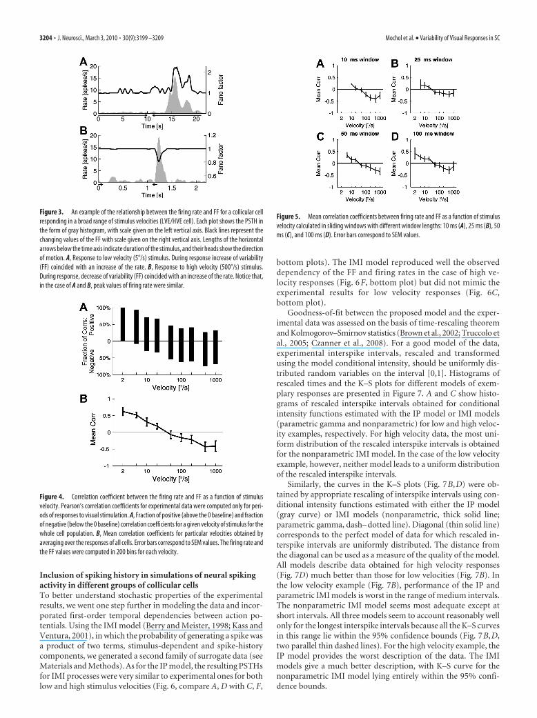
Figure 3. An example of the relationship between the firing rate and FF for a collicular cellresponding in a broad range of stimulus velocities (LVE/HVE cell). Each plot shows the PSTH inthe form of gray histogram, with scale given on the left vertical axis. Black lines represent thechanging values of the FF with scale given on the right vertical axis. Lengths of the horizontalarrows below the time axis indicate duration of the stimulus, and their heads show the directionof motion. A, Response to low velocity (5°/s) stimulus. During response increase of variability(FF) coincided with an increase of the rate. B, Response to high velocity (500°/s) stimulus.During response, decrease of variability (FF) coincided with an increase of the rate. Notice that,in the case of A and B, peak values of firing rate were similar.

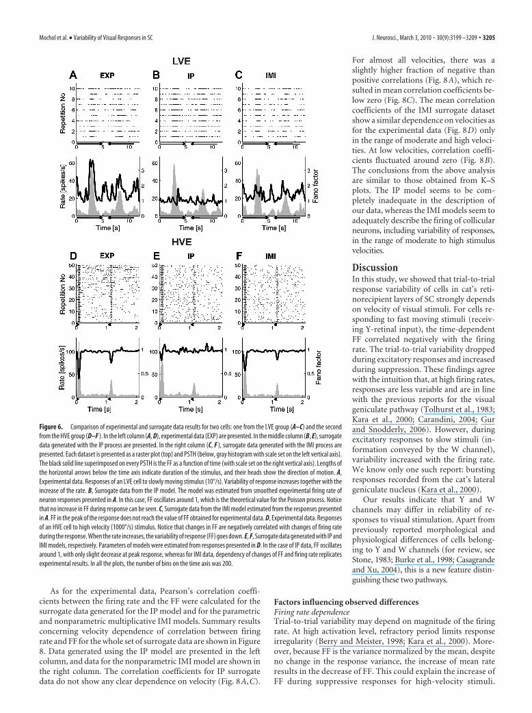
Figure 4. Correlation coefficient between the firing rate and FF as a function of stimulusvelocity. Pearson’s correlation coefficients for experimental data were computed only for peri-ods of responses to visual stimulation. A, Fraction of positive (above the 0 baseline) and fractionof negative (below the 0 baseline) correlation coefficients for a given velocity of stimulus for thewhole cell population. B, Mean correlation coefficients for particular velocities obtained byaveraging over the responses of all cells. Error bars correspond to SEM values. The firing rate andthe FF values were computed in 200 bins for each velocity.

Figure 5. Mean correlation coefficients between firing rate and FF as a function of stimulusvelocity calculated in sliding windows with different window lengths: 10 ms (A), 25 ms (B), 50ms (C), and 100 ms (D). Error bars correspond to SEM values.

3204 • J. Neurosci., March 3, 2010 • 30(9):3199 –3209 Mochol et al. • Variability of Visual Responses in SC

As for the experimental data, Pearson’s correlation coeffi-cients between the firing rate and the FF were calculated for thesurrogate data generated for the IP model and for the parametricand nonparametric multiplicative IMI models. Summary resultsconcerning velocity dependence of correlation between firingrate and FF for the whole set of surrogate data are shown in Figure8. Data generated using the IP model are presented in the leftcolumn, and data for the nonparametric IMI model are shown inthe right column. The correlation coefficients for IP surrogatedata do not show any clear dependence on velocity (Fig. 8A,C).

For almost all velocities, there was aslightly higher fraction of negative thanpositive correlations (Fig. 8A), which re-sulted in mean correlation coefficients be-low zero (Fig. 8C). The mean correlationcoefficients of the IMI surrogate datasetshow a similar dependence on velocities asfor the experimental data (Fig. 8D) onlyin the range of moderate and high veloci-ties. At low velocities, correlation coeffi-cients fluctuated around zero (Fig. 8B).The conclusions from the above analysisare similar to those obtained from K–Splots. The IP model seems to be com-pletely inadequate in the description ofour data, whereas the IMI models seem toadequately describe the firing of collicularneurons, including variability of responses,in the range of moderate to high stimulusvelocities.

DiscussionIn this study, we showed that trial-to-trialresponse variability of cells in cat’s reti-norecipient layers of SC strongly dependson velocity of visual stimuli. For cells re-sponding to fast moving stimuli (receiv-ing Y-retinal input), the time-dependentFF correlated negatively with the firingrate. The trial-to-trial variability droppedduring excitatory responses and increasedduring suppression. These findings agreewith the intuition that, at high firing rates,responses are less variable and are in linewith the previous reports for the visualgeniculate pathway (Tolhurst et al., 1983;Kara et al., 2000; Carandini, 2004; Gurand Snodderly, 2006). However, duringexcitatory responses to slow stimuli (in-formation conveyed by the W channel),variability increased with the firing rate.We know only one such report: burstingresponses recorded from the cat’s lateralgeniculate nucleus (Kara et al., 2000).

Our results indicate that Y and Wchannels may differ in reliability of re-sponses to visual stimulation. Apart frompreviously reported morphological andphysiological differences of cells belong-ing to Y and W channels (for review, seeStone, 1983; Burke et al., 1998; Casagrandeand Xu, 2004), this is a new feature distin-guishing these two pathways.

Factors influencing observed differencesFiring rate dependenceTrial-to-trial variability may depend on magnitude of the firingrate. At high activation level, refractory period limits responseirregularity (Berry and Meister, 1998; Kara et al., 2000). More-over, because FF is the variance normalized by the mean, despiteno change in the response variance, the increase of mean rateresults in the decrease of FF. This could explain the increase ofFF during suppressive responses for high-velocity stimuli.

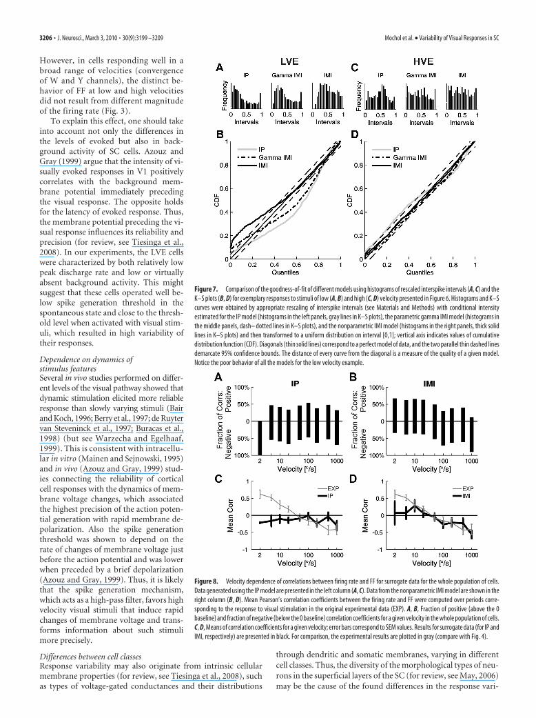
Figure 6. Comparison of experimental and surrogate data results for two cells: one from the LVE group (A–C) and the secondfrom the HVE group (D–F ). In the left column (A, D), experimental data (EXP) are presented. In the middle column (B, E), surrogatedata generated with the IP process are presented. In the right column (C, F ), surrogate data generated with the IMI process arepresented. Each dataset is presented as a raster plot (top) and PSTH (below, gray histogram with scale set on the left vertical axis).The black solid line superimposed on every PSTH is the FF as a function of time (with scale set on the right vertical axis). Lengths ofthe horizontal arrows below the time axis indicate duration of the stimulus, and their heads show the direction of motion. A,Experimental data. Responses of an LVE cell to slowly moving stimulus (10°/s). Variability of response increases together with theincrease of the rate. B, Surrogate data from the IP model. The model was estimated from smoothed experimental firing rate ofneuron responses presented in A. In this case, FF oscillates around 1, which is the theoretical value for the Poisson process. Noticethat no increase in FF during response can be seen. C, Surrogate data from the IMI model estimated from the responses presentedin A. FF in the peak of the response does not reach the value of FF obtained for experimental data. D, Experimental data. Responsesof an HVE cell to high velocity (1000°/s) stimulus. Notice that changes in FF are negatively correlated with changes of firing rateduring the response. When the rate increases, the variability of response (FF) goes down. E, F, Surrogate data generated with IP andIMI models, respectively. Parameters of models were estimated from responses presented in D. In the case of IP data, FF oscillatesaround 1, with only slight decrease at peak response, whereas for IMI data, dependency of changes of FF and firing rate replicatesexperimental results. In all the plots, the number of bins on the time axis was 200.

Mochol et al. • Variability of Visual Responses in SC J. Neurosci., March 3, 2010 • 30(9):3199 –3209 • 3205

However, in cells responding well in abroad range of velocities (convergenceof W and Y channels), the distinct be-havior of FF at low and high velocitiesdid not result from different magnitudeof the firing rate (Fig. 3).

To explain this effect, one should takeinto account not only the differences inthe levels of evoked but also in back-ground activity of SC cells. Azouz andGray (1999) argue that the intensity of vi-sually evoked responses in V1 positivelycorrelates with the background mem-brane potential immediately precedingthe visual response. The opposite holdsfor the latency of evoked response. Thus,the membrane potential preceding the vi-sual response influences its reliability andprecision (for review, see Tiesinga et al.,2008). In our experiments, the LVE cellswere characterized by both relatively lowpeak discharge rate and low or virtuallyabsent background activity. This mightsuggest that these cells operated well be-low spike generation threshold in thespontaneous state and close to the thresh-old level when activated with visual stim-uli, which resulted in high variability oftheir responses.

Dependence on dynamics ofstimulus featuresSeveral in vivo studies performed on differ-ent levels of the visual pathway showed thatdynamic stimulation elicited more reliableresponse than slowly varying stimuli (Bairand Koch, 1996; Berry et al., 1997; de Ruytervan Steveninck et al., 1997; Buracas et al.,1998) (but see Warzecha and Egelhaaf,1999). This is consistent with intracellu-lar in vitro (Mainen and Sejnowski, 1995)and in vivo (Azouz and Gray, 1999) stud-ies connecting the reliability of corticalcell responses with the dynamics of mem-brane voltage changes, which associatedthe highest precision of the action poten-tial generation with rapid membrane de-polarization. Also the spike generationthreshold was shown to depend on therate of changes of membrane voltage justbefore the action potential and was lowerwhen preceded by a brief depolarization(Azouz and Gray, 1999). Thus, it is likelythat the spike generation mechanism,which acts as a high-pass filter, favors highvelocity visual stimuli that induce rapidchanges of membrane voltage and trans-forms information about such stimulimore precisely.

Differences between cell classesResponse variability may also originate from intrinsic cellularmembrane properties (for review, see Tiesinga et al., 2008), suchas types of voltage-gated conductances and their distributions

through dendritic and somatic membranes, varying in differentcell classes. Thus, the diversity of the morphological types of neu-rons in the superficial layers of the SC (for review, see May, 2006)may be the cause of the found differences in the response vari-

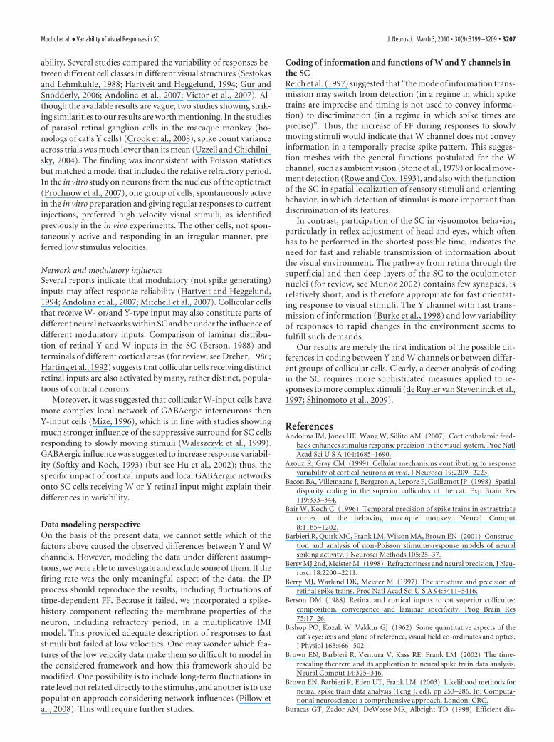
Figure 7. Comparison of the goodness-of-fit of different models using histograms of rescaled interspike intervals (A, C) and theK–S plots (B, D) for exemplary responses to stimuli of low (A, B) and high (C, D) velocity presented in Figure 6. Histograms and K–Scurves were obtained by appropriate rescaling of interspike intervals (see Materials and Methods) with conditional intensityestimated for the IP model (histograms in the left panels, gray lines in K–S plots), the parametric gamma IMI model (histograms inthe middle panels, dash– dotted lines in K–S plots), and the nonparametric IMI model (histograms in the right panels, thick solidlines in K–S plots) and then transformed to a uniform distribution on interval [0,1]; vertical axis indicates values of cumulativedistribution function (CDF). Diagonals (thin solid lines) correspond to a perfect model of data, and the two parallel thin dashed linesdemarcate 95% confidence bounds. The distance of every curve from the diagonal is a measure of the quality of a given model.Notice the poor behavior of all the models for the low velocity example.

Figure 8. Velocity dependence of correlations between firing rate and FF for surrogate data for the whole population of cells.Data generated using the IP model are presented in the left column (A, C). Data from the nonparametric IMI model are shown in theright column (B, D). Mean Pearson’s correlation coefficients between the firing rate and FF were computed over periods corre-sponding to the response to visual stimulation in the original experimental data (EXP). A, B, Fraction of positive (above the 0baseline) and fraction of negative (below the 0 baseline) correlation coefficients for a given velocity in the whole population of cells.C, D, Means of correlation coefficients for a given velocity; error bars correspond to SEM values. Results for surrogate data (for IP andIMI, respectively) are presented in black. For comparison, the experimental results are plotted in gray (compare with Fig. 4).

3206 • J. Neurosci., March 3, 2010 • 30(9):3199 –3209 Mochol et al. • Variability of Visual Responses in SC

ability. Several studies compared the variability of responses be-tween different cell classes in different visual structures (Sestokasand Lehmkuhle, 1988; Hartveit and Heggelund, 1994; Gur andSnodderly, 2006; Andolina et al., 2007; Victor et al., 2007). Al-though the available results are vague, two studies showing strik-ing similarities to our results are worth mentioning. In the studiesof parasol retinal ganglion cells in the macaque monkey (ho-mologs of cat’s Y cells) (Crook et al., 2008), spike count varianceacross trials was much lower than its mean (Uzzell and Chichilni-sky, 2004). The finding was inconsistent with Poisson statisticsbut matched a model that included the relative refractory period.In the in vitro study on neurons from the nucleus of the optic tract(Prochnow et al., 2007), one group of cells, spontaneously activein the in vitro preparation and giving regular responses to currentinjections, preferred high velocity visual stimuli, as identifiedpreviously in the in vivo experiments. The other cells, not spon-taneously active and responding in an irregular manner, pre-ferred low stimulus velocities.

Network and modulatory influenceSeveral reports indicate that modulatory (not spike generating)inputs may affect response reliability (Hartveit and Heggelund,1994; Andolina et al., 2007; Mitchell et al., 2007). Collicular cellsthat receive W- or/and Y-type input may also constitute parts ofdifferent neural networks within SC and be under the influence ofdifferent modulatory inputs. Comparison of laminar distribu-tion of retinal Y and W inputs in the SC (Berson, 1988) andterminals of different cortical areas (for review, see Dreher, 1986;Harting et al., 1992) suggests that collicular cells receiving distinctretinal inputs are also activated by many, rather distinct, popula-tions of cortical neurons.

Moreover, it was suggested that collicular W-input cells havemore complex local network of GABAergic interneurons thenY-input cells (Mize, 1996), which is in line with studies showingmuch stronger influence of the suppressive surround for SC cellsresponding to slowly moving stimuli (Waleszczyk et al., 1999).GABAergic influence was suggested to increase response variabil-ity (Softky and Koch, 1993) (but see Hu et al., 2002); thus, thespecific impact of cortical inputs and local GABAergic networksonto SC cells receiving W or Y retinal input might explain theirdifferences in variability.

Data modeling perspectiveOn the basis of the present data, we cannot settle which of thefactors above caused the observed differences between Y and Wchannels. However, modeling the data under different assump-tions, we were able to investigate and exclude some of them. If thefiring rate was the only meaningful aspect of the data, the IPprocess should reproduce the results, including fluctuations oftime-dependent FF. Because it failed, we incorporated a spike-history component reflecting the membrane properties of theneuron, including refractory period, in a multiplicative IMImodel. This provided adequate description of responses to faststimuli but failed at low velocities. One may wonder which fea-tures of the low velocity data make them so difficult to model inthe considered framework and how this framework should bemodified. One possibility is to include long-term fluctuations inrate level not related directly to the stimulus, and another is to usepopulation approach considering network influences (Pillow etal., 2008). This will require further studies.

Coding of information and functions of W and Y channels inthe SCReich et al. (1997) suggested that “the mode of information trans-mission may switch from detection (in a regime in which spiketrains are imprecise and timing is not used to convey informa-tion) to discrimination (in a regime in which spike times areprecise)”. Thus, the increase of FF during responses to slowlymoving stimuli would indicate that W channel does not conveyinformation in a temporally precise spike pattern. This sugges-tion meshes with the general functions postulated for the Wchannel, such as ambient vision (Stone et al., 1979) or local move-ment detection (Rowe and Cox, 1993), and also with the functionof the SC in spatial localization of sensory stimuli and orientingbehavior, in which detection of stimulus is more important thandiscrimination of its features.

In contrast, participation of the SC in visuomotor behavior,particularly in reflex adjustment of head and eyes, which oftenhas to be performed in the shortest possible time, indicates theneed for fast and reliable transmission of information aboutthe visual environment. The pathway from retina through thesuperficial and then deep layers of the SC to the oculomotornuclei (for review, see Munoz 2002) contains few synapses, isrelatively short, and is therefore appropriate for fast orientat-ing response to visual stimuli. The Y channel with fast trans-mission of information (Burke et al., 1998) and low variabilityof responses to rapid changes in the environment seems tofulfill such demands.

Our results are merely the first indication of the possible dif-ferences in coding between Y and W channels or between differ-ent groups of collicular cells. Clearly, a deeper analysis of codingin the SC requires more sophisticated measures applied to re-sponses to more complex stimuli (de Ruyter van Steveninck et al.,1997; Shinomoto et al., 2009).

ReferencesAndolina IM, Jones HE, Wang W, Sillito AM (2007) Corticothalamic feed-

back enhances stimulus response precision in the visual system. Proc NatlAcad Sci U S A 104:1685–1690.

Azouz R, Gray CM (1999) Cellular mechanisms contributing to responsevariability of cortical neurons in vivo. J Neurosci 19:2209 –2223.

Bacon BA, Villemagne J, Bergeron A, Lepore F, Guillemot JP (1998) Spatialdisparity coding in the superior colliculus of the cat. Exp Brain Res119:333–344.

Bair W, Koch C (1996) Temporal precision of spike trains in extrastriatecortex of the behaving macaque monkey. Neural Comput8:1185–1202.

Barbieri R, Quirk MC, Frank LM, Wilson MA, Brown EN (2001) Construc-tion and analysis of non-Poisson stimulus-response models of neuralspiking activity. J Neurosci Methods 105:25–37.

Berry MJ 2nd, Meister M (1998) Refractoriness and neural precision. J Neu-rosci 18:2200 –2211.

Berry MJ, Warland DK, Meister M (1997) The structure and precision ofretinal spike trains. Proc Natl Acad Sci U S A 94:5411–5416.

Berson DM (1988) Retinal and cortical inputs to cat superior colliculus:composition, convergence and laminar specificity. Prog Brain Res75:17–26.

Bishop PO, Kozak W, Vakkur GJ (1962) Some quantitative aspects of thecat’s eye: axis and plane of reference, visual field co-ordinates and optics.J Physiol 163:466 –502.

Brown EN, Barbieri R, Ventura V, Kass RE, Frank LM (2002) The time-rescaling theorem and its application to neural spike train data analysis.Neural Comput 14:325–346.

Brown EN, Barbieri R, Eden UT, Frank LM (2003) Likelihood methods forneural spike train data analysis (Feng J, ed), pp 253–286. In: Computa-tional neuroscience: a comprehensive approach. London: CRC.

Buracas GT, Zador AM, DeWeese MR, Albright TD (1998) Efficient dis-

Mochol et al. • Variability of Visual Responses in SC J. Neurosci., March 3, 2010 • 30(9):3199 –3209 • 3207

crimination of temporal patterns by motion-sensitive neurons in primatevisual cortex. Neuron 20:959 –969.

Burke W, Dreher B, Wang C (1998) Selective block of conduction in Y opticnerve fibres: significance for the concept of parallel processing. Eur J Neu-rosci 10:8 –19.

Carandini M (2004) Amplification of trial-to-trial response variability byneurons in visual cortex. PLoS Biol 2:E264.

Casagrande V, Xu X (2004) Parallel visual pathways: a comparative perspec-tive. In: The visual neuroscience (Chalupa L, Werner JS, eds), pp 494 –506. Cambridge, MA: Massachusetts Institute of Technology.

Chelvanayagam DK, Vidyasagar TR (2006) Irregularity in neocortical spiketrains: influence of measurement factors and another method of estima-tion. J Neurosci Methods 157:264 –273.

Crook JD, Peterson BB, Packer OS, Robinson FR, Troy JB, Dacey DM (2008)Y cell receptive field and collicular projection of parasol ganglion cells inmacaque monkey retina. J Neurosci 28:11277–11291.

Czanner G, Eden UT, Wirth S, Yanike M, Suzuki WA, Brown EN (2008)Analysis of between-trial and within-trial neural spiking dynamics. J Neu-rophysiol 99:2672–2693.

Dayan P, Abbott LF (2001) Theoretical neuroscience. Computational andmathematical modeling of neural systems. Cambridge, MA: Massachu-setts Institute of Technology.

de Ruyter van Steveninck RR, Lewen GD, Strong SP, Koberle R, Bialek W(1997) Reproducibility and variability in neural spike trains. Science275:1805–1808.

Distler C, Hoffmann KP (1991) Depth perception and cortical physiology innormal and innate microstrabismic cats. Vis Neurosci 6:25– 41.

Dreher B (1986) Thalamocortical and corticocortical interconnections inthe cat visual system. Relation to mechanisms of information processing.In: Visual neuroscience (Pettigrew JD, Sanderson KJ, Levick WR, eds), pp290 –314. Cambridge, UK: Cambridge UP.

Efron B (1979) Bootstrap methods: another look at the jackknife. AnnStatist 7:1–26.

Faisal AA, Selen LP, Wolpert DM (2008) Noise in the nervous system. NatRev Neurosci 9:292–303.

Fano U (1947) Ionization yield of rations. II. The fluctuations of the numberof ions. Phys Rev 72:26 –29.

Feldon P, Kruger L (1970) Topography of the retinal projection upon thesuperior colliculus of the cat. Vision Res 10:135–143.

Field GD, Chichilnisky EJ (2007) Information processing in the primateretina: circuitry and coding. Annu Rev Neurosci 30:1–30.

Gabbiani F, Koch C (1998) Principles of spike train analysis. In: Methods inneuronal modeling (Segev I, Koch C, eds), pp 313–360. Cambridge, MA:Massachusetts Institute of Technology.

Gerstner W, Kistler WM (2002) Spiking neuron models. Cambridge, UK:Cambridge UP.

Gur M, Snodderly DM (2006) High response reliability of neurons in pri-mary visual cortex (V1) of alert, trained monkeys. Cereb Cortex16:888 – 895.

Harting JK, Updyke BV, Van Lieshout DP (1992) Corticotectal projectionsin the cat: anterograde transport studies of twenty-five cortical areas.J Comp Neurol 324:379 – 414.

Hartveit E, Heggelund P (1994) Response variability of single cells in thedorsal lateral geniculate nucleus of the cat. Comparison with retinalinput and effect of brain stem stimulation. J Neurophysiol72:1278 –1289.

Hashemi-Nezhad M, Wang C, Burke W, Dreher B (2003) Area 21a of catvisual cortex strongly modulates neuronal activities in the superior col-liculus. J Physiol 550:535–552.

Hoffmann KP (1973) Conduction velocity in pathways from retina to supe-rior colliculus in the cat: a correlation with receptive-field properties.J Neurophysiol 36:409 – 424.

Holt GR, Softky WR, Koch C, Douglas RJ (1996) Comparison of dischargevariability in vitro and in vivo in cat visual cortex neurons. J Neurophysiol75:1806 –1814.

Hu D, Chelvanayagam DK, Vidyasagar TR (2002) Irregularity in corticalfiring in vivo cannot be explained by inhibition. Proc Aust Neurosci Soc13:219.

Johnson DH (1996) Point process models of single-neuron discharges.J Comput Neurosci 3:275–299.

Kara P, Reinagel P, Reid RC (2000) Low response variability in simulta-

neously recorded retinal, thalamic, and cortical neurons. Neuron27:635– 646.

Kass RE, Ventura V (2001) A spike-train probability model. Neural Comput13:1713–1720.

Lane RH, Kaas JH, Allman JM (1974) Visuotopic organization of the supe-rior colliculus in normal and Siamese cats. Brain Res 70:413– 430.

Lestienne R (2001) Spike timing, synchronization and information process-ing on the sensory side of the central nervous system. Prog Neurobiol65:545–591.

Mainen ZF, Sejnowski TJ (1995) Reliability of spike timing in neocorticalneurons. Science 268:1503–1506.

May PJ (2006) The mammalian superior colliculus: laminar structure andconnections. Prog Brain Res 151:321–378.

Mitchell JF, Sundberg KA, Reynolds JH (2007) Differential attention-dependent response modulation across cell classes in macaque visual areaV4. Neuron 55:131–141.

Mize RR (1996) Neurochemical microcircuitry underlying visual andoculomotor function in the cat superior colliculus. Prog Brain Res112:35–55.

Mochol G, Wojcik DK, Wypych M, Wrobel A, Waleszczyk WJ (2008a)Models of inhomogeneous point processing and information coding inthe visual system (in Polish). Medycyna Dydaktyka Wychowanie Rok XL2008 [Suplement 1]:103–107.

Mochol G, Wojcik DK, Wypych M, Wrobel A, Waleszczyk WJ (2008b) Dif-ferent cell populations in the superior colliculus use different codingschemes. Paper presented at AREADNE Research in Encoding and De-coding of Neural Ensembles Conference, Fira, Greece, June.

Munoz DP (2002) Commentary: saccadic eye movements: overview of neu-ral circuitry. Prog Brain Res 140:89 –96.

Paninski L, Pillow J, Lewi J (2007) Statistical models for neural encoding,decoding, and optimal stimulus design. Prog Brain Res 165:493–507.

Perkel DH, Gerstein GL, Moore GP (1967) Neuronal spike trains and sto-chastic point processes. I. The single spike train. Biophys J 7:391– 418.

Pettigrew JD, Cooper ML, Blasdel GG (1979) Improved use of tapetalreflection for eye-position monitoring. Invest Ophthalmol Vis Sci18:490 – 495.

Pillow JW, Shlens J, Paninski L, Sher A, Litke AM, Chichilnisky EJ, SimoncelliEP (2008) Spatio-temporal correlations and visual signalling in a com-plete neuronal population. Nature 454:995–999.

Poggio GF, Viernstein LJ (1964) Time series analysis of impulse sequencesof thalamic somatic sensory neurons. J Neurophysiol 27:517–545.

Press WH, Teukolsky SA, Vetterling WT, Flannery BP (2007) Numericalrecipes. Cambridge, UK: Cambridge UP.

Prochnow N, Lee P, Hall WC, Schmidt M (2007) In vitro properties ofneurons in the rat pretectal nucleus of the optic tract. J Neurophysiol97:3574 –3584.

Reich DS, Victor JD, Knight BW, Ozaki T, Kaplan E (1997) Response vari-ability and timing precision of neuronal spike trains in vivo. J Neuro-physiol 77:2836 –2841.

Rowe MH, Cox JF (1993) Spatial receptive-field structure of cat retinal Wcells. Vis Neurosci 10:765–779.

Schaette R, Gollisch T, Herz AVM (2005) Spike-train variability of auditoryneurons in vivo: dynamic responses follow predictions from constantstimuli. J Neurophysiol 93:3270 –3281.

Sestokas AK, Lehmkuhle S (1988) Response variability of X- and Y-cells inthe dorsal lateral geniculate nucleus of the cat. J Neurophysiol59:317–325.

Shinomoto S, Kim H, Shimokawa T, Matsuno N, Funahashi S, Shima K,Fujita I, Tamura H, Doi T, Kawano K, Inaba N, Fukushima K, Kurkin S,Kurata K, Taira M, Tsutsui K, Komatsu H, Ogawa T, Koida K, Tanji J,Toyama K (2009) Relating neuronal firing patterns to functional differ-entiation of cerebral cortex. PLoS Comput Biol 5:e1000433.

Softky WR, Koch C (1993) The highly irregular firing of cortical cells isinconsistent with temporal integration of random EPSPs. J Neurosci13:334 –350.

Soteropoulos DS, Baker SN (2009) Quantifying neural coding of event tim-ing. J Neurophysiol 101:402– 417.

Stone J (1983) Parallel processing in the visual system. Plenum, New YorkStone J, Dreher B, Leventhal A (1979) Hierarchical and parallel mechanisms

in the organization of visual cortex. Brain Res 180:345–394.

3208 • J. Neurosci., March 3, 2010 • 30(9):3199 –3209 Mochol et al. • Variability of Visual Responses in SC

Teich MC, Heneghan C, Lowen SB, Ozaki T, Kaplan E (1997) Fractal char-acter of the neural spike train in the visual system of the cat. J Opt Soc AmA Opt Image Sci Vis 14:529 –546.

Tiesinga P, Fellous JM, Sejnowski TJ (2008) Regulation of spike timing invisual cortical circuits. Nat Rev Neurosci 9:97–107.

Tolhurst DJ, Movshon JA, Dean AF (1983) The statistical reliability of sig-nals in single neurons in cat and monkey visual cortex. Vision Res23:775–785.

Truccolo W, Eden UT, Fellows MR, Donoghue JP, Brown EN (2005) Apoint process framework for relating neural spiking activity to spikinghistory, neural ensemble, and extrinsic covariate effects. J Neurophysiol93:1074 –1089.

Uzzell VJ, Chichilnisky EJ (2004) Precision of spike trains in primate retinalganglion cells. J Neurophysiol 92:780 –789.

Victor JD, Blessing EM, Forte JD, Buzas P, Martin PR (2007) Response vari-ability of marmoset parvocellular neurons. J Physiol 579:29 –51.

Waleszczyk WJ, Wang C, Burke W, Dreher B (1999) Velocity response pro-

files of collicular neurons: parallel and convergent visual informationchannels. Neuroscience 93:1063–1076.

Waleszczyk WJ, Wang C, Benedek G, Burke W, Dreher B (2004) Motionsensitivity in cat’s superior colliculus: contribution of different visual pro-cessing channels to response properties of collicular neurons. Acta Neu-robiol Exp (Wars) 64:209 –228.

Waleszczyk WJ, Nagy A, Wypych M, Berenyi A, Paroczy Z, Eordegh G, Ghaz-aryan A, Benedek G (2007) Spectral receptive field properties of neuronsin the feline superior colliculus. Exp Brain Res 181:87–98.

Wang C, Waleszczyk WJ, Benedek G, Burke W, Dreher B (2001) Conver-gence of Y and non-Y channels onto single neurons in the superior col-liculi of the cat. Neuroreport 12:2927–2933.

Warzecha AK, Egelhaaf M (1999) Variability in spike trains during constantand dynamic stimulation. Science 283:1927–1930.

Wojcik DK, Mochol G, Jakuczun W, Wypych M, Waleszczyk WJ (2009)Direct estimation of inhomogeneous Markov interval models of spiketrains. Neural Comput 21:2105–2113.

Mochol et al. • Variability of Visual Responses in SC J. Neurosci., March 3, 2010 • 30(9):3199 –3209 • 3209