Variability Analyses of Alfalfa-Reference to Grass-Reference Evapotranspiration Ratios in Growing and Dormant Seasons

Biological Systems Engineering

Biological Systems Engineering: Papers and

Publications

University of Nebraska - Lincoln Year

Variability Analyses of Alfalfa-Reference

to Grass-Reference Evapotranspiration

Ratios in Growing and Dormant Seasons

S. Irmak∗ A. Irmak† T. A. Howell‡

D. L. Martin∗∗ J. O. Payero†† K. S. Copeland‡‡

∗University of Nebraska-Lincoln, [email protected]†University of Nebraska-Lincoln, [email protected]‡USDA-ARS Conservation and Production Research Laboratory∗∗University of Nebraska-Lincoln, [email protected]††Dept. of Primary Industries and Fisheries‡‡USDA-ARS Conservation and Production Research Laboratory

This paper is posted at DigitalCommons@University of Nebraska - Lincoln.

http://digitalcommons.unl.edu/biosysengfacpub/82

Variability Analyses of Alfalfa-Reference to Grass-ReferenceEvapotranspiration Ratios in Growing and Dormant Seasons

S. Irmak, M.ASCE1; A. Irmak, M.ASCE2; T. A. Howell, M.ASCE3; D. L. Martin, M.ASCE4;J. O. Payero, M.ASCE5; and K. S. Copeland6

Abstract: Alfalfa-reference evapotranspiration �ETr� values sometimes need to be converted to grass-reference ET �ETo�, or vice versa,to enable crop coefficients developed for one reference surface to be used with the other. However, guidelines to make these conversionsare lacking. The objectives of this study were to: �1� develop ETr to ETo ratios �Kr values� for different climatic regions for the growingseason and nongrowing �dormant� seasons; and �2� determine the seasonal behavior of Kr values between the locations and in the samelocation for different seasons. Monthly average Kr values from daily values were developed for Bushland, �Tex.�, Clay Center, �Neb.�,Davis, �Calif.�, Gainesville, �Fla.�, Phoenix �Ariz.�, and Rockport, �Mo.� for the calendar year and for the growing season �May–September�. ETr and ETo values that were used to determine Kr values were calculated by several methods. Methods included thestandardized American Society of Civil Engineers Penman–Monteith �ASCE-PM�, Food and Agriculture Organization Paper 56 �FAO56�equation �68�, 1972 and 1982 Kimberly-Penman, 1963 Jensen-Haise, and the High Plains Regional Climate Center �HPRCC� Penman.The Kr values determined by the same and different methods exhibited substantial variations among locations. For example, the Kr valuesdeveloped with the ASCE-PM method in July were 1.38, 1.27, 1.32, 1.11, 1.28, and 1.19, for Bushland, Clay Center, Davis, Gainesville,Phoenix, and Rockport, respectively. The variability in the Kr values among locations justifies the need for developing local Kr valuesbecause the values did not appear to be transferable among locations. In general, variations in Kr values were less for the growing seasonthan for the calendar year. Average standard deviation between years was maximum 0.13 for the calendar year and maximum 0.10 for thegrowing season. The ASCE-PM Kr values had less variability among locations than those obtained with other methods. The FAO56procedure Kr values had higher variability among locations, especially for areas with low relative humidity and high wind speed. The1972 Kim-Pen method resulted in the closest Kr values compared with the ASCE-PM method at all locations. Some of the methods,including the ASCE-PM, produced potentially unrealistically high Kr values �e.g., 1.78, 1.80� during the nongrowing season, which couldbe due to instabilities and uncertainties that exist when estimating ETr and ETo in dormant season since the hypothetical referenceconditions are usually not met during this period in most locations. Because simultaneous and direct measurements of the ETr and ETo

values rarely exist, it appears that the approach of ETr to ETo ratios calculated with the ASCE-PM method is currently the best approachavailable to derive Kr values for locations where these measurements are not available. The Kr values developed in this study can beuseful for making conversions from ETr to ETo, or vice versa, to enable using crop coefficients developed for one reference surface withthe other to determine actual crop water use for locations, with similar climatic characteristics of this study, when locally measured Kr

values are not available.

DOI: 10.1061/�ASCE�0733-9437�2008�134:2�147�

CE Database subject headings: Evapotranspiration; Vegetation; Crops; Seasonal variations.

Introduction

Accurate crop water use estimates are essential for the develop-ment of modern irrigation management methodologies, optimumallocation of water and energy resources, and improved irrigation

planning and management practices. Reference evapotranspira-tion �ETref� adjusted with the crop coefficient �Kc� approach con-tinues to be one of the most commonly used procedures forestimating crop water requirements �ETc�. This is a practicalmethod because it provides a conservative means of estimating

1Assistant Professor, Dept. of Biological Systems Engineering, Univ.of Nebraska-Lincoln, 241 L.W. Chase Hall, Lincoln, NE 68583-0726�corresponding author�. E-mail: [email protected]

2Assistant Professor, School of Natural Resources and Dept. of CivilEngineering, Univ. of Nebraska-Lincoln, 311 Hardin Hall, Lincoln, NE68583-0973.

3Supervisory Agricultural Engineer and Research Leader,USDA-ARS Conservation and Production Research Laboratory, P.O.Drawer 10, Bushland, TX 79012-0010.

4Professor, Dept. of Biological Systems Engineering, Univ. ofNebraska-Lincoln, 243 L.W. Chase Hall, Lincoln, NE 68583-0726.

5Senior Research Scientist, Dept. of Primary Industries and Fisheries,Irrigated Farming Systems, 203 Tor St., P.O. Box 102, Toowoomba, Qld

4350, Australia.6Soil Scientist, USDA-ARS Conservation and Production Research

Laboratory, Water Management Research Unit, P.O. Drawer 10, Bush-land, TX 79012-0010.

Note. Discussion open until September 1, 2008. Separate discussionsmust be submitted for individual papers. To extend the closing date byone month, a written request must be filed with the ASCE ManagingEditor. The manuscript for this paper was submitted for review and pos-sible publication on November 29, 2006; approved on June 7, 2007. Thispaper is part of the Journal of Irrigation and Drainage Engineering,Vol. 134, No. 2, April 1, 2008. ©ASCE, ISSN 0733-9437/2008/2-147–159/$25.00.

JOURNAL OF IRRIGATION AND DRAINAGE ENGINEERING © ASCE / MARCH/APRIL 2008 / 147

ETc at progressive stages of crop development. Historically, grassand alfalfa have been used as the two reference surfaces for com-puting ETc under a variety of climatic conditions. Ideally, usinggrass-reference ET �ETo� or alfalfa-reference ET �ETr� to quan-tify ETc should result in similar values. There is no consensus onwhich reference surface should be chosen for a particular region,but the choice could be a function of climate characteristics of alocal region or location. For example, alfalfa may be preferablefor semiarid or arid climates because alfalfa tends to transpirewater at potential rates even under advective environments. Also,alfalfa has a vigorous and deeper root structure and is, therefore,less likely to suffer water stress compared with a shallow-rootedgrass crop. In places such as humid, subtropical climates wherealfalfa is not commonly grown the grass reference may be pref-erable.

The Kc values used to estimate ETc change during the growingseason and reflect the integrated effects of environmental, crop,and soil management factors such as leaf area, plant height, rateof crop development, crop planting date, and soil and weatherconditions. All of these factors are imbedded in the Kc valuesduring the development of the coefficients. Under the same con-ditions, the ET rate for grass is usually less than for alfalfa, par-ticularly under dry, hot, and windy conditions. Part of the reasonfor this is that the alfalfa crop that is taken as a reference is taller�0.5 m� than a grass-reference crop �0.12 m� and also has agreater leaf area �ASCE-EWRI 2005�. Alfalfa also has greateraerodynamic and surface conductance �Wright et al. 2000�. Thus,the Kc values for a given crop will be smaller when alfalfa is usedas a reference surface compared with the grass reference surface.The Kc values for specific crops have been developed to be usedwith generally one of the two reference crops. Therefore, Kc val-ues for grass-reference �Kco� and alfalfa-reference �Kcr� cannot beused interchangeably with ETr or ETo when computing ETc and acorrection factor would be necessary for adjustment.

Most agricultural weather station networks report either ETr orETo values. For a local region the weather station network may bereporting ETr, but the Kco values may be more commonly avail-able. In this case, either the weather network needs to report ETo

or the Kco values need to be converted to Kcr values to determineETc. Another important need to make the conversions arises whenempirical temperature or radiation-based equations need to beused to determine ETc from long-term climate data. Although therole of the “older” temperature or radiation-based models in ETestimations is somewhat diminishing they still have importantroles to play under certain conditions. In some cases long-term�i.e., 50–60 years or longer� water use information is needed toasses the long-term hydrological balances of a given watershedand other purposes such as determining or assessing the sustain-ability and/or impact of the irrigation development. In this caseone of the “older” noncombination equations has to be used be-cause of the unavailability of all input parameters to solve one ofthe “modern” combination equations �i.e., FAO56-PM, ASCE-PM� from the limited climate data. Thus, the “older” ET modelshave to be used with the appropriate Kc values to determine ETc.However, if a grass-based “older” ET equation is being used todetermine ETo but measured Kcr values are available locally, thenthe Kcr values need to be converted to Kco to determine ETc.Although the user may have an option to use an “older” alfalfa-reference ET equation, in many cases the availability of theclimate data necessary to compute ETo or ETr rather than theavailability of the Kc values dictates the decision on which the ETequation is used. Procedures are also needed to convert ETr andETo values obtained with different ETref methods. A literature

review revealed that there is no standard or suggested procedurefor making the conversions between the two reference surfaces.An extremely limited number of ETr to ETo ratios �Kr values�reported in the literature are not consistent and show significantvariations and they are limited to only one or two locations. Forinstance, Jensen et al. �1990� used Kr=1.15, but stated that thisvalue did not fully reflect differences in climatic conditionsamong locations. The Kr values could change with climate due tochanges in aerodynamic �ra� and stomatal �rs� resistance. Allen etal. �1994� reported Kr values from lysimeter sites for differentclimates, including six arid and five humid locations. The loca-tions were classified as arid or humid if the mean daily relativehumidity of the peak month was lower or greater than 60%. Con-trary to the Kr values reported by Jensen et al. �1990� the averageKr values ranged from 1.30 to 1.38 and from 1.12 to 1.39 for aridand humid locations, respectively. They reported that, in reality,air temperature, humidity, and wind speed above the evaporatingsurfaces are moderated by vapor flux and energy exchange at thesurface. Therefore, calculated Kr values may be 5–10% higherthan those that occur under field conditions. They concluded thatthe average value of 1.20 to 1.25 rather than 1.15 may have beenmore representative of the lysimeter sites that were evaluated.Regardless of the absolute accuracy of the Kr values obtained intheir study, the variation among Kr values suggests that the mag-nitude of Kc values, when calculated as Kc=ETc /ETref, can varywith climate. Literature review also revealed that the informationis lacking on the magnitude of variation in Kr values with theclimate and the change in Kr with the season within the sameclimatic conditions.

One procedure for estimating Kr values as a function of someof the climate variables was proposed by Allen et al. �1998� asEq. �68� in FAO56 Irrigation and Drainage Paper

Kr = ETr/ETo = C + �0.04�U2 − 2� − 0.004�RHmin − 45���h/3�0.3

�1�

where C=coefficient that represents the Kc value during the middevelopment period for alfalfa, and suggested as 1.05 for humidand calm conditions, 1.20 for semiarid and moderately windyconditions, and 1.35 for arid and windy conditions �Allen et al.1998�. The U2=average wind speed at 2 m height �m s−1�,RHmin=minimum daily relative humidity during the midseasongrowth stage �%�, and h=standard height for the alfalfa-referencesurface �0.5 m�. Eq. �1� adjusts Kr when RHmin and U2 differ from45% and 2 m s−1. Wright et al. �2000� evaluated Kr values ob-tained using Eq. �1� using lysimeter ETr and ETo measurements atBushland, Tex. and Kimberly, Ida. They stated that obtaining Kr

values from ETr and ETo estimated from combination-basedequations may be preferable to using Eq. �1�. The Kr values fromEq. �1� were approximately 3–8% greater than values derivedfrom lysimeter measurements, greater than values obtained withthe Kimberly–Penman �Wright 1982� method, and lower than val-ues estimated with the ASCE-PM method. Although the ideal andmost accurate approach would be to derive Kr values from localsimultaneous lysimeter measurements of ETr and ETo, locallysimeter data are extremely rare, and simultaneous measure-ments for the two reference crops rarely exist. Aforementionedstudies show that the technical information on the dynamics ofthe Kr values in different climatic conditions is lacking. Unan-swered questions of interest include the evaluation of temporaland spatial variability of Kr values, quantification of differencesamong Kr values obtained with different ETref methods, and trans-ferability of Kr values among climatic regions. The objectives of

148 / JOURNAL OF IRRIGATION AND DRAINAGE ENGINEERING © ASCE / MARCH/APRIL 2008

this study were to: �1� develop ETr to ETo ratios �Kr values� fordifferent climatic regions for the growing season and nongrowing�dormant� seasons; and �2� determine the variability �relative be-havior� and seasonal trend of Kr values within and between thelocations to asses whether the Kr values developed for one regioncan be used in other locations.

Methods

Study Sites

Daily ETr and ETo for several locations with different climaticcharacteristics were calculated using carefully screened dailyweather data. Locations included a semiarid and windy location�Bushland, Tex.�, a transition location between subhumid andsemiarid with strong winds �Clay Center, Neb.�, a location with aMediterranean climate �Davis, Calif�, a humid inland locationwith strong maritime and oceanic weather influences from theGulf of Mexico and Atlantic Ocean �Gainesville, Fla.�, an arid-temperate location �Phoenix, Ariz.�, and an inland humid location�Rockport, Mo�. Latitude, longitude, elevation, years studied, andrepresentative reference crop for each site are given in Table 1.Although few in number, these locations represented the diversityof climates needed to address the objectives of the study.

Weather Data Sets

Daily weather data sets for Bushland were measured by theUSDA-ARS Conservation and Production Research Laboratory atthe ET research facility at Bushland, Tex. Clay Center datasetswere measured by the High Plains Regional Climate Center�HPRCC 2006� at the University of Nebraska-Lincoln, SouthCentral Agricultural Laboratory, located approximately 150 kmwest of Lincoln, near Clay Center, Neb. The ETr values for ClayCenter were obtained directly from the HPRCC. Datasets atRockport were also obtained from the HPRCC. Datasets forDavis were obtained from the California Department of WaterResources, California Irrigation Management Information System

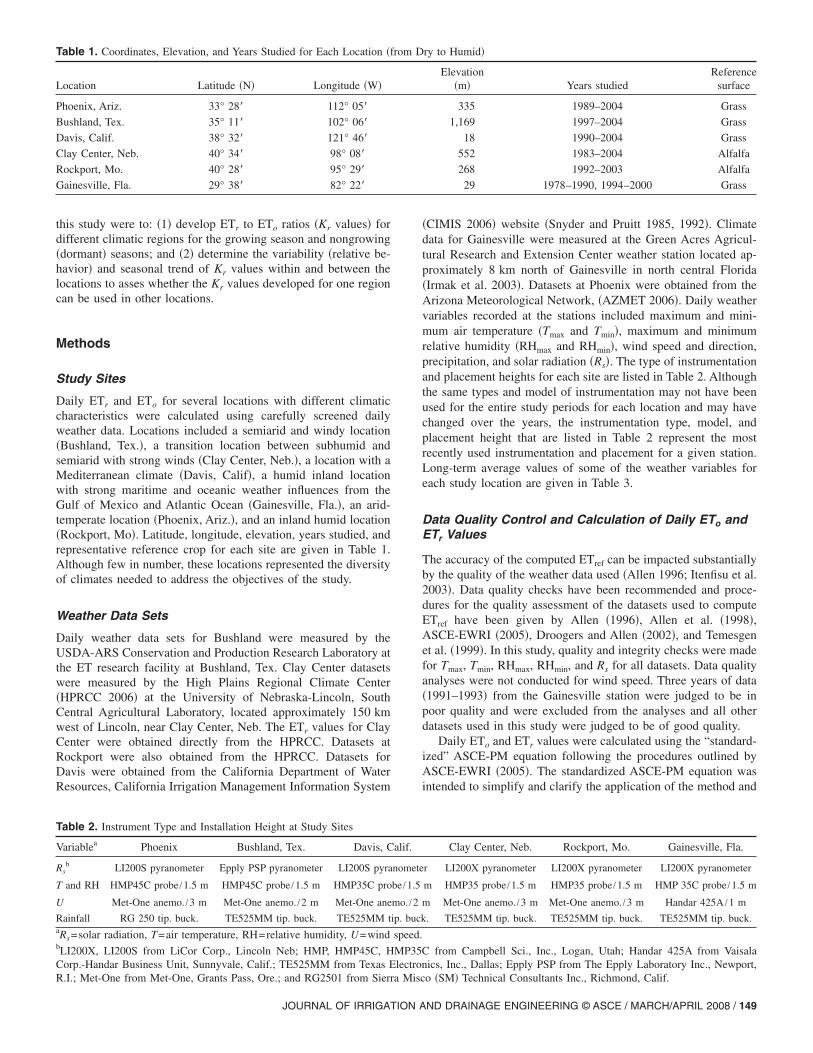
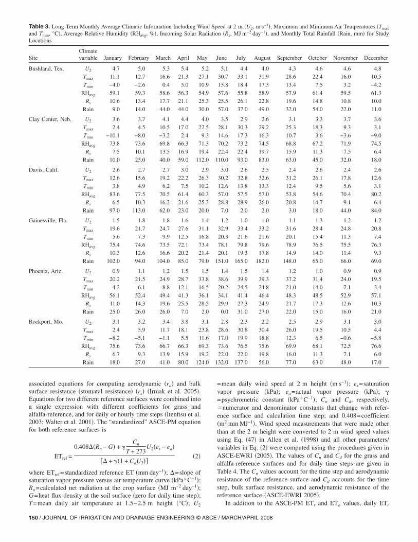
�CIMIS 2006� website �Snyder and Pruitt 1985, 1992�. Climatedata for Gainesville were measured at the Green Acres Agricul-tural Research and Extension Center weather station located ap-proximately 8 km north of Gainesville in north central Florida�Irmak et al. 2003�. Datasets at Phoenix were obtained from theArizona Meteorological Network, �AZMET 2006�. Daily weathervariables recorded at the stations included maximum and mini-mum air temperature �Tmax and Tmin�, maximum and minimumrelative humidity �RHmax and RHmin�, wind speed and direction,precipitation, and solar radiation �Rs�. The type of instrumentationand placement heights for each site are listed in Table 2. Althoughthe same types and model of instrumentation may not have beenused for the entire study periods for each location and may havechanged over the years, the instrumentation type, model, andplacement height that are listed in Table 2 represent the mostrecently used instrumentation and placement for a given station.Long-term average values of some of the weather variables foreach study location are given in Table 3.

Data Quality Control and Calculation of Daily ETo andETr Values

The accuracy of the computed ETref can be impacted substantiallyby the quality of the weather data used �Allen 1996; Itenfisu et al.2003�. Data quality checks have been recommended and proce-dures for the quality assessment of the datasets used to computeETref have been given by Allen �1996�, Allen et al. �1998�,ASCE-EWRI �2005�, Droogers and Allen �2002�, and Temesgenet al. �1999�. In this study, quality and integrity checks were madefor Tmax, Tmin, RHmax, RHmin, and Rs for all datasets. Data qualityanalyses were not conducted for wind speed. Three years of data�1991–1993� from the Gainesville station were judged to be inpoor quality and were excluded from the analyses and all otherdatasets used in this study were judged to be of good quality.

Daily ETo and ETr values were calculated using the “standard-ized” ASCE-PM equation following the procedures outlined byASCE-EWRI �2005�. The standardized ASCE-PM equation wasintended to simplify and clarify the application of the method and

Table 1. Coordinates, Elevation, and Years Studied for Each Location �from Dry to Humid�

Location Latitude �N� Longitude �W�Elevation

�m� Years studiedReference

surface

Phoenix, Ariz. 33° 28� 112° 05� 335 1989–2004 Grass

Bushland, Tex. 35° 11� 102° 06� 1,169 1997–2004 Grass

Davis, Calif. 38° 32� 121° 46� 18 1990–2004 Grass

Clay Center, Neb. 40° 34� 98° 08� 552 1983–2004 Alfalfa

Rockport, Mo. 40° 28� 95° 29� 268 1992–2003 Alfalfa

Gainesville, Fla. 29° 38� 82° 22� 29 1978–1990, 1994–2000 Grass

Table 2. Instrument Type and Installation Height at Study Sites

Variablea Phoenix Bushland, Tex. Davis, Calif. Clay Center, Neb. Rockport, Mo. Gainesville, Fla.

Rsb LI200S pyranometer Epply PSP pyranometer LI200S pyranometer LI200X pyranometer LI200X pyranometer LI200X pyranometer

T and RH HMP45C probe /1.5 m HMP45C probe /1.5 m HMP35C probe /1.5 m HMP35 probe /1.5 m HMP35 probe /1.5 m HMP 35C probe /1.5 m

U Met-One anemo. /3 m Met-One anemo. /2 m Met-One anemo. /2 m Met-One anemo. /3 m Met-One anemo. /3 m Handar 425A /1 m

Rainfall RG 250 tip. buck. TE525MM tip. buck. TE525MM tip. buck. TE525MM tip. buck. TE525MM tip. buck. TE525MM tip. buck.aRs=solar radiation, T=air temperature, RH=relative humidity, U=wind speed.bLI200X, LI200S from LiCor Corp., Lincoln Neb; HMP, HMP45C, HMP35C from Campbell Sci., Inc., Logan, Utah; Handar 425A from VaisalaCorp.-Handar Business Unit, Sunnyvale, Calif.; TE525MM from Texas Electronics, Inc., Dallas; Epply PSP from The Epply Laboratory Inc., Newport,R.I.; Met-One from Met-One, Grants Pass, Ore.; and RG2501 from Sierra Misco �SM� Technical Consultants Inc., Richmond, Calif.

JOURNAL OF IRRIGATION AND DRAINAGE ENGINEERING © ASCE / MARCH/APRIL 2008 / 149

associated equations for computing aerodynamic �ra� and bulksurface resistance �stomatal resistance� �rs� �Irmak et al. 2005�.Equations for two different reference surfaces were combined intoa single expression with different coefficients for grass andalfalfa-reference, and for daily or hourly time steps �Itenfisu et al.2003; Walter et al. 2001�. The “standardized” ASCE-PM equationfor both reference surfaces is

ETref =

0.408��Rn − G� + �Cn

T + 273U2�es − ea�

�� + ��1 + CdU2���2�

where ETref=standardized reference ET �mm day−1�; �=slope ofsaturation vapor pressure versus air temperature curve �kPa°C−1�;Rn=calculated net radiation at the crop surface �MJ m−2 day−1�;G=heat flux density at the soil surface �zero for daily time step�;T=mean daily air temperature at 1.5–2.5 m height �°C�; U2

=mean daily wind speed at 2 m height �m s−1�; es=saturationvapor pressure �kPa�; ea=actual vapor pressure �kPa�; �=psychrometric constant �kPa°C−1�; Cn and Cd, respectively,�numerator and denominator constants that change with refer-ence surface and calculation time step; and 0.408=coefficient�m2 mm MJ−1�. Wind speed measurements that were made otherthan at the 2 m height were converted to 2 m wind speed valuesusing Eq. �47� in Allen et al. �1998� and all other parameters/variables in Eq. �2� were computed using the procedures given inASCE-EWRI �2005�. The values of Cn and Cd for the grass andalfalfa-reference surfaces and for daily time steps are given inTable 4. The Cn values account for the time step and aerodynamicresistance of the reference surface and Cd accounts for the timestep, bulk surface resistance, and aerodynamic resistance of thereference surface �ASCE-EWRI 2005�.

In addition to the ASCE-PM ETr and ETo values, daily ETr

Table 3. Long-Term Monthly Average Climatic Information Including Wind Speed at 2 m �U2, m s−1�, Maximum and Minimum Air Temperatures �Tmax

and Tmin, °C�, Average Relative Humidity �RHavg, %�, Incoming Solar Radiation �Rs, MJ m−2 day−1�, and Monthly Total Rainfall �Rain, mm� for StudyLocations

SiteClimatevariable January February March April May June July August September October November December

Bushland, Tex. U2 4.7 5.0 5.3 5.4 5.2 5.1 4.4 4.0 4.3 4.6 4.6 4.8

Tmax 11.1 12.7 16.6 21.3 27.1 30.7 33.1 31.9 28.6 22.4 16.0 10.5

Tmin −4.0 −2.6 0.4 5.0 10.9 15.8 18.4 17.3 13.4 7.5 3.2 −4.2

RHavg 59.1 59.3 58.6 56.3 54.9 57.6 55.8 58.9 57.9 61.4 59.5 61.3

Rs 10.6 13.4 17.7 21.1 25.3 25.5 26.1 22.8 19.6 14.8 10.8 10.0

Rain 9.0 14.0 44.0 44.0 30.0 57.0 37.0 49.0 32.0 54.0 22.0 11.0

Clay Center, Neb. U2 3.6 3.7 4.1 4.4 4.0 3.5 2.9 2.6 3.1 3.3 3.7 3.6

Tmax 2.4 4.5 10.5 17.0 22.5 28.1 30.3 29.2 25.3 18.3 9.3 3.1

Tmin −10.1 −8.0 −3.2 2.4 9.3 14.6 17.3 16.3 10.7 3.6 −3.6 −9.0

RHavg 73.8 73.6 69.8 66.3 71.3 70.2 73.2 74.5 68.8 67.2 71.9 74.5

Rs 7.5 10.1 13.5 16.9 19.4 22.4 22.4 19.7 15.9 11.3 7.5 6.4

Rain 10.0 23.0 40.0 59.0 112.0 110.0 93.0 83.0 63.0 45.0 32.0 18.0

Davis, Calif. U2 2.6 2.7 2.7 3.0 2.9 3.0 2.6 2.5 2.4 2.6 2.4 2.6

Tmax 12.6 15.6 19.2 22.2 26.3 30.2 32.8 32.6 31.2 26.1 17.8 12.6

Tmin 3.8 4.9 6.2 7.5 10.2 12.6 13.8 13.3 12.4 9.5 5.6 3.1

RHavg 83.6 77.5 70.5 61.4 60.3 57.0 57.5 57.0 53.8 54.6 70.4 80.2

Rs 6.5 10.3 16.2 21.6 25.3 28.8 28.9 26.0 20.8 14.7 9.1 6.4

Rain 97.0 113.0 62.0 23.0 20.0 7.0 2.0 2.0 3.0 18.0 44.0 84.0

Gainesville, Fla. U2 1.5 1.8 1.8 1.6 1.4 1.2 1.0 1.0 1.1 1.3 1.2 1.2

Tmax 19.6 21.7 24.7 27.6 31.1 32.9 33.4 33.2 31.6 28.4 24.8 20.8

Tmin 5.6 7.3 9.9 12.5 16.8 20.3 21.6 21.6 20.1 15.4 11.3 7.4

RHavg 75.4 74.6 73.5 72.1 73.4 78.1 79.8 79.6 78.9 76.5 75.5 76.3

Rs 10.3 12.6 16.6 20.2 21.4 20.1 19.3 17.8 14.9 14.0 11.4 9.3

Rain 102.0 94.0 104.0 85.0 79.0 151.0 165.0 182.0 148.0 65.0 66.0 69.0

Phoenix, Ariz. U2 0.9 1.1 1.2 1.5 1.5 1.4 1.5 1.4 1.2 1.0 0.9 0.9

Tmax 20.2 21.5 24.9 28.7 33.8 38.6 39.9 39.3 37.2 31.4 24.0 19.5

Tmin 4.2 6.1 8.8 12.1 16.5 20.2 24.5 24.8 21.0 14.0 7.1 3.4

RHavg 56.1 52.4 49.4 41.3 36.1 34.1 41.4 46.4 48.3 48.5 52.9 57.1

Rs 11.0 14.3 19.6 25.5 28.5 29.9 27.3 24.9 21.7 17.3 12.6 10.3

Rain 25.0 26.0 26.0 7.0 2.0 0.0 31.0 27.0 22.0 15.0 16.0 21.0

Rockport, Mo. U2 3.1 3.2 3.4 3.8 3.1 2.8 2.3 2.2 2.5 2.9 3.1 3.0

Tmax 2.4 5.9 11.7 18.1 23.8 28.6 30.8 30.4 26.0 19.5 10.5 4.4

Tmin −8.2 −5.1 −1.1 5.5 11.6 17.0 19.9 18.8 12.3 6.5 −0.6 −5.8

RHavg 75.6 73.6 66.7 66.3 69.3 73.6 76.5 75.6 69.9 68.1 72.5 76.6

Rs 6.7 9.3 13.9 15.9 19.2 22.0 22.0 19.8 16.0 11.3 7.1 6.0

Rain 18.0 27.0 41.0 80.0 124.0 132.0 137.0 56.0 77.0 63.0 48.0 17.0

150 / JOURNAL OF IRRIGATION AND DRAINAGE ENGINEERING © ASCE / MARCH/APRIL 2008

values were computed with four other ETr methods that are de-scribed in Burman and Pochop �1994� and Jensen et al. �1990�.Therefore, a detailed description of each method is not given andthe reader is referred to original sources. For the ETr equationsother than ASCE-PM, the procedures on calculation of the equa-tion parameters associated with each equation were used. Themethods were: �1� Jensen–Haise �Jensen and Haise 1963�; �2�1972 Kimberly–Penman �Wright and Jensen 1972�; �3� 1982Kimberly–Penman �Wright 1982�; and �4� the HPRCC-Penmanequation. These models were selected because they represent themajority of the alfalfa-reference ET equations that are currentlybeing used in different applications. In this study, the HPRCC-Penman equation was used only at Clay Center. The HPRCCequation is a Penman-type �Penman 1948� combination equationand was modified for Nebraska �Mitchell, Neb.� climatic condi-tions by Kincaid and Heerman �1974� and has been adopted bythe HPRCC and has been widely used in North Dakota, Nebraska,Kansas, South Dakota, and Colorado as part of the HPRCC auto-mated weather network.

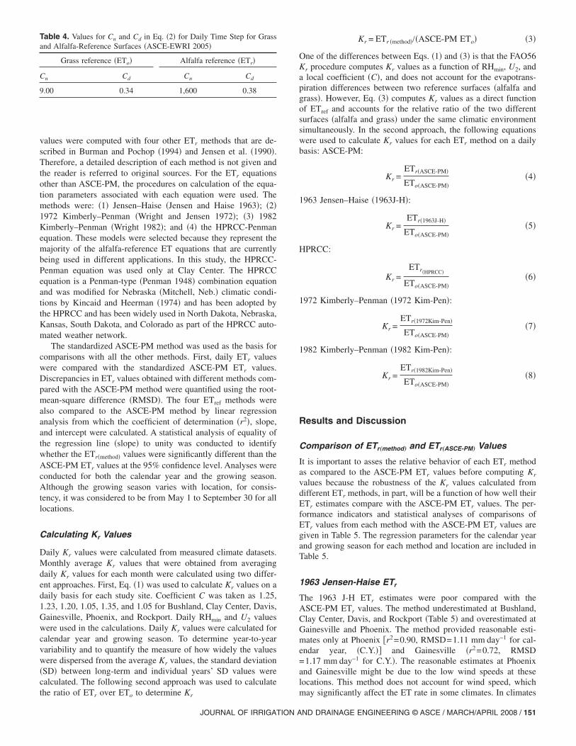
The standardized ASCE-PM method was used as the basis forcomparisons with all the other methods. First, daily ETr valueswere compared with the standardized ASCE-PM ETr values.Discrepancies in ETr values obtained with different methods com-pared with the ASCE-PM method were quantified using the root-mean-square difference �RMSD�. The four ETref methods werealso compared to the ASCE-PM method by linear regressionanalysis from which the coefficient of determination �r2�, slope,and intercept were calculated. A statistical analysis of equality ofthe regression line �slope� to unity was conducted to identifywhether the ETr�method� values were significantly different than theASCE-PM ETr values at the 95% confidence level. Analyses wereconducted for both the calendar year and the growing season.Although the growing season varies with location, for consis-tency, it was considered to be from May 1 to September 30 for alllocations.

Calculating Kr Values

Daily Kr values were calculated from measured climate datasets.Monthly average Kr values that were obtained from averagingdaily Kr values for each month were calculated using two differ-ent approaches. First, Eq. �1� was used to calculate Kr values on adaily basis for each study site. Coefficient C was taken as 1.25,1.23, 1.20, 1.05, 1.35, and 1.05 for Bushland, Clay Center, Davis,Gainesville, Phoenix, and Rockport. Daily RHmin and U2 valueswere used in the calculations. Daily Kr values were calculated forcalendar year and growing season. To determine year-to-yearvariability and to quantify the measure of how widely the valueswere dispersed from the average Kr values, the standard deviation�SD� between long-term and individual years’ SD values werecalculated. The following second approach was used to calculatethe ratio of ETr over ETo to determine Kr

Kr = ETr �method�/�ASCE-PM ETo� �3�

One of the differences between Eqs. �1� and �3� is that the FAO56Kr procedure computes Kr values as a function of RHmin, U2, anda local coefficient �C�, and does not account for the evapotrans-piration differences between two reference surfaces �alfalfa andgrass�. However, Eq. �3� computes Kr values as a direct functionof ETref and accounts for the relative ratio of the two differentsurfaces �alfalfa and grass� under the same climatic environmentsimultaneously. In the second approach, the following equationswere used to calculate Kr values for each ETr method on a dailybasis: ASCE-PM:

Kr =ETr�ASCE-PM�

ETo�ASCE-PM��4�

1963 Jensen–Haise �1963J-H�:

Kr =ETr�1963J-H�

ETo�ASCE-PM��5�

HPRCC:

Kr =ETr�HPRCC�

ETo�ASCE-PM��6�

1972 Kimberly–Penman �1972 Kim-Pen�:

Kr =ETr�1972Kim-Pen�

ETo�ASCE-PM��7�

1982 Kimberly–Penman �1982 Kim-Pen�:

Kr =ETr�1982Kim-Pen�

ETo�ASCE-PM��8�

Results and Discussion

Comparison of ETr„method… and ETr„ASCE-PM…

Values

It is important to asses the relative behavior of each ETr methodas compared to the ASCE-PM ETr values before computing Kr

values because the robustness of the Kr values calculated fromdifferent ETr methods, in part, will be a function of how well theirETr estimates compare with the ASCE-PM ETr values. The per-formance indicators and statistical analyses of comparisons ofETr values from each method with the ASCE-PM ETr values aregiven in Table 5. The regression parameters for the calendar yearand growing season for each method and location are included inTable 5.

1963 Jensen-Haise ETr

The 1963 J-H ETr estimates were poor compared with theASCE-PM ETr values. The method underestimated at Bushland,Clay Center, Davis, and Rockport �Table 5� and overestimated atGainesville and Phoenix. The method provided reasonable esti-mates only at Phoenix �r2=0.90, RMSD=1.11 mm day−1 for cal-endar year, �C.Y.�� and Gainesville �r2=0.72, RMSD=1.17 mm day−1 for C.Y.�. The reasonable estimates at Phoenixand Gainesville might be due to the low wind speeds at theselocations. This method does not account for wind speed, whichmay significantly affect the ET rate in some climates. In climates

Table 4. Values for Cn and Cd in Eq. �2� for Daily Time Step for Grassand Alfalfa-Reference Surfaces �ASCE-EWRI 2005�

Grass reference �ETo� Alfalfa reference �ETr�

Cn Cd Cn Cd

9.00 0.34 1,600 0.38

JOURNAL OF IRRIGATION AND DRAINAGE ENGINEERING © ASCE / MARCH/APRIL 2008 / 151

with strong winds, the saturated air above the plant canopy willbe constantly replaced with drier air, increasing vapor pressuredeficit and ET. However, in calm wind conditions, the saturatedair in the immediate surrounding of the crop canopy may not bereplaced as often, making ET less sensitive to wind speed. Inclimates with high humidity and low winds, the saturated airabove the canopy can be replaced with only slightly less humidair. Thus, one would expect the 1963 J-H equation to providebetter estimates of ETr in environments with calm winds com-pared with environments with strong winds. The 1963 J-H ETr

estimates were significantly different than the ASCE-PM ETr val-ues at all locations. The magnitude of underestimations at Bush-land, Clay Center, and Davis increased at high ET values��10 mm�. The method overestimated the ASCE-PM ETr valuesby 8 and 17% at Phoenix and Gainesville �Table 5�. The under-estimation was 24% at Clay Center, which was in agreement withthe value observed by Jensen et al. �1990� as 30% underestima-tions by this method at an arid and windy location �Scottsbluff,Neb.�. Estimations for the growing season resulted in lowerRMSD values at Clay Center and Rockport.

HPRCC Penman ETr

The HPRCC Penman ETr values were used and analyzed only atClay Center. The method provided good estimates with a high r2

value of 0.97 and low RMSD of 0.56 mm day−1. Estimates wereparallel to the ASCE-PM ETr values for the majority of the datarange. However, the equation did not respond to the changes inETr values greater than approximately 10 mm and the magnitudesof underestimations were larger at the higher ETr rates. Overall,estimations were within 6% of the ASCE-PM ETr values. TheRMSD value �0.63 mm day−1� for the growing season was higherthan for the calendar year �0.56 mm day−1� with similar slopes�0.94 versus 0.93�. The consistent lagging of the HPRCC ETr

values below the ASCE-PM ETr values at high ET values indi-cates calibration characteristics. The HPRCC Penman equationwas modified by Kincaid and Heermann �1974� for Mitchell, Neb,climatic conditions by changing the wind function of the originalPenman �1948� method. Kincaid and Heermann �1974� stated thatthe coefficients used in the wind function of the HPRCC Penmanequation were nearly the same as those reported by Jensen �1969�

Table 5. Root-Mean-Square Difference �RMSD� of Daily ETr Estimates, Regression Coefficients between ASCE-PM ETr and ETr �method�, and Test forEquality of Regression Line for Unity for Calendar Year �C.Y.� and Growing Season �G.S.�

Location and ETr

methods

RMSDa

of dailyestimate for

C.Y.�mm day−1�

Slopeb

�C.Y.� Interceptb�C.Y.�r2

�C.Y.�

Test forequality ofregression

line for C.Y.�t value�

RMSD of dailya

estimate and testfor equality for

G.S.�mm day−1�

Slopeb

�G.S.�Interceptb

�G.S.�r2

�G.S.�

Bushland, Tex.

1963 Jensen–Haise 4.36 0.59 −0.65 0.74 91.19c 4.51 �1,224�c 0.42 2.06 0.63

1972 Kimberly–Penman 0.87 1.01 0.47 0.97 −44.13c 0.79 �1,224�c 1.00 0.44 0.97

1982 Kimberly–Penman 1.08 0.97 −0.30 0.95 32.1c �P=0.44�d �1,224� 0.92 0.82 0.96

Clay Center, Neb.

1963 Jensen–Haise 2.23 0.76 −0.61 0.74 99.26c 1.95 �3,366�c 0.67 0.80 0.64

1974 HPRCC Penman 0.56 0.94 0.04 0.97 37.03c 0.63 �3,366�c 0.93 0.17 0.95

1972 Kimberly–Penman 0.48 1.00 0.24 0.98 −62.98c 0.47 �3,366�c 0.98 0.41 0.98

1982 Kimberly–Penman 0.67 0.98 −0.08 0.95 25.09c 0.51 �3,366�c 0.96 0.46 0.97

Davis, Calif.

1963 Jensen–Haise 2.23 0.71 −0.03 0.82 78.32c 2.36 �2,295�c 0.56 1.89 0.58

1972 Kimberly–Penman 0.41 0.97 0.16 0.99 �P=0.07�d 0.46 �2,295�c 0.92 0.58 0.96

1982 Kimberly–Penman 0.80 0.99 −0.31 0.96 39.68c �P=0.06�d �2,295� 0.93 0.53 0.91

Gainesville, Fla.

1963 Jensen–Haise 1.17 1.17 −0.50 0.73 −11.54c 1.33 �3,060�c 1.17 0.11 0.72

1972 Kimberly–Penman 0.24 1.02 0.10 0.99 −83.67c 0.27 �3,060�c 1.02 0.16 0.99

1982 Kimberly–Penman 0.54 1.07 −0.32 0.91 6.49c 0.55 �3,060�c 1.08 0.06 0.94

Phoenix, Ariz.

1963 Jensen–Haise 1.11 1.08 −0.64 0.90 11.16c 1.21 �2,448�c 0.84 1.80 0.62

1972 Kimberly–Penman 0.29 0.94 0.37 0.99 �P=0.09�d 0.34 �2,448�c 0.86 1.02 0.98

1982 Kimberly–Penman 0.83 1.12 −0.92 0.96 23.3c 0.86 �2,448�c 1.08 −0.32 0.85

Rockport, Mo.

1963 Jensen–Haise 1.93 0.83 −0.52 0.71 52.68c 1.51 �1,836�c 0.78 0.77 0.64

1972 Kimberly–Penman 0.36 1.01 0.14 0.99 −40.22c 0.36 �1,836�c 0.99 0.31 0.98

1982 Kimberly–Penman 0.67 0.97 −0.06 0.94 19.18c 0.53 �1,836�c 0.96 0.47 0.95aRMSD was calculated from daily ETr values for each method.bRegression coefficients where ETr �method�=slope�ASCE-PM ETr+intercept.cValues in parenthesis indicate number of observations for the growing season. For a given location, all days from May through September in each yearwere included in the analyses. C.Y.=Calendar year, G.S.=Growing season �May–September�.dThe slope of the regression line between the ETr �method� values and the ASCE-PM ETr values is significantly different �P�0.05� than the unity at the 5%significance level. The t values were reported only for calendar year analyses. The significance of the regression line was reported for the growing seasonanalyses.

152 / JOURNAL OF IRRIGATION AND DRAINAGE ENGINEERING © ASCE / MARCH/APRIL 2008

for Twin Falls, Id. However, in practical application, the HPRCCETr differs from the original equation of Kincaid and Heerman�1974�. In practical application of the original equation by theHPRCC, the maximum value of wind speed and vapor pressuredeficit �VPD� �es-ea in Eq. �2�� that can occur is limited to certainvalues. Thus, the equation does not respond to the effect of thewind speed and VPD on ETr after an approximately ETr value of�10 mm. The ETr calculations reported by HPRCC in the dailyweather data sets are made using a VPD limit of 2.3 kPa and windspeed limit of 5.1 m s−1 as suggested by Hubbard �1992�. Thesetwo conditions are the main cause of discrepancies between theHPRCC and the ASCE-PM ETr values at high ETr rates��10 mm�. These two conditions will cause some faulty ETr val-ues by the HPRCC Penman. Because the climatic conditions ofthe VPD above 2.3 kPa and wind speeds above 5.1 m s−1 areoften observed in many parts of Nebraska, especially during thegrowing season, the VPD and wind speeds above these limits canbe a substantial portion of the climate datasets in some parts ofthe state during hot, dry, and windy periods. These large VPDsand high wind speeds represent natural climatic demand forevaporative losses of the environment and should be reflected inthe ETr estimates. Eliminating the conditions on upper limits ofthe VPD and wind speed would greatly improve the performanceof the HPRCC Penman equation at high ET rates as comparedwith the ASCE-PM ETr.

1972 and 1982 Kimberly–Penman ETr

The 1972 Kim-Pen had the best agreement with the ASCE-PM atall locations. The ETr estimates correlated very well with theASCE-PM ETr values throughout the year, with low RMSD val-ues of 0.87, 0.48, 0.41, 0.24, 0.29, and 0.36 mm day−1 for Bush-land, Clay Center, Davis, Gainesville, Phoenix, and Rockport.The RMSD value of 0.48 mm day−1 for Clay Center was smallerthan the RMSD value obtained from the HPRCC Penman equa-tion �0.56 mm day−1�, which was originally calibrated for Ne-braska conditions. The 1972 Kim-Pen ETr estimates were notsignificantly different from the ASCE-PM ETr values at two lo-cations; Davis and Phoenix. This was the only method that hadnonsignificant �P�0.05� ETr estimates as compared with theASCE-PM estimates among all methods for the calendar year. Italso had the highest r2 values ��0.97� among all locations. Over-all, its estimates were within 3% of the ASCE-PM estimates withthe exception of Phoenix where the estimates were 6% lower thanthe ASCE-PM. Growing season estimates were very similar tothose obtained for the calendar year, but the magnitude of theunderestimations during the growing season increased from 3 to8% at Davis and from 6 to 14% at Phoenix. Although the 1972Kim-Pen method slightly over- or underestimated the ASCE-PMETr values, depending on location, it produced consistent esti-mates with less point scattering around the 1:1 line at both lowand high ETr rates throughout the year at all locations.

The 1982 Kim-Pen ETr estimates agreed well with ASCE-PMETr values. The RMSD values were, however, higher than for the1972 Kim-Pen at all locations, ranging from 0.54 mm day−1 atGainesville to 1.08 mm day−1 at Bushland. Underestimationswere within 3% of the ASCE-PM estimates at Bushland, ClayCenter, Davis, and Rockport. The poorest estimates were atGainesville and Phoenix, the two locations with the lowest windspeeds. The equation overestimated by 7 and 12% at Gainesvilleand Phoenix. The ETr estimates during the growing season wereconsiderably better than those in nongrowing seasons, especiallyat Bushland, Clay Center, Davis, and Rockport. The estimates

during the growing season were not significantly different fromthe ASCE-PM estimates at Bushland and Davis �Table 5�. Irmaket al. �2003� reported that the 1982 Kim-Pen was originally de-veloped for the period of April through October with a polyno-mial wind function. The original wind function did not behavecorrectly during November through March and later was changedto the �normal equation� wind function �J. L. Wright, personalcommunication� as given by Jensen et al. �1990�, which was thewind function used in this study. This wind function decreases toa base level for the winter months and accounts for the shorterdaylength.

Daily Kr Values for Calendar Year and Growing Season

ASCE-PM Kr

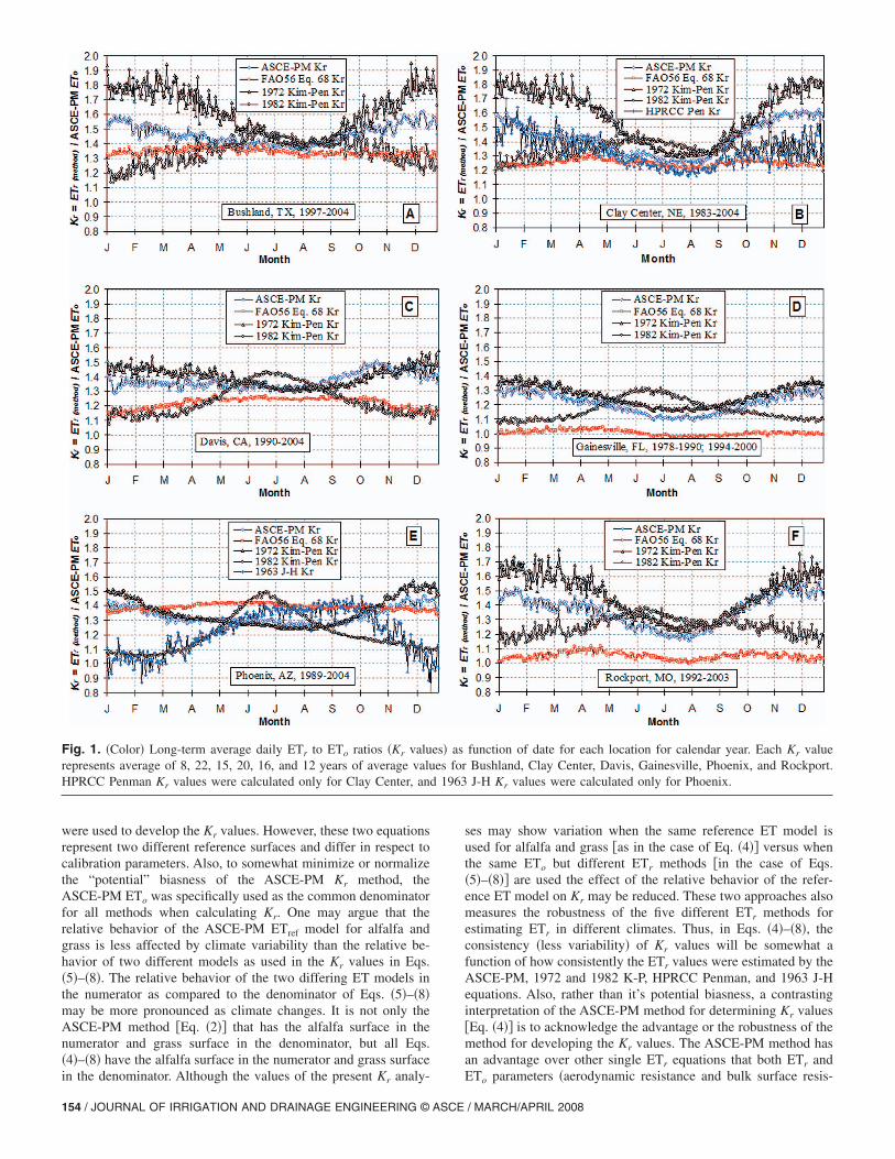
Although the ASCE-PM Kr values showed some variation be-tween the locations they were more consistent than other Kr val-ues �Fig. 1�. Values determined with the ASCE-PM consistentlyexhibited an increasing trend from summer towards the wintermonths at all locations with maximum values in December andJanuary. Although they differed in magnitude, the annual trend ofKr values was similar for all locations. The Kr values had lessvariation during the growing season �May–September� than thenongrowing �dormant� season. The largest day-to-day fluctuationduring the growing season was observed at Rockport, followed byClay Center and Gainesville. The largest Kr values were observedat Bushland and Clay Center, two locations where hot, dry, andwindy conditions cause high ET rates during the growing season.The large Kr values�1.38 during the summer months may reflectthe advective, dry, and high wind environment typical of Bush-land. These conditions are also often observed at Clay Center,especially during late July and early August where ETr can ex-ceed available energy �Rn� reflecting advective conditions. The Kr

values ranged from 1.38 in July and August to a maximum of1.55 and 1.56 in January and December, with calendar year andgrowing season averages of 1.46 and 1.40 �Table 6�. The lowestKr values were in Gainesville, ranging from 1.11 in July to 1.30 inJanuary. The Kr values were always greater than 1.11 during thecalendar year and growing season at all locations and the day-to-day variation of Kr values was very small during the year. Theaverage SD values among years were always less than 0.10 forthe calendar year and less than 0.08 for the growing season. Theseresults agree with those reported by Jensen et al. �1990� whoobserved Kr values ranging from a low of 1.03 for calm, humidconditions to a high of 1.45 for extremely windy and dry condi-tions. However, the ASCE-PM Kr values obtained in this studyare somewhat higher than other Kr values reported in the litera-ture and are close to some of the Kr values that are reported byother researchers. For example, in a lysimeter-measured alfalfaand grass ET study, Evett et al. �2000� reported that ETr was 1.15times higher than ETo at Bushland, Tex., for the growing season.Doorenbos and Pruitt �1977� suggested a Kr value of 1.15 for adry climate with light to moderate wind. Erpenbeck �1981� ob-tained an average Kr value of 1.21 using grass ET and pan evapo-ration data at Davis, Calif. Wright �1996� reported a seasonal Kr

value of 1.20 for Kimberly, Id.It should be noted that the less variability in Kr values does not

necessarily mean higher accuracy and the term “variability” mayalso reflect the relative behavior of the methods when calculatingthe Kr values. At first glance, the Kr values developed using theASCE-PM ETr and ETo values �Eq. �4�� might seem biased be-cause two standardized forms of the Penman–Monteith equation

JOURNAL OF IRRIGATION AND DRAINAGE ENGINEERING © ASCE / MARCH/APRIL 2008 / 153

were used to develop the Kr values. However, these two equationsrepresent two different reference surfaces and differ in respect tocalibration parameters. Also, to somewhat minimize or normalizethe “potential” biasness of the ASCE-PM Kr method, theASCE-PM ETo was specifically used as the common denominatorfor all methods when calculating Kr. One may argue that therelative behavior of the ASCE-PM ETref model for alfalfa andgrass is less affected by climate variability than the relative be-havior of two different models as used in the Kr values in Eqs.�5�–�8�. The relative behavior of the two differing ET models inthe numerator as compared to the denominator of Eqs. �5�–�8�may be more pronounced as climate changes. It is not only theASCE-PM method �Eq. �2�� that has the alfalfa surface in thenumerator and grass surface in the denominator, but all Eqs.�4�–�8� have the alfalfa surface in the numerator and grass surfacein the denominator. Although the values of the present Kr analy-

ses may show variation when the same reference ET model isused for alfalfa and grass �as in the case of Eq. �4�� versus whenthe same ETo but different ETr methods �in the case of Eqs.�5�–�8�� are used the effect of the relative behavior of the refer-ence ET model on Kr may be reduced. These two approaches alsomeasures the robustness of the five different ETr methods forestimating ETr in different climates. Thus, in Eqs. �4�–�8�, theconsistency �less variability� of Kr values will be somewhat afunction of how consistently the ETr values were estimated by theASCE-PM, 1972 and 1982 K-P, HPRCC Penman, and 1963 J-Hequations. Also, rather than it’s potential biasness, a contrastinginterpretation of the ASCE-PM method for determining Kr values�Eq. �4�� is to acknowledge the advantage or the robustness of themethod for developing the Kr values. The ASCE-PM method hasan advantage over other single ETr equations that both ETr andETo parameters �aerodynamic resistance and bulk surface resis-

Fig. 1. �Color� Long-term average daily ETr to ETo ratios �Kr values� as function of date for each location for calendar year. Each Kr valuerepresents average of 8, 22, 15, 20, 16, and 12 years of average values for Bushland, Clay Center, Davis, Gainesville, Phoenix, and Rockport.HPRCC Penman Kr values were calculated only for Clay Center, and 1963 J-H Kr values were calculated only for Phoenix.

154 / JOURNAL OF IRRIGATION AND DRAINAGE ENGINEERING © ASCE / MARCH/APRIL 2008

tance� were combined into a single equation having different cali-bration parameters and time step coefficients. Thus, theASCE-PM Kr method might provide a more conclusive indicationand/or information on the interpretation of the true variability inKr values between the locations and between the seasons for thesame location, and transferability of the Kr values from one loca-tion to another.

FAO56 KrThe Kr values obtained with the FAO56 method �Eq. �1�� fluctu-ated in a substantially narrower range throughout the calendaryear and growing season than any other method with nonconsis-tent values among locations �Fig. 1�. For example, Bushland,Davis, and Phoenix had maximum Kr values during the growingseason and the values steadily decreased towards the wintermonths. However, at Clay Center, Gainesville, and Rockport, aconsiderably different trend was observed, with the largest valuesduring spring and fall, and minimum values during the growingseason. This might be due to differences in the seasonal trends ofRHmin and U2 at different locations. Unlike the ASCE-PM, the

FAO56 procedure had the largest Kr values at Phoenix, followedby Bushland. The values ranged from 1.36 and 1.37 in Decemberand January to 1.42 in May and June. The Kr values were smallerat humid locations as compared with the arid and semiarid loca-tions. The smallest Kr values were obtained at Gainesville. Someof the Kr values produced by the FAO-56 method seem unusualand possibly unrealistic. For reasons stated earlier related to al-falfa and grass reference surfaces, one would expect ETr�ETo

for any climate. However, the Kr values obtained with thismethod averaged 1.01 for the calendar year and 0.99 for thegrowing season, indicating that ETr�ETo, which seems unusual.At Rockport, Kr values also seem low, averaging 1.05 for thecalendar year, and 1.04 for the growing season.

The inconsistent Kr values among locations obtained with thismethod might be due to the magnitude of the weather variables�RHmin and U2� used to develop and calibrate Eq. �1�. In thisequation, the base values of 45% and 2 m s−1 for RHmin and U2,respectively, seem too large and may not work for climatic con-ditions that differ significantly from those for which the equation

Table 6. Monthly Long-Term Average ETr to ETo Ratios �Kr Values� Calculated from Five Different ETr Methods �ASCE-PM, FAO56 Eq. �68�, 1963 J-H�for Phoenix only�, HPRCC Penman �for Clay Center Only�, 1972 Kim-Pen, and 1982 Kim-Pen� for Bushland, Tex., Clay Center, Neb., Davis, Calif.,Gainesville, Fla., Phoenix, Ariz., and Rockport, Mo.� for Calendar Year and Growing Season

Month

ASCE-PM Kr and SD values FAO56 Eq. �68� Kr and SD values 1963 J-H Krand

SD values�Phoenix�Bushland C. Center Davis G.ville Phoenix Rockport Bushland C. Center Davis G.ville Phoenix Rockport

January 1.55 �0.09� 1.55 �0.11� 1.35 �0.17� 1.30 �0.13� 1.40 �0.10� 1.47 �0.12� 1.33 �0.05� 1.23 �0.06� 1.15 �0.06� 1.01 �0.05� 1.37 �0.04� 1.03 �0.05� 1.03 �0.26�

February 1.50 �0.09� 1.46 �0.12� 1.36 �0.12� 1.29 �0.11� 1.36 �0.08� 1.41 �0.12� 1.34 �0.06� 1.24 �0.06� 1.18 �0.06� 1.02 �0.05� 1.38 �0.03� 1.04 �0.06� 1.02 �0.22�

March 1.46 �0.10� 1.42 �0.11� 1.35 �0.09� 1.25 �0.09� 1.31 �0.07� 1.39 �0.10� 1.35 �0.06� 1.27 �0.06� 1.21 �0.05� 1.03 �0.05� 1.39 �0.03� 1.08 �0.06� 1.11 �0.20�

April 1.44 �0.10� 1.42 �0.10� 1.35 �0.08� 1.22 �0.08� 1.30 �0.05� 1.38 �0.11� 1.36 �0.06� 1.29 �0.06� 1.24 �0.05� 1.04 �0.04� 1.41 �0.02� 1.09 �0.07� 1.18 �0.16�

May 1.42 �0.08� 1.33 �0.10� 1.33 �0.07� 1.18 �0.07� 1.30 �0.01� 1.30 �0.09� 1.37 �0.05� 1.26 �0.06� 1.24 �0.04� 1.02 �0.04� 1.42 �0.00� 1.06 �0.05� 1.26 �0.03�

June 1.40 �0.08� 1.30 �0.08� 1.33 �0.06� 1.13 �0.06� 1.30 �0.04� 1.24 �0.08� 1.36 �0.05� 1.25 �0.05� 1.25 �0.04� 0.99 �0.03� 1.42 �0.01� 1.04 �0.05� 1.35 �0.13�

July 1.38 �0.06� 1.27 �0.07� 1.32 �0.04� 1.11 �0.06� 1.28 �0.05� 1.19 �0.06� 1.34 �0.04� 1.23 �0.04� 1.25 �0.02� 0.98 �0.03� 1.40 �0.02� 1.02 �0.04� 1.37 �0.12�

August 1.38 �0.07� 1.28 �0.07� 1.35 �0.05� 1.12 �0.06� 1.27 �0.05� 1.22 �0.07� 1.32 �0.04� 1.22 �0.04� 1.25 �0.02� 0.98 �0.03� 1.39 �0.03� 1.02 �0.04� 1.38 �0.14�

September 1.44 �0.07� 1.41 �0.09� 1.41 �0.06� 1.16 �0.09� 1.29 �0.06� 1.33 �0.09� 1.33 �0.04� 1.25 �0.05� 1.25 �0.03� 0.99 �0.04� 1.39 �0.03� 1.05 �0.04� 1.40 �0.17�

October 1.48 �0.09� 1.51 �0.09� 1.47 �0.09� 1.21 �0.11� 1.34 �0.08� 1.44 �0.10� 1.33 �0.05� 1.26 �0.05� 1.24 �0.05� 1.00 �0.04� 1.39 �0.03� 1.06 �0.05� 1.33 �0.24�

November 1.53 �0.12� 1.58 �0.09� 1.45 �0.13� 1.26 �0.12� 1.41 �0.08� 1.49 �0.12� 1.33 �0.06� 1.25 �0.05� 1.19 �0.06� 1.00 �0.04� 1.38 �0.03� 1.05 �0.05� 1.20 �0.30�

December 1.56 �0.09� 1.59 �0.11� 1.42 �0.17� 1.28 �0.13� 1.42 �0.10� 1.50 �0.14� 1.33 �0.06� 1.23 �0.06� 1.17 �0.06� 1.00 �0.05� 1.36 �0.04� 1.03 �0.05� 1.04 �0.29�

C.Y. 1.46 �0.09� 1.43 �0.10� 1.37 �0.09� 1.21 �0.09� 1.33 �0.07� 1.36 �0.10� 1.34 �0.05� 1.25 �0.05� 1.22 �0.05� 1.01 �0.04� 1.39 �0.03� 1.05 �0.05� 1.22 �0.19�

G.S. 1.40 �0.07� 1.35 �0.08� 1.35 �0.06� 1.14 �0.07� 1.29 �0.04� 1.25 �0.08� 1.34 �0.05� 1.25 �0.05� 1.25 �0.03� 0.99 �0.03� 1.40 �0.02� 1.04 �0.04� 1.35 �0.12�

1972 Kim-Pen Kr and SD values 1982 Kim-Pen Kr and SD values HPRCC Krand

SD values�C. Center�Bushland C. Center Davis G.ville Phoenix Rockport Bushland C. Center Davis G.ville Phoenix Rockport

January 1.78 �0.17� 1.79 �0.24� 1.46 �0.13� 1.36 �0.09� 1.48 �0.11� 1.65 �0.21� 1.20 �0.14� 1.25 �0.22� 1.14 �0.11� 1.08 �0.06� 1.07 �0.06� 1.18 �0.14� 1.50 �0.26�

Febuary 1.79 �0.19� 1.76 �0.27� 1.46 �0.13� 1.35 �0.09� 1.40 �0.06� 1.61 �0.18� 1.25 �0.14� 1.31 �0.24� 1.13 �0.09� 1.09 �0.06� 1.06 �0.04� 1.21 �0.13� 1.44 �0.22�

March 1.76 �0.19� 1.72 �0.31� 1.43 �0.11� 1.31 �0.08� 1.34 �0.04� 1.59 �0.19� 1.29 �0.16� 1.33 �0.27� 1.15 �0.07� 1.11 �0.05� 1.09 �0.03� 1.23 �0.13� 1.41 �0.20�

April 1.68 �0.17� 1.66 �0.23� 1.43 �0.11� 1.27 �0.06� 1.31 �0.03� 1.53 �0.17� 1.33 �0.14� 1.35 �0.19� 1.21 �0.06� 1.16 �0.04� 1.17 �0.04� 1.27 �0.12� 1.37 �0.16�

May 1.56 �0.13� 1.51 �0.17� 1.38 �0.09� 1.23 �0.05� 1.29 �0.01� 1.39 �0.10� 1.38 �0.08� 1.39 �0.11� 1.32 �0.06� 1.25 �0.05� 1.32 �0.05� 1.32 �0.05� 1.29 �0.03�

June 1.49 �0.09� 1.39 �0.10� 1.35 �0.07� 1.19 �0.04� 1.27 �0.02� 1.31 �0.08� 1.46 �0.05� 1.42 �0.07� 1.41 �0.04� 1.29 �0.05� 1.46 �0.06� 1.36 �0.05� 1.24 �0.13�

July 1.41 �0.06� 1.32 �0.06� 1.32 �0.05� 1.17 �0.04� 1.25 �0.02� 1.25 �0.06� 1.45 �0.04� 1.38 �0.05� 1.40 �0.03� 1.27 �0.06� 1.41 �0.07� 1.31 �0.05� 1.20 �0.12�

August 1.41 �0.07� 1.33 �0.06� 1.32 �0.05� 1.18 �0.04� 1.25 �0.02� 1.26 �0.05� 1.40 �0.06� 1.33 �0.06� 1.34 �0.05� 1.20 �0.05� 1.29 �0.05� 1.27 �0.05� 1.20 �0.14�

September 1.49 �0.10� 1.44 �0.13� 1.34 �0.05� 1.21 �0.06� 1.29 �0.04� 1.35 �0.07� 1.40 �0.09� 1.35 �0.12� 1.25 �0.06� 1.16 �0.04� 1.20 �0.03� 1.27 �0.06� 1.28 �0.17�

October 1.60 �0.14� 1.59 �0.22� 1.41 �0.10� 1.26 �0.06� 1.38 �0.06� 1.45 �0.10� 1.38 �0.13� 1.37 �0.20� 1.20 �0.08� 1.14 �0.03� 1.17 �0.03� 1.25 �0.08� 1.30 �0.24�

November 1.69 �0.17� 1.76 �0.31� 1.45 �0.12� 1.31 �0.07� 1.49 �0.09� 1.57 �0.14� 1.30 �0.14� 1.38 �0.31� 1.15 �0.08� 1.11 �0.03� 1.14 �0.05� 1.23 �0.13� 1.33 �0.30�

December 1.79 �0.18� 1.80 �0.25� 1.50 �0.14� 1.35 �0.08� 1.53 �0.11� 1.62 �0.16� 1.28 �0.15� 1.30 �0.26� 1.15 �0.11� 1.10 �0.05� 1.11 �0.06� 1.19 �0.13� 1.40 �0.29�

C.Y. 1.62 �0.14� 1.59 �0.20� 1.40 �0.10� 1.27 �0.06� 1.36 �0.05� 1.46 �0.13� 1.34 �0.11� 1.35 �0.17� 1.24 �0.07� 1.16 �0.05� 1.21 �0.05� 1.26 �0.09� 1.33 �0.19�

G.S. 1.47 �0.09� 1.43 �0.12� 1.34 �0.06� 1.19 �0.05� 1.27 �0.02� 1.31 �0.07� 1.42 �0.06� 1.37 �0.10� 1.34 �0.5� 1.23 �0.05� 1.33 �0.05� 1.31 �0.05� 1.25 �0.12�

Note: Values in parenthesis indicate standard deviations �SD�. Long-term average SD values were calculated for each ETr method as the SD valuesbetween the long-term average Kr values and individual years’ Kr values for each year and averaged for long term. Each Kr and SD value represents anaverage of 8, 22, 15, 20, 16, and 12 years for Bushland, Clay Center, Davis, Gainesville, Phoenix, and Rockport. C.Y.=calendar year, G.S.=growingseason �May–September�.

JOURNAL OF IRRIGATION AND DRAINAGE ENGINEERING © ASCE / MARCH/APRIL 2008 / 155

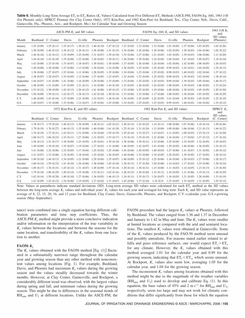
was developed. To further test this hypothesis, daily RHmin and U2

values for each study site were graphed in Figs. 2 and 3 to assessthe long-term magnitude and trend and possible effects of thebase values of RHmin and U2 on the performance of the FAO56 Kr

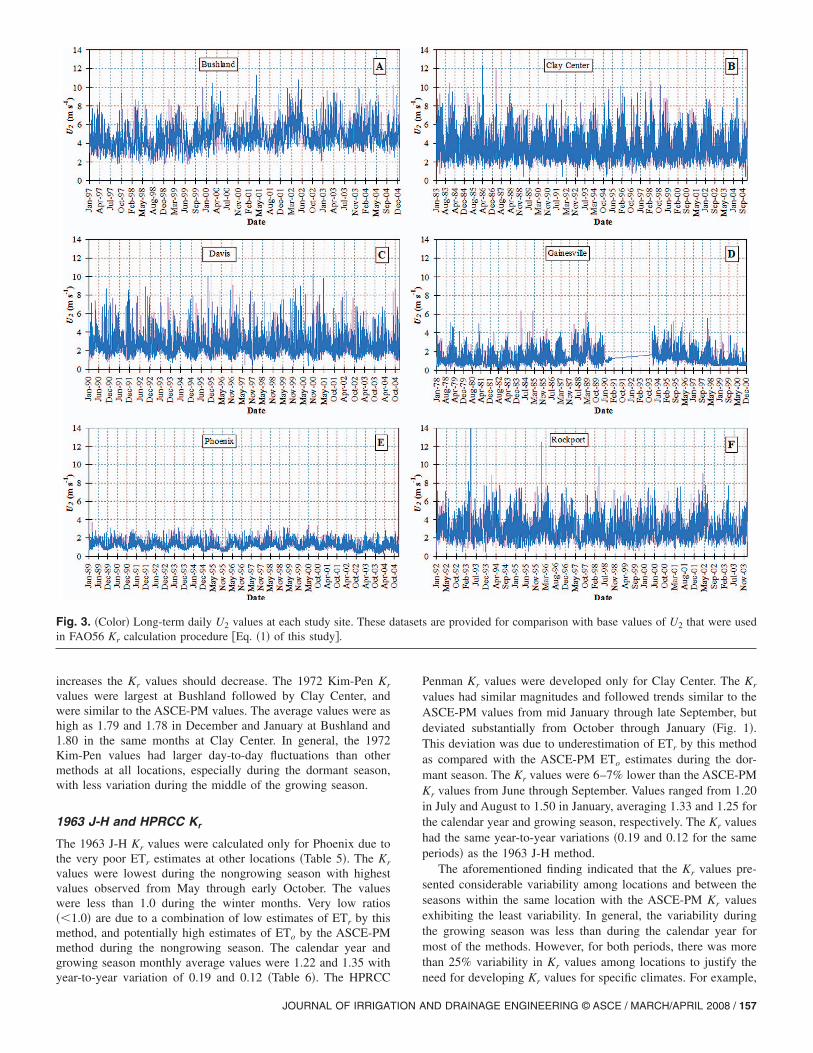
procedure in different climates. Usually, at Bushland and DavisRHmin is less than 45%, especially during the growing season�Fig. 2�. Fig. 3 indicates that U2 at Bushland is rarely below2 m s−1, whereas at Gainesville and Phoenix it rarely exceeds2 m s−1. At Rockport and Davis, U2 is less than 2 m s−1 approxi-mately 40% of the time. At Phoenix, RHmin is less than 45% about90% of the time. Therefore, for most of the time at this locationthe RHmin−45 and U2−2 terms in Eq. �1� would be either zero ornegative and Kr would only be a function of the coefficient C.Coefficient C alone cannot provide accurate or realistic Kr values.These findings suggest that the local calibration of Eq. �1� forRHmin and U2 for local climate will enhance its capability toprovide more realistic and consistent Kr values as compared to theASCE-PM Kr values.

1972 and 1982 Kim-Pen Kr

The Kr values from two Kimberly forms of Penman equationsshowed opposite trends. The 1972 Kim-Pen equation resulted inthe largest Kr values during the dormant �winter� season, anddecreased gradually towards the growing season �Fig. 1�. The1982 Kim-Pen produced the largest Kr values during the growingseason and decreased gradually towards winter. The oppositetrend in Kr values between the two equations might be due to acombination of differences in the wind functions used and theperformance in estimating ETr relative to the ASCE-PM ETr.Both Kim-Pen equations always resulted in Kr�1.0 with the low-est values obtained at the most humid location, Gainesville. Thegrowing season average Kr values were similar for both methods.The 1972 Kim-Pen method resulted in the closest Kr values com-pared with the ASCE-PM method at all locations. The 1972 Kim-Pen values were lowest during the growing season at Gainesville,and unlike other locations, this is the time of the year when thehighest RH occurs. Jensen et al. �1990� stated that as humidity

Fig. 2. �Color� Long-term daily RHmin values at each study site. These datasets are provided for comparison with base values of RHmin that wereused in FAO56 Kr calculation procedure �Eq. �1� of this study�.

156 / JOURNAL OF IRRIGATION AND DRAINAGE ENGINEERING © ASCE / MARCH/APRIL 2008

increases the Kr values should decrease. The 1972 Kim-Pen Kr

values were largest at Bushland followed by Clay Center, andwere similar to the ASCE-PM values. The average values were ashigh as 1.79 and 1.78 in December and January at Bushland and1.80 in the same months at Clay Center. In general, the 1972Kim-Pen values had larger day-to-day fluctuations than othermethods at all locations, especially during the dormant season,with less variation during the middle of the growing season.

1963 J-H and HPRCC Kr

The 1963 J-H Kr values were calculated only for Phoenix due tothe very poor ETr estimates at other locations �Table 5�. The Kr

values were lowest during the nongrowing season with highestvalues observed from May through early October. The valueswere less than 1.0 during the winter months. Very low ratios��1.0� are due to a combination of low estimates of ETr by thismethod, and potentially high estimates of ETo by the ASCE-PMmethod during the nongrowing season. The calendar year andgrowing season monthly average values were 1.22 and 1.35 withyear-to-year variation of 0.19 and 0.12 �Table 6�. The HPRCC

Penman Kr values were developed only for Clay Center. The Kr

values had similar magnitudes and followed trends similar to theASCE-PM values from mid January through late September, butdeviated substantially from October through January �Fig. 1�.This deviation was due to underestimation of ETr by this methodas compared with the ASCE-PM ETo estimates during the dor-mant season. The Kr values were 6–7% lower than the ASCE-PMKr values from June through September. Values ranged from 1.20in July and August to 1.50 in January, averaging 1.33 and 1.25 forthe calendar year and growing season, respectively. The Kr valueshad the same year-to-year variations �0.19 and 0.12 for the sameperiods� as the 1963 J-H method.

The aforementioned finding indicated that the Kr values pre-sented considerable variability among locations and between theseasons within the same location with the ASCE-PM Kr valuesexhibiting the least variability. In general, the variability duringthe growing season was less than during the calendar year formost of the methods. However, for both periods, there was morethan 25% variability in Kr values among locations to justify theneed for developing Kr values for specific climates. For example,

Fig. 3. �Color� Long-term daily U2 values at each study site. These datasets are provided for comparison with base values of U2 that were usedin FAO56 Kr calculation procedure �Eq. �1� of this study�.

JOURNAL OF IRRIGATION AND DRAINAGE ENGINEERING © ASCE / MARCH/APRIL 2008 / 157

the calendar year average values for the ASCE-PM were 1.46,1.43, 1.37, 1.21, 1.33, and 1.36 for Bushland, Clay Center, Davis,Gainesville, Phoenix, and Rockport. While the values were simi-lar for Bushland and Clay Center, they were about 7, 17, 8, and6% higher than the values for Davis, Gainesville, Phoenix, andRockport. Using one Kr value developed for a local climate usingone method in other climates could result up to a 20–25% differ-ence in estimating ET and Kc. The FAO56 procedure resulted inthe highest variability among locations for all methods. The Kr

values for Gainesville and Rockport calculated using the FAO56procedure were 25 and 22% lower than those for Bushland for thecalendar year, and 26 and 22% lower for the growing season.

Nongrowing „Dormant… Season ETref and Kr

Although, in many cases, the emphasis is on the growing seasonET and Kr values, the dormant season Kr and ETref values are ofinterest because they can be useful tools to asses the dormantseason evaporative demand of the atmosphere. As shown earlier,some of the methods produced some “potentially unrealistically”high �e.g., 1.78, 1.80� Kr values during the dormant periods. Thisis, in part, due to the unrealistic ETref estimations of the methods,including ASCE-PM ETr and ETo estimates. Allen et al. �1998�defined the dormant season as periods during which no agricul-tural crop has been planted. In temperate regions, the dormantseason may include periods of frost and continuously frozen con-ditions. Obviously the length of the dormant season varies amonglocations and it may be only 1 month or two at Gainesville or aslong as 6–7 months at other locations. The possible unrealisticestimates of the combination-based ETref equations have been ac-knowledged in the past. ASCE-EWRI �2005� stated that the ETfrom nonactive vegetation during dormant periods is generallyless than ETref because of the substantially increased surface re-sistance �rs�. While it is recognized that the ETref equations do notcompletely represent measurable quantities of evaporative de-mand of the air during dormant periods, the standardizedASCE-PM equation can still be useful as an evaporative index.The possible reasons for unrealistic ETref estimates by the com-bination methods can be a function of a combination of factors. Inaddition to the increased bulk surface resistance, rs, Jensen �2006,personal communication� suggested that the following conditionscontribute to unrealistic ETref estimates during dormant periods:�1� the change in the amount of daytime hours to nighttime hours;�2� the greater emphasis of the aerodynamic component of thecombination equation relative to the radiation component duringperiods with lower temperatures; and �3� unrealistic values of rs atlow temperatures. To address the greater effect of the aerody-namic component relative to the radiation component during pe-riods with lower temperatures, use of sum-of-hourly calculationsmay reduce the effect somewhat. The impacts of using 24 h av-erage weather data to predict ET that occurs mainly over approxi-mately an 8 h period also introduces errors during winter. Irmaket al. �2005� suggested that there is a benefit and potentialimprovement in accuracy when the standardized ASCE-PM pro-cedure is applied hourly instead of daily for ETref estimates, es-pecially during the dormant seasons. The hourly application helpsto account for impacts of abrupt changes in atmospheric condi-tions on ETref estimation.

Jensen �2006, personal communication� further stated that theunrealistic values of rs at low temperatures could affect ETr morethan ETo. Perhaps a rational approach for ETr would be to arbi-trarily increase the rs when temperatures fall below values thatcan sustain or mimic actively growing vegetation. This could be

based on alfalfa growth characteristics if the rs data are availableduring dormant periods. Also, one could assume that the vegeta-tion height �effective roughness� decreases either suddenly orgradually to some low base value such as 0.05 m as cold tem-peratures occur. The rs would be decreased following rains thatcause wet surface conditions. Furthermore, the calculation of Rn

during the growing season assumes an albedo ��� value of 0.23for a green vegetation surface, which is not realistic during dor-mant periods. Experimental knowledge and adequate proceduresto estimate soil heat flux �especially for hourly calculations� dur-ing freezing conditions are lacking. Thus, the “standardized” ref-erence surface conditions now used in the “standardized”ASCE-PM equation are not met during dormant periods, resultingin potentially unrealistic estimates of Kr values. The effect of thepotentially unrealistically high estimates of Kr values on ETref

estimates during the dormant period rather than growing seasonshould be lower than one would expect due to low ETr and ETo

values during the dormant periods. Nevertheless, information islacking on the “true” performance of the ETref estimates and“true” values of the Kr as determined by the combination equa-tions, including the ASCE-PM estimates during the dormant pe-riods. The analyses and comparisons of the dormant period ET bycombination methods against measured data and developing ro-bust methodologies to quantify dormant season ET and Kr areneeded.

Conclusions

The Kr coefficients that can enable conversions from ETr to ETo,or vice versa, were developed for six locations differing in cli-matic characteristics. The first approach of developing Kr valueswas ASCE-PM ETr to ETo ratios, and the second was the equa-tion proposed in FAO56 as a function of RHmin, U2, and a coef-ficient. The variability in Kr values among locations was large,suggesting the need to develop Kr values for a local region. Forexample, the Kr values developed with the ASCE-PM method inJuly were 1.38, 1.27, 1.32, 1.11, 1.28, and 1.19, for Bushland,Clay Center, Davis, Gainesville, Phoenix, and Rockport, respec-tively. In general, the variation in growing season Kr values wasless than for the calendar year. The magnitude of variation amonglocations was less for the ASCE-PM Kr values than for othermethods at all locations. The variability among locations waslarger for the FAO56 method, especially for areas with low rela-tive humidity and high wind speeds. Our findings suggest that thelocal calibration of this approach for minimum relative humidityand wind speed for local climate will enhance its capability toprovide more realistic and consistent Kr values as compared to theASCE-PM Kr values. In general, year-to-year variability in Kr forthe same location was low. The differences also varied substan-tially among locations for a given method, with the differencebeing lower when the ASCE-PM Kr values were used. Some ofthe methods produced high and “potentially” unrealistic Kr valuesduring the dormant periods. One can normally expect these veryhigh Kr values under conditions of very strong wind and verylarge VPD. However, the VPD during winter is not extremelylarge in some of the locations studied. Potentially unrealistic Kr

values might be due to inaccuracies in the ETref calculations dur-ing winter months. Because simultaneous and direct measure-ments of the ETr and ETo values rarely exist, it appears that theapproach of ETr to ETo ratios calculated with the ASCE-PMmethod is currently the best approach available to derive Kr val-ues for locations where these measurements are not available. The

158 / JOURNAL OF IRRIGATION AND DRAINAGE ENGINEERING © ASCE / MARCH/APRIL 2008

Kr values developed in this study can be useful for making con-versions from ETr to ETo, or vice versa, to enable using cropcoefficients developed for one reference surface with the other todetermine actual crop water use for locations, with similar cli-matic characteristics of this study, when locally measured Kr val-ues are not available.

Acknowledgments

A contribution of the University of Nebraska-Lincoln AgriculturalResearch Division, Lincoln, Nebraska, Journal Series No. 15160.The mention of trade names or commercial products is solely forthe information of the reader and does not constitute an endorse-ment or recommendation for use by the University of Nebraska-Lincoln or the USDA Agricultural Research Service.

References

Allen, R. G. �1996�. “Assessing integrity of weather data for referenceevapotranspiration estimation.” J. Irrig. Drain. Eng., 122�2�, 97–106.

Allen, R. G., Pereira, L. S., Raes, D., and Smith, M. �1998�. “Crop evapo-transpiration. Guidelines for computing crop water requirements.”FAO Irrig., and Drain. Paper No. 56, Rome, Italy.

Allen, R. G., Smith, M., Perrier, A., and Pereira, L. S. �1994�. “An updatefor the definition of reference evapotranspiration.” ICID Bulletin,43�2�, 1–34.

ASCE Environmental and Water Resources Institute �EWRI�. �2005�.“The ASCE standardized reference evapotranspiration equation.”Standardization of Reference Evapotranspiration Task CommitteeFinal Rep., R. G. Allen, I. A. Walter, R. L. Elliot, T. A. Howell, D.Itenfisu, M. E. Jensen, and R. L. Snyder, eds., ASCE, Reston, Va.

AZMET. �2006�. Arizona meteorological network, �http://ag.arizona.edu/azmet� �November 2006�.

Burman, R. D., and Pochop, L. O. �1994�. “Evaporation, evapotranspira-tion and climate data.” Developments in atmospheric science, Vol. 22,Elseiver Science, Amsterdam, The Netherlands.

CIMIS. �2006�. “California irrigation management information system.”�http://www.cimis.water.ca.gov� �November 2006�.

Doorenbos, J., and Pruitt, W. O. �1977�. “Guidelines for prediction ofcrop water requirements.” FAO Irrig., and Drain. Paper No. 24, re-vised, Rome, Italy.

Droogers, P., and Allen, R. G. �2002�. “Estimating reference evapotrans-piration under inaccurate data conditions.” Irrig. Drain. Syst., 16,33–45.

Erpenbeck, J. M. �1981�. “A methodology to estimate crop water require-ments in Washington State.” MS thesis, Washington State Univ., Pull-man, Wash.

Evett, S. R., Howell, T. A., Todd, R. W., Schneider, A. D., and Tolk, J. A.�2000�. “Alfalfa reference ET measurement and prediction.” Proc. 4thDecennial National Irrig. Symp., ASAE, St. Joseph, Mich., 266–272.

HPRCC. �2006�. High Plains Regional Climate Center, �http://

www.hprcc.unl.edu� �November 2006�.Hubbard, K. G. �1992�. “Climatic factors that limit daily evapotranspira-

tion in sorghum.” Climate Research, 2, 73–80.Irmak, S., Howell, T. A., Allen, R. G., Payero, J. O., and Martin, D. L.

�2005�. “Standardized ASCE-Penman-Monteith: Impact of sum-of-hourly vs. 24-h timestep computations at reference weather stationsites.” Transactions of the ASABE, 48�3�, 1063–1077.

Irmak, S., Irmak, A., Allen, R. G., and Jones, J. W. �2003�. “Solar and netradiation-based equations to estimate reference evapotranspiration inhumid climates.” J. Irrig. Drain. Eng., 129�5�, 336–347.

Itenfisu, D., Elliot, R. L., Allen, R. G., and Walter, I. A. �2003�. “Com-parison of reference evapotranspiration calculations as part of theASCE standardization effort.” J. Irrig. Drain. Eng., 129�6�, 440–448.

Jensen, M. E. �1969�. “Scheduling irrigations using computers.” ArabWat. World, 24�8�, 193–195.

Jensen, M. E., Burman, R. D., and Allen, R. G. �1990�. “Evapotranspira-tion and irrigation water requirements.” ASCE Manuals and Reportson Engineering Practices No. 70, ASCE, New York.

Jensen, M. E., and Haise, H. R. �1963�. “Estimating evapotranspirationfrom solar radiation.” J. Irrig. and Drain. Div., 89, 15–41.

Kincaid, D. C., and Heerman, D. F. �1974�. “Scheduling irrigations usinga programmable calculator.” USDA-ARS Rep. No. ARS-NC-12,USDA, Phoenix.

Penman, H. L. �1948�. “Natural evaporation from open water, bare soiland grass.” Proc. R. Soc. London, Ser. A, 193, 120–146.

Snyder, R. L., and Pruitt, W. O. �1985�. “Estimating reference evapo-transpiration with hourly data.” California Irrigation Management In-formation System Final Rep., Land, Air and Water Resources PaperNo. 10013-A, Chap. VII, Vol. 1, Univ. of California, Davis, Calif.

Snyder, R. L., and Pruitt, W. O. �1992�. “Evapotranspiration data man-agement in California.” Proc. ASCE Water Forum ’92, Irrig. andDrain. Session, ASCE, New York, 128–133.

Temesgen, B., Allen, R. G., and Jensen, D. T. �1999�. “Adjusting tem-perature parameters to reflect well-watered conditions.” J. Irrig.Drain. Eng., 125�1�, 26–33.

Walter, I. A., et al. �2001�. “The ASCE standardized reference evapo-transpiration equation.” Standardization of Reference Evapotranspira-tion Task Committee Rep., Environmental and Water ResourcesInstitute �EWRI� of ASCE.

Wright, J. L. �1982�. “New evapotranspiration crop coefficients.” J. Irrig.and Drain. Div., 108�IR2�, 57–74.

Wright, J. L. �1996�. “Derivation of alfalfa and grass reference evapo-transpiration.” Evapotranspiration and Irrigation Scheduling: Proc.,International Conf., Irrigation Association and International Commit-tee on Irrigation and Drainage, C. R. Camp, E. J. Sadler, and R. E.Yoder, eds., American Society of Agricultural Engineers, St. Joseph,Mich.

Wright, J. L., Allen, R. G., and Howell, T. A. �2000�. “Conversion be-tween evapotranspiration references and methods.” Proc. 4th Decen-nial National Irrigation Symp., American Society of Agricultural En-gineers, St. Joseph, Mich.

Wright, J. L., and Jensen, M. E. �1972�. “Peak water requirements ofcrops in Southern Idaho.” J. Irrig. and Drain. Div., 96�IR1�, 193–201.

JOURNAL OF IRRIGATION AND DRAINAGE ENGINEERING © ASCE / MARCH/APRIL 2008 / 159