Vapour-liquid equilibria of stockmayer fluids

Downloaded from UvA-DARE, the institutional repository of the University of Amsterdam (UvA)http://hdl.handle.net/11245/2.29993

File ID uvapub:29993Filename 135266y.pdfVersion unknown

SOURCE (OR PART OF THE FOLLOWING SOURCE):Type articleTitle Vapour-liquid equilibria of Stockmayer fluids: computer simulations and

perturbation theory.Author(s) M.E. van Leeuwen, B. Smit, E.M. HendriksFaculty UvA: UniversiteitsbibliotheekYear 1993

FULL BIBLIOGRAPHIC DETAILS:  http://hdl.handle.net/11245/1.427374

Copyright It is not permitted to download or to forward/distribute the text or part of it without the consent of the author(s) and/orcopyright holder(s), other than for strictly personal, individual use, unless the work is under an open content licence (likeCreative Commons). UvA-DARE is a service provided by the library of the University of Amsterdam (http://dare.uva.nl)(pagedate: 2014-11-27)

MOLECULAR PHYSICS, 1993, VOL. 78, No. 2, 271-283

Vapour-liquid equilibria of Stockmayer fluids

Computer simulations and perturbation theory

By M. E. VAN LEEUWEN, B. SMIT and E. M. HENDRIKS

Koninklijke/Shell-Laboratorium, Amsterdam, P.O. Box 3003, 1003 AA Amsterdam, The Netherlands

(Received 16 April 1992; accepted 1 July 1992)

Gibbs ensemble simulation data for Stockmayer fluids with #.2 = 3.0 and #.2 = 4.0 in the reduced temperature range of 0-77 (resp. 0.80)-0"98 and pre- sented and compared with predictions based on the perturbation theories of Stell, G., Rasaiah, J. C., and Narang, H., 1972, Molec. Phys., 23, 393; 1974, 27, 1393. The description of the reference fluid is improved by applying the mod- ified Benedict-Webb-Rubin equation of state instead of the Verlet-Weis imple- mentation of the Weeks-Chandler-Andersen perturbation scheme. Second virial coefficients predicted by perturbation theory to order #4 agree for Stock- mayer fluids with #,2 < 4 very well with exact values. Perturbation theory is capable of describing the low-density region of Stockmayer fluids with rather strong dipole moments. For these high values of the dipole moment, the Pad6 approximation of perturbation theory deviates significantly from the simulated coexistence curves in density and pressure. Compared with perturbation theory to order #4, however, it is a far better approximation of the Stockmayer fluid coexistence curve. The behaviour of the Pad6 approximation in the critical region is not satisfactory.

1. Introduction

Electrostatic interactions affect thermodynamic behaviour. For relatively simple polar model fluids several theories have been developed [1-3]. A convenient model for a polar fluid is a 'soft-core' dipolar molecule, represented by the Stockmayer potential (Lennard-Jones potential with an embedded point dipole). The two most important molecular theories for model polar fluids are integral equation theories and (Pople-Stell) perturbation theories.

If the Ornstein-Zernike equation is supplemented with an approximate closure relation, an integral equation is obtained for the direct correlation function and the radial distribution function [2]. For polar fluids this involves expansions of angular- dependent functions. Starting from the well known hypernetted-chain equation Patey and others [4-6] considered linear expressions (LHNC) and quadratic expressions (QHNC), and obtained a numerically tractable scheme. Fries and Patey [7] devel- oped a general method for fluids with anisotropic interactions, the reference hypernetted-chain (RHNC) theory. Lee et al. [8] applied this approximation to Stockmayer fluids, and found that the dielectric constant predicted with the full RHNC theory agrees better with computer simulation results than those predicted with the LHNC and QHNC theories.

Another approach to describe the behaviour of simple polar model fluids is the use of perturbation theories, as pioneered by Pople and further developed by Stell et al. [9-13]. In these theories, the free Helmholtz energy is expressed as the sum of a

0026-8976/93 $I0.00 �9 1993 Shell Research BV

272 M.E. van Leeuwen et al.

reference term and perturbation terms. For the Stockmayer fluid, it is convenient to use the Lennard-Jones fluid as a reference fluid and to make an expansion in terms of the dipole moment #. Perturbation theories have practical advantages: they are easier to apply than integral theories and they provide a tool for understanding the influence of a perturbation on thermodynamic behaviour. For thermodynamic purposes, the accuracy of the Pad6 approximation proposed by Stell et al. [12] has been found to be surprisingly high, considering the small number of terms used [14-17].

Molecular theories can be validated with 'exact' results from simulation exper- iments. For pure Stockmayer fluids, computer simulations of thermodynamic single- phase data were reported in references [17-21]. Static dielectric constants derived from computer simulations have been reported in references [22-26]. These results have been reviewed by de Leeuw et al. [27]. Since the availability of the Gibbs ensemble (Monte Carlo) simulation technique, introduced by Panagiotopoulos [28], some preliminary results concerning coexistence curves for Stockmayer fluids with low reduced dipole moment [29] have been reported. Mixtures of polar/non polar fluids have been investigated by de Leeuw et al. [30-32]. Mixtures of polar and polarizable Lennard-Jones fluids have been investigated by Mooij et al. [33].

Most computer simulations have been performed for lower values of the dipole moment. Because we are interested in the description of fluids with a realistic range of dipole moments, we wish to investigate for which value of the dipole moment the theories are valid. Smit et al. [29] have reported vapour-liquid equilibria calculations for Stockmayer fluids with reduced dipole moments #,2 ___ 1-0 and #,2 = 2.0 (the reduced dipole moment #* is defined as x~2/ea 3, where e and cr are the Lennard- Jones parameters). Here we present simulation results for Stockmayer fluids with # ,2= 3-0 and #,2 = 4.0 for the reduced temperature range of 0.77 (resp. 0.80) to 0-98. In addition to these simulation results, we offer an extensive comparison with the thermodynamic results predicted by the perturbation theory of Stell et al. [11,121.

2. Theory

In this section we review the essential aspects of the perturbation theory of Stell et al. [11, 12]. In our calculations, we have followed Stell's approach, except for the description of the reference fluid. We compare exact results for second virial coef- ficients with predictions from perturbation theory.

2.1. Pople -S te l l perturbation theory

The central idea of perturbation theory is to use a reference fluid with well known thermodynamic properties and to consider the potential of the 'actual' fluid as a (small) perturbation on a reference potential. This gives for the free energy f of a dipolar fluid:

f = fo + #2fl. + #4f2g 6 u + #'if + o(uS). (1)

For the Stockmayer potential, the term fl u vanishes by integration over angular coordinates (due to axial symmetry properties of the dipole field) [9], so that #4f2~ is the first non vanishing correction term. The superscript # indicates that only dipole-dipole interactions are taken into account.

Vapour-liquid equilibria o f Stockmayer fluids 273

For small values of #, it can be expected that only the #4 term gives a significant contribution to the free energy:

fo (u ~) = f u + u4f2#. (2)

Superscript LJ refers to the Lennard-Jones (reference) system. Stell et al. [11] give as expression for the perturbation term:

#.4 ~3#4f2u = 24T* (4/3uU - AzU)' (3)

where/3 = 1/knT, T* = knT/e , u is the internal energy, and Az(= 13pip - l) is the excess compressibility factor.

For #* > 1 we cannot expect this expansion to converge. This is a range of #* relevant to many real fluids [15-17]. In order to make a 'practical' estimate of these higher order terms, Stell et at. [12] use a (0, 1) Pad6 approximation:

f e ~ = f L J +/z - - , (4) 1 _ ~_Y_s .'f? /

where #6f3u represents the second correct term (0(#6)), which involves the three- particle distribution function g123. To estimate this term, Stell et al. used a par- ametrization of the hard-sphere data of Barker et al. [34]:

fl.3#,6p.2 "2"70797 + 1 "68918x -- 0"31570X 2] /3#6f3u = 9c 3 ] 7 0~90---~-xx ~ ~ ' 2 ~ ] ' (5)

where x = p*c 3 and c = a/cr, a being the hard-sphere diameter. We have used the same procedure as Stell et al. to obtain the hard-sphere diameter, taken from Verlet and Weis [35].

2.2. The reference term

In expressions (2-4) it is assumed that the free energy of the Lennard-Jones fluid is known accurately. The thermodynamics of a Lennard-Jones fluid determines fLJ and, through equation (3), #4f2u. For the Lennard-Jones fluid, Stell et al. based their calculations on the Verlet-Weis implementation [35] of the WCA perturbation theory given by Weeks, Chandler and Anderson [36]; some of their calculations were based on early computer simulation results.

Later, Nicolas et al. [37] published an analytical equation of state, the 33- parameter modified Benedic t -Webb-Rubin (MBWR) equation of state, that repro- duces Lennard-Jones computer simulation results (known until then). We have used this equation of state for the description of the reference fluid in the perturbation theory, in order to calculate coexistence properties and second virial coefficients of Stockmayer fluids.

2.3. Second virial coefficients

The second virial coefficient can be calculated to any desired accuracy via a converging series expansion of the classical statistical mechanical expression (equation (2.1) of reference [38]). Therefore, we can compare these exact results

274 M . E . van Leeuwen et al.

with predictions from perturbation theory even before we perform any computer simulations. This comparison will indicate if we can expect reasonable results from perturbation theory in the low-density region.

In the low-density limit of the second virial coefficient, the second correction term (of order #6) vanishes for dipolar molecules [39]. The second virial coefficient via the (0, 1) Pad6 approximation therefore reduces to that of first-order perturbation theory. The reduced second virial coefficient is calculated with

B.O(#4 ) -~ B *LJ #,4 ( 0B.LJ'~ 24T* B*LJ + 4 T * ~ / o r ,]' (6)

where B* = B/bo with b0 = 27rNaa 3. B *LJ is given by equation (5) of reference [37], NA is Avogadro's number. (We use the asterisk (,) to indicate reduction of quantities by means of the simplest combinations of e and a, and the star (,) to indicate reduction with respect to combinations of e and a which make use of hard-sphere values. The reduced second virial coefficients are related via B* = 27rB*,)

For various values of #*, we compare in figure 1 B *~ with the second virial coefficients calculated via the classical statistical mechanical expression for the Stockmayer potential. For #.2 < 4, perturbation theory predicts second virial coef- ficients very close to their exact values. With increasing #* deviations become increasingly apparent at low T*, which is in agreement with data of Pople [40].

The description of the second virial coefficient of the Lennard-Jones fluid in equation (6) is accurate, as the exact expression for B *LJ has been taken explicitly into account in the fitting procedure to obtain the MBWR equation of state. Apparently, the next term in the series expansion (of order #8) is small.

This observation leads to the following conclusion: perturbation theory is capable of describing the low-density region of Stockmayer fluids with #.2 < 4.

0 ' / / / / / / I 1 1 1

0.0 1.0 2.0 3.0 4.0 5.0 6.0 7.0 8.0 T"

Figure 1. Second virial coefficients of a Stockmayer fluid with #,2 ranging from 1 to 6. The solid curves ar~,exact; the data points are predicted values from perturbation theory: �9 = 1; [], = 2; zX, #'2 = 3; ~, #'2 = 4; V, #'2 = 5; + ,#*2=6.

Vapour-liquid equilibria of Stockmayer fluids 275

3. Computer simulations

Using the Gibbs ensemble [28], one can obtain data on coexisting vapour and liquid phases from a single simulation. Two phases are simulated in two separate subvolumes, to each of which periodic boundary conditions are applied. By choosing appropriate acceptance criteria in the Monte Carlo steps, one ensures that the two phases have the same temperature, pressure and chemical potential. These conditions are necessary and sufficient for thermodynamic equilibrium. The Gibbs ensemble is particularly suited for the calculation of two-phase equilibria. To impose the conditions of internal and mutual equilibrium on the two phases, one has to perform the following Monte Carlo steps: particle displacements, volume changes, and particle interchanges. A detailed description of this simulation technique can be found elsewhere [28,41,42]. It has been applied to many pure model fluids [28], [42-49]. For mixtures of various model fluids, vapour-liquid equilibria have been reported in [30-33], [42, 50, 51], and liquid-liquid equilibria in [50-54].

In our simulations, the Lennard-Jones potential was truncated at half the box size and the standard long-tail corrections were added [55]. The long-range dipolar interactions were handled with the Ewald summation technique using 'tinfoil' boundaries [27]. We used the same simulation procedure as reported in [29], except for the order of the Monte Carlo steps in the simulation cycle. Previously, trial configurations were generated according to a prescribed order: successive particle displacements, one volume change, successive particle exchanges. This scheme does not ensure microscopic reversibility. In the work presented here, at each Monte Carlo step the type of change is chosen at random. One cycle consists of (on average) Ndisp attempts to displace a random particle in one of the randomly chosen boxes, Nvol attempts to change the volume of the subsystems, and Nt~y attempts to exchange particles between the boxes. By applying this algorithm (explained in detail in reference [48]), the condition of detailed balance is fulfilled and there is no ambi- guity about the point of the cycle at which the ensemble should be sampled (i.e., after which Monte Carlo step the relevant data are collected with which the statistical averages are obtained). Furthermore, with respect to the scheme used earlier [29], the chance that the system becomes trapped in a metastable region is lowered [41], and the standard deviation in the chemical potential is significantly smaller [56].

In each run, Naisp was equal to the total number of molecules, and Nvol was always set to 1. Ntry was set to 200 for the lowest temperatures and was lowered to 50 for the highest temperatures. Per run, the total number of successful inter- changes always exceeded 5000. Error estimates were obtained by dividing the total simulation into 10 blocks, and calculating the standard deviations from block averages.

4. Results

4.1 Simulation results

The results of the Gibbs ensemble simulations are given in tables 1 and 2; the coexistence curves are shown in figures 2-5. The critical temperature and density are estimated from fitting the simulation results to the (mean-field approximation of the) law of rectilinear diameters and to a scaling law for the density [46] with critical exponent/3 = 0.32 [57]. These values are given in table 3, together with reported

276 M . E . van Leeuwen et al.

O ~

,,..4

Q

x ~ A X

X~" .......... �9 i . . . . . . . . . . A , X

-bg ".. ", ~ . i ~ " ~ " "A "•

,~,~ - q : ...

'\

\

o.oo 01 5 0'.50 o'.7s .oo p~

Figure 2. Coexistence curve for the Stockmayer fluid with/~,2 = 1. The results from Monte Carlo simulations in the Gibbs ensemble are taken from [29] (O, coexistence data points; O, averaged densities), the solid line connecting them results from the estimation of the critical temperature and density. For the perturbation theory results presented in this report, the calculations for the reference (Lennard-Jones) fluid are based on the MBWR equation of state of Nicolas et aL [37]. The dashed line represents results of perturbation theory to order /~4 (equation (2)), the dotted line results of the Pad6 approximation (equation (4)). Stell et al. based their calculations for the reference fluid on the Verlet- Weis perturbation scheme; their data points are represented as: x, 0(#4); and A, Pad6 approximation.

values for #,2 = 0 (Lennard-Jones fluid) [56], #,2 = 1, and #,2 = 2 [29]. In figure 6 the simulated coexistence (vapour) pressures are shown.

4.2. Perturbation theory results

We have calculated coexistence curves for various dipolar strengths with the perturbation theory of Stell et al. The results (for both the first-order theory and the Pad6 approximation) are presented in figures 2 -5 together with the simulation results. For comparison, we also included in figure 2 the original results of Stell et al., based on the Verlet-Weis implementation of WCA perturbation theory. In figure 6 the simulated coexistence (vapour) pressures are compared with the predictions based on the Pad6 approximation.

5. Discussion

5.1. First-order perturbation theory

First-order perturbation theory or, to be more exact, perturbation theory to order #4, treats the polar interactions as a one-term perturbation on interactions of the Lennard-Jones reference fluid (equation (2)). As may be expected for higher

Vapour-liquid equilibria of Stockmayer fluids 277

O~

I I �9 CO �9 I �9

�9 �9 I �9

1 ~ I ! �9 I ! �9

a . � 9 " . ' . " " " �9 - � 9 11, �9 I , - " " ' . I ' " . . , �9

~./ , .-" ~ i ' "'- , /

I I �9 , ; I �9 # �9 �9 , :

, - , - ,~ / , I ~ ', ~ - ,

~ F / f ; 7- ',

0.00 0.25 0.50 0.75 1.00 p"

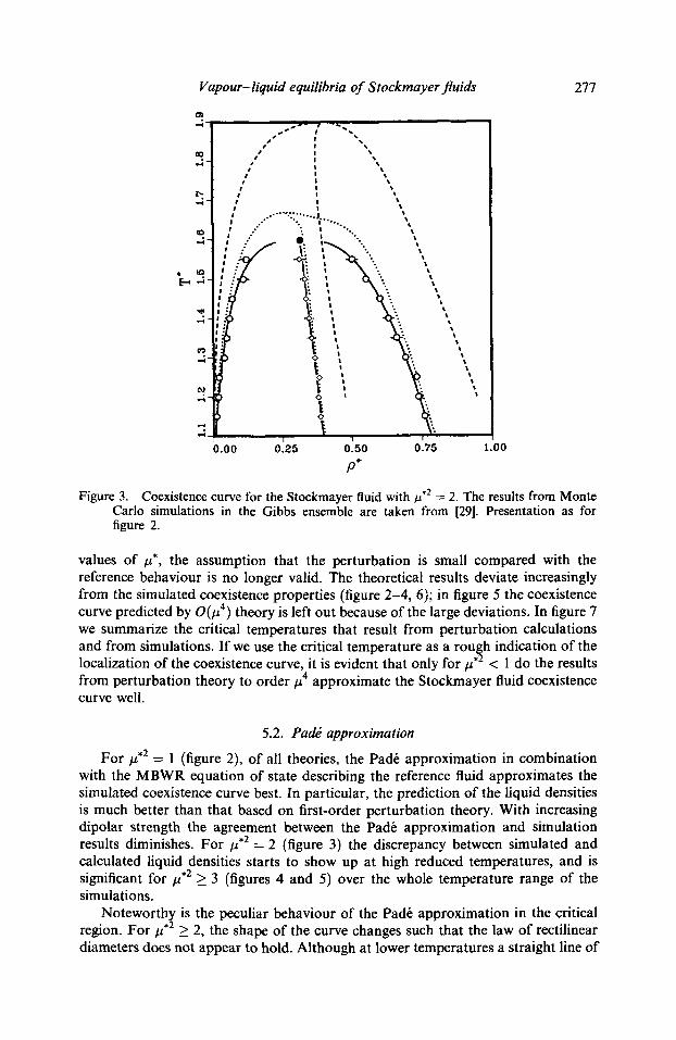
Figure 3. Coexistence curve for the Stockmayer fluid with #,2 = 2. The results from Monte Carlo simulations in the Gibbs ensemble are taken from [29]. Presentation as for figure 2.

values of #*, the assumption that the perturbation is small compared with the reference behaviour is no longer valid. The theoretical results deviate increasingly from the simulated coexistence properties (figure 2-4, 6); in figure 5 the coexistence curve predicted by O(# 4) theory is left out because of the large deviations. In figure 7 we summarize the critical temperatures that result from perturbation calculations and from simulations. I f we use the critical temperature as a rough indication of the localization of the coexistence curve, it is evident that only for #.2 < 1 do the results from perturbation theory to order #4 approximate the Stockmayer fluid coexistence curve well.

5.2. Pad~ approximation

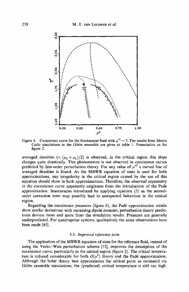
For #.2 = 1 (figure 2), of all theories, the Pad6 approximation in combination with the MBWR equation of state describing the reference fluid approximates the simulated coexistence curve best. In particular, the prediction of the liquid densities is much better than that based on first-order perturbation theory. With increasing dipolar strength the agreement between the Pad6 approximation and simulation results diminishes. For #,2 = 2 (figure 3) the discrepancy between simulated and calculated liquid densities starts to show up at high reduced temperatures, and is significant for #,2 _> 3 (figures 4 and 5) over the whole temperature range of the simulations.

Noteworthy is the peculiar behaviour of the Pad6 approximation in the critical region. For #,2 _> 2, the shape of the curve changes such that the law of rectilinear diameters does not appear to hold. Although at lower temperatures a straight line of

278 M.E. van Leeuwen et al.

0

i s

/ !

% ~ o /

I . . . . " : ' . . . . t : .." ".. " " . . . t

I .." . . . " .~ . . . .." ". " . . . �9

" y "# , "~- ~ ~

~ "~.

,.~ - , ~

' I i t ~ r

.oo 01zs o15o o17 1.oo p"

Figure 4. Coexistence curve for the Stockmayer fluid with , 2 = 3. The results from Monte Carlo simulations in the Gibbs ensemble are given in table 1. Presentation as for figure 2.

averaged densities (= (Pa + pL)/2) is observed, in the critical region this slope changes quite drastically. This phenomenon is not observed in coexistence curves predicted by first-order perturbation theory. For any value of/z .2 a curved line of averaged densities is found. As the MBWR equation of state is used for both approximations, any irregularity in the critical region caused by the use of this equation should show in both approximations. Therefore, the observed asymmetry in the coexistence curve apparently originates from the introduction of the Pad6 approximation. Inaccuracies introduced by applying equation (5) as the second- order correction term may possibly lead to unexpected behaviour in the critical region.

Regarding the coexistence pressures (figure 6), the Pad6 approximation results show similar deviations: with increasing dipole moment, perturbation theory predic- tions deviate more and more from the simulation results. Pressures are generally underpredicted. For quadrupolar systems, qualitatively the same observations have been made [45].

5.3. I m p r o v e d reference term

The application of the MBWR equation of state for the reference fluid, instead of using the Verlet-Weis perturbation scheme [12], improves the description of the coexistence curve, particularly in the critical region (figure 2). The critical tempera- ture is reduced considerably for both 0 (# 4) theory and the Pad6 approximation. Although the latter theory best approximates the critical point as estimated via Gibbs ensemble simulations, the (predicted) critical temperature is still too high.

Vapour-liquid equilibria of Stockmayer fluids

c~

279

0

0.0

�9 ~ ~ "'"'""'".....

0.2 0.4 0.6 p"

0.8

Figure 5. Coexistence curve for the Stockmayer fluid with #.2 = 4. The results from Monte Carlo simulations in the Gibbs ensemble are given in table 2. The coexistence curve predicted by perturbation theory to order #4 is not plotted in the figure, because of the large deviations�9 Presentation as for figure 2.

This can be assigned-at least part ly- to the overestimation of the critical temperature of the Lennard-Jones fluid by the MBWR equation of state. This equation was based upon computer simulation results from various sources. In most cases conventional (molecular dynamics and Monte Carlo) simulations were used to generate equilib- rium data. The critical temperature of the Lennard-Jones fluid estimated in the canonical ensemble is overestimated due to finite-size effects [58]. In the Gibbs ensemble finite-size effects partly cancel, and the simulations yield a better estimate of the critical point [41]. The MBWR equation of state is constrained to satisfy the critical point conditions (estimated via conventional simulations) and yields T c = 1 "35 whereas, from more recent Gibbs ensemble simulations [28, 56], it follows t h a t T ; LJ ~ 1.316-4-0.006. If plenty of accurate Lennard-Jones data become avail- able, to which the MBWR equation of state can be refitted, this should further improve the description of the Stockmayer fluid with perturbation theory.

6. Conclusion

We have presented Gibbs ensemble simulation data for the Stockmayer fluid with /z .2 = 3.0 and #,2 = 4.0, and compared these with predictions based on perturbation theories devised by Stell et al. [11, 12].

The perturbation theory second virial coefficients agree well with exact values�9 Perturbation theory is capable of describing the low-density region of Stockmayer fluids with #,2 < 4. For high values of the dipole moment, the Pad6 approximation

280 M . E . van Leeuwen et al.

iQ

i

0 . 4 0 . 6

�9 . . . �9

% ~z, ~ "-~h \ '#,++ ..,_ %

, . . . .. �9 ".1~• ~. ', ,,-,, "-..~, ..~. ~',-,o..., ,, 4,,... 4 , , -~ "4. \ '_ J "..., ~-.,~ , "~..

~ ".)�9 %. ", "...

i i

O . B 1 . 0

l/T*

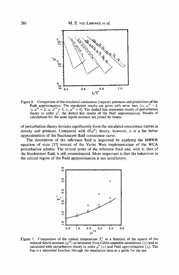
Figure 6. Comparison of the simulated coexistence (vapour) pressures and predictions of the Pad6 approximation. The simulation results are given with error bars (�9 # , 2 = 1; n, #,2 = 2; A, #,2 = 3; <>, #.2 = 4). The dashed line represents results of perturbation theory to order #4, the dotted line results of the Pad6 approximation. Results of calculations for the same dipole moment are joined by braces.

o f pe r tu rba t ion theory deviates significantly f rom the s imulated coexistence curves in density and pressure. C o m p a r e d with 0 ( # 4) theory, however , it is a far bet ter a pp rox ima t ion of the S tockmayer fluid coexistence curve.

The descript ion o f the reference fluid is improved by applying the M B W R equat ion of state [37] instead of the Ver le t -Weis implementa t ion of the W C A per tu rba t ion scheme. The critical poin t o f the reference fluid and, with it, that o f the S tockmayer fluid, is still overest imated. M o r e impor t an t is tha t the behav iour in the critical region o f the Pad6 app rox ima t ion is not satisfactory.

0

o

Q A

1~.0 L , , 0 . 0 2 . 0 3 . 0 4 . 0 5 . 0 * 2

Figure 7. Comparison of the critical temperature T~* as a function of the square of the reduced dipole moment (#,2) as estimated from Gibbs ensemble simulations (�9 and as calculated with perturbation theory to order/z 4 (<>) and Pad6 approximation (A). The line is a smoothed function through the simulation data as a guide for the eye.

Vapour-liquid equilibria of Stockmayer fluids 281

Table 1. Results of the Monte Carlo simulations in the Gibbs ensemble for the Stockmayer fluid with . 2 = 3.0. N is the number of particles used in the simulation, T* denotes the reduced temperature (= knT/e!, p* the reduced particle density (= pa3), p* denotes the reduced pressure (= pa3/e), E is the reduced internal energy (= E/e), #' denotes the reduced residual chemical potential. Subscripts G and L refer to the gas and the liquid phase, respectively. The number of cycles was 5000 for all runs.

Gas Phase Liquid Phase

N T* pb ~ e~ ub p~ e~ E~ ~s

216 1.40 0"0174 0"0204 -0"52 -6"22 0"731 0-023 -8"71 -61 216 1-45 0"0243 0"0284 -0'61 -6-01 0"711 0"054 -8-41 -6"26 216 1"50 0"0356 0"0374 -0"92 -5'82 0-6879 0"053 - 8 " 2 1 -6"07 216 1"55 0"0446 0-0475 - 1 " 0 1 -5"81 0"661 0"054 -7"91 -5"94 216 1"60 0 '0538 0"0566 -1.22 -5-71 0"621 0-054 -7-41 -5"94 216 1"65 0-07 t 0-0707 -1"63 -5"71 0"602 0"072 -7"22 -5"85 512 1"70 0"101 0"0936 -2"02 -5'61 0-571 0'103 -6"81 -5-6s 512 1-75 0"112 0"101 -2"03 -5-618 0"512 0"113 -6"32 -5"52 512 1"775 0"142 0.121 -2"54 -5"51 0'503 0-123 -6"22 -5'94

Table 2. Results of the Monte Carlo simulations in the Gibbs ensemble for the Stockmayer fluid with #,2 = 4.0. For definition of parameters see table 1.

Gas Phase Liquid Phase

216 1"65 0"0195 0-0254 -0.83 -7.23 0-701 0"034 -9"91 -71 216 1.70 0"0327 0-0375 -1.33 -6"92 0"681 0-025 -9"61 -72 216 1-75 0"0367 0.0447 -1-33 -6"92 0"651 0"045 -9 "3 1 -6"66 216 1"80 0"0487 0"0568 -1.73 -6"81 0'632 0-065 -9"02 -6"63 512 1.85 0"0506 0"0625 -1"72 -6"91 0"602 0-084 -8'62 -6"87 512 1.90 0"07010 0"0847 -2.33 -6.644 0"581 0"094 -8-31 -7'07 512 1"925 0"08012 0"0887 -2.33 -6"71 0"561 0" 103 -8-11 -6"63 512 1-95 0"08210 0-0948 -2.34 -6"71 0"511 0"063 -7 "6 1 -6-77 512 1-975 0"09217 0-0968 -2-54 -6-71 0"502 0"113 -7"52 -6-74 512 2.00 0.122 0 .1096 -3-04 -6"51 0"503 0"123 -7"43 -6"65 512 2.025 0'121 0"122 -3"12 -6'62 0-462 0"145 -7"32 -6"46

Table 3. Critical temperatures and densities for Stockmayer fluids of various dipolar strengths. The critical temperature and density were estimated from fitting the simulation results to the law of rectilinear diameters and to a scaling law for the density [46], with critical exponent j3 = 0.32 [57]. Values for the Lennard-Jones fluid (#,2 = O) are given as well.

#*2 ~ p~ Reference

0 1.3166 0"3046 [56] 1 1"411 0"301 [29] 2 1"601 0-31j [29] 3 1"821 0-3129 this work 4 2"061 0.289 s this work

282 M . E . van Leeuwen et al.

It is a known fact that perturbation theory is not as good with respect to predictions of structure [13, 59-61]. According to Goldman [62] the thermodynamic predictions are subject to a partial error cancellation. Since we now have simulation results for higher dipole moments than Goldman refers to, we find that his obser- vation is limited up to values of #,2 <_ 2. We agree with the remarks of Verlet and Weis [15] concerning the agreement with computer results for single-phase data: 'it should be realized that the Pad6 approximant is used to tame a wildly diverging series: the agreement obtained is therefore a great success'. Here, we have shown that the discrepancy between perturbation theory and computer simulations at higher dipole moment is indeed 'real'.

Since the RHNC approximation [8] yields better predictions of the static dielectric constant, it would be worthwhile comparing the simulation results with integral theory predictions of coexistence properties for such high dipole moments.

After completion of this work, we received a preprint of work done by J. K. Johnson, J. A. Zollweg, and K. E. Gubbins (submitted to Molec. Phys., 1992). They report a new set of parameters for the modified Benedict-Webb-Rubin equation of state, based on more accurate simulation results for the Lennard-Jones fluid.

In section 5 we suggest that this will improve the description of the Stockmayer fluid with perturbation theory. As expected, the critical temperature indeed reduces slightly: for #.2 = 4 it reduces from Tc* ---- 2-238 (old parameter set) to 2-214 (new parameter set). Compared with the critical temperature estimated from computer simulation results (T~* = 2.06), however, it is seen that the discrepancy between theory and simulation results remains of the same order of magnitude. In the critical region, the deviation of the straight line of averaged densities is still found, although the deviation is less abrupt.

References

[1] GRAy, G. G., and GUBBINS, K. E., 1984, Theory of Molecular Fluids, Vol. 1, Fundamentals (Clarendon Press).

[2] HANSEN, J. -P. and McDONALD, I. R., 1986, Theory of Simple Liquids, 2nd Edn (Academic Press).

[3] LEE, L. L., 1988, Molecular Thermodynamics of Nonideal Fluids (Butterworths). [4] PATEY, G. N., 1977, Molec. Phys. 34, 427. [5] PATEY, G. N., 1978, Molec. Phys. 35, 1413. [6] STELE, G., PATEY, G. N., and HOVE, J. S., 1981, Adv. chem. Phys., 48, 183. [7] FRIES, P. H., and PATEY, G. N., 1985, J. chem. Phys., 82, 429. [8] LEE, L. L., FRIES, P. H., and PATEY, G. N., 1985, Molec. Phys. 55, 751. [9] POPLE, J. A., 1954, Proc. R. Soc. Lond. A, 221, 498.

[10] GUBBINS, K. E., and GRAY, C. G., 1972, Molec. Phys. 23, 187. [11] STELE, G., RASAIAH, J. C., and NARANG, H., 1972, Molec. Phys., 23, 393. [12] STELE, G., RASAIAH, J. C., and NARANG, H., 1974, Molec. Phys. 27, 1393. [13] STELE, G., and WEIS, J. -J., 1977, Phys. Rev., 16, 757. [14] WANG, S. S., GRAY, C. G., and EGEESTAEF, P. A., 1973, Chem. Phys. Lett., 21, 123. [15] VEREET, L., and WEIS, J. -J., 1974, Molec. Phys. 28, 665. [16] PATEY, G. N., and VAEEEAU, J. P., 1974, J. chem. Phys., 61, 534. [17] MCDONALD, I. R., 1974, J. Phys., C 7, 1225. [18] ADAMS, D. J., and ADAMS, E. M., 1981, Molec. Phys., 42, 907. [19] KUSALIK, P. G., 1989, Molec. Phys., 67, 67. [20] PETERSEN, n. G., LEEUW, S. W. DE, and PERRAM, J. W., 1989, Molec. Phys., 66, 637. [21] SAAGER, B., FISCHER, J., and NEUMANN, M., 1991, Molec. Simulation., 6, 27. [22] POLLOCK, E. L., and ALDER, B. J., 1980, Physica A, 102, 1.

Vapour-liquid equilibria of Stockmayer fluids 283

[23] LEEUW, S. W. DE, PERRAM, J. W., and SMITH, E. R., 1983, Proc. R. Soc. Lond., A, 388, 177. [24] NEUMANN, M., 1983, Molec. Phys., 50, 841. [25] NEUMANN, M., STEINHAUSER, O., and PAWLEY, G. S., 1984, Molec. Phys., 52, 97. [26] LEVESQUE, D., and WEIS, J. -J., 1984, Physica A, 125, 270. [27] LEEUW, S. W., DE, PERRAM, J. W., and SMITH, E. R., 1986, Ann. Rev. Phys. Chem., 37, 245. [28] PANAGIOTOPOULOS, A. Z., 1987, Molec. Phys., 61, 813. [29] SMIT, B., WILLIAMS, C. P., HENDRIKS, E. M., and LEEOW, S. W. DE, 1989, Molec. Phys., 68,

765. [30] LEEUW, S. W. DE, WILLIAMS, C. P., and SMIT, B., 1988, Molec. Phys., 65, 1269. [31] LEEOW, S. W. DE, WILLIAMS, C. P., and SMrr, B., 1989, Fluid Phase Equilibria, 48, 99. [32] LEEUW, S. W. DE, Smrr, B., and WILLIAMS, C. P., 1990, J. chem. Phys., 93, 2704. [33] MoolJ, G. C. A. M., LEEOW, S. W. DE, WILLIAMS, C. P., and Smrr, B., 1990, Molec. Phys.,

71, 909. [34] BARKER, J. A., HENDERSON, D., and SMITH, W. R., 1969, Molec. Phys., 17, 579. [35] VERLET, L., and WEIS, J. -J., 1972, Phys. Rev. A. 5, 939. [36] WEEKS, J. D., CHANDLER, D., and ANDERSEN, H. C., 1971, J. chem. Phys., 54, 5237. [37] NICOLAS, J. J., GOBBleS, K. E., STREETr, W. B., and TILDESLEY, D. J., 1979, Molec. Phys.,

37, 1429. [38] ROWLrNSON, J. S., 1949, Trans. Faraday Soc., 45, 974. [39] Twu, C. H., GuBarNs, K. E., and GRAY, C. G., 1976, J. chem. Phys., 64, 5186-5297. [40] POPLE, J. A., 1954, Proc. R. Soc. Lond. A, 221, 508. [41] SMIT, B., DE SMEDT, eli., and FRENKEL, D., 1989, Molec. Phys., 68, 931. [42] PANAGIOTOPOULOS, A. Z., QUIRKE, N., STAPLETON, M., and TILDESLEY, D. J., 1988, Molec.

Phys., 63, 527. [43] RUDISILL, E. N., and CUMMINGS, P. T., 1989, Molec. Phys., 68, 629. [44] PABLO, J. J., DE, and PgAUSNqTZ, J. M., t989, Fluid Phase Equilibria, 53, 177. [45] STAPLETON, M. R., TIEDESLEY, D. J., PANAGIOTOPOULOS, A. Z., and QUmKE, N., 1989,

Molec. Simulation, 2, 147. [46] SMIT, B., and WILLIAMS, C. P., 1990, J. Phys. Condens. Mater, 2, 4281. [47] MIGUEL, E. DE, RULE, L. F., CHALAM, M., and GUBmNS, K. E., 1990, Molec. Phys., 71,

1223. [48] SMIT, B., and FRENKEL, D., 1991, J. chem. Phys., 94, 5663. [49] SMIT, B., 1992, J. chem. Phys., 96, 8639. [50] PANAGIOTOPOUEOS, A. Z., 1989, Int. J. Thermophys., 10, 447. [51] LEEOWEN, M. E. VAN, PETERS, C. J., SWAAN ARONS, J. DE, and PANAGIOTOPOULOS, A. Z.,

1991, Fluid Phase Equilibria, 66, 57. [52] AMAR, J. G., 1989, Molec. Phys., 67, 739. [53] STAPLETON, M. R., and PANAGIOTOPOULOS, A. Z., 1990, J. chem. Phys., 92, 1285. [54] KUIJPER, A. DE, SMIT, B., SCHOUTEN, J. A., and MICHELS, J. P. J., 1990, Europhys. Lett.,

13, 679. [55] ALLEN, M. P., and TtLDESLEY, D. J., 1989, Computer Simulation of Liquids, (Clarendon

Press). [56] SMIT, B., 1990, PhD thesis, Rijksuniversiteit Utrecht, The Netherlands. [57] STELE, G., 1974, Phys. Rev. Lett., 32, 286. [58] HANSEN, J. P., and VERLET, L., 1969, Phys. Rev. A, 184, 151. [59] Hm, E, J. S., and STELE, G., 1975, J. chem. Phys., 63, 5342. [60] GRAY, C. G., GUBBINS, K. E., and Twu, C. H., 1978, J. chem. Phys., 69, 182. [61] HAILE, J. M., and GRAY, C. G., 1980, Chem. Phys. Lett., 76, 583. [62] GOLDMAN, S., 1981, J. chem. Phys., 75, 4064.