Vanderplaats-chap1.pdf - UF MAE

1

CHAPTER

ONE1BASIC CONCEPTS

1-1 INTRODUCTIONThe concept of optimization is basic to much of what we do in our dailylives. The desire to run a faster race, win a debate, or increase corporateprofit implies a desire to do or be the best in some sense. In engineering, wewish to produce the “best quality of life possible with the resources avail-able.” Thus in “designing” new products, we must use design tools whichprovide the desired results in a timely and economical fashion. Numericaloptimization is one of the tools at our disposal.

In studying design optimization, it is important to distinguish betweenanalysis and design. Analysis is the process of determining the response of aspecified system to its environment. For example, the calculation of stressesin a structure that result from applied loads is referred to here as analysis.Design, on the other hand, is used to mean the actual process of defining thesystem. For example, structural design entails defining the sizes and loca-tions of members necessary to support a prescribed set of loads. Clearly,analysis is a sub-problem in the design process because this is how we eval-uate the adequacy of the design.

Much of the design task in engineering is quantifiable, and so we areable to use the computer to analyze alternative designs rapidly. The purposeof numerical optimization is to aid us in rationally searching for the bestdesign to meet our needs.

While the emphasis here is on design, it should be noted that thesemethods can often be used for analysis as well. Nonlinear structural analysisis an example where optimization can be used to solve a nonlinear energyminimization problem.

2 NUMERICAL OPTIMIZATION TECHNIQUES FOR ENGINEERING DESIGN

Although we may not always think of it this way, design can be definedas the process of finding the minimum or maximum of some parameterwhich may be called the objective function. For the design to be acceptable,it must also satisfy a certain set of specified requirements called constraints.That is, we wish to find the constrained minimum or maximum of the objec-tive function. For example, assume we wish to design an internal-combus-tion engine. The design objective could be to maximize combustionefficiency. The engine may be required to provide a specified power outputwith an upper limit on the amount of harmful pollutants which can be emit-ted into the atmosphere. The power requirements and pollution restrictionsare therefore constraints on the design.

Various methods can be used to achieve the design goal. One approachmight be through experimentation where many engines are built and tested.The engine providing maximum economy while satisfying the constraintson the design would then be chosen for production. Clearly this is a veryexpensive approach with little assurance of obtaining a true optimumdesign. A second approach might be to define the design process analyti-cally and then to obtain the solution using differential calculus or the calcu-lus of variations. While this is certainly an attractive procedure, it is seldompossible in practical applications to obtain a direct analytical solutionbecause of the complexities of the design and analysis problem.

Most design organizations now have computer codes capable of ana-lyzing a design which the engineer considers reasonable. For example, theengineer may have a computer code which, given the compression ratio, air-fuel mixture ratio, bore and stroke, and other basic design parameters, cananalyze the internal-combustion engine to predict its efficiency, power out-put, and pollution emissions. The engineer could then change these designvariables and rerun the program until an acceptable design is obtained. Inother words, the physical experimentation approach where engines are builtand tested is replaced by numerical experimentation, recognizing that thefinal step will still be the construction of one or more prototypes to verifyour numerical results.

With the availability of computer codes to analyze the proposeddesign, the next logical step is to automate the design process. In its mostbasic form, design automation may consist of a series of loops in the com-puter code which cycle through many combinations of design variables.The combination which provides the best design satisfying the constraints isthen termed optimum. This approach has been used with some success andmay be quite adequate if the analysis program uses a small amount of com-puter time. However, the cost of this technique increases dramatically as thenumber of design variables to be changed increases and as the computertime for a single analysis increases.

Consider, for example, a design problem described by three variables.Assume we wish to investigate the designs for 10 values of each variable.

BASIC CONCEPTS 3

Assume also that any proposed design can be analyzed in one-tenth of acentral processing unit (CPU) second on a digital computer. There are then10 combinations of design variables to be investigated, each requiring one-tenth second for a total of 100 CPU seconds to obtain the desired optimumdesign. This would probably be considered an economical solution in mostdesign situations. However, now consider a more realistic design problemwhere 10 variables describe the design. Again, we wish to investigate 10values of each variable. Also now assume that the analysis of a proposeddesign requires 10 CPU seconds on the computer. The total CPU time nowrequired to obtain the optimum design is 1011 seconds, or roughly 3200years of computer time! Clearly, for most practical design problems, a morerational approach to design automation is needed.

Numerical optimization techniques offer a logical approach to designautomation, and many algorithms have been proposed in recent years. Someof these techniques, such as linear, quadratic, dynamic, and geometric pro-gramming algorithms, have been developed to deal with specific classes ofoptimization problems. A more general category of algorithms referred toas nonlinear programming has evolved for the solution of general optimiza-tion problems. Methods for numerical optimization are referred to collec-tively as mathematical programming techniques.

Though the history of mathematical programming is relatively short,roughly 45 years, there has been an almost bewildering number of algo-rithms published for the solution of numerical optimization problems. Theauthor of each algorithm usually has numerical examples which demon-strate the efficiency and accuracy of the method, and the unsuspecting prac-titioner will often invest a great deal of time and effort in programming analgorithm, only to find that it will not in fact solve the particular optimiza-tion problem being attempted. This often leads to disenchantment withthese techniques which can be avoided if the user is knowledgeable in thebasic concepts of numerical optimization. There is an obvious need, there-fore, for a unified, non-theoretical presentation of optimization concepts.

The purpose here is to attempt to bridge the gap between optimizationtheory and its practical applications. The remainder of this chapter will bedevoted to a discussion of the basic concepts of numerical optimization. Wewill consider the general statement of the nonlinear constrained optimiza-tion problem and some (slightly) theoretical aspects regarding the existenceand uniqueness of the solution to the optimization problem. Finally, we willconsider some practical advantages and limitations to the use of these meth-ods.

Numerical optimization has traditionally been developed in the opera-tions research community. The use of these techniques in engineeringdesign was popularized in 1960 when Schmit [1] applied nonlinear optimi-zation techniques to structural design and coined the phrase “structural syn-thesis.” While the work of Ref. 1 was restricted to structural optimization,


the concepts presented there offered a fundamentally new approach to engi-neering design which is applicable to a wide spectrum of design problems.The basic concept is that the purpose of design is the allocation of scarceresources [2]. The purpose of numerical optimization is to provide a com-puter tool to aid the designer in this task.

1-2 OPTIMIZATION CONCEPTS Here we will briefly describe the basic concepts of optimization by meansof two examples.

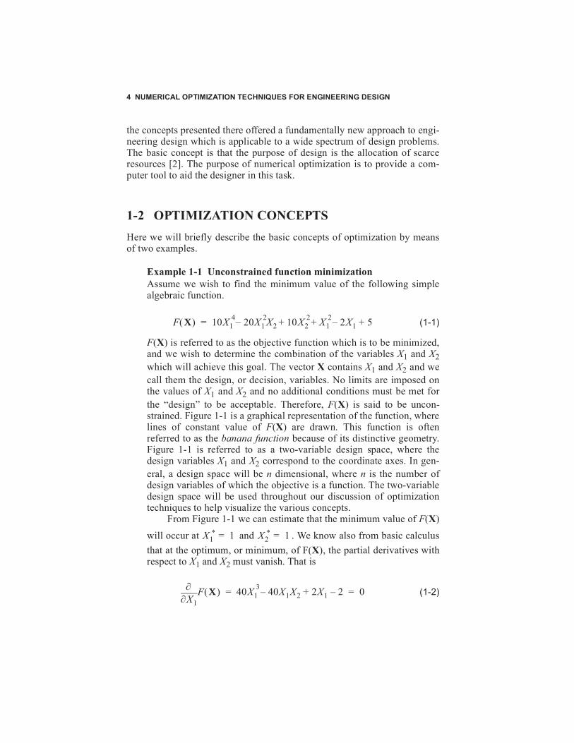
Example 1-1 Unconstrained function minimizationAssume we wish to find the minimum value of the following simplealgebraic function.

(1-1)

F(X) is referred to as the objective function which is to be minimized,and we wish to determine the combination of the variables X1 and X2which will achieve this goal. The vector X contains X1 and X2 and wecall them the design, or decision, variables. No limits are imposed onthe values of X1 and X2 and no additional conditions must be met forthe “design” to be acceptable. Therefore, F(X) is said to be uncon-strained. Figure 1-1 is a graphical representation of the function, wherelines of constant value of F(X) are drawn. This function is oftenreferred to as the banana function because of its distinctive geometry.Figure 1-1 is referred to as a two-variable design space, where thedesign variables X1 and X2 correspond to the coordinate axes. In gen-eral, a design space will be n dimensional, where n is the number ofdesign variables of which the objective is a function. The two-variabledesign space will be used throughout our discussion of optimizationtechniques to help visualize the various concepts.

From Figure 1-1 we can estimate that the minimum value of F(X)

will occur at and . We know also from basic calculusthat at the optimum, or minimum, of F(X), the partial derivatives withrespect to X1 and X2 must vanish. That is

(1-2)

F X( ) 10X14 20X1

2X2– 10X22 X1

2 2X1 5+–+ +=

X1* 1= X2

* 1=

X1∂∂ F X( ) 40X1

3 40X1X2– 2X1 2–+ 0= =

BASIC CONCEPTS 5

(1-3)

Solving for X1 and X2, we find that indeed and . Wewill see later that the vanishing gradient is a necessary but not suffi-cient condition for finding the minimum.

Figure 1-1 Two-variable function space.

In this example, we were able to obtain the optimum both graphicallyand analytically. However, this example is of little engineering value,except for demonstration purposes. In most practical engineering problemsthe minimum of a function cannot be determined analytically. The problemis further complicated if the decision variables are restricted to values

X2∂∂ F X( ) 20X1

2– 20X2 0=+=

X1* 1= X2

* 1=

0 1.0 2.0-1.0-2.0-1.0

0

1.0

2.0

3.0

4.0

X1

X2

F( ) = 65X

Optimum( ) = 4.0F X

35

14

6

9

75


within a specified range or if other conditions are imposed in the minimiza-tion problem. Therefore, numerical techniques are usually resorted to. Wewill now consider a simple design example where conditions (constraints)are imposed on the optimization problem.

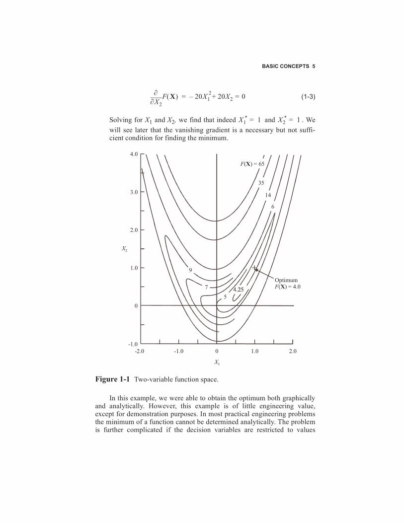
Example 1-2 Constrained function minimization Figure 1-2a depicts a tubular column of height h which is required tosupport a concentrated load P as shown. We wish to find the meandiameter D and the wall thickness t to minimize the weight of the col-umn. The column weight is given by

(1-4)

where A is the cross-sectional area and ρ is the material's unit weight. We will consider the axial load only, and for simplicity will ignore

any eccentricity, lateral loads, or column imperfections. The stress inthe column is given by

(1-5)

Figure 1-2 Column design for least weight.

W ρAh ρπDth= =

σ PA--- P

πDt----------= =

t

h

BASIC CONCEPTS 7

where stress is taken as positive in compression. In order to preventmaterial failure, this stress must not exceed the allowable stress . Inaddition to preventing material failure, the stress must not exceed thatat which Euler buckling or local shell buckling will occur, as shown inFigs. 1-2b and c. The stress at which Euler buckling occurs is given by

(1-6)

where E = Young's modulus I = moment of inertia

The stress at which shell buckling occurs is given by

(1-7)

where = Poisson's ratioThe column must now be designed so that the magnitude of the stressis less than the minimum of , , and . These requirements can bewritten algebraically as

(1-8)

(1-9)

(1-10)

In addition to the stress limitations, the design must satisfy thegeometric conditions that the mean diameter be greater than the wallthickness and that both the diameter and thickness be positive

(1-11)

(1-12)

(1-13)

Bounds of 10-6 are imposed on D and t to ensure that in Eq. (1-5)and in Eq. (1-7) will be finite.

σ

σbπ2EI4Ah2------------ π2E D2 t2+( )

32h2--------------------------------= =

σs2Et

D 3 1 ν2–( )-------------------------------=

ν

σ σb σs

σ σ≤

σ σb≤

σ σs≤

D t≥

D 10 6–≥

t 10 6–≥

σσs


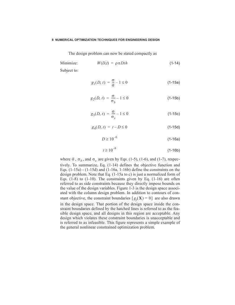
The design problem can now be stated compactly as

Minimize: (1-14)

Subject to:

(1-15a)

(1-15b)

(1-15c)

(1-15d)

(1-16a)

(1-16b)

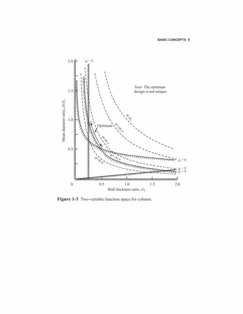
where , , and are given by Eqs. (1-5), (1-6), and (1-7), respec-tively. To summarize, Eq. (1-14) defines the objective function andEqs. (1-15a) - (1-15d) and (1-16a, 1-16b) define the constraints on thedesign problem. Note that Eq. (1-15a to c) is just a normalized form ofEqs. (1-8) to (1-10). The constraints given by Eq. (1-16) are oftenreferred to as side constraints because they directly impose bounds onthe value of the design variables. Figure 1-3 is the design space associ-ated with the column design problem. In addition to contours of con-stant objective, the constraint boundaries are also drawnin the design space. That portion of the design space inside the con-straint boundaries defined by the hatched lines is referred to as the fea-sible design space, and all designs in this region are acceptable. Anydesign which violates these constraint boundaries is unacceptable andis referred to as infeasible. This figure represents a simple example ofthe general nonlinear constrained optimization problem.

W D t( , ) ρπDth=

g1 D t,( ) σσ--- 1– 0≤=

g2 D t,( ) σσb------ 1– 0≤=

g3 D t,( ) σσs----- 1– 0≤=

g4 D t,( ) t D– 0≤=

D 10 6–≥

t 10 6–≥

σ σb σs

gj X( ) 0=[ ]

BASIC CONCEPTS 9

Figure 1-3 Two-variable function space for column.

2.00 0.5 1.0 1.5

1.0

1.5

2.0

0.5

Optimum

Note: The optimumdesign is not unique.

WW=

0

WW=

/30

WW

=2/30

WW=

/60

WW*=

/40

Wall thickness ratio, /t t0

Mea

n di

amet

er ra

tio,

/D

D0

g2 = 0

g4 = 0g1 = 0

g3 = 0


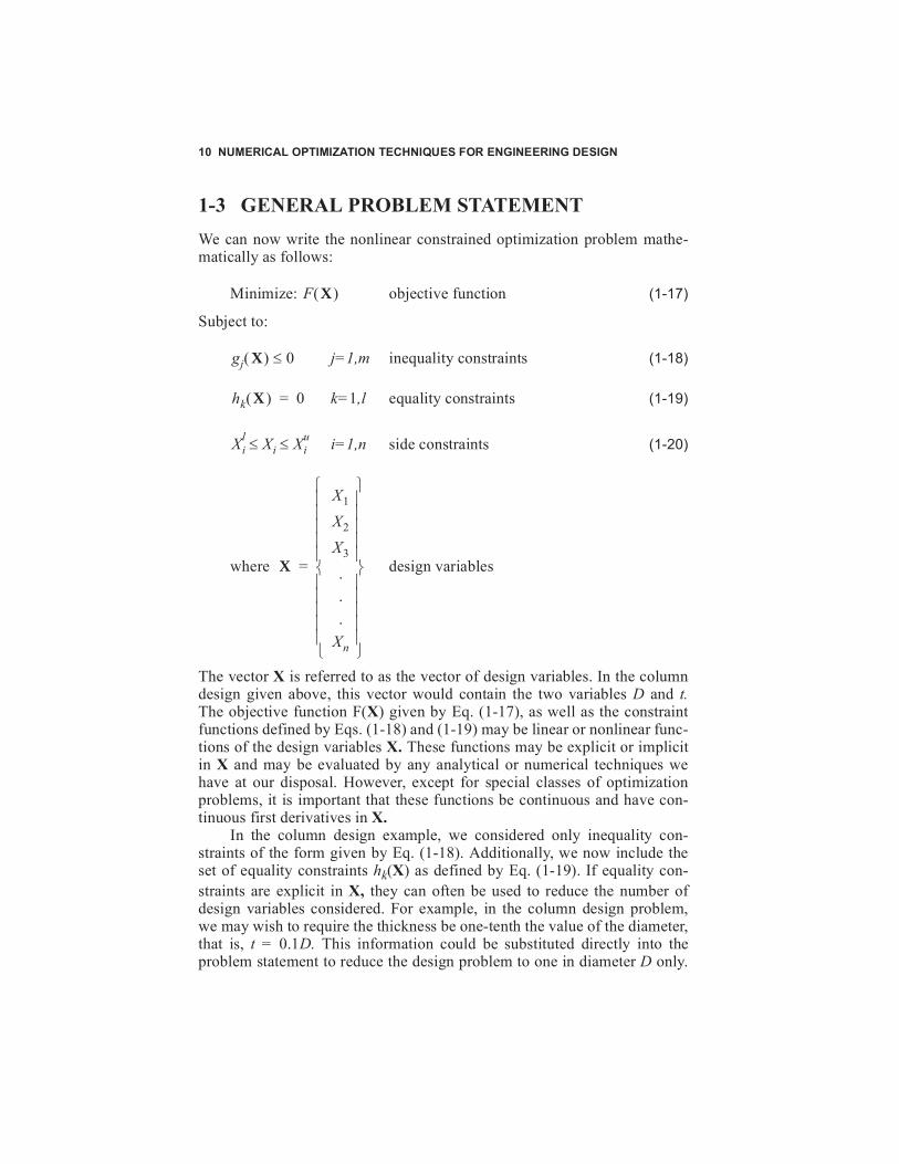
1-3 GENERAL PROBLEM STATEMENT We can now write the nonlinear constrained optimization problem mathe-matically as follows:

Minimize: objective function (1-17)

Subject to:

j=1,m inequality constraints (1-18)

k=1,l equality constraints (1-19)

i=1,n side constraints (1-20)

where design variables

The vector X is referred to as the vector of design variables. In the columndesign given above, this vector would contain the two variables D and t.The objective function F(X) given by Eq. (1-17), as well as the constraintfunctions defined by Eqs. (1-18) and (1-19) may be linear or nonlinear func-tions of the design variables X. These functions may be explicit or implicitin X and may be evaluated by any analytical or numerical techniques wehave at our disposal. However, except for special classes of optimizationproblems, it is important that these functions be continuous and have con-tinuous first derivatives in X.

In the column design example, we considered only inequality con-straints of the form given by Eq. (1-18). Additionally, we now include theset of equality constraints hk(X) as defined by Eq. (1-19). If equality con-straints are explicit in X, they can often be used to reduce the number ofdesign variables considered. For example, in the column design problem,we may wish to require the thickness be one-tenth the value of the diameter,that is, t = 0.1D. This information could be substituted directly into theproblem statement to reduce the design problem to one in diameter D only.

F X( )

gj X( ) 0≤

hk X( ) 0=

Xil Xi Xi

u≤ ≤

X

X1

X2

X3

.

.

.Xn

=

BASIC CONCEPTS 11

In general, h(X) may be either a very complicated explicit function of thedesign variables X or may be implicit in X.

Equation (1-20) defines bounds on the design variables X and so isreferred to as a side constraint. Although side constraints could be includedin the inequality constraint set given by Eq. (1-18), it is usually convenientto treat them separately because they define the region of search for theoptimum.

The above form of stating the optimization problem is not unique, andvarious other statements equivalent to this are presented in the literature.For example, we may wish to state the problem as a maximization problemwhere we desire to maximize F(X). Similarly, the inequality sign in Eq. (1-18) can be reversed so that g(X) must be greater than or equal to zero. Usingour notation, if a particular optimization problem requires maximization, wesimply minimize -F(X). The choice of the non-positive inequality sign onthe constraints has the geometric significance that, at the optimum, the gra-dients of the objective and all critical constraints point away from the opti-mum design.

1-4 THE ITERATIVE OPTIMIZATION PROCEDURE

Most optimization algorithms require that an initial set of design variables,X0, be specified. Beginning from this starting point, the design is updatediteratively. Probably the most common form of this iterative procedure isgiven by

(1-21)

where q is the iteration number and S is a vector search direction in thedesign space. The scalar quantity α* defines the distance that we wish tomove in direction S.

To see how the iterative relationship given by Eq. (1-21) is applied tothe optimization process, consider the two-variable problem shown in Fig-ure 1-4.

Assume we begin at point X0 and we wish to reduce the objectivefunction. We will begin by searching in the direction S1 given by

(1-22)

Xq

Xq 1–= α*

Sq+

S1 1.0–0.5–

=


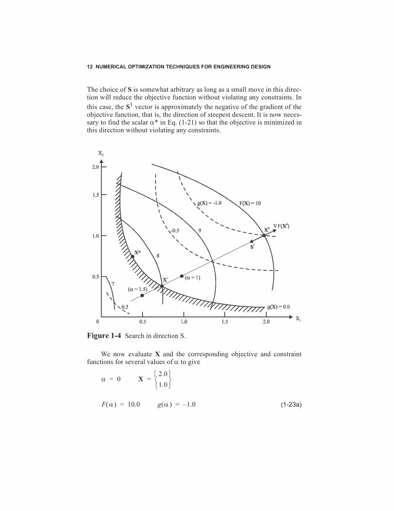
The choice of S is somewhat arbitrary as long as a small move in this direc-tion will reduce the objective function without violating any constraints. Inthis case, the S1 vector is approximately the negative of the gradient of theobjective function, that is, the direction of steepest descent. It is now neces-sary to find the scalar α* in Eq. (1-21) so that the objective is minimized inthis direction without violating any constraints.

Figure 1-4 Search in direction S.

We now evaluate X and the corresponding objective and constraintfunctions for several values of α to give

(1-23a)

α 0= X2.01.0

=

F α( ) 10.0= g α( ) 1.0–=

BASIC CONCEPTS 13

(1-23b)

(1-23c)

(1-23d)

where the objective and constraint values are estimated using Figure 1-4. Inpractice, we would evaluate these functions on the computer, and, usingseveral proposed values of α, we would apply a numerical interpolationscheme to estimate α*. This would provide the minimum F(X) in thissearch direction which does not violate any constraints. Note that by search-ing in a specified direction, we have actually converted the problem fromone in n variables X to one variable α. Thus, we refer to this as a one-dimensional search. At point X1, we must find a new search direction suchthat we can continue to reduce the objective without violating constraints.In this way, Eq. (1-21) is used repetitively until no further design improve-ment can be made.

From this simple example, it is seen that nonlinear optimization algo-rithms based on Eq. (1-21) can be separated into two basic parts. The first isdetermination of a direction of search S, which will improve the objectivefunction subject to constraints. The second is determination of the scalarparameter α∗ defining the distance of travel in direction S. Each of thesecomponents plays a fundamental role in the efficiency and reliability of agiven optimization algorithm, and each will be discussed in detail in laterchapters.

α 1.0= X2.01.0

= 1.01.0–0.5–

1.0

0.5

=+

F α( ) 8.4= g α( ) 0.2–=

α 1.5= X2.01.0

= 1.51.0–0.5–

0.50

0.25

=+

F α( ) 7.6= g α( ) 0.2=

α∗ 1.25= X∗ 2.01.0

= 1.251.0–0.5–

0.750

0.375

=+

F α∗( ) 8.0= g α*( ) 0.0=


1-5 EXISTENCE AND UNIQUENESS OF AN OPTIMUM SOLUTION

In the application of optimization techniques to design problems of practicalinterest, it is seldom possible to ensure that the absolute optimum designwill be found subject to the constraints. This may be because multiple solu-tions to the optimization problem exist or simply because numerical ill-con-ditioning in setting up the problem results in extremely slow convergence ofthe optimization algorithm. From a practical standpoint, the best approach isusually to start the optimization process from several different initial vec-tors, and if the optimization results in essentially the same final design, wecan be reasonably assured that this is the true optimum. It is, however, pos-sible to check mathematically to determine if we at least have a relativeminimum. In other words, we can define necessary conditions for an opti-mum, and we can show that under certain circumstances these necessaryconditions are also sufficient to ensure that the solution is the global opti-mum.

1-5.1 Unconstrained Problems First consider the unconstrained minimization problem where we only wishto minimize F(X) with no constraints imposed. We know that for F(X) to beminimum, the gradient of F(X) must vanish

(1-24a)

where

(1-24b)

F X( )∇ 0=

F X( )∇

X1∂∂ F X( )

X2∂∂ F X( )

.

.

.

Xn∂∂ F X( )

=

BASIC CONCEPTS 15

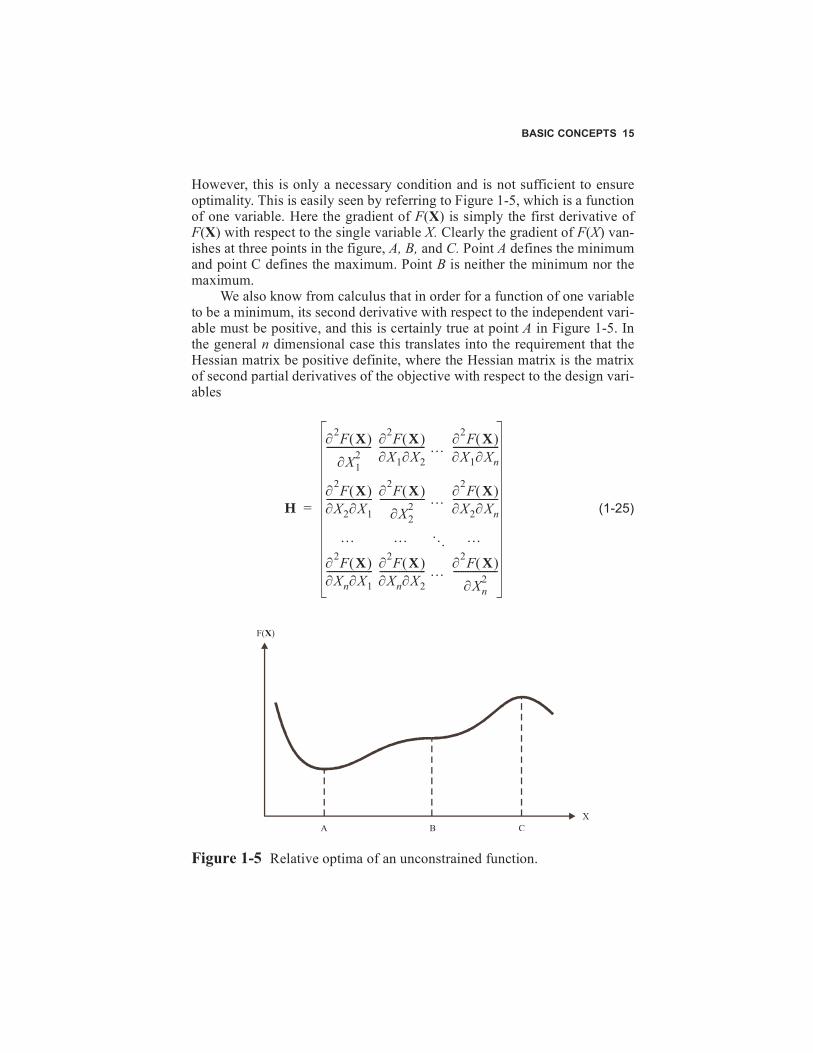
However, this is only a necessary condition and is not sufficient to ensureoptimality. This is easily seen by referring to Figure 1-5, which is a functionof one variable. Here the gradient of F(X) is simply the first derivative ofF(X) with respect to the single variable X. Clearly the gradient of F(X) van-ishes at three points in the figure, A, B, and C. Point A defines the minimumand point C defines the maximum. Point B is neither the minimum nor themaximum.

We also know from calculus that in order for a function of one variableto be a minimum, its second derivative with respect to the independent vari-able must be positive, and this is certainly true at point A in Figure 1-5. Inthe general n dimensional case this translates into the requirement that theHessian matrix be positive definite, where the Hessian matrix is the matrixof second partial derivatives of the objective with respect to the design vari-ables

(1-25)

Figure 1-5 Relative optima of an unconstrained function.

H

∂2F X( )

∂X12

------------------ ∂2F X( )∂X1∂X2------------------- … ∂2F X( )

∂X1∂Xn-------------------

∂2F X( )∂X2∂X1------------------- ∂2F X( )

∂X22

------------------ … ∂2F X( )∂X2∂Xn-------------------

… … ... …

∂2F X( )∂Xn∂X1------------------- ∂2F X( )

∂Xn∂X2------------------- … ∂2F X( )

∂Xn2

------------------

=

A B CX

F( )X


Positive definiteness means that this matrix has all positive eigenval-ues. If the gradient is zero and the Hessian matrix is positive definite for agiven X, this insures that the design is at least a relative minimum, but againit does not insure that the design is a global minimum. The design is onlyguaranteed to be a global minimum if the Hessian matrix is positive definitefor all possible values of the design variables X. This can seldom be demon-strated in practical design applications. We must usually be satisfied withstarting the design from various initial points to see if we can obtain a con-sistent optimum and therefore have reasonable assurance that this is the trueminimum of the function. However, an understanding of the requirementsfor a unique optimal solution is important to provide insight into the optimi-zation process. Also, these concepts provide the basis for the developmentof many of the more powerful algorithms which we will be discussing inlater chapters.

1-5.2 Constrained Problems Now, consider the constrained minimization problem and assume that, atthe optimum, at least one constraint on the design is active. It is no longernecessary that the gradient of the objective vanish at the optimum. Refer-ring to Figure 1-3, this is obvious. At the optimum, the objective function,being the weight of the tubular column, could be reduced by either reducingthe diameter or the wall thickness so that the components of the gradient ofthe objective function are clearly not zero at this point. However, any reduc-tion in the dimensions of the column in order to reduce the weight wouldresult in constraint violations.

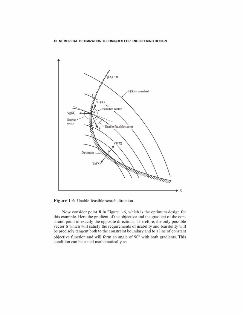
We can, at least intuitively, define the necessary conditions for a con-strained optimum by referring to Figure 1-6. Assume a design is specified atpoint A. In order to improve on this design, it will be necessary to determinea direction vector S which will reduce the objective function and yet notviolate the active constraint. We define any direction which will reduce theobjective as a usable direction. Clearly the line tangent to a line of constantvalue of the objective function at this point will bound all possible usabledirections. Any direction on the side of this line (hyperplane) which willreduce the objective function is defined as a usable direction, and this por-tion of the design space is referred to as the usable sector. Note that if wetake the scalar product of any direction vector S which we choose in theusable sector, with the gradient of the objective function, the result will be

negative to zero (that is, ). In other words, the angle betweenthese two vectors must be between 90o and 270o. This is because the scalarproduct is the product of the magnitudes of the vectors and the cosine of theangle between them. The cosine is only negative for angles between 90o and

ST F X( )∇ 0≤

BASIC CONCEPTS 17

270o. Similarly, a hyperplane tangent to the constraint surface at point Awill bound the feasible sector, where a direction vector S is defined as feasi-ble if a small move in this direction will not violate the constraint. In thiscase, the scalar product of S with the gradient of the constraint is negative or

zero ( ), so the angle between these two vectors must also bebetween 90o and 270o. In order for a direction vector S to yield an improveddesign without violating the constraint, this direction must be both usableand feasible, and any direction in the usable feasible sector of the designspace satisfies this criterion. It is noteworthy here that if the direction vectoris nearly tangent to the hyperplane bounding the feasible sector, a smallmove in this direction will result in a constraint violation but will reduce theobjective function quite rapidly. On the other hand, if the direction vector ischosen nearly tangent to the line of constant objective, we can move somedistance in this direction without violating the constraint, but the objectivefunction will not decrease rapidly and, if the objective is nonlinear, may infact begin to increase. At point A in Figure 1-6 a direction does exist whichreduces the objective function without violating the constraint for a finitemove.

In the general optimization problem there may be more than one activeconstraint at a given time in the design process, where a constraint is con-sidered active if its value is within a small tolerance of zero. If this is thecase, a direction vector must be found which is feasible with respect to allactive constraints. The requirement that a move direction be both usable andfeasible is stated mathematically as

Usable direction:

(1-26)

Feasible direction:

(1-27)

ST g X( )∇ 0≤

F X( )∇ TS 0≤

gj X( )∇ TS 0≤ for all j for which gj X( ) 0=


Figure 1-6 Usable-feasible search direction.

Now consider point B in Figure 1-6, which is the optimum design forthis example. Here the gradient of the objective and the gradient of the con-straint point in exactly the opposite directions. Therefore, the only possiblevector S which will satisfy the requirements of usability and feasibility willbe precisely tangent both to the constraint boundary and to a line of constantobjective function and will form an angle of 90o with both gradients. Thiscondition can be stated mathematically as

X1

BASIC CONCEPTS 19

(1-28)

(1-29)

unrestricted in sign (1-30)

Note that if there are no constraints on the design problem, Eq. (1-28)reduces to the requirement that the gradient of the objective function mustvanish, as was already discussed in the case of unconstrained minimization.

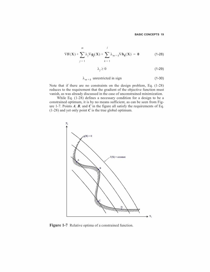
While Eq. (1-28) defines a necessary condition for a design to be aconstrained optimum, it is by no means sufficient, as can be seen from Fig-ure 1-7. Points A, B, and C in the figure all satisfy the requirements of Eq.(1-28) and yet only point C is the true global optimum.

Figure 1-7 Relative optima of a constrained function.

F X( )∇ λj gj X( )∇

j 1=

m

∑ λm k+ hk X( )∇

k 1=

l

∑+ + 0=

λj 0≥

λm k+


1-5.3 The Kuhn-Tucker Conditions Equation (1-28) is actually the third of a set of necessary conditions for con-strained optimality. These are referred to as the Kuhn-Tucker necessaryconditions.

The Kuhn-Tucker conditions define a stationary point of theLagrangian

(1-31)

All three conditions are listed here for reference and state simply that ifthe vector X* defines the optimum design, the following conditions must besatisfied:

1. is feasible (1-32)

2. (1-33)

3. (1-34)

(1-35)

unrestricted in sign (1-36)

Equation (1-32) is a statement of the obvious requirement that the optimumdesign must satisfy all constraints. Equation (1-33) imposes the requirementthat if the constraint gj(X) is not precisely satisfied [that is, ] thenthe corresponding Lagrange multiplier must be zero. Equations (1-34) to (1-36) are the same as Eqs. (1-28) to (1-30).

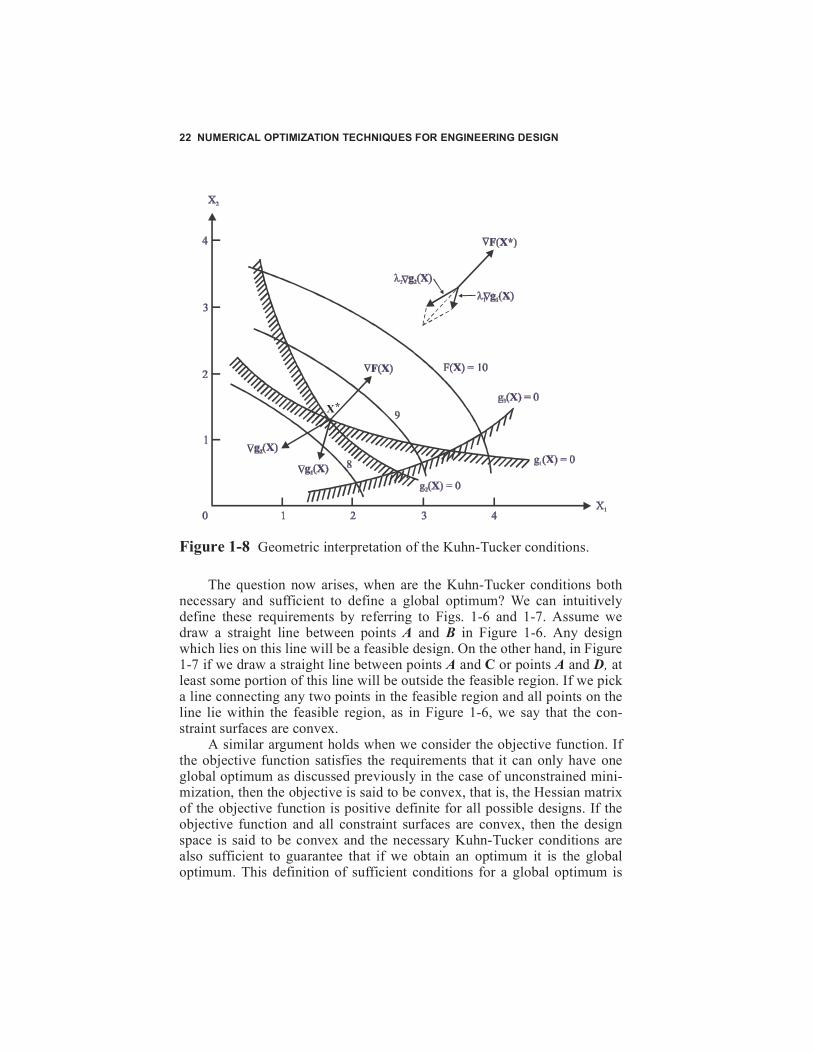
The geometric significance of the Kuhn-Tucker conditions can beunderstood by referring to Figure 1-8, which shows a two-variable minimi-zation problem with three inequality constraints. At the optimum, constraint

is not critical and so, from Eq. (1-33), . Equation (1-34)

requires that, if we multiply the gradient of each critical constraint [

and ] by its corresponding Lagrange multiplier, the vector sum of

L X λ,( ) F X( ) λjgj X( )

j 1=

m

∑ λm k+ hk X( )

k 1=

l

∑+ +=

X∗

λjgj X∗( ) 0= j 1 m,= λj 0≥

F X∗( )∇ λj gj X∗( )∇

j 1=

m

∑ λm k+ hk X∗( )∇

k 1=

l

∑+ + 0=

λj 0≥

λm k+

gj X( ) 0<

g3 X∗( ) λ3 0=

g1 X∗( )

g2 X∗( )

BASIC CONCEPTS 21

the result must equal the negative of the gradient of the objective function.Thus we see from Figure 1-8 that

(1-37a)

(1-37b)

Since and , the second Kuhn-Tucker condition issatisfied identically with respect to these constraints. Also, we see from Fig-ure 1-8 that X* is feasible and so each of the Kuhn-Tucker necessary condi-tions is satisfied.In the problem of Figure 1-8, the Lagrange multipliers are uniquely deter-mined from the gradients of the objective and the active constraints. How-ever, we can easily imagine situations where this is not so. For example,assume that we have defined another constraint, , which happens tobe identical to or perhaps a constant times . The constraintboundaries and would now be the same and theLagrange multipliers and can have any combination of values whichsatisfy the vector addition shown in the figure. Thus, we can say that one ofthe constraints is redundant. As another example, we can consider a con-straint which is independent of the other constraints, but at the opti-mum in Figure 1-8, constraints , and are all critical.Now, we may pick many combinations of , , and which will sat-isfy the Kuhn-Tucker conditions so that, while all constraints are indepen-dent, the Lagrange multipliers are not unique. These special cases do notdetract from the usefulness of the Kuhn-Tucker conditions in optimizationtheory. It is only necessary that we account for these possibilities whenusing algorithms that require calculation of the Lagrange multipliers.

F X∗( )∇ λ1 g1 X∗( )∇ λ2 g2 X∗( )∇+ + 0=

λ1 0≥ λ2 0≥

g1 X∗( ) 0= g2 X∗( ) 0=

g4 X( )

g1 X( ) g1 X( )

g1 X( ) 0= g4 X( ) 0=λ1 λ4

g5 X( )

g1 X( ) g2 X( ) g5 X( )

λ1 λ2 λ5


Figure 1-8 Geometric interpretation of the Kuhn-Tucker conditions.

The question now arises, when are the Kuhn-Tucker conditions bothnecessary and sufficient to define a global optimum? We can intuitivelydefine these requirements by referring to Figs. 1-6 and 1-7. Assume wedraw a straight line between points A and B in Figure 1-6. Any designwhich lies on this line will be a feasible design. On the other hand, in Figure1-7 if we draw a straight line between points A and C or points A and D, atleast some portion of this line will be outside the feasible region. If we picka line connecting any two points in the feasible region and all points on theline lie within the feasible region, as in Figure 1-6, we say that the con-straint surfaces are convex.

A similar argument holds when we consider the objective function. Ifthe objective function satisfies the requirements that it can only have oneglobal optimum as discussed previously in the case of unconstrained mini-mization, then the objective is said to be convex, that is, the Hessian matrixof the objective function is positive definite for all possible designs. If theobjective function and all constraint surfaces are convex, then the designspace is said to be convex and the necessary Kuhn-Tucker conditions arealso sufficient to guarantee that if we obtain an optimum it is the globaloptimum. This definition of sufficient conditions for a global optimum is

X*

BASIC CONCEPTS 23

actually more restrictive than is theoretically required but is adequate toprovide a basic understanding of the necessary and sufficient conditionsunder which a design is the true global optimum. A detailed discussion ofthe Kuhn-Tucker conditions as well as a concise definition of the suffi-ciency requirements can be found in Ref. 3.

Just as in the case of unconstrained minimization, it is seldom possiblein practical applications to know whether the sufficiency conditions are met.However, most optimization problems can be stated in many differentforms, and an understanding of the desirable characteristics of the designspace is often useful in helping us to cast the design problem in a form con-ducive to solution using numerical optimization.

Calculating the Lagrange Multipliers

Now consider how we might calculate the values of the Lagrange Mul-tipliers at the optimum. First, we know that if a constraint value is non-zero(within a small tolerance), then from Eq. (1-33), the correspondingLagrange multiplier is equal to zero. For our purposes here, both inequalityand equality constraints are treated the same, so we can treat them alltogether. It is only important to remember that the equality constraints willalways be active the optimum and that they can have positive or negativeLagrange Multipliers. Also, assuming all constraints are independent, thenumber of active constraints will be less than or equal to the number ofdesign variables. Thus, Eq. (1-34) often has fewer unknown parameters, than equations.

Because precise satisfaction of the Kuhn-Tucker conditions may not bereached, we can rewrite Eq. (1-34) as

(1-38)

where the equality constraints are omitted for brevity and R is the vector ofresiduals.

Now, because we want the residuals as small as possible (if all compo-nents of R = 0, the Kuhn-Tucker conditions are satisfied precisely), we canminimize the square of the magnitude of R. Let

(1-39a)

λj

F X∗( )∇ λj gj X∗( )∇

j 1=

m

∑+ R=

B F X∗( )∇=


and

(1-39b)

where M is the set of active constraints.Substituting Eqs. (1-39a) and (1-39b) into Eq. (1-38),

(1-40)

Now, because we want the residuals as small as possible (if all compo-nents of R = 0, the Kuhn-Tucker conditions are satisfied precisely), we canminimize the square of the magnitude of R.

Minimize (1-41)

Differentiating Eq. (1-41) with respect to λ and setting the result to zerogives

(1-42)

from which

(1-43)

Now if all components of λ corresponding to inequality constraints arenon-negative, we have an acceptable estimate of the Lagrange multipliers.Also, we can substitute Eq. (1-43) into Eq. (1-40) to estimate how preciselythe Kuhn-Tucker conditions are met. If all components of the residual vec-tor, R, are very near zero, we know that we have reached at least a relativeminimum.

Sensitivity of the Optimum to Changes in Constraint Limits

The Lagrange multipliers have particular significance in estimating howsensitive the optimum design is to the active constraints. It can be shownthat the derivative of the optimum objective with respect to a constraint isjust the value of the Lagrange multiplier of that constraint, so

(1-44)

A g1 X∗( )∇ g2 X∗( )∇ . . . gM X∗( )∇=

B Aλ+ R=

RTR B

TB 2λT

ATB λT

ATAλ+ +=

2ATB ATAλ 0=+

λ 2 ATA[ ]

1–A

TB–=

gj X*( )∂

∂ F X*( ) λj=

BASIC CONCEPTS 25

or, in more useful form;

(1-45)

If we wish to change the limits on a set of constraints, J, Eq. (1-45) issimply expanded as

(1-46)

Remember that Eq. (1-45) is the sensitivity with respect to gj. In prac-tice, we may want to know the sensitivity with respect to bounds on theresponse.

Assume we have normalized an upper bound constraint

(1-47)

where R is the response and Ru is the upper bound.

(1-48)

Similarly, for lower bound constraints

(1-49)

Therefore, the Lagrange multipliers tell us the sensitivity of the opti-mum with respect to a relative change in the constraint bounds, while theLagrange multipliers divided by the scaling factor (usually the matnitude ofthe bound) give us the sensitivity to an absolute change in the bounds.

Example 1-3 Sensitivity of the OptimumConsider the constrained minimization of a simple quadratic functionwith a single linear constraint.

Minimize (1-50)

Subject to; (1-51)

F X* δgj,( ) F X

*( ) λjδgj+=

F X* δgj,( ) F X*( ) λjδgj

jεJ∑+=

gjR Ru–

Ru---------------=

F X* δRu,( ) F X*( ) λjδRuRu

---------–=

F X* δRl,( ) F X*( ) λjδRlRl

--------+=

F X( ) X12 X2

2+=

g X( )2 X1 X2+( )–

2-------------------------------- 0≤=


At the optimum;

(1-52a)

and

(1-52b)

Now, assume we wish to change the lower bound on g from 2.0 to 2.1.From Eq. (1-49) we get

(1-53)

The true optimum for this case is

(1-54)

1-6 CONCLUDING REMARKS In assessing the value of optimization techniques to engineering design, it isworthwhile to review briefly the traditional design approach. The design isoften carried out through the use of charts and graphs which have beendeveloped over many years of experience. These methods are usually anefficient means of obtaining a reasonable solution to traditional designproblems. However, as the design task becomes more complex, we relymore heavily on the computer for analysis. If we assume that we have acomputer code capable of analyzing our proposed design, the output fromthis program will provide a quantitative indication of the acceptability andoptimality of the design. We may change one or more design variables andrerun the computer program to see if any design improvement can beobtained. We then take the results of many computer runs and plot theobjective and constraint values versus the various design parameters. Fromthese plots we can interpolate or extrapolate to what we believe to be theoptimum design. This is essentially the approach that was used to obtain theoptimum constrained minimum of the tubular column shown in Figure 1-3,

X* 1.01.0

= F X*( ) 2.0= g X*( ) 0.0=

F X*( )∇2.02.0

= g X*( )∇0.5–0.5–

= λ 4.0=

F X* δRl,( ) 2.0 4.0 0.12.0-------

+ 2.20= =

X* 1.051.05

= F X* δRl,( ) 2.205=

BASIC CONCEPTS 27

and this is certainly an efficient and viable approach when the design is afunction of only a few variables. However, if the design exceeds three vari-ables, the true optimum may be extremely difficult to obtain graphically.Then, assuming the computer code exists for the analysis of the proposeddesign, automation of the design process becomes an attractive alternative.Mathematical programming simply provides a logical framework for carry-ing out this automated design process. Some advantages and limitations tothe use of numerical optimization techniques are listed here.

1-6.1 Advantages of Numerical Optimization • A major advantage is the reduction in design time – this is especially true

when the same computer program can be applied to many design projects.

• Optimization provides a systematized logical design procedure. • We can deal with a wide variety of design variables and constraints

which are difficult to visualize using graphical or tabular methods. • Optimization virtually always yields some design improvement. • It is not biased by intuition or experience in engineering. Therefore, the

possibility of obtaining improved, nontraditional designs is enhanced. • Optimization requires a minimal amount of human-machine interaction.

1-6.2 Limitations of Numerical Optimization • Computational time increases as the number of design variables

increases. If one wishes to consider all possible design variables, the cost of automated design is often prohibitive. Also, as the number of design variables increases, these methods tend to become numerically ill-condi-tioned.

• Optimization techniques have no stored experience or intuition on which to draw. They are limited to the range of applicability of the analysis pro-gram.

• If the analysis program is not theoretically precise, the results of optimi-zation may be misleading, and therefore the results should always be checked very carefully. Optimization will invariably take advantage of analysis errors in order to provide mathematical design improvements.


• Most optimization algorithms have difficulty in dealing with discontinu-ous functions. Also, highly nonlinear problems may converge slowly or not at all. This requires that we be particularly careful in formulating the automated design problem.

• It can seldom be guaranteed that the optimization algorithm will obtain the global optimum design. Therefore, it may be desirable to restart the optimization process from several different points to provide reasonable assurance of obtaining the global optimum.

• Because many analysis programs were not written with automated design in mind, adaptation of these programs to an optimization code may require significant reprogramming of the analysis routines.

1-6.3 Summary Optimization techniques, if used effectively, can greatly reduce engineeringdesign time and yield improved, efficient, and economical designs. How-ever, it is important to understand the limitations of optimization techniquesand use these methods as only one of many tools at our disposal.

Finally, it is important to recognize that, using numerical optimizationtechniques, the precise, absolute best design will seldom if ever beachieved. Expectations of achieving the absolute “best” design will invari-ably lead to “maximum” disappointment. We may better appreciate thesetechniques by replacing the word “optimization” with “design improve-ment,” and recognize that a convenient method of improving designs is anextremely valuable tool.

REFERENCES

1. Schmit, L. A.: Structural Design by Systematic Synthesis, Proceedings, 2nd Conference on Electronic Computation, ASCE, New York, pp. 105 – 122, 1960.

2. Schmit, L. A.: Structural Synthesis – Its Genesis and Development, AIAA J., vol. 10, no. 10, pp. 1249 – 1263, October 1981.

3. Zangwill, W. I.: “Nonlinear Programming: A Unified Approach,” Prentice-Hall, Englewood Cliffs, N.J., 1969.

BASIC CONCEPTS 29

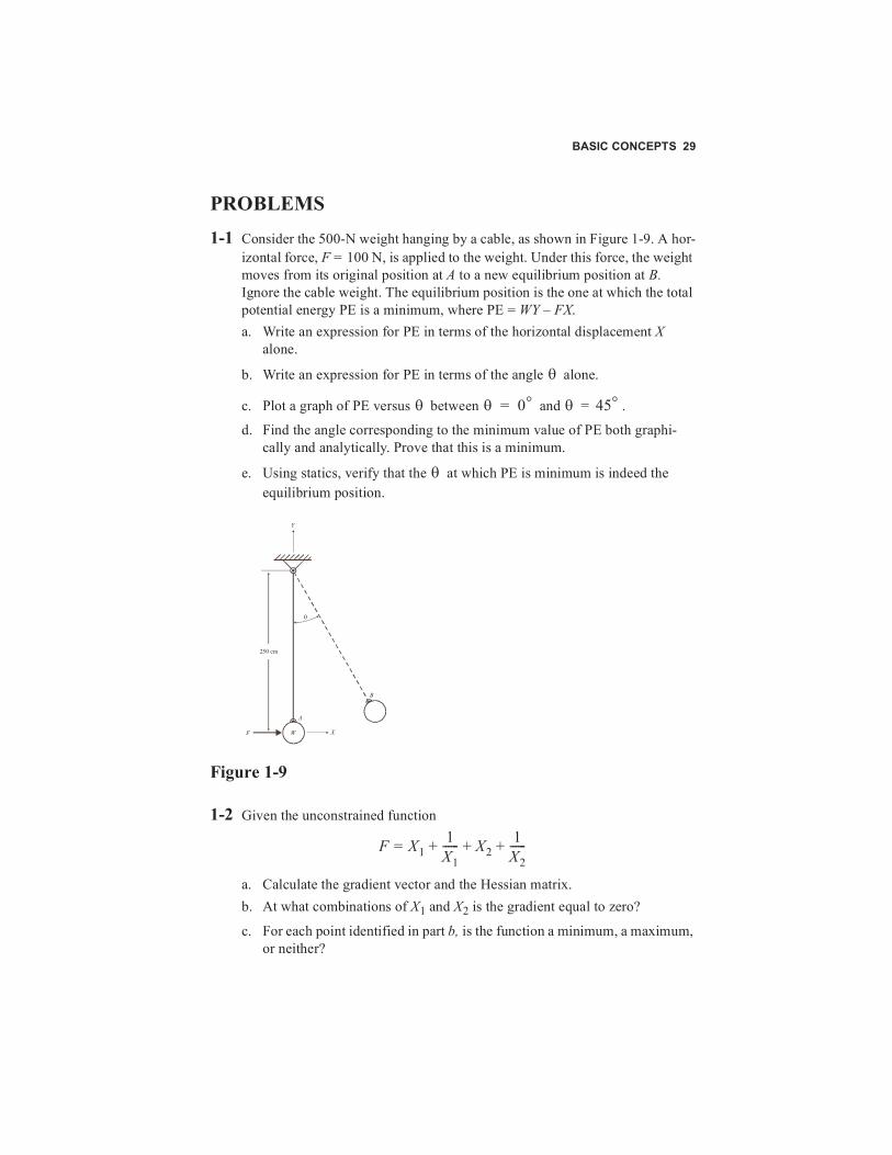
PROBLEMS 1-1 Consider the 500-N weight hanging by a cable, as shown in Figure 1-9. A hor-

izontal force, F = 100 N, is applied to the weight. Under this force, the weight moves from its original position at A to a new equilibrium position at B. Ignore the cable weight. The equilibrium position is the one at which the total potential energy PE is a minimum, where PE = WY – FX.a. Write an expression for PE in terms of the horizontal displacement X

alone.

b. Write an expression for PE in terms of the angle alone.

c. Plot a graph of PE versus between and = .

d. Find the angle corresponding to the minimum value of PE both graphi-cally and analytically. Prove that this is a minimum.

e. Using statics, verify that the at which PE is minimum is indeed the equilibrium position.

Figure 1-9

1-2 Given the unconstrained function

a. Calculate the gradient vector and the Hessian matrix.b. At what combinations of X1 and X2 is the gradient equal to zero?

c. For each point identified in part b, is the function a minimum, a maximum, or neither?

θ

θ θ 0°= θ 45°

θ

250 cm

W

A

B

X

Y

F

θ

F X1= 1X1------ X2

1X2------+ + +


1-3 Given the unconstrained function,

a. At X1 = 2 and X2 = 2, calculate the gradient of F.

b. At X1 = 2 and X2 = 2, calculate the direction of steepest descent.

c. Using the direction of steepest descent calculated in part b, update the design by the standard formula

Evaluate X1, X2 and F for = 0, 0.2, 0.5, and 1.0 and plot the curve ofF versus .

d. Write the equation for F in terms of alone. Discuss the character of this function.

e. From part d, calculate at .

f. Calculate the scalar product using the results of parts a and b and compare this with the result of part e.

1-4 Consider the constrained minimization problem:

Minimize: Subject to:

a. Sketch the two-variable function space showing contours of F = 0, 1, and 4 as well as the constraint boundaries.

b. Identify the unconstrained minimum of F on the figure. c. Identify the constrained minimum on the figure. d. At the constrained minimum, what are the Lagrange multipliers?

1-5 Given the ellipse , it is desired to find the rectangle of greatest area which will fit inside the ellipse. a. State this mathematically as a constrained minimization problem. That is,

set up the problem for solution using numerical optimization. b. Analytically determine the optimum dimensions of the rectangle and its

corresponding area. c. Draw the ellipse and the rectangle on the same figure.

F X12= 1

X1------ X2

1X2------+ + +

X1

X0= αS

1+α

α

α

dF dα⁄ α 0=

∇F S•

F X1 1–( )2 X2 1–( )2+=

X1 X2+ 0.5≤

X1 0.0≥

X 2⁄( )2 Y2+ 4=

BASIC CONCEPTS 31

1-6 Given the following optimization problem; Minimize: Subject to:

The current design is X1 = 1, X2 = 1. a. Does this design satisfy the Kuhn-Tucker necessary conditions for a con-

strained optimum? Explain. b. What are the values of the Lagrange multipliers at this design point?

1-7 Given the following optimization problem: Minimize: Subject to:

a. Plot the two-variable function space showing contours of F = 10, 12, and 14 and the constraint boundaries and .

b. Identify the feasible region. c. Identify the optimum.

F X1 X2+=

g1 2= X12– X2– 0≤

g2 4= X1– 3X2– 0≤

g3 30–= X1 X24+ + 0≤

F 10= X1 X2+ +

g1 5= X1– 2X2– 0≤

g21

X1------= 1

X2------ 2–+ 0≤

g1 0= g2 0=

Vanderplaats-chap1.pdf - UF MAE

Documents