Value of travel time savings of urban private travel: Comparison of Tokyo and Karlsruhe

Photo or figure (optional)

Value of Travel Time Savings of Urban Private Travel: Comparison of Tokyo and Karlsruhe

Hironori Kato, University of Tokyo Makoto Imai, University of Tokyo Kay W. Axhausen, ETH Conference paper STRC 2007

STRC

7 th Swiss Transport Research Conference Monte Verità / Ascona, September 12. – 14. 2007

Swiss Transport Research Conference __________________________________________________________________________ September 12 - 14, 2007

I

Value of Travel Time Savings of Urban Private Travel: Comparison of Tokyo and Karlsruhe Hironori Kato University of Tokyo 7-3-1, Hongo, Bunkyo-ku, 113-8656 Tokyo, Japan

Makoto Imai Ministry of Land, Infrastructure and Transport Tokyo, Japan

Kay W. Axhausen IVT, ETH CH - 8093 Zürich

Phone: +81-3-5841-7451 Fax: +81-3-5841-7496 email: [email protected]

Phone: Fax: email:

Phone: +41-1-633 3943 Fax: +41-1-633 1057 email: [email protected]

September 2007

Abstract

This paper formulates a time allocation model and estimates empirically the value of travel time saving (VTTS) with the model. First, we formulate an individual’s time and cost allocation for a week with three types of discretionary activities, after-work leisure activity, out-of-home leisure activity and in-home leisure activity. The model has the nested structure consisting of the following two models: one-day model and weekly model. The expected optimal duration and expenditure estimated from the one-day model will be used in the parameter estimation of the weekly model. Next, we apply the model to two activity diary surveys collected in the cities of Tokyo, Japan and Karlsruhe, Germany. Then, we determine the VTTSs of two cities with the estimated parameters. The empirical analysis shows that both the means and the modes of the simulated VTTSs for after-work leisure on a work day are higher than those for out-of-home leisure on a non-work day. As the variance of the simulated VTTSs in Tokyo is larger than that in Karlsruhe, the average VTTSs is also larger in Tokyo than those in Karlsruhe.

Keywords

Value of Travel Time Saving, Comparison, Karlsruhe, Tokyo


2

1. INTRODUCTION

In order to measure the benefit stemming from a transport project, the starting point is generally the traveller’s willingness to pay: the amount of money each individual would be willing to pay for the change in his or her circumstances (Small, 1999). Typically the dominant benefit component of a transport investment is the travel time saving. There have been many empirical and theoretical studies of the Value of Travel Time Saving (VTTS) after the economic theory of the time allocation was introduced in the 1960s. It was Becker (1965) who first suggested that a consumer gains only utility from the consumption of time, not from the goods consumed directly. After the Becker’s work, several researchers such as Oort (1969), De Serpa (1971) and Evans (1972) have developed the time allocation model in which consumer’s utility is maximized with respect to time and goods consumption under the constraints of the available time and money budgets. Simultaneously, several different definitions of the VTTS have been proposed (Jara-Diaz, 2000). Especially DeSerpa’s definition of VTTS is important as it includes two types of distinct value of time: a value of time as a resource and a value of time as a commodity.

As far as the empirical analysis of the VTTS is concerned, the disaggregate discrete choice model has been the most popular approach taken. Train and McFadden (1978) using the choice of mode for the home to workplace trip, show that the conditional indirect utility function formulated in discrete choice theory will give the value of travel time savings as the marginal substitution rate between travel time and travel cost. In similar manner, Truong and Hensher (1985) and later discussions (Bates, 1987) show how Becker’s model and De Serpa’s model can be incorporated into the VTTS estimation within the discrete choice model framework. On the other hand, the development of the activity-based approach to the travel demand analysis has been motivated since 1980s by the need to understand the consumer’s travel behaviour (Kitamura, 1988; Axhausen and Garling, 1992; Bhat and Koppelman, 1999). As these models neither intend to predict future demand nor to appraise transport investment, the empirical results derived from those analyses have not been considered as the ones to produce acceptable forecasts. Probably due to this, the measurement of VTTS with time allocation models has been quite limited, although many empirical activity-based models have been developed. However, this paper shows that a time allocation model can be used for the estimation of the characteristics of the VTTS even from an application point of view.

This paper models the individual activities with a time allocation model based on the ideas of the activity-based approach, and estimates the value of travel time saving of private travel. We follow the definition of the VTTS by De Serpa (1971) formulating a time allocation model with travel time consumption constraints. Especially, we focus on private travel, which includes after-work travel on a work day and non-work travel on a weekend day. This is


3

necessary because the valuation of saving time in non-work travel becomes gradually more important as the opportunities for leisure activity have increased in many countries (Schlich et al., 2004). For the empirical analysis, we use time-use data sets from Tokyo, Japan and Karlsruhe, Germany.

The rest of this paper is organized into three sections. The next section provides the mathematical formulation of two sub-models for daily and weekly time allocation. Section 3 presents the empirical analysis of the 2001 Tokyo Metropolitan Area activity-travel survey data and the Mobidrive data set from Karlsruhe. It also discusses the estimated values of travel time savings. The paper concludes in Section 4 with a summary of the important results and an outline of future research.


4

2. MODEL

2.1 Basic Structure

Activities can be grouped into two categories: mandatory and discretionary (Yamamoto and Kitamura, 1999). Mandatory activities are those in which an individual cannot choose to engage or not to engage, whereas discretionary activities are those in which an individual can choose to engage or not to engage. The amount of time and expenditure allocated to a mandatory activity are fixed because these activities must be performed whereas the amount of time and expenditure allocated to a discretionary activity and its location are at the discretion of the individual. We assume that working time and maintenance activity time on a work day are fixed and treat them as mandatory. From a long-term viewpoint, the working time may also be controllable by for example changing job or by changing its individual circumstance. However, in our research, we focus on the short-term. It can be anticipated that consumers’ time allocation decision on work and that on non-work days are not independent, and that there are interactions between the two because of the limited amounts of time and monetary budget available during a week. Therefore the time allocation model to discretionary leisure activities is formulated here as the consumers’ allocation of their non-work time over the week. The non-work activity is categorized into three types: in-home leisure, after-work leisure, and out-of-home leisure. First, in-home leisure is defined as those activities engaged in at home, including watching TV, playing a game, gardening, etc. No travel is required for in-home leisure. Such activities engaged in at home as taking a bath, having dinner and sleeping are also considered as in-home activities, but these are defined here as mandatory activities, which individuals cannot avoid. Next, after-work leisure is defined as those activities engaged in after finishing work on a work day (in most cases it is likely to be a weekday), including drinking at pubs, having dinner at restaurants, going shopping, etc. The travel associated with the after-work activity should start from individual’s workplace and should terminate at his/her home. Finally, out-of-home leisure is defined as activities on a non-work day. It may include visiting friends, going to theater, going shopping, etc. The travel for out-of-home leisure should start from individual’s home and terminate at his/her home.

The basic assumption is that an individual allocates his or her time and expenditure for discretionary activities so as to maximize his or her utility under the constraints of the available time and money budgets. Then, it is assumed that the individual allocates his/her time to either in-home or after-work leisure on a work day while the individual allocates his/her time to either to in-home or out-of-home leisure on a non-work day. It is assumed as


5

well that an individual never engage in two or more than two types of activities one at a time (monochromic time use). The time allocation model formulated has a nested structure. It consists of two sub-models: a one-day time allocation sub-model and a weekly time allocation sub-model, both of which are formulated as constrained utility maximization problems. The former sub-model is a Becker (1965) type time allocation model which allocates time and expenditure on a day given time and income. The weekly time allocation model is an Evans (1972) type time allocation model which determines the frequency of engaging in leisure activities at specific places in a given week by allocating time and expenditure under the constraints of the time and money budgets. The weekly time allocation model can be also regarded as a combination of a classical demand model and De Serpa’s model, because the utility is derived from both the frequencies of out-of-home or after-work activities at specific places and in-home leisure time. In a broad sense, we can regard the weekly time allocation model covering trip generation and destination choice simultaneously. As Kockelman (1998, 2001, 2004) shows this type of time allocation model retains the properties of the neoclassical microeconomic consumer demand model such as Roy’s Identity even with respect to time. The expected time and cost at a specific place which are used as input data for the weekly time allocation model are estimated with the one-day time allocation model. The above models take account of the heterogeneity of individual preferences by introducing socio-demographic variables and error components into the marginal utility in the utility functions. The parameter estimation is based on the Tobit model (Tobin, 1958) because the model includes inequality and equality constraints.

2.1.1 One-day time allocation model

Suppose an individual allocates fixed, positive amounts of time and expenditure to in-home leisure and to out-of-home leisure engaged in at place k on a given non-work day. In the same manner, suppose the individual allocates fixed, positive amounts of time and expenditure to in-home leisure and to after-work leisure engaged in at a place k on a given work day. Here, it is assumed that the individual engages in out-of-home or after-work leisure just at a single place k on that day. We assume that out-of-home leisure is not undertaken on a work day.

Then, let the utility of the individual on the given day be

( )daydaykkday LZLZU ,,, (1)

where kZ is the amount of expenditure allocated to the out-of-home leisure or the after-work

leisure engaged in at place k ; kL is the amount of time allocated to the out-of-home leisure or

to the after-work leisure engaged in at place k ; dayZ is the amount of expenditure allocated to


6

in-home leisure; and dayL is the amount of time allocated to in-home leisure. The individual’s

time allocation as an optimization problem is formulated as

( )daydaykkdayLZLZLZLZUMaximize

daydaykk,,,

,,, (2)

subject to daydayk IZZ ≤+ , daydayk TLL =+

0,0 >> kk LZ , 0,0 >> dayday LZ

where dayI represents the total amount of income for discretionary activities on that day and

dayT represents the total amount of time available for discretionary activities on that day. The

time and expenditure allocated are assumed to be positive, because the one day model expresses individual’s time allocation under a condition that the individual engages in the out-of-home leisure on that day. In our formulation, we assume work and maintenance activity time as given and fixed.

Following Kato and Matsumoto (2007), assume the utility of any activity to be the sum of two parts stemming from the consumption of time and from the consumption of expenditure corresponding to the activity. Then, let the total daily utility be the sum of the in-home leisure and the out-of-home leisure for a non-work day, and let the total daily utility be the sum of in-home leisure and after-home leisure for a work day. The total daily utility can be expressed as

),,,( daydaykkday LZLZU )()()()( dayZddayLdkZkkLk ZULUZULU +++= (3).

Then, let

)ln()( kLkkLk LLU α= (4a)

)ln()( kZkkZk ZZU α= (4b)

)ln()( dayLddayLd LLU α= (4c)

)ln()( dayZddayZd ZZU α= (4d)

be the functional form of each utility term. For ZdLdZkLk αααα ,,, in eq. (3), we specify the

following functions to allow for heterogeneity among individuals as

)exp( LkLk AX εα += (5a)

)exp( ZkZk BX εα += (5b)


7

)exp( nLd CY=α (5c)

)exp( nZd DY=α (5d)

where DCBA ,,, represents the vectors of unknown parameters, kX is a vector of exogenous

variables corresponding to place k , nY is a vector of exogenous variables corresponding to

individual attributes and Lε and Zε are normal random components varying independently

with a mean of zero and a variance of 22 , ZL σσ respectively. We use the exponential function

because we can expect the marginal utility with respect to time and expenditure allocated to activities to be positive. By applying the Kuhn-Tucker’s theorem to the optimization problem of eq. (2), the first-order conditions of optimality are derived as

)0(0 1** >=+− λdaykday ZZI (6a)

)0(0 1** >=+− μdaykday LLT (6b)

)0(0* => kkZ λ (6c)

)0(0* => kkL μ (6d)

)0(0* => daydayZ λ (6e)

)0(0* => daydayL μ (6f)

( ) ( )day

daydaykkday

k

daydaykkday

ZLZLZU

ZLZLZU

∂

∂=

∂

∂ ,,,,,, (6g)

( ) ( )day

daydaykk

k

daydaykkday

LLZLZU

LLZLZU

∂

∂=

∂

∂ ,,,,,, (6h)

where daydaykk μλμλμλ ,,,,, 11 are the Lagrange multipliers of the budget constraint, time

constraint, non-negativity constraints of kZ and kL , and non-negativity constraints of dayZ

and dayL respectively. The asterisks in superscript of variables indicate the corresponding

variables at their optima. Then, the two error components are derived from the first order optimality conditions and the assumptions about the utility function as

kndaykL AXCYLL −+−= )ln()ln( **ε (7a)


8

kndaykZ BXDYZZ −+−= )ln()ln( **ε (7b).

Finally, the following likelihood functions are obtained because of the assumptions of two normally distributed error terms:

⎥⎥⎦

⎤

⎢⎢⎣

⎡ −+−⋅

⋅=

L

kndayk

kLL

AXCYLL

LL

σφ

σ

)ln()ln(1 **

* (8a)

⎥⎥⎦

⎤

⎢⎢⎣

⎡ −+−⋅

⋅=

Z

kndayk

kZZ

BXDYZZ

ZL

σφ

σ

)ln()ln(1 **

* (8b)

where ( )⋅φ represents the probability density function of the normal distribution. The above

likelihood functions include DCBA ,,, and ZL σσ , as the unknown parameters. They can be

estimated by the maximization of the forms of the likelihoods above:

( )∑ +=n

ZLday LLLL lnln (9).

2.1.2 Weekly time allocation model

Suppose an individual allocates his/her time and expenditure to in-home and out-of-home leisure by deciding the frequency of visiting place k for out-of-home leisure on non-work days. In the same way, suppose the individual allocates his/her time and expenditure to in-home and after-work leisure by deciding the frequency of visiting place k for after-work leisure on work days. We assume that the unit time and the unit expenditure required for each leisure activity are constant and that the individual can allocate time and expenditure through the decision about the frequency of each leisure activity engagement.

Let the total utility of the individual in a given week be

( )weekweekHW

week ZLtU ,,,, NN (10)

where HW NN , are the vectors of frequencies of visiting places on work days and on non-work

days respectively; t is a vector of travel time; weekL and weekZ are the time and expenditure

allocated to in-home leisure, respectively. If we assume that an individual always chooses the shortest travel time path from an origin to a destination, we can fix the travel time as the minimum travel time from the origin to the destination. As the minimum travel time is given and fixed, the utility maximization problem with time and budget constraints for a week can be expressed as


9

{ } ( )weekweekHW

weekZL

ZLUMaxweekweek

HW,,,

,,,NN

NN (11a)

subject to

∑∑ ⎥⎦⎤

⎢⎣⎡

⎟⎠⎞⎜

⎝⎛ ++⎥⎦

⎤⎢⎣⎡

⎟⎠⎞⎜

⎝⎛ −+

k

Hk

Hk

Hk

kR

Wk

Wk

Wk cZNccZN **

weekweek IZ ≤+ (11b)

∑∑ ⎥⎦⎤

⎢⎣⎡

⎟⎠⎞⎜

⎝⎛ ++⎥⎦

⎤⎢⎣⎡

⎟⎠⎞⎜

⎝⎛ −+

k

Hk

Hk

Hk

kR

Wk

Wk

Wk tLNttLN **

weekweek TL =+ (11c)

)(0,0 kNN Hk

Wk ∀≥≥ , 0,0 >> weekweek LZ (11d)

where Hk

Wk NN , are frequencies of visiting place k on work days and on non-work days

respectively, **, Hk

Wk ZZ are the expected unit expenditures of the leisure engaged in at place

k on a work day and on a non-work day respectively, **, Hk

Wk LL are the expected unit time

allocated to the leisure engaged in at place k on a work day and on a non-work day respectively, H

kWk cc , are the unit expenditure associated with the activities on a work day and

on a non-work day respectively, Hk

Wk tt , are the unit times consumed by activities on a work

day and on a non-work day respectively, and weekweek TI , are the amount of income and time

available for the week.

In the same way as in the one-day time allocation model shown earlier, let the total weekly utility be the sum of the parts stemming from the in-home leisure, the out-of-home leisure on non-work days and the after-work leisure on work days. Let the in-home leisure utility be the sum of the consumption of time and from the consumption of money, which are expressed as

)ln()( weekGY

weekLw LeLU n= (12a)

)ln()( weekHY

weekZw ZeZU n= (12b)

where HG, are vectors of unknown parameters and nY is a vector of individual attributes.

Let the utilities for the out-of-home leisure and for the after-work leisure be respectively

)1ln()( += Wk

Wk

Wk

WNk NNU α (13a)

)1ln()( += Hk

Hk

Hk

HNk NNU α (13b)

where Hk

Wk αα , are location factors which are assumed to have the following functional forms:


10

[ )(exp RWk

Wtk

Wn

WWk ttXFYE −++= βα ]W

NkRWk

Wc cc εβ +−+ )( (14a)

[ ]HNk

Hk

Hc

Hk

Htk

Hn

HHk ctXFYE εββα ++++= exp (14b)

where HWHW FFEE ,,, represent vectors of unknown parameters, kX is a vector of the

exogenous variables corresponding to the place k , nY is a vector of individual attributes and Hk

Wk εε , are the error components, both of which follow the independent normal distribution

with a mean of zero and the variances of 22 , HN

WN σσ respectively.

The expected unit time and unit expenditure consumed are estimated with the one-day time allocation model. The relevant parts of the first-order optimality conditions of the one-day time allocation model are

**kday

CY

k

AX

LTe

Le nLk

−=

+ε (15a)

**kday

DY

k

BX

ZIe

Ze nZk

−=

+ε (15b).

Then, the optimal unit time and unit expenditure of the out-of-home leisure and the after-work leisure are

dayCYAX

AX

k Tee

eLnLk

Lk

⋅+

=+

+

ε

ε* (16a)

dayDYBX

BX

k Iee

eZnZk

Zk

⋅+

=+

+

ε

ε* (16b).

Therefore, the expected unit time and the expected unit expenditure are

[ ] 1** )()( HTdfLL dayLLLkk ⋅=⋅= ∫

∞

∞−εεε (17a)

[ ] 2** )()( HIdfZZ dayZZZkk ⋅=⋅= ∫

∞

∞−εεε (17b)

where 1H and 2H are

∫∞

∞−+

+

+

+

⎥⎥⎦

⎤

⎢⎢⎣

⎡⋅⎟⎟⎠

⎞⎜⎜⎝

⎛

+=⎟

⎟⎠

⎞⎜⎜⎝

⎛

+= LLCYAX

AX

CYAX

AXdf

eee

eeeEH

nLk

Lk

nLk

Lk

εεε

ε

ε

ε)(1 (18a)


11

∫∞

∞−+

+

+

+

⎥⎥⎦

⎤

⎢⎢⎣

⎡⋅⎟⎟⎠

⎞⎜⎜⎝

⎛

+=⎟

⎟⎠

⎞⎜⎜⎝

⎛

+= ZZDYBX

BX

DYBX

BXdg

eee

eeeEH

nZk

Zk

nZk

Zk

εεε

ε

ε

ε)(2 (18b)

where )( Lf ε and )( Zg ε are the probability density functions of the error terms Lε and Zε

respectively.

Finally, the first-order optimality condition of the weekly time allocation model is derived from the Kuhn-Tucker’s theorem as

( )Wk

weekweekHk

Wkweek

NLZU

∂

∂ ,,,NN⎟⎠⎞⎜

⎝⎛ −+−⎟

⎠⎞⎜

⎝⎛ −+− R

Wk

WkR

Wk

Wk ttLccZ *

2*

2 μλ

)()0(0

)0(0k

N

NWk

WkW

Nk ∀⎪⎩

⎪⎨⎧

=<

>=−= λ

(19a)

( )Hk

weekweekHk

Wkweek

NLZU

∂

∂ ,,,NN⎟⎠⎞⎜

⎝⎛ +−⎟

⎠⎞⎜

⎝⎛ +− H

kH

kHk

Hk tLcZ *

2*

2 μλ

)()0(0

)0(0k

N

NHk

HkH

Nk ∀⎪⎩

⎪⎨⎧

=<

>=−= λ

(19b)

( )0

,,,2 =−

∂∂

λweek

weekweekHk

Wkweek

ZLZU NN (19c)

( )0

,,,2 =−

∂∂

μweek

weekweekHk

Wkweek

LLZU NN (19d).

Employing the assumed functional forms of the utility function here in conjunction with the above first order optimality conditions, the likelihood functions are derived as

( ))(

)0(ln)1ln(

)0(ln)1ln(

11

***

***

*

k

NifSN

NifSN

NL

WkW

N

Wk

Wk

WkW

N

Wk

Wk

Wk

WNW

Nk ∀

⎪⎪

⎩

⎪⎪

⎨

⎧

=⎥⎦

⎤⎢⎣

⎡ ++Φ=

>⎥⎦

⎤⎢⎣

⎡ ++⋅

+⋅=

σ

σφ

σ (20a)

( ))(

)0(ln)1ln(

)0(ln)1ln(

11

***

***

*

k

NifSN

NifSN

NL

WkH

N

Hk

Hk

WkW

N

Hk

Hk

Hk

HNH

Nk ∀

⎪⎪

⎩

⎪⎪

⎨

⎧

=⎥⎦

⎤⎢⎣

⎡ ++Φ=

>⎥⎦

⎤⎢⎣

⎡ ++⋅

+⋅=

σ

σφ

σ (20b)

where


12

[ ])()(exp*

*

RWk

WcR

Wk

Wtk

Wn

Wn

week

RWk

Wk

Wk ccttXFYEGY

L

ttLS −−−−−−⋅

⎟⎠⎞⎜

⎝⎛ −+

= ββ

[ ])()(exp*

*

RWk

WcR

Wk

Wtk

Wn

Wn

week

RWk

Wk

ccttXFYEHYZ

ccZ−−−−−−⋅

⎟⎠⎞⎜

⎝⎛ −+

+ ββ (21a)

[ ]Hk

Hc

Hk

Htk

Hn

Hn

week

Hk

Hk

Hk ctXFYEGY

L

tLS ⋅−⋅−−−⋅

⎟⎠⎞⎜

⎝⎛ +

= ββexp*

*

[ ]Hk

Hc

Hk

Htk

Hn

Hn

week

Hk

Hk

ctXFYEHYZ

cZ⋅−⋅−−−

⎟⎠⎞⎜

⎝⎛ +

+ ββexp*

*

(21b)

and )(⋅φ is a probability density function of the normal distribution and )(⋅Φ is a cumulative

probability function corresponding to )(⋅φ . Finally, the unknown parameters are estimated by

the maximization of the following likelihood function:

∑∑∑∑ +=n k

HNk

n k

WNkweek LLLL lnln (22).


13

3. EMPIRICAL ANALYSIS

3.1 Samples

The data sources used for the empirical analyses are the 2001 Tokyo Metropolitan Area activity-travel survey data which was designed and conducted by East Japan Marketing & Communication, Inc. for the Tokyo Metropolitan Area in 2001, and the Mobidrive survey which was designed and conducted by a study team involving the Swiss Federal Institute of Technology (ETH) for the city of Karlsruhe, Germany in 1999. The Tokyo survey collected information on all activity episodes undertaken by 2 900 respondents over a week (see East Japan Marketing & Communication, Inc. (1997) for details of the survey and the sampling). The information collected on the activity episodes includes the type of activities and the duration for the activities, travel time/cost and individual and household socio-demographics. The Mobidrive survey collected information on all activity episodes undertaken by 159 respondents over a six-week continuous period (see Axhausen et al. (2002) for details of the survey and the sampling). The information collected on the activity episodes includes the type of activity, start and end times of activity participation, expenditure for the activity participation, travel time and cost and individual and household socio-demographics.

We generated the analysis sample with the following steps. First, for comparability, only data of individuals of 18 years or older are used. Second, only workers were selected. This is because the workers may have stronger incentives to participate in leisure activities during weekends than non-workers. Third, we selected data of rail-using commuters from the Tokyo data whereas respondents using all kinds of travel modes were selected from the Karlsruhe data. Of course, the commuters in Tokyo who use rail for going to workplaces may use another travel mode on non-work days. There are two reasons for selecting rail commuters in Tokyo. One is that the Tokyo survey originally focused on the behaviour of railway users due to the intentions of the original client. The other is that the modal share of rail for commuting is so high in Tokyo, for example, over 70% of commuters who work in central Tokyo use rail as of the year 2003. We can expect the survey therefore to represent the population of the sample as a whole. Fourth, we eliminate respondents who engaged in out-of-home leisure on a work day. Such respondents were not found in Tokyo but some were found in Karlsruhe. This reflects that an individual in Tokyo reach home later than in Karlsruhe, first because an average finishing work-time is later in Tokyo than in Karlsruhe and second because the average travel time is longer in Tokyo than in Karlsruhe.

Then, we calculate the individual constraints. First, the time constraint was calculated by subtracting the necessary time from a day or from a week under the assumption of nine hours


14

per day of obligatory activities. The assumption on the duration of obligatory activities is simple because no in-home time-use data is available for those surveys. For Tokyo, we assume the budget to be one-fourth of the monthly disposable income reported by the individuals, which excludes regular expenditure such as rent, insurance cost, commuting cost, education cost and so on. On the other hand, for Karlsruhe, we calculate the weekly budget constraint after estimating the weekly wage of individuals based on socio-demographic data. The details of the estimation are available in Greeven et al. (2005). The final sample for analysis includes the time-and-expenditure-use information of 389 individuals for Tokyo and 55 individuals for Karlsruhe with 389 weeks in Tokyo and 315 weeks in Karlsruhe. Table 1 shows the respondents’ mean socio-demographics, allocations of time and expenditure to leisure activities and travel as well as the time and budget constraints in the two cities. The following differences are visible. First, the mean of number of out-of-home leisure activities in Karlsruhe is about four-times larger than that in Tokyo. This may be partly because of differences in the definition of “out-of-home activities” between in Tokyo and in Karlsruhe. Out-of-door activities such as walking the dog, gardening a plot away from home, physical stretching and jogging are not included as out-of-home activities in the Tokyo data while all out-of-home activities are taken into account in the Mobidrive data. However, even if we allow for these differences, the individuals in Karlsruhe still seem to prefer going out of home more than those in Tokyo. Second, the mean of number of after-work leisure activities in Karlsruhe is about 2.5 times larger than that in Tokyo. This is probably because the work time in Tokyo is too long to find the time to engage in after-work leisure. For example, the international 2002 comparative analysis on labour statistics shows that the average annual work time in Japan is 1 954 hours whereas it is 1 525 hours in Germany. Third, the average travel time for out-of-home leisure per leisure activity is about 20 minutes in Karlsruhe whereas in Tokyo it is about 75 minutes. This results from the higher weekly frequency of out-of-home leisure in Karsruhe than in Tokyo, although the total travel time for out-of-home leisure in Karsruhe is larger than that in Tokyo. It should also reflect the differences in size between cities. These indicate that on non-work days the individuals in Karlsruhe tend to visit places close to their homes for out-of-home leisure compared with those in Tokyo. Fourth, the mean additional travel time for the after-work leisure is about eight minutes per activity in Tokyo where it is about thirty minutes in Karlsruhe. This may reflect the fact that the density of commercial facilities like restaurants, pubs and shops is so high at some places along the commuters’ travel routes in Tokyo that they need to consume just a small additional amount of travel time for after-work leisure. Fifth, the mean duration of leisure activities in Tokyo is almost same as or a little longer than that in Karlsruhe.

As for Tokyo, as the data of the unit expenditure of purchasing goods in leisure activities is not available in the original survey data, the study team in Tokyo conducted an additional survey on consumer purchase behaviour in November 2002 and collected the data.


15

3.2 Estimation results

The estimation results for the one-day and the weekly models are presented in Table 2 and Table 3, respectively. In the original formulation, we considered both travel time and travel cost in the utility function, but we eliminated travel cost in the estimation process because we found it highly correlated with travel time.

Table 1 Socio-demographic Variables and Allocations of Resources to Leisure unit mean standard deviation

TokyoNumber of observed individuals=389

Dummy variable of women (if an individual is a woman, 1, else 0) 0.170 0.376Dummy variable of marriage (if an individual is married, 1 else 0) 0.710 0.455Dummy variable on age in 30s (if an individual is 30s, 1 else 0) 0.280 0.450Dummy variable of age 40s (if an individual is in 40s, 1 else 0) 0.234 0.424Dummy variable of age 50s (if an individual is in 50s, 1 else 0) 0.193 0.395

Number of observed weeks=389Weekly freqency of out-of-home leisure activities in a week times 0.470 0.751Weekly frequency of after-work leisure activities in a week times 0.509 0.907Weekly travel time for out-of-home leisure activity participation hours 0.592 1.18Weekly travel cost for out-of-home leisure activity participation yen 211 605Weekly travel time for after-work leisure activity participation* hours 0.067 0.196Weekly travel cost for after-work leisure activity participation** yen 30.3 124Weekly expenditure budget yen 68123 34655

Number of observed weekend days with out-of-home leisure=287Daliy out-of-home leisure time hours 3.39 2.48Daily out-of-home leisure expenditure yen 5368 6635

Number of observed weekdays with after-work=290Daily after-work leisure time hours 2.01 1.56Daily after-work leisure expenditure yen 3561 3295

KarlsruheNumber of observed individuals=55

Dummy variable of child (if relation to one of the other familymembers is child, 1, else 0)

0.127 0.336

Dummy variable of rented house (if an individual's house rented, 1else 0)

0.673 0.474

Number of household members 2.80 1.18Dummy variable of age 50s (if an individual is in 50s, 1 else 0) 0.255 0.440Dummy variable for a seasonal ticket of local public transport (if anindividual has a seasonal ticket, 1 else 0)

0.291 0.458

Number of observed weeks=315Weekly freqency of out-of-home leisure activities in a week times 2.10 1.44Weekly frequency of after-work leisure activities in a week times 1.39 1.67Weekly travel time for out-of-home leisure activity participation hours 0.708 0.766Weekly travel cost for out-of-home leisure activity participation DM 12.0 32.0Weekly travel time for after-work leisure activity participation* hours 0.722 0.993Weekly travel cost for after-work leisure activity participation** DM 14.4 50.3Weekly expenditure budget DM 704 384

Number of observed weekend days with out-of-home leisure=527Daliy out-of-home leisure time hours 3.19 2.94Daily out-of-home leisure expenditure DM 47.1 75.2

Number of observed weekdays with after-work=1,493Daily after-work leisure time hours 1.77 2.22Daily after-work leisure expenditure DM 34.6 66.5

*[Weekly travel time for after-work leisure] = [Weekly travel time from workplace to places of after-work leisure] + [Weekly travel time from the places of after-work leisure to home] - [Weekly travel time from workplace to home]**[Weekly travel cost for after-work leisure] = [Weekly travel cost from workplace to places of after-work leisure] + [Weekly travel cost from the place of after-work leisure to home] - [Weekly travel cost from workplace to home]#1 US dollar = 121.51 yen (average in March 2001) = 1.863 DM (average in September 1999)


16

For the one-day model, two models are specified independently for work and non-work days, because the individual behaviour is expected to be different between these days. In Table 2, note that the density of retailers (number of retailers per square km) in Tokyo is derived from the official Commercial Statistics whereas the density in Karlsruhe is estimated from a sample-based database originally constructed by the Swiss Federal Institute of Technology, Zurich. For the estimation of the weekly model, as discussed before, it is necessary to use the expected unit time and the expected unit expenditure. Although they can be obtained by the integrals shown in equations (18a) and (18b), they cannot be obtained analytically. The expected unit time and unit expenditure were simulated for all sample individuals by applying the Simpson method to the integral of each individual.

Table 2 Estimation Results of the One-day Models

Explanatory Explanatory variablesvectors Parameter T-statistic Parameter T-statisticTokyoA Number of retailers per km2 0.000663 2.11

Dummy variable of car-ownership (1 if owning a car and 0 otherwise) –0.226 –1.67B Dummy variable of car-ownership (1 if owning a car and 0 otherwise) 1.07 1.13 1.21 2.22C Constant 0.885 4.74 1.20 4.74

Dummy variable of married woman (1 if married woman and 0 otherwise) 1.68 4.42Dummy variable of age in 30s (1 if in his/her 30s and 0 otherwise) –0.477 –1.94Dummy variable of age in 40s (1 if in his/her 30s and 0 otherwise) 0.404 2.43

D Constant –2.56 –10.1 –1.44 –2.92Dummy variable of female (1 if female and 0 otherwise) –3.07 –4.93Dummy variable of marriage status (1 if married and 0 otherwise) –1.37 –2.18Dummy variable of age in 40s or 50s (1 if in his/her 40s or 50s and 0otherwise)

1.59 2.55

σ2 Variance with respect to time 1.81 24.9 1.18 25.5Variance with respect to expenditure 4.30 24.8 4.47 25.5Initial log-likelihood –8957.1 –10377.7Final log-likelihood –5336.8 –5704.8Number of observations 290 287

KarlsruheA Constant –2.05 –39.0 –2.00 –26.7B Constant –0.527 –3.80 –1.67 –8.87C Dummy variable of age in 40s (1 if in his/her 40s and 0 otherwise) 0.138 2.48

Number of private vehicle ownership (1 if owning a private vehicle and 0otherwise)

–0.115 –3.19

Dummy variable of male (1 if male and 0 otherwise) –0.163 –2.00Dummy variable of age in 40s or 50s (1 if in his/her 40s or 50s and 0otherwise)

0.253 3.03

D Dummy variable of age in 20s (1 if in his/her 20s and 0 otherwise) 0.665 4.98Number of household members 0.114 2.67Number of private vehicle ownership –0.345 –3.67Dummy variable of rented house (1 if rented house and 0 otherwise) –0.397 –2.96

σ2 Variance with respect to time 0.665 40.1 0.896 31.1Variance with respect to expenditure 1.11 32.5 1.14 25.3Initial log-likelihood –8703.9 –6053.8Final log-likelihood –7545.0 –4865.0Number of observations 1164 527

Work day Non-work day


17

3.3 Estimation of the Values of Travel Time Savings

3.3.1 Derivation of the Value of Travel Time Savings

In order to estimate the Value of Travel Time Saving (VTTS), we will derive it following the definition of DeSerpa (1971) from the weekly model. First, we reformulate the individual time allocation model over a week with respect to the choice of travel time. This formulation is similar to the formulation of the weekly time allocation mode in equation (11), however, a vector of travel times is explicitly added to the weekly utility function as well as the minimum travel time constraint now has to be taken into an account. This formulation is equal to the

Table 3 Estimation Results of the Weekly Models

Explanatory Explanatory variablesvectors Parameter T-statistic Parameter T-statistic

E (Work day) Dummy variable of age in 30s or 40s (1 if in his/her 30s or40s and 0 otherwise)

–0.390 –3.17

Dummy variable of age in 50s (1 if in his/her 50s and 0otherwise)

0.287 2.08

Number of household members –0.187 –3.88F (Work day) Number of retailers per km2 0.00158 7.93 0.423 16.4β t (Work day) Travel time by urban rail –0.0129 –2.46

Travel time –0.00225 –2.78

E (Non-work day) Dummy variable of age 40s or 50s (1 if in his/her 40s or50s and 0 otherwise)

–0.398 –3.49

Dummy variable of a seasonal ticket of local publictransport (1 if owning a sesonal ticket of local publictransport and 0 otherwise)

0.414 3.48

F (Non-work day) Number of retailers per km2 0.00156 6.74Dummy variable of car-ownership (1 if owning a car and 0otherwise)

2.50 10.5

Dummy variable of Central Business District (1 if house islocated in CBD and 0 otherwise)

1.14 10.1

β t (Non-work day) Travel time by urban rail –0.00024 –0.140Travel time by automobile 0.00536 3.39Travel time –0.00296 –4.24

G Constant 3.94 20.6 4.58 29.0Dummy variable of child (1 if there is a child and 0otherwise)

0.786 4.85

H Constant 0.762 2.41Dummy variable of female (1 if female and 0 otherwise) –1.15 –2.79Dummy variable of marriage status (1 if married and 0otherwise)

0.309 1.21

Dummy variable of rented house (1 if rented house and 0otherwise)

4.17 18.6

σ2 Vaiance with respect to work day 1.20 17.9 1.54 20.9Variance with respect to non-work day 1.02 17.5 1.84 24.0Initial log-likelihood –2056.4 –21110.7Final log-likelihood –1139.8 –2839.5Number of observations 389 315

Tokyo Karlsruhe


18

original formulation if all individuals always choose the minimum travel time. We will apply the estimated parameters with the original model to the reformulate model for the simulation of the VTTS.

The Lagrange function of the re-formulated model is:

=weekLB ( )weekweekHW

week ZLU ,,,, tNN

⎥⎦

⎤⎢⎣

⎡−⎥⎦

⎤⎢⎣⎡ ⎟

⎠⎞⎜

⎝⎛ +−⎥⎦

⎤⎢⎣⎡ ⎟

⎠⎞⎜

⎝⎛ −+−+ ∑∑ week

k

Hk

Hk

Hk

kR

Wk

Wk

Wkweek ZcZNccZNI **

2 ˆλ

⎥⎦

⎤⎢⎣

⎡−⎥⎦

⎤⎢⎣⎡

⎟⎠⎞⎜

⎝⎛ +−⎥⎦

⎤⎢⎣⎡

⎟⎠⎞⎜

⎝⎛ −+−+ ∑∑ week

k

Hk

Hk

Hk

kR

Wk

Wk

Wkweek LtLNttLNT **

2 ˆμ

weekweekweekweekk

Hk

Hk

k

Wk

Wk LZNN μλλλ ++++ ∑∑

( ) ( ) ( ) ( )∑∑∑∑ −+−+−+−+k

Hk

Hk

Hk

k

Wk

Wk

Wk

k

Hk

Hk

Hk

k

Wk

Wk

Wk cccctttt ˆˆˆˆ ττκκ (23)

where the utility function is expressed as

),,,,( weekweekHW

week ZLU tNN ∑ ⎥⎦⎤

⎢⎣⎡ += +−++

k

Wk

ttXFYE NeWkR

Wk

Wtk

Wn

W)1ln()ˆ( εβ

[ ]∑ ++ +⋅++

k

Hk

tXFYE NeHk

Hk

Htk

Hn

H)1ln(εβ

)ln()ln( weekHY

weekGY ZeLe nn ++ (24).

One of the first-order conditions for optimality with respect to travel time is derived from the first derivative of the Lagrange function (23). An example for the work day is,

( )0

,,,, ***2 =+⋅−

∂∂ W

kWkW

k

weekweekHW

week Nt

ZLUκμ

tNN

(25)

Then we finally obtain the VTTS for the travel time on a work day by dividing equation (25) with the marginal utility with respect to income *

2λ :

**

**

*2

*

22

2

λλμ

λκ ∗∂∂

−⋅== weekU

WkweekW

k

WkW

k

tUNVTTS (26).

The VTTS of the travel time on a non-work day can be derived in the same way:


19

**

**

*2

*

22

2

λλ

μ

λκ ∗

∂∂−⋅== weekU

Hkweek

Hk

HkH

k

tUNVTTS (27).

We find that the VTTS consists of two parts as pointed out by De Serpa (1971): the value of time as a resource and the value of time as a commodity. Note the value of time as a resource in equations (26) and (27) is the product of the frequency of travel and the unit value of time as a resource which is the opportunity cost for one trip. This result is obtained because the weekly time allocation model considers the frequency of travel in a given week. When we formulate the individual time allocation model as a discrete choice model of travel, *W

kN in

equation (26) will be one, shown for example by Truong and Hensher (1985), because this model assumes that the individuals travel only once in a given period.

3.3.2 Calculation of the Value of Travel Time Savings

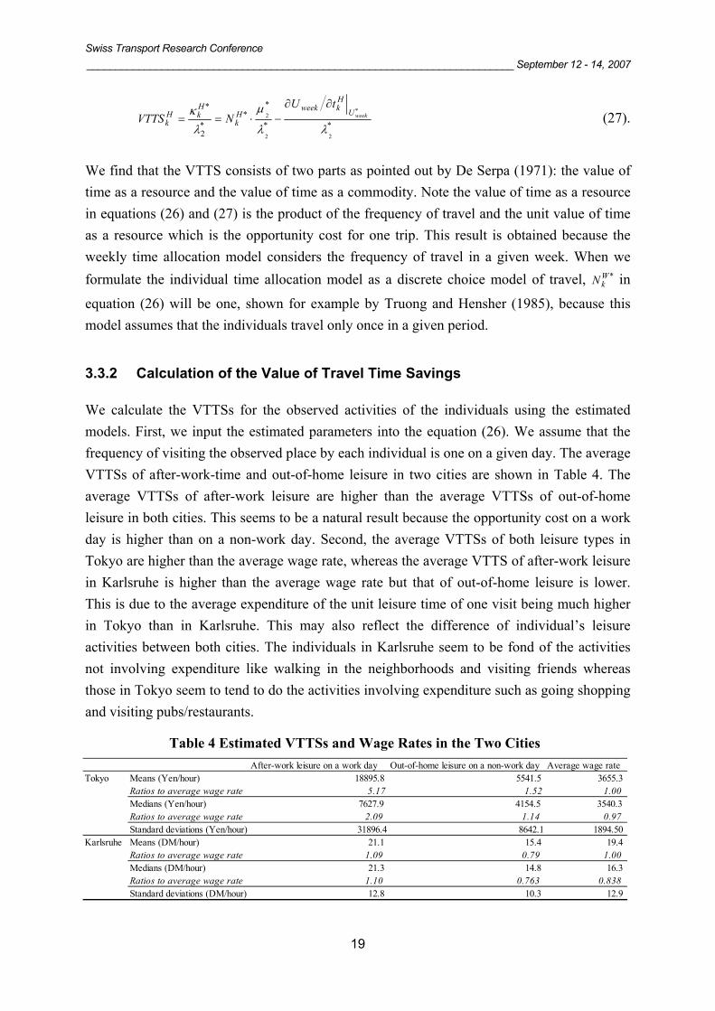
We calculate the VTTSs for the observed activities of the individuals using the estimated models. First, we input the estimated parameters into the equation (26). We assume that the frequency of visiting the observed place by each individual is one on a given day. The average VTTSs of after-work-time and out-of-home leisure in two cities are shown in Table 4. The average VTTSs of after-work leisure are higher than the average VTTSs of out-of-home leisure in both cities. This seems to be a natural result because the opportunity cost on a work day is higher than on a non-work day. Second, the average VTTSs of both leisure types in Tokyo are higher than the average wage rate, whereas the average VTTS of after-work leisure in Karlsruhe is higher than the average wage rate but that of out-of-home leisure is lower. This is due to the average expenditure of the unit leisure time of one visit being much higher in Tokyo than in Karlsruhe. This may also reflect the difference of individual’s leisure activities between both cities. The individuals in Karlsruhe seem to be fond of the activities not involving expenditure like walking in the neighborhoods and visiting friends whereas those in Tokyo seem to tend to do the activities involving expenditure such as going shopping and visiting pubs/restaurants.

Table 4 Estimated VTTSs and Wage Rates in the Two Cities After-work leisure on a work day Out-of-home leisure on a non-work day Average wage rate

Tokyo Means (Yen/hour) 18895.8 5541.5 3655.3Ratios to average wage rate 5.17 1.52 1.00Medians (Yen/hour) 7627.9 4154.5 3540.3Ratios to average wage rate 2.09 1.14 0.97Standard deviations (Yen/hour) 31896.4 8642.1 1894.50

Karlsruhe Means (DM/hour) 21.1 15.4 19.4Ratios to average wage rate 1.09 0.79 1.00Medians (DM/hour) 21.3 14.8 16.3Ratios to average wage rate 1.10 0.763 0.838Standard deviations (DM/hour) 12.8 10.3 12.9


20

In order to compare the VTTSs of the two types of leisure, we calculate the individual ratios. The results are shown in Figure 1. This indicates first that the variance of the VTTSs in Tokyo is much larger than that in Karlsruhe. Second the variance of the VTTSs for the out-of-home leisure is smaller than that for the after-work-leisure in both cities. Third, when we calculate the three-point moving averages of the marginal cumulative share curves, we obtain the modes at ratios of 0.49 for the after-work leisure in Tokyo; 0.46 for the out-of-home leisure in Tokyo; 1.14 for the after-work leisure in Karlsruhe; and 0.86 for the out-of-home leisure in Karlsruhe, respectively. These results imply that the reason for the high average VTTSs in Tokyo is the high variance of the VTTSs.

Figure 2 shows the comparisons between the VTTSs and the value of time (VTR) as a resource. Theoretically speaking, the VTR should be smaller than the VTTS and the

0

0.2

0.4

0.6

0.8

1

0 1 2 3 4 5

VTTSs of after-work leisure on a work day

VTTSs of out-of-home leisure on a non-work day

Ratio of VTTS to individual wage rate

Cum

ulat

ive

shar

e

Karlsruhe

0

0.2

0.4

0.6

0.8

1

0 1 2 3 4 5




Cum

ulat

ive

shar

e

Karlsruhe

0

0.2

0.4

0.6

0.8

1.0

0 10 20 30 40 50Ratios of VTTS and VTR to individual wage rate

Tokyo

Cum

ulat

ive

shar

e


Value of time as a resource (VTR)

0

0.2

0.4

0.6

0.8

1.0

0 10 20 30 40 50Ratios of VTTS and VTR to individual wage rate

Tokyo

Cum

ulat

ive

shar

e



Ratios of VTTS and VTR to individual wage rate

0

0.2

0.4

0.6

0.8

1.0

0 10 20 30 40 50


Value of time as a resource (VTR)Cum

ulat

ive

shar

e

Tokyo


0

0.2

0.4

0.6

0.8

1.0

0 10 20 30 40 50


Value of time as a resource (VTR)Cum

ulat

ive

shar

e

Tokyo

0

0.2

0.4

0.6

0.8

1.0

0 1 2 3 4 5




Cum

ulat

ive

shar

e

Karlsruhe

0

0.2

0.4

0.6

0.8

1.0

0 1 2 3 4 5




Cum

ulat

ive

shar

e

Karlsruhe

0

0.2

0.4

0.6

0.8

1.0

0 1 2 3 4 5




Cum

ulat

ive

shar

e

Karlsruhe

0

0.2

0.4

0.6

0.8

1.0

0 1 2 3 4 5




Cum

ulat

ive

shar

e

Karlsruhe

Figure 2 Comparisons between VTTSs and Value of Time as a Resource (VTR).

Figure 1 Ratios of VTTS to Individual Wage Rate.

0

0.2

0.4

0.6

0.8

1

0 10 20 30 40 50




Cum

ulat

ive

shar

eTokyo

0

0.2

0.4

0.6

0.8

1

0 10 20 30 40 50




Cum

ulat

ive

shar

eTokyo


21

differences of two values mean the value of time as a commodity (VTC). We can see in both cities that the shares of the VTC of a travel for after-work leisure are larger than the VTC of a travel for out-of-home leisure. This is quite reasonable because an individual travels for after-work leisure with a tighter time constraint than for out-of-home leisure.


22

4. CONCLUSIONS

We estimate empirically the value of travel time saving (VTTS) with a time allocation model. First, we formulate an individual’s time and expenditure allocation for a week with three types of discretionary activities, after-work leisure, out-of-home leisure and in-home leisure. We apply it to two activity diary surveys collected in the cities of Tokyo, Japan and Karlsruhe, Germany. We empirically derive the VTTSs in the two cities based on the estimated parameters. The analysis shows that both the means and the modes of the simulated VTTSs for after-work leisure on a work day are higher than those for out-of-home leisure on a non-work day. As the variance of the simulated VTTSs in Tokyo is larger than that in Karlsruhe, the average VTTSs is also larger in Tokyo than those in Karlsruhe.

Our model has still some points which should be examined further more. First, our model classifies the activities into three categories: in-home leisure, out-of-home leisure and after-work leisure. However, we did not distinguish the type of activity in more detail. As a matter of fact, out-of-home leisure and after-work leisure include various types of activities, for example, going shopping, going out for a walk and having dinner at restaurant, etc. An individual chooses a detailed type of activities and the chosen activities may be quite different between cities. For example, people may tend to go shopping more on a non-work day in Karlsruhe than in Tokyo. This possibly biases the estimates of VTTSs. Second, for analytical simplification, we assume that an individual engages in after-work leisure or in-home leisure on a work day. However, an individual who return home early on a work day may go somewhere for an out-of-home leisure. Tokyo data did not include any such individuals whereas Karlsruhe data included them. Thus we may need to improve a choice set of leisure type on a work day for more general model. Third, we assume an individual always chooses the shortest time travel mode and route. This makes the model estimation simple. On the contrary, this may not hold true for an individual who cares travel cost more seriously than travel time. If we incorporate the individual behaviours of choosing travel mode and travel route into our model, we should make our proposed model more complicated.


23

5. ACKNOWLEDGEMENTS

We are deeply grateful to East Japan Marketing & Communications, Inc. for permitting us to use the travel diary survey data in Tokyo. We also thank Paulina Greeven (University of Chile) and Stephan Schönfelder (ETH Zurich, now, Trafico, Wien) for supporting our data arrangement and analysis especially of the Mobidrive survey data.


24

6. REFERENCES

Axhausen, K. W. and Garling, T. Activity-based approaches to travel analysis: conceptual frameworks, models, and research problems. Transport Reviews, Vol. 12, pp. 323–341, 1992.

Axhausen, K. W., Zimmermann, A., Schönfelder, S., Rindsfuser, G. and Haupt, T. Observing the rhythms of daily life: A six-week travel diary. Transportation, Vol. 29, pp. 95–124, 2002.

Bates, J. J. Measuring travel time values with a discrete choice model: a note. The Economic Journal, Vol. 97, pp. 493–498, 1987.

Becker, G. A Theory of the allocation of time. The Economic Journal, Vol. 75, pp. 493–517, 1965.

Bhat, C. R. and Koppelman, F. S. A retrospective and prospective survey of time-use research. Transportation, Vol. 26, pp. 119–139, 1999.

De Serpa, A. C. A theory of the economics of time. The Economic Journal, Vol. 81, pp. 828–846, 1971.

East Japan Marketing & Communication, Inc. Moving Target: Basic Dataset, Kozai Publish Co., 1997 (in Japanese).

Evans, A. On the theory of the valuation and allocation of time. Scottish Journal of Political Economy, Vol. 19, pp. 1–17, 1972.

Greeven, P., Jara-Díaz, S. R., Munizaga, M. A. and Axhausen, K. W. Calibration of a joint time assignment and mode choice model system. Arbeitsberichte Verkehrs- und Raumplanung, No. 308, IVT, ETH, Zürich, 2005.

Jara-Diaz, S. D. Allocation and valuation of travel-time savings. Handbook of Transport Modelling, Hensher, D. A. and Button, K. J. eds., Elsevier Science Ltd, pp. 303–318, 2000.

Kato, H. and Matsumoto, M. Intra-household interaction analysis among a husband, a wife, and a child using the joint time allocation model, Presented at 86th Annual Meeting of the Transportation Research Board, Washington, D.C., 2007.

Kitamura, R. An evaluation of activity-based travel analysis. Transportation, Vol. 15, pp. 9–34, 1988.


25

Kockelman, K. M. A Utility-Theory-Consistent System-of-Demand-Equations Approach to Household Travel Choice, Ph.D. Dissertation, Department of Civil and Environmental Engineering, University of California at Berkeley, 1998.

Kockelman, K. M. A model for time- and budget-constrained activity demand analysis. Transportation Research, Vol. 35B, pp. 255–269, 2001.

Kockelman, K. M. and Krishnamurthy, S. A new approach for travel demand modeling: linking Roy’s Identity to discrete choice. Transportation Research, Vol. 38B, pp. 459–475, 2004.

Small, K. Project evaluation. Essays in Transportation Economics and Policy: A Handbook in Honor of John R. Meyer, Gómez-Ibáñez, J. A., William B. T., and Winston, C. eds., Brookings Institution, Washington, D.C. , pp. 137–177, 1999.

Oort, C. J. The evaluation of traveling time. Journal of Transport Economics and Policy, Vol.1, pp. 279–286, 1969.

Schlich, R., Schönfelder, S., Hanson, S. and Axhausen, K. W. Structures of leisure travel: Temporal and spatial variability. Transport Reviews, Vol. 24, pp. 219–237, 2004.

Tobin, J. Estimation of relationship for limited dependent variables. Econometrica, Vol. 26, pp. 24–36, 1958.

Train, K. and McFadden, D. The goods/leisure tradeoff and disaggregate work trip mode choice models. Transportation Research, Vol. 12, pp. 349–353, 1978.

Truong, T. P. and Hensher , D. A. Measurement of travel times values and opportunity cost from a discrete choice model. The Economic Journal, Vol. 95, pp. 438–451, 1985.

Yamamoto, T. and Kitamura, R. An analysis of time allocation and out-of-home discretionary activities across working days and non-working days. Transportation, Vol. 26, pp. 211–230, 1999.

Value of travel time savings of urban private travel: Comparison of Tokyo and Karlsruhe

Documents