VALUE-BASED, DEPENDENCY-AWARE INSPECTION AND TEST PRIORITIZATION by Qi Li A Dissertation Presented to the FACULTY OF THE USC GRADUATE SCHOOL UNIVERSITY OF SOUTHERN CALIFORNIA In Partial Fulfillment of the Requirements for the Degree DOCTOR OF PHILOSOPHY (COMPUTER SCIENCE) December 2012 Copyright 2012 Qi Li

Welcome message from author
This document is posted to help you gain knowledge. Please leave a comment to let me know what you think about it! Share it to your friends and learn new things together.
Transcript

VALUE-BASED, DEPENDENCY-AWARE INSPECTION AND TEST
PRIORITIZATION
by
Qi Li
A Dissertation Presented to the
FACULTY OF THE USC GRADUATE SCHOOL UNIVERSITY OF SOUTHERN CALIFORNIA
In Partial Fulfillment of the Requirements for the Degree
DOCTOR OF PHILOSOPHY (COMPUTER SCIENCE)
December 2012
Copyright 2012 Qi Li

ii
Dedication
To my parents

iii
Acknowledgements
My Ph.D dissertation could not be completed without the support of many hearts
and minds. I am deeply indebted to my Ph.D advisor Dr. Barry Boehm, for his great and
generous support for all my Ph.D research. I am deeply honored to be one of his students
and get direct and close advice from him all the time. My sincere thanks are also
extended to other committee members Dr. Stan Settles, Dr. Nenad Medvidovic, Dr.
Richard Selby, Dr. William Halfond and Dr. Sunita Chulani, for the invaluable guidance
on focusing my research and efforts on reviewing drafts of my dissertation.
Special thanks to my ISCAS advisors, Professor Mingshu Li, Professor Qing
Wang, and Professor Ye Yang. They led me into the academic world and cont inuously
encourage, support my research, and promote the in-depth collaborative research in our
joint lab of USC-CSSE & ISCAS.
The realization of this research effort also exists because of the tremendous
support from Dr. Jo Ann Lane and Dr. Ricardo Valerdi. In addition, this research could
not have been conducted without support from the University of Southern California
Center for Systems and Software Engineering courses, corporate, and academic
affiliates, especial thanks to Galorath Incorporated, NFS-China for giving me the chance
to apply this research into the real industrial projects , to USC-CSSE graduate-level
software engineering courses 577ab Year 2009-2011 students for their collaborative
effort on the Value-based Inspection and Testing experiments, to all my USC and ISCAS
colleagues and friends, life could not be more colorful without you.
Lastly, from the bottom of my heart, I would like to thank my family for their
unconditional love and support during my study.

iv
Table of Contents
Dedication................................................................................................................... ii
Acknowledgements .................................................................................................... iii
Chapter 1: Introduction ............................................................................................. 1
1.1. Motivation .................................................................................................... 1
1.2. Research Contributions.................................................................................. 4
1.3. Organization of Dissertation .......................................................................... 5
Chapter 2: A Survey of Related Work ....................................................................... 7
2.1. Value-Based Software Engineering .................................................................... 7
2.2. Software Review Techniques ............................................................................. 9
2.3. Software Testing Techniques............................................................................ 11
2.4. Software Test Case Prioritization Techniques ................................................... 12
2.5. Defect Removal Techniques Comparison.......................................................... 19
Chapter 3: Framework of Value-Based, Dependency-Aware Inspection and Test
Prioritization ............................................................................................................ 22
3.1. Value-Based Prioritization ............................................................................... 22
3.1.1. Prioritization Drivers ................................................................................. 23
3.1.1.1.Stakeholder Prioritization..................................................................... 23
3.1.1.2.Business /mission value ....................................................................... 24
3.1.1.3.Defect Criticality ................................................................................. 24
3.1.1.4.Defect Proneness ................................................................................. 25
3.1.1.5.Testing or Inspection Cost.................................................................... 25

v
3.1.1.6.Time- to-Market .................................................................................. 26
3.1.2. Value-Based Prioritization Strategy ........................................................... 26
3.2. Dependency-Aware Prioritization ..................................................................... 27
3.2.1.Loose Dependencies ................................................................................... 27
3.2.2.Tight Dependencies .................................................................................... 29
3.3. The Process of Value-Based. Dependency-Aware Inspection and Testing .......... 31
3.4. Key Performance Evaluation Measures ............................................................. 34
3.4.1. Value and Business Importance ................................................................. 34
3.4.2. Risk Reduction Leverage ........................................................................... 34
3.4.3. Average Percentage of Business Importance Earned (APBIE):.................... 35
3.5. Hypotheses, Methods to test ............................................................................. 36
Chapter 4: Case Study I-Prioritize Artifacts to be Reviewed .................................. 41
4.1. Background ..................................................................................................... 41
4.2. Case Study Design ........................................................................................... 45
4.3. Results............................................................................................................. 53
Chapter 5: Case Study II-Prioritize Testing Scenarios to be Applied...................... 65
5.1. Background ..................................................................................................... 65
5.2. Case Study Design ........................................................................................... 68
5.2.1. Maximize Testing Coverage ...................................................................... 68
5.2.2. The step to determine Business Value ........................................................ 70
5.2.3. The step to determine Risk Probability ....................................................... 71
5.2.4. The step to determine Cost......................................................................... 72

vi
5.2.5. The step to determine Testing Priority ........................................................ 74
5.3. Results............................................................................................................. 75
5.4. Lessons Learned .............................................................................................. 80
Chapter 6: Case Study III-Prioritize Software Features to be functionally Tested . 84
6.1. Background ..................................................................................................... 84
6.2. Case Study Design ........................................................................................... 84
6.2.1. The step to determine Business Value ........................................................ 84
6.2.2. The step to determine Risk Probability ....................................................... 86
6.2.3. The step to determine Testing Cost ............................................................ 92
6.2.4. The step to determine Testing Priority ........................................................ 93
6.3. Results............................................................................................................. 94
Chapter 7: Case Study IV-Prioritize Test Cases to be Executed............................ 102
7.1. Background ................................................................................................... 102
7.2. Case Study Design ......................................................................................... 103
7.2.1. The step to do Dependency Analysis ........................................................ 103
7.2.2. The step to determine Business Importance .............................................. 104
7.2.3. The step to determine Criticality .............................................................. 108
7.2.4. The step to determine Failure Probability ................................................. 109
7.2.5. The step to determine Test Cost ............................................................... 111
7.2.6. The step for Value-Based Test Case Prioritization .................................... 111
7.3. Results........................................................................................................... 114
7.3.1. One Example Project Results ................................................................... 114

vii
7.3.2. All Team Results:.................................................................................... 119
7.3.2.1 A Tool for Faciliating Test Case Prioritization: ................................... 120
7.3.2.2 Statistical Results for All Teams via this Tool ..................................... 124
7.3.2.3. Lessons learned ................................................................................ 132
Chapter 8: Threats to Validity ............................................................................... 133
Chapter 9: Next Steps............................................................................................. 138
Chapter 10: Conclusions ........................................................................................ 142
Bibliography ........................................................................................................... 144

viii
List of Tables
Table 1. Comparsion Results of Value-based Group A and Value-neutral Group B
.......................................................................................................................... 10
Table 2. Test Suite and List of Faults Exposed ................................................... 15
Table 3 Business Importance Distribution (Two Situations) ................................ 16
Table 4. Comparison for TCP techniques ............................................................ 18
Table 5. An Example of Quantifying Dependency Ratings ................................... 29
Table 6. Case Studies Overview .......................................................................... 38
Table 7.V&V assignments for Fall2009/2010 ...................................................... 44
Table 8. Acronyms.............................................................................................. 44
Table 9. Documents and sections to be reviewed.................................................. 45
Table 10. Value-neutral Formal V&V process ..................................................... 46
Table 11. Value-based V&V process ................................................................... 47
Table 12. An example of value-based artifact prioritization .................................. 48
Table 13. An example of Top 10 Issues ............................................................... 50
Table 14. Issue Severity & Priority rate mapping ................................................. 52
Table 15. Resolution options in Bugzilla .............................................................. 52
Table 16. Review effectiveness measures ............................................................ 53
Table 17. Number of Concerns ............................................................................ 54
Table 18. Number of Concerns per reviewing hour .............................................. 55
Table 19. Review Effort ...................................................................................... 56
Table 20. Review Effectiveness of total Concerns ................................................ 57

ix
Table 21. Average of Impact per Concern ............................................................ 58
Table 22. Cost Effectiveness of Concerns ............................................................ 59
Table 23. Data Summaries based on all Metrics ................................................... 62
Table 24. Statistics Comparative Results between Years ...................................... 61
Table 25 Macro-feature coverage ........................................................................ 68
Table 26. FU Ratings .......................................................................................... 70
Table 27. Product Importance Ratings ................................................................. 71
Table 28. RP Ratings ......................................................................................... 71
Table 29. Installation Type .................................................................................. 72
Table 30. Average Time for Testing Macro 1-3.................................................... 72
Table 31. Testing Cost Ratings ............................................................................ 73
Table 32. Testing Priorities for 10 Local Installation Working Environments ........ 74
Table 33. Testing Priorities for 3 Server Installation Working Environments ........ 75
Table 30. Value-based Scenario Testing Order and Metrics .................................. 76
Table 35. Testing Results .................................................................................... 77
Table 36. Testing Results (continued) .................................................................. 77
Table 37. APBIE Comparison ............................................................................. 79
Table 38. Relative Business Importance Calculation ............................................ 85
Table 39. Risk Factors’ Weights Calculation-AHP .............................................. 88
Table 40. Quality Risk Probability Calculation (Before System Testing).............. 90
Table 41. Correlation among Initial Risk Factors: ................................................ 91
Table 42. Relative Testing Cost Estimation.......................................................... 92
Table 43 Correlation between Business Importance and Testing Cost .................. 93

x
Table 44. Value Priority Calculation.................................................................... 94
Table 45. Guideline for rating BI for test cases................................................... 107
Table 46. Guideline for rating Criticality for test cases ....................................... 109
Table 47. Self-check questions used for rating Failure Probability ..................... 110
Table 48. Mapping Test Case BI &Criticality to Defect Severity& Priority ........ 118
Table 49. Relations between Reported Defects and Test Cases ........................... 119
Table 50. APBIE Comparison (all teams) .......................................................... 127
Table 51. Delivered Value Comparison when Cost is fixed (all teams)................ 128
Table 52. Cost Comparison when Delivered Value is fixed (all teams)................ 129
Table 53. APBIE Comparison (11 teams) .......................................................... 130
Table 54. Delivered Value Comparison when Cost is fixed (11 teams)................ 131
Table 55. Cost Comparison when Delivered Value is fixed (11 teams)................ 131

xi
List of Figures
Figure 1. Pareto Curves ........................................................................................ 2
Figure 2. Value Flow vs. Software Development Lifecycle .................................... 3
Figure 3. The “4+1” Theory of VBSE: overall structure ....................................... 8
Figure 4. Software Testing Process-Oriented Expansion of VBSE “4+1” Theory
and Key Practices ................................................................................................. 8
Figure 5. Value-based Review (VBR) Process .................................................... 10
Figure 6. Coverage-based Test Case Prioritization .............................................. 12
Figure 7. Comparison under Situation 1 ............................................................... 16
Figure 8. Comparison under Situation 2 ............................................................... 17
Figure 9. Overview of Value-based Software Testing Prioritization Strategy......... 22
Figure 10. An Example of Loose Dependencies ................................................... 28
Figure 11. An Example of Tight Dependencies .................................................... 30
Figure 12. Benefits Chain for Value-based Testing Process Implementation ......... 31
Figure 13. Software Testing Process-Oriented Expansion of “4+1” VBSE
Framework ......................................................................................................... 32
Figure 14. ICSM framework tailored for csci577 ................................................ 42
Figure 15. Scenarios to be tested ........................................................................ 67
Figure 16. Comparison among 3 Situations .......................................................... 79
Figure 17. Business Importance Distribution....................................................... 86
Figure 18. Testing Cost Estimation Distribution................................................... 93
Figure 19. Comparison between Value-Based and Inverse order ........................... 95
Figure 20. Initial Estimating Testing Cost and Actual Testing Cost Comparison .. 95

xii
Figure 21. BI, Cost and ROI between Testing Rounds ......................................... 96
Figure 22. Accumulated BI Earned During Testing Rounds ................................. 97
Figure 23. BI Loss (Pressure Rate=1%) ............................................................... 99
Figure 24. BI Loss (Pressure Rate=4%) .............................................................. 99
Figure 25. BI Loss (Pressure Rate=16%) ............................................................. 99
Figure 26. Value Functions for “Business Importance” and “Testing Cost” ......... 100
Figure 27. Dependency Graph with Risk Analysis ............................................. 104
Figure 28. Typical production function for software product features.................. 105
Figure 29. Test Case BI Distribution of Team01 Project ..................................... 108
Figure 30. Failure Probability Distribution of Team01 Project ............................ 111
Figure 31. In-Process Value-Based TCP Algorithm............................................ 114
Figure 32. PBIE curve according to Value-Based TCP (APBIE=81.9%) ............. 115
Figure 33. PBIE Comparison without risk analysis between Value-Based and Value-
Neutral TCP (APBIE_value_based=52%, APBIE_value_neutral=46%) .............. 117
Figure 34. An Example of Customized Test Case in TestLink ............................ 121
Figure 35. A Tool for facilitating Value-based Test Case Prioritization in TestLink
........................................................................................................................ 122
Figure 36. APBIE Comparison .......................................................................... 124
Figure 37. Delivered-Value Comparison when Cost is fixed ............................... 125
Figure 38. Cost Comparison when Delivered Value is fixed ............................... 126

xiii
Abbreviations
ICSM Phases:
ICSM: Incremental Commitment Spiral Model
VC: Valuation Commitment
FC: Foundation Commitment
DC: Development Commitment
TRR: Transition Readiness Review
RDC: Rebaselined Development Commitment
IOC: Initial Operational Capability
TS: Transition & Support
Artifacts developed and reviewed for USC CSCI577
OCD: Operational Concept Description
SSRD: System and Software Requirements Description
SSAD: System and Software Architecture Description
LCP: Life Cycle Plan
FED: Feasibility Evidence Description
SID: Supporting Information Document
QMP :Quality Management Plan
IP: Iteration Plan
IAR: Iteration Assessment Report
TP: Transition Plan

xiv
TPC: Test Plan and Cases
TPR: Test Procedures and Result
UM: User Manual
SP: Support Plan
TM: Training Materials
Value-Based, Dependency-Aware inspection and test prioritization
related
RRL: Risk Reduction Level
ROI: Return On Investment
BI: Business Importance
ABI: Accumulated Business Importance
PBIE: Percentage of Business Importance Earned
APBIE: Average Percentage of Business Importance Earned
AC: Accumulated Cost
FU: Frequency of Use
RP: Risk Probability
TC: Testing Cost
TP: Test Priority
PI: Product Importance
Others:
FV&V: Formal Verification & Validation

xv
VbV&V: Value-based Verification & Validation
Eval: Evaluation
ARB: Architecture Review Board

xvi
Abstract
As two of the most popular defect removal activities, Inspection and Testing are
of the most labor-intensive activities in software development life cycle and consumes
between 30% and 50% of total development costs according to many studies. However,
most of the current defect removal strategies treat all instances of software artifacts as
equally important in a value-neutral way; this becomes more risky for high-value
software under limited funding and competitive pressures.
In order to save software inspection and testing effort to further improve
affordability and timeliness while achieving acceptable software quality, this research
introduces a value-based, dependency-aware inspection and test prioritization strategy for
improving the lifecycle cost-effectiveness of software defect removal options. This
allows various defect removal types, activities, and artifacts to be ranked by how well
they reduce risk exposure. Combining this with their relative costs enables them to be
prioritized in terms of Return On Investment (ROI) or Risk Reduction Leverage (RRL).
Furthermore, this strategy enables organizations to deal with two types of common
dependencies among items to be prioritized. This strategy will help project managers
determine “how much software inspection/testing is enough?” under time and budget
constraints. Besides, a new metric Average Percentage of Business Importance Earned
(APBIE) is proposed to measure how quickly testing can reduce the quality uncertainty
and earn the relative business importance of the System Under Test (SUT).
This Value-Based, Dependency-Aware Inspection and Testing strategy has been
empirically studied and successfully applied on a series of case studies within different
prioritization granularity levels : (1). Prioritizing artifacts to be reviewed in 21 graduate-

xvii
level, real-client software engineering course projects; (2). Prioritizing testing scenarios
to be applied in an industrial project at the acceptance testing phase in Galorath, Inc.; (3).
Prioritizing software features to be functionally tested in an industrial project in the
China-NFS company; (4). Prioritizing test cases to be executed in 18 course projects. All
the comparative statistics analysis from the four case studies show positive results from
applying the Value-Based, Dependency-Aware strategy.

1
Chapter 1: Introduction
1.1.Motivation
Traditional verification & validation, and testing methodologies such as: path,
branch, instruction, mutation, scenario, or requirements testing usually treat all aspects of
software as equally important [Boehm and Basili, 2001], [Boehm, 2003]. This leads to a
purely technical issue leaving the close relationship between testing and business
decisions unlinked and the potential value contribution of testing unexploited [Ramler et
al., 2005]. However, commercial experience is often that 80% of the business value is
covered by 20% of the tests or defects, and that prioritizing by value produces significant
payoffs [Bullock, 2000], [Gerrard and Thompson, 2002], [Persson and Yilmazturk,
2004]. Also, current “Earned Value” systems fundamentally track the project progress
against the plan, and cannot track changes in the business value of the system being
developed. Furthermore, system value-domain problems are the chief sources of software
project failures, such as unrealistic expectations, unclear objectives, unrealistic time
frames, lack of user input, incomplete requirement, or changing requirements [Johnson,
2006]. All of these plus the increasing criticality of software within systems, make value-
neutral software engineering methods increasingly risky.
Boehm and Basili’s “Software Defect Reduction Top 10 List” [Boehm and Basili,
2001] shows that “Finding and fixing a software problem after delivery is often 100 times
more expensive than finding and fixing it during the requirements and design phase.
Current software projects spend about 40 to 50 percent of their effort on avoidable
rework. About 80 percent of avoidable rework comes from 20 percent of the defects.

2
About 80 percent of the defects come from 20 percent of the modules, and about half the
modules are defect free. About 90 percent of the downtime comes from, at most, 10
percent of the defects. Peer reviews catch 60 percent of the defects. Perspective-based
reviews catch 35 percent more defects than non-directed reviews. Disciplined personal
practices can reduce defect introduction rates by up to 75 percent” [Boehm and Basili,
2001].
Figure 1. Pareto Curves [Bullock, 2000]
The upper Pareto curve in Figure 1 comes from an experience report [Bullock,
2000] for which 20% of the features provide 80% of the business value. It shows that
among the 15 customer types, the first one nearly consists of 50% of the billing revenues
and that 80% of the test cases generate only 20% of the business value. So, focusing the
effort on the high-payoff test cases will generate the highest ROI. The linear curve is
representative of most automated test generation tools. It is equally likely to test the high
and low value types, so in general, it shows a linear payoff. Value-neutral method can do
even worse than this. For example, many projects focus on reducing the number of

3
outstanding problem reports as quickly as possible, leading to first fixing the easiest
problems such as typos, or grammar mistakes. This generates a value curve much worse
than the linear one.
From the perspective of VBSE, the full range of the software development
lifecycle (SDLC) is a value flow that begins with value objective assessment and capture
by value-based requirement acquisition, business case analysis, early design and
architecting, followed by value implementation by detailed architecting, and
development; and value realization by testing to ensure the value objectives are satisfied
before transitioned and delivered to customers by means of value-prioritized test cases
being executed and passed, as shown in Figure 2. Monitoring and controlling actual value
being earned by project’s results in terms of multiple value objectives can enable
organizations to pro-actively monitor and control not only fast-breaking risks to project
success in delivering expected value, but also fast-breaking opportunities to switch to
even higher-value emerging capabilities to avoid highly efficient waste of an
organization’s scarce resources.
Figure 2. Value Flow vs. Software Development Lifecycle
Value Objective Capture
Acquisition, Requirement
Design, Architect
Development
Test & Transition
Value Implementation
Value Realization

4
Each of the system’s value objectives is corresponding to at least one test item,
e.g. an operational scenario, a software feature, or a test case that is used to measure
whether this value objective is achieved or not in order to earn the relevant value. The
whole testing process could be seen as a Value Earned process by executing and
successfully passing one test case, and earning one piece of value etc. In the Value-Based
Software Engineering community, value is not only limited to purely financial terms, but
extended to as relative worth, utility or importance to provide help address software
engineering decisions [Boehm, 2003]. Business Importance in terms of Return On
Investment (ROI) is often used to measure the relative value of functions, components,
features or even systems for business domain software systems. So the testing process
under this business domain context could also be accordingly defined as a Business
Importance Earned process. To measure how quickly a testing strategy can earn the
business importance, especially under time and budget constraints, a new metric Average
Percentage of Business Importance Earned (APBIE) is proposed and will be introduced
in detail in Chapter 3.
1.2.Research Contributions
The research is intended to provide the following contributions:
Current software inspection and testing process investigation and analysis;
Propose a real “Earned Value” system to track business value of testing and
measure testing efficiency in terms of Average Percentage of Business
Importance Earned (APBIE);

5
Propose a systematic strategy for Value-Based, Dependency Aware Inspection &
Testing Processes;
Apply this strategy to a series of empirical studies with different granularities of
prioritization;
Elaborate decision criteria of testing/inspection priorities per project contexts,
which are helpful and insightful for real industry practices;
Implement an automatic tool for facilitating Value-Based, Dependency-Aware
prioritization.
1.3.Organization of Dissertation
The organization of this dissertation is as follows:
Chapter 2 presents a survey of results Value-Based Software Engineering,
software inspection techniques, software testing process strategies, software test case
prioritization techniques and defect removal techniques.
Chapter 3 introduces the methodology of Value-Based, Dependency Aware
inspection and testing prioritization strategy and process, proposes key performance
evaluation measures, research hypotheses, and methods to test the hypotheses.
Chapter 4-7 introduces the detailed steps and practices to apply the Value-Based,
Dependency Aware prioritization strategy onto four typical inspection and testing case
studies. For each case study, project backgrounds, case study designs, implementation
steps are introduced, comparative analysis is conducted, both qualitative and quantitative
results and lessons learned are summarized:

6
Chapter 4 introduces the prioritization of artifacts to be reviewed on USC-CSSE
graduate-level, real-client course projects for its formal inspection;
Chapter 5 conducts the prioritization of operational scenarios to be applied in
Galorath, Inc. for its performance testing;
Chapter 6 illustrates the prioritization of features to be tested on a Chinese
software company for its functionality testing;
Chapter 7 presents the prioritization of test cases to be executed on USC-CSSE
graduate level course projects at its acceptance testing phase.
Chapter 8 explains some threats to validity; Chapter 9 and 10 propose some future
research work and conclude the contributions of this research dissertation.

7
Chapter 2: A Survey of Related Work
2.1. Value-Based Software Engineering
Value-Based Software Engineering (VBSE) is a discipline that addresses and
integrates economic aspects and value considerations into the full range of existing and
emerging software engineering principles and practices, processes, activities and tasks,
technology, management and tools decisions in the software development context
[Boehm, 2003].
The engine in the center is the Success-Critical Stakeholder (SCS) Win-Win
Theory W [Boehm, 1988], [Boehm et al., 2007], which addresses what values are
important and how success is assured for a given software engineering organization. The
four supporting theories that it draws upon are utility theory, decision theory, dependency
theory, and control theory, respectively dealing with how important are the values, how do
stakeholders’ values determine decisions, how do dependencies affect value realization,
and how to adapt to change and control value realization.
VBSE key practices includes: benefits realization analysis; stakeholder Win-Win
negotiation; business case analysis; continuous risk and opportunity management;
concurrent system and software engineering; value-based monitoring and control and
change as opportunity. This process has been integrated with the spiral model of system
and software development and evolution [Boehm et al. , 2007] and its next generation
system and software engineering successor, the Incremental Commitment Spiral Model
[Boehm and Lane, 2007].

8
Figure 3. The “4+1” Theory of VBSE: overall structure [Boehm and Jain, 2005]
The Value-based Software Engineering theory is the fundamental theory for the
proposed Value-based Inspection and Test Prioritization strategy. Our strategy is VBSE
theory’s application on Software Testing and Inspection process. Our strategy’s mapping
to the VBSE’s “4+1” theory and key practices is shown in Figure 4.
Figure 4. Software Testing Process-Oriented Expansion of VBSE “4+1” Theory and Key Practices

9
2.2. Software Review Techniques
Up to date, many focused review or reading methods and techniques have been
proposed, practiced and proved to be superior to unfocused reviews. The most common
one in practice is checklist-based reviewing (CBR) [Fagan, 1976], others include
perspective-based reviewing (PBR) [Basili et al., 1996], [Li et al., 2008], defect-based
reading (DBR) [Porter et al., 1995], functionality-based reading (FBR) [Abdelrabi et al.,
2004] and usage-based reading (UBR) [Conradi and Wang, 2003], [Thelin et al., 2003].
However, Most of them are value-neutral (except UBR) and focused on one single aspect,
e.g. DBR focuses defect classification to find defects in artifacts and a scenario is a key
factor in DBR. UBR focuses on prioritizing use cases in order of importance from a user
perspective. FBR is proposed to trace framework requirements to produce well-
constructed framework and review the code.
As an initial value-based set of peer review guidelines [Lee and Boehm, 2005], its
process consists of: first, a win-win negotiation among stakeholders defines the priority of
each system capability; Based on the checklists for each artifact, domain expert will
determine the criticality of issue; next, the system capabilities with high priorities were
reviewed first; third, at each priority level, the high-criticality sources of risk were
reviewed first, as shown in Figure 5. The experiment uses Group A: 15 IV&V personnel
using VBR procedures and checklists, Group B 13 IV&V personnel using previous value-
neutral checklists. The result of the initial experiment found a factor-of-2 improvement in
value added per hour of peer review time as shown in Table 1.

10
Figure 5. Value-based Review (VBR) Process [Lee and Boehm, 2005]
Table 1. Comparsion Results of Value-based Group A and Value-neutral Group B [Lee and Boehm, 2005]
By Number P-
value
% Gr A
higher By Impact
P-
value
% Gr A
higher
Average of
Concerns 0.202 34
Average Impact of
Concerns 0.049 65
Average of
Problems 0.056 51
Average Impact of
Problems 0.012 89
Average of
Concerns per
hour
0.026 55
Average Cost
Effectiveness of
Concerns
0.004 105
Average of
Problems per
hour
0.023 61
Average Cost
Effectiveness of
Problems
0.007 108
As a new contribution to value-based V&V process development, the Value-
Based, Dependency-Aware prioritization strategy was then customized to develop a
systematic and multi-criteria process to quantitatively determine the priorit ies of
artifacts to be reviewed. This process adds Quality Risk Probability, Cost and

11
Dependency considerations into the prioritization and has been successfully applied on
USC-CSSE graduate level, real client course projects with statistically significant
improvement of review cost effectiveness, which will be introduced in Chapter 4.
2.3. Software Testing Techniques
Rudolf Ramler outlines a framework for value-based test management [Ramler et
al., 2005], it is a synthesis of current most relevant processes and a high-level guideline
without detail implementation specifications and empirical validation.
Stale Amland introduces a risk-based testing approach [Amland, 1999]. It states
that resources should be focused on those areas representing the highest risk exposure.
However, this method doesn’t consider the testing cost which is also an essential factor
during testing process.
Boehm and Huang propose a quantitative risk analysis [Boehm et al. , 2004] that
helps determine when to stop testing software and release the product under different
organizational contexts and different desired quality levels. However, it is a macroscopic
empirical data analysis without process guidance in detail.
Other relevant work includes usage-based testing, and statistical-based testing
[Cobb and Mills, 1990], [Hao and Mendes, 2006], [Kouchakdjian and Fietkiewicz, 2000],
[Musa, 1992], [Walton et al., 1995], [Whittaker and Thomason, 1994], [Williams and
Paradkar, 1999]. Usage model characterizes operational use of a software system, then
generate random test cases from the usage model, perform statistical testing of the
software, record any observed failure, and analyze the test results using a reliability model
to provide a basis for statistical inference of reliability of the software during operational
use. Statistical testing based on a software usage model ensures that the failures that will

12
occur most frequently in operational use will be found early in the testing cycle. However,
it doesn’t differentiate failure’s impact and operational usages’ business importance.
2.4. Software Test Case Prioritization Techniques
Most of current test case prioritization (TCP) techniques [Elbaum et al. , 2000],
[Elbaum et al., 2002], [Elbaum et al., 2004], [Rothermel et al. , 1999], [Rothermel et al.,
2001], are coverage-based, and aim to improve a test suite’s rate of fault detection, a
measure of how quickly faults are detected within the testing process, in order to get
earlier feedback on the System Under Test (SUT). The metric Average Percentage of
Faults Detected (APFD) is used to measure how quickly the faults are identified for a
given test suite. These TCP techniques are all based on coverage of statements or
branches in the programs, assuming that all the statements or branches are equally
important, all faults have equal severity and all test cases have equal costs. An example of
coverage-based test case prioritization is shown in Figure 6.
Figure 6. Coverage-based Test Case Prioritization [Rothermel et al., 1999]
S.Elbaum proposed a new “cost-cognizant” metric, APFDc, for assessing the rate
of fault of detection of prioritized test cases that incorporates varying test case and fault
costs [Elbaum et al., 2001], [Malishevsky et al., 2006], which should reward test cases
orders proportionally to their rate of “unit-of-fault-severity-detected-per-unit-test-cost”.

13
By incorporating context and lifetime factors, improved cost-benefit models are provided
for use in assessing regression testing methodology and effects of time constraints on the
costs and benefits of prioritization techniques [Do and Rothermel, 2006], [Do et al., 2008],
[Do and Rothermel, 2008]. However, he didn’t incorporate the failure probability in the
prioritization.
H.Srikanth presented a requirement-based system level test case prioritization
called the Prioritization of Requirements for Test (PORT) based on requirements volatility,
customer priority, implementation complexity, and fault proneness of the requirement to
improve the rate of detection of severe faults , measured by Average Severity of Faults
Detected (ASFD), however, she didn’t consider the cost of testing in the prioritization.
More recently, there has been a group of related work on fault-proneness test
prioritization based on failure prediction, the most representative one is CRANE
[Czerwonka et al., 2011], a failure prediction, change risk analysis and test prioritization
system at Microsoft Corporation that leverages existing research [Bird et al., 2009],
[Eaddy et al. , 2008], [Nagappan et al., 2006], [Pinzger et al., 2008], [Srivastava and
Thiagarajan, 2002], [Zimmermann and Nagappan, 2008], for the development and
maintenance of Windows Vista. It prioritized the selected tests by “changed blocks
covered per test cost unit” ratio [Czerwonka et al., 2011]. Their test prioritization is
mainly based on the program change analysis in order to estimate the more fault-prone
parts, however, program change is only one factor that would influence the failure
probability, other factors, e.g. personnel qualification, module complexity etc. should
influence the prediction of failure probability as well. Besides it didn’t consider the
business value from customers and the different importance levels of modules, and defects.

14
Some other fault/failure prediction work to identify the fault-prone components in a
system [58-60] is also relevant to our work. Other related work of test case prioritization
can be found at some recent systematic review work [Roongruangsuwan and Daengdej,
2010], [Yoo and Harman, 2011], [Zhang et al., 2009].
In our research, a new metric: Average Percentage of Business Importance Earned
(APBIE) to measure how quickly the SUT’s value is realized for a given test suite or how
quickly the business importance can be earned by testing under the VBSE environment.
The definition of APBIE will be introduced in detail in Chapter 3.
Comparison among TCP techniques
Most of the current Test Case Prioritization techniques [Elbaum et al., 2000, 2001
2002, 2004], [Malishevsky et al., 2006], [Do and Rothermel, 2006], [Do and Rothermel,
2008], [Do et al. , 2008], [Rothermel et al., 1999], [Rothermel et al., 2001], [Srikanth et al.,
2005] are under the prerequisite that: which test cases will expose which faults is known,
and aims to improve the rate of “fault detection”.
In order to predict the defect proneness to support more practical test case
prioritization, current research in this field trends to develop various defect prediction
techniques that serve as the basis for test prioritization [Bird et al., 2009], [Czerwonka et
al., 2011], [Eaddy et al., 2008], [Emam et al., 2001], [Nagappan et al., 2006], [Ostrand et
al., 2005, 2007], [P inzger et al. , 2008], [Srivastava and Thiagarajan, 2002], [Zimmermann
and Nagappan, 2008] .
In order to call for more attention to the value considerations into the current test
case prioritization techniques, we used a simple example as shown in Table 2 from
Rothermel’s paper [Rothermel et al., 1999] (which could also be representative of other

15
similar coverage-based TCP techniques) and constructed two situations as displayed in
Table 3 for this example. Although these two situations are emulated, they can represent
most of the real situations.
Table 2. Test Suite and List of Faults Exposed [Rothermel et al., 1999]
Fault
1 2 3 4 5 6 7 8 9 10
A X
X
B X
X X X
C X X X X X X X
D
X
E
X X X
Rothermel’s test case prioritization technique is under the perquisite that: which
test cases will expose which faults is known. Based on Rothermel’s method, the testing
order should be “C-E-B-A-D”, however, his prioritization doesn’t differentiate the
business importance of each test suite, let’s make some assumptions to show what his
prioritization can result in if the business importance of each test suite is know.
Let’s assume that test suite’s business importance is independent of faults seeded
as shown in Table 2. The business importance is from the customer’s value perspectives
on the relevant features that those test suites can represent.

16
Table 3 Business Importance Distribution (Two Situations)
Situation 1 (Best Case) Situation 2 (Worst Case)
Business
Importance
Accumulated
BI
Business
Importance
Accumulated
BI
C 50% 50% 5% 5%
E 20% 70% 10% 15%
B 15% 85% 15% 30%
A 10% 95% 20% 50%
D 5% 100% 50% 100%
APBIE
80%
40%
Situation 1: If it is lucky enough (the possibility should be very low in reality) that
the business importance percentage distribution of the five test suites is shown as in the
Situation 1 in Table 3, “C-E-B-A-D” is also the testing order if we apply Value-based
TCP. So the PBIE curves for both our method and Rothermel’s overlap as shown in
Figure 7. This testing order is the optimal for both rates of “business importance earned”
and “faults detected”.
Figure 7. Comparison under Situation 1
Start 1 2 3 4 5
PB
IE
Test Case Order
Ours
Rothermel

17
Situation 2: If the business importance percentage distribution of the five test
suites is shown as in the Situation 2 in Table 3 “C-E-B-A-D” is the Rothemel’s TCP order
with the APBIE=40%, however, our value-based method’s TCP order is “D-A-B-E-C”
with the APBIE=80% as shown in Figure 8. So our method can improve the testing
efficiency by a factor of 2 in terms of APBIE in this situation when compared with
Rothermel’s method.
Figure 8. Comparison under Situation 2
The comparison results shows that it is possible, but the possibility is extremely
low, that Rothermel’s testing order can overlap the value-based order, and most often time
the APBIE is lower than our value-based TCP technique. Because the two techniques have
different optimized goals: our method aims to improve APBIE, while his method aims to
improve “the rate of fault detection”.
Besides, a comprehensive comparison among the state-of-art TCP techniques is
shown in Table 4. The prioritization algorithm is the same, and all use the greedy
algorithm or its variants to first pick the best candidate, making the local optimal choice at
each step in order to achieve the global optimum. However, the selecting goals are
different, for Rothermel’s method, the goal is to pick the one that can expose the most
faults; while for our method, the goal is to pick the one that represents the highest testing
Start 1 2 3 4 5
PB
IE
Test Case Order
Rothermel's
Ours

18
value. Rothermel’s test case prioritization aims to improve “the rate of fault detection”,
measured by Average Percentage of Fault Detection (APFD), but our method’s goal aims
to improve “the rate of business importance earned”, measured by Average Percentage of
Business Importance Earned (APBIE).
Table 4. Comparison for TCP techniques
Rothermel et al., 1999
Elbaum et al., 2001
Srikanth et al., 2005
Czerwonka et al., 2011
Our method
Prioritization
algorithm
Greedy Greedy Greedy NA Greedy
Coverage-based Defect-Proneness based
Value-based
Goal Maximize
the rate of fault detected
Maximize
the rate of “unit-of-fault-severity-
detected-per-unit-test-cost”
Maximize
the rate of “severity of faults
Detected
Maximize
the chances of finding defects
in the
changed code
Maximize
the rate of business importance
earned
Measure APFD:
Average Percentage of Faults Detected
APFDc:
Average Percentage of Faults
Detected, incorporating testing Cost
ASFD:
Average Severity of Faults
Detected
FRP: Fix
Regression Proneness
APBIE:
Average Percentage of Business
Importance Earned
Assumption? under the prerequisite that which test case will
expose which faults is known, and those faults are seeded deliberately
No No
Practical? Infrequently, because of the assumption above Yes Yes
Factors for Prioritization
∙Risk Size? (business
importance + defect impact)
No Partial: consider the
defect severity
Partial: consider the
customer-assigned
priority
No Yes
∙Risk Probability?
No No Partial: consider requirement
change, complexity, fault prone.
Partial: mainly consider code
change impact by version control
systems
Yes
∙Cost? No Yes No No Yes
∙Dependency? No No No No Yes

19
As an additional case of the application of the Value-Based, Dependency-Aware
strategy, we recently experimented a more systematic value-based test case prioritization
of a set of test cases to be executed for acceptance and regression testing on the USC-
CSSE graduate-level, real-client course projects, with improved testing efficiency and
effectiveness, which will be introduced in Chapter 7. Our prioritization is more systematic,
because we synthetically consider the business importance from customers’ perspective,
the failure probability, the execution cost and dependency among them into the
prioritization.
2.5. Defect Removal Techniques Comparison
The efficiency of review and testing are compared in Constructive QUALity
Model (COQUALMO) [Boehm et al., 2000]. To determine the Defect Removal Fraction
(DRFs) associated with each of the six levels (i.e., Very Low, Low, Nominal, High, Very
High, Extra High) of the three profiles (i.e., automated analysis, people reviews, execution
testing and tools) for each of three types of defect artifacts (i.e., requirement defects,
design defects, and code defects), it conducted a two-round Delphi. This study found that
people review is the most efficient on removing requirement and design defects, and
testing is the most efficient on removing code defects.
Madachy and Boehm extended their previous work on COQUALMO and assessed
software quality process with the Orthogonal Defect Classification COnstructive QUALity
MOdel (ODC COQUALMO) that predicts defects introduced and removed, classified by
ODC types [Chillarege et al., 1992], [Madachy and Boehm, 2008]. A comprehensive
Delphi survey was used to capture more detailed efficiencies of the techniques (automated

20
analysis, execution testing, and tools, and peer reviews) against ODC defect categories as
an extension on the previous work [Boehm et al., 2000].
In [Jones, 2008], Capers Jones lists Defect Removal Efficiency of 16 combinations
of 4 defect removal methods: design inspections, code inspections, quality assurance, and
testing. These results show that, on one side, no single defect removal method is adequate,
on the other side, implies that removal efficiency from better to worse would be design
inspections, code inspections, testing and quality assurance. However, all the above defect
removal technique comparison work is based on Delphi surveys, and still lack quantitative
data evidence from industry.
Based on the experience from the manufacturing area that has been brought to the
software domain and software reliability models to predict the future failure behavior, S.
Wagner presents a model for quality economics of defect-detection techniques [Wagner
and Seifert, 2005]. This model is proposed to estimate the effects of a combination and
remove such influences when evaluating a single technique. However, this model is a
theoretic model without real industry data validation.
More recently, Frank Elberzhager presented an integrated two-stage inspection and
testing process on the code level [Elberzhager et al., 2011]. In particular, defect results
from an inspection are used in two-stage manner: first, prioritize parts of the system that
are defect-prone and then prioritizes defect types that appear often. However, the
combined prioritization is mainly using defects detected from inspection to estimate
failure probability in order to prioritize testing activities, without considerations on defect
removal technique efficiency comparison by defect type among inspection, testing or
other defect removal techniques.

21
We plan to collect real industry project data to compare the defect removal
techniques’ efficiency based on RRL to further calibrate ODC COQUALMO. And then
select or combine defect removal techniques by defect type to optimize the scarce
inspection and testing resources which will be discussed in Chapter 9 as our next-step
work.

22
Figure 9. Overview of Value-based Software Testing Prioritization Strategy
Chapter 3: Framework of Value -Based, Dependency-Aware Inspection and Test
Prioritization
This chapter will introduce the methodology of the Value-Based, Dependency
Aware inspection and testing prioritization strategy and process, proposes key
performance evaluation measures, research hypotheses and the methods to test those
hypotheses.
3.1. Value-Based Prioritization
The systematic and comprehensive value-based, risk-driven inspection and testing

23
prioritization strategy, proposed to improve their cost-effectiveness, is shown in Figure 9.
It illustrates the value-based inspection and testing prioritization’s methodology,
composed of four main consecutive parts: prioritization drivers, which deals with what are
the project success-critical factors are and how they influence the software inspection and
testing; prioritization strategy, which deals with how to make optimal trade-offs among
those drivers; prioritization case studies, which deals with how to apply the value-based
prioritization strategy into practices, especially under industry contexts and this part will
be introduced in detail from Chapter 4 to Chapter 7; and prioritization evaluation which
deals with how to track the business value of inspection and testing and measure their
cost-effectiveness. These fours questions from each part will be answered and explained
3.1.1. Prioritization Drivers
Most of the current testing prioritization strategies focus on optimizing one single
goal, i.e. coverage-based testing prioritization aims to maximum the testing coverage per
unit testing time, risk-driven testing aims to detect the most fault-prone parts at the earliest
time etc. Besides, seldom research work incorporates the business or mission value into
the prioritization. In order to build a systematic and comprehensive prioritization
mechanism, the prioritization should take all project success-critical factors into
consideration, i.e., business or mission value, testing cost, defect criticality, and defect-
prone probability, for some business critical projects, the time to market should also be
added into prioritization. The value-based prioritization drivers should include:
3.1.1.1.Stakeholder Prioritization
The first step of value-based inspection and testing is to identify Success-Critical
Stakeholders (SCSs) and understand their roles played during the inspection and testing

24
process and their respective win conditions. Direct stakeholders of testing are testing
team, especially testing manager, developers and project managers, who directly interact
with the testing team. In the spirit of value-based software engineering important parties
for testing are key customers as the source of value objectives, which set the context and
scope of testing. Marketing and product managers assist in testing for planning releases,
pricing, promotion, and distribution. We will look at the following factors that must be
considered when prioritizing the testing order of new features, and they represent SCSs’s
win conditions:
3.1.1.2.Business /mission value
Business or mission value is captured by business case analysis with the
prioritization of success-critical stakeholder value propositions; Business Importance of
having the features gives information as to what extent mutually agreed requirements are
satisfied and to what extent the software meets key customers’ value propositions.
CRACK (Collaborative, Representative, Authorized, Committed and Knowledgeable)
[Boehm and Turner, 2003] customer representatives are the source of features’ relative
business importance. Only if their most valuable propositions or requirements have been
understood clearly, developed correctly, tested thoroughly and delivered timely, the
project could be seen as a successful one. So under this situation, CRACK customer
representatives are most likely to be collaborative and knowledgeable to provide the
relative business importance information.
3.1.1.3.Defect Criticality
Defect criticality is captured by measuring the impact of absence of an expected
feature, not achieving a performance requirement, or the failure of a test case, Combining

25
with the business or mission value, it serves as the other factor to determine the Size of
Loss as shown in Figure 9.
3.1.1.4.Defect Proneness
Defect-proneness is captured by expert estimation based on historical data or past
experiences, design or implementation complexity, qualification of the responsible
personnel, code change impact analysis etc. Quality of the software product is another
success-critical factor that needs to be considered for the testing process. The focus of
quality risk analysis is on identifying and eliminating risks that are potential value
breakers and inhibit value achievements. The information of quality risk could help testing
manager with risk management, progress estimation, and quality management. Testing
managers are interested in the identification of problems particularly the problem trends
that helps to estimate and control testing process. By risk identification and analysis, it
will also provide the developing manager some potential process improvement
opportunities to mitigate project risks in the future. So both of the testing manager and
developing team are willing to be collaborative with each other to do the quality risk
analysis.
3.1.1.5.Testing or Inspection Cost
Testing or inspection cost is captured by expert estimation based on historical data
or past experiences, or by some state-of-art testing cost estimation techniques or tools;
Testing cost is considered as an investment in software development and should also be
seriously considered during the testing process. This would become more crucial as the
time-critical deliverables are required, e.g., when time-to-market greatly influences the
market share. If most of the testing effort is put into testing features or test cases, or

26
scenarios with relatively less business importance, that will lose more market share and
lead to decreasing customer’s profits, even negative profits in the worst case. Testing
managers are interested in making testing process more efficient, by putting more effort on
the features with higher business importance.
3.1.1.6.Time- to-Market
Time-to-market can greatly influence the effort distribution of software
developing and project planning. Because the testing phase serves as the adjacent phase
before software product transition and delivery, it will be influenced even more by
market pressure [Yang et al., 2008]. Sometimes, in the intense market competition
situation, sacrificing some software quality to avoid more market share erosion might be
a good organizational strategy. Huang and Boehm [Huang and Boehm, 2006] propose a
value-based software quality model that helps to answer the question “How much testing
is enough?” in three types of organizational contexts: early start-up, commercial, and
high finance. For example, an early start-up will have a much higher risk impact due to
market share erosion than the other two. Thus better strategy for an early start-up is to
deliver a lower quality product than invest in quality beyond the threshold of negative
returns due to market share erosion. Marketing and product managers help to provide the
market information and assist in testing for planning releases, pricing, promotion, and
distribution.
3.1.2. Value-Based Prioritization Strategy
The value-based inspection and testing prioritization strategy synthetically
considers business importance from the client’s value perspective combined with the
criticality of failure occurrence as a measure of the size of loss at risk. For each test item

27
(e.g. artifacts, testing feature, testing scenario, or test case), the probability of loss is the
probability that a given test item would catch the defect, estimated from an experience
base that would indicate defect-prone components or performers. Since Size (Loss) *
Probability (Loss) = Risk Exposure. This enables the testing items to be ranked by how
well they reduce risk exposure. Combining their risk exposures with their relative testing
costs enables the test items to be prioritized in terms of Return On Investment (ROI) or
Risk Reduction Leverage (RRL), where the quantity of Risk Reduction Leverage (RRL) is
defined as follows [Selby, 2007]:
Where REbefore is the RE before initiating the risk reduction effort and REafter is the
RE afterwards. Thus, RRL serves as the engine for the testing prioritization and is a
measure of the relative cost-benefit ratio of performing various candidate risk reduction
activities, e.g. testing in this case study.
3.2. Dependency-Aware Prioritization
In our case studies, two types of dependencies are dealt with, they are “Loose
Dependencies” and “Tight Dependencies”, their definitions, typical examples, and our
solutions to them are introduced as below:
3.2.1.Loose Dependencies
“Loose Dependencies” is defined as: it would be ok to continue task without
awareness of dependencies, but would be better with awareness. The typical case is those
dependencies among artifacts to be reviewed in the inspection process.

28
For example, Figure 10 illustrates the dependencies among four artifacts to be
reviewed for CSCI577ab course projects: System and Software Requirement Description
(SSRD), System and Software Architecture Description (SSAD), Acceptance Testing Plan
and Cases (ATPC), Supporting Information Description (SID). Although they are course
artifacts, they also represent typical requirement, design, test and other supporting
documents in real industrial projects. As shown in Figure 10, SSRD is the requirement
document and usually can be reviewed directly; in order to review use cases, UML
diagrams in SSAD, or test cases in ATPC, it is better to review requirements first in
SSRD at least to check whether those use cases, UML diagrams in SSAD or test cases in
ATPC cover all the requirements in SSRD, so SSAD and ATPC depend on SSRD as the
arrows illustrate in Figure 10. SID maintains the traceability matrices among
requirements in SSRD, use cases in SSAD and test cases in ATPC, so it is better to have
all the requirements, uses cases and test cases in hand when reviewing the traceability, so
SID depends on all the other three artifacts.
But it won’t bother or block to go ahead to review SSAD or ATPC without
reviewing SSRD, or review SID without refereeing all other artifacts. So we call this type
of dependencies “loose dependencies”.
Figure 10. An Example of Loose Dependencies

29
Basically, the more artifacts this document depends on, the higher the Dependency
rating is, and the lower the reviewing priority will be , which can be represented by the
formula as below:
In order to quantify the loose dependency and add it to the review priority
calculation, Table 5 displays a simple example. The number of artifacts this document
depends on is counted, qualitative ratings Low, Moderate and High are mapped, and
numeric values (1, 2, 3) are added in to calculating the priority. Other numeric values e.g.
(1, 5, 10) or (1, 2, 4) can also be used if necessary. The case study in Chapter 4 will
introduce more about how to deal with this type of the loose dependency into the Value-
Based prioritization.
Table 5. An Example of Quantifying Dependency Ratings
# of dependable artifacts Dependency Ratings Numeric Values
SSRD 0 Low 1
SSAD, ATPC 1 Moderate 2
SID 3 High 3
3.2.2.Tight Dependencies
“Tight Dependencies” is defined as: the successor task has to wait until all its
precursor tasks finish, the failure of the precursor will block the successor. The typical
case is the dependencies among the test cases to be executed during the testing process.

30
Figure 11. An Example of Tight Dependencies
Figure 11 illustrates a simple dependency tree among 7 test cases (T1-T7), each
node represents a test case, the numeric value in each node represents the RRL of the test
case. If T1 fails to pass, it will block all other test cases that depend on it, e.g. T3, T4, T5,
T6 and T7, and we call this type of dependencies “Tight Dependencies”. A prioritization
algorithm is proposed to deal with this type of dependencies, and it is a variant of the
greedy algorithm: it first selects the one with the highest RRL, and check whether it
depends on other test cases; if it has dependencies, and in its dependency set, recursively
selects the one with the highest RRL until selecting the one with no dependencies. The
detailed algorithm and prioritization logics will be introduced in Chapter 7.
For the 7 test cases in Figure 11, according to the algorithm, T2, T5 and T6 have
the highest RRL with the value of 9. However, T6 depends on T3 and T1, T5 depends on
T1, while T2 has no dependencies and can be directly executed. So T2 is the first test
case to be executed. Since both T5 and T6 depend on T1, T1 is tested in order to test
those high payoff T5 and T6. After T1 is passed, T5 with the highest RRL is unblocked
and ready for testing. Recursively running the algorithm results in the order “T2->T1-
>T5->T3->T6->T4->T7”. More test cases’ prioritization for real projects will be
introduced and illustrated in Chapter 7.

31
3.3. The Process of Value-Based. Dependency-Aware Inspection and Testing
Figure 12 displays the benefits chain for value-based testing process
implementation including all these SCSs’ roles and their win conditions if we consider
software testing as an investment during the whole software life cycle.
Figure 12. Benefits Chain for Value-based Testing Process Implementation
Figure 13 illustrates the whole process of this value-based software testing
method. This method helps test manager consider all the win-conditions from SCSs,
enact the testing plan and adjust it during testing execution. The main steps are as
follows:

32
Figure 13. Software Testing Process-Oriented Expansion of “4+1” VBSE Framework
Step 1: Define Utility Function of Business Importance, Quality Risk
Probability and Cost. After identifying SCSs and their win conditions, the next step is to
understand and create the single utility function for each win-condition and how they
influence the SCSs’ value propositions. With the assistance of the key CRACK customer,
the testing manager uses a method first proposed by Karl Wiegers [Wiegers, 1999] to get
the relative Business Importance for each feature. The developing manager and the test
manager accompanied with some experienced developers, calculate the quality risk
probability of each feature. The test manager with the developing team estimate the
testing cost for each feature This step brings the stakeholders together to consolidate their
value models and to negotiate testing objectives. This step is in line with the Dependency
and Utility Theory in VBSE that helps to identify all of the SCSs and understand how the
SCSs want to win.

33
Step 2: Testing Prioritization Decision for Testing Plan. Then business
importance, quality risk and testing cost are put together to calculate a value priority
number in terms of RRL for each item to be prioritized, e.g. artifact, scenario, feature, or
test case. This is like a multi-objective decision and negotiation process which follows
the Decision Theory in VBSE. Features’ value priority helps test manager enact the
testing plan, and resources should be focused on those areas representing the most
important business value, the lowest testing cost and highest quality risk.
Step 3: Control Testing Process according to Feedback. During the testing
process, each item’s value priority in terms of RRL is adjusted according to the feedback
of quality risk indicators and updated testing cost estimation. This step assists to control
progress toward SCS win-win realization which is according to the Control Theory of
VBSE.
Step 4: Determine How Much Testing is Enough under Different Market
Patterns. One of the strengths of “4+1” VBSE Dependency Theory is to uncover factors
that are external to the system but can impact the project’s outcome. It serves to align the
stakeholder values with the organizational context. Market factors would influence
organizations to different extent by different organizational contexts. A comparative
analysis is done in Chapter 6 for different market patterns and the result shows that the
value-based software testing method is especially effective when the market pressure is
very high.

34
3.4. Key Performance Evaluation Measures
3.4.1. Value and Business Importance
Some of the dictionary definitions of “value” (Webster 2002) are in purely
financial terms, such as “the monetary worth of something: marketable price.” However,
in the value-based software engineering community, it broader dictionary definition of
“value” as relative worth, utility or importance to provide help address software
engineering decisions. In our research, we usually use relative Business Importance to
capture the client’s business value.
3.4.2. Risk Reduction Leverage
The quantity of Risk Exposure (RE) is defined by:
Where Size (Loss) is the risk impact size of loss if the outcome is unsatisfactory,
Prob (Loss) is the probability of an unsatisfactory outcome.
The quantity of Risk Reduction Leverage (RRL) is defined as follows:
Where REbefore is the RE before initiating the risk reduction effort and REafter is the
RE afterwards. Thus, RRL is a measure of the relative cost-benefit ratio of performing
various candidate risk reduction or defect removal activities.
RRL serves as the engine for the prioritization strategy for different applications to
improve the cost-effectiveness of defect removal activities. Its quantity acquisition can be
different per its applications, project context and scenarios. For example, to quantify the
effectiveness of a review, Review Cost Effectiveness defined as below is a variant of RRL

35
under the condition that the defects detected are 100% resolved and removed, which drops
the Prob (Loss) is from 100% to 0%:
3.4.3. Average Percentage of Business Importance Earned (APBIE):
This metric is defined to measure how quickly the SUT’s value is realized by
testing.
Let T be the whole test case suite for the SUT containing m test items, T’ be a
selected and prioritized test suite subset containing n test items that will be executed and i
is the ith test items is in the test order T’. It is obvious that T’ T, and n≤m; The Total
Business Importance (TBI) for T is
After business importance for the m test items are all rated, TBI is a constant.
Initial Business Importance Earned (IBIE) is the sum of the business importance
for those test items in the set of T-T’.
.
It could be 0 when T=T’. The Percentage of Business Importance Earned (PBIEi)
when the ith test item in the test order T’ is passed is

36
Average Percentage of Business Importance Earned (APBIE) is defined as:
Average Percentage of Business Importance Earned (APBIE) is used to measure
how quickly the SUT’s value is realized, the higher it is, and the more efficient the test is
and it serves as another important metric to measure the cost-effectiveness of testing.
3.5. Hypotheses, Methods to test
A series of hypotheses are defined to be tested.
For value-based review process for prioritizing artifacts, the core hypothesis is:
H-r1:the review cost effectiveness of concerns/problems on the same artifact
package does not differ between value-based group (2010, 2011teams) & value-neutral
one (2009 teams);
Others auxiliary hypotheses include:
H-r2:the number of concerns/problems reviewers found does not differ between
groups;
H-r3:the Impact of concerns/problems reviewers found does not differ between
groups; and etc.
Basically, concerns/problems data based on the defined metrics are collected from
the tailored Bugzilla system and consolidated. Then their Mean, Standard Deviation will
be compared, T-test and F-test are used to test whether those hypotheses can be accepted
or rejected.
For value-based scenarios/features/test cases prioritization, the core hypothesis is:
H-t1: the value-based prioritization does not increase APBIE;

37
Others auxiliary hypotheses include:
H-t2: the value-based prioritization does not lead high-impact defects to be
detected earlier in the acceptance testing phase;
H-t3: the value-based prioritization does not increase “Delivered-Value when
Cost is Fixed” or does not save “Cost when Delivered-Value is fixed” under time
constraints;
To test H-t1 and H-t3, we will compare the experimented value-based testing case
study with value-neutral ones. Then their Mean, Standard Deviation will be compared, T-
test and F-test are used to test whether those hypotheses can be accepted or rejected.
To test H-t2, we will observe the issues reported in the Bugzilla system to check
whether issues with high priority and high severity are reported at the early stage of
acceptance phase.
Besides, its application from USC real-client course projects to other real industry
projects can further test these hypotheses. Furthermore, qualitative methods, such as
surveys or interviews will also be used in our case studies to complement the quantitative
results.
The Value-Based, Dependency-Aware prioritization strategy has been empirically
studied and applied on defect removal activities within different prioritization granularity
levels as summarized in Table 6.
prioritization of artifacts to be reviewed on USC-CSSE graduate level real-client
course projects for its formal inspection;
prioritization of operational scenarios to be applied in Galorath, Inc. for its
performance testing;

38
prioritization of features to be tested on a Chinese software company for its
functionality testing;
prioritization of test cases to be executed on USC-CSSE graduate level course
projects at its acceptance testing phase.
Table 6. Case Studies Overview
Case
Studies
Defect
Removal
Activities
Items to be
Prioriti zed
Granularity
for
Prioriti zation
Prioriti zation Drivers
Business
Value
Risk
Probability
Testing
Cost
Dependency
I:
USC
course
projects
Inspection Artifacts to
be reviewed
High-level Impacts to
Project
Rating Rating Yes
II:
Galorath,
Inc.
Performance
Testing
Operational
Scenarios to
be applied
High-level Frequency
of Use
Rating Rating No
III:
ISCAS
project
Functionality
Testing
Features to
be tested
Medium-level Benefit +
Penalty
Rating Rating No
IV:
USC
course
projects
Acceptance
Testing
Test Cases
to be
executed
Low-level Feature BI
+ Testing
Aspect
Rating Assume
equal
Yes
These four typical case studies cover the most commonly used defect removal
activities during the software development life cycle. Although the prioritization strategies
for them are all triggered by RRL, the ways to get the priorities and dependencies for the
items to be prioritized are different per the defect removal activity type and the project
context.

39
For example, the business case analysis can be implemented with various methods,
considering their ease of use and adaption under experiments’ environment. For example,
in the case study of value-based testing scenario prioritization in Chapter 5, we use
frequency of use (FU) combined with product importance as a variant of business
importance for operational scenarios; in the case study of value-based feature
prioritization for software testing in Chapter 6, Karl Wiegers’ requirement prioritization
approach [Wiegers, 1999] is adopted, which considers both the positive benefit of the
presence of a feature and the negative impact of its absence. In the case study of value-
based test case prioritization in Chapter 7, classic S-curve production function with
segments of investment, high-payoff, and diminishing returns [Boehm, 1981] are used to
train students for their project features’ business case analysis with the Kano model
[Kano] as a reference to complement their analysis for feature business importance
ratings. Test cases’ business importance is then determined by its corresponding
functions/components/features’ importance, and whether testing the core function of this
feature or not. As for the case study of determining the priority of artifacts (system
capabilities) in Chapter 4, the business importance is tailored to ratings of their
influences/impacts to the project’s success. The similarity for these different business case
analyses is that all using well-defined, context-based relative business importance ratings.
These four case studies have practical meanings in real industry and practitioners
can have 3 learner outcomes for each case study as below:
What are the value-based inspection and testing prioritization drivers and their trade-
offs?

40
What are the detailed practices and steps for the value-based inspections/ testing
process under project contexts?
How to track business value of testing and measure testing efficiency using a
proposed real earned value system, with real industrial evidences?

41
Chapter 4: Case Study I-Prioritize Artifacts to be Reviewed
4.1. Background
This case study for prioritizing artifacts to be reviewed was implemented in the
real-client projects’ verification and validation activities at USC graduate-level software
engineering course. The increasing growth of software artifact package motivates us to
prioritize the artifacts be reviewed with the goal to improve the review cost-effectiveness.
At USC, best practices from software engineering industries are introduced to
students through a 2-semester graduate software engineering course (Csci577a, b) with
real-client projects. From Fall 2008, the Incremental Commitment Spiral Model (ICSM)
[Boehm and Lane, 2007], a value-based, risk-driven software life cycle process model
was introduced and tailored as a guideline [ICSM-Sw] for this course as shown in Figure
14. It teaches and trains students skills such as understanding and negotiating stakeholder
needs, priorities and shared visions; rapid prototyping; evaluating COTS, services
options; business and feasibility evidence analysis; and concurrent plans, requirements
and solutions development.

42
In this course, students work in teams and are required to understand and apply
the Incremental Commitment Spiral Model for software engineering to real-world
projects. In CSCI 577b, student teams develop Initial Operational Capability (IOC)
products based on the best results from CSCI 577a. As the guideline for this course,
ICSM covers the full system development life cycle based on Exploration, Valuation,
Foundations, Development, and Operations phases as shown in Figure 14. The key to
synchronizing and stabilizing all of the concurrent product and process definition
activities is a set of risk-driven anchor point milestones: the Exploration Commitment
Review (ECR), Valuation Commitment Review (VCR), Foundation Commitment
Review (FCR), Development Commitment Review (DCR), Rebaselined Development
Commitment Review (RDCR), Core Capability Drivethrough (CCD), Transition
Readiness Review (TRR), and Operation Commitment Review (OCR). At these
milestones, the business, technical, and operational feasibility of the growing package of
specifications and plans is evaluated by independent experts. For the course, clients,
Figure 14. ICSM framework tailored for csci577 [ICSM-Sw]

43
professors and teaching assistants perform Architecture Review Board (ARB) activities
based on to evaluate the package of specifications and plans.
Most off-campus students come from real IT industry with rich experiences. They
often take on the roles of Quality Focal Point and Integrated Independent Verification
and Validation (IIV&V) to review set of artifacts to find any issues related to
completeness, consistency, feasibility, ambiguity, conformance, and risk in order to
minimize the issues found at ARB. A series of package review assignments are
consecutively given to them after development teams submit their packages during the
whole semester. The instructions for each assignment, together with artifact templates in
the ICSM Electronic Process Guide (EPG) [ICSM-Sw] provide reviewing entry and exit
criteria for each package review. Table 7 summarizes the content of the V&V reviews as
performed in Fall 2009 and Fall 2010 and 2011, and Table 8 gives the definitions of the
ICSM and all other acronyms used in this case study.

44
Table 7.V&V assignments for Fall2009/2010
V&Ver Assignment
Review Package 2009 V&V
Method
2010/2011 V&V
Method
Learn to Use Bugzilla System for Your Project Team
Eval of VC Package
OCD,FED, LCP FV&V FV&V
Eval of Initial Prototype
PRO FV&V FV&V
Eval of Core FC Package
OCD,PRO,SSRD**,SSAD,LCP,FED, SID FV&V VbV&V
Eval of Draft FC Package
OCD,PRO,SSRD**,SSAD,LCP,FED, SID FV&V VbV&V
Eval of FC/DC Package
OCD,PRO,SSRD**,SSAD,LCP,FED, SID, QMP, ATPC^, IP ̂
FV&V VbV&V
Eval of Draft DC/TRR Package
OCD,PRO,SSRD**,SSAD,LCP,FED, SID, QMP, ATPC^, IP^, TP ̂
VbV&V VbV&V
Eval of DC/TRR Package
OCD,PRO,SSRD**,SSAD,LCP,FED, SID, QMP, ATPC, IP, TP, IAR^,UM^,TM^,TPR ̂
VbV&V VbV&V
**: not required by NDI/NCS team;
^: only required by one-semester team;
Table 8. Acronyms
ICSM phases: VC: Valuation Commitment, FC: Foundation Commitment, DC: Development
Commitment, TRR: Transition Readiness Review, RDC: Rebaselined Development Commitment, IOC: Initial Operational Capability, TS: Transition & Support
Artifacts developed and reviewed for this course:
OCD: Operational Concept Description, SSRD: System and Software Requirements Description,
SSAD: System and Software Architecture Description, LCP: Life Cycle Plan, FED: Feasibility Evidence Description, SID: Supporting Information Document, QMP :Quality Management Plan, IP: Iteration Plan, IAR: Iteration Assessment Report, TP: Transition Plan, TPC: Test Plan and Cases, TPR: Test Procedures and Result, UM: User Manual, SP: Support Plan, TM: Training Materials
Others: FV&V: Formal Verification & Validation, VbV&V: Value-based Verification & Validation, Eval: Evaluation, ARB: Architecture Review Board

45
4.2. Case Study Design
The comparison analysis is conducted between 8 2010-teams and 13 2011-teams
that adopted the value-based prioritization strategy and 14 2009-teams adopting a value-
neutral method without prioritizing before reviewing. All the three years’ teams reviewed
the same content of three artifact packages as shown in Table 9.
Table 9. Documents and sections to be reviewed
Doc/Sec CoreFCP DraftFCP FC/DCP
1&2 sem 1&2 sem 2 sem 1 sem
OCD 100% 100% 100% 100%
FED AA(Section 1,5) NDI(Section1,3,4.1,4.2.1,4.2.2)
Section 1-5 Section 1-5 100%
LCP Section 1, 3.3 100% 100% 100%
SSRD AA(100%) NDI(N/A)
AA(100%) NDI(N/A)
AA(100%) NDI(N/A)
AA(100%) NDI(N/A)
SSAD Section 1, 2.1.1-2.1.3 Section 1, 2 Section 1, 2 100%
PRO Most critical/important use cases 100% 100% 100%
SID 100% 100% 100% 100%
QMP N/A N/A Section 1,2 100%
ATPC N/A N/A N/A 100%
IP N/A N/A N/A 100%
Year 2009 teams used a value-neutral formal V&V process (FV&V) to reviewing
the three artifact packages, a variant of Fagan inspection [Fagan, 1976] practice. The steps
they followed are:

46
Table 10. Value-neutral Formal V&V process
Step 1: Create Exit Criteria: From the original team assignment’s description and the related ICSM EPG completion criteria, generate a set of exit criteria that identify what needs to be present and the standard for acceptance of each document.
Step 2: Review and Report Concerns: Based upon the exit criteria, read (review) the documents and report concerns and issues into the Bugzilla [USC_CSSE_Bugzilla] system.
Step 3: Generate Evaluation Report
Management Overview - List any features of the solution described in this artifact that are particularly good, of which a non–technical client should be aware of.
Technical Details - List any features of the solution described in this artifact that you feel are particularly good, and which a technical reviewer should be aware of.
Major Errors & Omissions - List top 3 errors or omissions in the solution described in this artifact
that a non–technical client would care about. The description of an error (or omission) should be understandable to a non–technical client, and should explain why the error is worth the client’s attention.
Critical Concerns - List top 3 concerns with the solution described in this artifact that a non–
technical client would care about. The description of the concern should be understandable to a non–technical client, and should explain why the client should be aware of it. You should also suggest step(s) to take that would reduce or eliminate your concern.
Year 2010 and 2011 teams applied the value-based, dependency-aware
prioritization strategy to the review process with the guidelines for inspection as
summarized as in Table 11.

47
Table 11. Value-based V&V process
Step 1: Value-based V&V Artifacts Prioritization
Priority Factor Rating Guideline
Importance
5: most important
3: normal
1: least important
Without this document, the project can’t move forward or could even fail; it should be rated with high importance
Some documents serve a supporting function. Without them, the project still could move on; this kind of document should be rated with lower importance
Quality Risk
5: highly risky
3: normal
1: least risky
Based on previous reviews, the documents with intensive defects might be still
fault-prone, so this indicates a high quality risk
Personnel factors, e.g. the author of this documents is not proficient or motivated enough; this indicates a high quality risk
A more complex document might have a high quality risk
A new document or an old document with a large portion of newly added sections might have a high quality risk
Dependency
5: highly dependent
3:normal
1: not dependent
Sometimes some lower-priority artifacts are required to be reviewed at least for
reference before reviewing a higher-priority one. For example, in order to review SSAD or TPC, SSRD is required for reference.
Basically, the more documents this document depends on, the higher the Dependency rating is, and the lower the reviewing priority will be
Review Cost
5: need intensive effort
3: need moderate effort
1: need little effort
A new document or an old document with a large portion of newly added sections
usually takes more time to review and vice versa
A more complex document usually takes more time to review and vice versa
Determine Weights
Weights for each factor (Importance, Quality Risk, Review Cost, and
Dependency) could be set according to the project context. Default values are 1.0 for each factor
Priority Calculation
E.g: for a document, Importance=5, Quality Risk=3, Review Cost=2, Dependency = 1, default weights are used=> Priority= (5*3)/(2*1)=7.5
A spreadsheet [USC_577a_VBV&VPS, 2010] helps to calculate the priority automatically, 5-level ratings for each factor are VH, H, M, L VL with values from 5 to 1, intermediate values 2, 4 are also allowed.
Step 2: Review artifacts based on prioritization and report defects/issues
The one with higher priority value should be reviewed first
For each document’s review, review the core part of the document first. Report issues into the Bugzilla [USC_CSSE_Bugzilla] Step 3: List top 10 defects/ issues
List top 10 highest-risk defects or issues based on issues’ priority and severity

48
A real example of artifacts prioritization in one package review by a 2010-team
[USC_577a_VBV&VAPE, 2010] is displayed in Table 12. The default weight of 1.0 for
each factor is used. Based on the priority calculated, reviewing order follows SSRD, OCD,
PRO, SSAD, LCP, FED, SID. SSRD has the highest reviewing priority with the
rationales provided: SSRD contains the requirements of the system, without this
document, the project can't move forward or could even fail (Very-High Importance). This
is a complex document, and needs to be consistent with win conditions negotiation, which
might not be complete at this point, also, a lot of rework was required based on comments
from TA (Very-High Quality Risk). SSRD depends on few other artifacts (Low
Dependency). This is an old document, but it is complex with a lot of rework (Very-High
Review Cost).
Table 12. An example of value-based artifact prioritization
Weights: 1 1 1 1
Importance Quality Risk Dependency Review Cost Priority
LCP
M
This document describes
the life cycl e plan of the project. This document
serves as supporting function, without this, the
project still could move on. With his document, the
project could move more smoothly.
L
Based on previous
reviews, the author of this document has a
strong sense of responsibility.
L
M
A lot of new
sections added, but this
document is not very complex.
1.00
OCD
H
This document gives the
overall operational concept of the system. This
document is important, but it is not critical for this success of the system.
VH
This is a complex
document and a lot of the sections in this
document needed to be redone based on the
comments received from the TA.
M
SSRD
H
Old document,
but a lot of rework done. 1.67

49
FED
H
This document should be rated high because it
provides feasibility evidence for the project.
Without this document, we don't know whether the project is feasible.
H
The author of this document does not
have appropri ate time to complete this
document with quality work.
H
SSRD, SSAD
H
A lot of new section added to
this version of the document.
1.00
SSRD
VH
This document contains
the requirements of the system. Without this
document, the project can't move forward or even fail.
VH
This is a complex
document. This document needs to be
consistent with win conditions negotiation,
which might not be complete at this point.
Also, a lot of rework was required based on comments from TA.
L
VH
This is an old
document, but it is complex with a lot of rework.
2.50
SSAD
VH
This document contains
the architecture of the system. Without this
document, the project can't move forward or even fail.
VH
This is a complex
document and it is a new document. The
author of this document did not
know that this document was due
until the morning of the due date.
H
SSRD, OCD
VH
This is an old
document, but it is complex with
a lot of rework done for this version.
1.25
SID
VL
This document serves as supporting function,
without this document, the project still could move on,
but the project could move on more smoothly with this document.
L
This is an old document. Only
additions made to existing sections.
VH
OCD, SSRD, FED, LCP, SSAD, PRO
VL
This is an old document and
this document has no technical contents.
0.40
PRO
H
Without this document, the project can probably move
forward, but the system might not be what the
customer is expecting. This document allows the
customer to have a glimpse of the system.
L
This is an old document with little
new contents. The author has a high
sense of responsibility and he fixed bugs
from the last review in reasonable time.
M
FED
L
This is an old document with
little content added since last
version and not much rework required.
1.33
An example of Top 10 issues made by this team for CoreFCP evaluation is
displayed in Table 13. These Top 10 issues are communicated in a timely manner with
artifact authors to attract enough emphasis. The interesting finding is the relations between

50
the artifact priority sequence and the top 10 issues sequence: the issues with higher impact
usually exist in the artifacts with high priority, showing that the artifact prioritization
enables reviewers to focus on issues with high impact at least in this context. However, it
also helps avoid the potential problem of neglecting high-impact issues in lower-priority
artifacts, as in Issues 8 and 10.
Table 13. An example of Top 10 Issues
Summary Rationale
1 SSRD Missing important requirements.
A lot of important requirements are missing. Without these requirements, the system will not succeed.
2 SSRD Requirement supporting information too generic.
The output, destination, precondition, and post condition should be defined better. These description will allows the development team and the client better understand the requirements. This is important for system success.
3 SSAD Wrong cardinality in the system context diagram.
The cardinality of this diagram needs to be accurate since
this describes the top level of the system context. This is important for system success.
4 OCD The client and client advisor stakeholders should be concentrating
on the deployment benefits.
It is important for that this benefits chain diagram accurately shows the benefits of the system during deployment in order for the client to show to potential
investor to gather fund to support the continuation of system development.
5 OCD The system boundary
and environment missing support infrastructure.
It is important for the System boundary and environment
diagram to capture all necessary support infrastructure in order for the team to consider all risks and requirements related the system support infrastructure.
6 FED Missing use case references in the FED.
Capability feasibility table proves the feasibility of all system capabilities to date. Reference to the use case is
important for the important stakeholders to understand the capabilities and their feasibility.
7 FED Incorrect mitigation plan.
Mitigation plans for project risks are important to overcome the risks. This is important for system success.
8 LCP Missing skills and roles The LCP did not identify the skill required and roles for next semester. This information is important for the success of the project because the team next semester can
use these information and recruit new team members meeting the identified needed skills.

51
9 FED CR# in FED doesn't match with CR# in SSRD
The CR numbers need to match in both FED and SSRD for correct requirement references.
10 LCP COCOMO drivers rework
COCOMO driver values need to be accurate to have a better estimate for the client.
The three-year experiment issue data for the evaluation of CoreFCP, DraftFCP and
FC/DCP from total 35 teams is collected and extracted from the Bugzilla database. The
generic term “Issue” covers both “Concerns” and “Problems”. If the IV&Vers find any
issue, they report it as a “Concern” in Bugzilla and assign it to the relevant artifact author.
The author determines whether the concern is a problem or not.
As transformed in Table 14, Severity is rated from High (corresponding to ratings
of Blocker, Critical, Major in Bugzilla ), Medium (corresponding the rating of Normal in
Bugzilla), Low ( the ratings of Minor, Trivial, Enhancement in Bugzilla) with the value
from 3 to 1. Priority is rated from High (Resolve Immediately), Medium (Normal Queue),
Low (Not Urgent, Low Priority, Resolved Later) with the value from 3 to 1. The Impact of
an issue is the product of its Severity and Priority. The impact of an issue with high
severity and high priority is 9. Obviously, the impact of an issue is an element in the set
{1, 2, 3, 4, 6, and 9}.

52
Table 14. Issue Severity & Priority rate mapping
Rating for
Measurement
Rating in Bugzilla Value
Severity
High Blocker, Critical, Major 3
Medium Normal 2
Low Minor, Trivial, Enhancement 1
Priority
High Resolve Immediately 3
Medium Normal Queue 2
Low Not Urgent, Low Priority,
Resolved Later 1
The generic term “Issue” covers both “Concerns” and “Problems”. If the IV&Vers
find any issue, they report it as a “Concern” in Bugzilla and assign it to the relevant
artifact author. The author determines whether it needs fixing by choosing an option for
“Resolution” as displayed in Table 15. Whether an issue is a problem or not is easy to be
determined by querying the “Resolution” of the issue. “Fixed” and “Won’t Fix” mean the
issue is a problem and the other two options mean that it is not.
Table 15. Resolution options in Bugzilla
Resolution Options Instructions in Bugzilla
Fixed If the issue is a problem, after you fix the problem in the artifact, then choose “Fixed”
Won’t Fix
If the issue is a problem, but won’t be fixed for this time, then choose “Won’t Fix” and must provide the clear reason in “Additional Comments” why it can’t be fixed for this time
Invalid If the issue is not a problem then choose “Invalid” and must provide a clear reason in “Additional Comments”
WorksForMe If the issue really works fine, then choose “WorksForMe” and let the IVVer review this again

53
4.3. Results
Various measures in Table 16 are used to compare the performance of 2011, 2010
years’ value-based and 2009 value-neutral review process. The main goal of the Value-
based review or inspection is to increase the review cost effectiveness as defined in
Chapter 3.
Table 16. Review effectiveness measures
Measures Details
Number of Concerns The number of concerns found by reviewers
Number of Problems The number of problems found by reviewers
Number of Concerns per reviewing hour The number of concerns found by reviewers per reviewing hour
Number of Problems per reviewing hour The number of problems found by reviewers per reviewing hour
Review Effort Effort spent on all activities in the package review
Review Effectiveness of total Concerns
As defined in Chapter 3 but for concerns
Review Effectiveness of total Problems
As defined in Chapter 3 but for problems
Average of Impact per Concern Review Effectiveness of total Concerns/ Number of Concerns
Average of Impact per Problem Review Effectiveness of total Problems/ Number of Problems
Review Cost Effectiveness of Concerns
As defined in Chapter 3 but for concerns
Review Cost Effectiveness of Problems
As defined in Chapter 3 but for problems
Table 17 to Table 22 list the three years’ 35 teams’ performances on different
measures for concerns, and problems’ data is similar and is not listed here due to page
limitation. Mean and Standard Deviation values are calculated at the bottom of each
measure.

54
Table 17. Number of Concerns
2011 Teams 2010 Teams 2009 Teams
T-1 180 T-1 141 T-1 58
T-3 82 T-2 198 T-2 45
T-4 138 T-3 53 T-3 102
T-5 211 T-4 33 T-4 87
T-6 38 T-5 60 T-5 32
T-7 78 T-6 116 T-6 58
T-8 117 T-7 98 T-7 103
T-9 163 T-8 94 T-8 119
T-10 80
T-9 157
T-11 148
T-10 61
T-12 58
T-11 108
T-13 147
T-12 41
T-14 44
T-13 34
T-14 33
Mean 114.15 Mean 99.13 Mean 74.14
Stdev 54.99 Stdev 53.28 Stdev 38.75

55
Table 18. Number of Concerns per reviewing hour
2011 Teams 2010 Teams 2009 Teams
T-1 4.81 T-1 2.79 T-1 0.81
T-3 1.86 T-2 3.07 T-2 1.25
T-4 5.17 T-3 1.22 T-3 2.15
T-5 7.54 T-4 1.12 T-4 1.43
T-6 1.10 T-5 1.08 T-5 0.79
T-7 2.41 T-6 3.02 T-6 1.17
T-8 3.74 T-7 2.89 T-7 1.46
T-9 6.15 T-8 1.46 T-8 2.08
T-10 4.88 T-9 2.18
T-11 7.22 T-10 1.14
T-12 2.32 T-11 1.60
T-13 5.08 T-12 1.53
T-14 1.90 T-13 0.75
T-14 0.69
Mean 4.17 Mean 2.08 Mean 1.36
Stdev 2.12 Stdev 0.93 Stdev 0.52

56
Table 19. Review Effort
2011 Teams 2010 Teams 2009 Teams
T-1 37.44 T-1 50.5 T-1 71.2
T-3 44.06 T-2 64.6 T-2 36.1
T-4 26.69 T-3 43.5 T-3 47.5
T-5 27.98 T-4 29.5 T-4 61
T-6 34.6 T-5 55.35 T-5 40.5
T-7 32.4 T-6 38.4 T-6 49.5
T-8 31.25 T-7 33.95 T-7 70.5
T-9 26.5 T-8 64.3 T-8 57.2
T-10 16.4 T-9 72
T-11 20.5 T-10 53.5
T-12 25 T-11 67.5
T-13 28.95 T-12 26.85
T-14 23.1 T-13 45.5
T-14 48
Mean 28.84 Mean 47.51 Mean 53.35
Stdev 7.30 Stdev 13.37 Stdev 13.97

57
Table 20. Review Effectiveness of total Concerns
2011 Teams 2010 Teams 2009 Teams
T-1 888 T-1 790 T-1 242
T-3 396 T-2 872 T-2 186
T-4 527 T-3 233 T-3 334
T-5 1153 T-4 147 T-4 349
T-6 139 T-5 233 T-5 151
T-7 331 T-6 480 T-6 186
T-8 487 T-7 404 T-7 486
T-9 811 T-8 406 T-8 422
T-10 333
T-9 631
T-11 646
T-10 229
T-12 226
T-11 442
T-13 562
T-12 160
T-14 191
T-13 133
T-14 137
Mean 514.62 Mean 445.63 Mean 292
Stdev 297.92 Stdev 263.08 Stdev 155.05

58
Table 21. Average of Impact per Concern
2011 Teams 2010 Teams 2009 Teams
T-1 4.93 T-1 5.60 T-1 4.17
T-3 4.83 T-2 4.40 T-2 4.13
T-4 3.82 T-3 4.40 T-3 3.27
T-5 5.46 T-4 4.45 T-4 4.01
T-6 3.66 T-5 3.88 T-5 4.72
T-7 4.24 T-6 4.14 T-6 3.21
T-8 4.16 T-7 4.12 T-7 4.72
T-9 4.98 T-8 4.32 T-8 3.55
T-10 4.16
T-9 4.02
T-11 4.36
T-10 3.75
T-12 3.90
T-11 4.09
T-13 3.82
T-12 3.90
T-14 4.34
T-13 3.91
T-14 4.15
Mean 4.36 Mean 4.42 Mean 3.97
Stdev 0.54 Stdev 0.52 Stdev 0.44

59
Table 22. Cost Effectiveness of Concerns
2011 Teams 2010 Teams 2009 Teams
T-1 23.72 T-1 15.64 T-1 3.40
T-3 8.99 T-2 13.50 T-2 5.15
T-4 19.75 T-3 5.36 T-3 7.03
T-5 41.21 T-4 4.98 T-4 5.72
T-6 4.02 T-5 4.21 T-5 3.73
T-7 10.22 T-6 12.50 T-6 3.76
T-8 15.58 T-7 11.90 T-7 6.89
T-9 30.60 T-8 6.31 T-8 7.38
T-10 20.30
T-9 8.76
T-11 31.51
T-10 4.28
T-12 9.04
T-11 6.55
T-13 19.41
T-12 5.96
T-14 8.27
T-13 2.92
T-14 2.85
Mean 18.66 Mean 9.30 Mean 5.31
Stdev 10.94 Stdev 4.53 Stdev 1.86
Table 23 compares the Mean and Standard Deviation values for all the measures
between the three-year teams. To determine whether the differences between years based
on a measure is statistically significant or not, Table 24 compares every two years’ data
using the F-test and T-test. The F-test determines whether two samples have different
variances. If the significance (p-value) for F-test is 0.05 or below, the two samples have
different variances. This will determine which type of T-test will be used to determine
whether the two samples have the same mean. Two types of T-test are: Two-sample equal
variance (homoscedastic), and Two-sample unequal variance (heteroscedastic). If the

60
significance (p-value) for T-test is 0.05 or below, the two samples have different means.
For example, Table 24 shows that 2010’s value-based review teams had a 75.04% higher
Review Cost Effectiveness of Concerns than 2009’s value-neutral teams. The p-value for
F-test 0.0060 leads to choose “Two-sample unequal variance” type T-test. The p-value for
T-test 0.0218 is strong evidence (well below 0.05) that the 75.04% improvement has
statistical significance, the similar for its comparison between 2011 and 2009 (with F-test
0.0000, and T-test 0.0004), which rejects the hypothesis H-r1.
Table 23. Data Summaries based on all Metrics
2011 Team 2010 Team 2009 Team
Mean Stdev Mean Stdev Mean Stdev
Number of Concerns 114.15 54.99 99.13 53.28 74.14 38.75
Number of Problems 108.62 52.81 93.38 52.96 68.79 35.35
Number of Concerns per reviewing hour 4.17 2.12 2.08 0.93 1.36 0.52
Number of Problems per reviewing hour 3.96 2.04 1.96 0.92 1.26 0.48
Review Effort 28.84 7.30 47.51 13.37 53.35 13.97
Review Effectiveness of total Concerns 514.62 297.92 445.63 263.08 292.00 155.05
Review Effectiveness of total Problems 491.85 287.84 416.25 254.15 272.07 141.78
Average of Impact per Concern 4.36 0.54 4.42 0.52 3.97 0.44
Average of Impact per Problem 4.37 0.57 4.37 0.52 3.99 0.45
Review Cost Effectiveness of Concerns 18.66 10.94 9.30 4.53 5.31 1.86
Review Cost Effectiveness of Problems 17.80 10.54 8.69 4.32 4.97 1.73

61
Table 24. Statistics Comparative Results between Years
2011 Vs 2009 2010 Vs 2009 2011 Vs 2010
% 2011
Team higher
F-test T-test % 2010
Team higher
F-test T-test % 2011
Team higher
F-test T-test
(p-value) (p-value) (p-value) (p-value)
(p-value)
(p-value)
Number of Concerns 53.96% 0.225 0.0187 33.69% 0.3049 0.1093 15.16% 0.9752 0.2729
Number of Problems 57.90% 0.1656 0.0144 35.75% 0.1976 0.1026 16.32% 0.9454 0.2644
Number of Concerns per reviewing hour 206.77% 0 0.0002 53.17% 0.0636 0.0142 100.28% 0.0372 0.0031
Number of Problems per reviewing hour 213.33% 0 0.0002 55.16% 0.0393 0.0382 101.94% 0.044 0.0033
Review Effort -45.95% 0.0314 0 -10.94% 0.9509 0.1752 -39.31% 0.064 0.0003
Review Effectiveness of total Concerns 76.24% 0.0268 0.0136 52.61% 0.0949 0.0489 15.48% 0.7673 0.2985
Review Effectiveness of total Problems 80.78% 0.0169 0.0117 52.99% 0.0661 0.0502 18.16% 0.7671 0.2746
Average of Impact per Concern 9.74% 0.475 0.026 11.14% 0.5957 0.023 -1.26% 0.9358 0.4095
Average of Impact per Problem 9.46% 0.4398 0.0333 9.61% 0.6307 0.043 -0.13% 0.8602 0.4909
Review Cost Effectiveness of Concerns 251.23% 0 0.0004 75.04% 0.006 0.0218 100.66% 0.0271 0.0071
Review Cost Effectiveness of Problems 258.34% 0 0.0004 75.01% 0.0048 0.0233 104.75% 0.0254 0.0066
In Table 24 the shadowed sections represent that those comparisons are
statistically significant, we can see that 2010 teams’ performance improves from 2009
teams’ on most of the measures, except the number of concerns/problems, and review
effort. 2011 teams’ performance even improves from 2009 teams’ on all the measures.
Since Year 2010 and 2011 teams all adopted the same value-based inspection
process, their differences on the measures between the two years are expected to be
insignificant. However, we find that the review effort in 2011 is dramatically decreased,
which directly causes significant differences on other measures relevant to review effort
between 2010 and 2011, such as review effort, number of concerns/problems per
reviewing hour, review cost effectiveness of concerns/problems. The decreased review
effort in 2011 is due to 2011 year’s team size change: 2011 teams have an average size of
6.5 (6 or 7) developers with 1 reviewer each team, while 2010 teams have an average size
of 7.5 (7 or 8) developers with an average of 1.5 (1 or 2) reviewers each team, decreased

62
number of reviewers each team leads to the decreased review effort. This uncontrolled
factor might partially contribute to an overall factor of 2.5’s improvement from 2009 to
2011, or an overall 100% from 2010 to 2011 on review cost effectiveness of
concerns/problems, which might be a potential threat of validity to our positive results,
however, we also find that all other review effort irrelevant measures’ comparison
between 2010 and 2011 shows these two years’ performances are similar, such as average
of impact per concern/problem, number of concerns/problems. Two reviewers in each
team in 2010 usually overlapped reviewed all documents, they tend not to report
duplicated concerns if there was already a similar one in the concern list, so for 2010 and
2011, it makes sense that both years have nearly the same number of concerns (no
statistically significant), but review effort nearly doubled in 2010 since the reviewer size is
nearly twice as 2011. This might also give us some hints that one reviewer per team might
be enough for 577ab projects. This indicates that similar as the year 2010, reviewers tend
to report issues with higher severity and priority by using value-based inspection process.
This also minimizes the change of reviewer size’s threat to our results.
To sum up, these comparative analysis results show that the value-based review
method to prioritize artifacts can improve the cost effectiveness of reviewing activities,
and can enable reviewers to be more focused on artifacts with high importance and risks,
and capture concerns/problems with high impact.
Besides, to complement the quantitative analysis, a survey was distributed to
reviewers after introducing the Value-based prioritization strategy. In their feedback,
almost all 14 Year 2009 teams, 8 Year 2010 teams and 13 Year 2011 teams chose the
Value-based reviewing process. Various advantages are identified by reviewers, such as:

63
more streamlined, efficient, not a waste of time, more focused on most important
documents with high quality risks, more focused on non-trivial defects and issues, an
organized and systematic way to review documents in an integrated way, not treating
documents independently. Some example responses are as below:
“The value-based V&V approach holds a great appeal – a more intensive and
focused V&V process. Since items are prioritized and rated as to importance and
likelihood of having errors. This is meant for you to allocate your time according to how
likely errors (and how much damage could be done) will occur in an artifact. By choosing
to review those areas that have changed or are directly impacted by changes in the other
documents I believe I can give spend more quality time in reviewing the changes and give
greater emphasis on the changes and impacts.”
“Top 10 issue list gives a centralized location for showing the issues as opposed to
spread across several documents. Additionally, by prioritizing the significance of each
issue, it gives document authors a better picture of which issues they should spend more
time on resolving and let them know which ones are more important to resolve. Previously,
they would have just tackled the issues in any particular order, and may not have spent the
necessary time or detail to ensure proper resolution. Focusing on a top 10 list helps me to
look at the bigger picture instead of worrying about as many minor problems, which will
result in documents that will have fewer big problems.”
“For the review of the Draft FC Package, the Value-based IIV&V Process will be
used. This review process was selected because of the time constraint of this review.
There is only one weekend to review all seven Draft FC Package documents. The Value-
based review will allow me to prioritize the documents based on importance, quality risk,

64
dependencies, and reviewing cost. The documents will be reviewed based on its identified
priority. This allows documents more critical to the success of the project to be reviewed
first and given more time to. ”
These responses and the unanimous choice of using the Value-based process show
that the performers considered the Value-based V&V process to be superior to the formal
V&V process for achieving their project objectives. The combination of both qualitative
and quantitative evidence produced viable conclusions.

65
Chapter 5: Case Study II-Prioritize Testing Scenarios to be Applied
5.1. Background
This case study to prioritize testing scenarios was implemented at the acceptance
testing phase of one project in Galorath, Inc. [Galorath]. The project is designed to
develop automated testing macros/scripts for the company’s three main products (SEER-
SEM, SEER-H, and SEER-MFG) to automate their installation/un-installation/upgrade
processes. The three macros below automate the work-flow for installation test, un-
installation test and upgrade test respectively:
Macro1: New Install Test integrates the steps of:
Install the current product version->
Check correctness of the installed files and generate a report->
Export registry\ODBC\shortcut files->
Check correctness of those exported files and a generate report
Macro2: Uninstall Test integrates the steps of:
Uninstall the current product version->
Check whether all installed files are deleted after un-installation & generate a
report->
Export registry\ODBC\shortcut files->
Check whether registry\ODBC\shortcut files are deleted after un-installation and
generate a report

66
Macro 3: Upgrade Test integrates the steps of:
Install one of previous product versions->
Upgrade to the current version->
Check correctness of installed files & generate a report->
Export registry\ODBC\shortcut files->
Check correctness of those exported files & generate a report->
Uninstall the current product version->
Return to the beginning (finish until all previous product versions are all tested)
Secondly, these macros are going to be finally released to their testers, consultants,
developers for internal testing purpose at the end. They are supposed to run these macros
on their own machines or virtual machines on their host machines to do the installation
testing (not like a dedicated testing server) and they need to deal with various variables:
Different products’ (SEER-SEM, SEER-H, and SEER-MFG) installing, un-
installing and upgrading processes are different and should be recorded and replayed
respectively;
The paths of registry files vary due to different OS bit (32 bit or 64 bit);
The paths of shortcuts are different due to different operating systems (WinXP,
Vista, Win7, Server 2003, and Server 2008) and OS bit;
Different installation types (Local, Client, and Server) will result in different
installation which will be displayed in registry files;
In sum, the automation is supposed to work well for three types of installation type
(Local, Client, Server) on different various operating systems (i.e. Win7, Vista, WinXp…)

67
with 32bit or 64bit, and on various virtual machines as well. The combination of these
variables increases the operational scenarios to be tested at the phase of acceptance testing
before the fixed release time.
In our case study, we define one scenario as testing one product (SEER-MFG,
SEER-H or SEER-SEM) can be installed, uninstalled, upgraded from its previous versions
correctly without any performance issue on one operating system environment with one
type of installation.
For example, for Server type test, three types of servers need to be tested, i.e.
WinServer 2003x32, 2008x64, 2008x32, for each of the three SEER products, this results
in 3*3=9 scenarios; For Local or Client type test, the 10 operating systems to be workable
are listed in Table 32and Table 33, and for each of the three SEER products as well, so
this results in 10*3=30 scenarios as well. As show Figure 15, the number of leaf nodes is
3*3+10*3+10*3=69, which means there are 69 paths from the root to the leaf nodes,
which represents 69 scenarios to be tested before final release. The time required to test
one scenario is roughly (125+185+490)/3=267mins=4.4 hours (Table 31). So the time
required to run all 69 scenarios testing is 69*4.4=306 hours=39 working days. This effort
even doesn’t count the time for fixing and re-testing effort. Even several computers can be
paralleled to run the test at the same time, this is still impossible to be finished before the
fixed release time.
Figure 15. Scenarios to be tested

68
5.2. Case Study Design
In order to improve the cost-effectiveness of testing under the time constraint, both
coverage-based and value-based testing strategies are combined to serve this purpose.
5.2.1. Maximize Testing Coverage
As displayed in Table 25, Macro 3 covers all the functionalities and is supposed to
catch all defects that Macro 1 and Macro 2 have. So the coverage-based strategy is:
First test Macro3 according to the coverage-based testing principle. If defects are
found in Macro 3, check whether this defect also exists in the shared features for Macro 1
and Macro 2, if so, adapt this change to Macro 1 and 2 and test them as well.
So under the most optimistic situation that macro 3 passes without any
performance issues, the time of running macros only requires the time of running macro 3.
This could save some effort to test Macro 1 and Macro 2 individually.
Table 25 Macro-feature coverage
Features Macro 1 Macro 2 Macro 3
Install process X
X
Uninstall process
X X
Upgrade process
X
Export installed files X X
Compare files’ size, date and generate report1 X X
Export ODBC registry files X X X
Export Registry files X X X
Export shortcuts X X X
Combine files X X X
Compare file's content and generate report2 X X X

69
Besides, the value-based testing prioritization strategy was applied to further
improve testing cost-effectiveness by focusing the scarce testing resources on the most
valuable and risky parts of those macros. The project manager and the product manager
helped to provide the business value for scenarios based on their frequencies of use (FU),
combined with product importance (PI) as a variant for business value. Besides, from the
previous testing experiences and observances, we know that which environments are
tending to have more performance issues, which parts of the macros are tending to be the
bottleneck, all of this information can help with the estimation of scenarios’ Risk
Probability (RP). By this value-based prioritization, the testing effort is going to be put on
those scenarios with higher frequency of use, and higher risk probability ones, and avoid
testing some scenarios that are seldom/never used.
The following sections will introduce in detail how the testing priorities are
determined step by step. Basically, Table 26 to Table 28 displays the ratings guideline for
FU and RP, Table 30 and Table 31 shows the ratings guideline for TC, and illustrates all
the rating results for these scenarios. In this part, several acronyms are used as below:
FU: Frequency of Use
RP: Risk Probability
TC: Testing Cost
TP: Test Priority
BI: Business Importance
PI: Product Importance

70
5.2.2. The step to determine Business Value
In order to quantify the Frequency of Use (FU), a survey with a rating guideline in
Table 26 was sent to the project manager and the product manager for rating various
scenarios’ relative FU.
Table 26. FU Ratings
FU Ratings Rating Guideline
1 (+) Least frequently used, if we have enough time, it is ok to test;
3 (+++) Normally used, so need to test in a normal queue & and make sure work well;
5 (+++++) Most frequently used, so must be tested first & thoroughly and make sure the
macros work well;
Based on the ratings they provided, for the host machine, WinXP and Win 7 (x64)
have the highest frequency of use in Galorath, Inc. For server installation test, people in
Galorath, Inc. usually use virtual machines of WinServer 2003(x32) and WinServer
2008(x64) to represent server installation test and rated the highest. For Win 7(x32),
although its host machines are used not as many as Win XP and Win 7 (x64), but people
frequently use its virtual machine to do the test, so rated as the highest. For Vista (x64), it
is seldom used before, and they even don’t have a virtual copy, so it was rated as the
lowest as shown in Table 32 and Table 33, Besides, they also provided the product relative
importance ratings as shown in Table 27, which will be combined to determine the
business value of a scenario as well.

71
Table 27. Product Importance Ratings
Product Product Importance
SEER-MFG 2
SEER-H 2
SEER-SEM 3
5.2.3. The step to determine Risk Probability
In order to quantify the probability of a performance issue’s occurrence, Table 28
gives the rules of thumb for rating the probability. The subjective ratings will be based on
past experiences and observances.
Table 28. RP Ratings
RP Ratings Rating Guideline
0 Have been passed testing
0.3 Low
0.5 Normal
0.7 High
0.9 Very High
From previous random testing experiences on different operating systems, the
general performance order from low to high is Vista < WinXp(x32) < Win7(x64),
however, WinXP(x32) host machine has passed the test when these macros were
developed, so its RP rating is 0, even Win7(x64) is supposed to work better than WinXP
(x32), but it has never been thoroughly tested before, so we rated its RP as Low; Vista
(either x32 or x64) is supposed to have a lower performance, so we rated its RP as High.

72
Win7(x32) is supposed to work well as WinXP (x32) but not better than Win7 (x64), so
we rated its RP as Normal.
Besides, from previous random testing, we learned that virtual machine’s
performance is usually lower than the host machine, and our experiences were proved and
validated as they are in consistency with many discussions on some professional forums or
technical papers, so we rated virtual machine’s RP not lower than its host. These ratings
are also shown in Table 32 and Table 33. Furthermore, during our brainstorm of these
macros’ quality risks, the project manager provided the information that few defects were
found before for client type installation before and no recent modifications for the recent
release. So we only need to test Local and Server installation as shown in Table 29. This
information greatly reduced the testing scope and avoided testing the defect-free parts.
Table 29. Installation Type
Installation Type Need Test?
Local 1
Server 1
Client 0
5.2.4. The step to determine Cost
Table 30 shows the roughly estimated average time to run each macro. And the
total time of running all the three macros for one scenario is their sum 125mins.
Table 30. Average Time for Testing Macro 1-3
Macros Running Time
Macro 1 25mins
Macro 2 25mins
Macro 3 75mins

73
In fact, the time to run one scenario not only consists of the time running macros,
the testing preparation time is un-ignorable as well:
Setup testing environments, which includes: configuring all installation
prerequisites, setup expected results, install/configure COTS required for macro
execution.
If the operating system which the macros will be tested on is not available,
installing a proper one for testing requires even longer time.
So basically, we defined the three-level cost ratings as shown in Table 31, and the
cost relative rating is roughly 1:2:5.
Table 31. Testing Cost Ratings
Install OS (3hours)
Setup Testing Environments (60mins)
Run Macros (125mins)
Time (mins) Cost Ratings
X 125 1
X X 185 2
X X X 490 5
As shown in Table 32 and Table 33, for WinXP and Win7 (x64) host machines,
because we developed the macros on them, they both have been set up with testing
environments, the testing cost only consists of the time for running macros, so the cost
ratings is as low as 1. For Vista(64) and Win 7(x32), no one in Galorath, Inc. has their host
machines. It requires installing OS additionally, so they are rated as high as 5. For all
virtual machines, Galorath Inc. has their movable copies, we don’t need to install OS, but
has to setup testing environments on them, and so they are rated as 2.
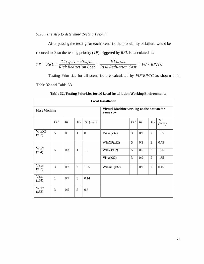
74
5.2.5. The step to determine Testing Priority
After passing the testing for each scenario, the probability of failure would be
reduced to 0, so the testing priority (TP) triggered by RRL is calculated as:
Testing Priorities for all scenarios are calculated by FU*RP/TC as shown in in
Table 32 and Table 33.
Table 32. Testing Priorities for 10 Local Installation Working Environments
Local Installation
Host Machine Virtual Machine working on the host on the same row
FU RP TC TP (RRL)
FU RP TC
TP (RRL)
WinXP (x32)
5 0 1 0 Vista (x32) 3 0.9 2 1.35
Win7 (x64)
5 0.3 1 1.5
WinXP(x32) 5 0.3 2 0.75
Win7 (x32) 5 0.5 2 1.25
Vista(x32) 3 0.9 2 1.35
Vista (x32)
3 0.7 2 1.05 WinXP (x32) 1 0.9 2 0.45
Vista (x64)
1 0.7 5 0.14
Win7 (x32)
3 0.5 5 0.3

75
Table 33. Testing Priorities for 3 Server Installation Working Environments
Server Installation
Win 7 (x64)
VM FU RP TC TP (RRL)
WinServer 2003x32
5 0.3 2 0.75
WinServer 2008x64
5 0.5 2 1.25
WinServer 2008x32
3 0.3 2 0.45
Combined with the product importance ratings in Table 27, the value-based
scenario testing prioritization algorithm is:
First test the scenario whose working environment has the highest TP (RRL);
For each selected operating system environment, first test SEER-SEM, which has
higher importance, and then test SEER-H or SEER-MFG, which have lower
importance.
5.3. Results
Table 34 shows the value-based testing prioritization order and the relevant metrics
based on this order. Several acronyms used are as below:
RRL: Risk Reduction Level
BI: Business Importance
ABI: Accumulated Business Importance
PBIE: Percentage of Business Importance Earned
APBIE: Average Percentage of Business Importance Earned
AC: Accumulated Cost

76
Table 34. Value-based Scenario Testing Order and Metrics
TP(RRL) Passed 1.5 1.35 1.35 1.25 1.25 1.05 0.75 0.75 0.45 0.45 0.3 0.14
FU(BI) 39 5 3 3 5 5 3 5 5 3 1 3 1
PBIE 48.15% 54.32% 58.02% 61.73% 67.90% 74.07% 77.78% 83.95% 90.12% 93.83% 95.06% 98.77% 100.00%
ABI 39 44 47 50 55 60 63 68 73 76 77 80 81
TC 1 1 2 2 2 2 2 2 2 2 2 5 5
AC 1 2 4 6 8 10 12 14 16 18 20 25 30
APC 3.33% 6.67% 13.33% 20.00% 26.67% 33.33% 40.00% 46.67% 53.33% 60.00% 66.67% 83.33% 100.00%
ABI/AC 39.00 22.00 11.75 8.33 6.88 6.00 5.25 4.86 4.56 4.22 3.85 3.20 2.70
The first row TP (RRL) in Table 34 shows the testing order we followed to do this
testing by first testing the scenario with higher RRL. This order enabled us to focus the
limited effort on testing more frequently used scenarios with higher risk probability to fail,
and supposed to improve the testing efficiency especially when the testing time and
resource is limited. The testing results by using the value-based testing prioritization
strategy are shown in Table 35 and Table 36. Due to the schedule constraint, and
according to the TP order, we didn’t do thorough test on WinXP (x32) Virtual Machine
working on host of Vista (x32) and Vista (x64) host machine, since they both has the
lowest frequency of use, they can be ignorable for testing if the time runs out. For Win7
(x32), although it is never tested, it is supposed to pass since its Virtual Machine copy,
which is supposed to have even lower performance, has passed the testing. Besides, if we
installed a Win 7 (x32) on a host machine to test, this will cause more time, and we
couldn’t finish other scenario testing which has higher TP and won’t require installing a
new OS before testing. Therefore, the testing strategy combines the considerations of all
critical factors and makes the testing results optimal under scarce testing resources.

77
Table 35. Testing Results
Local Installation
Host Machine Virtual Machine working on the host on the same row
WinXP (x32)
pass Vista (x32) pass
Win7 (x64) pass
WinXP (x32)
pass
Win7 (x32) pass
Vista (x32) pass
Vista (x32) pass WinXP (x32)
Never test, we are running out of time, FU is the lowest, no need to test when the testing time is limited
Vista (x64) Never test, we even don’t have VM for this, besides, we are running out of time, FU is the lowest, no need to test when the testing time is limited
Win7 (x32) Never test, we don’t have a host machine for this, but supposed to pass, since its VM has passed
Table 36. Testing Results (continued)
Server Installation
Win 7 (64)
WinServer 2003x32 pass
WinServer 2008x64 pass
WinServer 2008x32 pass
Figure 16 shows the results of value-based testing prioritization compared with
two other situations which might be common in testing planning as well. The three
situations for comparison are:
Situation 1: value-based testing prioritization strategy: this situation is exactly
what we did for the macro testing in Galorath, Inc., using the value-based scenario testing
strategy. We followed the Testing Priority (TP) to do the testing. Since our testing time is
limited, we had to stop testing when the Accumulated Cost (AC) reached 18 units as
shown in Figure 16. At this point, Percentage of Business Importance Earned (PBIE) is as
high as 93.83%;
Situation 2: Reverse of value-based, risk-driven testing strategy: this situation’s
testing order is reversed from Situation 1; when the AC reaches 18 units, PBIE is only

78
22.22%; this is the worst case, but this might be a common value-neutral situation in
reality as well.
Situation 3: The prioritization in Situation 1 considers all variables into the value-
based testing prioritization: not only prioritizes various operating systems, but also
prioritizes different products and different installation types. However, in the situation 3,
we do a partial value-based prioritization: we still prioritize products and operating
systems, but we assume that the installation type is equally important, so the client
installation type which has been proved to be defect-free should also be tested. The results
show a significant difference: when AC reaches 18 units, PBIE is only 58.02%; much of
the testing effort is wasted on testing the defect-free type. In fact, this “partial” value-
based prioritization is common in practice: testing managers often do prioritize tests in
practice, but the way they prioritize is often intuitive, and tends to ignore some factors into
prioritization, so this situation can represent most common situations in practice as well.
Since this situation still treats all installation types equally important, we still consider it as
a value-neutral one to differentiate the “complete, systematic, comprehensive and
integrated” value-based prioritization in Situation 1.

79
Figure 16. Comparison among 3 Situations
74.07%
77.78%
83.95%
90.12% 93.83%
95.06% 100.00%
4.94% 6.17% 9.88%
16.05% 22.22%
25.93%
58.02%
35.80%
39.51%
45.68%
51.85%
58.02% 61.73%
87.65%
0.00%
20.00%
40.00%
60.00%
80.00%
100.00%
8 10 12 14 16 18 20 22 24 26 28 30
PBIE-1 PBIE-2 PBIE-3
Stop
Table 37 compares APBIE of the three situations, and it is obvious that value-
based testing prioritization is the best in terms of APBIE. The case study in Galorath, Inc.
validates that the added value-based prioritization can improve the scenario testing’s cost-
effectiveness in terms of APBIE.
Table 37. APBIE Comparison
Comparison APBIE
Situation 1 (Value-based) 70.99%
Situation 2 (Inverse Order) 10.08%
Situation 3 (Value-neutral) 32.10%
Other value-neutral (or partial value-based) situations’ PBIE curves are supposed
to lie between the Situation 1 and Situation 2 in Figure 16, and are representative of the
most common situations in reality. From the comparative analysis, we can reject the

80
hypothesis H-t1 which means that value-based prioritization can improve the testing cost-
effectiveness.
5.4. Lessons Learned
Integrate and leverage the merits of state-of-art effective test prioritization
techniques: in this paper, we synthetically incorporated the merits of various test
prioritization techniques to maximize the testing cost effectiveness, i.e. coverage-based,
defect proneness-driven and most important incorporated the business value into the
testing prioritization. Value-based testing strategy introduced in this paper is not
independent of other prioritization techniques; on the contrary, it is the synthesis of all the
merits from other techniques with a focus on bridging the gap between business or
mission value from customers and the testing process.
Think more on trade-offs for automated testing at the same time: form our
experiences in this case study to establish automated testing at Galorath, Inc., we can also
see that establishing automated testing is a high risk as well as a high investment project
[Bullock, 2000]. The test automation is also software development, which might be also
expensive, fault-prone, and facing evolving and maintenance problems. Furthermore,
automated testing usually treats every scenario equally important.
However, the combination of value-based test prioritization and automated testing
might be a promising strategy and can even further improve the testing cost-effectiveness.
For example, adopting the value-based test case prioritization strategy can shrink the
testing scope by 60%, the remaining tedious manual testing effort can be further replaced
by an initial little investment to write some automated scripts to allow testing run by
computer programs overnight and save human effort by 90%, so by the strategy of

81
combining value-based test case prioritization and automated testing, the cost is reduced to
(1-60%)*(1-90%)=4% with a factor of 25’s RRL improvement. Anyway, this is also a
trade-off question among how much automated testing is enough based on its saving and
investment to establish.
In fact, any testing strategy has its own advantages; the most important for testing
practitioners is having a strong sense of combining the merits of these testing strategies to
continuously improve the testing process.
Team work is recommended to determine ratings. Prioritization factors’ ratings,
i.e. ratings of business importance, risk probability, testing cost, should not only
determined by a single person, this might introduce subjective bias which might cause the
prioritization misleading. Ratings should be discussed and brainstormed at team meetings
when more stakeholders involved to acquire more comprehensive information, resolve
disagreements and negotiate to consensus. For example, if we didn’t send out the
questionnaire to get the frequency of use of each scenario, we would treat all scenarios
equally important and couldn’t finish all the testing in a limited time. The worst situation
is that we installed some operating system sceneries that were seldom used and tested the
macros on them and finally found that it was no need to test them. The same for risk
probability: if we didn’t know that Client installation would not needed to test because it
seldom failed before and supposed to be defect-free, amount of testing effort would be put
on this unnecessary testing. So team work to discuss and understand the project under test
is very important to determine the testing scope and testing order.
Business case analysis is based on project contexts: from these empirical studies
so far, the most difficult, yet flexible part is how to determine the business importance for

82
the testing items via business case analysis: The business case analysis can be
implemented with various methods, considering their ease of use and adaption under
experiments’ environment. For example, in this case study of value-based testing scenario
prioritization, we use frequency of use (FU) combined with product importance as a
variant of business importance for operational scenarios; in the case study of value-based
feature prioritization for software testing in Chapter 5, Karl Wiegers’ requirement
prioritization approach [Wiegers, 1999] is adopted, which considers both the positive
benefit of the presence of a feature and the negative impact of its absence. In the case
study of value-based test case prioritization in Chapter 7, classic S-curve production
function with segments of investment, high-payoff, and diminishing returns [Boehm, 1981]
are used to train students for their project features’ business case analysis with the Kano
model [Kano] as a reference to complement their analysis for feature business importance
ratings. Test cases’ business importance is then determined by its corresponding functions,
components or features’ importance, and test cases’ usage, whether testing the core
function of this feature or not As for the case study of determining the priority of artifacts
(system capabilities) in Chapter 3, the business importance is tailored to ratings of their
influences/impacts to the project’s success. The similarity for these different business case
analyses is that all using well-defined, context-based relative business importance ratings.
Additional prioritization effort is a trade-off as well: Prioritization can be as easy
as in this case study or can be more deliberate. Too much effort on prioritization might
bring diminishing testing cost-effectiveness. “How much is enough” depends on the
project context and how easily we can get that information required for prioritization. It
should be kept in mind all the time that value-based testing prioritization aims at saving

83
effort, rather than increasing effort. In this case study, the information required for this
prioritization is from expert estimation (project managers, product manager and project
developers) with little cost, yet generate high pay-offs for the limited testing effort.
However, for this method’s application on large-scale projects which might have
thousands of test items to be prioritized, there has to be a consensus mechanism to collect
all the data. We started to implement an automatic way to support this method’s
application on large-scale industrial projects. This automation is designed to support
establishing the traceability among requirements, code, test cases and defects, so business
importance ratings for requirements can be reused for test items, the code’ change and
defect data can be used for predicting risk probability. The automation will also
experiment the sensitivity analysis on judging the correctness of ratings and how the
rating’s change can impact the testing order. The automation is supposed to generate
recommend ratings in order to save effort and provide reasonable ratings as well to
facilitate value-based testing prioritization.

84
Chapter 6: Case Study III-Prioritize Software Features to be functionally Tested
6.1. Background
This case study to prioritize features for testing was implemented at the system and
acceptance testing phase of one of an industry product’s (named “Qone” [Qone]) main
releases in a Chinese Software Organization. The release under test added nine features
with total Java codes of 32.6 KLOC in this release. The features are mostly independent
amendments or patches of some existing modules. The value-based prioritization strategy
was also applied to prioritize the 9 features to be tested based on their ratings of business
importance, Quality Risk Probability, and Testing Cost. Features’ testing value priorities
provide the decision support for the testing manager to enact the testing plan and adjust it
according to the feedback of quality risk indicators, such as defects numbers and defects
density and updated testing cost estimation. Defects data was collected automatically and
displayed real-time by this organization’s defect reporting and tracking system with
immediate feedback to adjust the testing priorities for the next testing round.
6.2. Case Study Design
6.2.1. The step to determine Business Value
To determine business importance of each feature, Karl Wiegers’ approach
[Wiegers, 1999] is applied in this case study. This approach considers both the positive
benefit of the presence of a feature and the negative impact of its absence. Each feature is
assessed in terms of the benefits it will bring if implemented, as well as the penalty that
will be incurred if it is not implemented. The estimates of benefits and penalties are
relative. A scale of 1 to 9 is used. For each feature, the relative benefit and penalty are

85
summed up and entered in the Total BI (Business Importance) column in Table 38 using
the following formula.
The sum of the Total BI column represents the total BI of delivering all features.
To calculate the relative contribution of each feature, divide its total BI by the sum of the
Total BI column. As we can see, there is an approximate Pareto distribution in which F1
and F2 contribute 22.2% of the features and 59.3% of the total BI.
Table 38. Relative Business Importance Calculation
Benefit Penalty Total BI BI %
Weights 2 1
F1 9 7 25 30.9%
F2 8 7 23 28.4%
F3 1 3 5 6.2%
F4 2 1 5 6.2%
F5 1 1 3 3.7%
F6 2 1 5 6.2%
F7 3 2 8 9.9%
F8 1 2 4 4.9%
F9 1 1 3 3.7%
SUM 28 25 81 1
Figure 17 shows the BI distribution of the 9 features. As we can see, there is an
approximate Pareto distribution in which F1 and F2 contribute 22.2% of the features and
59.2% of the total BI.

86
Figure 17. Business Importance Distribution
6.2.2. The step to determine Risk Probability
The risk analysis was performed prior to system testing start, but was
continuously updated during testing execution. It aims to calculate the risk probability for
each feature. We follow the four steps:
Step 1: List all risk factors based on past projects and experiences: set up the
n risks in the rows and columns of an n*n matrix. In our case study, according to this
Chinese organization’s past similar projects’ risk data. Four top quality risk factors with
the highest Risk Exposure are: Personnel Proficiency, Size, Complexity, and Design
Quality. Defects Proportion and Defects Density are usually used as hand-on metrics for
quality risk identification during the testing process and they together with the top four
quality risk factors to serve as the risk factors that would determine the feature quality
risk in this case study.
Step 2: Determine risk weights according to their impact degree to software
quality: different risk factor has different impact degrees to influence software quality
under different organizational contexts, and it is more reasonable to assign them different
30.9% 28.4%
6.2% 6.2% 3.7%
6.2% 9.9%
4.9% 3.7%
0.0%
5.0%
10.0%
15.0%
20.0%
25.0%
30.0%
35.0%
F1 F2 F3 F4 F5 F6 F7 F8 F9 Business Importance

87
weights before combining them to get one risk probability number for each feature. AHP
(The Analytic Hierarchy Process) Method [89], a powerful and flexible multi-criteria
decision-making method that has been applied to solve unstructured problems in a variety
of decision-making situations, ranging from the simple personal decisions to the complex
capital intensive decisions, is used to determine the weight for each risk factor. Based on
the understanding of risk factors and their knowledge and experience of their specific
relative impact degree to software quality in this organization’s context, the testing
manager collaborated with the developing manager to determine the weights of each
quality risk using AHP method.
In this case study, the calculation of quality risks weights is illustrated in Table
39. The number in each cell represents the value pair-wise relative importance: number of
1, 3, 5, 7, or 9 in row i and column j stands for that the stakeholder value in row i is
equally, moderately, strongly, very strongly, and extremely strongly more important than
the stakeholder value in column j, respectively. In order to calculate weight, each cell is
divided by the sum of its column, and then averaged by each row. The results of the final
averaged weight are listed in the bolded Weights column in Table 39. The sum of weights
equals 1.
If we are able to determine precisely the relative value of all risks, the values
would be perfectly consistent. For instance, if we determine that Risk1 is much more
important than Risk2, Risk2 is somewhat more important than Risk3, and Risk3 is slightly
more important than Risk1, an inconsistency has occurred and the result’s accuracy is
decreased. The redundancy of the pairwise comparisons makes the AHP much less
sensitive to judgment errors; it also lets you measure judgment errors by calculating the

88
consistency index (CI) of the comparison matrix, and then calculating the consistency
ratio (CR). As a general rule, CR of 0.10 or less is considered acceptable [Saaty, 1980].
In the case study, we calculated CR according to the steps in [Saaty, 1980], and the CR is
0.01, which means that our result is acceptable.
Table 39. Risk Factors’ Weights Calculation-AHP
Personnel Proficiency
Size Complexity Design Quality
Defects Proportion
Defects Density
Weights
Personnel Proficiency
1 1/3 3 3 1/3 1/5 0.09
Size 3 1 3 3 1 1 0.19
Complexity 1/3 1/9 1 1 1/7 1/9 0.03
Design Quality
1/3 1/7 1 1 1/7 1/9 0.04
Defects Proportion
3 1 7 7 1 1 0.27
Defects Density
5 3 9 9 1 1 0.38
Step 3: Score each risk factor for each feature: the testing manager’s in
collaboration with the developing manager scores each risk factor for each feature. The
estimate is of the degree to which the risk factor is present for each feature. 1 means the
factor is not present and 9 means the factor is very strong. A distinction must be made
between factor strength and action to be taken. 9 indicates factor strength, but does not
indicate what should be done about it.
Initial Risks are risk factors we use to calculate the risk probability before the
system testing and Feedback Risks such as Defects Proportion and Defects Density are
risk indicators used during the testing process and serve to monitor and control the testing
process.

89
Risks such as Personnel Proficiency, Complexity, and Design Quality etc. are
scored by the developing manager based on their understanding of each feature and pre-
defined scoring criteria. The organization also has its own defined scoring cr iteria for
each risk rating. For example, for Personnel Proficiency, Years of experience in
application, platform, language and tool serves as a surrogate for simply measuring it, the
scoring criteria the organization adopts are as follows:
1-More than 6 years, 3-More than 3years,
5-More than 1 year, 7-More than 6 months, 9-<2 months
Use of intermediate scores (2, 4, 6, 8) was allowed
More comprehensive measures for Personnel Proficiency could be a combination
of COCOMO II [Boehm et al. , 2000] personnel factors, e.g. ACAP (Analyst Capability),
PCAP (Programmer Capability), PLEX (Platform Experience), LTEX( Language and
Tool Experience) with other outside factors that might influence Personnel Proficiency,
e.g. reasonable workload, and work spirit and passion from psychological view.
Risks such as Size, Defects Proportion, Defects Density are scored based on
collected data, for example, if a feature’s size is 6KLOC and the largest feature’s size is
10KLOC, so the feature’s size risk is scored as 9*(6/10) 5.
Step 4: Calculate the risk probability for each feature: for each feature Fi,
after each risk factor’ score is obtained, following formula is used to combine all the risk
factors to get the risk probability Pi of Fi

90
jiR , is Fi’s risk value of jth risk factor, jW denotes the weight of jth risk factor.
Table 40 will calculate the Probability of the total initial risks that comes from each
feature before system test.
Table 40. Quality Risk Probability Calculation (Before System Testing)
Initial Risks Feedback Risks
Probability Personnel Proficiency
Size Complexity Design Quality
Defects Proportion
Defects Density
Weights 0.09 0.19 0.03 0.04 0.27 0.38
F1 5 3 1 1 0 0 0.13
F2 4 9 5 2 0 0 0.26
F3 3 3 5 5 0 0 0.14
F4 5 4 7 5 0 0 0.19
F5 5 2 3 3 0 0 0.12
F6 5 2 5 6 0 0 0.14
F7 5 4 5 2 0 0 0.17
F8 1 2 1 1 0 0 0.06
F9 1 1 1 1 0 0 0.04
Lessons Learned and Process Implication:
From the data of initial risks collected, some potential problems are found for this
organization:
Potential problem in tasks break down and allocation: the Feature F9 has the
least risks of both Personnel Proficiency and Complexity and it implies that one of the
most experience developers is responsible for the least complex feature. But for the most
complex feature F4, it is developed by the least experienced developer. This implies a
potential task allocation problem in this organization. Generally, it is highly risky to let

91
the least experienced staff to do the most complex task and also a resource waste to let
the most experienced developer to do the least complex task. In the future, the
organization should consider a more reasonable and efficient task allocation strategy to
mitigate risk.
Potential insufficient design capability: basically, the risk factors should be
independent when they are combined to generate a risk probability, which means that the
risk factors should not have strong interrelation among them. Based on the data from
Table 40, we do a correlation analysis among the risk factors, almost all risk factors don’t
have strong correlations (correlation coefficient>0.8). But it should be noted that the
correlation coeffic ient 0.76 between Complexity and Design Quality is high, which
means as the Complexity becomes an issue, the Design Quality also becomes a risky
problem. This could imply that the current designers or analysts are inadequate for their
work. To mitigate this risk, the project manager should consider recruiting analysts with
more requirements, high-level design and detailed design experiences in the future.
Table 41. Correlation among Initial Risk Factors:
Personnel Proficiency
Size Complexity Design Quality
Personnel Proficiency 1
Size 0.30 1
Complexity 0.56 0.48 1
Design Quality 0.44 -0.05 0.76 1
From Table 39, we could see that feedback risk factors: “Defect Proportion” and
“Defect Density” have the largest weights when they use AHP to determine the risk
items’ weights. This is reasonable, because initial risk factors are mainly used to estimate

92
the risk probability before system testing starts. As long as system testing starts, the
testing manager should be more concerned with each feature’s real and undergoing
quality situation to find which features are the most fault-prone. “Defect Proportion” and
“Defect Density” could serve to provide the real quality information and feedback during
the process of system testing. This is also the reason that probabilities in Table 40 are
low, since the initial risks are assigned smaller weights and there are no feedback risk
factors before system testing starts.
6.2.3. The step to determine Testing Cost
The test manager estimates the relative cost of testing each feature, again on a
scale ranging from a low of 1 to a high of 9. The test manager estimates the cost ratings
based on factors such as the developing effort of the feature, the feature complexity, and
the quality risks as shown in Table 42.
Table 42. Relative Testing Cost Estimation
Cost Cost%
F1 2 4.8%
F2 5 11.9%
F3 5 11.9%
F4 9 21.4%
F5 6 14.3%
F6 4 9.5%
F7 5 11.9%
F8 3 7.1%
F9 3 7.1%
sum 42 1

93
Figure 18. Testing Cost Estimation Distribution
A correlation analysis is done between the 9 features’ business importance and
estimated testing cost as shown in Table 43. The negative correlation denotes that the
most testing costly features might have less business importance to key customers.
Testing the features first with more business importance but less cost will definitely
improve the testing efficiency and maximize its ROI at the early stage of testing phase.
Table 43 Correlation between Business Importance and Testing Cost
BI Cost
BI 1
Cost -0.31 1
6.2.4. The step to determine Testing Priority
Similar as the scenario prioritization, after passing the testing for each feature, the
probability of failure would be reduced to 0, so the testing priority (TP) triggered by RRL
is calculated as:
4.8%
11.9% 11.9%
21.4%
14.3%
9.5%
11.9%
7.1% 7.1%
0.00%
5.00%
10.00%
15.00%
20.00%
25.00%
F1 F2 F3 F4 F5 F6 F7 F8 F9
Cost

94
And the Testing Priorities for the 9 features are shown in Table 44, the testing order is F1,
F2, F7, F6, F3, F4, F8, F5, and F9.
Table 44. Value Priority Calculation
BI % Probability Cost% Priority
F1 30.9 0.13 4.8 0.81
F2 28.4 0.26 11.9 0.63
F7 9.9 0.17 11.9 0.14
F6 6.2 0.14 9.5 0.09
F3 6.2 0.14 11.9 0.07
F4 6.2 0.19 21.4 0.05
F8 4.9 0.06 7.1 0.04
F5 3.7 0.12 14.3 0.03
F9 3.7 0.04 7.1 0.02
6.3. Results
After adapting the value-based prioritization strategy to determine the testing order
of the 9 features, the PBIE comparison between value-based order and its inverse order
(the most inefficient one) is shown in Figure 19 , and the difference of APBIE between the
two is 76.9%-34.1%=42.8% which means value-based testing order can improve the cost-
effectiveness by 42.8% than the worst case, other value-neutral (or partial value-based)
situations’ PBIE curves are supposed to lie between the these two PBIE curves, and are
representative of the most common situations in reality, and this further rejects hypothesis
H-t1.

95
Figure 19. Comparison between Value-Based and Inverse order
In our case study, the test manger plans to execute 4 rounds of testing. During
each round, test groups focus on 2-3 features with the highest current priority, and the
other features are tested by automated tools. The testing result is when the first round is
over, F1 and F2 satisfy the stop-test criteria, when the second round is over, F3, F6, F7
satisfied the stop-criteria, when the third round is over, F4, F8 satisfied the stop-test
criteria, and the last round is F5 and F9. And initial estimating testing cost and actual
testing cost comparison can be shown in Figure 20.
Figure 20. Initial Estimating Testing Cost and Actual Testing Cost Comparison
30.8%
59.2%
69.1%
75.3%
81.4%
87.6% 92.5%
96.2% 99.9%
3.7% 7.4%
12.3%
18.5%
24.7%
30.9%
40.7%
69.1%
99.9%
0.0%
10.0%
20.0%
30.0%
40.0%
50.0%
60.0%
70.0%
80.0%
90.0%
100.0%
1 2 3 4 5 6 7 8 9
PBIE
Features Value-Based Inverse
16.7
33.3 28.6
21.4 19.8 25.3
30.3 24.6
0.0 5.0
10.0 15.0 20.0 25.0 30.0 35.0
1 2 3 4
Co
st(P
erc
ent)
Testing Rounds
Estimate Actual

96
If we regard the testing activity as an investment, its value is realized when
features satisfy the stop-test criteria. The accumulated BI earned curve in Figure 22 is
like a production function, with higher pay-off at the earlier stage but diminishing return
later. Also from Figure 21 and Figure 22, we can see that when we finished the Round 1
testing, we earned 59.2% BI of all features, at a cost of only 19.8% of the all testing
process, the ROI is as high as 1.99. During the Round 2, we earned 22.2% BI, cost 25.3%
effort, and the ROI became negative as -0.12. We also can see, from Round 1 to Round 4,
both the BI earned line and the ROI line is descending. Round 3 and Round 4 earn only
18.5% BI but cost 54.9% effort. This shows that the Round 1 testing is the most cost
effective. Testing the features with higher value priority first is especially useful when the
market pressure is very high. In such cases, one could stop testing after finding a negative
ROI in Round 1. However, in some cases, continuing to test may be worthwhile in terms
of customer-perceived quality.
Figure 21. BI, Cost and ROI between Testing Rounds
Start Round 1 Round 2 Round 3 Round 4
BI Earned 0 59.2 22.2 11.1 7.4
Cost 0 19.8 25.3 30.3 24.6
Test_ROI 0 1.99 -0.12 -0.63 -0.70
-1
-0.5
0
0.5
1
1.5
2
0
14
28
42
56
70

97
Figure 22. Accumulated BI Earned During Testing Rounds
Consideration of Market Factors
Time to market can strongly influence the effort distribution of software
developing and project planning. As testing phase serves as the adjacent phase before
software product transition and delivery, it will be influenced even more by market
pressure [Huang and Boehm, 2006]. Sometimes, under the intense market competition
situation, sacrificing some software quality to avoid more market share erosion might be
a good organizational strategy.
In our case study, we use a simple function as follows to display the market
pressure’s influence to Business Importance:
Time represents the number of unit time cycle. A unit time cycle might be a year,
a month, a week even a day. For simplicity, in our case study, the unit time cycle is a
testing round. Pressure Rate is estimated and provided by market or product managers,
with the help of customers. It represents during a unit time cycle, what is the percentage
0
59.2
81.4
92.5 99.9
0
20
40
60
80
100
Start Round 1 Round 2 Round 3 Round 4
BI Earned

98
initial value of the software will depreciated. The more furious the market competition is,
the larger the Pressure Rate is. As we can see from the formula above, the longer the time
is, the larger the Pressure Rate is, the smaller is the present BI, and the larger the loss BI
caused by market erosion. In our case study, Due to we calculate the relative business
importance, the initial total BI is 100(%). When the Round n testing is over, the loss BI
caused by market share erosion is
. On the other hand, the earlier
the product enters the market, the larger the loss caused by poor quality. Finally, we can
find a sweet spot (the minimum) from the combined risk exposure due to both
unacceptable software quality and market erosion.
We assume three Pressure Rates 1%, 4% and 16% standing for low, medium and
high market pressure respectively in Figure 23 to Figure 25, and this could be also seen
as three types of organizational contexts: high finance, commercial and early start-up
[Huang and Boehm, 2006]. When market pressure is as low as 1% in Figure 23, the total
loss caused by quality and market erosion reaches the lowest point (sweet spot) at the end
of the Round 4.When the Pressure Rate is 4%, the lowest point of total loss is at the end
of Round 3 in Figure 24, which means we should stop testing and release this product
even F5 and F9 haven’t reached the stop-test criteria at the end of Round 3; this would
ensure the minimum loss. When the market pressure rate is as high as 16% in Figure 25,
we should stop testing at the end of Round 1.

99
Figure 23. BI Loss (Pressure Rate=1%)
Figure 24. BI Loss (Pressure Rate=4%)
Figure 25. BI Loss (Pressure Rate=16%)

100
Extension of Testing Priority Value Function:
In this case study, we use multi-objective multiplicative value function to
determine the testing priority. There is also another additive value function that can be
used to determine the testing priority as follows:
V(XBI), V(XC) and V(XRP) are single value functions for “Business Importance”,
“Cost” and “Risk Probability”. WBI, WC and WRP are relative weights for them
respectively. V(XBI+XC+XRP) is the multi-objective additive value function for testing
priority. For the single value functions of “Business Importance” and “Risk Probability”,
they are increasing preference, the larger the “Business Importance” or “Risk
Probability”, the higher the testing priority as shown in the left part of Figure 26. For the
single value function of “Testing Cost”, it is decreasing preference, the larger the Cost,
the lower the testing priority value as shown in the right part of Figure 26.
Figure 26. Value Functions for “Business Importance” and “Testing Cost”
Extension from the multiplicative value function to additive one also shows the
similar feature testing priorities result [Li, 2009]. No matter the value function is
multiplicative or additive, as long as they reasonably reflect the similar SCSs’ win

101
condition’ preferences, they are supposed to generate the similar priority results. From
our extension experiment, both dynamic prioritizations could make the ROI of testing
investment reach the peak at the early stage of testing, which is especially effective when
the time to market is limited. This extension of value function is also supported by Value-
Based Utility Theory.

102
Chapter 7: Case Study IV-Prioritize Test Cases to be Executed
7.1. Background
This case study for prioritizing test cases to be executed by using the Value-Based,
Dependency-Aware prioritization strategy was experimented on USC 2011 spring and fall
semester software engineering course’s a number of 18 projects. As an extension to
previous work for prioritizing testing features, this work prioritized test cases in a fine-
grained granularity with added considerations on test cases’ inner-dependency. Besides, it
tailored the Probability of Loss from the Risk Reduction Leverage (RRL) definition to test
case Failure Probability and used this as a trigger to shrink the regression test case suite by
excluding the stable features for the scarce testing resource.
A project named “Project Paper Less” [USC_577b_Team01, 2011] with 28 test
cases is used as an example to investigate the improved testing efficiency.
Through Fall 2010 CSCI 577a, Team01 students have already developed good
results of Operation Concept Description (OCD), System and Software Requirement
Description (SSRD), System, System and Software Architecture Description (SSAD) and
Initial Prototype together with various planning documents, such as Lifecycle Plan (LCP),
Quality Management Plan (QMP). From Spring 2011 CSCI 577b, they develop Initial
Operational Capability with concurrently generating Test Plan and Cases (TPC), students
are trained to write test cases according to the requirements in SSRD with Equivalence
Partitioning and Boundary Value Testing techniques [Ilene, 2003] to elaborate test cases.
Their test cases in the TPC cover 100% requirements in the SSRD and they have already
done some informal unit testing, integration testing before the acceptance testing. They

103
follow the Value-based Testing Guideline [USC_577b_VBATG, 2011] to do Value-based
test case prioritization (TCP), execute their acceptance testing according to the testing
order from the prioritization, record their testing results in the Value-based Testing
Procedure and Results (VbTPR) and report defects discovered to Bugzilla system
[USC_CSSE_Bugzilla] to report and track those defects until closure. From the next
section, the Value-based TCP steps will be introduced within Team01’s project’s context.
7.2. Case Study Design
7.2.1. The step to do Dependency Analysis
Most features in the SUT are not independent of each other and they typically have
precedence or coupling constraints between them that requires some features must be
implemented before others, or some must be implemented together [Maurice et al., 2005].
Similar for test cases, some test cases are required to be executed and passed before others
can be executed. The failure of some test cases can also block others to be executed.
Understanding the dependencies among test cases would benefit test case prioritization
and test planning; also they are useful information for rating business importance, failure
probability, criticality and even testing cost that will be introduced within the following
sections.
Based on the test cases in TPC [USC_577b_Team01, 2011], testers were asked to
generate dependency graphs for their test suites. They could be as simple as Team01’s test
case dependency tree in Figure 27, or could be much more complex, for example, one test
case node has more than one parental node. In Figure 27, for each test case, the bracket
associated with have two space holders for later filling in, one is for Testing Value
(=Business Importance*Failure Probability/Testing cost) and the other is Criticality. The

104
following sections will introduce in detail how to rate those factors, and use them for
prioritization.
Figure 27. Dependency Graph with Risk Analysis
7.2.2. The step to determine Business Importance
As for testing, the business importance of a test case is mainly determined by its
corresponding functions, components or features’ importance or value to clients. Besides,
due to the test case elaboration strategies, such as Equivalence Partitioning and Boundary
Value Testing, various test cases for the same feature are designed to test different aspects
of the feature with different importance as well. The first step to determine the Business
Importance of a test case is to determine the BI of its relevant function/feature. From
CSCI577a, students are educated and trained on how to do business cases analysis for
software project, and rate relative Business Importance for function/feature in a software
system from the client’s view, such as the importance of software, product, component, or
feature to his/her organization in terms of its Return on Investment [Boehm, 1981] as
shown in Figure 28. A general mapping instruction between function/feature BI rating
range as given in the box in Figure 28. And the range in production function (investment,
high-payoff, diminishing returns) are given to students for their references.

105
Basically the slope of the curve represents the ROI of the function, the higher the
slope, the higher the ROI, so the higher the BI of the function. The BI of the function in
the Investment segment is usually in the range from Very Low to Normal, since the early
Investment segment involves development of infrastructure and architecture which does
not directly generate benefits but which is necessary for realization of the benefits in the
High-payoff and Diminishing returns segments. For “Project Paper Less”, the Access
Control and User Management features should belong to the Investment segment. The
main application functions for this project such as Case Management, Document
Management features are the core capabilities for this system that the client most wants to
have and they are within High-payoff segment, so the BI of those functions are in the
range from High to Very High. Because of the scope and schedule constraints of the
course projects, these projects are usually small-scale and only require students developing
the core capabilities and seldom have some features that belong to Diminishing Return
segment.
Figure 28. Typical production function for software product features [Boehm, 1981]
BI: H-VH
BI: VL-N
BI: VL-N

106
The business importance of a test case is determined by the business importance of
its corresponding feature, function or module on one side, it is also determined by the
criticality magnitude of the failure occurrence on the other side. A guideline for rating a
test case’s Business Importance is shown in Table 45 by considering both two sides. The
ratings for Business Importance are from VL to VH, with corresponding values from 1 to
5. For example, for the Login function in the Access Control module, the tester used
Equivalence Partitioning test case generation strategy to generate two test cases: one is to
test whether a valid user can login, and the other is to test whether an invalid user cannot
login. Since the Access Control feature belongs to “Investment” segment and the tester
rated it as “Normal” benefit to the client. If the first test case to test whether a valid user
can login fails, the Login function won’t run and this will block other functions, such as
Case Management, Document Management, to be tested, so this test case should be rated
“Normal” according to the guideline in Table 45. On the other side, for the other test case
to test whether an invalid user cannot login should be rated “Low”, because if it fails, the
login can still run (the valid user can still login to test other functionalities without
blocking them). So its criticality magnitude is relatively smaller than the first test case and
deserves a relative lower rating “Low”. This is just an example for differentiating the
Business Importance of test cases elaborated by Equivalence Partitioning yet within the
same feature. There are other various cases applicable to differentiate the relative
importance by considering the criticality magnitude of failure occurrence as well.

107
Table 45. Guideline for rating BI for test cases
VH:5 This test case is used to test the functionality that will bring the Very High benefit for the client, without passing it, the functionality won’t run
H:4
This test case is used to test the functionality that will bring the Very High benefit for the client, without passing it, the functionality can still run
This test case is used to test the functionality that will bring the High benefit for the client, without passing, the functionality won’t run
N:3
This test case is used to test the functionality that will bring the High benefit for the client, without passing it, the functionality can still run
This test case is used to test the functionality that will bring the Normal benefit for the client, without passing it, the functionality won’t run
L:2
This test case is used to test the functionality that will bring the Normal benefit for the client, without passing it, the functionality can still run
This test case is used to test the functionality that will bring the Low benefit for the client, without passing it, the functionality won’t run
VL:1
This test case is used to test the functionality that will bring the Low benefit for the client, without passing it, the functionality can still run
This test case is used to test the functionality that will bring the Very Low benefit for the client, without passing it, the functionality won’t run
As a result of rating the total 28 test cases’ Business Importance for “Project Paper
Less”, the ratings’ distribution is shown in Figure 29, High, and Very High business
importance test cases consist more than half. This makes sense because most features
implemented are core capabilities, but still needs some “investment” capabilities that are
necessary for those core ones.

108
Figure 29. Test Case BI Distribution of Team01 Project
7.2.3. The step to determine Criticality
Criticality, as mentioned the above step, represents impact magnitude of failure
occurrence and what influences it will bring to the ongoing test. Combined with the
Business Importance from the client’s value perspective, they contribute to determine the
size of loss at risk. The empirical guideline for rating it is in Table 46. The ratings are
from VL to VH with values from 1 to 5. The common reason for this is that test cases
which with high Criticality should be passed as early as possible, otherwise, it would
block other test cases to be executed and might delay the whole testing process if defects
are not resolved soon enough.
Students are educated to refer the dependency tree/graph for rating this. For
“Project Paper Less” test case dependency tree as shown in Figure 27, for the ones TC-01-
01, TC-03-01 and TC-04-01, they are all rated Very High, because they are on the “critical
path” for executing all other test cases, if they fail, it would block most of the other test
cases to be executed and most of those blocked test cases have high Business Importance.
VL 11%
L 21%
N 14%
H 50%
VH 4%
VL L
N H
VH

109
Most of the other test cases are tree leaves, if they fail, they won’t block other test cases to
be executed and their Criticality are rated Very Low.
Table 46. Guideline for rating Criticality for test cases
VH:5 Block most (70%-100%) of the test cases, AND most of those blocked test cases have High Business Importance or above
H:4 Block most (70%-100%) of the test cases, OR most of those blocked test cases have High Business Importance or above
N:3 Block some (40%-70%) of the test cases, AND most of those blocked test cases have Normal Business Importance
L:2 Block a few (0%-40%) of the test cases, OR most of those blocked test cases have Normal Business Importance or below
VL:1 Won’t block any other test cases
7.2.4. The step to determine Failure Probability
The primary goal of testing is to reduce the uncertainty of the software product
quality before it is finally delivered to the client. Testing without risk analysis is a waste of
resources, and uncertainty and risk analysis are triggers for selecting the subset of test
suite, in order to focus the testing resources on the most risky, fault-prone features. A set
of self-check questions from different aspects or factors that might cause test case failure
are provided in Table 47 for students’ reference to rate the test case’s failure probability.
Students rated each test case’s Failure Probability based on those recommended factors or
others they might think of by themselves. The rating levels with numeric values are: Never
Fail (0), Least Likely to Fail (0.3), Have no idea (0.5), Most Likely to Fail (0.7), Fail for
sure (1).

110
Table 47. Self-check questions used for rating Failure Probability
Experience Did the test case fail before? --People tend to repeat previous mistakes, so does software. From pervious observations, e.g. unit test, performance
at CCD, or informal random testing, the test case failed before tends to fail again
Is the test case new? --The test case that hasn’t not been tested before has a higher probability to fail
Change Impact Does any recent code change (delete/modify/add) have impact on some features? --if so, the test cases for these features have a higher probability to fail
Personnel Are the people responsible for this feature qualified? -- If not, the test case for this feature tends to fail
Complexity Does the feature have some complex algorithm/ IO functions? --If so, the test case for this feature have a higher probability to fail
Dependencies Does this test cases have a lot of connections (either depend on or to be depended on) with other test case? --If so, this test case have a higher probability to fail
For “Project Paper Less”, before the acceptance testing, testers have already done
Core Capability Drive-through (CCD) for core capabilities developed in the first
increment, design-code review, unit test, informal random testing, testers have already
gained information and experiences about the health status of the software system they
developed. Based on this, they rated the Failure Probability for the whole 28 test cases.
The distribution of the rating levels are shown in Figure 30. Never Fail test cases consist
of more than half based on previous experiences and observations. So for those Never Fail
ones, they should be delayed to be executed at the end of each testing round if resources
are still available, or even not to be executed if time and testing resources are limited. So
in this way, quality risk analysis drives to shrink the test case suite and only choose to
execute those test case subsets with quality risks.

111
Figure 30. Failure Probability Distribution of Team01 Project
7.2.5. The step to determine Test Cost
Value-Based Software Engineering considers every activity as an investment. For
test activities, the cost/effort for executing each test case should also be considered for
TCP. However, estimating the effort to execute each test case is challenging [Deonandan
et al., 2010], [Ferreira et al., 2010]. Some practices simply suggest count the numbers of
steps to execute the test case. To simplify our experiment, students are also asked to write
test case on the same granularity level to make sure that every case has the nearly the same
number of steps to be executed as much as they can do, and assume that the cost for
executing each test case is the same.
7.2.6. The step for Value-Based Test Case Prioritization
As far as testers rated those factors above for each test case, Testing Value
triggered by RRL is defined as below:
Never Fail, 15, 54% Least Likely to
Fail, 6, 21%
Have no idea, 1, 4%
Most Likely to Fail, 6, 21%
Fail for sure, 0, 0%
Never Fail
Least Likely to Fail
Have no idea
Most Likely to Fail
Fail for sure

112
It is obvious from the definition of Testing Value that the Testing Value is in
proportion to Business Importance and Failure Probability and inversely proportional to
Testing cost. This allows test cases to be prioritized in terms of return on investment (ROI).
Students were asked to fill in each test case node with the number of Testing Value and
Criticality ratings as shown in Figure 27. Executing the ones with the highest Testing
Value and highest Criticality first is our basic prioritization strategy. However, due the
dependencies among test cases, a common situation is that testers cannot usually jump and
reach to the test case with the highest Testing Value directly without executing and
passing some others with lower Testing Value on the critical path to obtain the highest
one. For example, in Figure 27, TC-04-01 has the highest Testing Value (3.5) together
with highest Criticality rating (VH), but testers can’t directly execute it until TC-01-01 and
TC-03-01 on the critical path are executed and passed. So the factor of dependency should
also be added into the value-based TCP algorithm. Some key concepts below are
introduced to help understand the value-based TCP algorithm.
Passed: All steps in the test case generates the expected outputs that can make this feature work accordingly
Failed: As long as one of the steps in the test case generates an unexpected outputs to make this function can’t work or this failure would for sure block other test cases to be
executed if possible (some minor improvement suggestion doesn’t belong to this category )
NA: The test case is not able to be executed, there are some candidate reasons: This test case depends on another test case which fails; External factors, such as the testing environment e.g. the pre-condition could not be satisfied, or there is no required testing data, etc.

113
Dependencies Set: A test case’s Dependencies Set is the set of the test cases that this test case depends on. The Dependencies Set should include all dependent test cases, either directly or indirectly.
Ready-to-Test: it is a status of test cases, and its definition is: A test case is Ready-to-
Test only if the test case has no dependency or all the test cases in its Dependencies Set have been “Passed”.
Not-Tested-Yet: it is another status of test cases, and its definition is: A test case is Not-
Tested-Yet means this test case has not been tested yet so far.
The algorithm of value-based, dependency-aware Test Case Prioritization is shown
below with brief description in Figure 10. It is basically a variant of greedy algorithm with
the optimal goal of first selecting the Ready-to-Test one with the highest Testing Value
and Criticality to test.
Value First: Test the one with the highest Testing Value . If several test cases’ Testing Values are the same, test the one with the highest Criticality.
Dependency Second: If the test case selected from the first step is not “Ready-to-Test”, which means at least one of the test cases in its Dependencies Set is “Not-Tested-Yet”. In
such situation, prioritize the “Not-Tested-Yet” test cases according to “Value First” in this Dependencies Set and start to test until all test cases in the Dependencies Set are “Passed”. Then the test case with the highest value is “Ready-to-Test”.
Update the prioritization: After one round, update the Failure Probability based on updated observation from previous testing rounds.

114
Pick the one with the
highest Test Value (if the
same, choose the one
with higher Criticality)
Have dependencies?
All dependencies
passed?
Y
Start to testN
Y
Exclude the “Passed”
one for prioritization
Failed?
Exclude the “Failed” one
and the others “NA” that
depends on it for
prioritization
N
<<In the Dependencies Set>>
N
<<Ready-to-Test>>
<<Ready-to-Test>>
<<- -In the Whole Test
Case Set- ->>
Resovled?
Y
N
<<Report for Resolution>>
Figure 31. In-Process Value-Based TCP Algorithm
For “Project Paper Less”, 15 Never Fail test cases are excluded in the subset
selected to test, as shadowed in the dependency tree in Figure 27. For those test cases, it is
not necessary to test them deliberately if the testing effort or resources are limited; yet it is
ok to test them at the end of this round if time is still available. According to the Value-
Based TCP algorithm, the testing order for the remaining test cases is:
TC-04-01, TC-04-02, TC-04-03, TC-05-10, TC-18-01, TC-12-01, TC-11-01, TC-13-01, TC-02-01, TC-14-01, TC-03-04, TC-02-02, TC-03-02.
However, the testers still need to walk through TC-01-01 and TC-03-01 to reach
TC-04-01, but walking-through costs much less than deliberately testing and the effort for
it could be neglected.
7.3. Results
7.3.1. One Example Project Results
Average Percentage of Business Importance Earned (APBIE) is used to measure
how quickly the SUT’s value is realized, the higher it is, and the more efficient the test is.
Y

115
For the above test case prioritization for “Project Paper Less”, the BI, FP, Criticality
ratings could be found at [USC_577b_Team01, 2011].
For the whole T set of 28 test cases, we get TBI=88;
At the initial point of the testing round, 15 test cases were rated “Never Fail”
with no need to test in this testing round, they consist of the set T-T’. In total, they have
45 business importance, which means IBIE=45, and PBIE0=45/88=51.1%;
For the remaining 13 prioritized test cases to be executed in order in the set of
T’, PBIE1=(45+5)/88=56.8% when TC-04-01 is passed, PBIE2=(45+5+4)/88=61.4%
when TC-04-02 is passed… , PBIE13=(45+5+4+…+1)/88=100% when TC-03-02 is
passed and all 88 business importance is earned at this moment. The business importance
earned fast at the beginning and becomes slower to the end as shown in Figure 32;
The APBIE=(56.8%+61.4%…+100%)/13=81.9%;
Figure 32. PBIE curve according to Value-Based TCP (APBIE=81.9%)
56.8%
61.4%
65.9%
70.5%
75.0%
79.5%
84.1%
88.6%
92.0%
95.5%
96.6%
98.9%
100.0%
0.0%
10.0%
20.0%
30.0%
40.0%
50.0%
60.0%
70.0%
80.0%
90.0%
100.0%
PB
IE

116
As the obvious evidence above, risk analysis for Failure Probability for test cases
can help to select subset test case suite to focus effort on most risky test cases in order to
save testing cost and effort. However, the risk analysis should be based on previous hands-
on experiences and observations about the quality of the SUT. If testers have no idea about
the SUT health status before test, in practice, for example, the third party testing,
outsourcing testing etc. the Test Value should depend only on Business Importance before
their first test, assuming test cost is the same for each test case as an example dependency
tree shown in Figure 27. So in this case, all test cases should be prioritized, according to
the Value-Based TCP algorithm, the test order for the whole test suite without risk
analysis is:
TC-01-01, TC-03-01, TC-04-01, TC-05-01, TC-04-02, TC-04-03, TC-05-02, TC-05-03, TC-05-05, TC-05-07, TC-05-08, TC-05-10, TC-12-01, TC-18-01, TC-11-01, TC-13-01, TC-19-01, TC-02-01, TC-14-01, TC-
01-02, TC-02-02, TC-15-01, TC-16-01, TC-16-02, TC-16-03, TC-03-02, TC-03-03, TC-03-04
This testing order’s PBIE is displayed in square curve in Figure 33, with a
comparison with a commonly used value-neutral test order in diamond curve, which
follows the test case ID number or Breadth-First-Search (BFS) the dependency tree. It is
obvious that Value-Based TCP can earn business importance quicker than value-neutral
one. APBIE for Value-Based TCP is 52%, higher than value-neutral one 46%, which
rejects the hypothesis H-t1. This improvement would be more significant if the business
importance numeric values are not in a linear range from 1 to 5, but an exponential range
from 21 to 2
5.

117
Figure 33. PBIE Comparison without risk analysis between Value-Based and Value-Neutral TCP (APBIE_value_based=52%, APBIE_value_neutral=46%)
It is also should be noted that the 21.9% difference (81.9%-60%) with/without
Failure Probability analysis is contributed by risk analysis to select sub test case suite to
further improve the test efficiency. So the Value-Based TCP can improve testing cost-
effectiveness by selecting and prioritizing test cases in order to earn Business Importance
as early as possible, and this is especially useful when the testing schedule is tight and
testing resources are limited.
Value-Based TCP enables early execution for test cases with high business
importance and criticality, the failure of test cases would lead to defects reported to
responsible developers, and developers would arrange time to prioritize and fix defects
according to the degrees of severity and priority of those defects in an efficient way. In
fact, test cases’ business importance and criticality determine the severity and priority for
defects on the failure occurrence, as the mapping in Table 48. Basically, if test cases with
Very High business importance fail, the corresponding features/functions which brings
highest benefit to customers can’t work, it will cause large size of customer’s benefit loss,
0.0%
10.0%
20.0%
30.0%
40.0%
50.0%
60.0%
70.0%
80.0%
90.0%
100.0%
1 2 3 4 5 6 7 8 9 10 11 12 13 14 15 16 17 18 19 20 21 22 23 24 25 26 27 28
PB
IE
Test Case Order
Value-Neutral
Value-Based

118
and due to this reason, the relevant defect’s severity should be rated “Critical”; if test cases
with Very High criticality fail, it blocks most of other test cases with high business
importance to be executed, so the relevant defect should be “Resolve Immediately” in
order not to delay the whole testing process.
Table 48. Mapping Test Case BI &Criticality to Defect Severity& Priority
BI <-> Severity Criticality<->Priority
Value-Based TCP BI ratings
Defect Severity in Bugzilla
Value-Based
TCP Criticality ratings
Defect Priority in Bugzilla
VH Critical VH Resolve Immediately
H Major H
N Normal N Normal Queue
L Minor L Not Urgent,
Low Priority,
Resolve Later,
VL Trivial, Enhancement
VL
So if testers follow the Value-based TCP to select and prioritize test cases, it will
directly lead to early detection of high severity and priority defects for the above reasons if
potential defects exist.
For “Project Paper Less”, after the first round of acceptance testing, 4 defects are
reported to Bugzilla, their severity, priority and corresponding test cases with business
importance and criticality were shown in Table 49. From the ascending ordinal defect
sequence (the earlier defect report results in a foremost defect ID) and their relevant Test
Case ID, it is obvious that the value-based prioritization enable testers to detect high-
severity defects as early as possible, a lthough there were some mismatches between test
case Criticality ratings and defect Priority ratings. This is mainly because we didn’t
instruct students to report defects according to the mapping in Table 48 and Bugzilla has

119
Priority default value as Normal Queue and students might feel it is of no need to change,
or think that high-severity defects should be Resolved Immediately in common sense. Yet,
this in turns provides evidence that Value-Based TCP enables testers to detect the high-
severity faults at the early time if those potential faults exist. So from the observations of
defect reporting in Bugzilla for this project, defects with higher Priority and Severity are
reported earlier and resolved earlier. This can reject the hypothesis H-t2.
Table 49. Relations between Reported Defects and Test Cases
Defect ID in Bugzilla
Severity Priority Test Case ID BI FP Criticalit
y
#4444 Critical Resolve
Immediately TC-04-01
VH
0.7 VH
#4445 Major Normal Queue TC-04-03 H 0.7 VL
#4460 Major Normal Queue TC-05-10 H 0.7 VL
#4461 Major Resolve
Immediately TC-18-01 H 0.7 VL
7.3.2. All Team Results:
After all teams executed the acceptance testing with several follow-on regression
testing using the Value-Based TCP technique, a survey with several open questions are
sent and answered by the primary testers. Questions are mainly around their feelings and
feedback on applying the Value-Based TCP for the acceptance testing, problems they
encountered, and improvement suggestion. Some representative responses are shown
below:
“Before doing the prioritization, I had a vague idea of which test cases are
important to clients. But after going through the Value-Based testing, I had a better
picture as to which ones are of critical importance to the client.”

120
“I prioritized test cases mainly based on the sequence of the system work flow,
which is performing test cases with lower dependencies at first before using value-based
testing. I like the value-based process because it can save time by letting me focus on
more valuable test cases or risky ones. Therefore, it improves testing efficiency.”
7.3.2.1 A Tool for Faciliating Test Case Prioritization:
In the upper example case study, a semi-automatic spreadsheet was developed to
support its application on USC graduate software engineering course projects in 2011
spring semester. In order to further facilitate and automate its prioritization to save effort
and minimize human errors, and support its application on large-scale projects which
might have thousands of test cases to be prioritized, there indeed has to be a consensus
mechanism to collect all the required rating data. We implemented an automated and
integrated tool to support this method based on an open source, built on
PHP+MySQL+Apache platform, widely-used test case management toolkit TestLink.
We customized this system to incorporate the value-based dependency-aware test
case prioritization technique and is available at [USC_CSSE_TestLink], and used for USC
graduate software engineering course projects.
Figure 34 illustrates an example of the test case in the customized TestLink.

121
Figure 34. An Example of Customized Test Case in TestLink
Basically, it supports to:
Rate Business Importance, Failure Probability, and Test Cost by selecting the
ratings from the dropdown lists as shown in Figure 34, currently it supports for 5-
level ratings for each factor :Very Low, Low, Normal, High and Very High with
default numeric values from 1 to 5, and the Testing Value in terms of RRL for
each test case can be calculated automatically.
Manage test case dependencies by inputting other test cases that this test case
directly depends on as shown in the text field “Dependent Test Case” in Figure 34,
and dependencies are stored in the database for later prioritization.

122
Prioritize test cases according the value-based, dependency-aware prioritization
algorithm in Chapter 7 to generate a planned value-based testing order as
illustrated in Figure 35, in order to help testers to plan their testing more cost-
efficient. A value-neutral testing order which only deals with the dependencies
among test cases without considering the RRL of each test cases are also generated
for comparison.
Display the PBIE curves for both value-based and value-neutral testing orders
visually, and shows the APBIE for both orders at the bottom of the chart in Figure
35.
Figure 35. A Tool for facilitating Value-based Test Case Prioritization in TestLink

123
Several future feasible features are planned incrementally implemented into the
tool include:
Establish test case dependencies by dragging and dropping, and generate visible
dependency graph.
Establish the traceability matrix between the requirement specifications (TestLink
also maintains specifications) and test cases and category test cases by tagging
“core” or “auxiliary” to automatically obtain test case business importance ratings.
Establish the traceability matrix between test cases and defects (TestLink provides
interfaces to integrate with commonly used defect tracking systems, such as
Mantis and Bugzilla) in order to automatically predict the failure probability based
on the collected historical defect data. Other solutions to predict failure probability
include: integrate the code change analysis tool (e.g. Diff tool) and traceability
matrix to quantitatively predict code change’s impact on test cases’ failure
probability; establish a historical database and a measurement system to predict
software features’ fault-proneness and personnel qualifications.
Experiment sensitivity analysis for reasoning and judging the correctness of factors’
ratings.
By implementing these features, this tool is expected to automatically generate
recommended ratings for business importance, failure probability and won’t require testers
too much effort for inputting their ratings for each test case, which will greatly facilitate
the value-based TCP and add value to this technique.

124
7.3.2.2 Statistical Results for All Teams via this Tool
We imported these rating data in the test case prioritization spreadsheets for all
the 18 teams into the tool for facilitating comparative analysis.
Three measures are used for Value-Based and Value-Neutral testing strategies
comparative analysis : “APBIE”, “Delivered-Value when Cost is fixed”, “Cost when
Delivered-Value is fixed”. Besides, since 18 teams are trained to use the Value-Based
testing strategy, we also use T-test to see whether there is a statistically significant
improvement for these teams under experiment. It should be noted that both value-based
and value-neutral ones are dependency-aware, the difference is that value-based strategy
adds RRL in combination of business importance, failure probability and cost (in this
case study, assume each test case cost is the same) into prioritization, while the value-
neutral one just considers dependencies into prioritization without considering the value-
based factor RRL and this is typical in industry.
APBIE Comparison
APBIE is a new metric we proposed to measure how quickly a testing order can
earn the business or mission value. The higher it is, the more efficient the testing is. The
tool can automatically display APBIE comparison at the bottom of the chart in Figure 36.
Figure 36. APBIE Comparison

125
Delivered-Value Comparison when Cost is fixed (e.g. 50% test cases executed as shown below)
In reality, one situation is that a version’s release date is fixed. Before the fixed
deadline, which features can be delivered is determined by which features have passed
the quality criteria in terms of test cases. So maximizing the delivered value under a fixed
testing cost is usually the goal of a testing strategy. In this way, “Delivered-Value
Comparison when Cost is fixed” is a practical and effective testing measure under time
constraints. In Figure 37 and the analysis later, it compares the delivered value while the
testing cost is cut to 50%, which means only 50% of the test cases can be executed,
assuming the cost of running each test case is the same.
Figure 37. Delivered-Value Comparison when Cost is fixed
Cost Comparison when Delivered Value is fixed (e.g. 50% business Importance as shown below)
Another situation in the release planning is: for a release version, it requires
several features in the package to achieve a certain degree of customer satisfaction, for
example, in terms of a fixed percentage of the total business importance presented by all
the features in the backlog, e.g. 50%, should be delivered in the upcoming version as
soon as possible in order to satisfy the critical customers’ needs or enter the market the
earliest time to maximum the market share). So minimizing the testing cost while

126
achieving the required, fixed delivered value is the goal of this release situation. In this
case, “Cost Comparison when Delivered Value is fixed” is a practical and effective
testing measure under such value constraints. . In Figure 38 and the analysis later, it
compares the testing cost while the delivered value is set to 50%.
Figure 38. Cost Comparison when Delivered Value is fixed
Comparative Analysis Results:
For all 18 teams in Spring & Fall 2011, Table 50 tells us: the APBIE of the Value-
Based testing is always no less than the value-neutral one with statistical significance (p-
value for its t-test is highly below 0.05), more visually, this means the value-based testing
curve is always on top of the value-neutral testing curve, at least overlapped at the worst
case. So this can reject the hypothesis H-t1. However, the improvement of some projects
(Spring team 2, 3 and Fall team 3, 7, 8, 12, 13) as shadowed in Table 50, is not obvious,
explanations for this will be introduced later.

127
Table 50. APBIE Comparison (all teams)
APBIE # of TCs Value-Based Value-Neutral Improvement
2011S_T01 28 56.41% 46.38% 10.03%
2011S_T02 29 54.94% 53.80% 1.14%
2011S_T03 22 51.76% 50.75% 1.01%
2011S_T05 31 54.36% 51.87% 2.49%
2011S_T06 39 53.07% 50.40% 2.67%
2011F_T01 19 51.93% 45.98% 5.95%
2011F_T03 14 52.15% 50.33% 1.82%
2011F_T04 24 61.95% 53.62% 8.33%
2011F_T05 77 63.21% 42.07% 21.14%
2011F_T06 31 59.22% 53.31% 5.91%
2011F_T07 10 57.25% 56.25% 1.00%
2011F_T08 7 55.71% 54.76% 0.95%
2011F_T09 10 57.27% 51.51% 5.76%
2011F_T10 18 62.08% 57.23% 4.85%
2011F_T11 25 53.16% 51.39% 1.77%
2011F_T12 6 58.33% 58.33% 0.00%
2011F_T13 31 53.64% 53.25% 0.39%
2011F_T14 29 57.24% 48.17% 9.07%
Average 56.32% 51.63% 4.68%
F-test 0.5745
T-test 0.000661
Table 51 tells us: If the testing cost is fixed, e.g. only half of the total test cases
can be run before releasing, assuming the time for running each test case is the same, the
results show that the Value-Based testing always delivers not less business value than the
Value-Neutral one with statistical significance, so this can reject the hypothesis H-t3.
However, it is also noted that no obvious improvement for some projects (Spring team 2,
3 and Fall team 3, 7, 8, 12, 13) as above.
128
Table 51. Delivered Value Comparison when Cost is fixed (all teams)
PBIE 1/2 # of TCs Value-Based Value-Neutral Improvement
2011S_T01 14 60% 40% 20.00%
2011S_T02 15 61% 58% 3.00%
2011S_T03 11 52% 50% 2.00%
2011S_T05 16 56% 50% 6.00%
2011S_T06 20 59% 51% 8.00%
2011F_T01 10 60% 45% 15.00%
2011F_T03 7 50% 50% 0.00%
2011F_T04 12 70% 50% 20.00%
2011F_T05 39 70% 40% 30.00%
2011F_T06 16 65% 50% 15.00%
2011F_T07 5 53% 52% 1.00%
2011F_T08 4 60% 50% 10.00%
2011F_T09 5 58% 45% 13.00%
2011F_T10 9 63% 55% 8.00%
2011F_T11 13 55% 50% 5.00%
2011F_T12 3 50% 50% 0.00%
2011F_T13 16 51% 50% 1.00%
2011F_T14 15 60% 40% 20.00%
Average 58.50% 48.67% 9.83%
F-test 0.3822
T-test 0.000083
Table 52 tells us: If the business value to be delivered is fixed for a release, e.g.
50% of the total business value is planned to deliver as soon as possible to enter market
the earliest time, assuming the time for running each test case is the same, the Value-
Based testing always spends no less testing cost than the Value-Neutral one with
statistical significance, so this can reject the hypothesis H-t3. However, no obvious
improvement for some projects (Spring team 2, 3 and Fall team 3, 7, 8, 12, 13) as above.

129
Table 52. Cost Comparison when Delivered Value is fixed (all teams)
# of TCs when gaining 50% BI
Value-Based
Value-Neutral
# of TCs
Value-Based Cost%
Value-Neutral Cost%
Cost saving %
2011S_T01 12 17 28 42.86% 60.71% 17.86%
2011S_T02 13 13 29 44.83% 44.83% 0.00%
2011S_T03 11 11 22 50.00% 50.00% 0.00%
2011S_T05 13 16 31 41.94% 51.61% 9.68%
2011S_T06 18 21 39 46.15% 53.85% 7.69%
2011F_T01 9 11 19 47.37% 57.89% 10.53%
2011F_T03 7 7 14 50.00% 50.00% 0.00%
2011F_T04 8 14 24 33.33% 58.33% 25.00%
2011F_T05 21 51 77 27.27% 66.23% 38.96%
2011F_T06 11 16 31 35.48% 51.61% 16.13%
2011F_T07 5 5 10 50.00% 50.00% 0.00%
2011F_T08 4 4 7 57.14% 57.14% 0.00%
2011F_T09 4 6 10 40.00% 60.00% 20.00%
2011F_T10 7 9 18 38.89% 50.00% 11.11%
2011F_T11 11 13 25 44.00% 52.00% 8.00%
2011F_T12 3 3 6 50.00% 50.00% 0.00%
2011F_T13 16 16 31 51.61% 51.61% 0.00%
2011F_T14 12 18 29 41.38% 62.07% 20.69%
Average 44.01% 54.33% 10.31%
F-test 0.2616
T-test 0.000517
After re-checking those rating spreadsheets and re-interviewing with students
from those projects with no obvious improvement. Explanations are listed as below:
Most of the course projects are small-size, during the two-semesters, students
usually only have the time to focus on core capabilities’ implementation, it is hard for
some of them to differentiate the levels of business importance for those “equally
important “capabilities. This is also one partial reason for the small percentage of overall
improvement as well.
Especially for Spring team 02, 03 and Fall team 07,08,12,13, we discovered from
their prioritizations that nearly all the test cases’ business importance are rated High or

130
above. From this respective, they are rarely the value-based teams, although they are
trained to use the value-based strategy to differentiate the levels of business importance.
Some students don’t have strong capabilities or sense to do project business
analysis, resulting in nearly the same levels of business importance ratings;
Some teams have very small set of test cases, and this makes them even harder for
differentiating the business importance.
Based on the explanations above, the teams with no obvious improvement are in
fact the value-neutral teams, if we exclude them into the comparative analysis, the
performances on the three measures improve for obvious reasons as shown Table 53 to
Table 55. This further rejects H-t1 and H-t3.
Table 53. APBIE Comparison (11 teams)
APBIE # of TCs Value-Based Value-Neutral Improvement
2011S_T01 28 56.41% 46.38% 10.03%
2011S_T05 31 54.36% 51.87% 2.49%
2011S_T06 39 53.07% 50.40% 2.67%
2011F_T01 19 51.93% 45.98% 5.95%
2011F_T04 24 61.95% 53.62% 8.33%
2011F_T05 77 63.21% 42.07% 21.14%
2011F_T06 31 59.22% 53.31% 5.91%
2011F_T09 10 57.27% 51.51% 5.76%
2011F_T10 18 62.08% 57.23% 4.85%
2011F_T11 25 53.16% 51.39% 1.77%
2011F_T14 29 57.24% 48.17% 9.07%
Average 57.26% 50.18% 7.09%
F-test 0.8326
T-test 0.000704

131
Table 54. Delivered Value Comparison when Cost is fixed (11 teams)
PBIE 1/2 # of TCs Value-Based Value-Neutral Improvement
2011S_T01 14 60% 40% 20.00%
2011S_T05 16 56% 50% 6.00%
2011S_T06 20 59% 51% 8.00%
2011F_T01 10 60% 45% 15.00%
2011F_T04 12 70% 50% 20.00%
2011F_T05 39 70% 40% 30.00%
2011F_T06 16 65% 50% 15.00%
2011F_T09 5 58% 45% 13.00%
2011F_T10 9 63% 55% 8.00%
2011F_T11 13 55% 50% 5.00%
2011F_T14 15 60% 40% 20.00%
Average 61.45% 46.91% 14.55%
F-test 0.9339
T-test 0.000043
Table 55. Cost Comparison when Delivered Value is fixed (11 teams)
# of TCs when
gaining 50% BI
Value-
Based
Value-
Neutral
# of
TCs
Value-Based
Cost%
Value-Neutral
Cost%
Cost
saving %
2011S_T01 12 17 28 42.86% 60.71% 17.86%
2011S_T05 13 16 31 41.94% 51.61% 9.68%
2011S_T06 18 21 39 46.15% 53.85% 7.69%
2011F_T01 9 11 19 47.37% 57.89% 10.53%
2011F_T04 8 14 24 33.33% 58.33% 25.00%
2011F_T05 21 51 77 27.27% 66.23% 38.96%
2011F_T06 11 16 31 35.48% 51.61% 16.13%
2011F_T09 4 6 10 40.00% 60.00% 20.00%
2011F_T10 7 9 18 38.89% 50.00% 11.11%
2011F_T11 11 13 25 44.00% 52.00% 8.00%
2011F_T14 12 18 29 41.38% 62.07% 20.69%
Average 39.88% 56.76% 16.88%
F-test 0.7218
T-test 0.000065

132
7.3.2.3. Lessons learned
Intuitively, the benefit of the Value-Based testing strategy only comes after really
differentiating the business importance levels of the test cases to be prioritized. It makes
no sense for the Value-based testing prioritization if you give all the test cases the same
level of business importance.
Small-size projects usually focus on the core capabilities, of which the business
importance differences are not obvious, and results in not obvious improvement via the
Value-Based testing. For medium and large-size projects, as the project size grows, the
number of the test cases proportionally increases, the benefit of prioritizing test cases to
maximum the business value or minimum the test cost will surely become obvious and
significant in terms of improvement percentages. A correlation analysis is conducted
between the columns “Improvement” and “# of test cases” in Table 50, and the
Correlation Coefficient is 0.735, which means the “Improvement” and “# of test cases”
have a strong positive correlation, in other words, the more test cases to be prioritized, the
more improvement can be potentially achieved.
However, even the small percentage of effort savings on the fixed values or more
values delivered on the fixed costs will become significant in terms of monetary dollars,
especially for those large-scale projects with the investment of millions of dollars.

133
Chapter 8: Threats to Validity
Diversities of Projects and Subjects: for the Case Study I at USC graduate level
software engineering project course, especially for cross-project comparative analysis of
value-based review experiments, the 35 projects cover different applications with diverse
technical characteristics and different clients. Also, reviewers with different personnel
capabilities and non-uniform granularities of issues reported by different reviewers might
also impact the number of issues reported and reviewing effectiveness as displayed in this
experiment. These are sources of high variability across projects, and certainly contributed
to the large standard deviations seen for some of the results within the same year’s team,
2011, 2010 team’s high standard deviation for review cost effectiveness as an example in
Chapter 4. However, the comparison analysis is conducted on 2011,2010 teams using
value-based review, and 2009 teams using value-neutral one, and the distribution of
project application types, technical and clients/reviewers’ characteristics among the three
years are similar. So even the variability is high within one-year teams, but the general
similarity of the projects improves to some degree the three years’ comparison.
Meanwhile, to actively minimize the high variability, detailed guidelines and
instructions on how to report issues to Bugzilla (the customized issue tracking system) in a
consistent granularity, which attributes, e.g. Priority, Severity are especially required to
correctly report, are presented and distributed to reviewers for their learning and
understanding before they really act. Teaching Assistants periodically monitor reviewers’
performance without bias, quality check their issues reported, give more
instructions/training without bias for not-well-done performers; train review on issue
reporting to Bugzilla for the first few package reviews before value-based review is
134
introduced with detailed step-by-step guidelines; provide more office hours, training
sessions for answering questions and confusion if necessary can further lower down the
variability and reduce the effects of learning curve as well. Then comparison analysis is
done based on those more stable package reviews. In this way, the learning curve
variability is reduced.
Non-representativeness of Projects and Subjects: Although the development
teams are primarily full-time graduate level students with an average of less than 2 years’
industry experience, the reviewers are almost all full-time professional employees. Their
review schedule conflicts were similar to review schedule conflicts on the job. Thus the
results should be reasonably representative of industrial review practices. Besides, for
value-based testing practices, we also conducted the case studies in real industry projects
either at Galorath, Inc. or the Chinese Software Organization, and this can reduce this type
of threat.
Besides, voices from practitioners are good resources to further test our research
hypotheses, reduce the effects of the threats that are introduced by the quantitative data
analysis, and provide research improvement opportunities as well. So in and after each
empirical experiment, a series of surveys with various aspects for retrospection on the
experimented prioritization process is conducted to hear the feedback from practitioners.
To reduce the threats of being an experimenter as well as a grader, we state clearly in the
survey instructions “we do not grade on your choice, but on the rationale you provide for
your choice”. Also, in our general grading for issue reporting, criteria is kept that: grading
is not based on how the results are close to what we expected, but on whether students
report data in an honest and correct way for their real project context. References [20, 46]

135
have the detailed survey information and result analysis for the value-based review, while
[32] includes those for value-based test cases prioritization. In this way, we believe that
the quantitative and qualitative evidences can complement each other to test our research
hypotheses.
Correctness of Input Factors’ Values: The reviewing or testing priorities are
calculated based on the input factors, such as Business Importance, Risk Probability, or
Cost. The correctness of those factors’ ratings or values will directly influence the
correctness of output priorities. In our experiments, especially for student projects, we first
provided detailed guidelines to train students on how to determine factors’ values/ratings.
Students in each team determined the ratings or values based on a group consensus.
Besides, we asked students to provide rationales for their ratings. Teaching Assistants also
double-checked their rationales’ correctness and the consistency between the ratings and
their provided rationales to avoid the bias and errors of the subjective inputs to the largest
extent, in order to minimize the threats to the results’ validity. For other real industry
projects, such as the Chinese Software Organization project, and the Galorath, Inc. project,
those ratings are determined and validated by professional project managers, developers,
and testing managers, and thus minimizing the threat.
Applicability to Large-Scale Industrial Projects: For this method’s application on
large-scale projects, especially for test case level prioritization, which might have
thousands of test cases to be prioritized, there indeed has to be a consensus mechanism to
collect all the required data. In addition to the automatic tool that we have already
implemented for facilitating test case prioritization, several feasible capabilities to be
explored will include:

136
For dependency analysis, some existing dependency analysis tools will be
explored and integrated;
For business importance, some value management systems will be explored,
developed, and integrated. In this research, relative business importance in terms of ROI
is captured by understanding the S-curve Production Function in Figure 28. Other
Customer Value Analysis (CVA) techniques, such as the Kano Model [44] can also be
applicable. Besides, a real Value Management System (VMS) to capture, manage, monitor
and control the value flow for the whole software development lifecycle to facilitate
software decisions on various software engineering activities based on cost/benefit
analysis, business case analysis etc. is under-development and would support this.
For failure probability prediction, to minimize the bias of subjective risk
assessments, a sophisticated quantitative solution includes: using some candidate code
change analysis tool (e.g. Diff tool) and traceability matrix to quantitatively predict code
change’s impact on test cases’ failure probability; establishing a historical database and a
measurement system to predict software features’ fault-proneness and personnel
qualifications; and combining all these influencing factors with defined calculating rules
to estimate test case failure probability in a more comprehensive and unbiased way.
For reasoning/judging the correctness of factors’ ratings, and weights assigned to
them, we can experiment with sensitivity analysis;
We are also cooperating with some software management tool vendors to integrate
these above candidate features, e.g. Qone [45], a widely-used lifecycle project
management tool in China; Besides, IBM Rational Team Concert [92] is another option.
Since these tools are mature, they have accumulated mechanisms to collect and share

137
required data. It is easier for the method to be applied with these tools in real industry,
which will definitely have large systems that might have thousands of test cases. We
believe that prioritization would become more meaningful and efficient when the scale
becomes large.

138
Chapter 9: Next Steps
Our next steps would involve more data and empirical studies by applying the
Value-Based, Dependency-Aware prioritization strategy on exercising the lifecycle. A
phased-based selection of cost-effective defect removal options for various defect types in
Risk Reduction Leverage (RRL) priority order, can enable the various defect removal
options to be ranked or mixed by how well they reduce risk exposure for various defect
types. Combining this with their relative option costs enables them to be prioritized in
terms of return on investment, as initially investigated in [Madachy and Boehm, 2008] via
Orthogonal Defect Classification [Chillarege et al., 1992].
Three notional yet representative examples below might give some insights for
more data and empirical studies in industry settings, and they are also the points that we
want to get the most advice on the feasibility of these examples’ scenarios in industry
settings. And we also would like to take this opportunity to call for more cooperation from
industry.
Example 1: The first example is provided by Boehm in [Selby, 2007] to compare
the cost-effectiveness of two approaches for eliminating a type of error: suppose that the
loss incurred by having a particular type of interface error in a given software product is
estimated at one million dollars, and that from experience we can estimate that the
probability of this type of interface error being introduced into the software product is
roughly 0.3. Two approaches for eliminating this type of error are a requirements and
design interface checker, whose application will cost $20K and will reduce the error
probability to 0.1; and an interface testing approach, whose application will cost $150K

139
and will reduce the error probability to 0.05. The RRL of the two approaches are compared
as below:
RRL(R-D checker) =1000K*(0.3 -0.1)/20K=10
RRL (Test) =1000K*(0.3-0.05)/150K=1.67
Thus, the RRL calculation confirms that V&V investments in the early phases of
the software life cycle generally have high payoff ratios, and that V&V is a function that
needs to begin early to be most cost-effective. Defect removal techniques have different
detection efficiencies for different types of defects, and their effectiveness may vary over
the lifecycle duration. Also, the early defect detection activities can provide insights on
how to perform more cost-effective testing as discussed next.
Example 2: Similar calculations can help a software project determine the more
cost-effective mix of defect removal techniques to apply across the software life cycle. For
example, suppose the loss due to another type of defect is also 1000K, software peer
review can reduce this type of error’s occurring probability from 0.6 to 0.3 with reviewing
effort of 2PM: if this error’s probability can be continuously reduced by reviewing to 0.0,
it will cost an extra 8PM reviewing effort; however testing can reduce this to 0.0 by only
extra testing effort of 1PM. The RRL of the two strategies are compared as below:
RRL (Review Only)= 1000K*(0.6 -0.0)/(2+8)PM=60K/PM
RRL (Review+Test)=1000K*(0.6-0.0)/(2+1)PM=200K/PM
Thus, instead of using one single defect removal strategy, the mix of defect
removal options can further improve the cost-effectiveness. Additionally the techniques
may have overlapping capabilities for detecting the same type of defects, and it is difficult
to know how to best apply them, especially for the combination of cross-phase defect

140
removal options, e.g., when to stop reviewing and start to test, how much reviewing is
enough with combination of other options at hands are difficult. One option that might be
worthwhile attempting is applying Indifference Curves and Budget Constraints analysis
from Microeconomics Utility theory. The optimal combination is the point where the
indifference curve and the budget line are tangent. Another solution is investigated in
[Madachy and Boehm, 2008] with Dynamic Simulation tool support to determine the best
combination of techniques, their optimal order and timing. A further source of insights can
be the collection and analysis of Orthogonal Defect Classification data [Chillarege et al.,
1992] .
Example 3: Another option to simplify the above scenario is the combination of
different defect removal options at the same phase to reduce the costs in turns to improve
RRL. For example, at the acceptance testing phase, by adopting the value-based test case
prioritization strategy can shrink the testing scope by 60%, the remaining tedious manual
testing effort can be further replaced by an initial little investment to write some
automated scripts to allow testing run by computer programs overnight and save human
effort by 90%, so by the strategy of combining value-based test case prioritization and
automated testing, the cost is reduced to (1-60%)*(1-90%)=4% with a factor of 25’s RRL
improvement.
To the best of our knowledge so far, Example 1 and 3 might be more feasible to
implement within industrial settings than example 2, at least theoretically, even for
Example 1 and 3, the quantitative approach to obtain RRL becomes difficult as concerned
with the precise estimation of Size (Loss) and Prob (Loss). As the series of empirical
studies reflect, the place we put the most effort on is to customize the definition of RRL

141
and its quantitative analysis, practical meanings for each prioritization driver under
different applications within specific project contexts, and to translate their practical
meanings to practitioners through various examples and guidelines. On the other side,
even the estimates of probabilities and losses are imprecise, and the resulting approaches
will be more judgment-oriented strategies than they are fully quantitative optimal policies
[Selby, 2007].
The cost-effectiveness assessment of ODC defect removal options can be
implemented for different domains and operational scenarios in industrial settings. The
ODC Delphi survey will be revisited for the extra high usage of defect removal techniques
under more recent trends of Cloud Computing, Software as a Service (SaaS), and
Brownfield development.

142
Chapter 10: Conclusions
In this research, we propose the Value-Based, Dependency-Aware inspection and
test prioritization strategy to select and prioritize defect removal activities and artifacts by
how well they reduce risk exposure which is the product of the size of the loss and the
probability of loss. The technique considers business importance from the client’s value
perspective combined with the criticality of failure occurrence as a measure of the size of
loss at risk. The reduction probability of loss is the probability that a given inspection or
testing item would catch the defect. This enables the inspection or testing items to be
ranked by how well they reduce risk exposure. Combining this with their relative costs
enables the items to be prioritized in terms of return on investment.
We applied this strategy to a series of case studies that cover the most commonly
used defect removal activities during the software development life cycle, such as
inspection, functionality testing, performance testing, and acceptance testing. Both
quantitative and qualitative evidence from these case studies shows that this strategy
enables early execution for inspection and testing items with high business importance and
criticality, thus improving defect removal cost-effectiveness. The detailed steps, practices,
and lessons learned to design and implement this strategy in real industrial project
contexts provide the practical guidelines and insights for this strategy’s application in
future industrial projects.
As most of the current software testing strategies are coverage-based and value-
neutral with few empirical studies aiming to maximize testing cost-effectiveness in terms
of APBIE or other business-value or mission-value metrics. I hope that the results here
143
will stimulate further research and practice in value-based defect identification and
removal.
Furthermore, the automatic tool for facilitating test case prioritization is
implemented for this strategy’s future application in large-scale projects, which might
have thousands of test cases to be prioritized.
In the future, we will elaborate this technique for different defect types (algorithm,
interface, timing etc.) and find optimal cost-effective defect removal technique options for
different types of defects to further improve testing effectiveness.

144
Bibliography
[Abdelrabi et al. , 2004] Z. Abdelrabi, E.Cantone, M. Ciolkowski, and D. Rombach, D,
“Comparing code reading techniques applied to object oriented software frameworks
with regard to effectiveness and defect detection rate”, Proc, ISESE 2004, pp 239-248.
[Amland, 1999] S. Amland, “Risk Based Testing and Metrics”, 5th International
Conference EuroSTAR'99. 1999: Barcelona, Spain.
[Basili et al. , 1996] V. Basili, S. Green, O. Laitenberger, F. Lanubile, F.Shull,
S.Sorumgard, and M.Zelkowitz. “The empirical investigation of perspective-based
reading”, Intl. J. Empirical SW. Engr., 1(2) 1996, pp.133-164.
[Bird et al., 2009] C. Bird, N. Nagappan, P. Devanbu, H. Gall, and B. Murphy. “Putting It
All Together: Using Socio-technical Networks to Predict Failures”, In Proceedings of the
17th International Symposium on Software Reliability Engineering (ISSRE
2009),Mysore, India, 2009. 109-119
[Boehm, 1981] B. Boehm, “Software Engineering Economics”, Prentice Hall, 1981.
[Boehm, 1988] B. Boehm, “A Spiral Model of Software Development and
Enhancement”. IEEE Computer, 1988. 21(5): p. 61-72.

145
[Boehm et al. , 1998] B. Boehm, et al. , “Using the WinWin spiral model: a case study”.
IEEE Computer, 1998; 31(7): pp. 33-44.
[Boehm et al. , 2000] B. Boehm, et al. , “Software Cost Estimation with COCOMO II”.
Prentice Hall, NY(2000)
[Boehm and Basili, 2001] B. Boehm, and V. Basili, "Software Defect Reduction Top 10
List," Computer, vol. 34, no. 1, pp. 135-137, Jan. 2001, doi:10.1109/2.962984
[Boehm, 2003] B. Boehm, “Value-Based Software Engineering”. ACM Software
Engineering Notes, 2003; 28(2).
[Boehm and Turner, 2003] B. Boehm, and R. Turner, “Balancing Agility and Discipline:
A Guide for the Perplexed” , 2003: Addison-Wesley
[Boehm et al. , 2004] B. Boehm, et al. , “The ROI of Software Dependability: The iDAVE
Model”. IEEE Software, 2004; 21(3): pp. 54-61.
[Boehm and Jain, 2005] B.Boehm, and A. Jain, “An Initial Theory of Value-Based
Software Engineering” , Value-Based Software Engineering. 2005, Springer. pp. 16-37.

146
[Boehm and Lane, 2007] B.Boehm, and J. Lane, “Using the Incremental Commitment
Model to Integrate System Acquisition, Systems Engineering, and Software
Engineering” , CrossTalk, 2007.
[Boehm et al. , 2007] B. Boehm, et al. , “Guidelines for Lean Model-Based (System)
Architecting and Software Engineering (Lean MBASE)” , USC-CSSE, 2007.
[Bullock, 2000] J. Bullock, “Calculating the Value of Testing”, Software Testing and
Quality Engineering, May/June 2000, pp. 56-62.
[Chillarege et al., 1992] R. Chillarege, I.S. Bhandari, J.K. Chaar, M.J. Halliday, D.S.
Moebus, B.K. Ray, M.-Y. Wong, "Orthogonal Defect Classification-A Concept for In-
Process Measurements," IEEE Transactions on Software Engineering, vol. 18, no. 11, pp.
943-956, Nov. 1992, doi:10.1109/32.177
[Cobb and Mills, 1990] R.H.Cobb, and H.D.Mills, "Engineering software under statistical
quality control," Software, IEEE , vol.7, no.6, pp.45-54, Nov 1990
[Conradi and Wang, 2003] R.Conradi, and A.Wang. (eds.), “Empirical Methods and
Studies in Software Engineering: Experiences from ESERNET”, Springer Verlag, 2003.
[Czerwonka et al., 2011]
J.Czerwonka, R.Das, N.Nagappan, A.Tarvo, A.Teterev. “CRANE: Failure Prediction,

147
Change Analysis and Test Prioritization in Practice - Experiences from Windows”. In
Proceedings of ICST'2011. 357~366
[Deonandan et al. , 2010] I. Deonandan, R. Valerdi, J. Lane, F. Macias, “Cost and Risk
Considerations for Test and Evaluation of Unmanned and Autonomous Systems of
Systems “, IEEE SoSE 2010
[Do et al., 2008] H Do, S. Mirarab, L. Tahvildari, and G. Rothermel. 2008. “An empirical
study of the effect of time constraints on the cost-benefits of regression testing”. In
Proceedings of the 16th ACM SIGSOFT International Symposium on Foundations of
software engineering (SIGSOFT '08/FSE-16). ACM, New York, NY, USA, 71-82.
[Do and Rothermel, 2006] H. Do and G. Rothermel. 2006. “An empirical study of
regression testing techniques incorporating context and lifetime factors and improved
cost-benefit models”. In Proceedings of the 14th ACM SIGSOFT international
symposium on Foundations of software engineering (SIGSOFT '06/FSE-14). ACM, New
York, NY, USA, 141-151.
[Do and Rothermel, 2008] H. Do and G. Rothermel. 2008. “Using sensitivity analysis to
create simplified economic models for regression testing”. In Proceedings of the 2008
international symposium on Software testing and analysis (ISSTA '08). ACM, New York,
NY, USA, 51-62.

148
[Eaddy et al. , 2008] M.Eaddy, T.Zimmermann, K.D.Sherwood, V.Garg, G.C.Murphy,
N.Nagappan, A.V.Aho, "Do Crosscutting Concerns Cause Defects?," IEEE Transactions
on Software Engineering , vol.34, no.4, pp.497-515, July-Aug. 2008, doi:
10.1109/TSE.2008.36
[Elbaum et al., 2000] S. Elbaum, A. G. Malishevsky, and G. Rothermel, “Prioritizing test
cases for regression testing”. ISSTA 2000: 102-112
[Elbaum et al., 2001] S. Elbaum, A. G. Malishevsky, and G. Rothermel. 2001.
“Incorporating varying test costs and fault severities into test case prioritization”. In
Proceedings of the 23rd International Conference on Software Engineering (ICSE '01).
IEEE Computer Society, Washington, DC, USA, 329-338.
[Elbaum et al., 2002] S. Elbaum, A. G. Malishevsky, and Gregg Rothermel. 2002. “Test
Case Prioritization: A Family of Empirical Studies”. IEEE Trans. Softw. Eng. 28, 2
(February 2002), pp. 159-182.
[Elbaum et al., 2004] S. Elbaum, G. Rothermel, S. Kanduri, and A. G. Malishevsky. 2004.
“Selecting a Cost-Effective Test Case Prioritization Technique”. Software Quality
Control 12, 3 (September 2004), 185-210.
[Elberzhager et al., 2011] F.Elberzhager, J.Münch, D.Rombach, and B.Freimut. 2011.
“Optimizing cost and quality by integrating inspection and test processes”.

149
In Proceedings of the 2011 International Conference on on Software and Systems
Process (ICSSP '11). ACM, New York, NY, USA, 3-12. DOI=10.1145/1987875.1987880
[Emam et al. , 2001] K.E.Emam, W.Melo, J.C. Machado, “The prediction of faulty classes
using object-oriented design metrics”, Journal of Systems and Software, Volume 56,
Issue 1, 1 February 2001, Pages 63-75
[Fagan, 1976] M. Fagan, “Design and code inspections to reduce errors in program
development”, IBM Sys. J IS(3), 1976, pp. 182-211
[Ferreira et al., 2010] S. Ferreira, R. Valerdi, N. Medvidovic, J. Hess, I. Deonandan, T.
Mikaelian, “Gayle Shull Unmanned and Autonomous Systems of Systems Test and
Evaluation: Challenges and Opportunities”, IEEE Systems Conference 2010
[Galorath] Galorath Incorporated: http://www.galorath.com/
[Gerrard and Thompson, 2002] P. Gerrard and N. Thompson, “Risk-Based E-Business
Testing”, Artech House, 2002.
[Hao and Mendes, 2006] J. Hao and E.Mendes. 2006. “Usage-based statistical testing of
web applications”. In Proceedings of the 6th international conference on Web
engineering (ICWE '06). ACM, New York, NY, USA, 17-24

150
[Huang and Boehm, 2006] L. Huang, and B. Boehm, “How Much Software Quality
Investment Is Enough: A Value-Based Approach”. IEEE Software, 2006; 23(5): pp. 88-
95.
[ICSM-Sw] Instructional ICSM-Sw Electronic Process Guidelines:
http://greenbay.usc.edu/IICSMSw/index.html
[Ilene, 2003] B. Ilene, (2003), Practical Software Testing, Springer-Verlag, p. 623,
ISBN 0-387-95131-8
[Johnson, 2006] Jim Johnson. My Life Is Failure: 100 Things You Should Know to Be a
Better Project Leader, Standish Group International (August 30, 2006)
[Jones, 2008] C. Jones,: Applied Software Measurement: Global Analysis of Productivity
and Quality, 3rd Edition. McGraw-Hill, (2008)
[Kouchakdjian and Fietkiewicz, 2000] A.Kouchakdjian, R.Fietkiewicz, “Improving a
product with usage-based testing”, Information and Software Technology, Volume 42,
Issue 12, 1 September 2000, Pages 809-814
[Kano] Kano Model: :
http://people.ucalgary.ca/~design/engg251/First%20Year%20Files/kano.pdf

151
[Lee and Boehm, 2005] K. Lee, B. Boehm, Empirical Results from an Experiment on
Value-Based Review (VBR) Processes, in International Symposium on Empirical
Software Engineering. 2005.
[Li et al. , 2008] J. Li, L. Hou, Z. Qin, Q. Wang, G.Chen, “An Empirically-Based Process
to Improve the Practice of Requirement Review”. ICSP 2008: 135-146
[Li, 2009] Q. Li, “Using Additive Multiple-Objective Value Functions for Value-Based
Software Testing Prioritization”, University of Southern California , Technical Report
(USC-CSSE-2009-516)
[Li et al. , 2009] Q. Li, M. Li, Y. Yang, Q. Wang, T. Tan, B. Boehm, C. Hu: “Bridge the
Gap between Software Test Process and Business Value: A Case Study”. ICSP 2009:
212-223
[Li et al. , 2010a] Q. Li, Y. Yang, M. Li, Q. Wang, B. Boehm and C. Hu. “Improving
Software Testing Process: Feature Prioritization to Make Winners of Success-Critical
Stakeholders” Journal of Software Maintenance and Evolution (2010): Research and
Practice, n/a. doi: 10.1002/smr.512
[Li et al, 2010b] Q. Li, F. Shu, B. Boehm, Q. Wang: “Improving the ROI of Software
Quality Assurance Activities: An Empirical Study”. In Proceedings of International

152
Conference on Software Process (ICSP 2010): pp. 357-368, Paderborn, Germany, July
2010
[Li et al. , 2011] Q. Li, B. Boehm, Y. Yang, Q. Wang, “A Value-Based Review Process
for Prioritizing Artifacts” In Proceedings of 2011 International Conference on Software
and System Process (ICSSP 2011): pp. 13-22, Honolulu, USA, May 2011
[Li and Boehm, 2011] Q. Li, B. Boehm, “Making Winners for both education and
research: verfification and validation process improvement practice in a software
engineering course”, Proceedings of CSEE&T 2011, pp. 304-313
[Madachy and Boehm, 2008] R. J. Madachy, B. Boehm: “Assessing Quality Processes
with ODC COQUALMO”. ICSP 2008: 198-209
[Malishevsky et al., 2006] A. G. Malishevsky, J. R. Ruthruff, G. Rothermel, and S.
Elbaum. “Cost-cognizant test case prioritization”. Technical report, Department of
Computer Science and Engineering, University of Nebraska-Lincoln, March 2006.
[Maurice et al., 2005] S. Maurice, G. Ruhe, O. Saliu, and A. Ngo-The: “Decision support
for Value-based Software Release Planning”, S. Biffl, A Aurum, B. Boehm, Erdogmus,
and H.,Gruenbacher, P. (eds.). Value-Based Software Engineering.Springer Verlag (2005)

153
[Musa, 1992] J.D.Musa, "The operational profile in software reliability engineering: an
overview," 1992. Proceedings., Third International Symposium on Software Reliability
Engineering , vol., no., pp.140-154, 7-10 Oct 1992
[Nagappan et al., 2006] N. Nagappan, T. Ball, and A. Zeller. 2006. “Mining metrics to
predict component failures”. In Proceedings of the 28th international conference on
Software engineering (ICSE '06). ACM, New York, NY, USA, 452-461.
DOI=10.1145/1134285.1134349
[Ostrand et al., 2005] T.J. Ostrand, E.J. Weyuker, and R.M. Bell, "Predicting the location
and number of faults in large software systems," IEEE Transactions on Software
Engineering , vol.31, no.4, pp. 340- 355, April 2005, doi: 10.1109/TSE.2005.49
[Ostrand et al., 2007] T.J. Ostrand, E.J. Weyuker, and R.M. Bell. 2007. “Automating
algorithms for the identification of fault-prone files”. In Proceedings of the 2007
international symposium on Software testing and analysis (ISSTA '07). ACM, New York,
NY, USA, 219-227. DOI=10.1145/1273463.1273493
[Persson and Yilmazturk, 2004] C. Persson and N. Yilmazturk, “Establishment of
Automated Regression Testing at ABB: Industrial Experience Report on ‘Avoiding the
Pitfalls”, Proceedings, ISESE 2004, IEEE, August 2004, pp. 112-121.

154
[Pinzger et al., 2008] M.Pinzger, N.Nagappan, and B.Murphy. 2008. “Can developer-
module networks predict failures?”. In Proceedings of the 16th ACM SIGSOFT
International Symposium on Foundations of software engineering (SIGSOFT '08/FSE-
16). ACM, New York, NY, USA, 2-12. DOI=10.1145/1453101.1453105
[Porter et al., 1995] A.Porter, L. Votta, and V.Basili, “Comparing Detection Methods for
software Requirement Inspection: a Replicate Experiment”, IEEE Trans. Software Eng.,
vol 21, no 6, pp. 563-575, June 1995.
[Qone] Qone website: http://qone.nfschina.com/en/
[Ramler et al. , 2005] R. Ramler., S. Biffl, and P. Grunbacher, “Value-Based Management
of Software Testing”, Value-Based Software Engineering. 2005, Springer. pp. 226-244.
[Raz and Shaw, 2001] O. Raz, and M. Shaw, “Software Risk Management and
Insurance”, in Proceedings of Workshop on Economics-Driven Software Engineering
Research. 2001.
[Roongruangsuwan and Daengdej, 2010] S. Roongruangsuwan, and J. Daengdej, 2010.
“A test case prioritization method with practical weight factors”.. J. Software Eng., 4:
193-214. DOI: 10.3923/jse.2010.193.214

155
[Rothermel et al. , 1999] G. Rothermel, R. H. Untch, C. Chu, and M. J. Harrold, "Test
Case Prioritization: An Empirical Study," Software Maintenance, IEEE International
Conference on, p. 179, 15th IEEE International Conference on Software Maintenance
(ICSM'99), 1999
[Rothermel et al. , 2001] G. Rothermel, R. J. Untch, and C. Chu. 2001. “Prioritizing Test
Cases For Regression Testing”. IEEE Trans. Softw. Eng. 27, 10 (October 2001), pp.
929-948.
[RTC] Rational Team Concert: https://jazz.net/products/rational-team-concert/
[Saaty, 1980] T.L.Saaty, “The Analytic Hierarchy Process”. 1980, New York: McGraw-
Hill.
[Selby, 2007] R. Selby (Ed.), “Software Engineering: Barry W. Boehm's Lifetime
Contributions to Software Development, Management, and Research”, Wiley-IEEE
Computer Society Pr; 1 edition (June 4, 2007)
[Srikanth et al., 2005] H. Srikanth, L.Williams and J. Osborne, “System test case
prioritization of new and regression test cases”. In Proceedings of ISESE. 2005, 64-73.

156
[Srivastava and Thiagarajan, 2002] A. Srivastava, Thiagarajan, J., "Effectively
Prioritizing Tests in Development Environment", Proceedings of International
Symposium on Software Testing and Analysis, pp. 97-106, 2002
[Thelin et al. , 2003] T. Thelin, P.Runeson, and C.Wohlin, “Prioritized use cases as a
vehicle for software inspections”, Software, July/Aug 2003, pp. 30-33.
[USC_577a_VBV&VAPE, 2010] A Value-based V&V artifact prioritization example:
http://greenbay.usc.edu/csci577/fall2010/projects/team2/IIV&V/VbIIVV_CoreFCP_F10a
_T02.xls
[USC_577a_VBV&VPS, 2010] Value-based V&V prioritization spreadsheet,
http://greenbay.usc.edu/csci577/fall2010/site/assignments/IVV_Assign/Evaluation_of_C
oreFC_Package.zip
[USC_577b_Team01, 2011] Spring 2011 USC 577b Team 01: Project Paper Less:
http://greenbay.usc.edu/csci577/fall2010/projects/team1/
http://greenbay.usc.edu/csci577/spring2011/projects/team01/
[USC_577b_VBATG, 2011] USC 577b Value-based Acceptance Test Guideline:
http://greenbay.usc.edu/csci577/spring2011/uploads/assignments/Test_Activities_Schedu
le_Instructions.zip

157
[USC_CSSE_Bugzilla]USC Csci-577 Bugzilla issue tracking system:
http://greenbay.usc.edu/bugzilla3/
[USC_CSSE_TestLink] An automatic tool for faciliating test case prioritization:
http://greenbay.usc.edu/dacs/vbt/testlink/index.php
[Wagner and Seifert, 2005] S. Wagner, T. Seifert. 2005. “Software quality economics for
defect-detection techniques using failure prediction”. SIGSOFT Softw. Eng. Notes 30, 4
(May 2005), 1-6.
[Walton et al. , 1995] G.H.Walton, J.H.Poore, and C.J.Trammell (1995), “Statistical
testing of software based on a usage model”. Software: Practice and Experience, 25: 97–
108. doi: 10.1002/spe.4380250106
[Whittaker and Thomason, 1994] J.A.Whittaker, M.G.Thomason, "A Markov chain
model for statistical software testing", IEEE Transactions on Software Engineering ,
vol.20, no.10, pp.812-824, Oct 1994, doi: 10.1109/32.328991
[Wiegers, 1999] K. E.Wiegers, “First Things First: Prioritizing Requirements”. Software
Development, 1999. 7(10): pp. 24-30.
[Williams and Paradkar, 1999] C.Williams and A.Paradkar. 1999. “Efficient Regression
Testing of Multi-Panel Systems”. InProceedings of the 10th International Symposium on

158
Software Reliability Engineering (ISSRE '99). IEEE Computer Society, Washington, DC,
USA, 158
[Wu et al., 2010] D. Wu, Q. Li, M. He, B. Boehm, Y. Yang, S. Koolmanojwong:
“Analysis of Stakeholder/Value Dependency Patterns and Process Implications: A
Controlled Experiment”. HICSS 2010: 1-10
[Yang et al., 2008] Y. Yang, et al. , “An Empirical Analysis on Distribution Patterns of
Software Maintenance Effort”, Proceedings of 24th IEEE International Conference on
Software Maintenance, Beijing, China, 2008. pp. 456-459
[Yoo and Harman, 2011] S.Yoo, and M.Harman. (2011), “Regression testing
minimization, selection and prioritization: a survey”. Journal of Software Testing,
Verification and Reliability. doi: 10.1002/stvr.430
[Zhang et al. , 2009] L.Zhang, S.Hou, C.Guo, T.Xie, and H.Mei. 2009. “Time-aware test-
case prioritization using integer linear programming”. In Proceedings of the eighteenth
international symposium on Software testing and analysis (ISSTA '09). ACM, New York,
NY, USA, 213-224.
[Zimmermann and Nagappan, 2008 ] T.Zimmermann and N.Nagappan. “Predicting
defects using network analysis on dependency graphs”. In Proceedings of the 30th
international conference on Software engineering (ICSE '08). ACM, New York, NY,
USA, 531-540. DOI=10.1145/1368088.1368161
Related Documents