VALUE-AT-RISK (VaR) AND DYNAMIC PORTFOLIO SELECTION by Huaiying Gu A dissertation submitted in partial fulfillment of the requirements for the degree of Doctor of Philosophy (Mathematics) in The University of Michigan 2013 Doctoral Committee: Professor Haitao Li, Co-chair Professor Joseph G. Conlon, Co-chair Associate professor Edward L. Ionides Professor Mattias Jonsson Associate professor Kristen S. Moore

Welcome message from author
This document is posted to help you gain knowledge. Please leave a comment to let me know what you think about it! Share it to your friends and learn new things together.
Transcript

VALUE-AT-RISK (VaR) AND DYNAMIC
PORTFOLIO SELECTION
by
Huaiying Gu
A dissertation submitted in partial fulfillmentof the requirements for the degree of
Doctor of Philosophy(Mathematics)
in The University of Michigan2013
Doctoral Committee:
Professor Haitao Li, Co-chairProfessor Joseph G. Conlon, Co-chairAssociate professor Edward L. IonidesProfessor Mattias JonssonAssociate professor Kristen S. Moore

ACKNOWLEDGEMENTS
I would like to express my gratitude to the people who fostered my personal and
professional growth. I would like to give my sincerest thanks to my two advisors:
Professor Haitao Li and Professor Joseph G. Conlon for their encouragement, sup-
port, and enthusiasm in this work. I also would like to acknowledge Dr. Mattias
Jonsson, Dr. Kristen S. Moore and Dr. Edward L. Ionides for their effort and time in
serving as my committee members. From my family, I am also grateful to my parents
and husband who have given me endless amounts of love and spiritual support to
help me to do my best.
ii
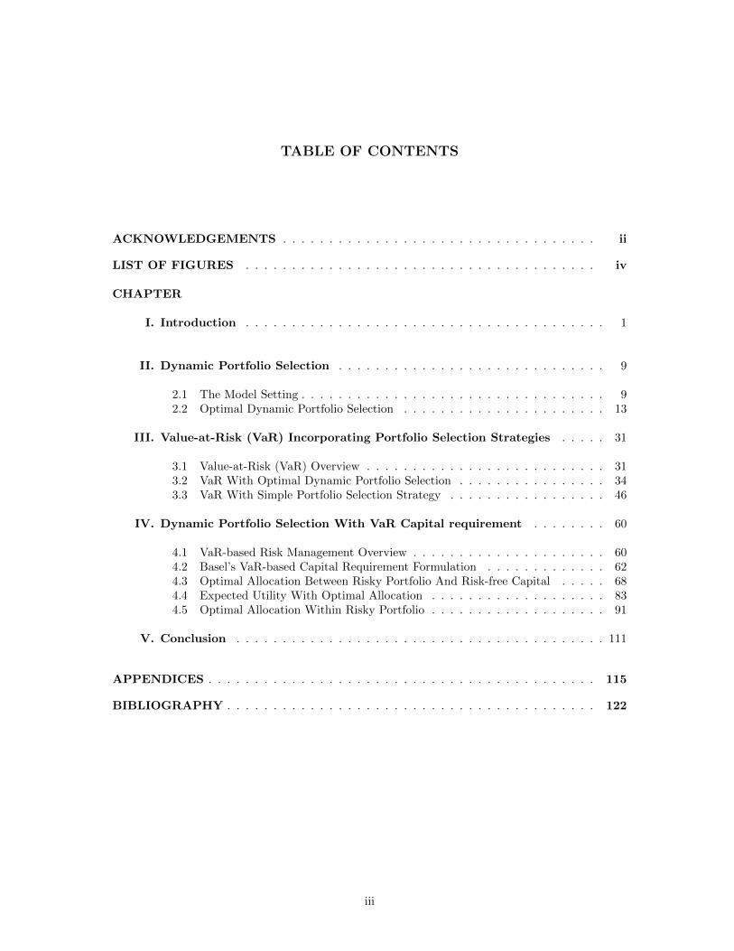
TABLE OF CONTENTS
ACKNOWLEDGEMENTS . . . . . . . . . . . . . . . . . . . . . . . . . . . . . . . . . . ii
LIST OF FIGURES . . . . . . . . . . . . . . . . . . . . . . . . . . . . . . . . . . . . . . iv
CHAPTER
I. Introduction . . . . . . . . . . . . . . . . . . . . . . . . . . . . . . . . . . . . . . . 1
II. Dynamic Portfolio Selection . . . . . . . . . . . . . . . . . . . . . . . . . . . . . 9
2.1 The Model Setting . . . . . . . . . . . . . . . . . . . . . . . . . . . . . . . . . 92.2 Optimal Dynamic Portfolio Selection . . . . . . . . . . . . . . . . . . . . . . 13
III. Value-at-Risk (VaR) Incorporating Portfolio Selection Strategies . . . . . 31
3.1 Value-at-Risk (VaR) Overview . . . . . . . . . . . . . . . . . . . . . . . . . . 313.2 VaR With Optimal Dynamic Portfolio Selection . . . . . . . . . . . . . . . . 343.3 VaR With Simple Portfolio Selection Strategy . . . . . . . . . . . . . . . . . 46
IV. Dynamic Portfolio Selection With VaR Capital requirement . . . . . . . . 60
4.1 VaR-based Risk Management Overview . . . . . . . . . . . . . . . . . . . . . 604.2 Basel’s VaR-based Capital Requirement Formulation . . . . . . . . . . . . . 624.3 Optimal Allocation Between Risky Portfolio And Risk-free Capital . . . . . 684.4 Expected Utility With Optimal Allocation . . . . . . . . . . . . . . . . . . . 834.5 Optimal Allocation Within Risky Portfolio . . . . . . . . . . . . . . . . . . . 91
V. Conclusion . . . . . . . . . . . . . . . . . . . . . . . . . . . . . . . . . . . . . . . . 111
APPENDICES . . . . . . . . . . . . . . . . . . . . . . . . . . . . . . . . . . . . . . . . . . 115
BIBLIOGRAPHY . . . . . . . . . . . . . . . . . . . . . . . . . . . . . . . . . . . . . . . . 122
iii

LIST OF FIGURES
Figure
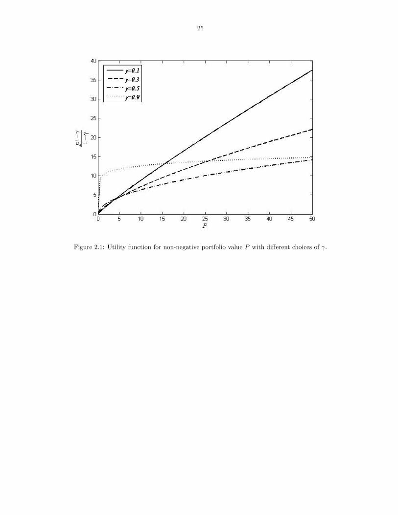
2.1 Utility function for non-negative portfolio value P with different choices of γ. . . . 252.2 Risky asset weight (dotted line) changes as the asset price (solid line) changes when
the share number of the asset is fixed. The risky asset price follows the GBM modelwith parameters: µ(S) = 0.000278, σ(S) = 0.0315 and T = 252 days. . . . . . . . . . 26
2.3 Risky asset share number (dotted line) changes as the asset price (solid line) changeswhen the weight of the asset is fixed. The risky asset price follows the GBM modelwith parameters: µ(S) = 0.000278, σ(S) = 0.0315 and T = 252 days. . . . . . . . . . 27
2.4 Phase line for the ODE of B(t) with different parameter choices. . . . . . . . . . . 282.5 The optimal weight ω∗ at time 0 changes with respect to R0 under the SV model.
When the correlation coefficient ρ is negative, the optimal weight could be decreas-ing with R0. The parameters are set as: ρ = −0.5, a = 0.21, c = 0.0015, d = 0.0015,g = 0.0525 and T = 252 days. . . . . . . . . . . . . . . . . . . . . . . . . . . . . . 29
2.6 The optimal weight ω∗ at time 0 changes with respect to a under the SV model.When the correlation coefficient ρ is negative, the optimal weight could be increas-ing with a. The parameters are set as: ρ = −0.5, R0 = 0.0119, c = 0.0015,d = 0.0015, g = 0.0525 and T = 252 days. . . . . . . . . . . . . . . . . . . . . . . . 30
3.1 Portfolio distributions comparison between the one without any trading (dottedline) and the one with optimal trading strategy (solid line). Each panel correspondsto different risk aversion parameter γ. The risky asset price follows GBM withparameters: µ(S) = 0.000278, σ(S) = 0.0315, and T = 252 days. . . . . . . . . . . . 53
3.2 VaR difference contour map with different volatility levels σ(S). The four straightlines in each panel represent the optimal risky asset weight with different level ofrisk aversion parameter γ. The risky asset price follows GBM with VaR horizonT = 252 days. . . . . . . . . . . . . . . . . . . . . . . . . . . . . . . . . . . . . . . . 54
3.3 VaR difference contour map with different VaR horizons T . The four straightlines in each panel represent the optimal risky asset weight with different levelof risk aversion parameter γ. The risky asset price follows GBM with volatilityσ(S) = 0.031497. . . . . . . . . . . . . . . . . . . . . . . . . . . . . . . . . . . . . . 55
3.4 Risky asset share number (dotted line) changes as the asset price (solid line) changeswith different risky asset weight. The risky asset weight is maintained during theinvestment horizon. The risky asset price follows GBM with parameters: µ(S) =0.000278, σ(S) = 0.031497, and T = 252 days. . . . . . . . . . . . . . . . . . . . . . 56
3.5 VaR difference with respect to the parameters for the stochastic process of riskyasset and investor decision. . . . . . . . . . . . . . . . . . . . . . . . . . . . . . . . 57
3.6 VaR difference with respect to the parameters for the stochastic process of the statevariable Y . . . . . . . . . . . . . . . . . . . . . . . . . . . . . . . . . . . . . . . . . 58
3.7 VaR% φ (in percentages) for difference choices of Rω, σω, and ρω. . . . . . . . . . . 594.1 The trinomial tree for the stochastic process of the state variable Y . The param-
eters of Y process are: c = 0.05, d = 0, 05, g = 0.1 and Y (0) = 1. The graphdemonstrates the first 21 time steps of the tree construction. . . . . . . . . . . . . . 106
iv

4.2 The dynamic programming procedure of finding optimal allocation ψ∗ on top of thetrinomial tree for the stochastic process of the state variable Y . The parametersof Y process are: c = 0.05, d = 0.05, g = 0.1 and Y (0) = 1. The parameters forthe risky portfolio are: Rω = 0.00051587, σω = 0.021 and ρω = −0.2. The Baselmultiplier is δ = 3.5 and investor risk-aversion parameter is γ = 0.5. The graphdemonstrates the first 11 time steps of the procedure. The numbers shown on eachtree node are the optimal weight ψ∗. . . . . . . . . . . . . . . . . . . . . . . . . . . 107
4.3 Expected utility Φ for difference choices of Rω, σω, and ρω. . . . . . . . . . . . . . 1084.4 Optimal xR selection for Φ in the GBM model. In the upper panel, the dashed
and dotted curves represent functions ψ0(xR) and G(xR), respectively. The red
continuous curve represent the function ψ(xR) which is the minimum of ψ0(xR) and
G(xR). The vertical lines passing the intersections of ψ0(xR) and G(xR) identifythe locations of xIR. In the lower panel, the three curves (dashed, dotted and
red continuous) represent the expected utilities when ψ0(xR), G(xR) and ψ(xR)are applied in calculation. The vertical lines identify the locations of the possible
maximizers: xψ0∗R , xG∗R and xIR. The markers are the corresponding expected utility
ψ(xR) of those candidates. . . . . . . . . . . . . . . . . . . . . . . . . . . . . . . . . 1094.5 The surface and contour map of Φ with respect to ρω and σω in the SV model.
In the lower panel, the square represents the global optimal solution. The circlesrepresent the best trial solutions so far at each iteration during the SA procedure.The triangle is the starting point of the procedure. The diamond is the best solutionat the end of the procedure. . . . . . . . . . . . . . . . . . . . . . . . . . . . . . . . 110
v
CHAPTER I
Introduction
Value-at-Risk (VaR) has gained increasing popularity in risk management and
regulation for a decade. However, the driving force for its use can be traced back
much further than a decade. According to the brief history of VaR described in [12]
[14], before the term “Value at Risk” was widely used in the mid 1990s, regulators
developed capital requirements for banks to reduce risk. After the Great Depression
and bank failures in the 1930s, the first regulatory capital requirement for banks were
enacted. The Securities Exchange Commission (SEC), established by the Securities
Exchange Act in 1934, required banks to keep their borrowings below 2000% of
their net capital. In 1975, SEC’s Uniform Net Capital Rule (UNCR) refined the
capital requirement in which bank’s financial assets were categorized into twelve
classes according to the security types. Each class has different capital requirement
represented by the haircut percentage. Depending on the risk, capital requirements
ranged from 0% for short term treasuries to 30% for equities. In 1980, the SEC
required financial firms to calculate the potential losses in different security classes
with 95% confidence over a 30-day interval. The capital requirements were tied to
this measure which was described as haircuts. Although the name “VaR” was not
used, it was virtually the one-month 95% VaR and banks are required to hold enough
1

2
capital to cover the potential loss. In the early 1990s, the Basel Committee updated
its 1988 accord to add the capital requirements for market risk [4] [5]. The market
risk capital requirement is calculated based on the 10-day VaR with 99% confidence
level of the bank’s risky assets portfolio. Now VaR is a widely used risk measure
of the possible loss on a specific portfolio of financial assets. VaR is often used by
commercial and investment banks to capture the potential loss in the value of their
traded portfolio. In most of the applications, the VaR is used to determine the capital
or cash reserves for ensuring that the future loss can be covered and the firm will
remain solvent. Moreover, the VaR can be used for an individual asset, a portfolio
of assets or an entire company. The risk can be specified more broadly or narrowly
for special use. For example, the VaR in investment banks is specified in terms of
market volatility, interest rate changes, and foreign exchange rate changes etc.
In most of the applications, the VaR estimations are always under the assumption
that there is no trading or adjustment in the underlying portfolio during VaR horizon.
As stated in Hull’s book [9],
“VaR itself is invariably calculated on the assumption that the portfolio will
remain unchanged during the time period.”
Apparently, this assumption is unrealistic in real life. For example, some insurance
companies use one-year VaR as their risk measure. If we assume there is no trading in
one year, it is unreasonable. Companies need to adjust their trading portfolios each
day according to changes in the market. The distribution of the portfolio without
trading is significantly different from the one with certain trading strategies. From
a statistical view, VaR is a percentile of the portfolio loss distribution in the given
investment horizon. The distribution of the portfolio value is the essential compo-
nent in the VaR estimation. The distribution of the portfolio value depends on the

3
portfolio selection strategy. Therefore, the selection strategy could have significant
impact on the VaR estimation. To reflect the true risk of the portfolio, the portfolio
adjustment during investment horizon must be incorporated in the VaR estimation,
especially when the investment horizon is long.
The first goal of this study is to incorporate portfolio selection strategies and
analyze the impact of those strategies in VaR estimation. For simplicity, we denote
the VaR incorporating portfolio selection strategies by “New VaR” and the one with
the assumption of no adjustment by “Old VaR”. There are two types of portfolio
selection strategies considered in this study. The first type represents the strate-
gies derived based on the framework established by Merton (1971)[20]. In this case,
the risk-averse investor is assumed to hold the portfolio over a fixed time interval
[0,T ] and try to maximize the expected utility of the terminal wealth. The optimal
portfolio weight can be expressed in terms of the solution of a nonlinear Partial Dif-
ferential Equation (PDE), namely Hamilton-Jacobi-Bellman (HJB) equation. The
second type represents the strategies in which the weights of each asset remain con-
stant during the whole investment horizon. We call this “simple portfolio selection
strategy”. Although this type of portfolio selection strategies is not as sophisticated
as the first one, its simplicity has made it gain a lot of popularity among many
institutional investors. We analyze the new VaR incorporating different portfolio
selection strategies and compare the difference between the new VaR and old VaR.
The second goal of this study mainly concentrates on the application of VaR in
dynamic portfolio selection. The theoretical applications of VaR in risk manage-
ment and regulation can be divided roughly into two main categories [16]. The
first category is to impose a limit on the VaR of the portfolio. Another is to set
aside a VaR-based capital for the risky portfolio. For the first category, there are

4
several papers analyzing the effects of the imposed VaR-limit. Vorst (2001) [26] ana-
lyzes the portfolios with options that maximize expected return under the VaR-limit
constraint. Basak and Shapiro (2001)[7] comprehensively analyze the optimal port-
folio policies of utility maximizing investors under the exogenously-imposed portfolio
VaR-limit constraints. For the second category, the Basel Committee on Banking
Supervision requires the banks to maintain a minimal level of eligible capital whose
amount is a function of the portfolio VaR. Comparing with the VaR-limit, the VaR
based capital risk management is conceptually different.
In the work of Basak and Shapiro, they consider the optimization problem with
the VaR-limit constraint. The formulation of their framework is given by:
(1.1)
maxP (T )>0E [U(P (T ))] ,
E [ξ(T )P (T )] 6 P (0),
V aRp(P, 0, T ) 6 V aR.
In this setting, P (0) and P (T ) are the initial and terminal value of the portfolio, U(·)
is the investor’s utility function, ξ(T ) is the state-price density at time T , T > 0 is the
investment horizon which coincides with the VaR horizon, and V aRp(P, 0, T ) is the
VaR of the terminal portfolio value P (T ) evaluated at time 0 with confidence level p
and V aR is exogenously-imposed limit on the VaR. There are two constraints in this
optimization framework. The first one is the constraint on the budget assuring the
expectation of the discounted portfolio value is no larger than the initial investment
in the unique martingale probability measure. The second constraint is the VaR-
limit on the terminal portfolio value. The optimal terminal portfolio value can be
described by a piecewise function of the state-price density ξ(T ). The possible range
of terminal value of ξ(T ) is divided into three intervals: (−∞, ξ), [ξ, ξ), and [ξ,∞)

5
which correspond to “good states”, “intermediate states”, and “bad states” of the
portfolio, respectively. Basak and Shapiro find that, whenever the constraint is
binding, the VaR risk managers are forced to reduce losses in the “intermediate
state” with the expense of increasing loss in the “bad states”. In other words, the
VaR risk managers tend to choose a larger exposure to risky assets than they would
have invested in the absence of the VaR-limit constraints. Consequently, this strategy
leads the losses in the worst states when the large loss occurs. Similarly, Vorst (2001)
[26] also shows that the optimal policies of maximizing expected portfolio return with
VaR-limit lead to a larger exposure to extreme losses.
In risk management with VaR-based capital requirement, the risk measure VaR is
applied in a completely different way. According to the financial agreement in Basel
Accord issued by the Basel Committee on Banking Supervision, the banks must
maintain a minimal level of eligible capital at all times as a function of the portfolio
VaR. The purpose of Basel Accord is to strengthen the soundness and stability of
the international banking system [3]. In 1996, an amendment on the market risk
capital requirement was added to Basel Accord [4],[5],[6]. In this amendment, the
bank’s assets are separated into two categories: Trading book and Banking book. The
trading book contains financial instruments that are intentionally held for short-term
resale and marked-to-market [15]. The banking book consists of loans that are not
marked-to-market and the major risk of this part is credit risk. By the amendment,
the bank has to hold capital to cover the market risk of the portfolio of different
traded instruments in the trading book. The market risk capital charge is equal to
the maximum of the previous day’s 10-day VaR and the average 10-day VaR over the
last 60 business days times a multiplicative factor δ. The 10-day VaR is calculated
at 99% confidence level. The multiplier δ is between 3 and 4 and it is determined by

6
back testing results [6]. To summarize, the market risk capital charge on any day t
is
(1.2) max
(δ
1
60
60∑i=1
V aR99%(P, t− i, 10), V aR99%(P, t− 1, 10)
),
where V aR99%(P, t− i, 10) is 10-day VaR of the portfolio on day t− i with confidence
level 99%.
Comparing with the practice of VaR-based capital risk management, the optimiza-
tion framework (1.1) with VaR-limit has two major shortcomings. First, it assumes
that the portfolio VaR is never reevaluated after the initial date. Many financial in-
stitutions with VaR-based risk management reevaluate VaR under certain frequency
and adjust their investment portfolios according to the updated VaR. For example,
banks complying with the Basel Accord are obligated to reevaluate the VaRs of the
risky portfolios in the trading book daily and reserve the capital according to the
updated VaRs. Therefore, the assumption of only one evaluation in VaR during
the investment horizon is not realistic. Second, the formulation (1.1) does not in-
corporate the risk capital requirement. The required capital is part of the regulated
portfolio and thus affects the portfolio VaR directly. Different trading strategies have
different VaRs which require different amounts of risk capital. The decision of banks
simultaneously influences the portfolio VaR and the required capital to cover the
risk. Therefore, in order to reflect the realistic risk management practice, the opti-
mization framework should incorporate the relationship between the risk-free asset
(used as risk capital) and the VaR of the risky portfolio.
Several studies analyze Basel Accord’s market risk requirement and develop opti-
mization framework to incorporate some characteristics of it. Inspired by the work
of Basak and Shapiro (2001), Kaplanski and Levy (2006) [16] analyze VaR-based
capital requirement regulation under an optimization formulation which is very sim-

7
ilar to (1.1). They transform the Basel’s market risk capital requirement into an
inequality constraint which puts a limit on the minimum of the portfolio terminal
value. The solution of this optimization problem also has a similar form to the so-
lution in formulation (1.1). Under their new framework, they analyze the efficiency
of the VaR-based capital requirement regulation with different choices of multiplier
δ. Their results show that there is an optimal level of required eligible capital from
the regulation standpoint and the current Basel’s range of δ is within the inefficient
range. However, the VaR constraint in their framework is evaluated only at the end
of the investment horizon. Cuoco, He, and Isaenko (2007) [11] derive the optimal
portfolio selection subject to the VaR limit which is reevaluated dynamically. In their
formulation, the trader must satisfy the specified risk limit during the investment
horizon. They show that the concern expressed in the work of Basak and Shapiro do
not apply. They also consider the formulation with tail conditional expectation limit
as the constraint in the optimization which is suggested by Basak and Shapiro for
correcting the shortcoming in VaR-limit formulation. Under the situation where the
constraint is constantly reevaluated, the tail conditional expectation limit is equiva-
lent to VaR limit. However, their analysis does not completely reflect Basel Accord’s
market risk requirement because their VaR constraint is not imposed on the amount
of risk-free capital. Keppo, Kofman, and Xu (2010) [17] analyze the undesirable ef-
fect of Basel’s credit and market risk requirements on the bank. They develop their
banking model to account for the market risk capital requirement by restricting the
holding of a risky portfolio within the certain range determined by the simplified
formulation (1.2). In their formulation, the relationship between the holding of a
risky portfolio and a risk-free asset is explicitly reflected in the constraints. That is,
the buffer capital has to be larger than the product of δ and the VaR of the risky

8
assets portfolio all the time. They show that if the expected return and volatility
of the risky assets portfolio are high, the market risk requirement raises the default
probability of the bank. That is, the market risk requirement is inefficient.
In this study, we extend those previous works in VaR application. There are two
major improvements we expect to accomplish. First, we construct a sophisticated
framework to develop the optimal portfolio selection strategy in which the Basel’s
VaR-based capital requirement is completely reflected. In other words, VaR-based
capital requirement is formulated in terms of a lower bound on risk free asset and
reevaluated all the time. Second, the framework can accommodate more complicated
risk asset models such as Stochastic Volatility (SV) model as well as the simple
Geometric Brownian Motion (GBM) model.
The rest of this paper is organized as follows. In Chapter II, we describe the gen-
eral model setting from which two famous models (GBM and SV) can be derived.
With this model setting, we apply Merton’s framework to derive the optimal port-
folio selection strategy when there is no constraint. In Chapter III, we analyze the
VaRs incorporating portfolio selection strategies and compare the difference between
the old VaR and new VaR. The strategies include optimal strategies derived from
Chapter II and the simple ones with constant weight. In Chapter IV, we describe
the framework for developing the optimal portfolio selection strategy in which the
Basel’s VaR-based capital requirement is completely reflected.

CHAPTER II
Dynamic Portfolio Selection
2.1 The Model Setting
We assume that the investor has two types of investment opportunities. The first
one is a risk free asset S0(t) with constant interest rate r. The second one is a group
of n risky assets whose prices is a vector process S(t) = (S1(t), ..., Sn(t))′ (′ denotes
transpose). Specifically, the asset prices satisfy the following stochastic differential
equations:
(2.1) dS0(t) = rS0(t)dt,
(2.2) dS(t) = D(S(t))µ(S)(Y (t))dt+D(S(t))σ(S)(Y (t))dW (S),
(2.3) dY (t) = µ(Y )(Y (t))dt+ σ(Y )(Y (t))dW (Y ).
In this setting, Y is a state variable for the presence of stochastic environment.
In this study, Y is used to describe the market volatility. W (S) is an n-dimensional
standard Brownian motion andW (Y ) is a standard Brownian motion. The correlation
between dW (Y ) and dW (S) is ρdt where ρ is a 1×n row vector. D(S(t)) is a diagonal
matrix with (S1(t), ..., Sn(t)) on the diagonal. The instantaneous expected return
µ(S)(Y ) is an n × 1 vector and the instantaneous standard deviation of diffusive
9

10
return σ(S)(Y ) is an n× n matrix. Both of them are functions of a one-dimensional
state variable Y . In the stochastic process of Y , the drift rate µ(Y )(Y ) and volatility
σ(Y )(Y ) are scalar functions of Y.
Moreover, we further assume that the instantaneous expected return µ(S)(Y ) and
standard deviation of diffusive return σ(S)(Y ) are formulated as follows
µ(S)(Y ) = r1n + abY
σ(S)(Y ) = a√Y ,
(2.4)
where 1n is the n-dimensional column vector with 1 in all components i.e. 1n =
(1, ..., 1)′, a is an invertible n × n matrix and b is an n × 1 vector. As a result, the
risk premium in (2.4) is abY . This form of risk premium is also used by Merton
(1980)[21], Pan (2002)[24], and Liu (2007)[19]. For the state variable Y , the drift
rate µ(Y )(Y ) and volatility σ(Y )(Y ) in (2.3) are formulated as follows
µ(Y )(Y ) = d− cY
σ(Y )(Y ) = g√Y ,
(2.5)
where the parameters c, d, and g are all assumed to be nonnegative. Moreover, we
restrict the parameters d and g to satisfy d > g2/2. If this inequality is violated,
Y (t) becomes 0 at some random time τ > 0 with probability 1, and then Y(t)=0 for
all t > τ . Y (t) is a mean reverting square root process. It is obvious that the state
variable Y is always positive. The same process is used in the CIR (1985)[10] for the
spot interest rate and Heston model(1993) [13] for the stochastic volatility.
The dynamics given in (2.1)-(2.3) is a generalized form which nests two models
considered in this study. These two models are, in the order of complexity, Geometric
Brownian Motion (GBM) model and Stochastic Volatility (SV) model.
Case I, Geometric Brownian Motion (GBM) model

11
This is the simplest form derived from the generalized model. In this case, the
stochastic volatility is not incorporated in the model. That is, Y = 1. The instan-
taneous expected return µ(S)(Y ) and standard deviation of diffusive return σ(S)(Y )
are then reduced to constants. The S process is formulated as follows
(2.6) dS(t) = D(S(t))(r1n + ab)dt+D(S(t))adW (S).
The risk premium R of the risky assets is a constant vector R = ab.
Case II, Stochastic Volatility (SV) model
In this case, the stochastic volatility Y is incorporated and the risk premium
R = abY is a time-varying random variable. Together with the setting (2.4)-(2.5),
the asset price dynamics becomes
(2.7) dS(t) = D(S(t))(r1n + abY (t))dt+D(S(t))a√Y (t)dW (S),
(2.8) dY (t) = (d− cY (t))dt+ g√Y (t)dW (Y ).
In this setting, the risky asset prices are driven by two sources of uncertainty: dif-
fusion in S dynamics, W (S), and diffusion in volatility dynamics, W (Y ). One should
notice that the model becomes the Heston model (1993) [13] for single risky asset
when a and b are reduced to scalars.
To construct the investor’s portfolio, we follow the framework and assumptions
in Merton (1971)[20]. The assumptions are:
1. there are no transaction costs;
2. short sales with full use of proceeds are allowed;
3. assets are traded continuously in time;
4. self-financing strategies are applied.

12
Given the initial wealth P0, the dynamics of the investor’s portfolio wealth P (t) is
given by
dP (t) = [ω′µ(S)(Y (t)) + (1− ω′1n)r]P (t)dt+ ω′σ(S)(Y (t))P (t)dW (S),(2.9)
where ω is an n × 1 vector which denotes the risky assets’ relative weights. In this
setting, ω represents the portfolio selection strategy used by the investor. It can be a
constant vector, or a time-varying vector, or even a vector of functions of any other
relevant variables such as Y . At time t, the investor’s total wealth P (t) is given by
P (t) = P0exp
∫ t
0
(ω′µ(S)(Y (u)) + (1− ω′1n)r − 1
2ω′Σ(S)(Y (u))ω
)du
+
∫ t
0
ω′σ(S)(Y (u))dW (S)(u)
,
(2.10)
where Σ(S)(Y (u)) = σ(S)(Y (u))σ(S)(Y (u))′.

13
2.2 Optimal Dynamic Portfolio Selection
In this study, we assume that the risk-averse investor holds the portfolio over a
fixed time interval [0,T ] and tries to maximize the expected utility E [U(P (T ))] over
terminal wealth. The objective function is only related to the portfolio value at time
T . Arrow (1971)[1] argues that there are three desirable properties for the investor’s
utility function. Those three properties and their mathematical formulations are:
1. positive marginal utility for wealth, i.e. dUdP
> 0;
2. decreasing marginal utility for wealth, i.e. d2UdP 2 < 0;
3. non-increasing absolute risk aversion, i.e. d(−d2UdP 2/
dUdP
)/dP ≤ 0.
Logarithmic, power, and negative exponential utility functions have these three de-
sired attributes. In this study, the power utility function is used and it has a constant
relative risk aversion ((−d2UdP 2/
dUdP
)P = γ) over the terminal wealth. The utility func-
tion is defined as follows
(2.11) U(P ) =
P 1−γ
1−γ , if P ≥ 0,
−∞, if P < 0,
where γ is the risk aversion coefficient within [0,1] and is an indicator of investor’s
risk appetite. The second part of the utility function is a constraint that prevents the
wealth from being negative. This utility function is a concave function and satisfies
all three desirable properties of investor’s utility function. The parameter γ would
be different for different investors. The smaller the γ is, the less risk averse the
investor is or the larger the investor’s risk appetite is . Figure 2.1 shows different
power utility functions with different choices of γ. This graph shows that as portfolio
wealth P becomes larger, the utility of the investor with large γ grows slower than

14
that of the investor with small γ. The utility function converges to P , U(P ) = P ,
as γ converges to 0. This is the risk neutral case.
2.2.1 Optimization framework for portfolio selection
Following the framework established by Merton (1971)[20], we define a value func-
tion for the formulations (2.1)-(2.3)
V (P, Y, t) = maxω(s)Ts=t
Et [U(P (T ))] .
and the Hamilton-Jacobi-Bellman(HJB) equation for V is:
maxω(t)Tt=0
Vt +
1
2ω′Σ(S)ωP 2VPP + ω′Σ(S,Y )PVPY +
1
2Σ(Y )VY Y
+[ω′µ(S) + (1− ω′1n)r]PVP + µ(Y )VY
= 0,
(2.12)
where
Σ(S) = σ(S)σ(S)′ ,
Σ(S,Y ) = σ(S)ρ′σ(Y ),
Σ(Y ) = σ(Y )σ(Y )′ .
(2.13)
The terminal condition is given by
V (P, Y, T ) =P 1−γ
1− γ.
In order to solve for the optimal portfolio weight ω∗, we introduce the ansatz
(2.14) V (P, Y, t) =1
1− γP 1−γf(Y, t),
where f is a function of Y and t satisfying the terminal condition f(Y, T ) = 1. Then,
the HJB equation (2.12) becomes
maxω(t)Tt=0
ft +
[(1− γ)ω′Σ(S,Y ) + µ(Y )
]fY +
1
2Σ(Y )fY Y
+(1− γ)[−γ
2ω′Σ(S)ω + ω′(µ(S) − r1n) + r
]f
= 0.
(2.15)

15
The first order condition with respect to ω is
Σ(S,Y )fY +(−γΣ(S)ω + µ(S) − r1n
)f = 0.
Then, the optimal portfolio weight is given by
(2.16) ω∗ =1
γΣ(S)−1 (
µ(S) − r1n)
+1
γΣ(S)−1
Σ(S,Y )fYf.
The function f in (2.16) is an unknown function. To solve for f , we can substitute
(2.16) back to (2.15) and obtain a PDE for f . The complete form of optimal portfolio
weight can be derived by solving the PDE of f .
2.2.2 The solution of a general PDE
Before solving for the optimal portfolio weight, we first derive the solution of
a general PDE. The special case of this PDE will be used in solving the portfolio
selection problem for SV model. In this section, we consider a general PDE
(2.17) ft + C1fY Y + C2fY + C3f 2Y
f+ C4f = 0,
with the terminal condition f(Y, T ) = 1. This PDE can not be solved analytically in
general. We impose some conditions on the coefficients of this PDE in order to solve
it. If all the coefficients C1, C2, C3, C4 of above PDE are linear in Y , say Ci = hi+ liY
for i = 1, ...4, then the ansatz of f is f(Y, t) = exp(A(t) + B(t)Y ), where A(t) and
B(t) are scalar functions. The corresponding partial derivatives of f are
ft = (At +BtY ) f,
fY = Bf,
fY Y = B2f.
(2.18)
When f(Y, t) = exp(A(t) +B(t)Y ) is substituted into the PDE (2.17), we have
(At +BtY )f + (h1 + l1Y )B2f + (h2 + l2Y )Bf + (h3 + l3Y )B2f + (h4 + l4Y )f = 0.

16
Combining all the like terms, we have:
(At + (h1 + h3)B2 + h2B + h4) +(Bt + (l1 + l3)B2 + l2B + l4
)Y = 0
In order to hold the equation for all Y, the coefficients of Y and Y 0 (terms not
related to Y) have to be zero, which leads to ordinary differential equations (ODEs)
for A(t) and B(t). The PDE (2.17) can be solved by solving the following two Riccati
equations:
(2.19) At + (h1 + h3)B2 + h2B + h4 = 0
(2.20) Bt + (l1 + l3)B2 + l2B + l4 = 0
with the terminal conditions A(T ) = 0 and B(T ) = 0. From the ODEs above, one
can notice that the ODE (2.19) for A(t) can be easily solved once B(t) is given. The
ODE for B(t) is a Riccati equation. In order to solve (2.20), we define q0 = −l4,
q1 = −l2, q2 = −(l1 + l3), and ξ =√
(q1)2 − 4q0q2. After the transformation the
equation (2.20) becomes
(2.21) Mtt − q1Mt + q0q2M = 0,
where B(t) = − Mt
Mq2. Depending on the value of ξ2, there are two possible solutions
for the equation (2.21).
Case I: ξ2 ≥ 0
The solution of (2.21) is given by M(t) = u1ev1t+u2e
v2t where v1,2 =q1±√q12−4q0q2
2
and u1 and u2 are certain constants to be determined by the terminal condition. From
B(t) = − Mt
Mq2, we have
B(t) = − Mt
Mq2
= −u1v1ev1t + u2v2e
v2t
(u1ev1t + u2ev2t)q2

17
By using the terminal condition, we have u1 = −u2v2v1e(v2−v1)T and the function B(t)
is given by
B(t) = − v1v2(−e−v1(T−t) + e−v2(T−t))
(−v2e−v1(T−t) + v1e−v2(T−t))q2
= − q0q2(−e(v2−v1)(T−t) + 1)
(−12(q1 + ξ)e(v2−v1)(T−t) + 1
2(q1 − ξ))q2
= − 2(eξ(T−t) − 1)q0
(q1 + ξ)(eξ(T−t) − 1) + 2ξ.
Case II, ξ2 < 0
By defining η =√
4q0q2 − (q1)2, the solution of (2.21) is given by M(t) =
e12q1t(u1cos(
12ηt) + u2sin(1
2ηt))
where and u1 and u2 are certain constants to be de-
termined by the terminal condition. Similarly, the function B(t) is given by
B(t) = − Mt
Mq2
= − q1
2q2
−η2(−u1sin(1
2ηt) + u2cos(
12ηt))
q2(u1cos(12ηt) + u2sin(1
2ηt))
By using the terminal condition, we have u1 = u2q1sin( η
2T )+ηcos( η
2T )
ηsin( η2T )−q1cos( η2T )
and
B(t) = − q1
2q2
+η(
q1sin( η2T )+ηcos( η
2T )
ηsin( η2T )−q1cos( η2T )
sin(η2t)− cos(η
2t))
2q2(q1sin( η
2T )+ηcos( η
2T )
ηsin( η2T )−q1cos( η2T )
cos(η2t) + sin(η
2t))
= − q1
2q2
+ηq1cos[
η2(T − t)]− η2sin[η
2(T − t)]
2q2(q1sin[η2(T − t)] + ηcos[η
2(T − t)])
= − q21 + η2
2q2(q1 + ηcot[η2(T − t)])
= − 2q0
q1 + ηcot[η2(T − t)]
.
Therefore, the complete form of B(t) is
(2.22) B(t) =
− 2(eξτ−1)q0
(q1+ξ)(eξτ−1)+2ξ, if ξ2 ≥ 0
− 2q0q1+ηcot[ η
2(T−t)] , if ξ2 < 0
where τ = T − t, η =√
4q0q2 − (q1)2, q0 = −l4, q1 = −l2, q2 = −(l1 + l3) and
ξ =√
(q1)2 − 4q0q2. Then we can substitute B(t) into ODE (2.19), A(t) can be
easily solved simply by integrating both sides of the equation.

18
Liu [19] did more general work for a PDE similar to (2.17). He makes each coeffi-
cient in the PDE quadratic in Y and solves the PDE up to the solutions of ordinary
differential equations. In order to get each coefficient quadratic in Y , a lot of compli-
cated restrictions are imposed on the parameters which involve tensors calculation
and require very tremendous computational effort for parameter calibration. There-
fore, for practical purpose we use simpler constraints on the drift and diffusion terms
by setting them as linear functions of the state variable Y .
2.2.3 Optimal portfolio weight solution
The optimal portfolio weight formula (2.16) is directly related to an unknown
function f . In order to derive the complete form, we need to substitute this formula
back to the HJB equation. Depending on the parameter settings of the two models
under consideration, we have the following cases.
Case I, Geometric Brownian Motion (GBM) model
In this simple case, the parameter setting for (2.4) and (2.5) are:
(2.23) Y = 1, c = d = g = 0
The second term of (2.16) is gone, the optimal portfolio weight becomes
(2.24) ω∗ =1
γΣ(S)−1 (
µ(S) − r1n)
=1
γ(aa′)−1R.
where R = µ(S) − r1n. Since Y = 1, there is no need to solve for the unknown
function f in this case. When the investor has only one risky asset in the portfolio,
the optimal weight ω∗ is positively related to the risky asset risk premium R. It
suggests that the investor should long the risky asset if its risk premium is positive
or short the risky asset otherwise. The volatility parameter σ(S) = a affects the
magnitude of the optimal weight . If the risky asset is very volatile the investor

19
should reduce the amount of risky asset in the long or short position. Moreover,
the optimal weight also depends on the risk-aversion of the given investor. If the
investor is more risk averse (larger γ), the optimal weight decreases in its magnitude.
If the investor has a great risk appetite (smaller γ), the optimal weight magnitude
increases.
Under the optimal trading strategy, the risky asset weight is a constant vector
when the asset price follows the GBM. Although the risky asset weight is kept con-
stant throughout the whole time interval, it does not mean that there is no trading.
On the contrary, the optimal strategy requires the investor to actively rebalance the
investment portfolio in order to maintain the optimal risky asset weight. In other
words, if the investor does not execute any trading within the given period, the quan-
tity of the asset does not change but the risky asset weight will change with the asset
price movement. In Figure 2.2, we show how the asset weight (dotted line) changes
with the asset price (solid line). If there is no trading during the given time period,
the relative asset weight increases (decreases) as the asset price increases (decreases).
Therefore, in order to maintain the constant risky asset weight, the investor needs
to buy or sell the risky assets according to the price movement as shown in the
Figure 2.3.
Case II, Stochastic Volatility (SV) model
For SV model, in order to solve ω∗, one needs to substitute the optimal weight
(2.16) into (2.15), then (2.15) becomes
ft +1
2Σ(Y )fY Y +
[µ(Y ) +
1− γγ
Σ(S,Y )′Σ(S)−1 (µ(S) − r1n
)]fY
+1− γ
2γΣ(Y,ρ)f
2Y
f
+ (1− γ)
[1
2γ
(µ(S) − r1n
)′Σ(S)−1
(µ(S) − r1n) + r
]f = 0,
(2.25)
20
where Σ(Y,ρ) = σ(Y )ρρ′σ(Y ). This PDE is a special case of the general PDE (2.17)
solved in the previous section. Together with (2.4), (2.5), and (2.13), the coefficients
C1, ..., C4 of the PDE are given by
C1 = h1 + l1Y =1
2Σ(Y )
=1
2g2Y,
C2 = h2 + l2Y = µ(Y ) +1− γγ
Σ(S,Y )′Σ(S)−1 (µ(S) − r1n
)= d+
(−c+
1− γγ
ρbg
)Y,
C3 = h3 + l3Y =1− γ
2γΣ(Y,ρ)
=1
2γ(1− γ)g2ρρ′Y,
C4 = h4 + l4Y = (1− γ)
[1
2γ
(µ(S) − r1n
)′Σ(S)−1
(µ(S) − r1n) + r
]= (1− γ)r +
1− γ2γ
b′bY.
Since the solution of the PDE (2.17) has the form f(Y, t) = exp(A(t) + B(t)Y ), the
optimal portfolio weight (2.16) becomes
(2.26) ω∗ =1
γa′−1b+
1
γa′−1ρgB,
where B is given by (2.22) with l1 = 12g2, l2 = −c + 1−γ
γρbg, l3 = 1−γ
2γg2ρρ′, and
l4 = 1−γ2γb′b.
The optimal risky asset weight in this case is time-varying due to the stochastic
state variable Y . The risk premium R = abY and the risky asset volatility σ(S) =
a√Y are positively related to Y . To analyze the optimal weight with respect to risk
premium, we define a constant vector R0 = ab, namely risk premium coefficient. The
optimal weight becomes
(2.27) ω∗ =1
γ(aa′)−1R0 +
1
γa′−1ρgB

21
The optimal weight of SV model is the sum of the myopic demand and the in-
tertemporal hedging demand caused by the dynamics of the state variable [19]. The
myopic demand is the risky asset weight that the investors would hold as if the state
variable is constant. It is virtually the optimal weight in GBM model. The intertem-
poral hedging demand is the adjustment on myopic demand for the uncertainty of
the state variable. When the correlation ρ between risky asset and state variable
is zero, the intertemporal hedging demand is zero since there is no needs to hedge
the uncertainty of Y . The intertemporal hedging demand converges to zero at the
end of the investment horizon. In particular, we have several remarks regarding this
time-varying function B(t).
Remark II.1. The function B(t) is non-negative and non-increasing on the interval
[0, T ].
In the SV model, we assume that a is an invertible matrix and g > 0. Together
with b = a−1R0, we have l1 = 12g2 > 0, l2 = −c + 1−γ
γρga−1R0, l3 = 1−γ
2γg2ρρ′ ≥ 0,
and l4 = 1−γ2γR′0(aa′)−1R0 ≥ 0. Moreover, the ODE of B (2.20) can be revised as
(2.28) Bt = Q(B) = −(l1 + l3)B2 − l2B − l4.
This ODE is an autonomous differential equation and can be analyzed on the phase
line. On the phase line (Figure 2.4), the solution of the ODE moves along B axis.
The number and positions of equilibrium points (Bt = 0) depend on the parameters:
l1, ..., l4. The line can be segmented by the equilibrium points (grey circles) and the
direction (solid arrows) of each segment is determine by the sign of Q(B). Together
with the terminal condition B(T ) = 0, we can determined the possible direction
(dotted arrows) for the solution B(t) on the interval [0, T ]. In the three panels of
Figure 2.4, all possible positions of equilibrium points are demonstrated. Given the

22
terminal condition B(T ) = 0 (black star), the possible solution must move toward the
black start on the phase line. Among all the segments shown on the diagram, only
those with dotted arrows are possible solutions. When R0 = 0, the terminal condition
coincides with the equilibrium and B is zero on the interval [0, T ]. The parameter
l2 determines the relative positions of equilibrium points on B axis. Another key
parameter ξ2 = l22 − 4(l1 + l3)l4 determines the number of the equilibrium points.
It’s obvious that all possible solutions always stay on the right-hand side of 0 on
the phase line and point from right to left (B ≥ 0 and Bt ≤ 0). Therefore, B(t) is
non-negative and non-increasing on the interval [0, T ].
Remark II.2. In the case of the portfolio with only one single risky asset, if ρ and
R0 are non-negative, B is non-decreasing with respect to R0 at any time t in [0, T ].
By taking the derivative with respect to R0 on both sides of ODE (2.28), we have
(2.29) Bt,R0 = −2(l1 + l3)BBR0 − l2BR0 −1− γγa
gρB − 1− γγa2
R0.
Denote BR0 by H(R0). The ODE above becomes
(2.30) H(R0)t = [−2(l1 + l3)B − l2]H(R0) − 1− γ
γagρB − 1− γ
γa2R0.
with the terminal condition H(R0)(T ) = 0. The solution of the ODE is given by
(2.31)
H(R0)(t) =
∫ T
t
(1− γγa
gρB(s) +1− γγa2
R0
)exp
∫ s
t
[2(l1 + l3)B(u) + l2]du
ds.
Apparently, H(R0) is non-negative when ρ and R0 are non-negative at any time t in
[0, T ]. Therefore, B is non-decreasing with respect to R0.
Remark II.3. In the case of the portfolio with one single risky asset, if ρ and R0
are non-negative, B is non-increasing with respect to the volatility coefficient a at
any time t in [0, T ].

23
Similarly, by taking the derivative with respect to a on both sides of ODE (2.28),
we have the following ODE with H(a) = Ba
(2.32) H(a)t = [−2(l1 + l3)B − l2]H(a) +
1− γγa2
gρR0B +1− γγa3
R20,
with the terminal condition H(a)(T ) = 0. The solution of the ODE is given by
(2.33)
H(a)(t) =
∫ T
t
(−1− γ
γa2gρR0B(s)− 1− γ
γa3R2
0
)exp
∫ s
t
[2(l1 + l3)B(u) + l2]du
ds.
Apparently, H(a) is non-positive when ρ and R0 are non-negative at any time t in
[0, T ]. Therefore, B is non-increasing with respect to a.
By taking the derivative of ω∗ (2.27) with respect to R0 and a respectively, we
have
ω∗R0=
1
γa2+
1
γaρgH(R0),
and
ω∗a = − 2
γa3R0 −
1
γa2ρgB +
1
γaρgH(a).
Based on the previous three remarks, it is very straightforward that ω∗R0≥ 0 and
ω∗a ≤ 0 . Therefore, we have the following result for the optimal risky asset weight.
Remark II.4. In the case of the portfolio with one single risky asset, if ρ and R0
are non-negative, ω∗ is non-decreasing with respect to R0 and is non-increasing with
respect to the volatility coefficient a at any time t in [0, T ].
However, when the correlation coefficient ρ is negative, the analysis for the optimal
weight is more complicated. As shown in Figure 2.5 - 2.6, the optimal weight could be
decreasing with R0 and increasing with a for certain parameter setting with negative
ρ.
Through the analysis of the optimal weight on risky asset, one can notice that
the GBM model and SV model share some common properties in optimal portfolio

24
selection. First, the risky asset weight is positively related to risk premium R in GBM
model. In SV model, the risky asset weight is positively related to risk premium
coefficient R0 when ρ ≥ 0 and R0 ≥ 0. Second, when risk premium is non-negative,
the risky asset weight decreases as the volatility (volatility coefficient in SV model)
a increases (ρ ≥ 0 is required in SV model). Some of these results can be used to
analyze the expected utility with the optimal risky asset weight. The analysis on
the expected utility is a fundamental element for optimal portfolio selection with
the constraints of VaR-based capital requirement. However, those results might not
be valid when ρ is negative in SV model. It induces lots of complexities in the
analysis of the next step. Therefore, it becomes very difficult for us to analyze the
relationship between the expected utility obtained by the optimal risky asset weight
and the related parameters.
25
Figure 2.1: Utility function for non-negative portfolio value P with different choices of γ.

26
Figure 2.2:Risky asset weight (dotted line) changes as the asset price (solid line) changes when theshare number of the asset is fixed. The risky asset price follows the GBM model withparameters: µ(S) = 0.000278, σ(S) = 0.0315 and T = 252 days.

27
Figure 2.3:Risky asset share number (dotted line) changes as the asset price (solid line) changeswhen the weight of the asset is fixed. The risky asset price follows the GBM modelwith parameters: µ(S) = 0.000278, σ(S) = 0.0315 and T = 252 days.

28
Figure 2.4: Phase line for the ODE of B(t) with different parameter choices.

29
Figure 2.5:The optimal weight ω∗ at time 0 changes with respect to R0 under the SV model. Whenthe correlation coefficient ρ is negative, the optimal weight could be decreasing withR0. The parameters are set as: ρ = −0.5, a = 0.21, c = 0.0015, d = 0.0015, g = 0.0525and T = 252 days.

30
Figure 2.6:The optimal weight ω∗ at time 0 changes with respect to a under the SV model. Whenthe correlation coefficient ρ is negative, the optimal weight could be increasing with a.The parameters are set as: ρ = −0.5, R0 = 0.0119, c = 0.0015, d = 0.0015, g = 0.0525and T = 252 days.

CHAPTER III
Value-at-Risk (VaR) Incorporating Portfolio SelectionStrategies
3.1 Value-at-Risk (VaR) Overview
To clarify the definition of VaR, we consider a portfolio whose value P (t) is a
time-dependent stochastic process. Given the portfolio value P (t) at any time t
and the investment horizon τ > 0, VaR with confidence level p is the loss in value
corresponding to p-quantile of the distribution of the portfolio loss P (t) − P (t + τ)
over the investment horizon. The confidence level p is usually a number slightly less
than 1 such as 99% in practice. In other words, if FP (t)−P (t+τ) denotes the cumulative
distribution function (cdf) of the loss in value over [t, t+ τ ], the VaR of the portfolio
at time t is
V aRp (P, t, τ) = F−1P (t)−P (t+τ)(p).
Another equivalent formulation of VaR can be derived as
(3.1) V aRp (P, t, τ) = P (t)− F−1P (t+τ)(1− p),
where FP (t+τ) is the cdf of the portfolio value P (t+τ) at time t+τ . Both formulations
provide the same information to the investors. That is, the loss of the portfolio over
the next investment horizon is no more than V aRp (P, t, τ) with probability p. For
example, if a portfolio’s two-week VaR with confidence level 95% is $1 million, it
31

32
means there is a 95% chance that the value of the portfolio will drop no more than
$1 million over any given two-week period. From a statistical view, this value at
risk measures the 1 − p critical value of the probability distribution of the changes
in market value. Apparently, there are three key elements in VaR definition, a
confidence level p, the distribution of P (t + τ) and a fixed time interval over which
the risk is assessed.
In the VaR estimation, the distribution of portfolio value P (t+τ) at the end of the
investment horizon is the key component. The P (t+τ) distribution is affected by the
initial value P (t) and the portfolio selection strategy applied during the investment
horizon [t, t + τ ]. In most applications of VaR, the VaR estimation is always under
the assumption that there is no trading during the VaR horizon. Apparently, this
assumption is unrealistic in real life. The distribution of a portfolio without trading
is significantly different from the one with certain trading strategy. In Figure 3.1,
the comparison of portfolio distributions is demonstrated. Two portfolios are both
constructed with one risky asset and one risk-free asset. The risky asset price follows
the GBM. Both portfolios start with the same risky asset weight which is the optimal
risky asset weight and the same initial value which is $100. However, one portfolio is
not subject to any change during the investment horizon (T = 252 days). Another
portfolio is always adjusted by the investor in order to maintain the optimal risky
asset weight. For all levels of risk aversion parameter γ, these two portfolio value
distributions are very different. Since the distributions are different, VaR estimations
are also different. To reflect the true risk of the portfolio, the adjustment during the
investment horizon must be incorporated in the VaR estimation, especially when the
investment horizon is long. In the rest of study, we refer to the old VaR as the VaR
with the assumption of no trading or rebalancing during the VaR horizon, and the

33
new VaR as the VaR incorporating certain trading strategy. The trading strategy
could be an optimal selection strategy or just as simple as the one with constant
weight on each asset.
The rest of this chapter is organized as follows. In the second section, we demon-
strate the new VaR estimation incorporating the optimal portfolio selection strategy
and analyze the difference between the old VaR and new VaR. In the third section, we
develop a theoretical framework to analyze the VaR incorporating a simple portfolio
selection strategy.

34
3.2 VaR With Optimal Dynamic Portfolio Selection
The main objective of this section is to demonstrate the VaR estimation incorpo-
rating the portfolio selection strategy and the difference between the new VaR and
the old VaR. The VaR analysis is based on the portfolio consisting of a risk-free asset
and one risky asset. One of the advantages of the analysis with only one risky asset
lies in the parameter dimension and the identification of essential factors. With one
single risky asset, the number of parameters is greatly reduced comparing to the
problem with multiple risky assets. Moreover, those important factors such as drift
rate and volatility can be easily identified as scalars. On the contrary, the drift rate
is a vector and the diffusion term is a matrix in the case of multiple risky assets.
Another advantage with one single risky asset is that analytical forms of VaRs can
be derived under certain model such as GBM model. Even with a simple portfolio
consisting of a risk-free asset and one single risky asset, the difference between the
old VaR and the new VaR is very significant. The difference between these two VaRs
depends on many factors such as drift rate, volatility, the length of VaR horizon, and
the investor’s risk-averseness. In the case of multiple risky assets, more variations
will be added on the VaR difference due to the increasing number of parameters.
Therefore, the simple case with only one risky asset is used to describe the impact.
In this study, two different models are used to describe the dynamics of the risky
asset: Geometric Brownian Motion (GBM) model and Stochastic Volatility (SV)
model. Under these two models, the analytical formulation for optimal portfolio
selection can be derived given that the investor’s utility over terminal wealth is a
concave function (2.11) with constant relative risk aversion.
Both old VaR and new VaR are calculated in this section. For the purpose of

35
comparison, we construct two portfolios. In the first portfolio, there is no trading ac-
tivity during the investment horizon. On the contrary, the second portfolio is actively
adjusted according to certain selection strategy. P (1) and P (2) denote the portfolio
value for the first portfolio and second portfolio, respectively. Both portfolios start
with the same initial wealth and initial risky asset weight. The VaR estimation is
based on the distribution of the wealth at the end of the investment horizon. It
is obvious that the VaR estimation based on P (1) gives the old VaR (V aR(1)) and
the VaR estimation based on P (2) gives the new VaR (V aR(2)). The analysis of the
impact of the portfolio selection on VaR is based on the difference between these two
VaRs. The VaR difference is represented by
G = V aR(1) − V aR(2).
Then, ifG is positive (negative), it means the old VaR overestimates (underestimates)
the true risk of the portfolio (the new VaR). For simplicity, the initial wealth is set
to be $100. Therefore, the estimations from either VaRs or VaR difference can be
viewed as the the percentage of the initial wealth. From all the following numerical
experiments, we notice that the VaR difference changes sign with various parameter
settings. The sign (positive or negative) of VaR difference shows whether the old
VaR overestimates or underestimates the risk of the portfolio (the new VaR). Even
with the GBM model in which analytical forms of VaR difference can be derived, the
relationship between VaR difference and relevant parameters is very complicated.
The numerical results suggest that the old VaR with no-trading assumption is not
suitable in a volatile market (large volatility)or for a long investment horizon.

36
3.2.1 The case with Geometric Brownian Motion (GBM) model
In this case, parameters and optimal risky asset weight are constants. In particu-
lar, the optimal risky weight ω∗ (2.24) is positively proportional to the risk premium
R = µ(S) − r with the multiplier 1/(γσ(S)2). Without loss of generality, we can first
start the analysis of VaR difference on the R−ω plane and concentrate on the effects
of general ω and other variables. After that, we can easily extend our analysis to
incorporate the optimal risky asset weight ω∗ which is represented by a straight line
on the R− ω plane.
The portfolio value P (2)(t) with constant risky asset weight ω also follows the
GBM
dP (2)(t) = [ω(µ(S) − r) + r]P (2)(t)dt+ ωσ(S)P (2)(t)dW (S).
Over the investment horizon [0,T ], the analytical solution of P (2)(T ) is given by:
P (2)(T ) = P (2)(0)exp
([ω(µ(S) − r) + r − 1
2ω2σ(S)2
]T + ωσ(S)
√TZ
),
where Z is a random variable following a normal distribution with mean zero and
standard deviation one. The weight ω in this portfolio is fixed. In order to keep ω
fixed, the investor needs to actively trade based on the market change. The VaR
calculation based on this strategy is essentially the new VaR, V aR(2).
For the purpose of comparison, we construct another portfolio with the same
initial risky asset weight ω and assume the investor will not execute any trading to
adjust the portfolio. The VaR calculation based on this assumption is essentially the
old VaR, V aR(1). Since the investor will not make any adjustment to the portfolio,
the number of shares in the risky asset does not change during the given time interval
and remains at ωP (1)(0)/S(0). The portfolio value P (1)(t) at time t = T is given by:
P (1)(T ) = P (1)(0)
ω exp
[(µ(S) − 1
2σ(S)2)T + σ(S)
√TZ
]+ (1− w)exp(rT )
.

37
VaR with confidence level p is the p-quantile of the loss distribution in portfolio
value over the time interval [0,T]. The confidence level p is usually set no less than
0.95. In Basel’s regulation [4], p is equal to 0.99 for the VaR estimation. By definition,
we can calculate the VaRs for the above two portfolios as follows:
V aR(1)p = P (1)(0)
1− ω exp
[(µ(S) − 1
2σ(S)2)T + σ(S)
√TZ1−p
]− (1− ω)exp(rT )
V aR(2)
p = P (2)(0)
1− exp
([ω(µ(S) − r) + r − 1
2ω2σ(S)2
]T + ωσ(S)
√TZ1−p
),
where Z1−p is the (1 − p)-quantile of the normal distribution with mean zero and
standard deviation one. In general, Z1−p is a negative number. In practice, we
usually use the 99th percentile of the loss and therefore Z1−p is the 1st percentile of
the normal distribution which is -2.3263.
For simplicity, we assume P (0) = P (1)(0) = P (2)(0) = 100. The difference F
between these two VaRs is:
G = V aR(1)p − V aR(2)
p
= P (0)erT [eg1 − ωeg2 − (1− w)] ,
where
g1 =
(ωR− 1
2w2σ(S)2
)T + ωσ(S)
√TZ1−p
g2 =
(R− 1
2σ(S)2
)T + σ(S)
√TZ1−p
R = µ(S) − r.
The difference between these two VaRs is a function with multiple variables such
as r, R, ω, σ(S) and T . If we consider the optimal trading strategy ω∗ (2.24), the
difference is also related to the risk aversion coefficient γ. To analyze the effects
of all these parameters, we plot the contour map of VaR difference on the R − ω
plane (Figures 3.2- 3.3) with different choices of σ(S) and T . In all the numerical

38
experiments, parameters r, R and σ(S) are set in terms of one trading day and we
assume that there are 252 trading days in one year. The Table 3.1 shows the range
of parameters and the corresponding measurement per year.
Parameter Value per trading day Value per yearr 0.00019841 5%R [−0.00019841, 0.00039683] [−5%, 10%]
σ(S) [0.0094, 0.0441] [15%, 70%]
Table 3.1: Parameter setting for numerical experiments with the GBM model.
There are some common patterns in Figures 3.2-3.3. First, it is obvious that
G = 0 when ω = 0 or ω = 1. When ω = 0 or ω = 1, it means that the investor does
not hold any risky asset or the investor spends all the wealth in the risky asset. In
either case, the strategy with the fixed weight is the same as the passive strategy (no
trading strategy) and therefore the difference in VaR between these two strategies
is zero. Second, when the weight is between 0 and 1, G is less than zero. G < 0
implies that the old VaR is less than the new VaR. Third, when ω > 1 or ω < 0,
VaR difference G is greater than zero. That is, the old VaR is greater than the new
VaR.
As we discussed before, even the simple trading strategy with fixed constant ω
requires the investor constantly to adjust the share number of the risky asset to
maintain the preset weight. To understand the common patterns shown in those
VaR difference contour maps, we need to derive the formula of risky asset share
number movement under the circumstance where the investor maintains constant
risky asset weight. At any given time t, the risky asset weight can be represented as
(3.2) ω =k(t)S(t)
P (2)(t),
where k(t) is the share number of the risky asset. Since the risky asset weight remains

39
fixed, the same formula holds at time t+ τ
(3.3) ω =k(t+ τ)S(t+ τ)
P (2)(t+ τ).
The ratio of share number between t and t+ τ is given by
k(t+ τ)
k(t)=
S(t)
S(t+ τ)
P (2)(t+ τ)
P (2)(t)
=exp
(ωR + r − 1
2ω2σ(S)2
)τ + ωσ(S)
√τZ
exp(R + r − 1
2σ(S)2
)τ + σ(S)
√τZ
= exp
−(1− ω)
[Rτ − 1
2(1 + ω)σ(S)2τ + σ(S)
√τZ
](3.4)
where Z is a random variable following a normal distribution with mean zero and
standard deviation one. Z is also the key variable that determines whether the risky
asset price S moves up or down between t and t+ τ . If Z satisfies
(3.5) Z > −
(R + r − 1
2σ(S)2
)√τ
σ(S),
the risky asset price increases from t to t + τ . Otherwise, it decreases. Regarding
the share number ratio, we have the following results.
Lemma III.1. On the interval [t, t + τ ], the share number ratio k(t + τ)/k(t) in
(3.4) has the following properties:
1. When ω > 1, the ratio k(t+ τ)/k(t) < 1 if risky asset price S decreases between
t and t+ τ ;
2. When 0 < ω < 1, the ratio k(t + τ)/k(t) > 1 if risky asset price S decreases
between t and t+ τ ;
3. When ω < 0, the ratio k(t+ τ)/k(t) < 1 if risky asset price satisfies
(3.6) S(t+ τ) > S(t)exp
(rτ +
1
2ωσ(S)2τ
).
40
Proof: When risky asset price S decreases between t and t+ τ , Z satisfies
(3.7) Z < −
(R + r − 1
2σ(S)2
)√τ
σ(S).
Substituting the above inequality into (3.4), we have the first two properties.
When (3.6) holds, Z satisfies the following inequality
(3.8) Z > −
(R− 1
2(1 + ω)σ(S)2
)√τ
σ(S).
Substituting the above inequality into (3.4), we have the last property.
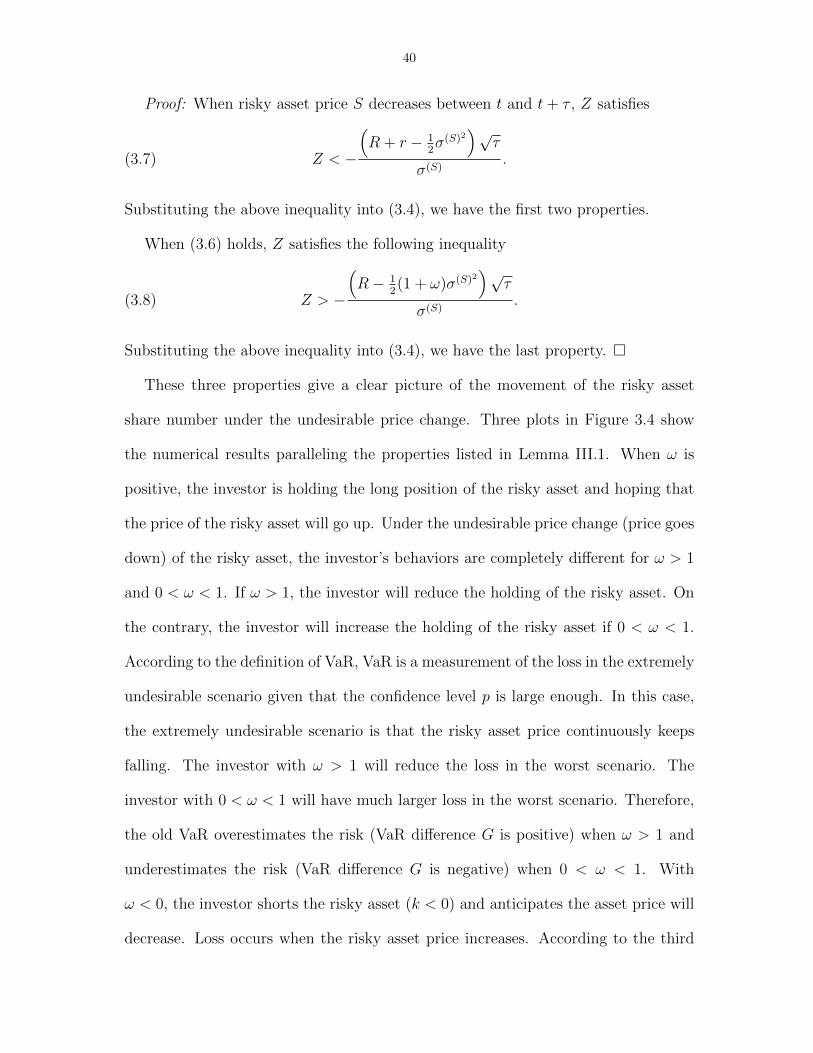
These three properties give a clear picture of the movement of the risky asset
share number under the undesirable price change. Three plots in Figure 3.4 show
the numerical results paralleling the properties listed in Lemma III.1. When ω is
positive, the investor is holding the long position of the risky asset and hoping that
the price of the risky asset will go up. Under the undesirable price change (price goes
down) of the risky asset, the investor’s behaviors are completely different for ω > 1
and 0 < ω < 1. If ω > 1, the investor will reduce the holding of the risky asset. On
the contrary, the investor will increase the holding of the risky asset if 0 < ω < 1.
According to the definition of VaR, VaR is a measurement of the loss in the extremely
undesirable scenario given that the confidence level p is large enough. In this case,
the extremely undesirable scenario is that the risky asset price continuously keeps
falling. The investor with ω > 1 will reduce the loss in the worst scenario. The
investor with 0 < ω < 1 will have much larger loss in the worst scenario. Therefore,
the old VaR overestimates the risk (VaR difference G is positive) when ω > 1 and
underestimates the risk (VaR difference G is negative) when 0 < ω < 1. With
ω < 0, the investor shorts the risky asset (k < 0) and anticipates the asset price will
decrease. Loss occurs when the risky asset price increases. According to the third

41
property, investor will reduce the number of the risky asset in short position when the
risky asset price is above certain level relative to the previous price. In other words,
the investor’s behavior reduces risk in the extremely undesirable scenario in which
the risky asset price continuously increases. Therefore, the old VaR overestimates
the risk and the VaR difference G is positive. These results imply that the strategies
used by investors could greatly change the risk characteristics of the portfolio. Since
the old VaR does not account for the investor’s strategy, it cannot reflect the true
risk of portfolio.
Another important result observed from Figures 3.2-3.3 is that the absolute mag-
nitude of the VaR difference increases as the volatility σ(S) or VaR horizon T increases
for all levels of ω and R. Under a highly volatile market or a long investment horizon,
the old VaR may largely underestimate or overestimate the risk. Based on the results
shown on the contour map, we found that the types of trading strategies (long or
short the risky asset) corresponding to different levels of ω determine whether the
old VaR overestimates or underestimates the true risk. However, the volatility and
the VaR horizon determine how big is the difference between the old VaR and the
true risk.
With all the analysis based on general ω above, the VaR difference with optimal
portfolio selection is straightforward. Based on the formula (2.24), the optimal weight
is linear to the risk premium with the slope equal to 1/γσ2. On the contour map
(Figures 3.2- 3.3), the optimal weight can be represented by a straight line passing
through the origin. With small γ (less risk averse investor), the optimal weight
line is steeper. VaR differences caused by the optimal portfolio selection strategy
for different investors can be observed on the corresponding straight line on the
map. For those aggressive investors with small γ, a small change in risk premium

42
would cause large change in VaR difference due to the large change in risky asset
weight. Moreover, given a fixed risk premium, VaR difference may be positive or
negative for different γ. This reflects the reality that different investors have various
strategies to achieve their investment goals and those strategies significantly impact
the VaR estimation. The old VaR without accounting for the investor’s strategy
cannot distinguish the risks among the investors with different levels of risk aversion.
3.2.2 The case with Stochastic Volatility (SV) model
Comparing with the GBM model, there are several obstacles for analyzing the VaR
difference in the SV model ((2.7)- (2.8)). First, there is no analytical form for either
the asset price or VaR. Therefore, the analysis cannot be done through deriving
formulas for some important variables such as VaR difference G and risky asset
share number k. Second, those important variables such as risk premium, volatility,
and optimal risky asset weight are time-varying. The previous analysis based on
the R − ω plane is not applicable in this case. Third, there are many parameters
in the SV model. Actually, there are 9 parameters included in the analysis. The
relationship among these parameters could be complicated. In order to overcome
these difficulties, we analyze the VaR difference based on a large random sample
from the parameter space. We draw a large sample (size of 50000) which is randomly
sampled in the 9-dimensional cube with the uniform distribution. The 9-dimensional
cube is constructed by specifying the range for each parameter. For each sample, the
optimal risky asset weight and VaR difference are calculated. The analysis is then
based on the observation of VaR difference distribution variation along different
parameters.
The parameters of the SV model can be categorized into two groups. The first
group is the group of parameters for the stochastic process of the risky asset and

43
investor’s decision: a, b, ρ, γ and T . Since R0 = ab is the risky premium coefficient,
the parameter R0 is used instead of using b alone. The second group is the parameters
for the stochastic process of the state variable Y : c, d, g and the initial value Y0.
Since the Y process is a mean-reverting process, the parameter d/c represents the
equilibrium of the process and c is the rate by which the variable reverts towards
the equilibrium. In the numerical experiments, we use the ratio d/c as a parameter
instead of using d alone. All the parameters are set in terms of one trading day and
we assume that there are 252 trading days in one year. The ranges of parameters in
both groups are given by the Tables 3.2-3.3. The ranges of all those 9 parameters
form a multi-dimensional cube in the parameter space. A large sample (size of 50000)
is drawn randomly from the uniform distribution. All the numerical experiments for
the VaR difference in the SV model are conducted based on this sample.
Parameter Rangea [0.001, 0.15]R0 [−0.000794, 0.002]ρ [−1, 1]γ [0.1, 0.9]T [22, 252]
Table 3.2:Parameter setting for the stochastic process of the risky asset price and investor decisionin numerical experiments (first group).
Parameter Rangec [0.005, 0.1]d/c [0.05, 2]g [0.01, 1]Y0 [0.05, 1.5]
Table 3.3:Parameter setting for the stochastic process of the state variable Y in numerical experi-ments (second group).
The process for identifying the relationship between the VaR difference and any
specific parameter can be divided into three steps. First, the optimal weight and VaR
difference are calculated for each element in the sample. The sample of VaR difference

44
is then formed. Second, the range of the specific parameter is evenly divided into
20 subintervals. Since the sampling is based on uniform distribution, the number
of samples falling into each subinterval is roughly 2500. Third, the VaR difference
sample is aligned with the subintervals of the specific parameter. The statistics such
as mean and quantiles of the 20 sub-samples of VaR difference are estimated. Unlike
the GBM model, the optimal risky asset weight is a function of time in the SV model.
In order to reveal the relationship between the VaR difference and the optimal risky
asset weight, the average value of ω∗ over the entire VaR horizon is used. Figures
3.5- 3.6 show the numerical results of the process for all the parameters. In each
plot, three statistics: mean, 5th-percentile and 95th-percentile of the VaR difference
are plotted against the given parameters. These three curves reveal the changes in
value and the range of the VaR difference changing with the parameters. The 6 plots
in Figure 3.5 demonstrate the relationship between the average optimal risky weight
ω∗average and parameters of risky asset price process and investor’s decision in the
first group. Graphs in Figure 3.6 demonstrate the results for the 4 parameters of
the state variable Y process in the second group. Compared with the results in the
first group, the curves of VaR difference related to second group are much flatter.
Therefore, the VaR difference is less sensitive to the parameters in the second group.
Apparently, the 6 parameters in the first group differ a lot in the relationship with
VaR difference. The results shown in the panels for parameters: ω∗average, T , and a
share some similarities with the results in the GBM case. Some common properties
lie in the panel of parameter ω∗average. First,the VaR difference tends to be zero when
the average weight, ω∗average, is close to 0 or 1. The mean of VaR difference is also
very close to zero when ω∗average is 0 or 1. Moreover, the range of VaR difference is
relatively narrow when ω∗average is 0 or 1. Second, when ω∗average is between 0 and 1,

45
most of the VaR difference samples are negative. Third, the value of VaR difference
tends to be positive when ω∗average is less than 0 or greater than 1. Although the range
of VaR difference increases dramatically when ω∗average is less than 0, most samples of
the VaR difference are positive. Other significant similarities with the GBM model
lie in the results with the VaR horizon T and volatility coefficient a. It is evident
that the range of VaR difference increases as T or a increases. In the other three
plots, three curves imply that both the value and range of the VaR difference change
along with the corresponding parameters. The range of VaR difference shrinks as γ
increases. That is because the holding of risky asset is less (in absolute magnitude)
for the investor with higher γ. In such case, the VaR differences tend to zero. Similar
pattern can be observed when the risk premium coefficient R0 is close to zero. For
the correlation coefficient ρ, the curves of VaR difference are relatively flat compared
to the other five plots. One can still observe that the range of VaR difference narrows
when ρ tends to 1.
No matter how different are the VaR difference patterns shown in all the plots,
they all convey the same information. That is, the old VaR with assumption of no
trading during the VaR horizon could not reflect the true risk when the investor ap-
plies some trading strategy (sometimes the strategy is optimal) in his/her investment.
Moreover, the difference between two VaRs is sensitive to some of the parameters.
When the model for risky asset price is more complicated (more parameters), the
number of key parameters increases and the range of VaR difference varies dramati-
cally.

46
3.3 VaR With Simple Portfolio Selection Strategy
In this section, the main objective is to analyze VaR incorporating simple portfolio
selection strategy for the portfolio consisting of risky assets only . Simple portfolio
selection strategy is a strategy in which the weight of each asset remains constant
during the whole investment horizon. Although this portfolio selection may not be
optimal, many investors always maintain their portfolio according to certain preset
structure in practice. Institutional investors have their own purposes and investment
guidelines for the portfolio. For example, in some insurance companies, an investment
portfolio could be used as capital for the loss reserve and the main goal of the
portfolio is not for the aggressive return. For all kinds of investment purposes, many
financial institutions have investment guideline documents in which the structure of
the portfolio is specified and the boundaries of all types of investment are given. In
some cases, the portfolio is maintained to match the preset target weight of each
type of asset. Therefore, the simple portfolio selection strategy is one of the popular
strategies in the real world. In 1996 amendment of Basel Accord [4],[5],[6], the
banks are required to calculate the VaR of the risky assets for market risk capital
requirement. The VaR estimation is essentially based on the portfolio consisting of
risky assets only.
To match reality, we construct a risky portfolio consisting of n risky assets: S(t) =
(S1(t), ..., Sn(t))′ with self-financing. The portfolio value is denoted by PR(t). With
the general setting in (2.2) and (2.4), the stochastic process for PR(t) is given by
(3.9) dPR(t) = (r + ω′abY (t))PR(t)dt+ ω′a√Y (t)PR(t)dW (S),
where ω satisfies the constraint ω′1n = 1. Since the term ω′adW (S) is essentially a lin-
ear combination of a random vector with multivariate normal distribution, ω′adW (S)

47
is equivalent to a normal random variable with zero mean and standard deviation
√ω′aa′ωdt. Therefore, we can define a 1-dimensional Brownian motion W (X) by
(3.10) dW (X) =ω′a√ω′aa′ω
dW (S).
The stochastic process PR(t) can be equivalently represented with a 1-dimensional
Brownian motion W (X) instead of the original n-dimensional Brownian motion W (S)
(3.11) dPR(t) = (r +RωY (t))PR(t)dt+ σω√Y (t)PR(t)dW (X),
where Rω = ω′ab and σω =√ω′aa′ω. Since the correlation between dW (Y ) and
dW (S) is ρ, the correlation between dW (Y ) and dW (X) is ρω = ρa′ω/√ω′aa′ω.
3.3.1 The case with Geometric Brownian Motion (GBM) model
Under the model of GBM, the risky portfolio PR(t) is given by
dPR(t) = (r +Rω)PR(t)dt+ σωPR(t)dW (X).(3.12)
Over the investment horizon [t, t+ τ ], the analytical solution of PR(t+ τ) is given by
PR(t+ τ) = PR(t)exp
([r +Rω −
1
2σ2ω
]τ + σω
√τZ
),
where Z is a random variable following a normal distribution with mean zero and
standard deviation one. By definition, the VaR of the risky portfolio PR(t) at time
t with confidence level p and VaR horizon τ > 0 is given by
(3.13) V aRp(PR, t, τ) = PR(t)
1− exp
([r +Rω −
1
2σ2ω
]τ + σω
√τZ1−p
),
where Z1−p is the (1 − p)-quantile of the normal distribution with mean zero and
standard deviation one. Based on the above VaR formulation, we can define a VaR
percentage (VaR%) function φ
(3.14) φ(p, τ, ω) = 1− exp([r +Rω −
1
2σ2ω
]τ + σω
√τZ1−p
).

48
The VaR% (φ) is not related to the size of the portfolio and only gives the relative
loss for the risky portfolio with simple portfolio strategy ω. This function is related
to the portfolio selection strategy ω, VaR confidence level p, and VaR horizon τ .
The VaR% (φ) is a good measurement for evaluating the risk of a certain portfolio
selection strategy.
Theorem III.2. For the simple portfolio selection policy ω, a risky portfolio PR
consists of n risky assets whose value processes follow GBM in (2.6) and the portfolio
value follows the stochastic process in (3.12). The VaR% (φ) (3.14) of the risky
portfolio PR with confidence level p and VaR horizon τ > 0 is a decreasing function
of Rω and an increasing function of σω if p > 50%.
Proof: The derivatives of φ (3.14) with respect to Rω and σω are
φRω = −τexp([r +Rω −
1
2σ2ω
]τ + σω
√τZ1−p
),
φσω = (σωτ −√τZ1−p)exp
([r +Rω −
1
2σ2ω
]τ + σω
√τZ1−p
).
(3.15)
It is evident that φRω is negative. If p > 50%, Z1−p is negative and then φσω is
positive. Therefore, the VaR% is a decreasing function of Rω and is an increasing
function of σω if p > 50%.
In practice, the VaR confidence level p is always above 90%. This theorem will
be applicable in all the VaR applications.
3.3.2 The case with Stochastic Volatility (SV) model
With the presence of state variable Y (t), the analytical solution of PR(t+ τ) over
the investment horizon [t, t+ τ ] is more complicated. From (3.11), PR(t+ τ) is given
by
(3.16)
PR(t+τ) = PR(t)exp
(∫ t+τ
t
[r +RωY (s)− 1
2σ2ωY (s)
]ds+
∫ t+τ
t
σω√Y (s)dW (X)(s)
).

49
Since Y (t) is also a stochastic process, these two integrations
(3.17) k1(t, τ) =
∫ t+τ
t
Y (s)ds and k2(t, τ) =
∫ t+τ
t
√Y (s)dW (X)(s),
are random variables with unknown distributions. The analytical form of VaR is
not available in this case. However, we still can analyze the VaR based on two key
parameters: Rω and σω. First, by definition, the VaR and VaR% (φ) of the risky
portfolio PR have the following forms
V aRp(PR, t, τ) = PR(t)
1− exp[rτ + F−1
K(t,τ)(1− p)]
,
φ(p, t, τ, ω) = 1− exp[rτ + F−1
K(t,τ)(1− p)],
(3.18)
where
(3.19) K(t, τ) =
(Rω −
1
2σ2ω
)k1(t, τ) + σωk2(t, τ).
and FK(t,τ) is the cdf of the random variable K(t, τ). The key component in VaR
estimation is the (1 − p)-quantile of K(t, τ), i.e. F−1K(t,τ)(1 − p). The relationship
between F−1K(t,τ)(1−p) and parameters Rω can be summarized in the following lemma.
Lemma III.3. F−1K(t,τ) is a non-decreasing function of Rω.
Proof: For simplicity, we denote K(t, τ), k1(t, τ), and k2(t, τ) by simpler symbols
K, k1, and k2 respectively. Based on (3.19), the random variable K is a linear
combination of two random variables: k1 and k2. The distribution function FK(x)
can be formulated
FK(x) = Prob
(k1, k2) |
(Rω −
1
2σ2ω
)k1 + σωk2 ≤ x
.
For the given pair of Rω,1 and Rω,2 satisfying Rω,1 < Rω,2, we have(Rω,1 −
1
2σ2ω
)k1 + σωk2 <
(Rω,2 −
1
2σ2ω
)k1 + σωk2,

50
because k1 is positive. For a real number x, the corresponding two sets of (k1, k2)
pairs satisfy(k1, k2) |
(Rω,2 −
1
2σ2ω
)k1 + σωk2 ≤ x
⊆
(k1, k2) |(Rω,1 −
1
2σ2ω
)k1 + σωk2 ≤ x
.
Therefore, the corresponding two cdfs FK1 and FK2 satisfy
(3.20) FK2(x) ≤ FK1(x).
By the definition of the inverse distribution function, we have
F−1K1
(q) = infx∈RFK1(x) ≥ q ,
F−1K2
(q) = infx∈RFK2(x) ≥ q ,
for any q ∈ [0, 1]. Based on (3.20), we have
FK2(x) ≥ q ⊆ FK1(x) ≥ q .
Therefore, the corresponding two inverse cdfs, F−1K1
and F−1K2
, satisfy
F−1K2
(q) ≥ F−1K1
(q).
and the statement of this lemma is then proven.
Based on this lemma and the formulation of VaR% in (3.18), the following theorem
can be directly derived.
Theorem III.4. For the simple portfolio selection policy ω, a risky portfolio PR
consists of n risky assets whose value processes follow the SV mdoel in (2.7-2.8) and
the portfolio value follows the stochastic process in (3.11). The VaR% (φ) (3.18)
of the risky portfolio PR with confidence level p and VaR horizon τ > 0 is a non-
increasing function of Rω.

51
Proof: By (3.18), VaR% is a decreasing function of F−1K(t,τ)(1− p). Together with
the Lemma III.3, The VaR% is a non-increasing function of Rω.
Unfortunately, we can not determine the relationship between the VaR% and σω
in this case. First, the parameter σω appears in both coefficients of random variables
k1 and k2. The range of random variable k2 covers all the real numbers. Second, the
correlation between k1 and k2 is unknown because the distributions of k1 and k2 are
unknown. In this study, we rely on numerical experiments to unfold the relationship
between the VaR% and σω. Figure 3.7 shows the VaR% (φ) with different choices of
Rω, σω and ρω. The range of those three parameters are summarized in the following
table. All the plots in Figure 3.7 indicate that VaR% (φ) decreases with Rω with all
Parameter RangeRω [0, 0.004]σω [0.01, 0.25]ρω −1,−0.5, 0, 0.5, 1c 0.05d/c 1g 0.1Y0 1τ 10 days
Table 3.4:Parameter setting for the numerical experiments of observing the relationships betweenVaR% φ and parameters: Rω, σω and ρω.
the choices of σω and ρω which matches the statement in Theorem III.4 and increases
with σω with all the choices of Rω and ρω. Moreover, the effect of σω on VaR% is
much larger than the effect of Rω.
By the theorems and lemma (III.2-III.4) and the numerical results shown in Fig-
ure 3.7, we establish the relationship between the VaR% (φ) and two key parameters:
Rω and σω for both GBM and SV models. By the risky portfolio formulation (3.11),
Rω and σω are essentially the risk premium (risk premium coefficient in the SV
model) and volatility (volatility coefficient in the SV model) of the risky portfolio.

52
The market risk capital requirement in Basel Accord puts an upper bound on the
amount of capital that the banks are allowed to invest in the risky portfolio. This
upper bound is directly related to the VaR of the risky portfolio. The portfolio se-
lection for the risky portfolio directly affects these two key parameters by which the
VaR and the maximal amount of capital on the risky assets are determined. If the
investors apply a very aggressive strategy (pursuing high risk premium) to build the
risky portfolio, their portfolio will be inevitably with high volatility and large VaR.
It leads to higher market risk capital requirement and smaller amount of capital
allocated to the risky assets. It may hurt the profitability of the portfolio overall.
The relationship revealed in the theorems above give banks the guidelines to build
the risky portfolio in the proper way such that enough amount of capital is allocated
to a risky portfolio with balanced risk premium and volatility. The theorems are the
important building blocks in developing optimal portfolio selection under the Basel’s
market risk capital requirement.

53
Fig
ure
3.1:
Por
tfol
iod
istr
ibu
tion
sco
mp
aris
onb
etw
een
the
on
ew
ith
out
any
trad
ing
(dott
edli
ne)
an
dth
eon
ew
ith
op
tim
al
trad
ing
stra
tegy
(soli
dli
ne)
.E
ach
pan
elco
rres
pon
ds
tod
iffer
ent
risk
aver
sion
para
met
erγ
.T
he
risk
yass
etp
rice
foll
ows
GB
Mw
ith
para
met
ers:µ(S
)=
0.000278,
σ(S
)=
0.03
15,
andT
=25
2d
ays.

54
Fig
ure
3.2:
VaR
diff
eren
ceco
nto
ur
map
wit
hd
iffer
ent
vola
tili
tyle
velsσ(S
).
Th
efo
ur
stra
ight
lin
esin
each
pan
elre
pre
sent
the
op
tim
al
risk
yass
etw
eigh
tw
ith
diff
eren
tle
vel
ofri
skav
ersi
on
para
met
erγ
.T
he
risk
yass
etpri
cefo
llow
sG
BM
wit
hV
aR
hori
zonT
=252
day
s.

55
Fig
ure
3.3:
VaR
diff
eren
ceco
nto
ur
map
wit
hd
iffer
ent
VaR
hori
zon
sT
.T
he
fou
rst
raig
ht
lin
esin
each
pan
elre
pre
sent
the
op
tim
al
risk
yass
etw
eight
wit
hd
iffer
ent
leve
lof
risk
aver
sion
para
met
erγ
.T
he
risk
yass
etp
rice
foll
ows
GB
Mw
ith
vola
tili
tyσ(S
)=
0.031497.

56
Fig
ure
3.4:
Ris
ky
asse
tsh
are
nu
mb
er(d
otte
dli
ne)
chan
ges
as
the
ass
etp
rice
(soli
dli
ne)
chan
ges
wit
hd
iffer
ent
risk
yass
etw
eight.
Th
eri
sky
asse
tw
eigh
tis
mai
nta
ined
du
rin
gth
ein
vest
men
th
ori
zon
.T
he
risk
yass
etp
rice
foll
ows
GB
Mw
ith
para
met
ers:
µ(S
)=
0.000278,
σ(S
)=
0.03
1497
,an
dT
=25
2d
ays.

57
Figure 3.5:VaR difference with respect to the parameters for the stochastic process of risky assetand investor decision.

58
Fig
ure
3.6:
VaR
diff
eren
cew
ith
resp
ect
toth
ep
ara
met
ers
for
the
stoch
ast
icp
roce
ssof
the
state
vari
ab
leY
.

59
Figure 3.7: VaR% φ (in percentages) for difference choices of Rω, σω, and ρω.

CHAPTER IV
Dynamic Portfolio Selection With VaR Capital requirement
4.1 VaR-based Risk Management Overview
In this study, we develop numerical schemes to find optimal portfolio selection
strategies of the trading book under Basel’s VaR-based capital requirement. The
trading book contains financial instruments that are intentionally held for short-
term resale and marked-to-market[15]. Ignoring the capital requirement for credit
risk from the banking book, we consider the portfolio consisting of risk-free asset
(used as capital) and marked-to-market risky assets. The group of risky assets forms
the risky portfolio. According to the Basel’s market risk capital requirement, the
amount of risk-free asset (1.2) is equal to the maximum of the previous day’s 10-day
VaR and the average 10-day VaR over the last 60 business days times a multiplicative
factor δ which is between 3 and 4. The VaR is estimated based on the risky portfolio
with 99% confidence level. For simplicity, we assume the market risk capital charge at
any time t is given by the positive part of the current 10-day VaR at 99% confidence
level multiplied by δ, i.e.
(4.1) δV aR99%(P, t, 10)+,
where x+ = max(x, 0). The positive operator + mathematically eliminates the pos-
sibilities of negative VaRs which lead negative risk capital requirement. Some of the
60

61
assets in the trading book might also have credit risk (e.g. corporate bond) and
counterparty risk (e.g. OTC derivative). In this study, since we mainly analyze the
effect of market risk in the trading book, we assume that the capital charges for the
risk other than market risk are zero.
By the Basel’s VaR-based capital requirement, the portfolio of the trading book
can be separated into two components: risk-free asset and risky portfolio consisting
of risky assets. The investment strategy can be decomposed into two allocation
problems. The first one is the capital allocation between the risk-free asset and risky
portfolio. The second one is the portfolio selection among the risky portfolio. These
two problems are actually coupled with each other. The decision on the second
problem determines the upper bound of the capital allocated in the risky portfolio.
On the other hand, the constraint in the first problem affects the bank’s decision
on the selection strategy of the risky portfolio. Aggressive strategy may give a high
return on the risky portfolio. However, the consequence of high volatility leads to
large VaR and reduces the amount of capital allocated to the risky portfolio and the
return of the total wealth.
The rest of this chapter is organized as follows. Section 2 describes the formu-
lation of the Basel’s VaR-based capital requirement. Section 3 derives the optimal
allocation between risk-free asset and risky portfolio under Basel’s market risk cap-
ital requirement. Section 4 analyzes the expected utility obtained by the optimal
allocation derived in section 3. Section 5 develops the process to find the optimal
allocation within the risky portfolio.

62
4.2 Basel’s VaR-based Capital Requirement Formulation
We assume that the trading book of the bank has one risk-free asset and n risky
assets. The price of risk-free asset is denoted by S0(t). The risk-free asset is used
as risk capital for the Basel’s VaR-based capital requirement. The prices of those
n risky assets are denoted by a vector process S(t) = (S1(t), ..., Sn(t))′ (′ denotes
transpose). The asset prices follow the general form in (2.1)-(2.3) which nests two
models (GBM and SV) under consideration in this study. The total wealth P (t) of
the whole trading book can be divided into two parts: risk-free capital PC(t) and
risky portfolio PR(t). The risk-free capital PC(t) is a portfolio consisting of only one
asset. That is the risk-free asset. The amount of capital allocated to the risk-free
capital or the share number of risk-free asset depends on the VaR of risky portfolio
PR. For the second part, the risky portfolio is a portfolio consisting of n risky assets
whose prices follow the process S(t). At any time t, the total wealth P (t) is the sum
of the risk-free capital PC(t) and the risky portfolio PR(t).
According to the Basel’s market risk capital requirement, at any time t, the
amount of risk-free capital should satisfy the following constraint
(4.2) PC(t) ≥ δV aRp (PR, t, τ)+ ,
where δ is a positive number between 3 and 4, τ=10, and p = 99%. Because of this
constraint, the bank needs to adjust the capital allocation between PC and PR from
time to time to achieve two goals. The first goal is to satisfy the Basel’s market risk
capital requirement and the second one is to maximize the return or utility of the
whole trading book. The optimization involves two allocation problems. The first
allocation problem is the allocation between PC and PR. It can be denoted by ψ

63
which is the relative weight of PR and satisfies
ψ =PRP.
The variable ψ is affected by the constraint in (4.2) and the bank’s decision which
depends on many factors such as risk aversion and investment purpose. The second
one is the allocation within the risky portfolio PR which can be denoted by an n-
dimensional vector ω. ω is the relative weight vector of n risky assets in PR and
satisfies ω′1n = 1. In this study, we assume that the simple portfolio selection
strategy is applied when the bank constructs the risky portfolio in the trading book.
That is, the relative weight vector ω of n risky assets is a constant vector. Under this
assumption, the bank always maintains the preset structure in the risky portfolio PR.
In this setting, the risky portfolio PR is equivalent to a portfolio with only one
hypothetical asset or index. This hypothetical index is constructed based on those n
risky assets by using the simple trading strategy ω and this constant relative weight
vector ω is always maintained. Therefore, with the general setting in (2.2) and (2.4),
the index value can be described by the following stochastic process
(4.3) dX(t) = (r + ω′abY (t))X(t)dt+ ω′a√Y (t)X(t)dW (S),
with initial value X(0) = 1. Since the term ω′adW (S) is essentially a linear combina-
tion of a random vector with multivariate normal distribution, ω′adW (S) is equivalent
to√ω′aa′ωdW (X) where the 1-dimensional standard Brownian motion W (X) is de-
fined as in (3.10)
(4.4) dW (X) =ω′a√ω′aa′ω
dW (S).
The stochastic process X(t) can be equivalently represented with the 1-dimensional
standard Brownian motion W (X) instead of the original n-dimensional Brownian

64
motion W (S)
(4.5) dX(t) = (r +RωY (t))X(t)dt+ σω√Y (t)X(t)dW (X),
where Rω = ω′ab and σω =√ω′aa′ω. Since the correlation between dW (Y ) and
dW (S) is ρ, the correlation between dW (Y ) and dW (X) is ρω = ρa′ω/√ω′aa′ω. One
can notice that Rω and σω are essentially the risk premium coefficient and volatility
coefficient of the index X.
The index dynamics in (4.5) reflects the return value on each unit of capital
invested in those n risky assets with the trading strategy ω. In other words, at any
time t, one unit of capital invested in the index will have
exp
∫ t+τ
t
(r +RωY (s)− 1
2σ2ωY (s)
)ds+
∫ t+τ
t
σω√Y (s)dW (X)(s)
in return after the investment horizon τ . Therefore, the index value X(t) can be
viewed as the “price” of the portfolio with strategy ω. The risky portfolio with
strategy ω is equivalent to buying the index X(t). If the bank invests PR(t) in the
index X(t) at time t, at the end of the investment interval [t, t + τ ], the value of
P (t+ τ) is given by
(4.6)
PR(t+τ) = PR(t)exp
(∫ t+τ
t
[r +RωY (s)− 1
2σ2ωY (s)
]ds+
∫ t+τ
t
σω√Y (s)dW (X)(s)
).
Based on this formulation, the τ -day VaR of PR(t) with confidence level p has the
following form
(4.7) V aRp (PR, t, τ) = PR(t)φ(p, Y, t, τ, ω),
where φ(p, Y, t, τ, ω) is the VaR percentage (VaR%) function defined in Chapter 3
and represents the risk of each capital unit invested on the index X. Based on

65
the theorems (III.2-III.4) and numerical experiments in the previous chapter, the
VaR% function φ is a decreasing function of Rω and an increasing function of σω if
p > 50%. These results give a very important guideline for the bank to construct its
risky portfolio with balanced return and volatility for achieving maximal utility of
the whole trading book.
With the hypothetical risky index X, we can view the total wealth P (t) from a
different perspective. The portfolio P (t) in the trading book is essentially a portfolio
consisting of two assets: S0 and X. The relative weight ψ of risky portfolio PR is
essentially the relative weight on the risky index X. The portfolio selection strategy ω
in risky portfolio directly affects the risk premium coefficient Rω, volatility coefficient
σω and the correlation ρω of the index X. The VaR of risky portfolio is the product
of PR and the VaR% function φ of X. Under the assumption of self-financing, the
total wealth P (t) can be described by the following stochastic process
(4.8) dP (t) = (ψRωY (t) + r)P (t)dt+ ψσω√Y (t))P (t)dW (X).
In this formulation, the relative weight ψ also represents the allocation strategy
between risk-free capital and risky portoflio. It could be a function of time or any
other relevant factors. Given the capital allocation between the risk-free capital and
the risky portfolio, we have PR(t) = ψP (t). Together with (4.7), the τ -day VaR with
probability p of the risky portfolio is
V aRp (PR, t, τ) = ψP (t)φ(p, Y, t, τ, ω).
Since PC(t) = (1 − ψ)P (t), the inequality (4.2) derived from Basel’s market risky
capital requirement becomes
(4.9) ψ ≤ 1
1 + δφ(p, Y, t, τ, ω)+.

66
Therefore, to construct the portfolio with risk-free capital and risky portfolio, the
bank has to cope with two control variables ψ and ω. ω represents the asset allocation
within the risky portfolio consisting of n risky assets and ω′1n = 1. ψ is the relative
weight on the risky portfolio with the strategy ω. The inequality (4.9) gives the
constraint on the risky portfolio construction strategy ω and the capital allocation
ψ on the risky portfolio. If the bank chooses a very aggressive strategy ω, it leads
a high VaR of PR which lowers the upper bound of the capital allocation ψ on the
risky portfolio and the return of the total wealth will be limited. On the other hand,
a conservative strategy ω can increase the upper bound for the capital allocated to
the risky portfolio. However, the low return on PR could reduce the return of the
total wealth. Therefore, to find a ω with balanced return and volatility in PR is the
essential part in the optimization process.
The process of finding optimal allocation to maximize the bank’s utility in trading
book can be divided into two steps. The first step is to develop the optimal ψ∗(ω)
for any given simple portfolio selection ω in the risky portfolio. In this step, we only
concentrate on deriving the optimal allocation between risk-free capital and risky
portfolio under the constraint (4.9). The optimal solution ψ∗ is a function of ω.
Moreover, the expected utility E [U(P (T ))] obtained by ψ∗ is also a function of ω.
In further analysis, we notice that ω affects ψ∗ and expected utility only through
three parameters: Rω, σω and ρω. Instead of performing analysis based on ω directly,
we develop the relationship between the expected utility E [U(P (T ))] with strategy
ω and the parameters Rω, σω and ρω of the risky index. The relationship is the
foundation for the second step. The second step is to find the optimal ω∗ based on
the results in first step. Since ω is an n-dimensional vector, searching for an optimal
solution in a high dimensional space could be very difficult. However, the results

67
from the first step can help us convert the searching space into a parameter space
formed by Rω, σω and ρω. That is, the result derived in the first step is used to
reduce the dimension of the problem.

68
4.3 Optimal Allocation Between Risky Portfolio And Risk-free Capital
In this section, the goal is to derive the optimal allocation strategy between the
risky portfolio and risk-free capital with the given simple portfolio selection strategy
ω in the risky portfolio. The allocation between the risky portfolio and risk-free
capital is represented by the relative weight ψ on the risky portfolio. As discussed
in the previous section, when ω is fixed, the risky portfolio with n risky assets is
equivalent to the portfolio with only one hypothetical risky index X. The stochastic
process ofX is given by (4.5). The relative weight ψ of the risky portfolio is essentially
the relative weight on the risky index X. The fixed ω may not be the optimal choice
for the allocation within risky portfolio. It just represents any one of the admissible
portfolio selection policies used by the bank in the risky portfolio. Since ω affects
the risk premium coefficient, volatility coefficient and correlation of the risky index,
the optimum ψ∗ is a function of the vector ω. With the optimum ψ∗(ω), the optimal
choice of ω can be derived in the next step.
The capital allocated in the risky portfolio is limited by the constraint (4.9) based
on Basel’s market risk capital requirement. According to the constraint (4.9), the
upper bound of the risky portfolio weight ψ is
1
1 + δφ(p, Y, t, τ, ω)+,
where φ(p, Y, t, τ, ω) is the VaR% function of X. For simplicity, we define
(4.10) G(δ, p, Y, t, τ, ω) =1
1 + δφ(p, Y, t, τ, ω)+.
Under the objective of maximizing utility over the investment horizon [0, T ], the
optimization problem for identifying the optimal policy ψ can be formulated as the

69
following framework
(4.11)
maxψ(t)Tt=0
E [U(P (T ))]
ψ ≤ G(δ, p, Y, t, τ, ω),
where the utility function is given by (2.11). The corresponding value function is
defined as
V (P, t) = maxψ(t)Tt=0
E[P (T )1−γ
1− γ
].
Apparently, this is a constrained optimization problem. We first derive the formula-
tion of optimum ψ∗ under the general forms (4.5) and (4.8) with the state variable Y
dynamics (2.3). After that, the generalized solution is applied in the further discus-
sion in those two models (GBM and SV) under consideration. In GBM model, the
analytical form of ψ∗ can be obtained. However, in SV model, the complete form of
ψ∗ comes from a system of two nonlinear PDEs with free boundary. Therefore, we
have to rely on numerical methods to obtain ψ∗.
Combining the framework established by Merton (1971)[20] with the constraint,
the HJB equation for the problem in (4.11) is:
(4.12)
maxψ(t)Tt=0
Vt +
1
2ψ2Σ(X)P 2VPP + ψΣ(X,Y )PVPY +
1
2Σ(Y )VY Y
+ (ψRωY + r)PVP + µ(Y )VY
= 0,
V (P, T ) = P 1−γ
1−γ ,
ψ ≤ G(δ, p, Y, t, τ, ω).
In this setting, the terms Σ(X), Σ(X,Y ), and Σ(Y ) are given by
Σ(X) = σ2ωY,
Σ(X,Y ) = σωρωgY,
Σ(Y ) = g2Y.
(4.13)

70
The terminal condition is given by
V (P, Y, T ) =P 1−γ
1− γ.
To solve the above optimization problem, we define a function
L = Vt +1
2ψ2Σ(X)P 2VPP + ψΣ(X,Y )PVPY +
1
2Σ(Y )VY Y
+ (ψRωY + r)PVP + µ(Y )VY + α(G− ψ),
where α is a non-negative Karush-Kuhn-Tucker (KKT) multiplier (dual feasibility).
In the KKT conditions, the first-order condition Lψ = 0 (stationarity) leads
(4.14) RωY PVP + P 2VPPΣ(X)ψ + Σ(X,Y )PVPY − α = 0.
Moreover, in the KKT conditions, the primal feasibility and complementary slackness
conditions are
(4.15) G(δ, p, Y, t, τ, ω)− ψ ≥ 0,
(4.16) α (G(δ, p, Y, t, τ, ω)− ψ) = 0.
From equation (4.14), we have
ψ =− 1
Σ(X)PVPP
[RωY VP + Σ(X,Y )VPY −
α
P
]=ψ0 +
α
Σ(X)P 2VPP,
(4.17)
with
(4.18) ψ0 = − 1
Σ(X)PVPP
[RωY VP + Σ(X,Y )VPY
].
One can notice that ψ0 is the optimal solution for the problem without constraint.
Therefore, the effect of the constraint is represented by the second term α/Σ(X)P 2VPP
in (4.17). From the complementary slackness condition (4.16), we have two possible

71
cases: α = 0 or ψ = G(δ, p, Y, t, τ, ω). The first case implies that ψ = ψ0 and ψ0
must satisfy the primal feasibility condition G(δ, p, Y, t, τ, ω)− ψ0 ≥ 0. In this case,
the constraint is not binding since the optimal solution of the unconstrained problem
satisfies the constraint. In the second case, the constraint is binding and the solution
is at the boundary of the constrain ψ = G(δ, p, Y, t, τ, ω). It implies
α = (G(δ, p, Y, t, τ, ω)− ψ0) Σ(X)P 2VPP
Therefore, we have the optimal solution ψ∗ as following
ψ∗ =
ψ0 if ψ0 < G(δ, p, Y, t, τ, ω)
G(δ, p, Y, t, τ, ω) otherwise
or
(4.19) ψ∗ = min (ψ0, G(δ, p, Y, t, τ, ω))
Substituting (4.19) into (4.12), the PDE of the value function V is given by
(4.20) 0 =
Vt + (ψ0RωY + r)PVP +1
2ψ2
0Σ(X)P 2VPP
+ ψ0Σ(X,Y )PVPY +1
2Σ(Y )VY Y + µ(Y )VY ,
if ψ0 < G(δ, p, Y, t, τ, ω)
Vt + (GRωY + r)PVP +1
2G2Σ(X)P 2VPP
+GΣ(X,Y )PVPY +1
2Σ(Y )VY Y + µ(Y )VY ,
otherwise
with the terminal condition V (P, T ) = P 1−γ
1−γ . In order to solve for V , we introduce
the ansatz
(4.21) V (P, Y, t) =P 1−γ
1− γf(Y, t).
Then, ψ0 in (4.18) is given by
(4.22) ψ0 =1
γΣ(X)−1
(RωY + Σ(X,Y )fY
f
).

72
Substituting the ansatz of V (4.21) and ψ0 (4.22) into the PDE (4.20), we obtain
(4.23)
0 =
ft +1
2Σ(Y )fY Y +
[µ(Y ) +
1− γγ
Σ(X,Y )′Σ(X)−1
RωY
]fY
+1− γ
2γΣ(Y,ρ)f
2Y
f+ (1− γ)
[1
2γΣ(X)−1
R2ωY
2 + r
]f,
if ψ0 < G(δ, p, Y, t, τ, ω)
ft +1
2Σ(Y )fY Y +
[(1− γ)GΣ(X,Y ) + µ(Y )
]fY
+
[(1− γ)(GRωY + r)− γ(1− γ)
2G2Σ(X)
]f,
otherwise
where Σ(Y,ρ) = σ(Y )ρ2ωσ
(Y ) and the terminal condition is f(Y, T ) = 1.
From formulas (4.19)-(4.23), the structure of the generalized solution of ψ∗ is
revealed. There are two components in the solution: ψ0 and G. The function G is
relatively straightforward once the VaR% function φ is given. The main obstacle for
us to derive ψ∗ is the component ψ0. The function ψ0 is related to a function f which
can be solved from PDE system (4.23). With different risky asset models, the PDE
system (4.23) could be completely different. In the rest of this section, we further
develop the procedure for obtaining ψ∗ with GBM and SV models.
In the GBM model the state variable Y is not present. f is a function of time
t and the PDEs in (4.23) are reduced to be ODEs. Moreover, ψ0 and G are just
constants. The formulation of the optimal solution ψ∗ is straightforward. That is
(4.24) ψ∗ = min
(Rω
γσ2ω
, G
).
In the SV model, the solution becomes much more complicated and the analytical
form can be obtained only when ρω = 0. In the case of ρω = 0, the optimal solution
ψ∗ is also straightforward because there is no need to solve the PDE for f . That is,
(4.25) ψ∗ = min
(Rω
γσ2ω
, G(δ, p, Y, t, τ, ω)
).
However, when ρω 6= 0, solving for ψ0 is very difficult because the key component f is
a solution of two PDEs (4.23) based on the switch condition ψ0 < G. Unfortunately,

73
the switch condition itself depends on the unknown function f . In other words,
the boundary between those two PDEs is to be determined and varies with Y and
t. This is a free boundary problem. Moreover, the first PDE is also a nonlinear
PDE. Solving such PDEs is very intractable even with numerical methods. In this
study, instead of solving the PDEs in (4.23), we develop a numerical scheme based
on dynamic programming to obtain the optimal solution ψ∗ for the SV model.
First, we discretize the continuous time model (4.8) and (2.3). For the stochastic
process of the total wealth, we discretize the stochastic process of the portfolio growth
rate RP (t) instead of the portfolio P (t). The relationship between RP (t) and P (t)
are formulated as follows
P (t) = P (0)exp(RP (t)) and RP (0) = 0.
By Ito lemma, the SDE of RP (t) is given by
(4.26) dRP (t) =
(r + ψRωY (t)− 1
2ψ2σ2
ωY (t)
)dt+ ψσω
√Y (t)dW (X).
To match setting of the numerical experiment, we represent the investment horizon
T in trading days and one time step corresponds to one trading day, i.e. ∆t = 1. All
time-varying processes or functions are estimated at the sequence of discrete time
points t = 0, 1, ..., T . To distinguish the discretized variables from the original ones,
we add ” ¯ ” on top of the corresponding notation of each variable. With explicit
Euler method, the recurrence relations of RP (t) and Y (t) are given by
RP,t+1 = RP,t +
(r + ψtRωYt −
1
2ψ2t σ
2ωYt
)+ ψtσω
√Ytz
(X)t
Yt+1 = Yt + d− cYt + g√Ytz
(Y )t .
(4.27)
where zX0 , zX1 ,..., are i.i.d. (identical independent distributed) standard normal and
zY0 , zY1 ,..., are also i.i.d. standard normal. In the setting above, z
(X)t and z
(Y )t are

74
two correlated standard normal random variables with correlation coefficient ρω.
Moreover, (z(X)t , z
(Y )t ) and (z
(X)s , z
(Y )s ) are independent with each other when t 6= s.
For simplicity, we can always represent z(X)t in terms of z
(Y )t and an auxiliary standard
normal random variable z(A)t
(4.28) z(X)t = ρωz
(Y )t +
√1− ρ2
ωz(A)t .
where z(A)t is independent with z
(Y )t . At any time point t, the total wealth Pt is given
by
(4.29) Pt = Pt−1exp(RP,t − RP,t−1).
Second, we apply the dynamic programming technique to find the optimal solu-
tionsψ∗0, ..., ψ
∗T−1
maximizing the expected utility of PT . The optimization can be
expressed as
maxψtT−1
t=0
E[P 1−γT
1− γ
],
with the constraint
ψt ≤ G(δ, p, Yt, t, τ, ω).
For simplicity, we denote G(δ, p, Yt, t, τ, ω) by G(Yt, t). The main principle of dy-
namic programming is that the optimal control sequenceψ∗0, ..., ψ
∗T−1
must also
be optimal for the remaining sequence at any intermediate time point t [8]. That is,ψ∗t , ..., ψ
∗T−1
must be optimal for conditional expectation Et
[P 1−γT
1−γ
]given all the
information at any time point 0 < t < T − 1. This property is very well known,
namely Principle of Optimality. Define the value function by
V (t, Pt, Yt) = Et[P 1−γT
1− γ|ψ∗t , ..., ψ
∗T−1
].
This value function gives the conditional expectation of the utility of the terminal
portfolio value given all the information up to time t and the optimal control se-

75
quence starting from t. With the value function, the principle of optimality can be
summarized by the Bellman equation
V (t, Pt, Yt) = maxψt<G(Yt,t)
Et[V (t+ 1, Pt+1, Yt+1)|ψt
],
with the terminal condition V (T, PT , YT ) =P 1−γT
1−γ . With the Bellman equation, we
can develop a numerical scheme to derive the optimal solution sequence ψ∗t T−1t=0
backwards over time.
Apparently, the optimal solution ψ∗ is also a function of Y . The approximate
solution ψ∗ generated by a numerical scheme cannot cover all possible Y at each
time step t. In this study, a trinomial tree model introduced by Nawalkha and Beli-
aeva [22] is used to approximate the stochastic process of Y . Binomial and trinomial
tree approaches are widely accepted techniques for derivative pricing. The stochastic
evolution of the underlying variable is represented by a tree structure in which the
tree nodes and links are associated with the discretized states and transition proba-
bilities. When the volatility of the stochastic process is constant, the corresponding
tree is recombining such that the number of tree nodes is significantly reduced and
computation based on the tree is tractable. However, the tree is non-recombing when
the volatility is time-varying. In the Nawalkha and Beliaeva’s work, an efficient tri-
nomial tree for the Cox, Ingersoll, and Ross (CIR) model is developed based on the
solution presented by Nelson and Ramaswamy (NR)[23]. In our model setting, the
stochastic process of Y (t) is essentially a CIR model. In order to achieve the re-
combining property of the tree for the square root process, Nelson and Ramaswamy
suggest using a transformation of the underlying variable such that the volatility of
the new variable is constant. For the CIR model, the transformation is given by
y(t) =2√Y (t)
g.

76
By taking the inverse of the above equation, the state variable Y (t) is given by
(4.30) Y (t) =y(t)2g2
4.
By Ito lemma, the SDE of y(t) is given by
dy(t) = µ(y)dt+ dW (Y ),
where
µ(y) =1
y
[1
2c
(4d
cg2− y2
)− 1
2
].
The trinomial tree is actually constructed based on y(t) instead of Y (t). The
resulted tree can be easily transformed into the one for Y (t) via the formula (4.30).
To distinguish from the original notations, the value of y on the tree node is denoted
by y. In the trinomial tree, the branches of each tree node y (except those at the
ending time point) go up to y + v√
∆t, stay at y and go down to y − v√
∆t in the
next time step. According to Nawalkha and Beliaeva’s work, the parameter v is
determined by
(4.31) v =
vc if |vc −
√1.5| < |ve −
√1.5|
ve otherwise
where vc and ve are given by
ve =y0/√
∆t
F loor(y0/√
1.5∆t)
vc =y0/√
∆t
F loor(y0/√
1.5∆t+ 1).
(4.32)
y0 is the initial value of y(t) at time t = 0. Between vc and ve, the final value of v is
the one closest to the starting value of√
1.5 in absolute distance. Moreover, there is
an additional constraint on v which is
(4.33) 1 6 v 6√
2.

77
This particular setting of v ensures that the probabilities are non-negative for three
different moves. For each tree node (except those at the end), the up, middle and
down moves are given by
yu = y + v(J + 1)√
∆t
ym = y + vJ√
∆t
yd = y + v(J − 1)√
∆t
(4.34)
where J is the multiple node jump indicator and is defined later. The corresponding
probabilities are given by
pu(y) =1
2v2− J
2+
1
2vµ(y)(y)
√∆t
pd(y) =1
2v2+J
2− 1
2vµ(y)(y)
√∆t
pm(y) = 1− 1
v2.
(4.35)
The jump indicator J is set as follows
(4.36) J = Floor
(µ(y)(y)
√∆t
v+
1
v2
).
To check whether pu, pm and pd are valid probabilities, we make several observations
based on the formulas (4.33)-(4.36). First, it is obvious that the sum of pu, pm and
pd is 1. Second, based on the inequality (4.33), pm is a number between 0 and 1.
Third, from the formula of J (4.36), we have
(4.37)µ(y)(y)
√∆t
v− 1
v26 J 6
µ(y)(y)√
∆t
v+
1
v2.
Substituting the inequality above into the formulas of pu and pd, we have
0 6 pu, pd 61
v2.
Therefore, the formulas of pu, pm and pd are valid probabilities for three different
movements in the trinomial tree.

78
Moreover, the parameter J essentially controls the evolution of the tree and pre-
vents the branches move into the infeasible range of the process. The formula of J
above ensures that J can take some integer value. When J = 0, there is no multiple
node jumps and the branches extend in three directions: up, middle and down. When
J ≥ 1, the tree branches reach the bottom level of the tree and move upward. When
J ≤ −1, the tree branches reach the upper bound of the tree and move downward.
Depending on the parameters, it is possible that the tree nodes could reach zero
if the number of time steps becomes large. When a tree node y becomes exactly
zero, the above formulations of branch movements and probabilities are not valid.
Nawalkha and Beliaeva provide a special treatment for it. In this case, the middle
and down moves are the same and they stay at zero, i.e.
(4.38) ym = yd = 0.
For the upward move, the up node is selected as the node closest to the zero line
where the following inequality is satisfied
(4.39) yu = v(J + 1)√
∆t ≥ 2
g
√d∆t.
The corresponding probabilities are given by
pu =4d∆t
y2ug
2
pm = 0
pd = 1− pu.
(4.40)
After the trinomial tree of y is constructed, it can be directly converted into the
tree for Y (t) by the formula (4.30). Figure 4.1 demonstrates the construction of a
trinomial tree for Y process with the first 21 time steps. The method recognizes
the upper and lower bounds of stochastic process and restricts the branches evolving

79
within the range. Denote the Y value on the tree nodes by Y . At any time t
(t = 0, ..., T ), there are nt tree nodes and the corresponding Y values are denoted by
Yt,1, ..., Yt,nt .
On top of the trinomial tree, we develop the numerical scheme to derive the
optimal solution sequence ψ∗t T−1t=0 backwards over time. Starting with time T − 1,
by the Bellman equation, the value function is given by
V (T − 1, PT−1, YT−1) = maxψT−1<G(YT−1,T−1)
ET−1
[V (T, PT , YT )|ψT−1
]= max
ψT−1<G(YT−1,T−1)ET−1
[P 1−γT
1− γ|ψT−1
]= max
ψT−1<G(YT−1,T−1)ET−1
[P 1−γT−1
1− γexp
(1− γ)
(r + ψT−1RωYT−1
−1
2ψ2T−1σ
2ωYT−1 + ψT−1σω
√YT−1z
(X)T−1
)|ψT−1
]= max
ψT−1<G(YT−1,T−1)
P 1−γT−1
1− γexp
(1− γ)
(r + ψT−1RωYT−1 −
γ
2ψ2T−1σ
2ωYT−1
).
(4.41)
Therefore, the optimal solution at time T − 1 is given by
(4.42) ψ∗T−1 = min
(Rω
γσ2ω
, G(YT−1, T − 1)
).
Since ψ∗T−1 is a function of YT−1, on the trinomial tree, the corresponding optimal
weight ψ∗T−1 for YT−1,1, ..., YT−1,nT−1 are denoted by ψ∗T−1,i
(4.43) ψ∗T−1,i = min
(Rω
γσ2ω
, GT−1,i
), i = 1, ..., nT−1,
where GT−1,i = G(YT−1,i, T − 1). Similarly, the value function for each YT−1,i can be
formulated by
(4.44) VT−1,i(PT−1) =P 1−γT−1
1− γAT−1,i,
where
(4.45) AT−1,i = exp
(1− γ)(r + ψ∗T−1,iRωYT−1,i −
γ
2ψ∗
2
T−1,iσ2ωYT−1,i
).

80
At time T −2, the computation is much more complicated because the correlation
between z(X) and z(Y ) needs to be considered in this step. In the previous step, the
expectation is estimated only based on z(X)T−1 because the terminal condition does not
depends on Y . However, the expectation at time T − 2 must be estimated based on
z(X)T−2 and z
(Y )T−2 together. On the trinomial tree, the tree node YT−2,i can reach three
possible tree nodes at time T − 1: YT−1,i1 , YT−1,i2 and YT−1,i3 where i1, i2 and i3
are integers between 1 and nT−1. The corresponding probabilities can be denoted by
q(T−2)i,i1
, q(T−2)i,i2
and q(T−2)i,i3
which are determined by the formulas in (4.35) and (4.40).
Given the transition from YT−2,i to YT−1,ij (j = 1, 2, 3), z(Y ) is approximated by
(4.46) z(Y )T−2,i,ij
=YT−1,ij − YT−2,i − d+ cYT−2,i
g√YT−2,i
.
Then, by formula (4.28) z(X) can be approximated by
(4.47) z(X)T−2,i,ij
= ρωz(Y )T−2,i,ij
+√
1− ρ2ωz
(A).
With this setting and the given condition YT−2 = YT−2,i, the expectation of V at
time T − 2 can be calculated as
ET−2
[V (T − 1, PT−1, YT−1)|ψT−2
]=ET−2
[3∑j=1
q(T−2)i,ij
P 1−γT−1
1− γAT−1,ij |ψT−2
]
=ET−2
[P 1−γT−2
1− γ
3∑j=1
q(T−2)i,ij
AT−1,ijexp
(1− γ)
(r + ψT−2RωYT−2,i
−1
2ψ2T−2σ
2ωYT−2,i + ψT−2σω
√YT−2,iz
(X)T−2,i,ij
)|ψT−2
]=P 1−γT−2
1− γ
3∑j=1
q(T−2)i,ij
AT−1,ijexp
(1− γ)
(r + ψT−2RωYT−2,i
+(1− γ)(1− ρ2
ω)− 1
2ψ2T−2σ
2ωYT−2,i + ψT−2σωρω
√YT−2,iz
(Y )T−2,i,j
)
(4.48)

81
For simplicity, we define a function
B(T−2)i,ij
(x) =exp
(1− γ)
(r + xRωYT−2,i +
(1− γ)(1− ρ2ω)− 1
2x2σ2
ωYT−2,i
+xσωρω
√YT−2,iz
(Y )T−2,i,ij
)(4.49)
Then, the expectation can be revised as
(4.50) ET−2
[V (T − 1, PT−1, YT−2,i)|ψT−2
]=P 1−γT−2
1− γ
3∑j=1
q(T−2)i,ij
AT−1,ijB(T−2)i,ij
(ψT−2).
According to the Bellman equation, we have
(4.51) V (T − 2, PT−2, YT−2,i) = maxψT−2<GT−2,i
ET−2
[V (T − 1, PT−1, YT−1)|ψT−2
].
The optimal solution ψ∗T−2,i can be obtained by the following optimization expression
(4.52) ψ∗T−2,i = arg maxψT−2<GT−2,i
P 1−γT−2
1− γ
3∑j=1
q(T−2)i,ij
AT−1,ijB(T−2)i,ij
(ψT−2).
The objective function is highly nonlinear. The traditional method of finding extreme
points by differentiation gives rise to a very complicated transcendental equation.
Therefore, this optimization problem has to be solved numerically. In this study,
we directly use optimization tools in MATLAB to find the maximizer in (4.52).
In MATLAB, the function fminbnd finds the minimum of a function in the given
interval. In order to utilize fminbnd, the negative of the original objective function is
used instead and the searching interval is set as [0, GT−2,i]. With the optimal solution
ψ∗T−2,i, we define
B(T−2)∗i,ij
= B(T−2)i,ij
(ψ∗T−2)
AT−2,i =3∑j=1
q(T−2)i,ij
AT−1,ijB(T−2)∗i,ij
.(4.53)
Then, the value function at time T − 2 with YT−2 = YT−2,i can be formulated as
(4.54) VT−2,i(PT−2) =P 1−γT−2
1− γAT−2,i.

82
In particular, when ρω = 0, the function B(T−2)i,ij
is simplified as
(4.55) B(T−2)i,ij
(x) = exp
(1− γ)(r + xRωYT−2,i −
γ
2x2σ2
ωYT−2,i
).
The optimal solution ψ∗T−2,i can be derived analytically, i.e.
(4.56) ψ∗T−2,i = min
(Rω
γσ2ω
, GT−2,i
).
This result matches the formulation in (4.25).
As we continue to move backwards (shown in Figure 4.2), the numerical scheme
can be formulated similarly at each step. That is, at time point T − k (k = 2, ..., T )
and the tree node YT−k,i (i = 1, ..., nT−k), the optimal solution ψ∗T−k,i and value
function VT−k,i(PT−k) can be obtained by
ψ∗T−k,i = arg maxψT−k<GT−k,i
P 1−γT−k
1− γ
3∑j=1
q(T−k)i,ij
AT−k+1,ijB(T−k)i,ij
(ψT−k)
B(T−k)∗i,ij
= B(T−k)i,ij
(ψ∗T−k)
AT−k,i =3∑j=1
q(T−k)i,ij
AT−k+1,ijB(T−k)∗i,ij
VT−k,i(PT−k) =P 1−γT−k
1− γAT−k,i.
(4.57)
Eventually, the complete ψ∗t,i for each t and possible i can be calculated. Moreover,
the expected utility with ψ∗ is given by V0,1(P0).

83
4.4 Expected Utility With Optimal Allocation
Now we have the optimal allocation strategy ψ∗ between risky portfolio and risk-
free capital. ψ∗ is closely related the simple portfolio selection strategy ω. However,
the effect of ω only takes place through three parameters: Rω, σω and ρω. Rω and σω
are the risk premium coefficient and volatility coefficient of the risky index X which
is constructed by simple portfolio selection strategy ω on n risky assets. Those three
parameters affect not only the optimum ψ∗ but also the maximal expected utility
obtained through ψ∗. To analyze the effect of ω on the expected utility, we don’t
need to perform the analysis directly on ω. Instead, we just need to analyze the
effects from those three parameters.
In order to further analyze those parameters, we define a function Φ which is
the expected utility of terminal total wealth in which the simple portfolio selection
strategy ω is used to construct the risky portfolio and the optimal weight ψ∗ in (4.19)
is used for allocation between risk-free capital and risky portfolio. That is,
(4.58) Φ(Rω, σω, ρω) = E[P (T )1−γ
1− γ
]and the terminal total wealth P (T ) has the following form derived from (4.8)
P (T ) = P (0)exp
∫ T
0
[r + ψ∗(s, Y )RωY (s)− 1
2σ2ωψ∗2(s, Y )Y (s)
]ds
+
∫ T
0
σωψ∗(s, Y )
√Y (s)dW (X)(s)
.
(4.59)
Apparently, Φ is the maximal expected utility for the given simple portfolio selection
strategy ω. The term ”maximal” is only for the fixed strategy ω. To avoid confusion,
we call Φ the ω-utility. Moreover, Φ is a function of three parameters: Rω, σω, and
ρω. In the next step, we analyze the effect of these parameters on the ω-utility for
two different models: GBM and SV.

84
4.4.1 The case with Geometric Brownian Motion (GBM) model
In this case, all the parameters are constants and state variable Y is not considered
in the model. Therefore, the parameter ρω is irrelevant. The other two parameters
Rω and σω are actually the risky premium and volatility of the index X. Based on
(3.14), VaR% (φ) is given by
(4.60) φ(p, τ, ω) = 1− exp([r +Rω −
1
2σ2ω
]τ + σω
√τZ1−p
).
The Theorem (III.2) states that the VaR% (φ) of the risky portfolio PR with con-
fidence level p and VaR horizon τ > 0 decreases with Rω and increases with σω if
p > 50%. Based on the characteristics of φ, the upper bound G of the risky portfolio
weight (4.10) increases with Rω and decreases with σω. Since ρω is not in the model,
the component ψ0 (4.18) becomes
(4.61) ψ0 =1
γ
Rω
σ2ω
.
It is evident that ψ0 also increases with Rω and decreases with σω if Rω > 0. Since
the optimal policy ψ∗ is the minimum of ψ0 and G, ψ∗ has the same relationship
to Rω and σω as ψ0 and G. Namely, ψ∗ increases with Rω and decreases with σω.
Since the purpose of holding the risky portfolio is pursuing the higher return over
the risk-free rate for the normal investor, the risky index is constructed in such a
way that its risk premium is positive. It is possible that there are some risky assets
with negative risk premium in the index. However, the bank can short those assets
to make the overall risk premium positive. Therefore, we can always assume that
the risk premium Rω of the risky index is positive. Based on this assumption, ψ0
is always positive and so is ψ∗. With all these properties of ψ∗, we can develop the
relationship between the ω-utility and the parameters: Rω and σω.

85
Theorem IV.1. Considering all the risky assets in the trading book follow the GBM
model (2.6), if the capital allocation of the trading book satisfies
1. the simple portfolio selection strategy (constant vector ω) is applied with Rω > 0;
2. the confidence level p of the risky portfolio VaR is greater than 50%;
3. the optimal policy ψ∗ from (4.19) is used to allocate capital between risky port-
folio and risk-free asset,
the expected utility of total wealth
(4.62) Φ(Rω, σω) = E[P (T )1−γ
1− γ
]is an increasing function of the index risk premium Rω and a decreasing function of
the index volatility σω.
Proof: First, we derive the formula for the expected utility of total wealth under
the optimal policy ψ∗. Based on (4.8), the stochastic process of total wealth P (t)
with ψ∗ under GBM model is given by
(4.63) dP (t) = (ψ∗Rω + r)P (t)dt+ ψ∗σωdW(X).
The analytic form of P (T ) is given by
(4.64) P (T ) = P (0)exp
(ψ∗Rω + r − 1
2ψ∗
2
σ2ω
)T + ψ∗σω
√TZ
,
where Z is a standard normal random variable. Then, the expected utility of P (T )
is
Φ(Rω, σω) = E[P (T )1−γ
1− γ
]=P (0)1−γ
1− γexp
(1− γ) (ψ∗Rω + r)T − 1
2(1− γ)γψ∗
2
σ2ωT
=P (0)1−γ
1− γexp
(1− γ)T
[ψ∗(Rω −
1
2γψ∗σ2
ω
)+ r
].
(4.65)

86
Since ψ∗ = min(ψ0, G), we have
(4.66) ψ∗ ≤ ψ0 or γψ∗σ2ω ≤ Rω
Given any pairs of (Rω,1, Rω,2) satisfying Rω,1 < Rω,2, the corresponding ψ∗1 and ψ∗2
satisfy ψ∗1 < ψ∗2. Together with (4.66), we have
ψ∗2
(Rω,2 −
1
2γψ∗2σ
2ω
)− ψ∗1
(Rω,1 −
1
2γψ∗1σ
2ω
)=(ψ∗2 − ψ∗1)
(Rω,2 −
1
2γψ∗2σ
2ω −
1
2γψ∗1σ
2ω
)+ ψ∗1(Rω,2 −Rω,1)
≥(ψ∗2 − ψ∗1)
(Rω,2
2− Rω,1
2
)+ ψ∗1(Rω,2 −Rω,1)
=1
2(ψ∗2 + ψ∗1)(Rω,2 −Rω,1) > 0.
(4.67)
Similarly, for any pair of (σω,1, σω,2) satisfying σω,1 < σω,2, the corresponding ψ∗1 and
ψ∗2 satisfy ψ∗1 > ψ∗2. Together with (4.66), we have
ψ∗2
(Rω −
1
2γψ∗2σ
2ω,2
)− ψ∗1
(Rω −
1
2γψ∗1σ
2ω,1
)=(ψ∗2 − ψ∗1)
(Rω −
1
2γψ∗2σ
2ω,2 −
1
2γψ∗1σ
2ω,1
)+
1
2γψ∗1ψ
∗2(σ2
ω,1 − σ2ω,2)
<(ψ∗2 − ψ∗1)
(Rω −
Rω
2− Rω
2
)+ 0
=0.
(4.68)
Based on the inequalities (4.67) and (4.68), the term ψ∗(Rω − 1
2γψ∗σ2
ω
)is an increas-
ing function of the index risk premium Rω and a decreasing function of the index
volatility σω. Therefore, the same property holds for the expected utility Φ(Rω, σω).
4.4.2 The case with Stochastic Volatility (SV) model
In this case, the analysis is much more difficult due to several reasons. First, the
optimal weight ψ∗ does not have an analytical formulation except when ρω = 0. Due
to the additional state variable Y , we have to rely on a numerical scheme to derive ψ∗

87
by using dynamic programming approach. Moreover, the numerical scheme based
on a trinomial tree is used to approximate the Y process. Therefore, there is no
analytical closed form for the expected utility of the terminal total wealth. Second,
the risky portfolio selection strategy ω affects three parameters: Rω, σω, and ρω.
All of them affect the expected utility of the terminal total wealth. In the study, we
derive the analytical result on the relationship between Φ and parameter Rω with the
condition ρω = 0. For the case of ρω 6= 0, we have to rely on numerical experiments.
First, we define a set of admissible simple portfolio selection strategies ω satisfying
ρω = xρ and σω = xσ for any given real numbers xρ ∈ [−1, 1] and xσ ≥ 0
(4.69) Γ(ρω ,σω)xρ,xσ = ω|ω′1n = 1 and ρω = xρ and σω = xσ.
The set of Rω on Γ(ρω ,σω)xρ,xσ can be defined as
(4.70) Ω(ρω ,σω)xρ,xσ = Rω|ω ∈ Γ(ρω ,σω)
xρ,xσ .
If the set Ω(ρω ,σω)xρ,xσ is not empty, we define the restriction of function Φ to Ω
(ρω ,σω)xρ,xσ as
(4.71) Φ|Ω
(ρω,σω)xρ,xσ
(Rω) = Φ(Rω, xσ, xρ) where Rω ∈ Ω(ρω ,σω)xρ,xσ .
The following theorem for the relationship between Φ and parameters Rω is then
restricted on the sets Ω(ρω ,σω)xρ,xσ where xρ = 0.
Theorem IV.2. Considering all the risky assets in the trading book follow the SV
model (2.7), if the capital allocation of the trading book satisfies
1. the simple portfolio selection strategy (constant vector ω)is applied with Rω > 0
and Ω(ρω ,σω)xρ,xσ is not empty with xρ = 0;
2. the optimal policy ψ∗ from (4.19) is used to allocate capital between risky port-
folio and risk-free asset;

88
the ω-utility Φ of total wealth restricted on the set Ω(ρω ,σω)xρ,xσ defined in (4.71), Φ|
Ω(ρω,σω)xρ,xσ
,
is a non-decreasing function of the index risk premium coefficient Rω.
Proof: Based on (4.59), Φ can be formulated as
Φ(Rω, σω, ρω) =P (0)1−γ
1− γE[exp
(1− γ)
∫ T
0
(r + ψ∗(s, Y (s))RωY (s)− 1
2σ2ωψ∗2(s, Y (s))Y (s)
)ds
+(1− γ)
∫ T
0
σωψ∗(s, Y (s))
√Y (s)dW (X)(s)
].
(4.72)
For simplicity, we define
K(Rω, σω, ρω) =(1− γ)
∫ T
0
(r + ψ∗(s, Y (s))RωY (s)− 1
2σ2ωψ∗2(s, Y (s))Y (s)
)ds
+ (1− γ)
∫ T
0
σωψ∗(s, Y (s))
√Y (s)dW (X)(s).
(4.73)
Since the state variable Y follows a stochastic process, K is a random variable with
unknown distribution. However, K|Y is a random variable with well known distri-
bution. When Y (t) is given over [0, T ],∫ T
0σωψ
∗(s, Y (s))√Y (s)dW (X)(s) is a normal
random variable with zero mean and variance∫ T
0σ2ωψ∗2(s, Y (s))Y (s)ds because the
correlation coefficient ρω between dW (X) and dW (Y ) is zero. Therefore, K|Y is a
normal random variable with mean
(1− γ)
∫ T
0
(r + ψ∗(s, Y (s))RωY (s)− 1
2σ2ωψ∗2(s, Y (s))Y (s)
)ds
and variance
(1− γ)2
∫ T
0
σ2ωψ∗2(s, Y (s))Y (s)ds.
Then, E[exp(K|Y )] has closed analytical form
E[exp(K|Y )] = exp
(1− γ)
∫ T
0
[r + Y (s)
(ψ∗(s, Y (s))Rω −
γ
2σ2ωψ∗2(s, Y (s))
)]ds
.

89
The ω-utility Φ can be formulated as
Φ =P (0)1−γ
1− γEY[E[exp(K|Y )]
].
Based on this formula, Φ and E[exp(K|Y )] have the same relationship with param-
eters Rω and σω when ρω = 0. Within the formulation of E[exp(K|Y )], the term
ψ∗Rω − γ2σ2ωψ∗2 is the key component for our analysis.
When the simple portfolio selection strategy is restricted on the set Γ(ρω ,σω)xρ,xσ with
xρ = 0 (ρω = 0), from (4.25), the optimal policy ψ∗ satisfies the following inequality
(4.74) ψ∗ ≤ ψ0 =1
γ
Rω
σ2ω
.
Moreover, ψ0 increases with Rω and decreases with σω. Since the risky portfolio upper
bound G is reciprocal with VaR% function (φ), G is a non-decreasing function of Rω
according to the Theorem III.4. Therefore, the optimal policy ψ∗ is a non-decreasing
function of Rω. Together with (4.74), we can prove the terms ψ∗Rω − γ2σ2ωψ∗2 is
a non-decreasing function of the index risk premium coefficient Rω by the same
method used in the proof of Theorem IV.1. Therefore, the same property holds for
the expected utility of total wealth restricted on the set Γ(ρω ,σω)xρ,xσ with xρ = 0 i.e.
Φ|Ω
(ρω,σω)xρ,xσ
.
For the case of ρω 6= 0, we have to rely on the numerical experiments to unfold
the relationship between Φ and those two parameters: Rω and σω. Figure 4.3 shows
the ω-utility Φ with different choices of Rω, σω and ρω. The range of those three
parameters are summarized in Table 4.1. All the plots of Figure 4.3 indicate the
same relationship between Φ and Rω, σω. First, Φ increases with Rω with all the
choices of σω and ρω. Theorem IV.2 only reveals the relation between Φ and Rω when
ρω = 0. Actually, the numerical results shown in Figure 4.3 suggest that the same
property holds for non-zero ρω. Second, Φ decreases with σω with all the choices of

90
Rω and ρω. These results give the banks the same guidelines as derived in the GBM
model. That is, the optimal allocation ω∗ lies in the balanced combination of risk
premium coefficient Rω and volatility coefficient σω.
Parameter Range or ValueRω [0, 0.004]σω [0.01, 0.25]ρω −1,−0.5, 0, 0.5, 1c 0.05d/c 1g 0.1Y0 1γ 0.5δ 3.5T 252 days
Table 4.1:Parameter setting for the numerical experiments of observing the relationship betweenΦ and parameters: Rω, σω and ρω.
In brief, the results from Theorems IV.1-IV.2 and the numerical results shown
in Figure 4.3 give a very important guideline in the next step for finding the opti-
mal allocation ω∗ within the risky portfolio. First, for any simple portfolio selection
strategy ω in the risky portfolio, the bank can achieve the maximal expected util-
ity (ω-utility Φ) of the total wealth through the allocation strategy ψ∗ formulated
in (4.19). Second, the strategy ω affects Φ of the total wealth through three pa-
rameters: Rω, σω and ρω. Especially, when certain condition is satisfied, Φ is an
increasing function of Rω and a decreasing function of σω. In the next step, since the
optimal allocation ω∗ within the risky portfolio is an n-dimensional vector, in order
to avoid searching in the n-dimensional space, the characteristics of ω-utility Φ must
be utilized in the optimization process.
91
4.5 Optimal Allocation Within Risky Portfolio
The goal of this section is to develop an algorithm to search for the optimal al-
location ω∗ within the risky portfolio. The results from Theorems IV.1-IV.2 and
numerical experiments in previous section lay down the groundwork for this step.
Although two different algorithms are developed based on different risky asset mod-
els, both of them utilize the relationship between ω-utility and parameters: Rω and
σω.
4.5.1 The case with Geometric Brownian Motion (GBM) model
In this case, the simple portfolio selection strategy ω affects the ω-utility Φ of the
total wealth through only two parameters: Rω and σω. According to the Theorem
IV.1, Φ is an increasing function of the index risk premium Rω and a decreasing
function of the index volatility σω. Therefore, when searching for the optimal ω∗, the
banks have two optimization processes simultaneously. The first one is to maximize
Rω and the second one is to minimize σω. Rω is linear with ω and σ2ω is quadratic
with ω i.e.
Rω = ω′ab and σ2ω = ω′aa′ω.
Unfortunately, these two parameters move together with ω. Usually, higher Rω comes
with higher σω. Therefore, the optimal ω∗ lies in the balanced combination of Rω
and σω. In order to avoid searching in an n-dimensional space, we first develop a
method to find the ω for a given Rω with the minimal σω.
Lemma IV.3. Considering the constrained minimization problem
minΘω=θ
ω′Aω
where A is an n × n positive definite matrix, Θ is an m × n (m < n) matrix and

92
θ is an m-dimensional vector, if there exist at least one solution ω satisfying the
constraint
(4.75) Θω = θ,
the solution of the problem is given by
(4.76) ω = −1
2A−1Θ′α,
where α is an m-dimensional vector, i.e. α = (α1, ..., αm)′. α is the solution of the
following linear equation
(4.77) − 1
2ΘA−1Θ′α = θ.
In particular, if the rank of matrix Θ is m, α is given by
(4.78) α = −2(ΘA−1Θ′)−1θ.
Proof: With the Lagrangian multiplier α = (α1, ..., αm)′, we define the Lagrange
function
L = ω′Aω + α′(Θω − θ).
The formula (4.76) can be directly derived from the first order condition of L
Lω = 2Aω + Θ′α = 0.
Substituting (4.76) into the constraint (4.75), we have the linear equation (4.77). If
there is at least one solution for the constrain (4.75), the vector θ is in the column
space of the matrix Θ. Since matrix A is positive definite, so is its inverse A−1. By
Cholesky decomposition, we have
A−1 = UU ′,

93
where U is a lower triangular and invertible matrix. Therefore, the matrix ΘA−1Θ′
can be formulated as
ΘUU ′Θ′.
By Theorem A.1 and A.5, the vector θ is also in the column space of the matrix
ΘUU ′Θ′ which guarantees the existence of solution in the linear equation (4.77). If
the rank of the matrix Θ is m, the matrix ΘUU ′Θ′ is invertible by Theorem A.1 and
A.6 and the solution of the linear equation can be represented in (4.78).
This lemma enables us to choose ω from the set
Γ(Rω)xR
= ω|1′nω = 1 and Rω = xR
with the lowest possible σω. Since the ω-utility Φ decreases with σω by Theorem
IV.1, the lemma essentially enables us to find the ω for the highest Φ within the pool
of strategies giving the same risk premium xR. We denote this lowest possible σω
for the given xR by σ(xR) and the corresponding ω by ω(xR). According to Lemma
IV.3, σ2(xR) and ω(xR) can be formulated as
ω(xR) = A−1Θ′(ΘA−1Θ′)−1θ,
σ2(xR) = θ′(ΘA−1Θ′)−1θ,
(4.79)
where A = aa′, Θ = (1n, ab)′ and θ = (1, xR)′. The optimal allocation ω∗ within the
risky portfolio lies in the set
Γ = ω(x)|x ∈ R,
where R is the set of all possible Rω. Therefore, only searching in the interval of
possible Rω is needed for the optimal ω∗. In other words, the optimization process
is essentially to search the optimal x∗R in the interval of Rω instead of searching in
the n-dimension space of ω. In order to develop the optimization framework, we also

94
need the following notations
ψ0(xR) =1
γ
xRσ(xR)2
,
G(xR) = G(xR, σ(xR)),
φ(xR) = φ(xR, σ(xR)),
ψ(xR) = min(ψ0(xR), G(xR)),
Φ(xR) = Φ(xR, σ(xR))
(4.80)
Equipped with the results in Lemma IV.3 and formulation of Φ in (4.65), we have
(4.81) Φ(xR) =P (0)1−γ
1− γexp
(1− γ)T
[ψ(xR)
(xR −
1
2γψ(xR)σ2(xR)
)+ r
].
The optimization process is essentially finding the suitable risk premium x∗R to max-
imize Φ(xR) and the maximum Φ∗ is the global maximum of Φ.
If the function Φ(xR) is differentiable, it is very straightforward to find the op-
timum x∗R. Unfortunately, Φ is not differentiable for all xR because ψ is not differ-
entiable. ψ is the minimum of ψ0 and G. Based on these two components of ψ, we
define
Φ(ψ0)(xR) =P (0)1−γ
1− γexp
(1− γ)T
[ψ0(xR)
(xR −
1
2γψ0(xR)σ2(xR)
)+ r
]Φ(G)(xR) =
P (0)1−γ
1− γexp
(1− γ)T
[G(xR)
(xR −
1
2γG(xR)σ2(xR)
)+ r
](4.82)
Then, Φ can be formulated in a different form
(4.83) Φ(xR) =
Φ(ψ0)(xR) if ψ0(xR) < G(xR)
Φ(G)(xR) otherwise
Therefore, the maximizer x∗R of Φ can be one of the following three cases:
1. the maximizer xψ0∗R of Φ(ψ0);

95
2. the maximizer xG∗R of Φ(G);
3. elements in xIR|ψ0(xIR) = G(xIR).
In brief, the optimization in this case can be reduced to the problem of finding
solutions for three simpler problems which can be solved either analytically or nu-
merically.
For the first case, xψ0∗R can be derived by solving the equation dΦ(ψ0)
dxR= 0. By
(4.82), we have
Φ(ψ0)(xR) =P (0)1−γ
1− γexp
(1− γ)T
(x2R
2γσ2(xR)+ r
).
The equation dΦ(ψ0)
dxR= 0 is equivalent to
d
(x2R
σ2(xR)
)/dxR = 0,
where σ2 is defined in (4.79). Then, we have
2xRσ2(xR)− x2
Rdσ2(xR)dxR
σ4(xR)= 0.
It is equivalent to the following equation
2σ2(xR)− xRdσ2(xR)
dxR= 0.
We set (ΘA−1Θ′)−1 = Λ, where
Λ =
α11 α12
α21 α22
.Then, the equation becomes
2σ2(xR)− xRdσ2(xR)
xR= 2α11 + 2(α12 + α21)xR + 2α22x
2R − 2α21xR − 2α22x
2R
= 2α1,1 + 2α1,2xR
= 0.

96
To get xψ0∗R , we just need to solve
α1,1 + α1,2xR = 0,
where αi,j is the element on ith row and jth column of the matrix Λ. Therefore, the
maximizer xψ0∗R of Φ(ψ0) is given by
(4.84) xψ0∗R = −α1,1
α1,2
.
For the second case, it is more complicated than the previous one. By (4.10), the
key component G is given by
G(xR) =1
1 + δφ(xR)+
and is piecewise differentiable with the exceptions on the set xR|φ(xR) = 0. More-
over, G = 1 for all xR with φ(xR) ≤ 0. We define
G(xR) =1
1 + δφ(xR).
Then, the function Φ(G) can be formulated as
(4.85)
Φ(G)(xR) =
P (0)1−γ
1−γ exp
(1− γ)T(xR − 1
2γσ2(xR) + r
)if φ(xR) ≤ 0
P (0)1−γ
1−γ exp
(1− γ)T[G(xR)
(xR − 1
2γG(xR)σ2(xR)
)+ r]
otherwise
From the second component of formulation (4.85), the traditional method of find-
ing extreme points by differentiation gives rise to a very complicated transcendental
equation. Therefore, there is no analytical solution for this case. In this study, we
directly use optimization tools in MATLAB to find the maximizer of Φ(G). In MAT-
LAB, the function fminbnd finds the minimum of a function in the given interval. In
order to utilize fminbnd, the objective function is set as −Φ(G) instead. The searching
interval is the possible range of xR.

97
For the third case, it is essentially finding the solution of a nonlinear equation
ψ0(xR) = G(xR) which can also be solved numerically. Denote this solution by
xIR. Again, we use the numerical analysis tools in MATLAB to find the solution
xIR. In MATLAB, the function fsolve finds the roots of nonlinear equation with a
given initial starting point. The solution obtained by the function fsolve varies with
the starting point. When there are multiple solutions for the equation, in order to
identify all the solutions in the given interval, we evenly sample multiple points in
the interval of xR and apply each of them as the starting point in the function fsolve.
Then, all possible solutions can be obtained.
In summary, the maximizer of Φ comes from one of xψ0∗R , xG∗R and xIR. The
first candidate can be derived analytically. The other two can be obtained by the
numerical tools in MATLAB. When xψ0∗R , xG∗R and xIR are available, we just need to
choose the one with the highest value of Φ as shown in Figure 4.4. In the numerical
experiments, the risky portfolio is constructed based on 10 risky assets. The risk
premium R = ab and diffusion coefficient a are a vector and a matrix, respectively.
The setting of the parameters are shown in the Table 4.2
Figure 4.4 shows the process of xR selection for maximizing Φ. In the upper panel,
the dashed and dotted curves represent functions ψ0(xR) and G(xR), respectively.
The red continuous curve represents the function ψ(xR) which is the minimum of
ψ0(xR) and G(xR). The vertical lines passing the intersections of ψ0(xR) and G(xR)
identify the locations of xIR. In the lower panel, the three curves (dashed, dotted and
red continuous) represent the expected utilities when ψ0(xR), G(xR) and ψ(xR) are
applied in the calculation. The vertical lines identify the locations of the possible
maximizers: xψ0∗R , xG∗R and xIR. The markers are the corresponding expected utilities
ψ(xR) of those candidates. It is obvious that the optimal x∗R is one of those four

98
candidates shown in the plot.
Parameter Range or Valuen 10γ 0.3δ 3.5T 252 days
Table 4.2:The parameter setting of the numerical experiment for finding the optimal x∗R with GBMmodel.
4.5.2 The case with Stochastic Volatility (SV) model
In this case, the optimization is much more complicated than the case with GBM
model. First, the simple portfolio selection strategy ω affects the ω-utility Φ of the
total wealth through three parameters: Rω, σω, and ρω. Their formulas are given as
follows
Rω = ω′ab and σ2ω = ω′aa′ω and ρω = ρa′ω/
√ω′aa′ω.
According to the numerical results shown in Figure 4.3, the relation between Φ and
those three parameters can be well determined. For any given ρω, Φ is an increasing
function of Rω and a decreasing function of σω. Second, the time complexity of
expected utility estimation for any given simple portfolio selection strategy ω is very
high. Due to the additional state variable Y , there is no closed-form expression for the
ω-utility Φ. The estimation of the ω-utility Φ relies on the numerical scheme based
on the trinomial CIR-tree and dynamic programming. In the numerical procedure,

99
we calculate the ψ∗ as well as the expected utility at each tree node iteratively. Based
on the formulas in (4.57), the calculation at each tree node involves an optimization.
At each time step, the number of tree nodes varies from 1 to nmax where nmax is the
maximal number of tree nodes at any time step. If the investment horizon is long
enough, most of the time steps are associated with nmax tree nodes. For example, in
order to determine the optimal ω∗ for one year investment horizon, the simulation is
performed based on the discretized model with 252 time steps. With the numerical
example shown in Figure 4.1, there are 25 tree nodes at each time step after t = 17.
The total number of tree nodes could be very large. Therefore, the estimation of
ω-utility Φ for one trial of ω is very time consuming. In practice, the total number
of trials is limited for the searching algorithm. When the number n of risky assets
is large, searching in an n-dimensional space is impossible because it needs large
number of trials to achieve acceptable solution. The main purpose of this section
is to reduce the scale of the optimization problem by reducing the dimension of the
searching space.
As mentioned before, the simple portfolio selection strategy ω only affects three
parameters: Rω, σω, and ρω. Moreover, the numerical results shown in Figure 4.3
imply that Φ is an increasing function of Rω and a decreasing function of σω for
any given ρω. Based on this fact, we first develop a method to find the ω with the
maximal Rω for the given parameters ρω and σω. Then, the searching space can be
reduced to the 2-dimensional parameter space. In such way, the number of trials can
be significantly reduced, especially when n 3.
Lemma IV.4. Considering the constrained maximization problem
maxΘω=θ
ω′Aω=x2
β′ω

100
where A is an n × n positive definite matrix, Θ is an m × n (m < n) matrix with
rank m, θ is an m-dimensional vector, β is an n-dimensional non-zero vector and x
is a scalar, if the following conditions are satisfied
1. β is not in the row space of Θ (or column space of Θ′);
2. x2 > θ′(ΘA−1Θ′)−1θ,
the solution of the problem is given by
(4.86) ω = − 1
2λA−1(β + Θ′α),
where λ is a scalar and α is an m-dimensional vector, i.e. α = (α1, ..., αm)′. α is
given by
(4.87) α = −κ0 − κ1λ.
and λ is one of the two solutions from the quadratic equation
(4.88) λ2(4x2 − 2θ′κ1) + β′A−1Θ′κ0 − β′A−1β = 0,
where κ0 and κ1 are given by
(4.89) κ0 = (ΘA−1Θ′)−1ΘA−1β and κ1 = 2(ΘA−1Θ′)−1θ.
Proof: With the Lagrangian multipliers α = (α1, ..., αm)′ and λ, we define the
Lagrange function
L = β′ω + α′(Θω − θ) + λ(ω′Aω − x2).
The formula (4.86) can be directly derived from the first order condition of L
Lω = β + Θ′α + 2λAω = 0.

101
Substituting (4.86) into the constraint Θω = θ, we have
ΘA−1Θ′α = −2λθ −ΘA−1β.
Since matrix A is positive definite, so is its inverse A−1. By Cholesky decomposition,
we have
A−1 = UU ′,
where U is a lower triangular and invertible matrix. Therefore, the matrix ΘA−1Θ′
can be formulated as
ΘUU ′Θ′.
Since the rank of matrix Θ is m, so is the rank of ΘU . Therefore, the matrix ΘUU ′Θ′
is invertible by Theorem A.6 and α can be represented in (4.87) with (4.89).
Substituting (4.86) and (4.87) into the constraint ω′Aω = x2, we have the quadratic
equation of λ in (4.88). Together with (4.89), the coefficient of λ2 is
4x2 − 2θ′κ1 = 4[x2 − θ′(ΘA−1Θ′)−1θ
].
Based on the second condition, we have 4x2−2θ′κ1 > 0. Moreover, by Theorem A.9,
we have
β′A−1Θ′κ0 − β′A−1β ≤ 0,
and the equality holds if and only if β ∈ Row(Θ). Since β is not in the row space of
Θ, the term β′A−1Θ′κ0− β′A−1β is always negative. That implies that the equation
in (4.88) always has two distinct solutions in real numbers. Moreover, between these
two solutions, one is the minimizer and another is the maximizer of β′ω with the
constraints Θω = θ and ω′Aω = x2.
When the ρω and σω are given, the set of ω is defined as
Γ(ρω ,σω)xρ,xσ = ω|1′nω = 1 and ρω = xρ and σω = xσ .

102
If Γ(ρω ,σω)xρ,xσ is not empty for the given xρ and xσ, the results of Lemma IV.4 can be
applied with the following adjustment
β = ab, Θ = (1n, aρ′)′, θ = (1, xρxσ)′, A = aa′, x2 = x2
σ.
The lemma enable us to choose the ω from the set Γ(ρω ,σω)xρ,xσ with highest possible
Rω. By the numerical results in previous section, the ω-utility Φ increases with the
Rω. Therefore, the lemma essentially enables us to find the ω for the highest Φ
within the pool Γ(ρω ,σω)xρ,xσ of strategies with correlation and volatility equal to xρ and
xσ, respectively. We denote this highest possible Rω for the given xρ and xσ by
R(xρ, xσ) and the corresponding ω and Φ by ω(xρ, xσ) and Φ(xρ, xσ), respectively.
The optimal allocation ω∗ within the risky portfolio lies in the set
Γ =ω(xρ, xσ)|xρ ∈ [−1, 1] and xσ ∈ Σ
,
where Σ is the set of all possible σω. Therefore, the optimization process is essentially
finding the suitable pair of (xρ, xσ) to maximize Φ(xρ, xσ) and the maximum Φ∗ is
the global maximum of Φ. The searching space is indeed 2-dimensional.
In this study, Simulated Annealing (SA) algorithm is used to search for the opti-
mal (x∗ρ, x∗σ). SA is a generic probabilistic metaheuristic method of locating a good
approximation to the global optimum for the global optimization problem. The
method was independently described by Kirkpatrick in 1983 [18] and by Cerny in
1985 [25]. SA starts with a randomly selected point in the searching space. At
each step, the algorithm randomly selects a neighbor point of the current point and
probabilistically decides whether moves to the new position or stays in the current
location. The probability leads the selection to move to the area with high objective
value (Φ in this case). In the pure SA method, only the current position is stored
and the algorithm stops when the preset conditions are met (Maximal number of

103
steps is used in this study). In this study, the SA algorithm always keeps track of
the best solution found so far because the estimation of Φ for one trial (xρ, xσ) is
time-consuming and should not be thrown away easily. When a new trial solution is
selected, its utility is compared to the utility of current solution. If the new solution
has higher utility, it replaces the current one and the algorithm starts from it in the
next step. However, if the utility of the new solution is lower, the algorithm accepts
the new solution with probability exp(Φi − Φi−1) where Φi−1 and Φi are utility of
current solution and new solution, respectively. Apparently, with this setting, the
new solution is definitely accepted if its utility is higher than the current one. On
the contrary, exp(Φi− Φi−1) is less than 1 and the new solution is accepted with this
probability. The procedure is outlined in the Algorithm 1. In Figure 4.5, an example
of SA searching is demonstrated. In this numerical experiment, a risky portfolio of
10 risky assets is used. The risk premium coefficients of all the risky assets can be
condensed in a 10-dimensional vector: R0 = ab. The diffusion term a is a 10 × 10
matrix. The correlation coefficient between dW (Y ) and dW (S) is also represented in
a 10-dimensional vector ρ. The setting of parameters are shown in the Table 4.3.
The upper panel of the Figure 4.5 shows the surface of Φ with respect to ρω and
σω. The lower panel shows the corresponding contour map. In the contour map,
we use different shapes to demonstrate how the SA procedure evolves and pushes
the sampling moving to the area around the global optimum. First of all, the square
represents the global optimal solution. Since our modified SA method keeps track on
the best solution found so far at each iteration, the best solution changes in each step
and moves toward to the optimal solution during the whole procedure. The small
circles represent the best solutions found so far at each iteration. The triangle is the
starting point and the diamond is the best solution at the end of the procedure. In

104
the numerical experiment shown in the figure, the diamond is very close to the square
at the end of 500 iterations. The accuracy of this algorithm mainly depends on the
number of iterations which is m in the Algorithm 1. Although SA algorithm may not
be the best way for searching the optimal solution, the main purpose of the section is
to reduce the dimension of the optimization problem. Moreover, any possible better
searching algorithm can be applied in this case. However, before using any searching
method, the dimension reduction technique we present in this study is crucial since
searching in a 2-dimensional space is obviously much more efficient than searching
in an n-dimensional space with n 2.
Parameter Range or Valuen 10c 0.05d/c 1g 0.1Y0 1γ 0.5δ 3.5T 252 days
Table 4.3: Parameter setting of the numerical experiments of SA method with SV model.

105
Algorithm 1 Find the optimal allocation ω∗1 for SV model
Initialization:Set β = ab; A = aa′; Θ = (1n, aρ
′)′;Set the iteration number m;Randomly select (xρ,0, xσ,0) from the feasible space [0, 1]× Σ;
Procedure:1: Set θ = (1, xρ,0xσ,0)′;
2: Calculate R0 = R(xρ,0, xσ,0) and ω0 = ω(xρ,0, xσ,0) and Φ0 = Φ(R0, xσ,0, xρ,0);
3: Set x∗ρ = xρ,0 and x∗σ = xσ,0 and Φ∗ = Φ0 and ω∗ = ω0;4: for all i = 1 to m do5: Randomly select (xρ,i, xσ,i) from the neighborhood of (xρ,i−1, xσ,i−1);6: Set θ = (1, xρ,ixσ,i)
′;
7: Calculate Ri = R(xρ,i, xσ,i) and ωi = ω(xρ,i, xσ,i) and Φi = Φ(Ri, xσ,i, xρ,i);8: Randomly select ε from [0, 1];9: if exp(Φi − Φi−1) < ε then
10: set xρ,i = xρ,i−1 and xσ,i = xσ,i−1;11: else12: if Φi > Φ∗ then13: Set x∗ρ = xρ,i and x∗σ = xσ,i and Φ∗ = Φi and ω∗ = ωi;14: end if15: end if16: end for17: Output the solution ω∗;

106
Fig
ure
4.1:
Th
etr
inom
ial
tree
for
the
stoch
asti
cp
roce
ssof
the
state
vari
ab
leY
.T
he
para
met
ers
ofY
pro
cess
are
:c
=0.0
5,d
=0,0
5,g
=0.1
an
dY
(0)
=1.
Th
egr
aph
dem
onst
rate
sth
efi
rst
21
tim
est
eps
of
the
tree
con
stru
ctio
n.

107
Fig
ure
4.2:
Th
edyn
amic
pro
gram
min
gp
roce
du
reof
fin
din
gop
tim
al
all
oca
tionψ∗
on
top
of
the
trin
om
ial
tree
for
the
stoch
ast
icp
roce
ssof
the
state
vari
ableY
.T
he
par
amet
ers
ofY
pro
cess
are
:c
=0.
05,d
=0.
05,g
=0.
1an
dY
(0)
=1.
The
para
met
ers
for
the
risk
yp
ort
foli
oare
:Rω
=0.
0005
1587
,σω
=0.
021
andρω
=−
0.2.
Th
eB
ase
lm
ult
ipli
erisδ
=3.
5an
din
vest
or
risk
-aver
sion
para
met
erisγ
=0.
5.
Th
egra
ph
dem
onst
rate
sth
efi
rst
11ti
me
step
sof
the
pro
ced
ure
.T
he
num
ber
ssh
own
on
each
tree
nod
eare
the
op
tim
al
wei
ghtψ∗ .

108
Figure 4.3: Expected utility Φ for difference choices of Rω, σω, and ρω.

109
Figure 4.4:Optimal xR selection for Φ in the GBM model. In the upper panel, the dashed anddotted curves represent functions ψ0(xR) and G(xR), respectively. The red continuous
curve represent the function ψ(xR) which is the minimum of ψ0(xR) and G(xR). The
vertical lines passing the intersections of ψ0(xR) and G(xR) identify the locations ofxIR. In the lower panel, the three curves (dashed, dotted and red continuous) represent
the expected utilities when ψ0(xR), G(xR) and ψ(xR) are applied in calculation. The
vertical lines identify the locations of the possible maximizers: xψ0∗R , xG∗R and xIR. The
markers are the corresponding expected utility ψ(xR) of those candidates.

110
Figure 4.5:The surface and contour map of Φ with respect to ρω and σω in the SV model. In thelower panel, the square represents the global optimal solution. The circles representthe best trial solutions so far at each iteration during the SA procedure. The triangleis the starting point of the procedure. The diamond is the best solution at the end ofthe procedure.

CHAPTER V
Conclusion
In this study, we analyze the combination of VaR and dynamic portfolio selection
strategy. First, we notice that the VaR estimation in most of the applications is based
on the assumption of no adjustment in the portfolio during the VaR horizon. Under
this assumption, the VaR does not reflect the risk of the underlying portfolio. In
order to reflect the risk induced by the portfolio adjustment during the VaR horizon,
the VaR incorporating portfolio selection strategy is developed. The analysis of the
new VaR reveals that any adjustment during the VaR horizon could have significant
impact on the risk of the portfolio. Second, when VaR is used as a constraint in
dynamic portfolio selection, it is not just applied on the terminal portfolio value.
According to the Basel’ market risk capital requirement, the 10-day VaR needs to
be estimated daily and the banks need to adjust the capital reserve according to the
updated VaR. The process of finding the optimal selection strategy can be divided
into two parts. The first one is the allocation problem between risk-free capital and
risky portfolio. The second one is the allocation within the risky portfolio. Each part
itself is also an optimization problem and involves sophisticated theoretical analysis
and numerical algorithm to achieve the optimal solution.
In Chapter II, we apply the framework established by Merton (1971)[20] and the
111

112
extended work by Liu [19] to derive the optimal portfolio selection strategies for the
GBM and SV models. In this case, the investor is assumed to be risk-averse and try
to maximize the expected utility over the terminal wealth. The optimal solution is
expressed in terms of the solution of HJB equation. Depending on the choice of the
model, the optimal weight vector of risky assets could be as simple as a constant
for the GBM model, or could be a very complicated and time-varying function for
the SV model. Moreover, for the portfolio with only one risky asset, the optimal
solution has a very simple relationship with risk premium and volatility (increases
with risk premium and decreases with volatility) in the GBM model. However, in
the SV model, the same relationship only holds if the correlation between risky asset
price and state variable Y is non-negative. The analysis in this chapter reveals the
complexity of the optimal solution when stochastic volatility is present.
In Chapter III, we analyze the VaR estimation incorporating the portfolio selection
strategy and the difference between the new VaR and the old VaR. Starting with
one single risky asset in the portfolio, we calculate the new VaR with the assumption
that the investors apply the optimal portfolio selection strategy in their portfolios.
In order to apply the preset strategy, the investors have to actively adjust their
portfolios according to the price movement of risky asset. The share number of
risky asset changes with the adjustment. Ultimately, the selection strategy could
lead to a significant change in the distribution of the portfolio value. Since VaR
is essentially a percentile of the portfolio loss, the VaR will be different when the
portfolio adjustment is incorporated in the estimation. Moreover, we also calculate
the old VaR and difference between those two different VaRs. Based on all the
numerical experiments, we notice that the VaR difference changes sign with various
parameter setting. The sign (positive or negative) of VaR difference shows whether

113
the old VaR overestimates or underestimates the risk of the portfolio. Moreover, the
relationships between VaR difference and relevant parameters are very complicated.
The numerical results suggest that the old VaR with no-trading assumption is not
suitable in the volatile market (large volatility) or for a long investment horizon.
Besides the optimal selection strategies, we also analyze the VaR with the simple
portfolio selection strategy in which the weight of each risky asset remains constant.
By applying the simple strategy in the risky portfolio, we can identify several impor-
tant parameters: Rω, σω and ρω. These three parameters are functions of the risky
asset weight vector and other parameters of the risky asset value process. If the
risky portfolio is viewed as one single asset, these parameters are the risky premium
(risk premium coefficient in the SV model), volatility (volatility coefficient in the SV
model) and correlation coefficient (with state variable Y ) of the risky portfolio. Ba-
sically, the risky asset weight vector affects the VaR estimation through those three
parameters. By theoretical analysis and numerical experiments, we can observe the
relationship between VaR and these parameters. That is, VaR decreases with Rω
and increases with σω. This finding is an important building block for finding the
optimal portfolio selection strategy with Basel’s market risk capital requirement.
In Chapter IV, we develop numerical schemes to find the optimal portfolio selec-
tion strategy under Basel’s VaR-based capital requirement. Essentially, the Basel’s
market risk capital requirement gives an upper bound on the weight of the risky
portfolio. In this study, we assume that the simple portfolio selection strategy is
applied when the bank constructs the risky portfolio in the trading book. The in-
vestment strategy can be decomposed into two allocation problems. The first one is
the capital allocation between risk-free capital and risky portfolio. The second one
is the portfolio selection among the risky assets in the risky portfolio.

114
By viewing the risky portfolio as a portfolio of one hypothetical asset or index
constructed by the simple portfolio selection strategy, we first solve the problem of
finding optimal allocation between risk-free capital and risky portfolio. Incorporating
the Basel’s market risk requirement, it becomes a constrained optimization problem.
For the GBM model, the analytical solution can be derived. For the SV model, we
have to rely on the dynamic programming technique to develop an iterative numerical
scheme to find the optimal solution based on the CIR-tree of state variable Y . With
the optimal allocation between risk-free capital and risky portfolio, we define the ω-
utility which is the maximal expected utility with the given simple portfolio strategy
ω. We also find that the ω-utility increases with Rω and decreases with σω. With
this finding, we can reduce the dimension of the searching space in the optimization
for ω.
To identify the optimal ω∗, the main difficulty is the dimension of the search space.
For a risky portfolio with n risky assets, searching in an n-dimensional space makes
the problem intractable when n is large. With the results in the previous step, the
searching space can be reduced to 1 or 2 dimensional space. Instead of finding the
ω to maximize the complicated ω-utility function, we first identify a set Γ of special
ω. In the GBM model, Γ includes all the ω giving minimal σω for each possible Rω.
In the SV model, Γ includes all the ω giving maximal Rω with each possible pair
of (ρω,σω). Since the parameter Rω is a linear function of ω and σω is a quadratic
function of ω, the element in Γ can be analytically derived. The optimal ω∗ lies
in the set Γ. Moreover, the searching space is only the domain of Rω or (ρω,σω).
The dimension of the search space is significantly reduced. In conclusion, we provide
a tractable solution to the dynamic portfolio selection strategy under the Basel’s
VaR-capital requirement.

APPENDICES
115

116
APPENDIX A
This appendix gives proofs and related definitions of several theorems used in this
study.
Theorem A.1. If A is an n×m matrix and B is an m×m invertible matrix, the
column space of A is the same as the column space of AB, i.e.
Col(A) = Col(AB).
Proof: For any x ∈ Col(A), there exists a vector u ∈ Rm×1 such that
Au = x.
Since B is invertible, we have
x = Au = ABB−1u.
Therefore, we have x ∈ Col(AB).
On the other hand, for any x ∈ Col(AB), there exists a vector u ∈ Rm×1 such
that
ABu = x.
It is evident that x ∈ Col(A). Therefore, Col(A) = Col(AB).

117
Definition A.2. Let W be the subspace of the vector space Rm, the orthogonal
complement of W (denoted by W⊥) is the set of vectors which are orthogonal to all
elements of W, i.e.
W⊥ = v|v′x = 0 for any x ∈ W.
Theorem A.3. Let W be a subspace of the vector space Rm and W⊥ be the orthogonal
complement of W , any vector x ∈ Rm can be represented as
x = u+ v,
where u ∈ W and v ∈ W⊥.
Proof: The detail of the proof is provided in [2],Page 111.
Theorem A.4. If A is an n×m matrix, the null space Null(A) of A is orthogonal
complement of the row space Row(A) of A.
Proof: For any vector x ∈ Row(A), there exist a vector u ∈ Rn s.t. u′A = x.
Given any vector v ∈ Null(A), we have
x′v = u′Av = 0.
Therefore, v ∈ Row(A)⊥ and it leads to Null(A) ⊆ Row(A)⊥.
On the other hand, for any vector v ∈ Row(A)⊥, we have Av = 0. It leads to
v ∈ Null(A) and Row(A)⊥ ⊆ Null(A).
Therefore, the null space Null(A) of A is orthogonal complement of the row space
Row(A) of A.
Theorem A.5. If A is an n × m matrix, the column space of A is same as the
column space of AA′, i.e.
Col(A) = Col(AA′).

118
Proof: For any vector y ∈ Col(A), there exists a vector x ∈ Rm such that
Ax = y.
By Theorem A.3 and A.4, we have
x = u+ v,
where u ∈ Row(A) and v ∈ Null(A). Since u ∈ Row(A), there exists a vector z ∈ Rn
such that
z′A = u′ or A′z = u.
Therefore, we have
y = Ax = A(u+ v) = Au = AA′z,
which implies y ∈ Col(AA′).
For any vector y ∈ Col(AA′), there exists a vector x ∈ Rn such that
AA′x = y,
which implies y ∈ Col(A).
Theorem A.6. If A is an n × m (n ≤ m) matrix satisfying Rank(A) = n, the
matrix AA′ is invertible.
Proof: From the theorem A.5, we have Col(A) = Col(AA′). Therefore, we have
Rank(AA′) = Rank(A) = n. Since AA′ is n× n matrix, AA′ is invertible.
Definition A.7. If a matrix A satisfies the following conditions
1. Av0 = v0 for any vector v0 in the subspace W ;
2. Av1 = 0 for any vector v1 in the subspace W⊥;
then A is a perpendicular projection operator onto the subspace W .

119
Theorem A.8. If A is an m×n (m ≤ n) matrix satisfying Rank(A) = m, the matrix
A′(AA′)−1A is a perpendicular projection operator onto the row space Row(A) of A.
Proof: According to the definition of perpendicular projection operator, the proof
is divided into two steps. First, for any vector v ∈ Row(A)⊥, we have Av = 0 by the
Definition A.2. Therefore, we have A′(AA′)−1Av = 0.
Second, for any vector v ∈ Row(A), there exist a vector x ∈ Rm satisfying A′x = v.
For an arbitrary vector y ∈ Rn, by Theorem A.3,we can decompose y as following
y = y0 + y1,
where y0 ∈ Row(A) and y1 ∈ Row(A)⊥. Since y0 ∈ Row(A), we can find a vector
z ∈ Rn satisfying A′z = y0. Therefore, we have
y′A′(AA′)−1Av =(z′A+ y′1)A′(AA′)−1Av
=z′AA′(AA′)−1Av
=z′Av
=z′Av + y′1A′x
=z′AA′x+ y′1A′x
=(z′A+ y′1)Ax
=y′v.
Since the vector y is chosen arbitrarily, the result above implies that A′(AA′)−1Av =
v. Therefore, A′(AA′)−1A is a perpendicular projection operator onto the row space
of A.
Theorem A.9. If A is an n× n positive definite matrix and X is a m× n(m ≤ n)
matrix satisfying Rank(X) = m, then the following inequality holds for any vector
β ∈ Rn
β′AX ′(XAX ′)−1XAβ − β′Aβ ≤ 0.
120
Moreover, the equality holds if and only if β ∈ Row(X).
Proof: Since matrix A is positive definite, by Cholesky decomposition, we have
A = UU ′,
where U is an lower triangular and invertible matrix. Therefore, the matrix XAX ′
can be formulated as
XUU ′X ′.
Since the rank of m×n matrix X is m, so is the rank of XU . Therefore, by Theorem
A.8, the matrix
U ′X ′(XUU ′X ′)−1XU
is a perpendicular projection operator onto row space Row(XU) of XU .
For any vector β ∈ Rn, the vector U ′β can be decomposed as
U ′β = y0 + y1
where y0 ∈ Row(XU) and y1 ∈ Row(XU)⊥. Moreover, y0 and y1 are orthogonal to
each other, i.e. y′0y1 = 0. Then, we have
β′AX ′(XAX ′)−1XAβ =β′UU ′X ′(XUU ′X ′)−1XUU ′β
=(y0 + y1)′y0
=y′0y0.
Since U ′ is invertible and U ′β = y0 + y1, we have
β′AX ′(XAX ′)−1XAβ − β′Aβ =y′0y0 − (y0 + y1)′U−1A(U ′)−1(y0 + y1)
=y′0y0 − y′0y0 − y′1y1
=− y′1y1 ≤ 0.

121
Based on previous inequality, the equality holds if and only if y1 = 0 which is
equivalent to U ′β ∈ Row(XU). The condition U ′β ∈ Row(XU) holds if and only
if there exists a vector x ∈ Rm such that (XU)′x = U ′β. Since U ′ is invertible,
(XU)′x = U ′β is equivalent to X ′x = β which implies β ∈ Row(X).

BIBLIOGRAPHY
122

123
BIBLIOGRAPHY
[1] Kenneth Arrow. Essays in the theory of risk-bearing. Markham Pub. Co. , Chicago, 1971.
[2] Sheldon Axler. Linear Algebra Done right. Springer, 1997.
[3] Basel Committee on Banking Supervision. International convergence of capital measurementand capital standards. Technical report, 1988.
[4] Basel Committee on Banking Supervision. Amendment to the capital accord to incorporatemarket risks. Technical report, 1996a.
[5] Basel Committee on Banking Supervision. Overview of the amendment to the capital accordto incorporate market risk. Technical report, 1996b.
[6] Basel Committee on Banking Supervision. Supervisory framework for the use of ’backtesting’ inconjunction with the internal models approach to market risk capital requirements. Technicalreport, 1996c.
[7] Suleyman Basak and Alex Shapiro. Value-at-risk based risk management: Optimal policiesand asset prices. Review of Financial Studies, 14(2):371–405, 2001.
[8] Dimitris Bertsimas and Andrew W. Lo. Optimal control of execution costs. Journal of Finan-cial Markets, 1(1):1–50, April 1998.
[9] John C.Hull. Risk Management and Financial Institutions. Pearson Prentice Hall, 2007.
[10] John C. Cox, Jonathan E. Ingersoll, and Stephen A. Ross. A theory of the term structure ofinterest rates. Econometrica, 53(2):385–407, 1985.
[11] Domenico Cuoco, Hua He, and Sergei Isaenko. Optimal dynamic trading strategies with risklimits. Operations Research, 56(2):358–368, 2008.
[12] Aswath Damodaran. Strategic Risk Taking: A Framework for Risk Management. WhartonSchool Publishing, 2007.
[13] S. L. Heston. A closed-form solution for options with stochastic volatility with applications tobond and currency options. Review of Financial Studies, 6:327–343, 1993.
[14] Glyn A. Holton. History of value-at-risk: 1922-1998. Working Paper, 2002.
[15] Philippe Jorion. Value at Risk. McGraw-Hill, New York, 2001.
[16] Guy Kaplanski and Haim Levy. Basel’s value-at-risk capital requirement regulation: An effi-ciency analysis. Journal of Banking and Finance, 31:1887–1906, 2007.
[17] Jussi Keppo, Leonard Kofman, and Xu Meng. Unintended consequences of the market riskrequirement in banking regulation. Journal of Economic Dynamics and Control, June 2010.
[18] S. Kirkpatrick, C. D. Gelatt, and M. P. Vecchi. Optimization by simulated annealing. Science,220(4598):671–680, 1983.

124
[19] Jun Liu. Portfolio selection in stochastic environments. Review of Financial Studies, 20(1):1–39, 2007.
[20] R. C. Merton. Optimum consumption and portfolio rules in a continuous-time model. Journalof Economic Theory, 3:373–413, 1971.
[21] R. C. Merton. On estimating the expected return on the market: An exploratory investigation.Journal of Financial Economics, 8:232–361, 1980.
[22] S. K. Nawalkha and N. A. Beliaeva. Efficient trees for cir and cev short rate models. Journalof Alternative Investments, 10(1):71–90, 2007.
[23] Daniel B Nelson and Krishna Ramaswamy. Simple binomial processes as diffusion approxima-tions in financial models. Review of Financial Studies, 3(3):393–430, 1990.
[24] Jun Pan. The jump-risk premia implicit in option prices: Evidence from an integrated time-series study. Journal of Financial Economics, 63:3–50, 2002.
[25] V. Cerny. Thermodynamical approach to the traveling salesman problem: An efficient simu-lation algorithm. Journal of Optimization Theory and Applications, (45):41–51, 1985.
[26] Ton Vorst. Optimal portfolios under a value at risk constraint. In 3rd European congress ofmathematics (ECM), Barcelona, Spain, July 10–14, 2000. Volume II, pages 391–397. Basel:Birkhauser, 2001.
Related Documents