Value at risk and the cross-section of hedge fund returns Turan G. Bali a,1 , Suleyman Gokcan b,2 , Bing Liang c, * a Department of Economics and Finance, Zicklin School of Business, Baruch College, City University of New York, 17 Lexington Avenue, Box 10-225, New York, NY 10010, United States b Merrill Lynch, Hedge Fund Management and Development Group, 2 World Financial Center, New York, NY 10281, United States c Department of Finance and Operations Management, Isenberg School of Management, University of Massachusetts, 121 Presidents Drive, Amherst, MA 01003-9310, United States Available online 1 December 2006 Abstract Using two large hedge fund databases, this paper empirically tests the presence and significance of a cross-sectional relation between hedge fund returns and value at risk (VaR). The univariate and bivariate portfolio-level analyses as well as the fund-level regression results indicate a significantly positive relation between VaR and the cross-section of expected returns on live funds. During the period of January 1995 to December 2003, the live funds with high VaR outperform those with low VaR by an annual return difference of 9%. This risk-return tradeoff holds even after controlling for age, size, and liquidity factors. Furthermore, the risk profile of defunct funds is found to be dif- ferent from that of live funds. The relation between downside risk and expected return is found to be negative for defunct funds because taking high risk by these funds can wipe out fund capital, and hence they become defunct. Meanwhile, voluntary closure makes some well performed funds with large assets and low risk fall into the defunct category. Hence, the risk-return relation for defunct funds is more complicated than what implies by survival. We demonstrate how to distinguish live funds from defunct funds on an ex ante basis. A trading rule based on buying the expected to live funds and selling the expected to disappear funds provides an annual profit of 8–10% depending on the investment horizons. Ó 2006 Elsevier B.V. All rights reserved. 0378-4266/$ - see front matter Ó 2006 Elsevier B.V. All rights reserved. doi:10.1016/j.jbankfin.2006.10.005 * Corresponding author. Tel.: +1 413 545 3180; fax: +1 413 545 3858. E-mail addresses: [email protected] (T.G. Bali), [email protected] (S. Gokcan), [email protected] (B. Liang). 1 Tel.: +1 646 312 3506; fax: +1 646 312 3451. 2 Tel.: +1 212 236 1915; fax: +1 212 236 2771. Journal of Banking & Finance 31 (2007) 1135–1166 www.elsevier.com/locate/jbf

Welcome message from author
This document is posted to help you gain knowledge. Please leave a comment to let me know what you think about it! Share it to your friends and learn new things together.
Transcript

Journal of Banking & Finance 31 (2007) 1135–1166
www.elsevier.com/locate/jbf
Value at risk and the cross-sectionof hedge fund returns
Turan G. Bali a,1, Suleyman Gokcan b,2, Bing Liang c,*
a Department of Economics and Finance, Zicklin School of Business, Baruch College, City University of New York,
17 Lexington Avenue, Box 10-225, New York, NY 10010, United Statesb Merrill Lynch, Hedge Fund Management and Development Group, 2 World Financial Center,
New York, NY 10281, United Statesc Department of Finance and Operations Management, Isenberg School of Management,
University of Massachusetts, 121 Presidents Drive, Amherst, MA 01003-9310, United States
Available online 1 December 2006
Abstract
Using two large hedge fund databases, this paper empirically tests the presence and significance ofa cross-sectional relation between hedge fund returns and value at risk (VaR). The univariate andbivariate portfolio-level analyses as well as the fund-level regression results indicate a significantlypositive relation between VaR and the cross-section of expected returns on live funds. During theperiod of January 1995 to December 2003, the live funds with high VaR outperform those withlow VaR by an annual return difference of 9%. This risk-return tradeoff holds even after controllingfor age, size, and liquidity factors. Furthermore, the risk profile of defunct funds is found to be dif-ferent from that of live funds. The relation between downside risk and expected return is found to benegative for defunct funds because taking high risk by these funds can wipe out fund capital, andhence they become defunct. Meanwhile, voluntary closure makes some well performed funds withlarge assets and low risk fall into the defunct category. Hence, the risk-return relation for defunctfunds is more complicated than what implies by survival. We demonstrate how to distinguish livefunds from defunct funds on an ex ante basis. A trading rule based on buying the expected to livefunds and selling the expected to disappear funds provides an annual profit of 8–10% dependingon the investment horizons.� 2006 Elsevier B.V. All rights reserved.
0378-4266/$ - see front matter � 2006 Elsevier B.V. All rights reserved.
doi:10.1016/j.jbankfin.2006.10.005
* Corresponding author. Tel.: +1 413 545 3180; fax: +1 413 545 3858.E-mail addresses: [email protected] (T.G. Bali), [email protected] (S. Gokcan),
[email protected] (B. Liang).1 Tel.: +1 646 312 3506; fax: +1 646 312 3451.2 Tel.: +1 212 236 1915; fax: +1 212 236 2771.

1136 T.G. Bali et al. / Journal of Banking & Finance 31 (2007) 1135–1166
JEL classification: G10; G11; C13
Keywords: Hedge fund; Value at risk; Cross-section of expected returns; Liquidity; Voluntary closure
1. Introduction
Due to flexible trading strategies, advantageous fee structure, low correlations with tra-ditional asset classes, and light regulatory oversight, hedge funds have gained tremendouspopularity lately. It is estimated that there are over 7000 hedge funds worldwide with atleast $870 billion under management.3 The NYSE market makers estimate that during2004 about half of the daily trading volume comes from hedge funds. Although hedgefunds are initially created for accredited investors, institutional investors such as invest-ment banks, public and private pension funds, university endowments and foundationsare heavily involved in investing in this alternative investment vehicle.4 This increasinginvolvement by institutional investors has raised public concerns on the risk profile ofhedge funds and the fiduciary duties of the financial institutions.
Academic literature on hedge funds has been largely focused on performance measures.For example, Fung and Hsieh (1997) extend Sharpe’s (1992) style analysis framework byincluding dynamic hedge fund investment strategies and argue that the extended modelcan provide an integrated framework for style analysis. Brown et al. (1999) examine theperformance of offshore hedge funds and attribute their performance to style effects ratherthan managerial skills. Ackermann et al. (1999) conclude that hedge funds outperformmutual funds but find mixed results when comparing them with various benchmarks.Liang (1999) finds that hedge fund investment strategies are different from those of mutualfunds. Recently Agarwal and Naik (2004) propose a general asset class factor modelcomprising of option-based and buy-and-hold strategies to benchmark hedge fundperformance.
All of the aforementioned studies analyze hedge fund performance relative to certainbenchmarks. An equally important question, largely unanswered, is about the risk profileof hedge funds and how to relate risk to fund returns. The debacle of Long-Term CapitalManagement LP (LTCM) highlighted the need for more academic studies on hedge fundrisk exposure. In this paper, we address the following primary questions: How to measurehedge fund risk? Can fund characteristics such as Value at Risk explain the cross-sectionalvariation in hedge fund returns? Do defunct funds have different risk profile from that ofthe live ones? Are other fund characteristics such as size, age, and liquidity factor proxiesfor fund risk?
Due to speculative bet and dynamic trading strategies, hedge fund returns often exhibitfat tails that are affected by event risk. For example, hedge funds suffered from huge lossesduring the 1997 Asian Currency Crisis and the 1998 Russian Debt Crisis. Hence, the tra-ditional risk measures such as standard deviation may not fully capture the risk character-istics of hedge funds. In fact, Jorion (2000) adopts a VaR approach to analyze LTCM’s
3 See ‘‘Registration Under the Advisers Act of Certain Hedge Fund Advisers’’ by the US SEC, 2004.4 Harvard University invests 12% of the $27 billion endowment in hedge funds. See Business Week, 3 January
2005.

T.G. Bali et al. / Journal of Banking & Finance 31 (2007) 1135–1166 1137
failure and concludes that LCTM underestimates its risk profile due to its reliance onshort-term history. Gupta and Liang (2005) compare VaR and traditional risk measuresin evaluating hedge fund risk and conclude that VaR is a better measure for hedge fundrisk than standard deviation due to negative skewness and substantial kurtosis in hedgefund returns. Meanwhile, assuming normality can underestimate the true risk and is inap-propriate in determining capital adequacy for the hedge fund industry. Furthermore, Baliand Gokcan (2004) estimate VaR for hedge fund portfolios using the thin-tailed normaldistribution, the fat-tailed generalized error distribution, the Cornish–Fisher (CF, 1937)expansion, and the extreme value theory (EVT) based approach of Bali (2003) that con-siders higher-order moments like skewness and kurtosis. They find the EVT approachand the CF expansion capture the tail risk better than the other approaches. Finally, usinga mean-conditional VaR framework, Agarwal and Naik (2004) demonstrate that the stan-dard mean-variance framework can underestimate the tail risk of hedge funds.
The above papers indicate that VaR provides a better characterization of hedge fundrisk than the traditional measures such as standard deviation. In addition to VaR, hedgefund returns can be affected by other risk factors such as liquidity risk. In fact, Liang(1999) indicates that the lockup feature is related to hedge fund returns. Recently, Aragon(2006) argues that the abnormal performance of hedge funds can be largely explained byliquidity risk premium that is measured by the lockup period. Many hedge funds have thelockup feature. Money invested in such funds is not allowed to withdraw immediately andfund managers have the flexibility to invest in illiquid securities. Aragon (2006) finds thatthe funds with lockup features outperform those without by 4% on an annual basis.5 Inaddition, Getmansky et al. (2004a) find that serial correlation in hedge fund returns isstronger compared to the traditional assets like mutual funds. They argue the autocorre-lation pattern can be explained by return smoothing or illiquidity in asset returns.
One of the most important relations in the asset pricing literature is the link betweenexpect return and risk of an asset. It is well documented that the expected asset returnsare related to systematic risk or market risk (the CAPM model), factor risk such as mac-roeconomic variables (the APT framework), and Fama and French (1992, 1993) factorssuch as size and book-to-market. Following the asset pricing literature, we examine thecross-sectional relation between expected return, risk, and other explanatory variablesof hedge funds in this paper.6
Our main focus is to test the presence and significance of a relationship between VaRand expected returns on hedge funds. We estimate VaR using the empirical distribution aswell as the Cornish–Fisher (CF) expansion to incorporate the higher-order moments infund returns. The empirical results indicate that the average return difference betweenthe high VaR and low VaR portfolios is both statistically and economically significant:Buying the higher VaR portfolio while short selling the low VaR portfolio generates anaverage annual return of 9% for the sample period of January 1995–December 2003. Theseresults hold not only for univariate sorting based on historical VaRs but also for the
5 Compared with the liquidity risk premium, VaR measures market risk and event risk. In order to betterunderstand the VaR-expected return relation, it is important to control for liquidity risk. As will be discussed laterin the paper, the significantly positive relation between VaR and the cross-section of hedge fund returns holdswith and without controlling for liquidity risk.
6 Bali and Cakici (2004) examine the cross-sectional relation between VaR and expected returns on individualstocks trading at NYSE, AMEX, and Nasdaq.

1138 T.G. Bali et al. / Journal of Banking & Finance 31 (2007) 1135–1166
bivariate sorting (first by age, asset size, or liquidity and then VaR). The cross-sectionalregression results indicate that VaR indeed has significant power in predicting hedge fundreturns, even after controlling for fund characteristics such as age, size, and liquidity risk.
Based on the observed risk changing patterns, we develop a trading rule to identify theexpected to live funds and the expected to disappear funds. We expect that the future livefunds will not have much change in their VaRs while the future defunct funds will mostlikely to face with a significant increase in their VaRs. The trading rule is to buy theexpected to live funds and sell the expected to disappear funds. With this simple tradingrule, we can generate an annual profit of 8–10% depending on the investment horizon.
To mitigate the survivorship bias issue, we analyze not only the live funds but also thedefunct funds. We document that the risk profile of the defunct funds is different from thatof the live funds. For the live funds, the risk-return relation is positive: the higher the tailrisk, the higher the hedge fund return. However, this relation is reversed for the defunctfunds: the higher the tail risk, the lower the realized return simply because high risk wipesout fund assets and makes them defunct. This makes intuitive sense. When a fund takeshigh risk, it may generate very high return so that the fund will survive. This is the exactrelation for live funds. However, high risk may also wipe out fund asset; hence it causes thefund to disappear. Therefore, for the defunct funds, the inverse relationship is consistentwith the market’s experience: high risk funds will lose capital and hence become defunct.Interestingly, some large and low risk funds choose to voluntarily stop reporting. Theirperformance is even better than the corresponding live funds. This risk-return relationfor defunct funds is more complicated than what is implied by survivor conditioning.
To the best of our knowledge, this paper is the first that explores the cross-sectionalrelation between hedge fund risk and return at both the individual fund level and the port-folio level in an asset pricing framework. The paper also contributes to the literature byshowing how to measure hedge fund risk and how to explain the cross-sectional variabilityin hedge fund returns.
The paper is organized as follows. Section 2 describes the data and methodology.Section 3 presents the empirical results. Section 4 provides some robustness checks.Section 5 concludes the paper.
2. Data and methodology
2.1. Data
We obtain the data from Tremont TASS (hereafter, TASS) and Hedge Fund Research,Inc. (hereafter, HFR). These two databases are the most commonly utilized databases byresearchers in academia and practitioners in hedge fund industry.7 As of December 2003,there are 2012 live funds and 1902 defunct funds in TASS. There are 2375 live funds inHFR.8 These numbers exclude fund of hedge funds to avoid double counting. For each
7 TASS is used by Fung and Hsieh (1997, 2000), Liang (2000), Lo (2001), Brown et al. (2001), Brown andGoetzmann (2003), Getmansky et al. (2004a), and Agarwal and Naik (2004). HFR is used by Ackermann et al.(1999) and Liang (2000).
8 We do not have the defunct fund information from HFR. However, Liang (2000) indicates that HFR carriesmuch less defunct funds than TASS. Hence, including defunct funds from TASS will largely solve for the problemof survivorship bias.

T.G. Bali et al. / Journal of Banking & Finance 31 (2007) 1135–1166 1139
fund, HFR and TASS provide large array of information including net-of-fee monthlyreturns, investment strategy, assets under management, fee structure, whether or not afund applies high water mark provision and hurdle rate, minimum investment, subscrip-tion and redemption information, lockup, etc.
To enlarge our sample we merge these two databases by eliminating those funds thatappear twice. A fund might appear twice, because they choose to report to both databases.To merge the data, we do three way sorting: by firm name, fund name, and database. Thishelps us to identify the funds that appear on both databases. In most cases, monthlyreturns reported to both databases are identical. In this case selection of the reported datato the HFR versus TASS is random. However, in some cases one database may have alonger return history than the other. In this case, we select the provider with a longer his-tory. After screening a total of 4387 live funds, we find that there are 1307 funds that areappearing twice.9 After excluding one of the repeating funds, we end up with a total uni-verse of 3080 unique funds. However, not all of these funds are included in our analysis forseveral reasons. First, in order to estimate the VaR of these funds we need 60 months ofreturns. Where 60 months of data is not available, a minimum of 24 months is used.Therefore, we require at least 2 years of performance history starting from January1995 to December 2003. This requirement leaves us with 2043 funds. Second, we concen-trate on the following strategies: equity hedge, macro, convertible arbitrage, distressedsecurities, merger arbitrage, event driven, fixed income, equity market neutral, statisticalarbitrage, short selling, sector funds and relative value arbitrage strategies.10 Accordingto HFR, these strategies cover 93.5% of all the assets managed by hedge funds as fourthquarter of 2003. Finally, we exclude the funds with assets under management less than $10million.11 This is to reduce any bias that might be caused by very small funds. After allthese requirements we have 1221 surviving (or live) funds left in our sample.
To mitigate survivorship bias, we also include defunct funds in our sample. There are1902 defunct funds from the TASS data. To be consistent, we select the defunct funds exe-cuting the aforementioned strategies and restrict them to have at least a 24 month returnhistory for estimating the VaR. After these requirements, we have 843 defunct funds left inour data sample.12 Table 1 presents the number of observations for each hedge fund cat-egory, the average values of the sample mean, standard deviation, skewness, and excesskurtosis of individual hedge fund returns. Table 1 also reports the results of the normalitytests that are presented as a percentage of rejection of the null hypothesis at the 1% signif-icance level. It is well documented that hedge fund returns are not normally distributed
9 TASS expects 50–60% of hedge funds in their database to overlap with the funds in HFR. These numbers arein line with our findings.10 We exclude funds of funds, managed futures, and emerging market funds. We want to focus on hedge funds,
rather than funds of funds and CTAs. We eliminate emerging market funds as they are not a specific style butconcentrating on emerging markets.11 Some index builders such as Credit Suisse First Boston also require a minimum asset of $10 million for the
member funds. Recently, the SEC has passed a regulatory rule to require major hedge funds with at least $25million assets under management and less than 2 year lockup periods to register as investment advisors. Liang(2003) indicates that small funds are more likely to have ineffective auditing and the returns numbers are morelikely to be problematic.12 We include small funds with assets below $10 million for defunct funds as nearly half of the defunct funds falls
in this category. Plus, defunct funds drop out of the databases at different dates so it is hard to impose a commonsize cutoff point since sizes at different time points are not comparable.

Table 1Basic statistics and the test of normality for hedge funds returns
Category N Mean Std dev Skew Kurt % Rejection of normality at the 1% significance level
Skewness (H0: Skew = 0)%
Kurtosis (H0: Ex Kurt = 0)%
JB test (H0: Normality)%
Live funds 1221 1.04 3.31 0.05 2.32 45.4 77.8 93.9Defunct funds 843 0.86 5.24 �0.14 4.09 52.8 73.2 91.8All funds 2064 0.97 4.06 �0.02 3.02 48.3 76.0 93.1
This table shows the number of observations (N) for each hedge fund category, the average values of the sample mean, standard deviation, skewness and excesskurtosis of individual hedge fund returns. The sample period is from January 1994 to December 2003. Live funds are from the combined TASS/HFR database.Defunct funds are from TASS database. The results of the normality tests are presented as a percentage of rejection of the null hypothesis at the significance level of1%. Funds with a minimum 24 months of return history are included in the analysis. Emerging markets funds, managed futures, and funds of funds are excluded.Live funds with less than $10 million of assets under management are excluded.
1140T
.G.
Ba
liet
al.
/J
ou
rna
lo
fB
an
kin
g&
Fin
an
ce3
1(
20
07
)1
13
5–
11
66

T.G. Bali et al. / Journal of Banking & Finance 31 (2007) 1135–1166 1141
(see Bali and Gokcan, 2004; Agarwal and Naik, 2004; Gupta and Liang, 2005). Table 1clearly shows that zero skewness is rejected about 50% of the time, excess kurtosis of zerois rejected about 75% of the time, and the Jarque–Bera (JB) test rejects normality for atleast 90% of the funds in our sample no matter we look at the live, defunct, or the totalsample.13 This confirms that standard deviation is an inappropriate measure for hedgefund risk because it calculates ‘‘average’’ fluctuations around the mean and ignores‘‘extreme’’ movements that generate significant skewness and kurtosis in the return distri-bution. We think that VaR provides a better characterization of price (or market) risk forhedge funds because it takes into account higher-order moments such as skewness andkurtosis along with the standard deviation.
2.2. Methodology
In this section, we present the methods of estimating VaRs and forming portfolios forour empirical tests.
Non-parametric VaR: There are three main decision variables that are required to esti-mate VaR – the confidence level, a target horizon, and an estimation model. In this paper,we use approximately 95% confidence level depending on data availability. The time hori-zon is 1 month. Estimation model for non-parametric VaR is based on the lower tail of theactual empirical distribution, i.e., we use monthly returns over the past 24–60 months (asavailable) to estimate non-parametric VaR from the empirical distribution of individualhedge fund returns.14 When we have 60 observations, we use the third (57/59 = 96.6%VaR) and the fourth lowest (56/59 = 94.9% VaR) observations for interpolating the95% VaR, while we have 24 observations, we interpolate between the second lowest andthe third lowest observations (22/23 = 95.7% and 21/23 = 91.3%). We use similar interpo-lation for other return history in between 24 and 60 months.15
Parametric VaR (CF VaR): The traditional parametric approaches to VaR assume thatreturns follow a normal distribution. Hence, the VaR measure depends on the mean andstandard deviation of the normal density, and the critical value corresponding to a confi-dence level. As shown in Jorion (2001) and others, the 1% normal VaR is calculated by thefollowing formula:
INormal ¼ l� 2:326r; ð1Þwhere l and r are, respectively, the sample mean and standard deviation of returns, and�2.326 is the critical value from the normal density corresponding to the confidence levelof 99%.
13 The standard errors of skewness and excess kurtosis statistics are, respectively,ffiffiffiffiffiffiffiffi6=n
pand
ffiffiffiffiffiffiffiffiffiffi24=n
p, where n is
the number of observations. The Jarque–Bera (JB) statistic is a formal statistic for testing non-normality based onthe skewness (S) and kurtosis (K) estimates, JB = n[(S2/6) + (K � 3)2/24)]. The statistic has a Chi-squaredistribution with two degrees of freedom under the null of the normal return distribution, with the critical valuesat the 5% and 1% significance level are 5.99 and 9.21, respectively.14 If a fund has less than 24 observations for any month, it is not included in the portfolios or is not used in the
cross-sectional regressions for that month.15 We use the Microsoft Excel’s percentile function to automatically calculate the 95% VaR. We also use a more
uniform VaR structure by restricting the sample to a set of hedge funds with 60 months of return data. In fact, wefind a stronger relation between VaR and the cross-section of hedge fund returns from this restricted sample.

1142 T.G. Bali et al. / Journal of Banking & Finance 31 (2007) 1135–1166
However, since hedge fund returns are skewed and fat-tailed we cannot use the aboveVaR formula that assumes a normal distribution. To account for non-normality ofreturns, we estimate VaR using the Cornish and Fisher (1937) expansion in the followingequation that adjusts INormal for the skewness and kurtosis of the empirical distribution:
ICFðaÞ ¼ lþ XðaÞ � r; ð2Þ
XðaÞ ¼ zðaÞ þ 1
6ðzðaÞ2 � 1ÞS þ 1
24ðzðaÞ3 � 3zðaÞÞK � 1
36ð2zðaÞ3 � 5zðaÞÞS2; ð3Þ
where l is the mean, r is the standard deviation of the past 24–60 monthly returns, andX(a) is the critical value based on the loss probability level, skewness, and kurtosis ofthe past 24–60 monthly returns. In Eq. (3), z(a) is the critical value from the normal dis-tribution for probability (1 � a), S is the skewness, and K is the excess kurtosis.16 Eqs. (2)and (3) indicate that the Cornish–Fisher expansion allows us to compute VaR for distri-bution with asymmetry and leptokurtosis. Note that if the distribution is normal, S and K
are equal to zero, which makes X(a) be equal to z(a).Note that the CF VaR takes higher-order moments or extreme events into consider-
ation, which is consistent with the extreme value theory approach applied by Guptaand Liang (2005). Recently, Bali and Panayiotis (2006) compare the risk measurement per-formance of alternative skewed fat-tailed distributions with the generalized Pareto (GPD)and generalized extreme value (GEV) distributions. Based on the unconditional and con-ditional coverage test results, they find that the skewed generalized t (SGT) distributionperforms as well as the GPD and GEV distributions. That is, the unconditional and con-ditional VaR measures of SGT are very similar to those obtained from the GPD and GEVdistributions. Bali and Theodossiou show that SGT yields an accurate characterization ofthe tails of the return distribution because of its additional skewness and kurtosis para-meters. We should note that the Cornish–Fisher expansion used in the paper providesan approximation to the tails of the SGT density by taking into account the skewnessand excess kurtosis of the empirical return distribution. Unfortunately, we cannot estimateVaR with SGT because of our limited number of observations.
Portfolio formation based on univariate sorting: Once we have the value-at-risk measuresfor each fund, we rank and place them into 10 decile portfolios based on their VaRs. Port-folio 1 has the lowest VaR and portfolio 10 has the highest VaR. The portfolio formationprocedure is very similar to Fama and French (1992), except that they update their port-folios annually, whereas we update ours on a monthly basis. Our estimation period forVaR starts in January 1990 and the test period is from January 1995 to December2003. For example, in January 1995 we estimate VaR for each fund based on the returnhistory from January 1990 to December 1994 and rank all the funds according to the esti-mated VaRs. Then 10 equally weighted portfolios are formed based on the VaR rank. Wecalculate the 1 month ahead portfolio returns in January 1995. Next month, by rollingover 1 month ahead, we re-estimate VaR for each fund, rank them based on the updatedVaR, and form new portfolios. This procedure is repeated until December 2003 when wehave no more data left. Therefore, we have 108 time series for the 10 equally weightedportfolios formed based on their VaRs. We generate these portfolios for both live anddefunct funds.
16 For example, z(a) equals �2.326 (�1.960) [�1.645] for the 1% (2.5%) [5%] VaR.

T.G. Bali et al. / Journal of Banking & Finance 31 (2007) 1135–1166 1143
The same procedure is conducted for the Age, Asset, and Liquidity portfolios. We havethree age (or asset) portfolios and two lockup portfolios. We use the lockup dummy tomeasure liquidity risk. The dummy variable (dlock) equals 1 if the fund reports a non-zerolockup period and zero otherwise.17
Portfolio formation based on bivariate sorting: To examine whether VaR can generateenough cross-sectional difference between portfolio 1 and portfolio 10 after controllingfor age, asset, and liquidity, we need to form portfolios first by age (asset or liquidity)and then by VaR. Hence, in addition to the univariate sorting, we need to form portfoliosbased on bivariate sorts. For example, to separate the age effect from VaR, we first rankhedge funds based on age and then VaR. Specifically, every month we first rank fundsbased on their ages. Then, we form low, medium, and high age groups with an equalamount of funds in each group. Finally, within each age group, funds are further rankedbased on their VaR and 10 equally weighted portfolios are formed based on the VaR. Thisprocedure is repeated every month starting from January 1995 until December 2003. Sim-ilar to the univariate sorting procedure, we have 108 time series of 10 equally weightedportfolios formed on VaR within each of the age (asset or liquidity) subgroup.18
Cross-sectional regressions: Similar to Fama and French (1992), we run the cross-sectional 1 month-ahead predictive regressions to examine the predictive power of VaRat the fund level. In fact, we adopt the Fama and MacBeth (1973) cross-sectional regressionframework. Specifically, we use the data from January 1990 to December 1994 to calculateVaR and then regress the cross-section of January 1995 returns on the calculated VaRs.
We continue to generate VaRs and run the cross-sectional regressions until we exhaustthe whole sample in December 2003. Once we obtain the 108 time series of slope coeffi-cients, we take the average of these coefficients and test their statistical significance usingthe standard t-statistics and the Newey and West (1987) t-statistics with six lags to correctfor autocorrelation and heteroscedasticity. We conduct both univariate and multivariateregressions with VaR, CF VaR, Age, Asset and the Lockup dummy.
3. Empirical results
3.1. Univariate sort
3.1.1. Sort by VaRWe form 10 portfolios by sorting individual hedge funds based on their estimated
VaR.19 Specifically, for each month from January 1995 to December 2003, we use the pre-vious 24–60 monthly returns (as available) to estimate VaR for each fund and then assignthe next month’s return to the current month’s VaR.20 Once the portfolios are formed andthe 1 month ahead returns are computed, the average return on portfolio i is calculated as
17 For funds with lockup periods, they are clustered around 1 year. Since there is not enough variation for thelockup period we use a dummy variable instead of the number of months.18 Note that we have only two liquidity groups.19 The portfolio breakpoints are determined in such a way that each portfolio contains 10% of the hedge funds
sorted by estimated VaR.20 The portfolios are formed to test the significance of a cross-sectional relation between VaR and the 1 month
ahead expected returns on hedge funds. We do not examine the ‘‘contemporaneous’’ cross-sectional relationbetween VaR and expected returns. Instead, following Fama and French (1992), we focus on the ‘‘predictive’’relation between VaR and the cross-section of hedge fund returns.

Table 2Average return on the portfolios of combined live and defunct funds sorted by non-parametric and parametricVaRs (January 1995–December 2003)
VaR for all funds CF VaR for all funds
Decile VaR (%) Return (%) Decile CF VaR (%) Return (%)
Low VaR 0.04 0.89 Low VaR �0.60 0.872 0.98 0.84 2 1.12 0.863 1.71 0.85 3 1.91 0.804 2.54 0.92 4 2.72 0.925 3.38 1.01 5 3.66 1.046 4.27 1.01 6 4.63 1.027 5.27 1.05 7 5.72 1.058 6.49 1.10 8 7.04 1.049 8.29 1.14 9 8.89 1.19High VaR 13.90 0.82 High VaR 14.43 0.82
Average return differential for VaR Average return differential for CF VaRHigh VaR–low VaR �0.07% High CF VaR–low CF VaR �0.05%Standard t-statistic �0.17 Standard t-statistic �0.14Newey–West t-statistic �0.16 Newey–West t-statistic �0.13
The first panel presents the average returns of the non-parametric VaR and the parametric VaR (CF VaR)portfolios for Deciles 1–10 for both live and defunct funds in our sample. The VaR and CF VaR values arecalculated using the past 24–60 monthly returns (as available) for each month from January 1995 to December2003. The original VaR values are multiplied by �1 so that we expect a positive relation between expected returnand downside risk. The second panel presents the average return differential between Deciles 10 and 1, thestandard t-statistics for the average return differential, and the Newey and West (1987) adjusted t-statistics forboth live and defunct funds.
1144 T.G. Bali et al. / Journal of Banking & Finance 31 (2007) 1135–1166
the equal-weighted average of the 1 month ahead returns on individual funds that are inportfolio i.21 In this setup, portfolio 1 has the lowest average VaR while portfolio 10 hasthe highest average VaR from 108 rolling time windows over the period of January 1995–December 2003.
We should also note that the original VaR measures are multiplied by �1 before form-ing the decile portfolios. The original maximum likely loss values are negative since theyare obtained from the left tail of the return distribution, but the variables used in portfolioformation are defined as �1 · (the maximum likely loss).
Since the VaR measures are constructed by moving 1 month ahead each time, the aver-age returns and average VaRs of 10 portfolios are obtained from the overlapping monthlyintervals. To correct for potential autocorrelation and heteroscedasticity, we calculate boththe standard t-statistics and the Newey and West (1987) adjusted t-statistics with six lags.
Table 2 shows the cross-sectional relation between VaR and expected returns for allfunds based on the pooled sample of both live and defunct funds. The results from theparametric (CF VaR) and non-parametric VaR measures are very similar except thatCF VaR has a slightly wider range across the 10 portfolios than that of non-parametric
21 For example, if a fund has 60 monthly return observations from January 1990 to December 1994. We firstestimate the non-parametric 5% VaR as the third lowest return observation over the past 5 years (January 1990–December 1994) and then assign the return of January 1995 to this estimated VaR. This procedure is repeatedrolling the sample by 1 month and for all funds in the sample with at least 24 monthly return observations. Finalresults are based on the average of these returns and VaRs obtained from the overlapping monthly intervals.

T.G. Bali et al. / Journal of Banking & Finance 31 (2007) 1135–1166 1145
VaR. The result in Table 2 indicates that, moving from Decile 1 to Decile 9, there is a posi-tive relation between VaR and expected returns on hedge funds. For example, the returndifference between Decile 9 and Decile 1 is 0.32% per month when CF VaR is used, and theVaR-return relation is almost monotonic except for Decile 10, which represents the highestVaR group and consists of many defunct funds. Interestingly, Decile 10 offers a monthlyreturn of only 0.82%, the lowest among all portfolios when the non-parametric VaR isused. Overall, the bottom panel in Table 2 shows that when both live and defunct fundsare considered, there is no positive and statistically significant average return differentialbetween Decile 10 (high VaR portfolio) and Decile 1 (low VaR portfolio). It seems thatthe monotonic risk-return relation is broken out by Decile 10. We conjecture that therisk-return relation is different for live and defunct funds as taking high risk can wipeout the assets for some funds that ultimately fall into the defunct category. Hence, analyz-ing the live and defunct funds together disguise the actual underlying relation betweenVaR and expected return on hedge funds, given the large proportion of the defunct fundsin hedge fund databases. Remember, there are 2012 live funds and 1902 defunct funds inthe TASS data. In contrast, the proportion of defunct funds in mutual funds is relativelysmall.22
To test the above hypothesis and gain further insight into the difference between liveand defunct funds as well as the nature of hedge fund closure, we need to examine thedownside risk and return characteristics of live and defunct funds separately. Table 3 pre-sents the portfolio returns of live and defunct funds based on their parametric (CF VaR)and non-parametric VaRs. For live funds, across 10 portfolios from low VaRs to highVaRs, returns generally increase with the portfolio rank. The relation is almost mono-tonic. Hence, the average return differential between portfolio 10 (high VaR portfolio)and portfolio 1 (low VaR portfolio) turns out to be positive, which gives the central resultof the paper that there is a statistically significant ‘‘positive’’ relation between VaR and thecross-section of expected returns on hedge funds, i.e., the more a fund can potentially fallin value the higher should be the expected return.
The highest portfolio return (1.65%) is corresponding to the highest VaR (11.7%). Theaverage return difference between portfolio 10 and portfolio 1 is 0.72% per month, or 9%per year, which is significant at the 5% level regardless we use the standard t-statistic or theNewey–West t-statistic. The result based on the parametric VaR (CF VaR) is even a littlestronger than that from the non-parametric VaR: There is a slightly wider VaR distribu-tion (from �0.57% to 12.07%) across 10 portfolios and the average return differencebetween the two extreme portfolios is slightly higher (0.73%) than that from the non-para-metric VaR. The difference is also significant at the 5% level. Based on the above result, ifone invests in the riskiest portfolio while short selling the least risky portfolio she will real-ize an annual profit of 9%.
Interestingly as shown in Table 3, for defunct funds the results are almost reversed. Thisconfirms our conjecture that the risk-return relation is different between live and defunctfunds. With a wider range in the VaR distribution, defunct funds are riskier than livefunds. Although the returns are somehow similar across the first nine portfolios, the neg-ative return from portfolio 10 is dramatically different from the others. In fact, portfolio 10
22 The attrition rate for offshore hedge funds is 14% according to Brown et al. (1999), 8.3% for hedge funds ingeneral according to Liang (2000). It is only 4.8% for mutual funds in Brown et al. (1992).

Table 3Average return of live and defunct fund portfolios sorted by non-parametric and parametric VaRs (January 1995–December 2003)
VaR CF VaR
Live Defunct Live Defunct
Decile VaR(%)
Return(%)
Decile VaR(%)
Return(%)
Decile CF VaR(%)
Return(%)
Decile CF VaR(%)
Return(%)
Low VaR 0.08 0.93 Low VaR 0.04 0.81 Low CF VaR �0.57 0.90 Low CF VaR �0.66 0.822 0.91 0.85 2 1.08 0.80 2 1.05 0.86 2 1.19 0.683 1.59 0.92 3 1.88 0.63 3 1.77 0.93 3 2.07 0.634 2.31 1.06 4 2.75 0.60 4 2.53 0.99 4 2.94 0.765 3.15 1.19 5 3.64 0.67 5 3.36 1.17 5 3.96 0.636 3.98 1.21 6 4.60 0.78 6 4.26 1.30 6 5.05 0.727 4.91 1.16 7 5.63 0.84 7 5.31 1.09 7 6.20 0.638 6.05 1.46 8 6.96 0.50 8 6.45 1.33 8 7.60 0.679 7.50 1.29 9 9.10 0.67 9 8.05 1.51 9 9.80 0.62High VaR 11.70 1.65 High VaR 15.74 �0.06 High CF VaR 12.07 1.63 High CF VaR 16.65 0.08
Average return differentialfor VaR
Average return differentialfor VaR
Average return differentialfor CF VaR
Average return differentialfor CF VaR
High VaR–low VaR 0.72% High VaR–low VaR �0.87% High CF VaR–low CF VaR 0.73% High CF VaR–low CF VaR �0.74%Standard t-statistic 2.15** Standard t-statistic �1.90* Standard t-statistic 2.26** Standard t-statistic �1.60Newey–West t-statistic 2.03** Newey–West t-statistic �1.89* Newey–West t-statistic 2.05** Newey–West t-statistic �1.67*
The first panel shows the average returns of the non-parametric VaR and the parametric VaR (CF VaR) portfolios for Deciles 1–10 for both live and defunct funds.The VaR and CF VaR values are calculated using the past 24–60 monthly returns (as available) for each month from January 1995 to December 2003. The originalVaR values are multiplied by �1 so that we expect a positive relation between expected return and downside risk. The second panel presents the average returndifferential between Deciles 10 and 1, the standard t-statistics for the average return differential, and the Newey and West (1987) adjusted t-statistics for both live anddefunct funds. ***, **, * denotes significance level at least at the 1%, 5%, and 10% level, respectively.
1146T
.G.
Ba
liet
al.
/J
ou
rna
lo
fB
an
kin
g&
Fin
an
ce3
1(
20
07
)1
13
5–
11
66

T.G. Bali et al. / Journal of Banking & Finance 31 (2007) 1135–1166 1147
(with the highest VaR of 15.74%) has a �0.06% monthly return while portfolio 1 (with thelowest VaR of 0.04% across the 108 time windows) earns 0.81%. Hence, the average returndifference between portfolios 10 and 1 is about �0.87% per month (or �10.95% per year)and significant at the 10% level based on either the standard t-statistic or the Newey–Westt-statistic. Liang (2000) indicates that the main reason for a fund to disappear from a data-base is poor performance although funds could get delisted from the database due to otherreasons such as mergers and acquisitions, voluntary withdraw, or name changes.23 When afund takes high risk, it can make sizeable profit hence it survives, or it can lose significantamount of capital hence it is wiped out. As a result, the ex-post VaR-return relationship ispositive for live funds, but it is negative for defunct funds. The parametric VaR (CF VaR)result for defunct funds is similar to that of the non-parametric VaR.
Previous literature on mutual funds indicates that conditioning on survival the risk-return relation is positive for live funds but negative for dead funds (see Brown et al.,1995). However, the situation here is more complicated than survival conditioning. Notethat we do not call the defunct funds ‘‘dead’’ as funds are closed down for nine differentreasons according to by Getmansky et al. (2004b). Survival conditioning can explain whythe riskiest funds are wiped out in the defunct group but fails to explain why the least riskyfunds earn the highest return.24 This is quite unique for hedge fund data: some well per-formed funds voluntarily withdraw from the data as they may not need more investors andwant to stay away from the public. These funds are usually large with low VaRs.25 Thefact that the returns from all portfolios are similar except for portfolio 10 may indicatethat only portfolio 10 contains really ‘‘dead’’ funds.
Overall, the results in Table 3 provide evidence for a positive and significant relationbetween VaR and expected returns on live funds, whereas the relation is negative and sig-nificant for defunct funds. Further, the nature of voluntary closure complicates the risk-return relation for defunct funds. In contrast, Table 2 clearly shows that when we poolthe live and defunct funds together, the average return differential between the highVaR and low VaR portfolios is not statistically different from zero; particularly, the mono-tonic relation is destroyed by the riskiest portfolio. Hence, when all funds are consideredsimultaneously, the actual underlying relation is canceled out as the proportion of defunctfunds is very large, and it becomes difficult to identify a positive and significant relationbetween downside risk and expected returns on hedge funds.
We must point out that the above risk-return relations for both live and defunct fundsare ex post instead of ex ante. In reality, how can an investor distinguish future live fundsfrom defunct funds before she makes the investment decision? In other words, if an inves-tor takes high value at risk for a high expected return, how can she achieve a high realizedreturn while avoiding a low return from funds that eventually become defunct?
Liang (2000) indicates that the main reason for a fund to disappear is poor perfor-mance.26 He observes that returns for defunct funds display a decreasing pattern in the last
23 Getmansky et al. (2004b) indicate that there are nine reasons why a fund may drop out of the TASS data.24 The CF VaR approach indeed shows that portfolio 1 with the lowest risk earns the highest return at 0.82%.25 We indeed show that the largest defunct funds have the highest return of 1.39% which is even higher than the
corresponding return (0.98%) for live funds (see Table 4).26 Although some funds exit the databases due to superior performance as they do not need any more marketing
channels, majority of funds leave the databases for reasons other than superior performance. Hence, theaggregate result for a fund to disappear is poor performance.

1148 T.G. Bali et al. / Journal of Banking & Finance 31 (2007) 1135–1166
24 months toward the exit dates. In the mean time, Gupta and Liang (2005) show thatVaR is an extremely useful measure for capturing the dynamics of hedge fund risk. Theydemonstrate that for defunct funds VaR increases dramatically for the last 5 years towardtheir exit dates while there is no such a changing risk pattern for live funds.
Fig. 1 is basically consistent with the results of Liang (2000) and Gupta and Liang(2005). In Fig. 1 returns for defunct funds show a clearly declining pattern in the last24 months while VaR shows a strong increasing pattern during the same time period.However, for live funds, VaR displays a declining pattern. Note that the sharp drop inVaR for the live funds is observed in the fourth month before December 2003, which isthe first month when August 1998 is excluded from the five-year estimation period. There-fore, the strong decreasing VaR pattern for the live funds is mainly caused by an outlier inAugust 1998 which corresponds to the Russian debt crisis.
Therefore, a practical investment strategy for investors is to invest in the expected tolive funds with no significant change in their VaRs in the past. A fund with dramaticincrease in risk together with decrease in returns may indicate that the fund has a highchance to become defunct and deliver inferior returns.
To form this simple trading rule ex ante, we decompose funds into two groups basedon the result in Fig. 1: expected to live and expected to become defunct. In Fig. 1,defunct funds show an increased VaR pattern over time while live funds show adecreased pattern, mainly caused by the month of August 1998.27 Therefore, we form10 VaR portfolios according to the percentage changes in VaRs. Specifically, we estimatethe 95% VaR (in December 1994) from 24 to 60 monthly return observations (as avail-able) during the period from January 1990 to December 1994. By moving 1 monthahead, we estimate these VaRs in a rolling sample. In December 1995, we comparethe annual percentage change in VaRs from December 1994 to December 1995. Basedon these VaR changes, we rank each fund and form 10 portfolios. Portfolio 1 containsthe funds with the most declining VaRs, portfolio 10 contains the funds with the mostincreasing VaRs, and portfolio 5 contains funds with no changes in VaRs. We thenexamine the portfolio performance in January 1996 to see if the trading strategy basedon buying the expected to live funds (portfolio 5) and selling the expected to drop funds(portfolio 10) can make any profit. We repeat the above process by moving 1 monthahead each time. This way, we have 96 monthly profits (the last monthly profit occurson December 2003) to compute the average trading profit and conduct the formal t-test.For robustness, we also calculate the 3 month average profit (from 94 monthly profits)based on a similar trading rule. The results are reported in Table 4. The average one(three) month ahead profit based on this ex ante trading rule is 0.78% (0.61%) per monthor 9.8% (7.6%) per year, which is significant at the conventional level. This result dem-onstrates that investors can make profit by buying the expected to live funds and sellingthe expected to drop funds ex ante.28
27 Gupta and Liang (2005) show a similar result with increasing risk pattern for defunct funds, but they find VaRis basically not changing for the live funds. We attribute the different results to different databases over differenttime periods.28 We also form a trading strategy of buying portfolio 1 with the largest decrease in VaRs and selling portfolio 10
with the largest increase in VaRs, the results are weaker (5.4% and 3.9% profits for 1 and 3 month holdingperiods, respectively) and available upon request.

Return History in the Last 24 Months
-5.00%
-4.00%
-3.00%
-2.00%
-1.00%
0.00%
1.00%
2.00%
3.00%
4.00%
5.00%
123456789101112131415161718192021222324
Mo
nth
ly R
etu
rn
Live Defunct
95% CF VaR in the Last 24 Months
0.04
0.05
0.06
0.07
0.08
12345678910111213141516171819202122232495
% C
F V
aR
Live Defunct
Fig. 1. Historical return and 95% VaR for live and defunct funds in the last 24 month history.
T.G. Bali et al. / Journal of Banking & Finance 31 (2007) 1135–1166 1149
The above profits are not adjusted for the trading costs. Even we include a round-triptrading cost of 1%, the profits will remain economically significant.29
3.1.2. Sort by age, size, and lockup
The hedge fund literature indicates that fund characteristics such as age, size, andlockup are related to the cross-section of hedge fund returns (see Liang, 1999). Therefore,VaR may not be the only factor that can explain return variations. Table 5 displays thereturn pattern when portfolios are formed by fund age, asset size, and lockup. Whenforming 10 portfolios by fund age, we find that fund returns generally decrease withage: younger funds on average outperform older funds by 0.28% per month or 3.4% per
29 Jagadeesh and Titman (1993) use a one-way trading cost of 0.5%. The trading cost now should be even lowerthan 0.5%.

Table 4Average trading profits based on buying the expected to live funds and selling the expected to disappear funds(January 1990–December 2003)
VaR change for all funds CF VaR change for all funds
Decile VaR change (%) Return (%) Decile CF VaR change (%) Return (%)
Low VaR change �219.01 0.86 Low VaR change �220.81 0.812 �15.95 0.82 2 �15.36 0.843 �8.52 0.96 3 �8.06 0.864 �3.58 1.02 4 �3.20 0.985 0.74 1.19 5 1.09 1.106 5.46 0.94 6 5.82 0.967 11.31 1.03 7 11.71 0.988 19.56 0.99 8 20.05 0.959 35.70 0.76 9 36.43 0.65High VaR change 249.81 0.41 High VaR change 254.02 0.49
Average profit differential for changing VaR Average profit differential for changing CF VaRExp live (5)–exp defunct (10) 0.78% Exp live (5)–exp defunct (10) 0.61%Standard t-statistic 3.46** Standard t-statistic 4.22**
Newey–West t-statistic 3.32** Newey–West t-statistic 2.88*
The first panel presents the average annual percentage changes in risk and the 1 month look-ahead returns fornon-parametric VaR and the parametric VaR (CF VaR) portfolios for Deciles 1–10 for both live and defunctfunds in our sample. The VaR and CF VaR values are calculated using the past 24–60 monthly returns (asavailable) for each month from January 1990 to November 2003. The original VaR values are multiplied by �1 sothat we expect a positive relation between expected return and downside risk. The percentage change in theannual VaR is used to predict the future live funds (with no risk change) and the future defunct funds (with largeVaR increase). The second panel presents the average profit differential between Deciles 5 and 10, representing atrading rule of buying the expected to live funds (portfolio 5) and the expected to disappear funds (portfolio 10).The standard t-statistics for the average return differential, and the Newey and West (1987) adjusted t-statisticsfor both live and defunct funds are also reported.
1150 T.G. Bali et al. / Journal of Banking & Finance 31 (2007) 1135–1166
year in the live fund group. This result is consistent with Chevalier and Ellison (1999) thatyoung mutual fund managers tend to take higher risk and are more eager to establish theircareer record than the seasoned managers. Compared to the live funds, defunct funds havemuch shorter life. Portfolio 10 has an average age of only 2.6 months, in contrast to26.3 months for live funds. The age effect is much stronger for defunct funds: the lowage portfolio (with a return of 1.82%) outperforms the high age portfolio (with a returnof only 0.5%) by 1.32% per month, which is significant at the 1% level.
When formed by asset size, portfolio returns are generally declining with asset size forlive funds. For example, the smallest fund group earns 1.71% per month while the largestone earns only 0.98%. The 0.72% return difference is significant at the 1% level. This is con-sistent with Berk and Green (2004) that funds display a decreasing return to scale due tocapacity limit or restrictions on certain investment strategies. It is well known that somemutual funds/hedge funds are closed to new investors because managers do not want theirfunds to become too large to manage.30 Funds belonging to a certain investment style usu-ally invest in securities that meet the criteria for that particular investment style. Limitedchoices for super securities together with the implementation difficulty from large blocktrading can result in limited asset size for the funds. Funds need to maintain this limited
30 One popular example is Fidelity Magelin that is closed to new investors.

Table 5Average return of the hedge fund portfolios sorted on age, asset, and lockup (January 1995–December 2003)
Live Defunct Live Defunct
Decile Age (inmonths)
Return(%)
Decile Age (inmonths)
Return(%)
Decile Ln(Asset) Return(%)
Decile Ln(Asset) Return(%)
High age 112.6 1.12 High age 102.6 0.50 HighLn(Asset)
20.34 0.98 HighLn(Asset)
20.09 1.39
2 101.36 1.12 2 74.0 0.64 2 19.36 1.04 2 18.88 0.933 86.88 1.26 3 56.9 0.64 3 18.83 0.99 3 18.31 0.794 74.19 1.18 4 44.2 0.67 4 18.42 1.02 4 17.84 0.555 63.19 1.19 5 34.5 0.77 5 18.05 1.12 5 17.42 0.536 53.84 1.21 6 26.8 0.57 6 17.71 1.22 6 16.98 0.437 45.58 1.30 7 20.0 0.87 7 17.31 1.44 7 16.57 0.708 38.53 1.30 8 13.9 0.86 8 16.88 1.49 8 16.04 0.309 32.05 1.37 9 8.2 1.23 9 16.36 1.56 9 15.43 0.70Low age 26.31 1.40 Low age 2.6 1.82 Low
Ln(Asset)15.31 1.71 Low
Ln(Asset)14.09 �0.02
Average return differential for age Average return differential for age Average return differential for asset Average return differential for assetLow age–high age 0.28% Low age–high age 1.32% Low asset–high asset 0.72% Low asset–high asset �1.41%Standard t-statistic 2.52** Standard t-statistic 7.03*** Standard t-statistic 5.31*** Standard t-statistic �3.19***
Newey–West t-statistic 2.08** Newey–West t-statistic 5.66*** Newey–West t-statistic 4.49*** Newey–West t-statistic �3.85***
Live funds Defunct funds
Portfolio dlock Return (%) Portfolio dlock Return (%)
No lockup 0 1.15 No Lockup 0 0.76Lockup 1 1.36 Lockup 1 1.44
Average return differential for lockup Average return differential for lockupLockup–no lockup 0.20% Lockup–no lockup 0.68%Standard t-statistic 3.16*** Standard t-statistic 6.52***
Newey–West t-statistic 2.92*** Newey–West t-statistic 5.31***
The first panel shows the average returns of the age and asset portfolios for Deciles 1–10 for both live and defunct funds. The second panel presents the average returndifferential between Deciles 10 and 1, the standard t-statistics for the average return differential, and the Newey and West (1987) adjusted t-statistics for both live anddefunct funds. The third and fourth panels display the corresponding results for the Lockup portfolios. ***, **, * denotes significance level at least at the 1%, 5%, and10% level, respectively.
T.G
.B
ali
eta
l./
Jo
urn
al
of
Ba
nk
ing
&F
ina
nce
31
(2
00
7)
11
35
–1
16
61151

1152 T.G. Bali et al. / Journal of Banking & Finance 31 (2007) 1135–1166
size for exercising their niche. When fund assets are small, the manager can fully investfund assets into their favorable securities and move quickly between different market sec-tors when needed. However, when fund assets grow due to superior performance or mar-keting efforts, fund managers may run out of favorable choices and be forced to invest insome relatively inferior securities. Therefore, there may exist an optimal fund size.
However, for defunct funds, the relation between return and asset size is reversed: thesmallest fund group suffers an average loss of 0.02% while the largest group has a gain of1.39% on a monthly basis. The �1.41% difference is significant at the 1% level. As we men-tioned earlier, funds may drop out of the database due to voluntary withdraw. The bestperformed funds in the defunct fund group can grow significantly in asset size and with-draw from the data vendors as they no longer need to report to the vendors for the pur-pose of seeking potential investors.31 They may also want to stay away from the public toprotect their proprietary trading strategies. In contrast, the smallest funds can disappearbecause of lacking critical asset mass to overweigh the operating costs or their asset sizesget shrunk as a result of poor performance. Interestingly, the largest portfolio here earnsthe highest return of 1.39% per month, even higher than 0.98% from the correspondinglive funds. This confirms our conjecture that well performed funds may voluntarily with-draw from data vendors since they do not need to disclose themselves in order to attractinvestors. Again, this type of voluntary closure is totally different from forced liquidationdue to poor performance.
Finally, as shown in Table 5, liquidity risk measured by the lockup dummy variableplays a very important role in explaining returns for both live funds and defunct funds.On average, funds with the lockup feature earn much higher return than funds without.The differences are all significant at the 1% level for both the live and defunct funds. Thisis consistent with Aragon (2006) that funds with the lockup feature invest in illiquid assetsand hence outperform those without the lockup feature.
The above results demonstrate that hedge fund returns are related to fund age, size, andliquidity risk. Hence, in order to study the relationship between risk and return for hedgefunds, we need to control for age, size, and lockup. In addition, age, size, and lockup mayintertwine with VaR as we do not expect funds with different age, size, or liquidity char-acteristics have the same value-at-risk profile. To separate one effect from another, in thefollowing analysis, we conduct bivariate sorting to form portfolios: we first sort funds bytheir ages (asset or lockup), and then form 10 portfolios by sorting funds based on theirestimated VaRs within each age (asset or lockup) group. By doing so, we can separatethe age (size or liquidity) effect from VaR and see if the VaR-expected return relation stillholds within each age (size or lockup) group.
3.2. Bivariate sort
Tables 6–8 report the results based on bivariate sorts.32 In Table 6 we first form threeage groups with equal amount of funds in each group, then we form 10 portfolios withineach age group based the estimated VaRs. For live funds in Panel A, although the relation
31 Some funds such as the Long Term Capital Management never reports to any data vendor. Other nameinclude Caxton, Moore, and Tudor.32 The CF VaR versions are presented in Tables 11–13 in the Appendix.
s

Table 6Average return of the hedge fund portfolios from bivariate sorts: First sorted by age and then VaR (January1995–December 2003)
Low age group Medium age group High age group
Decile VaR(%)
Return(%)
Decile VaR(%)
Return(%)
Decile VaR(%)
Return(%)
Panel A: Live funds
Low VaR �0.05 0.96 Low VaR 0.09 0.94 Low VaR 0.22 0.842 0.71 0.91 2 0.89 0.74 2 1.08 0.863 1.41 1.05 3 1.57 0.83 3 1.80 1.074 2.09 0.91 4 2.23 1.09 4 2.59 1.185 2.93 1.08 5 3.02 1.12 5 3.50 1.146 3.79 1.28 6 3.72 1.39 6 4.39 1.037 4.75 1.32 7 4.59 1.39 7 5.34 1.158 5.83 1.49 8 5.77 1.24 8 6.44 1.199 7.34 1.42 9 7.35 1.48 9 8.01 1.36High VaR 11.88 1.86 High VaR 11.61 1.63 High VaR 11.45 1.18
Low age group Medium age group High age groupHigh VaR–low VaR 0.90% High VaR–low VaR 0.69% High VaR–low VaR 0.34%Standard t-statistic 1.97** Standard t-statistic 1.57 Standard t-statistic 1.04Newey–West t-statistic 1.95* Newey–West t-statistic 1.50 Newey–West t-statistic 0.98
Low age group Medium age group High age group
Decile VaR(%)
Return(%)
Decile VaR(%)
Return(%)
Decile VaR(%)
Return(%)
Panel B: Defunct funds
Low VaR 0.01 1.00 Low VaR �0.03 0.89 Low VaR 0.24 0.552 0.99 0.80 2 1.06 0.65 2 1.14 0.903 1.91 0.57 3 1.95 0.57 3 1.84 0.604 2.79 0.70 4 2.84 0.69 4 2.63 0.695 3.58 0.67 5 3.73 0.76 5 3.48 0.666 4.42 0.67 6 4.72 0.85 6 4.60 0.677 5.43 0.91 7 5.76 0.95 7 5.80 0.418 6.80 0.75 8 7.02 0.53 8 7.09 0.609 9.16 0.48 9 9.26 0.98 9 9.27 0.69High VaR 16.09 �0.72 High VaR 15.59 0.05 High VaR 15.39 0.03
Low age group Medium age group High age groupHigh VaR–low VaR �1.72% High VaR–low VaR �0.83% High VaR–low VaR �0.52%Standard t-statistic �2.83*** Standard t-statistic �1.57 Standard t-statistic �0.89Newey–West t-statistic �3.27*** Newey–West t-statistic �1.28 Newey–West t-statistic �0.83
This table shows the average returns of the hedge fund portfolios first sorted by three age groups and then byVaR. The table also reports the average return differential between Deciles 10 and 1, the standard t-statistics forthe average return differential, and the Newey and West (1987) adjusted t-statistics. Panels A and B present resultsfor live and defunct funds, respectively. ***, **, * denotes significance level at least at the 1%, 5%, and 10% level,respectively.
T.G. Bali et al. / Journal of Banking & Finance 31 (2007) 1135–1166 1153
between VaR and return is similar across all three groups, it is the strongest in the low agegroup, where the average return difference between the two extreme portfolios is statisti-cally significant. The difference is insignificant in other two age groups. The VaR distribu-tion in the low age group is also the widest among all three groups. In other words, youngfunds are generally riskier than old funds. In the low age group, the portfolio with the

Table 7Average return of the hedge fund portfolios from bivariate sorts: First sorted by asset and then VaR (January1995–December 2003)
Low asset group Medium asset group High asset group
Decile VaR(%)
Return(%)
Decile VaR(%)
Return(%)
Decile VaR(%)
Return(%)
Panel A: Live funds
Low VaR 0.43 0.94 Low VaR 0.08 0.98 Low VaR �0.02 0.872 1.42 0.98 2 0.87 0.87 2 0.61 0.823 2.42 1.12 3 1.57 0.73 3 1.33 0.904 3.49 1.53 4 2.23 1.02 4 1.94 1.075 4.41 1.46 5 2.96 0.95 5 2.53 1.156 5.23 1.40 6 3.71 1.27 6 3.14 1.127 6.25 1.42 7 4.76 1.07 7 3.89 1.148 7.46 1.37 8 5.88 1.48 8 4.98 0.829 9.08 1.91 9 7.18 1.24 9 6.21 1.39High VaR 13.97 2.30 High VaR 10.79 1.40 High VaR 8.98 0.88
Low asset group Medium asset group High asset groupHigh VaR–low VaR 1.36% High VaR–low VaR 0.42% High VaR–low VaR 0.01%Standard t-statistic 2.79*** Standard t-statistic 1.00 Standard t-statistic 0.04Newey–West t-statistic 2.59** Newey–West t-statistic 0.94 Newey–West t-statistic 0.03
Low asset group Medium asset group High asset group
Decile VaR(%)
Return(%)
Decile VaR(%)
Return(%)
Decile VaR(%)
Return(%)
Panel B: Defunct funds
Low VaR 0.99 0.48 Low VaR 0.60 0.72 Low VaR �0.07 0.362 2.01 0.81 2 1.49 0.77 2 0.73 0.653 3.28 0.52 3 2.33 0.78 3 1.64 1.004 3.45 0.79 4 3.49 0.30 4 2.00 0.935 4.42 0.18 5 3.69 0.23 5 3.04 1.446 5.71 0.11 6 4.66 0.96 6 3.97 1.027 7.13 0.48 7 5.60 0.49 7 5.06 1.198 8.87 0.43 8 6.77 0.88 8 6.74 1.509 11.28 0.18 9 9.60 0.71 9 8.70 0.60High VaR 18.64 �1.95 High VaR 14.29 �0.84 High VaR 12.98 0.82
Low asset group Medium asset group High asset groupHigh VaR–low VaR �2.43% High VaR–low VaR �1.56% High VaR–low VaR 0.46%Standard t-statistic �2.00** Standard t-statistic �1.72* Standard t-statistic 0.65Newey–West t-statistic �2.04** Newey–West t-statistic �1.60 Newey–West t-statistic 0.77
This table shows the average returns of the hedge fund portfolios first sorted by three asset groups and then byVaR. The table also reports the average return differential between Deciles 10 and 1, the standard t-statistics forthe average return differential, and the Newey and West (1987) adjusted t-statistics. Panels A and B present resultsfor live and defunct funds, respectively. ***, **, * denotes significance level at least at the 1%, 5%, and 10% level,respectively.
1154 T.G. Bali et al. / Journal of Banking & Finance 31 (2007) 1135–1166
highest VaR earns an average monthly return of 1.86% during the period from January1995 to December 2003. In contrast, the portfolio with the lowest VaR in the high agegroup earns only 0.96%. The difference is 0.9% per month or 11.4% per year, which is sig-nificant at the 5% (or 10% according to the Newey–West t-statistic) level.

Table 8Average return of the hedge fund portfolios from bivariate sorts: First sorted by lockup and then VaR (January1995–December 2003)
Non-lockup funds (dlock = 0) Lockup funds (dlock = 1)
Decile VaR(%)
Return(%)
Decile VaR(%)
Return(%)
Panel A: Live funds
Low VaR 0.02 0.92 Low VaR 0.32 1.052 0.73 0.79 2 1.32 0.923 1.42 0.90 3 1.93 1.094 2.11 1.02 4 2.71 1.065 2.95 1.08 5 3.58 1.356 3.75 1.29 6 4.57 1.427 4.61 1.03 7 5.68 1.738 5.66 1.24 8 7.05 1.349 6.96 1.32 9 8.96 1.49High VaR 10.82 1.59 High VaR 12.86 1.52
Non-lockup funds (dlock = 0) Lockup funds (dlock = 1)High VaR–low VaR 0.67% High VaR–low VaR 0.47%Standard t-statistic 1.70* Standard t-statistic 1.42Newey–West t-statistic 1.59 Newey–West t-statistic 1.38
Non-lockup funds (dlock = 0) Lockup funds (dlock = 1)
Decile VaR(%)
Return(%)
Decile VaR(%)
Return(%)
Panel B: Defunct funds
Low VaR 0.06 0.76 Low VaR �0.09 1.442 1.05 0.68 2 0.95 0.713 1.81 0.62 3 1.84 0.584 2.63 0.66 4 3.17 0.425 3.49 0.63 5 4.18 1.346 4.42 0.78 6 5.25 1.327 5.45 0.73 7 6.73 0.718 6.72 0.63 8 8.24 0.339 8.88 0.52 9 9.94 1.47High VaR 15.99 �0.22 High VaR 14.28 0.65
Non-lockup funds (dlock = 0) Lockup funds (dlock = 1)High VaR–low VaR �0.98% High VaR–low VaR �0.79%Standard t-statistic �2.00** Standard t-statistic �1.28Newey–West t-statistic �1.96** Newey–West t-statistic �1.58
This table shows the average returns of the hedge fund portfolios first sorted by two lockup groups and then byVaR. The table also reports the average return differential between Deciles 10 and 1, the standard t-statistics forthe average return differential, and the Newey and West (1987) adjusted t-statistics. Panels A and B present resultsfor live and defunct funds, respectively. ***, **, * denotes significance level at least at the 1%, 5%, and 10% level,respectively. Note that there are not enough observations for defunct funds with lockup periods during the first12 months (January 1995–December 1995), we present the average of the following 96 months (January 1996–December 2003).
T.G. Bali et al. / Journal of Banking & Finance 31 (2007) 1135–1166 1155
The results for defunct funds are reported in Panel B, where portfolios with the highestVaRs still earn the lowest returns, similar to the result in Table 3. This is true across all agegroups. However, the average return difference between the two extreme portfolios is

1156 T.G. Bali et al. / Journal of Banking & Finance 31 (2007) 1135–1166
significant (at the 1% level) only for the low age group. The average return differencebetween the high VaR and low VaR portfolios is �1.72% per month and significant atthe 1% level. Young and highly risky funds are more likely to become defunct due to poorperformance.
Table 7 shows the results based on sorting by asset size and then VaR. Similar to theresults in Table 6 where portfolios are formed by age then VaR, the VaR-return relationin Panel A for live funds is especially strong for the low asset group. Small and risky fundsearn the highest return of 2.3%. The cross-sectional return difference from the two extremesize portfolios is 1.36% per month and significant at the 1% level. For the medium assetgroup, the relation is insignificant. For the high asset group, the VaR-return relation isalmost flat: the difference between the two extreme size portfolios is near zero. For defunctfunds in Panel B, the VaR-return relation is reversed and strong only for the low assetgroup: the average return difference between the two extreme size portfolios is �2.43%per month and is significant at the 5% level. Overall, small and risky funds suffer a lossof 1.95% per month.
Table 8 reports the results from sorting first by lockup dummy and then VaR. It seemsthat VaR is significant in explaining returns only in the no lockup group (dlock = 0) forboth the live (only marginally significant) and defunct funds. The direction of the relationbetween VaR and expected returns is positive for the lockup fund group (dlock = 1), butthe relation is statistically insignificant for this group partially because of relatively smallsample size, especially for the defunct funds.
The above analyses indicate that VaR-return relation holds even after we control forage, size, and lockup. However, the strength of the risk-return relation is complicatedby fund age, size, and liquidity risk. The VaR-return relation is especially strong for smalland young funds, probably because these funds are more risky and exhibit higher tail riskthan other funds.
3.3. Cross-sectional regressions
The above analyses are all done at the portfolio level. Although aggregation may give usmore power in statistical tests, we lose fund specific information. To consider different riskfactors in one model and include fund specific information, we use the fund-level cross-sec-tional regression analysis in this section. We present time-series averages of the slopecoefficients from the cross-sectional regressions of the 1 month ahead returns on non-para-metric VaR, parametric VaR, age, asset, and liquidity risk. The average slopes providethe standard Fama and MacBeth (1973) tests for determining which explanatory variableson average have non-zero expected premiums. Monthly cross-sectional regressions areconducted for the following univariate specifications as well as their multivariateversions:
Ri;tþ1 ¼ c0;t þ c1;tVaRi;t þ ei;tþ1; ð4ÞRi;tþ1 ¼ c0;t þ c2;tCFVaRi;t þ ei;tþ1; ð5ÞRi;tþ1 ¼ c0;t þ c3;tAgei;t þ ei;tþ1; ð6ÞRi;tþ1 ¼ c0;t þ c4;t logðAsseti;tÞ þ ei;tþ1; ð7ÞRi;tþ1 ¼ c0;t þ c5;tdlocki;t þ ei;tþ1; ð8Þ

Table 9Cross-sectional regressions of hedge fund returns on VaR, CF VaR, Age, assets, and lockup (live funds)
Model VaRi,t CFVaRi,t Agei,t Asseti,t dlocki,t AverageR2 (%)
1 0.0717 5.61(2.35)**
[2.39]**
2 0.0696 4.56(2.69)***
[2.78]***
3 �0.00003 0.13(�3.44)***
[�2.68]***
4 �0.0016 0.62(�6.52)***
[�5.42]***
5 0.0020 0.32(3.16)***
[2.92]**
6 0.0734 �0.00004 5.75(2.39)** (�2.61)**
[2.42]** [�2.09]**
7 0.0757 �0.0009 7.22(2.07)** (�2.73)***
[2.11]* [�2.64]***
8 0.0692 0.0011 5.70(2.25)** (1.82)*
[2.29]** [1.43]
9 0.0754 �0.00003 �0.0007 0.0011 7.44(2.06)** (�1.50) (�2.22)** (1.73)*
[2.06]** [�1.38] [�2.12]** [1.48]
10 0.0708 �0.00004 4.69(2.73)*** (�2.50)**
[2.80]*** [�2.02]**
11 0.0735 �0.0009 6.01(2.39)** (�3.01)***
[2.51]** [�3.09]***
12 0.0678 0.0013 4.68(2.62)** (2.11)**
[2.70]*** [1.69]*
13 0.0736 �0.00002 �0.0007 0.0014 6.24(2.48)** (�1.27) (�2.43)** (2.15)**
[2.48]** [�1.22] [�2.45]** [1.84]*
This table presents the time-series averages of the slope coefficients obtained from the monthly Fama andMacBeth (1973) regressions for live funds. The standard t-statistics given in parentheses are the average slopedivided by its time-series standard error. The Newey and West (1987) adjusted t-statistics are given in squarebrackets. The average adjusted R2 values are reported in the last column. ***, **, * denotes significance level at leastat the 1%, 5%, and 10% level, respectively.
T.G. Bali et al. / Journal of Banking & Finance 31 (2007) 1135–1166 1157

Table 10Cross-sectional regressions of hedge fund returns on VaR, CF VaR, age, assets, and lockup (defunct funds)
Model VaRi,t CFVaRi,t Agei,t Asseti,t dlocki,t Average R2 (%)
1 �0.0524 4.29(�2.01)**
[�2.10]**
2 �0.04 4.12(�1.64)[�1.58]
3 �0.00009 0.46(�6.18)***
[�4.39]***
4 0.0009 0.44(3.41)***
[3.33]***
5 0.0069 0.27(7.23)***
[5.86]***
6 �0.0540 �0.00002 4.42(�2.07)** (�1.24)[�2.17]** [�0.88]
7 �0.0172 0.0020 5.26(�0.62) (5.54)***
[�0.66] [5.02]***
8 �0.0533 0.0045 4.34(�2.04)** (4.55)***
[�2.14]** [4.34]***
9 �0.0191 �0.00005 0.0021 0.0024 5.33(�0.68) (�2.29)** (5.46)*** (2.12)**
[�0.73] [�1.96]* [5.05]*** [2.08]**
10 �0.0418 �0.00002 4.22(�1.72)* (�1.26)[�1.67]* [�0.90]
11 �0.0109 0.0020 4.96(�0.42) (5.58)***
[�0.44] [5.23]***
12 �0.0409 0.0044 4.17(�1.68)* (4.44)***
[�1.63] [4.12]***
13 �0.0132 �0.00004 0.0021 0.0025 4.99(�0.52) (�2.24)** (5.46)*** (2.14)**
[�0.54] [�1.92]** [5.18]*** [2.02]**
This table presents the time-series averages of the slope coefficients obtained from the monthly Fama andMacBeth (1973) regressions for defunct funds. The standard t-statistics given in parentheses are the average slopedivided by its time-series standard error. The Newey and West (1987) adjusted t-statistics are given in squarebrackets. The average adjusted R2 values are reported in the last column. ***, **, * denotes significance level at leastat the 1%, 5%, and 10% level, respectively.
1158 T.G. Bali et al. / Journal of Banking & Finance 31 (2007) 1135–1166

T.G. Bali et al. / Journal of Banking & Finance 31 (2007) 1135–1166 1159
where Ri,t+1 is the realized return on fund i in month t + 1, VaRi,t is the non-parametricVaR for fund i in month t, CFVaRi,t is the parametric VaR (CF VaR) for fund i in montht, Agei,t is the age of fund i in month t, log(Asseti,t) is the natural logarithm of asset size offund i in month t, and dlocki,t is the dummy variable for lockup period of fund i in montht. dlock = 1 if the lockup period is non-zero and dlock = 0 otherwise.
Tables 9 and 10 report the cross-sectional regression results from univariate (models1–5) and multivariate regressions (models 6–13) of the 1 month ahead returns on a setof fund characteristics such as VaR, CF VaR, age, size, and lockup dummy for live anddefunct funds. For each regression model in Tables 9 and 10, the first row presentsthe time series averages of the slope coefficients ci,t (i = 1, . . . , 5) over the 108 monthsfrom January 1995 to December 2003. The second row shows the standard t-statisticsin parentheses. The third row displays the Newey–West adjusted t-statistics in squarebrackets.
The univariate regression results on VaR (model 1) show that there is a significantrelation between non-parametric VaR and the expected returns for both the live (Table9) and defunct funds (Table 10). However, the signs for the two groups are in the oppositedirection. For live funds, the higher the risk, the higher the expected return. For defunctfunds it is the opposite. Turning to CF VaR (model 2), the regression result is evenstronger for the live funds, but it is insignificant for the defunct funds.33 These regressionresults are basically consistent with the portfolio results in Table 3 based on univariatesorting.
The age regression (model 3) indicates that younger funds have significantly higherreturns than old funds. This is true for both the live and defunct funds. The coefficientsare all significant at the 1% level. In the size regression (model 4), we have significant(at 1% level) average slope coefficients for both the live and defunct funds. Again, the signsare in the opposite direction: for live funds the smaller the fund, the higher the return; fordefunct funds the result is reversed. Small funds drop out of the database because of poorperformance while large funds get out may be due to self-withdraw. This is consistent withthe portfolio results in Table 5 based on univariate sorting.
For lockup dummy (model 5), the result is significant at either 1% or 5% level for boththe live and defunct funds. In other words, funds with lockup feature outperform thosefunds without due to liquidity premium. This is consistent with Aragon (2006).
Note that in the univariate regressions, the average R2 values are much higher for VaR/CF VaR regressions (above 4%) than those from age, asset, or liquidity regressions (below1%), indicating that VaR/CF VaR is a more important factor than the others in explainingthe cross-sectional variation in hedge fund returns.34
The multiple regression results are reported in models 6–13 in Tables 9 and 10 for thelive and defunct funds, respectively.35 As VaR/CF VaR is more important than other
33 This could be caused by the lack of enough observations on defunct funds as we mentioned earlier that thedefunct funds are generally much younger than the live funds.34 Note that earlier studies on individual stocks show that the average R2 values from the cross-sectional
regressions using all stocks (or only non-financial firms) traded on the NYSE, AMEX, and Nasdaq are in therange of 1–2%. Hence, the average R2 values presented in the paper for hedge fund returns are greater than thoseobtained from individual stocks.35 We have repeated our analysis for live funds by including small funds with assets under $10 million. The
results are even stronger. VaR/CF VaR remains as the only significant variable in the multiple regressions.

1160 T.G. Bali et al. / Journal of Banking & Finance 31 (2007) 1135–1166
variables, we keep them in all the sub-regressions. For live funds in Table 9, VaR (or CFVaR) is significant across all models. For all regression specifications, the asset variable issignificant at the conventional significance level. However, the age variable and lockupdummy are significant only in some of the models; they are subdued by factors such asVaR/CF VaR and size. Therefore, VaR and fund size are more important variables thanage and liquidity measure in explaining the cross-sectional differences for live funds basedon the multi-factor regression analysis. Overall, small, young, and risky funds with lockupfeature earn higher returns than other funds.
For defunct funds in Table 10, the results are slightly different. The liquidity premiumand size variable are more significant factors in explaining fund returns (they have highert-statistics than other variables) than VaR/CF VaR and age. Overall, less risky, large, andyoung funds with lockup feature earn higher returns than other funds. These fundsbecome defunct probably because of voluntary withdraw.
In summary, our regression analyses on individual funds confirm the portfolio resultsbased on univariate and bivariate sorting. Factors in explaining hedge fund returnvariability are slightly different in between the live and defunct funds. For live funds,VaR/CF VaR and fund size are the most significant factors. Live funds with higherrisk, smaller assets, younger age, and lockup periods outperform the other funds. Fordefunct funds, important factors are liquidity premium and size. The significance ofthe size variable may be consistent with the nature of voluntary closure. Overall, inthe defunct fund category, large, less risky, and young funds with lockup feature outper-form the other funds. Small and risky funds disappear due to poor performance. Thoselarge and less risky funds delivering superior returns choose to withdraw from thedatabases.
4. Robustness check
To assure that our empirical results are not affected by how we estimate VaRs, we pres-ent several robustness checks in this section.
4.1. 95% VaR based on 60 month return history only
In the previous sections, we have used 95% VaR estimated from 24 to 60 monthlyreturn observations (as available). Although these VaRs are all 95% VaRs, they areobtained from different return histories. To check whether using different number of obser-vations in the estimation of VaR affects our conclusions, we re-run our portfolio-level andfund-level analyses by requiring all funds having a minimum return history of 60 months.We use the third and fourth lowest observations to interpolate the 95% VaR for all funds.In this way, we restrict all funds to have the same confidence level (i.e., 95%) for the VaRestimates. Although this may induce more survivorship bias due to the minimum60 month requirement, we find the VaR results to be stronger than those reported inTables 1–9. For example, from the univariate sort of the VaR portfolios, we find the aver-age return difference between the high VaR and low VaR portfolios to be about 1% permonth as compared to 0.72% per month in Table 3. To save space, we do not reportthe results from these 95% VaRs. They are available upon request.

T.G. Bali et al. / Journal of Banking & Finance 31 (2007) 1135–1166 1161
4.2. 95% CF VaR
To make sure that our results are not biased towards the way we estimate non-paramet-ric VaR from the empirical return distribution, we repeat our analyses in Tables 5 and 6 byusing the parametric VaR (CF VaR) to capture higher-order moments in returns. Tables11–13 in the Appendix present the CF VaR results from bivariate sorts. They are very sim-ilar to the results in Tables 5–7 where we use the non-parametric VaRs.
4.3. Long-term predictability of VaR
Previously, we use the 1 month-ahead return to test the predictability of VaR. To checkthe long-run predictive power of VaR, we form portfolios using 1 year ahead returns. Forexample, we take the sample from January 1990 to December 1994 and calculate the 95%VaR. Instead of assigning the 1 month-ahead return (i.e., return of January 1995), weassign the 1 year-ahead return (i.e., the return of January 1996) to the estimated VaR.Then, we roll the sample for 1 month and calculate the VaR using the sample period ofFebruary 1990–January 1995. Then we assign the return of February 1996 to this esti-mated VaR. We repeat this procedure till we exhaust the entire sample. This way, we gen-erated 10 VaR portfolios and instead of having 108 months of observations we have96 months of observations. Based on the 1 year ahead returns from 96 rolling windowresults, the average return difference on the high and low VaR portfolios is still significantat the conventional levels for the live funds. Although the return difference for the twoextreme portfolios is insignificant for the defunct funds, the inverse relation betweenVaR and expected return still holds.
5. Conclusion
In this paper, using two large hedge fund databases from HFR and TASS, we analyzethe cross-sectional relationship between VaR and expected return with and without con-trolling for age, size, and liquidity factors. To the best of our knowledge, this is the firstpaper that addresses the cross-sectional relation between VaR, return, and other fundcharacteristics for hedge funds at both the fund level and the portfolio level. The empiricalresults can be summarized as follows:
First, based on sorting on the estimated VaR, we form 10 portfolios. We find that therisk-return relation is almost monotonic across portfolios except for the riskiest portfolio.Further examination by breaking down the sample into live versus defunct funds revealsdifferent risk-return behavior between the two fund groups. For the live funds, the highVaR portfolio outperforms the low VaR portfolio by 0.72% per month (or 9% per annum)during the period from January 1995 to December 2003. This result is both statisticallyand economically significant. Investors who buy the high VaR portfolio while short sellingthe low VaR portfolio can realize a 9% gain on an annual basis. Our results provide sup-port for the existence of a relation between downside risk and expected return on hedgefunds.
Second, the above risk-return relationship is almost reversed for defunct funds: thehigher the VaR the lower the expected return. Taking high risk by the defunct funds
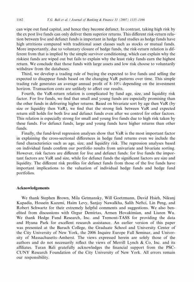
1162 T.G. Bali et al. / Journal of Banking & Finance 31 (2007) 1135–1166
can wipe out fund capital, and hence they become defunct. In contrast, taking high risk bythe ex post live funds can only deliver them superior returns. This different risk-return rela-tion between live and defunct funds is important in hedge fund studies as hedge funds havehigh attritions compared with traditional asset classes such as stocks or mutual funds.More importantly, due to voluntary closure of hedge funds, the risk-return relation is dif-ferent from that is implied by the simple survivor conditioning, which can explain why theriskiest funds are wiped out but fails to explain why the least risky funds earn the highestreturn. We conclude that those funds with large assets and low risk choose to voluntarilywithdraw from the databases.
Third, we develop a trading rule of buying the expected to live funds and selling theexpected to disappear funds based on the changing VaR patterns over time. This simpletrading rule generates an average annual profit of 8–10% depending on the investmenthorizon. Transaction costs are unlikely to affect our results.
Fourth, the VaR-return relation is complicated by fund age, size, and liquidity riskfactor. For live funds, we find that small and young funds are especially promising thanthe other funds in delivering higher returns. Based on bivariate sort by age then VaR (bysize or liquidity then VaR), we find that the strong link between VaR and expectedreturn still holds for both live and defunct funds even after we control for other factors.This relation is especially strong for small and young live funds due to high risk taken bythese funds. For defunct funds, large and young funds have higher returns than otherfunds.
Finally, the fund-level regression analyses show that VaR is the most important factorin explaining the cross-sectional differences in hedge fund returns even we include thefund characteristics such as age, size, and liquidity risk. The regression analyses basedon individual funds confirm our portfolio results from univariate and bivariate sorting.However, risk factors are different for live and defunct funds: for live funds the impor-tant factors are VaR and size, while for defunct funds the significant factors are size andliquidity. The different risk profiles for defunct funds from those of the live funds haveimportant implications to the valuation of individual hedge funds and hedge fundportfolios.
Acknowledgements
We thank Stephen Brown, Mila Getmansky, Will Goetzmann, David Hsieh, NikunjKapadia, Hossein Kazemi, Haim Levy, Sanjay Nawalkha, Salih Neftci, Lin Peng, andRobert Schwartz for their extremely helpful comments and suggestions. We also ben-efited from discussions with Ozgur Demirtas, Armen Hovakimian, and Liuren Wu.We thank Hedge Fund Research, Inc. and Tremont-TASS for providing the dataand Hyuna Park for excellent research assistance. An earlier version of this paperwas presented at the Baruch College, the Graduate School and University Center ofthe City University of New York, the 2006 Inquire Europe Fall Seminar, and Univer-sity of Massachusetts–Amherst. The views expressed herein are solely those of theauthors and do not necessarily reflect the views of Merrill Lynch & Co, Inc. and itsaffiliates. Turan Bali gratefully acknowledges the financial support from the PSC-CUNY Research Foundation of the City University of New York. All errors remainour responsibility.

T.G. Bali et al. / Journal of Banking & Finance 31 (2007) 1135–1166 1163
Appendix
Table 11
Average return of the hedge fund portfolios from bivariate sorts: First sorted by age and then CF VaR (January1995–December 2003)Low age group Medium age group High age group
Decile CF VaR(%)
Return(%)
Decile CF VaR(%)
Return(%)
Decile CF VaR(%)
Return(%)
Panel A: Live funds
Low CFVaR
�0.60 0.98 Low CFVaR
0.17 0.94 Low CFVaR
�1.30 0.85
2 0.93 0.89 2 1.05 0.77 2 1.13 0.843 1.67 1.09 3 1.73 0.78 3 1.96 0.984 2.34 1.02 4 2.49 1.14 4 2.72 1.035 3.20 0.98 5 3.24 1.07 5 3.59 1.036 4.11 1.24 6 3.97 1.43 6 4.75 1.017 5.08 1.32 7 4.90 1.57 7 5.82 1.178 6.15 1.31 8 6.25 1.05 8 6.94 1.189 7.83 1.49 9 8.02 1.44 9 8.39 1.53High CF
VaR12.21 1.96 High CF
VaR11.97 1.65 High CF
VaR11.93 1.39
High CF VaR–low CF VaR
0.98% High CF VaR–low CF VaR
0.71% High CF VaR–low CF VaR
0.54%
Standard t-statistic 2.22** Standard t-statistic 1.45 Standard t-statistic 1.54Newey–West t-statistic 2.12** Newey–West t-statistic 1.44 Newey–West t-statistic 1.36
Low age group Medium age group High age group
Decile CF VaR(%)
Return(%)
Decile CF VaR(%)
Return(%)
Decile CF VaR(%)
Return(%)
Panel B: Defunct funds
Low CFVaR
�0.74 1.03 Low CFVaR
�1.38 0.98 Low CFVaR
0.18 0.48
2 1.17 0.66 2 1.16 0.69 2 1.20 0.723 2.07 0.66 3 2.16 0.60 3 2.05 0.764 2.99 0.68 4 3.02 0.55 4 2.91 0.725 4.00 0.62 5 3.88 0.75 5 3.86 0.746 5.03 0.54 6 5.09 1.06 6 5.02 0.567 6.12 0.96 7 6.41 0.52 7 6.16 0.228 7.56 0.78 8 7.71 0.72 8 7.58 0.599 9.92 0.56 9 10.08 0.80 9 9.81 0.78High CF
VaR17.29 �0.66 High CF
VaR16.31 0.29 High CF
VaR16.01 0.24
High CF VaR–low CF VaR
�1.69% High CF VaR–low CF VaR
�0.69% High CF VaR–low CF VaR
�0.24%
Standard t-statistic �2.76*** Standard t-statistic �1.29 Standard t-statistic �0.40Newey–West t-statistic �3.10*** Newey–West t-statistic �1.02 Newey–West t-statistic �0.35
This table shows the average returns of the hedge fund portfolios first sorted by three age groups and then by CFVaR. The table also reports the average return differential between Deciles 10 and 1, the standard t-statistics forthe average return differential, and the Newey and West (1987) adjusted t-statistics. Panels A and B present resultsfor live and defunct funds, respectively. ***, **, * denotes significance level at least at the 1%, 5%, and 10% level,respectively.

Table 12Average return of the hedge fund portfolios from bivariate sorts: First sorted by asset and then CF VaR (January1995–December 2003)
Low asset group Medium asset group High asset group
Decile CF VaR(%)
Return(%)
Decile CF VaR(%)
Return(%)
Decile CF VaR(%)
Return(%)
Panel A: Live funds
Low CFVaR
�0.12 1.07 Low CFVaR
�1.76 0.89 Low CFVaR
0.04 0.84
2 1.57 0.95 2 0.94 0.88 2 0.83 0.773 2.53 1.24 3 1.67 0.90 3 1.59 0.864 3.61 1.34 4 2.38 0.75 4 2.17 1.035 4.66 1.37 5 3.16 1.19 5 2.73 0.926 5.66 1.22 6 3.95 1.01 6 3.47 1.207 6.59 1.55 7 5.06 1.10 7 4.35 1.288 7.80 1.46 8 6.21 1.46 8 5.38 0.779 9.61 1.78 9 7.68 1.33 9 6.81 1.38High CF
VaR14.29 2.46 High CF
VaR10.97 1.55 High CF
VaR9.69 1.09
High CF VaR–low CF VaR
1.39% High CF VaR–low CF VaR
0.65% High CF VaR–low CF VaR
0.24%
Standard t-statistic 2.80*** Standard t-statistic 1.45 Standard t-statistic 0.66Newey–West t-statistic 2.53** Newey–West t-statistic 1.32 Newey–West t-statistic 0.67
Low asset group Medium asset group High asset group
Decile CF VaR(%)
Return(%)
Decile CF VaR(%)
Return(%)
Decile CF VaR(%)
Return(%)
Panel B: Defunct funds
Low CFVaR
�1.17 0.63 Low CFVaR
0.75 0.77 Low CFVaR
0.12 0.48
2 1.94 0.66 2 1.72 0.83 2 0.91 0.583 3.17 1.05 3 2.64 0.76 3 1.84 1.274 3.35 0.98 4 3.85 0.40 4 2.25 0.965 4.35 �0.48 5 4.09 0.50 5 3.30 1.496 5.74 �0.14 6 5.24 0.67 6 4.47 1.047 7.01 0.46 7 6.18 0.63 7 5.80 0.888 8.76 0.57 8 7.50 0.96 8 7.52 1.089 10.81 0.46 9 10.26 �0.42 9 9.66 0.66High CF
VaR18.58 �1.85 High CF
VaR15.13 0.18 High CF
VaR14.15 1.32
High CF VaR–low CF VaR
�2.48% High CF VaR–low CF VaR
�0.59% High CF VaR–low CF VaR
0.84%
Standard t-statistic �1.81* Standard t-statistic �0.81 Standard t-statistic 1.17Newey–West t-statistic �1.94* Newey–West t-statistic �0.80 Newey–West t-statistic 1.56
This table shows the average returns of the hedge fund portfolios first sorted by three Asset groups and then byCF VaR. The table also reports the average return differential between Deciles 10 and 1, the standard t-statisticsfor the average return differential, and the Newey and West (1987) adjusted t-statistics. Panels A and B presentresults for live and defunct funds, respectively. ***, **, * denotes significance level at least at the 1%, 5%, and 10%level, respectively.
1164 T.G. Bali et al. / Journal of Banking & Finance 31 (2007) 1135–1166

Table 13Average return of the hedge fund portfolios from bivariate sorts: First sorted by lockup and then CF VaR(January 1995–December 2003)
Non-lockup funds (dlock = 0) Lockup funds (dlock = 1)
Decile CF VaR (%) Return (%) Decile CF VaR (%) Return (%)
Panel A: Live funds
Low CF VaR �0.02 0.88 Low CF VaR �1.89 1.052 0.91 0.80 2 1.34 0.883 1.65 0.87 3 2.07 1.014 2.40 0.97 4 2.76 1.195 3.20 1.02 5 3.74 1.406 4.00 1.20 6 5.00 1.427 4.94 1.15 7 6.15 1.328 6.06 1.26 8 7.47 1.389 7.45 1.54 9 9.41 1.78High CF VaR 11.31 1.46 High CF VaR 13.10 1.46
High CF VaR–low CF VaR 0.58% High CF VaR–low CF VaR 0.42%Standard t-statistic 1.52 Standard t-statistic 1.15Newey–West t-statistic 1.43 Newey–West t-statistic 1.09
Non-lockup funds (dlock = 0) Lockup funds (dlock = 1)
Decile CF VaR (%) Return (%) Decile CF VaR (%) Return (%)
Panel B: Dead funds
Low CF VaR �0.54 0.80 Low CF VaR �1.25 0.882 1.17 0.67 2 0.98 0.883 2.01 0.60 3 2.13 0.844 2.86 0.77 4 3.38 0.925 3.81 0.60 5 4.47 0.686 4.86 0.69 6 5.82 0.597 6.01 0.65 7 7.36 0.738 7.39 0.57 8 8.61 1.149 9.64 0.52 9 10.90 1.26High CF VaR 16.71 �0.11 High CF VaR 16.82 1.04
High CF VaR–low CF VaR �0.91% High CF VaR–low CF VaR 0.16%Standard t-statistic �1.96* Standard t-statistic 0.23Newey–West t-statistic �1.95* Newey–West t-statistic 0.24
This table shows the average returns of the hedge fund portfolios first sorted by two lockup groups and then byCF VaR. The table also reports the average return differential between Deciles 10 and 1, the standard t-statisticsfor the average return differential, and the Newey and West (1987) adjusted t-statistics. Panels A and B presentresults for live and defunct funds, respectively. ***, **, * denotes significance level at least at the 1%, 5%, and 10%level, respectively. Note that there are not enough observations for defunct funds with lockup periods during thefirst 12 months (January 1995–December 1995), we present the average of the following 96 months (January1996–December 2003).
T.G. Bali et al. / Journal of Banking & Finance 31 (2007) 1135–1166 1165
References
Ackermann, Carl, McEnally, Richard, Ravenscraft, David, 1999. The performance of hedge funds: Risk, return,and incentives. Journal of Finance 54, 833–874.
Agarwal, Vikas, Naik, Narayan, 2004. Risks and portfolio decisions involving hedge funds. Review of FinancialStudies 17, 63–98.

1166 T.G. Bali et al. / Journal of Banking & Finance 31 (2007) 1135–1166
Aragon, George, 2006. Share restriction and asset pricing: Evidence from the hedge fund industry. Journal ofFinancial Economics, in press.
Bali, Turan G., 2003. An extreme value approach to estimating volatility and value at risk. Journal of Business76, 83–108.
Bali, Turan G., Cakici, Nusret, 2004. Value at risk and expected stock returns. Financial Analysts Journal 60, 57–73.
Bali, Turan G., Gokcan, Suleyman, 2004. Alternative approaches to estimating VaR for hedge fund portfolios. In:Barry, Schachter (Ed.), Intelligent Hedge Fund Investing, . In: Risk Books. Incisive Media PLC, pp. 253–277.
Bali, Turan G., Theodossiou, Panayiotis, 2006. A conditional-SGT-VaR approach with alternative GARCHmodels. Annals of Operations Research, in press.
Berk, Jonathan, Green, Richard, 2004. Mutual fund flows and performance in rational markets. Journal ofPolitical Economy 112, 1269–1295.
Brown, Stephen J., Goetzmann, William N., 2003. Hedge funds with style. Journal of Portfolio Management 29,101–112.
Brown, S.J., Goetzmann, W.N., Ibbotson, R.G., Ross, S.A., 1992. Survivorship bias in performance studies.Review of Financial Studies 5 (4 (Winter)), 553–580.
Brown, Stephen J., Goetzmann, William N., Ross, Stephen A., 1995. Survival. Journal of Finance 50, 853–873.Brown, Stephen J., Goetzmann, William N., Ibbotson, Roger, 1999. Offshore hedge funds: Survival and
performance. Journal of Business 72, 91–117.Brown, Stephen J., Goetzmann, William N., Park, James, 2001. Careers and survival: Competition and risk in the
hedge fund and CTA industry. Journal of Finance 56, 1869–1886.Chevalier, Judith, Ellison, Glenn, 1999. Are some mutual fund managers better than others? Cross-sectional
patterns in behavior and performance. Journal of Finance 54, 875–899.Cornish, E.A., Fisher, R.A., 1937. Moments and cumulants in the specification of distributions. Review of the
International Statistical Institute, 307–320.Fama, Eugene, French, Kenneth, 1992. Cross-section of expected stock returns. Journal of Finance 47, 427–465.Fama, Eugene, French, Kenneth, 1993. Common risk factors in the returns on bonds and stocks. Journal of
Financial Economics 23, 3–56.Fama, Eugene, MacBeth, James, 1973. Risk, return and equilibrium: Empirical test. Journal of Political
Economy 81, 607–636.Fung, William, Hsieh, David, 1997. Empirical characteristics of dynamic trading strategies: The case of hedge
funds. Review of Financial Studies 10, 275–302.Fung, William, Hsieh, David, 2000. Performance characteristics of hedge funds and commodity funds: Natural
versus spurious biases. Journal of Financial and Quantitative Analysis 35, 291–307.Getmansky, Mila, Lo, Andrew, Makarov, Igor, 2004a. An econometric model of serial correlation and illiquidity
in hedge funds returns. Journal of Financial Economics 74, 529–610.Getmansky, Mila, Lo, Andrew, Mei, Shauna, 2004b. Sifting through the wreckage: Lessons from recent hedge-
fund liquidations. Journal of Investment Management 2, 6–38.Gupta, Anurag, Liang, Bing, 2005. Do hedge funds have enough capital? A value at risk approach. Journal of
Financial Economics 77, 219–253.Jagadeesh, Narasimhan, Titman, Sheridan, 1993. Returns to buying winners and selling losers: Implications for
stock market efficiency. Journal of Finance 48, 65–91.Jorion, Philippe, 2000. Risk management lessons from long term capital management. European Financial
Management 6, 277–300.Jorion, Philippe, 2001. Value-at-Risk: The New Benchmark for Controlling Market Risk. McGraw-Hill,
Chicago.Liang, Bing, 1999. On the performance of hedge funds. Financial Analysts Journal 55, 72–85.Liang, Bing, 2000. Hedge fund: The living and the dead. Journal of Financial and Quantitative Analysis 35, 309–
326.Liang, Bing, 2003. Hedge fund returns: Auditing and accuracy. Journal of Portfolio Management 29, 111–122.Lo, Andrew, 2001. Risk management for hedge funds: Introduction and overview. Financial Analysts Journal 57,
16–33.Newey, Whitney K., West, Kenneth D., 1987. A simple, heteroskedastic and autocorrelation consistent
covariance matrix. Econometrica 55, 703–708.Sharpe, William F., 1992. Asset allocation, management style and performance measurement. Journal of
Portfolio Management 18, 7–19.
Related Documents