INTERNATIONAL JOURNAL OF MICROSIMULATION (2016) 9(2) 106-122 INTERNATIONAL MICROSIMULATION ASSOCIATION Validation of Spatial Microsimulation Models: a Proposal to Adopt the Bland-Altman Method Kate A Timmins School of Sport and Exercise Science, University of Lincoln, Lincoln LN6 7TS, United Kingdom e-mail: [email protected] Kimberley L Edwards Arthritis Research UK Centre for Sport Exercise and Osteoarthritis, University of Nottingham C Floor, South Block, Queens Medical Centre, Nottingham, NG7 2UH, United Kingdom e-mail: [email protected] ABSTRACT: Model validation is recognised as crucial to microsimulation modelling. However, modellers encounter difficulty in choosing the most meaningful methods to compare simulated and actual values. The aim of this paper is to introduce and demonstrate a method employed widely in healthcare calibration studies. The ‘Bland-Altman plot’ consists of a plot of the difference between two methods against the mean (x-y versus x+y/2). A case study is presented to illustrate the method in practice for spatial microsimulation validation. The study features a deterministic combinatorial model (SimObesity), which modelled a synthetic population for England at the ward level using survey (ELSA) and Census 2011 data. Bland-Altman plots were generated, plotting simulated and census ward-level totals for each category of all constraint (benchmark) variables. Other validation metrics, such as R 2 , SEI, TAE and RMSE, are also presented for comparison. The case study demonstrates how the Bland-Altman plots are interpreted. The simple visualisation of both individual- (ward-) level difference and total variation gives the method an advantage over existing tools used in model validation. There still remains the question of what constitutes a valid or well-fitting model. However, the Bland Altman method can usefully be added to the canon of

Welcome message from author
This document is posted to help you gain knowledge. Please leave a comment to let me know what you think about it! Share it to your friends and learn new things together.
Transcript

INTERNATIONAL JOURNAL OF MICROSIMULATION (2016) 9(2) 106-122
INTERNATIONAL MICROSIMULATION ASSOCIATION
Validation of Spatial Microsimulation Models:
a Proposal to Adopt the Bland-Altman Method
Kate A Timmins
School of Sport and Exercise Science, University of Lincoln, Lincoln LN6 7TS, United Kingdom e-mail: [email protected]
Kimberley L Edwards
Arthritis Research UK Centre for Sport Exercise and Osteoarthritis, University of Nottingham C Floor, South Block, Queens Medical Centre, Nottingham, NG7 2UH, United Kingdom e-mail: [email protected]
ABSTRACT: Model validation is recognised as crucial to microsimulation modelling. However,
modellers encounter difficulty in choosing the most meaningful methods to compare simulated
and actual values. The aim of this paper is to introduce and demonstrate a method employed widely
in healthcare calibration studies.
The ‘Bland-Altman plot’ consists of a plot of the difference between two methods against the mean
(x-y versus x+y/2). A case study is presented to illustrate the method in practice for spatial
microsimulation validation. The study features a deterministic combinatorial model (SimObesity),
which modelled a synthetic population for England at the ward level using survey (ELSA) and
Census 2011 data. Bland-Altman plots were generated, plotting simulated and census ward-level
totals for each category of all constraint (benchmark) variables. Other validation metrics, such as
R2, SEI, TAE and RMSE, are also presented for comparison.
The case study demonstrates how the Bland-Altman plots are interpreted. The simple visualisation
of both individual- (ward-) level difference and total variation gives the method an advantage over
existing tools used in model validation. There still remains the question of what constitutes a valid
or well-fitting model. However, the Bland Altman method can usefully be added to the canon of

INTERNATIONAL JOURNAL OF MICROSIMULATION (2016) 9(2) 106-122 107
TIMMINS, EDWARDS Validation of Spatial Microsimulation Models: a Proposal to Adopt the Bland-Altman Method
calibration methods.
KEYWORDS: Validation, Bland Altman, Spatial Microsimulation.
JEL classification: C63 – Simulation Modelling.

INTERNATIONAL JOURNAL OF MICROSIMULATION (2016) 9(2) 106-122 108
TIMMINS, EDWARDS Validation of Spatial Microsimulation Models: a Proposal to Adopt the Bland-Altman Method
1. BACKGROUND
The goal of a spatial microsimulation model, in most cases, is to create a data set that mimics the
‘real-world situation’ as accurately as possible. To have confidence in the simulated data, it is
necessary to validate the model, comparing the output to actual data (Edwards & Tanton, 2012).
The validation process for microsimulation modelling has been broadly divided into two
components: internal (in-sample, or endogenous) and external (out-of-sample, or exogenous)
(Edwards & Tanton, 2012; O'Donoghue, Morrissey, & Lennon, 2014). Internal validation refers to
the process of comparing values from the simulated data set to the original data set. This includes
model calibration, whereby the model fit is assessed by comparing the actual and simulated values
for constraining (or benchmark) variables. In-sample validation also occurs where actual and
simulated outcomes are compared at an aggregate level (Ballas & Clarke, 2001). External validation
occurs where values are compared against data not used in the simulation.
Although the importance of validation is widely recognised (Edwards et al., 2011), researchers still
encounter difficulty in choosing the most meaningful methods to compare simulated and actual
values. To date, quantitative methods for internal validation that have been proposed or used
include:
o Coefficient of determination (R2)
o Standard Error about Identity (SEI) ( Ballas et al., 2007; Tanton & Vidyattama, 2010)
o Total Absolute Error (TAE) (Voas & Williamson, 2001)
o Standardized Absolute Error (SAE) (Edwards & Tanton, 2012)
o Root Mean Squared Error (RMSE) (Legates & McCabe Jr, 1999)
o Z-score or modified z-score (zm) (Voas & Williamson, 2001) or overall relative sum of z-
square scores (Tanton, Williamson, & Harding, 2014)
o E5 (Lovelace et al., 2015)
o Statistical techniques to derive confidence intervals (e.g. bootstrapping (Tanton, 2015))
o Statistical tests for difference (e.g. the t test (Edwards & Clarke, 2009), or a test based on
the Z-statistic (Rahman et al., 2013)).
A brief description of the methods appropriate for deterministic and other models is offered in
Table 1. The remainder of this paper will not directly discuss techniques for deriving confidence
intervals or tests for difference. Techniques to derive confidence intervals, although their potential
to aid in model calibration has been well argued, are not appropriate for deterministic models,
where iterative runs of the model would not result in different simulated populations. (See Voas

INTERNATIONAL JOURNAL OF MICROSIMULATION (2016) 9(2) 106-122 109
TIMMINS, EDWARDS Validation of Spatial Microsimulation Models: a Proposal to Adopt the Bland-Altman Method
and Williamson (Voas & Williamson, 2000) for a discussion of bootstrapping for combinatorial
models). Nor will hypothesis-driven tests be included in the comparison which follows, since
validation seeks to find agreement, rather than difference, and using tests for difference presume
that no observed difference can be interpreted as no difference. A discussion about the hazards of
‘accepting the null hypothesis’ is elegantly described by Altman and Bland (Altman & Bland, 1995).
The relative strengths and merits of these validation methods have been extensively explored by a
number of reviews (Edwards & Tanton, 2012; Lovelace et al., 2015; Rahman et al., 2013;
Scarborough et al., 2009).
Table 1 Methods to assess goodness-of-fit of spatial microsimulation models
Method Description
Correlation and R² Plots simulated area count against actual area count. The R2, or coefficient of determination, is the square of the Pearson correlation coefficient and gives an indication of fit.
Standard Error about Identity (SEI) In contrast to R², SEI reflects the error around the line of identity (x=y; also known as the line of equality), rather than the line of best fit.
Total Absolute Error (TAE) A sum of the error (the difference between simulated and actual population counts for each area) across a category.
Standardized Absolute Error (SAE) TAE is divided by the total expected count. The standardization allows comparison between tables.
Root Mean Squared Error (RMSE) The square root of the mean squared error. Gives an indication of error dispersion (if error follows a normal distribution).
z-score, modified z-score, and zm² The z-score is a cell level statistic that reflects the difference in the relative size of the category between actual and simulated populations. The modified score deals better with small cell counts, though an adjustment still needs to be made where area counts are 0. The zm² is an overall measure, summing the squared z-scores.
E5 A count of the number of areas where error is greater than 5%.
One of the chief problems encountered in validation, particularly in model calibration, is that there
is often a large quantity of values to compare, each with a varying degree of agreement between
actual and simulated values, so that gaining an overall assessment of model fit is challenging. On
the other hand, summary measures of model fit have the disadvantage of losing information
(Lovelace et al., 2015). One review concluded that a combination of approaches was necessary to
overcome these shortcomings (Kopec et al., 2010).
With such an arsenal of tools at modellers’ disposal, it may be questioned whether yet another
suggestion is necessary. However, the demonstration and discussion which follow will make clear
the advantages of a method for validation borrowed from the healthcare literature, the Bland
Altman plot. In particular, the Bland Altman plot, or BA plot, is unique in its ability to illustrate
both cell (area) level and overall (matrix) error.

INTERNATIONAL JOURNAL OF MICROSIMULATION (2016) 9(2) 106-122 110
TIMMINS, EDWARDS Validation of Spatial Microsimulation Models: a Proposal to Adopt the Bland-Altman Method
1.1. The Bland Altman method
Validation techniques are commonly employed in healthcare to calibrate clinical measurement
instruments. Typically, agreement between the instrument and a ‘gold standard’ is illustrated using
a method proposed by Martin Bland and Doug Altman (Bland & Altman, 1986) in the 1980s. This
method involves plotting the difference between two methods (x-y) against the mean (x+y/2). This
enables the examination of both the absolute and relative difference, and the shape of the plot
reveals how well two methods agree overall as well as across a range of values. A hypothetical
example is shown in Figure 1: a) showing perfect agreement and b) showing a more typical
comparison.
Figure 1 Hypothetical illustrations of Bland Altman plots
The method also typically incorporates a calculation of ‘limits of agreement’ (not shown in Figure
1): ±1.96*standard deviation of the differences, assuming the differences are normally distributed.
These limits illustrate where 95% of differences lie. When generated with the plots the limits are
typically denoted by horizontal lines
The features of the BA method have been well described and explored in the medical literature
and elsewhere. Indeed, the original 1986 paper is one of the most highly cited research papers ever
(Van Noorden, Maher, & Nuzzo, 2014). Discussions about its use in repeatability studies, the use
of confidence intervals, and interpretation are helpfully collated on Martin Bland’s website (Bland,
2011). The method is now well established in medical measurement comparison studies. A
systematic review found the method was adopted in 85% of studies validating medical instruments
(Zaki et al., 2012). As a result, most standard statistical packages now include options to produce
the plot with limits of agreement. In Stata, for example, BA plots can be generated using the ‘baplot’
command (Seed, 2014). Alternatively, it is possible to generate Bland Altman plots with trend lines

INTERNATIONAL JOURNAL OF MICROSIMULATION (2016) 9(2) 106-122 111
TIMMINS, EDWARDS Validation of Spatial Microsimulation Models: a Proposal to Adopt the Bland-Altman Method
rather than limits of agreement (using the ‘batplot’ command (Mander, 2016)) where the
assumption of normally distributed error is not met (and straight limits of agreement could be
misleading). In R, BA plots can be generated using the ‘MethComp’ package.
This paper is not intended as an exhaustive exposition about the relative merits and disadvantages
of all the methods described in Table 1. This has been clearly and comprehensively covered by
previous publications (Edwards & Tanton, 2012; Lovelace et al., 2015; Scarborough et al., 2009).
Nor is it an attempt to establish a framework for validation across all spatial microsimulation types,
which lies beyond the scope of its aims. Rather, the purpose is to draw attention to another
evaluation method, which satisfies many of the requirements identified in the literature, not least
that it is ‘fast, robust and easy to use’ (Voas & Williamson, 2001). The case study which follows
demonstrates the advantage of the BA plot in calibrating a spatial microsimulation model.
2. CASE STUDY
2.1. Introduction
This case study is merely intended as an illustration to demonstrate the use of validation methods
and compare these to the BA method. The principles of validation apply to many other
microsimulation models, particularly those based on combinatorial optimisation. A brief
description of the model is given in order to aid interpretation of the outputs.
2.2. Methods
2.2.1. The Model
Data on the prevalence of osteoarthritis (OA) – a debilitating condition of the joints – are not
available at a small-area level in the UK. In order to explore geographic patterns, a spatial
microsimulation model created a synthetic population data set for England.
Spatial microsimulation was performed using a deterministic combinatorial optimisation method,
encapsulated in an executable file, ‘SimObesity’. The model has been described previously
(Edwards & Clarke, 2009). In brief, a two stage process, of deterministic reweighting followed by
optimisation, is used. The model is deterministic and the order of constraint entry is
inconsequential. The optimisation stage uses a ‘floor’ function to convert reweights to integers
(‘whole persons’ rather than fractions which may result from the reweighting).
In this example, the data sets used were the English Longitudinal Study of Ageing (ELSA) (Marmot

INTERNATIONAL JOURNAL OF MICROSIMULATION (2016) 9(2) 106-122 112
TIMMINS, EDWARDS Validation of Spatial Microsimulation Models: a Proposal to Adopt the Bland-Altman Method
et al, 2015) (a nationally representative survey of older adults) and the 2011 Census data for England
(Office for National Statistics, 2011). For this study, data from Wave 6 of ELSA, collected in 2012-
13, were used (n=10,601), along with ward-level tables from the Census (England only). Wards are
key UK geographic boundaries (Office for National Statistics, 2013), of which there are 7,689 in
England with a mean population of ~5,500. The outcome for the model was OA. In the interests
of simplicity for this case study, just two benchmarks were used: age (7 categories: 50-54yr, 55-
59yr, 60-64yr, 65-69yr, 70-74yr, 75-79yr and ≥80yr) and sex (male/female). These two constraint
variables were cross-tabulated.
2.2.2. The validation
BA plots were generated using the ‘batplot’ command in Stata. Scatter plots are also presented. In
order to facilitate comparison with other commonly used validation methods, the following were
calculated: R2, TAE, SAE, RMSE, SEI and zm2.
R2 was derived using the Stata ‘regress’ command. TAE was calculated as the sum of error terms
in a constraint category (Voas & Williamson, 2000). SAE was taken as the TAE divided by the
expected total population count in that category (Edwards & Tanton, 2012). RMSE is the square
root of the mean squared error. SEI was calculated using the formula cited by Tanton et al (Tanton
& Vidyattama, 2010). Zm2 is the sum of squared modified z-scores (zm), as suggested by
Williamson et al (Williamson, Birkin, & Rees, 1998). The modified score (zm) better takes into
account low cell counts. It is still unable to deal with empty cells, however. In this paper, an
adjustment was made in the case of empty cells, as described by Williamson et al, where the error
was used instead of the zm.
Analyses were performed using Microsoft Excel and Stata Release 13 (StataCorp, 2013).
2.3. Results
Figure 2 shows scatter plots and coefficients of determination for the ward population counts
(‘Total’) as well as for each constraint category. Observed census counts are plotted on the x axis
and simulated counts on the y axis.

INTERNATIONAL JOURNAL OF MICROSIMULATION (2016) 9(2) 106-122 113
TIMMINS, EDWARDS Validation of Spatial Microsimulation Models: a Proposal to Adopt the Bland-Altman Method
Figure 2 Scatter plots for age and sex categories, simulated counts versus census ward totals
Figure 3 shows the BA plots for the same categories. In contrast to Figure 2, where the scatterplots
indicate near perfect correlation, Figure 3 demonstrates the variability of counts within individual
wards, as well as the heterogeneity across ward sizes. For all categories plotted, the majority of data
points fit along the horizontal 0 line, showing exact agreement for these wards. However, we can
also identify which categories are less well fitted: population counts for the oldest age category, for
example, Category 7, have been under- or over-simulated by as much as 15 individuals for several
wards. (Readers should take note of the y axis scale on each plot.) In addition, we can tell that this
discrepancy is prevalent only amongst the smaller wards, with the wider spread data points confined
to the left-hand side of the graph. Conversely, the simulated population in the youngest age group
is almost perfectly calibrated with census data, with a discrepancy of only 1 extra individual in each
of 2 wards. Finally, it can be seen that the total simulated ward counts either match exactly with
census numbers or under-represent by 1 individual (this under-estimation likely reflects the flooring
function employed by SimObesity in the optimisation algorithm, which prevents partial people
‘existing’ in the simulated dataset).

INTERNATIONAL JOURNAL OF MICROSIMULATION (2016) 9(2) 106-122 114
TIMMINS, EDWARDS Validation of Spatial Microsimulation Models: a Proposal to Adopt the Bland-Altman Method
Figure 3 Bland Altman plots for age and sex categories, simulated versus census ward totals
Total
Table 2 shows the corresponding metrics for each category: R2, SEI, TAE, SAE, RMSE, zm2 and
E5. It can be seen that R2 does not reflect the differences in fit of the categories which is described
by the other methods. All of the other measures agree that age group 1 is the best fitted category.
This is also evident in the BA plot for age category 1, which shows just two areas differ and by just
1 individual in each. Beyond this, however, the metrics imply differing pictures about the model
fit.
-2-1
01
Diff
eren
ce (s
im4_
tota
l-cen
_tot
al)
30.5 10055Average of sim4_total and cen_total
INTERNATIONAL JOURNAL OF MICROSIMULATION (2016) 9(2) 106-122 115
TIMMINS, EDWARDS Validation of Spatial Microsimulation Models: a Proposal to Adopt the Bland-Altman Method
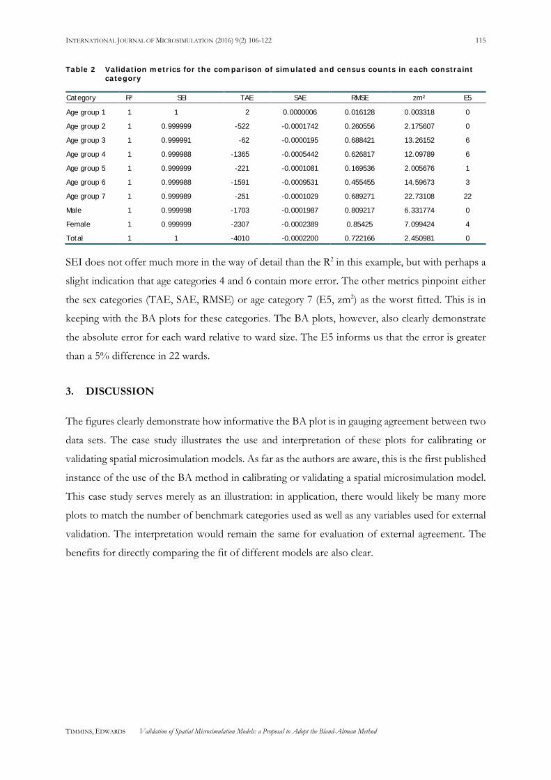
Table 2 Validation metrics for the comparison of simulated and census counts in each constraint category
Category R² SEI TAE SAE RMSE zm² E5
Age group 1 1 1 2 0.0000006 0.016128 0.003318 0
Age group 2 1 0.999999 -522 -0.0001742 0.260556 2.175607 0
Age group 3 1 0.999991 -62 -0.0000195 0.688421 13.26152 6
Age group 4 1 0.999988 -1365 -0.0005442 0.626817 12.09789 6
Age group 5 1 0.999999 -221 -0.0001081 0.169536 2.005676 1
Age group 6 1 0.999988 -1591 -0.0009531 0.455455 14.59673 3
Age group 7 1 0.999989 -251 -0.0001029 0.689271 22.73108 22
Male 1 0.999998 -1703 -0.0001987 0.809217 6.331774 0
Female 1 0.999999 -2307 -0.0002389 0.85425 7.099424 4
Total 1 1 -4010 -0.0002200 0.722166 2.450981 0
SEI does not offer much more in the way of detail than the R2 in this example, but with perhaps a
slight indication that age categories 4 and 6 contain more error. The other metrics pinpoint either
the sex categories (TAE, SAE, RMSE) or age category 7 (E5, zm2) as the worst fitted. This is in
keeping with the BA plots for these categories. The BA plots, however, also clearly demonstrate
the absolute error for each ward relative to ward size. The E5 informs us that the error is greater
than a 5% difference in 22 wards.
3. DISCUSSION
The figures clearly demonstrate how informative the BA plot is in gauging agreement between two
data sets. The case study illustrates the use and interpretation of these plots for calibrating or
validating spatial microsimulation models. As far as the authors are aware, this is the first published
instance of the use of the BA method in calibrating or validating a spatial microsimulation model.
This case study serves merely as an illustration: in application, there would likely be many more
plots to match the number of benchmark categories used as well as any variables used for external
validation. The interpretation would remain the same for evaluation of external agreement. The
benefits for directly comparing the fit of different models are also clear.

INTERNATIONAL JOURNAL OF MICROSIMULATION (2016) 9(2) 106-122 116
TIMMINS, EDWARDS Validation of Spatial Microsimulation Models: a Proposal to Adopt the Bland-Altman Method
Table 3 Summary of the strengths and weaknesses of validation methods presented
R² SEI TAE SAE RMSE zm Zm² E5 BA plot
Indication of individual area error X X X X X √ X √ √
Indication of systematic (overall) bias X √ √ √ X X √ X √
Identify outliers √ X X X X √ X √ √
Indication of error distribution (by area size) X X X X √ X X X √
Handles empty cells (0 counts) √ √ √ √ √ X X X √
Comparable across models (of different sizes) √ √ X √ X √ X √ √
Single overall metric (for each category) √ √ √ √ √ X √ √ X
Table 3 summarises the strengths and weaknesses of the methods used. The following points
summarise the key advantages of the BA plot.
3.1. Key advantages of the BA plot
3.1.1. Bland Altman plots are informative about overall error and individual area error
Huang & Williamson (Huang & Williamson, 2001) stressed the importance of examining both
local, cellular fit and tabular or overall fit. The latter allows an assessment of how well the model
performs overall, whilst the former can be used to identify key sources of error. Local fit is typically
examined using absolute or relative error or z-scores. If tables are large, it is challenging to identify
which are key sources of error. The E5 is helpful in summarizing how many areas could be
considered key sources of error, though it is still necessary to locate these. Most other metrics offer
a summary measure of category fit (R2, SEI, TAE, SAE, RMSE, zm2). In other words, these metrics
give an overall summary of the accuracy across all of the small areas. The BA plot, on the other
hand, provides information both about performance across all the geographic areas (bias, limits of
agreement) as well as displaying the error for each individual area which can be seen from the plot.
3.1.2. Bland-Altman plots identify systematic bias
Some of the standard methods in use do address systematic bias: for instance the TAE, SAE and
zm2 show both the overall size of inaccuracy (bias) as well as the direction of bias (whether it is an
under- or over-estimation). RMSE and SEI can be said to address bias; however, in using squared
values, the direction of bias is not given. The inability to detect systematic bias is one of the
common criticisms of the R2 measure (Lovelace et al., 2015). In most standard statistical packages,
a line of bias will be generated with each BA plot, showing for example if one measure consistently
underestimates at all levels of the scale.

INTERNATIONAL JOURNAL OF MICROSIMULATION (2016) 9(2) 106-122 117
TIMMINS, EDWARDS Validation of Spatial Microsimulation Models: a Proposal to Adopt the Bland-Altman Method
3.1.3. Bland-Altman plots reveal outliers
The visual representation of the error in the BA plot makes it easy to detect outliers, where error
is especially large for particular areas. In Stata, data points can be labelled (using the ‘valabel’ option)
so outliers can be identified, and, if necessary, potential explanations for the error investigated.
3.1.4. Bland-Altman plots can handle empty cell counts
Some calibration metrics – such as z-scores – have difficulty handling empty cells, or 0 cell counts
(Williamson et al., 1998). Empty cells are not unusual in spatial microsimulation modelling,
particularly where small areas are modelled. The BA plot does not entail division, therefore 0 counts
are not problematic
3.1.5. Bland-Altman plots show the error distribution
It is potentially informative to see if the variation of error is consistent across all population sizes,
or whether it is larger at one extreme. RMSE, although large variance at the extreme high populous
areas will affect the RMSE, does not illustrate the variability across the scale. The visual spread of
the data points on the BA plot would show, for example, if error was greater for larger areas (the
right-hand side of the plot) or smaller areas (to the left of the plot).
3.1.6. Bland-Altman plots can be compared across models
Several authors have identified the need for ‘scale-free metrics’ (Lovelace et al., 2015). Although
the BA plot cannot be said to be scale-free, it is possible to compare the visual characteristics of
plots on different scales. The comparison would rely on judgement of the relative visual
characteristics of the plots, rather than a directly comparable metric. Nevertheless, this is useful to
illustrate the comparative goodness of fit. It is especially relevant where the models to be compared
are of different sizes. Summary measures such as TAE depend not only on the size of the error,
but also the size of the matrix. As shown in the example used here, where TAE was seemingly high
at -4010, but this was across 7,689 wards
3.1.7. Bland-Altman plots are “robust, fast and easy to understand”
Lastly, BA plots have the distinct advantage over other methods in that they are “robust, fast and
easy to understand” (Voas & Williamson, 2001). They are not computationally demanding, and are
easily interpreted.

INTERNATIONAL JOURNAL OF MICROSIMULATION (2016) 9(2) 106-122 118
TIMMINS, EDWARDS Validation of Spatial Microsimulation Models: a Proposal to Adopt the Bland-Altman Method
3.2. Limitations
The BA plot does not offer a simple, single metric or criterion for judgement of model
performance. Rather, it offers an informative description of the error, from which an informed
decision can be made. Appraisal of validity is made on a case-by-case judgement. In medicine, this
decision will directly relate to the clinical relevance of any observed bias or heterogeneity. The
beauty of this is that the BA plot is widely applicable across tools, and across disciplines. The
potential downside is confusion surrounding the interpretation of BA plots. Bland and Altman
themselves recognised some of the common difficulties in interpreting the plots (Bland & Altman,
2003). In particular, there appears to have been widespread misunderstanding of the assumptions
for the calculation of limits of agreement.
In spatial microsimulation modelling, the literature reveals both criterion based approaches and
more subjective approaches to model appraisal. For example, Tanton and Vidyattama (Tanton &
Vidyattama, 2010) employ a criterion in validating the GREGWT model: the ‘TAE criteria’ is met
where the TAE for all constraints does not exceed the population of a small area (in their paper, a
statistical local error, SLA). This has the advantage of making validity assessment transparent and
uniform. However, the authors themselves point out that there is no statistical basis for this
criterion, and although based on modelling experience, it represents a somewhat arbitrary cut-off.
Other authors have advocated a “statistical approach” to determine if a model is valid (Rahman et
al., 2013). There are difficulties in such approaches, however: chiefly, because validation seeks to
assess agreement rather than difference, and therefore standard hypothesis-based approaches do
not readily apply. (See Altman and Bland (1995) for a discussion regarding ‘acceptance’ of the null
hypothesis.) For this reason, tests for difference (such as the t test (Edwards & Clarke, 2009)), were
not included in the comparisons presented here.
The case study used in this paper to demonstrate the BA plot used a deterministic combinatorial
optimisation model. Therefore, the BA plots could only be compared with validation methods
appropriate to this kind of model. It is likely that there are different considerations for alternative
types of model which were beyond the scope of this paper. For example, a range of further
validation methods have been proposed for probabilistic models (e.g. deriving confidence intervals
using multiple iterations (Tanton, 2015)) or regression-based models (this is covered well in a
review of regression model validation by Scarborough et al (Scarborough et al., 2009)). Although
BA plots could equally be used for these alternative models, further work would need to be carried
out to examine how the method compares.

INTERNATIONAL JOURNAL OF MICROSIMULATION (2016) 9(2) 106-122 119
TIMMINS, EDWARDS Validation of Spatial Microsimulation Models: a Proposal to Adopt the Bland-Altman Method
Similarly, this paper did not cover external validation, where outputs are compared to an exogenous
data set. The example presented here focusses only on internal convergence of the model
constraints; therefore only partially addressing the question of its validity. External validation was
not performed here because the case study was merely intended as an introduction to the BA
method, and also because there was not an external data set readily available. Again, further work
could explore its use in all aspects of validity. Often there may a trade-off between internal
convergence and external validity (Tanton & Vidyattama, 2010).
4. CONCLUSION
This case study clearly demonstrates the added benefit of using Bland Altman plots in model
validation. Bland Altman plots show not only overall agreement, but also agreement according to
ward size and an indication of individual ward error, which gives the method an advantage over
existing tools used in model validation. However, the Bland Altman method requires subjective
judgement about whether the model fit is ‘good’. This is both a strength (in that it is not blindly
interpreted on the basis of an arbitrary p value) and a weakness.
There still remains a lack of agreement among microsimulation modellers regarding what
constitutes a valid or well-fitting model (Edwards & Tanton, 2012). It remains for the community
to establish some form of consensus or guidance on best practice (Whitworth, 2013). It seems
unlikely that there is a one-size-fits-all quantitative tool to meet all needs. The information that we
require of a validation exercise – the size, direction, source and distribution of the error – is perhaps
too much to ask of a single, summary measure, and it may be misguided to seek one. Comparing
models according to a single measure may hide the nuanced differences between models – where
one performs well for low-density areas for instance. The impact of these differences will depend
on the purposes of the microsimulation. The choice of validation will remain dependent on the
nature of the research (Lovelace et al., 2015), as well as taking into account comparability with
previous literature and other models. Nevertheless, the Bland Altman method of assessing
agreement is a useful tool to add to the canon of calibration methods.
REFERENCES
Altman D G and Bland J M (1995) Statistics notes: absence of evidence is not evidence of absence,
BMJ, 311, 485.
Ballas D and Clarke G P (2001) Modelling the local impacts of national social policies: A spatial

INTERNATIONAL JOURNAL OF MICROSIMULATION (2016) 9(2) 106-122 120
TIMMINS, EDWARDS Validation of Spatial Microsimulation Models: a Proposal to Adopt the Bland-Altman Method
microsimulation approach, Environment and Planning C: Government and Policy, 19, 587-606.
Ballas D, Clarke G P, Dorling D et al. (2007) Using SimBritain to model the geographical impact
of national government policies, Geographical Analysis, 39(1), 44-77.
Bland J M. (2011) Design and analysis of measurement studies. https://www-
users.york.ac.uk/~mb55/meas/meas.htm
Bland J M and Altman D G (2003) Applying the right statistics: analyses of measurement studies,
Ultrasound in Obstetrics and Gynecology, 22, 85-93.
Edwards K L and Clarke G P (2009) The design and validation of a spatial microsimulation model
of obesogenic environments for children in Leeds, UK: SimObesity, Social Science & Medicine,
69, 1127-1134.
Edwards K L, Clarke G P, Thomas J et al. (2011) Internal and external validation of spatial
microsimulation models: small area estimates of adult obesity, Applied Spatial Analysis and
Policy, 4(281-300).
Edwards K L and Tanton R. (2012) 'Validation of spatial microsimulation models', in R. Tanton &
K. L. Edwards (Eds.), Spatial Microsimulation: a Handbook for Users, NL: Springer, SBM.
Huang Z and Williamson P (2001) A comparison of synthetic reconstruction and combinatorial
optimisation approaches to the creation of small-area microdata: Working Paper.
http://pcwww.liv.ac.uk/~william/microdata/workingpapers/hw_wp_2001_2.pdf
Kopec J A, Fines P, Manuel D G et al. (2010) Validation of population-based disease simulation
models: a review of concepts and methods, BMC Public Health, 10, 710.
Legates D R and McCabe Jr G J (1999) Evaluating the use of "goodness-of-fit" measures in
hydrologic and hydroclimatic model validation, Water Resources Research, 35(1), 233-241.
Lovelace R, Birkin M, Ballas D et al. (2015) Evaluating the performance of iterative proprtional
fitting for spatial microsimulation: new tests for an established technique, Journal of Artificial
Societies and Social Simulation, 18(2), 21.
Mander A. (2016) BATPLOT: Stata module to produce Bland-Altman plots accounting for trend.
http://econpapers.repec.org/software/bocbocode/s448703.htm

INTERNATIONAL JOURNAL OF MICROSIMULATION (2016) 9(2) 106-122 121
TIMMINS, EDWARDS Validation of Spatial Microsimulation Models: a Proposal to Adopt the Bland-Altman Method
Marmot M and al e. (2015) English Longitudinal Study of Ageing: Waves 0-6, 1998-2013.
O'Donoghue C, Morrissey K and Lennon J (2014) Spatial microsimulation modelling: a review of
applications and methodological choices, International Journal of Microsimulation, 7(1), 26-75.
Office for National Statistics. (2011) 2011 Census: Aggregate data (England and Wales) [computer
file]. Downloaded from: http://infuse.mimas.ac.uk.
Office for National Statistics. (2013) Statistical wards, CAS wards and ST wards.
www.ons.gov.uk/ons/index.html
Rahman A, Harding A, Tanton R et al. (2013) Simulating the characteristics of populations at the
small-area level: new validation techniques for a spatial microsimulation model in Australia,
Computational Statistics and Data Analysis, 57, 149.
Scarborough P, Allender S, Rayner M et al. (2009) Validation of model-based estimates (synthetic
estimates) of the prevalence of risk factors for coronary heart disease for wards in England,
Health & Place, 15(2), 596-605.
Seed P (2014) BAPLOT: Stata module to produce Bland-Altman plots, King's College London.
Retrieved from http://fmwww.bc.edu/repec/bocode/b/baplot.ado
StataCorp (2013) Stata Statistical Software: Release 13, College Station, TX: StataCorp LP.
Tanton R. (2015). Estimating confidence intervals in a spatial microsimulation model using survey
replicate weights. Paper presented at the Fifth World Congress of the International
Microsimulation Association (IMA), Esch-sur-Alzette, Luxembourg.
Tanton R and Vidyattama Y (2010) Pushing it to the edge: extending generalised regression as a
spatial microsimulation method, International Journal of Microsimulation, 3(2), 23-33.
Tanton R, Williamson P and Harding A (2014) Comparing two methods of reweighting a survey
file to small area data, International Journal of Microsimulation, 7(1), 76-99.
Van Noorden R, Maher B and Nuzzo R (2014) The top 100 papers, Nature, 514, 550-553.
Voas D and Williamson P (2000) An evaluation of the combinatorial optimisation approach to the
creation of synthetic microdata, International Journal of Population Geography, 6, 349-366.
Voas D and Williamson P (2001) Evaluating goodness-of-fit measures for synthetic microdata,
INTERNATIONAL JOURNAL OF MICROSIMULATION (2016) 9(2) 106-122 122
TIMMINS, EDWARDS Validation of Spatial Microsimulation Models: a Proposal to Adopt the Bland-Altman Method
Geographical and Environmental Modelling, 5(2), 177-200.
Whitworth A e. (2013). Evaluations and improvements in small area estimation methodologies.
Retrieved from http://eprints.ncrm.ac.uk/3210/1/sme_whitworth.pdf
Williamson P, Birkin M and Rees P (1998) The estimation of population microdata by using data
from small area statistics and sample of anonymised records, Environment and Planning
Analysis, 30, 785-816.
Zaki R, Bulgiba A, Ismail R et al. (2012) Statistical methods used to test for agreement of medical
instruments measuring continuous variables in method comparison studies: a systematic review,
Plos One, 7(5), e37908.
Related Documents