VALIDATION OF METHODS TO MEASURE MASS FLUX OF A GROUNDWATER CONTAMINANT THESIS Hyouk Yoon, Captain, ROKA AFIT/GES/ENV/06M-08 DEPARTMENT OF THE AIR FORCE AIR UNIVERSITY AIR FORCE INSTITUTE OF TECHNOLOGY Wright-Patterson Air Force Base, Ohio APPROVED FOR PUBLIC RELEASE; DISTRIBUTION UNLIMITED

Welcome message from author
This document is posted to help you gain knowledge. Please leave a comment to let me know what you think about it! Share it to your friends and learn new things together.
Transcript
VALIDATION OF METHODS TO MEASURE MASS FLUX OF A
GROUNDWATER CONTAMINANT
THESIS
Hyouk Yoon, Captain, ROKA
AFIT/GES/ENV/06M-08
DEPARTMENT OF THE AIR FORCE AIR UNIVERSITY
AIR FORCE INSTITUTE OF TECHNOLOGY
Wright-Patterson Air Force Base, Ohio
APPROVED FOR PUBLIC RELEASE; DISTRIBUTION UNLIMITED

The views expressed in this thesis are those of the author and do not reflect the official policy or position of the United States Air Force, Department of Defense, or the United States Government, the corresponding agencies of any government, NATO or any other defense organization.

AFIT/GES/ENV/06M-08
VALIDATION OF METHODS TO MEASURE MASS FLUX OF A GROUNDWATER CONTAMINANT
THESIS
Presented to the Faculty
Department of Systems and Engineering Management
Graduate School of Engineering and Management
Air Force Institute of Technology
Air University
Air Education and Training Command
In Partial Fulfillment of the Requirements for the
Degree of Master of Science in Environmental Engineering and Science
Hyouk Yoon, BS
Captain, Republic of Korea Army
March 2006
APPROVED FOR PUBLIC RELEASE; DISTRIBUTION UNLIMITED.

AFIT/GES/ENV/06M-08
VALIDATION OF METHODS TO MEASURE MASS FLUX OF A GROUNDWATER CONTAMINANT
Hyouk Yoon, BS
Captain, Republic of Korea Army
Approved:
/ SIGNED / 4 Mar 06 Dr. Mark N. Goltz (Chairman) date / SIGNED / 4 Mar 06 Dr. Carl G. Enfield date / SIGNED / 4 Mar 06 Dr. Junqi Huang date
AFIT/GES/ENV/06M-08
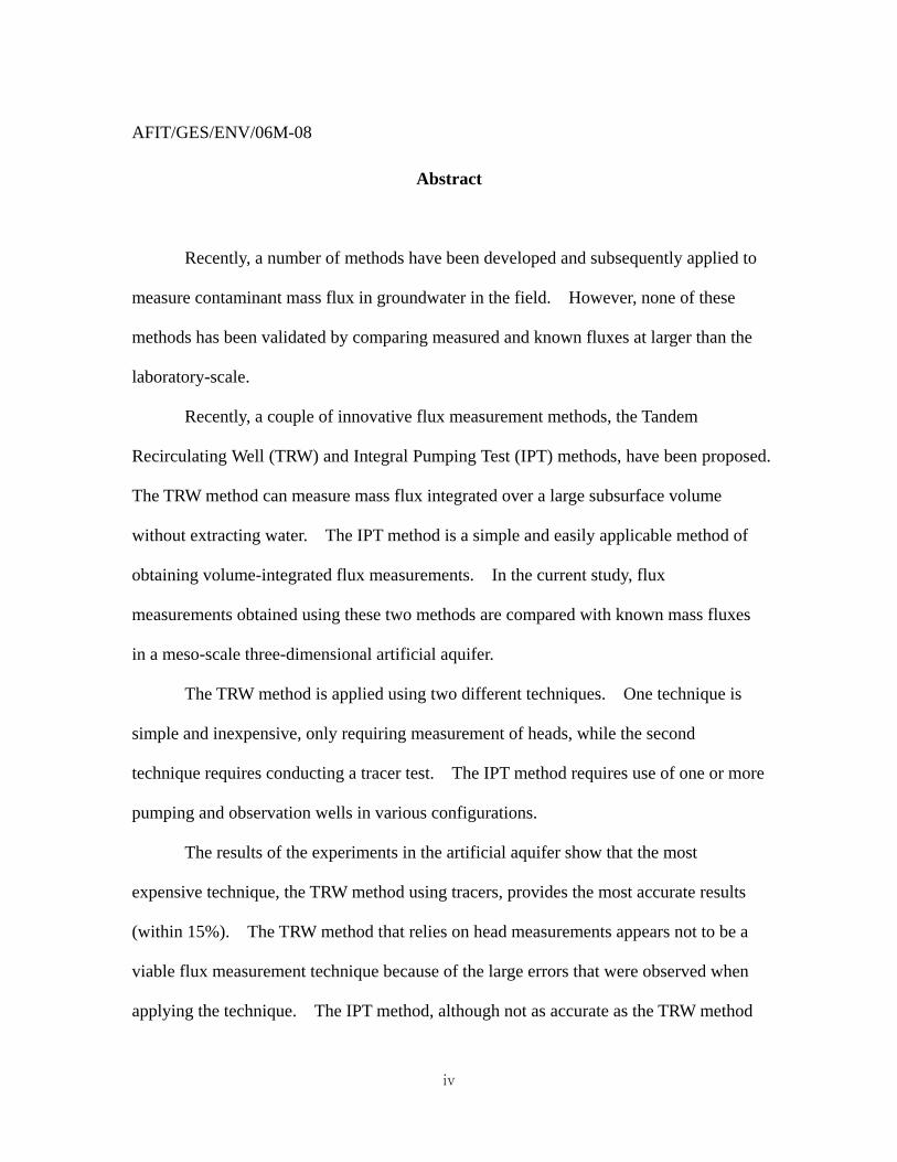
Abstract
Recently, a number of methods have been developed and subsequently applied to
measure contaminant mass flux in groundwater in the field. However, none of these
methods has been validated by comparing measured and known fluxes at larger than the
laboratory-scale.
Recently, a couple of innovative flux measurement methods, the Tandem
Recirculating Well (TRW) and Integral Pumping Test (IPT) methods, have been proposed.
The TRW method can measure mass flux integrated over a large subsurface volume
without extracting water. The IPT method is a simple and easily applicable method of
obtaining volume-integrated flux measurements. In the current study, flux
measurements obtained using these two methods are compared with known mass fluxes
in a meso-scale three-dimensional artificial aquifer.
The TRW method is applied using two different techniques. One technique is
simple and inexpensive, only requiring measurement of heads, while the second
technique requires conducting a tracer test. The IPT method requires use of one or more
pumping and observation wells in various configurations.
The results of the experiments in the artificial aquifer show that the most
expensive technique, the TRW method using tracers, provides the most accurate results
(within 15%). The TRW method that relies on head measurements appears not to be a
viable flux measurement technique because of the large errors that were observed when
applying the technique. The IPT method, although not as accurate as the TRW method
iv

using the tracer technique, does produce relatively accurate results (within 60%). IPT
method inaccuracies may be due to the fact that the method assumptions (infinite
homogeneous confined aquifer at equilibrium) were not well-approximated in the
artificial aquifer. While measured fluxes consistently underestimated the actual flux by
at least 36% and as much as 60%, it appears that errors may be reduced when one
accounts for potential violations of method assumptions.
v

Acknowledgments
I would like to thank my thesis advisor, Dr. Mark N. Goltz, for guiding me to
accomplish this thesis. Without his guidance and support, I would not have done this
work. Whenever I would like to give it up, he always encourage me to go through this
long road to the end. I would also like to thank my committee members, Dr. Carl G.
Enfield and Dr. Junqi Huang for their advice and guidance which made my thesis better.
I also thank Michael Brooks and A. Lynn Wood for advice to my experiments.
My sincere thanks to Murray Close, Mark Flintoft at the New Zealand Institute of
Environmental Science and Research and AquaLinc Research Ltd. for operating the
artificial aquifer and providing the data used in this study.
This study was partially supported by the Environmental Security Technology
Certification Program through Project CU-0318, Diagnostic Tools for Performance
Evaluation of Innovative In Situ Remediation Technologies at Chlorinated Solvent
Contaminated Sites. Also, I acknowledge the Air Force Center for Environmental
Excellence (AFCEE) who sponsored this research.
In addition, I am indebted to the Korean Army for providing me with this great
opportunity of Master’s degree program that has broadened my knowledge as well as
stimulated my understanding of military technology. I am going to try to serve my
country as much as my country has served me in rest of my military career.
Most importantly, I would like to thank my wife and daughter for being with me
during hard time. I also appreciate my parents and in-law’s in Korea for their support
and encouragement. I thank Mrs. Goltz for encouraging me and taking care of my
family. I never forget everyone who supported me and had a hard time with me.
Hyouk Yoon
vi

Table of Contents Page
Abstract............................................................................................................................. iv
Acknowledgments ............................................................................................................ vi
Table of Contents ............................................................................................................ vii
List of Figures................................................................................................................... ix
List of Tables...................................................................................................................... x
I. Introduction................................................................................................................ 1
1.1 Motivation .............................................................................................................. 1
1.2 Research Objectives............................................................................................... 4
1.3 Research Approach................................................................................................ 4
1.4 Study limitations .................................................................................................... 5
II. Literature review ................................................................................................ 6
2.1 Introduction ........................................................................................................... 6
2.2 Background............................................................................................................ 6
2.3 Tandem recirculating well (TRW) method ........................................................... 8
2.3.1 Multi-dipole technique to measure hydraulic conductivity...........................9
2.3.2 Tracer test technique to measure hydraulic conductivity ............................11
2.4 Integral pump test (IPT) method ........................................................................ 13
III. Methodology ...................................................................................................... 17
3.1 Introduction ......................................................................................................... 17
3.2 Artificial aquifer .................................................................................................. 17
3.3 TRW experiment .................................................................................................. 18
vii
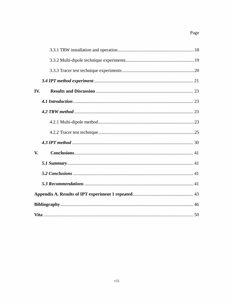
Page
3.3.1 TRW installation and operation...................................................................18
3.3.2 Multi-dipole technique experiments............................................................19
3.3.3 Tracer test technique experiments ...............................................................20
3.4 IPT method experiment ....................................................................................... 21
IV. Results and Discussion ..................................................................................... 23
4.1 Introduction ......................................................................................................... 23
4.2 TRW method ........................................................................................................ 23
4.2.1 Multi-dipole method....................................................................................23
4.2.2 Tracer test technique....................................................................................25
4.3 IPT method .......................................................................................................... 30
V. Conclusions........................................................................................................ 41
5.1 Summary .............................................................................................................. 41
5.2 Conclusions ......................................................................................................... 41
5.3 Recommendations ............................................................................................... 41
Appendix A. Results of IPT experiment 1 repeated..................................................... 43
Bibliography .................................................................................................................... 46
Vita ................................................................................................................................... 50
viii

List of Figures
Page
Figure 1. Plan view of a contaminated site (Einarson and Mackay, 2001)......................... 7
Figure 2. Tandem Recirculating Wells (TRWs) .................................................................. 8
Figure 3. Genetic algorithm procedure ..............................................................................11
Figure 4. TRW fractional flows and tracer injection screens (Goltz et al., 2004) ............ 12
Figure 5. Example of IPT approach with 3 pumping wells and one observation well ..... 16
Figure 6. Plan and vertical views of sampling wells in the artificial aquifer (Bright et al.,
2002) .......................................................................................................................... 18
Figure 7. Plan view showing two TRWs........................................................................... 19
Figure 8. Bromide concentration over time at TRW screens ............................................ 26
Figure 9. . Nitrate concentration over time at TRWs........................................................ 27
Figure 10. Plot to determine Darcy velocity for IPT Experiment 1.................................. 33
Figure 11. Plot to determine Darcy velocity for IPT Experiment 2.................................. 33
Figure 12. Plot to determine Darcy velocity for IPT Experiment 3 (α = 0°) .................... 34
Figure 13. Plot to determine Darcy velocity for IPT Experiment 3 (α = 26.6°) ............... 34
Figure 14. Plot to determine Darcy velocity for IPT Experiment 3 (α = 63.4°) ............... 35
Figure 15. Image wells used to account for no-flow boundaries in IPT experiments ...... 36
ix
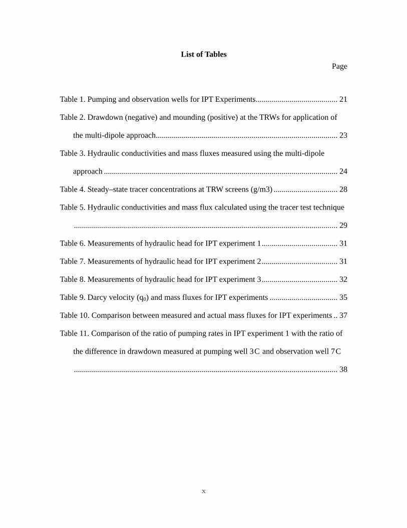
List of Tables Page
Table 1. Pumping and observation wells for IPT Experiments......................................... 21
Table 2. Drawdown (negative) and mounding (positive) at the TRWs for application of
the multi-dipole approach........................................................................................... 23
Table 3. Hydraulic conductivities and mass fluxes measured using the multi-dipole
approach ..................................................................................................................... 24
Table 4. Steady–state tracer concentrations at TRW screens (g/m3) ................................ 28
Table 5. Hydraulic conductivities and mass flux calculated using the tracer test technique
.................................................................................................................................... 29
Table 6. Measurements of hydraulic head for IPT experiment 1...................................... 31
Table 7. Measurements of hydraulic head for IPT experiment 2...................................... 31
Table 8. Measurements of hydraulic head for IPT experiment 3...................................... 32
Table 9. Darcy velocity (q0) and mass fluxes for IPT experiments .................................. 35
Table 10. Comparison between measured and actual mass fluxes for IPT experiments .. 37
Table 11. Comparison of the ratio of pumping rates in IPT experiment 1 with the ratio of
the difference in drawdown measured at pumping well 3C and observation well 7C
.................................................................................................................................... 38
x

VALIDATION OF METHODS TO MEASURE MASS FLUX OF A GROUNDWATER
CONTAMINANT
I. Introduction
1.1 Motivation
Groundwater is a critical resource, and groundwater contamination by industrial
and agricultural chemicals is an important problem throughout the world. To deal with
this problem, many countries are making efforts to clean up the groundwater in their
regions and a number of technologies and approaches have been developed and used for
remediation of groundwater contamination. Due to time and budget constraints, it is
important that the contaminated sites that pose the greatest risk to human health and the
environment be cleaned up first. In addition, the most efficient technologies should be
employed to clean up contaminated sites. In the past, contaminant concentration has
been the key parameter used to help decision makers quantify the risk posed by a
contaminated site or the efficiency of a remediation technology. However, in recent
years, a number of investigators have proposed using contaminant mass flux rather than
concentration as a measure to support remediation decision-making (Einarson and
Mackay, 2001; Soga et al., 2004; U.S. EPA, 2005).
Mass flux is defined as the mass of contaminant crossing a unit cross sectional
area of aquifer per unit time. Quantifying mass flux allows us to: 1) prioritize
contaminated groundwater sites for remediation, 2) evaluate the effectiveness of source
1

removal technologies or natural attenuation, and 3) define a source term for groundwater
contaminant transport modeling. The ability to measure the mass flux of contaminant in
the subsurface is crucial to our effort to manage groundwater contamination (Einarson
and Mackay, 2001).
Over the past several years, researchers have been developing methods to measure
contaminant mass flux in groundwater (Bockelmann et al., 2003). These methods
include the conventional approach of taking concentration measurements at many points
using multilevel sampling wells to estimate flux. Innovative methods include: 1) the
integral groundwater investigation method (IGIM) which uses a pump test to measure
contaminant flux (Bockelmann et al., 2003) and 2) the ‘flux meter’ method that quantifies
flux by using a sorbing permeable media placed in a monitoring well to intercept
contaminated groundwater and release resident tracers (Hatfield et al., 2004). These
methods, however, may be expensive, either because of the need to install numerous
monitoring wells (e.g. the multilevel sampling approach and the flux meter technique) or
the requirement to extract and manage large volumes of contaminated water (e.g. the
IGIM).
Kim (2005) recently reviewed mass flux measurement methods and found that an
innovative method, known as the tandem recirculating well (TRW) method, which makes
use of two re-circulating wells that do not extract groundwater from the subsurface, had
potential to accurately measure flux while avoiding the disadvantages of other methods
currently in use or under development. The key limitation of the TRW method is that
except for the initial study reported by Kim (2005), it is untested. Kim’s study validated
the TRW method in an artificial aquifer, where a known flux was measured. Two
2

measurement techniques were used; the multi-dipole technique, which relies on the
measurement of drawdown and mounding at each TRW, and the tracer test technique,
where a tracer is injected into each TRW to quantify the interflow of water between the
two re-circulating wells (Kim, 2005). Kim’s studies showed that due to the difficulty
measuring the relatively small magnitudes of drawdown and mounding induced by the re-
circulating wells in the artificial aquifer, the multi-dipole technique was extremely
inaccurate. However, the tracer test technique resulted in relatively accurate flux
measurements while avoiding the disadvantages of other flux measurement methods
currently in use. Kim’s studies were limited to two experiments in the artificial aquifer.
The flow rates in the wells and through the artificial aquifer were limited and did not vary
significantly in the two experiments. Based on the potential demonstrated in these
initial studies, further investigation is clearly warranted.
Another new flux measurement method was recently suggested by Brooks (2005).
The new method is a simplification of the IGIM that has been tested at a number of sites
in Europe (INCORE, 2003). The new method makes use of integral pump test (IPT)
data to directly estimate groundwater Darcy velocity without measuring hydraulic
conductivity. Knowing concentration and Darcy velocity, flux can be determined. The
method works by measuring the head difference between piezometers and pumping wells
as a function of flow in the pumping wells. While this new method has been applied a
few times in the field, no study under controlled conditions has been conducted to
quantify its accuracy.
3

1.2 Research Objectives
The ultimate goal of this study is to provide remedial project managers and
regulators with an accurate and credible flux measurement tool that they can use as a
basis for decision making. The objectives of this particular thesis research are to
validate the TRW and IPT methods under various conditions and investigate
improvements to the methods that may increase their accuracy. To support the objective,
we will attempt to find an answer to the following research questions: how is the
accuracy of flux measurement by the TRW method, using either the multi-dipole or tracer
technique, affected by: a) the number of tracers, b) flow rate in the TRWs? Similarly,
we will attempt to determine how: a) number, b) orientation of pumping and monitoring
wells, affect the accuracy of the IPT method. We hypothesize that the operating
conditions of the TRW and IPT methods can be optimized to increase the accuracy of the
flux measurements. For example, we would imagine that larger flow rates in the TRWs
with respect to groundwater flow will improve the accuracy of the multi-dipole approach.
1.3 Research Approach
(1) Conduct a literature review of TRW and IPT methods.
(2) Validate the TRW and IPT flux measurement methods using data obtained
from meso-scale artificial aquifer experiments, where actual contaminant flux is known
- using different chemicals (e.g. nitrate, bromide) as tracers for TRWs
- changing the TRW pumping rates and the water flow rate through the aquifer
- using different numbers of pumping wells for the IPT method
- varying the locations and orientations of the IPT pumping wells and monitoring
4
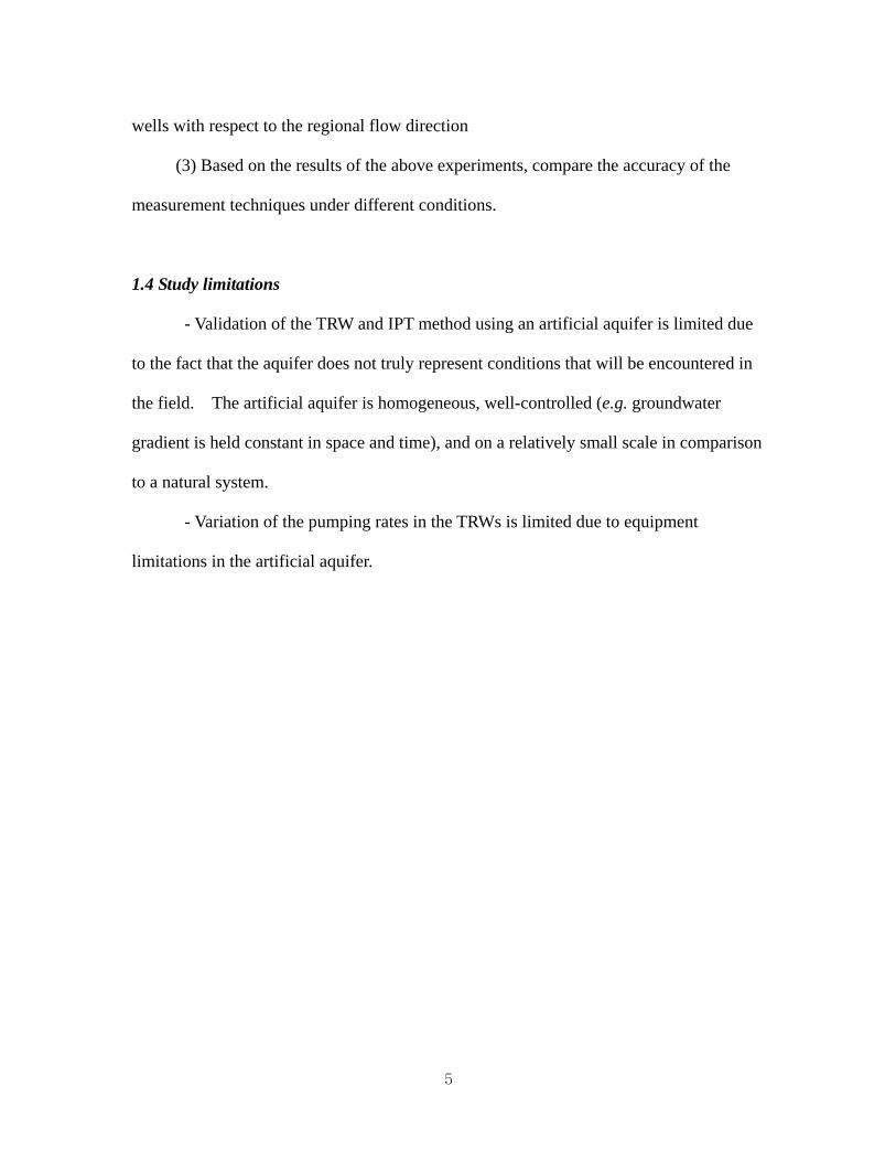
wells with respect to the regional flow direction
(3) Based on the results of the above experiments, compare the accuracy of the
measurement techniques under different conditions.
1.4 Study limitations
- Validation of the TRW and IPT method using an artificial aquifer is limited due
to the fact that the aquifer does not truly represent conditions that will be encountered in
the field. The artificial aquifer is homogeneous, well-controlled (e.g. groundwater
gradient is held constant in space and time), and on a relatively small scale in comparison
to a natural system.
- Variation of the pumping rates in the TRWs is limited due to equipment
limitations in the artificial aquifer.
5

II. Literature review
2.1 Introduction
In this chapter, we review the literature regarding TRW and IPT methods. After
looking at why flux is an important parameter to measure, we investigate in some detail
the particulars of the TRW and IPT flux measurement methods, which are the focus of
this study.
2.2 Background
The goal of groundwater remediation is to reduce the risk posed to human and
environmental receptors by contaminants in the subsurface. Thus, when cleaning up a
source of groundwater contamination or evaluating the movement of contaminants in a
groundwater plume, our focus should not be on the contaminant concentration; it should
be on the rate with which contaminant mass is transported toward receptors (i.e. the
contaminant mass flux). Einarson and Mackay (2001) showed how the risk, which is a
function of the contaminant concentration at a receptor, is related to the flux of
contaminant. Considering the example of a contaminant plume being captured by a
water supply well (Figure 1), Einarson and Mackay (2001) showed that the contaminant
concentration (Csw) in a downgradient water supply well, pumping at rate Qsw can be
calculated as:
Csw = Mf ×A / Qsw (1)
where Mf is the contaminant mass flux[ML-2T] emanating from a contaminant source
whose plume is captured by the supply well and A[L2] is area of the capture zone
6

orthogonal to the groundwater flow direction that is captured by well.
Supply well capture zone
Source
Contaminant PlumeConcentration (C)
Mass flux (Mf)
Cross Sectional Area (A)
Supply well
Pumping rate Q
Darcy velocity (q0)
Supply well capture zone
Source
Contaminant PlumeConcentration (C)
Mass flux (Mf)
Cross Sectional Area (A)
Supply well
Pumping rate Q
Supply well capture zone
Source
Contaminant PlumeConcentration (C)
Mass flux (Mf)
Cross Sectional Area (A)
Supply well
Pumping rate Q
Supply well capture zone
Source
Contaminant PlumeConcentration (C)
Mass flux (Mf)
Cross Sectional Area (A)
Supply well
Pumping rate Q
Supply well capture zone
Source
Contaminant PlumeConcentration (C)
Mass flux (Mf)
Cross Sectional Area (A)
Supply well
Pumping rate Q
Darcy velocity (q0)
Figure 1. Plan view of a contaminated site (Einarson and Mackay, 2001)
Mf can be obtained from equation (2):
Mf = q × C (2)
where q is the Darcy velocity of the groundwater [L/T] and C [ML-3] is the contaminant
concentration emanting from the source area. As shown in equation (2), contaminant
concentration, C, is only one component of mass flux. Even though the concentration of
contaminant leaving the source area is high, if the Darcy velocity is small, the impact of
the source on the downgradient water supply well will be small. As described above, it
is contaminant mass flux, rather than contaminant concentration, that is key in
determining the risk posed by a contaminant source and plume. To measure the
contaminant mass flux, the following methods are in use or being developed: (1) the
transect method (Borden et al., 1997), (2) the passive flux meter (PFM) method (Hatfield
7
et al., 2004), (3) the integral groundwater investigation method(IGIM) (Bockelmann et
al., 2003), (4) the integral pump test (IPT) method, which is a modified version of the
IGIM, proposed by Brooks (2005), and (5) the tandem recirculating well (TRW) method
(Kim, 2005; Huang et al., 2005).
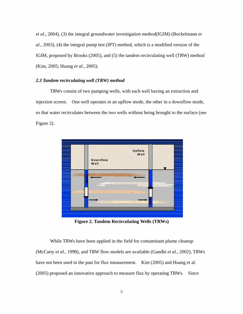
2.3 Tandem recirculating well (TRW) method
TRWs consist of two pumping wells, with each well having an extraction and
injection screen. One well operates in an upflow mode, the other in a downflow mode,
so that water recirculates between the two wells without being brought to the surface (see
Figure 2).
Dow nflowW ell
U pflowW ell
Figure 2. Tandem Recirculating Wells (TRWs)
While TRWs have been applied in the field for contaminant plume cleanup
(McCarty et al., 1998), and TRW flow models are available (Gandhi et al., 2002), TRWs
have not been used in the past for flux measurement. Kim (2005) and Huang et al.
(2005) proposed an innovative approach to measure flux by operating TRWs. Since
8

contaminant mass flux can be calculated as the product of the groundwater Darcy
velocity (q0) and contaminant concentration (C), and, by Darcy’s Law, Darcy velocity is
the product of hydraulic gradient (i) and hydraulic conductivity (K), the following
equation can be used to calculate contaminant mass flux (Mf):
CiKM f ××= (3)
The TRW method involves individually measuring K, i, and C in order to
determine contaminant mass flux. Hydraulic gradient may be determined by measuring
the piezometric surface at the two TRWs, with the pumps turned off, and a third
piezometer. Volume-averaged contaminant concentration in the TRWs can be measured
by sampling the contaminated water as it flows through the wells. To measure hydraulic
conductivity, two techniques, both of which were tested by Kim (2005), were proposed.
These two techniques, the multi-dipole technique and the tracer technique, are described
in detail below.
2.3.1 Multi-dipole technique to measure hydraulic conductivity
The multi-dipole technique is based on the dipole flow test method to measure
hydraulic conductivity developed by Kabala (1993). The dipole flow test involves use
of a dual-screen well, with a packer separating the screens. The well is pumped at a
constant rate, with water flowing in a downward direction; that is, water is extracted from
the aquifer into the well through the upper screen and injected into the aquifer through the
lower screen. From transient or steady-state drawdown measurements at the upper
screen, estimates can be obtained for the value of vertical and horizontal hydraulic
conductivity (Kabala, 1993).
9

Goltz et al. (2006) presented an analytical equation to calculate drawdown resulting
from operation of a TRW system operating in a horizontally infinite aquifer. Using this
analytical formula, if the parameters describing the system are known (well pumping
rates, hydraulic gradient, the radius and coordinates of the pumping wells, vertical
coordinates of the top and bottom screens, and the thickness of the aquifer) the drawdown
and mounding of the wells can be measured to allow calculation of hydraulic
conductivities using inverse methods.
By operating the TRWs at a series of different flow rates, the drawdown at the
downflow well and the mounding at the upflow well can be measured at each flow rate.
Then the analytical formula can be applied to obtain the “best” value of hydraulic
conductivity that maximizes the objective function:
∑=
−+
=N
i
icalc
imeas
obj
HH
F
1
2)(1
1 (4)
where and indicate the measured and calculated hydraulic heads at the iimeasH i
calcH th
flow rate, respectively, and N is the total number of head measurements. The method
can be applied assuming isotropic (that is, horizontal and vertical hydraulic conductivities
are the same) or anisotropic conductivities. A genetic algorithm (Carroll, 1996) may be
used to determine the best value of hydraulic conductivity that maximizes the objective
function (see Figure 3). In this algorithm, each individual value is improved genetically
over generations.
10

Assume hydraulic conductivity of an individual
(k if isotropic or kr and kz if anisotropic)
Calculate drawdown/mounding based on
analytical formula (Goltz et al., 2006)
Compare measured and calculated drawdown/mounding and evaluate Fobj (Equation
(2)) for the individual
Repeat for N individuals and M generations until “best” value of k or kr/ kz is found (the value that maximizes Fobj)
Figure 3. Genetic algorithm procedure
2.3.2 Tracer test technique to measure hydraulic conductivity
The tracer test technique involves operating the TRWs and using tracers to
measure hydraulic conductivity.
In Figure 4, Iij represents the fraction of flow entering injection well screen i that
originated at extraction well screen j. As shown in figure 4, tracers can be injected at
11

the two injection well screens of the two TRWs. If we assume the flow field and the
tracer concentrations at the four well screens are at steady-state, the four unknown
fractional flows can be obtained using the following four mass balance equations:
3434131
3434131
2424121
2424121
BIBIBAIAIABIBIBAIAIA
=+=+=+=+
(5)
where Ai and BB
Figure 4. TRW fractional flows and tracer injection screens (Goltz et al., 2004)
i are the concentrations of tracers A and B measured at screen i (Huang et
al., 2005). As shown by equation (5), these steady-state tracer concentrations are key to
determining the four fractional flows accurately. It is potentially difficult to accurately
measure the steady-state values of the concentration because there may be concentration
fluctuations over time along with random measurement errors. Fortunately, Kim (2005)
found that the values of fractional flow obtained from equation (5) were relatively
insensitive to the method used in averaging the concentration measurements obtained at
the TRWs.
Upflow
well
Downflow
well
I13
I42
I43I12
Tracer A injection
Tracer B Injection
S2
S1
S4
S3
Q34Q12
12
erical m
odel
With the estimates of the four fractional flows based on the tracer test, inverse
num odeling can be used to obtain the hydraulic conductivity as follows.
Assuming a value of hydraulic conductivity, the three dimensional numerical flow m
MODFLOW (Harbaugh and McDonald, 1996) can be used to simulate interflows
between the four TRW well screens. The optimal hydraulic conductivity should
maximize the following objective function:
∑∑= =
−+
=inj extN
i
N
j
calcij
measij
obj
IIF
1 1
2)(1
1 (6)
where and are the measured and calculated fractional flows, respectively,
and Ninj and Next are the number of injection and extraction well screens, respectively.
the IPT method as a method that can be used to
x,y)
measijI calc
ijI
The method can be applied assuming isotropic (that is, horizontal and vertical
hydraulic conductivities are the same) or anisotropic conductivities. A genetic
algorithm (Carroll, 1996) may be used to determine the best value of hydraulic
conductivity that maximizes the objective function.
2.4 Integral pump test (IPT) method
Brooks (2005) recently suggested
obtain an estimate of contaminant mass flux averaged over a large subsurface volume.
The method avoids the data analysis complexities of the IGIM, which requires multiple
concentration measurements over time, and unlike the IGIM and TRW techniques, it does
not require separate measurements of hydraulic conductivity and hydraulic gradient.
Assuming a homogeneous, isotropic, confined aquifer with uniform thickness
under steady-state and uniform flow conditions, the complex potential at some point (
13

(W(x,y)) can be expressed by equation (5) (Javandel, et al., 1984; Christ, J. A. 1997);
),(),(),( yxiyxyxW
ψφ += (7)
Where φ (x,y) is the real velocity potential and ψ (x,y) is the imag
ity potential
inary stream function
at location (x,y).
The veloc (φ ) at (x, y) is calculated by superposing the potentials due
to the uniform regional flow and pumping well sinks (Javandel, et al., 1984):
[ ] 122
0 )()(ln1)sincos(),( CyyxxQyxqyx ii
N
i +−+−++−= ∑ααφ 14 B i=π
(8)
rcy velocity of uniform regional flow [LT-1]
the positive x-axis [-]
ll [L3T-1]
well, respectively [L]
ead (h) is related to the velocity potential by equation (9) (Javandel, et al.,
where
q0 = Da
α = angle between the direction of regional flow and
B = Aquifer thickness [L]
Qi = Pumping rate of ith we
xi, yi = x, y coordinates of ith pumping
N = Total number of pumping wells
C1 = Constant
The hydraulic h
1984):
2CKh +=φ (9)
nd C2 is a cwhere K is the hydraulic conductivity a onstant.
Combining equations (8) and (9), we obtain:
[ ] CyyxxQBKK
yxqyxh
N
++−
= ∑0 1)sincos(),(
αα iii
i +−+−=
22
1
)()(ln4π
(10)
or
14
[ ] CyyxxQT
yxT
Bqyxh ii
N
ii +−+−++−= ∑
=
22
1
0 )()(ln4
1)sincos(),(π
αα (11)
where C is a constant and T is the transmissivity [L2T-1] (T = KB).
ular to the regional
e
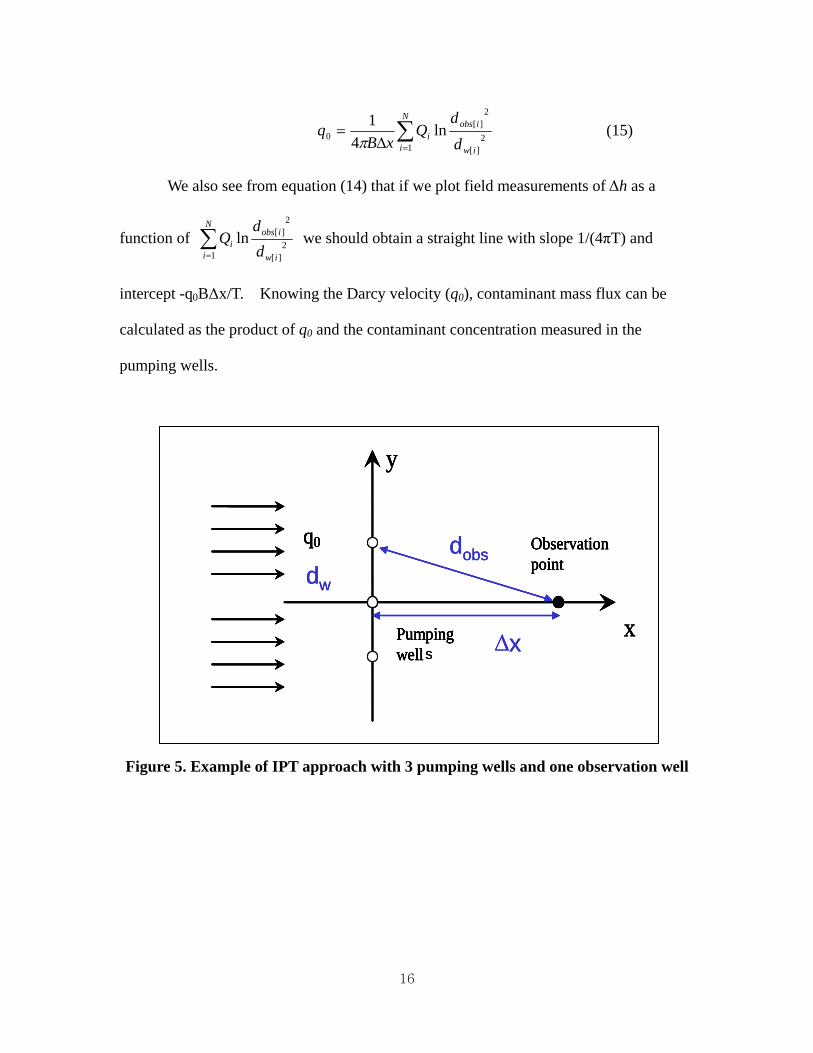
If we have N pumping wells aligned along the y-axis perpendic
groundwater flow direction (which is defined as the positive x-direction), and a single
observation well on the x-axis at a distance xobs downgradient of the pumping wells (se
Figure 5), we can use equations (12) and (13) to calculate the heads at the pumping well
located at the origin and the observation well, respectively.
CdQxBq
xh iw
N
iww +−= ∑ 2][
0 ln1)0,(TT i
+=14π
(12)
CdQT
xT
Bqxh obs =)0,( iobs
N
iiobs ++− ∑
=
2][
1
0 ln4
1π
(13)
ius of pumping well at the origin [L]
-axis [L]
g well at the origin [L]
where
xw = rad
xobs = distance to the observation well along x
dw[i] = distance from the ith pumping well to the pumpin
dobs[i] = distance from the ith pumping well to the observation well
Subtracting equation (12) from (13):
2][
2][
1
0 ln4
1
iw
iobsN
ii d
dQ
Tx
TBq
h ∑=
+Δ−=Δπ
(14)
where Δx is xobs – xw and Δh is the difference in heads measured at the pumping well at
ed by equation (15):
the origin and the observation well.
We see that when Δh=0, q0 can be obtain
15
2][
2][
10 ln
41
iw
iobsN
ii d
dQ
xBq ∑
=Δ=
π (15)
We also see from equation (14) that if we plot field measurements of Δh as a
function of 2][
2][
1
lniw
iobsN
ii d
dQ∑
=
we should obtain a straight line with slope 1/(4πT) and
intercept -q0BΔx/T. Knowing the Darcy velocity (q0), contaminant mass flux can be
calculated as the product of q0 and the contaminant concentration measured in the
pumping wells.
x
y
q0 Observation point
Pumping well ∆x
dobsdw
s
x
y
q0 Observation point
Pumping well ∆x
dobsdw
x
y
q0 Observation point
Pumping well
x
y
q0 Observation point
Pumping well ∆x
dobsdw
s
Figure 5. Example of IPT approach with 3 pumping wells and one observation well
16

III. Methodology
3.1 Introduction
This chapter describes the detailed procedure for measuring mass flux using the
TRW and IPT methods. In section 3.2, the artificial aquifer which is used for the flux
measurement experiments is described. In section 3.3, experimental conditions and
details on the two techniques used in the TRW method, the multi-dipole technique and
the tracer test technique, are explained. In section 3.4, experimental conditions and
details on the operation of the IPT method are described.
3.2 Artificial aquifer
Evaluation of the TRW and IPT methods was conducted in a meso-scale three
dimensional, confined artificial aquifer in Canterbury, New Zealand (Bright et al.,2002)
(figure 6).
The inner dimensions of the relatively homogeneous sand aquifer are 9.5 m long,
by 4.7 m wide, by 2.6 m deep. The aquifer is filled with coarse sand that was dry sieved
to fall within the size range 0.6 to 1.2 mm in diameter. Constant-head tanks at the
aquifer’s upstream and downstream ends are used to control the hydraulic gradient. The
bottom and sides of the aquifer are no-flow boundaries lined with impermeable butyl
rubber.
As shown in Figure 6, there are 45 wells installed on a l m by 1 m grid, with 9
columns and 5 rows. Each well is a 2.5 cm diameter tube extending to the bottom of the
aquifer. Most of the wells have four sampling ports at depths of 0.4 m, 1.0 m, 1.6 m, and
17

2.2 m below the top of the aquifer, with two wells having seven sampling points. Each
sampling port consists of a 7.5 cm long section of well screen with a Teflon sample tube
extending from the sampling depth to an automatic sample collector (Bright et al., 2002;
Kim, 2005). In the TRW and IPT method evaluations, flux of chloride, which is
naturally present in the water, was measured.
4.7
m
1 2 3 4 5 6 7 8 9
E
D
C
B
A
9.5 m
Upstrea
m tank
Sampling
well (3E)
Downstrea
m tank
0.4m
1.0m
1.6m
2.0m
Depth of
sampling
points (m)
Figure 6. Plan and vertical views of sampling wells in the artificial aquifer (Bright et al., 2002)
3.3 TRW experiment
3.3.1 TRW installation and operation
A TRW well pair was installed in the artificial aquifer at locations 7B and 7D
(Figure 7, the upflow TRW at 7D and the downflow at 7B). Water containing chloride
18
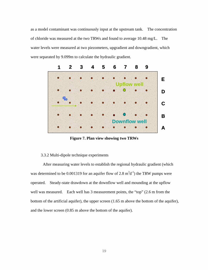
as a model contaminant was continuously input at the upstream tank. The concentration
of chloride was measured at the two TRWs and found to average 10.48 mg/L. The
water levels were measured at two piezometers, upgradient and downgradient, which
were separated by 9.099m to calculate the hydraulic gradient.
1 2 3 4 5 6 7 8 9
E
D
C
B
ADownflow well
Upflow well
q0
1 2 3 4 5 6 7 8 9
E
D
C
B
ADownflow well
Upflow well
q0
Figure 7. Plan view showing two TRWs
3.3.2 Multi-dipole technique experiments
After measuring water levels to establish the regional hydraulic gradient (which
was determined to be 0.001319 for an aquifer flow of 2.8 m3d-1) the TRW pumps were
operated. Steady-state drawdown at the downflow well and mounding at the upflow
well was measured. Each well has 3 measurement points, the “top” (2.6 m from the
bottom of the artificial aquifer), the upper screen (1.65 m above the bottom of the aquifer),
and the lower screen (0.85 m above the bottom of the aquifer).
19

3.3.3 Tracer test technique experiments
TRWs were installed in the artificial aquifer at locations 7B and 7D (the upflow
TRW at 7D, the downflow at 7B). The injection screens (the upper screen of the upflow
well and the lower screen of the downflow well) and the extraction screens (the lower
screen of the upflow well and the upper screen of the downflow well) were constructed
using 2.5 cm diameter PVC. The injection/extraction screens are 22.5 cm long, each
consisting of two 7.5 cm long PVC slotted sections separated by a 7.5 cm long PVC blank.
The injection and extraction screens in each well are separated by 1.28 m, with the upper
and lower end of each screen isolated using inflatable rubber packers. Two pumps were
used (one for each TRW) to extract water from the extraction screen and inject water into
the injection screen at a specified flow rate.
After measuring the water levels at two piezometers, upgradient and
downgradient, to calculate the hydraulic gradient (determined to be 0.00148 at an aquifer
flow rate of 2.94 m3d-1), the TRW pumps were turned on. The downflow and upflow
wells were operated at 2.56 m3d-1 and 2.32 m3d-1, respectively. Bromide tracer was
injected into the injection screen of the upflow well and nitrate injected into the injection
screen of the downflow well. Injection of bromide and nitrate tracers was continued for
240 and 336 hours, respectively, until steady-state concentrations were reached at the two
extraction screens. Concentrations of bromide, chloride, and nitrate were measured over
time at all four TRW screens, for application of the tracer test technique.
The concentration of chloride at all screens averaged 10.48 mg/L.
20

3.4 IPT method experiment
For measuring mass flux using the IPT method, three experiments were
implemented under different conditions. Experiment 1 was repeated in order to obtain a
preliminary estimate of method precision. Table 1 shows the pumping and observation
wells used in the three IPT experiments run in the artificial aquifer.
In IPT experiments 1 and 3, a single pumping well was used while in experiment
2 three pumping wells were used. In experiments 1 and 2 the pumping and/or
observation wells were aligned perpendicular to the groundwater regional flow direction
while in experiment 3 the observation wells were at an angle to the regional flow
direction.
Table 1. Pumping and observation wells for IPT Experiments
Experiment Pumping well Observation well
1 3C 7B, 7C, 7D
2 2B, 2C, 2D 8B, 8C, 8D
0° 7D
26.6° 6C 3
63.4°
4D
5B
To obtain plots of Δh as a function of 2][
2][
1ln
iw
iobsN
ii d
dQ∑
=
all three IPT experiments
were conducted with four pumping rates. To apply Equation (15) it is necessary that the
plot of Δh as a function of 2][
2][
1ln
iw
iobsN
ii d
dQ∑
=
cross the x-axis (Δh = 0), so it is desirable
21

that pumping rates be chosen so that two of the pumping rates lead to positive values of
Δh and two lead to negative values. Prior to running the tests, back-of-the-envelope
calculations were accomplished to estimate the appropriate four pumping rates.
In each experiment, the pumps were started at the lowest pumping rate and kept
running until steady-state water levels were reached. In this study, it was estimated that
18 hrs of constant pumping was adequate to achieve steady-state conditions in the
artificial aquifer. After running the pumping well for 18 hours, the hydraulic head at
the pumping well was observed for at least 1 hour, and if the water level remained
constant, equilibrium conditions were assumed. After measuring the water levels of the
pumping and observation wells at the lowest pumping rate, the rate was increased. This
was repeated until all four pumping rates were run for each experiment.
22
IV. Results and Discussion
4.1 Introduction
In section 4.2, the data and flux measurement results obtained from TRW method
experiments are presented and analyzed. In section 4.3, the data and results form IPT
method experiments are presented and analyzed.
4.2 TRW method
4.2.1 Multi-dipole method
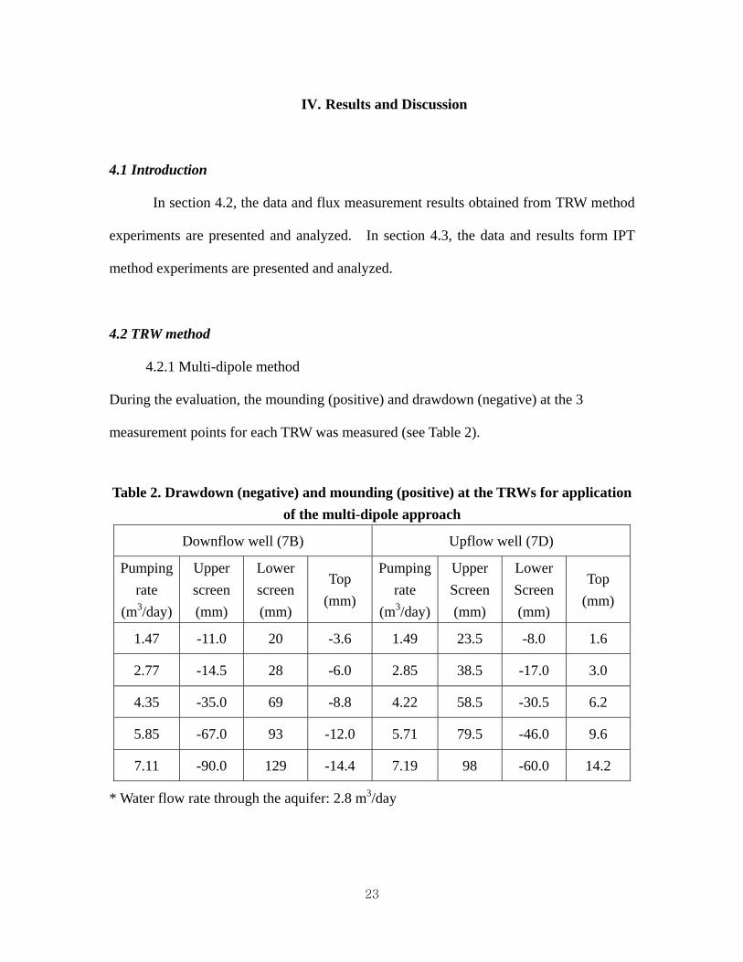
During the evaluation, the mounding (positive) and drawdown (negative) at the 3
measurement points for each TRW was measured (see Table 2).
Table 2. Drawdown (negative) and mounding (positive) at the TRWs for application of the multi-dipole approach
Downflow well (7B) Upflow well (7D)
Pumping rate
(m3/day)
Upper screen (mm)
Lower screen (mm)
Top (mm)
Pumpingrate
(m3/day)
Upper Screen (mm)
Lower Screen (mm)
Top (mm)
1.47 -11.0 20 -3.6 1.49 23.5 -8.0 1.6
2.77 -14.5 28 -6.0 2.85 38.5 -17.0 3.0
4.35 -35.0 69 -8.8 4.22 58.5 -30.5 6.2
5.85 -67.0 93 -12.0 5.71 79.5 -46.0 9.6
7.11 -90.0 129 -14.4 7.19 98 -60.0 14.2
* Water flow rate through the aquifer: 2.8 m3/day
23

As described earlier, a genetic algorithm (Carroll, 1996) was used to obtain the
best fit value of hydraulic conductivity that maximized the objective function in Equation
(4) for all five pumping rates.
Table 3. Hydraulic conductivities and mass fluxes measured using the multi-dipole approach
Hydraulic conductivity (m/d)
Mass fluxes (g/m2*d) Pumping rate
(L/min) Anisotropic (kr ≠ kz)
Isotropic (kr = kz)
Measured Actual
Downflow Upflow kr kz k Anisotropic (using kr)
Isotropic
1.47 1.49 8.15 0.15 5.16 0.11 0.07
2.77 2.85 10.26 0.31 4.93 0.14 0.07
4.35 4.22 4.63 0.07 3.81 0.06 0.05
5.85 5.71 5.53 0.11 3.40 0.08 0.05
7.11 7.19 4.52 0.05 3.30 0.06 0.05
Using all data 4.56 0.05 4.68 0.06 0.06
2.41
* kr : Horizontal hydraulic conductivity, kz : Vertical hydraulic conductivity
Table 3 shows the best fit values of hydraulic conductivity, chloride mass flux
measured, and actual mass flux. The actual chloride mass flux of 2.41 g m-2d-1 was
determined by multiplying the chloride concentration of 10.48 g/m3 by the flow through
the aquifer (2.8 m3d-1) and dividing by the cross-sectional area of the aquifer (12.2 m2).
As shown in Table 2, the measured mass fluxes are one to two orders of magnitude less
than the actual flux. It appears that the multi-dipole technique is insufficiently accurate
24

to be used to measure flux. Kim (2005) speculated that the inaccuracy was due to the
sensitivity of method results to relatively small head measurements, and that increasing
the TRW pumping rates would improve measurements. Results from this study,
however, indicate that increased TRW pumping rates do not improve results, and method
inaccuracies are due to some other problem.
4.2.2 Tracer test technique
TRWs were installed in the artificial aquifer at locations 7B and 7D (the upflow
TRW at 7D, the downflow at 7B). The injection screens (the upper screen of the upflow
well and the lower screen of the downflow well) and the extraction screens (the lower
screen of the upflow well and the upper screen of the downflow well) were constructed
using 2.5 cm diameter PVC. The injection/extraction screens are 22.5 cm long, each
consisting of two 7.5 cm long PVC slotted sections separated by a 7.5 cm long PVC blank.
The injection and extraction screens in each well are separated by 1.28 m, with the upper
and lower end of each screen isolated using inflatable rubber packers. Two pumps were
used (one for each TRW) to extract water from the extraction screen and inject water into
the injection screen at a specified flow rate.
After measuring the water levels at two piezometers, upgradient and
downgradient, to calculate the hydraulic gradient (determined to be 0.00148 at an aquifer
flow rate of 2.94 m3d-1), the TRW pumps were turned on. The downflow and upflow
wells were operated at 2.56 m3d-1 and 2.32 m3d-1, respectively. Bromide tracer was
injected into the injection screen of the upflow well and nitrate injected into the injection
screen of the downflow well. Injection of bromide and nitrate tracers was continued for
25

240 and 336 hours, respectively, until steady-state concentrations were reached at the two
extraction screens. Concentrations of bromide, chloride, and nitrate were measured over
time at all four TRW screens, for application of the tracer test technique.
The concentration of chloride at all screens averaged 10.48 mg/L. Figures 8 and
9 show the concentration of bromide and nitrate, respectively, over time at the four TRW
well screens.
0
5
10
15
20
25
0 100 200 300 400Time (hours)
Con
cent
ratio
n (m
g/L
)
Upflow injectionDownflow injection
DownflowextractionUpflowextraction
Figure 8. Bromide concentration over time at TRW screens
26

0
2
4
6
8
10
12
14
0 100 200 300 400Time (hours)
Con
cent
ratio
n (m
g/L
)
UpflowinjectionDownflowinjectionDownflowextractionUpflowextraction
Figure 9. . Nitrate concentration over time at TRWs
Note that to apply equation (5) the steady-state tracer concentrations at the well
screens are needed. As shown in Figure (8), the bromide concentration has reached
steady-state at about 145 hours. Bromide steady-state concentration is obtained by
averaging the measured concentrations from 145 to 205 hours. As shown in Figure (9),
the nitrate concentration also has reached steady-state at about 145 hours. Nitrate
steady-state concentration is obtained by averaging the measured concentrations from
145 to 301 hours. Table 4 lists the steady-state concentrations of tracers at the TRW’s
four screens. Kim (2005) used four different methods to estimate steady-state
concentrations over different time ranges and found that the results were not sensitive to
the estimation method.
27

Table 4. Steady–state tracer concentrations at TRW screens (g/m3)
Upflow Downflow Tracer
injection extraction injection extraction
Bromide 22.10 7.94 7.00
(6.84) 7.00
(7.17)
Nitrate 3.26
(3.28) 3.26
(3.24) 10.87 3.63
* Note that according to the tracer test technique theory, bromide concentrations in the extraction and injection screens of the downflow well and the nitrate concentrations in the extraction and injection screens of the upflow well should be the same. Average values are used in this study. Numbers in parentheses indicate measured concentrations before averaging.
Perhaps the main disadvantage of the tracer test technique is the cost of tracers
and their analysis. Kim (2005) proposed a cost-saving method based upon using a
single tracer. If one assumes symmetry between the flow fields induced by each of
the TRWs, it is possible to extrapolate the results of a test using a single tracer in order to
apply the tracer test technique. If we assume symmetry, looking at Figure 4, we see I13
is equal to I42 and I12 is equal to I43. Thus, the four unknowns in equation (5) are
reduced to two unknowns, and it is only necessary to measure the steady-state
concentrations of a single tracer at the four well screens to solve the two equations with
two unknowns. Note that to apply this technique, it’s also necessary to assume both
TRWs are pumping at the same rate.
Table 5 shows the hydraulic conductivities and mass fluxes calculated using the
tracer test technique. Values of hydraulic conductivity assuming anisotropy and
isotropy were obtained by using a genetic algorithm (Carroll, 1996) to obtain the best fit
28

value of hydraulic conductivity that maximized the objective function in Equation (6).
In the top row of Table 5 (the two-tracer method), results are presented based on the
steady-state concentrations of both the bromide and nitrate tracers at the four well screens.
The next four rows present results for the one tracer method described in the paragraph
above. The actual chloride mass flux of 2.53 g m-2d-1 was determined by multiplying
the chloride concentration of 10.48 g/m3 by the flow through the aquifer (2.94 m3d-1) and
dividing by the cross-sectional area of the aquifer (12.2 m2).
Table 5. Hydraulic conductivities and mass flux calculated using the tracer test technique
Mass flux (g/m2*d) Hydraulic conductivity(m/d) Measured
Anisotropic (kr ≠ kz)
Isotropic (kr = kz)
Method Tracer Pumping
rate (m3/day)
kr kz k
Anisotropic
(using kr) Isotropic
Actual
Two tracers
Br-Nitrate
Upflow: 2.59 Downflow: 2.32
98.3 49.7 183.5 1.52 2.85
Br 2.46 114 65.0 183.2 1.77 2.84
Nitrate 2.46 100 51.0 198.3 1.56 3.08
Br 2.59 97.7 50.9 188.1 1.51 2.92
One tracer
Nitrate 2.32 98.2 50.8 187.1 1.52 2.90
2.53
For the two-tracer test assuming isotropy, the measurement overestimates the
actual flux by only 13 %. For the one tracer test assuming isotropy, the measured mass
fluxes are also close to the actual value, overestimating the actual value between 13% and
22%. It appears that at least in the relatively homogeneous conditions of the artificial
aquifer, the assumption of symmetry is appropriate and results obtained from a single
29

tracer approximate the results obtained using two tracers. Assuming anisotropy, the
mass flux measurements were lower than those assuming isotropy, underestimating the
actual value between 30% and 40%. It appears that for the relatively homogeneous and
isotropic artificial aquifer, the mass fluxes measured by the tracer test technique when
assuming isotropy are better than those measured assuming anisotropic conditions.
Similarly, Kim (2005) found that for the artificial aquifer, results obtained when assuming
isotropy were significantly more accurate than were obtained assuming anisotropy.
4.3 IPT method
Table 6, 7 and 8 show the measurements of the hydraulic head at each pumping
and observation well at all pumping rates for Experiments 1, 2, and 3 respectively. To
apply the IPT method, the regional flow direction must be determined. The regional
flow direction can be determined by head measurements with the pumps turned off. The
coordinate system is set up with the pumping well at the origin. In the case of multiple
pumping wells (Experiment 2), the center well is located at the origin and the other wells
are aligned on the y-axis. The x-axis is defined as the line connecting the pumping well
at the origin with an observation well. In the case of Experiments 1 and 2, the x-axis
was the line connecting the pumping well at 3C with observation well 7C (experiment 1)
or the line connecting the pumping well at 2C with the observation well at 8C
(experiment 2). In both cases, the x-axis and regional groundwater flow direction
coincided, so α in Equation (6) was set equal to 0.
30
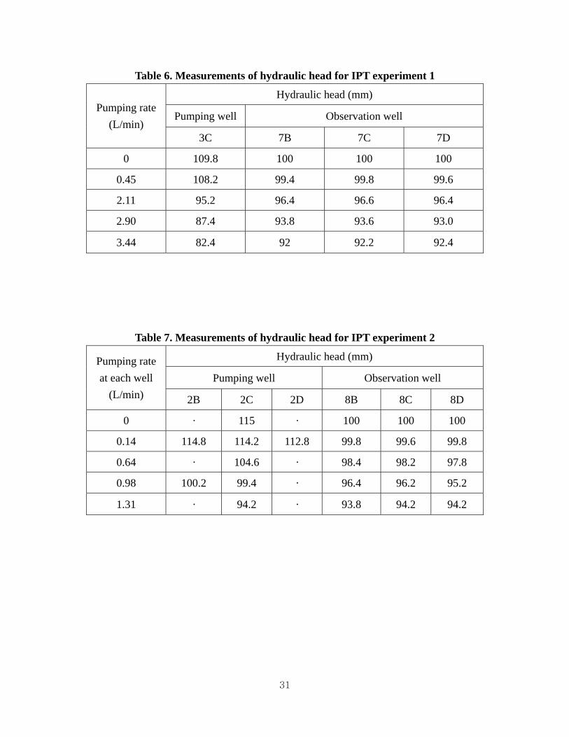
Table 6. Measurements of hydraulic head for IPT experiment 1
Hydraulic head (mm)
Pumping well Observation well Pumping rate
(L/min) 3C 7B 7C 7D
0 109.8 100 100 100
0.45 108.2 99.4 99.8 99.6
2.11 95.2 96.4 96.6 96.4
2.90 87.4 93.8 93.6 93.0
3.44 82.4 92 92.2 92.4
Table 7. Measurements of hydraulic head for IPT experiment 2
Hydraulic head (mm)
Pumping well Observation well Pumping rate at each well
(L/min) 2B 2C 2D 8B 8C 8D
0 · 115 · 100 100 100
0.14 114.8 114.2 112.8 99.8 99.6 99.8
0.64 · 104.6 · 98.4 98.2 97.8
0.98 100.2 99.4 · 96.4 96.2 95.2
1.31 · 94.2 · 93.8 94.2 94.2
31

Table 8. Measurements of hydraulic head for IPT experiment 3
Hydraulic head (mm)
Pumping well Observation well Pumping rate
(L/min) 4D 5B 6C 7D
0 105.0 102.6 100.0 98.0
2.0 91.6 96.2 94.8 93.0
2.5 87.4 94.6 93.0 91.4
3.0 84.0 93.0 91.4 90.2
4.18 74.8 87.6 87.4 86.8
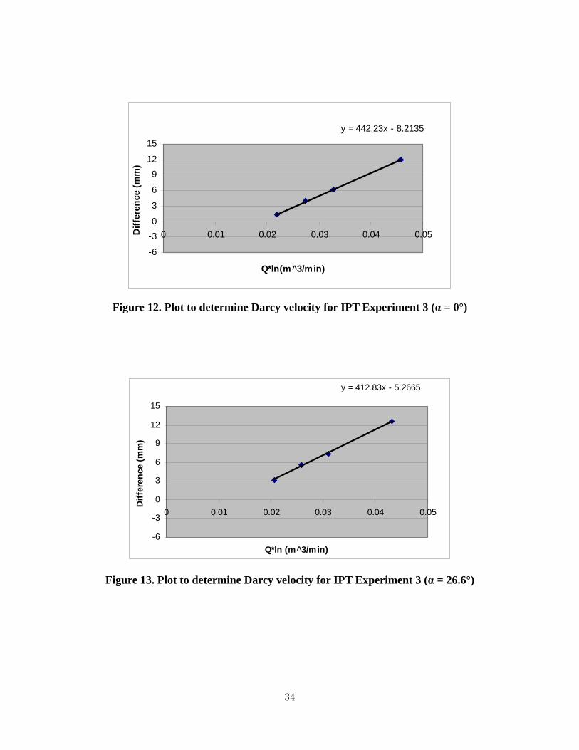
For experiment 3, where the pumping well was at 4D, the value of α was 0.464
radians (26.6°), and 1.11 radians (63.4°) for the observation wells at 7D, 6C, and 5B,
respectively. For the three experiments, the Δh vs 2][
2][
1
lniw
iobsN
ii d
dQ∑
=
plots are shown in
Figures from 10 to 14. Note that in accordance with the theory, the plots are relatively
linear, with correlation coefficients close to 1.0. The fact that the study was done in a
relatively homogeneous confined artificial aquifer undoubtedly contributed to the
linearity of the results.
Using equation (15), the intercept of the x-axis in Figure 10 can be used to derive
the Darcy velocity (q0). Multiplying Darcy velocity by the concentration gives us an
estimate of flux. Darcy velocities and flux measured by each experiment are shown in
Table 9. The actual chloride mass flux was determined by multiplying the chloride
concentration of 10.48 g/m3 by the flow through the aquifer (3.75, 3.95, and 3.82 m3d-1
for experiments 1, 2, and 3, respectively) and dividing by the cross-sectional area of the
aquifer (12.2 m2).
32

y = 528.95x - 11.455R2 = 0.9982
-10
-5
0
5
10
15
0 0.01 0.02 0.03 0.04 0.05
Q*Ln (m^3/min)
Diffe
renc
e (m
m)
Figure 10. Plot to determine Darcy velocity for IPT Experiment 1
y = 629.17x - 15.603R2 = 0.9761
-20
-15
-10
-5
0
5
0 0.005 0.01 0.015 0.02 0.025 0.03
∑Q*ln(ε) (m^3/min)
Diffe
rece
s(m
m)
Figure 11. Plot to determine Darcy velocity for IPT Experiment 2
33
y = 442.23x - 8.2135
-6
-30
3
6
912
15
0 0.01 0.02 0.03 0.04 0.05
Q*ln(m^3/min)
Diff
eren
ce (m
m)
Figure 12. Plot to determine Darcy velocity for IPT Experiment 3 (α = 0°)
y = 412.83x - 5.2665
-6
-3
0
3
6
9
12
15
0 0.01 0.02 0.03 0.04 0.05
Q*ln (m^3/min)
Diff
eren
ce (m
m)
Figure 13. Plot to determine Darcy velocity for IPT Experiment 3 (α = 26.6°)
34

y = 354.44x - 2.3034
-6
-3
0
3
6
9
12
15
0 0.01 0.02 0.03 0.04 0.05
Q*ln (m^3/min)
Diff
eren
ce (m
m)
Figure 14. Plot to determine Darcy velocity for IPT Experiment 3 (α = 63.4°)
Table 9. Darcy velocity (q0) and mass fluxes for IPT experiments
Mass flux (g/m2*d) Experiment
∑Q*ln(ε) (Δh=0) (m3/min)
q0(m/day) Measured Actual
1 0.022 0.24 2.51 4.64
2 0.025 0.18 1.91 4.89
0° 0.018 0.28 2.90
26.6° 0.013 0.28 3.00 3
63.4° 0.006 0.29 3.00
4.72
Note from Table 9 that the measured mass flux underestimates the actual flux by
between 36% and 60%. This large an error is somewhat surprising, given the relative
homogeneity of the artificial aquifer. We can consider several possible sources of error.
There are a number of assumptions upon which the IPT method is based. The method
35

assumes the IPT is conducted in a confined aquifer, with infinite boundary conditions,
uniform regional flow, and hydraulic heads are at steady state. Clearly, the artificial
aquifer is not an infinite system. In order to account for the no-flow boundary
established by the walls of the artificial aquifer, image wells can be used, as shown in
Figure 15. Table 10 shows the measured fluxes when accounting for the no-flow
boundaries. It appears that the measured flux is more accurate by between 7% and 19%
when accounting for the boundaries.
2.35m
2.35m
I1
I5
I7
I2
I3
Observation
I4
I8
I6
Pumping
2.35m
2.35m
Boundaries2.35m
2.35m
I1
I5
I7
I2
I3
Observation
I4
I8
I6
Pumping
2.35m
2.35m
2.35m
2.35m
I1
I5
I7
I2
I3
Observation
I4
I8
I6
Pumping
2.35m
2.35m
Boundaries
Figure 15. Image wells used to account for no-flow boundaries in IPT experiments
36
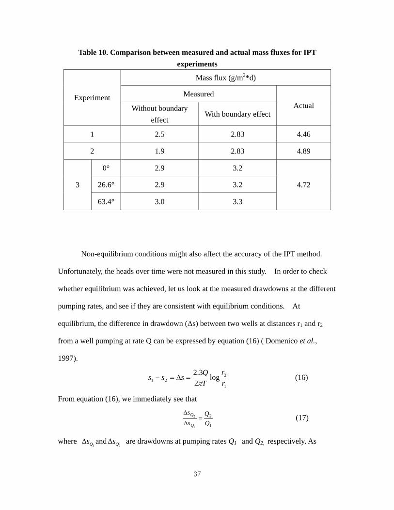
Table 10. Comparison between measured and actual mass fluxes for IPT experiments
Mass flux (g/m2*d)
Measured Experiment Without boundary
effect With boundary effect
Actual
1 2.5 2.83 4.46
2 1.9 2.83 4.89
0° 2.9 3.2
26.6° 2.9 3.2 3
63.4° 3.0 3.3
4.72
Non-equilibrium conditions might also affect the accuracy of the IPT method.
Unfortunately, the heads over time were not measured in this study. In order to check
whether equilibrium was achieved, let us look at the measured drawdowns at the different
pumping rates, and see if they are consistent with equilibrium conditions. At
equilibrium, the difference in drawdown (Δs) between two wells at distances r1 and r2
from a well pumping at rate Q can be expressed by equation (16) ( Domenico et al.,
1997).
1
221 log
23.2
rr
TQsss
π=Δ=− (16)
From equation (16), we immediately see that
1
2
1
2
s
s
Q
Q =Δ
Δ (17)
where and are drawdowns at pumping rates Q1 2QsΔ QsΔ 1 and Q2, respectively. As
37

shown in equation (17), the ratio of Δs should be proportional to the ratio of pumping
rates.
Table 11. Comparison of the ratio of pumping rates in IPT experiment 1 with the ratio of the difference in drawdown measured at pumping well 3C and observation
well 7C
i Qi (L/min) Δsi (mm) Ratio Qi/Q1 Ratio Δsi/ Δs1
1 0.45 1.40 1.00 1.0
2 2.11 11.20 4.69 8.0
3 2.90 16.00 6.46 11.4
4 3.44 19.60 7.65 14.0
Table 11 compares the ratio of pumping rates in IPT experiment 1 with the ratio of
the difference in drawdown measured at pumping well 3C and observation well 7C.
From the table, we see that the ratios, which should be equal, differ by a factor of almost
2. Based on this, we suspect that we may not have achieved equilibrium.
Assuming the observation well had reached equilibrium at the lowest pumping
rate of 0.45 L/min and that the pumping well had reached equilibrium at all pumping
rates, but the head measurements at the observation wells at the higher pumping rates
have not reached equilibrium, we can adjust the observation well heads according to the
ratio of pumping rate Q. After adjusting the head measurements and recalculating, the
measured mass flux for experiment 1 and 2 become 4.89 and 6.88 g m-2d-1, respectively,
while the actual mass fluxes for the two experiments were 4.64 and 4.89 g m-2d-1,
respectively (errors of 5% and 40%). Adjusting the observed heads in experiment 3 did
38

not affect the measured mass flux. Presumably, this is because the lowest pumping rate
in experiment 3 was 2.0 L/min (as opposed to 0.45 L/min and 0.42 L/min for experiments
1 and 2, respectively), so the assumption that we are at equilibrium at the lowest pumping
rate may be incorrect for experiment 3.
While the analysis above assumed that the artificial aquifer might not reach
equilibrium after 18 hours pumping, a MODFLOW simulation showed this might not be
a good assumption. In order to see how long the pumping well would have to be
pumped to reach equilibrium, MODFLOW was run to simulate the conditions of
experiment 1 with a pumping rate of 2.11 L/min. The simulation showed that equilibrium
at the observation well was reached after 21 seconds and 1.08 minutes assuming realistic
storativities of 2.7E-4 and 2.7E-3, respectively. It appears that 18 hours should be more
than adequate to attain equilibrium.
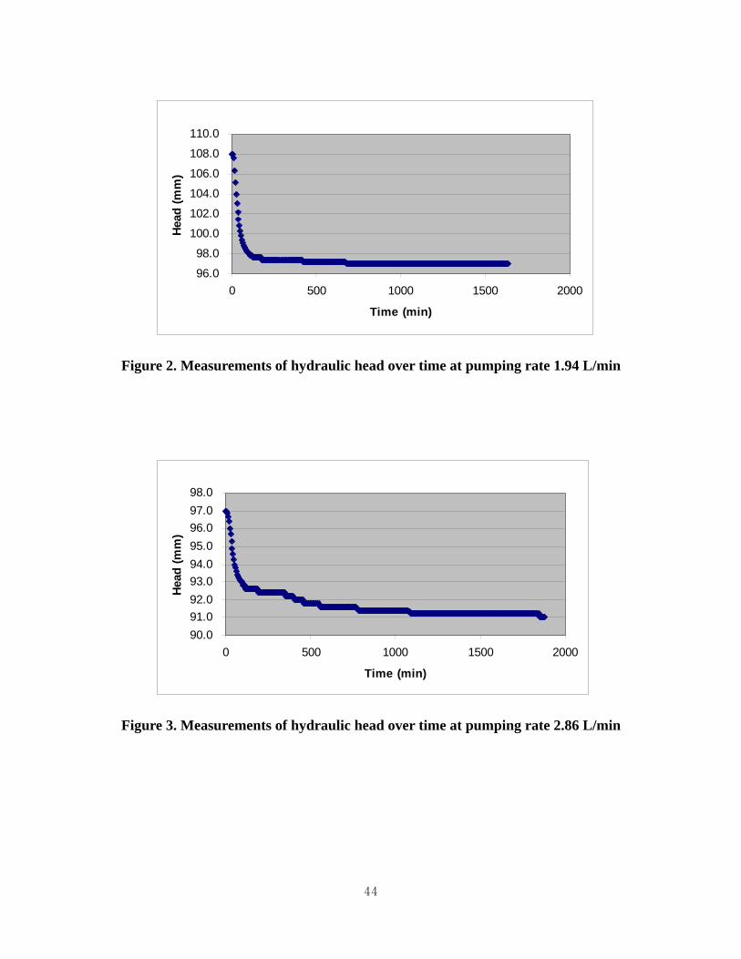
In order to check the equilibrium condition, experiment 1 was repeated. Based on
the data of head measurements over time at the pumping well, it appeared that the
pumping well reached equilibrium after 500 min (8.3 hours) at all pumping rates (see
Appendix A, Figure 1 - 4).
Another assumption that could affect the measurement is that the aquifer is
confined. When the TRWs are pumped at high rates, dewatering could occur so that the
water level might go below the confining layer of the artificial aquifer and unconfined
conditions would result. If the aquifer is dewatered, this might also lead to violation of
our assumption of equilibrium, as the time required for a confined aquifer to reach
equilibrium at a given pumping rate is much greater than the time required for a confined
aquifer. The possibility of dewatering was investigated during the second run of
39

experiment 1, but dewatering was not observed.
Another source of error is measurement error. It is difficult to measure the head
accurately because the differences of head being measured at each pumping rate are just a
few mm (see Figure 6, 7, and 8). For example, a measurement error of Δh of just 2 mm
could change the measured flux by 5%.
Measurement error can be analyzed by comparing the two runs of experiment 1.
Appendix A shows the results of the second run of experiment 1. The measured mass
fluxes for experiment 1 were 2.51 and 3.10 g m-2d-1 for the first and second runs,
respectively. Using these duplicate measurements, the 90% confidence interval for the
true value can be estimated using equation (18) (McClave et al., 2001)
)(2/ nstx α± (18)
Where
x = average of values
2/αt = t statistic having (n-1) degrees of freedom
s = standard deviation
n = number of samples
As a result, the 90% confidence interval for experiment 1 is from 0.94 to 4.67 g
m-2d-1. That is, we can say with 90% confidence that the true mass flux for experiment
1 falls in between 0.94 and 4.67 g m-2d-1. We see that the 90% confidence interval
includes the actual value of 4.64 g m-2d-1.
40

V. Conclusions
5.1 Summary
In recent years, investigators have proposed contaminant mass flux as a critical
measurement needed to support decision making at contaminated sites. Methods of
measuring contaminant mass flux are being developed, and need to be validated. Two
innovative approaches, the TRW and IPT methods, have been suggested to measure the
mass flux. In this study, measurements from these two methods were compared with
known fluxes in an artificial aquifer.
5.2 Conclusions
Results from using TRWs with the multi-dipole technique show that the measured
mass fluxes were one or two orders of magnitude lower than the actual flux, and the
technique appears to be not useable. Results of the tracer test technique show promise,
with measurements within 15% of actual fluxes. Also encouraging was the fact that, at
least in an artificial aquifer, the more inexpensive single tracer approach was
approximately as accurate as the approach that used two tracers. The IPT method also
shows promise. While measured fluxes underestimated the actual flux by at least 36%,
it appears that errors may be reduced when one accounts for potential violations of
method assumptions (infinite homogeneous confined aquifer, equilibrium conditions).
5.3 Recommendations
Based on the potential of the TRW method using the tracer technique, further
41
investigation is warranted. At Canterbury, New Zealand is a second facility that was
constructed as a heterogeneous artificial aquifer. The TRW method can be validated in
this second facility, to see how accurate it is under more realistic conditions of aquifer
heterogeneity. In addition, replicate TRW experiments to allow for a more rigorous
statistical analysis should be conducted.
Further investigation of the IPT method is needed in the homogeneous aquifer.
Replicate experiments to allow for a more rigorous statistical analysis should be
conducted, and the validity of method assumptions assessed. Follow-on studies should
focus on developing procedures to help assure method assumptions are satisfied.
42

Appendix A. Results of IPT experiment 1 repeated
Table 1. Measurements of hydraulic head for IPT experiment 1 repeated
Hydraulic head (mm)
Pumping well Observation well Pumping rate
(L/min) 3C 7C
0 110.2 100.0
0.41 108.0 99.2
1.94 97.2 96.0
2.86 91.2 93.8
3.28 89.4 93
107.0
107.5
108.0
108.5
109.0
109.5
110.0
110.5
0 200 400 600 800 1000 1200 1400 1600
Time (min)
Head
(mm
)
Figure 1. Measurements of hydraulic head over time at pumping rate 0.41 L/min
43
96.0
98.0
100.0
102.0
104.0
106.0
108.0
110.0
0 500 1000 1500 2000
Time (min)
Head
(mm
)
Figure 2. Measurements of hydraulic head over time at pumping rate 1.94 L/min
90.091.092.093.094.095.096.097.098.0
0 500 1000 1500 2000
Time (min)
Head
(mm
)
Figure 3. Measurements of hydraulic head over time at pumping rate 2.86 L/min
44

89.289.489.689.890.090.290.490.690.891.091.2
0 200 400 600 800 1000 1200
Time (min)
Head
(mm
)
Figure 4. Measurements of hydraulic head over time at pumping rate 3.28 L/min
y = 382.35x - 10.232R2 = 0.9892
-10.00
-8.00
-6.00
-4.00
-2.00
0.00
2.00
4.00
6.00
0 0.01 0.02 0.03 0.04
Q*ln (m^3/min)
Hea
d di
ffere
nce
(mm
)
Figure 5. Plot to determine Darcy velocity for IPT Experiment 1 repeated
45

Bibliography
Annable, M.D., Hatfield K., Cho, J., Klammler, H., Parker, B.L., Cherry, J. A., Rao, P.,
Field-scale evaluation of the passive flux meter for simultaneous measurement of
groundwater and contaminant fluxes, Environ. Sci. Technol., 39 (18), 7194-
7201, 2005.
Newell C. J., Conner J. A., Rowen D. L., Groundwater Remediation Strategies Tool,
Publication number 4730, Regulatory Analysis and Scientific Affairs Department,
American Petroleum Institute (API), December 2003.
Bockelmann, A., D. Zamfirescu, T. Ptak, P. Grathwohl, and G. Teutsch, Quantification of
mass fluxes and natural attenuation rates at an industrial site with a limited
monitoring network: a case study, J Contam. Hyd., 60: 97-121, 2003.
Borden, R. C., R. A. Daniel, L. E. LeBrun IV, and C. W. Davis, Intrinsic bioremediation
of MTBE and BTEX in a gasoline-contaminated aquifer, Water Resources
Research, 33(5):1105-1115, 1997.
Bright, J., F. Wang, and M. Close, Influence of the amount of available K data on
uncertainty about contaminant transport prediction, Ground Water, 40(5): 529-
534, 2002
Brooks, M., “Evaluation of Remedial Performance by Contaminant Flux as
Measured using Integral Pump Test: Uncertainty Assessment,” Draft paper, 2005.
Christ, J. A., A modeling study for the implementation of in situ cometabolic
bioremediation of trichloroethylene-contaminated groundwater, MS thesis,
46

AFIT/GEE/ENV97D-03, Department of system and engineering management, Air
Force Institute of Technology, Wright-Patterson AFB OH, 1997.
Domenico, P. A. and Schwartz F. W. Physical and chemical hydrogeology. New York:
John Wiley & Sons, inc., 1998.
Einarson, M. D. and D. M. Mackay, Predicting impacts of groundwater contamination,
Env. Sci.& Tech., 35(3):66A-73A, 2001.
Gandhi, R. K., G. D. Hopkins, M. N. Goltz, S.M. Gorelick, and P. L. McCarty, Full-scale
demonstration of in situ cometabolic biodegradation of trichloroethylene in
groundwater, 1: Dynamics of a recirculating well system, Water Resources
Research, 38(4):10.1029/2001WR000379, 2002a.
Gandhi, R. K., G. D. Hopkins, M. N. Goltz, S. M. Gorelick, and P. L. McCarty, Full-
scale demonstration of in situ cometabolic biodegradation of trichloroethylene in
groundwater, 2: Comprehensive analysis of field data using reactive transport
modeling, Water Resources Research, 38(4):10.1029/2001WR000380, 2002b.
Goltz, M. N., J. Huang, M. E. Close, M. Flintoft, and L. Pang, Use of horizontal flow
treatment wells to measure hydraulic conductivity without groundwater
extraction, submitted J.Contam. Hyd., 2006.
Harbaugh, A. W. and M. G. McDonald, User’s documentation for MODFLOW-96, an
update to the U.S. geological survey modular finite-difference ground-water flow
model, U.S. Geological Survey Open-File Report 96-485, 1996.
47

Hatfield, K., M. Annable, J. Cho, P. S. C. Rao, and H. Klammler, A direct passive
method for measuring water and contaminant fluxes in porous media, J Contam.
Hyd., 75: 155-181, 2004.
Huang, J., M.E. Close, S.J. Kim, J. Bright, and M.N. Goltz, Use of an Innovative Mass
Flux Measurement Method to Evaluate Groundwater Source Remediation
Technology Performance, The 1st International Conference on Challenges in Site
Remediation: Proper Site Characterization, Technology Selection and Testing,
and Performance Monitoring, Chicago, IL, 23-27 October 2005.
Javandel, I., Doughty C., Tsang, C. F., Groundwater Transport: Handbook of
Mathematical Models, Washington, DC: American Geophysical Union, 1984.
Kabala, Z. J., Dipole flow test; a new single-borehole test for aquifer characterization,
Water Resource Research, 29(1): 99-107, 1993.
Kim, S. J., Validation of an innovative groundwater contaminant flux measurement
method, MS thesis, AFIT/GES/ENV/05-02, Department of system and
engineering management, Air Force Institute of Technology, Wright-Patterson
AFB OH, 2005.
Kuber, M., Finkel, M., Contaminant mass discharge estimation in groundwater based on
multi-level point measurement: A numerical evaluation of expected errors,
J Contam. Hyd., 84: 55-80, 2006.
McCarty, P. L., M. N. Goltz, G. D. Hopkins, M. E. Dolan, J. P. Allan, B. T. Kawakami,
and T. J. Carrothers, Full-scale evaluation of in situ cometabolic Degradation of
trichloroethylene in groundwater through toluene injection, Env. Sci. & Tech.,
32(1):88-100, 1998.
48

McClave, J. T., Benson, P. G., Sinicich T., Statistics for Business and Economics, Upper
Saddle River, NJ, Prentice-Hall, Inc., 2001
Ptak, T., L. Alberti, S. Bauer, M. Bayer-Raich, S. Ceccon, P. Elsass, T. Holder, C.Kolesar,
D. Muller, C. Padovani, G. Rinck, G. Schafer, M. Tanda, G. Teutsch, and A.
Zanini, Integrated concept for groundwater remediation, Integral groundwater
investigation, Contract No. EVK-CT-1999-00017, INCORE, June 2003.
Soga, K., Page, J.W.E., Illangasekare, T.H., A review of NAPL source zone
remediation efficiency and the mass flux approach, J Hazard. Material., 110: 13-
27, 2004.
U.S. Environmental Protection Agency (EPA). “Mass flux evaluation finds SEAR
continues to reduce contaminant plume,” Technology News and Trends, 17: 4-5,
March 2005.
49

Vita
Captain Hyouk Yoon graduated from Dae-shin High School in Dae-jeon, Republic
of Korea in 1993. He entered Korea Military Academy (KMA) where he received the
Bachelor of Science in Chemistry. Upon graduation, he received the commission of 2nd
Lieutenant, Army Infantry Officer.
He successfully performed various assignments in all around Korea for ten years.
In August 2003, he entered the Graduate School of Engineering and Management, Air
Force Institute of Technology. Upon graduation, he will be assigned to the Combined
Forces Command (CFC) at Yong-san, Seoul.
50
REPORT DOCUMENTATION PAGE Form Approved OMB No. 074-0188
The public reporting burden for this collection of information is estimated to average 1 hour per response, including the time for reviewing instructions, searching existing data sources, gathering and maintaining the data needed, and completing and reviewing the collection of information. Send comments regarding this burden estimate or any other aspect of the collection of information, including suggestions for reducing this burden to Department of Defense, Washington Headquarters Services, Directorate for Information Operations and Reports (0704-0188), 1215 Jefferson Davis Highway, Suite 1204, Arlington, VA 22202-4302. Respondents should be aware that notwithstanding any other provision of law, no person shall be subject to an penalty for failing to comply with a collection of information if it does not display a currently valid OMB control number. PLEASE DO NOT RETURN YOUR FORM TO THE ABOVE ADDRESS. 1. REPORT DATE (DD-MM-YYYY) 23-03-2006
2. REPORT TYPE Master’s Thesis
3. DATES COVERED (From – To) Aug 2004 – Mar 2006
5a. CONTRACT NUMBER
5b. GRANT NUMBER
4. TITLE AND SUBTITLE Validation of methods to measure mass flux of a groundwater contaminant
5c. PROGRAM ELEMENT NUMBER
5d. PROJECT NUMBER 5e. TASK NUMBER
6. AUTHOR(S) Yoon, Hyouk, Captain, Republic of Korea Army (ROKA)
5f. WORK UNIT NUMBER
7. PERFORMING ORGANIZATION NAMES(S) AND ADDRESS(S) Air Force Institute of Technology Graduate School of Engineering and Management (AFIT/EN) 2950 Hobson Way WPAFB OH 45433-7765
8. PERFORMING ORGANIZATION REPORT NUMBER AFIT/GES/ENV/06M-08
10. SPONSOR/MONITOR’S ACRONYM(S)
9. SPONSORING/MONITORING AGENCY NAME(S) AND ADDRESS(ES) Col Mark H. Smith AFCEE/TD 3300 Sidney Brooks Brooks City-Base TX 78235 DSN 240-3332 [email protected] 11. SPONSOR/MONITOR’S
REPORT NUMBER(S)
12. DISTRIBUTION/AVAILABILITY STATEMENT APPROVED FOR PUBLIC RELEASE; DISTRIBUTION UNLIMITED.
13. SUPPLEMENTARY NOTES 14. ABSTRACT In this study, flux measurements obtained using two methods are compared with known mass fluxes in a meso-scale three-dimensional artificial aquifer. One method, the tandem recirculating well (TRW) method, is applied using two different techniques. One technique is simple and inexpensive, only requiring measurement of heads, while the second technique requires conducting a tracer test. The second method, the integrated pump test (IPT) method, requires use of one or more pumping and observation wells in various configurations. The results of the experiments in the artificial aquifer show that the most expensive technique, the TRW method using tracers, provides the most accurate results (within 15%). The TRW method that relies on head measurements is very inaccurate, so the technique appears not to be viable for flux measurement. The IPT method, although not as accurate as the TRW method using the tracer technique, does produce relatively accurate results (within 60%). IPT method inaccuracies appear to be due to the fact that the method assumptions were not well-approximated in the artificial aquifer.
15. SUBJECT TERMS Groundwater, Contaminant, Mass Flux, Measurement, Validation, Artificial aquifer 16. SECURITY CLASSIFICATION OF:
19a. NAME OF RESPONSIBLE PERSON Mark N. Goltz (ENV)
REPORT U
ABSTRACT U
c. THIS PAGE U
17. LIMITATION OF ABSTRACT UU
18. NUMBER OF PAGES 61 19b. TELEPHONE NUMBER (Include area code)
(937) 255-3636, ext 4638; e-mail: [email protected] Standard Form 298 (Rev: 8-98) Prescribed by ANSI Std. Z39-18
1
Related Documents