Validation of Aura Microwave Limb Sounder Ozone by ozonesonde and lidar measurements

Validation of Aura Microwave Limb Sounder Ozone by ozonesonde

and lidar measurements

Y. B. Jiang,1 L. Froidevaux,1 A. Lambert,1 N. J. Livesey,1 W. G. Read,1 J. W. Waters,1

B. Bojkov,2 T. Leblanc,3 I. S. McDermid,3 S. Godin-Beekmann,4 M. J. Filipiak,5

R. S. Harwood,5 R. A. Fuller,1 W. H. Daffer,1 B. J. Drouin,1 R. E. Cofield,1 D. T. Cuddy,1

R. F. Jarnot,1 B. W. Knosp,1 V. S. Perun,1 M. J. Schwartz,1 W. V. Snyder,1 P. C. Stek,1

R. P. Thurstans,1 P. A. Wagner,1 M. Allaart,6 S. B. Andersen,7 G. Bodeker,8 B. Calpini,9

H. Claude,10 G. Coetzee,11 J. Davies,12 H. De Backer,13 H. Dier,14 M. Fujiwara,15

B. Johnson,16 H. Kelder,6 N. P. Leme,17 G. Konig-Langlo,18 E. Kyro,19 G. Laneve,20

L. S. Fook,21 J. Merrill,22 G. Morris,23 M. Newchurch,24 S. Oltmans,16 M. C. Parrondos,25

F. Posny,26 F. Schmidlin,27 P. Skrivankova,28 R. Stubi,9 D. Tarasick,12 A. Thompson,29

V. Thouret,30 P. Viatte,9 H. Vomel,31 P. von Der Gathen,32 M. Yela,25 and G. Zablocki33

Received 10 April 2007; revised 2 August 2007; accepted 31 October 2007; published 15 December 2007.

[1] We present validation studies of MLS version 2.2 upper tropospheric andstratospheric ozone profiles using ozonesonde and lidar data as well as climatological data.Ozone measurements from over 60 ozonesonde stations worldwide and three lidar stationsare compared with coincident MLS data. The MLS ozone stratospheric data between150 and 3 hPa agree well with ozonesonde measurements, within 8% for the globalaverage. MLS values at 215 hPa are biased high compared to ozonesondes by �20% atmiddle to high latitude, although there is a lot of variability in this altitude region.Comparisons between MLS and ground-based lidar measurements from Mauna Loa,Hawaii, from the Table Mountain Facility, California, and from the Observatoire de Haute-Provence, France, give very good agreement, within �5%, for the stratospheric values.The comparisons between MLS and the Table Mountain Facility tropospheric ozone lidarshow that MLS data are biased high by �30% at 215 hPa, consistent with that indicatedby the ozonesonde data. We obtain better global average agreement between MLS andozonesonde partial column values down to 215 hPa, although the average MLS values atlow to middle latitudes are higher than the ozonesonde values by up to a few percent. MLS

1Jet Propulsion Laboratory, California Institute of Technology,Pasadena, California, USA.

2NASA Goddard Space Flight Center, Greenbelt, Maryland, USA.3Jet Propulsion Laboratory, California Institute of Technology, Table

Mountain Facility, Wrightwood, California, USA.4Service d’Aeronomie/Institut Pierre-Simon Laplace, Centre National

de la Recherche Scientifique–Universite Pierre et Marie Curie, Paris,France.

5Institute of Atmospheric and Environmental Science, University ofEdinburgh, Edinburgh, UK.

6Royal Netherlands Meteorological Institute, de Bilt, Netherlands.7Danish Meteorological Institute, Copenhagen, Denmark.8National Institute of Water and Atmospheric Research, Lauder, New

Zealand.9Aerological Station Payerne, MeteoSwiss, Payerne, Switzerland.10Meteorological Observatory Hohenpeissenberg, German Weather

Service, Hohenpeissenberg, Germany.11South African Weather Service, Irene, South Africa.12Environment Canada, Downsview, Ontario, Canada.13Royal Meteorological Institute of Belgium, Brussels, Belgium.14Meteorological Observatory Lindenberg, German Weather Service,

Lindenberg, Germany.15Graduate School of Environmental Earth Science, Hokkaido

University, Sapporo, Japan.

Copyright 2007 by the American Geophysical Union.0148-0227/07/2007JD008776$09.00

16Global Monitoring Division, Earth System Research Laboratory,NOAA, Boulder, Colorado, USA.

17Laboratorio De Ozonio, Instituto Nacional de Pesquisas Espaciais,Sao Paulo, Brazil.

18AlfredWegener Institute for Polar andMarine Research, Bremerhaven,Germany.

19Arctic Research Center, Finnish Meteorological Institute, Sodankyla,Finland.

20Centro di Ricerca Progetto San Marco, Universita degli Studi di Roma‘‘La Sapienza,’’ Rome, Italy.

21Malaysian Meteorological Service, Petaling Jaya, Selangor, Malaysia.22Graduate School of Oceanography, University of Rhode Island,

Narragansett, Rhode Island, USA.23Department of Physics and Astronomy, Valparaiso University,

Valparaiso, Indiana, USA.24Atmospheric Science Department, University of Alabama–Huntsville,

Huntsville, Alabama, USA.25National Institute for Aerospace Technology, Madrid, Spain.26Laboratoire de l’Atmosphere et des Cyclones, La Reunion, France.27NASA Goddard Space Flight Center, Wallops Island, Virginia, USA.28Czech Hydrometeorological Institute, Prague, Czech Republic.29Department of Meteorology, Pennsylvania State University, State

College, Pennsylvania, USA.30Laboratoire d’Aerologie, Centre National de la Recherche Scientifique,

Toulouse, France.31Cooperative Institute for Research in Environmental Science,

University of Colorado, Boulder, Colorado, USA.32Alfred Wegener Institute, Potsdam, Germany.

JOURNAL OF GEOPHYSICAL RESEARCH, VOL. 112, D24S34, doi:10.1029/2007JD008776, 2007ClickHere

for

FullArticle

D24S34 1 of 20

http://dx.doi.org/10.1029/2007JD008776

v2.2 ozone data agree better than the MLS v1.5 data with ozonesonde and lidarmeasurements. MLS tropical data show the wave one longitudinal pattern in the uppertroposphere, with similarities to the average distribution from ozonesondes. High uppertropospheric ozone values are also observed by MLS in the tropical Pacific from June toNovember.

Citation: Jiang, Y. B., et al. (2007), Validation of Aura Microwave Limb Sounder Ozone by ozonesonde and lidar measurements,

J. Geophys. Res., 112, D24S34, doi:10.1029/2007JD008776.

1. Introduction

[2] The Microwave Limb Sounder (MLS) is one of fourinstruments on the Earth Observing System (EOS) Aurasatellite which was launched on 15 July 2004 and placed intoa near-polar orbit at �705 km altitude, with a �1:45 p.m.ascending equatorial crossing time. The Aura missionobjectives are to study the Earth’s ozone, air quality, andclimate [Schoeberl et al., 2006a, 2006b]. MLS [Waters etal., 1999, 2006] contributes to this objective by measuringatmospheric temperature profiles from the troposphere tothe thermosphere, and more than a dozen atmosphericconstituent profiles, as well as cloud ice water content [Wuet al., 2006] from millimeter- and submillimeter-wavelengththermal emission of Earth’s limb with seven radiometerscovering five broad spectral regions.[3] Initial ozone validation results using MLS v1.5 data

include the early work of Froidevaux et al. [2006], as wellas results of comparisons between MLS and ground-basedmicrowave profiles [Hocke et al., 2006], and the analyses ofZiemke et al. [2006] and D. Yang et al. (Midlatitudetropospheric ozone columns derived from Aura OMI andMLS data using the TOR approach and mapping techni-ques, submitted to Journal of Geophysical Research, 2007,hereinafter referred to as Yang et al., submitted manuscript,2007), focusing on stratospheric columns and resultingtropospheric ozone residual column abundances, using acombination of MLS and OMI data.[4] In this paper, we present validation results of the

newly released MLS version 2.2 (or v2.2) ozone productfrom the upper troposphere to the upper stratospherethrough comparisons with global ozonesonde and ground-based lidar measurements. Although MLS measures ozonein several spectral bands [Waters et al., 1999, 2006], thispaper focuses on the ‘‘MLS standard product’’ for ozone,which is obtained from radiance measurements near240 GHz and provides the best overall precision for thewidest vertical range. There are related papers focusing onvalidation of the 240 GHz MLS ozone (and CO) data in theupper troposphere and lower stratosphere [Livesey et al.,2007], mainly for pressures of 100 hPa and larger, and in thestratosphere and lower mesosphere (L. Froidevaux et al.,Validation of Aura Microwave Limb Sounder Stratosphericozone measurements, submitted to Journal of GeophysicalResearch, 2007, hereinafter referred to as Froidevaux et al.,submitted manuscript, 2007), using satellite, aircraft andground-based ozone measurements. Version 2.2 is currentlyin the early stages of reprocessing and is therefore morelimited in terms of available days than version 1.5, withabout 3 months of v2.2 reprocessed data, covering selecteddays in 2004, 2005, and 2006. A recent minor software

patch has led to version 2.21, with results that are essentiallyidentical to v2.20 results for the vast majority of days.[5] In section 2, we summarize the data usage and

screening recommendations for MLS v2.2 ozone profiles.Section 2 also provides a brief description of the estimatedMLS ozone uncertainties, both random and systematic,which we generally refer to as precision and accuracy. Weprovide the comparisons between MLS ozone and ozone-sonde profiles in section 3, followed by section 4 onground-based lidar measurement comparisons. Section 5summarizes the results and suggests improvements neededin future versions.

2. MLS Ozone Measurements

[6] For an overview of the MLS spectral bands, main linefrequencies, and target molecules, see Waters et al. [2006].The overall MLS retrieval approach is discussed by Liveseyet al. [2005, 2006] and the calculation specifics of the MLSradiance model (or ‘‘forward model’’) are described byRead et al. [2006] and Schwartz et al. [2006]. MLS radiancespectra and residuals are discussed by Livesey et al. [2007]and Froidevaux et al. (submitted manuscript, 2007), whoshow that the radiance fits are generally very good (within�1%) although there is typically poorer closure in thelowermost height region (upper troposphere).

2.1. Data Usage and Screening

[7] The MLS v2.2 ozone data files provide the ozoneabundance fields as well as the estimated (single profile)precision fields and related data screening flags. The rec-ommendations for screening the MLS v2.2 ozone profilesare similar but not identical to those given by Livesey et al.[2005] for version 1.5 data. A detailed illustration of thesedata screening fields is given by Livesey et al. [2005] forMLS v1.5 data. We recommend the use of only even valuesof the ‘‘Status’’ field. Also there is now a slightly differentthreshold value for the ‘‘Quality’’ flag, which refers to theoverall radiance fit for each profile; users should use onlyQuality > 0.4 for the stratosphere (Froidevaux et al.,submitted manuscript, 2007) and Quality > 1.2 for theupper troposphere [Livesey et al., 2007]; we have conser-vatively used the Quality > 1.2 in this work. A new fieldnamed ‘‘Convergence’’ is also used in v2.2, and it refers tothe ratio of the radiance fit chi-square value for each profileto the chi-square value that the retrieval would have beenexpected to reach. Users should retain only ozone profileswith Convergence < 1.8, which eliminates only about 1% ofthe available daily ozone profiles.[8] The data usage guidelines for MLS v2.2 ozone are

summarized in Table 1. While more work of a very detailednature is needed to further refine the data screening recom-

D24S34 JIANG ET AL.: MLS OZONE VALIDATION

2 of 20

D24S34

mendations provided above, these recommendations willgenerally safely allow for the use of more than roughly 97%of the available daily MLS ozone profiles. As the retrievalsat pressures larger than 215 hPa are not deemed satisfactoryenough at this time [Livesey et al., 2007], we will onlyconsider ozone at pressures of 215 hPa or less in thefollowing comparisons.

2.2. Resolution, Precision, and Accuracy

[9] As described for atmospheric retrievals by Rodgers[1976], the vertical and horizontal (along the MLS subor-bital track) resolutions can be visualized through the use of

the averaging kernel matrix. The averaging kernels forozone have values very close to unity and are sharplypeaked; the influence of a priori profile information onthe retrievals is negligible [Livesey et al., 2007; Froidevauxet al., submitted manuscript, 2007]. The vertical resolutionis 2.7 to 3 km from the upper troposphere to the lowermesosphere.[10] The precision of the MLS ozone profiles is estimated

by the MLS retrieval calculations, following the Rodgers[1976] formulation; these uncertainty estimates are providedin the MLS Level 2 files (for each profile), as the diagonalvalues of the error covariance matrix. The estimated root

Table 1. MLS v2.2 Ozone Data Usage Guidelines

Flag Meaning/Usage Values to Use

Status can indicate operational or retrievalproblems, and possible influence of clouds

even

Quality radiance fit by the retrieval algorithms >0.4 (stratosphere), >1.2 (uppertroposphere)

Convergence (new for v2.2) ratio of the radiance fit to that expected bythe retrieval algorithms

<1.8

Precision negative if large contribution of a priori tothe retrieved value

>0

Pressure range useful vertical range 215–0.02 hPa

Figure 1. Global distribution of ozonesonde stations considered in this work.


3 of 20

D24S34

mean square precision for MLS ozone retrievals is typicallyfairly constant as a function of latitude; precision values canbe as low as 20 to 30 ppbv from 100 to 215 hPa, andincrease by an order of magnitude (�0.3 ppmv) near 1 hPa[Livesey et al., 2007; Froidevaux et al., submitted manu-script, 2007].[11] Simulation results for MLS ozone point to possible

biases of about 5 to 10% (or 0.05 to 0.2 ppmv) for most ofthe stratosphere, down to 100 hPa, with precision (randomerrors on single profiles) of 2 to 30% (Froidevaux et al.,

submitted manuscript, 2007). Expected uncertainties in-crease, in percent, for MLS vertical retrieval grid pressuresof 147 and 215 hPa, especially in the tropics, where ozoneabundances are low [Livesey et al., 2007].

3. Comparisons of MLS and Ozonesonde Data

[12] Ozonesondes are balloon-borne in situ instrumentsthat continuously measure the ozone concentration as theyascend or descend in the atmosphere. A profile of ozone is

Table 2. Ozonesonde Site Information for Comparisons Used in This Work

Site Name Latitude LongitudeContact orData Source

Number of CoincidentProfiles With Aura MLS

Alert (NU), Canada 82.50 �62.33 D. Tarasick/J. Davies (EC/MSC) 2Ascension Island, United Kingdom �7.98 �14.42 F. Schmidlin (NASA/GSFC) 30Belgrano (Argentina), Antarctica �77.85 �34.55 M. Yela (INTA) 15Boulder (CO), USA 40.00 �105.25 S. Oltmans/B. Johnson (NOAA/ESRL) 25Bratts Lake (SK), Canada 50.20 �104.70 D. Tarasick/J. Davies (EC/MSC) 7Churchill (MB), Canada 58.74 �94.07 D. Tarasick/J. Davies (EC/MSC) 8Cotonou, Benin 6.21 2.23 A. Thompson (PSU), V. Thouret (CNRS/LA) 16De Bilt, Netherlands 52.10 5.18 M. Allaart (KNMI) 36Edmonton (AB), Canada 53.55 �114.11 D. Tarasick/J. Davies (EC/MSC) 9Egbert (ON), Canada 44.23 �79.78 D. Tarasick/J. Davies (EC/MSC) 10Eureka (NU), Canada 79.99 �85.94 D. Tarasick/J. Davies (EC/MSC) 4Goose.Bay (NF), Canada 53.31 �60.36 D. Tarasick/J. Davies (EC/MSC) 15Heredia, Costa Rica 10.00 �84.10 H. Vomel (NOAA/ESRL) 4Hilo (HI), USA 19.43 �155.04 S. Oltmans/B. Johnson (NOAA/ESRL) 10Hohenpeissenberg, Germany 47.80 11.00 H. Claude (DWD) 92Houston (TX), USA 29.72 �95.40 G. Morris (Valparaiso U.) 6Huntsville (AL), USA 35.28 �86.59 S. Oltmans (NOAA/ESRL), M. Newchurch

(U. Alabama-Huntsville)31

Irene, South Africa �25.90 28.22 A. Thompson (PSU), G. Coetzee (SAWS) 11Jokioinen, Finland 60.80 23.50 E. Kyro (FMI) 13Kagoshima, Japan 31.60 130.60 JMA, WOUDC 5Keflavik, Iceland 63.97 �22.60 M. C. Parrondos (INTA) 16Kelowna (BC), Canada 49.93 �119.40 D. Tarasick/J. Davies (EC/MSC) 7La Reunion, France �21.06 55.48 F. Posny (U. de La Reunion) 18Lauder, New Zealand �45.04 169.68 G. Bodeker (NIWA) 32Legionowo, Poland 52.40 20.97 Grzegorz Zablocki (IMGW) 40Lindenberg, Germany 52.20 14.10 Horst Dier (DWD) 17Malindi, Kenya �2.99 40.19 A. Thompson (PSU), G. Laneve (U. Rome) 7Marambio (Argentina), Antarctica �56.72 �64.23 E. Kyro (FMI) 25Naha (Okinawa), Japan 26.20 127.70 JMA, WOUDC 11Nairobi, Kenya �1.27 36.80 B. Calpini (MeteoSwiss) 28Narragansett (RI), USA 41.49 �71.42 S. Oltmans/B. Johnson (NOAA/ESRL),

J. Merrill (U. Rhode Island)25

Natal, Brazil �5.42 �35.38 N. P. Leme (INPE), F. Schmidlin(NASA GSFC)

21

Neumayer, Antactica �70.70 �8.30 G. Konig-Langlo (AWI) 24Ny Aalesund (Spitsbergen), Norway 78.93 11.95 P. von Der Gathen (AWI) 6Pago Pago, American Samoa �14.23 �170.56 S. Oltmans/B. Johnson (NOAA/ESRL) 21Paramaribo, Suriname 5.81 �55.21 H. Kelder (KNMI) 14Payerne, Switzerland 46.80 7.00 P. Viatte/R. Stubi (MeteoSwiss) 102Praha, Czech Republic 50.00 14.45 P. Skrivankova (CHMI) 20Resolute (NU), Canada 74.71 �94.97 D. Tarasick/J. Davies (EC/MSC) 2San Cristobal (Galapagos), Ecuador �0.92 �89.60 S. Oltmans/B. Johnson (NOAA/ESRL) 11Sapporo, Japan 43.10 141.30 JMA, WOUDC 15Scoresbysund, Greenland 70.50 �22.00 S. B. Andersen (DMI) 16Sepang (Kuala Lumpur), Malysia 2.73 101.70 A. Thompson (PSU), C.P. Leong (MMS) 8Sodankyla, Finland 67.39 26.65 E. Kyro (FMI) 34Summit, Greenland 72.60 �38.50 S. Oltmans/B. Johnson (NOAA/ESRL) 3Suva, Fiji �18.13 178.40 S. Oltmans/B. Johnson (NOAA/ESRL) 5Syowa, Japan �69.00 39.60 JMA, WOUDC 21Tateno, Japan 36.10 140.10 JMA, WOUDC 13Thule, Greenland 76.50 �68.70 S. B. Andersen (DMI) 2Trinidad Head (CA), USA 40.80 �124.16 S. Oltmans/B. Johnson (NOAA/ESRL) 9Uccle, Belgium 50.80 4.35 H.De Backer (KMI) 91Wallops Island (VA), USA 37.90 �75.50 F. Schmidlin (NASA GSFC) 14Watukosek (Java), Indonesia �7.50 112.60 A. Thompson (PSU), M. Fujiwara (U. Hokkaido) 6Yarmouth (NS), Canada 43.87 �66.11 D. Tarasick/J. Davies (EC/MSC) 10


4 of 20

D24S34

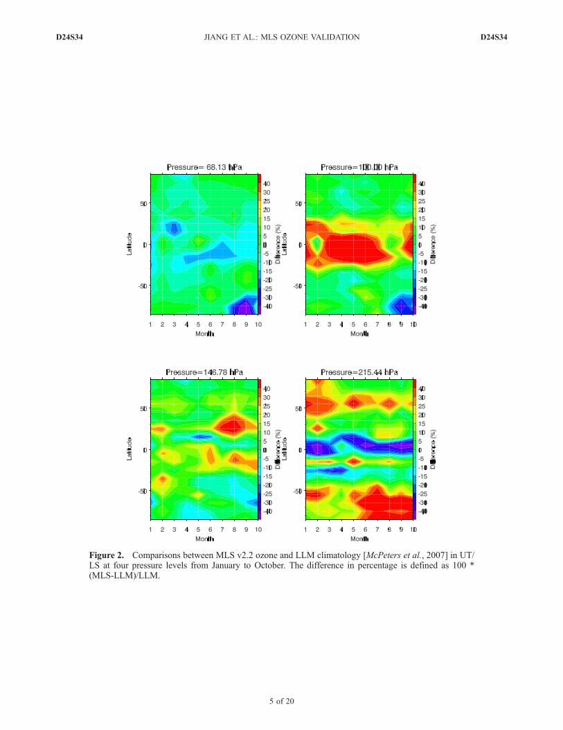
Figure 2. Comparisons between MLS v2.2 ozone and LLM climatology [McPeters et al., 2007] in UT/LS at four pressure levels from January to October. The difference in percentage is defined as 100 *(MLS-LLM)/LLM.


5 of 20

D24S34

Figure 3. Comparisons between MLS v2.2 ozone and LLM climatology [McPeters et al., 2007] in sixlatitude bins. The solid line represents the averaged percentage differences 100 * ((MLS-LLM)/LLM)between v2.2 and LLM climatology.


6 of 20

D24S34

obtained up to the burst point of the balloon, often ataltitude in excess of 30 km or a pressure as low as 5 to10 hPa. Ozonesonde measurements are the most accuratemeans of providing high vertical resolution ozone profiles.The detection limit is typically less than 2 ppbv, as com-pared to the typical clean background value of 30 ppbv fortropospheric ozone. Measurement uncertainty is about 10%in the troposphere, 5% in the stratosphere up to 10 hPa and5–25% between 10 and 3 hPa [Bodeker et al., 1998; Borchiet al., 2005; Kerr et al., 1994; Smit et al., 2007; Thompsonet al., 2007a, 2007b, 2007c; World Climate ResearchProgramme, 1998]. We have used ozonesonde measure-ments available from the Aura Validation Data Center(AVDC) as well as some soundings from the World Ozoneand Ultraviolet Data Center (WOUDC) in Toronto (http://www.woudc.org/). More than 70 stations were considered

in this study, but considering the criteria we use to select theMLS and correlative data profiles and the availability ofv2.2 and sonde data at the time of writing, some of thepotentially available comparisons are currently missing.Figure 1 shows the global distribution of these stations.There is good coverage in the Northern Hemisphere highlatitude, but the Southern Hemisphere coverage is sparse:only 4 stations at high southern latitudes, and 1 (Lauder,New Zealand) at the southern midlatitudes. The tropicalstations are mainly from the Southern Hemisphere Addi-tional Ozonesondes (SHADOZ) project. The ozonesondesites and number of coincident profiles with MLS observa-tions (when more than one exists) are listed in Table 2, withmost of the data made available at the Aura Validation DataCenter (AVDC); data from the sites labeled WOUDC wereobtained directly from the WOUDC. Examination of ozo-

Figure 4. Comparisons between MLS v2.2, v1.5 ozone and ozonesonde measurements in 6 latitudebins. Solid circle and connected line represents the averaged percentage differences (100 * (MLS-Sonde)/Sonde) between v2.2 and ozonesondes, while solid triangle and connected line shows the averagedpercentage differences between v1.5 and ozonesondes. Dashed line gives the standard deviation of thedifferences (in percent) between v2.2 and ozonesondes. Heavy solid line shows the combined precisions(in percent) for v2.2 and ozonesondes, using 5% precision for the sondes. The error bar on each datapoint (dot) is twice the precision in the mean differences (and is often too small to see). The solid darkgray line represents the averaged percentage differences (100 * (MLS-LLM)/LLM) between v2.2 andLLM climatology.


7 of 20

D24S34

nesonde measurements suggests that station-to-stationbiases exist between the different sites because of differ-ences in data processing technique and sensor solution andvarying hardware [Johnson et al., 2002; Thompson et al.,2003; Smit et al., 2007].[13] In order to get good statistics, we chose coincident

MLS and ozonesonde profiles to be within ±2� latitude,±10� longitude and on the same (GMT) day. We havelooked at the comparisons using tighter criteria and whilethese results improve slightly (by 5% or less), this will notaffect the main conclusions given here. In the comparisons,we have filtered the MLS data as pointed out in section 2.1,and used only cloud free profiles, based on the MLS cloudscreening criteria (Status = 0). There are total 1196 profilesfound in 2004, 2005 and 2006 based on the coincidencesbetween MLS v2.2 and ozonesonde profiles. We havedegraded the high-resolution ozonesonde profiles by usingtwo methods: a least squares fit of the fine resolutionpressure grid to the MLS ozone retrieval grid, and also,the use of MLS averaging kernels to smooth the ozonesondedata after the least squares fit to the MLS grid. There arenegligible differences between the two methods, and theresults of comparisons are not very sensitive to the methodchosen, as expected, because of the sharply peaked nature

of the MLS averaging kernels. We have used the averagingkernel method to degrade the ozonesonde high-resolutionprofiles throughout this work.[14] In order to check the bias of MLS ozone versus

climatology, we show comparisons between MLS v2.2ozone and LLM climatology [McPeters et al., 2007] inupper troposphere at four pressure levels in Figure 2. At thetime of writing, there are no more than 10 days of MLS v2.2data in August, November and December. We plot onlyJanuary to October with interpolated August data. The LLMclimatology combines data from the Stratospheric Aerosoland Gas Experiment II (SAGE II; 1988–2001), the UpperAtmosphere Research Satellite Microwave Limb Sounder(MLS; 1991–1999), and ozonesondes (1988–2002). At68 hPa (and lower pressures, not shown), the comparisongives agreement within 5%, with a few places such asAntarctic ozone hole where MLS values are 10–20% lowerthan LLM. At the upper tropospheric levels, MLS valuesoscillate about the LLM climatology. At 100 hPa, MLSozone is larger by as much as �40% in the tropical regionand lower by �30% in the Antarctic ozone hole. WhileMLS ozone biases are lower (�20%) in the tropics andhigher (�20%) in the higher latitude in both hemispheres at215 hPa level. The MLS shows better agreement with LLM

Figure 5. Scatterplots of MLS versus ozonesondes from all the stations for all the coincidences onselected pressure levels, color-coded in five latitude bins. The heavy black lines are the linear fits to thedata.


8 of 20

D24S34

climatology at 147 hPa level as compared to 100 hPa and215 hPa levels. The differences at 147 hPa have someseasonal variability in the tropical and midlatitude regionswith some biases as high as �20%.[15] Figure 3 shows comparisons between MLS v2.2 and

LLM climatology in 6 latitude bins. MLS ozone values aregenerally within �5% of LLM data down to 50 hPa,although there are some larger differences at high southernlatitudes. Better agreement is reached in the Northern Hemi-sphere stratosphere. The standard deviations (variability) ofMLS and LLM climatology (not shown here) track verywell in the stratosphere, but they deviate from each other inthe upper troposphere and lower stratosphere. In the uppertroposphere, the standard deviation of MLS is about twiceas large as that of the LLM climatology.[16] As pointed out by Froidevaux et al. (submitted

manuscript, 2007), improved algorithms in MLS v2.2 ozonehave generally led to reduced biases in comparison to MLSv1.5. For example, MLS v2.2 has largely corrected thesmall negative slope that existed in v1.5 comparisons withSAGE II. Figure 4 shows the average differences (definedas 100 * (MLS-Sonde)/Sonde) between ozonesonde profiles

and MLS v2.2 and v1.5 data (for the same days) for sixdifferent latitude bins. MLS v2.2 data show better agree-ment with ozonesonde values than the MLS v1.5 data in thestratosphere (100–5 hPa). The MLS v2.2 data and ozone-sonde data agree with each other from 50 to 5 hPa to within�5% except in the tropics where �15% positive bias isobserved at 50 hPa. MLS v2.2 profiles still show mostlyhigh biases compared to ozonesondes in the lower altituderange. MLS and ozonesonde values are within �12% at 100and 147 hPa except in the tropical latitude bin �20� to 20�where the bias is �20%. At 215 hPa, MLS ozone is higherby 20% to 35% compared to ozonesondes in extratropicallatitudes, but lower by 14% in the tropics. In most latitudebins, the comparisons still show a negative slope from theupper troposphere to about 10 hPa. This plot also shows thatthe comparisons between MLS and ozonesondes are quitesomewhat different from the climatology comparisons (darkgray lines). The combined precision estimate (heavy solidline in Figure 4) is obtained from the root sum square (rss)of the (random) uncertainties provided in the MLS data filesand the 5% precision assumed for ozonesonde measure-ments. The standard deviations of the differences (dashed

Figure 6. Averaged ozone profiles differences between MLS v2.2 and ozonesondes for each station, infive latitude bins. Profiles at (top) pressure 120–3 hPa and (bottom) at pressure 250–80 hPa. Red linesshow the mean of the difference. Note that the differences are given in ppbv for the upper troposphere/lower stratosphere region (Figure 6, bottom) and as a percentage for the stratosphere (Figure 6, top). Theerror bars (pink) are examples of the 2s combined precisions for sites Syowa, Lauder, Hawaii,Hohenpeissenberg and De Bilt, in their respective latitude bins. Precisions in the averages for each bin(red curves) are even smaller (and are not shown).


9 of 20

D24S34

Figure 7. (left) Latitudinal distributions of average ozone from each ozonesonde station (red triangles)compared with MLS ozone data (black dots) on selected pressure levels, as indicated. The error bars arethe standard deviation (variability). (right) Differences (MLS minus sonde data) in ppmv. The error barsshow twice the standard error in the mean differences.


10 of 20

D24S34

Figure 8. Ozone vertical distribution from 20 hPa to 215 hPa in the equatorial region (±15� in latitude)for four seasons (months indicated by first letters at top left for each panel), using 2004 and 2005 data.(left) From the MLS v1.5 ozone data available and (right) from the ozonesonde measurements in 2004and 2005, which mostly come from the SHADOZ network.


11 of 20

D24S34

Figure 9. (left) Latitudinal distributions of averaged ozone at each low-latitude ozonesonde station (redtriangles), with the standard deviation (variability) shown as error bars (red bar), compared with MLSozone data (black dots) and their error bars (black bar) at three pressure levels. (right) Differences (MLSminus ozonesonde data) in ppbv. The error bars show twice the standard error in the mean differences.


12 of 20

D24S34

line in Figure 4) are larger than these combined precisionestimates, especially in the UT/LS. While atmosphericvariability could play some role in the larger UT/LS scatter,we also noted this larger variability versus the LLMclimatology, and this is a topic for further study. The largerdifferences (absolute and scatter) in the UT/LS may becaused by the sensitivity of the retrieval in that region, sincethe ozone in that region only contributes a very smallfraction of the total MLS ozone signal. We note that theformal accuracy estimates for MLS ozone in the uppertroposphere [Livesey et al., 2007] are larger than the averagedifference observed in Figure 5.[17] The MLS v2.2 ozone abundances are well correlated

with the ozonesonde values at all pressure levels except at316 hPa, as shown in Figure 5. The 316 hPa level ozonevaries between �0.2 ppmv to 0.4 ppmv, and is not recom-mended for scientific use. There are a few questionableprofiles (outliers) at various levels. Figure 6 presents aver-

aged difference (100 * (MLS-sonde)/sonde) profiles foreach station grouped by latitude bin. The largest differencesare at lower altitudes. Most of the averaged profiles (fromeach site) agree with MLS within �10% in the midstrato-sphere. There are some larger, unexplained differences forsome sites. In the tropical upper troposphere, most differ-ences are within 30 ppbv, and the average is within�10 ppbv.The MLS accuracy estimates in this region is �20 ppbv[Livesey et al., 2007].[18] Figure 7 summarizes the MLS and ozonesonde

averaged comparisons for each site versus latitude, withabundances on Figure 7 (left) and differences on Figure 7(right). The MLS data track the ozonesonde data very wellas a function of latitude. Both data sets show smaller ozonemixing ratios in the equatorial region and larger ozone atmiddle-to-high latitude from 215 hPa to 46 hPa, with achange in the sign of this latitudinal gradient from 21 to10 hPa. This consistent picture points to the robustness of

Figure 10. (top) Averaged column ozone at each station as compared with MLS ozone data and(bottom) their differences in percentage. In Figure 10 (top), the black circles are the MLS column ozonewith the standard deviation (variability) and ozonesonde columns are represented by red triangles withthe standard deviation (variability). Figure 10 (bottom) shows column differences between MLS ozoneand ozonesondes with twice the standard error in the mean differences. The (connected) red dotsrepresent the averaged differences over 20� latitude bins in the Northern Hemisphere and 30� latitudebins in the Southern Hemisphere.


13 of 20

D24S34

Figure 11. Scatterplots of MLS ozone columns versus ozonesonde columns above four selectedpressure levels from all the stations for all the coincidences, color-coded in five latitude bins. The heavyblack lines are the linear fits to the data.


14 of 20

D24S34

the MLS v2.2 retrievals even for the upper troposphere,where ozone contributes only a small fraction to the totalemission. The small ozone mixing ratios (<100 ppbv) inthe equatorial region below 100 hPa level represent typicalupper tropospheric ozone values, and will be examined inmore detail in Figure 9.[19] As presented in Figure 7 (right), the differences

between MLS and ozonesondes are less than 100 ppbvfor most of the stations in the upper troposphere and lowerstratosphere (100 hPa to 215 hPa), and differences tend tooscillate between positive and negative values. The differ-ences are large at stations in the tropical region and north of30�N for all pressure levels.[20] Tropospheric pollution and the global effects of

regional pollution have received increased attention in thepast decade. Tropospheric ozone is a precursor of OHradicals and as such influences tropospheric chemistry and

global climate change. Ozone distribution in UT/LS is theresult of a combination of transport and chemical processes.The zonal wave one in the tropical distribution of ozone andthe tropical Atlantic ozone paradox [Thompson et al., 2003;Sauvage et al., 2006] are interesting examples of variationsin tropospheric ozone, and better characterization of thespatial and temporal variations of tropospheric ozone isneeded.[21] The well-known enhancements in tropospheric

ozone over the tropical Atlantic (�165–90�W in longitude)[Thompson et al., 2003; Jourdain et al., 2007] are shownboth in the MLS ozone data and in the ozonesonde measure-ments (Figure 8) in December, January, and February (DJF)and March, April, and May (MAM). This phenomenonappears to be associated with pollution from biomassburning in Africa and South America and the tropicalcirculation. Moreover, MLS data also show enhanced ozone

Figure 12. Comparisons between MLS v2.2, v1.5 ozone and lidar measurements at three stations. (top)Averaged profiles of MLS v2.2 (open circles), v1.5 (open triangles) and lidar (open red triangles).(bottom) Average percentage differences between MLS v2.2 and lidar data (solid circles) and the averagepercentage differences between MLS v1.5 and lidar data (solid triangles). Error bars represent twice theprecision (standard error) in these mean differences. Dashed lines give the standard deviations of themean differences between v2.2 and lidar data. Heavy solid line shows the combined precisions forthe v2.2 and lidar measurements. The shaded area is the ±5% region.


15 of 20

D24S34

in the tropical Pacific (�35�W–8�E in longitude) in June,July, and August (JJA), and in September, October, andNovember (SON), which may not appear in ozonesondemeasurements because of their sparse coverage. The higherozone in the tropical Pacific in JJA and SON may also becaused by biomass burning, followed by cross-continentaltransport of polluted air lofted into the upper troposphere.There is also the possibility that stratosphere-troposphereexchange plays a role. The lower stratosphere ozone in thetropical region is relatively uniform longitudinally andshows no signal of the tropospheric wave one pattern.[22] Figure 9 shows the comparisons in detail in the

equatorial region at 215 hPa, 147 hPa and 100 hPa in theupper troposphere. The averaged differences for each sta-tion are within 50 ppbv at 215, 146 and 100 hPa, althoughthere is significant variability from site to site. The standarderrors are within about 30 ppbv, which is roughly consistentwith the results of analyses by Livesey et al. [2007], usingaircraft data sources. There is slightly significant bias in thetropical upper tropospheric comparisons (see Figure 4). The215 hPa high bias of �20% seen in Figure 4 arises mainlyfrom the middle and high latitudes (south of �20� and northof 20�).[23] Ozone column abundance is another parameter of

interest used in the process of validating MLS data againstozonesonde measurements. The MLS column ozone abun-dances are estimated to have a (1s) precision of 3%, for atypical column value obtained from the integration of anindividual MLS ozone profile (Froidevaux et al., submitted

manuscript, 2007), with an estimated (2s) accuracy of 4%(or 8 DU). Comparisons of column ozone measurementsfrom MLS and column data from the CCD based ActinicFlux Spectroradiometers (CAFS) during various Aura Vali-dation Experiment (AVE) campaigns (N. J. Petropavlovskikhet al., Validation of Aura Microwave Limb Sounder O3 andCO observations in the upper troposphere and lower strato-sphere, manuscript in preparation, 2007) confirm that suchuncertainty estimates are reasonable, as do column compar-isons between MLS and other satellite-based ozone meas-urements (Froidevaux et al., submitted manuscript, 2007;Yang et al., submitted manuscript, 2007). Figure 10 givesthe averaged ozone partial column from MLS v2.2 data andozonesonde partial column from each station, and thedifferences. The MLS ozone partial column and ozonesondepartial column are calculated between common upper andlower pressure levels where good measurements are madefor both MLS and ozonesondes. As seen in Figure 7, theozone partial columns also show good correspondence inthe meridional variations, and the mean differences aremostly within 10% with a few fliers. Typically, twice thestandard error shown in Figure 10 is about 3%.[24] More detailed partial column ozone scatterplots of

MLS versus ozonesonde partial column ozone above fourselected pressure levels are shown in Figure 11; differentlatitude bins are color-coded in this plot. There is a 1.4%average difference (MLS values higher than sonde values)for columns above 316 hPa, and this difference decreases aspressure decreases. The correlation coefficients for all

Figure 13. Same as Figure 12 except that the lidar data are from the Table Mountain Facilitytropospheric ozone measurements; and the pressure levels are from 215 to 22 hPa.


16 of 20

D24S34

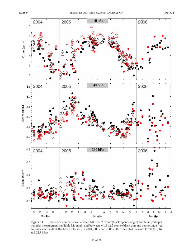
Figure 14. Time series comparisons between MLS v2.2 ozone (black open triangle) and lidar (red opentriangle) measurements at Table Mountain and between MLS v2.2 ozone (black dot) and ozonesonde (reddot) measurements at Boulder, Colorado, in 2004, 2005 and 2006 at three selected pressure levels (10, 46,and 215 hPa).


17 of 20

D24S34

pressure levels are about 0.95; MLS column ozone in thetropics shows larger biases, as expected from this Figure 10.

4. Comparisons of MLS Versus Lidar OzoneData

[25] We have analyzed comparisons between MLS ozoneand ozone from four lidars located at three NDACC(Network for the Detection of Atmospheric CompositionChange, formerly NDSC) stations [Leblanc and McDermid,2000; Leblanc et al., 2006; McDermid et al., 1990; Godin etal., 1989; Godin-Beekmann et al., 2003], namely Observ-atoire de Haute-Provence (OHP) in France (43.93�N,5.71�E), Mauna Loa, Hawaii (19.5�N, 155.7�W), and theTable Mountain Facility, California (34.5�N, 117.7�W).These lidars are high power differential absorption lidars(or DIAL) which make precise measurements of strato-spheric ozone concentration profiles from �20 to 50 kmaltitude. This technique requires two (or more) laser wave-lengths which are chosen such that one coincides with aregion of high absorption, specific to the species beingmeasured, and the other is tuned into the wings of thisfeature to a wavelength with much lower absorption. Theconcentration of ozone is retrieved by measuring the differ-ent absorption of the backscatter data at the two wave-lengths.[26] The estimated accuracy (or systematic uncertainty)

for the Table Mountain Facility ozone number density lidarprofiles is below 0.05 � 1018 molecules/m3 (or 1–5%) forthe vertical range 15–50 km and can occasionally increaseto 0.3 � 1018 molecules/m3 (or 10–50%) for heights below15 km. The translation to mixing ratio adds another 1–3%uncertainty due to the use (and associated uncertainty) ofexternal measurements or model outputs of pressure andtemperature. The temperature and pressure data used forOHP correspond to nearby radiosoundings performed dailyin Nimes, complemented at higher altitude by the COSPARInternational Reference Atmosphere (CIRA) [Rees, 1988]model. Hawaii and Table Mountain lidars use NationalCenters for Environmental Prediction (NCEP) operationalanalysis data interpolated to the location and time of thelidar measurements, and local Hilo radiosondes complementthe Hawaii database. In this validation study against lidarmeasurements, we have degraded the high-resolution lidarprofiles to MLS data grid by using the averaging kernelmethod as pointed out in section 3.[27] Figure 12 shows the averaged profiles of available

MLS v2.2 data and coincident lidar measurements (within±2� latitude, ±10� longitude and for nighttime only) andtheir percentage differences (defined as 100 * (MLS-lidar)/

lidar) at the three lidar stations. The comparisons with thetropospheric ozone lidar measurements at Table MountainFacility are discussed later. MLS v2.2 shows better agree-ment with lidar data than v1.5. MLS v2.2 ozone gives bestagreement with lidar in the 2 hPa to 50 hPa region, wherethe differences are within 5%. The relatively larger differ-ences (>10%) around 1 hPa and higher, for all three stations,may be caused by poorer lidar measurements in this region.For the Haute Provence station, averaged differences areless than 5% at 100 and 146 hPa, and 20% at 215 hPa. At147 hPa, MLS v2.2 ozone is lower by �20% (uncertainty10%) compared to both the Mauna Loa and the TableMountain Facility measurements. On average, on the basisof these three stations, MLS v2.2 agrees with lidar measure-ments to better than �5% from 5 hPa to 100 hPa. Thecomparisons also show larger standard deviations of themean differences for pressures of 100 hPa and larger.Calculations of partial column ozone abundances above215 hPa over the three lidar stations indicate that MLSv2.2 data agree with the lidars to better than 5%.[28] Figure 13 shows the comparisons between MLS low

altitude ozone and that measured by the Table Mountaintropospheric ozone lidar. The tropospheric ozone lidarmeasurement system provides a more reliable comparisonfor this altitude region in the upper troposphere. The differ-ences between MLS v2.2 ozone and lidar are within 8%down to 147 hPa, but MLS shows a high bias (�30%) at215 hPa, which is consistent with the ozonesonde measure-ments. The estimated combined precision is about 10% atpressures less than 100 hPa and increases to �25% forpressures larger than 100 hPa. The standard deviations ofthe mean differences (dashed lines) are higher than 10%and increase to more than 50% in the upper troposphere.Figure 13 also highlights the better agreement versus lidarsfor MLS v2.2 than MLS v1.5 data in the stratosphere.[29] In Figure 14, we present the time series of MLS

ozone, ozonesonde measurements at Boulder, Colorado andlidar measurements at Table Mountain Facility in 2004,2005 and 2006 at three pressure levels. The troposphericlidar measurement is used at 215 hPa level in the compar-ison. These two stations are the closest stations we can findfor the comparisons of the three different kinds of measure-ments, and they should have similar spatial and temporalozone variability. In general, the MLS v2.2 ozone tracksboth the ozonesonde and lidar measurements well as afunction of season. The ozone abundance at 215 hPa showsa weak seasonal variability with enhanced values aroundspring, but shows a strong seasonal cycle at both 46 and10 hPa. The ozone distribution reaches its maximum in the

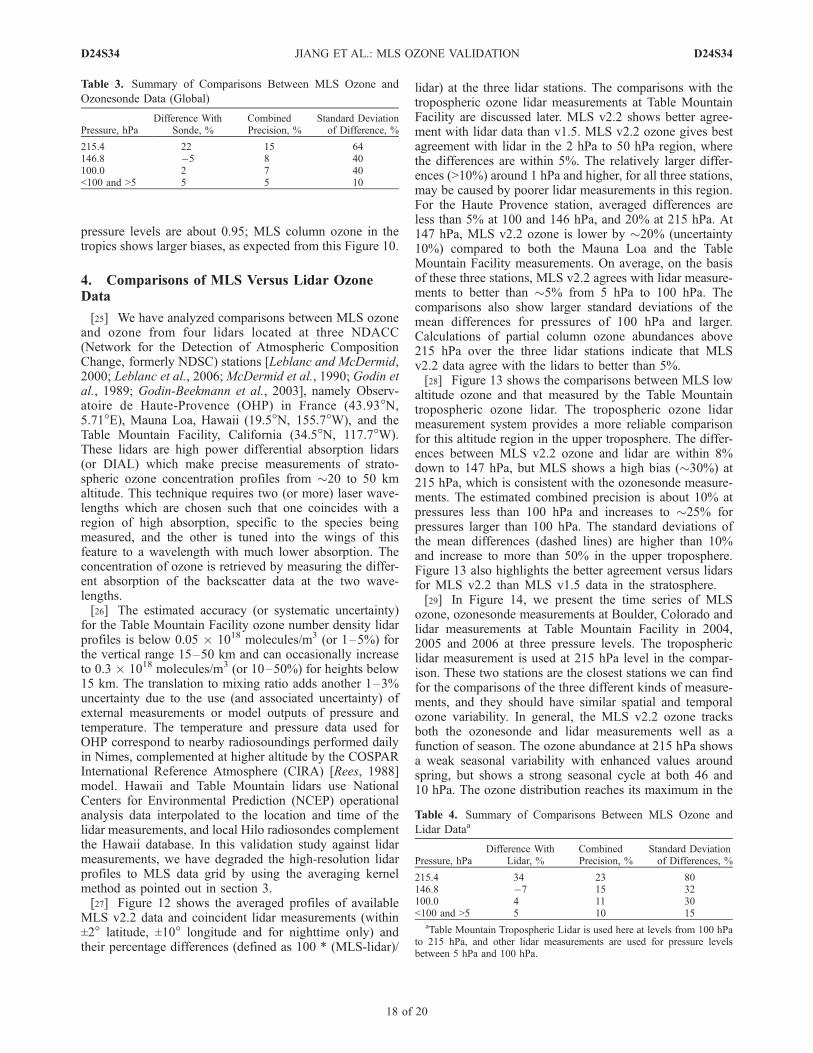
Table 3. Summary of Comparisons Between MLS Ozone and

Ozonesonde Data (Global)

Pressure, hPaDifference With

Sonde, %CombinedPrecision, %

Standard Deviationof Difference, %

215.4 22 15 64146.8 �5 8 40100.0 2 7 40<100 and >5 5 5 10

Table 4. Summary of Comparisons Between MLS Ozone and

Lidar Dataa

Pressure, hPaDifference With

Lidar, %CombinedPrecision, %

Standard Deviationof Differences, %

215.4 34 23 80146.8 �7 15 32100.0 4 11 30<100 and >5 5 10 15

aTable Mountain Tropospheric Lidar is used here at levels from 100 hPato 215 hPa, and other lidar measurements are used for pressure levelsbetween 5 hPa and 100 hPa.


18 of 20

D24S34

summer at 10 hPa, while it reaches its maximum in thespring at 46 hPa.

5. Summary and Conclusions

[30] This paper presents the validation results of newlyreleased Aura MLS v2.2 ozone in the upper troposphere andlower stratosphere using worldwide ozonesonde andground-based lidar measurements. In the upper troposphereand lower stratosphere, MLS ozone is generally biased highat middle to high latitudes, as compared to ozonesondes, butwithin 20% or 20 ppbv, on average, in the tropics. In themiddle stratosphere, MLS is within 7% of the globalozonesonde measurements. Averaged over each ozonesondestation, the column ozone comparisons against MLS showbetter than 10% agreement, but there is no significant biasglobally.[31] Comparisons to three sets of lidar measurements from

Hawaii, Table Mountain, and Haute Provence in Franceshow excellent agreement (within about 5%) in the strato-sphere and MLS ozone biases higher by 35% at 215 hPalevel. This study also shows that the temporal variations inMLS ozone and in midlatitude ozone from the Boulder, CO,ozonesondes and the Table Mountain Facility, CA, lidartrack each other very well. The global results of comparisonsbetween ozonesondes and lidars are listed in Tables 3 and 4.The results from the lidar comparisons are consistent withthat from the ozonesonde comparisons in the lower altituderange. However, the comparisons between MLS ozone andaircraft in situ and lidar data do not give strong evidence for ahigh MLS bias at 215 hPa of more than 15% [Livesey et al.,2007; Froidevaux et al., submitted manuscript, 2007].Because of the somewhat inconsistent evidence of a highMLS bias at 215 hPa, the accuracy estimate for MLS v2.2ozone at 215 hPa has been set at about 20 ppbv + 20% (seethe above references), rather than the somewhat lowerestimate of 20 ppbv + 10% expected from simulations andsensitivity studies (see the above two references). Furtherdetailed investigations using more reprocessed MLS v2.2data may shed more light on these issues.

[32] Acknowledgments. This work at the Jet Propulsion Laboratory,California Institute of Technology, was performed under contract withNASA. We are very grateful to the MLS instrument and data/computeroperations and development team (at JPL and from Raytheon, Pasadena)for their support through all the phases of the MLS project, in particularD. Flower, G. Lau, J. Holden, R. Lay, M. Loo, G. Melgar, D. Miller,B. Mills, M. Echeverri, E. Greene, A. Hanzel, A. Mousessian, S. Neely,C. Vuu, and P. Zimdars. We greatly appreciate the work of those involved inthe Aura Validation Data Center at the NASA Goddard Space Flight Center,as this has been the main data repository for Aura correlative/validation datasince the Aura launch. Thanks to Jennifer Logan for providing the WOUDCdata. Thanks to the Aura Project for their support throughout the years(before and after the Aura launch), in particular M. Schoeberl, A. Douglass(also as cochair of the Aura validation working group), E. Hilsenrath, andJ. Joiner. We also acknowledge the support from NASA Headquarters;P. DeCola for MLS and Aura; and M. Kurylo, J. Gleason, B. Doddridge,and H. Maring, especially in relation to the Aura validation activities andcampaign planning efforts.

ReferencesBodeker, G. E., I. S. Boyd, and W. A. Matthews (1998), Trends and varia-bility in vertical ozone and temperature profiles measured by ozone-sondes at Lauder, New Zealand: 1986 – 1996, J. Geophys. Res.,103(D22), 28,661–28,681.

Borchi, F., J.-P. Pommereau, A. Garnier, and M. Pinharanda (2005), Eva-luation of SHADOZ sondes, HALOE and SAGE II ozone profiles at the

tropics from SAOZ UV-Vis remote measurements onboard long durationballoons, Atmos. Chem. Phys., 5, 1381–1397.

Froidevaux, L., et al. (2006), Early validation analyses of atmosphericprofiles from EOSMLS on the Aura satellite, IEEE Trans. Geosci. RemoteSens., 44(5), 1106–1121.

Godin, S., G. Megie, and J. Pelon (1989), Systematic Lidar Measurementsof the Stratospheric Ozone Vertical Distribution, Geophys. Res. Lett.,16(6), 547–550.

Godin-Beekmann, S., J. Porteneuve, and A. Garnier (2003), SystematicDIAL ozone measurements at Observatoire de Haute-Provence, J. Envir-on. Monit., 5, 57–67.

Hocke, K., N. Kampfer, D. G. Feist, H. Calisesi, J. H. Jiang, and S. Chabrillat(2006), Temporal variance of lower mesospheric ozone over Switzerlandduring winter 2000/2001, Geophys. Res. Lett., 33, L09801, doi:10.1029/2005GL025496.

Johnson, B. J., S. J. Oltmans, H. Vomel, H. G. J. Smit, T. Deshler, andC. Kroger (2002), Electrochemical concentration cell (ECC) ozone-sonde pump efficiency measurements and tests on the sensitivity to ozoneof buffered and unbuffered ECC sensor cathode solutions, J. Geophys.Res., 107(D19), 4393, doi:10.1029/2001JD000557.

Jourdain, L., et al. (2007), Tropospheric vertical distribution of tropicalAtlantic ozone observed by TES during the Northern African biomassburning season, Geophys. Res. Lett., 34, L04810, doi:10.1029/2006GL028284.

Kerr, J. B., et al. (1994), The 1991 WMO international ozonesonde inter-comparison at Vanscoy, Canada, Atmos. Ocean, 32, 685–716.

Leblanc, T., and I. S. McDermid (2000), Stratospheric ozone climatologyfrom Lidar measurements at Table Mountain (34.4�N, 117.7�W) andMauna Loa (19.5�N, 155.6�W), J. Geophys. Res., 105, 14,613–14,623.

Leblanc, T., O. P. Tripathi, I. S. McDermid, L. Froidevaux, N. J. Livesey,W. G. Read, and J. W. Waters (2006), Simultaneous lidar and EOS MLSmeasurements, and modeling, of a rare polar ozone filament event overMauna Loa Observatory, Hawaii, Geophys. Res. Lett., 33, L16801,doi:10.1029/2006GL026257.

Livesey, N. J., et al. (2005), EOS MLS version 1.5 Level 2 data quality anddescription document, Tech. Rep. D-32381, Jet Propul. Lab., Pasadena,Calif.

Livesey, N. J., et al. (2006), Retrieval algorithms for the EOS MicrowaveLimb Sounder (MLS), IEEE Trans. Geosci. Remote Sens., 44(5), 1144–1155.

Livesey, N. J., et al. (2007), Validation of Aura Microwave Limb SounderO3 and CO observations in the upper troposphere and lower stratosphere,J. Geophys. Res., doi:10.1029/2007JD008805, in press.

McDermid, I. S., S. M. Godin, and T. D. Walsh (1990), Lidar measurementsof stratospheric ozone and intercomparisons and validation, Appl. Opt.,29, 4914–4923.

McPeters, R. D., G. J. Labow, and J. Logan (2007), Ozone climatologicalprofiles for satellite retrieval algorithms, J. Geophys. Res., 112, D05308,doi:10.1029/2005JD006823.

Read, W. G., Z. Shippony, M. J. Schwartz, N. J. Livesey, and W. V. Snyder(2006), The clear-sky unpolarized forward model for the EOS MicrowaveLimb Sounder (MLS), IEEE Trans. Geosci. Remote Sens., 44(5), 1367–1379.

Rees, D. (Ed.) (1988), CIRA 1986, Adv. Space Res., 8 (5–6).Rodgers, C. D. (1976), Retrieval of atmospheric temperature and composi-tion from remote measurements of thermal radiation, Rev. Geophys., 14,609–624.

Sauvage, B., V. Thouret, A. M. Thompson, J. C. Witte, J.-P. Cammas,P. Nedelec, and G. Athier (2006), Enhanced view of the ‘‘tropical Atlanticozone paradox’’ and ‘‘zonal wave one’’ from the in situ MOZAIC andSHADOZ data, J. Geophys. Res., 111, D01301, doi:10.1029/2005JD006241.

Schoeberl, M. R., et al. (2006a), Overview of the EOS Aura mission, IEEETrans. Geosci. Remote Sens., 44(5), 1066–1074.

Schoeberl, M. R., et al. (2006b), Chemical observations of a polar vortexintrusion, J. Geophys. Res., 111, D20306, doi:10.1029/2006JD007134.

Schwartz, M. J., W. G. Read, and W. Van Snyder (2006), EOS MLS for-ward model polarized radiative transfer for Zeeman-split oxygen lines,IEEE Trans. Geosci. Remote Sens., 44, 1182–1191.

Smit, H. G. J., et al. (2007), Assessment of the performance of ECC-ozonesondes under quasi-flight conditions in the environmental simula-tion chamber: Insights from the Juelich Ozone Sonde IntercomparisonExperiment (JOSIE), J. Geophys. Res., 112, D19306, doi:10.1029/2006JD007308.

Thompson, A. M., et al. (2003), Southern Hemisphere Additional Ozone-sondes (SHADOZ) 1998–2000 tropical ozone climatology: 2. Tropo-spheric variability and the zonal wave-one, J. Geophys. Res., 108(D2),8241, doi:10.1029/2002JD002241.

Thompson, A. M., J. C. Witte, H. G. J. Smit, S. J. Oltmans, B. J. Johnson,V. W. J. H. Kirchhoff, and F. J. Schmidlin (2007a), Southern HemisphereAdditional Ozonesondes (SHADOZ) 1998–2004 tropical ozone clima-


19 of 20

D24S34

tology: 3. Instrumentation, station-to-station variability, and evaluationwith simulated flight profiles, J. Geophys. Res., 112, D03304,doi:10.1029/2005JD007042.

Thompson, A. M., et al. (2007b), Intercontinental Chemical TransportExperiment Ozonesonde Network Study (IONS) 2004: 1. Summertimeupper troposphere/lower stratosphere ozone over northeastern NorthAmerica, J. Geophys. Res., 112, D12S12, doi:10.1029/2006JD007441.

Thompson, A. M., et al. (2007c), Intercontinental Chemical TransportExperiment Ozonesonde Network Study (IONS) 2004: 2. Troposphericozone budgets and variability over northeastern North America, J. Geo-phys. Res., 112, D12S13, doi:10.1029/2006JD007670.

Waters, J. W., et al. (1999), The UARS and EOS Microwave Limb SounderExperiments, J. Atmos. Sci., 56, 194–218.

Waters, J. W., et al. (2006), The Earth Observing System Microwave LimbSounder (EOS MLS) on the Aura satellite, IEEE Trans. Geosci. RemoteSens., 44(5), 1075–1092.

World Climate Research Programme (1998), SPARC/IOC/GAWassessmentof trends in the vertical distribution of ozone, stratospheric processes andtheir role in climate, Global Ozone Res. Monit. Proj. Rep. 43, WorldMeteorol. Organ., Geneva, Switzerland.

Wu, D. L., J. H. Jiang, and C. P. Davis (2006), EOS MLS cloud icemeasurements and cloudy-sky radiative transfer model, IEEE Trans.Geosci. Remote Sens., 44(5), 1156–1165.

Ziemke, J. R., S. Chandra, B. N. Duncan, L. Froidevaux, P. K. Bhartia, P. F.Levelt, and J. W. Waters (2006), Tropospheric ozone determined fromAura OMI and MLS: Evaluation of measurements and comparison withthe Global Modeling Initiative’s Chemical Transport Model, J. Geophys.Res., 111, D19303, doi:10.1029/2006JD007089.

��M. Allaart and H. Kelder, Royal Netherlands Meteorological Institute,

NL-3730 AE de Bilt, Netherlands.S. B. Andersen, Danish Meteorological Institute, DK-20100 Copenhagen,

Denmark.G. Bodeker, National Institute of Water and Atmospheric Research,

Lauder, New Zealand.B. Bojkov, NASA Goddard Space Flight Center, Greenbelt, MD 20771,

USA.B. Calpini, R. Stubi, and P. Viatte, Aerological Station Payerne,

MeteoSwiss, CH-1530 Payerne, Switzerland.H. Claude, Meteorological Observatory Hohenpeissenberg, German

Weather Service, D-82383 Hohenpeissenberg, Germany.G. Coetzee, South African Weather Service, Irene 0062, South Africa.R. E. Cofield, D. T. Cuddy, W. H. Daffer, B. J. Drouin, L. Froidevaux,

R. A. Fuller, R. F. Jarnot, Y. B. Jiang, B. W. Knosp, A. Lambert, N. J.Livesey, V. S. Perun, W. G. Read, M. J. Schwartz, W. V. Snyder, P. C. Stek,R. P. Thurstans, P. A. Wagner, and J. W. Waters, Jet Propulsion Laboratory,California Institute of Technology, Pasadena, CA 91109, USA.([email protected])J. Davies and D. Tarasick, Environment Canada, Downsview, ON,

Canada M3H 5T4.

H. De Backer, Royal Meteorological Institute of Belgium, B-1180Brussels, Belgium.H. Dier, Meteorological Observatory Lindenberg, German Weather

Service, D-15864 Lindenberg, Germany.M. J. Filipiak and R. S. Harwood, Institute of Atmospheric and

Environmental Science, University of Edinburgh, Edinburgh EH9 3JZ, UK.L. S. Fook, Malaysian Meteorological Service, Jalan Sultan, 46667

Petaling Jaya, Selangor, Malaysia.M. Fujiwara, Graduate School of Environmental Earth Science,

Hokkaido University, Sapporo 060-0810, Japan.S. Godin-Beekmann, Service d’Aeronomie/Institut Pierre-Simon La-

place, Centre National de la Recherche Scientifique–Universite Pierre etMarie Curie, F-75252 Paris, France.B. Johnson and S. Oltmans, Global Monitoring Division, Earth System

Research Laboratory, NOAA, Boulder, CO 80305, USA.G. Konig-Langlo, Alfred Wegener Institute for Polar and Marine

Research, D-27515 Bremerhaven, Germany.E. Kyro, Arctic Research Center, Finnish Meteorological Institute, FIN-

99600 Sodankyla, Finland.G. Laneve, Centro di Ricerca Progetto San Marco, Universita degli Studi

di Roma ‘‘La Sapienza,’’ I-00185 Rome, Italy.T. Leblanc and I. S. McDermid, Jet Propulsion Laboratory, California

Institute of Technology, Table Mountain Facility, Wrightwood, CA 92397,USA.N. P. Leme, Laboratorio De Ozonio, Instituto Nacional de Pesquisas

Espaciais, Sao Paulo 12201-970, Brazil.J. Merrill, Graduate School of Oceanography, University of Rhode

Island, Narragansett, RI 02882, USA.G. Morris, Department of Physics and Astronomy, Valparaiso University,

Valparaiso, IN 46383, USA.M. Newchurch, Atmospheric Science Department, University of Alabama–

Huntsville, Huntsville, AL 35805, USA.M. C. Parrondos and M. Yela, National Institute for Aerospace

Technology, E-28850 Madrid, Spain.F. Posny, Laboratoire de l’Atmosphere et des Cyclones, F-97715 La

Reunion, France.F. Schmidlin, NASA Goddard Space Flight Center, Wallops Island, VA

23337, USA.P. Skrivankova, Czech Hydrometeorological Institute, 143 06 Prague,

Czech Republic.A. Thompson, Department ofMeteorology, Pennsylvania State University,

State College, PA 16802, USA.V. Thouret, Laboratoire d’Aerologie, Centre National de la Recherche

Scientifique, F-31400 Toulouse, France.H. Vomel, Cooperative Institute for Research in Environmental Science,

University of Colorado, Boulder, CO 80309, USA.P. von Der Gathen, Alfred Wegener Institute, D-14473 Potsdam,

Germany.G. Zablocki, Institute of Meteorology and Water Management, UI

Zegrzynska 38, 05-120 Legionowo, Poland.


20 of 20

D24S34

Validation of Aura Microwave Limb Sounder Ozone by ozonesonde and lidar measurements

Documents