VALIDATION OF ANALYTICAL METHODS IN A PHARMACEUTICAL ...

Quim. Nova, Vol. 43, No. 8, 1190-1203, 2020https://dx.doi.org/10.21577/0100-4042.20170589

*e-mail: [email protected]

VALIDATION OF ANALYTICAL METHODS IN A PHARMACEUTICAL QUALITY SYSTEM: AN OVERVIEW FOCUSED ON HPLC METHODS

Breno M. Marsona, Victor Concentinoa, Allan M. Junkerta, Mariana M. Fachia, Raquel O. Vilhenaa and Roberto Pontaroloa,*,

aDepartmento de Farmácia, Universidade Federal do Paraná 80210-170, Curitiba – PR, Brasil

Recebido em 01/04/2020; aceito em 20/05/2020; publicado na web em 08/07/2020

Analytical validation has fundamental importance in the scope of Good Manufacturing Practice (GMP) for pharmaceutical products since it establishes scientific evidence that an analytical procedure provides reliable results. However, even with validation guidelines available it is very common to observe misunderstandings in the execution of validation and data interpretation. The misguided approaches of validation guidelines, allied with a disregard for the peculiarities of the analytical techniques, the nature of the sample, and the analytical purpose, have significantly contributed to oversights in analytical validation. This work aims to present a critical overview of the validation process in pharmaceutical analysis, addressing relevant aspects of various analytical performance parameters, their different means of accomplishment and limitations in face of the analytical techniques, the nature of the sample, and the analytical purpose. To help in the planning and execution of the validation process, some case studies are discussed, mainly in the area of high-performance liquid chromatography (HPLC).

Keywords: analytical validation, pharmaceutical analysis, analytical method

INTRODUCTION

Analytical methods play an essential role in the adequate fulfillment of product quality attributes. However, the proper quality can only be reached if the analytical method undergoes an appropriate validation process. Analytical validation comprises a formal, systematic, and documented tool that measures the ability of an analytical method to provide reliable, accurate, and reproducible results.1–3

In this context, the main regulatory agencies around the world have proposed several guidelines regarding analytical validation, such as the Agência Nacional de Vigilância Sanitária (ANVISA) (2017), World Health Organization (WHO) (2016), European Medicines Agency (EMA) (2016), and Food and Drug Administration FDA (2015).2,4–6 Moreover, the guidelines proposed by the International Council for Harmonization (ICH) serve as a worldwide basis for both regulatory authorities and the pharmaceutical industry.

Despite the availability of several guidelines, very often reviewing the scientific literature, analytical validations have been performed with misconception or in an incomplete way.7,8 A disregard for the peculiarities related to the analytical technique being adopted, the type and nature of the sample, and the analytical purpose have significantly contributed to such mistakes. Another relevant factor that adds to these misunderstandings is the consideration of regulatory guidelines as exhaustive checklists for analytical validation processes. However, once regulatory guidelines have a comprehensive normative character, not only the case-by-case peculiarities will be covered.

In this way, the aim of this work is to critically discuss analytical validation by evaluating the concepts and different accomplishments of each analytical performance parameter, as well as their limitations. Thus, we hope to contribute to the critical understanding of analytical validation, demystifying part of the usual concept that regulatory guidelines should be used as a standard and exhaustive checklist. In the pharmaceutical area, different analytical techniques such as infrared and ultraviolet-visible spectrometry, thermal analysis,

and chromatography are applied. Since high performance liquid chromatography (HPLC) has been more prominent among pharmaceutical analytical applications, this review prioritizes the discussion based on this technique.

ANALYTICAL VALIDATION PARAMETERS

In the pharmaceutical industry, there is broad consensus regarding the types of analytical procedures that need to be validated. Regulatory guidelines related to the validation of drug methods advise the use of (I) identification tests, (II) limit tests for impurities, (III) quantitative tests for impurities, and (IV) quantitative tests for active pharmaceutical ingredients (potency of the bulk material or drug assays).2,3,5,9,10 Depending on the analytical purpose, different validation parameters may be required, such as selectivity, matrix effects, linearity, precision, accuracy, range, detection and quantification, and robustness. Although there is convergence among the recommendations of the main regulatory guidelines, for the analyst that is planning an analytical validation it is important to adopt the requirements of the regulatory agency of the country in which the study will be applied. Moreover, it is essential that the technical “sense” prevails in analytical validation so that the real purpose is met. Thus, more analytical performance parameters must be evaluated for analytical validation to be appropriate for the intended purpose.

Selectivity, Specificity, and the Matrix Effect

Interferents are compounds that distort the analyte response.11 In chromatographic analysis, two main types of agents cause interference. Interferences can react with the analyte of interest, increasing or decreasing the instrumental response, thus causing a proportional error (matrix effect). In this case, the interferer does not necessarily produce a chromatographic peak, and the interference is detected in recovery studies or in the evaluation of the matrix effect. Another situation is where the interferent produces a chromatographic peak that overlaps or coelutes with the analyte of interest (selectivity).

VALIDATION OF ANALYTICAL METHODS IN A PHARMACEUTICAL QUALITY SYSTEM: AN OVERVIEW FOCUSED ON HPLC METHODS

Breno M. Marsona, Victor Concentinoa, Allan M. Junkerta, Mariana M. Fachia, Raquel O. Vilhenaa and Roberto Pontaroloa,*,

aDepartmento de Farmácia, Universidade Federal do Paraná 80210-170, Curitiba – PR, Brasil

Assu

ntos

Ger

ais

https://orcid.org/0000-0002-7049-4363

Validation of analytical methods in a pharmaceutical quality system 1191Vol. 43, No. 8

In this case, there is a positive effect on the response since the response of the interferer is added to the response of interest.11

All analytical methods must be able to unequivocally determine a property of interest, which is the basis of any analytical procedure. Furthermore, if such characteristic is not ensured, several other analytical requirements, such as linearity, accuracy, and precision, will be seriously compromised. Therefore, the selectivity/specificity should be considered from the beginning of method development, considering the properties of both the analyte and matrix. Since this is the most fundamental parameter, it should be the first to be evaluated in an analytical validation. Selectivity as an analytical validation parameter, according to the ICH (2005), WHO (2016), and ANVISA (2017), demonstrates the ability of an analytical method to identify or unequivocally quantify the analyte of interest in the presence of other components, such as impurities, degradation products, and matrix components.2,6,9 On the other hand, the term specificity is defined as the ability to provide a response for only the compound of interest, even in the presence of other compounds. Although such terms are used almost as synonyms, the term selectivity is more comprehensive since a minority of analytical methods are essentially specific. In the case of chromatographic methods, the vast majority are selective. Evaluation of the selectivity is normally required for validation of identification tests, assays (both active pharmaceutical ingredients and finished products), and purity tests.2,5,6,9

In general, the selectivity is evaluated by comparing a sample containing only the analyte and a sample containing the possible interferents, which may be added in suitable amounts. In liquid chromatography (LC), this parameter is usually verified by the absence of interferents at the same retention time of the analyte of interest.12

Demonstration of the selectivity depends on the intended objective of the analytical method, as well as the type of sample. Therefore, the evaluation procedures may be slightly different depending on the type of validation test. In identification assays, selectivity must be demonstrated to ensure the identity of an analyte. Thus, the method must be able to distinguish structurally similar compounds that may be confused with the analyte of interest. These potential interferents should be selected by taking into account the possibility of their presence in the sample, including intrinsically related compounds such as impurities and degradation products, as well as potentially adulterating or contaminating compounds, which are also structurally similar and also structurally similar.

With respect to identification assays, selectivity is proven when positive results are only obtained for samples containing the analyte of interest, and negative results are obtained for samples of the potential interferents. That is, the acceptance criterion for this type of assay is a negative result for those interferents.11,13 In chromatographic methods, it is expected that no interferer should elute at the same retention time of the substance of interest. That is, the blank chromatograms should not show peaks or baseline distortions near the retention time of the analyte, and the interferences should not overlap with the analyte.14 In cases where samples with no analyte of interest are impossible to obtain, e.g., degradation products are not available, the selectivity of the chromatographic methods may be assessed by examination of peak homogeneity or peak purity tests. A peak purity test shows that there is no co-elution, and this may be assessed by using photodiode array (PDA) or mass spectrometry MS detectors.15 It is important to note that the assessment of peak purity by PDA detection has limitations. If the spectra in the UV–vis range If the spectra in the range from ultraviolet-visible (UV–vis) acquired for a co-eluted interferer is similar to the analyte of interest, false positive results may be indicated. The analyst should be aware that only the absence of co-elution evidence is possible, but never proof of peak

homogeneity. Moreover, the analyte peak must be well resolved from the other compounds present in the sample. Generally, a resolution greater than 1.5 is assumed as an indicator of minimum overlapping between two peaks. However, the resolution is strongly dependent on the size and tailing of the involved peaks, and such threshold is valid only for two equal-sized and Gaussian peaks.11,13 Considering the existing limitations, other approaches could be applied, e.g., variations in the chromatographic conditions, peak shape analysis, re-chromatography of peak fractions, and tandem mass spectrometry, preferably in combination, which increases increasing the confidence in the method.

On the other hand, for methods of quantification, demonstration of selectivity should ensure the accuracy and precision of the assay or potency of the analyte of interest. That is, it should be ensured that the excipients and other possible interferents (including other drugs present in the same formulation) do not influence the analytical response of the analyte of interest.

When a placebo is available, a simple way to evaluate the selectivity is to compare the free matrix of the substance of interest with the matrix added to this substance (standard). In this case, no interferer should coelute with the substance of interest.14 It is important to note that for an interferer to be detected it must present an adequate response. Coelution of impurities with less than 1% presence usually cannot be detected.13 For quantification of impurities, if standards are available the sample can be spiked with appropriate quantities of impurities, and an adequate chromatographic separation should occur appropriate impurities quantities and an adequate chromatographic separation should be showed. In addition, the results of spiked samples may be compared with the non-spiked samples using a statistical test (e.g., t-test), verifying that the results were not altered by the presence of the impurities. Conversely, when the impurity standards are not available, the analyte of interest may be subjected to stress conditions.2,9 The evaluation may be done by demonstrating peak purity and resolution. Therefore, with respect to the degradants, only those that may be expected to be present in real samples should be considered relevant. Otherwise, no further relevant aspect about the selectivity of the method will be evaluated.

When no adequate placebo can be prepared, the selectivity may be evaluated by adding a known amount of a drug substance to an authentic batch of the drug product (standard addition). In this case, an analytical curve is made by the addition of the substance of interest in the sample, which is then compared with an analytical curve without the presence of the matrix. The two analytical curves are then compared, and if they are similar the method is considered selective and the matrix did not cause interference with the method.12 In addition to what was already highlighted, in quantification assays it is also necessary to establish a maximum tolerance limit for the variation of the analyte response being measured. In a content assay, the analyte concentration when in the presence of a possible interferer may not vary beyond the uncertainty considered in the method (e.g., 5%). If the content falls outside this range, it may mean that the interferer contributed to the addition of an error. Thus, it is necessary to have an estimate of the uncertainty associated with the nominal concentration of the analyte under study in order to establish the maximum tolerance limit.12,16 The maximum acceptable difference may be assessed by statistical tests of significance, e.g., t-test and 95% confidence interval (CI). A detailed discussion of the use of these tools is presented for the accuracy of the analytical validation parameter.

Moreover, the addition of a standard to the matrix can be used to evaluate the effect of the matrix. As stated earlier, the matrix effect occurs when there is an increase or decrease in the instrumental response of the analyte of interest due to the interference of one or more components of the sample. Evaluations of matrix effects

Marson et al.1192 Quim. Nova

involves comparing the calibration curve obtained with the fortified matrix against a calibration curve obtained with the solvent. The experimental design is similar to that discussed in section on accuracy . According to ANVISA (2017), both curves should be stablished in triplicates and in the same levels of linearity. By comparing the slope coefficients, one can evaluate the parallelism of the lines. The presence of parallelism is indicative of the absence of the matrix effect, and its demonstration must be performed by means of an adequate statistical evaluation, e.g., by the t-test, adopting a level of significance of 5% in the hypothesis test.2 However, an adequate set of data must be obtained to allow for adequate determination of the variance of the values to be compared.

Calibration Curve and Range

Linearity can be defined as the ability to produce results that are directly, or through a well-defined mathematical transformation, proportional to the different concentrations of an analyte in a set of n calibration points within a given range.2,9,17,18 Generally, linearity is expressed by a linear regression calculated using a mathematical relationship established through the obtained instrumental results with an analyte at different concentrations according to the chosen working range.8

The widespread use of the term linearity may be incorrect because the presence of linearity, although preferable, is not essential for the usability of a method since several analytical procedures have intrinsically nonlinear responses. Therefore, the terms analytical calibration curve or standard curve would be more appropriate for this validation parameter. However, considering linear regression is the most preferred approach and the majority of the official compendiums and regulatory guidelines, the discussion herein will be based on it.13

The linear model evaluates the relationship between two variables by fitting a linear equation that can be represented by Equation 1, where a is defined as the intercept of the regression line, b is defined as the slope of the regression line, and e is the error in the model, which is the difference between the observed value and the value on the true regression line.8

y = a + bx + e (1)

A linear calibration curve can be obtained by a single or multipoint system, in which only one or several sets of concentrations may be used to calculate the instrumental response versus the relationship with concentration. However, the design of multipoint calibration experiments strongly depends on the purpose of the experiment and on existing knowledge. Some aspects are extremely important in the planning of experiments for a calibration study, e.g., (I) the range of concentration covered; (II) influence of the matrix; (III) number of sequences of calibration to carry out; (IV) number of calibration levels and their distribution; (V) number of replicates for each calibration level; (VI) type of calibration mode (internal/external); and (VII) fitting the calibration data.

The concentration levels used to construct the linearity test should be based on the concentration range intended to be analyzed that meets adequate precision and accuracy. Some ranges are usually harmonized across the different guidelines, showing small variations according to method finalities.2,9,18,19 The recommended ranges are the following: · For the assay of a substance, 80% to 120% of the expected value.· For content uniformity, 70% to 130% of the expected value.· For a dissolution test, 20% below the lowest expected value to

20% above the highest expect value.· For determination of an impurity, limit of quantification

or reporting level to 120% of the specification. In case of

simultaneous analysis of the assay and impurity, based on area normalization, limit of quantification or reporting level to 120% of the expected for the target substance.

In the latter case, considering the determination of an impurity concomitantly with an active pharmaceutical ingredient based on area normalization, it is important that the response to the detector is linear from the limit of quantification to the expected 100% of the expected response, or a little more. There is no need for a calibration curve in this situation. On the other hand, in the case of an impurity and an active pharmaceutical ingredient simultaneously quantified, in which an equivalent response factor (= 1) or not (≠ 1) is assumed, linearity must be proven from the limit of quantification of impurity to 120% of the active pharmaceutical ingredient content. This purpose (dosing in a very wide concentration range) in the same method is only valid if the range is linear. It must be ensured that there is a certain equidistance between the points or that the data is weighted.

However, if a different range needs to be chosen, it is possible to either increase or reduce its size since it is technically justified. The linearity can be evaluated through a standard analytical curve or through a standard analytical curve in matrix. This will depend on the matrix effect of the analytical method.

Some practical aspects should be considered regarding the design of the calibration experiment. Despite not being included in most guidelines, ideally, at least three independent sequences of calibration should be carried out to help overcome some possible practical limitations, such as the evaluation of only one source of variation, e.g., the natural accuracy of the instrument. Moreover, the magnitude of the instrument response could vary considerably from day to day due to several factors, so it is recommended that different calibration sequences be analyzed over at least 2–3 different days composed of different sets of analytical runs. Additionally, analyzing each calibration level in replicates is an excellent way to minimize the random calibration error and to increase the precision of the values predicted from the measurements of real samples.8 Considering the convenience of replicate measurements against practical aspects such as time and cost, three replicates at each concentration level can be considered appropriate. More replicates may not represent significant gain versus the cost.

Different numbers of calibration levels can be found in the literature. Generally, there is a consensus that 5–6 calibration levels are the minimum necessary to carry out an appropriate calibration.2,9,18 In general, a greater number of points results in better representability of the calibration curve, mainly when large intervals are required. According to the official pharmacopeias and regulatory guidelines, in order to evaluate the linearity as analytical performance parameter, the calibration levels must be prepared from a reference standard and, whenever possible, individually at the beginning of the experiment (weighted individually).2,9,18 Although not ideal, when it is not feasible, it is acceptable to prepare the curve from the same stock solution, prepared by a single weighing.

How the levels are distributed in the working range is very important. Evenly distributed concentrations are considered the best option, and they are normally easily obtained at small concentration ranges. However, for a wide calibration range this is not always a simple or viable situation to achieve. Calibration designs based on standard concentrations that correspond to multiples of the next concentration are frequently found in practice. Yet, such approach should be strongly discouraged because the relatively broad spacing of the upper standards in such geometric series could mask the situation where the detector is reaching saturation and the instrument’s responses are levelling off somewhere between the last two standards. Therefore, when necessary, it is preferable to use a distribution where


the concentrations of the upper standards differ by a constant amount, not by a constant factor.8

In addition, the calibration mode can be achieved either by external or internal standard (ESTD/ISTD) methodologies. Although ISTD is generally a better choice, from a quantitative point of view the experimental data should be carefully checked before choosing the methodology. There is no general rule for choosing the ISTD, so different aspects of the analytical procedure should be considered during the development stages, e.g., sample preparation, instrumental technique used, and availability of a substance with high similarity to the structure of interest.

The linearity should first be evaluated by means of visual inspection of the graph obtained from the analyte’s instrumental response (dependent variable) in relation to the variation in concentration (independent variable). This practice can be useful in identifying possible outliers, points of influence, and linear or non-linear data trends. In the case of an apparent linear relationship, the next step is fitting the experimental data by calibration functions and appropriate evaluation by statistical tests, e.g., least-squares regression and verification of the homoscedasticity of the data.9,15,19

Normally, most lab chromatographic systems work with light as a detection source, e.g., UV–vis, refractive index detector, and fluorescence. Generally, a linear response range is observed in low concentration, but with an increase in the analyte’s concentration the response fluctuates due to excess analyte molecules in the path of the light, moving out of the linear dynamic range. Taking Figure 1a as an example, by visual inspection it is possible to observe different response levels as the analyte concentration increases. During visual inspection, it is also important to observe if the calibration range appears to be within the linear dynamic range. This can be achieved by plotting the response factors versus the concentration level (Figure 1b). Ideally, in the expected concentration range the sensitivity should remain practically constant within a defined tolerance. A confidence limit of 5% was suggested by Dorschel et al. (1989) and Huber (1998), representing a good interval for visual inspection.20,21

As pointed out, if the results appear to be linear, the data should be fitted by a regression method. There are various regression methods, such as regression, multiple linear regression, nonlinear regression, principal component regression, and partial least squares regression.8 Generally, the statistical method used is the least-squares unweighted linear regression. This statistical tool is based on minimizing the distance between the experimental points and the regression line, known as residuals (Figure 2). Normally, such a statistical method works well for most cases. In general, evaluation of the regression line’s quality begins with the determination coefficient (R2); however, it should not be limited to just that. R2 shows the proportion by which the variance of the dependent variable is reduced by knowledge of

the corresponding independent variable, that is, the proportion of variability in the response that is explained by the regression model.8

Ideally, R2 should be equal to one, but, usually, values higher than 0.990 are considered adequate. Although a good indicator, the determination coefficient should not be used as the only parameter to judge the obtained regression line because even with a high value it is possible to observe deviations in the linearity, especially in regions of low or high concentration.2,12,13

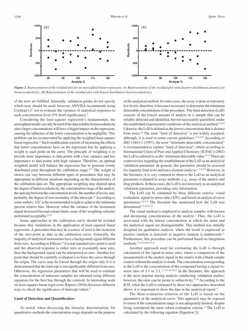
Linearity should be evaluated by examination of the plot of residuals produced by linear regression. A visual evaluation of the pattern of the residuals plot is very simple and allows for straightforward inspection of the error’s variance. Homoscedasticity is the term used to describe the constant variance of the errors throughout the different levels of the concentrations. To evaluate the data’s homoscedasticity, two approaches can be used. The first is graphical analysis of the residues by the concentration; the expected behavior of the data is a constant distribution around zero (Figure 3a). In the case of heteroscedasticity, it is possible to see a clear tendency on the graph. The points will be distributed as a cone, with smaller residues on lower levels and larger residues on higher levels (Figure 3b). Although useful, graphical analysis of the residual plot cannot be considered a potent tool to identify deviations from the linear regression model once no statistical test is involved.8,13,22

Conversely, the second approach to check for homoscedasticity is through use of a statistical test. Any of the following homoscedasticity tests can be used: Cochran, Levene, Brown-Forsythe, or Breusch-Pagan, provided that the conditions necessary for the application

Figure 1. (a) Representation of a typical plot of analytical response versus analyte concentration level. (b) Plot of the response factors versus analyte concen-tration level (dashed lines represent the tolerance limits)

Figure 2. The principle of least-squares regression. The vertical distances between the experimental data and the regression line (i.e., the residuals, dotted lines) are squared, and the line is varied until the sum of the squared residuals is at the minimum


of the tests are fulfilled. Generally, validation guides do not specify which tests should be used; however, ANVISA recommends using Cochran’s C test to evaluate the variance of analytical responses to each concentration level (5% level significance).2

Considering the least-squares regression’s fundamentals, the unweighted model can only be used if the data exhibits homoscedasticity since larger concentrations will have a bigger impact on the regression, causing the influence of the lower concentration to be negligible. This problem can be circumvented by applying the weighted least-squares linear regression.13 Such modification consists of increasing the effects that lower concentrations have on the regression line by applying a weight to each point on the curve. The principle of weighting is to provide more importance to data points with a low variance and less importance to data points with high variance. Therefore, an optimal weighted model will balance the regression line to generate evenly distributed error throughout the calibration range.8,13 The weight of choice can vary between different types of procedures that may be appropriate in different situations depending on the characteristics of the calibration data set. The appropriate weighting may depend upon the degree of heteroscedasticity, the concentration range of the analyte, the spacing between the concentration levels, the number of levels, and, probably, the degree of non-normality of the intercept.23 According to some authors, 1/X2 is the recommended weight to achieve the minimum percent relative bias. However, when the variance of the instrument signal increased beyond certain limits, none of the weighting schemes performed acceptably.23,24

Some approaches to the calibration curve should be avoided because they limitations in the application of least-squared linear regression. A procedure that may be a source of error is the inclusion of the zero-point as data in the calibration curve. Generally, the majority of analytical instruments have a background signal different from zero. According to Ellison,25 if a real standard zero-point is used and the observed response is either zero or reasonably near zero, then the background signal can be interpreted as zero. Another key point that should be carefully evaluated is to force the curve through the origin. The curve may be forced through the origin only if it is demonstrated that the intercept is not significantly different from zero. Otherwise, the regression parameters that will be used to estimate the concentration of unknown samples are obtained using different equations for the best line through the centroid. In interesting work on least-squares linear regression, Raposo (2016) discusses different ways to check the significance of intercept values.8

Limit of Detection and Quantification

As noted, when discussing the linearity determination, for quantitative methods the concentration range depends on the purpose

of the analytical method. In some cases, the assay is done at extremely low levels; therefore, it becomes necessary to determine the minimum detectable concentration of the procedure. The limit detection (LoD) consists of the lowest amount of analyte in a sample that can be reliably detected and identified, but not necessarily quantified, under the established experimental conditions of the analytical method.2,5,6,9 Likewise, the LoD is defined as the lowest concentration that is distinct from noise.26 The term “limit of detection” is not widely accepted; although, it is used in some current guidelines.2,5,6,9,19 According to ISO 11843-1 (1997), the term “minimum detectable concentration” is recommended to replace “limit of detection”, whilst according to International Union of Pure and Applied Chemistry (IUPAC) (2002) the LoD is referred to as the “minimum detectable value.”1,27 There are controversies regarding the establishment of the LoD as an analytical validation parameter. In general, this parameter should be assessed for impurity limit tests and trace element analysis.1,2,6,9,19 However, in the literature, it is very common to observe the LoD as an analytical parameter evaluated in assay methods, e.g., assay of the analyte and drug products. In these cases, the LoD is not necessary as an analytical validation parameter, providing only information.

The LoD can be estimated by three different criteria: visual evaluation, signal-to-noise ratio (S/N), and based on analytical curve parameters.2,6,9,19 The literature has mentioned how the LoD was determined.5,9,19,28–31

The visual method is employed to analyze samples with known and decreasing concentrations of the analyte.2 Thus, the LoD is associated with the lowest concentration at which the noise and the analytical signal are distinguishable. This method was initially designed for qualitative analysis, where the result is expressed as positive (analyte is detected) or negative (analyte is undetected).31 Furthermore, this procedure can be performed based on integration methods.9,14,15,28,29,31,32

Another approach used for estimating the LoD is through calculation of the signal-to-noise ratio, where a comparison of the measurement of the analyte signal in the matrix with a blank sample (matrix without the analyte) is made. The concentration corresponding to the LoD is the concentration of the compound having a signal-to-noise ratio of 3:1 or 2:1.2,5,9,14,28–30,32 In the literature, this approach is the most popular among analysts conducting validation studies; however, the ratio can be prone to subjectivity.13,28 According to the ICH, when the LoD is estimated by these two approaches described above, it is important to show the data in the analytical report.9

The third evaluation criterion of the LoD is based on the parameters of the analytical curve. This approach may be exposed to errors if the concentration range is not adequately limited, despite being considered the most robust evaluation criteria.13 The LoD is calculated by the following equation (Equation 2):

Figure 3. Representation of the residual plot for an unweighted linear regression. (A) Representation of the residual plot with aleatory distribution around zero (homoscedasticity). (B) Representation of the residual plot with biased distribution (heteroscedasticity)


LoD = 3.3 × SD / S (2)

where SD is the standard deviation of the intercepts of the calibration curve or the residual standard deviation of the curve13,15,31 and S is the mean of the slope of the linearity plot. For this test, the analytical curves should be made in the matrix containing the compound of interest and the concentration range should be closest to the LoD.5,9,13-15,29-33 The SD is usually acquired under repeatability conditions of acquisition. However, in order to obtain the most representative SD the analyst should acquire analytical curves through intermediate precision condition. Beyond that, the number of replicates should be enough to ensure a reliable estimate and to avoid large random variation.3,31 The number of replicates varies according to the analytical guideline. While INMETRO (2010) suggests at least 7 replicates, the IUPAC (2002) describes at least 6, and EURACHEM (2014) considers 6 to 15 samples necessary.1,3,19 The ANVISA (2017) does not address the appropriate number.2

When the LoD is obtained by calculation or extrapolation according to Equation 2, that estimate should be confirmed by independent analyses of an appropriate number of samples prepared at a concentration close to that value.2,19

Moreover, other alternatives to measure the LoD are available,34,35 but their uses are discouraged since they are not widely accepted.3,31 This range of methods makes selection difficult. However, all approaches lead to comparable data, whether correctly applied or not.13

This parameter is not robust and can be altered by small changes in the analytical system. Thus, LoD should be always performed in order to expose the operating performance. Moreover, the LoD is matrix-sensitive can vary even for small matrix differences. Thus, it is necessary to determine this parameter for each sample.3,19,31

A common mistake is to employ the instrumental limit of detection (LoDI) to express the LoD or the sensitivity of the analytical method. The LoDI indicates the performance of the equipment and decreases with a reduction in the noise of the apparatus or with an increase in the sensitivity and is used in the comparison of the performance of the equipment and methodologies. The LoDI may be established through the analysis of blank samples, not including any sample preparation steps.3,19,31 Thus, the LoDI can be measured by the relationship between the mean values of the blank samples (x) and their standard deviation(s), and t is the quantile of the Student’s distribution, dependent on the sample size and confidence level, according the Equation 3.1,19,31

LoD = x + t.s (3)

It is important to note that when the determined analyte concentration is close to the LoDI, two situations can occur in the expression of the results: false positives or false negatives. Thus, when the LoD is estimated on different days, the higher LoD should be adopted to minimize false positives. Instead, false negative results can be minimized when reported as “value below LoD”.31

The limit of quantitation (LoQ) is defined as the lowest amount of analyte in a sample that can be quantitatively measured with suitable accuracy and precision under experimental conditions established for the analytical method.2,5,9 The LoQ is also referred to as the quantification limit, quantitation limit, and limit of determination.19,31 Moreover, in some cases when the LoQ corresponds to the first level of the analytical curve, this can be referred to as the lower limit of quantification (LLoQ). Similar to the LoD, the LoQ is expressed as concentration. However, this should be reported as associated with its precision and accuracy.2,13,19,28,30

Similar to the LoD, several approaches may be used to establish

the LoQ, with the S/N ratio and the relationship between the standard deviation of the response and the slope of the curve being commonly used.6,9,15,28,29,32 Moreover, the evaluation of the criteria used in the LoQ should be adequately supported.5,9,28–30

In the literature, determination of the LoQ by the S/N ratio is usually performed, in which a S/N value of at least 10 is required.2,5,9 However, due to S/N ratio limitation in some analytical techniques, the approach most suggested is the calculation through the parameters of the analytical curve, using the equation below (Equation 4):

LoQ = 10 × SD / S (4)

where SD is the standard deviation of the intercepts of the calibration curve or the residual standard deviation of the curve and S is the mean of the slope of the linearity plot.2,3,9,12 All approaches relevant to the LoD should be considered for the LoQ, as well. Thus, to estimate the SD, an appropriate number of independent samples must be analyzed. The analytical curves should be made in a matrix within a range closest to the LoQ. The analyst should acquire analytical curves through intermediate precision conditions. Furthermore, the LoQ depends on the study matrix and may vary over time; therefore, it should be re-evaluated or monitored periodically, mainly when the concentration of analyte in the real sample is close to this value.3,31

The determination of the LoQ as an analytical validation parameter is recommended for impurity quantification tests and when measurements are performed on samples with low levels of analyte. Furthermore, if the first level of the analytical curve is higher than the LoQ, then it is not necessary to estimate the LoQ since it has been shown that the first level of the curve meets the requirements.2,6,9,19

Accuracy

Accuracy is the parameter that is responsible for assessing the agreement between the result found by the analytical method under evaluation and the value that is accepted as true or as a reference.2,6,9,18 Preferably, the assessment of accuracy should be conducted after confirmation of specificity/selectivity, determination of the linear range, and determination of the precision of the method.2,9 The accuracy should be verified using a minimum of nine determinations, considering the specified range of the analytical method. Thus, at least three determinations at the concentration corresponding to the midpoint of the interval (normally 100%) and three additional determinations for both extreme concentrations of the range of quantification (lower and higher) are expected. Moreover, it is fundamental that all replicates of the samples be prepared independently from the beginning of the process, avoiding serial dilutions.2,9

Several procedures can be used to demonstrate the accuracy of an analytical method. The choice may depend on sample type, analytical technique, availability of reference materials, or reference methods. When available, the use of a certified reference material (CRM) may be used to determine the accuracy by comparing the measured values from the analytical method (relative and normalized errors) to the certified reference value.2,6,9 CRMs are materials characterized by a metrologically valid procedure for one or more specified properties, accompanied by a certificate that provides the value of the specified property, its associated uncertainty, and a statement of metrological traceability (National Institute of Standards and Technology, USA).36 The recovery percentage determined by the ratio between the experimental mean and the certified value, including the confidence intervals, can also be used to express the accuracy.2,9 Therefore, the certified value is assumed to be 100%, and the value determined corrected by the dilutions is assumed to be the experimental value (Equation 5). The variability associated with the CRM preparation


steps may influence the recovery value. Generally, a CRM is available for pure substances, but limited to complex products such as medicines.

(5)

Analytical reference methods can also be used to determine the accuracy of the method.2,9,18 Well characterized and independent reference procedures may comprise pharmacopeial methods as well as other analytical methods developed by other organizations admitted by the technical sector.9 The accuracy can be determined in a similar way as Equation 5, substituting the term “certified value (CRM)” for the experimental mean obtained by the reference procedure.2,9 The percentage of recovery of the procedure under analytical validation should be expresses by the CIs obtained by both procedures.

The agreement between the means obtained by the procedure under analytical validation and the reference analytical procedure can also be used to demonstrate the accuracy. For example, hypothesis tests such as the F-test followed by the t-test can be used as a comparison criterion.19 However, it is important to consider that analytical procedures based on different physicochemical properties may differ in specificity and precision, systematically influencing the results. Since the purpose of this approach is not to demonstrate that the two methods are equivalent, but rather to verify the accuracy of the procedure to be validated, statistical significance tests should be used with caution.13 For instance, the obtained results for the same sample when analyzed by a titration procedure and by a chromatographic procedure may be different. If this effect can be quantified, the results should be corrected before performing the statistical comparison. If a correction is not possible, the assumptions of the significance test are violated, and these statistical comparisons become inadequate.13

Experience has shown us that some aspects are critical when a reference procedure is used as an approach for accuracy. First, obtaining previous evidence about the suitability of the reference procedure is indispensable. Thus, partial validation should be done in the laboratory. In addition, it is important that the concentration ranges of both methods are equivalent so that the influence of the analytical concentration and the variability imposed by the different dilution steps are minimized.

A recovery study of a drug substance added to the matrix may be performed when a CRM or a reference procedure is not available. In this case, the samples consist of a mixture of sample components (placebo) added with known quantities of the reference substance. The accuracy is expressed in terms of the recovery of the theorical amount of analyte added (Equation 6).

(6)

This approach is widely applied to samples with complex matrices, where all sample components are easily available. Basically, the matrix must be prepared separately through weighing and mixing of all components, and the amounts of the drug substance must be added to the matrix covering the whole working range. From our experience, the addition of analyte to the matrix should be performed for all evaluated levels. Thus, the influence of all expected sample preparation steps is properly evaluated. Unlike when a solution of matrix is spiked with a standard solution, such influences are suppressed by overestimating the recovery values. The percentage of recovery can be influenced by the precision of the analyte addition process (weighing and mixing), incorporating a variation into the recovered value.

For biological medicines and herbal medicines in which a matrix free of the analyte is not available or its preparation is not possible, a procedure such as that described above may be performed. For this, one can fortify an authentic sample of the medicament with known amounts of standard. In this situation, if the matrix to be used contains 100% of the analyte of interest, the concentration range evaluated will naturally be above the range defined for the routine application of the analytical method. In order to provide more meaningful evidence, it is recommended that the upper limit be not too far from the routine. This approach may be influenced by the dependence of the precision as a function of the determined concentration, which is a summation of the original content of the matrix plus the added amount of analyte.13 Alternatively, the addition of the analyte of interest can be performed at a sample amount equivalent to 50% of the analyte concentration, e.g., obtaining final theoretical concentrations of 80%, 100%, and 120%. This approach allows for evaluation of the accuracy at the same levels of the proposed range for the application of the method in the laboratory routine. However, the influence of the matrix is halved. Thus, if it is proven that there is no matrix effect, such procedure is adequate. If available, a sample with a low concentration of the analyte of interest can be fortified, thereby maintaining the full influence of the matrix under the appropriate concentration levels. The recovery can be calculated with Equation 7.

(7)

Whenever the standard addition procedure is used, use of the same reference substance to obtain fortified matrix samples is recommended. Thus, errors related to the uncertainty of the purity of the analyte of interest are minimized.37

The assessment of the accuracy of pure substances by the addition of standard to the matrix has limited applicability, making it extremely difficult to evaluate the accuracy when CRMs or reference methods are not available. However, every effort should be made to identify an appropriate method of comparison. Instead of quantitative comparison, the results could be supported by another analytical technique, such as verification of the very high purity of a drug substance by differential scanning calorimetry (DSC).38 For an impurities assay, use of the standard addition technique may be a viable alternative. However, greater variability may be expected at low concentration ranges due to the more pronounced effects of the matrix. Generally, at low concentrations, a representative fraction of the analyte may be chemically related to the matrix (e.g., adsorbed), contributing to low recovery.1,26

The maximum acceptable variation for the recovery percentage depends on factors such as the analyte fraction in the sample, sample processing, and the level of quality associated with the methods used. Statistical tests of significance, such as the t-test, and 95% CI may be used to support the assessment of accuracy. However, such statistical tests do not consider variations in practical relevance. For instance, small variabilities at one or more levels of accuracy, which present no practical risk for routine application, may be identified as significant. The t-test describes the relationship between the difference of two means and a standard deviation, with the maximum allowable difference given as a function of the standard deviation. In its turn, the mean recovery may be tested statistically versus the theorical value. If the 95% CI includes the theoretical value, it can be inferred that there is no influence of the concentration on the recovery. If the theoretical value is not included within the CI but the observed standard deviations are acceptable, additional evaluations should be performed to compare statistical significance to practical relevance. In contrast to the significance tests, where confidence intervals must


include the theorical value, equivalence tests must be within an acceptable user-defined range. Here, the user can define an acceptable difference, i.e., a measure of the practical relevance.13

Another alternative is to use absolute acceptance limits, defined as the maximum acceptable absolute difference for recovery, e.g., <2% for the assay of a substance by HPLC. Such approach may be derived from practical experience gained during various validation processes carried out in the same laboratory. However, these differences should be close to 100% and properly grounded on the performance characteristics and measurement uncertainty associated with the analytical procedure in question. In addition, it is recommended that the results obtained be plotted in order to detect trends or the concentration dependence.39 The dispersion of the results may be influenced by the concentration at which the analyte is in the matrix, as well as the concentration at which it is determined analytically. Acceptance limits can also be stipulated considering the dispersion of values as a function of concentration. Normally, the associated deviations increase as the analyte concentration decreases (both relative to the fraction found in the matrix, as well as the analytical concentration).40 According to the range of analyte concentration present in the matrix, acceptable recovery values may be given according to Table 1.41 When the recovery is determined by the matrix fortification procedure that already contains the analyte of interest, it should be considered the original content in the sample plus the quantity added for the application of Table 1.

Precision

Analytical results are influenced by systematic (determinate) and random (indeterminate) errors.13 Systematic errors are caused by problems that persist throughout the entire experiment, and they may be methodological, instrumental, or personal mistakes. Such errors are repeatable in a set of measurements, diverting the experimental results from the direction of the true value. Conversely, random errors are inconsistent and unrepeatable, caused by uncontrollable or unknown variables that lead to dispersion in the data. These errors cannot be corrected or deleted, characterizing the precision of the analytical method.13

The precision of an analytical method represents the closeness among multiple measurements acquired through the analysis of homogeneous samples under similar specified conditions.2,6,9 This analytical validation parameter should be realized for tests and assays for quantitative determinations, and it is usually expressed as the coefficient of variation (CV) or the relative standard deviation (RSD), which is the ratio between the standard deviation and the

mean, multiplied by 100.2,9 This normalization allows for direct comparison.33 Beyond that, dispersion of the data can be expressed as the SD, CI, or variance (the SD square).13 Regarding an analytical procedure, each step has its own variabilities that contribute to the overall dispersion of the results. According to some validation guidelines,2,5,6,9 precision may be considered at three levels: repeatability, intermediate precision, and reproducibility. However, some authors categorize the dispersion of the results in the precision through four categories: system precision, repeatability, intermediate precision, and reproducibility (Figure 4).13,42

According to current guidelines, the system precision, or instrumental precision, is not considered to be a level that should be assessed. This level of precision addresses the variability in the analytical system, mainly of the instrument (e.g., in chromatographic procedures, smalls changes in the injection system or pump flow may interfere with the separation process and the integration of compounds, leading to small variabilities). Although not necessary, knowing such variability can be essential to establishing criteria for system suitability tests, which are carried out through sequential repetitive injections of the same sample.18

The within-laboratory variability of an analytical method must be determined by repeatability and intermediate precision tests.42 Repeatability reflects the agreement among the values obtained through successive measurements under the same operating conditions and the same analyst within a short period of time.2,9,33,42 Repeatability evaluates the contribution of sample preparation to the variability of the method and can be influenced by dilution, weighing, homogenization, and extraction. This term is considered synonymous to intra-day precision and differs from instrumental precision.15,29,43

In practice, samples should be prepared independently from the start of the analytical procedure, and for the same solid and semi-solid samples the same stock solution cannot be used. Repeatability can be determined by performing a minimum of six replicates individually prepared at 100% of the test concentration, or nine determinations should be used with three different concentration levels (low, medium, and high) prepared in triplicate and covering the specified range for the procedure.2,6,9 Considering that precision is modified by the concentration of the analyte, especially if the analytical method covers a large concentration range, and that the samples tested should be representative of the whole, the points tested in this parameter should ideally encompass the limits established by the method.

Table 1. Expected recovery as a function of analyte concentration

Analyte mass fraction in the matrix

Unit Mean recovery (%)

100 100% 98–102

10 10% 98–102

1 1% 97–103

0.1 0.1% 95–105

0.01 100 ppm (mg kg–1) 90–107

0.001 10 ppm (mg kg–1) 80–110

0.0001 1 ppm (mg kg–1) 80–110

0.00001 100 ppb (µg kg–1) 80–110

0.000001 10 ppb (µg kg–1) 60–115

0.0000001 1 ppb (µg kg–1) 40–120

Figure 4. Representation of precision levels and their respective contributions


In this approach, acceptance criteria are defined and justified according to the test performed and its objective, based on the intrinsic variability of the method, the working range, and the analyte concentration in the sample.2 When the results obtained do not meet the acceptance criteria, new solutions should be prepared, and in case of failure again the possible causes of error must be investigated. The expected values for repeatability are equivalent to 2/3 of the results obtained for reproducibility.13,40 The acceptance limits commonly found in the pharmaceutical industries are up to 2% for CV. It is important to note that the distribution of the repeatability reflects the complexity of the sample, its preparation, and the analytical technique used.13,44

The Eurachem guideline (2014) and INMETRO (2016) suggest precision limits based on the SD.3,19 Thus, it is possible to define the repeatability limits, which enables the analyst to define whether the difference between the analyses conducted is significant at a specified level of confidence. The limit may be calculated using the following equation, (Equation 8):

(8)

where r is the repeatability limit, is related to the difference between two measurements, and t is the two-tailed Student t-value for a specified number of degrees of freedom (which relates to the estimate of the SD) at the required level of confidence. For relatively large numbers of degrees of freedom, the t-value with a 95% confidence level is approximately 2; therefore, the following equation is obtained for the repeatability in these cases (Equation 9).

r = 2.8 × SD (9)

The acceptance criteria for intermediate precision and reproducibility are calculated in a similar way, replacing the SD (repeatability) for the SD obtained for the intermediate precision or the reproducibility.3,19,42

Intermediate precision expresses the effect of within-laboratory variations due to events such as different days, analysts, and equipment, or a combination of these factors, in order to reflect the expected routine laboratory variability.2,6,9,33 The intermediate precision includes the influence of additional random effects according to the intended use of the method in the same laboratory and can be regarded as an estimate of the long-term variability. Moreover, such an evaluation assesses the procedural capacity to provide the same results, considering that in different analytical runs changes in the reagent or supplier lots may occur, as well as variations in calibration standards, equipment recalibration, and alterations in temperatures.13,42

Regarding intermediate precision, also referred to as inter-assay precision, this can be determined through the analysis of similar samples on different days, with different analysts and different instruments.2,9,45 The required number of determinations and levels tested in order to evaluate the intermediate precision follows the same recommendation for repeatability and can also be expressed by the RSD. Moreover, planning and execution should include the same approach in terms of concentration levels and the same number of determinations previously performed in the repeatability assessment.2,9

It is very important to address intermediate precision appropriately since it is an estimate of the expected variability. Firstly, the RSD for the two series of analyses (repeatability and intermediate precision tests) should be calculated. In sequence, the results obtained in the two series results (mean ± SD) should be statistically equivalent (e.g., F-test and t-test) .13,19 The F-test evaluates whether the observed

variances between groups of measures are statistically equivalent. The t-test is then used to verify if the means of the results of the two groups can be considered statistically equal. However, sometimes the two series of measurements may differ significantly by such statistical test. This is particularly frequent in the case of good performance measurements in which the two sets show little scatter. If at the level of significance adopted there is no significant difference between the means, it is considered that the method has adequate intermediate precision. However, when there is a difference between the precision levels, the cause needs to be identified by investigation of the individual effects of the various factors. Depending on the cause, the recommended solution consists of defining absolute upper limits for the various precision levels since duly justified.

The last test used to evaluate the precision of a method consists of testing the reproducibility, which expresses the agreement among the results obtained in different laboratories that analyze homogeneous samples.2,5,6,9 This parameter provides the largest expected precision because it is obtained by varying all the factors that may compromise the results.15,42 Reproducibility should be measured in at least two laboratories, although IUPAC recommends a minimum of five, ideally eight.12 Acceptance criteria like those established for repeatability and intermediate precision also apply to reproducibility.

As an acceptance criterion for reproducibility, the equation by Horwitz et al. (1980) can be utilized. This equation establishes the exponential relationship between the values of the RSD and the analyte concentration (C) (Equation 10).1,40,46–49

RSDr = 2(1 – 0.5logC) (10)

The predicted relative standard deviation of reproducibility (RSDr) obtained by the Horwitz equation is independent on the nature of the analyte, matrix, and analytical technique. However, this equation is limited to concentrations below 120 µg kg–1 (ppb) because the values obtained for the RSD are extremely high.1,46,48,49 To contemplate these smaller concentrations, Thompson proposed a modified equation according to analyte concentration (Equations 11-13),19,46,47 as follows:

Concentration: < 1.2 × 10–7 RSDr = 0.22 × C (11)Concentration: 1.2 × 10–7 ≤ C ≥ 0.138 RSDr = 0.02 × C(0.8495) (12)Concentration: > 0.138 RSDr = 0.01 × C(0.5) (13)

In addition, as a criterion of acceptability, the precision can be calculated by the ratio of Horwitz (RazHor) (Equation 14), which correlates the experimentally obtained RSD from the collaborative trial (RSDr) with the predicted RSD obtained by the Horwitz equation (PRSDr).13,47,48

RazHor = RSDr / PRSDr (14)

The reproducibility of the method is satisfactory when the RazHor value is close to 1 and the acceptable limit is up to 2. Values greater than 2 demonstrate that the analytical method performs poorly and that participating laboratories should review their techniques and procedures in order to identify possible errors. For the intra-laboratory repeatability assays, the RSD must be between 1/2 and 2/3 of the value calculated by the Horwitz equation.19,48

Robustness

The robustness of an analytical method describes its ability to withstand small and deliberate variations in analytical parameters, whilst maintaining acceptable precision and accuracy.2,9,18,19 The primary goal of robustness studies is to identify the method variables

lilian.faria

Rectangle


that are critical to ensure reliability and reproducibility of the results and to monitor routine analysis. Most experimental conditions are susceptible to normal fluctuations and occasional mistakes. The robustness provides essential information to predict the behavior of the results, maintaining the quality of the analysis, and occasionally guides troubleshooting during the daily execution of the method.

These parameters should ideally be accessed during the development of the method prior to validation, whereas evaluation of their effect can be easily done when manipulating the method to achieve the optimal method conditions.9,50 The changes in the chromatographic conditions applied during method development are often harsh; however, it helps to indicate what parameters should be narrowed during validation.

There is no standard that describes which parameters should be evaluated in the analysis of robustness. They must be determined by the analyst and will differ with different equipment and applied techniques. There are some suggestions of which parameters to choose, shown in Table 2.50–52

As mentioned above, these are suggestions of commonly evaluated parameters, and nothing restrains the analyst from including a pertinent parameter that may imply a detectable deviation in selectivity or signal intensity. The choice of “small and deliberate” changes of each parameter to be evaluated in the robustness must be determined in order to contemplate a range of values consistent with variations within the laboratory routine. For instance, when changing the flow from 1 mL min–1 to 1.1 mL min–1 and changing the mobile phase proportion from 50% to 49%, the analyst must ask if these changes are probable in terms of the instrument’s fluctuation (Is it probable that the pump’s flow rate will reach this fluctuation of 10%? Is it possible that the pumping of the mobile phase proportion will differ by 1%?). If these changes that are inherent to the equipment are probable, then verification of their influences must be conducted during robustness tests.

The variable response to quantify and evaluate the robustness of the method will also be dependent on the purpose of the method and may be different for each parameter and sometimes directly related to specific ones. For instance, if the method purpose is identification of a specific analyte among its impurities by LC, the resolution, peak purity, and capacity factor might be good variables to evaluate since these parameters demonstrate the selectivity of the analyte. Given the relevance, the analyst may add any quantifiable variable response.

Robustness tests are conducted in univariate and multivariate ways. The univariate approach involves varying each parameter individually in order to identify the influence of this change. The deviation limits that are acceptable in univariate experiments are represented graphically and statistically. Graphical evaluation is useful for expressive effects, (e.g., a change that exceeds the normal equipment fluctuation in terms of retention time, peak resolution, and tailing factor), but may lead to misinterpretation of discrete effects. Then, Student’s t test can be used to compare the similarity of the result obtained in the standard condition and in the altered condition.

The majority of analysts apply the univariate way in any situation; however, the investigation can be useful to evaluate few parameters, making it impractical as the number of parameters increases. For example, if the test has 7 alternating parameters, the analyst must run 128 analyses, varying each factor individually to achieve all possible combinations of conditions. Whereas the impracticality number of experiments, the analyst may adopt the systematic approach with multivariate experimental design, which is a mathematical tool to minimize the sample number, using combinatory designs to vary parameters simultaneously, rather than one at a time. This approach is more effective at evaluating a higher number of parameters and

Table 2. Potential factors to examine during robustness tests

Separation technique Factors

Liquid chromatography (LC)

Proportion of mobile phase constituentsMobile phase pH

Buffer concentrationFlow rate

Column temperatureGradient elution - initial mobile phase

Slope of gradientStationary phase

Column manufacturerWavelength of detection

Gas chromatography (GC)

Type of columnInjector temperatureColumn temperatureDetector temperature

Initial and final temperatureSlope of the temperature gradient

Carrier gas type/compositionGas flow rate

Split or splitless conditionsSplit flowLiner type

Column manufacturerColumn stationary phase

Thin layer chromatography (TLC)

Eluent compositionpH of the mobile phase

TemperatureDevelopment distance

Spot shapeSpot size

Batch of the platesVolume of sample

Drying conditions (temperature, time)

Capillary electrophoresis (CE)

Electrolyte concentrationBuffer pH

Concentration of additivesTemperature

Applied voltageSample injection timeSample concentration

Rinse timesWavelength of detection

Sample preparation technique Factors

Solid phase extraction (SPE)

Sorbent typeSorbent manufacturer

Sorbent massSample mass or volume

Wash solventElution solvent

Evaporation temperaturepH of sample

pH of buffer constituents in solvents

Matrix solid phase dispersion (MSPD)

Sorbent typeSorbent manufacturer

Sorbent masspH of samplepH of buffer

Sonication timeEvaporation temperature

Wash solventElution solvent

Sample mass or volume

Adapted from Karageorgou, Heyden and Dejaegher.50-52


allows for the detection of the effect of each parameter individually, as well as its synergies.50,53

There are several ways to design a multifactorial experiment. The most common examples are utilization of fractional factorial and Plackett-Burman designs.50 An example of a fractional factorial design is the Youden’s Square design, and, in combination with Youden’s test, it can evaluate the influence of each parameter individually. However, interactions between the different factors cannot be detected.51 In addition to Youden’s test, evaluation of the robustness data from multivariate experiments can be achieved through probability plots and effect plots. There are normal and half-normal probability plots. Normal probability plots are used to assess whether the data set is approximately normally distributed, while half-normal probability plots can identify the important parameters and interactions between the factors. Probability plots draw a line through the data, and a sample that deviates from the line is considered to be critical to the method (Figure 5). The effect plot uses bars as graphical representation, and the Pareto chart shows the magnitude of the effects, that is, the influence of individual and joint effects on the evaluated response (Figure 5).53

When no significant effects are found on these graphical plots, the method may be considered robust to the specific parameter. Regardless of the chosen parameters, the variable response, and its robustness, it is possible to continue the validation process since robustness is not a parameter for approval or rejection of the analytical condition. The results of robustness are an indicative of what is criticality to the method and what factors must be followed carefully to ensure the reproducibility of results.

Stability Studies of Analytical Solutions

Chemical compounds may decompose during the preparation of solutions or during storage (post preparation and prior to analysis, short-term, and long-term storage).11 Therefore, pre-establishing the handling and storage conditions is fundamental for proper analytical development, as well as for later analytical validation. Pre-determining the stability profile of the analytical solutions in the early stages of method development makes it possible to reduce spending on the use of freshly prepared solutions for each test, maintaining reliability. Additionally, the experimental data helps us to understand the limitations of the analytical method, assisting in planning the analytical validation procedure.5

Several guidelines concerning analytical validation agree that analytical stability is part of robustness and recommend its execution during the development stage.2,5,6,9,18 However, its additional accomplishment as an analytical validation parameter should be understood as an indispensable step because the reliability on results only can be assumed after all validation parameters have been confirmed. Although recommended, few details on procedures and

criteria are shown by the guidelines. The guidelines are limited to requirement “should be done.” Given this, the analyst must ensure that all critical variables and the best way to carry them out are detailed in the analytical validation protocol. Critical variables include all conditions under which solutions will be subjected during routine work, reflecting the real situations during the handling, storage, and analysis of the standards and samples.

During the laboratory routine, the storage of stock solutions allows for better use of the reference chemical substances. Stock solutions may be kept under several conditions during their life cycle (storage under bench-top at room temperature, refrigerated, and freezing). Despite application for a distinct scope, some stances adopted by bioanalytical guides may help to better evaluate the analytical methods A good example of how to proceed is given by the ANVISA guide for the validation of bioanalytical methods.2 For instance, if the stock solutions are stored in a freezer, the maximum number of freezes–thaw cycles must be determined. For this, it is important to ensure that freezing of the solution occurs by a period that, at a minimum, guarantees complete freezing and only then the solution is thawed to the handling temperature. The number of cycles under such a condition is determined by maintaining the stability of the analyte of interest, which should be always quantified immediately after each freeze–thaw cycle. In a routine application, after the stock solution has been thawed, it usually remains under bench top conditions for some time. Thus, it is recommended that the period evaluated under this bench-top condition comprises the time spent for the first preparation plus possible re-preparation, including the time required to confirm any handling error. The evaluation time required will depend on the analytical technique used. Usually, this evaluation lasts for a few hours, contemplating at least 6 hours.

Analytical solutions obtained from stock solutions or from samples should also be evaluated under bench top and handling conditions. If this condition is different or not covered by auto-sampler storage conditions, short periods of up to 24 hours are enough for this assessment. Conversely, when different auto-sampler conditions than bench-top conditions are used, the expected residence time for the analytical run shall be assessed. For instance, dissolution testing assessed by the liquid chromatography technique may extend over more than two days. Generally, stability studies for such case must be performed for 48 to 72 hours due to the large required time of the analytical run. If the bench condition is the same as the analysis, the same reasoning that is applied to the auto-sampler condition can be used.13

Additionally, it is important that for each stability period time to be evaluated, the measurements should be performed in replicate. Preferably, six replicated assays of one sample solution should be carried out, which is indispensable for the assessment of certain statistical tools.13 If an internal standard is used, its stability must

Figure 5. Half-normal probability plot (A) and Pareto chart (B)


also be ensured under the same conditions and periods of storage and handling of other solutions.5 Another major point that must be considered in the stability study of analytical solutions is the evaluation of solutions at extreme concentrations of the quantification interval.54 In applications such as dissolution testing, the range of quantification may be broad and the stability solution at the lower end of the interval may be significantly different from the 100%.

Normally, in an analytical run where the stability of the analytical system is kept under the same conditions (e.g., under the same repeatability conditions, such as the method, analyst, instrumentation, location, and conditions of use), deviations in absolute responses can be neglected and direct comparisons between responses can be safely performed.55 For example, the direct comparison between the areas under the peak, obtained by HPLC, or the absorbance values obtained by spectrophotometry, are adequate when such conditions are satisfied.

However, when the responses to be compared are obtained from different analytical runs, drifts in responses may occur and the use of such data may be inadequate or influence the results. Such deviations may occur if the measurements are susceptible to variations in analytical conditions through the days or weeks necessary to stability of stock solutions. This is especially important in analytical techniques that require new start up whenever used. For example, it is very for common chromatographic techniques to show certain analytical variability due to different mobile phase preparations, use of solvents from different batches, loss of source intensity and linearity of the response due to the natural wear (UV–vis), differences in the intensity of ionization of the analyte of interest (hyphenation with MS). When such analytical variability is identified, for each evaluated period measurement of freshly prepared solutions is also recommended. Thus, rather than the absolute responses, it is possible to use the recovery values or analytical concentration as parameters of comparison, minimizing that variations that occur as a function of time. A similar approach is recommended in the validation of bioanalytic methods.2,54

A very important aspect to consider in stability studies of analytical solutions is the assessment of the results by statistical tools. One way to evaluate stability of analytical solution is through the CV calculated for all values obtained in the different time intervals. If the CV of all values obtained at different time intervals does not exceed more than 20% of the corresponding response (e.g. drug content) at the initial analysis, it is assumed that there is no trend.56 The stability can also be evaluated by comparing the obtained recoveries of all time intervals against the initially obtained recovery. If the observed result for each period is within a predefined tolerance range and duly justified (for instance, a tolerance range that can be derived from intermediate precision), it is assumed that there is no trend.13

Analytical stability can also be determined by means of specific statistical tests since the test conditions are satisfied. The t-test can be used to investigate whether there is a difference between two means or between a mean and a reference value. Analysis of variance (ANOVA) can be applied to verify if there are differences among means if more than two time intervals are evaluated. However, if differences are found among the means, ANOVA does not show which time interval is different. Therefore, it should be followed by multiple comparison tests, such as the Tukey test, to determine which time intervals are different.57 Acceptance limits defined as fixed values may also be assumed. For instance, variability of <2% is assumed to be normal. However, it is important that the detection of non-acceptable variations be consistent with the variability of the analytical system (system precision). For example, a variability on the order of 2% after a given time interval may be associated with either loss of stability or variability of the analytical system. If the system precision is

around 1%, then it can be assumed that the obtained value with a 2% difference is reliable and represents loss of stability. However, if the actual variability of the method is ≥2%, it is not possible to assume such variability as loss of stability.13 Therefore, when fixed values are assumed as acceptance limits, the maximum uncertainty associated with the analytical measurement should be considered for proper evaluation of the stability results.

Finally, it is important to note that if during the routine application of the analytical method the conditions of storage and handling are different or occur outside the validated conditions, the analytical stability should be re-evaluated under these new conditions.

System Suitability

By experimental assays and scientific evidence, method validation ensures that the analytical procedure is suitable for its intended use under the specified conditions.5,9 Even so, it may be equivocating to assume that the quality of the results generated by any analytical method, when applied in the daily routine, will be always accurate due one analytical validation effectively carried out in a qualified equipment. Several aspects may influence the quality of the results since any analytical procedure is susceptible to occasional deviations that can lead to systemic errors or increases in random error. Once the equipment undergoes qualification, it is safe to say that the equipment’s components are able to provide reliable results. However, during the laboratory activities, the equipment may be subject of efficiency loss or malfunction. The step that measure this adequacy is called system suitability tests (SSTs), and this system verification is carried out before or in parallel to any analytical run on the daily routine of the laboratory, aiming to ensure that the system is adequate, ratifying that its functions are within predefined limits by the time of use.15

Although a comprehensive evaluation of the whole process is recommended, the SST often is translated in the verification of analytical equipment. Aspects related to sample preparation, analytical validation, and equipment qualification are also liable to verification. For example, usage of a calibrated weight to verify the accuracy of the weighing balance, testing the volume drawn in a micropipette by weighing different volumes of water, and even utilization of a buffer solution with known pH to evaluate the pH meter are ways to evaluate the components that are relevant to sample preparation, which is a fundamental part of system suitability evaluation. These verification steps are needed, and by covering the suitability of all adjacent processes linked to the methodology the data’s reliability and consistency are ensured to the analytical procedure.

Generally, SST parameters in liquid chromatography analysis may include resolution (Rs), number of theorical plates (N), tailing factor (T), capacity factor (k), relative retention time (RRT), S/N ratio, and repeatability (RSD of peak response and retention time).2,18,58 These parameters are important since they indicate sensitivity, precision, selectivity, and efficiency. Sensitivity and precision are principally limited to the performances of the injector and detector, whilst selectivity and efficiency relate to the stationary and mobile phases.13 These are the most common parameters when monitoring SST in a chromatograph system; however, the analyst should not comprise the analysis of SST for only these and must be aware of what is relevant when monitoring the system suitability and what may imply a detectable deviation in the process.

To access the SST prior to method development, the analyst may inject replicates of the same sample to evaluate the suitability of the equipment (e.g., evaluate the low RSD and reproducibility of the retention time and peak resolution of the standard in relation to its impurities, implying suitability of injector and mobile phase pump). In this way, it is possible to perform system verification of


components that are inherent to the equipment prior to accessing the SST parameters that are obtained during method development and validation. Furthermore, during analysis it is possible to verify the loss in the system’s efficiency by using quality control samples between study samples during a run sequence. In long run sequences, not every system is capable of maintaining suitable system until the end of the analytical run. To address this, analysis of a standard with known SST parameters may be undertake between the batch samples to verify the reproducibility of these parameters in relation to the previous determination of the same sample over the course of the run sequence. The criteria of the interval at which the quality control samples should be submitted is subjective, and this decision must be made based on the capacity of the instrument in maintaining the reproducibility of its data during long analyses. It is important to note that in the interval applied, the quality control sample must be stable and soluble in the solution in order to evaluate the system without a reduction in the standard’s content.

By the time that the method is developed, there is enough information to generate an SST for the proposed method with the parameters provided from the results (e.g., theoretical plates, peak resolution, tailing factor, capacity factor, chromatogram of the optimal chromatographic condition). It is important to use the parameters of the optimized method for system verification since the value of some parameters can be influenced by the chromatographic conditions provided.

The values of the parameters are refined with robustness assays during validation since this step provides valuable information about what is critical to causing a deviation. In addition, the results of the robustness assays assist in determining the SST parameters limits for the different parameters. The conditions applied to the robustness tests result in an acceptable and probable outcome.59

In this way, any failure of the system suitability tests may indicate that the performance of the analytical procedure will be outside the validation scope or there will be loss of operational capacity of the equipment. Whenever a failure of SST is observed, an investigation must be conducted to address the poor performance, and often the SST parameters guide the analyst of what component may be compromised. For instance, a high RSD of the same sample may imply an injector problem. Distinct peak resolution from the expected suggests a problem with the loss of chromatographic column efficiency and/or composition of mobile phase pump (pumping wrong proportion). A compromised S/N ratio indicates a problem with detector efficiency. After making the necessary adjustments, another system suitability test should be performed. Only then can the sample analyses be performed.13

CONCLUSION

An analytical method should be validated before its implementation in a quality control routine. The validation procedure is essential to ensuring reliable and accurate method performance. Despite several regulatory agencies addressing this validation, there is still a lack of uniformity in the methodology used for validation and acceptance criteria due to misunderstandings in data interpretation and execution. One of the first steps during the validation process is to define its purpose and to detail the conditions under which it will be applied in order to achieve a reliable and truthful method.

It is important to note that the validation process is continuous and should be maintained over the entire life of the method. If an analytical method undergoes changes beyond the operational ranges covered during the analytical validation, then revalidation is necessary. In addition, periodic revalidation of analytical methods should be performed according to a time period that is scientifically justifiable.

ACKNOWLEDGMENTS

The authors express their gratitude for research funding to the CAPES (Brazilian Federal Agency for Support and Evaluation of Graduate Education within the Ministry of Education of Brazil) - Finance Code 001.

REFERENCES

1. IUPAC; Harmonized guidelines for single-laboratory validation of methods of analysis; Pure Appl Chem. 2002, 74, 835.

2. ANVISA; Agência Nacional de Vigilância Sanitária Resolução da Diretoria Colegiada – RDC nº 166 de 24 de julho de 2017; Brasília, 2017.

3. Eurachem; Eurachem Guide: The Fitness for Purpose of Analytical Methods—A Laboratory Guide to Method Validation and Related Topics, B. Magnusson, B.; Örnemark, U., eds; 2014.

4. European Medicines Agency; Guideline on process validation for finished products - information and data to be provided in regulatory submissions; London, 2016.

5. U. S. Food and Drug Administration; Analytical procedures and methods validation for drugs and biologics Guidance for Industry; Rockville, 2015.

6. WHO; Guidelines on validation - Appendix 4 - Analytical method Validation; Geneva, 2016.

7. Fachi, M. M.; Leonart, L. P.; Cerqueira, L. B.; Pontes, F. L. D.; de Campos, M. L.; Pontarolo, R.; J Chromatogr B Analyt Technol Biomed Life Sci. 2017, 1055, 61.

8. Raposo, F.; TrAC Trends in Analytical Chemistry. 2016, 77, 167. 9. European Medicines Agency; ICH Harmonised tripartite guideline -

Validation of analytical procedures: text and methodology Q2 (R1); London, 2005.

10. WHO; WHO Expert Committee on Specifications for Pharmaceutical Preparations; Geneva, 2018.

11. Peris-Vicente, J.; Esteve-Romero, J.; Carda-Broch, S.; Anal Separation Science. 2015, 5, 1757.

12. Bonfilio, R.; Cazedey, E. C. L.; Araújo, M. B. D.; Nunes Salgado, H. R.; Crit Rev Anal Chem. 2012, 42, 87.

13. Ermer, J.; Miller, J. H. M.; Method validation in pharmaceutical analysis: A guide to best practice; Wiley: New Jersey, 2006.

14. Ribani, M.; Bottoli, C. B. G.; Collins, C. H.; Jardim, I. C. S. F.; Melo, L. F. C.; Quim Nova. 2004, 27, 771.

15. Paithankar, H.; Int J Univers Pharm Bio Sci. 2013, 2, 229. 16. González, A. G.; Herrador, M. Á.; TRAC-Trend Anal Chem. 2007, 26,

227. 17. Kroll, M. H.; Emancipator, K.; Clin Chem. 1993, 39, 405. 18. United States Pharmacopoeial Convention; USP 41-NF 36, chapter

<1225> Validation of compendial procedures; United States Pharmacopoeia: North Bethesda, 2018.

19. Inmetro; Orientação sobre validação de métodos analíticos DOQ-CGRE-008. Rio de Janeiro, 2016.

20. Huber, L.; LC GC Eur. 1998, 11, 96. 21. Dorschel, C. A.; Anal Chem. 1989, 61, 951A. 22. Jurado, J.; Alcázar, A.; Muñiz-Valencia, R.; Ceballos-Magaña, S.;

Raposo, F.; Talanta. 2017, 172, 221. 23. Jain, R. B.; Clin Chim Acta. 2010, 411, 270. 24. Almeida, A. M.; Castel-Branco, M. M.; Falcão, A. C.; J Chromatogr B.

2002, 774, 215. 25. Ellison, S. L.; Barwick, V. J.; Farrant, T. J. D.; Practical statistics for the

analytical scientist: a bench guide, 2nd ed., Royal Society of Chemistry: London, 2009.

26. Thompson, M.; Ellison, S. L.; Wood, R.; Pure Appl Chem. 2002, 74, 835.


27. Ortiz, M.; Sarabia, L.; Herrero, A.; Sánchez, M.; Sanz, M.; Rueda, M.; Giménez, D.; Meléndez, M.E.; Chemometr Intel Lab. 2003, 69, 21.

28. Araujo, P.; J Chromatogr B Analyt Technol Biomed Life Sci. 2009, 877, 2224.

29. Belouafa, S.; Habti, F.; Benhar, S.; Belafkih, B.; Tayane, S.; Hamdouch, S.; Bennamara, A.; Abourriche, A.; Int J Metrol Qual Eng. 2017, 8, 9.

30. Shabir, G. A.; J Valid Technol. 2005, 10, 314. 31. Kruve, A.; Rebane, R.; Kipper, K.; Oldekop, M. L.; Evard, H.; Herodes,

K.; Ravio, P.; Leito, I.; Anal Chim Acta. 2015, 870, 29. 32. Ravisankar, P.; Navya, C. N.; Pravallika, D.; Sri, D. N.; IOSR J Pharm.

2015, 5, 7. 33. Theodorsson, E.; Bioanalysis. 2012, 4, 305. 34. Fonollosa, J.; Vergara, A.; Huerta, R.; Marco, S.; Anal Chim Acta. 2014,

810, 1. 35. Huber, W.; Accredit Qual Assur. 2003, 8, 213. 36. NIST; http://www.nist.gov/, acessada em Agosto 2019. 37. Epshtein, N.; Pharml Chem J. 2004, 38, 212. 38. Giron, D.; Encyclopedia of Pharmaceutical Science and Technology;

Swarbrick, J., eds.; 4th ed., CRC Press: Boca Raton; 2013. 39. Crowther, J.; Jimidar, I.; Niemeijer, N.; Salomons, P.; Qualification

of laboratory instrumentation, validation, and transfer of analytical methods; Miller, J.M.; Crowther, J.B., eds; 2000.

40. AOAC International; Appendix F: Guidelines for Standard Method Performance Requirements; Rockville, 2016.

41. Giron, D.; J Therm Anal Calorim. 2002, 68, 335. 42. Boqué, R.; Maroto, A.; Riu, J.; Rius, F. X.; Validation of Analytical

Methods. Grasas Aceites. 2002, 53, 128. 43. Kazusaki, M.; Ueda, S.; Takeuchi, N.; Ohgami, Y.; Chromatography.

2012, 33, 65.

44. Bouabidi, A.; Rozet, E.; Fillet, M.; Ziemons, E.; Chapuzet, E.; Mertens, B.; Klinkenberg, R.; Ceccato, A.; Talbi, M.; Streel, B.; Bouklouze, A.; Boulanger, B.; Hubert, P.; J Chromatogr A. 2010, 1217, 3180.

45. Tiwari, G.; Tiwari, R.; Pharm Methods. 2010, 1, 25. 46. Nolet, L. M. L.; Lambropoulou, D. A.; Chromatographic analysis of the

environment: mass spectrometry based approaches; 4th ed., CRC Press: Boca Raton, 2017.

47. Côté, I.; Robouch, P.; Robouch, B.; Bisson, D.; Gamache, P.; LeBlanc, A.; Dumas, P.; Pedneault, M.; Accred Qual Assur. 2012, 17, 389.

48. Linsinger, T. P. J.; Josephs, R. D.; TRAC Trend Anal Chem. 2006, 25, 1125.

49. Thompson, M.; Royal Society of Chemistry. 2004, 17, 1. 50. Dejaegher, B.; Vander Heyden, Y.; Acta Chromatogr. 2009, 21, 161. 51. Karageorgou, E.; Samanidou, V.; J Chromatogr A. 2014, 1353, 131. 52. Vander Heyden, Y.; Nijhuis, A.; Smeyers-Verbeke, J.; Vandeginste, B.;

Massart, D.; J Pharmaceut Biomed Anal. 2001, 24, 723. 53. Swartz, M. E.; Krull, I. S.; Handbook of analytical validation; CRC

Press: Boca Raton, 2012. 54. U. S. Food and Drug Administration; Bioanalytical Method Validation

- Guidance for Industry; Rockville, 2018. 55. Bloch, M.; In Method Validation in Pharmaceutical Analysis: A Guide

to Best Practice; Ermer, J.; Miller, J. H. McB., eds; Wiley: New Jersey, 2004, chapter 5.

56. Huber, L.; Validation and qualification in analytical laboratories; 2nd ed.; CRC Press: Boca Raton, 2007.

57. Kao, L. S.; Green, C. E.; J Surg Res. 2008, 144, 158. 58. U. S. Food and Drug Administration; Validation of Chromatographic

Methods; Rockville, 1994. 59. Vander Heyden, Y.; Jimidar, M.; Hund, E.; Niemeijer, N.; Peeters, R.;

Smeyers-Verbeke, J.; Massart, D.L.; Hoogmartens, J.; J Chromatogr A. 1999, 845, 145.

This is an open-access article distributed under the terms of the Creative Commons Attribution License.

VALIDATION OF ANALYTICAL METHODS IN A PHARMACEUTICAL ...

Documents