Vacuum polarization and hadronic contribution to muon g−2 from lattice QCD

arX

iv:h

ep-l

at/0

3120

32v1

18

Dec

200

3

Vacuum Polarisation and Hadronic

Contribution to muon g − 2 from Lattice QCD

M. Gockeler a,b, R. Horsley c, W. Kurzinger d,e, D. Pleiter d,

P. E. L. Rakow f, G. Schierholz d,g

aInstitut fur Theoretische Physik, Universitat Leipzig,D-04109 Leipzig, Germany

bInstitut fur Theoretische Physik, Universitat Regensburg,D-93040 Regensburg, Germany

cSchool of Physics, University of Edinburgh,Edinburgh EH9 3JZ, UK

dJohn von Neumann-Institut fur Computing NIC,Deutsches Elektronen-Synchrotron DESY,

D-15735 Zeuthen, GermanyeInstitut fur Theoretische Physik, Freie Universitat Berlin,

D-14195 Berlin, GermanyfTheoretical Physics Division, Department of Mathematical Sciences,

University of Liverpool, Liverpool L69 3BX, UKgDeutsches Elektronen-Synchrotron DESY,

D-22603 Hamburg, Germany

[QCDSF Collaboration]

DESY 03-199

Edinburgh 2003/22

Leipzig LU-ITP 2003/031

Liverpool LTH 615

Abstract

We compute the vacuum polarisation on the lattice in quenched QCD using non-perturbatively improved Wilson fermions. Above Q2 of about 2 GeV2 the resultsare very close to the predictions of perturbative QCD. Below this scale we see signsof non-perturbative effects which we can describe by the use of dispersion relations.We use our results to estimate the light quark contribution to the muon’s anomalousmagnetic moment. We find the result 446(23)×10−10, where the error only includesstatistical uncertainties. Finally we make some comments on the applicability of theOperator Product Expansion to our data.

Key words: QCD, Lattice, e+e− Annihilation, muon anomalous magnetic momentPACS: 11.15.Ha, 12.38.-t, 12.38.Bx, 12.38.Gc, 16.65.+i

Preprint submitted to Elsevier Science

1 Introduction

The vacuum polarisation Π(Q2) provides valuable information on the in-terface between perturbative and non-perturbative physics. It has been thesubject of intensive discussions in the literature.

The vacuum polarisation tensor is responsible for the running of αem, whichmust be known very accurately for high-precision electro-magnetic calcula-tions. To calculate the hadronic contribution to the anomalous magnetic mo-ment of the muon we need to know the vacuum polarisation at scales from∼ 100 MeV to many GeV. Perturbative QCD will be unreliable at the low endof this scale, so a non-perturbative calculation on the lattice would be useful.

The vacuum polarisation Π(Q2) is defined by

Πµν(q) = i∫

d4x eiqx〈0|T Jµ(x)Jν(0)|0〉 ≡ (qµqν − q2gµν) Π(Q2), (1)

where Jµ is the hadronic electromagnetic current

Jµ(x) =∑

f

ef ψf (x)γµψf (x) =2

3u(x)γµu(x) −

1

3d(x)γµd(x) + · · · (2)

and Q2 ≡ −q2 (so that Q2 > 0 for spacelike momenta, Q2 < 0 for timelike).Π can be computed on the lattice for spacelike momenta Q2 > 0.

Π can also be calculated in perturbation theory. Π has to be additivelyrenormalised, even the one-loop diagram (with no gluons involved) is loga-rithmically divergent. This renormalisation implies that the value of Π can beshifted up and down by a constant depending on scheme and scale without anyphysical effects. However theQ2 dependence of Π(Q2) is physically meaningful,and it must be independent of renormalisation scheme or regularisation.

Experimentally Π can be calculated from data for the total cross sectionof e+e− → hadrons with theoretical predictions of QCD by means of thedispersion relations [1]

12π2Q2 (−1)n

n!

(

d

dQ2

)n

Π(Q2) = Q2∫ ∞

4m2π

dsR(s)

(s+Q2)n+1, (3)

where

R(s) =σe+e−→hadrons(s)

σe+e−→µ+µ−(s)=

(

3s

4πα2em

)

σe+e−→hadrons(s) . (4)

The first derivative of the vacuum polarisation (the n = 1 term in eq.(3)) is

2

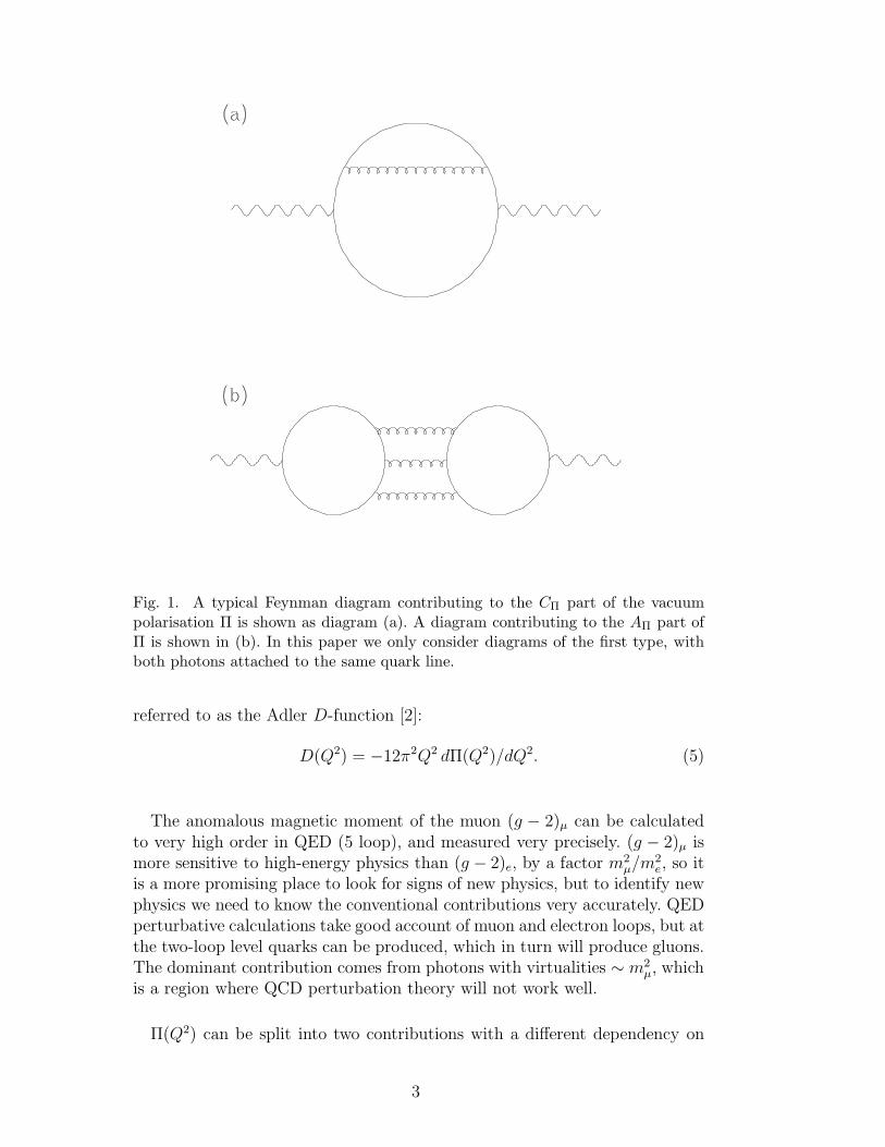
Fig. 1. A typical Feynman diagram contributing to the CΠ part of the vacuumpolarisation Π is shown as diagram (a). A diagram contributing to the AΠ part ofΠ is shown in (b). In this paper we only consider diagrams of the first type, withboth photons attached to the same quark line.

referred to as the Adler D-function [2]:

D(Q2) = −12π2Q2 dΠ(Q2)/dQ2. (5)

The anomalous magnetic moment of the muon (g − 2)µ can be calculatedto very high order in QED (5 loop), and measured very precisely. (g − 2)µ ismore sensitive to high-energy physics than (g − 2)e, by a factor m2

µ/m2e, so it

is a more promising place to look for signs of new physics, but to identify newphysics we need to know the conventional contributions very accurately. QEDperturbative calculations take good account of muon and electron loops, but atthe two-loop level quarks can be produced, which in turn will produce gluons.The dominant contribution comes from photons with virtualities ∼ m2

µ, whichis a region where QCD perturbation theory will not work well.

Π(Q2) can be split into two contributions with a different dependency on

3

the quark charges, as shown in Fig.1,

−12π2Π(Q2) =∑

f

e2f CΠ(µ2, Q2, mf) +∑

f,f ′

efef ′ AΠ(µ2, Q2, mf , mf ′). (6)

The CΠ term begins with a tree-level term which is O(α0s), while the first

contribution to the AΠ term is O(α3s). Furthermore, if flavour SU(3) is a good

symmetry, the contribution to AΠ from the three light flavours (u, d, s) cancelsbecause eu + ed + es = 0, and the only surviving contributions to AΠ comewhen both f and f ′ are heavy quarks (c, b, t). In this paper we will concentrateon the CΠ term, both because it is larger, and because it is much easier tomeasure on the lattice.

For large (spacelike) momenta CΠ(µ2, Q2, mf) can be expressed by meansof the Operator Product Expansion, OPE

CΠ(µ2, Q2, mf ) = c0(µ2, Q2, mf) +

cF4 (µ2, Q2)

(Q2)2mf 〈ψfψf〉 (7)

+cG4 (µ2, Q2)

(Q2)2

αs

π〈G2

µν〉 +c ′F4 (µ2, Q2)

(Q2)2

∑

f ′

mf ′ 〈ψf ′ψf ′〉 + O(1/(Q2)3),

where c0, cF4 , c ′F4 and cG4 are the Wilson coefficients and µ is the renormali-

sation scale parameter in some renormalisation scheme such as MS. The f ′

sum extends over the flavours of the sea quarks (internal quark loops not di-rectly connected to the photon lines). The Wilson coefficients can be computedin perturbation theory, while the non-perturbative physics is encoded in thecondensates mf 〈ψfψf (µ)〉, αs〈G2

µν(µ)〉, etc.

Perturbatively the functions D, eq.(5), and R, eq.(4), are known to fourloops for massless quarks [3,4], while the coefficient c0 is known to three loopsin the massive case [5]. The coefficients cF4 , c ′F4 and cG4 are known up toO(α2

s) [6,7,8] for massless quarks.

In this paper we shall compute Π(Q2) on the lattice and compare the resultwith current phenomenology [9]. Preliminary results of this calculation werepresented in [10].

The structure of this paper is as follows. After this Introduction we discussthe lattice setup in Sections 2 and Appendix A. The results are presented inSection 3 and Appendix C. In Section 4 and Appendix B we compare withperturbation theory. In Sections 5 and 6 we present a simple model whichdescribes our lattice data well. In Section 7 we use this model to give a lat-tice estimate of the hadronic contribution to the muon’s anomalous magnetic

4

moment. Finally in Section 8 we make some comments on the applicability ofthe Operator Product Expansion, and give our conclusions in Section 9.

2 Lattice Setup

We work with non-perturbatively improved Wilson fermions. For the actionand computational details, as well as for results of hadron masses and decayconstants, see [11,12,13]. Full details of the vacuum polarisation calculationcan be found in [14].

To discretise the hadronic electromagnetic current

Jemµ (x) =

∑

f

efJfµ (x) (8)

we use the conserved vector current

Jfµ (x) =

1

2

(

ψf (x+ aµ)(1 + γµ)U†µ(x)ψf (x)

− ψf (x)(1 − γµ)Uµ(x)ψf (x+ aµ))

(9)

where a is the lattice spacing. From now on we work with a Euclidean metricand write

Jfµ (q) =

∑

x

eiq(x+aµ/2)Jfµ (x) (10)

with

qµ =2

asin

(aqµ2

)

. (11)

On the lattice the photon self-energy Π is not simply given by 〈Jfµ (x)Jf

ν (0)〉.This is because the lattice Feynman rules include vertices where any numberof photons couple to a quark line (not just the single-photon vertex of thecontinuum) [15]. We are therefore led to define

Πµν(q) = Π(1)µν (q) + Π(2)

µν (q) , (12)

with

Π(1)µν (q) = a4

∑

x

eiq(x+aµ/2−aν/2)〈Jfµ (x)Jf

ν (0)〉 , (13)

and

Π(2)µν (q) = −aδµν〈J (2)

µ (0)〉 . (14)

5

where

J (2)µ (x) =

1

2

(

ψ(x+ aµ)(1 + γµ)U†µ(x)ψ(x)

+ ψ(x)(1 − γµ)Uµ(x)ψ(x+ aµ))

.(15)

It then follows that (12) fulfils the Ward identity

qµΠµν(q) = qνΠµν(q) = 0 . (16)

The conserved vector current (9) is on-shell as well as off-shell improved [16]in forward matrix elements. In non-forward matrix elements, such as the vac-uum polarisation, it needs to be further improved,

J impµ (x) = Jµ(x) +

1

2ia cCV C∂ν

(

ψ(x)σµνψ(x))

, (17)

where we have some freedom in choosing ∂ν on the lattice. Any choice mustpreserve (16), and ideally it should keep O(a2) corrections small. Consideringthe fact that the conserved vector current Jµ(x) ‘lives’ at x+aµ/2, the natural(or naive) choice for the improved operator would be

J impµ (q)= Jµ(q) +

1

2iacCV C

∑

x

eiq(x+aµ/2) 1

4a

(

Tµν(x+ aν)

+Tµν(x+ aµ+ aν) − Tµν(x− aν) − Tµν(x+ aµ− aν))

= Jµ(q) +1

2cCV C cos(aqµ/2) sin(aqν)

∑

x

eiqxTµν(x) , (18)

where Tµν(x) ≡ ψ(x)σµνψ(x). Unfortunately it turns out that this choiceintroduces very large O(a2Q2) errors into Π. We found that

J impµ (q) ≡ Jµ(q) + cCV C sin(aqν/2)

∑

x

eiqxTµν(x) (19)

was a better choice of improved current, because it makes the O(a2Q2) termsmuch smaller, and so we will adopt this definition. The difference betweenthe definitions (18) and (19) is O(a2Q2), so we are free to choose whicheverdefinition leads to the largest scaling region in Q2 (both agree at small Q2).

In Fig.2 we show the unimproved polarisation tensor along with the twodifferent choices of improvement term in the case of free fermions. The bestagreement with continuum physics comes from using (19), which is the pre-scription we will use in the rest of this paper.

6

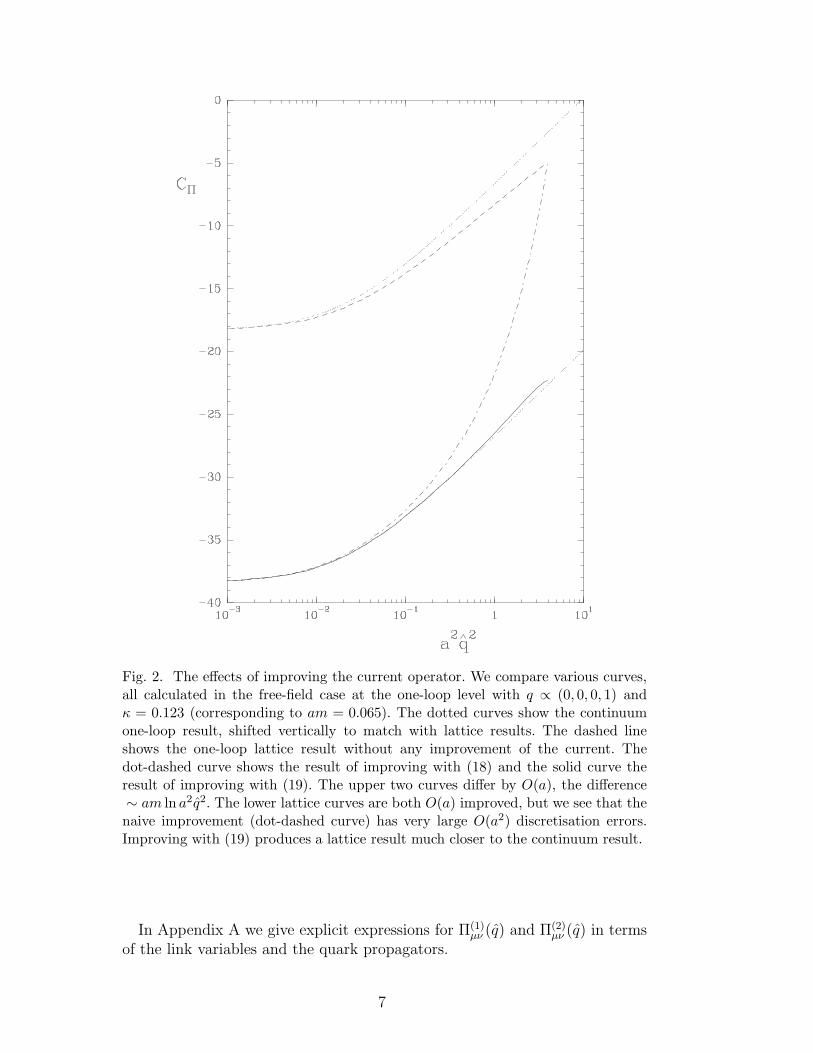
Fig. 2. The effects of improving the current operator. We compare various curves,all calculated in the free-field case at the one-loop level with q ∝ (0, 0, 0, 1) andκ = 0.123 (corresponding to am = 0.065). The dotted curves show the continuumone-loop result, shifted vertically to match with lattice results. The dashed lineshows the one-loop lattice result without any improvement of the current. Thedot-dashed curve shows the result of improving with (18) and the solid curve theresult of improving with (19). The upper two curves differ by O(a), the difference∼ am ln a2q2. The lower lattice curves are both O(a) improved, but we see that thenaive improvement (dot-dashed curve) has very large O(a2) discretisation errors.Improving with (19) produces a lattice result much closer to the continuum result.

In Appendix A we give explicit expressions for Π(1)µν (q) and Π(2)

µν (q) in termsof the link variables and the quark propagators.

7

3 Lattice Calculation

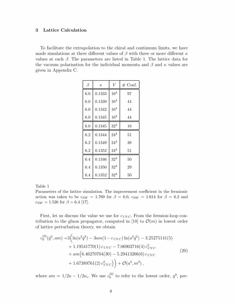
To facilitate the extrapolation to the chiral and continuum limits, we havemade simulations at three different values of β with three or more different κvalues at each β. The parameters are listed in Table 1. The lattice data forthe vacuum polarisation for the individual momenta and β and κ values aregiven in Appendix C.

β κ V # Conf.

6.0 0.1333 164 97

6.0 0.1339 164 44

6.0 0.1342 164 44

6.0 0.1345 164 44

6.0 0.1345 324 16

6.2 0.1344 244 51

6.2 0.1349 244 38

6.2 0.1352 244 51

6.4 0.1346 324 50

6.4 0.1350 324 29

6.4 0.1352 324 50

Table 1Parameters of the lattice simulation. The improvement coefficient in the fermionicaction was taken to be cSW = 1.769 for β = 6.0, cSW = 1.614 for β = 6.2 andcSW = 1.526 for β = 6.4 [17].

First, let us discuss the value we use for cCV C . From the fermion-loop con-tribution to the gluon propagator, computed in [18] to O(m) in lowest orderof lattice perturbation theory, we obtain

c(0)0 (q2, am) =3

(

ln(a2q2) − 3am(1− cCV C) ln(a2q2) − 3.25275141(5)

+ 1.19541770(1) cCV C − 7.06903716(4) c2CV C

+ am(

6.46270704(30)− 5.29413266(6) cCV C

+ 1.67389761(2) c2CV C

)

)

+ O(a2, m2) ,

(20)

where am = 1/2κ − 1/2κc. We use c(0)0 to refer to the lowest order, g0, per-

8

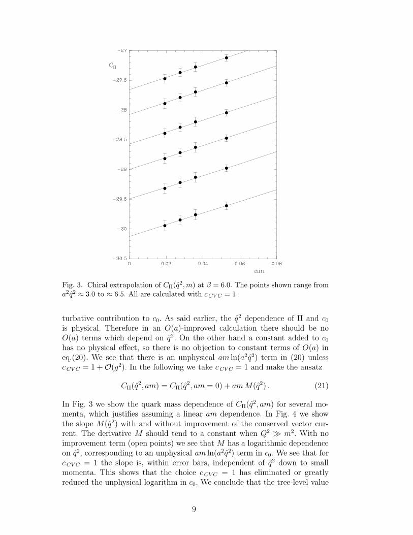
Fig. 3. Chiral extrapolation of CΠ(q2,m) at β = 6.0. The points shown range froma2q2 ≈ 3.0 to ≈ 6.5. All are calculated with cCV C = 1.

turbative contribution to c0. As said earlier, the q2 dependence of Π and c0is physical. Therefore in an O(a)-improved calculation there should be noO(a) terms which depend on q2. On the other hand a constant added to c0has no physical effect, so there is no objection to constant terms of O(a) ineq.(20). We see that there is an unphysical am ln(a2q2) term in (20) unlesscCV C = 1 + O(g2). In the following we take cCV C = 1 and make the ansatz

CΠ(q2, am) = CΠ(q2, am = 0) + amM(q2) . (21)

In Fig. 3 we show the quark mass dependence of CΠ(q2, am) for several mo-menta, which justifies assuming a linear am dependence. In Fig. 4 we showthe slope M(q2) with and without improvement of the conserved vector cur-rent. The derivative M should tend to a constant when Q2 ≫ m2. With noimprovement term (open points) we see that M has a logarithmic dependenceon q2, corresponding to an unphysical am ln(a2q2) term in c0. We see that forcCV C = 1 the slope is, within error bars, independent of q2 down to smallmomenta. This shows that the choice cCV C = 1 has eliminated or greatlyreduced the unphysical logarithm in c0. We conclude that the tree-level value

9

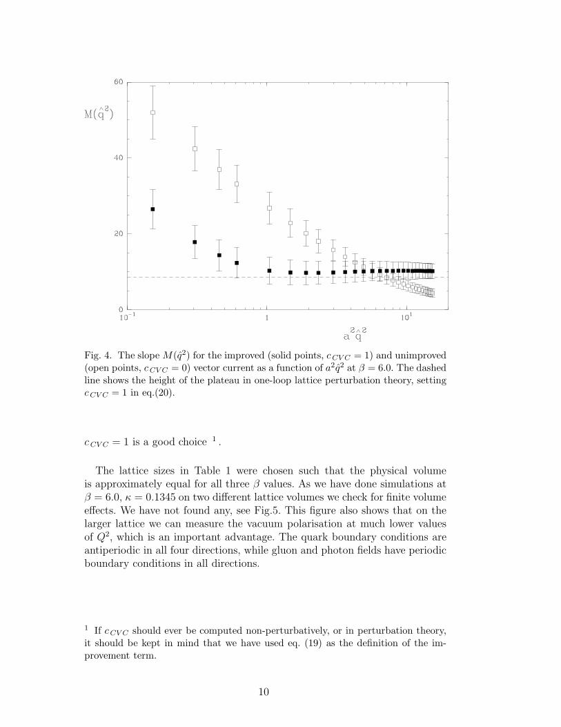
Fig. 4. The slope M(q2) for the improved (solid points, cCV C = 1) and unimproved(open points, cCV C = 0) vector current as a function of a2q2 at β = 6.0. The dashedline shows the height of the plateau in one-loop lattice perturbation theory, settingcCV C = 1 in eq.(20).

cCV C = 1 is a good choice 1 .

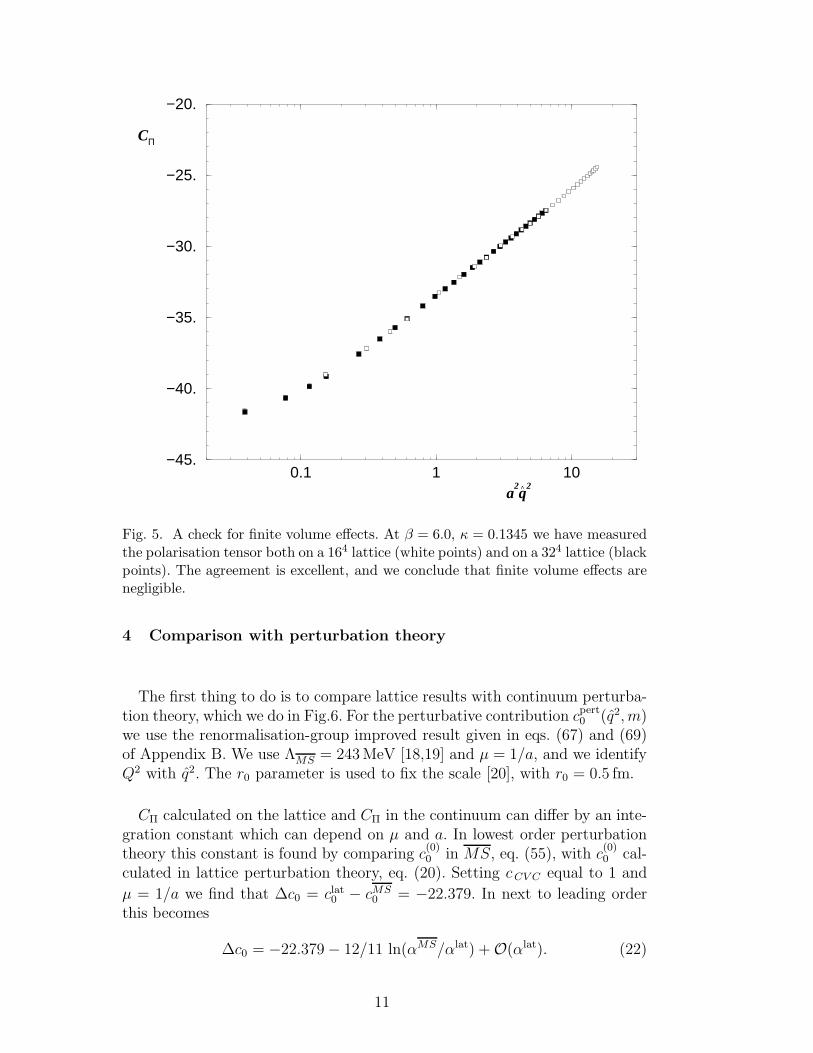
The lattice sizes in Table 1 were chosen such that the physical volumeis approximately equal for all three β values. As we have done simulations atβ = 6.0, κ = 0.1345 on two different lattice volumes we check for finite volumeeffects. We have not found any, see Fig.5. This figure also shows that on thelarger lattice we can measure the vacuum polarisation at much lower valuesof Q2, which is an important advantage. The quark boundary conditions areantiperiodic in all four directions, while gluon and photon fields have periodicboundary conditions in all directions.

1 If cCV C should ever be computed non-perturbatively, or in perturbation theory,it should be kept in mind that we have used eq. (19) as the definition of the im-provement term.

10

0.1 1 10a

2q

2

−45.

−40.

−35.

−30.

−25.

−20.

CΠ

>

Fig. 5. A check for finite volume effects. At β = 6.0, κ = 0.1345 we have measuredthe polarisation tensor both on a 164 lattice (white points) and on a 324 lattice (blackpoints). The agreement is excellent, and we conclude that finite volume effects arenegligible.

4 Comparison with perturbation theory

The first thing to do is to compare lattice results with continuum perturba-tion theory, which we do in Fig.6. For the perturbative contribution cpert

0 (q2, m)we use the renormalisation-group improved result given in eqs. (67) and (69)of Appendix B. We use ΛMS = 243 MeV [18,19] and µ = 1/a, and we identifyQ2 with q2. The r0 parameter is used to fix the scale [20], with r0 = 0.5 fm.

CΠ calculated on the lattice and CΠ in the continuum can differ by an inte-gration constant which can depend on µ and a. In lowest order perturbationtheory this constant is found by comparing c

(0)0 in MS, eq. (55), with c

(0)0 cal-

culated in lattice perturbation theory, eq. (20). Setting cCV C equal to 1 and

µ = 1/a we find that ∆c0 = clat0 − cMS0 = −22.379. In next to leading order

this becomes

∆c0 = −22.379 − 12/11 ln(αMS/αlat) + O(αlat). (22)

11

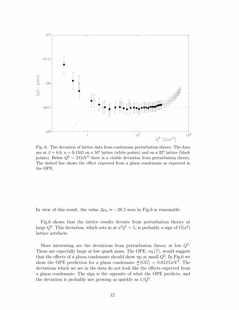
Fig. 6. The deviation of lattice data from continuum perturbation theory. The dataare at β = 6.0, κ = 0.1345 on a 164 lattice (white points) and on a 324 lattice (blackpoints). Below Q2 ∼ 2GeV2 there is a visible deviation from perturbation theory.The dotted line shows the effect expected from a gluon condensate as expected inthe OPE.

In view of this result, the value ∆c0 ≈ −28.5 seen in Fig.6 is reasonable.

Fig.6 shows that the lattice results deviate from perturbation theory atlarge Q2. This deviation, which sets in at a2q2 ∼ 5, is probably a sign of O(a2)lattice artefacts.

More interesting are the deviations from perturbation theory at low Q2.These are especially large at low quark mass. The OPE, eq.(7), would suggestthat the effects of a gluon condensate should show up at small Q2. In Fig.6 weshow the OPE prediction for a gluon condensate α

π〈GG〉 = 0.012 GeV4. The

deviations which we see in the data do not look like the effects expected froma gluon condensate. The sign is the opposite of what the OPE predicts, andthe deviation is probably not growing as quickly as 1/Q4.

12

5 A simple model of the vacuum polarisation at low Q2

We have seen that perturbation theory, even when supplemented with highertwist terms from the operator product expansion, has difficulty in explainingthe low Q2 region of the data. Can we understand this region in some otherway?

The cross section ratio R(s) is given by the cut in the vacuum polarisa-tion, or in other words there are dispersion relations which give the vacuumpolarisation if we know R(s).

β κ amPS amV 1/fV

6.0 0.1333 0.4122(9) 0.5503(20) 0.2055(14)

6.0 0.1339 0.3381(15) 0.5017(40) 0.2217(15)

6.0 0.1342 0.3017(13) 0.4904(40) 0.2293(14)

6.0 0.1345 0.2561(15) 0.4701(90) 0.2387(90)

6.2 0.1344 0.3034(6) 0.4015(17) 0.2210(20)

6.2 0.1349 0.2431(6) 0.3663(27) 0.2403(24)

6.2 0.1352 0.2005(9) 0.3431(60) 0.2474(47)

6.4 0.1346 0.2402(8) 0.3107(16) 0.2252(21)

6.4 0.1350 0.1933(7) 0.2800(20) 0.2423(19)

6.4 0.1352 0.1661(10) 0.2613(40) 0.2448(35)

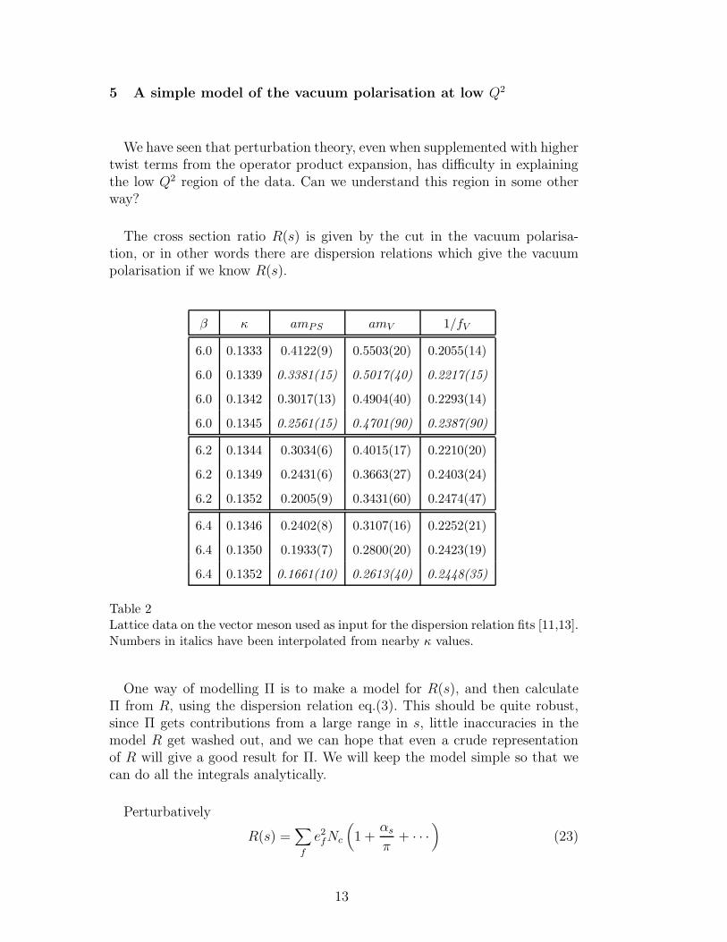
Table 2Lattice data on the vector meson used as input for the dispersion relation fits [11,13].Numbers in italics have been interpolated from nearby κ values.

One way of modelling Π is to make a model for R(s), and then calculateΠ from R, using the dispersion relation eq.(3). This should be quite robust,since Π gets contributions from a large range in s, little inaccuracies in themodel R get washed out, and we can hope that even a crude representationof R will give a good result for Π. We will keep the model simple so that wecan do all the integrals analytically.

Perturbatively

R(s) =∑

f

e2fNc

(

1 +αs

π+ · · ·

)

(23)

13

where Nc is the number of colours (3 in our case). We know that really thelow s behaviour of R is more complicated than that, it is dominated by theρ(770), ω(782) and φ(1020) mesons. Following [7], let us make the followingmodel for R. We ignore the splitting between the ρ and ω, which comes fromthe AΠ-type diagrams which we have dropped. We also treat these mesons asnarrow resonances, each contributing a δ function to R. The continuum partof R takes a while to climb up to the value in eq.(23). We will represent thisrise by a step function at some value s0. So, our model is

R(s) =∑

f

e2f(

Aδ(s−m2V ) +BΘ(s− s0)

)

(24)

where we would expect B to be slightly above 3 in order to match eq.(23).

Using the dispersion relation, this R(s) translates into a vacuum polarisation

CΠ(Q2) = B ln(a2Q2 + a2s0) − A/(Q2 +m2V ) +K (25)

where K is a constant which is not determined from the dispersion relation,and which never appears in any physical quantity. Again we identify the con-tinuum quantity Q2 with the lattice quantity q2.

The constant A can be expressed in terms of the decay constant fV , whichhas been measured on the lattice. The cross section for the production of anarrow vector resonance, V , is [7]

σe+e−→V (s) = 12π2δ(s−m2V )

ΓV →e+e−

mV. (26)

The partial width ΓV →e+e− is related to a meson decay constant gV [21,7] by

ΓV →e+e− =

(

4πα2em

3

)

mV

g2V

, (27)

where

〈0|Jemµ |V, ε〉 = εµ

m2V

gV. (28)

Here εµ is the polarisation vector of the meson. On the lattice it is more naturalto define decay constants fV in terms of currents with definite isospin [11]

〈0|Vµ|V, ε〉 = εµm2

V

fV(29)

with

VI=1µ =

1√2

(

uγµu− dγµd)

(30)

for the ρ0 and

VI=0µ =

1√2

(

uγµu+ dγµd)

(31)

14

for the ω (ignoring any ss admixture in the ω). The relationship between thetwo definitions is

1

gρ

=eu − ed√

2

1

fρ

=1√2

1

fρ

, (32)

1

gω=eu + ed√

2

1

fω=

1

3√

2

1

fω. (33)

In terms of these decay constants

R(s) =∑

V

12π2δ(s−m2V )m2

V

g2V

+ continuum (34)

=12π2δ(s−m2ρ)m2

ρ

f 2ρ

(eu − ed)2

2

+12π2δ(s−m2ω)m2

ω

f 2ω

(eu + ed)2

2+ continuum. (35)

Neglecting annihilation diagrams implies that mω = mρ and fω = fρ. Ex-perimentally both relations are fairly accurate. The mass ratio mω/mρ is1.02. fω = fρ implies Γω→e+e− = 1

9Γρ0→e+e−, while the experimental ratio

is 0.089(5) [22]. Equating the mass and decay constant of the ω and ρ ineq. (35) gives

R(s) = 12π2δ(s−m2ρ)m2

ρ

f 2ρ

(

e2u + e2d)

+ continuum ; (36)

so

A = 12π2m2V

f 2V

. (37)

6 Dispersion relation fits

We first try making fits to the lattice data for the vacuum polarisation CΠ

using eq. (25) with B,K and s0 as free parameters. To avoid problems fromlattice artefacts of O(a2q2) we have only used data with a2q2 < 5. We will callthis simple ansatz Fit I. A, the weight of the vector meson contribution, isdetermined by eq. (37). The vector meson masses and decay constants whichwe use are shown in Table 2. They have been taken from [11,13]. We cancompare the values for B and K with the one-loop lattice perturbation theoryresult, eq. (20), which gives B = 3 and K = −27.38 + am 8.53.

15

β κ V a2s0 B K χ2

6.0 0.1333 164 0.395(32) 3.13(6) -32.98(11) 4.3

6.0 0.1339 164 0.397(43) 3.13(8) -33.14(14) 2.2

6.0 0.1342 164 0.391(39) 3.10(8) -33.18(13) 3.0

6.0 0.1345 164 0.409(61) 3.11(9) -33.30(16) 2.5

6.0 0.1345 324 0.403(79) 3.12(10) -33.30(18) 0.7

6.2 0.1344 244 0.282(21) 3.10(5) -32.94(7) 1.9

6.2 0.1349 244 0.278(24) 3.07(5) -33.06(8) 1.9

6.2 0.1352 244 0.253(25) 3.06(5) -33.10(7) 2.2

6.4 0.1346 324 0.164(13) 3.06(3) -32.68(5) 0.8

6.4 0.1350 324 0.150(14) 3.03(4) -32.76(6) 0.6

6.4 0.1352 324 0.124(12) 3.02(3) -32.78(5) 1.2

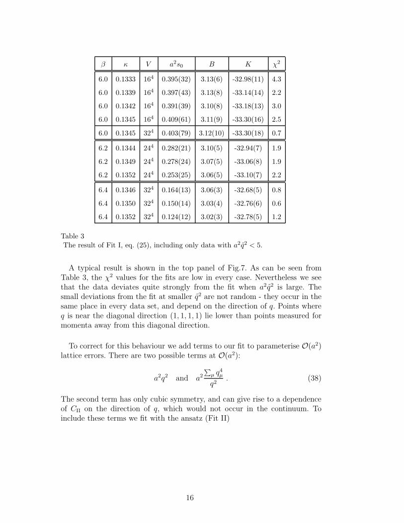
Table 3The result of Fit I, eq. (25), including only data with a2q2 < 5.

A typical result is shown in the top panel of Fig.7. As can be seen fromTable 3, the χ2 values for the fits are low in every case. Nevertheless we seethat the data deviates quite strongly from the fit when a2q2 is large. Thesmall deviations from the fit at smaller q2 are not random - they occur in thesame place in every data set, and depend on the direction of q. Points whereq is near the diagonal direction (1, 1, 1, 1) lie lower than points measured formomenta away from this diagonal direction.

To correct for this behaviour we add terms to our fit to parameterise O(a2)lattice errors. There are two possible terms at O(a2):

a2q2 and a2

∑

µ q4µ

q2. (38)

The second term has only cubic symmetry, and can give rise to a dependenceof CΠ on the direction of q, which would not occur in the continuum. Toinclude these terms we fit with the ansatz (Fit II)

16

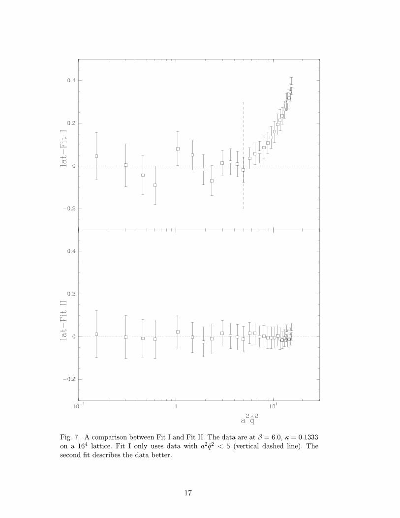
Fig. 7. A comparison between Fit I and Fit II. The data are at β = 6.0, κ = 0.1333on a 164 lattice. Fit I only uses data with a2q2 < 5 (vertical dashed line). Thesecond fit describes the data better.

17

CΠ(q2) = B ln(a2q2 + a2s0) −A

q2 +m2V

+K + U1a2q2 + U2h(q) (39)

where

h(q) =

∑

µ sin4 aqµ − 14

(

∑

µ sin2 aqµ)2

a2q2≈ a2

[∑

µ q4µ

q2− 1

4q2

]

. (40)

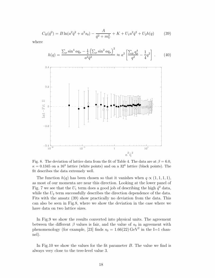
Fig. 8. The deviation of lattice data from the fit of Table 4. The data are at β = 6.0,κ = 0.1345 on a 164 lattice (white points) and on a 324 lattice (black points). Thefit describes the data extremely well.

The function h(q) has been chosen so that it vanishes when q ∝ (1, 1, 1, 1),as most of our momenta are near this direction. Looking at the lower panel ofFig. 7 we see that the U1 term does a good job of describing the high q2 data,while the U2 term successfully describes the direction dependence of the data.Fits with the ansatz (39) show practically no deviation from the data. Thiscan also be seen in Fig.8, where we show the deviation in the case where wehave data on two lattice sizes.

In Fig.9 we show the results converted into physical units. The agreementbetween the different β values is fair, and the value of s0 in agreement withphenomenology (for example, [23] finds s0 = 1.66(22) GeV2 in the I=1 chan-nel).

In Fig.10 we show the values for the fit parameter B. The value we find isalways very close to the tree-level value 3.

18

β κ V a2s0 B K χ2

6.0 0.1333 164 0.357(50) 3.00(12) -32.97(17) 1.52

6.0 0.1339 164 0.357(68) 2.99(16) -33.13(23) 0.69

6.0 0.1342 164 0.354(62) 2.97(15) -33.18(21) 0.83

6.0 0.1345 164 0.37(10) 2.97(17) -33.30(25) 0.70

6.0 0.1345 324 0.35(11) 2.92(33) -33.22(28) 0.06

6.0 0.1345 164&324 0.358(77) 2.93(11) -33.22(15) 1.49

6.2 0.1344 244 0.262(35) 3.00(12) -32.94(12) 0.14

6.2 0.1349 244 0.252(40) 2.94(13) -33.05(14) 0.12

6.2 0.1352 244 0.232(38) 2.95(12) -33.11(12) 0.13

6.4 0.1346 324 0.156(21) 3.01(11) -32.69(7) 0.08

6.4 0.1350 324 0.144(23) 2.99(12) -32.78(9) 0.10

6.4 0.1352 324 0.117(18) 2.97(10) -32.81(7) 0.11

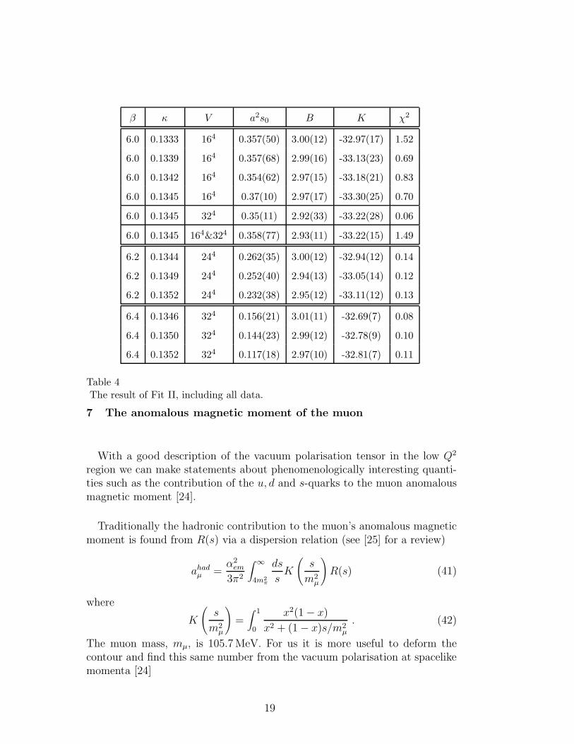
Table 4The result of Fit II, including all data.

7 The anomalous magnetic moment of the muon

With a good description of the vacuum polarisation tensor in the low Q2

region we can make statements about phenomenologically interesting quanti-ties such as the contribution of the u, d and s-quarks to the muon anomalousmagnetic moment [24].

Traditionally the hadronic contribution to the muon’s anomalous magneticmoment is found from R(s) via a dispersion relation (see [25] for a review)

ahadµ =

α2em

3π2

∫ ∞

4m2π

ds

sK

(

s

m2µ

)

R(s) (41)

where

K

(

s

m2µ

)

=∫ 1

0

x2(1 − x)

x2 + (1 − x)s/m2µ

. (42)

The muon mass, mµ, is 105.7 MeV. For us it is more useful to deform thecontour and find this same number from the vacuum polarisation at spacelikemomenta [24]

19

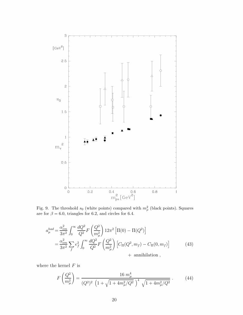
Fig. 9. The threshold s0 (white points) compared with m2ρ (black points). Squares

are for β = 6.0, triangles for 6.2, and circles for 6.4.

ahadµ =

α2em

3π2

∫ ∞

0

dQ2

Q2F

(

Q2

m2µ

)

12π2[

Π(0) − Π(Q2)]

=α2

em

3π2

∑

f

e2f

∫ ∞

0

dQ2

Q2F

(

Q2

m2µ

)

[

CΠ(Q2, mf ) − CΠ(0, mf)]

(43)

+ annihilation ,

where the kernel F is

F

(

Q2

m2µ

)

=16 m4

µ

(Q2)2(

1 +√

1 + 4m2µ/Q

2)4 √

1 + 4m2µ/Q

2. (44)

20

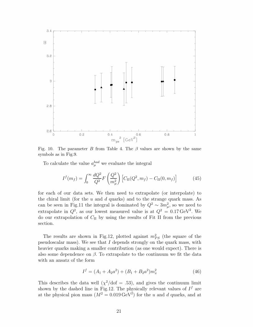
Fig. 10. The parameter B from Table 4. The β values are shown by the samesymbols as in Fig.9.

To calculate the value ahadµ we evaluate the integral

If(mf) =∫ ∞

0

dQ2

Q2F

(

Q2

m2µ

)

[

CΠ(Q2, mf) − CΠ(0, mf)]

(45)

for each of our data sets. We then need to extrapolate (or interpolate) tothe chiral limit (for the u and d quarks) and to the strange quark mass. Ascan be seen in Fig.11 the integral is dominated by Q2 ∼ 3m2

µ, so we need to

extrapolate in Q2, as our lowest measured value is at Q2 = 0.17 GeV2. Wedo our extrapolation of CΠ by using the results of Fit II from the previoussection.

The results are shown in Fig.12, plotted against m2PS (the square of the

pseudoscalar mass). We see that I depends strongly on the quark mass, withheavier quarks making a smaller contribution (as one would expect). There isalso some dependence on β. To extrapolate to the continuum we fit the datawith an ansatz of the form

If = (A1 + A2a2) + (B1 +B2a

2)m2π (46)

This describes the data well (χ2/dof = .53), and gives the continuum limitshown by the dashed line in Fig.12. The physically relevant values of If areat the physical pion mass (M2 = 0.019 GeV2) for the u and d quarks, and at

21

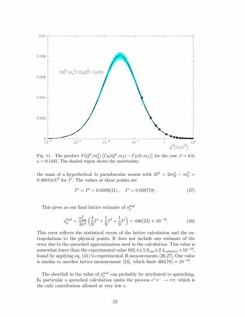
Fig. 11. The product F (Q2/m2µ)[

CΠ(Q2,mf ) − CΠ(0,mf )]

for the case β = 6.0,κ = 0.1345. The shaded region shows the uncertainty.

the mass of a hypothetical ss pseudoscalar meson with M2 = 2m2K −m2

π =0.468 GeV2 for Is. The values at these points are

Iu = Id = 0.0389(21) , Is = 0.0287(9) . (47)

This gives as our final lattice estimate of ahadµ

ahadµ =

α2em

3π2

(

4

9Iu +

1

9Id +

1

9Is)

= 446(23) × 10−10. (48)

This error reflects the statistical errors of the lattice calculation and the ex-trapolations to the physical points. It does not include any estimate of theerror due to the quenched approximation used in the calculation. This value issomewhat lower than the experimental value 692.4±5.9exp±2.4radiative×10−10,found by applying eq. (41) to experimental R measurements [26,27]. Our valueis similar to another lattice measurement [24], which finds 460(78) × 10−10.

The shortfall in the value of ahadµ can probably be attributed to quenching.

In particular a quenched calculation omits the process e+e− → ππ, which isthe only contribution allowed at very low s.

22

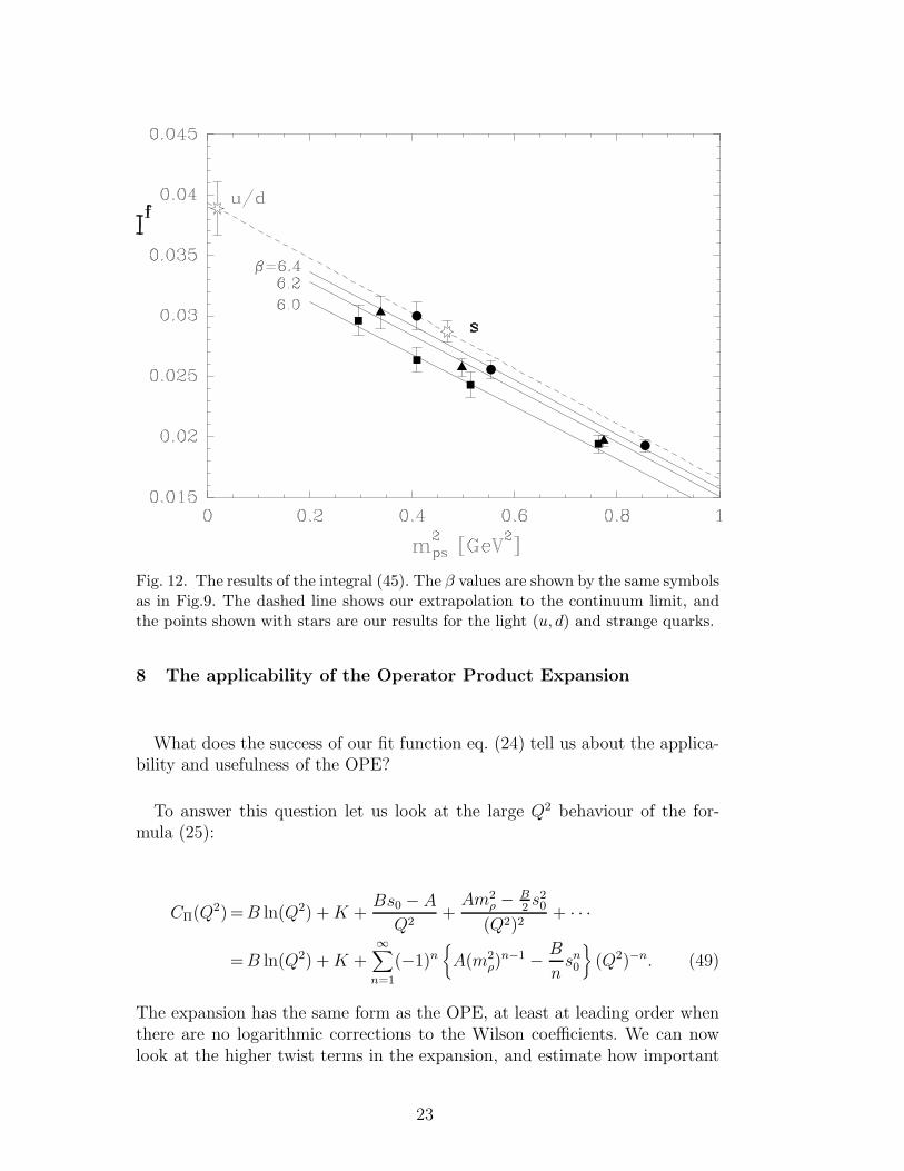
Fig. 12. The results of the integral (45). The β values are shown by the same symbolsas in Fig.9. The dashed line shows our extrapolation to the continuum limit, andthe points shown with stars are our results for the light (u, d) and strange quarks.

8 The applicability of the Operator Product Expansion

What does the success of our fit function eq. (24) tell us about the applica-bility and usefulness of the OPE?

To answer this question let us look at the large Q2 behaviour of the for-mula (25):

CΠ(Q2)=B ln(Q2) +K +Bs0 − A

Q2+Am2

ρ − B2s20

(Q2)2+ · · ·

=B ln(Q2) +K +∞∑

n=1

(−1)n{

A(m2ρ)

n−1 − B

nsn0

}

(Q2)−n. (49)

The expansion has the same form as the OPE, at least at leading order whenthere are no logarithmic corrections to the Wilson coefficients. We can nowlook at the higher twist terms in the expansion, and estimate how important

23

they are in comparison with the gluon condensate contribution.

By looking at the first few terms we can relate our parameters s0 and A tothe condensates in the OPE. In the chiral limit there is no 1/Q2 term, so

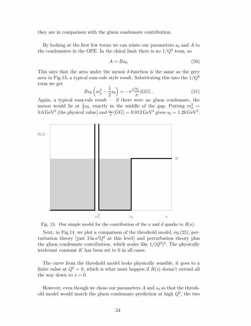
A = Bs0. (50)

This says that the area under the meson δ-function is the same as the greyarea in Fig.13, a typical sum-rule style result. Substituting this into the 1/Q4

term we get

Bs0

(

m2ρ −

1

2s0

)

= −π2αs

π〈GG〉 . (51)

Again, a typical sum-rule result — if there were no gluon condensate, themeson would lie at 1

2s0, exactly in the middle of the gap. Putting m2

ρ =

0.6 GeV2 (the physical value) and αs

π〈GG〉 = 0.012 GeV4 gives s0 = 1.26 GeV2.

Fig. 13. Our simple model for the contribution of the u and d quarks to R(s).

Next, in Fig.14, we plot a comparison of the threshold model, eq.(25), per-turbation theory (just 3 ln a2Q2 at this level) and perturbation theory plusthe gluon condensate contribution, which scales like 1/(Q2)2. The physicallyirrelevant constant K has been set to 0 in all cases.

The curve from the threshold model looks physically sensible, it goes to afinite value at Q2 = 0, which is what must happen if R(s) doesn’t extend allthe way down to s = 0.

However, even though we chose our parameters A and s0 so that the thresh-old model would match the gluon condensate prediction at high Q2, the two

24

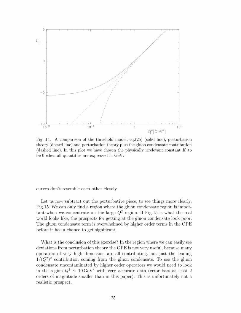
Fig. 14. A comparison of the threshold model, eq.(25) (solid line), perturbationtheory (dotted line) and perturbation theory plus the gluon condensate contribution(dashed line). In this plot we have chosen the physically irrelevant constant K tobe 0 when all quantities are expressed in GeV.

curves don’t resemble each other closely.

Let us now subtract out the perturbative piece, to see things more clearly,Fig.15. We can only find a region where the gluon condensate region is impor-tant when we concentrate on the large Q2 region. If Fig.15 is what the realworld looks like, the prospects for getting at the gluon condensate look poor.The gluon condensate term is overwhelmed by higher order terms in the OPEbefore it has a chance to get significant.

What is the conclusion of this exercise? In the region where we can easily seedeviations from perturbation theory the OPE is not very useful, because manyoperators of very high dimension are all contributing, not just the leading1/(Q2)2 contribution coming from the gluon condensate. To see the gluoncondensate uncontaminated by higher order operators we would need to lookin the region Q2 ∼ 10 GeV2 with very accurate data (error bars at least 2orders of magnitude smaller than in this paper). This is unfortunately not arealistic prospect.

25

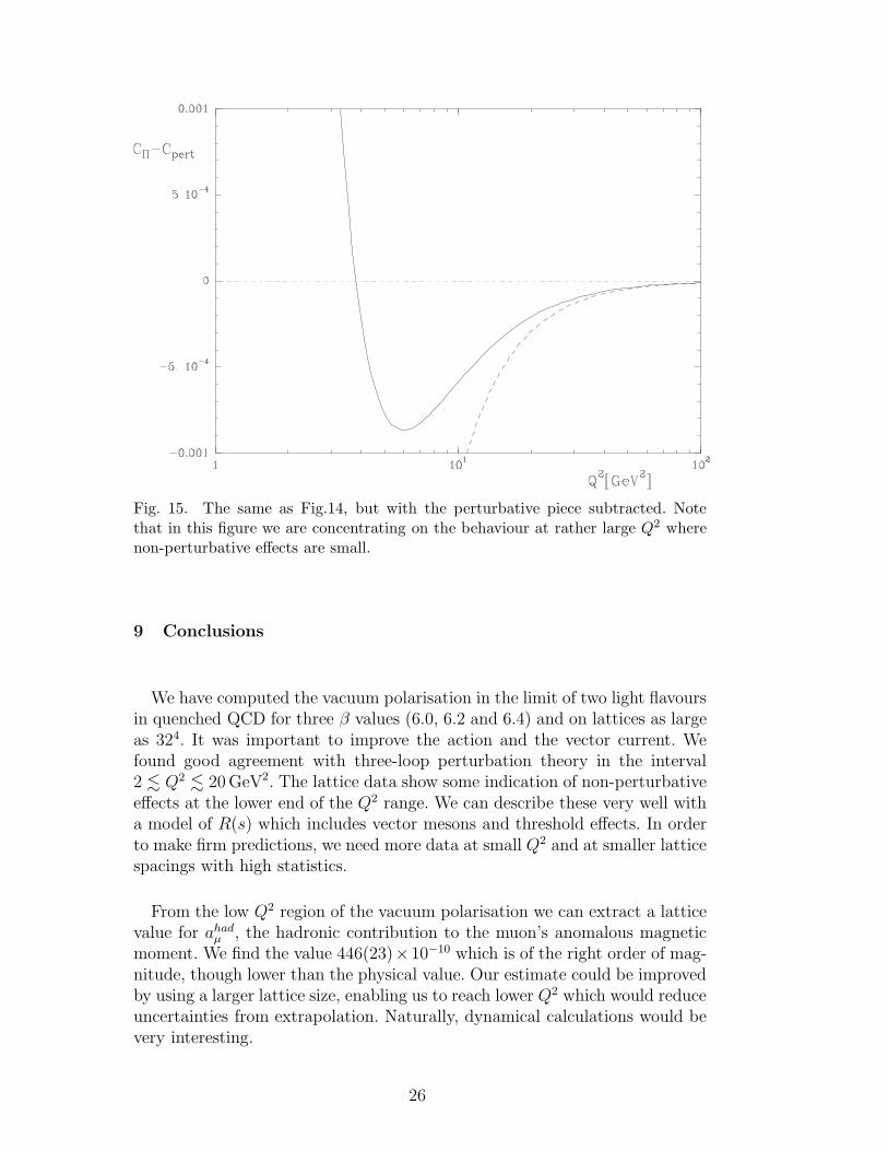
Fig. 15. The same as Fig.14, but with the perturbative piece subtracted. Notethat in this figure we are concentrating on the behaviour at rather large Q2 wherenon-perturbative effects are small.

9 Conclusions

We have computed the vacuum polarisation in the limit of two light flavoursin quenched QCD for three β values (6.0, 6.2 and 6.4) and on lattices as largeas 324. It was important to improve the action and the vector current. Wefound good agreement with three-loop perturbation theory in the interval2 . Q2 . 20 GeV2. The lattice data show some indication of non-perturbativeeffects at the lower end of the Q2 range. We can describe these very well witha model of R(s) which includes vector mesons and threshold effects. In orderto make firm predictions, we need more data at small Q2 and at smaller latticespacings with high statistics.

From the low Q2 region of the vacuum polarisation we can extract a latticevalue for ahad

µ , the hadronic contribution to the muon’s anomalous magneticmoment. We find the value 446(23)×10−10 which is of the right order of mag-nitude, though lower than the physical value. Our estimate could be improvedby using a larger lattice size, enabling us to reach lower Q2 which would reduceuncertainties from extrapolation. Naturally, dynamical calculations would bevery interesting.

26

Acknowledgements

The numerical calculations were performed on the Quadrics computers atDESY Zeuthen. We thank the operating staff for their support. This work wassupported in part by the European Community’s Human Potential Programunder Contract HPRN-CT-2000-00145, Hadrons/Lattice QCD, as well as bythe DFG (Forschergruppe Gitter-Hadronen-Phanomenologie) and BMBF.

We would like to thank C. Michael and T. Teubner for useful comments.

Appendix A

We denote the quark propagator from lattice points x to y by G(x, y). ForΠ(1)

µν (q) we then obtain

Π(1)µν (q) =

a4

4

∑

x

eiq(x+aµ/2−aν/2)

Tr⟨

(1 + γν)U†ν(0)γ5G

†(x+ aµ, 0)γ5(1 + γµ)U†µ(x)G(x, aν)

− (1 − γν)Uν(0)γ5G†(x+ aµ, aν)γ5(1 + γµ)U

†µ(x)G(x, 0)

− (1 + γν)U†ν(0)γ5G

†(x, 0)γ5(1 − γµ)Uµ(x)G(x+ aµ, aν)

+ (1 − γν)Uν(0)γ5G†(x, aν)γ5(1 − γµ)Uµ(x)G(x+ aµ, 0)

⟩

− a5

4cCV C

∑

x

eiq(x+aµ/2)qλ

Tr⟨

(1 + γµ)U†µ(x)G(x, 0)σνλγ5G

†(x+ aµ, 0)γ5

− (1 − γµ)Uµ(x)G(x+ aµ, 0)σνλγ5G†(x, 0)γ5

⟩

+a5

4cCV C

∑

x

eiq(x−aν/2)qσ

Tr⟨

(1 + γν)U†ν(0)γ5G

†(x, 0)γ5σµσG(x, aν)

− (1 − γν)Uν(0)γ5G†(x, aν)γ5σµσG(x, 0)

⟩

− a6

4c2CV C

∑

x

eiqxqλqσ

Tr⟨

σµσG(x, 0)σνλγ5G†(x, 0)γ5

⟩

,

(52)

27

where the improvement term has been integrated by parts. For Π(2)µν (q) we

obtain

Π(2)µν (q) =

a

2δµνTr

⟨

(1 + γν)U†ν(0)G(0, aν) + (1 − γν)Uν(0)G†(0, aν)

⟩

. (53)

To compute Π(1)µν (q) and Π(2)

µν (q) we have to do a minimum of five inversions foreach gauge field configuration (and each κ value), which makes the calculationcomputationally quite expensive, in particular on 324 lattices.

Appendix B

Perturbative results

Before we describe the lattice calculation in detail, we present here theperturbative Wilson coefficients c0, c

F4 and cG4 . We will work in the quenched

approximation, in which contributions from sea quarks are neglected, andwhich corresponds to c ′F4 = 0.

We write

c0(µ2, Q2, m) = c

(0)0 (µ2, Q2, m) +

αs(µ2)

πCF c

(1)0 (µ2, Q2, m) (54)

+(αs(µ

2)

π

)2(

C2F c

(2)0 (µ2, Q2, m) + CFCA c

(2) ′0 (µ2, Q2, m)

)

+ · · · ,

with CF = 4/3 and CA = 3 for SU(3). These coefficients can be found ineqs. (27)-(30) of [5] (recall that Q2 ≡ −q2). In the MS scheme the coefficients

c(0)0 , c

(1)0 , c

(2)0 and c

(2) ′0 read

c(0)0 (µ2, Q2, m) = −9

4

20

9− 4

3lnQ2

µ2− 8

m2

Q2+(4m2

Q2

)2(1

4+

1

2lnQ2

m2

)

, (55)

c(1)0 (µ2, Q2, m) = −9

4

55

12− 4ζ(3)− ln

Q2

µ2− 4m2

Q2

(

4 − 3 lnQ2

µ2

)

+(4m2

Q2

)2( 1

24+ ζ(3) +

11

8lnQ2

m2

+3

4ln2 Q

2

m2− 3

2lnQ2

m2lnQ2

µ2

)

,

(56)

28

c(2)0 (µ2, Q2, m) = −9

4

− 143

72− 37

6ζ(3) + 10ζ(5) +

1

8lnQ2

µ2

− 4m2

Q2

(1667

96− 5

12ζ(3) − 35

6ζ(5)

− 51

8lnQ2

µ2+

9

4ln2 Q

2

µ2

)

,

(57)

c(2) ′0 (µ2, Q2, m) = −9

4

44215

2592− 227

18ζ(3) − 5

3ζ(5)− 41

8lnQ2

µ2

+11

24ln2 Q

2

µ2+

11

3ζ(3) ln

Q2

µ2

− 4m2

Q2

(1447

96+

4

3ζ(3) − 85

12ζ(5)

− 185

24lnQ2

µ2+

11

8ln2 Q

2

µ2

)

,

(58)

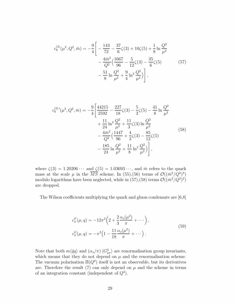
where ζ(3) = 1.20206 · · · and ζ(5) = 1.03693 · · · , and m refers to the quarkmass at the scale µ in the MS scheme. In (55),(56) terms of O((m2/Q2)3)modulo logarithms have been neglected, while in (57),(58) terms O((m2/Q2)2)are dropped.

The Wilson coefficients multiplying the quark and gluon condensate are [6,8]

cF4 (µ, q) = −12π2(

2 +2

3

αs(µ2)

π+ · · ·

)

,

cG4 (µ, q) = −π2(

1 − 11

18

αs(µ2)

π+ · · ·

)

.

(59)

Note that both m〈qq〉 and (αs/π) 〈G2µν〉 are renormalisation group invariants,

which means that they do not depend on µ and the renormalisation scheme.The vacuum polarisation Π(Q2) itself is not an observable, but its derivativesare. Therefore the result (7) can only depend on µ and the scheme in termsof an integration constant (independent of Q2).

29

Renormalisation Group Improvement

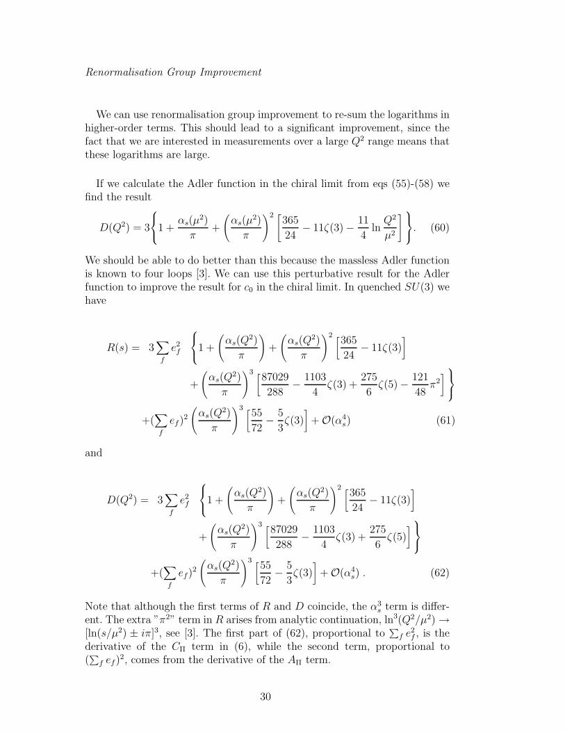
We can use renormalisation group improvement to re-sum the logarithms inhigher-order terms. This should lead to a significant improvement, since thefact that we are interested in measurements over a large Q2 range means thatthese logarithms are large.

If we calculate the Adler function in the chiral limit from eqs (55)-(58) wefind the result

D(Q2) = 3

1 +αs(µ

2)

π+

(

αs(µ2)

π

)2 [365

24− 11ζ(3) − 11

4lnQ2

µ2

]

. (60)

We should be able to do better than this because the massless Adler functionis known to four loops [3]. We can use this perturbative result for the Adlerfunction to improve the result for c0 in the chiral limit. In quenched SU(3) wehave

R(s) = 3∑

f

e2f

1 +

(

αs(Q2)

π

)

+

(

αs(Q2)

π

)2 [365

24− 11ζ(3)

]

+

(

αs(Q2)

π

)3 [87029

288− 1103

4ζ(3) +

275

6ζ(5) − 121

48π2]

+(∑

f

ef)2

(

αs(Q2)

π

)3 [55

72− 5

3ζ(3)

]

+ O(α4s) (61)

and

D(Q2) = 3∑

f

e2f

1 +

(

αs(Q2)

π

)

+

(

αs(Q2)

π

)2 [365

24− 11ζ(3)

]

+

(

αs(Q2)

π

)3 [87029

288− 1103

4ζ(3) +

275

6ζ(5)

]

+(∑

f

ef)2

(

αs(Q2)

π

)3 [55

72− 5

3ζ(3)

]

+ O(α4s) . (62)

Note that although the first terms of R and D coincide, the α3s term is differ-

ent. The extra ”π2” term in R arises from analytic continuation, ln3(Q2/µ2) →[ln(s/µ2) ± iπ]3, see [3]. The first part of (62), proportional to

∑

f e2f , is the

derivative of the CΠ term in (6), while the second term, proportional to(∑

f ef)2, comes from the derivative of the AΠ term.

30

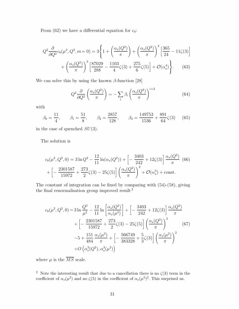
From (62) we have a differential equation for c0:

Q2 ∂

∂Q2c0(µ

2, Q2, m= 0) = 3

1 +

(

αs(Q2)

π

)

+

(

αs(Q2)

π

)2 [365

24− 11ζ(3)

]

+

(

αs(Q2)

π

)3 [87029

288− 1103

4ζ(3) +

275

6ζ(5)

]

+ O(α4s)

. (63)

We can solve this by using the known β-function [28]

Q2 ∂

∂Q2

(

αs(Q2)

π

)

= −∑

i

βi

(

αs(Q2)

π

)i+2

(64)

with

β0 =11

4, β1 =

51

8, β2 =

2857

128, β3 =

149753

1536+

891

64ζ(3) (65)

in the case of quenched SU(3).

The solution is

c0(µ2, Q2, 0) = 3 lnQ2 − 12

11ln(αs(Q

2)) +[

− 3403

242+ 12ζ(3)

]

αs(Q2)

π(66)

+[

− 2301587

15972+

273

2ζ(3)− 25ζ(5)

]

(

αs(Q2)

π

)2

+ O(α3s) + const.

The constant of integration can be fixed by comparing with (54)-(58), givingthe final renormalisation group improved result 2

c0(µ2, Q2, 0)= 3 ln

Q2

µ2− 12

11ln

[

αs(Q2)

αs(µ2)

]

+[

− 3403

242+ 12ζ(3)

]

αs(Q2)

π

+[

− 2301587

15972+

273

2ζ(3) − 25ζ(5)

]

(

αs(Q2)

π

)2

(67)

−5 +151

484

αs(µ2)

π+[

− 566749

383328+

5

3ζ(3)

]

(

αs(µ2)

π

)2

+O(

α3s(Q

2), α3s(µ

2))

where µ is the MS scale.

2 Note the interesting result that due to a cancellation there is no ζ(3) term in thecoefficient of αs(µ

2) and no ζ(5) in the coefficient of αs(µ2)2. This surprised us.

31

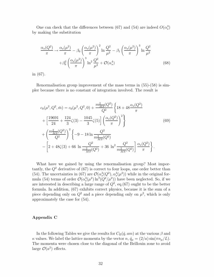
One can check that the differences between (67) and (54) are indeed O(α3s)

by making the substitution

αs(Q2)

π→ αs(µ

2)

π− β0

(

αs(µ2)

π

)2

lnQ2

µ2− β1

(

αs(µ2)

π

)3

lnQ2

µ2

+β20

(

αs(µ2)

π

)3

ln2 Q2

µ2+ O(α4

s) (68)

in (67).

Renormalisation group improvement of the mass terms in (55)-(58) is sim-pler because there is no constant of integration involved. The result is

c0(µ2, Q2, m) = c0(µ

2, Q2, 0) +m2

MS(Q2)

Q2

{

18 + 48αs(Q

2)

π

+[

19691

24+

124

3ζ(3) − 1045

3ζ(5)

]

(

αs(Q2)

π

)2

(69)

+

(

m2MS

(Q2)

Q2

)2 {

−9 − 18 lnQ2

m2MS

(Q2)

−[

2 + 48ζ(3) + 66 lnQ2

m2MS

(Q2)+ 36 ln2 Q2

m2MS

(Q2)

]

αs(Q2)

π

}

.

What have we gained by using the renormalisation group? Most impor-tantly, the Q2 derivative of (67) is correct to four loops, one order better than(54). The uncertainties in (67) are O(α3

s(Q2), α3

s(µ2)) while in the original for-

mula (54) terms of order O(α3s(µ

2) ln3(Q2/µ2)) have been neglected. So, if weare interested in describing a large range of Q2, eq.(67) ought to be the betterformula. In addition, (67) exhibits correct physics, because it is the sum of apiece depending only on Q2 and a piece depending only on µ2, which is onlyapproximately the case for (54).

Appendix C

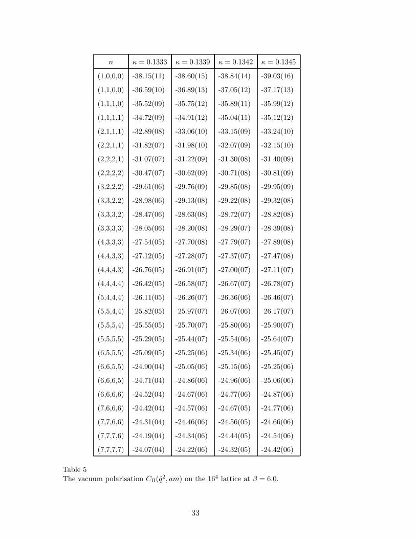
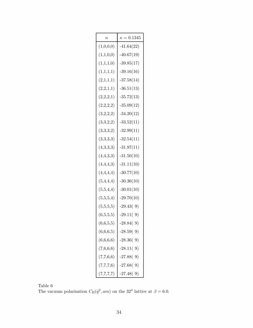
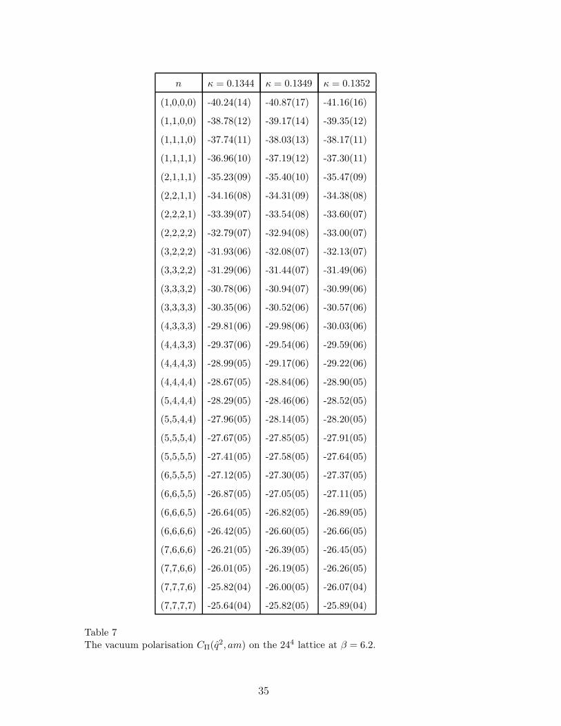
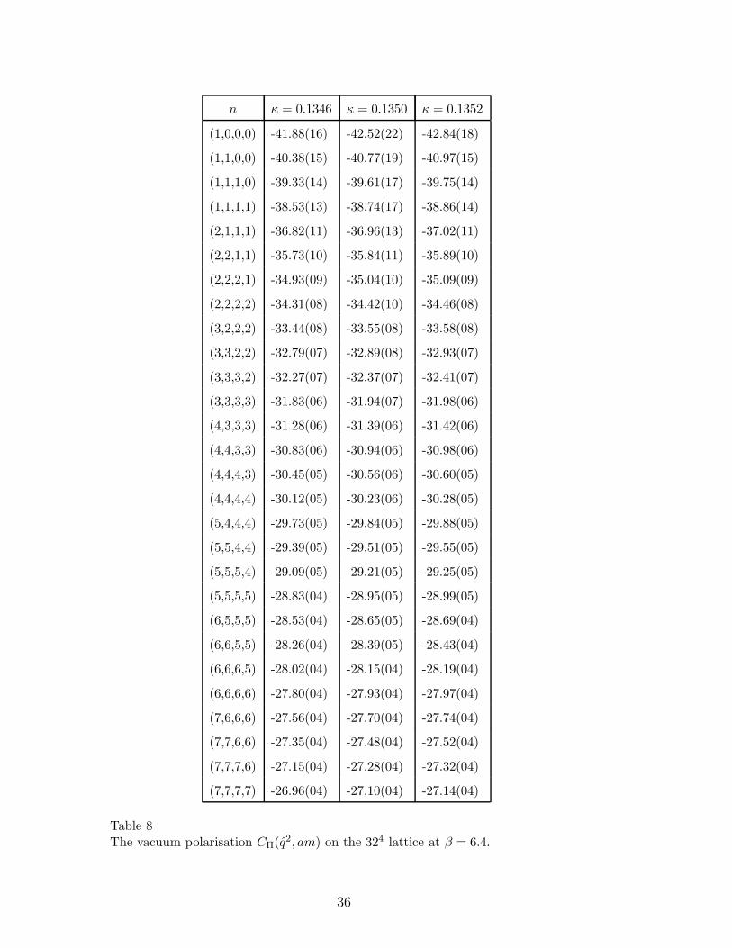
In the following Tables we give the results for CΠ(q, am) at the various β andκ values. We label the lattice momenta by the vector n, qµ = (2/a) sin(πnµ/L).The momenta were chosen close to the diagonal of the Brillouin zone to avoidlarge O(a2) effects.

32

n κ = 0.1333 κ = 0.1339 κ = 0.1342 κ = 0.1345

(1,0,0,0) -38.15(11) -38.60(15) -38.84(14) -39.03(16)

(1,1,0,0) -36.59(10) -36.89(13) -37.05(12) -37.17(13)

(1,1,1,0) -35.52(09) -35.75(12) -35.89(11) -35.99(12)

(1,1,1,1) -34.72(09) -34.91(12) -35.04(11) -35.12(12)

(2,1,1,1) -32.89(08) -33.06(10) -33.15(09) -33.24(10)

(2,2,1,1) -31.82(07) -31.98(10) -32.07(09) -32.15(10)

(2,2,2,1) -31.07(07) -31.22(09) -31.30(08) -31.40(09)

(2,2,2,2) -30.47(07) -30.62(09) -30.71(08) -30.81(09)

(3,2,2,2) -29.61(06) -29.76(09) -29.85(08) -29.95(09)

(3,3,2,2) -28.98(06) -29.13(08) -29.22(08) -29.32(08)

(3,3,3,2) -28.47(06) -28.63(08) -28.72(07) -28.82(08)

(3,3,3,3) -28.05(06) -28.20(08) -28.29(07) -28.39(08)

(4,3,3,3) -27.54(05) -27.70(08) -27.79(07) -27.89(08)

(4,4,3,3) -27.12(05) -27.28(07) -27.37(07) -27.47(08)

(4,4,4,3) -26.76(05) -26.91(07) -27.00(07) -27.11(07)

(4,4,4,4) -26.42(05) -26.58(07) -26.67(07) -26.78(07)

(5,4,4,4) -26.11(05) -26.26(07) -26.36(06) -26.46(07)

(5,5,4,4) -25.82(05) -25.97(07) -26.07(06) -26.17(07)

(5,5,5,4) -25.55(05) -25.70(07) -25.80(06) -25.90(07)

(5,5,5,5) -25.29(05) -25.44(07) -25.54(06) -25.64(07)

(6,5,5,5) -25.09(05) -25.25(06) -25.34(06) -25.45(07)

(6,6,5,5) -24.90(04) -25.05(06) -25.15(06) -25.25(06)

(6,6,6,5) -24.71(04) -24.86(06) -24.96(06) -25.06(06)

(6,6,6,6) -24.52(04) -24.67(06) -24.77(06) -24.87(06)

(7,6,6,6) -24.42(04) -24.57(06) -24.67(05) -24.77(06)

(7,7,6,6) -24.31(04) -24.46(06) -24.56(05) -24.66(06)

(7,7,7,6) -24.19(04) -24.34(06) -24.44(05) -24.54(06)

(7,7,7,7) -24.07(04) -24.22(06) -24.32(05) -24.42(06)

Table 5The vacuum polarisation CΠ(q2, am) on the 164 lattice at β = 6.0.

33

n κ = 0.1345

(1,0,0,0) -41.64(22)

(1,1,0,0) -40.67(19)

(1,1,1,0) -39.85(17)

(1,1,1,1) -39.16(16)

(2,1,1,1) -37.58(14)

(2,2,1,1) -36.51(13)

(2,2,2,1) -35.72(13)

(2,2,2,2) -35.09(12)

(3,2,2,2) -34.20(12)

(3,3,2,2) -33.52(11)

(3,3,3,2) -32.99(11)

(3,3,3,3) -32.54(11)

(4,3,3,3) -31.97(11)

(4,4,3,3) -31.50(10)

(4,4,4,3) -31.11(10)

(4,4,4,4) -30.77(10)

(5,4,4,4) -30.36(10)

(5,5,4,4) -30.01(10)

(5,5,5,4) -29.70(10)

(5,5,5,5) -29.43( 9)

(6,5,5,5) -29.11( 9)

(6,6,5,5) -28.84( 9)

(6,6,6,5) -28.59( 9)

(6,6,6,6) -28.36( 9)

(7,6,6,6) -28.11( 9)

(7,7,6,6) -27.88( 9)

(7,7,7,6) -27.68( 9)

(7,7,7,7) -27.48( 9)

Table 6The vacuum polarisation CΠ(q2, am) on the 324 lattice at β = 6.0.

34

n κ = 0.1344 κ = 0.1349 κ = 0.1352

(1,0,0,0) -40.24(14) -40.87(17) -41.16(16)

(1,1,0,0) -38.78(12) -39.17(14) -39.35(12)

(1,1,1,0) -37.74(11) -38.03(13) -38.17(11)

(1,1,1,1) -36.96(10) -37.19(12) -37.30(11)

(2,1,1,1) -35.23(09) -35.40(10) -35.47(09)

(2,2,1,1) -34.16(08) -34.31(09) -34.38(08)

(2,2,2,1) -33.39(07) -33.54(08) -33.60(07)

(2,2,2,2) -32.79(07) -32.94(08) -33.00(07)

(3,2,2,2) -31.93(06) -32.08(07) -32.13(07)

(3,3,2,2) -31.29(06) -31.44(07) -31.49(06)

(3,3,3,2) -30.78(06) -30.94(07) -30.99(06)

(3,3,3,3) -30.35(06) -30.52(06) -30.57(06)

(4,3,3,3) -29.81(06) -29.98(06) -30.03(06)

(4,4,3,3) -29.37(06) -29.54(06) -29.59(06)

(4,4,4,3) -28.99(05) -29.17(06) -29.22(06)

(4,4,4,4) -28.67(05) -28.84(06) -28.90(05)

(5,4,4,4) -28.29(05) -28.46(06) -28.52(05)

(5,5,4,4) -27.96(05) -28.14(05) -28.20(05)

(5,5,5,4) -27.67(05) -27.85(05) -27.91(05)

(5,5,5,5) -27.41(05) -27.58(05) -27.64(05)

(6,5,5,5) -27.12(05) -27.30(05) -27.37(05)

(6,6,5,5) -26.87(05) -27.05(05) -27.11(05)

(6,6,6,5) -26.64(05) -26.82(05) -26.89(05)

(6,6,6,6) -26.42(05) -26.60(05) -26.66(05)

(7,6,6,6) -26.21(05) -26.39(05) -26.45(05)

(7,7,6,6) -26.01(05) -26.19(05) -26.26(05)

(7,7,7,6) -25.82(04) -26.00(05) -26.07(04)

(7,7,7,7) -25.64(04) -25.82(05) -25.89(04)

Table 7The vacuum polarisation CΠ(q2, am) on the 244 lattice at β = 6.2.

35

n κ = 0.1346 κ = 0.1350 κ = 0.1352

(1,0,0,0) -41.88(16) -42.52(22) -42.84(18)

(1,1,0,0) -40.38(15) -40.77(19) -40.97(15)

(1,1,1,0) -39.33(14) -39.61(17) -39.75(14)

(1,1,1,1) -38.53(13) -38.74(17) -38.86(14)

(2,1,1,1) -36.82(11) -36.96(13) -37.02(11)

(2,2,1,1) -35.73(10) -35.84(11) -35.89(10)

(2,2,2,1) -34.93(09) -35.04(10) -35.09(09)

(2,2,2,2) -34.31(08) -34.42(10) -34.46(08)

(3,2,2,2) -33.44(08) -33.55(08) -33.58(08)

(3,3,2,2) -32.79(07) -32.89(08) -32.93(07)

(3,3,3,2) -32.27(07) -32.37(07) -32.41(07)

(3,3,3,3) -31.83(06) -31.94(07) -31.98(06)

(4,3,3,3) -31.28(06) -31.39(06) -31.42(06)

(4,4,3,3) -30.83(06) -30.94(06) -30.98(06)

(4,4,4,3) -30.45(05) -30.56(06) -30.60(05)

(4,4,4,4) -30.12(05) -30.23(06) -30.28(05)

(5,4,4,4) -29.73(05) -29.84(05) -29.88(05)

(5,5,4,4) -29.39(05) -29.51(05) -29.55(05)

(5,5,5,4) -29.09(05) -29.21(05) -29.25(05)

(5,5,5,5) -28.83(04) -28.95(05) -28.99(05)

(6,5,5,5) -28.53(04) -28.65(05) -28.69(04)

(6,6,5,5) -28.26(04) -28.39(05) -28.43(04)

(6,6,6,5) -28.02(04) -28.15(04) -28.19(04)

(6,6,6,6) -27.80(04) -27.93(04) -27.97(04)

(7,6,6,6) -27.56(04) -27.70(04) -27.74(04)

(7,7,6,6) -27.35(04) -27.48(04) -27.52(04)

(7,7,7,6) -27.15(04) -27.28(04) -27.32(04)

(7,7,7,7) -26.96(04) -27.10(04) -27.14(04)

Table 8The vacuum polarisation CΠ(q2, am) on the 324 lattice at β = 6.4.

36

References

[1] F.J. Reinders, H. Rubinstein and S. Yazaki, Phys. Rep. 127 (1985) 1; S. Narison,“QCD Spectral Sum Rules”, World Scientific, 1989.

[2] S.L. Adler, Phys. Rev. D10 (1974) 3714.

[3] S.G. Gorishny, A.L. Kataev and S.A. Larin, Phys. Lett. B 259 (1991) 144;L.R. Surguladze and M.A. Samuel, Phys. Rev. Lett. 66 (1991) 560, erratumibid 2416.

[4] K.G. Chetyrkin, Phys. Lett. B391 (1997) 402 (hep-ph/9608480).

[5] K.G. Chetyrkin, J.H. Kuhn and M. Steinhauser, Nucl. Phys. B482 (1996) 213.

[6] M.A. Shifman, A.I. Vainshtein and V.I. Zakharov, Nucl. Phys. B147 (1979) 385.

[7] M.A. Shifman, A.I. Vainshtein and V.I. Zakharov, Nucl. Phys. B147 (1979) 448.

[8] S.C. Generalis, J. Phys. G15 (1989) L225; K.G. Chetyrkin, S.G. Gorishnyand V.P. Spiridonov, Phys. Lett. 160B (1985) 149; V.P. Spiridonov andK.G. Chetyrkin, Yad. Fiz. 47 (1988) 818 [Sov. J. Nucl. Phys. 47 (1988) 522].

[9] S. Eidelman, F. Jegerlehner, A.L. Kataev and O. Veretin, Phys. Lett. B454(1999) 369 (hep-ph/9812521).

[10] M. Gockeler, R. Horsley, W. Kurzinger, V. Linke, D. Pleiter, P.E.L. Rakow andG. Schierholz, Nucl. Phys. (Proc. Suppl.) 94 (2001) 571 (hep-lat/0012010);M. Gockeler, R. Horsley, W. Kurzinger, V. Linke, D. Pleiter, P.E.L. Rakow andG. Schierholz, (hep-lat/0310027).

[11] M. Gockeler, R. Horsley, H. Perlt, P. Rakow, G. Schierholz, A. Schiller andP. Stephenson, Phys. Rev. D57 (1998) 5562. (hep-lat/9707021).

[12] M. Gockeler, P.E.L. Rakow, R. Horsley, D. Petters, D. Pleiter and G. Schierholz,in Lattice fermions and structure of the vacuum, p. 201, eds. V. Mitrjushkin andG. Schierholz (Kluwer, Dordrecht, 2000); M. Gockeler, R. Horsley, D. Petters,D. Pleiter, P.E.L. Rakow, G. Schierholz and P. Stephenson, Nucl. Phys. (Proc.Suppl.) 83 (2000) 203 (hep-lat/9909160).

[13] M. Gockeler et al., in preparation.

[14] W. Kurzinger, Ph.D. Thesis (in German), Freie Universitat Berlin (2001);http://www.diss.fu-berlin.de/2001/220/

[15] “Quantum Fields on a Lattice”, I. Montvay and G. Munster, CUP 1994.

[16] S. Capitani, M. Gockeler, R. Horsley, H. Perlt, P.E.L. Rakow, G. Schierholz andA. Schiller, Nucl. Phys. B593 (2001) 183.

[17] M. Luscher, S. Sint, R. Sommer, P. Weisz and U. Wolff, Nucl. Phys. B491 (1997)323.

37

[18] S. Booth, M. Gockeler, R. Horsley, A.C. Irving, B. Joo, S. Pickles, D. Pleiter,P.E.L. Rakow, G. Schierholz, Z. Sroczynski and H. Stuben, Phys. Lett. B519(2001) 229.

[19] S. Capitani, M. Luscher, R. Sommer and H. Wittig, Nucl. Phys. B544 (1999)669; P. Boucaud, G. Burgio, F. Di Renzo, J.P. Leroy, J. Micheli, C. Parrinello,O. Pene, C. Pittori, J. Rodriguez-Quintero, C. Roiesnel and K. Sharkey, JHEP0004 (2000) 006.

[20] M. Guagnelli, R. Sommer and H. Wittig, Nucl. Phys. B535 (1998) 389.

[21] O. Dumbrajs, R. Koch, H. Pilkuhn, G.C. Oades, H. Behrens, J.J. De Swart andP. Kroll, Nucl. Phys. B216 (1983) 277.

[22] Review of Particle Physics, K. Hagiwara et al., PR D66 (2002) 010001.

[23] R.A. Bertlmann, G. Launer and E. de Rafael, Nucl. Phys. B250 (1985) 61.

[24] T. Blum, Phys. Rev. Lett. 91 (2003) 052001; T. Blum, hep-lat/0310064.

[25] A. Nyffeler, hep-ph/0305135.

[26] S. Eidelman and F. Jegerlehner, Z. Phys. C 67 (1995) 585

[27] F. Jegerlehner, J. Phys. G 29 (2003) 101; K. Hagiwara, A.D. Martin, D. Nomuraand T. Teubner, Phys. Lett. B 557 (2003) 69; K. Hagiwara, A.D. Martin,D. Nomura and T. Teubner, hep-ph/0312250; M. Davier, S. Eidelman,A. Hocker and Z. Zhang, Eur. Phys. J. C 27 (2003) 497.

[28] T. van Ritbergen, J.A.M. Vermaseren and S.A. Larin, Phys. Lett. B400 (1997)379; J.A.M. Vermaseren and S.A. Larin and T. van Ritbergen, Phys. Lett. B405(1997) 327.

38