UWFDM-984 BUCKY-1 - A 1-D Radiation Hydrodynamics ...

€

W I S C O N SI N

•

FU

SIO

N•

TECHNOLOGY• INS

TIT

UT

E

FUSION TECHNOLOGY INSTITUTE

UNIVERSITY OF WISCONSIN

MADISON WISCONSIN

BUCKY-1 – A 1-D Radiation HydrodynamicsCode for Simulating Inertial Confinement

Fusion High Energy Density Plasmas

J.J. MacFarlane, G.A. Moses, R.R. Peterson

August 1995

UWFDM-984

DISCLAIMER

This report was prepared as an account of work sponsored by anagency of the United States Government. Neither the United StatesGovernment, nor any agency thereof, nor any of their employees,makes any warranty, express or implied, or assumes any legal liabilityor responsibility for the accuracy, completeness, or usefulness of anyinformation, apparatus, product, or process disclosed, or represents thatits use would not infringe privately owned rights. Reference herein toany specific commercial product, process, or service by trade name,trademark, manufacturer, or otherwise, does not necessarily constitute orimply its endorsement, recommendation, or favoring by the United StatesGovernment or any agency thereof. The views and opinions of authorsexpressed herein do not necessarily state or reflect those of the UnitedStates Government or any agency thereof.

BUCKY-1 – A 1-D Radiation Hydrodynamics Code

for Simulating Inertial Confinement Fusion

High Energy Density Plasmas∗

J. J. MacFarlane, G. A. Moses, and R. R. Peterson

Fusion Technology InstituteUniversity of Wisconsin-Madison

1500 Johnson DriveMadison, WI 53706

August 1995

UWFDM-984

∗This work has been supported in part by the U.S. Department of Energy through Contract No.DE-AS08-88DP10754.

Contents

1. Overview 1-1

2. BUCKY-1 Units and Notation 2-1

2.1. Units . . . . . . . . . . . . . . . . . . . . . . . . . . . . . . . . . . . . . . . . . . . . . 2-1

2.2. Notation . . . . . . . . . . . . . . . . . . . . . . . . . . . . . . . . . . . . . . . . . . . 2-1

2.2.1. Notation in the Documentation . . . . . . . . . . . . . . . . . . . . . . . . . . 2-1

2.2.2. Notation in the Code . . . . . . . . . . . . . . . . . . . . . . . . . . . . . . . 2-2

2.3. Lagrangian Coordinates . . . . . . . . . . . . . . . . . . . . . . . . . . . . . . . . . . 2-2

3. Conservation Equations 3-1

3.1. Mass Conservation . . . . . . . . . . . . . . . . . . . . . . . . . . . . . . . . . . . . . 3-1

3.2. Momentum Conservation . . . . . . . . . . . . . . . . . . . . . . . . . . . . . . . . . 3-2

3.2.1. Quiet Start . . . . . . . . . . . . . . . . . . . . . . . . . . . . . . . . . . . . . 3-4

3.3. Energy Conservation . . . . . . . . . . . . . . . . . . . . . . . . . . . . . . . . . . . . 3-4

3.4. Coefficients and Source Terms in the Energy Equations . . . . . . . . . . . . . . . . 3-9

3.4.1. Thermal Conductivity . . . . . . . . . . . . . . . . . . . . . . . . . . . . . . . 3-9

3.4.2. Electron-Ion Coupling Coefficient . . . . . . . . . . . . . . . . . . . . . . . . . 3-11

3.4.3. Coupling to the Radiation Field . . . . . . . . . . . . . . . . . . . . . . . . . 3-11

3.4.4. Coupling to the Thermonuclear Burn Reaction Products . . . . . . . . . . . . 3-13

3.4.5. Ion Beam and Laser Energy Deposition Source Terms . . . . . . . . . . . . . 3-13

4. Radiation Transport Models 4-1

4.1. Multigroup Diffusion . . . . . . . . . . . . . . . . . . . . . . . . . . . . . . . . . . . . 4-1

4.2. Method of Short Characteristics . . . . . . . . . . . . . . . . . . . . . . . . . . . . . 4-4

4.3. Variable Eddington Model . . . . . . . . . . . . . . . . . . . . . . . . . . . . . . . . . 4-4

4.4. Non-LTE CRE Line Transport . . . . . . . . . . . . . . . . . . . . . . . . . . . . . . 4-11

4.4.1. Introduction . . . . . . . . . . . . . . . . . . . . . . . . . . . . . . . . . . . . 4-11

4.4.2. Statistical Equilibrium Model . . . . . . . . . . . . . . . . . . . . . . . . . . . 4-12

4.4.3. Radiative Transfer Model . . . . . . . . . . . . . . . . . . . . . . . . . . . . . 4-15

4.4.4. Atomic Physics Models . . . . . . . . . . . . . . . . . . . . . . . . . . . . . . 4-22

4.4.5. Interface Between CRE and Radiation-Hydrodynamics Models . . . . . . . . 4-23

4.5. Mechanics of CRE/Radiation-Hydrodynamics Interface . . . . . . . . . . . . . . . . 4-24

5. Equations of State and Opacity Tables 5-1

5.1. EOSOPA EOS and Opacity Tables . . . . . . . . . . . . . . . . . . . . . . . . . . . . 5-2

5.2. SESAME EOS Tables . . . . . . . . . . . . . . . . . . . . . . . . . . . . . . . . . . . 5-3

6. Fast Ion Energy Deposition 6-1

7. Laser Deposition Model 7-1

8. Fusion Burn Energy Deposition 8-1

8.1. Fusion Reactions . . . . . . . . . . . . . . . . . . . . . . . . . . . . . . . . . . . . . . 8-1

8.2. Fusion Charged Particle Reaction Product Transport . . . . . . . . . . . . . . . . . . 8-4

8.2.1. Time-Dependent Particle Tracking Method . . . . . . . . . . . . . . . . . . . 8-4

8.2.2. Implementation of TDPT . . . . . . . . . . . . . . . . . . . . . . . . . . . . . 8-10

8.3. Nuclear Energy Deposition Model . . . . . . . . . . . . . . . . . . . . . . . . . . . . 8-20

9. Rapid X-ray Deposition in Cold Media 9-1

10.Vaporization and Condensation Modeling 10-1

11.Energy Conservation Check 11-1

12.Time Step Control 12-1

13.Code Structure 13-1

13.1. Subroutines . . . . . . . . . . . . . . . . . . . . . . . . . . . . . . . . . . . . . . . . . 13-1

13.2. The Common Blocks . . . . . . . . . . . . . . . . . . . . . . . . . . . . . . . . . . . . 13-18

14.Input and Output Files 14-1

15.NAMELIST Input Variables 15-1

16.Compiling and Running 16-1

17.Sample Calculations 17-1

17.1. Example 1: Isentropic Compression of a DT Shell . . . . . . . . . . . . . . . . . . . . 17-1

17.2. Example 2: Al Witness Plate Shock Breakout . . . . . . . . . . . . . . . . . . . . . . 17-3

17.3. Example 3: LIBRA Implosion Simulation . . . . . . . . . . . . . . . . . . . . . . . . 17-3

17.4. LIBRA Fusion Burn and Target Breakup . . . . . . . . . . . . . . . . . . . . . . . . 17-8

17.5. Example 5: Target Chamber Non-LTE Buffer Gas Simulation . . . . . . . . . . . . . 17-11

1. Overview

BUCKY-1 is a one-dimensional (1-D) radiation-hydrodynamics code developed at

the University of Wisconsin Fusion Technology Institute to study Inertial Confinement

Fusion (ICF) high energy density plasmas. This code has been constructed in large part by

integrating pieces from several other simulation codes which were developed at the University

of Wisconsin to study target physics and target chamber design issues for ICF reactors. Its

history is rooted primarily in the following codes:

• PHD-IV [1] — A 1-D radiation-hydrodynamics code written to simulate ICF target

implosions, fusion burn, and energy partitioning during target breakup.

• MF-FIRE [2] — A 1-D radiation-hydrodynamics code for simulating the response of

a target chamber buffer gas to a high-gain ICF microexplosion.

• CONRAD [3] — A descendant of MF-FIRE which includes the capability of

simulating the vaporization of solid or liquid surfaces exposed to the x-rays and fast

debris ions from high-gain targets.

• NLTERT [4] — A non-LTE collisional-radiative equilibrium (CRE) code with detailed

radiation transport packages used to study the radiative, atomic, and spectral

properties of ICF-related laboratory plasmas.

The code utilizes high-quality equation of state (EOS) and multigroup opacity tables

generated by EOSOPA [5], which provides data for both low-Z and high-Z plasmas over

densities ranging from the dilute ideal gas region to highly compressed matter. In addition

to integrating parts of previously written codes, a number of new packages and options have

been added. These include: a new multiangle, multifrequency radiation transfer model based

on the method of short characteristics; an escape probability model for energy deposition

of neutrons created during the DT burn phase; a simple laser energy deposition model; the

1-1

ability to simulate the response of thin foil targets to an external radiation source; and more

flexibility in setting up and running multilayer, multimaterial problems, including the ability

to select different EOS packages (EOSOPA or SESAME) for each layer. Also it is worth

noting that the output from this code has been set up to interface readily with our non-LTE

spectral analysis code. This allows for an efficient means of turning temperature and density

distributions predicted by BUCKY-1 into detailed emission or absorption spectra, which can

then be directly compared with spectra obtained in laboratory plasma experiments.

This code and its predecessors have been used to simulate a variety of plasmas.

Examples include:

• Simulation of the breakup and energy partitioning of high-gain ICF targets [6]–[8];

• Simulating the response of materials (Au foils, Al witness plates) to hohlraum radiation

drives [9]–[11];

• Investigating the response of non-LTE buffer gas plasmas to ICF high-gain

microexplosions [12, 13] and to laser-produced blast waves generated by fast ions [14];

• Studying the vaporization and condensation of solid and liquid surfaces exposed to

ICF target x-rays and debris ions [15, 16];

• Simulation of “plastic sandwich” targets heated by intense Li beams [17, 18];

• Investigating the x-ray emission from shocks generated in the winds of high-luminosity

stars [19].

At various stages of development, many of the models in the code have been tested and

benchmarked. The reader should note, however, that the code is continually being modified

and upgraded, and that we must continue our efforts to test the code and benchmark against

experimental data whenever possible.

1-2

The major features of BUCKY-1 are as follows. It is a 1-D Lagrangian hydrodynamics

code which can simulate plasmas in planar, cylindrical, or spherical geometries. It solves

a single fluid equation of motion (electrons and ions are assumed to move together) with

pressure contributions from electrons, ions, radiation, and fast charged particles. Shocks

are handled using a von Neumann artificial viscosity. Energy transfer in the plasma can

be treated using either a one-temperature (Ti = Te) or two-temperature (Ti �= Te) model.

Both the electrons and ions are assumed to have Maxwellian distributions defined by Ti and

Te. Thermal conduction for each species is treated using Spitzer conductivities, with the

electron conduction being flux-limited. The two temperature equations are coupled by an

electron-ion energy exchange term and each equation has a PdV work term.

Radiation emission and absorption terms are coupled to the electron temperature

equation. Multifrequency radiation intensities are computed using a choice of several

radiation transport packages: (1) a flux-limited radiation diffusion model; (2) a multiangle

radiative transfer model based on the method of short characteristics (presently, planar

geometry only); (3) a variable Eddington radiative transfer model (spherical geometries);

and (4) a non-LTE line radiation transport package based on escape probability techniques.

The sum of the contributions to emission and absorption from all frequency groups are

then coupled to the electron energy equation as source terms. Multifrequency opacities are

obtained from EOSOPA tables. When the CRE line transport model is invoked, non-LTE

atomic level populations are computed self-consistently with the line radiation field. In this

case, collisional and radiative atomic data are obtained from ATBASE [20] tables.

In addition to radiation, a number of other physical processes are included in the

electron and ion energy equations as source terms: fast ion (beam or target debris) energy

deposition; heating due to the deposition of fast charged particles and neutrons during the

fusion burn phase; laser energy deposition; and x-ray heating of a cold buffer gas. Fusion burn

equations from DT, DD, and DHe3 reactions are solved and the charged particle reaction

1-3

products are transported and slowed using a time-dependent particle tracking algorithm.

Neutrons are deposited in the target using an escape probability model. Fast ions from an

ion beam or target microexplosion debris are tracked using a time-, energy-, and species-

dependent stopping power model. Stopping powers are computed using a Lindhard model

at low projectile energies and a Bethe model at high energies [21]. Laser energy is deposited

using an inverse Bremsstrahlung attenuation model, with a dump of the remaining laser

energy at the critical surface.

The source code for BUCKY-1 (without common blocks inserted) is about 27,000

lines. The code is typically run on UNIX workstations (HP 700 series, SUN, IBM RS6000,

Silicon Graphics) which have 32 – 80 MB of RAM. The memory required depends on the

size of the arrays, which are easily adjusted by the user. A preprocessor is used to allow for

ease in adjusting array sizes and machine portability. The main functions of the preprocessor

are to: insert common blocks in the source code; define array sizes through PARAMETER

statements; and insert machine-dependent source code. The CPU time required for typical

calculations on HP 715 and 735 workstations ranges from several minutes to several hours,

depending on the complexity of the problem. Results are plotted using separate software

which reads a binary output file created during the simulation.

1-4

2. BUCKY-1 Units and Notation

2.1. Units

The units in BUCKY-1 are primarily those listed in Table 2.1. However, two sections

of the code which were extracted from PHD-IV (the fusion burn package) and NLTERT (the

non-LTE line radiation package) remain in the units of their original code. Thus, some unit

conversion is done at the beginning and end of calls to these packages. The units for these

are listed in the last two columns in Table 2.1.

Table 2.1. BUCKY-1 Units

General Fusion Burn Non-LTE LineQuantity Units Units Transport Units

Mass grams grams gramsLength cm cm cm

Time s shakes = 10−8 s sTemperature eV keV eVEnergy J jerks = 1016 ergs ergs

Pressure J/cm3 jerks/cm3 —

2.2. Notation

2.2.1. Notation in the Documentation

The notation in the documentation for the time and space indices used in solving

the partial differential equations is quite standard. The time index appears as a superscript

and the space index appears as a subscript (e.g., T n+1/2ej−1/2

). The zone boundaries are denoted

by whole integer subscripts and the zone centers are denoted by half integer subscripts.

The inner zone boundary has the subscript j = 0 and the outer boundary has the index

j = JMAX. The equation of motion is “advanced” from time level tn−1/2 to time level tn+1/2

and the temperature and radiation equations are advanced from level tn to level tn+1.

2-1

2.2.2. Notation in the Code

The notation in BUCKY-1 is summarized in Table 2.2. The last two characters of the

variable name distinguish whether it is a zone centered or a zone boundary quantity, and the

time level in the finite difference equations at which the quantity is evaluated. The first four

or less characters represent the name of the quantity. This will describe either a physical

quantity (e.g., TE2A is the zone center and electron temperature at time level n + 1) or

the name will correspond to the notation used in the documentation (e.g., OMC2B is the

electron-ion coupling coefficient, ωc, at time level n+ 1/2). The letter “E” generally means

electron, “N” means ion, and “R” means radiation.

Table 2.2. Variable Notation

1 – zone boundary A – tn+1

2 – zone center B – tn+1/2

C – tn

D – tn−1/2

2.3. Lagrangian Coordinates

The hydrodynamic description of a fluid can be expressed in two equivalent forms.

In the Eulerian approach, attention is centered at positions r in a fixed reference frame

and the change in the fluid properties is observed at this position. In other words, the

coordinate system is stationary and the fluid flows through it. In the Lagrangian approach,

the coordinate system is tied to the fluid at time t = 0 and moves with the fluid velocity,

u(r, t). We observe a “cell” of fluid at time t = 0 and follow its evolution for t > 0. In the

Lagrangian form, a new independent variable is defined to replace the spatial vector, r. In

one dimension this is given by

dmo = ρ(r)rδ−1dr (2.1)

where the units of the Lagrangian mass, mo, are given in Table 2.3.

2-2

Table 2.3. Lagrangian Units

Geometry δ Mass (m0) Energy

Planar 1 grams/cm2 J/cm2

Cylindrical 2 grams/cm·radian J/cm·radianSpherical 3 grams/steradian J/steradian

In Lagrangian coordinates, the mass within each zone remains constant throughout

the calculation, while the zone boundary radii, rj, are functions of time. The continuity

equation is automatically satisfied and new densities are computed by new zone boundary

positions and the ratio of mass to volume. (The constant zone mass is not strictly true

when thermonuclear burn calculations are done and particles are transported across zone

boundaries.)

2-3

3. Conservation Equations

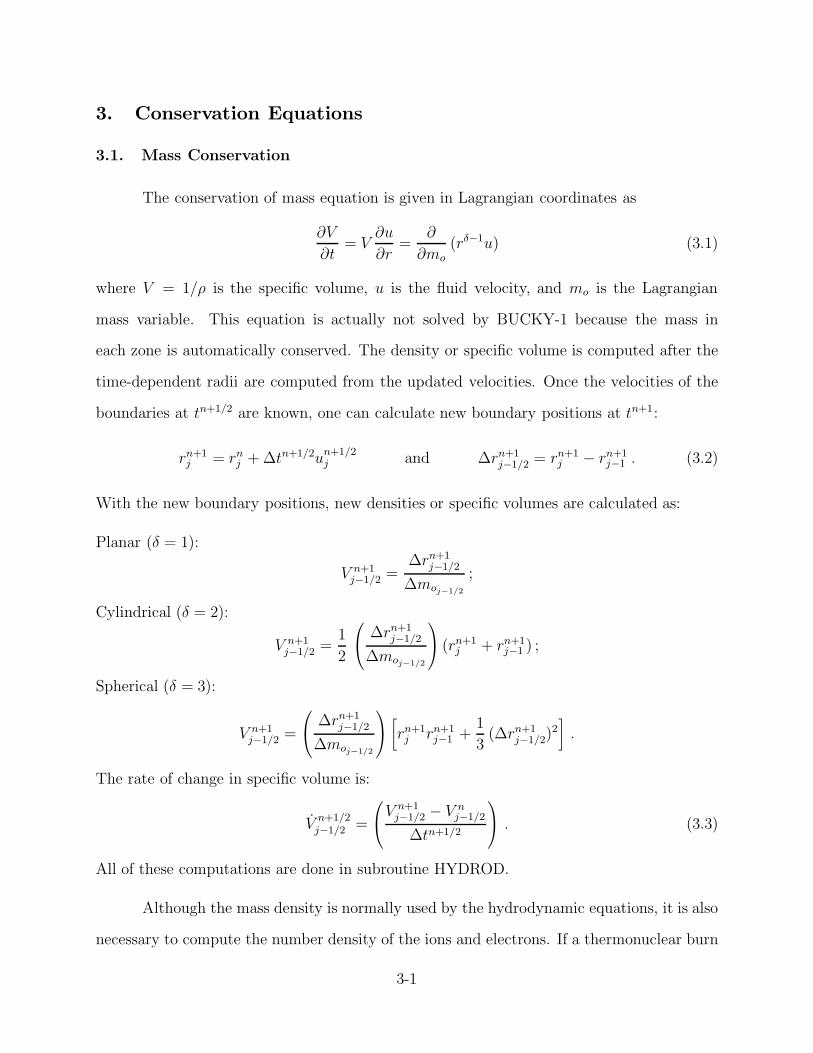
3.1. Mass Conservation

The conservation of mass equation is given in Lagrangian coordinates as

∂V

∂t= V

∂u

∂r=

∂

∂mo(rδ−1u) (3.1)

where V = 1/ρ is the specific volume, u is the fluid velocity, and mo is the Lagrangian

mass variable. This equation is actually not solved by BUCKY-1 because the mass in

each zone is automatically conserved. The density or specific volume is computed after the

time-dependent radii are computed from the updated velocities. Once the velocities of the

boundaries at tn+1/2 are known, one can calculate new boundary positions at tn+1:

rn+1j = rnj +∆tn+1/2un+1/2j and ∆rn+1j−1/2 = rn+1j − rn+1j−1 . (3.2)

With the new boundary positions, new densities or specific volumes are calculated as:

Planar (δ = 1):

V n+1j−1/2 =

∆rn+1j−1/2

∆moj−1/2

;

Cylindrical (δ = 2):

V n+1j−1/2 =

1

2

∆rn+1j−1/2

∆moj−1/2

(rn+1j + rn+1j−1 ) ;

Spherical (δ = 3):

V n+1j−1/2 =

∆rn+1j−1/2

∆moj−1/2

[

rn+1j rn+1j−1 +1

3(∆rn+1j−1/2)

2].

The rate of change in specific volume is:

V n+1/2j−1/2 =

V n+1

j−1/2 − V nj−1/2

∆tn+1/2

. (3.3)

All of these computations are done in subroutine HYDROD.

Although the mass density is normally used by the hydrodynamic equations, it is also

necessary to compute the number density of the ions and electrons. If a thermonuclear burn

3-1

calculation is done then the ionic species in each zone can change and the ion number density

(ni), average charge (Z), and average atomic weight (A) are given by:

ni = nD + nT + nHe4 + nHe3 + nP + no , (3.4)

Z =[(nD + nT + nP ) ∗ 1 + (nHe4 + nHe3) ∗ 2 + no ∗ Zo]

ni, (3.5)

A =[nP + nD ∗ 2 + (nT + nHe3) ∗ 3 + (nHe4) ∗ 4 + no ∗ Ao]

ni, (3.6)

where nD and nT are the deuterium and tritium particle densities, nHe3 and nHe4 are the He

isotope particle densities, and no and Zo refer to the density and mean charge of non-burn

(Z > 2) species.

3.2. Momentum Conservation

The momentum conservation equation is solved in the one fluid approximation, where

the plasma electrons and ions are assumed to flow together as one fluid with no charge

separation effects (i.e., electric fields) included. In the one-dimensional approximation there

are also no self-generated magnetic fields, and the conservation of momentum equation, in

Lagrangian form, becomes simply:

∂u

∂t= −1

ρ

∂

∂r(P + q) = −rδ−1

∂

∂mo(P + q) + uTN , (3.7)

where P = Pe + Pi + Pr is the total fluid pressure, q is the von Neumann artificial viscosity,

and uTN is the velocity change due to momentum exchange from the slowing down of fast

(non-thermal) particles. The explicit difference equation used to solve this P.D.E. is given

by:un+1/2j − un−1/2

j

∆tn= −(rδ−1)nj

[∆Pnj +∆qn−1/2j ]

∆moj

+ uTNj ; (3.8)

hence

un+1/2j = un−1/2

j − (rδ−1)nj [∆Pnj +∆qn−1/2j ] (

∆tn

∆moj

) + ∆tn uTNj (3.9)

3-2

where

Pnj−1/2 = Pn

ej−1/2+ Pn

ij−1/2+ Pn

rj−1/2∆Pn

j = P nj+1/2 − Pn

j−1/2

∆moj = (∆moj+1/2+∆moj−1/2

)/2 ∆qn−1/2j = qn−1/2j+1/2 − qn−1/2j−1/2

∆tn = (∆tn+1/2 +∆tn−1/2)/2

(3.10)

and ˙uTN is defined in Section 8. Equation (3.9) is solved in subroutine HYDROD. The

artificial viscosity is introduced into the inviscid equation of motion to handle shocks. Its

function is to smooth shock fronts over about 3 zones by adding a small amount of dissipation

into the equation. It is non-zero only when a zone is under compression. It is given by the

following expressions which are computed in subroutine QUE:

qn−1/2j−1/2 = 0∂V

n−1/2j−1/2

∂t> 0 (expansion)

qn−1/2j−1/2 = 2

(un−1/2j −u

n−1/2j−1/2

)2

Vn−1/2

j−1/2

∂Vn−1/2j−1/2

∂t< 0 (compression) .

(3.11)

The difference equation advances the velocities at the zone boundaries from tn−1/2 to tn+1/2.

It is an explicit difference equation in that the unknown, un+1/2j , is explicitly expressable

in terms of known quantities at earlier times. For constant ∆t and ∆x, this equation is

accurate to order ∆x2 and ∆t2. The numerical stability of this equation away from shocks

is insured if

cs∆t

∆x< 1 , (3.12)

where cs is the maximum sound speed in the system. This is the Courant condition and is

derived from purely mathematical arguments, but has physical interpretation as well. When

this condition is maintained, a disturbance in the fluid cannot pass through more than one

mesh interval in a time step, thus assuring that it will be resolved by the finite difference

mesh. The time step in BUCKY-1 is adjusted on each time cycle to insure that the Courant

condition is satisfied. The time step control algorithm is discussed in Section 12.

3-3

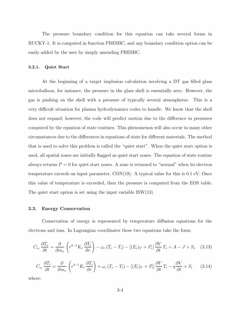
The pressure boundary condition for this equation can take several forms in

BUCKY-1. It is computed in function PRESBC, and any boundary condition option can be

easily added by the user by simply amending PRESBC.

3.2.1. Quiet Start

At the beginning of a target implosion calculation involving a DT gas filled glass

microballoon, for instance, the pressure in the glass shell is essentially zero. However, the

gas is pushing on the shell with a pressure of typically several atmospheres. This is a

very difficult situation for plasma hydrodynamics codes to handle. We know that the shell

does not expand; however, the code will predict motion due to the difference in pressures

computed by the equation of state routines. This phenomenon will also occur in many other

circumstances due to the differences in equations of state for different materials. The method

that is used to solve this problem is called the “quiet start”. When the quiet start option is

used, all spatial zones are initially flagged as quiet start zones. The equation of state routine

always returns P = 0 for quiet start zones. A zone is returned to “normal” when its electron

temperature exceeds an input parameter, CON(19). A typical value for this is 0.1 eV. Once

this value of temperature is exceeded, then the pressure is computed from the EOS table.

The quiet start option is set using the input variable ISW(13).

3.3. Energy Conservation

Conservation of energy is represented by temperature diffusion equations for the

electrons and ions. In Lagrangian coordinates these two equations take the form:

Cve

∂Te

∂t=

∂

∂mo

(rδ−1Ke

∂Te

∂r

)− ωc (Te − Ti)− [(Ee)V + Pe]

∂V

∂tTe +A− J + Se (3.13)

Cvi

∂Ti

∂t=

∂

∂mo

(rδ−1Ki

∂Ti

∂r

)+ ωc (Te − Ti)− [(Ei)V + Pi]

∂V

∂tTi − q

∂V

∂t+ Si (3.14)

where:

3-4

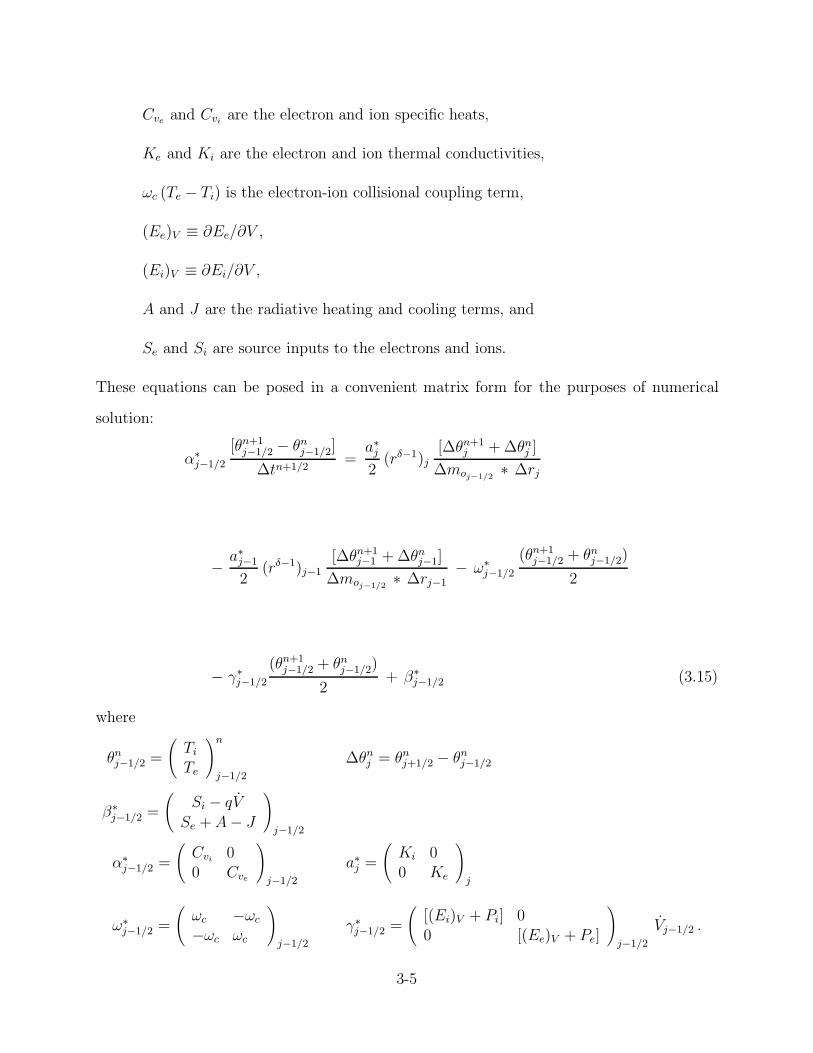
Cve and Cvi are the electron and ion specific heats,

Ke and Ki are the electron and ion thermal conductivities,

ωc (Te − Ti) is the electron-ion collisional coupling term,

(Ee)V ≡ ∂Ee/∂V ,

(Ei)V ≡ ∂Ei/∂V ,

A and J are the radiative heating and cooling terms, and

Se and Si are source inputs to the electrons and ions.

These equations can be posed in a convenient matrix form for the purposes of numerical

solution:

α∗j−1/2

[θn+1j−1/2 − θnj−1/2]

∆tn+1/2=

a∗j2(rδ−1)j

[∆θn+1j +∆θnj ]

∆moj−1/2∗ ∆rj

−a∗j−12

(rδ−1)j−1[∆θn+1j−1 +∆θnj−1]

∆moj−1/2∗ ∆rj−1

− ω∗j−1/2

(θn+1j−1/2 + θnj−1/2)

2

− γ∗j−1/2

(θn+1j−1/2 + θnj−1/2)

2+ β∗

j−1/2 (3.15)

where

θnj−1/2 =

(Ti

Te

)n

j−1/2∆θnj = θnj+1/2 − θnj−1/2

β∗j−1/2 =

(Si − qV

Se +A− J

)j−1/2

α∗j−1/2 =

(Cvi 00 Cve

)j−1/2

a∗j =

(Ki 00 Ke

)j

ω∗j−1/2 =

(ωc −ωc

−ωc ωc

)j−1/2

γ∗j−1/2 =

([(Ei)V + Pi] 00 [(Ee)V + Pe]

)j−1/2

Vj−1/2 .

3-5

Rearranging we find

αj−1/2(θn+1j−1/2 − θnj−1/2) = aj(∆θn+1j +∆θnj )− aj−1(∆θn+1j−1 +∆θnj−1)

−ωj−1/2(θn+1j−1/2 + θnj−1/2)− γj−1/2(θ

n+1j−1/2 + θnj−1/2) + βj−1/2 (3.16)

where

αj−1/2 =

(Cvi 00 Cve

)j−1/2

∆moj−1/2

∆tn+1/2

βj−1/2 =

(Si − qV

Se + A− J

)j−1/2

∆moj−1/2

aj =1

2

(Ki 00 Ke

)j

(rδ−1)j

∆rj

ωj−1/2 =1

2

(ωc −ωc

−ωc ωc

)j−1/2

∆moj−1/2

γj−1/2 =1

2

([(Ei)V + Pi] 0

0 [(Ee)V + Pe]

)j−1/2

Vj−1/2∆moj−1/2. (3.17)

Combining terms in identical values of θ we finally obtain the familiar form:

− Aj−1/2 θn+1j+1/2 +Bj−1/2 θ

n+1j−1/2 − Cj−1/2 θ

n+1j−3/2 = Dj−1/2 (3.18)

where

Aj−1/2 = aj

Bj−1/2 = αj−1/2 + ωj−1/2 + γj−1/2 + aj + aj−1

Cj−1/2 = aj−1

Dj−1/2 = aj(θnj+1/2 − θnj−1/2)− aj−1(θ

nj−1/2 − θnj−3/2)

− (γj−1/2 + ωj−1/2 − αj−1/2) (θnj−1/2) + βj−1/2 . (3.19)

3-6

In the above difference equations, all coefficient matrices are evaluated at tn+1/2, hence

αj−1/2 = αn+1/2j−1/2 , etc. The solution to Eq. (3.18) of the form [22]:

θn+1j−1/2 = Ej−1/2 θn+1j+1/2 + Fj−1/2 (3.20)

where

Ej−1/2 = (Bj−1/2 − Cj−1/2 · Ej−3/2)−1 · Aj−1/2

Fj−1/2 = (Bj−1/2 − Cj−1/2 · Ej−3/2)−1 · (Dj−1/2 + Cj−1/2 · Fj−3/2) . (3.21)

The boundary conditions determine E1/2, F1/2, and θn+1JMAX+1/2. For plasma boundaries where

there is no heat flux (such as the inner boundary in spherical geometry):

E1/2 = (B1/2)−1 · A1/2 F1/2 = (B1/2)

−1 ·D1/2 . (3.22)

At the outer boundary, the option of specifying a temperature boundary condition or a zero

heat flux condition is reserved. For a temperature boundary condition

θn+1JMAX+1/2 = θn+1bc . (3.23)

For zero heat flux we demand

θn+1JMAX+1/2 = θn+1JMAX−1/2 . (3.24)

Hence, there are two equations and two unknowns:

θn+1JMAX−1/2 = θn+1JMAX+1/2

θn+1JMAX−1/2 = EJMAX−1/2 θn+1bc + FJMAX−1/2 . (3.25)

This specification of θn+1bc will insure no conductive heat flux across the outer plasma

boundary which is an appropriate condition for a plasma expanding into a vacuum. Since the

boundary is moving in the Lagrangian scheme, it will always be a plasma-vacuum interface

and no heat flux can be conducted across it.

3-7

The BUCKY-1 subroutine structure, as in PHD-IV [1], closely follows this algorithm

for solving the temperature equations. The matrices and vector, α, a, ω, γ, and β, are

evaluated in the subroutine MATRIX and the matrices and vectors, A, B, C, D, E, F, are

evaluated in the subroutine ABCPL2. The final solution for the temperatures, Eq. (3.20), is

executed in subroutine ENERGY. The boundary conditions are obtained from the subroutine

TEMPBC. The segregation of this algorithm into these subroutines was done to isolate

the numerical analysis from the physics of the code. Subroutine PLSCF2 takes physical

quantities, ωc, Ke, etc., and combines them into quantities that are used for the numerical

solution. In this sense it is the interface routine between the physics and numerical parts of

the code. To add new terms to the temperature equations, only PLSCF2 (and PLSCF1 for

the 1-T option) needs to be changed, minimizing the chance of disturbing the numerics of

ABCPL2.

The difference method used here is a backward substitution solution to the implicit

Crank-Nicholson difference scheme. All values of θ are evaluated at both tn and tn+1, hence

we cannot express θn+1 in terms of only variables at tn. This implicit numerical scheme

requires the solution of a matrix equation. Because we are solving two coupled equations and

the usual scalar coefficients are now matrices, the matrix to be inverted is block tridiagonal

with 2×2 blocks. For linear equations the Crank-Nicholson scheme is unconditionally stable

and accurate to order (∆t)2 and (∆x)2 and will generally allow much larger time steps for this

diffusion equation than an explicit scheme. For this nonlinear problem, however, stability

problems can arise unless the time step is restricted, as is done in subroutine TIMING and

discussed in Section 12.

3-8

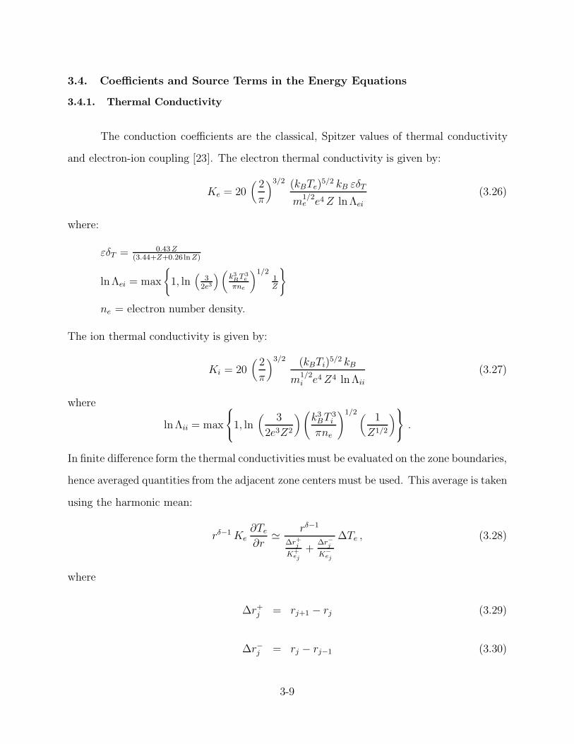
3.4. Coefficients and Source Terms in the Energy Equations

3.4.1. Thermal Conductivity

The conduction coefficients are the classical, Spitzer values of thermal conductivity

and electron-ion coupling [23]. The electron thermal conductivity is given by:

Ke = 20(2

π

)3/2 (kBTe)5/2 kB εδT

m1/2e e4Z lnΛei

(3.26)

where:

εδT = 0.43Z(3.44+Z+0.26 lnZ)

lnΛei = max

{1, ln

(32e3

)(k3

BT 3e

πne

)1/21Z

}

ne = electron number density.

The ion thermal conductivity is given by:

Ki = 20(2

π

)3/2 (kBTi)5/2 kB

m1/2i e4Z4 lnΛii

(3.27)

where

lnΛii = max

1, ln

(3

2e3Z2

)(k3BT

3i

πne

)1/2 (1

Z1/2

) .

In finite difference form the thermal conductivities must be evaluated on the zone boundaries,

hence averaged quantities from the adjacent zone centers must be used. This average is taken

using the harmonic mean:

rδ−1Ke∂Te

∂r� rδ−1

∆r+jK+

ej

+∆r−jK−

ej

∆Te , (3.28)

where

∆r+j = rj+1 − rj (3.29)

∆r−j = rj − rj−1 (3.30)

3-9

K+ej

=C2 T

2ejT 1/2ej+1/2

(4 + Zj+1/2) (lnΛei)j+1/2

K−ej

=C2 T 2ej

T 1/2ej−1/2

(4 + Zj−1/2)(lnΛei)j−1/2. (3.31)

A similar expression is used for the ions, with

K+i =

C1 T 2ij T1/2ij+1/2

(Λj+1/2)1/2 (Zj+1/2)4 (lnΛii)j+1/2

K−i =

C1 T 2ij T1/2ij−1/2

(Λj−1/2)1/2 (Zj−1/2)4 (lnΛii)j−1/2. (3.32)

These expressions will most heavily weight the lowest conductivity in the zones centered at

j + 1/2 or j − 1/2.

In the presence of strong thermal gradients, that is large fluxes, the diffusion

approximation can break down and predict unphysically large thermal fluxes. To adjust

for this, the electron thermal conduction is augmented with a flux limiter. This maximum

permissible flux is defined in the classical manner:

qmax =3√3

8(nekBTe)

(kBTe

me

)1/2. (3.33)

In finite difference form, this is expressed as

qn+1/2maxj= C3 (n

n+1/2ej−1/2

+ nn+1/2ej+1/2

) T n+1/2ej

[(T n+1/2ej−1/2

)1/2 + (T n+1/2ej+1/2

)1/2] . (3.34)

Note that this quantity is evaluated on a zone boundary. The electron and ion thermal

conductivities and the electron thermal flux limit are computed in the subroutine PCOND2.

The flux limit is implemented by redefining the electron element of the a matrix as

a22j =(r

n+1/2j )δ−1

∆rj+1/2

K+ej

+∆rj−1/2

K−ej

+|Tn+1/2

ej+1/2−T

n+1/2ej−1/2

|qmaxj

(3.35)

This quantity is computed in subroutine PLSCF2.

3-10

3.4.2. Electron-Ion Coupling Coefficient

The electron and ion temperatures are coupled by the expression

∂Te

∂t=

Ti − Te

tei. (3.36)

In terms of the electron and ion diffusion equations this expression becomes

Cve

∂Te

∂t= · · · + Cve

tei(Ti − Te) + · · ·

hence, the definition of the coupling coefficient is

ωc =Cve

tei= Cveνei (3.37)

where:

νei =8(2π)1/2

3m1/2

e e4N2A

(Z

A

)2 lnΛei

(kBTe)3/2ρ (3.38)

NA = Avogadro’s number

A = ion atomic weight

Z = ion charge

Cve = electron specific heat.

In finite difference form this is

ωcj−1/2= C28Cve,j−1/2

(Zj−1/2

Aj−1/2

)2(lnΛei)j−1/2

Vj−1/2(Tej−1/2)3/2

, (3.39)

where all quantities are evaluated at time level n + 1/2. This coefficient is computed in

subroutine OMEGAC.

3.4.3. Coupling to the Radiation Field

The electron temperature equation is explicitly coupled to the radiation field through

emission and absorption terms. The radiative transfer models used to determine these terms

are described in Section 4.

3-11

The emission term is simply computed as

J = 4σSB V σEP T

4e (3.40)

where

σSB = Stefan-Boltzmann constant

V = specific volume

σEP = Planck emission opacity

Te = electron temperature.

For multigroup calculations this term has a corresponding multigroup value, Jg, such that

J =G∑

g=1

Jg , (3.41)

where

Jg =8π(kTe)4

c2 h3σEP,g

∫ xg+1

xg

dxx3

ex − 1,

xg ≡hνgkTe

.

The absorption term is given by

A = cσAP ER (3.42)

where

c = speed of light

σAP = Planck absorption opacity

ER = radiation energy density.

In multifrequency group calculations this is given by

A = cG∑

g=1

σgPE

gR . (3.43)

3-12

These terms are SRE2B (emission) and SER2B (absorption) in the code and they are

computed in RADTRn (n = 1, 2, or 3, depending on the transport model). They contribute

to the electron source term, BET22B, which is computed in PLSCF2.

3.4.4. Coupling to the Thermonuclear Burn Reaction Products

The charged particle reaction products from the fusion reactions are transported

through the plasma and slowed down as described in Section 9. This calculation is done

independent of the plasma hydrodynamics and is coupled to the hydrodynamics explicitly

through source terms in the electron and ion temperature equations. The energy source in

each zone due to charged particle energy redeposition to electrons and ions is accumulated

in the variables SETN2B and SNTN2B by the routine TNBURN. These quantities then

contribute to the BET12B and BET22B source terms in the temperature equations. These

are computed in PLSCF2.

Neutrons produced during the fusion burn can redeposit their energy back in the

target. The neutron energy deposition rate is computed in TNBURN and stored in the

array SNEU2B. It then contributes to the ion source term BET12B in PLSCF2.

3.4.5. Ion Beam and Laser Energy Deposition Source Terms

The deposited energy from the incident ion beam or target debris is computed in

IONDEP. The energy is put into the vector SION2B for the source to electrons. This source

rate contributes to the BET22B term in the energy equations. It is computed in PLSCF2.

The laser energy deposited is put into the vector SLAS2B, and is handled similar to SION2B.

It is computed in subroutine LASDEP.

3-13

4. Radiation Transport Models

4.1. Multigroup Diffusion

In the multigroup diffusion option, the radiation transport equation can be written

as:

V∂Eg

R

∂t=

∂

∂mo

(rδ−1 κg

R

∂EgR

∂r

)− 4

3Eg

R V − cσgP,AEg

R + Jg , g = 1, · · · , G (4.1)

where

ER is the radiation energy density,

κgR is the radiation conductivity for frequency group g,

Jg is the rate of radiation emitted by the plasma into group g,

σgP,A is the Planck absorption opacity for group g,

σgP,E is the Planck emission opacity for group g,

σgR is the Rosseland opacity for group g.

Mathematically,

EgR =

∫ hνg+1

hνg

dhν ER(r, hν, t) (4.2)

Ag = cσgP,AE

gR (4.3)

Jg =8πkT 4ec2h3

σgP,E

∫ xg+1

xg

dxx3

ex − 1; x =

hν

kTe(4.4)

κgR =

cV

3σgR

(4.5)

A =G∑

g=1

Ag (4.6)

J =G∑

g=1

Jg . (4.7)

This set of G+1 equations is solved individually and the terms A and J are computed. These

terms are then explicitly included in the electron temperature equation which is solved next.

4-1

The multigroup equations are written in finite difference form as:

Eg,n+1R − Eg,n

R

∆tn+1/2=

1

∆moj−1/2

rδ−1j(

∆rKg

R

)j+

(∆Eg

R

F gR

)j

(Eg,n+1Rj+1/2

−Eg,n+1Rj−1/2

)

−rδ−1j−1(

∆rKg

R

)j−1

+(∆Eg

R

F gR

)j−1

(Eg,n+1Rj−1/2

− Eg,n+1Rj−3/2

)

− Eg,n+1Rj−1/2

4

3Vn−1/2 − cσg

P,Aj−1/2Eg,n+1

R + Jg,n+1R (4.8)

for group g. The quantity FR is the flux limiter. This is reduced using the notation

αj−1/2 (Eg,n+1Rj−1/2

− Eg,nRj−1/2

) = aj(Eg,n+1Rj+1/2

− Eg,n+1Rj−1/2

)− aj−1(Eg,n+1Rj−1/2

−Eg,n+1Rj−3/2

)

− γj−1/2Eg,n+1Rj−1/2

− ωj−1/2Eg,n+1Rj−1/2

+ βj−1/2 (4.9)

where:

αj−1/2 = Vj−1/2∆moj−1/2/∆tn−1/2

aj = rδ−1j /((∆r/KgR)j +∆Eg

Rj/F g

Rj)

γj−1/2 = (4 Vj−1/2/3)∆moj−1/2

ωj−1/2 = cσgP,Aj−1/2

∆moj−1/2

βj−1/2 = Jgj−1/2∆moj−1/2

The coefficients α, a, γ, ω, and β should in principle be evaluated at tn+1/2. However, values

at that time are not yet known so they are evaluated at tn. These terms are regrouped in

the familiar form

−Aj−1/2Eg,n+1Rj+1/2

+Bj−1/2Eg,n+1Rj−1/2

− Cj−1/2Eg,n+1Rj−3/2

= Dj−1/2 , (4.10)

4-2

where

Aj−1/2 = aj

Bj−1/2 = αj−1/2 + aj + aj−1 + γj−1/2 + ωj−1/2

Cj−1/2 = aj−1

Dj−1/2 = αj−1/2Eg,nRj−1/2

+ βj−1/2 .

We then express the solution as

Eg,n+1Rj−1/2

= EEj−1/2 ∗ Eg,n+1Rj+1/2

+ FFj−1/2 1 ≤ j ≤ JMAX

En+1RJMAX+1/2

= ERBCBoundary Condition .

(4.11)

Then we can compute

EEj−1/2 = Aj−1/2/(Bj−1/2 − Cj−1/2 ∗ EEj−3/2) (4.12)

FFj−1/2 = (Dj−1/2 + Cj−1/2 ∗ FFj−3/2)/(Bj−1/2 − Cj−1/2 ∗ EEj−3/2) (4.13)

for 2 < j ≤ JMAX and

EE1/2 = A1/2 / B1/2 (4.14)

FF1/2 = D1/2 / B1/2 (4.15)

for j = 1. The above radiative boundary conditions, which apply to spherical plasmas, are

the default. The radiative boundary conditions can be adjusted with the parameter ISW(9).

Once the radiation specific energies have been computed, then the absorption is

computed as:

Agj−1/2 = cσg

P,Aj−1/2Eg,n+1

Rj−1/2(4.16)

Aj−1/2 =G∑

g=1

Agj−1/2 . (4.17)

4-3

4.2. Method of Short Characteristics

(To be supplied)

4.3. Variable Eddington Model

The multigroup variable Eddington method in BUCKY-1 is based on the model in

PHD-IV. This is a moment expansion of the photon transport equation in the angular

variable where only the first two moment equations are kept. These moment equations

are given by:

µ0 :∂Eν

∂t+

1

rα−1∂

∂r(rα−1Fν) + cσa,νEν = Jν (4.18)

µ1 :1

c

∂Fν

∂t+ c

[∂Pν

∂r+

α − 1

2r(3Pν − Eν)

]+ (σa,ν + σs,ν)Fν = 0 . (4.19)

The specific intensity Iν(r, µ, t) is related to the radiation energy density Eν(r, t), the

radiation flux Fν(r, t), and radiation pressure Pν(r, t), by:

Eν(r, t) =2πc

∫ 1−1 dµIν(r, µ, t)

Fν(r, t) =2πc

∫ 1−1 dµµIν(r, µ, t)

Pν(r, t) =2πc

∫ 1−1 dµµ

2Iν(r, µ, t) .

Other definitions are:

α = 3 spherical, α = 1 planar geometry

σa,ν = absorption cross section

σs,ν = scattering cross section

Jν = emission source function.

This truncated set of equations is closed by a semi-empirical expression for the pressure

tensor

Pν = fνEν , (4.20)

4-4

where fν is called the Eddington factor. A major requirement of fν is that it reduce to a

value of 1/3 in optically thick regions and to a value of 1 in optically thin regions. This gives

the correct result for both diffusion and free-streaming radiation.

The frequency dependence of the radiation equations is treated using a multifrequency

group formalism. The spectrum is divided into G groups and the equations are written as:

∂Eg

∂t+

∂F g

∂rα+ cσg

P,AEg = Jg g = 1, · · · , G (4.21)

1

c

∂F g

∂t+ αc

(3fg − 1

2fg

)∂

∂r(rα−1fgEg) + αc

(1− fg

2fg

)rα−1

∂

∂r(fgEg) + σg

RFg = 0 (4.22)

where

Eg =∫ g+1

gEνdν (4.23)

F g =∫ g+1

gF νdν (4.24)

fg =1

3

[1 +

2

c

F g

Egµi(g)

](4.25)

σgP =

∫ g+1

gBν(T )σν

adν/∫ g+1

gBν(T )dν (4.26)

(σgR)

−1 =∫ g+1

g(σν

a + σνs )

−1 ∂Bν(T )

∂Tdν/

∫ g+1

g

∂Bν

∂tdν (4.27)

and

F g = αrα−1F g . (4.28)

This set of G one-group equations can now be solved using an implicit numerical method.

When the number of frequency groups is specified to be one, then a one temperature variable

Eddington treatment is used. The variable Eddington equations require no flux limiting in

their solution.

In the case of the diffusion limit we have

fg → 1/3 (4.29)

4-5

and

1

c

∂F g

∂t� σgFg

R (4.30)

hence, we get

αcrα−1∂

∂r

Eg

3+ σ

gFgR = 0 (4.31)

or

F g = − αc

3σgR

rα−1∂

∂rEg (4.32)

or

F g = − c

3σgR

∂Eg

∂r(Fick′s Law) . (4.33)

In the limit of free streaming:

fg → 1 (4.34)

σgR → 0 (4.35)

hence we get

1

c

∂F g

∂t+ αc

∂

∂r(rα−1Eg) = 0 . (4.36)

Plugging this into the “energy equation” gives us a wave-like solution.

Next we write these two equations in finite difference form using a fully implicit

differencing scheme as follows:

En+1j−1/2 −En

j−1/2

∆tn+1/2+

F n+1j − F n+1

j−1rαj − rαj−1

+ cσPj−1/2E

n+1j−1/2 = Jn+1/2

j−1/2 (4.37)

F n+1j − F n

j

∆tn+1/2+ αc

(3f − 1

2f

)n

j

(rα−1fE)n+1j+1/2 − (rα−1fE)n+1j−1/212(rj+1 − rj−1)

+ αc

(1− f

2f

)n

j

rα−1j

(fE)n+1j+1/2 − (fE)n+1+1j−1/212(rj+1 − rj−1)

+ σRj F n+1

j = 0 (4.38)

4-6

where we have dropped the group index g for convenience. The flux equation is written

again forF n+1j−1 − F n

j−1∆tn+1/2

= r.h.s. , (4.39)

and these two equations are solved for

F n+1j − F n+1

j−1 .

This expression is substituted into the energy equation and terms multiplyingEn+1j+1/2, E

n+1j−1/2,

and En+1j−3/2 are collected as

− Aj−1/2En+1j+1/2 +Bj−1/2E

n+1j−1/2 − Cj−1/2E

n+1j−3/2 = Dj−1/2 (4.40)

where

Aj−1/2 =

{1

rαj − rαj−1

αc2∆t2

1 + c∆tσRj

fj+1/2∆rj

[(3f − 1

2f

)nj

rα−1j+1/2 +(

1 − f2f

)nj

rα−1j

]}(4.41)

Bj−1/2 =αc2∆t2

rαj − rαj−1fj−1/2

{1

1 + c∆tσRj

1∆rj

[(3f − 1

2f

)nj

rα−1j−1/2 +(

1 − f2f

)nj

rα−1j

](4.42)

+1

1 + c∆tσRj−1

1∆rj−1

[(3f − 1

2f

)nj−1

rα−1j−1/2 +(

1 − f2f

)nj−1

rα−1j−1/2

]}+ 1 + c∆tσPj−1/2

Cj−1/2 =1

rαj − rαj−1

11 + c∆tσRj−1

fj−3/2∆rj−1

[(3f − 1

2f

)nj−1

rα−1j−3/2 +(

1 − f2f

)nj−1

rα−1j−1

](4.43)

Dj−1/2 = ∆t Jn+1/2j−1/2 + Enj−1/2 +∆t

rαj − rαj−1

[Fnj−1

1 + c∆tσRj−1−

Fnj1 + c∆tσRj

]. (4.44)

In terms of some code variables, these expressions reduce to:

RADj−1/2 = rαj − rαj−1 RDj =rj+1−rj−1

2RS2Bj−1/2 = rα−1j−1/2

ED3j =(3f−12f

)nj

ED1j =(1−f2f

)nj

A1j =1

1+c∆tσRj

T1 = αc2∆t2

(4.45)

4-7

where all values in these coefficients are taken at tn+1. Substituting, we get:

Aj−1/2 =T1

RADj−1/2A1j

fj+1/2RDj

[ED3j RS2Bj+1/2 + ED1j RS1Bj ] (4.46)

Bj−1/2 =T1

RADj−1/2fj−1/2

[A1jRDj

(ED3j RS2Bj−1/2 + ED1j RS1Bj) (4.47)

+A1j−1RDj−1

(ED3j−1 RS2Bj−1/2 + ED1j−1 RS1Bj−1)

]+ 1 + c∆tσP

j−1/2

Cj−1/2 =T1

RADj−1/2A1j−1

fj−3/2RDj−1

[ED3j−1 RS2Bj−3/2 + ED1j−1 RS1Bj−1] (4.48)

Dj−1/2 = Enj−1/2 +∆tJn+1/2

j−1/2 +∆t

RADj−1/2[F n

j−1A1j−1 − F nj A1j] . (4.49)

This tridiagonal set of equations is now solved in the standard way using a forward sweep

of the mesh and then a backward substitution, just as we do with the electron and ion

temperature equations. That is,

Ej−1/2 = EEj−1/2Ej+1/2 + FFj−1/2 (4.50)

where

EEj−1/2 =Aj−1/2

Bj−1/2 −Cj−1/2EEj−3/2(4.51)

FFj−1/2 =Dj−1/2 + Cj−1/2FFj−3/2

Bj−1/2 − Cj−1/2EEj−3/2. (4.52)

Once the energy densities are computed, the flux is computed as

F n+1j =

F nj

1 + c∆tσRj

− αc2∆t

1 + c∆tσRj

1

∆rj

(3f − 1

2f

)n

j

[(rα−1fE)n+1j+1/2

− (rα−1fE)n+1j−1/2

]+

(1− f

2f

)n

j

rα−1j [(fE)n+1j+1/2 − (fE)n+1j−1/2]

. (4.53)

4-8

The boundary conditions for thse equations must be carefully applied. There are two

different cases of interest depending on whether the boundary zone is optically thick or thin.

At the boundary, the radiation field can be specified by an incoming component I− and an

outgoing component I+. For streaming radiation

I(µ) = I+ δ(µ− 1) µ ≥ 0I(µ) = 0 µ < 0I(µ) = 0 µ ≥ 0

I(µ) = I− δ(µ+ 1) µ < 0

(4.54)

which gives for the total boundary flux

F = cE − 2F− . (4.55)

For optically thin boundary zones we use the form

FJMAX = cEJMAX−1/2 − 2F− , (4.56)

where the energy density is evaluated at the zone center. This is admissible because in the

thin case the energy density is nearly uniform over the boundary zone.

For piecewise isotropic radiation

I(µ) = I+ µ ≥ 0I(µ) = I− µ < 0 ,

(4.57)

which gives for the total boundary flux

F =c

2E − 2F− , (4.58)

where F− is the incoming flux. For the case of thick boundary zones EJMAX is extrapolated

from EJMAX−1/2 using the expression

EJMAX = −c

(fJMAX−1/2 EJMAX − fJMAX−1/2 EJMAX−1/2

12σRJMAX−1/2

∆rJMAX−1/2

). (4.59)

The boundary flux for the thick case then becomes

FJMAX =c

2

(fJMAX−1/2DENOM

)EJMAX−1/2 − 2

(fJMAX−1/2DENOM

)F− (4.60)

4-9

where DENOM = fJMAX−1/2 + 14σRJMAX−1/2

∆rJMAX−1/2. These forms of the boundary

conditions require that the A,B,C, and D coefficients be reformulated for the boundary

zone. For the thin boundary condition

AJMAX = 0

BJMAX = 1 + c∆tσPj−1/2+

αc∆trα−1j

rαj − rαj−1+

αc2∆t2

1 + c∆tσRj−1

fj−1/2rαj − rαj−1

1

∆rj−1

(3f − 1

2f

)n

j

rα−1j +

(1− f

2f

)n

j−1rα−1j−1

CJMAX =αc2∆t2

1 + c∆tσRj−1

fj−3/2rαj − rαj−1

1

∆rj−1

(3f − 1

2f

)n

j−1rα−1j−3/2 +

(1− f

2f

)n

j−1rα−1j−1

DJMAX = Enj−1/2 +∆tJn+1/2

j−1/2 +∆t

rαJ − rαj−1

2F n+1

− +F nj−1

1 + c∆tσRj−1

(4.61)

where j = JMAX. For the thick case

AJMAX = 0

BJMAX = 1 + c∆tσRj−1/2+

(2αc∆trα−1j

rαj − rαj−1

) 1

2fj−1/2

fj−1/2 +14σRj−1/2∆rj−1/2

+αc2∆t2

1 + c∆tσRj−1

fj−1/2(rαj − rαj−1

)1

∆rj−1

(3f − 1

2f

)n

j−1rα−1j +

(1− f

2f

)n

j−1rα−1j−1

CJMAX =αc2∆t2

1 + c∆tσRj−1

fj−3/2(rαj − rαj−1)

1

∆rj−1

(3f − 1

2f

)n

j−1rα−1j−3/2 +

(1− f

2f

)n

j

rα−1j−1

DJMAX = Enj−1/2 +∆tJn+1/2

j−1/2

+∆t

rαj − rαj−1

2F n+1

− + fj−1/2fj−1/2 +

14σRj−1/2∆rj−1/2

+F nj−1

1 + c∆tσRj−1

. (4.62)

4-10

The energy densities and fluxes are computed in RADTR1. The A,B,C, and D coefficients

are obtained from ABCRD1.

A very important quantity in this transport technique is the Eddington factor. It

is this factor that closes the set of moment equations and also determines the accuracy of

the method. The Eddington factor is computed from a model of two concentric radiating

spheres. The factor is given as

fg =1

3

[1 +

2F g

cEgµgi

](4.63)

where µgi is the cosine of the angle between the point of interest and the surface of a

sphere that is 2/3 of a mean free path inward from the point of interest. Hence, fg is

determined by σgP , F

g, and Eg. The values of F g and Eg from the previous evaluation of

multifrequency energy densities and fluxes are used to compute fg. These computations

are done in subroutine EDFACT. [For slab geometry the diffusion limit is always used (i.e.,

fg = 1/3). This is not correct and should be fixed at some time.]

4.4. Non-LTE CRE Line Transport

4.4.1. Introduction

As has been noted in previous work [12, 13], multigroup radiation diffusion models,

which are commonly used in radiation-hydrodynamics codes, can sometimes be very

inaccurate for simulating the radiative properties of laboratory plasmas. This is especially

true for plasmas which are optically thick to line radiation but optically thin to the

continuum. This occurs for several reasons. First, resonant self-absorption — that is, the

trapping of line radiation in their optically thick cores — can significantly inhibit the flow

of radiation through the plasma. This cannot be accurately treated in “multigroup” models

unless the photon energy grid is chosen such that individual lines are resolved. Second, high

temperature laboratory plasmas are often not in local thermodynamic equilibrium (LTE).

In many cases, the atomic level populations — and therefore the opacities — are a function

4-11

of not only the local temperature and density, but also the radiation field. Because of this,

models utilizing table look-up opacities which depend only on the temperature and densities

can be inaccurate. Third, radiation diffusion models are based on the assumption that the

photon mean free paths are small compared to the plasma dimensions. This assumption is

also not valid for many types of laboratory plasmas.

In this section, we describe the features of a radiation transport algorithm we have

developed to investigate the radiative properties of high energy density plasmas. This

is a non-LTE radiative transfer model, or collisional-radiative equilibrium (CRE) model,

which can be used to calculate emission and absorption spectra, as well as radiative energy

transport. Given a temperature and density distribution for a plasma, the CRE model

computes atomic level populations and the radiative flux through the plasma. The models are

1-D, and can be applied to plasmas in planar, cylindrical, and spherical geometries. Opacity

effects are considered in computing both the atomic level populations (via photoexcitation

and photoionization) and the radiation flux.

4.4.2. Statistical Equilibrium Model

Atomic level populations are calculated by solving multilevel, steady-state atomic rate

equations self-consistently with the radiation field. For multilevel systems, the rate equation

for atomic level i can be written as:

dni

dt= −ni

NL∑j �=i

Wij +NL∑j �=i

nj Wji = 0 , (4.64)

where Wij and Wji represent the depopulating and populating rates between levels i and j,

ni is the number density of level i, and NL is the total number of levels in the system. For

upward transitions (i < j),

Wij = Bij Jij + ne Cij + βij + ne γij , (4.65)

4-12

while for downward transitions,

Wji = Aji +Bji Jji + neDji + ne (αRRji + αDR

ji ) + n2e δji , (4.66)

where ne is the electron density and Jij (≡∫φij(ν)Jν dν) is the frequency-averaged mean

intensity of the radiation field for a bound-bound transition. The rate coefficients in the

above equations are:

Aij = spontaneous emission

Bij = stimulated absorption (i < j) or emission (i > j)

Cij = collisional excitation

Dij = collisional deexcitation

αRRij = radiative recombination

αDRij = dielectronic recombination

βij = photoionization plus stimulated recombination

γij = collisional ionization

δij = collisional recombination.

Atomic cross sections for the above terms are described briefly in Section 4.4.4. In this

detailed configuration accounting model each atomic level of a given gas species can in

principle be coupled to any other level in that gas. The degree of coupling between levels

depends on how the atomic data files are generated by ATBASE [20].

The statistical equilibrium equations depend on the atomic level populations in a

nonlinear fashion (through the radiation intensity and electron density). Because of this,

an iterative procedure is used to obtain atomic level populations which are self-consistent

with the radiation field. At present, the coupled set of steady-state rate equations is solved

using the LAPACK linear algebra package [24]. Besides inverting the statistical equilibrium

4-13

equation matrix to obtain the level populations, LAPACK also contains algorithms for

improving the condition of the matrix via scaling, as well as iterative refinement. The

overall procedure for computing the level populations is as follows:

1. Make an initial guess for population distributions (e.g., LTE, optically thin, or

populations from previous hydrodynamics time step)

2. Compute radiative rate coefficients

3. Compute coefficients for statistical equilibrium matrix (NL ×NL)

4. Solve matrix for level populations

5. If new populations are consistent with previous iteration, calculation is complete;

otherwise go back to step 2.

Steps 2 through 4 are performed one spatial zone at a time. This is possible because we

employ an accelerated lambda iteration procedure (ALI) which utilizes the diagonal of the

Λ-operator [25].

To improve the rate of convergence for this iterative procedure we utilize an

acceleration technique based on the work of Ng [26, 27]. The Ng acceleration method

is applied every several (typically 2 to 6) iterations to obtain updated solutions to the

solution vector x. In our case, the solution vector is the level population of a spatial zone.

The “accelerated” solution is calculated from solutions obtained during the previous several

iterations — that is, the evolution, or history, of the convergence becomes important. The

accelerated solution vector after the n’th iteration can be written as:

xn =

(1−

M∑m=1

αm

)xn−1 +

M∑m=1

αmxn−m−1, (4.67)

where xm−n is the solution vector of the (n−m)’th iteration. The acceleration coefficients,

α, are determined from the solution of

Aα = b, (4.68)

4-14

where the elements of A and b are given by:

Aij =D∑

d=1

(∆xnd −∆xn−i

d )(∆xnd −∆xn−j

d ), (4.69)

bi =D∑

d=1

∆xnd(∆xn

d −∆xn−id ),

and

∆xkd ≡ xk

d − xk−id .

The quantity xkd refers to the d’th element of x on iteration cycle k. The order of the

acceleration method, M , represents the number of previous cycles used to compute the

accelerated solution for x.

In our radiative transfer code M can be chosen to have a value from 2 to 4. It is

found that using M = 2 provides very good acceleration to the converged solution. This

method has proven to be particularly valuable in improving the computational efficiency of

our radiative transfer simulations.

4.4.3. Radiative Transfer Model

The CRE algorithms utilize an angle- and frequency-averaged escape probability

model. The advantage of the escape probability model is that it is fast; i.e., it is a

computationally efficient method for computing resonant self-absorption effects on both the

non-LTE atomic level populations and the radiation flux. In this model, the stimulated

absorption and emission rates can be written in terms of zone-to-zone coupling coefficients:

naj Bji Jij − na

i Bij Jij =

−Aji∑ND

e=1 nej Q

eaji (i < j)

Aij∑ND

e=1 nei Q

eaij (i > j)

where Qea is defined as the probability a photon emitted in zone e is absorbed in zone

a, ni is the population density of level i, the superscripts e and a denote the emitting

and absorbing zones, respectively, and ND is the number of spatial zones. Our model

utilizes a computationally efficient method for computing angle- and frequency-averaged

4-15

escape probability coupling coefficients in planar, cylindrical, and spherical geometries for

Doppler, Lorentz, and Voigt line profiles. (This method is based largely on the work of

J. Apruzese et al. [28]–[30]).

Consider first the 1-D planar geometry shown in Fig. 4.1. The distance traversed as

a photon travels from point 1 to point 2 is z12/µ, where µ ≡ cos θ and θ is the angle between

the direction of propagation and the normal to the slab surface. In this geometry, the angle-

and frequency-averaged escape probability, Pe, can be computed directly:

Pe(τc) =∫ 1

0Pe(τc/µ) dµ , (4.70)

where Pe is the frequency-averaged escape probability (described below). The probability a

photon emitted in zone e traverses a depth τB between zones e and a, and is then absorbed

in zone a is

Qea =1

2τe

∫ τe

0[Pe(τB + τ )− Pe(τB + τa + τ )] dτ . (4.71)

Note that τe, τB , and τa are the optical depths in the direction normal to the slab surface.

The first term within the integral represents the probability a photon will get to the nearer

surface of zone a without being absorbed, while the second term represents the probability the

photon is absorbed before exiting the surface farther from zone e. The coupling coefficients

are efficiently computed using analytic expressions.

Evaluation of the coupling coefficients in cylindrical and spherical geometries is more

difficult because Eq. (4.70) is not valid and angle-averaged escape probabilities cannot

be computed directly. For these geometries, it was found [29] that introducing a “mean

diffusivity angle,” θ ≡ cos−1 µ, for which

Pe

(τ

µ

)∼=

∫ 1

0Pe

(τ

µ

)dµ , (4.72)

leads to solutions that compare reasonably well with exact solutions. The meaning of the

mean diffusivity angle is clarified in Fig. 4.2. The quantities τe, τa, and τB again represent

the line center optical depths of the emitting and absorbing zones and the depth between

4-16

Figure 4.1. Schematic illustration of photon transport in planar geometry.

4-17

zone e zone a

Pt. 2

Pt. 1

θ

z12

τ aeτ Bτ

z / µ12

them, respectively. In this case, however, the optical depths are computed along the ray

defined by θ and the midpoint of the emitting zone.

It can also be seen from Fig. 4.2 that additional geometrical complications arise when

the absorbing zone is inside the emitting zone. To overcome this, while at the same time

maintaining computational efficiency, we take advantage of the reciprocity relation:

N iQij = N jQji , (4.73)

where N i and N j are the total number of absorbing atoms in zones i and j, respectively. (A

proof of this relation is given in Ref. [29]). Thus, in cylindrical and spherical geometries the

coupling coefficients are given by:

Qea =1

τe

∫ τe

0[Pe(τB + τ )− Pe(τB + τa + τ )] dτ , (4.74)

where Pe is the non-angle-averaged escape probability. The Qea are calculated using

Eq. (4.71) only for the cases when the absorbing zone is at a larger radius than the emitting

zone. Otherwise, the reciprocity relation is used. It has been shown [29] that using µ = 0.51

leads to solutions for 2-level atoms that are accurate to within 25% for a wide range of total

optical depths.

The frequency-averaged probability a photon will traverse a distance equivalent to a

line center optical depth τc is:

Pe(τc) =∫ ∞

0φ(ν) e−τνdν , (4.75)

where φ(ν) is the normalized line profile (∫φ(ν) dν = 1), and

τν = τcφ(ν)/φ(ν0) .

The quantity ν0 represents the frequency at line center.

4-18

Figure 4.2. Schematic illustration of photon transport in cylindrical and sphericalgeometries.

4-19

θ

∆τd

τd

The profiles considered for bound-bound transitions are:

Doppler : φ(ν) = (π1/2∆νD)−1 e−x2D , xD = ν−ν0

∆νD

Lorentz : φ(ν) = 4Γ

11+x2

L, xL = 4π

Γ(ν − ν0)

Voigt : φ(ν) = (π1/2∆νD)−1H(a, xD) , a = Γ4π∆νD

.

(4.76)

The parameter Γ can be interpreted as the reciprocal of the mean lifetimes of the upper and

lower states, ∆νD is the Doppler width of the line, and

H(a, xD) =a

π

∫ ∞

−∞

e−y2

(xD − y)2 + a2(4.77)

is the Voigt function [31].

In evaluating the escape probability integrals we use an approach similar to that

of Apruzese et al. [28]–[30]. Simple analytic fits to accurate numerical solutions to the

frequency-averaged escape probabilities were obtained for each profile. For bound-bound

transitions, complete frequency redistribution is assumed; i.e., the emission and absorption

profiles are identical.

For Doppler profiles we use:

Pe(τc) =

2.329 [tan−1(0.675τc + 0.757) − tan−1(0.757)] , τc ≤ 5.18

0.209 + 1.094 [ln τc]1/2 , τc > 5.18 ,(4.78)

while for Lorentz profiles we use:

Pe(τc) =

1.707 ln(1 + 0.586 τc) , τc ≤ 5.18

−0.187 + 1.128 τ 1/2c , τc > 5.18 .(4.79)

For Voigt profiles, the escape probability integrals were fitted to two different regimes

of the Voigt broadening parameter a. For a < 0.49,

Pe(τ ) =

(1 + 1.5τ )−1 (τ ≤ 1),

0.4τ−1 (1 < τ ≤ τc),

0.4(τcτ )−1/2 (τ > τc),

(4.80)

4-20

where

τc ≡0.83

a(1 + a1/2).

For a ≥ 0.49,

Pe(τ ) =

(1 + τ )−1 (τ ≤ 1),

0.5 τ−1/2 (τ > 1).(4.81)

The fits for Voigt profiles are typically accurate to about 20%, although errors of up to

40% can occur. Note, however, that in our model the frequency-averaged escape probability

integrals are used only to compute the level populations self-consistently with the radiation

field. The frequency-dependent spectral calculations do not directly use frequency-averaged

escape probabilities.

We now discuss the transport of bound-free radiation in the context of the escape

probability model. The frequency-averaged escape probability is obtained by averaging the

attenuation factor, e−τν , over the emission profile φE:

Pe(τ0, α0) =∫ ∞

ν1φE(ν, α0) exp(−τν)dν, (4.82)

where

φE(ν, α0) =exp(−hν/kTe)

νE1(α0)

and

α0 ≡ hν1/kTe.

The optical depth and frequency at the photoionization edge are τ0 and ν1, respectively, τν

is the optical depth at frequency ν, Te is the electron temperature, and E1(x) represents the

exponential integral of order 1. The quantities h and k as usual refer to the Planck constant

and Boltzmann constant, respectively.

As in the case of line transport, frequency-averaged escape probabilities have been

fitted to simple analytic functions to allow for computationally efficient solutions. The curve

4-21

fits are given by:

Pe(τ0, α0) =

e−γ1t , t ≤ 1.0

t−1/3 exp[−γ1 − γ2(t1/3 − 1)] , t > 1.0(4.83)

where

γ1(α0) = 2.01α0 − 1.23α3/20 + 0.210α20,

γ2(α0) = 1.01α0 + 0.0691α3/20 − 0.0462α20 ,

and t ≡ τ0/3. The fits are accurate to about 15% over a wide range of parameter space:

0.3 < α0 < 10 and values of τ0 such that Pe(τ0, α0) ≥ 10−5.

The photoionization rate in zone a is obtained by summing the recombinations over all

emitting zones e. Thus, the photoionization rate (corrected for stimulated recombinations)

from lower level ? to upper level u can be written as:

β4u = 4π∫ ∞

νo

αbfν

hνJaν

(1−

(nau

na4

)(na4

nau

)∗

e−hν/kTe

)dν

=ND∑e=1

Neu n

ee α

err Q

ea, (4.84)

where αbfν is the photoionization cross section, Jν is the radiation mean intensity, (n4/nu)∗

refers to the LTE population ratio [31], αerr is the radiative recombination rate coefficient for

zone e, nee is the electron density in zone e, and ND is the total number of spatial zones in

the plasma.

4.4.4. Atomic Physics Models

Atomic structure calculations for energy levels are performed using a configuration

interaction (CI) model using Hartree-Fock wavefunctions [20]. An L-S coupling scheme is

used to define the angular momentum coupling of electrons. Rate coefficients for collisional

and radiative transitions are calculated as follows. Collisional excitation and ionization rates

4-22

are computed using a combination of semiclassical impact parameter, Born-Oppenheimer,

and distorted wave models [32]–[34]. The corresponding inverse processes were specified

from detailed balance arguments. Rate coefficients for dielectronic recombination are

computed using a Burgess-Mertz model [35] in conjunction with Hartree-Fock energies and

oscillator strengths. Photoionization cross sections and radiative recombination rates are

obtained from Hartree-Fock calculations. Details of the atomic physics calculations are

given elsewhere [20].

4.4.5. Interface Between CRE and Radiation-Hydrodynamics Models

Overview of CRE/Radiation-Hydrodynamics Coupling

At present, the CRE model is coupled to BUCKY-1 as follows. Line radiation and

continuum radiation are transported separately. The continuum radiation, which includes

bound-free and free-free processes, is transported using the previously existing multigroup

radiation diffusion model in BUCKY-1. This approach should provide a reasonable

approximation because continuum opacities vary relatively smoothly with frequency (i.e.,

compared to bound-bound transitions). Continuum opacities for each photon energy group

in this case are a function of the local density and temperature, but independent of the

radiation field.

Line radiation is transported using the CRE escape probability model. Here, the rate

at which energy is gained (absorbed) and lost (emitted) in each spatial zone is computed

for each bound-bound transition. This transfer of energy is then included in the radiation-

hydrodynamics plasma energy equation as a source term.

On each hydrodynamic time step, once T (r), ne(r), and the atomic level populations

are known, the radiation emission and absorption rates are easily computed from the zone-

to-zone coupling coefficients, Qea. The emission rate in zone d due to all bound-bound

4-23

transitions can be written as:

Jd =∑u>4

∆Eu4Au4 ndu (4.85)

where Au4 is the spontaneous emissison rate for the transition u → ?, ∆Eu4 is the transition

energy, and ndu is the number density of atoms in the upper state of the transition in zone

d. To determine the absorption rate for zone d, we add the contribution of photons emitted

in each zone:

Ad = (∆V d)−1∑u>4

∆Eu4Au4

∑e

neu ∆V eQed (4.86)

where ∆V d is the volume of zone d.

The radiant energy flux escaping at the plasma boundary at each time step is

computed by subtracting the absorption rate for all zones from the emission rate summed

over zones:

Fsurface = (Area)−1∑u>4

∆Eu4Au4

∑e

neu ∆V e (1−

∑a

Qea) . (4.87)

4.5. Mechanics of CRE/Radiation-Hydrodynamics Interface

The interfacing between the CRE and radiation-hydrodynamics (R-H) models occurs

at the following points:

• initialization and input,

• R-H plasma energy algorithm, and

• R-H radiation-dependent algorithms.

A single variable (NLTERT in BUCKY-1) must be read in during input to the R-H simulation

to invoke the CRE line transport calculation. If the CRE model is not invoked, the above

interface points are bypassed, in which case all CRE input and output files are not utilized.

Four CRE routines are utilized during the R-H initialization procedure:

4-24

• BDATAC – a block data routine

• CLEARC – initializes variables to zero

• INNLTE – reads input for CRE model

• INITC1 – performs some CRE initializations.

The last three subroutines are called from the R-H initialization/input subroutine.

Four CRE subroutines are called from one of the R-H plasma energy subroutines for

each hydrodynamic time step:

• LODCB1 – loads R-H variables into CRE common blocks

• NLPOPS – computes atomic level populations

• LINRAD – computes line radiation emission and absorption rates for each spatial

zone

• LODCB2 – stores CRE results in R-H common blocks.

The CRE line transport algorithms are invoked during each time cycle of the R-H simulation

prior to the solution of the plasma energy equation. The results are stored in the CRE

common block /CREOUT/ (see also Section 13.2). The results are then read into R-H

common block for use in the following algorithms:

4-25

• computation of plasma energy source term

• computation of flux across outer plasma boundary

• monitoring of energy conservation

• output.

The variable names used in the above algorithms are given in subroutine LODCB2.

4-26

5. Equations of State and Opacity Tables

The equations of state and opacities must be supplied for each material by the user

in tabular form. The exception to this is when an ideal gas EOS is selected (using ISW(12)).

Currently, BUCKY-1 has the capability of using EOSOPA [5] and IONMIX [36] EOS/opacity

tables and SESAME [37] EOS tables. The selection of table type is made using the variables

IZEOS, IDEOS, and IDOPAC. IZEOS is used to specify the EOS/opacity file name (our

present convention is to use the atomic number; e.g., for Al IZEOS = 13, and the EOS file

would be named either ‘eos.dat.uw.13’ (EOSOPA) or ‘eos.dat.sm.13’ (SESAME)). IDEOS

and IDOPAC are used to specify the format type of the table:

IDEOS(kmat) =

0 EOSOPA (old)1 IONMIX2 SESAME

3 EOSOPA (new)

and

IDOPAC(kmat) =

0 EOSOPA (old)1 IONMIX2 not used

3 EOSOPA (new)

where ‘kmat’ is the material index.

Note that each material has its own identifier. This allows for considerable flexibility

in selecting EOS and opacity data. For example, EOSOPA EOS and opacity data could

be selected for material 1, while material 2 could use SESAME EOS tables and EOSOPA

opacity tables. The option to use SESAME opacity data is currently not available because

the multifrequency opacity data available to the open community is limited.

The option to use IONMIX EOS/opacity tables has been continued in BUCKY-1.

IONMIX generates data using relatively simple (hydrogenic ion) atomic models, which were

used in CONRAD ICF target chamber calculations. However, the data for EOSOPA tables

is generated using considerably more sophisticated atomic models and should be used in

5-1

place of IONMIX whenever possible. We choose to continue the option for IONMIX tables

to allow for ease in comparing with previous calculations.

EOS/opacity quantities are evaluated at the hydro temperature and densities by

interpolating on the T − ρ grid. Presently, a bilinear interpolation is used (based on a

log T , log ρ mesh). It is anticipated that higher order interpolation schemes will be added

in the future.

5.1. EOSOPA EOS and Opacity Tables

EOSOPA generates EOS and multifrequency opacity data on a two-dimensional grid

of temperatures and densities. The EOS and opacity tables can utilize different T − ρ grids.

Generally, EOSOPA computes multifrequency data for a large number of frequency groups

(typically, ∼ 500). Tables can then be generated with a smaller number of frequency groups

using our REGROUP post-processor. This allows a convenient method for generating tables

with a different frequency structure without having to needlessly recalculate large amounts

of EOS and atomic data.

The data generated by EOSOPA includes the following:

Z Mean charge state (esu)

EP Specific plasma (ions plus electrons) internal energy (J/g)

(∂EP/∂T ) EP temperature-derivative (J/g/eV)

(∂EP/∂n) EP density-derivative (J/cm3/g)

Ei Specific ion internal energy (J/g)

Ee Specific electron internal energy (J/g)

(∂Ei/∂T ) Ei temperature-derivative (J/g/eV)

(∂Ee/∂T ) Ee temperature-derivative (J/g/eV)

Pi Ion pressure (erg/cm3)

Pe Electron (erg/cm3)

5-2

(∂Pi/∂T ) Pi temperature-derivative (erg/cm3/eV)

(∂Pe/∂T ) Pe temperature-derivative (erg/cm3/eV)

σR Rosseland mean group opacity (cm2/g)

σEP Planck mean emission group opacity (cm2/g)

σAP Planck mean absorption group opacity (cm2/g)

Separate emission and absorption Planck opacities are computed to allow for non-LTE

conditions, in which case Kirchoff’s relation (ην = κν Bν) is not valid.

Example results from an EOSOPA calculation are shown in Figure 5.1, which shows

energy and pressure isotherms for Al. In the low density regime, the nonlinear behavior due

to ionization/excitation is clearly seen. The cohesive, degeneracy, and pressure ionization

effects are also apparent in the high-density regime. EOSOPA also computes high quality

opacities for both low-Z and high-Z materials.

5.2. SESAME EOS Tables

BUCKY-1 can also use SESAME-formatted EOS tables. This is presently done by

copying tabular data for the material of interest into a file called ‘eos.dat.sm.NN’, where NN

is specified by the input variable IZEOS. An example of a SESAME data file for Al is shown

in Figure 5.2, where selected parts are shown indicating the various types of tables (e.g.,

201, 301, · · · , 401). Note that BUCKY-1 reads SESAME data from a single ASCII file for

each material, as opposed to one large SESAME library.

5-3

Figure 5.1. Isotherms of energy and pressure for Al generated using EOSOPA hybrid model.

5-4

Figure 5.2. Example SESAME data file for Al.

5-5

6. Fast Ion Energy Deposition

Fast ions, either due to an ion beam or target debris, transfer energy and momentum

to a plasma by collisions. The rate at which ions transfer their momentum and energy to

the background (target) is calculated by the stopping power expression:

S =1

Nbg

(dE

dx

)fe

+

(dE

dx

)be

+

(dE

dx

)nucl

(6.1)

where dEdx

is the kinetic energy lost by a projectile ion as it traverses a distance dx through a

background medium of density Nbg. The 3 terms on the right hand side of Eq. (6.1) represent

(from left to right) the contributions from collisions with free electrons, bound electrons, and

nuclei of the target plasma.

The free electron contribution to the stopping power is given by [21]:

(dE

dx

)fe

=(ωpq1e

v1

)2G(y2) ln Λfe (6.2)

where

G(y2) = erf(y)− 2√πe−y2

and

ωp =

(4πe2ne

me

)1/2

is the plasma frequency. The quantity y is the ratio of the projectile ion velocity v1 to the

mean electron velocity 〈ve〉, erf(y) is the error function, q1 is the projectile ion charge state, e

is the electron charge, ne is the electron density, and me is the electron mass. The Coulomb

logarithm is given by

Λfe = (0.764 v1)/(ωpbmin)

where

bmin = ao max

[q1

(v1vo

)2,v12vo

],

6-1

ao is the Bohr radius, and vo is the Bohr velocity (= 2.2× 108 cm/s). At high temperatures,

the target plasma is highly ionized and the stopping power is dominated by the free electron

term. Under these conditions, the stopping power is proportional to q21 .

Inelastic scattering with bound electrons and elastic nuclear scattering are important

at low temperatures. The nuclear contribution can be written as:

(dE

dx

)nucl

= C1ε1/2 exp{−45.2(C2ε)

0.277} (6.3)

where

ε = E/A1 (MeV/amu)

C1 = (4.14× 106MeVcm2g−1)ρ2A22

(A1A2

A1 +A2

)3/2 ((Z1Z2)1/2

Z2/31 + Z2/32

)3/4

and

C2 =(

A1A2A1 +A2

)(Z1Z2)

−1 (Z2/31 + Z

2/32 )−1/2 .

The subscripts 1 and 2 refer to the projectile ion and target plasma, respectively. A, Z, and

ρ represent the atomic weight, atomic number, and mass density, respectively.

The bound electron contribution is calculated using one of two theories, depending on

the projectile ion velocity. Lindhard-Scharff theory [38] is valid when the projectile velocity

is small compared to the orbital velocity of the bound electrons. In this case, the bound

electrons are treated as a “cloud”, as opposed to point charges. The expression for the

Lindhard-Scharff stopping power is:

(dE

dx

)LS

= (3.84× 1018 keV cm−1)N2Z7/61 Z∗

2

[Z2/31 + (Z∗2 )2/3]3/2

(E1A1

)1/2(6.4)

where E1 is the debris ion kinetic energy in keV, and Z∗2 is the average number of bound

electrons per nucleus. At low velocities, the rate at which the debris ions lose their energy is

proportional to their velocity. When the projectile ion velocities are large compared to the

electron orbital velocities, the bound electrons can be treated as point charges, and Bethe

6-2

theory is used to determine the energy loss rate. The expression for the Bethe stopping

power is [21]:

(dE

dx

)Bethe

=(ωpq1e

v1

)2 [ln

[2mev21

〈Φ2〉(1− v21/c2)

]−

(v1c

)2](6.5)

where 〈Φ2〉 is the average ionization potential of the background plasma. To ensure a smooth

transition between the 2 models, we interpolate to get the total bound electron stopping

power:

(dE

dx

)be

=

(dEdx

)LS

v1 < vL

(1− f)(dEdx

)LS

+ f(dEdx

)Bethe

vL ≤ v1 ≤ vB

(dEdx

)Bethe

v1 > vB

(6.6)

where vL = Z2/31 vo and vB = 3Z2/31 vo, and f = (v1 − vL)/(vB − vL).

In some cases, the time-dependence of the projectile ions’ charge states must be

computed to accurately determine the energy deposition. In BUCKY-1, we consider the

following reactions in calculating the rate of change in the mean ionization: collisional

ionization and recombination, radiative recombination, and recombination due to charge

exchange with the background plasma. The debris ion ionization populations are computed

by solving the coupled set of rate equations:

dNq

dt= Nq−1neCq−1 +Nq+1(n

2eα

collq+1 + neα

radq+1 +Nbgv1σcx,q+1)

− Nq(neCq + n2eαcollq + neα

radq +Nbgv1σcx,q) (6.7)

where Nq is the number of ions in the qth ionization state, Nbg is the target plasma number

density, and σcx,q is the charge exchange cross section. Cq, αcollq , and αrad represent the

collisional ionization, collisional recombination, and radiative recombination rate coefficients,

respectively. Expressions for these quantities are based on a hydrogenic ion model [36].

Eq. (6.7) neglects charge exchange reactions in which the projectile ions increase with charge.

To properly include these reactions, BUCKY-1 would have to also track the time-dependence

6-3

of the background plasma ionization populations, something it is not currently set up to do.

This can cause the projectile ion charge states to fall to anomalously low values. This will

be discussed in more detail below.

To calculate the charge exchange reaction rates, we use the classical cross sections

given by Knudson et al. [39]:

αq

πa2oq1=

12Z2/32

[(αva

vo

)−2− (βZ2)−2

], v1 < αva

83ξ−7

[(Z

2/32

8ξ7

)3/5−

(αva

vo

)3]

+12Z2/32

[(Z

2/32

8ξ7

)−2/5− (βZ2)

−2], αva < v1 < βZ2vo

83ξ−7

[(βZ2)3 −

(αva

vo

)3], v1 > βZ2vo

(6.8)

where ξ = q−2/71 (v1/vo), va = vo(〈Φ2〉/13.6 eV)1/2, βZ2 = Z

2/32 + αva/vo, and α is an

adjustable parameter.

Values for α were found by fitting Eq. (6.8) to experimental data for ion-neutral charge

exchange reactions [39]. The selected values for α are: 0.25 for H, 0.40 for He, 0.46 for Ar,

and 0.54 for Xe. Values for other atoms are obtained by simple interpolation. The agreement

between the calculated and experimental cross sections is reasonably good, suggesting the

scaling laws used by Knudson et al. are reliable for a wide range of projectile ions.

When the background plasma is ionized, the charge exchange cross sections decrease

dramatically when the projectile ion kinetic energy is not large enough to overcome the

Coulomb repulsion energy. To model this effect, we use a low velocity cutoff for the cross

sections of ion-ion charge exchange reactions that is given by [40]:

vcrit = (6× 105 cm/s) q2/7 (Φ2/13.6 eV) . (6.9)

6-4

When the target plasma is ionized and the projectile ion velocity is less than the cutoff

velocity, the charge exchange cross section is zero in BUCKY-1; otherwise, the Knudson

values are used.

6-5

7. Laser Deposition Model

A simple laser energy deposition model has been recently added to BUCKY-1. Laser

light is absorbed using an inverse Bremsstrahlung model at electron densities below the

critical density:

ne,crit =εomew2L

e2, (7.1)

where εo is the permittivity in free space (= 1/4π in cgs units), and wL = 2π c/λL is the

angular frequency of the laser light. In terms of the laser wavelength,

ne,crit = (1.11× 1021 cm−3)λ−2µm . (7.2)

For a laser power incident on the outer boundary, PL (Rmax), the energy absorbed in a time

interval ∆t within a zone bounded by r1 and r2 is:

∆Ed = ∆t∫ r2

r1dr PL(r, t) · κ

= ∆t PL (Rmax, t)∫ r2

r1dr κ e−κ(Rmax−r)

= ∆t PL (Rmax, t)∫ τ2

τ1dτ e−τ , (7.3)

where κ is the absorption coefficient, and dτ = −κdr is the optical depth (which is measured

with respect to the outer boundary).

The absorption coefficient can be written as [41]:

κ = (2π)1/2(16π

3

)e6

c (mekTe)3/2Z n2e

lnΛ

ω2L (1− (ωP /ωL)2)1/2

= (1.08× 105 cm−1)T−3/2eV λ−2

µm Zβ2

(1− β)1/2ln Λ (7.4)

where ωP is the plasma frequency, β = ne/ne,crit, and ln Λ is the Coulomb logarithm.

At present, there are no corrections for stimulated Brillouin scattering (SBS) or other

anomalous processes. This geometry is currently limited to laser light which propagates

radially inward, striking the outer boundary of the target plasma first. It is expected the

laser deposition model in BUCKY-1 will be upgraded in the future.

7-1

8. Fusion Burn Energy Deposition

The fusion burn reaction and energy deposition package was extracted essentially

intact from PHD-IV. The only modification is the addition of a neutron energy deposition

model which currently utilizes a simple escape probability algorithm (described in

Section 8.3).

8.1. Fusion Reactions

The thermonuclear reactions of greatest interest at this time are the deuterium-tritium

reaction

1D2 + 1T

3 → 2He4 (3.5 MeV) + 0n1 (14.1 MeV) (8.1)

and the deuterium-deuterium and deuterium-helium 3 reactions

1D2 + 1D

2 −−−↗ 2He3 (.82 MeV) + 0n1 (2.45 MeV)

↘ 1T3 (1.01 MeV) + 1p1 (3.02 MeV)

(8.2)

1D2 + 2He3 → 2He4 (3.6 MeV) + 1p

1 (14.7 MeV) . (8.3)

The thermal reaction rates for these reactions are plotted in Fig. 8.1. BUCKY-1 includes the

reaction rates for these three reactions and solves the rate equations describing the depletion

of the individual species:

dnT

dt= −nTnD〈σv〉DT

dnD

dt= −nTnD〈σv〉DT − n2

D 〈σv〉DD − nHe3nD 〈σv〉DHe3

dnHe3

dt= −nDnHe3 〈σv〉DHe3 . (8.4)

These are solved using simple Euler difference equations. Several subroutines are involved

in the solution of these equations. Subroutine TNREAC computes the number of reactions

on a given time cycle and subroutine TNBURN computes the reduction in the number of

8-1

Figure 8.1. Temperature dependence of D-T, D-D, and D-3He reaction rates.

8-2

Table 8.1. Fitting Parameters for Reaction Rates

DT DD DHe3

A1 -21.38 -15.51 -27.76

A2 -25.20 -35.32 -31.02A3 -7.101× 10−2 -1.290× 10−2 2.789× 10−2

A4 1.938× 10−4 2.680× 10−4 -5.532× 10−4

A5 4.925× 10−6 -2.920× 10−6 3.029× 10−6

A6 -3.984× 10−8 1.275× 10−8 -2.523× 10−9

r .2935 .3735 .3597

deuterons, tritons, and He3 in each zone due to the reactions on a given cycle. Subroutine

DEPLET computes new number densities of all of the ionic species as a result of depletion

and transport of the ions. All of the reaction products from these three reactions may be

transported and this will be discussed in the next section. The reaction rates are computed

in subroutine SIGMAV using either a table look-up procedure or analytical formulas. The

formulas are more accurate, particularly at the low temperatures characteristic of today’s

experiments. The table look-up is cheaper, however, and is well suited for thermonuclear

burn studies of high gain pellets where the ion temperatures are between 10 and 100 keV.

The tables of reaction rates cut off at 1 keV and are linearly interpolated. The analytical

formula used to compute the reaction rates is:

〈σv〉 = exp[A1/Tr + A2 + A3T + A4T

2 + A5T3 + A6T

4]

where A1−6 and r are tabulated for DT, DD, and DHe3 in Table 8.1.

8-3

8.2. Fusion Charged Particle Reaction Product Transport

8.2.1. Time-Dependent Particle Tracking Method

To accurately describe the fusion burn process, the transport and thermalization of

reaction products must be treated along with the thermonuclear reaction rate equations.

In BUCKY-1 the charged particle transport and slowing down is treated using the time-

dependent particle tracking (TDPT) algorithm. This technique is not a finite difference

method and is similar to Monte Carlo.

On each time step the reaction products created in each zone are equally divided into

a number of directions and the “bunch” of particles in each direction is tracked along a ray,

as shown in Fig. 8.2. The bunch is assumed to always move along this straight ray and slow

down as it is transported. In crossing a zone the bunch of charged particles will lose some

amount of energy which is tallied for each zone on each time step. This energy is then used

as a source term in the electron and ion temperature equations.

If a bunch of particles loses all of its energy in crossing a zone then the ions in this

bunch have thermalized and they are added back into the thermal background plasma in this

zone. Particle bunches are tracked in this way until they lose all of their energy or until the

current time step is completed. If they have not thermalized in a time ∆tTN, their number

(N), position (R), direction (µ), and velocity (V ) are saved in a data structure and their

transport is continued in the next time step.

The basic equation solved by the TDPT algorithm is the range-energy relationship

for a fast ion in a thermal plasma

− dv

ds= A + B/v3 = K(v) (8.5)

A = Ao(Z2/m) lnΛene/T 3/2e Ao = CONTN3

B = Bo(Z2/m) lnΛi∑

i Z2i ni/ρ Bo = CONTN4

(8.6)

8-4

Figure 8.2. Schematic illustration of time-dependent particle tracking.

8-5

where the A term is due to scattering on electrons and the B term is due to scattering on ions.

The straight line approximation is valid as long as the slowing down is due to collisions with

electrons. The plot of Eq. (8.5) in Fig. 8.3 shows that this is generally valid. Equation (8.5)

is solved along a ray, between zone boundaries by integrating it along its exact path length:

∆s =∫ vo

vo−∆Vg(v) dV , (8.7)

where ∆s is the distance across the zone along the particle trajectory, vo is the particle

velocity on entering the zone, ∆v is the velocity loss in crossing the zone, and

g(v) = [K(v)]−1 . (8.8)

The A and B terms are evaluated using the temperature and density of the zone.

Equation (8.7) is an integral equation for ∆v and can be solved using a Taylor expansion

g(v) = g(vo) + (v − vo) g′(v0) + · · ·

= go + (v − vo) g′o . (8.9)

Substitution into Eq. (8.7) yields

∆s go∆v − 1/2 g′o(∆v)2 . (8.10)

This expression can be inverted and solved to second order for ∆v as

∆v = ∆s/[go(1− 1/2 g′o/g

2o∆s)] , (8.11)

or equivalently

∆v = K(vo)∆s/[1 + 1/2k′(vo)∆s] . (8.12)

This procedure is accurate for ∆v/vo 1; however, should ∆v/vo ≥ 1, then the particles

have thermalized within the zone so again the error to energy redeposition will not be serious.

Only the partition of energy to the electrons and ions will be important. The total energy

lost in a zone is simply

∆E = 1/2m[v20 − (vo −∆v)2]N , (8.13)

8-6

Figure 8.3. Slowing of α particles in D-T at 5× 1026 cm−3.

8-7

where N is the number of ions in the bunch streaming along a given ray. The fraction of

this energy going to the electrons is

∆E(e) = A(∆s/∆v)∆E . (8.14)

Should the particles slow to thermal energy in the zone (∆v/vo ∼ 1), then the fraction of

energy going to electrons can be obtained from the results of an infinite medium calculation,

tabulated as a function of electron temperature. Then the loss to ions in either case is

∆E(i) = ∆E −∆E(e) . (8.15)

In addition to energy redeposition, the nonthermal ions also impart momentum to the zone:

m∆v N cosα = M ∆u , (8.16)

where M is the zone mass, m is the nonthermal particle mass, and α is the angle between

the trajectory of the ions and the outward radial direction.

A “bunch” of particles (say, alphas) created at position rj−1/2 at time tn+1/2 and

traveling along a ray in direction µm can be totally characterized by four numbers: the

number of particles in the “bunch”, N ; the position of this bunch of particles, R; the direction

of these particles with respect to the radius vector to position R, µ; and the velocity of the

particles, V . Particles can be “tracked” from their origin or birthplace to the position that

they reach after a time ∆t, the time step. At this time their new position, direction, velocity,

and number of them can be stored until the next time step. Such an algorithm requires that

the energy-time relationship be integrated along the rays:

− dv

dt=

−v dv

ds= Av + B/v2 = J(v) . (8.17)

In exact analogy to the solution of Eq. (8.5), Eq. (8.17) can be integrated to give

∆v = Jo∆t/[1 + 1/2J ′o∆t] . (8.18)

8-8

In addition to these relations, we must also know the distance travelled in a time ∆t and

the time taken to move a distance ∆s. These are given by

∆t∆s = (∆v/Jo) + 1/2J ′o(∆v/Jo)

2 (8.19)

∆s∆t = (∆v/Ko) + 1/2K ′o(∆v/Ko)

2 . (8.20)

Storing the numbers, positions, directions, and velocities of particles created on previous

time steps that are still streaming requires Ns words of computer memory, where

Ns = NZ × (N+A N+

T + N−A N−

T )× Np × 4 (8.21)

and

NZ = number of zones

N+A = number of directions with µ > 0

N−A = number of directions with µ ≤ 0

N+T = number of time steps to remember particles starting in a µ > 0 direction

N−T = number of time steps to remember particles starting in a µ < 0 direction

Np = number of different kinds of particles to be tracked.

The number of time steps necessary to follow particles starting in an outward direction

will be less than the number required for inward directed particles so provision is made to

optimize the amount of necessary storage by utilizing this fact. Also, with such a scheme,

there is always the possibility that a bunch of particles that have been remembered for

N±T future time steps will neither have thermalized or escaped the plasma. In such a case,

these particles are forced to thermalize or escape by using a time-independent tracking. In

practice, enough storage can usually be provided to minimize the effects of this problem.

The advantage of this time-dependent particle tracking algorithm is the reasonably accurate

8-9

treatment of the slowing down process and energy redeposition at a very reasonable cost.

The disadvantage is the rather complex logic required to execute the algorithm, necessitating

very careful programming.

8.2.2. Implementation of TDPT

With the physics description of the time dependent particle tracking algorithm given

in the previous section, this section will deal with the implementation of this algorithm in

BUCKY-1.

Subroutine TNBURN is the first routine called by the hydrodynamics part of

BUCKY-1 (called in subroutine PLSCF2). The major results of the thermonuclear burn

calculation, so far as the hydrodynamics is concerned, are the electron and ion energy sources

due to charged particle reaction products (SETN2B and SNTN2B), the ion source term

due to neutron energy deposition (SNEU2B), and the momentum source term (DUTN).

TNBURN first determines whether a thermonuclear burn calculation will be done on this

hydrodynamic time cycle by calling the logical function DOTN. If a calculation is to be done

on this cycle the variables that tally up the energy and momentum deposited in each zone for

this cycle are set to zero. Then the “starting points” for the reaction products are computed.

Although the number of reactions in each zone are computed, the resultant reaction products

from several zones may be grouped together and started from the same point in order to

save computation time, as shown in Fig. 8.4. Next the number of reactions in each zone

are computed by calling the subroutine TNREAC. If only DT reactions are to be computed

(ITN=l) then only the 3.5 MeV alpha particle need be transported. Two transport options

exist for each reaction product. These are determined by the switches (LHE4, LP, LT,

LHE3, LPS, LHE4S). LHE4=1 means that a simple local energy deposition of the DT alpha

energy is made where the user can specify the fraction of energy deposited and the remaining

energy is lost. The fraction of alphas corresponding to the fraction of energy deposited are

returned to the background plasma in the zone where they were created. If the alphas are

8-10

Figure 8.4. Grouping zones for charged particle reaction product transport.

8-11

to be transported using TDPT (LHE4=2) then DIRECT is called to determine the number

of alphas traveling in each initial direction. This is not straightforward because zones may

be grouped together at one starting point. TRANSP is then called to transport 3.5 MeV

alphas. Once this is done the subroutine CPSPEC is called if the option is set to compile a

charged particle spectrum escaping from the plasma surface. Control then goes to the end

of the subroutine, which will be explained later. The other branch at the computed GOTO

calls for DD and DT thermal reactions (ITN=2) or DD, DT, and DHe3 thermal reactions

(ITN=3). First the 1.01 MeV tritons from the DD reaction are allowed to react nonthermally

with deuterium. This is crudely approximated by assuming a fraction of the triton energy

(1.01 MeV) is deposited locally and the resultant 3.5 MeV alpha particles are added to the

source of alphas that will be transported later. The remaining tritons that have not reacted

nonthermally are now transported using either the local deposition approximation (LT=l) or

the TDPT method (LT=2). Next the 0.82 MeV He3 reaction product from the DD reaction

is treated. The nonthermal He3 reactions with deuterium are computed in the same way

as the tritons and the remaining He3 is transported using either local deposition (LHE3=1)

or TDPT (LHE3=2). Next the DD 3.02 MeV proton reaction product is transported using

local deposition (LP=1) or TDPT (LP=2). Then the DT 3.5 MeV alpha reaction product

is transported using local deposition (LHE4=1) or TDPT (LHE4=2). If ITN=2 then only

DD and DT thermal reactions are computed and control goes to the end of TNBURN. If

ITN=3, then DHe3 reaction products are also transported and DHe3 thermal reactions may

also be computed. The 14.7 MeV proton reaction product is transported by either local

deposition (LPS=1) or TDPT (LPS=2). Then the 3.6 MeV alpha particle reaction product

is transported using local deposition (LHE4S=1) or TDPT (LHE4S=2). At the end of

TNBURN thermonuclear energy source terms for the temperature equations, SETN2B and

SNTN2B, are computed from the energy tallying variables, DEPETN and DEPNTN, and

the thermonuclear time step, DTTN. The momentum transfer term, DUTN, is calculated

and the depletion of the numbers of D, T, and He3 in each zone, due to reactions is computed.

8-12

Next, the total numbers of reactions on this cycle, DTREAC, DDREAC, and DHE3RE are

divided by the time step to give a reaction rate.

The next routine discussed is the logical function DOTN. This routine determines

whether a thermonuclear burn calculation is to be done on the current hydrodynamic time

cycle and also determines the thermonuclear burn time step, DTTN, which may be greater

than or equal to the hydrodynamic time step, DTB. If ITN=0 then no thermonuclear

calculation is being done in this PHD-IV computation. If ITN < 0 then a thermonuclear

calculation will start when the ion temperature exceeds CONTN(1). For instance, if a full

implosion and burn calculation is done, then the burn part won’t start until the ignition

conditions are met. If ITN > 0 then a burn calculation is underway. If the hydrodynamic

simulation time (TC) is less than the thermonuclear time, TTN, then this hydrodynamic

time step is still within the last thermonuclear time step and the rate of thermonuclear

energy production, SETN2B and SNTN2B, computed from the last burn time step is still

used. If TC > TTN then the rate of thermonuclear energy production must be updated by

doing another burn calculation. The thermonuclear time step is computed using the formula

∆tTN = Max (∆tn+1/2, ∆tTNMIN) .

The thermonuclear time step can never be less than the hydrodynamic time step but it may

be greater if the hydrodynamic time step becomes less than ∆tTNMIN, an input variable.

This lower limit for the burn time step can be adjusted to give the best results with the

least computing cost. These varying time steps are illustrated in Fig. 8.5. The energy and

momentum redeposition are computed as rates so they are proportionally distributed over the

several hydrodynamic time steps that fall within one burn time step. The redeposition of the

reaction products and the depletion of the reactant is done all at once on each thermonuclear

calculation and this of course is an approximation.

Whereas the subroutine TNBURN contains the logic of choosing the transport

technique for each of the six possible reaction products (3.5 MeV alpha, 1.01 MeV triton,

8-13

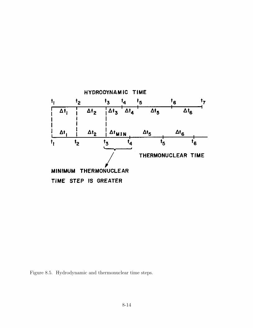
Figure 8.5. Hydrodynamic and thermonuclear time steps.

8-14

3.02 MeV proton, 0.82 MeV He3, 14.7 MeV proton, and 3.6 MeV alpha), the subroutine

TRANSP contains the logic of transporting a particular reaction product from all previous

time cycles and the newborn reaction products on the current cycle. TNBURN passes the

vectors in the data structure which correspond to the number (N), position (R), direction (µ),

and velocity (V ) of this reaction product from the past remembered time cycles. TRANSP

does not distinguish the type of charged particle it is transporting; from this point on all

of the transport calculation is generally applicable for any fast ion with properties given by

TNMASS, ZTN, and CAB. The call to ABCSLO computes the A and B coefficients in the ion

range-energy relation (Eq. 8.5) for this type of reaction product. The outer loop is indexed

over the zone numbers (IZ). This is not strictly true, for this index is over the starting points

of the reaction products (remember that the products from several zones may be grouped

together). The next inner loop indexes over the initial directions or angles of the rays

along which particles stream (IA). The innermost loop indexes over all of the remembered

particle bunches from previous time cycles (IT). The oldest particles are transported first

(IT=1) and the function IZIAIT is called to get the index into the vectors of N, R, U, and

V that corresponds to these particles. The subroutine SLOW is called to transport and slow

down these particles. The new values of N, R, U, and V are returned by SLOW into the

variables NDUM, RDUM, UDUM, and VDUM. These are the oldest particles and there is

no more room left in the data structure to save them for another cycle. If they have not

been thermalized after this last transport calculation then they must be forced to slow down

or escape the plasma or they must be forgotten. Either of these choices is available but

the first one is the best. To force them to thermalize or escape, the thermonuclear time

step, DTTN, is set to a very high value and SLOW is called again. After this the time

step is restored to its correct value. The inner loop indices (IT) over all of the remaining

“remembered” bunches of particles that originally started in direction µIA from starting

position RIZ. The total number of previous bunches that are remembered is a function of

the direction in which they start out (NT(IA)). Those bunches of particles that start in an

8-15

inward direction, µ ≤ 0, are remembered for more cycles than those that start in an outward

direction. Typically the inward directed particles are remembered for twice as many cycles;

however, this number can be inputted by the user. The index of each of these bunches of

particles (I) is computed by IZIAIT, and SLOW is called to transport them. SLOW returns

the results through its argument list to the next lower index (I - 1). In this way the bunches

of particles age. A bunch of particles starts out newborn at index IT=NT(IA) and works its

way down to IT=1 as it grows older. Presumably they will thermalize before reaching IT=1

and will be removed from the calculation. The last call to SLOW by TRANSP transports

the new reaction products that have been created on the current time step.

The function IZIAIT is necessary because the data structure elements are not simple

three-dimensional FORTRAN arrays R(IZ,IA,IT) because the maximum value of IT depends

on IA. Consequently the formula given in Fig. 8.6 is used to compute the index.

The subroutine SLOW is the workhorse of the transport calculation and is also the

most complex. It has the task of transporting one bunch of particles for a time ∆tTN(DTTN)

and then returning the new position, direction, and velocity of these particles. The values

that it receives are NOLD, ROLD, UOLD, and VOLD and the values that it returns are

NNEW, RNEW, UNEW, and VNEW. First SLOW determines whether there really are any

particles to transport in this bunch; they may have thermalized on a previous time cycle.

If there are none then NNEW is also set to zero and SLOW returns to TRANSP. If there

are particles, then the inputted values are saved in local variables because the variables in

the data structure are saved in single precision while all computations done by the burn

calculation are in double precision, therefore the transfer of the data structure values to the

local variables is a change in variable type. Next the zone index (J) that corresponds to

the zone in which this bunch of particles resides is computed by the function JZONE. If J

< JMAX then the particles are still within the plasma boundary but if J=JMAX then the

particles may either be within the outer zone or on its boundary. If RSAVE ≥ R1B (JMAX)

8-16

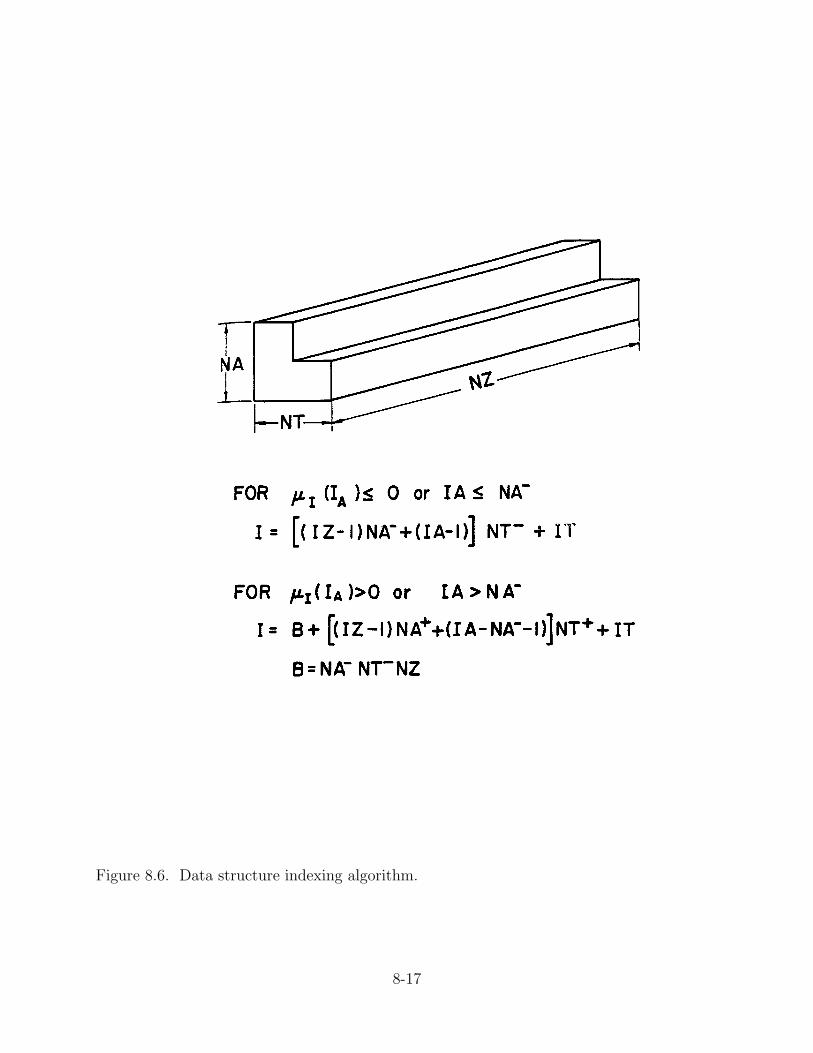
Figure 8.6. Data structure indexing algorithm.

8-17

then the particles have escaped from the plasma and the number of them and their energy is

tallied. If a charged particle spectrum is requested then they are added into the appropriate

energy group in the CPN vector for later processing by CPSPEC. If they have not escaped

from the plasma then FDS is called to compute the distance from their current position

(RSAVE) to the next zone boundary that they will intersect, index JNEXT. This distance is

DS. Then DELTAV is called to compute the velocity lost (DVDS) in traversing this distance

(DS) and also the velocity lost (DVDT) in transporting for a time DTSAVE. Whichever

velocity loss is smallest is set equal to DV. If DVDT is smallest, then the bunch of particles

does not reach the next zone boundary before the time step is over so FDSDT is called to

compute the distance traveled DSDT in the time DTSAVE. The subroutine ENEMA is called

to tally the energy deposited in zone J as a result of this loss in velocity. RMUV is called to

compute the new velocity, position, and direction of this bunch of particles after they have

moved this distance. These new values are stored into NNEW, RNEW, UNEW, and VNEW

and SLOW returns to TRANSP. If DVDS is smallest, then the bunch of particles reaches

the zone boundary before the end of the time step so FDTDS is called to compute the time

required (DTDS) to travel the distance DS. The time remaining in the thermonuclear time

step is then computed:

DTSAVE = DTSAVE−DTDS , (8.22)

and ENEMA is called to tally the energy deposited in zone J by the velocity loss DV. RMUV

is called to get the new position, direction, and velocity of these particles. The particles’

velocity must now be adjusted relative to the fluid velocity of the new zone that they are

entering:

VSAVE = VSAVE− 1

2[U1B(JJ + 1)− UlB(JJ− 1)] ∗USAVE (8.23)

and the new zone index JNEXT (which was saved from the FDS computation) is put into

the working index, J. A test is made to insure that the relative velocity of the particles, after

the above adjustment, is still positive and if it is, control goes back to the beginning of the

subroutine to transport the particles through the next zone or until the time step runs out. If

8-18

in either of the cases, DV=DVDS or DV=DVDT, the relation DV ≥ VSAVE is encountered,

then the bunch of particles have lost all of their energy (i.e. they have thermalized). In this

case, the difference between their initial velocity (VSAVE) and their thermal velocity at the

ion temperature in zone J is used for DV in the computation of the energy deposited by

ENEMA and the particles are added to the thermal background plasma in zone J. NNEW

is set to zero and SLOW returns to TRANSP.

The function JZONE very simply determines the zone index corresponding to the

zone in which a bunch of particles at radius RSAVE are residing. The subroutine FDS

is much more complex, and computes the distance to the next boundary that a bunch of

particles at position R and moving in direction µ will intersect. If µ = 1, then the problem

is trivial. If µ = −1, then the problem is trivial except that a special case must be made for

particles in the center zone for they will go through the origin. If µ �= 1 and �= −1 and is

greater than 0 then they must certainly intersect the outer boundary of the zone in which

they reside

DS = −Rµ+ (R2j − R2 + (Rµ)2)1/2 . (8.24)

If µ ≤ 0 then they may or may not intersect the inner boundary of the zone J. If

1− µ2 < (Rj−1/R)2 (8.25)

then they intersect the inner boundary and

DS = −Rµ+ (R2j−1 −R2 + (Rµ)2)1/2 , (8.26)

otherwise they miss the inner boundary and intersect the outer boundary and Eq. (8.24)

applies. In slab geometry the calculations are trivial.

The next subroutine called by SLOW is DELTAV and it computes the velocity loss in

traveling the distance to the next zone boundary (DS) and the velocity loss in traveling for

the time step (DTSAVE). These values are computed according to Eqs. (8.12) and (8.18).

The subroutine also has two additional entry points, FDSDT and FDTDS, where the distance

8-19

travelled in time DTSAVE and time taken to travel the distance DS are computed according

to Eq. (8.20) and Eq. (8.19).

The subroutine RMUV is called to compute the new position, direction and velocity

of a bunch of particles after they have been transported. It first computes the new velocity

and then skips to the end if slab or planar geometry is used. If spherical geometry is used

then it tests to see if µ = 1. If it is, then the calculation is trivial. If µ = −1, then a special

case must be made for the center zone, otherwise the calculation is also trivial. If µ �= 1 and

µ �= −1, then the calculation is slightly less trivial and the law of cosines must be used to

compute the new position and direction:

R1 = (R2o +∆s2 − 2Ro ∆s µo)

1/2 (8.27)

µ1 =∆s2 + R2

1 − R2o

2R1∆s. (8.28)

If the transport was the result of moving a distance ∆s (DS) then the new position of the

bunch of particles must be on a zone boundary. In this case (I=0) the new position is not

computed but is set equal to RIB(JNEXT) to avoid any roundoff error in the computation.

The last routine called by SLOW is ENEMA. This subroutine computes the energy

lost by the bunch of particles and partitions it between the electrons and ions, according

to Eqs. (8.13) to (815). It then tallies these energies deposited in zone J into the variables

DEPETN(J) and DEPNTN(J). It then computes the change in fluid velocity as a result of

the momentum deposition (DELTAV) according to Eq. (8.16) and tallies this into the vector

DUTN(J).

8.3. Nuclear Energy Deposition Model

The release of energy in a DT fusion reaction is split between the neutron and alpha

particle reaction products:

21D+ 3

1T → 10n (14.1MeV) + 4

2He(3.5MeV) . (8.29)

8-20

The 3.5 MeV charged alpha particle has a short range in highly compressed DT, with a range

of about 0.3 g/cm2. The neutral 14 MeV neutron has a much longer range of ≈ 4.15 g/cm2.

The total cross section for 14 MeV neutrons on D, T, and 42He is dominated by elastic

scattering, and has a value of σtotal � 1barn for each of D, T, and He.

Thus, the range of 14 MeV neutrons is roughly comparable to the ρR-value of a highly

compressed high gain ICF target. Detailed neutron transport analyses of neutron energy loss

through collisions with DT nuclei show that roughly 3-4 MeV per fusion neutron is deposited

in the target by collisions. This is comparable to the energy deposition by the charged alpha

particles. Thus, treatment of neutron collisions in the target is important to the high yield

target energetics even if it is not critical to the ignition process itself.

In elastic collisions between neutrons and nuclei the average energy loss is given by

∆E =(1− α

2

)Ei ,

where

α ≡(

A − 1

A − 2

)2

assuming the elastic scattering is isotropic. Thus for D, T, and He:

∆ED

= 6.27MeV

∆ET

= 5.29MeV

∆EHe

= 6.27MeV .

At present, we neglect He and average the D and T contributions to get

∆EDT

= 5.78MeV .

If Yneutron is the neutron yield on a particular time step, then the neutron energy deposited

is

Eneutron = Yneutron (1− e−τ)∆EDT

, (8.30)

8-21

where τ is a measure of the likelihood that a neutron will escape without a collision. We

can estimate τ as:

τ =ρR

ρRo,

where ρR is the ρR-value of the DT fuel, and ρRo is related to the 14.1 MeV neutron mean

free path in DT.

A previous escape probability analysis [42] shows that for ρR ≥ 3 g/cm2, at least two

collisions should be treated, while for ρR = 2 g/cm2 one collision is a good approximation.

They also compute the average energy deposited per fusion neutron and find it to be nearly

linear over the ρR range of interest. Thus, we can approximate

(1− e−τ ) ≈ τ

to get

EDepneutron =

Yneutron∆EDT

ρRoρR .

Using their results, one obtains

EDepneutron (MeV) = Yneutron (0.64) ρR (g/cm2) .

We then distribute the deposited energy in the fuel zones by using a ρ∆R scaling. Then,

the neutron deposition rate is given by:

(Sn)nj−1/2 = (1.602× 10−13 J/g/s) Yneutron (s

−1) · 0.64 (MeV cm2g) · (ρ∆r)j−1/2

∆mj−1/2

, (8.31)

where ∆mj−1/2 is the zone mass. This deposition rate is calculated at the end of subroutine

TNBURN.

8-22

9. Rapid X-ray Deposition in Cold Media

A rapid x-ray deposition model is used to determine the heating of an ICF target

chamber buffer gas and first surface material due to the x-rays emitted from a high gain

target. An exponential x-ray attenuation model [43] is used for this purpose. A table of

attenuation coefficients [44] for elements with atomic numbers ranging from 1 to 100 and

x-ray energies ranging from 0.01 to 1000 keV is provided with the code. These cross sections

are valid for cold (unionized) materials. As the code is presently written, gases composed of

only one element can be used to attenuate the x-rays.

The initial x-rays that are photo-absorbed by the gas reduce the number of bound

electrons available to interact with subsequent x-rays, so the attenuation coefficient decreases

as x-rays are deposited. A method of modifying the photoelectric attenuation coefficient of

the gas to account for increasing ionization has been developed for this purpose [43]. By

counting the number of electrons ejected from each electron shell as the x-rays are deposited,

the contribution to the photoelectric attenuation coefficient from each shell can be reduced

by an amount proportional to the number of missing electrons. Additionally, the number of

electrons lost due to the initial gas temperature is included even though this effect is usually

very small. Although simple, this model does at least give the correct attenuation for the

limiting cases of a completely neutral and completely ionized atom. The accuracy of this

model at intermediate levels of ionization has not been determined. In this version of the

code, the model for computing the reduction in photoelectric absorption can only be used

with neon, argon, xenon, lithium, carbon, beryllium, oxygen, silicon, helium or nitrogen gas.

To extend the model to other gases, the number of electrons in each shell of the neutral atom

and the energies of the K, L, and M shells must be added to the EDATA subroutine.

The x-rays emitted by the target can be assumed to be Planckian or an inputted

multigroup spectrum. In either case, the code divides the x-ray spectrum into energy groups.

The x-rays in each group are then attenuated frequency by frequency.

9-1

This code is written to treat the incident x-rays as either an instantaneous or time-

dependent source. In both cases, the x-rays are treated as having an infinite propagation

speed.

9-2

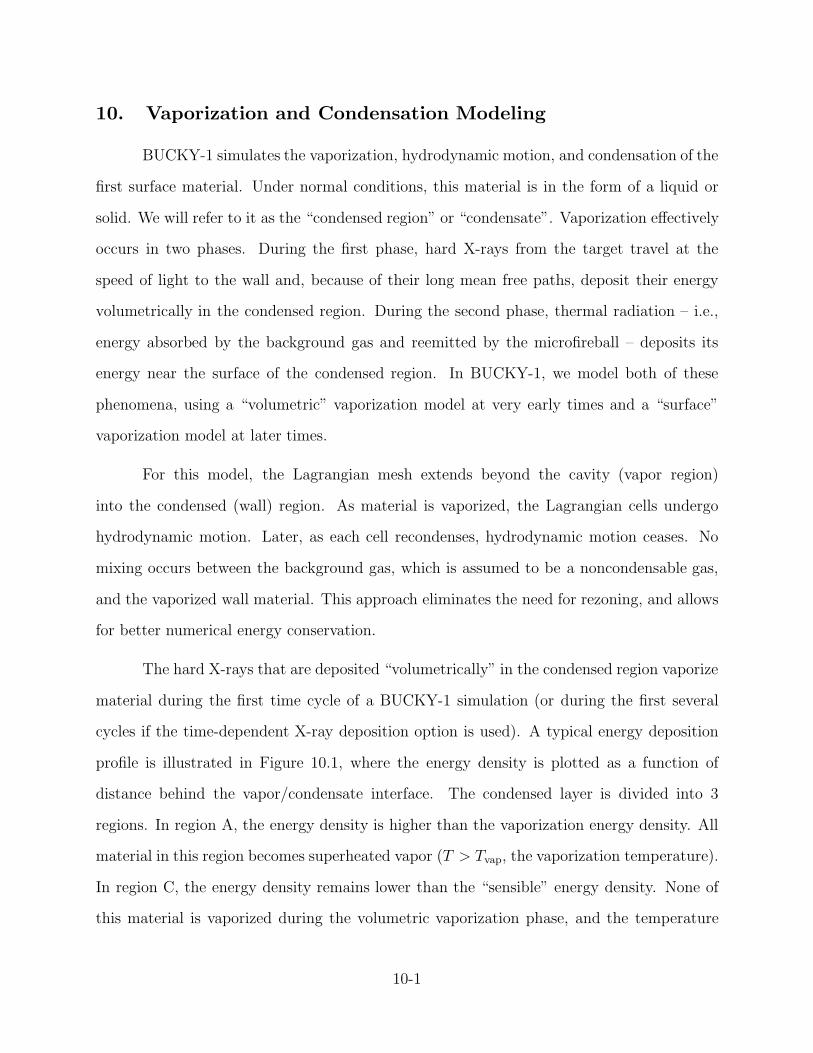
10. Vaporization and Condensation Modeling

BUCKY-1 simulates the vaporization, hydrodynamic motion, and condensation of the

first surface material. Under normal conditions, this material is in the form of a liquid or

solid. We will refer to it as the “condensed region” or “condensate”. Vaporization effectively

occurs in two phases. During the first phase, hard X-rays from the target travel at the

speed of light to the wall and, because of their long mean free paths, deposit their energy

volumetrically in the condensed region. During the second phase, thermal radiation – i.e.,

energy absorbed by the background gas and reemitted by the microfireball – deposits its

energy near the surface of the condensed region. In BUCKY-1, we model both of these

phenomena, using a “volumetric” vaporization model at very early times and a “surface”

vaporization model at later times.

For this model, the Lagrangian mesh extends beyond the cavity (vapor region)

into the condensed (wall) region. As material is vaporized, the Lagrangian cells undergo

hydrodynamic motion. Later, as each cell recondenses, hydrodynamic motion ceases. No

mixing occurs between the background gas, which is assumed to be a noncondensable gas,

and the vaporized wall material. This approach eliminates the need for rezoning, and allows

for better numerical energy conservation.

The hard X-rays that are deposited “volumetrically” in the condensed region vaporize

material during the first time cycle of a BUCKY-1 simulation (or during the first several

cycles if the time-dependent X-ray deposition option is used). A typical energy deposition

profile is illustrated in Figure 10.1, where the energy density is plotted as a function of

distance behind the vapor/condensate interface. The condensed layer is divided into 3

regions. In region A, the energy density is higher than the vaporization energy density. All

material in this region becomes superheated vapor (T > Tvap, the vaporization temperature).

In region C, the energy density remains lower than the “sensible” energy density. None of

this material is vaporized during the volumetric vaporization phase, and the temperature

10-1

Figure 10.1. Condensed layer vaporization regions.

10-2

Distance Behind Interface (µm)

0 10 20 30

Sp

ecif

ic E

ner

gy

Dep

osi

tio

n (

J/g

)

Sensible Heat

Vaporization Energy

A B C

remains below Tvap. In region B, the energy density lies between the vaporization and

sensible energies, and the temperature throughout the region is equal to Tvap. To determine

the amount of material from region B that gets vaporized, we redistribute the energy so

that: (1) none of the condensed region has an energy density between the vaporization and

sensible values, and (2) energy is conserved.

After material is vaporized, the pressure in the vapor region near the interface becomes

very high because of the high density. This causes material to be rapidly accelerated away

from the interface, and provides a “recoil” impulse to the wall. BUCKY-1 monitors the

pressure at the interface and computes the impulse on the wall directly.

The amount of material vaporized during the volumetric phase can be adjusted by

setting ISW(25) = 2. This allows only material with energy densities greater than the

vaporization energy density to be vaporized. That is, none of the material in region B is

vaporized. This model is less reliable, however, because energy is not conserved.

The primary distinction between the vapor and condensed phases is that vapor

cells undergo hydrodynamic motion. The condensed region cells remain stationary due to

chemical bonding. In addition, the conservation of momentum and energy equations are

solved over all vapor cells. In the condensed region, a one-dimensional conduction equation

is solved to determine the energy transport within the region.

After the volumetric deposition phase, radiant energy transported to the condensed

region will be effectively deposited at the surface of the interface because of the shorter

photon mean free paths. The vaporization and condensation rates are calculated using the

kinetic theory model described by Labuntsov and Kryukov [45]. The mass vaporization rate

is given by:

(dm/dt)v =2

3Psat Awall

(µ

RTv

)1/2

(10.1)

where Awall is the surface area of the wall, Tv is the vapor temperature, R is the gas constant,

µ is the mean atomic weight of the condensable material, and Psat is the saturation vapor

10-3

pressure:

Psat = exp

{∆Hv

kTvap,o

(1− Tvap,o

Tc

)}bar . (10.2)

∆Hv is the specific heat of vaporization, k is Boltzmann’s constant, Tc is the condensate

temperature at the interface, and Tvap,o is the vaporization temperature at 1 bar. The mass

condensation rate is:

(dm/dt)c =2

3fsfNCPvapAwall

(µ

RTv

)1/2

(10.3)

where fs is the sticking coefficient, FNC is a correction factor for noncondensable gas effect,

and Pvap is the vapor pressure given by the ideal gas law:

Pvap = ρvRTv

µ(10.4)

where ρv is the vapor density.

Lagrangian cells undergo hydrodynamic motion only after an entire cell is vaporized.

Figure 10.2 illustrates the evolution of mesh points during a typical simulation. Vapor cells

are to the left of the dashed line and the condensed region is to the right of it. The “+”s

represent the cell boundaries and the vertical dashed line represents the vapor/condensate

interface. A short time after the target explodes (t1 = to + ε), the target’s hard X-rays are

deposited in the condensed region, vaporizing a number of cells. Since the vaporized mass is

not in general an integral number of cells, the interface is located between cell boundaries.

At later times (t2), the vapor expands away from the wall while thermal radiation from the

fireball vaporizes additional cells. No mass is ever exchanged between Lagrangian cells as

mixing effects are neglected.

As the radiative flux from within the cavity subsides and the temperature at

the surface of the condensed region drops, the condensation rate begins to exceed the

vaporization rate. Again, the interface is tracked as condensation occurs. In Figure 10.2

shows vapor moving toward the interface as material recondenses back onto the surface

(t3 and t4). If any portion of a Lagrangian cell has condensed, it no longer undergoes

hydrodynamic motion.

10-4

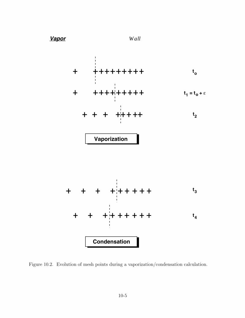
Figure 10.2. Evolution of mesh points during a vaporization/condensation calculation.

10-5

Vaporization

t = t + ε1 o

t2

to

t3

t4

Condensation

Vapor Wall

To calculate energy transport withing the condensed region, BUCKY-1 solves the

one-dimensional conduction equation:

CPdT

dt=

κ

ρ

d2T

dx2+ S (10.5)

where CP is the specific heat at constant pressure, κ is the thermal conductivity, ρ is the

density in the condensed region, T is the temperature, and x the spatial coordinate. S is

a source term which accounts for the energy deposition from the radiative heat flux and

debris ions. In practice, only the first cell has a non-zero source term because the heat

flux is assumed to be deposited at the surface. The conduction equation is also subject to

the following boundary conditions. The temperature at the back of the condensed layer is

constant (Dirichlet condition) as heat flows through the back of the condensed region. At

the vapor/condensate interface, the conductive heat flux is assumed to be zero (Neumann

condition).

10-6

11. Energy Conservation Check

Energy conservation is monitored for the plasma and, if applicable, condensate system.

At the end of each time step, a check is made to ensure that the difference equations

are conserving energy. After integrating the energy equations over time and space, the

conservation equations for the plasma, condensate, and radiation can be written as:

Ions ei + TP = eoi + T op +Hi −Xe−i − Fi −Gi−e −Gi−R −Wi (11.1)

Electrons ee = eoe +He − ER−e +Xe−i − Fe +Gi−e −We (11.2)

Radiation eR = eoR + ER−e − FR +Gi−R +WR (11.3)

Total Target eTOT + TP = eoTOT + T oP +HTOT −WTOT − FTOT (11.4)

Condensate ec = eoc + FR + Fe + Fi − JPT −QB +HC (11.5)

The superscript “o” signifies the initial values. The physical definitions of each term are:

ex total internal energy of the ions, electrons, radiation, or condensate

Tp total kinetic energy of the plasma

Hx total source of energy to the ions, electrons, radiation, or condensate

ER−e total radiation energy exchanged between the plasma and radiation field

Fx total energy conducted across the boundaries from the

ions, electrons, or radiation

Gi−x work exchanged between the ions and radiation (x = R) or electrons (x = e)

Wx work done on the boundary by ions, electrons, or radiation

QB total energy conducted through the back of the condensed region

JPT total energy exchanged during phase transformation between the

plasma and condensate

Equation (11.4) states that the total internal plus fluid kinetic energy at a given time (tn+1)

must equal the initial internal and kinetic energy plus all source energy up to this time,

minus all heat conducted across the outer boundary, all work done on the outer boundary,

and all energy lost to radiation up to this time.

11-1

The term, Ge, appears because the electrons and ions have their own temperature

and pressure but are constrained to move together at the same fluid velocity. This is the

total work done by the ions on the electrons to maintain this constraint. Each of these terms

at time step “n” is given in finite difference form as follows:

en+1x =JMAX∑j=1

(Ex)N+1J−1/2∆moJ−1/2

, x = e, i, R (11.6)

T n+1 =1

2

JMAX∑j=1

∆moj(Un+1/2j )2

Hn+1x = Hn

x +∆tn+1/2JMAX∑j=1

(Sx)n+1/2j−1/2 ∆moj−1/2

(11.7)

Xn+1e−i = Xn

e−i +∆tn+1/2JMAX∑j=1

(Re−i)n+1/2j−1/2 ∆moj−1/2

(11.8)

En+1R−e = En

R−e +∆tn+1/2JMAX∑j=1

(QR−e)n+1/2j−1/2 ∆moj−1/2

(11.9)

Gn+1i−R = Gn

i−R +∆tn+1/2JMAX∑j=1

Un+1/2j (rδ−1)n+1/2j (Pn+1/2

Rj+1/2− P n+1/2

Rj−1/2)

+ ∆tn+1/2 un+1/2JMAX (rδ−1)n+1/2JMAX [P n+1/2

RJMAX+1/2− Pn+1/2

RJMAX−1/2]/2

+ inner boundary term (j = 1) (11.10)

F n+1P = F n

P +∆tn+1/2

rδ−1(

∆rκP

)n+1/2

JMAX

(T n+1/2PJMAX+1/2

− T n+1/2PJMAX−1/2

) P = e or i

+ inner boundary term (j = 1) (11.11)

F n+1R = F n

R +∆tn+1/2

rδ−1(

∆rκR

)+ ∆ER

FR

n+1/2

JMAX

(En+1/2RJMAX+1/2

− En+1/2RJMAX−1/2

)

+ inner boundary term (j = 1) (11.12)

W n+1x = W n

x +∆tn+1/2{un+1/2JMAX (rδ−1)

n+1/2JMAX P

n+1/2JMAX

}(11.13)

11-2

Jn+1PT = Jn

PT +∆tn+1/2[(

dm

dt

)n

P

−(dm

dt

)n

c

]· [en+1P − en+1c ] (11.14)

Qn+1B = Qn

B +∆tn+1/2

rδ−1

∆rκP

n+1/2

JMAXC

(T n+1/2eJMAXC+1/2

− T n+1/2eJMAXC−1/2

) (11.15)

BUCKY-1 calculations usually conserve energy to within better than 2–5%.

11-3

12. Time Step Control

After each time step, the next time step is determined from a set of stability and

accuracy constraints. The new time step is determined by

∆tn+3/2 = Max

[∆tmin,Min

(∆tmax,

K1

Rn+11

,K2∆tn+1/2

Rn+12

, · · · K5∆tn+1/2

Rn+15

)](12.1)

where

Rn+11 = Max

[(V n+1

j−1/2 Pn+1j−1/2)

1/2/∆rn+1/2j−1/2

](12.2)

Rn+12 = Max

[(V n+1

j−1/2 − V nj−1/2)/V

n+1/2j−1/2

](12.3)

Rn+13 = Max

[(En+1

Rj−1/2− En

Rj−1/2)/E

n+1/2Rj−1/2

](12.4)

Rn+14 = Max

[(T n+1

ij−1/2− T n

ij−1/2)/T n+1/2

ij−1/2

](12.5)

Rn+15 = Max

[(T n+1

ej−1/2− T n

ej−1/2)/T n+1/2

ej−1/2

](12.6)

The maximum values of R1 through R5 are found by sweeping over the zones. The input

parameters K1 through K5 determine the severity of each constraint. The default value for

K1, K2, K4, and K5 is 0.05. The default value of K3 is set to 0.10.

12-1

13. Code Structure

BUCKY-1 is written in FORTRAN 77. The code is written to run primarily on UNIX

workstations. At the University of Wisconsin it has been utilized on HP, SUN, and IBM

RS6000 workstations. It (in previous forms) has also been run on CRAY X-MP and Y-MP

supercomputers. A pre-processor operates on the source code to make FORTRAN (.f) files.

During this time, machine-dependent parts of the code (e.g., time and date calls, vector

merge operations, etc.) are inserted appropriately into the “.f” files. This allows for the

code to be used conveniently on multiple platforms.

13.1. Subroutines

A flow diagram of the BUCKY-1 subroutines is shown in Figures 13.1 through 13.4.

Below, each of the subroutines is listed along with brief description of its use. The first 2

listed are the main driver program and a block data subroutine for data initialization. The

rest of the subroutines are listed in alphabetical order.

13-1

Figure 13.1. Flow diagram for BUCKY-1.

13-2

INITIA

CLEARC

INIT1

INIT2

RDEOSx

ZONERx

INIT3

INIT4

INITX

INIT7

INIT9

INITC1

INNLTE

DFALTS

READA2

INPUT3

HYDROD

NUMDEN

QUE NEGTCK

TEMPBC

ENERGY

ABCPL1 ABCPL2

PLSCF2

PCOND2

OMEGAC

PCOND1

PLSCF1

IONDEP

LASDEP

RADTR1

RADTR2

RADTR3

RTLINE

TDXRAY

TNBURN

WALLVP

EOS1

EOS2

EOS1

PLKINT

QUE

COND1D

TRIDAG

TABLE2

POINT

TABLE0

POINT0

OPCUW1

TABLE4

EOSUW1

BILIN2

BLCOEF

BILIN3

OPCUW2

EOSUW2

EOSSM

EOS ECHECK TIMING SHIFTT QUITB

OUT

WBIN

BUCKY-1 (MAIN)

OUT

OUT3

WBIN

Figure 13.2. Flow diagram for BUCKY-1 initialization routines.

13-3

INNLTE

DFALTS

READA2

INPUT3

CROS

CROSI

EOS

SPECP

XMU

GASDEP

DYNDEP

EDATA

EOS1

INIT4

EOS

TEMPBC

QUE

RTANGL

PLKINT

DTABLE

INITXINIT2

RDEOSn(n=0,1,2)

ZONERx(x=2,3,4,C,P)

Initialization Routines

Figure 13.3. Flow diagram for BUCKY-1 energy source routines.

13-4

LASDEP RADTR3

EMISSN

OPACMG

PLKINT

SHORTC

Flow Diagram for Energy Sources

TDXRAY

EDATA

DYNDEP

IONDEP

ISOURC

FINDJ

TDEPZ1

TRIDAG

EDEPOS

DEDX

GFUN

XLNFUN

AIPFUN

RADTR1

ABCRD1

EDFACT

RADDEN

EMISSN

PLKINT

RADTR2

EMISSN

PLKINT

ABCRD2

RADCOF

RCOND

RTLINE

seeFig. 13.4

TNBURN

DOTN

TNREAC

LOCAL

DIRECT

CPSPEC

TRANSP

TNSLOW

IZIAIT

SLOW

JZONE

FDS

DELTAV

ENEMA

RMUV

PLKINT

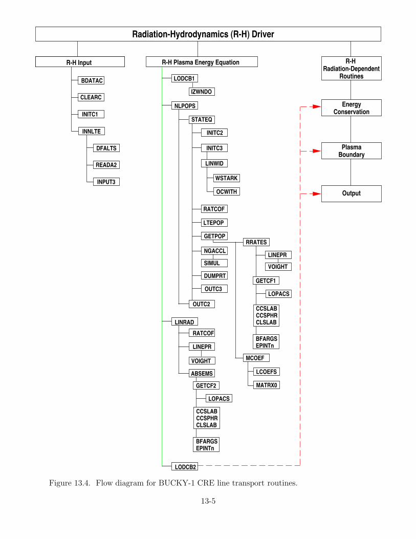
Figure 13.4. Flow diagram for BUCKY-1 CRE line transport routines.

13-5

LODCB1

IZWNDO

NLPOPS

STATEQ

INITC2

INITC3

LINWID

WSTARK

OCWITH

RATCOF

GETPOP

DUMPRT

OUTC3

OUTC2

LINRAD

Radiation-Hydrodynamics (R-H) Driver

R-H Radiation-Dependent

Routines

EnergyConservation

PlasmaBoundary

Output

R-H Plasma Energy EquationR-H Input

INPUT3

READA2

DFALTS

INNLTE

INITC1

CLEARC

BDATAC

LTEPOP

NGACCL

SIMUL

RRATES

LINEPR

VOIGHT

LOPACS

GETCF1

CCSLABCCSPHRCLSLAB

BFARGSEPINTn

MCOEF

LCOEFS

MATRX0

RATCOF

LINEPR

ABSEMS

VOIGHT

LOPACS

GETCF2

CCSLABCCSPHRCLSLAB

BFARGSEPINTn

LODCB2

Table 13.1. BUCKY-1 Subroutines

SubroutineName Called By Calls To Description

MAIN INITIA, HYDROD, ENERGY, main driver programWALLVP, ECHECK, EOS, OUT,QUITB, SHIFTT, TIMING

BDATAC block data routine for initializing constantsABCPL1 ENERGY PLSCF1 computes A, B, C, D, E, and F coefficients used to

solve the plasma temperature equation when usingthe 1-T option (Tion = Te)

ABCPL2 ENERGY PLSCF1 same as for ABCPL1, but for 2-T option (Tion 6= Te)

ABCRD1 RADTR1 — computes A, B, C, D, E, and F coefficients used tosolve the radiation transport equation for a specifiedfrequency group when using the variable Eddingtonoption

ABCRD2 RADTR2 RADCOF same as for ABCRD1, but for radiation diffusionoption

AIPFUN XLNFUN — computes the average ionization potential of thebackground gas for use in the Bethe stopping powerequation

BILIN2 EOSSM, EOSUW2, — performs bilinear interpolation on EOS tablesOPCUW2

BILIN3 OPCUW2 — performs bilinear interpolation on multigroup opacitytables

BLCOEF EOSSM, EOSUW2, LOCATE sets up coefficients for bilinear interpolationOPCUW2

COND1D WALLVP TRIDAG solves the 1-dimensional conduction equation for thecondensed region

13-6

Table 13.1. (Continued)

SubroutineName Called By Calls To Description

CPSPEC TNBURN — tallies charged particle fusion reaction products escaping outermostLagrangian zone

CROS INITX — reads the photoionization cross sections for the x-ray attenuationmodel

CROSI INITX — searches through the x-ray cross section table and computes the crosssection of the gas

DEDX EDEPOS GFUN, XLNFUN computes the ion deposition stopping power

DELTAV SLOW — computes change in velocity for a bunch of fast charged particlesDEPLET — computes new number densities for the different ionic species that

can change due to fusion burningDIRECT TNBURN — computes the number of particles starting in each angular direction

after creation from fusion burnDOTN TNBURN — determines whether fusion burn calculation is to be done on each

hydrodynamic time stepDTABLE INIT4 — sets up tables for interpolation using Newton divided difference

schemeDYNDEP GASDEP, TDXRAY — computes the x-ray deposition and the new absorption cross section

of each zoneECHECK MAIN — computes the integrals used in the energy conservation checkEDATA GASDEP, TDXRAY — provides the electron shell structure of the cold gas for the x-ray

deposition calculationEDEPOS IONDEP DEDX computes the ion deposition stopping powerEDFACT RADTR1 — computes Eddington factors when using variable Eddington radiation

transport model

13-7

Table 13.1. (Continued)

SubroutineName Called By Calls To Description

EMISSN RADTR(1,2,3) computes the frequency-dependent radiation emissionENEMA SLOW — computes energy lost to background electrons and ions by fast

charged particles from fusion reactionsENERGY MAIN ABCPL1, ABCPL2, solves electron and ion energy equations

NEGTCK, TEMPBCEOS MAIN, INIT4, EOSSM, EOSUW1, computes the equation of state quantities

INITX EOSUW2, OPCUW1,OPCUW2, PRESBC

EOS1 EOS2, GASDEP, POINT1, TABLE1 computes the equation of state quantitiesWALLVP

EOS2 WALLVP EOS1 computes the equation of state quantities

EOSSM EOS BILIN2, BLCOEF looks up equation of state data for SESAME tablesEOSUW1 EOS POINT, TABLE2, looks up equation of state data from EOSOPA and/or

TABLE4 IONMIX tablesEOSUW2 EOS BILIN2, BLCOEF looks up equation of state data from EOSOPA and/or IONMIX

tablesFDS SLOW — computes the distance from the position of a bunch of fusion reaction

products to the next zone boundaryFINDJ IONDEP — finds the index of the zone an ion bunch is located withinFNEWT TEMPBC — interpolation function using Newton divided difference scheme

GASDEP INITX DYNDEP, EDATA, computes the temperature of the gas after x-rayEOS1 deposition

13-8

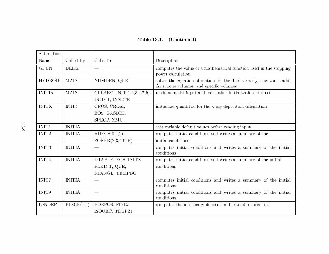
Table 13.1. (Continued)

SubroutineName Called By Calls To Description

GFUN DEDX — computes the value of a mathematical function used in the stoppingpower calculation

HYDROD MAIN NUMDEN, QUE solves the equation of motion for the fluid velocity, new zone radii,∆r’s, zone volumes, and specific volumes

INITIA MAIN CLEARC, INIT(1,2,3,4,7,9), reads namelist input and calls other initialization routinesINITC1, INNLTE

INITX INIT4 CROS, CROSI, initializes quantities for the x-ray deposition calculationEOS, GASDEP,SPECP, XMU

INIT1 INITIA — sets variable default values before reading inputINIT2 INITIA RDEOS(0,1,2), computes initial conditions and writes a summary of the

ZONER(2,3,4,C,P) initial conditions

INIT3 INITIA — computes initial conditions and writes a summary of the initialconditions

INIT4 INITIA DTABLE, EOS, INITX, computes initial conditions and writes a summary of the initialPLKINT, QUE, conditionsRTANGL, TEMPBC

INIT7 INITIA — computes initial conditions and writes a summary of the initialconditions

INIT9 INITIA — computes initial conditions and writes a summary of the initialconditions

IONDEP PLSCF(1,2) EDEPOS, FINDJ computes the ion energy deposition due to all debris ionsISOURC, TDEPZ1

13-9

Table 13.1. (Continued)

SubroutineName Called By Calls To Description

ISOURC IONDEP — computes the number of debris ions emitted from the source duringa given time interval

IZIAIT TRANSP — determines index in data structure that holds information on fusionreaction products

JZONE SLOW — determines zone index that a bunch of fusion reaction products areresiding in

LASDEP PLSCF(1,2) — computes laser energy deposition at each zone

LLAM OMEGAC, PCOND1, — computes log Λ for the thermal conductivityPCOND2

LOCAL TNBURN — computes the energy deposited in the background electrons and ionsfrom fusion reaction products if “local dump” approximation is used

LOCATE BLCOEF — locate indices for EOS bilinear interpolationsNEGTCK ENERGY — checks for negative temperatures after solution of plasma energy

equationNUMDEN HYDROD — computes number densities from the specific volume

OMEGAC PLSCF2 LLAM computes the ion-electron energy coupling coefficientsOPACMG RADTR3 PLKINT calculates opacity grid for short characteristics radiation transport

optionOPCUW1 EOS POINT, POINT0, looks up multigroup opacities from EOSOPA and/or

TABLE2, TABLE0 IONMIX tables

OPCUW2 EOS BILIN2, BILIN3, looks up multigroup opacities from EOSOPA and/orBLCOEF IONMIX tables

13-10

Table 13.1. (Continued)

SubroutineName Called By Calls To Description

OUT MAIN, QUITB OUT1, OUT3, WBIN writes output at the end of specified simulation times ornumber of cycles

OUT1,3 OUT — writes output at the end of specified simulation times ornumber of cycles

PCOND1 PLSCF1 LLAM computes plasma thermal conductivities for 1-T optionPCOND2 PLSCF2 LLAM same as PCOND1, but for 2-T option

PLKINT EMISSN, INIT4, — returns the integral of the Planck functionTEMPBC, OPACMG,WALLVP

PLSCF1 ABCPL1 IONDEP, LASDEP, computes α, γ, a, and β coefficients used to solve thePCOND1, RADTR(1,2,3), plasma temperature equation when using the 1-T optionRTLINE, TDXRAY,TNBURN

PLSCF2 ABCPL2 IONDEP, LASDEP, same as PLSCF1, but for the 2-T option.PCOND2, OMEGAC,RADTR(1,2,3), RTLINE,TDXRAY, TNBURN

POINT EOSUW1, OPCUW1 — finds pointers in the equation of state tablesPOINT1 EOS1 — finds pointers in the equation of state tables

POINT0 OPCUW1 — finds pointers in the multigroup opacity tablesQUE HYDROD, INIT4, — computes the artificial viscosity

WALLVP

13-11

Table 13.1. (Continued)

SubroutineName Called By Calls To Description

QUITB MAIN OUT, WBIN wraps up the calculation at the end and performs final printoutsPRESBC EOS sets pressure boundary conditions

RADCOF ABCRD2 RCOND computes α, γ, ω, a, and β coefficients used to solve the radiation energyequation for a specified frequency group when using the multifrequencyradiation diffusion

RADDEN RADTR1 — computes radiation energy densities in each zone when using variableEddington radiation transport model

RADTR1 PLSCF(1,2,3) ABCRD1, EDFACT, computes radiation energy densities when using variable Eddingtontransport model

EMISSN, RADDENRADTR2 PLSCF(1,2,3) ABCRD2, EMISSN computes radiation energy densities when using radiation diffusion model

RADTR3 PLSCF(1,2,3) EMISSN, OPACMG, computes radiation energy densities when using short characteristicsSHORTC transport model

RCOND RADCOF — computes the radiation conductivity for a specified frequency group whenusing the multifrequency radiation diffusion option

RDEOS0 INIT2 — read in the equation of state and opacity data (EOSOPA format)RDEOS1 INIT2 — read in equation of state and opacity data (IONMIX format)RDEOS2 INIT2 — read in equation of state data (SESAME format)

RMUV SLOW — computes new position, direction of motion, and velocity of fast fusionreaction products

RTANGL INIT4 — sets up angles and integration weights for multiangle radiation transportoption

13-12

Table 13.1. (Continued)

SubroutineName Called By Calls To Description

RTLINE PLSCF(1,2) LINRAD, LODCB1, controls CRE line radiation algorithmsLODCB2, NLPOPS

SHIFTT MAIN — shifts values of variables at (n+ 1) to variables at (n) at the endof a time step.

SHORTC RADTR3 — solves radiation transport equation using method of shortcharacteristics

SIGMAV TNREAC — computes fusion reaction rates

SLOW TRANSP DELTAV, ENEMA, computes the slowing down of fast fusion reaction productsFDS, JZONE, RMUV

SPECP INITX — computes the x-ray spectrumTABLE1 EOS1 — interpolates in the equation of state tables using the pointers

TABLE2 EOSUW1, OPCUW1 — interpolates in the equation of state tablesTABLE4 EOSUW1 — interpolates in the equation of state tablesTABLE0 OPCUW1 — interpolates in the opacity tables

TDEPZ1 IONDEP TRIDAG computes the time-dependent debris ion ionization populationsTDXRAY PLSCF(1,2) DYNDEP, EDATA computes the time-dependent x-ray deposition

TEMPBC ENERGY, INIT4 FNEWT, PLKINT computes the plasma temperature and radiation specific energyboundary conditions

TIMING MAIN — computes a new time step and determines whether the calculationis over

13-13

Table 13.1. (Continued)

SubroutineName Called By Calls To Description

TNBURN PLSCF(1,2) CPSPEC, DIRECT, main routine for fusion burn calculationDOTN, LOCAL,TNREAC, TRANSP

TNREAC TNBURN SIGMAV computes the number of DT, DD, and DHe3 reactions ineach zone

TNSLOW TRANSP — sets up coefficients for the slowing down of fast fusionreaction products

TRANSP TNBURN IZIAIT, SLOW, transport solver for fusion reaction productsTNSLOW

TRIDAG COND1D, TDEPZ1 — tridiagonal matrix solver for the condensed regionconduction equation and the rate equations for the time-dependent charge state calculations

WALLVP MAIN COND1D, EOS1, computes vaporization/condensation of wall materialEOS2, QUE,PLKINT

WBIN OUT, QUITB — writes binary output to unit 8 for post-processingXLNFUN DEDX AIPFUN computes log Λ for the stopping power calculations

XMU INITX — calculates the mass attenuation coefficients for the x-raydeposition calculations

ZONERC, ZONERP INIT2 — zoning setup routineZONER2,3,4

13-14

Table 13.1. (Continued)

SubroutineName Called By Calls To Description

ABSEMS LINRAD GETCF2 Computes CRE line power densities and fluxes.BFARGS CCSLAB, CCSPHR, CLSLAB — Sets up bound-free escape probability parameters.

CLSLAB GETCF1, GETCF2 EPINT1 Computes escape probability coupling coefficientsfor Doppler profiles in planar geometry.

CLSLAB GETCF1, GETCF2 EPINT9, BFARGS Computes escape probability coupling coefficientsfor bound-free transitions in planar geometry.

CCSPHR GETCF1, GETCF2 EPINT2, EPINT3, Computes escape probability coupling coefficients forBFARGS

bound-bound and bound-free transitions in planargeometry.

DFALTS INNLTE — Initialize variables and set default values for CRE calculation.CLEARC Hydro initialization — Initializes some CRE variables to zero.

subroutineDUMPRT MATRX0, STATEQ — Writes CRE radiative transfer parameters to output files.

EPINT1 CLSLAB, CCSPHR — Computes escape probability integral fora Doppler profile.

EPINT2 CLSLAB, CCSPHR — Computes escape probability integral fora Lorentz profile.

EPINT3 CLSLAB, CCSPHR — Compute escape probability integral fora Voigt profile.

EPINT9 CLSLAB, CCSPHR — Compute escape probability integral forbound-free transitions.

GETCF1 RRATES CCSLAB, CCSPHR, Compute zone-to-zone coupling coefficients for allCLSLAB, LOPACS transitions.

13-15

Table 13.1 (Continued)

SubroutineName Called By Calls To Description

GETCF2 ABSEMS CCSLAB, CCSPHR, Compute zone-to-zone coupling coefficients for all transitions.CLSLAB, LOPACS

GETPOP STATEQ MCOEF1, RRATES Computes CRE atomic level populations for all gas species.

INITC1 Hydro initialization — Initialize some atomic parameters and print out controlsubroutine switches and constants for CRE calculation.

INITC2 STATEQ — Initialize radiative transfer parameters for CRE calculation.INITC3 STATEQ LINWID Initialize line profile parameters for CRE calculation.

INNLTE Hydro initialization INPUT3, READA2, Input controller routine for CRE calculation.subroutine DFALTS

INPUT3 INPUT — Reads in photoionization data for CRE calculation.IZWNDO LODCB1 — Sets range of ionization stages to be considered for each

spatial zone in CRE calculation.LCOEFS MCOEF0 — Sets up statistical equilibrium matrix coefficients.

LINEPR LINRAD, RRATES VOIGT Computes line profile parameters.LINWID INITC3 WSTARK, OCWITH Sets up line broadening parameters.

LOPACS GETCF1, GETCF2 — Computes source functions and opacities for a given line.LTEPOP STATEQ — Computes LTE populations for each zone.MATRX0 MCOEF1 LAPACK routines Inverts statistical equilibrium matrix to get atomic level

populations for 1 spatial zone.MCOEF1 GETPOP LCOEFS, MATRX0 Sets up and solves statistical equilibrium equations

for all zones.

LINRAD Hydro plasma RATCOF, LINEPR, ABSEMS Computes line radiation absorption and emission ratesenergy subroutines for each spatial zone.

13-16

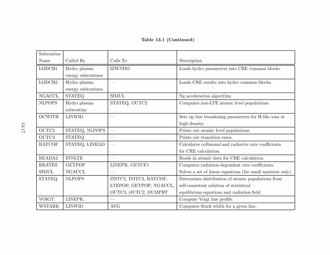
Table 13.1 (Continued)

SubroutineName Called By Calls To Description

LODCB1 Hydro plasma IZWNDO Loads hydro parameters into CRE common blocks.energy subroutines

LODCB2 Hydro plasma — Loads CRE results into hydro common blocks.energy subroutines

NGACCL STATEQ SIMUL Ng acceleration algorithm.

NLPOPS Hydro plasma STATEQ, OUTC2 Computes non-LTE atomic level populations.subroutine

OCWITH LINWID — Sets up line broadening parameters for H-like ions athigh density.

OUTC2 STATEQ, NLPOPS — Prints out atomic level populations.OUTC3 STATEQ — Prints out transition rates.

RATCOF STATEQ, LINRAD — Calculates collisional and radiative rate coefficientsfor CRE calculation.

READA2 INNLTE — Reads in atomic data for CRE calculation.RRATES GETPOP LINEPR, GETCF1 Computes radiation-dependent rate coefficients.SIMUL NGACCL — Solves a set of linear equations (for small matrices only).

STATEQ NLPOPS INITC2, INITC3, RATCOF, Determines distribution of atomic populations fromLTEPOP, GETPOP, NGACCL, self-consistent solution of statisticalOUTC3, OUTC2, DUMPRT equilibrium equations and radiation field.

VOIGT LINEPR, — Compute Voigt line profile.

WSTARK LINWID AVG Computes Stark width for a given line.

13-17

13.2. The Common Blocks

Listed below are the common blocks used in BUCKY-1. For each common block, the variable

name, type, dimensions, and a brief description of each variable is provided. In most cases, the

dimensions of variables are specified by quantities defined in PARAMETER statements. This,

when used with the pre-processor, allows the dimensions of all like arrays to be changed quickly by

modifying just one line of code.

The parameters defining the array sizes are:

Parameter Sets the MAXIMUM number of:

MXZONS spatial zones

MXMATR materials (i.e., EOS tables)

MXREGN regions for spatial gridding

MXTTAB temperatures in EOS tables

MXDTAB densities in EOS tables

MXTTBO temperatures in opacity tables

MXDTBO densities in opacity tables

MXGTAB frequency groups in opacity tables

MXIDPT ion bunches for ion deposition model

MXIDPE ion energy groups for ion deposition model

MXIDPX ion species for ion deposition model

MAXTDQ ionization stages for time-dependent ion deposition model

MXSAVE time-dependent quantities saved for final output

MXLVLS atomic levels for CRE model

MXIONZ ionization stages for CRE model

MXGASS gas species for CRE model

MXDATT temperatures in atomic data tables used by CRE model

MXDATD densities in atomic data tables used by CRE model

MXTRNS atomic transitions in CRE model

MXSSHL atomic subshells in CRE model

MXLVLI levels in atomic data tables used by CRE model

13-18

For many of the variables, the second to the last letter indicates whether the variable is at

a zone center or zone boundary, and the last letter denotes the time level. The suffixes are:

1 – zone boundary

2 – zone center

A – tn+1

B – tn+1/2

C – tn

D – tn−1/2

The letter R will appear in a variable name if the quantity is associated with the radiation field, N

if the quantity is associated with the ions, and E if associated with the electrons. Thus, TR2B(J) is

the radiation temperature in the center of zone j at time tn+1/2, and UlD(J) is the fluid velocity on

the zone j boundary at time tn−1/2. The common blocks are listed below along with their meaning

and units.

13-19

COMMON/TIME/

Variable Type Dimensions Units Description

TA R*8 — sec tn+1 timeTB R*8 — sec tn+1/2

TC R*8 — sec tn

TD R*8 — sec tn−1/2

DTB R*8 — sec ∆tn+1/2

DTC R*8 — sec ∆tn = (∆tn+1/2 + ∆tn−1/2)/2DTD R*8 — sec ∆tn−1/2

DT R*8 — sec ∆tn+3/2, the new time stepTMAX R*8 — sec total time for the simulationDTMIN R*8 — sec minimum allowed time stepDTMAX R*8 — sec maximum allowed time stepDTIONT R*8 — sec time step for updating debris ion deposition propertiesDTVAZ R*8 — sec time step after vaporization of first wall zoneTSPEC R*8 — sec simulation time for specifying user-prescribed time step (DTSPEC)DTSPEC R*8 — sec time step corresponding to TSPEC

13-20

COMMON/TEMPER/

Variable Type Dimensions Units Description

TN2A R*8 MXZONS eV (TP )n+1j−1/2 plasma, or ion, temperatures

TN2B R*8 MXZONS eV (TP )n+1/2j−1/2

TN2C R*8 MXZONS eV (TP )nj−1/2

TN1B R*8 MXZONS eV (TP )n+1/2j

TNSR2B R*8 MXZONS eV1/2

√(TP )n+1/2

j−1/2

TE2A R*8 MXZONS eV (Te)n+1j−1/2 electron temperatures

TE2B R*8 MXZONS eV (Te)n+1/2j−1/2

TE2C R*8 MXZONS eV (Te)nj−1/2

TE1B R*8 MXZONS eV (Te)n+1/2j

TESR2B R*8 MXZONS eV1/2

√(Te)

n+1/2j−1/2

TR2A R*8 MXZONS eV (TR)n+1j−1/2 radiation temperatures

TR2B R*8 MXZONS eV (TR)n+1/2j−1/2

TR2C R*8 MXZONS eV (TR)nj−1/2

TR1B R*8 MXZONS eV (TR)n+1/2j

TBC R*8 MXZONS eV temperature boundary condition

13-21

COMMON/CNTROL/

Variable Type Dimensions Units Description

CON R*8 100 — real constants (see Table 15.3)ISW I*4 100 — control switches (see Table 15.2)IEDIT I*4 100 — intermediate output cycle frequencies (see Table 15.4)IO I*4 31 — primary output frequency vectorINDEX I*4 MXZONS — a vector used for output indexingT1 R*8 MXZONS — temporary vectorT2 R*8 MXZONS — temporary vectorT3 R*8 MXZONS — temporary vectorT4 R*8 MXZONS — temporary vectorTGROW R*8 — — max. percentage that ∆t can increase in one cycleTEDIT R*8 — sec time at which output freq. switches from 10(1) to 10(11)GEOFAC R*8 — — a geometry factor; l, 2π, 4πR3N R*8 — — worst case for ∆TP/TPTSCC R*8 — — Courant condition time step controlTSCV R*8 — — ∆V/V time step controlR1 R*8 — — worst case for Courant conditionR2 R*8 — — worst case for ∆V/VIDELTA I*4 — — 1 = cartesian 2 = cylindrical 3 = sphericalIDELM1 I*4 — — 0 = cartesian 1 = cylindrical 2 = sphericalNCYCLE I*4 — — time cycle indexNMAX I*4 — — max number of time stepsJMAX I*4 — — max number of spatial zonesJMAXM1 I*4 — — JMAX-1JMAXP1 I*4 — — JMAX+1 used for indexingJMAXP2 I*4 — — JMAX+2

13-22

COMMON/CNTROL/ (Continued)

Variable Type Dimensions Units Description

JMAXV0 I*4 — — maximum spatial index for vapor phase at t = 0JMAXV I*4 — — maximum spatial index for vapor phaseJMINC I*4 — — minimum spatial index for condensed phaseJMAXT I*4 — — maximum spatial index for condensed phaseNCZONS I*4 — — initial number of zones in condensed phaseILUNIT I*4 — — output units for flux quantitiesJCOUR I*4 — — zone index of Courant condition worst caseJSPVOL I*4 — — zone index of ∆V/V worst caseJNTEMP I*4 — — zone index of ∆TP/TP worst caseIZONE I*4 — — zone index of worst case of Courant, ∆V/V , ∆TP/TPITYPE I*4 — — 1 = Courant 2 = ∆V/V 3 = ∆ER/ER 4 = ∆TP/TP worst restrictionNREGNS I*4 — — total number of zoning regionsNVREGN I*4 — — number of plasma (vapor) regionsNCREGN I*4 — — number of condensed matter regionsJMN MXREGN — — minimum spatial index of each regionJMX MXREGN — — maximum spatial index of each regionIITYPE I*4 — — 0 = physical -1 = min ∆t 1 = max ∆tIIZONE I*4 — — zone # of worst case if the ∆t is ∆tmax or ∆tmin

ICOND I*4 — — principal time step constraintICOND2 I*4 — — secondary time step constraint if primary is ∆tmin or ∆tmax

IUNIT I*4 — — cm2, radian-cm, steradian for δ = 1, 2, 3TSCTN R*8 — — ∆TP/TP time step control

13-23

COMMON/CNTROL/ (Continued)

Variable Type Dimensions Units Description

IOBIN I*4 — — output frequency of binary outputRADIUS R*8 — cm the radius of the first wallR3R R*8 — — worst case for ∆ER/ERTSCTR R*8 — — ∆ER/ER time step controlJRTEMP I*4 — — zone index of ∆ER/ER worst caseNFG R*8 — — the number of frequency groupsNMAT I*4 — — number of gas typesR3E R*8 — — worst case for ∆Te/TeTPROUT R*8 500 sec if ISW(66) > 0, text output timesTPBOUT R*8 500 sec if ISW(66) > 0, binary output timesDTPOUT R*8 — sec if ISW(66) > 0, text output time intervalDTBOUT R*8 — sec if ISW(66) > 0, binary output time intervalTPRBEG R*8 — sec if ISW(66) > 0, beginning time of text outputTPBBEG R*8 — sec if ISW(66) > 0, beginning time of binary outputIPROUT I*4 — — index for text output timeIPBOUT I*4 — — index for binary output timeNFDOUT I*4 — — number of text outputs per binary outputIDEOS I*4 MXMATR — EOS material indexIDOPAC I*4 MXMATR — opacity material index

13-24

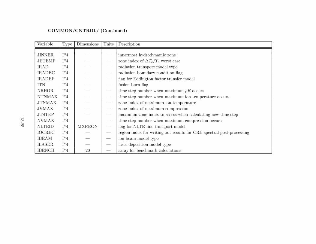
COMMON/CNTROL/ (Continued)

Variable Type Dimensions Units Description

JINNER I*4 — — innermost hydrodynamic zoneJETEMP I*4 — — zone index of ∆Te/Te worst caseIRAD I*4 — — radiation transport model typeIRADBC I*4 — — radiation boundary condition flagIRADEF I*4 — — flag for Eddington factor transfer modelITN I*4 — — fusion burn flagNRHOR I*4 — — time step number when maximum ρR occursNTNMAX I*4 — — time step number when maximum ion temperature occursJTNMAX I*4 — — zone index of maximum ion temperatureJVMAX I*4 — — zone index of maximum compressionJTSTEP I*4 — — maximum zone index to assess when calculating new time stepNVMAX I*4 — — time step number when maximum compression occursNLTEID I*4 MXREGN — flag for NLTE line transport modelIOCREG I*4 — — region index for writing out results for CRE spectral post-processingIBEAM I*4 — — ion beam model typeILASER I*4 — — laser deposition model typeIBENCH I*4 20 — array for benchmark calculations

13-25

COMMON/HYDROD/

Variable Type Dimensions Units Description

U1D R*8 MXZONS cm/sec un−1/2j fluid velocity

U1B∗∗ R*8 MXZONS un+1/2j

DR2B R*8 MXZONS cm ∆rn+1/2j−1/2 zone widths

DR2A R*8 MXZONS ∆rn+1j−1/2

R1C R*8 MXZONS cm rnj radiusR1B R*8 MXZONS r

n+1/2j

R1A R*8 MXZONS rn+1j

RS1C R*8 MXZONS (rnj )δ−1

RS1B R*8 MXZONS (rn+1/2j )δ−1

RS1A R*8 MXZONS (rn+1j )δ−1

PR2C R*8 MXZONS J/cm3 (PR)nj−1/2 radiation pressure

PR2B R*8 MXZONS (PR)n+1/2j−1/2

PR2A R*8 MXZONS (PR)n+1j−1/2

PN2C R*8 MXZONS J/cm3 (PP )nj−1/2 plasma, or ion, pressurePN2B R*8 MXZONS (PP )n+1

j−1/2

PN2A R*8 MXZONS (PP )n+1j−1/2

PE2A R*8 MXZONS J/cm3 (Pe)n+1j−1/2 electron pressure

PE2B R*8 MXZONS (Pe)n+1/2j−1/2

PE2C R*8 MXZONS (Pe)nj−1/2

P2C R*8 MXZONS J/cm3 Pnj−1/2 total pressureP2A R*8 MXZONS Pn+1

j−1/2

V2C R*8 MXZONS cm3/g V nj−1/2 specific volume

V2B R*8 MXZONS Vn+1/2j−1/2

13-26

COMMON/HYDROD/ (Continued)

Variable Type Dimensions Units Description

V2A R*8 MXZONS V n+1j−1/2

V0 R*8 MXZONS cm3/g initial specific volumeCOMPR R*8 MXZONS — V0/V compressionVDOT2B R*8 MXZONS cm3/g − s V

n+1/2j−1/2 time derivative of sp. volume

DMASS2 R*8 MXZONS δ = 1: g/cm2 δmoj−1/2Langrangian mass

δ = 2: g/cm/radδ = 3: g/ster

DMASS1 R*8 MXZONS see above δmoj = (δmoj−1/2+ δmoj+1/2

)/2

Q2B R*8 MXZONS J/cm3 qn+1/2j−1/2 artificial viscosity

VOL2B R*8 MXZONS cm3 Vn+1/2j−1/2 zone volume

VOL2A R*8 MXZONS cm3 Vn+1/2j−1/2

DMOM1C R*8 MXZONS cm/sec2 momentum lost by debris ions during ∆tn

DMASS0 R*8 MXZONS see above initial values of DMASS2VMAX R*8 MXZONS — maximum compressionTAVMAX R*8 MXZONS sec time of maximum compressionTOTMS0 R*8 MXZONS grams initial massRINNER R*8 — cm inner radius of innermost zoneRHORMX R*8 — g/cm2 maximum value of ρRRHOR R*8 — g/cm2 current value of ρRTRHOR R*8 — sec time at which maximum ρR was achievedTNMAX R*8 — eV maximum ion temperatureTATNMX R*8 — sec time at which maximum ion temperature occurredPRBC R*8 — J/cm3 pressure at outermost boundary

13-27

COMMON/ESCOM/

Variable Type Dimensions Units Description

ER2C R*8 MXZONS J/cm3 EnRj−1/2

radiation energy density

ENT2B R*8 MXZONS J/g/eV (Cv)n+1/2j−1/2 plasma specific heat

EET2B R*8 MXZONS J/g/eV (Cv)n+1/2j−1/2 electron specific heat

ER2B R*8 MXZONS J/cm3 En+1/2Rj−1/2

radiation energy density

PNT2B R*8 MXZONS J/cm3/eV (PP )n+1/2Tj−1/2

temperature derivative of ion pressure

PET2B R*8 MXZONS J/cm3/eV (Pe)T temperature derivative of electron pressureER2A R*8 MXZONS J/cm3 (ER)n+1

j−1/2 radiation energy density

ER2B R*8 MXZONS J/cm3 (ER)n+1/2j−1/2 radiation energy density

EN2A R*8 MXZONS J/g (EP )n+1j−1/2 ion, or plasma, specific internal energy

EE2A R*8 MXZONS — (Ee)n+1j−1/2 electron specific internal energy

DE2A R*8 MXZONS cm3 (ne)n+1j−1/2 electron number density

DN2A R*8 MXZONS cm3 (nP )n+1j−1/2 ion number density

DE2B∗∗ R*8 MXZONS cm3 (ne)n+1/2j−1/2 electron number density

DN2B∗ R*8 MXZONS cm3 (nP )n+1/2j−1/2 ion number density

ATW2B∗ R*8 MXZONS amu An+1/2j−1/2 average ion atomic weight

ATWQ2B R*8 MXZONS amu1/2 square root of ATW2BZT2B R*8 MXZONS esu/eV ∂Z/∂T

n+1/2j−1/2 temperature derivative of average charge

ENN2B R*8 MXZONS J/cm3 scaled density derivative of specific energyZ2B∗∗ R*8 MXZONS esu Z

n+1/2j−1/2 average charge

13-28

COMMON/ESCOM/ (Continued)

Variable Type Dimensions Units Description

ZSQ2B R*8 MXZONS esu2 (Zn+1/2j−1/2 )2 average squared charge

DD2A R*8 MXZONS cm−3 number density of deuterium at (n+ 1)DD2B R*8 MXZONS cm−3 number density of deuterium at (n+ 1/2)DT2A R*8 MXZONS cm−3 number density of tritium at (n + 1)DT2B R*8 MXZONS cm−3 number density of tritium at (n + 1/2)DO2A R*8 MXZONS cm−3 number density of non-DT ions at (n+ 1)DO2B R*8 MXZONS cm−3 number density of non-DT ions at (n+ 1/2)ATWO R*8 MXZONS amu atomic weight of non-DT ionsZO2B R*8 MXZONS esu mean charge of non-DT ionsXNO2A R*8 MXZONS — DO2A * VOL2AJMAT I*4 MXZONS — material type indexVBC I*4 MXZONS cm3/g specific volume boundary conditionAD I*4 MXZONS —AT I*4 MXZONS — coefficients defining the grid for the equations of stateBD I*4 MXZONS —BT I*4 MXZONS —EBC I*4 MXZONS — radiation energy density boundary conditionRAD I*4 MXZONS — 1/ADRAT I*4 MXZONS — 1/ATRBT I*4 MXZONS — 1/BTRBD I*4 MXZONS — 1/BD

13-29

COMMON/ESCOM1/

Variable Type Dimensions Units Description

ZTAB R*8 MXTTAB, esu EOS table for mean charge stateMXDTAB,MXMATR

DZDTAB R*8 same as above esu/eV EOS table for (dZ/dT )ENTAB R*8 same as above J/g EOS table for specific ion internal energyENTTAB R*8 same as above J/g/eV EOS table for (∂Eion/∂T )ENNTAB R*8 same as above eV−1 EOS table for scaled (∂Eion/∂ρ)EETAB R*8 same as above J/g EOS table for specific electron internal energyEETTAB R*8 same as above J/g/eV EOS table for (∂Ee/∂T )PNTAB R*8 same as above J/cm3 EOS table for ion pressurePNTTAB R*8 same as above J/cm3/eV EOS table for (∂Eion/∂T )PETAB R*8 same as above J/cm3 EOS table for electron pressurePETTAB R*8 same as above J/cm3/eV EOS table for (∂Pe/∂T )RRTAB R*8 MXGTAB, cm2/g Rosseland opacity table

MXTTAB,MXDTAB,MXMATR

RPTAB R*8 same as above cm2/g Planck opacity table (absorption)RPETAB R*8 same as above cm2/g Planck opacity table (emission)

13-30

COMMON/ESCOM1/ (Continued)

Variable Type Dimensions Units Description

ADTAB R*8 MXMATR — ρ-increment for EOS tableATTAB R*8 MXMATR — T -increment for EOS tableBDTAB R*8 MXMATR — log10 of ρmin in EOS tableBTTAB R*8 MXMATR — log10 of Tmin in EOS tableRADTAB R*8 MXMATR — ρ-increment for opacity tableRATTAB R*8 MXMATR — T -increment for opacity tableRBDTAB R*8 MXMATR — log10 of ρmin in opacity tableRBTTAB R*8 MXMATR — log10 of Tmin in opacity tableTMPTAB R*8 MXTTAB, eV temperature grid for SESAME EOS table

MXMATR,5RHOTAB R*8 MXTTAB, g/cm3 density grid for SESAME EOS table

MXMATR,5RADCON R*8 MXMATR,3 — multiplier for opacitiesNTTAB I*4 MXMATR — number of temperatures in EOS tableNDTAB I*4 MXMATR — number of densities in EOS tableNTTABO I*4 MXMATR — number of temperatures in opacity tableNDTABO I*4 MXMATR — number of densities in opacity tableNTMPTB I*4 MXMATR,5 — number of temperatures in SESAME EOS tableNRHOTB I*4 MXMATR,5 — number of densities in SESAME EOS tableIZEOS I*4 MXMATR — file identifier for EOS/opacity tables

13-31

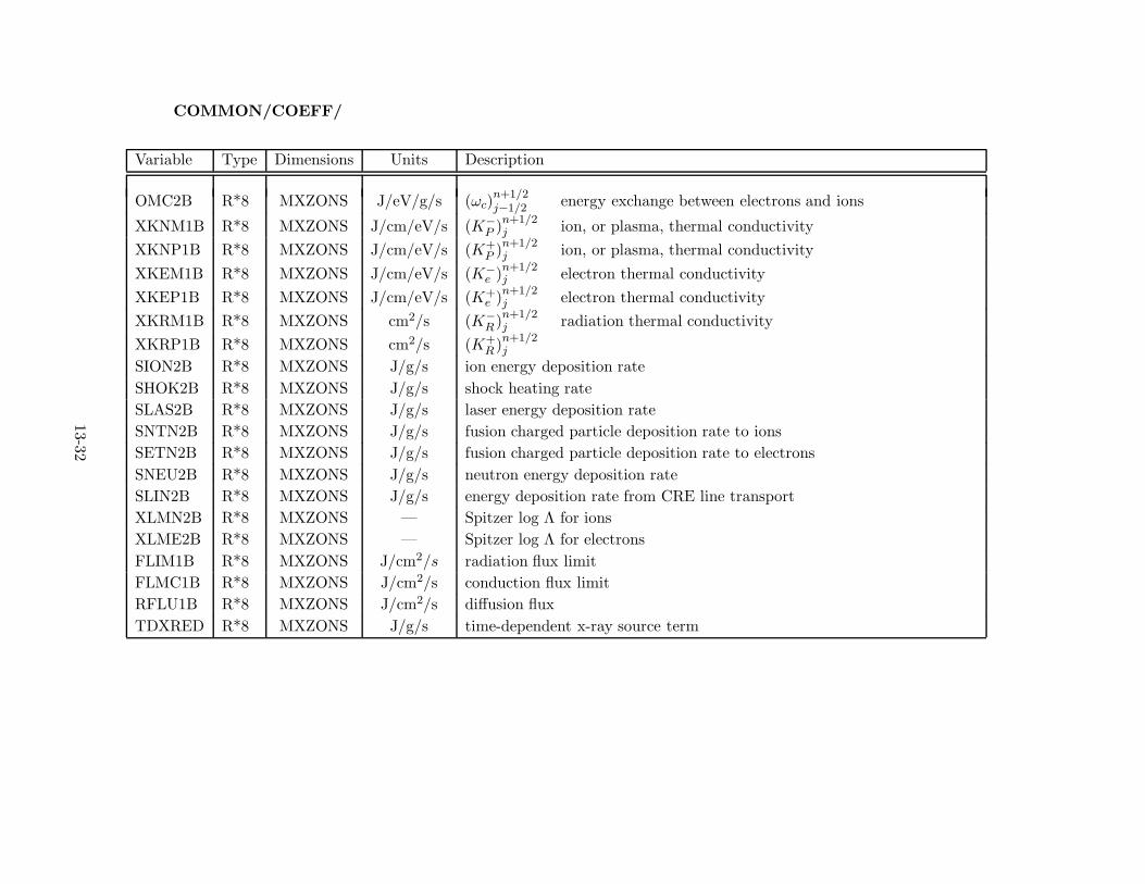
COMMON/COEFF/

Variable Type Dimensions Units Description

OMC2B R*8 MXZONS J/eV/g/s (ωc)n+1/2j−1/2 energy exchange between electrons and ions

XKNM1B R*8 MXZONS J/cm/eV/s (K−P )n+1/2j ion, or plasma, thermal conductivity

XKNP1B R*8 MXZONS J/cm/eV/s (K+P )n+1/2

j ion, or plasma, thermal conductivityXKEM1B R*8 MXZONS J/cm/eV/s (K−e )n+1/2

j electron thermal conductivityXKEP1B R*8 MXZONS J/cm/eV/s (K+

e )n+1/2j electron thermal conductivity

XKRM1B R*8 MXZONS cm2/s (K−R )n+1/2j radiation thermal conductivity

XKRP1B R*8 MXZONS cm2/s (K+R )n+1/2

j

SION2B R*8 MXZONS J/g/s ion energy deposition rateSHOK2B R*8 MXZONS J/g/s shock heating rateSLAS2B R*8 MXZONS J/g/s laser energy deposition rateSNTN2B R*8 MXZONS J/g/s fusion charged particle deposition rate to ionsSETN2B R*8 MXZONS J/g/s fusion charged particle deposition rate to electronsSNEU2B R*8 MXZONS J/g/s neutron energy deposition rateSLIN2B R*8 MXZONS J/g/s energy deposition rate from CRE line transportXLMN2B R*8 MXZONS — Spitzer log Λ for ionsXLME2B R*8 MXZONS — Spitzer log Λ for electronsFLIM1B R*8 MXZONS J/cm2/s radiation flux limitFLMC1B R*8 MXZONS J/cm2/s conduction flux limitRFLU1B R*8 MXZONS J/cm2/s diffusion fluxTDXRED R*8 MXZONS J/g/s time-dependent x-ray source term

13-32

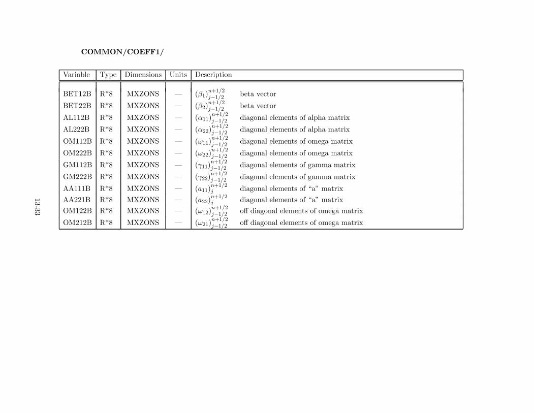
COMMON/COEFF1/

Variable Type Dimensions Units Description

BET12B R*8 MXZONS — (β1)n+1/2j−1/2 beta vector

BET22B R*8 MXZONS — (β2)n+1/2j−1/2 beta vector

AL112B R*8 MXZONS — (α11)n+1/2j−1/2 diagonal elements of alpha matrix

AL222B R*8 MXZONS — (α22)n+1/2j−1/2 diagonal elements of alpha matrix

OM112B R*8 MXZONS — (ω11)n+1/2j−1/2 diagonal elements of omega matrix

OM222B R*8 MXZONS — (ω22)n+1/2j−1/2 diagonal elements of omega matrix

GM112B R*8 MXZONS — (γ11)n+1/2j−1/2 diagonal elements of gamma matrix

GM222B R*8 MXZONS — (γ22)n+1/2j−1/2 diagonal elements of gamma matrix

AA111B R*8 MXZONS — (a11)n+1/2j diagonal elements of “a” matrix

AA221B R*8 MXZONS — (a22)n+1/2j diagonal elements of “a” matrix

OM122B R*8 MXZONS — (ω12)n+1/2j−1/2 off diagonal elements of omega matrix

OM212B R*8 MXZONS — (ω21)n+1/2j−1/2 off diagonal elements of omega matrix

13-33

COMMON/COEFF2/

Variable Type Dimensions Units Description

E11 R*8 MXZONS — (E11) all elements of the “E” matrixE12 R*8 MXZONS — (E11)E21 R*8 MXZONS — (E21)E22 R*8 MXZONS — (E22)F1 R*8 MXZONS — (F1) both components of the “F” vectorF2 R*8 MXZONS — (F2)B11 R*8 MXZONS — (B11) all elements of the “B” matrixB12 R*8 MXZONS — (B12)B21 R*8 MXZONS — (B21)B22 R*8 MXZONS — (B22)D1 R*8 MXZONS — (D1) both elements of the “D” vectorD2 R*8 MXZONS — (D2)

13-34

COMMON/ECKCOM/

Variable Type Dimensions Units Description

T1A R*8 MXZONS J/x (T )n+1j kinetic energy of fluid

GGGE2A R*8 MXZONS J/x (Ge)n+1j−1/2 radiation-gas work

HHHR2B R*8 MXZONS J/x (HR)n+1/2j−1/2 radiation source

HHHH2B R*8 MXZONS J/x (HP )n+1/2j−1/2 ion source term

HHHE2B R*8 MXZONS J/x (He)n+1/2j−1/2 electron source term

EEEC2A R*8 MXZONS J/x (Ec)n+1j−1/2 electron-ion energy exchange

EEER2A R*8 MXZONS J/x (ER)n+1j−1/2 radiation-electron energy exchange

FSAVE R*8 MXSAVE J/cm2/s heat fluxes at first wallPSAVE R*8 MXSAVE J/cm2 pressures at first wallTSAVE R*8 MXSAVE s times of heat fluxes and pressuresEEEER0 R*8 — J/x ERo total initial radiation internal energyEEEEN0 R*8 — J/x EPo total initial ion internal energyEEEEE0 R*8 — J/x Eeo total initial electron energyEEEEER R*8 — J/x (ER)n+1 total radiation internal energyEEEEEN R*8 — J/x (EP )n+1 total ion internal energyEEEEEE R*8 — J/x (Ee)n+1 total electron internal energyTTTTTT R*8 — J/x (T )n+1 total fluid kinetic energyHHHHHR R*8 — J/x (HR)n+1 total radiation source termHHHHHN R*8 — J/x (HP )n+1 total ion source termHHHHHE R*8 — J/x (HE)n+1 total electron source termEEEEEC R*8 — J/x (Ec)n+1 total radiation-gas energy exchangedGGGGGE R*8 — J/x (Ge)n+1 total work done by ions on electrons

13-35

COMMON/ECKCOM/ (Continued)

Variable Type Dimensions Units Description

WWWWWR R*8 — J/x (WR)n+1 total work done on radiationWWWWWN R*8 — J/x (WP )n+1 total work done on ionsWWWWWE R*8 — J/x (WE)n+1 total work done on electronsFFFFFR R*8 — J/x (FR)n+1 total radiation heat lost across outer boundariesFFFFFN R*8 — J/x (FP )n+1 total ion heat loss across outer boundariesFFFFFE R*8 — J/x (Fe)n+1 total electron heat loss across outer boundariesWWWWR R*8 — J/x (WR)n+1 total work done on radiation on last cycleWWWWN R*8 — J/x (WP )n+1 total work done on ions on last cycleWWWWE R*8 — J/x (WE)n+1 total work done on electrons on last cycleFFFFR R*8 — J/x (fR)n+1 total radiation lost at outer bd. on last cycleFFFFN R*8 — J/x (fP )n+1 total ion energy lost at outer bd. on last cycleFFFFE R*8 — J/x (fe)n+1 total electron energy lost at outer bd. on last cycleHHHHR R*8 — J/x (hR)n+1 total radiation source term on last cycleHHHHN R*8 — J/x (hP )n+1 total ion source term on last cycleHHHHE R*8 — J/x (he)n+1 total ion source term on last cycleGGGGE R*8 — J/x (ge)n+1 total work to maintain one fluid on last cycleENLHS R*8 — J/x left side of ion energy balance equationENLHS R*8 — J/x left side of electron energy balance equationETLHS R*8 — J/x left side of total energy balance equationERRHS R*8 — J/x right side of radiation energy balance equationERLHS R*8 — J/x left side of radiation energy balance equationENRHS R*8 — J/x right side of ion energy balance equationEERHS R*8 — J/x right side of electron energy balance equationETRHS R*8 — J/x right side of total energy balance equationTTTTN0 R*8 — J/x initial kinetic energyPMAX R*8 — J/cm3 maximum pressure at the wall

13-36

COMMON/ECKCOM/ (Continued)

Variable Type Dimensions Units Description

TIMP R*8 MXSAVE J/s/cm3 pressure impulse at first wallHFINTG R*8 MXSAVE J/cm2 heat fluence at first wallVMSAVE R*8 MXSAVE g mass vaporized from first wallDMSAVE R*8 MXSAVE g/s mass vaporization rateTSKNSV R*8 MXSAVE eV first wall skin temperatureTBLSAV R*8 MXSAVE eV average temperature in boundary layerPSATSV R*8 MXSAVE erg/cm3 saturation vapor pressure at first wallPVAPSV R*8 MXSAVE erg/cm3 vapor pressure at first wallERAD2A R*8 MXZONS J radiation energy in each zoneFFFFFL R*8 — J total line radiation lost across boundariesFFFFL R*8 — J line radiation lost across bd. on last cycleCOOLCR R*8 MXREGN J/s/cm3−δ continuum radiation cooling rateCOOLLR R*8 MXREGN J/s/cm3−δ line radiation cooling rateFLXBDC R*8 MXREGN+1 J/cm2/s continuum radiation flux at region interfacesFLXBDL R*8 MXREGN+1 J/cm2/s line radiation flux at region interfacesRFLINT R*8 MXREGN+2 J/cm2 time-integrated radiation energy lost across inner and outer boundariesRFLOUT R*8 MXREGN+2 J/cm2 time-integrated radiation energy lost across inner and outer boundariesEEERAD R*8 — J total radiation energyETN R*8 — J total energy generated from fusion reactionsECPT R*8 — J total charged particle energy generated from fusion reactionsEDTTN R*8 — J total energy generated from DT reactionsEDDTN R*8 — J total energy generated from DD reactionsEDHE3T R*8 — J total energy generated from D-HE3 reactions

13-37

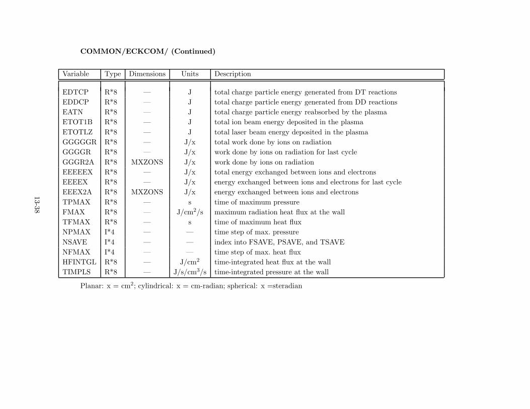
COMMON/ECKCOM/ (Continued)

Variable Type Dimensions Units Description

EDTCP R*8 — J total charge particle energy generated from DT reactionsEDDCP R*8 — J total charge particle energy generated from DD reactionsEATN R*8 — J total charge particle energy reabsorbed by the plasmaETOT1B R*8 — J total ion beam energy deposited in the plasmaETOTLZ R*8 — J total laser beam energy deposited in the plasmaGGGGGR R*8 — J/x total work done by ions on radiationGGGGR R*8 — J/x work done by ions on radiation for last cycleGGGR2A R*8 MXZONS J/x work done by ions on radiationEEEEEX R*8 — J/x total energy exchanged between ions and electronsEEEEX R*8 — J/x energy exchanged between ions and electrons for last cycleEEEX2A R*8 MXZONS J/x energy exchanged between ions and electronsTPMAX R*8 — s time of maximum pressureFMAX R*8 — J/cm2/s maximum radiation heat flux at the wallTFMAX R*8 — s time of maximum heat fluxNPMAX I*4 — — time step of max. pressureNSAVE I*4 — — index into FSAVE, PSAVE, and TSAVENFMAX I*4 — — time step of max. heat fluxHFINTGL R*8 — J/cm2 time-integrated heat flux at the wallTIMPLS R*8 — J/s/cm3/s time-integrated pressure at the wall

Planar: x = cm2; cylindrical: x = cm-radian; spherical: x =steradian

13-38

COMMON/IONCOM/

Variable Type Dimensions Units Description

ATN2B R*8 MXZONS esu atomic number of the background plasmaDIMASS R*8 MXZONS g debris ion mass deposited in each Lagrangian cell during one time stepXIKE2B R*8 MXZONS J debris ion energy deposited in the plasmaTOTION R*8 MXZONS J total debris energy deposited in each Lagrangian cellXIONIN R*8 MXIDPT, ions/s ion flux array

MXIDPE,MXIDPX

BEAMCD R*8 MXZONS ions/cm2/s ion beam particle current densityBEAMEN R*8 MXZONS keV ion energy kinetic energyEIONIN R*8 MXIDPT, keV ion flux array

MXIDPE,MXIDPX

TIONIN R*8 MXIDPT sec ion time arrayAWION R*8 MXIDPX amu atomic weight of the debris ionsANION R*8 MXIDPX — atomic number of the debris ionsQ1INIT R*8 MXIDPX esu initial charge state of the debris ionsCDEPCN R*8 MXIDPX,5 — constants used in stopping power calculation

13-39

COMMON/IONCOM/ (Continued)

Variable Type Dimensions Units Description

ATNION R*8 MXIDPX — debris ion atomic numberATWION R*8 MXIDPX amu debris ion atomic weightWALION R*8 — J debris ion energy deposited in the wallTIONEN R*8 — sec estimated ending time of ion energy depositionSRCION R*8 — J total ion energy emitted by the sourceNIX R*8 — — number of debris ion speciesNIE R*8 — — number of debris ion energy binsNIT R*8 — — number of debris ion time binsPLSION R*8 — J time-integrated ion energy deposited in the entire background plasmaPLSIKE R*8 — J time-integrated ion energy deposited in the background plasma by stopped ionsZ1EFF R*8 — esu effective charge state of debris ionsWALIEB R*8 — J/s ion energy deposition rate at the wallZ1MIN R*8 MXIDPT esu minimum projectile charge

13-40

COMMON/XRAY/

Variable Type Dimensions Units Description

EXRAY R*8 MXZONS keV the energy of the x-rays in each groupFXRAY R*8 MXZONS J/keV the energy in each x-ray groupUXRAY R*8 MXZONS cm2/g x-ray attenuation coefficients computed from tablesIZ I*4 MXZONS — the atomic number of the plasmaTDXAMP R*8 (100,20) — time-dependent x-ray amplitudesATTENC R*8 (100,5) — attenuation coefficientsCOEF R*8 (100,4) — coefficients computed from x-ray cross section tablesELIM R*8 100 — a vector used in computing the x-ray cross sectionsXRTIM R*8 20 sec times at which x-ray amplitudes are specifiedXAMP R*8 100 J/keV the amplitude of an input x-ray spectrumXEHIST R*8 101 keV the energy of the x-rays in each group of the input spectrumCRLOC I*4 100 — data for x-ray stopping cross sectionsCRA R*8 3884 — data for x-ray stopping cross sectionsCRB R*8 971 — data for x-ray stopping cross sectionsCRHD R*8 10 — data for x-ray stopping cross sectionsCRZOA R*8 100 — data for x-ray stopping cross sectionsCONFAC R*8 (2,2) — data for x-ray stopping cross sections

13-41

COMMON/XRAY/ (Continued)

Variable Type Dimensions Units Description

IATTEN I*4 6 — data for x-ray stopping cross sectionsEDGE R*8 5 keV the minimum x-ray energy required for absorption by electrons in each shellSHELEL R*8 5 — the number of electrons in each shellKEDGE I*4 — — the number of shells the plasma atoms haveONEZOA R*8 — — a coefficient used in computing the x-ray scattering cross sectionNXRG I*4 — — number of x-ray groupsKEV R*8 — keV the blackbody temperature of a blackbody x-ray spectrumFLUX R*8 — J the total energy in x-rays input by the userSUMFLU R*8 — J the energy in the x-ray spectraNXRT I*4 — — the number of times at which the input intensity is givenNUM I*4 — — a number generated by the code in searching through the x-ray

cross section tablesTXRED R*8 — J the x-ray energy absorbed by the plasmaETXR R*8 — —EETXR R*8 — —STDXR R*8 — —SSTDXR R*8 — —EXRW R*8 — —EEXRW R*8 — —NIZJ I*4 — —

13-42

COMMON/MFRAD/

Variable Type Dimensions Units Description

ERFD2A R*8 MXGTAB, J/g frequency dependent radiation specific energy at tn+1

MXZONSERFD2C R*8 MXGTAB, J/g frequency dependent radiation specific energy at tn

MXZONSSRFD2B R*8 MXGTAB, J/g/s frequency dependent radiation emission energy at tn+1/2

MXZONSSR2B R*8 MXGTAB, cm2/g frequency dependent Rosseland opacity

MXZONSSP2B R*8 MXGTAB, cm2/g frequency dependent Planck absorption opacity

MXZONSSPE2B R*8 MXGTAB, cm2/g frequency dependent Planck emission opacity

MXZONSSER2B R*8 MXZONS J/g/s frequency integrated radiation absorptionSRE2B R*8 MXZONS J/g/s frequency integrated radiation emission termHNU1 R*8 MXGTAB+1 keV boundaries of frequency groupsHNU2 R*8 MXGTAB keV centers of frequency groupsRFDOUT R*8 MXGTAB,2 J frequency dependent radiation energy flux at first wall

on a given time cycleRFDINT R*8 MXGTAB,2 J time integrated frequency dependent radiation energy flux

at first wall up through a given time cycle

13-43

COMMON/WALVAP/

Variable Type Dimensions Units Description

DELXC R*8 MXZONS cm cell sizes in the condensed regionTCN2A R*8 MXZONS eV temperature in the condensed regionTCN2B R*8 MXZONS eV temperature in the condensed regionTCN2C R*8 MXZONS eV temperature in the condensed regionXKCOND R*8 MXZONS J/cm/s/eV thermal conductivity in the condensed regionRHOCND R*8 — g/cm3 mass density of the condensed regionQHEATV R*8 — J/g specific heat of vaporization of the condensed regionCPHEAT R*8 — J/g/eV specific heat of the condensed regionTVAPO R*8 — eV vaporization temperature at 1 barTWALLB R*8 — eV temperature at the back of the condensed regionDELXCT R*8 — cm total width of the condensed regionUNSENS R*8 — J/g specific internal energy at the vaporization temperatureUNVAP R*8 — J/g specific internal energy required to vaporize (UNSENS + QHEATV)TVAP R*8 — eV vaporization temperatureDMVCDT R*8 — g/sec net vaporization rateIZFILM R*8 — amu atomic number of the condensed regionTMASVP R*8 — g total mass vaporizedFRACMV R*8 — – mass fraction of the interface zone in the vapor phaseFRACMC R*8 — – mass fraction of the interface zone in the condensed phaseUNFINP R*8 — J time-integrated radiation and debris ion energy added to the

condensed regionDUFINP R*8 — J radiation and debris ion energy added to the condensed regionHVSTOR R*8 — J time-integrated energy stored in the heat of vaporizationDHVSTO R*8 — J energy stored in the heat of vaporizationWVSTOR R*8 — J time-integrated work energy due to phase change

13-44

COMMON/WALVAP/ (Continued)

Variable Type Dimensions Units Description

DWVSTO R*8 — J work energy due to phase changeHVSTO0 R*8 — J energy stored in the heat of vaporization due to prompt x-raysUNFLM0 R*8 — J initial internal energy of the condensed regionUNFLMT R*8 — J total internal energy of the condensed regionUNBACK R*8 — J time-integrated energy conducted through the back of the condensed regionDUNBAK R*8 — J energy conducted through the back of the condensed regionUVAPMT R*8 — J time-integrated energy added to the vapor phase due to phase changeDUVPMT R*8 — J energy added to the vapor phase due to phase changeUCNDMT R*8 — J time-integrated energy added to the condensed region due to phase changeDUCNMT R*8 — J energy added to the condensed region due to phase changeVAPMAS R*8 — J vapor mass of the non-condensable and condensable gasesQRAD R*8 — J/cm2 radiant heat for last cycleQCOND R*8 — J/cm2 condensation heat for last cycleAWFILM R*8 — amu atomic weight of solid/liquidTOTMSN R*8 — g total mass of condensed regionFSTICK R*8 — — sticking coefficient for condensationQVOL R*8 MXZONS J/cm3/s rate of radiation energy depositionUNFLM R*8 MXZONS J/g specific internal energy in condensed regionQINT R*8 100 J/cm2/s x-ray flux onto first wallFXMU R*8 100 cm2/g x-ray attenuation coefficientPSAT R*8 — erg/cm3 saturation vapor pressurePVAP R*8 — erg/cm3 vapor pressureAVGTMP R*8 — eV average temperature of boundary layerTSKIN R*8 — eV skin temperature of condensed region

13-45

COMMON/DBUGCM/

Variable Type Dimensions Units Description

NOBUG I*4 — — logical flag; true if no debug output requestedNAMEDB I*4 10 — subroutine names for which debug output is requestedNCYCLD I*4 10 — beginning cycle number for debug outputICYCLD I*4 10 — cycle increment for debug outputTBEGDB R*8 10 sec simulation time at which debug output beginsTENDDB R*8 10 sec simulation time at which debug output ends

COMMON/TDION/

NQTDEP I*4 — — maximum number of ionization states tracked in atime-dependent debris ion calculation

IQMIN I*4 MXIDPX — minimum charge state for debris ions in rate equation solutionIQMAX I*4 MXIDPX — maxmum charge state for debris ions in rate equation solutionQ1MIN R*8 MXIDPX esu minimum allowable charge state for debris ionsPOTEN R*8 MAXTDQ, — ionization potentials for debris ions

MXIDPXFRTDIZ R*8 MAXTDQ — fractional ionization abundances of the debris ions

MXIDPTMXIDPEMXIDPX

BGPOTN R*8 50 eV ionization potentials for the background plasmaRATCN R*8 7,MAXTDQ, — constants used in rate equations for debris ions

MXIDPXZ1AVER R*8 MXIDPT esu average charge state for each debris ion group

MXIDPEMXIDPX

13-46

COMMON/TNCOM/

Variable Type Dimensions Units Description

CONTN R*8 20 — constants used by the thermonuclear burn part of the code (see Table 15.5)DEPETN R*8 MXZONS Jk the accumulated energy deposited into the electrons in each zone by the

streaming reaction products on a TN burn time stepDEPNTN R*8 MXZONS Jk save as above except for ionsDTTN R*8 — sh the thermonuclear burn time stepTTN R*8 — sh the thermonuclear burn timeZHE4 R*8 — esu the charge of He4

ZHE3 R*8 — esu the charge of He3

ZP R*8 — esu the charge of a protonZT R*8 — esu the charge of a tritonVSAVE R*8 — cm/sh a working variable in SLOW that contains the velocity of the transporting

bunch of particlesUSAVE R*8 — — a working variable in SLOW that contains the cosine of the angle µ that

specifies the direction of the transporting particlesRSAVE R*8 — cm a working variable in SLOW that contains the radius of the transporting

particlesDTSAVE R*8 — sh a working variable in SLOW that contains the time remaining in the transport

of the particlesDVDT R*8 — cm/sh ∆V∆t — the velocity lost by the transporting particles during the

thermonuclear time stepDV R*8 — cm/sh ∆V — the smaller of ∆V∆T and ∆V∆S

DVDS R*8 — cm/sh ∆V∆S — the velocity lost by the transporting particles in the distance∆S to the next zone boundary

DS R*8 — cm ∆S — the distance from the transporting particles current position tothe next zone boundary that they will cross

DSDT R*8 — cm ∆S∆t — the distance that the particles would travel during the TN time stepDTDS R*8 — cm ∆t∆s — the time that it will take the particles to move the distance ∆s

to the next zone boundary

13-47

COMMON/TNCOM/ (Continued)

Variable Type Dimensions Units Description

RNEXT R*8 — cm the radius of the next zone boundary that the transporting particles will crossAN14 R*8 — — the number of 14.1 MeV neutrons created during the current TN time stepAN14T R*8 — — the total number of 14 MeV neutrons created up to the current timeEN14T R*8 — J total energy of 14 MeV neutrons createdAN245 R*8 — — the number of 2.45 MeV neutrons created on the current TN time stepAN245T R*8 — — the number of 2.45 MeV neutrons created up to the current timePESCTN R*8 — — total number of charged particle reaction products that have escaped the plasmaEESCTN R*8 — Jk total energy of charged particle reaction products that have escaped the plasmaAESCAP R*8 — — not usedZTN R*8 — esu charge of the particles being transportedTNMASS R*8 — g mass of the particle being transportedHE4M R*8 — g mass of He4

HE3M R*8 — g mass of He3

TM R*8 — g mass of a tritonPM R*8 — g mass of a protonKO R*8 — — terms in the solution of the integral equation used to compute the slowing downJO R*8 — — terms in the solution of the integral equation used to compute the slowing downKOP R*8 — — terms in the solution of the integral equation used to compute the slowing downJOP R*8 — — terms in the solution of the integral equation used to compute the slowing downSLOWE R*8 MXZONS sh−1 the electron, ion, and nuclear contributions to the slowingSLOWI MXZONS cm3/sh4 down of charged particle reaction productsSLOWN MXZONS sh−1 − dv

dS = SLOWE + SLOWI/V3 + SLOWNENERG R*8 — Jk total energy lost by one bunch of transporting particles in a zone,

used in ENEMAENERGE R*8 — Jk energy lost by one bunch of transporting particles in a zone to electronsENERGN R*8 — Jk energy lost by one bunch of transporting particles in a zone to ions

13-48

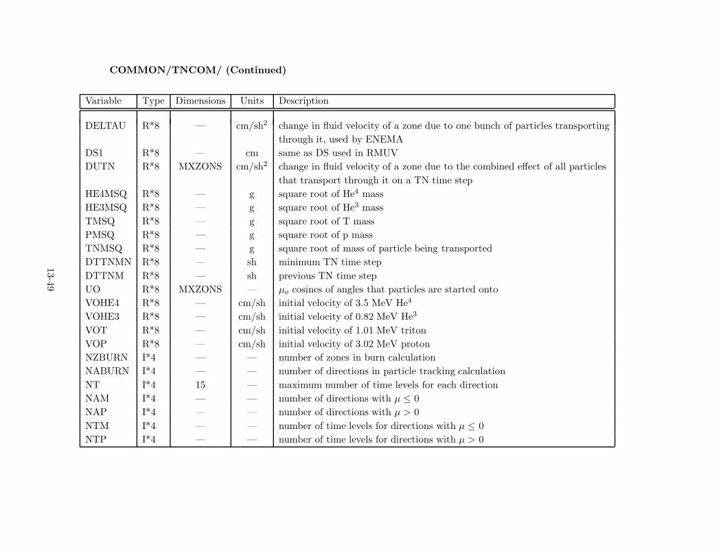
COMMON/TNCOM/ (Continued)

Variable Type Dimensions Units Description

DELTAU R*8 — cm/sh2 change in fluid velocity of a zone due to one bunch of particles transportingthrough it, used by ENEMA

DS1 R*8 — cm same as DS used in RMUVDUTN R*8 MXZONS cm/sh2 change in fluid velocity of a zone due to the combined effect of all particles

that transport through it on a TN time stepHE4MSQ R*8 — g square root of He4 massHE3MSQ R*8 — g square root of He3 massTMSQ R*8 — g square root of T massPMSQ R*8 — g square root of p massTNMSQ R*8 — g square root of mass of particle being transportedDTTNMN R*8 — sh minimum TN time stepDTTNM R*8 — sh previous TN time stepUO R*8 MXZONS — µo cosines of angles that particles are started ontoVOHE4 R*8 — cm/sh initial velocity of 3.5 MeV He4

VOHE3 R*8 — cm/sh initial velocity of 0.82 MeV He3

VOT R*8 — cm/sh initial velocity of 1.01 MeV tritonVOP R*8 — cm/sh initial velocity of 3.02 MeV protonNZBURN I*4 — — number of zones in burn calculationNABURN I*4 — — number of directions in particle tracking calculationNT I*4 15 — maximum number of time levels for each directionNAM I*4 — — number of directions with µ ≤ 0NAP I*4 — — number of directions with µ > 0NTM I*4 — — number of time levels for directions with µ ≤ 0NTP I*4 — — number of time levels for directions with µ > 0

13-49

COMMON/TNCOM/ (Continued)

Variable Type Dimensions Units Description

IBASE I*4 — — used to index into TND, actually = 0IBETA I*4 — — NTM = NTP * IBETALHE4 I*4 — — switch to determine transport technique for 3.5 MeV He4

LHE3 I*4 — — switch to determine transport technique for 0.82 MeV He3

LT I*4 — — switch to determine transport technique for 1.01 MeV tritonLP I*4 — — switch to determine transport technique for 3.02 MeV protonsNBORN R*8 MXZONS — the number of particles born in each zoneRBORN R*8 MXZONS — the radius where the particles born in each zone are startedJSAVE I*4 — — the index of the zone where a transporting bunch of particles currently resideJMAXTN I*4 — — the index of the outer most zone where TN fuel is foundJNEXT I*4 — — the index of the next zone boundary that a transporting bunch of particles

will crossLDOTN L*4 — — logical variable that tells UEPLET that a thermonuclear calculation was done

on the current time stepIMAXTN I*4 — — the maximum number of words used in the vector TND;

must be less than 16000LLEFTO L*4 — — logical variable that tells TRANSP that a bunch of particles have run out

of time levels and must be forced to stop or escapeNG I*4 — — number of energy groups used to accumulate the spectrum of escaping

charged particlesIRBORN I*4 MXZONS — index to choose the zones where charged particles will startINBORN I*4 MXZONS — index to choose the zone where particles from a given zone will startVOPS R*8 — cm/sh initial velocity of 14.7 MeV protonVOHE4S R*8 — cm/sh initial velocity of 3.6 MeV He4

LHE4S I*4 — — switch to determine transport technique for 3.6 MeV He4

LPS I*4 — — switch to determine transport technique for 14.7 MeV proton

13-50

COMMON/TNCOM1/

Variable Type Dimensions Units Description

NHE42A R*8 MXZONS — number of He4 in each zone at (n + 1)NHE32A R*8 MXZONS — number of He3 in each zone at (n + 1)NP2A R*8 MXZONS — number of protons in each zone at (n + 1)NT2A R*8 MXZONS — number of tritons in each zone at (n + 1)ND2A R*8 MXZONS — number of deuterons in each zone at (n + 1)NTTN R*8 MXZONS — number of tritons in each zone, used in computing the number of

reactions on the next time step, used in CREATENDTN R*8 MXZONS — same as NTTN except for deuteronsNHE3TN R*8 MXZONS — same as NTTN except for He3

DHE3RE R*8 MXZONS sh−1 number of D-He3 reactions on a TN time step, used in CREATE, divided bythe time step in TNBURN to give the D-He3 rate of reaction

DTREAC R*8 MXZONS sh−1 same as DHE3RE except for D-T reactionsDDREAC R*8 MXZONS sh−1 same as DHE3RE except for D-D reactionCABTN R*8 — — coefficient used for computiny particle slowing down Z2/mCABHE4 R*8 — — values of CAB for HE4

CABHE3 R*8 — — values of CAB for HE3

CABT R*8 — — values of CAB for TCABP R*8 — — values of CAB for pNDTO R*8 MXZONS — initial number of deuterons and tritons in each zone,

used to compute fractional burnupCPEN R*8 100 keV energy boundaries defining the group structure used to

accumulate the escaping charged particle spectrumCPN R*8 100 — number of particles accumulated into each energy group on a TN

time step, used in CPSPEC

13-51

COMMON/TNDATA/

Variable Type Dimensions Units Description

INHE4, IRHE4, IUHE4, IVHE4, I*4 — — indexes into TND to define the storage for N, R, µ, VINHE3, IRHE3, IUHE3, IVHE3, for the transport calculationINP, IRP, IUP, IVP,INT, IRT, IUT, IVTISPHE4, ISPHE3, ISPT, ISPP I*4 — — indices into TND to define storage to accumulate

spectra for He4, He3, T, and PINHE4S, IRHE4S, IUHE4S I*4 — — indices into TND to define storage for D-He3 reactionIVHE4S, INPS, IRPS, productsIUPS, IVPSTND R*8 16,000 — storage vector to save information for time dependent

particle tracking method, output spectra13-52

COMMON/ZONING/

Variable Type Dimensions Units Description

REGMAS R*8 MXREGN g/cm2 (δ = 1) region massg/cm (δ = 2)

g (δ = 3)REGMS1 R*8 MXREGN same as above mass of inner sub-regionREGMS2 R*8 MXREGN same as above mass of middle sub-regionREGMS3 R*8 MXREGN same as above mass of outer sub-regionZONFAC R*8 MXREGN — zone mass factor (∆mj+1 = ∆mj * ZONFAC)ZONFAC1 R*8 MXREGN — zone mass factor for inner sub-regionZONFAC2 R*8 MXREGN — zone mass factor for middle sub-regionZONFAC3 R*8 MXREGN — zone mass factor for outer sub-regionSLABWD R*8 — cm slab widthJZN1 I*4 MXREGN — number of zones in inner sub-regionJZN2 I*4 MXREGN — number of zones in middle sub-regionJZN3 I*4 MXREGN — number of zones in outer sub-region

13-53

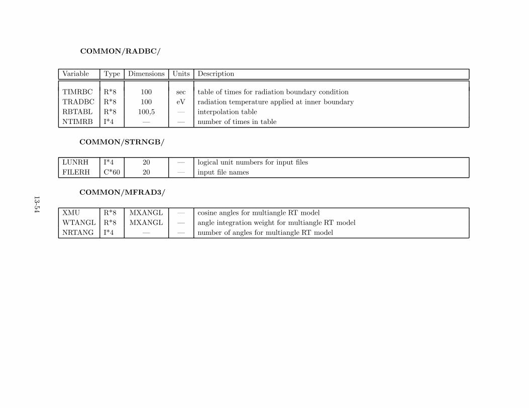
COMMON/RADBC/

Variable Type Dimensions Units Description

TIMRBC R*8 100 sec table of times for radiation boundary conditionTRADBC R*8 100 eV radiation temperature applied at inner boundaryRBTABL R*8 100,5 — interpolation tableNTIMRB I*4 — — number of times in table

COMMON/STRNGB/

LUNRH I*4 20 — logical unit numbers for input filesFILERH C*60 20 — input file names

COMMON/MFRAD3/

XMU R*8 MXANGL — cosine angles for multiangle RT modelWTANGL R*8 MXANGL — angle integration weight for multiangle RT modelNRTANG I*4 — — number of angles for multiangle RT model

13-54

COMMON/MFRAD2/

Variable Type Dimensions Units Description

FR1A R*8 MXZONS J/cm2/s radiation flux from variable Eddington modelFRFD1A R*8 MXGTAB J/cm2/s frequency-dependent radiation flux from variable Eddington model

MXZONSFRFD1C R*8 MXGTAB J/cm2/s frequency-dependent radiation flux from variable Eddington model

MXZONSRS2B R*8 MXZONS cmδ−1 (rδ−1)n+1

j−1/2)RAD R*8 MXZONS cmδ rδj − rδj−1

RD R*8 MXZONS cm (rn+1j − rn+1

j−1 )/2ED1 R*8 MXZONS — (1− f)/2fED3 R*8 MXZONS — (3f − 12)/2fA1 R*8 MXZONS g/cm2 2δ(σRj−1/2 + σRj+1/2)/2E R*8 — — used in the solution of the freq. dependent radiation energy densitiesF R*8 — — used in the solution of the freq. dependent radiation energy density

13-55

14. Input and Output Files

Table 14.1 lists the input, output and scratch files utilized by BUCKY-1. Also

listed are their logical unit numbers (LUN), names (for UNIX systems), types, and a brief

description of their contents. There are 7 types of input files. The main input file to be

used for all radiation-hydrodynamics calculations is ‘bucky.inp’. This is the NAMELIST

input file used to define the hydro problem (initial conditions, zoning, I/O, etc.). A detailed

description of the variables used in this file is given in Section 15.

The EOS and opacity data tables for each material are read in and stored in

COMMON at the beginning of the calculation. Unless an ideal gas EOS is used, the user

must supply these tables. The file name is given by ‘eos.dat.II.KK’, where ‘II’ is either

‘uw’ if a University of Wisconsin EOS table (EOSOPA or IONMIX) or ‘sm’ if a SESAME

table. The quantity ‘KK’ refers to the material ID — which is supplied by the user with the

NAMELIST input variable IZEOS. Typically, this can be the Z of the plasma. For example,

‘eos.dat.uw.13’ could be used to define the EOSOPA table for aluminum. However, any

integer could be used for any material. Using the material atomic number is simply a useful

convention if dealing with non-mixtures. The SESAME tables are assumed to be in their

“standard” ASCII format. A condensed listing of the SESAME EOS file for Al (No. 3717)

is given in Figure 5.2.

For simulating plasmas irradiated by intense ion beams, the user can specify the

beam parameters either in the namelist input file, or by supplying a file to be read in

(‘bucky.beam.dat’). This file is read in by the subroutine INIT3. Currently, the format of

this data file is specific to PBFA-II data generated from SOPHIA output [46]. However, the

code can easily be modified to read in time-dependent ion beam parameters in a different

format.

The file defined by the variable “filerh(1)” contains time-dependent radiation

temperatures which are applied at the “inner” (j = 1) boundary. This has been used

14-1

Table 14.1. BUCKY-1 Input and Output Files

UnitNumber Name Type Description

2 nltert.inp Input NAMELIST input for non-LTE CRE modules3 eos.dat.II.KK∗ Input EOSOPA (II=“uw”) or SESAME (II=“sm”) EOS/opacity data file4 rt.atom.dat.NN∗∗ Input Atomic structure and rate data for CRE calculations5 bucky.inp Input Hydro NAMELIST input file6 bucky.out Output Main ASCII output file8 bucky.bin Output Main binary output file (for plotting)10 bucky.beam.data Input Incident ion beam parameters11 xray.dat Input X-ray cross sections for cold material12 cre.popul.dat Output Monitors status of CRE calculation14 bucky.bd.dat Output Plottable boundary radiation flux data15 bucky.enrgy.dat Output Plottable energy conservation data16 bucky.regn.Ts.dat Output Average temperatures for each plasma region17 filerh(1)† Input Incident radiation flux at boundary18 pixsec.dat.NN∗∗ Input Photoionization cross sections for CRE calculation41 rate 1 Output Transition rate tables from CRE calculation42 rate 2 Output Rate coefficient tables from CRE calculation49 bucky.ppCRE Output Plasma parameters which are used by CRE code for computing

detailed spectra54 aul.scratch Scratch Scratch file for CRE input55 ioscratch Scratch Scratch file for hydro and CRE input58 rt.inp.debug Output Writes namelist input file for standalone CRE code (NLTERT)

70+JJ‡ bucky.regn.JJ.Avgs‡ Output Region-averaged quantities T, p, Z, dE/∂x, Jbeam, Ebeam∗KK = IZEOS (given in NAMELIST input; usually the atomic number)∗∗NN = atomic number†filerh(1) is defined in hydro NAMELIST input‡JJ = plasma region

14-2

to simulate the response of Al witness plates and Au foils to hohlraum radiation fields. The

file is read in by the subroutine INIT4 if the NAMELIST variable IRADBC=1. The format

simply assumes two-column data with 8 header records.

The file ‘xraydat’ contains x-ray cross sections for computing the deposition of x-rays

in cold (nonionized) material. The data are from Adams and Biggs [44]. The file is read

in if ISW(11)�=1. This data is generally used to determine the x-ray energy deposition in a

buffer gas and solid or liquid surfaces exposed to the x-rays from a high-gain ICF target.

When a non-LTE CRE calculation is performed the collisional and radiative data is

contained in 2 files: ‘rt.atom.dat.NN’ and ‘pixsec.dat.NN’, where NN is the atomic number

of the gas species. These data are generated using the ATBASE [20] suite of atomic physics

codes.

The primary output files are ‘bucky.out’ and ‘bucky.bin’. ‘bucky.out’ contains the

descriptive output, such as the temperature, density, pressure, etc. distributions at the

selected simulation times for output. Binary data used for plotting is written to ‘bucky.bin’.

This data is currently read in and plotted using our BUCKY PLOT post-processor, which

now features a easy-to-use graphical user interface for plotting.

Other output files of note include: ‘bucky.regn.Ts.dat’, which contains (mass-

weighted) average temperatures for each plasma region; ‘bucky.ppCRE’, which contains

hydro results to be read in and post-processed with our CRE code for detailed spectral

calculations; and ‘bucky.regnJJ.Avgs’ (JJ = region index), which contains several time-

dependent region-averaged quantities relevant to ion beam-heated targets.

14-3

15. NAMELIST Input Variables

The user defines the parameters of a problem with the namelist input file. Through

it, the user specifies the plasma constituents, initial conditions, zoning, time step controls,

radiation transport model parameters, ion or laser beam characteristics, fusion burn

parameters, and/or target chamber first wall properties. In addition, the user can specify

the frequency of plottable output, and request the printing of various debug output. With

the exception of parameters needed for a non-LTE line transport calculation, all of the

namelist variables are contained in the file ‘bucky.inp’. Non-LTE line transport variables

are contained in ‘nltert.inp’. Table 15.1 lists each of the namelist variable names, along

with their type, dimensions, units, and default values. Table 15.2 contains a list of control

switches (ISW) which are typically used to select various options. Table 15.3 defines elements

of CON, an array of real constants used throughout the code. Table 15.4 lists the debugging

array elements (IEDIT) and the subroutines in which they are utilized. Constants used in the

fusion burn package (CONTN) are given in Table 15.5. Tables 15.6, 15.7, and 15.8 define the

elements of ISWCRE, CONCRE, and IEDCRE, which are the non-LTE CRE counterparts

of ISW, CON, and IEDIT.

In regards to zoning, the subroutine ZONER4 currently provides the greatest

flexibility for setting up the spatial mesh. The grid is set up region by region. An example

of this is shown in Fig. 15.1. For a multilayer target, a region would normally consist of

a material layer. Note in Fig. 15.1 that there are 3 “materials” (Al, CH, and Au) and 4

“regions”. The material index is used to calculate properties of a plasma species (e.g., EOS

or opacity) while a region is used for setting up the zoning. In principle, each of the materials

in this example could be subdivided into multiple regions.

In ZONER4, each region is divided into 3 subregions (see bottom of Fig. 15.1). The

central portion consists of equal mass zones. The other subregion zone widths are based on

15-1

a constant mass progression factor (ZONFC1 and ZONFC3). Thus, in subregion 1:

∆mj+1 = ∆mj ∗ (1 + ZONFC1) ,

while in subregion 3:

∆mj−1 = ∆mj ∗ (1 + ZONFC3) .

This allows for setting up the spatial grid with progressively smaller zone widths near

boundaries. The total amount of mass in each region is defined with the input variable

REGMAS. REGMS1 and REGMS3 define the masses in the inner and outer subregions,

respectively. The mass in the central subregion is REGMAS–REGMS1–REGMS3. JMAX

is the total number of zones. JMN and JMX are the minimum and maximum zone indices

for each region. JZN1 and JZN3 are used to specify the number of zones in subregions 1 and

3, respectively. Several examples of input files are shown in Section 17.

15-2

Figure 15.1. Schematic illustration of spatial grid setup using subroutine ZONER4.

15-3

Region 1

CH

Material 2

Region 2

Al

Material 1

Region 3

Au

Material 3

Region 4

CH

Material 2

subregion2

subregion3

subregion1

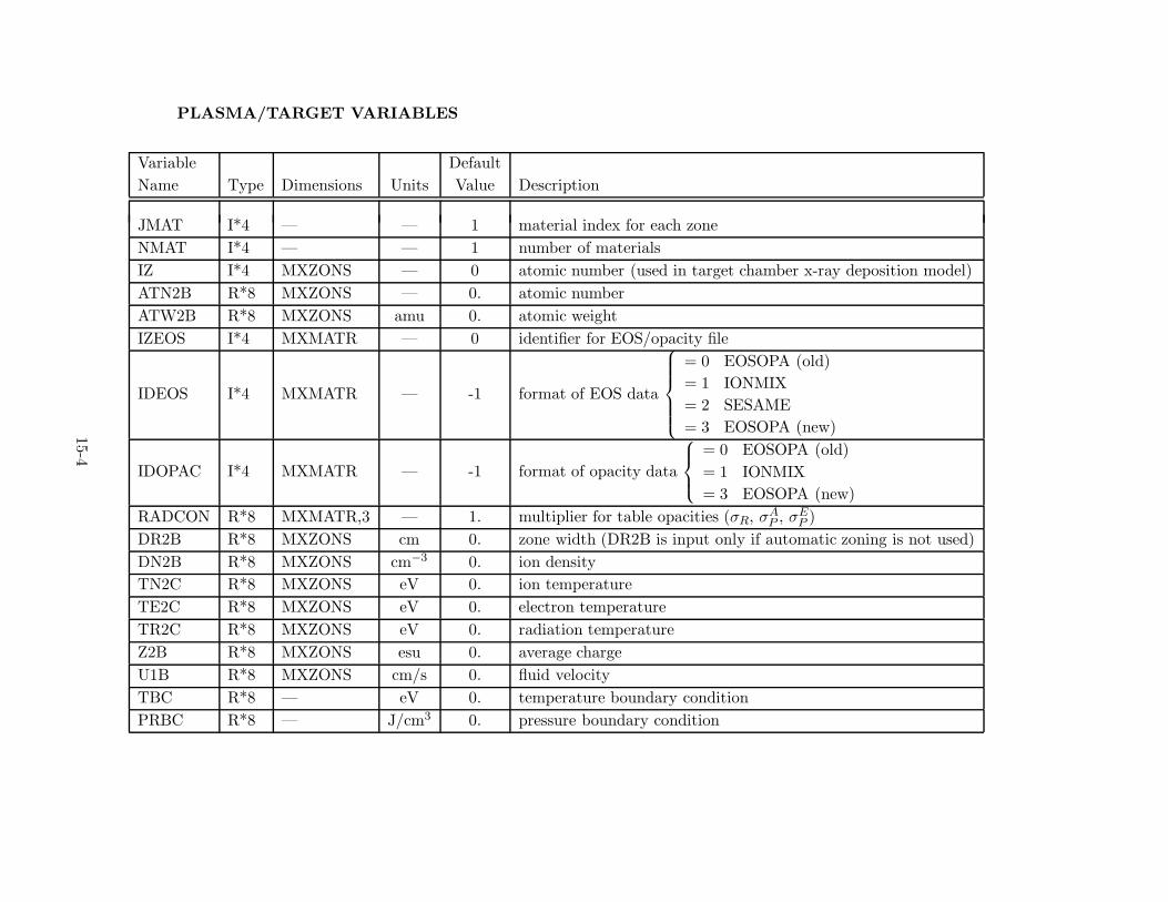
PLASMA/TARGET VARIABLES

Variable DefaultName Type Dimensions Units Value Description

JMAT I*4 — — 1 material index for each zoneNMAT I*4 — — 1 number of materialsIZ I*4 MXZONS — 0 atomic number (used in target chamber x-ray deposition model)ATN2B R*8 MXZONS — 0. atomic numberATW2B R*8 MXZONS amu 0. atomic weightIZEOS I*4 MXMATR — 0 identifier for EOS/opacity file

IDEOS I*4 MXMATR — -1 format of EOS data

= 0 EOSOPA (old)= 1 IONMIX= 2 SESAME= 3 EOSOPA (new)

IDOPAC I*4 MXMATR — -1 format of opacity data

= 0 EOSOPA (old)= 1 IONMIX= 3 EOSOPA (new)

RADCON R*8 MXMATR,3 — 1. multiplier for table opacities (σR, σAP , σ

EP )

DR2B R*8 MXZONS cm 0. zone width (DR2B is input only if automatic zoning is not used)DN2B R*8 MXZONS cm−3 0. ion densityTN2C R*8 MXZONS eV 0. ion temperatureTE2C R*8 MXZONS eV 0. electron temperatureTR2C R*8 MXZONS eV 0. radiation temperatureZ2B R*8 MXZONS esu 0. average chargeU1B R*8 MXZONS cm/s 0. fluid velocityTBC R*8 — eV 0. temperature boundary conditionPRBC R*8 — J/cm3 0. pressure boundary condition

15-4

ZONING VARIABLES

Variable DefaultName Type Dimensions Units Value Description

IDELTA I*4 — — 0 if 1, planar geometry; if 2, cylindrical geometry; if 3, spherical geometryJMAX I*4 — — 0 number of spatial zonesRADIUS R*8 — cm 0. target chamber radius (at J = JMAX)R1B R*8 MXZONS cm 0. zone boundary positionsRINNER R*8 — cm 0. inner radius of zone J = 1NVREGN I*4 — — 0 number of vapor (plasma) regionsNCREGN I*4 — — 0 number of solid/liquid regionsJMN I*4 MXREGN — 0 minimum zone index of each regionJMX I*4 MXREGN — 0 maximum zone index of each regionREGMAS R*8 MXREGN g/x∗ 0. region massZONFAC R*8 MXREGN — 0. mass progression factor: (∆mj+1 = ∆mj * (1 + ZONFAC))JZN1 I*4 MXREGN — 0 number of zones in inner subregionJZN3 I*4 MXREGN — 0 number of zones in outer subregionREGMS1 R*8 MXREGN g/x∗ 0. mass in inner subregionREGMS3 R*8 MXREGN g/x∗ 0. mass in outer subregionZONFC1 R*8 MXREGN — 0. mass progression factor for inner subregionZONFC3 R*8 MXREGN — 0. mass progression factor for outer subregion∗x = cm2 for planar, cm for cylindrical geometry.

15-5

INPUT/OUTPUT VARIABLES

Variable DefaultName Type Dimensions Units Value Description

IO I*4 31 — -1 output controller for text file:(1) hydrodynamic quantities(2) energy conservation(3) number densities(4) short edit(5) multifrequency radiation(6) fusion burn(9)CRE post-processing

IOBIN I*4 — — -1 binary output frequencyNFDOUT I*4 — — 1 number of binary outputs per frequency-dependent binary outputIOCREG I*4 — — 0 region index for CRE post-processing outputFILERH C*60 20 — — file names for input:

(1) TR(t) at inner boundaryTPROUT R*8 500 sec 1040 output simulation times (if ISW(66) = 1)DTPOUT R*8 500 sec -1. if > 0, TPROUT = TPRBEG + (i – 1) * DTPOUTTPRBEG R*8 500 sec 0. if > 0, TPROUT = TPRBEG + (i – 1) * DTPOUTTPBOUT R*8 500 sec 1040 binary output simulation times (if ISW(66) = 1)DTBOUT R*8 500 sec -1. if > 0, TPBOUT = TPBBEG + (i – 1) * DTBOUTTPBBEG R*8 500 sec 0. if > 0, TPBOUT = TPBBEG + (i – 1) * DTBOUT

15-6

TIME CONTROL VARIABLES

Variable DefaultName Type Dimensions Units Value Description

NMAX I*4 — — 0 maximum number of hydro time stepsTMAX R*8 — sec 0. maximum simulation timeDTB R*8 — sec 1.e-12 initial time stepTA R*8 — sec 0. initial simulation timeDTMIN R*8 — sec 10−1 * DTB minimum time stepDTMAX R*8 — sec 10−2 * TMAX maximum time stepTSCC R*8 — sec 0.05 time step control – CourantTSCTN R*8 — sec 0.05 time step control – ∆Ti/TiTSCTE R*8 — sec 0.05 time step control – ∆Te/TeTSCTR R*8 — sec 0.1 time step control – ∆ER/ER

TSCV R*8 — sec 0.05 time step control – ∆V/V

TGROW R*8 — sec 1.5 limits time step growth to TGROW * DTBDTVAZ R*8 — sec 0. vaporization time step controlTSPEC R*8 — sec -1. special times for time step resetDTSPEC R*8 — sec 0. value of time step reset

15-7

RADIATION TRANSPORT VARIABLES

Variable DefaultName Type Dimensions Units Value Description

IRAD I*4 — — 2 radiation transport model:0 ⇒ no radiation transport1 ⇒ Eddington factor model2 ⇒ diffusion model3 ⇒ multiangle short characteristics model

NFG I*4 — — 0 number of frequency groupsIRADBC I*4 — — 0 flag or radiation at boundary:

0 ⇒ no incident radiation1 ⇒ read data from ‘filerh(1)’

IRADEF I*4 — — 1 boundary condition flag for Eddington factor modelNRTANG I*4 — — 2 number of angles used in multiangle RT model

15-8

ION DEPOSITION VARIABLES

Variable DefaultName Type Dimensions Units Value Description

IBEAM I*4 — — 0 ion beam flag:0 ⇒ no ion beam1 ⇒ outward moving beam2 ⇒ inward moving beam

ANION R*8 MXIDPX — 0. atomic number of ionsAWION R*8 MXIDPX amu 0. atomic weight of ionsQ1MIN R*8 MXIDPX esu 0. minimum charge state for ionsQ1INIT R*8 MXIDPX esu 1. initial charge state for ionsTIONIN R*8 MXIDPX sec 0. time grid for ion beam inputEIONIN R*8 MXIDPT keV 0. kinetic energy per ion

MXIDPEMXIDPX

XIONIN R*8 MXIDPT ions/s/x 0. ion beam fluxMXIDPEMXIDPX

NIT I*4 — — 200 number of ion time binsNIE I*4 — — 1 number of ion energy binsNIX I*4 — — 1 number of ion speciesNQTDEP I*4 — — 5 number of charge states considered in time-dependent

projectile charge model∗x = cm2 for planar, cm for cylindrical geometry.

15-9

LASER DEPOSITION VARIABLES

Variable DefaultName Type Dimensions Units Value Description

ILASER I*4 — — 0 if > 0, compute laser energy deposition

FUSION BURN VARIABLES

ITN I*4 — — 0 If 0, no fusion burn calculation;if 1, only DT reactions;if 2, DT and DD reactions;if 3, DT, DD, and DHe3 reactionsif < 0 (-1, -2, or -3) fusion burn calculations starts after Tion > CONTN(1)

NZBURN I*4 — — 0 number of zones where fusion reaction products are startedNABURN I*4 — — 3 number of angles for fusion reaction productsNAP I*4 — — 1 number of angles with µ > 0 in which fusion reaction products

are startedIBETA I*4 — — 2 number of time levels that charged particles starting in µ ≤ 0

are followedDTTNMN R*8 — shakes 10−4 minimum time step allowed for fusion burn cycleJMAXTN I*4 — — JMAX maximum zone index containing fuelDD2B R*8 MXZONS cm−3 0. deuterium number densityDT2B R*8 MXZONS cm−3 0. tritium number densityDO2B R*8 MXZONS cm−3 0. number density of non-DT speciesATWO R*8 MXZONS amu 0. atomic weight of non-DT speciesZO2B R*8 MXZONS esu 0. mean charge of non-DT species

15-10

FUSION BURN VARIABLES (Continued)

Variable DefaultName Type Dimensions Units Value Description

LHE4 I*4 — — 2 switches to control transport method for 3.5 MeV alphas,LHE3 I*4 — — 1 0.82 MeV He3, 3.02 MeV protons, 1.01 MeV tritons,LP I*4 — — 1 3.6 MeV alphas, and 14.7 MeV protons:LT I*4 — — 1 1 ⇒ local depositionLHE4S I*4 — — 1 2 ⇒ time-dependent particle trackingLPS I*4 — — 1NG I*4 — — 0 number of energy groups used to accumulate escaping charged

particle spectrum (used when ISW(22) �= 0)CPEN R*8 100 keV 0. lower energy boundary of groups used to accumulate charged

particle spectrum (used when ISW(22) �= 0)IRBORN I*4 MXZONS — 1 zone indices where charged particles are started

(must be NZBURN of these)INBORN I*4 MXZONS — 1 zone indices where charged particles containing fuel are started

(must be JMAXTN of these)

15-11

WALL VAPORIZATION VARIABLES

Variable DefaultName Type Dimensions Units Value Description

NCZONS I*4 — — 0 number of Lagrangian cells in the condensed regionRHOCND R*8 — g/cm3 0. mass density of the condensed regionXKCOND R*8 — J/cm/s/eV 0. thermal conductivity of the condensed regionQHEATV R*8 — J/g 0. specific heat of vaporization of the condensed regionCPHEAT R*8 — J/g/eV 0. specific heat of the condensed regionIZFILM R*8 — — 0. atomic number of the condensed regionAWFILM R*8 — amu 0. atomic weight of condensed regionTVAP0 R*8 — eV 0. vaporization temperature at 1 barTWALLB R*8 — eV 0. temperature at the back of the condensed regionDELXC R*8 MXZONS cm 0. zone widths for the condensed regionTCN2C R*8 MXZONS eV 0. temperatures in the condensed regionDELXCT R*8 — cm 0. total width of the condensed region

15-12

X-RAY DEPOSITION VARIABLES

Variable DefaultName Type Dimensions Units Value Description

FLUX R*8 — J 0. the total energy of a blackbody x-ray spectrumNXRG I*4 — — 25 the number of energy groups in the x-ray spectrumKEV R*8 — keV 0. the blackbody temperature of a blackbody x-ray spectrumXEHIST R*8 101 keV 0. the bounds of energy groups in an arbitrary histogramXAMP R*8 100 J/keV 0. the amplitude of the groups of an arbitrary histogramCONFAC R*8 2,2 — 1. density multiplier in x-ray deposition calculationNXRT I*4 — — 0 number of mesh times in time-dependent x-ray historyXRTIM R*8 20 sec 0. mesh times in time-dependent x-ray historyTDXAMP R*8 100,20 J/keV-S 0. time-dependent x-ray amplitudes; in this 2-dimensional

matrix, the first index is the frequency group and the secondis the time index

15-13

MISCELLANEOUS VARIABLES

Variable DefaultName Type Dimensions Units Value Description

ISW I*4 100 — Table 15.2 control switchesCON R*8 100 — Table 15.3 array of constantsIEDIT I*4 100 — -1 debugging switches (see Table 15.4)IBENCH I*4 20 — 0 switches for benchmark calculationsCONTN R*8 20 — Table 15.5 constants used in fusion burn model

INITIALIZATION FLAG FOR CRE CALCULATION

NLTEID I*4 MXREGN — 0 non-LTE radiative transfer (RT) flag(if > 0, use CRE RT model for line transport)15-14

CRE ATOMIC MODEL PARAMETERS

Variable DefaultName Type Dimensions Units Value Description

NGASES I*4 MXREGN — 1 number of gas species (maximum number = MXGASS)ATOMNM R*8 MXGASS — 0. atomic numberATOMWT R*8 MXGASS amu 0. atomic weightFRACSP R*8 MXZONS, — 1 for igas=1 fractional concentration of gases in each zone

MXGASS 0 for igas>1Example for homogeneous binary plasma with 20 zones:

FRACSP(1,1) = 20*0.5FRACSP(1,2) = 20*0.5

Example for layered plasma:FRACSP(1,1) = 10*1., 10*0.FRACSP(1,2) = 10*0., 10*1.

KGASRG I*4 MXGASS, — 0 gas species indexMXREGN

SPREGN R*8 MXGASS, — 0. SPREGN[KGASRG(igas,iregn),iregn] = fractional gas abundanceMXREGN

WIZMIN R*8 MXGASS, — 0. parameter for ionization window minimumWIZMAX R*8 MXGASS, — 0. parameter for ionization window maximumISELCT I*4 MXLVLI, — 0 array to select atomic levels from atomic data files

MXGASS 1 ⇒ on (or select); 0 ⇒ off (default)

CRE RADIATIVE TRANSFER PARAMETERS

ILINEP I*4 — — 1 line profile type (1 ⇒ Doppler; 2 ⇒ Lorentz; 3 ⇒ Voigt)ISWCRE (7) I*4 100 — 0 compute photoexcitation if equal to 0ISWCRE (8) I*4 100 — 0 compute photoionization if equal to 0

15-15

OTHER CRE PARAMETERS

Variable DefaultName Type Dimensions Units Value Description

SeeCONCRE R*8 100 — Table 15.6 array of constants (see Table 15.6)ISWCRE I*4 100 — 0 array of integer switches (see Table 15.7)IEDCRE I*4 100 — 0 array of edit (debugging) flags (see Table 15.8)IBENCH I*4 20 — 0 array used for benchmark test calculations

IBENCH(3) = 1: 2-level atom with κ ∝ r−2

2: 2-level atom with κ ∝ r−2 and Bν ∝ r−2

IPLOT I*4 30 — 0 array of plot switches (currently not used)

CRE CONVERGENCE PARAMETERS

ERRMXF R*8 — — 1.e-3 maximum error allowed in fractional populationsduring convergence procedure

IMAXSE I*4 — — 40 maximum number of iterations during convergence procedureCRSWCH R*8 20 — 1.0 collisional-radiative switching parameters

(used in subroutine STATEQ; see [35])(generally not needed for laboratory plasmas)

NGCYCL I*4 — — 4 apply Ng acceleration every NGCYCL’th cycleNGORDR I*4 — — 2 order of Ng accelerationNGBEGN I*4 — — 0 iteration cycle at which to begin Ng acceleration

15-16

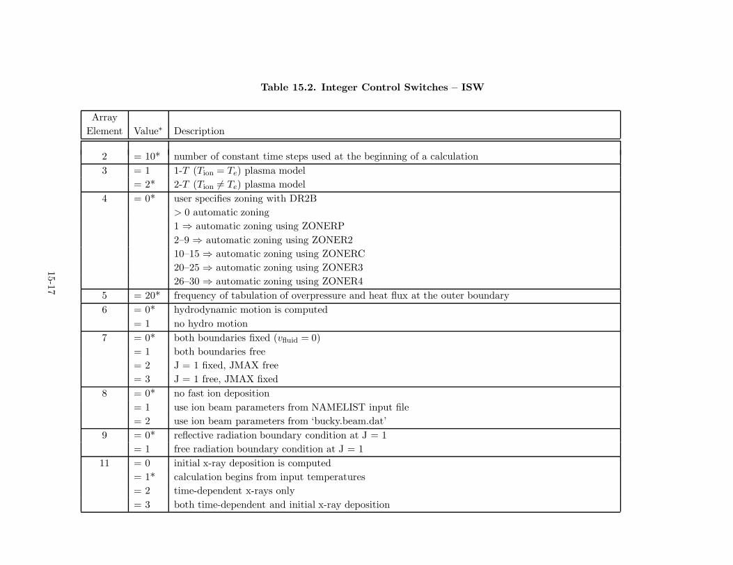
Table 15.2. Integer Control Switches – ISW

ArrayElement Value∗ Description

2 = 10* number of constant time steps used at the beginning of a calculation3 = 1 1-T (Tion = Te) plasma model

= 2* 2-T (Tion �= Te) plasma model4 = 0* user specifies zoning with DR2B

> 0 automatic zoning1 ⇒ automatic zoning using ZONERP2–9 ⇒ automatic zoning using ZONER210–15 ⇒ automatic zoning using ZONERC20–25 ⇒ automatic zoning using ZONER326–30 ⇒ automatic zoning using ZONER4

5 = 20* frequency of tabulation of overpressure and heat flux at the outer boundary6 = 0* hydrodynamic motion is computed

= 1 no hydro motion7 = 0* both boundaries fixed (vfluid = 0)

= 1 both boundaries free= 2 J = 1 fixed, JMAX free= 3 J = 1 free, JMAX fixed

8 = 0* no fast ion deposition= 1 use ion beam parameters from NAMELIST input file= 2 use ion beam parameters from ‘bucky.beam.dat’

9 = 0* reflective radiation boundary condition at J = 1= 1 free radiation boundary condition at J = 1

11 = 0 initial x-ray deposition is computed= 1* calculation begins from input temperatures= 2 time-dependent x-rays only= 3 both time-dependent and initial x-ray deposition

15-17

Table 15.2. (Continued)

ArrayElement Value∗ Description

12 = 0* equation of state tables are used= 1 ideal gas equation of state is used; CON(5) must be input via NAMELIST

13 = 0* no quiet start= 1 use quiet start option; CON(19) defines temperature at which hydro starts

16 = 0* if negative temperature is found, print it and stop> 0 if negative temperature is found, fix it and print out every ISW(16)’th cycle.

20 = 0* no condensation or vaporization= 2 calculate vaporization of first surface

21 = 0* left-over particles in the TDPT algorithm are forced to stop by allowing them to transportuntil they stop or escape

= 1 left-over particles are ignored (forgotten)22 = 0* no escaping charged particle spectrum is computed

= 1 an alpha particle spectrum is computed (CPEN specifies the energy groups, NG specifies thenumber of groups)

23 = 0* start charged particle reaction products in each zone= 1 group charged particle starting zones according to the indices in INBORN and IRBORN

24 = 0* use table look up to compute 〈σv〉 (SIGMAV) for DT, DD, DHe3

= 1 use analytic formulas to compute 〈σv〉 (SIGMAV) for DT, DD, DHe3

25 = 0* redistribute energy in wall vaporization model= 2 do not redistribute energy

27 = 0* get P and P -derivatives from EOS tables= 1 compute P and P -derivative from Z

28 = 0* get Cv from specific energy table= 1 get Cv from table lookup

15-18

Table 15.2. (Continued)

ArrayElement Value∗ Description

29 = 0* get (dE/dV )T from specific energy table< 0 get (dE/dV )T from ENNTAB table> 0 get (dP/dT )V from PNTTAB table

30 = 0* use input values for properties of film= 1 calculate properties of film

31 = 0* use Q1INIT (= constant) for ion charge in ion deposition calculations= 1 compute time-dependence of debris ion charge states

32 = 0* no debris ion mass added to vapor cells= 1 add debris ion mass to vapor cells as ions stop

34 = 0* no electron thermal flux limit is used= 1 classical flux limit is used

38 = 0* calculate variable Eddington factor= 1 use CON(38) for Eddington factor

48 = 0* calculate ion stopping (dE/dx)= 1 use CON(48) for ion stopping (dE/dx)

50 = 0* no non-LTE CRE line radiation transport= 1 use non-LTE CRE model for line radiation transport (automatically set by NLTEID)

66 = 0* output results based on number of hydro cycles= 1 output results based on simulation time

71 = 0* use 1st order method for short characteristics radiation transport= 1 use 2nd order method for short characteristics radiation transport

77 = 0* get Z2B from table lookup= 1 compute Z2B from ZO2B in NUMDEN

∗An asterisk indicates default value.

15-19

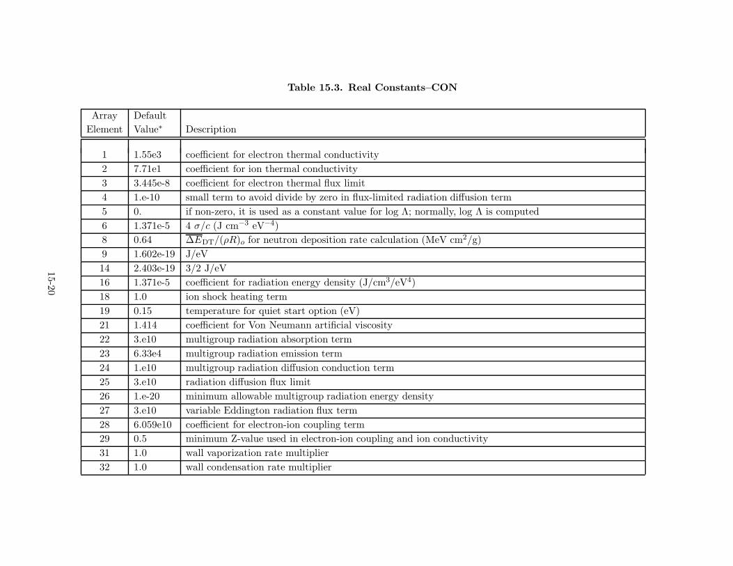
Table 15.3. Real Constants–CON

Array DefaultElement Value∗ Description

1 1.55e3 coefficient for electron thermal conductivity2 7.71e1 coefficient for ion thermal conductivity3 3.445e-8 coefficient for electron thermal flux limit4 1.e-10 small term to avoid divide by zero in flux-limited radiation diffusion term5 0. if non-zero, it is used as a constant value for log Λ; normally, log Λ is computed6 1.371e-5 4 σ/c (J cm−3 eV−4)8 0.64 ∆EDT/(ρR)o for neutron deposition rate calculation (MeV cm2/g)9 1.602e-19 J/eV14 2.403e-19 3/2 J/eV16 1.371e-5 coefficient for radiation energy density (J/cm3/eV4)18 1.0 ion shock heating term19 0.15 temperature for quiet start option (eV)21 1.414 coefficient for Von Neumann artificial viscosity22 3.e10 multigroup radiation absorption term23 6.33e4 multigroup radiation emission term24 1.e10 multigroup radiation diffusion conduction term25 3.e10 radiation diffusion flux limit26 1.e-20 minimum allowable multigroup radiation energy density27 3.e10 variable Eddington radiation flux term28 6.059e10 coefficient for electron-ion coupling term29 0.5 minimum Z-value used in electron-ion coupling and ion conductivity31 1.0 wall vaporization rate multiplier32 1.0 wall condensation rate multiplier

15-20

Table 15.3. (Continued)

Array DefaultElement Value∗ Description

33 0. vaporization/condensation flux correction34 31.2 coefficient for reducing condensation rate due to presence of a non-condensable gas35 1. charge exchange cross section multiplier for fast ion energy deposition36 0. mass progression factor for automatic zoning in ZONER2 and ZONERC.37 0. mass progression multiplier for condensed region38 0.333 if ISW(38) = 1 or planar geometry, use for variable Eddington factor42 1. multiplier for (dE/dx) in ion stopping model43 1. multiplier for intensities in cold x-ray deposition model44 1. multiplier for ion beam current (flux) densities in ion stopping45 2.0 ion thermal velocity term47 1. relative debris ion velocity term48 0. if ISW(48) = 1, use constant (dE/dx) (eV cm2/ion)75 1. multiplier for radiation temperature boundary condition77 1. multiplier for fusion charged particle deposition rate80 35.e-9 collapse time for implosion benchmark calculation (sec)81 7.5e9 laser intensity for implosion benchmark calculation (J/s)82 0.96 time constant for implosion benchmark calculation

15-21

Table 15.4. Debugging Switches

Array Subroutine Writing Array Subroutine Writing Array Subroutine WritingElement Debug Output Element Debug Output Element Debug Output

32 ABCPL1 14 HYDROD 17 RADTR11 ABCPL2 50 IONDEP 17 RADTR162 ABCRD1 85 IZIAIT 17 RADTR221 ABCRD2 37 JZONE 17 RADTR346 CPSPEC 47 LOCAL 26 RCOND54 DEDX 36 NEGTCK 83 RMUV

39,40 DELTAV 19 NUMDEN 65,67 SHORTC18 DEPLET 9 OMEGAC 45 SIGMAV

51,91 ECHECK 64 OPACMG 86 SLOW52 EDEPOS 90 OUT3 13 TABLE263 EDFACT 31 PCOND1 13 TABLE420 EMISSN 31 PCOND2 13 TABLEO42 ENEMA 27 PLSCF1 16 TEMPBC35 ENERGY 27 PLSCF2 81 TNBURN24 EOS 12 POINT 44 TNREAC41 EOS1 12 POINTO 43 TNSLOW38 FDS 17,22 RADCOF 33,34 TRANSP7 GASDEP 66 RADDEN 55 WALLVP

15-22

Table 15.5. Description of Constants in Vector – CONTN

CONTN Value Description

1 4.EO lower limit on Ti for computing thermonuclear reactions. Also if ITN < 1 then after Tibecomes greater than this, the thermonuclear calculation is started

2 6.9325E-13 coefficient for thermal velocity used in SLOW3 8.35E-46 coefficient for charged particle slowing down on electrons SLOWE4 6.67E-69 coefficient for charged particle slowing down on ions SLOWI5 1.E22 lower limit on D and T density for computing thermonuclear reactions – to avoid

computations where very few reactions will occur6 2.EO value of DTTNMN used to force particles to slow down in TRANSP (see ISW(21))7 .666EO correction for average chord length in 1st zone when only 3 directions are used; this is

used in zone 1 when only 3 directions are used to avoid having all particles traversethe zone along its full diameter

8 .5EO when fast charged particlesthermalize in a zone, this fraction of the lost energy is givento the electrons and the rest is given to the ions

9 .98EO when the cosine of the direction angle is > CONTN(9) it is set to 1 so that square rootcalculations are avoided in RMUV

10 .7939EO fraction of radius of first zone where particles are started. One half of the first zone mass isinside this radius and the other half is outside this radius

11 1.EO fraction of charged particles deposited in local deposition option12 1.EO fraction of T that burn in flight due to beam-plasma nonthermal reactions13 1.EO fraction of He3 that burn in flight due to beam-plasma nonthermal reactions

15-23

Table 15.6. Control Switches - ISWCRE

ArrayElement Value* Description

6 0* Start with populations from previous hydro time step1 Start with LTE populations2 Start with coronal populations3 Return LTE populations4 Return coronal populations

7 0* Include photoexcitation effects in calculation of atomic level populations8 0* Include photoionization effects in calculation of atomic level populations20 0* Non-LTE equation of state: E = Eion + Ee + Eiz

1 E = Eion + Ee + Eiz + Edegen

2 E = Eion + Ee + Eiz + EDH

3 E = Eion + Ee + Eiz + Edegen + EDH

23 0* Compute Voigt parameter1 Set Voigt parameter = CONCRE (23)2 Estimate T and avoigt from rate coefficients

30 0 Compute g in Stark width calculation1* Set g = 0.2 in Stark width calculation

34 0* Use LAPACK matrix scaling1 Use LAPACK + NLTERT matrix scaling

38 0* No equation of state calculation1 Compute internal energy and pressure (Not currently an option)

39 0* No multigroup opacity calculation1 Compute multigroup opacities (Not currently an option)

99 0* Dump output and stop when ill-conditioned matrix is encountered*An asterisk (*) indicates default value.

15-24

Table 15.7. Real Constants - CONCRE

Array DefaultElement Value Description

6 1.e-30 Minimum value of fractional level population12 0.1 Scaling parameter for statistical equilibrium matrix elements19 1.e-5 Minimum fractional population used to test convergence20 1.0 Multiplier for natural line width21 1.0 Multiplier for Doppler line width22 1.0 Multiplier for Stark line width23 1.0 Multiplier for Voigt profile broadening parameter (see also ISWCRE (23))24 1.0 Multiplier for ion dynamic broadening

(hydrogenic Lyman series)26 1.0 Multiplier for bound-bound opacity27 1.0 Multiplier for bound-free opacity28 1.0 Multiplier for free-free opacity42 1.0 Multiplier for collisional deexcitation rate43 1.0 Multiplier for spontaneous emission rate45 1.0 Multiplier for collisional recombination rate46 1.0 Multiplier for radiative recombination rate47 1.0 Multiplier for dielectronic recombination rate57 0.3 Minimum value of ∆E/T for ionization windowing58 30. Maximum value of ∆E/T for ionization windowing

15-25

Table 15.8. Debugging Switches - IEDCRE

Array Element Subroutine Writing Debug Output

7 ABSEMS18 CCSLAB18 CLSLAB

12,55 GETCF112,55 GETCF216 GETPOP78 GPOPAC48 IIXSEC44 INITC2

28,29 INNLTE32 IZWNDO61 LINEPR

66,80 LINWID62 LODCB162 LODCB2

11,27 LOPACS1,14,54 MATRX0

77 MESHMG78 MGOPAC34 NGACCL63 NLPOPS41 RATCOF

47,81 READA26,15 STATEQ92 VOIGT81 WSTARK

15-26

16. Compiling and Running

In this section, we briefly describe how to set up BUCKY-1 for running a calculation.

Figure 16.1 shows an example MAKEFILE for this procedure. We start with the source

(“.src”) files for each subroutine and the file containing the common blocks. At the top

of the comdecks file are 2 “*define” statements: “*define hp” and “*define double”. The

first is used to specify the platform for running. Options are “hp” for HP workstations,

“sun” for SUN workstations, “rs6” for IBM RS6000 workstations, and “cray” for CRAY

supercomputers. This tells the preprocessor to look for machine-dependent strings in the

source code, and load them into the FORTRAN deck (“.f” files). An example of this is

the time and date of the calculations, which are printed out at the top of the output. The

second string, “double”, refers to double precision for variables beginning with A-H and O-Z.

This is highly recommended for 32-bit workstations. For 64-bit machines such as a CRAY

supercomputer, single precision (“*define single”) should be adequate.

Near the top of the MAKEFILE are two directories for the source code files, and

one for the destination directory (“destdir”) where the user will run the calculation. The

first source directory (“dold”) is the location of files for the latest “base”, or version, of

BUCKY-1 (base 7 in the example). The second contains files which have been modified from

the base version. The sequence of commands at the end of the MAKEFILE — subroutine

by subroutine — run the preprocessor (using a simple “update” algorithm) to create a “.f”

file, which is then compiled. Any compilation errors are written to a file named “Errs”.

The user can specify compilation flags on the ‘make’ command line. This is most

easily done using an ‘alias’ command. For example, one can define aliases such as (for ksh

shell);

alias mkb=’rm -f Errs; make “FFLAGS=+E1 +T -g -C” -f Bucky.make bucky.exe; more Errs’

alias mkbf=’rm -f Errs; make “FFLAGS=+E1 +T +O1” -f Bucky.make bucky.exe.opt; more Errs’

16-1

Figure 16.1. Example MAKEFILE for BUCKY-1.

16-2

Then, by simply typing “mkb” or “mkbf” from the source decks directory, one gets either

an executable which can be used with a debugger “a.out”, or an optimized executable

“a.out.opt”. These files are placed in the directory specified by “destdir” at the top of

the MAKEFILE.

16-3

17. Sample Calculations

In this section, we show example input decks for 5 calculations. Also shown are

some selected results which the user can compare with to check if the code is installed and

running properly. The examples are: (1) the isentropic compression of a DT shell; (2) a

shock breakout simulation for a radiatively-driven Al witness plate; (3) a LIBRA implosion

simulation; (4) the fusion burn and breakup of a LIBRA target; and (5) a simulation of the

response of a non-LTE target chamber buffer gas to a high-gain ICF microexplosion.

17.1. Example 1: Isentropic Compression of a DT Shell

This is a calculation performed to benchmark the code against the previously

published results of Kidder [47]. The input file is shown in Figure 17.1. IBENCH(1) =

−2 indicates this is a “benchmark” calculation in which a specific time-dependent pressure

boundary condition is applied. It also specifies that the initial temperature and density

distributions be set up as in the Kidder [47] calculation. The inner radius (RINNER) of

the shell is 0.12 cm in this spherically symmetric (IDELTA = 3) calculation. An ideal gas

EOS is used (ISW(12) > 0) for DT (ATW2B = 2.5). Z2B = 1 specifies that the DT is fully

ionized. No radiation transport is considered (IRAD = 0). CON(80), CON(82) and PRBC

are used to specify the time-dependent pressure at the outer boundary. The calculation is

run out to a simulation time (DTMAX) of 18.15 ns.

The zoning option used (ISW(4) = 26 ⇒ subroutine ZONER4 is used) divides the

plasma into 1 region (NVREGN = 1) and 3 sub-regions (see Sec. 15 for a discussion of

this zoning option). The mass of the DT is 75 µg, which is usually specified directly with

REGMAS. However, because the densities are readjusted after the zoning takes place (at

present, this occurs only for this series of implosion benchmark calculations), the number

specified by REGMAS in this case is not the true region mass, but was adjusted to give

75 µg with the density profile given by Kidder.

17-1

Figure 17.1. Example input file for implosion benchmark calculation.

17-2

Figure 17.2 shows Lagrangian zone positons as a function of time from the BUCKY-1

simulation (3 plot on the left). On the right are the results of Kidder. Note that the

trajectories of the DT zones are very similar in the 2 calculations, including the time of void

closure.

17.2. Example 2: Al Witness Plate Shock Breakout

This is a simulation of a shock breakout experiment involving an Al witness plate

attached to the side of a high-Z hohlraum. The namelist input file is shown in Figure 17.3.

The hohlraum radiation field is represented by a time-dependent radiation boundary

condition (IRADBC = 1), which is currently a 1-T Planckian spectrum, TR(t). The input

file for TR(t) is ‘SNL.Al.burn.dat’. Note that the file input values are multiplied by 1.06

(CON(75)).

Radiation is transported using the multiangle short characteristics model (IRAD

= 3). Two angles are used (NRTANG). The EOS/opacity data utilized is generated by

EOSOPA [5], (IDEOS and IDOPAC = 0), and is contained in the file ‘eos.dat.uw.13’ (IZEOS

= 13). The mass of the Al foil is 0.0486 g/cm2, which corresponds to a thickness of 180 µm.

The initial conditions are T = 0.1 eV (TN2C) and solid density (DN2B = 6.0e22).

Results from this calculation are shown in Figure 17.4. Also shown are shock breakout

data from NOVA experiments performed by R. Olson [48].

17.3. Example 3: LIBRA Implosion Simulation

Figure 17.5 shows an example input file which could be used to run an implosion

calculation for a high-gain light ion-driven target. (This is not meant to be a “working”

target, but only to illustrate how to set up the input file.) The target is a spherical (IDELTA

= 3) multi-material target composed of an inner DT layer of 5 mg (REGMAS(1) = 5.e-3), a

CH ablator of 9.08 mg, a C foam layer of 17.4 mg (which is zoned up as 2 regions: a 6.9 mg

17-3

Figure 17.2. Lagrangian zone positions vs. time for implosion benchmark calculation. Left:BUCKY-1 results; Right: Kidder [47] results.

17-4

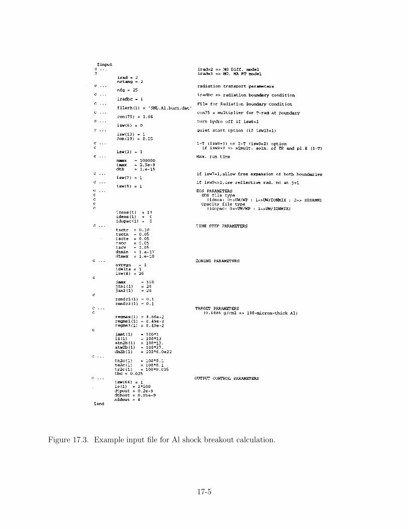
Figure 17.3. Example input file for Al shock breakout calculation.

17-5

Figure 17.4. Lagrangian zone positions vs. time for Al shock breakout calculation.

17-6

Figure 17.5. Example input file for LIBRA implosion calculation.

17-7

inner and 10.5 mg outer component), and an Au case of 240 mg. There are 40 spatial zones

(JMAX) and the array JMAT is used to specify the material index for each zone (1 ⇒ DT,

2 ⇒ CH, 3 ⇒ C, 4 ⇒ Au). The EOS/opacity file of each material is identified by its atomic

number (see IZEOS), except for CH, where the data has been put in ‘eos.dat.uw.05’.

The initial temperature throughout the target is 0.1 eV (TN2C and TE2C). The

density distributions are specified by DN2B. Note that DN2B should equal the sum of DD2B

(deuterium), DT2B (tritium), and DO2B (“other”; i.e., non-DT).

Radiation is transported using a 20-group (NFG) radiation diffusion (IRAD = 2)

model.

This has an inward-propagating (IBEAM) ion beam composed of fully charged Li

ions (ANION, AWION, Q1INIT). The variables TIONIN, EIONIN, and XIONIN specify a

40 ns, 30 TW foot and a 20 ns, 300 TW main pulse of 30 MeV Li ions.

Figure 17.6 shows the beam energy deposition in the target at simulation times of 20,

40, 50, and 60 ns. The range shortening due to hot stopping can be easily seen.

17.4. LIBRA Fusion Burn and Target Breakup

Figure 17.7 shows the input file for a LIBRA target breakup [7] simulation. The

composition of the target is similar to that in the above example. The main difference from

above is that the initial conditions are meant to be approximately representative of those at

the start of ignition. The DT shell is divided into 3 regions, with a central high-temperature

core (TN2C = 8000 eV, DN2C = 1.2e25 cm−3), surrounded by 2 lower temperature, but

higher density DT regions. The DT is surrounded by layers of CH, C, and Pb. In this

calculation there is no ion beam as the target starts at conditions capable of sustaining DT

burn.

The fusion burn package is turned on (ITN = 1). There are 10 burn zones (NZBURN)

and the number of angles used in the charged particle tracking algorithm (NABURN) is 3.

17-8

Figure 17.6. Time-integrated ion energy deposition profiles for LIBRA implosion simulation.

17-9

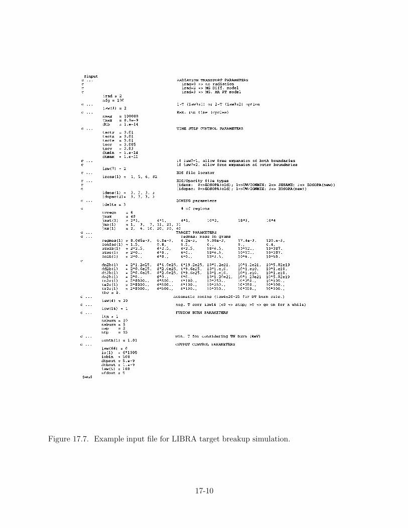
Figure 17.7. Example input file for LIBRA target breakup simulation.

17-10

Sample results for the frequency-dependent x-ray output and the overall energy

partitioning are shown in Figure 17.8.

17.5. Example 5: Target Chamber Non-LTE Buffer Gas Simulation

Figure 17.9 shows the input file for a target chamber calculation involving a non-LTE

buffer gas. The target chamber has a radius (RADIUS) of 6.5 meters, and is filled with a

Ne buffer gas (ATN2B = 10, ATW2B = 20) of density 3.54 × 1016 cm3 (≈ 1 torr at room

temperature). The solid first wall (NCZONS = 40) is composed of graphite (RHOCND

= 2.26 g/cm3; IZFILM = 6). Vaporization of the first wall material is modelled by setting

ISW(20) = 2. The x-ray flux from the target located at the center of the chamber is specified

by XEHIST and XAMP using a model with 48 frequency groups (NXRG). The values in the

x-ray flux array XAMP are multiplied by CON(43). The target debris ions expand radially

outward (IBEAM = 1) in a 5 ns square pulse. EIONIN and IONIN specify the ion kinetic

energies and particle fluxes. Four different ion species (NIX) are considered (protons, “DT”,

He, and C) for this direct-drive target.

Radiation for the continum is transported using a 20-group (NFG) diffusion model

(IRAD=2). For this calculation, the opacity tables were generated without any contributions

from bound-bound transitions. Line radiation is treated separately using a non-LTE CRE

model (NLTEID = 1). When this option is used, a second namelist file, ‘nltert.inp’, is read

in containing the atomic modeling and radiation transport parameters (see Figure 17.10). A

total of 108 atomic energy levels was selected for this calculation (sum of non-zero ISELCT

elements). Detailed results from calculations of this type are described elsewhere [13].

17-11

Figure 17.8. Time-integrated x-ray output and energy partitioning from LIBRA targetbreakup simulation.

17-12

Figure 17.9. Example input file (‘bucky.inp’) for non-LTE buffer gas simulation.

17-13

Figure 17.10. Non-LTE atomic data input file (‘nltert.inp’) for non-LTE buffer gas

simulation.

17-14

References[1] Moses, G.A., “PHD-IV — A Plasma Hydrodynamics, Thermonuclear Burn, Radiative

Transfer Computer Code,” University of Wisconsin Fusion Technology Institute ReportUWFDM-194 (Revised August1985).

[2] Moses, G.A., Peterson, R.R., and McCarville, T.J., “MFFIRE - A MultifrequencyRadiative Heat Transfer Hydrodynamics Code,” Computer Physics Communications36, 249 (1985).

[3] Peterson, R.R., MacFarlane, J.J., and Moses, G.A., “CONRAD — A CombinedHydrodynamics–Condensation/Vaporization Computer Code,” University of WisconsinFusion Technology Institute Report UWFDM-670 (Revised July 1988).

[4] MacFarlane, J.J., “NLTERT — A Code for Computing the Radiative Properties of Non-LTE Plasmas,” University of Wisconsin Fusion Technology Institute Report UWFDM-931 (December 1993).

[5] Wang, P., “EOSOPA — A Code for Computing the Equations of State and Opacitiesof High Temperature Plasmas with Detailed Atomic Models,” University of WisconsinFusion Technology Institute Report UWFDM-933 (December 1993).

[6] Badger, B., et al., “HIBALL — A Conceptual Heavy Ion Beam Fusion Reactor Study,”University of Wisconsin Fusion Technology Institute Report UWFDM-625 (December1984).

[7] MacFarlane, J.J., Moses, G.A., Wang, P., Sawan, M.E., and Peterson, R.R., “NumericalSimulation of Target Microexplosion Dynamics for the LIBRA-SP Inertial ConfinementFusion Reactor,” University of Wisconsin Fusion Technology Institute Report UWFDM-973 (December 1994).

[8] Peterson, R.R., Moses, G.A., MacFarlane, J.J., and Wang, P., Fusion Technology 26,780 (1994).

[9] Wang, P., MacFarlane, J.J., Moses, G.A., and Mehlhorn, T.A., “Atomic PhysicsCalculations in Support of Numerical Simulations of High Energy Density Plasmas,”presented at the 36th Annual Meeting of the APS Division of Plasma Physics,Minneapolis, MN (November 1994).

[10] Peterson, R.R., Simmons, K., MacFarlane, J.J., Wang, P., and Moses, G.A., “ComputerSimulations of the Debris and Radiation Emission from an Ignited NIF Target,”presented at the 36th Annual Meeting of the APS Division of Plasma Physics,Minneapolis, MN (November 1994).

[11] MacFarlane, J.J., Wang, P., Peterson, R.R., and Moses, G.A., presentations at LawrenceLivermore National Laboratory and Los Alamos National Laboratory (1995).

[12] J.J. MacFarlane and P. Wang, Phys. Fluids B3, 3494 (1991).

18-1

[13] MacFarlane, J.J., Peterson, R.R., Wang, P., and Moses, G.A., Fusion Technology 26,886 (1994).

[14] MacFarlane, J.J., Moses, G.A., and Peterson, R.R., Phys. Fluids B1, 635 (1989).

[15] Peterson, R.R., in “Laser Interaction and Related Plasma Phenomena, Vol. 7,” editedby H. Hora and G. Miley, Plenum Publ. Corp., p. 591 (1986).

[16] Peterson, R.R., Fusion Technology 13, 279 (1988).

[17] Bailey, J.E., et al., in preparation (1995).

[18] MacFarlane, J.J., Wang, P., Chung, H.K., and Moses, G.A., “Spectral Diagnostics, IonStopping Power, and Radiation-Hydrodynamics Modeling in Support of Sandia LightIon Beam Fusion Experiments,” University of Wisconsin Fusion Technology InstituteReport UWFDM-979 (April 1995).

[19] MacFarlane, J.J. and Cassinelli, J.P., Astrophys. J. 347, 1090 (1989).

[20] Wang, P., “ATBASE Users’ Guide,” University of Wisconsin Fusion TechnologyInstitute Report UWFDM-942 (December 1993).

[21] Melhorn, T.A. “A Finite Material Temperature Model for Ion Energy Deposition inIon-Driven ICF Targets,” SAND80-0038, Sandia National Laboratories, Albuquerque,NM, May 1980; also J. Appl. Phys. 52, 6522 (1981).

[22] Richtmyer, R.D. and Morton, K.W., Difference Methods for Initial Value Problems,Interscience Publishers, New York (1967).

[23] Spitzer, L., Physics of Fully Ionized Gases, Second Edition, Interscience Publishers,New York (1962).

[24] Anderson, E., et al., LAPACK Users’ Guide (SIAM, Philadelphia, 1992).

[25] MacFarlane, J.J., Astron. Astrophys. 264, 153 (1992).

[26] Ng, K.C., J. Chem. Phys. 61, 2680 (1974).

[27] Auer, L., in Numerical Radiative Transfer, edited by W. Kalkoten, CambridgeUniversity Press, Cambridge, U.K. (1987), p. 101.

[28] Apruzese, J.P., Davis, J., Duston, D., and Whitney, K.G., J.Q.S.R.T. 23, 479 (1980).

[29] Apruzese, J.P., J.Q.S.R.T. 25, 419 (1981).

[30] Apruzese, J.P., J.Q.S.R.T. 34, 447 (1985).

[31] Mihalas, D., Stellar Atmospheres, Second Edition, Freeman and Company, New York(1978).

[32] Burgess, A. and Chidichchimo, M.C., Mon. Not. R. Astron. Soc. 203, 1269 (1983).

18-2

[33] Seaton, M.J., in Atomic and Molecular Processes, edited by D.R. Bates, Academic, NewYork (1962) p. 374.

[34] Sobelman, I.I., Vainshtein, L.A., and Yukov, E.A., Excitation of Atoms andBroadening of Spectral Lines, Springer-Verlag, New York (1981).

[35] Post, D.E., Jensen, R.V., Tarter, C.B., Grasberger, W.H., and Lokke, W.A., At. DataNucl. Data Tables 20, 397 (1977).

[36] MacFarlane, J.J. , “IONMIX - A Code for Computing the Equation of State andRadiative Properties of LTE and Non-LTE Plasmas,” Comput. Phys. Commun. 56,259 (1989).

[37] “SESAME: The Los Alamos National Laboratory Equation of State Database,” LANLReport LA-UR-92-3407, edited by S.P. Lyon and J.D. Johnson (1992).

[38] Lindhard, J. and Scharff, M., “Energy Dissipation by Ions in the keV Range,” Phys.Rev. 124, 128 (1961).

[39] Knudson, H., Haugen, H.K., and Hvelplund, P., “Single-Electron-Capture CrossSections for Medium and High Velocity, Highly Charged Ions Colliding with Atoms,”Phys. Rev. A23 , 597 (1981).

[40] Hyman, E., Mulbrandon, M., and Giuliani, J.L., “Charge Exchange Cross SectionUpdate,” ETHANL Proceedings No. 7, SRI International, Menlo Park, CA, July 1987.

[41] Duderstadt, J.J., and Moses, G.A., Inertial Confinement Fusion (Wiley, New York,1982), p. 145.

[42] Goel, B., and Henderson, D.L., “A Simple Method to Calculate Neutron EnergyDeposition in ICF Targets,” Kernforschungszentrum Karlsruhe Report No. KfK-4142(1986).

[43] McCarville, T.J., Moses, G.A., and Kulcinski, G.L., “A Model for Depositing InertialConfinement Fusion X-Rays and Pellet Debris Into a Cavity Gas,” University ofWisconsin Fusion Technology Institute Report UWFDM-406 (April 1981).

[44] Adams, K.G. and Biggs, F., “Efficient Computer Access to Sandia Photon CrossSections II,” SC-RR-71-0507, Sandia Laboratory, Albuquerque, NM, December 1971.

[45] Labuntov, D.A., and Kryukov, A.P., Int. J. Heat Mass Transfer 22, 989 (1979).

[46] Haill, T.A., private communication (1995).

[47] Kidder, R.E., Nucl. Fusion 16, 3 (1976).

[48] Olson, R.E., private communication (1994).

18-3