UvA-DARE is a service provided by the library of the University of Amsterdam (http://dare.uva.nl) UvA-DARE (Digital Academic Repository) Micro-level stochastic loss reserving Antonio, K.; Plat, H.J. Link to publication Citation for published version (APA): Antonio, K., & Plat, R. (2010). Micro-level stochastic loss reserving. Amsterdam: Universiteit van Amsterdam. General rights It is not permitted to download or to forward/distribute the text or part of it without the consent of the author(s) and/or copyright holder(s), other than for strictly personal, individual use, unless the work is under an open content license (like Creative Commons). Disclaimer/Complaints regulations If you believe that digital publication of certain material infringes any of your rights or (privacy) interests, please let the Library know, stating your reasons. In case of a legitimate complaint, the Library will make the material inaccessible and/or remove it from the website. Please Ask the Library: http://uba.uva.nl/en/contact, or a letter to: Library of the University of Amsterdam, Secretariat, Singel 425, 1012 WP Amsterdam, The Netherlands. You will be contacted as soon as possible. Download date: 07 Jul 2018

Welcome message from author
This document is posted to help you gain knowledge. Please leave a comment to let me know what you think about it! Share it to your friends and learn new things together.
Transcript
UvA-DARE is a service provided by the library of the University of Amsterdam (http://dare.uva.nl)
UvA-DARE (Digital Academic Repository)
Micro-level stochastic loss reserving
Antonio, K.; Plat, H.J.
Link to publication
Citation for published version (APA):Antonio, K., & Plat, R. (2010). Micro-level stochastic loss reserving. Amsterdam: Universiteit van Amsterdam.
General rightsIt is not permitted to download or to forward/distribute the text or part of it without the consent of the author(s) and/or copyright holder(s),other than for strictly personal, individual use, unless the work is under an open content license (like Creative Commons).
Disclaimer/Complaints regulationsIf you believe that digital publication of certain material infringes any of your rights or (privacy) interests, please let the Library know, statingyour reasons. In case of a legitimate complaint, the Library will make the material inaccessible and/or remove it from the website. Please Askthe Library: http://uba.uva.nl/en/contact, or a letter to: Library of the University of Amsterdam, Secretariat, Singel 425, 1012 WP Amsterdam,The Netherlands. You will be contacted as soon as possible.
Download date: 07 Jul 2018

Micro–level stochastic loss reserving
Katrien Antonio ∗ Richard Plat †
June 4, 2010
Abstract
1 To meet future liabilities general insurance companies will set–up reserves. Predicting
future cash–flows is essential in this process. Actuarial loss reserving methods will help themto do this in a sound way. The last decennium a vast literature about stochastic loss reserving
for the general insurance business has been developed. Apart from few exceptions, all of
these papers are based on data aggregated in run–off triangles. However, such an aggregatedata set is a summary of an underlying, much more detailed data base that is available to the
insurance company. We refer to this data set at individual claim level as ‘micro–level data’.We investigate whether the use of such micro–level claim data can improve the reserving
process. A realistic micro–level data set on liability claims (material and injury) from a
European insurance company is modeled. Stochastic processes are specified for the variousaspects involved in the development of a claim: the time of occurrence, the delay between
occurrence and the time of reporting to the company, the occurrence of payments and their
size and the final settlement of the claim. These processes are calibrated to the historicalindividual data of the portfolio and used for the projection of future claims. Through an out–
of–sample prediction exercise we show that the micro–level approach provides the actuarywith detailed and valuable reserve calculations. A comparison with results from traditional
actuarial reserving techniques is included. For our case–study reserve calculations based on
the micro–level model are to be preferred; compared to traditional methods, they reflect realoutcomes in a more realistic way.
1 Introduction
We develop a micro–level stochastic model for the run–off of general insurance (also called
‘non–life’ or ‘property and casualty’) claims. Figure 1 illustrates the run–off (or development)
process of a general insurance claim. It shows that a claim occurs at a certain point in time
(t1), consequently it is declared to the insurer (t2) (possibly after a period of delay) and one or
several payments follow until the settlement (or closing) of the claim. Depending on the nature
of the business and claim, the claim can re–open and payments can follow until the claim finally
settles.
At the present moment (say τ) the insurer needs to put reserves aside to fulfill his liabilities
in the future. This actuarial exercise will be denoted as ‘loss’ or ‘claims reserving’. Insurers, share
holders, regulators and tax authorities are interested in a rigorous picture of the distribution of
future payments corresponding with open (i.e. not settled) claims in a loss reserving exercise.
General insurers distinguish between RBNS and IBNR reserves. ‘RBNS’ claims are claims that are
∗University of Amsterdam, Roetersstraat 11, 1018 WB Amsterdam, The Netherlands, email: [email protected].
Katrien Antonio acknowledges financial support from the The Actuarial Foundation and from NWO through a Veni
2009 grant.†University of Amsterdam, Eureko/Achmea Holding and Netspar, email: [email protected] authors would like to thank Jan–Willem Vulto and Joris van Kempen for supplying and explaining the data.
Please note that the original frequency and severity data have been transformed for reasons of confidentiality.
1

Figure 1: Development of a general insurance claim
t1 t2 t3 t4 t5 t6 t7 t8 t9
Occurrence
Notification
Loss payments
Closure
Re–opening
Payment
Closure
IBNR
RBNS
Reported to the insurer But Not Settled, whereas ‘IBNR’ claims Incurred But are Not Reported
to the company. For an RBNS claim occurrence and declaration take place before the present
moment and settlement occurs afterwards (i.e. τ ≥ t2 and τ < t6 (or τ < t9) in Figure 1). An
IBNR claim has occurred before the present moment, but its declaration and settlement follow
afterwards (i.e. τ ∈ [t1, t2) in Figure 1). The interval [t1, t2] represents the so–called reporting
delay. The interval [t2, t6] (or [t2, t9]) is often referred to as the settlement delay. Data bases
within general insurance companies typically contain detailed information about the run–off
process of historical and current claims. The structure in Figure 1 is generic for the kind of
information that is available. In this paper we will use the label ‘micro–level’ data to denote this
sort of data structures.
With the introduction of Solvency 2 (in 2012) and IFRS 4 Phase 2 (in 2013) insurers face
major challenges. IFRS 4 Phase 2 will define a new accounting model for insurance contracts,
based on market values of liabilities. In the document “Preliminary Views on Insurance Con-
tracts” (May 2007, discussion paper) the IASB (‘International Accounting Standards Board’)2
states that an insurer should base the measurement of all its insurance liabilities (for reserving)
on ‘best estimates’ of the contractual cash flows, discounted with current market discount rates.
On top of this, a margin that market participants are expected to require for bearing risk should
be added to this.
Solvency 2 will lead to a change in the regulatory required solvency capital for insurers.
Depending on the type of business, at this moment this capital requirement is a fixed percentage
of the mathematical reserve, the risk capital, the premiums or the claims. Under Solvency 2 the
so–called Solvency Capital Requirement (‘SCR’) will be risk–based, and market values of assets
and liabilities will be the basis for these calculations.
The measurement of future cash flows and its uncertainty thus becomes more and more
important. That also gives rise to the question whether the currently used techniques can be
improved. In this paper we will address that question for general insurance. Currently, reserving
for general insurance is based on data aggregated in run–off triangles. In a run–off triangle
observable variables are summarized per arrival year and development year combination. The
term arrival year (‘AY’) or year of occurrence is used by general actuaries to indicate the year in
which the accident took place. For a claim from AY t its first development year will be year titself, the second development year is t + 1 and so on. An example of a run–off triangle is given
in Table 3 and 4. A vast literature exists about techniques for claims reserving, largely designed
2http://www.iasb.org/NR/rdonlyres/08C8BB09-61B7-4BE8-AA39-A1F71F665135/0/InsurancePart1.pdf
2

for application to loss triangles. An overview of these techniques is given in England and Verrall
(2002), Wuthrich and Merz (2008) or Kaas et al. (2008). These techniques can be applied to
run–off triangles containing either ‘paid losses’ or ‘incurred losses’ (i.e. the sum of paid losses
and case reserves).
The most popular approach is the chain–ladder approach, largely because of is practicality.
However, the use of aggregated data in combination with the chain–ladder approach gives rise
to several issues. A whole literature on itself has evolved to solve these issues, which are (in
random order):
(1) Different results between projections based on paid losses or incurred losses, addressed by Quarg
and Mack (2008), Postuma et al. (2008) and Halliwell (2009).
(2) Lack of robustness and the treatment of outliers, see Verdonck et al. (2009).
(3) The existence of the chain–ladder bias, see Halliwell (2007) and Taylor et al. (2003).
(4) Instability in ultimate claims for recent arrival years, see Bornhuetter and Ferguson (1972).
(5) Modeling negative or zero cells in a stochastic setting, see Kunkler (2004).
(6) The inclusion of calendar year effects, see Verbeek (1972) and Zehnwirth (1994).
(7) The possibly different treatment of small and large claims, see Wuthrich and Alai (2009).
(8) The need for including a tail factor, see for example Mack (1999).
(9) Over parametrization of the chain–ladder method, see Wright (1990) and Renshaw (1994).
(10) Separate assessment of IBNR and RBNS claims, see Schnieper (1991) and Liu and Verrall (2009).
(11) The realism of the Poisson distribution underlying the chain–ladder method.
(12) When using aggregate data, lots of useful information about the claims data remains unused, as
noted by England and Verrall (2002) and Taylor and Campbell (2002).
Most references above present useful additions to or comments on the chain–ladder method,
but these additions cannot all be applied simultaneously. More importantly, the existence of
these issues and the substantial literature about it indicate that the use of aggregate data in
combination with the chain–ladder technique (or similar techniques) is not always adequate for
capturing the complexities of stochastic reserving for general insurance.
England and Verrall (2002) and Taylor and Campbell (2002) questioned the use of aggre-
gate loss data when the underlying extensive micro–level data base is available as well. With
aggregate data, lots of useful information about the claims data remain unused. Covariate in-
formation from policy, policy holder or the past development process cannot be used in the
traditional stochastic model, since each cell of the run–off triangle is an aggregate figure. Quot-
ing England and Verrall (2002) (page 507) “[. . . ] it has to be borne in mind that traditional
techniques were developed before the advent of desktop computers, using methods which could be
evaluated using pencil and paper. With the continuing increase in computer power, it has to be
questioned whether it would not be better to examine individual claims rather than use aggregate
data.”.
As a result of the observations mentioned above, a small stream of literature has emerged
about stochastic loss reserving on an individual claim level. Arjas (1989), Norberg (1993) and
Norberg (1999) formulated a mathematical framework for the development of individual claims.
Using ideas from martingale theory and point processes, these authors present a probabilistic,
rather than statistical, framework for individual claims reserving. Haastrup and Arjas (1996)
continue the work by Norberg and present a first detailed implementation of a micro–level
3

stochastic model for loss reserving. They use non–parametric Bayesian techniques which may
complicate the accessibility of the paper. Furthermore, their case study is based on a small data
set with fixed claim amounts. Recently, Larsen (2007) revisited the work of Norberg, Haastrup
and Arjas with a small case–study. Zhao et al. (2009) and Zhao and Zhou (2010) present
a model for individual claims development using (semi–parametric) techniques from survival
analysis and copula methods. However, a case study is lacking in their work.
In this paper micro-level stochastic model is used to quantify the reserve and its uncertainty
for a realistic general liability insurance portfolio. Stochastic processes for the occurrence times,
the reporting delay, the development process and the payments are fit to the historical individual
data of the portfolio and used for projection of future claims and its (estimation and process)
uncertainty. Both the Incurred But Not Reported (IBNR) reserve as well as the Reported But Not
Settled (RBNS) reserve are quantified and the results are compared with those of traditional
actuarial techniques.
We investigate whether the quality of reserves and their uncertainty can be improved by
using more detailed claims data instead of the classical run–off triangles. Indeed, a micro–level
approach allows much closer modeling of the claims process. Lots of the above mentioned is-
sues will not exist when using a micro–level approach, because of the availability of lots of data
and the potential flexibility in modeling the future claims process. For example, covariate infor-
mation (e.g. deductibles, policy limits, calendar year) can be included in the projection of the
cash flows when claims are modeled at an individual level. The use of lots of (individual) data
avoids robustness problems and over parametrization. Also the problems with negative or zero
cells and setting the tail factor are circumvented, and small and large claims can be handled
simultaneously. Furthermore, individual claim modeling can provide a natural solution for the
dilemma within the traditional literature whether to use triangles with paid claims or incurred
claims. This dilemma is important because practicing actuaries put high value to their compa-
nies’ expert opinion which is expressed by setting an initial case reserve. Incurred payments are
the sum of paid losses and these case reserves. Using micro–level data we use the initial case
reserve as a covariate in the projection process of future cash flows.
The remainder of the paper is organized as follows. First, the data set is introduced in
Section 2. In Section 3 the statistical model is described. Results from estimating all components
of the model are in Section 4. Section 5 presents the prediction routine and in Section 6 we give
results and a comparison with traditional actuarial techniques. Section 7 concludes.
2 Data
The data set used in this paper contains information about a general liability insurance portfolio
(for private individuals) of a European insurance company. The available data consist of the
exposure per month from January 2000 till August 2009, as well as a claim file that provides a
record of each claim filed with the insurer from January 1997 till August 2009. Note that we are
missing exposure information for the period January 1997 till December 1999, but the impact
of this lack on our reserve calculations will be very small.
Exposure The exposure is not the number of policies, but the ‘earned’ exposure. That implies
that two policies which are both only insured for half of the period are counted as 1. Figure 2
shows the exposure per month. Note that the downward spikes correspond to the month Febru-
ary.
4

Figure 2: Available exposure per month
from January 2000 till August 2009.
0 20 40 60 80 100 120
4000
050
000
6000
070
000
8000
0
Exposure
January 2000 (t=0) − August 2009 (t=116)
expo
sure
Random development processes The claim file
consists of 1,525,376 records corresponding with
491,912 claims. Figure 3 shows the development
of three claims, taken at random from our data set.
It shows the timing of events as well as the cost of
the corresponding payments (if any). These are in-
dicated as jumps in the figure. Starting point of the
development process is the accident date. This is
indicated with a sub-title in each of the plots and
corresponds with the point x = 0. The x-axis is in
months since the accident date. The y-axis repre-
sents the cumulative amount paid for the claim.
Figure 3: Development of 3 random claims from the data set.
0 2 4 6 8
050
010
0015
0020
00
time since origin of claim (in months)
Development of claim 327002
Acc. Date 15/03/2006
−1 0 1 2 3 4
050
010
0015
0020
00
time since origin of claim (in months)
Development of claim 434833
Acc. Date 01/10/2008
0 5 10 15
020
040
060
080
0
time since origin of claim (in months)
Development of claim 216542
Acc. Date 05/02/2003
Rep. DelayPaymentSettlement
Type and number of claims In this general liability portfolio, we have to deal with two types
of claims: material damage (‘material’) and bodily injury (‘injury’).
Figure 4: Number of open and closed claims of type material (left) and injury (right).
Number of Material Claims
Arrival Year
# cl
aim
s
1998 2000 2002 2004 2006 2008
2800
032
000
3600
040
000 # Claims
Closed Claims
Number of Injury Claims
Arrival Year
# cl
aim
s
1998 2000 2002 2004 2006 2008
600
700
800
900
# ClaimsClosed Claims
Figure 4 shows the number of claims per arrival year, and whether they are closed or still open
(at the end of August 2009). The development pattern and loss distributions of these claim types
5

are usually very different. In practice they are therefore treated separately in separate run–off
triangles. Following this approach, we will treat them separately too.
Reporting and settlement delay Important drivers of the IBNR and RBNS reserves are the
reporting delays and settlement delays. Figure 5 shows the reporting delays for material and
injury claims. The reporting delay is the time that passes between the occurrence date of the
accident and the date it was reported to the insurance company. It is measured in months since
occurrence of the claim. Of course, the reporting delay is only available for claims that have been
reported to the insurer at the present moment. Figure 5 shows the settlement delay separately
for injury and material claims. The settlement delay is the time elapsed between the reporting
date of the claim and the date of final settlement by the company. It is measured in months and
only available for closed claims. These figures show that the observed reporting delays are of
similar length for material and injury losses. However, the settlement delay is very different.
The settlement delay is far more skewed to the right for the injury claims than for the material
claims.
Figure 5: Upper: reporting delay for material (left) and injury (right) claims. Lower: settlement
delay for material (left) and injury (right) claims.
Reporting Delay: Material
in months since occurrence
Fre
quen
cy
0 1 2 3 4 5 6
050
000
1000
0020
0000
3000
00
Reporting Delay: Injury
in months since occurrence
Fre
quen
cy
0 1 2 3 4 5 6
010
0020
0030
0040
00
Settlement Delay: Material
in months since occurrence
Fre
quen
cy
0 10 20 30 40 50
050
000
1500
0025
0000
Settlement Delay: Injury
in months since occurrence
Fre
quen
cy
0 10 20 30 40 50
050
010
0015
00
6
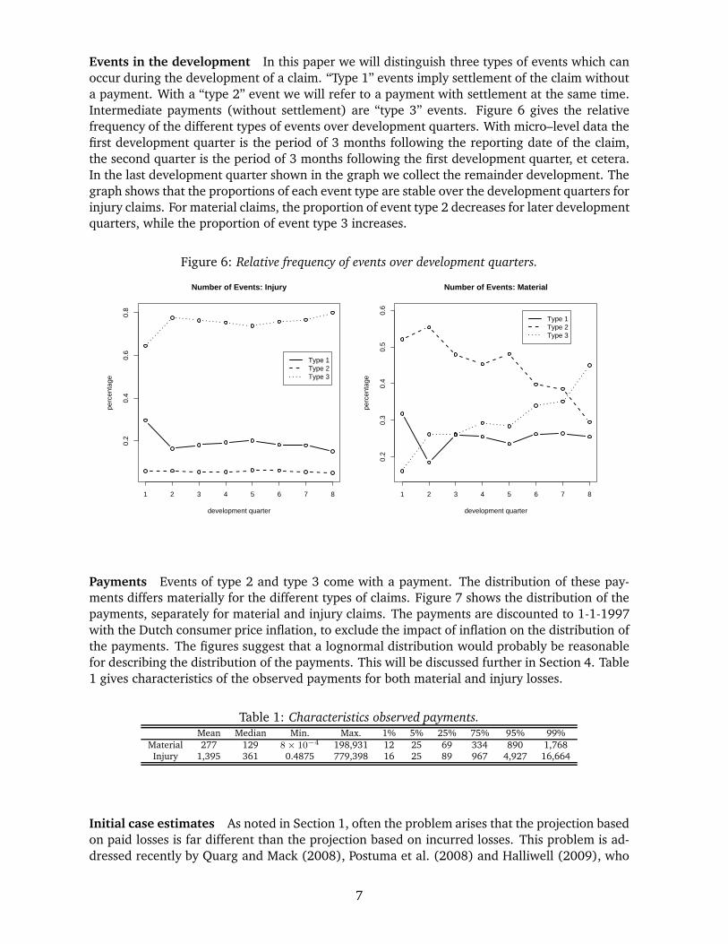
Events in the development In this paper we will distinguish three types of events which can
occur during the development of a claim. “Type 1” events imply settlement of the claim without
a payment. With a “type 2” event we will refer to a payment with settlement at the same time.
Intermediate payments (without settlement) are “type 3” events. Figure 6 gives the relative
frequency of the different types of events over development quarters. With micro–level data the
first development quarter is the period of 3 months following the reporting date of the claim,
the second quarter is the period of 3 months following the first development quarter, et cetera.
In the last development quarter shown in the graph we collect the remainder development. The
graph shows that the proportions of each event type are stable over the development quarters for
injury claims. For material claims, the proportion of event type 2 decreases for later development
quarters, while the proportion of event type 3 increases.
Figure 6: Relative frequency of events over development quarters.
1 2 3 4 5 6 7 8
0.2
0.4
0.6
0.8
Number of Events: Injury
development quarter
perc
enta
ge
Type 1Type 2Type 3
1 2 3 4 5 6 7 8
0.2
0.3
0.4
0.5
0.6
Number of Events: Material
development quarter
perc
enta
ge
Type 1Type 2Type 3
Payments Events of type 2 and type 3 come with a payment. The distribution of these pay-
ments differs materially for the different types of claims. Figure 7 shows the distribution of the
payments, separately for material and injury claims. The payments are discounted to 1-1-1997
with the Dutch consumer price inflation, to exclude the impact of inflation on the distribution of
the payments. The figures suggest that a lognormal distribution would probably be reasonable
for describing the distribution of the payments. This will be discussed further in Section 4. Table
1 gives characteristics of the observed payments for both material and injury losses.
Table 1: Characteristics observed payments.Mean Median Min. Max. 1% 5% 25% 75% 95% 99%
Material 277 129 8 × 10⁻⁴ 198,931 12 25 69 334 890 1,768Injury 1,395 361 0.4875 779,398 16 25 89 967 4,927 16,664
Initial case estimates As noted in Section 1, often the problem arises that the projection based
on paid losses is far different than the projection based on incurred losses. This problem is ad-
dressed recently by Quarg and Mack (2008), Postuma et al. (2008) and Halliwell (2009), who
7

Figure 7: Distribution of payments for material (right) and injury (left) claims.
Material Payments
Log scale
Fre
quen
cy
0 2 4 6 8 10
050
0010
000
2000
030
000
Injury Payments
Log scale
Fre
quen
cy
0 2 4 6 8 10 12 14
050
010
0015
00simultaneously model paid and incurred losses. Disadvantage of those methods is that models
based on incurred losses can be instable because the methods for setting the case reserves are
often changed (for example, as a result of adequacy test results or profit policy of the company).
Reserving models that are directly based on these case reserves (as part of the incurred losses)
can therefore be instable. However, the case reserves may have added value as an explain-
ing variable when projecting future payments. We have defined different categories of initial
case reserves (separately for material claims and injury claims) that can be used as explanatory
variables. Table 2 shows the number of claims, the average settlement delay (in months) and
the average cumulative paid amount for these categories. The table clearly shows the differ-
ences in settlement delay and cumulative payments for the different initial reserve categories.
Therefore, it might be worthwhile to include these categories as explanatory variables in the
prediction routine.
Table 2: Initial reserve categories.Material Injury
Initial Average Average Cum. Initial Average Average Cum.Case Reserve # claims settl. delay payments Case Reserve # claims settl. delay payments
(months) (months)
≤ 10, 000 465,015 1.87 252 ≤ 1, 000 3,709 9.87 2,570> 10, 000 385 10.88 7,950 (1,000 -15,000] 5,165 15.17 3,872
> 15, 000 360 35.2 33,840
3 The statistical model
By a claim i is understood a combination of an occurrence time Ti, a reporting delay Ui and a
development process Xi. Hereby Xi is short for (Ei(v), Pi(v))v∈[0,Vi]. Ei(vij) := Eij is the type
of the jth event in the development of claim i. This event occurs at time vij, expressed in time
units after notification of the claim. Vi is the total waiting time from notification to settlement
for claim i. If the event includes a payment, the corresponding severity is given by Pi(vij) := Pij .
The different types of events are specified in Section 2. The development process Xi is a jump
8

process. It is modeled here with two separate building blocks: the timing and type of events and
their corresponding severities. The complete description of a claim is given by:
(Ti, Ui,Xi) with Xi := (Ei(v), Pi(v))v∈[0,Vi]. (1)
Assume that outstanding liabilities are to be predicted at calendar time τ . We distinguish
IBNR, RBNS and settled claims.
• for an IBNR claim: Ti + Ui > τ and Ti < τ ;
• for an RBNS claim: Ti+Ui ≤ τ and the development of the claim is censored at (τ−Ti−Ui),i.e. only (Ei(v), Pi(v))v∈[0,τ−Ti−Ui] is observed;
• for a settled claim: Ti + Ui ≤ τ and (Ei(v), Pi(v))v∈[0,Vi] is observed.
3.1 Position dependent marked Poisson process
Following the approach in Arjas (1989) and Norberg (1993) we treat the claims process as
a Position Dependent Marked Poisson Process (PDMPP), see Karr (1991). In this application,
a point is an occurrence time and the associated mark is the combined reporting delay and
development of the claim. We denote the intensity measure of this Poisson process with λand the associated mark distribution with (PZ|t)t≥0. In the claims development framework
the distribution PZ|t is given by the distribution PU |t of the reporting delay, given occurrence
time t, and the distribution PX|t,u of the development, given occurrence time t and reporting
delay u. The complete development process then is a Poisson process on claim space C =[0,∞) × [0,∞) × χ with intensity measure:
λ(dt) × PU |t(du) × PX|t,u(dx) with (t, u, x) ∈ C. (2)
The reported claims (which are not necessarily settled) belong to the set:
Cr = {(t, u, x) ∈ C|t + u ≤ τ}, (3)
whereas the IBNR claims belong to:
Ci = {(t, u, x) ∈ C|t ≤ τ, t + u > τ}. (4)
Since both sets are disjoint, both processes are independent (see Karr (1991)). The process of
reported claims is a Poisson process on C with measure
λ(dt) × PU |t(du) × PX|t,u(dx) × 1[(t,u,x)∈Cr ]
= λ(dt)PU |t(τ − t)1(t∈[0,τ ])︸ ︷︷ ︸
(a)
×PU |t(du)1(u≤τ−t)
PU |t(τ − t)︸ ︷︷ ︸
(b)
×PX|t,u(dx)︸ ︷︷ ︸
(c)
. (5)
Part (a) is the occurrence measure. The mark of this claim is composed by a reporting delay,
given the occurrence time (its conditional distribution is given by (b)), and the conditional
distribution (c) of the development, given the occurrence time and reporting delay. Similarly,
the process of IBNR claims is a Poisson process with measure:
λ(dt)(1 − PU |t(τ − t)
)1(t∈[0,τ ])
︸ ︷︷ ︸
(a)
×PU |t(du)1u>τ−t
1 − PU |t(τ − t)︸ ︷︷ ︸
(b)
×PX|t,u(dx)︸ ︷︷ ︸
(c)
, (6)
where similar components can be identified as in (5).
9
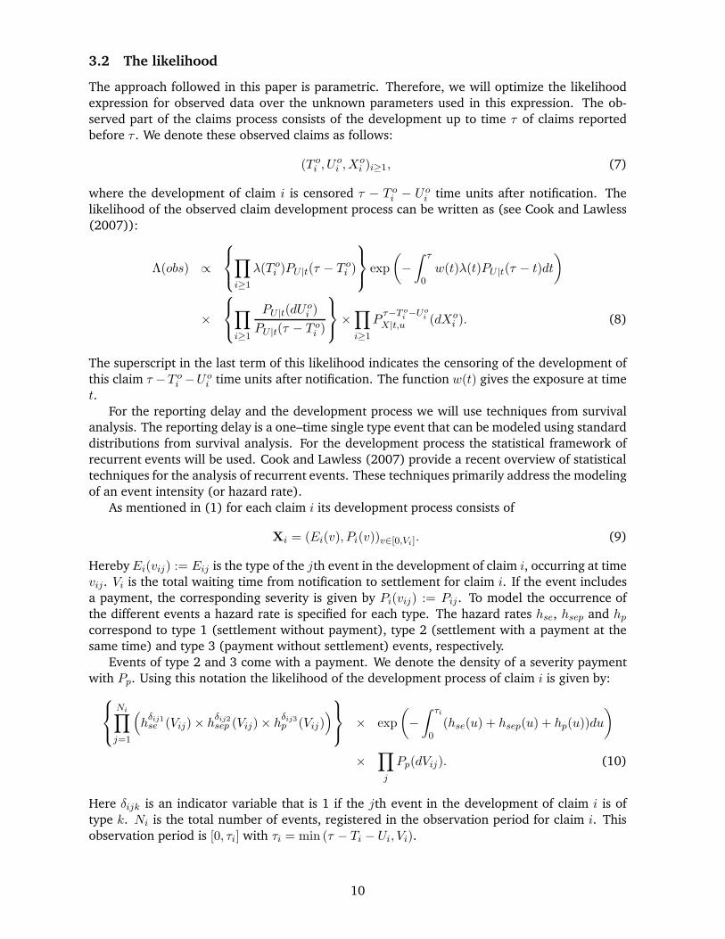
3.2 The likelihood
The approach followed in this paper is parametric. Therefore, we will optimize the likelihood
expression for observed data over the unknown parameters used in this expression. The ob-
served part of the claims process consists of the development up to time τ of claims reported
before τ . We denote these observed claims as follows:
(T oi , Uo
i ,Xoi )i≥1, (7)
where the development of claim i is censored τ − T oi − Uo
i time units after notification. The
likelihood of the observed claim development process can be written as (see Cook and Lawless
(2007)):
Λ(obs) ∝
∏
i≥1
λ(T oi )PU |t(τ − T o
i )
exp
(
−
∫ τ
0w(t)λ(t)PU |t(τ − t)dt
)
×
∏
i≥1
PU |t(dUoi )
PU |t(τ − T oi )
×∏
i≥1
Pτ−T o
i −Uoi
X|t,u (dXoi ). (8)
The superscript in the last term of this likelihood indicates the censoring of the development of
this claim τ −T oi −Uo
i time units after notification. The function w(t) gives the exposure at time
t.For the reporting delay and the development process we will use techniques from survival
analysis. The reporting delay is a one–time single type event that can be modeled using standard
distributions from survival analysis. For the development process the statistical framework of
recurrent events will be used. Cook and Lawless (2007) provide a recent overview of statistical
techniques for the analysis of recurrent events. These techniques primarily address the modeling
of an event intensity (or hazard rate).
As mentioned in (1) for each claim i its development process consists of
Xi = (Ei(v), Pi(v))v∈[0,Vi]. (9)
Hereby Ei(vij) := Eij is the type of the jth event in the development of claim i, occurring at time
vij. Vi is the total waiting time from notification to settlement for claim i. If the event includes
a payment, the corresponding severity is given by Pi(vij) := Pij . To model the occurrence of
the different events a hazard rate is specified for each type. The hazard rates hse, hsep and hp
correspond to type 1 (settlement without payment), type 2 (settlement with a payment at the
same time) and type 3 (payment without settlement) events, respectively.
Events of type 2 and 3 come with a payment. We denote the density of a severity payment
with Pp. Using this notation the likelihood of the development process of claim i is given by:
Ni∏
j=1
(
hδij1se (Vij) × h
δij2sep (Vij) × h
δij3p (Vij)
)
× exp
(
−
∫ τi
0(hse(u) + hsep(u) + hp(u))du
)
×∏
j
Pp(dVij). (10)
Here δijk is an indicator variable that is 1 if the jth event in the development of claim i is of
type k. Ni is the total number of events, registered in the observation period for claim i. This
observation period is [0, τi] with τi = min (τ − Ti − Ui, Vi).
10

Combining (8) and (10) gives the likelihood for the observed data:
Λ(obs) ∝
∏
i≥1
λ(T oi )PU |t(τ − T o
i )
exp
(
−
∫ τ
0w(t)λ(t)PU |t(τ − t)dt
)
×
∏
i≥1
PU |t(dUoi )
PU |t(τ − T oi )
×∏
i≥1
Ni∏
j=1
(
hδij1se (Vij) × h
δij2sep (Vij) × h
δij3p (Vij)
)
× exp
(
−
∫ τi
0(hse(u) + hsep(u) + hp(u))du
)
×∏
i≥1
∏
j
Pp(dVij). (11)
3.3 Distributional assumptions
We discuss the likelihood in (11) in more detail. Distributional assumptions for the various
building blocks, being the reporting delay, the occurrence times –given the reporting delay
distribution– and the development process, are presented. At each stage it is possible to include
covariate information such as the initial case reserve classes. Our final choices and estimation
results will be covered in Section 4.
Reporting delay The notification of the claim is a one–time single type event that can be
modeled using standard distributions from survival analysis (such as the Exponential, Weibull
or Gompertz distribution). Figure 5 indicates that for a large part of the claims the claim will be
reported in the first few days after the occurrence. Therefore we use a mixture of one particular
standard distribution with one or more degenerate distributions for notification during the first
few days. For example, for a mixture of a survival distribution fU with n degenerate components
the density is given by:
n−1∑
k=0
pkI{k}(u) +
(
1 −n−1∑
k=0
pk
)
fU |U>n−1(u), (12)
where I{k} = 1 for the kth day after occurrence time t and I{k} = 0 otherwise.
Occurrence process When optimizing the likelihood for the occurrence process the reporting
delay distribution and its parameters (as obtained in the previous step) are used. The likelihood
L ∝
∏
i≥1
λ(T oi )PU |t(τ − T o
i )
exp
(
−
∫ τ
0w(t)λ(t)PU |t(τ − t)dt
)
, (13)
needs to be optimized over λ(t). We use a piecewise constant specification for the occurrence
rate:
λ(t) =
λ1 0 ≤ t < d1
λ2 d1 ≤ t < d2
...
λm dm−1 ≤ t < dm,
(14)
with intervals such that τ ∈ [dm−1, dm) and w(t) := wl for dl−1 ≤ t < dl.
11

Let the indicator variable δ1(l, ti) be 1 if dl−1 ≤ ti < dl, with ti the occurrence time of claim
i. The number of claims in interval [di−1, di) can be expressed as:
Noc(l) :=∑
i
δ1(l, ti). (15)
The likelihood corresponding with the occurrence times is given by
L ∝ λNoc(1)1 λ
Noc(2)2 . . . λNoc(m)
m
∏
i≥1
PU |t(τ − ti)
× exp
(
−λ1w1
∫ d1
0PU |t(τ − t)dt
)
exp
(
−λ2w2
∫ d2
d1
PU |t(τ − t)dt
)
× . . . exp
(
−λmwm
∫ dm
dm−1
PU |t(τ − t)dt
)
. (16)
Optimizing over λl (with l = 1, . . . ,m) leads to:
λl =Noc(l)
wl
∫ dl
dl−1PU |t(τ − t)dt
. (17)
Development process A piecewise constant specification is used for the hazard rates. This
implies:
h{se,sep,p}(t) =
h{se,sep,p};1 for 0 ≤ t < a1
h{se,sep,p};2 for a1 ≤ t < a2
...
h{se,sep,p};d for ad−1 ≤ t < ad.
(18)
This piecewise specification can be integrated in a straightforward way in likelihood specifica-
tion (11), although the resulting expression is complex in notation. The optimization of the
likelihood expression can be done analytically (which results in very elegant and compact ex-
pressions) or numerically. It might be worthwhile to fit the distribution separately for ‘first
events’ in the development and ‘later events’. This will be investigated in Section 4.
Payments Events of type 2 and type 3 come with a payment. Section 2 showed that the
observed distribution of the payments has similarities with a lognormal distribution, but there
might be more flexible distributions that fit the historical payment data better. Therefore, next to
the lognormal distribution, we experimented with a generalized beta of the second kind (GB2),
Burr and Gamma distribution. Covariate information such as the initial reserve category and the
development year is taken into account.
4 Estimation results
The outcomes of calibrating these distributions to the historical data are given. Given the very
different characteristics of material claims and injury claims, the processes described in Sec-
tion 3 are fitted (and projected) separately for both types of claims. This is line with actuarial
practice, where usually separate run–off triangles are constructed for material and injury claims.
Optimization of all likelihood specifications was done with the Proc NLMixed routine in SAS.
12

Reporting delay We will use a mixture of a Weibull distribution and 9 degenerate components
corresponding with settlement after 0, . . . , 8 days. Figure 8 illustrates the fit of this mixture of
distributions to the actually observed reporting delays.
Figure 8: Reporting delay for material (left) and injury (right) claims plus degenerate components
and truncated Weibull distribution.
Fit Reporting Delay − ’Material’
In months since occurrence
Den
sity
0.0 0.5 1.0 1.5 2.0 2.5 3.0
01
23
45 Weibull / Degenerate
Observed
Fit Reporting Delay − ’Injury’
In months since occurrence
Den
sity
0.0 0.5 1.0 1.5 2.0 2.5 3.0
01
23
4
Weibull / DegenerateObserved
Occurrence process Given the above specified distribution for the reporting delay, the like-
lihood (16) for the occurrence times can be optimized. Monthly intervals are used for this,
ranging from January 2000 till August 2009. Point estimates and a corresponding 95% confi-
dence interval are shown in Figure 9.
Figure 9: Estimates of piecewise specification for λ(t): (left) material and (right) injury claims.
0 20 40 60 80 100 120
0.04
0.05
0.06
0.07
0.08
Occurrence process: Material
t
lam
bda(
t)
0 20 40 60 80 100 120
0.00
050.
0010
0.00
150.
0020
Occurrence process: Injury
t
lam
bda(
t)
Development process For the different events that may occur during the development of a
claim, the use of a constant, Weibull as well as a piecewise constant hazard rate was investigated.
13

In the piecewise constant hazard rate specification for the development of material claims, the
hazard rate was assumed to be continuous on four month intervals: [0 − 4) months, [4 − 8)months, . . ., [8 − 12) months and ≥ 12 months. For injury claims, the hazard rate was assumed
continuous on intervals of six months: [0 − 6) months, [6 − 12) months, . . ., [36 − 42) months
and ≥ 42 months. Figure 10 shows estimates for Weibull and piecewise constant hazard rates.
All models are estimated separately for ‘first events’ and ‘later events’.
Figure 10: Estimates for Weibull and piecewise constant hazard rates: (upper) injury claims and
(lower) material claims.
0 20 60 100
0.00
0.04
0.08
0.12
Type 1 − Injury
t.grid
h.gr
id
firstlaterWeibull
0 20 60 100
0.00
00.
010
0.02
00.
030
Type 2 − Injury
t.grid
h.gr
id
0 20 60 100
0.05
0.10
0.15
0.20
0.25
Type 3 − Injury
t.grid
h.gr
id
0 5 10 20 30
0.1
0.2
0.3
0.4
0.5
Type 1 − Mat
t.grid
h.gr
id
0 5 10 20 30
0.0
0.1
0.2
0.3
0.4
Type 2 − Mat
t.grid
h.gr
id
0 5 10 20 30
0.05
0.10
0.15
0.20
Type 3 − Mat
t.grid
h.gr
id
The piecewise constant specification reflects the actual data. The figure shows that the Weibull
distribution is reasonably close to the piecewise constant specification. In the rest of this paper
we will use the piecewise constant specification. Because the Weibull distribution is a good
alternative, we explain how to use both specifications in the prediction routine (see Section 5).
Payments Several distributions have been fitted to the historical payments (which were dis-
counted to 1-1-1997 with Dutch price inflation). We examined the fit of the Burr, gamma and
lognormal distribution, combined with covariate information. Distributions for the payments
are truncated at the coverage limit of 2.5 million euro per claim. A comparison based on BIC
showed that the lognormal distribution achieves a better fit than the Burr and gamma distribu-
tions. When including the initial reserve category as covariate or both the initial reserve category
and the development year, the fit further improves. Given these results, the lognormal distribu-
tion with the initial reserve category and the development year as covariates will be used in the
prediction. The covariate information is included in both the mean (µi) and standard deviation
14

(σi) of the lognormal distribution for observation i:
µi =∑
r
∑
s
µr,sIDYi=sIi∈r
σi =∑
r
∑
s
σr,sIDYi=sIi∈r. (19)
Hereby r is the initial reserve category and DYi is the development year corresponding with ob-
servation i. IDYi=s and Ii∈r are indicator variables denoting whether observation i corresponds
with DY s and reserve category r. Figure 11 shows corresponding qqplots.
Figure 11: Normal qqplots corresponding with the fit of log(payments) including initial reserve and
development year as covariate information.
−10 −5 0 5
−4
−2
02
4
Normal QQplot Payments: Material
Emp. Quant.
The
or. Q
uant
.
−4 −2 0 2 4
−4
−2
02
4
Normal QQplot Payments: Injury
Emp. Quant.
The
or. Q
uant
.
5 Predicting future cash–flows
5.1 Prediction routine
To predict the outstanding liabilities with respect to this portfolio of liability claims, we distin-
guish between IBNR and RBNS claims. The following step by step approach allows to obtain
random draws from the distribution of both IBNR and RBNS claims.
Predicting IBNR claims As noted in Section 3, an IBNR claim occurred already but has not
yet been reported to the insurer. Therefore, Ti + Ui > τ and Ti < τ with Ti the occurrence time
of the claim and Ui its reporting delay. The Tis are missing data: they are determined in the
development process but unknown to the actuary at time τ . The prediction process for the IBNR
claims requires the following steps:
(a) Simulate the number of IBNR claims in [0, τ ] and their corresponding occurrence
times.
According to the discussion in Section 3 the IBNR claims are governed by a Poisson process
with non–homogeneous intensity or occurrence rate:
w(t)λ(t)(1 − PU |t(τ − t)), (20)
15

where λ(t) is piecewise constant according to specification (14). The following property
follows from the definition of non–homogeneous Poisson processes:
NIBNR(l) ∼ Poisson
(
λlwl
∫ dl
dl−1
(1 − PU |t(τ − t))dt
)
, (21)
where NIBNR(l) is the number of IBNR claims in time interval [dl−1, dl). Note that the inte-
gral expression has already been evaluated (numerically) in the fitting procedure. Given
the simulated number of IBNR claims nIBNR(l) for each interval [dl−1, dl), the occurrence
times of the claims are uniformly distributed in [dl−1, dl).
(b) Simulate the reporting delay for each IBNR claim
Given the simulated occurrence time ti of an IBNR claim, its reporting delay is simulated
by inverting the distribution:
P (U ≤ u|U > τ − ti) =P (τ − ti < U ≤ u)
1 − P (U ≤ τ − ti). (22)
In case of our assumed mixture of a Weibull distribution and 9 degenerate distributions
this expression has to be evaluated numerically.
(c) Simulate the initial reserve category
For each IBNR claim an initial reserve category has to be simulated for use in the develop-
ment process. Given m initial reserve categories, the probability density for initial reserve
category c is:
f(c) =
{
pc for c = 1, 2, . . . ,m − 1
1 −∑m−1
k=1 pk for c = m.(23)
The probabilities used in (23) are the empirically observed percentages of policies in a
particular initial reserve category.
(d) Simulate the payment process for each IBNR claims
This step is common with the procedure for RBNS claims and will be explained in the next
paragraph.
Predicting RBNS claims Given the RBNS claims and the simulated IBNR claims, the process
proceeds as below. Note that we use the piecewise hazard specification for the development
process. As an alternative for the analytical specifications given below, numerical routines could
be used. Using the alternative Weibull specification would require numerical operations as well.
(e) Simulate the next event’s exact time
In case of RBNS claims, the time of censoring ci of claim i is known. For IBNR claims
this censoring time ci := 0. The next event – at time vi,next – can take place at any time
vi,next > ci. To simulate its exact time we need to invert: (with p randomly drawn from a
Unif(0, 1) distribution)
P (V < vi,next|V > ci) = p
m
P (ci < V ≤ vi,next)
1 − P (V ≤ ci)= p. (24)
16

From the relation between a hazard rate and cdf, we know
P (V ≤ vi,next) = 1 − exp
(
−
∫ vi,next
0
∑
e
he(t)dt
)
, (25)
with e ∈ {se, sep, p}. For instance with a Weibull specification for the hazard rates this
equation will be inverted numerically. With a piecewise constant specification for the
hazard rates numerical routines can be used as well. However, as an alternative closed–
form expressions can be derived. Step (e) should then be replaced by (e1) − (e2):
(e1) Simulate the next event’s time interval
In case of RBNS claims, the time of censoring ci of claim i belongs to a certain interval
[ak−1, ak). The next event – at time vi,next > ci – can take place in any interval from
[ak−1, ak) on. The probability that vi,next belongs to a certain interval [ak−1, ak) is
given by:
P (ak−1 ≤ V < ak|V > ci) =
{P (ci<V <ak)1−P (V ≤ci)
if ci ∈ [ak−1, ak)P (ak−1≤V <ak)
1−P (V ≤ci)if ci 6∈ [ak−1, ak).
(26)
Using the notation introduced above the involved probabilities can be expressed as
(for instance):
P (ci < V < ak)
1 − P (V < ci)=
P (V < ak) − P (V ≤ ci)
1 − P (V ≤ ci)
=1 − exp
{−∫ ak
0
∑
e he(t)dt}− 1 + exp
{−∫ ci
0
∑
e h2(t)dt}
exp{−∫ ci
0
∑
e he(t)dt} ,
=exp{−
∑
e∑d
l=1 hel[(al−al−1)δ2(l,ci)+(ci−al−1)δ1(l,ci)]}−exp{−∑
e∑d
l=1 hel[(al−al−1)δ2(l,ak)+(ak−al−1)δ1(l,ak)]}exp{−
∑
e∑d
l=1hel[(al−al−1)δ2(l,ci)+(ci−al−1)δ1(l,ci)]}
,
(27)
with e ∈ {se, sep, p}, δ2(l, t) is 1 if t > al and 0 otherwise and δ1(l, t) is 1 if al−1 ≤t < al and 0 otherwise.
(e2) Simulate the exact time of the next event
Given the time interval of the next event, [ak−1, ak), we simulate its exact time by
inverting the following equation for vi,next
P (V < vi,next|ci < V < ak) = p if ci ∈ [ak−1, ak);
P (V < vi,next|ak−1 ≤ V < ak) = p otherwise, (28)
where p is randomly drawn from a Unif(0, 1) distribution. For instance, for P (V <vi,next|ak−1 ≤ V < ak) = p this inverting operation goes as follows:
P (V < vi,next) = pP (ak−1 ≤ V < ak) + P (V < ak−1)
m
1 − exp
{
−
∫ vi,next
0
∑
e
he(t)dt
}
= pP (ak−1 ≤ V < ak) + P (V < ak−1)
m
− log [1−pP (ak−1≤V <ak)−P (V <ak−1)]=∑
e
∑k−1l=1 hel(al−al−1)+
∑
e hek(vi,next−ak−1)
m
vi,next=− log [1−pP (ak−1≤V <ak)−P (V <ak−1)]−
∑
e∑k−1
l=1hel(al−al−1)
∑
e hek+ak−1, (29)
with e ∈ {se, sep, p}.
17

(f) Simulate the event type Given the exact time of the next event, its type is simulated using
the following argument
lim△v→0
P (E = e|v ≤ V < v + △v) = lim△v→0
P (v≤V <v+△v∩E=e)△v
P (v≤V <v+△v)△v
=he(v)
∑
e he(v), (30)
where e ∈ {se, sep, p}.
(g) Simulate the corresponding payment Given the covariate information for claim i, the
payment can be drawn from the appropriate lognormal distribution. Note that the cumu-
lative payment cannot exceed the coverage limit of 2.5 million per claim.
(h) Stop or continue Depending on the simulated event type in step (f), the prediction stops
(in case of settlement) or continues.
In the next section, this prediction process will be applied separately for the material claims and
the injury claims.
5.2 Comment on parameter uncertainty
With respect to the uncertainty of predictions a distinction has to be made between process
uncertainty and estimation or parameter uncertainty (see England and Verrall (2002)). The
process uncertainty will be taken care of by sampling from the distributions proposed in Sec-
tion 3. To include parameter uncertainty the bootstrap technique or concepts from Bayesian
statistics can be used. While a formal Bayesian approach is very elegant, it generally leads to
significantly more complexity, which is not contributing to the accessibility and transparency of
the techniques towards practicing actuaries. Applying a bootstrap procedure would be possible,
but is very computer intensive, since our sample size is very large and several stochastic pro-
cesses are used. To avoid computational problems when dealing with parameter uncertainty,
we will use the asymptotic normal distribution of our maximum likelihood estimators. At each
iteration of the prediction routine we sample each parameter from its corresponding asymptotic
normal distribution. Note that –due to our large sample size– confidence intervals are narrow.
This is in contrast with run–off triangles where sample sizes are typically very small and param-
eter uncertainty is an important point of concern.
6 Numerical results
The prediction process described in Section 5 is applied separately for the material and injury
claims. In this Section results obtained with the micro–level reserving model are shown. Our
results are compared with those from traditional techniques based on aggregate data. We show
results for an out–of–sample exercise, so that the estimated reserves can be compared with
actual payments. This out–of–sample test is done by estimating the reserves per 1-1-2005. The
data set that is available at 1-1-2005 can be summarized using run-off triangles, displaying data
from arrival years 1999 – 2004. Table 3 (material) and 4 (injury) show the run–off triangles
that are the basis for this out–of–sample exercise. The lower triangle is known up to 3 cells. The
actual observations are given in bold. Of course, these were not known at 1-1-2005 so cannot
be used as input for calibration of the models.
18

Table 3: Run–off triangle material claims (displayed in thousands), arrival years 1997-2004.
Arrival Development Year
Year 1 2 3 4 5 6 7 8
1997 4,380 972 82 9 36 27 34 11
1998 4,334 976 56 35 76 24 0.572 17
1999 5,225 1,218 59 108 108 12 0.390 0
2000 5,366 1,119 161 14 6 4 0.36 10
2001 5,535 1,620 118 119 13 3 0.350 2
2002 6,539 1,547 67 65 17 5 9 8.8
2003 6,535 1,601 90 21 31 7 1.7
2004 7,109 1,347 99 76 20 13
Table 4: Run–off triangle injury claims (displayed in thousands), arrival years 1997-2004.
Arrival Development Year
Year 1 2 3 4 5 6 7 8
1997 308 635 366 530 549 137 132 339
1998 257 481 312 336 269 56 179 78
1999 292 589 410 273 254 287 132 97
2000 316 601 439 498 407 371 247 275
2001 465 846 566 566 446 375 147 240
2002 314 615 540 449 133 131 332 1,082
2003 304 802 617 268 223 216 173
2004 333 864 412 245 273 100
Output from the micro–level model The distribution of the reserve per 1-1-2005 is deter-
mined for the individual (micro–level) model proposed in this paper. We will first look at the
output that becomes available when using the micro–level model. Figure 12 shows results for
injury payments done in calendar year 2006, based on 10,000 simulations. In Table 4 this is
the diagonal going from 412, 268, . . . , up to 97. The first row in Figure 12 shows (from left to
right): the number of IBNR claims reported in 2006, the total amount of payments done in this
calendar year and the total number of events occurring in 2006. The IBNR claims are claims
that occurred before 1-1-2005, but were reported to the insurer during calendar year 2006. The
total amount paid in 2006 is the sum of payments for RBNS claims and IBNR claims, which are
separately available from the micro–model. In the second row of plots we take a closer look
at the events registered in 2006 by splitting into type 1–type 3 events. In each of the plots
the black solid line indicates what was actually observed. This figure shows that the predictive
distributions from the micro–level model are realistic, given the actual observations. Only the
actual number of IBNR claims is far in the tail of the distribution. However, note that this relates
to a relatively low number of IBNR claims.
Comparing reserves The results from the micro–level model are now compared with results
from two standard actuarial models developed for aggregate data. To the data in Tables 3
and 4, a stochastic chain–ladder model is applied which is based on the overdispersed Poisson
distribution and the lognormal distribution, respectively. With Yij denoting cell (i, j) from a run–
off triangle, corresponding with arrival year i and development year j, the model specifications
for overdispersed Poisson ((31)) and lognormal ((32)) are given below. Both aggregate models
19
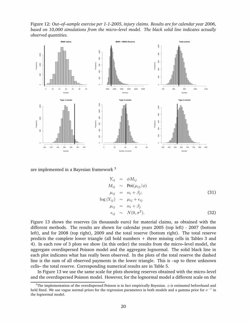
Figure 12: Out–of–sample exercise per 1-1-2005, injury claims. Results are for calendar year 2006,
based on 10,000 simulations from the micro–level model. The black solid line indicates actually
observed quantities.
IBNR claims
Number
Fre
quen
cy
5 10 15 20 25 30 35
050
010
0015
00IBNR + RBNS Reserve
Reserve
Fre
quen
cy
1000 2000 3000 4000 5000 6000
020
040
060
080
010
00
Total events
Number
Fre
quen
cy
700 800 900 1000 1100
020
040
060
080
010
00
Type 1 events
Number
Fre
quen
cy
100 120 140 160 180 200 220
050
010
0015
00
Type 2 events
Number of events
Fre
quen
cy
0 20 40 60 80
020
040
060
080
010
0012
00Type 3 events
Number
Fre
quen
cy
500 550 600 650 700 750 800 850
020
040
060
080
010
00
are implemented in a Bayesian framework 3
Yij = φMij
Mij ∼ Poi(µij/φ)
µij = αi + βj ; (31)
log (Yij) ∼ µij + ǫij
µij = αi + βj
ǫij ∼ N(0, σ2). (32)
Figure 13 shows the reserves (in thousands euro) for material claims, as obtained with the
different methods. The results are shown for calendar years 2005 (top left) - 2007 (bottom
left), and for 2008 (top right), 2009 and the total reserve (bottom right). The total reserve
predicts the complete lower triangle (all bold numbers + three missing cells in Tables 3 and
4). In each row of 3 plots we show (in this order) the results from the micro–level model, the
aggregate overdispersed Poisson model and the aggregate lognormal. The solid black line in
each plot indicates what has really been observed. In the plots of the total reserve the dashed
line is the sum of all observed payments in the lower triangle. This is –up to three unknown
cells– the total reserve. Corresponding numerical results are in Table 5.
In Figure 13 we use the same scale for plots showing reserves obtained with the micro–level
and the overdispersed Poisson model. However, for the lognormal model a different scale on the
3The implementation of the overdispersed Poisson is in fact empirically Bayesian. φ is estimated beforehand and
held fixed. We use vague normal priors for the regression parameters in both models and a gamma prior for σ−1 in
the lognormal model.
20

x–axis is necessary because of the long right tail of the frequency histogram obtained for this
model. These unrealistically high reserves (see Table 5) are a disadvantage of the lognormal
model for the portfolio of material claims. Concerning the Poisson model for aggregate data,
we conclude from Figure 13 that the overdispersed Poisson model overstates the reserve; the
actually observed amount is always in the left tail of the histogram. For instance, in the plots
with the total reserve, the median of the simulations from overdispersed Poisson is at 2,785,000
euro, the median of the simulations from the micro–level model is 2,054,430 euro, whereas the
total amount registered for the lower triangle is 1,861,000 euro. Recall that the latter is the
total reserve up to the three unknown cells in Triangle 3. The best estimates (see the ‘Mean’
or ‘Median’ columns) obtained with the micro–level model are realistic and closer to the true
realizations than the best estimates from aggregate techniques.
Figure 14 shows the distributions of the reserve (in thousands of euro) for the different
methods for injury claims. Once again the actual payments are indicated with a solid black
line. The results of the lognormal model are now presented on the same scale as the other
two models. Corresponding numerical results are in Table 6. All models do well for calendar
year 2005, the individual model does the best job for calendar years 2006 and 2007. For these
calendar years the actual amount paid is –again– in the very left tail of the distributions obtained
with aggregate techniques. The overdispersed Poisson and the lognormal model perform better
in calendar years 2008 and 2009. Note however that calendar years 2008 and 2009 were
extraordinary years, when looking at injury payments. In 2009 the two highest claims of the
whole data set settled with a payment in 2009. The highest (the 779,383 euro payment shown
in Table 4) is extremely far from all other payments in the data set. The observed outcome from
calendar year 2009 should be considered as a very pessimistic scenario. Indeed, this realized
outcome is in the very right tail of the distribution obtained with the individual model. The
year 2008 was less extreme, but had an unusual number of very large claims (of the 15 highest
claims in the data set, 4 of them occurred in 2008).
Note Although we only present the results obtained for the out–of–sample test that calculates
reserves per 1-1-2005, we also calculated reserves per 1-1-2006/2007/2008/2009. Our conclu-
sions for these tests were similar to those reported above. Full details are available on the home
page of the first author.
Table 5: Out–of–sample exercise per 1-1-2005: numerical results for material claims (in thou-
sands), 6,000 simulations for the micro–level model..
Method Outcome Year Mean Median Min. Max. 5% 25% 75% 90% 95% 99.5%
Micro–level 1,537 CY 2005 1,404 1,342 1,093 5,574 1,204 1,272 1,449 1,627 1,783 3,143139 06 307 248 76 2,738 138 191 346 498 630 1,779123 07 246 183 30 2,740 72 123 286 444 618 1,688
39 08 146 98 7 2,426 30 61 164 283 402 1,22523 09 52 26 0 2,216 4 12 53 104 167 639
> 1,861 Total 2,208 2,054 1,374 7,875 1,622 1,831 2,401 2,871 3,305 5,074
Aggregate ODP 1,537 CY 2005 2,000 1,989 1,194 3,028 1,591 1,834 2,166 2,321 2,431 2,674139 06 324 309 44 774 177 265 376 442 486 597123 07 214 199 0 619 88 155 265 332 354 464
39 08 144 133 0 553 44 88 177 243 265 35423 09 66 66 0 376 0 22 88 133 155 243
> 1,861 Total 2,803 2,785 1,613 4,354 2,232 2,564 3,028 3,271 3,426 3,846
Aggregate LogN. 1,537 CY 2005 5,340 2,253 70 587,500 497 1,146 4,896 10,790 17,985 77,671139 06 699 410 32 164,200 135 254 710 1,231 1,818 6,522123 07 380 228 8 23,720 67 137 403 734 1,110 3,731
39 08 326 167 2 48,850 41 93 317 627 998 4,05323 09 163 71 1 33,660 14 36 146 304 499 2,051
> 1,861 Total 7,071 3,645 201 645,500 1,110 2,135 6,936 13,692 21,931 84,712
21

Table 6: Out–of–sample exercise per 1-1-2005: numerical results for injury claims (in thousands),
10,000 simulations for the micro–level model.
Method Outcome Year Mean Median Min. Max. 5% 25% 75% 90% 95% 99.5%
Micro–level 2,957 CY 2005 2,548 2,453 1,569 6,587 1,951 2,212 2,764 3,154 3,499 4,5671,532 06 1,798 1,699 909 6,790 1,246 1,477 2,001 2,393 2,703 3,7521,020 07 1,254 1,159 453 4,945 774 968 1,420 1,778 2,088 3,1251,060 08 884 776 267 4,381 458 613 1,024 1,393 1,694 2,7431,354 09 390 313 63 3,745 149 226 448 678 908 1,875
> 7, 923 Total 7,386 7,209 4,209 14,850 5,666 6,489 8,092 9,035 9,721 11,725
Aggregate ODP 2,957 CY 2005 2,798 2,774 1,727 8,247 2,259 2,553 2,994 3,233 3,380 4,2981,532 06 2,134 2,112 1,065 6,723 1,670 1,929 2,314 2,498 2,627 3,4721,020 07 1,721 1,708 845 6,172 1,286 1,525 1,892 2,076 2,186 3,0491,060 08 1,286 1,249 551 5,933 882 1,102 1,433 1,616 1,727 2,6271,354 09 759 735 220 4,114 478 625 863 992 1,084 1,543
> 7, 923 Total 9,639 9,478 5,474 40,670 7,660 8,688 10,360 11,200 11,770 17,360
Aggregate LogN. 2,957 CY 2005 2,948 2,882 1,175 6,729 2,181 2,570 3,254 3,648 3,944 4,9441,532 06 2,251 2,196 957 6,898 1,623 1,940 2,500 2,825 3,050 3,9341,020 07 1,817 1,759 567 5,313 1,244 1,526 2,040 2,355 2,583 3,4261,060 08 1,377 1,315 374 5,768 864 1,110 1,571 1,861 2,087 2,9441,354 09 815 768 195 4,054 472 632 941 1,151 1,313 1,867
> 7, 923 Total 10,277 10,040 4,459 26,010 7,661 8,954 11,310 12,680 13,730 17,590
7 Conclusions
The measurement of future cash flows and their uncertainty becomes more and more impor-
tant, also for general insurance portfolios. Currently, reserving for general insurance is based on
data aggregated in run–off triangles. A vast literature on techniques for claims reserving exists,
largely designed for application to loss triangles. The most popular approach is the chain–ladder
approach, largely because of is practicality. However, the use of aggregate data in combination
with the chain–ladder approach gives rise to several issues, implying that the use of aggregate
data in combination with the chain–ladder technique (or similar techniques) is not fully ade-
quate for capturing the complexities of stochastic reserving for general insurance.
In this paper micro–level stochastic modeling is used to quantify the reserve and its uncer-
tainty for a realistic general liability insurance portfolio. Stochastic processes for the occurrence
times, the reporting delay, the development process and the payments are fit to the historical
individual data of the portfolio and used for projection of future claims and its (estimation and
process) uncertainty. A micro–level approach allows much closer modeling of the claims pro-
cess. Lots of issues mentioned in our discussion of the chain–ladder approach will not exist
when using a micro–level approach, because of the availability of lots of data and the potential
flexibility in modeling the future claims process.
The paper shows that micro–level stochastic modeling is feasible for real life portfolios with
over a million data records, and that it gives the flexibility to model the future payments re-
alistically, not restricted by limitations that exist when using aggregate data. The prediction
results of the individual (micro–level) model are compared with models applied to aggregate
data, being an overdispersed Poisson and a lognormal model. We present our results through
an out–of–sample exercise, so that the estimated reserves can be compared with actual pay-
ments. Conclusion of the out–of–sample test is that –for the case–study under consideration–
traditional techniques tend to overestimate the real payments. Predictive distributions obtained
with the micro–model reflect reality in a more realistic way: ‘regular’ outcomes are close to the
median of the predictive distribution whereas pessimistic outcomes are in the very right tail. As
such, reserve calculations based on the micro-level model are to be preferred; they reflect real
outcomes in a more realistic way.
22

The results obtained in this paper make it worthwhile to further investigate the use of micro–
level data for reserving purposes. Several directions for future research can be mentioned. One
could try to refine the performance of the individual model with respect to very pessimistic
scenarios by using a combination of e.g. a lognormal distribution for losses below and a gen-
eralized Pareto distribution for losses above a certain threshold. Analyzing the performance of
both the micro–level model and techniques for aggregate data on simulated data sets will bring
more insight in their performance. In that respect it is our intention to collect and study new
case–studies.
23

Figure 13: Out–of–sample results per 1-1-2005, material claims. Top left to bottom left: calendar years 2005-2006-2007. Top right to bottom right:
calendar years 2008-2009-total reserve. In each graph the black vertical line indicates the amount that was actually paid in that calendar year. The
dashed black line in the graph of the total reserve corresponds with the sum of all payments done in calendar years 2005 up to 2009. Up to three
missing cells (see Table 3) this is the total reserve.Micro−level: CY 2005
Reserve
Fre
qu
en
cy
1000 1500 2000 2500 3000
05
00
10
00
15
00
Aggregate Model − ODP: CY 2005
Reserve
Fre
qu
en
cy
1000 1500 2000 2500 3000
02
00
40
06
00
80
01
00
0
Aggregate Model − Lognormal: CY 2005
Reserve
Fre
qu
en
cy
0 5000 10000 15000 20000 25000 30000
05
00
10
00
15
00
Micro−level: CY 2008
Reserve
Fre
qu
en
cy
0 200 400 600 800 1000 1200
02
00
40
06
00
80
0
Aggregate Model − ODP: CY 2008
Reserve
Fre
qu
en
cy
0 200 400 600 800 1000 1200
05
00
10
00
15
00
20
00
25
00
30
00
Aggregate Model − Lognormal: CY 2008
Reserve
Fre
qu
en
cy
0 500 1000 1500 2000
05
00
10
00
15
00
20
00
Micro−level: CY 2006
Reserve
Fre
qu
en
cy
0 200 400 600 800 1000 1200
01
00
20
03
00
40
05
00
Aggregate Model − ODP: CY 2006
Reserve
Fre
qu
en
cy
0 200 400 600 800 1000 1200
05
00
10
00
15
00
20
00
Aggregate Model − Lognormal: CY 2006
Reserve
Fre
qu
en
cy
0 500 1000 1500 2000 2500 3000
05
00
10
00
15
00
Micro−level: CY 2009
Reserve
Fre
qu
en
cy
0 100 200 300 400 500
05
00
10
00
15
00
20
00
25
00
Aggregate Model − ODP: CY 2009
Reserve
Fre
qu
en
cy
0 100 200 300 400 500
05
00
10
00
15
00
20
00
Aggregate Model − Lognormal: CY 2009
Reserve
Fre
qu
en
cy
0 200 400 600 800
05
00
10
00
15
00
Micro−level: CY 2007
Reserve
Fre
qu
en
cy
0 200 400 600 800 1000 1200
01
00
20
03
00
40
05
00
Aggregate Model − ODP: CY 2007
Reserve
Fre
qu
en
cy
0 200 400 600 800 1000 1200
05
00
10
00
15
00
20
00
25
00
30
00
Aggregate Model − Lognormal: CY 2007
Reserve
Fre
qu
en
cy
0 500 1000 1500 2000
05
00
10
00
15
00
Micro−level: Total
Reserve
Fre
qu
en
cy
2000 3000 4000 5000 6000 7000
01
00
20
03
00
40
05
00
60
07
00
Aggregate Model − ODP: Total
Reserve
Fre
qu
en
cy
2000 3000 4000 5000 6000 7000
02
00
40
06
00
80
01
00
01
20
0
Aggregate Model − Lognormal: Total
Reserve
Fre
qu
en
cy
0 5000 10000 15000 20000 25000 30000
05
00
10
00
15
00
24
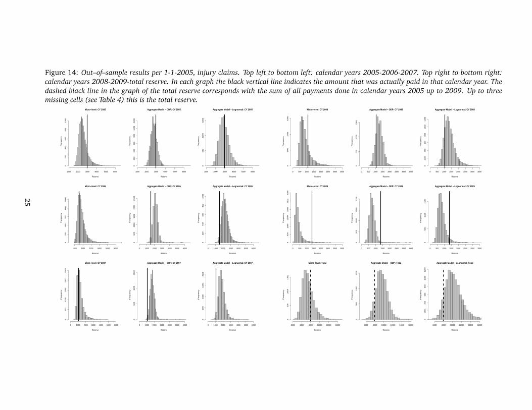
Figure 14: Out–of–sample results per 1-1-2005, injury claims. Top left to bottom left: calendar years 2005-2006-2007. Top right to bottom right:
calendar years 2008-2009-total reserve. In each graph the black vertical line indicates the amount that was actually paid in that calendar year. The
dashed black line in the graph of the total reserve corresponds with the sum of all payments done in calendar years 2005 up to 2009. Up to three
missing cells (see Table 4) this is the total reserve.Micro−level: CY 2005
Reserve
Fre
qu
en
cy
1000 2000 3000 4000 5000 6000
02
00
40
06
00
80
01
00
0
Aggregate Model − ODP: CY 2005
Reserve
Fre
qu
en
cy
1000 2000 3000 4000 5000 6000
02
00
40
06
00
80
01
00
01
20
0
Aggregate Model − Lognormal: CY 2005
Reserve
Fre
qu
en
cy
1000 2000 3000 4000 5000 6000
05
00
10
00
15
00
Micro−level: CY 2008
Reserve
Fre
qu
en
cy
0 500 1000 1500 2000 2500 3000 3500
05
00
10
00
15
00
Aggregate Model − ODP: CY 2008
Reserve
Fre
qu
en
cy
0 500 1000 1500 2000 2500 3000 3500
05
00
10
00
15
00
Aggregate Model − Lognormal: CY 2008
Reserve
Fre
qu
en
cy
0 500 1000 1500 2000 2500 3000 3500
02
00
40
06
00
80
01
00
01
20
0
Micro−level: CY 2006
Reserve
Fre
qu
en
cy
1000 2000 3000 4000 5000 6000
02
00
40
06
00
80
01
00
0
Aggregate Model − ODP: CY 2006
Reserve
Fre
qu
en
cy
0 1000 2000 3000 4000 5000 6000
05
00
10
00
15
00
20
00
25
00
Aggregate Model − Lognormal: CY 2006
Reserve
Fre
qu
en
cy
0 1000 2000 3000 4000 5000 6000
02
00
40
06
00
80
01
00
0
Micro−level: CY 2009
Reserve
Fre
qu
en
cy
0 500 1000 1500 2000 2500 3000 3500
05
00
10
00
15
00
20
00
25
00
30
00
Aggregate Model − ODP: CY 2009
Reserve
Fre
qu
en
cy
0 500 1000 1500 2000 2500 3000 3500
05
00
10
00
15
00
20
00
Aggregate Model − Lognormal: CY 2009
Reserve
Fre
qu
en
cy
0 500 1000 1500 2000 2500 3000 3500
05
00
10
00
15
00
Micro−level: CY 2007
Reserve
Fre
qu
en
cy
0 1000 2000 3000 4000 5000 6000
05
00
10
00
15
00
20
00
25
00
Aggregate Model − ODP: CY 2007
Reserve
Fre
qu
en
cy
0 1000 2000 3000 4000 5000 6000
05
00
10
00
15
00
Aggregate Model − Lognormal: CY 2007
Reserve
Fre
qu
en
cy
0 1000 2000 3000 4000 5000 6000
05
00
10
00
15
00
20
00
Micro−level: Total
Reserve
Fre
qu
en
cy
4000 6000 8000 10000 12000 14000
05
00
10
00
15
00
Aggregate Model − ODP: Total
Reserve
Fre
qu
en
cy
6000 8000 10000 12000 14000 16000
05
00
10
00
15
00
Aggregate Model − Lognormal: Total
Reserve
Fre
qu
en
cy
6000 8000 10000 12000 14000 16000
02
00
40
06
00
80
01
00
01
20
0
25

References
E. Arjas. The claims reserving problem in non–life insurance: some structural ideas. ASTIN
Bulletin, 19(2):139–152, 1989.
R.L. Bornhuetter and R.E. Ferguson. The actuary and IBNR. Proceedings CAS, 59:181–195,
1972.
R. Cook and J. Lawless. The statistical analysis of recurrent events. Springer New York, 2007.
P.D. England and R.J. Verrall. Stochastic claims reserving in general insurance. British Actuarial
Journal, 8:443–544, 2002.
S. Haastrup and E. Arjas. Claims reserving in continuous time: a nonparametric Bayesian ap-
proach. ASTIN Bulletin, 26(2):139–164, 1996.
L.J. Halliwell. Chain–ladder bias: its reason and meaning. Variance, 1:214–247, 2007.
L.J. Halliwell. Modelling paid and incurred losses together. CAS E-forum spring 2009, 2009.
R. Kaas, M. Goovaerts, J. Dhaene, and M. Denuit. Modern actuarial risk theory: using R. Kluwer,
The Netherlands, 2008.
A.F. Karr. Point processes and their statistical inference. Marcel Dekker INC, 1991.
M. Kunkler. Modelling zeros in stochastic reserving models. Insurance: Mathematics and Eco-
nomics, 34(1):23–35, 2004.
C.R. Larsen. An individual claims reserving model. ASTIN Bulletin, 37(1):113–132, 2007.
H. Liu and R. Verrall. Predictive distributions for reserves which separate true IBNR and IBNER
claims. ASTIN Bulletin, 39(1):35–60, 2009.
T. Mack. The standard error of chain–ladder reserve estimates: recursive calculation and inclu-
sion of a tail–factor. ASTIN Bulletin, 29:361–366, 1999.
R. Norberg. Prediction of outstanding liabilities in non-life insurance. ASTIN Bulletin, 23(1):
95–115, 1993.
R. Norberg. Prediction of outstanding liabilities ii. model extensions variations and extensions.
ASTIN Bulletin, 29(1):5–25, 1999.
B. Postuma, E.A. Cator, W. Veerkamp, and E.W. van Zwet. Combined analysis of paid and
incurred losses. CAS E–Forum Fall 2008, 2008.
G. Quarg and T. Mack. Munich chain ladder: a reserving method that reduces the gap be-
tween IBNR projections based on paid losses and IBNR projections based on incurred losses.
Variance, 2:266–299, 2008.
A. Renshaw. Modelling the claims process in the presence of covariates. ASTIN Bulletin, 24:
265–285, 1994.
R. Schnieper. Separating true IBNR and IBNER claims. ASTIN Bulletin, 21(1):111–127, 1991.
G. Taylor and M. Campbell. Statistical case estimation. Research paper number 104, The Univer-
sity of Melbourne, Australia, (1), 2002.
26

G. Taylor, G. McGuire, and A. Greenfield. Loss reserving: past, present and future. Research
paper number 109, The University of Melbourne, Australia, (1), 2003.
H.G. Verbeek. An approach to the analysis of claims experience in motor liability excess of loss
reinsurance. ASTIN Bulletin, 6:195–202, 1972.
T. Verdonck, M. Van Wouwe, and J. Dhaene. A robustification of the chain–ladder method.
North American Actuarial Journal, 13(2):280–298, 2009.
T.S. Wright. A stochastic method for claims reserving in general insurance. J. Inst. Actuar., 117
(1):677–731, 1990.
M. Wuthrich and D. Alai. Modelling small and large claims in a chain–ladder framework. Work-
ing paper, 2009.
Mario V. Wuthrich and Michael Merz. Stochastic claims reserving methods in insurance. Wiley
Finance, 2008.
B. Zehnwirth. Probabilitstic development factor models with applications to loss reserve vari-
ability. prediction intervals and risk based capital. CAS Forum Spring, 2:447–606, 1994.
X. B. Zhao and X. Zhou. Applying copula models to individual claim loss reserving methods.
Insurance: Mathematics and Economics, 46(2):290–299, 2010.
X. B. Zhao, X. Zhou, and J. L. Wang. Semiparametric model for prediction of individual claim
loss reserving. Insurance: Mathematics and Economics, 45(1):1–8, 2009.
27
Related Documents