_utonomous Integrated GPS gauon Experiment for OMV_ _- ...

1

_utonomous Integrated GPS

gauon Experiment for OMV_ _-....... -

I Fq .1 Study........_:_-:Y:_::-_II:'I:;i_I';:,I_]_I_-:7_::C;;;L--::;:::: ......................

__ _ - .................... : _ _ ........................ : _

Uncl as

HI/04 0_71. Z18

https://ntrs.nasa.gov/search.jsp?R=19900011653 2020-03-19T22:48:56+00:00Z

L_

<_2 ..- ?::

_ _:_--- _Z

: : :--: -:

- :f7

;:{:2::_ :

£ :

• Z:

±

T

±:: =

_2

=

:Y

F _:-:= -....

t=

-- -- E ......... ZZ

_1 21.| m ...... ---

|

!

r _-_

"2

NASA Contractor Report 4267

Autonomous Integrated GPS/INS

Navigation Experiment for OMV:

PHASE I Feasibility Study

Triveni N. Upadhyay, George J. Priovolos,

and Harley Rhodehamel

Mayflower Communications Company, Inc.

Reading, Massachusetts

Prepared for

George C. Marshall Space Flight Center

under Contract NAS8-38031

National Aeronautics andSpace Administration

Office of Management

Scientific and TechnicalInformation Division

1989

FOREWORD

The research results described in this report was

sponsored by NASA Marshall Space Flight Center, Marshall Space

Flight Center, AL under the SBIR Phase I Program, Contract No.

NAS8-38031. The NASA COTR on the program was Mr. A. Wayne

Deaton, EL23.

The research was carried out by Mayflower Communications

Company, Inc. during the period February - August 1989. The

Principal Investigator on the project was Dr. Triveni N.

Upadhyay.

Several individuals and organizations provided technical

data and support which were essential to the successful

completion of the Phase I research. Mr. Wayne Deaton EL23,

and Mr. Larry Brandon, of NASA MSFC provided us data on GPS

navigation requirements for future advanced STSs and the data

on NASA atmospheric drag models. Mr. Chuck Shortwell and Mr.

Albert T. Monulki, TRW OMV Program, were helpful in providing

OMV GN&C description including preliminary definition of the

telemetry data and interface to the OMV OBC.

Excellent administration support in the preparation of

the report was provided by Ms. Joan Beaulieu and Ms. Angela

Russo.

iii

J

PRECEDING PAGE BLANK NOT FILMED

AUTONOMOUS INTEGRATED GPS/INS NAVIGATION EXPERIMENT FOR OMV

TABLE OF CONTENTS

Section Title Page

1

i.i

1.2

INTRODUCTION

Background

Outline of the Report

1

1

4

2 PHASE I TECHNICAL OBJECTIVES AND APPROACH 5

3

3.1

3.2

3.3

3.3.1

3.3.2

3.3.3

3.3.4

3.3.5

PHASE I RESULTS

Common GN&C Requirements

OMV OBC Interface Requirements

Integrated GPS/INS Navigation Filter Design

Navigation and Attitude Sources

Gravity and Atmospheric Drag Models

GPS Satellite Visibility

Navigation Filter Implementation

Performance Results

Memory and Throughput Analysis

Experiment Validation Test Plan

9

i0

13

15

17

19

30

43

59

72

78

SUMMARY - CONCLUSIONS 8O

5 REFERENCES 86

iv

SECTION 1

INTRODUCTION

Mayflower Communications Company, Inc., has prepared this

final report on the basis of the results of its SBIR Phase I

research, Topic No. 88-1-09.10, of the same title. The Phase

I research was carried out under Contract No. NAS8-38031.

1.1 Background

The emphasis on space-based autonomous systems to support

government and commercial needs is expected to continue into

the future. Future space missions will require increased

automation, up to fully autonomous operations, to meet the

need for faster decisions, continual coverage and increased

survivability [i, i0, ii]. The cost of ground tracking and

contingency mission planning to support these missions is

expected to be very high. Furthermore, the tracking accuracy

and coverage of these ground stations, as well as space-based

tracking stations such as TDRSS, will need to be improved to

support future missions, e.g., NASA TOPEX [21], which will

further increase the cost.

The requirement for improved spacecraft navigation

accuracy and autonomy has resulted in heavy reliance on GPS

satellite signals [2-5, 9, 28]. Previous efforts [8, 9] have

not fully explored the synergism between GPS and an Inertial

Navigation System (INS) to obtain the best accuracy out of

these two sensors for spacecraft applications. The proposed

autonomous, integrated GPS/INS navigation system experiment is

an integrated Kalman filter that combines several GPS-based

attitude determination techniques to obtain an accurate,

continuous, navigation solution for all phases of a spacecraft

mission, thereby providing improved accuracy and extremeflexibility in mission planning.

The Phase I research focused on the experiment

definition. A successful experiment demonstration, via a

Phase II Program, will pave the way for developing an

autonomous, integrated GPS/INS navigation system to improvethe total navigation performance of advanced Space

Transportation Systems (STSs) such as OMV, STV and Space

Station. A tightly-integratedGPS/INS navigation filter

design was analyzed in Phase I and was shown, via detailed

computer simulation, to provide precise position, velocity and

attitude data to support absolute navigation (orbit

determination), relative navigation (rendezvous and docking)

and attitude control (pointing and tracking) requirements of

future NASA missions. The application of the integrated

GPS/INS navigation filter was also shown to provide the

opportunity to calibrate inertial instrument errors which is

particularly useful in reducing INS error growth during times

of GPS outages. Feasibility of implementing a reconfigurable

integrated GPS/INS navigation filter was analyzed in Phase I.

Mayflower is currently developing a rule-based expert Resource

System Manager for an Advanced GPS Receiver program under Air

Force sponsorship.

Phase I analysis and simulation results indicate that an

attitude accuracy of 0.i degrees or better (1-sigma) can be

achieved during an orbit maneuver (thrust phase) as well as

during the coast phase using a 2-channel sequential GPS

receiver. Application of this technique is expected to

provide further improvement in attitude determination

accuracies (better than 0.i degree) for higher thrust

vehicles, such as STV (Space Transfer Vehicle).

2

During the course of the Phase I research it was

established that the proposed GPS/INS navigation processing

technology applies to a wide class of NASA missions, e.g.,

OMV, Space Station, Space Transfer Vehicle (STV). While in

many spacecraft applications (such as OMV) GPS is viewed as an

augmentation to the existing GN&Csensors, in some advanced

applications (such as STV), only GPS may provide the requiredmission accuracies. The very-tight flight-path angle

requirements for STV for entry point into the atmosphere

(- 4.5 ° ± .036 ° at 65 nmi) for aerobraking may require anaccurate GPS navigation solution at high altitude

(geosynchronous). The entry point into the atmosphere for agiven flight-path angle must be precise, with an altitudetolerance in the order of ± 280 m for a flexible aerobrake

[5]. A more stringent entry corridor altitude requirement

will result in reduced exit velocity error.

In Phase I we proposed to use the OMVas the

demonstration platform for this experiment since it is already

planned to have onboard IMUs, two GPS receivers and two GPSantennae. Furthermore, the OMVGPS receiver will have the

measurements and other data available in an appropriate output

format for implementing the proposed integrated navigation

filter. While OMVprovides a good target platform for

demonstration and for possible flight implementation to

provide improved capability, a successful proof-of-conceptground demonstration can be obtained using any simulated

mission scenario data, such as STV, Shuttle-C, Space Station,

Earth Observation Systems (EOS). A follow-on Phase III

program is expected to implement the Phase II developed

software design and navigation processing technology in a

future NASA/DoD mission.

1.2 Outline of the Report

Section 2 of the report describes the Phase I technical

objectives and our approach to accomplish these objectives.

Section 3 summarizes the Phase I results. The primary

result in this section is the design and implementation of the

integrated GPS/INS navigation filter. Simulation results for

an OMV high-thrust trajectory using this filter are presented

in this section. Finally, preliminary results of a memory and

throughput analysis of this filter for a real-time

implementation are also discussed.

Section 4 summarizes the main findings of the Phase I

research and outlines the plan for a follow-on program to

demonstrate this experiment.

4

SECTION 2

PHASE I TECHNICAL OBJECTIVES AND APPROACH

The focus of the Phase I research was an Experiment

Definition Study. The primary objective of the study was to

ascertain the feasibility of the proposed integrated GPS/INS

navigation processing for the OMV to provide improved total

navigation performance and flexibility in mission planning.

Specific technical objectives of the Phase I study were:

i• Identify the required interfaces between the OMV and

the integrated GPS/Inertial filter and determine

that the data (telemetry) will be available at the

required rate/format to evaluate the proposed

navigation algorithms•

• Analyze and evaluate the real-time implementation

issues•

. Identify the scope of specific application and test

software to be developed during the Phase II effort,

define the algorithms, and develop a test validation

plan.

All of the Phase I objectives have been met. Close

cooperation and excellent working relationship between

Mayflower, NASA MSFC and TRW personnel was established which

was instrumental in achieving the planned objectives•

The Phase I technical approach consisted of configuring

the experiment such that it can maximally utilize the GN&C

sensors and data available onboard the OMV and such that it be

executed on a non-interfering basis to the prime OMV

development effort.

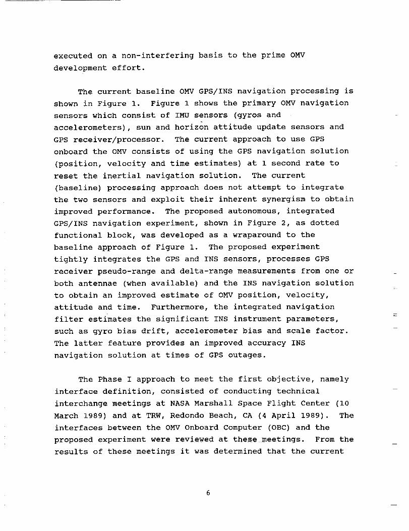
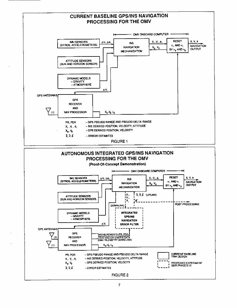
The current baseline OMVGPS/INS navigation processing is

shown in Figure i. Figure 1 shows the primary OMVnavigationsensors which consist of IMU sensors (gyros and

accelerometers), sun and horizon attitude update sensors and

GPS receiver/processor. The current approach to use GPSonboard the OMVconsists of using the GPS navigation solution

(position, velocity and time estimates) at 1 second rate to

reset the inertial navigation solution. The current

(baseline) processing approach does not attempt to integratethe two sensors and exploit their inherent synergism to obtain

improved performance. The proposed autonomous, integrated

GPS/INS navigation experiment, shown in Figure 2, as dottedfunctional block, was developed as a wraparound to the

baseline approach of Figure i. The proposed experiment

tightly integrates the GPS and INS sensors, processes GPSreceiver pseudo-range and delta-range measurements from one or

both antennae (when available) and the INS navigation solution

to obtain an improved estimate of OMVposition, velocity,

attitude and time. Furthermore, the integrated navigation

filter estimates the significant INS instrument parameters,

such as gyro bias drift, accelerometer bias and scale factor.The latter feature provides an improved accuracy INS

navigation solution at times of GPS outages.

The Phase I approach to meet the first objective, namelyinterface definition, consisted of conducting technical

interchange meetings at NASA Marshall Space Flight Center (i0

March 1989) and at TRW, Redondo Beach, CA (4 April 1989). The

interfaces between the OMV Onboard Computer (OBC) and the

proposed experiment were reviewed at these meetings. From the

results of these meetings it was determined that the current

CURRENT BASELINE GPS/INS NAVIGATION

PROCESSING FOR THE OMV

J4

I IMU SENSORS _._

(GYROS, ACCELEROMETERS)

Al-r ITUDE SENSORS

(SUN AND HORIZON SENSOR)

OMV ONBOARD COMPUTER ii

INS

NAVIGATION

MECHANIZATION

I

Xi ,Vi ,e_ I RESET

: i x I ANDv_Xg, Vg BY xg AND vg: L

GPS ANTENNAS

DYNAMIC_GRAVITyMODELS- ATMOSPHERE

t

GPS _l

RECEIVER

AND

NAV PROCESSOR

PR, POR

XI ,V_,0Ix_,vg_,_,_

Xg,Vg,tg

- GPS PSEUDO RANGE AND PSEUDO DELTA RANGE

- INS DERIVED POSITION, VELOCITY, A'I-FITUDE

-GPS DERIVED POSITION, VELOCITY

- ERROR ESTIMATES

FIGURE 1

X,V,B

NAVlGA?ION

OUTPUT

AUTONOMOUS INTEGRATED GPS/INS NAVIGATION

PROCESSING FOR THE OMV

(Proof-Of.Concept Demonstration)

I 4

I IMU SENSORS

(GYROS, ACCELEROMETERS)

ATTITUDE SENSORS(SUN AND HORIZON SENSOR)

I DYNAMIC MODELS- GRAVITY- ATMOSPHERE

GPS ANTENNAS

OMV ONO()A_ COMPUTER

!

GPS

RECEIVER

AND

NAV PROCESSOR

PFI. PDR

Xi , _ , 0 i

xg,vg

_, _,,_

INS

NAVIGATION

MECHANIZATION

!,x,, ) _._,_

(DOWNLINK) ; '

IINTEGRATED I

GPS/INS II

NAVIGATION I

• ERROR FILTER mI

Xg,Vg,tg

"I

- GPS PSEUDO RANGE AND PSEUDO DELTA RANGE

- INS DERIVED POSITION, VELOCITY, ATTITUDE

Xi ,Vi ,8i

X_, Vg

UP'LINK)

II RESET i X.V,o: x i AND v i NAVIGATION

L BY xg AND vg OUTPUT

POST-PROCESSING

-GPS DERIVED POSITION. VELOCITY

- ERROR ESTIMATES

CURRENT BASELINETRW DESIGN

rmwwQi

i m PROPOSED EXPERIMENTI.... j SSIR PHASES lyll

FIGURE 2

7

OMV telemetry data plan includes all the data required to

implement the proposed integrated GPS/INS navigation

experiment.

The integrated navigation filter design and real-time

implementation issues were addressed during the Phase I study.

The primary tool for analysis and evaluation of the integrated

filter performance was the Mayflower GINSS (GPS/Inertial

Navigation System Simulation) software package. This computer

program has been developed by Mayflower over several years and

has been applied successfully on other government programs.

The approach to address the real-time implementation issues

consisted of : (i) converting the conventional Kalman filter

equations to a more robust U-D factor implementation [14]

which requires only single precision word length for

preserving numerical accuracy, and (2) developing a memory and

throughput estimate for the integrated navigation filter using

OMV OBC instruction times.

Our approach to meeting the third technical objective,

namely identifying the application and test software, and

developing a test and validation plan has followed the TRW OMV

GN&C Guidance and Navigation Design Validation Test Plan

outlined in the OMV PDR Document [8]. The approach consisted

of validating the navigation filter algorithms using our GINSS

software package. The navigation filter algorithm was

verified in Phase I by carrying out extensive evaluation using

different system parameters and initial conditions.

8

SECTION 3

PHASE I RESULTS

Specific results of the Phase I Experiment Definition and

Feasibility Study are presented in this section. In order to

facilitate the reading and evaluation of Phase I results we

have patterned this section to match the Phase I Statement of

Work (SOW), that is, a subsection number below corresponds to

a task of the same number in the Phase I SOW.

The primary result described in this section concerns the

design, implementation and evaluation of the proposed

integrated GPS/INS navigation filter. The filter design

involved models of IMU sensor errors, GPS receiver measurement

errors, gravity and atmospheric drag models, and Kalman filter

equations implemented in the U-D factor form. The interface

design between the OMV OBC, which implements the INS

navigation mechanization equations, and the integrated GPS/INS

filter (Figure 2) utilizing the OMV telemetry data was

developed. These interfaces are discussed in Section 3.2.

The GPS and INS navigation sensors and the gravity and

atmospheric drag models and their effect on the orbit

prediction accuracy are described in Section 3.3. This

section also includes the results of GPS satellite visibility

for the OMV. The performance evaluation results for two

specific test cases : (i) good initial conditions and (2) poor

initial conditions are reported in Section 3.3.5 for a high-

thrust trajectory. The first test case (good initial

conditions) corresponds to an orbit transfer phase where GPS

was assumed to be available during the coast phase prior to

the start of the burn. The second test case (poor initial

conditions or a worst-case analysis) assumes GPS outage during

the coast phase and, therefore, initial conditions for the

orbit transfer phase correspond to a pure INS solution.

Excellent position, velocity and attitude accuracy wasdemonstrated for both the test cases. Similar results were

also obtained for an OMVlow-thrust trajectory.

Applicability of the proposed experiment to a wide classof NASA missions is described next.

3.1 Common GN&C Requirements for Advanced STSs

The navigation and attitude update requirements for

several NASA missions were reviewed during the Phase I study.

The objective was to assess how the results of the proposed

experiment can be used to support the goal of developing

autonomous, fault-tolerant GN&C systems for future NASA

missions. Specific attention was devoted to the OMV, Space

Station, OTV and NASA's Earth Science Geostationary Platforms.

Navigation accuracy requirements of these missions are

summarized in this section.

r

The OMV orbit navigation accuracy requirements described

in Table 1 [8] can be significantly improved by employing the

proposed integrated navigation filter algorithm. Simulation

results for OMV trajectories, and OMV navigation sensors"

parameters are described in Section 3.3.5.

The NASA GPS navigation requirements for the Space

Station are summarized in Table 2. Recent studies by Hughes,

Axiomatix and Texas Instruments [9] have concluded that these

Space Station navigation and attitude update requirements can

be met by GPS tracking of the Space Station.

10

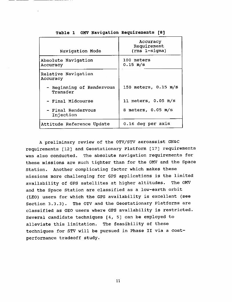
Table 1 OMV Navigation Requirements [8]

Navigation Mode

Absolute Navigation

Accuracy

Relative Navigation

Accuracy

- Beginning of RendezvousTransfer

- Final Midcourse

- Final Rendezvous

Injection

Accuracy

Requirement

(rms 1-sigma)

i00 meters

0.15 m/s

150 meters, 0.15 m/s

ii meters, 0.05 m/s

8 meters, 0.05 m/s

Attitude Reference Update 0.16 deg per axis

A preliminary review of the OTV/STV aeroassist GN&C

requirements [12] and Geostationary Platform [17] requirements

was also conducted. The absolute navigation requirements for

these missions are much tighter than for the OMV and the Space

Station. Another complicating factor which makes these

missions more challenging for GPS applications is the limited

availability of GPS satellites at higher altitudes. The OMV

and the Space Station are classified as a low-earth orbit

(LEO) users for which the GPS availability is excellent (see

Section 3.3.3). The OTV and the Geostationary Platforms are

classified as GEO users where GPS availability is restricted.

Several candidate techniques [4, 5] can be employed to

alleviate this limitation. The feasibility of these

techniques for STV will be pursued in Phase II via a cost-

performance tradeoff study.

II

Table 2 NASA Space Station Navigation Requirements [9

Accuracy

Navigation Mode (rms 1-sigma)

Target Absolute Navigation [28] i0 meters (1-sigma)

Relative Navigation [28] 3 meters (1-sigma)

at Docking/Berthing

Relative Navigation without

Docking Maneuvers [9]

Attitude Update [9]

30 meters (1-sigma)

or 1% of the rangebetween the two

spacecrafts, which-

ever is the greater

0.01 degree

The preliminary navigation requirements for the OTV and

Geostationary Platform are given below.

Position/Velocity

Accuracy

Attitude Alignment

Accuracy

GEOSTATIONARY

PLATFORM [12]

5m -50 m (3 o)

depending on

pointing and

control system

requirements

OTV

AEROASSIST

PHASE [17]

15 m (3-0) LEO

0.02 m/s

340 m (3-0) GEO

0.03 m/s

0.074 degree (3-0)

15 minutes after

stellar update

This brief review of advanced STSs navigation

requirements supports the claim of general applicability of

the proposed experiment to a wide class of future NASA

missions.

12

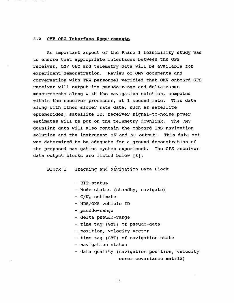
3.2 OMV OBC Interface Requirements

An important aspect of the Phase I feasibility study was

to ensure that appropriate interfaces between the GPS

receiver, OMV OBC and telemetry data will be available for

experiment demonstration. Review of OMV documents and

conversation with TRW personnel verified that OMV onboard GPS

receiver will output its pseudo-range and delta-range

measurements along with the navigation solution, computed

within the receiver processor, at 1 second rate. This data

along with other slower rate data, such as satellite

ephemerides, satellite ID, receiver signal-to-noise power

estimates will be put on the telemetry downlink. The OMV

downlink data will also contain the onboard INS navigation

solution and the instrument _V and _e output. This data set

was determined to be adequate for a ground demonstration of

the proposed navigation system experiment. The GPS receiver

data output blocks are listed below [8]:

Block I Tracking and Navigation Data Block

- BIT status

- Mode status (standby, navigate)

- C/N o estimate

- NDS/ONS vehicle ID

- pseudo-range

- delta pseudo-range

- time tag (GMT) of pseudo-data

- position, velocity vector

- time tag (GMT) of navigation state

- navigation status

- data quality (navigation position, velocity

error covariance matrix)

13

Block II Almanac and Ephemeris Data Block

The corrections to the navigation state vector estimated

by the filter can be computed in real-time on a ground

computer and these corrections can be uploaded to the host

vehicle to form a closed loop system around the experiment

(Figure 2).

m

14

• 3.3 Integrated GPS/INS Navigation Filter Design

A tightly-integrated GPS/INS navigation filter design is

presented in this section. The navigation filter equations,

implemented in the U-D factor form, are described here. The

proposed integrated GPS/INS navigation filter combines several

GPS-based attitude determination techniques to obtain an

accurate and continuous navigation solution for all phases of

a spacecraft mission, thereby providing improved accuracy and

extreme flexibility in mission planning. The three GPS-based

attitude determination techniques employed here are:

l• Velocity vector matching technique employing one GPS

antenna during spacecraft orbit maneuvers

. Interferometric GPS carrier phase processing

technique using two or more antennae during

spacecraft coast and maneuver phases

• Attitude vector matching technique employing one GPS

antenna during spacecraft rotation maneuvers

The autonomous integrated GPS/INS navigation experiment will

use a combination of these techniques for providing improved

total navigation solution. The focus of the presentation in

this section is on the first technique which is considered the

primary technique for the OMV attitude determination.

Modifications to the navigation filter to implement the other

two techniques are also identified.

Location of the two GPS antennae on the OMV is shown in

Figure 3. The two antennae are separated in Y axis by

approximately 5 meters in the fully deployed position.

15

LOW GAIN ANTENNA ASSEMBLY(REVISED PLUME IMPINGEMENT CONFIGURATION

7,'t }}"TRW $p_, i

|H_*_qi G_tp " ORIGINAL PAGE IS

®

El; 0

o,/ \

%_IW 0° TO 95*

OF POOR QUALITY

/

Fig. 3 :

@

Location of

®

the GPS

• Antenna Baseline Separation

• 209.6 In_5.]m

Antennae on the OMV.

GN&C HARDWARE BLOCK DIAGRAMi

tl4mt.lt G,I.I

i i

• L

Global J

Positioning I'--I

Sys,e JlJRendezvous __J

Radar J ]

, !Inertial

Measurement

Unit

Earth

Sensor

SunSensor

rg '£n'7<Z£7nTg',Ta1 Management Subsystem

I I

Uni, F_ I unit I" Iuo,t I'.

11 i I"'"" I I"l _"'_ I I ii

I Onboard

I ComputerI

L-

Courtesy NASA CXqV Program Office

Fig. 4 : Simplified GN&C Block

r_r_pulsion Subsystem

Throttle Variable

Control Thrust

I Electron;cs Engines

i. ]

.+

Valve

DriveElectronics

Contingency

Hold

Elec:ronics

.__ OimbalElectronicsAssembly

"1

Thrusters

1 --...J

Diagram.

i

Gimbal-_" Drive

Assembly

Ir----,'- --_I SBand/G"°balI1 lPosifion,nn ill

I ISvste m J I

! |Antenna ] 1i,,." __'.,l

16

3.3.1 Naviqation and Attitude Sensors - GPS and INS

The OMV guidance, navigation and control (GN&C) subsystem

performs completely automatic spacecraft operation for orbit

change, rendezvous and station keeping [15; p. 112]. A

simplified block diagram of the GN&C subsystem is shown in

Figure 4.

Redundant sensor assemblies provide the information

required by the onboard computer (OBC) software to guide and

control the OMV automatically through its mission phases.

Each sensor complement consists of a GPS receiver, a

rendezvous radar, an inertial measurement unit (IMU), an Earth

sensor and a sun sensor.

The primary navigation sensor on the OMV is the GPS

receiver [8; p. 2-5]. It provides accurate flight vehicle

position and velocity in Earth centered coordinates. Inertial

attitude reference is obtained by the IMU gyros and is

propagated by a closed-form integration algorithm using

quaternions. The Earth and sun sensors provide periodic

attitude reference updates to correct for gyro drifts. The

overall attitude accuracy achieved with this design is better

than 1° per axis [15; p. 113].

Ground tracking of the spacecraft provides a means to

estimate the navigation errors and upload the corrections.

Tracking of GPS satellites by the OMV GPS receiver provides an

autonomous capability to update the INS position and velocity

[16; p. 8].

OMV orbital position and velocity (ephemeris calculation)

is propagated by the OBC using a fourth order numerical

integrator of the Runge-Kutta type for the numerical

17

integration of the differential equations of motion [8; p. 2-5].

OMV Global Positioning STstem (GPS) Receiver

The OMV GPS receiver is a 2-channel sequential receiver

being developed by Rockwell International, Satellite and Space

Electronics Division. The size, power and weight estimates

are 9.9" x 7.1" x 2.3", 13 Watts and 6 ibs, respectively.

The receiver will output data at a rate of 1 per second.

The accuracy of the receiver-computed position is 393 ft (3-o)

per axis using C/A code and 367 ft (3-o) per axis using P-Code

(GDOP=4.3). The velocity accuracy is 0.86 ft/sec (3-o) per

axis (GDOP=4.3). The GPS receiver measurement error model (l-

o) for the integrated navigation filter evaluation is given

below:

Receiver Pseudo-Range Measurement Noise

Receiver Delta-Range Measurement Noise

Clock Frequency Drift Rate

Delta Range Integration Interval

= 1.8 m

= 2.5 cm

= 10 -8 sec/sec

= 0.I sec

L

GPS environment errors (e.g., satellite ephemeris error,

satellite clock error, iono/tropospheric errors and multipath

errors) used in this evaluation are described in [2].

OMV Inertial Measurement Unit (IMU)

The OMV IMU is the modified SKIRU IV produced by Singer-

Kearfott. The unit contains two MOD II E/S GYROFLEX gyros,

which are 2-Degree-of-Freedom, dry tuned-rotor gyros, without

temperature control. The gyro performance characteristics are

as follows:

18

Gyro Bias Drift

Input Axis Alignment

Scale Factor Linearity and Asymmetry

Scale Factor Stability

0.022 deg/hr, 3-o

7 arcsec , 3-o

40 ppm

93 ppm , 3-o

The unit also contains three MODVII accelerometers, which are

single-axis, subminiature, linear, pendulus devices. The

accelerometer performance characteristics are as follows:

Bias Stability

Scale Factor Linearity and Asymmetry

27 micro-g,0.155%

3--G

3.3.2 Gravit7 and Atmospheric Draq Models

There are times during the OMV mission when prediction of

the vehicle orbit is required (e.g., rendezvous and docking).

The two prominent perturbing accelerations at the OMV

altitudes are the ones induced by the geopotential and the

atmospheric drag.

Currently, the OMV OBC orbit predictor utilizes a second

degree zonal harmonic (J2) model to compute the orbital

perturbations due to the non-central part of the Earth's

gravitational field, whereas the magnitude of the atmospheric

drag perturbing acceleration is an input constant [8; p. 2-5].

The effects of ignoring terms, other than J2, in the reference

geopotential model on the OMV orbit prediction were analyzed.

It was shown that inclusion of a (2,2) model will

significantly improve the orbit prediction accuracy at a

minimal computational cost.

19

_ffects of the Geopotential Modeling

In order to study the effects of the geopotential

modeling on the OMV orbit prediction accuracy we generated

three orbital arcs. The first one, termed the (8,8) orbit,

was designated as our reference orbit. It was generated

assuming that the Earth is completely modeled by the Goddard

Earth Model T1 (GEM-T1) to degree and order 8 [19]. The

second orbit, termed the J2 orbit, was generated assuming that

the Earth is an ellipsoid of revolution with the GEM-T1

fundamental parameters. The third orbit, termed the (2,2)

orbit, was generated assuming that the Earth is completely

modeled by GEM-T1 to degree and order 2. The duration of each

orbit was six hours and a new point was computed every five

minutes. The orbital eccentricity e=0.001 and the inclination

i=35 ° was assumed for all three arcs. Each orbit was

generated at two altitudes, namely 150 nmi (277.8 km) and 250

nmi (463 km), which correspond to orbital periods of

approximately 89 min and 94 min respectively.

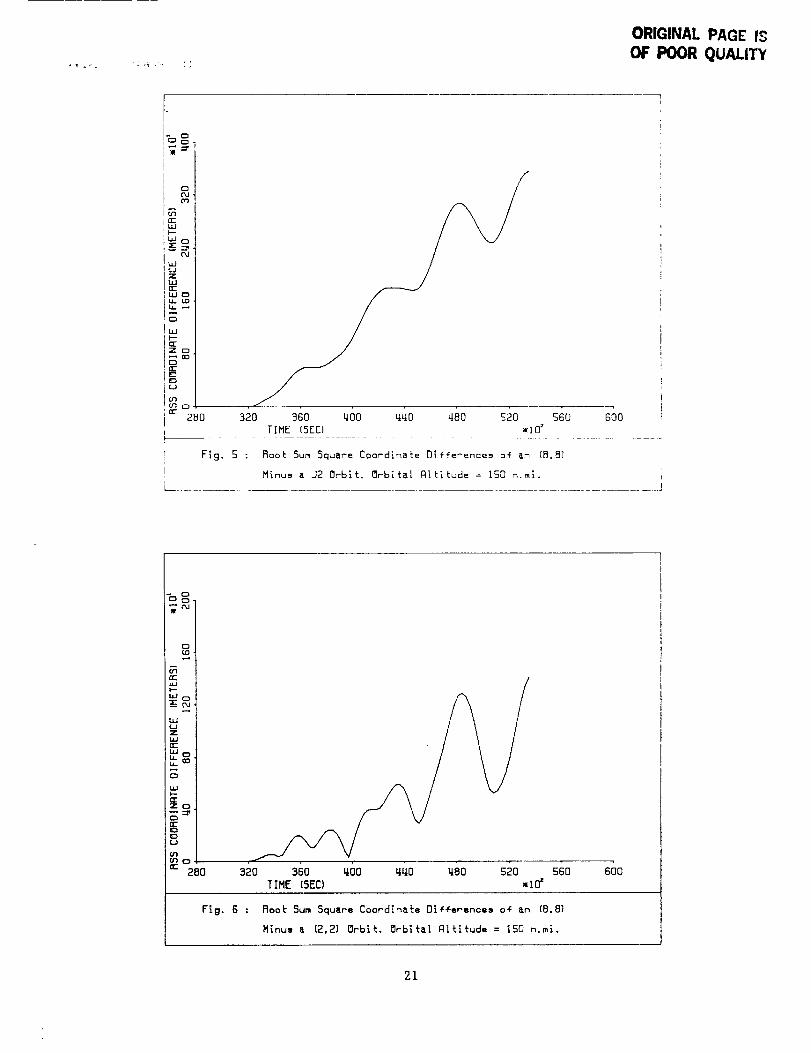
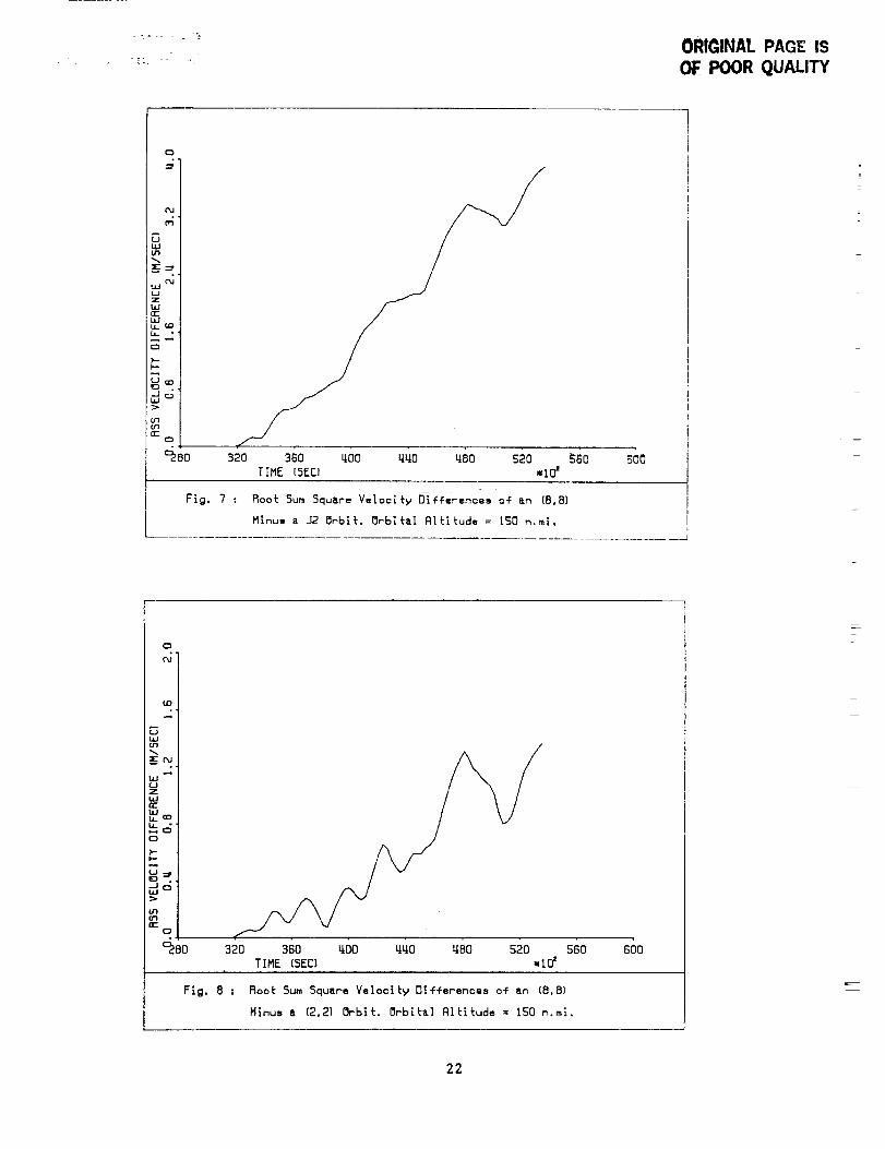
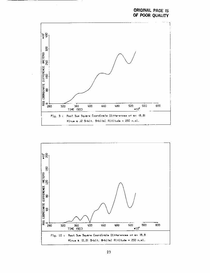
The Root Sum Square (RSS) differences in coordinates and

velocities between the (8,8) and J2, and the (8,8) and (2,2)

orbits for an orbital altitude of 150 nmi are shown in Figures

5, 6, 7 and 8, whereas the same differences at an orbital

altitude of 250 nmi are shown in Figures 9, i0, Ii and 12.

Examination of Figures 5, 6, 7 and 8 indicates that at an

orbital altitude of 150 nmi the RSS coordinate difference

(with respect to the (8,8) reference model) is 3.6 km for the

J2 orbit and 1.4 km for the (2,2) orbit, whereas the

corresponding RSS velocity difference is 4 m/sec for the J2

orbit and 1.4 m/sec for the (2,2) orbit. Furthermore,

inspection of Figures 9, i0, II and 12 indicates that at an

orbital altitude of 250 nmi, the RSS coordinate difference is

3.0 km for the J2 orbit and 0.9 km for the (2,2) orbit whereas

r

Z0

ORIGINAL PAGE f$OF POOR QUALITY

!

n-WI--

PJ

_3CJZU.J

t.J3_

___

p-

L..I

28O 320 360 400 q_O LJ80 520 560

TIME (SF_CI _I0 _

FIg. 5 : Root Sum Square Coordinate O[fferences of &n (8,8)

M_nus a J20r6_t. Or6[lal AlIi_ude = ISO n.m_.

600

C3

UJ

LI,J o

W

ZWrr

W

C_ZC_

" 280 320 360 400 440 480 520

TIME (SEC) ItO Z

560

FIg. 6 : Roo_: Sum 5quire Coorcl[n&ie Differences of &n (8.81

Minus I (2,2l 0r61_. Orbltal Al_:[_:ude = 150 n,m_.

600

21

ORI(_INAL PAGE IS

OF POOR QUALITY

C_

o,J

Ot_JU_

t.ij C_J

bLJrr

h •

r_

>--F--

LJ GO

do

320 360 L_O0 V,LIO Li80 520TIME (5[C) =I0z

Fig. ? : Root Sum SquAre Velocity 0_fferences of _n (8,8)

Minu, a J20r61t, Orbi(al Ql(i(ude = ISO n,ml,

_60

ijj _

°tZbJrr"

C)

>-p--M

fr-O

TIME (5EC) _IO'' L r

Fig. 8 : Root Sum Square Velocity O|fferences of an (8,8)

M|nus s (2.21 Orblt. Orbital Altltude = 150 n.m_.

22

ORIGINAL PAGE IS

OF POOR QUALITY

w -- i

1C3cu,It_

n-'WI--

htc:D

LIJLJZ

zo_C3

oc 280 320 360 400 440 480 520 560

TIME (5EC) =I0'

600

FIO. 9 : Boot Sum 5quire CoordinB_e Oifference_ of &n (8,8)

Minul • J20r6_. Orbi_l Al_i_ude = 250 n.ml.

trbd

__cu

bJ

Z

U-

W

MrZC_

C_

0{.J

_m

_" !80 320 360 400 4_0 480 520

TIME (SEC) mid _

Fig. 10 : Boo_ 5um Square Coordlna(e D|fferencea of an (8.B

Minum m (2,2) Or6lL Orbital Al_i_udm = 250 n.m_.

23

OF POOR QUALITY

C_

:=I

OO

ObJ

_J_JUZb.JE

_ •

ff'l

¢'e-

32o 3_o .oo ..o .oo s_OTIME (SEC) nlO"

's6o _6o

Fio. ii : Boot Sum Square Velocity Differmncwm of an (8,B}

Minus • J20rblt, OrB|taI Altltude : 250 n.m_•

m

c)

oo

0bJ

°

UZhiE

__®

>-I-,-

re-

=_B0 320 360 _00 _LI0 riB0 520TIME (SEC} mlO'

S60

Fig. 12 : Boot Sum 5quire Velocity Otfferenceg of an (B,B}

M|nus a [2,2] 0rb_t. 0r61tal A1tltuch. : 250 n.m;.

600

24

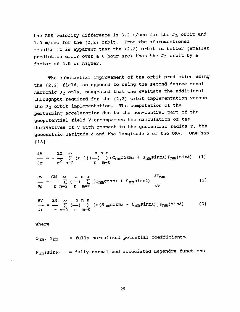
the RSS velocity difference is 3.2 m/sec for the J2 orbit and

1.0 m/sec for the (2,2) orbit. From the aforementioned

results it is apparent that the (2,2) orbit is better (smaller

prediction error over a 6 hour arc) than the J2 orbit by a

factor of 2.5 or higher.

The substantial improvement of the orbit prediction using

the (2,2) field, as opposed to using the second degree zonal

harmonic J2 only, suggested that one evaluate the additional

throughput required for the (2,2) orbit implementation versus

the J2 orbit implementation. The computation of the

perturbing acceleration due to the non-central part of the

geopotential field V encompasses the calculation of the

derivatives of V with respect to the geocentric radius r, the

geocentric latitude 4 and the longitude A of the OMV. One has

[1B]

aV GM

ar r 2 n=2

ann

(n+l) (--) _(CnmcOsml + Snmsinml)Pnm(Sin_)

r m=0

(i)

av GM oo a n n aPnm

(--) _ (Cnm cosml + Snmsinml )

r n=2 r m=0 _

(2)

aV

8A

GM _ ann

(--) _ [m(SnmcOsml - CnmsinmA) ]Pnm(Sin_)r n=2 r m=0

(3)

where

Cnm, Snm

Pnm (s in4 )

= fully normalized potential coefficients

= fully normalized associated Legendre functions

25

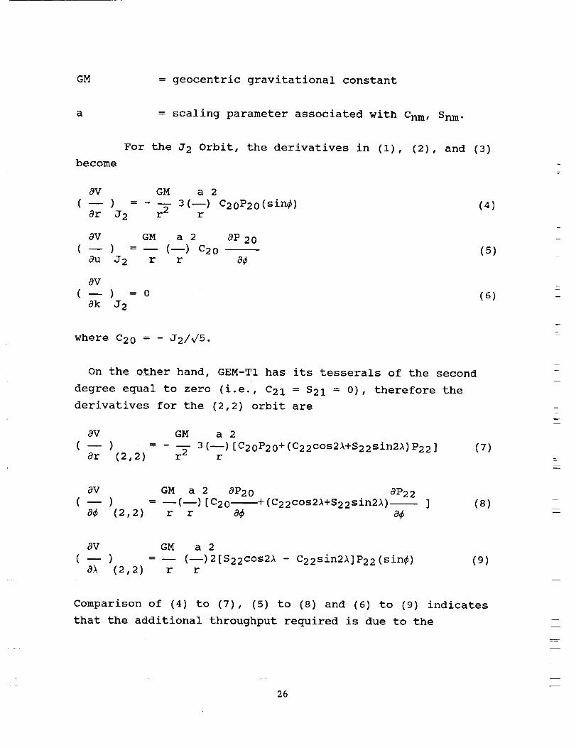
GM = geocentric gravitational constant

a = scaling parameter associated with Cnm , Snm.

For the J2 Orbit, the derivatives in (I),

become

_V GM a 2

( -- ) = - -- 3 (--) C20P20 (sin_)8r J2 r2 r

aV GM a 2 8P 20

( -- ) - (__) C20

au J2 r r a4

aV

(--) = 0

ak J2

where C20 = - J2/_5.

(2), and (3)

(4)

(5)

(6) E

On the other hand, GEM-T1 has its tesserals of the second

degree equal to zero (i.e., C21 = S21 = 0), therefore the

derivatives for the (2,2) orbit are

aV

(I)ar (2,2)

GM a 2

= - -- 3 (--) [C20P20 + (C22cos2A+S22sin2A) P22 ]r 2 r

aV

(--)a4 (2,2)

GM a 2 aP20 aP22

- (__) [C20--+(C22cos2A+S22sin21 )-

r r a_ a_

(7)

(8)

av GM

(__)al (2,2) r

a 2

(--)2[S22cos2A - C22sin21]P22(sin_)r

(9)

Comparison of (4) to (7), (5) to (8) and (6) to (9) indicates

that the additional throughput required is due to the

26

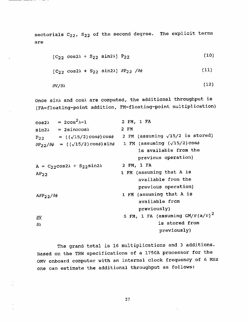
sectorials C22, $22 of the second degree.are

The explicit terms

[C22 cos21 + $22 sin21] P22

[C22 cos2l + S22 sin21] 8P22 /84

(i0)

(ii)

av/a_ (12)

Once sinl and cosl are computed, the additional throughput is

(FA=floating-point addition, FM=floating-point multiplication)

cos21

sin2Â

P22

aP22/a_

= 2cos21-i

= 2sinlcosl

= ((Vl5/2)cos_)cos4

= ( (Vl5/2)cos4)sin#

A = C22cos21 + S22sin21

AP22

AaP2 2/a4

av

a),

2 FM, 1 FA

2 FM

2 FM (assuming _15/2 is stored)

1 FM (assuming (_15/2)cos4

is available from the

previous operation)

2 FM, 1 FA

1 FM (assuming that A is

available from the

previous operation)

1 FM (assuming that A is

available from

previously)

5 FM, 1 FA (assuming GM/r(a/r) 2

is stored from

previously)

The grand total is 16 multiplications and 3 additions.

Based on the TRW specifications of a 1750A processor for the

OMV onboard computer with an internal clock frequency of 6 MHz

one can estimate the additional throughput as follows:

27

16FM + 3FA = 16x13 + 3x15 = 253 clock cycles

hence

Throughput = 253x(i/6)x10 -6 sec = 42.17 _sec per update

This additional throughput estimate appears to be

negligible in light of the resulting improvement of the orbit

by a factor of 2.5.

Effects of the Atmospheric Drag

In order to study the effects of the atmospheric drag on

the OMV orbit prediction accuracy we generated two six hour

orbital arcs, computing a new point every five minutes. The

first orbit was Keplerian, whereas the second one was

perturbed by the atmospheric drag. The orbital eccentricity

was e=0.001, the inclination was i=35 ° and the altitude was

150 nmi for both orbits. The air density required for the

computation of the perturbing acceleration due to the

atmospheric drag was computed assuming a Jacchia-Groves

atmospheric model (Global Reference Atmospheric Model-GRAM)

[20] as implemented by the subroutine "GRAM". The RSS

differences in coordinates and velocities between the two

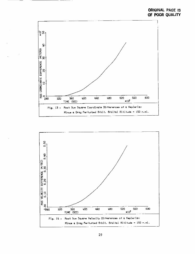
orbits are shown in Figures 13 and 14.

In Figures 13 and 14 one can observe a secular behavior

of the atmospheric drag effects. The RSS coordinate

difference grows to approximately 400 m and the RSS velocity

difference grows to 0.5 m/sec at the end of the six hour arc.

This is a significant effect_ However, implementation of the

GRAM routine in the onboard computer of the OMV is a

formidable task due to both the memory required by the routine

and its associated files and the throughput required for the

z

L

r

zF

D--

28

ORIGINAL PAGE IS

OF POOR QUALITY

_l.nl

I

I

_4

J

d

EO.

3E3

J

F_g. 13 ;

360 400 4_0 480 520

TIME (SEC) mlOZ

SGO 600

Roo_ 5um Square Coordlnate Differences of a Kepleri&n

M_nus a Orlg Perturbed Orbit. Orbital gltitude = ISO n.ml.

0W

°

ujC)UZ

UJn--

UJC3U-Cdu_ ,1

N_

I--

¢rc)

_8o s2o

F_g. 14 :

360 400 440 480 520 SGO GO0

TIME (5EC} =10'

Root Sum Square Velocity Oif+erences o+ a Keplerian

Minus a Drag Perturbed Orbit. Orbital Rll_tude = iSO n.ml.

29

operation of the routine. Therefore, alternate models to

describe the atmosphere should be examined such that both the

drag effect is reduced and the computational burden on the OBC

of the OMV is contained to within feasible limits.

3.3.3 GPS Satellite Visibility-One Antenna

A study to determine the visibility of the GPS satellites

to the OMV GPS antennae was carried out. The primary GPS

constellation of 21 satellites [27] was used for this

investigation. Twelve hour orbital arcs were generated to

cover a full period of the GPS satellites. An antenna look

angle of ii0 ° and two OMV orbital altitudes (250 nmi and i000

nmi) and two inclinations (27 ° and 55 °) were utilized. The GPS

satellite selection and the computation of the Geometric

Dilution of Precision (GDOP) was carried out once per minute,

due to the rapidly changing geometry.

The visibility study was carried out assuming that there

was no rotation of the OMV body frame with respect to inertial

space, such that its Y-axis was always parallel to the Y-axis

of the inertial frame. This may not be a realistic

assumption, since the OMV will probably be oriented towards

the sun at all times for power reasons. However, while on one

hand the above assumption has practically no influence on the

visibility study due to the homogeneity of the GPS

constellation, on the other hand, this assumption can be very

easily relaxed by incorporating attitude data in our analysis

(e.g., quaternions or Euler angles).

In the course of our study an interesting notion came

about, namely that of antenna switching. Since the OMV has

two GPS antennae, the effect of antenna switching on the GPS

satellite visibility was analyzed. The idea is that software

3O

commands on the OMVOBC or ground control commands could beutilized to switch from one GPS antenna to the other to ensure

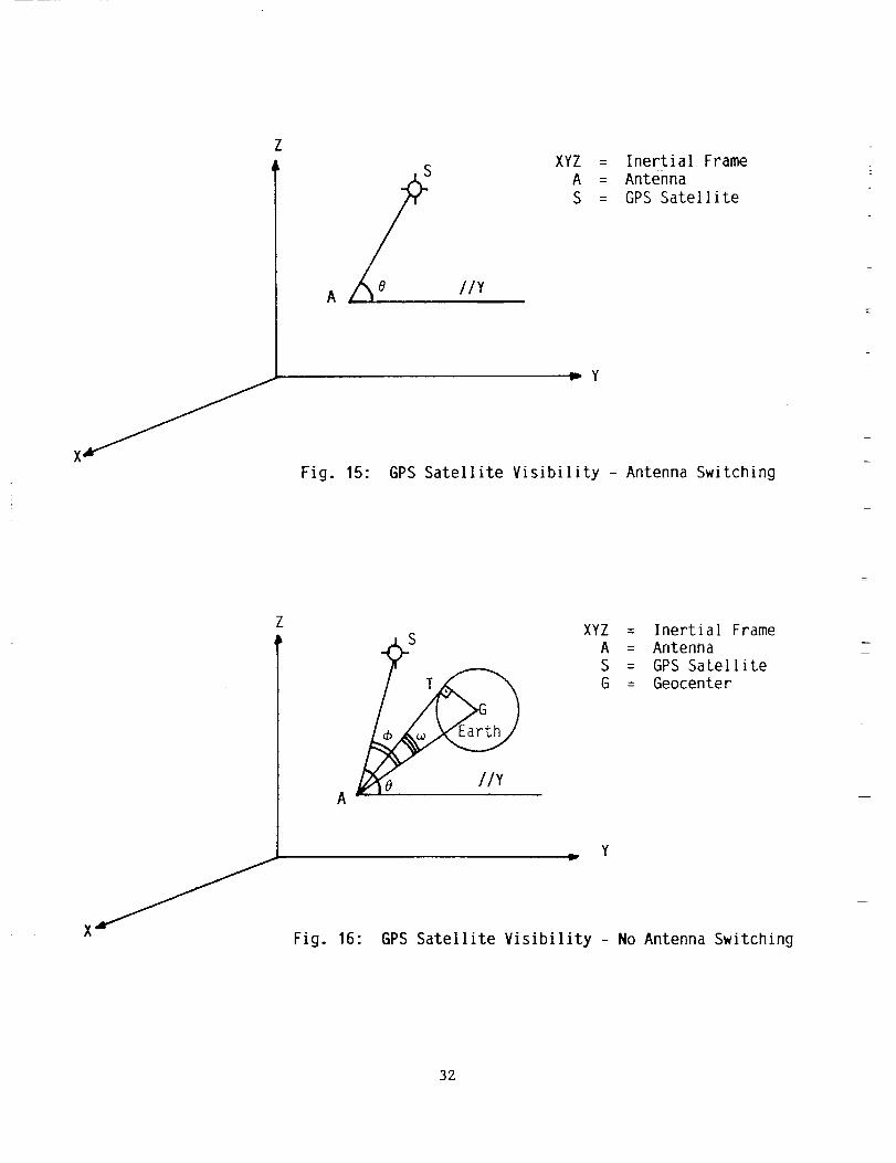
the best possible visibility of the GPS constellation. Figure

15 shows the geometry with antenna switching, whereas Figure

16 shows the geometry without antenna switching.

For the case of antenna switching (Fig. 15), let the

coordinates of the GPS satellite S be (Xs, YS, ZS) in theinertial frame and let the coordinates of the OMV's antenna A

be (XA, YA, ZA) in the same frame. The visibility criterionis

#_< z

where z is the antenna look angle of ii0 degrees. Now

# = cos-l<iAZ,iAS >

where iAZ and iAS are the unit vectors along the antenna

zenith and along the direction AS respectively. One has

iAZ = [ 0 1 0 ]T

and

iAS = [ XS - XA, YS - YA, ZS - ZA]T/rAS

where

rAS = [(Xs - XA) 2 + (Ys - YA) 2 + (Zs - ZA)2] I/2

Hence the visibility criterion becomes

cos-l[(Ys - YA)/rAS] _ z

31

llY

XYZ = Inertial FrameA = AntennaS = GPS Satellite

_Y

Fig. 15: GPS Satellite Visibility - Antenna Switching

?

//Y

XYZ = Inertial Frame

A = Antenna

S = GPS Satellite

G = Geocenter

p Y

Fig. 16: GPS Satellite Visibility - No Antenna Switching

32

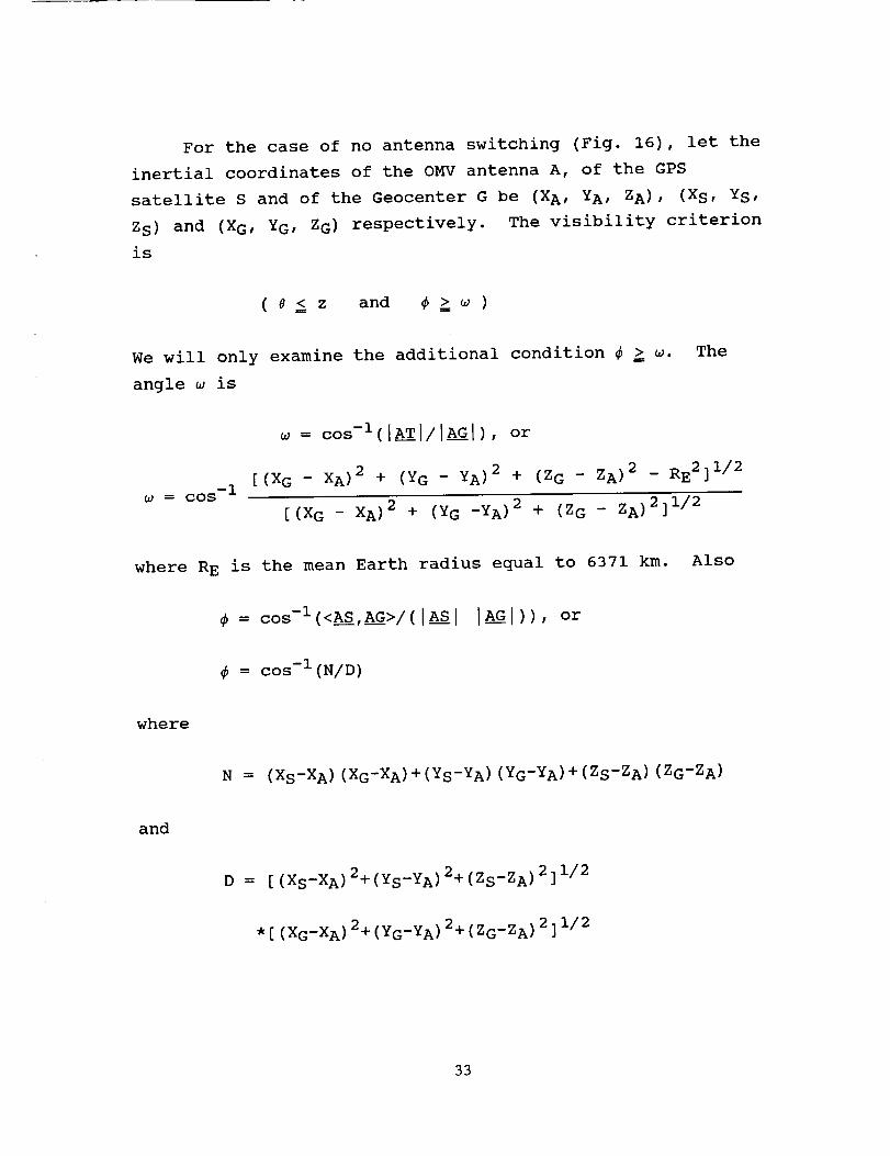
For the case of no antenna switching (Fig. 16), let the

inertial coordinates of the OMV antenna A, of the GPS

satellite S and of the Geocenter G be (XA, YA, ZA), (Xs, YS,

ZS) and (XG, YG, ZG) respectively. The visibility criterion

is

( 8 _ z and _ _ w )

We will only examine the additional condition # _ _.

angle w is

The

= cos -I

w = cos-I([A_TT[/IAGI), or

[(XG - XA) 2 + (YG - YA) 2 + (ZG - ZA) 2 - RE2]1/2

[(XG - XA) 2 + (YG -YA) 2 + (ZG - ZA) 2] I/2

where R E is the mean Earth radius equal to 6371 km. Also

= cos-I(<A_SS,A__GG>/([AS 1 [AG])), or

= cos -I (N/D)

where

N = (Xs-XA) (XG-XA)+(Ys-YA) (YG-YA)+(Zs-ZA) (ZG-ZA)

and

D = [ (Xs-XA) 2+ (ys_YA) 2+ (Zs_ZA) 2 ]1/2

, [ (XG_XA) 2+ (yG_YA) 2+ (ZG_ZA) 2] 1/2

33

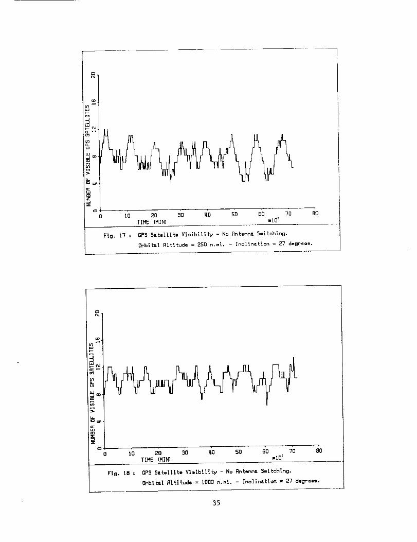
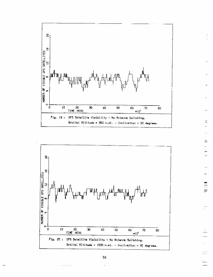
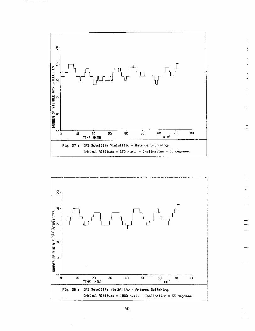
Figures 17 through 20 show the visibility results withoutantenna switching for the two different altitudes and the two

inclinations. Figures 21 through 24 show the corresponding

GDOPf0r the respective altitudes and inclinations.

Furthermore, Figures 25 through 32 are similar to 17 through

24 but with antenna switching.

From Fig. 17 one can observe that the average number ofvisible GPS satellites at an altitude of 250 nmi and at an

inclination of 27° is approximately 7, whereas the minimum is4 and the maximum is 12. From Fig. 18 one can see that at an

altitude of i000 nmi and at the same inclination, the average

number of visible satellites is approximately 9 with a minimum

of 6 and a maximum of 13, i.e., the visibility is better at

the higher altitude. This result is also apparent from

comparison of Fig. 19 to 20. On the other hand, comparison ofFig. 17 to 19 and 18 to 20 indicates practically no influence

of the inclination on the visibility. Inspection and

comparison of Figures 21 through 24 indicate similar influenceof the altitude and the inclination on the GDOP, and that at

the i000 nmi altitude, the GDOPupper bound is approximately3.

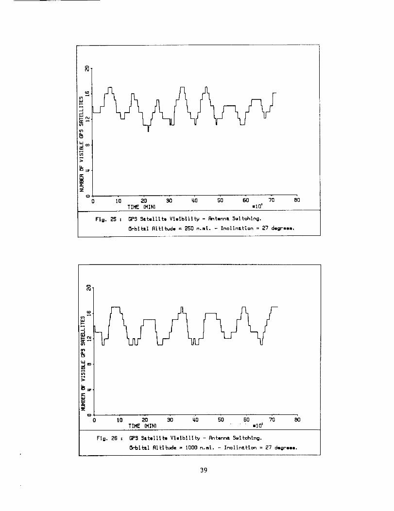
From Figures 25 through 28 one can observe an averagenumber of 13 visible satellites with no less than I0 and as

much as 17 always in view. Furthermore, it is also

interesting to note that the altitude influences the results

much less in this case. Moreover, from Figures 29 through 32

one can see that the GDOPhas an upper bound of approximately

2.5 without any poor geometry regions (such as the ones in

Figures 21 and 23) and that the influence of the altitude isonly marginal.

34

tO

U3_J

.J

.J

U3

LO

03

E_=r

LU00

z

0 t6 2o 3o _o s'oTIHfi (MIN)

60 70 80_10 t

F_g. 17 : BP_ 5_Eell[_e V_s_6[llty - No An_enns 5=[_chlng.

Orb[tll Altitude = 250 n.ml. - In¢lin_kion = 27 degrees.

tO..q

03t_

M

nmtIJO0

Z

1'o _o 3o _'o so 6o _o 8oTIN[ (HINI mlO I

Fig, t8 : GP$ Ss_ellt_e Vle[6ll[6_ - No AnEennl SwL_ch[ng.

Or"6_ Rl_|_ude = tO00 n.m_. - Incl[nsfi[on = 27 deOreee.

35

86

F[ O. 19 : GP$ 5_lellile VI#[6[I_ W - No Anlenna 5w[(ching.

Orb[Ill A1(|_:ude = 250 n.m|. - InclinaE[on = 55 degrees.

Fig. 20 : GP5 5_t=Illt= Y[={6[ltty - No AnEenna 5=[Ech[ng.

Or61t=l AltlbJde = lO00 n.ml. - Incl[n_l|on = SS degree=.

36

I

C_

M-

0 lO 20 30 u_O 50 60 70

TIME (MIN] _I0'

Fig. 21 : Geometric Dilution of Preclsion - No An_enn_ 5wi_cKing.

Or6_l_I Al_il_Jde = 250 n.m_. - Incllna_ion = 27 degreee.

z

-J

u

M-

K_

Io 2'o 3'o Co s'o G'o 7'oTIME [MIN] _I0'

BO

F_@, 22 : Geom_tr|c O_lu_ion of Prec|slon - No Rn_enna Sw_ch|n@.

Orb{_$1Rltil_Jde = 1000 n.m{, - Inci_n&_on = 27 dlgrnl,

37

(3

I

l

_=I

i

Io io _o 3o 40 so 6o 7o Bo

TIME (MINI mlO'

Fig. 23 : Geome_rlc OIlu_|on of Prec:|81on - No Antenna 5wi_rd_ing.

Orbital Qlti_ude = 250 n. ml. - Incl[na_[on = 55 dogroom.

L

o

If

:=,

Z

rr_O_

2:

C)_j

I--

.-J

I'--

I.U

o i'o 2'o 3'o _o so _'o ?oTIME [MINI ,10 _

8'O

Fig. E_ : Geomi_r|c Ollu_|on of Prec181on - No Rn_ennl 5wltchlng.

Orbi_tl @l_ibJde = lOOO n. ml, - Incl|n&_|on = 55 degrees.

38

OJ

OO

rlLJ

7/

11

t_

I.

;=..q

T"

r

¢3

0 16 2'o 3'o _'o 5"0 6"o 76TIME (MIN) =I0'

Fig. 25 = GP5 5at=lilt= Vt={billty - Antenns 5=Itching.

Orbital A1tItud= = 250 n,m_. - IncltnaE_on = 27 d=gr===.

¢0

bJI--

_J

O_O.(.9

P-i¢/3

h

R"

0 16 2o so _o so _o vo 8oTIME (MIN) =10'

Ftg. 26 : GP5 5st=lift= V1=161116/ - Ant=nna 5=Itching.

Or61b_l Rltltud= = 1000 n. ml. - IncllnaEton = 27 degrn=.

39

BO

Fig. 27 : GP5 51Emlllt= Vi=i611|L'y - Flntann_ S=itchlng.

Or61tsl Altltudl = 2SO n,ml. - In=llnaEion = 55 degrems.

C3CU

(D

&/314.1I-'-M...I

CX: "-'

_n,(3

h

E:

Z

F

C3

0 I'o _ 3'o _o s'o Go ?oTIME {MIN) rot0'

8O

Fig. 28 : GPS Satelllt= Vimlbillb/ - Antenna S=iEchlng.

Orbltll AIEib._e = 1000 n.ml. - In=llns_ion = SS degr=e=.

E

m

E

4O

m

:=F

Z0

¢3

Z

F-

.J

o 1"o

Ftg. 29 •

2"o 3'o _'o s.0 6'o _oTIME {MINI _tO =

BO

Geometrl¢ Dilution of Precision - Rntenn_ 5=itchtng,

Orb{_[ R[t[_u¢ie = 250 n.s{. - Inel{nsE[on = 27 degre=o.

C3

:=F

ZI0

O-

ZI004

.J

(J

F--LU

LUC_

o 1.0 2o _o _o so 6o _oTIME {MINI m10z

8O

F|g. 30 : Geometrlc O11ution of Prec|mlon - Rn_ennl 5=itching.

Orbital RttItude = I000 n.m_, - InclInat{om = 27 degree=.

41

w_

Z

N

bJ_

G

Nt.l

i,,,-

0W

o 16 2'o 36 _o 56 6'o _oTIME (MIN] ",10z

B'O

F|Q. Sl : GeomeErlc D|lu_:|on of PreoI=|on - RnEmnn_ 5*|robing.

Or6i_l Al_l_ude = 250 n. ml. - Inol[n_ion = SS doOreeo.

ID

1{3

Z:

..J

_J

L

_t

o 1o 26 36 _o 5o 6o foTIME (MINI llOl

FIg. 32 : Geome_r|c O|lut[on of Prec|a|on - An_ennl 5wlbchlng.

8rbi_al Al_ib_de = 1000 n.ml. - Incllna_lon = SS degren.

m

42

Comparison of the results without and with antennae

switching indicates that the latter yields an improvement of

the results by a factor of 1.5.

3.3.4 Naviqation Filter Implementation

The integrated GPS/INS navigation filter is implemented

as an extended-Kalman filter for simultaneously estimating the

navigation error states and dominant IMU instrument errors.

For the Phase I analysis involving OMV, the IMU instrument

errors included in the filter states are the gyro bias drift

and the accelerometer scale factor errors. For this

application, the accelerometer bias errors were not considered

significant [7]. The integrated filter implementation is

based on the functional block diagram shown in Figure 2. The

filter incorporates GPS receiver measurements of pseudo-range

(code phase) and delta-range (integrated carrier phase) to

estimate the filter states. The error states included in the

navigation filter for the OMV application are:

Position 3

Velocity 3

Alignment 3

Gyro bias drift 3

Accelerometer scale factor 3

GPS clock time bias 2

and frequency drift

Total 17

We introduced two new features in our navigation filter.

The first one was the implementation of the filter in its U-D

factor formulation. The second one was the incorporation of

43

the second degree zonal harmonic in the filter. The first

feature improves the numerical stability (robustness) of the

filter while working with single precision numbers. The

second feature improves the navigation performance of thesystem.

U-D Factors

The implementation of the integrated GPS/INS navigation

filter in the on-board computer of the OMV places an

additional memory and throughput re_rement on the mission.

Consequently, any effort to reduce the aforementioned burden

is desirable. From the filter standpoint, an important step

towards reducing memory and computation requirements is the

implementation of the U-D factor formulation of the filter as

opposed to its conventional Kalman formulation. In this

section the conventional Kalman filter equations and the U-D

factors equations for the Kalman filter are presented. A

comparison between the two formulations is also presented

here.

Conventional Kalman Filter Formulation

The conventional formulation of the discrete Kalman

filter is [22; p. Ii0]

fi) Time Update:

^(-) ^(+)_k = #k,k-i Xk-i (13)

44

(-) (+) TPk = _k,k-i Pk-i _k,k-i + Qk-i

(ii) Measurement Update:

(14)

^(+) ^(-) ^(-)Xk = x k + Kk (zk - H k Xk ) (15)

(+) (-)Pk = (I - Kk Hk) Pk (16)

(-) T (-) T

Kk = Pk Hk (Hk Pk Hk + Rk) -I (17)

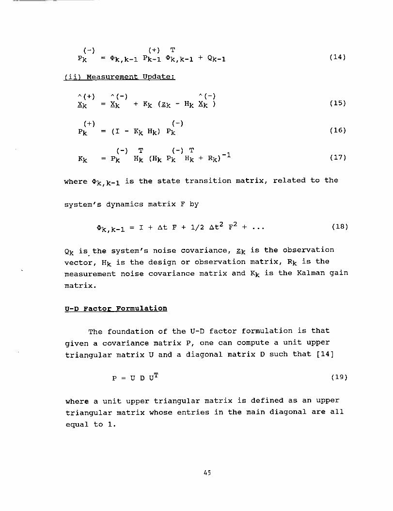
where _k,k-i is the state transition matrix, related to the

system's dynamics matrix F by

_k k-i = I + At F + 1/2 At 2 F 2 + ... (18)

Qk is the system's noise covariance, Zk is the observation

vector, H k is the design or observation matrix, R k is the

measurement noise covariance matrix and K k is the Kalman gain

matrix.

U-D Factor Formulation

The foundation of the U-D factor formulation is that

given a covariance matrix P, one can compute a unit upper

triangular matrix U and a diagonal matrix D such that [14]

P = U D U T (19)

where a unit upper triangular matrix is defined as an upper

triangular matrix whose entries in the main diagonal are all

equal to i.

45

i) .Time Update:

(+)Let U and D be the U-D factors of Pk-I such that

(+)Pk-i = U D U T

and define

(20)

then

W = [_k,k_l U I] (21)

(22)

=

WBW T =[_k,k-i U T] I°°j[TTjU • k, k-i

0 Qk I

= [_k,k_l U I] D U _ k,k-i

Qk

T T

= _k,k-i uDU _k,k-i + Qk

(+) T

= #k,k-I Pk-i Sk,k-I + Qk

L_

i.e. r

(-)Pk = wBwT

(23)

46

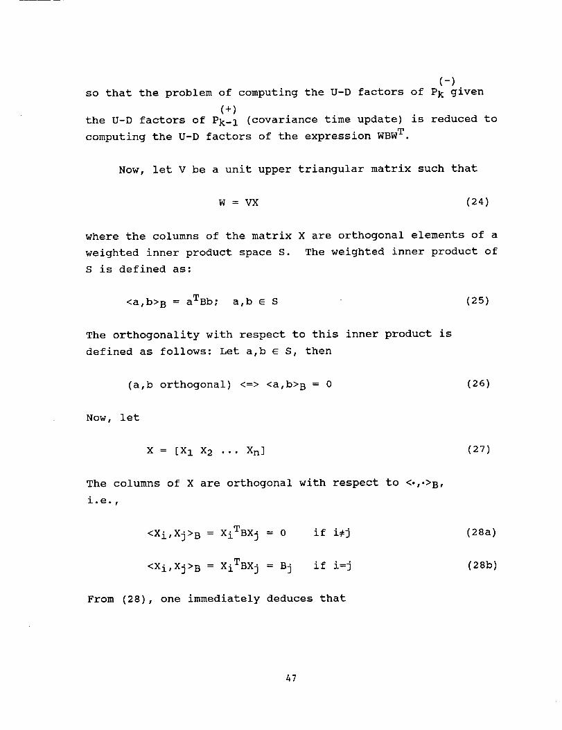
(-)so that the problem of computing the U-D factors of Pk given

(+)

the U-D factors of Pk-I (covariance time update) is reduced to

computing the U-D factors of the expression WBW T.

Now, let V be a unit upper triangular matrix such that

w = vx (24)

where the columns of the matrix X are orthogonal elements of a

weighted inner product space S. The weighted inner product of

S is defined as:

<a,b> B = aTBb; a,b e S (25)

The orthogonality with respect to this inner product is

defined as follows: Let a,b e S, then

(a,b orthogonal) <=> <a,b> B = 0 (26)

Now, let

X = [X 1 X 2 ... Xn] (27)

The columns of X are orthogonal with respect to <','>B,

i.e.,

<Xi,Xj>B = xiTBxj = 0

<Xi,Xj>B = xiTBxj = Bj

if i#j (28a)

if i=j (28b)

From (28), one immediately deduces that

47

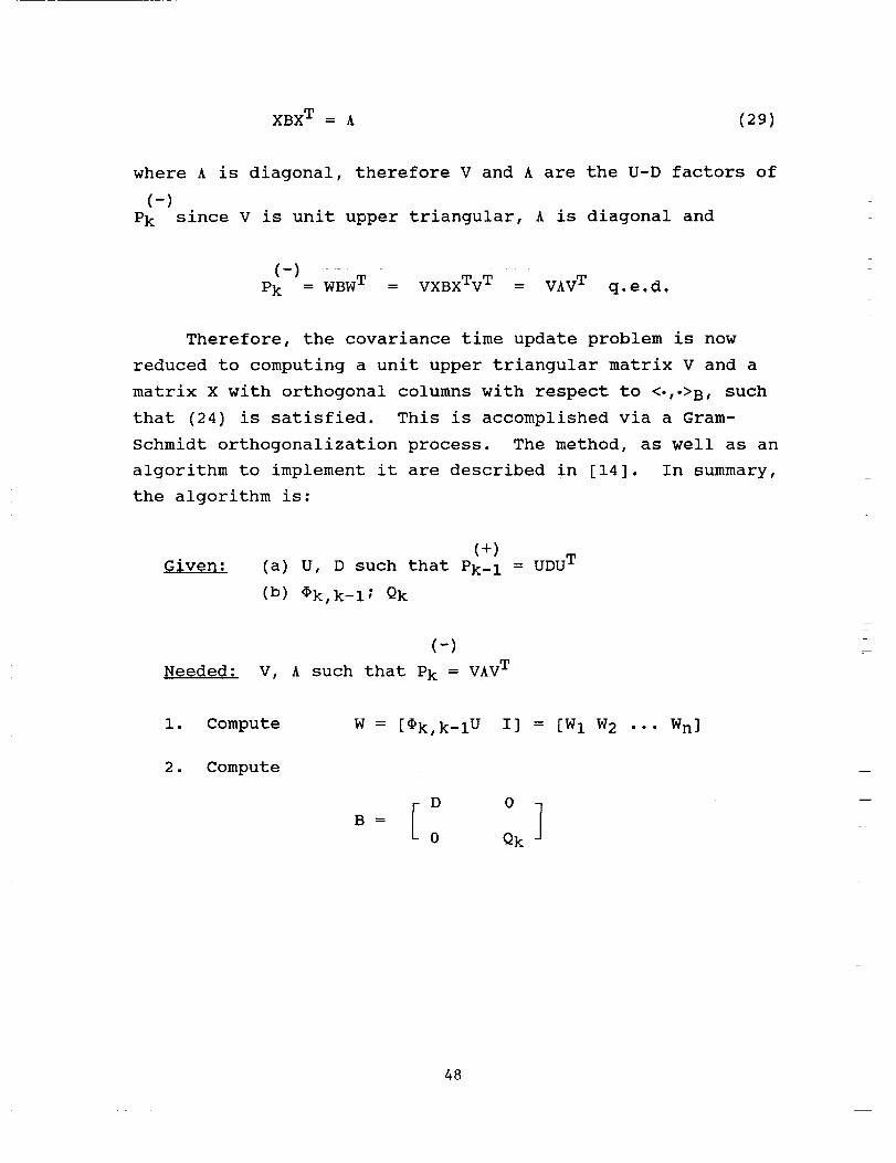
XBXT = A (29)

where A is diagonal, therefore V and A are the U-D factors of

(-)Pk since V is unit upper triangular, A is diagonal and

(-)Pk = wBwT = VxBxTvT = vAvT q.e.d.

Therefore, the covariance time update problem is now

reduced to computing a unit upper triangular matrix V and a

matrix X with orthogonal columns with respect to <','>B, such

that (24) is satisfied. This is accomplished via a Gram-

Schmidt orthogonalization process. The method, as well as an

algorithm to implement it are described in [14]. In summary,

the algorithm is:

(+)Given: (a) U, D such that Pk-I = uDuT

(b) _k,k-l; Qk

Needed:

(-)

V, A such that Pk = vAvT

F

i. Compute

2. Compute

W = [_k, k-i U

D

0

I] = [W 1 W 2 ... Wn]

48

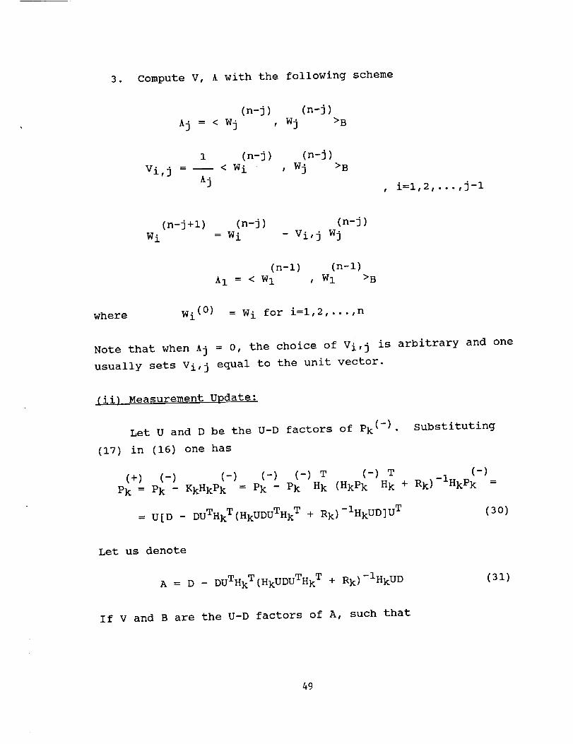
3. Compute V, A with the following scheme

(n-j) (n-j)

Aj = < Wj , Wj >B

Vi, j -

1 (n-j) (n-j)

< W i , Wj

Aj

>B

, i=l,2,...,j-i

(n-j+l) (n-j)

w i = w i

(n-j)

- Vi, j Wj

(n-l) (n-l)

A1 = < W1 , W1 >B

where Wi(0) = W i for i=l,2,...,n

Note that when Aj = 0, the choice of Vi, j is arbitrary and one

usually sets Vi, j equal to the unit vector.

(ii) Measurement Update:

Let U and D be the U-D factors of Pk (-) . Substituting

(17) in (16) one has

(+) (-) (-) (-) (-) T (-) T (-)

Pk = Pk - KkHkPk = Pk - Pk Hk (HkPk Hk + Rk )-IHkPk =

= U[D - DUTHkT(HkUDUTHk T + Rk)-IHkUD] uT (30)

Let us denote

A = D - DUTHkT(HkUDUTHk T + Rk)-IHk uD (31)

If V and B are the U-D factors of A, such that

49

A = VBVT (32 )

and

w = uv (33)

then W and B are the U-D factors of Pk (+) , since:

wBwT = UvBvTu T = UAU T = Pk (+) , or

Pk (+ ) = wBwT (34)

Therefore, the problem of computing the U-D factors of Pk (+)

given the U-D factors U and D of Pk (-) (covariance measurement

update) is reduced to computing the U-D factors V and B of the

matrix A, because given V and B one can compute W from (33).

The algorithm is [14]:

Given: (a) U,D such that Pk (-) = UDU T

(b) H k; R k

Needed: W, B such that Pk (+)

i. Compute f = UTHk T

= WBW T

2. Set

g = Df = DUTHk T

a 0 = Rk, then, for j=l,2,...,n:

w

aj = aj_ 1 + fj gj

aj -i

Bj - mj (Bj = Dj if aj=0)

aj

50

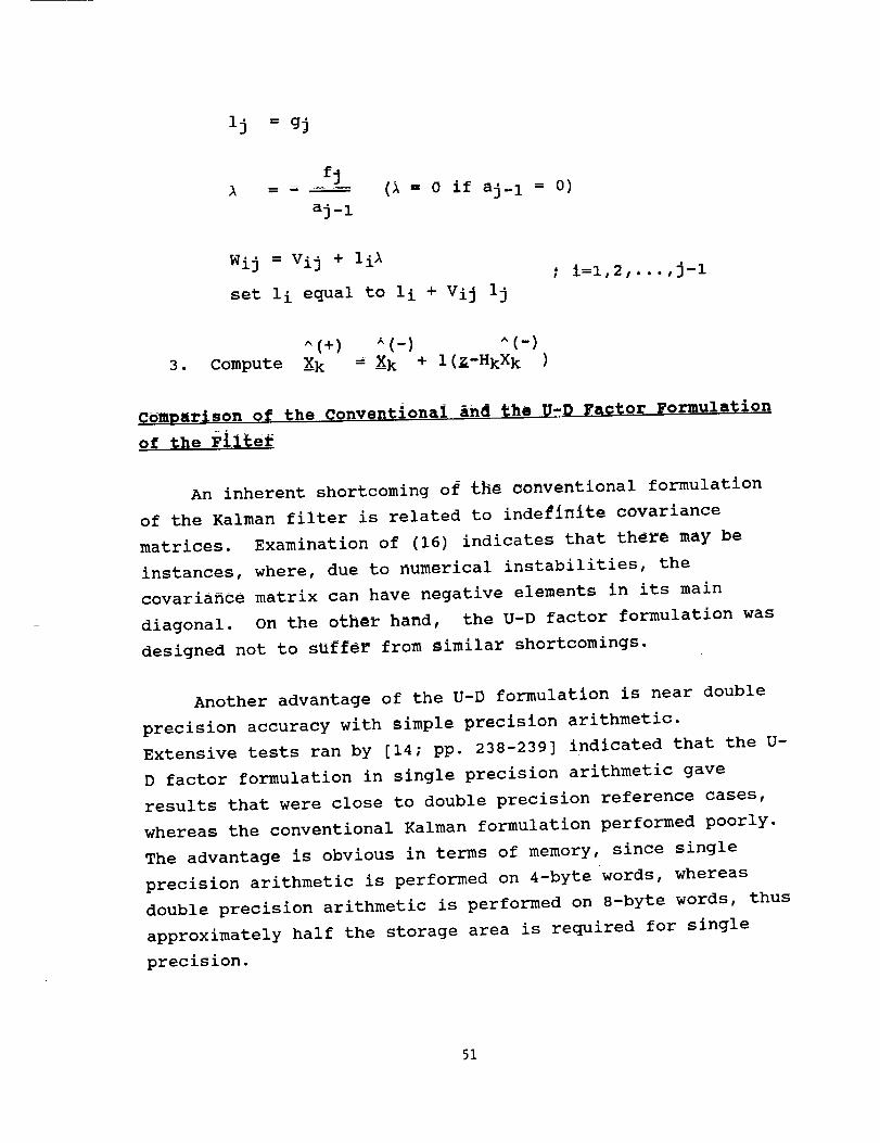
lj = gj

fj

aj_l(A - 0 if aj- 1 = 0)

Wij i Vij + l i_

set ii equal to ii + Vij lj

' i=l 2 . j-i' , t " " ,

•

^(+) ^(-)Compute Xk = X k ÷ i (Z-HkX k )

Comparison of the Cgnventional _nd £he U-D T,a¢_or Formulation

of the F1i£e_

An inherent shortcoming of £h_ conventional formulation

of the Kalman filter is related to indefinite covariance

matrices. Examination of (16) indicates that th_e may be

instances, where, due to numerical instabilities, the

covarian_e matrix can have negative elements in its main

diagonal. On the oth_ hand, the U-D factor formulation was

designed not to sUff_ from similar shortcomings•

Another advantage of the U-D formulation is near double

precision accuracy with simple precision arithmetic.

Extensive tests ran by [14; pp. 238-239] indicated that the U-

D factor formulation in single precision arithmetic gave

results that were close to double precision reference cases,

whereas the conventional Kalman formulation performed poorly.

The advantage is obvious in terms of memory, since single

precision arithmetic is performed on 4-byte words, whereas

double precision arithmetic is performed on 8-byte words, thus

approximately half the storage area is required for single

precision•

51

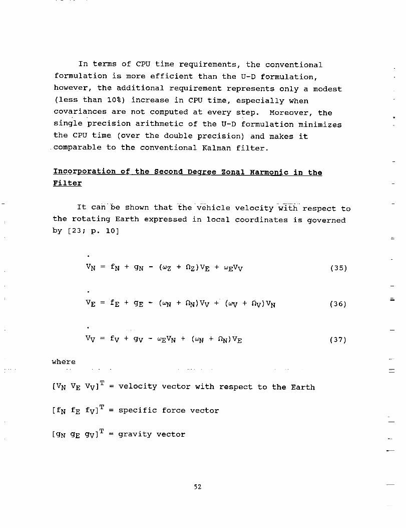
In terms of CPU time requirements, the conventional

formulation is more efficient than the U-D formulation,

however, the additional requirement represents only a modest

(less than 10%) increase in CPU time, especially when

covariances are not computed at every step. Moreover, the

single precision arithmetic of the U-D formulation minimizes

the CPU time (over the double precision) and makes it

comparable to the conventional Kalman filter.

Incorporation of the Second Deqree Zonal Harmonic in the

Filter

It can be shown that the vehicle velocity with respect to

the rotating Earth expressed in local coordinates is governed

by [23; p. i0]

VN = fN + gN - (wZ + Nz)VE + WEVv (35)

VE = _E + gE - (_N + nN)Vv + (_ + nv)V_ (36)

Vv = fv + gv - WEVN + (WN + _N)VE

where

[V N V E VV] T = velocity vector with respect to the Earth

[fN fE fv] T = specific force vector

[gN gE gv] T = gravity vector

(37)

52

[WN _E wV] T = angular velocity of the local frame with respect

to inertial space

[nN _E NV] T = angular velocity of the Earth with respect to

inertial space

or, using the relationships of Table 3-2 in [23, p. 27], one

has

V N = fN+gN-VE2tan4/r-2nVEsin4-VNVv/r (38)

V E = fE+gE-VEVv/r-2_Vvcos#+VEVNtan4/r+2_VNsin_ (39)

V v = fv+gV+VN2/r+VE2/r+2nVECOS4 (40)

where

r = geocentric radius of the vehicle

= latitude of the vehicle

= Earth rotation rate.

Taking the total differentials of (38), (39) and (40)

yields the differential equations governing the velocity

errors. One has

6V N = - [ (VE/rcos4) 2 +2nVECOS4/r ]6XN+ (VE 2 tan4+VNVv) 6Xv/r 2

- (2VEt a n4/r+ 2 n s in_ )6V E -Vv6VN/r-VN6VV/r+6 gN (41)

6V E = (VEVN/(rcos4) 2+2nVvsin4/r+2nVNCOS4/r)6X N

53

+ (VvVE-vEvNta n4) 6Xv/r 2 + (V N t a n4-V v) 6VE/r

+ (VEtan4/r+2nsin4) 6V N- (2Ncos4+VE/r) 6Vv+6g E (42)

6VV = -2nVEsin46XN/r- (VN2+VE 2 )6Xv/r2+ (2ncos4+2VE/r) 6v E

+ 2VN6VN/r+6g v (43)

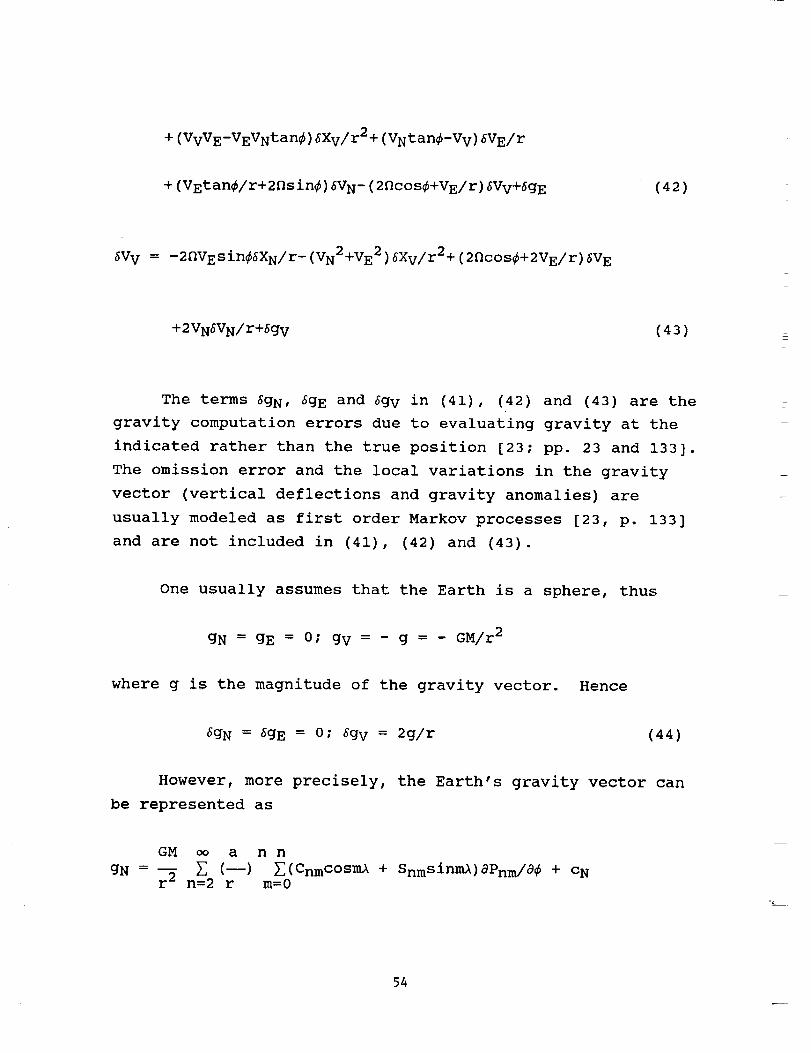
The terms 6gN, 6g E and 6gv in (41), (42) and (43) are the

gravity computation errors due to evaluating gravity at the

indicated rather than the true position [23; pp. 23 and 133].

The omission error and the local variations in the gravity

vector (vertical deflections and gravity anomalies) are

usually modeled as first order Markov processes [23, p. 133]

and are not included in (41), (42) and (43).

=

One usually assumes that the Earth is a sphere, thus

gN = gE = 0; gv = - g = - GM/r2

where g is the magnitude of the gravity vector. Hence

6gN = 6g E = 0; 6g v = 2g/r (44)

However, more precisely, the Earth's gravity vector can

be represented as

gN -

GM _ a

E (--)r 2 n=2 r

n n

_(CnmcOsml + Snmsinml)aPnm/a _ + c Nm=0

'L

54

GM _ ann

- n_ (--) _ [m(SnmcOsml-Cnmsinml)]Pnm(Sin_)+CEgEr 2 cos_ =2 r m=0

GM _ ann

gv = - --_[ l+_(n+l) (--) _ (CnmcOsml+Snmsinml) Pnm (sin4) ]+c vr_ n=2 r m=0

where CN,C E and c v are the components of the centrifugal force

vector c along the North, East and Up local coordinate system.

The centrifugal force in an Earth-fixed XYZ coordinate system

is given by [24; p. 47]

c = [D2X, _2y, 0]T

and the rotation matrix from XYZ to N,E,V is [25; p. 70]

[ -sin4cosl -sin4sinl c%s4 ]R = -sinl cosl

cos4cosl cos4sinl sin4

where 4 and I are the latitude and longitude of the origin of

the N, E, V system. Moreover, the Cartesian geocentric

coordinates X and Y are given by [26; p. 16]

X = rcos4cosl

Y = rcos#sinl

where r is the geocentric distance to the point of interest.

Thus

cN =-_rsin4cosl

c E = 0

55

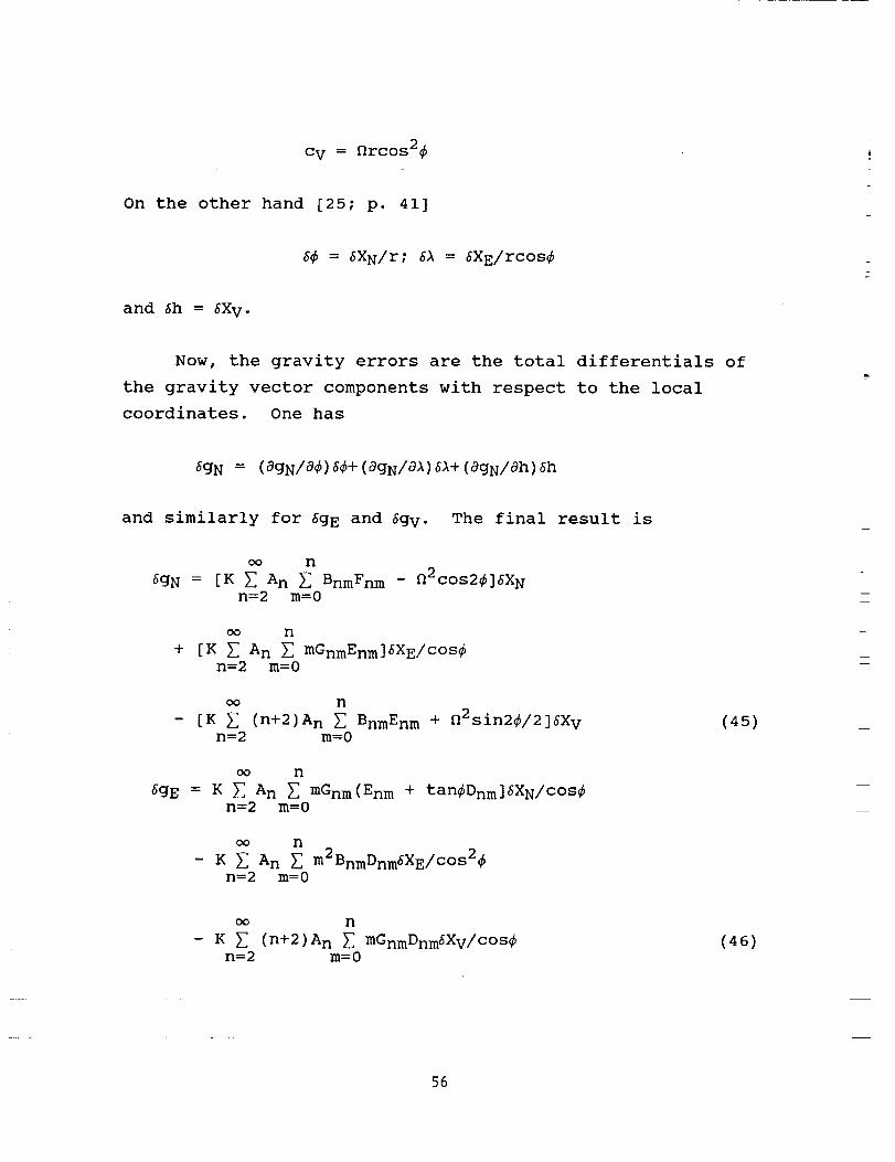
cv = Drcos2_

On the other hand [25; p. 41]

and 6h = 6Xv.

64 = 6XN/r; 6A = 6XE/rcos 4

Now, the gravity errors are the total differentials of

the gravity vector components with respect to the local

coordinates. One has

6gN = (8gN/84) 64+ (agN/aA )6_+ (agN/ah )6h

and similarly for 6g E and 6g v. The final result is

oo n

6g N = [K _ A n _ BnmFnm - n2cos2416XN

n=2 m=0

n

+ [K _ A n _ mGnmEnm]6XE/COS 4n=2 m=0

n

- [K _ (n+2)A n _ BnmEnm + n2sin24/216Xv

n=2 m=0

n

6g E = K _ A n _ mGnm(Enm + tan¢Dnm]6XN/COS 4n=2 m=0

co n

- K _ A n _ m2BnmDnm6XE/COS24

n=2 m=0

(45)

oo n

- K _ (n+2)A n _ mGnmDnm6Xv/cos 4n=2 m=0

(46)

56

where

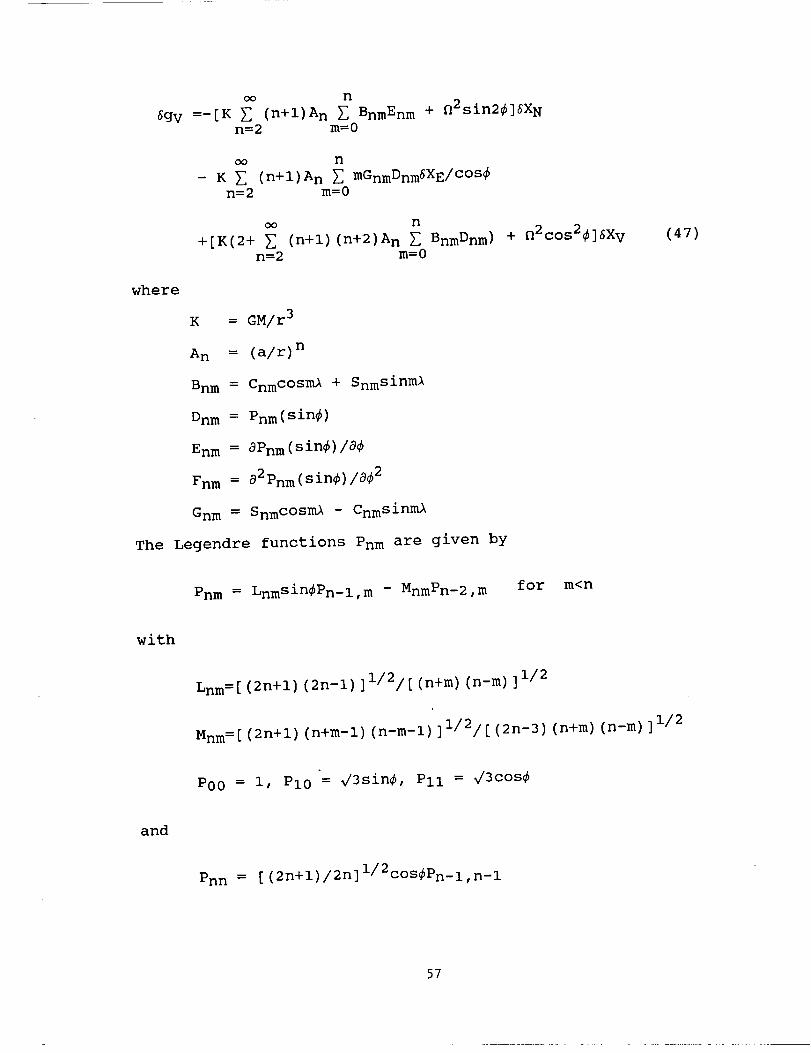
n6g v =-[K _ (n+l)A n _ BnmEnm + n2sin2416XN

n=2 m=0

n

- K _ (n+l)A n _ mGnmDnm6XE/COS_

_=2 m=0

oo n

+[K(2+ _ (n+l)(n+2)A n _ BnmDnm ) + n2cos2_]6Xv

n=2 m=0

K = GM/r 3

A n = (a/r) n

Bnm = CnmcOsml + Snmsinml

Dnm = Pnm(Sin4)

Enm = aPnm (sin4)/a4

Fnm = 82pnm(Sin4)/842

Gnm = SnmcOsml - Cnmsinml

The Legendre functions Pnm are given by

(47)

Pnm = Lnmsin4Pn-l,m - MnmPn-2,m for m<n

with

Lnm=[ (2n+l) (2n-l) ]1/2/[ (n+m) (n-m) ]1/2

Mnm=[ (2n+l) (n+m-l) (n-m-l)]1/2/[ (2n-3) (n+m) (n-m)]1/2

P00 = I, Pl0 = _3sin4, Pll = _3cos4

and

Pnn = [ (2n+l)/2n]i/2cos4Pn_l,n_l

57

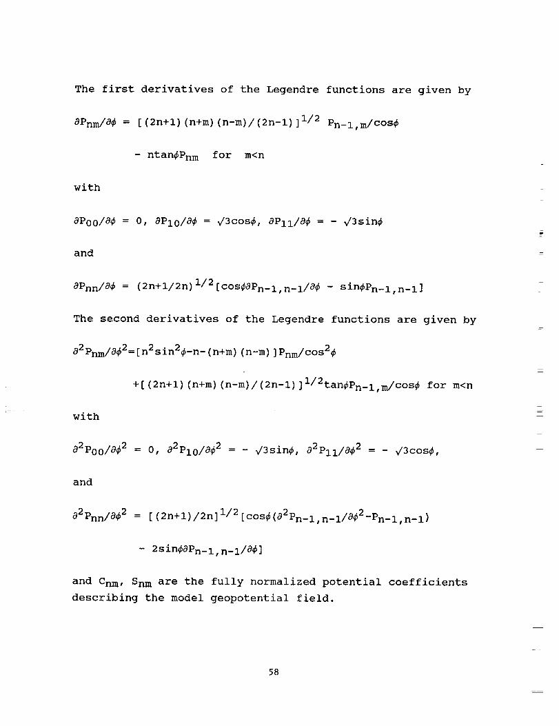
The first derivatives of the Legendre functions are given by

aPnm/a_ = [ (2n+l) (n+m) (n-m)/(2n-l) ]1/2 Pn_l,m/COS 4

- ntan4Pnm for m<n

with

aPoo/a4 = o, aPlo/a4, = _3cos4, aPll/a _ = - _/3sin4

and

aPnn/a _ = (2n+i/2n) l/2[cos_aPn_l ,n_I/a_ _ sin4Pn_l,n_l]

The second derivatives of the Legendre functions are given by

a 2 Pnm/a42= [n 2 s in24-n - (n+m) (n-m) ]Pnm/COS2#

+[ (2n+l) (n+m) (n-m)/(2n-l) ]i/2tan#Pn_l,m/COS4 for m<n

with

a2poo/a42 = o, a2plo/aq_ 2 = - _3sin_, a2pll/a# 2 = - _3cos_,

and

a2Pnn/a_ 2 = [ (2n+l)/2n]l/2[cos_(a2Pn_l,n_l/a@2-pn_l,n_l)

- 2sin4aPn_l, n-i/a4]

and Cnm , Snm are the fully normalized potential coefficients

describing the model geopotential field.

58

In the event that only the second degree zonal harmonic

J2 needs to be considered one has Cnm = Snm = 0 except for C20

= - J2/_5. Thus, considering that

P20 = V5(3sin2#-l)/2, aP20/a_ = 3_5sin24/2 and

a2p20/a_ 2 = 3_5cos2_/2

the gravity error equations become

GM a 2

6g N = -[3_(7) J2cos2_ + n2cos2_]6XN

GM a 2

+[ 6r3--(--)r J2sin2_ + n2sin2_/2 ]6Xv

6g E = 0

9GM a 2

6gv = [_(_-) J2 - D2]sin246XN

GM a 2

+ [r3_ [2-6(--)_ J2(3sin24-1)] + n2cos2416Xv

(48)

(49)

(5o)

Equations (48), (49) and (50) were incorporated in our

navigation filter in order to consider the J2 effects.

However, equations (45), (46) and (47) can be implemented if

the incorporation of a higher resolution and accuracy field is

desired. The value of J2 used in the filter is 0.0010826258

which corresponds to the GEM-T1 model.

3.3.5 PerformanceResults

We used the GPS Inertial Navigation System Simulation

(GINSS) software to evaluate the performance of the integrated

59

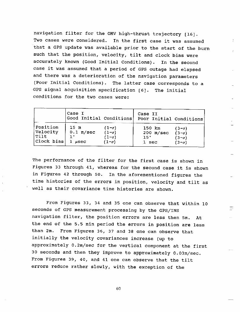
navigation filter for the OMVhigh-thrust trajectory [16].Two cases were considered. In the first case it was assumed

that a GPS update was available prior to the start of the burn

such that the position, velocity, tilt and clock bias were

accurately known (Good Initial Conditions). In the second

case it was assumed that a period of GPS outage had elapsed

and there was a deterioration of the navigation parameters

(Poor Initial Conditions). The latter case corresponds to a

GPS signal acquisition specification [6]. The initial

conditions for the two cases were:

Position

VelocityTilt

Clock bias

Case I

Good Initial Conditions

15 m (l-a)

0.I m/sec (l-a)

1° (l-a)1 _sec (l-a)

Case II

Poor Initial Conditions

150 km (3-a)

200 m/sec (3-a)

15° (3-°)1 sec (3-o)

The performance of the filter for the first case is shown in

Figures 33 through 41, whereas for the second case it is shown

in Figures 42 through 50. In the aforementioned figures the

time histories of the errors in position, velocity and tilt as

well as their covariance time histories are shown.

r

From Figures 33, 34 and 35 one can observe that within i0

seconds of GPS measurement processing by the GPS/INS

navigation filter, the position errors are less then 5m. At

the end of the 5.5 min period the errors in position are less

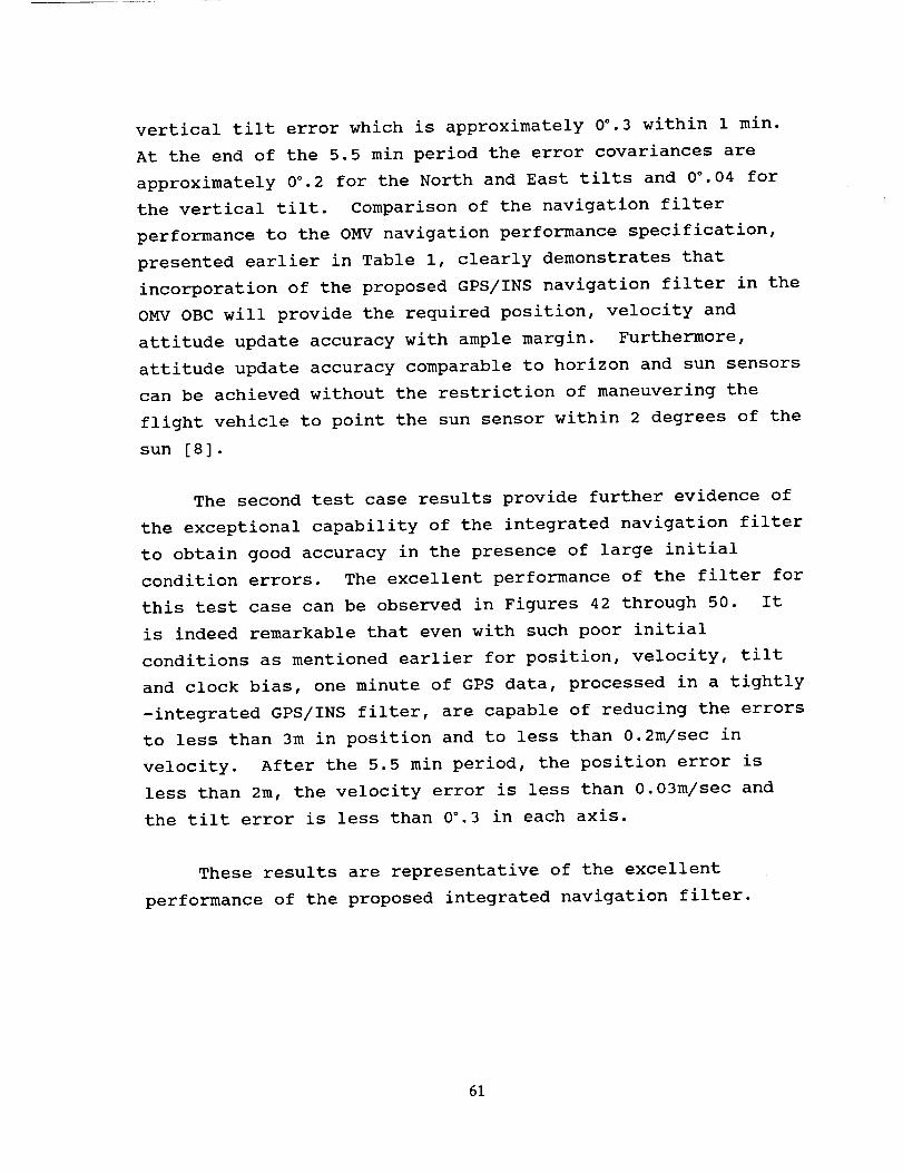
than 2m. From Figures 36, 37 and 38 one can observe that

initially the velocity covariances increase (up to

approximately 0.2m/sec for the vertical component at the first

30 seconds and then they improve to approximately 0.03m/sec.

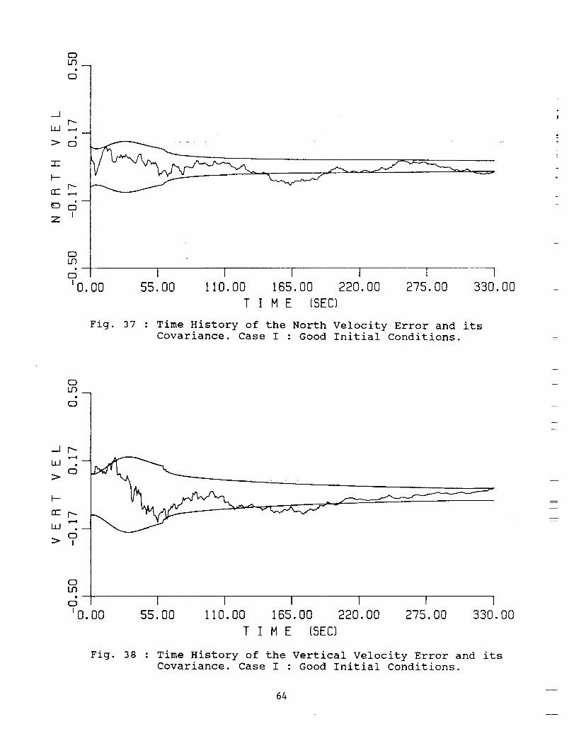
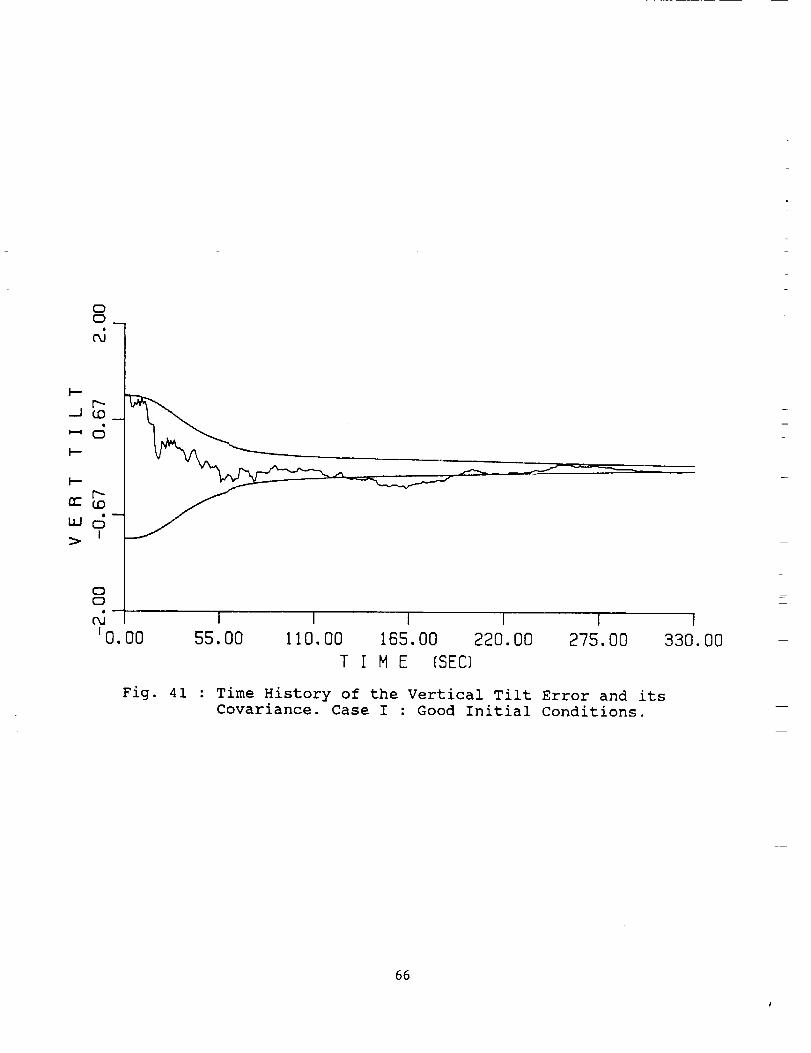
From Figures 39, 40, and 41 one can observe that the tilt

errors reduce rather slowly, with the exception of the

m

6O

vertical tilt error which is approximately 0°.3 within 1 min.At the end of the 5.5 min period the error covariances are

approximately 0°.2 for the North and East tilts and 0°.04 for

the vertical tilt. Comparison of the navigation filter

performance to the OMV navigation performance specification,

presented earlier in Table i, clearly demonstrates that

incorporation of the proposed GPS/INS navigation filter in the

OMV OBC will provide the required position, velocity and

attitude update accuracy with ample margin. Furthermore,

attitude update accuracy comparable to horizon and sun sensors

can be achieved without the restriction of maneuvering the

flight vehicle to point the sun sensor within 2 degrees of the

sun [8].

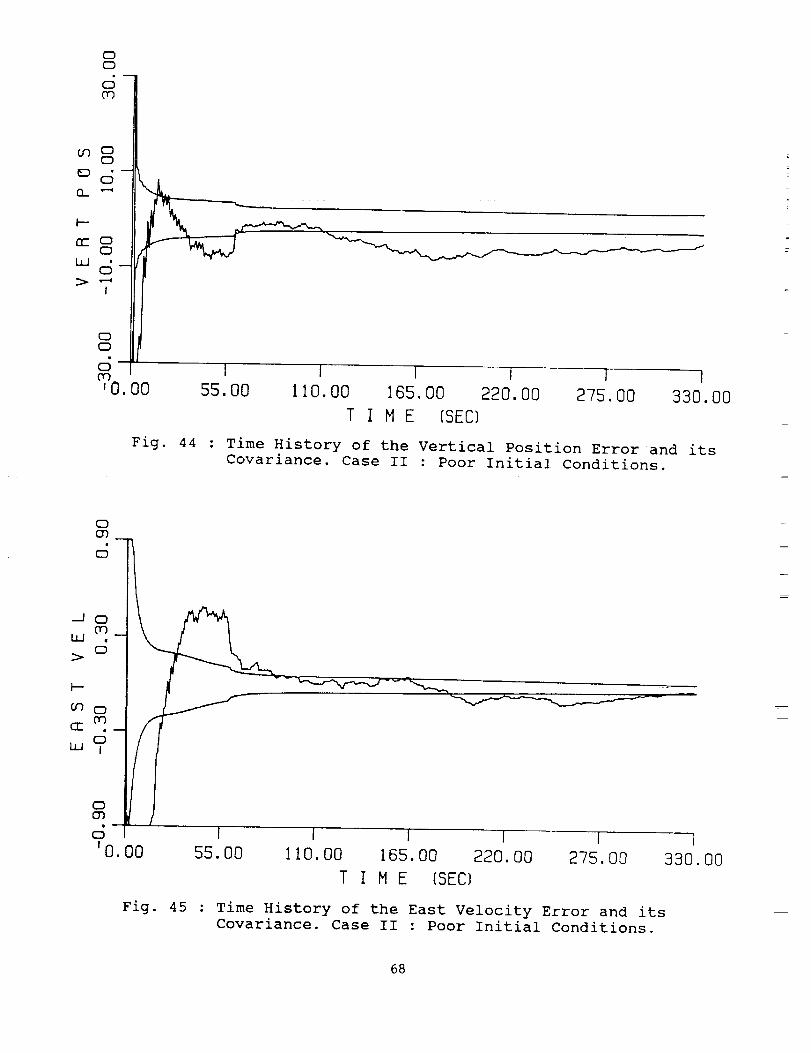
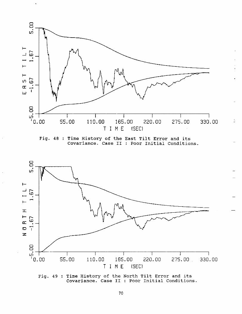
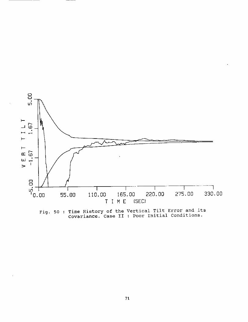
The second test case results provide further evidence of

the exceptional capability of the integrated navigation filter

to obtain good accuracy in the presence of large initial

condition errors. The excellent performance of the filter for

this test case can be observed in Figures 42 through 50. It

is indeed remarkable that even with such poor initial

conditions as mentioned earlier for position, velocity, tilt

and clock bias, one minute of GPS data, processed in a tightly

-integrated GPS/INS filter, are capable of reducing the errors

to less than 3m in position and to less than 0.2m/sec in

velocity. After the 5.5 min period, the position error is

less than 2m, the velocity error is less than 0.03m/sec and

the tilt error is less than 0°.3 in each axis.

These results are representative of the excellent

performance of the proposed integrated navigation filter.

61

CDCD

ou_-0-

IO,O0

.,..,,..,-

I I I I I 1

55. O0 l 1 O, O0 165, O0 220, O0 275. O0 330. O0

T I I'I E (SEC)

Fig. 33 : Time History of the East Position Error and its

Covariance. Case I : Good Initial Conditions. m

CDCD

00

ooo

7-

IZ

CDCD

'0.00

f

I I I I I I

55. O0 110. O0 165. O0 220. O0 275. O0 330. O0

T I H E (SEC)

Fig. 34 : Time History of the North Position Error and its

Covariance. Case I : Good Initial Conditions.

62

h

m

'0.00

f

I I I I I I

55,00 110.00 165.00 220, O0 275,00 330,00

T I M E (SEC)

Fig. 35 : Time History of the Vertical Position Error and its

Covariance. Case I : Good Initial Conditions.

c3Uo

-J r-

>

09e--W

C9U9

10.

I I I I I I

)0 55.00 110.00 165.00 220.00 275.00 330.00

T I M E (SEC)

Fig. 36 : Time History of the East Velocity Error and its

Covariance. Case I : Good Initial Conditions.

63

CDU9

m

Z

cc

_cS-J

Z

CD5O

10.

l I I J I I

)0 55.00 II0.00 165,00 220.00 275,00 330.00

T I M E (SEC)

Fig. 37 : Time History of the North Velocity Error and its

Covariance. Case I : Good Initial Conditions.

CD5O_

>

w

>?

CD5O

lO. O0

I l I I r I

55. O0 110. O0 165. O0 220. O0 275. O0 330. O0

T I M E (SEC)

Fig. 38 : Time History of the Vertical Velocity Error and its

Covariance. Case I : Good Initial Conditions.

r

L

m

L

64

CDCD

C9

UJ

CDC3

tO.O0 55. O0

I I I I I

11O,O0 165. O0 220, O0 275. O0 330. O0

T I H E (SEC)

Fig. 39 : Time History of the East Tilt Error and its

Covariance. Case I : Good Initial Conditions.

oc3

J t'--

_dI--

-1-

Z

0

_d- I'0.O0 55. O0

I I I i I

t 10. O0 165. O0 220. O0 275. O0 330. O0

T I H E [SEC)

Fig. 40 : Time History of the North Tilt Error and its

Covariance. Case I : Good Initial Conditions.

65

oc9

CD

I

I I I I I I_0.00 55.00 110.00 165.00 220,00 275.00 330,00

T I M E (SEC)

Fig. 41 : Time History of the Vertical Tilt Error and its

Covariance. Case I : Good Initial Conditions.

66

I I i I I I

55, O0 110. O0 t65. O0 220, O0 275. O0 330, O0

T I H E ISECI

Fig. 42 : Time History of the East Position Error and its

Covariance. Case II : Poor Initial Conditions.

0CD

03

00

n-

CD

,-4

Z I

OO

d0o'0.00

I I I I I I

55.00 110.00 165.00 220. O0 275,00 330, O0

T I H E {SECI

Fig. 43 : Time History of the North Position Error and itsCovariance. Case II : Poor Initial Conditions.

67

CDCD

O9

O_

p-

uJO

I

CDCD

6O9'0,00

I I I I 1 1

55.00 110,00 165,00 220.00 275,00 330,00

T I M E (SEC)

Fig. 44 : Time History of the Vertical Position Error and itsCovariance. Case II : Poor Initial Conditions.

0cD

i,l

> CD

00 Of

,,o,

CD

'0.00

I I I I I I

55. O0 1 I0. O0 165. O0 220, O0 275. O0 330. O0

T I H E (SEC)

Fig. 45 : Time History of the East Velocity Error and itsCovariance. Case II : Poor Initial Conditions.

F

68

CD

>_

I-

o_Z I

CD

I I I I I I

55. O0 110. O0 165. O0 220. O0 275. O0 330. O0

T I M E (SEC)

Fig. 46 : Time History of the North Velocity Error and its

Covariance. Case II : Poor Initial Conditions.

CDCD

6

-J CD09

_- C3

UJ O9

>o

CDCD

I I 1 t I

'0.00 55.00 ltO.O0 165.00 220.00 275,00 330.00

T I M E (SEC)

Fig. 47 : Time History of the Vertical Velocity Error and its

Covariance. Case II : Poor Initial Conditions.

69

CDCD

=Tw

I I I I I IC

JO.O0 55.00 II0.00 165.00 220.00 275.00 330.00 -

T I M E [SECI

Fig. 48 : Time History of the East Tilt Error and its

Covariance. Case II : Poor Initial Conditions.

CDCD

3i

n-

ED I

Z

@

'0.00

I I I I I I

55.00 ii0.00 165.00 220.00 275.00 330.00

T I M E (SECI

Fig. 49 : Time History of the North Tilt Error and itsCovariance. Case II : Poor Initial Conditions.

70

CDCD

.--4

I

CDC9

I I I 1 I

55. O0 1 tO. O0 165. O0 220. O0 2-/5. O0 330. O0

T [ M E (SEC)

Fig. 50 : Time History of the Vertical Tilt Error and its

Covariance. Case II : Poor Initial Conditions.

71

3.6 Memory and Throuqhput AnalTsis

In order to successfully demonstrate the feasibility of

the proposed autonomous integrated GPS/INS navigation

experiment, efficient algorithms must be identified and

demonstrated that meet performance requirements and do not

stress available computer resources. We carried out, under

Phase-I, the analysis that identifies the required software,

interfaces between existing modules onboard the OMV and the

new navigation software, and the memory and throughput

estimates of this software. The following sections address

these results in detail.

Required Software

The current baseline GPS/INS processing for the OMV was

shown in Figure i. In this, a loosely-coupled GPS/INS system,

the GPS position and velocity is used to update or reset the

INS position and velocity solution. In a tightly-coupled

GPS/INS system (Figure 2), the GPS measurements are processed

in an integrated navigation filter which estimates errors in

position, velocity, attitude, and INS instrument errors such

as gyro bias drifts and accelerometer scale factors. The INS

instrument errors can thus be calibrated, providing superior

navigation solution at all phases of the mission. It is this

integrated navigation filter and the interfaces to the

baseline TRW OMV navigation processing which is investigated

here.

w

The functions performed by the Integrated GPS/INS

Navigation Error Filter, shown in Figure 2, are:

Implementation of the Kalman Filter equations

(propagation of the error states with time, and

incorporation of the GPS measurements)

72

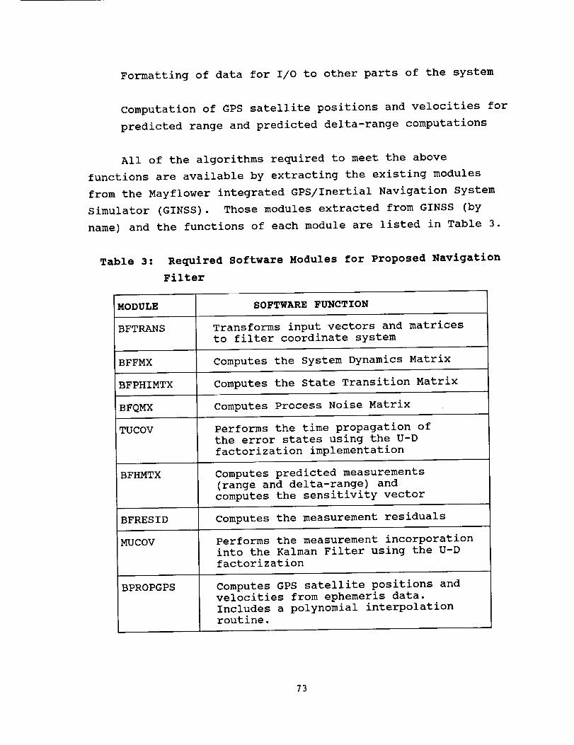
Formatting of data for I/O to other parts of the system

Computation of GPS satellite positions and velocities for

predicted range and predicted delta-range computations

All of the algorithms required to meet the abovefunctions are available by extracting the existing modules

from the Mayflower integrated GPS/Inertial Navigation System

Simulator (GINSS). Those modules extracted from GINSS (by

name) and the functions of each module are listed in Table 3.

Table 3: Required Software Modules for Proposed Navigation

Filter

MODULE SOFTWARE FUNCTION

BFTRANS Transforms input vectors and matrices

to filter coordinate system

BFFMX Computes the System Dynamics Matrix

BFPHIMTX Computes the State Transition Matrix

BFQMX Computes Process Noise Matrix

TUCOV Performs the time propagation of

the error states using the U-D

factorization implementation

BFHMTX Computes predicted measurements

(range and delta-range) and

computes the sensitivity vector

BFRESID Computes the measurement residuals

MUCOV Performs the measurement incorporation

into the Kalman Filter using the U-D

factorization

BPROPGPS Computes GPS satellite positions and

velocities from ephemeris data.

Includes a polynomial interpolationroutine.

73

The above modules meet all the processing requirements to

implement the Integrated GPS/INS Navigation Filter. These

modules were combined into a single file, and the interfaces

were modified to conform to the new functionality required by

the changed context of their environment. This file was used

to estimate memory and throughput of the Integrated GPS/INS

Navigation Error Filter, as detailed in the following two

sections.

The Kalman Filter in this software is implemented by

using the U-D factorization algorithms (see Section 3.3.4).

This results in near double-precision accuracy while computing

in slngle-precision floating point arithmetic. Ais0, no

negative numbers can be computed for the main diagonal of the

covariance matrix as can happen with the conventional Kalman

Filter implementation. Published results [13] show no

negative impact in throughput by using this implementation, as

opposed to the conventional implementation.

Memory Requirements Analysis

In order to estimate the memory requirements for the new

software, the extracted sections of code from GINSS (listed in

Table 3) were used. This code was then compiled and linked

using Digital Equipment Corporation's FORTRAN version 5.1.

The size of the resultant executable file is shown in Table 4.

On another program, Mayflower has written FORTRAN and Ada

benchmarks (which perform the same functions) in order to

obtain information on code storage requirements and throughput

inefficiencies which might be imposed due to Ada compiler

immaturity. Using an unoptimized Ada compiler we found

roughly a 90% penalty in executable file size. While this

consideration would increase the memory requirements for code

74

storage to over 14K, we estimate the required size to be

nearer 7.5K for the following reasons: i) The code as tested

was not optimized for real-time operation; 2) Ada compilers

targeted for real-time code production produce tight,efficient code.

Table 4: Executable File Size

Compiler Size of .EXE

(16-bit words)

DEC 7.5K

For an estimate of the data memory requirements, we

looked at two different approaches to arrive at a number for

the integrated filter. The first involves manually going

through the code, and counting variables and arrays to come up

with an estimate of the data memory requirements. This first

method results in a value of 2.95K 16-bit words for the data

size. In the second approach, we used published formulae [13,

14] based on types of computations used to implement the

Kalman Filter, number of states, and number of measurements

available at one time. Using the formulae resulted in a value

of 2.90K 16-bit words for the data size. These two values are

summarized in Table 5. Both of these numbers include the

storage required for GPS satellite ephemeris, position, and

velocity values.

Table 5: Data Memory Requirement

Method

i. Counting

2. Formula

Data Size

(16-bit words)

2.95K

2.90K

75

Throuqhput Analvsis

The throughput analysis was completed using the same code

used for the memory requirement estimate. The FORTRAN code

was analyzed to define the number of times each statement

would be executed per filter cycle (one time propagation and

two measurement incorporations). Then the operations in each

statement were counted and multiplied by the number of times

the statements are executed per filter cycle. This is done

for every line in a program, and then all program totals are

summed. The results of this procedure is shown in Table 6.

There are 3 columns in Table 6. The first is the total

number of operations of the designated type that take place

during one filter cycle (which corresponds to one second of

real-time). Using details of the OMV's onboard computer (OBC)

444R 2 instruction set, the operation counts can be converted

to the number of processor cycles. These numbers are shown in

the second column of the Table. For the operations of array

indexing and loads, two numbers are shown; worst and

realistic cases. The worst case assumes every array element's

address must be computed individually, and then that array

element must be loaded as a separate operation. This is very

unrealistic for filter operation, as explained in the

following paragraph and so realistic numbers (less by a factor

of four) are included for these two operations. With the

above assumptions the total number of cycles required is 1.2 x

106 . Assuming a 6 MHz clock frequency, this cycle loading

represents 20% of the available throughput of one processor.

Table 6 reveals that close to 50 percent of CPU cycles

are spent computing the memory locations of the variable

arrays used in the filter, and in loading those values into

registers where they can be used in computations. These

values reflect no consideration for memory access

r

76

2

r,.

uJ

oo<(9m

><Z

l:_ _ rJ cq

C4J

4-)

_O_

_) u_Ln,-4 oo

_O r4_O_

_J NN

_cq ,-4 rq

m

o 0.,.-i

_ o_ o

x_O _

O

H

H

N_:>,(1) ,_

_-N-,4 m.p

,--4

t_o_4

N

o

oo

,-4

U3O,-4

N

U'_O

ooL_

o4

--4

-,'44J,-4

V')H

U_U3OOH,-'_

NN

e'l_D_it13

ooo

g

O

oc_

t_or4

N

COU_

ooo

,gL_

_R

O _-_

ooH

A

_D_OO0Hr,-I

NN

O

mmm

I1_

r"O

im

_m

>

Z

O

:3

OL-

r-H.

I--

77

optimization, and assume addresses must be computed for every

individual array element. This clearly is very unrealistic

for real-time code. Also, the values in Table 6 assume all

elements in the matrices are non-zero, and thus need to be

used in the computations. Because of sparseness in the

matrices, many multiplications and additions need not be

carried out. Although we have coded our filter implementation

to skip operations when matrix elements are equal to zero, the

numbers in Table 6 assume every matrix operation will be

carried out. For example, roughly 60 percent of the elements

in the state transition matrix are zero. This will reduce the

number of computations involved by at least a factor of two.

Therefore, the 20% loading factor which was stated in the

previous paragraph is very conservative for real-time code

which will be optimized for its specific function.

3.7 Experiment Validation Test Plan

The validation and testing of the reconfigurable

integrated GPS/INS navigation error filter will take place in

three stages. These three stages are:

i) Reconfigurable filter performance testing

2) Validation of knowledge-based resource allocation

expert system

3) Testing of real-time software with simulated or real

spacecraft telemetry data

Each stage is briefly described below:

h

F

L

m

i) During the development of the navigation error

filter, GINSS will be relied upon to provide most of the

testing and validation. The Monte Carlo capabilities

have been recently demonstrated and will be used

78

extensively to verify the different modes of operation of

the reconfigurable filter. The capability to choose what

states to estimate will be invaluable during the early

stages of this effort.

2) Different mission scenarios will be run in GINSS to

validate the operation of the knowledge-based resource

allocation in selecting the appropriate filter states to

use for different mission phases.

3) We will either simulate telemetry data or obtain real

data from NASA for one of the advanced STS missions.

This will be used to test that all data interfaces are

correct, the software performs as expected (using GINSS

Monte Carlo statistics, and performance evaluations from

ground stations, and other references where possible).

79

SECTION 4

SUMMARY - CONCLUSIONS

This report documents the results of a study on an

autonomous integrated GPS/INS navigation experiment for the

Orbit Maneuvering Vehicle (OMV). This investigation was

carried out by Mayflower Communications Co., Inc. as an SBIR

Phase I effort under Contract No. NAS8-38031. In this

section, the results of the SBIR Phase I are summarized and

conclusions are drawn.

The navigation and attitude update requirements for

several NASA missions were reviewed during the Phase I study.

Specific attention was devoted to the OMV, the OTV/STV, the

Space Station and the Earth Science Geostationary Platforms.

Careful examination of the aforementioned requirements

established the applicability of the studied experiment to a

wide variety of future NASA missions.

An important aspect of the Phase I investigation was to

ensure that the appropriate interfaces between the GPS

receiver, the OMV OBC and the telemetry data will be available

for the demonstration of the experiment. Review of OMV

documents and discussion with TRW personnel verified the

availability of these interfaces. It was concluded that both

the 1-second-rate and the slower-rate data, required for a

ground demonstration of the navigation experiment will be

available at the telemetry downlink.

A tightly-integrated GPS/INS navigation filter design was

presented as an alternative to the current OMV configuration

in which GPS signals are used to compute the vehicle's

position and velocity and the IMU gyros are utilized to

80

provide inertial attitude reference. The inherent synergismof the GPS and the INS is taken into consideration and the

outcome is improved navigation solution and attitudedetermination. The error models associated with the Rockwell

International GPS receiver as well as the Singer-KearfottSKIRU IV unit are presented.

There are times, during the OMVmission, at which

prediction of the vehicle's orbit is required. Currently,this task is performed by the OMVOBC using a fourth order

Runge-Kutta integrator, where the second degree zonal harmonic

J2 is used to model the geopotential and the atmospheric drag

acceleration is an input constant. As far as the geopotentialmodelling is concerned, we compared six hour arcs of an (8,8)

reference orbit to both a J2 and a (2,2) orbit. Theconclusion was that the (2,2) orbit yields smaller prediction

errors than the J2 orbit by a factor of 2.5 or larger.

Furthermore, this improvement was introduced at a minimalcomputational cost, since the additional throughput required

to implement it is only 42 _sec per update. As far as the

atmospheric drag modelling is concerned, comparison of a

Keplerian orbit to a drag perturbed orbit indicated that the

Root Sum Square error in coordinates is approximately 400m and

in velocity is 0.5 m/sec after six hours. This is asignificant effect and appropriate models which will not

introduce a large computational burden on the OBC should beexamined.

A study to determine the visibility of the GPS satellites

to the OMVGPS antennae was carried out. The primary GPS

constellation of 21 satellites [27] was used for this

investigation. Twelve hour orbital arcs were generated to

cover a full period of the GPS satellites. An antenna look

angle of II0 ° and two OMV orbital altitudes (250 nmi and i000

81

nmi) and two inclinations (27" and 55 °) were utilized. TheGPS satellite selection and the computation of the Geometric

Dilution of Precision (GDOP) was carried out once per minute,

due to the rapidly changing geometry. We examined the antenna

switching idea, according to which, whenever the visibility to

one antenna became poor, OBC control or ground commands couldbe used to switch to the other antenna.

Without antenna switching, both the number of the visibleGPS satellites and the GDOPare improved at the I000 nmi

orbital altitude as compared to the 250 nmi altitude. On the

other hand, the orbital inclination influences the results

only marginally. With antenna switching, both the number ofthe visible GPS satellites and the GDOPare marginally

influenced by the orbital altitude and inclination.

Furthermore, antenna switching almost doubles the number of

visible GPS satellites and it eliminates areas with poor

geometry.

The integrated GPS/INS navigation filter was implemented

as an extended Kalman filter to estimate navigation errors,dominant IMU instrument errors and dominant GPS clock errors.

The 17 error states included for the OMVapplication are 3 for

position, 3 for velocity, 3 for attitude, 3 for gyro bias

drift, 3 for accelerometer scale factor and 2 for GPS clock.Two new features were introduced in our filter. The first one

was the implementation of the U-D factor equations for the

time and measurement update of the states and the covariances

and the second one was the incorporation of the second degreezonal harmonic in the filter.

The U'D factor formulation of the filter introduces two

improvements. The first one is that it guarantees positivedefiniteness of covariance matrices. The conventional

82

formulation of the Kalman filter may result in indefinitecovariance matrices due to numerical instabilities. The U-D

factor formulation is designed not to suffer from similar

shortcomings, which improves the robustness of the filter.

The second improvement is that the U-D factor formulation

yields near double-precision accuracy with single precision

arithmetic, hence, it lowers significantly the memory

requirements.

Mayflower's GPS inertial _avigation System Simulation

(GINSS) software was used to evaluate the performance of the

integrated navigation filter for the OMV high-thrust

trajectory. Two cases were considered. In the first case it

was assumed that a GPS update was available prior to the start

of the burn such that the position, velocity, tilt and clock

bias were accurately known. In the second case it was assumed

that a period of GPS outage had elapsed which resulted in

deterioration of the navigation parameters (the latter case

corresponds to a GPS signal acquisition specification). The

duration of the burn was 5.5 minutes. The results from both

test cases indicated excellent performance of the filter. The

OMV navigation performance specification (Table i) was met

with ample margin even after a GPS outage. Furthermore,

attitude update accuracy comparable to horizon and sun sensors

was achieved without the restriction of maneuvering the

vehicle such that the sun sensor points within 2 degrees of

the sun.

The memory and throughput requirements to implement the

integrated GPS/INS navigation filter in the OMV OBC were

analyzed. In order to do this, the existing modules were

extracted from GINSS and they were combined in a single file,

after modifying the interfaces to conform to their new

environment. The resulting file was compiled and linked using

83

DEC's FORTRANversion 5.1 and the size of the executable file

was 7.5K 16-bit words, which is our estimate for the memoryrequirement of the software. The memory requirement for the

data was arrived at in two ways. At first, manually goingthrough the code and, secondly, via published formulae. The

estimates were 2.95K 16-bit words from manual counting and

2.90K 16-bit words from the formulae. On the other hand, the

aforementioned file was used to estimate the throughput, whichwas 1.8 x 106 444R2 cycles for a worst case and 1.2 x 106

444R2 cycles for a realistic case.

The final aspect of this investigation was to develop atesting and validation plan for the experiment. This planincludes testing of the performance of the reconfigurable

filter, validation of the knowledge-based resource allocation

expert system and testing of real-time software with simulated

or real telemetry data.

Mayflower is planning on submitting a follow-on SBIR

Phase II Proposal on the autonomous integrated GPS/INS

navigation experiment for the OMV/STV. The focus of the

proposed SBIR Phase II research will be a proof-of-concept

experiment demonstration of an autonomous integrated GPS/INS

navigation system which can be readily implemented in real-

time onboard computers to improve the total navigation

performance of advanced Space Transportation Systems such as

the OMV, the AOTV, the Space Station and the Shuttle-C. The

autonomous aspect of the proposed experiment refers to the

software reconfigurability feature of the integrated filter to

provide optimum performance taking into account changes in the

mission scenario, thus allowing extreme flexibility in missioncontingency planning.

L

m

84

The specific technical objectives of the SBIR Phase II

will be to develop the integrated filter algorithms for

absolute and relative navigation and for attitude

determination. These algorithms will be designed and

implemented in Ada for ease of transportability to variousNASA missions and will be tested using simulated telemetry

data. A real-time, knowledge-based, resource allocation

expert system will be developed to implement the automatic

reconfigurability of the navigation filter. The feasibility

and applicability of the advanced integrated GPS/INS

navigation system will be analyzed for a on high altitude,

high thrust missions such as the Space Transfer Vehicle (STV).

A follow-on Phase III program is expected to implement thePhase II developed software design and navigation processing

technology in a future NASA/DoD mission.

85

5. REFERENCES

lo

.

,

•

•

.

•

.

•

Wagner, R.E. and A.N. Bladsel, "An Approach to Autonomous

Attitude Control For Spacecraft", Advances in the

Astronautical Sciences, Volume 66, Proceedings of the

Annual Rocky Mountain Guidance and Control Conference,

January 30 - February 3, 1988, Keystone, Colorado, pp 51-64

Upadhyay, Triveni N. and Harley Rhodehamel, OMV Attitude

Update Using GPS: Feasibility Study, Mayflower

Communications, Company, Inc., Final Report No. MCC-R-

88010, Contract No. NAS8-36363, NASA Marshall Space

Flight Center, February 1988

Upadhyay, Triveni N., Harley Rhodehamel and A wayne

Deaton, "Feasibility of Using GPS Measurements for OMV

Attitude Update", Proceedings Institute of Navigation,

National Technical Meeting, Santa Barbara, CA, January1988

Maki, Stanley C., "Problems and Solutions for GPS Use

Beyond the 12 Hour Orbit", Proceedings Institute of

Navigation, National Technical Meeting, Santa Barbara,

CA, January 1988, pp 187-193

Maki, Stanley C., "Optimization of a GPS User Experiment

at GEO", Proceedings of the Satellite Division's

International Technical Meeting, Institute of Navigation,

Colorado Springs, CO, September 19-23, 1988, pp 203-210

EauiDment Specification OMV:

No. 75-0202P, June 1988

GPS Receiver Set, TRW CI

EauiDmeDt Speci$_cat_on for OMV Inertial Measurement

Uni____t,TRW, CI No. 75-0203P, November 1987

OMV Preliminary Desiqn Review, Volume 4 - Avionics, Part

4 - Guidance, Navigation and Control, TRW Space &

Technology Group, NASA Contract No. NAS8-36800, Marshall

Space Flight Center, 22 August 1988

Ward, Phil and J. Rath, Spacecraft Applications of

Advanced Global Positioninq System Technoloqy, Texas

Instruments, Inc., Final Report UI-780130-F, Contract No.

NAS9-17781, NASA Johnson Space Center, June 1988

86

REFERENCES CONTINUED

10.

11.

12.

Daley, Philip, C. and Allison L. Thornbrugh, "Autonomous

Spacecraft Operations - Problems and Solutions", AIAA -

Computers in Aerospace Conference, 6th, Wakefield, MA,

October 7-9, 1987, pp 332-336

Donzelli, P., B. Ankermoeller, B. Sorensen and R.

Katzenbeisser, Expert System Study for Spacecraft

Measurement, Final Report, Dornier-Werke G.m.b.H.,

Friedrichshafen, West Germany, February 1987 (NTIS HC

A06)

OTV Contract Definition and System Analysis _tudy, Final

Review, Volume II, Part II Technical Summary, Martin

Marietta, July 1986

13. Gura, I.A. and Bierman, A.B., "On Computational

Efficiency of Linear Filtering Algorithms", Aerospace

Report No. TR-0059(6521-01)-I, November 1970

14. Thornton, Catherine L. and Bierman, Gerald J. "UDU T

Covariance Factorization for Kalman Filtering", Control

and Dynamic Systems, Vol. 17, 1980

15.

16.

17.

18.

Rose, R.E., H. Schmeichel, C.P. Shortwell and R.A.

Werner, "Automated Low-Thrust Guidance for the Orbital

Maneuvering Vehicle", Proceedings of the Annual Rocky

Mountain Guidance and Control Conference, Keystone, CO,

Vol. 66, 1988

Upadhyay, Triveni N. and Harley Rhodehamel, "Autonomous

Integrated GPS/INS Navigation Experiment for OMV",

Proposal, SBIR Phase I, Mayflower Communications Company,

Inc., Reading, MA, 1988

NASA's Earth Science Geostationary Platforms, A Program

Status, October 1988

Upadhyay, Triveni N., George J. Priovolos, Wallace E.

VanderVelde and Harley Rhodehamel, "STS-GPS Tracking

Experiment for Gravitation Estimation: Feasibility

Study", Final Report, AFGL-TR-89-0035, MCCI-TR-89-861002,

Mayflower Communications Company, Inc., Reading, MA,

February 1989

- 87

REFERENCES CONTINUED

19.

20.

21.

22.

23.

24.

25.

26.

27.

28.

Marsh, J.G., et al., "An Improved Model of the Earth's

Gravitational Field: GEM-T1", NASA Technical Memorandum

4019, 1987

French, R., "VAX Computer Implementation of a Preliminary

Version of the GRAM Subroutine for AFE Simulations",

NASA/MSFC, Huntsville, AI, May 1988

Yunck, Thomas P., William G. Melbourne, C.L. Thoronton,

"GPS-Based Satellite Tracking System for Precise

Positioning",. IEEE Trans. on Geoscience and Remote

Sensing, Vol. GE-23, No. 4, July 1985

Gelb, A. (ed.), Applied Optimal Estimation, The Analytic

Sciences Corporation, Reading, MA, 1986

Windall, W.S., P.A. Grundy, "Inertial Navigation System

Error Models", DTIC, TR-03-73, May, 1973

Heiskanen, W.A., H. Moritz, Physical Geodesy, W.H.

Freeman and Co., San Francisco, CA, 1967

Rapp, R.H., "Geometric Geodesy - Part I", Classnotes,

GS658, Department of Geodetic Science & Surveying, OSU,

Columbus, OH, March 1984

Torge, W., Geodesy, Walter de Gruyter, Berlin - New York,

1980

Green, G.B., P.D. Massatt, H.W. Rhodus, "The GPS 21

Primary Satellite Constellation", Journal of the

Institute of Navigation, Vol. 36, No. i, Spring, 1989

Slides from NASA Symposium on GPS Space Applications,

hosted by Jet Propulsion Laboratory, Pasadena, CA,

November 1987

88

m

Report Documentation Page

1. Report No. I 2. Government Acce_ion No.

]NASA CR-4267

4. Title and Subtitle

Autonomous Integrated GPS/INS Navigation

Experiment for OMV: PHASE I Feasibility Study

7.Author(s)

Trivenl N. Upadhyay, George J. Priovolos,

and Harley Rhodehamel

9. Performing Organization Name and Addre_

Mayflower Communications Company, Inc.

80 Main Street

Reading, MA 01867

12. Sponsoring Agency Name and Address

National Aeronautics and Space Administration

Washington, DC 20546

"1-5 Supplementary Notes

3. Recipient'sCatalog No.

5. Report Date

January 1990

6. Performing Organization Code

8. Performing Organization Report No.

MCCI-TR-89-89 i002

10. Work Unit No.

M-621

11. Contract or Grant No.

NAS8-38031

13. Type of Report and Period Covered

01-18-89 - 09-30-89

Final Contractor Re__qrt__

14. Sponsoring Agency Code

NASA Technical Monitor: A. Wayne Deaton, Systems Analysis and Integration

Laboratory, Marshall Space Flight Center, MSFC, Alabama 35812

16. Abstract

The Phase I research focused on the experiment definition. A tightly-integrated

_GPS/INS_navigation filter design was analyzed in lhhase I and was shown, via

detailed computer simulation, to provide precise position, velocity and attitude

(alignment) data to support navigation and attitude control requirements of

future NASA missions. The application of the integrated filter was also shown to

provide the opportunity to calibrate inertial instrument errors which is particularl _

useful in reducing INS error growth during times of GPS outages. While _MV_

provides a good target platform for demonstration and for possible flight

implementation to provide improved capability, a successful proof-of-concept

ground demonstration can be obtained using any simulated mission scenario data,

such as STV, Shuttle-C, Space Station.

I_-_ _ _...-¢ .41_ _, _ :., _. ,d_ ta , _i_

17. Key Words (Suggested by Authorls))

GPS Space Transportation System

INS

OMV

Autonomous

N_igat_[on F_i! ter19 Gecur,t¥ Classd. (of this report)

Unclassified

I20. Security Classif. (of this page)

Unclassified

Distribution Statement

Unclassifled/Unlimited

Subject Category: 04

21. No. of pages [_. Price

91 / A05

NASA FORM I_6 OCT

For sale by the National Technical Information Service, Springfield, VA 22161-2171

NASA-Langley, 1989