Using Software Model Checking for Software Certification by Ali Taleghani A thesis presented to the University of Waterloo in fulfilment of the thesis requirement for the degree of Doctor of Philosophy in Computer Science Waterloo, Ontario, Canada, 2010 c Ali Taleghani 2010

Welcome message from author
This document is posted to help you gain knowledge. Please leave a comment to let me know what you think about it! Share it to your friends and learn new things together.
Transcript
Using Software Model Checking forSoftware Certification
by
Ali Taleghani
A thesispresented to the University of Waterloo
in fulfilment of thethesis requirement for the degree of
Doctor of Philosophyin
Computer Science
Waterloo, Ontario, Canada, 2010
c©Ali Taleghani 2010
I hereby declare that I am the sole author of this thesis. This is a truecopy of the thesis, including any required final revisions, as accepted by myexaminers.
I understand that my thesis may be made electronically available to thepublic.
ii
Abstract
Software certification is defined as the process of independently confirmingthat a system or component complies with its specified requirements and isacceptable for use. It consists of the following steps: (1) the software pro-ducer subjects her software to rigorous testing and submits for certification,among other documents, evidence that the software has been thoroughly ver-ified, and (2) the certifier evaluates the completeness of the verification andconfirms that the software meets its specifications. The certification processis typically a manual evaluation of thousands of pages of documents thatthe software producer submits. Moreover, most of the current certificationtechniques focus on certifying testing results, but there is an increase in usingformal methods to verify software. Model checking is a formal verificationmethod that systematically explores the entire execution state space of asoftware program to ensure that a property is satisfied in every programstate.
As the field of model checking matures, there is a growing interest inits use for verification. In fact, several industrial-sized software projectshave used model checking for verification, and there has been an increasedpush for techniques, preferably automated, to certify model checking results.Motivated by these challenges in certification, we have developed a set ofautomated techniques to certify model-checking results.
One technique, called search-carrying code (SCC), uses information col-lected by a model checker during the verification of a program to speed upthe certification of that program. In SCC, the software producer’s modelchecker performs an exhaustive search of a program’s state space and createsa search script that acts as a certificate of verification. The certifier’s modelchecker uses the search script to partition its search task into a number ofsmaller, roughly balanced tasks that can be distributed to parallel modelcheckers, thereby using parallelization to speed up certification.
When memory resources are limited, the producer’s model checker canreduce its memory requirements by caching only a subset of the model-checking-search results. Caching increases the likelihood that an SCC verifi-cation task runs to completion and produces a search script that representsthe program’s entire state space. The downside of caching is that it can
iii

result in an increase in search time. We introduce cost-based caching, thatachieves an exhaustive search faster than existing caching techniques.
Finally, for cases when an exhaustive search is not possible, we presenta novel method for estimating the state-space coverage of a partial modelchecking run. The coverage estimation can help the certifier to determinewhether the partial model-checking results are adequate for certification.
iv
Acknowledgements
My PhD and this thesis took a total of six years to finish. I would like touse this section to thank all those who helped and supported me throughoutthis long process.
First and foremost, I would like to thank my supervisor Dr. JoanneAtlee. Jo, thank you for believing in me from the beginning and acceptingto work with me. Throughout the entire program, your continued guidanceand support helped me to be a better student and a better researcher. Youshowed me how to aim higher, not to take shortcuts, and ultimately, producebetter results. You were always patient with me and guided me to the rightdirection. Your advice regarding better research and clear writing skills willalways stay with me. I hope we can continue to work together in the future.
I would like to thank my PhD committee members: Dr. Rance Cleave-land, Dr. Nancy Day, Dr. Patrick Lam and Dr. Ian Goldberg. Thank youfor agreeing to be part of my committee, reading my thesis so carefully, andproviding me with lots of great feedback. Your comments have helped mecreate a better thesis.
Finishing a PhD does not only take lots of academic work, but thereis also a lot of administrative work involved. It was because of the greatadministrative staff at UW that my studies went so smoothly. I would liketo thank Margaret Towell, Wendy Rush, Jessica Miranda, and Paula Zisterfor performing all the necessary administrative work and make it seem soeasy. Thanks for being so patient with us graduate students and remindingus of deadlines several times!
My time as a PhD student was mostly fun. That was mainly because ofmy great fellow WatForm students. Thanks to my “roomies” Zarrin, Shoham,and Samaneh. You guys made being in the office fun. I will miss our manychats and our discussions about the meaning of a phd and life in general.Shahram and Pourya, you guys are great friends that I can always dependon. I hope we will stay in touch in the future. Alma and Vlad, we were in ittogether from the beginning. Thanks for being great officemates. Thanks toeveryone in the lab for being always supportive and easy to get along with.
Besides the support inside the university, I had tremendous help andsupport outside the university. I would like to thank my wife Vida for under-standing me and encouraging me when things got tough. Vida, you enteredmy life in the middle of my phd and had to deal with my occasional moodswings when my experiments went wrong or my disappointments when some
v

paper did not get accepted. You were always patient and understanding. Iam grateful that you are part of my life.
Finally, I would like to thank my parents – even though these few lines willnever be enough. You have been there for me from the beginning. Anything Iam now and anything I have ever achieved is because of you. You have alwaysbeen there for me, supported me and helped me get through the difficultiesof life. This PhD has been only possible because of you and your sacrifices.It is great to know that there is always two people in life that have my back.
vi
Contents
List of Figures . . . . . . . . . . . . . . . . . . . . . . . . . . . . . . xi
List of Tables . . . . . . . . . . . . . . . . . . . . . . . . . . . . . . xii
1 Introduction 1
1.1 Verification . . . . . . . . . . . . . . . . . . . . . . . . . . . . 2
1.1.1 Software Testing . . . . . . . . . . . . . . . . . . . . . 2
1.1.2 Formal Verification . . . . . . . . . . . . . . . . . . . . 3
1.2 Software Certification . . . . . . . . . . . . . . . . . . . . . . . 4
1.3 Certifying Formal Verification . . . . . . . . . . . . . . . . . . 6
1.3.1 Current Research in Certifying Formal Verification . . 7
1.4 Contributions and Scope of the Thesis . . . . . . . . . . . . . 7
1.4.1 Search Carrying Code . . . . . . . . . . . . . . . . . . 9
1.4.2 SCC with State-Space Caching . . . . . . . . . . . . . 10
1.4.3 State-Space Coverage Estimation . . . . . . . . . . . . 11
1.4.4 Thesis Validation . . . . . . . . . . . . . . . . . . . . . 12
1.5 Thesis Organization . . . . . . . . . . . . . . . . . . . . . . . . 13
2 Background and Related Work 14
2.1 Model Checking . . . . . . . . . . . . . . . . . . . . . . . . . . 14
2.1.1 Software Model Checking . . . . . . . . . . . . . . . . 16
2.2 State-Space Reduction Strategies . . . . . . . . . . . . . . . . 18
2.2.1 Partial Order Reduction . . . . . . . . . . . . . . . . . 19
2.2.2 Abstract Interpretation . . . . . . . . . . . . . . . . . . 19
vii
2.2.3 Symmetry Reduction . . . . . . . . . . . . . . . . . . . 21
2.2.4 Program Slicing . . . . . . . . . . . . . . . . . . . . . . 21
2.3 State-Space Search Strategies . . . . . . . . . . . . . . . . . . 22
2.3.1 Parallel Model Checking . . . . . . . . . . . . . . . . . 22
2.3.2 Random State-Space Searches . . . . . . . . . . . . . . 24
2.3.3 Partial State-Space Searches . . . . . . . . . . . . . . . 24
2.4 State-Space Caching . . . . . . . . . . . . . . . . . . . . . . . 25
2.4.1 Hit-Based Caching . . . . . . . . . . . . . . . . . . . . 25
2.4.2 Age-Based Caching . . . . . . . . . . . . . . . . . . . . 26
2.4.3 Stratified Caching . . . . . . . . . . . . . . . . . . . . . 26
2.4.4 Depth-Based Caching . . . . . . . . . . . . . . . . . . . 26
2.5 Software Certification . . . . . . . . . . . . . . . . . . . . . . . 27
2.6 State-Space Coverage Estimation . . . . . . . . . . . . . . . . 31
3 Certification by Search Carrying Code 33
3.1 Search-Carrying Code . . . . . . . . . . . . . . . . . . . . . . 34
3.1.1 Search Script Construction . . . . . . . . . . . . . . . . 36
3.1.2 Search Script Usage . . . . . . . . . . . . . . . . . . . . 37
3.1.3 Trustful Certification . . . . . . . . . . . . . . . . . . . 41
3.1.4 Evaluation of SCC . . . . . . . . . . . . . . . . . . . . 43
3.1.5 Search Script Size . . . . . . . . . . . . . . . . . . . . . 45
3.2 Parallel SCC . . . . . . . . . . . . . . . . . . . . . . . . . . . . 47
3.2.1 Partitioning the State Space . . . . . . . . . . . . . . . 48
3.2.2 Parallel Certification . . . . . . . . . . . . . . . . . . . 54
3.2.3 Correctness . . . . . . . . . . . . . . . . . . . . . . . . 54
3.2.4 Parallel Trustful Certification . . . . . . . . . . . . . . 58
3.2.5 Implementation and Evaluation . . . . . . . . . . . . . 60
3.3 Discussion . . . . . . . . . . . . . . . . . . . . . . . . . . . . . 63
3.3.1 Transition- vs. State-Based Certificates . . . . . . . . . 63
3.3.2 Properties . . . . . . . . . . . . . . . . . . . . . . . . . 64
3.3.3 Scalability . . . . . . . . . . . . . . . . . . . . . . . . . 64
viii
3.3.4 Parallel Model Checking . . . . . . . . . . . . . . . . . 66
3.3.5 Using Different Model Checkers . . . . . . . . . . . . . 67
3.3.6 Model-Dependent Reduction Techniques . . . . . . . . 67
3.3.7 Property-Specific Reduction Techniques . . . . . . . . 69
3.4 Summary . . . . . . . . . . . . . . . . . . . . . . . . . . . . . 70
4 State-Space Caching 71
4.1 Introduction . . . . . . . . . . . . . . . . . . . . . . . . . . . . 71
4.2 Cost-Based Caching . . . . . . . . . . . . . . . . . . . . . . . . 73
4.2.1 Cost-Based Caching Algorithm . . . . . . . . . . . . . 74
4.2.2 State Spaces with Strongly Connected Components . . 78
4.2.3 Implementation . . . . . . . . . . . . . . . . . . . . . . 82
4.2.4 Experiments and Results . . . . . . . . . . . . . . . . . 83
4.2.5 Discussion of Cost-Based Caching . . . . . . . . . . . . 87
4.3 Eliminating Duplicate Transitions . . . . . . . . . . . . . . . . 89
4.3.1 Eliminating Duplicate Transitions . . . . . . . . . . . . 90
4.3.2 Implementation and Evaluation . . . . . . . . . . . . . 93
4.4 Memory Optimization for Certification . . . . . . . . . . . . . 93
4.4.1 Memory Optimization Algorithm . . . . . . . . . . . . 94
4.4.2 Evaluation . . . . . . . . . . . . . . . . . . . . . . . . . 95
4.5 Summary . . . . . . . . . . . . . . . . . . . . . . . . . . . . . 96
5 State-Space Coverage Estimation 97
5.1 Coverage Estimation . . . . . . . . . . . . . . . . . . . . . . . 98
5.1.1 Exhaustive-Search Phase . . . . . . . . . . . . . . . . . 103
5.1.2 Random-Search Phase . . . . . . . . . . . . . . . . . . 104
5.1.3 Memory Management . . . . . . . . . . . . . . . . . . . 105
5.2 Evaluation . . . . . . . . . . . . . . . . . . . . . . . . . . . . . 106
5.2.1 Experiments and Results . . . . . . . . . . . . . . . . . 107
5.3 Discussion . . . . . . . . . . . . . . . . . . . . . . . . . . . . . 110
5.3.1 Rate of Discovering New States . . . . . . . . . . . . . 110
ix
5.3.2 BFS Level Graphs for Estimation . . . . . . . . . . . . 111
5.3.3 BFS vs. DFS During the Exhaustive-Search Phase . . 113
5.3.4 Round-Robin Execution of Random-Search Phase Searches114
5.4 Summary . . . . . . . . . . . . . . . . . . . . . . . . . . . . . 115
6 Conclusion and Future Work 116
Bibliography . . . . . . . . . . . . . . . . . . . . . . . . . . . . . . 120
x

List of Figures
3.1 Sample reachability graph of a program . . . . . . . . . . . . . 37
3.2 Perfect search of a state space . . . . . . . . . . . . . . . . . . 42
3.3 Reachability graph with its script and Subgraphs . . . . . . . 49
3.4 Result of partitioning after one iteration of algorithm . . . . . 51
3.5 Subgraphs with scripts and initialization paths . . . . . . . . . 52
3.6 Script partition for trustful SCC . . . . . . . . . . . . . . . . . 59
4.1 Sample reachability graph with each state’s associated cost in
parentheses . . . . . . . . . . . . . . . . . . . . . . . . . . . . 75
4.2 Sample reachability graphs with cycles. Values in parentheses
show each state’s cost value. . . . . . . . . . . . . . . . . . . . 81
4.3 Sample reachability graph . . . . . . . . . . . . . . . . . . . . 90
5.1 Schematic example of our estimation algorithm . . . . . . . . 99
5.2 Rate of discovering new states for the Dining Philosopher Pro-
gram . . . . . . . . . . . . . . . . . . . . . . . . . . . . . . . . 111
5.3 BFS level graph for Elevator program . . . . . . . . . . . . . . 112
5.4 BFS level graph for RWVSN program . . . . . . . . . . . . . . 113
xi

List of Tables
3.1 Java Programs Used for Evaluation . . . . . . . . . . . . . . . 44
3.2 Results for SCC Verification and Certification . . . . . . . . . 46
3.3 Results for Parallel SCC Certification . . . . . . . . . . . . . . . 61
3.4 Average and Maximum Lengths of Initialization Paths . . . . . . 62
4.1 Comparison of Cost-Based Caching to Other Caching Tech-
niques at Cache Sizes of 15%, 25% and 50% . . . . . . . . . . 85
4.2 Comparison of Cost-Based Caching to Other Caching Tech-
niques at Cache Sizes of 75% and 95% . . . . . . . . . . . . . 86
4.3 Memory Usage During Certification after Optimization . . . . 96
5.1 State-Space Coverage Estimation Results . . . . . . . . . . . . 108
xii

Chapter 1
Introduction
The IEEE Standard Glossary of Software Engineering Terminology [IEE90]
defines certification as “the process of confirming that a system or compo-
nent complies with its specified requirements and is acceptable for operational
use”. This general definition has been widely adopted in the software certifi-
cation literature [AdAdLM07, TC95, WR94, Mai07]. Certification could be
applied to software systems across a wide range of domains, but because of its
high cost, certification is mostly applied to safety-critical systems. For exam-
ple, the Federal Aviation Administration (FAA) requires that any software
used in an airborne environment be certified to be safe and reliable [RTC92].
Similarly, software used in other safety-critical systems, such as medical de-
vices and nuclear power plants, must be certified to be safe and to behave
according to its specified requirements [Mai07].
An implication of the formal definition of certification is that the certifi-
cation process only confirms adherence to the specifications and ensures that
verification has been performed satisfactorily. Thus, prior to certification, a
verification process must establish the software’s adherence to the specified
requirements. In general, verification is performed by the software producer,
whereas certification is done by the software consumer or an independent
body (e.g., a third-party certifier). In this thesis, we refer to the software
1
producer as the entity that is responsible for creating and verifying a software
program, and we refer to the certifier as the entity that receives a software
program and certifies that it complies with its advertised properties.
1.1 Verification
Software verification refers to the process of determining whether the prod-
uct(s) of one software-development phase fulfill the specified requirements
established during the previous phase [IEE90]. Software verification occurs
throughout the evolution of a software product, and a variety of verification
techniques are used in isolation or in combination to show that the software
behaves according to its specifications. Two common techniques to verify
software are software testing and formal verification.
1.1.1 Software Testing
Software testing refers to the activity in which a software system is executed
under specified conditions and the test results are compared to the expected
results [IEE90]. There exist various levels of testing activities, each with
its own specific goals. For example, unit testing involves the testing of a
software module or “unit”. The goal of unit testing is to ensure that the
tested module satisfies its requirements and can be integrated with other
components of the system. System testing, on the other hand, tests the
entire integrated hardware and software system to ensure that it meets its
specified requirements.
Software testing is often the verification method of choice because it pro-
duces results quickly and can handle large software systems. However, testing
is not exhaustive and only covers a subset of all possible execution traces of a
program. Therefore, it is not suitable to show that a given property is satis-
fied in all program states [Dij72]. Testing is more suited to finding execution
2
traces that violate a property rather than to demonstrate that a program
satisfies some required property.
1.1.2 Formal Verification
The goal of formal verification is to show that a software component or
system satisfies its correctness criteria. Formal-verification techniques are
in general exhaustive and consider all execution traces of a program for a
given property. The most common formal verification techniques are model
checking [CGP99] and theorem proving [GM93, KM97].
Model checking is an automated method that systematically and exhaus-
tively explores the execution state space of a model M of a system S, and
checks that a specified property P is satisfied in each state of M ’s state space.
Model checkers are implemented using either an explicit [CE81, QS82] or
symbolic representation [BCM+90] of the program’s state space. In explicit
state model checking [CE81, QS82], states are enumerated on the fly and
each visited state is saved in some data structure (e.g., hash table) against
which new states are compared. The purpose of the hash table is to avoid re-
exploration of a previously visited state. Symbolic model checking [BCM+90]
avoids storing states individually and instead uses formulas in propositional
logic to represent sets of states that are explored and reasoned about to-
gether. As a result, symbolic model checking can potentially handle very
large state spaces.
Automated theorem proving involves the development of mathematical
proofs that deductively argue that the system exhibits desired properties.
Given that developing proofs is a hard task and it is generally not possible
to automate the entire proof construction, most theorem provers allow the
user to specify intermediate lemmas to be proved by the automated theorem
prover on the way to the proof of a conjecture.
Model checking and automated theorem proving can often not handle
real-world software because model checking is very memory intensive and
3

often runs out of time or memory resources, and theorem proving is compu-
tationally expensive and requires expert human interaction. However, there
are indications that the field of formal verification is maturing and formal
verification techniques can be used to verify large software programs. In
fact, several industrial-sized software projects have used formal methods for
verification [Abr06, BBFM99, tBGKM08, tBML+05].
1.2 Software Certification
In software certification, a third-party certifier confirms that a software com-
ponent or system meets its specified requirements. To ease certification,
certain government and private organizations publish certification standards
[ISO06, RTC92, Und98] that include a set of guidelines that the software
producer should follow in order to create trustworthy and certifiable soft-
ware. These standards often include a list of deliverables that the software
producer must create during development and submit for certification.
Certification standards tend to specify guidelines on either the process
used to develop the software (process-oriented) [Sof07] or the properties of
the final software product (product-oriented) [MW08]. In process-oriented
certification, the certifier evaluates the process and the people that were
used to develop the software. It is believed that following high standards in
development and using highly-qualified developers leads to high-quality soft-
ware [Sof07]. Others [Mai07, DS09] argue that product-oriented certification
should be the main approach when evaluating a software program because it
is possible to follow a high-quality process but still create software that fails.
The focus of this thesis is on product-oriented certification.
Certification standards outline various documents and deliverables that
the software producer must create, in addition to the end product, and sub-
mit for certification. In general, the software producer is required to docu-
ment the different phases of the software’s production, including planning,
4
development, verification and management of the system. For example, the
certification standard DO-178B [RTC92], which is used by the Federal Avia-
tion Administration (FAA) to certify software for airborne systems, requires
that the software producer submit, among others: the software requirements
specification, software-design documentation, source code, executable object
code, and test data. As another example, the US Food and Drug Adminis-
tration (FDA) requires that the Software Requirements Specification (SRS),
a deliverable that documents all the requirements for a software system, does
not contain ambiguous, incomplete or unverifiable requirements [US 02]. Test
data submitted for certification must include, among others, documentation
of the test plan, test cases, test results, and test coverage.
The software producer submits the final software product plus other re-
quired documents to the certification authority (certifier) for certification.
The certifier can be the same organization that published the certification
standard or can be a third-party certifier who has been authorized to perform
certifications on behalf of another organization. The certifier’s responsibil-
ity is to confirm that the software producer has taken the necessary steps
to produce trustworthy software and that the software program satisfies its
advertised properties. In the case of the SRS required by the FDA, the cer-
tifier would confirm that the SRS and the evidence regarding its validation
show that the requirements are unambiguous, complete and verifiable. The
certifier would also review the test cases and their results to confirm that the
tests are complete and that the results demonstrate that the new software
component can inter-operate with existing ones.
In general, certification standards do not specify how the evidence sub-
mitted to the certifier should be evaluated [CTvGS98], and in most cases,
the evidence is evaluated manually. However, given the sheer volume of as-
sociated artifacts, this form of certification is very time consuming and can
be error prone because it relies on humans reading thousands of pages of
documents. In fact, in some cases, certification has taken so long that the
5
product has become obsolete by the time certification has finished [Wil07].
On the other hand, if more certifiers are used to speed up the process,
then certification becomes prohibitively expensive for smaller software ven-
dors. Thus, there is a push towards automated software-certification tech-
niques [DFS04, LGW07, LPR01].
1.3 Certifying Formal Verification
Advances in formal-verification techniques enable corresponding advances
in certification. A software producer must have some means of creating
and submitting for certification some form of proof or certificate that the
program satisfies its advertised properties; and the certifier must have some
means of using the certificate to check the producer’s claims. In fact, there
have been calls for new techniques, preferably automated, to certify software
that has been verified using formal methods [DFS04, LPR01, WBH+05]. We
believe that any technique for certifying formal-verification results must at
least satisfy the following conditions:
1. Verification should produce an output that serves as a certificate that
verification has been performed, and that can be submitted along with
the final product for certification. The certifier would use the certifi-
cate to check the producer’s claims regarding the software’s advertised
properties.
2. If verification is automated, then certification should also be automated
to decrease the workload of the human certifier and make the certifica-
tion results more dependable and reproducible.
3. In general, certification should be faster than verification, otherwise,
the certifier might just as well repeat the verification process. Specif-
ically, automated certification should be faster than automated verifi-
cation.
6
1.3.1 Current Research in Certifying Formal Verifica-
tion
In the research community, the use of formal methods for certification has
not been extensively researched. The first work in this area was the use of
proof-carrying code (PCC) [Ire05, Nec97]. In PCC, the software producer
verifies via theorem proving that his program satisfies a set of predefined
safety properties, and provides as evidence a safety proof. The certifier cer-
tifies the program by checking the validity of the accompanying safety proof
against the code. PCC certification has not been widely adopted because
it can certify only the properties that are substantiated by the safety proof.
Moreover, because many properties of a program are generally undecidable,
PCC verification has so far focused on program-independent security prop-
erties such as memory safety, type safety, and resource bounds. The size of
safety proofs is another shortcoming of PCC.
There has also been some work on certifying model-checking results:
abstraction-carrying code (ACC) [XH04] and model-carrying code (MCC)
[SVB+03]. In both cases, the program to be certified is accompanied by an
abstract model of the program. Since the abstract model is smaller than the
original program, certification of it is faster than verification. ACC and MCC
are property-independent certification techniques, and can be used to certify
any property that is specified in temporal logic [CGP99]. However, their
models are conservative abstractions, which means that they could report
spurious errors.
1.4 Contributions and Scope of the Thesis
In our proposed scenario, a software producer uses model checking to verify
her software and produces and submits for certification a “certificate” of ver-
ification. This certificate is constructed in such a way that it can be used by
the certifier to speed up the automated certification of the model-checking
7

results. Because model checking is an exhaustive search of a program’s state
space, its success depends on the size of the program and the available com-
puting resources (e.g., time and memory). We distinguish between three
possible outcomes of verification model checking:
1. A model-checking search runs to completion and produces a definitive
result. A positive result (“true”) means that the property being model
checked is satisfied in all program states.
2. The model checker has insufficient memory to complete the search.
However, the model checker can be modified to cache only a subset of
search results, thereby reducing its memory requirements enough for
the search to run to completion — at the expense of increased search
time because the model checker might search the same states more than
once.
3. The model checker does not have sufficient resources to complete the
search, even with caching. In this case, the goal is to provide partial
results that might be useful for certification.
Thesis Statement: Model-checking based techniques can be used to
facilitate the automated certification of explicit-state model-checking results
for invariants, assertions and deadlocks. We present the following three tech-
niques:
• A model-checking-based certification method that (1) can be used to
automatically certify a invariants, assertions and deadlocks, (2) is faster
than automated verification, and (3) can be parallelized.
• A novel state-space caching technique that achieves an exhaustive model-
checking search, in cases where model checking would otherwise termi-
nate prematurely, faster than existing caching methods;
8

• A state-space coverage estimation method that provides more accurate
estimation results than previous approaches when an exhaustive search
is not possible.
We describe each technique in more detail below.
1.4.1 Search Carrying Code
We present a new technique to certify model-checking results called search
carrying code (SCC) [TA10]. A software producer who wants her product
certified conducts a model-checking search of the program. During model
checking, the producer’s model checker creates a search script for the program
to be certified. The search script encodes the search path that the model
checker followed in its exploration of the program’s state space. The search
script acts as a certificate of model checking.
During certification, the certifier’s model checker uses the search script
to direct its search of the program’s state space to speed up re-verification of
the program. In order to protect against a producer who submits a tampered
search script, that perhaps hides problems in the program, the search script
is constructed in such a way so that its veracity can be checked on the fly.
Basic SCC certification achieves only slight reductions in certification
time because the model checker re-explores the entire state space of the
program being certified. However, SCC can be optimized via parallel model
checking. In parallel SCC, the search script, which encodes the certification
search task, is partitioned into multiple scripts, each covering a different
region of the program’s state space. The certifier then uses the collection
of scripts to search the program’s state space in parallel. Because of the
way that the certification task is partitioned, parallel SCC avoids many of
the problems that arise in traditional parallel model checking, such as high
degrees of communication, synchronization among parallel processors, or the
uneven splitting of search spaces.
9
1.4.2 SCC with State-Space Caching
One of the main obstacles to successful model checking is the state explosion
problem: the size of a program’s state space grows exponentially in proportion
to the number of variables in the program and the number of concurrently
executing components. The model checker keeps track of each visited state
during the search, and it might run out of memory before completing the
search.
Today’s model checkers employ a variety of techniques to combat the
state-space explosion problem. One such method is state-space caching [Hol87],
where the model checker caches only a subset of the already-visited program
states.
When the cache is full and the search visits a new state, the model checker
replaces a state in the cache with the newly visited state. Model checking
with state-space caching limits the amount of memory that is used to store
already-visited states. As a result, the model checker may explore parts of
the program’s state space if a previously visited state is not found in the
cache and is thus deemed unvisited, causing re-exploration of the state space
that is reachable from it. Thus, a model-checking search that employs state-
space caching uses less memory, but requires more time than a traditional,
non-cached search.
We introduce a new state-space caching technique, referred to as cost-
based caching, that replaces states in the cache according to the cost of re-
exploring the state and the state space that is reachable from it. For acyclic
state spaces, our method can calculate the exact cost for each state and for
cyclic state spaces, our method calculates an under-count of the cost value.
Nonetheless, our empirical evaluation shows that cost-based caching achieves
exhaustive coverage of a program’s state space faster than existing caching
techniques.
Cost-based caching is useful for SCC verification because when memory
resources are limited, it increases the likelihood that a verification task runs
10
to completion. However, the resulting search script would record the verifier’s
search path through the program’s state space, including re-explorations.
We describe how to identify and remove from the search script duplicate
transitions that would cause the certifier’s model checker to revisit regions
of a program’s state space. An SCC-certification search that uses a script
produced by SCC verification with cost-based caching has an execution time
comparable to that of a non-cached exhaustive search.
We also introduce a memory-optimization technique that reduces the
memory requirements of SCC certification. In particular, we show how to use
the information in the search script to reduce the number of already-visited
states that the model checker must keep track of. As a result, up to 85% less
memory is needed for SCC certification compared to SCC verification.
1.4.3 State-Space Coverage Estimation
Even with state-of-the-art memory-reduction techniques, there are still cases
where an exhaustive search of a program’s state space terminates prema-
turely due to insufficient memory. In such cases, an estimate of how much
of the program’s state space was covered during verification can be useful
in certification. Such an estimate would be analogous to test-coverage re-
sults in that it reflects the degree to which the verification was complete.
The software producer submits an estimate of the program’s state space that
was covered during verification. The certifier uses the estimate in deciding
whether to (1) accept the partial verification as being sufficient, (2) ask the
software producer to perform a more thorough verification, or (3) re-model
check the software herself and compare the resulting estimated coverage to
the level of coverage reported by the software producer.
We present a new method [TA09] for estimating on the fly, during model
checking, the percentage of the program’s state space that has been covered.
Our estimation method is based on Monte Carlo sampling of the unexplored
state space.
11
1.4.4 Thesis Validation
The thesis was validated as follows:
We implemented each of our three techniques in the explicit-state software
model checker Java PathFinder (JPF) [VBHP00, LV01]. To evaluate the
performance of each technique, we used a set of nine Java programs that
were used in previous research studies.
In the case of SCC, we want to evaluate whether (1) certification can
be automated, (2) SCC-based certification is faster than automated verifica-
tion, and (3) SCC-based certification can be parallelized. We use our nine
evaluation programs to show that it is possible to automatically create a
certificate of verification that can be used to automatically certify a specific
class of model checking results, and that the certificate can be used to speed
up certification. We also evaluate the effectiveness of parallelizing SCC such
that there is no overlap between the work performed by each processor. Our
results show that parallel SCC can achieve speed up factors of up to n, for
n processors, when the program comes from an un-trusted source. SCC can
achieve speed up factors of up to 5n when the program comes from a trusted
source
For cost-based caching, the goal is provide the software producer with a
technique that increases the number of cases where she can achieve an ex-
haustive search of the state space and submits an SCC search script that rep-
resents the search of the entire program. For this, we implement six common
caching techniques in JPF and compare the time it takes for an exhaustive
search using these six techniques to the time it takes for an exhaustive search
using cost-based caching. Our results indicate that cost-based caching is up
to 25% faster than existing techniques.
Finally, when an exhaustive search of the state space is not possible, then
the coverage estimation should be accurate enough to (1) help the software
producer to effectively choose the next verification step and (2) provide the
certifier with a clear indication whether to accept or reject the partial model-
12

checking results. We evaluate the accuracy of our estimation technique by
estimating the coverage of partial model checking runs, while varying the
actual coverage of the state space. Our empirical studies show that, on
average, our algorithms coverage estimates differ from the actual coverage
by less than 10 percentage points, with a standard deviation of about 5
percentage points regardless of whether the actual state-space coverage is
low (3%) or high (95%).
1.5 Thesis Organization
This thesis is organized as follows. In Chapter 2, we present background
material and related work on software certification, software model check-
ing, state-based caching techniques, and state-space coverage estimation. In
Chapter 3, we present search carrying code (SCC) and describe how the
certification task can be partitioned into multiple search tasks that can be
distributed to parallel model checkers. We evaluate the performance of SCC
and parallel SCC on a suite of Java programs. In Chapter 4, we introduce
cost-based caching applied to a state-space search. We combine cost-based
caching with SCC and compare its performance to existing caching tech-
niques. We also describe how to reduce memory requirements for SCC certi-
fication. In Chapter 5, we describe our algorithm for estimating the coverage
of a partial model-checking search and evaluate its accuracy on a set of Java
programs. Finally, we conclude with Chapter 6 and describe future work.
13
Chapter 2
Background and Related Work
In this chapter, we first present background material that is necessary to
understand the model-checking technologies used in our research. We then
describe the state of the art of certification and state-space coverage estima-
tion.
2.1 Model Checking
Model checking is an automated method to systematically explore the ex-
ecution state space of the model of a system and to check that a specified
property is satisfied in each state. The inputs to the model checker are a
model M that represents the behaviour of a system S and a property P to
be checked in every state of M . The model checker exhaustively explores all
the paths through M while checking that P is true at each reachable state.
System models are often represented as a state-transition graph called a
Kripke structure. A Kripke structure M is a four tuple M = (S, S0, R, L)
where
1. S is a finite set of states.
2. S0 ⊆ S is the set of initial states.
14
3. (R ⊆ S × S) is a transition relation such that for every state s ∈ S
there is at least one state s′ ∈ S such that R(s, s′).
4. L : S → 2AP is a function that labels each state with a set of atomic
propositions AP that are true in that state.
The paths in a Kripke structure represent all possible computations of the
system.
The property P is often specified as a temporal logic formula. Temporal
logic formulas are used to express properties of temporal orderings of events.
The two most widely used temporal logics are linear-time logic (LTL) [Pnu77]
and computation-tree logic (CTL) [CE82]. LTL formulas are used to express
properties related to all paths in the model, whereas CTL formulas can be
used to discriminate between paths.
Model checkers are implemented using either an explicit-state [CE81,
QS82] or symbolic representation [BCM+90] of the model’s state space. In
explicit-state model checking, states are enumerated on-the-fly and each ex-
plored state is typically stored in a hash table; the model checker checks new
states against the contents of the hash table, to avoid re-examining states.
Explicit-state model checking is generally more memory intensive than sym-
bolic model checking because each state is explicitly represented and stored.
However, this approach can handle dynamic creation of objects and threads,
and thus is the primary choice for model checking software.
Symbolic model checking avoids storing states individually and instead
uses formulas in propositional logic to represent sets of states that are ex-
plored and reasoned about together. The states and transition relation are
often encoded in a variant of Binary Decision Diagrams (BDD) [Bry86]. Sym-
bolic model checking works best with a static transition relation and hence
does not deal well with dynamic creation of objects and threads. It is there-
fore better suited for model checking hardware models rather than program
models.
15
2.1.1 Software Model Checking
The input to a software model checker is a software program, such as a
Java program. The goal of the model checker is to search the program’s
execution state space and check that each state satisfies some property P .
Let V = {v1, ..., vn} be the dynamic set of program variables. For an object-
oriented program, such as a Java program, V includes declared variables,
dynamic variables (heap-based objects), and information about concurrent
threads. We assume that the variables in V range over a finite set D. A
valuation for V is a function that maps every variable v in V to a value in
D. A state in a program’s execution represents the current set of program
variables and the valuation of those variables.
Definition 2.1.1. A state S of a program is a valuation d : V → D.
Definition 2.1.2. A program’s initial state S0 is the state of the program
at the start of its execution.
In other words, a state is a snapshot of a program’s execution. The system
transitions between states by executing the statements of the program.
Definition 2.1.3. A transition from one program state to another reflects
the execution of one program statement and shows the effects of that state-
ment as applied to the transition’s source (program) state.
The granularity of the statement that is executed by a transition depends on
the programming language and the model checker. For Java programs, it is
often a single byte-code instruction.
Given the definitions of a state and transition, we can now define the
set of all reachable states of a program and the graph that represents all
executions of the program.
Definition 2.1.4. A reachable state of a program is a state that results
from applying a sequence of program statements to the initial state. The
sequence of program statements must reflect an execution of the program.
16

Definition 2.1.5. A program’s state space is the set of all reachable states
in the program.
Definition 2.1.6. A program’s reachability graph is a directed graph
where each of the program’s reachable states is represented by a vertex, and
there is a directed edge from state Si to state Sj if there exists a transition
(program statement) in Si that can be executed in Si and that moves the
program execution from state Si to state Sj.
There is no restriction on the number of incoming transitions into a state
and outgoing transitions from a state.
The software model checker starts its search in the program’s initial state
and performs an exhaustive search of the program’s reachability graph until
all states in the program’s state space have been visited and all transitions
have been explored.
Definition 2.1.7. A visited state is a state that has been reached in a model-
checking search, and has been verified to satisfy property P .
Definition 2.1.8. A partially explored state is a visited state that has at
least one outgoing transition that has not been explored in the model-checking
search.
Definition 2.1.9. A fully explored state is a visited state whose outgoing
transitions have all been explored in the model-checking search.
To ensure that its searches terminate, the model checker keeps two data
structures: a worklist of partially explored states and the set of visited states.
Definition 2.1.10. A model-checking worklist is a list of partially explored
states.
The worklist represents the set of states that have been visited during the
model-checking search and who still have at least one unexplored transition.
17

When the model checker visits a new state Si, it inserts Si into the work-
list and into the set of visited states. During each iteration of the search,
the model checker selects a state from the worklist and explores one of its
unexplored transitions. When a state is fully explored, it is removed from
the worklist. In the case of a depth-first search, the worklist is a stack. The
search terminates when the worklist is empty. The list of visited states is
often a hash table.
Currently, there exist a wide variety of software model checkers [BR01b,
LV01, RDH03] that support various programming languages and use different
techniques to handle very large state spaces. Java Pathfinder (JPF) [VBHP00,
LV01], the model checker developed at NASA Ames Center, is one of the
most-widely used software model checkers, mainly because of its rich set
of features and continued support and development. It is a custom-made
explicit-state model checker for Java programs. JPF accepts as input Java
byte code and performs an exhaustive search of the state space to find dead-
locks, invariant violations, and assertion violations. For this thesis, we im-
plemented all our algorithms on top of JPF.
2.2 State-Space Reduction Strategies
One of the main obstacles to model checking is the state-explosion prob-
lem [CGJ+01]: the size of a program’s state space grows exponentially with
the number of variables and components in the program. As a result, an
exhaustive search may not be possible because the model checker runs out
of memory in its effort to keep track of all of the visited states. Also, model
checking typically works on finite-state systems, but dynamically-created ob-
jects and threads may cause a program to be infinite state. For these reasons,
software model checkers use various state-space abstraction techniques to re-
duce the size of the state space and make analyzing programs more feasible.
We describe four commonly used techniques below.
18
2.2.1 Partial Order Reduction
The goal of partial-order reduction (POR) [God96] is to reduce the size of
the state space that must be searched by exploiting the commutativity of
concurrently executed transitions. POR identifies transitions whose execu-
tions could be interleaved in any order and whose interleavings result in the
same program state. It then executes only one such interleaving. POR is
suitable only for asynchronous systems. In synchronous systems, concurrent
transitions are executed simultaneously and are not interleaved.
POR searches reduced graphs without ever constructing a program’s full
reachability graph, which might be too big to fit in memory. The reduced
model preserves all of the properties of the original model, except for prop-
erties that include the temporal-logic operator “next”. The “next” operator
checks that a certain property is true after executing one transition from the
current state. Thus, to check such a property, the model must include all
possible transitions.
Finding all transitions of the current state that are independent of others
and can be interleaved in any order is difficult because it requires knowledge
of the entire state space, which is not known in advance. As a result, model
checkers use heuristics and possibly stronger conditions to make POR both
feasible and fast [CGP99, VBHP00]. Java Pathfinder, for example, uses a
transition’s associated byte-code instruction to identify independent transi-
tions. Only about 10% of Java byte-code instructions can have effects across
thread boundaries. For such transitions, all interleavings must be explored,
but the remaining transitions are independent and can be interleaved in any
order.
2.2.2 Abstract Interpretation
Abstract Interpretation [CC77, GS97] is based on the observation that the
specification of a system often depends on simple relationships among data
19

values rather than on actual data values. As a result, it may be possible to
model actual data values in the system as a small set of abstract data values.
If we extend the abstraction and apply it to states and transitions that refer
to abstract states, it is possible to obtain an abstract version of the system
under consideration. The idea is to merge together all of the states that have
the same labeling of abstract variable values. In the reduced graph, every
state will have a unique labeling. Simulation [CC77] is used to ensure that
the abstract graph simulates the original one: If model M has a transition
between two states, then in the abstract state space there there must be a
transition between the corresponding abstract states. The abstracted system
is often smaller than the actual system and therefore faster to verify.
As an example, suppose x is a variable and the domain Dx is the set
of all integers. If we are interested in expressing a property involving the
sign of x, then we can create a domain Ax of abstract values for x, with
Ax = {a0, a+, a−}. We define a mapping hx from Dx to Ax as follows:
hx(d) =
a0 if d = 0,
a+ if d > 0,
a− if d < 0
Using this abstraction, we need only three atomic propositions to express
the abstract values of x. It may no longer be possible to express properties
that depend on the actual values of x because by using abstraction, we are
reducing the amount of knowledge about the values of a variable, but in
many cases, knowing just the abstract values is enough. Also, the model
checker cannot always determine a unique abstract value, for example, after
an operation such as x++.
20

2.2.3 Symmetry Reduction
The main idea of symmetry reduction [ES96, ID96, CJEF96] is to exploit
symmetries between states and therefore model check a reduced and abstract
state space. Symmetries represent equivalence relations on program states.
During model checking, one can disregard a state if an equivalent state has
already been explored. A canonicalization function usually maps each state
to a unique representative from its equivalence class.
Software systems can exhibit different types of symmetries, but two types
that are unique to object-oriented software, such as Java programs, are class
loading and garbage collection [VBHP00]. Non-determinism, either from a
program’s concurrency or its environmental input, can cause classes to be
loaded or objects to be created in different orders in different executions.
The resulting states may be deemed to be different. Comparing all possible
permutations of the order in which classes are loaded and objects are created
can be very expensive. Thus, modern software model checkers use a canon-
icalization function [VBHP00] that equates states that are identical except
for the order in which classes and objects are loaded.
The second possible source of symmetry is dynamic program variables
(e.g., objects) that are no longer referenced, and are referred to as “garbage”
[VBHP00]. Two states are considered to be equivalent if they are identical
except for any “garbage” that they contain.
2.2.4 Program Slicing
The goal of program slicing [Wei81] is to remove from a program statements
that do not affect the results of a particular test case or analysis. Program
slicing consists of specifying a point of interest in the program, identifying
the set of variables or property of interest, and removing program statements
that cannot affect the values of the specified variables at the given program
point. The idea is that a smaller (sliced) program results in a smaller program
21
state space. In general, finding a minimal program slice is an undecidable
problem [Wei81], but approximations are often effective.
A program slice can be computed statically or dynamically [Wei81]. For
static slicing, the slice is computed without executing the program. The
resulting slice includes all program statements that affect the variable(s) of
interest at the point of interest for all possible inputs. In dynamic slicing,
the slice is computed for a given input and the resulting program execution
trace.
A static program slice is often created using a technique called backward
slicing, in which the slice is computed by working backward in the program.
Starting from the point of interest, all program statements that cannot affect
the specified variables are identified and removed. Forward slicing is the
opposite of backward slicing and is often used for dynamic slices to avoid the
recording and storage of very long execution traces.
2.3 State-Space Search Strategies
Another way to combat state-space explosion is to modify the way that the
model checker searches a program’s state space. These methods include
searching the state space in parallel, searching it randomly to find an error
before memory is exhausted, and searching only those parts of the state space
that are more likely to contain errors. Below, we describe these methods in
more detail.
2.3.1 Parallel Model Checking
The goal of parallel model checking is to distribute a model-checking task
among parallel processors. In general, the challenge in parallel model check-
ing is to distribute the workload evenly. Stern and Dill were one of the first
to introduce this idea by parallelizing the Murϕ explicit-state verifier [SD97].
In this initial work, model checking was performed on a set of networked ma-
22
chines, each having its own memory and processor. The goal was to reduce
both search time and memory requirements of a model-checking search. A
static hashing function determined in advance how to distribute program
states among the processors during the search. In such an approach, it is
possible that the hashing results in an uneven distribution of states and the
search proceeds at different speeds on different processors. Moreover, state
information must be passed between processors whenever a state is created on
a processor other than its assigned one, creating a significant communication
overhead.
Subsequent works by other researchers investigate how to improve local
and global load-balancing and reduce communication among processors [NC97,
KM05]. Nicol and Ciardo [NC97] present a global load-balancing algorithm
in which all processors communicate with each other to distribute their load.
If a processor has too many states to process, it will try to offload some of that
work to other, possibly idle processors. To reduce communication, Kumar
and Mercer [KM05] propose a heuristic in which each processor communi-
cates only with three neighboring processors when trying to offload some of
its work.
Recently, with the advent of multi-core computers, there has been in-
creased research on reducing the search time of parallel model checking on
shared-memory architectures [BBR07, IB06]. In these systems, the overhead
of communication among processors is greatly mitigated because information
is no longer sent over a network. Nonetheless, the problems of load balancing
and synchronizing of access to shared resources remain. In the latter case,
processors must be able to deposit into each others worklist of partially ex-
plored states, and they share a hash table of state fingerprints. Interestingly,
some works [BBR07, IB06] report that after reaching a certain number of
parallel processors, search time starts to increase again as new processors
are added because the synchronization overhead dominates any benefit from
parallelization.
23
Another problem is that an even partitioning of a program’s states into
multiple search tasks does not guarantee that the workloads will be balanced.
Processors are utilized only if they have states to process. If a program’s
reachability graph is spindly rather than bushy, then progress may be ham-
pered by the slow production of new states to be explored as processors wait
for the output of other processors.
2.3.2 Random State-Space Searches
The idea of random walks and randomized state-space search was first sug-
gested by West [Wes86]. In each step of a random walk, the algorithm
randomly chooses an outgoing transition of the current state and explores
it. If the current state does not have any outgoing transitions, the al-
gorithm restarts from the initial state. Since the original random walk
method was introduced, many optimizations have been suggested to im-
prove its effectiveness in finding errors. These optimizations include re-
initializing the search frequently to avoid getting trapped in a strongly con-
nected component [PHvB05], performing local exhaustive searches once a
certain search depth has been reached [SG03], keeping a small cache of vis-
ited states [TPIZ01], and running parallel random walks [TPIZ01, SG03].
The Lurch model checker [OM03] uses random walks to perform partial
searches of large state spaces. Lurch inserts newly discovered states at ran-
dom indices in the worklist to randomize the search. Dwyer et al. [DEPP07]
perform random searches of the state space by randomizing the order in
which child states are explored. They parallelize this method by distributing
the search to multiple non-communicating machines.
2.3.3 Partial State-Space Searches
Stateless model checking [God97, MQ08] is another method for exploring
large state spaces. In stateless model checking, the search does not keep
24
track of already-visited states. Instead, there is a bound on the depth of the
search, to keep the model checker from continuously visiting the same states.
The result is a partial search of the state space.
Bounded model checking [BCC+03, BCCZ99] is a partial search that is
exhaustive up to some bound k on the length of execution traces. If no
bug is found, one increases k until either a bug is found or some pre-defined
upper-bound is reached.
2.4 State-Space Caching
The state-space-explosion problem is linked to the requirement for storing
already-visited states during the search to (1) guarantee termination and (2)
save time by avoiding re-exploration of states. State-space caching [Hol87]
combats this problem by limiting the amount of memory used to store visited
states. A cache of visited states is maintained. When the cache is full, states
in the cache are replaced by newly discovered states. Of course, by removing
a state Si from the cache, the model checker commits itself to possibly re-
exploring Si and its children if Si is revisited through a different path in
the reachability graph. For acyclic state spaces, termination and thus a full
state-search are guaranteed [God97, Hol88, DH82]. For cyclic state spaces,
the model checker must be able to detect states that form strongly connected
components to guarantee termination and a full coverage. We describe these
issues in Chapter 4.
State-space caching techniques differ in their cache replacement policies.
A cache replacement policy dictates how states are chosen for replacement
when the cache is full. We explain the most commonly used policies below.
2.4.1 Hit-Based Caching
In hit-based caching [Hol87], states in the cache are replaced based on the
number of times they have been revisited (referred to as the number of cache
25
hits). The work in [Hol87] investigates policies that replace states that have
had the most hits and states that have had the fewest hits.
2.4.2 Age-Based Caching
In age-based caching [Hol87], states in the cache are replaced based on the
length of time that they have been in the cache. In particular, a state that
has been in the cache the longest is selected first. The intuition behind this
method is that the longer a state remains in the cache, the fewer cache hits
it will receive in the future.
2.4.3 Stratified Caching
The authors of [Gel04] propose stratified caching, which uses each state’s
distance from the root of the depth-first-search graph (referred to as a state’s
search level) as the criteria for replacement. When the cache is full, the model
checker specifies that all states at search levels k modulo m are available for
replacement. Thus, all states at search levels k, k + m, k + 2m, ... could be
removed.
Stratified caching places an upper limit on the number of descendant
states that must be re-explored if a removed state Si is revisited because it
guarantees that all of Si’s already-visited descendant states are still in the
cache, unless they reside at search levels selected for replacement.
2.4.4 Depth-Based Caching
Depth-based caching [Hol87] also uses a state’s search level as the criteria for
replacement. This technique is similar to stratified caching, but instead of
replacing all states at a certain search level, it replaces the deepest states in
the reachability graph first. The main idea is that the deepest states probably
have fewer reachable descendant states. As a result, replacing states deep in
the reachability graph should result in re-exploring less of the state space if
26
the removed state is revisited after its descendant states have been removed
from the cache.
2.5 Software Certification
In this section, we review the state of the art of software certification, fo-
cussing on product-oriented certification. We categorize the research into
three major areas: testing-based approaches, static-based approaches, and
formal-methods-based approaches.
Testing-Based Certification
Current certification standards emphasize the use of testing and test results
to assess the quality of a software system. The software producer tests a
program to build an argument that the program satisfies its requirements.
She submits for certification the program to be certified, along with doc-
umentation of the test cases and their results. For example, the DO-178B
standard [RTC92] requires that a software producer submit, along with other
artifacts, the following documents:
• Software-verification test cases and procedures
• Software verification results, including reviews of all requirements, de-
sign, and code; and test results of executable code.
Because testing exercises only a subset of a program’s execution traces, cur-
rent certification standards require various test-coverage metrics to measure
the adequacy of the test results. These metrics include:
• Statement coverage [Hua75] — the percentage of all program state-
ments that were executed.
• Decision or branch coverage [Hua75] - the percentage of all branches in
the program that were explored.
27
• Condition coverage [Mye79] — the percentage of all atomic boolean
sub-expressions that have been tested for both their true and false
value.
• Condition/decision coverage [Mye79] — combination of decision and
condition coverage.
• Modified condition/decision coverage (MC/DC) [RTC92] — extends
condition/decision criteria with the requirement that each condition
should affect the decision outcome independently. For avionics soft-
ware, testing is required to achieve MC/DC coverage [RTC92].
Many certification standards require only a manual inspection of the test
cases and their results, but research suggests that re-running of some or all
of the test cases should be used to automate certification [WR94, MLP+01,
Gho99]. In this scenario, the test cases and their results are submitted to the
certifier in some standard format (e.g., XML). The certifier either manually
inspects the documents or uses automated tools to re-run the test cases and
compare the results to the expected results. It might still be necessary to
manually inspect the test cases to ensure that they achieve the necessary
coverage and that they actually check the desired properties.
User-based certification [Voa00, YJ03] is based on the assumption that
testing is a somewhat artificial evaluation of software quality and does not
exercise a program in the manner that it will be used in operation. User-
based certification proposes to use information collected during operational
use as a measure of the quality of a program. In one approach [Voa00], the
certifier distributes instrumented code to a select set of users and collects
information about any errors that occur while they use the software. A
second approach [YJ03] uses some other form of initial certification (such
as a static approach, described below) and then updates the results of the
certification as new errors are discovered during the program’s use. The main
28

argument against this kind of certification is that uncertified or partially-
certified code is distributed to users — a scenario that we want to avoid in
the first place. This approach may be applicable only to non-safety-critical
software.
Static-Based Certification
Researchers [OWB05, ABJ10] have shown that there is a correlation between
static properties of a software program and the quality of the program. Static
properties refer to any information about the software that does not require
its execution.
The work in [OWB05] uses the structure of the program files and their
change history to predict the number of errors in each program file. For
example, the size of a program file (in terms of lines of code) and its type (e.g.,
SQL file) can be used to predict the number of errors in the file. Arisholm et
al. [ABJ10] build models that predict faults in a program based on the static
properties of the program such as the number of instance variables, number
of methods called by each class, and the number of super- and subclasses.
The models are built using historical information about the program under
investigation and other analyzed programs.
Formal-Methods-Based Certification
Even though formal methods focus on the question of software correctness,
very little is said about them in most certification standards. The certifica-
tion standard DO-178B [RTC92] simply proposes that the results of formal
methods, if they are used at all, be inspected. In the research community,
the use of formal methods for certification has not been extensively studied.
The first work in this area was the use of proof carrying code (PCC) [Nec97].
The premise of PCC is that proof checking is faster and simpler than the-
orem proving. In PCC, the software producer verifies via theorem proving
that his program satisfies a set of predefined safety properties, and provides
29
as evidence a safety proof. The certifier certifies the program by checking the
validity of the accompanying safety proof against the code.
However, PCC certification can only (re)verify the properties that are
substantiated by the safety proof. Moreover, PCC requires significant in-
frastructure, including inference rules for reasoning about code, efficient rep-
resentations of safety proofs, and efficient and trustworthy proof checkers
that can quickly validate safety proofs about programs. Because reasoning
about general properties of programs is complex, PCC has so far been ap-
plied to only program-independent security properties (e.g., memory safety,
type safety, resource bounds). Most research on PCC focuses on reducing
the size of proofs [BJT07] and generalizing the kinds of properties that can
be proved [AAR+10, NS06].
There has also been some work on certifying model checking results:
abstraction-carrying code (ACC) [XH04] and model-carrying code (MCC)
[SVB+03]. In both cases, the program to be certified is accompanied by an
abstract model of the program. In ACC, this abstract model is an abstract
interpretation [CC77] of the program. In MCC, the model is an extended
finite-state automaton over the alphabet of system calls, and is synthesized
from the program’s execution traces. In both cases, certification is a two-
step process: (1) certifying that the model is a faithful abstraction of the
program and (2) certifying that the model respects the desired properties.
In ACC, certification is done offline. In MCC, model fidelity is checked at
runtime by monitoring the program, which incurs a performance penalty of
2% to 30% [SVB+03]. ACC and MCC can both accommodate infinite-state
programs and both are property-independent, which means that they can
be used to check additional properties. However, ACC and MCC models
are conservative abstractions, which means that a model may have more be-
haviours than the program it is modeling. As a result, errors reported by the
model checker may not be actual errors of the program.
30

2.6 State-Space Coverage Estimation
When memory and time resources are limited, a model-checking search might
end prematurely without exploring a program’s entire reachable state space.
For such cases, an estimate of the state-space coverage can help a certifier to
determine how much confidence to have in the partial model-checking results.
In previous work [Tal07], we suggested that it may be possible to sam-
ple unexplored transitions as a means to estimating the size of a program’s
state space, but we did not explore this idea further. Other researchers
have investigated the problem of state-space coverage estimation. Pelanek
et al. [Pv08] propose two techniques for estimating state-space coverage. In
the first technique, the model checker executes two random partial searches
of a program’s state space and uses the overlap between the two searches to
estimate coverage. The second technique uses breath-first search (BFS) level
graphs for state-space coverage estimation. A BFS level graph plots for each
level of a breath-first search the number of states in the BFS worklist. At the
end of a partial model-checking search, the corresponding BFS level graph is
only a partial plot because the model checker did not explore all BFS levels.
The authors use the partial BFS level graphs to predict the shape of the full
BFS level graph, and thus estimate coverage. The authors evaluated both
algorithms on 160 randomly generated reachability graphs and measured the
accuracy of both coverage estimation algorithms in terms of whether they
could classify the actual coverage of a search into the correct coverage range:
< 3%, 4%-25%, or 26%-100%. The algorithm that estimated coverage based
on two random partial searches performed best. This algorithm was able to
classify the coverage of a search into the correct range for 72% of the 160
example reachability graphs.
Dingle et al. [DK08] try to estimate the actual size of a program’s state
space by applying least-squares fitting to partial BFS level graphs. The main
assumption of this work is that BFS level graphs have regular, parabola-shape
curves that can be described by a quadratic formula: y = ax2 + bx for some
31
a and b. Given a partial BFS level graph from a partial model-checking
search, the authors try to solve for the values a and b, and thereby obtain a
representation of the complete BFS level graph. The authors evaluated their
approach on three programs whose state-space searches ended prematurely
after 25%, 50%, and 75% of the programs’ state spaces had been explored.
Their results show that their algorithm can estimate the size of a program’s
state space with an accuracy from 66% to 93%, on their examples.
Others have explored how a state-space search relates to code coverage
or to specification coverage [RDHR04, GV04]. Rodrguez et al. [RDHR04]
describe and implement a framework for the Bogor model checker [RDH03]
that supports branch coverage and specification coverage. Branch coverage
judges how many of the branches in the program have been exercised and
its results can be used to adjust the environment used to run the program
if the environment does not exercise a satisfying percentage of branches in
the program. Specification coverage describes how much of the program
code a specification exercises and can be used to modify the specification
in situations where the specification is satisfied without ever exercising the
intended program segments. Gore et al. [GV04] describe a branch-coverage
module for JPF that tries to exercise all branches of a program and reports
the percentage of branches covered. None of these works estimate state-space
coverage.
32
Chapter 3
Certification by Search
Carrying Code
In this chapter, we introduce the concept of search-carrying code (SCC),
a technique that uses information collected during successful verification of a
program (via explicit-state model checking) to ease subsequent certification
(via explicit-state model checking) of the same program. Ideally, it should be
faster to certify a program than it was to verify it in the first place because
the certifier could otherwise just re-verify the program.
Our approach focuses on paths through a program’s reachability graph.
During verification, a software producer uses her model checker to explore a
program’s reachability graph and record the search paths as a search script.
Because the search script records the search of the program’s entire reach-
ability graph, it effectively acts as a certificate of model checking: it is a
sound and complete representation of the program’s reachability graph for
the purpose of model checking. The software producer submits the software
program with the associated search script for certification. The certifier’s
model checker takes the search script as input and uses it to speed up the
task of re-examining the program. We describe SCC certification in Chap-
ter 3.1.
33
Basic SCC achieves only modest time savings because the certifier’s model
checker must still search the program’s entire reachability graph. But SCC
certification can be parallelized much more effectively/ than traditional par-
allel model checking. The main challenge in parallel model checking is bal-
ancing the workload among parallel processors. This challenge is mitigated
in SCC certification because the search task is known in advance and is en-
coded in the search script. The search script can be partitioned in such a
way that parallel processors perform roughly the same amount of work and
the processors need not communicate or synchronize with each other. The
time savings are roughly proportional to the number of parallel processors.
We describe parallel SCC in Chapter 3.2.
3.1 Search-Carrying Code
Explicit-state software model checking exhaustively examines a program’s
state space, checking for conformance with desired properties. During verifi-
cation of a program, the emphasis is on finding bugs and ultimately showing
that a program is free of certain classes of errors. For certification, the goal
is to confirm that a program behaves as advertised, and possibly to check for
additional non-advertised properties. The goal of search-carrying code
(SCC) is to use information collected during model-checking-based verifi-
cation of a program to speed up model-checking-based certification of the
program. The main idea of SCC is as follows.
A software producer’s model checker performs a traditional exhaustive
search and verification of a program’s state space. At the same time, the
model checker constructs a search script that encodes the sequence of all
transitions and their destination states that the model checker explored.
Definition 3.1.1. An SCC search script of a program is a sequence of
transitions (i.e., program statements) and their resultant target states. The
sequence corresponds to a depth-first search of the program’s entire reacha-
34

bility graph.
During SCC certification, a certifier’s model checker uses the provided
search script to direct its search of the program’s state space and certifies
that verification was performed. In general, SCC can be used to certify
safety properties of programs (e.g., program invariants or assertions), and
to confirm absence of deadlocks. We discuss properties in more detail in
Section 3.3.
SCC certification can detect if a provided search script deviates from a
program’s state space. Deviations may be intentional in the case of tam-
pering, or may be accidental if a program has changed since the script was
created. There are three types of deviation: (1) the script includes a nonexis-
tent transition, (2) the script omits a transition, or (3) the script incorrectly
claims that a transition leads to an already-visited state. The first two types
of deviation are easily detected: in the first case, the program has no pro-
gram statement that matches the script’s transition instruction; and in the
second case, the script instructs the model checker to end the exploration of
a state before it is fully explored. In both cases, the model checker detects
the discrepancy and the certification fails. The third type of deviation is
more menacing because, if undetected, it results in a partial search of the
program’s state space: the mislabelled state is deemed to have already been
visited, so the model checker does not test the state and does not explore the
state space that is reachable from it. To detect this third type of deviation,
SCC certification must re-explore the program’s entire reachability graph: it
must not only visit and verify all states in the state space, it must also ex-
plore all transitions emanating from those states to check whether they lead
to new, unvisited states. Thus, the search script encodes the full reachability
graph, i.e., every transition between program states.
Given that SCC certification entails searching a program’s entire reacha-
bility graph, it might seem surprising that SCC achieves any savings at all.
As will be seen, modest savings come from being able to confirm the script’s
35
encoding of the reachability graph, rather than determining the reachability
graph, as is the case in traditional model checking. More significant sav-
ings come from parallelizing SCC certification. We describe parallel SCC in
Section 3.2.
In the special case of trustful SCC certification, the software producer and
the verification results are trusted. However, the certifier wants to certify
additional properties of the program, and the software producer is unable
or unwilling to check these. Because the software producer is trusted, the
certifier may choose not to check the veracity of the script. As a result,
we can aggressively optimize the certification task for speed. We describe
trustful certification in Section 3.1.3.
3.1.1 Search Script Construction
An SCC search script records all transitions in a program’s reachability graph
and each transition’s destination state. In order to reduce the size of the
search script, the script records a destination state’s ID instead of some form
of state encoding.
Definition 3.1.2. A state ID in the search script is a unique identifier. Its
value reflects the order in which a state was visited during the SCC verifica-
tion search.
The model checker assigns state IDs starting with identifier S1, incrementing
the state ID by 1 each time a new state is discovered. During certification,
the model checker keeps a mapping between state IDs and state encodings.
We describe this in more detail below.
Consider Figure 3.1, which depicts the reachability graph of an artifi-
cially simple program. Transition labels abstractly represent the program
statements being executed. The numbering of transitions reflects the order
in which transitions were explored relative to other transitions from the same
source state. The script for this program’s reachability graph is:
36
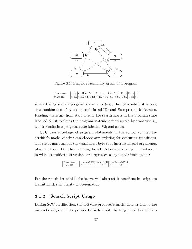
S1
S4
S5S2
S3
t1
t2
t3 t1
t1
t1
t1
t2
t2
Figure 3.1: Sample reachability graph of a program
Trans instr: – t1 t1 B t2 t1 B t2 t1 B B t3 t1 B B B B t2 B
State ID: S1 S2 S1 S2 S3 S1 S3 S4 S2 S4 S3 S5 S4 S5 S3 S2 S1 S4 S1
where the tis encode program statements (e.g., the byte-code instruction;
or a combination of byte code and thread ID) and Bs represent backtracks.
Reading the script from start to end, the search starts in the program state
labelled S1; it explores the program statement represented by transition t1,
which results in a program state labelled S2; and so on.
SCC uses encodings of program statements in the script, so that the
certifier’s model checker can choose any ordering for executing transitions.
The script must include the transition’s byte code instruction and arguments,
plus the thread ID of the executing thread. Below is an example partial script
in which transition instructions are expressed as byte-code instructions:
Trans instr: – aload 0(0) aload 1(1) B getfield#5(0)State ID: S1 S2 S1 S2 S3
For the remainder of this thesis, we will abstract instructions in scripts to
transition IDs for clarity of presentation.
3.1.2 Search Script Usage
During SCC certification, the software producer’s model checker follows the
instructions given in the provided search script, checking properties and au-
37
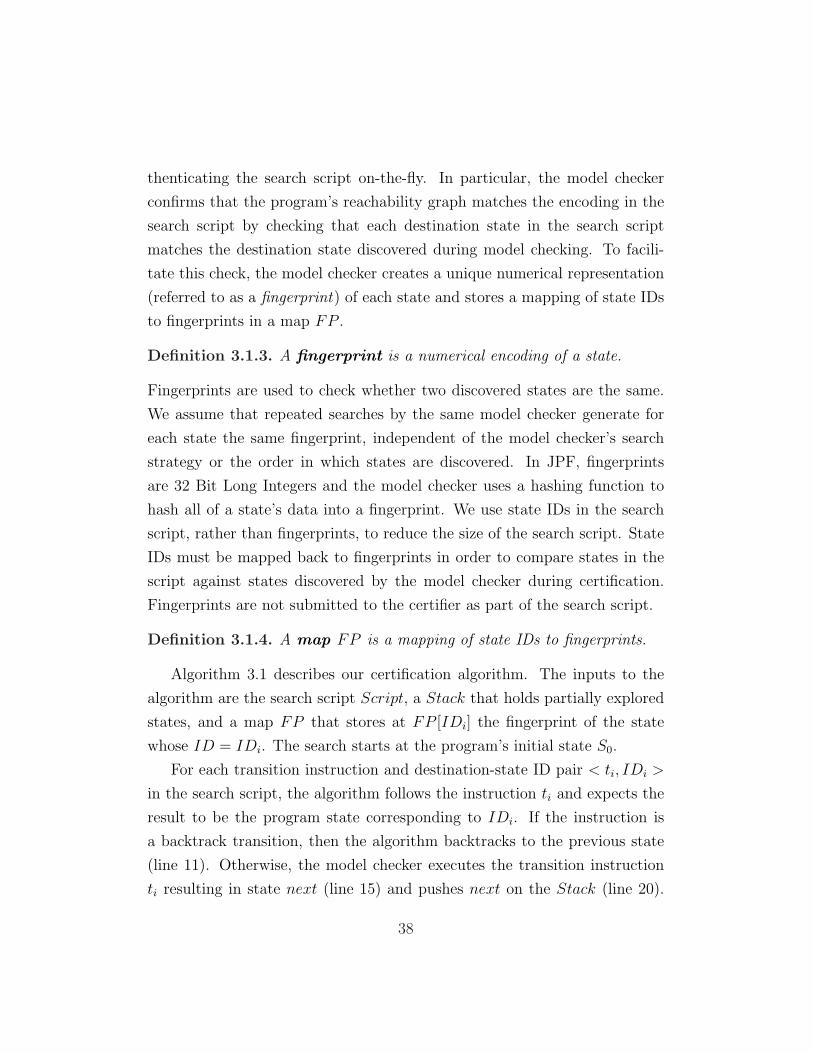
thenticating the search script on-the-fly. In particular, the model checker
confirms that the program’s reachability graph matches the encoding in the
search script by checking that each destination state in the search script
matches the destination state discovered during model checking. To facili-
tate this check, the model checker creates a unique numerical representation
(referred to as a fingerprint) of each state and stores a mapping of state IDs
to fingerprints in a map FP .
Definition 3.1.3. A fingerprint is a numerical encoding of a state.
Fingerprints are used to check whether two discovered states are the same.
We assume that repeated searches by the same model checker generate for
each state the same fingerprint, independent of the model checker’s search
strategy or the order in which states are discovered. In JPF, fingerprints
are 32 Bit Long Integers and the model checker uses a hashing function to
hash all of a state’s data into a fingerprint. We use state IDs in the search
script, rather than fingerprints, to reduce the size of the search script. State
IDs must be mapped back to fingerprints in order to compare states in the
script against states discovered by the model checker during certification.
Fingerprints are not submitted to the certifier as part of the search script.
Definition 3.1.4. A map FP is a mapping of state IDs to fingerprints.
Algorithm 3.1 describes our certification algorithm. The inputs to the
algorithm are the search script Script, a Stack that holds partially explored
states, and a map FP that stores at FP [IDi] the fingerprint of the state
whose ID = IDi. The search starts at the program’s initial state S0.
For each transition instruction and destination-state ID pair < ti, IDi >
in the search script, the algorithm follows the instruction ti and expects the
result to be the program state corresponding to IDi. If the instruction is
a backtrack transition, then the algorithm backtracks to the previous state
(line 11). Otherwise, the model checker executes the transition instruction
ti resulting in state next (line 15) and pushes next on the Stack (line 20).
38
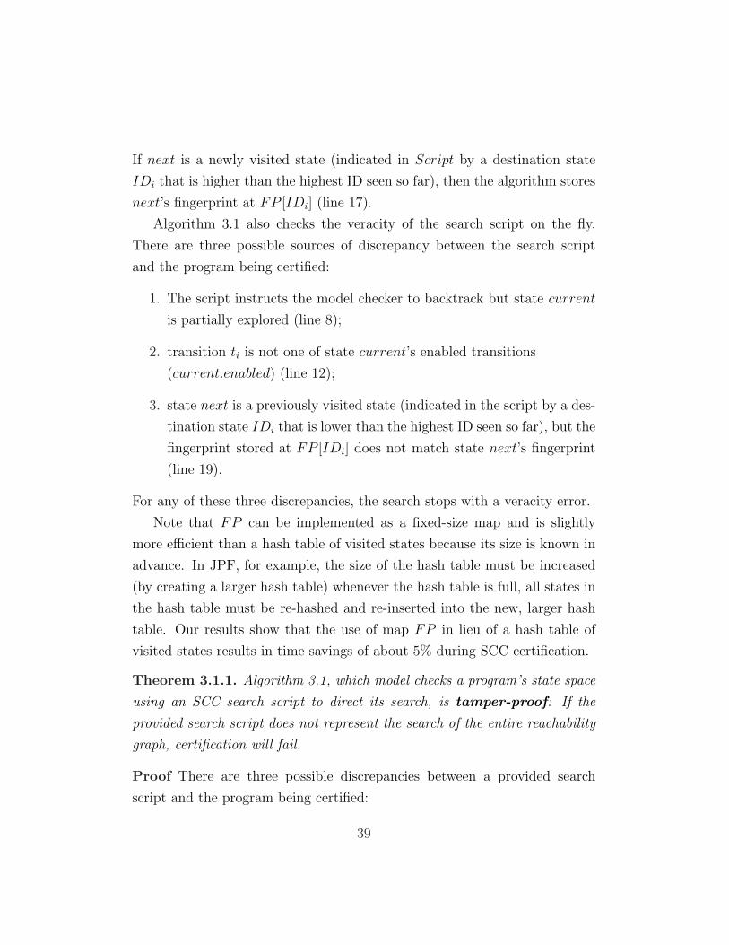
If next is a newly visited state (indicated in Script by a destination state
IDi that is higher than the highest ID seen so far), then the algorithm stores
next’s fingerprint at FP [IDi] (line 17).
Algorithm 3.1 also checks the veracity of the search script on the fly.
There are three possible sources of discrepancy between the search script
and the program being certified:
1. The script instructs the model checker to backtrack but state current
is partially explored (line 8);
2. transition ti is not one of state current’s enabled transitions
(current.enabled) (line 12);
3. state next is a previously visited state (indicated in the script by a des-
tination state IDi that is lower than the highest ID seen so far), but the
fingerprint stored at FP [IDi] does not match state next’s fingerprint
(line 19).
For any of these three discrepancies, the search stops with a veracity error.
Note that FP can be implemented as a fixed-size map and is slightly
more efficient than a hash table of visited states because its size is known in
advance. In JPF, for example, the size of the hash table must be increased
(by creating a larger hash table) whenever the hash table is full, all states in
the hash table must be re-hashed and re-inserted into the new, larger hash
table. Our results show that the use of map FP in lieu of a hash table of
visited states results in time savings of about 5% during SCC certification.
Theorem 3.1.1. Algorithm 3.1, which model checks a program’s state space
using an SCC search script to direct its search, is tamper-proof: If the
provided search script does not represent the search of the entire reachability
graph, certification will fail.
Proof There are three possible discrepancies between a provided search
script and the program being certified:
39

Algorithm 3.1: Certification Algorithm1 Input : Script ; /∗ search s c r i p t encoding r e a c h a b i l i t y graph ∗/2 Input : Stack ; /∗ wo r k l i s t o f p a r t i a l l y exp lo red s t a t e s ∗/3 Input : FP ; /∗ mapping between s t a t e IDs and f i n g e r p r i n t s ∗/4 push (S0 ) onto Stack ;5 for each < ti, IDi > in Script{6 current = top s t a t e on Stack ;7 i f (ti == B ){8 i f (current == p a r t i a l l y exp lored )9 throw ve r a c i t y e r r o r ;
10 else11 pop (current) from Stack ;12 else i f (ti /∈ current.enabled)13 throw ve r a c i t y e r r o r ;14 else {15 next = succ(current, ti)16 i f (IDi h ighe s t ID scanned so f a r )17 FP [IDi] = next.fingerprint ;18 else i f (FP [IDi] 6= next.fingerprint)19 throw ve r a c i t y e r r o r ;20 push (next) onto Stack ;21 }22 }
1. The script instructs the model checker to explore a transition ti (i.e.,
a program statement) at a particular point in the search, but that
transition does not exist in the program’s reachability graph. Line 12
in Algorithm 3.1 detects this discrepancy and the search stops.
2. The script instructs the model checker to backtrack from a partially
explored state Si, that is, the script instructs the model checker to
not explore one or more transitions that emanate from Si. Line 8 in
Algorithm 3.1 detects this discrepancy and the search stops.
3. The search script states that two transitions ti and tj have the same
destination state with the same state IDi. However, in the program’s
reachability graph, the two transitions lead to different program states.
Line 19 in Algorithm 3.1 detects this discrepancy and the search stops.
When ti is explored, the fingerprint of its destination state is stored at
FP [IDi]. When tj is subsequently explored, the model checker com-
40
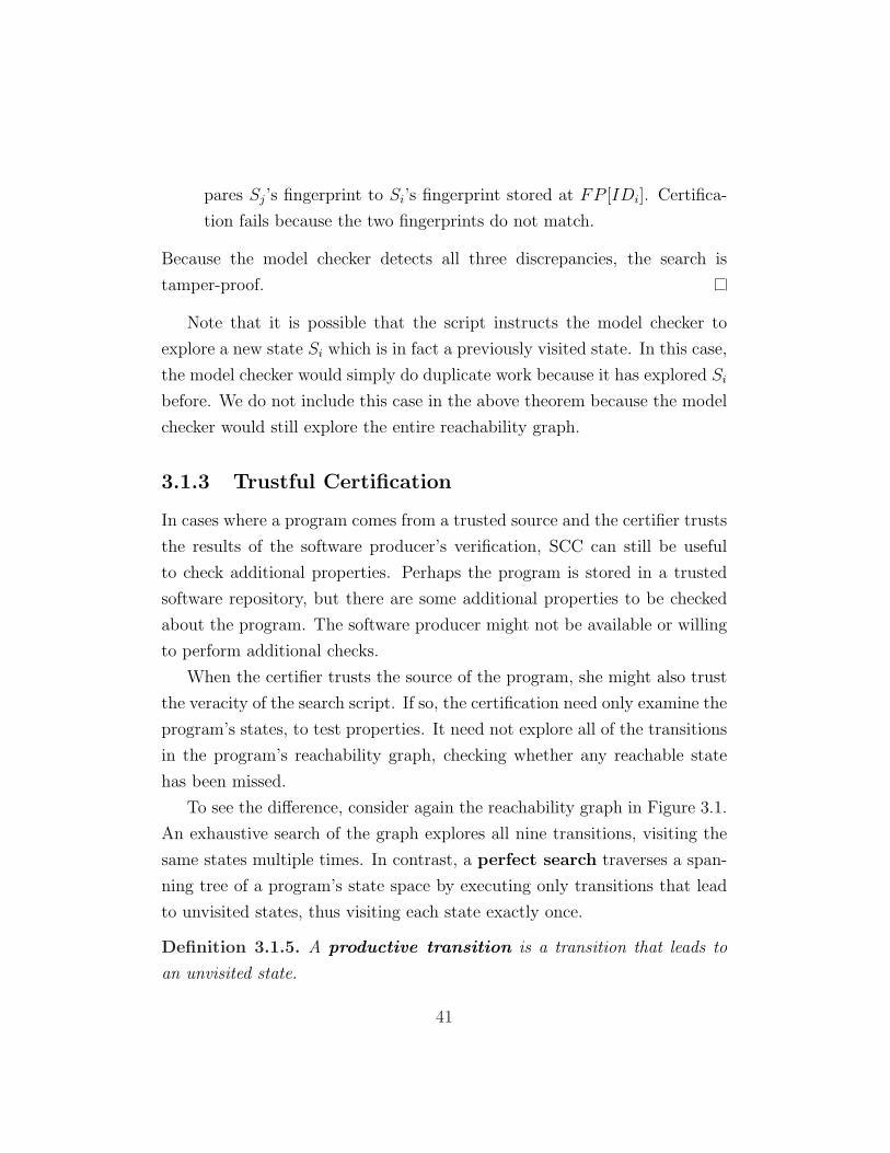
pares Sj’s fingerprint to Si’s fingerprint stored at FP [IDi]. Certifica-
tion fails because the two fingerprints do not match.
Because the model checker detects all three discrepancies, the search is
tamper-proof.
Note that it is possible that the script instructs the model checker to
explore a new state Si which is in fact a previously visited state. In this case,
the model checker would simply do duplicate work because it has explored Si
before. We do not include this case in the above theorem because the model
checker would still explore the entire reachability graph.
3.1.3 Trustful Certification
In cases where a program comes from a trusted source and the certifier trusts
the results of the software producer’s verification, SCC can still be useful
to check additional properties. Perhaps the program is stored in a trusted
software repository, but there are some additional properties to be checked
about the program. The software producer might not be available or willing
to perform additional checks.
When the certifier trusts the source of the program, she might also trust
the veracity of the search script. If so, the certification need only examine the
program’s states, to test properties. It need not explore all of the transitions
in the program’s reachability graph, checking whether any reachable state
has been missed.
To see the difference, consider again the reachability graph in Figure 3.1.
An exhaustive search of the graph explores all nine transitions, visiting the
same states multiple times. In contrast, a perfect search traverses a span-
ning tree of a program’s state space by executing only transitions that lead
to unvisited states, thus visiting each state exactly once.
Definition 3.1.5. A productive transition is a transition that leads to
an unvisited state.
41

t2
t1
t3backtrack
S1
S2
S3 S4
S5
t2
Figure 3.2: Perfect search of a state space
Definition 3.1.6. A perfect search of a program explores only productive
transitions of the program’s reachability graph. The resulting search traverses
one possible spanning tree of the reachability graph.
Figure 3.2 depicts a depth-first, perfect search of the graph from Fig-
ure 3.1. Solid lines represent productive transitions and dashed lines repre-
sent backtracks to parent states. Backtracking does not constitute “visiting”
a state because the work of constructing and testing the state is already done.
Thus, each state is visited exactly once. The corresponding search script is:
Trans instr: t1 t2 t2 B t3
The script need not record the transitions’ target state IDs because trustful
certification does not check the veracity of the script.
In this manner, trustful SCC effects a perfect search of a program’s state
space. The software producer provides a program and matching trustful
search script. During certification, the certifier’s model checker uses the
search script to direct its search of the program’s state space. Thus, there
is no need to create or maintain state fingerprints or a hash table of visited
states, resulting in additional savings.
42
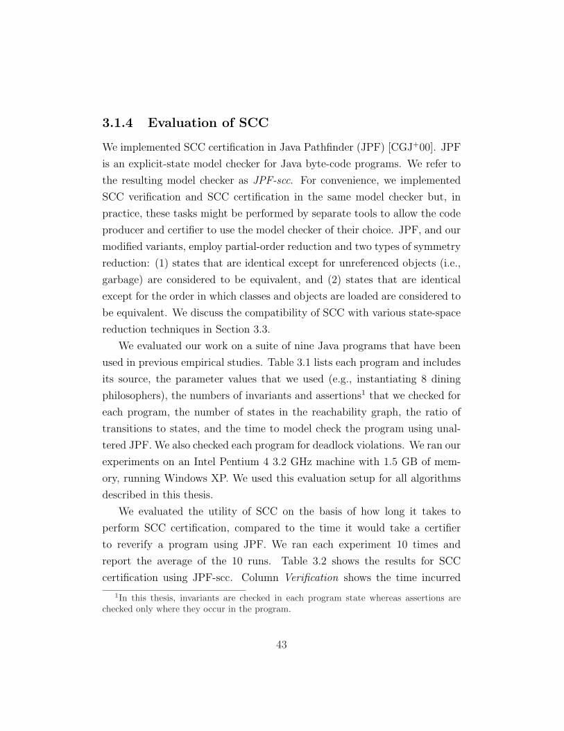
3.1.4 Evaluation of SCC
We implemented SCC certification in Java Pathfinder (JPF) [CGJ+00]. JPF
is an explicit-state model checker for Java byte-code programs. We refer to
the resulting model checker as JPF-scc. For convenience, we implemented
SCC verification and SCC certification in the same model checker but, in
practice, these tasks might be performed by separate tools to allow the code
producer and certifier to use the model checker of their choice. JPF, and our
modified variants, employ partial-order reduction and two types of symmetry
reduction: (1) states that are identical except for unreferenced objects (i.e.,
garbage) are considered to be equivalent, and (2) states that are identical
except for the order in which classes and objects are loaded are considered to
be equivalent. We discuss the compatibility of SCC with various state-space
reduction techniques in Section 3.3.
We evaluated our work on a suite of nine Java programs that have been
used in previous empirical studies. Table 3.1 lists each program and includes
its source, the parameter values that we used (e.g., instantiating 8 dining
philosophers), the numbers of invariants and assertions1 that we checked for
each program, the number of states in the reachability graph, the ratio of
transitions to states, and the time to model check the program using unal-
tered JPF. We also checked each program for deadlock violations. We ran our
experiments on an Intel Pentium 4 3.2 GHz machine with 1.5 GB of mem-
ory, running Windows XP. We used this evaluation setup for all algorithms
described in this thesis.
We evaluated the utility of SCC on the basis of how long it takes to
perform SCC certification, compared to the time it would take a certifier
to reverify a program using JPF. We ran each experiment 10 times and
report the average of the 10 runs. Table 3.2 shows the results for SCC
certification using JPF-scc. Column Verification shows the time incurred
1In this thesis, invariants are checked in each program state whereas assertions arechecked only where they occur in the program.
43

Tab
le3.
1:Jav
aP
rogr
ams
Use
dfo
rE
valu
atio
nSou
rce
Pro
gram
Par
amet
ers
Pro
per
ties
#Sta
tes
#Tra
ns
Tim
e#
Inv/#
Ass
ert
#Sta
tes
(sec
)
[CG
J+00
]D
inin
gP
hilos
opher
(8)
#philos
opher
s1/
220
9014
5.2
220
[San
]B
ounded
Buffer
(5,4
,4)
buffer
size
,#pro
d,#
cons
1/3
7869
877.
110
88[P
SD
]N
asa
KSU
Pip
elin
e(4
,1)
stag
esiz
e,#
list
ener
s3/
459
512
4.1
45[S
an]
Nes
ted
Mon
itor
(5,4
,4)
buffer
size
,#pro
d,#
cons
6/4
7194
16.
999
[San
]P
ipel
ine
(7)
stag
esiz
e3/
382
011
6.1
101
[San
]RW
VSN
(4,4
)#
read
ers,
#w
rite
rs3/
422
7116
5.1
245
[San
]R
eplica
ted
Wor
kers
(5,2
)#
wor
kers
,#it
ems
4/5
7100
225.
186
0[D
HH
+06
]Sle
epin
gB
arber
(2,4
,3)
#bar
ber
,#cu
stom
ers,
#ch
airs
4/5
1452
194
4.3
1308
[Dav
]E
leva
tor(
5,10
,10)
#el
evat
ors,
#floor
s,#
peo
ple
4/8
3860
328.
411
67
44
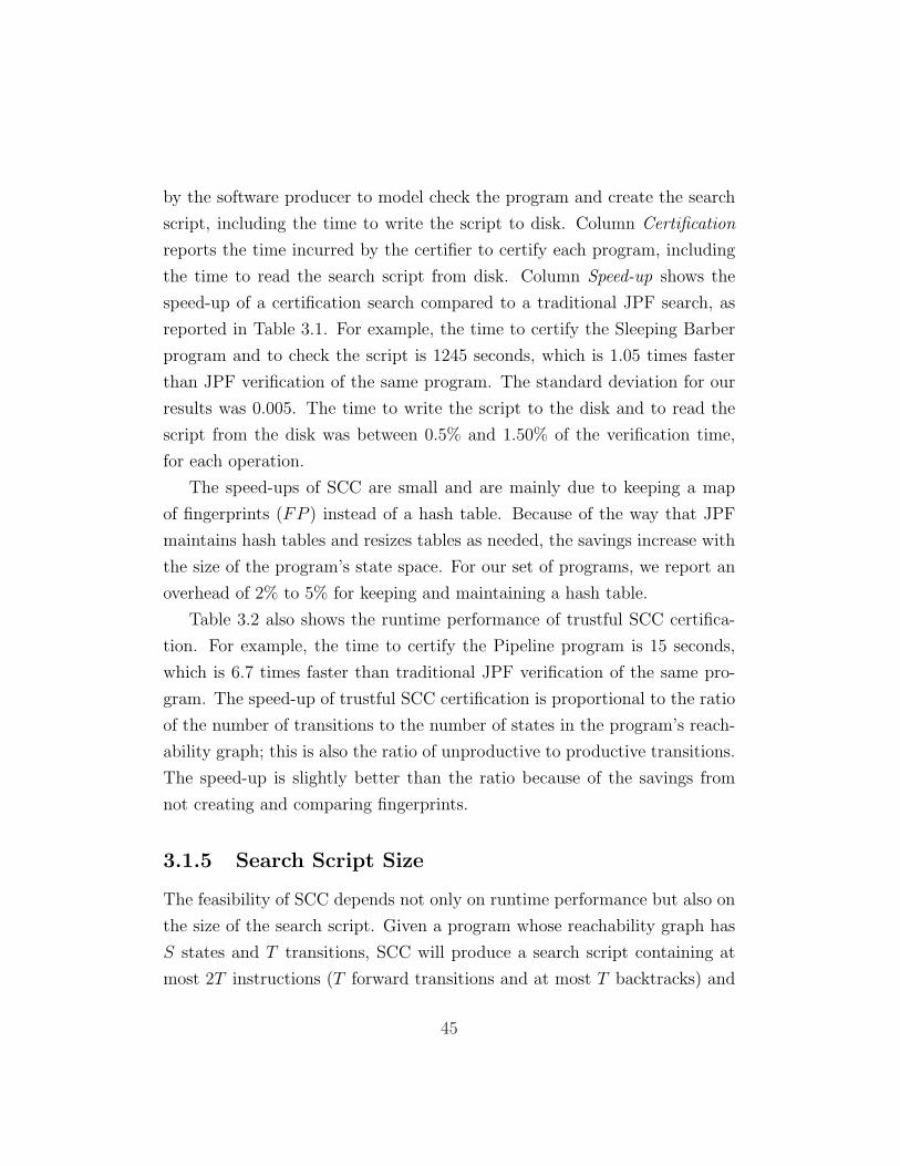
by the software producer to model check the program and create the search
script, including the time to write the script to disk. Column Certification
reports the time incurred by the certifier to certify each program, including
the time to read the search script from disk. Column Speed-up shows the
speed-up of a certification search compared to a traditional JPF search, as
reported in Table 3.1. For example, the time to certify the Sleeping Barber
program and to check the script is 1245 seconds, which is 1.05 times faster
than JPF verification of the same program. The standard deviation for our
results was 0.005. The time to write the script to the disk and to read the
script from the disk was between 0.5% and 1.50% of the verification time,
for each operation.
The speed-ups of SCC are small and are mainly due to keeping a map
of fingerprints (FP ) instead of a hash table. Because of the way that JPF
maintains hash tables and resizes tables as needed, the savings increase with
the size of the program’s state space. For our set of programs, we report an
overhead of 2% to 5% for keeping and maintaining a hash table.
Table 3.2 also shows the runtime performance of trustful SCC certifica-
tion. For example, the time to certify the Pipeline program is 15 seconds,
which is 6.7 times faster than traditional JPF verification of the same pro-
gram. The speed-up of trustful SCC certification is proportional to the ratio
of the number of transitions to the number of states in the program’s reach-
ability graph; this is also the ratio of unproductive to productive transitions.
The speed-up is slightly better than the ratio because of the savings from
not creating and comparing fingerprints.
3.1.5 Search Script Size
The feasibility of SCC depends not only on runtime performance but also on
the size of the search script. Given a program whose reachability graph has
S states and T transitions, SCC will produce a search script containing at
most 2T instructions (T forward transitions and at most T backtracks) and
45

Tab
le3.
2:R
esult
sfo
rSC
CV
erifi
cati
onan
dC
erti
fica
tion
SC
Cce
rtifi
cati
onTru
stfu
lSC
Cce
rtifi
cati
on
Pro
gram
(siz
e)V
erifi
cati
onScr
ipt
Cer
tifica
tion
Spee
d-u
pScr
ipt
Cer
tifica
tion
Spee
d-u
p(s
ec)
size
(KB
)(s
ec)
size
(KB
)(s
ec)
Din
ing
Philos
opher
(4K
B)
221
104
213
1.03
2535
6.3
Bou
nded
Buffer
(6K
B)
1090
329
1036
1.04
7413
08.
4N
ASA
KSU
Pip
elin
e(2
KB
)45
9144
1.02
229
5N
este
dM
onit
or(7
KB
)10
045
971.
019
147.
1P
ipel
ine
(5K
B)
102
5199
1.01
1115
6.7
RW
VSN
(9K
B)
246
102
236
1.03
2939
6.3
Rep
lica
ted
Wor
kers
(15K
B)
862
272
819
1.05
7214
06.
1Sle
epin
gB
arber
(8K
B)
1310
492
1245
1.05
187
245
5.3
Ele
vato
r(2
9KB
)11
6924
811
221.
0454
129
9
46
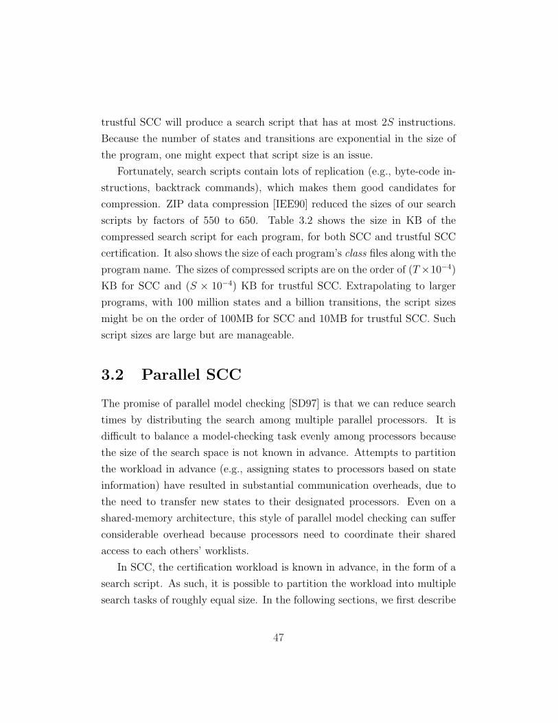
trustful SCC will produce a search script that has at most 2S instructions.
Because the number of states and transitions are exponential in the size of
the program, one might expect that script size is an issue.
Fortunately, search scripts contain lots of replication (e.g., byte-code in-
structions, backtrack commands), which makes them good candidates for
compression. ZIP data compression [IEE90] reduced the sizes of our search
scripts by factors of 550 to 650. Table 3.2 shows the size in KB of the
compressed search script for each program, for both SCC and trustful SCC
certification. It also shows the size of each program’s class files along with the
program name. The sizes of compressed scripts are on the order of (T×10−4)
KB for SCC and (S × 10−4) KB for trustful SCC. Extrapolating to larger
programs, with 100 million states and a billion transitions, the script sizes
might be on the order of 100MB for SCC and 10MB for trustful SCC. Such
script sizes are large but are manageable.
3.2 Parallel SCC
The promise of parallel model checking [SD97] is that we can reduce search
times by distributing the search among multiple parallel processors. It is
difficult to balance a model-checking task evenly among processors because
the size of the search space is not known in advance. Attempts to partition
the workload in advance (e.g., assigning states to processors based on state
information) have resulted in substantial communication overheads, due to
the need to transfer new states to their designated processors. Even on a
shared-memory architecture, this style of parallel model checking can suffer
considerable overhead because processors need to coordinate their shared
access to each others’ worklists.
In SCC, the certification workload is known in advance, in the form of a
search script. As such, it is possible to partition the workload into multiple
search tasks of roughly equal size. In the following sections, we first describe
47
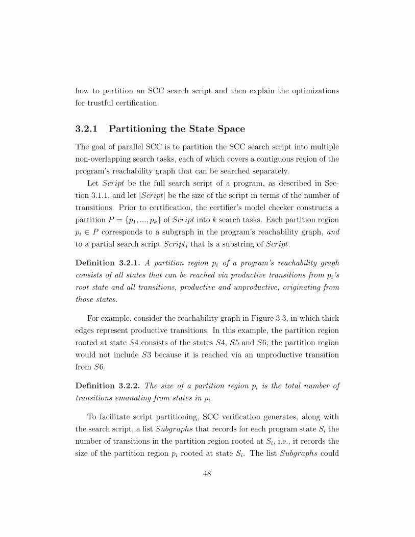
how to partition an SCC search script and then explain the optimizations
for trustful certification.
3.2.1 Partitioning the State Space
The goal of parallel SCC is to partition the SCC search script into multiple
non-overlapping search tasks, each of which covers a contiguous region of the
program’s reachability graph that can be searched separately.
Let Script be the full search script of a program, as described in Sec-
tion 3.1.1, and let |Script| be the size of the script in terms of the number of
transitions. Prior to certification, the certifier’s model checker constructs a
partition P = {p1, ..., pk} of Script into k search tasks. Each partition region
pi ∈ P corresponds to a subgraph in the program’s reachability graph, and
to a partial search script Scripti that is a substring of Script.
Definition 3.2.1. A partition region pi of a program’s reachability graph
consists of all states that can be reached via productive transitions from pi’s
root state and all transitions, productive and unproductive, originating from
those states.
For example, consider the reachability graph in Figure 3.3, in which thick
edges represent productive transitions. In this example, the partition region
rooted at state S4 consists of the states S4, S5 and S6; the partition region
would not include S3 because it is reached via an unproductive transition
from S6.
Definition 3.2.2. The size of a partition region pi is the total number of
transitions emanating from states in pi.
To facilitate script partitioning, SCC verification generates, along with
the search script, a list Subgraphs that records for each program state Si the
number of transitions in the partition region rooted at Si, i.e., it records the
size of the partition region pi rooted at state Si. The list Subgraphs could
48

S2
S3 S4 S5
S6
S7
S8 S9S10
S1
t1
t1
t1
t1
t1
t1
t2
t1 t1 t2
t1t2
t2
t2
t3 t3
16
15
7
4
0
2
1
4
1
1
S1
S2
S3
S4
S5
S6
S7
S8
S9
S10
Subgraphs
S1 S10S7S10S2S8S9S5S9S8S4S8S3S8S2S3S7S6S7S3S4S6S3S6S5S6S4S5S4S3S2 S1S2
t2 Bt1t1 t1t1 t1t1t1t1t1 t2t2t2t2 t3t3BBBBBBBBBB B B B B B-
Script
(16)
(15)
(7) (4)
(4)(1) (1)
(1) (0)
(2)
Figure 3.3: Reachability graph with its script and Subgraphs
be generated during certification from the search script. We ask the code
producer to provide Subgraphs in order to reduce certification time. Ba-
sically, during verification, the model checker performs a depth-first search
of the program state space. As each new state Si is encountered, an entry
indexed by state ID is added to Subgraphs. As Si’s child states are explored
and the sizes of their subtrees are computed, the size of Si is updated. The
Subgraphs list is provided to the certifier, along with the program and search
script. In SCC certification, the size of a Subgraphs list is less than 10% of
the size of the search script, and in trustful SCC certification, the size of
Subgraphs is less than 20% of the size of the search script. The percent-
ages are different because the size of Subgraphs is the same for trustful and
tamper-proof certification, but their script sizes are different.
Figure 3.3 shows an example reachability graph with its corresponding
Script and Subgraphs. The Subgraphs table shows for each state Si (left
column) the size of the partition region (right column) rooted at Si. For ex-
ample, the partition region rooted at state S4 consists of the states S4, S5, S6
49
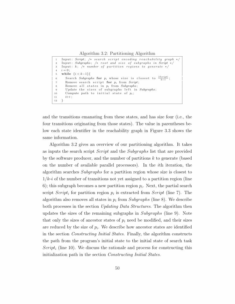
Algorithm 3.2: Partitioning Algorithm1 Input : Script ; /∗ search s c r i p t encoding r e a c h a b i l i t y graph ∗/2 Input : Subgraphs ; /∗ root and s i z e o f subgraphs in Script ∗/3 Input : k ; /∗ number o f p a r t i t i o n reg ions to generate ∗/4 i = 0 ;5 while {i < k−1}{6 Search Subgraphs for pi whose s i z e i s c l o s e s t to
|Script|k−i
;
7 Remove search s c r i p t for pi from Script ;8 Remove a l l s t a t e s in pi from Subgraphs ;9 Update the s i z e s o f subgraphs l e f t in Subgraphs ;
10 Compute path to i n i t i a l s t a t e o f pi ;11 i++ ;12 }
and the transitions emanating from these states, and has size four (i.e., the
four transitions originating from those states). The value in parentheses be-
low each state identifier in the reachability graph in Figure 3.3 shows the
same information.
Algorithm 3.2 gives an overview of our partitioning algorithm. It takes
as inputs the search script Script and the Subgraphs list that are provided
by the software producer, and the number of partitions k to generate (based
on the number of available parallel processors). In the ith iteration, the
algorithm searches Subgraphs for a partition region whose size is closest to
1/k−i of the number of transitions not yet assigned to a partition region (line
6); this subgraph becomes a new partition region pi. Next, the partial search
script Scripti for partition region pi is extracted from Script (line 7). The
algorithm also removes all states in pi from Subgraphs (line 8). We describe
both processes in the section Updating Data Structures. The algorithm then
updates the sizes of the remaining subgraphs in Subgraphs (line 9). Note
that only the sizes of ancestor states of pi need be modified, and their sizes
are reduced by the size of pi. We describe how ancestor states are identified
in the section Constructing Initial States. Finally, the algorithm constructs
the path from the program’s initial state to the initial state of search task
Scripti (line 10). We discuss the rationale and process for constructing this
initialization path in the section Constructing Initial States.
50
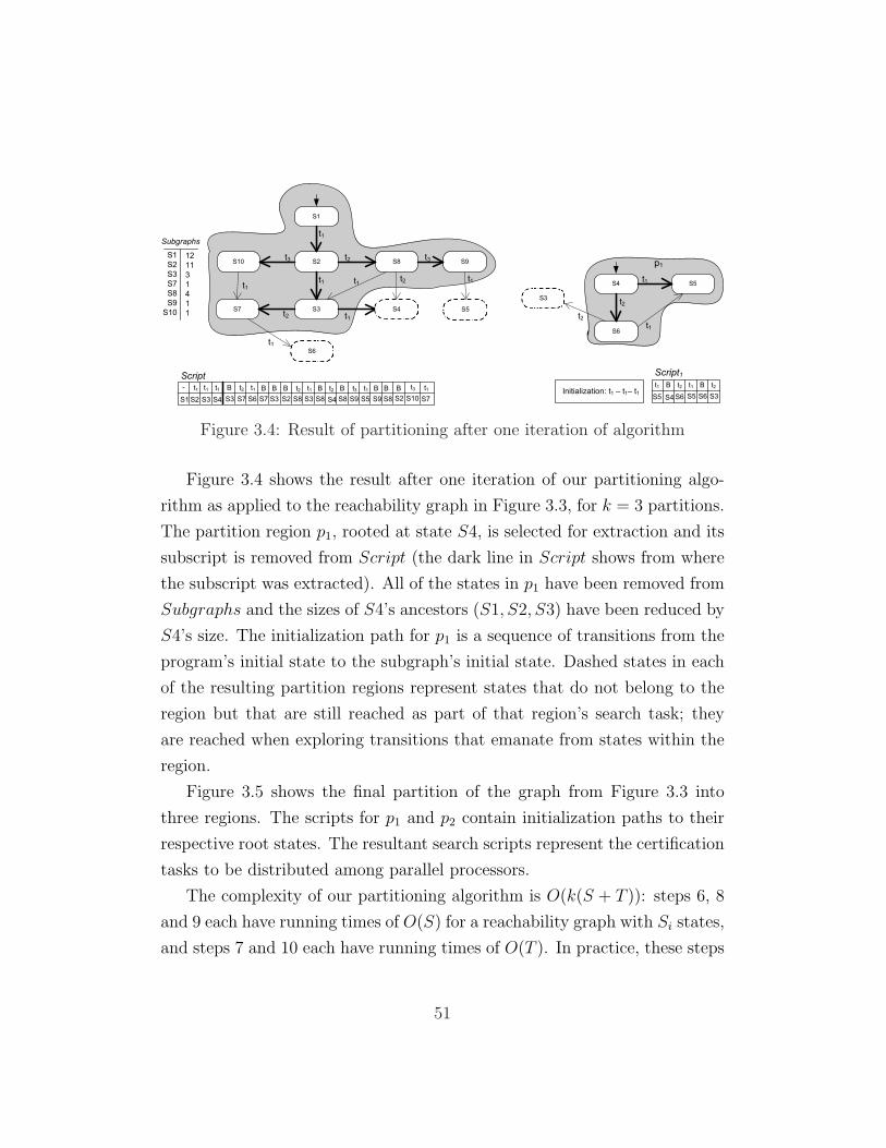
S2
S3S7
S8 S9S10
S1
t1
t1
t1
t1
t2
t1 t1 t2
t1 t2t2
t3 t312
11
3
1
4
1
1
S1
S2
S3
S7
S8
S9
S10
Subgraphs
S1 S7S10S2S8S9S5S9S8S4S8S3S8S2S3S7S6S7S3S4S3S2
t2 t1t1 t1t1t1t1t1 t2t2 t3t3BBBBBB B B B-
Script1
S4 S5
S6
t1
t1
t2
S3S6S5S6S4S5
t1 t1 t2t2 BB
p1
Script
Initialization: t1 – t1– t1
S3
S6
S4 S5
Figure 3.4: Result of partitioning after one iteration of algorithm
Figure 3.4 shows the result after one iteration of our partitioning algo-
rithm as applied to the reachability graph in Figure 3.3, for k = 3 partitions.
The partition region p1, rooted at state S4, is selected for extraction and its
subscript is removed from Script (the dark line in Script shows from where
the subscript was extracted). All of the states in p1 have been removed from
Subgraphs and the sizes of S4’s ancestors (S1, S2, S3) have been reduced by
S4’s size. The initialization path for p1 is a sequence of transitions from the
program’s initial state to the subgraph’s initial state. Dashed states in each
of the resulting partition regions represent states that do not belong to the
region but that are still reached as part of that region’s search task; they
are reached when exploring transitions that emanate from states within the
region.
Figure 3.5 shows the final partition of the graph from Figure 3.3 into
three regions. The scripts for p1 and p2 contain initialization paths to their
respective root states. The resultant search scripts represent the certification
tasks to be distributed among parallel processors.
The complexity of our partitioning algorithm is O(k(S + T )): steps 6, 8
and 9 each have running times of O(S) for a reachability graph with Si states,
and steps 7 and 10 each have running times of O(T ). In practice, these steps
51
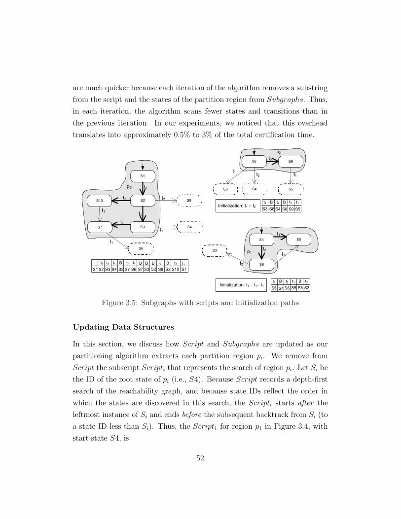
are much quicker because each iteration of the algorithm removes a substring
from the script and the states of the partition region from Subgraphs. Thus,
in each iteration, the algorithm scans fewer states and transitions than in
the previous iteration. In our experiments, we noticed that this overhead
translates into approximately 0.5% to 3% of the total certification time.
S2
S3
S4 S5
S6
S7
S8 S9
S1
p2
p1
p3
S10
t3
t3
t1
t1
t1
t2
t1
t2
t1
t1t1t2
t1
t1
t2
t2
S3
S5S4S3
S6
S4
S8
S3S6S5S6S4S5
t1 t1 t2t2 BBInitialization: t1 – t1– t1
S5S9S8S4S8S3
t1 B t1t2BInitialization: t1 – t2
t3
S1 S7S10S2S3S7S6S7S3S4S3S2
t1t1t1t1t1 t2 t3BBBB- t2
S8
B
S2
Figure 3.5: Subgraphs with scripts and initialization paths
Updating Data Structures
In this section, we discuss how Script and Subgraphs are updated as our
partitioning algorithm extracts each partition region pi. We remove from
Script the subscript Scripti that represents the search of region pi. Let Si be
the ID of the root state of pi (i.e., S4). Because Script records a depth-first
search of the reachability graph, and because state IDs reflect the order in
which the states are discovered in this search, the Scripti starts after the
leftmost instance of Si and ends before the subsequent backtrack from Si (to
a state ID less than Si). Thus, the Script1 for region p1 in Figure 3.4, with
start state S4, is
52

p1: t1 B t2 t1 B t2 B B
S5 S4 S6 S5 S6 S3 S6 S4
Note that Scripti must have the same number of forward transitions as the
size of pi in Subgraphs. Otherwise, there is a discrepancy between Script
and Subgraphs and the partitioning of Script fails. After discarding trailing
backtrack commands, we obtain a search script Script1 that specifies the
search of region p1, starting from the initial state of p1:
p1 (S4): t1 B t2 t1 B t2
S5 S4 S6 S5 S6 S3
Given a partition region pi, updating Subgraphs entails removing all
entries that correspond to states in the region (line 8 in our partitioning
algorithm). Again, let Si be the ID of the root state of pi. Any state in
Scripti whose ID is greater than or equal to Si refers to a state in the region
pi and must be removed from Subgraphs. For example, in Script1, states
S4, S5, and S6 are removed from Subgraphs.
Each iteration of the partitioning algorithm produces a script for a differ-
ent partition region. When the algorithm terminates, what remains of Script
forms a search script for the kth region. Figure 3.5 shows the search scripts
for each partition region.
“Constructing” Initial States
Each Scripti starts at the root state of a partition region pi. We could at-
tempt to construct the corresponding “initial” program state for each search
task, but JPF program states are complex and are difficult to construct
and restore: they comprise not only the variable valuation but also informa-
tion about threads and the progress of the search. Instead, we prefix each
search script with an initialization path: a sequence of transitions from
the program’s initial state to the start state of the search task. We discuss
in Section 3.2.5 the overhead incurred by this decision.
53

To construct the initialization path, the original Script is scanned from
start to end. Every time a transition is reached, it is pushed onto a stack.
Every time a backtrack command is read, the top transition is popped off the
stack. When a state ID Si is first encountered, the transitions in the stack
make up the initialization path from the program’s initial state to state Si.
For example, the initialization path to p1’s root state is: t1 t1 t1. Note that
this algorithm does not construct the shortest path to a given state, but it
does construct the shortest path with respect to the given script.
The states along the initialization path are all ancestor states of Si in the
reachability graph. Thus, we can use the same process to update the sizes of
the subgraphs remaining in Subgraphs after removing all states of pi from
Subgraphs (line 9 of the algorithm).
3.2.2 Parallel Certification
The program and search scripts are distributed to parallel processors, which
run the certifier’s model checker. Each processor creates its own local copy
of FP , which maps state IDs to program-state fingerprints. If a processor
detects any discrepancy between its search script and the program, it raises
an error. In addition, once all processors have finished their certification
tasks, the processors’ FP maps are compared to ensure that all processors
map state IDs to the same fingerprints. Any mismatch is reported as an
error. This final check on the veracity of the search scripts performs at most
nS comparisons, where n is the number of processors and S is the total
number of states.
3.2.3 Correctness
Our partitioning algorithm divides a search script in such a way that the
resulting subscripts cover all states and transitions of the original script.
Theorem 3.2.1. Given a search script Script of a program’s reachability
54

graph, Algorithm 3.2 divides Script into k subscripts such that each result-
ing subscript represents a depth-first search of a subgraph of the reachability
graph.
Proof We show that (1) each extracted subscript Scriptj records a depth-
first search and (2) the subscript Scriptk that remains after all Scriptjs have
been extracted from Script, also represents a depth-first search.
Each iteration of the partitioning algorithm extracts a search subscript
Scriptj that corresponds to a leaf subgraph pj of a program’s reachability
graph, and is rooted at state Sj.
Let ti,j be a productive transition from state Si to state Sj (i.e., the first
transition in Script that leads to Sj), and let Bj,i be a backtrack transi-
tion from state Sj back to state Si. Because Script represents a DFS of
the program’s reachability graph, the subscript Scriptj between ti,j and Bj,i
represents a depth-first search of all states reachable from Sj via productive
transitions, and all transitions emanating from those states. Thus, Scriptj
represents a depth-first search.
After the extraction of Scriptj from Script (line 7), the source state of
ti,j, Si, is the same as the destination state of Bj,i. Thus, the removal of
the sequence does not affect the continuity of the search script, and after the
(k−1)th iteration of the algorithm, Scriptk represents a depth-first serch.
Theorem 3.2.2. Given a search script Script of a program’s reachability
graph, Algorithm 3.2 divides Script into k subscripts such that the resulting
subscripts cover all states and transitions of the reachability graph.
Proof By construction, Script represents a DFS of a program’s entire reach-
ability graph. Each iteration of the partitioning algorithm extracts a search
subscript Scripti that corresponds to a leaf subgraph pi of the reachability
graph. The subgraph is rooted at state Si and it includes all of the states
that are reachable from Si via productive transitions and includes all transi-
55
tions originating from those states. By Theorem 3.2.1, Scripti is a depth-first
search and explores all transitions and visits each state in pi.
When the algorithm terminates, what remains of Script is a search sub-
script Scriptk for a kth subgraph. The subgraph is rooted at the program’s
initial state S1, and includes all of the states that are reachable from S1 via
productive transitions up to and excluding the root states of the extracted par-
tition regions, and all of the transitions originating from those states. Again,
by Theorem 3.2.1, Scriptk is a depth-first search and explores all transitions
and visits each state in pk. In this manner, the algorithm splits Script with-
out removing any states or transitions (except backtrack transitions).
Theorem 3.2.3. Parallel SCC certification is tamper-proof: If the pro-
vided search scripts do not match the program’s reachability graph, certifica-
tion will fail.
Proof By Theorem 3.1.1, the search of Scripti on processori would fail if
there is a discrepancy between a subscript Scripti and the corresponding
subgraph pi of the reachability graph.
We have also to show that parallel SCC detects discrepancies between
transitions in different scripts. It is possible that transition ti in subscript
Scripti and transition tj in Scriptj have the same destination state with
the same state ID. However, in the program’s reachability graph, the two
transitions lead to different program states.
When ti is explored on processori, the state ID and fingerprint of its
destination state Si are stored in FPi. When tj is explored on processorj,
the state ID and fingerprint of its destination state Sj are stored in FPj.
Once both processors have completed their search tasks, a master processor
compares Si’s fingerprint in FPi to Sj’s fingerprint in FPj. Certification fails
because the two fingerprints do not match.
Given that the software producer provides the list Subgraphs, we must en-
sure that tampering of the provided Subgraphs does not adversely affect the
56
partitioning of the script in such a way that it influences the certification
results
Theorem 3.2.4. Given a search script Script of a program’s reachability
graph and a list Subgraphs that is not accurate with respect to the program’s
reachability graph, Algorithm 3.2 either fails or still produces subscripts that
cover disjoint regions and, taken together, cover the program’s entire reach-
ability graph.
Proof There are three possible cases of discrepancy between Subgraphs and
the reachability graph.
• Subgraphs lists an incorrect size for the subgraph rooted at some state
Si: If Algorithm 3.2 chooses state Si as the root state of a region, then
line 8 of Algorithm 3.2 will fail because the number of transitions in the
subscript does not match the size of the subgraph listed in Subgraphs.
If Algorithm 3.2 does not choose state Si as the root state of a region,
then the algorithm may choose different partition regions in line 6 than
it would have chosen if it had been given correct Subgraphs sizes. Al-
gorithm 3.2 (line 6) uses the sizes in Subgraphs to select the subgraph
that partitions the reachability graph into equal-sized subgraphs us-
ing a greedy algorithm. If there is a large discrepancy between the
provided Subgraphs sizes and the subgraphs’ actual sizes, then, in the
worst case, there will be a larger standard deviation in the sizes of the
resulting subscripts.
• Subgraphs is missing the entry for a state Si: Let pj be the region to
be extracted and let Sj be the root state of pj. If state Si belongs to pj,
then line 8 of Algorithm 3.2 will fail because the algorithm does not find
Si in Subgraphs when extracting the states within pj from Subgraphs.
If Si is an ancestor state of Sj, then line 9 of Algorithm 3.2 will fail
because the algorithm does not find Si in Subgraphs when updating
57
the sizes of Sj’s ancestor states. Otherwise, the algorithm will produce
partitions whose sizes have a larger standard deviation, as explained in
the previous case.
• Subgraphs includes an additional entry Sk: If Algorithm 3.2 chooses Sk
as the root state of a subgraph, line 7 of Algorithm 3.2 will fail because
the algorithm does not find Sk in Script. Otherwise, the algorithm may
choose different partition regions, and there may be a larger standard
deviation in the sizes of the resulting subscripts.
3.2.4 Parallel Trustful Certification
The algorithm for partitioning a search script for trustful certification is simi-
lar to the algorithm presented in Figure 3.2, but is applied to a trustful Script
(which contains no unproductive transitions). The only difference between
the algorithms is that the partitioning algorithm for trustful certification re-
moves the productive transitions that span regions (e.g., the transition from
S3 to S4 in Figure 3.4). Figure 3.6 shows the partitions that we obtain for
parallel trustful certification of the sample reachability graph given in Fig-
ure 3.3. The regions represent spanning subtrees of the original reachability
graph.
Theorem 3.2.5. Given a trustful search script Script of a program’s reach-
ability graph, Algorithm 3.2 divides Script into k subscripts such that each
resulting subscript represents a perfect search of a subgraph of the reachability
graph.
Proof We show that (1) each extracted subscript Scriptj records a perfect
search and (2) the Scriptk that remains after all of the Scriptjs have been
extracted from Script represents a perfect search.
58

S2
S3
S4 S5
S6
S7
S8 S9S1
p2
p1
p3
S10
p3: t1 - t1 - t3 - B - B - t3
p2: t1 – t2 - t3
p1: t1 - t1 - t1 - t1 - B - t2
t3
t3
t3
t1
t1t1
t2
Figure 3.6: Script partition for trustful SCC
Let ti,j be a productive transition from state Si to state Sj (i.e., the first
transition in Script that leads to Sj) , and let Bj,i be a backtrack transi-
tion from state Sj back to state Si. Because Script represents a DFS of
the program’s reachability graph, the subscript Scriptj between ti,j and Bj,i
represents a perfect search of all states reachable from Sj.
After the extraction of Scriptj from Script (line 7), the source state of
ti,j, Si, is the same as the destination state of Bj,i. Thus, the removal of
the sequence does not affect the continuity of the search script, and after the
(k − 1) iteration of the algorithm, Scriptk represents a perfect search.
Theorem 3.2.6. Given a trustful search script Script of a program’s reach-
ability graph, Algorithm 3.2 divides Script into k subscripts such that the
resulting subscripts cover all states of the program’s reachability graph.
Proof By construction, Script represents a perfect search of every state of
a program’s reachability graph. Each iteration of the partitioning algorithm
extracts a search subscript Scripti that corresponds to a leaf subgraph pi of a
program’s reachability graph. The subgraph is rooted at state Si, it include
all states that are reachable from Si via productive transitions. By Theorem
3.2.5, Scripti is continuous and visits each state in pi.
59

When the algorithm terminates, what remains of Script is a search sub-
script Scriptk for a kth subgraph. The subgraph is rooted at the program’s
initial state S1 and includes all of the states that are reachable from S1 via
productive transitions up to and excluding the root states of the extracted
partition regions. By Theorem 3.2.5, Scriptk is continuous and visits each
state in pk. In this manner, the resulting partitioning covers all states of the
program’s reachability graph.
3.2.5 Implementation and Evaluation
We implemented parallel SCC in Java Pathfinder and refer to the resulting
model checker as JPF-pscc. For convenience, JPF-pscc supports both verifi-
cation and certification modes. In the verification mode, JPF-pscc generates
a search script to be used during certification. In certification mode, JPF-
pscc can be used to partition the search script into k scripts or to model
check the program using one of k scripts to direct its search. At the end of
a certification task, JPF-pscc outputs its FP map. At present, a separate
program is needed to compare the FP s from all certification tasks.
To evaluate the performance of parallel SCC, we used JPF-pscc to parti-
tion each program’s state space into 10, 50 and 100 certification tasks (i.e.,
sub-search scripts). Because the sizes of the resulting scripts are not exactly
equal, we report for each program the time it takes to examine the largest
subscript. To this time we have added (1) the time it takes to partition the
search script and (2) the time it takes to compare all FP maps sequentially.
In practice, the actual time of this latter task would be less because the
search tasks would finish at different rates and FP maps could be compared
against a current master map as tasks complete.
Table 3.3 shows the results for parallel SCC certification and parallel
trustful SCC certification. For each certification method and the number of
subscripts (10, 50, or 100), the column Max task lists the size of the largest
sub-search script for each program; size is reported as a percentage of the
60
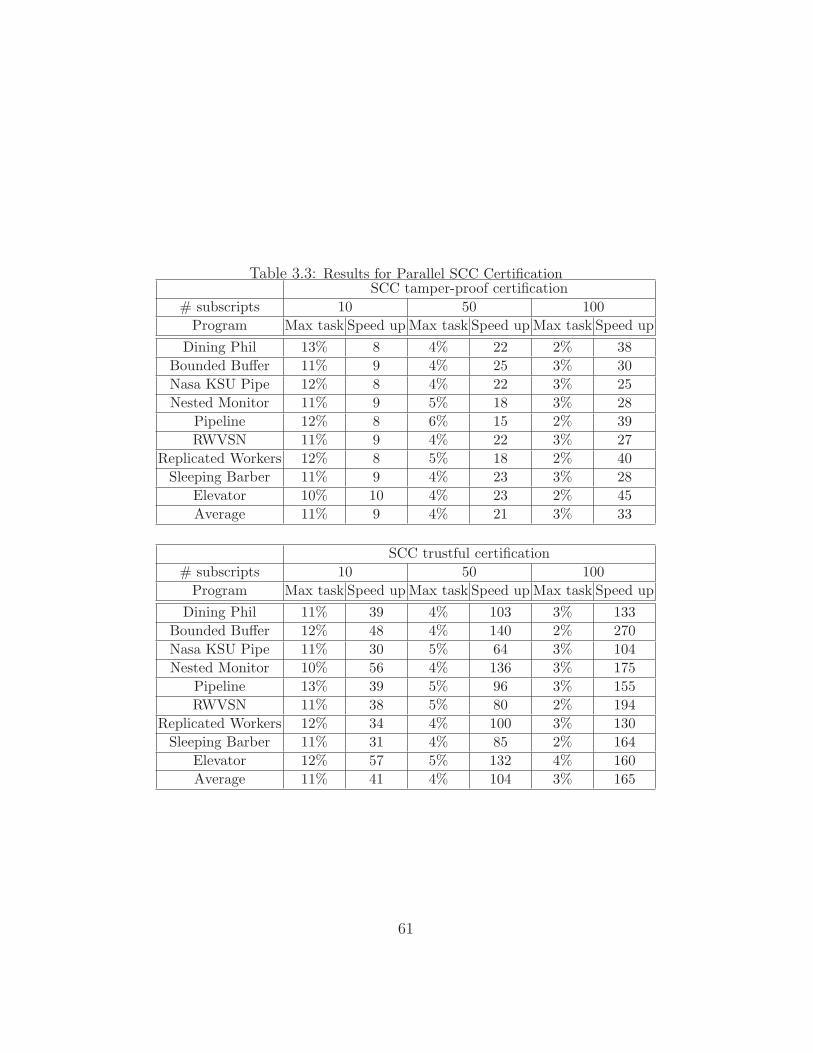
Table 3.3: Results for Parallel SCC CertificationSCC tamper-proof certification
# subscripts 10 50 100Program Max task Speed up Max task Speed up Max task Speed up
Dining Phil 13% 8 4% 22 2% 38Bounded Buffer 11% 9 4% 25 3% 30Nasa KSU Pipe 12% 8 4% 22 3% 25Nested Monitor 11% 9 5% 18 3% 28
Pipeline 12% 8 6% 15 2% 39RWVSN 11% 9 4% 22 3% 27
Replicated Workers 12% 8 5% 18 2% 40Sleeping Barber 11% 9 4% 23 3% 28
Elevator 10% 10 4% 23 2% 45Average 11% 9 4% 21 3% 33
SCC trustful certification# subscripts 10 50 100
Program Max task Speed up Max task Speed up Max task Speed upDining Phil 11% 39 4% 103 3% 133
Bounded Buffer 12% 48 4% 140 2% 270Nasa KSU Pipe 11% 30 5% 64 3% 104Nested Monitor 10% 56 4% 136 3% 175
Pipeline 13% 39 5% 96 3% 155RWVSN 11% 38 5% 80 2% 194
Replicated Workers 12% 34 4% 100 3% 130Sleeping Barber 11% 31 4% 85 2% 164
Elevator 12% 57 5% 132 4% 160Average 11% 41 4% 104 3% 165
61

Table 3.4: Average and Maximum Lengths of Initialization Paths# subgraphs 10 50 100
Program Avg Max Avg Max Avg Maxpath path path path path path
Dining Phil 11 16 13 16 12 18Bounded Buffer 75 615 217 6742 139 6678Nasa KSU Pipe 14 19 14 24 15 26Nested Monitor 14 77 24 119 33 114
Pipeline 12 20 14 25 19 29RWVSN 50 495 57 785 101 845
Replicated Workers 35 50 45 74 45 75Sleeping Barber 12 25 17 35 25 31
Elevator 50 68 71 75 71 78Average 31 153 53 877 53 876
size of the full search script. For each certification method and number of
subscripts, the column Speed-up reports the speed-up in certification time
over the time to verify the entire program using unmodified JPF, as reported
in Table 3.1.
The speed-up factors reported in Table 3.3 are not simply the product of
the speed-up factors reported for nonparallel SCC certification (in Section 3)
and the number of parallel processors employed. This is partly because of
the time needed to compare FP maps at the end of certification, and partly
because the search tasks vary in size and we report the timings associated
with the largest task. Most certification subscripts carry an initialization
path prefix, which adds to the size of the script. Table 3.4 reports the av-
erage (column Avg path) and longest (column Max path) initialization paths
for the scripts generated for parallel SCC certification for our evaluation pro-
grams. Most path lengths are relatively short, and JPF-pscc can explore
approximately 1000 transitions per second. The results for the Bounded
Buffer program show that the subscripts generated for this program have
much longer initialization paths than the other evaluation programs. After
62
evaluating these results, we noticed that this program has a deeper reach-
ability graph compared to the other programs and thus, several subgraphs
end up having long initialization paths. The lengths of initialization paths
for trustful SCC certification are similar.
In SCC certification, the size of the largest subscript determines the op-
timum number of processors to use during certification. For example, when
partitioning the search script of the Dining Philosophers program into 10
subscripts for SCC certification, the size of the largest resulting subscript is
13% of the size of the full script. For this program and partitioning, the
optimum number of parallel processors is 10. Taking this into consideration,
the results show that the speed up for parallel SCC certification is on average
a factor of n, for n processors. Trustful SCC certification can achieve a speed
up of up to a factor of 5n, for n processors.
3.3 Discussion
In this section we discuss some outstanding issues with SCC, including some
of our design decisions, restrictions on the properties that can be checked,
scalability, requirements on the model checker(s) used, and compatibility
with search-space reduction techniques.
3.3.1 Transition- vs. State-Based Certificates
Our SCC search script encodes all of the transitions of a program’s reacha-
bility graph. It might seem more efficient to generate, instead, a state-based
certificate that encodes the states because (1) there are fewer states than
transitions and (2) properties are ultimately checked on states, rather than
on transitions. The problem with this approach is that it is less resistant
to tampering. A malicious software producer could doctor the certificate,
omitting states from the certificate or adding nonexistent states. Thus, the
63
certifier would still need to explore the program’s reachability graph (and the
destination states of all transitions) to check the veracity of the certificate.
3.3.2 Properties
Safety properties play an important role in formal verification because they
assert that the system stays within required bounds and does not perform any
“wrong” actions [ES96]. SCC can be used to certify invariants and program
assertions, and can also check for deadlocks. For example, an interesting
invariant for a safety critical system that could be checked with SCC would
be:
safety switch on → system off
Because the search script encodes all transitions of a program’s reachability
graph, SCC can also be used to check invariants over consecutive states, such
as the property
(x = 5) → next(x = 8)
which states that if the value of x is 5, then in the next state its value will be
8. Even when certification is parallelized, each SCC search task is responsible
for covering a set of contiguous states and all of their outgoing transitions.
Thus, every pair of consecutive states is captured in a search script, making
it possible to certify invariants over consecutive states. In contrast, trustful
SCC does not cover all transitions, so it does not cover all pairs of consecutive
states. Thus, trustful SCC can soundly certify only state properties.
3.3.3 Scalability
A number of factors affect the scalability of search carrying code. For one,
SCC certification is limited to finite-state programs. However, this limitation
applies in general to explicit-state model checking. Thus, if a program can
be verified using explicit-state model checking, then it can be verified and
64

certified using SCC. If the software producer uses abstractions to produce a
finite state space for SCC verification, then the certifier must use the same
abstractions and must check that the abstractions preserve the properties
being proven.
Another factor is that the results of our experiments (reported in Ta-
ble 3.3) suggest that the benefits of parallelization diminish as we increase
the number of subscripts we divide an SCC script into. Our partitioning
algorithm does not partition a script into subscripts of exactly equal size,
plus the resulting subscripts are prefaced by initialization paths of varying
lengths. As such, the speed up in certification time is bounded by the amount
of time it takes to certify the largest subscript. In the worst cases, when a
script is partitioned into 50 or 100 subscripts, the largest subscript is 2 to 3
times the size that would be expected if the subscripts were truly equal sized.
We do not know whether the observed diminishing of returns is due to the
small sizes of the programs in our test suite, or is inherent to our approach.
More experiments on larger programs are needed to answer this question.
A more serious issue is the size of the search script that the software
producer provides, likely over a network, to the certifier. The size of a com-
pressed script, in number of bytes, is on the order of the number of states
in the program’s state space — which could be very large in the worst case,
where the program’s state space is at the limit of what can be model checked.
In this thesis, we assign the responsibility of partitioning the script to the cer-
tifier, on the assumption that she knows how many processors are available
and thus knows how many subscripts to create. However, in cases where the
script is large, it may be prudent for the software producer to partition the
search script. This would certainly be the case if it turns out that there is a
limit to how evenly the script can be partitioned into subscripts, as discussed
above. When the producer partitions the search script, then the certifier’s
model checker must ensure that it has received the collection of all states
and transitions in the reachability graph. For this, one master processor
65

must keep track of each state processed on each processor and ensure that if
a transition leads to a state that belongs to another region then that state is
indeed processed by another processor.
3.3.4 Parallel Model Checking
One of the main challenges of traditional parallel model checking is to evenly
distribute the work among parallel processors. In most techniques, the pro-
gram’s state space is partitioned in advance (e.g., based on hash values of
state IDs or fingerprints); thus, during model checking, states must often be
transferred to their assigned processors for processing [BR01a, KM05, NC97,
SD97].
On a distributed memory architecture, this strategy results in substantial
communication overhead. On a shared memory architecture, communication
among processors is negligible, but the processors must synchronize their ac-
cess to shared variables: processors must be able to deposit into each other’s
worklist of unprocessed states, and they share a hash-table of state finger-
prints. Interestingly, some researchers report [BBR07, IB06] that, beyond
an optimal number of processors, the search time starts to increase with
the number of additional processors because the synchronization overhead
dominates any benefit from parallelization. Parallelized SCC does not suffer
from this overhead because the reachability graph is partitioned in advance
in such a way that no communication or synchronization among processors is
necessary. Each processor works independently of others, and shares informa-
tion with an administrator process (which collects and compares fingerprint
maps) only at the end of its search task.
Another problem with traditional approaches is that workload balance
does not depend solely on an even distribution of the state space. Processors
are utilized only if they have states to process. If a program’s reachability
graph is spindly rather than bushy, then progress is hampered by the slow
production of new states, and processors sit idle waiting for the output of
66

other processors. In contrast, parallelized SCC partitions the search script
based on the shape of the reachability graph, and assigns whole subgraphs,
not single states, to processors. All scripts can be processed in parallel and
no processor waits for the output of another processor.
3.3.5 Using Different Model Checkers
In our work, we augmented JPF for use in both SCC verification and SCC
certification. Currently, the software producer and certifier must use the
same model checker to use SCC. This might seem like a restriction, however,
certification is a confirmation that verification was performed and that it was
thorough. Certification is not a reconfirmation that the advertised properties
hold. As such, it is reasonable to expect the certifier to use the same model
checker as the software producer because the certifier is simply checking that
verification is complete.
3.3.6 Model-Dependent Reduction Techniques
A key question of any new model checking technique is whether and how
it works in conjunction with existing search-reduction techniques, especially
those described in Chapter 2. We discuss model-dependent reduction tech-
niques in this section and property-dependent techniques in the next section.
We expect SCC to complement model-dependent reduction techniques,
as long as (1) the reduction techniques are applied first so that the search
script encodes the reduced reachability graph, and (2) the verifier and cer-
tifier model checkers agree on the abstractions applied. We consider only
automatic reduction techniques; techniques that rely on user-input (e.g., ab-
straction functions [GS97]) are not safe, because a malicious software pro-
ducer could specify an unsound abstraction.
Symmetry Reduction [ES96] reduces the size of the state space by ex-
ploiting symmetries among states. There are a number of different techniques
67

for identifying symmetries [MDC06], but the ultimate effect with respect to
JPF model checking is that symmetric states are assigned the same finger-
print.
In SCC verification, symmetries result in a reduced reachability graph
being explored, and a smaller search script being generated. If the same
model checker is used during SCC certification, then it identifies the same
symmetries, symmetric states are assigned the same fingerprint, and the
shape of the reduced reachability graph matches the search script. If the
software producer and consumer use different model checkers, the checkers
must implement the same reductions.
Currently, it is not realistic to expect different model checkers to use the
exact same symmetry reductions. But if model checkers were parameterized
with respect to their state-space reduction techniques and algorithms, then
requiring both model checkers to use the same symmetry reductions would
not be a limitation. In fact, there has already been some work [DHJ+01,
HDPR02] in parameterizing model checkers with respect to their state-space
reduction strategies.
Partial Order Reduction (POR) [God96] tries to identify independent
transitions and execute only one of the possible interleavings. During SCC
verification, the model checker detects independent transitions, explores only
one interleaving, and records only that interleaving in the search script. The
entire interleaving is recorded as a single transition in the search script (i.e.,
ti is one complete interleaving). If the same model checker is used during
SCC certification, then the certifier model checker identifies the same sets of
independent transitions, chooses the same interleavings (as long as decisions
are deterministic), and disables the other interleavings. As a result, the POR
interleavings chosen during certification match the search script.
Because a POR interleaving is treated as a single, long transition, it
is never partitioned among different subscripts and during certification, an
entire interleaving is assigned to a single processor. Thus, POR does not
68

interfere with SCC, even after parallelization.
If different model checkers are used for SCC verification and SCC certifi-
cation, they must both use the same POR heuristics to (1) determine which
transitions are independent, (2) select which interleaving to explore, and (3)
check that the interleaving reduction is correct. It might seem unrealistic for
both model checkers to use the same heuristics, but we believe a parameter-
ized approach to state-space reductions, as described above, could address
this limitation.
3.3.7 Property-Specific Reduction Techniques
The goal of property-specific reduction techniques is to reduce the search
space (and search script) to those program states that are relevant to the
property being checked. Such reductions are problematic for SCC because
the software producer does not know in advance which properties are of
interest to the certifier and thus cannot apply the appropriate reductions.
Moreover, the certifier cannot simply apply the reduction techniques herself
because the resulting reduced program would no longer correspond to the
supplied search script. Such techniques can only be useful if they can be
applied to the search script rather than to the program.
Consider program slicing [Wei81], which is a commonly used property-
specific reduction technique that reduces the size of the search space by
ignoring program statements that are not relevant for a given property. Tra-
ditional program slicing cannot be used in conjunction with SCC for the
reasons given above, but it might be possible for the certifier to slice the
search script instead, given that the script’s transition instructions (which
are bytecodes) literally encode the program statements. The certifier model
checker would need to be able to determine from a transition instruction
in the search script whether the transition is relevant to the property being
checked. It would also need to perform a definition-use analysis on the script,
69
which is a much larger artifact to analyze than the original program2. Lastly,
not all irrelevant transitions can be removed from the search script because
the sliced script must still be a valid path in the program’s reachability graph.
We are still investigating the problem of script slicing. Although it seems
to be possible, it is not clear whether the resulting reductions will be signifi-
cant. In general, the savings achieved by program slicing cannot be predicted
in advance, and it is possible that slicing provides no significant savings at
all — especially when checking a large collection of varied properties, such
as during certification. This is not the case for SCC — we can predict the
achievable time savings accurately based on (1) the number of transitions
that were eliminated during script slicing and (2) the number of processors
available for parallel certification.
3.4 Summary
In this chapter, we presented search carrying code (SCC) as a technique
to certify software from an untrusted source. The search script in SCC
represents a sound and complete exploration of the reachability graph of
the program to be certified, and can be used to speed up certification and
perform veracity checks of the provided search script.
The time savings of basic SCC are small, but the ideas of SCC can be
applied to parallel model checking. Using a combination of SCC and parallel
model checking, we were able to speed up the certification of model-checking
results by a factor of up to n for n parallel processors for tamper-proof
certification, and by a factor of up to 5n for n parallel processors for trustful
certification
2The analysis would be linear in the size of the script.
70
Chapter 4
State-Space Caching
4.1 Introduction
In the previous chapter, we introduced SCC, a technique for certifying a pro-
gram that had been verified using software model checking. SCC requires
that the software producer’s model checker perform an exhaustive search of
the program’s state space and create for certification a search script that
represents a search of the program’s entire reachability graph. However,
one of the main obstacles to model checking is the state-explosion prob-
lem [CGJ+01]: the size of a program’s state space grows exponentially with
the number of variables and components in the program. As a result, an
exhaustive search may not be possible because the model checker runs out
of memory as it keeps track of all visited states.
There exist numerous approaches to combat the state-explosion problem
(see Chapter 2), and one of these methods is state-space caching. The goal of
state-space caching is to perform an exhaustive search of the state space but
to use less memory than a traditional model-checking search uses. Instead of
keeping track of all of the visited states, the model checker stores in a cache
only a subset of visited states. When the cache becomes full, the model
checker replaces states in the cache with newly discovered states. Which
71
state to replace next depends on the cache-replacement policy that the model
checker uses. There exist several cache-replacement policies including age-
based caching [Hol87], stratified caching [Gel04], hit-based caching [Hol87]
and depth-based caching [Hol87]. For a detailed description of these replace-
ment policies, refer to Chapter 2.
If a state Si is removed from the cache and is subsequently revisited, it is
deemed a new state and, as a result, the model checker re-explores Si and any
of Si’s descendant states that have also been removed from the cache. Thus,
although state-space caching reduces memory requirements by limiting the
cache size, it increases search time because states may be visited and tested
more than once.
State-space caching is useful in SCC when an exhaustive verification of a
program’s state space is not possible given the available memory resources.
In such situations, the software producer’s model checker can use state-space
caching to achieve a complete search of the program’s state space and output
a search script that covers the program’s entire reachability graph. In gen-
eral, a depth-first search of an acyclic state space is guaranteed to terminate
with an exhaustive search when the model checker uses state-space caching.
For cyclic state space, the model checker must detect a cycle in order for the
search to terminate. We describe these issues in this chapter. Of course, be-
cause the search time could increase significantly, the verifier’s model checker
might still not achieve an exhaustive coverage within a reasonable period of
time.
In this chapter, we introduce a novel cache-replacement policy, called
cost-based caching. Cost-based caching replaces states in the cache based
on the potential cost of re-exploring the state space that is reachable from
the state to be removed. Our evaluation of cost-based caching shows that it
achieves exhaustive coverage of a program’s state space in a shorter amount
of time than existing cache-replacement policies and thus is more likely to
terminate within a given time frame.
72

The downside of state-space caching is that the model checker may explore
sections of the state space more than once. A literal recording of the resulting
search produces a search script in which states and transitions are repeatedly
explored. In Chapter 4.3, we describe how to detect and remove replicated
parts of a search script before SCC certification. As a result, the time it
takes to perform SCC certification using a script created by a model checker
that employed state-space caching is the same as the time it would take to
perform a regular SCC certification.
Finally, in Chapter 4.4, we describe a memory-optimization technique for
SCC certification in which the certifier’s model checker removes any entry
from the FP map if it is known that the state will not be revisited during the
model-checking search. Removing such entries reduces the memory needs of
SCC certification by up to 89%.
4.2 Cost-Based Caching
In general, for any state-space caching technique, when the cache is full
then the model checker must remove states in the cache to store newly-
discovered states. Due to eviction, some replaced states might need to be
revisited later in the search, causing re-exploration of the replaced states and
their descendant states. The goal of current cache-replacement policies is to
identify states in the cache that have a low chance of being revisited and to
select them for replacement when new states are discovered. For example,
one current approach employs an age-based replacement policy, in which
the states chosen for replacement are those that have been in the cache the
longest. However, consider a state S1 that has been in the cache for the
longest period of time and that has many descendant states. It might be
unwise to replace S1 because if its descendant states are also removed from
the cache and if S1 is revisited, then all of its descendant states will also be
re-explored.
73

Existing cache-replacement policies for state-space caching do not con-
sider the “cost” of removing from the cache a state that might be later revis-
ited. Informally, the cost of replacing a state Si is the work that the model
checker must redo if Si is revisited. We propose a cost-based replacement
policy that selects for replacement a state Si based on the cost, in the worst
case, of revisiting Si later in the search. The worst-case cost of replacing a
state is the maximum number of states that would have to be re-explored if
Si were later revisited. In practice, the actual cost may be lower if, when Si
is revisited, some of its descendant states are in the cache and thus need not
be re-explored.
4.2.1 Cost-Based Caching Algorithm
Cost-based caching is similar to other caching techniques in that it performs
a depth-first search of the program’s reachability graph and maintains (1)
a stack of partially explored states and (2) a cache of visited states. The
replacement policy selects for removal from the cache the state with the
lowest cost. Note that the cost of replacing Si is not necessarily the number
of Si’s descendant states. For example, consider the sample reachability
graph in Figure 4.1, which shows in parentheses below each state identifier
the cost of replacing that state. The cost of replacing state S3 is 3 because the
model checker will re-explore a maximum of three states (S3, S5, S6) if S3 is
revisited. In this case, the cost of replacing S3 is equal to the number of its
descendant states plus 1. However, consider state S2 in the same reachability
graph. The cost of replacing S2 is 7 even though it has only 4 descendant
states. Because S2 is part of a directed acyclic graph (DAG), some of its
descendant states (S5, S6) might be visited more than once if they are not
found in the cache either time they are visited during the re-exploration of
the states reachable from S2. Thus, they are counted more than once when
calculating the cost of replacing S2.
Definition 4.2.1. Given a program whose reachability graph is finite and
74
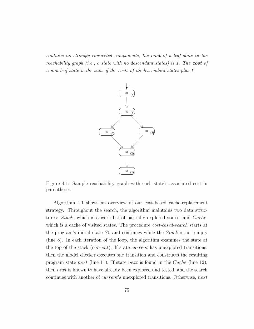
contains no strongly connected components, the cost of a leaf state in the
reachability graph (i.e., a state with no descendant states) is 1. The cost of
a non-leaf state is the sum of the costs of its descendant states plus 1.
S2
S3 S4
S5
S6
S1
(1)
(2)
(3) (3)
(7)
(8)
Figure 4.1: Sample reachability graph with each state’s associated cost inparentheses
Algorithm 4.1 shows an overview of our cost-based cache-replacement
strategy. Throughout the search, the algorithm maintains two data struc-
tures: Stack, which is a work list of partially explored states, and Cache,
which is a cache of visited states. The procedure cost-based-search starts at
the program’s initial state S0 and continues while the Stack is not empty
(line 8). In each iteration of the loop, the algorithm examines the state at
the top of the stack (current). If state current has unexplored transitions,
then the model checker executes one transition and constructs the resulting
program state next (line 11). If state next is found in the Cache (line 12),
then next is known to have already been explored and tested, and the search
continues with another of current’s unexplored transitions. Otherwise, next
75
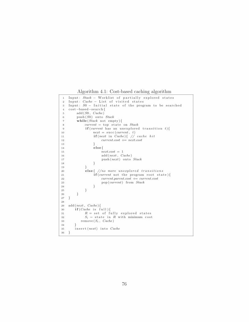
Algorithm 4.1: Cost-based caching algorithm1 Input : Stack − Workl i st o f p a r t i a l l y exp lored s t a t e s2 Input : Cache − L i s t o f v i s i t e d s t a t e s3 Input : S0 − I n i t i a l s t a t e o f the program to be searched4 cost−based−search {5 add (S0 , Cache)6 push (S0) onto Stack7 while (Stack not empty ){8 current = top s t a t e on Stack9 i f (current has an unexplored t r a n s i t i o n t){
10 next = succ (current , t)11 i f (next in Cache){ // cache h i t12 current.cost += next.cost13 }14 else {15 next.cost = 116 add (next , Cache)17 push (next) onto Stack18 }19 }20 else { //no more unexp lored t r a n s i t i o n s21 i f (current not the program root s t a t e ){22 current.parent.cost += current.cost23 pop (current) from Stack24 }25 }26 }27 }28
29 add (next , Cache){30 i f (Cache i s f u l l ){31 R = se t o f f u l l y exp lored s t a t e s32 Si = s ta t e in R with minimum cos t33 remove (Si , Cache)34 }35 i n s e r t (next) i n to Cache36 }
76
is deemed an unvisited state: it is added to the Cache using the procedure
add (line 16) and is also pushed onto the top of the Stack (line 17). As each
state current is fully explored (line 20), it is popped off the Stack and the
algorithm continues with the next partially explored state at the top of the
Stack.
For each state in the cache, the algorithm keeps a variable cost whose
value represents a state’s cost as calculated so far in the search. Leaf states
are assigned a cost of 1. For any other state, the cost is the sum of the costs
of its descendant states plus 1. Algorithm 4.1 updates a state’s cost under
three conditions:
• When a state next is first visited (line 15), then the model checker
initializes its cost to 1.
• When a state next is revisited (line 12), then the model checker adds
the value of next’s cost to the cost value of its parent state (current).
• When a state’s exploration finishes (i.e., it has no unexplored outgoing
transition) (line 22), then the value of the state’s cost is added to the
cost of its parent state. The parent state is the previous state on the
Stack.
The procedure add (line 29) selects the state to be removed from the Cache,
on the basis of our cost-based replacement policy. If the cache is full, then
procedure add removes, from among all fully-explored states in the cache, the
state with the smallest cost and inserts state next into the Cache. If more
than one state have the same cost value, then add randomly chooses one for
replacement. The procedure add selects among fully-explored states only,
because the cost of a partially explored state is still being determined. We
discuss the requirement that R must be non-empty in Chapter 4.2.5. For a
fully-explored state Si, its cost correctly represents the maximum number of
states that must be re-explored if Si is revisited.
77

Theorem 4.2.1. Given a program whose reachability graph is finite and
contains no strongly connected components, Algorithm 4.1 correctly calculates
the cost of each state in the reachability graph.
Proof We prove this theorem by induction: a newly visited state is assigned
the cost of 1 (line 15) and its cost does not change if it has no descendant
states. Thus, leaf states are correctly assigned the cost of 1.
For a non-leaf state Si, its cost can change when (1) Si is visited for the
first time, (2) when Si leads to a descendant state that is found in the Cache,
and (3) when Si leads to a descendant state that is not found in the Cache.
When Si is visited for the first time, its cost is set to 1 (line 15). Let
us assume that the descendant states of Si have the correct cost values. A
state Si’s cost value will be correctly updated with the cost values of its
descendant states: if Si’s descendant state Sd is found in the Cache, we
know that its value of cost is final. If the value of cost were not final, then
the search is still exploring the state space reachable from Sd. If this search
is now revisiting Sd, then there must be a strongly connected component
in the reachability graph. But the reachability graph contains no strongly
connected components. Thus, Sd’s cost is added to Si’s cost (line 13); if Sd is
not found in the Cache, then Sd is deemed an unvisited state and its cost is
added to the cost of Si, once Sd has been fully explored (line 22). Thus, all
states of the reachability graph will be assigned a cost value that corresponds
to the definition of cost.
4.2.2 State Spaces with Strongly Connected Compo-
nents
In general, strongly connected components in a reachability graph pose no
problem for an explicit-state search because the model checker keeps track
of all visited states and detects when a program state is revisited. When
state-space caching is used, however, the search may re-explore states that
78
are not found in the cache. If states that are re-explored are part of a
strongly connected component in the reachability graph, then it is possible
for the search to continually revisit states and continually not find them in
the cache.
The method that other caching techniques use to guarantee termination
of a search is to keep a state in the Cache until the state is fully explored and
removed from the Stack. Algorithm 4.1 already implements this strategy:
procedure add replaces only fully-explored states (i.e., states no longer on the
Stack) whose cost values have been fully determined. Thus, Algorithm 4.1
eventually terminates, and the search covers the program’s entire state space.
Definition 4.2.2. A strongly connected component in the reachability
graph is a set of states C such that there exists a path between any two states
in C.
Theorem 4.2.2. Given a program that has a finite reachability graph whose
depth is smaller than the available memory, Algorithm 4.1 terminates having
searched the entire reachability graph.
Proof It has been shown [God97, Hol88, DH82] that a stacked search (a
search that keeps a stack as a worklist of partially explored states) of a pro-
gram whose reachability graph is finite and contains no strongly connected
components is guaranteed to terminate and to cover the program’s entire
state space if the depth of the reachability graph is smaller than the avail-
able memory. Thus, we only have to show that our algorithm is guaranteed
to terminate if the reachability graph is finite and has strongly connected
components.
Let C be a set of states that form a strongly connected component in the
reachability graph, and let Si be the first state in C that is revisited. We
have to show that the algorithm does not re-explore any state in C when Si
is revisited.
79
State Si is guaranteed to be in the Stack because the strongly connected
component from Si to Si represents part of the exploration of a transition
emanating from Si. This exploration has not yet finished and thus Si is still
in the Stack. Because Si is in the Stack, it is also guaranteed to be in the
Cache (line 31). Thus, the model checker will deem Si as visited and the
search will backtrack without re-exploring the states in C.
For state spaces that have strongly connected components, we cannot
use the Definition 4.2.1 for a state’s cost value because states in a strongly
connected component can all be reached from each other so each state in
the strongly connected component can reach the same set of states of the
reachability graph. As a result, states in a strongly connected component
must share the same cost value.
Definition 4.2.3. Given a program whose reachability graph is finite and
contains strongly connected components, the cost of a state Si is as follows:
• If Si is a leaf state, then the cost of Si is 1.
• If Si is a non-leaf state and is not part of a strongly connected compo-
nent, then the cost of Si is the sum of the costs of its descendant states
plus 1.
• If Si is part of a strongly connected component C, then the cost of Si
is the number of states in C plus the sum of the costs of all of the
descendant states not in C of the states in C.
Unfortunately, Algorithm 4.1 does not accurately compute state costs when
the reachability graph contains strongly connected components. Consider
the sample reachability graph in Figure 4.2a. We list in parentheses the cost
values that Algorithm 4.1 would compute for each state in this graph. In this
simple example, the state sequence S2, S3, S4, S5 forms a strongly connected
80
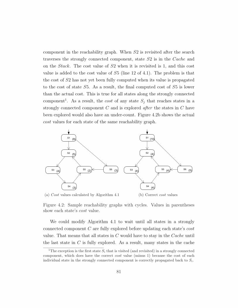
component in the reachability graph. When S2 is revisited after the search
traverses the strongly connected component, state S2 is in the Cache and
on the Stack. The cost value of S2 when it is revisited is 1, and this cost
value is added to the cost value of S5 (line 12 of 4.1). The problem is that
the cost of S2 has not yet been fully computed when its value is propagated
to the cost of state S5. As a result, the final computed cost of S5 is lower
than the actual cost. This is true for all states along the strongly connected
component1. As a result, the cost of any state Sj that reaches states in a
strongly connected component C and is explored after the states in C have
been explored would also have an under-count. Figure 4.2b shows the actual
cost values for each state of the same reachability graph.
S1
S3
S4
S5 S6
S2
(2)
(3)
(4)
(5)
(3)
(9)
(a) Cost values calculated by Algorithm 4.1
S1
S3
S4
S5 S6
S2
(4)
(4)
(4)
(4)
(5)
(10)
(b) Correct cost values
Figure 4.2: Sample reachability graphs with cycles. Values in parenthesesshow each state’s cost value.
We could modify Algorithm 4.1 to wait until all states in a strongly
connected component C are fully explored before updating each state’s cost
value. That means that all states in C would have to stay in the Cache until
the last state in C is fully explored. As a result, many states in the cache
1The exception is the first state Si that is visited (and revisited) in a strongly connectedcomponent, which does have the correct cost value (minus 1) because the cost of eachindividual state in the strongly connected component is correctly propagated back to Si.
81
would not be available for replacement which would make the replacement
policy less effective. We chose not to implement this alternate approach
to computing the costs of states and accept the inherent inaccuracy of cost
values that arise in state spaces with strongly connected components. Despite
the inaccuracies, we show empirically that cost-based caching is effective.
4.2.3 Implementation
We implemented our cost-based replacement policy in Java Pathfinder (JPF),
by modifying JPF’s depth-first search implementation. We refer to the re-
sulting model checker as JPF-cache.
JPF-cache uses a stack to keep track of partially-explored states and a
cache to keep track of visited states. For efficiency, the cache is implemented
using two data structures: a hash table that stores the fingerprints of visited
states (as before) and a list that stores cost values for each state in the cache.
Corresponding fingerprint and cost values have pointers to each other. The
list of cost values is divided into two sections:
• A priority queue Q which holds the cost values of fully-explored states,
which are candidates for replacement. The model checker keeps Q
sorted throughout the search, such that the first element always holds
the smallest cost value.
• A list L that holds the cost values of partially-explored states, which
are currently on the search stack. List L can remain unsorted.
When JPF-cache visits a new state Si and the cache is full, it removes the
first element of Q and its corresponding fingerprint from the cache’s hash-
table. The model checker then inserts Si at the top of the search stack,
inserts Si’s fingerprint into the cache’s hash-table, and adds Si’s cost value
(which is initially 1) to L. The model checker creates pointers that relate
the fingerprint and cost data elements. Once all of Si’s transitions have been
82
explored and Si is removed from the stack, Si’s cost value is transferred from
L to Q, and Q is re-sorted with the new element.
Performance
Only the tasks associated with updating cost values and adding and removing
them from the cache incur a performance overhead. Adding a newly visited
state (with cost value 1) to L takes constant time because list L is unsorted.
As long as the cost value remains in L, it can be located in constant time (by
following the pointer from the state’s entry in the hash table) and updated
in constant time. When a state is fully-explored, its cost value must be
transferred from L to Q and Q must be re-sorted. The time for this operation
is O(log S), for a priority queue Q with S states. Once a state has been added
to Q, its cost value no longer changes because it is fully explored.
4.2.4 Experiments and Results
In our experiments, we evaluated how well our cost-based replacement strat-
egy performs, compared to other types of replacement strategies. This eval-
uation assesses whether cost-based caching enables a model-checking search
to run to completion in cases where there was insufficient memory for a
traditional non-cached model-checking search.
In these experiments, we compared the performance for JPF-cache to im-
plementations of cost-based (column Cost), random (column Random), age-
based (column Age), hit-based (column Hits), stratified (column Stratified),
and depth-based (column Depth) caching in JPF. We evaluated JPF-cache
and the implementations of the other five caching techniques on our nine
evaluation programs as described in Chapter 3.1.4. The reachability graphs
of all our evaluation programs contained strongly connected components.
To simulate different cache sizes, we imposed an artificial memory limit on
the size of the cache, limiting it to 15%, 25%, 50%, 75%, and 95% of the total
83

state-space size of each program. For each program, caching technique, and
cache size, we allowed the model-checking search to run until it terminated
(with full state-space coverage) or until its execution time exceeded 25 times
the amount of time needed for a traditional non-cached search. We measured
performance in terms of the time (CPU time) that the model checker takes
to achieve full coverage. We repeated each experiment 10 times and report
the average results.
Table 4.1 and Table 4.2 show the results for our experiments, with each
table reporting the results for a different cache size. There are two columns
of data for each caching method. The first column (Time) reports the time
to search each program as a factor of the time needed for a non-cached,
traditional model-checking search. A value of TO means that the search
did not terminate in its allocated time. The second column (RW ) reports
for each program the amount of redundant work performed by the model
checker; this number represents the total number of transitions explored as a
factor of the total number of transitions in the program’s reachability graph.
We report a value of N/A when the search timed out, i.e., for TO values.
For example, when model checking the Dining Philosophers program with a
state space cache that can store only 25% of the program’s states using the
random cache-replacement policy, the search takes approximately 14 times
longer than a non-cached search of that program, and explores about 13
times more transitions than are in the program’s reachability graph.
The results show that cost-based caching is up to 25% faster than the
other five caching techniques (except in one case) for the cache sizes of 15%,
25%, and 50%. Cost-based caching is as fast or faster than the other five
caching techniques for the remaining two cache sizes. The advantage of cost-
based caching seems to improve as the cache size decreases. Random caching
almost always performs second best on all programs and cache sizes. We did
not observe any specific pattern among the performances of the other caching
methods.
84
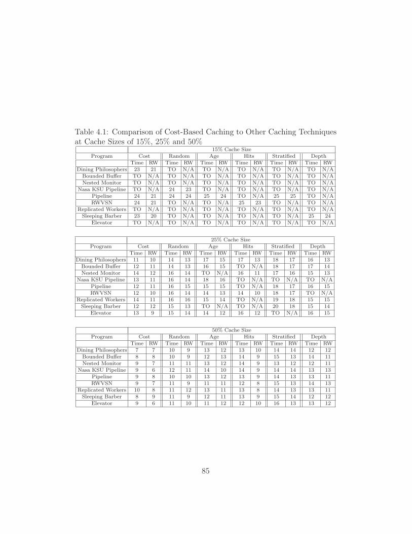
Table 4.1: Comparison of Cost-Based Caching to Other Caching Techniquesat Cache Sizes of 15%, 25% and 50%
15% Cache SizeProgram Cost Random Age Hits Stratified Depth
Time RW Time RW Time RW Time RW Time RW Time RWDining Philosophers 23 21 TO N/A TO N/A TO N/A TO N/A TO N/A
Bounded Buffer TO N/A TO N/A TO N/A TO N/A TO N/A TO N/ANested Monitor TO N/A TO N/A TO N/A TO N/A TO N/A TO N/A
Nasa KSU Pipeline TO N/A 24 23 TO N/A TO N/A TO N/A TO N/APipeline 24 21 24 24 25 24 TO N/A 25 25 TO N/ARWVSN 24 21 TO N/A TO N/A 25 23 TO N/A TO N/A
Replicated Workers TO N/A TO N/A TO N/A TO N/A TO N/A TO N/ASleeping Barber 23 20 TO N/A TO N/A TO N/A TO N/A 25 24
Elevator TO N/A TO N/A TO N/A TO N/A TO N/A TO N/A
25% Cache SizeProgram Cost Random Age Hits Stratified Depth
Time RW Time RW Time RW Time RW Time RW Time RWDining Philosophers 11 10 14 13 17 15 17 13 18 17 16 13
Bounded Buffer 12 11 14 13 16 15 TO N/A 18 17 17 14Nested Monitor 14 12 16 14 TO N/A 16 11 17 16 15 13
Nasa KSU Pipeline 13 11 16 14 18 16 TO N/A TO N/A TO N/APipeline 12 11 16 15 15 15 TO N/A 18 17 16 15RWVSN 12 10 16 14 14 13 14 10 18 17 TO N/A
Replicated Workers 14 11 16 16 15 14 TO N/A 19 18 15 15Sleeping Barber 12 12 15 13 TO N/A TO N/A 20 18 15 14
Elevator 13 9 15 14 14 12 16 12 TO N/A 16 15
50% Cache SizeProgram Cost Random Age Hits Stratified Depth
Time RW Time RW Time RW Time RW Time RW Time RWDining Philosophers 7 7 10 9 13 12 13 10 14 14 12 12
Bounded Buffer 8 8 10 9 12 13 14 9 15 13 14 11Nested Monitor 9 7 11 11 13 12 14 9 13 12 12 11
Nasa KSU Pipeline 9 6 12 11 14 10 14 9 14 14 13 13Pipeline 9 8 10 10 13 12 13 9 14 13 13 11RWVSN 9 7 11 9 11 11 12 8 15 13 14 13
Replicated Workers 10 8 11 12 13 11 13 8 14 13 13 11Sleeping Barber 8 9 11 9 12 11 13 9 15 14 12 12
Elevator 9 6 11 10 11 12 12 10 16 13 13 12
85
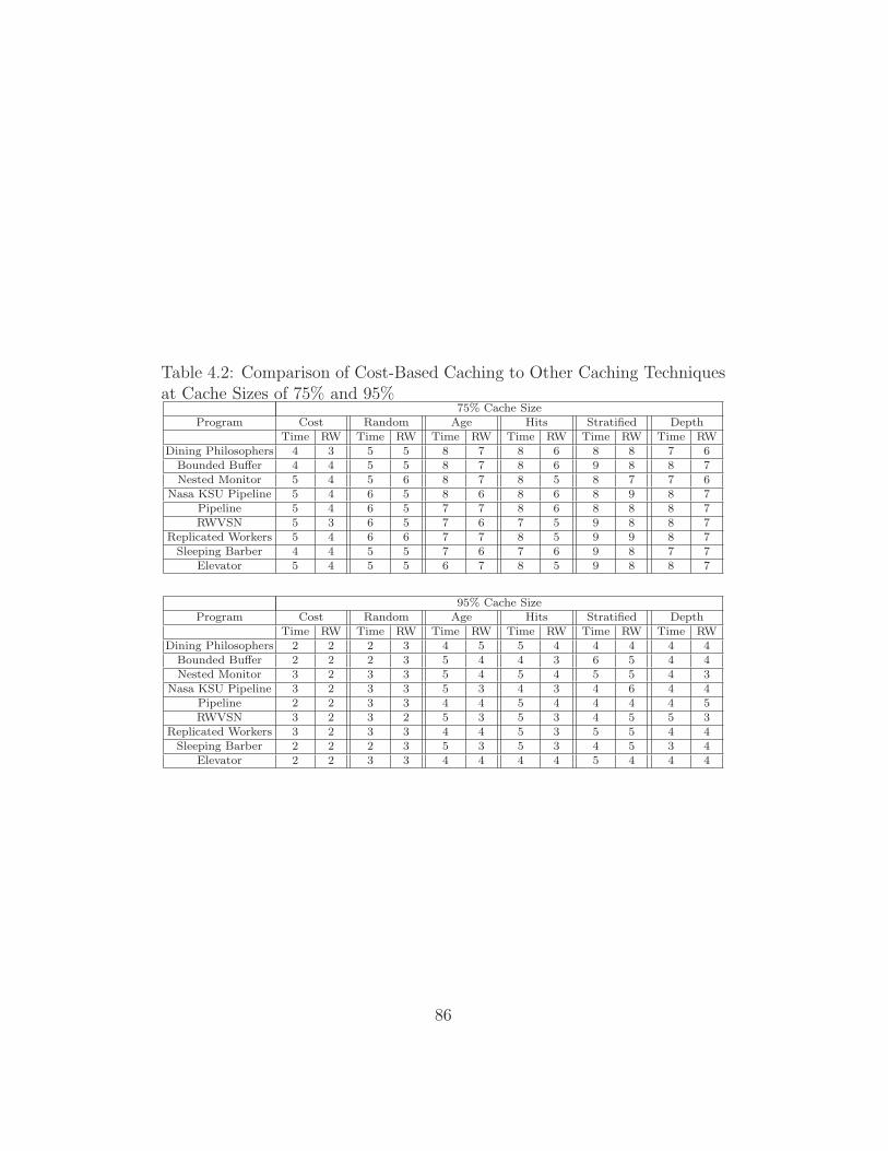
Table 4.2: Comparison of Cost-Based Caching to Other Caching Techniquesat Cache Sizes of 75% and 95%
75% Cache SizeProgram Cost Random Age Hits Stratified Depth
Time RW Time RW Time RW Time RW Time RW Time RWDining Philosophers 4 3 5 5 8 7 8 6 8 8 7 6
Bounded Buffer 4 4 5 5 8 7 8 6 9 8 8 7Nested Monitor 5 4 5 6 8 7 8 5 8 7 7 6
Nasa KSU Pipeline 5 4 6 5 8 6 8 6 8 9 8 7Pipeline 5 4 6 5 7 7 8 6 8 8 8 7RWVSN 5 3 6 5 7 6 7 5 9 8 8 7
Replicated Workers 5 4 6 6 7 7 8 5 9 9 8 7Sleeping Barber 4 4 5 5 7 6 7 6 9 8 7 7
Elevator 5 4 5 5 6 7 8 5 9 8 8 7
95% Cache SizeProgram Cost Random Age Hits Stratified Depth
Time RW Time RW Time RW Time RW Time RW Time RWDining Philosophers 2 2 2 3 4 5 5 4 4 4 4 4
Bounded Buffer 2 2 2 3 5 4 4 3 6 5 4 4Nested Monitor 3 2 3 3 5 4 5 4 5 5 4 3
Nasa KSU Pipeline 3 2 3 3 5 3 4 3 4 6 4 4Pipeline 2 2 3 3 4 4 5 4 4 4 4 5RWVSN 3 2 3 2 5 3 5 3 4 5 5 3
Replicated Workers 3 2 3 3 4 4 5 3 5 5 4 4Sleeping Barber 2 2 2 3 5 3 5 3 4 5 3 4
Elevator 2 2 3 3 4 4 4 4 5 4 4 4
86
Analysis of the amount of redundant work done because of caching also
shows an interesting pattern. In most cases, the factor of increase in execution
time is comparable to the factor of the amount of redundant work done,
but for cost-based caching, the redundant-work factor is considerably lower
than the additional-time factor. This suggests that, for cost-based caching,
considerable search time is spent on maintaining the priority queue.
4.2.5 Discussion of Cost-Based Caching
In this section, we discuss some issues regarding cost-based caching.
Ratio of Transitions to States and Applicability of Caching
The ratio of the number of incoming transitions to the number of states in a
program’s reachability graph can play an important role in the performance
of any state-space caching technique. A high ratio means that many states
have several incoming transitions and thus will be visited several times during
the search. Therefore, there is a higher chance that large parts of the state
space could be repeatedly explored. When the ratio is close to 1 (i.e., low),
then most states will be visited only once and the running time of the search
is linear in the number of transitions.
Many works on caching assume that the reachability graph has a low ratio
of the number of transitions to the number of states. In [Gel04, Hol87], for
example, most of the evaluation programs have a transition-to-state ratio of
1.2 to 2.1. The programs in our evaluation suite are taken from the model-
checking literature and the transition-to-state ratio is much higher: the col-
umn (T/S) in Table 3.1 shows that this ratio for our evaluation programs
ranges between 4.1 and 8.4. Thus, state-space caching techniques need to be
optimized for and evaluated on programs that have high transition-to-state
ratios.
87

Memory Requirements
The memory overhead of cost-based caching is similar to that of other state-
space caching techniques. In cost-based caching, an additional count variable
is maintained for each state in the cache. The memory overhead of other
caching techniques is similar as each method requires, for each state in the
cache, the state’s fingerprint plus some additional piece of information (e.g.,
the number of hits to a state, the age of a state, the depth of a state in
the reachability graph) that is used in the implementation of the cache-
replacement policy. Only the random-replacement policy does not require
any additional data.
One of the requirements of any cache-based search is that there be enough
memory available to hold the search stack (i.e., the worklist of partially-
explored states). Otherwise, the search may terminate prematurely, without
achieving full state-space coverage if states in the stack must be replaced, or
there exist no fully explored states in the cache for replacement. It might
be necessary to swap parts of the stack between the hard disk and main
memory, or to grow and shrink the cache size dynamically to accommodate
a large stack. This topic is beyond the scope of this thesis.
Combining SCC and State-Space Caching
Remember that during SCC verification, the model checker assigns an in-
teger state ID to each newly discovered state. State IDs start at 0 and
are incremented by one each time a new state is reached. This number-
ing scheme does not work if the producer’s model checker uses state-space
caching because each revisited state that has been removed from the cache is
considered to be a new state and is assigned a new ID. An SCC search script
that records state IDs cannot be used to check the veracity of the search
script, because the same state might have been assigned two different IDs.
Thus, SCC verification with state-space caching records states’ fingerprints
rather than state IDs. The software producer’s model checker then performs
88
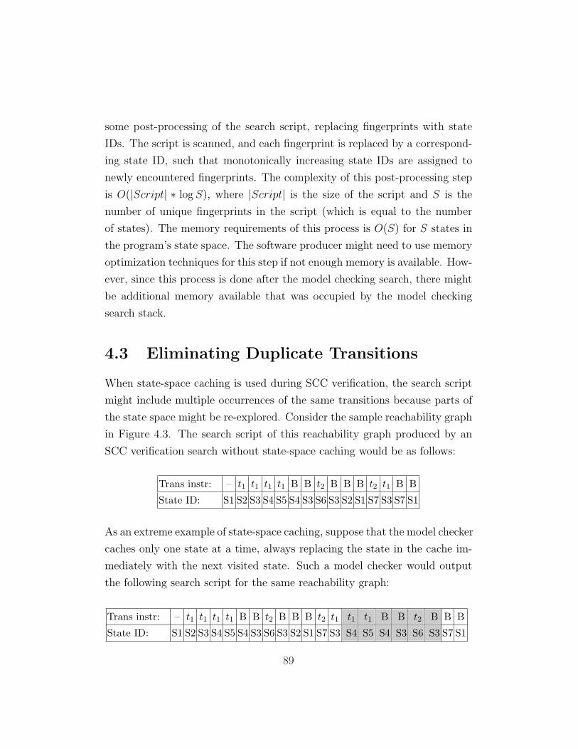
some post-processing of the search script, replacing fingerprints with state
IDs. The script is scanned, and each fingerprint is replaced by a correspond-
ing state ID, such that monotonically increasing state IDs are assigned to
newly encountered fingerprints. The complexity of this post-processing step
is O(|Script| ∗ log S), where |Script| is the size of the script and S is the
number of unique fingerprints in the script (which is equal to the number
of states). The memory requirements of this process is O(S) for S states in
the program’s state space. The software producer might need to use memory
optimization techniques for this step if not enough memory is available. How-
ever, since this process is done after the model checking search, there might
be additional memory available that was occupied by the model checking
search stack.
4.3 Eliminating Duplicate Transitions
When state-space caching is used during SCC verification, the search script
might include multiple occurrences of the same transitions because parts of
the state space might be re-explored. Consider the sample reachability graph
in Figure 4.3. The search script of this reachability graph produced by an
SCC verification search without state-space caching would be as follows:
Trans instr: – t1 t1 t1 t1 B B t2 B B B t2 t1 B B
State ID: S1 S2 S3 S4 S5 S4 S3 S6 S3 S2 S1 S7 S3 S7 S1
As an extreme example of state-space caching, suppose that the model checker
caches only one state at a time, always replacing the state in the cache im-
mediately with the next visited state. Such a model checker would output
the following search script for the same reachability graph:
Trans instr: – t1 t1 t1 t1 B B t2 B B B t2 t1 t1 t1 B B t2 B B B
State ID: S1 S2 S3 S4 S5 S4 S3 S6 S3 S2 S1 S7 S3 S4 S5 S4 S3 S6 S3 S7 S1
89

S1
S5
S4
S3
S7S2
t1
t1
t1
t1t1
t2
S6
t2
Figure 4.3: Sample reachability graph
The gray-colored cells reflect duplicate transitions and backtrack commands
that the software producer’s model checker executes as a result of state-space
caching. If such a script is submitted for SCC certification, the certifier’s
model checker would follow the instructions in the search script and per-
form the same redundant work that was performed during verification. To
speed up certification, these duplicate transitions should be removed from
the search script.
4.3.1 Eliminating Duplicate Transitions
In the following, we describe an algorithm that identifies and removes du-
plicate transitions from an SCC search script, such that the resulting script
represents a continuous search of the entire reachability graph.
Our algorithm is based on the observation that any sequence of transi-
tions that represents the re-exploration of a state Sj and some (or all) of its
descendant states will have the following form2:
2A productive exploration of Sj would also have this form.
90
ti,j − tj,k − ...−Bx,j −Bj,i (4.1)
where
• ti,j represents a previously-unexplored transition from state Si to an
already-visited state Sj;
• tj,k represents a previously-explored transition from state Sj to one of
state Sj’s child states, Sk;
• Bx,j represents the backtrack transition from the last fully-explored
child state of state Sj back to state Sj;
• Bj,i represents the backtrack transition to state Sj’s parent state.
The goal of our algorithm is to remove from the search script the sub-
sequences tj,k − ... − Bx,j that record a re-exploration of state Sj and its
descendants, leaving the transitions ti,j−Bj,i, which are the transition to the
already-visited state Sj and the backtrack transition back to the parent state
of Sj. For example, given the reachability graph in Figure 4.3, our algorithm
identifies the following sequence which represents revisiting Sj, re-exploring
Sj and all its descendant states, and finally backtracking to Sj’s parent state
Si:
tS7,S3 − tS3,S4 − tS4,S5 −BS5,S4 −BS4,S3 − tS3,S6 −BS6,S3 −BS3,S7
The algorithm then removes the sequence that represents exploring Sj and
its descendant states.:
tS3,S4 − tS4,S5 −BS5,S4 −BS4,S3 − tS3,S6 −BS6,S3
91

Algorithm 4.2: Algorithm for removing duplicate transitions from the searchscript
1 Input : Script − Search s c r i p t o f the program to be c e r t i f i e d2
3 Scan Script from s t a r t to end4 For each t r a n s i t i o n tj,k in Script{5 i f tj,k has been p r ev i ou s l y scanned{6 remove tj,k and a l l t r a n s i t i o n s up to , but not inc lud ing ,7 f i r s t backtrack from Sj to a s t a t e whose ID i s l e s s than j8 }9 }
The pseudo-code of our algorithm is shown in Algorithm 4.2. The model
checker scans the script from start to end and keeps track of the transitions
scanned. If a duplicate transition tj,k is discovered, then the model checker
removes tj,k and all transitions in the script up to but not including the
backtrack transition from Sj.
Theorem 4.3.1. Given a search script that was obtained from an SCC veri-
fication search that used state-space caching, Algorithm 4.2 correctly removes
duplicate transitions such that the resulting script does not contain any dupli-
cate transitions and represents a depth-first search of the entire reachability
graph.
Proof Algorithm 4.2 removes only duplicate transitions. Consider line 6 of
Algorithm 4.2, which removes a subsequence tj,k, ..., Bk,j. The search script
records a DFS of the program’s state space. Thus, the subsequence being
removed starts with duplicate transition tj,k, and records the search of a
subset of the states reachable from the transition’s source state Sj. Suppose
by way of contradiction that this subsequence contains a transition tl,m that
is not a duplicate transition. Then the source state of tl,m, state Sl, is not
fully explored. However, state Sl is reachable from state Sj. State Sj has
been fully explored: if tj,k is a duplicate transition, then its source state
was previously fully explored, removed from the Cache, and subsequently
revisited. If Sj was fully explored, then Sl was fully explored.
92
When Algorithm 4.2 terminates, the resulting script is continuous because
Algorithm 4.2 removes only subsequences of the form tj,k, ..., Bk,j. The source
state of tj,k, Sj, is the same as the destination state of Bk,j. Thus, the removal
of the sequence does not affect the continuity of the search script.
4.3.2 Implementation and Evaluation
We implemented the above duplicate-transition-elimination algorithm in JPF-
cache (i.e., the implementation of cost-based caching in JPF) and refer to
the resulting model checker as JPF-cache-rem. At the end of SCC verifica-
tion, JPF-cache-rem scans the script from start to end and keeps track of
already-scanned transitions. The model checker maintains an array trans
of linked lists and stores at index i all transitions that emanate from state
Si. When a new transition ti,j is scanned, the model checker traverses the
list of transitions stored at trans[i] to determine whether ti,j is a duplicate
transition.
The running time of the algorithm is O(k∗|Script|), where |Script| is the
size of the script in terms of the number of forward and backtrack transitions,
and k is the maximum number of transitions emanating from a state. For
JPF-cache-rem, the time to remove duplicate transitions was between 0.5%
to 2% of the time of SCC verification with cost-based caching. The memory
requirement for Algorithm 4.2 is O(T ) for T transitions in the reachability
graph.
4.4 Memory Optimization for Certification
Caching reduces memory requirements during SCC verification. It is, how-
ever, possible that memory usage is also a concern during certification, for
example, if the certifier’s model checker has less memory than the software
producer’s model checker.
93

During SCC certification, the certifier’s model checker maintains a map-
ping FP of state IDs to fingerprints for all states in the state space. The
size of FP is comparable to the size of the hash table that the software pro-
ducer’s model checker keeps. Our method for reducing memory requirements
for certification is based on the observation that at any point during certifi-
cation, the map FP needs to store only the fingerprints for those states that
are still to be (re)visited. Recall that the map FP is used to check that all
occurrences of a state ID in the search script correspond to the same state
with the same fingerprint in the model-checking search. Thus, once a state,
with ID Sk, has be visited for the last time (i.e., there are no future references
to Sk in the search script), its entry can be safely removed from FP .
4.4.1 Memory Optimization Algorithm
Our goal is to identify when it is safe for the certifier’s model checker to
remove a state ID and its associated fingerprint from FP . By removing
mappings that are no longer required, we should be able to reduce the mem-
ory requirements for SCC certification.
The search script is preprocessed before certification: the search script is
scanned backwards from end to start and the first occurrence of each state
ID Sk as the destination state of a transition is marked in the script. Since
during certification, the model checker processes the script in the opposite
direction (from start to end), this preprocessing marks the last transition
whose target state is Sk.
This preprocessing of the search script requires almost3 as much memory
as a complete FP . Thus, instead of performing this step during certification,
we ask the software producer to mark the script before submitting the script
for certification.
Theorem 4.4.1. Asking the software producer to mark the last occurrence
3It requires less memory because only state IDs need to be stored.
94
of each state ID in the search script does not affect the tamper-proofness of
certification.
Proof If the software producer’s model checker marks the script such that a
state ID Si is removed too early from FP , certification will fail because the
certifier’s model checker fails to find Si in FP .
The running time of this algorithm is O(|Script|), where |Script| is the
size of the search script in terms of the total number of forward and backtrack
transitions that appear in the script. The memory usage of the algorithm is
O(S) for S states in the program’s state space.
4.4.2 Evaluation
We implemented the above algorithm in JPF and measured the degree of sav-
ings in memory usage during certification. In particular, we were interested
to see how much memory this algorithm could save compared to a search
that uses a FP that maintains entries for all states.
For each program, we measured the maximum number of entries in FP
needed for SCC certification and compared this value to the total number
of states in the state space. Table 4.4.2 shows the results of our evaluation.
For each program, column Memory Usage shows the maximum size of the
map FP during certification, expressed as a percentage of the number of
entries in FP in a non-optimized certification search. The results show that
by removing no-longer needed entries from FP , certification requires only
11% to 30% of the amount of memory normally required.
Note that this optimization only works for sequential SCC certification
and not for parallel SCC because at the end of parallel certification, the
entries of all FP s have to be compared and thus entries cannot be removed
before the end of certification.
95

Table 4.3: Memory Usage During Certification after OptimizationProgram Memory Usage
Dining Philosophers 26%Bounded Buffer 23%Nested Monitor 30%
Nasa KSU Pipeline 17%Pipeline 11%RWVSN 27%
Replicated Workers 14%Sleeping Barber 20%
Elevator 29%
4.5 Summary
In this chapter, we presented novel ways to tackle the state-space explo-
sion problem, with techniques that mildly reduce memory usage during SCC
verification and SCC certification. In particular, we presented cost-based
caching, a novel cache-replacement policy that replaces states in the cache
based on the cost of re-exploring them and their descendant states. In addi-
tion, we described a strategy to remove duplicate transitions from the search
script that are a consequence of using a cached-based verification search.
Finally, we presented a memory-optimization strategy for SCC certification
that removes entries from the map FP once the are no longer needed.
96
Chapter 5
State-Space Coverage
Estimation
In Chapter 4, we described how cost-based caching could decrease the mem-
ory requirements for SCC verification and increase the likelihood that the
verification task runs to completion. Yet, it is still possible that, even after
applying state-of-the-art memory-reduction techniques, many programs are
too large to be searched exhaustively and the search ends prematurely due
to insufficient memory.
When a program’s state space is too large for an exhaustive search, an
estimate of how much of the state space is covered during verification can be
useful in certifying the adequacy of the partial model-checking results. Such
coverage information is similar to test coverage, where exhaustive coverage
is not attainable [PM00] and the certifier must assess the correctness of a
software program based on partial test-coverage results.
When a program is too large to be model checked exhaustively, the soft-
ware producer might submit for certification an estimate of the percentage
of the program’s state space covered during verification. The certifier might
accept the partial results as being adequate for certification, or reject them
and demand higher or full state-space coverage. Alternatively, the certifier
97
might opt to re-verify (via model checking) the program, and compare the
estimated state-space coverage of her search to the reported state-space cov-
erage of the software producer’s verification.
In this chapter, we propose a new method [TA09] for estimating the
state-space coverage of a model-checking search, when the search terminates
prematurely due to insufficient memory. Our approach uses Monte Carlo
techniques to sample unexplored transitions in the reachability graph of the
program being model checked. The algorithm counts the number of unvis-
ited states that are reachable via sampled transitions and extrapolates from
this an estimation of the number of states still unvisited when the search
terminates. Given that the sampling of unexplored transitions is random1,
the resulting search covers a random set of states and thus the probability
that the model checker visits an error state are not affected.
This chapter is organized as follows. In Section 5.1, we outline our ap-
proach to estimating state-space coverage. In Section 5.2, we describe our
implementation in JPF, and we report our evaluation of the accuracy of the
state-space coverage estimation. In Section 5.3, we discuss some alternate
approaches.
5.1 Coverage Estimation
Some programs are too large to be exhaustively model checked, in which case
we would like to have an estimate of the percentage of the program’s state
space that a model-checking search covered. In general, it is possible to use
the number of variables in a program and the number of parallel executing
components to obtain the total possible number of states in a program’s state
space. This number, however, is in most cases a gross over-estimation because
in practice many of these states would not be reachable in the execution of
the program. In fact, one of the purposes of model checking is to determine
1We use Java’s mechanism for obtaining random generated numbers for this step.
98

the program’s set of reachable states.
When there is insufficient memory for an exhaustive search, the software
producer’s model checker has two goals: (1) to explore and examine the
program’s state space and (2) to estimate the percentage of the program’s
state space covered by the search. It may be that, for these two goals, the
best strategy for searching the state space is different. In general, we would
expect a verification search to be a systematic exploration of a program’s
entire state space, whereas an estimation search should cover different parts
of the program’s state space to collect as much information as possible about
the shape and size of the state space. Thus, we divide a model-checking
search into two phases: The first phase focuses on a systematic search of
the program’s state space, and the second focuses on collecting information
needed to estimate state-space coverage.
S1
S2 S3 S4
S5 S6 S7 S8
S9 S10S11
S12
exhaustive
phase
S13random
phase
random
phase
165432
Figure 5.1: Schematic example of our estimation algorithm
99

Definition 5.1.1. The exhaustive-search phase of a model-checking search
is a (possibly partial) breadth-first search of a program’s state space, starting
from the program’s initial state.
A percentage of the memory available to the model checker is reserved
for this phase. We program the model checker to keep track of the amount of
memory utilized as a percentage of total memory available. If this memory
limit is reached before the model checker completes its search, then the model
checker switches strategy and uses the remaining memory for the random-
search phase.
Definition 5.1.2. The random-search phase of a model-checking search
is a collection of depth-first searches, each starting from a randomly chosen
set of transitions in the program’s reachability graph for which the model
checker has discovered the starting state but not the destination state.
During the random-search phase, the model checker uses the remaining
memory to search regions of the program’s state space that are reachable
from transitions that were unexplored during the exhaustive-search phase. As
explained in Chapter 2, the model checker maintains a worklist of partially-
explored states. When the exhaustive-search phase ends, the model checker
uses the worklist as a source of unexplored transitions from which to ran-
domly select starting points of the random-search-phase searches. Figure 5.1
shows how a program’s reachability graph might be searched by this two-
phased search. The states within the lighter-shaded region labelled “exhaus-
tive phase” are those covered during the algorithm’s exhaustive-search phase,
and the states within the darker-shaded regions labelled “random phase” are
those visited during the random-search phase.
We note that the random-search phase continues to search and test the
program’s state space. Thus, even if we set aside some memory for the
purpose of estimation, that memory will be used to explore and test new
states. The random-search phase ends when either all of the memory is
exhausted or the state space is fully explored.
100

We employ Monte Carlo techniques to estimate the number of unexplored
states. The model checker counts the number of new states discovered during
the searches of randomly chosen transitions, and extrapolates an estimate of
the number of new states that would be discovered if all of the unexplored
transitions left over from the exhaustive-search phase were explored.
We assume that the ratio of (a) the number of new states discovered
during the random-search phase to (b) the number of transitions sampled
from the worklist during that phase is comparable to the ratio of (c) the
total number of unvisited states that remain at the end of the random-search
phase to (d) the total number of unexplored transitions in the worklist that
remain at the end of the random-search phase:
(a)#states found during random-search phase(b)# sampled transitions from worklist
≈ (5.1)
(c)# unvisited states(d)# unsampled transitions from worklist
The estimation algorithm measures the italicized values in Equation 5.1 and
solves for the number of unvisited states.
During experimentation, we discovered that we obtain more accurate re-
sults if (1) we sample only productive, unexplored transitions (where a tran-
sition is productive if it leads to an unvisited state), and (2) we count only
the productive transitions that remain unexplored at the end of the random-
search phase:
(a)#states found during random-search phase(b)# sampled productive transitions from worklist
≈ (5.2)
(c)# unvisited states(d)# unsampled productive transitions from worklist
101
It is important to mention that by considering productive transitions only,
our algorithm deviates from traditional Monte Carlo techniques. Normally,
sampling is performed on the full data set and it is assumed that the data set
does not change as a result of sampling. In our case, however, the data set
(unexplored productive transitions in the worklist) changes throughout the
random-search phase because the exploration of a sampled transition may
cause other transitions in the worklist to become unproductive. Similarly,
the number of productive transitions that remain in the worklist at the end
of the random-search phase might be an overestimate, since not all transi-
tions would be deemed productive if the sampling were exhaustive. Still,
the number of productive, unexplored transitions in the worklist at the end
of the random-search phase is a smaller overestimation than the number of
productive, unexplored transitions in the worklist at the start of the random-
search phase. Also, our algorithm assumes that the reachability graph is
well-connected and that the sampling can reach into a large portion of the
reachability graph.
In the example shown in Figure 5.1, for example, the exhaustive-search
phase ends with three states in the worklist (S2, S3, S4) that together have
six unexplored transitions emanating from them (numbered 1 to 6). Suppose
that during the random-search phase, the model checker samples two tran-
sitions, 1 and 5, and discovers a total of six new states before it runs out of
memory. At the end of the random-search phase, four transitions remain un-
explored (dashed transitions), of which only two transitions are productive.
Using these values in Equation 5.2, the estimated number of unvisited states
is (6÷ 2)× 2 = 6.
Once we obtain the estimated number of unvisited states, we compute
the estimated state-space coverage using Equation 5.3. UnV isited is the
estimated number of states in the unexplored portions of the program’s state
space: this value is obtained from Equation 5.2. V isited is the number of
unique states discovered during the combination of the exhaustive-search and
102
random-search phases:
%Coverage =V istited
V isited + UnV isited∗ 100 (5.3)
To complete the example shown in Figure 5.1, the estimated state-space
coverage would be (10) ÷ (10 + 6) = 63%. The actual state-space coverage
in this example is 77%.
In the next sections, we describe the exhaustive-search and random-search
phases in more detail.
5.1.1 Exhaustive-Search Phase
The main purpose of the exhaustive-search phase is to verify the program
and to discover any property violations. If the exhaustive-search phase ends
without achieving full state-space coverage, we want a large sampling pool of
partially-explored states whose unexplored transitions can be sampled during
the random-search phase.
We use a breath-first search (BFS) for this phase and continue exploring
the state space until the memory allocated to exhaustive searching has all
been utilized. A BFS is less efficient than a depth-first search (DFS) because
there is more context switching with respect to the state currently being
explored. However, a BFS is more effective than a DFS at populating the
worklist because the worklist of a DFS (stack) contains only the state cur-
rently being explored and all of its ancestor states, whereas the worklist of
a BFS (queue) contains all of the partially-explored child states of any state
visited so far. Another advantage of using BFS during the exhaustive-search
phase is that it ensures that the model checker tests all execution paths up to
some length, where the length is determined by the exhaustive-search-phase
memory limit. Thus, the exhaustive-search phase can be thought of as a
form of bounded model checking [WR94].
103
5.1.2 Random-Search Phase
The goals of the random-search phase are to (1) sample unexplored pro-
ductive transitions to estimate the ratio of unvisited states per unexplored
transition (left-hand side of Equation 5.2) and (2) count the number of pro-
ductive transitions that remain unexplored at the end of the random-search
phase (value for (d2) on the right-hand side of Equation 5.2). We describe
how to obtain both values below.
Number of Unvisited States per Unexplored, Productive Transition
The model checker samples the unexplored transitions in the worklist, one
at a time, and counts the number of unvisited states that are reached from
each. If a sampled transition leads to an already-visited state, then it is
deemed unproductive and we pick another transition. Each sample is an
exhaustive search of the state space that is reachable from a productive
transition. Either BFS or DFS can be used in these state-space searches. We
chose to use DFS because it is generally faster.
To obtain an accurate coverage estimation, it is desirable to sample the
reachability graph as uniformly as possible. Thus, to improve the breadth of
sampling during the random-search phase, the model checker randomly se-
lects unexplored transitions from the worklist. Selecting transitions randomly
has an additional benefit for certification: if the program contains errors, the
chances that the model checker visits an error state are not hindered.
Productive, unexplored transitions are randomly selected and explored
until either no more unexplored transitions remain in the worklist or the
memory allocated to the random-search phase is exceeded. The former case
corresponds to an exhaustive search of the state space. In the latter case,
the model checker calculates the average number of unvisited states that each
sampled, productive transition discovered.
104
Number of Remaining Unexplored Productive Transitions
At the end of the random-search phase, the model checker counts the number
of unexplored productive transitions that remain in the worklist. For that,
the model checker traverses the worklist, executes every unexplored transition
of every state in the list, and checks whether the destination state is unvisited.
The model checker does not explore beyond the destination states. This step
requires only negligible additional memory: the model checker discards all of
the destination states that it creates during this step and retains only unique
integer representation (fingerprint) of each states in a hash table of visited
states, in order to recognize repeat visits to the same state.
5.1.3 Memory Management
The exhaustive-search phase and random-search phase both require memory
to execute: in both phases, the model checker stores partially-explored states
in a worklist and separately maintains fingerprints of visited states in a hash
table. How the available memory is divided between the two phases can
affect the accuracy of the estimation results.
In general, we might expect to obtain a more accurate coverage estimate
if the exhaustive-search phase reached deeper into the program’s state space
before the random-search phase starts. This is because the shape of the
reachability graph may not be regular and may contain bottlenecks or regions
that can be reached via only a few transitions. If the exhaustive-search phase
progresses through these bottlenecks, then the unexplored portions of the
reachability graph that remain are more strongly connected and are more
equally reachable via searches of randomly selected unexplored transitions.
On the other hand, when the amount of total available memory is very
small compared to the amount of memory needed for an exhaustive search,
it is important that there be enough memory available during the random-
search phase so that the individual depth-first searches can reach enough
105
states to return a large value for the average number of new states per
sampled transition. Thus, in these cases, allocating more memory to the
random-search phase may be more effective.
We experimented with allocating different percentages of available mem-
ory to each phase of a model-checking search and we report the results in
Section 5.2.1.
5.2 Evaluation
We embedded our search algorithm with state-space coverage estimation into
Java Pathfinder and refer to the resulting model checker as JPF-coverage.
We evaluated the accuracy of our algorithm’s coverage estimations by model
checking the nine evaluation programs described in Chapter 3.1.4 and ar-
tificially constraining the model checker’s memory resources, such that the
searches terminate prematurely. We then compare JPF-coverage’s reported
state-space coverage estimates against the actual percentages of the pro-
grams’ state space covered by the model checker. We used the first four
programs of our evaluation suite as tuning programs to fine-tune our search
algorithm, with respect to how memory is allocated between search phases.
We used all nine evaluation programs to evaluate the accuracy of our coverage
estimations.
To simulate constrained memory environments, we varied the percentage
of program states that the model checker can search during each phase.
Specifically, we limited the total amount of memory available to a model-
checking search to be 3%, 10%, 25%, 50%, 75% or 95% of a program’s state
space. We refer to these six memory thresholds as coverage limits. We used
JPF-coverage to model check each of the evaluation programs in the context
of each coverage limit. We then compared coverage estimates reported by
JPF-coverage against the actual percentages of state space covered (i.e., the
coverage limit) by the model checker.
106

In practice, the size of a program’s state space is not known in advance.
However, one could use JPF’s facilities for keeping track of memory usage to
determine when the exhaustive-search phase has utilized the percentage of
total memory that is allocated to it. Such a memory-tracking facility could
easily be incorporated into other model checkers by simply keeping track of
the available system memory.
5.2.1 Experiments and Results
In this section, we present the experiments for evaluating JPF-coverage and
report our results.
In the first set of experiments, we varied the amount of memory allo-
cated to the exhaustive-search and random-search phases, and we compared
the resulting coverage estimations with respect to their accuracy. We used
coverage limits of 10%, 25%, and 75% (referred to as tuning limits), and
the percentage of memory allocated to the exhaustive-search phase ranged
between 40% and 90% of the available memory (artificially restricted by the
tuning limit), in 10% increments. The rest of the memory (minus a small
amount to compute the estimation at the end) is allocated to the random-
search phase. We performed this experiment for all tuning programs and
tuning coverage limits.
The results show that for low coverage limits, where a search terminates
before a significant fraction (10% to 25%) of a program’s state space is ex-
plored, it is best to allocate 50% of available memory to the exhaustive-search
phase. For higher coverage limits (75% and higher), it is best to allocate 70%
of available memory to the exhaustive-search phase. Because we do not know
ahead of time whether a model-checking search is likely to achieve low, high,
or complete coverage of a program’s state space, we allocate 60% of available
memory to the exhaustive-search phase. This is the allocation that we used
in all of our subsequent experiments, for all coverage limits.
To assess the accuracy of JPF-coverage in estimating state-space cov-
107

Tab
le5.
1:Sta
te-S
pac
eC
over
age
Est
imat
ion
Res
ult
sC
over
age
Lim
it3%
10%
25%
ProgramDev
iati
on(%
poin
ts)B
estW
orst
Avg
σB
estW
orst
Avg
σB
estW
orst
Avg
σ
Din
ing
Phi
loso
pher
s4
147
43
118
44
169
5B
ound
edB
uffer
35
32
14
23
316
96
Nas
aK
SUP
ipel
ine
26
32
27
43
412
73
Nes
ted
Mon
itor
24
22
210
64
313
75
Pip
elin
e4
108
31
115
32
1810
7RW
VSN
13
21
17
53
26
32
Rep
licat
edW
orke
rs9
2516
73
96
42
103
4Sl
eepi
ngB
arbe
r2
75
22
115
43
106
3E
leva
tor
12
12
27
42
29
45
Ave
rage
38
53
29
53
312
65
Cov
erag
eLim
it50
%75
%95
%
ProgramDev
iati
on(%
poin
ts)B
estW
orst
Avg
σB
estW
orst
Avg
σB
estW
orst
Avg
σ
Din
ing
Phi
loso
pher
s5
1510
42
2315
55
1910
5B
ound
edB
uffer
719
115
1231
237
437
146
Nas
aK
SUP
ipel
ine
15
32
318
67
515
84
Nes
ted
Mon
itor
29
54
520
133
614
103
Pip
elin
e2
96
33
145
54
85
2RW
VSN
721
186
216
106
415
104
Rep
licat
edW
orke
rs10
2314
77
1710
56
1612
4Sl
eepi
ngB
arbe
r8
2415
73
145
42
85
3E
leva
tor
19
54
1127
173
25
32
Ave
rage
515
95
520
106
415
84
108

erage, we model checked each program with respect to each coverage limit
10 times and report the results in Table 5.2.1. The first four rows, which
are shaded, show the results for the four tuning programs. The deviation be-
tween a coverage estimate and a search’s actual coverage (set by the coverage
limit) is expressed in terms of percentage points: the absolute value of the
difference between the estimated percentage of state space covered and the
actual percentage of state space covered. We report the smallest deviation
(column Best), the largest deviation (column Worst), and the average devi-
ation (column Avg) of ten runs; we also report the standard deviation of the
deviations (column σ). For example, consider a search of the Pipeline pro-
gram with a coverage limit 25%. A perfect estimate would report that 25% of
the program’s state space had been covered by the search. The best estimate
(out of ten) reported by our algorithm was off by 2 percentage points, the
worst estimate was off by 18 percentage points, the average deviation was
10 percentage points, and the standard deviation from the average estimate
was 7 percentage points.
The standard deviation illustrates the variability of our results: one stan-
dard deviation indicates the range of values, centered around an average,
within which 60%-70% of estimates fall, assuming a normal distribution.
Thus, a standard deviation of 5 percentage points indicates that most of our
estimates fall within ±5% of the reported average coverage estimate. Our
worst coverage estimate (of nine programs and six coverage limits, with each
combination run ten times) was off by 37 percentage points.
To evaluate the performance overhead of our approach to estimating
state-space coverage, we compared model checking with coverage estimation
to model checking without coverage estimation. Model checking with cover-
age estimation allocates 60% of available memory to the exhaustive-search
phase. Thus, in our first performance evaluation, model checking without
coverage estimation also searches a program’s state space using a BFS un-
til the search utilizes 60% of available memory and then switches to a DFS
109

for the remainder of the search. The results showed that, for all programs
and coverage limits, our model checking with state-space coverage estima-
tion is not slower than normal model checking. This was expected because
our approach does not include any2 steps that would affect its performance
compared to a model checking run without estimation.
In the second performance evaluation, we compared the search time of
JPF-coverage with the search time of model checking without coverage esti-
mation, where the latter employed a DFS for the entire search. The results
showed that the overhead was between 12% and 38%, depending on the
evaluation program.
5.3 Discussion
Throughout our work, we experimented with various coverage-estimation
techniques and optimizations of our current algorithm. In this section, we
describe lessons learned with respect to the most important experiments.
5.3.1 Rate of Discovering New States
It seems intuitive that the rate of discovering new states would decrease dur-
ing the course of a search and that we can use this information to improve our
coverage estimate. In particular, the algorithm could keep a running total of
the ratio of the number of transitions to the number of states, and could com-
pare the current rate of newly-discovered states (measured at fixed intervals)
against the overall ratio. To test this hypothesis, we performed exhaustive
searches of our tuning programs and counted, for fixed intervals, the fraction
of transitions that are productive (i.e., that lead to new states). Figure 5.2
shows the rate of discovering new states for one of our tuning programs. The
2Random selection of unexplored transitions and the estimation calculation add onlya negligible amount of time.
110

0
0.2
0.4
0.6
0.8
1
0 20 40 60 80 100
Fra
ctio
n pr
oduc
tive
tran
sitio
ns
% of total transitions explored
Figure 5.2: Rate of discovering new states for the Dining Philosopher Pro-gram
x-axis shows the progress of the search in terms of the percentage of all tran-
sitions explored, and the y-axis shows the fraction of explored productive
transitions so far.
As can be seen, the rate of discovering new states drops quickly at the
start of the search and then decreases slowly for the rest of the search. All
evaluation programs exhibit similarly shaped graphs, although the steep drop
occurs at different stages of the search for different programs. Given that the
rate does not noticeably vary throughout most of a search, including up to
the end of a search, we were not able to deduce any particular properties
that could be used to improve coverage estimation.
5.3.2 BFS Level Graphs for Estimation
We might expect that a BFS of a program’s state space would produce a
worklist whose size varies regularly and predictably over the course of a
complete model checking run. That is, in early phases of the search, the size
111
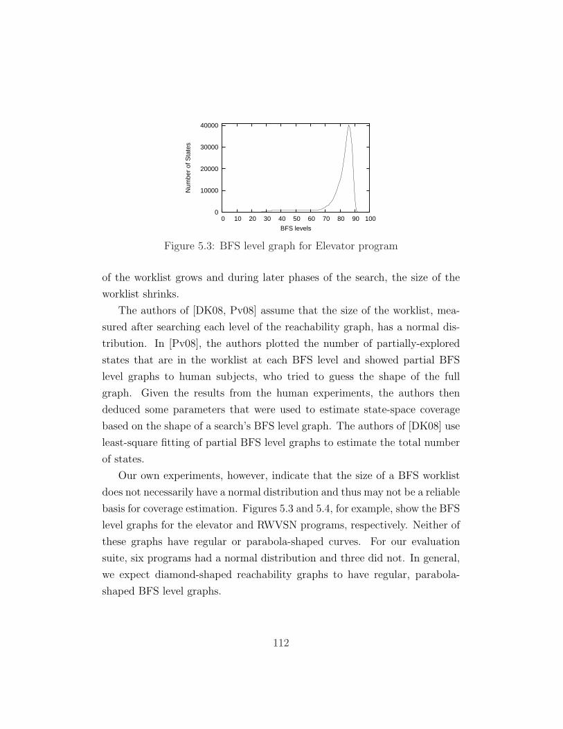
0
10000
20000
30000
40000
0 10 20 30 40 50 60 70 80 90 100
Num
ber
of S
tate
s
BFS levels
Figure 5.3: BFS level graph for Elevator program
of the worklist grows and during later phases of the search, the size of the
worklist shrinks.
The authors of [DK08, Pv08] assume that the size of the worklist, mea-
sured after searching each level of the reachability graph, has a normal dis-
tribution. In [Pv08], the authors plotted the number of partially-explored
states that are in the worklist at each BFS level and showed partial BFS
level graphs to human subjects, who tried to guess the shape of the full
graph. Given the results from the human experiments, the authors then
deduced some parameters that were used to estimate state-space coverage
based on the shape of a search’s BFS level graph. The authors of [DK08] use
least-square fitting of partial BFS level graphs to estimate the total number
of states.
Our own experiments, however, indicate that the size of a BFS worklist
does not necessarily have a normal distribution and thus may not be a reliable
basis for coverage estimation. Figures 5.3 and 5.4, for example, show the BFS
level graphs for the elevator and RWVSN programs, respectively. Neither of
these graphs have regular or parabola-shaped curves. For our evaluation
suite, six programs had a normal distribution and three did not. In general,
we expect diamond-shaped reachability graphs to have regular, parabola-
shaped BFS level graphs.
112

0
5000
10000
15000
20000
25000
30000
0 10 20 30 40 50 60 70 80
Num
ber
of S
tate
s
BFS levels
Figure 5.4: BFS level graph for RWVSN program
5.3.3 BFS vs. DFS During the Exhaustive-Search Phase
In our approach, an important design decision is the search strategy used
during the exhaustive-search phase. DFS is popular because it is fast: the
program stack can be used to store the worklist of partially explored states,
so there is less context switching when the next state is explored. However,
we use BFS because we hypothesize that having a larger worklist at the start
of the random-search phase results in a more accurate estimation.
To test this hypothesis, we experimented with using DFS rather than BFS
during the exhaustive-search phase. We ran both versions of JPF-coverage
on all nine programs and six coverage limits (54 cases), running each case 10
times.
Using DFS during the exhaustive-search phase produced estimation re-
sults in 44 cases that were inaccurate between 11 and 21 percentage points
(average of 14 percentage points); produced estimation results in 3 cases that
were inaccurate between 0 and 2 percentage points (average of 1 percentage
point); and produced estimation results in 7 cases that were inaccurate be-
tween 5 and 10 percentage points (average of 7 percentage points). The
results confirm that using BFS during the exhaustive-search phase is likely
to improve the accuracy of our algorithm’s coverage estimates.
113

5.3.4 Round-Robin Execution of Random-Search Phase
Searches
One risk of the current design for the random-search phase of our algorithm
is that the remaining memory is exhausted while searching the first sampled
(unexplored) transition, and that this can result in estimates that are wildly
off base: the estimate may be way too high (or way too low) if the number of
new states that are reached from this one transition is much higher (or much
lower) than the average number of new states per unexplored transition.
We hypothesized that we could improve the accuracy of our estimates by
sampling multiple unexplored transitions at once.
To test this hypothesis, we modified the random-search phase of our pro-
totype to sample several unexplored transitions in parallel in a round-robin
fashion: exploring a fixed number of transitions of a DFS of some unexplored
transition before switching to another DFS of another unexplored transition.
The model checker keeps a separate DFS stack (worklist) for each sampled
transition, and stores partially-explored states for each DFS in that DFS’s
local worklist. There is one shared global hash table that stores fingerprints
of visited states. If a DFS finishes before the search runs out of memory,
then the model checker picks a new unexplored transition from the worklist
and starts a new DFS.
To evaluate this technique, we varied the number of transitions that are
sampled in parallel and evaluated the accuracy of the resulting estimation.
We observed that when our algorithm samples five to ten unexplored transi-
tions in parallel, the accuracy of its coverage estimate improves for the tuning
limits of 10% and 25% but worsens for the tuning limit of 75%. When the
number of parallel searches is above 15, then estimation accuracy improves
for the coverage limit of 75% but worsens for the coverage limits of 10% and
25%.
It seems that when state-space coverage is low, it is better to sample a
smaller number of transitions so that the searches of the sampled transitions
114
finish. If too many transitions are sampled, then the number of new states
discovered per sampled transition is low (because the counts do not finish)
and the algorithm underestimates coverage. The opposite is true when state-
space coverage is high.
In general, we do not know in advance whether state-space coverage will
be low, high, or complete, and thus we do not know how many transitions
to sample. This method may become more applicable if there is a way to
determine on-the-fly whether the coverage is likely to be low or high. We
are exploring the possibility of performing the random-search phase of our
algorithm more than once, in which case the estimated coverage from one ex-
ecution could be used to tune the estimation algorithm in the second random-
search phase.
5.4 Summary
In this chapter, we have presented a strategy for estimating the state-space
coverage of a model-checking search that terminates prematurely due to in-
sufficient memory. Our strategy would provide useful feedback to the certifier
for deciding how much confidence to place in partial verification results. We
have implemented our algorithm in Java Pathfinder and have evaluated the
implementation on a suite of Java programs.
115
Chapter 6
Conclusion and Future Work
In this thesis, we have presented a set of techniques for certifying software
that was previously verified using model checking. Below, we summarize each
contribution and describe limitations and future work for each technique.
Search Carrying Code
In Chapter 3, we present search carrying code (SCC), a novel model-checking-
based method to certify model-checking results. In SCC, the software pro-
ducer submits with her program a search script that represents a search path
through the program’s reachability graph. The certifier’s model checker uses
the search script to direct and speed up its search of the same program.
SCC certification is property-independent. Rather than encoding the ver-
ification results for the program’s advertised properties, like a PCC certifi-
cate, an SCC search script encodes instructions for searching the program’s
entire state space. The script can be used to re-model check the program
for any program invariant or safety assertion, whether it is an advertised
property or an additional property of interest to the certifier (or the software
consumer).
SCC certification is amenable to efficient parallel model checking: the cer-
tifier’s model checker partitions the search script into a collection of mutually-
116

disjoint search scripts, and the scripts are distributed to parallel executing
processors. In our evaluation, we have shown that parallel SCC speeds up
certification up to 5n, for n parallel processors, when the source of the pro-
gram is trusted, and SCC speeds up certification up to n, for n parallel
processors, when the source of the program is un-trusted.
Future Work: We implemented SCC verification and SCC certification
in the same model checker, JPF. However, it is desirable that search scripts
are model-checker independent so that the software producer and certifier
can use any explicit-state model checker of their liking. In Chapter 3.3, we
discussed an outline for using different model checkers for verification and cer-
tification. In the future, we have to determine how different model checkers
interpret transition statements and whether it is possible to match state-
ments in the scripts to statements in the program. In addition, we have to
survey different state-space reduction techniques that model checkers employ
and compare the implementation of each technique in each model checker. It
may be possible to identify commonalities among the implementations and
thus, parameterize reduction techniques. In case certain reduction techniques
must be disabled to use SCC, we must determine whether the benefit of SCC
outweighs the benefit of the reduction technique.
Another limitation of SCC is the size of the search script that the software
producer provides, likely over a network, to the certifier. We show that, for
our evaluation programs, the size of the search script, in number of bytes,
is on the order of the number of states in the program’s state space. For
industrial-sized programs where the program’s state space is at the limit of
what can be model checked, the size of the search script could be very large.
Thus, the amount of time it would take to download it over the network would
make any time savings achieved by SCC certification seem insignificant. It
is an open problem whether the size of the search script can be further
reduced. It may be possible to use alternative representations and encodings
of the information in the search script in order to reduce its size. Also, it
117
may be possible to eliminate some information (e.g., backtracks) from the
search script altogether, but still be able to partition the script and check its
veracity.
State-Space Caching
In Chapter 4, we introduce a new cache-replacement strategy, cost-based
caching, for use in explicit state-space searches. State-space caching is useful
during SCC verification when memory resources are limited and the goal is
a full coverage of the state space (i.e., to produce a search script for SCC
certification). Our evaluation shows that state-space caching using a cost-
based cache-replacement strategy can achieve a full coverage of our evaluation
programs in a shorter time than caching using other replacement strategies,
and thus is more likely to terminate.
We also presented a memory-optimization technique that reduces the
memory requirements for SCC certification by removing state information
from the model checker’s table of visited states, if it is known that a state
will not be visited again for the remainder of the search. Using this method
in SCC certification, we reduced the memory requirements for certifying our
nine evaluation programs by 70% to 89%.
Future Work: Our experiments show that for our evaluation programs,
there is a significant increase in the time it takes to complete a search when
the model checker uses state-space caching. Without significant search-
time reductions, the software producer might be unwilling to use state-space
caching techniques. An open problem is whether the search time of a cached
search using our cost-based replacement policy can be significantly decreased
by optimizing how cost information is computed, stored, and kept sorted.
Also, future work can investigate how to calculate accurate cost values for
state spaces with strongly connected components. For that, we must keep
track of all states in a strongly connected component and update their cost
values once the last state in such a component has been fully explored. It re-
118

mains to see whether keeping absolutely accurate cost values decreases search
time significantly.
Our method for optimizing memory for certification can currently only
be used only with non-parallel SCC because at the end of parallel certifi-
cation, the entries of all FP s have to be compared. Because non-parallel
SCC certification does not achieve significant time savings, it is important
to explore ways to extend this optimization technique to parallel SCC. On
a distributed-memory architecture, reducing memory for certification might
not be an issue because in total, there is more memory available than on a
single processor. On a shared-memory architecture, memory could be opti-
mized by using a shared FP between all processors.
State-Space Coverage Estimation
When it is not possible to perform an exhaustive search of a program’s state
space, then an estimate of the amount of the state space that is covered
by a search can help the certifier to determine whether the partial model-
checking results are adequate for certification. In Chapter 5, we presented
an algorithm that estimates the percentage of a program’s state space that is
covered in a model-checking search when the search terminates prematurely
due to insufficient memory. Our method is based on Monte-Carlo sampling
of the unexplored portion of the state space.
Future Work: With any estimation, more research is needed to improve
the accuracy of the estimation. One possible approach would be to explore
strategies that employ multiple estimation runs, such as merging the results
from independent estimations or using the results of one estimation run to
incrementally refine a second estimation run. Another approach would be
to investigate whether state-space properties (e.g., ratio of discovering new
states) can serve as preliminary indicators of state-space coverage. Such
indicators could be used to tune our estimation algorithm on-the-fly (e.g.,
tuning the percentage of memory allocated to the exhaustive-search phase
119

versus the memory allocated to the random-search phase, based on early
indications as to whether the state space coverage will be low or high).
120

Bibliography
[AAR+10] Amal Ahmed, Andrew W. Appel, Christopher D. Richards,Kedar N. Swadi, Gang Tan, and Daniel C. Wang. Semanticfoundations for typed assembly languages. ACM Trans. Pro-gram. Lang. Syst., 32(3):1–67, 2010.
[ABJ10] Erik Arisholm, Lionel C. Briand, and Eivind B. Johannessen.A systematic and comprehensive investigation of methods tobuild and evaluate fault prediction models. Journal of Systemsand Software, 83(1):2–17, 2010.
[Abr06] Jean-Raymond Abrial. Formal methods in industry: achieve-ments, problems, future. In Proceedings of the 28th interna-tional conference on Software engineering, pages 761–768, NewYork, NY, USA, 2006. ACM.
[AdAdLM07] Alexandre Alvaro, Eduardo Santana de Almeida, and Sil-vio Romero de Lemos Meira. A component quality assuranceprocess. In Fourth international workshop on Software qualityassurance, pages 94–101, 2007.
[BBFM99] Patrick Behm, Paul Benoit, Alain Faivre, and Jean-Marc Mey-nadier. Meteor: A successful application of b in a large project.In Proceedings of the Wold Congress on Formal Methods in theDevelopment of Computing Systems-Volume I, pages 369–387,London, UK, 1999. Springer-Verlag.
[BBR07] Jiri Barnat, Lubos Brim, and Petr Rockai. Scalable multi-coreLTL model-checking. In SPIN, pages 187–203, 2007.
121
[BCC+03] Armin Biere, Alessandro Cimatti, Edmund M. Clarke, OferStrichman, and Yunshan Zhu. Bounded model checking. Ad-vances in Computers, 58:118–149, 2003.
[BCCZ99] Armin Biere, Alessandro Cimatti, Edmund M. Clarke, andYunshan Zhu. Symbolic model checking without BDDs. InProc. of the Conf. on Tools and Algorithms for the Construc-tion and Analysis of Systems, pages 193–207, 1999.
[BCM+90] Jerry R. Burch, Edmund M. Clarke, Kenneth L. McMillan,David L. Dill, and L. J. Hwang. Symbolic Model Checking:1020 States and Beyond. In LICS, pages 428–439, 1990.
[BJT07] Frederic Besson, Thomas Jensen, and Tiphaine Turpin. Smallwitnesses for abstract interpretation-based proofs. In Proceed-ings of the 16th European conference on Programming, pages268–283, 2007.
[BR01a] Thomas Ball and Sriram K. Rajamani. Automatically validat-ing temporal safety properties of interfaces. In Proc. of Int.SPIN Workshop on Model Checking of Software, pages 103–122, 2001.
[BR01b] Thomas Ball and Sriram K. Rajamani. The SLAM toolkit.In Proc. of Int. Conf. on Computer Aided Verification, pages260–264, 2001.
[Bry86] Randal E. Bryant. Graph-based algorithms for boolean func-tion manipulation. IEEE Trans. Comput., 35(8):677–691,1986.
[CC77] Patrick Cousot and Radhia Cousot. Abstract interpretation:a unified lattice model for static analysis of programs by con-struction or approximation of fixpoints. In Proc. of Princ. ofProg. Lang., pages 238–252, 1977.
[CE81] Edmund M. Clarke and E. Allen Emerson. Design and synthe-sis of synchronization skeletons using branching-time temporallogic. In Logic of Programs, pages 52–71, 1981.
122

[CE82] Edmund M. Clarke and E. Allen Emerson. Design and synthe-sis of synchronization skeletons using branching-time temporallogic. In Logic of Programs, Workshop, pages 52–71, 1982.
[CGJ+00] Edmund M. Clarke, Orna Grumberg, Somesh Jha, Yuan Lu,and Helmut Veith. Counterexample-guided abstraction refine-ment. In Computer Aided Verification, pages 154–169, 2000.
[CGJ+01] Edmund M. Clarke, Orna Grumberg, Somesh Jha, Yuan Lu,and Helmut Veith. Progress on the state explosion problemin model checking. In Informatics - 10 Years Back. 10 YearsAhead., pages 176–194, London, UK, 2001. Springer-Verlag.
[CGP99] Edmund M. Clarke, Orna Grumberg, and Doron A. Peled.Model Checking. Mit Press, 1999.
[CJEF96] Edmund M. Clarke, Somesh Jha, Reinhard Enders, andThomas Filkorn. Exploiting symmetry in temporal logic modelchecking. Formal Methods in System Design, 9(1/2):77–104,1996.
[CTvGS98] D.N. Christodoulakis, C. Tsalidis, C.J.M. van Gogh, and V.W.Stinesen. Towards an automated tool for software certification.In IEEE Int. Workshop on Tools for Artificial Intelligence,pages 670–676, 1998.
[Dav] Daniel Davies. http://ddavies.home.att.net/NewSimulator.html.
[DEPP07] Matthew B. Dwyer, Sebastian Elbaum, Suzette Person, andRahul Purandare. Parallel randomized state-space search. InProc. of the 29th Int. Conf. on Software Eng., pages 3–12,2007.
[DFS04] Ewen Denney, Bernd Fischer, and Johann Schumann. Us-ing automated theorem provers to certify auto-generatedaerospace software. In In Proceedings of International JointConference on Automated Reasoning (IJCAR04), volume 3097of LNCS, pages 198–212. Springer, 2004.
123
[DH82] Gerard Holzmann Delft and Gerard J. Holzmann. A theoryfor protocol validation. IEEE Transactions on Computers,31:730–738, 1982.
[DHH+06] Matthew B. Dwyer, John Hatcliff, Matthew Hoosier,Venkatesh Ranganath, and Todd Wallentine. Evaluatingthe effectiveness of slicing for model reduction of concurrentobject-oriented programs. In Proc. of the Conf. on Toolsand Algorithms for the Construction and Analysis of Systems,pages 73–89, 2006.
[DHJ+01] Matthew B. Dwyer, John Hatcliff, Roby Joehanes, ShawnLaubach, Corina S. Pasareanu, Hongjun Zheng, and WillemVisser. Tool-supported program abstraction for finite-stateverification. In Proc. of Int. Conf. on Software Engineering,pages 177–187, 2001.
[Dij72] Edsger W. Dijkstra. Chapter i: Notes on structured program-ming. pages 1–82, 1972.
[DK08] Nicholas J. Dingle and William J. Knottenbelt. State-spacesize estimation by least-squares fitting. In Proceedings of the24th UK Performance Engineering Workshop, page 347357,2008.
[DS09] Damian Dechev and Bjarne Stroustrup. Model-based product-oriented certification. In ECBS ’09: Proceedings of the 200916th Annual IEEE International Conference and Workshop onthe Engineering of Computer Based Systems, pages 295–304,2009.
[ES96] F. Allen Emerson and A. Prasad Sistla. Symmetry and modelchecking. International Journal of Formal Methods in SystemDesign, 9(1/2):105–131, August 1996.
[Gel04] Jaco Geldenhuys. State caching reconsidered. In Proc. of SPINWorkshop, pages 23–38, 2004.
[Gho99] Anup K. Ghosh. Certifying e-commerce software for secu-rity. In Proc. of the Int. Workshop on Advance Issues of
124
E-Commerce and Web-Based Information Systems, page 64,1999.
[GM93] M. J. C. Gordon and T. F. Mehlham. Introduction to HOL: aTheorem Proving Environment for Higher Order Logic. Cam-bridge University Press, New York, USA, 1993.
[God96] Patrice Godefroid. Partial-Order Methods for the Verificationof Concurrent Systems: An Approach to the State-ExplosionProblem. Springer-Verlag New York, Inc., Secaucus, NJ, USA,1996.
[God97] Patrice Godefroid. Model checking for programming languagesusing verisoft. In Proc. of Symp. on Principles of programminglanguages, pages 174–186, 1997.
[GS97] Susanne Graf and Hassen Saıdi. Construction of abstract stategraphs with pvs. In Proceedings of the 9th International Con-ference on Computer Aided Verification, pages 72–83, 1997.
[GV04] A. Groce and W. Visser. Heuristics for model checking Javaprograms. Int’l Jour. on Soft. Tools for Tech. Transfer,6(4):260–276, 2004.
[HDPR02] John Hatcliff, Matthew B. Dwyer, Corina S. Pasareanu, andRobby. Foundations of the bandera abstraction tools. In Theessence of computation: complexity, analysis, transformation,pages 172–203, 2002.
[Hol87] Gerard J. Holzmann. Automated protocol validation in argos:Assertion proving and scatter searching. IEEE Trans. Softw.Eng., 13(6):683–696, 1987.
[Hol88] Gerard J. Holzmann. Algorithms for automated protocol val-idation. ATT TECHNICAL JOURNAL, 69:163–188, 1988.
[Hua75] J. C. Huang. An approach to program testing. ACM Comput.Surv., 7(3):113–128, 1975.
[IB06] Cornelia P. Inggs and Howard Barringer. Ctl* model checkingon a shared-memory architecture. Form. Methods Syst. Des.,29(2):135–155, 2006.
125

[ID96] C. Norris Ip and David L. Dill. State reduction using reversiblerules. In Proceedings of the 33rd annual Design AutomationConference, pages 564–567, 1996.
[IEE90] IEEE. IEEE Standard Glossary of Software Engineering Ter-minology. 1990.
[Ire05] Andrew Ireland. On the scalability of proof carrying code forsoftware certification. In Workshop on Software CertificateManagement, pages 31–34, 2005.
[ISO06] ISO/IEC 25051 (2006). Software Product Quality Require-ments and Evaluation (SQUARE) Requirements for Qualityof Commercial Off-the-shelf (COTS) Software Product and In-structions for Testing. International Organization for Stan-dardization, 2006.
[KM97] Matt Kaufmann and J. S. Moore. An industrial strength the-orem prover for a logic based on common lisp. IEEE Trans.Softw. Eng., 23(4):203–213, 1997.
[KM05] R. Kumar and E.G. Mercer. Load balancing parallel explicitstate model checking. In Workshop on Parallel and DistributedMethods in Verification, pages 19–34, 2005.
[LGW07] Seok-Won Lee, Robin A. Gandhi, and Siddharth Wagle. To-wards a requirements-driven workbench for supporting soft-ware certification and accreditation. In ICSEW ’07: Proceed-ings of the 29th International Conference on Software Engi-neering Workshops, page 53, Washington, DC, USA, 2007.IEEE Computer Society.
[LPR01] Michael Lowry, Thomas Pressburger, and Grigore Rosu. Cer-tifying domain-specific policies. In ASE ’01: Proceedings of the16th IEEE international conference on Automated software en-gineering, page 81, Washington, DC, USA, 2001. IEEE Com-puter Society.
[LV01] Flavio Lerda and Willem Visser. Addressing dynamic issuesof program model checking. In Proc. of Int. SPIN Workshopon Model Checking of Software, pages 80–102, 2001.
126

[Mai07] Tom S. E. Maibaum. Challenges in software certification. In9th International Conference on Formal Engineering Methods,pages 4–18, 2007.
[MDC06] A. Miller, A. Donaldson, and M. Calder. Symmetry in tempo-ral logic model checking. ACM Comp. Surv., 38(3), 2006.
[MLP+01] John Morris, Gareth Lee, Kris Parker, Gary A. Bundell, andChiou Peng Lam. Software component certification. Computer,34(9):30–36, 2001.
[MQ08] Madanlal Musuvathi and Shaz Qadeer. Fair stateless modelchecking. In Proc. of Conf. on Programming language designand implementation, pages 362–371, 2008.
[MW08] Tom Maibaum and Alan Wassyng. A product-focused ap-proach to software certification. Computer, 41:91–93, 2008.
[Mye79] Glenford J. Myers. Art of Software Testing. John Wiley &Sons, Inc., 1979.
[NC97] David M. Nicol and Gianfranco Ciardo. Automated paral-lelization of discrete state-space generation. Journal ParallelDistributed Computing, 47(2):153–167, 1997.
[Nec97] George C. Necula. Proof-carrying code. In Symp. on Prin. ofProgramming Languages, pages 106–119, 1997.
[NS06] Zhaozhong Ni and Zhong Shao. Certified assembly program-ming with embedded code pointers. In 33rd ACM SIGPLAN-SIGACT Symp. on Principles of Prog. Languages, pages 320–333, 2006.
[OM03] David Owen and Tim Menzies. Lurch: a lightweight alterna-tive to model checking. In International Conference on Soft-ware Engineering and Knowledge Engineering, pages 158–165,2003.
[OWB05] Thomas J. Ostrand, Elaine J. Weyuker, and Robert M. Bell.Predicting the location and number of faults in large soft-ware systems. IEEE Transactions on Software Engineering,31(4):340–355, 2005.
127
[PHvB05] Radek Pelanek, T. Hanzl, I Cerna, and L. Brim. Enhancingrandom walk state space exploration. In Int. Workshop onFormal Methods for Industrial Critical Systems, pages 98–105,2005.
[PM00] Mauro Pezze and MichalYoung. Software Testing and Anal-ysis: Process, Principles, and Techniques. Wiley, New York,USA, 2000.
[Pnu77] Amir Pnueli. The temporal logic of programs. In Proceedingsof the 18th Annual Symposium on Foundations of ComputerScience, pages 46–57, 1977.
[PSD] David Park, Ulrich Stern, and David Dill.http://verify.stanford.edu/uli/icse/workshop.html.
[Pv08] Radek Pelanek and Pavel Simecek. Estimating state spaceparameters. In Proceedings of the 7th international Workshopon Parallel and Distributed Methods in Verification, 2008.
[QS82] Jean-Pierre Queille and Joseph Sifakis. Specification and veri-fication of concurrent systems in cesar. In Symposium on Pro-gramming, pages 337–351, 1982.
[RDH03] Robby, Matthew B. Dwyer, and John Hatcliff. Bogor: anextensible and highly-modular software model checking frame-work. In Proc. of the European Software Engineering Confer-ence, pages 267–276, 2003.
[RDHR04] Edwin Rodrguez, Matthew B. Dwyer, John Hatcliff, andRobby. A flexible framework for the estimation of coveragemetrics in explicit state software model checking. In Proc. ofthe 2004 Int. Workshop on Construction and Analysis of Safe,Secure, and Interoperable Smart Devices, 2004.
[RTC92] RTCA Inc. and EUROCAE. DO-178B: Software Considera-tions in Airborne Systems and Equipment Certification. 1992.
[San] Santos Laboratory. http://www.cis.ksu.edu/santos/case-studies/counterexample case study.
128
[SD97] U. Stern and D. L. Dill. Parallelizing the Murϕ verifier. InProc. of the Conf. on Computer Aided Verification 97, volume1254, pages 256–267, 1997.
[SG03] Hemanthkumar Sivaraj and Ganesh Gopalakrishnan. Randomwalk based heuristic algorithms for distributed memory modelchecking. In Electronic Notes Theor. Comput. Sci, 2003.
[Sof07] Software Engineering Institute - Carnegie Mellon University.Capability Maturity Model (CMM) ver. 1.2, 2007.
[SVB+03] R. Sekar, V. N. Venkatakrishnan, Samik Basu, SandeepBhatkar, and Daniel C. Duvarney. Model-carrying code: apractical approach for safe execution of untrusted applications.In Proc. of 19th Symp. on Operating Sys. Principles, pages 15–28, 2003.
[TA09] Ali Taleghani and Joanne M. Atlee. State-space coverage es-timation. In ASE ’09: Proceedings of the 2009 IEEE/ACMInternational Conference on Automated Software Engineering,pages 459–467, 2009.
[TA10] Ali Taleghani and Joanne M. Atlee. Search carrying code.In To appear ASE ’10: Proceedings of the 2010 IEEE/ACMInternational Conference on Automated Software Engineering,2010.
[Tal07] Ali Taleghani. Using software model checking for software com-ponent certification. In ICSE COMPANION ’07: Companionto the proceedings of the 29th International Conference on Soft-ware Engineering, pages 99–100, 2007.
[tBGKM08] Maurice H. ter Beek, Stefania Gnesi, Nora Koch, and FrancoMazzanti. Formal verification of an automotive scenario inservice-oriented computing. In ICSE ’08: Proceedings of the30th international conference on Software engineering, pages613–622, New York, NY, USA, 2008. ACM.
[tBML+05] Maurice H. ter Beek, Mieke Massink, Diego Latella, StefaniaGnesi, Alessandro Forghieri, and Maurizio Sebastianis. A case
129

study on the automated verification of groupware protocols.In ICSE ’05: Proceedings of the 27th international conferenceon Software engineering, pages 596–603, New York, NY, USA,2005. ACM.
[TC95] William M. Thomas and Deborah A. Cerino. Predicting soft-ware quality for reuse certification. In TRI-Ada ’95: Proceed-ings of the conference on TRI-Ada ’95, pages 367–377, 1995.
[TPIZ01] Enrio Tronci, Giuseppe Della Penna, Benedetto Intrigila, andMarisa Venturini Zilli. A probabilistic approach to automaticverification of concurrent systems. In Proc. of the Asia-Pacificon Software Eng. Conf., page 317, 2001.
[Und98] Underwriter Laboratories. UL-1998: Standard for safety - Soft-ware in programable components. 1998.
[US 02] US Food and Drug Administration. General principles of soft-ware validation; Final guidance for industry and FDA staff.2002.
[VBHP00] W. Visser, G. Brat, K. Havelund, and S. Park. Model check-ing programs. In Proc. of Int. Conf. on Automated SoftwareEngineering, pages 3–12, 2000.
[Voa00] Jeffrey Voas. Developing a usage-based software certificationprocess. Computer, 33(8):32–37, 2000.
[WBH+05] Bruce W. Weide, Paolo Bucci, Wayne D. Heym, Murali Sitara-man, and Giorgio Rizzoni. Issues in performance certificationfor high-level automotive control software. SIGSOFT Softw.Eng. Notes, 30(4):1–6, 2005.
[Wei81] M. Weiser. Program slicing. In Proceedings of the 5th Inter-national Conference on Software Engineering, pages 439–449,1981.
[Wes86] C.H. West. Protocol validation by random state exploration.In Proc. of the 7rd Workshop on Protocol Specification, Testingand Verification, 1986.
130
[Wil07] William Jackson. Under Attack: Common Criteria has loadsof critics, but is it getting a bum rap. Government ComputerNews, 2007.
[WR94] Claes Wohlin and Per Runeson. Certification of software com-ponents. Software Engineering, 20(6):494–499, 1994.
[XH04] Songtao Xia and James Hook. Certifying temporal propertiesfor compiled C programs. In Proc. of the Conf. on Verif.,Model Check., and Abstr. Interpret., pages 161–174, 2004.
[YJ03] Yu Yangyang and B W Johnson. A BBN approach to certify-ing the reliability of cots software systems. In Reliability andMaintainability Symp., pages 19 – 24, 2003.
131
Related Documents