Using relaxations in Maximum Density Still Lifeusers.monash.edu/~mbanda/papers/cp09-sl.pdf · The board is said to be a still-life at time t if it is unchanged by these rules, i.e.,

Using relaxations in Maximum Density Still Life

Geoffrey Chu1, Peter J. Stuckey1, and Maria Garcia de la Banda2

1 NICTA Victoria Laboratory,Department of Computer Science and Software Engineering,

University of Melbourne, Australia{gchu,pjs}@csse.unimelb.edu.au

2 Faculty of Information Technology,Monash University, Australia

[email protected]

Abstract. The Maximum Density Sill-Life Problem is to fill an n × nboard of cells with the maximum number of live cells so that the boardis stable under the rules of Conway’s Game of Life. We reformulate theproblem into one of minimising “wastage” rather than maximising thenumber of live cells. This reformulation allows us to compute strong up-per bounds on the number of live cells. By combining this reformulationwith several relaxation techniques, as well as exploiting symmetries viacaching, we are able to find close to optimal solutions up to size n = 100,and optimal solutions for instances as large as n = 69. The best previousmethod could only find optimal solutions up to n = 20.

1 Introduction

The Game of Life was invented by John Horton Conway and is played on aninfinite board. Each cell c in the board is either alive or dead at time t. Thelive/dead state at time t + 1 of cell c, denoted as state(c, t + 1), can be obtainedfrom the number l of live neighbours of c at time t and from state(c, t) as follows:

state(c, t + 1) =

l < 2 dead [Death by isolation]l = 2 state(c, t) [Stable condition]l = 3 alive [Birth condition]l > 3 dead [Death by overcrowding]

The board is said to be a still-life at time t if it is unchanged by these rules,i.e., it is the same at t + 1. For example, an empty board is a still-life. Given afinite n×n region where all other cells are dead, the Maximum Density Still-lifeProblem aims at computing the highest number of live cells that can appear in astill life for the region. The density is thus expressed as the number of live cellsover the n× n region.

The raw search space of the Maximum Density Still-life Problem has size2n2

. Thus, it is extremely difficult even for “small” values of n. Previous searchmethods using IP [1] and CP [2] could only solve up to n = 9, while a CP/IPhybrid method with symmetry breaking [2] could solve up to n = 15. An attemptusing bucket elimination [6] reduced the time complexity to O(n223n) but in-creased the space complexity to O(n22n). This method could solve up to n = 14

before it ran out of memory. A subsequent improvement that combined bucketelimination with search [7], used less memory and was able to solve up to n =20. In this paper we combine various techniques to allow us to solve instancesup to n = 50 completely or almost completely, i.e. we prove upper bounds andfind solutions that either achieve that upper bound or only have 1 less live cell.We also obtain solutions that are no more than 4 live cells away from our provenupper bound all the way to n = 100. The largest completely solved instance isn = 69.

The contributions of this paper are as follows:

– We give a new insightful proof that the maximum density of live cells inan infinite still life is 1

2 . This proof allows us to reformulate the maximumdensity still-life problem in terms of minimising “wastage” rather than max-imising the number of live cells.

– We derive tight lower bounds on wastage (which translate into upper boundson the number of live cells) that can be used for pruning.

– We define a static relaxation of the original problem that allows us to cal-culate closed form equations for an upper bound on live cells for all n. Andwe do this in constant time by using CP with caching. We conjecture thatthis upper bound is either equal to the optimum, or only 1 higher for all n.

– We identify a subset of cases for which we can improve the upper bound by 1by performing a complete search on center perfect solutions. This completesthe proof of optimality for the instances where our heuristic search was ableto find a solution with 1 cell less than the initial upper bound.

– We define a heuristic incomplete search using dynamic relaxation as a looka-head method that can find optimal or near optimal solutions all the way upto n = 100.

– We find optimal solutions for n as large as 69, more than 3 times larger thanany previous methods, and with a raw search space of 24761.

2 Wastage reformulation

The maximum density of live cells in an infinite still life is known to be 12 [5, 4].

However, that proof is quite complex and only applies to the infinite plane. Inthis section we provide a much simpler proof that can easily be extended to thebounded case and gives much better insight into the possible sub-patterns thatcan occur in an optimal solution. The proof is as follows.

First we assign an area of 2 to each cell (assume the side length is√

2). Wewill partition the area of each dead cell into two 1 area pieces and distributethem among its live neighbours according to the local pattern found around thedead cell. It is clear that if we can prove that all live cells on the board end upwith an area ≥ 4, then it follows that the density of live cells is ≤ 1

2 .The area of a dead cell is assigned only to orthogonal neighbouring live cells,

i.e., those that share an edge with the dead cell. We describe as “wastage” thearea from a dead cell that does not need to be assigned to any live cell for theproof to work (i.e., it is not needed to reach our 4 target for live cells). Table 1shows all possible patterns of orthogonal neighbours (up to symmetries) around

Pattern:

? ?

? ?

? ?

??

? ?

??

? ?

??

? ?

??

? ?

??

Beneficiaries {} { S } {S, W} {E, W} {E, W} {}Wastage 2 1 0 0 0 2

Table 1. Possible patterns around dead cells, showing where they donate their areaand any wastage of area.

Pattern:

? ???

? ? ???

? ? ???

?

Area received 1 1 0

Table 2. Contributions to the area of a live cell from its South neighbour.

a dead cell. Live cells are marked with a black dot, dead cells are unmarked, andcells whose state is irrelevant for our purposes are marked with a “?”.

Each pattern indicates the beneficiaries, i.e., the North, East, South or Westneighbours that receive 1 area from the center dead cell, and the resulting amountof wastage. As it can be seen from the table, a dead cell gives 1 area to each ofits live orthogonal neighbours if it has ≤ 2 live orthogonal neighbours, 1 area tothe two opposing live orthogonal neighbours if it has 3, and no area if it has 4.Note that, in the table, wastage occurs whenever the dead cell has ≤ 1 or 4 liveorthogonal neighbours. As a result, we only need to examine the 3 borderingcells on each side of a live cell, to determine how much area is obtained fromthe orthogonal neighbour on that side. For example, the area obtained by thecentral live cell from its South neighbour is illustrated in Table 2.

The area obtained by a live cell can therefore be computed by simply addingup the area obtained from its four orthogonal neighbours. Since each live cellstarts off with an area of 2, it must receive at least 2 extra area to end upwith an area that is ≥ 4. Let us then look at all possible patterns around alive cell and see where the cell will receive area from. Table 3 shows all possibleneighbourhoods of a live cell (up to symmetries). For each pattern, it shows thebenefactors, i.e., the North, East, South or West neighbours that give 1 area tothe live cell, and the resulting amount of wastage, which occurs whenever a livecell receives more than 2.

Note that the last pattern does not receive sufficient extra area, just 1 fromthe South neighbour. However, the last two patterns always occur together inunique pairs due to the still-life constraints (each of the central live cells has 3neighbours so the row above the last pattern, and the row below the second lastpattern must only consist of dead cells). Hence, we can transfer the extra 1 areafrom the second last pattern to the last.

Pattern:

Benefactors: {N,S} {N,E,S} {N,E,S,W} {S,W} {N,S,W}Wastage: 0 1 2 0 1

Pattern:

Benefactors: {S,W} {N,S} {E,S,W} {E,S} {E,W}Wastage: 0 0 1 0 0

Pattern:

Benefactors: {S,W} {S,W} {S,W} {N,E,W} {S}Wastage: 0 0 0 1 −1

Table 3. Possible patterns around a live cell showing area benefactors and any wastage.

Clearly, all live cells end up with an area ≥ 4, and this completes our proofthat the maximum density on an infinite board is 1

2 .The above proof is not only much simpler than that of [5, 4], it also provides

us with good insight into how to compute useful bounds for the case in which theboard is finite. In particular, it allows us to know exactly how much we have lostfrom the theoretical maximum density by looking at the amount of “wastage”produced by the patterns in the currently labeled cells.

To achieve this, we reformulate the objective function in the Bounded Maxi-mum Density Still Life Problem as follows. For each cell c, let P (c) be the 3× 3pattern around that cell. Note that if c is on the edge of the n × n region, thedead cells beyond the edge are also included in this pattern. Let w(P ) be thewastage for each 3× 3 pattern as listed in Tables 1 and 3. Define w(c) for eachcell c as follows. If c is within the n × n region, then w(c) = w(P (c)). If c is inthe row immediately beyond the n× n region and shares an edge with it (thereare 4n such cells), then w(c) = 1 if the cell in the n × n region with which itshares an edge is dead, and w(c) = 0 otherwise. For all other c, let w(c) = 0. LetW =

∑w(c) over all cells.

Theorem 1. Wastage and live cells are related by

live cells =n2

2+ n− W

4(1)

Proof. We adapt the proof for the infinite board to the n × n region. Let usassign 2 area to each cell within the n× n region, and 1 area to each of the 4n

cell in the row immediately beyond the edge of the n× n region. Now, for eachdead cell within the n × n region, partition the area among its live orthogonalneighbours as before. For each dead cell in the row immediately beyond the n×nregion, give its 1 area to the cell in the n × n region with which it shares anedge. Again, since the last two 3 × 3 patterns listed above must occur in pairs,we transfer an extra 1 area from one to the other. Note also that the secondlast pattern of Table 3 cannot appear on the South border (which would meanthat the last pattern appeared outside the shape) since it is not stable in thisposition. Clearly, after the transfers, all live cells once again have ≥ 4 area, andwastage for the 3 × 3 patterns centered around cells within the n × n regionremain the same. However, since we are in the finite case, we also have wastagefor the cells which are in the row immediately beyond the edge of the n × nregion. These dead cells always give 1 area to the neighbouring cell which is inthe n×n region. If that cell is live, the area is received. If that cell is dead, that1 area is wasted. The reformulation above counts all these wastage as follows.The total amount of area that was used was 2n2 from the cells within the n× nregion and 4n from the 4n cells in the row immediately beyond the edge, for atotal of 2n2 + 4n. Now, 4 times live cells will be equal to the total area minusall the area wasted, and hence we end up with Equation (1). �

We can trivially derive some upper bounds on the number of live cells usingthis equation. Clearly W ≥ 0 and, thus, we have live cells ≤ bn2

2 + nc. Also, bythe still life constraints, there cannot be three consecutive live cells along theedge of the n × n region. Hence, there is always at least 1 wastage per 3 cellsalong the edge and we can improve the bound to live cells ≤ bn2

2 + n − b 13ncc.While this bound is very close to the optimal value for a small n, it differs fromthe true optimum by O(n) and will diverge from the optimum for a large n. Weprovide a better bound in the next section.

3 Closed form upper bound

Although in the infinite case there are many patterns that can achieve exactly12 density, it turns out that in the bounded case, the boundary constraints forcesignificant extra wastage. As explained in the previous section, the still life con-straints on the edge of the n × n region trivially force at least 1 wastage per 3edge cells, however, it can be shown by exhaustive search that even this theoret-ical minimal wastage of 1/3 per edge cell is unattainable for an infinitely longedge due to the still life constraints on the inside of the n× n region.

There is also no way to label the corner without producing some extrawastage. For example, for a 6×6 corner, naively we expect to have (6+6)/3 = 4wastage forced by the still life constraints on the boundary. However, due to thestill life constraints within the corner, there is actually no way to label a 6 × 6corner without at least 6 wastage.

Examination of the optimal solutions found by other authors show that, inall instances, all or almost all wastage is found either in the corners or within 3rows from the edge. This leads to the following conjecture:

8x8 8x8

8x88x8

3x

3x

x3 x3

Fig. 1. The relaxed version of the problem, only filling in the 8×8 corners and the 3rows around the edge.

Conjecture 1. All wastage forced by the boundary constraints of an n×n regionmust appear either in the 8× 8 corners, or within 3 rows from the edge.

If this conjecture is true, then it should be possible to find a good lowerbound on the amount of forced wastage simply by examining the corners andthe first few rows from the edge.

We thus perform the following relaxation of the bounded still life problem.We keep only the variables representing the four 8 × 8 corners of the board, aswell as the variables representing cells within 3 rows of the edge (see Figure 1).All variables in the middle are removed. The still life constraints for fully sur-rounded cells, including cells on the edge of the n× n region, remain the same.The still life constraints for cells neighbouring on removed cells are relaxed asfollows: dead cells are always considered to be consistent with the problem con-straints, and live cells are considered to be consistent as long as they do nothave more than 3 live neighbours (otherwise any extension to the removed cellswould violate the original constraints). The objective function is modified as fol-lows: fully surrounded cells have their wastage counted as before, live cells withneighbouring removed cells have no wastage counted, and dead cells with neigh-bouring removed cells have 1 wastage counted if and only if it is surrounded by≥ 3 dead unremoved cells (since any extension to the removed cells will resultin a pattern with ≥ 1 wastage). Clearly, since we have relaxed the constraints,and also potentially ignored some wastage in our count, any lower bound we geton wastage in this relaxed problem is a valid lower bound on the wastage in theoriginal problem.

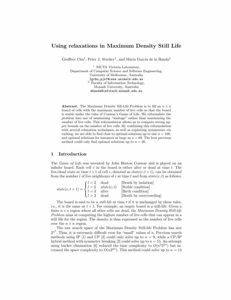
Since the constraint graph of this relaxed problem has bounded, very lowpath-width, it can easily be solved using CP with caching in O(n) time (see [3]Theorem 13.2). In practice, solving the 8 × 8 corners is the hardest and takes8s. An example corner solution is shown in Figure 2(a). Solving the width 3edge takes milliseconds. The results of calculating the bound from the relaxedproblem for small n is shown in Table 4.

Because of the high symmetry of the edge subproblem (full translationalsymmetry), the edge bounds starts to take on a periodic pattern for n sufficiently

(a) (b)

Fig. 2. An optimal 8×8 North West corner pattern with 7 wastage highlighted, and(b) the periodic pattern for an optimal North edge with 4 wastage per period 11highlighted.

large, at which point we can derive a closed form equation for their values forall n. The periodicity comes from the fact that it can be shown that the optimalperiodic edge pattern (see Figure 2(b)) has period 11, and any sufficiently longoptimal edge pattern will have a series of these in the middle.

Since the set of optimal solutions for the 8× 8 corners remain the same forany n > 16, and we can derive a closed form equation for the edge bounds forlarge n, we can calculate a closed form equation for the lower bound on wastagefor the whole relaxed problem for any n sufficiently large. For n ≥ 50 it is:

min wastage =

8 + 16× bn/11c, n ≡ 0, 1, 2 mod 1112 + 16× bn/11c, n ≡ 3, 4 mod 1114 + 16× bn/11c, n ≡ 5 mod 1116 + 16× bn/11c, n ≡ 6, 7 mod 1118 + 16× bn/11c, n ≡ 8 mod 1120 + 16× bn/11c, n ≡ 9, 10 mod 11

(2)

A lower bound on wastage can be converted into an upper bound on live cellsusing Equation (1):

live cells ≤⌊

2n2 + 4n−min wastage

4

⌋(3)

We will call the live cell upper bound calculated from our closed form wastagelower bounds the “closed form upper bound”. If Conjecture 1 is true and allforced wastage must appear within a few rows of the edge, then this closed formupper bound should be extremely close to the real optimal value.

Conjecture 2. The maximum number of live cells in an n× n region is⌊2n2 + 4n−min wastage

4

⌋or one less than this, where min wastage is the optimal solution to the relaxedproblem of Figure 1 (given by Equation (2) for n ≥ 50). �

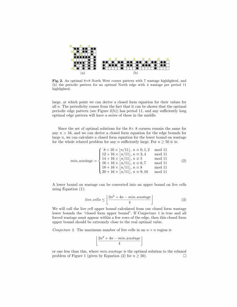
n optimal upper bound8 36 369 43 4410 54 5511 64 6512 76 7713 90 9114 104 10415 119 12016 136 13617 152 15218 171 17219 190 19020 210 210

Table 4. Upper bound by relaxation for small n, shown in bold if it is equal to theoptimal solution.

Conjecture 2 is true for previously solved n. As it can be seen from Table 4,for n ≤ 20, our upper bound is never off the true optimum by more than 1, andis often equal to it.

As our new results in Table 5 show, our conjecture is also true for at leastup to n = 50. The bound is also achievable exactly for n as high as 69. Forlarger n our solver is too weak to guarantee finding the optimal solution andthus we cannot verify the conjecture. We believe the conjecture is true becausealthough not all 3×3 patterns are perfect (waste free), there are a large numberof perfect ones and there easily appears to be enough different combinations ofthem to label the center of an n × n region perfectly. Indeed, since we alreadyknow that there are many ways to label an infinite board perfectly, the boundaryconstraints are the only constraints that can force wastage.

4 Finding optimal solutions

In the previous section, we found a relaxation that allows us to find very goodupper bounds in constant time. However, in order to find an optimal solution it isstill necessary to tackle the size 2n2

search space. The previous best search basedmethods could only find optimal solutions up to n = 15, with a search spaceof 2225. Here, we attempt to find solutions up to n = 100, which has a searchspace of 210000, a matter of 3000 orders of magnitude difference. Furthermore,optimal solutions are extremely rare: 1682 out of 2169 for n = 13, 11 out of 2196

for n = 14, and so on [7]. Clearly, we are going to need some extremely powerfulpruning techniques.

For some values of n, the closed form upper bound calculated in the previoussection is already the true upper bound. For such instances we simply need tofind a solution that achieves the upper bound and, therefore, we can use anincomplete search. We take advantage of this by looking only for solutions of aparticular form: those where all wastage lies in the 8×8 corners or within 3 rowsof the edge, and the “center” is labeled perfectly with no wastage whatsoever.

16x8

8x88x8

3x

x3

x3

16x8

Previously filled

8x8x 16x8

8x88x8

3x

x3

x316x8

Previously filled

8x8x

(a) (b)

Fig. 3. Dynamic relaxation lookahead for still-life search: (a) shows darkened the areaof lookahead, (b) shows the change in lookahead on labelling an additional columnwhen super-row width is 4 and lookahead width is 8.

We call such solutions “center perfect”. Our choice is motivated by the factthat, while there are many ways to label the center perfectly, there are very fewways to label the edge with the minimum amount of wastage. Since we are onlyallowed a very limited number of wastage on the entire board, they should notbe used to deal with the center cells. Searching only for center perfect solutions,allows us to implement our solver more simply and to considerably reduce thesearch space.

4.1 Dynamic relaxation as lookahead

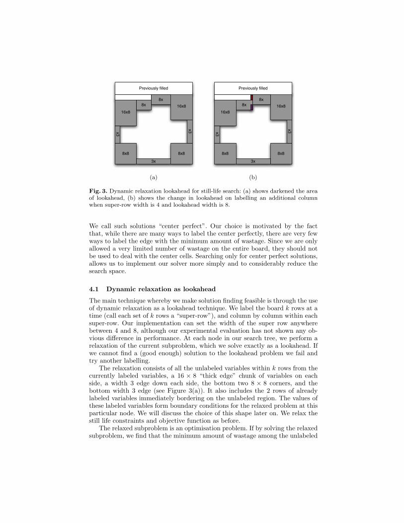
The main technique whereby we make solution finding feasible is through the useof dynamic relaxation as a lookahead technique. We label the board k rows at atime (call each set of k rows a “super-row”), and column by column within eachsuper-row. Our implementation can set the width of the super row anywherebetween 4 and 8, although our experimental evaluation has not shown any ob-vious difference in performance. At each node in our search tree, we perform arelaxation of the current subproblem, which we solve exactly as a lookahead. Ifwe cannot find a (good enough) solution to the lookahead problem we fail andtry another labelling.

The relaxation consists of all the unlabeled variables within k rows from thecurrently labeled variables, a 16 × 8 “thick edge” chunk of variables on eachside, a width 3 edge down each side, the bottom two 8 × 8 corners, and thebottom width 3 edge (see Figure 3(a)). It also includes the 2 rows of alreadylabeled variables immediately bordering on the unlabeled region. The values ofthese labeled variables form boundary conditions for the relaxed problem at thisparticular node. We will discuss the choice of this shape later on. We relax thestill life constraints and objective function as before.

The relaxed subproblem is an optimisation problem. If by solving the relaxedsubproblem, we find that the minimum amount of wastage among the unlabeled

variables, plus the amount of wastage already found in the labeled variables,exceeds the wastage upper bound for the original problem, then clearly thereare no solutions in the current branch and the node can be pruned. Since theconstraint graph of the relaxed problem has low path-width, it can be solved inlinear time using CP with caching. In practice though, we exploit symmetriesand caching to solve it incrementally in constant time (see below). Lower boundscalculated for particular groups of variables (such as corners, edges, and super-rows) are cached. These can be reused for other subproblems. We also use thesecached results as a table propagator, as they can immediately tell us whichparticular value choices will lead to wastage lower bounds that violate the currentupper bound.

The relaxed problem can be solved incrementally in constant time as follows.When we travel to a child node, the new relaxed problem at that node is not thatdifferent from the one at the previous node (see Figure 3(a) and (b), respectively).A column of k variables from the previous relaxation has now been removed fromthe relaxation and labeled (new top dark column in Figure 3(b)), and a newcolumn of k variables is added to the relaxation (new bottom dark column inFigure 3(b)). By caching previous results appropriately, it is possible to lookupall the solutions to the common part of the two relaxed problems (cached whensolving the previous relaxation). Now we simply need to extend those solutionsto the new column of k variables, which takes O(2k) time but is constant for afixed k. There is sufficient time/memory to choose a k of up to 12. The larger kis, the greater the pruning achieved but the more expensive the lookahead is. Inpractice, k = 8 seems to work well. With k = 8, we are able to search around1000 nodes per second and obtain a complete depth 400+ lookahead in constanttime.

The choice of the shape of the lookahead is important, and is based on ourconjectures as well as on extensive experimentation. The most important vari-ables to perform lookahead on are the variables where wastage is most likelyto be forced by the current boundary constraints. Conjecture 1 can be appliedto our relaxed subproblems as well. It is very likely that the wastage forced bythe boundary constraints can be found within a fixed number of rows from thecurrent boundary. Thus, the variables near the boundary are the ones we shouldperform lookahead on. The reason for the 16 × 8 thick edge chunk of variablescomes from our experimentation. It was found that the lookahead is by far theweakest around the “corners” of the subproblem, where we have boundary con-straints on two sides. A lookahead using a thinner edge (initially width 3) oftenfailed to see the forced wastage further in and, thus, allowed the solver to getpermanently stuck around those “corners”. By using a thicker edge, we increasethe ability of the lookahead to predict forced wastage and thus we get stuckless often. A 16 × 8 thick edge is still not sufficiently large to catch all forcedwastage, but we are unable to make it any larger due to memory constraints, asthe memory requirement is exponential in the width of the lookahead.

Interestingly, if Conjecture 1 is indeed true for the subproblems, and we canget around the memory problems and perform a lookahead with a sufficient widthto catch all forced wastage, then the lookahead should approach the strength ofan oracle, and it may be possible to find optimal solutions in roughly polynomial

time! Indeed, from our results (see Table 5), the run time required to find optimalsolutions does not appear to be growing anywhere near exponentially in n2.

4.2 Search strategy

The search strategy is also very important. A traditional depth first branchand bound strategy is doomed to failure, as it will tend to greedily use up thewastage allowance to get around any problem it encounters. If it maxes out onthe wastage bound early on, then it is extremely unlikely that it will be able tolabel the rest of the board without breaking the bound. However, we may notbe able to tell this until much later on, since the center can often be labeledperfectly. Therefore, the search will reach extremely deep parts of the searchtree, even though there is no chance of success and we will essentially be stuckforever. Instead, we need a smarter search strategy that has more foresight.

Intuitively, although labeling the top parts of the board optimally is difficult,it is much easier than labeling the final part of the board, since the final partof the board will have boundary constraints on every side, making it extremelydifficult to get a perfect labeling with minimal wastage. Thus, we would like tosave all our wastage allowance until the end. We accomplish this by splitting thesearch into two phases. The first phase consists of labeling all parts of the boardother than the last 8 rows, and the second phase consists of the last 8 rows. Inthe first phase, we use a variation of limited discrepancy search (LDS), designedto preserve our wastage allowance as much as possible. We describe this in thenext paragraph. If we manage to get to the last 8 rows, then we switch to anormal depth first search where the wastage allowance is used as necessary tofinish off labeling the last few rows.

Our LDS-like algorithm is as follows. We define the discrepancy as the amountby which a value choice causes our wastage lower bound to increase. Note thatthis is totally different from defining it as the amount of wastage caused by avalue choice. For example, if our lookahead tells us that a wastage of 10 is un-avoidable among the unlabeled variables, and we choose a value with 1 wastage,after which our lower bound for the rest of the unlabeled variables is 9, thenthere is no discrepancy. This is because even though we chose a value thatcaused wastage, the wastage was forced. We are thus still labeling optimally(as far as our lookahead can tell). On the other hand, if the lookahead tells usthat 10 wastage is unavoidable, and we choose a value with 0 wastage, afterwhich our lower bound becomes 11, then there is a discrepancy. This is because,even though we did not cause immediate wastage, we have in fact labeled sub-optimally as this greedy choice causes more wastage later on. Discrepancy basedon increases in wastage lower bounds is far better than one based on immediatewastage, as greedily avoiding wastage often leads to substantially more wastagelater on! Note that by definition, there can be multiple values at each node withthe same discrepancy, all of which should be searched at that discrepancy level.

Our search also differs from traditional LDS in the way that discrepanciesare searched. Traditional LDS assumes that the branching heuristic is weakat the top of the tree, and therefore tries discrepancies at the top of the treefirst. This involves a lot of backtracking to the top of the tree and is extremelyinefficient for our case, since the branching heuristic for still life is not weak at

the top of the tree and our trees are very deep. Hence, we order the search to trydiscrepancies at the leaves first, which makes the search much closer to depth-firstsearch. This is substantially more efficient and is in fact crucial for solving ourrelaxations incrementally. We also modify LDS by adding local restarts. This isbased on the fact that, for problems with as large a search space as this, completesearch methods are doomed to failure, as mistakes require an exponential timeto fix. Instead, we do incomplete LDS by performing local restarts at randomintervals dependant on problem size, during which we backtrack by a randomisedamount which averages to two super-rows. Value choices with the same numberof discrepancies are randomly reordered each time a node is generated, so whena node is re-examined, the solver can take another path. Given the size of thesearch space, we do not wait until all nodes with the current discrepancy aresearched before we try a higher discrepancy. Instead, after a reasonable amountof time (around 20 min) we give up and increase the discrepancy. Essentially,what we are doing is to try to use as little of our wastage at the top as possibleand save more for the end. But if it feels improbable that we can label the topwith so little wastage, then we use more of our allowance for the top.

5 Improving the upper bound

The incomplete search described in the previous section does not always finda solution equal to the closed form upper bound in the allocated time. Forsome of the cases in which this happens, we can perform a different kind ofsimplified search that also allows us to prove optimality. This simplified searchis based on Equation (3) and, in particular, on the fact that wastage lowerbounds are converted into live cell upper bounds by being rounded down. Forinstance, if our wastage lower bound gives us live cells ≤ b100.75c, then weactually have live cells ≤ 100. This means that the live cell upper bound we getis actually slightly stronger whenever the numerator is not divisible by 4. Sincethe upper bound is strengthened, it means that we do not always have to achievethe minimum amount of forced wastage in order to achieve the live cell upperbound. Let us define spare = (2n2 + 4n −min wastage) mod 4. The sparevalue (0, 1, 2 or 3) tells you how many “unforced” (by the boundary constraints)wastage we can afford to have and still achieve the closed form upper bound.In other words, although the boundary constraints force a certain number ofwastage, we can afford to have spare wastage anywhere in the n×n region andstill achieve the closed form upper bound.

It is interesting to consider the instances of n for which spare = 0. We believethat these are the instances where our closed form upper bound is most likelyto be off by one. This is because when spare = 0, the closed form upper boundcan only be achieved if there are no “unforced” wastage, and this can make theproblem unsolvable. In other words, when spare = 0, any optimal solution thatachieves the closed form upper bound must also be center perfect, since the edgeand corner variables alone are sufficient to force all the wastage allowed. Thus, acomplete search on center perfect solutions is sufficient to prove unsatisfiability ofthis value and improve the upper bound by 1. If we have already found a solutionwith 1 less live cell than the closed form upper bound, this will constitute a full

proof of optimality. A complete search on center perfect solutions with minimumwastage is in fact quite feasible. This is because the corner, edges and center allhave to be labeled absolutely perfectly with no unforced wastage, and there arevery few ways to do this. For spare > 0 however, none of this is possible, as thespare “unforced” wastage can occur in an arbitrary position in the board, andproving that no such solution exists requires staggeringly more search.

6 Results

Our solver is written in C++ and compiled in g++ with O3 optimisation. Itis run on a Xeon Pro 2.4GHz processor with 2Gb of memory. We run it for alln between 20 and 100. Smaller values of n have already been solved and aretrivial for our solver. In Table 5, we list for each instance n, the lower bound(best solution found), the upper bound (marked with an asterisk if improved by1 through complete search), the time in seconds taken to find the best solution,and the time in seconds taken to prove the upper bound. Each instance was runfor at most 12 hours.

There are two precomputed tables which are used for all instances and areread from disk. These include tables for the 8 × 8 corner which takes 8s tocompute and 16k memory to store, and a “thick edge” table consisting of awidth 8 edge which takes 17 minutes to compute and ∼400Mb of memory. Sincethese are calculated only once and used for all instances the time used is notreflected in the table.

As can be seen, “small” instances like 20 ≤ n ≤ 30 which previously took daysor were unsolvable can now be solved in a matter of seconds (after paying theabove fixed costs). The problem gets substantially harder for larger n. Beyondn ∼ 40, we can no longer reliably find the optimal solution. However, we are stillable to find solutions which are no more than 3-4 cells off the true optimum allthe way up to n = 100. The run times for the harder instances have extremelyhigh variance due to the large search space and the scarcity of the solutions. Ifthe solver gets lucky, it can find a solution in mere seconds. Otherwise, it cantake hours. Thus, the run time numbers are more useful as an indication of whatis feasible, rather than as a precise measure of how long it takes.

Our memory requirements are also quite modest compared to previous meth-ods. The previous best method used an amount of memory exponential in n andcould not be run for n > 22. Our solver, on the other hand, uses a polyno-mial amount of memory. For n = 100 for example, we use ∼ 400 Mb for theprecomputed tables and ∼ 120 Mb for the actual search.

7 Conclusion

We reformulate the Maximum Density Still Life problem into one of minimisingwastage. This allows us to calculate very tight upper bounds on the numberof live cells and also gives insight into the patterns that can yield optimal so-lutions. Using a boundary based relaxation, we are able to prove in constanttime an upper bound on the number of live cells for all n which is never off thetrue optimum by more than one for all n ≤ 50. We further conjecture that this

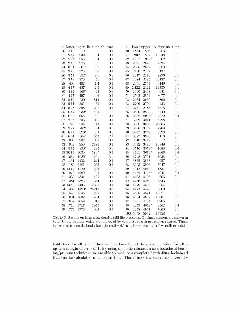
n lower upper lb. time ub. time n lower upper lb. time ub. time20 210 210 0.1 0.1 60 1834 1836 4.3 0.121 232 232 0.4 0.1 61 1897 1897 15648 0.122 253 253 3.4 0.1 62 1957 1959* 62 0.123 276 276 0.1 0.1 63 2021 2023 7594 0.124 301 301* 0.5 0.1 64 2085 2087 389 0.125 326 326 0.6 0.1 65 2150 2152 137 0.126 352 352* 2.1 6.2 66 2217 2218 2296 0.127 379 379 51 0.1 67 2284 2285 26137 0.128 406 407 1.4 0.1 68 2351 2354 3149 0.129 437 437 2.5 0.1 69 2422 2422 14755 0.130 466 466* 45 0.3 70 2490 2493 641 0.131 497 497 0.6 0.1 71 2562 2564 3077 0.132 530 530* 1815 0.1 72 2634 2636 866 0.133 563 563 60 0.1 73 2706 2709 433 0.134 598 598 207 0.1 74 2781 2783 3575 0.135 632 632* 1459 1.9 75 2856 2858 5440 0.136 668 668 0.1 0.1 76 2932 2934* 5879 3.437 706 706 1.1 0.1 77 3009 3011 5298 0.138 743 744 43 0.1 78 3088 3090 20865 0.139 782 782* 3.4 3.3 79 3166 3169 2768 0.140 823 823* 3.3 10.0 80 3247 3249 8328 0.141 864 864* 553 2.1 81 3327 3330 113 0.142 906 907 1.6 0.1 82 3410 3412 2 0.143 949 950 2176 0.1 83 3492 3495 10849 0.144 993 993* 285 3.4 84 3576 3579* 1083 3.645 1039 1039 3807 0.1 85 3661 3664* 3666 0.646 1084 1085* 101 3.4 86 3748 3751 7628 0.147 1131 1132 244 0.1 87 3835 3838 957 0.148 1180 1181 265 0.1 88 3923 3926 5047 0.149 1229 1229* 563 10 89 4012 4015 1837 0.150 1279 1280 9.2 0.1 90 4102 4105* 7047 3.251 1330 1331 105 0.1 91 4193 4196 605 0.152 1381 1383 354 0.1 92 4286 4289 8843 0.153 1436 1436 4326 0.1 93 4379 4382 2254 0.154 1489 1490* 25219 3.3 94 4473 4476 3669 0.155 1543 1545 296 0.1 95 4568 4571 10871 0.156 1601 1602 484 0.1 96 4664 4667 16801 0.157 1657 1659 816 0.1 97 4761 4764 36205 0.158 1716 1717 1950 0.1 98 4859 4862* 3462 3.459 1774 1776 992 0.1 99 4958 4961 7660 0.1

100 5058 5062 15458 0.1Table 5. Results on large max-density still life problems. Optimal answers are shown inbold. Upper bounds which are improved by complete search are shown starred. Timesin seconds to one decimal place (in reality 0.1 usually represents a few milliseconds)

holds true for all n and thus we may have found the optimum value for all nup to a margin of error of 1. By using dynamic relaxation as a lookahead learn-ing/pruning technique, we are able to produce a complete depth 400+ lookaheadthat can be calculated in constant time. This prunes the search so powerfully

Fig. 4. An optimal solution to 69×69.

that we can find optimal (or near optimal) solutions for a problem where thesearch space grows as 2n2

. The largest n for which the problem is completelysolved is n = 69 (shown in Figure 4). Further, we have proved upper and lowerbounds that differ by no more than 4 for all n up to 100. All of our solutionscan be found at www.csse.unimelb.edu.au/~pjs/still-life/.

Acknowledgments. We would like to thank Michael Wybrow for helping us gen-

erate the still life pictures used in this paper. NICTA is funded by the Australian

Government as represented by the Department of Broadband, Communications and

the Digital Economy and the Australian Research Council.

References

1. R. Bosch. Integer programming and conway’s game of life. SIAM Review, 41(3):596–604, 1999.

2. R. Bosch and M. Trick. Constraint programming and hybrid formulations for threelife designs. In Proceedings of the International Workshop on Integration of AIand OR Techniques in Constraint Programming for Combinatorial OptimizationProblems, CP-AI-OR’02, pages 77–91, 2002.

3. R. Dechter. Constraint Processing. Morgan Kaufman, 2003.4. N. Elkies. The still-life density problem and its generalizations.

arXiv:math/9905194v1.5. N. Elkies. The still-life density problem and its generalizations. Voronoi’s Impact

on Modern Science: Book I, pages 228–253, 1998. arXiv:math/9905194v1.6. J. Larrosa and R. Dechter. Boosting search with variable elimination in constraint

optimization and constraint satisfaction problems. Constraints, 8(3):303–326, 2003.7. J. Larrosa, E. Morancho, and D. Niso. On the practical use of variable elimination

in constraint optimization problems: ’still-life’ as a case study. Journal of ArtificialIntelligence Research, 2005.