Using Peltier cells to study solid–liquid–vapour … Peltier cells to study solid–liquid–vapour transitions and supercooling S15 Figure 1. Schematic picture of the experimental

IOP PUBLISHING EUROPEAN JOURNAL OF PHYSICS

Eur. J. Phys. 28 (2007) S13–S27 doi:10.1088/0143-0807/28/3/S02

Using Peltier cells to studysolid–liquid–vapour transitions andsupercooling

Giacomo Torzo1, Isabella Soletta2 and Mario Branca3

1 ICIS-CNR and Physics Department of Padova University, Padova, Italy2 Liceo Scientifico Fermi, Alghero, Italy3 Chemical Department of Sassari University, Sassari, Italy

E-mail: [email protected], [email protected] and [email protected]

Received 28 September 2006, in final form 8 November 2006Published 30 April 2007Online at stacks.iop.org/EJP/28/S13

AbstractWe propose an apparatus for teaching experimental thermodynamics inundergraduate introductory courses, using thermoelectric modules and areal-time data acquisition system. The device may be made at low cost,still providing an easy approach to the investigation of liquid–solid andliquid–vapour phase transitions and of metastable states (supercooling). Thethermoelectric module (a technological evolution of the thermocouple) is byitself an interesting subject that offers a clear example of both thermo-electric(Seebeck effect) and electro-thermal (Peltier effect) energy transformation.We report here some cooling/heating measurements for several liquids andmixtures, including water, salt/water, ethanol/water and sodium acetate,showing how to evaluate the phenomena of freezing point depression andelevation, and how to evaluate the water latent heat.

(Some figures in this article are in colour only in the electronic version)

1. Introduction

Introductory courses in thermodynamics are normally focused on the study of equilibriumstates that may be described through a reduced number of macroscopic variables and formthe necessary base for a general understanding. Similarly the quasi-static transformations,defined by infinitesimal heat exchanges with ideal reservoirs with infinite thermal capacity,are usually studied.

In contrast, in real laboratory experiments, quasi-static transformations or ideal heatreservoirs do not exist and frequently we do not reach true equilibrium states.

0143-0807/07/030013+15$30.00 c© 2007 IOP Publishing Ltd Printed in the UK S13

S14 G Torzo et al

In the present paper we describe an apparatus that, exploiting Peltier cells and a real-timedata acquisition system, makes possible to study several transformations that proceed throughnon-equilibrium states, allowing a rather deep insight on the investigated processes.

One advantage of the set-up described here is that the time required to carry out oneexperiment is normally in the range from 10 to 20 min, well within the 45 min typicallyavailable for lab class experiments.

2. Metastable states. Supercooling

The common idea of equilibrium is based on the experience that any system tends to evolveto a state of minimum energy in which its macroscopic behaviour becomes stable. Thereforea system that exhibits a stable behaviour is normally assumed to be an equilibrium state.

However, we know that some long-lived states that appear to be equilibrium states areinstead metastable states that may evolve into states of lower free energy. This may occurspontaneously, or may be necessarily an external triggering phenomenon. Examples ofmetastable states requiring an external trigger are chemical mixtures (such as gunpowderor mixtures of explosive gases, which react after sufficient heat input), or more simply anysupercooled liquid.

Supercooling in water is a phenomenon known for a long time [1]; it was first observedby Daniel Gabriel Fahrenheit in 1724, and later by Joseph Black. But almost any liquid can becooled to a metastable state by a sufficiently rapid cooling through the freezing point [2]. Thesolid phase grows from the liquid phase by increasing the size of initial crystalline clusters.These crystal seeds on the other hand may form only by passing over an energy barrier dueto the large surface-to-volume ratio of any small object. In the absence of such crystal seedsthe liquid phase may be maintained at temperatures much lower than the freezing point.Supercooled water may exist down to −40 ◦C. However, ice may form at higher temperature,depending on the cooling speed and on the presence of impurities that favour crystal seedsformation.

A popular supercooled liquid at room temperature [3] is the tri-hydrated sodium acetate(NaCOOCH3 3H2O), whose large latent heat produces huge temperature changes that areeasily observed even without any measuring device, for example in the ‘hand-warmer bags’.

3. Experimental set-up

The experimental set-up was designed to obtain, at low cost4 a useful temperature rangefrom −20 ◦C to 120 ◦C with a liquid sample volume of about 10 cm3. This allows us toinvestigate both freezing transitions and boiling temperatures in several common liquids, witheasy measurements that can be normally completed within half an hour.

The working principle of thermoelectric devices (Peltier cells) was well described in thisJournal by Kraftmakher [4] and it will not repeated here.

The system (see figure 1) is made of a sample holder (an aluminium pot) which is thermallycoupled to the ‘cold plate’ of a Peltier stack (made of two cells connected in series); the ‘hotplate’ of the stack is thermally coupled to an aluminium heat sink, linked to room temperatureby a standard PC blower.

A real-time data-acquisition system monitors the temperatures of sample, cold and hotplates during cooling/heating runs, allowing us to graph, not only the time evolution of thesample, but also the temperature gradients in different parts of the device.

4 The total cost of the components, excluding the power supply and the data acquisition system, is less than 100 euro.

Using Peltier cells to study solid–liquid–vapour transitions and supercooling S15

Figure 1. Schematic picture of the experimental set-up. (Not shown the neoprene insulating cap,the power supply and the data acquisition system).

3.1. The thermoelectric module

We use two identical cells instead of a pyramidal stack to simplify the device constructionand thermal insulation. The multi-stage cooling modules are in fact usually configured with asmaller cell on the cold side and a larger one at the hot side because the larger cell must pumpalso the energy dissipated by the Joule effect that adds to the energy transferred by the smallercell. We selected the cheap model [5] Pke128a0020 (http://www.opitec.it) whose dimensionsare 40 × 40 × 4.7 mm, with a nominal maximum power of 33 W.

The heat sink is a commercial component, commonly used to cool the computers CPU,which is sold with forced ventilation provided by a 12 V dc blower.

The sample holder is a square aluminium pot, dimensioned to match the geometry of thePeltier cells minimizing the surface area of the sample holder subject to moisture condensationand to radiation/convection thermal coupling with the ambient. It has 9 mm inner height,3 thin walls (2 mm) and a thicker one (8 mm), where a hole is drilled to host a thermometer.A second thermometer is suspended inside the pot to monitor the sample temperature, and athird thermometer is placed in a hole drilled on the aluminium heat sink.

If the thermal coupling between the sample holder and the ‘cold plate’ and between theheat sink and the ‘hot plate’ is good enough, we may assume the first thermometer measuresthe temperature of the cold plate and the third thermometer measures the temperature of thehot plate.

S16 G Torzo et al

The role of ‘cold’ and ‘hot’ plates obviously is exchanged when passing from cooling runto heating run.

The Peltier cells are thermally anchored to the sample holder and to the heat sink by usingthermally conductive grease and by applying a strong pressure to the contacting surfaces.

An important part of the device is the PVC flange, with a rectangular top aperture and fourretaining screws, that presses the ‘sandwich’ made of the sample holder plus the two Peltiercells, against the heat sink.

An elastic sealing, obtained from a rubber sheet 2 mm thick, maintains the high pressure,applied at room temperature, despite the changes of the geometry induced by different thermalexpansion coefficients in cooling/heating processes.

An outer (removable) cap made of insulating material (neoprene foam) covers the sampleholder to reduce the thermal coupling with the ambient during the measurements.

3.2. The data-acquisition system

We adopted the LabPro interface from Vernier (http://www.vernier.com), connected to aPC through USB port, that offers a very good cost/performance ratio, but similar productsare perfectly suited for our set-up, for example those produced by PASCO Scientific(http://www.pasco.com) or CMA (http://www.cma.science.uva.nl).

One advantage of the adopted interface is that it may also be used replacing the personalcomputer with a handheld graphic calculator, e.g. the Texas Instrument TI92, or TI89, orTI-Voyager (see the examples shown in the LEPLA Minerva Project at http://www.lepla.eu).

3.3. The thermometers

We used as temperature sensors the integrated-circuits National LM61 in a plastic TO92envelope (4.5 mm diameter, 5 mm length), with a nominally constant sensitivity of+10 mV K−1 and an output offset of +600 mV at T = 273 K.

The transfer function (calibrating equation) for this sensor is therefore T (◦C) = V∗100–60.The offset allows reading negative temperatures without the need for a negative supply:

the three-wire sensor in fact may be powered by the 5 V output supplied at the interfaceanalogue input (raw-voltage mode, range 0–5 V). No special skill is required for interfacingthis analogue sensor: only a cable with BT plug on one end must be used, and properconnections of the three sensor pins (ground, +5 V, output), as specified in the LabPro manual.It must also be noted that the wires connecting the sensor to the BT cable must be thin (e.g.30AWG), in order to reduce the thermal link between the sensor and room temperature.

One detail is very important, that is, the sample thermometer must be carefully placedhorizontally at the free surface of the liquid; therefore its position must be re-adjusted whenthe sample volume is changed. In fact, if the sensor is completely immersed in the liquidsample, it does not faithfully measure the temperature of the liquid–solid mixture when thesolid–liquid interface (that moves in the bottom–top direction) reaches the thermometer height.On the other hand if the sensor only touches the liquid surface the thermal coupling with thesample becomes poor.

We fixed the sensor, by a heat-shrinkable tube, to one end of a metal wire. The otherend of the wire is loop-shaped and blocked by one of the four retaining screws; by properlybending the wire, the sensor may be positioned at the required height.

The poor nominal accuracy of LM61B (a maximum error of 3 ◦C and a typical error of1 ◦C in the range −30 ◦C +100 ◦C) is mostly due to deviations from linearity, and this doesnot prevent reliable evaluation of temperature differences smaller than 1 ◦C. We tested several

Using Peltier cells to study solid–liquid–vapour transitions and supercooling S17

Figure 2. The temperature of the 12 cm3 water sample as a function of time. Black line:temperature T1 (sample); dark grey line: temperature T2 (sample holder); light grey line:temperature T3 (heat sink).

units and we found that the spread in the values of the measured temperatures was always lessthat 0.6 ◦C in the full range.

3.4. Power supply

The current supplied to the Peltier cells to transfer heat from the cold plate to the hot plate,(or vice versa, depending on the sign of the Peltier bias voltage) is fed by a power supply (e.g.0–30 V, 0–3 A).

The only requirement for the power supply is a small output ripple, and it may operateeither at constant voltage or at constant current. A commercial (wall-plug) power supply with12 V dc output feeds the blower.

4. Exploring phase transitions in various systems

The introductory experiment should be carried out using a sample of water. This makes easierthe students’ understanding of the results, and moreover the collected data may be later usedfor a calibration of the effective heat capacity of the system (see section 5). Later the studentsmay explore more complex systems, such as binary mixtures.

4.1. Supercooling of water

In figure 2 we report the result obtained while cooling a 12 cm3 water sample. The black curvemarks the temperature T1 of the sample, as measured by a sensor placed horizontally insidethe water, but close to the free surface. The dark-grey curve traces the temperature T2 of the

S18 G Torzo et al

aluminium pot, which is in good thermal contact with the cold plate of the Peltier cell. Thelight-grey curve traces the temperature T3 of the hot plate.

The shown cooling run starts from room temperature (20 ◦C) with the power supplyfeeding 1.4 A current, at 11 V, to the Peltier module. By recording also the temperature of thecold plate we may evaluate the temperature difference �T = T1–T2 across the sample volume.

The temperatures measured by the sample and cold plate thermometers decrease followinga nearly exponential curve due to the increasing thermal leak that steadily lowers the net heattransfer from the cold plate to the hot plate.

Near T1 = 4 ◦C we may observe a slight change in the slope, and a reduction of �T (thatwill decreases to about 5 ◦C at t = 300 s). This phenomenon is due to the anomaly of thewater density at T = 4 ◦C [6].

When cooling the sample from the bottom, at the beginning the lower water layers (cooler)are denser than the higher layers, and no convective flow contributes to the heat exchange withinthe fluid sample. The small thermal conductivity of water (0.56 W m−1 K−1 to be comparedwith the values 0.7 W m−1 K−1 for glass and 2.3 W m−1 K−1 for ice [7]) maintains a largegradient �T ≈ 8 ◦C. As soon as the water maximum density is crossed at about T = 4 ◦C,the water bottom layers (cooler) become lighter than the layers above (warmer), an convectiveflows begins, reducing the temperature gradient within the sample volume.

At t ≈ 250 s, the water temperature crosses the 0 ◦C value without freezing: supercoolingbegins. The sample enters into a metastable state, remaining liquid at temperatures below thefreezing temperature. In the run reported in figure 2 the metastable state collapses at t = 318 s,showing a steep rising, followed by a plateau at T = 0 ◦C.

Also the cold plate temperature T2 increases rapidly, proving that the water has transferreda large amount of heat to the container. This energy is released by the sudden freezing thewater layers close to the aluminium walls. The heat flush is so large that even the hot platemarks a slight temperature rise at the time t = 318 s, as shown by the light-grey curve T3.

On the plateau region, the top liquid water layers behave as a powerful heat source (latentheat) for the underlying solid water layers. All the energy drained by the bottom layers issupplied by the phase change so that the liquid temperature remains constant, while the coldplate temperature keeps on cooling at a smaller rate.

From t = 340 s to t = 690 s, the T1 curve is flat, then it starts bending, even if part of thesample is still liquid. This is due to the fact that the thermometer is partially coupled to thesolid phase, which is not isothermal (a strong gradient affects the ice layers due to the largeheat transfer).

Finally, near the time t = 750 s, almost all the liquid has been frozen, and �T is about 7 ◦C.The completion of freezing is marked by a slight increment in the slope of the cold platetemperature curve; at this time the heat load at the cold plate side (missing the latent heat ofsolidification) is due only to the specific heat of ice. This last feature is more visible when thepower supply to the Peltier cells is increased (see, for example, the similar plot in figure 10).

When the phase transition is completed in the whole volume, the T1 and T2 curves getcloser until (at t > 1100 s) the temperature difference becomes quite small (�T < 1 ◦C), dueto the fact that the thermal conductivity in ice is five times larger than in water. The residualsmall gradient is due to the heat leaking to the sample thermometer from the top (radiation,air convection and conduction through the thermometers wires).

At t = 1200 s the power supply of the Peltier cell is switched off and the heat flow isinverted because the inactive thermoelectric device is a good thermal conductor that links thesample holder to room temperature. Because now the major part of heat is supplied to the cellfrom bottom, the anomaly at T = 4 ◦C now inhibits the convection below 4 ◦C and induceconvection above 4 ◦C. The effect of the increased thermal coupling due to convective flow is

Using Peltier cells to study solid–liquid–vapour transitions and supercooling S19

Figure 3. Temperature of salt/water mixtures as a function of time. The legend shows thequantities of NaCl dissolved per 100 g of water in different samples.

also marked by a change in the slope of T2. As a result the temperature difference drops from�T = −8 ◦C at t = 2300 s to �T = −4 ◦C at t = 2500 s.

This short series of data includes a large amount of information and hints for classroomdiscussions. It may introduce the students to a critical reading of plots and to a refining ofanalysis. The data also reveal unexpected details, not shown in textbooks that normally discussideal situations where transformations are quasi-static and involve homogeneous samples.

4.2. Water/salt mixtures

The water/salt mixture is a system particularly suited for educational experiments [8]; it is acommon system with important applications in physics, chemistry and biology. It is part ofthe common knowledge both of teachers and of students. The NaCl/H2O mixtures are easy tobe prepared, using tap water and kitchen salt, without any special prerequisite or sophisticatedlaboratory tools, and therefore they may be proposed for experiments both for introductorycourses in university science labs, or even in secondary high schools.

In the following we describe some results, obtained using our apparatus to show firstlythe freezing point depression in solutions (as well as the supercooling effect), then the boilingpoint elevation.

In figure 3 we report several cooling runs taken with mixture with increasing salt content.By increasing the NaCl concentration the freezing temperature decreases, showing clearly thephenomenon of freezing point depression. From these data the students may infer how muchsalt must be used to melt out the ice on the streets in the case of very cold winter!

We observe that while in pure water the freezing plateau maintains a rather constanttemperature, in salt solutions the temperature clearly decreases with time. This effect is dueto the change in concentration during freezing. Therefore the freezing temperatures must beextrapolated [9] from the cooling curves, as shown in figure 3 (curve 4).

S20 G Torzo et al

Figure 4. Temperature of salt/water mixtures as a function of time. The legend show the quantitiesof NaCl dissolved per 100 g of water in different samples.

Table 1. (∗) Values derived from the eutectic plot of the NaCl/water mixture.

Weight Weight T peak value T extrapolated value Reference [11] (∗)(g) (%) (◦C) (◦C) (◦C)

0 0 0,2 0,2 02.5 2 −3 −2 −14.5 4 −5 −3 −29.0 8 −7 −6 −5

14.0 12 −12 −10 −920.0 17 −15 −13 −13

Despite the relative simple procedure here used, the results are in fair agreement with datareported in the literature [10], as shown in table 1.

In the sample with maximum concentration (here 20 g of salt in 100 g of water correspondsto a NaCl concentration of 17%, slightly lower than the eutectic concentration of 23%) thesupercooling effect almost disappears, probably because at the lowest temperatures the coolingspeed becomes low enough to allow crystal seeds nucleation at a temperature close to thefreezing point.

Using the same apparatus, by simply reversing the sign of the current supplied to thePeltier cells, we may explore also the phenomenon of the boiling point elevation.

In figure 4 we report several heating runs taken with mixture with increasing salt content.By increasing the NaCl concentration the boiling temperature increases from 100 ◦C up

to about 106 ◦C at the saturated solution (36 g of salt in 100 g of water corresponds to themaximum NaCl concentration of 26.5%).

Here we may compare the measured values of the boiling temperature in different samplesT(m) = Tb + �T with those predicted by the formula �T = i Kb · m, where Tb is the boilingpoint for the solvent, Kb is the boiling point elevation constant and m the molal concentration

Using Peltier cells to study solid–liquid–vapour transitions and supercooling S21

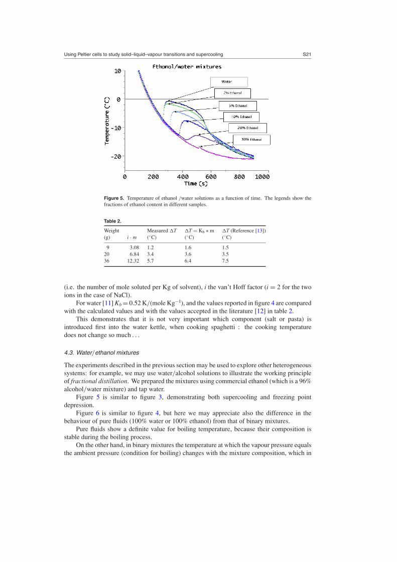
Figure 5. Temperature of ethanol /water solutions as a function of time. The legends show thefractions of ethanol content in different samples.

Table 2.

Weight Measured �T �T = Kb ∗ m �T (Reference [13])(g) i · m (◦C) (◦C) (◦C)

9 3.08 1.2 1.6 1.520 6.84 3.4 3.6 3.536 12.32 5.7 6.4 7.5

(i.e. the number of mole soluted per Kg of solvent), i the van’t Hoff factor (i = 2 for the twoions in the case of NaCl).

For water [11] Kb = 0.52 K/(mole Kg−1), and the values reported in figure 4 are comparedwith the calculated values and with the values accepted in the literature [12] in table 2.

This demonstrates that it is not very important which component (salt or pasta) isintroduced first into the water kettle, when cooking spaghetti : the cooking temperaturedoes not change so much . . .

4.3. Water/ethanol mixtures

The experiments described in the previous section may be used to explore other heterogeneoussystems: for example, we may use water/alcohol solutions to illustrate the working principleof fractional distillation. We prepared the mixtures using commercial ethanol (which is a 96%alcohol/water mixture) and tap water.

Figure 5 is similar to figure 3, demonstrating both supercooling and freezing pointdepression.

Figure 6 is similar to figure 4, but here we may appreciate also the difference in thebehaviour of pure fluids (100% water or 100% ethanol) from that of binary mixtures.

Pure fluids show a definite value for boiling temperature, because their composition isstable during the boiling process.

On the other hand, in binary mixtures the temperature at which the vapour pressure equalsthe ambient pressure (condition for boiling) changes with the mixture composition, which in

S22 G Torzo et al

Figure 6. Temperature of ethanol/water solutions as a function of time. The legend shows thenominal volume fraction of ethanol content in different water samples at the start of heating.

Table 3. The effective ethanol volume fraction is calculated from nominal values assuming astarting mixture of 96% ethanol in water (commercial alcohol). The expected Tb values are takenfrom [14].

Ethanol volume Ethanol molal Expected Measuredfraction (%) fraction (%) Tb (◦C) Tb (◦C)

0 0 100 99.314.4 5.0 91 8924 9.1 88 8748 23.2 83 8396 88.4 79 78

turns changes during the boiling process, because mainly the component with lower boilingtemperature does evaporate.

As a consequence, the heating curves of pure fluids show a horizontal plateau at theboiling temperature, while mixture’s heating curves show only a change in slope when boilingbegins.

Table 3 compares the measured values of the measured boiling temperatures (thetemperatures where the T1 curves change slope) and the expected values [13].

4.4. Supercooling of sodium acetate

A cooling run with sodium acetate does not offer substantial news about supercooling, but itmay amaze the students with the very large amount of heat that the sample delivers when themetastable liquid relaxes into the solid phase.

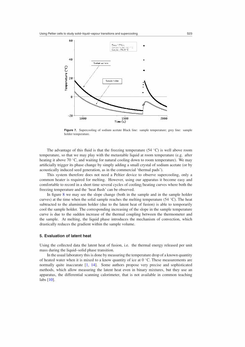
Figure 7 shows an example of such transition where the sample temperature jumps upabout 70 ◦C in few seconds (from −15 ◦C to 54◦C). The temperature rise would be even largerif the sample would not be thermally coupled to the aluminium holder: part of the heat flushis in fact transmitted to the sample holder whose temperature rise is about 13 ◦C.

Using Peltier cells to study solid–liquid–vapour transitions and supercooling S23

Figure 7. Supercooling of sodium acetate Black line: sample temperature; grey line: sampleholder temperature.

The advantage of this fluid is that the freezing temperature (54 ◦C) is well above roomtemperature, so that we may play with the metastable liquid at room temperature (e.g. afterheating it above 70 ◦C, and waiting for natural cooling down to room temperature). We mayartificially trigger its phase change by simply adding a small crystal of sodium acetate (or byacoustically induced seed generation, as in the commercial ‘thermal pads’).

This system therefore does not need a Peltier device to observe supercooling, only acommon heater is required for melting. However, using our apparatus it become easy andcomfortable to record in a short time several cycles of cooling/heating curves where both thefreezing temperature and the ‘heat flush’ can be observed.

In figure 8 we may see the slope change (both in the sample and in the sample holdercurves) at the time when the solid sample reaches the melting temperature (54 ◦C). The heatsubtracted to the aluminium holder (due to the latent heat of fusion) is able to temporarilycool the sample holder. The corresponding increasing of the slope in the sample temperaturecurve is due to the sudden increase of the thermal coupling between the thermometer andthe sample. At melting, the liquid phase introduces the mechanism of convection, whichdrastically reduces the gradient within the sample volume.

5. Evaluation of latent heat

Using the collected data the latent heat of fusion, i.e. the thermal energy released per unitmass during the liquid–solid phase transition.

In the usual laboratory this is done by measuring the temperature drop of a known quantityof heated water when it is mixed to a know quantity of ice at 0 ◦C. These measurements arenormally quite inaccurate [1, 14]. Some authors propose very precise and sophisticatedmethods, which allow measuring the latent heat even in binary mixtures, but they use anapparatus, the differential scanning calorimeter, that is not available in common teachinglabs [10].

S24 G Torzo et al

Figure 8. Repeated heating/cooling cycles of sodium acetate. Black line: sample temperature;dark-grey line: sample holder temperature; light-grey line: temperature of the Peltier cell platecoupled to room temperature by air blower.

Our method is less direct than those found in the literature but it offers a fast and easydata acquisition.

In order to evaluate the latent heat from the data taken during a liquid solid phase transition,we must know the sample specific heat c, its mass m and the effective heat capacity of thesample holder Cx.

From the slope S = dT/dt of the cooling curve for the sample holder, measured near thefreezing temperature, we evaluate the cooling power W = S (c m + Cx).

The energy supplied to the sample holder in a time interval �t, near the freezingtemperature, is therefore approximated by the product W �t.

Then we measure, on the sample cooling curve, the time �tx passed from the instantof crossing the freezing temperature until the end of the plateau (when the curve slope startincreasing).

The total energy supplied to the sample is therefore E = W �tx − Cx (T2−T1), where T2

and T1 are the temperatures of the sample holder at the beginning and end of the time interval�tx. In our measurements this temperature difference is almost negligible, so that we mayapproximate the above relation with E = W �tx.

The latent heat L may be therefore calculated as

L = E/m = W �tx/m = S �tx (cm + Cx)/m.

The parameter Cx is greater that the nominal heat capacity C = mal cal (calculated from its massmal and the aluminium specific heat cal). The Peltier cell in fact does cool also the material thatis in thermal contact with the sample holder (the cell itself, the retaining cap and the insulatingcap . . . ).

We may however evaluate Cx by comparing the cooling slopes of two curves, one takenwith the mass m1 of water (S1) and the other with the empty sample holder (S0), using the samepower input for the Peltier cells. In fact from the two relations W = S1 (c m1 + Cx), and W =S0 Cx we get

Using Peltier cells to study solid–liquid–vapour transitions and supercooling S25

Figure 9. Procedure to calculate the effective heat capacity as explained in the text. Run takendriving the Peltier cell with I = 1.6 A. The data points linearly interpolated are those enclosed inthe square brackets.

Cx = c m1 S1/(S0 − S1).

In our apparatus the value of Cx, calculated from the two cooling runs shown in figure 9(one with empty sample holder and one with 5 cm3 of water) may be assumed to be about(45 ± 4) J K−1, much larger than the value 18 J K−1 calculated for the 20 g aluminium sampleholder.

Using the calculated value of Cx, the known value of the water specific heat c =4.18 J g−1 C−1 and the values obtained from the cooling run reported in figure 10 [m =(6 ± 0.2) g, �tx = (342 ± 4) s, S = 0.083 ± 0.001) ◦C s−1], we obtain for the water latentheat L = (332 ± 38) J g−1, a value in good agreement with the known value L = 335 J g−1.

Note that the calculated value of Cx is a constant (it should not depend on the powerapplied to the Peltier cells, i.e. on the value of the heat flux drained from the sample holder).

6. Comparing Peltier and Seebeck effects

The system we have described may also be used to give practical examples of the efficiency oftwo energy conversion processes: the Peltier effect converts electric power into heat transferbetween two reservoirs, the Seebeck effect converts the heat flux into electric power [15, 16].

This may be obtained by adding a simple option: a toggle switch, at the end of a cooling orheating run, disconnects the wires feeding the Peltier cell from the power supply and connectsthem to a motor driving a small propeller.

The students will see the Peltier module converted into a thermoelectric generator thatexploits the thermal gradient to produce a dc current: this is the Seebeck effect, usuallymentioned when studying the thermocouple.

S26 G Torzo et al

Figure 10. Cooling run, with I = 1.8 A with a water sample; m = 6 g, t1 = 198 s, t2 = 540 s, S1 =0.083 ◦C s−1.

By measuring the power spent by the power supply (the product W = IV) during thecooling/heating run, and the same quantity while driving the propeller, the students may getan idea of the small efficiency of the complete energy transformation: less than 1% of theelectrical power spent by the power supply is converted into power used by the motor [17].

For example, in the run shown in figure 2 the power source supplies about 15.4 W during1210 s of cooling, thus dissipating about E1 = 18.6 kJ of electrical energy. On the other hand,the system gained the free energy H1 by cooling 12 g of water from the initial temperatureT1 = 21 ◦C to 0 ◦C, then H2 by cooling 12 g of ice from 0 ◦C to T2 = −21 ◦C. Becausealso the aluminium sample holder was cooled, we may optimistically evaluate an extra gainin enthalpy H3 for cooling from T1 to T2 a mass equivalent to the calculated heat capacityCx = 45 J ◦C−1.

The total gain in enthalpy (using the water specific heat cw = 4.18 J g−1 ◦C−1 and theice specific heat ci = 2.04 J g−1 ◦C−1) was therefore at maximum H = H1 + H2 + H3 =7.5 kJ, with an energy loss of about E1 – H = 11.1 kJ. We may note that more than 50% of theenthalpy is related to the latent heat.

The efficiency of the electro thermal conversion was about H/E1 = 40%.During the heating shown in figure 2 the Peltier module was connected to the motor and

we measured a starting voltage across the motor winding of about 1.9 V with a current of about0.05 A, corresponding to a starting Wout = IV = 0.1 W. However, the product Wout was linearlydecreasing with the temperature difference �T between hot and cold plates. The propeller infact stopped rotating about at the time t = 2600 s, when the electrical power output due to theSeebeck effect became comparable with the friction losses.

Even assuming a constant power output equal to the initial Wout for the full heating curvelasting about 1600 s, the enthalpy converted into electrical energy would be about E2 0.15 kJ,with an efficiency E2/H of about 2%.

Using Peltier cells to study solid–liquid–vapour transitions and supercooling S27

The overall efficiency of the two processes was therefore less than 1%.

7. Conclusions

We designed this apparatus in order to use it with our students in an introductory undergraduatecourse next year. Therefore we do not have yet checked it within a real course. However,the tests we made show that it offers a wide range of didactical applications. It may beused both for qualitative and quantitative investigations, substituting the traditional devicesfor heating/cooling. Its use is quite simple and easy, allowing us to study the dynamics ofseveral phenomena in thermodynamics, exploiting a real-time data acquisition system.

We have shown some examples, beginning with the classic phase change experiment(water/ice/water), adding the possibility of easy evaluation of the thermal exchanges occurringduring the phase transitions, allowed by the simultaneous use of three temperature sensors.

The device outputs experimental plots which are complex and rich of information, andquite reproducible, suitable for analysis at different levels (depending on the didactic goals ofthe teacher and on the age of the students).

The experiments with binary mixtures (either water/salt or water/ethanol) may also beeasy performed, adding information on metastable states, which are rarely studied in textbooks.We added also one example on latent heat evaluation derived from the analysis of the coolingcurves.

The proposed examples should suggest more activities aimed at improving the studentsability in focusing a phenomenon and interpreting the experimental result within the frame oftheoretical models.

References

[1] Guemez J, Fiolhais C and Fiolhais M 2002 Reproducing Black’s experiments: freezing point depression andsupercooling of water Eur. J. Phys. 23 83–91

Guemez J, Fiolhais C and Fiolhais M 2002 Revising the Black’s experiments on the latent heat of water Phys.Teach. 40 26–31

[2] Vali G 1971 Supercooling of water and nucleation of ice Am. J. Phys. 39 1125–8[3] Menon N 1999 A simple demonstration of a metastable state Am. J. Phys. 67 1109–10[4] Kraftmakher Y 2005 Simple experiments with a thermoelectric module Eur. J. Phys. 26 959–67[5] Similar devices are produced by Melcor Corporation http://www.melcor.com (model CP 1.4-127-10L), or by

Beijng Huimao Cooling Equipment Co. http://www.huimao.com (model TEC1-12704T125)[6] Branca M and Soletta I 2005 Thermal expansion: using calculator-based laboratory technology to observe the

anomalous behaviour of water J. Chem. Educ. 82 613–5[7] Andersen E S, Jespergaard P and Østersgard O 1985 Data Book (Pordenone: Studio Tesi Ed.) p 124[8] Guemez J, Fiolhais C and Fiolhais M 2005 Quantitative experiments on supersaturated solutions for the

undergraduate thermodynamics laboratory Eur. J. Phys. 26 25–31[9] Hoare J P 1960 Freezing point measurement J. Chem. Educ. 37 146–7

[10] Han B, Hwan C J, Dantzig J A and Bischof J C 2006 A quantitative analysis on latent heat of an aqueous binarymixture Cryobiology 52 146–51

[11] Atkins P 1998 Physical Chemistry (Oxford: Oxford University Press)[12] Washburn E W 1928 International Critical Tables of numerical Data, Physics, Chemistry and Technology

vol III (New York: McGraw-Hill) p 326[13] http://homedistiller.org/calc.htm[14] Mak S Y and Chun C K W 2000 Phys. Educ. 35 181–6[15] Gupta V K, Shanker G, Saraf B and Sharma N K 1984 Experiment to verify the second law of thermodynamics

using a thermoelectric device Am. J. Phys. 52 625–8[16] Cvahte H and Strnad J 1988 A thermoelectric experiment in support of the second law Eur. J. Phys. 9 11–7[17] Gordon J M 1991 Generalized power versus efficiency characteristics of heat engines: the thermoelectric

generator as an instructive illustration Am. J. Phys. 59 551–5