Using multivariate clustering to characterize ecoregion borders

Ecologists have long used massive datasets as the basis for visualizing eco-region maps.1,2 Ecoregions are areascontaining similar environmental con-

ditions that are classified for particular purposes.For example, the US Department of Agriculturepublishes a map of Plant Hardiness Zones, whichdivides the US into different ecoregions so thatgardeners can select appropriate plants andshrubs for their particular area. The ecoregion isone of the most important concepts in managingand understanding landscape ecology.3,4 Unfor-tunately, ecologists have long struggled with ex-actly how and where to locate the dividing linesbetween ecoregions.5,6

Historically, the process of regionalization—drawing ecoregion borders—has been subjec-tive: experts have attempted to integrate andweigh all of the environmental characteristicsand draw the borders accordingly, often withoutbeing able to elucidate the logic behind their

lines. This subjectivity leads to frequent revi-sions5–8 and disagreements over particular loca-tions,9 and hampers widespread acceptance anduse of such maps. Some experts, in fact, are un-able to correctly identify actual ecoregion mapsfrom synthetic maps simulated using a fractaltechnique.10

Part of the problem is the variable nature ofthe borders between ecoregions. Some bordersare very sharp and distinct, and you can literallystand with your feet in two clearly different re-gions. Ecologists call such unequivocal and easy-to-locate borders ecotones, because they representsharp cuts. However, most borders are more likethe M.C. Escher woodcut Sky and Water I(www.cs.rochester.edu/u/si/images/escher/birds_fish.gif), in which black birds slowly transform intowhite fish. Although the picture clearly containstwo distinct creatures, it’s difficult to locate a lineof demarcation between them. We define a newterm, ecopause, to indicate the indistinct natureof such borders. But a border may actuallychange character along its length. For example,a border can begin in one geographic locationas an ecotone and transform slowly along itslength into an ecopause. Unfortunately, ecolo-gists have had only simple lines with which tovisualize these many types of borders.

Locating ecoregion borders is a multivariatedecision process that must consider a large geo-

18 COMPUTING IN SCIENCE & ENGINEERING

USING MULTIVARIATE CLUSTERINGTO CHARACTERIZE ECOREGIONBORDERS

The authors’ clustering technique unambiguously locates, characterizes, and visualizesecoregions and their borders. When coded with similarity colors, it can produce planar mapviews with sharpness contours that are visually rich in ecological information and representintegrated visualizations of complex and massive environmental data sets.

M A S S I V E D A T AV I S U A L I Z A T I O N

WILLIAM W. HARGROVE

University of Tennessee FORREST M. HOFFMAN

Oak Ridge National Laboratory

1521-9615/99/$10.00 © 1999 IEEE

JULY/AUGUST 1999 19

graphic data set for each of multiple environ-mental conditions. We have developed an ob-jective technique called Multivariate GeographicClustering, which objectively computes borderplacement between ecoregions, given maps of allenvironmental conditions under consideration.Our technique lets us locate and visualize eco-region borders, and portray the instantaneoussharpness of those borders at every point alongthe line. Here, we present our technique and of-fer sample visualizations.

Multivariate Geographic Clustering

Rather than relying on expertise, MultivariateGeographic Clustering uses standardized valuesfor each selected environmental condition in amap’s individual raster cells as coordinates thatspecify the cell’s position in environmental dataspace. The number of dimensions in data spaceequals the number of environmental character-istics. Two raster cells with similar environmen-tal characteristics from anywhere in the map willappear near each other in data space; their close-ness and relative position quantitatively reflectsenvironmental similarities.

Our algorithm disassembles the map cells fromgeographic space and uses the standardized valueof each of the environmental characteristics ascoordinates to replot the cells in environmentaldata space. Because the density of cells in dataspace is variable, we use an iterative classificationprocedure to group nearby cells into clustersbased on similar environmental conditions.

The processTo begin the process, the user specifies the de-sired number of clusters. The initial part of thealgorithm then examines observations sequen-tially to find the most widely separated set ofcells that will constitute the initial cluster“seeds.” Each map cell is then compared againstall cluster seeds and assigned membership in thecluster closest to it in terms of Euclidean dis-tance. After all map cells are assigned, new clus-ter centroids are calculated as the mean of eachcoordinate in the cluster. At this point, the iter-ative assignment procedure repeats. Cells do notmove in environmental data space; rather, thecluster centroids slowly migrate until theyachieve equilibrium. When fewer than a speci-fied number of map cells change cluster assign-ments in a particular iteration, the process halts.

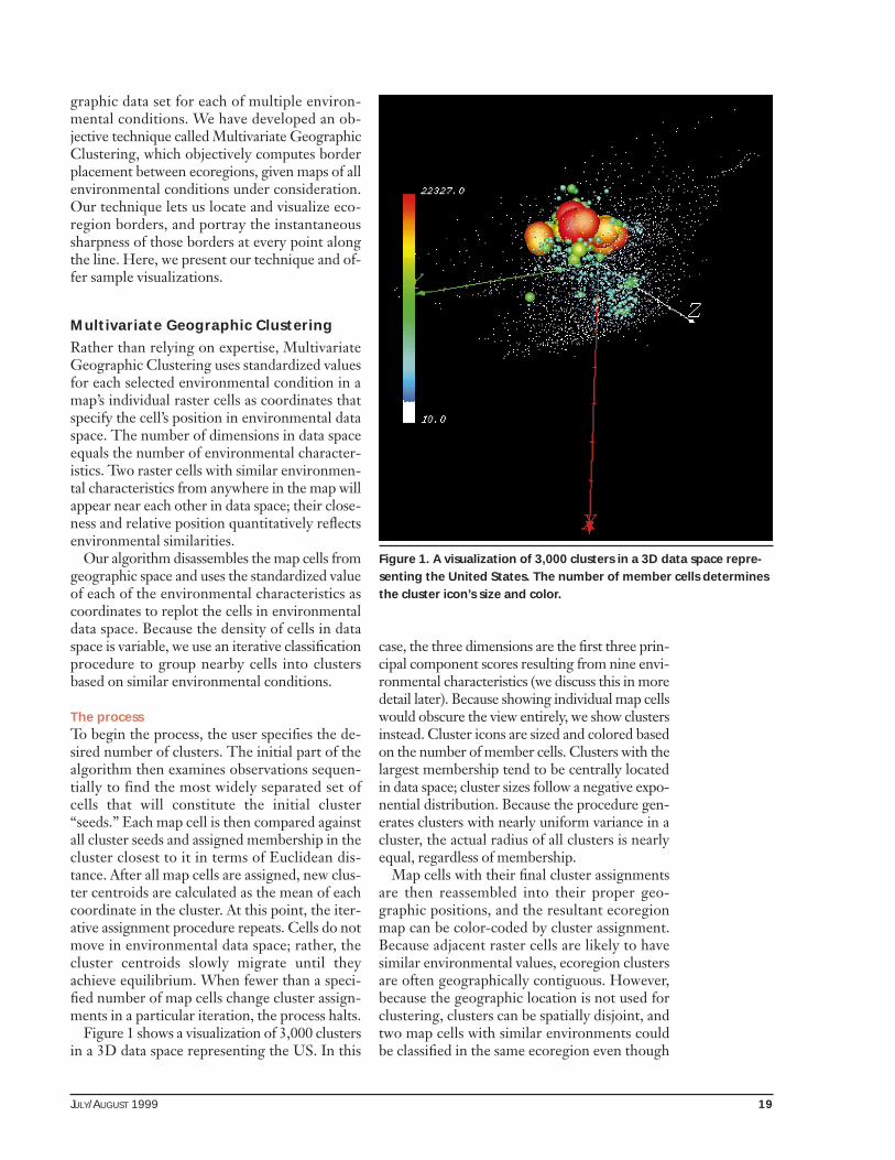
Figure 1 shows a visualization of 3,000 clustersin a 3D data space representing the US. In this

case, the three dimensions are the first three prin-cipal component scores resulting from nine envi-ronmental characteristics (we discuss this in moredetail later). Because showing individual map cellswould obscure the view entirely, we show clustersinstead. Cluster icons are sized and colored basedon the number of member cells. Clusters with thelargest membership tend to be centrally locatedin data space; cluster sizes follow a negative expo-nential distribution. Because the procedure gen-erates clusters with nearly uniform variance in acluster, the actual radius of all clusters is nearlyequal, regardless of membership.

Map cells with their final cluster assignmentsare then reassembled into their proper geo-graphic positions, and the resultant ecoregionmap can be color-coded by cluster assignment.Because adjacent raster cells are likely to havesimilar environmental values, ecoregion clustersare often geographically contiguous. However,because the geographic location is not used forclustering, clusters can be spatially disjoint, andtwo map cells with similar environments couldbe classified in the same ecoregion even though

Figure 1. A visualization of 3,000 clusters in a 3D data space repre-senting the United States. The number of member cells determinesthe cluster icon’s size and color.

20 COMPUTING IN SCIENCE & ENGINEERING

they are widely separated geographically. For ex-ample, two widely spaced but environmentallysimilar mountaintops could be classified in thesame ecoregion cluster.

ImplementationWe have implemented Multivariate GeographicClustering in a parallel algorithm coded in C us-ing the Message Passing Interface. Our code isdynamically load-balancing and fault-tolerant,and it performs both initial seed-finding and it-erative cluster assignment in parallel. The clus-tering algorithm is inherently parallelizable, be-cause individual nodes can independently classifya portion of all cells, and then combine resultsat the end of the iteration.

We developed the Multivariate GeographicClustering parallel algorithm and code on a highlyheterogeneous Beowulf-class parallel machineconstructed from surplus 486- and Pentium-basedPCs. This 128-node “Stone SouperComputer” isdescribed elsewhere11 and online at www.esd.ornl.gov/facilties/beowulf.

We performed many empirical regionaliza-tions for the conterminous US at one-square-kilometer resolution for up to nine environ-mental characteristics12,13 and have divided theUS into as many as 7,000 distinct ecoregions.14

At this resolution, each of the nine US environ-mental-condition maps comprises more than 7.8million cells. This map, data, and ecoregion res-olution surpasses what ecoregion experts usuallyaccomplish.

The example US ecoregions we show here arefrom a Multivariate Geographic Clustering at a

resolution of four square kilometers on nineparticular environmental characteristics impor-tant to plant growth. The environmental char-acteristics we considered included elevation,slope, soil bulk density, mineral soil depth, bed-rock depth, mean annual temperature, mean an-nual precipitation, soil water-holding capacity,and mean annual solar insolation, includingcloud interception.

Our first principal-component analysis groupedsoil density, soil depth, and bedrock depth into aprincipal component encompassing soil factors.The second PCA grouped temperature and pre-cipitation, and inverse elevation and slope. Thethird PCA grouped solar insolation and inversesoil water-holding capacity. We used the threeprincipal components as the axes for the envi-ronmental data space and the basis for thisecoregionalization.

Figure 2 shows the resulting map of the con-terminous US, which is divided into 50 distinctecoregions based on the nine environmentalconditions and identified by randomly assignedcolors. Although this map contains about half amillion cells, each with nine characteristics, par-allel Multivariate Geographic Clustering can ef-ficiently handle much larger problems.

Color-coding similaritiesVisualizing ecoregions with random colors em-phasizes the location of the borders. However,ecologists might also want to see the relative mixof conditions in bordering ecoregions. Becausethe cluster centroid’s final location is, by defini-tion, central, its coordinates describe the aver-age ecological conditions in the cluster eco-region. Comparing centroid coordinates fromtwo ecoregions quantifies the differences be-tween the average environments in each.

If, through PCA, we condense numerous “raw”environmental variables into three orthogonalprincipal-component axes in the environmentaldata space, we can perform a one-to-one scalarmapping of the first, second, and third principalcomponent scores to a red-green-blue (RGB)color triplet. In this way, we can combine thethree coordinates for each cluster centroid tospecify a unique color for that ecoregion. Underthis similarity-colors scheme, each ecoregion’scolor indicates the relative mix of each environ-mental factor. Comparing adjacent ecoregions isthus simple: ecoregions of similar colors havesimilar environments.

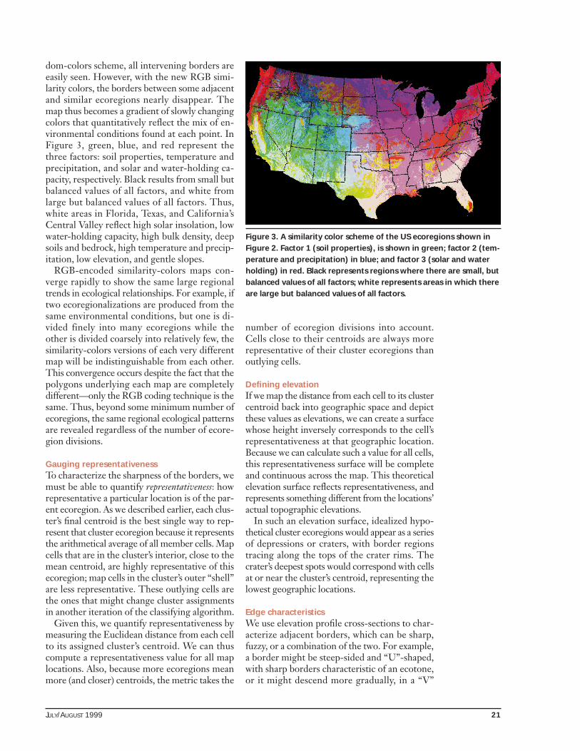
Figure 3 shows Figure 2’s ecoregions using thesimilarity-colors scheme. With Figure 2’s ran-

Figure 2. Using nine environmental conditions, the Multivariate Ge-ographic Clustering technique segregated the continental US into50 distinct ecoregions, represented by randomly assigned colors.

JULY/AUGUST 1999 21

dom-colors scheme, all intervening borders areeasily seen. However, with the new RGB simi-larity colors, the borders between some adjacentand similar ecoregions nearly disappear. Themap thus becomes a gradient of slowly changingcolors that quantitatively reflect the mix of en-vironmental conditions found at each point. InFigure 3, green, blue, and red represent thethree factors: soil properties, temperature andprecipitation, and solar and water-holding ca-pacity, respectively. Black results from small butbalanced values of all factors, and white fromlarge but balanced values of all factors. Thus,white areas in Florida, Texas, and California’sCentral Valley reflect high solar insolation, lowwater-holding capacity, high bulk density, deepsoils and bedrock, high temperature and precip-itation, low elevation, and gentle slopes.

RGB-encoded similarity-colors maps con-verge rapidly to show the same large regionaltrends in ecological relationships. For example, iftwo ecoregionalizations are produced from thesame environmental conditions, but one is di-vided finely into many ecoregions while theother is divided coarsely into relatively few, thesimilarity-colors versions of each very differentmap will be indistinguishable from each other.This convergence occurs despite the fact that thepolygons underlying each map are completelydifferent—only the RGB coding technique is thesame. Thus, beyond some minimum number ofecoregions, the same regional ecological patternsare revealed regardless of the number of ecore-gion divisions.

Gauging representativenessTo characterize the sharpness of the borders, wemust be able to quantify representativeness: howrepresentative a particular location is of the par-ent ecoregion. As we described earlier, each clus-ter’s final centroid is the best single way to rep-resent that cluster ecoregion because it representsthe arithmetical average of all member cells. Mapcells that are in the cluster’s interior, close to themean centroid, are highly representative of thisecoregion; map cells in the cluster’s outer “shell”are less representative. These outlying cells arethe ones that might change cluster assignmentsin another iteration of the classifying algorithm.

Given this, we quantify representativeness bymeasuring the Euclidean distance from each cellto its assigned cluster’s centroid. We can thuscompute a representativeness value for all maplocations. Also, because more ecoregions meanmore (and closer) centroids, the metric takes the

number of ecoregion divisions into account.Cells close to their centroids are always morerepresentative of their cluster ecoregions thanoutlying cells.

Defining elevation If we map the distance from each cell to its clustercentroid back into geographic space and depictthese values as elevations, we can create a surfacewhose height inversely corresponds to the cell’srepresentativeness at that geographic location.Because we can calculate such a value for all cells,this representativeness surface will be completeand continuous across the map. This theoreticalelevation surface reflects representativeness, andrepresents something different from the locations’actual topographic elevations.

In such an elevation surface, idealized hypo-thetical cluster ecoregions would appear as a seriesof depressions or craters, with border regionstracing along the tops of the crater rims. Thecrater’s deepest spots would correspond with cellsat or near the cluster’s centroid, representing thelowest geographic locations.

Edge characteristicsWe use elevation profile cross-sections to char-acterize adjacent borders, which can be sharp,fuzzy, or a combination of the two. For example,a border might be steep-sided and “U”-shaped,with sharp borders characteristic of an ecotone,or it might descend more gradually, in a “V”

Figure 3. A similarity color scheme of the US ecoregions shown inFigure 2. Factor 1 (soil properties), is shown in green; factor 2 (tem-perature and precipitation) in blue; and factor 3 (solar and waterholding) in red. Black represents regions where there are small, butbalanced values of all factors; white represents areas in which thereare large but balanced values of all factors.

22 COMPUTING IN SCIENCE & ENGINEERING

shape, characteristic of an ecopause. Also, be-cause edge properties are dependent on each ad-jacent cluster, each side has distinct (and possiblydifferent) properties. Although initially coun-terintuitive, this “sidedness” property is logical,given that we are characterizing the transitionfrom the border to the centroid independentlyon each side. Thus, for example, a border mightbe sharp on one side and fuzzy on the other.

To visualize border sharpness, we use contourlines. As Figure 4 shows, closely spaced contoursreflect steep sides and therefore a sharp ecotone;widely spaced contours indicate gradually slop-ing crater walls and a fuzzy, gradual ecopause.We can also represent borders that change fromfuzzy to sharp or vice versa, as the figure shows.

Visualization examples

We have used our clustering technique to produceecoregion maps for many areas. Here we examinein detail ecoregions and borders from the south-eastern US and southern and central California.Full-size high-resolution versions of these visual-izations, along with other examples, are availableonline at www.esd.ornl.gov/~hnw/borders.

Figure 5 shows a 3D visualization of the rep-resentativeness surface for Alabama, southwestGeorgia, and northern Florida. Each square inthe mesh represents a single four-square-kilo-meter raster cell; we find the cell’s elevation bymeasuring the Euclidean distance between it andthe centroid of its cluster. Cluster membershipis shown in Figure 5 as the (random) color of

(a) (b) (c) (d)

Figure 4. Using contour lines, we can visualize borders that are (a) sharp on both sides, (b) fuzzy on both sides, and (c)mixed. We can also represent (d) borders that change sharpness characteristics along their length.

Figure 5. Representativeness topography forAlabama (upper left), southwest Georgia (upperright), and northern Florida. Ecoregions areshown as random colors.

Figure 6. Southeastern ecoregions representedwith equal-elevation contours draped onto therepresentativeness surface to visualize the sharp-ness of the ecoregion borders.

JULY/AUGUST 1999 23

each cell. The representativeness topography iscontinuous and interpretable at this resolution.

The region’s major cities (Atlanta, Macon, andColumbus) are shown as a discontinuous purpleurban cluster. From west to east, four rivers (theFlint, Ocmulgee, Oconee, and Ogeechee) areseen as linear extensions of central Georgia’skelly-green piedmont ecoregion, flowing intothe state’s red coastal plain. In southern Al-abama, the red coastal plain and kelly-greenpiedmont ecoregion colors interdigitate, show-ing single cells of red within green and viceversa. The light-green southwestern Appalachi-ans pass through northeast Georgia into easternAlabama. In northwestern Alabama, the olive-drab ridge-and-valley ecoregion forms a higher-elevation representativeness plateau.

Figure 6 shows equal-elevation representative-ness contours visualizing the sharpness of theseecoregion borders. In southern Alabama, the con-tours’ random orientation and meandering char-acter near the red coastal plain and kelly-greenpiedmont ecoregions clearly indicate that this bor-der is an ecopause. In contrast, northern Alabama’sclosely-spaced, parallel contour lines separating thekelly-green piedmont from the olive-drab ridge-and-valley represent this border as a sharp ecotone.

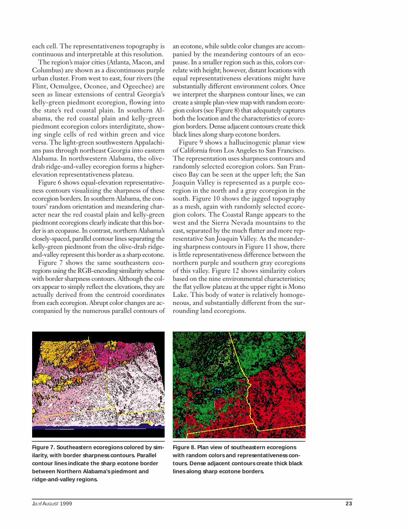
Figure 7 shows the same southeastern eco-regions using the RGB-encoding similarity schemewith border sharpness contours. Although the col-ors appear to simply reflect the elevations, they areactually derived from the centroid coordinatesfrom each ecoregion. Abrupt color changes are ac-companied by the numerous parallel contours of

an ecotone, while subtle color changes are accom-panied by the meandering contours of an eco-pause. In a smaller region such as this, colors cor-relate with height; however, distant locations withequal representativeness elevations might havesubstantially different environment colors. Oncewe interpret the sharpness contour lines, we cancreate a simple plan-view map with random ecore-gion colors (see Figure 8) that adequately capturesboth the location and the characteristics of ecore-gion borders. Dense adjacent contours create thickblack lines along sharp ecotone borders.

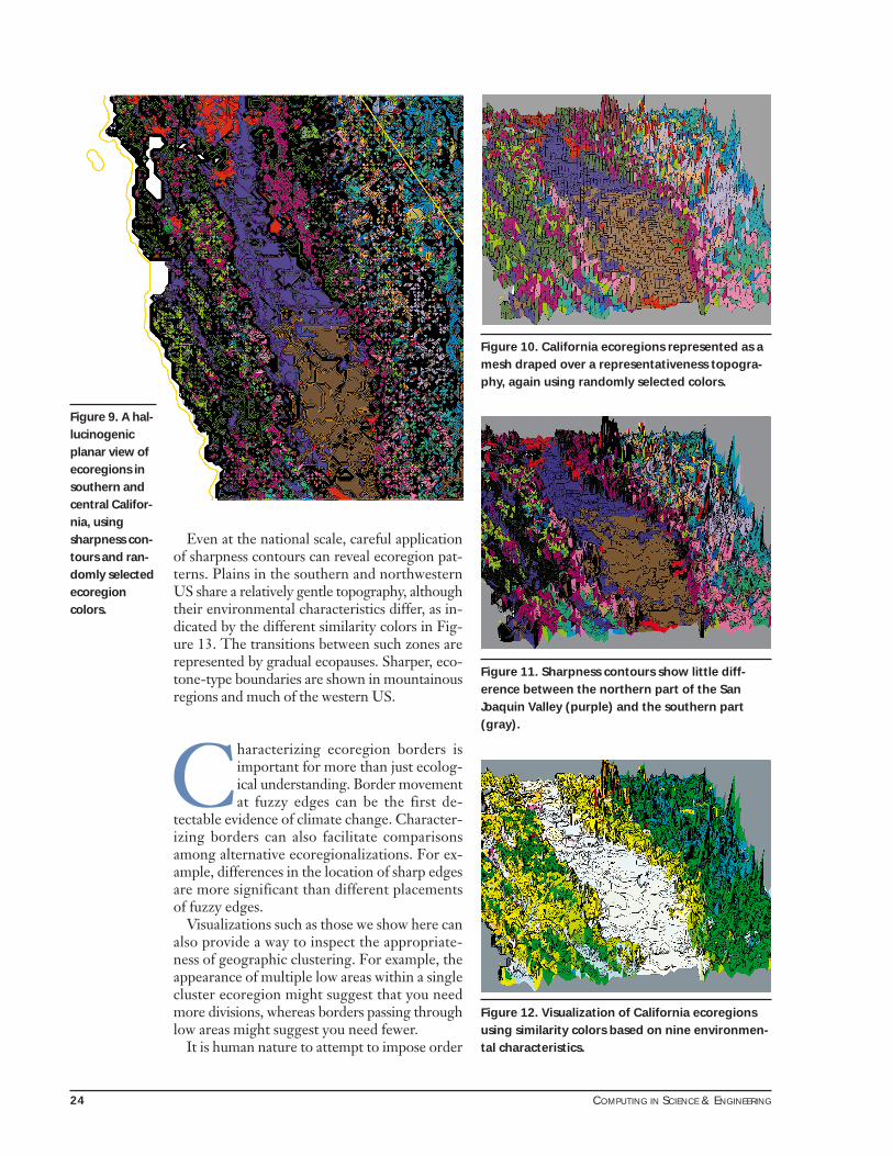
Figure 9 shows a hallucinogenic planar viewof California from Los Angeles to San Francisco.The representation uses sharpness contours andrandomly selected ecoregion colors. San Fran-cisco Bay can be seen at the upper left; the SanJoaquin Valley is represented as a purple eco-region in the north and a gray ecoregion in thesouth. Figure 10 shows the jagged topographyas a mesh, again with randomly selected ecore-gion colors. The Coastal Range appears to thewest and the Sierra Nevada mountains to theeast, separated by the much flatter and more rep-resentative San Joaquin Valley. As the meander-ing sharpness contours in Figure 11 show, thereis little representativeness difference between thenorthern purple and southern gray ecoregionsof this valley. Figure 12 shows similarity colorsbased on the nine environmental characteristics;the flat yellow plateau at the upper right is MonoLake. This body of water is relatively homoge-neous, and substantially different from the sur-rounding land ecoregions.

Figure 7. Southeastern ecoregions colored by sim-ilarity, with border sharpness contours. Parallelcontour lines indicate the sharp ecotone borderbetween Northern Alabama’s piedmont andridge-and-valley regions.

Figure 8. Plan view of southeastern ecoregionswith random colors and representativeness con-tours. Dense adjacent contours create thick blacklines along sharp ecotone borders.

24 COMPUTING IN SCIENCE & ENGINEERING

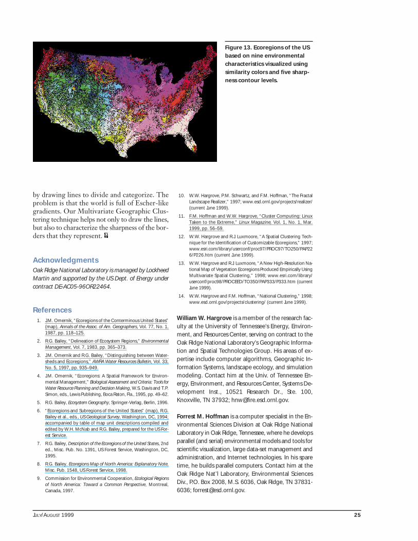
Even at the national scale, careful applicationof sharpness contours can reveal ecoregion pat-terns. Plains in the southern and northwesternUS share a relatively gentle topography, althoughtheir environmental characteristics differ, as in-dicated by the different similarity colors in Fig-ure 13. The transitions between such zones arerepresented by gradual ecopauses. Sharper, eco-tone-type boundaries are shown in mountainousregions and much of the western US.

Characterizing ecoregion borders isimportant for more than just ecolog-ical understanding. Border movementat fuzzy edges can be the first de-

tectable evidence of climate change. Character-izing borders can also facilitate comparisonsamong alternative ecoregionalizations. For ex-ample, differences in the location of sharp edgesare more significant than different placementsof fuzzy edges.

Visualizations such as those we show here canalso provide a way to inspect the appropriate-ness of geographic clustering. For example, theappearance of multiple low areas within a singlecluster ecoregion might suggest that you needmore divisions, whereas borders passing throughlow areas might suggest you need fewer.

It is human nature to attempt to impose order

Figure 10. California ecoregions represented as amesh draped over a representativeness topogra-phy, again using randomly selected colors.

Figure 11. Sharpness contours show little diff-erence between the northern part of the SanJoaquin Valley (purple) and the southern part(gray).

Figure 12. Visualization of California ecoregionsusing similarity colors based on nine environmen-tal characteristics.

Figure 9. A hal-lucinogenicplanar view ofecoregions insouthern andcentral Califor-nia, usingsharpness con-tours and ran-domly selectedecoregioncolors.

JULY/AUGUST 1999 25

by drawing lines to divide and categorize. Theproblem is that the world is full of Escher-likegradients. Our Multivariate Geographic Clus-tering technique helps not only to draw the lines,but also to characterize the sharpness of the bor-ders that they represent.

AcknowledgmentsOak Ridge National Laboratory is managed by LockheedMartin and supported by the US Dept. of Energy undercontract DE-AC05-96OR22464.

References1. J.M. Omernik, “Ecoregions of the Conterminous United States”

(map), Annals of the Assoc. of Am. Geographers, Vol. 77, No. 1,1987, pp. 118–125.

2. R.G. Bailey, “Delineation of Ecosystem Regions,” EnvironmentalManagement, Vol. 7, 1983, pp. 365–373.

3. J.M. Omernik and R.G. Bailey, “Distinguishing between Water-sheds and Ecoregions,” AWRA Water Resources Bulletin, Vol. 33,No. 5, 1997, pp. 935–949.

4. J.M. Omernik, “Ecoregions: A Spatial Framework for Environ-mental Management,” Biological Assessment and Criteria: Tools forWater Resource Planning and Decision Making, W.S. Davis and T.P.Simon, eds., Lewis Publishing, Boca Raton, Fla., 1995, pp. 49–62.

5. R.G. Bailey, Ecosystem Geography, Springer-Verlag, Berlin, 1996.

6. “Ecoregions and Subregions of the United States” (map), R.G.Bailey et al., eds., US Geological Survey, Washington, DC, 1994;accompanied by table of map unit descriptions compiled andedited by W.H. McNab and R.G. Bailey, prepared for the US For-est Service.

7. R.G. Bailey, Description of the Ecoregions of the United States, 2nded., Misc. Pub. No. 1391, US Forest Service, Washington, DC,1995.

8. R.G. Bailey, Ecoregions Map of North America: Explanatory Note,Misc. Pub. 1548, US Forest Service, 1998.

9. Commission for Environmental Cooperation, Ecological Regionsof North America: Toward a Common Perspective, Montreal,Canada, 1997.

10. W.W. Hargrove, P.M. Schwartz, and F.M. Hoffman, “The FractalLandscape Realizer,” 1997; www.esd.ornl.gov/projects/realizer/(current June 1999).

11. F.M. Hoffman and W.W. Hargrove, “Cluster Computing: LinuxTaken to the Extreme,” Linux Magazine, Vol. 1, No. 1, Mar.1999, pp. 56–59.

12. W.W. Hargrove and R.J. Luxmoore, “A Spatial Clustering Tech-nique for the Identification of Customizable Ecoregions,” 1997;www.esri.com/library/userconf/proc97/PROC97/TO250/PAP226/P226.htm (current June 1999).

13. W.W. Hargrove and R.J. Luxmoore, “A New High-Resolution Na-tional Map of Vegetation Ecoregions Produced Empirically UsingMultivariate Spatial Clustering,” 1998; www.esri.com/library/userconf/proc98/PROCEED/TO350/PAP333/P333.htm (currentJune 1999).

14. W.W. Hargrove and F.M. Hoffman, “National Clustering,” 1998;www.esd.ornl.gov/projects/clustering/ (current June 1999).

William W. Hargrove is a member of the research fac-ulty at the University of Tennessee’s Energy, Environ-ment, and Resources Center, serving on contract to theOak Ridge National Laboratory’s Geographic Informa-tion and Spatial Technologies Group. His areas of ex-pertise include computer algorithms, Geographic In-formation Systems, landscape ecology, and simulationmodeling. Contact him at the Univ. of Tennessee En-ergy, Environment, and Resources Center, Systems De-velopment Inst., 10521 Research Dr., Ste. 100,Knoxville, TN 37932; [email protected].

Forrest M. Hoffman is a computer specialist in the En-vironmental Sciences Division at Oak Ridge NationalLaboratory in Oak Ridge, Tennessee, where he developsparallel (and serial) environmental models and tools forscientific visualization, large data-set management andadministration, and Internet technologies. In his sparetime, he builds parallel computers. Contact him at theOak Ridge Nat’l Laboratory, Environmental SciencesDiv., P.O. Box 2008, M.S. 6036, Oak Ridge, TN 37831-6036; [email protected].

Figure 13. Ecoregions of the USbased on nine environmentalcharacteristics visualized usingsimilarity colors and five sharp-ness contour levels.