Using MATLAB to Compute Heat Transfer in Free Form Extrusioncdn.intechopen.com/pdfs/21961/InTech-Using_matlab_to_compute_he… · Using MATLAB to Compute Heat Transfer in Free Form

22

Using MATLAB to Compute Heat Transfer in Free Form Extrusion

Sidonie Costa, Fernando Duarte and José A. Covas University of Minho

Portugal

1. Introduction

Rapid Prototyping (RP) is a group of techniques used to quickly fabricate a scale model of a part or assembly using three-dimensional computer aided design (CAD) data (Marsan, Dutta, 2000). A large number of RP technologies have been developed to manufacture polymer, metal, or ceramic parts, without any mould, namely Stereolithography (SL), Laminated Object Manufacturing (LOM), Selected Laser Sintering (SLS), Ink-jet Printing (3DP) and Fused Deposition Modeling (FDM). In Fused Deposition Modelling (developed by Stratasys Inc in U.S.A.), a plastic or wax filament is fed through a nozzle and deposited onto the support (Pérez, 2002; Ahn, 2002; Ziemian & Crawn, 2001) as a series of 2D slices of a 3D part. The nozzle moves in the X–Y plane to create one slice of the part. Then, the support moves vertically (Z direction) so that the nozzle deposits a new layer on top of the previous one. Since the filament is extruded as a melt, the newly deposited material fuses with the last deposited material. Free Form Extrusion (FFE) is a variant of FDM (Figure 1), where the material is melted and deposited by an extruder & die (Agarwala, Jamalabad, Langrana, Safari, Whalen & Danthord, 1996; Bellini, Shor & Guceri, 2005). FFE enables the use of a wide variety of polymer systems (e.g., filled compounds, polymer blends, composites, nanocomposites, foams), thus yielding parts with superior performance. Moreover, the adoption of co-extrusion or sequential extrusion techniques confers the possibility to combine different materials for specific properties, such as soft/hard zones or transparent/opaque effects.

Fig. 1. Free Form Extrusion (FFE).

www.intechopen.com

MATLAB – A Ubiquitous Tool for the Practical Engineer

454

Due to their characteristics - layer by layer construction using melted materials - FDM and FFE may originate parts with two defects: i) excessive filament deformation upon cooling can jeopardize the final dimensional accuracy, ii) poor bonding between adjacent filaments reduces the mechanical resistance. Deformation and bonding are mainly controlled by the heat transfer, i. e., adequate bonding requires that the filaments remain sufficiently hot during enough time to ensure adhesion and, simultaneously, to cool down fast enough to avoid excessive deformation due to gravity (and weight of the filaments above them). Therefore, it is important to know the evolution in time of the filaments temperature and to understand how it is affected by the major process variables. Rodriguez (Rodriguez, 1999) studied the cooling of five elliptical filaments stacked vertically using via finite element methods and later found a 2D analytical solution for rectangular cross-sections (Thomas & Rodriguez, 2000). Yardimci and Guceri (Yardimci & S.I. Guceri, 1996) developed a more general 2D heat transfer analysis, also using finite element methods. Li and co-workers (Li, Sun, Bellehumeur & Gu, 2003; Sun, Rizvi, Bellehumeur & Gu, 2004) developed an analytical 1D transient heat transfer model for a single filament, using the Lumped Capacity method. Although good agreement with experimental results was reported, the model cannot be used for a sequence of filaments, as thermal contacts are ignored. The present work expands the above efforts, by proposing a transient heat transfer analysis of filament deposition that includes the physical contacts between any filament and its neighbours or supporting table. The analytical analysis for one filament is first discussed, yielding an expression for the evolution of temperature with deposition time. Then, a MatLab code is developed to compute the temperature evolution for the various filaments required to build one part. The usefulness of the results is illustrated with two case studies.

2. Heat transfer modelling

During the construction of a part by FDM or FFE, all the filaments are subjected to the same heat transfer mechanism but with different boundary conditions, depending on the part geometry and deposition sequence (Figure 2).

Fig. 2. Example of a sequence of filaments deposition.

Consider that N is the total number of deposited filaments and that Tr(x,t) is the temperature at length x of the r-th filament (r Є {1,…,N}) at instant t. The energy balance for an element dx of the r-th filament writes as:

sup

in int

Energy in at one face Heat loss by convection with surroundings

Heat loss by conduction with adjacent filaments or with port

Change ernal energy Energy out at opposite face

⎧ −⎪ =⎨−⎪⎩= +

www.intechopen.com


455

This can be expressed as a differential equation. After some assumptions and simplifications (Costa, Duarte & Covas, 2008):

( ) ( )1 1

1i i i

n nr

conv r i r E i r i r ri i

T Ph a T T h a T T

t CA = =⎛ ⎞⎛ ⎞∂ = − − λ − + λ −⎜ ⎟⎜ ⎟⎜ ⎟∂ ρ ⎝ ⎠⎝ ⎠∑ ∑ (1)

where P is filament perimeter, ρ is density, C is heat capacity, A is area of the filament cross-

section, hconv is heat transfer coefficient, n is number of contacts with adjacent filaments or

with the support, λi is fraction of P that in contact with an adjacent filament, TE is

environment temperature, hi is thermal contact conductance for contact i ( {1,..., }i n∈ ) and

irT is temperature of the adjacent filament or support at contact i ( {1,..., 1}ir N∈ + , ir r≠ ,

T1,…, TN are temperatures of filaments, TN+1 is support temperature). In this expression,

variables ir

a are defined as (see Figure 3):

1

, {1,..., }, {1,..., }0ir

if the r th filament has the i th contacta i n r N

otherwise

− −⎧= ∀ ∈ ∀ ∈⎨⎩ (2)

Fig. 3. Contact areas of a filament (n = 5).

Considering that:

( )( ) ( )

1

1

1

1 1

1 1

,..., 1

1

,...,,...,

n i i

i i i

n

n

n n

r r conv r i r i ii i

n n

conv r i E r i i ri i

r r

r r

b a a h a a h

h a T a h T

Q a ab a a

= =

= =

⎧ ⎛ ⎞= − λ + λ⎪ ⎜ ⎟⎪ ⎝ ⎠⎪ ⎛ ⎞⎨ − λ + λ⎜ ⎟⎪ ⎝ ⎠⎪ =⎪⎩

∑ ∑∑ ∑ (3)

equation (1) can be re-written as:

www.intechopen.com


456

( ) ( )1

1

( )( ) ,...,

,..., n

n

rr r r

r r

T tVCT t Q a a

tPL b a a

∂ρ + =∂ (4)

Since the coefficients are constants, the characteristic polynomial method can be used to yield the solution:

( )( ) ( ) ( ) ( )1

1 1

,...,

0( ) ,..., ,...,

r rnr

n n

PL b a at t

VCr r r r r rT t T Q a a e Q a a

− −ρ= − + (5)

In this expression, tr is the instant at which the r-th filament starts to cool down or contact

with another filament and 0 ( )r r rT T t= is the temperature of the filament at instant tr. Taking

k as thermal conductivity, the Biot number can be defined (Bejan, 1993):

( )

1,...,

nr rb a aABi

P k= (6)

When Bi is lower than 0.1, the filaments are thermally thin, i.e., thermal gradients throughout the cross section can be neglected. In this case, Eq. (5) becomes:

( )( ) ( ) ( ) ( )1

1 1

,...,

00.1 ( ) ,..., ,...,

r rnr

n n

PL b a at t

VCr r r r r rBi T t T Q a a e Q a a

− −ρ≤ ⇒ = − + (7)

3. Computer modelling

Equations (5) and (7) quantify the temperature of a single filament fragment along the

deposition time. In practice, consecutive filament fragments are deposited during the

manufacture of a part. Thus, it is convenient to generalize the computations to obtain the

temperature evolution of each filament fragment at any point x of the part, for different

deposition techniques and 3D configuration structures.

3.1 Generalizing the heat transfer computations

Up-dating the thermal conditions: The boundary conditions must be up-dated as the deposition develops. The code activates the physical contacts and redefines the boundary conditions for a specific filament position, time and deposition sequence. For all the filaments, three variables need to be up-dated: - time tr (TCV-1): instant at which the r-th filament starts cooling down, or enters in

contact with another filament; - temperature Tr0 (TCV-2): temperature at tr; - -vector ari (TCV-3): in Eq. (3), sets in the contacts for the r-th filament (i∈ {1,...,n}, where

n is the number of contacts). Simultaneous computation of the filaments temperature: During deposition, some filaments are

reheated when new contacts with hotter filaments arise; simultaneously, the latter cool

down due to the same contacts. This implies the simultaneous computation of the filaments

temperature via an iterative procedure. The convergence error was set at ε = 10-3, as a good

compromise between accuracy and the computation time.

www.intechopen.com


457

Deposition sequence: The deposition sequence defines the thermal conditions TCV-1, TCV-2 and TCV-3. Three possibilities were taken in: unidirectional and aligned filaments, unidirectional and skewed filaments, perpendicular filaments (see Figure 4). In all cases, the filaments are deposited continuously under constant speed (no interruptions occur between successive layers). Some parts with some geometrical features may require the use of a support material, to be removed after manufacture. This possibility is considered in the algorithm for unidirectional and aligned filaments.

a) b) c)

Fig. 4. Deposition sequences: a) unidirectional and aligned filaments; b) unidirectional and skewed filaments; c) perpendicular filaments.

3.2 Computing the temperatures

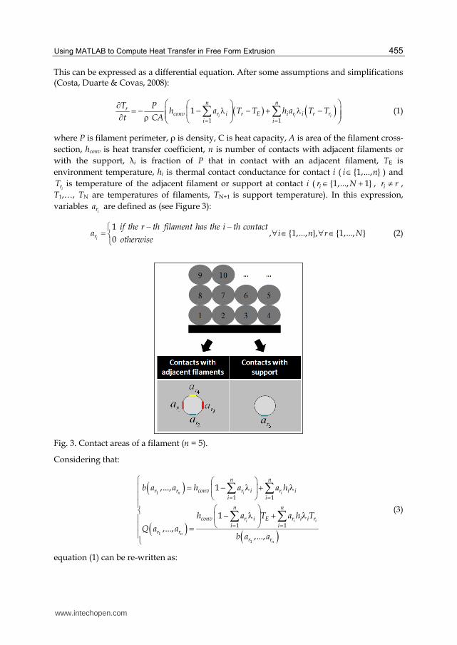
The computational flowchart is presented in Figure 5 and a MatLab code was generated. In order to visualize the results using another software (Excel, Tecplot...), a document in txt format is generated after the computations, that includes all the temperature results along deposition time.

4. MatLab code for one filament layer

In order to illustrate how the MatLab code “FFE.m” was implemented, the segment dealing with the temperature along the deposition time for the first layer of filaments, using one or two distinct materials, is presented here. The code has the same logic and structure for the remaining layers.

4.1 Input variables

Two arguments need to be introduced in this MatLab function: - A matrix representing the deposition sequence, containing m rows and n columns, for

the number of layers and maximum number of filaments in a layer, respectively. Each cell is attributed a value of 0, 1, or 2 for the absence of a filament, the presence of a filament of material A or of a filament of material B, respectively. An example is given in Figure 6.

- The vertical cross section of the part (along the filament length) where the user wishes to know the temperature evolution with time.

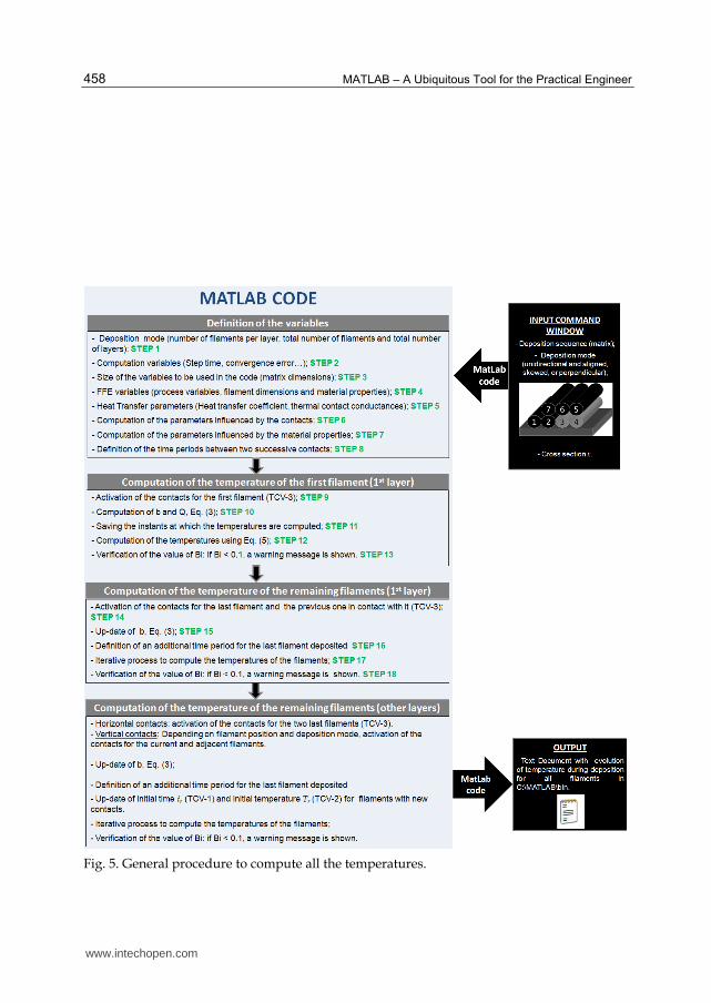
The code includes one initial section where all the variables are defined (Figure 7), namely environment and extrusion temperatures, material properties, process conditions, etc. The dimensions of all matrixes used are also defined.

www.intechopen.com


458

Fig. 5. General procedure to compute all the temperatures.

www.intechopen.com


459

Fig. 6. Example of deposition sequence and corresponding input matrix.

function FFE(matrix,x) %____________________________________ STEP 1 ____________________________________ %Definition of the vector that contains the number of total filaments in each layer matrix_lin = size(matrix,1); matrix_col = size(matrix,2); vector = zeros(matrix_lin,2); contar = 0; for i = matrix_lin:-1:1 contar = contar + 1; for j = 1:matrix_col if matrix(i,j) ~= 0 vector(contar,1) = vector(contar,1) + 1; end end end %Number of layers m = length(vector(:,1)); %Number of filaments n = 0; for j = 1:m if m == 1 n = vector(1,1); else if vector(j,2) <= 1 n = n + vector(j,1); end end end %____________________________________ STEP 2 ____________________________________ %Computation variables passo = 0.05; %Step time temp_mais = 15; %Additional time computation after construction of the part erro = 0.001; %Convergence error

www.intechopen.com


460

%____________________________________ STEP 3 ____________________________________ %Definition of the size of the variables h = zeros(1,5); lambda = zeros(1,5); a = zeros(n,5); T = zeros (n,5); vec_b = zeros(n,5); vec_Q = zeros(n,5); b = zeros(1,n); Q = zeros(1,n); T_begin = zeros(1,n); dif = zeros(1,n); Biot = zeros(1,n); save_T = zeros(1,n); old_T = zeros(1,n); save_lim = zeros(1,n); viz = zeros(11,n); %____________________________________ STEP 4 ____________________________________ %Process Variables T_L = 270; %Extrusion temperature (ºC) T_E = 70; %Temperature of the envelope (ºC) v = 0.02; %Velocity of the extrusion head (m/sec) for lin = 1:n %Temperature of support (ºC) T(lin,1) = T_E; end %Filament dimensions w = 0.0003; %Layer Thickness (meters) L = 0.02; %Length of the filament (meters) area = pi * (w/2)^2; %Area of the cross section of filament (meters^2) per = pi * w; %Perimeter of the cross section of filament (meters) vol = area*L; %Volume of the filament A_p = per*L; %Superficial area of the filament % Material Properties %Thermal conductivity (W/m.K) conductivity(1) = 0.1768; % material A conductivity(2) = 0.5; % material B %Density (kg/m^3) ro(1) = 1050; % material A ro(2) = 1500; % material B %Specific heat (J/kg.K) C(1) = 2019.7; % material A C(2) = 2500.7; % material B %____________________________________ STEP 5 ____________________________________ % Heat transfer coefficient (lost of heat by natural convection) h_conv = 45; %Thermal contact conductances between h(1,1) = 200; % filament and left adjacent filament h(1,2) = 200; % filament and down adjacent filament h(1,3) = 200; % filament and right adjacent filament h(1,4) = 200; % filament and top adjacent filament h(1,5) = 10; % filament and support %Fraction of perimeter contact between lambda(1,1) = 0.2; % filament and left adjacent filament lambda(1,2) = 0.25; % filament and down adjacent filament lambda(1,3) = 0.2; % filament and right adjacent filament lambda(1,4) = 0.25; % filament and top adjacent filament lambda(1,5) = 0.25; % filament and support

Fig. 7. Definition of the variables.

The parameters used in Equation (5) and those necessary to compute variables b and Q

(in Eq. (3)) must also be defined. Finally, the time increment between two consecutive

contacts is calculated taking into consideration the type of deposition sequence

(Figure 8).

www.intechopen.com


461

%____________________________________ STEP 6 ____________________________________ %Definition of the parameters influenced by the contacts for col = 1:5 for lin = 1:n vec_b(lin,col) = h(1,col)*lambda(1,col); vec_Q(lin,col) = vec_b(lin,col)*T(lin,col); end end

%____________________________________ STEP 7 ____________________________________ %Definition of the parameters influenced by the material properties contar = 0; number_filament = 0; for i = matrix_lin:-1:1 contar = contar + 1; if isodd(contar) == 1 for j = 1:matrix_col if matrix(i,j) ~= 0 number_filament = number_filament + 1; escalar(number_filament) = -per/(ro(matrix(i,j))*area*C(matrix(i,j))); esc(number_filament) = h_conv/(ro(matrix(i,j))*L*C(matrix(i,j))); kt(number_filament) = conductivity(matrix(i,j)); end end else for j = matrix_col:-1:1 if matrix(i,j) ~= 0 number_filament = number_filament + 1; escalar(number_filament) = -per/(ro(matrix(i,j))*area*C(matrix(i,j))); esc(number_filament) = h_conv/(ro(matrix(i,j))*L*C(matrix(i,j))); kt(number_filament) = conductivity(matrix(i,j)); end end end end %____________________________________ STEP 8 ____________________________________ %Definition of the periods of time between two successive contacts for i = 1:(n+2) if isodd(i) == 1 limite(i,1) = (i*L-x)/v; limite(i,2) = (i*L+x)/v; else limite(i,1) = limite(i-1,2); limite(i,2) = ((i+1)*L-x)/v; end end for road = 1:n linha = 0; for i = 0:passo:limite(n,2) linha = linha + 1; temp(linha,road) = T_L; end end

Fig. 8. Definition of the parameters to be used for the computation of temperatures and time between two consecutive contacts.

4.2 Computation of the temperatures for the first filament of the first layer

Computation of the temperatures starts with the activation of the contact between the first

filament and the support. Parameters b and Q (equation (3)) are calculated (Figure 9).

www.intechopen.com


462

The temperatures are computed at each time increment; confirmation of the value of Biot number (Eq. (6)) is also made: if greater than 0.1, the code devolves a warning message (Figure 10).

for layer = 1:m if layer == 1 for num = 1:vector(layer,1) if num == 1 %____________________________________ STEP 9 ____________________________________ a(num,5) = 1; %Activation of the contact with support %____________________________________ STEP 10 ____________________________________ %Definition of the variables b and Q defined in equation Eq. 7 b(num) = h_conv*(1-lambda*a(num,:)') + vec_b(num,:)*a(num,:)'; Q(num) = (h_conv*(1-lambda*a(num,:)')*T_E + vec_Q(num,:)*a(num,:)')/b(num);

Fig. 9. Activation of the contacts and computation of b and Q for the first filament.

%____________________________________ STEP 11 ____________________________________ p = 0; for t = 0:passo:limite(num,1) p = p+1; abcissa(p) = t; end %____________________________________ STEP 12 ____________________________________ %Computation of the temperatures of the first filament for t = (limite(num,1)+passo):passo:limite_final p = p+1; abcissa(p) = t; temp(p,num)=(T_L-Q(num))*exp(escalar(num)*b(num)*(t-limite(num,1))) +Q(num); end %Saving the last temperature of the period time of cooling down T_begin(num) = temp(p,num); %____________________________________ STEP 13 ____________________________________ %Verification of the value of Biot Number Biot(num) = (vol/A_p)*(b(num)/kt(num)); if Biot(num)>=0.1 'WARNING! We cannot use a Lumped System' End

Fig. 10. Computation of the temperatures for the first filament and verification of the value of the Biot number.

4.3 Computation of the temperatures for the remaining filaments of the first layer

Before proceeding to the remaining filaments of the first layer, the lateral and support

contacts for each filament being deposited must be defined, as well as for the previous one.

Consequently, the variable b in expression Eq. (3) is up-dated (Figure 11).

At this point, only the lateral and support contacts must be defined, since only the first layer

is being computed. For the remaining layers, other contacts (such as the vertical ones) must

be considered. Once each filament is deposited, the code checks whether the part has been

completed. If so, it remains in the same conditions during a pre-defined time, in order to

reach the equilibrium temperature (Figure 12).

www.intechopen.com


463

%____________________________________ STEP 14 ____________________________________ else %Activation of the contacts a(num-1,3) = 1; a(num,1) = 1; a(num,5) = 1; %____________________________________ STEP 15 ____________________________________ %Up-dating of the variable b for j = 1:num b(j) = h_conv*(1-lambda*a(j,:)') + vec_b(j,:)*a(j,:)'; end

Fig. 11. Activation of the contacts for the current and previous filaments and up-dating of variable b.

%____________________________________ STEP 16 ____________________________________ if m == 1 if num == vector(layer,1) limite_final = limite(num,2) + temp_mais; else limite_final = limite(num,2); end else limite_final = limite(num,2); end

Fig. 12. Definition of an additional time for the last filament.

Finally, the temperatures of the remaining filaments are computed. At each time increment, the temperatures of the adjacent filaments are saved and parameter Q (Eq. (3) is up-dated. The value of the Biot number is checked before the deposition of a new filament (Figure 13). for t = (limite(num,1)+passo):passo:limite_final p = p+1; abcissa(p) = t; last = p-1; for j = 1:num save_T(j) = temp(last,j); end %____________________________________ STEP 17 ____________________________________ %Iterative process for q = 1:100000 %Saving contacts and temperatures of adjacent filaments for j = 1:num if j == 1 T(j,3) = save_T(j+1); viz(3,j) = j+1; end if j > 1 & j < num T(j,1) = save_T(j-1); viz(1,j) = j-1; T(j,3) = save_T(j+1); viz(3,j) = j+1; end if j == num T(j,1) = save_T(j-1); viz(1,j) = j-1; end for k = 1:5 if T(j,k) ~= 0 & k ~= 5

www.intechopen.com


464

vec_Q(j,k) = vec_b(j,k)*T(j,k); end end %Up-dating of the variable Q Q(j) = (h_conv*(1-lambda*a(j,:)')*T_E + vec_Q(j,:)*a(j,:)')/b(j); old_T(j) = save_T(j); end %Computation of the temperatures if num == 2 save_T(1) = (T_begin(1)-Q(1))*exp(escalar(1)*b(1)* (t-limite(1,1)))+Q(1); save_T(2) = (T_L-Q(2))*exp(escalar(2)*b(2)*(t-limite(1,1)))+Q(2); save_lim(1,1) = limite(num,1); save_lim(1,2) = limite(num,1); else for j=1:num-2 save_T(j) = (T_begin(j)-Q(1))*exp(escalar(j)*b(j)* (t-save_limite(1,j)))+Q(j); end save_T(num-1) = (T_begin(num-1)-Q(num-1))* exp(escalar(num-1)*b(num-1)*(t-limite(num,1)))+Q(num-1); save_T(num) = (T_L-Q(num))* exp(escalar(num)*b(num)*(t-limite(num,1)))+ Q(num); save_lim(1,num-1) = limite(num,1); save_lim(1,num) = limite(num,1); end for j = 1:num dif(j) = abs(save_T(j)-old_T(j)); end try = 1; stop = 0; for j = 1:num if dif(try) < erro try = try+1; end if try == num+1; stop = 1; end end if stop == 1 for j = 1:num temp(p,j) = save_T(j); end break; end end end T_begin(num) = temp(p,num); %End of iterative process %____________________________________ STEP 18 ____________________________________ %Verification of the Biot Number for j=1:num Biot(j) = (vol/A_p)*(b(j)/kt(j)); if Biot(j)>=0.1 'WARNING! We can not use a Lumped System' j Biot(j) end end end end

www.intechopen.com


465

end end

Fig. 13. Computation of the temperature of the filaments of the first layer and verification of the Biot number.

5. Results

In order to demonstrate the usefulness of the code developed, two case studies will be discussed. The first deals with a part constructed with two distinct materials, while the second illustrates the role of the deposition sequence.

5.1 Case study 1

Consider the small part with the geometry presented in Figure 14, to be manufactured under the processing conditions summarized in Table 1.

Fig. 14. Geometry of the part.

Property Value

Extrusion temperature (ºC) 270

Environment temperature (ºC) 70

Extrusion velocity (m/s) 0.025

Filament length (m) 0.02

Cross section x (m) 0.01

Geometric form of cross section circle

Cross section diameter (m) 0.00035

Contact ratio 88%

Heat transfer coefficient (convection) (W/m2ºC) 60

Thermal contact conductance with filaments (W/m2ºC) 180

Thermal contact conductance with support (W/m2ºC) 10

Thermal conductivity ( W/mºC) materials A / B 0.1768 / 0.5

Specific heat (J/kgºC) materials A / B 2019.7 / 2500.7

Density materials A / B 1.05 / 1.5

Table 1. Processing conditions

www.intechopen.com


466

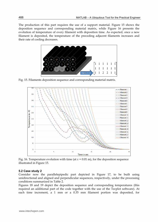
The production of this part requires the use of a support material. Figure 15 shows the deposition sequence and corresponding material matrix, while Figure 16 presents the evolution of temperature of every filament with deposition time. As expected, once a new filament is deposited, the temperature of the preceding adjacent filaments increases and their rate of cooling decreases.

Fig. 15. Filaments deposition sequence and corresponding material matrix.

Fig. 16. Temperature evolution with time (at x = 0.01 m), for the deposition sequence illustrated in Figure 15.

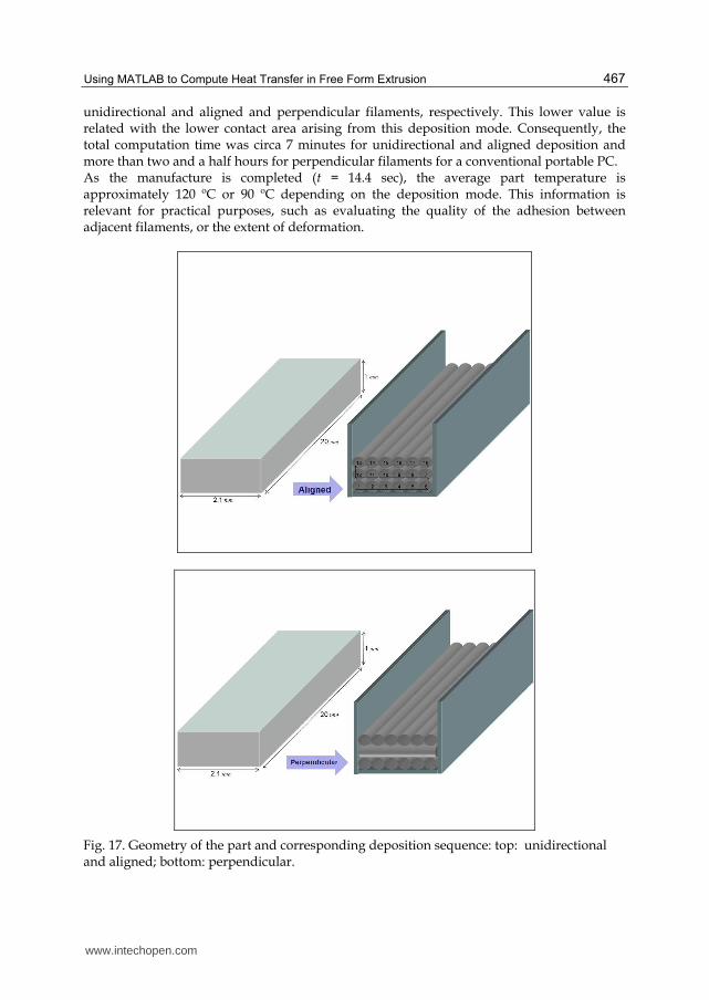
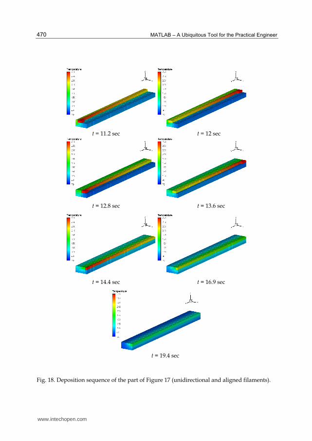
5.2 Case study 2 Consider now the parallelepipedic part depicted in Figure 17, to be built using unidirectional and aligned and perpendicular sequences, respectively, under the processing conditions summarized in Table 2. Figures 18 and 19 depict the deposition sequence and corresponding temperatures (this required an additional part of the code together with the use of the Tecplot software). At each time increment, a 1 mm or a 0.35 mm filament portion was deposited, for

www.intechopen.com


467

unidirectional and aligned and perpendicular filaments, respectively. This lower value is related with the lower contact area arising from this deposition mode. Consequently, the total computation time was circa 7 minutes for unidirectional and aligned deposition and more than two and a half hours for perpendicular filaments for a conventional portable PC. As the manufacture is completed (t = 14.4 sec), the average part temperature is approximately 120 ºC or 90 ºC depending on the deposition mode. This information is relevant for practical purposes, such as evaluating the quality of the adhesion between adjacent filaments, or the extent of deformation.

Fig. 17. Geometry of the part and corresponding deposition sequence: top: unidirectional and aligned; bottom: perpendicular.

www.intechopen.com


468

Property Value

Extrusion temperature (ºC) 270

Environment temperature (ºC) 70

Extrusion velocity (m/s) 0.025

Filament length (m) 0.02

Geometric form of cross section circle

Cross section diameter (m) 0.00035

Contact ratio 88%

Heat transfer coefficient (convection) (W/m2ºC) 70

Thermal contact conductance with filaments (W/m2ºC) 200

Thermal contact conductance with support (W/m2ºC) 15

Thermal conductivity ( W/mºC) 0.1768

Specific heat (J/kgºC) 2019.7

Density 1.05

Table 2. Processing conditions

t = 0 sec t = 0.8 sec

t = 1.6 sec t = 2.4 sec

t = 3.2 sec t = 4 sec

www.intechopen.com


469

t = 4.8 sec t = 5.6 sec

t = 6.4 sec t = 7.2 sec

t = 8 sec t = 8.8 sec

t = 9.6 sec t = 10.4 sec

www.intechopen.com


470

t = 11.2 sec t = 12 sec

t = 12.8 sec t = 13.6 sec

t = 14.4 sec t = 16.9 sec

t = 19.4 sec

Fig. 18. Deposition sequence of the part of Figure 17 (unidirectional and aligned filaments).

www.intechopen.com


471

t = 0 sec t = 0.8 sec

t = 1.6 sec t = 2.4 sec

t = 3.2 sec t = 4 sec

t = 4.8 sec t = 7.4 sec

www.intechopen.com


472

t = 9.6 sec t = 9.9 sec

t = 10.7 sec t = 11.5 sec

t = 12.3 sec t = 13.1 sec

t = 13.6 sec t = 14.4 sec

www.intechopen.com


473

t = 16.9 sec t = 19.4 sec

Fig. 19. Deposition sequence of the part of Figure 17 (perpendicular filaments).

6. Conclusion

In Free Form Extrusion, FFE, a molten filament is deposited sequentially to produce a 3D part without a mould. This layer by layer construction technique may create problems of adhesion between adjacent filaments, or create dimensional accuracy problems due to excessive deformation of the filaments, if the processing conditions are not adequately set. This chapter presented a MatLab code for modelling the heat transfer in FFE, aiming at determining the temperature evolution of each filament during the deposition stage. Two case studies illustrated the use of the programme.

7. References

Rodriguez, J. F. (1999). Modelling the mechanical behaviour of fused deposition acrylonitrile-butadiene-styrene polymer components, Ph.D. Dissertation, Department of Aeorospace and Mechanical Engineering, University of Notre Dame, Notre Dame, USA

Thomas, J. P. & Rodríguez, J. F. (2000). Modeling the fracture strength between fused deposition extruded roads, Solid Freeform Fabrication Symposium Proceeding, Austin.

Yardimci, M. A. & Guceri, S. I. (1996). Conceptual framework for the thermal process modelling of fused deposition, Rapid Prototyping Journal, 2, 26-31.

Li, L.; Sun, Q.; Bellehumeur, C. & Gu, P. (2003). Modeling of bond formation in FDM process, Trans. NAMRI/SME, 8, 613-620.

Sun, Q.; Rizvi, G.C.; Bellehumeur, C. & Gu, T. P. (2004). Experimental study and modeling of bond formation between ABS filaments in the FDM process, Proc. SPE ANTEC'2004.

Costa, S.; Duarte, F. & Covas, J. A. (2008). Towards modelling of Free Form Extrusion: analytical solution of transient heat transfer, Esaform 2008, Lyon, France.

Bejan, A. (1993). Heat Transfer, John Wiley & Sons, Inc., New York. Marsan, A.; Dutta, D. (2000). A review of process planning techniques in layered manufacturing,

Rapid Prototyping Journal, Vol.6, No.1, pp. 18-35, ISSN 1355-2546. Pérez, C. J. L. (2002). Analysis of the surface roughness and dimensional accuracy capability of fused

deposition modelling processes, International Journal of Production Research, Vol.40, Issue 12, pp. 2865 – 2881, ISSN 1366-588X.

Ahn, S. H. (2002). Anisotropic material properties of fused deposition modeling ABS, Rapid Prototyping Journal, Vol.8, No.4, pp. 248–257, ISSN 1355-2546.

Ziemian, C. W. & Crawn, P. M. (2001). Computer aided decision support for fused deposition modeling, Rapid Prototyping Journal, Vol.7, No.3, pp. 138-147, ISSN 1355-2546.

www.intechopen.com


474

Agarwala, M. K.; Jamalabad, V. R.; Langrana, N. A.; Safari, A.; Whalen, P. J. & Danthord, S. C. (1996). Structural quality of parts processed by fused deposition, Rapid Prototyping Journal, Vol.2, No.4, pp. 4-19, ISSN 1355-2546.

Bellini, A.; Shor, L. & Guceri, S. (2005). New developments in fused deposition modeling of ceramics, Rapid Prototyping Journal, Vol.11, No.4, pp. 214-220, ISSN 1355-25.

www.intechopen.com

MATLAB - A Ubiquitous Tool for the Practical EngineerEdited by Prof. Clara Ionescu

ISBN 978-953-307-907-3Hard cover, 564 pagesPublisher InTechPublished online 13, October, 2011Published in print edition October, 2011

InTech EuropeUniversity Campus STeP Ri Slavka Krautzeka 83/A 51000 Rijeka, Croatia Phone: +385 (51) 770 447 Fax: +385 (51) 686 166www.intechopen.com

InTech ChinaUnit 405, Office Block, Hotel Equatorial Shanghai No.65, Yan An Road (West), Shanghai, 200040, China

Phone: +86-21-62489820 Fax: +86-21-62489821

A well-known statement says that the PID controller is the â€œbread and butterâ€ of the control engineer. Thisis indeed true, from a scientific standpoint. However, nowadays, in the era of computer science, when thepaper and pencil have been replaced by the keyboard and the display of computers, one may equally say thatMATLAB is the â€œbreadâ€ in the above statement. MATLAB has became a de facto tool for the modernsystem engineer. This book is written for both engineering students, as well as for practicing engineers. Thewide range of applications in which MATLAB is the working framework, shows that it is a powerful,comprehensive and easy-to-use environment for performing technical computations. The book includesvarious excellent applications in which MATLAB is employed: from pure algebraic computations to dataacquisition in real-life experiments, from control strategies to image processing algorithms, from graphical userinterface design for educational purposes to Simulink embedded systems.

How to referenceIn order to correctly reference this scholarly work, feel free to copy and paste the following:

Sidonie Costa, Fernando Duarte and Jose ́ A. Covas (2011). Using MATLAB to Compute Heat Transfer in FreeForm Extrusion, MATLAB - A Ubiquitous Tool for the Practical Engineer, Prof. Clara Ionescu (Ed.), ISBN: 978-953-307-907-3, InTech, Available from: http://www.intechopen.com/books/matlab-a-ubiquitous-tool-for-the-practical-engineer/using-matlab-to-compute-heat-transfer-in-free-form-extrusion

Using MATLAB to Compute Heat Transfer in Free Form Extrusioncdn.intechopen.com/pdfs/21961/InTech-Using_matlab_to_compute_he… · Using MATLAB to Compute Heat Transfer in Free Form

Documents