Using Local Planar Geometric Invariants to Match and Model Images of Line Segments

Using Local Planar Geometric Invariantsto Match and Model Images of Line SegmentsPatrick Gros Olivier Bournez Edmond BoyerGravir - Cnrs - Inria Rhone AlpesMatching Line Segments Using Local Planar InvariantsGravir - Cnrs - Inria Rhone AlpesZIRST - 655, avenue de l'Europe - 38330 Montbonnot - [email protected]

1

Using Local Planar Geometric Invariantsto Match and Model Images of Line SegmentsAbstractImage matching consists of �nding features in di�erent images thatrepresent the same feature of the observed scene. It is a basic process invision whenever several images are used. This paper describes a matchingalgorithm for lines segments in two images. The key idea of the algorithmis to assume that the apparent motion between the two images can be ap-proximated by a planar geometric transformation (a similarity or an a�netransformation) and to compute such an approximation. Under such anassumption, local planar invariants related the kind of transformationused as approximation, should have the same value in both images. Suchinvariants are computed for simple segment con�gurations in both imagesand matched according to their values. A global constraint is added toinsure a global coherency between all the possible matches: all the localmatches must de�ne approximately the same geometric transformationbetween the two images. These �rst matches are veri�ed and completedusing a better and more global approximation of the apparent motion bya planar homography, and an estimate of the epipolar geometry.If more than two images are considered, they are initially matchedpairwise, then global matches are deduced in a second step. Finally, froma set of images representing di�erent aspects of an object, it is possible tocompare them, and to compute a model of each aspect using the matchingalgorithm.This work uses in a new way many elements already known in vision:some of the local planar invariants used here were presented as quasi-invariants by Binford and studied by Ben-Arie in his work on the PeakingE�ect. The algorithm itself uses other ideas coming from the geometrichashing and the Hough algorithms. Its main limitations come from theinvariants used. They are really stable when they are computed for a pla-nar object or for many man-made objects which contain many coplanarfacets and elements. On the other hand, the algorithm will probably failwhen used with images of very general polyhedrons. Its main advantagesare that it still works even if the images are noisy and the polyhedral ap-proximation of the contours is not exact, if the apparent motion betweenthe images is not in�nitesimal, if they are several di�erent motions in thescene, and if the camera is uncalibrated and its motion unknown.The basic matching algorithm is presented in section 2, the veri�cationand completion stages in section 3, the matching of several images isstudied in section 4 and the algorithm to model the di�erent aspects ofan object is presented in section 5. Results obtained with the di�erentalgorithms are shown in the corresponding sections.1 IntroductionImage matching is one of the most di�cult basic problems in vision. It appearswhenever several images are considered. For example, consider the reconstruc-tion problem: from two images of a three-dimensional object, compute the2

geometry (i.e. shape) of the object. Two problems must be solved, matchingand reconstruction:1. given a point of the object, �nd its projection in each image;2. once both projections are known, compute the position of the objectpoint.The �rst problem is usually speci�ed di�erently: given an image pointm1, �nd the corresponding point m2 in the other image and the object pointM of which they are both projections. The process of �nding correspondingpointsm1 andm2 is called image matching (to distinguish it from image-modelmatching).Many papers have been published in the past on the image matching prob-lem. Many methods deal with grey level images: in this case, the algorithmtries to match every pixel of both images. Each pixel contains a value, thegrey level, which encodes the light intensity received in one point of the sensorplane. These methods can be classi�ed in three groups, as in [1].Correlation: these use cross-correlation to measure the similarity of two im-age regions. Given a region in the �rst image, they search for the mostsimilar region in the second image. Constraints arising from the cam-era geometry can be used to limit the size of the search space: epipolargeometry is a good example. Other limitations may be purely algorith-mic: for example, the regions considered must have borders parallel tothe image axis. Such methods have a long history in photogrammetry[2, 3] and computer vision [4]. Improvements are regularly published[5, 6, 7, 8, 9, 10].Relaxation: in these methods, the �rst few matches are guessed. Constraintsderived from these are then used to compute further matches. This pro-cess is repeated until no new matches can be found. For example, seeMarr and Poggio [11, 12], Grimson [13, 14], and Pollard et al. [15, 16].Dynamic programming: in this case, the matching problem is formulatedas the minimization of a function of many discrete variables. Examplescan be found in [17, 18].When higher level features are available in images, such as edge points orline segments, the matching problem is slightly di�erent. Such features areless numerous but richer in information; in particular, they have geometriccharacteristics that can be used to aid matching. They are also usually morereliable than grey level values. On the other hand, it is no longer possible toobtain dense matches or reconstructions with such features. Another di�cultproblem is relevance: a curved shape represented by line segments is hard tomatch because the de�nition of the segments is very instable.Several methods adapted to such features have been proposed.Prediction and veri�cation: these methods are similar to relaxation tech-niques. Some initial matches are guessed, then constraints are deduced3

from them, that allow the guesses to be veri�ed and further matches tobe found [19, 20].Subgraph isomorphism: adjacency relations between image tokens are mod-eled as the edges or vertices of a graph, and standard methods for �nd-ing subgraph isomorphisms can be applied. These methods demand thatthere be little noise in the images, and use no geometric information. Inaddition, their complexity is often very high. Several examples can befound in [21, 22].Geometric invariants: for images obtained by perspective projection, pro-jective invariants can be computed to characterize - and hence to match- point and line con�gurations [23, 24]. Various invariants have been sug-gested [25, 26, 27, 28]. Until now, these methods have mainly been usedfor planar or very simple scenes.Quasi-invariants : some authors also use quantities which are not exactly in-variant under the projection mapping used to model the camera. Thesequantities are usually invariants of a more restrictive set of transforma-tions, but remain \almost invariant" for \typical" camera displacements.Binford [29] de�nes quasi-invariants geometrically as measurements thatare equal to a quantity computed in the scene for at least one particulartransformation, and that are constant to �rst order when the transfor-mation is perturbed (i.e. the �rst order term of the Taylor expansion ofthe quasi-invariant with respect to the transformation vanishes). If thesecond order term also vanishes, the quasi-invariant is said to be strong.Binford proves that the angle between two segments, and the length ratioof these segments are quasi-invariants. We will use these two quantitiesin the present paper. He also proves that the a�ne coordinates de�nedin a plane in the scene are strong invariants. We will also use a�necoordinates, but in the image rather than in the scene. These a�necoordinates may correspond to non coplanar points in the scene, and arenot quasi-invariants.By design, quasi-invariants are stable for non degenerate projective trans-formations. This explains why they can be used successfully for matchingand recognition tasks.The peaking e�ect: Ben-Arie [30] studied the probability distributions ofangles and length ratios of two segments from random viewing directions,and he noticed that \the probability density of the ratio of the projectedangle to the original angle has a sharp peak at the unity ratio, that is tosay, at the point where the projected angle equals the original angle. Asimilar peaking phenomenon appears in the probability density curve ofthe ratio of distances; the peak is at the point where the ratio of distancesin the image equals the ratio of the depicted distances in the scene... theprobability that a projected angle will have values between double andhalf of the original angle is more than 84%! The same span of proportionswith regards to projected distances has a probability of more than 86%!"4

He uses his statistical measurements to compute a metric for the com-parison of scene and image ratios and angles. This is used in a relaxationmethod in his recognition system. [31, 32] describe other recognition sys-tems based on the peaking e�ect. The same statistical distance is used,but within a prediction-veri�cation scheme, where pose estimation of theobject is used as veri�cation.In our method, we bene�t fully from the peaking e�ect and we use thesame kind of features: angles and ratios. But we use the peaking e�ect ina quite di�erent way. The three previous papers describe image-3D modelmatching techniques, while we have an image-image matching technique.We do not compare angles computed from a 3D model to image angles,but only angles in two di�erent images. Furthermore our system is notbased on relaxation or prediction-veri�cation, but on geometric hashingand Hough transform.Geometric hashing: Lamdan and Wolfson [33, 34, 23] have developed animage matching method based on a�ne local invariants. In each image,they consider all triplets of points as a�ne frames, and compute the a�neplanar coordinates of all the points in all these frames. Then they try to�nd which pair of frames in di�erent images give the same coordinatesto the points. If a pair is found, the match is done. The same method isused when a new image is to be matched to an image database. In thiscase the system �nds the database image having the best correspondencewith the new image.Lamdan and Wolfson justify the use of a�ne planar invariants by prac-tical considerations. Projective invariants would have given too combi-nations and the similarities are sometimes too poor to describe apparentmotion. Their system gives good results, but remains very computationintensive.Our system has many similarities to the peaking e�ect and geometric hash-ing methods discussed in the literature. A more detailed comparison is pre-sented at the end of paragraph 2.1.Our approach. The method proposed in this paper is based on line seg-ments, possibly linked one to the other at their endpoints. The key idea ofthe algorithm is to assume that the apparent motion can be approximatedby a geometric transformation, i.e. a similarity or an a�ne transformation.Under such an assumption, planar invariants associated with simple segmentcon�gurations can be computed and matched between the di�erent images. Toinsure a global coherency between all the possible matches, a global constraintis used: all the matches must de�ne approximately the same apparent motion.The matches are then veri�ed and completed using a better approximationof the apparent motion by a planar homography and an estimate of epipolargeometry.The invariants we use are planar algebraic invariants. They are not neces-sarily invariant under perspective projection, but they are invariant between5

images whenever the apparent motion can be approximated by a planar ge-ometric transformation. They are known to be stable when computed fromimages of planar objects. Man-made objects usually contain many planar sur-faces: the algorithm will work with them.On the other hand, the algorithm can fail with very general polyhedralobjects, but such objects are barely used in usual life. For curved objects, thetools and invariants used should be very di�erent (see [35]).If several images are considered, they are matched pairwise and globalmatches are deduced in a second stage. If the images represent di�erent aspectsof an object, the matching algorithm can be used as a measurement of similaritybetween images, and the images representing a same aspect can be grouped,and give rise to a 2D model of this aspect.The main advantages of our method are the following:1. It needs no knowledge of the camera calibration, motion or epipolar ge-ometry. The apparent motion is not assumed to be very small, so themethod is usable in cases where tracking methods would fail.2. Objects in the scene can have independent motions. Results with twodi�erent motions are shown at paragraph 3.4.3.3. It works with real noisy images. In such images, the polyhedral approxi-mation of the contours is often inexact and some segments are unstable.This is particularly true if the scene contains curved objects. The topol-ogy of the graph formed by the segments is known to be very unstable.Using local quasi-invariants makes our method robust against this.4. The use of geometric quasi-invariants associated with a few common seg-ment con�gurations substantially reduces the number of possible matches,so the complexity is much smaller than that of subgraph isomorphismtechniques.The main limit of the method comes from the approximation of the appar-ent motion. The validity of this approximation is quite clear for planar objectsaccording to Ben-Arie and Binford, but it is hard to determine the exact setof 3D objects for which the algorithm will not fail.The paper is organized as follows. Section 2 describes the matching al-gorithm for two images. Section 3 shows how these initial matches can beimproved and completed using global constraints. Section 4 considers the caseof several images and section 5 shows how to go from image matching to objectmodeling.2 Matching two images2.1 Matching algorithmThis section considers the case where two images of line segments are to bematched. Such images are usually obtained from grey level images by edge6

extraction [36, 37], and polygonal approximation of the edge lines. Segmentextremities may be used as junctions between segments, and each image maybe seen as a graph of segments and vertices. Fig. 3 shows some examples. Theproblem is to match the segments and their extremities between images.It is clear that corresponding features do not have the same pixel coordi-nates in the two images. The coordinate di�erence is called apparent motion.Apparent motion is not a 2D geometrical transformation. For example, twoscene points can give the same projection in one image and di�erent projec-tions in the other one. However, for generic views of nearly coplanar ensemblesof features, the apparent relative motion is well approximated by a 2D trans-formation. Our system uses 2D similarity or a�ne models to approximate therelative motion of small ensemble of nearby line segments and points.The stages of the algorithm are as follows:1. One of the two kinds of approximation (similarity or a�ne) is chosen,and local invariants are calculated for the salient feature con�gurations:angles and length ratios for similarities, and a�ne coordinates for a�netransformations.2. These invariants are matched between the two images according to theirvalues and to thresholds derived from the noise level.3. When the invariants of two con�gurations match, the similarity or a�netransformation between the con�gurations is computed.4. The transformations are represented as points in a parameter space: fourparameters for similarities (two translations, one rotation, and one scalingfactor), and six parameters for a�ne transformations (four parametersfor the linear part and two for the translation).5. Correct matches de�ne transformations close to the best approximationto the apparent motion, so points in the parameter space tend to clusterin a small region. On the other hand, false matches are not correlatedwith one another and their corresponding points are scattered across theparameter space. Thus we search for a small region of parameter spacewhere the point accumulation is maximal. This allows us to compute anapproximation to the apparent motion and to separate correct matchesfrom false ones.6. Invariant matches give rise to con�guration matches, and feature matchesare deduced from these. In case of ambiguity, only the most probablematches are considered as correct: for example, if a feature a is matched5 times to feature b, and only once to feature c, the match (a; b) is con-sidered to be correct.The stages are explained in detail below, for similarities and then for a�netransformations. Finally, we show some experimental results. But �rst wecompare our method with geometric hashing and peaking e�ects methods.7

Comparison with Wolfson's geometric hashing. Geometric hashing, aspresented in [33, 34, 23], deals with a�ne planar invariants. Points are ex-tracted from both images. Each triplet of points is considered as an a�nebasis and the a�ne coordinates of all the other points are computed in theseframes. The coordinates obtained in di�erent frames in each image are thencompared to see if any two frames correspond. If this is the case, point matchesmay be deduced directly from the comparison.The main similarities with our method are the use of local planar invariantswhich are not object invariants, and the use of a more global approximationto the apparent motion to constrain the matching.But there are important di�erences: in geometric hashing no topologicalstructure is used, while we use the segments and their adjacency to reduce thecombinatorics. If the approximation of planar apparent motion is not globalvalid, it is very often quite accurate for nearby points linked by segments. Suchpoints are often linked by segments or edges on the object itself, frequentlycorresponding to the borders of planar facets, for which a planar a�ne orsimilarity transformation is often a robust approximation to the true apparentmotion.A second di�erence is the method used to compare invariants. In geometrichashing there is a global comparison of the invariants, for each triplet in bothimages in all the possible frames in both images. This is very computationintensive. Our methods compares local invariants pairwise. After that, we usea Hough technique to �nd sets of coherent matches, and �nally to computethe best approximation to the apparent motion. Furthermore, if objects in thescene have di�erent motions, these correspond to di�erent apparent motionsin the images. While it is easily possible to search for two such motions in ourHough space, the comparison is much more di�cult with geometric hashing.As a conclusion, our method use several ideas also present in geometrichashing. But other methods, like the use of a Hough technique, are appliedat crucial points of the algorithm and allow us to avoid the weaknesses ofgeometric hashing.Comparison with peaking e�ect methods. Our method also shares someassumptions and ideas with the peaking e�ect methods. We use the samefeatures, angles and ratios, so we bene�t from the properties demonstrated inBen-Arie's paper, but our context is quite di�erent. We use no 3D model ordata, and our matching method is based on a voting technique and requiresno veri�cation step like localization. This allows us to match against severaldi�erent images in parallel, and to achieve image recognition without having toconsider each possible image individually. This is also the case with geometrichashing. A recognition system based on our matching process is presented in[38].2.2 Approximation by a similaritySimilarities are compositions of isometries and scalings. We will consider onlydirect similarities, i.e. compositions of rotations, translations and scalings.8

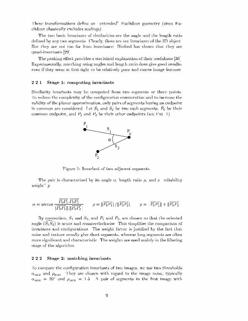
These transformations de�ne an \extended" Euclidean geometry (since Eu-clidean classically excludes scalings).The two basic invariants of similarities are the angle and the length ratiode�ned by any two segments. Clearly, these are not invariants of the 3D object.But they are not too far from invariance: Binford has shown that they arequasi-invariants [29].The peaking e�ect provides a statistical explanation of their usefulness [30].Experimentally, matching using angles and length ratio does give good results,even if they seem at �rst sight to be relatively poor and coarse image features.2.2.1 Stage 1: computing invariantsSimilarity invariants may be computed from two segments or three points.To reduce the complexity of the con�guration enumeration and to increase thevalidity of the planar approximation, only pairs of segments having an endpointin common are considered. Let S1 and S2 be two such segments, P0 be theircommon endpoint, and P1 and P2 be their other endpoints (see Fig. 1).S

1

S2

2P

0P

1P

α

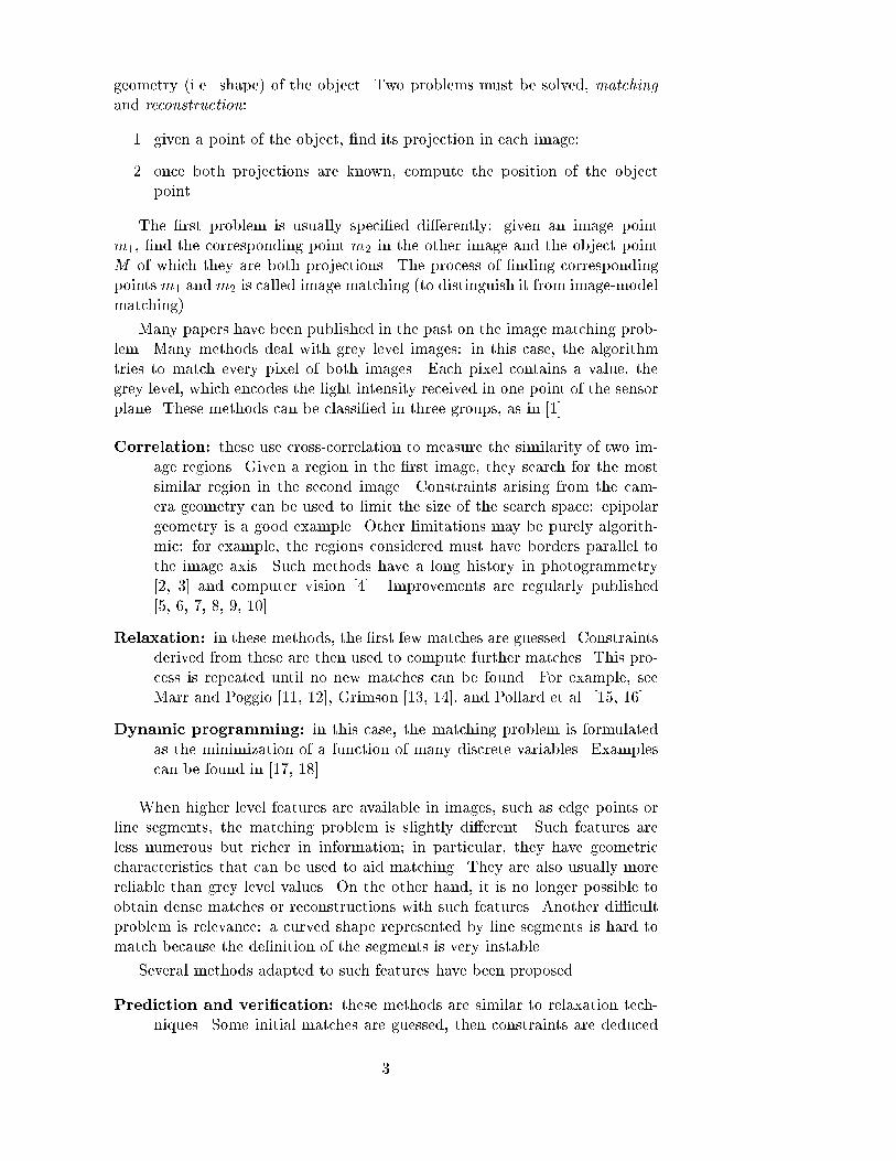
Figure 1: Invariant of two adjacent segments.The pair is characterized by its angle �, length ratio �, and a \reliabilityweight" p.� = arccos ��!P0P1:��!P0P2k��!P0P1k:k��!P0P2k � = k��!P0P1k=k��!P0P2k p = k��!P0P1k+ k��!P0P2kBy convention, S1 and S2, and P1 and P2, are chosen so that the orientedangle ([S1S2) is acute and counterclockwise. This simpli�es the comparison ofinvariants and con�gurations. The weight factor is justi�ed by the fact thatnoise and texture usually give short segments, whereas long segments are oftenmore signi�cant and characteristic. The weights are used mainly in the �lteringstage of the algorithm.2.2.2 Stage 2: matching invariantsTo compare the con�guration invariants of two images, we use two thresholds�max and �max. They are chosen with regard to the image noise, typically�max = 20� and �max = 1:5. A pair of segments in the �rst image with9

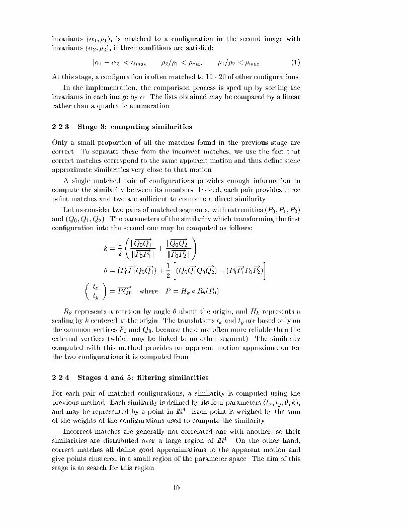
invariants (�1; �1), is matched to a con�guration in the second image withinvariants (�2; �2), if three conditions are satis�ed:j�1 � �2j < �max �2=�1 < �max �1=�2 < �max (1)At this stage, a con�guration is often matched to 10 - 20 of other con�gurations.In the implementation, the comparison process is sped up by sorting theinvariants in each image by �. The lists obtained may be compared by a linearrather than a quadratic enumeration.2.2.3 Stage 3: computing similaritiesOnly a small proportion of all the matches found in the previous stage arecorrect. To separate these from the incorrect matches, we use the fact thatcorrect matches correspond to the same apparent motion and thus de�ne someapproximate similarities very close to that motion.A single matched pair of con�gurations provides enough information tocompute the similarity between its members. Indeed, each pair provides threepoint matches and two are su�cient to compute a direct similarity.Let us consider two pairs of matched segments, with extremities (P0; P1; P2)and (Q0; Q1; Q2). The parameters of the similarity which transforming the �rstcon�guration into the second one may be computed as follows:k = 12 k���!Q0Q1kk��!P0P1k + k���!Q0Q2kk��!P0P2k !� = ( \��!P0P1���!Q0Q1) + 12 �( \���!Q0Q1���!Q0Q2)� ( \��!P0P1��!P0P2)�� txty � = ��!PQ0 where P = Hk � R�(P0)R� represents a rotation by angle � about the origin, and Hk represents ascaling by k centered at the origin. The translations tx and ty are based only onthe common vertices P0 and Q0, because these are often more reliable than theexternal vertices (which may be linked to no other segment). The similaritycomputed with this method provides an apparent motion approximation forthe two con�gurations it is computed from.2.2.4 Stages 4 and 5: �ltering similaritiesFor each pair of matched con�gurations, a similarity is computed using theprevious method. Each similarity is de�ned by its four parameters (tx; ty; �; k),and may be represented by a point in IR4. Each point is weighed by the sumof the weights of the con�gurations used to compute the similarity.Incorrect matches are generally not correlated one with another, so theirsimilarities are distributed over a large region of IR4. On the other hand,correct matches all de�ne good approximations to the apparent motion andgive points clustered in a small region of the parameter space. The aim of thisstage is to search for this region. 10

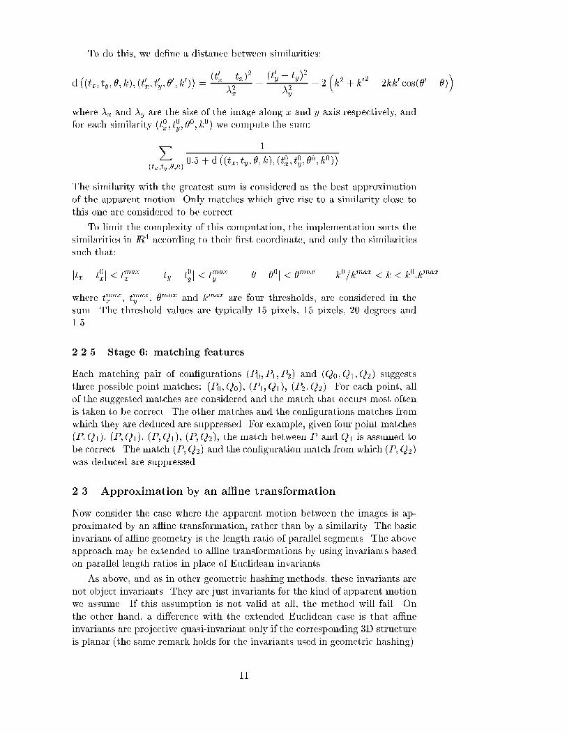
To do this, we de�ne a distance between similarities:d �(tx; ty; �; k); (t0x; t0y; �0; k0)� = (t0x � tx)2�2x + (t0y � ty)2�2y + 2�k2 + k02 � 2kk0 cos(�0 � �)�where �x and �y are the size of the image along x and y axis respectively, andfor each similarity (t0x; t0y; �0; k0) we compute the sum:X(tx;ty;�;k) 10:5 + d �(tx; ty; �; k); (t0x; t0y; �0; k0)�The similarity with the greatest sum is considered as the best approximationof the apparent motion. Only matches which give rise to a similarity close tothis one are considered to be correct.To limit the complexity of this computation, the implementation sorts thesimilarities in IR4 according to their �rst coordinate, and only the similaritiessuch that:jtx � t0xj < tmaxx jty � t0yj < tmaxy j� � �0j < �max k0=kmax < k < k0:kmaxwhere tmaxx , tmaxy , �max and kmax are four thresholds, are considered in thesum. The threshold values are typically 15 pixels, 15 pixels, 20 degrees and1.5.2.2.5 Stage 6: matching featuresEach matching pair of con�gurations (P0; P1; P2) and (Q0; Q1; Q2) suggeststhree possible point matches: (P0; Q0), (P1; Q1), (P2; Q2). For each point, allof the suggested matches are considered and the match that occurs most oftenis taken to be correct. The other matches and the con�gurations matches fromwhich they are deduced are suppressed. For example, given four point matches(P;Q1), (P;Q1), (P;Q1), (P;Q2), the match between P and Q1 is assumed tobe correct. The match (P;Q2) and the con�guration match from which (P;Q2)was deduced are suppressed.2.3 Approximation by an a�ne transformationNow consider the case where the apparent motion between the images is ap-proximated by an a�ne transformation, rather than by a similarity. The basicinvariant of a�ne geometry is the length ratio of parallel segments. The aboveapproach may be extended to a�ne transformations by using invariants basedon parallel length ratios in place of Euclidean invariants.As above, and as in other geometric hashing methods, these invariants arenot object invariants. They are just invariants for the kind of apparent motionwe assume. If this assumption is not valid at all, the method will fail. Onthe other hand, a di�erence with the extended Euclidean case is that a�neinvariants are projective quasi-invariant only if the corresponding 3D structureis planar (the same remark holds for the invariants used in geometric hashing).11

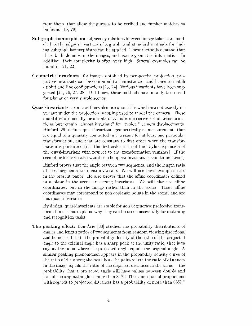
Before matching, and without prior information, it is impossible to know whichsets of segments correspond to planar structures.The main justi�cation for using a�ne invariants is that a�ne planar trans-formations provide a much wider set of transformations, that permits a betterapproximation of the apparent image motion.In this section, we discuss only the di�erences between the similarity ap-proximation and the a�ne approximation; the overall approach remains thesame.2.3.1 Stage 1: computing invariantsThree segments or four points are needed to compute an a�ne invariant, inthe general case where the points or segments are not collinear. To limitthe complexity, we consider only two kinds of con�gurations, called Z or Ycon�gurations.I

P01

P

3P

2P

P0 1P

3P

2P

Figure 2: De�nition of invariants from a Z (left) or Y (right) three-segmentcon�guration.For a Z con�guration, such as that shown in Fig. 2, two invariants arede�ned. � = k�!P3Ik=k�!P0Ik and � = k�!P2Ik=k�!P1IkTo reduce ambiguity, the con�guration points are labeled so that � is greaterthan or equal to 1.In the case of Y con�gurations, the invariants are the a�ne coordinates ofP0 with respect to the three other points P1, P2 and P3. These coordinates arede�ned as follows: � a1P1 + a2P2 + a3P3 = P0a1 + a2 + a3 = 0The con�guration points are labeled in such a way that a1 is smaller than a2and a2 is smaller than a3. In both cases, the con�guration is weighed by thesum of length of the three segments.2.3.2 Stage 2: matching invariantsThe a�ne matching process follows exactly the same algorithm as for similar-ities. Only the matching conditions (1) are di�erent. For two Z con�gurationswith invariants (�1; �1) and (�2; �2), the conditions are:�1 < k�2 �2 < k�1 �1 < k�2 �2 < k�112

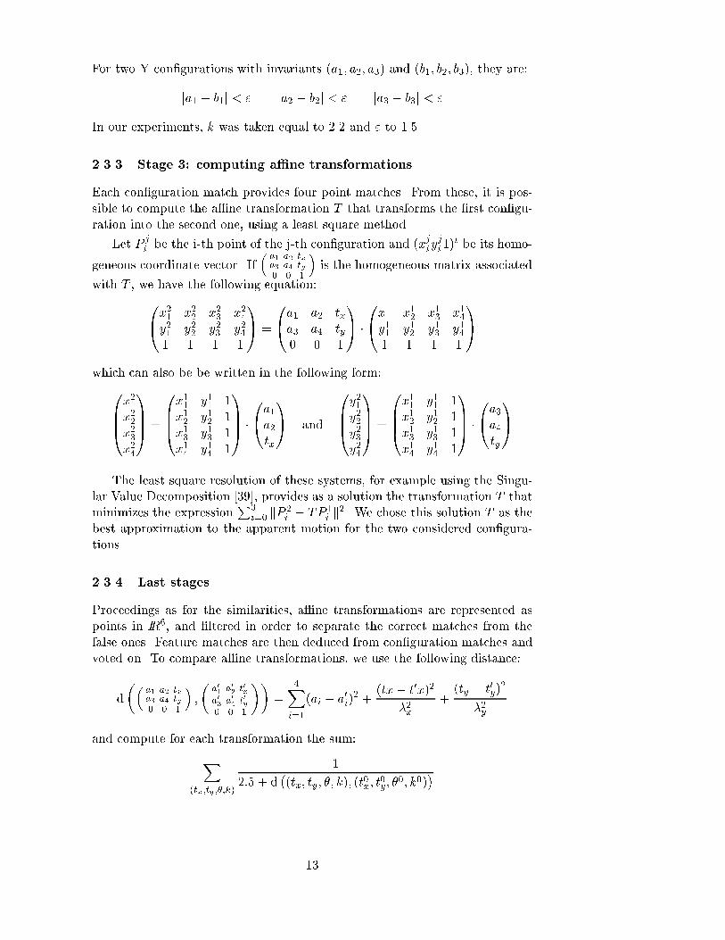
For two Y con�gurations with invariants (a1; a2; a3) and (b1; b2; b3), they are:ja1 � b1j < " ja2 � b2j < " ja3 � b3j < "In our experiments, k was taken equal to 2.2 and " to 1.5.2.3.3 Stage 3: computing a�ne transformationsEach con�guration match provides four point matches. From these, it is pos-sible to compute the a�ne transformation T that transforms the �rst con�gu-ration into the second one, using a least square method.Let P ji be the i-th point of the j-th con�guration and (xjiyji 1)t be its homo-geneous coordinate vector. If � a1 a2 txa3 a4 ty0 0 1 � is the homogeneous matrix associatedwith T , we have the following equation:0@x21 x22 x23 x24y21 y22 y23 y241 1 1 11A = 0@a1 a2 txa3 a4 ty0 0 11A �0@x11 x12 x13 x14y11 y12 y13 y141 1 1 1 1Awhich can also be be written in the following form:0BB@x21x22x23x241CCA = 0BB@x11 y11 1x12 y12 1x13 y13 1x14 y14 11CCA �0@a1a2tx1A and 0BB@y21y22y23y241CCA = 0BB@x11 y11 1x12 y12 1x13 y13 1x14 y14 11CCA �0@a3a4ty1AThe least square resolution of these systems, for example using the Singu-lar Value Decomposition [39], provides as a solution the transformation T thatminimizes the expression P3i=0 kP 2i � TP 1i k2. We chose this solution T as thebest approximation to the apparent motion for the two considered con�gura-tions.2.3.4 Last stagesProceedings as for the similarities, a�ne transformations are represented aspoints in IR6, and �ltered in order to separate the correct matches from thefalse ones. Feature matches are then deduced from con�guration matches andvoted on. To compare a�ne transformations, we use the following distance:d�� a1 a2 txa3 a4 ty0 0 1 � ;� a01 a02 t0xa03 a04 t0y0 0 1 �� = 4Xi=1(ai � a0i)2 + (tx� t0x)2�2x + (ty � t0y)2�2yand compute for each transformation the sum:X(tx;ty;�;k) 12:5 + d �(tx; ty; �; k); (t0x; t0y; �0; k0)�13

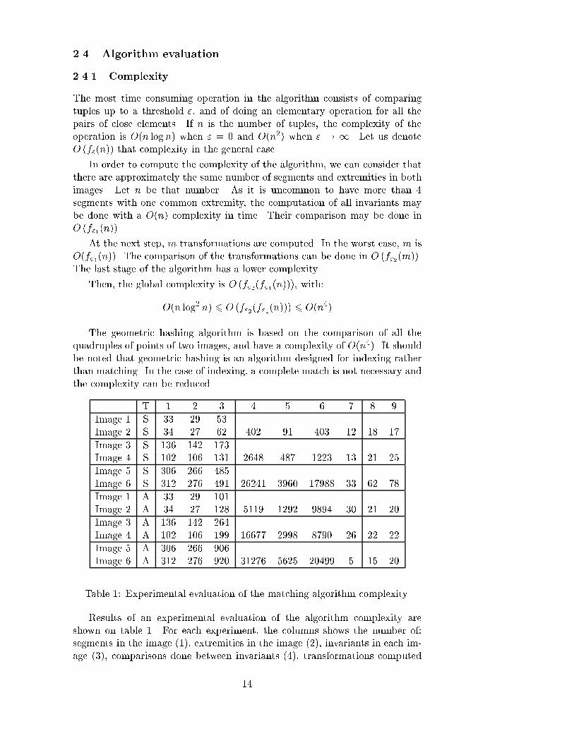
2.4 Algorithm evaluation2.4.1 ComplexityThe most time consuming operation in the algorithm consists of comparingtuples up to a threshold ", and of doing an elementary operation for all thepairs of close elements. If n is the number of tuples, the complexity of theoperation is O(n log n) when " = 0 and O(n2) when " ! 1. Let us denoteO (f"(n)) that complexity in the general case.In order to compute the complexity of the algorithm, we can consider thatthere are approximately the same number of segments and extremities in bothimages. Let n be that number. As it is uncommon to have more than 4segments with one common extremity, the computation of all invariants maybe done with a O(n) complexity in time. Their comparison may be done inO (f"1(n)).At the next step, m transformations are computed. In the worst case, m isO(f"1(n)). The comparison of the transformations can be done in O (f"2(m)).The last stage of the algorithm has a lower complexity.Then, the global complexity is O (f"2(f"1(n))), with:O(n log2 n) 6 O (f"2(f"1(n))) 6 O(n4)The geometric hashing algorithm is based on the comparison of all thequadruples of points of two images, and have a complexity of O(n4). It shouldbe noted that geometric hashing is an algorithm designed for indexing ratherthan matching. In the case of indexing, a complete match is not necessary andthe complexity can be reduced.T 1 2 3 4 5 6 7 8 9Image 1 S 33 29 53Image 2 S 34 27 62 402 91 403 12 18 17Image 3 S 136 142 173Image 4 S 102 106 131 2648 487 1223 13 21 25Image 5 S 306 266 485Image 6 S 312 276 491 26241 3960 17988 33 62 78Image 1 A 33 29 101Image 2 A 34 27 128 5119 1292 9894 30 21 20Image 3 A 136 142 264Image 4 A 102 106 199 16677 2998 8790 26 22 22Image 5 A 306 266 906Image 6 A 312 276 920 31276 5625 20499 5 15 20Table 1: Experimental evaluation of the matching algorithm complexity.Results of an experimental evaluation of the algorithm complexity areshown on table 1. For each experiment, the columns shows the number of:segments in the image (1), extremities in the image (2), invariants in each im-age (3), comparisons done between invariants (4), transformations computed14

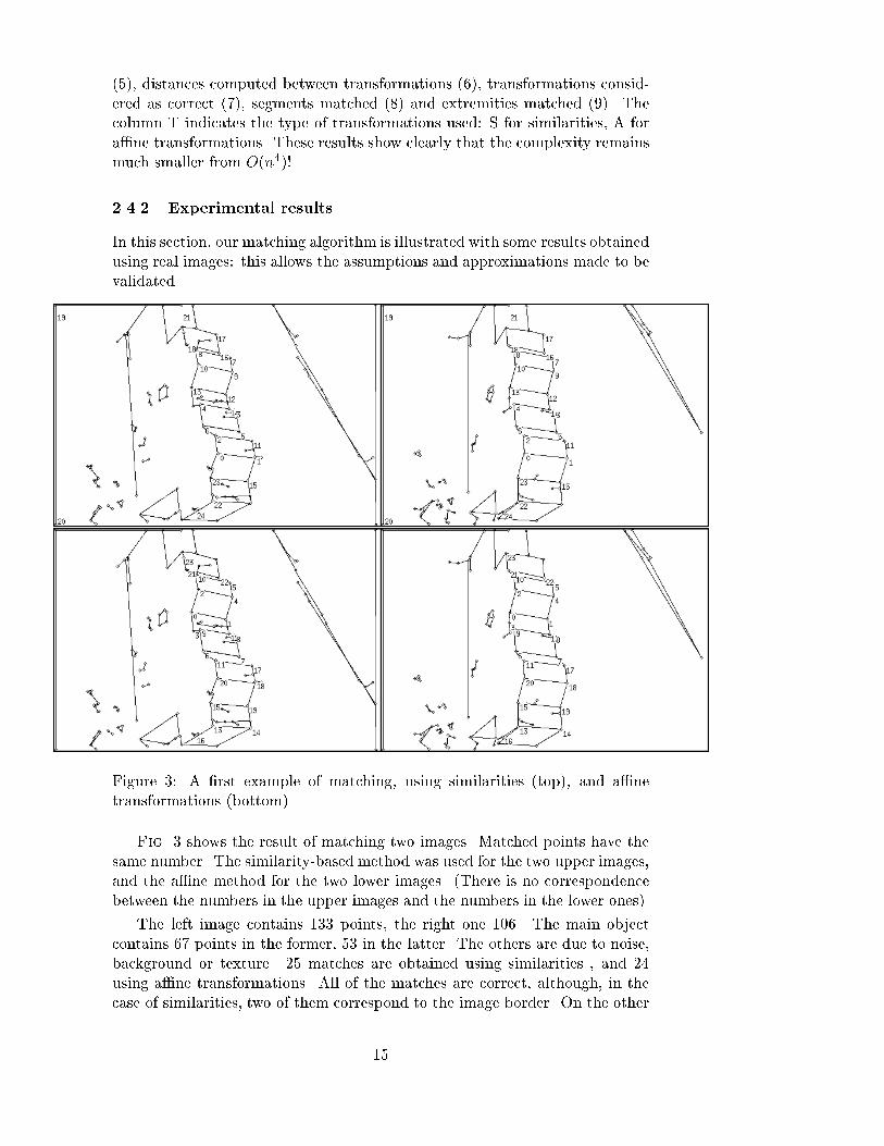
(5), distances computed between transformations (6), transformations consid-ered as correct (7), segments matched (8) and extremities matched (9). Thecolumn T indicates the type of transformations used: S for similarities, A fora�ne transformations. These results show clearly that the complexity remainsmuch smaller from O(n4)!2.4.2 Experimental resultsIn this section, our matching algorithm is illustrated with some results obtainedusing real images: this allows the assumptions and approximations made to bevalidated.

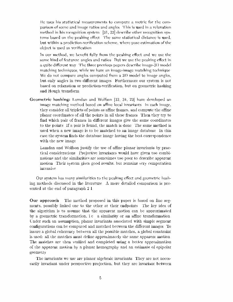
Figure 3: A �rst example of matching, using similarities (top), and a�netransformations (bottom).Fig. 3 shows the result of matching two images. Matched points have thesame number. The similarity-based method was used for the two upper images,and the a�ne method for the two lower images. (There is no correspondencebetween the numbers in the upper images and the numbers in the lower ones).The left image contains 133 points, the right one 106. The main objectcontains 67 points in the former, 53 in the latter. The others are due to noise,background or texture. 25 matches are obtained using similarities , and 24using a�ne transformations. All of the matches are correct, although, in thecase of similarities, two of them correspond to the image border. On the other15

hand, some points clearly belonging to the object are not matched. This is dueto imperfect segmentation (for example segments split in two by a vertex), orto regions where the apparent motion is not well approximated by a similarityor even an a�ne transformation (due to perspective e�ects for example).Clearly, planar local invariants are su�ciently robust for reliable matching,even when the apparent motion is visibly far from an exact similarity or ana�ne transformation.

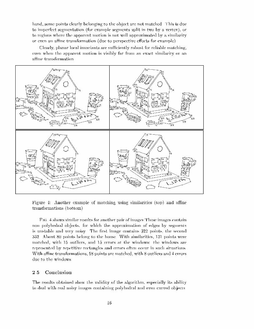
Figure 4: Another example of matching using similarities (top) and a�netransformations (bottom).Fig. 4 shows similar results for another pair of images These images containnon polyhedral objects, for which the approximation of edges by segmentsis unstable and very noisy. The �rst image contains 322 points, the second352. About 80 points belong to the house. With similarities, 131 points werematched, with 15 outliers, and 15 errors at the windows: the windows arerepresented by repetitive rectangles and errors often occur in such situations.With a�ne transformations, 58 points are matched, with 8 outliers and 4 errorsdue to the windows.2.5 ConclusionThe results obtained show the validity of the algorithm, especially its abilityto deal with real noisy images containing polyhedral and even curved objects.16

Of course, the matching obtained is not complete, and the next section showshow these initial results can be improved.The method appears to be general and not speci�c to the particular kindsof local invariants used. To demonstrate this, we used other kinds of invariants,such as Euclidean invariants computed from three segments. The results aresimilar.Another idea would be to use projective invariants, computed using crossratios. In this case, the problem is that the computation of such invariants andof the corresponding homographies between con�gurations is very sensitiveto noise. This makes the search for an accumulation point in IR8 extremelydi�cult. Our conclusion was that projective invariants are only useful formatching when the data is very precise.As a conclusion, we can say that our algorithm is robust, and that itsrobustness comes from the use of simple local planar invariants. They appearto be a powerful tool to deal with images where noise forbids to use exact andmore sensitive invariants. They make a big part of the originality and of thesuccess of our method.3 Improving image matchingThe algorithm described in the previous section provides an initial match be-tween two images without any prior information. The results may contain afew incorrect matches and miss correct ones: apparent motion approximationby a similarity or an a�ne transformation is too restrictive for some imageregions.However, once an initial match is found, other �ner tools can be used toevaluate the validity of computed matches, and to �nd new ones. A �rst toolis the approximation of apparent motion by a 2D homography. When theobserved object is planar, this is not an approximation, but an exact com-putation. A second tool is epipolar geometry. This only gives point to linecorrespondences rather than point to point ones, however it is exact for bothplanar and non planar objects. The computation and use of these two toolsare described in this section.These tools are particularly interesting when the scene contains an objectmoving against a �xed background, as the mobile object will fail to de�ne thesame epipolar geometry or homography as the rest of the scene. This opensnew directions for applications of the matching method.3.1 Projective approximation of apparent motionAs similarities or of an a�ne transformations may not approximate the appar-ent motion well over large image regions, a �rst idea is to use a transformationwith more parameters. In the Klein hierarchy [40], the next class after thea�ne transformations is the projective ones (homographies). At least fourpoints are necessary to de�ne a homography between two images. The match-ing algorithm described in the previous section provides, in general, more than17

four correspondences, and this redundancy allows the computation instabilitydescribed in the conclusion 2.5 to be suppressed.Several methods are available to compute a homography between two im-ages from at least four matches.3.1.1 Linear least squares methodThe �rst and simplest method is linear least squares as in stage 3 of para-graph 2.3. Let (P 1i ; P 2i ) be the matches obtained previously, and T be thehomography which minimizes Pi kP 2i ^ (T:P 1i )k2, with homogeneous matrix� a11 a12 a13a21 a22 a23a31 a32 a33 �. If the equations P 2i / T:P 1i are written as it was done in para-graph 2.3, T can be obtained by solving the system of equations by singularvalue decomposition.3.1.2 Robust least median squares methodReal images are always noisy and some false matches always fall within thethresholds of the matching algorithm. The least squares method uses all thematches, including the errors. A few errors are su�cient to cause inaccuracyof the computed transformation, even at the points given to compute it. Aleast median squares method can correct this drawback by detecting outliers.The algorithm is the following:1. Four point matches are chosen randomly.2. The homography T de�ned by these four matches is computed using thelinear method.3. The errors kP 2i ^(T:P 1i )k2 are computed for all of the remaining matches,and their median " is found and associated with T (more generally, thex%-ian error can be used for x 6= 50).This process is repeated su�ciently many times that the probability ofchoosing at least one set of four correct matches is very high. The �nal esti-mation of the homography is the transformation T whose associated value " isthe smallest.This method allows outliers in the data to be detected. Any matches givingan error three times greater than the median (or twice greater than " if x isgreater than 50), may be considered to be outliers and eliminated. The bestestimate of the homography is independent of these outliers, and turns outto be good enough for many applications. For a more accurate result, it ispossible to re�ne the estimate using the non linear method below.The number of times the three stages 1, 2, and 3 must be repeated and thepercentage x depend on the the fraction of outliers in the data. x must be lessthan the estimate rate of outliers in the data. 50% may be taken as a defaultvalue, but the result is of course better with a better estimation of the realrate. 18

If y is the real fraction of false matches in the data, the probability ofchoosing at least one con�guration of n correct matches in m trials is [41]:P = 1� [1� (1� y)n]mIf we assume that y = 40% and we want P > 0:99, 34 iterations are su�cient.As indicated in [41], this method can be improved by requiring that the chosenpoints are well distributed in the images. According to our experimental re-sults, the additional time this requires is hardly justi�ed by the improvementof the result.3.1.3 Non linear optimization methodThe two previous methods are not symmetric with respect to the images. Twoimages play di�erent roles in the criterionPi kP 2i ^ (T:P 1i )k2 to be minimized,and this may have consequences on the result.This expression may be symmetrized:Xi �kP 2i ^ T:P 1i k2 + kP 1i ^ T�1:P 2i k2�A linear resolution is no longer possible. The results of the least mean ormedian squares methods may be used as an initial estimate of the solution ina non linear optimization method, such as that of Levenberg-Marquardt [39].The linear solution usually provides a good enough approximation to thereal solution to insure convergence within a few iterations. On the other hand,the elimination of outliers by the least median squares method seems necessaryto obtain accurate results in most cases. The non linear method is sensitive tothe quality of the initial estimate of the solution: this is yet another argumentfor the use of the robust method rather than that of the linear one.3.1.4 ConclusionIn our experiments, we used the least median squares method to remove out-liers. It gives much better results than the simple linear method. On theother hand, our data are not precise enough to have a real improvement of theresults when using the non linear optimization method. In all cases, homogra-phies work best for scenes that are not too deep.3.2 Epipolar geometry computationEpipolar geometry is the geometric relation between two images of the samescene, and is summarized by the fundamental matrix F . This 3 � 3 rank2 matrix veri�es tP 2:F:P 1 = 0 for every couple of matched points (P 1; P 2),represented by their homogeneous coordinates. Many methods of computationof this matrix from point matches have been proposed in the literature. Theymay be classi�ed in three groups:� linear methods, which allow epipolar geometry to be computed directlyfrom point matches; 19

� robust methods, which allow outliers to be detected and eliminated.� non linear methods, which provide very accurate results but require aninitial estimate of the solution.Here are short descriptions of the main methods:Simple linear method: this considers the problem as a simple system oflinear equations. The fundamental matrix F is de�ned up to a scalefactor and one of its coe�cient may be taken equal to 1. The matrixis then found by solving the equations tP 2:F:P 1 = 0, for at least eightdi�erent point matches, using the SVD method. This method has a fewdrawbacks: the system to be solved is ill-conditioned and the rank thecomputed matrix is often equal to 3 as soon as the data are not exact.Hartley's method: the previous method may be signi�cantly improved inseveral ways [42]: �rst, changing the coordinate basis allows to correctthe ill-conditioning of the initial system. Second, setting the smallestsingular value of the linear solution to zero guarantees that the obtainedmatrix is singular.Boufama's method: a new method was recently proposed [43]. Based ona di�erent formulation of the problem, it allows a singular fundamentalmatrix to be found by a simple resolution. For planar scenes, the twoprevious methods provide meaningless results, while Boufama's methodprovides correct pencils of epipolar lines: every point of every epipolarline has its corresponding point on the corresponding epipolar line.Least median squares method: as with the homography computation, itis possible to use a robust method based on the least median squares.This method may be improved in several ways, concerning the way thepoints are chosen, or the linear method used : : : Such improvements aredescribed in [41].Non linear optimization method: the �rst method could provide a nonsingular matrix. To correct this, the criterion Pi k tP 2i :F:P 1i k2 may beminimized under the constraint detF = 0. This may be done by using anon linear optimization algorithm such as Levenberg-Marquardt [39].The main drawback of this method is the instability of the function F 7!Pi k tP 2i :F:P 1i k2, which admits many local minima; the correct solution,i.e. the one that corresponds to the true camera motion, is not alwayseven the global minimum of the function as soon as the images are noisy.To use this method, one must eliminate the outliers with the robustmethod �rst, and give a very good �rst estimation of the result.For our matching purpose, we generally use the least median squares methodwith the linear Boufama's method. They provide robust epipolar pencils whichcan be e�ciently used for matching. On the other hand, the epipoles are notused and their position need not be determined precisely.20

3.3 Corrections and improvementsThe tools described above allow the results obtained with the matching algo-rithm presented in the �rst section of the paper to be signi�cantly improved.� Computing epipolar geometry or approximating the apparent motionwith a homography using robust methods allows outliers to be detected.The mean-error found when computing the homography may be used todecide whether the scene is planar or not. In the former case, Boufama'smethod or the robust method associated with Boufama's one should beused to compute the epipolar geometry. In the latter case, the epipo-lar geometry should be used since the homography cannot accuratelyapproximate the apparent motion.� New matches may be deduced from those already found. Let s1 be asegment whose endpoints are a1 and a2. If only one of these, say a1,is matched to a point b1 in the other image, we can search for anotherpoint b2 in this image, such that there exists a segment between b1 andb2 and a2 and b2 are compatible with respect to epipolar geometry or thehomography approximating the apparent motion. If neither a1 nor a2are matched, it is possible to look for a segment s2 whose extremities b1and b2 respect the epipolar and homography constraints with a1 and a2.� Finally, we can search among all the unmatched points in both imagesfor all the couples (a; b) that satisfy the epipolar and homography con-straints. However, this may give incoherent results with respect to imagetopology and should be used with considerable care.3.4 Experimental results3.4.1 Improved matchesFig. 5 and 6 show results obtained from the matches shown in Fig. 3 and4: the epipolar geometry and the homography were computed using a robustmethod, and the outliers were detected and eliminated. Fig. 7 and 8 show theresults obtained after the improvement stage.It is of course possible that new errors are introduced during this last stage.However they must be at least approximately correct from a geometrical view-point, because they must respect the two constraints.On the other hand, some points are still not matched. This is mostlybecause the homography gives a good approximation to the apparent motiononly in part of the image. In the remaining part, it suppresses any new matches.The performance of these stages are summarized in Tab.2. The columnsObject 1 and Object 2 concern the images of Fig. 3, while the columns House 1and House 2 concern the images of Fig. 4. Each entry of the �rst line is thenumber of points in the corresponding image. The following lines provide thenumber of points matched using the matching algorithm described in section 2and the number of false matches, the number of remaining matches and errorsafter the outliers detection stage, and the �nal number of matches and errors.21

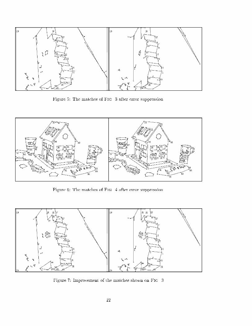
Figure 5: The matches of Fig. 3 after error suppression.

Figure 6: The matches of Fig. 4 after error suppression.

Figure 7: Improvement of the matches shown on Fig. 322

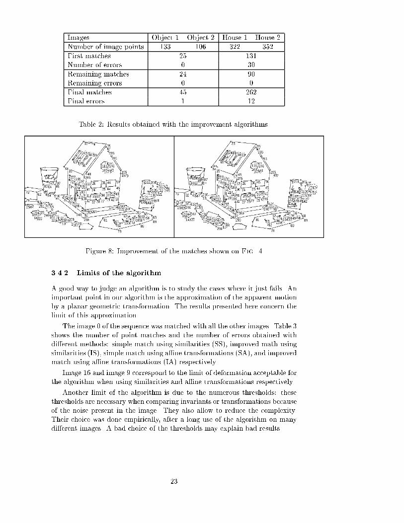
Images Object 1 Object 2 House 1 House 2Number of image points 133 106 322 352First matches 25 131Number of errors 0 30Remaining matches 24 90Remaining errors 0 0Final matches 45 262Final errors 1 12Table 2: Results obtained with the improvement algorithms.

Figure 8: Improvement of the matches shown on Fig. 43.4.2 Limits of the algorithmA good way to judge an algorithm is to study the cases where it just fails. Animportant point in our algorithm is the approximation of the apparent motionby a planar geometric transformation. The results presented here concern thelimit of this approximation.The image 0 of the sequence was matched with all the other images. Table 3shows the number of point matches and the number of errors obtained withdi�erent methods: simple match using similarities (SS), improved math usingsimilarities (IS), simple match using a�ne transformations (SA), and improvedmatch using a�ne transformations (IA) respectively.Image 16 and image 9 correspond to the limit of deformation acceptable forthe algorithm when using similarities and a�ne transformations respectively.Another limit of the algorithm is due to the numerous thresholds: thesethresholds are necessary when comparing invariants or transformations becauseof the noise present in the image. They also allow to reduce the complexity.Their choice was done empirically, after a long use of the algorithm on manydi�erent images. A bad choice of the thresholds may explain bad results.23

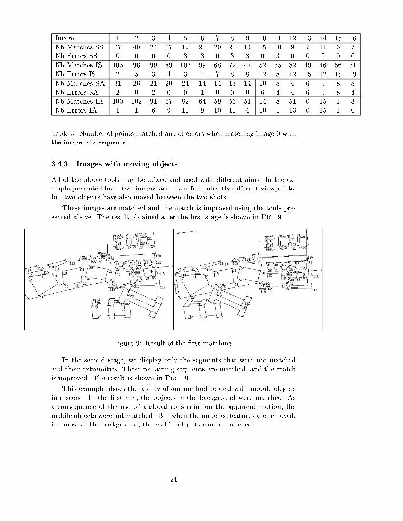
Image 1 2 3 4 5 6 7 8 9 10 11 12 13 14 15 16Nb Matches SS 27 40 24 27 19 20 20 21 14 15 10 9 7 11 6 7Nb Errors SS 0 0 0 0 3 3 0 3 3 0 3 0 0 0 0 0Nb Matches IS 105 96 99 89 102 99 68 72 47 52 55 82 49 46 56 51Nb Errors IS 2 5 3 4 3 4 7 8 8 12 8 12 15 12 15 19Nb Matches SA 31 26 21 20 24 14 14 13 14 10 8 4 6 9 8 8Nb Errors SA 2 0 2 0 0 1 0 0 0 6 4 4 6 9 8 4Nb Matches IA 100 102 91 67 82 64 59 56 51 14 8 51 0 15 1 3Nb Errors IA 1 1 6 9 11 9 10 11 4 10 1 13 0 15 1 0Table 3: Number of points matched and of errors when matching image 0 withthe image of a sequence.3.4.3 Images with moving objectsAll of the above tools may be mixed and used with di�erent aims. In the ex-ample presented here, two images are taken from slightly di�erent viewpoints,but two objects have also moved between the two shots.These images are matched and the match is improved using the tools pre-sented above. The result obtained after the �rst stage is shown in Fig. 9.

Figure 9: Result of the �rst matching.In the second stage, we display only the segments that were not matchedand their extremities. These remaining segments are matched, and the matchis improved. The result is shown in Fig. 10.This example shows the ability of our method to deal with mobile objectsin a scene. In the �rst run, the objects in the background were matched. Asa consequence of the use of a global constraint on the apparent motion, themobile objects were not matched. But when the matched features are removed,i.e. most of the background, the mobile objects can be matched.24

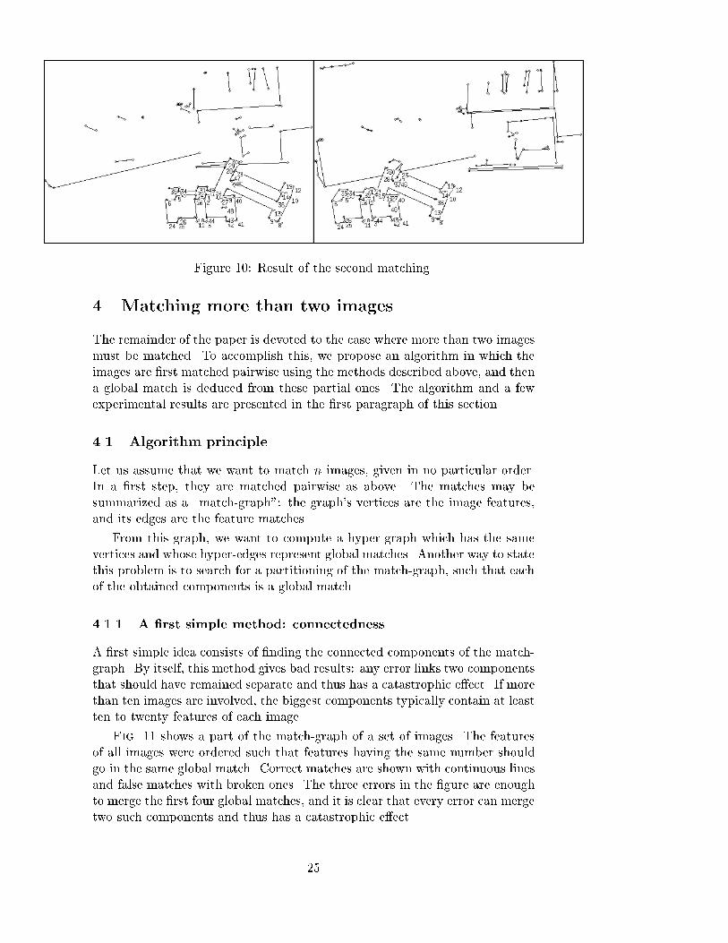
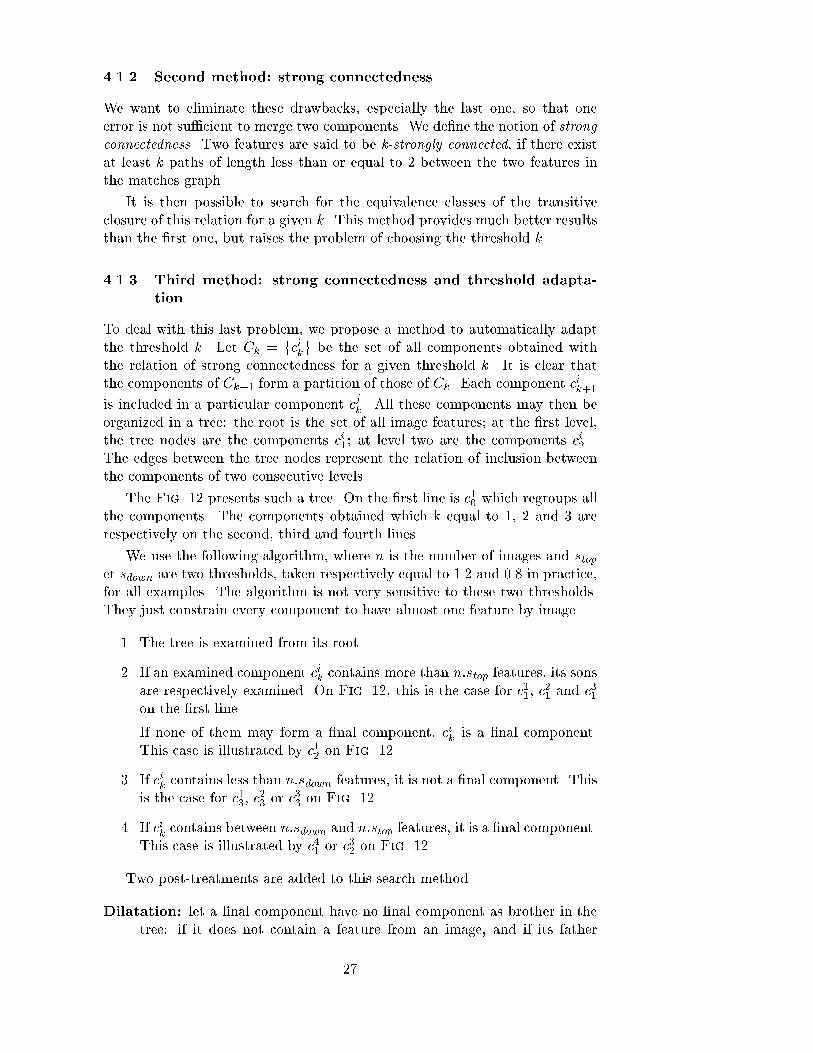
Figure 10: Result of the second matching.4 Matching more than two imagesThe remainder of the paper is devoted to the case where more than two imagesmust be matched. To accomplish this, we propose an algorithm in which theimages are �rst matched pairwise using the methods described above, and thena global match is deduced from these partial ones. The algorithm and a fewexperimental results are presented in the �rst paragraph of this section.4.1 Algorithm principleLet us assume that we want to match n images, given in no particular order.In a �rst step, they are matched pairwise as above. The matches may besummarized as a \match-graph": the graph's vertices are the image features,and its edges are the feature matches.From this graph, we want to compute a hyper-graph which has the samevertices and whose hyper-edges represent global matches. Another way to statethis problem is to search for a partitioning of the match-graph, such that eachof the obtained components is a global match.4.1.1 A �rst simple method: connectednessA �rst simple idea consists of �nding the connected components of the match-graph. By itself, this method gives bad results: any error links two componentsthat should have remained separate and thus has a catastrophic e�ect. If morethan ten images are involved, the biggest components typically contain at leastten to twenty features of each image.Fig. 11 shows a part of the match-graph of a set of images. The featuresof all images were ordered such that features having the same number shouldgo in the same global match. Correct matches are shown with continuous linesand false matches with broken ones. The three errors in the �gure are enoughto merge the �rst four global matches, and it is clear that every error can mergetwo such components and thus has a catastrophic e�ect.25

IMAGE 1

IMAGE N

IMAGE 4

IMAGE 3

IMAGE 2

feature 1feature 2feature 3feature 4

feature n

feature 1

feature 2

feature 3

feature 4feature n

feat

ure

1

feat

ure

2

feat

ure

3

feat

ure

4 feat

ure

n

feat

ure

1fe

atur

e 2

feat

ure

3fe

atur

e 4

feat

ure

n

feature 1feature 2feature 3feature 4

feature n

False matches

Correct matches

Figure 11: When considering connected components, every error has a catas-trophic e�ect.The drawbacks of this method are threefold:� the existence of a single path between two features is too weak a relation,and does not take the available redundancy into account. Consider twocases: in the �rst one, there exists only one path between two featuresf1 and f2, and the length of this path is 10; in the second case, thereexist 10 paths of length 2 between these two features. It is clear that theprobability that f1 and f2 are in the same global match is much biggerin the second case than it is in the �rst one. We would like the algorithmto take such an information into account.� the constraints of the problem are neglected: it is not common for twofeatures of the same image to belong to the same global match (althoughit does happen when a corner gives rise to two points rather than one).The case of 3 features of the same image may be excluded a priori. Idealcomponents should contain, in the best case, one feature of every image.� as stated before, every error has a catastrophic e�ect.26

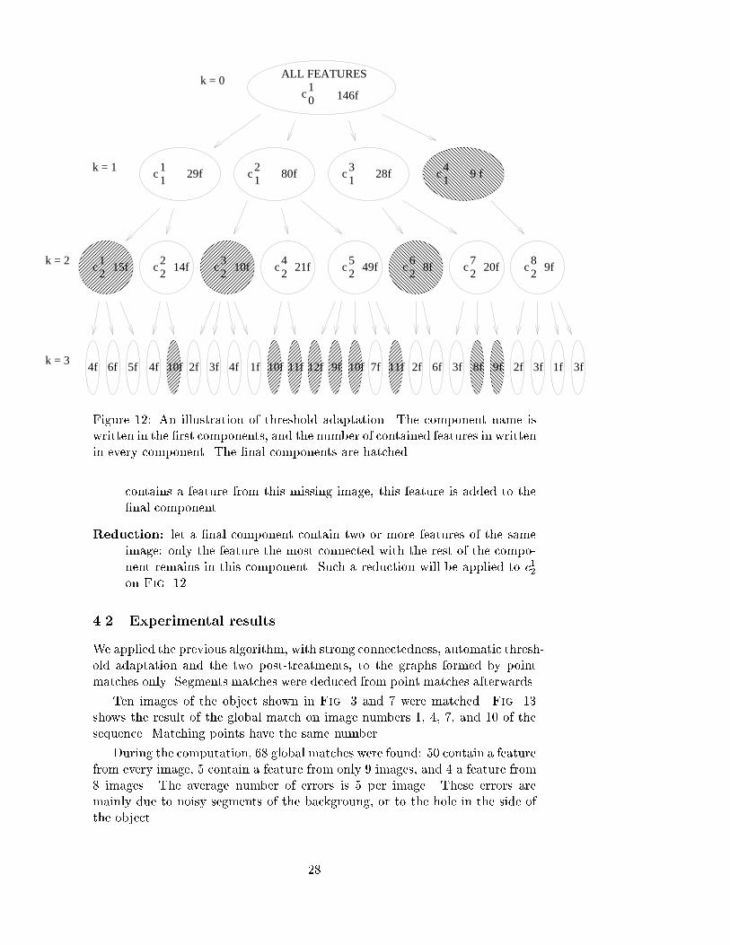
4.1.2 Second method: strong connectednessWe want to eliminate these drawbacks, especially the last one, so that oneerror is not su�cient to merge two components. We de�ne the notion of strongconnectedness. Two features are said to be k-strongly connected, if there existat least k paths of length less than or equal to 2 between the two features inthe matches graph.It is then possible to search for the equivalence classes of the transitiveclosure of this relation for a given k. This method provides much better resultsthan the �rst one, but raises the problem of choosing the threshold k.4.1.3 Third method: strong connectedness and threshold adapta-tionTo deal with this last problem, we propose a method to automatically adaptthe threshold k. Let Ck = fcikg be the set of all components obtained withthe relation of strong connectedness for a given threshold k. It is clear thatthe components of Ck+1 form a partition of those of Ck. Each component cik+1is included in a particular component cjk. All these components may then beorganized in a tree: the root is the set of all image features; at the �rst level,the tree nodes are the components ci1; at level two are the components ci2...The edges between the tree nodes represent the relation of inclusion betweenthe components of two consecutive levels.The Fig. 12 presents such a tree. On the �rst line is c10 which regroups allthe components. The components obtained which k equal to 1, 2 and 3 arerespectively on the second, third and fourth lines.We use the following algorithm, where n is the number of images and stopet sdown are two thresholds, taken respectively equal to 1.2 and 0.8 in practice,for all examples. The algorithm is not very sensitive to these two thresholds.They just constrain every component to have almost one feature by image.1. The tree is examined from its root.2. If an examined component cik contains more than n:stop features, its sonsare respectively examined. On Fig. 12, this is the case for c11, c21 and c31on the �rst line.If none of them may form a �nal component, cik is a �nal component.This case is illustrated by c12 on Fig. 12.3. If cik contains less than n:sdown features, it is not a �nal component. Thisis the case for c13, c23 or c33 on Fig. 12.4. If cik contains between n:sdown and n:stop features, it is a �nal component.This case is illustrated by c41 or c32 on Fig. 12.Two post-treatments are added to this search method.Dilatation: let a �nal component have no �nal component as brother in thetree: if it does not contain a feature from an image, and if its father27

k = 0

k = 1

k = 2

k = 3

ALL FEATURES

c01

ccccccc1

cccc11 1

213

14

2 22

23

24

25

26

27

c28

9 f

9f8f10f

80f

21f 49f14f

5f 4f 10f 2f 3f 4f 1f 10f 11f 12f 9f 10f 11f7f 2f 6f 8f 9f3f

20f

28f

2f 3f 1f 3f

15f

29f

146f

6f4fFigure 12: An illustration of threshold adaptation. The component name iswritten in the �rst components, and the number of contained features in writtenin every component. The �nal components are hatched.contains a feature from this missing image, this feature is added to the�nal component.Reduction: let a �nal component contain two or more features of the sameimage: only the feature the most connected with the rest of the compo-nent remains in this component. Such a reduction will be applied to c12on Fig. 12.4.2 Experimental resultsWe applied the previous algorithm, with strong connectedness, automatic thresh-old adaptation and the two post-treatments, to the graphs formed by pointmatches only. Segments matches were deduced from point matches afterwards.Ten images of the object shown in Fig. 3 and 7 were matched. Fig. 13shows the result of the global match on image numbers 1, 4, 7, and 10 of thesequence. Matching points have the same number.During the computation, 68 global matches were found: 50 contain a featurefrom every image, 5 contain a feature from only 9 images, and 4 a feature from8 images. The average number of errors is 5 per image. These errors aremainly due to noisy segments of the backgroung, or to the hole in the side ofthe object. 28

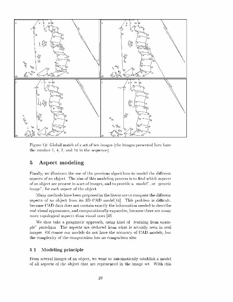
Figure 13: Global match of a set of ten images (the images presented here havethe number 1, 4, 7, and 10 in the sequence).5 Aspect modelingFinally, we illustrate the use of the previous algorithms to model the di�erentaspects of an object. The aim of this modeling process is to �nd which aspectsof an object are present in a set of images, and to provide a \model", or \genericimage", for each aspect of the object.Many methods have been proposed in the literature to compute the di�erentaspects of an object from its 3D CAD model[44]. This problem is di�cult,because CAD data does not contain exactly the information needed to describereal visual appearance, and computationally expansive, because there are manymore topological aspects than visual ones [45].We thus take a pragmatic approach, using kind of \learning from exam-ple" paradigm. The aspects are deduced from what is actually seen in realimages. Of course our models do not have the accuracy of CAD models, butthe complexity of the computation has no comparison also.5.1 Modeling principleFrom several images of an object, we want to automatically establish a modelof all aspects of the object that are represented in the image set. With this29

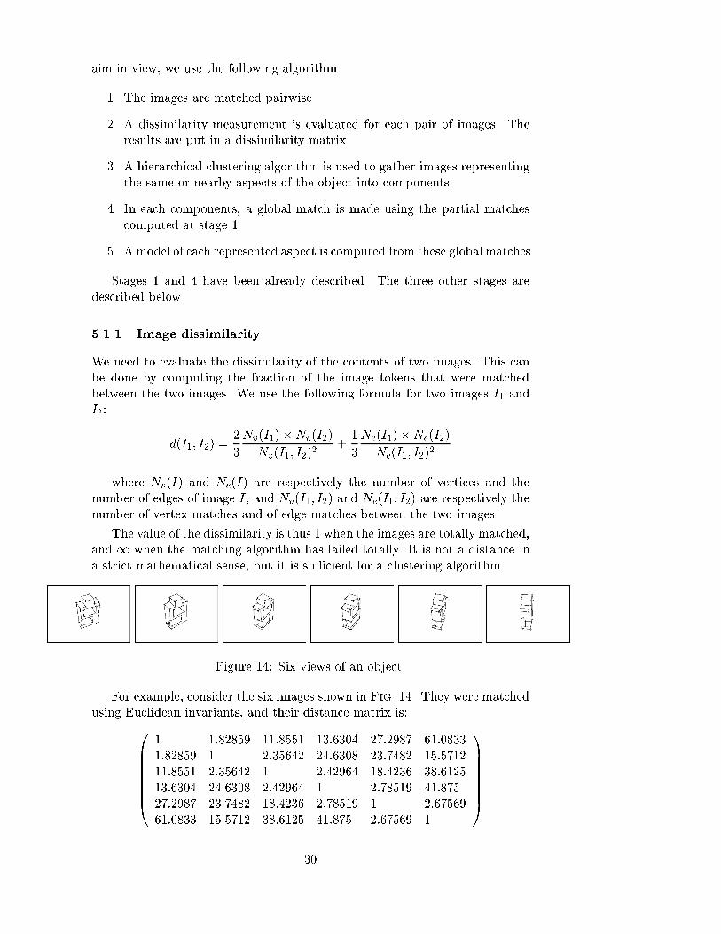
aim in view, we use the following algorithm.1. The images are matched pairwise.2. A dissimilarity measurement is evaluated for each pair of images. Theresults are put in a dissimilarity matrix.3. A hierarchical clustering algorithm is used to gather images representingthe same or nearby aspects of the object into components.4. In each components, a global match is made using the partial matchescomputed at stage 1.5. A model of each represented aspect is computed from these global matches.Stages 1 and 4 have been already described. The three other stages aredescribed below.5.1.1 Image dissimilarityWe need to evaluate the dissimilarity of the contents of two images. This canbe done by computing the fraction of the image tokens that were matchedbetween the two images. We use the following formula for two images I1 andI2: d(I1; I2) = 23Nv(I1)�Nv(I2)Nv(I1; I2)2 + 13Ne(I1)�Ne(I2)Ne(I1; I2)2where Nv(I) and Ne(I) are respectively the number of vertices and thenumber of edges of image I, and Nv(I1; I2) and Ne(I1; I2) are respectively thenumber of vertex matches and of edge matches between the two images.The value of the dissimilarity is thus 1 when the images are totally matched,and 1 when the matching algorithm has failed totally. It is not a distance ina strict mathematical sense, but it is su�cient for a clustering algorithm.Figure 14: Six views of an object.For example, consider the six images shown in Fig. 14. They were matchedusing Euclidean invariants, and their distance matrix is:0BBBBBB@ 1 1:82859 11:8551 13:6304 27:2987 61:08331:82859 1 2:35642 24:6308 23:7482 15:571211:8551 2:35642 1 2:42964 18:4236 38:612513:6304 24:6308 2:42964 1 2:78519 41:87527:2987 23:7482 18:4236 2:78519 1 2:6756961:0833 15:5712 38:6125 41:875 2:67569 1

1CCCCCCA30

5.1.2 Hierarchical clusteringNumerous clustering methods are proposed in the literature [46, 47]. Theyusually require either a threshold or the �nal number of clusters to be given asinput to the algorithm.As we do not have any idea of the number of clusters that should be ob-tained in our case, we preferred to use a hierarchical merging method based ona threshold to partition the initial image set.1. Each image is put in a di�erent set.2. The two nearest sets (the least dissimilar ones) are merged if their dis-similarity is smaller than a given threshold.3. The dissimilaritymatrix is updated. The dissimilarity between two imagesets is, by de�nition, the mean dissimilarity between the images of the�rst set and the images of the second one.4. The stages 2 and 3 are repeated until no more sets can be merged.Updating the matrix is easy. If I; J and K are three image sets, and if jLjdenotes the number of elements of a set L:d(I [ J;K) = 1jI [ J j:jKj Xi2I[J;k2K d(i; k)= jIjjI [ J jd(I;K) + jJ jjI [ J jd(J;K)The choice of threshold is critical. In our experiments, we had to adapt thethreshold according to the image quality. Noisy images need large thresholds(between 10 and 20), while exact data, coming from CAD models for example,needs smaller ones (around 2 or 3).5.1.3 ModelingIn the last stage of the process, the images have been grouped into componentsthat partition the initial image set, and in each component, the images havebeen globally matched. The aim of the last stage is to establish a \modelimage" for each component.For each component, a key image is chosen. All of the other images in thecomponent are transformed by a homography to be as close as possible to thechosen image (this homography was already computed during the matchingimprovement stage).The model is a new image which contains the vertices and edges presentin at least 60% of the component images. For features that are chosen to bepart of the model, their positions are computed as the mean position of thecorresponding features in the transformed images.The rate of 60% is smaller than the sdown threshold previously used, becausethe reduction post-treatment may reduce the number of features in the globalmatches. 31

5.2 Experimental results

24

40

58

6

32

36

38

34

282620 22

1816

14

8

10

12

42

44

46

4850

5254

56

4

2

6866

64 62

70

72

74

76

78

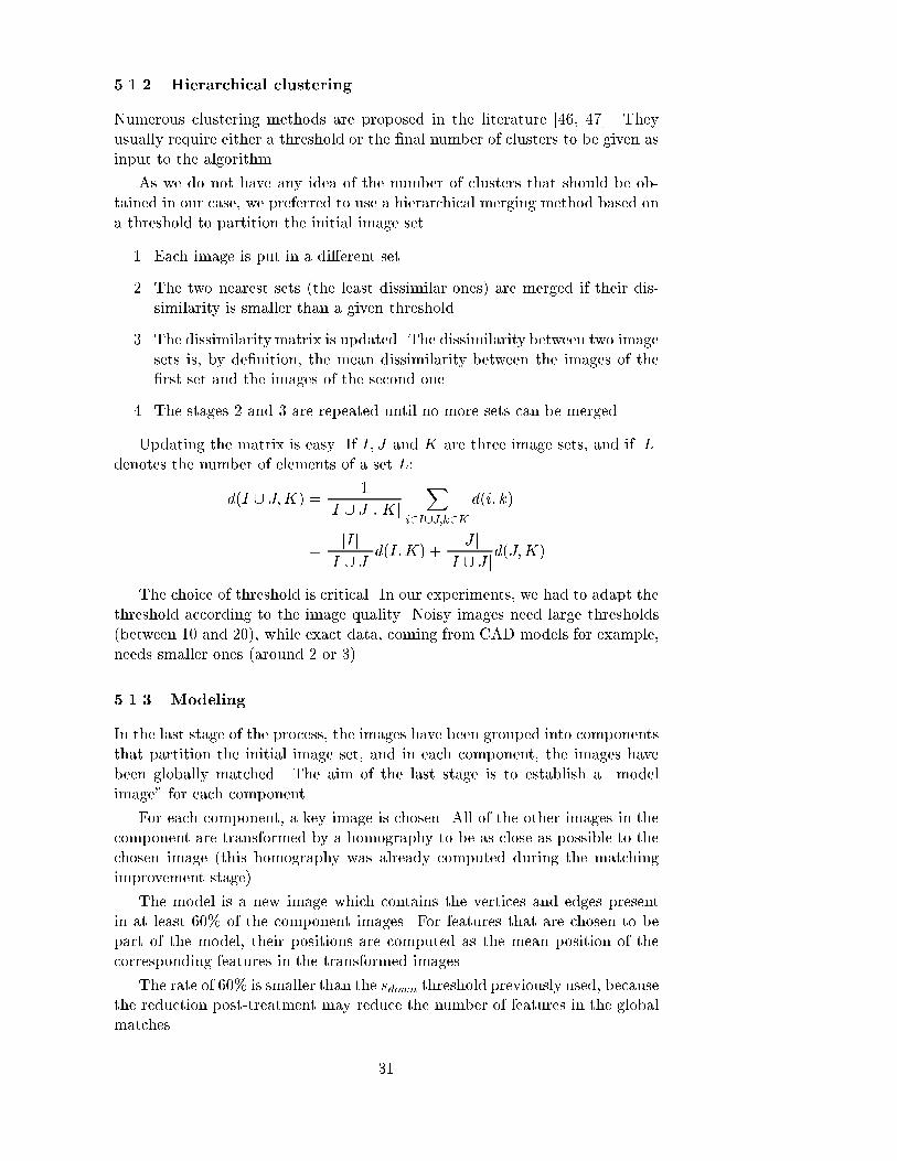
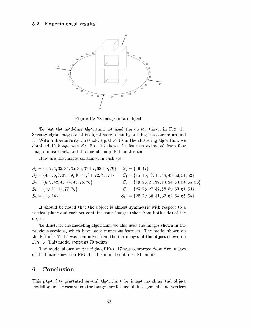
Figure 15: 78 images of an object.To test the modeling algorithm, we used the object shown in Fig. 15.Seventy eight images of this object were taken by turning the camera aroundit. With a dissimilarity threshold equal to 10 in the clustering algorithm, weobtained 10 image sets Si: Fig. 16 shows the features extracted from fourimages of each set, and the model computed for this set.Here are the images contained in each set:S1 = f1; 2; 3; 33; 34; 35; 36; 37; 67; 68; 69; 70g S6 = f46; 47gS2 = f4; 5; 6; 7; 38; 39; 40; 41; 71; 72; 73; 74g S7 = f15; 16; 17; 18; 48; 49; 50; 51; 52gS3 = f8; 9; 42; 43; 44; 45; 75; 76g S8 = f19; 20; 21; 22; 23; 24; 53; 54; 55; 56gS4 = f10; 11; 12; 77; 78g S9 = f25; 26; 27; 57; 58; 59; 60; 61; 63gS5 = f13; 14g S10 = f28; 29; 30; 31; 32; 62; 64; 65; 66gIt should be noted that the object is almost symmetric with respect to avertical plane and each set contains some images taken from both sides of theobject.To illustrate the modeling algorithm, we also used the images shown in theprevious sections, which have more numerous features. The model shown onthe left of Fig. 17 was computed from the ten images of the object shown onFig. 3. This model contains 70 points.The model shown on the right of Fig. 17 was computed from �ve imagesof the house shown on Fig. 4. This model contains 181 points.6 ConclusionThis paper has presented several algorithms for image matching and objectmodeling, in the case where the images are formed of line segments and vertices32

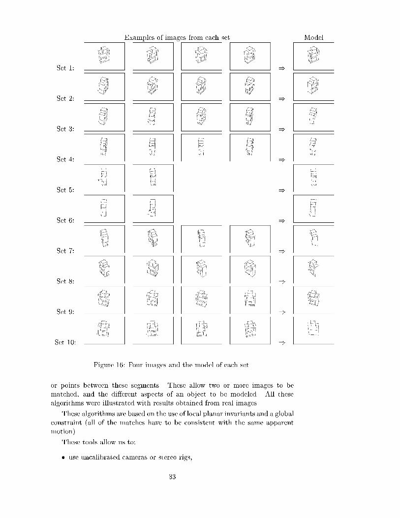
Examples of images from each set ModelSet 1: )Set 2: )Set 3: )Set 4: )Set 5: )Set 6: )Set 7: )Set 8: )Set 9: )Set 10: )Figure 16: Four images and the model of each set.or points between these segments. These allow two or more images to bematched, and the di�erent aspects of an object to be modeled. All thesealgorithms were illustrated with results obtained from real images.These algorithms are based on the use of local planar invariants and a globalconstraint (all of the matches have to be consistent with the same apparentmotion).These tools allow us to:� use uncalibrated cameras or stereo rigs,33

Figure 17: The two obtained models.� manage the case where there are mobile objects in the scene,� work with noisy images and occluded objects,� keep a low complexity.These advantages allow us to deal with problems for which no other ex-isting method is applicable, and the results clearly show the robustness of themethods.The work may be extended in three directions.1. The basic algorithm, that of two image matching, is based on the exis-tence of local quasi-invariants. It ought to work with other features, suchas curves for example.2. The models we obtain summarize the object features that are stable andcharacteristic. These may be used to recognize the object in other images.The problem is to be able to index such models in a data base, and tohave an e�cient search algorithm.3. The modeling process is quite close to the \learning from example"paradigm. The problem is to show that our modeling technique really isa learning process, i.e. that the models that are built allow a better andfaster recognition than the initial images.References[1] O. Faugeras. Three-Dimensional Computer Vision - A Geometric View-point. Arti�cial intelligence. M.I.T. Press, Cambridge, MA, 1993.[2] R.E. Kelly, P.R.H. McConnel, and S.J. Mildenberger. The Gestalt pho-tomapper. Photogrammetric Engineering and Remote Sensing, 43:1407{1417, 1977. 34

[3] W. F�orstner and A. Pertl. Photogrammetric standard methods and digitalimage matching techniques for high precision surface measurements. InE.S. Gelsema and L.N. Kanal, editors, Pattern Recognition in Practice II,pages 57{72. Elsevier Science Publishers, 1986.[4] D.B. Gennery. Modelling the Environment of An Exploring Vehicle byMeans of Stereo Vision. Ph.d. thesis, Stanford University, June 1980.[5] H.K. Nishihara. PRISM, a pratical real-time imaging stereo matcher.Technical Report Technical Report A.I. Memo 780, Massachusetts Insti-tute of Technology, 1984.[6] M. Kass. A computational framework for the visual correspondence prob-lem. In Proceedings of the 8th International Joint Conference on Arti�cialIntelligence, Karlsruhe, Germany, pages 1043{1045, August 1983.[7] M. Kass. Linear image features in stereopsis. International Journal ofComputer Vision, 1(4):357{368, January 1988.[8] A.W. Gruen. Adaptative least squares correlation: a powerful imagematching technique. S. Afr. Journal of Photogrammetry, Remote Sensingand Cartography, 14(3):175{187, 1985.[9] P. Anandan. A computational framework and an algorithm for the mea-surement of visual motion. International Journal of Computer Vision,2:283{310, 1989.[10] P. Fua. A parallel stereo algorithm that produces dense depth maps andpreserves image features. Machine Vision and Applications, 1990.[11] D. Marr and T. Poggio. Cooperative computation of stereo disparity.Science, 194:283{287, 1976.[12] D. Marr and T. Poggio. A computational theory of human stereo vision.Proceedings of the Royal Society of London, B 204:301{328, 1979.[13] W.E.L. Grimson. A computer implementation of the theory of humanstereo vision. Philosophical Tansactions of the Royal Society of London,B292(1058):217{253, 1981.[14] W.E.L. Grimson. Computational experiments with a feature based stereoalgorithm. ieee Transactions on Pattern Analysis and Machine Intelli-gence, 7(1):17{34, 1985.[15] S.B. Pollard. Identifying Correspondences in Binocular Stereo. PhD thesis,University of She�eld, 1985.[16] S.B. Pollard, J.E.W. Mayhew, and J.P. Frisby. PMF: A stereo corre-spondence algorithm using a disparity gradient constraint. Perception,14:449{470, 1985.[17] H.H. Baker and T.O. Binford. Depth from edge- and intensity- basedstereo. In Proceedings of the 7th International Joint Conference on Arti-�cial Intelligence, pages 631{636, August 1981.35

[18] Y. Ohta and T. Kanade. Stereo by intra and inter-scanline search us-ing dynamic programming. ieee Transactions on Pattern Analysis andMachine Intelligence, 7(2):139{154, 1985.[19] G. M�edioni and R. Nevatia. Segment-based stereo matching. ComputerVision, Graphics and Image Processing, 31:2{18, 1985.[20] N. Ayache and B. Faverjon. E�cient registration of stereo images bymatching graph descriptions of edge segments. International Journal ofComputer Vision, 1(2):107{132, April 1987.[21] T. Skordas. Mise en correspondance et reconstruction st�er�eo utilisant unedescription structurelle des images. Th�ese de doctorat, Institut NationalPolytechnique de Grenoble, France, 1988.[22] L. H�erault. R�eseaux de neurones r�ecursifs pour l'optimisation combina-toire. Th�ese de doctorat, Institut National Polytechnique de Grenoble,France, 1991.[23] H.J. Wolfson. Model-based object recognition by geometric hashing. InO. Faugeras, editor, Proceedings of the 1st European Conference on Com-puter Vision, Antibes, France, pages 526{536. Springer-Verlag, April 1990.[24] C.A. Rothwell. Hierarchical object descriptions using invariants. In Pro-ceeding of the darpa{esprit workshop on Applications of Invariants inComputer Vision, Azores, Portugal, pages 287{303, October 1993.[25] D. Forsyth, J. Mundy, and A. Zisserman. Transformationnal invariance - aprimer. In Proceedings of the British Machine Vision Conference, Oxford,England, pages 1{6, September 1990.[26] D. Forsyth, J.L. Mundy, A. Zisserman, and C. Rothwell. Invariant de-scriptors for 3D object recognition and pose. In Proceeding of the darpa{esprit workshop on Applications of Invariants in Computer Vision, Reyk-javik, Iceland, pages 171{208, March 1991.[27] J.L. Mundy and A. Zisserman, editors. Geometric Invariance in ComputerVision. The MIT Press, Cambridge, MA, USA, 1992.[28] J.L. Mundy and A. Zisserman, editors. Proceedings of the Second esprit- arpa Workshop on Applications of Invariance on Computer Vision,Ponta Delagada, Azores, Portugal, October 1993.[29] T.O. Binford and T.S. Levitt. Quasi-invariants: Theory and exploitation.In Proceedings of darpa Image Understanding Workshop, pages 819{829,1993.[30] J. Ben-Arie. The probabilistic peaking e�ect of viewed angles and dis-tances with application to 3D object recognition. ieee Transactions onPattern Analysis and Machine Intelligence, 12(8):760{774, August 1990.36

[31] C.F. Olson. Probabilistic indexing for object recognition. ieee Transac-tions on Pattern Analysis and Machine Intelligence, 17(5):518{522, May1995.[32] I. Shimshoni and J. Ponce. Probabilistic 3D object recognition. In Proceed-ings of the 5th International Conference on Computer Vision, Cambridge,Massachusetts, USA, pages 488{493, 1995.[33] Y. Lamdan and H.J. Wolfson. Geometric hashing: a general and e�cientmodel-based recognition scheme. In Proceedings of the 2nd InternationalConference on Computer Vision, Tampa, Florida, USA, pages 238{249,1988.[34] Y. Lamdan, J.T. Schwartz, and H.J. Wolfson. A�ne invariant model-based object recognition. ieee Journal of Robotics and Automation,6:578{589, 1990.[35] I. Weiss. Geometric invariants and object recognition. International Jour-nal of Computer Vision, 10(3):207{231, 1993.[36] J. Canny. A computational approach to edge detection. ieee Transactionson Pattern Analysis and Machine Intelligence, 8(6):679{698, 1986.[37] R. Deriche. Using Canny's criteria to derive a recursively implemented op-timal edge detector. International Journal of Computer Vision, 1(2):167{187, 1987.[38] B. Lamiroy and P. Gros. Rapid object indexing and recognition using en-hanced geometric hashing. In Proceedings of the 4th European Conferenceon Computer Vision, Cambridge, England, volume 1, pages 59{70, April1996. Postscript version available at ftp://ftp.imag.fr/pub/MOVI/publications/Lamiroy eccv96.ps.gz.[39] W.H. Press, B.P. Flannery, S.A. Teukolsky, and W.T. Vetterling. Numer-ical Recipes in C. Cambridge University Press, 1988.[40] F. Klein. Le programme d'Erlangen. Collection \Discours de la m�ethode".Gauthier-Villars, Paris, 1974.[41] Z. Zhang, R. Deriche, O. Faugeras, and Q.T. Luong. A robust techniquefor matching two uncalibrated images through the recovery of the un-known epipolar geometry. Rapport de recherche 2273, INRIA, May 1994.[42] R. Hartley. In defence of the 8-point algorithm. In Proceedings ofthe 5th International Conference on Computer Vision, Cambridge, Mas-sachusetts, USA, pages 1064{1070, June 1995.[43] B. Boufama and R. Mohr. Epipole and fundamental matrix estimationusing the virtual parallax property. In Proceedings of the 5th InternationalConference on Computer Vision, Cambridge, Massachusetts, USA, pages1030{1036, June 1995.37

[44] L. Shapiro and K. Bowyer, editors. ieee Workshop on Directions in Au-tomated CAD-Based Vision, Maui, Hawai, 1991. ieee Computer SocietyPress.[45] K. Bowyer. Why aspect graphs are not (yet) practical for computer vision.In Proceedings of the ieee workshop on Direction on automated cad-basedVision, Maui, Hawaii, USA, pages 97{104, 1991.[46] E. Diday and J.C. Simon. Clustering analysis. In K.S. Fu, editor, Com-munication and Cybernetics. Springer-Verlag, 1976.[47] G.L. Scott and H.C. Longuet-Higgins. Feature grouping by "relocalisa-tion" of eigenvectors of the proximity matrix. In Proceedings of the BritishMachine Vision Conference, Oxford, England, pages 103{108, September1990.

38