Using Information Gain to Analyze and Fine Tune the ... · Using Information Gain to Analyze and Fine Tune the Performance of Supply Chain Trading Agents ... Information Gain Analysis

Using Information Gain to Analyze and Fine

Tune the Performance of Supply Chain Trading

Agents

James Andrews, Michael Benisch, Alberto Sardinha, and Norman Sadeh

School of Computer Science, Carnegie Mellon University

Abstract. The Supply Chain Trading Agent Competition (TAC SCM)was designed to explore approaches to dynamic supply chain trading.During the course of each year’s competition historical data is loggeddescribing more than 800 games played by different agents from aroundthe world. In this paper, we present analysis that is focused on deter-mining which features of agent behavior, such as the average lead timerequested for supplies or the average selling price offered on finished prod-ucts, tend to differentiate agents that win from those that do not. Wepresent a visual inspection of data from 16 games played in one bracketof the 2006 TAC SCM semi-final rounds. Plots of data from these gameshelp isolate behavioral features that distinguish top performing agentsin this bracket. We then introduce a metric based on information gainto provide a more complete analysis of the 80 games played in the 2006TAC SCM quarter-final, semi-final and final rounds. The metric capturesthe amount of information that is gained about an agent’s performanceby knowing its value for each of 20 different behavioral features. Usingthis metric we find that, in the final rounds of the 2006 competition,winning agents distinguished themselves by their procurement decisions,rather than their customer bidding decisions. We also discuss how weused the analysis presented in this paper to improve our entry for the2007 competition, which was one of the six finalists that year.

Keywords. Automated trading, electronic commerce, supply chain man-agement, agent performance analysis, TAC SCM.

1 Introduction

As the Internet helps mediate an increasing number of supply chain transac-tions, there is a growing interest in investigating the potential benefits of moredynamic supply chain practices [1, 2]. Since its inception, the Supply ChainTrading Agent Competition (TAC SCM) has served as a competitive test bedfor this purpose [1]. TAC SCM pits against one another trading agents developedby teams from around the world, with each agent using its own unique strat-egy. Agents are responsible for running the procurement, planning and biddingoperations of a PC assembly company, while competing with others for bothcustomer orders and supplies under varying market conditions.

2 James Andrews, Michael Benisch, Alberto Sardinha, and Norman Sadeh

During the course of each year’s competition more than 800 games are played.The logs of these games provide ample data for evaluating the strengths andweaknesses of techniques implemented by different agents. The primary mea-sure of an agent’s performance in TAC SCM is its average overall profit overa game – with each game simulating one year of operation. This metric allowsus to determine which agents perform best across a wide variety of conditions.However, examining only average profit does not tell us what differentiated win-ning agents from the others. Answering this question is of practical interest toagent designers, and may also help transfer insights from the competition toreal world supply chain problems. In this paper, we investigate which featuresof agent behavior best distinguish top performing TAC SCM agents in the 2006competition’s quarter-final, semi-final and final rounds.

We begin with a close look at statistical features of 6 different agents in onebracket of the 2006 semi-final rounds (this bracket accounted for 16 games),such as the average quantity they requested from component suppliers each day.Plots from these games reveal unique patterns, or “fingerprints,” which allow usto isolate behavioral features that distinguish top performing agents.

Using a quantitative analysis technique, we estimate the ability of 20 differ-ent features to differentiate winners over a larger collection of 80 different games.Our technique involves calculating the amount of information gained about anagent’s performance by knowing its value for each feature (e.g., the average leadtime it requested from component suppliers). Results on data from the 2006 finalrounds include a ranking of features based on their information gain, providinginsight into the collection of features that made winning agents unique. In par-ticular we find that, in the final rounds of the 2006 competition, winning agentsdistinguished themselves by decisions related to the procurement of components,rather than those related to bidding for customer orders.

Finally, we discuss how the insights gained from the analysis in this paperhelped us refine our entry for the 2007 competition [3]. In particular, we decidedto place a greater emphasis on long-term procurement (i.e., purchasing partslong in advance). We found that our improvements helped our agent procurecomponents significantly cheaper and with greater reliability – and ultimatelyreach the finals that year.

The remainder of this paper is organized as follows: We first provide a briefoverview of the TAC SCM game. The following section describes related effortsin analyzing and presenting tools to analyze the TAC SCM games. Section 4describes our visual inspection of feature plots from the 2006 semi-finals. InSection 5 we present our information gain-based analysis and apply it to all ofthe games from the 2006 quarter-finals, semi-finals and finals. Section 6 brieflydescribes how we used the analysis in this paper to improve our agent for the 2007competition. The final section discusses additional uses of our technique such ashow it could be extended by agent developers to identify potential weaknessesin their entry.

Information Gain Analysis of Supply Chain Trading Agents 3

2 TAC SCM overview

The TAC SCM game is played over a simulated period of 220 game days, and oneach day agents are required to make several decisions. They are responsible forsending requests to suppliers, offers to customers, and a production plan to theirfactory. Each request to a supplier for a specific component includes a quantity,lead time (the number of days before the order is delivered), and reserve price(the maximum the agent is willing to pay for the parts). Suppliers then respondwith offers that specify actual quantities, prices, and lead times. When an agentplaces an order, parts are scheduled for delivery into its inventory. Agents canalso respond to requests made by customers for finished PCs. These requestsspecify a quantity, due date, reserve price, and PC type. Agents can compete foreach customer request by submitting offers with a specific price. The agent withthe lowest price for each request is awarded an order. Upon delivery of the orderthe revenue for the transaction is placed in its bank account – minus possibletardiness penalties. Orders that are overly late are canceled. For a more detaileddescription of the game, readers are directed to [4].

3 Related work

Several researchers in the Trading Agent Competition community have presentedmethods for analyzing competition data to gain insights about agent perfor-mance.

In [5] and [6] the University of Michigan team applied game theoretic analysisto abstracted versions of the TAC games. The abstracted games were estimatedempirically from the results of repeated simulations with different combinationsof strategies. Their analysis revealed interesting best response and equilibriumrelationships. The Michigan team also presented methods for estimating theefficiency and power of different entities in the TAC SCM market [7].

In [8] we analyzed data from the seeding rounds of the 2005 competition todetermine that the strong performance of our agent, CMieux, was largely at-tributable to significantly cheaper component purchase prices than other agents.

Tool kits such as our Analysis Instrumentation Toolkit [9] and the SwedishInstitute for Computer Science (SICS) Game Data Toolkit1 allow teams to an-alyze historical log files from a single TAC SCM game. These tools provide anin-depth view of the B2B and B2C interactions through graphical front-ends.

Several teams have also analyzed controlled experiments using different con-figurations of their own agent and publicly available agent binaries.

In [10] the team from the University of Minnesota presented techniques tomanipulate the market environment of the simulator. By controlling variousmarket factors, such as aggregate demand and supply, they suggest that TacTex,a top performing agent, loses its edge when market pressure is high. In [11] theSouthampton team presented experiments with variants of their own agent that

1 Available at http://www.sics.se/tac/.


are more or less risk seeking in choosing selling prices, and in [12] they providesimilar analysis with respect to lead times on component orders. In [13] theUniversity of Texas team evaluated variants of their own agent against publiclyavailable binaries of other agents. They used the results of their experiments tofine-tune various parameters in their final agent and guide future development.

The analysis methods presented in this paper differ from existing techniquesin the following two ways: i) we systematically investigate the question of whichbehavioral features are associated with successful performance across all agentsin a large collection of games and ii) we perform all of our analysis on actualcompetition data, as opposed to offline controlled experiments.

4 Feature plot analysis

Historical data from the TAC SCM competition provides a large data source forstudying the effectiveness of different supply chain trading techniques. However,it is worth noting that by analyzing historical data from the competition wemust limit ourselves to analyzing only low-level actions taken by each agent,rather than the underlying algorithms or techniques. In this section, we analyzeplots of statistical features of such actions for six different agents from the 2006semi-finals games containing our agent, CMieux. The full data set consists of 16games from the 2006 semi-finals group 1 (games 5097-5104 on tac3.sics.se and5580-5587 on tac4.sics.se) with agents placing in the following order: Deep-Maize [14], Maxon, Botticelli [15], CMieux [8], Mertacor [16], and Southampton-SCM [12].

Out of all the feature plots we examined, the following best illustrate howagents can be distinguished by features of their low-level behavior. Each of theplots presented shows qualitative differences between the six agents. By analyz-ing these plots we are able to identify unique characteristics of the agents, andgain insights into why some performed better than others.

4.1 Lead time vs. game day

In TAC SCM, agents can decide how far in advance to order components. Werefer to the difference between the day an order is placed and the day that itis to be delivered as the order’s lead time. Figure 1 shows plots of the averagecomponent order lead time (Y axis) on each game day (X axis) of the differentagents2. These plots show that agents are easily distinguished by the extent towhich they used long lead times early in the game, the length of their maximumlead time, and their most commonly used lead times.

The two best performing-agents from this round, DeepMaize and Maxon,feature substantially longer early-game lead times. Both of these agents placed

2 Plots presented in this section examine behavior with respect to one specific com-ponent. Aggregating data across multiple components washed out potentially inter-esting details, and plots for other components were not noticeably different.


orders at the beginning of the game that had due dates towards the end of thegame, while the other agents did not. DeepMaize and Maxon also both reducetheir lead times well before Mertacor, CMieux, and Botticelli. The latter threeappear to maintain long lead times until they approach the end of the game.SouthamptonSCM takes a hybrid of these two approaches, reducing lead timesbefore necessary but still much later in the game.

Maxon and Mertacor take very different approaches to the mid-game, withMertacor almost exclusively using longer lead times, and Maxon primarily re-lying on short ones. Maxon also seems to exhibit a single mid-game ’spike’ inlead times, placing orders with uncharacteristically long lead times near day 120.This is either a fixed restock point or an attempt to disrupt the procurement ofother agents. Mertacor’s, and, to a lesser extent, SouthamptonSCM’s plots show’bands,’ which most likely correspond to specific long-term order lead times thatare chosen to simplify their decision processes.

Game Day

Lead

Tim

e

0

50

100

150

200

0 50 100 150 200

Botticelli CMieux

0 50 100 150 200

DeepMaize

Maxon

0 50 100 150 200

Mertacor

0

50

100

150

200SouthamptonSCM

Fig. 1. A plot showing the average lead time and game day of component orders placedby six different agents during the 2006 semi-finals for the Pintel 2Ghz component (othercomponents yield similar plots).

4.2 Lead time vs. order quantity

Figure 2 shows plots of the average lead time of component orders (Y axis)against their average quantity (X axis). These plots illustrate that agents differin the extent to which they place large orders with long lead times.

Placing component orders with long lead times and large quantities corre-sponds to increased risk. Thus, the extent to which an agent is willing to increaseboth can be seen as a reflection of its attitude towards risk. The lead time vs.


order quantity plots showcase the different approaches of the agents: Maxon,Mertacor, CMieux and DeepMaize each appear reluctant to place orders withlong lead times and large quantities. The trade-off is less pronounced for Botti-celli and SouthamptonSCM. Maxon, Mertacor and DeepMaize each show unique’bands,’ with DeepMaize considering only a handful of fixed order quantities,Mertacor considering only fixed lead times, and Maxon fixing a combination ofthe two attributes.

Order Quantity

Lead

Tim

e

0

50

100

150

200

500 1000

Botticelli CMieux

500 1000

DeepMaize

Maxon

500 1000

Mertacor

0

50

100

150

200SouthamptonSCM

Fig. 2. A plot showing the average lead time and average order quantity per day ofcomponent orders placed by six different agents during the 2006 semi-finals for thePintel 2Ghz component.

4.3 Reserve price vs. order price

When TAC SCM agents send component requests to suppliers, they have theoption of specifying a reserve price – or the maximum per-unit price they arewilling to pay for the requested components. The difference between an agent’sreserve price and its order price indicates to what extent the agent’s reserveprice impacted its procurement cost. Figure 8 in the Appendix shows a plotof each agent’s average component order price (Y axis) against that agent’saverage offered reserve price (X axis). This plot illustrates that agents employedvariations of three different strategies for choosing their reserve prices: fixedreserve prices, dynamic reserve prices, and reserve prices equal to purchase prices.

Maxon and Mertacor appear to choose from a few fixed reserve prices.SouthamptonSCM and Botticelli appear to use their reserve prices to more ag-gressively limit their order prices, since they are consistently close to their pur-chase prices. CMieux and DeepMaize have more dynamic strategies for choosing


reserve prices, although a few ‘bands’ of fixed reserve price do appear in theDeepMaize plot.

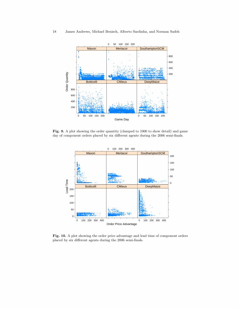
4.4 Order quantity vs. game day

Figure 9 in the Appendix shows a plot of each agent’s average order quantity(Y axis) on each game day (X axis). Agents demonstrate unique choices formaximum order quantity, minimum order quantity, and the specific quantitiesthey ordered repeatedly.

Mertacor, DeepMaize, and, to a lesser extent, Maxon each appear to favororders greater than roughly 100 components at the beginning of the game. Maxonchose a maximum order quantity of about 200 units after the beginning of thegame, while SouthamptonSCM and CMieux appear to consider at most about400. Botticelli, Mertacor, and DeepMaize are all willing to go above 800 unitson occasion. Bands on the graphs of DeepMaize and SouthamptonSCM suggestthese agents were frequently choosing the same quantity on their orders.

4.5 Order price advantage vs. lead time

Figure 10 in the Appendix shows a plot of each agent’s average order lead time (Yaxis) against the average component order price “advantage,” or the differencebetween the their price and the best price (X axis). In these plots, agents canbe distinguished by the extent to which they require better price advantages toconsider long lead times.

Maxon and DeepMaize, for example, have a clear ’triangle’ structure to theirgraphs, implying that they were only willing to accept orders with long lead timeswhen they could get them at relatively good prices. Mertacor, SouthamptonSCMand Botticelli’s plots have almost rectangular shapes, implying a more generalacceptance of long lead times. CMieux appears to have a hybrid approach, withthe triangle structure only being apparent for lead times above about 25 days.

5 Information gain analysis

Visual inspection provides a useful starting point for our analysis, however ingeneral it is time consuming for large data sets, subjective and error prone. Inthis section we introduce a more systematic technique to automate the type ofinformal analysis discussed in Section 4. Our technique considers the correspon-dence of particular features with top performance, or their information gain, andprovides insight into the collection of features that made winning agents unique.By using a metric for comparing several different features at once, we are ableto rank more than 20 different features across all 80 games from the 2006 finalrounds.


5.1 Measuring information gain

In this analysis we calculate the amount of information gained about an agent’sperformance by knowing its value for different features. Information gain is apopular measure of association in data mining applications. The informationgained about an outcome O from an attribute A is defined as the expecteddecrease in entropy of O conditioned on A. The following equations can be usedto calculate the information gained about a discrete outcome O from a discreteattribute A, which we denote as IG(O, A). We use H(O) to denote the entropyof O, H(O | A) to denote the entropy of O given A, and P (a) to denote theprobability that attribute A takes on value a in the data.

IG(O, A) = H(O) − H(O | A) (1)

H(O) = −∑

o∈O

P (o) log2(P (o))

H(O | A) =∑

a∈A

P (a)H(O | A = a)

H(O | A = a) = −∑

o∈O

P (o | a) log2(P (o | a))

Intuitively, IG(O, A) is how much better the value of O can be predicted byknowing the value of A. For a more detailed explanation of information gain asused in this paper see, for example, [17].

In our analysis we use the information gain metric to determine how muchbetter we can predict an agent’s success by knowing features of its behavior. Forour data set, we construct a collection of performance observations, with oneobservation for each agent in each game. Performance observations include anoutcome value, indicating whether or not the agent placed first3 and 20 differentreal-valued attributes of its behavior.

Before we can calculate the information gain of the attributes, we must dis-cretize them. This is accomplished by splitting the space between the minimumand maximum values of each attribute evenly into 2k partitions, for a positiveinteger k. In our results we present the information gain of all different featureswith k varied between 1 and 6. For a particular attribute, using larger values ofk will tend to increase (and cannot decrease) its information gain4. Therefore,using values of k that are too large can lead to a form of “over-fitting,” whereevery attribute can uniquely distinguish every outcome. However, smaller valuesof k may overlook the ability of an attribute to distinguish winning agents fromlosing ones. Nonetheless, we observe that for all k ≥ 4 (yielding 16 or morepartitions) we can extract a consistent ranking.

3 We later extend this technique to consider other outcomes: specifically, whether ornot an agent finished in the top 3 positions.

4 This is because performances in separate partitions remain separated as k increases.


5.2 Information gain example

To illustrate our use of information gain we will walk through the followingshort example. As in our primary analysis, we will consider the outcome valueof a performance to be whether or not an agent placed first. In our examplewe will evaluate the information gained by knowing the maximum lead time anagent requested on any component order in the game. We will only considerthe feature using 2 partitions: one for less than 50 and the other for greaterthan or equal to 50. From 6 games we will create 36 performance observations(assuming 6 agents in each game). Note that 6

36 are first place performances,giving the outcome variable over our data set an entropy of:

H(O) = −

[

6

36log

(

6

36

)

+30

36log

(

30

36

)]

≈ 0.65 (2)

Now assume that 8 of the 36 performances had lead times greater than 50,including 5 of the 6 winning performances. In other words, the probability ofobserving a long lead time is 8

36 , the probability of an agent winning giventhat it had a long lead time is 5

8 , and the probability of observing a winningperformance without a long lead time is 6−5

36−8 = 128 .

We can now calculate the conditional entropy of the outcome variable inthe case where the maximum lead time attribute is greater than or equal to 50(“long”) and when it is less than 50 (“short”),

H(O | “long”) = −

[

5

8log

(

5

8

)

+3

8log

(

3

8

)]

≈ 0.95 (3)

H(O | “short”) = −

[

1

28log

(

1

28

)

+27

28log

(

27

28

)]

≈ 0.22 (4)

Using the conditional entropy we can calculate the average entropy of the out-come variable conditioned on the lead time attribute, A,

H(O | A) = P (“long”)H(O | “long”) + P (“short”)H(O | “short”) ≈ 0.38 (5)

Finally, the information gain of the outcome, O, from the attribute A, is thedifference between the entropy of O independent of A, and its average entropyconditioned on A,

IG(O, A) = H(O) − H(O | A) ≈ 0.27 (6)

Note that, because the initial entropy of the “first place” feature is about 0.65,the maximum possible information gain for any feature is also 0.65.


5.3 Information gain results

We now present the information gain of 20 different features across 6 values of k

(representing 2, 4, 8, 16, 32, and 64 partitions). Our data set included all of the80 games from the 2006 final rounds. Figure 3 shows the information gain of 6different features at each level of discretization. It illustrates that upon reaching16 or more partitions, features that provide more information tend to do soat finer discretization levels as well. Therefore, despite the potential drawbacksassociated with the discretization process, we are still able to extract a fairlyconsistent ranking of features based on their ability to differentiate winningagents.

0.2

0.3

0.4

0 10 20 30 40 50 60 70

Info

rmat

ion

gain

Number of discrete partitions (2k)

Largest lead timeAverage lead time

Average early order quantityAverage reserve price

Small order percentageReserve price slack

Fig. 3. A plot showing the information gain for 6 different features at varying levels ofdiscretization (k ∈ {1, . . . , 6}). The maximum possible information gain of any featureis ≈ 0.65.

Table 1 shows the information gain for all 20 different features at three dif-ferent partition levels: 16, 32 and 64 (a table including information gain levelsfor less than 16 partitions is available in an earlier version of this paper [18]).The features are ranked into 8 categories that are consistent from 16 partitionson. The ranking illustrates that the two features providing the most informa-tion about an agent’s performance were both related to its decisions about leadtimes on component orders. Additionally, 8 of the top 10 features in the rankingwere related to decisions about component orders, such as their average quantityand reserve prices. Notably absent from the top distinguishing features were alldemand-oriented features: the highest of these, total sell quantity (in revenue),tied with four other features for rank 7. This suggests that top agents were ableto distinguish themselves primarily based on the collection of features that char-acterized their procurement strategy (which is consistent with previous findingsin [8] regarding the 2005 seeding rounds).


Rank Feature 16 part. 32 part. 64 part.

1 Maximum lead time (supply) 0.347 0.385 0.4182 Average lead time (supply) 0.339 0.368 0.4043 Average early component order quantity (sent before day 25) 0.324 0.354 0.3914 Average reserve price (supply) 0.304 0.314 0.345

Small component order percentage (quantity ≤ 100) 0.286 0.316 0.341Average reserve price slack(supply) 0.294 0.312 0.334

7 Last-minute component order percentage (lead time ≤ 3) 0.262 0.285 0.324Short lead time component order percentage (lead time ≤ 10) 0.277 0.289 0.309

Total revenue (demand) 0.274 0.287 0.304Total quantity sold (demand) 0.262 0.275 0.302

11 Average quantity ordered per day (supply) 0.259 0.271 0.30012 Average RFQ due date (demand) 0.243 0.265 0.29113 Average factory utilization 0.222 0.230 0.274

Average selling price (demand) 0.225 0.233 0.246Average purchase price (supply) 0.217 0.240 0.244Minimum bank account value 0.220 0.222 0.241

Purchase price standard deviation (supply) 0.206 0.215 0.239Average stock value 0.223 0.229 0.238

Average order price advantage (supply) 0.226 0.234 0.236Unsold stock at end of game 0.216 0.217 0.227

Table 1. The information gain of the 20 different features we tested at each level ofdiscretization between 16 and 64. The features are sorted by information gain at 64partitions and ranked into groups that are distinguishable at each discretization levelfrom 16 to 64 partitions.

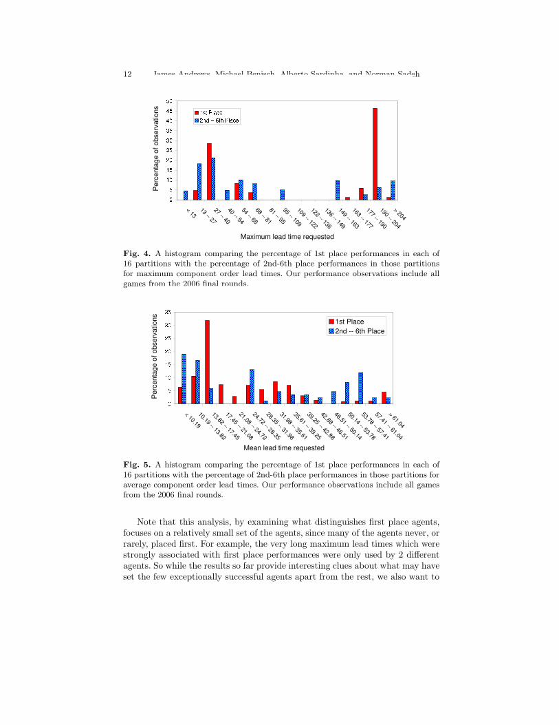
When calculating information gain for a feature, we determine the percentageof 1st place performances which occupy each partition for each feature, andlikewise for the percentage of 2nd-6th place performances. Once we’ve identifiedan interesting feature, we can examine this information more directly with ahistogram, showing us where exactly the distinctions between agents could bemade. Figure 4, for example, shows a histogram comparing the percentage of 1stplace performances in each of 16 partitions with the percentage of 2nd-6th placeperformances in those partitions for maximum component order lead times.

We can see from this plot that a significant percentage of the winning per-formances used very long maximum lead times – from 190 to 204 days – whilethe second most prominent winning performance tended to keep maximum leadtimes at only 27 to 40 days. This clues us in to two strong strategies from the2006 final rounds: winning agents tended to either order components almost tothe end of the game at the very beginning, or they were more conservative anddid not risk long lead times. Agents who restricted themselves to even shortertime ranges, or who took the large middle ground between 40 and 190 days, didnot tend to be as successful.

Figure 5 shows a similar histogram examining the second most distinguishingfeature: mean component order lead time. In this plot we see that, although alarge maximum lead time was beneficial, agents who used long lead times exces-sively did not tend to perform well. Very few wins are observed for mean leadtimes greater than 40, while the plurality of lead times for winning performancessits at the relatively low range of 13 to 18. Finally we can see that for both winsand losses, the lower average lead times were a more popular choice.


Fig. 4. A histogram comparing the percentage of 1st place performances in each of16 partitions with the percentage of 2nd-6th place performances in those partitionsfor maximum component order lead times. Our performance observations include allgames from the 2006 final rounds.

Fig. 5. A histogram comparing the percentage of 1st place performances in each of16 partitions with the percentage of 2nd-6th place performances in those partitions foraverage component order lead times. Our performance observations include all gamesfrom the 2006 final rounds.

Note that this analysis, by examining what distinguishes first place agents,focuses on a relatively small set of the agents, since many of the agents never, orrarely, placed first. For example, the very long maximum lead times which werestrongly associated with first place performances were only used by 2 differentagents. So while the results so far provide interesting clues about what may haveset the few exceptionally successful agents apart from the rest, we also want to


0.2

0.3

0.4

0 10 20 30 40 50 60 70

Info

rmat

ion

gain

Number of discrete partitions (2k)

Average lead timeAverage reserve price

Largest lead timeSmall order percentage

Short lead time percentageReserve price slack

Fig. 6. A plot showing the information gained about whether or not an agent placed3rd or better for 6 different features at varying levels of discretization (k ∈ {1, . . . , 6}).

examine what more widely used behaviors were associated with success. To doso, we re-define our measure of success from “the agent placed first” to “theagent placed at least third.”

Rank Feature 16 part. 32 part. 64 part.

1 Average lead time (supply) 0.368 0.406 0.458Average reserve price (supply) 0.333 0.408 0.441

3 Maximum lead time (supply) 0.325 0.392 0.4314 Small component order percentage (quantity ≤ 100) 0.293 0.329 0.400

Short lead time component order percentage (lead time ≤ 10) 0.266 0.370 0.396Average reserve price slack (supply) 0.251 0.336 0.394

Last-minute component order percentage (lead time ≤ 3) 0.234 0.337 0.387Total revenue (demand) 0.246 0.358 0.379

Average early component order quantity (sent before day 25) 0.283 0.339 0.377Total quantity sold (demand) 0.239 0.343 0.363

Average quantity ordered per day (supply) 0.239 0.334 0.355Average order price advantage (supply) 0.225 0.334 0.340

13 Average order price (supply) 0.290 0.316 0.33014 Average RFQ due date (demand) 0.243 0.268 0.299

Average stock value 0.206 0.271 0.28516 Average factory utilization 0.207 0.236 0.284

Minimum bank account value 0.204 0.248 0.270Average selling price (demand) 0.220 0.249 0.260Unsold stock at end of game 0.211 0.252 0.260

Purchase price standard deviation (supply) 0.225 0.240 0.254

Table 2. The information gain of the 20 different features we tested at each levelof discretization between 16 and 64 partitions, with respect to 3rd-place or betterperformances. The features are sorted by information gain at 64 partitions and rankedinto groups that are distinguishable with 32 and 64 partitions. The maximum possibleinformation gain of any feature is 1.


The results of this extension are shown graphically in Figure 6 and in atable format in Table 2 for partition sizes of 16, 32 and 64 (results for smallerpartition sizes are available in an earlier version of this paper [18]. These figuresillustrate that the relative ordering of features is less consistent than before.Nonetheless, we are still able to extract 6 distinct levels of information across 32and 64 partitions. Many of our observations about first place agents hold true inthis new ranking: decisions about component ordering continue to dominate theranking, taking 9 of the 12 top spots. If we rank on the information gained at64 partitions, all features in the top 10 previously remain in the top 10. Thereare certainly differences in the ranking – maximum lead time, for example, hasfallen from being the most important feature to being third most important – butfeatures which differentiated first place agents appear to continue to differentiatesuccessful agents more generally.

6 Incorporating these insights into our agent

One of the main take away messages from the analysis in this paper is that inthe 2006 TAC SCM competition, the top agents made purchases with longerlead times, especially at the beginning of the game. The preference for long-term procurement contracts is consistent with real world managerial insightthat such contracts have better guarantees of availability, and lower prices. Weincorporated this intuition into our 2007 TAC SCM entry, CMieux, by placing agreater emphasis on long-term procurement, and in that year’s competition ouragent was one of the six agents to reach the finals.

Placing supply orders with long lead times requires overcoming two majorchallenges. The first is estimating a safe level of demand for the long term future,so that the agent is not stuck with excess supply. We approached this by con-servatively estimating that demand would be one full standard deviation belowthe mean given in the TAC SCM specification [4].

The second challenge was an increase in the number of possible lead timesto consider. To address this issue we split the long-term period into large non-overlapping buckets, and focused procurement efforts on buckets with greaterprojected unmet demand and lower prices. As more agents adopt a long termprocurement strategy, such as the one described above, it is possible that thebenefits will become less pronounced. However, in the 2007 competition we foundthat our long term procurement strategy helped our agent procure componentssignificantly cheaper and with greater reliability [3].

Figure 7 illustrates the change in the lead time “fingerprint” of our agentfrom 2006 to 2007, which clearly shoes a greater emphasis on orders with longlead times.


Game Day

Lead

Tim

e

0

50

100

150

0 50 100 150 200

CMieux (2006 semifinals)

0 50 100 150 200

CMieux (2007 finals)

Fig. 7. A plot showing the average lead time and game day of component orders placedby CMieux during the 2006 semi-finals (left) and the 2007 finals (right) for the Pintel2Ghz component. Based on the analysis in this paper, CMieux was adapted in 2007 toplace a greater emphasis on orders with long lead times.

7 Discussion

This paper presented an investigation into which collection of behavioral featuresdifferentiated winning TAC SCM agents during the 2006 final rounds. We beganwith a visual inspection of games from one bracket of the 2006 semi-finals. Plotsfrom these games revealed unique patterns, or “fingerprints,” which allowed usto isolate behavioral features that distinguished top performing agents in thisbracket.

Because this type of visual analysis is time consuming, subjective and errorprone, we proceed to develop a systematic methodology to automatically analyzelarger data sets. We applied a quantitative technique to all of the 80 gamesin the 2006 final rounds. This technique involved calculating the amount ofinformation gained about an agent’s performance by knowing its value for eachof 20 different features. The most informative features turned out to be related todirect decisions regarding component orders, such as the lead times and reserveprices used. These features differentiated winning agents in the 2006 final roundssignificantly more than those related to costs and revenues.

Our information gain-based analysis technique was limited to examining theinformativeness of individual features. Extending our technique to consider theeffects of combinations of features may provide additional insight. For example,knowing an agent’s average selling price and average buying price together wouldprobably be very informative. However, this raises additional concerns aboutover-fitting: using several features at once may uniquely identify each agent,instead of their shared characteristics.

As previously mentioned, our information gain-based technique can also beextended to consider other outcomes. For example, it may be interesting to in-vestigate which features distinguish the worst agents. This can be accomplished


by simply changing the outcome variable associated with each performance ob-servation.

Finally, an agent designer may wish to answer the question, “what featuresdifferentiate games her agent wins from games it doesn’t?” This can be accom-plished by modifying the information gain technique in the following ways. First,only consider performance observations of the agent in question. Second, use fea-tures related to the game overall, such as its average customer demand, ratherthan features of a specific agent’s behavior.

8 Acknowledgments

This work was supported in part by the National Science Foundation ITR grant0205435, by a grant from SAP Labs, and by Carnegie Mellon University’s e-SCMLab.

References

1. Arunachalam, R., Sadeh, N.: The supply chain trading agent competition. Elec-tronic Commerce Research Applications 4(1) (2005) 63–81

2. Sadeh, N., Hildum, D., Kjenstad, D., Tseng, A.: Mascot: an agent-based archi-tecture for coordinated mixed-initiative supply chain planning and scheduling. In:Proceedings of Agents Workshop on Agent-Based Decision Support in Managingthe Internet-Enabled Supply-Chain. (1999)

3. Benisch, M., Sardinha, A., Andrews, J., Ravichandran, R., Sadeh, N.: CMieux:Adaptive strategies for supply chain management. Electronic Commerece ResearchApplications Forthcoming.

4. Collins, J., Arunachalam, R., Sadeh, N., Eriksson, J., Finne, N., Janson, S.: Thesupply chain management game for 2006 trading agent competition (TAC SCM).Technical Report CMU-ISRI-05-132, School of Computer Science, Carnegie MellonUniversity (November 2006)

5. Kiekintveld, C., Vorobeychik, Y., Wellman, M.: An analysis of the 2004 supplychain management trading agent competition. In Poutr, H.L., Sadeh, N., Jan-son, S., eds.: Agent-Mediated Electronic Commerce: Designing Trading Agentsand Mechanisms. Number 3937 in Lecture Notes in AI, Springer-Verlag (2006)99–112

6. Wellman, M.P., Jordan, P.R., Kiekintveld, C., Miller, J., Reeves, D.M.: Empiricalgame-theoretic analysis of the TAC market games. In: Proceedings of AAMASWorkshop on Game-Theoretic and Decision-Theoretic Agents. (2006)

7. Jordan, P.R., Kiekintveld, C., Miller, J., Wellman, M.P.: Market efficiency, salescompetition, and the bullwhip effect in the TAC SCM tournaments. In: Proceed-ings of AAMAS Workshop on Trading Agent Design and Analysis (TADA). (2006)

8. Benisch, M., Andrews, J., Sardinha, A., Sadeh, N.: CMieux: Adaptive strategiesfor supply chain management. In: Proceedings of International Conference onElectronic Commerce (ICEC). (2006)

9. Benisch, M., Andrews, J., Bangerter, D., Kirchner, T., Tsai, B., Sadeh, N.: CMieuxanalysis and instrumentation toolkit for TAC SCM. Technical Report CMU-ISRI-05-127, School of Computer Science, Carnegie Mellon University (September 2005)


10. Borghetti, B., Sodomka, E., Gini, M., Collins, J.: A market-pressure-based perfor-mance evaluator for TAC SCM. In: Proceedings of AAMAS Workshop on TradingAgent Design and Analysis (TADA). (2006)

11. He, M., Rogers, A., David, E., Jennings, N.R.: Designing and evaluating an adap-tive trading agent for supply chain management applications. In: Proceedings ofIJCAI Workshop on Trading Agent Design and Analysis (TADA). (2005)

12. He, M., Rogers, A., Luo, X., Jennings, N.R.: Designing a successful trading agentfor supply chain management. In: Proceedings of Autonomous Agents and Multi-agent Systems (AAMAS). (2006)

13. Pardoe, D., Stone, P.: Predictive planning for supply chain management. In:Proceedings of Automated Planning and Scheduling. (2006)

14. Kiekintveld, C., Wellman, M.P., Singh, S., Estelle, J., Vorobeychik, Y., Soni, V.,Rudary, M.: Distributed feedback control for decision making on supply chains.In: Proceedings of Automated Planning and Scheduling. (2004)

15. Benisch, M., Greenwald, A., Grypari, I., Lederman, R., Naroditsky, V., Tschantz,M.: Botticelli: A supply chain management agent. In: Proceedings of AutonomousAgents and Multi-Agent Systems (AAMAS). (2004)

16. Kontogounis, I., Chatzidimitriou, K., Symeonidis, A., Mitkas, P.: A robust agentdesign for dynamic SCM environments. In: Hellenic Joint Conference on ArtificialIntelligence (SETN’06). (2006)

17. Mitchell, T.M.: Machine Learning. McGraw Hill (1997)18. Andrews, J., Benisch, M., Sardinha, A., Sadeh, N.: What differentiates a winning

agent: An information gain based analysis of TAC SCM. In: AAAI Workshop onTrading Agent Design and Analysis (TADA). (2007)

9 Appendix

This appendix includes three plots that were omitted from the main text.

Order Price

Res

erve

Pric

e

0

500

1000

1500

500 600 700 800 9001000

Botticelli CMieux

500 600 700 800 9001000

DeepMaize

Maxon

500 600 700 800 9001000

Mertacor

0

500

1000

1500

SouthamptonSCM

Fig. 8. A plot showing the reserve price and order price of component orders placedby six different agents during the 2006 semi-finals.


Game Day

Ord

er Q

uant

ity

200

400

600

800

0 50 100 150 200

Botticelli CMieux

0 50 100 150 200

DeepMaize

Maxon

0 50 100 150 200

Mertacor

200

400

600

800

SouthamptonSCM

Fig. 9. A plot showing the order quantity (clamped to 1000 to show detail) and gameday of component orders placed by six different agents during the 2006 semi-finals.

Order Price Advantage

Lead

Tim

e

0

50

100

150

200

0 100 200 300 400

Botticelli CMieux

0 100 200 300 400

DeepMaize

Maxon

0 100 200 300 400

Mertacor

0

50

100

150

200SouthamptonSCM

Fig. 10. A plot showing the order price advantage and lead time of component ordersplaced by six different agents during the 2006 semi-finals.

Using Information Gain to Analyze and Fine Tune the ... · Using Information Gain to Analyze and Fine Tune the Performance of Supply Chain Trading Agents ... Information Gain Analysis

Documents