Using High Resolution Satellite Imagery to Map Aquatic ... Report . August, ... white water lily (Nymphaea orderata), and the invasive Eurasian watermilfoil ... indicators of water

Using High Resolution Satellite Imagery to Map Aquatic Macrophytes on Multiple Lakes in Northern Indiana: A Case Study to Test Applicability for Management.

1,2 Gidley, S.L., 1,3 Tedesco, L.P., 1,2 Wilson, J.S., and 2 Johnson, D.P. 1 Center for Earth and Environmental Science

2 Department of Geography 3 Department of Earth Science

IUPUI 723 W. Michigan Street Indianapolis, IN 46202

Corresponding Author: Lenore P. Tedesco [email protected]

Indiana Department of Natural Resources, Lake and Reservoir Enhancement Program

Final Report

August, 2010

Note: This report is based almost entirely on the master’s thesis research and document prepared by Susan L. Gidley entitled “Using High Resolution Satellite Imagery to Map Aquatic Macrophytes on Multiple Lakes in Northern Indiana” submitted in October, 2009 to IUPUI. A copy of the thesis is available online or through IUPUI University Library. Additional information was added to discuss costs and benefits from this approach for lake and aquatic plant management.

ii

EXECUTIVE SUMMARY

Resource managers need to be able to quickly and accurately map aquatic plants

in freshwater lakes and reservoirs for regulatory purposes, to monitor the health of native

species, to monitor the spread of invasive species, and understand the relationships

between fisheries, aquatic plant beds and shoreline development. Site surveys and

transects can be expensive and time consuming, and low resolution imagery is not

detailed enough to map multiple, small lakes spread out over large areas. This study

evaluated methods for mapping aquatic plants using high resolution Quickbird satellite

imagery obtained in 2007 and 2008. The study area included nine lakes in northern

Indiana chosen because they are used for recreation, have residential development along

their shorelines, support a diverse wildlife population, have well developed macrophyte

beds and are susceptible to invasive species. An unsupervised classification was used to

develop two levels of classification. The Level I classification divided vegetation into

detailed classes of emergent and submerged vegetation based on plant structure. In the

Level II classification, these classes were combined into more general categories. The

distribution of macrophyte beds was rapidly mapped using both classifications and rapid

comparisons could be made among the 9 study lakes with regard to percentage cover and

overall macrophyte bed type. Overall accuracy of the Level I classification was 68% for

the 2007 imagery and 58% for the 2008 imagery. The overall accuracy of the Level II

classification was higher for both the 2007 and 2008 imagery at 75% and 74%,

respectively. Classes containing bulrushes were the least accurately mapped in the Level

I classification. In the Level II classification, the least accurately mapped class was

submerged vegetation. Water and man-made surfaces were mapped with the highest

degree of accuracy in both classification schemes. Overhanging trees and shoreline

vegetation contributed to classification error. Overall, results of this research suggest that

high resolution imagery provides useful information for natural resource managers

especially with regard to the location and distribution of macrophyte beds. It is most

applicable to mapping general aquatic vegetation categories, such as submerged and

emergent vegetation, and providing estimates of macrophyte bed coverage in lakes.

iii

ACKNOWLEDGEMENTS

Funding for this project was provided by a grant from the Indiana Department of

Natural Resources, Lake and River Enhancement Program to the Center for Earth and

Environmental Science (CEES) at IUPUI. CEES and the Indiana Department of Natural

Resources completed the field work done during the 2007 field season.

Gwen White was instrumental in bringing the project need to our attention and to

working to help weave management needs and challenges into the project so that the

work could be best tailored to benefit the IDNR and its field and management staff. John

Brittenham, Taylor University helped with plant identification, and allowed the use of his

boat during the 2008 field season.

Jeff Wilson, Lenore Tedesco, and Dan Johnson served on the thesis committee

for Susan Gidley and provided guidance, patience, and a tremendous amount of feedback

throughout this project.

iv

TABLE OF CONTENTS

List of Tables .................................................................................................................v

List of Figures .............................................................................................................. vi

Introduction ....................................................................................................................1

Background ....................................................................................................................6

Methods........................................................................................................................11

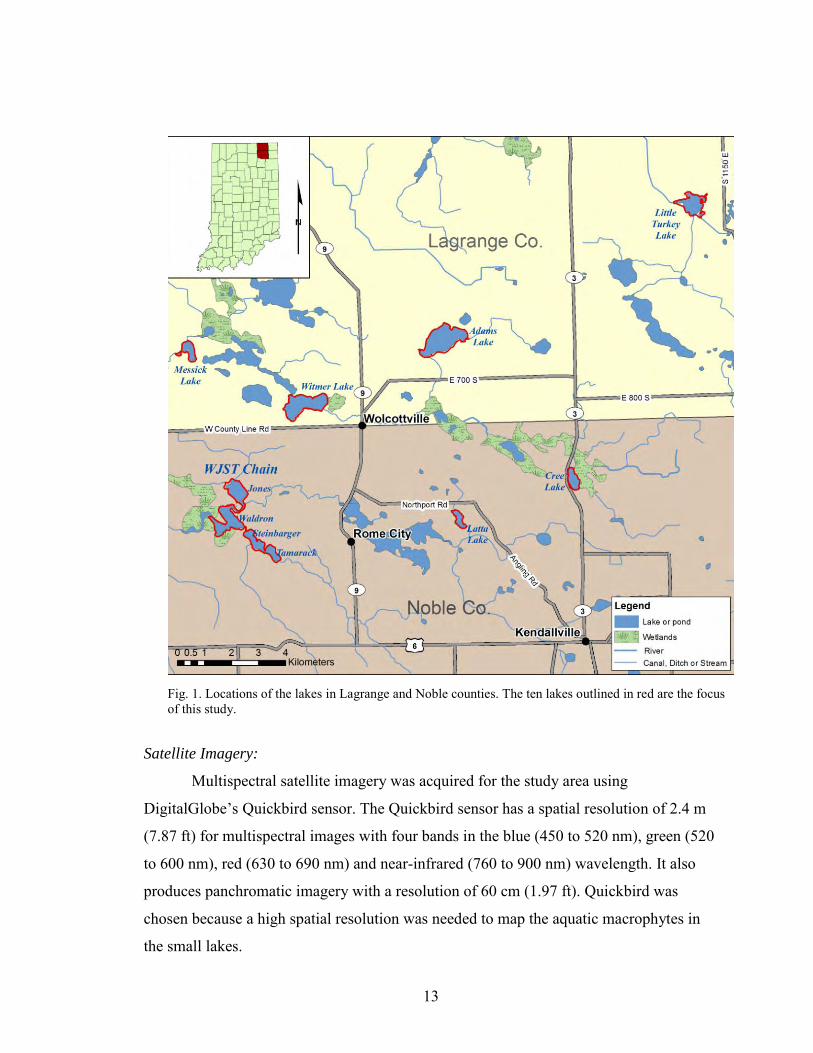
Study Area .............................................................................................................11

Satellite Imagery ....................................................................................................13

Field Data ...............................................................................................................16

Classification..........................................................................................................19

Accuracy Assessment ............................................................................................26

Results ..........................................................................................................................28

Level I ....................................................................................................................28

Level II ...................................................................................................................39

Conclusion ...................................................................................................................46

Appendix A ..................................................................................................................51

Appendix B ..................................................................................................................61

References ....................................................................................................................71

v

LIST OF TABLES

Table 1. Lake and water characteristics of the lakes utilized in this study. .......................12 Table 2. Plant species seen in the field ..............................................................................18

Table 3. Level I Classes .....................................................................................................22

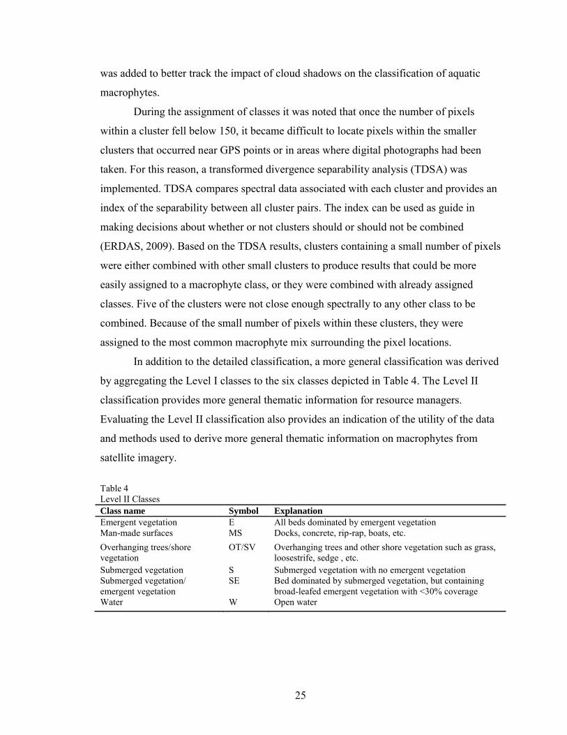
Table 4. Level II Classes ....................................................................................................25

Table 5. Level I vegetation coverage summary for all lakes in hectare (acres) .................31

Table 6. Level I amount of coverage for all lakes (percentages) ......................................32

Table 7. Level I accuracy assessment, September 2007 imagery ......................................33

Table 8. Level I accuracy assessment, September 2008 imagery ......................................34

Table 9. Level II vegetation summary for all lakes in hectare (acres) ...............................41

Table 10. Level II amount of coverage for all lakes (percentages) ...................................42

Table 11. Level II accuracy assessment, September 2007 imagery ..................................44

Table 12. Level I accuracy assessment, September 2008 imagery ....................................44

vi

LIST OF FIGURES

Figure 1. Locations of the lakes in Lagrange and Noble counties. The ten lakes outlined in red are the focus of this study. .........................................................................13 Figure 2. Cree Lake from the Sept. 15, 2007 imagery. The white circle shows an area of cloud interference. .........................................................................................................14 Figure 3. Waldron and Witmer Lakes in the Sept. 6, 2008 imagery showing the cloud and shadow interference. ....................................................................................................15 Figure 4. Latta Lake from Aug. 6, 2008 and Sept. 6, 2008. The image from Aug. 6 on the left shows the effects of wind and sun glint on the lake’s surface while the Sept. 6 image has no such problems. .................................................................................16 Figure 5. A zoned mixed bed of pickerelweed (Pontederia cordata), white water lily (Nymphaea orderata), and the invasive Eurasian watermilfoil (Myriophyllum

spicatum) in front of a house with lawn. Latta Lake, GPS point 1179, 2007. ...................17 Figure 6. The initial, rough classification for Adams Lake in the Sept. 2008 imagery. ....21

Figure 7. The image on the left (Adams Lake, pt. 474) shows the typical, floating habit of white water lilies (Nymphaea oderata) while the image on the right (Cree Lake, pt. 920) shows the vegetation with leaves extending above the water surface. .......24 Figure 8. The classified Sept. 6, 2008 image of Adams Lake on the left and an aerial photograph of Adams Lake on the right. ...........................................................................28 Figure 9. The location of lakes in the September 2008 imagery that were not a part of this study. ............................................................................................................................................. 49

1

INTRODUCTION

Inland wetlands, lakes, and ponds are important environmental resources that

store excess floodwaters, improve water quality, provide habitat for fish and wildlife, and

recharge groundwater aquifers (Ozesmi and Bauer 2002). Aquatic plants have been

recognized as important components of these freshwater ecosystems (Olmanson et al.

2002). Emergent aquatic macrophytes provide shade, cover, and help maintain cooler

water temperatures necessary for fish and other aquatic organisms (Jakubauskas et al.

2000; Vis et al. 2003). Submerged aquatic macrophytes form diverse habitats that are

utilized by fish, invertebrates and algae, and they can also be an early indicator of

declining wetland health (Lehmann and Lachavanne 1999; Vis et al. 2003; Wolter et al.

2005). In recent years, better environmental protection of aquatic environments has

created a need for increased mapping of aquatic vegetation by consultants, citizen groups,

and state and local agencies (Madden 2004; Olmanson et al. 2002; Shuman and Ambrose

2003).

Standard methods of mapping aquatic macrophytes beds involve surveys of

vegetation using sampling and field observations along quadrants or transects. These

methods are often expensive and time consuming (Jakubauskas et al. 2002; Nelson et al.

2006; Vis et al. 2003). Extensive field data collection in areas of dense vegetation or

wetland and aquatic environments that are difficult to access make traditional methods

impractical (Jakubauskas et al. 2002; Jensen et al. 1986). In addition, ground sampling

and mapping techniques can disturb the vegetative beds and wildlife (Shuman and

Ambrose 2003). These techniques are also impractical to use when inventorying many

lakes spread out over large distances (Nelson et al. 2006). Standard mapping methods are

also challenging to implement when it’s necessary to account for rapid changes in aquatic

macrophyte extent and density, especially when looking at a seasonal or interannual time

scale (Jakubauskas et al. 2002).

Despite difficulties in obtaining the information, being able to quickly and

economically map aquatic macrophyte beds is vital for their effective management.

Accurate maps allow resource managers to assess the composition of plant beds and the

2

abundance of species either directly or indirectly (Turner et al. 2003; Olmanson et al.

2002; Wolter et al. 2005). Changes in growth patterns of aquatic plants are important

indicators of water quality which can impact humans, wildlife, and fisheries (Jakubauskas

et al. 2000; Valta-Hulkkonen et al. 2005). High resolution satellite imagery is a

potentially cost-effective way to gather information about aquatic macrophyte

communities. In particular, remote sensing can be used to economically map aquatic

vegetation in lakes spread out over a large area, costing as little as one half traditional

surveying methods (Valta-Hulkkonen et al. 2005).

Previous studies have shown that remote sensing can be an effective tool for

mapping aquatic macrophyte beds in saltwater, brackish water, and freshwater

environments (Ciraolo et al. 2006; Everitt et al. 2005; Jakubauskas et al. 2002; Laba et al.

2008; Marshall and Lee 1994; Sawaya et al. 2003; Underwood et al. 2006; Wolter et al.

2005). Remote sensing is most effective in mapping emergent and floating macrophyte

beds, and less so with submerged macrophytes (Laba et al. 2008; Marshall and Lee 1994;

Nelson et al. 2006; Underwood et al. 2006; Valta-Hulkkonen et al. 2005; Vis et al. 2003).

Historically, aerial photography has been the most widely used method of obtaining

detailed aquatic vegetation data and is still used today (Jensen et al. 1986; Marshall and

Lee 1994; Valta-Hulkkonen et al. 2005). However, as the spatial resolution of satellites

has improved, there has been a shift to using satellite imagery to map aquatic vegetation

(Everitt et al. 2005; Everitt et al. 2008; Jakubauskas et al. 2002; Laba et al. 2008; Madden

2004; Nelson et al. 2006; Olmanson et al. 2002; Ozemi and Bauer 2002; Sawaya et al.

2003; Wolter et al. 2005). Satellite imagery is more effective than aerial photography

when researchers need high resolution imagery that covers a large geographic area

(Madden 2004). Using satellite imagery produces maps which can be used to prioritize

areas of vegetation removal and allows for the assessment of the success or failure of

aquatic plant control efforts (Jakubauskas et al. 2002; Madden 2004).

Satellite imagery has also been used to track and monitor the spread of invasive

species (Madden 2004). Such monitoring across multiple sites could facilitate the

detection of new or spreading invasive species early enough that eradication efforts could

be successful (Laba et al. 2008). Information from these monitoring systems could then

be used as input into models which can predict future plant distribution and assist in

3

making future management decisions (Mironga 2004). Information on changes in the

surrounding land uses over time is also provided (Ozesmi and Bauer 2002).

An invasive species is any species of plant or animal that is not native to that ecosystem

and “whose introduction does or is likely to cause economic or environmental harm or

harm to human health” (Executive Order 13112 1999). Invasive aquatic plant species can

have severe ecological and economic impact and can adversely impact navigation,

nutrient cycling in wetlands and lakes, water quality, drinking water supplies,

hydropower facilities, irrigation, fisheries, recreation, wildlife, and native vegetation

diversity (Jakubauskas et al. 2002; Laba et al. 2008; Madden 2004; Underwood et al.

2006). Federal and state governments spend millions of dollars annually on plant

management programs (Jakubauskas et al. 2002). A major proportion of these budgets are

targeted towards the monitoring and control of invasive plant species.

IDNR’s LARE program was started in 1988 and began providing funding for the

development of aquatic vegetation management plans in 2004. The aquatic vegetation plans

consisted of a survey of the plant communities present in the lakes, a catalogue of

invasive species, fisheries data, and methods for managing any nuisance or invasive

species. In order to prepare these plans, either IDNR personnel or private companies have

been contracted to survey aquatic macrophytes using traditional field-based plant survey

methods.

The purpose of this study was to test a method for mapping aquatic macrophyte

vegetation, both emergent and submerged, using Quickbird satellite imagery so that the

resulting maps will be useful to resource managers in a variety of ways including:

1) Outlining the extent of vegetative beds for management purposes

2) Monitoring the extent and health of native plant species

3) Monitoring the current extent and spread of invasive plant species

4) Identification of man-made shoreline and lake structures such as docks,

erosion control structures, etc.

These goals were chosen for several reasons. Outlining the extent of vegetative

beds has important management implications. Under Indiana law, vegetative beds larger

than 58 m2 (625 ft2) are considered areas of “special concern” by the Indiana

4

Administrative Code Title 312 Article 11 (2005). Disrupting, spraying to control

vegetation, or otherwise impacting such beds requires both permits and special review.

However, vegetative beds with a surface area of less than 58 m2 (625 ft2) that are near a

boat landing can be managed with the use of pesticides and without a permit if they meet

certain other conditions (IDNR LARE Reports: Adams Lake 2008; Indiana

Administrative Code Title 312 Article 11). In addition, owners must obtain a permit and

go through a special review in order to disrupt these large beds by building a permanent

pier or other structure. Outlining the extent of current vegetative beds would allow for

better enforcement of this law and would allow the IDNR to better target areas which can

be managed without a permit. Being able to identify man-made structures from satellite

imagery would allow the IDNR to better track permanent structures already in place and

to locate areas where permits are needed for further construction. Currently, pesticide

applications in several Indiana lakes are partially funded by the LARE program to control

invasive species. Examples of LARE-funded projects in the northern Indiana study area

include Adams, Little Turkey, and Messick (IDNR LARE Reports: Adams Lake 2008;

IDNR LARE Reports: Five Lakes 2007; IDNR LARE Reports: Little Turkey Lake 2008).

The use of high resolution satellite imagery provides maps of the distribution of aquatic

macrophyte communities and offers the potential to greatly reduce the need for ground

surveys to monitor the impact of aquatic vegetation control programs.

Both emergent and submerged vegetation were mapped in this study. Mapping at

the species level was preferred, but broader categories of plant structure were the primary

focus of the current study given the limitations of species-level identification from

remotely sensed imagery. Special attention was given to finding an efficient, repeatable

process that can then be applied to many lakes spread across a region.

To this end, ten lakes in northern Indiana were chosen by the IDNR as

representative of the type of lakes found in the study area that had available ground-truth

data available. These lakes were all small (less than 125.45 surface hectares (310 acres))

and covered a wide variety of depths, water qualities, and aquatic macrophyte bed

composition. In addition, problem or invasive species were found in all ten of the lakes.

Invasive species occurring in the lakes included Eurasian watermilfoil (Myriophyllum

spicatum), purple loosestrife (Lythum salicaria), curly leaf pondweed (Potamogeton

5

crispus), and brittle naiad (Najas minor). Eurasian watermilfoil was of particular concern

because of its aggressive growth, detrimental effects on native plant communities, and

ability to impede human recreational activities (IDNR LARE Reports: Adams Lake 2008;

IDNR LARE Reports: Five Lakes 2007; IDNR LARE Reports: Indian Lakes 2001; IDNR

LARE Reports: Little Turkey Lake 2008; Jakubauskas et al. 2002). These lakes are used

extensively for recreation, have residential development along their shorelines, support a

diverse and healthy wildlife population, and are susceptible to invasive species (IDNR

LARE Reports: Adams Lake 2008; IDNR LARE Reports: Cree Lake 2005; IDNR LARE

Reports: Five Lakes 2007; IDNR LARE Reports: Indian Lakes 2001; IDNR LARE

Reports: Little Turkey Lake 2008).

6

BACKGROUND

The study of aquatic macrophytes using remote sensing techniques has been less

comprehensive than that of terrestrial vegetation because of the additional challenges

associated with water reflectance, differentiating between different macrophyte species,

and the small scale of freshwater aquatic environments compared to the resolution of

most sensors (Nelson et al. 2006; Underwood et al. 2006). It is known that different types

of aquatic vegetation have subtly different spectral reflectance signatures, which differ

greatly from open water and non-vegetated areas (Marshall and Lee 1994; Ozesmi and

Bauer 2002; Peñuelas et al. 1993; Underwood et al. 2003). However, in the case of mixed

beds, the varying contribution of each emergent macrophytes species to the total

coverage remains difficult (Underwood et al. 2006; Vis et al. 2003).

Mapping submerged aquatic vegetation with remote sensing can be problematic.

The electromagnetic radiation reflected or radiating from submerged vegetation must

cross the air-water interface (Wolter et al. 2005). In addition, because water absorbs

much of the electromagnetic spectrum used in remote sensing, a major complication in

remotely sensing submerged vegetation is depth of the macrophyte canopy in the water

column (Han and Rundquist 2003; Peñuelas et al. 1993; Wolter et al. 2005). Non-canopy

forming submerged vegetative species are the most commonly misclassified submerged

vegetation (Valta-Hulkkonen et al. 2005; Vis et al. 2003; Wolter et al. 2005).

Studies that have been able to map submerged vegetation have reported that it can

be sensed and classified to a maximum depth between 2 m and 3 m (6.5 ft and 9.8 ft)

(Han 2002; Sawaya et al. 2003; Welch and Remillard 1988). However, submerged

vegetation is harder to remotely sense when concentrations of algae increase and in water

with increased turbidity (Han and Rundquist 2003; Underwood et al. 2006; Valta-

Hulkkonen et al. 2005; Vis et al. 2003). When submerged vegetation is mapped,

researchers often label it only as “submerged” with no attempt to differentiate between

species or plant structure types (Saway et al. 2003; Welch and Remillard 1988; Wolter et

al. 2005). For this reason, researchers have primarily used remote sensing to detect dense

homogenous clusters of submersed vegetation (Nelson et al. 2006; Underwood et al.

7

2006; Vis et al. 2003; Zhu et al. 2007). At least one study has shown that it is possible to

differentiate between different submerged macrophytes using remote sensing. Pinnel et

al. (2004) were able to distinguish between the two submerged macrophyte groups Chara

and Potomageton using hyperspectral sensors.

Previous work has approached the problem of aquatic vegetation remote sensing

from a number of different directions. Ackleson (2003) reviewed historical and recent

efforts to model light fields in shallow, marine environments. More advanced remote

sensing systems and a better understanding of what the current remote sensing systems

are finding can be achieved by understanding how light propagates through the water

column. This work is geared more towards submerged vegetation than to emergent

vegetation.

Researchers have also done experimental work on how various environmental

characteristics affect the spectral signature of aquatic vegetation. Han (2002) examined

the effects of depth on reflectance from marine species of sea grass. As depth increased,

the reflectance decreased. Han and Rundquist (2003) studied the effects of depth on the

spectral signatures of coontail (Ceratophyllum demersum), a submerged, freshwater

macrophyte. They also considered the effects of depth in both clear and algae-laden

waters. In the study, the authors found that as depth increased, the amount of reflectance

from the submerged macrophyte decreased, particularly in the infrared and green parts of

the spectrum. Another study on submerged vegetation examined a type of eel grass

(Vallisneria spiralis) but focused on coverage as opposed to depth in both a laboratory

and in algae-laden waters in the field (Yuan and Zhang 2007). As the amount of coverage

of the submerged macrophyte decreased, the amount of reflectance decreased; again,

most heavily in infrared and green wavelengths. Of particular interest is that Yuan and

Zhang (2007) found that the “green peak” was more evident in algae-laden waters and

did not decrease as quickly with a decrease in coverage in algae-laden waters as in clear

waters. The presence of algae emphasizes the green portion of the spectrum and masks

the decrease in the spectral signature with respect to coverage that is normally seen in

non-algae laden waters. Jakubauskas et al. (2000) studied the effects of canopy coverage

on the spectral signature of the emergent macrophyte spatterdock or yellow pond lily

(Nuphar polysepalum). The authors found that as the coverage of emergent macrophyte

8

decreased, the amount of reflectance decreased in the green and infrared parts of the

spectrum. Similar results were also found using water hyacinth (Eichornia crassipes) and

percent coverage in Texas waterways (Jakubauskas et al. 2002). The researchers

concluded that even though this work was done at close range with hand-held

hyperspectral sensors, the high correlations between vegetation cover and infrared

reflectance should be transferable to satellite sensors with broader bandwidths

(Jakubauskas et al. 2000).

Aerial photography, hyperspectral airborne imagery, and satellite imagery are all

used to map aquatic vegetation remotely (Madden 2004). Aerial photography is relatively

inexpensive and there is a large amount of archival data available for researchers to

utilize (Underwood et al. 2003; Welch and Remillard 1988). Historically satellite

imagery was preferred over aerial photography when mapping macrophyte species that

were closely spaced or intermixed with each other (Jensen et al. 1986). This was because

aerial photography had poor spectral resolution when compared to multispectral remote

sensors and could contain variations in brightness caused by light fall off and bi-

directional effects (Jensen et al. 1986; Valta-Hulkkonen et al. 2004). For this reason,

Jensen et al. (1986) and Moore et al. (2000) stated that aerial photography is best suited

to interpretation of homogenous emergent beds and is not adequate to map most

submerged vegetation. Another problem was that visual interpretation of aerial

photography was a labor intensive process (Marshall and Lee 1994; Nelson et al. 2006).

Advances in aerial photography have improved both the spatial and spectral

resolution in some cases making aerial photograph equivalent or superior to high

resolution satellite imagery (Madden 2004). However, aerial photography still has limited

use when assessing macrophyte distributions across many small bodies of water spread

across a large geographical area (Nelson et al. 2006). This is because even high resolution

cameras mounted on an aircraft do not have as great a field of view as a sensor on a

satellite (Madden 2004). For this reason, aerial photography requires multiple passes to

cover the same area acquired at one point in time by satellite imagery. These additional

passes can introduce changes in light and atmospheric conditions, which in turn can

affect classification attempts (Jensen 2007; Valta-Hulkkonen et al. 2004).

9

High spectral and spatial resolution satellite imagery provides more detailed

spectral information relative to traditional photography that can be used to classify

aquatic macrophyte species (Jensen et al. 1986). Early satellites, such as Landsat TM,

with moderate spatial and spectral resolutions were unable to identify mixed beds or

invasive species unless they dominated the beds (Laba et al. 2008). Coarser resolutions

have also been linked to lower accuracies in classifications (Everitt et al. 2008) and are

not suited to mapping most submerged aquatic vegetation (Underwood et al. 2006).

Newer satellites, such as Quickbird and IKONOS, have provided more detailed results

when it comes to spatial and spectral resolution (Everitt et al. 2005; Everitt et al. 2008;

Jakubauskas et al. 2002; Laba et al. 2007; Olmanson et al. 2002; Sawaya et al. 2003).

Hyperspectral satellites and airborne scanners have been used to map submerged

vegetation in shallow water lagoons (Ciraolo et al. 2006), and in mapping invasive

species over an entire freshwater delta (Underwood et al. 2006). While hyperspectral

imagery can be useful in discriminating between vegetation and exotic species, the large

data volume inherent in this method makes it challenging for use by resource managers

without sufficient expertise and data processing capabilities (Madden 2004).

Generally, permanently flooded or open water ponds and lakes are the easiest

freshwater ecosystems on which to map aquatic macrophytes (Ozesmi and Bauer 2002).

The majority of existing studies focus on one lake or wetland, though some cover large

lakes or whole regions (Underwood et al. 2006; Wolter et al. 2005; Zhu et al. 2007). One

of the reasons that studies have focused on single locations is that lakes can vary widely

in suspended sediments, Secchi depth transparency, and chlorophyll content, all of which

can influence how aquatic macrophytes are remotely sensed, though there is some debate

about this (Nelson et al. 2006). Studies that focused on a large number of lakes spread out

over a large area are fewer in number and often broader in scope than just mapping

aquatic macrophytes (Nelson et al. 2006; Sawaya et al. 2003; Valta-Hulkkonen et al.

2005).

The number of vegetative and non-vegetative classes that authors attempt to map

varies greatly from study to study. Most of the studies reviewed have used 5-10 classes

(Everitt et al. 2005; Everitt et al. 2008; Jensen et al. 1986; Mackey et al. 1992; Olmanson

et al. 2002; Sawaya et al. 2003; Valta-Hulkkonen et al. 2005; Vis et al. 2005; Wolter et

10

al. 2005). These studies rarely map to the species level; instead, plant types are

aggregated by either leaf or plant structure (Mackey et al. 1992; Nelson et al. 2006;

Olmanson et al. 2002; Saway et al. 2003; Valta-Hulkkonen et al. 2005; Vis et al. 2003)

into ecological categories (Everitt et al. 2005; Jensen et al. 1986), or a mixture of the two

(Welch and Remillard 1988). Laba et al. (2008) mapped twenty classes, some at the

species level. The rest were classified using ecological categories (such as wooded

swamp, scrub/shrub, salt meadow, etc). Others chose to group plants based on criteria

known to cause differences in spectral signature, such as plant cover (Nelson et al. 2006;

Wolter et al. 2005) or in the case of submerged vegetation, depth (Olmanson et al. 2002;

Sawaya et al. 2003). In some cases, such as Everitt et al. (2005, 2008) and Underwood et

al. (2006), the focus was on mapping a particular invasive species instead of mapping a

broad range of macrophytes. Therefore, all other plants were grouped into a few broad

categories.

11

METHODS

Study Area:

The study area consisted of ten lakes in Lagrange Co. and Noble Co. in northern

Indiana spread out over 220 km2. These lakes include Adams Lake, Cree Lake, Jones

Lake, Latta Lake, Little Turkey, Messick Lake, Steinbarger Lake, Tamarack Lake,

Waldron Lake, and Witmer Lake (Fig. 1). Waldron, Jones, Steinbarger, and Tamarack are

a chain lake system connected by a series of narrow waterways. They are collectively

referred to as the WJST chain. These lakes range in size from Adams with a total surface

area of 125 ha (308 acres) to Latta with a surface area of just 18 ha (45 acres). The

maximum depth of the lakes is 28.35 m (93 ft) in Adams with average depths in the lakes

ranging from 10.67 m to 2.59 m (25 ft to 8.5 ft). Lake clarity varies from very good in

Cree with secchi depths between 2.47 m to 2.59 m (8.1 ft to 8.5 ft) to poor in Little

Turkey with a secchi depth of less than 0.98 m (< 3.2 ft). Table 1 shows size, depth, and

clarity information for all the lakes in the study area with the exception of Latta, where

there is no depth or clarity information available.

Table 1 Lake and water characteristics of the lakes utilized in this study.

Lake Name County

Surface Area

in hectares

(acres)

Max Depth in

meters

(ft)

Avg. Depth in

meters (ft) Clarity

Secchi Depth in

meters (ft)

2007 Recorded

Secchi Depth in

meters (ft) Adams Lagrange 125 (308) 28.35 (93) 7.62 (25) Good 1.52 – 2.74 (5 – 9)

Cree Noble 31 (76) 7.92 (26) 4.79 (15.7) Very good 2.47 – 2.59 (8.1 – 8.5) 2.83 (9.3)

Jones Noble 46 (114) 7.62 (25) 2.59 (8.5) Low 1.22 (4) -

Latta Noble 18 (45) - - - - -

Little Turkey Lagrange 55 (135) 10.97 (36) 3.51 (11.5) Low < 0.98 (< 3.2) 0.58 (1.9)

Messick Lagrange 28 (68) 16.46 (54) 6.40 (21) Intermediate - -

Steinbarger Noble 30 (73) 11.89 (39) 6.71 (22) Intermediate 1.07 – 2.90 (3.5 – 9.5) 0.64 (2.1)

Tamarack Noble 20 (50) 11.28 (37) 5.33 (17.5) Intermediate 1.07 – 2.44 (3.5 – 8) -

Waldron Noble 87 (216) 13.72 (45) 4.27 (14) Low 1.22 (4) -

Witmer Lagrange 83 (204) 16.46 (54) 10.67 (35) Low 1.07 (3.5) -

Source: IDNR Lake Reports: Adams Lake 2008; IDNR LARE Reports: Cree Lake 2005; IDNR LARE Reports: Five Lakes 2007; IDNR LARE Reports: Indian Lakes 2001; IDNR LARE Reports:

Little Turkey Lake 2008; 2007 Field Data

12

13

Satellite Imagery:

Multispectral satellite imagery was acquired for the study area using

DigitalGlobe’s Quickbird sensor. The Quickbird sensor has a spatial resolution of 2.4 m

(7.87 ft) for multispectral images with four bands in the blue (450 to 520 nm), green (520

to 600 nm), red (630 to 690 nm) and near-infrared (760 to 900 nm) wavelength. It also

produces panchromatic imagery with a resolution of 60 cm (1.97 ft). Quickbird was

chosen because a high spatial resolution was needed to map the aquatic macrophytes in

the small lakes.

Fig. 1. Locations of the lakes in Lagrange and Noble counties. The ten lakes outlined in red are the focus of this study.

14

Satellite imagery was acquired for the study area on September 15, 2007, August

6, 2008, and September 6, 2008. These late summer dates were used because the optimal

time to map the areal extent of

emergent and submerged vegetation is

late in the growing season when full

emergence has occurred but before the

beds have begun to senesce or die

back due to frost (Mackey 1992;

Marshall and Lee 1994; Nelson et al.

2006; Wolter et al. 2005).

Each of the satellite images is

less than optimal in some way. Heavy

cloud cover over the study area

obscured all of the study lakes but

Cree Lake in the September 15, 2007

imagery. Cree Lake had some cloud effects over the southern portion of the lake in this

image date, but was otherwise of good quality (Fig 2). The image acquired on September

6, 2008 covers Adams, Latta, Messick, Witmer, and the WJST chain. It was of good

quality with minimal effects of wind drift, sun glint, and cloud cover. Witmer and

Waldron Lake are impaired by thin cloud cover in this image. In Witmer Lake, a shadow

cast from a cloud affects less than 5% of the shoreline. Shadows and clouds on Waldron

Lake obscure about 40% of the shoreline (Fig. 3).

Fig. 2. Cree Lake from the September 15, 2007 imagery. The white circle shows an area of cloud interference.

15

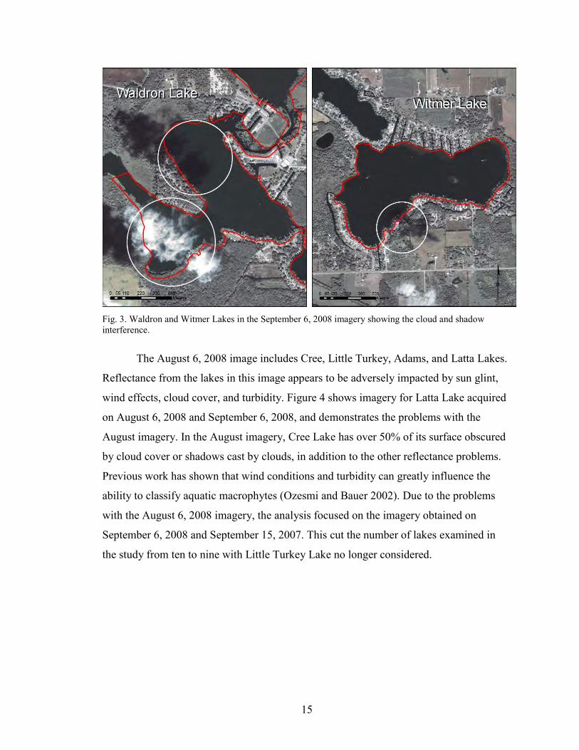
Fig. 3. Waldron and Witmer Lakes in the September 6, 2008 imagery showing the cloud and shadow interference.

The August 6, 2008 image includes Cree, Little Turkey, Adams, and Latta Lakes.

Reflectance from the lakes in this image appears to be adversely impacted by sun glint,

wind effects, cloud cover, and turbidity. Figure 4 shows imagery for Latta Lake acquired

on August 6, 2008 and September 6, 2008, and demonstrates the problems with the

August imagery. In the August imagery, Cree Lake has over 50% of its surface obscured

by cloud cover or shadows cast by clouds, in addition to the other reflectance problems.

Previous work has shown that wind conditions and turbidity can greatly influence the

ability to classify aquatic macrophytes (Ozesmi and Bauer 2002). Due to the problems

with the August 6, 2008 imagery, the analysis focused on the imagery obtained on

September 6, 2008 and September 15, 2007. This cut the number of lakes examined in

the study from ten to nine with Little Turkey Lake no longer considered.

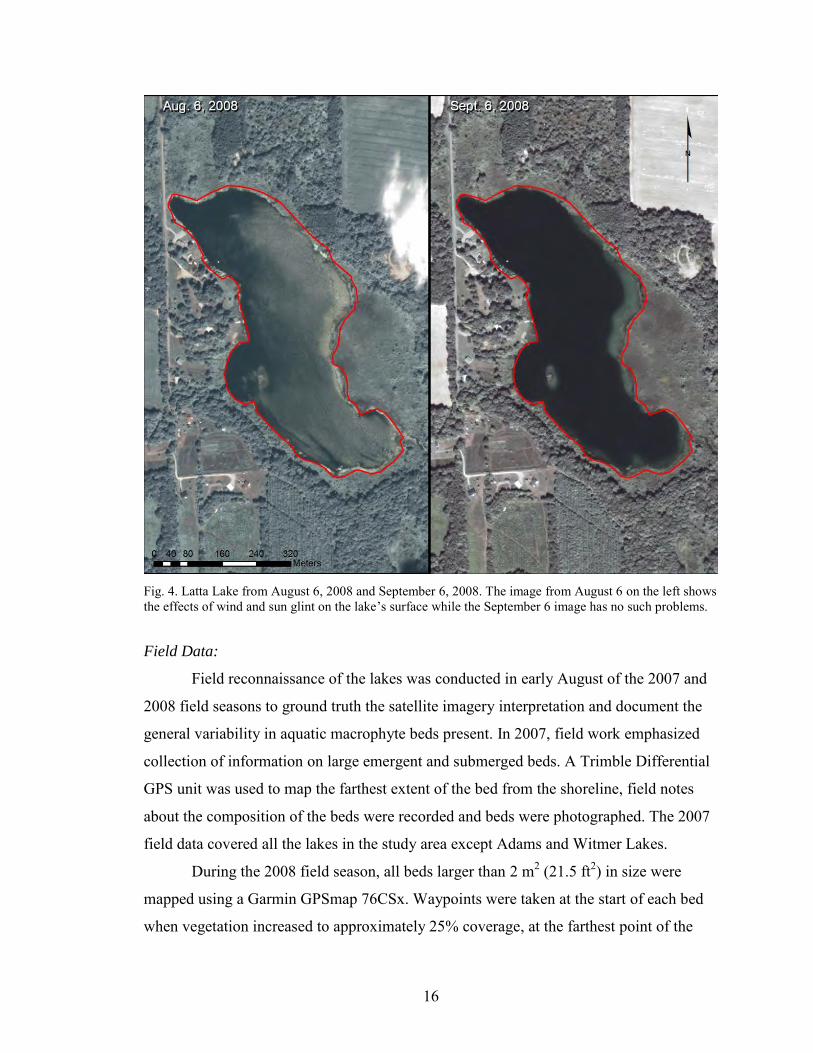
16

Fig. 4. Latta Lake from August 6, 2008 and September 6, 2008. The image from August 6 on the left shows the effects of wind and sun glint on the lake’s surface while the September 6 image has no such problems.

Field Data:

Field reconnaissance of the lakes was conducted in early August of the 2007 and

2008 field seasons to ground truth the satellite imagery interpretation and document the

general variability in aquatic macrophyte beds present. In 2007, field work emphasized

collection of information on large emergent and submerged beds. A Trimble Differential

GPS unit was used to map the farthest extent of the bed from the shoreline, field notes

about the composition of the beds were recorded and beds were photographed. The 2007

field data covered all the lakes in the study area except Adams and Witmer Lakes.

During the 2008 field season, all beds larger than 2 m2 (21.5 ft2) in size were

mapped using a Garmin GPSmap 76CSx. Waypoints were taken at the start of each bed

when vegetation increased to approximately 25% coverage, at the farthest point of the

17

bed from shore, and at the end of each bed. Waypoints were also recorded where the

composition of the bed changed and where the beds were photographed. Plant

identification, bed composition estimates, and distance to shore measurements were

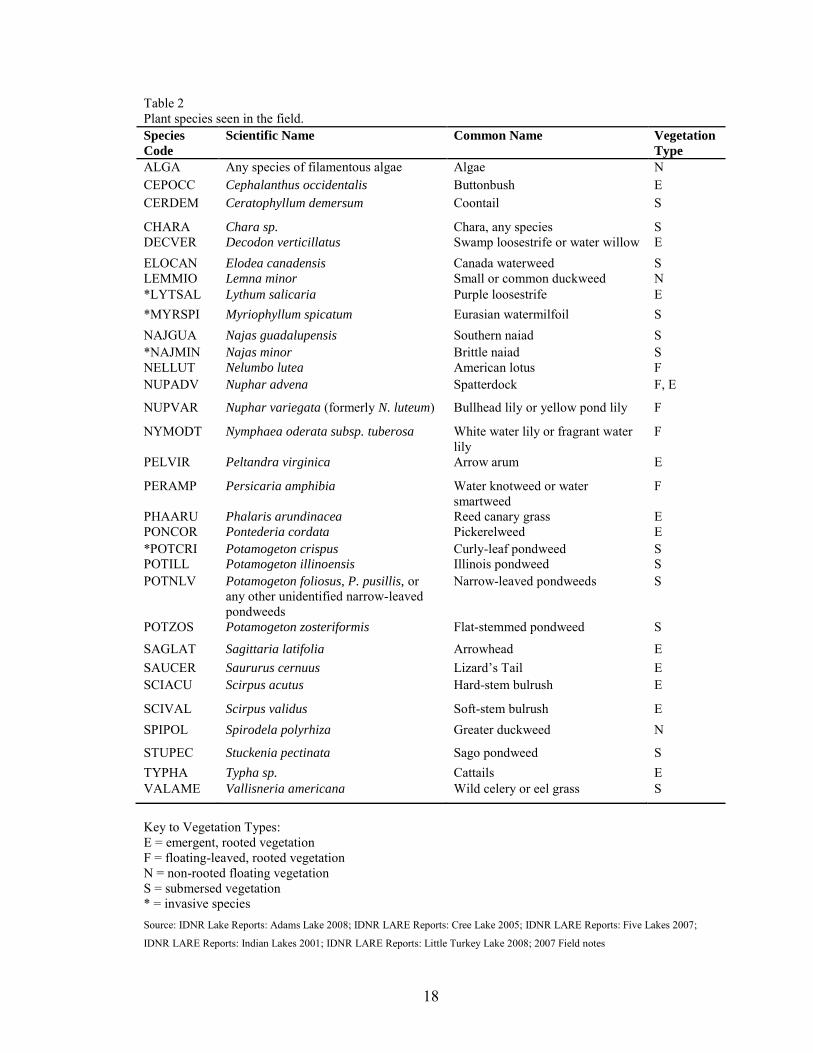
recorded. Table 2 gives a list of the major species and bed formers found in the lakes in

the two field seasons.

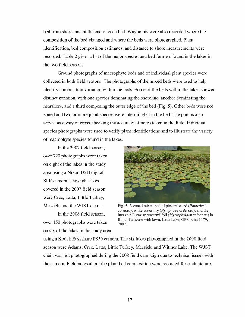
Ground photographs of macrophyte beds and of individual plant species were

collected in both field seasons. The photographs of the mixed beds were used to help

identify composition variation within the beds. Some of the beds within the lakes showed

distinct zonation, with one species dominating the shoreline, another dominating the

nearshore, and a third composing the outer edge of the bed (Fig. 5). Other beds were not

zoned and two or more plant species were intermingled in the bed. The photos also

served as a way of cross-checking the accuracy of notes taken in the field. Individual

species photographs were used to verify plant identifications and to illustrate the variety

of macrophyte species found in the lakes.

In the 2007 field season,

over 720 photographs were taken

on eight of the lakes in the study

area using a Nikon D2H digital

SLR camera. The eight lakes

covered in the 2007 field season

were Cree, Latta, Little Turkey,

Messick, and the WJST chain.

In the 2008 field season,

over 150 photographs were taken

on six of the lakes in the study area

using a Kodak Easyshare P850 camera. The six lakes photographed in the 2008 field

season were Adams, Cree, Latta, Little Turkey, Messick, and Witmer Lake. The WJST

chain was not photographed during the 2008 field campaign due to technical issues with

the camera. Field notes about the plant bed composition were recorded for each picture.

Fig. 5. A zoned mixed bed of pickerelweed (Pontederia

cordata), white water lily (Nymphaea orderata), and the invasive Eurasian watermilfoil (Myriophyllum spicatum) in front of a house with lawn. Latta Lake, GPS point 1179, 2007.

18

Table 2 Plant species seen in the field. Species

Code

Scientific Name Common Name Vegetation

Type

ALGA Any species of filamentous algae Algae N CEPOCC Cephalanthus occidentalis Buttonbush E CERDEM Ceratophyllum demersum Coontail S

CHARA Chara sp. Chara, any species S DECVER Decodon verticillatus Swamp loosestrife or water willow E ELOCAN Elodea canadensis Canada waterweed S LEMMIO Lemna minor Small or common duckweed N *LYTSAL Lythum salicaria Purple loosestrife E *MYRSPI Myriophyllum spicatum Eurasian watermilfoil S NAJGUA Najas guadalupensis Southern naiad S *NAJMIN Najas minor Brittle naiad S NELLUT Nelumbo lutea American lotus F NUPADV Nuphar advena Spatterdock F, E

NUPVAR Nuphar variegata (formerly N. luteum) Bullhead lily or yellow pond lily F

NYMODT Nymphaea oderata subsp. tuberosa White water lily or fragrant water lily

F

PELVIR Peltandra virginica Arrow arum E

PERAMP Persicaria amphibia Water knotweed or water smartweed

F

PHAARU Phalaris arundinacea Reed canary grass E PONCOR Pontederia cordata Pickerelweed E *POTCRI Potamogeton crispus Curly-leaf pondweed S POTILL Potamogeton illinoensis Illinois pondweed S POTNLV Potamogeton foliosus, P. pusillis, or

any other unidentified narrow-leaved pondweeds

Narrow-leaved pondweeds S

POTZOS Potamogeton zosteriformis Flat-stemmed pondweed S

SAGLAT Sagittaria latifolia Arrowhead E SAUCER Saururus cernuus Lizard’s Tail E SCIACU Scirpus acutus Hard-stem bulrush E

SCIVAL Scirpus validus Soft-stem bulrush E SPIPOL Spirodela polyrhiza Greater duckweed N

STUPEC Stuckenia pectinata Sago pondweed S TYPHA Typha sp. Cattails E VALAME Vallisneria americana Wild celery or eel grass S

Key to Vegetation Types: E = emergent, rooted vegetation F = floating-leaved, rooted vegetation N = non-rooted floating vegetation S = submersed vegetation * = invasive species Source: IDNR Lake Reports: Adams Lake 2008; IDNR LARE Reports: Cree Lake 2005; IDNR LARE Reports: Five Lakes 2007;

IDNR LARE Reports: Indian Lakes 2001; IDNR LARE Reports: Little Turkey Lake 2008; 2007 Field notes

19

Classification:

The shorelines of the nine lakes were outlined using heads-up digitizing with the

60 cm Quickbird panchromatic image. The boundary between water and land was traced

on screen and converted into a file that represented the shoreline of the lakes at the time

the satellite imagery was captured. In areas where there was there was doubt as to where

the boundary was, the line was drawn to maximize the amount of aquatic vegetation

included even if that meant that shore vegetation was sometimes included in the study

area. This effectively masked out the land, leaving only the lakes in the study area to be

analyzed.

One of the goals of the study was to find an efficient, non-labor intensive way of

classifying the aquatic macrophyte beds. Marshall and Lee (1994) found that the process

of selecting training classes and the subsequent signature evaluation needed in a

supervised classification was a time consuming process. An added problem was that the

majority of the aquatic macrophyte beds in the lakes chosen by the IDNR varied in either

composition or in coverage. Such variability within the beds made finding suitable

training classes for a supervised classification difficult. Finally, work done by Everitt et

al. (2005, 2008) showed that a supervised classification does not produce significantly

better results than an unsupervised classification when mapping macrophyte species.

For these reasons, an unsupervised classification using the Iterative Self-

Organizing Data Analysis Technique (ISODATA) algorithm was run on the eight lakes in

the September 2008 imagery and separately on Cree Lake in the September 15, 2007

imagery. The unsupervised classification was limited to a maximum of 300 spectral

clusters for the eight lakes in the 2008 imagery because of the large number of differing

bed characteristics and environments found within the eight lakes. The 2007 imagery

covers a smaller area, contains fewer macropyhte species and does not show as much

variation in lacustrine environments as the 2008 imagery. For this reason, a maximum of

only 50 clusters was chosen for 2007 imagery covering just Cree Lake. The convergence

threshold was left at the default of 0.95 and the maximum number of iterations in both

cases was set to fifty (ERDAS 2009; Jensen 2005). Since the two images were processed

separately, no radiometric correction, atmospheric correction, or normalization was

performed.

20

Both unsupervised classifications produced similar patterns in the number of

pixels assigned to spectral clusters. Some of these clusters contained very low pixel

counts, ranging from 0 to 100 pixels, while others were very large; the largest cluster

occurred in the 2008 imagery and contained 25,961 pixels.

When the unsupervised classification was run on both sets of imagery, an unusual

pattern was noticed. Many of the clusters that were separated out towards the beginning

and middle of the analysis contained a relatively low number of pixels, while those that

were separated out towards the end of the analysis contained a much greater number of

pixels. In the 2008 imagery, seven of the last eight clusters were 2 to 6 times larger than

other clusters. A similar pattern emerged in the 2007 imagery, with the last two clusters

being more than 2 times the size of previous clusters. Looking at the average spectral

signatures for these clusters showed that in both cases all of the larger clusters had a

“typical” vegetation curve with high reflectance in green and NIR bands, indicating that

they corresponded to emergent vegetation. In order to capture as much detail as possible

on emergent vegetation, these clusters were subject to cluster busting with the maximum

number of clusters set at 30 in the 2008 imagery and at 10 in the 2007 imagery. In both

cases, all clusters resulting from the cluster busting were populated with pixels.

The average spectral signatures of all clusters were examined. The clusters were

divided into rough categories based on their spectral signature as an initial step in the

classification process. These initial classes were shadowed water, water, water/unknown,

submerged vegetation, possible submerged vegetation, man-made surfaces, and emergent

vegetation (Fig. 6).

A Normalized Difference Vegetation Index (NDVI ) was calculated using the red

and NIR bands of the satellite imagery with the following formula:

ρnir – ρred

NDVI = -------------------------------- ρnir + ρred

Previous studies have shown that NDVI has positive correlation with aquatic macrophyte

plant cover (Jakubauskas et al. 2000; Peñuelas et al. 1993) and can be used to help

21

differentiate vegetation and other surfaces from one another (Ozesmi and Bauer 2002).

Because the NDVI is a ratio, it reduces many forms of multiplicative noise such as

shadows. This is particularly important in the current study because two of the study

lakes have significant effects caused by cloud shadow. In addition, several of the lakes

have a large number of man-made structures, such as docks, which extend into

macrophyte beds. Some of these structures are narrow enough that pixels are mixed with

vegetation, and throw shadows onto nearby beds. NDVI was evaluated as a potential tool

in addition to the unsupervised classification to help decrease the pixel confusion and

help separate these man-made structures from the vegetation beds.

The next step was to match field data to the spectral clusters resulting from the

unsupervised classification of the 2007 and 2008 imagery. The classified image was

imported into ArcGIS. The GPS data for the 2007 and 2008 field seasons were overlaid

on the cluster image. Clusters were assigned a highly visible color and the type of

vegetation contained in each cluster based on the GPS points was noted. The location of

the pixels in each cluster was also compared to both the field notes and digital

Fig. 6. The initial classification for Adams Lake in the September 2008 imagery.

22

photographs of the bed from the 2008 field season. In the case of the WJST chain, no

digital photographs were available for the 2008 field season so the field notes for 2008

were supplemented by the digital photographs collected in 2007. The 2007 digital

photographs were also used in areas where the 2008 photographs were not taken. Based

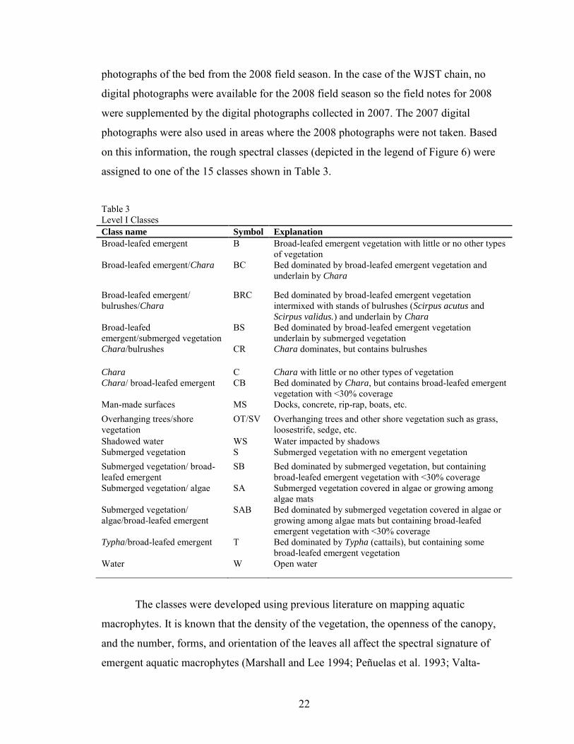
on this information, the rough spectral classes (depicted in the legend of Figure 6) were

assigned to one of the 15 classes shown in Table 3.

Table 3 Level I Classes Class name Symbol Explanation Broad-leafed emergent B Broad-leafed emergent vegetation with little or no other types

of vegetation Broad-leafed emergent/Chara BC Bed dominated by broad-leafed emergent vegetation and

underlain by Chara

Broad-leafed emergent/ bulrushes/Chara

BRC Bed dominated by broad-leafed emergent vegetation intermixed with stands of bulrushes (Scirpus acutus and

Scirpus validus.) and underlain by Chara Broad-leafed emergent/submerged vegetation

BS Bed dominated by broad-leafed emergent vegetation underlain by submerged vegetation

Chara/bulrushes CR Chara dominates, but contains bulrushes

Chara C Chara with little or no other types of vegetation Chara/ broad-leafed emergent CB Bed dominated by Chara, but contains broad-leafed emergent

vegetation with <30% coverage Man-made surfaces MS Docks, concrete, rip-rap, boats, etc. Overhanging trees/shore vegetation

OT/SV Overhanging trees and other shore vegetation such as grass, loosestrife, sedge, etc.

Shadowed water WS Water impacted by shadows Submerged vegetation S Submerged vegetation with no emergent vegetation Submerged vegetation/ broad-leafed emergent

SB Bed dominated by submerged vegetation, but containing broad-leafed emergent vegetation with <30% coverage

Submerged vegetation/ algae SA Submerged vegetation covered in algae or growing among algae mats

Submerged vegetation/ algae/broad-leafed emergent

SAB Bed dominated by submerged vegetation covered in algae or growing among algae mats but containing broad-leafed emergent vegetation with <30% coverage

Typha/broad-leafed emergent T Bed dominated by Typha (cattails), but containing some broad-leafed emergent vegetation

Water W Open water

The classes were developed using previous literature on mapping aquatic

macrophytes. It is known that the density of the vegetation, the openness of the canopy,

and the number, forms, and orientation of the leaves all affect the spectral signature of

emergent aquatic macrophytes (Marshall and Lee 1994; Peñuelas et al. 1993; Valta-

23

Hulkkonen et al. 2005). In particular, four major types of emergent vegetation existed

within the lakes in this study. One is broad-leafed surface vegetation such as white water

lilies (Nymphaea oderata), bullhead lilies (Nuphar variegata), and American lotus

(Nelumbo lutea). Another is broad-leafed above surface vegetation such as spatterdock

(Nuphar advena), arrow arum (Peltandra virginica), and pickerelweed (Pontederia

cordata). A third type is tall, broad-leafed vegetation, such as cattails (Typha sp.). The

final type of vegetation is tall and thin with small or no leaves such as the bulrushes

Scirpus acutus and Scirpus validus.

Past studies suggested classification would be able to separate out the broad-

leafed vegetation that floated on the surface of the water from the broad-leafed vegetation

that rose above the water surface (Laba et al. 2008; Nelson et al. 2006; Peñuelas et al.

1993; Sawaya et al. 2003). Initially, an additional set of classes was developed showing

this distinction. However, as the clusters were assigned to different classes it became

obvious that broad-leafed surface vegetation and broad-leafed above surface vegetation

were highly confused with each other. A contributing factor may be that one of the

species that normally lays flat on the water, Nymphaea oderata, was observed with leaves

curled or entirely above the water’s surface in several parts of the study area (Fig. 7).

This added an additional complication when assigning classes to a particular category. In

the end, surface and above surface vegetation was assigned to one class designated as

“broad-leafed emergent.” At least one other study has reported similar problems with

classification algorithms being unable to separate different types of broad-leafed

vegetation (Marshall and Lee 1994).

One of the goals of this study was to attempt to map the invasive species within

the lakes. Since it was a major component of submerged beds, special focus was placed

on mapping Eurasian watermilfoil (Myriophyllum spicatum). Work by previous authors

has shown that it is possible to differentiate between different submerged vegetation to a

limited extent (Pinnel et al. 2004; Peñuelas et al. 1993). Pinnel et al. (2004) concluded

that the spectral differences detected between the submerged macropyhtes Chara and

pondweeds (Potamogeton) is a function of their growth heights and that the spectral

response is dependent on water depth and clarity. Size, density, and the homogeneity of

24

the beds also determine how well one submerged macropyhte can be differentiated from

another (Pinnel et al. 2004; Peñuelas et al. 1993). Early on in the classification, it was

noted that there was no discernible spectral difference between two of the major types of

submerged vegetation in the study area: the native coontail (Ceratophyllum demersum)

and the invasive Eurasian watermilfoil (Myriophyllum spicatum). These were combined

into the class labeled “submerged vegetation”. Because of previous studies had been able

to differentiate between Chara and other submerged vegetation and the fact that Chara

has calcium deposits on its surface which could affect its spectral signature, it was placed

in a separate class (IDNR LARE Reports: Adams Lake 2008).

Classes were then divided based on the following critera: type of submerged

vegetation and presence and type of emergent vegetation. The presence or absence of

macrophytic green algae was added because previous work suggests that its presence can

affect the recorded spectral signature (Han and Rundquist 2003; Yuan and Zhang 2007).

Classes for man-made surfaces and overhanging trees/shore vegetation were added

because they make up a significant part of the study area. A class for shadowed water

Fig. 7. The image on the left (Adams Lake, pt. 474) shows the typical, floating habit of white water lilies (Nymphaea oderata) while the image on the right (Cree Lake, pt. 920) shows the vegetation with leaves extending above the water surface.

25

was added to better track the impact of cloud shadows on the classification of aquatic

macrophytes.

During the assignment of classes it was noted that once the number of pixels

within a cluster fell below 150, it became difficult to locate pixels within the smaller

clusters that occurred near GPS points or in areas where digital photographs had been

taken. For this reason, a transformed divergence separability analysis (TDSA) was

implemented. TDSA compares spectral data associated with each cluster and provides an

index of the separability between all cluster pairs. The index can be used as guide in

making decisions about whether or not clusters should or should not be combined

(ERDAS, 2009). Based on the TDSA results, clusters containing a small number of pixels

were either combined with other small clusters to produce results that could be more

easily assigned to a macrophyte class, or they were combined with already assigned

classes. Five of the clusters were not close enough spectrally to any other class to be

combined. Because of the small number of pixels within these clusters, they were

assigned to the most common macrophyte mix surrounding the pixel locations.

In addition to the detailed classification, a more general classification was derived

by aggregating the Level I classes to the six classes depicted in Table 4. The Level II

classification provides more general thematic information for resource managers.

Evaluating the Level II classification also provides an indication of the utility of the data

and methods used to derive more general thematic information on macrophytes from

satellite imagery.

Table 4 Level II Classes Class name Symbol Explanation Emergent vegetation E All beds dominated by emergent vegetation Man-made surfaces MS Docks, concrete, rip-rap, boats, etc. Overhanging trees/shore vegetation

OT/SV Overhanging trees and other shore vegetation such as grass, loosestrife, sedge , etc.

Submerged vegetation S Submerged vegetation with no emergent vegetation Submerged vegetation/ emergent vegetation

SE Bed dominated by submerged vegetation, but containing broad-leafed emergent vegetation with <30% coverage

Water W Open water

26

Accuracy Assessment:

The conventional method of assessing the accuracy of a classification is to use an

error matrix that compares the agreement between classes predicted through image

processing to those observed independently of the classification. Independent

observations are collected either through visual interpretation of imagery, by visiting

selected sample sites or doing field work in the study area (Congalton and Green 1999).

Error matrixes were used to assess the classification results in the current study. Accuracy

assessments were run separately on the 2007 and 2008 imagery because the images were

analyzed and classified separately. Additionally, independent error matrixes were derived

for both the Level I and Level II classifications. Congalton and Green (1999)

recommended that a stratified random sample of at least 50 points per class be used to

populate error matrixes for an accuracy assessment. For the fifteen Level I classes, that

would mean using 750 points. Another option is using the binomial distribution formula,

which says that a minimum of 203 sample points is an acceptable sample size when the

expected accuracy is 85% and an acceptable error is 5% (Congalton and Green 1999;

Jensen 2005). A review of the literature shows that the number of points used in accuracy

assessment in similar studies tends to be lower than even this. In general, the number of

points chosen to assess accuracy in the literature ranges from 100 to 200 points per site

(Everitt et al. 2005; Everitt et al. 2008; Laba et al. 2008; Sawaya et al. 2003; Wolter et al.

2005). This was used as the guideline for determining the number of points used in the

current study.

In order to assess the accuracy of all of the classes, a stratified random sample

was used to select points for both images in the Level I classification using the sampling

tools in ERDAS Imagine 9.3. Because of the large amount of noise inherent in creating

thematic maps using classification methods, a smoothing function was used to

preferentially select pixels that were surrounded by other pixels of the same class. A

minimum of fifteen points per class was specified, but this was not achieved in smaller

classes that contained small clusters or scattered pixels. On Cree Lake in the 2007

imagery, 150 points were selected across twelve classes present in Cree Lake. A total of

350 points across fifteen classes were selected for the 2008 imagery because it contained

more pixels and more classes.

27

Certain points were eliminated from this first selection because they fell within

the “unclassified” portion of the image. Another selection was run using the same criteria

to select additional points to bring the final number up to 150 for the 2007 imagery and

350 for the 2008 imagery.

A second accuracy assessment was completed for the Level II classification using

the same methods as in the accuracy assessment for the Level I classification with one

change. Because there were fewer classes in the Level II classification, a minimum of

thirty points per class was specified for the 2008 imagery and a minimum twenty points

per class in the 2007 imagery. The same number of total points and the smoothing

function was held constant for the second accuracy assessment.

In order to validate the classification of a remotely sensed landscape two

measures are typically presented. The first measure, known as producer’s accuracy is the

probability of a pixel being correctly classified. For instance if the study is primarily

interested in the ability to correctly classify macrophytic vegetation one would divide the

total number of pixels classified as a given vegetation type by the number of pixels of that

vegetation type from the reference matrix. A second measure, user’s accuracy, is the

probability that a pixel classified as a certain land cover type is indeed correctly assigned.

This metric is calculated by dividing the total number of correct pixels classified as a

vegetation type by the total number of pixels classified as that wetland type from the

classification algorithm. These measures combined provide an overall indication of the

accuracy of the unsupervised classification. Both metrics should be compared in unison

as they can diverge significantly; such a divergence can potentially indicate a problem in

the classification procedure. For example, a producer of such a map could potentially

assert that 92% of the time a water pixel is indeed classified as water. A user of the map

may have a problem with the classification in that only 70% of the pixels classified as

water are indeed water upon field inspection.

28

RESULTS

Level I:

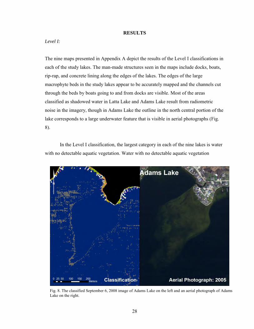
The nine maps presented in Appendix A depict the results of the Level I classifications in

each of the study lakes. The man-made structures seen in the maps include docks, boats,

rip-rap, and concrete lining along the edges of the lakes. The edges of the large

macrophyte beds in the study lakes appear to be accurately mapped and the channels cut

through the beds by boats going to and from docks are visible. Most of the areas

classified as shadowed water in Latta Lake and Adams Lake result from radiometric

noise in the imagery, though in Adams Lake the outline in the north central portion of the

lake corresponds to a large underwater feature that is visible in aerial photographs (Fig.

8).

In the Level I classification, the largest category in each of the nine lakes is water

with no detectable aquatic vegetation. Water with no detectable aquatic vegetation

Fig. 8. The classified September 6, 2008 image of Adams Lake on the left and an aerial photograph of Adams Lake on the right.

29

covered 386.75 ha (955.7 acres) of the 458.74 ha (1133.7 acres) classified across all nine

of the study lakes. This is not surprising given that most of the vegetation found in these

lakes occurs along the shoreline with only a few larger beds in Adams Lake, Jones Lake,

Tamarack Lake, and Waldron Lake.

For the majority of the lakes, the second largest class is broad-leafed emergent

vegetation that is underlain by submerged vegetation. The exception is Cree Lake, where

the second largest class is broad-leafed emergent vegetation underlain by Chara. All

classes containing Chara are larger in area in Cree Lake than in any of the other lakes.

This observation is supported by the field data collected in 2007 and 2008 which shows

that in Cree Lake Chara is the dominant submerged vegetation while in the other lakes,

Eurasian watermilfoil (Myriophyllum spicatum) and coontail (Ceratophyllum demersum)

make up the majority of submerged beds. Large Chara beds can also be found in Witmer

Lake and Adams Lake.

Jones Lake had the largest area covered in cattails (Typha sp.) at 2.02 ha (5 acres),

which is not surprising given the large cattail beds on the western portion of the lake.

Both Waldron Lake and Jones Lake have very large areas of submerged vegetation with

visible algae at 3.80 ha (8.8 acres) and 3.56 ha (9.4 acres), respectively, compared to the

other lakes. Overall, the most common macrophyte class in the lakes was broad-leafed

emergent vegetation with underlying submerged vegetation. This covered 22.78 ha (56.3)

acres. The IDNR LARE Report (2008) states that 95% of the shoreline of Adams Lake is

developed. These data are consistent with the results of the image classifications

developed in the current study, which show that the proportional area covered by man-

made surfaces is highest in Adams Lake. The area covered by each class by lake is

provided in Table 5. Table 6 summarizes the proportional area of each class.

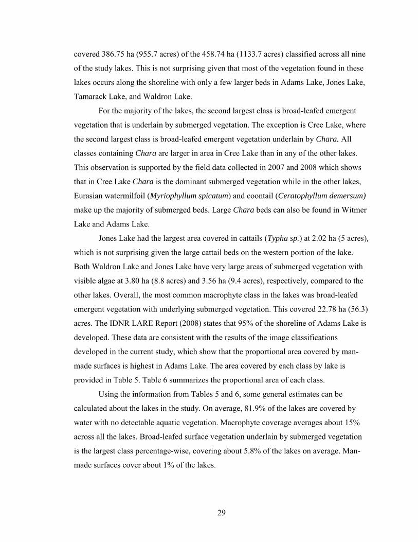
Using the information from Tables 5 and 6, some general estimates can be

calculated about the lakes in the study. On average, 81.9% of the lakes are covered by

water with no detectable aquatic vegetation. Macrophyte coverage averages about 15%

across all the lakes. Broad-leafed surface vegetation underlain by submerged vegetation

is the largest class percentage-wise, covering about 5.8% of the lakes on average. Man-

made surfaces cover about 1% of the lakes.

30

Adams Lake has the largest percentage of water, with 91.4% of its area being

covered by water with no discernible aquatic vegetation. Jones Lake has the lowest

percentage of its area covered with water at 70.4%. Given this, it is unsurprising that

Adams Lake has the lowest percent coverage of all macrophytes at 5.8% while Jones

Lake has over a quarter of its area covered by aquatic vegetation. Adams Lake also has

2.0% of its 123.81 ha (306 acres) classified as man-made surfaces. Latta Lake had the

lowest amount of man-made surfaces with 0.4% of its 17.99 ha (44.6 acres). While

Witmer Lake has the highest amount of bulrushes underlain by Chara in terms of

hectares, Latta Lake has a higher percentage of its area covered in bulrushes underlain by

Chara. Nearly 1% of Latta Lake’s is covered by this class, while the average across the

lakes is only 0.3%. Messick Lake has the highest percentage of overhanging tree/shore

vegetation at 3.4%, which is not surprising given the relatively low amount of residential

development along its shoreline.

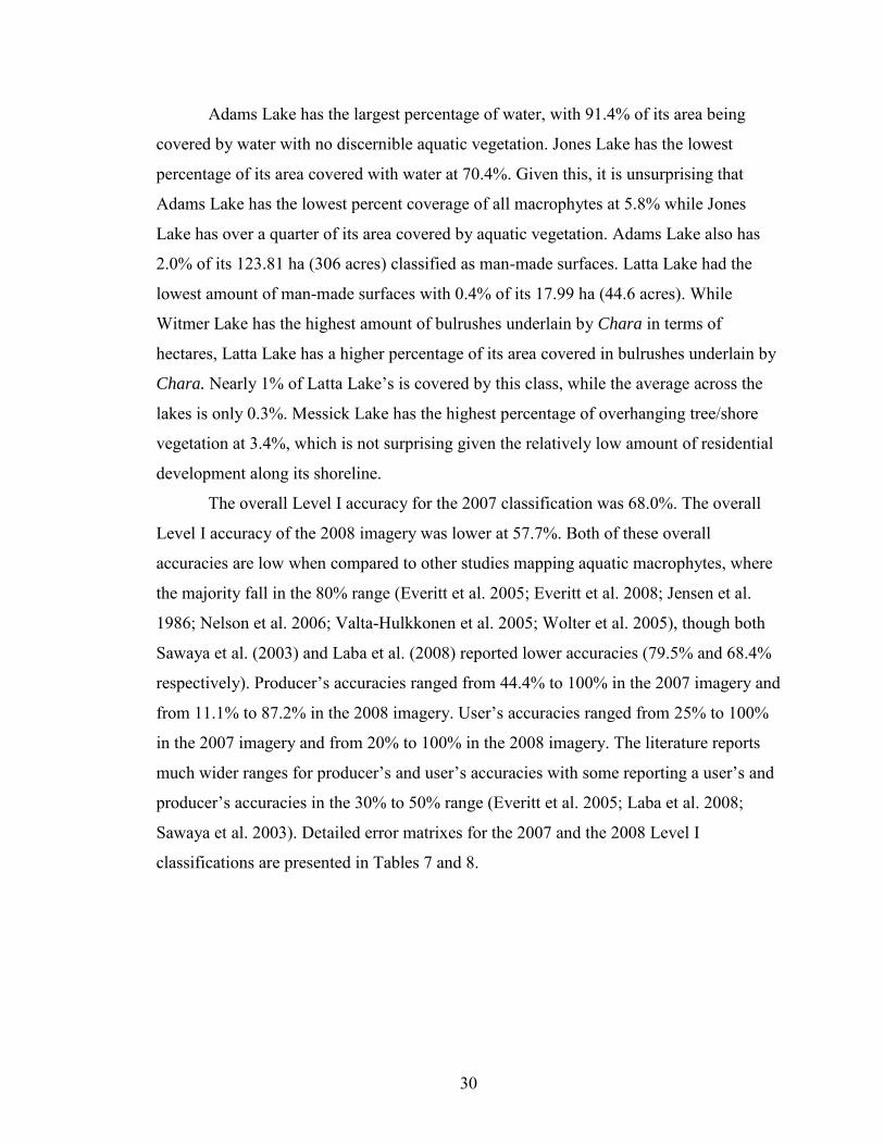
The overall Level I accuracy for the 2007 classification was 68.0%. The overall

Level I accuracy of the 2008 imagery was lower at 57.7%. Both of these overall

accuracies are low when compared to other studies mapping aquatic macrophytes, where

the majority fall in the 80% range (Everitt et al. 2005; Everitt et al. 2008; Jensen et al.

1986; Nelson et al. 2006; Valta-Hulkkonen et al. 2005; Wolter et al. 2005), though both

Sawaya et al. (2003) and Laba et al. (2008) reported lower accuracies (79.5% and 68.4%

respectively). Producer’s accuracies ranged from 44.4% to 100% in the 2007 imagery and

from 11.1% to 87.2% in the 2008 imagery. User’s accuracies ranged from 25% to 100%

in the 2007 imagery and from 20% to 100% in the 2008 imagery. The literature reports

much wider ranges for producer’s and user’s accuracies with some reporting a user’s and

producer’s accuracies in the 30% to 50% range (Everitt et al. 2005; Laba et al. 2008;

Sawaya et al. 2003). Detailed error matrixes for the 2007 and the 2008 Level I

classifications are presented in Tables 7 and 8.

Table 5 Level I vegetation coverage summary for all lakes in hectare (acres)

Key: W – Water, CR – Chara/bulrushes, C – Chara, CB – Chara/broad-leafed emergent, S – Submerged vegetation, SB - Submerged vegetation/ broad-leafed emergent, SA - Submerged vegetation/ algae, SAB – Submerged vegetation/algae/broad-leafed emergent, BC - Broad-leafed emergent/Chara, BS - Broad-leafed emergent/submerged vegetation, T - Typha/broad-leafed emergent, M - Man-made surfaces, OT/SV - Overhanging trees/shore vegetation

Lake W CR C CB S SB SA SAB BC BS T M OT/SV Total

Adams 113.15 (279.6)

0.20 (0.5)

0.48 (1.2)

0.08 (0.2)

0.24 (0.6)

0.20 (0.5)

1.29 (3.2)

0.40 (1.0)

0.53 (1.3)

2.79 (6.9)

0.93 (2.3)

2.47 (6.1)

1.05 (2.6)

123.81 (306)

Cree 19.30 (47.7)

- 0.85 (2.1)

0.45 (1.1)

0.32 (0.8)

0.45 (1.1)

- - 1.70 (4.2)

0.89 (2.2)

- 0.16 (0.4)

0.32 (0.8)

24.44 (60.3)

Jones 36.14 (89.3)

0.08 (0.2)

0.12 (0.3)

0.04 (0.1)

0.32 (0.8)

0.20 (0.5)

3.56 (8.8)

0.40 (1.0)

0.36 (0.9)

6.68 (16.5)

2.02 (5.0)

0.28 (0.7)

1.13 (2.8)

51.33 (126.9)

Latta 15.46 (38.2)

0.16 (0.4)

0.16 (0.4)

0.04 (0.1)

0.08 (0.2)

0.08 (0.2)

0.28 (0.7)

0.04 (0.1)

0.24 (0.6)

0.93 (2.3)

0.28 (0.7)

0.08 (0.2)

0.16 (0.4)

17.99 (44.6)

Messick 23.19 (57.3)

0.08 (0.2)

0.16 (0.4)

0.04 (0.1)

0.12 (0.3)

0.08 (0.2)

1.09 (2.7)

0.16 (0.4)

0.12 (0.3)

1.46 (3.6)

0.36 (0.9)

0.32 (0.8)

0.97 (2.4)

28.17 (69.6)

Steinbarger 26.87 (66.4)

0.08 (0.2)

0.16 (0.4)

0.04 (0.1)

0.12 (0.3)

0.12 (0.3)

1.38 (3.4)

0.20 (0.5)

0.20 (0.5)

1.25 (3.1)

0.36 (0.9)

0.28 (0.7)

0.81 (2.0)

31.87 (78.8)

Tamarack 15.66 (38.7)

0.04 (0.1)

0.04 (0.1)

- 0.12 (0.3)

0.12 (0.3)

1.01 (2.5)

0.12 (0.3)

0.24 (0.6)

1.94 (4.8)

0.61 (1.5)

0.16 (0.4)

0.53 (1.3)

20.59 (50.9)

Waldron 46.94 (116.0)

0.20 (0.5)

0.32 (0.8)

0.08 (0.2)

0.32 (0.8)

0.20 (0.5)

3.80 (9.4)

0.49 (1.2)

0.28 (0.7)

4.82 (11.9)

1.09 (2.7)

0.77 (1.9)

1.58 (3.9)

60.89 (150.5)

Witmer 90.04 (222.5)

0.28 (0.7)

0.61 (1.5)

0.08 (0.2)

0.28 (0.7)

0.12 (0.3)

1.90 (4.7)

0.24 (0.6)

0.12 (0.3)

2.02 (5.0)

0.73 (1.8)

1.70 (4.2)

1.46 (3.6)

99.59 (246.1)

Total 386.75 (955.7)

1.12 (2.8)

2.90 (7.2)

0.85 (2.1)

1.92 (4.7)

1.57 (3.9)

14.31 (35.4)

2.05 (5.1)

3.79 (9.4)

22.78 (56.3)

6.38 (15.8)

6.22 (15.4)

8.01 (19.8)

458.74 (1133.7)

31

Table 6 Level I amount of coverage for all lakes

Key: W – Water, CR – Chara/bulrushes, C – Chara, CB – Chara/broad-leafed emergent, S – Submerged vegetation, SB - Submerged vegetation/ broad-leafed emergent, SA - Submerged vegetation/ algae, SAB – Submerged vegetation/algae/broad-leafed emergent, BC - Broad-leafed emergent/Chara, BS - Broad-leafed emergent/submerged vegetation, T - Typha/broad-leafed emergent, M - Man-made surfaces, OT/SV - Overhanging trees/shore vegetation

Lake W CR C CB S SB SA SAB BC BS T M OT/SV All

macrophytes

Adams 91.4% 0.2% 0.4% 0.1% 0.2% 0.2% 1.0% 0.3% 0.4% 2.3% 0.8% 2.0% 0.8% 5.8%

Cree 79.0% 0.0% 3.5% 1.8% 1.3% 1.8% 0.0% 0.0% 7.0% 3.6% 0.0% 0.7% 1.3% 19.1%

Jones 70.4% 0.2% 0.2% 0.1% 0.6% 0.4% 6.9% 0.8% 0.7% 13.0% 3.9% 0.5% 2.2% 26.8%

Latta 85.9% 0.9% 0.9% 0.2% 0.4% 0.4% 1.6% 0.2% 1.3% 5.2% 1.6% 0.4% 0.9% 12.7%

Messick 82.3% 0.3% 0.6% 0.1% 0.4% 0.3% 3.9% 0.6% 0.4% 5.2% 1.3% 1.1% 3.4% 13.0%

Steinbarger 84.3% 0.3% 0.5% 0.1% 0.4% 0.4% 4.3% 0.6% 0.6% 3.9% 1.1% 0.9% 2.5% 12.3%

Tamarack 76.1% 0.2% 0.2% 0.0% 0.6% 0.6% 4.9% 0.6% 1.2% 9.4% 3.0% 0.8% 2.6% 20.6%

Waldron 77.1% 0.3% 0.5% 0.1% 0.5% 0.3% 6.2% 0.8% 0.5% 7.9% 1.8% 1.3% 2.6% 19.1%

Witmer 90.4% 0.3% 0.6% 0.1% 0.3% 0.1% 1.9% 0.2% 0.1% 2.0% 0.7% 1.7% 1.5% 6.4%

Average 81.9% 0.3% 0.8% 0.3% 0.5% 0.5% 3.4% 0.5% 1.4% 5.8% 1.6% 1.0% 2.0% 15.1%

32

Table 7 Level I accuracy assessment, September 2007 imagery

W CR C CB SAB S SB SA BC BS M

OT/

SV User's Accuracy

W 31 2 93.9% CR 0.0% C 13 1 1 1 1 2 68.4% CB 3 8 1 3 2 47.1% SAB 0.0% S 1 4 80.0% SB 1 3 3 3 1 1 25.0% SA 0.0% BC 2 1 17 5 4 58.6% BS 1 1 4 8 57.1% M 12 100% OT/SV 3 6 66.7%

Producer’s Accuracy 100% 0.0% 65.0% 53.3% 0.0% 44.4% 42.9% 0.0% 68.0% 53.3% 92.3% 60.0%

Overall Accuracy

68.0% Key: W – Water, CR – Chara/bulrushes, C – Chara, CB – Chara/broad-leafed emergent, SAB – Submerged vegetation/algae/broad-leafed emergent, S – Submerged vegetation, SB - Submerged vegetation/ broad-leafed emergent, SA - Submerged vegetation/ algae, BC - Broad-leafed emergent/Chara, BS - Broad-leafed emergent/submerged vegetation, M - Man-made surfaces, OT/SV - Overhanging trees/shore vegetation

33

34

Table 8 Level I accuracy assessment, September 2008 imagery

WS W CR C CB BRC SAB S SB SA BC BS M T OT/

SV

User's

Accuracy

WS 16 5 1 5 1 1 55.2% W 2 95 1 2 1 1 93.1% CR 2 1 1 3 1 1 1 1 0.0% C 2 2 3 1 1 2 1 1 23.1% CB 1 2 2 1 1 1 2 20.0% BRC 0.0% SAB 1 1 2 2 0.0% S 2 2 2 2 1 22.2% SB 1 1 1 2 20.0% SA 1 2 1 2 3 1 15 2 1 2 50.0% BC 1 4 2 6 2 1 37.5% BS 1 1 1 1 2 2 1 2 22 5 16 40.7% M 1 2 1 12 1 70.6% T 1 1 1 1 7 10 9 33.3% OT/SV 18 100% Producer’s Accuracy

64.0%

87.2% 0.0%

42.9%

20.0% 0.0% 0.0%

11.1%

12.5%

57.7%

54.6%

57.9%

70.6%

62.5%

36.7%

Overall

Accuracy

57.7% Key: W – Water, WS - Shadowed water, CR – Chara/bulrushes, C – Chara, CB – Chara/broad-leafed emergent, BRC - Broad-leafed emergent/ bulrushes/Chara, SAB – Submerged vegetation/algae/broad-leafed emergent, S – Submerged vegetation, SB - Submerged vegetation/ broad-leafed emergent, SA - Submerged vegetation/ algae, BC - Broad-leafed emergent/Chara, BS - Broad-leafed emergent/submerged vegetation, M - Man-made surfaces, T - Typha/broad-leafed emergent, OT/SV - Overhanging trees/shore vegetation

34

35

All eight lakes in the 2008 imagery were classified together in an attempt to

reduce the amount of processing time and to make the classification scheme more

uniform across all lakes. One of the issues with this approach is that the aquatic

vegetation and lake characteristics differ from one lake to the next and these differences

can be lost when classifying all lakes together. An example of this is the macrophyte

American lotus (Nelumbo lutea). American lotus (Nelumbo lutea) has leaves up to 100

cm (3.28 ft) in diameter and is a significant component of the beds along the southern

shore of Waldron Lake, but was not observed in any of the other study lakes. No classes

show the presence of this distinct emergent species. Another problem is that areas can be

classified as macrophytes that do not exist in that lake, but exist in others. One example

of this is the submerged aquatic plant Chara sp. This macrophyte forms large beds in

Adams Lake and Latta Lake, smaller beds in Messick Lake, but is not present in

significant amounts in the WJST chain or Witmer Lake. However, as seen in Table 7,

Chara appears in all the lakes in the classification. Marshall and Lee (1994) came to the

conclusion that spectral signatures, especially at the species level, were not fully

transportable to other lakes in their study of mapping freshwater aquatic vegetation in

Walkinshaw and Big Pearl Lakes in northwestern Ontario. It is likely that simultaneous

classification is one of the reasons why the overall Level I accuracy of the 2008 imagery

is lower than that of the 2007 imagery, which focused solely on Cree Lake.

Some of the highest accuracies in the Level I assessment were found in the

categories of water and man-made structures in both the 2007 and 2008 imagery. Water

had a user’s accuracy of 93.9% and a producer’s accuracy of 100% in the 2007 imagery

and a similarly high user’s accuracy of 93.1% and a lower producer’s accuracy of 87.2%

in the 2008 imagery. Man-made structures had a user’s accuracy of 100% and a

producer’s accuracy of 92.3% in the 2007 imagery. The user’s and producer’s accuracy

in the 2008 imagery is lower at 70.6% for both.

The lowest accuracies in the Level I assessment were for beds that contained

bulrushes, Scirpus acutus and Scirpus validus. All of the beds containing bulrushes in

both the 2007 and 2008 imagery have a user’s and producer’s accuracy of 0%. In general,

bulrushes and other tall, thin macrophytes with no prominent leaves (such as horsetails)

are the least accurately mapped aquatic macrophyte (Laba et al. 2008; Marshall and Lee

36

1994). In the current study, bulrushes were most often mischaracterized as Chara or as

broad-leafed emergent vegetation underlain by Chara. Marshall and Lee (1994) state that

while bulrushes are easily visible when viewed laterally from a boat, it is difficult to

discern these plants from an overhead position. This could explain the low accuracies in

classes containing bulrushes, despite the fact that areas with large and relatively dense

bulrush beds exist in the study area, such as in the southwest corner of Adams Lake.

One of the major sources of error in the Level I classification of the 2008 imagery

was the confusion between aquatic macrophytes and shoreline vegetation, usually in the

form of overhanging trees and mowed grass. The user’s accuracy for the overhanging

tree/shore vegetation class was 100%, indicating that when an area is classified as

overhanging tree or shore vegetation, it has a high chance of actually being an

overhanging tree or shore vegetation. However, the producer’s accuracy for this class is

46.2%. The error matrix shows that the overhanging tree/shore vegetation is often

classified as broad-leafed emergent vegetation and occasionally as cattails (Typha sp.).

This explains the low producer’s accuracy for the category.

Work by Han and Rundquist (2003) has shown that the reflectance in the NIR is

relatively low for submerged vegetation when compared to terrestrial vegetation.

Equivalent work comparing emergent aquatic macrophytes and terrestrial vegetation was

not found in a literature review. In some areas around the study lakes, grass and other

non-aquatic vegetation grew right up to the water’s edge while in the water, aquatic

vegetation formed dense beds that also extended to the water’s edge. Parts of tree

canopies were included in the image because these trees overhang the water. Since many

of the smaller aquatic macrophyte beds grow very near to the shore, effort was made to

come as close to the shoreline as possible so as to include these smaller beds. In many

cases, identifying the exact shoreline was difficult in the panchromatic imagery and,

when digitizing, preference was given to including more terrestrial vegetation rather than

excluding aquatic vegetation. This additional terrestrial vegetation contributed to

confusion with macrophytes in the accuracy assessment.

Cattails (Typha sp.) and other broad-leafed emergent vegetation had a relatively

high producer’s accuracy compared to other categories in the 2008 imagery, but a low

user’s accuracy. In addition to being confused with different types of shoreline

37

vegetation, such as grass and overhanging trees, it was often confused with broad-leafed

emergent vegetation. It is known that Typha sp. has variations in growth patterns which

can complicate classifications (Ozesmi and Bauer 2002). A review of the field data shows

that the class containing cattails (Typha sp.) was more often confused with broad-leafed

emergent vegetation classes that did not contain cattails in areas where the vegetation was

dense (canopy coverage between 80-100%) and in areas where the vegetation was

dominated by above surface species such as spatterdock (Nuphar advena) and arrow

arum (Peltandra virginica).

Another problem classifying aquatic macrophytes in small lakes is that the

shadows of trees along the shoreline or from obstructions in the water, such as docks, can

interfere with spectral signatures (Sawaya et al. 2003; Valta-Hulkkonen et al. 2005).

Cloud shadows also contribute to this problem. While the classification was able to

differentiate shadows when they occurred in areas of open water, it was not able to do the

same for vegetation. Often in areas where shadows occurred, emergent vegetation was

classified as submerged vegetation and submerged vegetation was classified incorrectly

as Chara.

Submerged vegetation in all forms had relatively low accuracies in both the 2007

and 2008 images. Chara had a much higher user’s accuracy and producer’s accuracy in

the 2007 imagery than in the 2008 imagery. The same trend holds for the submerged

vegetation class. In the 2008 imagery, areas classified as Chara or submerged vegetation

were not confused with each other. Instead, most of the confusion with Chara was with

categories that also contained Chara such as bulrushes with Chara and broad-leafed

emergent vegetation with Chara. This is also true for the submerged vegetation class in

the 2008 imagery, with most of the confusion being between classes containing

submerged vegetation and broad-leafed emergent vegetation or classes with submerged

vegetation and algae.

There is confusion between classes containing Chara and classes containing

submerged vegetation in the 2007 imagery of Cree Lake. In particular, a large Chara bed

on the eastern side of Cree Lake is classified as submerged vegetation or submerged

vegetation with broad-leafed emergent vegetation. A possible reason for this confusion is

reflectance off of the lake bottom. Lake bottoms have been shown to cause confusion in

38

classification of aquatic macrophytes, especially when classifying submerged vegetation

(Marshall and Lee 1994; Valta-Hulkkonen et al. 2005; Wolter et al. 2005). Peñuelas et al.

(1993) suggested the reason that Chara could be differentiated from other submerged

vegetation, such as coontail (Ceratophyllum demersum) and Myriophyllum, was because

it had slightly lower reflectance values. In areas such as the shelf on the east side of Cree

Lake, it is possible that bottom reflectance in addition to the reflectance from Chara is

causing the misclassification.

The confusion between areas with different submerged vegetation and emergent

vegetation, particularly in areas where the emergent vegetation coverage is less than 30%,

can be explained. As the depth of submerged vegetation in the water column increases,

there is a dramatic drop in reflectance in the NIR band and a corresponding drop in the

green part of the spectrum (Han and Rundquist 2003). This drop in the NIR band also

occurs as the percentage of coverage in submerged vegetation decreases (Yuan and

Zhang 2007). In addition, as the percentage of cover in emergent, floating vegetative beds

decreases, there is also a dramatic drop in reflectance in the NIR band and again, a less

dramatic decrease in the green part of the spectrum (Jakubauskas et al. 2000). These

effects occur because of the increase in water area exposed to the sensor (Han and

Rundquist 2003; Jakubauskas et al. 2000; Yuan and Zhang 2007). An attempt was made

to separate areas with low emergent coverage into different classes from areas with

higher emergent coverage, and areas with solely submerged vegetation. The low

accuracies shown for these classes indicate that this was not particularly successful.

The presence of algae, both in the water column and growing on the submerged

vegetation, is another confounding factor in differentiating between different submerged

macrophytes, and between emergent and submerged vegetation. There is some debate

about whether and how much the presence of algae disrupts the detection of submerged

macrophytes. At least one study has found no correlation between water clarity or algae

concentrations and the ability of sensors to detect submerged macrophytes (Nelson et al.

2006). Empirical work suggests that submerged macrophyte signatures become confused

in algae laden waters. Submerged vegetation still shows a rapid decreased in the NIR

band with depth, but a large “green peak” occurs due to the algae (Han and Rundquist

2003; Yuan and Zhang 2007). Even as depth increases or the coverage of the submerged

39

macrophyte bed decreases, the amount of green light reflected back remains relatively

high. In this study, dense algae mats were sometimes confused with submerged

vegetation. Algae growing on the submerged macrophytes is thought to have caused

some of the confusion between different species and between submerged macrophyte

beds and beds containing low, broad-leafed emergent vegetation.

Finally, a possible issue contributing to error in the classifications was bottom

reflectance. Stumpf and Holderied (2003) indicate that high-resolution satellite imagery

can detect bottom reflectance up to 20 m (65.6 ft) in depth. Early analysis indicated that

only limited areas within the lakes showed signs of bottom reflectance in their spectra

and these areas were incorporated into the water category. For this reason, bottom

reflectance was initially not thought to be an issue. After the final classification had been

completed, the IDNR provided bathymetry maps derived from hydroaccoustic data

obtained during 2007. This led to a review of the water classes for possible reflectance. A

comparison of the bathymetry maps and several of the water classes that have possible

bottom reflectance shows a distinct similarity between the two within Adams Lake, Latta

Lake, Messick Lake, and Witmer Lake. Therefore, in some portions of shallow lakes,

bottom reflectance may be classed as water. Given that these areas are still water – and

not vegetation, this challenge should not impact the vegetation classifications

significantly. No such correlation exists in the WJST chain in the 2008 imagery or within

Cree Lake in the 2007 imagery.

Level II:

The nine maps presented in Appendix B depict the results of the Level II

classifications in each of the study lakes. As in the Level I classification, in the Level II

classification of the 2008 imagery the largest category for all the lakes is water with no

detectable aquatic vegetation. The second largest class for all lakes is emergent

vegetation which covers a total of 32.97 ha (81.5 acres) across all nine lakes. The

smallest class is man-made surfaces, which only cover 6.22 ha (15.4 acres) across all nine

of the lakes.

Jones Lake had the largest amount of emergent vegetation at 9.06 ha (22.4 acres),

again probably due to the large cattail bed in northwestern portion of the lake as well as

40

large beds in the channel leading to Witmer Lake. At 4.37 ha (10.8 acres), Waldron Lake

has the largest amount of submerged vegetation of any of the lakes. It also has the largest

amount of overhanging tree/shore vegetation of any of the lakes in terms of area. As the

smallest lake in the study, Latta Lake had the smallest area of each of the classes in the

Level II classification. The sole exception was with the mixed submerged/emergent

vegetation class where Tamarack Lake, the second smallest lake in the study, had only

0.28 ha (0.7 acres). Latta Lake had 0.36 ha (0.9 acres). Adams Lake had the largest area

covered by the mixed submerged/emergent vegetation class with 1.21 ha (3 acres). A

detailed breakdown of the Level II classes by lake can be seen in Table 9.

The percent coverage for the Level II classes is summarized in Table 10. The

average proportion covered by emergent vegetation is 8.8%. Submerged vegetation, on

average, covers about 4.6% of the lakes while the mixed submerged/emergent vegetation

class covers, on average, only 1.7% of the lakes. Jones Lake, which as previously stated

has the highest percentage of its surface covered by macrophytes, has the highest

percentage of its area covered by emergent macropyhtes at 17.7% and by submerged

macropyhtes at 7.7%. Waldron Lake has the highest area of submerged vegetation at 4.37

ha (22.4 acres), but it only covers 7.2% of the 60.89 ha (150.5 acres) that make up its

area. Cree Lake had the highest amount of its area covered by the mixed

emergent/submerged vegetation class at 3.6%.

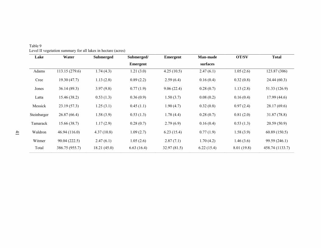
Table 9 Level II vegetation summary for all lakes in hectare (acres)

Lake Water Submerged Submerged/

Emergent

Emergent Man-made

surfaces

OT/SV Total

Adams 113.15 (279.6) 1.74 (4.3) 1.21 (3.0) 4.25 (10.5) 2.47 (6.1) 1.05 (2.6) 123.87 (306)

Cree 19.30 (47.7) 1.13 (2.8) 0.89 (2.2) 2.59 (6.4) 0.16 (0.4) 0.32 (0.8) 24.44 (60.3)

Jones 36.14 (89.3) 3.97 (9.8) 0.77 (1.9) 9.06 (22.4) 0.28 (0.7) 1.13 (2.8) 51.33 (126.9)

Latta 15.46 (38.2) 0.53 (1.3) 0.36 (0.9) 1.50 (3.7) 0.08 (0.2) 0.16 (0.4) 17.99 (44.6)

Messick 23.19 (57.3) 1.25 (3.1) 0.45 (1.1) 1.90 (4.7) 0.32 (0.8) 0.97 (2.4) 28.17 (69.6)

Steinbarger 26.87 (66.4) 1.58 (3.9) 0.53 (1.3) 1.78 (4.4) 0.28 (0.7) 0.81 (2.0) 31.87 (78.8)

Tamarack 15.66 (38.7) 1.17 (2.9) 0.28 (0.7) 2.79 (6.9) 0.16 (0.4) 0.53 (1.3) 20.59 (50.9)

Waldron 46.94 (116.0) 4.37 (10.8) 1.09 (2.7) 6.23 (15.4) 0.77 (1.9) 1.58 (3.9) 60.89 (150.5)

Witmer 90.04 (222.5) 2.47 (6.1) 1.05 (2.6) 2.87 (7.1) 1.70 (4.2) 1.46 (3.6) 99.59 (246.1)

Total 386.75 (955.7) 18.21 (45.0) 6.63 (16.4) 32.97 (81.5) 6.22 (15.4) 8.01 (19.8) 458.74 (1133.7)

41

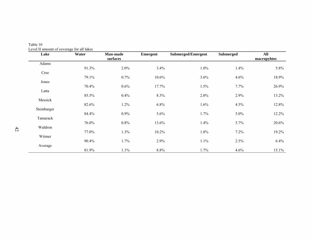
Table 10 Level II amount of coverage for all lakes

Lake Water Man-made

surfaces

Emergent Submerged/Emergent Submerged All

macropyhtes

Adams 91.3% 2.0% 3.4% 1.0% 1.4% 5.8%

Cree 79.1% 0.7% 10.6% 3.6% 4.6% 18.9%

Jones 70.4% 0.6% 17.7% 1.5% 7.7% 26.9%

Latta 85.5% 0.4% 8.3% 2.0% 2.9% 13.2%

Messick 82.6% 1.2% 6.8% 1.6% 4.5% 12.8%

Steinbarger 84.4% 0.9% 5.6% 1.7% 5.0% 12.2%

Tamarack 76.0% 0.8% 13.6% 1.4% 5.7% 20.6%

Waldron 77.0% 1.3% 10.2% 1.8% 7.2% 19.2%

Witmer 90.4% 1.7% 2.9% 1.1% 2.5% 6.4%

Average 81.9% 1.1% 8.8% 1.7% 4.6% 15.1%

42

Error matrixes for the 2007 and the 2008 Level II classifications are presented in

Tables 11 and 12. The overall accuracies for both maps increased in the Level II

classification. The overall Level II accuracy for the 2007 classification of Cree Lake was

74.6% while the overall Level II accuracy of the eight lakes in the 2008 map was 74.3%.

Producer’s accuracies ranged from 52.4% to 100% in the 2007 classification and 51.7%

to 85.8% in the 2008 classification. These error ranges are more narrow relative to the

Level I classification and indicate that the Level II classification does a better job of

correctly classifying aquatic vegetation. The user’s accuracies range from 27.8% to 98%

in the 2007 classification and 33.3% to 97.1% in the 2008 classification. These results are

comparable to those derived from the Level I classification.

While the Level I classification was more detailed than the Level II, it also had a

lower accuracies in most categories. The highest accuracies in the Level II classification

were found in the categories of water in both the 2007 and 2008 imagery. Water had a

user’s accuracy of 98% and a producer’s accuracy of 90.4% in the 2007 imagery and

user’s accuracy of 97.1% and a lower producer’s accuracy of 85.8% in the 2008 imagery.

Man-made structures had lower user’s accuracies in the Level II classification than in the

Level I classification of the 2007 imagery at 63.2% but had a producer’s accuracy of

100%. There was an increase in the confusion between man-made structures and both

emergent and submerged vegetation in 2007 imagery. Confusion between man-made

structures and submerged and emergent vegetation is also seen in the Level II 2008

imagery. The user’s accuracy is 71% and producer’s accuracy is 73.3%. In the Level II

classification of the 2007 imagery, the mixed class of submerged/emergent vegetation

had a high user’s and producer’s accuracy at 75%.

Table 11 Level II accuracy assessment, September 2007 imagery

Water Submerged Submerged/

Emergent

Emergent Man-made surfaces OT/SV

User's

Accuracy

W 47 1 98.0% S 4 11 4 2 52.4% SE 1 1 15 2 1 75.0% E 22 2 91.7% MS 3 4 12 63.2% OT/SV 1 12 5 27.8%

Producer’s Accuracy 90.4% 68.8% 75.0% 52.4% 100% 62.5%

Overall

Accuracy

74.6%

Table 12 Level II accuracy assessment, September 2008 imagery

Water Submerged Submerged/

Emergent

Emergent Man-made surfaces OT/SV

User's

Accuracy

W 133 2 2 97.1% S 9 15 5 6 3 7 33.3% SE 7 8 13 2 1 1 40.6% E 1 1 1 46 2 20 64.8% MS 5 2 2 22 71.0% OT/SV 1 2 31 91.2%

Producer’s Accuracy 85.8% 51.7% 68.4% 79.3% 73.3% 52.5%

Overall

Accuracy

74.3%

44

45

Although the Level II classification had higher overall accuracies, it suffered from

some of the same problems as the Level I classification. The most significant of these is

the confusion between shore vegetation and aquatic macrophytes. The user’s accuracy for

the overhanging tree/shore vegetation class in the 2008 imagery was 91.2%, indicating

that when an area is classified as overhanging tree or shore vegetation, it has a high

chance of actually being an overhanging tree or shore vegetation. However, the

producer’s accuracy for this class is 52.5%. As in the Level I classification, overhanging

trees and other types of shore vegetation were most often misclassified as emergent

vegetation.

It is interesting to note that in the Level II assessment for the 2007 imagery, the

exact opposite phenomenon happened. In the 2007 imagery overhanging trees/shore

vegetation had a very low user’s accuracy of 27.8% but a higher producer’s accuracy of

62.5%. Areas of emergent vegetation were often misclassified as overhanging trees/shore

vegetation (13 cases) with at least one case of mixed submerged/emergent being

misclassified as overhanging trees/shore vegetation. This indicates that the amount of

vegetation classified as shore vegetation in the 2007 imagery is exaggerated in the

classification.

Confusion between the mixed emergent/submerged vegetation beds and

submerged vegetation becomes more evident in the Level II analysis than in the Level I

analysis as does the confusion between emergent and submerged vegetation. As in the

Level I analysis, this is probably because of similar spectral responses of emergent

macrophytes as the density of the canopy decreases and as the depth of submerged

macrophytes increases.

46

CONCLUSIONS

Using high spatial resolution imagery and unsupervised classification to map

aquatic macrophytes in small lakes for management purposes is possible. This study

presents maps of the distribution of aquatic macrophyte beds in nine northern Indiana

lakes and provides estimates of the area covered by different macrophyte classes and

man-made structures. Two of the four management objectives outlined by the IDNR were

met. First, it was possible to outline the extent of emergent and submerged vegetative

beds within these lakes for management purposes. Second, the classification was able to

accurately map man-made structures in both sets of imagery. The analysis was unable to

differentiate the invasive species Eurasian watermilfoil (Myriophyllum spicatum) from

the native species coontail (Certatophyllum demersum), and these two submerged

macrophytes were grouped into one class. The analysis was able to differentiate between

Chara and other submerged macrophytes to a limited extent, but accuracies were still

low. Therefore, two of the study goals are topics for further research: mapping the health

and extent of native species, and the extent and spread of invasive species.

The study results provide information important for management decisions. For

example, while coontail (Ceratophyllum demersum) and Chara were considered nuisance

plants in Cree Lake, funding was not available through the LARE program to control

them because they are not invasive plants (IDNR LARE Reports: Cree Lake 2005).

However, monitoring is still needed in Cree Lake because of the threat of invasive

species, like Eurasian watermilfoil (Myriophyllum spicatum), spreading within the lake.

Since the high resolution satellite imagery mapping methods tested in this study cannot

differentiate between Eurasian watermilfoil (Myriophyllum spicatum), and the native

species coontail (Certatophyllum demersum), a sudden spread of the invasive species

within the lake could go unnoticed without field data. These results also cast doubt onto

whether image-based methods would be useful in monitoring the spread of invasive

species such as hydrilla (Hydrilla verticillata), which has recently been found in Indiana.

The Level II analysis accurately mapped vegetative beds in the study lakes and

was effective in mapping man-made surfaces in both analyses. Pesticides are often used

47

to manage invasive species in the vegetative beds in the lakes. Their use requires

monitoring to track the effectiveness of the pesticides and to track their effect on native

species. While using the satellite imagery cannot differentiate what species are being

affected within the bed, it can be used to track the reduction in size of the beds that result

from pesticide applications. Once this occurs, a field team could document what species

recolonize the area. In addition, the analysis provides a lake-wide view of all the man-

made structures and the locations of large beds within the lakes. Maps made with this

information could be useful to resource managers in matching existing permits with

structures and determining which structure are in violation. Again, a ground check would

be necessary to confirm the presence of structures for legal purposes, but maps derived

using the image processing methods in this study can help to guide this process. Overall,

mapping using high resolution satellite imagery cannot completely replace traditional

field surveys, but can be used to guide these processes and provide overview information

that would be difficult to collect using field methods alone.

This study revealed several problems that should be addressed in future work. The

accuracies in the Level I classification were low, but comparable to results of similar

studies in the peer-reviewed literature. Laba et al. (2008) reported a result of 68.4% for

the overall accuracy while classifying invasive wetland species using Quickbird satellite

imagery of in the Hudson River National Estuarine Research Reserve, which is similar to

the 68% for Cree Lake in the 2007 imagery. The Level II classification was more

successful and the smaller number of classes is more comparable (in terms of thematic

detail) to other work on aquatic macrophyte mapping (Everitt et al. 2005; Everitt et al.

2008; Jensen et al. 1986; Mackey et al. 1992; Olmanson et al. 2002; Sawaya et al. 2003;

Valta-Hulkkonen et al. 2005; Vis et al. 2005; Wolter et al. 2005). In an attempt to

comprehensively map the aquatic plants in the study lakes, the heads-up digitizing

process used to identify shorelines from the panchromatic imagery included overlapping

shore vegetation. Since most macrophyte beds in the study lakes grow up to the water’s

edge, the problem becomes which is more important in the heads-up digitization process:

inclusion of all possible aquatic macropyhte beds or exclusion of shore vegetation? In

future applications, the tradeoffs between these approaches need to be considered

carefully.

48

Another issue to consider in future work is the impact of bottom reflectance on

spectral signatures captured in imagery, which can impact classification results. The

IDNR has recently made available bathymetric data that could help inform and

potentially improve mapping results in future studies. While bathymetric data for the

lakes did not become available until after much of the current study was completed,

initial inspection of these data suggests a potential correlation between water depth and

several spectral features apparent in visual interpretation of the imagery. It is known that

sandy bottoms are more often confused with submerged vegetation than muck bottoms

(Wolter et al. 2005) and it is possible that areas in the study lakes with sandy bottoms

have more confusion than areas without. This is an issue that needs to be explored in

further studies.

Classifying all eight lakes together in the 2008 imagery instead of processing each

lake separately may have contributed to lower accuracies, particularly in the Level I

maps. This approach may also have masked areas in lakes with unique environments.

However, classifying all eight lakes simultaneously did allow for a large area to be

classified in a relatively short amount of time. Resource managers will need to decide

whether time or accuracy is more vital when determining whether to classify lakes in

bulk or separately. When making these types of decisions, the desired thematic detail

should also be considered. It is likely that more accurate species-level maps could be

developed by processing lakes individually. More general maps designed to inform

decisions about total aquatic plant cover can be created using the simultaneous

classification approach.

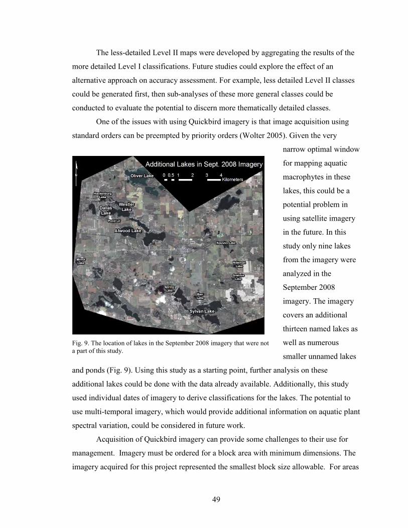
49

The less-detailed Level II maps were developed by aggregating the results of the

more detailed Level I classifications. Future studies could explore the effect of an

alternative approach on accuracy assessment. For example, less detailed Level II classes

could be generated first, then sub-analyses of these more general classes could be

conducted to evaluate the potential to discern more thematically detailed classes.

One of the issues with using Quickbird imagery is that image acquisition using

standard orders can be preempted by priority orders (Wolter 2005). Given the very

narrow optimal window

for mapping aquatic

macrophytes in these

lakes, this could be a

potential problem in

using satellite imagery

in the future. In this

study only nine lakes

from the imagery were

analyzed in the

September 2008

imagery. The imagery

covers an additional

thirteen named lakes as

well as numerous

smaller unnamed lakes

and ponds (Fig. 9). Using this study as a starting point, further analysis on these

additional lakes could be done with the data already available. Additionally, this study

used individual dates of imagery to derive classifications for the lakes. The potential to

use multi-temporal imagery, which would provide additional information on aquatic plant

spectral variation, could be considered in future work.

Acquisition of Quickbird imagery can provide some challenges to their use for

management. Imagery must be ordered for a block area with minimum dimensions. The

imagery acquired for this project represented the smallest block size allowable. For areas

Fig. 9. The location of lakes in the September 2008 imagery that were not a part of this study.

50

of the state with high densities of lakes such as Noble and LaGrange Counties this

approach has several benefits – notably that the satellite imagery acquisition costs can be

spread over several lakes so that the per lake imagery cost is relatively low. Indeed, there

are 13 other lakes that were captured in the imagery that were not analyzed in this study.

Conversely, the satellite imagery acquisition cost ($8322) cannot be reduced in the event

that a specific lake or area with only a few lakes is of interest. Thus, the cost/benefit

ratio of this approach is somewhat dependent on the area of the state where it is being

used and the lake density.

In summary, this study has shown that high resolution satellite imagery can be

used to map aquatic vegetation in small lakes for management purposes. Areal estimates

of general thematic classes, such as submergent and emergent vegetation, can be

generated for multiple lakes simultaneously. High resolution satellite imagery was also

successfully used to identify the presence of man-made structures in lakes that could help

guide more detailed field assessments for regulatory purposes. Further study is needed to

determine whether alternative methods and data sources (such as multi-temporal imagery,

bathymetric data, and different image processing approaches) can be used to derive more

detailed maps with species-level classes that are important for natural resource

management decisions.

51

Appendix A

Level I Classification Maps

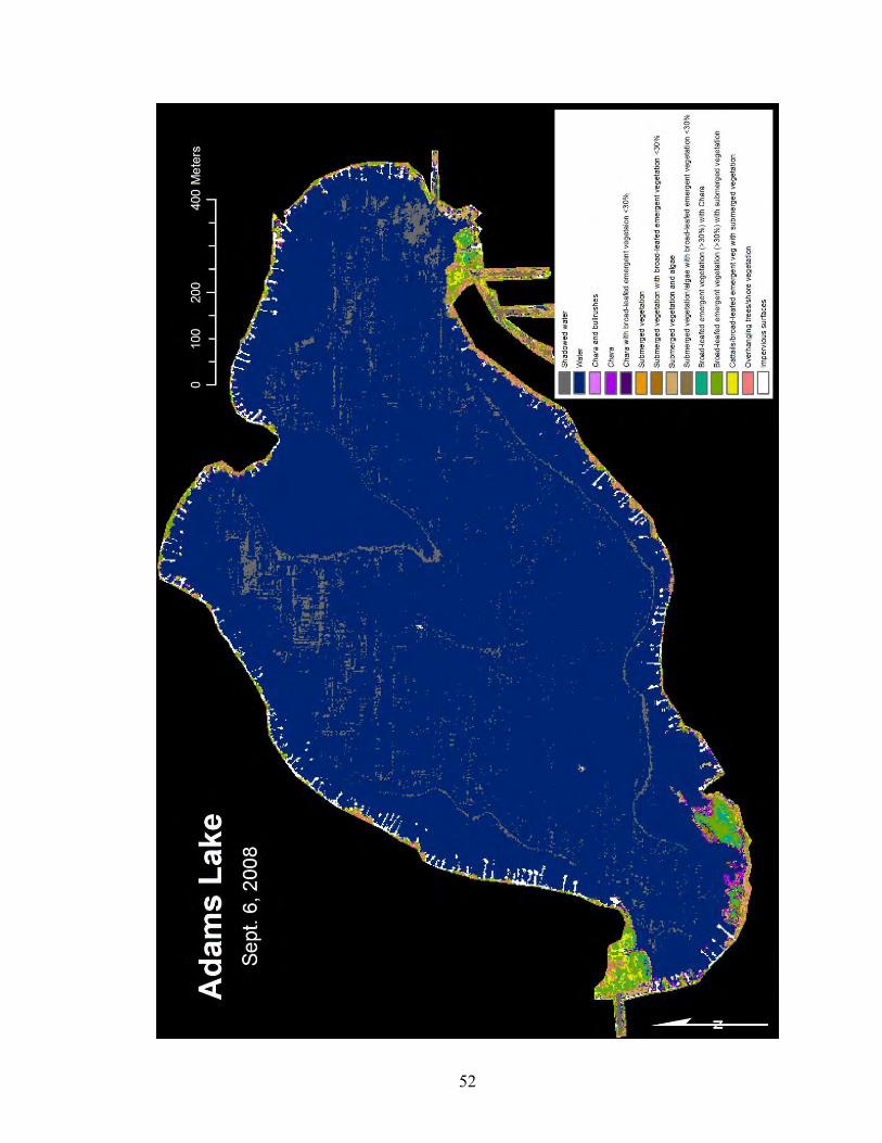
52

53

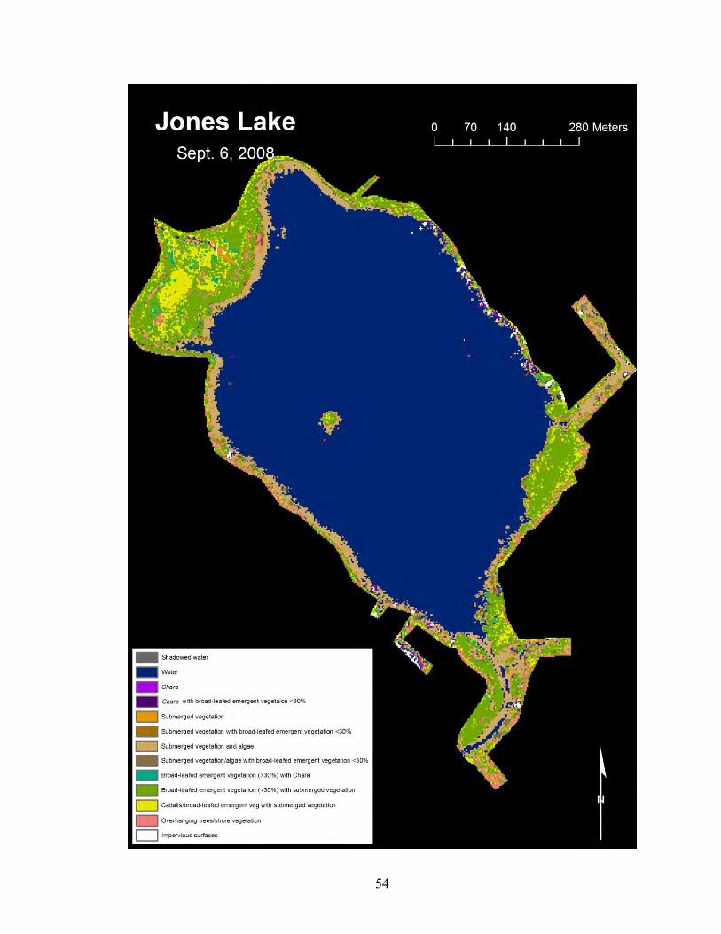
54

55

56

57

58

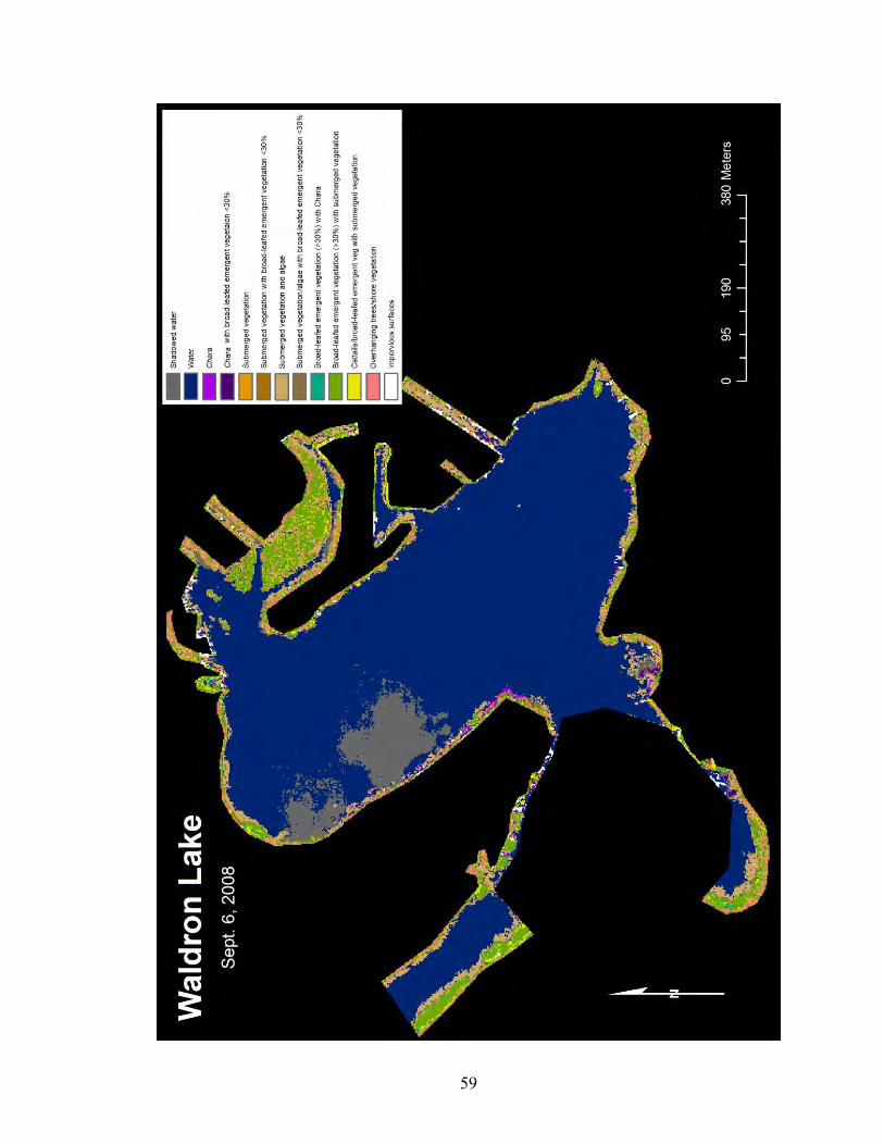
59

60

61

Appendix B

Level II Classification Maps

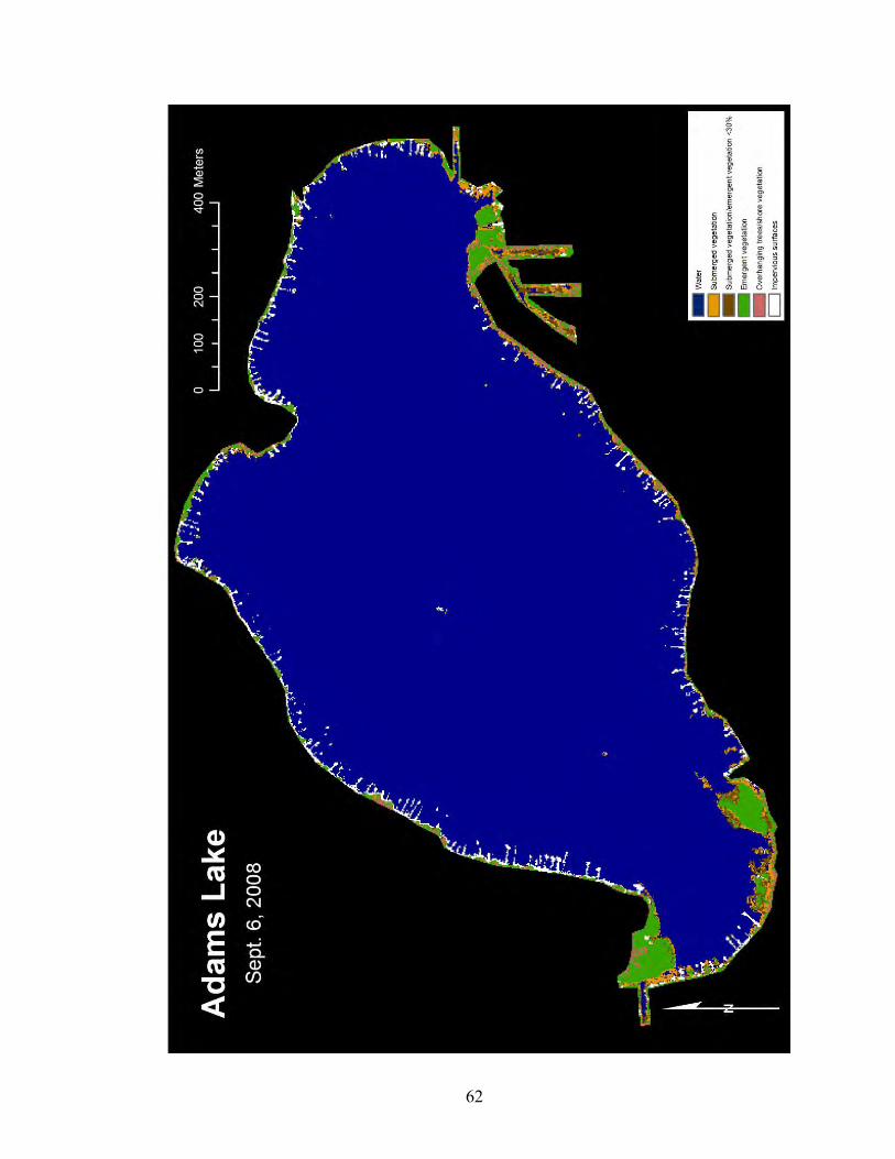
62

63

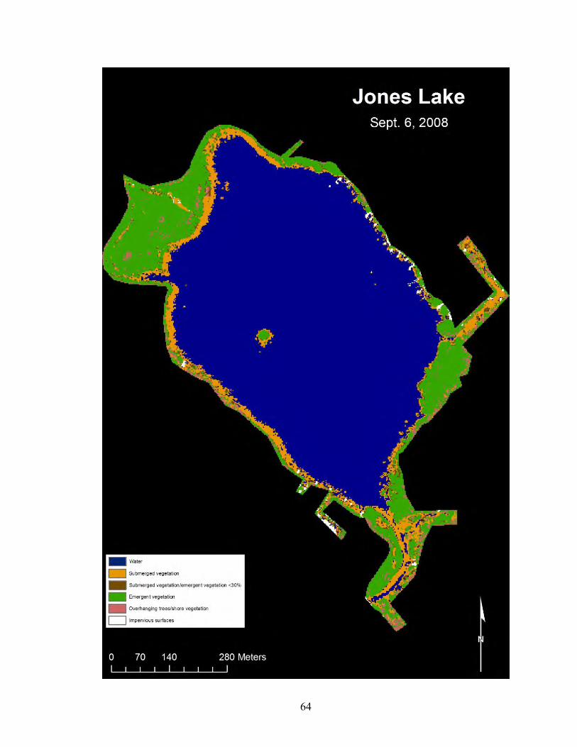
64

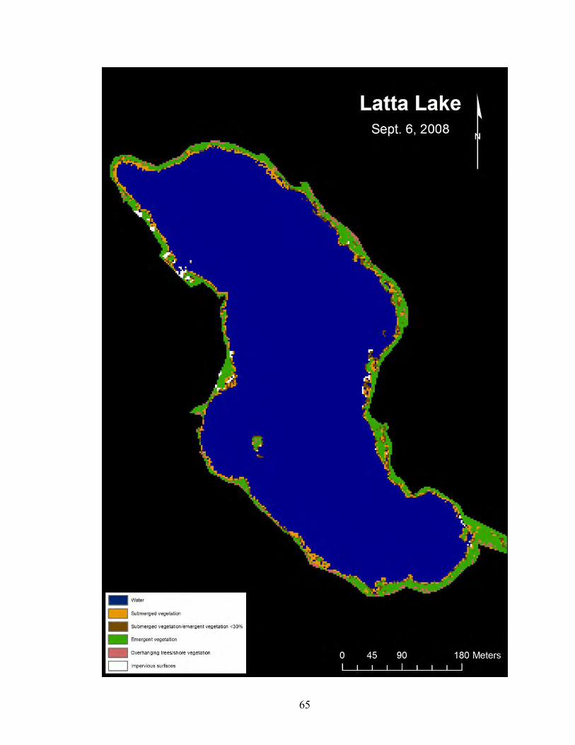
65

66

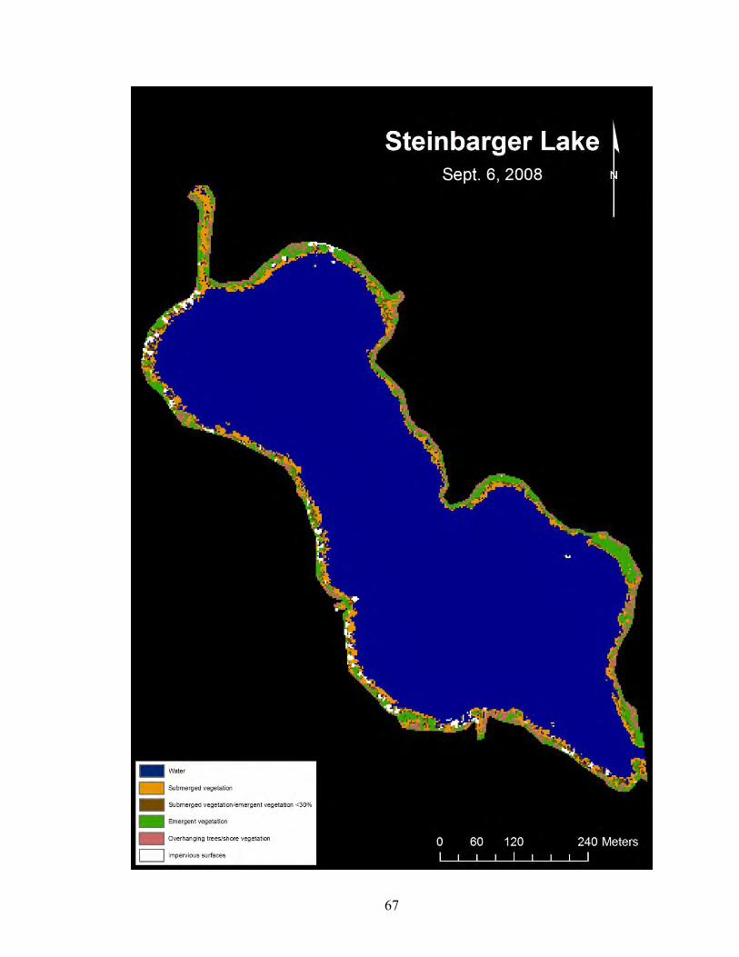
67

68

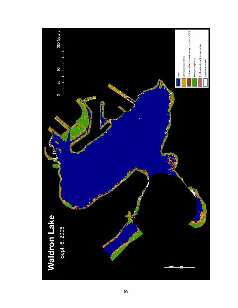
69

70

71

REFERENCES

Ackleson, S. G. 2003. Light in Shallow Waters: A Brief Research Review. Limnology

and Oceanography. 48(1): 323-328. Ciraolo, G., E. Cox, G. La Loggia, and A. Maltese. 2003. The classification of submerged

vegetation using hyperspectral MIVIS data. Annals of Geophysics. 49(1): 287-294.

Cook, C. 1996. Aquatic Plant Book. Amsterdam/New York: SPB Academic Publishing. Congalton, R. G., and K. Green. 1999. Assessing the Accuracy of Remotely Sensed Data:

Principles and Practices. London/New York: Lewis Publishers. ERDAS. 2009. ERDAS Field Guide. Norcross: ERDAS Inc. Everitt, J. H., C. Yang, D. R. Escobar, C. F. Webster, R. I. Leonard, and M. R. Davis.

1999. Using remote sensing and spatial information technologies to detect and map two aquatic macrophytes. Journal of Aquatic Plant Management. 37: 71-80.

Everitt, J. H., C. Yang, and C. J. Deloach. 2005. Remote Sensing of Giant Reed with

Quickbird Satellite Imagery. Journal of Aquatic Plant Management. 43: 81-85. Everitt, J. H., C. Yang, and C. J. Deloach. 2008. Comparison of Quickbird and SPOT 5

Satellite Imagery for Mapping Giant Reed. Journal of Aquatic Plant

Management. 46: 77-82. Executive Order 13112 on Invasive Species. 1999. Federal Register: Presidential

Documents. 64(25): 6183-6186. Han, L. 2002. Spectral reflectance of Thalassia testudinum at varying depths. IEEE.

2123-2125. Han, L., and D. Rundquist. 2003. The spectral responses of Ceratophyllum demersum at

varying depths in an experimental tank. International Journal of Remote Sensing. 24(4): 859-864.

IDNR LARE Project Reports. 2008. Adams Lake aquatic vegetation management plan.

Aquatic Weed Control, Retrieved Apr. 4, 2009. http://www.in.gov/dnr/fishwild/3303.htm

IDNR LARE Project Reports. 2008. Little Turkey aquatic vegetation management plan.

Aquatic Weed Control, Retrieved Apr. 4, 2009. http://www.in.gov/dnr/fishwild/3303.htm

72

IDNR LARE Project Reports. 2007. Five Lakes Aquatic Vegetation Management Plan

Update. JFNew, Retrieved Apr. 4, 2009. http://www.in.gov/dnr/fishwild/3303.htm IDNR LARE Project Reports. 2005. Cree Lake aquatic vegetation management plan.

Aquatic Weed Control, Retrieved Apr. 4, 2009. http://www.in.gov/dnr/fishwild/3303.htm

IDNR LARE Project Reports. 2001. Indiana Lakes Improvement Project. Retrieved Apr.

4, 2009. http://www.in.gov/dnr/fishwild/3303.htm IDNR LARE Project Reports. 1992. Feasibility studies of ten LaGrange county lakes.

F.X. Browne Associates, Inc., Retrieved Apr. 4, 2009. http://www.in.gov/dnr/fishwild/3303.htm

Indiana Administrative Code Title 312 Article 11. 2005. Lake construction activities.

Retrieved Aug. 27, 2009. http://www.in.gov/legislative/iac/iac_title Jakubauskas, M., K. Kindscher, A. Fraser, D. Debinski, and K. P. Price. 2000. Close-

range remote sensing of aquatic macrophyte vegetation cover. International

Journal of Remote Sensing. 21(18): 3533-3538. Jakubauskas, M. E., D. L. Peterson, S. W. Campbell, F. deNoyelles, S. D. Campbell, and

D. Penny. 2002. Mapping and monitoring invasive aquatic plant obstructions in navigable waterways using satellite multispectral imagery. FIEOS 2002

Conference Proceedings. Jensen, J. R., M. Hodgeson, and E. Christensen. 1986. Remote Sensing Inland Wetlands:

a Multispectral Approach. Photogrammetric Engineering and Remote Sensing. 52(1): 87-100.

Jensen, J. R. 2005. Introductory Digital Image Processing. 3rd ed. Upper Saddle River:

Pearson Prentice Hall. Jensen, J. R. 2007. Remote Sensing of the Environment. 2nd ed. Upper Saddle River:

Pearson Prentice Hall. Laba, M., R. Downs, S. Smith, S. Welsh, C. Neider, S. White, M. Richmond, W. Philpot,

and P. Baveye. 2008. Mapping invasive wetland plants in the Hudson River National Estuarine Research Reserve using Quickbird satellite imagery. Remote

Sensing of Environment. 112: 286-300. Lehmann, A., and J. Lachavanne. 1999. Changes in the water quality of Lake Geneva

indicated by submerged macrophytes. Freshwater Biology. 42: 457-466. Mackey, H. E., J. R. Jensen, S. Narumarani, and O. Weatherbee. 1992. Measurement of

seasonal and yearly aquatic macrophyte changes in a reservoir using multidate

73

aerial photography and SPOT digital remote sensor data. Proceedings of the Annual Meeting of Photogrammetry and Remote Sensing.

Madden, M. 2004. Remote Sensing and Geographic Information System Operations for Vegetation Mapping of Invasive Exotics. Weed Technology. 18: 1457-1463.

Marshall, T., and P. F. Lee. 1994. Mapping aquatic macrophytes through digital image

analysis of aerial photographs: an assessment. Journal of Aquatic Plant

Management. 32: 61-66. Mironga, J. M. 2004. Geographic Information Systems (GIS) and remote sensing in the

management of shallow tropical lakes. Applied Ecology and Environmental

Research. 2(1): 82-103. Moore, K. A., D. J. Wilcox, and R. J. Orth. 2000. Analysis of the abundance of

submersed aquatic vegetation communities in Chesapeake Bay. Estuaries. 23(1): 115-127.

Nelson, S. A. C., K. S. Cheruvelil, and P. Soranno. 2006. Satellite remote sensing of

freshwater macrophytes and the influence of water clarity. Aquatic Botany. 85: 289-298.

Olmanson, L. G., M. E. Bauer, and P. L. Brezonik. 2002. Aquatic vegetation surveys

using high-resolution IKONOS imagery. FIEOS 2002 Conference Proceedings. Ozesmi, S. L., and M. E. Bauer. 2002. Satellite remote sensing of wetlands. Wetlands

Ecology and Management. 10: 381-402. Peñuelas, J., J. A. Gamon, K. L. Griffin., and C. B. Field. 1993. Assessing community

type, plant biomass, pigment composition and photosynthetic efficiency of aquatic vegetation from spectral reflectance. Remote Sensing of the Environment. 46: 110-118.

Pinnel, N., T. Heege, and S. Zimmermann. 2004. Spectral discrimination of submerged

macrophytes in lakes using hyperspectral remote sensing data. SPIE Proceedings

Ocean Optics XVII. 1-15. Remillard, M. M., and R. A. Welch. 1993. GIS technologies for aquatic macrophyte

studies: modeling applications. Landscape Ecology. 8: 163-175. Sawaya, K. E., L. G. Olmanson, N. J. Heinert, P. L. Brezonik, and M. E. Bauer. 2003.

Extending satellite remote sensing to local scales: land and water resource monitoring using high-resolution imagery. Remote Sensing of Environment. 88: 144-156.

74

Shima, L. J., and R. R. Anderson. 1976. The use of aerial color infrared photography in mapping vegetation of a freshwater marsh. Chesapeake Science. 17(2): 74-85.

Shuman, C. S., and R. F. Ambrose. 2003. A comparison of remote sensing and ground-

based methods for monitoring wetland restoration success. Restoration Ecology. 11(3): 325-333.

Stumpf, R. P., and K. Holderied. 2003. Determination of water depth with high-

resolution satellite imagery over variable bottom types. Limnology and

Oceanography. 48(1): 547-556. Teng, F. 2006. Monitoring the underwater light climate for aquatic vegetation in Poyang

Lake by remote sensing. Master’s thesis. International Institute for Geo-information Science and Earth Observation.

Turner, W., S. Spector, N. Gardiner, M. Fladeland, E. Sterling, and M. Steininger. 2003.

Remote Sensing for biodiversity science and conservation. Trends in Ecology and

Evolution. 18(6): 306-314. Underwood, E., S. Ustin, and D. DiPietro. 2003. Mapping nonnative plants using

hyperspectral imagery. Remote Sensing of Environment. 86: 150-161. Underwood, E., M. J. Mulitsch, J. A. Greenberg, M. L. Whiting, S. L. Ustin, and S. C.

Kefauver. 2006. Mapping invasive aquatic vegetation in the Sacramento-San Joaquin Delta using hyperspectral imagery. Environmental Monitoring and

Assessment. 121: 47 -64. Valta-Hulkkonen, K., A. Kanninen, and P. Pellikka. 2004. Remote sensing and GIS for

detecting changes in the aquatic vegetation of a rehabilitated lake. International

Journal of Remote Sensing. 25(24): 5745-5758. Valta-Hulkkonen, K., A. Kanninen, R. Ilvonen, and J. Leka. 2005. Assessment of aerial

photography as a method for monitoring aquatic vegetation in lakes of varying tropic status. Boreal Environment Research. 10: 57-66.

Vis, C., C. Hudon, and R. Carignan. 2003. An evaluation of approaches used to

determine the distribution and biomass of emergent and submerged aquatic macrophytes over large spatial scales. Aquatic Botany. 77: 187-201.

Welch, R., and M. M. Remillard. 1988. Remote sensing and Geographic Information

System techniques for aquatic resource evaluation. Photogrammetric Engineering

and Remote Sensing. 54(2): 177-185. Wolter, P. T., C. A. Johnston, and G. J. Niemi. 2005. Mapping submerged aquatic

vegetation in the US Great Lakes using Quickbird satellite data. International

Journal of Remote Sensing. 26(23): 5255-5274.

75

Yuan, L., and L. Zhang. 2007. The spectral responses of submerged plant Vallisneria

spiralis with varying biomass using spectroradiometer. Hydrobiologia. 579: 291-99.

Zhu, B., D. G. Fitzgerald, S. B. Hoskins, L. G. Rudstam, C. M. Mayer, and E. L. Mills.

2007. Quantification of historical changes of submerged aquatic vegetation cover in two bays of Lake Ontario with three complementary models. Journal of Great

Lakes Research. 33: 122-135.