Using depth maps to find interesting regions

Using depth maps to find interesting regions

Michael Borck∗, Richard Palmer∗, Geoff West∗, Tele Tan†∗Department of Spatial Sciences

Curtin University, CRC for Spatial Information, [email protected], [email protected], [email protected]

†Department of Mechanical EngineeringCurtin University, CRC for Spatial Information, Australia

[email protected]

Abstract—Automated recognition and analysis of objects inimages from urban transport corridors are important for manyapplications including asset management, measurement, location,analysis and change detection. Vehicle-based mobile mappingsystems capture co-registered imagery and 3D point cloud in-formation over hundreds of kilometers of transport corridor.Methods for extracting information from these large datasetsare labour intensive and automatic methods are desired. Thispaper uses a depth map to segment regions of interest in colourimages. Quantitative tests were carried out on two datasets.Experiments show that the resulting regions are relatively coarse,but overall the method is effective, and has the benefit of easyimplementation.

Keywords—mobile mapping, depth map, filtering, visual atten-tion

I. INTRODUCTION

This paper describes one stage of a multi-stage system tospeed up the processing of mobile mapping data. A simplemethod for detecting salient regions in images is proposed. Itrequires a co-registered depth map, maximal filter, differencingand thresholding image processing operations. The parametersof the system can be manipulated by the user to give ideally100% detection. The trade-off is a significant number ofspurious regions. However the overall result is that the numberof regions that have to be further analysed is reduced meaningmore complex and hence more computational intense methodscan be used to increase performance. Results show that thissimple approach significantly reduces the search space. Be-cause depth can be used to scale the size of the bounding boxesdescribing the regions this overcomes the need to considermany scales to allow for objects at different distances fromthe sensors [1].

Data from two different systems were used in this research.The Earthmine system captures panoramic imagery and usesstereo algorithms to generate co-registered 3D point clouds.The AAM system provides generated co-registered imageryand 3D point clouds captured from mobile scanning systems.In both systems depth maps are generated fomr the resultingpoint clouds.

This paper uses an unsupervised approach to detectinginteresting regions. Presented are results showing the classifi-cation performance of the system on a variety of objects, howa user uses the system, and suggests plans for future work.

II. BACKGROUND

This paper proposes a simple system that uses depth mapsto identify regions constrained by bounding boxes in colourimagery for later processing in recognition systems. Usingbounding boxes for selecting regions from images that isolatean object from the rest of the image is commonly used inrecognition systems. Automatically identifying these regionsis a difficult task.

A. Depth Map Characteristics

A depth map encodes the distance to the given scenepixels for a certain perspective. Depth maps record the firstsurface seen and cannot display information about occludedsurfaces, surfaces seen or refracted through transparent objector reflected in mirrors. The depth map is usually aligned withthe color view of the same scene.

Depth can be precisely estimated during the data capturestage. It is usually converted to integer values (e.g., in 256gray-scale gradations). Ideally, the depth range and resolutionshould be properly maintained by suitable scaling, shifting,and quantizing [2]. These transformations should be invertible.Depth quantization is normally done in linear or logarith-mic scale. The latter approach allows better preservation ofgeometry details for closer objects, while higher geometrydegradation is tolerated for objects at longer distances [2].

This paper uses relative depth as the primary selectioncriterion to identify interesting regions. As this relationship isencoded in the quantized values, the depth maps, as generatedfrom each system, are sufficient.

B. Image Processing Operations

This research combines a variety of filters and imageprocessing operations. Filtering is a fundamental operation ofimage processing and computer vision. The value of the filteredimage at a given location is a function of the values of theinput image in a small neighborhood of the same location.Two pixels can be close to one another, that is, occupy nearbyspatial location, or they can be similar to one another, that is,have nearby values. Closeness refers to vicinity in the spatialdomain, similarity refers to vicinity in the range of values.

The intuition is that images typically vary slowly, soclose by pixels are likely to have similar values, and isappropriate to consider them together. The noise values thatcorrupt these nearby pixels are mutually less correlated than

the signal values, so noise is filtered away while the signal ispreserved [3]. Filters have been used in contrast enhancementand normalization [4], texture description [5], edge detection[6], and thresholding [7].

Histogram equalization is a method for modifying thedynamic range and contrast of an image by altering thatimage such that its intensity histogram has a desired shape.For this research the Contrast Limited Adaptive HistogramEqualization (CLAHE) [4] is used to enhance the depth map.CLAHE is a histogram equalization method that spreads outthe most frequent colour values in an image to improve thecontrast.

Maximum filters attribute to each pixel in an image a newvalue equal to the maximum value in a neighborhood aroundthat pixel. The neighborhood stands for the shape of the filter.

Thresholding is used to create a binary image. Otsu’smethod [8] calculates an optimal threshold by maximizing thevariance between two classes of pixels, which are separatedby the threshold. This method also minimizes the intra-classvariance.

In this paper, the CLAHE method, Otsu’s threshold methodand the maximal filter method implementations are used fromthe python image processing library scikit-image [9].

C. Visual Attention

Visual attention is a useful preprocessing step in a computervision task. Visual attention is the ability to rapidly detectthe interesting parts of a given scene. Using such a prepro-cessing step in computer vision permits a rapid selection of asubset of the available information before further processing.The selected locations represent the conspicuous parts of thescene, on which further computer vision tasks can focus. Auseful application of visual attention is to reduce the costof subsequent high level tasks like segmentation and objectrecognition, which are known to be computationally complex.

Several computational models of attention have been pre-sented in previous works [10] . Most of them are based onthe feature integration principle [11]. Numerous features areextracted from the scene. Typically these features are colour,texture, and gradient based. Colour and gradient featuresand often calculated over different resolutions. According toeach feature, conspicuous parts of the image are detected. Acombination of the detected conspicuous parts gives rise to thefinal map of attention named a saliency map. Little attentionhas been devoted so far to scene depth as a source for visualsaliency.

Existing models have been extended to incorporate depthmaps by extracting and including depth features. Apply thefeature integration principle to produce a saliency map [12].

Point clouds, local surface properties and proximity withinthe point cloud have been used to produce two saliency maps[13]. These are integrated together using a simple averagingalgorithm.

Using multiple cues, including depth cues, and motion [14]produce a tracked mask from a combination of back projection,histograms and a phase based algorithm.

Range image form 3D laser scans have been used to detectobject silhouettes. [15] They do not use colour and performobject based detection on the detected silhouettes.

Techniques, methodologies, and algorithms to discoverinteresting regions in spatial datasets have been discussed [16].The focus was on applying machine learning algorithms.

D. Data

Earthmine have developed a server-based system that al-lows querying via location to obtain data about a particularlocation. The data can be accessed using a number of methodse.g. randomly, from a number of known locations, or bydriving along the capture pathway.

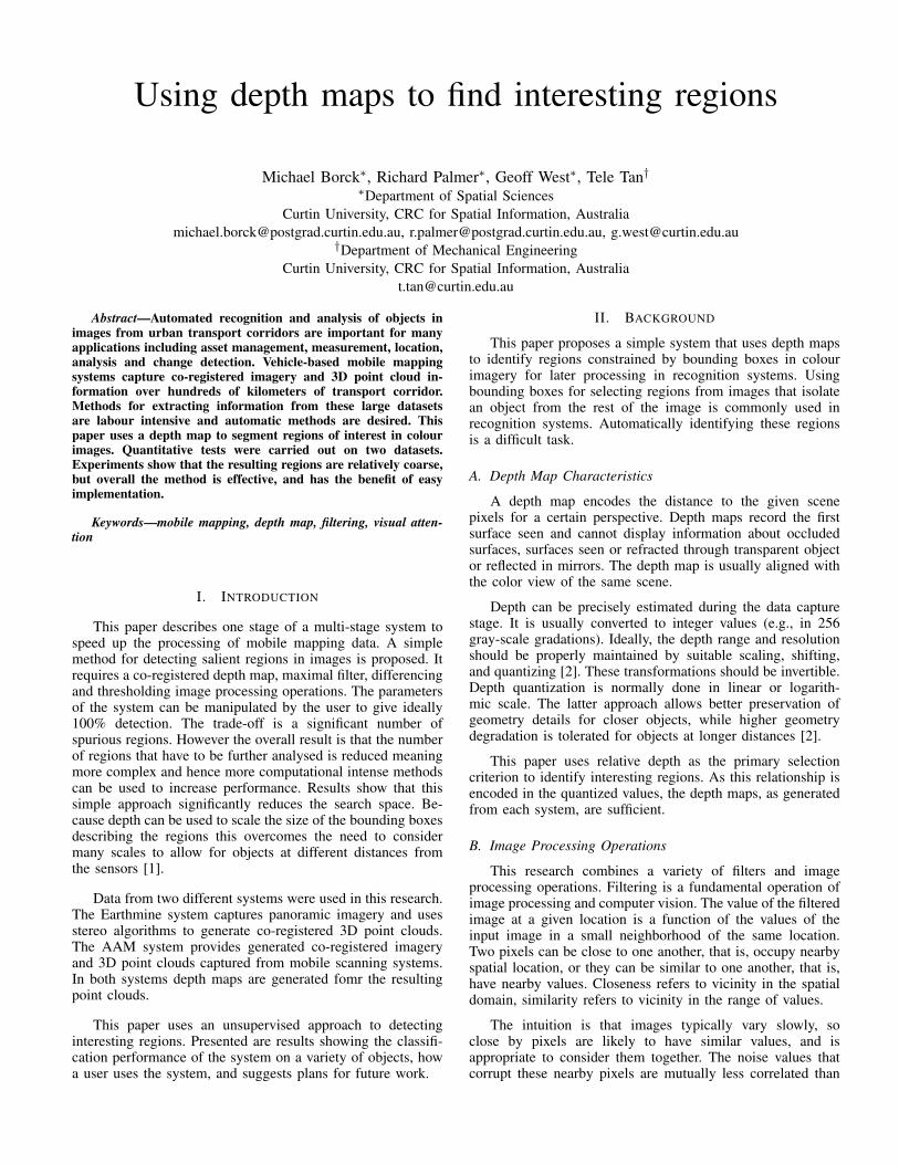
Pairs of panoramic stereo pairs are captured typically at10 metre spacing down a transport corridor. Each panorama ismade up of images from four cameras pointing to the front,back, left and right of the vehicle. Each panorama is usedto generate a 3D point cloud that surrounds the position ofthe cameras using a template matching approach based on thealgorithm on one of the Mars landers [17]. For each of thefour images: front, back, left and right, a depth image canbe generated that is co-registered with the colour image. Ineach of these images, dark pixels mean far from the cameras,and light pixels mean close to the cameras. The colour imagesare typical of street scenes and captured at shutter speeds thatreduce blur as the vehicle could be travelling at 60-80 kph. Thedepth images can be seen to correspond to the colour imagesespecially with large scale parts of the environment. Smallscale objects are picked out such as lamp posts. As with manystereo algorithms, features such as edges are relied upon to givethe best estimation of depth from disparity and smooth areasrequire interpolation between reliable depth estimates to builda full depth map. Importantly the Earthmine data does produceconfidence maps corresponding to the depth data although theyare not currently used in this work.

(a) (b) (c) (d)

Fig. 1. Example of co-registered colour image and depth map from Earthmineand AAM dataset (a) Earthmine Original colour image (b) Earthmine Co-registered depth map (c) AAM Original colour image (d) AAM Co-registereddepth map

The AAM data was obtained from a 3D laser rangingdevice that spins to capture the angle and distance of pointsin a vertical plane to an accuracy of typically 2 cms outto a range of 150 m. Still or video cameras added to thesystem enable imagery to be acquired that is then co-registeredwith the point clouds. The data is transformed such that co-registered colour and range imagery is produced. Compre-hensive 3D as-built information was collected along the 7kmstretch of Geelong Road in Footscray (west of Melbournecentral business district). A 3D laser mapper was deployed tocollect single-head multiple laser scan data along the route.A minimum of 6-passes were made in each direction at

500kHz capture rate. The on-board navigation system includeda single-antenna Global Navigation Satellite System (GNSS)and optical diagnostic monitoring interface. A Ladybug cameracaptured simultaneous imagery during the drive. 120 controlpoints were independently measured using real time kinematicGNSS. Comprehensive 3D vector extraction was made fromthe data.

The dataset came with a time-stamped meta data file con-taining capture times and vehicle/camera location for imagery.The captured points were used with time-stamps within themeta-data to calculate the position of the camera within thepoint cloud. Then the vehicle orientation parameters wereused to orient the view correctly into the imagery. Each pointwas parsed to discover which view it was part of (front 90degrees, left 90 degrees, rear 90 degrees and right 90 degrees).Calculating the vector from the camera origin to the point andcomparing this with the canonical normalised view vectors foreach of the four views allowed a depth map for each view tobe generated. Figure 1c and Figure 1d show an example of thecolour image and depth map generated from this process.

III. REGION DETECTION

Ground truth annotated regions are identified in the colourimages. The depth maps are used to detect hypothesis regionsto be evaluated against the ground truth annotations. Thesesteps are further explained below.

A. Ground Truth Annotations

First the colour images are aligned with the co-registereddepth maps. This ensures every pixel in the image has anassociated depth value, otherwise it is set to black. A highquality depth map results in a colour image having a depthvalue for every pixel. A low quality or incomplete depth mapresults in part of the colour image being masked out. This isimportant when creating ground truth data as it is unfair toassess the success of the procedure against regions that do notcontain depth.

Constraints are placed on the ground truthing based on thetask domain. For this paper the task is asset management ofstreet furniture in urban and semi-rural environments. Cars andpeople are dead space. Building facades, trees, sky, road, andpavement are background. Examples of valid objects includestreet lights, rubbish bins, park benches, traffic lights, electricalcontrol boxes, telephone booth, postal boxes etc. Objects mustbe fully contained within the image, not be occluded, nottouching the image border and recognisable from within thealigned colour image.

B. Hypothesis Generation

In a scene, objects exist at different depths. Local peaksin a depth map indicate that an object is closer to the camerathan its surroundings. The proposed method segments out someelements that are closer than their surroundings. The methodis non-iterative, local, and simple. Relative depth is used asthe primary selection criterion to identify multiple regions ofinterest in colour images. The model can be implemented bysimple filtering, difference and thresholding operations. Theprocess combines grey levels of a depth map on both theirgeometric closeness and their pixel value similarity, and prefers

near values to distant values in both domain and range. Objectsat the same or similar distance and in-image spatially close willbe contained within the same bounding box. The output is a setof bounding boxes that map to regions in the colour image. Thehypothesis being that these bounding boxes identify interestingregions.

Traditional thresholding will discard pixels less than aspecified value. In a depth map this means objects in thedistance will be removed. What is needed is a process thatdiscards the background keeping distinct objects. Using anadaptive threshold algorithm on the depth map also producespoor results due the noise and quality of the depth maps. Themethod devised applies a histogram equalization algorithm tothe depth map. Then a maximal filter is used to make localpeaks stand out. The image is then dilated to fill any localholes. To remove the background, which essentially is unal-tered in the process, the dilated image is subtracted from theoutput of the maximal filter. This creates an image that containsonly local peaks. This local peak image is thresholded andbounding boxes for each thresholded segment are determined.These bounding boxes are the hypothesised interesting regions.

A large number of local image peaks indicates either anoisy image or a busy scene and will generate a large numberof spurious bounding boxes. To reduce this effect one of twothreshold methods are chosen. If a large number of localimage peaks are detected then Otsu’s threshold algorithm isapplied, otherwise the image threshold value is set to 0 so thateverything not background is segmented and labeled.

C. Evaluation

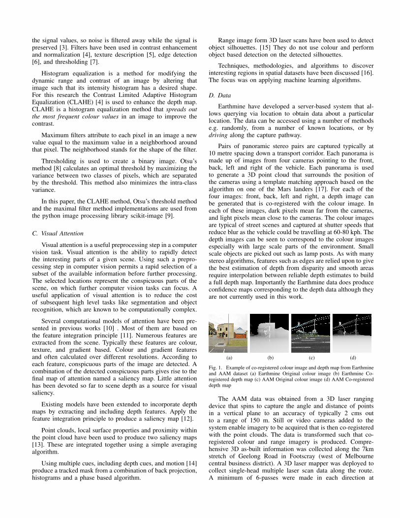
This research uses similar bounding box evaluation criteriaas used in [18]. The criteria used are cover, and overlap. Inaddition this paper measures the spurious proportion. Covermeasures how much of the ground truth annotation rectangleis covered by the detection hypothesis rectangle. Overlap mea-sure how much the detection hypothesis rectangle overlaps theground truth annotation rectangle. Figure 2 show the differencebetween the two measures. The spurious proportion measuresthe proportion of the image covered by hypothesised regionsthat do not overlap with ground truth annotations. Together,these criteria allow us to compare detected hypotheses againstground truth annotations. In all of the following experiments, ifcover and overlap are above 50% and the spurious proportion isless than 20% the detection is deemed to be a successful result.To visually asses the process, the colour image has the labeledsegments, detected hypothesised regions, and the ground truthannotations overlaid on the aligned colour image.

Fig. 2. Example showing the difference between overlap and cover evaluationcriteria. Solid line represents ground truth annotation rectangle, dashed linerepresents detection hypothesis rectangle

IV. EXPERIMENTS

Two experiments were conducted using real-world datasetsfrom Eartmine and AAM.

A. Earthmine Dataset

The Earthmine dataset experiment consisted of 100 imagesusing a variety of front, back, left and right views. Groundtruthing of the Earthmine data resulted in 29 different objectcategories across 373 interesting regions being identified. Thespecific object categories are not important other than toindicate the variety of objects having varying aspect ratios thatare contained within the interesting regions.

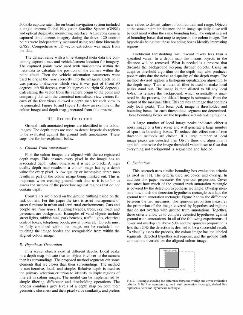
The depth maps for the Earthmine dataset were calculatedfrom real-world spatial coordinates. For pixels in the distancewithin the image there are significant errors and noise in thedata. For this reason the range of the depth maps was clippedto 30 metres. For left and right tiles this has little effect whenthey are aligned with the depth maps. For the front and backimage tiles approximately half the image is set to black as nodepth information is available. Figure 3a is an example of theoriginal colour image from the Earthmine dataset. Figure 3bshows the resulting colour image after being aligned with thedepth map. Note the little depth information in the sky regions.

(a) (b)

Fig. 3. Example of colour image and the colour image aligned with the depthmap from the Earthmine dataset (a) Original colour image (b) Aligned colourimage

B. AAM Dataset

The AAM dataset experiment consisted of 61 images ofa variety of views. Ground truthing resulted in 12 objectcategories and 193 regions being identified as interesting.

Although RGB imagery was available with the AAMdataset it was unregistered resulting in misaligned imagery anddepth information. The depth map and the colour image weregenerated from the depth and colour values already registeredwith the laser scan data. This means the depth maps and colourimages are already aligned. This also explains the unnaturallook of the colour images in the AAM dataset (see figure 1c).

C. Detecting Hypothesised Regions

After ground truthing each dataset, the depth maps wereprocessed. Although real world datasets are inherently noisy,we also added Gaussian noise to each dataset giving us a totalof four datasets. A script allowed the automatic processing ofeach depth map in the dataset. There is only a single parameter

with the method than can be modified, the size of the maximumfilter. For these experiments it was fixed to a size of 20 pixelssquare for both datasets. Images of each step were produced.Labeled segments, detected hypothesis rectangles and groundtruth bounding boxes were overlaid on the aligned colourimage. Finally, the hypothesised regions were evaluated forcover, overlap and spurious proportion compared against theground truth annotations.

V. RESULTS AND DISCUSSION

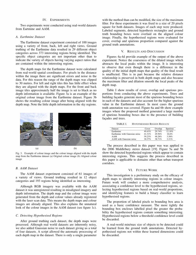
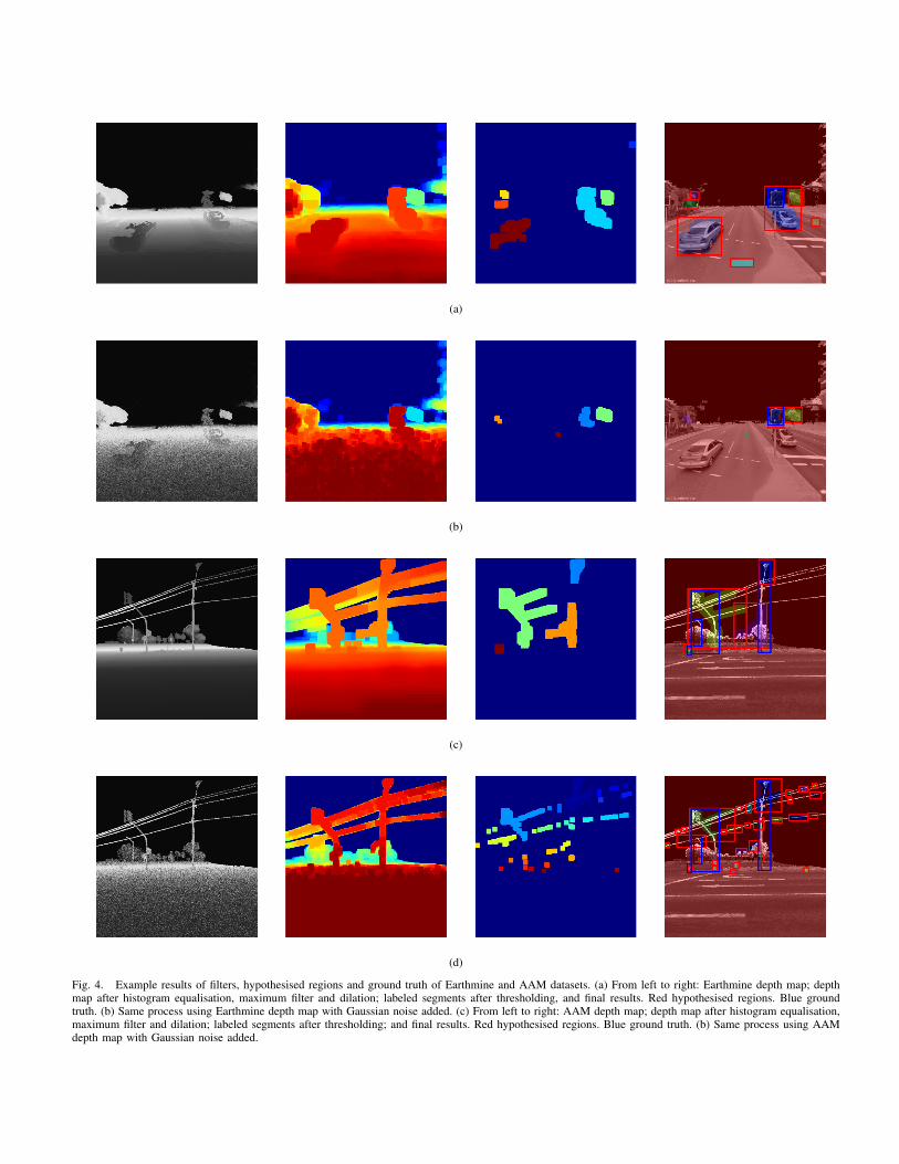
Figures 4a-4d provide example of the output of the aboveexperiment. Notice the coarseness of the dilated image whichabstracts the local peaks within the image. It is interestingto observe that even though there is a difference in thequality of the initial depth maps that quality of the final resultis unaffected. This is in part because the relative distancerelationship is preserved in both depth maps and also becausethe maximum filter and dilation smooth the local peaks of thedepth map.

Table I show results of cover, overlap and spurious pro-portions from conducting the above experiments. Trees andbuilding facades generate most of the spurious bounding boxesin each of the datasets and also account for the higher spuriousvalue in the Earthmine dataset. In most cases the groundtruth annotation was covered. Figure 6a and 6b show exampleimages where the proposed method generated a large numberof spurious bounding boxes due to the presence of buildingfacades and trees.

TABLE I. HYPOTHESISED REGION RESULTS

Dataset Cover Overlap SpuriousEarthmine 49.43% 29.74% 12.18%Earthmine with Gaussian noise 41.31% 29.56% 16.6%AAM 59.23% 48.28% 3.58%AAM with Gaussian noise 30.37% 38.71% 2.21%

The process described in this paper was was applied tothe 2006 Middlebury stereo dataset [19]. Figure 5a and 5bshow the detected hypothesied regions which appear to containinteresting regions. This suggests the process described inthis paper is applicable to domains other than urban transportcorridors.

VI. FUTURE WORK

This investigation is a preliminary study on the efficacy ofdepth maps to identify interesting regions in colour images.Future work will conduct a more comprehensive analysis,associating a confidence level to the hypothesised regions, se-lecting hypothesised regions based on real-world proportions,and identifying features to build a binary classifier to learnhypothesised regions.

The proportion of labeled pixels to bounding box area isused as a basic confidence measure. The more tightly thebounding box encloses labelled pixel the greater the proba-bility the hypothesised regions contain something interesting.Hypothesised regions below a threshold confidence level couldbe discarded.

A real-world min/max size of objects to be detected couldbe learned from the ground truth annotations. Detected hy-pothesised regions not within these learned dimensions couldbe discarded.

(a)

(b)

(c)

(d)

Fig. 4. Example results of filters, hypothesised regions and ground truth of Earthmine and AAM datasets. (a) From left to right: Earthmine depth map; depthmap after histogram equalisation, maximum filter and dilation; labeled segments after thresholding, and final results. Red hypothesised regions. Blue groundtruth. (b) Same process using Earthmine depth map with Gaussian noise added. (c) From left to right: AAM depth map; depth map after histogram equalisation,maximum filter and dilation; labeled segments after thresholding; and final results. Red hypothesised regions. Blue ground truth. (b) Same process using AAMdepth map with Gaussian noise added.

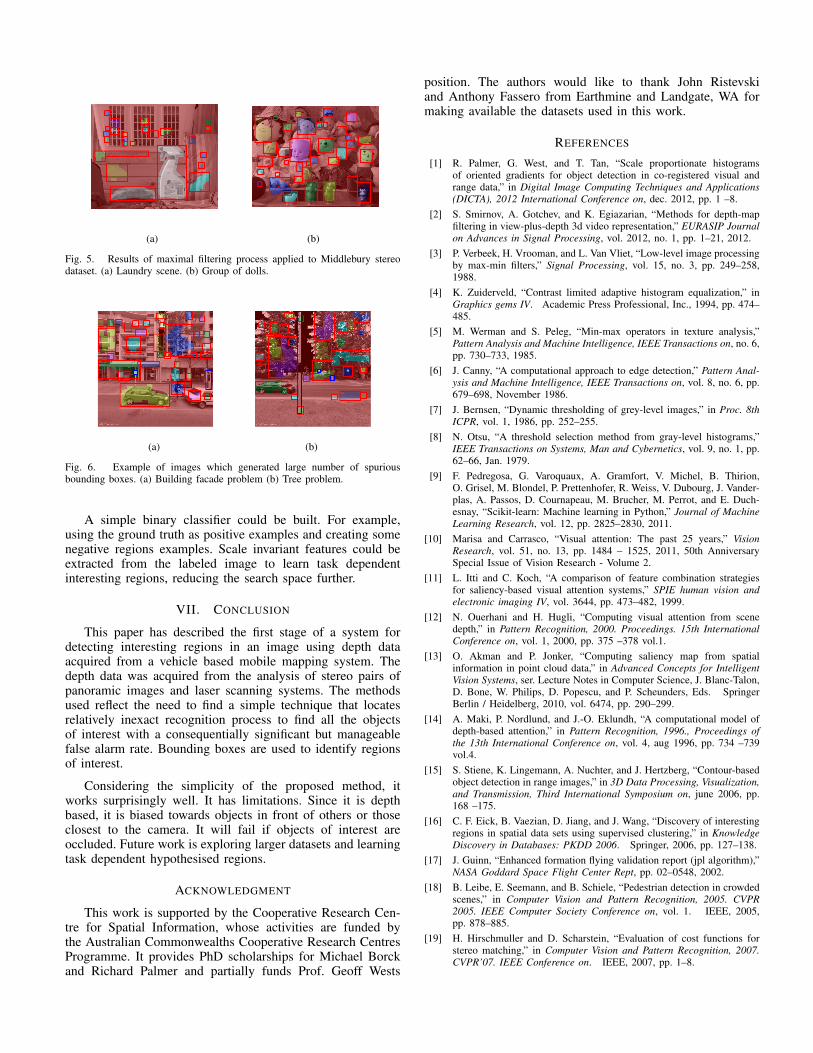
(a) (b)

Fig. 5. Results of maximal filtering process applied to Middlebury stereodataset. (a) Laundry scene. (b) Group of dolls.

(a) (b)

Fig. 6. Example of images which generated large number of spuriousbounding boxes. (a) Building facade problem (b) Tree problem.

A simple binary classifier could be built. For example,using the ground truth as positive examples and creating somenegative regions examples. Scale invariant features could beextracted from the labeled image to learn task dependentinteresting regions, reducing the search space further.

VII. CONCLUSION

This paper has described the first stage of a system fordetecting interesting regions in an image using depth dataacquired from a vehicle based mobile mapping system. Thedepth data was acquired from the analysis of stereo pairs ofpanoramic images and laser scanning systems. The methodsused reflect the need to find a simple technique that locatesrelatively inexact recognition process to find all the objectsof interest with a consequentially significant but manageablefalse alarm rate. Bounding boxes are used to identify regionsof interest.

Considering the simplicity of the proposed method, itworks surprisingly well. It has limitations. Since it is depthbased, it is biased towards objects in front of others or thoseclosest to the camera. It will fail if objects of interest areoccluded. Future work is exploring larger datasets and learningtask dependent hypothesised regions.

ACKNOWLEDGMENT

This work is supported by the Cooperative Research Cen-tre for Spatial Information, whose activities are funded bythe Australian Commonwealths Cooperative Research CentresProgramme. It provides PhD scholarships for Michael Borckand Richard Palmer and partially funds Prof. Geoff Wests

position. The authors would like to thank John Ristevskiand Anthony Fassero from Earthmine and Landgate, WA formaking available the datasets used in this work.

REFERENCES

[1] R. Palmer, G. West, and T. Tan, “Scale proportionate histogramsof oriented gradients for object detection in co-registered visual andrange data,” in Digital Image Computing Techniques and Applications(DICTA), 2012 International Conference on, dec. 2012, pp. 1 –8.

[2] S. Smirnov, A. Gotchev, and K. Egiazarian, “Methods for depth-mapfiltering in view-plus-depth 3d video representation,” EURASIP Journalon Advances in Signal Processing, vol. 2012, no. 1, pp. 1–21, 2012.

[3] P. Verbeek, H. Vrooman, and L. Van Vliet, “Low-level image processingby max-min filters,” Signal Processing, vol. 15, no. 3, pp. 249–258,1988.

[4] K. Zuiderveld, “Contrast limited adaptive histogram equalization,” inGraphics gems IV. Academic Press Professional, Inc., 1994, pp. 474–485.

[5] M. Werman and S. Peleg, “Min-max operators in texture analysis,”Pattern Analysis and Machine Intelligence, IEEE Transactions on, no. 6,pp. 730–733, 1985.

[6] J. Canny, “A computational approach to edge detection,” Pattern Anal-ysis and Machine Intelligence, IEEE Transactions on, vol. 8, no. 6, pp.679–698, November 1986.

[7] J. Bernsen, “Dynamic thresholding of grey-level images,” in Proc. 8thICPR, vol. 1, 1986, pp. 252–255.

[8] N. Otsu, “A threshold selection method from gray-level histograms,”IEEE Transactions on Systems, Man and Cybernetics, vol. 9, no. 1, pp.62–66, Jan. 1979.

[9] F. Pedregosa, G. Varoquaux, A. Gramfort, V. Michel, B. Thirion,O. Grisel, M. Blondel, P. Prettenhofer, R. Weiss, V. Dubourg, J. Vander-plas, A. Passos, D. Cournapeau, M. Brucher, M. Perrot, and E. Duch-esnay, “Scikit-learn: Machine learning in Python,” Journal of MachineLearning Research, vol. 12, pp. 2825–2830, 2011.

[10] Marisa and Carrasco, “Visual attention: The past 25 years,” VisionResearch, vol. 51, no. 13, pp. 1484 – 1525, 2011, 50th AnniversarySpecial Issue of Vision Research - Volume 2.

[11] L. Itti and C. Koch, “A comparison of feature combination strategiesfor saliency-based visual attention systems,” SPIE human vision andelectronic imaging IV, vol. 3644, pp. 473–482, 1999.

[12] N. Ouerhani and H. Hugli, “Computing visual attention from scenedepth,” in Pattern Recognition, 2000. Proceedings. 15th InternationalConference on, vol. 1, 2000, pp. 375 –378 vol.1.

[13] O. Akman and P. Jonker, “Computing saliency map from spatialinformation in point cloud data,” in Advanced Concepts for IntelligentVision Systems, ser. Lecture Notes in Computer Science, J. Blanc-Talon,D. Bone, W. Philips, D. Popescu, and P. Scheunders, Eds. SpringerBerlin / Heidelberg, 2010, vol. 6474, pp. 290–299.

[14] A. Maki, P. Nordlund, and J.-O. Eklundh, “A computational model ofdepth-based attention,” in Pattern Recognition, 1996., Proceedings ofthe 13th International Conference on, vol. 4, aug 1996, pp. 734 –739vol.4.

[15] S. Stiene, K. Lingemann, A. Nuchter, and J. Hertzberg, “Contour-basedobject detection in range images,” in 3D Data Processing, Visualization,and Transmission, Third International Symposium on, june 2006, pp.168 –175.

[16] C. F. Eick, B. Vaezian, D. Jiang, and J. Wang, “Discovery of interestingregions in spatial data sets using supervised clustering,” in KnowledgeDiscovery in Databases: PKDD 2006. Springer, 2006, pp. 127–138.

[17] J. Guinn, “Enhanced formation flying validation report (jpl algorithm),”NASA Goddard Space Flight Center Rept, pp. 02–0548, 2002.

[18] B. Leibe, E. Seemann, and B. Schiele, “Pedestrian detection in crowdedscenes,” in Computer Vision and Pattern Recognition, 2005. CVPR2005. IEEE Computer Society Conference on, vol. 1. IEEE, 2005,pp. 878–885.

[19] H. Hirschmuller and D. Scharstein, “Evaluation of cost functions forstereo matching,” in Computer Vision and Pattern Recognition, 2007.CVPR’07. IEEE Conference on. IEEE, 2007, pp. 1–8.