Using Bus Probe Data for Analysis of Travel Time Variability

Title Using Bus Probe Data for Analysis of Travel Time Variability

Author(s) Uno, Nobuhiro; Kurauchi, Fumitaka; Tamura, Hiroshi; Iida,Yasunori

Citation Journal of Intelligent Transportation Systems (2009), 13(1): 2-15

Issue Date 2009-01

URL http://hdl.handle.net/2433/123445

Right Copyright © 2009 Taylor & Francis.

Type Journal Article

Textversion author

KURENAI : Kyoto University Research Information Repository

Kyoto University

1

USING BUS PROBE DATA FOR ANALYSIS OF TRAVEL TIME VARIABILITY

Nobuhiro Uno, Fumitaka Kurauchi, Hiroshi Tamura and Yasunori Iida

1 Department of Urban Management, Kyoto University, Japan

E-mail: [email protected] 2 Department of Civil Engineering, Gifu University, Japan

3 Recruit Co.,Ltd., Japan 4 Institute for Systems Science Research, Japan

ABSTRACT The rapid progress of information technology (IT) may provide us new insights into understanding traffic phenomena, and could help mitigate traffic problems. One of the key applications of IT to traffic and transport analysis is the identification of the location of moving objects using the global positioning system (GPS) . It is expected that detailed traffic analysis could be carried out using these data. In this paper, we first summarise the various applications of probe data in transport analysis. GPS data is merely a sequence of locations, and further data transformation such as map matching, data reduction, processing, and reporting is needed to use them effectively. We then discuss the application of bus probe data to evaluating travel time variability and the level of service (LOS) of roads. A methodology for evaluating the road network from the viewpoint of travel time stability and reliability using bus probe data is proposed. Travel time distributions of arbitrary routes are estimated by statistically summing up directly observed multiple travel time distributions. Based on the development of methodologies to estimate travel time distributions of arbitrary routes covered by the bus probe survey, this study proposes an approach to evaluate the LOS of road networks based on the concept of travel time reliability. KEYWORDS Global Positioning System, Probe Data, Travel Time Variability 1. INTRODUCTION The rapid progress of information technology (IT) may provide us new insights into understanding traffic phenomena, and could help mitigate traffic problems. One of the key applications of IT to traffic and transport analysis is the identification of the location of moving objects using the global positioning system (GPS) . It is expected that detailed traffic analysis could be carried out using these data. The GPS consists of a series of satellites that orbit the earth, broadcasting signals to receivers on the ground. A receiver can determine its location using data from at least four satellites. The GPS

2

was developed by the US Department of Defence for military purposes, and was opened for public use in 1984. There are now 31 GPS satellites available. The performance of the GPS had, in the past, been limited by artificial degradation of the signal through the process of selective availability (SA), but the US Government removed that on May 1, 2000. Ochieng and Sauer (2001) reported that the 74% of data are accurate within 10 m without SA, compared to only 24% with SA. Furthermore, no significant difference is apparent between the level of accuracy achievable with differential positioning and post-SA stand-alone navigation. Zito et al. (1995) were the first to address the use of GPS data for traffic engineering. They discussed the accuracy of the GPS and its potential for traffic analysis, and suggested that geographical information systems (GIS) could be used efficiently for managing the data obtained by the GPS. They demonstrated that whenever possible, the direct GPS speed should be used since calculating a speed using the time between two locations gives poor results. The accuracy of GPS data at that time was not reliable and additional technology such as dead reckoning systems were required to increase the accuracy. Since many low-cost GPS receivers are now on the market, it is not difficult to apply this type of analysis. In the field of traffic and transport research, a moving object, such as a vehicle or person equipped with a GPS receiver, is called a ‘probe’. The GPS data are merely a sequence of locations, and further data transformations are needed to make them meaningful to transport analysts. In this paper, we summarise the methodologies and issues involved in these transformation techniques. We also describe our recent work on travel time reliability based on bus probe data. We propose an approach for evaluating the road network from the viewpoint of travel time stability and reliability using bus probe data. Based on the development of methodologies for estimating travel time distributions of arbitrary routes covered by the bus probe survey (BPS), we propose an approach to evaluate the level of service (LOS) of road networks based on the concept of travel time reliability. 2. GPS DATA FOR TRAFFIC ANALYSIS This section briefly reviews using the GPS for traffic analysis. We first discuss the methodologies of transforming GPS data to traffic-related indicators, and then summarise the advantages and disadvantages of GPS data. We also describe the applications of GPS data to traffic analysis. 2.1 Data Transformation GPS data merely consist of location information for the moving object1. Depending on the sample size and data acquisition frequency, the amount of data may be very large. Processing is therefore essential to transform the data into transport-related indicators. The general procedure consists of these four steps, further illustrated in Figure 1: · Map matching: matching the GPS data to a digital map · Data reduction: transforming the series of locations into link/path specific information · Data processing: aggregating individual vehicle data

1 There are some GPS receivers that can determine the direct speed using gyro sensors. Zito et al. (1995) suggests using the direct speed whenever possible for reasons of accuracy.

3

· Data reporting: generating indicators easily understood by the users

2.1.1 Map Matching GPS data obtained from probe vehicles should generally indicate that the vehicles are on roads. In some cases, the vehicle could legitimately be off the road, in a car park, for example. The first procedure should be to match the location data to reasonable traffic facilities. There is plenty of research available on how to do this, ranging from simple topological matching methods to more sophisticated techniques such as probabilistic or fuzzy-logic matching. We will not discuss details of this technology further, but there is an excellent review of them in Quddus et al. (2006). One of the important features of probe vehicle data is that they are a sequence of locations of the same object over time. This means it is not sufficient simply to match the plot to the closest road segment. It is important also to consider the connectivity of segments. Asakura et al.(1999) and Sugino et al.(2000) proposed a map matching algorithm for probe person data using a two-step model that first extracted a sub-network from the complete network and then generated k shortest paths. The path within k shortest paths which is the most similar to the probe data trajectory is selected as an actually used path. The map used for matching may also be outdated. Noronha and Goodchild (2000) suggested the need to develop methods for correcting map data geometrically, so that locations are more accurately captured, stored, and communicated. Also Quddus et al. (2006) investigated a quality indicator representing the level of confidence (integrity), which can be used in map-matching algorithms. 2.1.2 Data Reduction Three-dimensional datasets of vehicle locations quickly become too large to handle, and the detailed information may not be needed anyway in subsequent analysis. It is therefore essential to transform these location plots into a form that is more familiar to transport professionals, such as links or path travel times. The procedures to do this involve data reduction since they greatly reduce the size of the data. Quiroga and Bullock (1998) proposed a data structure that consisted of a segmentation code, vehicle ID, starting time, and travel time. The segment lengths should be determined very carefully since traffic phenomena may not be clearly identifiable if the segments are too long. Quiroga and Bullock (1998) discussed the

Map matching Data reduction Data processing Data reporting

[ ] ( )K

∫∞

=0

dxxxftE

Figure 1. Data transformation

4

adequate length of segments using simulated data, and concluded that less than 0.2 miles might be appropriate for clear characterization of localised congestion. This is far shorter than the usual definition of link segments based on physical discontinuities. The data reduction technique is further complicated if we consider person-based analysis. There are two distinct differences between vehicle-based and person-based probe data. First, we need to consider the travel mode for person-probe data. This is sometimes difficult since the GPS antenna may be shielded for some travel modes such as subways. Draijer et al. (2000) investigated the accuracy and reliability of probe data collection for different modes. They reported that 90% of automobile trips but only 50% of tram and train trips could be recorded. The second problem is to detect the start and end points of travel. In the case of vehicle-based probe data, this information can easily be acquired as the engine switches on and off. This, however, does not apply to a person-based system. Asakura and Hato (2004) proposed a move-or-stay identification technique that considered time constraints, while Du and Aultman-Hall (2007) proposed a heuristic model to extract dwell time and travel time. 2.3.3 Data Processing To represent the characteristics of a time interval or link segment, the reduced data may be further transformed into aggregated values such as average travel time. To do this, an adequate time interval must be determined. According to Quiroga and Bullock (1998), the sampling speed or time interval between consecutive GPS points has to be less than half the shortest segment travel time to achieve 100% segment coverage. In a practical sense, a segment length of 0.2 miles and the corresponding time interval are rather unrealistic. The length of segments and time intervals, therefore, should be determined according to the specific objectives of the analysis being conducted. Quiroga and Bullock (1998) concluded that median speed is better than harmonic mean speed for representing traffic flow conditions. Hellinga and Fu (2002) noted that there is a systematic bias in the mean sample estimate of probe vehicles on arterial road networks. This is mainly due to the signal effect, and they proposed a way to account for this. 2.2.4 Data Reporting The last and most important aspect of using the GPS is displaying the results of the calculations or estimates. To use probe vehicle data, the results should be clearly and easily indicated. For this purpose, a geographical information system (GIS) is usually the best solution. GIS techniques have a significant role in the storage, analysis, and reporting of various data sets such as turning movement counts at intersections, road crash data, speed, travel time and delay data, and origin-destination (OD) data. Taylor et al. (2000) developed an integrated GPS-GIS for collecting on-road traffic data from a probe vehicle. 2.2 Characteristics of GPS Data-Oriented Analysis The advantages and disadvantages of GPS data-oriented analysis are summarised in Table 1. There are numerous advantages of using GPS data. One of the positive features is the ease of obtaining data. Since data can be stored automatically and electronically, there is no additional load for data

5

coding. If an adequate data real-time reduction/processing/reporting system is available, the probe vehicle data can be used for real-time traffic management and control. Furthermore, if the same ID is assigned to the same moving object over a prolonged period, the day-to-day variations of each specific object can also be analysed. Another advantage of probe data analysis is that they give direct observations of the travel time. In traffic engineering, the space mean velocity is important rather than the spot speed. Since a traffic detector can only observe velocity at one location, the space mean velocity is generally estimated from the observed speed. In contrast, the true space mean velocity can be obtained from probe vehicle data. The major drawback of probe vehicle data is data management. Depending on the length of the time interval, the size of the database may become extraordinary large and difficult to handle. If real-time observation is required, the data transaction cost is very expensive since mobile phone communication is needed. Also, since the accuracy of GPS heavily depends on the observation condition, the accuracy of obtained data may differ by the condition. Another bias which should be considered is the difference between sampled objects and others. It is common to use more or less ‘public’ vehicles such as taxis, buses and freight vehicles as probe data samples. Then, data obtained by these vehicles may not represent the whole population. For instance, taxi drivers may like to drive within the busy city centre since there is higher possibility of finding customers. 2.3 Application of GPS Technology for Transport Analysis Based on past experience, GPS data can be applied to following fields: · Automatic incident detection · Supporting instruments for diary survey · Complementary observation system of travel time · Variability analysis of travel time 2.3.1 Automatic Incident Detection Identifying an accident as quickly as possible is very important, especially for emergency response issues and encouraging detours. Automatic incident detection (AID) systems are expected to support this requirement, and probe data can be a source of information. The traditional AID concept uses traffic detectors that continuously observe the density of traffic flow. This means that AID is only possible along a route where detectors are installed. The velocity change of probe vehicles may also detect an incident. Sethi et al (1995) and Thomas and Hefeez (1998) evaluated

Table 1. Advantages and disadvantages of probe data Advantages:

· Day-to-day observation is possible · Data can be automatically stored in electronic form · Direct observation of travel time is possible · Real-time observation is possible

Disadvantages: · Enormous amount of data to handle and process · Transaction cost if real-time observation needed · Data bias

6

the potential of using probe vehicles for AID, and concluded that the detection accuracy was acceptable. Both these analysis were based on simulations. To our knowledge, this has never been tested in practice. 2.3.2 Supporting Instruments for Diary Survey The second application of GPS data is to study the movement of people. The first trial of this was by Murakami and Wagner (1999), who used personal digital assistants equipped with a GPS receiver to capture daily vehicle-based patterns in Lexington, Kentucky in the fall of 1996. They collected data from 100 households for 6 days, and showed the potential of using GPS technology to study personal behaviour more accurately. Since then, other research has been conducted in similar fields. Draijer et al. (2000), performed a similar survey but monitored all modes including public transit, bicycle, and foot. The instruments they used weighed up to 2 kgs, but their equivalents today are much smaller and lighter. There have been a number of relevant studies performed in Japan (e.g., Hato, 2006; Tanabe et al., 2007) that used mobile phones equipped with GPS receivers to integrate web-based diary surveys with GPS tracking technologies. Figure 2 shows one example that made use of a web application, which solicited data that are not available from the GPS including items such as trip purpose and the number of accompanying persons. Using this system, the accuracy of the data is much better since the respondents can refresh their memory by looking at the screen. 2.3.3 Complementary Observation System of Travel Time Travel times are generally estimated by roadside detectors. Travels time cannot be observed on a road without any onsite observation instruments, although some estimation techniques have been proposed. The probe vehicle approach is one efficient method of collecting LOS information and data about the source of traffic congestion. The reliability of probe vehicle data for estimating the travel time should be investigated. Lee et al. (2006) examined the relationship between the probe vehicle size and the travel time collection reliability using both simulated and field data. Their results suggested that the operational characteristics of probe vehicles are very important when constructing reliable information systems to guarantee meeting network coverage requirements. Cheu et al. (2002) also discussed the population and size of probe vehicles using a simulation-based analysis. They concluded that the improvement in the accuracy of link speed estimation diminishes when the probe vehicle population in the network reaches 15%. They further concluded that to achieve an absolute error in the estimated average link speed of less than 5.0 km/h at least 95% of the time, there should at least 4 to 5% active probes in the total network traffic volume, or at least ten probes that have successfully traversed a link. Another promising area for GPS applications is in the capture of day-to-day trends. Figure 3 depicts the day-to-day adaptation behaviour of route choice in response to traffic situations. 2.3.4 Variability Observation of Travel Time

The last and probably the most important application of GPS data is for the observation of travel time variability. In our highly-valued society, unexpected delays may result in substantial losses. The variability of service levels should be analysed as well as just the average LOS for road design

7

and control. Probe data is well suited for obtaining the variability of travel time since it is a source of direct observation. Travel times obtained from probe vehicle data can be used to identify variabilities. There is a multitude of Japanese research on this type of analysis, including a series of works by the authors to evaluate travel time variability. This is summarised in the next section.

Figure 2. Web-diary system with probe trajectories (Tanabe et al., 2007)

Figure 3. Example of variations in commuting routes. (Tanabe et al., 2007)

8

3. EVALUATING TRAVEL TIME RELIABILITY USING BUS PROBE DATA 3.1 Motivation With the rapid progress of IT, people hope to reduce various types of uncertainty in their decision-making processes. Also, intense progress in socioeconomic activities may lead to an increase in the value of time for each person. Under such circumstances, it becomes more important to provide travellers with stable road transportation. Therefore, road transportation should be evaluated from the viewpoint of travel time reliability (Iida, 1999; Uno et al., 2002). Many researchers have pursued appropriate ways to apply data obtained from probe surveys so as to diagnose problems and evaluate the performance of road networks. Some examples are He et al., 2002; Lorkowski et al., 2004; and List and Demers, 2006. The aim of our study was to develop an approach for evaluating the travel time reliability of road networks using bus probe survey (BPS) data obtained in some cities by the Japanese Ministry of Land, Infrastructure, and Transport (MLIT). One of the advantages of a BPS is that it can easily provide data on fluctuations in travel time because the buses travel repeatedly along the same fixed routes. However, at the same time, the BPS data may overestimate the travel time due to the time spent at bus stops. To enhance the strength and overcome the weakness of BPS data, our study adopted approaches to correct travel times obtained from bus probes and combine multiple travel time distributions into one distribution. Another aim of this study was to propose an approach for evaluating the LOS of a road network based on the concept of travel time reliability. 3.2 Data Used to Develop the Data Revision Method 3.2.1 Outline of the Bus Probe Data In order to evaluate the benefit of probe car survey, MLIT has been collecting the bus probe data in Kansai District since2001 In Hirakata City, our study area, almost all buses operated by Keihan Bus Company are equipped with GPS receiver, and locations of the bus are recorded every 1 second. GPS data are stored in the memory of on-board equipment, and are uploaded when the buses come back to vehicle depot at the end of the day. These data included the longitude, latitude and altitude of successive bus positions, but no information about the bus route number, bus stops, departure records, or arrival records. This study focuses on 18 bus routes, which are provided by more than 100 buses, to cover the major arterial streets in Hirakata. The typical operating hours are from 6:00 to 23:00, and service frequency varies from 6 minutes in the peak hour to 30 minutes for less popular bus routes. We used the bus probe data collected by the MLIT during the period from 13 to 24 December, 2003. 3.2.2 Supplemental Surveys Using a Probe System Since the BPS data give only the trajectories of the bus locations measured by the GPS receiver and no supplementary information, it was necessary to develop a methodology using a type of GIS to include the location of the bus stops to estimate the operational modes of the bus, such as running, stopping at a bus stop, and stopping at an intersection. To obtain the background data such as bus stop locations, we used a supplemental ‘bus trip survey’. An investigator assigned to each bus route observed the operational modes and completed the survey while recording the bus location with a GPS unit.

9

Clearly, the travel speed of the bus tends to be lower than that of passenger vehicles. Therefore both the travel speed and trajectory from the bus probe need to be corrected to represent the ‘ordinary traffic conditions’ that correspond to passenger vehicles. To determine the ordinary traffic conditions, we also conducted a floating survey using a passenger car. We drove along the bus route with GPS receiver and collected the travel time without stopping at the bus stop. Four bus routes are selected for this survey, and for each direction of the route, floating data of passenger cars are collected. The floating car departs the origin of each bus route every hour on the hour from 10 to 19 o’clock. 10 floating car data are collected for each direction of the bus route. Drivers are required to follow the vehicles travelling in a normal manner in order for grasping the ordinary traffic condition. Note that floating car did not synchronise the departure time with the bus. It means that the floating car may be slower at some sections than the bus because of signals, slow vehicles and so on. The travel time obtained from this passenger car probe survey was used as a suitable baseline to represent the ordinary traffic conditions. The supplemental bus trip and passenger car probe surveys were conducted on 17 and 23 December, 2003. 3.3 Revision of the Bus Probe Data The process of estimating the travel time distribution from an OD pair from the bus probe data consists of following four steps: 1) extracting the corresponding trajectory of every bus operation from the probe data, 2) correcting the travel time directly measured by the bus probe to account for the increase due to stopping at bus stops, 3) testing the conformity between an observed travel time distribution and a theoretical distribution, and 4) creating the travel time distribution for the road section under evaluation based on the directly observed multiple travel time distributions. We cover all the steps in some detail in this paper; Steps 1) and 2) are explained in more detail in Uno et al., 2004. 3.3.1 Extracting Trajectories from the Probe Data It is first necessary to extract the trajectory of the bus for the route to be analysed from the bus probe data. The original data are accumulated on a daily basis and include the trajectory of the various routes along which the bus travels on that day. If we define the bus route as a sequence of major intersections along the route, the corresponding trajectories can be extracted by matching the bus probe data with the defined bus route. The trajectory data of the bus operation should then be matched with the appropriate network link. For the probe survey by passenger car, it is clear that the map matching process is critical for obtaining the credible information about the traffic condition on network. For BPS, the road sections on which each bus travels are known in advance, and hereby the prior information about route can play an important role to drastically reduce the error in map matching process. It is one of the merits for the BPS. 3.3.2 Correcting the Travel Time Considering Stopping at Bus Stops To obtain an accurate travel speed and time estimate, we used a correction method composed of three steps.

10

(a) Detection of stops at bus stops We used the bus probe data to detect stopping at bus stops. If the velocity at time t is denoted by vt, the distance to bus stop i is denoted by lit and Rit is a variable representing whether or not the bus stops at a stop according to

⎩⎨⎧

=stopbusaathaltingnot

stopbusaathaltingRit ,0

,1

then the rule that determines whether or not the bus has stopped at a bus stop is

01

==≤≤

it

ititt

RelseRthenLlandVvif

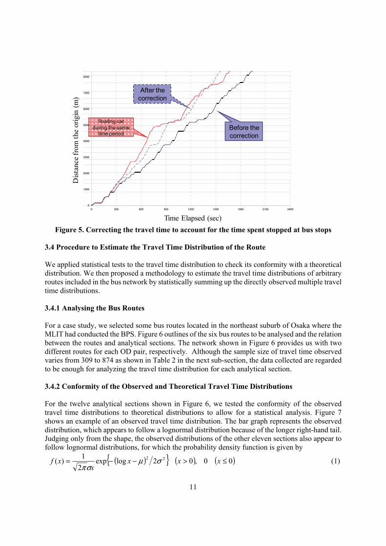
Here, V and L represent the upper limits of the velocity and distance from a bus stop, respectively. For our study, we used values of V = 3.0 km/h and L = 23.7 m. With these values, we could properly classify stopping or not stopping at a bus stop 92% of the time. (b) Detection of deceleration (or acceleration) before (or after) stopping at bus stops It is also necessary to adjust the bus speed during deceleration and acceleration before and after stopping at bus stops. We used a rule to distinguish the deceleration and acceleration modes of the bus from other modes as follows: ‘after determining that the bus may stop at a bus stop, we examine the bus trajectory before and after the stop. If it appears that the estimated velocity of the bus tends to decrease (or increase) monotonically, the corresponding travel mode can be classified as deceleration (or acceleration).’ (c) Eliminating increases in travel time due to stopping at bus stops Figure 4 graphically shows the method used to adjust the travel speed measured by the bus probe. First, we assumed that the time during which the bus stops at a bus stop will be properly detected and eliminated. Then we used the speed of the bus just before it starts to decelerate (or just after it finishes accelerating) for the travel speed during deceleration (or acceleration). In our previous research, we conducted a case study to confirm the effectiveness this procedure (Uno et al. (2004)). The results shown in Figure 5 suggest that the procedure is in fact effective for properly correcting the travel speed measured by the bus probe.

Figure 4. Conceptual diagram of the process used to adjust the travel speed of a bus

11

枚方市駅北口

禁野口

市民病院前

中宮住宅前

関西外大

都が丘

須山町

田ノ口

田ノ口中央

田ノ口団地

招提南町

招提中町

招提口

養父ヶ丘

関西記念病院前

南船橋

船橋

藤原

あさひ

モール街

樟葉駅

0

1000

2000

3000

4000

5000

6000

7000

8000

0 300 600 900 1200 1500 1800 2100 2400

時間(sec)

起点

から

の距

離(m

) Before the correction

After the correction

floating car during the same

time period

Dist

ance

from

the

orig

in (m

)

Time Elapsed (sec) Figure 5. Correcting the travel time to account for the time spent stopped at bus stops

3.4 Procedure to Estimate the Travel Time Distribution of the Route We applied statistical tests to the travel time distribution to check its conformity with a theoretical distribution. We then proposed a methodology to estimate the travel time distributions of arbitrary routes included in the bus network by statistically summing up the directly observed multiple travel time distributions. 3.4.1 Analysing the Bus Routes For a case study, we selected some bus routes located in the northeast suburb of Osaka where the MLIT had conducted the BPS. Figure 6 outlines of the six bus routes to be analysed and the relation between the routes and analytical sections. The network shown in Figure 6 provides us with two different routes for each OD pair, respectively. Although the sample size of travel time observed varies from 309 to 874 as shown in Table 2 in the next sub-section, the data collected are regarded to be enough for analyzing the travel time distribution for each analytical section. 3.4.2 Conformity of the Observed and Theoretical Travel Time Distributions For the twelve analytical sections shown in Figure 6, we tested the conformity of the observed travel time distributions to theoretical distributions to allow for a statistical analysis. Figure 7 shows an example of an observed travel time distribution. The bar graph represents the observed distribution, which appears to follow a lognormal distribution because of the longer right-hand tail. Judging only from the shape, the observed distributions of the other eleven sections also appear to follow lognormal distributions, for which the probability density function is given by

( ){ } ( ) ( )00,02logexp21)( 22 ≤>−−= xxx

xxf σμ

σπ (1)

12

Here, μ and σ represent the mean and standard deviation of log x, and x represents the travel time.

Section 1→

←Section 6

Section 7→

←Section 10 Section 8→

←Section 9

Secti

on2→

←

Secti

on5

Sect

ion

3 →

←Se

ctio

n4

Section11→

←Section 12

Hirakata Sta. Nagao

Sta.

Kuzuha Sta.

No. of Bus stops: 21

Distance: 8km

No. of Bus stops: 19Distance: 6.5km

Hirakata20

Hirakata 39 Hirakata94

No. of Bus stops: 21

Distance: 7.2km

Figure 6. Outline of routes

0

20

40

60

80

100

120

140

60 120 180 240 300 360 420 480 540 600 660 720 780 840 900 960 1020 1080 1140 1200 1260 1320 1380

Frequency

Travel Time (sec.)

Observed Theoretical

Number of Samples ｎ=437Average Travel Time µ=312 secSD of Travel Time s = 91 sec

Figure 7. Observed and theoretical distributions

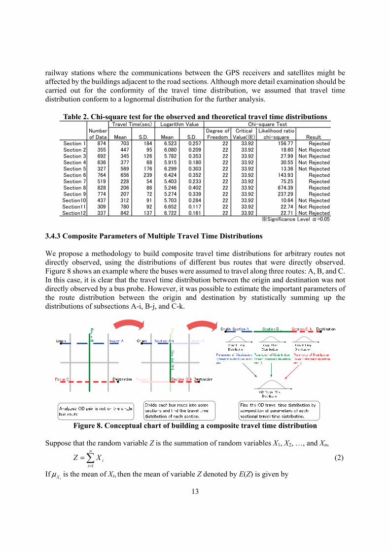
The line shown in Figure 7 gives the theoretical lognormal distribution with the same mean and variance as the observed travel time distribution. The shape of this line resembles that of the observed travel time distribution. We applied the chi-square test for both observed and theoretical travel time distributions. The null hypothesis is that the observed travel time distribution conforms to the lognormal distribution. Table 2 shows the results. Among the twelve analytical sections, the null hypotheses of five sections were rejected, but those of other the seven sections were not. The observed travel times in the five rejected sections included some data points with large measurement errors. Most of the five sections were located in the highly developed area near

13

railway stations where the communications between the GPS receivers and satellites might be affected by the buildings adjacent to the road sections. Although more detail examination should be carried out for the conformity of the travel time distribution, we assumed that travel time distribution conform to a lognormal distribution for the further analysis.

Table 2. Chi-square test for the observed and theoretical travel time distributions

Number Degree of Critical Likelihood ratioof Data Mean S.D. Mean S.D. Freedom Value(※) chi-square Result

Section 1 874 703 184 6.523 0.257 22 33.92 156.77 RejectedSection 2 355 447 95 6.080 0.209 22 33.92 18.60 Not RejectedSection 3 692 345 126 5.782 0.353 22 33.92 27.99 Not RejectedSection 4 636 377 68 5.915 0.180 22 33.92 30.55 Not RejectedSection 5 327 569 176 6.299 0.303 22 33.92 13.36 Not RejectedSection 6 764 656 239 6.424 0.352 22 33.92 143.93 RejectedSection 7 519 228 54 5.403 0.233 22 33.92 75.25 RejectedSection 8 828 206 86 5.246 0.402 22 33.92 674.39 RejectedSection 9 774 207 72 5.274 0.339 22 33.92 237.29 RejectedSection10 437 312 91 5.703 0.284 22 33.92 10.64 Not RejectedSection11 309 780 92 6.652 0.117 22 33.92 22.74 Not RejectedSection12 337 842 137 6.722 0.161 22 33.92 22.71 Not Rejected

Travel Time(sec) Logarithm Value Chi-square Test

※Significance Level α=0.05 3.4.3 Composite Parameters of Multiple Travel Time Distributions We propose a methodology to build composite travel time distributions for arbitrary routes not directly observed, using the distributions of different bus routes that were directly observed. Figure 8 shows an example where the buses were assumed to travel along three routes: A, B, and C. In this case, it is clear that the travel time distribution between the origin and destination was not directly observed by a bus probe. However, it was possible to estimate the important parameters of the route distribution between the origin and destination by statistically summing up the distributions of subsections A-i, B-j, and C-k.

Figure 8. Conceptual chart of building a composite travel time distribution

Suppose that the random variable Z is the summation of random variables X1, X2, …, and Xn,

∑=

=n

iiXZ

1 (2)

IfiXμ is the mean of Xi, then the mean of variable Z denoted by E(Z) is given by

14

∑=

=n

iX i

ZE1

)( μ (3)

Assuming that the standard deviation of Xi and the correlation coefficient between Xi and Xj are denoted by

iXσ and ji XXρ respectively, the variance of Z is given by

∑∑∑−

= +==

+=1

1 11

2 2)(n

i

n

ijXXXX

n

iX jijii

ZV ρσσσ (4)

The variance of Z can only be estimated if the correlation coefficient ji XXρ is available. In this

study, the correlation coefficient ji XXρ can be estimated using the travel time measured by the bus

probe. 3.4.4 Conformity of the Composite and Observed Travel Time Distributions In Sections 3.4.2 and 3.4.3, we assumed that the composite travel time distribution was also lognormal with a mean and variance given by Equations (3) and (4). We validated this assumption with statistical tests. As shown in Figure 6, each bus route analysed in this study was divided into three sections for the sake of analytical convenience. For each route, it was possible to obtain both the observed and composite travel time distributions by statistically summing up the travel time distributions of the three sections. We then applied the chi-square test to the observed and composite distributions.

0

20

40

60

80

100

120

400 600 800 1000 1200 1400 1600 1800 2000 2200 2400 2600 2800 3000 3200 3400 3600 3800 4000 4200 4400

Frequency

Travel Time (sec.)

Observed Composite

■Observed Travel Time DistributionNumber of Samples n= 354Average Travel Time µ=1531 secSD of Travel Time s = 283 sec

■Composite Distriobution (Log-Normal)Average Travel Time µ=1495 secSD of Travel Time s = 302 sec

Figure 9. Comparison between observed and composite travel time distributions

Figure 9 shows the set of composite and observed travel time distributions corresponding to bus route 39 destined to Kuzuha Station (see Figure 6). The line and bar graphs represent the composite and observed distributions, respectively, and they have similar shapes. Assuming that the composite distribution of the travel time follows a lognormal distribution with a mean and variance

15

given by Equations (3) and (4), the null hypothesis to be tested is that the composite travel time conforms to the observed distribution. Table 3 shows the results of chi-square test. Although the sample size of travel time observed varies from 308 to 521 for each route as shown in Table 3, the data collected are regarded to be enough for testing statistically the travel time distribution. For four out of six routes, the null hypotheses were not rejected. Therefore, we used a lognormal distribution to represent the composite travel time distribution.

Table 3. Chi-square test for the composite and observed distributions Number Degree of Critical Likelihood ratio

Bus Route Destination of Data Mean S.D. Mean S.D. Freedom Value(※) chi-square Result20 Nagao Sta. 521 1121 226 1137 228 18 28.87 45.29 Rejected

Hirakata Sta. 439 1153 299 1175 330 17 27.59 44.04 Rejected39 Kuzuha Sta. 354 1531 283 1495 302 20 31.41 29.21 Not Rejected

Hirakata Sta. 328 1630 416 1602 407 17 27.59 9.72 Not Rejected94 Nagao Sta. 308 1364 139 1362 165 19 30.14 28.97 Not Rejected

Kuzuha Sta. 335 1371 233 1394 249 18 28.87 27.36 Not Rejected

Travel Time(sec) Composed Travel Time(sec) Chi-square Test

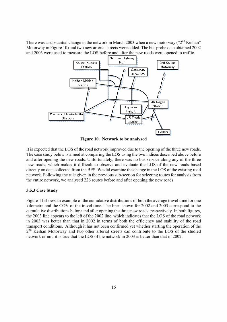
※Significance Level α=0.05 3.5 Evaluating the LOS of the Road Network We originally evaluated the LOS of the road network from the viewpoint of travel time reliability. The application and discussion above focused only on several routes of the network. It is therefore necessary to extend the aggregate route-based evaluation in the previous sections to a network-based evaluation to determine the LOS for the entire network. In other words, it is necessary to use the travel time distribution of each route to evaluate the LOS of the network. 3.5.1 Indices Among the various factors that affect the LOS of the road network, we focused on both the efficiency and stability of the road transport conditions. In that sense, the ideal road transport condition is defined as that under which travellers can reach their destinations in rapid and reliable manner. We adopted two indices for the LOS. The average travel time for one kilometre was used to evaluate the efficiency of the network. The coefficient of variation (COV) of the travel time was used to evaluate the reliability of the network. Although it is not fully confirmed that the observed or composite travel time distribution conforms the log-normal one based on the statistical tests in section 3.4, the relationship described by equations (3) and (4) holds regardless of the original distribution. Accordingly, the indices using the average and variance of travel time are regarded to be valid for analyzing LOS of network at least. These indices can be calculated from the travel time distribution for each route, and their cumulative distributions were used to evaluate the LOS of the entire network. In a real network, there are multiple routes between any OD pair. Therefore, it is necessary to define the set of routes to be analysed between the OD pair. For the sake of convenience, we assumed that the routes under consideration did not exceed 120% of the distance of the shortest route. 3.5.2 Data Used for the Network-Based Evaluation For the case study below, we used the MLIT bus probe data collected during the four months of October and December 2002, and October and December 2003. The network to be analyzed is shown in Figure 10. The roads to be considered in the analysis here are represented by the solid line.

16

There was a substantial change in the network in March 2003 when a new motorway (“2nd Keihan” Motorway in Figure 10) and two new arterial streets were added. The bus probe data obtained 2002 and 2003 were used to measure the LOS before and after the new roads were opened to traffic.

Figure 10. Network to be analyzed

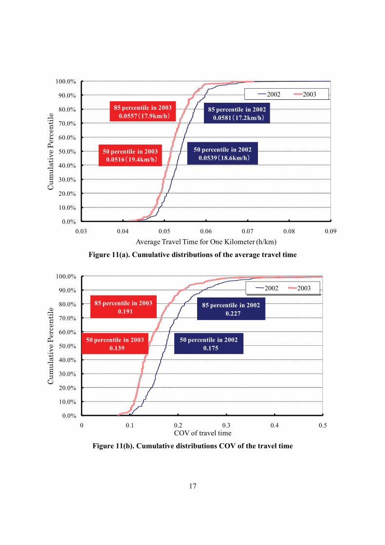
It is expected that the LOS of the road network improved due to the opening of the three new roads. The case study below is aimed at comparing the LOS using the two indices described above before and after opening the new roads. Unfortunately, there was no bus service along any of the three new roads, which makes it difficult to observe and evaluate the LOS of the new roads based directly on data collected from the BPS. We did examine the change in the LOS of the existing road network. Following the rule given in the previous sub-section for selecting routes for analysis from the entire network, we analysed 226 routes before and after opening the new roads. 3.5.3 Case Study Figure 11 shows an example of the cumulative distributions of both the average travel time for one kilometre and the COV of the travel time. The lines shown for 2002 and 2003 correspond to the cumulative distributions before and after opening the three new roads, respectively. In both figures, the 2003 line appears to the left of the 2002 line, which indicates that the LOS of the road network in 2003 was better than that in 2002 in terms of both the efficiency and stability of the road transport conditions. Although it has not been confirmed yet whether starting the operation of the 2nd Keihan Motorway and two other arterial streets can contribute to the LOS of the studied network or not, it is true that the LOS of the network in 2003 is better than that in 2002.

17

0.0%

10.0%

20.0%

30.0%

40.0%

50.0%

60.0%

70.0%

80.0%

90.0%

100.0%

0.03 0.04 0.05 0.06 0.07 0.08 0.09

Cum

ulat

ive P

erce

ntile

Average Travel Time for One Kilometer (h/km)

2002 2003

85 percentile in 20030.0557（17.9km/h）

85 percentile in 20020.0581（17.2km/h）

50 perentile in 20030.0516（19.4km/h）

50 percentile in 20020.0539（18.6km/h）

Figure 11(a). Cumulative distributions of the average travel time

0.0%

10.0%

20.0%

30.0%

40.0%

50.0%

60.0%

70.0%

80.0%

90.0%

100.0%

0 0.1 0.2 0.3 0.4 0.5

Cum

ulat

ive P

erce

ntile

COV of travel time

2002 2003

85 percentile in 20030.191

50 percentile in 20020.175

50 percentile in 20030.139

85 percentile in 20020.227

Figure 11(b). Cumulative distributions COV of the travel time

18

4. CONCLUDING REMARKS We suppose that no one might deny the importance and significance in evaluating the LOS of network utilizing the real observation. This kind of evaluation is expected to lead to improvement in management and control for road network. Although the most of road networks has been equipped with various types of sensors, such as loop detectors, ultrasonic detectors, AVI (Automated Vehicle Identifier), the information obtained from these devices are limited to the observations at a certain location or section. Accordingly, the information obtained by the conventional devices mentioned above might not be fully suitable for analyzing the spatial and temporal changes in traffic condition on road network. Because of the rapid progress and deployment of ITS, the innovative change in sensing technologies has occurred for a last decade. Among the various sensing technologies developed in the area of ITS, the probe vehicle survey using GPS is regarded as one of the most practical and effective methodologies to obtain the information on the spatial and temporal changes in traffic condition on road network. In this sense, firstly we discussed and summarised various applications of GPS data in transport analysis. GPS data are merely a sequence of locations, and further data transformations such as map matching, data reduction, processing, and reporting are needed to make them meaningful to transport analysts. The methodologies and issues affecting these transformation techniques were summarised in this paper. The major advantages of probe data analysis are automatic data observation, real time processing, and direct observation of travel time. The drawbacks can be data handling and transaction cost if real-time observations are required. Probe data can be applied to automatic incident detection, supporting diary surveys, and observations of travel time and its variability. This paper described our recent work on travel time reliability based on bus probe data. We proposed an approach to evaluate road networks from the viewpoint of travel time stability and reliability using bus probe data. To overcome the drawbacks inherent in bus probe data, we adopted a methodology to correct the travel time observed by bus probes by eliminating increases due to stopping at bus stops. In addition, we proposed a methodology to estimate travel time distributions of arbitrary routes by statistically summing up the directly observed multiple travel time distributions. Based on the development of methodologies to estimate travel time distributions of arbitrary routes covered by the BPS, we proposed an approach to evaluate the LOS of a road network based on the concept of travel time reliability. We used two indices for the LOS. The average travel time for one kilometre was used to evaluate the efficiency of the network. The COV of the travel time was used to evaluate the reliability of the network. The cumulative distributions of these indices were used to evaluate the LOS of a network in a case study. Clearly, what we have explained in this paper can be regarded as an initial step to evaluate the LOS of network using date obtained from BPS. The followings are the research issues that should be considered in our further study: 1) It is necessary for us to continue the statistical analysis of travel time distributions. Especially,

we try to find out the theoretical distribution which conforms to the observed distribution. 2) It is important for us to find out the factors which may give the significant influence to the LOS

of network. The factors to be tested include weather condition, design of road, land use along road and so on.

19

ACKNOWLEDGMENT This research was supported by the ‘Innovation and Integration of Technologies for a New Society’ project funded by the Japanese Ministry of Land, Infrastructure, and Management. We wish to thank the Institute of Systems Science Research and our former students: Yusuke Nagahiro and Yusuke Yamawaki, for supporting the analysis of bus probe data. REFERENCES Asakura, Y. and Hato, E. (2004). Tracking Survey for Individual Travel Behaviour Using Moble

Communication Insturments, Transportation Research C, 12, 273-291. Asakura, Y., Hato, E., Nishibe, Y., Daito, T., Tanabe, J., and Koshima,, H. (1999) Monitoring

Travel Behaviour Using PHS Based Location Positioning Service System, Proceedings of the 6th ITS World Congress, CD-ROM.

Cheu, R.L., Xie, C., and Lee, D.H. (2002). Probe Vehicle Population and Sample Size for Arterial Speed Estimation, Computer-Aided Civil and Infrastructure Engineering, 17, 53-60.

Draijer, G., Kalfs, N., and Perdok, J. (2000). Global Positioning System as Data Collection Method for Travel Research, Transportation Research Record, 1719, 147-153.

Du, J. and Aultman-Hall, L. (2007). Increasing the Accuracy of Trip Rate Information from Passive Muti-day GPS Travel Datasets: Automatic Trip End Identification Issues, Transportation Research A, 41, 220-232.

Hato, E. (2006). Development of MoALs (Mobile Activity Loggers Supported by GPS-Phones) for Travel Behavior Analysis, paper presented at the 85th Annual Meeting of Transportation Research Board.

He, R.R., Liu, H.X., et al. (2002). Study Travel Time Variability from Probe Vehicle Data. Proceedings of the 7th International Conference on Application of Advanced Technologies in Transportation, ASCE, CD-ROM.

Hellinga, B.R. and Fu, L. (2002). Reducing Bias in Probe-based Arterial Link Travel Time Estimates, Transportation Research C, 10, 257-273.

Iida, Y. (2002). Basic Concepts and Future Directions of Road Network Reliability Analysis. Journal of Advanced Transportation 33, 125-134.

Lee, C. Lee, S., Kim, T., and Kim, J.H. (2006). Experiments and Experiences on the Relationship between the Probe Vehicle Size and the Travel Time Collection Reliability, Knowledge-based Intelligent Information and Engineering System, Part 3, Proceedings Lecture Notes in Artificial Intelligence, 4253, 556-563.

List, G.F. and Demers, A. (2006). Estimating Highway Facility Performance from AVL Data. Proceedings of the 5th International Symposium on Highway Capacity and Quality of Service, TRB, 319-328.

Lorkowski, S., Mieth, P., Thiessenhusen, K.-U., Chauhan, D., Passfeld, B., and Schafer, R.-P. (2004). Towards Area-Wide Traffic Monitoring-Applications Derived from Probe Vehicle Data. Proceedings of the 8th International Conference on Application of Advanced Technologies in Transportation, ASCE, CD-ROM.

Murakami, E. and Wagner, D.P. (1999). Can Using the Global Positioning System (GPS) Improve Trip Reporting? Transportation Research C, 7(2-3), 149-165.

Noronha, V. and Goodchild, M.F. (2000). Map Accuracy and Location Expression in

20

Transportation – Reality and Prospects, Transportation Research C, 8, 53-69. Ochieng, W.Y. and Sauer, K. (2002). Urban Road Transport Navigation: Performance of the

Global Positioning System After Selective Availability, Transportation Research C, 10(3), 171-187.

Quddus, M.A., Ochieng, W.Y. and Noland, R.B. (2006) Integrity of Map-Matching Algorithms, Transportation Research C, 14, 283-302.

Quiroga, C.A. and Bullock, D. (1998). Travel Time Studies with Global Positioning and Geographic Information Systems: An Integrated Methodology, Transportation Research C, 6(1-2), 101-127.

Sethi, V., Bhandari, N., Koppelman, F.S., and Schofer, J.L. (1995). Arterial Incident Detection Using Fixed Detector And Probe Vehicle Data, Transportation Research C, 3C (2), 99-112.

Sugino, K., Asakura, Y., Daito, T., and Matsuo, T. (2000). Traffic Information Service in Road Network Using Mobile Location Data, Proceedings of the 7th ITS World Congress, CD-ROM.

Thomas, N. and Hafeez, B. (1998). Simulation of an Arterial Incident Environment with Probe Reporting Capability, Transportation Research Record, 1644, 116-123.

Taylor, M.A.P., Woolley, J.E., and Zito, R. (2000). Integration of the Global Positioning System and Geographical Information Systems for Traffic Congestion Studies, Transportation Research C, 8(1-6), 257-285.

Tanabe, J., Asakura, Y., Itsubo, S., Maekawa, T., and Okutani, T. (2007). Uncertainty of Travel Time and Route Choice Behaviour – Empirical Analysis Using Probe Person Data, Proceedings of the 3rd International Symposium on Transport Network Reliability (INSTR2007).

Uno, N., Iida, Y., and Kawaratani, S. (2002). Effects of Dynamic Information System on Travel Time Reliability of Road Network. Traffic and Transportation Studies, ASCE, 911-918.

Uno, N., Iida, Y., Murakami, N., and Nakagawa, S. (2004). A Practical Approach to Correct Bus Probe Data for Evaluating Travel Time Reliability of Road Network. 2nd International Symposium on Transport Network Reliability, Proceedings of Technical Session, 49-55.

Zito, R., D’Este, G., and Taylor, M.A.P. (1995). Global Positioning Systems In The Time-Domain – How Useful a Tool For Intelligent Vehicle-Highway Systems? Transportation Research C, 3 (4): 193-209.