Using a water treatment residual and compost co-amendment ...

Durham E-Theses

Using a water treatment residual and compost

co-amendment as a sustainable soil improvement

technology to enhance �ood holding capacity

KERR, HEATHER,CATHARINE

How to cite:

KERR, HEATHER,CATHARINE (2019) Using a water treatment residual and compost co-amendment as

a sustainable soil improvement technology to enhance �ood holding capacity, Durham theses, DurhamUniversity. Available at Durham E-Theses Online: http://etheses.dur.ac.uk/12983/

Use policy

The full-text may be used and/or reproduced, and given to third parties in any format or medium, without prior permission orcharge, for personal research or study, educational, or not-for-pro�t purposes provided that:

• a full bibliographic reference is made to the original source

• a link is made to the metadata record in Durham E-Theses

• the full-text is not changed in any way

The full-text must not be sold in any format or medium without the formal permission of the copyright holders.

Please consult the full Durham E-Theses policy for further details.

http://www.dur.ac.uk

http://etheses.dur.ac.uk/12983/

http://etheses.dur.ac.uk/12983/

http://etheses.dur.ac.uk/policies/

Academic Support O�ce, Durham University, University O�ce, Old Elvet, Durham DH1 3HPe-mail: [email protected] Tel: +44 0191 334 6107

http://etheses.dur.ac.uk

2

http://etheses.dur.ac.uk

Using a water treatment residual and compost

co-amendment as a sustainable soil improvement

technology to enhance flood holding capacity

Heather Kerr

A thesis submitted in fulfilment of the requirements for the degree of Doctor of

Philosophy

School of Engineering and Computing Sciences Durham University

September 2018

ii

Abstract

The recycling of clean wastes, such as those from the treatment of drinking water,

has gained importance on the environmental agenda due to rising costs of landfill

disposal and movement towards a ‘zero’ waste economy. More than one third of

the globe’s soils are degraded and as such policies towards determining soil health

parameters and reversing destruction of the globe’s most valuable non-renewable

source are at the forefront of environmental debate. This thesis questions the

opportunity for water treatment residual (WTR) to be used as a beneficial material

for the co-amendment of soil with compost to improve the soil’s flood holding

capacity (Kerr et al., 2016), which includes functions such as the water holding

capacity, hydraulic conductivity, soil structure and shear strength. Currently, water

treatment residual is typically sent to landfill for disposal, but this research shows

that the reuse of WTR as a co-amendment is able to improve the flood holding

capacity of soils. This research crosses the boundary between geotechnical and

geoenvironmental and provides a holistic approach to quantifying a soil from both

perspectives.

Iron based water treatment residual from Northumbrian Water Ltd was used in

both laboratory and field trials to establish the effect of single WTR and a compost

and WTR co-amendment on the water holding capacity (the gravimetric water

content, volumetric water content, volume change of samples i.e. swelling and

shrinkage), and the effect of amendment on the erosional resistance, hydraulic

conductivity and shear strength compared to a control soil. A series of four trials

were conducted to develop and establish a novel method to determine the water

holding capacity, supplemented by standard geotechnical methods to determine

the flood holding capacity. The use of x-ray computed tomography has provided

accompanying information on the morphology of dried WTR and changes in the

internal characteristics of amended soil between a dry and wet state. The

amendment application rate ranges from 10 – 50%.

Experiments have shown that the single amendment of WTR, compared to a

control soil, yields significant increases in the hydraulic conductivity (by up to a

factor of 28), increases the shear strength of soils at low testing pressure (25 kPa)

by 129%, increases the maximum gravimetric water content by up to 13.7%, and

iii

improves swelling by up to 12% (but only at the highest amendment rate, 30%),

increases the maximum void ratio when saturated by 11%, and reduces shrinkage

by maintaining porosity by 14%. However the application of WTR as a single

amendment has implications for the chemical health of the soil as it is highly

effective at immobilising phosphorous as and such cannot not effectively be used

as a soil amendment. The single application of compost yielded significant

improvement in the water holding capacity (improving gravimetric water content

by up to 34.7%, increasing the sample volume by up to 83.3%, and increased the

void ratio by 8.2%), however this application reduces the hydraulic conductivity

by up to 84.5% and the shear strength by 3% compared to the control soil.

Co-amendment using compost and WTR (in two forms, air dried 80% solids and

wet at 20% solids, as produced from water treatment works) improved the flood

holding capacity of soils by retaining the structural improvements of amendment

using WTR and the water holding capacity improvements of compost. Compared to

the control soil, for co-amended soils the gravimetric water content was improved

by up to 25%, the volume increased by up to 51.7%, experienced 13% less

shrinkage and an 11.5% increase in maximum void ratio. The hydraulic

conductivity was also improved by up to 475%, and shear strength was increased

at both low and high testing pressures by to 53.8%.

Taking into account these effects of co-amendment on essential soil functions that

determines a soil’s flood holding capacity (maximum gravimetric water content,

volume change, resistance against shrinkage, void ratio (porosity), hydraulic

conductivity and shear strength), the economical and environmental sustainability

issues, the co-amendment of soil using compost and WTR may provide a solution

to both recycling clean waste product and improving the quality of soil.

iv

I. Table of Contents

1. Introduction 1

1.1 Threats to soil 2

1.2 Soil health policy 4

1.3 Engineering soils; soil amendment and waste recycling 8

1.4 Thesis outline 9

2. Fundamentals of Soils 12

2.1. Soil formation 12

2.1.1 Natural processes of soil formation 14

2.1.2 Pedogenesis (soil change and characteristics) 18

2.2 Geo-environmental aspects of soil 20

2.2.1 Soil organic matter 20

2.2.2 Soil aggregation 22

2.3 Geotechnics of soil 27

2.3.1 Soil structure 27

2.3.2 Definitions of soil structure 30

2.3.3 Factors affecting soil structure 34

2.3.4 Soil erosion 38

2.3.5 Soil erodibility indices 40

2.3.6 Soil shear strength and stress 46

2.4 Soil water 50

2.4.1 Important soil water relationships 50

2.4.2 Soil water definitions 53

2.4.3 Measuring soil water 60

2.4.4 Hydraulic conductivity 62

2.4.5 Measuring hydraulic conductivity 65

2.5 Concluding remarks 66

3. Water Treatment Residual (WTR) 68

3.1 An introduction to WTR production, storage and disposal 68

3.1.1 Water processing and production of WTR 71

3.1.2 Water Treatment Residual management and disposal 75

v

3.1.3 Northumbrian Water disposal of WTR 80

3.2 WTR characterisation 83

3.2.1 Physical properties 83

3.2.2 Chemical properties 87

3.2.3 Nutrient values 89

3.2.4 Potentially toxic elements (PTEs) 91

3.3 WTR as a resource 93

3.3.1 WTR as a soil substitute 93

3.3.2 Recycling waste 95


4. Measuring Change in Soils 98

4.1 Materials 100

4.1.1 Soil 100

4.1.2 Compost 101

4.1.3 Water Treatment Residual (WTR) 101

4.1.4 Silica 101

4.2 Material storage, handling and preparation 102

4.2.1 Soil 103

4.2.2 Water Treatment Residual (WTR) 105

4.2.3 Compost and Silica 105

4.3 Material characterisation 106

4.3.1 Particle size distribution 106

4.3.2 Classification and description of soils 108

4.3.3 Volume and density (dry, bulk & particle) 109

4.3.4 Moisture content 112

4.3.5 Material characterisation results 116

4.4 Experimental trial methods 121

4.4.1 Core production methodology 122

4.4.2 Trial 1 123

4.4.3 Trial 2 125

4.4.4 Trial 3 126

4.4.5 Trial 4 (Final Trial) 128

4.4.6 Density and water content considerations 131

vi

4.4.7 Statistical testing 133

4.5 Erosional resistance testing 136

4.5.1 The Veitch method 136

4.5.2 Fall cone test 138

4.6 Triaxial testing 138


5. Results and Discussion 144

5.1 Water holding capacity 144

5.1.1 Initial results: Trials 1 &2 144

5.1.2 WHC Trial 3 151

5.1.2.1 Effect of single amendment at different proportions 153

on GWC: 5050, 6040 and 7030

5.1.2.2 Effect of single compost amendment on GWC 156

5.1.2.3 Effect of single WTR/silica amendment on GWC 157

5.1.2.4 Effect of co-amendment vs single amendment on GWC 158

5.1.2.5 Effect of density and initial water content on GWC 161

5.1.2.6 Relationships between compost and GWC 165

5.1.2.7 Relationships between WTR/silica and GWC 167

5.1.2.8 Volumetric and density changes 168

5.1.2.9 Concluding remarks: Trial 3 171

5.1.3 WHC Trial 4 173

5.1.3.1 Effect of single amendment at different proportions: 178

7030, 8020, 9010 on GWC

5.1.3.2 Effect of single amendment at different proportions: 182

7030, 8020, 9010 on volume & VWC/VWCi

5.1.3.3 Effect of single compost amendment on GWC, VWC, 188

VWCi and volume

5.1.3.4 Effect of single WTRd/WTRw amendment on GWC, 190

VWC, VWCi and volume

5.1.3.5 Effect of co-amendment on GWC, VWC, VWCi and 194

volume

5.1.3.6 Effect of co-amendment vs single amendment on GWC, 196

VWC, VWCi and volume

vii

5.1.3.7 Concluding remarks: Trial 4 204

5.2 Erosional resistance 208

5.2.1 Drop testing (Veitch method) 208

5.2.2 Fall cone testing 210

5.2.3 Concluding remarks 215

5.3 Triaxial testing 216

5.3.1 Hydraulic conductivity 216

5.3.2 Shear strength 220

5.3.2.1 Stress strain relationships 220

5.3.2.2 Stress paths 225

5.3.2.3 Concluding remarks 231

6. X-ray Computed Tomography 232

6.1 Introduction to XRCT 232

6.1.1 Primary research into XRCT 235

6.1.2 Recent applications and uses of XRCT 235

6.1.3 Applications of XRCT for soil research 238

6.2 Limitations of XRCT technology 242

6.2.1 Sample size and resolution stand-off 242

6.2.2 Imaging artefacts and corrections 244

6.2.2.1 Beam hardening 244

6.2.2.2 Partial volume effects 246

6.2.2.3 Image noise 246

6.2.3 Water content and volume change of samples 247

6.2.4 Thresholding 248

6.3 Overcoming issues of segmentation in heterogeneous materials 251

6.3.1 Tracers in solution 252

6.3.2 OM identification 254

6.4 XRCT methodology and results 258

6.4.1 Machinery and settings 259

6.4.2 Initial scanning 260

6.4.3 Exploratory use of XRCT, Durham 264

6.4.4 High resolution scanning, Stellenbosch 278

6.4.5 High resolution scanning, Durham 284

viii

6.5 Discussion and concluding remarks 288

7. Weetslade Field Trial: Engineering soil for flood resilience proof of 290

concept at the field scale

7.1 Introduction 290

7.1.1 Background 290

7.1.2 Project overview 291

7.1.3 Beneficiaries and project aims 292

7.2 Site overview and methods 295

7.2.1 Measuring VWC and soil suction 299

7.2.2 Measuring geotechnical soil parameters 300

7.3 Field trial results 301

7.2.3 Water holding capacity 302

7.2.4 Soil water potential 310

7.2.5 Soil strength 315

7.4 Discussion and catchment implications 316


8. Conclusions and Recommendations for Future Work 320

8.1 Concluding summary 323

8.2 Recommendations for future work 327

9. Bibliography: References and websites 329

II. List of Tables

Table 1: Summary of varying definitions of the terms bulk density and dry density. Pg 31

Table 2: Summary of applicable geotechnical definitions on soil. Pg 33

Table 3: Key properties of three soil water types; gravitational, capillary and hygroscopic. Pg 52

Table 4: Important definitions for soil and soil-water relationships. Pg 54-56

Table 5: Summary of key changes to samples in Figure 9. Pg 59

Table 6: Hydraulic conductivity classes based on speed of water movement. Pg 63

Table 7: Summary of important particulate, chemical and biological constituents found in water

according to their source. Pg 69

Table 8: Concentration of PTEs in WTRs as derived by Finlay (2015), Elliot (1990), McBridge

(1994), BSIPAS-100 specification, and Sewage Sludge Directive 86/278/EEC. Pg 79

ix

Table 9: Standard Rules summary of positive and negative impacts of land spreading of WTR

(Natural Resources Wales, 2017). Pg 80

Table 10: WTR production figures from Northumbrian Water Ltd, 2010 – 2015 (Finlay, 2015 via

pers comm L Dennis, NWL), and WTR production figures from 2014-2018 from Greenhouse Gas

Data Returns, which include Essex and Suffolk values (pers comms E. Higgins, NWL). Pg 81

Table 11: Typical physical properties and chemical constituents of alum and iron sludges from

chemical precipitation (from Crittenden et al., 2012). Pg 84

Table 12: Data on the chemical and physical parameters of WTR obtained across various

locations in the NE of England (WTR range) compared to specific Mosswood data and typical soil

values. Pg 88

Table 13: Concentrations of nutrients in WTR compared to typical soil, compost and biosolids

values. Pg 91

Table 14: Water contents of WTR2 dried at different temperatures, where the value is derived

using Equation 13 (mass of water/ mass of solids). Values in brackets describe the water content

by wet basis GWC. These values are compared to a small range of vales derived by Basim (1999),

denoted by *. Pg 115

Table 15: Results of material characterisation and analysis including physical and chemical

attributes, where values are obtained from analysis undertaken by Derwentside Environmental

Testing Services (DETS) using methods DETSC 2301# and 2008# and from Finlay (2015). Pg 116

Table 16: Chemical analysis of materials undertaken by DETS using methods DETSC 2301# and

2008#, including information from Finlay (2015). Bold typeface signifies that the concentration

exceeds BSI PAS100 regulations, and bold typeface with * signifies that the concentration exceeds

EU Biosolids regulations (Sewage sludge directive 86/278/EC). Pg 117

Table 17: Typical ranges for soil, WTR and compost, sourced from Finlay (2015) in addition to

other literature. Pg 118

Table 18: Amendment proportions for samples used in Trial 1, using three materials. Pg 124

Table 19 Soil amendment ratios used in Trial 2 according to the dry mass of each component. Pg

126

Table 20: Soil amendments used in Trial 3. Bulk & dry density and water content values are for

individual cores at production. Pg 127

Table 21: Soil amendment ratios used for Trial 4. Pg 128-9

Table 22: Summary of method parameters for Trials 1 -4. Pg 132

Table 23: Soil amendments used in Trial 3. Bulk & dry density and water content values are for

individual cores at production. Pg 152

Table 24: Summary of amendment proportions for Trial 3. Pg 162

Table 25: Soil amendment ratios used for Trial 4. Pg 174

Table 26: Average Cu values for soils categorised into their amendment properties. Pg 214

Table 27: Average Cu values for soils after one wetting and drying cycle categorised into their

amendment properties. Pg 214

x

Table 28: Values of maximum water content in obtained from the triaxial cell apparatus,

compared to the maximum water content achieved by samples in Trial 4. Pg 219

Table 29: Summary of triaxial cell data for unamended soil (Soil2) and five 30% amendments. Pg

220

Table 30: Angle of friction values for unamended soil (Soil2) and five amendments, calculated

from stress path graphs. Pg 227

Table 31: Example size vs resolution capability of the Xradia/Zeiss XRM 410 machine [23]. Pg 260

Table 32: Lower auto-thresholding values chosen for Experiment 4 samples. Pg 265

Table 33: summary of porosity values derived from XRCT for samples Soil2, and AM11-AM15, and

comparisons with calculated porosity for dry samples based on particle density and volume

measurements, and triaxial derived porosity for wet samples. Pg 267

Table 34: Summary statistics of WTR analysis from Volume Graphics 3.2 porosity/inclusion

analysis. Pg 279

Table 35: Values of bulk density for unamended and amended plots over time. Pg 301

Table 36: Summary of triaxial cell strength testing on samples from Weetslade Country Park. Pg

316

Table 37: Summary of soil function data, comparing the control (Soil2) with single amendments

of WTRd, WTRw, and compost, and against co-amendment of WTRd/WTRw with compost at ratios

of 10, 20 and 30%. Data are absolute values of change and (the percentage increase or decrease

compared to the control). Pg 322

III. List of Figures

Figure 1: Schematic representation of a hypothetical soil profile. Pg 18

Figure 2: Simplified schematic of a soil aggregate. Pg 23

Figure 3: A simplified diagram of partially saturated volume of soil and associated three phase

soil diagram. Pg 28

Figure 4: Triangular classification chart of soil based on texture. Pg 30

Figure 5: The effect of compaction on soils structure. Pg 36

Figure 6: Mohr-Coulomb failure envelope. Pg 48

Figure 7: Examples of failure envelope gradients, cohesion and angle of friction values for

granular and cohesive soils. Pg 49

Figure 8: Stages of water retention in the soil matrix. Pg 51

Figure 9: Gravimetric water content, volumetric water content and density of five example

samples to represent change during wetting. Pg 58

Figure 10: Typical soil water retention curve. Pg 62

Figure 11: Maximum water content as a function of bulk density. Pg 64

Figure 12: Triaxial cell apparatus set up for testing hydraulic conductivity and shear strength. Pg

66

Figure 13: Schematic diagram of clean raw water in a water treatment production plant. Pg 73

xi

Figure 14: Photos of WTR, (a) freshly produced from the water treatment plant at Mosswood

water treatment plant (b) oven-dried water treatment residual, clearly showing iron oxide

(orange rust colour) precipitates. Pg 83

Figure 15: Comparison of WTR compaction curves from dry and wet sides for WTR (Hseih &

Raghu, 1997), against the compaction curve of a typical loamy clay soil. Pg 86

Figure 16: Example of the Proctor standard test for compaction of soil at different water

contents, annotated with optimum moisture content, maximum bulk dry density, wet and dry

sides of optimum. Pg 109

Figure 17: Schematic of volume and mass proportions in a soil with mass and volume equation 7.

Pg 109

Figure 18: Example of a field moist soil, with the values of properties noted on the diagram. Pg

113

Figure 19: Particle size distribution for Soil2, silica and WTR2d performed as per BS1377 (Part 2:

1990). Pg 119

Figure 20: Proctor compaction curve for Soil2 determining the maximum bulk density as

1.91 g/cm3 at gravimetric water content of 16% (0.16), shown by the red dashed lines. Pg 119

Figure 21: Sample annotations based on individual units (core/sample), groups of cores of the

same composition (S1 or AM8), and samples of different composition (Soil 1, AM2 etc). Pg 121

Figure 22: Schematic of sample (core) production using a split mould and compaction pin. The

core removed from the mould is 76 mm x 38 mm. Pg 122

Figure 23: Proctor compaction mould method for soil core production. Pg 123

Figure 24: Split mould and static compaction press method. Pg 130

Figure 25: Schematic diagram (left) of the Veitch method used to test aggregate stability of disk

shaped samples and a photo of a sample during testing (right). Pg 137

Figure 26: Schematic of the strain (ε) and stress (σ) states undergone by a sample during triaxial

testing. Pg 139

Figure 27: Example of Mohr Circles, plotted with a failure envelope (which is idealistic and

unlikely to be linear), angle of friction, and cohesion (c). Pg 142

Figure 28: Example of stress strain curves for a soft material (black dashed), a typical stress

strain curve of a soil for which the maximum strength is coincidental with the critical state

(black), and an over-consolidated sample that reaches a peak strength and subsequently reaches

an ultimate state with increasing axial strain (red). Pg 142

Figure 29: Example of stress paths for dilatant (black) and compressive (blue) samples to the

critical state line (red). Pg 142

Figure 30: Trial 1’s average gravimetric water content for Samples S1 and T1A-T1E. Pg 145

Figure 31: Trial 1’s average volumetric water content (VWC) and VWCi. Pg 146

Figure 32: Trial 1’s average dry density (Dd) and bulk density (BD) of samples, where n = 3 with

the exception of S1 where n = 1, at the start point and 24 hours after submersion. Pg 146

Figure 33: Trial 2’s average GWC (where n = 4) over 72 hours of submersion. Pg 147

xii

Figure 34: Trial 2’s average VWC and VWCi (where n = 4) over 72 hours of submersion. Pg 149

Figure 35: Trial 2’s average dry density (annotated with Dd) and bulk density (annotated with

BD) of samples (n = 4) over 72 hours of submersion. Pg 160

Figure 36: Average GWC of samples up to 240 hours of wetting according to the method outlined

in section 4.4.4. n is between 5 and 8. Pg 151

Figure 37: Average effect of single amendment at a 50% rate on gravimetric water content. Pg

153


154


155

Figure 40: Average effect on gravimetric water content of single amendment with compost at

30% and 40% rate against the control, Soil2. Pg 156

Figure 41: Average effect on gravimetric water content of single amendment with WTR2d and

silica (Si) at various amendment rates against the control, Soil2. Pg 157

Figure 42: Average effect on gravimetric water content of co-amendment with WTR2d and

compost at various amendment rates against the control, Soil2. Pg 158

Figure 43: Average effect on gravimetric water content of co-amendment and single amendment

at a 50% application rate against the control, Soil2. Pg 159





Figure 46: (A) Maximum GWC as a function of the dry density of samples against the control,

Soil2. (B) Dry density of samples compared to their initial water content. Pg 162

Figure 47: Average gravimetric water content (top) and average volumetric water content

(bottom) for unamended soil at three bulk densities (Unam. 1.4, Unam 1.6 and Unam 1.8 g/cm3)

and (bottom) for a 30% WTR co-amended soil (WTR/comp 1.4, WTR/comp 1.6, and WTR/comp

1.8 g/cm3). n = 12. Pg 164

Figure 48: Maximum GWC of samples against the proportion of compost in the amendment as

either a single amendment (40 or 30%) or as part of a co-amendment (25, 20 or 15%). Pg 165

Figure 49: Average increase in grams of water after 24 hours for samples amended with compost

as either a single amendment (40 or 30%) or as part of a co-amendment (25, 20 or 15%),

suggesting a rate of water uptake. Pg 166

Figure 50: Average maximum GWC of samples amended with WTR or silica either as a single

amendment (50, 40 or 30%) or as part of a co-amendment (25, 20 or 15%). Pg 167

Figure 51: Average increase in grams of water after 24 hours for samples amended with WTR2d

or silica as either a single amendment (50, 40 or 30%) or as part of a co-amendment (25, 20 or

15%), suggesting a rate of water uptake. Pg 168

xiii

Figure 52: Average volumetric water content change of samples against the control, Soil2, over a

240-hour wetting period. VWC start values range between 0.21 and 0.26 for samples at 0.14 GWC,

and between 0.33 and 0.35 for samples at 0.25 GWC due to small differences in sample volume. Pg

169

Figure 53: Average volumetric water content (i) change of samples against the control, Soil2,

over a 240-hour wetting period. VWC start values range between 0.21 and 0.26 for samples at

0.14 GWC, and between 0.33 and 0.35 for samples at 0.25 GWC due to small differences in sample

volume. Pg 169

Figure 54: Average bulk density change of samples over 240 hours of wetting. Pg 170

Figure 55: Average GWC change of 15 samples against the control Soil2 (unamended soil) over a

1056 wetting and drying period. Pg 175

Figure 56: Average change in volume of cores of 15 samples against the control (Soil2) over a

1056 wetting and drying period. Pg 176

Figure 57: Average change in volumetric water content (VWC) of 15 samples against the control

(Soil2) over a 1056 wetting and drying period. Pg 176

Figure 58: Average change in VWCi change of 15 samples against the control (Soil2) over a 1056

wetting and drying period. n = 12. Pg 176

Figure 59: Average GWC for samples with a single amendment at 30%. Pg 178



Figure 62: Average effect of single 30% amendments on the volume, VWC and VWCi of samples.

Pg 183

Figure 63: Average effect of single 20% amendments on the volume, VWC and VWCi of samples.

Pg 185

Figure 64: Average effect of single 10% amendment on the volume, VWC and VWCi on samples.

Pg 187

Figure 65: Average effect of single compost amendment at different proportions of amendment,

30%. 20% and 10% on GWC. Pg 188


30%. 20% and 10% on volume. Pg 188


30%. 20% and 10% on VWC and VWCi. Pg 189

Figure 68: Average effect of single WTR2d and WTR2w amendment at different proportions of

amendment, 30%. 20% and 10% on GWC. Pg 190

Figure 69: Average effect of single WTR2d and WTR2w amendment at different proportions of

amendment, 30%. 20% and 10% on VWC and VWCi. Pg 192

Figure 70: Average effect of co-amendment at different proportions of amendment, 30%. 20%

and 10% on GWC. Pg 194

xiv

Figure 71: Average effect of co-amendment at different proportions of amendment, 30%, 20%

and 10% on volume, VWC and VWCi. Pg 195

Figure 72: Average effect of single amendment vs co-amendment at 30% amendment on GWC. Pg

196

Figure 73: Average effect of single amendment vs co-amendment at 30% amendment on volume,

VWC and VWCi. Pg 198


199

Figure 75: Average effect of single amendment vs co-amendment at 20% amendment on volume,



202

Figure 77: Average effect single amendment vs co-amendment at 10% amendment on volume,


Figure 78: Average number of drops required for deformation and breaking for unamended soil

and 15 amendments. Samples annotated with * have been through one wetting and drying cycle

prior to testing. Pg 208

Figure 79: Undrained shear strength (Cu) for Trial 3 samples conducted according to BS1377:

1990. Pg 210

Figure 80: Undrained shear strength results from fall cone testing on samples from Trial 4

(BS1377). Pg 211

Figure 81: Average undrained shear strength values for Trial 4 samples from fall cone testing

(BS1377). Pg 212

Figure 82: Hydraulic conductivity of samples conducted in a triaxial cell at pressures of 25, 50

and 100 kPa. Pg 217

Figure 83: Stress strain curve for unamended soil at three cell pressures, Pg 221

Figure 84: Stress strain graphs for AM11-AM15 at three confining pressures, where blue plots

data from 25 kPa, orange plots data from 50 kPa, and 100 kPa in grey. Pg 222

Figure 85: Stress strain curve for unamended soil and five amendments tested at 25 kPa. Pg 224



Figure 88: Stress paths and critical state lines for all samples tested in the triaxial cell. Pg 226

Figure 89: Stress paths for unamended soil, and five 30% amendments at a cell pressure of 25

kPa. Dashed lines indicate the critical state line, which coincides with the peak failure. Pg 229

Figure 90: Stress paths for unamended soil and five 30% amendments at a cell pressure of 100

kPa. Dashed lines indicate the critical state line, which coincides with the peak failure. Pg 229

Figure 91: Schematic diagram of the XRCT system using cone-beam X-ray and a cylindrical core

soil sample. Pg 232

xv

Figure 92: Example image of a 3D sample and a single XRCT image ‘slice’ through the material

and an example histogram, giving the frequency of pixels with a given attenuation coefficient. Pg

234

Figure 93: An example of sample size against resolution standoff, a lower resolution is required to

capture a whole sample, and for higher resolution only a small portion of a sample is able to be

captured. Pg 242

Figure 94: Beam hardening example on a cylindrical sample of soil, taken from data processing

on AM13 (70S 30WTR2w redried), the light halo is evidence of beam hardening on the edge of the

material. Pg 244

Figure 95: Partial volume effect, where low resolution scanning includes more than one material

in a single voxel, thereby averaging the two values of attenuation as a result. Pg 246

Figure 96: Segmented image of a lime treated sand bentonite mixtures from Hashemi et al.

(2015), where macro-voids are shown in blue, bentonite shown in green and sand in red. Pg 248

Figure 97: XRCT scans of (A) 100% soil, (B) 100% compost, (C) 100% WTR1w at 50 µm resolution.

Pg 262

Figure 98: XRCT image at 50 µm resolution on a 38 mm Ø sample of 50% soil, 25% compost and

25% WTR1w. Pg 263

Figure 99: Void ratio change of Soil2 and AM11-AM15 derived thresholding of XRCT data in

Avizo. Pg 266

Figure 100: Unamended soil (Soil2) images from XRCT scanning at 25 μm resolution (top) soil in

dry, wet and re-dried states (bottom). Pg 270

Figure 101: 30% single compost amendment (AM11) images from XRCT scanning at 25 μm

resolution (top) soil in dry, wet and re-dried states (bottom). Pg 271

Figure 102: 30% single WTR2d (AM12) images from XRCT scanning at 25 μm resolution (top) soil

in dry, wet and re-dried states (bottom). Pg 272

Figure 103: 30% single WTR2w amendment (AM13) images from XRCT scanning at 25 μm

resolution (top) soil in dry, wet and re-dried states (bottom). Pg 274

Figure 104: 30% co-amendment with compost and WTR2d (AM14) images from XRCT scanning at

25 μm resolution (top) soil in dry, wet and re-dried states (bottom). Pg 275

Figure 105: 30% co-amendment with compost and WTR2w (AM15) images from XRCT scanning

at 25 μm resolution (top) soil in dry, wet and re-dried states (bottom). Pg 276

Figure 106: Unfiltered XRCT image of WTR2d at a resolution of 6 μm (left) and a 3D

reconstruction of the 3D surface of the particle, where the green slice indicates the position of the

left image. Pg 280

Figure 107: Image of WTR2d with an adaptive gauss filter, and surface determination of

pores/cracks; (right) single X axis slice and (left) single Y axis slice, where the blue line indicates

the position of the X axis slice. Pg 281

Figure 108: XRCT porosity/inclusion analysis on WTR2d . Pg 282

xvi

Figure 109: (top left) Unprocessed image of WTR2d and (top right) unprocessed image of WTR2d

having been submerged in water. Images with adaptive gauss filter applied to remove

background noise, (bottom left) single X axis slice of submerged WTR2d and (bottom right) single

Y axis slice of submerged WTR2d. Red arrow indicates the growth of a central defect when the

sample is wetted. Pg 283

Figure 110: XRCT image of Soil2 in dry and wet states, sieved to 2.8 mm compared to Soil2 sieved

to 6.3 mm at a resolution of 20 µm. Pg 285

Figure 111: Soil2 2.8mm (dry vs wet, top) and Soil2 6.3 mm (dry vs wet, bottom) thresholding. Pg

286

Figure 112: AM12 2.8mm (dry vs wet, top) and AM14 6.3 mm (dry vs wet, bottom) thresholding

Pg 286

Figure 113: Comparison of void ratios derived from XRCT and triaxial cell where Soil2 is

unamended soil and AM14 is a 30% co-amendment with WTR2d. Pg 287

Figure 114: Ordinance Survey map of the Weetslade Country Park with an aerial Google Maps

image of the study area (in red) [24]. Pg 295

Figure 115: Flood map for the Seaton Burn [24] of the area local to Weetslade (identified in the

red box). Pg 296

Figure 116: Schematic of field trial plots, location of amended plots and location of sensors on the

two amended plots. Pg 297

Figure 117: Slope profile average for the Weetslade embankment test site, where the location of

sensors in Figure 2 are shown. Data from Ellis (2017). Pg 298

Figure 118: Photos of the field site on week post construction, and in the 2 months following for

both an amended plot and an unamended plot. Pg 301

Figure 119: Schematic of EC5 sensor locations by zone. Sensors in red did not return any data

(probe fault). Pg 302

Figure 120: All EC-5 sensor data displaying VWC for May. Rainfall data presented in blue and

grey blue are from Ablemarle and the onsite weather station respectively. Pg 304

Figure 121: Volumetric water content of sensors in Zone 1 at Weetslade during May, with rainfall

data obtained from an installed weather station (narrow light blue) and from Ablemarle (thick

dark blue). Pg 305

Figure 122: Volumetric water content of the soils in Zone 3 at Weetslade during May, with

rainfall data obtained from an installed weather station (light blue) and from Ablemarle (dark

blue). Pg 306

Figure 123: VWC decline in % for each sensor from the peak of their VWC during a rainfall event.

The table below compares the sensors based on their location on the slope. Pg 307

Figure 124: Long term VWC of amended and unamended plots in Zone 1 as recorded by EC5

sensors. Rainfall data is from the onsite weather station. Pg 308

Figure 125: Long term VWC of amended and unamended plots in Zone 3 as recorded by EC5

sensors. Rainfall data is from the onsite weather station. Pg 310

xvii

Figure 126: Schematic of MPS6 sensors location by zone on the slope. Pg 310

Figure 127: SWP in unamended soil for the period of May (Um4 0.1 and Um4 0.2 did not collect

data during this period). Rainfall data sourced from Ablemarle weather station. Pg 312

Figure 128: SWP in amended soil for the period of May (Am4 0.1 did not collect data during this

period). Rainfall data sourced from Ablemarle weather station. Pg 312

Figure 129: SWP for sensors in Zone 3 on the Weetslade field trial. Pg 313

Figure 130: SWP of amended soil plots for the second data period, where -12.00 on the Y axis

corresponds to a -1200 kPa suction. Pg 314

Figure 131: SWP of unamended soil for the second data period. Um4 data is not available due to

sensor failure. Rainfall data is from the onsite weather station. -12.00 on the Y axis corresponds

to a -1200 kPa suction. Pg 314

Figure 132: SWP of amended and unamended plots in Zone 3 on the Weetslade field Rainfall data

is from the onsite weather station. -12.00 on the Y axis corresponds to a -1200 kPa suction. Pg

315

IV. List of Equations

Eq. 1: Dokuchaev formula for principal factors of soil formation. Pg 13

Eq. 2: Coulomb failure criterion. Pg 47

Eq. 3: Critical shear stress as a function of effective cohesion and effective friction angle. Pg 47

Eq. 4: Matric suction formula. Pg 51

Eq. 5: Hydraulic conductivity (k), where q is the permeability coefficient (flow in m3/second), L is

the length of the sample in m, A is the cross-sectional area of the soil (m2) and h is the pressure

head (m). Craig (2004). Pg 63

Eq. 6: Calculation of the silt and clay fraction of a soil based on the wet sieving procedure BS1377.

Pg 106

Eq. 7: Mass and volume calculations for a soil body. Pg 109

Eq. 8: Bulk density calculation for soil. Pg 110

Eq. 9: Ratio of components in amendments. Pg 110

Eq. 10: Dry density (Dd) calculation. Pg 110

Eq. 11: Equivalent particle density which links the gravimetric water content (w) and particle

density (Pd) for any combination of components. Pg 110

Eq. 12: Compost particle density calculation. Pg 112

Eq.13: Dry basis gravimetric water content calculation for the soil sample in Figure 17. Pg 113

Eq. 14: Wet basis gravimetric water content calculation for the soil sample in Figure 17. Pg 113

Eq. 15: Volumetric water content (θv) calculation for the sample in Figure 17. Pg 114

Eq. 16: Volumetric water content (𝜃𝑣𝑖) calculation using an instantaneous volume of soil of

Figure 17. Pg 114

Eq. 17: Hansbo formula. Pg 138

xviii

Eq. 18: Skempton’s B value calculation where ∆𝑢 is the difference between initial and maximum

pore pressure and ∆𝜎3 is the difference between initial and maximum cell pressure. Pg 140

Eq 19: Calculation M, the slope of the critical state line. Pg 225

Eq 20: Calculation to obtain the angle of friction from M (Craig, 2004). Pg 225

V. List of Abbreviations

BD – bulk density

Dd – dry density

DETS – Derwentside Environmental Testing Services

FHC – flood holding capacity

GWC – gravimetric water content

LOI – loss on ignition

NWL – Northumbrian Water Ltd

OM – organic matter

VWI – volumetric water content

WHC – water holding capacity

WTR – Water Treatment Residual

WTRd – air dried WTR (80% solids)

WTRw – unprocessed WTR (20% solids)

VI. Acknowledgements

Firstly, I would like to give my greatest thanks to my supervisor Dr Karen Johnson,

without which none of this work would have been possible. Not only has she

helped me through the learning and research stages with enthusiasm, she has

supported me throughout my time in the Engineering department and helped me

juggle my academic commitments as well as those on the rugby pitch. Secondly, I

would like to thank David Toll for his advice and expertise on the geotechnical side

of soil, Kev and Rich for providing expertise and technical support the lab, and Ed

Higgins at Northumbrian Water for all things WTR. Thirdly I would like to thank

the work of many MEng students that have provided me with some critical

information about water treatment residual, from which I’ve manged to learn

more than my own time would permit. Finally, endless thanks must go to my

family and friends for their long serving support and encouragement over the past

five years.

xix

Statement of Copyright

“The copyright of this thesis rests with the author. No quotation from it should be published without the author's prior written consent and information derived from it should be acknowledged.”

1

1. Introduction

There is currently a disconnect between geotechnical and geoenvironmental (soil

science) research, with respect to the fundamental philosophies, definitions and the

viewpoint on soils. The geotechnical world sees the presence of organic matter and

processes of volume change in soils as a fundamental flaw in its use as a material

(Franklin et al., 1973), however in geoenvironmental engineering the emphasis on

preserving soil functions by maintaining organic matter for its long-term

sustainability is forefront (Quotes B- E). This thesis focuses on developing research

at the boundary of geotechnical and geoenvironmental work, in a world that splits

up soils, water and organic matter, by researching soil with a holistic view of

changes in soil function when soils are flooded. The water holding capacity,

permeability characteristics, shear strength and erosional resistance of soils are

components are critical for the health of our ecosystems, however they are seldom

viewed simultaneously to assess a soil’s potential to withstand degrading events

such as flooding.

“It is generally accepted that the presence of organic matter in soils acts to the

detriment of their engineering qualities”

Quote A Franklin et al. (1973)

“A nation that destroys its soils is a nation that destroys itself”

Quote B Roosevelt (1937) in Lal et al. (2007)

“There is a need to increase the volume of pore space a soil can retain under a given

load through soil or crop management or the use of soil amendments”

Quote C Angers et al. (1987)

“there is great potential in managing the soil to increase its organic matter as a

means of alleviating the problem of soil compaction

Quote D Ohu et al. (1985)

“There is limited appreciation of the role of organic matter in influencing the

compatibility of agricultural soils”

Quote E Soane (1990)

In light of increasing threats to soil health and movement towards a ‘zero waste’

economy, the work in this thesis assesses the impact of recycling waste materials

2

from the clean drinking water industry in combination with compost to amend soils.

This is discussed in reference to the concept of ‘flood holding capacity’, defined by

Kerr et al. (2016) as “the ability or capacity of a soil to take up and store flood water

upon submersion without significant soil erosion or loss of shear strength and to resist

the detrimental impacts of flooding on soil structure and critical eco- service

functions”. A discussion of flood holding capacity assesses the implications of using

a combination of physical metrics - volumetric water content, permeability and

shear strength in order to characterize how soils respond to flood and drought

conditions. We do this in order to both understand how we may better assess soil

function and how we might maintain and even enhance soil function with the use of

soil improvement technologies. This is very timely for two reasons. Firstly, since the

UK Government’s Sustainable Soils Alliance has just launched a call in August 2018

for to define soil health and secondly the UN has just announced that soil health

underpins all the UK’s Sustainable Development Goals.

1.1 Threats to soil

Soil is a highly valuable natural non-renewable resource, and fundamental to life on

Earth. It is arguably the most important natural resource on earth due to the wide

range of eco-system functions that it performs as part of the water, nitrogen and

carbon cycles, where soil organic matter generates and regulates every ecosystem

service that sustains life on earth (Lal, 2003). The complex matrix of soil allows it to

function as Earth’s largest environmental filter, providing an enormous carbon sink,

providing a habitat for plants and organisms while recycling nutrients and filtering

harmful materials. The structural characteristics of soil render it somewhat like a

sponge, with the ability to hold, transmit water and regulate its movement, which

provides a natural flood defence by mitigating extremes in precipitation. However,

one third of soil across the globe is moderately to highly degraded (FAO & ITPS,

2015), where degradation can be defined as a decline in soil function (Lal, 2009),

split into three aspects: physical, chemical and biological (Dexter, 2004). Physically

degraded soil has reduced structural ability and as a result is more susceptible to

erosion, compaction and reduced water infiltration, which increase the likelihood of

flooding. Chemical degradation typically involves acidification, nutrient depletion,

greater concentrations of heavy metals, and contamination from industry, which

affect the productivity of the soil. Biological degradation of soil is typically

3

characterised by a loss in soil organic carbon, increased green house gas emissions,

loss of plant and micro-organism biodiversity (Lal, 2009). There are a multitude of

implications of degradation, which include the loss of food yield and security, the

loss of critical functions such as carbon and water storage and increased risk to

impacts from flooding and erosion. Although this thesis focuses on the physical

characteristics of soil and its interaction with water, the importance of the biological

and chemical functions of soil cannot be underestimated. Often once the processes

of soil degradation begin, a downward spiral ensues if there is no intervention in

destructive anthropogenic processes that accelerate soil degradation. Anthrosols,

i.e. a soil that has been heavily modified by human activities occupy a very small

percentage of the earth’s surface (0.0004%), but are becoming larger with

continued influence of society on soils (FAO Soils Group, 2000)

Mbagwu & Obi (2003) and Biancalani et al. (2012) suggest that soil erosion is the

most prevalent mechanism of soil degradation worldwide, affecting approximately

85% of land. Soil erosion is in fact a natural geologic process, however accelerated

soil erosion as the result of anthropogenic influences is a negative process and

destroys the resource of soil far faster than it can ever recover (Lal, 2003 & 2015).

Rozanov et al, (1990) state that more soil has been lost in the last 10,000 years than

is currently available for agricultural use. A common reference on the magnitude of

erosion is to Oldeman (1994) who states that water erosion affects 1094 million ha

of land across the globe, which represents approximately 12% of the land used by

mankind. Many assessments of soil erosion are lacking in quantitative, unbias and

reliable data due to the difficulty in timely and accurate detection of soil erosion (Lal,

2003; Obalum et al., 2017), and the lack of a universal definition of ‘soil erosion’.

Readers are directed to Lal (2003) and Lal (2009) which provide thorough reviews

of global erosion trends and processes and an overview of soil quality and

management of soil degradation, however the fundamental message is that we are

unsustainably degrading our most valuable natural resource, which has both

tangible and intangible effects on the productivity and functions of our soils.

In the UK, degradation of soil typically occurs through erosion, compaction, soil

contamination and loss of nutrients including organic matter (Hamza & Anderson,

2005; Van Oost et al., 2007). Research at Cranfield University has suggested that soil

4

degradation costs the England & Wales economy an estimated £1.2 billion per year

(Graves et al., 2015), however Environmental Audit Committee (2017) suggest that

we are still complacent to degradation. According to UK Climate Projections

(Murphy et al., 2009), as a result of climate change the UK is likely to experience

hotter drier summers and warmer wetter winters, with increased likelihood of

extreme weather events. The KPMG suggest that the cost of flooding in the UK could

rise to £6 billion of which £2 billion included flood defence repairs, higher renewal

insurance costs, and loss of agriculture yield (Hershey, 2016, [1]). The need to

preserve soils so that they are less vulnerable to these extremes and may be able to

help mitigate their effects, is vital. Although the economic effects of soil degradation

are tangible for processes directly dependent on soil such as crop yield, the impact

of soil degradation also includes increased risk of flooding due to detrimental

changes in soil structure and water holding capacity as a result of compaction and

the loss of soil organic matter.

1.2 Soil health policy

At the World Soils Conference (2018), the UN announced that all sustainable

development goals are reliant on healthy soils (UN News, 2018 [2]). The importance

of protecting soil and remediating soils degraded by human activity (anthrosols) is

slowly being better recognised by governments and local authorities, i.e. bodies that

may be able to insight and regulate long term change in how we treat soils. Soil

quality and soil sustainability are key words that have appeared at important global

environmental agendas, in Agenda 21 (section 2) of the Rio Summit (UNCED, 1992),

at the UN Framework Convention on Climate Change (UNFCCC, 1992), and in

Articles 3.3 & 3.4 of the Kyoto protocol (UNFCCC, 1997), where attempts to quantify

the level of degradation of the globe’s soils have been made. Sustainability is defined

as “development that meets the needs of the present without compromising the ability

of future generations to meet their own needs” (Brutland et al., 1987), however the

term quality is much more difficult to define, and the reason for on-going debate on

how to best measuring improvements. Soil quality is a concept with varying

perceptions, due to a historic lack of definition or legislation unlike legislated

determinations of water or air quality. Karlen et al. (1997) suggest that at the most

basic level, soil quality is the capacity of a soil to function, where function refers to

the dynamic nature of soil encompassing three critical components; sustained

5

biological productivity, environmental quality and plant/animal health. The concept

of ‘soil quality’ can be adapted to the particular use of that soil, i.e. for agriculture,

remediation of waste, recreation or for the development of urban areas, hence why

an interdisciplinary approach is needed to assess the soil in context of its

application. Commonly the organic matter content is used as an indicator of the soil

quality due its vital role in many functions of the soil (Obalum et al., 2017) and the

relative ease of measurement, however the single measurement of soil parameter is

not wholly sufficient to determine the total response of a soil, such as degree of soil

erosion, to a given perturbation, such as flooding (Dexter & Czyz, 2000; Karlen et al.,

1997; Acton & Gregorich, 1995; USDA-NRCS, 1996; Öztaş 2002).

The concept of soil quality is suggested by Karlen et al. (1997) to be simultaneously

redundant and impossible as ‘everyone’ knows what makes a good soil however due

to the heterogeneity in soil orders, quantifying the natural differences is a

challenging task. To provide guidelines and targets to determine soil health,

parameters to indicate a soil’s quality are required. The difficulty with trying to

implement soil policy across the globe is the lack of access to evidence needed for

the implementation of policy (clear cause-effect links), the long-term nature of the

processes of soil change (which may take decades before detection) and a

disconnection between the needs of urbanising human societies and the needs of

soil (FAO, 2015 [3]). The FAO (2015) suggest that there are four critical priorities to

maintain soil as a sustainable resource and avoid further degradation of our planet’s

most important resource.

- Sustainable soil management: minimising further degradation to provide

food security

- Stabilisation or increase of global soil organic matter stores and

identification of SOC improving strategies and implementation.

- Stabilisation or reduction of global nitrogen and phosphorous fertilizer use

in areas close to the limits of total fixation, and increase in areas of nutrient

deficiency.

- Improvement in condition of the soil and our ability to observe and monitor

these changes through improvements in knowledge on soils

6

In the UK a Soil Strategy for England was published in 2009. Recent events such as

the 2013/2014 floods that cost an estimated £1.3 billion in damages have placed

soils firmly on the policy agenda (Environment Agency, 2016 [7]). In October 2017,

the Sustainable Soils Alliance (SSA [4]) was launched at a parliamentary reception

where MP Michael Gove stated that soils are the UK’s most valuable source and

suggested that improving soil health would be at the heart of future policy (referring

to DEFRA’s A Green Future: Our 25 Year Plan to Improve the Environment, 2018).

This statement describes the newfound governmental/policy maker attention that

soil is rightfully gaining (Krzywoszynska, 2017 [8]). The event was attended by 200

experts and leaders, which represent various parts of the soil communities in the

UK (academics, farmers, industries) in addition to MPs, from which four distinct

tasks or areas requiring political attention were concluded:

- A regulatory framework to promote best practise and deter harmful soil

management practise

- A viable system for the monitoring and evaluation of the quality of our soils

- A robust compliance system of economic incentives balanced with regulatory

measures

- Investment in training, education and public communication, and a career

path for farming as a profession

A number of key statistics stated in this report are particularly prevalent in this

piece of research, and highlight the magnitude of the issue of soil degradation in the

UK;

- The contribution of damaged soils to flooding events is estimated to be

£233 m per year (Securing UK Soil Health, 2015 [9]).

- Compaction threatens 35% of Europe’s soil and contributes to flooding (Soil:

worth standing your ground for, 2011 [10]).

- The UK has lost 84% of its fertile topsoil since 1850, with erosion continuing

at a rate of 1-3 cm/year (The Committee on Climate Change report, 2015

[11]).

7

- The central estimate for annual (quantifiable) costs of soil degradation in

England & Wales is £1.2 bn, linked to loss of organic content of soils (47%),

compaction (39%) and erosion (12%) (Graves et al., 2015).

- 300,000 Ha of UK soils are contaminated with PTEs (Environmental Audit

Committee Report on Soil Health, 2016 [12]).

- UK soils store over 10 billion tonnes of carbon in the form of organic matter

(The Welsh Government State of Natural Resources Report, 2017 [13]),

which is 50 x the UK annual GHG emissions.

As a result of increasing concern over the health of UK soils, a number of policies

and targets within long-term frameworks have recently emerged. An example of

this positive change towards safe guarding soils is the ‘new farming rules for water’

(DEFRA, 2018), introduced to standardise good farming practices and protect water

quality, which requires land managers to test their soils every five years and take

measures to sustain soil and prevent pollution from runoff or soil erosion into local

water bodies. The remit of the legislation, enforced by the Environment Agency,

includes ammonia pollution from the application of fertilizers, and the effects of

cultivation and irrigation methods employed.

Currently the UK follows DEFRA’s 2011 strategy (Safeguarding our soils: A strategy

for England [14]), with a headline target that by 2030, all soils in England will be

managed sustainably and degradation threats tackled successfully. The strategy

states that spreading recycling material to land is important for increasing soil

organic matter while diverting suitable materials from landfill. The UK government

has committed to the 4per1000 initiative, which aims to increase soil organic matter

by 0.4% each year (UN Climate Change Convention, Paris 2015 [15]). Although

ambitious, if each nation were to achieve this goal, 75% of the global annual

greenhouse emissions would be offset and would contribute to the limitation of

global temperature increase (<2 °C) beyond which the IPCC indicates that the effects

of climate change would be significant [5].

8

1.3 Engineering soils; soil amendment and waste recycling

The previous section discussed the wider implications of soil degradation across the

globe and with specific reference to the UK and emerging policy on how to best

improve our soils which includes increasing organic matter content of soils.

However, this emerging policy does not cover the important research area of how

we can optimise specific soil functions such as flood resilience. This thesis focuses

on engineering soils by adding mineral and organic amendments in order to

optimise 3 soil functions, the water holding capacity (the maximum volume of water

a soil can hold), the hydraulic conductivity (the speed at which water can move

through the soil), and the shear strength and erosional resistance (which

determines how well a soil can resist the effects of shearing and erosional forces).

The economic costs of flooding are readily measurable when considering the effects

on buildings, infrastructure and knock on impacts to businesses after an event (e.g.

£1.3 billion for recent floods in 2013/2014). However, both the role of soils in being

able to help mitigate these flooding events through water storage and vice versa the

role of flooding in having a long-term deleterious effect on soil health (soil is often

literally washed away) has not been studied. In an increasingly urbanised

environment, soils could provide significant mitigation to flooding should their

quality be maintained or improved, such that they are able to store and transmit

water while retaining their structure and resistance to erosion. The water holding

capacity of a soil, and therefore the resilience to flood and drought is dependent on

the organic matter content, where just 1% mass increase in organic carbon can yield

a volumetric water increase of 1.16% (Minasny & McBratney, 2018). However, soil

is routinely degraded by the permanent removal of organic matter through

agricultural practices. For example, in 2014, 30 million tonnes (out of a total of

100MT) of organic wastes produced from land were not returned to the land

meaning that carbon levels are falling (House of Lords, 2014 [6]). This vicious cycle

of soil degradation can be broken if organic matter is replaced and stabilised at

sustainable rates.

Previous work at Durham University (ROBUST) has shown that minerals such as

manganese oxides are able to stabilise organic carbon in sediments (although the

mechanism is not fully characterised). Further work at Durham has shown that the

9

mineral waste Water Treatment Residuals (abbreviated as ‘WTR’, from clean water

treatment) when added to contaminated soil can immobilise heavy metal pollution

(McCann et al., 2015 and 2018) and although this includes the immobilisation of

phosphorous (which is detrimental for plants), this issue is mitigated if sufficient

supplementary P is added with the co-amendment of compost. Although initial

positive effects on the soil quality in the laboratory have been recorded, the long-

term benefits or wide-scale field application of recycling waste WTR minerals into

soil are currently not quantified due to the relative novelty of research into its effect

and slow rate of measurable soil change. Restrictive legislation in the UK on the use

of landfill has pushed the agenda of recycling waste by industry to new heights, and

companies such as Northumbrian Water Ltd (NWL) are working hard to explore

disposal avenues that close the loop on waste production by recycling organic

wastes back to land, under the guidance of EA regulations.

1.4 Thesis outline

The effects of adding compost and WTR as single amendments to soil are well

characterised in a geochemical context. However there is no known research that

assesses the effect of co-application on the flood holding capacity of soils, which

includes an holistic analysis of the water holding capacity, hydraulic properties and

shear strength of soils amended with co-applications of compost and WTR. This

work aims to provide information for water companies on how they may best

manage their WTR mineral waste. Currently the disposal criteria for WTR are based

on the presence of heavy metals and nutrient values, and WTR may only be spread

to land should the concentration of these in soils match acceptable levels. In effect,

companies such as NWL may spread the WTR on land providing it is not of detriment

to the soil. This thesis provides an investigation into the WTR produced in the NE of

the UK (by NWL), and although the makeup of WTRs is highly dependent on the

region in which clean water is treated, this research has global implications. The

flood resilience of soils is investigated, but the ability of WTRs to increase drought

resilience is important in developing countries such as South Africa, that have larger

extremes in flood and drought scenarios, therefore this work may provide insight in

how to best improve both drought and flood resilience by reusing WTR wastes in

conjunction with organic amendments.

10

The aim of this thesis was to establish the effects of adding water treatment residual

and compost to soil, with respect to the water holding capacity, hydraulic

conductivity and shear strength, and hence establish if using WTR with compost can

improve soil function, rather than just being sent to landfill. An assessment of soil’s

‘flood holding capacity’ was achieved by completing the following specific

objectives:

1) Development of novel water holding capacity experiments to assess the

maximum gravimetric and volumetric water content of amended and

unamended soils over at least one wetting and drying sequence.

2) Erosional resistance testing of amended and unamended soils through fall

cone penetrometer and a newly developed ‘Veitch’ method.

3) Assessment of hydraulic conductivity of amended and unamended soils

using a triaxial cell apparatus

4) Assessment of shear strength properties of amended and unamended soils

using a triaxial cell apparatus

5) Analysis of amended and unamended soils using X-ray Computed

tomography, in order to understand the effect of amendment on soil

structure.

6) Field trial application of the co-amendment at Weetslade Country Park.

This thesis is structured in the following way:

Chapter 2 provides an introduction to important soil relationships relevant to the

flood holding capacity of soils (e.g. soil organic matter and aggregation) and

important characteristics of soil structure, before exploring current limitations of

soil analysis, with particular reference to the way in we measure water in soil.

Chapter 3 summarises how water treatment residual is produced, stored and

disposed of, with particular reference to the operation of Northumbrian Water Ltd,

and subsequent characterisation of WTR and a discussion on implications for use as

a soil amendment.

11

Chapter 4 characterises materials used in the thesis, the methods used (with the

exception of XRCT) including the development of a new methodology for water

holding capacity trials, erosional resistance testing and triaxial testing.

Chapter 5 subsequently provides the analysis and discussion obtained from the

testing outlined in Chapter 4.

Chapter 6 provides a head-to-toe introduction of the theory, discussion of methods

and analysis of results obtained from using x-ray computed tomography on

amended soils. In addition, there is a micro-scale analysis of air-dried WTR.

Chapter 7 discusses a field trial using the co-amendment conducted at Weetslade

Country Park, Northumberland.

Chapter 8 summaries the major findings and provides a summary.

12

2. Fundamentals of Soils

In a geotechnical content, the word soil refers to the unbonded mineral matter

formed due to weathering, where the term ‘topsoil’ means the highly organic

upper layers of a soil’s profile in which plants grow, in which water fluctuates

above the water table and has variable characteristics based on water content and

compression (Powrie, 2004). Soils are a complex, unique and irreplaceable

essential resource formed under the influence of plants, micro-organisms, soil

biota, water and air from a parent material due to physical, chemical and biological

weathering processes (Breemen & Buurman, 2002). They provide a substrate for

plant growth, biochemical cycling of water, and elements such as carbon and

nitrogen. They form a critical subsystem of many ecosystems. Soils take up to a

millennium to form from a relatively inert geological substrate; practises such as

abusive agricultural management, land clearing and reclamation, erosion (natural

and anthropogenic), salinization, desertification, and the use of land for industry

and housing are destroying soil faster than it can ever form. At the most

fundamental level, soil matter is a three phase matrix of solid, liquid and gas

(Richards, 1965) formed from the interaction of weathering and biological activity

upon a parent material (igneous/metamorphic/sedimentary rocks); i.e. a soil is

comprised of mineral matter, organic matter, water and air in various proportions.

A more wholesome definition includes soil as a natural body comprised of

minerals, organic compounds, living organisms, water and air (Gerrard, 2014).

2.1 Soil formation

How a soil develops depends on five factors; parent material (mineralogy of the

rocks), time, climate, topography and organisms (vegetation, fauna and soil biota)

(Dokuchaev, 1898; Jenny, 1980; Brady & Weil, 2016). Brady and Weil (2016)

describe the sequence of factors as “dynamic natural bodies having properties

derived from the combined effect of climate and biotic activities (organisms), as

modified by topography, acting on parent material over periods of time”.

Subsequent processes of hydrology and human influence have been added later. To

study the effect of one factor, a soil forming factor (state factor) approach is used,

where all others remain constant e.g. chronosequence (soil age changes),

climosequence (climate changes), and toposequence (elevation changes). This

13

approach, however, assumes that these factors are independent and each has an

equal influence on soil formation. Shaw (1930) modified the original Dokuchaev

formula for principal factors of soil formation:

S = M (C + V)t + D

Equation 1: Dokuchaev formula for principle factors of soil formation, where soil (S)

is formed from parent material (M), by the operation of climatic factors (C) and

vegetation (V) over time (t), modified by erosion or deposition on the soil surface (D).

PARENT MATERIAL (M): The characteristics of different soils tend to reflect their

parent material (particularly in young soils); igneous or metamorphic rocks tend

to produce acidic and sandy (siliceous granite and gneiss) or non-acid and clayey

(basalt and diorite) soils. Sedimentary rocks e.g. limestone and sandstone produce

sandy or clayey soil, and shale produces clayey soil due to the presence of clay

minerals. Parent material can come directly from bedrock in situ such as colluvium

or scree at the base of hillslopes and mountains moved via the force of gravity, but

much parent material is derived from other sources and deposited. Material can be

transported by ice in terminal or lateral moraines, where the deposit is called

glacial till and has a large particle size distribution. Matter deposited by water

(rivers and overland flow, lacustrine (lakes) or marine (oceans)) provides greater

sorting of particles as greater forces are required to move larger pieces. Large

pieces of mineral matter are found upstream at water sources, and smaller

fractions are found downstream due to lower water energy and attrition forces

acting during particle movement. Loess or aeolian (wind) transport moves the

finest particles over large areas.

CLIMATE (C): This determines temperature and rainfall regimes, which are

typically considered independently despite simultaneous operation (Mackey &

Burnham, 1964), and is the most important factor in a soil’s development. It

governs the rate and type of soil formation due to its effect on weathering

(physical & chemical), vegetation and microbes (decomposition and humification),

precipitation and evaporation (percolation, capillary action and leaching), and

temperature (rate of chemical and biological reactions).

ORGANISMS & BIOTIC FACTORS (V) Different species of organism contribute to

soil formation in varying degrees, but are vital in the degradation of plant material

14

and subsequent humus formation (total organic compounds, soil organic matter

excluding un-decayed plant and animal matter). They are also significant in

physical and chemical weathering. Temperature is particularly important as it

affects the range of microorganisms that can be active.

TIME (t): The speed of soil production is based on many factors. The type of

parent material is significant as generally rocks with a lower silica content are

broken up more quickly by physical or chemical weathering. The topography

affects the speed of mineral build up, e.g. steep slopes are eroded, thereby

constantly impeding the build-up of parent material, whereas river plains

constantly have sediment deposition. Soils on alluvial planes and slopes tend to be

younger than plateaux as the age of a soil is closely related to relief. Warm climates

speed up the production of soil due to increased rates of biological processes.

Depending on the climate, a soil can take decades to millennia to form. Soils cannot

be characterised once as they do not remain a static, stable object, therefore time is

a natural dimension in the formation and consideration of soil through its

development and change through pedogenic processes.

TOPOGRAPHY (D): This influences the climate due to differences in altitude

(colder and more precipitation at higher altitudes). Steeper slopes at higher

altitude have thinner, less developed soils due to erosion, lower water infiltration,

reduced vegetation and lower temperatures, all of which stunts the development

of soil and organic matter. Topography also influences movement and

accumulation of water and as discussed in subsequent sections, the water content

of soil dictates many of its properties.

2.1.1 Natural processes of soil formation

Natural processes of soil formation and change are split into physical, chemical and

biological categories, although of course these are all interlinked as no processes

can occur independently. Initially, to start the process of soil formation, rocks are

physically weathered (Boeker & Grondelle, 1995). To produce the mineral matter

at a sufficient scale to create soil, physical weathering breaks down rock into

smaller parts either by thermal or mechanical means. Minerals expand to different

degrees due to water or temperature, causing stress within the rock and provide

areas of weakness because of changes in temperature either across a surface or

between inner and outer layers of the rock. An example of this is onionskin

15

weathering where the outer layers of a rock are heated and cooled repeatedly,

fracturing the outer layers. Mechanical weathering (frost shattering) occurs due to

the expansive nature of water when it freezes. When water penetrates small cracks

in the rocks surface and freezes, the volume change of the water in combination

with mineral swelling and shrinking is sufficient to initiate stresses that fracture

the rock. Additionally, plant growth can cause mechanical breakdown due to root

growth.

Chemical weathering (hydrolysis, carbonation, hydration, acid dissolution and

redox) changes the chemical and physical composition of rock minerals (McBridge,

1994; Sparks, 2003). Simply speaking, it is the transformation of minerals to

solutes (dissolved substances) and solid residues. The majority of igneous and

metamorphic rocks consist of silicate and metal ions (silicates such as Si2O52-) with

free silica (SiO2) forms e.g. quartz (Breemen & Buurman, 2002). These primary

minerals weather to iron (Fe) and aluminium (Al) oxides, clay minerals and

secondary minerals, also called amorphous silicates (Breemen & Buurman, 2002).

The formation of clay minerals and iron compounds is extremely important as

these secondary minerals have large, charged surfaces, which strongly influence

soil characteristics. Primary minerals that resist chemical change e.g. quartz (part

of granite) are simply physically broken down to form sand. Minerals such as

feldspars or micas are vulnerable to decomposition by organic and inorganic acids

and are broken down into secondary (soil) minerals (e.g. clay).

‘Soil minerals’ is a term used to describe the combination of secondary minerals

with highly resistant primary minerals. The formation of secondary minerals and

‘soil minerals’ is a process that may take thousands of years, depending on climate.

Weathering agents for chemical weathering are water, organic and inorganic acids,

complexing agents and oxygen. Weathering without leaving a solid residue is

called congruent dissolution (Breemen & Buurman, 2002); an example of this is

complete dissolution of olivine to Mg2+ (magnesium cation) and H4SiO4 (silicic acid,

the dominant form of dissolved silica in waters). Where the concentration of these

dissolved materials is high, some of this can be precipitated (MgCO3, magnesium

carbonate) and is called incongruent dissolution of a mineral by decomposition or

reaction in the presence of liquid, converting one solid to another. This is common

16

due to the presence of iron and aluminium in more minerals. The breakdown of

primary minerals into secondary minerals occurs through a variety of

mechanisms:

- Hydrolysis is the most common of these processes, where water molecules

(H2O) dissociate into charged particles (hydrogen ions (H+) and hydroxyl

ions (OH-)) that break the bonds holding minerals together.

- Carbonation is essentially hydrolysis sped up due to biological activity,

where carbon dioxide (CO2) respired from soil organisms forms carbonic

acid (H2CO2) when in contact with water. The carbonic acid dissociates to

provide hydrogen ions, enhancing the processes of hydrolysis. Plant roots

provide two-fold mechanisms for chemical weathering, due to the

production of carbonic acid at the root surface as it respires, and the

excretion of sugars that are converted to acids when used by

microorganisms.

- Hydration is the weakening of minerals after the absorption of water,

making them vulnerable. Some minerals such as sodium chloride or

potassium chloride may be dissolved by water (dissolution) and removed in

solution.

- The redox process (oxidation and reduction) weakens minerals due to

chemical changes and loss of electrons (oxidation) or gaining elections

(reduction). Oxygen (O2) is an important weathering agent for minerals

containing elements in a lower oxidation state. Iron, sulphur and

manganese are examples of elements that often occur in more than one

oxidation state, where iron exists as native iron, ferrous iron (Fe2+) and

ferric iron (Fe3+). The redox of iron (Fe), manganese (Mn), sulfur (S) and

organic compounds influence a number of soil properties. Most soils are

oxic, i.e. compounds are in an oxidated state and hydrous oxides of Fe3+,

Mn3+, Mn4+ are stable, whereas in anoxic soils that lack O2, reduced Fe2+and

Mn2+ minerals are stable. Organic matter is very influential in the state of

soils as photosynthesis by plants produce localised strongly reduced

conditions. Well-drained soils remain oxic due to diffusion from the

atmosphere. When a wet soil is sealed (perhaps during flooding) and gas

diffusion is very slow, if decomposable organic matter is present then the

soil will become anoxic very quickly. Once O2 surplus is used by respiration,

17

OM is oxidised by Mn (ΙV), Mn (ΙΙΙ), Fe(ΙΙΙ) and S(VΙ). The presence of Fe

(ΙΙΙ) usually is predominant and therefore it is the typical oxidant for

organic matter in waterlogged conditions; iron plays a critical role in the

chemistry of flooded soils.

Although biological processes can be covered under both physical and chemical

brackets, they are of significant importance due to the complex nature of soil.

Biological processes are driven by plant growth and subsequent microbial action

on dead plant material, which forms the organic ‘parent material’ for soils (see

section 2.2.1) The influence of soil organisms is vital for the production of a

healthy soil, although the biological aspects of soil are not covered in the scope of

this thesis. Briefly, biota such as earthworms, nematodes, beetles, ants and

millipedes aerate the soil by increasing porosity, adding organic acids and CO2.

Biota have a significant role in the formation of soil aggregates (see section 2.2.2),

whereas organic materials provide physical or chemical binding agents for soil

mineral matter in the form of roots and fungal hyphae and humic acids. Soil air is

an important constituent that governs the activity of the biological processes in

soil. It is typically carbon dioxide enriched and has a high oxygen demand

especially at the surface horizons, which diffuses from the large air pool in the

atmosphere. The availability of O2 controls the rate of respiration (along with the

temperature, water content, nutrient supply and organic matter content). The

diffusion of gases is 10,000 times faster in air than through water, therefore the

water content of a soil is particularly important for processes that require oxygen.

During wet periods, soils are often anaerobic, inducing redox reactions.

Waterlogging encourages the production of gleying conditions (causes production

of wetland soil), changes in pH, accumulation of organic matter due to anaerobic

decomposition, production of toxic by-products (Ross, 1989), and finally soil

ripening.

The pedosphere (soil geosphere) has many important relationships with the

surrounding geospheres (atmosphere, biosphere, hydrosphere and lithosphere).

The interaction between these spheres is evident in a number of global cycles,

namely hydrological, carbon and nitrogen cycles. There are continual exchanges of

water between the hydrosphere and pedosphere through various means, such as

18

precipitation, transpiration and evaporation, as water is transferred in different

states. Soil stores vast quantities of carbon, readily available to organisms as CO2,

and as locked in carbohydrate molecules in soil organic matter and hydrocarbon

compounds in rock. Nitrogen moves through the global systems in a variety of

forms; plants, species of soil bacteria and cyanobacteria assimilate nitrogen from

the atmosphere. Oades (1993) provides a thorough discussion of the biological

influence on soil processes, particularly the relationship between biota and

aggregation or disaggregation processes. In addition, readers are directed to Paul

(2014) and Gerrard (2014) for complete reviews of the interaction between

microbes and soil, ecology and biochemistry, as there is not scope for a thorough

discussion of the biological elements of soil processes here.

2.1.2 Pedogenesis (soil change and characteristics)

As the component parts of a soil are being formed, the soil matter also undergoes a

number of complex processes that change the characteristics of the soil, which are

dependent on the environment in which soil is formed. Soil formation across the

globe occurs differently, and subsequently there are thousands of soils recognised

around the world, each of which has a unique set of characteristics based on their

pedological development. These are classified into 10 orders that are based on the

properties of ‘”horizons’ within the soil. For example, across in the UK, histosols

(which frequently form in water saturated areas and are derived from organic

matter e.g. peat) account for 3.3% of the world’s soils (Bohm, 1976). Alfisols (clay

enriched and fertile soil formed under hardwood forests) are most common,

covering 13% of the world’s land area, (Hillel, 2008).

Figure 1: Schematic representation of a

hypothetical soil profile. The A horizon is shown

with an aggregated crumb like structure, the B

horizon with columnar structure and the C

horizon with incompletely weathered rock

fragments (Hillel, 1998)

19

According to Breemen & Buurman (2002), the movement of water, dissolved

substances (solutes) and suspended particles, temperature gradients or

fluctuations, shrinkage and swelling are the main soil physical processes that

influence specific soil formation. The interaction of these processes produces soil

horizons within a soil profile (Figure 1). Soil is not uniform in nature and consists

of a number of layers or horizons that have variable characteristics based on

depth. The soil surface conditions affect the important processes such as radiant

and thermal energy exchange and the movement of water and gas. The upper

horizon i.e. the top layer of the soil is where the majority of biological activity

occurs and therefore where proportionally the most organic matter is held within

the soil. The next layer, the B-horizon, contains the accumulation of small particles

such as clay or carbonates that have been transported by water movement. The

parent material forms horizon C; for residual soil formed in situ from bedrock this

horizon would be weathered material, or may be alluvial, Aeolian or glacial

sediments (Hillel, 1998)

A critical factor in the pedogenesis of soils is the movement of water into, through

and out of a soil. Only 0.03% of the world’s water is mobile in the hydrological

cycle, of which 0.005% is in the soil (Strahler & Strahler, 1976). The movement of

water through a soil either by gravity or through capillary action changes the soil

properties over time. Capillary action and leaching determine where water and

soluble minerals are within a soil profile. Under drying conditions, moisture moves

towards the surface against gravity, however where precipitation exceeds

evaporation from the soil surface, minerals are leached downward through the

soil. Eluviation is the general term for the movement of soil material in solution,

which includes leaching, cheluviation and lluviation. Leaching involves the

movement of soluble soil components (organic and inorganic) in percolating

water, commonly decalcification/calcification and podzolisation on siliceous soils.

Cheluviation is the translation of metal cations (iron and aluminium) by soluble

organic complexes, which include polyphenols (from plant foliage and litter) and

condensed humic and fulvic acids. Lessivage is the movement of clay in suspension

(only once detached from colloids), typically deposited when soils dry or water

movement becomes negligible. Illuvation is the introduction of salts or colloids (of

clay, iron and aluminium oxides and hydroxides, and organic matter) into a soil

20

horizon by percolating water. The mechanisms of this process are still debated, but

thought to happen through changing mobility of solutes.

2.2 Geo-environmental aspects of soil

Krull et al. (2004) provide a vastly expansive discussion of the functions of organic

matter and the effect it has on soil properties (particularly on aggregate stability,

cation exchange capacity, buffer capacity and water holding capacity); readers are

directed to this publication for a thorough review. The following sections

summarise the important functions of organic matter and aggregation in soils.

2.2.1 Soil organic matter

Soil organic matter (SOM) is all dead organic material within a soil, although in

reality there are many parts of living matter that are incumbent with mineral

matter and cannot be readily separated. The largest fraction of SOM is humus,

which is heavily decomposed plant material that is dark in colour, acidic and

hydrophilic. The decomposition of plant material is the inverse of photosynthesis,

and in oxic conditions, SOM is unstable and oxidises to CO2 and H2O when broken

down. Nutrients are released in their ionic forms during decomposition (inorganic

solutes and gases) and this process, called mineralisation, is completed

predominantly by fungi and bacteria. The vast majority of dead biomass is

mineralised with a small fraction converted into humus. Decomposition rates are

controlled by the climate and the material being broken down, e.g. fine roots and

deciduous leaves in moderate temperatures and sufficient supply of oxygen and

nutrients are typically broken down within a year but branches take decades and

trees up to centuries to break down (Breemen & Buurman, 2002).

To form a soil, organic matter must be incorporated to the mineral matter

produced from weathering of a parent material, occurring due to bioturbation (the

movement of roots and soil animals through the soil profile altering the structure

of sediments and weathered material on the surface of a weathering horizon by

homogenising the soil constituents). Soil organic matter binds the mineral

particles together into aggregates, which are an essential part of a soil’s structure.

The majority of soil organic matter is present in the upper layers of the soil (top

soil), and ranges in composition from plant matter and animal tissue to humus

21

(decomposed matter). Humus is dark decomposed material that forms the

majority of SOM, produced by humification. Humus does not have a specific form

and humic substances are characterised by their behaviour, such as interaction

with metals. The rate at which humification occurs is based on the temperature

(optimum temperatures are in the range of 25-35° C), water content, nutrient

availability and microbial biomass. The processes of decomposition and

humification by enzymes, earthworms and other organisms, determine the

quantity of typically plant-derived material that is broken down into the basic

constituents; cellulose, hemicellulose, lignin, protein & amino acids and waxes. In

an environment where there is no organic matter present, and only mineral matter

from the weathering of rock is available, organisms that are able to survive in

water and nutrient limited environments are able to colonise in order to produce a

soil. They are able to obtain nitrogen, an essential element plant growth using

photosynthesis and N-fixation. Lichens are typically a primary coloniser as the

symbiotic relationship between algae and fungi, where algae obtain carbon and

nitrogen through photosynthesis and N-fixation and pass the surplus to fungi,

which chemically weather the rock with acid to release minerals for algae. Once

the lichens die, mineral matter weathered from the rock surface combines with the

organic material to produce soil, a process that allows further colonisation by

plants requiring soil to grow. Organic matter accumulates at the surface of the soil

and is mixed with mineral matter to form aggregates by microbial activity. It is

typical of the uppermost horizons of the soil to be darker and higher in organic

matter than lower down in the profile as soil organisms are only active near the

surface.

It is well known that organic matter is a critical substance in the formation and

function of soil due to its influence on soil stability, aggregation, water holding

capacity, carbon sequestration, infiltration, permeability, microbial function, crop

yield and has implications for the engineering properties of a soil (Adejumo, 2012;

Arias et al., 1999; Ekwue 1990; Hayes & Swift, 1990; Hudson, 1994; Hollis et al.,

1977; Jastrow & Miller, 1997; Lal, 1993; Le Bissonais 1996; Majumder et al., 2008;

Puppala et al., 2007;). As such the quantity of organic matter in a soil is often used

as an indicator of soil health due to its vital role in the improvement of soil

properties and processes (Lal, 1993; Obalum et al., 2017). It is commonly stated

22

that organic matter has the ability to hold up to 10 times its own weight in water,

although this may vary in magnitude where Hudson (1994) showed that a silt loam

with 4% organic matter holds more than twice that of the same soil with only 1%

organic matter. As well as being able to hold water in the material itself, organic

matter also aids the aggregation of materials in the soil, which creates a network of

voids pores within the soil, through which water, air and microbes move through

the soil profile. In this thesis, there is a focus on the influence of organic matter on

the water holding capacity and water retention properties of a soil as well as the

effect on soil structural stability. These prominent beneficial effects of organic

matter are seen as a result of the relationship between organic matter and soil

aggregation, as described below.

2.2.2 Soil aggregation

Soil aggregates are fundamentally grouped soil particles that are bound strongly

by physical and chemical bonds, providing soil structure. A range of biotic and

abiotic processes create aggregates, which are characterised by their higher

internal strength the surrounding soil matrix (Bronick & Lal, 2005; Kemper &

Rosenau, 1986). A number of comprehensive reviews on the detailed processes of

aggregation are available (Harris et al., 1966; Swift, 1991; Tisdall, 1994), so these

are summarised briefly in order to provide understanding in their role in soil

health and erodibility. Aggregates are formed when the colloid of particles is able

to resist the breakdown forces of rehydration, and typically its resistance to

breakdown during wetting tests the ‘’stability’’ of an aggregate. As shown in Figure

2, the formation of aggregates creates voids between the larger colloids called

pores. Pores are classified by their equivalent diameter, and although these values

are variable in older literature, the Soil Science Glossary (2008) defines a

macropore as >75 µm, mesopores 30 – 75 µm, micropores 5-30 µm,

ultramicropores 0.1 – 5 µm and cryptopores as <0.1 µm. Generally, macropores

only contain water if the soil is saturated and found between aggregates, caused by

root penetration and movement of biota within the soil. Mesopores typically hold

water under suction (capillary water, see section 2.4.1) and are critical sources of

water for plants. Micropores contain water that is only extractable by plants (but

otherwise immobile) and the only movement of solutes into and out of the pore are

by diffusion. Ultramicropores provide habitats for microorganisms, however

23

anything contained within cryptopores is protected from microrganisms due to

their size.

Figure 2: Simplified schematic of a soil aggregate, where sand silt and clay particles

are bound together by organic matter. Pore spaces are created within the aggregate

which may be filled with air, water or a combination of the two.

Aggregate stability affects a number of key soil parameters including shear

strength and structural stability carbon stabilization, soil porosity, water

infiltration, aeration, compactibility, water retention, hydraulic conductivity,

resistance to erosion by water and overland flow (An et al., 2010). As such

aggregate stability is widely recognised as a key indicator of soil as it determines

the productivity and resistance to degradation (An et al., 2010; Barthes & Roose,

2002). It is closely related to organic matter quantity, water content, cropping

history (Beare et al., 1994), clay particles, humic substances, oxides of iron and

aluminium, free CaCO3, silica and polyvalent cations (Almajmaie et al., 2017;

Blackburn & Pierson, 1994; Cruse & Larson, 1977; Herrick et al., 2001; Karlen &

Stott, 1994; Nearing & Bradford, 1985; Pierson et al., 1994; Tisdall, 1996; Wander

et al., 1994). In general, good structure for plant growth relies on the presence of

aggregates 1-10 mm in diameter that remain stable when wetted (Tisdall & Oades,

1982). Aggregates that are not water stable are liable to breakdown by runoff and

rainfall and release individual soil particles that cause the surface of the soil to seal

and crust (Fattet et al., 2011; Legout et al., 2005; Loch & Foley, 1994; Martinez-

Mena et al,. 1999; Ramos et al., 2003).

Silt particle

Clay particle

Sand particle

Pore/Void

Organic matter

24

Six et al. (2004) provide a thorough review of aggregate formation, and readers are

directed to their publication for an in-depth review of the plethora of processes

important for this process. Four substances are stressed to be critical in the

formation of peds (aggregates); organic binding agents (microbial gum, an organic

polysaccharide in the form of ropes and nets), organic matter, iron and aluminium

oxides, and clay (Abiven et al., 2009; Arias et al., 1996; Edwards & Bremner, 1967;

Mortland, 1970; Tisdall & Oades, 1982). Microaggregates are assumed to be

stabilised by persisting binding agents (humic substances), whereas macro

aggregates by transient or temporary organic materials (Six et al., 2004).

Organic binding agents can be split down into transient (polysaccharides),

temporary (physical binding by roots and fungal hyphae) and persistent (resistant

aromatic components, polyvalent metal cations) (Tisdall & Oades, 1982).

Polysaccharides originate from microbial cells and plant roots and contain both

hydroxyl and carboxyl groups that bind through Van der Waal bonds and H+ bonds

between clay surfaces and micro-aggregates in order to form larger aggregates.

The effect of organic matter is not to hold primary materials together; rather it

modifies the forces by which particles are attracted to each other (Chesworth,

2008). Tidsall & Oades (1982) considered microbial gum and organic matter

separately and found that the relationship between organic matter and soil

aggregation is only marginal, and it is the microbial gum within organic matter that

means its effect on aggregation is significant.

Most soil scientists acknowledge that soil organic matter conservation has a

positive effect on the soil properties (Chirinda et al., 2010; Hargreaves et al., 2008;

Papini et al., 2011), where aggregate stability is strongly linked to organic matter

(Arthur et al., 2011; Le Bissonnais & Arrouyays, 1997; Leroy et al., 2008; Six et al.,

2004), especially when the clay content of a soil is low (Hartmann & De Boodt,

1974). Tejade et al. (2006) found that organic matter acted as a cementing factor

necessary for flocculating soil particles and forming stable aggregates. Soil organic

carbon (SOC) input in the soil by roots corresponds to temporary binding agents

which bind micro-aggregates into macro-aggregates, and SOC and root length

density (roots equivalent <0.5 mm dia) were the variables best explaining

25

variations in aggregate stability (Fattet et al., 2011; Gale et al., 2000; Wander &

Yang, 2000).

Grieve (1980), however, found that the decline in aggregate stability is not always

proportional to reduction in organic matter. The effects of organic matter on

aggregate stability are two fold as it can act as both aggregating and disaggregating

depending on its composition (Mbagwu & Bazzoffi, 1996). On one hand organic

matter reduces aggregate stability as it allows water to penetrate the soil more

quickly due to improved soil structure and pore size, which encouraging erosion

by slaking. On the other hand, it can reduce slaking as it reduces infiltration rate

and causes runoff (Wallis & Horne, 1992) due to increased water repellency and

cohesion once the organic matter has been dried, and improves long-term stability

when erosional processes such as rainfall and runoff are dominant (Chenu et al.,

2000; Sullivan 1990). To resolve this issue of simultaneous increase and decrease

in soil erodibility from the addition of organic matter due to changing speed of

movement into and through the soil, cohesion must be increased, i.e. improve the

shear strength. As cohesion increases, the properties of individual particles

become less important and removal of particles is resisted by the shear strength of

a cohesive soil fabric (Bryan, 2000).

There is general agreement that Fe and Al oxides are proficient in the stabilisation

of aggregates (De Ploey & Poesen, 1981) as they interact with organic matter in

macro-aggregate stability through their flocculation capacity. Harris et al. (1966)

suggests that the stability of aggregates is based on cementation of finer soil

particles by CaO, CaCO3 and iron & aluminium oxides. Oades (1990) observed that

in soils with >10% Fe and Al oxides, the contribution of organic matter to

aggregate stability is diminished. Arias et al. (1996) found that iron oxides are a

major flocculating and binding agent in the formation of micro-aggregates and

appears to be the main inorganic binding agent of aggregates >200 μm. This is due

either to (1) electrostatic binding between positively charged oxides and

negatively charged clay minerals, neutralizing the surface charge and allowing

colloids to form, (2) the formation of a bridge between particles by oxide coating

or (3) organic materials being bound and adsorbed by oxides on mineral surfaces

26

(Whalen & Sampedro, 2010). Oxisols are very stable due to the presence of iron

oxide, and this bonding prevalent in soils with less organic matter.

Clay particles tend to flocculate in an orderly fashion and have a large surface area

producing surface tension of the curved menisci (Chesworth, 2008), and when

dried with organic molecules the proximity means that hydroxyls of the polymers

form hydrogen bonds with exposed oxygen atoms on the clay surfaces, and this is

leads to aggregate formation. The binding effect of clay particles to organic

molecules is discussed by Zhang & Horn (2001) and possible precipitation as gels

on clay surfaces is discussed by Amezketa (1999).

The complex relationship between the factors affecting aggregate stability (AS) are

reviewed in detail by Amezketa (1999), Emerson & Greenland (1990), Harris et al.,

(1966), Lynch & Bragg (1985), Mbagwu & Bazzoffi (1998), Oadies (1984), and

Saygin et al., (2012). Briefly, the factors affecting AS are grouped into two

categories; firstly intrinsic (invariant) primary characteristics or external factors

(climate, biological factors, agricultural management) and secondly dynamic

internal factors (electrolyte concentration, types of exchangeable cations,

exchangeable sodium percent, clay mineralogy, contents of CaCO3, organic matter,

Fe and Al oxides). As they are critical in the formation of aggregates, in general

soils with higher amounts of iron oxide, organic matter, calcium ions in association

with clay, and microorganisms have a greater aggregate stability (USDA, 1996).

Saygin et al. (2012) concluded that three main soil properties play a major role in

aggregate stability, these are: organic matter (Chenu, 1989; Emerson, 1967;

Haynes & Swift, 1990; Kazman et al., 1983), the presence of iron and aluminium

oxides and oxyhydrides (Le Bissonnais & Singer 1993; Römkens et al., 1977) and

exchangeable sodium percent (in sodic soils). An assessment of how to quantify

soil erodibility and soil aggregate stability can be found in section 2.3.4

27

2.3 Geotechnics of soil

The previous section highlighted the important chemical and biological processes

in soils, which are important for the soil ecosystem and its function as a producer,

its job in the carbon/nitrogen cycles etc. The following section looks at soil in a

geotechnical aspect, where soils are characterised based on their physical

structure and mechanical characteristics, which are important in civil engineering.

2.3.1 Soil structure

A soil’s structure influences its ability to perform critical ecosystem functions such

as the cycling of nutrients, water and carbon. Structure is the arrangement of

primary particles into aggregates, which are separated by planes of weakness. The

structure enables a dynamic relationship between solid, water and air where the

discrete nature of aggregates results in the creation of pores (voids) that are larger

than possible between the primary particles. The soil structure affects root

development and penetration, movement and retention of water in the soil

(permeability, infiltration and percolation rates), soil erodibility and shear

strength of a soil (Gerrard, 2014). The term structure refers to the way in which

individual particles that comprise soil are bound together and can be described in

reference to the size, shape and arrangement of the aggregates, in reference to the

voids or a combination of the two. The soil structure or matrix can be determined

as incoherent or coherent (Paton et al., 1995), where incoherent soils behave as if

they were single grained and coherent soils have a stable relationship between

particle and voids. Coherent soils are further classified by their predominant grain

size, closeness of packing and degree of inheritance (of characteristics from the

parent material). Soil can be described by its consistency when manipulated,

where laboratory tests (Atterberg Limits) are used to classify the soil as brittle,

plastic, friable, compact, loose, soapy, firm, sticky, tenacious or thixotropic. These

properties are based on the physical make up of a soil and the water content.

In the field, the description of soils is based on the shape, arrangement, and size of

peds that separate them into classes (spheroidal, plate-like, block-like and prism-

like). There is a large volume of literature on the intricate details of soil structure,

and a number of comprehensive reviews have been produced, with far more

information than can be included in the following thesis (Harris et al., 1966, Horn

28

et al., 1994, Kay, 1998). The most important elements of a soil’s development and

related processes detailed above enable subsequent discussions on soil structure

and the specific relationship between organic matter and water. The classification

of soils, which can be divided into form, stability, resilience and vulnerability, is

dependent on the properties of the soil (Lal et al., 1997). The geometric

characteristics are based on the organisation of the solid components within the

soil matrix, a heterogeneous arrangement of void and solid space. The spatial

arrangement of particles and interstitial spaces forms a structure that spans 9

scales (nm-m).

Figure 3: A simplified diagram of a partially saturated volume of soil and the

associated three-phase soil diagram where VA = volume of air (gas), Vw = volume of

water (liquid), Vv = volume of voids, Vs = volume of solids (soil) and V = total volume.

The relative proportions of the three phases - solids (mineral matter and organic

matter), liquid and gas - are dynamic, where soil water and air are more readily

changeable, and the solid phase (mineral and organic matter) is less readily

changed in short periods of time. These are mostly determined by their

development environment, and an example of this ratio is presented in Figure 3.

Where structure refers to the arrangement of particles within a soil, texture refers

to the relative proportions of sand silt and clay in a soil, which includes gravel and

stones. Mineral particles of a soil that are <2 mm are split into three fractions of

material which determine their classification; sand, silt and clay. Sands are the

GAS

LIQUID

SOLIDS

VA Vv Vw V

Vs

29

largest fraction (quartz grains) at 0.06-2 mm in diameter; silt the interim (0.002 -

0.06 mm), clay the smallest fraction <2 μm (0.002 mm) and any particles >2 mm

are stones or gravel. Sand and silt particles are created as a function of physical

weathering and are chemically similar or unchanged from their parent rock

(typically silicate minerals). Clay particles, conversely, have undergone chemical

weathering and are therefore different physically and chemically in composition to

the parent material, and are smaller than silt or sand particles. Chemical

weathering, as described above, disintegrates minerals into their constituents,

after which they are able to crystallise to form a variety of secondary clay minerals.

Interlocking silica sheets and sheets of aluminium oxide form the structure of clay

minerals, with the ratio of silica to aluminium being the dividing factor when

classifying them (common clays are kaolinite, illite and montmorillonite).

It is important to note that although fractions of clay are denoted by their size, the

physical breakdown of rock can produce any size particle so that clay size particles

may in fact be quartz (Rautereau et al., 2017). Clays and clay size particles hold

water because they are more compactible, have a high surface to volume ratio, and

they reduce pore size. Readers are directed to Mitchell & Soga (2005) and Powrie

(2004) for a detailed description of a soil’s mineralogy, structural and

compositional characteristics and the formation of different clay species. Soils are

split into types or classes based on the ratio of sand, silt and clay as shown below

in Figure 4. There are a variety of laboratory and manual tests that can be carried

out to determine classification; these will be discussed in Chapter 4. There are

various different global soil classification systems such as the North American

Unified Soil Classification System (USCS), but in the UK the BS ISO 11277:2009 is

used as a standard (and shall be in the following thesis). An in-depth discussion of

the many different soil types and intricacies of their formation and make up is not

needed here, readers are directed to Avery (1980) for a complete soil system

summary, which describes the characteristics of different soil types/groups and

sub groups.

Particle size distribution (PDS) is a necessary index for soils, as it is crucial to make

this characterisation to determine which fraction may control the engineering

properties; texture is an important characteristic for critical soil parameters such

30

SAND CLAY

0 20 40 60 80 100 SILT

CLAY

SANDY CLAY

SANDY & SILTY CLAY

SILTY CLAY

CLAYEY & SANDY SILT

SILTY CLAY WITH SAND

SANDY CLAY WITH SILT

CLAYEY SAND CLAY

SILT SANDY SILT SLIGHTLY CLAYEY SAND

SAND SILTY SAND

as water holding capacity and hydraulic conductivity due to the effects of texture

on the voids in the soil matrix (Gupta & Larson, 1979; Van Genuchten, 1980),

where soils with a high sand content have a high hydraulic conductivity and low

water retention at ‘field capacity’ and the inverse relationship is apparent for soils

with a high clay content (Rawls et al., 1982, Saxton & Rawls, 2006). This is as a

result of a higher surface area in clayey soils due to the small particles, which

provides the soil with a high number of small pores that retain water. Conversely

sandy soils have a lower surface area and fewer, larger pores. The proportion of

each of these fractions determines the classification of soil according to the

textural triangle (Figure 4). Although there are large areas that, for example

determine a soil as clay, these soils are very rarely only clay and will contain silt-

sized particles exhibiting the properties of clay.

Figure 4: Triangular classification chart of soil based on texture (Head & Epps, 1980)

2.3.2 Definitions of soil structure

The terms associated with the structure of soil are variable, with no standalone or

universal definitions that are applied to the literature despite common standards

in place for their measurement (Koolen, 1987). Table 1 provides a summary of the

discrepancy between common terms used to describe soils such as bulk density.

This term is routinely used but often refers to the mass and volume of soil in one of

two states, wet (field moist) or dry (oven dried). The term bulk refers to the

31

collective mass of an object, and density is the mass divided by volume, therefore

the bulk density of a soil can simultaneously refer to the dry or wet mass, e.g. bulk

density is described by Leege & Thompson (1997) as the volume occupied by soil

in both wet and dry states depending on the application. Furthermore, issues arise

in converting between dry density and wet bulk density as the dry density of a wet

sample (i.e. the oven dried mass divided by the volume of the wet soil) is not equal

to the wet bulk density of the same sample when dry, due to shrinkage and one

cannot simply convert from one to the other. As shown in Table 1 below, the terms

‘bulk’ and ‘density’ when used together mean ‘total mass over total volume’.

Term Definition

Bulk Collective mass of any object

Density The quantity of matter in a unit of bulk (mass/volume)

Term & Definition given to describe BD Source

Bulk Density

Referring BD as total wet mass/volume

Ratio between total weight (mass) and total volume of soil ISSMFE (1981)

Mass per unit volume of the soil including any water it

contains

BS1377 (Part 2,

1990)

The weight (mass) of a material (including solid particles and

any contained water) per unit volume including voids

DSIR, 1952 p 524

Total weight (mass) including contained water divided by the

volume

Capper & Cassie

(1949)

Mass of bulk soil, including solid particles, water and air,

contained in a unit volume

Head (1980, Vol1)

Mass per unit volume which includes mass of air or water in

the voids

Chudley (2006)

Total wet bulk over volume Schaub-Szabo &

Leonard (1999)

Bulk density

Referring to BD as total dry mass/volume – soil is measured in wet state and then

32

dried to determine moisture content

The mass of dry soil per unit bulk

volume

Soil Science Society of America (1997)

Ratio of the mass of dry solids to the

bulk volume of the substrate

Blake & Hartge (1986)

Dry mass per unit volume (in a moist

state)

Wallach (2008)

The mass of soil solids per unit volume Van den Akker & Soane (2005)

Mass of unit volume of dry soil Buckman and Brady (1960)

Weight of solids divided by total

volume

Brewer (1964)

Unit dry weight Haug (2018)

Volume weight Levanon et al. (1988)

Apparent bulk density Wilson (1983)

Bulk density/specific volume Foth 1991)

Table 1: Summary of varying definitions of the terms bulk density and dry density

The definitions deemed “correct” and therefore used in the remainder of this thesis

are:

BULK DENSITY (BD) = total mass of bulk divided by total volume of bulk

DRY DENSITY (Dd) = mass of dry solids divided by total volume of a wet sample.

Typical bulk densities for soils in the UK are between 0.2 g/cm3 for highly organic

soils and 1.95 g/cm3 for very compacted soil (Emmett et al., 2010). For organic

matter (compost) dry density ranges from 0.1 to 0.4 g/cm3 and bulk density ranges

from 0.5 to 0.9 g/cm3 (Agnes & Leonard, 2003). The differences in bulk density

between soil and organic matter are due to the particle densities of each material,

where soil mineral matter is typically cited as 2.65 g/cm3 and this is the particle

density of the main component, quartz. There are a number of other important

terms used when describing the structure of a soil that are pertinent to this thesis

and require outlining as a point of reference for further discussion in the chapter,

relating to the internal properties of the soil (Table 2).

33

Term (and synonyms) Definition

Porosity

A measure of the volume of voids, Vv (which is occupied by air

and/or water) within a volume of soil, V.

Void ratio Ratio between volume of voids, Vv, to the volume of soil, V. (Vv/Vs)

Can be calculated using the dry bulk density (BD) and particle

density (Pd)

100% - (BD/Pd * 100) = % pore space

e.g. 1.56/2.65 x 100 = 60% solid matter = 40% pore space

Can be calculated by the difference between the mass at saturation

of a sample and the oven dried mass, as mass = volume for water due

to density of 1g/cm3 e.g. for a 400 g sample of soil at saturation,

with the mass of 200 g being water, the porosity is 50%.

Particle density

(Specific density

Absolute density

True density)

Mass of a particle per unit volume

(Flint & Flint, 2002)

Specific gravity Specific gravity is a ratio of the mass of a material to the mass of

an equal volume of water at 4 °C.

Gs = (Ps/Pw)

where Ps = density of solid and Pw = density of water

Because specific gravity is a ratio, it is a unit-less quantity. For

example, the specific gravity of water at 4 °C is 1.0 while its density

is 1.0 g/cm3.

Saturated density Bulk density at full saturation

Submerged density When a soil mass is submerged, buoyancy reduces the mass.

Upward force is equal to the volume x density of water

Specific volume The volume containing unit mass of solid material (i.e. the volume

of 1 kg of soil)

Table 2: Summary of applicable geotechnical definitions on soil

The bulk density and water content of compost can be readily measured (mass per

volume technique, Agnew & Leonard, 2003) but particle density is more difficult as

it needs an air volume measurement (Agnew et al., 2003). Particle densities of

compost (organic matter) of a biosolids origin are between 1.3 and 1.4 g/cm3

(Das & Keener, 1997), Agnew et al. (2003) suggest a typical range of 1.5 to 1.8

g/cm3, and values of up to 2.31 g/cm3 have been reported for dairy manure

(Weindorf & Wittle, 2016). The bulk density values are generally much higher for

soils due to structural differences between the materials in addition to their

34

particle differences, soil minerals have no voids and regular packing, whereas

organic matter has a vast number of voids and air space contained within its

structure (Villar et al., 1993).

2.3.3 Factors affecting soil structure

The distribution of the solid phase is based on the ratio of sand silt and clay (soil

texture) and presence of organic matter often governs the relationship between

solid matter and air or water phases. Moisture content is recognised as being one

of the most important factors in soil structure (Soane & Kershaw, 1987). However,

the relationship between solid and liquid is co-dependant, i.e. the structural

properties of a soil both determine and are determined by the water content of the

soil. The amount of water and organic matter in a soil determines the extent to

which a soil becomes compacted under pressure, which in turn determines the

bulk density, pore space/porosity and void ratio of the soil. The bulk density and

porosity of a soil then subsequently determine the infiltration rate (movement of

water into the soil surface, under unsaturated conditions) and permeability (rate

of movement through a soil, also called hydraulic conductivity) and therefore affect

the water content of the soil. This section aims to explore these co-dependant

relationships.

Soil compactibility (i.e. the inverse of a soil’s ability to resist compaction) is

directly related to water content, texture, and organic matter content during the

application of force (Mosaddeghi et al., 2000). Compression in soils causes a

reduction in total pore space and void ratio, by reducing macro-pores and

increasing micro-pores (Richard et al., 2001), and thus changes hydraulic

conductivity as compaction reduces total pore space and macro-pore space while

increasing micro-pore space (Foth, 1991). There isn’t a standalone or universal

definition of compactibility, rather a number of ways of measuring it (Koolen,

1987), which includes uniaxial compression or tests measuring bulk density at a

given level of impact loading (typically Proctor, 1933). Compression testing uses a

range of pressure (up to 1000 kPa) to calculate a compression index. Proctor

(1933) showed that soil compaction under a given effort is changeable dependant

on the water content of a soil. It is clear from Figure 5 that the water content at

compaction controls the density of a soil, resulting from the change in suction (the

35

energy required to extract a unit volume of water from soil) and physical

properties that are changeable with water content.

Soils have large suctions when they are relatively dry (section 2.4.1) meaning that

large aggregates are difficult to deform and the compactibility of the soil is low.

Soil increases in susceptibility to compaction with increasing water content to the

point of maximum density (optimum water content), after which the water within

the voids prevents compaction, and additional water reduces the bulk density due

to an increased proportion of lower density material in relation to the soil mass

(i.e. water at 1 g/cm3 instead of soil minerals of 2.65 g/cm3). The optimum water

content for maximum (dry) density is reached at a point where aggregates are

packed most efficiently (Agnew & Leonard, 2003; Ahn et al., 2008; Madejon et al.,

2002; Malinska & Richard, 2006; Mitchell & Soga, 2005; Tarantino & Tombolato,

2005).

Soils compacted dry of optimum water content have a flocculated structure i.e.

random soil particle orientation, and when wetted will take up much more water

and swell to a greater extent. They will exhibit better multidirectional permeability

and be less compressible than wet compacted soils (although unsaturated soils

may collapse or compress upon wetting). Soils compacted wet of optimum have a

dispersed structure and are orientated perpendicular to the application of stress

due to intra-particle lubrication as a result of the film of water surrounding each.

These soils shrink more when dried due to better packing of particles (as charge

deficiencies are satisfied, resulting in particle orientation) and are only permeable

along particle orientation. Although bulk density increases with moisture content

when the soil is compacted dry of optimum, the particle size does not have a

significant effect on bulk density (Druilhe et al., 2008). With more small particle

sizes (<20 mm), the effect of higher bulk density with high water content is greater

(Huet et al., 2012). Second to water content, organic matter content is one of the

largest influences on the compactibility and bulk density of a soil (although of

course the amount of organic matter also influences how much water is in the soil

before it undergoes compaction).

36

Water content

Dry

den

sity

Flocculated

Highly dispersed

Highly flocculated

Dispersed

Figure 5: The effect of compaction on soil structure (adapted from Lamb, 1958)

Organic matter affects the compactibility, bulk density and water content of a soil

in the following ways, according to Soane (1990). Firstly, it provides binding

forces within aggregates or between particles, where long chain molecules bind

soil mineral particles together, helping aggregation and resisting compactive

efforts. Secondly, it gives the soil elasticity, which is often determined by the

relaxation ratio i.e. the bulk density of a test material under specified stress in

relation to the bulk density after stress has been removed. Thirdly, organic matter

has a dilution effect, as the density of organic matter is significantly lower than soil

matter; bulk density of organic matter is between 0.5 and 0.9 g/cm3 (Gerrard,

2014) with a particle density ranging from 1.2 to 2.3 g/cm3 (Agnew et al., 2003;

Das & Keener, 1997; Weindorf & Wittle, 2016). Therefore, combining soil matter

with organic matter will reduce the bulk density regardless of compaction.

Fourthly, organic matter changes the electrical charge within a soil where some

organic liquids increase the hydraulic conductivity of clays (Brown & Thomas,

1987), which allows water to move through the soil at a greater rate.

Penultimately, organic coating increases friction between particles (Beekman,

1987), making the sample less susceptible to compaction, however this is only

applicable at low compost rate application (20-30% amendment) and beyond this

threshold there is no further improvement or a decline in shear strength (Mitchel

37

& Soga, 2005; Puppala et al., 2007). Lastly, and perhaps most importantly, organic

matter increases the amount of water that a soil can hold, increasing net water

availability near saturation (Sullivan & Miller, 2001).

There are differing arguments on the effect of organic matter on geotechnical

properties such as shear strength, volume change and compactibility. Should the

organic content fall within a range of 6 – 20% then the soil properties are similar

to a mineral soil, but beyond 20% the organic content of the soil governs the entire

properties of the soil (Edil, 1997). Mitchel & Soga (2005) argue that organic matter

in soil decreases the shear strength and increases compressibility characteristics,

reduces volume changes and reduces shrinkage. Similarly Adejumo (2012) found

that organic matter addition increases plasticity and compressibility, and reduces

shear strength. In general the influence of organic matter on compressibility is

based on the initial void ratio, i.e. the greater the porosity, the greater the

compressibility. Zaffar et al. (2017) found that waste water biochar amendment

reduced the plastic limit, tensile strength and cohesion, but simultaneously

improves the hydraulic conductivity, bulk density, water retention capacity,

aggregation and aggregate stability, total porosity and pore size distribution

(Aggelides & Londra, 2000). Puppala et al. (2007) found that the addition of

organic matter increased the optimum moisture content (as more water was

required to compact the sample to the maximum density), and increased the free

swell of samples. The shear strength increased with an addition of organic matter,

although beyond 40% application rate, the shear strength decreased. Similarly,

Zong et al. (2014) found that the pH, swelling behaviours, shear strength

parameters, compaction and Atterberg limits are reported to be improved by the

addition of organic matter, in the form of biochar. It appears therefore that the

effect of organic matter in soil is two-fold; organic matter increases the volume of

water likely to be held in a soil sample, while providing structural stability that

reduces the compactibility of the soil.

From a geotechnical perspective, the addition of organic matter has beneficial

effects for the water holding capacity (reduced bulk density, increased macro-

porosity, improved hydraulic conductivity, high infiltration rate, aggregate

stability, volume change, primary compactibility etc), but is detrimental to the

38

shear strength, secondary compactibility, cohesiveness, and vulnerability to

particular erosional processes. Therefore there is a trade-off between the positive

and “’negative” impacts of organic matter inclusion. The based on the application

for which soil is being used, where in civil mechanics organic matter is detrimental

to applications such as road manufacture, but in softer soil engineering the

addition of organic matter may alleviate shortcomings of the soil.

2.3.4 Soil erosion

As discussed in the introductory chapter, soil erosion is one of the main causes of

land deterioration, with 1094 million hectares of land affected globally (Bridges &

Oldeman, 1999; Lal, 2003), resulting from aggregate breakdown and detachment

(Le Bissonnais, 1996). On a macro-scale, the climatic factors controlling the

severity of erosion are rainfall, topography and vegetative cover. However, when

these remain constant there is a degree of variability in soil loss, a factor

recognised by Bennett (1926), leading to Middleton (1930) coining the term soil

erosivity and Cook (1936) soil erodibility.

Erodibility is a term used to describe the inverse ability of a soil to resist the

detachment and transportation of particles by erosional forces such as rainfall

impact and runoff water (Coote et al., 1988; Saygin et al., 2012). It cannot be

measured directly but is inferred, by the combination of a number of given

conditions, from simulated rainfall and runoff (Larionov et al., 2017). There is no

single, simple and measurable soil property that can wholly represent the

response of a soil to erosion factors (Lal, 1990), nor is there a standardised

procedure or instrumentation with which is it measured (Almajmaie et al., 2017;

Bryan 1968). In fact the use of the term ‘erodibility’ in difference contexts by

different research has meant that the definition is exceptionally vague and can be

used to summarise all erosional processes on a soil, or in some cases is restricted

to particular processes (Bryan et al., 1989). For example, Imerson & Vis (1984)

used the term to describe the susceptibility of an aggregate to raindrop impact,

however Bryan (1974) used the term to describe breakdown in small flumes under

a rainfall simulator.

39

Initially soil erodibility literature revolved around three assumptions: Firstly, that

erodibility can be wholly defined and is valid for all breakdown mechanisms.

Secondly, that it can be defined using a small number of physical soil processes and

lastly, that erodibility is not affected by short term changes e.g. moisture content

(Bryan et al., 1989). However the processes that are now known to largely govern

erodibility are dynamic and have changing cycles of varying magnitude (Bryan,

2000; Wischmeier & Mannering, 1969). The multitude of factors contributing to

soil loss include the particle size distribution (sand, silt & clay and organic matter),

soil pH, soil structure (Wischmeier & Smith, 1978), soil density, gradient of the soil

slope, air-filled pore space, aggregation (Cruse & Larson, 1977), parent material,

water temperature (Mutchler & Carter, 1983) and soil moisture potential (Bruce-

Okine & Lal, 1975).

There are four categories of soil erosion; slaking, breakdown by differential

swelling, mechanical breakdown by rainfall and physio-chemical breakdown.

When wetted there are a number of forces that breakdown soil; the air within

aggregates and in soil pores is rapidly compressed, soil materials undergo

differential swelling, and the energy of rain splash and runoff produce shear forces.

These forces are most apparent when the soil is dry and produce maximum

aggregate rupture by slaking and swelling. However, as the soil begins to wet and

higher degrees of saturation are reached, the initial stresses are reduced and

rainfall impact and runoff forces become the predominant mechanisms of erosion.

This is as a result of the difference in bonding mechanisms between aggregates

(strong long-term slowly developing) and the bonds that form coherent, shear

resistant soils (short-term weaker bonds that form quickly and dominate fabric

coherence) (Bryan, 2000).

Slaking is the breakdown of aggregates when dry soil is rapidly immersed in water,

which causes air trapped in pore space and inter-aggregate air to compress and

then expand (Truman et al., 1990). Slaking is affected by the rate of water

movement into the soil (affected by soil porosity, pore connectivity, antecedent

moisture and rate of wetting, Loch, 1994). Soils are eroded by swelling as soils

containing high amounts of clay are liable to swell and slake upon wetting due to

differential swelling rates as water pushes clay particles apart (Le Bissonnais,

40

1996; Reichert et al., 2009). Rainfall is a predominant soil erosion mechanism,

where the net loss of soil downslope consists of three parts: impact of the

raindrop, soil particle detachment and then displacement of the soil particle (Terry

et al., 1993). The rate of loss is determined by the soil erodibility and rainfall

erosivity i.e. the ability of rain to detach and transport soil (Epema & Riezebos,

1983), which is dependent on the kinetic energy of the rain (Morgan, 2009). Lastly

mechanical breakdown, which includes rainfall impact, is erosion from runoff due

to the shear forces of rainfall and water running over the surface of the soil. These

forces cause aggregates to shatter into fine soil particles, the degree to which is

proportional to the raindrop size and energy (Furbish et al., 2007). These fine

particles block pores throats as they are moved downward by capillary flow

(Legout et al., 2005) and significantly reduces infiltration causing surface ponding

and further slaking (Gholami et al., 2013).

2.3.5 Soil erodibility indices

To understand the risk of erosion, the identification of erosion indicators is

necessary as the direct measurement erosion in the field is expensive and time-

consuming (Barthes & Roose, 2002). There is a wealth of research that has

suggested a number of indicators for erodibility, as it cannot be directly measured

using a single index. The erodibility of a soil can be inferred directly using

aggregate stability or indirectly from easily measurable parameters such as

organic matter content, shear strength and bulk density. There are numerous

methodologies for the determination of erodibility based on aggregate stability

(Kemper & Rosenay, 1986; Le Bissonais, 1996; Marquez et al., 2004; Yoder, 1936)

and readers are directed to Lal (1988) for a thorough list of soil erodibility indexes

based on aggregate stability parameters that can be measured in the laboratory.

More recently Nimmo & Perkins (2002) discuss the variations on widely used

standardised methods. The following section briefly outlines aggregate stability as

an index for soil erodibility and the use relationship of indirect proxies (organic

matter and shear strength) with soil erodibility.

Aggregate stability and the related breakdown processes are very closely linked to

soil erodibility (Andre & Anderson, 1961; Barthes & Roose, 2002; Hairsine & Hook,

1994; Le Bissonnais et al., 2007), and although the use of aggregation as an

41

erodibility index is very complex, it is a well-used parameter. Aggregate stability

can be inferred by evaluating the percentage water stable aggregates, the degree of

soil detachment from rainfall/runoff or linked with the organic matter content,

clay content and shear strength of a soil (Amezketa et al., 1996; Beare & Bruce,

1993; Bruce-Okine & Lal, 1975; Le Bissonnais, 1990; Kemper & Koch, 1966;

Kemper and Rosenau, 1986; Lock & Foley, 1994; Loch & Smith, 1986; Pierson &

Mulla, 1989; Ramos et al., 2003; Young, 1984). However these indicators of

aggregate stability are often considered independently, meaning that soil

aggregates shown to be water stable by testing methods, may not be so when

subjected to rainfall testing methods and vice versa, showing that a single index is

not appropriate to determine aggregate stability as breakdown mechanisms work

in different ways (Ramos et al., 2003). Another caveat to using aggregate stability

as an indicator for erosion through comparisons of water stable aggregates, runoff

and rainfall simulations is that these methods are often conducted on rehandled or

sieved samples, which may not be at all representative of field phenomena.

At present there is no standard choice for one test of aggregate stability over

another, and the selection is based on the researcher or the type of erosion that is

predominately important (An et al., 2010). A number of publications have

attempted to fine the ‘best’ method for testing aggregate stability but at present

that is no single equation that could be utilised to related soil detachment of nine

soils to the ratio identified (Al-Durrah & Bradford, 1982). Larionov et al., (2017)

suggest that rupture rate of inter-aggregate bonds (through various mechanisms)

can be used for the determination of erodibility as it correlates well with easily

determined soil parameters e.g. density, infiltration rate, bulk density and organic

matter. The most common direct indictors of aggregate stability are the percentage

of water stable aggregates (after slaking), or the degree of soil detachment from

rainfall/runoff. Although these methods are considered independently, there is

often a direct relationship between them. Some work also infers the aggregate

stability from readily measurable parameters that are known to influence

aggregate stability (organic matter, Fe, clay etc).

Each researcher suggests a particular method to best characterise aggregate

stability. For example Amezketa et al. (1996) found that tests that involved slaking

42

were the closest correlated with rainfall simulations and suggest that either test

suffices. However, Loch & Foley (1994) recommended that simulated rainfall is

preferable because the results are relevant to soils in the field. Others discuss the

merits of different sieving methods for water stable aggregates, for example Le

Bissonnais (1996) who compares the results of fast wetting, slow wetting and

stirring after pre-wetting to cover all breakdown mechanisms. Barthes & Roose

(2002) suggest fast wetting as the simplistic way to test aggregate stability.

The percentage of water stable aggregates (WSA%) remaining after a period of

testing (e.g. aggregates tested by cracking (slow wetting), slaking (fast wetting)

and mechanical breakdown) is one of the most efficient indicators of erodibility

(Haynes & Swift, 1990, Le Bissonais, 1996; Luk, 1979). The test involves taking air-

dried soil sieved to a particular fraction (typically 2 mm), and wetting it in various

ways before sieving it for a given period of time, after which the proportion of

aggregates remaining on the sieve is taken along, enabling the calculation of

dispersion ratios (Lal & Elliot 1994). There are strong relationships between water

stable aggregates and the detachment of soil from rainfall and runoff, where Luk

(1979) found that for simulated runoff and raindrop impact, soil detachment was

strongly negatively correlated with % of water stable aggregates >0.5 mm, and

suggested that erodibility was better indicated by aggregate stability than the

component parts of a soil (i.e. organic carbon, sand or clay content). In addition

WSA% aggregates have a strong negative relationship with shear strength and

gravimetric water content (Coote et al, 1988). However the results of sieving to

determine WSA% are very dependent on the preparation and specific test

conditions. For example Haynes & Swift (1990) compared Yoder’s (1936) method

of wetting against different periods of wetting and field moist vs air dried

aggregates. They found that the duration of sieving was a key factor and found that

prolonged sieving reduced the WSA% to a near constant value for all samples

tested. They also concluded that unstable aggregates have low organic content, air-

drying of aggregates before testing has variable effects and that WSA% can be

inferred by soil properties such as clay ratio and particle size distribution,

although direct testing is preferable.

43

Rainfall erosion occurs when an aggregate is destroyed or broken down by

raindrops, should the detaching force of the raindrop overcome the intrinsic

resisting force of the aggregate (Mbagwu & Bazzoffi, 1998; Kinnell, 2005).

Aggregate stability can be inferred by the amount of soil lost as a result of rainfall

impact. Once soil particles are detached they are moved by the processes of drop

splash, raindrop-induced flow transport, or transport by flow without raindrop.

Soils that are exposed to rainfall are susceptible to the formation of a seal, which

reduces infiltration and increases subsequent erosion by runoff, but protects the

underlying soil from further rainfall erosion (Le Bissonais & Arrouays, 1997;

Kinnell, 2005; Legout et al., 2005; Loch & Foley, 1994; Römkens et al., 1977; Moore

& Singer, 1990). Degradation of the soil surface by rainfall has been identified as a

key factor in the degree of erosion by runoff and flow (Léonard & Richard, 2004).

Cruse & Larson (1977) and Al-Durrah & Bradford (1982), Nearing & Bradford

(1985) and Luk et al., (1989) have observed significant relationships between soil

strength and splash detachment in the lab. In addition soil strength is the only

proxy parameter that consistently correlates with rainfall detachment (Agassi &

Bradford, 1999).

Varying developments on the raindrop techniques used by McCalla (1944), Low

1954, Bruce-Okine & Lal (1975), De Vleeschauwer et al. (1978), Mbagwu (1986)

are used to test the vulnerability of soil to raindrop erosion, however they are not

without their limitations as the majority cannot duplicate rainfall intensity and

energy (Agassi & Bradford, 1999). There is a large range of drop size, drop heights

and drop rates used for aggregate stability determination (An et al., 2012, Norton,

1987). The power of the raindrop is critical in the breakdown of an aggregate on

impact, where the most important factors affecting the total shear stress of a

raindrop are; impact velocity, angle of impact, raindrop diameter, shape, surface

tension, number and duration of impacts (Nearing et al., 1986; Truman et al.,

1990). These conditions are difficult to replicate in a laboratory setting (using

rainulators), therefore the kinetic energy (KE index) required to breakdown or

disrupt an aggregate to a given degree has been used as an indication of the

susceptibility of a soil to erosion by rainfall.

44

Rudimentary testing of aggregate stability by rainfall conducted by Cruse & Larson

(1977) investigated the weight of detached particles through water drop impact as

an estimate for aggregate stability. Similarly the water drop test procedure

described by Low (1967) used large mass water drops to compensate for low fall

height, as with increasing height the aim of drops is reduced. The research

suggested that large drops at a rapid rate of delivery allow extreme rainfall

conditions to be replicated. However if the aggregate fails to respond after 40-50

drops then subsequent drops will have no further impact effect and other

mechanisms of breakdown will take over. Imeson & Vis (1984) used a 1 cm3 piece

of soil and dropped water by a pipette from a height of 10 cm. The number of

water drops required to breakdown the soil structure was recorded (raises human

error and bias for end point). Soils were kept field moist to avoid irreversible

formation of stable aggregates by drying and the test specimens were passed

through a 4.8 mm sieve, after which water drops were added until all aggregates

passed a 2.8 mm sieve. Imeson & Vis (1984) suggest this as the most suitable

method for evaluating highly erodible soils (20-30 impacts).

More recently Loch et al. (2001) used an oscillating rainfall simulator for rainfall

experiments and found that higher aggregate stability was associated with lower

bulk densities (as a function of land management where compacted soils were

subjected to poor farming practises, destroying aggregate stability and macro-

porosity ratio). Many studies are limited as they only consider the single drop

effects of rainfall (Ekwue & Seepersad, 2015), neglecting the soil wetting that

occurs in continuous rainfall (Stuttart, 1984), which reduces soil shear penetration

resistance (Cruse & Larson, 1977) and increases infiltration rates, aggregate

breakdown and seal formation (Bryan & Poesen, 1989). Barthès et al., (1999)

compared the values of soil erodibility tested by rainfall simulation to values

derived from wet sieving for WSA% and found that at the start of rainfall

simulation, there was a close relationship between soil loss from runoff and

WSA%.

There are two primary proxy indicators of aggregate stability, the organic matter

content and the shear strength of the soil. These two parameters go hand in hand

as organic matter influences the shear strength of a soil, however testing methods

45

are such that one either characterises one or the other. As discussed previously in

section 2.2.2 soil organic matter plays a chief part in aggregate stability due to its

influence on cohesion and wettability (Chenu et al., 2000; Oades, 1984; Sullivan,

1990; Tisdall & Oades, 1982) and can be therefore be used as a proxy to determine

aggregate stability. Haynes & Swift (1990) found that soil organic matter content

and water content were the best indicators of aggregate stability, and similarly

Wischmeier & Mannering (1969) consider organic matter to be the second most

influential property affecting soil erodibility after soil texture and in general, the

aggregate stability of soil is positively correlated with the organic carbon content

and therefore it can be used as a predominant indicator of aggregate stability due

to the protection provided against slaking (Le Bissonnais, 2006). Chenu et al.,

(2000) showed that organic matter in association with clay minerals increased the

hydrophobicity, assessed by measuring drop penetration times on 3-5 mm

aggregates. Water repellency is a phenomenon where the wetting of a soil is

delayed from being immediately absorbed (Scott, 2000). During extensive drying

periods, the organic fraction becomes water repellent (Doerr et al., 2000) causing

inhibited infiltration (Imeson et al., 1992) and increases overland flow (McGhie &

Posner, 1980, Witter et al., 1991). Soils that are water repellent are more

susceptible to erosion by overland flow, caused by the reduction in infiltration

capacity of the soil (Shakesby et al., 2003, Scott & Van Wyk, 1990).

Lastly, the shear strength of a soil represents a simple but physically significant

parameter that integrates physical, chemical and mineralogical soil properties into

one readily measureable parameter, which can then be associated with erodibility

(Agassi & Bradford, 1999). Soil erosion mechanics are strictly linked to indices of

soil strength (Mouzai & Bouhadef, 2001; Nearing & Bradford, 1985). A major factor

governing substrate mass movement is the shear strength of soil (Terzaghi, 1942)

and there are numerous studies that have linked a soil’s shear strength with the

erodibility of a soil, by using aggregate stability as an erodibility indicator (Fattet

et al. 2011; Frei et al. 2003). If a direct link could be firmly established between

aggregate and soil shear strength through further research, it would allow a better

understanding of the mechanisms involved (Frei et al., 2003).

46

A full discussion of shear strength and stress characteristics pertinent to soils is

discussed in the subsequent section (2.3.6), although a brief description is needed

here in relation to soil erosion mechanics. Soil shear strength is one of the best

predictors of critical shear stress, although few studies have explored the

relationship between the two (Franti et al., 1999, Torri et al., 1987, Rauws &

Govers, 1988). The critical shear stress is an important soil parameter that governs

detachment of soil particles by runoff, giving the threshold at which soil aggregates

will break down due to shearing forces. There are a number of factors upon which

critical shear stress depends; firstly cohesion of the small aggregates which is

dependent on the chemistry of the colloid, secondly the size, form and spatial

organisation of aggregates and lastly the presence of roots and hyphae that

directly impact structural stability and indirectly improve aggregation (Léonard &

Richard, 2004).

The relationship between shear strength of soils and their erodibility has been well

established. Cruse & Larson (1977) showed that detachment of soil by raindrops

was negatively correlated to shear strength (for wet soils), measured by triaxial

testing. Léonard & Richard (2004) used a shear vane device to measure shear

strength of the soil immediately after a flow experiment measuring soil loss and

found a direct correlation between erosion and shear strength. Similarly Nearing &

West (1988) found a relationship between shear strength (from fall cone and

torvane methods) and mean weight diameter of aggregates.

2.3.6 Soil shear strength and stress

Stress (the intensity of force) in soil causes deformation in three ways, elastic

deformation, change in volume due to water expulsion (consolidation), and

slippage of soil particles relative to one another (shear failure). Soil strength can be

expressed in various forms, such as compressive strength, shear strength, and

tensile strength. In a soil subject to tillage, compressive strength is a measure of

the soil surface’s ability to resist penetration, shear strength is a measure of how

well a soil resists varying directional forces before it fails and tensile strength is a

measure of how much a soil can resist being pulled apart. The stress/strain

relationship reaches a point at which the soil cannot longer deform through

expansion or contraction and the bond between particles is broken. The term

47

shear strength is defined as the maximum shear resistance that a soil can offer

under defined conditions of effective pressure and drainage against shear force

(Head, 1980) as the result of resistance to movement at interparticle contacts due

to particle interlocking, physical bonds formed across the contact areas (resulting

from surface atoms sharing electrons at the interparticle contacts) and chemical

bonds or cementation (Craig, 2004). At any given point on any plane in the soil

mass, if the shear stress is equal to or greater than the shear strength of the soil,

then failure will occur (Craig, 2004). It is not a fundamental property of soil and is

related to the conditions of the soil; effective stress, drainage conditions, density of

particles, and rate and direction of strain (change in unit length/deformation due

to stress). The shearing behaviour of a saturated soil is related to the effective

stress (σ’), which is total stress (σ) minus the pore water pressure (μw). The shear

strength of a soil was originally expressed by Coulomb as a linear function of the

normal stress at failure on the plane;

𝜏𝑓 = 𝑐 + 𝜎𝑓 tan 𝜙

Equation 2: Coulomb failure criterion, where τf is normal stress at failure c and ϕ are

the cohesion (intercept) and the angle of friction (angle of shearing resistance)

respectively.

However, equation 2 does not hold for saturated soil as under load, the saturated

soil shares the normal stress between soil particles and the water and the

resistance to shear therefore depends on the effective stress (σ’). Shear stress in a

soil can only be resisted by the soil matrix, i.e. the solid particles, therefore shear

stress must be expressed as a function of effective normal stress, denoted with ‘

shown in Equation 3:

𝜏𝑓 = 𝑐′ + 𝜎𝑓′ 𝑡𝑎𝑛 𝜙

Equation 3: Critical shear stress as a function of effective cohesion and effective

friction angle, where τf is effective normal stress at failure c’ and ϕ’ are the effective

cohesion (intercept) and the angle of friction (angle of shearing resistance)

respectively.

48

By conducting a series of compression tests on an set of identical specimens of soil,

the states of stress can be presented using Mohr circles which plot shear stress (τ)

against effective normal stress (σ’), acting across two planes within a body of soil.

Here we are interested in the ability of saturated samples to resist shearing forces,

as amendments aim to improve the ability of saturated soils to remain intact

against erosional forces.

Figure 6: Mohr-Coulomb failure envelope where τ is shear stress and σ’ is effective

stress.

By drawing Mohr circles, calculated from data produced typically in a triaxial cell,

one can establish the critical shear stress (failure envelope) above which the

sample experiences failure. Figure 6 provides an example of Mohr circles with a

failure envelope (joining the maximum stress of each circle, each of which

correspond to difference cell pressures during testing,), which plots the shear

stress against the normal effective stress. c’ (cohesion) is taken at the intersect of

the failure envelope with the Y axis, and the angle of friction (Φ’) is measured from

the angle of the failure envelope line against the x-axis. Granular soils with little

cohesion will have a steep failure envelope gradient that crosses the Y-axis near 0

with a high angle of friction, and crumble easily when dry. Conversely cohesive

soils, typically fine grained or highly clayey have a low gradient failure envelope.

and low angle of friction (Figure 7).

𝜏

𝜎 (𝜎3′)2 (𝜎3′)1 (𝜎1′)1 (𝜎1′)2

∁′ 𝜙′

𝜏𝑚𝑎𝑥2

𝜏𝑚𝑎𝑥1

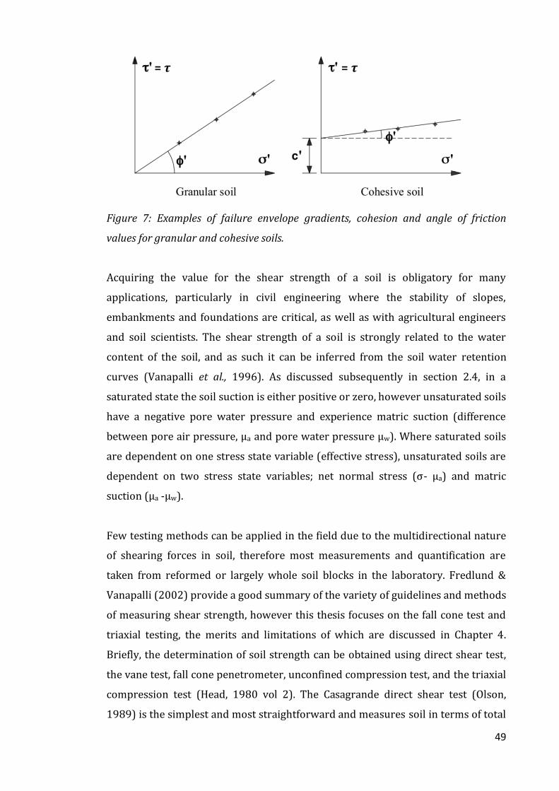
49

Figure 7: Examples of failure envelope gradients, cohesion and angle of friction

values for granular and cohesive soils.

Acquiring the value for the shear strength of a soil is obligatory for many

applications, particularly in civil engineering where the stability of slopes,

embankments and foundations are critical, as well as with agricultural engineers

and soil scientists. The shear strength of a soil is strongly related to the water

content of the soil, and as such it can be inferred from the soil water retention

curves (Vanapalli et al., 1996). As discussed subsequently in section 2.4, in a

saturated state the soil suction is either positive or zero, however unsaturated soils

have a negative pore water pressure and experience matric suction (difference

between pore air pressure, μa and pore water pressure μw). Where saturated soils

are dependent on one stress state variable (effective stress), unsaturated soils are

dependent on two stress state variables; net normal stress (σ- μa) and matric

suction (μa -μw).

Few testing methods can be applied in the field due to the multidirectional nature

of shearing forces in soil, therefore most measurements and quantification are

taken from reformed or largely whole soil blocks in the laboratory. Fredlund &

Vanapalli (2002) provide a good summary of the variety of guidelines and methods

of measuring shear strength, however this thesis focuses on the fall cone test and

triaxial testing, the merits and limitations of which are discussed in Chapter 4.

Briefly, the determination of soil strength can be obtained using direct shear test,

the vane test, fall cone penetrometer, unconfined compression test, and the triaxial

compression test (Head, 1980 vol 2). The Casagrande direct shear test (Olson,

1989) is the simplest and most straightforward and measures soil in terms of total

= 𝝉 = 𝝉

50

stress, during which the sample is slowly horizontally sheared until a point of

failure. The in-situ vane test, covered extensively by Chandler (1988), is a quick

and simple test that may be applied in the field to determine the undrained shear

strength of soil using an instrument with four blades. Penetrometers measure the

force required to push or drive a device into the soil and readers are directed to

Bengough et al., (2001) and Lowery & Morrison (2002) for extensive reviews on

soil penetrometers and penetrability.

Triaxial testing, covered in detail in Chapter 4, can be further divided into

unconsolidation-undrained test (UU), consolidated undrained test (CU), and the

consolidated drained test (CD). The UU test is the fastest where failure occurs

within 25 minutes and the drainage valves are closed, the CU test is sufficiently

slow to allow equalisation of pore pressure during consolidation, and the CD test is

slow enough to allow negligible pore pressure variation. This apparatus allows the

total control of parameters such as pore water pressure, consolidation and

shearing, which allows a thorough analysis of the characteristics of a soil under

shearing conditions.

2.4 Soil water

The following section covers the two most important soil water relationships, the

relationship between water content and suction and the hydraulic conductivity of

a soil. One of the greatest points of contention and a key argument of this thesis is

the lack of multidisciplinary terms for water in soil and in particular the lack of

wholesome parameters with which to determine how a soil responds to water,

where single and sometimes vague terms such as water holding capacity are

insufficient to describe a variety of soils to wetting and flooding (Kerr et al., 2016).

2.4.1 Important soil water relationships

The water content of a soil plays a crucial role in the physical and biological

functions of soil including water infiltration, redistribution and movement of water

through the soil, shear properties, germination of seeds, plant growth and

microbial functions. The interaction of the three soil phases (described in section

2.3.1) creates negative pore water pressure known as soil suction, which is a

51

critical component for the geotechnical properties of a soil. Suction is simply

defined as the potential energy of water within voids of a soil (unsaturated) in

comparison with ‘free water’ (Lu & Likos, 2004; Beckett, 2011), where the

relationship is briefly; the drier a soil, the greater the suction and the lower the

potential. Values for suction are expressed using negative kPa or pF (capillary

potential, which represent the logarithm of the suction expressed in cm of water,

Schofield, 1935), as water in voids has less potential than free water and can be

expressed using equation 4;

𝜓𝑚 = 𝐶(𝜅) + 𝐴 (𝑡)

Equation 4: Matric suction, where C is the capillary component described as a

function of the liquid-gas curvature 𝜅, and A is the adsorptive component as a

function of film thickness (t)) Gens (2010).

Osmotic suction occurs when a semi-permeable membrane separates two

solutions, one with a higher concentration of solute. This ‘membrane’ can be

created by clay particles that form very small voids (Beckett, 2011), and the

chemical potential is reduced. Matric suction, also known as capillary pressure,

occurs due to pressure from dry soil on its surrounding soil to equalise the

moisture content of the entire unit. The combination of matric and osmotic suction

is referred to as the total suction. There are three types of forces attributed to the

presence of water: adhesion (attraction of soil water to soil particles), cohesion

(attraction of water to water molecules), and capillary (through adhesion and

cohesion water can move through small tubes against the forces of gravity).

Figure 8: Stages of water retention in the soil matrix. (A) Gravitational water at

complete saturation, no air present (θSAT) (B) Capillary/meniscus water in

unsaturated soil, both air and water present between soil particles (θFC) (C)

Hygroscopic water at permanent wilting point, where only water adsorbed to soil

surface remains (θPW) from Kerr et al. (2016)

(A) (B) (C)

52

Wheeler & Karube (1996) suggest that water is held in four layers around soil

particles, and excludes water that is chemically combined (hydration) in the

mineral structure. The key properties of these different categories of water in soil

are shown in Table 3 and these four layers are;

- Hygroscopic adsorbed water held to the solid particle by electrical

attraction and unable to be removed by oven drying (Figure 8C)

- Hygroscopic water that cannot be removed by air drying but can be by oven

drying

- Capillary water, held by surface tension and removable by air drying

(meniscus water, Figure 8B)

- Gravitational water, removable by drainage (bulk water, Figure 8A)

WATER TYPE

Gravitational water (A) Capillary Water (B) Hygroscopic water (C)

Moves under the influence of

gravity

Mostly available for

plant growth

Not available to plants

Found in macropores

Held by cohesion and

adhesion in capillaries

(micropores)

Held on the particle surface

very tightly by adhesion

(high in clays due to high

surface area) caused by

forces of Van der Waals or

chemisorption

Moves rapidly out of well drained

soils

Quantity of water is a

function of pore space

(total volume) and pore

size

Force of gravity insufficient

to break the force between

soil and water molecule

Not available to plants

As soil dries, water

tension (kPa) increases

Removable by air drying

Only removed with heating

(oven drying)

Occupies air space, therefore can

drown plants

Leaves soil within 2-3 days

Table 3: Key properties of three soil water types; gravitational, capillary and

hygroscopic

53

2.4.2 Soil water definitions

Before the chapter progresses further, a list of soil water definitions is required as

many terms are used synonymously or incorrectly according to their original

definition, which is confusing to researchers and does not allow for confidence in

comparing values presented in literature. This section also discusses how some of

these terms are not adequate to cover the response to soil under conditions where

the soil changes over time physically (volume change) and at saturation. Table 4

gives definitions of water terms as used in this thesis and where applicable a

description and synonyms commonly associated with the term. These are derived

from as many sources as possible, and the given description is the best fit or a

standardised definition (e.g. as given by British Standards).

There are many different ways in which the mass or volume and distribution of

water in soil can be quantified, both directly and indirectly. It is important to know

the water content of a soil for a variety of applications such as the calibration of

climate models and use in agricultural/horticultural systems as it affects

parameters such as soil organic matter decomposition, soil respiration and carbon

sequestration (Bittelli, 2011). The measurement of soil water through direct or

indirect methods is standardised and simple (such as British Standards and ASTM

(American Society for Testing and Materials)) and will be discussed in Chapter 4.

However the definition or interpretations of ‘water holding capacity’ (WHC), or

maximum water holding capacity is exceptionally variable within soil science

literature and across other disciplines. WHC is used synonymously with other

descriptors such as; the water held at field capacity i.e. maximum amount of water

held in a soil against the forces of gravity OR the water available to plants (i.e. the

amount of water held between field capacity and wilting point). It is the use of

interchangeable terms that suggests the ‘maximum’ amount of water a soil can

hold is only the water held against gravity, meaning research on the end point of

the saturation scale i.e. flooding is limited by definition.

54

SOIL WATER TERMS (terms and description or alternative term)

Saturation All pores are filled with water. Air is no longer present in the pore space; therefore soil matrix is a two-phase

material with zero suction. This is not always equal to the pore space due to air trapped within the soil (usually 0-

10%) and saturation is usually 0.95 x porosity (effective saturation).

Effective saturation If air is present, saturation occurs when water fills all the pores that it can reach as air will still remain in the

smallest pores. This is more likely in the field than saturation as defined above.

Usually equal to porosity.

Degree of saturation The volume of water divided by the volume of voids, generally expressed as %. It is 100% when the soil is fully

saturated, and requires a knowledge of the total volume of the specimen.

Field Capacity

Drained upper limit

Moisture content of the soil after all gravitational water has drained and usually occurs 2-3 days after rainfall.

This is the maximum amount of water a soil can hold against gravity.

It can be measured using a value of 0.1 mm/day flux or the water held at a suction of -0.33 bars.

Maximum/Water holding

capacity (WHC)

(Maximum) water holding capacity is the amount of water held at full saturation without drainage (undrained).

Various additional definitions, where maximum WHC was originally defined as the most amount of water that can

be held at field capacity.

Wilting Point

Lower limit of extraction

Moisture content of a soil at which plants can no longer reach water within the soil. This is typically defined as -

1500 kPa.

Oven dry Soil that has been dried at 105°C for 24 hours.

Removes all types of water from the soil except adsorbed water (held to the soil particle by electrical attraction)

55

Plant available water Water that is held in the soil between field capacity and wilting point (-0.33 and -15 bar) and is able to be

utilised by a plant.

Generally considered to be approximately 50% of the field capacity.

Porosity

Pore Space

The volume of voids within a bulk of soil.

Calculated as the 1- (bulk density/particle density x 100). ‘

Pore size (distribution) The cumulative size of each pore within a soil.

Permeability

Hydraulic conductivity

These terms all describe the rate at which water is able to move through a body of soil through the pore

network, with values in mm or inches of water/time.

Infiltration rate The rate of movement of water into a soil from the surface

Percolation Downward movement of water within a soil.

Gravimetric water

content (GWC)

The mass of water to the mass of dry solids (dry basis GWC)

The mass of water to the total mass of the wet sample (wet basis GWC)

Volumetric water content

(VWC)

Θv = Θ (GWC) * Bd (OR) = Vw/Vs

Volumetric water content as originally defined.

Θv = Θ (GWC)* Bdi (OR) = Vwi/Vsi

Volumetric water content using the instantaneous volume of a soil (at the point of measurement).

where Vw = volume of water and Vs = volume of solids, Dd = dry density.

Suction The energy required for extracting a unit volume of water from soil, measured in kPa (Fredlund & Rahardjo,

1993).

56

Soil water retention

curve

The relationship between (matric) suction in a soil and the water content of a soil. Also called suction-water

content relationship, retention curves, moisture retention curves and numerous variations thereupon.

Matric suction The difference between the pore-air and the pore water pressure. The relationship between matric suction and

degree of saturation is presented in a soil water retention curve

Table 4: Important definitions for soil and soil-water relationships

57

The difficulty with defining soils in saturated or near saturated state is that the

meaning of ‘holding’ water is too broad; there is a distinct difference between

retain and hold. Water may retain a given volume of water under gravity when free

draining, but will hold or contain a given volume of water when there is static

water i.e. flood conditions. The concept of field capacity is used in most literature

as a key soil water indicator and is typically quantified using suction values to

determine the point at which all water has drained due to the force of gravity from

the largest pores in the soil and only water held against the force of gravity

remains. The typical definition is ‘moisture content of the soil after all gravitational

water has drained and usually occurs 2-3 days after rainfall’. It can also be

quantified using the flux values where field capacity is reached when the flux is

negligible (ml/hour), or in the lab the moisture content can be determined as

-0.33 kPa suction by calculating a soil water retention curve (SWRC) (see section

2.4.3). However field capacity is largely an academic value and not particularly

easy to apply to field conditions as strict laboratory processes control its

measurement. In reality, some soils take far longer than 2-3 days to drain freely

under gravity. Actual field capacity ranges from -10 to -20 kPa (Rose, 2004), for

soils with <20% clay and >20% clay respectively. It is not uncommon for soils to be

wetter than field capacity under free draining conditions should rainfall exceed the

drainage rate. We are interested in how much water a mass of soil can hold at

saturation and how it is retained once drying begins to occur, therefore the

concept of field capacity may only be applied during the drying phase.

As mentioned previously, the water holding capacity of a soil, here defined as the

maximum amount of water a soil sample can hold when undrained, can be

measured gravimetrically and volumetrically. These provide an index of the mass

or volume of water that a soil can hold, or give an indication of the degree of

saturation. Gravimetric water content (GWC) is referenced to a mass of solids,

whereas volumetric water content (VWC) and degree of saturation are based on

ratios of the original volume of a soil. However VWC doesn’t account for the

volume change of a soil under wetting as it swells, as it references the value back to

the original volume (based on mass and density), and not the instantaneous

volume and assumes that no or negligible volume changes have occurred

(Fredlund, 2002). Should the volume of a soil remain stable as the water content

58

increases, i.e. the soil is non deformable, the gravimetric, volumetric and degree of

saturation values can be referenced to the constant start value. However should

the volume increase as the water content increases, only gravimetric water content

can be referred back to the original constant. Commonly used methods to present

the water retention characteristics of a soil, such as a soil water retention curve

(SWRC, section 2.4.3) do not take into account the volume change of a sample, and

indeed one cannot compare the volumetric or gravimetric values without

knowledge of both. This is a major drawback of using single measurements to

determine soil change as used in an SWRC. Figure 9 shows the differences in how

values are presented, adapted from Kerr et al. (2016).

Figure 9: GWC, VWC and density of five samples to represent change during wetting.

Sample 1 represents the original sample, where samples 2-5 present theoretical

different changes in water content and volume during wetting (adapted from Kerr et

al., 2016).

In Figure 9, sample 1 is the original soil mass, volume and water mass, where

samples 2-5 represent various changes in water mass, volume, and density. Sample

2 has taken up 12.5 g of water but has not changed in volume as a result of

swelling. Sample 3 and 4 have taken up the same mass (and volume) of water as

Sample 2, however the bulk volume has changed. Sample 5 has taken up more

water than samples 2, 3 and 4 and has increased in volume. These changes result

in different gravimetric and volumetric water content values, due to the change in

density and volume of samples. It is clear therefore that the terms GWC and VWC

are not capable of describing the proportional physical changes in the soil, and

V = 175 cm3 Vw = 75 cm3

Mass = 250 g V = 125 cm3

Vw = 37.5 cm3

Mass = 212.5 g

V = 100 cm3 Vw = 25 cm3

Mass = 200 g

§

V = 150 cm3 Vw = 37.5 cm3

Mass = 212.5 g

SAMPLE 2 SAMPLE 5 SAMPLE 4 SAMPLE 3 SAMPLE 1

V = 100 cm3 Vw = 37.5 cm3

Mass = 212.5 g

59

only reference values to the original state. Soils that swell to a greater degree than

other soils under the same wetting conditions appear to perform more poorly

when assessing their volumetric water content (sample 3 vs sample 4). Therefore

it is imperative to record the instantaneous volume and mass of soil samples

during measurements over time in order to thoroughly assess the change (as seen

in Table 5), presented as VWCi (GWC * dry density of sample at the point of

measurement).

Sample Mass

(g)

Mass

of

solids

Mass

of

water

(g)

Volume

(cm3)

Bulk

Density

(g/cm3)

Dry

Density

(g/cm3)

GWC(%)

dry

basis

VWC VWC

(corrected)

1 200 175 25 100 2 1.75 14.3 25 25

2 212.5 175 37.5 100 2 1.75 21.4 37.5 37.5

3 212.5 175 37.5 125 1.7 1.4 21.4 37.5 30

4 212.5 175 37.5 150 1.42 1.17 21.4 37.5 25

5 250 175 50 175 1.43 1.0 28.6 50 28.6

Table 5: Summary of key changes to samples in Figure 9 (above) where VWC

(corrected) is the volumetric water content relative to the instantaneous volume of

the sample, not the original volume.

Samples 3 and 4 have the same water mass change, shown by the gravimetric

water content of change of 14.4 - 21.4 %, it is only an index of water content

change and is not affected by the physical parameters of a soil, it is a ratio of the

water to the dry mass of the soil solids. Volumetric water content, however, is

subject to structural changes of the soil mass as it is a ratio of volume of water

(which is directionally related to the mass) to the volume of the bulk (wet) soil.

Sample 2 and 3 have the same volumetric water content, despite Sample 2 having a

proportionally greater volume of water to total soil volume (37.5 cm3 water to 125

cm3 of soil in comparison to 37.5 cm3 to 150 cm3, respectively). Original VWC gives

an indication of the volumetric change in comparison to the original volume. The

instantaneous volume of the soil must be taken and used for the secondary

volumetric water content equation (using either the volume of solids or the dry

density (Dd) in addition to using the typical VWC equation in order to provide

60

accurate volumetric water content of the soil at the time of sampling. Fredlund

(2002) suggests that should a volume change occur during wetting, converting the

volumetric water content to gravimetric by assuming a specific gravity (definition

in section 2.2.2.) for the soil solids gives an accurate representation of real data

when the volume change is unknown.

2.4.3 Measuring soil water

The moisture content of a soil determines its behaviour, and measuring this value

under defined test conditions can provide classification in order to assess soil’s

engineering properties (Head, 1980). It can be expressed as the gravimetric water

content, volumetric water content, or degree of saturation. A simple method of

water quantification is to oven dry samples and obtain a dry mass, where samples

are oven dried at 105°C for 24 hours (Evett et al., 2008) and gravimetric water

content is expressed as a ratio of the mass of water to the mass of either the dry

solids (dry basis GWC) or to the total mass of wet solids (wet basis GWC) as

defined in table 4. However this thermo-gravimetric method is destructive and

allows a singular characterisation of the soil to be taken. Indirect methods allow in

situ measurements of soil water content by quantifying a proxy variable and using

empirical or physical relationships to calibrate the variable against water content.

Examples of indirect measurement include; dielectric methods (uses the

differences in electric permittivity values between solid, liquid and gas), resistivity

methods, neutron scattering, measurements of soil thermal properties. These

applications are useful in the field where the transport of samples is not viable

(such as a field study over time).

Although the quantification of gravimetric or volumetric water content of a soil is

essential, it does not provide information on the relationship between capillary

potential/pressure (suction) as a function of the degree of saturation, which is

critical for the understanding of soil processes such as infiltration, redistribution,

solute transport and compaction (Bachmann & R. van der Ploeg, 2002; Garcia et al.,

2014; Klute, 1986; Sorrenti et al., 2016). Knowledge of the water retention

characteristics of a soil is also important for understanding the behaviour of soil

materials in an unsaturated state (Fredlund, 2002; Fredlund & Xing, 1994; Toll et

al., 2015). Capillary pressure (suction) is directly affected by soil texture, particle

61

size distribution, pore space geometrics, interfacial tension, temperature, and

organic matter content (which directly affects water retention due to hydrophilic

nature and indirectly affects water retention due to soil structure modification).

The water retention of soils, i.e. the relationship between water content and

suction, can be described using a soil water retention curve (abbreviated

henceforth as SWRC). An SWRC provides important information on unsaturated

soils (Fredlund, 2000; Parvin et al., 2017) and can be used to define important

parameters such as plant available water, in the estimation of permeability (van

Genuchten, 1980), hydraulic conductivity (Mualem, 1976) and for the

interpretation of shear strength (Vanapalli et al., 1996), therefore its usefulness as

a soil indicator is widespread. Despite a wealth of research and knowledge on pore

space, the SWRC typically uses the volumetric water content and a simplified

representation of the pore system. As mentioned previously the SWRC therefore

ignores important physical effects such as volumetric change of soil, which limits

the accurate identification of the soil’s relative water content There are numerous

methods for determining the SWRC, which uses standardised procedures such as

the evaporation method (Gardner & Miklich, 1962) to produce a wetting and a

drying curve between 0 kPa suction (saturation) and 1500 kPa (permeant wilting

point), however each method has its own limitations (Tarantino et al., 2008).

The term hysteresis or hysteric refers to the phenomenon whereby water content

at a given pressure for a wetting soil is less than that of a drying soil (Klute, 1986).

This gives the ‘characteristic’ curves as shown below in Figure 10. Should a sample

begin in a saturated or close to saturated state and is subject to drying, it will

follow the primary drying curve (red, Figure 10). As water content decreases and

suction increases, the largest pores begin to desaturate (air entry value), followed

by drainage of finer and finer pores until residual suction is reached where there

are negligible water content changes with further increases in suction. Beyond the

point of residual suction, water is only held within the soil matrix adsorbed onto

clay particles (McQueen & Miller, 1974).

Should a sample start from an oven-dried state and then subjected to wetting, the

soil will follow the primary wetting curve. The water entry value is the suction at

62

which water enters pores, at which point the moisture content increases

significantly and suction decreases as the water content increases until suction

reaches 0, and the soil is saturated. The end point value of gravimetric water

content/volumetric water content is lower at the end of an absorption curve

(wetting curve is followed) in comparison to the start point value of an adsorption

curve (drying curve) due to irrecoverable shrinkage of the sample during drying or

air bubbles trapped within the soil pores that prevent full saturation (rendering

the sample effectively saturated, see section 2.4.2 for definition). If the wetting or

drying of a sample is interrupted, the soil will follow a scanning curve that returns

the soil to the alternative curve wetting or drying curve (Figure 10).

Figure 10: Typical soil water retention curve (after Toll et al., 2012).

2.4.4 Hydraulic conductivity

The speed of water movement through a soil is of significant importance, for

functions such as the supply of water to plants and aquifers and entry of water into

the soil (Klute & Dirksen, 1986). The hydraulic properties of the soil are a measure

of the conductivity and the water retention characteristics i.e. the ability to

transmit and store water, respectively. Permeability is the most variable

engineering soil property and can change by 10 orders of magnitude considering

the size range of particles (gravel – clay), as seen in Table 6.

63

Saturated hydraulic conductivity

Classes Micrometres per second Centimetres per hour

Very high Over 100 36

High 10- 100 3.6 - 36

Moderate 1- 10 0.36 – 3.6

Moderately low 0.1 – 1 0.036 – 0.36

Low 0.01 – 0.1 0.0036 – 0.036

Very low Less than 0.01 Less than 0.0036

Table 6: Hydraulic conductivity classes based on speed on water movement (Foth,

1991)

𝑘 =𝑞𝐿

𝐴ℎ

Equation 5: Hydraulic conductivity (k), where q is the permeability coefficient (flow

in m3/second), L is the length of the sample in m, A is the cross-sectional area of the

soil (m2) and h is the pressure head (in m). Craig (2004).

The relationship between the rate of permeant flow and hydraulic gradient was

discovered by Darcy (1856). The coefficient of permeability (used synonymously

with hydraulic conductivity) states that the discharge velocity of flow through a

porous medium is proportional to the hydrostatic pressure causing flow (hydraulic

gradient) and inversely proportional to the permeant viscosity. The formula in

Equation 5 applies Darcy’s Law and is used to derive the hydraulic conductivity

obtained from a constant head test. There are a number of factors that affect how

quickly water moves through a body of soil; particle size distribution, void ratio

(porosity), soil structure, state of stress or stress history (i.e. compaction), degree

of saturation, thixotrophy (term discussed below), and gradient (Reid, 1988: Head

1980 vol 2).

Firstly, the particle size distribution of a soil governs the porosity to a large extent

(Chan & Govindaraju, 2004) and therefore conductivity, as smaller particles create

smaller voids that increase the resistance the flow of water. It is common for the

conductivity of a soil to be related to the void ratio of a soil, where the higher the

void ratio (volume of pores to the volume of soil), the greater the conductivity due

to a higher number of flow paths. The caveat, however, is that two identically

prepared samples may have different conductivities due to tiny differences in soil

64

structure, despite having the same void ratio. Therefore although important, the

void ratio only governs the conductivity to a limited extent and it is rather the

distribution of voids (tortuosity) through the soil matrix that is important.

Secondly, as discussed previously (2.3.1), the structure of soil is dependent on its

forming factors, compaction, water content and organic matter content. Soils that

are compacted dry of optimum (see 2.3.3) take up much more water than soils

compacted when wet of optimum as they have multidirectional permeability due

to random soil particle orientation. Once a soil has been compacted, the resultant

density of the soil influences the infiltration rate (speed at which water may enter

the soil) is a direct function of the density of a soil, and ultimately determines the

maximum water content of the soil (Figure 11).

Figure 11: Maximum water

content as a function of bulk

density (from Taylor &

Gardner, 1963)

Thirdly, the degree of saturation is also crucially important in permeability

measurements. Darcy’s Law assumes saturation, but if water does not fill all voids

within a soil, air bubbles can block the flow of fluid, which therefore invalidates the

assumption (Head, 1980). Soils with a high number of air filled voids have lower

conductivity (Olson & Daniel 1981) than pores saturated or partially filled with

water. Barden & Sides (1970) reported a difference of 60-100% in hydraulic

conductivity as a function of the saturation level.

Fourthly, thixotrophy (the ability of a soil mass to gain strength over time) affects

the results of laboratory derived hydraulic conductivity, and indeed other tests.

Disturbing the soil creates some alignment of particles during compaction, but

65

over time the soil will return to a more flocculated state. Mitchell et al. (1965)

compared specimens immediately after preparation and 21 days after preparation

and reported greater conductivities in the latter samples. This effect, depending on

the water content at preparation, can be in the order of a magnitude difference in

conductivity (Dunn, 1983). Lastly, the gradient (differences in head) in laboratory

testing is artificially increased to speed up the processes of testing, however this

consolidates the sample through axial deformation, which in turn causes particle

migration and closing of macrospores. Darcy’s Law assumes laminar flow; but

artificially increasing the gradient is likely to cause turbulent flow (Reid, 1987). In

combination, the increased gradient reduces the hydraulic conductivity of a

sample.

2.4.5 Measuring hydraulic conductivity

Hydraulic conductivity for unsaturated soils can be measured in the laboratory, in

the field using suction and tensiometers to measure the change, which includes the

instantaneous profile method (Daniel, 1982; Munoz et al., 2008), the Gardner

(1956) or Corey’s method (Green & Corey, 1971) in various types of infiltration

column (Duong et al., 2014), and it can be predicted empirically using the SWRC

(Fredlund et al., 1994). For the most accurate assessment of soil hydraulic

properties, they should be measured directly whenever possible, therefore the use

of empirical methods for estimating hydraulic conductivity will not be discussed

further. Testing hydraulic conductivity in a saturated soil can be done using the

falling head or constant head test, or alternatively in a triaxial cell (as described in

Chapter 4). For simple and rapid testing of hydraulic conductivity, the falling head

test uses water in a piezometer (tube) to provide a pressure head (water pressure

in terms of the height of a column above the datum level, Head 1980) that passes

through a saturated sample of fine-grained soil. The constant head test provides a

continuous flow of water at the same pressure, used to test clean sands or large

grained soils.

66

Figure 12: Triaxial cell apparatus set up for testing hydraulic conductivity and shear

strength. A high air entry (HAE) porous stone is at the base of the specimen with an

HAE value of 100 kPa. Water pressure is measured at the base (pore water pressure

μw) and air pressure measured at the normal porous stone at the top of the specimen

(pore air pressure, μa). From Lu & Likos (2004).

Controlled tests hydraulic conductivity can be also conducted using triaxial cell

apparatus where the suction, water content, pore water & air pressure, and rate of

flow through the sample can all be controlled and monitored. As per the set up in

Figure 12, the sample tested in a triaxial cell has a porous filter stone at each end

with tubing containing the length of the sample.

2.5 Concluding remarks

This chapter has outlined the fundamental knowledge base for the research

contained within the thesis, including an introduction to the various important

mechanisms of soil pedogenesis, and critical interactions between soil minerals,

organic matter and external influences that determine the make-up of a soils; its

texture, structure, relationship with water, erodibility and shear strength

characteristics. The most important findings from a review of literature are as

follows:

Axial loading ram

Confining cell

Coarse porous stone

Specimen

Membrane

HAE disk

Pedestal

Confining stress Pore water Pore air pressure pressure

Deviator stress

67

Current definitions surrounding soil, soil water and soil parameters such as

density are insufficiently determined. There are no universal definitions for

terms such as water holding capacity or soil erodibility. As it is unlikely that

a universal term will be used, each research piece needs clear definitions of

what they determine to be, for example, the water holding capacity;

o Here, the water holding capacity is stated as the maximum water

content of a soil at saturation. Other documents use the field capacity

as the water holding capacity.

o Soil erodibility has no universal method of quantification, rather a

number of indicators that may suggest how erodible a soil is to a

water input, which may either be the resistance to degradation

under wetting through rainfall or submersion. Soil erodibility may

also be inferred indirectly through quantification of organic matter,

the presence of clay and water content.

As summarised in Kerr et al. (2016), the quantification of water in soil on

both a gravimetric and volumetric basis, after a soil has been subjected to

wetting is inconsistent.

o Gravimetric water content must be reported on a dry or wet basis,

without this statement the quantification, one cannot compare

literature.

o Volumetric water content is typically reported according to the

original volume of soil, however under wetting most soils swell.

Therefore the volumetric water content value, should the original

volume be used in the calculation, is incorrect. In order to provide

values that compare the original volume of soil to the volume of

water to a change in the same sample after water uptake and volume

change, the instantaneous soil volume must be used in calculations.

68

3. Water Treatment Residual (WTR)

This chapter explores the production, storage and disposal processes and

physiochemical characteristics of water treatment residual (WTR) with specific

reference to waste produced in the NE of England by Northumbrian Water Ltd.

(NWL). Much of the information on water treatment processing has come from

personal communication with Luke Dennis (NWL) conducted by Finlay (2015),

supplemented by personal communication with Ed Higgins (NWL).

3.1 An introduction to WTR production, storage and disposal

There are 27 different companies across the UK that produce the 5.29 trillion litres

of clean water used in the UK each year. Eight companies provide more than 75%

of the water; Thames Water provides 18.2% of this, followed by Severn Trent

Water 12.6%, United Utilities 11.8%, Yorkshire Water 8.5%, Anglian Water 8.1%,

Affinity Water 6.1%, Dŵr Cymru Welsh Water 5.5% and Northumbrian Water

4.7%. Although one of the smaller companies, Northumbrian Water alone has 55

treatment works, supplying 1.1 billion litres of water every day to 4.4 million

people in the North East of England (Northumbrian Water Ltd [16]). The

remaining 19 companies account for less than 25% of the remaining supply.

‘Clean water treatment’ refers the production of potable water using raw water

from groundwater (aquifers and springs) and surface water sources (streams and

rivers), as opposed to ‘wastewater treatment’, referring to the processing of water

containing sewage, agricultural waste and industrial sources of pollution. The

primary aim of the clean water treatment process is to remove contaminants to

produce water that meets particular thresholds for human consumption, as

dictated by the governing body responsible for the water being produced. This

includes pathogens e.g. bacteria, viruses and eggs of parasitic worms, potentially

toxic chemicals from human activity e.g. fertiliser, and natural chemicals e.g.

fluorides, arsenic and those influencing smell, colour and taste. The success of

using the coagulant-enhanced flocculation and settlement method, which is

common practice for 70% of water treatment works, relies on the removal of

turbidity and organic matter such that the water falls within the maximum

permitted concentration levels of turbidity according to drinking water standards

69

(Keeley et al., 2014). Crittenden et al. (2012) provide a good summary of important

constituents commonly found in water sources (Table 7).

Table 7: Summary of important particulate, chemical and biological consituents

found in water according to their source (Crittenden et al., 2012, adapted from

Tchobanoglous and Schroeder, 1985)

Typically water in NE England is sourced predominantly from surface water

sources such as rivers that contain suspended (>1.0 μm), colloidal (0.001-1 μm)

and dissolved particles (<0.45 μm), the remaining water being taken from

groundwater sources. Northumbrian Water, for example, takes 85.5% of its water

Source Particulate constituents Ionic and dissolved constituents Gases and neutral species

Collodial Suspended Positive ions Negative ions

Contact of water

with minerals,

rocks and soils

(e.g. weathering)

Clay

Silica (SiO2)

Ferric oxide (Fe2O3)

Aluminium oxide

(Al2O3)

Magnesium dioxide

(MnO3)

Clay, silt,

sand and

other

inorganic

soils

Calcium (Ca2+)

Iron (Fe2+)

Magnesium (Mg2+)

Manganese (Mn2+)

Potassium (K+)

Sodium (Na+)

Zinc (Zn2+)

Bicarbonate (HCO-)

Borate (H2BO3-)

Carbonate (CO32-)

Chloride (Cl-)

Fluoride (F-)

Hydroxide (OH-)

Nitrate (NO3_)

Phosphate (PO43-)

Sulphate (SO42-)

Carbon dioxide (CO2)

Silicate (H4SiO4)

Rain in contact

with atmosphere

Hydrogen (H+) Bicarbonate (HCO-)

Chloride (Cl-)

Sulphate (SO42-)


Nitrogen (N2)

Oxygen (O2)

Sulphur Dioxide (SO2)

Decomposition of

organic matter in

environment

Humic substances Cell

fragments

Ammonium (NH4+)

Hydrogen (H+)

Sodium (Na+)

Bicarbonate (HCO-)

Chloride (Cl-)

Hydroxide (OH-)

Nitrate (NO3_)

Nitrite (NO2-)

Sulphide (HS-)

Sulphate (SO42-)

Ammonia (NH3)


Hydrogen sulphide (H2S)

Hydrogen (H2)

Methane (CH4)

Nitrogen (N2)

Oxygen (O2)

Silicate (H4SiO4)

Living organisms Bacteria, algae,

viruses.

Algae,

diatoms,

minute

animals, fish

etc.

- - Ammonia (NH3)


Hydrogen sulphide (H2S)

Hydrogen (H2)

Methane (CH4)

Nitrogen (N2)

Oxygen (O2)

Municipal,

industrial and

agricultural

sources and other

human activity

Inorganic and organic

solids, constituents

causing colour,

chlorinated organic

compounds, bacteria,

worms, viruses etc

Clay, silt, grit

and other

inorganic

solids,

organic

compounds,

oil,

corrosion

products etc.

Inorganic ions, including a variety of

anthropogenic compounds and heavy metals,

organic molecules, colour etc.

Chlorine (Cl2)

Sulphur dioxide (SO2)

70

from surface sources, 4.5% from ground sources and 10% from mixed sources. In

comparison with groundwater, there is a significantly greater quantity of natural

organic matter (NOM) and inorganic material (from the weathering of rocks) in

surface water. The presence of NOM, a complex matrix including components such

as zooplankton, bacteria, viruses, clay-humic acid complexes, humic acids, proteins

and polysaccharides (Bolto & Gregory, 2007), has several effects on water quality

and creates significant issues during the process of water treatment as it reacts

with metal ion coagulants. Typically the quantity of NOM is indicated using total

organic carbon (TOC) as a proxy measure where NOM is approximately twice the

concentration of TOC. Groundwater sources commonly have TOC ranges of

0.1-2 mg/L and surface sources have a TOC range of 1-20 mg/L (Crittenden et al.,

2012). The concentration of NOM in the water source and pH often determines the

coagulant dose, as at a higher pH NOM is more ionised and the number of essential

positive charges on metal coagulants are reduced (O’Melia et al., 1999). Suspended

particulates, mainly inorganics such as silica, aluminosilicates, iron oxides,

manganese oxides and organics, which range from 10 μm to sub-micron colloidal

size (Thurman, 1985), supply an adsorption surface for microbes and humic

substances that to some extent protects them from the disinfection process in

water treatment. The presence of dissolved organic compounds (materials that

pass through a membrane with pores of <0.45 μm) causes discolouration of water,

taste and odour in addition to the potential formation of carcinogenic chlorinated

hydrocarbons during disinfection with chlorine.

Water treatment is therefore a stringent process to remove the large range of

differing sizes of organic and inorganic particulates. The process of extracting

these particulates is difficult because the negative charge of each particle enables

to them to be held in suspension for many days, meaning that natural

sedimentation of water for clarification would be infeasible as a treatment method

considering the demand for clean water. Particulates only settle when they lose

their negative charge and are then able to coagulate with other particles, but the

range of pH at which different particles lose their charge is wide ranging (2-12

pH). This presents difficulty for the water companies and the treatment process

requires the careful use of pH regulators. In the majority of treatment plants a pH

of between 6 and 8 is maintained to complete the necessary processes whilst

71

avoiding accelerated corrosion of equipment that occurs at lower pH range

(Crittenden et al., 2012).

3.1.1 Water processing and production of WTR

Drinking water production has approximately 11 stages, from abstraction of the

raw water until the point at which water exported from the plant is fit for human

consumption. Briefly, the steps of water treatment are as follows (Thames Water,

2014 [17]) where WTR is removed from the process at the sedimentation stage

(5); subsequent water processing information is only included for informational

purpose. Figure 13 on page 72 describes the processing of WTR removed at the

sedimentation stage.

1. Abstract of raw water – Water is taken and pumped to the treatment plant

from surface sources (rivers and streams) and groundwater sources

(aquifers and springs).

2. Reservoir storage – water is held on a long-term basis before use, here there

is natural settling of some contaminants and breakdown of organic matter

by UV radiation in sunlight and organism action. This also evens out any

temporal changes in water quality.

3. Screening – graduated metal grills (5-15 cm spacing) remove large debris

such as twigs, leaves and man-made detritus. Fine screens (5-20 mm

spacing) trap smaller debris during movement of water from reservoir to

treatment plant. Where raw water is of particularly poor quality cascades

are primarily used to increase dissolved oxygen content, to reduce carbonic

acid content and raise the pH (limiting the corrosiveness of water).

4. Clarification – coagulants, flocculent aids and pH regulators are released

into the water during rapid mixing to remove fine particulates (or colloids)

such as clay, silt, organic materials and metal oxides that cannot be

removed by filtering or natural sedimentation alone.

5. Sedimentation – Water that has been dosed with coagulants, flocculation

aids and pH regulators is retained in sedimentation tanks for the required

period for the smallest particles to settle out of suspension with slow water

movement (0.1-0.3 m/s, WHO, 1996). This allows coagulated particles to

flocculate, creating larger flocs. If the speed of water movement is too fast,

72

flocs breakdown. The settled particles form a sludge (WTR), at the bottom

of the tank, which is then extracted for further processing (see Figure 13).

6. Filtration – After the majority of particulate matter has been settled out of

suspension, the remaining solids are removed by sieving the material

through rapid gravity filters made from gravel, sand and charcoal and then

through slow fine sand filters.

7. Aeration – removal of compounds and dissolved metals by oxidation in

order to make subsequent removal more efficient.

8. Granular Activated Carbon (GAC) – water is passed through porous carbon

particles to remove organic compounds, chemicals such as pesticides as

well as removal of odour and taste.

9. Ozone dosing – highly reactive ozone helps to breakdown organic material

and pesticides that are not effectively treated in the previous step.

10. Disinfection – typically water is dosed with chlorine for a sufficient time

period to kill micro-organisms.

11. Ammoniation – addition of ammonia encourages long lasting disinfection by

combining with chlorine to form chloramines.

73

Figure 13: Schematic diagram of clean raw water in a water treatment production

plant (Crittenden et al., 2005)

The clarification and sedimentation of materials removed from the raw water are

the initial processes in water treatment, as shown in Figure 13. The term water

treatment residual (WTR) or water treatment sludge encompasses any liquid,

semi-solid, and solid phases of by-product removed during the clean water

treatment process. From herewith in we use the term WTR. Although residuals can

originate from 22 of the processes in the treatment plant, producing solid and semi

solid waste, liquid waste and gaseous waste, here the term WTR refers to the

WATER IN

INLET SCREENING (Stage 3)

INLET MIXING CHANNEL (Stage 4)

Coagulant (Alum and Fe), Sulphuric Acid Dosing, DADMAC dosing, Poly-electrolyte dosing

CLARIFICATION & SEDIMENTATION

TANK (Stage 5)

CLARIFIED WATER TO RAPID GRAVITY FILTERS FOR FURTHER TREATMENT

SLUDGE COLLECTION

SLUDGE BUFFER TANK

Polyelectrolyte dosing SLUDGE

THICKENER TANK

SLUDGE PRESS

SLUDGE TO LANDFILL OR

STORAGE

74

sludge resulting from the chemical precipitation of incoming waters only. Other

waste produced from the plants may include waste from the initial screening

process between reservoir and treatment plant or spent sorbents used in the

treatment process to sorb constituents such as arsenic, fluoride or remove

hardness.

Coagulation is defined by Crittenden et al., (2012) as the addition of a chemical to

water with the objective to destabilise particles, so they aggregate or form a

precipitate that will sweep particles from solution or absorb dissolved

constituents. As outlined above, coagulant is added to take colloidal particles that

are present in the incoming water out of suspension by removing the negative

charge. This allows particles to coagulate together, flocculate into a larger mass of

particles and settle out of suspension. The type and dose of coagulants chosen in

the specific water treatment plant depends on the characteristics of source water,

such as NOM concentration, temperature, and type of particulates present.

Coagulants used in the UK for the water treatment process are hydrolysing metal

salts, typically aluminium sulphate (Al2(SO4)3) or ferric sulphate (Fe2(SO4)3),

however there are also a number of other common coagulants available including

prehydrolosed alum and ferric chloride. Typical precipitation reactions for iron

and alum-based coagulants can be found in Crittenden et al., (2012) however

essentially the end products of the precipitation and dissociation reactions to form

metal hydroxides are AlOH3 and FeOOH depending on the type of WTR. A total of

0.53 kg sludge/kg of ferric sulphate and 0.66 kg sludge/kg of ferric chloride on a

dry solids basis is typically produced in these reactions, not including the addition

of polymers for increased coagulation. These insoluble hydroxides adsorb onto the

negatively charge surface of particulates in the water, meaning the repellent force

keeping them in suspension is lost and the coagulation process can begin. Both the

zero point of charge of ions and the functionality of the coagulants are dependent

on pH, therefore regulators such as calcium hydroxide (Ca(OH)2) or sodium

carbonate (Na2CO3) are added to ensure the water is within the operating region of

coagulant chemicals, 5.5-7.7 pH for Al and 5-8.5 pH for Fe (Crittenden et al., 2012).

Flocculent aids, such as polyelectrolytes (anionic, cationic or non-ionic), poly-

DADMAC (polydiallydimethyl ammonium chloride), and sodium alginate, are often

75

added to accelerate the formation of larger and stronger flocs by adsorbing to

destabilised particles and creating bridges. This speeds up the sedimentation

process as larger flocs settle more quickly according to Stokes Law (Bolto &

Greogory, 2007). Typically synthetic organic cationic and anionic polymers are

selected as they are cheaper than their natural organic counterparts as effective

flocculent aids, but the specific choice depends on the sludge properties and

mixing environment (O’Brien & Novak, 1977).

After the clarification stage (4) the water dosed with coagulant, flocculent aid and

pH regulators is then piped to sediment tanks, the design of which varies at each

treatment plant. During the sedimentation stage (5) the principal in each tank is

the same, an inlet channel at the top of the tank delivers water that is slowly mixed

in order to increase the contact of coagulated particles and form larger flocs that

are quicker to fall out of suspension. This however requires a slow flow in the

settling zone of 0.1-0.3 m/s to retain links between the larger flocs. The flocculated

particles form sludge (which is now termed WTR) at the bottom of the tank, which

is then mechanically extracted. Once the sludge has been removed from the

sedimentation tank it is dewatered using centrifuges. In some plants further

flocculent aid, e.g. poly-DADMAC, is added to the sludge at this stage essentially to

squeeze the water out of the flocs by inward movement of the particles within it.

Depending on the process chosen by the plant, WTR is either exported as sludge, if

dewatered by centrifuge, or as a ‘cake’ if a filter press is used to dewater by

compacting the sludge. Dry solid concentrations range between 1 and 6% with the

use of polymers in the sludge thickener tank, after which centrifuges, filters or belt

presses achieve a maximum of around 20% dry solids. Less expensive or less

energy intensive options are available at this stage, such as lagoons and drying

beds but require large areas of land (Fulton, 1976). Each WTR produced by this

process will have different chemical characteristics depending on the raw water

source used, but is directly related by the choice of chemicals used during

treatment.

3.1.2 Water Treatment Residual management and disposal

The initial processes of removing matter from raw water produces vast quantities

of sludge; the UK uses more than 325,000 tonnes of coagulant per year (Henderson

76

et al., 2009), which costs ~£28 million. Sludge production is increasing because of

population growth and temporal changes in raw water quality due to climate

fluctuations. In a report published in 2014 (Water UK Standards, 2014), UK

production of WTR sludge was approximated to be 131,000 tonnes (of ‘dry’ solids,

approximately 655,000 wet tonnes), 44% of which is Al based, 32% Fe sludge, and

the remaining 24% of sludge attributed to ‘other formats’. 75,980 tonnes (60%) of

produced sludge was disposed of via landfill, 37,990 tonnes (28%) to sewage

works for further treatment and the remaining 17,003 tonnes (12%) disposed of

via ‘minor’ disposal routes such as spreading to agricultural land, use as soil

conditioners, and use in brick and cement production (Water UK Standards, 2014).

The greatest challenge to the water industry, according to the Water UK standards

report, is the treatment and disposal of the ~100,000 tonnes of coagulant based

sludges produced per year, a figure which has likely increased in the four years

since the publication was released. All countries in the EU must comply with the

1998 EU Drinking Water Directive (98/83/EC), under which the Drinking Water

Inspectorate (DWI), a UK independent body that was formed in 1990, regulates

each regional water company in England, Wales and N. Ireland (the Drinking

Water Quality Regulator oversees Scotland) to ensure that companies abide by the

rules and regulations stated by the EU directive.

WTR cannot be sent for biological digestion or incineration due to low calorific

value, in contrast to sludges produced by wastewater works (sewage) for which

this is common practise (Ulmert & Sarner, 2005). The potential high concentration

of PTEs and metals in the WTR as well as the high water content further limits

disposal methods. To discard the waste from water treatment plants in an

environmentally appropriate way, potentially toxic constituents of WTR must be

identified before disposal and be compared to the lowest acceptable presence or

concentration of a substance, e.g. arsenic as defined by local legal standards.

In the UK prior to 1960 there were very few regulatory constraints on WTR

therefore it was typically discharged into local water bodies as a return to source

(Elliot et al., 1990), stored in artificial lagoons or spread directly onto land, which

could potentially lead to negative environmental and aesthetic impacts such as

discoloration of local water sources and turbidity. The physical properties of the

77

WTR specific to each plant define how the responsible producers must process the

waste. Currently there are a number of options currently under research for

environmentally sound alternatives for the disposal of WTR via landfill, which

include disposal on land as soil amendment (requires a special licence from the

Environment Agency) or co-amendment with wastewater biosolids (sewage

sludge) and organic matter (discussed extensively in section 3.3), discharge to a

wastewater collection system, or reuse in building and fill materials. As they are

the easiest forms of disposal, landfill and land spreading are the options typically

chosen (L. Dennis, pers comms, 2015).

WTR is tested to determine how it may be disposed of using leachate tests, in

which WTR is exposed to a mildly acidic solution similar to what may be found in

municipal waste plants and the resulting leachate exposure is tested for the

concentration of toxic elements, according to the waste acceptance procedures

outlined by The Landfill Directive. The majority of WTRs tested in this way are

non-hazardous, therefore landfill is an appropriate (but not sustainable) method

for disposal. WTR disposed of via landfill is typically transported from the water

treatment plant in haulage trucks; as the transport and landfill fees are charged

per mass, WTRs are dewatered to the minimal volume that is economical (Keeley

et al., 2014).

Landfill is regulated by the Landfill Directive (Council Directive 1999/31/EC) and

has three classifications; hazardous waste, non-hazardous waste and inert waste.

Landfill had previously been recognised as the ‘best practicable environmental

option’ for the disposal of particular waste types, including WTR, however the

implementation of landfill tax in 1996 as a deliberate policy intervention to find

more sustainable reuse of waste has made this an ever decreasingly economical

option; since 1996 the tax has increased from a standard rate of £7 per tonne to

£82.60 per tonne from April 2015. Lower risk wastes, i.e. ‘naturally occurring

materials’ determined by the Waste Framework Directive (2008/98/EC) and the

Landfill Tax Order, have a tax of only £2.60, usually determined by the LOI test

where wastes <10% qualify for the lower band of tax. WTRs are considered an

inert waste and are charged as per the lower band. Considering that the UK

produces approximately 655,000 tonnes of WTR per year, this would raise an

78

annual disposal cost of £2 million should it all be disposed of via landfill. The

limitations for the addition of waste to landfill are as follows according to the

Council Decision (2003/31/EC). For waste to be accepted for landfill they must

comply with the limits outlined in Table 8.

The increasing levies on landfilling enforced by the government have forced water

companies to investigate alternative disposal strategies (Keeley et al., 2014). Since

2008 the Environmental Permitting Regulations have monitored waste

management activities, however these are now called Environment Agency

standard rules (2016 [18]). The Standard Rules regulate the quantity of waste

allowed to be applied during one year, where WTR is classified as ‘sludges from

water clarification’ (List B: waste code 190902), under the general bracket of

recover or use of waste on land. Standard rules 2010 No 4 (mobile plant for land-

spreading), No 5 (mobile plant for reclamation, restoration or improvement of

land), No 11 (treatment to produce aggregate or construction materials) and No 12

(treatment of waste to produce soil, soil substitutes and aggregate) all allow WTR

to be applied to land with a number of limitations. Table 8 highlights the typical

values for WTRs in the UK, Mosswood specific details and a comparison with soils,

and biosolids. These values are assessed against limits for land application, based

on two directives, the Sludge directive (and the BSI PAS 100 specification (which

sets a minimum compost quality baseline for biowastes) as currently there is no

particular directive for water treatment sludge.

Briefly, these detail that the application is not permitted in the following areas:

within groundwater source protection zone 1, 10 m of a watercourse, 50 m from

any spring, well, or any borehole used to supply water for domestic or food

production purposes, nor 50 m from any well, spring or from any borehole used

for the supply of water for human consumption. The application is also not

permitted within 250 m of the presence of Great Crested Newts, where it is linked

to the breeding ponds of the newts by good habitat, nor within 50 m of a site that

has relevant species or habitats protected under the Biodiversity Action Plan that

the Environment Agency considers at risk to this activity, nor within 50 m from a

National Nature Reserve (NNR), Local Nature Reserves (LNR), Local Wildlife Site

(LWS), Ancient woodland or Scheduled Ancient Monument.

79

Table 8: Concentration of PTE in WTRs as derived by Finlay (2015), Elliot (1990),

McBridge (1994), BSIPAS-100 specification, and Sewage Sludge Directive

86/278/EEC. Underlined = exceedance of PAS-100 regulations

The main concerns for application on land are due to concerns over aluminium

based coagulant sludges becoming mobile at pH <5, and deficiencies in P as a result

of either Fe or Al based WTR application which stunts plant growth and causes

induced phosphate deficiency in plants (see section 3.2.3). Before the application

of waste to land, it must be analysed thoroughly to indicate all substances that may

be reasonably expected to be present, i.e. evidence of potential nutrients, and

whether the sludge presents any agricultural benefit to where it’s being applied, in

addition to any potential contaminants that may harm the land. Evidence must also

be provided that application of waste will not cause the build up of PTEs

(potentially toxic elements) to harmful levels. Table 9 presents the potential

benefits and negative impacts of land spreading of WTR according to the Natural

Resource Wales (2017 [19]) advice on the Standard Rules. Currently there is a

significant body of research on the effect of adding WTR to soil (discussed in

section 3.3), however concerns over the long-term effects of land application have

meant that this method of disposal is still limited.

WTR Cd

(mg/kg)

Cr

(mg/kg)

Cu

(mg/kg)

Hg

(mg/kg)

Ni

(mg/kg)

Pb

(mg/kg)

Zn

(mg/kg)

Mosswood 2.36 ±

1.42 31.5 ± 7.2 27 ± 8

0.28 ±

0.25 92 ± 35 85 ± 72

665 ±

405

WTR range 0.2 - 3.6 7.8 - 39 7.9 - 36 0.06 - 1.4 10 - 120 4 - 160 28 -

1100

Soil range 0.06 - 1.1 7 - 221 6 - 80 0.02 - 0.41 4 - 55 10 - 84 17 - 125

Biosolids

typical 0.1 - 13.6 28 - 509

25 -

2481 0.1 - 2.0

2.6 -

389

8.1 -

850

32 -

2070

PAS-100

regs 1.5 100 200 1 50 200 400

Biosolids

regs 20 / 1000 16 300 750 2500

80

Potential benefits Potential negative impacts

Nitrogen and potassium source from

bacterial cell debris

Precipitated phosphate

Source of secondary plant nutrient,

sulphur

May contain trace elements e.g. Mg

May contain a significant amount of

organic matter (is raw water source is

from peaty soil)

Sludge may provide sand and fine grit

for the improvement of heavy soils, and

also adding body to medium and lighter

soils

Some sludges can providing a liming

benefit

Iron staining on crops

Elevated aluminium levels in soil

Phosphorous availability limitation at

extremes of pH (optimum between pH

6 and 7)

At low pH Al, Mg, Mn, Fe and Zn become

more available and may induce plant

toxicity.

Damage to roots through cell division

inhibition and reduction in transport of

P from roots to shoots.

Table 9: Standard rules summary of positive and negative impacts of land spreading

of WTR (Natural Resources Wales, 2017).

3.1.3 Northumbrian Water WTR disposal

The following information has been obtained via personal communication with

Luke Dennis and Ed Higgins. Table 10 below presents a summary of WTR

produced by Northumbrian Water between 2010 and 2018 (includes Essex and

Suffolk production), which highlights that all WTR is disposed of via land

spreading with application rates of up to 120 tonnes per hectare (in non-nitrate

vulnerable zones). Considering that Northumbrian Water only produces 4.7% of

clean water in the UK, total annual figures may total around 1.49 million wet

tonnes (around 300,000 total dry solids), which is almost double the 131,000 total

dry solids estimated in 2014 by the UK Water Standards (2014). For biosolids the

application rate tends to be about 17 tonnes/Ha (and will be lower in Nitrate

Vulnerable Zones) whereas WTR, due to its much lower nutrient levels, can be

81

applied up to 120 tonnes/Ha. This value is up to the discretion of the Environment

Agency (EA) and if necessary, the EA can request only 80 or even 60 tonnes/Ha is

applied.

WTR type Total WTR

produced

(wet tonnes)

Ferric-

WTR

(%)

Alum-WTR

(%)

Alum/

Ferric mix-

WTR (%)

Disposal route

2010-11 69666 80 13.5 6.5

Recycled to

land

2011-12 64871 78.4 13.9 7.7

2012-13 62871 76.4 16 7.6

2013-14 55966 72.1 14.7 13.2

2014-15 61235 67.2 17.8 15

2014-15 73331 Total dry solids 13973 WTR to

agriculture

under permits

Waste recovery

permit

2015-16 78253 Total dry solids 14610

2016-17 75835 Total dry solids 13411

2017-2018 78599 Total dry solids 14488

Table 10: WTR production figures from Northumbrian Water Ltd, 2010 – 2015

(Finlay, 2015 via pers comm L Dennis, NWL), and WTR production figures from

2014-2018 from Greenhouse Gas Data Returns, which include Essex and Suffolk

values (pers comms E. Higgins, NWL)

Almost all WTR produced by NW is recycled to land under the Environmental

Agency Standard Rules, however other companies do not recycle to the same

extent and rely on landfill. Some WTR went to different outlets in 2015 (reasons

undisclosed), but in general NW avoid landfill due to its vast expense and instead it

is taken to sewage treatment plants. For land application, their contractor has a

standard rules permit and then applies to the EA to carry out a deployment on a

particular farm, where the WTR is incorporated into the soil. The WTR is analysed

for an extensive range of values such as PTEs, nutrients, dry and organic matter; a

range which is actually a more extensive list than the biosolids one but does not

require analysis or microbiological determinants. A qualified expert has to explain

to the EA why the WTR is of benefit to the land and compare the sludge to a

suitable set of limits. The comparison might be with the Sludge Regulations or with

the PAS100 list (see Table 8) but either way, the WTR sludge cannot exceed the

82

limits. If the application rate is sufficiently low that fewer PTEs are applied to the

field and the mean concentration is then within limits, then contractors may

discuss this with the EA to allow spreading of WTR exceeding these thresholds.

The field soil is also analysed as above but interestingly, the EA very rarely asks for

this analysis and concentrates far more on what is in the WTR. The deployment for

each farm lasts for one year therefore analysis must be conducted annually

(however NWL analyse on a quarterly basis for operational reasons). The EA have

it within their discretion to ask NWL to lower the application rate or they may

even disallow the deployment.

There are a number of implications for WTR’s use as a resource, despite currently

being successfully applied to land as a disposal mechanism. Firstly, as the

treatment of drinking water is designed to remove PTEs and undesirable

substances, these substances may be concentrated in the residual, whereby the

concentration fluctuates depending on the composition of raw water used at the

time. Some WTRs may therefore exceed the maximum threshold of BSIPAS100 or

EU Biosolids regulations, preventing them from use in applications such as land

spreading. To be able to use the WTR for soil remediation or improvement, these

values will need to be routinely monitored with careful consideration of mean

concentration of PTEs (see 3.1.3). Secondly WTR exported from water processing

plants has a very high water content, as a result of the cost/benefit trade-off

between the costs to dewater the material at the treatment works against the cost

of transporting and disposing of the material. It is currently uneconomical to

dewater the WTR further to achieve a higher dry solids content to create a lower

volume waste stream, despite growing expenses associated with disposal. It is

critical therefore to evaluate the effect of water treatment residuals in a wet

format, or to determine if further processing is required such as continued

dewatering or drying of the WTR.

83

3.2 WTR characterisation

At the most basic level water treatment residual (WTR), is typically comprised of

50-60% FeOOH (iron oxide, where Fe makes up 59% of the mass of FeOOH) and

~40% natural organic matter, which is predominately exported as a sludge with

20% solids from water treatment plants. The typical physical and chemical

properties of WTR presented below are were available compared with ‘typical’ soil

values (although soils are exceptionally heterogeneous in their nature).

3.2.1 Physical properties

Figure 14: Photos of WTR, (a) freshly produced from the water treatment plant at

Mosswood water treatment plant (b) oven-dried water treatment residual, clearly

showing iron oxide (orange rust colour) precipitates.

Basim (1999) states that WTRs have significantly different characteristics

depending on the water treatment plants, and therefore it is difficult to give

‘typical’ values. Figure 14 shows the WTR in its raw ‘wet’ form, resembling a peaty

soil/used coffee grinds (A), and oven dried WTR (B), which shows how the

A B

84

material when dried becomes brittle, angular particles. The greatest influence on

the variation in geotechnical characteristics is the water content, as it alters the

floc structure, particle size of solids and ion concentration. Table 11 presents a

range of ‘typical’ values from Crittenden et al., (2012).

Table 11: Typical physical properties and chemical constituents of alum and iron

sludges from chemical precipitation (from Crittenden et al., 2012)

WTR sludge in its raw form is the combination of fine dissolved and suspended

solids found in the raw water source, metal hydroxides used in the coagulation

phases and a large quantity of water trapped in the loose structure. The coagulants

are attached to the suspended solids by electrostatic bonds that physically trap

material and water and allow flocculation to occur. Water is therefore the limiting

factor to how coagulated the sludge can become. Typically WTR is characterised by

the parameters highlighted in Table 11, as the disposal methods and management

of WTR is determined by these values (after Crittenden et al., 2012). The physical

characteristics of WTR summarised in Table 11 suggest what one might assume to

be free flowing sludge, however as shown in Figure 14, freshly produced WTR

‘cake’ or ‘sludge’ has a texture not unlike soil, with a crumbly texture similar to a

sandy loam soil. Without handling of the substance, it is difficult to see that it has

~80% water content and appears like used coffee grinds. Over time, presumably as

Property Units Alum Sludge Iron Sludge

Total solids % 0.1-4 0.25-3.5

Dry bulk density g/cm3 1.2-1.5 1.2-1.8

Wet bulk density g/cm3 1-1.1 1.05-1.2

Specific resistance (rate at which

WTR can be dewatered) mins/kg

10-50 x 10-11 40-150 x 10-11

Dynamic viscosity at 20 °C

(resistance to tangential or shear

stress)

N.s/m2 2-4 x 10-3 2-4 x 10-3

Initial settling velocity m/h 2.2-2.5 1-5

pH 6-8 6-8

Al % 15-40 -

Fe % - 4-21

Silicates and inert materials % 35-70 35-70

Natural organic matter (NOM) % 10-25 5-15

85

a function of the continued work of flocculants, water held within the structure is

exuded from the clods, which forms irregularly shaped, denser material

surrounded with water containing suspended solids that render it completely

black.

O’Kelly (2008) performed geotechnical analysis of WTR and found that it had high

plasticity, high compressibility and very low permeability, factors that were

attributed to the coagulant bound water, high organic content and charge

destabilisation within the flocs. Basim (1999) characterised WTR as plastic but

unlike clays, WTRs lose all plasticity when dried and instead behave like granular

materials. Proctor compaction testing methods are covered in section 4.3; the

compaction characteristics vary depending on whether tests are conducted on

WTRs that have gone from ‘wet’ to ‘dry’ or from ‘dry’ to ‘wet (Hseih & Raghu,

1997). Soils typically exhibit a one-peak compaction curve, where the soil becomes

denser when compacted at higher water content to a point of ‘optimum water

content’ at which the highest density is reached. In typical dry to wet testing, the

WTR exhibits a typical compaction curve shown by soils (Figure 15), however in

wet to dry tests, the WTR exhibits no optimal water content for maximum dry

density and continues to increase in density as it dries (attributed to the loss of low

density water, floc structure collapse and the process of cementation). Hseih &

Raghu (1997) conclude that unless the solids content of the WTR is near to the

optimum solids content of around 85% (water content at which the compaction

test gives the highest density), it is very difficult to compact the residual.

Interestingly, after testing of wet to dry samples, Hseih & Raghu (1997) found that

after submerging the samples for one week, the strong interparticle adhesion

could not be broken down, similar to thixotropic characteristics shown by some

soils that results from the reorientation of soil particles. This characteristic is

attributed to the cementation occurring when soluble ions in floc water (Ca2+, Al3+,

Fe3+) are adsorbed in solid particles during drying and interparticle bonding

occurs. Although thixotropic soils do not retain strength lost after drying, WTR

have an increase in strength because of the reorientation (termed ‘thixotropic

hardening’), which is an irreversible process. As a result of differences in water

86

content, the shear strength of WTRs range between 70 kPa and 316.8 kPa, where

higher solids content correlates with a higher shear strength.

Figure 15: Comparison of WTR compaction curves from dry and wet sides for WTR

(Hseih & Raghu, 1997), against the compaction curve of a typical loamy clay soil.

The particle density of WTRs range from 1.87 – 2.71 g/cm3 (Basim, 1999; Hseih &

Raghu, 1997), where the higher values are due to higher proportions of iron and

lower values are from higher proportions of comparatively of low-density organic

matter. Much like water in soils, water in WTR residuals can be classified into four

categories:

1. Free water – surrounding residual flocs, freely moves by gravity.

2. Floc water – water trapped within voids of the flocs, can freely move within

the floc but cannot be removed unless the floc structure is destroyed.

3. Capillary water – held by surface tension on the particles.

4. Adsorbed water – held within the colloidal solids and only removable at

very high temperatures.

Hseih & Raghu (1997) also found that there was little difference in the

determination of water content at room temperature (~24 °C), low-temperature

oven (35-40 °C) and conventional oven drying at 105 °C, although there was no

concern over the organic matter fraction removal at the high temperature. The

solid phase of WTR consists mainly of particles ranging from 1 nm to 1 μm (clay

sized fraction), which do not undergo any chemical reactions during the water

treatment process (Bohn et al., 1985), and organic materials (colloidal polymers).

0

0.5

1

1.5

2

2.5

1 2 4 8 16 32 64 128 256

Dry

de

nsi

ty (

g/

cm3)

Water content %

WTR from wet

WTR from dry

Soil

87

Basim (1999) attributes the high plasticity, shrinkage, compressibility and low

strength to the presence of organic matter. The two-sided effect of organic matter

on the engineering properties of soil is well known (Chapter 2, section 2.2.1), as

organic matter may both improve the aggregate stability through water repellency

and bonding but may also work to the detriment of a soils shear properties.

There have been numerous studies that have used WTR in its various formats

(dried, dewatered or wet) as a soil substitute or for soil amendment. For example

Dayton & Basta (2001) tested the potential for 17 WTRs (from the US) that had

been air-dried and crushed to 2 mm to be used as a soil substitute for the growth

of tomatoes. The WTRs were all considered sufficient for crop growth in terms of

nutrient provision, but due to phosphorous immobilisation the yield was poor.

Similarly, detwatered WTRs were used by Basta et al, (2000) due to their physical

and chemical characteristics similar to fine textured soils (DeWolfe, 2006).

Rengasamy et al. (1980) and Scambilis (1977) found that adding wet sludge

altered the mechanical properties of soil by increasing aggregation and cohesion

within the samples with application rates of up to 2 tonnes/ha (10,000m2).

Gharaibeh (2009) has provided a thorough review of the drying process, which

provides the characteristics of WTR through a series of drying experiments on

ferric residuals, conducted because of the need to optimise or accelerate drying

time for WTRs for operational reasons in treatment plants. However, there are no

known publications that have directly compared the potential effects of WTR at

different moisture contents for various soil parameters.

3.2.2 Chemical Properties

As discussed previously there are two main types of WTR, one produced as a bi-

product of water treatment using Al based coagulants and the other Fe based.

There are a number of treatment plants in North of the UK that use Al, Fe, or a

mixture of the two for their production. Table 12 presents a physiochemical

comparison of WTR properties analysed in 2011 from nine plants in NE England

(Finlay, 2015). Due to different source water in each location and particular

processes in each individual treatment plant, there is a broad range of property

values. These would likely change throughout the year, where the concentration of

contaminants is dependent to some degree on the volume and movement of

88

precipitation preceding water collection. Typically WTRs have a very high water

content despite their peaty soil like appearance, where solids comprise only 20-

30% of the mass. The Fe content varies between 31% and 37% in iron-based

residuals, where Al content varies between 15% and 18% for Al based residuals.

WTR from Horsley combined Al & Fe treatment has 6.1% Al and 14% Fe content.

WTR Coag

type

WTR

form

GWC

% pH

EC

(µS/

cm)

Al % Fe % LOI550

(%)

Total

C

(%)

Mn

(mg/k

g)

Moss

wood Fe Sludge

78 ±

1.6

4.7 ±

0.5

239 ±

168 0.28 31

48 ±

2.7

21.4

± 2.2

1825

± 665

WTR Fe/Al Sludge

or cake

75 –

85.2

4.1 –

7.2

39 –

405

0.21

- 21

0.8 -

41 36 – 70

13 –

26

370 –

5100

Soils n/a n/a 2-50 5 - 8 <400

0 7.1 4 5

1.5 -

35

80 -

1300

Table 12: Data on the chemical and physical parameters of WTR obtained across

various locations in the NE of England (WTR range) compares with specific

Mosswood data and typical soil values. Obtained from research conducted November

2011 on WTR retrieved from 9 different water treatment plants (Finlay, 2015), soil

typical from Brady & Weil (2016) in Dayton & Basta (2001).

Loss on ignition testing (LOI) in this case overestimates the organic matter content

present in the WTR, as in addition to the burning of organic material, dehydration

of metal oxides and clays also occurs between 105 °C and 550 °C, therefore LOI can

only be used as an approximate measure. Total carbon provides a good

representation of organic C content in WTRs, and the use of Thermo TOC1200

found <0.1% inorganic C. Mosswood WTR, used in this research, contains roughly

31% FeOOH & water (where FeOOH accounts for 50% and water for 8%) and 40%

NOM.

The conductivity of WTR is relatively low, suggesting that despite the high

concentration of metal ions (iron, aluminium and manganese) these are not in a

soluble form (Dayton & Basta, 2001; Nagar, 2009). All the WTRs tested by Finlay

(2015) were acidic, ranging from pH 4.1-7.2 attributed to the coagulants and

89

organic matter. Aluminium coagulant is required in smaller doses for the same

particulate removal than iron coagulant, explaining the discrepancy between

quantity in the end product (Crittenden et al., 2005). The Fe and Al present in WTR

are mostly amorphous hydrous metal oxides (Elliot, 1990).

Iron oxides comprise the majority of WTR, but importantly are also common

constituents of soils (Cornell & Schwertmann, 2003), and play extremely

important roles in the chemistry of soils (e.g. sorption, redox, aggregation, plant

nutrients, pedogenesis and absorbent properties) due to high specific areas and

reactivity (Sparks, 2003). Iron oxides are able to influence soil properties even at

low concentrations, where the typical range for the majority of soils varies

between <1 and 100’s of g/kg. As discussed in Chapter 2, the fundamental role of

organic matter and Fe in the formation and stabilisation of aggregates is well

known (Arias et al., 1999). Iron oxides and OM are the most important constituents

in soil affecting phosphorous reactions and the rate of adsorption/desorption

(Fink et al., 2016) affect the reactions and rate. The positive effect of organic

carbon on the water retention characteristics of a soil are well studied, where

compost is commonly stated as being able to hold 10 times its own weight in water

(Hudson 1994; Rawls et al., 2004), although there is debate on the opposing effects

of organic matter to either increase aggregate stability (Bartoli et al., 1992) or

favouring dispersion (Arduino et al., 1989). Aggregation is key for soil structural

properties including porosity (a measure of the volume of pore to the volume of

soil material), which has a fundamental role in the water holding capacity of a soil.

In addition, aggregation plays a key role in the shear strength and erosional

resistance of soils to erosional forces such as overland flow.

3.2.3 Nutrient values

The nutrient values and potentials of WTR have been at the forefront of WTR

research to date. The excessive application of organic amendments as method to

increase yield on agricultural land has negative environmental impacts. The

contamination of ground and surface water with excess nitrogen and phosphorus

is a key problem associated with organic rich amendments, leading to

eutrophication of rivers and lakes (Sharpley et al., 2001). Phosphorus and heavy

metal mobility in soils are also of environmental significance as they pose threats

90

to both humans and animals. As such, WTR has been used as a low-cost co-

amendment with biosolids to control nutrient rich leachates and runoff resulting

from the application of organic matter, due to its ability to sorb phosphorous

(Agyin-Birikorang et al., 2007; Ahmed et al., 2012; Basta et al., 2003; Bayley et al.,

2008; Dayton et al., 2003; Dayton & Basta, 2005; Eaton & Sims, 2003; Elliot et al.,

2002; Gallimore et al., 1999; Ippolito & Barbarick, 2006; Jacobs & Teppen, 2001;

Makris et al., 2005, Makris et al., 2004, Mahdy et al., 2013; O’Connor et al., 2002;

Staats et al., 2004;). There are numerous studies on this application of WTR owing

to the economic benefit of recycling the material in addition to biosolids

(Athamenh et al., 2015) and success in nullifying issues of surplus P and N in

agricultural settings where a range of organic matter has been applied, although

some report P deficiencies at higher application rates and concerns around

potential elevated Al-phytotoxicity after the application of Al based WTRs (Agyin-

Birikorang et al., 2007; Bai et al., 2014; Basta et al., 2003; Bayley et al., 2008;

Busalacchi, 2012; Cox et al., 1997; Dayton et al., 2003; Dayton & Basta, 2001; Elliot

et al., 2002; Gallimore et al., 1999; Ippolito et al., 2009; Tvergyak et al., 2012;

Peters & Basta, 1996; O’Connor & Elliot 2003; Wendling et al., 2013). Much of this

literature is revolved around the nutrient behaviours of soils due to co-

amendment, but there are no known publications that have compare the effects of

WTR and organic amendment with a specific focus on the water retention

properties or soil structure, perhaps as a result of the well-known effects of the

component parts of WTR and organic matter on soil properties such as

aggregation.

Nitrogen, phosphorus, potassium and nitrogen are four of the most important

nutrients required by plants as these support essential plant functions such as

creation of amino acids for proteins, DNA and cell membranes, enzymes for

respiration and photosynthesis and production of chlorophyll (Epstein, 1972;

Gurevitch et al., 2002; Hewitt & Smith, 1974; Sahrawat, 2006). Therefore the

concentration of these substances in WTR is important if WTR is to be used as a

soil amendment or substitute and must be considered when using it as a co-

amendment. In Table 13, WTR’s total N is slightly higher than found in soil (0.5-

1.1% compared to 0.5). The ratio of C:N is important as at a ratio of 25:1,

mineralisation and immobilisation of N, i.e. the microbial transformation of organic

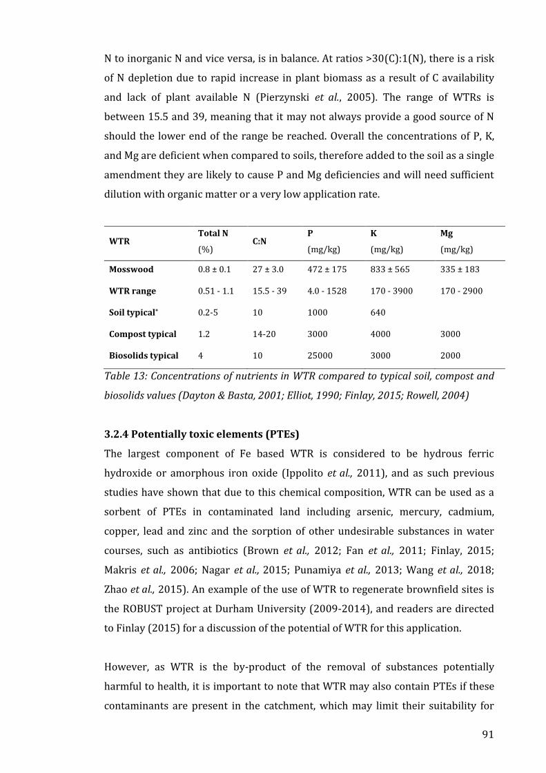
91

N to inorganic N and vice versa, is in balance. At ratios >30(C):1(N), there is a risk

of N depletion due to rapid increase in plant biomass as a result of C availability

and lack of plant available N (Pierzynski et al., 2005). The range of WTRs is

between 15.5 and 39, meaning that it may not always provide a good source of N

should the lower end of the range be reached. Overall the concentrations of P, K,

and Mg are deficient when compared to soils, therefore added to the soil as a single

amendment they are likely to cause P and Mg deficiencies and will need sufficient

dilution with organic matter or a very low application rate.

WTR Total N

(%) C:N

P

(mg/kg)

K

(mg/kg)

Mg

(mg/kg)

Mosswood 0.8 ± 0.1 27 ± 3.0 472 ± 175 833 ± 565 335 ± 183

WTR range 0.51 - 1.1 15.5 - 39 4.0 - 1528 170 - 3900 170 - 2900

Soil typical* 0.2-5 10 1000 640

Compost typical 1.2 14-20 3000 4000 3000

Biosolids typical 4 10 25000 3000 2000

Table 13: Concentrations of nutrients in WTR compared to typical soil, compost and

biosolids values (Dayton & Basta, 2001; Elliot, 1990; Finlay, 2015; Rowell, 2004)

3.2.4 Potentially toxic elements (PTEs)

The largest component of Fe based WTR is considered to be hydrous ferric

hydroxide or amorphous iron oxide (Ippolito et al., 2011), and as such previous

studies have shown that due to this chemical composition, WTR can be used as a

sorbent of PTEs in contaminated land including arsenic, mercury, cadmium,

copper, lead and zinc and the sorption of other undesirable substances in water

courses, such as antibiotics (Brown et al., 2012; Fan et al., 2011; Finlay, 2015;

Makris et al., 2006; Nagar et al., 2015; Punamiya et al., 2013; Wang et al., 2018;

Zhao et al., 2015). An example of the use of WTR to regenerate brownfield sites is

the ROBUST project at Durham University (2009-2014), and readers are directed

to Finlay (2015) for a discussion of the potential of WTR for this application.

However, as WTR is the by-product of the removal of substances potentially

harmful to health, it is important to note that WTR may also contain PTEs if these

contaminants are present in the catchment, which may limit their suitability for

92

land application. Table 8 (from section 3.1.2, displayed again on page 91,) provides

concentration values of a number of PTEs present in WTR in comparison to the

PAS100 and biosolids (Directive 86/278/EEC) regulations. Substances that are

within the PAS100 threshold are allowed to be spread across land without the

need of an environmental permit, however those exceeding PAS100 thresholds

must be disposed of in a different way. WTRs that did not fall below the threshold

concentration for PAS100 of a particular substance are underlined, however it can

be seen that the majority of WTRs have low concentrations of PTEs in comparison

to typical biosolids and in some cases low in comparison to soil e.g. Cr.

Table 8: Concentration of PTE in WTRs as derived by Finlay, 2015, Elliot (1990),

McBridge (1994), BSIPAS-100 specification, and Sewage Sludge Directive

86/278/EEC. Underlined = exceedance of PAS-100 regulations

The focus of this research is on the WTR produced from the use of Fe based

coagulant, specifically from Mosswood water treatment works. The site, located at

NZ0650, next to Derwent Reservoir, which collects water from a catchment of

110km2 and provides a daily yield of 112,320 m3 per day [NWL, 20]. Water coming

into the treatment plant may vary over time due to fluctuations in climate or land

use practises that affect the chemistry and physical properties of water, therefore

there are changes in the physiochemical properties of WTR over time. This means

that any results obtained for experiments using Mosswood derived WTR may not

be wholly comparable to WTR used from a different time or place.

WTR Cd

(mg/kg)

Cr

(mg/kg)

Cu

(mg/kg)

Hg

(mg/kg)

Ni

(mg/kg)

Pb

(mg/kg)

Zn

(mg/kg)

Mosswood 2.36 ±

1.42 31.5 ± 7.2 27 ± 8

0.28 ±

0.25 92 ± 35 85 ± 72

665 ±

405

WTR range 0.2 - 3.6 7.8 - 39 7.9 - 36 0.06 - 1.4 10 - 120 4 - 160 28 -

1100

Soil range 0.06 - 1.1 7 - 221 6 - 80 0.02 - 0.41 4 - 55 10 - 84 17 - 125

Biosolids

typical 0.1 - 13.6 28 - 509

25 -

2481 0.1 - 2.0

2.6 -

389

8.1 -

850

32 -

2070

PAS-100

regs 1.5 100 200 1 50 200 400

Biosolids

regs 20 / 1000 16 300 750 2500

93

3.3 WTR as a resource

3.3.1 Using WTR as a single amendment to soil or as a soil substitute

Although much literature has discussed the use of WTR to reduce the excessive

addition of P and N to groundwater and surface water sources resulting from the

application of biosolids or other organic matter, relatively there is much less

literature on the merits of WTR as a single amendment soil conditioner or as a soil

substitute. Land based applications have historically centred around using sludge

as a substitute for agricultural limestone but increasing attention has been paid to

land application as a sustainable disposal mechanism, as already employed by NW

(Basta, et al., 2000, Titshall & Hughes, 2005), due to the similarities in geochemical

properties of WTR and soil (Elliot & Demsey, 1991).

Soil conditioning (treatment that modifies a soil’s properties to improve crop

growth) resulting from the input of organic matter is an advantage of the

application of WTR and although Elliot & Dempsey (1991) suggest that the effects

are quite small, there is a consensus that the use of WTR as a soil conditioner is

generally beneficial to soil, with the exception of potential P depletion causing

reducing in crop yields. For a residual to be considered as a substitute for soil it

must imitate soil and/ or maintain soil quality defined as “the capacity of a soil to

function, within an ecosystem and land-use boundaries, to sustain biological

productivity, maintain environmental quality and promote plant and animal health”

(Doran & Parkin, 1996) and similarly “to perform its three principal functions

(economic productivity, environmental regulation and aesthetic and cultural

values)” by Lal (1993).

There has been a handful of research papers that considers the single application

of WTR or use of WTR as a soil replacement, with conflicting results in respect to

phosphorus and crop growth; Heil & Barbarick (1989) found that WTRs at >15

g/kg reduced the yield of sorghum-sundangrass and similarly Skene et al., (1995)

experienced decreased growth of broad beans at 20 g/kg even with the use of

fertilizer. Basta et al., (2000) also evaluated the use of WTR as a soil substitute by

measuring the growth of bermudagrass, and showed that mean yields were

94

dependant on the type of WTR used, where both tissue P concentrations and

available P were below adequate for two out of three WTRs tested.

Similarly, Dayton & Basta (2001) characterised WTR for use as a soil substitute

and found that high application rates (>10%) have caused P deficiency in crops.

However, Oladeji et al. (2009) suggest that excessive application of WTR could

deplete plant available P and cause Al phytotoxicity when considering Al based

residuals, however even with an application rate of 25% single amendment or up

to 10% in a 2 year field study, there were no effects on the yield of grass nor the

phytotoxicity. Silveira et al. (2013) that found that incorporation of WTR caused an

11% yield suppression compared to surface application, but in general there were

no adverse effects of up to 70 Mg ha-1. Elliot (1990) however found that 20-100

g/kg enhanced tomato growth due to a liming effect (5.3-8.0 pH change). Beneficial

use of WTR therefore in a geochemical perspective is heavily dependent on the

application rate, where careful monitoring is needed of both the constituents of the

WTR to be spread, and the effect on the receiving soil.

Most of the literature on WTR looks at whether it can improve crop yields and this

literature is not covered in detail here. The reader is referred to Ippolito et al.,

(2011) which provide a brief summary on this topic. While some most studies have

reported the effects of amendment of soil WTR from a purely geochemical

perspective, some research has mentioned positive improvements in soil qualities,

such as water retention and pH (Basta et al., 2000; Bugbee & Frink, 1985; Owen,

2002; Pecku et al., 2005; Rengasamy et al., 1980;), although none have these as a

primary objective of study. Bugbee & Frink (1985) used WTR amendment up to

670 g/kg, which yielded increases in water holding capacity and aeration

(although these values are not quantified). They also found that the increase in

productivity as a result of improved soil structure was sufficient to offset P

deficiencies. Owen (2002) applied ferric WTR to agricultural land and suggested it

was beneficial to grassland and livestock. They found that the most economical

way of spreading sludge (accounting for all costs including centrifuging) is using

4% dry solids directly onto land at £4.50/m3 (which is £107/tonne of dry solids).

95

Moodley et al. (2004) and subsequently Moodley & Hughes (2006) used WTR as a

single amendment to soil and evaluated the changes in water retention, hydraulic

conductivity and evaporation at the field scale. Moodley et al. (2004) found that

differences from the control plot were only measurable after 2 years and only at

the highest application rate of 1.3 tonnes/ha were water retention and hydraulic

conductivity improved, and hence suggest that very high application rates of WTR

are required to observe differences in the physical properties of soils). At

application rates of up to 1.3 tonnes/ha, they reported that WTR incorporated to a

depth of 20 cm increased the saturated hydraulic conductivity of soils linearly with

application rate, and increased total porosity due to reduction in bulk density. An

increase water holding capacity was attributed to the performance of polymers in

the WTR in aggregation of the soil, where WTR amended soil increases the water

held at a particular matric potential, although the change in retention properties

were suggested to be affected by the WTR properties itself rather than an

interaction with the soil. The water loss from WTR amended soil was less than a

control soil which echoes findings from Kemper et al. (1994), where evaporation

was reduced by 10-20%. This finding was attributed to the addition of coarse WTR

grains which reduce the capillary action at low matric potentials and therefore

lower the unsaturated hydraulic conductivity. Moodley & Hughes (2006) also

suggest that aggregates of WTR have high stability and a limited potential for

swelling due to the binding effects of polymers.

3.3.2 Recycling waste

Moves to reuse many different types of waste over the past decade have meant

that the investigation into the potential benefits of waste is ever growing. This

comes as a result of increasing costs for disposal and concerns over sustainability;

DEFRA’s 2010-2015 policy paper on waste and recycling stated that the UK

generates 177 million tonnes of waste annually, which is both a poor use of

resources and has detrimental effects on business and household economies. This

includes industrial waste products, where the EU directive aims to reduce the

dependence on landfill for disposal and increase the recycling of wastes. In a

report on UK statistics on waste generation (DEFRA, 2018 [21]), mineral waste

(39%, 79 million tonnes) and soils (26.7%, 54.2 million tonnes) were the largest

contributors in 2014 (from a total of 202.8 million tonnes in 2014), compared to

96

just 10% by households. Of the waste that is deposited into landfill, mineral wastes

only account for 7%, however soils account for 45% of the total material. Mineral

wastes account for 50% of the recycled and other recovery treatment method

total, where soils only account for 10%. These figures go someway to showing that

there is increasing recycling of natural materials, but that it is not yet sufficiently

sustainable.

The cost of processing and disposing of WTR accounts for a significant proportion

of the operating costs of water treatment works, the cost of which increases each

year because of increasingly stringent disposal regulations (Babatunde & Zhao,

2007) therefore the disposal of residuals is a formidable challenge (Hseih & Raghu,

1997). As outlined in the introductory chapter, the reduction in soil quality

worldwide is a major issue and the remediation of soils is key on the agenda

(Tvergyak, 2012). Simultaneously there is a need to close the loop between

sustainable sludge management and water treatment and as such there are

increasing attempts to find beneficial uses for WTR (Babatunde & Zhao, 2007). The

potential for using a waste material as a sustainable method with which to

improve soil has been identified for the immobilisation of PTEs (McCann et al.,

2018) and phosphorous (Ippolito et al., 2011), however there are few studies that

have explored the effect of WTR amendment on the water retention and hydraulic

conductivity of soil, and none that have explored the effect of WTR amendment on

the water retention characteristics and shear strength of soils. The exploration for

WTR’s use in soil for structural and water holding improvements is, for lack of a

better word, exciting. Being able not only to recycle a waste, but also use it to

benefit the function of soil may change the value of WTR and indeed Goldbold et

al., (2003) and Rensburg & Morgenthal (2003) have advocated that WTR could

offer one of the greatest commercial potential for reuse.


The increasing generation of WTR remains an inevitable prospect as our demand

for clean water grows globally, and therefore the sustainable disposal of increasing

volumes of sludge is an ever-growing concern. While small-scale land application

is sufficient for the time being, further research is needed into the whole scale

effect of WTR application on land. To date much focus has been ensuring that the

97

application of WTR isn’t detrimental to soil (as a single amendment or with the

application of biosolids), or on its capacity to return soils to acceptable

concentrations of P and PTEs. A critical factor in the effective reuse of WTR from

water treatment works is legislation (Babatunde & Zhao, 2007) and although

companies currently follow guidelines for disposal there are no WTR specific

legislations.

There is no question that the reuse of WTR provides a unique and sustainable

opportunity for water treatment companies from an economic standpoint

(Godbold et al., 2003) and to benefit contaminated land. This thesis questions the

opportunity for WTR to be used as a beneficial material for the amendment of soil

to improve water holding characteristics, including hydraulic conductivity and to

improve soil structure and shear strength in order to make soils more resistant to

soil erosion and degradation, rather than exploring land application as just a

method for disposal. This in turn provides an economical, chemical and physical

benefit to the recycling of WTR into soil, in addition to addressing soil erosion and

flooding issues that are of critical concern.

98

4. Measuring Change in Soils

The following chapter discusses the methodology behind a novel approach to

quantifying soils with a focus on what parameters are important for soils to

function effectively during flooding events, i.e. its ‘flood holding capacity’. This

chapter will outline the technical aspects of collecting reproducible and reliable

data for this thesis. The first part of the chapter introduces the materials used in

this thesis, soil from St Anthony Lead (Soil 1) and Nafferton Farm (Soil 2), Water

Treatment Residual (WTR) from Honey Hill (WTR1) and Mosswood (WTR2),

compost and silica, with an outline of how these materials were prepared, stored

and analysed. The subsequent sections outline the development and refinement of

methods to make and test ‘cores’ for flood holding capacity (Trials 1-4). Three trial

studies were conducted in order to develop the processes and methods, before a

full-scale experiment was completed, ensuring that these were the appropriate

tests to produce robust data that was both valid and most importantly

reproducible in other laboratory or field settings.

Chapter 2 discussed the relationship of water to various physical and chemical

properties of soil, and concluded that there are currently flaws in the

measurement of water in soils. The new methodology described in this chapter

addresses some of these issues, thereby providing a method to quantifiably

measure soils in a way that encompasses the stresses undergone during flooding.

The methods used have been developed using British Standards where applicable,

with novel additions where these are not available. The remainder of the chapter

outlines other testing undertaken on the samples from Trial 4 including soil

erosion tests, shear testing, and hydraulic conductivity testing. A further method to

assess soil, X-ray computed tomography (XRCT) has also been used in this thesis

but owing to its complexity and novelty in the field of science, a full discussion of

methods and results are contained within its own Chapter 6. To the author’s

knowledge there have been no studies that have used the methods outline in Trial

4 to wholly quantify soils in respect to their maximum water holding capacity,

whilst including the shear strength and erosional resistance, volume change and

hydraulic conductivity as a function to which ‘flood holding capacity’ is attributed.

In order to provide clarity in terms used hereafter in the chapter and remaining

99

thesis, the following list of definitions describes what is meant by each term or the

acronym for each term.

AMENDED – An amended soil contains compost, WTR and or silica in varying

degrees in addition to an original soil.

AMENDMENTS – The addition of compost or WTR or silica to soil is an amendment

of the original soil (S1 or S2).

COMPOST – Decomposed organic matter from plants, leaf litter or garden waste

used to fertilise soil.

CORE – Material of a given sample that has been formed into a cylindrical unit 38

mm x 76 mm for testing.

FLOOD HOLDING CAPACITY (FHC) The ability or capacity of a soil to take up and

store flood water upon submersion without significant soil erosion or loss of shear

strength, and resistance to the detrimental impacts of flooding on soil structure and

critical eco-service functions (Kerr et al., 2016).

GRAVIMETRIC WATER CONTENT (GWC) – a ratio of the mass of water to the mass

of dry matter.

REPLICATE – An additional sample with the same composition as previously used,

e.g. Soil 1 had 12 replicate cores, meaning there were 12 cores produced using only

Soil1.

SAMPLE – A type of soil amendment, where the ‘sample’ refers to AM1 or Soil2.

SOIL – Soil derived from either St Anthony’s Lead (S1) works or Nafferton Farm

(S2).

UNAMENDED - refers to the use of soil without any additional material.

VOLUMETRIC WATER CONTENT (VWC) – a ratio of the volume of water in a soil to

the volume of dry solids.

VOLUMETRIC WATER CONTENT i (VWCi) – a ratio of the volume of water in a soil

to the volume of dry solids at the point of measurement.

WATER HOLDING CAPACITY (WHC) – the maximum amount water a unit of soil can

or could hold at saturation based as a function of GWC, volume and VWC/VWCi

WTR – Water treatment residual, a waste from water treatment works as

discussed in Chapter 3. WTR is discussed in relation to its water content and

termed oven dry (WTRod), air dried 280% solids (WTRd) or as received or ‘wet’

20% solids (WTRw)

100

4.1 Materials

Four trials were conducted to develop a methodology to measure a soil’s ‘flooding

holding capacity’, which used a number of different materials as described below.

Values for chemical/biological characteristics were obtained using Derwentside

Environmental Testing Services (DETS), an ISO 17025 accredited analytical

service. Physical testing was completed in the department as per British Standards.

4.1.1 Soil

Two soils were used for experimental trials, Soil 1 from St Anthony Lead works

and Soil 2 from Nafferton Farm. Soil 1 was obtained from the former St. Anthony

lead works in Newcastle upon Tyne (NZ287629), historically a site of

anthropogenic heavy metal pollution in operation between 1840 and the 1930’s.

Characterisation carried out by Finlay (2015) derived by X-ray Florescence (XRF)

for Soil 1, determined 6.6 pH and 73 g kg-1 organic carbon. The site is

heterogeneously contaminated with Pb, As and Zn with a mean concentration of

6954, 8820 and 1987 mg kg-1, respectively. This soil was chosen for preliminary

trials as it has been well characterised by Finlay (2015). Soil 1 posed a potential

threat to human health due to high oral bio-accessibility of lead, however this was

taken into account with appropriate COSHH regulation guidance for health and

safety.

Soil 2 sourced from Nafferton Farm (NZ064657) is an agricultural soil and

replaced Soil 1 (StALW) in latter trials to eliminate health & safety hazards posed

by the soil and the degradation effect of long-term storage. Specific preparation

and storage methods followed for Soil 1 were unknown, therefore sourcing new

material enabled control of the storage and preparation of components from

collection to final use. 300 kg of soil was obtained in June 2014 (and stored as per

section 4.2) from the 300 ha site at Nafferton farm, which is currently the site for a

cooperative project called BIONICS that investigates the biological and engineering

impacts of climate change on slopes. Soil 2 was characterised by DETS, the results

of which are in 4.3.7

101

4.1.2 Compost

All compost used in the experiments was obtained from a Newcastle based

company called Com-vert, sourced in 2011 for Trials 1 and 2 (Compost 1) and in

2014 for Trials 3 and 4 (Compost 2). The compost is made to the Soil Association

Organic Standards and meet PAS100 (2011) quality standards. The PAS100

specification, prepared and published by the British Standards Institution (BSI)

provides requirements for the compost processing, input materials and minimum

quality to ensure that composted materials are consistently fit for their intended

use (PAS100, 2011). As a result of this process compost can be defined as “solid

particulate material that is the result of composting, that has been sanitized and

stabilized and that confers beneficial effects when added to the soil, used as a

component of a growing medium, or is used in another way in conjunction with

plants” (PAS100, 2011).

4.1.3 Water Treatment Residual

Water treatment residual (WTR) was obtained from Honey Hill (WTR1) for Trials

1&2 and from Mosswood (WTR2) for Trials 3&4. WTR1 was characterised by

Finlay (2015) and had a gravimetric moisture content of 81.4 ±0.1%, organic

content (determined by LOI) 54.1±0.1%, 4.1 pH, Fe 35%. WTR 2 was collected

from Mosswood water treatment works due to its proximity to Durham University,

where the research was conducted. There was a marked difference between the

texture of WTR1 and WTR2, where WTR1 had significantly separated into solid

materials and water; as discussed in Chapter 3 the flocculants and coagulants used

in the water treatment process continue to bind particles together and expel any

water within the matrix. WTR2 in contrast had a dry crumbly soil texture, despite

having similar water content to WTR1. The difference in appearance between

WTR1 and WTR2 were due to the age of the materials, WTR1 was obtained from

Honey Hill in 2011 and WTR2 was obtained in 2014 from Mosswood, therefore

water was still held in the coagulated material in WTR2.

4.1.4 Silica

Washed Silica was obtained from Leighton Buzzard supplies. The silica was oven

dried to remove any water accumulated in storage. Silica is chemically inert and is

102

able to impart structural properties in isolation and therefore was used to replace

WTR2d in Trial 3.

4.2 Material storage, handling and preparation

The handling and storage of materials can profoundly affect the results of analysis

(Sheppard & Addison, 2008), particularly for subtle soil measures such as biotic

functions, bioavailable elements or studies of organic matter (Kaiser et al., 2001).

The typical sequence observed and followed for this study is as follows:

Collect samples from the field

Reduce clump size and mix sample

Subsample for appropriate testing e.g. moisture content

Dry remaining sample if appropriate to a moisture content suitable for

storage duration

Typically soils are ground so that all material passes through a 2 mm to ensure a

composite and homogeneous sample for testing. Although this is acceptable

practice for some testing such as chemical analysis, for more sensitive physical

measures such as macro-pore properties, sieving to <2 mm affects microbial

mineralisation rates, extractable iron and aluminium concentrations, oxygen

uptake, rate of decomposition and can increase extractable phosphorous by 165%

in some soils (Craswell & Waring, 1972; Hassink, 1992; Neary & Barnes, 1993;

Peterson & Klug, 1994; Ross, 1992; Turner & Haygarth, 2003). Although suggested

as best practise for the long-term storage of materials, drying a soil at room

temperature (which very often results in a moisture content similar to oven dried

soil) causes organisms to die or become dormant, dissolved inorganic materials

become concentrated in remaining pore water, organic materials will coagulate

and deform, and aggregates will stabilise and cause hydrophobicity of the soil

(Elmholt et al., 2008; Semmel et al., 1990). For the types of analysis required in

this methodology, the suggested procedures for the storage materials were: field

moist or workable moisture content, with moderate breakdown of aggregates, and

minimal storage time (unless refrigerated). Therefore, as described below, soils

and compost were not dried for storage. The water content of the WTR was used in

both wet (as received) and air-dried forms. All materials were sieved to 6.3 mm to

reduce sieving artefacts as mentioned above.

103

4.2.1 Soil

For particular soil tests, preparation and storage can profoundly affect the

properties of soil (Rimmer, 1991; Sheppard & Addison, 2008). Air-drying is the

accepted procedure to preserve samples without degradation, which may be

supplemented with mixing and physical breakdown of aggregates (Tan, 2005), and

this method was believed to be the procedure for storage of Soil 1. However air

drying as a preservation technique is only accepted in geotechnics and not

preferable for geochemical/geoenvironmental use (Dowding et al., 2005),

therefore the Soil 2 was kept at field moisture content and was used immediately.

Samples were kept indoors to regulate their temperature, as high temperatures,

i.e. those exceeding 35°C are detrimental to physical and biological functions of the

soil (Bartlett & James, 1980). This includes, but is not limited to, oxidation of

sulphur in some soils that produces sulphuric acid when wetting and reduces the

soil pH, cementation of soil aggregates (Bullock et al., 1988), oxidation and loss of

organic matter, oxidation of Fe2+ to Fe3+, changes in P fixation related to Al and Fe

chemistry and an increase of exchangeable Mn (Sherman & Harmer, 1943).

At the site, there was heavy plant growth on the topsoil deposit with numerous

large stones and non-organic material. The reason for the growth and origin of

contaminants is unknown however the majority of large fragments (>7 mm)

present were removed before storage, including roots, biota, pebbles and all non-

organic matter such as brick fragments, glass and plastic. For this initial screening,

large soil aggregates were broken down through a 20 mm sieve. In total 81 kg

(27% of total soil mass) were removed from the excavated soil. The remaining

219 kg was sealed in plastic bags to avoid the loss of soil moisture and stored

inside at a constant temperature. Soil2 was then passed through a second

screening; Datta et al. (2014) found that sieve mesh size was a significant factor in

soil disturbance, affecting soil pore structure and organic matter fractions. For

physical and chemical analysis soils are typically sieved through apertures ranging

from 0.5-10 mm (usually 2 mm) in order to remove unwanted fragments such as

litter, roots and stones and then mechanically ground to homogenize the material.

However sieving at this scale accelerates C mineralization, N immobilization and

denitrification (Situala et al., 2000), with finer sieves exacerbating this effect and

104

resulting in a flush of C and N due to break down of aggregates and increased

surface area.

To maintain the soil as close to field conditions as possible whilst enabling the

material to be used at a size appropriate to the scale of research being undertaken,

all soil matter was passed through a 6.3 mm sieve (Datta et al., 2014). This

accommodated some small aggregate particles that had formed naturally and

avoided sieving the soil too finely. Soil cores compacted for testing were 38 mm in

diameter; therefore the largest particles in each sample would comprise a

maximum of 10% of the total core surface area should one take a slice of the core.

A further 14.2 kg of stones and other fragments were removed from the soil during

this second screening. Each sample bag contained soil of different areas through

the soil profile due to the use of a mattock and shovel to retrieve the soil; the upper

most samples contained high quantities of root matter and biota and had low

water content with a sandy texture. Samples obtained from lower in the soil profile

were much denser and contained larger stones, had a higher water content and

appeared to have a more clayey texture. All sieved soil was mixed for a period of

10 minutes to reduce heterogeneity. The fundamental rationale for compositing

the soil is that following the mixing process, a sample taken from the whole then

yields a valid mean point for chemical or physical testing (Tan, 2005).

The 204 kg of soil passing the 6.3 mm sieve was then divided using the riffling

method into 2 kg subsamples and returned to polythene storage bags. Briefly, the

riffle method (Head, 1980) uses a large riffle box to divide the sample into two

parts. In this process soil is separated through a number of slotted paths in the box

with the aim of randomly dividing the sample. Once the sample is passed through

the box, one half of the sample is put aside. The remaining half is then passed

through the box, again putting one half aside. This process is repeated until the

division of the sub-sample firstly gave 500 g for particle size analysis and (8

repetitions) then gave 2 kg sub-samples (approximately 60 repetitions in total).

105

4.2.2 Water Treatment Residual (WTR)

WTR was stored in two forms, firstly it was unprocessed and sealed ‘as received’ to

be used for research in the format in which it is produced by the water company

(WTRw), and secondly was air dried (WTRd) to provide a granular, coffee grind like

material that was more easily handled and did not completely saturate samples

and render them to a slurry. WTR1d was air dried at room temperature and broken

down by hand periodically. Once dried, this was sieved to 2 mm and stored in

sealed plastic bags until use in Trials 1 & 2 and WTR1w was unprocessed. Similarly,

approximately half of WTR2 was air-dried over a number of days, with periodic

breakdown of the larger aggregates to ensure that these did not harden and

become one large solid mass. Once dried, WTR2d was passed through a 6.3 mm

sieve to approximate the maximum aggregate size of the soil and sealed for storage

before use in Trial 4 to ensure that it did not take up moisture from the

surrounding air. The remaining mass of WTR2 was kept sealed and unprocessed

(WTR2w).

4.2.3 Compost and silica

Fifteen 40-litre bags of compost were delivered in October 2014 and stored

outside until their use. Compost was not processed before use, with the exception

of the removal of large twigs and other large particles during mixing with soil

mineral matter and/or WTR. Silica was oven dried to remove any moisture

accumulated during storage, but otherwise unprocessed.

106

4.3 Material characterisation

British standards were followed to characterise all materials as described above,

where brief descriptions of these methods are subsequently outlined.

4.3.1 Particle size distribution

For Soil 2, a particle size analysis (particle size distribution) was conducted

according to BS1377 (Part 2:1990). Three fractions, all of which can be subdivided

into finer size fractions, are present in soil, sand (0.06-2 mm), silt (0.002-0.06 mm)

and clay (<0.002 mm). Simple dry sieving was not appropriate as the method is

only applicable to clean granular materials with negligible quantities of silt or clay.

In a dry state, clay and silt are able to adhere to the surface of sand grains.

Therefore, the wet sieving procedure was followed to calculate particle size.

According to BS1377, the minimum mass of 500 g was obtained using the riffling

method (as described previously). Coarse material removed during the secondary

screening was re-added to the sieved soil to obtain the coarser fraction particle

size curve for the material. The soil sample was weighed (W1) using a mass

balance and then oven dried overnight at 105°C and left to cool in a desiccator. The

dried sample was then weighed on a balance to ensure the minimum mass

threshold was met (to an accuracy of ±0.1% of the total mass) (W2). A standard set

of sieve apertures was used for the classification; 37.5 mm, 20 mm, 10 mm, 6.3

mm, 3.35 mm, 2 mm, 1.18 mm 600 μm, 300 μm, 150 μm and 63 μm. Soil was

crushed and then washed with a water jet to remove the clay and silt particles

adhered to the surface of sand grains, as these cannot be removed sieving alone. To

avoid overloading of sieves, three sieves were nested together (2 mm, 212 μm and

63 μm). Material passing through the 63 μm sieve was collected for a pipette

hydrometer test and oven dried overnight at 105°C. The dried and cooled material

was weighed to ±0.01% of mass (W3). The silt & clay proportion of the total

sample was calculated using equation 6:

< 63 𝜇𝑚 % =𝑊2 − 𝑊3

𝑊2

Equation 6: Calculation of the silt and clay fraction of a soil based on the wet sieving

procedure BS1377

The cooled oven-dried soil was placed into the standard sieves in a stack shaker

for 10 minutes. Once the shaking cycle was complete, the proportion retained on

107

each sieve was weighed, giving the proportional value of each fraction. The pipette

method of sedimentation of the fine fraction (also BS1377: 2, 1990) was used to

calculate the silt and clay proportion of material passing the <63 μm sieve. The

procedure is based on the relationship between settling velocity and particle

diameter (developed by Stokes, 1851). Although Stokes’ Law makes a number of

assumptions, including the assumption that particles are spherical (unlike clays

and clay sized grains that are more plate like), the use of sedimentation through

pipette analysis is standard practice in geotechnics. Briefly, the test requires a

sample to be taken at a depth (h) at a given time (t) at which all particles coarser

than X mm have been eliminated (Gee & Or, 2002), where the settling times for

clay fractions can be calculated at a given time and temperature. 12.5 g of dry soil

that has passed a 63 μm sieve are dispersed with 25 ml of sodium

hexametaphosphase (NaPO4, called Calgon) in a conical flask containing 500 ml of

water. The conical flask is shaken for 3-4 hours at 25 °C to disperse and

disaggregate all individual particles. The contents of the flask are added to a

testing bath, after which three 9.67 g aliquots are taken by pipette at 4m30s, 46

minutes and 6h54m to quantify the concentration of particles of 0.02 mm, 0.006

mm and 0.002 mm equivalent diameter, respectively. This assumes a particle

density of 2.65 g/cm3.

As discussed in Chapter 3 (section 3.2.1), particle size distribution (PSD) for WTRs

has been performed by hydrometer analysis in the wet form (produced by water

treatment plants) where 95% of residual solids passed the 74 μm sieve, but when

air-dried the PSD included larger grain sizes, even when the air-dried material was

pulverised. Issues with settling of both WTR2w and WTR2d in hydrometer

measurements were experienced during testing by Hsieh & Raghu (1997) and

Basim (1999), therefore analysis by hydrometer of wet PSD was not attempted for

WTR2. For WTR2d the process of obtaining a ‘particle size distribution’ was

completed using simple dry sieving (BS1377: 1990 Test 7 B) as per section 4.3.1

and a sample placed into a stack of 10 sieves for a period of 10 minutes. Obtaining

PSD from dry sieving does not give an individual particle size of WTR2d but was

conducted to obtain information on the sizes of WTR2d ‘grains’ achieved by manual

breakdown during air-drying in this particular research.

108

Given the effect that surface area has on the water holding capacity of soil and the

shear properties (Chapter 2, section 2.3.6) it is important to know if the

predominant size fraction of WTR2d is fine or coarse. The caveat, however, is that

the test may not have been wholly accurate as, due to the brittle nature of dry

WTR, larger pieces may have been broken down due to the sieving process, which

may have given an erroneous reading for the contribution of the finer fraction. In

general Basim (1999) found that the materials become more granular as they dry

due to cementation from organic matter and oxides present, therefore the test

wholly reflects the duration of drying and breakdown methods used during the

drying process.

4.3.2 Classification and description of soils

The standard light Proctor compaction test (BS1377, 1990: Test 12) derives the

optimum water content at which the maximum density can be achieved with a

given compaction effort. This test was completed using Soil 2 and briefly, three

layers of Soil 2 were added to the 1000 cm3 Proctor mould, using 27 compaction

strikes of a 2.5 kg hammer from 300 mm to compact each layer. The soil water

content is incrementally increased to test compactibility across a range of water

contents. The standard light Proctor tests initially uses a dry soil that is tested as

described above, then broken down and wetted to increase the water content

before completing another test. The density of the sample increases with the

increase of water content until maximum density is achieved, after which the

density decreases due to the addition of less dense water (1 g/cm3) to soil matter

(2.65 g/cm3); results are typically reported in Figure 16. Atterberg tests were also

conducted on Soil2, where Atterberg limits are a measure of the critical water

content that separate the soil into different states of consistency, defined at the

shrinkage limit (uncommonly tested), plastic limit and liquid limit. A fall cone test

was used to determine the liquid limits and a thread (roll) test was completed to

determine the plastic limit (BS1377: 1990 Part 2). Soil2 was determined as

inorganic clay of medium plasticity (the soil exhibits plastic properties at 7-17%

water content).

109

Figure 16: Example of the Proctor standard test for compaction of soil at different

water contents, annotated with optimum moisture content, maximum bulk dry

density, wet and dry sides of optimum.

4.3.3 Volume and density (bulk, dry & particle)

Bulk density and dry density were calculated for each core using the volume of a

sample and mass of dry solids (Figure 17). The volume of individual components

also allows empirical calculations of dry density and the void ratio.

V

Vv Va Air Ma

Vw Water Mw

VWTR WTR MWTR

Vc Compost Mc

Vs Soil Ms

Figure 17: Schematic of volume and mass proportions in a soil with mass and volume

equation 7.

Bulk density is ratio of the mass to the bulk volume of the soil, which includes the

volume of the solids and pore space, air and water. Dry density is therefore a ratio

1.8 - 1.6 - 1.4 - 1.2 - 1.0 -

Bu

lk d

ry d

en

sity

(g

/cm

3)

6 8 10 12 14 16 18 Moisture content (%)

Dry side Wet side O

pti

mu

m w

ater

con

ten

t

Maximum (optimum) dry density

100% compaction

Equation 7: 𝑉 = 𝑉𝑠 + 𝑉𝑐 + 𝑉𝑊𝑇𝑅 + 𝑉𝑤 + 𝑉𝑎 = 𝜌𝑠𝑀𝑠 + 𝜌𝑐𝑀𝑐 + 𝜌𝑊𝑇𝑅𝑀𝑊𝑇𝑅 + 𝜌𝑤𝑀𝑤

+ 𝑉𝑎 where ρx = particle density. If saturated Va = 0

110

of the mass of oven-dried solids to the volume of the sample and ‘equivalent

particle density’ can be calculated using the ratio of components.

𝐵𝐷 = 𝑀

𝑉

Equation 8: Bulk density calculation for soil where M= mass of moist sample and V is

total volume of the sample.

𝑅𝐶 = 𝑀𝑐

𝑀𝑠

𝑅𝑊𝑇𝑅 = 𝑀𝑊𝑇𝑅

𝑀𝑠

Equation 9: Ratio of components in amendments where Rc = ratio of compost, Mc is

mass of compost, Ms is mass of soil solids, RWTR is ratio of WTR and MWTR is mass of

WTR

𝐷𝑑 = 𝑀𝑆 + 𝑀𝑐 + 𝑀𝑊𝑇𝑅

𝑉

= 𝑀𝑠 + 𝑀𝐶 + 𝑀𝑊𝑇𝑅

𝜌𝑠𝑀𝑠 + 𝜌𝑐𝑀𝑐 + 𝜌𝑊𝑇𝑅𝑀𝑊𝑇𝑅+ 𝜌𝐶𝑀𝑊

Equation 10: Dry density (Dd) calculation where 𝜌s is particle density of soil, 𝜌c is

particle density of compost, 𝜌WTR is particle density of WTRd (where WTR2 is assumed

to have the same value)

𝜌𝐸𝑞 = 𝜌𝑠 + 𝜌𝑐𝑅𝑐 + 𝜌𝑊𝑇𝑅𝑅𝑊𝑇𝑅

1 + 𝑅𝑐 + 𝑅𝑊𝑇𝑅

=1 + 𝑅𝑐 + 𝑅𝑊𝑇𝑅

𝜌𝐸𝑞(1 + 𝑅𝑐 + 𝑅𝑊𝑇𝑅) + 𝜌𝑤𝑤(1 + 𝑅𝑐 + 𝑅𝑊𝑇𝑅)

𝜌𝑑 =1

𝜌𝐸𝑞 + 𝜌𝑤𝑤

Equation 11: Equivalent particle density which links the gravimetric water content

(w) and particle density (𝜌d) for any combination of components

The particle density of WTR2d and compost were derived using pycnometry, a

method that uses a vessel with a precisely known volume to allow density

determination. The particle density (as defined in Chapter 2) was assumed for

Soil2 to be 2.65 g/cm3. WTR2d was tested for particle density using BS1377: 1990

111

Part 2 (small pycnometer method). 2 mm sieved WTR2d that had been air was

oven dried at 30° C for 72 hours immediately before testing to remove remaining

water. Air removal is a critical factor in the particle density testing, where testing

standards suggest the removal by either gently heating the contents of the

pyncometer or applying a vacuum. As discussed in Chapter 3 – heating of WTR has

considerable effects on the geophysical properties (loss of volatile solids and

organic matter) and therefore the latter was chosen. Each test subject was de-aired

for 3 days and produced densities of 2.11 ± 0.81 g/cm3 (where minimum = 2.1099,

maximum = 2.118). In comparison, two tests in which subjects were only de-aired

for 30 minutes produced densities of 2.127 and 2.103. It must be noted that Basim

(1999) found that the higher the temperature used to dry the WTR, the higher the

particle density, which is attributed to the loss of the organic phase at

temperatures. Therefore should the test be conducted using 105 °C, a higher

particle density is expected (approximately 0.2 g/cm3 increase between samples

dried at 60 °C and 105 °C). As the samples are exposed to higher temperatures, in

addition to organic matter reduction, calcium oxide, iron oxide and aluminium

come out of solution and act as a cement between the solid material, and hence

increasing the particle density.

A method described by Weindorf & Wittie (2016), adapted from Blake & Hartge

(1986) was followed for measuring the particle density of compost, using hexane

in place of traditional methods using water in the pyncometer. The use of hexane

facilitates low density particle submersion as it has a lower density than water

(0.655 g/cm3). The method briefly involved oven-drying compost at 70 °C for 24

hours, before passing it through a 2 mm sieve. Next, 6-8 g of dried compost was

added to a 100 ml volumetric flask of known mass and weighed on a mass balance

to an accuracy of ±0.0001 g. Approximately 40 ml of de-aired hexane was added to

the volumetric flask to completely immerse the compost, however following the

gentle swirling technique as used by Weindorf & Wittie (2016), many particles

remained buoyant and air bubbles continued to be trapped even after 24 hours of

immersion. Therefore, the flask containing compost and 40 ml of hexane was de-

aired for a period of 3 minutes. De-aired hexane was then added to bring the

sample to volume (100 ml) and left to settle for a number of hours. Any additional

hexane required was then added and the mass was recorded. Particle density was

112

then calculated using Equation 12. The compost particle density (𝜌𝑑) was found to

be 1.675 ± 0.33 g/cm3 where the number of repeats (n) = 12.

𝜌𝑑 = 𝜌ℎ(𝑊𝑐)

[𝑊𝑐 − (𝑊𝑐𝑏 − 𝑊ℎ)⁄

Equation 12: Compost particle density calculation where ρh = density of hexane

(g/cm3), Wc = weight of oven dried compost (g), Wch = weight of compost and hexane

(g), and Wh = weight of 100 ml of pure hexane (g)

4.3.4 Moisture content

As per discussion in Chapter 2, the moisture content of a soil (or any material) can

be expressed gravimetrically or volumetrically. Conventional temperatures for

testing (105 -110 °C) remove both gravitational and capillary water present in the

pores, however this temperature may also remove significant amounts of organic

matter in highly organic soils. According to BS1377 (1990) to determine

gravimetric water content (GWC) a moist sample of material of known mass is put

into a metal container and placed into an oven at 105°C for 24 hours.

GWC can be expressed using a on a wet mass basis or on a dry mass basis. For

example, for a soil that weighs 100 g in a field moist condition, containing 80 g of

dry solids, with a dry density of 1.5 g/cm3 (bulk density = 1.89 g/cm3) and a

volume of 53 cm3 (as shown in Figure 17) the equations for GWC dry basis and

GWC wet, give different values. It is therefore very important to note which

equation is used in literature. Typically, Equation 13 (dry basis) is used, giving the

mass of water in the moist bulk of soil to the mass of dry solids as a ratio (0.2) or

can be given as a percentage, i.e. 20%. Equation 14 expresses GWC on a wet weight

basis and relates the mass of water to the total mass of the moist bulk of soil

(Gardner, 1986). The difference between the two is not negligible, therefore is it

critical to note if the GWC is calculated on a dry or wet basis. For soils the

difference between wet and dry is not too dissimilar, but for materials such as

WTR that may have 80 g of water to every 20 g of dry solids there is a large

difference in values for dry basis and wet basis; 4 (400%) and 0.8 (80%)

respectively. For the purposes of this thesis, Equation 8 will be used to express the

GWC as it is used in the majority of literature.

113

Figure 18: Example of a field moist soil, with the values of properties noted on the

diagram.

𝜽 =𝑴𝒘

𝑴𝒔

𝜃 =𝑀𝑤

𝑀𝑠 + 𝑀𝑐 + 𝑀𝑊𝑇𝑅

=𝑀𝑤

𝑀𝑠(1 + 𝑅𝑐 + 𝑅𝑊𝑇𝑅)

=0.25 or 25% GWC

Equation 13: Dry basis gravimetric water content calculation for the soil sample on a

dry basis in Figure 17 where Mw = mass of water, Ms = mass of dry solids

𝜽 =𝑴𝒘

𝑴

= 0.2 or 20% GWC

Equation 14: Wet basis gravimetric water content calculation for the soil sample in

Figure 17 where Mw = mass of water and M = mass of moist soil

Volumetric water content is a measure of the volume of water relative to the

volume of the soil bulk, however this value is only calculated relative to the

original volume (Equation 15). To account for swelling in the soil, the volume or

dry density (Dd) of soil at the point of measurement (instantaneous, i) is used

rather than using the original values (Equation 16). Both volumetric measures will

be used in the presentation of results to enable comparison to the majority of data

produced, but also to provide an insight into the absolute volumetric water

behaviour using VWCi, which gives a ratio between the volume of water to the

volume of the sample.

Mw =Water (& air) 20 g

Ms = Soil 80 g M = Total Mass 100 g

Volume = 53 cm3 Dry density = 1.5 g/cm3 Bulk density = 1.89 g/cm3

114

𝜽𝒗 =𝑽𝒘

𝑽𝒔

= 𝐺𝑊𝐶 ∗ 𝐷𝑑

= 0.37 or 37.7% VWC

Equation 15: Volumetric water content (θv ) calculation for the sample in Figure 17

using the original volume of soil as a constant; where Vw = volume of water, Vs =

original volume of solids

𝜽𝒗𝒊 =𝑽𝒘

𝑽𝒔𝒊

= 𝐺𝑊𝐶 ∗ 𝐷𝑑𝑖

= 0.37 or 37.5% VWC

Equation 16: Volumetric water content (𝜃𝑣𝑖) calculation using an instantaneous

volume of soil of Figure 17; where Vw = volume of water and Vsi = volume of

instantaneous soil

The determination of the GWC of soil at 105 °C is standard practice, however table

14 provides evidence that values obtained for the GWC of WTR and compost are

dependent on the temperature at which the test is conducted. At higher

temperatures, the difference in GWC is attributed to the loss organic matter as

drying samples at the conventional 105 °C may induce the removal of volatile

solids. This gives inaccurately high-water contents for WTR and compost. The GWC

of WTR was determined from material air dried at 20 °C (WTR2d), 30 °C and 60 °C

for 48 hours and at 105 °C for 24 hours. Similarly the water content of compost

was derived at both 60 and 105 °C to determine a difference in the water content

value. As discussed in Chapter 3 (section 3.2.1), Hseih & Raghu (1997) found that

there was little difference in water lost from WTR at temperatures of 24 °C, 30-40

°C and 105 °C. Basim (1999) conversely found that for WTR there was 3.44-10.25

% of weight lost in the test between 60 and 105 °C, due to the loss of organic

matter. Table 14 supports Hseih & Raghu’s findings, showing that there is little

difference between the derived water contents at either 60 °C or 105 °C for WTR2w

suggesting that organic matter may even be removed at the lower temperature, or

not at all in this case. In tests conducted on Mosswood WTR2w, there was less than

1% difference in the GWC between 60 and 105 °C.

115

Sample

(n = 3)

Air dried

at 20 °C

WC

at 30 °C

WC

at 60 °C

WC

at 105°C WC at 105 °C

– 60 °C 48 hours 24 hours

(wet basis GWC)

*values derived by Basim (1999)

WTR2w

From

treatment

plant

1.14

(0.53)

*1.8-5.12

2.18

(0.69)

4.51

(0.82)

*1.97-5.7

4.94

(0.83)

*2.4-6.0

0.43

(0.001)

*0.13-0.45

WTR2d

Air dried

@ 20C

n/a 0.21

(0.30)

0.53

(0.35)

0.78

(0.44)

0.25

(0.009)

Compost2 n/a n/a 0.61 ± 1.4 0.71 ± 1.3 0.04 ± 0.005

Table 14: Water contents of WTR2 dried at different temperatures, where the value is

derived using Equation 13 (mass of water/ mass of solids). ‘n =’ denotes the number

of repeat tests. Values in brackets describe the water content by wet basis GWC.

These values are compared to a small range of values derived by Basim (1999),

denoted by *

However, there is a 32% difference in values between GWC of WTR2d dried at 60

and 105 °C. This is presumably due to the water becoming more difficult to remove

as it becomes trapped in the ‘dried’ WTR (see Chapter 6, section 6.4.3), therefore at

60 °C there is much less water removed than at 105 °C. The alternative is that the

water removal is the same for WTR2w and WTR2d and the difference is due to the

more effective removal of organic material once the WTR has been air-dried

because of a higher surface area of exposed organic matter. Although literature

suggests the use of 70 °C to dry compost to avoid significant loss of organic matter

(Agnew & Leonard, 2003; Pansu & Gautheyrou, 2007), results from testing

compost showed that there was only a very small difference in the water content

of compost dried at 60 °C and 105 °C, therefore calculations were taken using the

conventional 105 °C.

116

4.3.5 Material characterisation results

Table 15: Results of material characterisation and analysis including physical and chemical attributes, where values are obtained from analysis

undertaken by Derwentside Environmental Testing Services (DETS) using methods DETSC 2301# and 2008# and from Finlay (2015).

Material Sourced Sieving Moisture content

% (dry basis) pH

Total

Carbon

%

TOC

%

LOI550

%

EC

(μs/cm)

Total

N %

Fe

%

Al

%

Soil 1 40%

sand

30% silt

30% clay

St Anthony lead

works, 2011 6.3 mm (air dried) 11.7 6.6 4.7 n/a n/a 220 0.21 4.1 8.1

Soil 2 Nafferton Farm,

2014 6.3 mm 16 7.5 n/a 2.3 3.96 n/a n/a

25000

mg/kg n/a

Compost 1

Comvert,

2011

n/a

Large twigs and non-

organic material

removed

33 7.4 15 n/a n/a 1700 1.13 2.8 4.1

Compost 2 Comvert,

2014 55 8.1 n/a 14 13.9 n/a n/a

16000

mg/kg n/a

WTR1w

Honey Hill, 2011 n/a

83

±2 5

±0.6

23.4

±0.2 12.6

51

±2.4

224

±119 0.7

29.3

± 4.2

0.5

± 0.2 WTR1d Honey Hill, 2011 2-4 mm n/a n/a

WTR2w Mosswood,

2014 n/a 80 ± 2

4.7

±0.5 21.4 27.9

48

±2.7

239

±168 0.8

28.8

±1.7

0.4

±0.3 WTR2d Mosswood,

2014

6.3 mm

(air dried)

18 ± 2 n/a

Silica Leighton buzzard n/a 0 n/a 0 0 0 n/a n/a n/a n/a

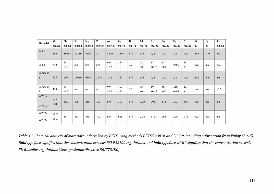
117

Table 16: Chemical analysis of materials undertaken by DETS using methods DETSC 2301# and 2008#, including information from Finlay (2015).

Bold typeface signifies that the concentration exceeds BSI PAS100 regulations, and bold typeface with * signifies that the concentration exceeds

EU Biosolids regulations (Sewage sludge directive 86/278/EC).

Material Mn

mg/kg

Pb

mg/kg

K

mg/kg

Mg

mg/kg

P

mg/kg

As

mg/kg

Zn

mg/kg

B

mg/kg

Cd

mg/kg

Cr

mg/kg

Cu

mg/kg

Hg

mg/kg

Ni

mg/kg

Si

%

Ca

%

Se

mg/kg

Soil 1

350 6954* 15240 4500 407 8820 1987 n/a n/a n/a n/a n/a n/a 20.6 0.78 n/a

Soil 2 730 80

±0.3 n/a n/a n/a

6.9

±0.2

150

±1 1.2

0.2

±0.1

17

±0.15

17

±0.2 <0.05

15

±1 n/a n/a <0.5

Compost

1

525 136 19010 6560 2942 10.4 250 n/a n/a n/a n/a n/a n/a 13.5 3.24 n/a

Compost

2 460

46

±0.3 n/a n/a n/a

9.9

±0.2

150

±01 6.3

0.4

±0.1

19

±0.15

46

±0.2

0.10

±0.05

12

±1 n/a n/a <0.5

WTR1w

1350

±289 31.6 425 245 352 n/a 210 n/a 0.78 29.5 17.8 0.62 49.3 n/a n/a n/a

WTR1d

WTR2w 1825

±665 85 833 335 472 n/a 665 n/a 2.36 31.5 26.8 0.28 91.5 n/a n/a n/a

WTR2d

118

Table 17: Typical ranges for soil, WTR and compost, sourced from Finlay (2015) in addition to other literature. Bold typeface signifies that the

concentration exceeds BSI PAS100 regulations, and bold typeface with * signifies that the concentration exceeds EU Biosolids regulations (Sewage

sludge directive 86/278/EC).

Ma

teri

al

Mo

istu

re

con

ten

t %

pH

TO

C

%

LO

I 55

0

%

To

tal

carb

on

%

EC

(u

s/cm

)

Total

N %

Fe

%

Al

%

Mn

mg/kg

Pb

mg/kg

K

mg/kg

Mg

mg/kg

P

mg/kg

Zn

mg/kg

Cd

mg/kg

Cr

mg/kg

Cu

mg/kg

Hg

mg/kg

Ni

mg/kg

Soil n/a n/a n/a 5 3 n/a 0.02-

0.5% 4 7.1

80-

1300 10-84 640 n/a 1000

17-

125

0.06-

1.1

7-

221* 6-80

0.02-

0.41 4-55

WTR 72-

85

4.1-

7.2 n/a 36-70

13-

26

39-

405

0.051-

1.1

0.8-

41

0.21-

21

370-

5100 5-160

170-

3900

170-

2900

4-

1528

28-

1100

0.2-

36* 7.8-38 7.9-36

0.05-

1.4

10-

120

Compost 30-

60% n/a n/a n/a n/a n/a 1.2 n/a n/a n/a n/a 4000 3000 3000 n/a n/a n/a n/a n/a n/a

119

Figure 19: Particle size distribution for Soil2, silica and WTR2d performed as per

BS1377 (Part 2: 1990)

Figure 20: Proctor compaction curve for Soil2 determining the maximum (optimum)

bulk density as 1.91 g/cm3 at gravimetric water content of 16% (0.16), shown by the

red dashed lines.

Figure 19 presents the particle size distribution of the three materials used in

Trials 3 & 4, retrieved following wet sieving and pipette sedimentation BS1377

(Part 2, 1990). Finlay (2015) conducted PSD testing on Soil 1 and found that it

comprised 40% sand, 30% silt, 30% clay and is therefore a clay loam (Rowell,

1994), which tends to have high water holding capacity, poor aeration, is

0

10

20

30

40

50

60

70

80

90

100

Pe

rce

nta

ge

pa

ssin

g

Particle size

Soil2

Silica

WTR2d

1.5

1.55

1.6

1.65

1.7

1.75

1.8

1.85

1.9

1.95

0 5 10 15 20 25

Bu

lk d

en

sity

(g

/cm

3)

Gravimetric water content (%)

120

susceptible to compaction and has a high resistance to pH change (Brady & Weil,

2016). Soil 2 comprised 61.8% sand, 25.1% silt and 13.1% clay, and is therefore

classified as a sandy loam. The characteristics of sandy loam mean that this soil

type is naturally well draining due to the high proportion of sand, with typical

hydraulic conductivity of 14-42.34 μm/sec, and bulk densities of 1.55- 1.75 g/cm3

(USDA, [23]). Figure 20 displays the relationship between water content and bulk

density according to the Proctor compaction method for Soil2, where the

maximum density of 1.91 g/cm3 was achieved at 16% water content.

121

4.4 Experimental trial methods

As highlighted in Chapter 2 there is a need to quantify the parameters of soil in

relation to their ‘flood holding capacity’. Traditional testing methods to determine

the water holding capacity of a soil use a variety of apparatus, where samples

usually start at complete saturation and are then placed into closed chambers on a

porous plate, after which negative pressure is applied. Water is forced from the

sample under pressure, typically to -0.33 kPa to determine the field capacity, and

up to -1500 kPa to determine the water content or degree of saturation at wilting

point. To the author’s knowledge, there are few if any, known processes to test

water holding capacity that are conducted without external pressure in order to

determine maximal WHC (saturation) and through the drying phase. To simulate

the process of wetting and drying in the field due to the processes of capillary

action, infiltration and gravitational drainage, a new method (Kerr et al., 2016) was

developed.

Four water holding capacity trials were conducted during the research for this

thesis, where Trials 1 and 2 were used for the development of a core making

methodology, and Trials 3 and 4 were more expansive robust trials (greater

repetitions) that produced the data on which this thesis is based. The terms

‘sample’, ‘core’ etc have already been defined at the start of the chapter. Each

amendment (sample) henceforth is given a single label (e.g. A1), as shown in

Figure 21.

[Core]

[----------------------Soil 1/sample----------------]

[------------AM 2-------------]

Figure 21: Sample annotations based on individual units (core/sample), groups of

cores of the same composition (S1 or AM8), and samples of different composition

(Soil 1, AM2 etc)

122

4.4.1 Core production methodology

Cores were created using either a split mould (Figure 22: Trials 1 and 4) or using

the Proctor compaction mould (Figure 23: Trials 2 and 3). The 76 mm x 38 mm

cylinder was chosen as this size of split mould allowed many samples or ‘cores’ to

be produced using the same procedure and apparatus found in many soil

laboratories, with the additional benefit of being a manageable size of sample

when considering the number of samples required to be made. Soil is very

heterogeneous in its nature; therefore many replicates are required in order to

produce statistically significant results.

Figure 22: Schematic of sample (core) production using a split mould and

compaction pin. The core removed from the mould is 76 mm x 38 mm.

Compaction tool Split mould Soil sample Base plate

38 mm

76

mm

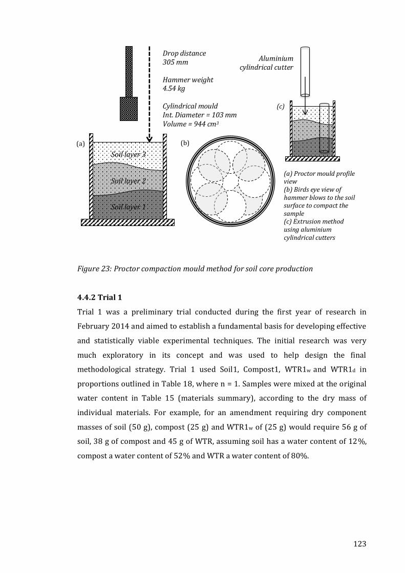
123

Figure 23: Proctor compaction mould method for soil core production

4.4.2 Trial 1

Trial 1 was a preliminary trial conducted during the first year of research in

February 2014 and aimed to establish a fundamental basis for developing effective

and statistically viable experimental techniques. The initial research was very

much exploratory in its concept and was used to help design the final

methodological strategy. Trial 1 used Soil1, Compost1, WTR1w and WTR1d in

proportions outlined in Table 18, where n = 1. Samples were mixed at the original

water content in Table 15 (materials summary), according to the dry mass of

individual materials. For example, for an amendment requiring dry component

masses of soil (50 g), compost (25 g) and WTR1w of (25 g) would require 56 g of

soil, 38 g of compost and 45 g of WTR, assuming soil has a water content of 12%,

compost a water content of 52% and WTR a water content of 80%.

Drop distance 305 mm Hammer weight 4.54 kg Cylindrical mould Int. Diameter = 103 mm Volume = 944 cm3

v

v

Soil layer 3

Soil layer 2

Soil layer 1

(a) Proctor mould profile view (b) Birds eye view of hammer blows to the soil surface to compact the sample (c) Extrusion method using aluminium cylindrical cutters

(a) (b)

Aluminium cylindrical cutter

(c)

124

Table 18: Amendment proportions for samples used in Trial 1, using three materials.

‘n =’ denotes the number of repeat tests.

Each core was made using a split mould (Figure 22, section 4.4.1) and a plastic

graduated compaction plunger, where three equal layers of sample were

compacted into the mould using 25 strikes, which approximates the Proctor light

compaction method, although the compaction effort was unregulated as a hand-

held hammer was used directly on the compaction plunger. The water content of

samples ranged from 12% to 44% for the different amendments (Table 18). As

discussed in Chapter 2 (section 2.3.3), samples with a higher water content were

compacted to a greater extent and produced very dense samples, however drier

amendments were more difficult to compact and required much higher compactive

effort to yield a sample with sufficient aggregate stability for handling and

extraction from the mould. The mass of samples ranged from 112 g to 146 g as

mass was added to mould until the extracted core would hold together, giving a

broad range of densities.

Once produced, each core was weighed and measured with digital callipers before

being inserted into a latex membrane (typically used for tri-axial testing) and

stoppered at each end with a 38 mm porous disk to minimise soil loss when

submerged. Samples were completely submerged for a period of 24 hours and

weighed and measured again once the membrane had been carefully removed.

This method was not sufficiently precise and yielded poor results, with the

Sample

n = 3

Soil %

SOIL 1

Compost %

COMPOST1

WTR%

WTR1

GWC

%

Bulk density (BD) & dry

density (Dd) g/cm3

Soil 1

100 0 0 12 1.71 (BD)

1.55 (Dd)

T1A 50 50 0 33 1.67 – 1.87 (BD)

1.12 – 1.25 (Dd)

T1B 50 25 25 (WTR1w) 44 1.53 – 1.71(BD)

0.86 – 0.93 (Dd)

T1C 50 25 25 (WTR1d) 22 1.63 – 1.76 (BD)

1.27 – 1.38 (Dd)

T1D 50 40 10 (WTR1w) 38 1.54 – 1.60 (BD)

0.96 – 0.99 (Dd)

T1E 50 40 10 (WTR1d) 29 1.59 – 1.69 (BD)

1.13 – 1.20 (Dd)

125

following action points leading into Trial 2: control of water content at initial

production, control of compaction effort to ensure a similar sample density,

greater homogenization of component parts to reduce error, change of saturation

method and sample casing and increase of sample size to account for unavoidable

heterogeneity.

4.4.3 Trial 2

In this second trial, Soil 1 and WTR1d were air-dried and WTR1w was excluded so

that water content could be controlled, as soil only retains hygroscopic water once

air dried (Figure 8C). Compost was kept as received water content (33%) as air-

drying (discussed in section 4.2) has a number of degenerative effects such as

increased water repellence, mineral surface acidity and microbe mortality (Kaiser

et al., 2015). Soil 1 and WTR1d were gently crushed to pass a 2 mm sieve to

increase homogeneity of samples. As in Trial 1, samples were mixed proportionally

according to the dry mass of components and water was added to make the

samples to 13.5% water content (Table 19). The value of 13.5% water content was

chosen as it was the driest state in which the samples could be produced and still

retain their form. Following the standard light proctor test protocol (27

compaction blows and three layers of sample), one large cylindrical sample was

created, from which four cores were extruded using aluminium cylindrical cutters

and a machine press (Figure 23). Cores were then painted with three coats of

liquid latex to provide a thin, impermeable membrane designed to replicate the

external pressure of surrounding soil and to reduce the soil loss from the cores

during wetting. To initiate testing, samples were put onto wet sand to allow water

to enter the sample gradually over 48 hours before complete submersion; this was

to avoid trapping air in the centre of the sample and reduce erosion of the end

faces by slaking. At 48 hours samples were completely submersed and a 5 cm head

was maintained. Every 24 hours the samples were weighed and measured over a

period of 72 hours.

The drawback to the method used in Trial 2 was that the structure and natural

heterogeneity of soil was partially destroyed by air drying and breaking down to

<2 mm, which may have reduced the water uptake rate and total water holding

126

capacity (as a result of pore size reduction and potential hydrophobicity as

discussed in relation to aggregate size and air drying in section 2.2)

Table 19: Soil amendment ratios used in Trial 2 according to the dry mass of each

component. ‘n =’ denotes the number of repeat tests.

4.4.4 Trial 3

Trial 3 included a greater number of amendments and repetitions (Table 20),

which included the use of silica that aimed to replicate the structural effect of WTR

(due to the inert nature of silica), rather than the geochemical effect. Soil2, WTR2d,

Compost 2 were used as the materials for this trial and were processed as outlined

in section 4.2 (sieved to 6.3 mm, Soil2 field moist and WTR2d air dried). Samples

were mixed according to their dry mass and then slowly air-dried to 14% water

content. For those samples that were <14% GWC when mixed, water was added to

make up the deficit. Once at 14% water content the samples were sealed until use

to avoid moisture loss.

The proctor mould method (Figure 23) used in Trial 2 was also used for Trial 3.

During the production of samples, amendments containing compost (with the

exception of A6) would not adhere sufficiently to enable them to be removed from

the mould at 14% water content and required a further addition of water

(increasing the samples to 25% water content). Once produced, the cores were

Sample

n= 4

Soil 1 % Compost 1 % WTR1d % Bulk density (BD)

dry density (Dd) g/cm3

Soil 1 100% 0 0 1.86 – 1.93 (BD)

1.64 – 1.70 (Dd)

T2A 50% 50% 0 1.61 – 1.66 (BD)

1.42 – 1.46 (Dd)

T2B 50% 0 50% 1.51 – 1.58 (BD)

1. 33 – 1.39 (Dd)

T2C 50% 25% 25% 1.55 – 1.61 (BD)

1.37 – 1.42 (Dd)

T2D 50% 40% 10% 1.54 – 1.61 (BD)

1.35 – 1.41 (Dd)

T2E 50% 30% 20% 1.56 – 1.63 (BD)

1.37 – 1.44 (Dd)

127

painted with liquid latex as discussed previously. For Trial 3, the wetting method

was altered from Trial 2 to allow samples to take up water from the saturated sand

for a longer period of time before submersion. Cores were measured and weighed

at 24 hour intervals for a period of 120 hours before being fully submerged for a

further 120 hours.

Table 20: Soil amendments used in Trial 3. Bulk & dry density and water content

values are for individual cores at production. F1 and F2 were omitted from the trial

as the composition F1 would not yield a stable core before testing began and F2 fell

apart considerably during wetting, invalidating the data. ‘n =’ denotes the number of

repeat tests.

F1 and F2 were omitted from the trial; during the production of F1 it was clear that

this amendment would not yield sufficiently stable cores to extrude and paint with

latex. During the wetting of F2 there was significant soil loss from the ends of the

cores, giving a false indication of the mass; therefore, this data could not be used.

Sample

N= 8

Soil

2%

Compost

2%

WTR2d

%

Silica

%

Bulk density (BD)/

dry density (Dd)

g/cm3 average

Water

content

Soil 2 100 1.85/1.60 14

F1 50 50 n/a n/a

A1 50 50 1.55/1.37 14

A2 50 50 1.89/1.66 14

A3 50 25 25 1.49/1.19 25

A4 50 25 25 1.56/1.25 25

A5 60 40 1.42/1.25 14

A6 60 40 1.75/1.54 14

A7 60 40 1.96/1.73 14

A8 60 20 20 1.49/1.19 25

A9 60 20 20 1.50/1.20 25

A10 70 30 1.51/1.20 25

A11 70 30 1.62/1.43 14

A12 70 30 1.78/1.57 14

A13 70 15 15 1.52/1.22 14

F2 70 15 15 n/a 14

128

Although the water content and compaction effort remained consistent across the

board, due to the variation of specific density of component parts and the different

extents to which samples compacted under the same effort, the dry and bulk

density of samples were significantly different. In some cases, the degeneration of

a number of cores meant a reduction in the total number of cores for different

amendments; some cores had significant loss of soil from the open ends during the

wetting process, giving a false reading for the mass and indicating what would

appear as a loss in water content.

4.4.5 Trial 4 (Final Trial)

Trial 4 included the finalised water holding capacity method and four other tests

(outlined in section 4.5). In this trial, the mass and volume change during both the

wetting and drying was observed over time, with two wetting and two drying

periods. Silica was removed from the testing materials and replaced by WTR2w as

realistically, WTR would be added to soil in the form in which it is produced by

water treatment companies, i.e. unprocessed and with a GWC of ~80%. Once the

unprocessed WTR (WTR2w in this case), is incorporated into the soil, it would air

dry naturally over time, this is the reason why all component materials were mixed

at their stored water contents (Table 15) relative to their dry mass and then air

dried to 17.5% GWC (Table 21).

Sample Soil2 % Compost2 % WTR2

Soil2 100 0 0

AM1 90 10 0

AM2 90 0 10 WTR2d

AM3 90 0 10 WTR2w

AM4 90 5 5 WTR2d

AM5 90 5 5 WTR2w

AM6 80 20 0

AM7 80 0 20 WTR2d

AM8 80 0 20 WTR2w

AM9 80 10 10 WTR2d

AM10 80 10 10 WTR2w

AM11 70 30 0

AM12 70 0 30 WTR2d

129

Table 21: Soil amendment ratios used for Trial 4.

Sixteen cores were made for each amendment, twelve of which were used for WHC

testing, four of which were stored for use in triaxial testing (section 4.6) and XRCT

(Chapter 6). These parameters were chosen so that all amendments would hold

together during both the preparation stages and through wetting and drying

cycles. By controlling the mass of each core, the resulting data would give an

indication of the water holding capacity per unit mass of material. Previous trials

had cores of varying density and mass, which meant there were many independent

factors to consider during the analysis of results. The density of cores in Trial 3

were representative of what would occur in field conditions, where soil or

amended soil at GWC of 14 or 25% had been subjected to a given compactive effort

(e.g. by machinery or cattle). Trial 4 in comparison relates the water holding

capacity to a given volume and mass of soil or amended soil.

The split mould method (Figures 22 and 24) was used to create 175 g cores, BD of

2 g/cm3 and Dd 1.75 g/cm3, using Soil 2, WTR2d, WTRw and compost 2. Each 25 g

layer was scored on the surface after compaction to ensure that subsequent layers

adhered to the previous layer. For samples that contained compost, each core was

left in the split mould on the static press until the displacement needle remained

stable (Figure 24A) to ensure that compost did not rebound and deform the

sample before it had been painted with latex as in Figure 24C. Although the water

content of different amendments was the same, it is likely for amendments with

compost that the majority of water retained by the sample was contained within

the compost as it acts as a sponge, rather than in the surrounding soil material.

Samples without compost in contrast are likely to have homogeneous dispersion of

water within them. By leaving the core in the mould with a static pressure applied,

water held preferentially by compost is able to disperse evenly through the

sample.

AM13 70 0 30 WTR2w

AM14 70 15 15 WTR2d

AM15 70 15 15 WTR2w

130

Once cores were removed from the split mould, they were immediately painted

with liquid latex and geotextile (both highly permeable and elastic) was tied

around the base to ensure no loss of soil. Cores were stored in airtight containers

in the fridge until all cores were made. Samples, as with Trials 2 & 3, were placed

onto saturated sand to begin the wetting cycle, during which the cores were

weighed and measured every 24 hours. The initial wetting took up to 216 hours

(the point at which the mass plateaued), after which they were flooded for a period

of 48 hours (total of 264 hours). Cores were then placed on oven dry sand to begin

the drying cycle, and once again weighed and measured every 24 hours until their

mass reached 175 g. This process was completed twice to give two wetting and

two drying cycles.

Figure 24: Split mould and static compaction press method. (a) Top left - Pressure

gauge on static compaction press. (b) Top right - Split mould and static compaction

press. (c) Bottom left - Samples with high compost additions (where left has been

removed from mould immediately after compaction and right after 1 hour of

pressure equilibration). (d) Bottom right – Finished sample with latex coating and

geotextile wrap

Static compaction press Graduated compaction rod Split mould Baseplate

131

4.4.6 Density and water content considerations

Below is a summary of methods, method development and parameters used

during Trials 1-4 (Table 22). As discussed in Chapter 2 (section 2.3.3) the following

relationships between water content, compactive effort and density are known;

Water content: the water content of a soil controls the resultant degree of

compaction for a given compactive effort, where the addition of water increases

susceptibility to compaction and the bulk density increases up to the ‘optimum’

point where maximum (dry) density is reached (Figure 20).

Compaction effort: compacting different soils at a constant water content and

compaction force will result in samples of different densities as some materials

deform more easily than others (e.g. soil becomes much denser than compost at

the same compactive force).

Density: different soil composition requires variable compactive effort to make a

sample to a given dry density when using a constant mass. Amendments with high

proportions of compost will require a greater compactive effort to reach the

required dry density.

Water content was chosen as the control parameter for Trials 2-4, as it is a critical

factor in the structure of soils during compaction and it is important to have a

constant starting moisture content for trials considering the water content change

over time. As Head (1980) states, the criterion for compaction must be

ascertained: either compaction to bring the soil to a specified dry density (or void

ratio) or to apply the soil for a known compactive effort. Compaction was

controlled in Trials 2, 3 and 4 using either the Proctor method or a static press,

giving variable resultant densities of samples, despite constant water content, due

to the properties of the amendments.

As discussed in previous chapters the dry density and state of compaction of a soil

sample largely governs how water moves into and through a soil (see section

2.4.4), where dry density and total porosity are commonly used parameters to

characterize this attribute (Håkansson & Lipiec, 2000). Efforts to find a parameter

that eliminated the differences in optimum compaction values have mainly

revolved around relating the bulk density to a reference point, i.e. a bulk density

obtained by a standardised compaction effort e.g. 200 kPa at a standard water

132

content. The issue is that much of this testing is for different soils, not amendment

soils that contain high levels of organic matter.

For Trial 4 the water content and density were chosen control factors. Low dry

density samples of the sample soil composition have a greater total pore volume

and therefore have more space for water than denser samples, the exception being

clays that can hold large amounts of water due to their high surface area and high

micro-porosity despite their density. The bulk density and mass of cores were

therefore chosen as constant factors to remove the effect of density variability, in

addition to the control of water content. The known drawbacks to the use of this

method firstly that compost is compacted to a significant degree to achieve the

required density, removing one of the positive effects on structure that compost

imparts, and secondly each amendment will be at different degrees of compaction.

Unfortunately, one can only choose two options from the three parameters of

density, water content and compactive effort.

Table 22: Summary of method parameters for Trials 1 -4

Trial

#

# of

samples

# of

amendments

(inc. soil

alone)

Period of

wetting

Period

of

drying

Bulk density

(BD)

dry density

(Dd) g/cm3

Water

content

%

Exterior

coating of

cores

1 3 6 24 hours n/a 1.53 – 1.87

(BD)

0.86 – 1.55

(Dd)

11.7-44

Rubber

membrane

2 4 6 48 h sand

bed, 72 hours

flood

n/a 1.51 – 1.93

(BD)

1.33 – 1.70

(Dd)

13.5 Latex

3 8 16 144 h sand

bed

Up to 336

hours

flooding

n/a 1.42 – 1.96

(BD)

1.19 – 1.66

(Dd)

14 & 25 Latex

4 12 16 216 h sand

bed

48 h flood

216 h 2.0 (BD)

1.73 (Dd)

17.5 Latex &

geotextile

133

4.4.7 Statistical testing

The use of statistics is widely used in science to test whether the central

tendencies, i.e. mean or median, of two or more groups are significantly different

from one another (Ruxton, 2006). In statistical testing a null H0 and an alternative

hypothesis Ha are required, where the former is the default position that there is

no relationship (dependent) or no difference (independent samples), and the

alternative hypothesis states that there is a relationship or difference between two

data sets. The significance level (a) is the probability of rejecting the null

hypothesis, where typically this value is 0.05 (95%) or 0.01 (99%), and the p value

is the probability of a result being of the same value should H0 be true. Statistical

significance is achieved when p < a, and therefore one can accept the alternative

hypothesis by rejecting the null hypothesis. The smaller the p value, the greater the

significance, therefore one can have degrees of significance. Data can be split into

two groups based on their theoretical distributions (parameters), which determine

the type of statistical analysis that can be used. Parametric statistical tests make a

number of assumptions about the data including the normality population

distribution, and variance, however non-parametric tests make fewer assumptions

and do not require ‘normally distributed data’ (Altman & Bland, 2009).

Parametric methods include t-tests and analysis of variance (ANOVA) for testing

differences and least squared regression and correlation for testing the

relationship of dependent variables. Non-parametric methods include the

Wilcoxon Mann-Whitney U or rank sum test (MWU), Kolmogorov-Smirnov and

sign test, which work using the rank of data rather than making assumptions about

the distribution or variance of the data. The issue with checking normality in small

data sets is that it is difficult as formal testing has low power, so violations of the

assumptions may not be detected, but with a large number of samples (n) you can

depend on the central limit theorem. This means that with enough observations

with a finite level of variance, the mean of the samples will equal the mean of the

population as a whole, the asymptomatic normality of the test statistic and t

distribution. With no way to accurately check this, one must assume no normality

and use non-parametric methods. Rank tests are reasonable defaults if one expects

non-normality, due to small sample size and apparent presence of outliers that

134

skew plotted data (which is likely to be the case with data based on soil

variability).

In an attempt to statistically model data produced, a report conducted by Perksy

(2017) developed a mathematical model that allowed important qualitative

statements about the physical properties of the tested soils with mathematical

rigour, focusing on the drying phase of data from Trial 4. Bayesian Inference with

Markov Monte Carlo was used to perform analysis and deduce the properties of a

population as a whole by incorporating prior knowledge of soil characteristics and

data from the experiment. However, the use of this method to determine statistical

difference requires an extended knowledge of mathematics, beyond the current

knowledge base of the author.

The Mann Whitney test (MWU, Mann & Whitney, 1947) is commonly used to

compare the efficacy of two treatments in medicine, and can be applied to other

disciplines that have a similar research aim. It is commonly used as an alternative

to t-tests when data are not normally distributed or other assumptions of

parametric data are not met, therefore the data are non-parametric (Ruxton, 2006;

Fagerland & Sandvik, 2009). As the MWU test compares the sum of ranks, it is less

likely to spuriously indicate significance because of the presence of outliers

(therefore it is more robust). The MWU test is the default test for comparing

ordinal measurements (such as mass) with similar distributions. It does however

assume that two independent samples have the same shape (distribution) and

spread (variance), but with difference medians and location (Skovlund & Fenstad,

2001).

The MWU detects if 2 or more samples come from the same distribution, or

whether the medians of the group are different. The null hypothesis is therefore

that is it equally likely for one randomly selected value from one sample to be less

or greater than a randomly selected value from the other sample. For this research

therefore, the null hypothesis is that a core of material is equally likely to have a

higher or lower water holding capacity that a core of material from a different

amendment. The test therefore determines if the samples were taken from the

same population (i.e. there is no difference in WHC) or different populations. The

135

alternative hypothesis states that one distribution is greater than the other. The

test makes the following assumptions:

1. The data are ordinal i.e. one observation can be shown to be greater than

another e.g. by use of decimals.

2. The dependent variable (WHC as defined by the GWC) is not normally

distributed.

3. The data of the two groups have equal variances.

4. The shapes of the distribution are the same, although the location can be

different.

5. The sample drawn from the population is random.

The data from WHC testing were assumed to be non-parametric due to the small

sample size (n = 12) that effectively invalidates normality testing and in addition

typical parametric analysis requires groups of data greater than 15. The MWU is

commonly known as a test for equality of medians, however it actually is able to

detect differences in shape and spread rather than just a difference in means (Hart,

2001). The Mann Whitney statistic is highly informative as it gives the probability

that one group individual will score higher than the other, particularly in the

analysis of controlled treatment trials. For the purposes of this test, only the

statistical significance is needed, as the distribution of data is of lesser importance

and the hypothesis are as follows:

H0 = there is no difference between the control sample (Soil 1 or Soil 2) and the

amended sample (AM1-AM16)

Ha1 = there is a difference between the control sample (Soil 1 or Soil 2) and the

amended sample (AM1-AM16), where the amendment is expected to increase the

water holding capacity of the soil, as indicated by the gravimetric water content.

Ha2= there is a difference between samples with different amendments (e.g. AM1 vs

AM2), however the direction of change is not known

The primary alternative hypothesis (Ha1) was tested assuming the amended

sample would be greater than the control, which suggests the use of a one-tailed

136

test however a two tailed test was used for both the primary and secondary

alternative hypothesis to avoid missing a detrimental (decrease) impact of

amendment on the WHC. A significance level of 95% was chosen, therefore ‘a’ must

be less than 0.05 to be given a significant result. Due to the differences in initial

parameters (water content and density) and very small data sets where n = 5-8

statistical testing between sample populations, testing was not appropriate on data

from Trials 2-3.

For the statistical analysis of Trial 4, significance tests were not performed on the

time series as a whole, but at important points through the wetting and drying

cycles; 24 hours, 288 hours (maximum GWC), 312 hours (24 hours of drying), 600

hours (24 hours of rewetting), 912 hours (second maximum GWC), 936 (second 24

hours of drying), 1068 hours (end point).

4.5 Erosional resistance testing

According to Lal (2003) the choice of an appropriate index for testing erodibility of

soils is governed by the relevance to the processes that control soil erosion in the

natural field environment. It is for this reason that, as stated in Chapter 2 there is

no standard index by which erodibility is measured. Two methods were used to

measure the erodibility and cohesiveness of amended soils; the Veitch method and

fall cone penetrometer. The former is a novel method using water drop erosion to

a determined point of failure (KE index, measuring the kinetic energy required to

disrupt an aggregate), and the latter is a standardised method that tests the shear

properties of a saturated soil. These tests were chosen to test the effect of

amendment on the cohesion and stability of samples under rainfall simulation. As

stated in literature (Chapter 2, section 2.3.5), rainfall simulation is suggested as the

most suitable method to approximate the erodibility of a soil. For this reason, the

Veitch method was developed to test the stability of a small soil sample under a

controlled supply of drops.

4.5.1 The Veitch method

Discs of 10 mm height x 38 mm diameter were formed as per amendments in Trial

4 (Table 21), using the static press and split mould method with a single 25 g layer

of material compacted at 17.5% GWC to a density of 2 g/cm3 (BD), 1.73 g/cm3 (Dd).

137

The test was designed to induce rapid wetting under rainfall simulation to test the

ability of the sample to resist slaking and aggregate breakdown. The subjectivity of

other tests, which use single drops to break a sample down to a given end point, is

somewhat negated by designating an easily identifiable end point of the test (when

the surface of the sample or the whole of sample first experiences failure, through

cracking as in Figure 25, or slumping) and using a controlled rate of water

delivery. Drops fell onto the centre of the sample from a height of 310 mm, with a

resultant drop velocity of 2.46 m/s and a kinetic energy of 0.00036 Joules.

Although the test had significantly lower velocity than natural rainfall, which

ranges from 2 – 7 m/s depending on drop size 0.5- 2.6 mm and rainfall intensity 1-

6 mm/hour respectively (Pruppacher, 1981), this was the greatest height

achievable in lab to ensure that drops reliably fell centrally on the sample. Samples

were mounted onto a curved plastic standing with a radius of 37 mm. 24 replicates

of each amendment were tested, where half were tested immediately after

production, and the remaining 12 samples were completely saturated and dried

back to a mass of 25 g. This was to replicate the effects of a wetting and drying

cycle on the materials. The time from initial drop to the point of failure was

recorded, from which the number of drops and mass of water required for failure

could be calculated. The sample was immediately removed from the plastic mount,

weighed and placed into an oven for 24 hours at 105° C to calculate the water

content.

Figure 25: Schematic diagram (left) of the Veitch method used to test aggregate

stability of disk shaped samples and a photo of a sample during testing (right)

Drop height 310 mm

5 drops per second = 0.12 g/s

Watson-Marlow pump

Sample failure

Sample

Radius = 37 mm

138

4.5.2 Fall cone test

The fall cone test is commonly used as a quick test of undrained shear strength

following Hansbo’s equation (Equation 17) and testing using this method followed

the procedures described in BS1377: 1990. Samples were made following the

procedures used in Trial 4, but to dimensions of 38 mm x 38 mm (four layers

rather than seven) to match the fall cone test apparatus requirements. Briefly, the

test uses a stainless steel cone to penetrate a saturated soil sample under the

influence of gravity where the apex is flush with the surface of the sample, after

which the depth of penetration is measured using a dial gauge after 5 seconds have

passed from release of the cone (Tanaka et al., 2012). 24 replicates were

completed for each amendment, 12 of which were tested 24 hours after production

and 12 of which were tested having been fully saturated and air-dried back to the

initial water content. The undrained shear strength in kPa can be calculated using

Equation 12 from the data obtained in the testing.

𝐶𝑢 = 𝑘 ∝ (𝑚𝑔

𝑑2)

Equation 17: Hansbo formula, where Cu = undrained shear strength, m is mass of the

cone, g is gravity, d is the penetration depth and k∝ is the cone factor based on cone

angle (ranges between 0.1 and 1). Hansbo (1957).

4.6 Triaxial testing

Triaxial testing has several advantages over other shear testing methods as

complete control of testing conditions, including the measurement of the drainage

conditions, pore pressure, volumetric changes, compressibility, permeability,

stress distribution can be obtained with ease. The drawback of this method is that

it is very time intensive (and therefore expensive) and may not truly reflect the

effects of loading that may occur in the field. However the test provides accurate,

adaptable data that provides a reliable test for the shear characteristics of a

specimen. The triaxial test is performed on cylindrical specimens that are either

trimmed from field samples, or as in this research, synthesised in the lab to best

represent field conditions. The sample is contained within an impermeable latex

membrane before being mounted for testing in the triaxial cell (Figure 26).

139

Pore water

pressure u

q

σc

σc

σc σc σr = σc = σ3

σa = q + σc = σ1

q

Specimen length (L)

ε = Axial strain = ΔL/L

σc = Confining pressure σ1 = Major principle stress = axial stress σa σ3= Minor principle stress = radial stress σr q = Deviator stress = F/A = Axial load/Area σ’1 = Major principle effective stress = σ1- u σ’3 = Minor principle effective stress = σ3 - u

Some cores may have been subject to thixotropic effects due to the duration over

which testing was completed. The samples were tested according to their

amendment number (i.e. Soil 2 and AM1 were tested first and AM13, AM14 last);

therefore this must be factored into the results. The procedure for testing the

shear strength of the soil was as follows and includes a brief description of the

steps taken. For a thorough review of the process readers are directed to Lade

(2016) for information on initial set ups and test procedures. All samples from

Trial 4 were tested for their permeability at pressures of 25 kPa, 50 kPa and

100 kPa. Three cell pressures of 25 kPa, 50 kPa and 100 kPa were used for Soil 2,

and AM11-AM15 in order to produce a set of Mohr’s circles, stress strain curves

and stress paths. This meant three samples were used for the shear strength

testing as the process destroys each core by testing it to failure. For permeability

measurements (AM1-AM10), only one core was used where permeability testing at

25 kPa was completed before increasing the cell pressure to test at 50 kPa and so

forth.

Figure 26: Schematic of the strain (ε) and stress (σ) states undergone by a sample

during triaxial testing

140

An experienced lab technician completed the consolidated undrained triaxial

testing according to BS 1377-8:1990 Part 8, which comprises briefly: firstly, test

specimens were measured (average radius and height), weighed and inserted into

a latex tube, into which air free porous disks are placed at the end face of each

cylindrical specimen. The sample was then placed into the triaxial cell and secured

using rubber O-rings. Once the cell was sealed, it was filled with water and the

saturation of the sample was started, where cell pressure (not exceeding 305 kPa)

and back pressure (aiming to reach 300 kPa) was applied. The saturation process

aims to fill all voids with water and properly de-air the pore pressure transducer

and drainage lines. Pore water pressure readings were taken until the change was

negligible, as an increase in pore water pressure suggests air presence. Skempton’s

B value (a determination of how saturated the sample is) was calculated once cell

pressure was increased by 100 kPa. For some materials, the B value will reach 1

(100%) at full saturation, however for very dense samples this value may only

reach 0.91. The level of saturation, calculated using Equation 18 must have been

< 95% or 0.95 before consolidation could begin, which indicated a saturation level

exceeding 99%.

𝐵 =∆𝑢

∆𝜎3

Equation 18: Skempton’s B value calculation where ∆𝑢 is the difference between

initial and maximum pore pressure and ∆𝜎3 is the difference between initial and

maximum cell pressure.

At this point the sample was fully saturated and all voids were filled with water. In

the subsequent phase, called consolidation, cell pressure was increased to the

specified limit (325, 350 or 400 kPa). Readings were taken until the volume change

of the specimen was negligible and 95% of the excess pore pressure, created as a

result of cell pressure change, had dissipated. This process brought the specimen

to a given effective stress (total pressure/stress – back pressure) required for

shearing and permeability tests. The permeability of the sample was tested prior

to shearing by applying a 15 kPa difference in pore pressure, and the volume

change in water above and below the sample measured to be able to calculate the

permeability using Equation 5 (section 2.4.4.)

141

𝑘 =𝑞𝐿

𝐴ℎ

Equation 5: Hydraulic conductivity (k), where q is the permeability coefficient (flow

in m3/second), L is the length of the sample in m, A is the cross-sectional area of the

soil (m2) and h is the pressure head (in m). Craig (2004).

After testing the permeability of the sample, it was sheared; during the shearing

process the vertical load, pore water pressure and vertical displacement were

monitored until there was a change in displacement (height of the sample) of 20%

of the original height of the sample. This entire process was completed three times,

to test the hydraulic properties and shear strength at three pressures, 25, 50 and

100 kPa.

From this data, hydraulic gradients, Mohr circles/stress strain graphs and stress

paths may be determined. The shear strength is the maximum shear stress,

determined from the radius of the Mohr’s circles (example in Figure 27) or from

the stress strain graph (Figure 28). From Mohr’s circles we may obtain the angle of

friction and the cohesion values. However cohesion is a vague concept, as only

soils with physio-chemical bonding have a true cohesion, but many soils will show

an apparent cohesion in triaxial testing as the result of volume change, which gives

a higher peak state than critical state (apparent cohesion, as discussed in Chapter

5, section 5.3.2). As the failure envelope drawn in Figure 27 is at the discretion of

the person obtaining the value, the values of cohesion and angle of friction are

exceptionally sensitive to the gradient of the failure line, which may be drawn far

from the ‘true’ value. In addition the Mohr circle only shows the condition at one

axial stress point. As we are able to obtain the maximum shear strength from a

stress strain curve (by dividing the deviator stress by two, Figure 28), and from

stress paths (Figure 29) one can obtain the angle of friction, critical state line and

peak line, we may use these two representations rather than Mohr’s circles to

analyse the continuous variation in behaviour rather than just a snapshot of the

point of failure.

142

Figure 27: Example of Mohr Circles, plotted with a failure envelope (which is

idealistic and unlikely to be linear), angle of friction, and cohesion (c).

Figure 28: Example of stress strain curves for a soft material (black dashed), a typical

stress strain curve of a soil for which the maximum strength is coincidental with the

critical state (black), and an overconsolidated sample that reaches a peak strength

and subsequently reaches an ultimate state with increasing axial strain (red).

Figure 29: Example of stress paths for dilatant (black) and compressive (blue)

samples to the critical state line (red)

Shea

r st

ress

Principle stress

c

Friction angle ϕ

Shea

r st

ress

Axial strain

Shea

r st

ress

Axial strain

Critical state line

143


This chapter has outlined specific details regarding the source, preparation and

storage of materials used in this research. These materials have been characterised

using British Standards. The chapter clarifies the methods of testing gravimetric

water and volumetric water content values, and subsequently outlines the

development of methods to determine the water holding capacity through

Trials 1-4 which briefly comprise;

Trial 1: Exploratory trial to test core production methods with materials in

‘field’ condition.

Trial 2: Exploratory trail to test core production methods using texturally

homogenised and air-dried materials, wetted to a consistent water content.

Trial 3: Large scale trial using two controls (water content and compaction

effort) for core production using the Proctor mould method, testing 13

different amendments, up to 50% amendment, with up to 12 repetitions

(n = 12). Materials used in this trial were Soil 2, compost, silica and WTR2d

Trial 3: Final large-scale trial using two controls (water content and bulk

density) for core production using the split mould method. Trial 4 tested 15

different amendments, up to 30% amendment where n = 12. Materials used

in this trial were Soil 2, compost, WTR2d and WTR2w.

In addition to water holding capacity trials, the chapter outlined triaxial apparatus

methods by which the hydraulic conductivity and shear strength of soils were

tested, a British Standard test to determine the undrained shear strength (fall cone

test), and a novel test (the Veitch method) to determine the erodibility of a soil via

raindrop detachment.

144

5. Results and Discussion

The following chapter presents data on four soil functions, WHC, erosional

resistance, shear strength and hydraulic conductivity. This includes experiments

completed for this thesis and supplementary work completed conducted by

students under supervision of the author, for the purposes of measuring soils and

their amended counterparts, which is pertinent for the discussion on what effect

amendment has on soils.

5.1 Water holding capacity

The testing of the water holding capacity of soils and amended soils was completed

over four trials using a novel methodology. Initial testing used only a small variety

of amendments, where Trials 3 and 4 had a much greater range of amendments

and replicates (denoted by n =).

5.1.1 Initial results: Trials 1 & 2

The outcome of Trials 1 & 2 determined how Trials 3 & 4 were conducted and as

such the results from Trials 1 & 2 are presented here in order to briefly discuss the

limitations of their design and are not used to inform the discussion of hypotheses.

Each trial is discussed to demonstrate how the various methods and initial

parameters such as moisture content are enormously important in determining

the data produced. Figures 30-34 below show the change in gravimetric water

content, volumetric water content and density respectively in Trial 1. As discussed

in Chapter 4, all volumetric water contents (VWC) will also be displayed with the

instantaneous volumetric water content (VWCi), which is a ratio of the volume of

water to the volume of bulk soil at the point of measurement rather than VWC,

which is the ratio of volume of water to the original volume of the soil. Samples are

labelled S1, corresponding to unamended Soil1, and T1A, T1B, T1C, T1D and T1E

corresponding to amendments using Soil1 (S), Compost1 (C) and WTR1d or

WTR1w, which are outlined below each figure.

145

S1 T1A T1B T1C T1D T1E

100 % soil 50S 50C 50C 25C

25WTR1w

50S 25C

25WTR1d

50S 40C

10WTR1w

50S 40C

10WTR1d

where S =Soil1 and C = Compost1

Figure 30: Trial 1’s average gravimetric water content of Samples S1 and T1A-T1E

where n = 1. ‘Start’ indicates the initial conditions of the samples, and ‘24 hours’

indicates the GWC after 24 hours of submersion.

The initial GWC for Trial 1 (shown in Figure 30) was considerably different

between samples, ranging from 0.13 (S1) to 0.79 (T1B). In general, the samples

with the highest change were the ones that began with the lowest GWC, where T1C

had the greatest increase (from 0.28 to 0.65) compared with unamended soil

(S1: from 0.13 to 0.47). The starting water content is therefore of essential

importance as samples with greater initial gravimetric water content will be able

to take up less water pro rata and therefore a direct comparison cannot be made.

The volumetric responses of samples (Figure 31) are similar to the gravimetric

water content change show in Figure 30. In general, the greatest change in VWC

was shown for samples with lower initial VWC (S1 and T1C).

0.00

0.20

0.40

0.60

0.80

1.00


Gra

vim

etr

ic w

ate

r co

nte

nt

Sample

START

24 HOURS

146


100 % soil 50S 50C 50C 25C

25WTR1w

50S 25C

25WTR1d

50S 40C

10WTR1w

50S 40C

10WTR1d


Figure 31: Trial 1’s average volumetric water content (VWC) and VWCi, where n = 3

with the exception of S1 where n = 1, at the start point and 24 hours after

submersion.


100 % soil 50S 50C 50C 25C

25WTR1w

50S 25C

25WTR1d

50S 40C

10WTR1w

50S 40C

10WTR1d


Figure 32: Trial 1’s average dry density (Dd) and bulk density (BD) of samples, where

n = 3 with the exception of S1 where n = 1, at the start point and 24 hours after

submersion.

0.00

0.20

0.40

0.60

0.80

1.00

1.20


Vo

lum

etr

ic w

ate

r co

nte

nt

Sample

START

24 HOURS

24 HOURSi

0.00

0.20

0.40

0.60

0.80

1.00

1.20

1.40

1.60

1.80

2.00


De

nsi

ty g

/cm

3

Sample

START Dd

START BD

24 HOURS Dd

24 HOURS BD

147

As shown in Figure 32, there were small changes in the bulk density and dry

density as a result of volume change of the samples as they took up water. The dry

density decrease was lowest for S1 (0.08 g/cm3), and largest for T1C (0.34 g/cm3).

The bulk density of all samples increased with the exception of S1, which had a

0.29 decrease, the former of which is due to an increase in water in amended

samples without a large change increase in sample volume.


100 % soil 50S 50C 50S 50WTR2d 50S 25C

25WTR1d

50S 40C

10WTR1d

50S 30C

20WTR1d

where S = Soil1 and C = Compost1

Figure 33: Trial 2’s average GWC (where n = 4) over 72 hours of submersion.

In Trial 2, S1 remains as the unamended soil and 5 amendments are annotated

T2A – T2E. All component materials (soil, compost and WTR) were air-dried

before mixing and the controlled addition of water after combination meant that

the initial gravimetric water content was equal for all samples, improving the

methodology from Trial 1. As a result of this change a better comparison can be

made between samples than in the previous trial where the initial water content

was variable (Figure 31). All values of GWC were greater than unamended soil

over time with the exception of T2B (50S 25C 25WTR1W). T2D (50% co-

amendment) had the highest GWC after 72 hours of submersion, above the single

50% amendment of compost (T1A). However, literature suggests that the soil with

the greatest amount of organic matter is likely to hold the most water (up to 10

0.10

0.15

0.20

0.25

0.30

0.35

0.40

0.45

START 24 48 72

Gra

vim

etr

ic W

ate

r C

on

ten

t

Hours

S1

T2A

T2B

T2C

T2D

T2E

148

times its own weight, see section 2.2.1). This result comes as a non sequitur and

provides an example of why keeping materials such as compost as close to ‘field’

conditions as possible is crucially important, rather than removing their beneficial

properties (water holding capacity and structural improvement) by air drying and

grinding. Although all amendments were made up to the same water content, the

air-drying of compost and soil would have been detrimental to the water holding

capacity. As discussed in the methods chapter, the breakdown and drying of

materials is likely to have compromised or altered the benefit of the addition of dry

WTR or compost from a structural perspective (Kaiser et al., 2015). Therefore

these results do not reflect how an amendment may affect the maximum GWC of a

soil.

Figure 34 shows the volumetric response of samples over the wetting period of 72

hours. It clearly displays the importance of having both the VWC and VWCi

information. Should one just look at the VWC of S1 vs amended samples, only T2D

has a higher VWC, however this is compared to their original volumes. What you

cannot see is that for all amended samples (excluding T2B) is that their bulk

volume has also increased, meaning that the VWCi (ratio of volume of water to

volume of solids) is greater than unamended soil.

149


100 % soil 50S 50C 50S 50WTR2d 50S 25C

25WTR1d

50S 40C

10WTR1d

50S 30C

20WTR1d


Figure 34: Trial 2’s average VWC and VWCi (where n = 4) over 72 hours of

submersion.

0.15

0.20

0.25

0.30

0.35

0.40

0.45

0.50

0.55

0.60

START 24 48 72

Vo

lum

etr

ic w

ate

r co

nte

nt

Hours

S1

T2A

T2B

T2C

T2D

T2E

0.00

0.05

0.10

0.15

0.20

0.25

0.30

0.35

0.40

START 24 48 72

Vo

lum

etr

ic w

ate

r co

nte

nt

i

Hours

S1

T2A

T2B

T2C

T2D

T2E

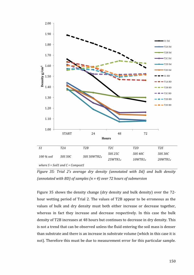
150


100 % soil 50S 50C 50S 50WTR2d 50S 25C

25WTR1d

50S 40C

10WTR1d

50S 30C

20WTR1d


Figure 35: Trial 2’s average dry density (annotated with Dd) and bulk density

(annotated with BD) of samples (n = 4) over 72 hours of submersion

Figure 35 shows the density change (dry density and bulk density) over the 72-

hour wetting period of Trial 2. The values of T2B appear to be erroneous as the

values of bulk and dry density must both either increase or decrease together,

whereas in fact they increase and decrease respectively. In this case the bulk

density of T2B increases at 48 hours but continues to decrease in dry density. This

is not a trend that can be observed unless the fluid entering the soil mass is denser

than substrate and there is an increase in substrate volume (which in this case it is

not). Therefore this must be due to measurement error for this particular sample.

1.00

1.10

1.20

1.30

1.40

1.50

1.60

1.70

1.80

1.90

2.00

START 24 48 72

De

nsi

ty g

/cm

3

Hours

S1 Dd

T2A Dd

T2B Dd

T2C Dd

T2D Dd

T2E Dd

S1 BD

T1A BD

T2B BD

T2C BD

T2D BD

T2E BD

151

In general, all amendments appear to reduce the respective bulk and dry densities

in comparison with unamended soil.

5.1.2 WHC Trial 3

Briefly, samples were placed onto a saturated bed of sand to allow uptake from the

base of each core before being fully submerged after 96 hours. The test was

deemed complete and the measurement of mass and volume of samples ceased

when the mass reached a stable value (<0.5 g difference to previous value),

indicating no further uptake of water, or a decline in mass that indicated that the

soil was beginning fall away from the ends of the core. The number of repeats

within each amendment sample (n) is noted in the each figure reference, as these

were variable; eight cores were made for each amendment, however some of these

cores deteriorated during the wetting process and data is not provided for these

cores. Figure 36 provides an overview of the gravimetric water content (GWC) of

Soil2 and 13 amendments over a wetting period of 240 hours, following the

methods outlined in Chapter 4 (4.4.4), where the amendment proportions are

outlined subsequently in Table 23.

Figure 36: Average GWC of samples up to 240 hours of wetting according to the

method outlined in section 4.4.4. n is between 5 and 8. The measurement of some

amendments ceased once the mass reached a plateau. Note that samples have two

different starting GWC, 0.14 (14%) and 0.25 (25%).

0.100

0.200

0.300

0.400

0.500

0.600

0.700

0.800

START 24 48 72 96 120 144 168 192 216 240

Gra

vim

etr

ic w

ate

r co

nte

n

HOURS

Soil2

A1

A2

A3

A4

A5

A6

A7

A8

A9

A10

A11

A12

A13

152

Table 23: Soil amendments used in Trial 3. Bulk & dry density and water content

values are for individual cores at production. F1 and F2 were omitted from the trial,

as the composition of F1 would not yield a stable core before testing began and F2

fell apart considerably during wetting, invalidating the data. A8 and A9 are noted

with an asterisk as these samples, across all testing measures, were substantially

lower than trends in the remainder of tests would suggest.

Table 23 provides a summary of the amendment proportions; however, these are

also provided on each of the subsequent Figures (37-54) for better interpretation

of results. As noted previously, the number and letter annotation at the end of each

line represents the relative proportion and amendment respectively; the

shorthand used is S (Soil2), C (compost2), WTR2d, and Si (silica). Error bars on

each graph represent the minimum and maximum values obtained for each

amendment. At this stage, the data were not searched for anomalies as soil is

exceptionally heterogeneous by nature and therefore for a small sample size

(maximum 8) the assumption that a data point is anomalous, is not reasonable. For

this reason, the data were not statistically tested for significance of differences.

The following sections will review the effect of amendment on the GWC as a result

Sample

n= 8

Soil

2%

Compost

2%

WTR2d

%

Silica % Bulk density (BD)/dry

density (Dd) g/cm3

Water

content

Soil 2 100 1.85/1.60 14

F1 50 50 n/a n/a

A1 50 50 1.55/1.37 14

A2 50 50 1.89/1.66 14

A3 50 25 25 1.49/1.19 25

A4 50 25 25 1.56/1.25 25

A5 60 40 1.42/1.25 14

A6 60 40 1.75/1.54 14

A7 60 40 1.96/1.73 14

A8* 60 20 20 1.49/1.19 25

A9* 60 20 20 1.50/1.20 25

A10 70 30 1.51/1.20 25

A11 70 30 1.62/1.43 14

A12 70 30 1.78/1.57 14

A13 70 15 15 1.52/1.22 14

F2 70 15 15 n/a n/a

153

of different amendments, and the effect of amendment on the density and volume

change trends as a result of different amendments. One must note that some

samples start the wetting cycle at a GWC of 0.14 and some start at 0.25. As stated

in section 4.4.4 of Chapter 4, this was due to the need for more water in

amendments containing compost so as to create robust cores (with the exception

of A5 = 60S 40C).

5.1.2.1 Effect of single amendment at different proportions on GWC: 5050,

6040, and 7030

Figure 37: Average effect of single amendment at a 50% rate on gravimetric water

content. A1 is 50S 50WTR2d and A2 is 50S 50Si. A5 is also included as a single

compost amendment as F1 (50S 50C) was not included in the data set. Soil2 is the

control. Soil2 n = 5, A1 n = 5, A2 n = 7, A5 n =7

Figure 37 presents the GWC values for unamended soils and two 50% single

treatment amendments (A1 and A2). For comparative purposes, A5 is also

included as a single amendment of compost at 60%. As discussed in Chapter 4, the

production of cores at 50% compost was not possible (F1). The GWC of A1 (50%

soil, 50% WTR2d) is almost identical over time to the control sample (unamended

soil, Soil2), suggesting that the addition of dried WTR does not improve or

decrease the GWC, where the maximum GWC for A1 was 0.326 and the maximum

for unamended soil was 0.319. The addition of silica at a 50% rate (A2) however,

100S

50S 50WTR2d

50S 50Si

60S 40C

0.10

0.20

0.30

0.40

0.50

0.60

0.70

0.80

0.90

START 24 48 72 96 120 144 168 192

Gra

vim

etr

ic w

ate

r co

nte

nt

HOURS

Soil2

A1

A2

A5

154

appreciably reduces the amount of water the soil can hold, where a maximum GWC

of 0.224 was reached. The rate of mass increase was similar for both unamended

soils and AM1, nearing maximum GWC after 24 hours of wetting. A single

amendment of compost, even at a lower amendment ratio of 40%, performs better

than any single amendment at 50%, reaching a maximum of 0.777. There are no

overlaps in the maximum/minimum error bars, suggesting this result is significant

(although no statistical testing has been performed).


content. A5 is 60S 40C, A6 is 60S 40WTR2d and A7 is 60S 40Si. Soil2 is the control.

Soil2 n = 5, AM5 n = 7, AM6 n = 7, AM7 n = 7. The dashed grey line indicates the point

of flooding.

Figure 38 compares the GWC of unamended soil and three amended samples at a

40% amendment rate (A5, A6 and A7). A 40% amendment of WTR2d reduces the

maximum GWC of the soil compared to the control (0.319) with a maximum of

0.229. The 40% amendment of silica has a similar effect, reaching a maximum GWC

of 0.207. Within 24 hours of wetting the majority of GWC change has occurred for

unamended soil, A6 and A7, and the GWC plateaus. In contrast, a 40% amendment

of compost (A5) gives a maximum GWC value of 0.787; the increase in GWC is

rapid in the first 24 hours and continues to increase at 72 hours after a small lull,

presumably due to the compost slowly expanding once wet. It is difficult to tell is

100S

60S 40C

60S 40 WTR2d

60S 40Si

0.10

0.20

0.30

0.40

0.50

0.60

0.70

0.80

0.90

START 24 48 72 96 120 144 168 192

Gra

vim

etr

ic w

ate

r co

nte

nt

HOURS

Soil2

A5

A6

A7

155

this is a measurement error or a real effect. Although no statistical testing has been

conducted, there is no overlap of error bars between soil and AM5 in Figure 38,

which may suggest that the difference is significant.


content. A10 is 70S 30C, A11 is 70S 30WTR2d and A12 is 70S 30Si. Soil2 is the control.

Soil2 n = 5, A10 n = 8, A11 n = 8, A12 n = 5.

Figure 39 compares the GWC over time of unamended soil and three other

amendments (A10, A11 and A12). The amendment at a 30% rate of silica (A12)

reduces the GWC in comparison with unamended soil and reaches the maximum of

0.261 within 48 hours. The addition of WTR2d at a 30% rate (A11) marginally

increases the maximum GWC compared with unamended soil (0.326 and 0.319

respectively) and increases the rate of GWC change in comparison with

unamended soil in the first 24 hours. The amendment of compost at a 30% rate

(A10) results in a higher GWC than any other 30% single amendment, reaching a

0.434 maximum. This however may due to a higher initial GWC, effectively giving

this amendment a head start. As discussed in Chapter 2 (section 2.4.4), the

hydraulic conductivity of a more saturated sample is higher than that of an

unsaturated sample, therefore benefitting the sample with a higher initial water

content.

100S

70SS 30C

70S 30WTR2d70S 30Si

0.10

0.15

0.20

0.25

0.30

0.35

0.40

0.45

0.50

START 24 48 72 96 120 144 168 192 216 240

Gra

vim

etr

ic w

ate

r co

nte

nt

HOURS

Soil2

A10

A11

A12

156

5.1.2.2 Effect of single compost amendment on GWC

Figure 40: Average effect on GWC of single amendment with compost at 30% and

40% rate against the control, Soil2. A5 is 60S 40C and A10 is 70S 30C. Soil2 n = 5, A5

n = 7, A10 n = 8. A10 started at 0.25 GWC due to the presence of compost. A5 was the

only compost amendment to remain at 0.14 GWC. The dashed line shows where the

samples were flooded during the wetting process

The effect of a single amendment with compost appears to be related to the

proportion of amendment, although not necessarily linearly, where an amendment

at a 40% rate (A5) has a much greater maximum GWC than an amendment at 30%

(A10) at 0.787 to 0.434 respectively. The trends in the two lines are also different,

where A10 appears to reach near maximum GWC within 24 hours but A5 has a

sharp increase during the first 24 hours, followed by a lull and then a slow increase

until the maximum point. This is likely due to the wetting process and subsequent

response of compost; samples were initially only placed onto saturated sand and

then flooded after 96 hours. Although unamended soil and 30% compost did not

respond to the extra input of water, 40% compost continued to increase in GWC.

Considering that 30% compost did not respond in the same way to wetting,

suggests that this may be a function of measurement error in some part.

100S

60S 40C

70S 30C

0.10

0.20

0.30

0.40

0.50

0.60

0.70

0.80

0.90

START 24 48 72 96 120 144 168 192 216 240

Gra

vim

etr

ic w

ate

r co

nte

nt

HOURS

Soil2

A5

A10

157

5.1.2.3 Effect of single WTR/silica amendment on GWC

Figure 41: Average effect on gravimetric water content of single amendment with

WTR2d and silica (Si) at various amendment rates against the control, Soil2. A1 is

50S 50WTR2d, A2 is 50S 50Si, A6 is 60S 40WTR2d, A7 is 60S 40Si, A11 is 70S

30WTR2d and A12 is 70S 30Si. Soil2 n = 5, A1 n = 5, A2 n = 7, A6 n = 7, A7 = 7, A11 n =

8, A12 n = 5.

Figure 41 shows the effect of single amendments of WTR2d and single

amendments of silica at various proportions. Silica was added to replicate the

structural effect of WTR, albeit to a limited extent due to the particle size

distribution differences. As shown by Figure 19 the particle size range of silica was

quite narrow, where the majority of particles were between 425 μm and 600 μm.

In comparison, the WTR2d had a large range, where 40% of the WTR2d ‘particles’

are smaller than 425 μm and 20% are of a clay size fraction (<63 μm). The

presence of the finer fraction is critical in the water holding capacity of the soil

(Rawls et al., 1982; Saxton & Rawls, 2006) and the addition of coarse particles is

likely to have caused the reduction in water holding capacity of soils amended with

silica. The rate of hydraulic conductivity, based on the same theory, is predicted to

increase with the addition of coarser materials; however, this is not evident in

Figure 41 as the rate of water uptake is lower for all single silica amended samples

than unamended soil.

100S

50S 50WTR2d

50S 50Si60S 40WTR2d

60S 40Si

70S 30WTR2d

70S 30Si

0.10

0.15

0.20

0.25

0.30

0.35

0.40

START 24 48 72 96 120 144 168 192

Gra

vim

etr

ic w

ate

r co

nte

nt

HOURS

Soil2

A1

A2

A6

A7

A11

A12

158

With the exception of A11 (50S 50WTR2d) and A1 (70S 30WTR2d), which appear

to be within the margin of error shown by the maximum/minimum error bars, the

addition of WTR or silica as single amendments have a negative influence on the

GWC of a soil compared with unamended soil. The large overlap in error bars for

all samples show that there is a significant amount of heterogeneity of GWC within

the set of 12 cores in a sample.

5.1.2.4 Effect of co-amendment vs single amendment: GWC

Figure 42: Average effect on gravimetric water content of co-amendment with

WTR2d and compost at various amendment rates against the control, Soil2. A3 is 50S

25C 25WTR2d, A4 is 50S 25C 25Si, A8 is 60S 20C 20WTR2d, A9 is 60S 20C 20Si and

A13 is 70S 15C 15WTR2d. F2 is 70S 15C 15Si but this data is not included. Soil2 n = 5,

A3 n = 7, A4 n = 8, A8 n = 8, A9 n = 8, A13 n = 8.

Figure 42 presents a general view of the effect of co-amendment on the GWC of 5

co-amendments against the unamended soil. In general, all co-amendments using

WTR2d perform better than their silica co-amended equivalent (as discussed

previously). With the exception of 40% silica co-amendment, all co-amendments

with WTR2d increase the GWC in comparison with unamended soil, where greater

proportions of amendment increase yield higher GWC despite different initial

GWC. Figures 43-45 show the effect of co-amendment against a single amendment

at various amendment ratios, where the general trend shows that compost has the

100S

50S 25C 25WTR2d

50S 25C 25Si60S 20C 20WTR2d

60S 20C 20Si

70S 15C 15WTR2d

0.10

0.15

0.20

0.25

0.30

0.35

0.40

0.45

0.50

0.55

START 24 48 72 96 120 144 168 192 216 240

Gra

vim

etr

ic w

ate

r co

nte

nt

HOURS

Soil2

A3

A4

A8

A9

A13

159

greatest effect on the GWC of a sample, regardless of what other material is added,

i.e. co-amendments have higher GWCs than single amendments of WTR or silica,

due to the presence of compost.

Figure 43: Average effect on gravimetric water content of co-amendment and single

amendment at a 50% application rate against the control, Soil2. A1 is 50S 50WTR2d,

A2 is 50S 50Si, A3 is 50S 25C 25WTR2d and A4 is 50S 25C 25Si. Soil2 n = 5, A1 n = 5,

A2 n = 7, A3 n = 8, A4 n = 8.

At a 50% amendment rate, as shown in Figure 43, in comparison with single

amendment, the co-amendment with WTR2d or silica improves the GWC by 31%

for WTR2d and 49% for silica, although this may be a function of the co-

amendments starting at a higher GWC. The co-amendment improves the GWC by

30% (WTR) and 28% (Si). As discussed the single amendment of WTR2d (A1) or

silica (A2) at a 50% shows either negligible difference or a reduction in the GWC.

100S

50S 50WTR2d

50S 50Si

50S 25C 25 WTR2d

50S 25C 25Si

0.10

0.15

0.20

0.25

0.30

0.35

0.40

0.45

0.50

0.55

START 24 48 72 96 120 144 168 192

Gra

vim

etr

ic w

ate

r co

nte

nt

HOURS

Soil2

A1

A2

A3

A4

160


amendment at a 40% application rate against the control, Soil2. A5 is 60S 40C, A6 is

60S 40WTR2d, A7 is 60S 40Si, A8 is 60S 20C 20WTR2d and A9 is 60S 20C 20Si. Soil 2

n = 5, A5 n = 7, A6 n = 7, A7 n = 7, A8 n = 8, A9 n = 8

At a 40% amendment rate shown in Figure 44 the single amendment of compost

(A5) has the highest GWC (0.787) in comparison with any co-amendment at the

same proportion. Figure 45 similarly shows that a single amendment of compost

at 30% proportion (A10) has a greater GWC than any co-amendment at 0.434 and

unamended soil. Importantly however, at a 30% amendment rate, the WTR co-

amendment performs almost as well as the single amendment of compost (0.40.3

vs 0.434). It is also interesting to note that although A13 (30% WTR amendment)

had an initially lower GWC than A10 (30% compost), after 24 hours the GWC of the

co-amendment was higher than the single amendment. This suggests that although

amendments with compost alone hold more total water than amendment with any

other material, the co-amendment with WTR2d increases the rate of water

movement into the material. This suggestion is supported by hydraulic

conductivity data later in the chapter (section 5.3.1).

100S

60S 40C

60S 40WTR2d

60S 40Si

60S 20C 20WTR2d

60S 20C 20Si

0.10

0.20

0.30

0.40

0.50

0.60

0.70

0.80

0.90

START 24 48 72 96 120 144 168 192 216 240

Gra

vim

etr

ic w

ate

r co

nte

nt

HOURS

Soil2

A5

A6

A7

A8

A9

161


amendment at a 30% application rate against the control, Soil2. A10 is 70S 30C, A11

is 70S 30WTR2d, A12 is 70S 30Si, and A13 is 70S 15C 15WTR2d. Soil2 and A12 n = 5,

A10, A11 and A13 n = 8

5.1.2.5 Effect of density and initial water content on GWC

As discussed previously in Chapter 2, the relationship between water content and

density is co-dependent (section 2.3) where the water content affects the resultant

density of a soil under compressive force, and in turn the density of that soil affects

the maximum water content, as a result of porosity differences (where in general

lower density soils have higher porosity). In Figure 46, we are able to compare the

dry density of amendments based on their initial water contents, where A1, A2, A5,

A6, A7, A11, A12, and A13 started at 0.14 GWC and A3, A4, A8, A9 and A10 started

at 0.25 GWC (where a reminder of compositions is presented in Table 24). Figure

46 shows that the initial water content at compaction affects the degree to which

the sample is compacted, as those samples compacted at 0.25 (orange bars) are

less dense than samples compacted at 0.14 (with the exception of A5). However,

this difference may be wholly accountable to the variance in materials within each

amendment rather than the water content; samples compacted at 0.25 all

contained compost, a material of low density with high elasticity parameters, both

of which reduce the compactibility of the material. In contrast samples compacted

at 0.14 contain denser materials (silica, soil and WTR).

100S

70S 30C

70S 30WTR2d

70S 30Si

70S 15C 15WTR2d

0.10

0.15

0.20

0.25

0.30

0.35

0.40

0.45

0.50

START 24 48 72 96 120 144 168 192 216 240

Gra

vim

etr

ic w

ate

r co

nte

nt

HOURS

Soil2

A10

A11

A12

A13

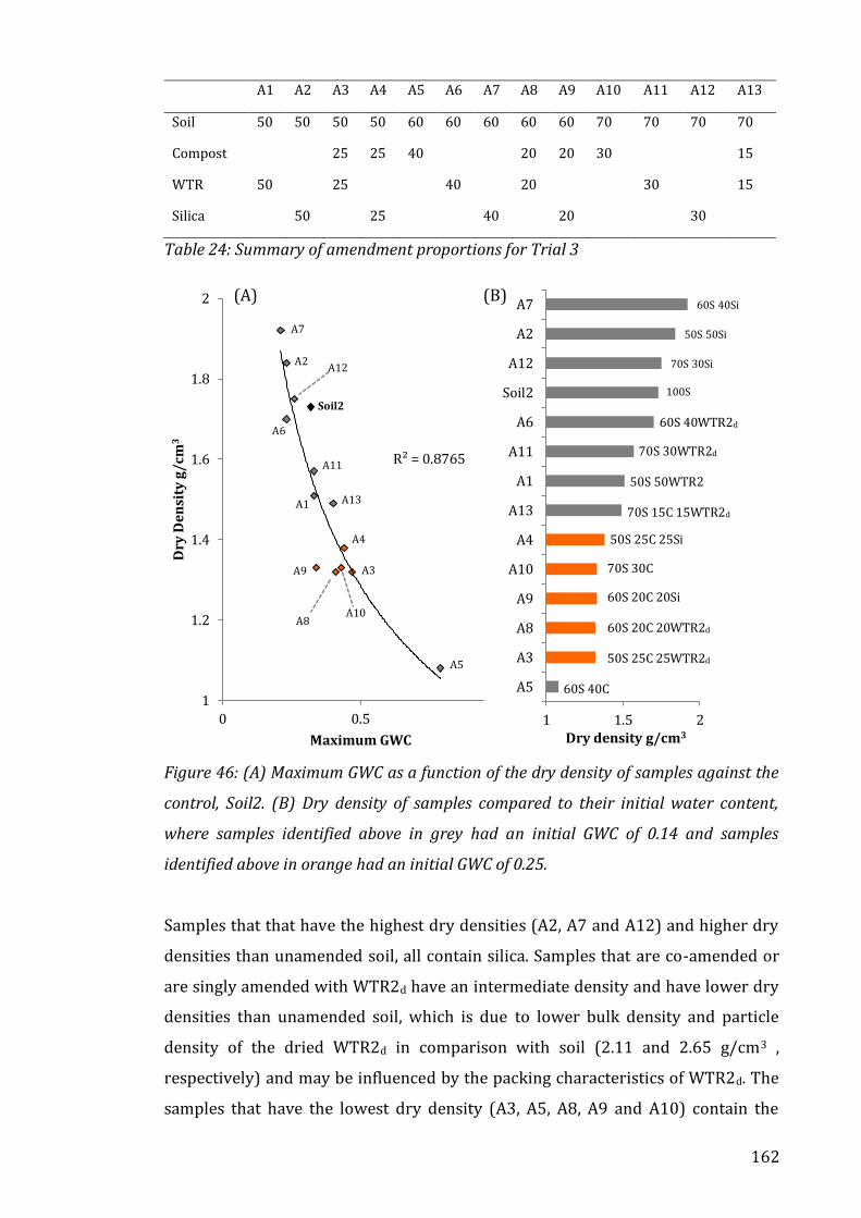
162

A1 A2 A3 A4 A5 A6 A7 A8 A9 A10 A11 A12 A13

Soil 50 50 50 50 60 60 60 60 60 70 70 70 70

Compost 25 25 40 20 20 30 15

WTR 50 25 40 20 30 15

Silica 50 25 40 20 30

Table 24: Summary of amendment proportions for Trial 3

Figure 46: (A) Maximum GWC as a function of the dry density of samples against the

control, Soil2. (B) Dry density of samples compared to their initial water content,

where samples identified above in grey had an initial GWC of 0.14 and samples

identified above in orange had an initial GWC of 0.25.

Samples that that have the highest dry densities (A2, A7 and A12) and higher dry

densities than unamended soil, all contain silica. Samples that are co-amended or

are singly amended with WTR2d have an intermediate density and have lower dry

densities than unamended soil, which is due to lower bulk density and particle

density of the dried WTR2d in comparison with soil (2.11 and 2.65 g/cm3 ,

respectively) and may be influenced by the packing characteristics of WTR2d. The

samples that have the lowest dry density (A3, A5, A8, A9 and A10) contain the

A5

A3

A4

A8A10

A9

A13A1

A11

Soil2

A12

A6

A2

A7

R² = 0.8765

1

1.2

1.4

1.6

1.8

2

0 0.5 1

Dry

De

nsi

ty g

/cm

3

Maximum GWC

100S

70S 30Si

50S 50Si

60S 40Si

1 1.5 2

A5

A3

A8

A9

A10

A4

A13

A1

A11

A6

Soil2

A12

A2

A7

Dry density g/cm3

60S 40WTR2d

70S 30WTR2d 50S 50WTR2 70S 15C 15WTR2d

50S 25C 25Si

70S 30C

60S 20C 20Si 60S 20C 20WTR2d

50S 25C 25WTR2d

60S 40C

(A) (B)

163

highest proportions of compost, which as discussed in Chapter 2 is a function of

the low particle density of compost and high resistance to compaction.

The dry density of the sample therefore directly affects the maximum GWC as a

result of two factors. Firstly, regardless of the materials within the sample, it is

well known that soil with lower dry densities have higher void ratios which allow

more water to be contained with in the sample. Secondly, the materials that cause

a soil sample to have a lower dry density due to either low particle density or due

to low bulk density of the material, i.e. compost or WTR2d, themselves impart

better water holding capacity, giving the result that lower density soils have a

higher GWC. In addition, high-density materials such as silica, are unable to

incorporate water with their matrix, whereas low density compost is very porous.

Therefore, for materials that occupy the same volume, their individual capacity to

hold water is very different. Figure 46 shows this, where amendments that have a

lower initial dry density (as a factor of initial water content and material make up)

have higher maximum GWC than samples with higher dry density.

This effect is supported by the data produced by Laurie (2017, Figure 47

unpublished), which shows that density affects the GWC for unamended soil that

have been compacted to different densities at the same water content. Laurie also

compared the effect of co-amendment at different densities against unamended

soil. Cores were prepared in the same way as those for Trial 4 using a static

compaction press (Figure 24), where n = 12 and initial water content was 0.16

(16%) at an amendment rate of 70% soil, 15% WTR2d and 15% compost. Cores

were compacted to three different bulk densities, 1.4, 1.6 and 1.8 g/cm3 to test the

effect of density on the GWC. For comparison in Trial 3 A13 (also 70S 15C

15WTR2d) had an initial bulk density of 1.69 g/cm3 and unamended soil had an

initial bulk density of 1.97 g/cm3. Discussed subsequently, this is also comparable

to AM14 in Trial 4, which had an initial bulk density of 2 g/cm3.

164

Figure 47: Average gravimetric water content (top) and average volumetric water

content (bottom) for unamended soil at three bulk densities (Unam. 1.4, Unam 1.6

and Unam 1.8 g/cm3) and (bottom) for a 30% WTR co-amended soil (WTR/comp 1.4,

WTR/comp 1.6, and WTR/comp 1.8 g/cm3). n = 12. Dashed lines connecting lines

between phases indicates an extended drying period during which samples were not

measured. Data collected by Laurie (2017).

Figure 47 shows there is a direct relationship between bulk density and GWC

across two wetting and drying cycles where the lower the density, the higher the

GWC reached. In addition, the maximum GWC of amended soils was higher at all

densities than unamended soil e.g. at 1.4 g/cm3 unamended soil reached a GWC of

0.49 and amended soil reached a GWC of 0.90. The difference between unamended

and amended soil was statistically significant (p<0.1). The trends shown in Figure

47 show that during the second wetting cycle, the GWC of co-amended samples

was similar to the values obtained in the primary wetting, whereas unamended

0

0.2

0.4

0.6

0.8

1

6-Dec 13-Dec 20-Dec 27-Dec 3-Jan 10-Jan 17-Jan 24-Jan 31-Jan 7-Feb 14-Feb 21-Feb

Gra

vim

etr

ic W

ate

r C

on

ten

t

Time (days)Unam. 1.4 Unam. 1.6 Unam. 1.8WTR/comp 1.4 WTR/comp 1.6 WTR/comp 1.8Unam. 1.4 interm Unam. 1.4 part 2 Unam. 1.6 interim

0

0.1

0.2

0.3

0.4

0.5

0.6

0.7

6-Dec 13-Dec 20-Dec 27-Dec 3-Jan 10-Jan 17-Jan 24-Jan 31-Jan 7-Feb 14-Feb 21-Feb

Vo

lum

etr

ic W

ate

r C

on

ten

t

Time (days)

Unam. 1.4 Unam. 1.6 Unam. 1.8WTR/comp 1.4 WTR/comp 1.6 WTR/comp 1.8Unam. 1.4 interim Unam. 1.4 part 2 Unam. 1.6 interim

165

samples held less water during the second wetting cycle. This suggests that co-

amendment reduced shrinkage (which is unrecoverable in soil) as a result of

drying and therefore the soil structure (voids) were maintained, allowing higher

GWC (Laurie, 2017).

5.1.2.6 Relationships between compost and GWC

The previous figures have gone into detail about the differences in GWC identified

between various amendments. The following section attempts to obtain between

trends in GWC and the presence of compost with the GWC of samples.

Figure 48: Maximum GWC of samples against the proportion of compost in the

amendment as either a single amendment (40 or 30%) or as part of a co-amendment

(25, 20 or 15%).

Figure 48 shows that compost amendment has a positive effect on the maximum

GWC achieved, which concurs with literature discussed in Chapter 2. There is a

significant positive trend denoted by the trend line (R2 = 0.63), indicating that the

greater the proportion of compost, the higher the GWC maximum. Only one sample

(40% compost) had a higher maximum GWC (A5 at 0.79) than co-amendments.

Importantly, at 30% amendment rate, the co-amendment with WTR2d (A13, 0.4)

reaches a similar maximum to the single amendment of 30% compost (A10, 0.43).

This shows that at lower amendment proportions, which are the least unrealistic

application rates for land spreading, there is no disadvantage to using a co-

amendment with WTR2d over compost. The addition of co-amendment improves

A5: 60S 40C

A8: 60S 20C 20WTR2d

A4: 50S 25C 25Si

A9: 60S 20C 20Si

A10: 70S 30C

A3: 50S 25C 25WTR2d

A13: 70S 15C 15WTR2d

Soil2 100S

R² = 0.6371

0

0.1

0.2

0.3

0.4

0.5

0.6

0.7

0.8

0.9

0 5 10 15 20 25 30 35 40

Ma

xim

um

GW

C

Percentage compost

166

the maximum GWC of a soil by between 20 and 32% depending on application

rate.

Figure 49: Average increase in grams of water after 24 hours for samples amended

with compost as either a single amendment (40 or 30%) or as part of a co-

amendment (25, 20 or 15%), suggesting a rate of water uptake.

Figure 49, shows that there is only a very weak relationship between compost

proportion and the rate of uptake in the primary 24 hours of wetting, denoted as

grams of water taken up in 24 hours. Unamended soil has the lowest uptake of all

samples (39.13 g). It is clear that the co-amendment of soil with WTR2d yields a

better water uptake compared to the single amendment of compost over the first

24 hours of wetting, where 30% co-amendment (A13, 66.38 g) and 50% co-

amendment (A3, 67.2 g) have a greater uptake in 24 hours than 40% single

amendment of compost (A5, 66.37 g).

Importantly, the co-amendment at 30% (A13) takes up ~17% more water than the

30% single amendment of compost (A10, 55.08 g) in the first 24 hours. There is

negligible difference between 50% and 30% co-amendment ratios, despite a

greater proportional amendment for the former, however A8 and A9 (20% co-

amendment) appear to perform sub-par, where one would expect a co-amendment

of 40% (A8) to reach a value between those for 30% (A13) and 50%. The values of

A8 and A9 throughout the analysis of Trial 3’s data performed poorly, countering

the general trend whereby greater proportions of amendment yield greater change

against unamended soil. The information in Figure 49 is important as the initial

A5: 60S 40CA3: 50S 25C

25WTR2d

A8: 60S 20C 20WTR2d

A9: 60S 20C 20Si

A10: 70S 30C

A4: 50S 25C 25Si

A13: 70S 15C 15WTR2d

Soil2: 100SR² = 0.3904

35

40

45

50

55

60

65

70

0 5 10 15 20 25 30 35 40 45

Gra

ms

of

wa

ter

Percentage compost

167

period of wetting is critical in extreme weather scenarios (where rainfall is

heaviest) and the infiltration rate is key to reduce soil erosion through overland

flow, as with a good infiltration and percolation rate, water will enter the soil

profile rather than immediately forming runoff as with saturated soils. Analysis of

data suggests that WTR2d increases the rate of uptake whereas compost, although

providing a higher maximum GWC, may not have a higher uptake in the first 24

hours due to hydrophobicity initially preventing water from entering the soil body.

5.1.2.7 Relationships between WTR/silica and GWC

The important piece of information to take from these figures is that WTR2d elicits

a higher maximum GWC and greater increase in GWC over 24 hours than the

amendments of silica for both co-amendment and single amendment. The addition

of silica results in a 3-30% lower maximum GWC than the WTR2d proportional

equivalent which is likely to be a result of differences particle size distribution

discussed in section 4.3.1. Information on the detailed surface and shape

characteristics of WTR2d are provided in Chapter 6, and this provides evidence as

to why the effect of WTR2d addition is so effective in improving the WHC in

comparison to the amendment of other coarse grain materials.

Figure 50: Average maximum GWC of samples amended with WTR or silica either as

a single amendment (50, 40 or 30%) or as part of a co-amendment (25, 20 or 15%)

A3

A9A13A1

A11

A6

A8

A4

Soil2

A12

A2A7

R² = 0.1042

R² = 0.2971

0

0.1

0.2

0.3

0.4

0.5

0.6

0 10 20 30 40 50

Ma

xim

um

GW

C

Percentage amendment

WTR

Silica

168

Figure 51: Average increase in grams of water after 24 hours for samples amended

with WTR2d or silica as either a single amendment (50, 40 or 30%) or as part of a co-

amendment (25, 20 or 15%), suggesting a rate of water uptake.

5.1.2.8 Volumetric and density changes

Figures 52 and 53 show the volumetric water content and volumetric water

content i change over time for 14 samples against the control, Soil2 (unamended).

As discussed in section 2.4.2, we must view the volumetric water content with

knowledge of either the volume change of samples and/or the gravimetric water

content of samples to supplement this measurement so that we may determine

relative changes between samples. The volumetric water content change in Figure

52 follows a similar pattern to the trends seen between different amendments for

the gravimetric water content where A5 (60S 40C) has the greatest maximum

VWC, showing that it had both the greatest change in GWC and volume. In general

co-amendments have a greater VWC than single amendments at the same

proportion, where silica single amendments had a negligible or detrimental

influence, shown by a reduction in VWC.

The VWCi in Figure 53 shows the instantaneous volumetric water content, which

relates the volume of water in the sample to the volume of the sample at the time

of measurement, rather than VWC that relates the volume of water in a sample to

the original volume of the sample.

R² = 0.0059R² = 0.2333

30

35

40

45

50

55

60

65

70

0 10 20 30 40 50 60

Gra

ms

of

wa

ter

in 2

4 h

ou

rs

Percentage amendment

Silica

WTR

169

Figure 52: Average volumetric water content change of samples against the control,

Soil2, over a 240-hour wetting period. VWC start values range between 0.21 and 0.26

for samples at 0.14 GWC, and between 0.33 and 0.35 for samples at 0.25 GWC due to

small differences in sample volume.

Figure 53: Average volumetric water content (i) change of samples against the

control, Soil2, over a 240-hour wetting period. VWC start values range between 0.21

and 0.26 for samples at 0.14 GWC, and between 0.33 and 0.35 for samples at 0.25

GWC due to small differences in sample volume.

0.10

0.20

0.30

0.40

0.50

0.60

0.70

0.80

0.90

START 24 48 72 96 120 144 168 192 216 240

VW

C

HOURS

Soil2

A1:50S 50WTR2d

A2: 50S 50Si

A3: 50S 25C 25WTR2d

A4: 50S 25C 25Si

A5: 60S 40C

A6: 60S 40WTR2d

A7: 60S 40Si

A8: 60S 20C 20WTR2d

A9: 60S 20C 20Si

A10: 70S 30C

A11: 70S 30WTR2d

A12: 70S 30Si

A13: 70S 15C 15WTR2d

0.10

0.20

0.30

0.40

0.50

0.60

0.70

START 24 48 72 96 120 144 168 192 216 240

VW

Ci

HOURS

Soil2

A1: 50S WTR2d

A2: 50S 50Si

A3: 50S 25C 25WTR2d

A4: 50S 25C 25Si

A5: 60S 40C

A6: 60S 40WTR2d

A7: 60S 40Si

A8: 60S 20C 20WTR2d

A9: 60S 20C 20Si

A10: 70S 30C

A11: 70S 30 WTR2d

A12: 70S 30Si

A13: 70S 15C 15WTR2d

170

As discussed previously, VWC as a measure does not account for volumetric

change of the sample. When we view the volumetric changes by VWCi, the

decreases shown by unamended soil, A1, A10 and A12 indicate that the samples

are increasing in volume at a greater rate than they are taking up water. Samples

that have a fairly horizontal trend either experience no change after an initial

wetting period or undergo similar increases in volume and gravimetric water

content. Samples that have a positive trend increase in GWC faster than they swell.

It is therefore vital that the VWC and VWCi are viewed in tandem with the volume

and GWC measurements of samples.

Figure 54: Average bulk density change of samples over 240 hours of wetting.

Figure 54 shows that some amendments are more prone to swelling than others,

expanding to hold more water, however it is difficult to compare the relative

density changes as the starting density of each amend is different. Amendments

that included silica or WTR2d tended to have little response to wetting in terms of

sample volume, which as Moodley & Hughes (2006) found was due to the binding

effects of polymers in the WTR. As samples such as A5 (60S 40C) take up water,

the bulk density increases as the water fills the voids present in the compost.

Unamended soil experiences the largest drop in bulk density as a result of swelling.

1.20

1.40

1.60

1.80

2.00

2.20

START 24 48 72 96 120 144 168 192 216 240

Bu

lk d

en

sity

g/

cm3

HOURS

Soil2

A1: 50S 50WTR2d

A2: 50S 50Si

A3: 50S 25C 25WTR2d

A4: 50S 25C 25Si

A5: 60S 40C

A6: 60S 40WTR2d

A7: 60S 40Si

A8: 60S 20C 20WTR2d

A9: 60S 20C 20Si

A10: 70S 30C

A11: 70S 30WTR2d

A12: 70S 30Si

A13: 70S 15C15WTR2d

171

5.1.2.9 Concluding remarks: Trial 3

The results from Trial 3 have shown that the water holding capacity is greatly

affected by proportion of compost in the samples, which also determined the initial

bulk density of the sample after compaction. Under the same compactive effort,

samples with compost required a higher water content to be able to produce

samples for testing, and it is unknown to what extent this affected subsequent

measurements. The addition of silica, designed to test the physical effect of WTR2d

addition without a geochemical effect did not provide a large degree of insight,

owing to the differences in particle size distribution. By adding silica, the water

holding capacity decreased, while the theoretical beneficial effects of a larger grain

size in increasing the hydraulic conductivity were not apparent. Should the

experiment be repeated, a careful assessment of particle size distribution is

needed for the WTR2d to ensure that the silica matches the high proportion of fine

particles as these are likely the reason for WTR2d providing higher water holding

capacity. The key summary points from Trial 3 are as follows:

1. Single amendment with WTR does not improve the maximum GWC of the soil

but does improve hydraulic conductivity (rate of uptake in 24 hours). Single

compost amendments have the highest maximum GWC at all amendment ratios

40% and 50% single amendment of WTR or silica does not improve the

GWC compared to unamended soil.

Single 40% compost increases the maximum GWC by 60% compared to

unamended soil (0.319 to 0.787)

30% single amendment of silica has an 18% lower maximum GWC than

unamended soil.

30% single amendment of WTR increases the rate of uptake by 11% after

24 hours, while achieving a similar maximum GWC to soil.

Silica doesn’t effectively replace WTR due to the difference in size fractions.

All single amendments of WTR or silica (excluding both 40% single

amendments and 50% silica) increase the rate of uptake in the first 24

hours by up to 42% compared to unamended soil.

2. In general the co-amendments have higher GWC than unamended soil regardless

of the addition of WTR or silica, therefore the co-amendment benefit is dependent

on the amount of compost you add, not the other half of the co-amendment.

172

The addition of co-amendment improves the maximum GWC of a soil by

between 20 and 32% depending on application rate.

At 50% co-amendment, the GWC is improved by 30% (WTR) and 28% (Si)

compared to unamended soil

At 50% co-amendment improves GWC by 31% (WTR) and 49% (Si)

compared to the single amendment of each material

At a 30% amendment rate, WTR co-amendment (0.4) performs equally well

to single compost amendment (0.43) and both better than soil (0.32)

3. Co-amendment improves the rate of water uptake compared to single

amendment of compost

Co-amendment improves the rate of uptake by 17% for 30% amendment in

the first 24 hours - important in flood scenarios

30 and 50% co-amendment have the same rate of water uptake in the first

24 hours compared to 40% single compost

4. The bulk density of the samples is dependent on the materials used for

amendment, not due to the initial water content. Co-amendment stabilises the

samples on drying.

Soil at lower density has a higher GWC as a result of different void ratios,

compared to more densely packed soil (Laurie, 2017).

Co-amendment reduces the shrinkage during drying and therefore

improves the GWC

Compost allows the lowest bulk density and greatest volume change

(reduction in density during wetting) owing to the material’s low density

with high elasticity.

173

5.1.3 WHC Trial 4

As discussed in the previous section (5.1.2), there are general trends to suggest

that the single amendment of WTR has a negative influence on the maximum GWC

compared to soil alone but improves the hydraulic conductivity in the initial 24

hours of wetting. The single amendment of compost increases the maximum GWC

to the greatest extent but has much less effect on the rate of uptake. The take home

point from Trial 3 is that although compost has the best GWC, the co-amendment

improves both the gravimetric water content maximum and the rate of uptake

compared to unamended soil, which is important as part of the soil’s ‘flood holding

capacity’. However, a statistically viable comparison of results from Trial 3 are

difficult to make due to differences in the density and initial water content of

samples before wetting.

In Trial 4 we are able to directly compare the gravimetric and volumetric water

content and density responses of different amendments as the initial conditions

have been controlled. This data set also provides two wetting and two drying

cycles. Table 25 serves as a reminder for the amendment proportions used in Trial

4, Figure 55 provides an overview of the GWC changes and Figure 56-58 show an

overview of VWC, VWCi and volume changes. The amendments proportions used

in Trial 4 were almost completely different to those used in Trial 3, where the

amendment proportions were changed to be much lower and aimed to reflect

amendment quantities that may be used in the field.

As discussed in Chapter 4 (section 4.4.7) statistical significance has been

conducted using a Mann Whitney test at particular points along the time series. On

each figure, green markers indicate that the difference between the amendment

and unamended soil is statistically significant (p <0.01), and red indicates no

significance. As there are two wetting and two drying phases, the data will be

analysed as a time sequence using the terms 1st wetting (0-228 hours), 1st drying

(228-576 hours), 2nd wetting (576-816 hours), and 2nd drying (816 – 1104 hours).

Drying rates in the 2nd drying are slower than in the 1st drying as container lids

were left in place allowing limited airflow and water evaporation, which slowed

the rate of drying, and were not a function of the water holding capacity of

samples. AM1 and AM2 dry at a much faster rate than any other amendment or

174

unamended soil due to being unintentionally completely uncovered during the

second period of drying. Error bars are not presented on the subsequent graphs as

the overlap between them makes them difficult to distinguish.

Table 25: Soil amendment ratios used for Trial 4

Figures 55-58 respectively show the general trends in the GWC, volume change,

VWC and VWCi of all samples over two wetting and drying cycles, the second of

which (2nd wetting and 2nd drying) may be more relatable to how the amended

samples would perform in the real world. This is because the results from the 1st

wetting and drying cycle may to some degree reflect the effects of the production

process and may have behaved more uniformly because of the control of density,

mass, and water content rather than due to the influence of the amendments

themselves. In general, during the 1st wetting the majority of amendments improve

the GWC, volume increase, VWC and VWCi compared to unamended soil.

Sample Soil2 % Compost2 % WTR2

Soil2 100 0 0

AM1 90 10 0

AM2 90 0 10 WTR2d

AM3 90 0 10 WTR2w

AM4 90 5 5 WTR2d

AM5 90 5 5 WTR2w

AM6 80 20 0

AM7 80 0 20 WTR2d

AM8 80 0 20 WTR2w

AM9 80 10 10 WTR2d

AM10 80 10 10 WTR2w

AM11 (T3:A10) 70 30 0

AM12 (T3: A11) 70 0 30 WTR2d

AM13 70 0 30 WTR2w

AM14 (T3:A13) 70 15 15 WTR2d

AM15 70 15 15 WTR2w

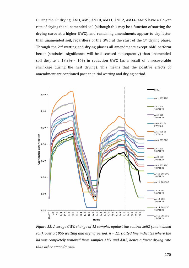
175

During the 1st drying, AM3, AM9, AM10, AM11, AM12, AM14, AM15 have a slower

rate of drying than unamended soil (although this may be a function of starting the

drying curve at a higher GWC), and remaining amendments appear to dry faster

than unamended soil, regardless of the GWC at the start of the 1st drying phase.

Through the 2nd wetting and drying phases all amendments except AM8 perform

better (statistical significance will be discussed subsequently) than unamended

soil despite a 13.9% - 16% in reduction GWC (as a result of unrecoverable

shrinkage during the first drying). This means that the positive effects of

amendment are continued past an initial wetting and drying period.

Figure 55: Average GWC change of 15 samples against the control Soil2 (unamended

soil), over a 1056 wetting and drying period. n = 12. Dotted line indicates where the

lid was completely removed from samples AM1 and AM2, hence a faster drying rate

than other amendments.

0.14

0.19

0.24

0.29

0.34

0.39

0.44

0.49

ST

AR

T

48

96

14

4

19

2

24

0

28

8

33

6

38

4

43

2

48

0

52

8

57

6

62

4

67

2

72

0

76

8

81

6

86

4

91

2

96

0

10

08

10

56

10

80

Gra

vim

etr

ic w

ate

r co

nte

nt

Hours

Soil 2

AM1: 90S 10C

AM2: 90S10WTR2d

AM3: 90S10WTR2w

AM4: 90S 5C5WTR2d

AM5: 90S 5C5WTR2w

AM6: 80S 20C

AM7: 80S20WTR2d

AM8: 80S20WTR2w

AM9: 80S 10C10WTR2d

AM10: 80S 10C10WTR2w

AM11: 70S 30C

AM12: 70S30WTR2d

AM13: 70S20WTR2w

AM14: 70S 15C15WTR2d

AM15: 70S 15C15WTR2w

176

Figure 56: Average change in volume of cores of 15 samples against the control

(Soil2) over a 1056 wetting and drying period. n = 12

Figure 57: Average change in volumetric water content (VWC) of 15 samples against

the control (Soil2) over a 1056 wetting and drying period. n = 12

Figure 58: Average change in VWCi change of 15 samples against the control (Soil2)

over a 1056 wetting and drying period. n = 12

80

90

100

110

120

130

140

150

ST

AR

T

48

96

14

4

19

2

24

0

28

8

33

6

38

4

43

2

48

0

52

8

57

6

62

4

67

2

72

0

76

8

81

6

86

4

91

2

96

0

10

08

10

56

FIN

AL

Vo

lum

e c

m3

HOURS

Soil2AM1AM2AM3AM4AM5AM6AM7AM8AM9AM10AM11AM12AM13AM14AM15

0.20

0.30

0.40

0.50

0.60

0.70

0.80

STA

RT 48

96

14

4

19

2

24

0

28

8

33

6

38

4

43

2

48

0

52

8

57

6

62

4

67

2

72

0

76

8

81

6

86

4

91

2

96

0

10

08

10

56

FIN

AL

Vo

lum

etr

ic w

ate

r co

nte

nt

HOURS

Soil2

AM1

AM2

AM3

AM4

AM5

AM6

AM7

AM8

AM9

AM10

AM11

AM12

AM13

AM14

AM15

0.20

0.25

0.30

0.35

0.40

0.45

0.50

0.55

0.60

ST

AR

T

48

96

14

4

19

2

24

0

28

8

33

6

38

4

43

2

48

0

52

8

57

6

62

4

67

2

72

0

76

8

81

6

86

4

91

2

96

0

10

08

10

56

FIN

AL

Vo

lum

etr

ic w

ate

r co

nte

nt

i

HOURS

Soil2

AM1

AM2

AM3

AM4

AM5

AM6

AM7

AM8

AM9

AM10

AM11

AM12

AM13

AM14

AM15

177

The average volume of soil cores (Figure 56) show considerable fluctuations over

time presumably as a result of human error (±3.5 cm3) when measuring the

samples, as it is illogical for samples to swell and shrink over a wetting cycle unless

they undergo collapse (which is not the case here), and values that deviate from

what should be a smooth line trend are a function of measurement error only. The

values for VWC in Figure 57 are higher than VWCi shown in Figure 58 due to

difference reference points, the former being the original volume of the sample,

and latter being the instantaneous volume of the sample.

Figures 56-58 provide only an overview of results, but a brief analysis of these

graphs indicates that, as seen in Trial 3, the volumetric increases are greater in the

first wetting than the second wetting, as there is unrecoverable shrinkage during

the first drying. A low value for VWC or VWCi is not unfavourable provided there is

significant volume change of the sample, and hence why the volume data is

required as part of the volumetric assessment. An ideal soil, i.e. one that

experiences high volume change after wetting (which decreases the bulk density

and increases the volume of voids) and has a high value for VWCi (not necessarily

VWC) will accommodate flood water better than a soil that experiences less

volume increase and has a lower VWCi. Samples with a higher VWC or VWCi in the

second wetting, do not necessarily indicate an improvement but instead reflects

the volume change of the sample being lower than in the first wetting cycle. This

results in a higher value for VWC and VWCi as they are relative to the volume of

the soil. AM11 (70S 30C) and AM15 (70S 15C 15WTR2w) provide an exemplar for

improving the WHC as they have the highest sample volumes after the second

wetting and the highest proportion of water to solids (VWCi).

178

5.1.3.1 Effect of single amendment at different proportions: 7030, 8020, 9010 on GWC & VWC/VWCi

Figure 59: Average GWC for samples with a single amendment at 30%. Green markers indicate statistical significance in the difference

between amendments and Soil2 (unamended soil), red markers indicate there is no significance in the difference.

70S 30C70S 30WTR2d

70S 30WTR2w

0.15

0.20

0.25

0.30

0.35

0.40

0.45

0.50

Gra

vim

etr

ic w

ate

r co

nte

nt

Hours

Soil 2 AM11

AM12 AM13

179


between amendments and Soil2 (unamended soil), red markers indicate there is no significance in the difference.

80S 20C

80S 20WTR2d

80S 20WTR2w

0.15

0.20

0.25

0.30

0.35

0.40

0.45G

rav

ime

tric

wa

ter

con

ten

t

Hours

Soil 2 AM6

AM7 AM8

180


between amendments and Soil2 (unamended soil), red markers indicate there is no significance in the difference

.

90S 10C90S 10WTR2d

90S 10WTR2w

0.14

0.19

0.24

0.29

0.34

0.39G

rav

ime

tric

wa

ter

con

ten

t

Hours

Soil 2 AM1

AM2 AM3

181

Figure 59 shows that a 30% single amendment of compost results in a higher

maximum GWC (0.50) than single amendments of WTR2d (0.42) or WTR2w (0.41)

at 30% or soil alone (0.36). It appears that the rate of uptake into all samples was

similar, with the exception of unamended soil, as shown by the gradient of the

lines. All samples reached their maximum GWC at the end of the first wetting

phase. AM12 (70S 30WTR2d) and AM13 (70S 30WTR2w) achieved 93% of their

water uptake within the first 24-28 hours. AM11 (70S 30C) and Soil2 (100S) in

contrast only reached 84% of the their maximum GWC within the first 24 hours

and continued to take up water at a similar rate until saturation.

During the second wetting phase, in general all amendments held less water and

were slower to increase in GWC than the previous wetting cycle (due to expected

shrinkage as discussed in Chapter 2). During the second drying phase AM13 (70S

30WTR2w) and AM11 (70S 30C) dried faster than AM12 (70S 30WTR2d). AM13

(30% WTR2w) appeared to take up and release water faster than the other

samples, including unamended soil. There is no statistical significance in the

difference between AM12 and AM13 until 912 hours is reached, beyond which the

difference remains significant (p <0.01). AM11 is statistically significantly different

from AM12 and AM13 over the whole time series (p <0.01), as compost is able to

take up water within its structure and expands during wetting, therefore it is likely

to hold the most water, however WTR2 cannot take water into its structure and is

not known to swell during wetting (Moodley & Hughes, 2006). WTR2d and WTR2w

may achieve a higher GWC compared to unamended soil due to an increase in

surface area by the addition of fine materials.

The response of soil amendments at a 20% single amendment (Figure 60) are

similar to the response at 30%, where compost again has the highest GWC (0.43)

and WTR2d (AM7) has a maximum of 0.38. WTR2w (AM8) and unamended soil

both reach 0.36. AM8 (80S 20WTR2w), appears to have no effect on the GWC, as

shown by the red markers (no statistical difference) at this amendment rate. AM6

(20% compost) and AM7 (20% WTR2d) are statistically significantly higher than

unamended soil (p <0.01) and the difference between AM6 and AM7 is also

statistically significant (p <0.01). Soil2 appears to dry slower than all amended

samples during the 1st drying phase, however this effect is not apparent during the

182

2nd drying phase. WTR single amendments experience 10% reduction in GWC

between 1st and 2nd wetting peaks, compared to compost amendment that

experiences a 12% reduction and unamended soil a 14% reduction. This suggests

that the effect of WTR in increasing the GWC is sustained over time (discussed

subsequently).

The trend in Figure 61 shows that during at a 10% amendment ratio, during the 1st

wetting only AM3 (90S 10WTR2w) has a statistically significantly higher GWC than

unamended soil reaching a peak of 0.39 (p <0.01). AM1 (90S 10C) and AM2 (90S

10WTRd) are not significantly different from unamended soil during the 1st

wetting, both reaching a peak of 0.36. In the first drying phase, 10% compost dried

much faster than all other samples (hence it was able to drop to 0.15), as shown by

the gradient of the line. Unamended soil and 10% WTR2w followed a similar trend

to each other whilst drying, however 10% WTR2d dried faster than soil alone

(conversely to the 30% in which the WTR2d dried at a slower rate). This suggests

that coarser material added by WTR2d increased the rate of drying, possibly due to

a higher ratio of large voids which drain faster than smaller pores, present in the

unamended soil and WTR2w amended soil. 24 hours into the 2nd wetting phase, all

amendments are significantly higher than soil (as shown by the green markers

from 336 hours onwards, p <0.01). Unamended soil, 10% WTR2w and 10% WTR2d

experience a reaction in the maximum GWC (14, 13 and 3% respectively) than in

their first wetting phase, however 10% compost had a 3% increase in the GWC.

This suggests that at 10% single amendment, the addition of compost or 10%

WTR2d provide some structural stabilisation such that samples are able to retain

porosity after an initial drying period which allows them to hold more water than

samples that experience shrinkage.

5.1.3.2 Effect of single amendment at different proportions: 7030, 8020, 9010

on volume & VWC/VWCi

Figure 62 shows that the single amendment of compost at 30% results in the

highest maximum sample volume (149.5 cm3) in comparison with unamended soil

(124.1 cm3) and single amendments at 30% of WTR2d and WTR2w, reach

124.7 cm3 and 129 cm3 respectively. 30% compost has significantly higher sample

volume than soil and 30% WTR amendments and 30% WTR2d is statistically

183

better than 30% WTR2w (p <0.01), with the exception of the 2nd wetting peak

(912h) and the end of the 2nd drying cycle (1056 hours).

Figure 62: Average effect of single 30% amendments on the volume, VWC and VWCi

of samples. Green markers indicate statistical significance in the difference between

amendments and Soil2 (unamended soil), red markers indicate there is no

significance in the difference.

70S 30C

70S 30WTR2d

70S 30WTR2w

80

90

100

110

120

130

140

150

VO

LU

…

24

72

12

0

16

8

21

6

26

4

31

2

36

0

40

8

45

6

50

4

55

2

60

0

64

8

69

6

74

4

79

2

84

0

88

8

93

6

98

4

10

32

10

80

Vo

lum

e c

m3

HOURS

288.000 AM11

AM12 AM13

70S 30C70S 30WTR2d

70S 30WTR2w

0.20

0.30

0.40

0.50

0.60

0.70

0.80

VO

LU

…

24

72

12

0

16

8

21

6

26

4

31

2

36

0

40

8

45

6

50

4

55

2

60

0

64

8

69

6

74

4

79

2

84

0

88

8

93

6

98

4

10

32

10

80

Vo

lum

etr

ic w

ate

r co

nte

nt

HOURS

288.000 AM11

AM12 AM13

70S 30C

70S 30WTR2d

70S 30WTR2w

0.20

0.25

0.30

0.35

0.40

0.45

0.50

0.55

0.60

VO

L…

24

72

12

0

16

8

21

6

26

4

31

2

36

0

40

8

45

6

50

4

55

2

60

0

64

8

69

6

74

4

79

2

84

0

88

8

93

6

98

4

10

32

10

80

Vo

lum

etr

ic w

ate

r co

nte

nt

i

HOURS

288.000 AM11

AM12 AM13

184

Figure 62 shows that the VWC for all 30% single amendments is statistically higher

(p <0.01) than unamended soil (with the exception of 600 hours for both WTR

30% amendments and 1056 hours for 30%). The VWC for 30% WTR single

amendments were not statistically different from one another in the first wetting

and drying phases however, in the second wetting and drying phases WTR2d

(AM12) was significantly higher than WTR2w (AM13) (p < 0.01). Figure 62 shows

that the VWCi, a ratio of the volume of water to the instantaneous volume of soil, is

statistically higher for all amendments at a 30% single amendment than

unamended soil. This effect is particularly prevalent during the second wetting and

drying phases, where any amendment reduces the shrinkage during the 1st drying

allowing samples to take up a higher volume of water to the volume of soil in the

second period of drying. The higher values for volume and VWC are expected for

compost-amended samples due to expansion upon wetting.

Figure 63 below similarly shows that using a single amendment at 20%, compost

(AM6) has the greatest volume change, VWC and VWCi compared to unamended

soil, however at this application rate it is the only single amendment to perform

consistently better than soil (p <0.01). AM7 (20% WTR2d) has a statistically

significant lower volume change than unamended soil (p <0.01) during the first

wetting and drying cycle and is no different to unamended soil during the second

wetting and drying phases. AM8 (20% WTR2w) is either statistically lower

(p <0.01) or performs no differently to unamended soil for volume, VWC and VWCi

(with the exception of the 2nd wetting and drying volume changes). This suggests

that at a 20% rate, the single amendment of soil with WTR in either form provides

either no improvement or a reduction in the sample volume compared to

unamended soil.

185

Figure 63: Average effect of single 20% amendments on the volume, VWC and VWCi

of samples. Green markers indicate statistical significance in the difference between



80S 20C

80S 20WTR2d

80S 20WTR2w

80

90

100

110

120

130

140

VO

LU

ME

24

72

12

0

16

8

21

6

26

4

31

2

36

0

40

8

45

6

50

4

55

2

60

0

64

8

69

6

74

4

79

2

84

0

88

8

93

6

98

4

10

32

10

80

Vo

lum

e c

m3

HOURS

288.000 AM6

AM7 AM8

80S 20C

80S 20WTR2d80S 20WTR2w

0.20

0.25

0.30

0.35

0.40

0.45

0.50

0.55

0.60

0.65

0.70

VO

LU

…

24

72

12

0

16

8

21

6

26

4

31

2

36

0

40

8

45

6

50

4

55

2

60

0

64

8

69

6

74

4

79

2

84

0

88

8

93

6

98

4

10

32

10

80

Vo

lum

etr

ic w

ate

r co

nte

nt

HOURS

288.000 AM6

AM7 AM8

80S 20C

80S 20WTR2d

80S 20WTR2w

0.25

0.30

0.35

0.40

0.45

0.50

VO

LU

…

24

72

12

0

16

8

21

6

26

4

31

2

36

0

40

8

45

6

50

4

55

2

60

0

64

8

69

6

74

4

79

2

84

0

88

8

93

6

98

4

10

32

10

80

Vo

lum

etr

ic w

ate

r co

nte

nt

i

HOURS

288.000 AM6

AM7 AM8

186

Figure 64 (below) shows that using a single amendment at a 10% ratio causes little

difference in volume, VWC and VWCi during the first wetting and drying cycle

compared to unamended soil, a trend also shown in the gravimetric water content

change in Figures 59-61. This may reflect the low dosage of amendment where a

10% amendment is not enough to see a difference in response in the first wetting

and drying cycles due to limitations on how homogenously the amendment can be

mixed through the soil. However, during the second wetting and drying phases,

there is a significant difference between unamended soil and 10% amendments for

all volumetric measurements, suggesting that a wetting and drying cycle was

needed to initiate to bind potential new aggregates to improve the structure of soil.

A 10% single amendment with compost (AM1) still yields the largest change in

volume, VWC and VWCi, in comparison with unamended soil, however the

magnitude of the difference is expectedly less than 20% or 30% amendments. The

volume change of all 10% amendments during the 1st wetting and drying phases

are significantly lower or equal to unamended soil, however during the 2nd wetting

and drying phases, they are significantly higher than unamended soil (p <0.01).

This effect is contradictory to the effect of 20%, where the significance in

difference remains the same during the 1st and 2nd wetting and drying sequences.

At 10% amendment we see that there is an improvement over time, and in fact the

10% amendments in the second wetting cycle have higher GWC, volume, VWC and

VWCi than the 20% amendment. The apparent ‘poor’ performance of 20%

amendments in comparison to the 30% and 10% amendments, where in theory

they should fall between the values of the two, may perhaps reflect a fault in

manufacture, which would cause these particular set of samples to fall sub-par.

187

Figure 64: Average effect of single 10% amendment on the volume, VWC and VWCi

on samples. Green markers indicate statistical significance in the difference between



90S 10C90S 10WTR2d

90S 10WTR2w

80

85

90

95

100

105

110

115

120

125

130

ST

AR

T

48

96

14

4

19

2

24

0

28

8

33

6

38

4

43

2

48

0

52

8

57

6

62

4

67

2

72

0

76

8

81

6

86

4

91

2

96

0

10

08

10

56

FIN

AL

Vo

lum

e c

m3

HOURS

Soil2 AM1

AM2 AM3

90S 10C90S 10WTR2d

90S 10WTR2w

0.20

0.25

0.30

0.35

0.40

0.45

0.50

0.55

0.60

0.65

0.70

STA

RT 48

96

14

4

19

2

24

0

28

8

33

6

38

4

43

2

48

0

52

8

57

6

62

4

67

2

72

0

76

8

81

6

86

4

91

2

96

0

10

08

10

56

FIN

AL

Vo

lum

etr

ic w

ate

r co

nte

nt

HOURS

Soil2 AM1

AM2 AM3

90S 10C

90S 10WTR2d

90S 10WTR2w

0.20

0.25

0.30

0.35

0.40

0.45

0.50

0.55

STA

RT 48

96

14

4

19

2

24

0

28

8

33

6

38

4

43

2

48

0

52

8

57

6

62

4

67

2

72

0

76

8

81

6

86

4

91

2

96

0

10

08

10

56

FIN

AL

Vo

lum

etr

ic w

ate

r co

nte

nt

i

HOURS

Soil2 AM1

AM2 AM3

188

5.1.3.3 Effect of single compost amendment on GWC, VWC, VWC and volume

Figure 65: Average effect of single compost amendment at different proportions of

amendment, 30%. 20% and 10% on GWC. Green markers indicate statistical

significance in the difference between amendments and Soil2 (unamended soil), red

markers indicate there is no significance in the difference.


amendment, 30%. 20% and 10% on volume. Green markers indicate statistical



90S 10C

80S 20C

70S 30C

0.14

0.19

0.24

0.29

0.34

0.39

0.44

0.49

STA

RT 48

96

14

4

19

2

24

0

28

8

33

6

38

4

43

2

48

0

52

8

57

6

62

4

67

2

72

0

76

8

81

6

86

4

91

2

96

0

10

08

10

56

10

80

Gra

vim

etr

ic w

ate

r co

nte

nt

Hours

Soil 2 AM1

AM6 AM11

90S 10C

80S 20C

70S 30C

80

90

100

110

120

130

140

150

STA

RT 48

96

14

4

19

2

24

0

28

8

33

6

38

4

43

2

48

0

52

8

57

6

62

4

67

2

72

0

76

8

81

6

86

4

91

2

96

0

10

08

10

56

FIN

AL

Vo

lum

e c

m3

HOURS

Soil2 AM1

AM6 AM11

189


amendment, 30%. 20% and 10% on VWC (top) and VWCi (bottom). Green markers

indicate statistical significance in the difference between amendments and Soil2

(unamended soil), red markers indicate there is no significance in the difference. AM1

was uncovered during the 2nd drying, hence a steeper curve than the remaining

samples.

Figure 65 indicates that, as seen in Trial 3, the GWC increase is proportional to the

ratio of single compost amendment, where a 30% single amendment yields a

34.7% improvement in maximum GWC, a 20% amendment yields a 13.3%

improvement compared to unamended soil. 10% compost amendment yields no

difference in the first wetting but then shows a 17.5% improvement in the second

wetting. Figure 66 shows that the volume change during the 1st wetting and drying

echoes trends in GWC, where AM11 (30% compost) and AM6 (20% compost) are

90S 10C

80S 20C70S 30C

0.20

0.30

0.40

0.50

0.60

0.70

0.80

STA

RT 48

96

14

4

19

2

24

0

28

8

33

6

38

4

43

2

48

0

52

8

57

6

62

4

67

2

72

0

76

8

81

6

86

4

91

2

96

0

10

08

10

56

FIN

AL

Vo

lum

etr

ic w

ate

r co

nte

nt

HOURS

Soil2 AM1

AM6 AM11

90S 10C

80S 20C

70S 30C

0.20

0.25

0.30

0.35

0.40

0.45

0.50

0.55

0.60

STA

RT 48

96

14

4

19

2

24

0

28

8

33

6

38

4

43

2

48

0

52

8

57

6

62

4

67

2

72

0

76

8

81

6

86

4

91

2

96

0

10

08

10

56

FIN

AL

Vo

lum

etr

ic w

ate

r co

nte

nt

i

HOURS

Soil2 AM1

AM6 AM11

190

significantly higher than unamended soil (p <0.01), but AM1 (10% compost) is

significantly lower (p <0.01). Once again, during the 2nd wetting, all single compost

amendments perform better than unamended soil as they comparatively

experience greater volume change during the second wetting cycle. Figure 67

presents the VWC and VWCi of compost single amendments compared with

unamended soil. As these values are a function of the GWC and volume change of

samples, once again we see that the greater the amendment using compost, the

greater the increase in volumetric water content. Interestingly the 9010 (AM1) is

higher during the second wetting than the 8020 (AM6) amendment for both VWC

and VWCi, however this may reflect the poor performance of 20% amendments in

general across the entire Trial.

5.1.3.4 Effect of single WTRd/WTRw amendment on GWC, VWC, VWCi and

volume

Figure 68: Average effect of single WTR2d and WTR2w amendment at different

proportions of amendment, 30%. 20% and 10% on GWC. Green markers indicate

statistical significance in the difference between amendments and Soil2 (unamended

soil), red markers indicate there is no significance in the difference.

90S 10WTR2d

90S 10WTR2w

80S 20WTR2d

80S 20WTR2w

70S 30WTR2d

70S 30WTR2w

0.15

0.20

0.25

0.30

0.35

0.40

STA

RT 48

96

14

4

19

2

24

0

28

8

33

6

38

4

43

2

48

0

52

8

57

6

62

4

67

2

72

0

76

8

81

6

86

4

91

2

96

0

10

08

10

56

10

80

Gra

vim

etr

ic w

ate

r co

nte

nt

Hours

Soil 2 AM2

AM3 AM7

AM8 AM12

AM13

191

Figures 68 and 69 show the effect of single amendments of WTR2d and WTR2w at

various proportions on the water holding capacity (GWC, volume, VWC and VWCi)

compared with unamended soil. In Figure 68, both of the 30% WTR amendments

(AM12 and AM13) have the highest maximum GWC (0.42 and 0.41 respectively) in

both wetting phases. Although most of the single WTR amendments statistically

significantly improve the GWC compared to unamended soil, the effect appears not

to be simply a function of the amount or the type of amendment in the soil. Neither

10% WTR2d or 20% WTR2w are significantly different from unamended soil

during the 1st wetting and drying cycle, however their counterparts AM3

(10WTR2w) and AM7 (20WTR2d) both have statistically significantly higher GWC

than unamended soil (p <0.01), which suggests that there is not a steadfast

relationship between the use of wet or dry WTR with the resultant change in GWC.

During the 2nd wetting and drying, although the highest amendment proportions

still have the highest overall GWC, the 10% amendments of WTR (AM2 and AM3)

have higher GWC than the 20% single amendments (AM7 and AM8), which again

reflects the general poor performance of 20% amendments. The difference

between the use of WTR2d and WTR2w isn’t always significant nor is there a

consistent trend with which type of WTR performs best in terms of increasing the

GWC of soil.

Figure 69 shows that the samples with the highest GWC also have the highest

volume change, however 30% WTR2w (AM13) is the only amendment that has a

statistically significantly higher volume than unamended soil during the first

wetting and drying cycle (p <0.01) reaching a maximum of 129 cm3 compared to

unamended soil achieving maximum of 124.1 cm3. All single amendments with the

exception of AM7 have a statistically significantly higher sample volume than

unamended soil during the second wetting and drying phases, where AM2 (10%

WTR2d) has the highest secondary max of 115.7 cm3. Similarly, to the GWC change

shown in Figure 68, there appears to be no trend in volume change that

corresponds with either the proportion of amendment or the type of WTR added.

We know from informal submersion experiments that dried WTR does not swell

upon wetting despite its high organic content (which may be due to the organic

matter being ‘locked in’ by the drying process), however we have not quantified

192

the behaviour of organic matter present in WTR2w. The addition of WTR must

therefore either improve soil structure so that the soil is able to swell to a better

Figure 69: Average effect of single WTR2d and WTR2w amendment at different

proportions of amendment, 30%. 20% and 10% on VWC and VWCi. Green markers

indicate statistical significance in the difference between amendments and Soil2

(unamended soil), red markers indicate there is no significance in the difference.

90S 10WTR2d

90S 10WTR2w

80S 20WTR2d

80S 20WTR2w

70S 30WTR2d

70S 30WTR2w

85.0

90.0

95.0

100.0

105.0

110.0

115.0

120.0

125.0

130.0

STA

RT 48

96

14

4

19

2

24

0

28

8

33

6

38

4

43

2

48

0

52

8

57

6

62

4

67

2

72

0

76

8

81

6

86

4

91

2

96

0

10

08

10

56

FIN

AL

Vo

lum

e c

m3

HOURS

Soil2 AM2AM3 AM7AM8 AM12AM13

90S 10WTR2d

90S 10WTR2w

80S 20WTR2w

70S 30WTR2d

80S 20WTR2d

70S 30WTR2w

0.20

0.25

0.30

0.35

0.40

0.45

0.50

0.55

0.60

0.65

0.70

STA

RT 48

96

14

4

19

2

24

0

28

8

33

6

38

4

43

2

48

0

52

8

57

6

62

4

67

2

72

0

76

8

81

6

86

4

91

2

96

0

10

08

10

56

FIN

AL

Vo

lum

etr

ic w

ate

r co

nte

nt

HOURS


90S 10WTR2d

90S 10WTR2w

80S 20WTR2d

80S 20WTR2w

70S 30WTR2d

70S 30WTR2w

0.20

0.25

0.30

0.35

0.40

0.45

0.50

STA

RT 48

96

14

4

19

2

24

0

28

8

33

6

38

4

43

2

48

0

52

8

57

6

62

4

67

2

72

0

76

8

81

6

86

4

91

2

96

0

10

08

10

56

FIN

AL

Vo

lum

etr

ic w

ate

r co

nte

nt

i

HOURS


193

extent than soil alone, or the presence of organic matter causes a greater degree of

swelling. As the latter is unlikely, as Moodley & Hughes (2006) suggest, due to the

presences of binding agents, the inclination is to accept the former conclusion that

WTR aids soil structure to improve volume change. The high surface area

particularly of wet WTR, due to the high fraction of very fine particles (95% are

<75 μm) may also account for the increase in volume compared to unamended soil,

as water can coat each individual particle, whereas in samples amended with

compost we see such an increase in volume because the compost swells in

isolation within the soil.

Figure 69 shows that AM3 (10 WTR2w), AM12 (30 WTR2d) and AM13 (30 WTR2w)

are the only amendments that remain significantly higher in VWC and VWCi than

unamended soil over all four phases (p <0.01). AM7 and AM8 (20 WTR2d/WTR2w

respectively) are no different to unamended soil, or are significantly lower for

VWC and VWCi. AM2 (10 WTR2d) is only significantly different during the second

wetting phase but reaches the highest secondary maximum for both VWC (0.607)

and VWCi, (0.473). Overall, the highest proportion single amendments of WTR2d

or WTR2w (30%) illicit the largest improvements in GWC, volume, VWC and VWCi,

however the relationship between 10% and 20% amendment proportions is less

clear as a 20% amendment does not always perform better than a 10%

amendment. Despite the addition of WTR2w appearing to outperform WTR2d when

comparing amendments at the same proportion, there are some exceptions to this

which means a preference to the form of WTR is not able to be concluded.

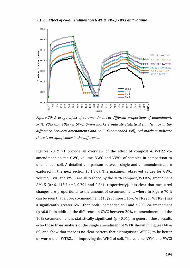
194

5.1.3.5 Effect of co-amendment on GWC & VWC/VWCi and volume

Figure 70: Average effect of co-amendment at different proportions of amendment,

30%. 20% and 10% on GWC. Green markers indicate statistical significance in the

difference between amendments and Soil2 (unamended soil), red markers indicate

there is no significance in the difference.

Figures 70 & 71 provide an overview of the effect of compost & WTR2 co-

amendment on the GWC, volume, VWC and VWCi of samples in comparison to

unamended soil. A detailed comparison between single and co-amendments are

explored in the next section (5.1.3.6). The maximum observed values for GWC,

volume, VWC and VWCi are all reached by the 30% compost/WTR2w amendment

AM15 (0.46, 143.7 cm3, 0.794 and 0.561, respectively). It is clear that measured

changes are proportional to the amount of co-amendment, where in Figure 70 it

can be seen that a 30% co-amendment (15% compost, 15% WTR2d or WTR2w) has

a significantly greater GWC than both unamended soil and a 20% co-amendment

(p <0.01). In addition the difference in GWC between 20% co-amendment and the

10% co-amendment is statistically significant (p <0.01). In general, these results

echo those from analysis of the single amendment of WTR shown in Figures 68 &

69, and show that there is no clear pattern that distinguishes WTR2d to be better

or worse than WTR2w in improving the WHC of soil. The volume, VWC and VWCi

90S 5C 5WTR2d

90S 5C 5WTR2w

80S 10C 10WTR2d

80S 10C 10WTR2w

70S 15C 15WTR2d

70S 15C 15WTR2w

0.15

0.20

0.25

0.30

0.35

0.40

0.45

0.50

ST

AR

T

48

96

14

4

19

2

24

0

28

8

33

6

38

4

43

2

48

0

52

8

57

6

62

4

67

2

72

0

76

8

81

6

86

4

91

2

96

0

10

08

10

56

10

80

FIN

AL

Gra

vim

etr

ic w

ate

r co

nte

nt

Hours

Soil 2AM4AM5AM9

195

changes as shown in Figure 71 below also show that the volumetric change of

samples is dependent on the co-amendment rate, where 30% co-amendment using

Figure 71: Average effect of co-amendment at different proportions of amendment,

30%, 20% and 10% on volume, VWC and VWCi. Green markers indicate statistical



90S 5C 5WTR2d

90S 5C 5WTR2w

80S 10C 10WTR2d

80S 10C 10WTR2w

70S 15C 15WTR2d

70S 15C 15WTR2w

80

90

100

110

120

130

140

150

STA

RT 48

96

14

4

19

2

24

0

28

8

33

6

38

4

43

2

48

0

52

8

57

6

62

4

67

2

72

0

76

8

81

6

86

4

91

2

96

0

10

08

10

56

FIN

AL

Vo

lum

e c

m3

HOURS


90S 5C 5WTR2d

90S 5C 5WTR2w

80S 10C 10 WTR2d

80S 10C 10WTR2w

70S 15C 15WTR2d

70S 15C 15WTR2w

0.20

0.30

0.40

0.50

0.60

0.70

0.80

STA

RT 48

96

14

4

19

2

24

0

28

8

33

6

38

4

43

2

48

0

52

8

57

6

62

4

67

2

72

0

76

8

81

6

86

4

91

2

96

0

10

08

10

56

FIN

AL

Vo

lum

etr

ic w

ate

r co

nte

nt

HOURS


90S 5C 5WTRd

90S 5C 5WTR2w

80S 10C 10WTR2d

80S 10C 10WTR2w

70S 15C 15WTR2d

70S 15C 15WTR2w

0.20

0.25

0.30

0.35

0.40

0.45

0.50

0.55

0.60

STA

RT 48

96

14

4

19

2

24

0

28

8

33

6

38

4

43

2

48

0

52

8

57

6

62

4

67

2

72

0

76

8

81

6

86

4

91

2

96

0

10

08

10

56

FIN

AL

Vo

lum

etr

ic w

ate

r co

nte

nt

i

HOURS


196

WTR2w (AM15) has the highest volume, VWC and VWCi over the entire time series.

Wet WTR gives a significantly higher sample volume than dry WTR at the 30% co-

amendment rate, however at a 20% amendment rate the volume change is

significantly higher for amendments with dried WTR. There is no statistical

difference in volume change between wet and dry WTR at 10% co-amendment.

5.1.3.6 Effect of co-amendment vs single amendment on GWC & VWC/VWCi and

volume

Figure 72: Average effect of single amendment vs co-amendment at 30% amendment

on GWC. Green markers indicate statistical significance in the difference between



Figure 72 compares the effect of single amendment at 30% to co-amendment at

the same rate on GWC through the wetting and drying process. All amendments

have a significantly higher GWC than unamended soil, where the single

amendment of compost at 30% (AM11) has the highest overall GWC, peaking at

0.50 and is significantly different from the next highest performing amendments

(p <0.01). As also seen in Trial 3, AM14 and AM15, the co-amended samples, have

higher GWC values than the single amendments of either WTR2d (AM12) or

WTR2w (AM13) across the whole of the time series. Although the single

70S 30C

70S 30WTR2d

70S 30WTR2w

70S 15C 15 WTR2d

70S 15C 15WTR2w

0.14

0.19

0.24

0.29

0.34

0.39

0.44

0.49

STA

RT 48

96

14

4

19

2

24

0

28

8

33

6

38

4

43

2

48

0

52

8

57

6

62

4

67

2

72

0

76

8

81

6

86

4

91

2

96

0

10

08

10

56

10

80

FIN

AL

Gra

vim

etr

ic w

ate

r co

nte

nt

Hours

Soil 2 AM11

AM12 AM13

AM14 AM15

197

amendment of WTRd performs better in general than WTRw, the inverse is

apparent when the sample is co-amended, where all co-amendments with WTR2w

perform better than WTR2d counterparts. Importantly, the GWC of all co-amended

samples remain higher than unamended soil during the second wetting and drying.

In Figure 72, only one amendment dries faster than unamended soil (AM13, 30%

WTR2w), which suggests that although this amendment has a high capacity to hold

water, this amendment then allows drainage of the soil at a greater rate than

unamended soil and does not retain the water.

Figure 73 compares the volume change of samples where the single amendment of

compost has the greatest volume change (AM11), reaching a maximum of

149.5 cm3 compared to unamended soil at 124.1 cm3, and was significantly better

than all other treatments (p <0.01), with the exception of AM15 at 600h and 912h.

Although all samples undergo swelling and shrinkage during the 1st wetting and

drying, the amended samples shrink to a lesser degree than unamended soil

(which shrinks back to a volume of 96 cm3) where in contrast amended samples

reach between 103 and 114 cm3 despite being dried to a similar GWC. There is

proportionally much less change during the 2nd wetting and drying phases,

suggesting that amendment stabilises the soil over time to reduce shrinkage.

Figures 72 and 73 suggests that by co-amending the samples, the soil inherits the

beneficial water holding capacity of compost while inheriting the beneficial

structural changes that WTR impact on the soil.

Figure 73 also compares the VWC and VWCi of single and co-amended samples,

which reflect the GWC and volume change of samples over time. Overall, co-

amendments have higher values than single amendments at the same amendment

proportion, and considering that the co-amendments also have the highest sample

volumes this means that they hold more water than unamended soil and single

amendments (excluding AM11, 70S 30C). Amendments with the highest VWC,

AM11 (70S 30C) and AM15 (70S 15C 15WTR2w), are not statistically different

from each other, showing therefore that the co-amendment performs equally well

to a single amendment, where AM15 reaches a maximum VWC of 0.79 and AM11

reaches 0.77.

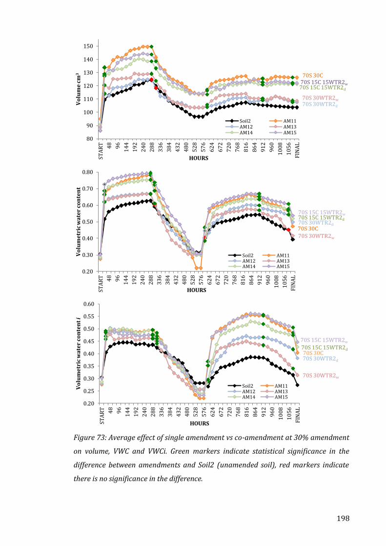
198


on volume, VWC and VWCi. Green markers indicate statistical significance in the



70S 30C

70S 30WTR2d

70S 30WTR2w

70S 15C 15WTR2d

70S 15C 15WTR2w

80

90

100

110

120

130

140

150

STA

RT 48

96

14

4

19

2

24

0

28

8

33

6

38

4

43

2

48

0

52

8

57

6

62

4

67

2

72

0

76

8

81

6

86

4

91

2

96

0

10

08

10

56

FIN

AL

Vo

lum

e c

m3

HOURS

Soil2 AM11AM12 AM13AM14 AM15

70S 30C70S 30WTR2d

70S 30WTR2w

70S 15C 15WTR2d

70S 15C 15WTR2w

0.20

0.30

0.40

0.50

0.60

0.70

0.80

STA

RT 48

96

14

4

19

2

24

0

28

8

33

6

38

4

43

2

48

0

52

8

57

6

62

4

67

2

72

0

76

8

81

6

86

4

91

2

96

0

10

08

10

56

FIN

AL

Vo

lum

etr

ic w

ate

r co

nte

nt

HOURS


70S 30C70S 30WTR2d

70S 30WTR2w

70S 15C 15WTR2d

70S 15C 15WTR2w

0.20

0.25

0.30

0.35

0.40

0.45

0.50

0.55

0.60

STA

RT 48

96

14

4

19

2

24

0

28

8

33

6

38

4

43

2

48

0

52

8

57

6

62

4

67

2

72

0

76

8

81

6

86

4

91

2

96

0

10

08

10

56

FIN

AL

Vo

lum

etr

ic w

ate

r co

nte

nt

i

HOURS


199

In Figure 73, the VWC of single 30% amendments of compost or WTR (AM11,

AM12 and AM12) are 16% lower than their co-amended counterparts (AM14 and

AM15) throughout the two wetting and drying cycles. VWCi, a measure of the

instantaneous volume of water to the volume solids provides a good indicator of

the volumetric response over time, not just a comparison to the original state of a

sample. All single and co-amendments in Figure 73 have significantly higher VWCi

than unamended soil (p <0.01), however this difference is exacerbated during the

2nd wetting and drying phases, where 30% co-amendment has a 31% higher VWCi

value than unamended soil and importantly performs equally well as a single 30%

compost amendment. The higher VWCi in the 2nd wetting and drying phases

indicates that there is a greater volume of water to the volume of solids than the 1st

wetting and drying phases, however this is due to the reduction of the bulk volume

of solids, not an increased GWC. As the volume change is known, it can be

concluded that amendment with either 30% compost or a 30% co-amendment of

WTR2 yield similar increases in the WHC of the soil, where single using WTR

amendment only yields a small increase.





80S 20C

80S 20WTR2d

80S 20WTR2w

80S 10C 10WTR2d

80S 10C 10WTR2w

0.14

0.19

0.24

0.29

0.34

0.39

0.44

STA

RT 48

96

14

4

19

2

24

0

28

8

33

6

38

4

43

2

48

0

52

8

57

6

62

4

67

2

72

0

76

8

81

6

86

4

91

2

96

0

10

08

10

56

10

80

FIN

AL

Gra

vim

etr

ic w

ate

r co

nte

nt

Hours

Soil 2 AM6

AM7 AM8

AM9 AM10

200

Figures 74 & 75 compare single 20% amendments with co-amendment at the same

ratio and have a similar trend to those seen for the 30% amendment. The greatest

increase in GWC (up to 0.44) is achieved by both the co-amendments (AM9 or

AM10) or single amendment of compost (AM6), where there is no statistical

difference between the three. This suggests that at a 20% amendment ratio, the co-

amendment performs as well as a single amendment of compost for GWC change.

As shown previously, the co-amendments perform better than single amendments,

and although 20% single amendment with WTR2d (AM7) increases the GWC, it is

significantly lower than single amendment of compost (AM6) and co-amendments

AM9 and AM10 (p <0.01). The 20% single amendment with WTR2w (AM8) has no

statistical difference to unamended soil.

In Figure 75 there is no statistical difference between the increase in VWC for the

single amendment of compost and the co-amendment at 20%, where co-

amendments again perform better than their single amendment. For VWCi shown

in Figure 75, the trend remains the same. At 20% amendment rate there is no

difference in the improvement of GWC, volume, VWC and VWCi, between adding

compost only and a compost/WTR2 co-amendment.

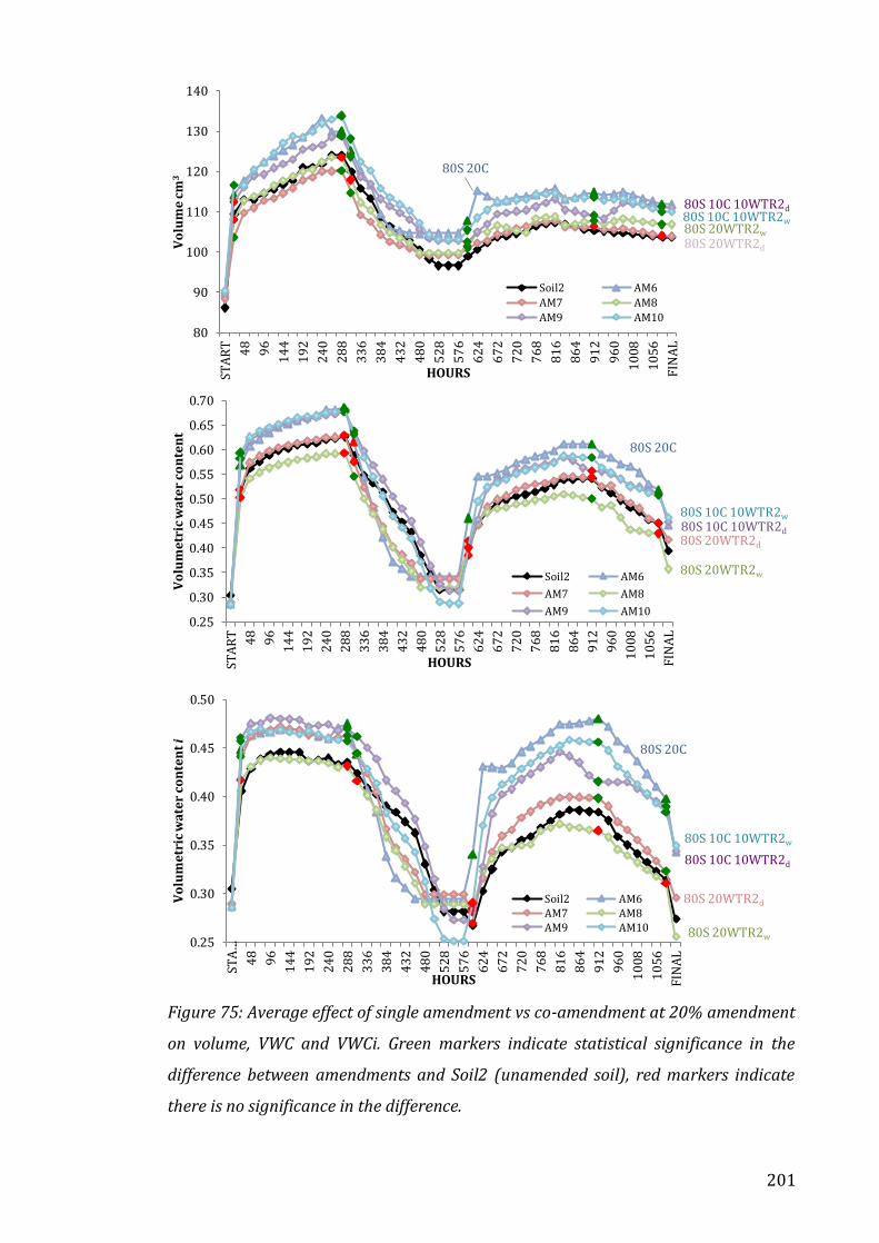
201


on volume, VWC and VWCi. Green markers indicate statistical significance in the



80S 20C

80S 20WTR2d

80S 20WTR2w

80S 10C 10WTR2d80S 10C 10WTR2w

80

90

100

110

120

130

140

STA

RT 48

96

14

4

19

2

24

0

28

8

33

6

38

4

43

2

48

0

52

8

57

6

62

4

67

2

72

0

76

8

81

6

86

4

91

2

96

0

10

08

10

56

FIN

AL

Vo

lum

e c

m3

HOURS

Soil2 AM6

AM7 AM8

AM9 AM10

80S 10C 10WTR2w

80S 20WTR2d

80S 20WTR2w

80S 10C 10WTR2d

80S 20C

0.25

0.30

0.35

0.40

0.45

0.50

0.55

0.60

0.65

0.70

STA

RT 48

96

14

4

19

2

24

0

28

8

33

6

38

4

43

2

48

0

52

8

57

6

62

4

67

2

72

0

76

8

81

6

86

4

91

2

96

0

10

08

10

56

FIN

AL

Vo

lum

etr

ic w

ate

r co

nte

nt

HOURS

Soil2 AM6

AM7 AM8

AM9 AM10

80S 20C

80S 20WTR2d

80S 20WTR2w

80S 10C 10WTR2d

80S 10C 10WTR2w

0.25

0.30

0.35

0.40

0.45

0.50

STA

…

48

96

14

4

19

2

24

0

28

8

33

6

38

4

43

2

48

0

52

8

57

6

62

4

67

2

72

0

76

8

81

6

86

4

91

2

96

0

10

08

10

56

FIN

AL

Vo

lum

etr

ic w

ate

r co

nte

nt

i

HOURS


202





Figures 76 and 77 compare single 10% amendments with co-amendments at the

same ratio. The differences between unamended soil and the amended samples are

much smaller, as expected, than the larger amendment proportions. At 10%

amendment, the single compost amendment no longer has the highest GWC change

for the first wetting and drying. In Figure 76 only 10% single WTR2w (AM3) and

10% co-amendment with WTR2w (AM5) are statistically significantly different

from unamended soil over the whole time series (p <0.01). AM4 (10% co-

amendment with WTR2d) is not statistically different from unamended soil despite

the WTR2w counterpart performing well. During the 2nd wetting and drying all

amendments at 10% amendment or co-amendment had a higher GWC than

unamended soil (with the exception of AM4), where the single amendment of

compost held the most water during the second wetting.

The volume of samples shown in Figure 77 during the 1st wetting and drying

phases are not significantly different from unamended soil for any amendment and

all return to a similar volume at the end of the 1st drying phase. However, during

the 2nd wetting and drying, 10% single amendments of compost (AM1) and WTR2

90S 10C90S 10WTR2d

90S 10WTR2w90S 5C 5WTR2d

90S 5C 5WTRw

0.14

0.19

0.24

0.29

0.34

0.39

STA

RT 48

96

14

4

19

2

24

0

28

8

33

6

38

4

43

2

48

0

52

8

57

6

62

4

67

2

72

0

76

8

81

6

86

4

91

2

96

0

10

08

10

56

10

80

FIN

AL

Gra

vim

etr

ic w

ate

r co

nte

nt

Hours

Soil 2 AM1AM2 AM3AM4 AM5

203

Figure 77: Average effect single amendment vs co-amendment at 10% amendment

on VWC and VWCi. Green markers indicate statistical significance in the difference

between amendments and Soil2 (unamended soil), red markers indicate there is no


90S 10C90S 10WTR2d

90S 10WTR2w

90S 5C 5WTR2d

90S 5C 5WTR2w

80

85

90

95

100

105

110

115

120

125

130

STA

RT 48

96

14

4

19

2

24

0

28

8

33

6

38

4

43

2

48

0

52

8

57

6

62

4

67

2

72

0

76

8

81

6

86

4

91

2

96

0

10

08

10

56

FIN

AL

Vo

lum

e c

m3

HOURS

Soil2 AM1

AM2 AM3

AM4 AM5

90S 10C

90S 10WTR2d

90S 10WTR2w

90S 5C 5WTR2d

90S 5C 5WTRw

0.25

0.30

0.35

0.40

0.45

0.50

0.55

0.60

0.65

0.70

STA

RT 48

96

14

4

19

2

24

0

28

8

33

6

38

4

43

2

48

0

52

8

57

6

62

4

67

2

72

0

76

8

81

6

86

4

91

2

96

0

10

08

10

56

FIN

AL

Vo

lum

etr

ic w

ate

r co

nte

nt

HOURS

Soil2 AM1

AM2 AM3

AM4 AM5

90S 10C

90S 10WTR2d

90S 10WTR2w

90S 5C 5WTRd

90S 5C 5WTR2w

0.20

0.25

0.30

0.35

0.40

0.45

0.50

0.55

STA

RT 48

96

14

4

19

2

24

0

28

8

33

6

38

4

43

2

48

0

52

8

57

6

62

4

67

2

72

0

76

8

81

6

86

4

91

2

96

0

10

08

10

56

FIN

AL

Vo

lum

etr

ic w

ate

r co

nte

nt

i

HOURS

Soil2 AM1

AM2 AM3

AM4 AM5

204

(AM2 and AM3) have a higher volume peak than co-amendments at the same ratio,

which is a non sequitur to the effect of co-amendments at 30 and 20% proportions.

Figure 77 also compares the VWC and VWCi of 10% amendment and shows that

the VWC during the 1st wetting and drying is only significantly higher for one

amendment (AM3, 10% WTR2w, p <0.01) in comparison to unamended soil. During

the secondary wetting phase, all amendments except AM4 (10% co-amendment

with WTR2d) are significantly greater than unamended soil (p <0.01). This

provides further evidence that at a low amendment proportion (10%), due to the

heterogeneous distribution of the amendment, the soil requires an initial wetting

and drying period for these amendments to take effect whereas at higher

amendment proportions of 20 and 30%, the effect is more readily measured.

Similarly, Figure 77 shows that during the 2nd wetting and drying, the VWCi

increases significantly, and as discussed previously, we know that the volume of

the unamended soil is also lower than the amendments, meaning the increase in

VWCi is not just a function of smaller samples.

5.1.3.7 Concluding remarks: Trial 4

This summary section concludes the major findings with a statement heading and

subsequent bullet pointed supplementary information: (A) firstly from the average

effect of single amendments on the gravimetric water content, volume, VWC and

VWCi change over time, (B) secondly from the comparison of different amendment

ratios of compost and then WTR, and (C) lastly major findings from the

comparison of co-amendments against the control and the single amendments. All

values are for an n = 12 and where p <0.01.

(A) The single amendment of compost improves all parameters better than the single

amendment using WTR.

1. GWC of single amendments at 30%

Single 30% compost results in a GWC that is 20% higher than single

amendments of WTR or 34.7% higher than soil.

30% single amendments of WTR reached 93% of their GWC maximum

within 24 hours

30% single amendment of compost reached 84% of maximum GWC within

24 hours

205

30% WTR2d dried slower than any other 30% single amendment.

There is no statistical difference between WTR2w and WTR2d (until 912

hours)

Compost is statistically better than single amendments of WTR (p <0.01)

During the second drying, WTR amended samples experience a 6% less

reduction in GWC compared to compost at 16%.


Compost again has the highest GWC, and is significantly different from

WTR2d 20% amendment.

20% single WTR2w is not significantly different from unamended soil.

30% single amendment of WTR2d performs equally well to 20%

amendment of compost (p <0.01)

WTR amendment experiences 2% less reduction in GWC than compost at

12%.


Only 10% WTR2w is significantly higher than soil (0.39) during the first

wetting

During the second phase of wetting all amendments significantly higher

than soil

10% WTR2w has a 13% reduction in GWC, 10% WTR2d only has a 3%

reduction in GWC, and 10% compost achieves a 3% increase in the GWC in

the second phase of drying,

4. Volumetric changes were higher for all single amendments, and largest for

compost amended samples

Compost had the biggest volume change (44.1%) compared to unamended

soil

WTR2w achieved up to 12% increase in volume compared to unamended

soil, but WTR2d restricted swelling in the first phase of wetting and only

reached 7.3% better volume than soil at 30% amendment.

VWC/VWCi was higher than unamended soil for all 30% amendments.

No difference between WTR2w and WTRd during the first phases for

VWC/VWCi, but WTR2d was statistically significantly higher than WTR2w

during second phases.

206

(B) The GWC response to amendment was greater with higher proportions of

material (compost), however the relationship was not as linear for the use of WTR.

1. Single compost at increasing proportion:

30% increases the GWC by 34.7% and 20% by 13.2% but no significance for

10% during the 1st wetting

10% amendment increased the GWC by 83.3% compared to unamended

soil in the second wetting, 20% by 29.3% and 30% by 59.2% compared to

the control soil.

2. Single WTR2d and WTR2w at increasing proportion:

30% WTR addition gives the highest GWC increase, and is 16.5% higher

than unamended soil

No trends are apparent between addition of wet or dry for GWC change,

where all amendments statistically significantly improve the GWC (except

AM8)

WTR amendments make no difference to GWC on the first wetting at 10%

amendment ratio.

All single WTR amendments improve the volume increase during second

wetting (except AM7), and reduced shrinkage during drying.

Despite this, only 30% WTR amendment has a significantly higher

VWC/VWCi than unamended soil

(C) Co-amendments perform better than single amendments of WTR, and in some

cases perform equally well to the single amendment of compost for GWC, volume and

VWC/VWCi

30% single amendment of compost has the highest overall increase in GWC

(34.7%), however co-amendments perform up to 24.7% better than soil

and 9% better than single amendments of WTR.

The trend in the volume change of samples is the same as found for GWC,

but no overall trends separating the performance of WTR2d and WTR2w

At 30%, the co-amendment improves the VWCi during the second wetting

by up to 31%, which is equal to the VWCi achieved by single compost at

30%

At 20% amendment there is no statistical difference in the improvement

between co-amendments and single compost for maximum GWC.

207

20% amendment does not increase the volume of samples for any

amendment during the 1st wetting, however all co-amendments are

significantly higher in volume during the 2nd wetting than soil and the single

amendments of WTR.

Only 10% WTR2w amendment improves the VWC/VWCi during the 1st

wetting, however all amendments improve the VWC during the 2nd phase of

wetting but the WTR2d co-amendment is no longer better than the single

amendment.

To summarise the findings from Trial 3 and 4, single amendment using WTR

improves the GWC (with two exceptions) and volume change of samples (using

WTR2w at 30% amendment) which may occur due to high surface area of the WTR

particles as a result of fine particle size, as the material is not known to swell upon

wetting despite high organic content. WTR also reduces the extent of shrinkage

when the samples are dried, suggesting that the soil architecture has been

beneficially changed due to WTR addition and ‘cementing’ occurs during drying

(Moodley & Hughes, 2006). The single amendment of compost improves the

maximum water content of the samples to the greatest extent as the material itself

swells, opening up more space for water to be held water to be held within the

sample, however upon drying this space shrinks and the porosity is lost to a large

extent. The addition of co-amendment yields the benefit of both amendments,

where the water holding capacity is increased as a function of improved maximum

gravimetric water content, and improved structural characteristics that reduce

shrinkage upon drying to maintain pore space for further wetting cycles.

Stabilizing pore space during drying will allow better infiltration and percolation

rates through the soil for future events, which improves a soil’s ‘flood holding

capacity’ according to the definition by Kerr et al. (2016). Although a single

compost amendment results in the best improvement of water holding capacity at

high amendment rates, as discussed in Chapter 2 excessive application of compost

has detrimental effects on the soil geochemical environment and on the

geotechnical properties of the soil. At realistic field application rates (<10%), the

difference in the effect of compost is not as pronounced as in 30% application rates

and the co-amendment therefore performs equally well.

208

5.2 Erosional resistance

5.2.1 Drop testing (Veitch method)

Figure 78: Average number of drops required for deformation and breaking for unamended soil and 15 amendments. Samples annotated with *

have been through one wetting and drying cycle prior to testing. n = 12 and error bars present the maximum and minimum values in each data set.

No statistical testing was performed on this data.

0.0

5.0

10.0

15.0

20.0

25.0

30.0

35.0

40.0

45.0

50.0

0

1000

2000

3000

4000

5000

6000

7000

Wat

er c

on

ten

t %

Nu

mb

er o

f d

rop

s

Sample #

Breaking PointDeformationWater content

209

Figure 78 shows the average number of water drops until deformation and breakage

for unamended soils and samples AM1-AM15. ‘Deformation’ occurred when the flat

surface of the sample cracked, slumped or started to erode. ‘Breaking’ occurred

when a piece of soil became detached from the soil. Each sample had one of two

treatments, where one was tested 24 hours after production, and the other tested

after one wetting and drying cycle as annotated with an * on the X axis. No statistical

analysis was performed on this data; however, the large error bars suggest that

there may be no significance in any differences shown in the graph and trends are

only apparent. All amended samples deformed with fewer drops than soil (1280

drops), however on average four amendments were able to sustain more than or as

many drops as unamended soil before breakage, 10% co-amendment (WTR2d), 20%

WTR2w, 20% co-amendment of WTR2d and WTR2w and 30% co-amendment with

WTR2d. In general, samples that had been subjected to one wetting and drying cycle

deformed and reached breaking point with fewer drops than the sample tested after

production with the exception of 10% WTR2w and 30% co-amendment with WTR2d

(AM2 and AM14)

The water contents of samples at the breaking point in Figure 78 (shown on the

secondary Y axis) ranged between 29% and 37%, which indicates that the samples

were fully saturated the point of breakage as these values were similar to the

maximum water content achieved in Trial 4. It appears then, that samples broke

when they reached full saturation, and those samples that took up water most

quickly (as shown in the WHC trials in section 5.1 and subsequently in hydraulic

conductivity testing in section 5.3.1), had the fewest drops required to breakdown.

This presumably is a function of slaking whereby the rapid intake of water causes

air bubbles to become trapped and pressurised which causes them to burst and

breakdown aggregates. For samples that had a lower rate of wetting, this effect was

less prominent and the samples remained intact for a longer period of wetting. For

any robust conclusions to be drawn about the erodibility of samples after

amendment, the Veitch method likely requires some further refinement and the

number of samples needs to be greatly increased in an attempt to reduce the

deviation between each test as a result of extreme heterogeneity in the material

tested.

210

5.2.2 Fall cone testing

The following figures 79-81 show the undrained shear strength values obtained from fall cone testing on both samples from Trial 3 (conducted

by Mansfield, 2015) and Trial 4.

Figure 79: Undrained shear strength (Cu) for Trial 3 samples conducted according to BS1377: 1990 with reference table (right). Error bars denoted

max and minimum values for each sample, where n = 5. (Left) Table with a summary of sample amendments.

Max point of error bar = 110.34

0.0

10.0

20.0

30.0

40.0

50.0

60.0

70.0

80.0

Un

dra

ine

d s

he

ar

stre

ng

th (

Cu

in

kP

a)

Sample

Sample

N= 8

Soil

2%

Compost

2%

WTR2d

%

Silica

%

Soil 2 100

A1 50 50

A2 50 50

A3 50 25 25

A4 50 25 25

A5 60 40

A6 60 40

A7 60 40

A8 60 20 20

A9 60 20 20

A10 70 30

A11 70 30

A12 70 30

A13 70 15 15

211

Figure 80: Undrained shear strength results from fall cone testing on samples from Trial 4 (BS1377) where n = 12. Samples annotated with * have

been fully saturated and dried to the same moisture content (0.16) as samples that were tested 24 hours after production. Black boxes are Q2-Q3

and whiskers on each box show the maximum and minimum values derived. Diamond markers indicate outliers in the data that cannot be omitted

but would skew the data significantly.

10

0S

90

S 1

0C

90

S 1

0W

TR

2d

90

S 1

0W

TR

2w

90

S 5

C 5

WT

R2

d

90

S 5

C 5

WT

R2

w

80

S 2

0C

80

S 2

0W

TR

2d

80

S 2

0W

TR

2w

80

S 1

0C

10

WT

R2

d

80

S 1

0C

10

WT

R2

w

70

S 3

0C

70

S 3

0W

TR

2d

70

S 3

0W

TR

2w

70

S 1

5C

15

WT

R2

d

70

S 1

5C

15

WT

R2

w

0

20

40

60

80

100

120

140

160

180

Un

dra

ine

d s

he

ar

stre

ng

th (

Cu

in k

Pa

)

Sample

212

10% amendment 20% amendment 30% amendment

Figure 81: Average undrained shear strength values for Trial 4 samples from fall cone testing (BS1377). Red dashed lines indicate the error i.e. the

minimum and maximum value obtained for the samples where n = 12. Samples annotated with * have been fully saturated and dried to the same

moisture content (0.16) as samples that were tested 24 hours after production. AM1, AM2, AM11 and AM15 are not significantly different from

Soil2, and AM2*, AM11*, AM14* and AM15* are not significantly different from Soil2*. The remaining amended samples have a significantly higher

Cu (two tailed at alpha level of 0.05) than both Soil2 and Soil2*.

0

20

40

60

80

100

120

140

160

Un

dra

ine

d s

he

ar

stre

ng

th (

Cu

)

Sample

213

Figure 79 presents results of fall cone testing using on samples from Trial 3 and

shows that unamended has a low Cu (2.1) in comparison with the majority of

amendments, where A2 (50% silica amendment), A5 (40% compost) A9 (40% co-

amendment with silica), A11 (30% compost) and A12 (30% silica) have similarly

low values of CU ranging from 0.9 to 3.5. There appears to be no trend between the

addition of WTR2d in the undrained shear strength as A1 (50% WTR2d), A6 (40%

WTR2d) and A11 (30% WTR2d) have values that do not correspond with the

proportion of amendment. No trends are apparent between proportion of compost

or silica either, however in general it appears that the addition of any material

improves the undrained shear strength in comparison to unamended soil.

Figures 80 and 81 show the range of Cu (undrained shear strength) values obtained

for fall cone testing on samples from Trial 4. Figure 80 shows the Q1-Q3 box plots;

where whiskers show the remaining data, and diamond markers show apparent

outliers. It is clear that there is a great degree of heterogeneity in the values of

undrained shear strength within each set of 12 replicates per sample, as apparent

in erosional testing. This may be accounted for by the heterogeneity of the sample

surface, where in one test the fall cone may have struck soil and in another it strikes

a piece of dried WTR (WTR2d) or a piece of compost, and the total effect of the

amendment is not tested rather the direct shear properties of component itself. In

general, it appears in Figure 80 that the single amendments using WTR2w had the

highest shear strength

As shown in Figure 81, 10% co-amendments AM4 and AM5, AM8 (20% single

WTR2w amendment), AM12* and AM13 (30% single WTR2d and WTR2w

amendments respectively) all have similarly high mean values of ~80 Cu, compared

to unamended soil of 6.66 or 14.83*. Mann Whitney U statistical testing was used to

test for significant difference between samples, and despite large range of values

(error) for each amendment, the majority of amendments are significantly better

than unamended soil for undrained shear strength (p <0.05) The exceptions are

AM1 (90S 10C), AM2 (90S 10WTR2d), AM11 (70S 30C) and AM15 (70S 15C

15WTR2w). There doesn’t appear to be a single component that is responsible for

insignificance in the difference between the amended sample and unamended soil.

In addition, there does not appear to be an obvious difference between the shear

214

strength of samples tested just after production and the samples tested after one

wetting and drying (annotate with *), where Soil2*, AM1*, AM2*, AM9*, AM11*,

AM12*, AM14* and AM15* have higher shear strength values than the same samples

tested after production, and the remaining *amendments have lower values for Cu

than their respective samples.

Soil2 = 6.66

Single amendment of WTR Single amendment of C Co-amendment Sample Cu average Sample Cu average Sample Cu average

AM2 10.67 AM1 10.47 AM4 86.33 AM3 46.98 AM6 19.44 AM5 88.84

AM7 38.14 AM11 8.67 AM9 23.24 AM8 84.19 AM10 37.58

AM12 39.70 AM14 8.08 AM13 32.35 AM15 9.03

Table 26: Average Cu values for soils categorised into their amendment properties. Red

titles indicate no significance between the value and unamended soil.

Soil2* = 14.83 Single amendment of WTR Single amendment of C Co-amendment

Sample Cu average Sample Cu average Sample Cu average

AM2* 20.25 AM1* 22.47 AM4* 23.79

AM3* 35.14 AM6* 34.03 AM5* 28.20 AM7* 47.69 AM11* 10.55 AM9* 28.24

AM8* 55.04 AM10* 23.23 AM12* 87.90 AM14* 14.30

AM13* 32.35 AM15* 12.49

AM1 = 90S 10C, AM2 = 90S 10WTR2d, AM3 = 90S 10WTR2w, AM4 = 90S 5C 5WTR2d, AM5 = 90S 5C 5WTR2w,

AM6 = 80S 20C, AM7 = 80S 20WTR2d, AM8 = 80S 20WTR2w, AM9 = 80S 10C 10WTR2d, AM10 = 80S 10C 10WTR2w,

AM11 = 70S 30C, AM12 = 70S 30WTR2d, AM13 = 70S 30WTR2w, AM14 = 70S 15C 15WTR2d, AM15 = 70S 15C 15WTR2w

Table 27: Average Cu values for soils after one wetting and drying cycle (annotated

with *) categorised into their amendment properties. Red titles indicate no

significance between the value and unamended soil.

Table 26 shows that the greater the proportion of compost, the lower the shear

strength (which links with literature in Chapter 2) and in general the amendment

using WTR2 increases the Cu of soil to the largest degree against unamended soil.

Importantly the use of co-amendment at a rate of 10% (AM4 and AM5) increases

the Cu more than higher application rates of co-amendment, presumably because of

215

the increase in compost, which reduces the shear strength at a greater rate than

WTR increases it. The application of 10% or 20% co-amendments have higher mean

Cu values than any single amendment of compost, however 30% co-amendments

have similar values to single compost 30% amendment (8.08, 9.03 and 8.67

respectively). The amendment using WTR2w increases the shear strength compared

to unamended soil to a higher degree than the addition of WTR2d, which can be

attributed to the cementing properties of the wet WTR outlined by Moodley &

Hughes. Table 27 indicates the same differences shown in Table 26, for samples

subjected to a wetting and drying cycle (annotated with *). For these samples, all

single amendments of WTR2 have higher values than any single amendment of

compost or a co-amendment at the same proportion of amendment.

5.2.3 Concluding remarks

The erosional resistance testing in section 5.2.1 did not provide conclusive results

due to large deviation in the values obtained via the Veitch method. All amendments

required fewer drops to deform than unamended soil which suggests that aggregate

stability is lower for amended samples. This is likely due to the erosional process

associated with a rapid intake of water, reflected by the high-water content of

samples at point of complete failure (breakage) as a result of better water holding

capacity and infiltration rate. Further conclusions are difficult to make owing to the

rudimentary nature of the Veitch method; therefore, refinements are required in the

methodology and a greater number of samples are needed to improve the accuracy

and reliability of results.

Fall cone testing in section 5.2.2 showed that in Trial 3 the 40% single amendment

of WTR2d improved the Cu value by a factor of 28 (60.4) compared to unamended

soil (2.1), although the 50% and 30% single amendments do not achieve such high

improvement rates, their averages were 15.6 and 1.9 respectively. Samples that

contained compost or silica as single or co-amendment had low undrained shear

strength. Fall cone testing for Trail 4 samples showed that the amendment with

compost at any ratio provided the lowest undrained shear strength, and were not

significantly different from unamended soil. There does not appear to be a trend

between the ratio of amendment and the improvement in shear strength, nor

between the type of WTR added.

216

5.3 Triaxial testing

Core samples synthesised during Experiment 4 were tested in a triaxial cell to

measure their hydraulic conductivity and shear strength. All amendments were

tested for their hydraulic conductivity, however only the largest amendment

proportions (AM11-AM15) were tested for shear strength due to the long-term

nature of the testing procedure.

5.3.1 Hydraulic conductivity

The saturated hydraulic conductivity of a soil is a function of many parameters

including soil texture, clay content, organic matter, and soil aggregation (Hillel,

2008; Moutier et al., 2000), and is widely used as an indicator of soil quality

(Reynolds et al., 2000; Lim et al., 2016) as it reflects good soil structure. Figure 82

shows the variation in hydraulic conductivity measured on specimens of the

unamended soil and soils with amendments, at three different confining stress

levels (25 kPa, 50 kPa and 100 kPa), using a hydraulic gradient of 15 kPa. As

expected, the hydraulic conductivities are lower at greater stress levels, as

increasing the confining stress causes a reduction in porosity, making water flow

more difficult. Silt and medium plasticity clays typically have a permeability of

around 10-10 m/s, however as shown in Figure 82 unamended soil (Soil2) has a high

permeability of 1.26 – 6.73 x 10-7 m/s depending on confining pressure (which

equates to 0.006-0.34 ml/hr, as shown in Table 28).

The 30% single amendment of WTR2d (AM12) has the highest hydraulic

conductivity (up to 1.77 x 10-5 m/s at 25 kPa), followed by single amendments of

30% WTR2w, 20% WTR2d and WTR2w (reaching maximum conductivities of 7.22,

3.81 and 5.32 x 10-6 m/s at 25 kPa respectively). WTR2d is able to increase the

hydraulic conductivity of unamended soil by a factor of 26, however the single

amendment of WTR2w at the same rate increases the hydraulic conductivity by a

factor of 11, compared to soil alone at 6.72 x 10-7 m/s. This difference in

performance may be due to particle size differences, where WTR2w adds fines

< 75 m, whereas WTR2d has a particle size distribution that includes larger grains

of up to 3 mm; the addition of coarse material increases the hydraulic conductivity

(Boadu, 2000).

217

Figure 82: Hydraulic conductivity of samples conducted in a triaxial cell at pressures of 25, 50 and 100 kPa, on a log scale. Samples AM1,

AM2 and AM3 were only tested at 25 kPa and do not feature on the graph; their k values were 1x E-06, 6.48 x E-07 and 4.06 x E-06 m/s

respectively. n = 1 for all samples. Tests on samples AM4, AM5, AM6, AM9 and AM10 were conducted for all cell pressures on the same

specimen, all other samples used one specimen for each cell pressure as the sample was sheared to end the test.

20

30

40

50

60

70

80

90

100

1.0

E-0

8

1.0

E-0

7

1.0

E-0

6

1.0

E-0

5

Ce

ll P

ress

ure

(k

Pa

)

Hydraulic Conductivity (m/s)

Soil2

AM4 10% co-am WTR2d

AM5 10% co-am WTR2w

AM6 20% C

AM7 20% WTR2d

AM8 20% WTR2w

AM9 20% co-am WTR2d

AM10 20% co-am WTR2w

AM11 30% C

AM13 30% WTR2w

AM12 30% WTR2d

AM14 30% co-am WTR2d

AM15 30% co-am WTR2w

218

The 20% and 30% single amendments of compost have the lowest overall hydraulic

conductivity at the highest pressures (2.06 and 7.33 x 10-8 m/s or 0.6 and

0.32 ml/hour, respectively) compared to soil. However, at 25 kPa there is negligible

difference between AM11 (30% compost) and soil, and the rate of water movement

is twice as fast for AM6 (20% compost) compared to soil alone. This suggests that

the addition of organic matter hinders the movement of water through a sample at

high pressures due to increased tortuosity and increased compressibility of the

sample (Lim et al., 2016), but provides preferential flow path ways shown by higher

hydraulic conductivity at low pressure. The 10% co-amendment of WTR2d/w (AM4

and AM5 respectively) perform marginally better that the unamended soil reaching

maximums of 8.27 x 10-7 and 1.29 x 10-6 m/s respectively. With greater proportions

of co-amendment, the hydraulic conductivity increases, where the 20% co-

amendment (AM9 and AM10) perform better, i.e. have a higher hydraulic

conductivity than the soil, by a factor of 5, and a 30% co-amendment by a factor of

6 compared to soil alone. With the exception of AM12, WTR added in the wet form

gives a higher hydraulic conductivity than the addition of dried WTR, although it is

unknown if the difference is of any statistical significance.

Table 28 presents the maximum water contents recorded in the triaxial cell at

100 kPa compared to the maximum water contents recorded in Trial 4. For the

former, the water content is measured at the end of the triaxial test after the soil has

undergone consolidation, and as such it is both compressed and restricted from

swelling to the same degree as Trial 4 due uniform external pressure, which in effect

reduces the porosity. Therefore, as shown the maximum water contents are higher

for samples in Trial 4 as these were allowed to swell without restriction. In general,

samples with the highest proportion of amendments, and therefore the highest

surface area (contributed by WTR, see chapter 6 for details) or the highest available

pore space (contributed by compost) in comparison to volume of soil, had the

highest water content. When comparing amendments at the same ratio, the single

WTR and co-amendments have similarly high maximum water content to single

compost amendments, which suggests that WTR is able to improve the hydraulic

conductivity to the same extent if the swelling factor is removed. The reason for 10%

amendments having a higher maximum water content than the 20% amendments

219

in the triaxial cell is unknown, although as discussed previously in the analysis of

Trial 4 data, the 20% amendments did not perform as expected.

Sample Max water content at 100 kPa

Max water content Trial 4

Soil2 (100S) 26.36 36.3

AM1 (90S 10C) 26.38 35.9

AM2 (90S 10WTR2d) 26.09 35.7

AM3 (90S 10WTR2w) 27.28 39

AM4 (90S 5C 5WTR2d) 26.39 37.2

AM5 (90S 5C 5WTR2w) 24 39

AM6 (80S 20C) 25.07 42.2

AM7 (80S 20WTR2d) 23.78 38.2

AM8 (80S 20WTR2w) 24.63 36

AM9 (80S 10C 10WTR2d) 24.25 41.2

AM10 (80S 10C 10WTR2w) 24.04 42.1

AM11 (70S 30C) 32.45 50.1

AM12 (70S 30WTR2d) 31.45 42.3

AM13 (70S 30WTR2w) 32.95 41.1

AM14 (70S 15C 15WTR2d) 31.92 46.4

AM15 (70S 15C 15 WTR2w) 33.5 46.5

Table 28: Values of maximum water content in obtained from the triaxial cell

apparatus, compared to the maximum water content achieved by samples in Trial 4.

In summary, the hydraulic conductivity is increased with the addition of WTR by up

to a factor of 28, where the use of WTR2d performs better than WTR2w, presumably

as a function of the addition of coarse particles. Compost in general reduces the

hydraulic conductivity of samples due to the compressibility of the material which

reduces the porosity of compost amended samples as they are placed under stress

in the triaxial testing equipment.

220

5.3.2 Shear strength

Sample Composition 25 kPa 50 kPa 100 kPa Angle of

friction

Soil2 100S 69 kPa 123 kPa 179 kPa 33.7°

AM11 70S 30C 84 kPa 105 kPa 165 kPa 36.6°

AM12 70S 30WTR2d 115 kPa 200 kPa 174 kPa 33.0°

AM13 70S 30WTR2w 158 kPa 113 kPa 174 kPa 33.2°

AM14 70S 15C 15WTR2d 106 kPa 53 kPa 252 kPa 37.3°

AM15 70S 15C 15WTR2w 78 kPa 129 kPa 249 kPa 37.6°

Table 29: Summary of triaxial cell data for unamended soil (Soil2) and five 30%

amendments. Bold values indicate the highest shear stress value, and red values

indicate erroneous values.

From triaxial data produced in the Durham University laboratory by a skilled

technician, stress paths and stress/strain graphs have been derived for Soil2

(unamended soil) and samples AM11- AM15. The three important parameters that

we can analyse from triaxial testing are; the shear strength of a sample (shown by

stress/strain paths), the tendency of a sample to dilate or contract, and the frictional

resistance or angle of friction (both shown by stress paths). As shown in Table 29,

unamended soil had a maximum shear strength of 179 kPa, which classifies the soil

as ‘stiff’ and is typical for a sandy loam, and an angle of friction of 33.7° (where the

maximum values obtained by sands are 40° and soft clays would be expected to have

an angle of friction between 20° and 25°, Craig, 2004).

5.3.2.1 Stress strain relationships

Stress strain graphs show the relationship between increasing axial strain and the

resultant deviator stress (q) on the sample (the stress difference between the axial

stress and the confining stress applied to the sample). Figure 83 provides an

exemplary plot of this relationship for Soil2 at 25, 50 and 100 kPa. The slope of the

stress (q) versus axial strain plot indicates the stiffness of the soil. Samples having a

soft response, would show greater strain as the stress (q) increases, i.e. the slope of

the curve would be shallower. The dashed line overlaid on the graph shows a typical

stress strain curve for a dense coarse grained soil or an over consolidated fine

221

grained soil, where the peak indicates the point of maximum shear stress (the peak

shear strength), after which the soil progresses to a lower ‘critical state’ where no

further volume change or distortion occurs with increasing strain, as the soil flows

as a frictional fluid and exhibits no cohesion (Schofield & Wroth, 1968). A loose

coarse grained sand or normally consolidated fine grained soil will not demonstrate

a peak but will reach the maximum shear stress at the ultimate (critical) state, as

demonstrated by the data in Figure 83. At the Critical State there is a unique

relationship between q (deviator stress in kPa), p’ (mean effective stress) and the

specific volume of the sample (volume of soil particles per unit volume). The

majority of stress strain curves for the data presented subsequently display no

distinct peak but instead plateau, suggesting that the shear strength is generally

reached at the critical state (ultimate state).

Figure 83: Stress strain curve for unamended soil at three cell pressures.

222

All samples experienced their highest shear strength at 100 kPa and lowest shear

strength at 25 kPa. Testing at 50 kPa produced erroneous results (shown in red in

Table 29), which did not fall between the values of 25 and 100 kPa and therefore

cannot be taken forward in this analysis. Figure 84 highlights differences in stress-

strain behaviour between each amendment. It is clear from the comparison of

orange data lines (50 kPa) with the 25 kPa (blue) and 100 kPa (grey) lines that these

tests at 50 kPa were either incomplete (AM13 and AM15) and did not reach failure,

taken to be at 20% axial strain (as can be seen for tests at 25 and 100 kPa where the

stress-strain behaviour reaches a plateau by this value of strain) or had erroneous

data as the values for 50 kPa should sit between those for 25 kPa and 100 kPa. The

50 kPa reading for AM11 almost reaches a plateau as it was only sheared to 15%.

AM12 at 50 kPa appears to have higher shear strength than at 100 kPa, and AM14

at 50 kPa has a lower shear strength than the 25 kPa (although considering the trend

of the line, should the test have been completed to failure, the value may have been

AM11 AM12

AM13 AM14

AM15 Figure 84: Stress (y axis)- strain (x axis)

graphs for AM11-AM15 at three

confining pressures, where blue plots

data from 25 kPa, orange plots data from

50 kPa, and 100 kPa in grey.

223

satisfactory). The subsequent figures compare the stress strain relationship at cell

pressures of 25 kPa, 50 kPa and 100 kPa.

Figure 85 presents the 25 kPa tests, which indicates that unamended soil has the

lowest shear strength (70 kPa). The reasons for these responses are discussed later.

Figure 86 shows the stress strain relationship of amended soils compared to

unamended soil at 50 kPa, however as mentioned previously these tests were

incomplete or erroneous (with the exception of soil alone). AM11 (30% compost)

and AM15 (30% co-amendment with WTR2w) are the only two data sets from which

reliable conclusions can be drawn, as their values fall between those obtained for 25

and 100 kPa. Although the test has been cut short of sample failure, the trend line of

30% compost (AM11) suggests that it would not exceed the shear strength of soil at

failure, where the maximum recorded value for shear strength was 105 kPa

compared to unamended soil at 124 kPa. The projection for 30% co-amendment

(AM15) suggests that the maximum shear strength would be higher than the 129

kPa maximum recorded. Figure 87 shows the stress strain of samples tested at 100

kPa. Unamended soil, shown in black is stiffer than any of the amended samples,

shown by the steeper gradient in q (kPa) as the axial strain increases. Single

amendments of compost, WTR2d and WTR2w do not show any improvements in

shear strength compared to the unamended soil (165, 174 and 174 kPa

respectively). However, both co-amendments have a higher shear strength than soil

by a factor of 1.4, where soil reaches a maximum of 179 and co-amendments AM14

and AM15 reach 252 kPa and 249 kPa respectively. The reasons for this will be

discussed after an interpretation of the stress paths and critical state lines.

224

Figure 85: Stress strain curve for unamended soil and five amendments tested at 25

kPa where AM11 = 70S 30C, AM12 = 70S 30WTR2d, AM13 = 70S 30WTR2w, AM14 = 70S

15C 15WTR2d, AM15 = 70S 15C 15WTRw



15C 15WTR2d, AM15 = 70S 15C 15WTRw

0

100

200

300

400

500

0 0.05 0.1 0.15 0.2 0.25

q (

kP

a)

Axial strain

AM11

AM12

AM13

AM14

AM15

Soil2

0

100

200

300

400

500

0 0.05 0.1 0.15 0.2 0.25

q (

kP

a)

Axial strain

AM11

AM12

AM13

AM14

AM15

Soil2

225



15C 15WTR2d, AM15 = 70S 15C 15WTRw

5.3.2.2 Stress paths

The answer to why there seems to be a synergistic relationship between compost

and WTR when added to soil lies in the analysis of the stress path data, from which

we can determine contractive or dilatant tendencies of a sample when sheared, and

M (the slope of the critical state line) can be calculated using Equation 19, from

which the angle of friction is obtained using Equation 20.

𝑀 =𝑞

𝑝′

Equation 19: Calculation M, the slope of the critical state line.

𝜙𝑐′ = 𝑠𝑖𝑛−1 (3𝑀

𝑀 + 6)

Equation 20: Calculation to obtain the angle of friction from M (Craig, 2004 pg 123)

Stress paths are used to represent the states of stress in a sample during loading

until the point of failure (the failure envelope), by plotting the deviator stress (q)

against the mean effective stress (p’). As the soil is sheared, it will move through

different states of stress towards the Critical State Line. Figures 88, 89 and 90 show

0

100

200

300

400

500

0 0.05 0.1 0.15 0.2 0.25

q (

kP

a)

Axial strain

AM11

AM12

AM13

AM14

AM15

Soil2

226

Figure 88: Stress

paths and critical

state lines for all

samples tested in the

triaxial cell. Data for

AM13 at 50 kPa has

not been included due

to machine error

giving spurious

results.

227

the effective stress paths for unamended soil and five amendments. The strength of

a soil is dependent on the slope of the failure envelope (angle of friction) and how

far up the failure envelope a soil can travel (based on its tendency to dilate or

contract). Therefore, the dilatant tendencies and angle of friction provide us

information on why and how one soil has different shear strength to another as

shown in the stress strain graphs above.

Critical State lines have been drawn through the endpoints of the stress paths in

Figure 88. In all cases the lines pass through the origin (showing no cohesion) as

would be expected for the Critical State. The Critical State stress ratio (M) has been

determined for each soil and amendment type (Eq. 19). Equation 20 has then been

used to calculate the angle of friction for this state.

Sample Composition Angle of friction

Soil2 100S 33.7°

AM11 70S 30C 36.6°

AM12 70S 30WTR2d 33°

AM13 70S 30WTR2w 33.2°

AM14 70S 15C 15WTR2d 37.3°

AM15 70S 15C 15WTR2w 37.6°

Table 30: Angle of friction values for unamended soil (Soil2) and five amendments,

calculated from stress path graphs.

Table 30 highlights the angle of friction achieved by each amendment, which has

been determined from the angle of the critical state line. Unamended soil has a

relatively high angle of friction of 33.7°. The single addition of WTR does not

improve the frictional response of the soil as AM12 and AM13 have similar angles of

friction (33.0 and 33.2°). However, all samples with compost amendment showed a

significant increase in angle of friction. Single 30% compost amendment (AM11) has

a higher angle of friction than unamended soil (33.7°) at 36.6°. The angle of friction

of both the co-amended samples (AM14 and AM15) are also considerably higher

(37.3° and 37.6°) than unamended soil. Therefore, it is clear that the compost

produces a significant improvement in angle of friction (whether present at 15% or

30%), whereas the addition of WTR alone produces no benefit in terms of angle of

228

friction. We can now look at the stress paths to see how the pore water pressure

responses influence the shape of the stress paths. Samples that have a more dilatant

tendency can climb further up the failure envelope. Therefore, soils that have a low

angle of friction can still show greater strength due to the generation of negative

changes in pore water pressure.

In general, the curves in Figure 88 show an initial tendency for elastic compression,

causing the generation of positive excess PWP in the samples. An excess of pore

pressure indicates that pore water is exerting pressure on soil particles, which

reduces the contact stress between the particles and makes the sample more

susceptible to failure. If the sample continues to show a tendency to compress under

load, the stress path will veer to the left and reach the failure envelope at a low

stress. However, with continued shearing, the materials become dilatant in

tendency, producing negative changes in PWP causing the curves to move to the

right of the graph. As a general rule, the higher the dilatancy of a material, the higher

the maximum shear stress that can be resisted by the material.

In Figure 89, at 25 kPa, all amended soils reach a higher stress before failure than

unamended soil, which shows the lowest stress ratio (angle of friction). The WTR

amended soils (AM12 and AM13) do show higher stress ratios than unamended soil

at this stress level, implying there could some curvature to the failure envelope (as

this was not evident in the angles of friction calculated by considering the whole

stress range). This could imply that particle crushing is taking place at the higher

stress level (100 kPa) that restricts the development of frictional resistance.

AM12 and AM13 show the greatest dilative tendency at 25 kPa, therefore the pore

water pressure drops and they climb the furthest up the critical state line and

therefore have the highest shear strength at this pressure. The frictional response

of single compost (AM11) and co-amendments (AM14 and AM15) appear to be very

similar to each other and hence reach similar maximum shear strength (84.53, 106.

17, and 78.35 kPa).

229

Figure 89: Stress paths for unamended soil, and five 30% amendments at a cell

pressure of 25 kPa. Dashed lines indicate the critical state line, which coincides with

the peak failure.

Figure 90: Stress paths for unamended soil and five 30% amendments & co-

amendments at a cell pressure of 100 kPa. Dashed lines indicate the critical state line,

which coincides with the peak failure. The AM12 and AM13 are almost identical and

hence only AM13 may be observed.

230

It was difficult to analyse trends at 50 kPa as only unamended soil, AM11 (30%

compost) and AM15 (30% co-amendment) appeared to have legitimate data, and

these were stopped before reaching 20% strain, and therefore these data are not

included here. Figure 90 shows the stress paths for unamended soil and amended

samples at 100 kPa; it is clear that the responses of the samples are different to the

lower cell pressure. The WTR amended soils, AM12 and AM13, show almost

identical stress paths to unamended soil, so the benefits of improved dilation seen

at 25kPa are not evident at this higher stress level. This might suggest that at the

higher pressure the WTR becomes crushable and instead of particles being forced

around one another, they are crushed and break under shearing. This would be

consistent with the observation that the stress ratios are different at 25 kPa and 100

kPa.

At this higher stress level, the compost-amended sample (AM11) appears to be

restricted from a tendency to dilate, due to the compressibility of compost. This

means the PWP increases initially (shown on the graph as the green data line

extends furthest to the left), after which the compost does dilates. However, overall

the generation of negative pore water pressure is restricted, thus giving lower

strength. The co-amendments (AM14 and AM15) also show increased contractive

tendencies but with further shearing do generate more dilation and hence these

result in the highest strengths.

From a geotechnical perspective, the results show that the addition of compost

produces an increase in the angle of friction. However, the benefits of a higher failure

envelope are cancelled out by the fact that compost amended soils generate more

positive pore water pressure, so a single amendment of compost does not produce

an overall increase in strength. The addition of WTR produces benefits in strength

at low stress levels (25 kPa) due to increased dilatant tendencies, but these benefits

are lost at the higher stress level (100 kPa). It is suggested that the higher stress

level results in crushing of the WTR, thus restricting the dilatant tendency.

The co-amendment of compost and WTR provides the benefit of increased angle of

friction while maintaining the dilatant tendency even at the higher stress level. It is

possible that the compost provides some “cushioning” of the WTR, thus preventing

231

it from crushing (which limits the dilatant tendency in the WTR alone). Therefore,

the combination of the higher angle of friction (due to the compost) supported by

dilatant tendency (due to the WTR) gives the highest strengths.

5.3.2 Concluding remarks

The shear strength, identified in the stress strain graphs, is dependent firstly on the

slope of the failure envelope (angle of friction) and secondly how far up the failure

envelope the soil can travel (as seen from the stress paths). The angle of friction

represents the “intrinsic” strength of the soil, which is independent of the initial

state (density). The dilative behaviour will depend on the initial state (higher

density will mean more dilation) or stress level (higher stresses will suppress

dilation). A soil that has a greater dilative tendency generates more negative pore

water pressure and will climb further up the envelope to a higher strength. At low

pressure, all amendments improve the shear strength and dilative tendency of the

soil, however at high pressure the dilative tendency of the amendments is

suppressed, and the angle of friction becomes more prevalent in how the soils

respond. The co-amendment of compost and WTR provides the benefit of increased

angle of friction while maintaining the dilatant tendency even at the higher stress

level. Therefore, the combination of the higher angle of friction (due to the compost)

supported by dilatant tendency (due to the WTR) gives the highest strengths.

232

6. X-ray Computed Tomography

6.1 Introduction to XRCT

Figure 91: Schematic diagram of the XRCT system using cone-beam X-ray and a

cylindrical core soil sample (Helliwell et al., 2013, adapted from Wildenschild et al.,

2002)

X-ray computed tomography (XRCT) is the imaging of an object by acquiring

images of an object through a series of x-ray radiograms after which tomographic

reconstruction can occur in 3D (Figure 91). The key concept of this method is that

imaging is achieved based on the different densities of materials; at the most basic

level XRCT relies on the measurement of x-ray attenuation by detector after x-rays

pass through an object, where the beam experiences progressive attenuation due

to interaction with the atoms in the material (Taina et al., 2008). Three

components are required, the x-ray source (conventional x-ray tube or

synchrotron light source), a sample stage that rotates the sample through 360°,

and either an x-ray detector or a scintillator screen and charged couple device

camera (Helliwell et al., 2013; Smith et al., 2014); for an overview of a detailed

technical description of XRCT, readers are directed to Ketcham & Carlson (2001),

Cnudde & Boone (2013), and Liu et al. (2016), all of whom give thorough

summaries of the technology and applications. The greatest advantage of this

technique is that it is a powerful non-destructive tool that allows an investigation

of the internal structure of a material at high resolutions up to <5 um (Iassonov et

al., 2009; Peth, 2010). This allows comparisons of the same sample over time or for

processes such as fluid movement (Rozenbaum, 2011; Van den Bulcke et al., 2009),

stress or strain (Zabler et al., 2008) and allows time-lapse monitoring (Mokso et

233

al., 2011). Technological improvements, particularly over the last decade, have

meant this technology is widely used in engineering geology (Jacobs & Cnudde,

2009) and soil science (Helliwell et al., 2013), although for soil research the

visualisation of smaller particles and voids has been limited by spatial resolution.

The information obtained from the scanners can be stored as individual JPEG or

TIFF files for each slice, meaning that even the most basic software can be used to

visualise the internal structure of an object. For quantitative analysis, 3D volumes

can be analysed in specially developed software packages, ranging from open

source and free programmes like Image J to high spec packages such as Avizo Fire

and Volume Graphics (VG Studio Max) among many others. The caveat is that each

package requires considerable training, they are generally expensive software

packages and the data processing is subject to systematic and user based error.

Images from x-ray scanning are based on a grey-scale, where each pixel in the

image is designated a shade of grey based on the attenuation coefficient recorded

by the detector after x-rays pass through the material. Dense materials soak up

more x-rays than less dense materials and therefore their attenuation coefficient is

higher. Wildenschild et al. (2002) and Ketcham & Carlson (2001) provide

comprehensive documents outlining the fundamentals of XRCT and readers are

direct to these publications for further information. There are currently no

standards for the application of XRCT and as with all research methods, XRCT is

not without limitations. Image analysis is complicated by artefacts (system-based

errors) that cause misinterpretation of data, such as image noise, partial volume

effects, beam hardening, and ring artefacts. Limited correction of these known

errors can be completed using filters and calibration of equipment. These issues

will be briefly discussed in subsequent sections.

234

Figure 92: (top) Example image

of a 3D sample and a single XRCT

image ‘slice’ through the

material. White represents a

high attenuation coefficient (u)

of the material in that pixel, and

black represents low attenuation

coefficient; (bottom) an example

histogram, giving the frequency

of pixels with a given

attenuation coefficient. Each bell

curve corresponds to a single

material.

XRCT data are commonly processed by thresholding, which is a segmentation

technique that identifies two or more populations (of material) in the image, the

simplest of which is global segmentation that separates materials based on the μ

values in the image histogram (Figure 92). Thresholding of an image therefore

classifies all pixels below a given grey-value as one material, and all pixels with a

grey-value above the selected threshold as a different material. Local thresholding

techniques that take into account surrounding voxel intensities may provide the

user with more accurate data (Al-Raoush & Willson, 2005), however there is still

heated debate into the reliability of either types of thresholding owing to its fairly

novel application to soil science. In general the thresholding of soil is particularly

complicated as each voxel is likely to contain more than one material (due to low

resolution scans and or infinitesimal material), resulting in their attenuation

values being proportionally averaged, giving rise to the partial volume effect

discussed subsequently (Clausnitzer & Hopmans, 2000; Ketcham & Carlson, 2001).

There is currently a lag between technological improvement of XRCT and the

methods with which to process, segment and refine 3D images (Iassonov et al.,

2009); the following sections will discuss the challenges faced with analysing data

produced using XRCT.

235

6.1.1 Primary research into XRCT

The first uses of XRCT after Hounsfield’s development were for medical purposes

for non-destructive visualisation of the human body (Gawler et al., 1974; Lcdley et

al 1974; Paxton & Ambrose, 1974). Following this, the application of XRCT began

in other research areas such as palaeontology (Conroy & Vannier, 1987), marine

sciences (Boespflug et al., 1995), industrial applications (Hopkins et al., 1981) and

geosciences (Vinegar & Wellington, 1987). The use of XRCT in soil science began

with Petrovic et al. (1982) who used the technique to show a linear relationship

between x-ray attenuation and bulk density of glass beads, from which they were

able to determine high resolution soil bulk density to a precision of 19 mg/cm3.

Hainsworth & Aylmore (1983) used XRCT to study the process of root-related

water absorption, Crestana et al. (1986) used XRCT to observe changes in

attenuation as a wetting front passed through the specimen, and Anderson et al.

(1988) evaluated the potential for XRCT to reconstruct and analyse macro-pores in

undisturbed soil cores. Although these scans were relatively coarse (~ 1 mm), this

flurry of research was an important step in developing interest in this method for

analysis. As Young et al. (2001), Helliwel et al. (2013) and Taina et al. (2008)

describe, soil systems are fundamentally characterised by the complicated

distribution of organic and mineral particles in their matrix. Therefore being able

to place soil processes such as water movement in a hierarchical physical

framework is critical for soil science. However due to great heterogeneity in soil

characteristics, there have been significant limitations for experimental and

theoretical based insights into a soil’s spatial architecture; XRCT bridges this gap

by moving away from high resolution thin sections and electron microscopy that

are limited to 2D, into viewing soil structure in 3D which provides immediate

valuable quantitative assessment rather than an extrapolation from 2D research

(Anderson & Hopmans, 1994).

6.1.2 Recent applications and uses of XRCT

Schulter et al. (2014), Helliwell et al. (2013), Jacobs & Cnudde (2009), Taina et al.

(2009), Peth (2010) provide detailed reviews of the use of XRCT in soil,

engineering and geology sciences. In the last 36 years XRCT has had drastic

advances in the technological production of images, with increasing speed of

acquisition and image quality and perhaps most importantly vastly improved

236

computer processing abilities, such that high resolution XRCT (or commonly called

micro-CT or μCT, based on the very high resolution), capable of a resolution of

<200 µm and use desktop based controlling & analysis systems are now

commonplace (Baraka-Lokmane et al., 2009; Cnudde & Boone, 2013). A number of

studies produced between 1992 and 2007 have been based on data with voxel

sizes of 10 – 100’s of mm, which reflects on-going refinement over time (Taina et

al., 2008). Practical limitations of technology meant that modern micro-CT, with

resolutions in the order of <10 µm was not achieved until 1995 (Lindquist et al.,

1996), and at this scale of observation of particles is limited to sand and silt sized

fractions. Ketcham & Carlson (2001) provide a thorough review of the cutting edge

imaging at the time, but today it still proves to be a critical text for practitioners

(Wildenschild & Sheppard, 2013); Cnudde & Boone (2013) state that

improvements in the technology are reaching the current physical limits of

development based on cost, sample size and computer power; to image a 1 cm3

sample to 2 μm requires almost 1TB of data to process (Young et al., 2001).

To date there have been many published papers on the use of XRCT or μCT for soil-

based applications which include;

- macro-pore characterisation (>75 um) in large soil cores (Elliot & Heck,

2007; Devereux et al., 2012; Parvin et al., 2017; Pierret et al., 2002 and

1999; Schlüter et al., 2011 and 2014; Wang et al., 2012),

- micro-pore (5 – 75 um) characterisation in samples < 3 mm (Nunan et al.,

2006; Peth et al., 2008),

- pore networks (Munkholm et al., 2012; Peth et al., 2015; Sleutel et al., 2008;

Sok et al., 2010),

- aggregate characterisation (Feeney et al., 2006; Garbout et al., 2013;

Helliwell et al., 2013; Nunan et al., 2006; Papadopoulos et al., 2009; Peth et

al., 2008; Voltolini et al., 2017),

- porosity and hydraulic conductivity (Anderson et al., 2003; Clausnitzer &

Hopmans 2000; Elliot et al., 2010; Hamamoto et al., 2016; Heijs et al., 1995;

Ketcham & Carlson, 2001; Mooney 2002; Peyton et al., 1992, Tracy et al.,

2015),

- pore diameter (Anderson et al., 1990),

- pore tortuosity (Moldrup et al., 2001; Perret et al., 1999)

237

- fracture analysis (Kling et al., 2016),

- fluid flow analysis (Mooney et al., 2012),

- visualisation of organic matter (Bouckaert et al., 2009; Peth et al., 2014l

Sleutel et al., 2008 and 2010),

- soil biological experiments (Feeney et al., 2006; Van den Bulcke et al., 2009;

McNamara et al., 2003),

- soil bulk density analysis (Anderson et al., 1990; Jenessen & Heyerdahl,

1988; Petrovic et al., 1982),

- soil compaction and consolidation (Keller et al., 2013; Ma et al., 2015; Pires

et al., 2007, 2010; Tracy et al., 2012),

- strain mapping (Bay et al., 1999; Higo et al., 2011; Peth et al., 2010b),

- soil structure (Pagenkemper et al., 2014; Rogasik, et al., 2003),

- root analysis (Kuka et al., 2013; Mooney et al., 2012),

- water content (Crestana et al., 1985; Hopmans et al., 1992),

- gas transport parameters (Naveed et al., 2013),

- chemical distribution patterns (Clarke et al., 2016),

- the effects of agricultural practises (Gantzer & Anderson, 2002; Olsen &

Borreson, 1997; Rogasik et al., 2003),

- surface sealing and raindrop impact (Fohrer et al., 1999; Macedo et al.,

1998;).

- multiscale variation in Fe and C within aggregates to characterise pore

structure and cementation (Yu et al., 2017)

Critically to the study of these phenomena we may also view the soil in real-time

so that dynamic processes that influence key structural parameters can be

quantified and explored. Despite a wide range of applications, current

segmentation and processing methods to identify various parameters pores are

user dependant and have a large impact on results obtained from XRCT data

(Beckers et al., 2014).

Owing to the relative novelty of the science, there are a number of research gaps in

the application of XRCT, particularly in respect to soils. There has been little work

on the organic components of soil in comparison to mineral solids, where most has

focussed on the analysis of non-mineral solids such as roots (Blais, 2005; Heck &

Elliot, 2006; Heeraman et al., 1997; Pierret et al., 1999; Steppe et al., 2004;). This is

238

likely due to the difficulties in differentiating water, organic matter and pore space;

Heck and Elliot (2006) found that organic materials such as wood and lignite had

HU values of 0-1000, which is within the range of attenuation values for water,

owing to organic matter’s typical high water content, porous nature, and the low

density of carbon. Digital images of thin slices have long been the traditional

method with which to quantify soil structure (Drees et al., 1994; Pagliai et al.,

2004; VandenBygaart et al., 1999), but there are drawbacks in the destructive and

2D nature of this method (Hazlett, 1997; Øren & Bakke, 2002). Resulting from the

evolution of CT systems to include micro scale study, the visualisation of complete

3D pore networks at sub-micron scales has been possible (Brunke et al., 2007 &

2010; Weinekotter 2008). Pores or voids have a significant role in soil health and

soil function, therefore visualisation and quantification of porosity improves our

understanding (Perret et al., 1999’; Peth et al., 2008). The application of XRCT

means that one can, in theory, directly quantify and analyse the structure of soil in

3D and discriminate between soil phases (air, water and mineral) and organic

matter (Bouckaert et al., 2009; Rogasik et al., 1999; Sleutel et al., 2008).

Discrimination between pores and mineral matter is relatively easy, but as will be

discussed subsequently, the addition of other matter (organic matter, WTR, water)

makes discrimination between phases more difficult.

6.1.3 Applications of XRCT for soil research

Two paradigms exist in the analysis of soil structure (De Gryze et al., 2006), one is

the measurement of pores (Young et al., 2001) and the other is the measurement

of soil particles or soil aggregates, which is arguably much easier to accomplish in

comparison (Six et al., 2004). The basic structural characteristics of soils, aggregate

size and shape, compaction, and water distribution highly influence the pore

network (Hamamoto et al., 2016), where the pore network in turn influences the

properties of soil. The following section describes the benefits, limitations and

gaps in current research surrounding porosity measurements in XRCT.

A comprehensive definition of a pore appears to be “a part of the pore space,

homotopic to a ball, bounded by the solid and connected to the other pores by

throats of minimal surface area” (Plougonven, 2009). Values for the size of a

macro-pore range from > 1 mm (Perret et al., 1999), to >80 μm (Brady & Weil,

2016) to >60 μm (Ghezzehei & Or, 2005), therefore >0.75 mm/ 75 μm is used here

239

as the boundary of a macro-pore, although the nomenclature for the size of pore in

this research is of little consequence. While macro-pores only constitute a

relatively small proportion of overall pore volume within a soil, it is well

recognised that they dominate the rate of flux near saturation and control the

speed at which solutes, water, microorganisms and air move through the soil to

lower within the profile (Luxmoore et al., 1990; Perret et al., 1999 Pierret et al.,

2002; Wildenschild et al., 2002). Despite continued efforts to review traditional

models of water movement, they do not provide adequate descriptions of the

complex process involved in heterogeneous soils and there is a lack of detailed or

quantitative relationships between pore structure and flow dynamics in soil (Luo

et al., 2008; Lin et al., 2005; Šimůnek et al., 2003; Köhne & Mohanty, 2005).

Until the 1990s the characterisation of macro-pores (>75 μm) in undisturbed soils

was hindered by a lack of non-destructive methods (Anderson et al., 1990).

Although pores may be visualised well in XRCT for homogeneous materials such as

rock and fine sands, the quantification of pores in more complex material is much

less simple. Much of the published work that traces water movement through soil

columns using medical CT is limited to a resolution of 1 mm, however industrial CT

scanners may reach 5 μm; there is a considerable trade-off between resolution,

sample size and the number of possible images taken over time. Currently the

smallest pores that researchers are able to quantify are in the order of 15-20 μm

considering that the highest resolutions being used are in the order of 5 μm (see

section 6.2.1), hence an emphasis on macro-pores.

Traditional 2D destructive methods have quantified pores using dye tracers (Flury

& Wai, 2003) and indirect methods involved the collection of leachate through

gravity or capillary suction to measure preferential flow, however these 2D

methods don’t offer information about flow pathways or structural organisation

(Luo et al., 2008). For example, by using XRCT Perret et al. (1999) were able to

detail the geometry and topology of macropore networks, and found that 80% of

the network was comprised of just one independent pore path. As well as enabling

the pore volume to be calculated, XRCT also provides information about the

distribution, shape, and connectivity of pores within a sample (Anderson et al.,

1990; Gantzer & Anderson, 2002; Peyton et al., 1992; Rachman et al., 2005).

Attempts to model pore geometry and networks often simplify the shape of pores

240

into spherical or cylindrical representations (Lin et al., 1999), however recently

more realistic models are being produced using information from XRCT that

account for irregularities between pore shape, pore throat diameters and pore

topology (e.g. Mooney & Korosak. 2009; Vogel et al., 2005)

CT imaging permits actual characterisation of pores and porosity rather than

inferred values, although there are a number of machine parameters such as

resolution and sample volume that subtly affect the quantification of porosity in

the same sample (Rab et al., 2014; Wildenschild et al., 2002). The caveat to using

XRCT to wholly characterise the pores and porosity of a material is that the

porosity values derived from CT scanning are heavily dependant on user bias

during thresholding (as shown by Baveye et al. (2010) and Iassonov et al. 2009)),

therefore there must be some validation of the values obtained, and only by

comparing them with real values obtained from thin slices, or comparison with a

known maximum volume of voids at saturation such as recorded in a triaxial test,

can the accuracy of porosity measurements be determined.

There are a number of papers that have attempted to validate porosity

measurements derived from XRCT by comparing them with either empirical or

experimentally determined porosity values. Iassonov et al. (2009) compared

directly measured and image analysis derived porosities on a range of natural and

artificial porous media, all of which yielded different results depending on the

thresholding technique and operator. Given the same volume of soil scanned at a

resolution of 180 μm, porosity values ranged from 0.019-0.110% depending on the

thresholding method used. At a resolution of 5.9 μm, the void ratio measurement

of glass beads ranged between 0.499 and 0.576, where the measured (real) value

was 0.508. They suggest local image information and the application of locally

adaptive techniques to be the only promising options. Iassonov et al. (2009)

concluded that although manual segmentation is time consuming, has operator

bias and thresholding inconsistencies, unsupervised processing is not yet viable

due to the inconsistency of results even when analysing different images of an

identical material, and for materials with clear discretisation between pore and

media. An option that is currently being explored for the characterisation of pore

structure is the use of contrast agents, e.g. Luo et al. (2008) used a high resolution

industrial CT scanner and digital radiograph to quickly collect images over time,

241

allowing them to observe flow processes effectively, similarly to Bresson et al.

(2004) and Maruyama et al. (2003). A 60g /L KI solution was used (as used in

Perret et al., 2000 and Clausnitzer & Hopmans, 2000). From this research, Luo et

al. (2008) suggest that an optimal approach to accurately quantify porosity for a

soil is to scan the soil completely saturated and completely dry, however these

extremes are difficult to reach and between the two scans, and the soil is subject to

strain during swelling.

Echoing outcomes of research by Rab et al. (2014), Parvin et al. (2017) used XRCT

to study macropores and the dynamic of soil drying close to saturation, in

comparison with an evaporation method to determine porosity using a soil water

retention curve (SWRC). The use of XRCT allowed them to make better

quantificaton of macropores than interpretation from a SWRC. This is as a result of

more extensive macropore identification in XRCT, where all pores can be

visualised but evaporation methods only identify connected macro-pores. The

precision of XRCT porosity analysis methods has also been determined by

comparing values derived for rock or bentonite mixture samples from CT with the

results of vacuum saturation and Hg-porosimetry tests (Farber et al., 2003; Hall et

al., 2013; Hashemi et al., 2015; Van Geet et al., 2003). As CT determined porosity

includes both connected and unconnected pores, values are typically higher than

vacuum or Hg-p as these only determine the connected pores.

It is clear from the previous discussions that XRCT presents huge opportunity to

characterise soil based on the porosity and pore structure, for which there are

number of ways to determine values of porosity. Limitations arise due to

inadequate research on threshold validation, as these tend to be user biased and

have large discrepancies depending on how each user decides to process their

data. The use of contrast agents, comparisons with SWRC and other secondary

methods appear to be the foremost suggestions. In this research, we may be able to

compare porosity/pore thresholding to the maximum porosity in the triaxial tests

in combination with empirically derived void space from particle density as a

validation for porosity gained from image analysis, as well as providing insight into

the effect of co-amendment on the location of water uptake between wet and dry

samples (there are limitations to this, which are discussed subsequently in section

6.2.2).

242

6.2 Limitations of XRCT technology

The greatest limitation of this technology is that despite the provision of

recommended default settings by the manufacturers or software companies, there

are no fixed or standard accepted protocols for XRCT scanning or the analysis of

the data produced and many of the parameters critical to the output of the scan,

e.g. tube voltage, exposure time, filters and sample size, are often arbitrarily

chosen by the user and therefore extremely subjective (Baveye et al., 2010). As

many images are prone to technical issues (Iassonov et al., 2009) there are a

variety of user dependent pre-processing steps required, all of which affect the end

picture and quantification obtained from processing.

There are as many papers on XRCT data processing as there are about soil

tomography itself, which has produced an enormous grey area in the field of data

processing (Beckers et al., 2014). Segmentation of the volume into phases based on

the grey value (attenuation coefficient, ) is user biased and not comparable

between systems or between different scans on the same machine in some

instances. Segmentation methods for analysis of material phases in scanning are

currently lagging behind improvements in the technical ability of scanners and

computer capabilities for processing the data. The subsequent sections briefly

describe the issues with using XCRT in general and with an application to soils.

6.2.1 Sample size and resolution stand off

Figure 93: An example of sample size against resolution standoff, a lower resolution

is required to capture a whole sample, and for higher resolution only a small portion

of a sample is able to be captured.

As a general rule, the smaller the object to be scanned the great the resolution

achievable, although with heterogeneous material there are significant issues with

243

representativeness of the subsample (Baveye et al., 2002), which is a critical

consideration of research across the entire spectrum of soil studies and not limited

to XRCT. Although large-scale processes are governed by small-scale process, a

representative elementary volume (REV) is needed to accurately extrapolate the

information in one sub-sample, whereby repeated measurements of a small area

across a larger sample have an acceptably low variance in values. Scanning at a

resolution that is too coarse for relative size of material grains of interest provides

problems for latter analysis of the images, as shown in Figure 93, giving rise to

issues such partial volume effects (see section 6.2.2.2). High resolution images, in

the order of 5 -10 μm, can only be obtained with samples that are < 2 mm in

diameter (Mees et al., 2003). However as Baveye et al. (2002) indicate from their

research, for samples that are less 10 mm3 the values derived for volumetric air

content, volumetric water content, gravimetric water content and dry density each

exhibit significant and erratic fluctuations. Values derived for volumetric air

content stabilise as the sample size increases, however dry density values do not

reach a stabile value suggesting that even the 70 x 70 x 30 mm3 reference volume

is still insufficiently large to determine it as an REV. Generally speaking for

industrial CT machines, for a single scan or sub-volume, samples of <18 mm in

diameter may achieve a resolution of 10 μm, and samples of <45 mm diameter may

achieve a resolution of 25 μm.

Resolution is important when analysing porosity as the quantification of the

volume or frequency of micro-pores (5-75 μm) is reliant on the resolution; should

one wish to identify a single pore, according to Ketcham (2005), it requires 21

voxels (3 x 3 x 3) to wholly identify the spherical shape. Given a resolution of 5 μm,

the smallest pore one could effectively quantify is 15 μm. To resolve the issue of

resolution vs sample size, multi scale imagining is gaining importance (Cnudde &

Boone, 2013; Wildenschild & Sheppard, 2013; Sok et al., 2010), as a high-

resolution scan of a large object may be achieved with repeated sub-volume scans.

The drawback of this method is that is it very time consuming and therefore

expensive, and produces vast data sets that require large memory banks and high

spec computers to process the data.

244

6.2.2 Imaging artefacts and corrections

Imaging artefacts, subtle complications of computer tomography, occur due to

machine limitations and are problematic for quantitative analysis of the CT image

(Ketcham & Carlson, 2001). There are a number of methods that can remove the

effects of machine-derived errors, but any filtering or processing applied to images

can remove true features or in some cases, produce more artefacts. Many of these

steps are taken to aid segmentation and other processes required for quantitative

analysis (Glasbey & Horgan, 1995), however the choices made at this point by the

user have a great impact on the performance of subsequent analysis, particularly

with highly heterogeneous materials such as soil (Kaestner et al., 2008). Little

work has currently been done to estimate the impact of image acquisition and

reconstruction settings on the quality of 3D soil images and subsequent analysis

upon them (Houston et al., 2013). Vaz et al. (2011) provide a detailed current

assessment of the effect of various machine and reconstruction settings on

subsequent soil images, which goes towards a guideline for XRCT users.

6.2.2.1 Beam hardening and ring artefacts

Figure 94: Beam hardening example on a cylindrical sample of soil, taken from data

processing on AM13 (70S 30WTR2w redried), the light halo is evidence of beam

hardening on the edge of the material.

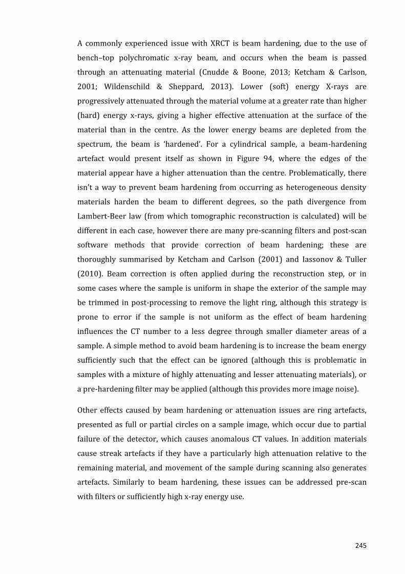
245

A commonly experienced issue with XRCT is beam hardening, due to the use of

bench–top polychromatic x-ray beam, and occurs when the beam is passed

through an attenuating material (Cnudde & Boone, 2013; Ketcham & Carlson,

2001; Wildenschild & Sheppard, 2013). Lower (soft) energy X-rays are

progressively attenuated through the material volume at a greater rate than higher

(hard) energy x-rays, giving a higher effective attenuation at the surface of the

material than in the centre. As the lower energy beams are depleted from the

spectrum, the beam is ‘hardened’. For a cylindrical sample, a beam-hardening

artefact would present itself as shown in Figure 94, where the edges of the

material appear have a higher attenuation than the centre. Problematically, there

isn’t a way to prevent beam hardening from occurring as heterogeneous density

materials harden the beam to different degrees, so the path divergence from

Lambert-Beer law (from which tomographic reconstruction is calculated) will be

different in each case, however there are many pre-scanning filters and post-scan

software methods that provide correction of beam hardening; these are

thoroughly summarised by Ketcham and Carlson (2001) and Iassonov & Tuller

(2010). Beam correction is often applied during the reconstruction step, or in

some cases where the sample is uniform in shape the exterior of the sample may

be trimmed in post-processing to remove the light ring, although this strategy is

prone to error if the sample is not uniform as the effect of beam hardening

influences the CT number to a less degree through smaller diameter areas of a

sample. A simple method to avoid beam hardening is to increase the beam energy

sufficiently such that the effect can be ignored (although this is problematic in

samples with a mixture of highly attenuating and lesser attenuating materials), or

a pre-hardening filter may be applied (although this provides more image noise).

Other effects caused by beam hardening or attenuation issues are ring artefacts,

presented as full or partial circles on a sample image, which occur due to partial

failure of the detector, which causes anomalous CT values. In addition materials

cause streak artefacts if they have a particularly high attenuation relative to the

remaining material, and movement of the sample during scanning also generates

artefacts. Similarly to beam hardening, these issues can be addressed pre-scan

with filters or sufficiently high x-ray energy use.

246

6.2.2.2 Partial volume effects

Figure 95: Partial volume effect, where low resolution scanning includes more than

one material in a single voxel, thereby averaging the two values of attenuation as a

result.

A partial volume effect occurs when a single pixel or voxel covers an area that

includes more than one material, resulting in a CT value that is an average value of

the two or more materials (Figure 95). This produces errors when thresholding as

some pixels may be misclassified as one material, when in fact it is a mixture of

two, sometimes classified as ‘mixels’ (Choi et al., 1999; Hussein et al., 2015). Should

the averaged value be sufficiently similar to the range of values for a given material

(such as water) then thresholding will overestimate the presence of that material.

Due to the resolution limitations of CT technology, all particle edges in a material

will be blurred to some extent, making the images difficult to quantitatively

interpret with a high degree of certainty. Although the partial volume effect is a

limitation in the broader scope of XRCT studies, the effect has been used

advantageously in medical CT to trace two-phase fluid flow in soil (Wellington &

Vinegar, 1987). The movement of fluid can be identified at a resolution

considerably finer than the image resolution by detecting subtle attenuation

changes within the material (Ketcham & Carlson, 2001), even if the resolution is

too low to observe the change directly.

6.2.2.3 Image noise

The scattering of x-rays as they pass through the material being scanned causes

image noise, which may also occur as a result of reflected x-rays that reach the

detector. This results in random variations in brightness on the image and reduces

the image quality by producing a mottled or grainy appearance. Noise may also be

2

2 3.5

5

5

10

10

3.5 7 7.5

7.5

6

247

produced by detector drift, but should a sample be mounted correctly this is less

common. Image noise disrupts manual thresholding as there are erratic values in

the image histogram, however this can be resolved by either noise-reduction

before segmentation, morphological noise-reduction on post thresholding

segmented data, or by using a method that tolerates noise (Wildenschild &

Sheppard, 2013). As there is no a priori knowledge of material data in soil analysis,

the first option is omitted. Disturbance of an image by scatter and noise usually

requires a smoothing filter to be applied to suppress the noise during the scanning

process e.g. Gauss filters, although this process is detrimental to resolution and

sharp edged features. A thorough review of filtering and image enhancement

methods can be found in Kaestner et al. (2008), which covers the use of pre-scan

filters, noise reduction, post processing operations such as erosion and dilation to

remove noise and artefacts in the images (Soille & Vogt, 2009). The caveat to these

enhancement processes is that they may remove true features and therefore

caution is advised whenever altering the image.

6.2.3 Water content and volume change of samples

Although XRCT provides a fantastic opportunity to analysis materials over time, or

through wetting and drying cycles, there are limitations that hinder the direct

comparison of scans. In theory the correct alignment of dry and wet scans allows

subtraction analysis to separate fluid phases and visualise phase distribution in the

structure (Schnaar & Brusseau, 2005 and 2006; Wildenschild et al., 2002).

However, when soils are wetted there may be considerable movement of

particular markers within the sample (key particles on which one image is

registered with another) due to density changes as the bulk density is reduced.

Where flow is involved, the analysis of soil between dry and wet states tends to

ignore any swell/shrink behaviour and simply (incorrectly) assumes that any

change is due to water (Young et al., 2012). Even in samples that undergo no

swelling under wetting, the presence of water exacerbates the partial volume

effect; Higo et al. (2011) took a sample of sand 18 mm Ø by 17.7 mm in height and

observed the water retention behaviour during a drying and wetting process using

XRCT. Images were trinarised (three phase separation) into the soil phase, pore

water phase and pore air phase. The thresholding technique was required to

account for the partial volume effect as voxels sharing both soil phase and air

248

phase were incorrectly identified as a water phase as the value of the former is an

average of solid and air phases, thus giving a similar value (Hashemi et al., 2015;

Higo et al., 2011).

6.2.4 Thresholding

Figure 96: Segmented image of a lime treated sand bentonite mixtures from Hashemi

et al. (2015), where macro-voids are shown in blue, bentonite shown in green and

sand in red

Thresholding (also called binarisation or segmentation) is crucial for the analysis

of three phase systems such as soil, particularly where the same sample material is

scanned through drying or wetting stages and later compared in order to separate

fluid phases, perform geometric analysis and identify phase or pore distribution

through the material (Iassonov et al., 2009; Wildenschild et al., 2002). As images of

the scanned material are presented as a range values on grey scale histogram,

which represents the relative attenuation of a particle, thresholding is a technique

used to separate phases in a material in order to quantify some aspect of space e.g.

porosity, whereby a grey value is used as the cut off between one material and

another. This is shown in Figure 96, where the grey image has been segmented

into three materials based on the attenuation characteristics. The choice of

thresholding or segmentation technique entirely controls the resulting

measurements (Baveye et al., 2010, Taina et al., 2008; Zhang, 2001), however there

are currently countless methods from which to choose (Dey et al., 2010; Sezgin &

Sankur, 2004), none of which are the ‘correct’ or ideal method as each is particular

to the research on which it was based. Readers are directed to Tuller et al. (2013)

249

for an extensive review and comparison of global and locally adaptive methods for

segmentation of XRCT data of porous materials.

For fairly homogenous materials such as sand the process of thresholding is

relatively easy as void space and material have distinctly different ranges of

attenuation, however two-way or three-way segmentation of soil provides a

substantial challenge. As discussed, most thresholding methods are not suited to a

highly heterogeneous material such as soil and as such require highly skilled

operators to provide acceptably accurate segmentation (Iassonov et al., 2009).

Baveye et al. (2010), Helliwell et al. (2013), Iassonov et al. (2009), Kaesnter et al.

(2008) and Wang et al. (2011) all concur that thresholding is the most important

step in data analysis and affects all subsequent processing, where subjective

decisions during the thresholding processes critically determine outputs such as

porosity, surface area and network structure.

Briefly, thresholding techniques are divided into global or local methods and

further into fully automated or manual user dependent categories. Traditional

global methods use a cut off value between clear peaks in a histogram to

distinguish between two or more phases, however in general the value of the cut

off is arbitrary and inadequate (Lindquist et al., 1996) and results in truncation of

the histogram. Global thresholding, which although rudimentary, is the most

common approach for quantitative space analysis and fluid mechanics, and few

studies implement more advanced or complicated techniques despite growing

technology to do so (Iassonov et al., 2009; Sezgin & Sanker, 2004). Local

thresholding may provide the user with more accurate results as instead of using

one value, a variable (adaptive) threshold is used based on local characteristics

(Pierret et al., 2002) such indicator kridging, which classifies each a pixel/voxel as

either pore or solid based on its greyscale value and local spatial correlation

structure. This method requires two thresholds, one threshold below which all

pixels are pores, and one value above which all pixels are solids (Al-Raoush &

Willson, 2005; Houston et al., 2013; Oh & Lindquist, 1999; Wang et al., 2011; Zhou

et al., 2013). This method is an optimal segmentation tool when considering

bimodal histogram patterns, however it is somewhat limited for use on unimodal

histograms or in materials were visual inspection cannot sufficiently assess the

250

appropriate thresholds, and instead the global Otsu method (1979) is preferable

for unimodal histograms (Wang et al., 2011).

Other local thresholding techniques include edge detection (Sheppard et al., 2004;

Schlüter et al., 2010), however this method requires the careful manual selection

of seed regions to enable satisfactory thresholding and is therefore a very labour

intensive method (Kaestner et al., 2008). Region growing methods are based on

the assumption that should one select a single voxel or region of interest (ROI),

then all surrounding and connected voxels that have sufficiently similar u value

must belong to the same object, scaled relatively by the mean intensity of the

sample (Ketcham, 2005). This method would be highly applicable in determining

the surface of complicated materials, and determining the extent to which a

substance such as water would penetrate a material upon submersion.

Baveye et al. (2010) compared the outcomes and approaches to thresholding of 13

XRCT experts on three test images and found that each analysis was unique to the

individual, with no single method yielding the ‘best’ results. There is no way to

select the best method as each could be approximately correct or best suited to a

given application or desired outcome. Baveye et al., (2010) therefore stress the

need for physical standards (Thompson et al., 2012; Sleutel et al., 2008), adoption

of specific procedures for accuracy assessment, and a development in the

processing of data that does not require a binary image. Similarly, Iassonov et al.

(2009) compared 14 segmentation methods on macro porous soils, sand-bentonite

mixtures and precision glass beads and found that only a handful of the methods

performed well for all three materials, where only the Ostu (1979) method and CL-

Ridler (Ridler & Calvard, 1978) gave ‘adequate’ binarisation for global methods.

Locally adaptive methods had more accurate performance than the range of global

thresholding methods used but had significant limitations; the indicator kridging

method by Oh & Lindquist (1999) overall had the best segmentation quality,

however this method was labour intensive even for a skilled operator and the

outcome is not only sensitive to the thresholds chosen (Zhou et al., 2013), but is

really only effective on bimodal histograms.

The conclusion from a review of current research is that there are countless

methods for segmentation but there is little to determine their relative ‘success’ in

giving real values for parameters such as porosity and bulk density, and as such

251

the rationale for choosing a particular method is down to the user’s preference.

Due to vastly different scales, resolutions and processes, the results from different

studies are very difficult to compare (Zhou et al., 2013). There are benefits and

limitations to both approaches; local methods allow some small variations to be

taken into account through the sample, however global methods are easier to

conduct and require less computational power. Wang et al. (2011) show that the

performance of a thresholding technique is not always based on the complexity of

the method, where a global method (Otsu, 1979) is more efficient than the local

method employed by Oh & Lindquist (1999). The underlying reason for

uncertainty in the methods is that validation and performance assessment is a

missing element for this type of research due to its relative infancy. Validation only

occurs should thresholding techniques give values close to an empirically or

experimentally derived value. There is an overwhelming need for reliable and

consistent automated algorithms that do not yield any operator bias, which in turn

may be applied to a large range of materials (Iassonov et al., 2009).

Regardless of the method chosen, the problem with thresholding soil is that due to

the volume of sample and resolution achievable (10’s of μm for samples up to 40

mm Ø), many voxels will be vulnerable to partial volume effects and there will be a

great deal of noise in the image due to the extreme heterogeneity of soil samples,

which is attributed to different mineralogy of soil matter, the presence of low

density organic matter and the presence of both water and air in pore space. In

addition many of the important structures in soil that are critical to their function

e.g. micro-pores (5-75 μm) are lost completely within voxels should the image

scale exceed 5-10 μm. Sub-micron & single value micron scanning is achievable but

requires very small samples, however the heterogeneity of soil means that sub-

sampling to this extent may not be at all representative. There are a number of

options available to threshold soil for the purposes of analysing porosity, water

movement, stress and strain, which shall be discussed subsequently in section 6.4.

6.3 Overcoming issues of segmentation in heterogeneous materials

Distinguishing between pore space, soil OM, soil mineral matter and water is

currently limited by both the technology of CT and the software with which to

processes acquired data, despite increasingly high resolution and image quality.

There are many publications that attempt to use different methods of thresholding

252

to identify pore space or water in both easily segmentent bimodal images and in

images where there are significant attenuation similarities between phases that

result in unimodal histograms (Peth et al., 2008). Baveye et al. (2010) propose that

porosity measurements may be a fast and ready way to validate the accuracy of

thresholding, as its measurement it does not affect the procedure of scanning (Al-

Raoush & Willson, 2005). Research by Beckers et al. (2014) questions if visible

porosity provides a useful and robust benchmark for segmentation and analyses if

it can be used for the basis of thresholding by comparing to 4 other methods;

(Ostu, 1979), Schlüter et al. (2010), Hapca et al. (2013) and Houston et al. (2013).

They found that global segmentation methods provide good agreement between

XRCT derived information on retention and SWRC derived from macroscopic

measurements. The porosity-based method is robust as it agrees with macroscopic

measurements regardless of the pre-processing of images, however there is still a

need in the field of XRCT to be able to effectively quantify the images without the

need for comparison of data from secondary methods.

6.3.1 Tracers in solution

One method of overcoming the subjective and complicated process of

differentiating between solid phases, water, and air in highly heterogeneous

materials is the use of contrast agents by addition of compounds to water or other

liquids (Kaestner et al., 2008; Luo et al., 2008; Van Loo et al., 2014; Wildenschild et

al., 2002). As discussed previously, pore sizes range from centimetres down to the

nano-scale level, whereby the spatial location of pores through a soil matrix has a

profound impact on the location of water, microorganisms and soil organic matter

(Ekschmitt et al., 2008). The technique of using tracers (contrast agents) has great

potential for phase and porosity identification and has been used for many years in

medical applications, where heavy elements are used to improve the diagnostic

capabilities of low resolution scanners (Caltagirone et al., 2015; Granton et al.,

2008), and increasingly in geological and petroleum science applications (Alajmi et

al., 2009; Hirono et al., 2003; Yang et al., 2016). The drawback of using any form of

tracer is that it may change the density, viscosity, contact angle or surface tension

of the fluid in which the agent is immersed and users may experience issues with

crystallisation, therefore this must be acknowledged should it be used for

modelling flow behaviour. The concentration of tracer is also important, such that

253

it gives sufficiently high attenuation that exceeds the distribution of the solid

phases in non-absorptive materials. For materials that will allow water to enter,

such as organic matter, the addition of contrast agent causes simultaneous

attenuation increases in the pore space and absorptive structures (Kaestner et al.,

2008).

There is a growing body of literature on the use of contrast agents to measure

porosity or hydraulic properties in real-time in rocks or generally uniform sandy

soils whereby a solution containing a contrast agent is used to fill pores within a

sample, typically sodium iodide (Alajmii et al., 2009), potassium iodide, potassium

bromide, xenon (Akin & Kovscek, 2003; Wildenschild et al., 2002) and calcium

iodide used as a tracer by Kaestner et al. (2008). However, the use of tracers in

heterogeneous soils is currently very limited despite a number of papers that have

explored the theory of contrast application; Hussein et al. (2015) suggest the use of

a contrast agent to completely remove the need for thresholding and therefore

provide valid porosity values without secondary assessment of accuracy. One

sample that has been fully saturated using a soluble contrast agent (which has a

higher attenuation coefficient than the solid material), can be compared with a

sample that has been full saturated using water alone, which has a zero

attenuation coefficient. As the values of soil mineral matter (impenetrable solid

material) do not change when the sample is wetted, these voxels can be matched

between the two scans. The voxels fully occupied by pores will also (in theory) be

identical, therefore the total pore space can be identified, as any remaining voxels

that have been subject to partial volume effects and contain a mixture of solid and

pore space can be classified as mixels (Choi et al., 1999). This therefore automates

the process of thresholding as the pore space is clearly identified by the tracer;

however this requires a priori knowledge of the CT values of the solid material,

therefore its application for extremely heterogenic materials such as soil is less

effective, especially when organic matter with a similar attenuation value to pore

space is added.

There is also a lack of data surrounding the study of soils containing significant

proportions of organic matter, including the investigation of biochemical

interactions (Voltolini et al., 2017) and the importance of pore geomorphology in

the processes of aggregation and decomposition of OM (Peth et al., 2014; Sleutel et

254

al., 2012), which comes as a direct result of technique limitations with which to

determine the location of OM (Young et al., 2001). The identification of organic

matter is especially difficult as the x-ray attenuation coefficients of OM fall

between the range of values typical of pores (water or air) and the mineral

component of soil (Kaestner et al., 2006; Peth et al., 2014), therefore creating

unimodal histograms. Thresholding of samples with overlapping μ values is

further complicated by factors such as partial volume effects. The current research

gap in the study of OM in XRC is slowly being filled; there is growing interest in

using agents to stain the OM directly.

6.3.2 OM identification

It is still well recognised that discriminating between soil phases and the

quantification of organic matter, particularly at high water contents, remains a

challenging prospect (Helliwell et al., 2013), however there have been some

attempts at identifying organic matter without the use of tracers; De Gryze et al.

(2006) attempted to visualise OM in 3D using CT data at a resolution of 13.4 μm

without the use of tracers (although effective optical resolution was 27 μm due to

removal of all single voxel data points). They were able to identify the histogram as

bimodal through modelling and were able to produce the histograms for each

constituent. A threshold attenuation coefficient was determined by manual

selection of pore areas in 5 random locations, although the quality of the

tomographic images didn’t allow organic matter to be located based on the

attenuation coefficients alone. In this case manual selection of pores and

subsequent thresholding was used, as automated three-phase classification was

too insensitive to pick up on the very subtle differences in contrast between OM

and pore space or water. However, De Grzye et al. (2006) stated at the time that

CT scanning cannot be used together with staining techniques that are

commonplace in thin sections e.g. Chenu & Plante (2006), but instead suggest that

porosity and pore morphology can be directly observed.

Sleutel et al. (2008) attempted to segment pore space, OM and mineral particles in

sand/OM mixtures but found that there were large overlaps in both the u values of

OM and mineral and (more problematically) between pore space and OM. Quinton

et al. (2009) similarly found significant challenges in distinguishing between water

and organic matter, especially when saturated as the attenuation values are very

255

similar; Ketteridge & Binley (2011) experienced the same issue when trying to

quantify characteristics of peat and resorted to using lead nitrate to flush the

sample in order to contrast the components of interest. Elyeznasni et al. (2012)

were able to detect coarse organic matter in XRCT images at a resolution of

68-88 μm in samples that had a very high concentration of OM, but had difficulty in

quantifying fine sized OM and in identifying any OM when mixed with a sandy soil.

They suggest that comparing XRCT images with observations from thin slices

would aid in determining a suitable threshold and also aid in standardising

protocols for obtaining sensible porosity values in OM rich materials. As a

concluding remark to the research by Elyeznasi et al. (2012), they also suggest the

extended use of staining techniques (e.g. Peth et al., 2010a). Chenu & Plante (2006)

used lead, silver and uranium in transmission electron microscopy to stain 2D thin

sections of soil and OM, the theory being that colloidal soil OM has a strong affinity

for heavy metal cations (e.g. Fe3+) due to ligands that form chelates and then

complexes with the metal (Van Loo et al., 2014), therefore the use of compounds

containing heavy metal which preferentially adsorb to OM and not to soil minerals,

is ideal for this application.

Recent literature goes towards providing evidence that staining has potential

within XRCT research and removes issues of unimodal histograms and the need for

modelling to find suitable thresholds, or comparisons with 2D thin sections for

validation of chosen thresholds, in order to identify organic matter (Peth et al.,

2014). Peth et al. (2010a) for example used osmium as a staining agent due to its

interaction with C-bonds of organic compounds (Hayes et al., 1963), allowing

visualisation of even fine OM that has been adsorbed onto clay minerals and

cannot be observed discretely (Chenu & Plante, 2006). Osmium was used to stain

OM in air dried samples (in vapour form) and is distinguishable from other

material in XRCT images due to its high atomic number, although bright spots

attributable to other soil minerals and compound such as Fe-Oxides may have

complicated the quantitative analysis.

One of the first (known) publications that has investigated the effect of using

different stain on organic matter and mineral samples rather than using tracer to

identify the spatial location of water, was Van Loo et al. (2014). In their research,

52 compounds containing heavy elements were dissolved in deionised water and

256

their attenuation was assessed for suitability to be used as a contrast agent.

Secondly their suitability to enhance the x-ray attenuation of pure OM and

respective impacts on soil mineral matter (MM) were taken into account.

Preferable contrast agents either had good relative effect on the attenuation of

water without staining the SOM significantly (Cwater) or a high ability to stain SOM

compared to air (CSOM). The best four agents for staining SOM were chosen for

further testing on three samples, OM alone, MM alone and an OM/MM mix; these

were phosphomolybdenic acid (PMA), silver nitrate, lead nitrate and lead acetate.

Osmium tetroxide, used by Peth et al. (2010a) performed similarly well to the four

best agents chosen by Van Loo et al. (2014) in terms of Cwater and CSOM, but was not

very soluble in water (maximum of 6.5 g/100 ml compared to 44-216 g).

Samples were forcibly saturated to avoid crystal formation, and excess solution

was removed before sealing the sample to permit a reaction between the sample

and the contrast agent. Samples were then dried at 20C before scanning. A

reference sample was included for each sample that followed the same procedure,

with the use of deionised water alone. Van Loo et al. (2014) evaluated the shift in

x-ray attenuation between the control and each contrast agent and found in the

control sample there was little contrast between the air and SOM (as found by

Sleutel et al., 2008). When contrast agents were used, the air and MM values

remained the same but the value of the SOM particles were then higher on average

than the MM particles, therefore the contrast agent must increase the U values of

OM sufficiently that it can be then distinguished from the MM. KI (potassium

iodide) in Van Loo et al. (2014) had one of the greatest effects on the relative x-ray

attenuation of water (0.88) but very little attenuation change for SOM (0.09),

where iodine on its own makes negligible difference. They also found that using

staining agents has no impact on the u value of air or mineral matter.

Other work that has used contrast agents includes Heijs et al. (1995) who took one

sample and compared the dry and wet scans. They followed the procedure of

Booltink & Bouma, (1991) and used 15 mm of water with kalium iodide solution

(HU value of 2900), scanned a sample 25 cm x 12.3 cm to a resolution of 0.27 mm.

This work allowed the binary image of the water content distribution to be

compared with the air filled macropores. Similarly, Luo et al. (2008) used KI

solution at 6.6 ml/min for 23 hours through a satiated soil column. The soil column

257

was 10 cm Ø x 30 cm height and scanned to a resolution of 0.1 x 0.1 x 0.13 mm.

Solute transport was measured in real time by scanning two critical positions, after

which the whole column was scanned to obtain the solute distribution. Similarly

Wildenschild et al (2002) used KI Iodine (absorption edge at 33.7keV), allowing

water to be clearly distinguished from the air and solid phases. Kaestner et al.

(2008) used CaI (chosen for its preservation of clayey soil aggregates) at a

concentration of 4% for optimal contrast, although this was not tested by Van Loo

et al., (2014), therefore a comparison of its effectiveness cannot be made.

The use of contrast agent (KI) was attempted for visualising porosity in Soil2 and

AM14 (70S 15C and 15WTR2d) at concentration of 1 mol (166 g/L or 16% %w/v),

which although more than KI solutions used in Clausnitzer & Hopmans, 2000, Luo

et al. (2008) and Perret et al. (2000), was used in order to rapidly stain the soil

pores. It became apparent in the initial analysis of scan results and in personal

communication with Stephan Le Roux (an expert XRCT technician at Stellenbosch

scanning facilities) that the use of iodine as a tracer creates more problems than it

aims to solve. The high density of the iodine creates a high number of artefacts,

image noise, and due to partial volume effects, increases the attenuation of the

entire material such that the distinction between phases and different materials

within the sample is actually more difficult than when no tracer was used. A great

deal of investigation into optimal tracer concentrations and machine parameters

to produce images that can be readily analysed is required. The use of tracers for

phase identification has considerable potential, but the complexity and labour

intensive nature of this process of investigation is well beyond the scope of this

thesis.

258

6.4 XRCT methodology and results

The previous discussions have outlined the benefits and flexibility of using XRCT

for high-resolution imaging, modelling, and quantification of porous media and

fluid distributions in 3D (Werth et al., 2010). Despite a growing range of

possibilities using XRCT and increasing sophistication in scanning and analysis,

there a number of issues with the use of this technology that need to be addressed

in order for it to be used as a comparative and reliable tool. System faults (such as

partial volume effect, beam hardening and other artefacts) and user-based faults

with thresholding limit the application of XRCT; the resolution/sample size trade

off remains problematic when studying heterogeneous material. Given the rapid

development of this method of 3D representation since its beginning, it is likely

that these issues will be resolved sooner rather than later using new technologies

such as dual energy. Once standardisation occurs in the set up and processing of

data, XRCT will continue to improve material research.

The following section discusses the different methods used for this thesis to obtain

critical information on the effect of using WTR and co-amendment on soil. The aim

of using XRCT was in an attempt to answer questions about the effect of WTR on

soil, particularly why it changes the water retention properties of soils and how it

may interact with compost. The research explores a currently sparse area of study,

and to the authors knowledge there are no XRCT papers that have looked in detail

at WTR or attempted to analyse soils with co-amendments. The aims of using high-

resolution imaging were to;

1) determine structural changes as a result of WTR2d and WTR2w amendment

and co-amendment with compost,

2) determine if WTR can be characterised in the images,

3) determine the internal structure & porosity of WTR2d,

4) determine how WTR reacts when exposed to water,

5) test the ability of tracers to enhance our ability to characterise pore space.

The machine settings and data outputs of XRCT scanning retrieved for this thesis

were in all cases fully directed by highly skilled technicians, both in Durham and

Stellenbosch. Given that this area of research is novel, the methods explored and

subsequent results presented here are to illustrate the potential of using XRCT to

259

reconstruct and quantify particular parameters in soils that have been amended

with highly organic components, and to view the internal structure of WTRd at

high resolution. The approach is very well suited to the complex analysis of highly

heterogeneous material that are less well served by 2D analysis.

6.4.1 Machinery and settings

Three machines were used for the production of XRCT images, an Xradia/Zeiss

VersaXRM 410 system (Durham University), Phoenix VtomeXC series machine, and

a Phoenix VtomeXC series machine (both at Stellenbosch University). The

following gives a very brief outline of their capabilities. Data from the scans was

stored as stack of TIFFs after reconstruction, to enable any program to be

subsequently used for analysis .The data from the Xradia machine was processed

using Avizo 9.4.0 and data from the Phoenix systems were processed using Volume

Graphics 3.2.0 software. Both of these software packages are highly complicated

and advanced, but for the research analysis presented here the computation

outcomes are likely to be negligibly different. All data processing was under the

supervision of a skilled technician.

Xradia/Zeiss Versa XRM 410:

150kV 10W microfocus x-ray source

2k x 2k 16bit CCD x-ray camera

A single macro lens (0.4X) for large field of view scans and three high

resolution lens (4X,10X&20X) for region of interest scans.

4 axis motorised sample stage with 15 kg load capacity and 360 degree

rotation, and maximum sample size of 300 mm

Up to 0.9 um resolution

A single 3D volume takes between 4 and 24 hours to scan depending on

resolution

260

Sample diameter (Ø) Full sample scan voxel

size

High resolution scan

voxel size

<5 mm 3um 1-2um

<18 mm 10um 5um

<45 mm 25um 10um

Table 31: Example size vs resolution capability of the Xradia/Zeiss XRM 410 machine

[23, Xradia]

As shown in Table 31, the resolution of the scanned images range from 1-40 µm,

depending on a range of factors including the sample size and the required field of

view and the time taken to perform the scan.

Phoenix VTomeXC series

450kV, fast cone beam CT with scatter correct

ASTM E1695 guidelines for scanning

Robust, small footprint

Maximum sample size 500 mm Ø x 1000 mm

Up to 5 µm resolution

Phoenix VTomeXM series

300kV/500W scatter correct microfocus CT

Industry leading magnification dual tube configuration for µCT

2 µm maximum resolution

Maximum sample size up to 500 mm Ø, 600 mm height

Maximum 3D sample size 290 mm Ø, 400 mm

Maximum sample weight 50 kg, high accuracy up to 10 kg

Scan time is <4 hours

6.4.2 Initial scanning

Initial scans were conducted in 2013 on field moist, loosely packed samples of 50S,

25C, 25C (by dry mass), 100% soil, 100% compost and 100% WTR1w, at a

resolution of 50 µm, using 140kV/10W power to ensure sufficient x-rays passed

through the samples considering the material density and size of the samples

being scanned (38 mm Ø x 50 mm). These scans were exploratory in their nature

and were used to test if distinct structures were identifiable and decide if

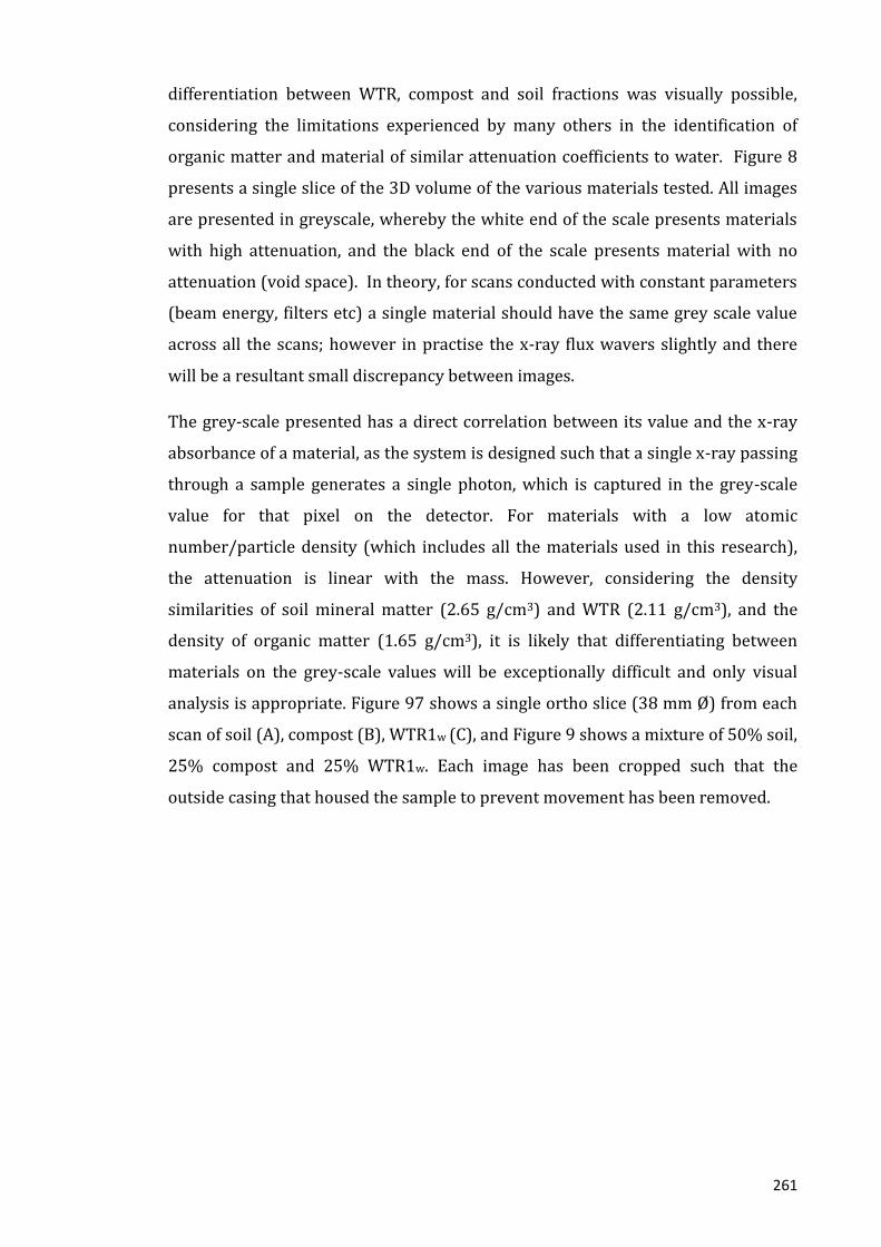
261

differentiation between WTR, compost and soil fractions was visually possible,

considering the limitations experienced by many others in the identification of

organic matter and material of similar attenuation coefficients to water. Figure 8

presents a single slice of the 3D volume of the various materials tested. All images

are presented in greyscale, whereby the white end of the scale presents materials

with high attenuation, and the black end of the scale presents material with no

attenuation (void space). In theory, for scans conducted with constant parameters

(beam energy, filters etc) a single material should have the same grey scale value

across all the scans; however in practise the x-ray flux wavers slightly and there

will be a resultant small discrepancy between images.

The grey-scale presented has a direct correlation between its value and the x-ray

absorbance of a material, as the system is designed such that a single x-ray passing

through a sample generates a single photon, which is captured in the grey-scale

value for that pixel on the detector. For materials with a low atomic

number/particle density (which includes all the materials used in this research),

the attenuation is linear with the mass. However, considering the density

similarities of soil mineral matter (2.65 g/cm3) and WTR (2.11 g/cm3), and the

density of organic matter (1.65 g/cm3), it is likely that differentiating between

materials on the grey-scale values will be exceptionally difficult and only visual

analysis is appropriate. Figure 97 shows a single ortho slice (38 mm Ø) from each

scan of soil (A), compost (B), WTR1w (C), and Figure 9 shows a mixture of 50% soil,

25% compost and 25% WTR1w. Each image has been cropped such that the

outside casing that housed the sample to prevent movement has been removed.

262

LOW attenuation (low density) (high density) attenuation HIGH

Figure 97: XRCT scans of (A) 100% soil, (B) 100% compost, (C) 100% WTR1w at

50µm resolution

In these images we can see that at 50 µm resolution the individual particles, macro

pores and voids can be identified in the soil (Figure 95a) where the densest

minerals such as Fe oxides (~5 g/cm3), clays and quartz (2.65 g/cm3) appear as

bright white spots and voids are black. In Figure 97B, dark grey areas (organic

matter) are irregularly arranged with large black void spaces. There appear to be a

number of darker grey areas, which may be areas of high water content (due to

reduced attenuation coefficient). There are a number of dense particles (white)

(A) 100% Soil (B) 100%

compost

(C) 100%

WTR2w

38 mm

263

that are presumably small pieces of soil mineral or other contamination in the

compost, but go someway to providing us with an idea of the contrast between soil

minerals and organic matter. In Figure 97C, the metal and organic elements of

WTR1w are clearly contrasting; concentrated volumes of Fe oxides of WTR were

apparent when oven drying the material for characterisation (Figure 14,

Chapter 3). The image in Figure 97C provides further evidence to the uneven

distribution of Fe in the WTR; in the largest solid particle we can identify streaks of

higher density material (presumably iron) perhaps formed due to gradual settling

of the WTR in the tank. The presence of other heavy elements, such as Cd, Cr, Cu

and Mg (Table 8, Chapter 3) in the WTR may also account for some of the bright

spots. The surrounding free fluid has a higher attenuation than water, suggesting

the presence of low-density suspended solids (organic matter). The black colour of

the sludge provides further evidence that organic matter is present in the free

fluid.

Figure 98: XRCT image at 50 µm resolution on a 38 mm Ø sample of 50% soil, 25%

compost and 25% WTR1w.

As the sample shown in Figure 98 was mixed by dry mass of each material, there is

a greater volume proportion of both compost and WTR1w to soil, owing to their

264

high water content and lower particle densities, the majority of the image appears

as the mixture of compost and WTR1w (Table 14, Chapter 4). The darker pore

space is still relatively easy to determine, and the frayed edged of the compost

allows us to identify the larger clumps of aggregates of organic matter. Small bright

grains are likely to be quartz minerals although these could equally be iron rich

deposits in the WTR. Discriminating between the WTR and compost is now

exceptionally tricky as they have similar attenuation coefficients, and at this

resolution, the particle shape and porosity are not clear. Subsequent to initial

scanning, over the remaining period of research, three scanning investigations

were completed;

1. Durham (2016) – investigation of samples from Experiment 4 (Chapter 4,

4.4.5) to a resolution of 25 μm,

2. Stellenbosch (2016) –WTR2d to a resolution of 6 μm

3. Durham (2018) – 15 μm resolution scanning of Soil2 and AM14 to

investigate optimum machine parameters and the effects of sieving to

different sizes.

6.4.3 Exploratory use of XRCT, Durham (2016)

Moving forward from initial scans, in 2016 single soil cores from each amendment

in Experiment 4 were scanned in three states; ‘dry’ (as produced at 17.5% GWC),

‘wet’’ (fully saturated), and redried’’ (air-dried back to 14 or 25% GWC). The cores

were 38 mm Ø x 76 mm length and were sealed for the duration of the scan to

avoid moisture loss in the warm scanning environment. The images were taken at

a power of 140kV and current of 71W, using an HE2 filter (for beam hardening

correction) and a 3 second exposure time. The field of view was 40 x 40 x40 mm,

giving a voxel size of 25 µm for data sets that were 2004 x 2048 pixels (X, Y) and

2007 projections (Z). The data were reconstructed using appropriate centre shift

(ranging between -0.4 and 0.3) and beam hardening correction (0.1). Having

underestimated the time required to process each data set, only Soil2 and A10-A13

were processed using Avizo 9.4.0, as these contained the highest concentration of

amendment, under the direction of a highly skilled technician.

Briefly, each stack of TIFFs was imported into Avizo for a particular sample e.g.

Soil2 dry, Soil2 wet and Soil2 re-dried. The original dry data set was trimmed

265

vertically (Z axis) to remove roughly 5 mm from ends of the sample such that

subsequent analysis did not include edge effects and any breakdown of the ends

under wetting. Using the cropped dry data as a basis, a distinct pattern of bright

particles were identified in each sample, to which the wet and re-dried samples

were registered by rotating the data appropriately and then resampled using

Lanzos interpolation. Finally each data set was finely cropped vertically to match

the end points of the dry data. This was to allow a better visual comparison

between the data, although during the wetting and re-drying there was a small

shift in the location and orientation of some particles due to swelling and

shrinkage. In order to threshold the data, the data volumes were cropped into

cubes (removing the edges of the samples), which measured between 1200 x 1200

x 1200 to 950 x 950 x 950 pixels/voxels and equates to samples of 25 mm3. For

each material, auto-thresholding low was conducted, where a suitable upper

threshold value to select all the dark pore space was chosen manually. These

values are present in Table 32 and reflect the difference in relative attenuation of

each scan.

Soil2

100S

AM11

70S 30C

AM12

70S

30WTR2d

AM13

70S

30WTR2w

AM14

70S 15C

15WTR2d

AM15

70S 15C

15WTR2w

Dry 7200 13500 11500 9000 5600 8700

Wet 7200 13000 9000 9000 9500 14000

Redry 9700 14600 13500 12500 7000 8500

Table 32: Lower auto-thresholding values chosen for Experiment 4 samples

The values presented in Table 32 are derived from porosity analysis based on data

from XRCT thresholding, volume of pores at the end stage of triaxial testing and

values derived using information on the bulk volume and particle density for core

samples. The void ratio of each sample gives an indication of how the void space

changed between the sample in its dry state, having been saturated and then re-

dried.

Before the discussion of results, it must be noted that void space as defined by the

XRCT only captures the macro-pores; therefore if a sample has a high porosity but

these pores are very fine, the void ratio & volume of voids will be low in

comparison with a sample that has a greater proportion of large pores. This

266

analysis therefore favours samples with greater macro-porosity and under values

samples with micro-porosity. The void ratio is also, as a result, much lower for

XRCT than the values derived from triaxial testing and calculated porosity. The

volume of voids is an absolute value in µm3, and the void ratio is a ratio of the

volume of voids to the total volume (which in this case is the cubic cropped region

of each sample). Pagliai (1988) suggested that typical porosity values (void ratio)

for very compact soil is <0.005, compact soil 0.05 -0.1, moderately porous 0.1-0.25

where 0.1 is the lower limit for ‘good’ soil structure (Pagliai & Vignozzi, 2002),

highly porous 0.25-0.40 and extremely porous when porosity is <0.4. It must be

accounted for that estimates of porosity become less precise in highly compacted

soils (Periard et al., 2016). Table 33 and Figure 99 show the results of porosity

determination. When compared with the values of Pagliai (1988), it is apparent

that the relative degree of compaction of samples is variable between

amendments.

Figure 99: Void ratio change of Soil2 and AM11-AM15 derived thresholding of XRCT

data in Avizo.

0

0.05

0.1

0.15

0.2

0.25

0.3

0.35

0.4

0.45

0.5

1 1.5 2 2.5 3

Vo

id R

ati

o

Soil2

AM11

AM12

AM13

AM14

AM15

DRY WET REDRY

267

Sample Volume of

voids (Vv)

Void ratio

(Vr)

Soil2 dry 1858 µm3 0.117

Soil2 wet 2127 µm3 0.127

Soil2 re-dried 1052 µm3 0.062

Soil2 dry (calc) (25.97) mm3 0.315

Soil2 wet (Triax) 36.1 mm3 0.390

AM11 dry 2566 µm3 0.196

AM11 wet 7810 µm3 0.459

AM11 re-dried 3195 µm3 0.208

AM11 dry (calc) (23.97) mm3 0.376

AM11 wet (Triax) 45.34 mm3 0.442

AM12 dry 788 µm3 0.057

AM12 wet 4390 µm3 0.291

AM12 re-dried 1289 µm3 0.088

AM12 dry (calc) (19.99) mm3 0.347

AM12 wet (Triax) 42.38 mm3 0.422

AM13 dry 1781 µm3 0.119

AM13 wet 3936 µm3 0.312

AM13 re-dried 2631 km µm3 0.235

AM13 dry (calc) (23.50) mm3 0.382

AM13 wet (Triax) 44.38 mm3 0.433

AM14 dry 1504.47 µm3 0.089

AM14 wet 4594.43 µm3 0.229

AM14 re-dried 2886.45 µm3 0.161

AM14 dry (calc)

AM14 wet (Triax)

(18.88) mm3 0.330

43.88 mm3 0.433

AM15 dry 1342.24 µm3 0.102

AM15 wet 3583.83 µm3 0.207

AM15 re-dried 3081.27 µm3 0.196

AM15 dry (calc) (20.96) mm3 0.264

AM15 wet (Triax) 44.83 mm3 0.435

Table 33: summary of

porosity values derived

from XRCT for samples

Soil2, and AM11-AM15,

and comparisons with

calculated porosity for dry

samples based on particle

density and volume

measurements, and

triaxial derived porosity

for wet samples.

268

In Figure 99, unamended soil (Soil2) has a fairly low relative change in void

volume and void ratio between dry and wet states, followed by a reduction in void

ratio after re-drying due to unrecoverable shrinkage (0.117 - 0.127 – 0.06). In

general, the values of porosity derived from the triaxial test are considerably

higher than for XRCT derived porosity (Table 33), but this reflects the pore sizes

present in the soil, as smaller pores cannot be characterised by XRCT and therefore

the dry porosity is underestimated by XRCT for all samples. For example, the

triaxial derived wet porosity of AM11, AM12 and AM13 are negligibly different

from one another (0.442, 0.422 and 0.433) however the XRCT derived wet

porosity values show a larger difference (0.459, 0.291, 0.312).

AM11 (70S 30C) has the highest initial void ratio, and largest porosity change

(+0.26 compared to soil of +0.01), which is perhaps a reflection of the large pores

in the sample as a result of the addition of compost. For the 30% single compost

amendment (AM11) the large increase in Vv and Vr is explained by decreasing

bulk density and increase in sample volume when it is wetted as described in

analysis in section 5.1.3.3. Although there is a large change in void ratio between

dry and wet states, the compost amended sample returns to a similar void ratio

when redried, suggesting that the compost may operate in isolation to improve the

water holding capacity by increasing the void volume but it has no considerable

effect on the soil structure.

The 30% single addition of WTR2d and WTR2w (AM12 and AM13 respectively)

increases the pore volume (4390 and 3937 µm3) in comparison to unamended soil

(2127 µm3) when the sample is wetted. Although both have a lower void ratio

(0.291 and 0.312) than the single amendment with compost (0.459) when wet, it

appears that the void ratio remains higher when the sample is re-dried when using

WTR2w (0.235) in comparison with the use of WTR2d (0.088) or compost (0.208)

as an amendment, where the void ratio almost returns to the starting value with

the use of dried WTR. This effect may occur due to the cementing factor of wet

WTR as described in Chapter 3 (Basim, 1999; Moodley & Hughes, 2006), which

means that once the soil is wetted, the soil architecture is preferentially changed

such that it experiences less shrinkage and retains porosity when redried.

Despite co-amended samples having the highest wet void ratio (0.229 and 0.307)

in comparison to unamended soil (0.127), the dry XRCT derived porosities for both

269

AM14 and AM15 (0.089 and 0.102) are lower than unamended soil (0.117). In

addition, the wet XRCT derived porosity values for co-amendments are 0.06 and

0.005 lower than the values for single amendments. One might expect the co-

amendment of WTR and compost to have a void volume & void ratio between the

values of compost and single amendments. Nonetheless, as discussed for Trial 4

WHC results (section 5.1.3), the co-amended samples importantly do not lose

porosity as a result of volume decrease when redried, unlike the unamended soil,

single compost or WTR2d amendments. The low void volume and void ratios

values derived for co-amendment (AM14 and AM15) may be due to thresholding

issues as the higher proportion of low density materials makes the selection of a

‘sensible’ threshold difficult as a greater proportion of the sample is highlighted. As

the attenuation of organic matter and water is fairly similar, due to the resolution,

separating pores in these materials is far more subjective than more homogeneous

materials (unamended soil) or in samples where there are clear boundaries

between each material (such as AM12, Figure 102).

The porosity values derived from XRCT in Table 33 are based on the thresholding

of the entire 3D volume i.e. >2000 slices. Figures 100-105 show a single

representative slice from each sample in their dry, wet and re-dried states as well

as the same slice with the auto-thresholded pore space overlain to demonstrate

the differences between each sample. For each image, the dry sample slice has a

diameter of 38 mm and wet and re-dried samples have a diameter of between

38 and 42 mm. The size differences in samples at each stage of wetting has been

clearly outlined in Chapter 5 (section 5.1.3), therefore these images are sized

uniformly for visualisation purposes. To provide a comparison between scans, the

contrast in each image was adjusted such that each bright spot (soil mineral) has

an approximately equal white value. Dried samples appear lighter due to a

generally higher attenuation of the sample as the majority of the sample is

comprised of soil mineral with small volumes of air or water, which are darker. In

wet samples, the water has a lower attenuation value that solid particles, thereby

giving the entire image a dark appearance.

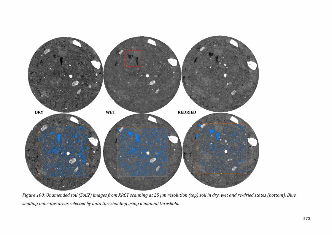
270

Figure 100: Unamended soil (Soil2) images from XRCT scanning at 25 μm resolution (top) soil in dry, wet and re-dried states (bottom). Blue

shading indicates areas selected by auto thresholding using a manual threshold.

DRY WET REDRIED

271

Figure 101: 30% single compost amendment (AM11) images from XRCT scanning at 25 μm resolution (top) soil in dry, wet and re-dried states

(bottom). Blue shading indicates areas selected by auto-thresholding using a manual threshold.

DRY WET REDRIED

272

Figure 102: 30% single WTR2d (AM12) images from XRCT scanning at 25 μm resolution (top) soil in dry, wet and re-dried states (bottom). Blue

shading indicates areas selected by auto-thresholding using a manual threshold.

DRY WET REDRIED

273

XRCT images of Soil2 are shown in Figure 100, where the top row shows a single

slice of the 3D volume for the dry, wet and re-dried sample. In these images, large

individual particles can be easily identified as well as pores, presented as dark

spots. When the sample is wet, the image becomes much less clear as the water has

in effect blurred the image; the partial volume effect means that voxels containing

both water and higher attenuating material have been averaged to a lower value

and voids have increased in their attenuation due to water presence. This gives the

image an overall narrower histogram. Small pieces of organic matter present in the

soil sample (red box) have clearly swelled when water has been added, and

remained at a higher volume & lower bulk density than the original sample.

In Figure 101 (AM11, 70S 30C), the presence of organic matter is clear to see,

where there are large portions of dark, irregularly shaped pieces of material which

surround soil aggregates. In the wet image, these patches of organic matter swell

and due to an increase in water in these materials they have a higher attenuation

than in the dry image. The difference can also be easily identified when viewing the

three images at the bottom of the figure with auto-thresholding overlay.

Figure 102 (AM12, 70S 30WTR2d) is an exceptionally informative series of images,

and provides an indication of what occurs inside the sample as it goes through a

wetting phase. In the dry images solid pieces of WTR2d are clearly visible and are

to some degree distinguishable from soil mineral matter due to their irregular

shape, such as the triangular piece highlighted in the red box. Small cracks in the

dried WTR are apparent, presumably from the process of core production, and

once the sample has been wetted these defects are then filled with water and

expand. Interestingly once the sample is redried, the voids created when the

sample was wet remain considerably wider than in the original state, despite the

values in Table 33 suggesting that this porosity is lost upon drying. It is difficult to

determine why such large voids are created around the dried WTR but as

discussed in Chapter 3 (WTR) once dried WTR is immersed in water, gas is emitted

while the dried WTR breaks down into smaller fragments.

274

Figure 103: 30% single WTR2w amendment (AM13) images from XRCT scanning at 25 μm resolution (top) soil in dry, wet and re-dried states

(bottom). Blue shading indicates areas selected by auto-thresholding using a manual threshold.

DRY WET REDRIED

275

Figure 104: 30% co-amendment with compost and WTR2d (AM14) images from XRCT scanning at 25 μm resolution (top) soil in dry, wet and re-

dried states (bottom). Blue shading indicates areas selected by auto-thresholding using a manual threshold.

DRY WET REDRIED

276

Figure 105: 30% co-amendment with compost and WTR2w (AM15) images from XRCT scanning at 25 μm resolution (top) soil in dry, wet and re-

dried states (bottom). Blue shading indicates areas selected by auto-thresholding using a manual threshold.

DRY WET REDRIED

277

Figure 103 shows the 30% single amendment of WTR2w, where the sludge has

been mixed through soil and then air-dried to 17.5% water content before being

compacted into a core. WTR2w tested immediately after export from the water

treatment works, as discussed in Chapter 3 (3.2.1) comprises particles ranging

between 1nm and 1 μm in size (Bohn et al., 1995) and Chapter 4 (4.3.2) where

75% of particle pass a 74 um sieve (Raghu et al., 1995). However, importantly

there appear to be small dried pieces present in the sample, suggesting that the

mixing process doesn’t necessarily spread the fine grained material

homogeneously through the soil, and over time clumps of WTR are able to dry as

larger aggregates which appear otherwise identically to the dried WTR in Figure

100. As a result, the XRCT image shows that the WTR2w is mixed thoroughly with

the soil, with some areas of larger WTR particles. This may indicate why, in the

triaxial testing in the previous chapter, that WTR amendments have similar

frictional response but different dilatancy behaviours at lower pressures.

The attenuation of water in the sample in the wet image in Figure 103 is clear, as

non-absorptive materials stand out against a darker background. Again, the dried

WTR pieces have fractured into smaller sized particles and created a small void

between the pieces. Although the image quality of the re-dried material is

compromised by beam hardening (giving an artificially higher attenuation

coefficient on the outer surface of the core), it appears that the channels opened up

by water during the wetting have remained open, supporting the hypothesis that

WTR added in a wet form may create a stronger soil architecture. The analysis of

Figure 102 and 103 go some way into describing why we saw such a difference in

the hydraulic conductivity of samples with both WTR2d and WTR2w in comparison

with samples containing compost. It is apparent that during wetting, the effect of

WTR is to open up large flow paths, through which water may flow with greater

speed than through varying size of pore throats.

Figures 104 and 105 show the effect of wetting and drying on 30% co-amended

samples using WTR2d and WTR2w, respectively. In Figure 102 large pieces of

compost are still visible in the dry, wet and redried sample; however identifying

the WTR in the dry sample is much more difficult. Manual identification is required

to recognise the WTR pieces by their shape and fracturing characteristics when

they are wetted. Attempts to threshold the histogram to identify WTR in this

278

instance does not work due to the similar attenuation with soil mineral. The wet

image in Figure 104 reflects the high water holding capacity of AM14 as shown in

GWC testing in section 5.1.3, where again large voids appear around the dried

pieces of WTR and the attenuation of compost increases significantly as it takes in

water. When AM14 redries, the void spaces remain apparent and soil aggregates

appear slightly more distinguishable from organic components than in the original

image. In Figure 105, the wet WTR has effectively smoothed the image as it has

been evenly mixed with the soil and compost (with the exception of some dried

pieces) and as a result the differentiation between the three materials in the

sample is very difficult.

6.4.4 High resolution scanning, Stellenbosch

In August 2016, single micron resolution images of WTR2d. were obtained using a

Phoenix VtomeXM machine, using a power of 150kV and current of 90W. The scan

took approximately 2 hours and gave a resolution of 6 µm. Five small >6.3 mm

pieces of the air-dried WTR2d were scanned in a small plastic vial for the first scan,

after which the WTR2d was completely submerged in water and sealed for a 3

hours before the sample was rescanned. This was, in practice, sufficient time for

any immediate water movement into the specimen, without compromising the

integrity of the solids. As discussed in Chapter 3, in previous submersion tests, the

WTR breaks down into smaller fragments while emitting air bubbles, after which

the smaller pieces remain unchanged in solution.

High resolution scanning of the WTR2d revealed some key features of this material

in its dried form, and what changes occur once the dried piece of WTR is then

submerged in water. Image processing had few steps;

1. Firstly the image had an adaptive gauss filter applied to remove image noise

and the background (air or water).

2. To calculate the pore volumes, the surface of the particles was determined

using the erode/dilate tool.

3. Defect surface determination was calculated.

4. Regions of interest were extracted and inverted from steps 2&3, on which

pore/inclusion analysis was run.

279

WTR2d 6 µm WTR2d WET 6 µm

Total volume of material (mm3) 136.81 103.55

Total volume of pores

(defect volume, mm3) 13.45 11.29

Defect volume ratio % 8.95 9.83

Volume of voids connected to

outside(mm3) 13.34 10.64

Volume of voids disconnected (mm3) 0.112 0.683

Surface of voids (mm2 ) 1499.34 1373.42

Number of defects 32438 18264

Number of defects per volume 237.10 176.38

Maximum defect size (mm3) 7.83 9.76

Surface of voids to volume 10.96 13.26

Pore size diameters Count Count

<14.756/14.77 µm 27964 15725

<92.86/112.22 µm 3040 1805

<170.97/209.67 µm 782 394

<249.07/307.12 µm 279 186

<327.175/404.47 µm 150 59

Table 34: Summary statistics of WTR analysis from Volume Graphics 3.2

porosity/inclusion analysis

As shown in Table 34, the majority of pores or defects present in the WTR2d are

connected to the outside of the particle and are essentially cracks into the centre of

the material. A very small proportion of pores (0.008%) are entirely disconnected

from the surface in the dried state, but when wetted the volume of disconnected

pores increases by a factor of 10 (to 0.06%), which is likely to be because of mass

fracturing and breakdown of the original dried pieces, which leaves a greater

proportion of disconnected volume of pores. The total volume of the ‘wetted’ WTR

is lower than the original volume due to pieces breaking off into very fine

fragments. In comparison a uniform block of material, the effective surface area of

the WTR2d particle is exceptionally large due to the effect of surface connected

voids; 1499 cm2 when dry and 1373 mm2 when wetted where in comparison a

cube of equal volumes would have surface areas of 159.15 cm2 and 131.98 cm2

respectively. This high surface area is important for chemical interactions as well

280

as providing a surface on which to hold water, increasing the water holding

capacity of the soil.

Figure 106 shows an unprocessed image of the WTR2d in high resolution (6 µm)

and provides a good indication of the crack structure within the sample. As

outlined in Table 33, 99.2% of the identifiable voids (shown in black) are

connected to the outside surface of the material, also highlighted in Figure 107.

The irregular external shape of the particle as a result of drying is well presented.

Figure 106: Unfiltered XRCT image of WTR2d at a resolution of 6 um (left) and a 3D

reconstruction of the 3D surface of the particle, where the green slice indicates the

position of the left image

281

Figure 107 shows the surface determination of voids/defects; interestingly,

although the large pore (~1 mm) in the centre of the particle appears isolated in

this single 2D slice, 3D analysis reveals that it is connected to the external surface

of the WTR2d by tiny cracks (<10 um) in the solid material. The variable size and

shape of pores (defects) in the sample is more clearly shown in Figure 108, which

highlights the maximum diameter of each defect. In this image we can see that

defects that almost span the entire width of the particle are present, suggesting

that as the WTR2d dries it traps air within its structure, which may slowly escape

once the material is solidified. This may also explain why the material emits

bubbles when submerged, as the cracks to these pockets are expanded and the

total fracture causes the air to be released.

Figure 108 highlights the porosity in dried WTR, where red pores are at the larger

end of the scale (6-7 mm maximum diameter) and blue pores are 0.01-1.6 mm. The

central right photo shows the 3D sample as a whole, and shows that there is a

heterogeneous spread of pore sizes across the sample. Figure 107 shows what

happens to the dried particle once it has been submerged in water, critically the

expansion of internal pores. A direct comparison between scans is difficult as the

Figure 107: Image of WTR2d with an

adaptive gauss filter, and surface

determination of pores/cracks; (right)

single X axis slice and (left) single Y axis slice, where the blue line indicates the

position of the X axis slice

282

Figure 108: XRCT porosity/inclusion analysis on WTR2d

283

Figure 109: (top left) Unprocessed image of WTR2d and (top right) unprocessed

image of WTR2d having been submerged in water. Images with adaptive gauss filter

applied to remove background noise, (bottom left) single X axis slice of submerged

WTR2d and (bottom right) single Y axis slice of submerged WTR2d. Red arrow

indicates the growth of a central defect when the sample is wetted.

DRY WET

WET WET

284

particles moved and broke apart after wetting and therefore the image shows a

representative slice from both the dry and wet WTR that show the largest defect in

the centre of the particle. It is difficult to ascertain if water has entered the defect,

although considering the difference in attenuation value between the surrounding

water and inside the defect it appears not; therefore, this increase in defect size is

not an influence of water pressure. At the bottom of Figure 109, the image has

been filtered to remove water noise and the defects are more apparent. The XRCT

scan shows that the three main particles of the WTR2d have fractured and created

a number of smaller pieces at the base of the material. Statistics from the defect

analysis shows little difference between the size distribution of the defects in the

particles in the dry state and submerged state, where 80% of the pores were

<0.5 mm and the remaining 20% are the large defects easily identifiable in the

XRCT images.

6.4.5 High resolution scanning in Durham

Having scanned samples from Experiment 4 at a resolution of 25 μm, freshly

produced samples of Soil2 and AM14 (70S 15C 15WTR2d) were scanned in 2018

with the objective of achieving the highest resolution possible and to optimise

machine settings and enable better visualisation. In order to achieve this, samples

of Soil2 and AM14 were produced using the materials from Experiment 4

(17.5%WC and sieved to 6.3 mm), according to the split mould method (section

4.4.1). The core diameter remained the same at 38 mm, but the height was halved

to reduce the size of samples (giving 38 mm Ø x 38 mm height). In addition, two

further samples of Soil2 and AM14 were produced to the same dimensions, where

the pre-mixed material was further sieved to 2. 8 mm. This was to test the effect of

different particle size on the packing of grains and pore size distribution.

Under the supervision of Dr Kate Dobson (independent research fellow in Earth

Sciences, Durham University), the samples were scanned to a resolution of 20 µm

while dry, and then scanned again after being saturated with water. The machine

parameters were changed to 90V and 10 W so that lower density materials were

better represented. The images were processed using the same method as

described in section 6.4.3. Void ratios, calculated as a ratio of the volume of the

cropped cube (from the centre of the sample) to the volume of material classified

285

as pores by thresholding. Figures 110-112 show the high image quality obtained at

a better resolution using smaller samples and different machine parameters.

In Figure 110, the images show a distinct difference in the structure of soil sieved

to 2.8 mm and 6.3 mm, with larger pores and soil mineral particles present in the

latter. In the images of 2.8 mm soil small aggregates are more apparent than in the

coarser sieved material. The materials appear much better defined in the image of

6.3 mm sieved material in comparison with 2.8 mm, which may be a function of

material size vs scan resolution. However, we are still not able to visually

discriminate between organic matter and pore space, and between WTR2d and soil

due to similar attenuation values, nor are we able to use the unimodal histogram to

aid discrimination.

Figure 110: XRCT image of Soil2 in dry and wet states, sieved to 2.8 mm compared to

Soil2 sieved to 6.3 mm at a resolution of 20 µm.

DRY 2.8 mm WET 2.8 mm


286

Figure 111: Soil2 2.8mm (dry vs wet, top) and Soil2 6.3 mm (dry vs wet, bottom)

thresholding

Figure 112: AM12 2.8mm (dry vs wet, top) and AM14 6.3 mm (dry vs wet, bottom)

thresholding





287

Figures 111 and 112 show the thresholding process on Soil 2 and AM14 in wet and

dry states. In each case the wet sample has a greater number of voids due to

swelling of the samples as water fills each pore, however there is a large difference

in values of pore volume and void ratio obtained between 2.8 mm sieved samples

and 6.3 mm samples. This can be attributed again to the fact that as we threshold

the samples, the thresholding process favours samples with large and obvious

pores as the selection of a critical value is user based. Figure 113 provides a

graphical representation of this difference, where void ratio values are compared

with the values derived from triaxial testing. As discussed previously, the values

for triaxial void ratio are higher as they include the micro-pores that are not

quantifiable by XRCT, and are at full saturation, whereas samples in the XRCT have

only been saturated under gravity. Figure 113 clearly shows that in a dry format,

the void ratios of samples at 6.3 mm are higher than at 2.8 mm, whereas when the

samples are wet the void ratio is higher in 6.3 mm samples, presumably because

the pores are larger and therefore we can better visualise the water.

Figure 113: Comparison of void ratios derived from XRCT and triaxial cell, where

Soil2 is unamended soil and AM14 is a 30% co-amendment with WTR2d

Soil2 6.3 DRY

Soil2 6.3 WET

Soil2 2.8 DRY

Soil2 2.8 WET

AM14 6.3 DRY

AM14 2.8 WET

AM14 2.8 DRY

AM14 6.3 WET

0.3

0.32

0.34

0.36

0.38

0.4

0.42

0.44

0 0.02 0.04 0.06 0.08 0.1 0.12 0.14

Tria

xial

vo

id r

atio

Void ratio XRCT

288

6.5 Discussion and concluding remarks

This chapter has demonstrated the potential of the application of XRCT to the

study of soils. The method provides a non-destructive measurement tool for the

visualisation of 3D internal soil structures including the pore network, and

arrangement of soil particles, and allows us to view the same sample at different

moisture contents. The use of XRCT on soil is currently limited by the pitfalls of the

technology (artefacts, image noise etc), the stand-off between resolution, sample

size and representative volumes, and a lack of clarify in guides to processing the

vast data sets produced by CT scanners, owing to the sparse but growing field of

related literature. Although researchers can readily complete the segmentation of

relatively binary images to a high degree of accuracy with validation from

empirical measurements, the results obtained from attempts to binarize or

segment the soil volume into three phases are lacking. Although the set up of

samples, scan settings and initial analysis required a skilled technician, with a little

guidance this technology is accessible to new users and therefore the research

gaps identified in the previous discussion should close as rapidly as the technology

was adopted for this novel area of research.

The use of XRCT in this thesis was exploratory and focused on discovering which

important soil parameters could be calculated or determined using the technology.

The aims set out at the beginning of the research firstly revolved around

characterising soil structure with the addition of WTR2d and WTR2w as single

amendments and as part of a co-amendment. Secondary to this, the research was

aimed to determine if WTR could be characterised in the images, including

visualisation of the internal structure & porosity of WTR2d, how WTR reacts when

exposed to water and in testing the ability of tracers to enhance our ability to

characterise pore space. Initial scans conducted to a resolution of 25 µm over a

single wetting cycle, provided some critical information about the structural

characteristics of amended soil, and in particular the behaviour of WTR2 through

this process. It is clear that WTR2d experiences a failure that can be best described

as fracturing when exposed to wetting, which creates voids around the particle

that remain open when the soil is redried and may provide preferential flow paths

that aid in infiltration and percolation should the sample be wetted again.

Although the differentiation between organic matter and WTR was unsuccessful

289

from a computing point of view, we are able to see the aggregation of materials

once the sample has been redried in co-amended samples.

In very high resolution scans of WTR2d conducted in Stellenbosch, it was

determined that >99% of the defects or voids in the material were connected to

the external surface of the material, providing the dried material with an

exceptionally high surface to volume ratio (10.96 when dry and 13.26 when wet).

It became apparent from the visual comparison of dry and submerged scans that

the dried WTR fractures along the larger cracks and as a result the defects are

widened. This may also explain why, upon submersion, dried WTR emits bubbles

as air may become trapped in pockets as the WTR dries.

The use of iodine as a contrast agent was unfortunately not successful, and hence

the reason that current research into the use of tracers in soils is sparse. The

addition of highly attenuating contrast agent KI in water indiscriminately

increased the attenuation of the entire soil mass such that porosity could not be

effectively measured. Staining the organic matter or WTR directly with a gas or

liquid prior to its inclusion in the co-amendment, or using a staining agent that

only targets OM is likely to be one of the only methods to easily segment organic

fractions from the remainder of the material. The combination of low-density

organic matter and Fe oxides will further complicate attempts to identify the

material based on the attenuation value of the material.

The final scans conducted on samples sieved to different sizes revealed little more

information on the use of XRCT and confirmed that, even at the optimum machine

settings and highest resolution currently possible for samples of the dimensions

used, an in-depth analysis of porosity is only achievable for the largest of pores in

the sample. In addition, the values in Table 33 highlight the vast differences in void

ratio based on the analysis of scans of a similar material by the same user.

290

7. Weetslade Field Trial: Engineering soil for flood resilience proof of concept

at the field scale

7.1 Introduction

As discussed in Chapter 3, although a number of studies have looked into the use of

WTR as a soil amendment for the improvement of a variety of soil parameters,

these values have only been determined in the laboratory or in small artificial plots

on a singular soil type (Elliot & Dempsey, 1991), therefore their effect on different

soil types on a field scale are currently unknown. Chapters 5 and 6 have outlined

the effects of WTR on the water retention of soils and shear strength properties of

soils with the application of single WTRd and WTRw and co-amendment of both

these materials with compost. In the majority of testing, there was little difference

in the performance of using WTR in the form in which it is exported from the water

treatment plant (~20% solids, WTR2w), compared to the air dried and sieved

format used for trials 3 and 4 (~ 20% water content, WTR2d). This suggests that

there is no need for further processing of the WTR for use in this application, and

that WTR can be used in its raw format without any detriment to the soil

engineering properties in comparison to WTR that has been further processed. To

the greatest extent possible, initial factors in the laboratory experiments, such as

density, moisture content and sample mixing, have been thoroughly controlled in

order to gain a meaningful understanding of the changes imparted. In reality the

documentation of any beneficial or detrimental changes in a field setting is much

more difficult to obtain. In order to validate the effects of WTR that have been

observed in the laboratory, a full-scale field experiment was conducted at

Weetslade Country Park, Northumberland in the early months of 2017.

7.1.1 Background

The field study, much like the rest of this thesis was built upon the ROBUST

project, which provides a framework for community led regeneration of

brownfield sites using sustainable technologies. Waste materials (such as the Fe

based WTR used for research in Chapters 3-6) may be used in conjunction with

compost to transform contaminated wastelands, which in turn improves the health

and wellbeing of the local community. Weetslade Country Park is already a prime

example of this, having been turned into a large public amenity from the remnants

291

of a coal-mining pit. The value of natural environments and the health benefits

associated with green spaces is well known (Mitchell & Popham, 2007), however

the value of soil as a critical partner in the implementation of sustainable green

spaces is overlooked. As discussed in Chapter 1 soil degradation costs England and

Wales up to £1.2 billion/year (National Audit Office, 2014) as a result of

detrimental land practises and climate change, and as such soil regeneration and

protection is high on the Government’s environmental agenda; Michel Gove MP

(Environment Secretary) recently announced that, as a result of a soil health

inquiry, soil health targets are now implemented by the a parliamentary group

called the Sustainable Soils Alliance. Northumbrian Water, among many other

water companies, is keen to expand their knowledge of the application of WTRs on

land to enable this method to develop as a long term, sustainable disposal option.

7.1.2 Project overview

The Weetslade field trial aimed to build on successful laboratory results (Chapter

5), which have shown that on a small scale the addition of WTR can improve soil

structure, water-holding capacity and as such improve the flood holding capacity

of a loam topsoil (Kerr et al., 2016). The Weetslade trial was designed to provide

‘proof of concept’ such that the amendment technology could be applied to other

sites across the North of the UK within the NWL catchment area, where flooding

and soil erosion are particularly prevalent. The field trail also aimed to inform the

partners on possibilities of using the waste amendment technology for engineering

flood resilience in South African cities that produce similar waste materials.

The projected timeline for the project was briefly:

16th Sept – 1st October 2016 – the Researcher spent time working with NWL

initially to facilitate sharing of data on this project and establish which are the best

by-products to use for the field trial. In addition, the plans for the field trial were

finalised and a contractor identified (with help from the Land Trust). The output is

a database summarising the properties of NWL by-products with a cost benefit

analysis of using them as soil amendments carried out. In addition, plans for the

field trial were finalised in conjunction with NWL and other academic partners to

ensure that this facility is a long-term resource for urban soil engineering research.

292

1st October 2016 – 1st March 2017 – 2 months were dedicated to project

management of the site working to establish the field trial on site. This constituted

a long-term resource for Durham in the field of urban soil engineering.

7.1.3 Beneficiaries and project aims

Not including academics, there are four benefactors of this research. First and

foremost, Northumbrian Water is the main partner to benefit from the reuse of

their waste material. As discussed extensively in Chapter 3 increasing costs and

production of WTR have pushed water companies ever further into finding long-

term sustainable disposal avenues. This project looks at cost-effective sustainable

ways of maintaining and enhancing soil health and improving flood resilience

within an urban country park, but results are relevant to both urban and

agricultural settings. Northumbrian Water will benefit as the technology uses by-

products, which have no current market value and therefore in doing this it closes

the loop by reusing wastes as resources for the iron rich water industry waste

products. NWL currently spends significant funds on disposing of waste products

to landfill. For example, in just this small project we will be diverting 30 tonnes,

which is equivalent to £2400 in potential disposal costs (should landfill be the

disposal route, as typical for water treatment works). On a longer-term basis NWL

is interested in improving water quality across the catchment (chemicals and

suspended solids in particular), which in turn may also reduce the volume of

treatment waste. Flooding issues are also key on the agenda, where Northumbrian

Water along with other industries such as property development, land-holding

(The Land Trust), insurers in flood risk, tourism and recreation boards, agriculture

and food, are interested in reducing flood risk across the UK. The Land Trust is

particularly interested in the long-term management of public spaces to improve

resilience to flooding and as such allowed the research to be carried out at

Weetslade Country Park.

The second beneficiaries are national policy makers in governmental departments

such as the Department for Environment, Food & Rural Affairs (DEFRA), the

Department of Energy and Climate Change (DECC), the Environment Agency, the

Scottish Environment Protection Agency (SEPA), the Forestry Commission, Natural

England and Public Health England. This work may also have consequences for the

293

Water Framework Directive and legislation surrounding groundwater abstraction

licenses, as the Environment Agency are increasingly looking towards

immobilising pollutant using soil amendments while increasing transmission of

overland flow into aquifers. Thirdly, local policy makers (local planning

authorities) and LEPs such as Newcastle City Council closely follow research of this

nature to consider these amendments on brownfield sites in Newcastle to improve

local flood resilience. The final beneficiaries are organisations that influence policy

making or are engaging in the implementation of the policy at a sub-national level

through a variety of environmental programmes, e.g. National Trust, River &

Wildlife Trusts and the RSPB.

There are additional impacts to the field trial at Weetslade that go beyond direct

advantages to the beneficiaries identified and include the effect on engineering and

geography research as well as economic and societal impacts. The direct impact on

an engineering basis is the empowerment of communities to use water industry

by-products as soil amendments to regenerate land, using the ROBUST

methodology, which can both improve soil health and provide flood resilience to

transform wasteland into green space. The ‘geography impact’ is that by enhancing

urban resilience to flooding and improving soil health, communities are likely to

see an increase in their health and wellbeing. This ‘proof of concept’ project may

allow researchers (e.g. Dr Johnson) to continue policy work with the Government’s

Environmental Audit Committee exploring how urban soils can be better protected

and is relevant not only to both the Engineering and Geography departments at

Durham University, but also countrywide. In addition, there is global potential as

the research extends to Stellenbosch University soil science, looking at how to

increase urban flood and drought resilience using similar waste minerals in

Southern African cities.

Although the economic benefits to Northumbrian Water are clearly identified,

where the sustainable incorporation of WTR into soil will reduce disposal costs, it

is as yet too early for commercial opportunities to be closely defined. Once a proof

of concept exists from laboratory work and the wide scale field application, as well

as continuing with NWL as a partner, talks can begin with the insurance industry

about the potential of urban flood resilience technologies to reduce flooding risks.

294

The contaminated land industry and developers are also as potential end-users (as

well as farmers in agricultural settings), where engineers are looking for

sustainable technologies to stabilise ground, which ensure geotechnical strength

for our built infrastructure at the same time as maintaining soil functions.

The work has important societal impacts; without making soil a priority and

protecting this resource we risk losing the ecosystem services and functions that

soils offers us in both urban and rural environmental settings. If we lose these

services, then soil is not being protected for future generations and hence we are

not treating this resource sustainably. The soil amendments trialled in this

proposal will help place the UK at the forefront of soil amendment techniques to

enhance soil health and therefore generate potential economic impact through

uptake by the existing contaminated land industry. Rolling these interventions out

across both urban and rural hinterlands will help enhance soil health and increase

water holding capacity and shear strength where it most needed, helping future-

proof communities against flooding and therefore potential generating both

economical and societal impact. By further developing the ROBUST methodology

to include flood resilience as one the many advantages of transforming wasteland

into green space, we will be enabling a range of communities to work with local

authorities and industry to identify and regenerate local land using soil

amendments (sourced from industry) to enhance flood resilience in our cities.

In summary, the overall aim of the field trial is to develop a suite of technologies to

maintain and enhance soil health and soil structure in urban environments by

providing proof of concept (improvement in flood holding capacity) from

laboratory work to the field scale. This is both timely and essential as in

approximately 25 years there won’t be any urban soil left to protect, due to soil

sealing with tarmac and concrete during urban development. The use of NWL by-

products (common across the Water Industry) allows the company to explore the

potential to close the loop (recycling) for this product, thereby saving money

(diverting waste from landfill) and making their processes more sustainable.

Improving soil’s ability to retain water during flooding events and improve water

quality in the NWL catchment would also be beneficial, although this is a long-term

295

goal as opportunities for using these technologies strategically in more rural

catchments would need to be explored in conjunction with hydrological modelling.

The objectives of this field trial were:

- Objective 1: Determine if there is a change in the water holding capacity of a

water treatment residual amended soil in a field environment

o Using soil moisture and soil potential sensors in the field.

- Objective 2: Assess the shear strength and erosional resilience of water

treatment residual amended soil

o By taking soil samples from the field and reforming them in a lab for

triaxial testing

7.2 Site overview and methods

Figure 114: Ordinance Survey map of the Weetslade Country Park with an aerial

Google Maps image of the study area (in red) [24].

The Northumberland Wildlife Trust manages the 38 ha Weetslade Country Park,

which belongs and is managed by the Land Trust (shown in Figure 114), with help

from volunteers from the local community. The park is located in the Seaton Burn

catchment in Northumbria, North East England, to the north of Gosforth Park and

296

is within a ‘strategic wildlife corridor’. The local area was used for mining from the

1800’s and Weetslade Colliery, upon which the park was built, was an active

coalmine from 1903 to 1967. Mining operations have left the local soil heavily

degraded with the contamination of arsenic and lead in the topsoil (Baker et al.,

2004), where Weetslade Park soil is classified at slowly permeable wet slightly

acid but base-rich loamy and clayey. After its closure the site was left to recover

naturally and in the 1990s was designated as a Site of Nature Conversation

Interest. In 2006 the site was transformed into the Green Flag award winning

green space it is today, and contains important habitats for scrubs, hedgerows,

marsh, wetland and reed beds, which accommodate otters and kingfishers among

other species. Today the Land Trust estimate that the green space at Weetslade has

contributed £1.48 million to the local health sector and £1.14 million toward crime

reduction (Land Trust, 2015 [25]), however these benefits are at risk on account of

local flooding (Figure 115). In addition, there is considerable potential for

contaminants within the soil to be mobilised in flood events, such as those that

occurred in September 2008, June 2012 and September 2012. These events were

experienced due to increasingly extreme weather events in the last decade

(Murphy et al., 2009) and exacerbated by soil compaction and urbanisation

(Environment Agency, 2013[26]).

Figure 115: Flood map for the Seaton Burn [24] of the area local to Weetslade

(identified in the red box)

297

In the area rainfall varies seasonally, with the majority of the annual 698.6 mm

precipitation falling in the winter (Met Office, 2017a [27]). The area consists

predominantly of agricultural land with small urban settlements. The Seaton Burn

itself is heavily modified as a result of mining in the area, which has had severe

impacts on the water quality due to agricultural and urban inputs containing silt,

sediment, oils and pesticides (Baker et al., 2004). As a result, the river has been

classified as moderate for ecological and chemical qualities by the EA (2016 [28]).

River modification and the presence of compacted agricultural soils from intensive

farming in the area have contributed to surface water flooding. Recent flooding in

the Seaton Burn catchment has caused a number of properties to be affected, loss

of income to the agricultural sector and the mobilisation of contaminants into the

local watercourse (Jarvis & Mayes, 2012).

Figure 116: Schematic of field trial plots, location of amended plots and location of

sensors on the two amended plots.

In March 2017, works to transform a SW facing embankment within Weetslade

Park (red box in Figure 114 and Figure 115) were conducted by WL Straughan &

Sons Ltd (a local landscape and environmental contractors). Briefly, the works

consisted of marking out 6 plots, 20 m in width and 15 m in length down the

embankment (Figure 116). All six plots were treated in the same way so that the

results between three unamended plots and three amended plots soil could be

298

directly compared. Using a large JCB, firstly the top 10 cm of soil that was

vegetated with grass was removed and stored for subsequent replacement on the

field plots. Secondly each bare soil plot was dug to a depth of 30 cm, which was the

maximum depth possible due to the presence of heap spoil underneath the ‘clean’

soil cap. Three ‘unamended’ plots were lined with an impermeable membrane

(Visqueen) and the soil was returned to the plot, this was to provide some degree

of control on the inputs to the plot – where only rainfall could provide the soil with

moisture, and to avoid any cross contamination of ‘groundwater’ between

amended and unamended plots. Grass removed in the first stage was then

returned to the surface.

Figure 117: Slope profile average for the Weetslade embankment test site, where the

location of sensors in Figure 2 are shown. Data from Ellis (2017).

The remaining three plots were amended with a 10% co-amendment (mass by wet

weight). The three 20 x 15 m plots had a total of ~600-630 tonnes of soil removed

during the excavation (given a bulk density of the soil at 1.2 – 1.4 g/cm3).

Therefore for a 10% amendment, 27.5 tonnes of water treatment residual

(delivered by James Enderby, a contractor of Northumbrian Water) and 27.5

tonnes of compost (from Straughan & Sons Ltd) were delivered to the site

immediately prior to their use, and mixed together on site before application. The

empty plots were lined with Visqueen, before being filled with a mixture of soil and

the co-amendment, after which they were recovered with the grass layer removed

in the initial stages. Each plot (~200 tonnes of soil) had 20 tonnes of co-

amendment applied; however unlike the laboratory application of co-amendment,

299

the spreading of the co-amendment within the plots was very coarse due to the use

of the JCB.

7.2.1 Measuring VWC and soil suction

The following sensors were installed on two plots, one amended and one

unamended as per Figure 115 at depths of 10 cm and 20 cm. A weather station was

also set up at the base of the embankment at the centre of the 6-plot area. Each

sensor is maintenance free but requires data to be collected manually from the

loggers on a 30-day basis, and from the weather station on a quarterly basis.

Weekly data collection started in May of 2017, which captured two wetting and

drying cycles, however loggers were water damaged after one month due to an

unexpectedly heavy two-day period of rain. Replacement loggers were installed in

August, where data was initially taken in September. As a result, there is a gap in

data between 1st June and 9th August for SWP probes (MPS6, SWP) and between 1st

June and 1st September for VWC probes (EC-5, VWC).

Volumetric water content: TDR (Decagon ECH20) Probe EC-5 and loggers (Decagon

Em50-Em5b)

- 14 probes and 3 loggers

- The EC-5 delivers research-grade VWC accuracy at a price that makes large

sensor networks economically practical. Accuracy: 0.1% VWC (mineral soil)

- 15 minute interval logging

Soil water potential:

- 10 MPS6 sensors (Decagon) and 2 loggers (Em50)

- Matric water potential sensor that provides long term, maintenance free

soil water potential and temperature readings at any depth without

sensitivity to salts. Range is from field capacity to air dry.

- Accuracy SWP: ±(10%+ 2 kPa) from -9 to -100 kPa, resolution of 0.1 kPa

and 0.1°C

Weather station

- Solar panel, tipping rain gauge, net radiometer, wind gauge

300

7.2.2 Measuring geotechnical soil parameters

In addition, three supplementary laboratory tests were conducted by an MEng

student (Ellis, 2017) to provide information on the soil type, bulk density and soil

shear strength of the site. Firstly, simple Mason jar tests (crude versions of a

hydrometer test described in section 4.3.1) were conducted on the unamended soil

to classify the soil (Saxton & Rawls, 2006), which required the addition of soil, a

dispersant such as Calgon (sodium hexametaphosphate) and water to a jar. These

were shaken and left to settle for 24 hours, after which the depth of soil settled at

various time points after a second mixing is recorded. Weetslade soil was

characterised as a clay loam, with high clay content (38% sand, 33% silt and 29%

clay).

Secondly, 20 random soil cores were taken from across the field plots in June 2017

to ascertain the average bulk density and water content of the amended and

unamended plots, where unamended plots averaged 1.15 g/cm3 and amended

plots averaged 1.06 g/cm3 (the statistical significance of the difference is

unknown). These low values of bulk density are expected, as the plots were not

compacted after being re-laid, with the exception of the JCB used to excavate the

site. Lastly, triaxial testing was conducted on reformed soil cores to obtain values

for shear strength. 30 amended and 30 unamended cores were prepared using the

split mould method (see Chapter 4, section 4.4.1), to a bulk density of 1.8 g/cm3; as

discussed previously this value was chosen to represent a compacted soil and was

a density at which cores were sufficiently robust for testing (in addition to being

comparable to previous triaxial testing). Here the soils taken from each plot were

sieved to 6.3 mm before being brought to 15% water content for compaction. An

undrained, unconsolidated triaxial (often called the ‘quick’) test was conducted on

each core after 24 hours, where the test procedure is the same as the consolidated

test in section 4.6 but without the consolidation stage. Ten cores were tested at

each confining pressure for both amended and unamended samples (25 kPa,

50 kPa and 100 kPa).

301

7.3 Field trial results

The following section briefly presents both initial and longer-term findings from

the field site. Immediately following the construction of the trial plots, the topsoil

was mostly bare as the grass/vegetation layer removed by the JCB at the beginning

was replaced only loosely. However, as the root network was preserved, the

vegetation present was re-established relatively quickly as shown in Figure 118.

Figure 118: Photos of the field site on week post construction, and in the 2 months

following for both an amended plot and an unamended plot

Although no quantitative data were taken, it appeared that there was more growth

on the amended plots (with the exception of the unamended plot nearest the

Weetslade meadow). A brief study was undertaken by Ellis (2017) on 6th June

2017 which identified common wasteland soil flora (buttercups, perennial rye

grass, sheep fescue, quaking grass, dandelion, barron brome, alsike clover,

common bent grass, Shasta daisies, and mushrooms (exclusive to amended plots).

June 2017

n =10

February 2018

n =3

Unamended 1.15 g/cm3 1.27-1.41 g/cm3

Amended 1.06 g/cm3 1.13-1.35 g/cm3

Table 35: Values of bulk density for unamended and amended plots over time

302

In February 2018, cores were taken by another MEng student (Lamb-Camarena,

2018) to retest the bulk density of the amended and unamended plots, which gave

values of 1.13-1.35 g/cm3 for the amended plot and values of 1.27-1.41 g/cm3 for

the unamended plots, although according to Student t-test statistical test the

difference between the two was not significant (this may be a reflection of the low

number of repetitions where n = 3). It appears that in the 11 months subsequent to

trial completion, the soil had settled and the bulk density of both plots had

increased, likely due to the effects of wetting and drying that settle the soil to

increase bulk density (shown in Table 34). No bioturbuation was observed in the

sample pits, where the crude mixing of organic matter and WTR was still apparent.

It is unknown how long it will take for the plots become homogenised by

bioturbation and other natural processes therefore it must be noted that any single

sample taken from the field trial or any probe placed to data may not capture the

properties of the entire body of soil, and may provide erroneous data in non-

representative areas of the plot.

7.3.1 Water holding capacity

AMENDED Zone 1 UNAMENDED

Am1 0.2

Am1 0.1

Um1 0.2

Um1 0.1

Zone 2

Am2 0.2

Am2 0.1 No sensors

Zone 3

Am3 0.2

Am3 0.1

Um3 0.2

Um3 0.1

Zone 4

Am4 0.2

Am3 0.1

Um4 0.2

Um4 0.1

Figure 119: Schematic of EC5 sensor locations by zone. Sensors in red did not return

any data (probe fault).

EC-5 sensors recorded the volumetric water content (VWC) of soils in amended

and unamended plots, where sensors were labelled as per Figure 119. Amended

303

sensors were labelled Am1 – Am4 with two depths of 0.2 m and 0.1 m, and

similarly unamended sensors were labelled Um1 – Um3 again at two depths of

0.2 m and 0.1 m. The data is presented based on the location on the slope (shown

in Figure 116), as sensors from the top of the slope are likely to provide different

readings for the same rain event due to the gradient on the slope for, where water

will preferentially flow to the bottom. Due to sensor malfunction, only in Zone 1

and Zone 3 can we compare the unamended and amended plots. There are fewer

sensors on the unamended plot due to budget constraints. The two data periods of

3rd May – 30th May 2017 and 1st Sept 2017 – 04th March 2018 are presented

separately due to the large time gap between the two. It must be noted that the

weather station appears to have recorded rainfall events incorrectly, beginning on

the 22nd May. According to hourly data obtained from Albemarle weather station,

11 miles west of Weetslade (Met Office, 2017b [29]), two distinct periods of

precipitation occurred 13-16th May (~14 mm) and 19-20th May (~3 mm), neither

of which are recorded by the weather station installed onsite, but are picked up by

the EC-5 sensors as shown by an increase in VWC. Two precipitation events have

been recorded by the weather station on 22nd and 23rd May, however the lack of

response from the sensors and lack of supplementary data from Albemarle

indicates that this may be a false reading. Additionally, the rainfall event at the

start of June that flooded the sensors has not been recorded by the weather

station, despite ~47 mm of rain falling within a few days. For the second data

period, the weather station recorded extremely high rainfall values (up to

157.3 mm/hour) however according to Met Office data (2017a), average monthly

rainfall typically does not exceed 60 mm, therefore any values above this for a

single event have been removed. It is apparent that the calibration performed on

the rainfall gauge is incorrect and so, although rainfall events are recorded, the

numeric quantities associated are not accurate. It is for this reason that data from

both rainfall stations are displayed on subsequent figures for the period of May.

304

Figure 120: All EC-5 sensor data displaying VWC for May. Rainfall data presented in

blue and grey blue are from Ablemarle and the onsite weather station respectively.

In Figure 120, the volumetric water content of the unamended and amended plots

is shown for the first period of data collection for all sensors. There is negligible

response to the 13 mm (total) rainfall event 13th – 16th May the majority of sensors

(with the exception of Am1 0.2), however on the 20th May all sensors recorded an

increase in the VWC on the both amended and unamended plots despite a much

lower total precipitation of 3.2 mm. This may be a result of hydrophobicity of the

clayey soil in the period preceding 13th May, where soils were dried by high

ambient temperatures (Met Office, 2017a). There are two rainfall events recorded

by the onsite weather station during May, on the 22nd and 23rd May, however these

appear to have no effect on the volumetric water content of the samples (despite

being quite significant rainfall totals of 14.7 mm and 8 mm) and are suggested to

be false readings. This is a large range of VWC values, due to the gradient of the

slope, where the values for sensors in Zone 3 are in general higher than those in

Zone 1 as a result of water movement downslope.

305

Figure 121: Volumetric water content of sensors in Zone 1 at Weetslade during May,

with rainfall data obtained from an installed weather station (light blue) and from

Ablemarle (dark blue).

In Figure 121, the unamended soil in slope Zone 1 has in general a lower VWC than

the amended plot. All sensors in this zone have a similar VWC increase for the

rainfall event 19-21st May of around 5%. Both of the shallow sensors experience a

faster reduction in VWC after the rainfall event. There is little observable

difference in the rate of VWC change. Figure 122 shows the VWC for amended soil

during May in zone 3, which is approximately 4 m downslope from Zone 1. The

VWC is expectedly generally higher than at the top of the slope (Zone 1), where

again the amended plot has a higher VWC can the unamended plot. It appears that

the shallower sensor has recorded a higher value than the deeper sensor in the

amended plot, which may be down to sensor error or its placement in a ‘wetter’

part of the amendment, but could also suggest water retention is high in the upper

layers of the amended soil. In the unamended plot, the deeper sensor has a higher

VWC at the beginning and end of the month, however drops below the value for

the shallower sensor before the rainfall events on the 13th -16th May and 19-21st

May, after which it has a higher VWC.

306

Figure 122: Volumetric water content of the soils in Zone 3 at Weetslade during May,

with rainfall data obtained from an installed weather station (light blue) and from

Ablemarle (dark blue).

After the rainfall event on the 20th May, no further rainfall occurred before the end

of the data period and therefore drying characteristics could be evaluated. Figure

123, produced by Ellis (2017), shows the % of VWC lost after the peak VWC of each

sensor shown in the previous figures, which is calculated over time to show the

rate of drying between amended and unamended. The graph in Figure 123 shows

that unamended soils (triangle points along the drying trendlines) in general

release water more quickly than their amended counterparts, where the table

below the graph compares the sensors based on their location in the slope. In the

first 24 hours, the loss of soil moisture was faster in the unamended soils, where

Am3 (0.2) declined 9% less than the unamended equivalent Um3 (0.2) after 216

hours. Additionally, sensors on the steeper part of the slope (lower half) recorded

5% faster VWC reduction than the remainder of the sensors, suggesting that these

areas drained faster.

307

Figure 123: VWC decline in % for each sensor from the peak of their VWC during a

rainfall event. The table below compares the sensors based on their location on the

slope.

Am1 Um1 Am1 Um1 Am3 Um3 Am3 Um3

Um3 (0.2) Um3 (0.1)

Um1 (0.2) Um1 (0.1)

ZONE1 ZONE3

308

Figure 124: Long term VWC of amended and unamended plots in Zone 1 as recorded

by EC5 sensors. Rainfall data is from the onsite weather station.

Figure 124 shows the long-term trends in VWC recorded by sensors in the

amended and unamended plots in zone 1. As discussed above, it appears that the

rainfall gauge installed at the base of the slope has recorded some values for

rainfall but there appears to be very inconsistent correlation between rainfall

events and an increase in VWC for any of the sensors. For example, the rainfall

event at the beginning of august only elicited a response in Um1 (0.1), but on the

27th November, all VWC values increased as a result of ~ 5 mm total rainfall. The

most obvious errors in recording are the three rainfall events recording more than

60 mm in either a singe day or over a period of a few days. These have been

included to provide an indication of the magnitude of error. Data from the rainfall

gauge clearly needs calibrating, as the response of soil to different intensities of

rain is important; we need an idea of how rapidly soil can incorporate a volume of

water to enable an assessment of its ability to cope with rainfall intensities that are

likely to cause flooding.

In general, there is only a small numerical difference between the VWC values of

amended and unamended plots, although it appears that the unamended plot

values are mostly higher than the amended plot, with the exception of January

309

2018 onwards were Am1 0.1 has the highest VWC. It appears the from the 20th

November onwards that the plots near their maximum respective VWC as a result

of persistent rainfall events during wet winter months, and the difference in VWC

between amended and unamended plots is reduced. As discussed in Chapter 2, the

VWC is not a reflection of the total amount of water within a body of soil, but a

relative value that compares the volume of water to the volume of soil. For two

soils that are unsaturated and hold the same amount of water on a gravimetric

basis, a soil with a lower bulk density (assuming the same particle density) will

have a lower VWC as the volume of the water remains constant but the volume of

soil is higher for the lower bulk density soil. This means that without a priori

knowledge of the bulk density or the gravimetric water content, we are still able to

assume that the soil with a lower VWC (amended) than another soil (unamended)

may still hold more water. The bulk density measurements in Table 35 show that

amended soil has a lower bulk density than unamended soil, which given the same

gravimetric water content, would result in a lower VWC for amended soil.

However as these bulk density measurements are not statistically significant

further bulk density measurements are required in addition to ascertaining the

gravimetric water content. The VWC is higher for unamended soil when the soils

are unsaturated as the amended soil experiences greater volume change (reducing

bulk density), however, the values of VWC for amended soils reaches a similar

value to the unamended soil when the soils are saturated in winter months as the

proportion of water to volume of solids is greater. This may also indicate that it

holds more water than the unamended soil, as if the VWC value is similar and the

volume of the amended soil is greater, then this means the volume of water is

greater than in unamended soil.

Figure 125 shows the long-term trends in VWC recorded by sensors in the

amended and unamended plots in zone 3. The malfunction of sensors Am3 (0.2)

and Um3 (0.2) mean we can only take information from the 0.1 sensors in Zone 3.

Between September and November, the VWC of amended soil (Am3 0.1) was

higher than the unamended soil (Um3 0.1) at its peaks, but has a lower VWC after

long drying periods. The response of amended soil to moisture is clearly much

greater, as the unamended soil experience much less fluctuation in VWC values

during this period, however from the 22nd November onwards the response of

310

both soils to rainfall events is similar and the VWC of the unamended soil becomes

higher that the amended soil as they reach near saturation.

Figure 125: Long term VWC of amended and unamended plots in Zone 3 as recorded

by EC5 sensors. Rainfall data are from the onsite weather station.

7.3.2 Soil water potential (SWP)

AMENDED Zone 1 UNAMENDED

No sensors No sensors

Zone 2

Am2 0.2

Am2 0.1 No sensors

Zone 3

Am3 0.2

Am3 0.1

Um3 0.2

Um3 0.1

Zone 4

Am4 0.2

Am3 0.1

Um4 0.2

Um4 0.1

Figure 126: Schematic of MPS6 sensors location by zone on the slope. Sensors in red

did not record data.

311

The formal definition of soil water potential is “the amount of work per unit

quantity of pure water that must be done by external forces to transfer reversibly

and isothermically an infinitesimal amount of water from the standard state to the

soil at the point under consideration” (Or et al., 2002). MPS6 sensors recorded the

soil water potential (SWP), which is a measure of soil energy state, i.e. soil’s

potential to take up more water, measured in kPa using a moisture content sensor.

For this quantification a reference state is required, which in this case is pure

water, where the SWP is 0 kPa. There is a direct relationship between VWC and

SWP, where the higher the water content, the lower (closer to 0) the SWP as the

soil has less potential to take on more water. For the period of May, three MPS6

sensors did not record data (Am4 0.1, Um4 0.1 and Um4 0.2) hence their exclusion

from the data set, and due to this only Zone 3 can be used for direct comparison of

amended and unamended plots (Figure 126).

In Figure 127, Um 0.1 shows an increasingly high SWP (shown by a reduction in

the kPa) during the first 12 days of May and reached -0.47 kPa due to drying of the

soil. Um 0.2 in contrast has very little change in SWP during this period, suggesting

that water from this layer of the soil is not moved through evaporation. During the

rainfall event on 13th May, the soil took a couple of days to respond to the wetting,

and although there was little VWC change shown by EC5 sensors in Figures 120-

124, Um 0.1 experienced a reduction in SWP. The rainfall even on 19th May caused

a reduction in SWP for both sensors.

In Figure 128 there is a large range of values for SWP depending on which sensor

is selected in the amended plot. Figure 128 shows that the SWP is highest in the

shallower sensors (Am3 and Am2 0.1), which agrees with data in Figure 126, again

due to this layer drying out more efficiently than the lower layer during a period

without rainfall. Conversely to the VWC data, sensors higher up the embankment

have less SWP, which suggests that these areas are less easily able to take up

water.

312

Figure 127: SWP in unamended soil for the period of May (Um4 0.1 and Um4 0.2 did

not collect data during this period). Rainfall data sourced from Ablemarle weather

station.

Figure 128: SWP in amended soil for the period of May (Am4 0.1 did not collect data

during this period). Rainfall data sourced from Ablemarle weather station.

313

Figure 129 compares the values for SWP between unamended and amended plots

in Zone 3 on the slope. The suction values for Um3 (0.1) are very high relative to

the other sensors, with suctions of up to -400 kPa, suggesting that there is a very

high soil potential which reflects the long period of drying identified in the VWC

figures previously. There also a high degree of ‘noise’ (measurement error) shown

by the vertical fluctuation of the Um3 (0.1) data line over a single day. After the

rainfall event on the 15th May, all sensors reach a SWP of between -0.1 and 0.02

(-100 and -0.20 kPa) due to wetting of the soil. The amended soils have a lower

SWP than unamended soil after the rainfall event, however this is likely to reflect

the suction properties of soil rather than the capacity of each soil to take up water.

Figure 129: SWP for sensors in Zone 3 on the Weetslade field trial.

Figures 130 and 131 present the long-term data from MPS6 sensors on the SWP of

soils on the amended and unamended plot respectively and Figure 132 compares

the two data sets in Zone 3 on the slope. It appears in Figure 130 that the sensors

higher on the slope (Am2 and Am3) have a lower SWP than the sensor at the base

of the slope (Am4), which is a non sequitur as this suggests that base of the slope

has drier soils than the top. This however may be a measurement error

considering the high volume of noise for the Am4 sensor, where the probe is not

fully in contact with the soil for example.

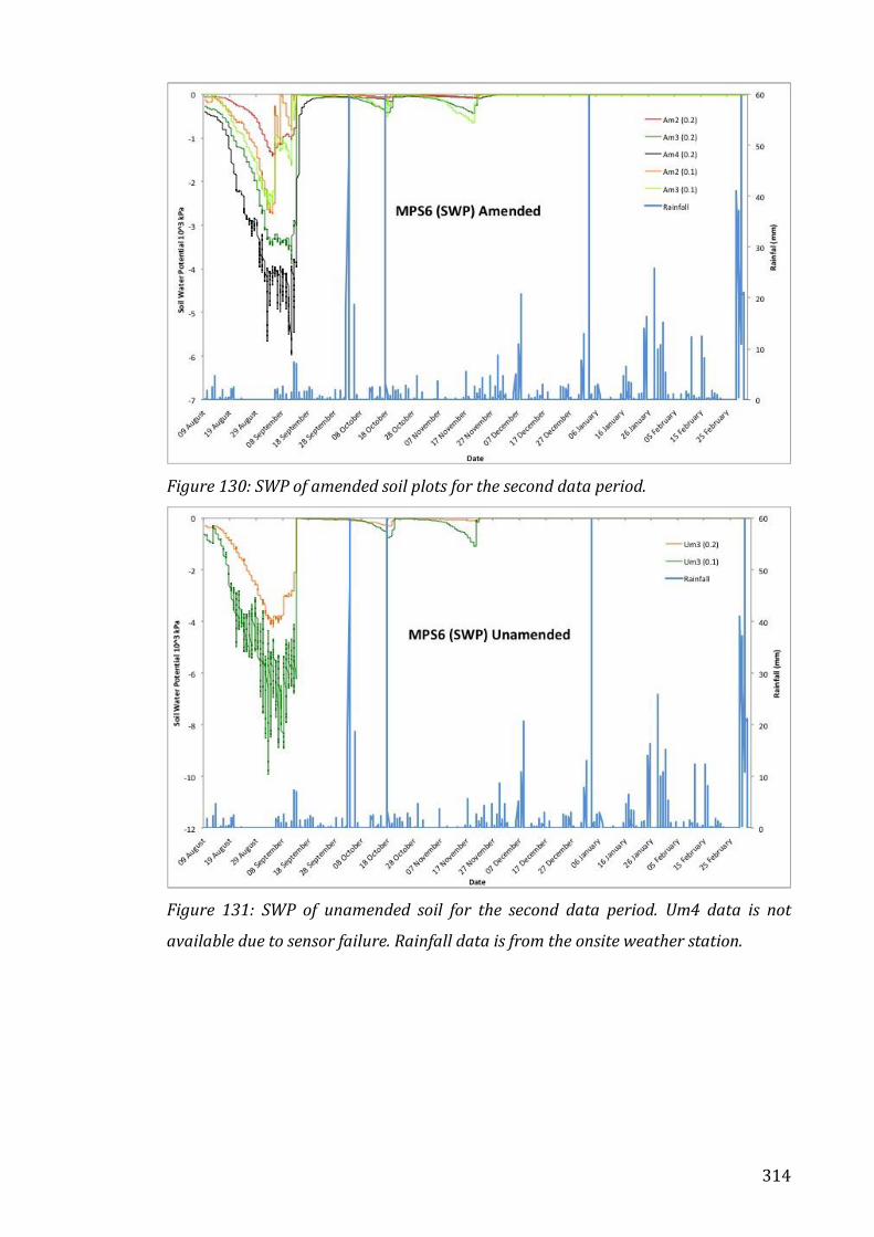
314

Figure 130: SWP of amended soil plots for the second data period.

Figure 131: SWP of unamended soil for the second data period. Um4 data is not

available due to sensor failure. Rainfall data is from the onsite weather station.

315

Figure 132: SWP of amended and unamended plots in Zone 3 on the Weetslade field

Rainfall data is from the onsite weather station. -12.00 on the Y axis corresponds to a

-1200 kPa suction

7.3.3 Soil strength

Triaxial testing was conducted by Ellis (2017) on 30 amended and 30 unamended

reformed soil cores to obtain values for shear strength using an undrained,

unconsolidated triaxial (often called the ‘quick’) test at cell pressures of 25, 50 and

100 kPa, the results of which are shown in Table 36. The average shear strength of

unamended soil was determined to be 124.02 ± 20.7 kPa (using Tresca’s theory),

which is typical of soils of clay loam (with high clay content) and determines it as a

‘stiff’ soil (Craig, 2004). The maximum shear strength of 168.51 kPa of unamended

soil is at 25 kPa, where cohesion was 99 kPa and the angle of friction was 7.4°.

Amended soil had a maximum shear strength of 185.64 kPa, achieved during the

100 kPa test, where cohesion was 112 kPa and the angle of friction of 20.3°. These

results echo those from Chapter 5, where the amended samples had better shear

strength at the highest pressure compared to unamended soil.

There is not a significant difference in the shear strength of amended soil at the

lowest confining pressure (25 kPa), however there is a statistical improvement in

the maximum shear strength of amended soil at higher pressures in comparison to

unamended soil, as well as improved cohesion and angle of friction, which suggests

316

that the soil aggregate stability is greater in the amended sample and as such is

better able to resist shear forces.

Unamended (n=10) Amended (n=10)

25 kPa average

(not significant)

146.55 ± 22 kPa 143.27 ± 29 kPa

50 kPa average 110.78 ± 27 kPa 163.69 ± 15 kPa

100 kPa average 114. 73 ± 10 kPa 162. 73 ± 18 kPa

Average shear

strength

124.02 ± 20.7 kPa 156.6 ± 20.6 kPa

Maximum shear

strength

168.51 (25 kPa) 185.64 (100 kPa)

Cohesion 99 kPa 112 kPa

Angle of friction 7.4° 20.3°

Table 36: Summary of triaxial cell strength testing on samples from Weetslade

Country Park.

7.4 Discussion and catchment implications

The re-establishment of vegetation on the soil plots was very quick due to

preservation of the root network during the construction of the plots. A

quantitative analysis is required for any assumptions to be validated, however the

brief analysis of vegetation by Ellis (2017) suggested that there was a greater

amount of growth on amended plots. Soil bulk density was tested in June 2017 and

February 2018, and showed that there was a small increase in the bulk density of

both amended and unamended plots in the 11 months succeeding the

implementation of the field plots (however no statistical testing was performed

between unamended and amended values of initial bulk density, nor between the

bulk density values at obtained at different times). In addition, the data from

February indicated no statistical significance in the different between the

unamended and amended plots, although this may be due to a low number of

repeats. It is very clear therefore that a thorough study with numerous repeats is

317

required to drawn concrete conclusions on the bulk density characteristics of both

the unamended and amended plots.

Assessment of data from EC5 (VWC) and MPS 6 (SWP) sensors installed on two

plots on the Weetslade embankment trial site has revealed that in general the VWC

is dependent on the depth of the sensor and the location of the sensor on the

embankment. During the first period of data collection (May, 2017) the VWC of

amended plots were 5.4% (at a depth of 0.2) and 22% higher (at a depth of 0.1)

than unamended plots (no comparison could be made in Zone 2 as there were no

sensors in the unamended plot at this point on the slope, and in Zone 4 there were

malfunctions in the unamended sensors). Data produced by Ellis (2017) shows

that in this time period the unamended soils released water at a faster rate (up to

9%) than amended soils in the period immediately after a rainfall event,

suggesting that amended soils have better water retention than the unamended

soil. Additionally, sensors lower on the slope recorded a 5% faster VWC reduction

than sensors at the top of the slope, showing the effect of gradient on the

movement of water through the field plots.

However looking at the long-term data between September 2017 and March 2018,

the VWC of the unamended soil is in general higher than the amended soil. This

may be as a result of two factors, the difference in water retention for different soil

types, and/or the method of measurement. Weetslade soil was classified by Ellis

(2017) as a clay loam with high clay content; it is well known that clays hold more

water than other soil types due to the high surface area of clay particles and high

number of micro-pores (Craig, 2004). By adding co-amendment to the Weetslade

soil, the soil particle size has been altered to include a greater proportion of

coarser particles, which although improve the soil structure, reduce the amount of

water that the soil can hold under a particular suction while in an unsaturated

state as the macro-pores present in the amended soil are not able to hold onto the

water as well as micro-pores.

The average SWP of unamended soil was higher than the amended plot, due firstly

to the difference in VWC and secondly due to the different textural composition of

the soils as the results of the amendment. As discussed in Chapter 2, the

318

relationship between water content and suction is simple, the lower the water

content, the higher the suction, although this relationship affected by the texture of

a soil. Larger negative suctions, as shown by negative SWP (kPa) are more typical

of clays in comparison to sandy soils due to the difference in water retention

properties. Therefore at the same water content the clay will have a higher SWP.

The differences in SWP may therefore be a reflection on the texture of the soil

rather than on its ability to take up more water, as we have seen that water

movement through the amended soil is faster in laboratory tested soils.

Nonetheless, it is difficult to compare the effects of amendment on different soils,

where a clay soil behaves differently to the loam soils tested in Trials 1-4.

High suctions are indicative of high shear strength and although Weetslade soil is

classified as a stiff soil due to its highly cohesive aggregates (Craig, 2004) with a

maximum shear strength of 168.51 kPa, the shear strength of amended soil was

higher at 185.64 kPa. The increase in shear strength of amended soils, shown by

this data, is positive for the soil’s erosional resistance in a flooded state, as soils

more resistance to shearing forces are less likely to breakdown as a result of

raindrop and runoff erosion (as discussed in Chapter 2, section 2.3.5).

The wider implications of the field application of WTR are difficult to assess for the

Seaton Burn catchment and requires the application of WTR co-amendment to a

range of different of soils such that the effect of co-amendment can be determined

for a range of soil textures. According to laboratory results, should a WTR co-

amendment be applied to a soil, in general it will reduce the bulk density and

compactibility of a soil. For a granular soil, the addition of fine particles and

organic matter are likely to increase the water holding capacity, water retention

and shear strength and improve hydraulic conductivity of the soil (as shown by

testing results in Chapter 5). It appears that conversely to laboratory results the

application of the co-amendment to a highly clay soil is likely to reduce the water

content at field capacity (i.e. water held against the force of gravity after a rainfall

event) in the soil based on the VWC, but these results must be discussed with

reference to bulk density and gravimetric water content values that can be derived

by taking samples from the field and assessing them according to the appropriate

tests (discussed in Chapter 4, section xxx). It must also be noted that the soils at

319

Weetslade have not been subjected to the same degree of saturation as those in the

lab, which were submerged for a long period of time.


The VWC of unamended soils are on average 18% higher than amended soils at a

depth of 0.2, and around 3% lower than amended soils at a depth of 0.1 for long-

term data despite initial trend to suggest that the amended plot had a higher VWC.

To determine if this difference is due to volume change of the soils (as described in

Chapter 2), further field samples are required to be taken for analysis of GWC and

density. Triaxial results from reformed soil samples show that the shear strength

of amended of soil (185.64 kPa) is statistically significantly higher than

unamended soil (168.51 kPa). Further laboratory tests will be required to test the

erosional resilience. The discussion has attempted to explore further benefits of

water treatment amended soil to the local environment through assessments of

the field site, including vegetation surveys and consideration of the wider

catchment, but this is a challenging process due to the inconclusive results of

current data. A number of supplementary tests are required to wholly assess the

effect of WTR co-amendment on Weetslade soil, along with continued monitoring

of the field trial over a longer period of time.

320

8. Conclusions and Recommendations for Future Work

This thesis has outlined novel methods with which to quantify soil functions, which

allow us to assess their flood holding capacity. This includes the water holding

capacity, the hydraulic conductivity, the shear strength and erosional properties of

the soil. Current methods of measuring water in soils need to include both an

assessment gravimetric water content and volume change, in order to accurately

assess the ability of soils to hold water and so volumetric water content does take

swelling into account (and can lead to an underestimation of water holding

capacity). This thesis has begun to bridge the gap between geotechnical and

geoenvironmental perspectives of analysing soil with the by exploring the

following avenues:

1) Development of novel water holding capacity experiments to assess the

maximum gravimetric and volumetric water content of amended and

unamended soils over at least one wetting and drying sequence.

2) Erosional resistance testing of amended and unamended soils through fall

cone penetrometer and a newly development method (Veitch, 2016).

3) Assessment of hydraulic conductivity of amended and unamended soils

using triaxial cell.

4) Assessment of shear strength properties of amended and unamended soils

using triaxial cell.

5) Analysis of amended and unamended soils using X-ray Computed

tomography, in order to understand the effect of amendment on soil

structure.

6) Field trial application of the co-amendment at Weetslade Country Park.

Water Treatment Residual (WTR), a by-product of the clean drinking water

industry has been used in conjunction with compost as a co-amendment, using the

WTR at 20% solids (WTRw) and air-dried at 20% water content (WTRd). The reuse

and or recycling of this clean waste is an important avenue of research for water

companies in the UK and across the world due to increasing costs of disposal.

Simultaneously there is a timely need to improve the health of the UK’s soils in

order to mitigate the historic effect of degrading practises. Improvements in

321

important soil functions as a result of both single WTR and the co-amendment of

WTR and compost have been highlighted in the previous chapters. The significant

findings are summarised as follows: (a) maximum gravimetric water content, (b)

sample volume increase, (c) shrinkage, which refers to the difference in maximum

sample volume between the 1st wetting and 2nd wetting sequences (d) maximum

void ratio (porosity) as determined by either XRCT or triaxial testing (d) hydraulic

conductivity and (e) shear strength. Values for a-c are derived from Trial 4, d from

XRCT and d,e & f from triaxial testing. These are summarised in Table

322

Soil Function

- Indicates no significance in

improvement. Red indicates significant

negative influence

%

amend-

ment

Control

(Soil2)

Single WTRd

20% water content

Single WTRw

20% solids

Single compost

Co-amendment

WTRd

Co-amendment

WTRw

1st wetting & drying

Maximum gravimetric water content

(0.18 starting value)

10

20

30

0.372

-

0.382 (2.7%)

0.423 (13.7%)

0.390 (4.9%)

-

0.410 (9.9%)

-

0.421 (13.2%)

0.501 (34.7%)

-

0.412 (10.8%)

0.464 (24.7%)

0.390 (4.8%)

0.412 (10.8%)

0.465 (25%)

Volume (change) in cm3

(86.2 cm3 starting value)

10

20

30

+37.9 +27.9 (-26.4%)

+31.7 (-16.4%)

+36.3 (-4.2%)

-

-

+39.9 (5.3%)

-

+39.9 (5.3%)

+54.6 (44.1%)

-

-

+47.7 (25.9%)

+35.7 (-5.8%)

+38.8 (2.4%)

+57.5 (51.7%)

Shrinkage (1st volume peak– 2nd

volume peak)

10

20

30

-18.8 (15.2%) +1.6 (1.4%)

-13.8 (11.5%)

-15.7 (12.6%)

-17.1 (13.5%)

-15.9 (12.8%)

-18.8 (14.5%)

+0.77 (0.65%)

-15.3 (11.7%)

-24.2 (16.2%)

-15.3 (10.7%)

-19.6 (15.3%)

-17.8 (12.8%)

-15.3 (12.4%)

-20.2 (15.1%)

-21.1 (14.6%)

Maximum void ratio (XRCT/Triax) 30 0.127/0.390 0.291/0.422 0.312/0.433 0.459/0.442 0.229/0.433 0.207/0.435

Hydraulic conductivity (25 kPa) 30 6.73 x E-07 1.77 x E-07 7.22 x E -06 6.28 x E-07 2.77x E-06 3.86 X E-06

Shear strength (25/100kPa) 30 69/179 115/174 158/174 84/165 106/252 78/248

2nd wetting and drying cycle

Maximum gravimetric water content 10

20

30

0.314 0.353 (12.4%)

0.331 (5.4%)

0.378 (20.4%)

0.339 (8%)

-

0.351 (11.8%)

0.369 (17.5%)

0.375 (19.4%)

0.417 (32.8%)

-

0.339 (8%)

0.391 (24.5%)

0.35 (11.5%)

0.361 (14.9%)

0.391 (24.5%)

Volume (change) cm3 (from original) 10

20

30

+19.1 -

+17.9 (-6.3%)

+20.5 (7.3%)

+21.4 (12%)

+17.5 (-8.4%)

+21.1 (10.5%)

+35.0 (83.3%)

+24.7 (29.3%)

+30.4 (59.2%)

+20.2 (5.8%)

+19.1

+29.7 (55.5%)

+20.5 (7.3%)

+23.3 (22%)

+36.4 (90.6%)

Original – dried porosity (XRCT) 30 -47% +54.4% +97.5% +6.1% +80.9% +92.2%

Table 37: Summary of soil function data, comparing the control (Soil2) with single amendments of WTRd, WTRw, and compost, and against co-amendment of

WTRd/WTRw with compost at ratios of 10, 20 and 30%. Data are absolute values of change and (the percentage increase or decrease compared to the control)

323

8.1 Concluding summary

1. Water treatment residual as a single amendment imparts important physical

changes to soil and can beneficially modify the soil to increase the maximum

gravimetric water content, sample volume, maximum void ratio (porosity),

reduces shrinkage (loss of soil volume/porosity), increase hydraulic

conductivity and shear strength at low stress. There is no statistically

significant advantage in processing the wet WTRw (20% solids) to lower the

water content (WTRd, 20% gravimetric water content).

a) WTRd statistically significantly improves the maximum gravimetric

water content of samples by between 2.7% and 13.7% (20 and 30%

amendment) during the 1st wetting cycle, and by between 5.4 and 20.4%

(10-30% amendment) during the 2nd wetting cycle, against the control

soil (n=12, p<0.05). 10% amendment did not yield a statistically

significant improvement during the 1st wetting cycle.

WTRw statistically significantly improves the maximum gravimetric

water content of samples by between 4.9% and 9.9% (10 and 30%

amendment) during the 1st wetting cycle, and by between 8 and 11.8%

(10 and 30% amendment) during the 2nd wetting cycle, against the

control soil (n=12, p<0.05). 20% amendment did not yield a statistically

significant improvement.

b) Only the addition of WTRw at 30% amendment statistically significantly

improves the volume increase (5.3%) compared to the control soil

during the 1st wetting cycle (n = 12, p<0.01).

WTRd (30% amendment) had a statistically significant increase (7.3%)

in sample volume compared to the control soil during the 2nd wetting

cycle (n =12, p<0.01).

WTRw had a statistically significant increase of between 10.5 and 12%

(30 and 10% amendment) in sample volume compared to the control

soil during the 2nd wetting cycle (n =12, p<0.01).

c) WTRd amended samples experienced between 1.4 and 12.6% (10-30%

amendment) reduction in maximum sample volume (shrinkage)

between the 1st wetting and 2nd wetting sequences, compared to the

control soil which had a 15.2% reduction in maximum volume

(shrinkage). (n = 12, p<0.01).

324

WTRw amended samples experienced between 12.8 and 14.5% (20 and

30% amendment) reduction in maximum sample volume (shrinkage)



(shrinkage). (n = 12, p<0.01).

d) WTRd increased the maximum void ratio by 129% (XRCT)/8.2%

(Triaxial), compared to the control soil (n=1).

WTRw increased the maximum void ratio by 145% (XRCT)/11%

(Triaxial) compared to the control soil (n=1).

e) WTRw as a single amendment improves the hydraulic conductivity of

soil by a factor of 28 (30% amendment), by a factor of 10 for WTR2d

(30% amendment), a factor of 6 for 20% WTR2d and 8 for 20% WTR2w,

a factor of 6 for 10% WTR2w, and doubles K with 10% WTR2d.

f) WTRd improves the shear strength of soil at low testing pressure

(25 kPa) by 67%, but reduces the shear strength at high testing pressure

(100 kPa) by 3% compared to unamended soil.

WTRw improves the shear strength of soil at low testing pressure

(25 kPa) by 129% but reduces the shear strength at high testing

pressure (100 kPa) by 3% compared to unamended soil.

2. Compost as a single amendment increases maximum gravimetric water

content, sample volume, maximum void ratio (porosity), and reduces shrinkage

(loss of soil volume/ porosity) on drying at low amendment ratios, however the

amendment increases shrinkage (at high amendment ratio), reduces hydraulic

conductivity and saturated shear strength of the soil. The effect of compost was

greater during the 2nd wetting cycle compared to the 1st wetting cycle.

a) Compost statistically significantly improved the maximum gravimetric

water content of samples by between 13.2 and 34.7% (20 and 30%

amendment) during the 1st wetting cycle, and by between 17.5 and

32.8% (10-30% amendment) during the 2nd wetting cycle, against the

control soil (n=12, p<0.05). 10% amendment did not yield a statistically

significant improvement during the 1st wetting cycle.

b) Compost amendment statistically significantly improved the volume

increase during wetting by between 5.3 and 44.1% (20 and 30%

325

amendment) compared to the control soil during the 1st wetting cycle (n

= 12, p<0.01).

Compost amendment statistically significantly improved the volume

increase during wetting by between 29.3 and 83.3% (20 and 10%

amendment) compared to the control soil during the 2st wetting cycle (n

= 12, p<0.01).

c) Compost amended samples experienced an increase in sample volume

during wetting (0.65% at 10% amendment) and between 11.7 and

16.2% (20 and 30% amendment) reduction in maximum sample volume

(shrinkage) between the 1st wetting and 2nd wetting sequences,

compared to the control soil which had a 15.2% reduction in maximum

volume (shrinkage) between the two wetting phases (n = 12, p<0.01).

d) Compost increased the maximum void ratio on wetting by 261%

(XRCT)/8.2% (Triaxial), compared to the control soil (n=1).

e) Compost as a single amendment reduces the saturated hydraulic

conductivity by 3.65% (10 amendment), 84.5% (20% amendment),

6.6% (30% amendment) compared to the control soil (n=1)

f) Compost improves the saturated shear strength of soil at low testing

pressure (25 kPa) by 21.7%, but reduces the shear strength at high

testing pressure (100 kPa) by 2.8% compared to unamended soil.

3. Co-amendment of WTR with compost appears to provide soil with the well-

known benefits of compost addition (enhanced water holding capacity and

swelling) in addition to the geotechnical improvements of the WTR (structural

stabilisation through reduced shrinkage on drying, improved saturated

hydraulic conductivity and saturated shear strength at 100 kPa). Co-

amendments therefore perform better than single amendments of compost or

WTR in terms of their ‘flood holding capacity’.

a) Co-amendment using WTRd statistically significantly improved the

maximum gravimetric water content of samples by between 10.8 and

27.4% (20 and 30% co-amendment) during the 1st wetting cycle and

between 8 and 24.5% (20 and 30% amendment) during the 2nd wetting

cycle (n=12, p<0.01), compared to the control soil.

Co-amendment using WTRw statistically significantly improved the

maximum gravimetric water content of samples by between 4.5 and

326

25% (10 - 30% co-amendment) during the 1st wetting cycle and

between 11.5 and 24.5% (10- 30% amendment) during the 2nd wetting

cycle (n=12, p<0.01), compared to the control soil.

b) WTRd co-amendment statistically significantly improved the volume

increase by 25.9% (30% amendment) during the 1st wetting cycle and

between 5.8 and 55.5% (10 and 30% amendment) during the 2nd

wetting cycle compared to the control soil (n = 12, p<0.01).

WTRw co-amendment statistically significantly improved the volume

increase by between 2.4 and 51.7% (20 and 30% amendment)

compared to the control soil during the 1st wetting cycle and by 7.3 and

90.6% (10-30% amendment) during the 2nd wetting cycle compared to

the control soil (n = 12, p<0.01).

c) WTRd amended samples experienced between 10.7 and 12.8% (10 and




(shrinkage). (n = 12, p<0.01).

WTRw amended samples experienced between 12.4 and 14.6% (10 and




(shrinkage). (n = 12, p<0.01).

d) WTRd co-amendment increased the maximum void ratio on wetting by

80% (XRCT)/11% (Triaxial), compared to the control soil (n=1).

WTRw co-amendment increased the maximum void ratio on wetting by

63% (XRCT)/11.5% (Triaxial), compared to the control soil (n=1).

e) WTRd co-amendment increases the saturated hydraulic conductivity by

23% (10 amendment), 355% (20% amendment), 313% (30%

amendment) compared to the control soil (n=1).

WTRw co-amendment increases the saturated hydraulic conductivity by

91% (10 amendment), 330% (20% amendment), 475% (30%

amendment) compared to the control soil (n=1).

f) WTRd co-amendment improves the saturated shear strength of soil at

low testing pressure (25 kPa) by 53.6% and increases the shear

327

strength at high testing pressure (100 kPa) by 40.8% compared to

unamended soil.

WTRw co-amendment improves the saturated shear strength of soil at

low testing pressure (25 kPa) by 13%, and increases the saturated shear

strength at high testing pressure (100 kPa) by 38.5% compared to

unamended soil.

4. Erosional testing was inconclusive and requires method refinement to allow

sufficient analysis.

5. Visualisation of WTR amended samples using XRCT allowed the identification

of void spaces around WTRd (20% GWC) pores in saturated samples that

remained present once the sample was dried, i.e. the porosity was retained. As

n <2000, this provided quantifiable evidence of soil architecture change with

the addition of WTR by analysis of void ratios.

6. Data from the Weetslade field trial has thus far provided inconclusive data on

the field application of a 10% co-amendment, and further investigation of

supplementary soil parameters such as bulk density and gravimetric water

content is needed to quantify changes in soil properties.

8.2 Recommendations for future work

Taking into account the effect of co-amendment on essential soil functions that

determines a soil’s flood holding capacity (maximum gravimetric water content,

volume change, resistance against shrinkage, void ratio (porosity), hydraulic

conductivity and shear strength) and the economic and environmental

sustainability issues, it is worth considering a co-amendment over the single

amendment of compost or WTR. The research contained within this thesis has

shown that on a short-term basis at a small scale, that the application of compost

and WTR has considerable influence on the flood holding capacity. In order for this

information to effectively feed back into the policy framework of companies such

as Northumbrian Water and the Environment Agency in regard to waste

management, the following research questions need to be addressed;

- Can we use WTR as a single amendment in soil on a long-term basis without

negative geochemical consequence, e.g. detrimentally affecting P

availability for plants?

328

- What are the long-term effects, of co-amendment with WTR and compost

over numerous wetting and drying cycles, on the flood holding capacity of

soils?

- What is the bio-chemical effect of the addition of WTR to soils in either wet

or dry forms?

- Considering ‘cementation effects’ suggested to occur to soils with the

addition of WTR in Trial 4, what are the long-term structural effects of

WTR/compost addition on soil, with respect to volume changes and shear

strength?

- What is the maximum quantity of either single amendment or co-

amendment that is permissible on land (as current guidelines are based on

EU regulations on sewage sludge and EA discretion), without detrimental

effects on the soil’s plant functions and water chemistry?

- Should research determine that the long-term application of WTR/compost

amendment has no implications, can we use land spreading/soil

amendment to completely close the loop on WTR waste? Are there enough

brownfield sites or areas of flood vulnerability to incorporate the waste?

329

9. Bibliography: References & websites Abiven, S., Menasseri, S., & Chenu, C. (2009). The effects of organic inputs over time on soil aggregate stability–A literature analysis. Soil Biology and Biochemistry, 41(1), 1-12. Acton, D. F., & Gregorich, L. J. (1995). Understanding soil health. Publications-Canada Department of Agriculture, 5-10. Adejumo, T. E. (2012). Effect of organic content on compaction and consolidation characteristics of Lagos organic clay. Electron. J. Geotechn. Eng.(EJGE), 17, 2201-2211. Agassi, M., & Bradford, J. M. (1999). Methodologies for interrill soil erosion studies. Soil and Tillage Research, 49(4), 277-287. Aggelides, S. M., & Londra, P. A. (2000). Effects of compost produced from town wastes and sewage sludge on the physical properties of a loamy and a clay soil. Bioresource technology, 71(3), 253-259. Agnew, J. M., & Leonard, J. J. (2003). The physical properties of compost. Compost Science & Utilization, 11(3), 238-264. Agnew, J. M., Leonard, J. J., Feddes, J., & Feng, Y. (2003). A modified air pycnometer for compost air volume and density determination. Canadian Biosystems Engineering, 45, 6-27. Agyin-Birikorang, S., O'connor, G. A., Jacobs, L. W., Makris, K. C., & Brinton, S. R. (2007). Long-term phosphorus immobilization by a drinking water treatment residual. Journal of environmental quality, 36(1), 316-323. Ahmed, F. N., & Lan, C. Q. (2012). Treatment of landfill leachate using membrane bioreactors: A review. Desalination, 287, 41-54. Ahn, H. K., Richard, T. L., & Glanville, T. D. (2008). Optimum moisture levels for biodegradation of mortality composting envelope materials. Waste Management, 28(8), 1411-1416. Akin, S., & Kovscek, A. R. (2003). Computed tomography in petroleum engineering research. Geological Society, London, Special Publications, 215(1), 23-38. Al-Durrah, M. M., & Bradford, J. M. (1982). Parameters for Describing Soil Detachment Due to Single Waterdrop Impact 1. Soil Science Society of America Journal, 46(4), 836-840. Al-Raoush, R. I., & C. S. Willson (2005), Extraction of physically representative pore network from unconsolidated porous media systems using synchrotron microtomography. Journal of Hydrology., 300, 44–64.

330

Alajmi, A. F., Grader, A., & Alkafeef, S. F. (2009). Evaluation of tracer diffusion in layered system using X-ray CT. Petroleum Science and Technology, 27(11), 1134-1150. Almajmaie, A., Hardie, M., Acuna, T., & Birch, C. (2017). Evaluation of methods for determining soil aggregate stability. Soil and Tillage Research, 167, 39-45. Altman, D. G., & Bland, J. M. (2009). Parametric v non-parametric methods for data analysis. Bmj, 338, a3167. Amezketa, E. (1999). Soil aggregate stability: a review. Journal of sustainable agriculture, 14(2-3), 83-151. Amezketa, E., Singer, M. J., & Le Bissonnais, Y. (1996). Testing a new procedure for measuring water-stable aggregation. Soil Science Society of America Journal, 60(3), 888-894. An, J., Zheng, F., Lu, J., & Li, G. (2012). Investigating the role of raindrop impact on hydrodynamic mechanism of soil erosion under simulated rainfall conditions. Soil Science, 177(8), 517-526. An, S., Mentler, A., Mayer, H., & Blum, W. E. (2010). Soil aggregation, aggregate stability, organic carbon and nitrogen in different soil aggregate fractions under forest and shrub vegetation on the Loess Plateau, China. Catena, 81(3), 226-233. Anderson, S. H., & Hopmans, J. W. (1994). Tomography of soil-water-root processes. Soil Science Society of America, American Society of Agronomy, and Crop Science Society of America. Anderson, S. H., Gantzer, C. J., & Brown, J. R. (1990). Soil physical properties after 100 years of continuous cultivation. Journal of Soil and Water Conservation, 45(1), 117-121. Anderson, S. H., Peyton, R. L., & Gantzer, C. J. (1990). Evaluation of constructed and natural soil macropores using X-ray computed tomography. Geoderma, 46(1-3), 13-29. Anderson, S. H., Wang, H., Peyton, R. L., & Gantzer, C. J. (2003). Estimation of porosity and hydraulic conductivity from X-ray CT-measured solute breakthrough. Geological Society, London, Special Publications, 215(1), 135-149. André, J. E., & Anderson, H. W. (1961). Variation of soil erodibility with geology, geographic zone, elevation, and vegetation type in northern California wildlands. Journal of Geophysical Research, 66(10), 3351-3358. Angers, D. A., Kay, B. D., & Groenevelt, P. H. (1987). Compaction Characteristics of a Soil Cropped to Corn and Bromegrass. Soil Science Society of America Journal, 51(3), 779-783. Arduino, E., Barberis, E., & Boero, V. (1989). Iron oxides and particle aggregation in B horizons of some Italian soils. Geoderma, 45(3-4), 319-329.

331

Arias, M., Barral, M. T., & Diaz-Fierros, F. (1999). Effects of organic matter, iron and aluminium on soil structural stability. In Effect of Mineral-Organic-Microorganism Interactions on Soil and Freshwater Environments (pp. 79-88). Springer, Boston, MA. Arias, M., Barral, M. T., & Díaz?Fierros, F. (1996). Effects of associations between humic acids and iron or aluminium on the flocculation and aggregation of kaolin and quartz. European Journal of Soil Science, 47(3), 335-343. Arthur, E., Cornelis, W. M., Vermang, J., & De Rocker, E. (2011). Effect of compost on erodibility of loamy sand under simulated rainfall. Catena, 85(1), 67-72. Athamenh, B. M., Salem, N. M., El-Zuraiqi, S. M., Suleiman, W., & Rusan, M. J. (2015). Combined land application of treated wastewater and biosolids enhances crop production and soil fertility. Desalination and Water Treatment, 53(12), 3283-3294. Avery, B. W. (1980). Soil classification for England and Wales. Soil classification for England and Wales. (14). Babatunde, A. O., & Zhao, Y. Q. (2007). Constructive approaches toward water treatment works sludge management: an international review of beneficial reuses. Critical Reviews in Environmental Science and Technology, 37(2), 129-164. Bachmann, J., & van der Ploeg, R. R. (2002). A review on recent developments in soil water retention theory: interfacial tension and temperature effects. Journal of Plant Nutrition and Soil Science, 165(4), 468-478. Bai, L., Wang, C., He, L., & Pei, Y. (2014). Influence of the inherent properties of drinking water treatment residuals on their phosphorus adsorption capacities. Journal of Environmental Sciences, 26(12), 2397-2405. Baker, A., Ward, D., Lieten, S. H., Periera, R., Simpson, E. C., & Slater, M. (2004). Measurement of protein-like fluorescence in river and waste water using a handheld spectrophotometer. Water Research, 38(12), 2934-2938. Baraka-Lokmane, S., Main, I. G., Ngwenya, B. T., & Elphick, S. C. (2009). Application of complementary methods for more robust characterization of sandstone cores. Marine and Petroleum Geology, 26(1), 39-56. Barden, L., & Sides, G. (1970). "Engineering behavior and structure of compacted clay." Journal of Soil Mechanics and Foundations Division., ASCE, 96(4), 1171-1200. Barthès, B., & Roose, E. (2002). Aggregate stability as an indicator of soil susceptibility to runoff and erosion; validation at several levels. Catena, 47(2), 133-149. Barthès, B., Albrecht, A., Asseline, J., De Noni, G., & Roose, E. (1999). Relationship between soil erodibility and topsoil aggregate stability or carbon content in a cultivated Mediterranean highland (Aveyron, France). Communications in Soil Science and Plant Analysis, 30(13-14), 1929-1938.

332

Bartlett, R., & James, B. (1980). Studying dried, stored soil samples—Some pitfalls 1. Soil Science Society of America Journal, 44(4), 721-724. Bartoli, F., Burtin, G., & Guerif, J. (1992). Influence of organic matter on aggregation in Oxisols rich in gibbsite or in goethite. II. Clay dispersion, aggregate strength and water-stability. Geoderma, 54(1-4), 259-274. Basim, S. C. (1999). Physical and geotechnical characterization of water treatment plant residuals (Doctoral dissertation, New Jersey Institute of Technology, Department of Civil and Environmental Engineering). Basta, N. T., Dayton, E. A., Storm, D. E., & DeWolfe, J. R. (2003). Advances in WTR research to manage P in soil, runoff, manure, and biosolids. Proceedings of the Water Environment Federation (1), 745-753. Basta, N. T., Zupancic, R. J., & Dayton, E. A. (2000). Evaluating soil tests to predict bermudagrass growth in drinking water treatment residuals with phosphorus fertilizer. Journal of environmental quality, 29(6), 2007-2012. Baveye, P., Rogasik, H., Wendroth, O., Onasch, I., & Crawford, J. W. (2002). Effect of sampling volume on the measurement of soil physical properties: simulation with X-ray tomography data. Measurement Science and Technology, 13(5), 775. Baveye, P.C., Laba, M., Otten, W., Bouckaert, L., Sterpaio, P.D., Goswami, R.R., Grinev, D., Houston, A., Hu, Y., Liu, J. & Mooney, S., 2010. Observer-dependent variability of the thresholding step in the quantitative analysis of soil images and X-ray microtomography data. Geoderma, 157(1-2), pp.51-63. Bay, B. K., Smith, T. S., Fyhrie, D. P., & Saad, M. (1999). Digital volume correlation: three-dimensional strain mapping using X-ray tomography. Experimental mechanics, 39(3), 217-226. Bayley, R. M., Ippolito, J. A., Stromberger, M. E., Barbarick, K. A., & Paschke, M. W. (2008). Water treatment residuals and biosolids coapplications affect semiarid rangeland phosphorus cycling. Soil Science Society of America Journal, 72(3), 711-719. Beare, M. H., & Bruce, R. R. (1993). A comparison of methods for measuring water-stable aggregates: implications for determining environmental effects on soil structure. In Soil Structure/Soil Biota Interrelationships (pp. 87-104). Beare, M. H., Hendrix, P. F., & Coleman, D. C. (1994). Water-stable aggregates and organic matter fractions in conventional-and no-tillage soils. Soil Science Society of America Journal, 58(3), 777-786. Beckers, E., Plougonven, E., Roisin, C., Hapca, S., Léonard, A., & Degré, A. (2014). X-ray microtomography: a porosity-based thresholding method to improve soil pore network characterization. Geoderma, 219, 145-154.

333

Beckett, C., & Thomas, S. (2011). The role of material structure in compacted earthen building materials: Implications for design and construction (Doctoral dissertation, Durham University). Beekman, F. (1987). Soil strength and forest operations. Doctoral Thesis, Department of Forest Technique, Agricultural University, Wageningen, The Netherlands 168 pp. Bennett, H. H. (1926). Some comparisons of the properties of humid-tropical and humid-temperate American soils; with special reference to indicated relations between chemical composition and physical properties. Soil Science, 21(5), 349-376. Biancalani, R., Petri, M., Bunning, S. E., Salvatore, M., & Tubiello, F. N. (2012). The use of soil organic carbon as an indicator of soil degradation. Energia Ambiente e Innovazione, 4, 5, 73-78. Bittelli, M. (2011). Measuring soil water content: A review. HortTechnology, 21(3), 293-300. Blackburn, W. H., & Pierson, F. B. (1994). Sources of variation in interrill erosion on rangelands. Variability in rangeland water erosion processes, 1-9. Blais, K. E. (2005). Measurement of physical and hydraulic properties of organic soil using computed tomographic imagery (Doctoral dissertation, Department of Geography-Simon Fraser University). Blake, G.R. & Hartge K. H. (1986) Bulk Density. In Klute (Ed.) SSSA Book Series 5, Methods of Soil Analysis, Part 1 – Physical and Mineralogical Methods. Planning, 8, 79. Boadu, F. K. (2000). Hydraulic conductivity of soils from grain-size distribution: new models. Journal of Geotechnical and Geoenvironmental Engineering, 126(8), 739-746. Boecker, E., & van Grondelle, R. (1995). Environmental Physics. Physics Today, 48, 66. Boespflug, X., Long, B. F. N., & Occhietti, S. (1995). CAT-scan in marine stratigraphy: a quantitative approach. Marine Geology, 122(4), 281-301. Böhm, W. (1976). In situ estimation of root length at natural soil profiles. The Journal of Agricultural Science, 87(2), 365-368. Bohn, H. L., McNeal, B.L. & O’Connor, G.A. (1985) Soil Chemistry. 2nd Edition, Wiley, New York. Bolto, B., & Gregory, J. (2007). Organic polyelectrolytes in water treatment. Water research, 41(11), 2301-2324.

334

Booltink, H. W. G., & Bouma, J. (1991). Physical and morphological characterization of bypass flow in a well-structured clay soil. Soil Science Society of America Journal, 55(5), 1249-1254. Bouckaert, L., Van Loo, D., Sleutel, S., De Neve, S., Jacobs, P., & Van Hoorebeke, L. (2009). Application of X-ray tomography for quantification of the soil pore structure and visualization of soil organic matter. Geochimica et Cosmochimica Acta Supplement, 73, p A145. Brady & Weil (2016) The Nature and Properties of Soils (15th Edition). Pearson Bresson, L. M., Moran, C. J., & Assouline, S. (2004). Use of bulk density profiles from X-radiography to examine structural crust models. Soil Science Society of America Journal, 68(4), 1169-1176. Brewer, R. (1964). Fabric and Mineral Analysis Of Soils, New York. John Wiley & Sons. Bridges, E. M., & Oldeman, L. R. (1999). Global assessment of human-induced soil degradation. Arid soil research and rehabilitation, 13(4), 319-325. Bronick, C. J., & Lal, R. (2005). Soil structure and management: a review. Geoderma, 124(1-2), 3-22. Brown, K. W., & Thomas, J. C. (1987). A Mechanism by which Organic Liquids Increase the Hydraulic Conductivity of Compacted Clay Materials 1. Soil Science Society of America Journal, 51(6), 1451-1459. Brown, S. L., Clausen, I., Chappell, M. A., Scheckel, K. G., Newville, M., & Hettiarachchi, G. M. (2012). High-iron biosolids compost–induced changes in lead and arsenic speciation and bioaccessibility in co-contaminated soils. Journal of Environmental Quality, 41(5), 1612-1622. Bruce-Okine, E., & Lal, R. (1975). Soil erodibility as determined by raindrop technique. Soil Science, 119(2), 149-157. Brundtland, G. H. (1987). What is sustainable development. Our common future, 8-9. Brunke, O., Neuber, D., & Lehmann, D. K. (2007). NanoCT: visualizing of internal 3D-structures with submicrometer resolution. MRS Online Proceedings Library Archive, 990. Brunke, O., Santillan, J., & Suppes, A. (2010). Precise 3D dimensional metrology using high-resolution x-ray computed tomography (μCT). In Developments in X-Ray Tomography VII (Vol. 7804, p. 78040O). International Society for Optics and Photonics. Bryan, R. B. (1968). The development, use and efficiency of indices of soil erodibility. Geoderma, 2(1), 5-26.

335

Bryan, R. B. (1974). Water erosion by splash and wash and the erodibility of Albertan soils. Geografiska Annaler: Series A, Physical Geography, 56(3-4), 159-181. Bryan, R. B. (2000). Soil erodibility and processes of water erosion on hillslope. Geomorphology, 32(3-4), 385-415. Bryan, R. B., & Poesen, J. (1989). Laboratory experiments on the influence of slope length on runoff, percolation and rill development. Earth Surface Processes and Landforms, 14(3), 211-231. Bryan, R. B., Govers, G., & Poesen, J. (1989). The concept of soil erodibility and some problems of assessment and application. Catena, 16(4-5), 393-412. BS 1377: 1990. (1990). Methods of test for soils for civil engineering purposes—Part 2: classification tests. Buckman, H. O., & Brady, N. C. (1960). The nature and properties of soils. Soil Science, 90(3), 212. Bugbee, G. J., & Frink, C. R. (1985). Alum sludge as a soil amendment: Effects on soil properties and plant growth. Bulletin-Connecticut Agricultural Experiment Station, New Haven (USA). Bullock, M. S., Nelson, S. D., & Kemper, W. D. (1988). Soil cohesion as affected by freezing, water content, time and tillage. Soil Science Society of America Journal, 52(3), 770-776. Busalacchi, D. M. (2012). Evaluation of biosolids as a soil amendment for use in ecological restoration (Doctoral dissertation, The Ohio State University). Caltagirone, C., Bettoschi, A., Garau, A., & Montis, R. (2015). Silica-based nanoparticles: a versatile tool for the development of efficient imaging agents. Chemical Society Reviews, 44(14), 4645-4671. Capper, P. L., & Cassie, W. F. (1969). The mechanics of engineering soils. Chan, T. P., & Govindaraju, R. S. (2004). Estimating soil water retention curve from particle-size distribution data based on polydisperse sphere systems. Vadose Zone Journal, 3(4), 1443-1454. Chandler, R. J. (1988). The in-situ measurement of the undrained shear strength of clays using the field vane. In Vane shear strength testing in soils: field and laboratory studies. ASTM International. Chenu, C. (1989). Influence of a fungal polysaccharide, scleroglucan, on clay microstructures. Soil Biology and Biochemistry, 21(2), 299-305. Chenu, C., & Plante, A. F. (2006). Clay-sized organo-mineral complexes in a cultivation chronosequence: revisiting the concept of the ‘primary organo-mineral complex’. European Journal of Soil Science, 57(4), 596-607.

336

Chenu, C., Le Bissonnais, Y., & Arrouays, D. (2000). Organic matter influence on clay wettability and soil aggregate stability. Soil Science Society of America Journal, 64(4), 1479-1486. Chesworth, W. (2008). Encyclopaedia of soil science. Springer Science & Business Media. Chirinda, N., Olesen, J. E., Porter, J. R., & Schjønning, P. (2010). Soil properties, crop production and greenhouse gas emissions from organic and inorganic fertilizer-based arable cropping systems. Agriculture, ecosystems & environment, 139(4), 584-594. Choi, H. S., Haynor, D. R., & Kim, Y. (1991). Partial volume tissue classification of multichannel magnetic resonance images-a mixel model. IEEE Transactions on Medical Imaging, 10(3), 395-407. Chudley, R., & Greeno, R. (2006). Building construction handbook. Routledge. Clarke, C. E., Majodina, T. O., du Plessis, A., & Andreoli, M. A. G. (2016). The use of X-ray tomography in defining the spatial distribution of barite in the fluvially derived palaeosols of Vaalputs, Northern Cape Province, South Africa. Geoderma, 267, 48-57. Clausnitzer, V., & Hopmans, J. W. (2000). Pore-scale measurements of solute breakthrough using microfocus X-ray computed tomography. Water Resources Research, 36(8), 2067-2079. Cnudde, V., & Boone, M. N. (2013). High-resolution X-ray computed tomography in geosciences: A review of the current technology and applications. Earth-Science Reviews, 123, 1-17. Commission Directive (2003) CD 31/EC The Commission of the European Community Conroy, G. C., & Vannier, M. W. (1987). Dental development of the Taung skull from computerized tomography. Nature, 329(6140), 625-627. Cook, H. L. (1936). The nature and controlling variables of the water erosion process. Soil science society of America Journal, 1(C), 487-494. Coote, D. R., Malcolm-McGovern, C. A., Wall, G. J., Dickinson, W. T., & Rudra, R. P. (1988). Seasonal variation of erodibility indices based on shear strength and aggregate stability in some Ontario soils. Canadian Journal of Soil Science, 68(2), 405-416. Cornell, R. M., & Schwertmann, U. (2003). The iron oxides: structure, properties, reactions, occurrences and uses. John Wiley & Sons. Council Directive (1999). 31/EC of 26 April 1999 on the landfill of waste. Official journal L, 182(16), 07.

337

Cox, A. E., Camberato, J. J., & Smith, B. R. (1997). Phosphate availability and inorganic transformation in an alum sludge-affected soil. Journal of Environmental Quality, 26(5), 1393-1398. Craig, R. F. (2004). Craig's soil mechanics. CRC Press. Craswell, E. T., & Waring, S. A. (1972). Effect of grinding on the decomposition of soil organic matter—I. The mineralization of organic nitrogen in relation to soil type. Soil Biology and Biochemistry, 4(4), 427-433. Crestana, S., Cesareo, R., & Mascarenhas, S. (1986). Using a computed tomography miniscanner in soil science. Soil Science, 142(1), 56. Crestana, S., Mascarenhas, S., & Pozzi-Mucelli, R. S. (1985). Static and dynamic three-dimensional studies of water in soil using computed tomographic scanning. Soil Science, 140(5), 326-332. Crittenden J., Trussel R., Hand D., Howe K., Tchobanoglous G. (2005) Coagulation, mixing and flocculation. Water Treatment: Principles and Design, 2nd edition, John Wiley & Sons, New Jersey:664-691. Crittenden, J. C., Trussell, R. R., Hand, D. W., Howe, K. J., & Tchobanoglous, G. (2012). MWH's water treatment: principles and design. John Wiley & Sons. Cruse, R. M., & Larson, W. E. (1977). Effect of Soil Shear Strength on Soil Detachment due to Raindrop Impact 1. Soil Science Society of America Journal, 41(4), 777-781. Daniel, D. E. (1982). Measurement of Hydraulic Conductivity of Unsaturated Soils with Thermocouple Psychrometers 1. Soil Science Society of America Journal, 46(6), 1125-1129. Darcy, H. (1856) Determination of the laws of the flow of water through sand. Les Fontaines publiques de la ville de Dijon. Pp. 590-594. Paris: Victor Dalmont. Das, K., & Keener, H. M. (1997). Moisture effect on compaction and permeability in composts. Journal of environmental engineering, 123(3), 275-281. Datta, R., Vranová, V., Pavelka, M., Rejšek, K., & Formánek, P. (2014). Effect of soil sieving on respiration induced by low-molecular-weight substrates. International Agrophysics, 28(1), 119-124. Dayton, E. A., & Basta, N. T. (2001). Characterization of drinking water treatment residuals for use as a soil substitute. Water Environment Research, 73(1), 52-57. Dayton, E. A., & Basta, N. T. (2005). Use of drinking water treatment residuals as a potential best management practice to reduce phosphorus risk index scores. Journal of environmental quality, 34(6), 2112-2117. Dayton, E. A., Basta, N. T., Jakober, C. A., & Hattey, J. A. (2003). Using treatment residuals to reduce phosphorus in agricultural runoff. Journal-American Water Works Association, 95(4), 151-158.

338

De Gryze, S., Jassogne, L., Six, J., Bossuyt, H., Wevers, M., & Merckx, R. (2006). Pore structure changes during decomposition of fresh residue: X-ray tomography analyses. Geoderma, 134(1-2), 82-96. De Ploey, J. D., & Poesen, J. (1981). Aggregate stability, runoff generation and interrill erosion. In Richards, K.S. Arnett, R.R. & Ellis, S (Eds). Geomorphology and Soils, George Allen & Unwin, London 99-120 De Vleeschauwer, D., Lal, R., & De Boodt, M. (1978). Comparison of detachability indices in relation to soil erodibility for some important Nigerian soils. Pedologie, 28(1), 5-20. Devereux, R. C., Sturrock, C. J., & Mooney, S. J. (2012). The effects of biochar on soil physical properties and winter wheat growth. Earth and Environmental Science Transactions of the Royal Society of Edinburgh, 103(1), 13-18. DeWolfe, J. (2006). Water residuals to reduce soil phosphorous. American Water Works Association. Research Foundations, Denvier, Colorado USA. Dexter, A. R. (2004). Soil physical quality: Part I. Theory, effects of soil texture, density, and organic matter, and effects on root growth. Geoderma, 120(3-4), 201-214. Dexter, A. R., & Czyż, E. A. (2000). Soil physical quality and the effects of management. In Soil Quality, Sustainable Agriculture and Environmental Security in Central and Eastern Europe (pp. 153-165). Springer, Dordrecht. Dey, V., Zhang, Y., & Zhong, M. (2010). A review on image segmentation techniques with remote sensing perspective. ISPRS, Austria. Doerr, S. H., Shakesby, R. A., & Walsh, R. (2000). Soil water repellency: its causes, characteristics and hydro-geomorphological significance. Earth-Science Reviews, 51(1-4), 33-65. Dokuchaev, V. V. (1898). Study of Zones in Nature. St. Petersburg. Doran, J. W., & Parkin, T. B. (1996). Quantitative indicators of soil quality: a minimum data set. In Doran, J.W. & Jones, A, J. (Eds) Methods for assessing soil quality/editors. No 631. 46 D6 Dowding, C. E., Borda, M. J., Fey, M. V., & Sparks, D. L. (2005). A new method for gaining insight into the chemistry of drying mineral surfaces using ATR-FTIR. Journal of colloid and interface science, 292(1), 148-151. Drees, L. R., & Ransom, M. D. (1994). Light microscopic techniques in quantitative soil mineralogy. Quantitative methods in soil mineralogy, 137-176. Druilhe, C., Benoist, J., Radigois, P., Téglia, C., & Trémier, A. (2008). Sludge composting: influence of the waste physical preparation on initial free air space, air permeability and specific surface. ORBIT.

339

DSIR Road Research Laboratory. (1952). Soil mechanics for road engineers. HM Stationery Office. Vol 1 Pt 1. Dunn, R. J. (1983). Hydraulic conductivity of soils in relation to the subsurface movement of hazardous wastes. California Univ., Berkeley (USA). Duong, T. V., Cui, Y. J., Tang, A. M., Dupla, J. C., & Calon, N. (2014). Effect of fine particles on the hydraulic behavior of interlayer soil in railway substructure. Canadian Geotechnical Journal, 51(7), 735-746. Environmental Audit Committee (2017) Soil Health Report. House of Commons. Available: https://publications.parliament.uk/pa/cm201617/cmselect/cmenvaud/180/180.pdf Eaton, R. A., & Sims, J. T. (2003). Effect of water treatment residuals on phosphorus in soils and leachate. Proceedings of the Water Environment Federation, (1), 737-744. Edil, T. B. (1997). Construction over peats and organic soils. In Conference on Recent Advances in Soft Soil Engineering (pp. 5-7). Edwards, A. P., & Bremner, J. M. (1967). Microaggregates in Soils 1. Journal of Soil Science, 18(1), 64-73. Ekwue, E. I. (1990). Organic-matter effects on soil strength properties. Soil and Tillage Research, 16(3), 289-297. Ekwue, E. I., & Seepersad, D. (2015). Effect of soil type, peat, and compaction effort on soil strength and splash detachment rates. Biosystems Engineering, 136, 140-148. Elliot, H.A. (1990) Land application of water treatment sludges: impacts and management. The Foundation and American Water Works Association (Denver, CO). Elliot, T. R., & Heck, R. J. (2007). A comparison of optical and X-ray CT technique for void analysis in soil thin section. Geoderma, 141(1-2), 60-70. Elliot, T. R., Reynolds, W. D., & Heck, R. J. (2010). Use of existing pore models and X-ray computed tomography to predict saturated soil hydraulic conductivity. Geoderma, 156(3-4), 133-142. Elliott, H. A., & Dempsey, B. A. (1991). Agronomic effects of land application of water treatment sludges. Journal-American Water Works Association, 83(4), 126-131. Elliott, H. A., Dempsey, B. A., & Maille, P. J. (1990). Content and fractionation of heavy metals in water treatment sludges. Journal of Environmental Quality, 19(2), 330-334. Elliott, H. A., O'Connor, G. A., Lu, P., & Brinton, S. (2002). Influence of water treatment residuals on phosphorus solubility and leaching. Journal of Environmental Quality, 31(4), 1362-1369.

340

Ellis, N. (2017) An assessment of water treatment residual amended soil as a form of natural flood management. Unpublished Master’s Thesis, Durham University. Dept of Geography. Elmholt, S., Schjønning, P., Munkholm, L. J., & Debosz, K. (2008). Soil management effects on aggregate stability and biological binding. Geoderma, 144(3-4), 455-467. Elyeznasni, N., Sellami, F., Pot, V., Benoit, P., Vieublé-Gonod, L., Young, I., & Peth, S. (2012). Exploration of soil micromorphology to identify coarse-sized OM assemblages in X-ray CT images of undisturbed cultivated soil cores. Geoderma, 179, 38-45. Emerson, W. W. (1967). A classification of soil aggregates based on their coherence in water. Soil Research, 5(1), 47-57. Emerson, W. W., & Greenland, D. J. (1990). Soil aggregates—formation and stability. In Soil colloids and their associations in aggregates (pp. 485-511). Springer, Boston, MA. Emmett, B.A., Reynolds, B., Chamberlain, P.M., Rowe, E., Spurgeon, D., Brittain, S.A., Frogbrook, Z., Hughes, S., Lawlor, A.J., Poskitt, J. and Potter, E., (2010). Countryside survey: soils report from 2007. NERC Environmental Information Data Centre. Epema, G. F., & Riezebos, H. T. (1983). Fall velocity of waterdrops at different heights as a factor influencing erosivity of simulated rain. In De Ploey, Rainfall simulation runoff and soil erosion (pp. 1-17). Epstein, E. (1972). Mineral nutrition of plants: principles and perspectives. John Wiley & Sons, New York Evett, S. (2008). Gravimetric and volumetric direct measurements of soil water content (No. IAEA-TCS--30). Fagerland, M. W., & Sandvik, L. (2009). The Wilcoxon–Mann–Whitney test under scrutiny. Statistics in medicine, 28(10), 1487-1497. Fan, J., He, Z., Ma, L. Q., Yang, Y., Yang, X., & Stoffella, P. J. (2011). Immobilization of copper in contaminated sandy soils using calcium water treatment residue. Journal of Hazardous Materials, 189(3), 710-718.

FAO and ITPS. (2015). Status of the World’s Soil Resources (SWSR) – Main Report. Food and Agriculture Organization of the United Nations and Intergovernmental Technical Panel on Soils, Rome, Italy

FAO Soils Group (2000). Anthrosol (definition) Encyclopaedia Britannica. Farber, L., Tardos, G., & Michaels, J. N. (2003). Use of X-ray tomography to study the porosity and morphology of granules. Powder Technology, 132(1), 57-63. Fattet, M., Fu, Y., Ghestem, M., Ma, W., Foulonneau, M., Nespoulous, J., Le Bissonnais, Y. & Stokes, A., (2011). Effects of vegetation type on soil resistance to erosion:

341

Relationship between aggregate stability and shear strength. Catena, 87(1), pp.60-69. Feeney, D.S., Crawford, J.W., Daniell, T., Hallett, P.D., Nunan, N., Ritz, K., Rivers, M. & Young, I.M., (2006). Three-dimensional microorganization of the soil–root–microbe system. Microbial Ecology, 52(1), pp.151-158. Finlay, N. (2015). Using Water Treatment Residual to immobilise lead for in-situ remediation of contaminated soil (Doctoral dissertation, Durham University). Fink, J. R., Inda, A. V., Tiecher, T., & Barrón, V. (2016). Iron oxides and organic matter on soil phosphorus availability. Ciência e Agrotecnologia, 40(4), 369-379. Flint, A. L., & Flint, L. E. (2002). 2.2 Particle Density. Methods of soil analysis: Part 4 physical methods 4, 229-240. Flury, M., & Wai, N. N. (2003). Dyes as tracers for vadose zone hydrology. Reviews of Geophysics, 41(1). Fohrer, N., Berkenhagen, J., Hecker, J. M., & Rudolph, A. (1999). Changing soil and surface conditions during rainfall: single rainstorm/subsequent rainstorms. Catena, 37(3-4), 355-375. Foth, H. D (1991) Fundamentals of Soil Science. 8th Edition. John Wiley & Sons. Franklin, A. G., Orozco, L. F., & Semrau, R. (1973). Compaction and strength of slightly organic soils. Journal of Soil Mechanics & Foundations Div, 99(7). Franti, T. G., Laflen, J. M., & Watson, D. A. (1999). Predicting soil detachment from high-discharge concentrated flow. Transactions of the ASAE, 42(2), 329. Fredlund, D. G. (2002). Use of soil-water characteristic curves in the implementation of unsaturated soil mechanics. In Proceedings of the 3rd International Conference on Unsaturated Soils, Recife, Brazil (Vol. 3, pp. 887-902). Fredlund, D. G., & Vanapalli, S. K. (2002). 2.7 Shear Strength of Unsaturated Soils. Methods of soil analysis: Part, 4, 329-361. Fredlund, D. G., & Xing, A. (1994). Equations for the soil-water characteristic curve. Canadian Geotechnical Journal, 31(4), 521-532. Fredlund, D. G., Xing, A., & Huang, S. (1994). Predicting the permeability function for unsaturated soils using the soil-water characteristic curve. Canadian Geotechnical Journal, 31(4), 533-546. Frei, M., Böll, A., Graf, F., Heinimann, H. R., & Springman, S. (2003). Quantification of the influence of vegetation on soil stability. In Proceeding of the International Conference on Slope Engineering (pp. 872-877). Department of Civil Engineering. Fulton, G. P. (1976) Alum recovery and waste disposal in water treatment. U.S. Patent 3,959,133.

342

Furbish, D. J., Hamner, K. K., Schmeeckle, M., Borosund, M. N., & Mudd, S. M. (2007). Rain splash of dry sand revealed by high-speed imaging and sticky paper splash targets. Journal of Geophysical Research: Earth Surface, 112(F1). Gale, W. J., Cambardella, C. A., & Bailey, T. B. (2000). Root-derived carbon and the formation and stabilization of aggregates. Soil Science Society of America Journal, 64(1), 201-207. Gallimore, L. E., Basta, N. T., Storm, D. E., Payton, M. E., Huhnke, R. H., & Smolen, M. D. (1999). Water treatment residual to reduce nutrients in surface runoff from agricultural land. Journal of Environmental Equality, 28(5), 1474-1478. Gantzer, C. J., & Anderson, S. H. (2002). Computed tomographic measurement of macroporosity in chisel-disk and no-tillage seedbeds. Soil and Tillage Research, 64(1-2), 101-111. Garbout, A., Munkholm, L. J., & Hansen, S. B. (2013). Temporal dynamics for soil aggregates determined using X-ray CT scanning. Geoderma, 204, 15-22. García, G. M., Pachepsky, Y. A., & Vereecken, H. (2014). Effect of soil hydraulic properties on the relationship between the spatial mean and variability of soil moisture. Journal of Hydrology, 516, 154-160. Gardner, W. H. (1986). Water content. In Klute (Eds) Methods of Soil Analysis: Part 1—Physical and Mineralogical Methods, 1. 493-544. Gardner, W. R. (1956). Calculation of Capillary Conductivity from Pressure Plate Outflow Data 1. Soil Science Society of America Journal, 20(3), 317-320. Gardner, W. R., & Miklich, F. J. (1962). Unsaturated conductivity and diffusivity measurements by a constant flux method. Soil Science, 93(4), 271-274. Gawler, J., Bull, J. W. D., Du Boulay, G. H., & Marshall, J. (1974). Computer-assisted tomography (EMI scanner): Its place in investigation of suspected intracranial tumours. The Lancet, 304(7878), 419-423. Gee, G. W., & Or, D. (2002). 2.4 Particle-size analysis. Methods of soil analysis. Part, 4(598), 255-293. Gerrard, J. (2014). Fundamentals of Soils. Routledge. Ghezzehei, T. A., & Or, D. (2005). Liquid fragmentation and intermittent flow regimes in unsaturated fractured media. Water Resources Research, 41(12). Gholami, L., Sadeghi, S. H., & Homaee, M. (2013). Straw mulching effect on splash erosion, runoff, and sediment yield from eroded plots. Soil Science Society of America Journal, 77(1), 268-278. Glasbey, C. A., & Horgan, G. W. (1995). Image analysis for the biological sciences (Vol. 1). Chichester: Wiley.

343

Godbold, P., Lewin, K., Graham, A., & Barker, P. (2003). The potential re-use of water utility products as secondary commercial materials (UC 6081). Swindon: Water Research Council. Granton, P. V., Pollmann, S. I., Ford, N. L., Drangova, M., & Holdsworth, D. W. (2008). Implementation of dual-and triple-energy cone-beam micro-CT for post reconstruction material decomposition. Medical Physics, 35(11), 5030-5042. Graves, A.R., Morris, J., Deeks, L.K., Rickson, R.J., Kibblewhite, M.G., Harris, J.A., Farewell, T.S. & Truckle, I., (2015). The total costs of soil degradation in England and Wales. Ecological Economics, 119, pp.399-413. Green, R. E., & Corey, J. C. (1971). Calculation of Hydraulic Conductivity: A further Evaluation of some Predictive Methods 1. Soil Science Society of America journal, 35(1), 3-8. Grieve, I. C. (1980). The magnitude and significance of soil structural stability declines under cereal cropping. Catena, 7(1), 79-85. Gupta, S., & Larson, W. E. (1979). Estimating soil water retention characteristics from particle size distribution, organic matter percent, and bulk density. Water Resources Research, 15(6), 1633-1635. Gurevitch, J., Scheiner, S. M., & Fox, G. A. (2002). The ecology of plants. Sinauer Associates Incorporated. Sunderland Hainsworth, J. M., & Aylmore, L. A. G. (1983). The use of computer assisted tomography to determine spatial distribution of soil water content. Soil Research, 21(4), 435-443. Hairsine, P.B., Hook, R.A., (1994). Relating soil erosion by water to the nature of the soil surface. In: So, H.B., Smith, G.D., Raine, S.R., Schafer, B.M., Loch, R.J. (Eds.). Sealing, Crusting and Hardsetting Soils, Productivity and Conservation. Australian Society of Soil Science Inc., Victoria. University of Queensland, Brisbane, pp. 77–91. Håkansson, I., & Lipiec, J. (2000). A review of the usefulness of relative bulk density values in studies of soil structure and compaction. Soil and Tillage Research, 53(2), 71-85. Hall, M. R., Mooney, S. J., Sturrock, C., Matelloni, P., & Rigby, S. P. (2013). An approach to characterisation of multi-scale pore geometry and correlation with moisture storage and transport coefficients in cement-stabilised soils. Acta Geotechnica, 8(1), 67-79. Hamamoto, S., Moldrup, P., Kawamoto, K., Sakaki, T., Nishimura, T., & Komatsu, T. (2016). Pore network structure linked by X-ray CT to particle characteristics and transport parameters. Soils and Foundations, 56(4), 676-690.

344

Hamza, M. A., & Anderson, W. K. (2005). Soil compaction in cropping systems: A review of the nature, causes and possible solutions. Soil and Tillage Research, 82(2), 121-145. Hansbo, S. (1957). A new approach to the determination of the shear strength of clay by the fall-cone test. Royal Swedish Geotechnical Institute. Hapca, S. M., Houston, A. N., Otten, W., & Baveye, P. C. (2013). New local thresholding method for soil images by minimizing grayscale intra-class variance. Vadose Zone Journal, 12(3). Hargreaves, J., Adl, M. S., Warman, P. R., & Rupasinghe, H. V. (2008). The effects of organic amendments on mineral element uptake and fruit quality of raspberries. Plant and Soil, 308(1-2), 213-226. Harris, R. F., Chesters, G., & Allen, O. N. (1966). Dynamics of soil aggregation. In Advances in Agronomy (Vol. 18, pp. 107-169). Academic Press. Harris, R. F., Chesters, G., & Allen, O. N. (1966). Soil Aggregate Stabilization by the Indigenous Microflora as Affected by Temperature. Soil Science Society of America Journal, 30(2), 205-210. Hart, A. (2001). Mann-Whitney test is not just a test of medians: differences in spread can be important. BMJ: British Medical Journal, 323(7309), 391. Hartmann, R., & De Boodt, M. (1974). The influence of the moisture content, texture and organic matter on the aggregation of sandy and loamy soils. Geoderma, 11(1), 53-62. Hashemi, M. A., Massart, T. J., Salager, S., Herrier, G., & François, B. (2015). Pore scale characterization of lime-treated sand–bentonite mixtures. Applied Clay Science, 111, 50-60. Hassink, J. (1992). Effects of soil texture and structure on carbon and nitrogen mineralization in grassland soils. Biology and Fertility of Soils, 14(2), 126-134. Haug, R. (2018). The practical handbook of compost engineering. Routledge. Hayes, T. L., Lindgren, F. T., & Gofman, J. W. (1963). A quantitative determination of the osmium tetroxide-lipoprotein interaction. The Journal of Cell Biology, 19(1), 251. Haynes, R. J., & Swift, R. S. (1990). Stability of soil aggregates in relation to organic constituents and soil water content. Journal of Soil Science, 41(1), 73-83. Hazlett, R. D. (1997). Statistical characterization and stochastic modelling of pore networks in relation to fluid flow. Mathematical Geology, 29(6), 801-822. Head, K. H. (1980) Manual of Soil Laboratory Testing: Shear strength and compressibility tests. Vol 2.

345

Head, K.H. (1980). Soil Classification and Compaction Tests. Vol 1. Plymouth: Pentech Press. Heck, R. J., & Elliot, T. (2006). Distinguishing Among Soil Solid Phases Using Micro-CT Scanning. In 18th World Congress of Soil Science, Philadelphia, PA, USA. Heeraman, D. A., Hopmans, J. W., & Clausnitzer, V. (1997). Three dimensional imaging of plant roots in situ with X-ray computed tomography. Plant and Soil, 189(2), 167-179. Heijs, A. W., De Lange, J., Schoute, J. T., & Bouma, J. (1995). Computed tomography as a tool for non-destructive analysis of flow patterns in macroporous clay soils. Geoderma, 64(3-4), 183-196. Heil, D. M., & Barbarick, K. A. (1989). Water treatment sludge influence on the growth of sorghum-sudangrass. Journal of Environmental Quality, 18(3), 292-298. Helliwell, J.R., Sturrock, C.J., Grayling, K.M., Tracy, S.R., Flavel, R.J., Young, I.M., Whalley, W.R. and Mooney, S.J., (2013). Applications of X-ray computed tomography for examining biophysical interactions and structural development in soil systems: a review. European Journal of Soil Science, 64(3), pp.279-297. Henderson, J., Raucher, R., Weicksel, S., Oxenford, J., & Mangravite, F. (2009). Supply of critical drinking water and wastewater treatment chemicals. Water Research Foundation, Denver. Herrick, J. E., Whitford, W. G., De Soyza, A. G., Van Zee, J. W., Havstad, K. M., Seybold, C. A., & Walton, M. (2001). Field soil aggregate stability kit for soil quality and rangeland health evaluations. Catena, 44(1), 27-35. Hewitt, E. J., & Smith, T. A. (1974). Plant mineral nutrition. English Universities Press Ltd. Higo, Y., Morishita, R., Kido, R., Khaddour, G., & Salager, S. (2016). Local water-retention behaviour of sand during drying and wetting process observed by micro x-ray tomography with trinarisation. Japanese Geotechnical Society Special Publication, 2(16), 635-638. Higo, Y., Oka, F., Kimoto, S., Sanagawa, T., & Matsushima, Y. (2011). Study of strain localization and microstructural changes in partially saturated sand during triaxial tests using microfocus X-ray CT. Soils and Foundations, 51(1), 95-111. Hillel, D. (2008) Soil in the Environment: Crucible of Terrestrial Life (1st Edition). Elsevier Hillel, D. (1998). Environmental soil physics: Fundamentals, applications, and environmental considerations. Elsevier. Hirono, T., Takahashi, M., & Nakashima, S. (2003). In situ visualization of fluid flow image within deformed rock by X-ray CT. Engineering Geology, 70(1-2), 37-46.

346

Hollis, J. M., Jones, R. J. A., & Palmer, R. C. (1977). The effects of organic matter and particle size on the water-retention properties of some soils in the West Midlands of England. Geoderma, 17(3), 225-238. Hopkins, F. F., Morgan, I. L., Ellinger, H. D., Klinksiek, R. V., Meyer, G. A., & Thompson, J. N. (1981). Industrial tomography applications. IEEE Transactions on Nuclear Science, 28(2), 1717-1720. Hopmans, J. W., Vogel, T., & Koblik, P. D. (1992). X-ray tomography of soil water distribution in one-step outflow experiments. Soil Science Society of America Journal, 56(2), 355-362. Horn, R., Taubner, H., Wuttke, M., & Baumgartl, T. (1994). Soil physical properties related to soil structure. Soil and Tillage Research, 30(2-4), 187-216. Houston, A. N., Schmidt, S., Tarquis, A. M., Otten, W., Baveye, P. C., & Hapca, S. M. (2013). Effect of scanning and image reconstruction settings in X-ray computed microtomography on quality and segmentation of 3D soil images. Geoderma, 207, 154-165. Hsieh, H. N., & Raghu, D. (1997). Criteria development for water treatment plant residual monofills. American Water Works Association. Hudson, B. D. (1994). Soil organic matter and available water capacity. Journal of Soil and Water Conservation, 49(2), 189-194. Huet, J., Druilhe, C., Tremier, A., Benoist, J. C., & Debenest, G. (2012). The impact of compaction, moisture content, particle size and type of bulking agent on initial physical properties of sludge-bulking agent mixtures before composting. Bioresource Technology, 114, 428-436. Hussein, E. M., Agbogun, H. M. D., & Al, T. A. (2015). Calibration-free quantification of interior properties of porous media with x-ray computed tomography. Applied Radiation and Isotopes, 97, 130-139. Iassonov, P., & Tuller, M. (2010). Application of segmentation for correction of intensity bias in X-ray computed tomography images. Vadose Zone Journal, 9(1), 187-191. Iassonov, P., Gebrenegus, T., & Tuller, M. (2009). Segmentation of X-ray computed tomography images of porous materials: A crucial step for characterization and quantitative analysis of pore structures. Water Resources Research, 45(9). Imeson, A. C., & Vis, M. (1984). Assessing soil aggregate stability by water-drop impact and ultrasonic dispersion. Geoderma, 34(3-4), 185-200. Imeson, A. C., Verstraten, J. M., Van Mulligen, E. J., & Sevink, J. (1992). The effects of fire and water repellency on infiltration and runoff under Mediterranean type forest. Catena, 19(3-4), 345-361.

347

Ippolito, J. A., & Barbarick, K. A. (2006). Phosphorus extraction methods for water treatment residual-amended soils. Communications in soil science and plant analysis. Ippolito, J. A., Barbarick, K. A., & Elliott, H. A. (2011). Drinking water treatment residuals: a review of recent uses. Journal of Environmental Quality, 40(1), 1-12. Ippolito, J. A., Barbarick, K. A., Stromberger, M. E., Paschke, M. W., & Brobst, R. B. (2009). Water treatment residuals and biosolids long-term co-applications effects to semi-arid grassland soils and vegetation. Soil Science Society of America Journal, 73(6), 1880-1889. ISSMFE (1981) Technical Terms, Symbols and Definition in English, French, German, Italian, Portuguese, Russian, Spanish and Swedish Used in Soil Mechanics and Foundation Engineering. Fifth ed. International Society for Soil Mechanics and Foundation Engineering. Printed by The Bryant Press Limited, Toronto, Ontario, Canada. Jacobs, L. W., & Teppen, B. J. (2001). Alum WTR as an amendment for phosphorus-enriched soils. Proceedings of the Water Environment Federation, 2001(1), 864-877. Jacobs, P., & Cnudde, V. (2009). Applications of X-ray computed tomography in engineering geology’ or ‘looking inside rocks….Engineering Geology, 3(103), 67-68. Jarvis, A. P., & Mayes, W. M. (2012). Prioritisation of abandoned non coal mine impacts on the environment SC030136/R2: the national picture. Environment Agency Report SC030136, 14. Jastrow, J. D., & Miller, R. M. (1997). Soil aggregate stabilization and carbon sequestration: feedbacks through organomineral associations. Soil processes and the carbon cycle, 11, 207. Jenny, H. (1980). The Soil Resource Origin Behaviour. Springer-Verglag New York, 377 pp. Jenssen, P. D., & Heyerdahl, P. H. (1988). Soil column descriptions from X-ray computed tomography density images. Soil Science, 146(2), 102-107. Kaestner, A., Lehmann, E., & Stampanoni, M. (2008). Imaging and image processing in porous media research. Advances in Water Resources, 31(9), 1174-1187. Kaestner, A., Schneebeli, M., & Graf, F. (2006). Visualizing three-dimensional root networks using computed tomography. Geoderma, 136(1-2), 459-469. Kaiser, K., Kaupenjohann, M., & Zech, W. (2001). Sorption of dissolved organic carbon in soils: effects of soil sample storage, soil-to-solution ratio, and temperature. Geoderma, 99(3-4), 317-328. Kaiser, M., Kleber, M., & Berhe, A. A. (2015). How air-drying and rewetting modify soil organic matter characteristics: an assessment to improve data interpretation and inference. Soil Biology and Biochemistry, 80, 324-340.

348

Karlen, D. L., & Stott, D. E. (1994). A framework for evaluating physical and chemical indicators of soil quality. Defining soil quality for a sustainable environment, 53-72. Karlen, D. L., Mausbach, M. J., Doran, J. W., Cline, R. G., Harris, R. F., & Schuman, G. E. (1997). Soil quality: a concept, definition, and framework for evaluation (a guest editorial). Soil Science Society of America Journal, 61(1), 4-10. Kay, B. D. (1998). Soil structure and organic carbon: a review. Soil Processes and the Carbon Cycle, 198, 169-197. Kazman, Z., Shainberg, I., & Gal, M. (1983). Effect of low levels of exchangeable sodium and applied phosphogypsum on the infiltration rate of various soils. Soil Science, 135(3), 184-192. Keeley, J., Jarvis, P., & Judd, S. J. (2014). Coagulant recovery from water treatment residuals: a review of applicable technologies. Critical reviews in environmental science and technology, 44(24), 2675-2719. Keller, T., Lamandé, M., Peth, S., Berli, M., Delenne, J.Y., Baumgarten, W., Rabbel, W., Radjai, F., Rajchenbach, J., Selvadurai, A.P.S. & Or, D. (2013). An interdisciplinary approach towards improved understanding of soil deformation during compaction. Soil and Tillage Research, 128, pp.61-80. Kemper, W. D., & Koch, E. J. (1966). Aggregate stability of soils from western United States and Canada. Measurement procedure, correlation with soil constituents. No 1355 Agricultural Research Service, US Department of Agriculture. Kemper, W. D., & Rosenau, R. C. (1986). Aggregate stability and size distribution. 425-442 In Klute (Ed) SSSA Book Series 5, Methods of Soil Analysis, Part 1 – Physical and Mineralogical Methods. Planning, 8, 79. Kemper, W. D., Nicks, A. D., & Corey, A. T. (1994). Accumulation of water in soils under gravel and sand mulches. Soil Science Society of America Journal, 58(1), 56-63. Kerr, H., Johnson, K., Toll, D. G., & Mansfield, F. Flood Holding Capacity: A Novel Concept to Evaluate the Resilience of Amended Soils. In Geo-Chicago 2016 (pp. 393-409). Ketcham, R. A. (2005). Three-dimensional grain fabric measurements using high-resolution X-ray computed tomography. Journal of Structural Geology, 27(7), 1217-1228. Ketcham, R. A., & Carlson, W. D. (2001). Acquisition, optimization and interpretation of X-ray computed tomographic imagery: applications to the geosciences. Computers & Geosciences, 27(4), 381-400. Kettridge, N., & Binley, A. (2011). Characterization of peat structure using X‐ray computed tomography and its control on the ebullition of biogenic gas bubbles. Journal of Geophysical Research: Biogeosciences, 116(G1).

349

Kinnell, P. I. A. (2005). Raindrop-impact-induced erosion processes and prediction: a review. Hydrological Processes: An International Journal, 19(14), 2815-2844. Kling, T., Huo, D., Schwarz, J. O., Enzmann, F., Benson, S., & Blum, P. (2016). Simulating stress-dependent fluid flow in a fractured core sample using real-time X-ray CT data. Solid Earth, 7(4). Klute, A., & Dirksen, C. (1986). Laboratory methods. Methods of soil analysis: part 1—physical and mineralogical methods, 687-734. Köhne, J. M., & Mohanty, B. P. (2005). Water flow processes in a soil column with a cylindrical macropore: Experiment and hierarchical modeling. Water resources research, 41(3). Koolen, A. J. (1987). Deformation and compaction of elemental soil volumes and effects on mechanical soil properties. Soil and Tillage Research, 10(1), 5-19. Krull, E. S., Skjemstad, J. O., & Baldock, J. A. (2004). Functions of soil organic matter and the effect on soil properties (p. 129). Canberra: Cooperative Research Centre for Greenhouse Accounting. Kuka, K., Illerhaus, B., Fox, C. A., & Joschko, M. (2013). X-ray computed microtomography for the study of the soil–root relationship in grassland soils. Vadose Zone Journal, 12(4). Lade, P. V. (2016). Triaxial testing of soils. John Wiley & Sons. Lal, R. (1988). Erodibility and erosivity. pp: 141-160. Soil Erosion Research Methods. CRC Press. New York, EEUU. Lal, R. (1990). Soil erosion and land degradation: the global risks. In Advances in soil science (pp. 129-172). Springer, New York, NY. Lal, R. (1993). Tillage effects on soil degradation, soil resilience, soil quality, and sustainability. Soil and Tillage Research, 27(1-4), 1-8. Lal, R. (2003). Soil erosion and the global carbon budget. Environment international, 29(4), 437-450. Lal, R. (2009). Challenges and opportunities in soil organic matter research. European Journal of Soil Science, 60(2), 158-169. Lal, R. (2015). Restoring soil quality to mitigate soil degradation. Sustainability, 7(5), 5875-5895. Lal, R., & Elliot, W. (1994). Erodibility and erosivity. Soil Erosion Research Methods, 1, 181-208. Lal, R., Kimble, J. M., Follett, R. F., & Stewart, B. A. (Eds.). (1997). Soil processes and the carbon cycle (Vol. 11). CRC press.

350

Lal, R., Reicosky, D. C., & Hanson, J. D. (2007). Evolution of the plow over 10,000 years and the rationale for no-till farming. 1-12 Lamb-Camerena, P. (2018) Soil improvement technologies to enhance flood resilience in urban soils. Durham University. Dept of Engineering. Unpublished thesis. Larionov, G. A., Dobrovol’skaya, N. G., Kiryukhina, Z. P., Krasnov, S. F., Litvin, L. F., Gorobets, A. V., & Sudnitsyn, I. I. (2017). Effect of soil density, tensile strength, and water infiltration on the rupture rate of interaggregate bonds. Eurasian Soil Science, 50(3), 335-340. Laurie, K (2017). The impact of soil amendment on water holding capacity and soil structure for varying degrees of compaction. Durham University, Dept. of Engineering. Unpublished MSc Thesis. Lcdley, R. S., Di Chiro, G., Luessenhop, A. J., & Twigg, H. L. (1974). Computerized transaxial X-ray tomography of the human body. Science, 186(4160), 207-212. Le Bissonnais, Y. (2006). Aggregate breakdown mechanisms and erodibility. Encyclopedia of Soil Science, 2, 40-44. Le Bissonnais, Y. L. (1990). Experimental study and modelling of soil surface crusting processes. Catena, Supplement, (17), 13-28. Le Bissonnais, Y. L. (1996). Aggregate stability and assessment of soil crustability and erodibility: I. Theory and methodology. European Journal of Soil Science, 47(4), 425-437. Le Bissonnais, Y. L., & Singer, M. J. (1993). Seal formation, runoff, and interrill erosion from seventeen California soils. Soil Science Society of America Journal, 57(1), 224-229. Le Bissonnais, Y., & Arrouays, D. (1997). Aggregate stability and assessment of soil crustability and erodibility: II. Application to humic loamy soils with various organic carbon contents. European Journal of Soil Science, 48(1), 39-48. Le Bissonnais, Y., Blavet, D., De Noni, G., Laurent, J. Y., Asseline, J., & Chenu, C. (2007). Erodibility of Mediterranean vineyard soils: relevant aggregate stability methods and significant soil variables. European Journal of Soil Science, 58(1), 188-195. Leege, P. B., & Thompson, W. H. (1997). Test methods for the physical examination of compost and composting. Beltsville, MD: US Composting Council. Legout, C., Leguedois, S., & Le Bissonnais, Y. (2005). Aggregate breakdown dynamics under rainfall compared with aggregate stability measurements. European Journal of Soil Science, 56(2), 225-238. Léonard, J., & Richard, G. (2004). Estimation of runoff critical shear stress for soil erosion from soil shear strength. Catena, 57(3), 233-249.

351

Leroy, B. L. M., Herath, H. M. S. K., Sleutel, S., De Neve, S., Gabriels, D., Reheul, D., & Moens, M. (2008). The quality of exogenous organic matter: short-term effects on soil physical properties and soil organic matter fractions. Soil Use and Management, 24(2), 139-147. Levanon, D., Danai, O., & Masaphy, S. (1988). Chemical and physical parameters in recycling organic wastes for mushroom production. Biological Wastes, 26(4), 341-348. Lim, T. J., Spokas, K. A., Feyereisen, G., & Novak, J. M. (2016). Predicting the impact of biochar additions on soil hydraulic properties. Chemosphere, 142, 136-144. Lin, H. S., McInnes, K. J., Wilding, L. P., & Hallmark, C. T. (1999). Effects of soil morphology on hydraulic properties I. Quantification of soil morphology. Soil Science Society of America Journal, 63(4), 948-954. Lin, H., Bouma, J., Wilding, L. P., Richardson, J. L., Kutilek, M., & Nielsen, D. R. (2005). Advances in Hydropedology. Advances in Agronomy, 85, 1-89. Lindquist, W. B., Lee, S. M., Coker, D. A., Jones, K. W., & Spanne, P. (1996). Medial axis analysis of void structure in three-dimensional tomographic images of porous media. Journal of Geophysical Research: Solid Earth, 101(B4), 8297-8310. Liu, Y., Kiss, A. M., Larsson, D. H., Yang, F., & Pianetta, P. (2016). To get the most out of high resolution X-ray tomography: A review of the post-reconstruction analysis. Spectrochimica Acta Part B: Atomic Spectroscopy, 117, 29-41. Loch, R. J. (1994). A method for measuring aggregate water stability of dryland soils with relevance to surface seal development. Soil Research, 32(4), 687-700. Loch, R. J., & Foley, J. L. (1994). Measurement of aggregate breakdown under rain-Comparison with tests of water stability and relationships with field measurements of infiltration. Soil Research, 32(4), 701-720. Loch, R. J., & Smith, G. D. (1986). Measuring aggregate stability under rainfall. Assessment of Soil Surface Sealing and Crusting. F. Callebaut, D. Gabriels, and MF De Boodt (eds.). Flanders Research Center for Soil Erosion and Soil Conservation, Ghent, Belgium, 146-153. Loch, R.J., Robotham, B.G., Zeller, L., Masterman, N., Orange, D.N., Bridge, B.J., Sheridan, G. & Bourke, J.J., (2001). A multi-purpose rainfall simulator for field infiltration and erosion studies. Soil Research, 39(3), pp.599-610. Low, A. J. (1954). The study of soil structure in the field and the laboratory. Journal of Soil Science, 5(1), 57-74. Low, A. J. (1967). Measurement of stability of moist soil aggregates to falling waterdrops according to Low. West-European Methods for Soil Structure Determination, 51-78. Lu, N., & Likos, W. J. (2004). Unsaturated soil mechanics. Wiley.

352

Luk, S. H. (1979). Effect of soil properties on erosion by wash and splash. Earth Surface Processes, 4(3), 241-255. Luk, S. H., Chen, H., Cai, Q. G., & Jia, Z. J. (1989). Spatial and temporal variations in the strength of loess soils, Lishi, China. Geoderma, 45(3-4), 303-317. Luo, L., Lin, H., & Halleck, P. (2008). Quantifying soil structure and preferential flow in intact soil using X-ray computed tomography. Soil Science Society of America Journal, 72(4), 1058-1069. Luxmoore, R. J., Jardine, P. M., Wilson, G. V., Jones, J. R., & Zelazny, L. W. (1990). Physical and chemical controls of preferred path flow through a forested hillslope. Geoderma, 46(1-3), 139-154. Lynch, J. M., & Bragg, E. (1985). Microorganisms and soil aggregate stability. In Advances in Soil Science (pp. 133-171). Springer, New York, NY. Ma, R., Cai, C., Li, Z., Wang, J., Xiao, T., Peng, G., & Yang, W. (2015). Evaluation of soil aggregate microstructure and stability under wetting and drying cycles in two Ultisols using synchrotron-based X-ray micro-computed tomography. Soil and Tillage Research, 149, 1-11. Macedo, A., Crestana, S., & Vaz, C. M. P. (1998). X-ray microtomography to investigate thin layers of soil clod. Soil and Tillage Research, 49(3), 249-253. Mackney, D., & Burnham, C. P. (1964). The soils of the West Midlands (No. 2). Agricultural Research Council. Rothamsted Experimental Station. Madejón, E., D?az, M. J., López, R., & Cabrera, F. (2002). New approaches to establish optimum moisture content for compostable materials. Bioresource Technology, 85(1), 73-78. Mahdy, A. M., Elkhatib, E. A., & Lin, Z. Q. (2013). Effects of drinking water treatment residuals on soil solution composition and phosphorus speciation in biosolid-amended soils of Kafr El-Dawar, Egypt, and Troy, USA. Agrochimica, 57(4), 315-336. Majumder, B., Mandal, B., Bandyopadhyay, P. K., Gangopadhyay, A., Mani, P. K., Kundu, A. L., & Mazumdar, D. (2008). Organic amendments influence soil organic carbon pools and rice–wheat productivity. Soil Science Society of America Journal, 72(3), 775-785. Makris, K. C., Harris, W. G., O'Conno, G. A., & Obreza, T. A. (2004). Phosphorus immobilization in micropores of drinking-water treatment residuals: implications for long-term stability. Environmental Science & Technology, 38(24), 6590-6596. Makris, K. C., Harris, W. G., O'Connor, G. A., Obreza, T. A., & Elliott, H. A. (2005). Physicochemical properties related to long-term phosphorus retention by drinking-water treatment residuals. Environmental Science & Technology, 39(11), 4280-4289.

353

Makris, K. C., Sarkar, D., & Datta, R. (2006). Aluminum-based drinking-water treatment residuals: a novel sorbent for perchlorate removal. Environmental Pollution, 140(1), 9-12. Malinska, K.A., Richard, T.L. (2006). The effect of moisture content, bulking agent ratio and compaction on permeability and air-filled porosity in composting matrices. ORBIT Biological Waste Management from Local to Global. In Proceedings of the International Conference pp 181-190. Mann, H. B., & Whitney, D. R. (1947). On a test of whether one of two random variables is stochastically larger than the other. The Annuals of Mathematical Statistics, 50-60. Mansfield, F. (2015). Development of a repeatable method for mixing, wetting and compacting soil samples. Unpublished MEng Thesis at Durham University. Marquez, C. O., Garcia, V. J., Cambardella, C. A., Schultz, R. C., & Isenhart, T. M. (2004). Aggregate-size stability distribution and soil stability. Soil Science Society of America Journal, 68(3), 725-735. Martınez-Mena, M., Deeks, L. K., & Williams, A. G. (1999). An evaluation of a fragmentation fractal dimension technique to determine soil erodibility. Geoderma, 90(1-2), 87-98. Maruyama, T., Tada, A., Iwama, K., & Horino, H. (2003). Direct observation of soil water movement through soil macropores using soft X-rays and stereographing. Soil Science, 168(2), 119-127. Mbagwu, J. S. (2004). Aggregate stability and soil degradation in the tropics (No. INIS-XA--989). Lecture at the College on Soil Physics Trieste, March 2003 Mbagwu, J. S. C. (1986). Erodibility of Soils Formed on a Catenary Toposequence in South-Eastern Nigeria as Evaluated by Different Indexes. East African Agricultural and Forestry Journal, 52(2), 74-80. Mbagwu, J. S. C., & Bazzoffi, P. (1998). Soil characteristics related to resistance of breakdown of dry soil aggregates by water-drops. Soil and Tillage Research, 45(1-2), 133-145. McBride, M. B. (1994). Environmental Chemistry of Soils. Oxford University Press, New York. McCalla, T. M. (1944). Water-drop method of determining stability of soil structure. Soil Science, 58(2), 117-122. McCann, C. M., Peacock, C. L., Hudson-Edwards, K. A., Shrimpton, T., Gray, N. D., & Johnson, K. L. (2018). In situ arsenic oxidation and sorption by a Fe-Mn binary oxide waste in soil. Journal of Hazardous Materials, 342, 724-731. McCann, C.M., Gray, N.D., Tourney, J., Davenport, R.J., Wade, M., Finlay, N., Hudson-Edwards, K.A. and Johnson, K.L., (2015). Remediation of a historically Pb

354

contaminated soil using a model natural Mn oxide waste. Chemosphere, 138, pp.211-217. McGhie, D. A., & Posner, A. M. (1980). Water repellence of a heavy textured Western Australian surface soil. Soil Research, 18(3), 309-323. McNamara, N.P., Black, H.I.J., Beresford, N.A, Parekh, N.R. (2003) Effects of acute gamma irradiation on chemical, physical and biological properties of soils. Applied Soil Ecology 24. 117–132. McQueen, I. S., & Miller, R. F. (1974). Approximating soil moisture characteristics from limited data: Empirical evidence and tentative model. Water Resources Research, 10(3), 521-527. Mees, F., Swennen, R., Van Geet, M., & Jacobs, P. (2003). Applications of X-ray computed tomography in the geosciences. Geological Society, London, Special Publications, 215(1), 1-6. Middleton, H. E. (1930). Properties of soils which influence soil erosion (No. 178). US Dept. of Agriculture. Minasny, B., & McBratney, A. B. (2018). Limited effect of organic matter on soil available water capacity. European Journal of Soil Science, 69(1), 39-47. Mitchell, J. K., & Soga, K. (2005). Fundamentals of soil behaviour (Vol. 3). New York: John Wiley & Sons. Mitchell, J., Hooper, D., and Campanella, R. (1965). Permeability of compacted clay. Journal of Soil Mechanics and Foundations Division., ASCE, 91(4), 41-65. Mokso, R., Marone, F., Haberthür, D., Schittny, J. C., Mikuljan, G., Isenegger, A., & Stampanoni, M. (2011). Following dynamic processes by X-ray tomographic microscopy with sub-second temporal resolution. In AIP conference proceedings (Vol. 1365, No. 1, pp. 38-41). Moldrup, P., Olesen, T., Komatsu, T., Schjønning, P., & Rolston, D. E. (2001). Tortuosity, diffusivity, and permeability in the soil liquid and gaseous phases. Soil Science Society of America Journal, 65(3), 613-623. Moodley, M., & Hughes, J. C. (2006). The effects of a polyacrylamide-derived water treatment residue on the hydraulic conductivity, water retention and evaporation of four contrasting South African soils and implications for land disposal. Water Science and Technology, 54(5), 227-234. Moodley, M., Johnston, M. A., Hughes, J. C., & Titshall, L. W. (2004). Effects of a water treatment residue, lime, gypsum, and polyacrylamide on the water retention and hydraulic conductivity of two contrasting soils under field conditions in KwaZulu-Natal, South Africa. Soil Research, 42(3), 273-282.

355

Mooney, S. J. (2002). Three-dimensional visualization and quantification of soil macroporosity and water flow patterns using computed tomography. Soil Use and Management, 18(2), 142-151. Mooney, S. J., & Korošak, D. (2009). Using complex networks to model two-and three-dimensional soil porous architecture. Soil Science Society of America Journal, 73(4), 1094-1100. Mooney, S. J., Pridmore, T. P., Helliwell, J., & Bennett, M. J. (2012). Developing X-ray computed tomography to non-invasively image 3-D root systems architecture in soil. Plant and Soil, 352(1-2), 1-22. Moore, D. C., & Singer, M. J. (1990). Crust formation effects on soil erosion processes. Soil Science Society of America Journal, 54(4), 1117-1123. Morgan, R. P. C. (2009). Soil erosion and conservation. John Wiley & Sons. Mortland, M. M. (1970). Clay-organic complexes and interactions. Advances in Agronomy, 22(75), 117. Mosaddeghi, M. R., Hajabbasi, M. A., Hemmat, A., & Afyuni, M. (2000). Soil compactibility as affected by soil moisture content and farmyard manure in central Iran. Soil and Tillage Research, 55(1-2), 87-97. Moutier, M., Shainberg, I., & Levy, G. J. (2000). Hydraulic gradient and wetting rate effects on the hydraulic conductivity of two calcium vertisols. 1211-1219. Mouzai, L., & Bouhadef, M. (2001). Soil compaction effects on splash erosion characteristics. In Proceedings of the 3rd Jordanian Civil Engineering Conference (Vol. 2, pp. 95-104). Mualem, Y. (1976). A new model for predicting the hydraulic conductivity of unsaturated porous media. Water Resources Research, 12(3), 513-522. Munkholm, L. J., Heck, R. J., & Deen, B. (2012). Soil pore characteristics assessed from X-ray micro-CT derived images and correlations to soil friability. Geoderma, 181, 22-29. Munoz, J. J., De Gennaro, V., & Delaure, E. (2008). Experimental determination of unsaturated hydraulic conductivity in compacted silt. In Unsaturated soils: advances in geo-engineering: proceedings of the 1st European Conference on Unsaturated Soils, E-UNSAT (pp. 123-127). Murphy, J.M., Sexton, D.M., Jenkins, G.J., Booth, B.B., Brown, C.C., Clark, R.T., Collins, M., Harris, G.R., Kendon, E.J., Betts, R.A. & Brown, S.J., (2009). UK climate projections science report: climate change projections. Mutchler, C. K., & Carter,C. E. (1983). Soil erodibility variation during the year. Transactions of the ASAE, 26(4), 1102-1104.

356

Nagar, R., Sarkar, D., Makris, K. C., Datta, R., & Sylvia, V. L. (2009). Bioavailability and bioaccessibility of arsenic in a soil amended with drinking-water treatment residuals. Archives of Environmental Contamination and Toxicology, 57(4), 755-766. Nagar, R., Sarkar, D., Punamiya, P., & Datta, R. (2015). Drinking water treatment residual amendment lowers inorganic arsenic bioaccessibility in contaminated soils: a long-term study. Water, Air, & Soil Pollution, 226(11), 366. Naveed, M., Hamamoto, S., Kawamoto, K., Sakaki, T., Takahashi, M., Komatsu, T., Moldrup, P., Lamandé, M., Wildenschild, D., Prodanovic, M. & de Jonge, L.W., (2013). Correlating gas transport parameters and X-ray computed tomography measurements in porous media. Soil Science, 178(2), pp.60-68. Nearing, M. A., & Bradford, J. M. (1985). Single Waterdrop Splash Detachment and Mechanical Properties of Soils. Soil Science Society of America Journal, 49(3), 547-552. Nearing, M. A., & West, L. T. (1988). Soil strength indices as indicators of consolidation. Transactions of the ASAE, 31(2), 471-0476. Nearing, M. A., Bradford, J. M., & Holtz, R. D. (1986). Measurement of Force vs. Time Relations for Waterdrop Impact. Soil Science Society of America Journal, 50(6), 1532-1536. Neary, A. J., & Barnes, S. R. (1993). The effect of sample grinding on extractable iron and aluminum in soils. Canadian Journal of Soil Science, 73(1), 73-80. Nimmo, J. R., & Perkins, K. S. (2002). 2.6 Aggregate stability and size distribution. Methods of Soil Analysis: Part, 4, 317-328. Norton, L. D. (1987). Micromorphological study of surface seals developed under simulated rainfall. Geoderma, 40(1-2), 127-140. Nunan, N., Ritz, K., Rivers, M., Feeney, D. S., & Young, I. M. (2006). Investigating microbial micro-habitat structure using X-ray computed tomography. Geoderma, 133(3-4), 398-407. O'Brien, J. H., & Novak, J. T. (1977). Effects of pH and mixing on polymer conditioning of chemical sludge. Journal-American Water Works Association, 69(11), 600-605. O'Connor, G. A., & Elliott, H. A. (2003). Water Treatment Residuals Effects on Biosolids-P Reactions. Proceedings of the Water Environment Federation,, 762-777. O'Connor, G. A., Elliott, H. A., & Lu, P. (2002). Characterizing water treatment residuals phosphorus retention. Annual Proceedings Soil and Crop Science Society of Florida, 61, 67-73. O’Kelly, B. C. (2008). Geotechnical properties of a municipal water treatment sludge incorporating a coagulant. Canadian Geotechnical Journal, 45(5), 715-725.

357

O’Melia, C. R., Becker, W. C., & Au, K. K. (1999). Removal of humic substances by coagulation. Water Science and Technology, 40(9), 47-54. Oades, J. M. (1984). Soil organic matter and structural stability: mechanisms and implications for management. Plant and Soil, 76(1-3), 319-337. Oades, J. M. (1990). Associations of colloids in soil aggregates. In Soil colloids and their associations in aggregates (pp. 463-483). Springer, Boston, MA. Oades, J. M. (1993). The role of biology in the formation, stabilization and degradation of soil structure. In Soil Structure/Soil Biota Interrelationships (pp. 377-400). Obalum, S. E., Chibuike, G. U., Peth, S., & Ouyang, Y. (2017). Soil organic matter as sole indicator of soil degradation. Environmental Monitoring and Assessment, 189(4), 176. Oh, W., & Lindquist, W. B. (1999). Image thresholding by indicator kriging. IEEE Transactions on Pattern Analysis & Machine Intelligence, (7), 590-602. Ohu, J. O., Raghavan, G. S. V., McKyes, E., Stewart, K. A., & Fanous, M. A. (1985). The effects of soil compaction and organic matter on the growth of bush beans. Transactions of the ASAE, 28(4), 1056-1061. Oladeji, O. O., Sartain, J. B., & O'Connor, G. A. (2009). Land application of aluminum water treatment residual: Aluminum phytoavailability and forage yield. Communications In Soil Science and Plant Analysis, 40(9-10), 1483-1498. Oldeman, L. R. (1994). The global extent of soil degradation1 In: Greenland DJ. Szabolcs I., (Eds). Soil resilience and sustainable land use. Wallingford: CAB International, 99-1181. Olsen, P. A., & Børresen, T. (1997). Measuring differences in soil properties in soils with different cultivation practices using computer tomography. Soil and Tillage Research, 44(1-2), 1-12. Olson R.E. (1989) Direct shear testing. Advanced Geotechnical Laboratory. Department of Construction Engineering Chaoyang University of Technology. Olson, R. E., & Daniel, D. E. (1981). Measurement of the hydraulic conductivity of fine-grained soils. In Permeability and Groundwater Contaminant Transport. ASTM International. Or, D., Wraith, J. M., & Warrick, A. W. (2002). Soil water content and water potential relationships. Soil physics companion, 1, 49-84. Øren, P. E., & Bakke, S. (2002). Process based reconstruction of sandstones and prediction of transport properties. Transport in Porous Media, 46(2-3), 311-343. Otsu, N. (1979). A threshold selection method from gray-level histograms. IEEE transactions on systems, man, and cybernetics, 9(1), 62-66.

358

Owen, P. G. (2002). Water-Treatment Works’ Sludge Management. Water and Environment Journal, 16(4), 282-285. Özta, T. (2002). Assessment of soil quality. In International Conference on Sustainable Land Use and Management (pp. 10-13). Pagenkemper, S., Uteau Puschmann, D., Peth, S., & Horn, R. (2014). Investigation of soil structure development and properties of macropore networks with X-ray computed tomography. In EGU General Assembly Conference Abstracts (Vol. 16). Pagali, M. (1988). Soil porosity aspects. International Agrophysics, 4(3), 215-232. Pagliai, M., & Vignozzi, N. (2002). The soil pore system as an indicator of soil quality. Advances in GeoEcology, 35, 69-80. Pagliai, M., Vignozzi, N., & Pellegrini, S. (2004). Soil structure and the effect of management practices. Soil and Tillage Research, 79(2), 131-143. Pansu, M., & Gautheyrou, J. (2007). Handbook of soil analysis: mineralogical, organic and inorganic methods. Springer Science & Business Media. Papadopoulos, A., Bird, N. R. A., Whitmore, A. P., & Mooney, S. J. (2009). Investigating the effects of organic and conventional management on soil aggregate stability using X-ray computed tomography. European Journal of Soil Science, 60(3), 360-368. Papini, R., Valboa, G., Favilli, F., & L’abate, G. (2011). Influence of land use on organic carbon pool and chemical properties of Vertic Cambisols in central and southern Italy. Agriculture, Ecosystems & Environment, 140(1-2), 68-79. Parvin, N., Beckers, E., Plougonven, E., Léonard, A., & Degré, A. (2017). Dynamic of soil drying close to saturation: What can we learn from a comparison between X-ray computed microtomography and the evaporation method. Geoderma, 302, 66-75. Paton, T. R. (1995). Soils: a new global view. CRC Press. Paul, E. A. (2014). Soil microbiology, ecology and biochemistry. Academic press. Paxton, R., & Ambrose, J. (1974). The EMI scanner. A brief review of the first 650 patients. The British Journal of Radiology, 47(561), 530-565. Pecku, S., Hunter, C. H., & Hughes, J. C. (2006). The effects of water treatment residues on soil respiration and microbial community structure. Water Science and Technology, 54(5), 215-225. Périard, Y., Gumiere, S. J., Long, B., Rousseau, A. N., & Caron, J. (2016). Use of X-ray CT scan to characterize the evolution of the hydraulic properties of a soil under drainage conditions. Geoderma, 279, 22-30. Persky, E. D. (2017) Statistical Analysis Soil Adsorption Data: Project Report. Unpublished report, Durham University Department of Mathematics

359

Perret, J., Prasher, S. O., Kantzas, A., & Langford, C. (1999). Three-dimensional quantification of macropore networks in undisturbed soil cores. Soil Science Society of America Journal, 63(6), 1530-1543. Perret, J., Prasher, S. O., Kantzas, A., & Langford, C. (2000). A two-domain approach using CAT scanning to model solute transport in soil. Journal of Environmental Quality, 29(3), 995-1010. Peters, J. M., & Basta, N. T. (1996). Reduction of excessive bioavailable phosphorus in soils by using municipal and industrial wastes. Journal of Environmental Quality, 25(6), 1236-1241. Petersen, S. O., & Klug, M. J. (1994). Effects of sieving, storage, and incubation temperature on the phospholipid fatty acid profile of a soil microbial community. Applied and Environmental Microbiology, 60(7), 2421-2430. Peth, S., 2010 Applications of microtomography in soils and sediments. In: Singh, B., Gräfe, M. (Eds.), Developments in Soil Science. Elsevier, pp. 73–101.

Peth, S., Chenu, C., Garnier, P., Nunan, N., Pot, V., Beckmann, F., Ogurreck, M. & Horn, R., (2010A). Non-invasive localization of soil organic matter by Osmium staining using SR-μCT. Annual report of the Hamburger Synchrotron Strahlungslabor HASYLAB am Deutschen Elektronen-Synchrotron DESY in der Helmholtz-Gesellschaft HGF. Peth, S., Chenu, C., Leblond, N., Mordhorst, A., Garnier, P., Nunan, N., Pot, V., Ogurreck, M. and Beckmann, F., (2014). Localization of soil organic matter in soil aggregates using synchrotron-based X-ray microtomography. Soil Biology and Biochemistry, 78, pp.189-194. Peth, S., Horn, R., Beckmann, F., Donath, T., Fischer, J., & Smucker, A. J. M. (2008). Three-dimensional quantification of intra-aggregate pore-space features using synchrotron-radiation-based microtomography. Soil Science Society of America Journal, 72(4), 897-907. Peth, S., Nellesen, J., Fischer, G., & Horn, R. (2010B). Non-invasive 3D analysis of local soil deformation under mechanical and hydraulic stresses by μCT and digital image correlation. Soil and Tillage Research, 111(1), 3-18. Peth, S., Wittig, M. C., Uteau Puschmann, D., Pagenkemper, S., Haas, C., Holthusen, D., & Horn, R. (2015). Pore morphologies of root induced biopores from single pore to network scale investigated by XRCT. In EGU General Assembly Conference Abstracts (Vol. 17). Petrovic, A. M., Siebert, J. E., & Rieke, P. E. (1982). Soil Bulk Density Analysis in Three Dimensions by Computed Tomographic Scanning. Soil Science Society of America Journal, 46(3), 445-450. Petrovic, A. M., Siebert, J. E., & Rieke, P. E. (1982). Soil Bulk Density Analysis in Three Dimensions by Computed Tomographic Scanning. Soil Science Society of America Journal, 46(3), 445-450.

360

Peyton, R. L., Haeffner, B. A., Anderson, S. H., & Gantzer, C. J. (1992). Applying X-ray CT to measure macropore diameters in undisturbed soil cores. Geoderma, 53(3-4), 329-340. Pierret, A., Capowiez, Y., Belzunces, L., & Moran, C. J. (2002). 3D reconstruction and quantification of macropores using X-ray computed tomography and image analysis. Geoderma, 106(3-4), 247-271. Pierret, A., Moran, C. J., & Pankhurst, C. E. (1999). Differentiation of soil properties related to the spatial association of wheat roots and soil macropores. Plant and Soil, 211(1), 51-58. Pierson, F. B., & Mulla, D. J. (1989). An improved method for measuring aggregate stability of a weakly aggregated loessial soil. Soil Science Society of America Journal, 53(6), 1825-1831. Pierson, F. B., Van Vactor, S. S., Blackburn, W. H., & Wood, J. C. (1994). Incorporating small scale spatial variability into predictions of hydrologic response on sagebrush rangelands. Variability in Rangeland Water Erosion Processes, 23-34. Pierzynski, G. M., & Gehl, K. A. (2005). Plant nutrient issues for sustainable land application. Journal of Environmental Quality, 34(1), 18-28. Pires, L. F., Bacchi, O. O., & Reichardt, K. (2007). Assessment of soil structure repair due to wetting and drying cycles through 2D tomographic image analysis. Soil and Tillage Research, 94(2), 537-545. Pires, L. F., Borges, J. A., Bacchi, O. O., & Reichardt, K. (2010). Twenty-five years of computed tomography in soil physics: A literature review of the Brazilian contribution. Soil and Tillage Research, 110(2), 197-210. Plougonven, E. (2009). Link between the microstructure of porous materials and their permeability (Doctoral dissertation, Université Sciences et Technologies-Bordeaux). Powrie, W. (2004) Soil mechanics: concepts and applications (2nd edition), Taylor & Francis, 704pp. Proctor, R. (1933). Fundamental principles of soil compaction. Engineering News-Record, 111(13). Pruppacher, H. R. (1981). The microstructure of atmospheric clouds and precipitation. In Clouds their Formation, Optical Properties, and Effects (pp. 93-186). Punamiya, P., Sarkar, D., Rakshit, S., & Datta, R. (2013). Effectiveness of aluminum-based drinking water treatment residuals as a novel sorbent to remove tetracyclines from aqueous medium. Journal of Environmental Quality, 42(5), 1449-1459. Puppala, A. J., Pokala, S. P., Intharasombat, N., & Williammee, R. (2007). Effects of organic matter on physical, strength, and volume change properties of compost

361

amended expansive clay. Journal of Geotechnical and Geoenvironmental Engineering, 133(11), 1449-1461. Quinton, W. L., Elliot, T., Price, J. S., Rezanezhad, F., & Heck, R. (2009). Measuring physical and hydraulic properties of peat from X-ray tomography. Geoderma, 153(1-2), 269-277. Rab, M. A., Haling, R. E., Aarons, S. R., Hannah, M., Young, I. M., & Gibson, D. (2014). Evaluation of X-ray computed tomography for quantifying macroporosity of loamy pasture soils. Geoderma, 213, 460-470. Rachman, A., Anderson, S. H., & Gantzer, C. J. (2005). Computed-tomographic measurement of soil macroporosity parameters as affected by stiff-stemmed grass hedges. Soil Science Society of America Journal, 69(5), 1609-1616. Ramos, M. C., Nacci, S., & Pla, I. (2003). Effect of raindrop impact and its relationship with aggregate stability to different disaggregation forces. Catena, 53(4), 365-376. Rautureau, M., Gomes, C., Liewig, N., & Katouzian-Safadi, M. (2017). Clays and Health. Properties and Therapeutic Uses. Springer International Publishing, Switzerland. Pp 5-31. Rauws, G., & Covers, G. (1988). Hydraulic and soil mechanical aspects of rill generation on agricultural soils. Journal of Soil Science, 39(1), 111-124. Rawls, W. J., Brakensiek, D. L., & Saxton, K. E. (1982). Estimation of soil water properties. Transactions of the ASAE, 25(5), 1316-1320. Rawls, W. J., Nemes, A., & Pachepsky, Y. A. (2004). Effect of soil organic carbon on soil hydraulic properties. Developments in soil Science, 30, 95-114. Reichert, J. M., Suzuki, L. E. A. S., Reinert, D. J., Horn, R., & Håkansson, I. (2009). Reference bulk density and critical degree-of-compactness for no-till crop production in subtropical highly weathered soils. Soil and Tillage Research, 102(2), 242-254. Reid, R. A. (1988). Triaxial permeability device (No. AFIT/CI/NR-88-75). AIR FORCE INST OF TECH WRIGHT-PATTERSON AFB OH. Rengasamy, P., Oades, J. M., & Hancock, T. W. (1980). Improvement of soil structure and plant growth by addition of alum sludge. Communications in Soil Science and Plant Analysis, 11(6), 533-545. Reynolds, W. D., Bowman, B. T., Brunke, R. R., Drury, C. F., & Tan, C. S. (2000). Comparison of tension infiltrometer, pressure infiltrometer, and soil core estimates of saturated hydraulic conductivity. Soil Science Society of America Journal, 64(2), 478-484. Richard, G., Cousin, I., Sillon, J. F., Bruand, A., & Guérif, J. (2001). Effect of compaction on the porosity of a silty soil: influence on unsaturated hydraulic properties. European Journal of Soil Science, 52(1), 49-58.

362

Richards, L. (1965). Physical Condition of Water in Soil 1. Black, C.A. (Ed) Methods of Soil Analysis. Part 1. Physical and Mineralogical Properties, Including Statistics of Measurement and Sampling, 128-152. Agronomy 9 Ridler, T. W., & Calvard, S. (1978). Picture thresholding using an iterative selection method. IEEE trans syst Man Cybern, 8(8), 630-632. Rimmer, D. L. (1991). Soil storage and handling. Soils in the Urban Environment, 76-86. Rogasik, H., Crawford, J. W., Wendroth, O., Young, I. M., Joschko, M., & Ritz, K. (1999). Discrimination of soil phases by dual energy X-ray tomography. Soil Science Society of America Journal 4. No 63 741-751. Rogasik, H., Onasch, I., Brunotte, J., Jegou, D., & Wendroth, O. (2003). Assessment of soil structure using X-ray computed tomography. Geological Society, London, Special Publications, 215(1), 151-165. Römkens, M. J. M., Roth, C. B., & Nelson, D. W. (1977). Erodibility of Selected Clay Subsoils in Relation to Physical and Chemical Properties. Soil Science Society of America Journal, 41(5), 954-960. Rose, C. W. (2004). An introduction to the environmental physics of soil, water and watersheds. Cambridge University Press. Ross, D. J. (1992). Influence of sieve mesh size on estimates of microbial carbon and nitrogen by fumigation-extraction procedures in soils under pasture. Soil Biology and Biochemistry, 24(4), 343-350. Rowell, D. L. (2014). Soil science: Methods & applications. Routledge. Rozanov BG, Targulian V, Orlov DS. Soils (1990) In: Jordan, M., Meyer, W. B., Kates, R. W., Clark, W. C., Richards, J. F., Turner, B. L., & Mathews, J. T. The earth as transformed by human action: global and regional changes in the biosphere over the past 300 years. CUP Archive. Rozenbaum, O. (2011). 3-D characterization of weathered building limestones by high resolution synchrotron X-ray microtomography. Science of the Total Environment, 409(10), 1959-1966. Ruxton, G. D. (2006). The unequal variance t-test is an underused alternative to Student's t-test and the Mann–Whitney U test. Behavioral Ecology, 17(4), 688-690. Sahrawat, K. L. (2006). Plant nutrients: sufficiency and requirements. Encyclopedia of soil science, 1306-1310 Saxton, K. E., & Rawls, W. J. (2006). Soil water characteristic estimates by texture and organic matter for hydrologic solutions. Soil Science Society of America Journal, 70(5), 1569-1578.

363

Saygın, S. D., Cornelis, W. M., Erpul, G., & Gabriels, D. (2012). Comparison of different aggregate stability approaches for loamy sand soils. Applied Soil Ecology, 54, 1-6. Scambilis, D.W. (1977) Land disposal of chemical sludges. PhD dissertation, University of Missouri, Columbia. Schaub-Szabo, S. M., & Leonard, J. J. (1999). Characterizing the bulk density of compost. Compost Science & Utilization, 7(4), 15-24. Schlüter, S., Sheppard, A., Brown, K., & Wildenschild, D. (2014). Image processing of multiphase images obtained via X-ray microtomography: a review. Water Resources Research, 50(4), 3615-3639. Schlüter, S., Weller, U., & Vogel, H. J. (2010). Segmentation of X-ray microtomography images of soil using gradient masks. Computers & Geosciences, 36(10), 1246-1251. Schlüter, S., Weller, U., & Vogel, H. J. (2011). Soil-structure development including seasonal dynamics in a long-term fertilization experiment. Journal of Plant Nutrition and Soil Science, 174(3), 395-403. Schnaar, G., & Brusseau, M. L. (2005). Pore-scale characterization of organic immiscible-liquid morphology in natural porous media using synchrotron X-ray microtomography. Environmental Science & Technology, 39(21), 8403-8410. Schnaar, G., & Brusseau, M. L. (2006). Characterizing pore-scale configuration of organic immiscible liquid in multiphase systems with synchrotron X-ray microtomography. Vadose Zone Journal, 5(2), 641-648. Schofield, A., & Wroth, P. (1968). Critical state soil mechanics (Vol. 310). London: McGraw-Hill. Schofield, R. K. (1935). The pF of water in soil. In Trans. of the Third International Congress on Soil Science, 2, Plenary Session Papers, 30 July-7 August, 1935 Oxford, UK (pp. 37-48). Scott, D. F. (2000). Soil wettability in forested catchments in South Africa; as measured by different methods and as affected by vegetation cover and soil characteristics. Journal of Hydrology, 231, 87-104. Scott, D. F., & Van Wyk, D. B. (1990). The effects of wildfire on soil wettability and hydrological behaviour of an afforested catchment. Journal of Hydrology, 121(1-4), 239-256. Semmel, H., Horn, R., Hell, U., Dexter, A. R., & Schulze, E. D. (1990). The dynamics of soil aggregate formation and the effect on soil physical properties. Soil Technology, 3(2), 113-129. Sezgin, M., & Sankur, B. (2004). Survey over image thresholding techniques and quantitative performance evaluation. Journal of Electronic imaging, 13(1), 146-166.

364

Shakesby, R. A., Chafer, C. J., Doerr, S. H., Blake, W. H., Wallbrink, P., Humphreys, G. S., & Harrington, B. A. (2003). Fire severity, water repellency characteristics and hydrogeomorphological changes following the Christmas 2001 Sydney forest fires. Australian Geographer, 34(2), 147-175. Sharpley, A. N., McDowell, R. W., Weld, J. L., & Kleinman, P. J. (2001). Assessing site vulnerability to phosphorus loss in an agricultural watershed. Journal of Environmental Quality, 30(6), 2026-2036. Shaw, C. F. (1930). Potent factors in soil formation. Ecology, 11(2), 239-245. Sheppard, A. P., Sok, R. M., & Averdunk, H. (2004). Techniques for image enhancement and segmentation of tomographic images of porous materials. Physica A: Statistical mechanics and its applications, 339(1-2), 145-151. Sheppard, S. C., & Addison, J. A. (2008). Soil sample handling and storage. In Soil Sampling and Methods of Analysis, 4. Sherman, G. D., & Harmer, P. M. (1943). The Manganous-Manganic Equilibrium of Soils. Soil Science Society of America Journal, 7(C), 398-405.a Sitaula, B. K., Hansen, S., Sitaula, J. I. B., & Bakken, L. R. (2000). Effects of soil compaction on N2O emission in agricultural soil. Chemosphere-Global Change Science, 2(3-4), 367-371.

Šimůnek, J., Jarvis, N. J., Van Genuchten, M. T., & Gärdenäs, A. (2003). Review and comparison of models for describing non-equilibrium and preferential flow and transport in the vadose zone. Journal of Hydrology, 272(1-4), 14-35. Six, J., Bossuyt, H., Degryze, S., & Denef, K. (2004). A history of research on the link between (micro) aggregates, soil biota, and soil organic matter dynamics. Soil and Tillage Research, 79(1), 7-31. Skene, T. M., Oades, J. M., & Kilmore, G. (1995). Water treatment sludge: a potential plant growth medium. Soil Use and Management, 11(1), 29-33. Skovlund, E., & Fenstad, G. U. (2001). Should we always choose a nonparametric test when comparing two apparently nonnormal distributions. Journal of Clinical Epidemiology, 54(1), 86-92. Sleutel, S., Abdul Kader, M., Ara Begum, S., & De Neve, S. (2010). Soil-organic-matter stability in sandy cropland soils is related to land-use history. Journal of Plant Nutrition and Soil Science, 173(1), 19-29. Sleutel, S., Bouckaert, L., Buchan, D., Van Loo, D., Cornelis, W. M., & Sanga, H. G. (2012). Manipulation of the soil pore and microbial community structure in soil mesocosm incubation studies. Soil Biology and Biochemistry, 45, 40-48. Sleutel, S., Cnudde, V., Masschaele, B., Vlassenbroek, J., Dierick, M., Van Hoorebeke, L., Jacobs, P. & De Neve, S., (2008). Comparison of different nano-and micro-focus X-

365

ray computed tomography set-ups for the visualization of the soil microstructure and soil organic matter. Computers & Geosciences, 34(8), pp.931-938. Smith, J. C., Augarde, C. E., & Beckett, C. T. S. (2014). The use of XRCT to investigate highly unsaturated soil mixtures. In Khalili, N., Russell, A., & Khoshghalb, A. (Eds.). Unsaturated soils: research & applications. CRC Press. Soane, B. D. (1990). The role of organic matter in soil compactibility: a review of some practical aspects. Soil and Tillage Research, 16(1-2), 179-201. Soane, B. D., & Kershaw, C. D. (1987). survey of the incidence and control of soil over-compaction problems on Scottish farms. Agricultural Engineer. Soil Science Society of America. (2008). Glossary of soil science terms 2008. ASA-CSSA-SSSA. Soille, P., & Vogt, P. (2009). Morphological segmentation of binary patterns. Pattern Recognition Letters, 30(4), 456-459. Sok, R. M., Knackstedt, M. A., Varslot, T., Ghous, A., Latham, S., & Sheppard, A. P. (2010). Pore scale characterization of carbonates at multiple scales: Integration of Micro-CT, BSEM, and FIBSEM. Petrophysics, 51(06). Sorrenti, G., Ventura, M., & Toselli, M. (2016). Effect of biochar on nutrient retention and nectarine tree performance: A three-year field trial. Journal of Plant Nutrition and Soil Science, 179(3), 336-346. Sparks, D. L. (2003). Environmental soil chemistry. Elsevier. Staats, K. E., Arai, Y., & Sparks, D. L. (2004). Alum amendment effects on phosphorus release and distribution in poultry litter–amended sandy soils. Journal of Environmental Quality, 33(5), 1904-1911. Steppe, K., Cnudde, V., Girard, C., Lemeur, R., Cnudde, J. P., & Jacobs, P. (2004). Use of X-ray computed microtomography for non-invasive determination of wood anatomical characteristics. Journal of Structural Biology, 148(1), 11-21. Stokes, G. G. (1851). On the effect of the internal friction of fluids on the motion of pendulums (Vol. 9, p. 8). Cambridge: Pitt Press. Strahler, A. N., & Strahler, A. H. (1976). Elements of physical geography. Wiley. Stuttard, M. J. (1984). Effect of clod properties on clod stability to rainfall: Laboratory simulation. Journal of Agricultural Engineering Research, 30, 141-147. Sullivan, D. M., & Miller, R. O. (2001). Compost quality attributes, measurements, and variability. Compost Utilization in Horticultural Cropping Systems, 95-120. Sullivan, L. A. (1990). Soil organic matter, air encapsulation and water-stable aggregation. Journal of Soil Science, 41(3), 529-534.

366

Swift, R.S. (1991) Effect of humic substances and polysaccharides on soil aggregation. In Wilson, W.S. (Ed) ‘Advances in soil organic matter research: The impact on agriculture and the environment; pp 153-162 (The Royal Society of Chemistry: Cambridge). Taina, I. A., Heck, R. J., & Elliot, T. R. (2008). Application of X-ray computed tomography to soil science: A literature review. Canadian Journal of Soil Science, 88(1), 1-19. Tan, K. H. (2005). Soil sampling, preparation, and analysis. CRC press. Tanaka, H., Hirabayashi, H., Matsuoka, T., & Kaneko, H. (2012). Use of fall cone test as measurement of shear strength for soft clay materials. Soils and Foundations, 52(4), 590-599. Tarantino, A., & Tombolato, S. (2005). Coupling of hydraulic and mechanical behaviour in unsaturated compacted clay. Géotechnique, 55(4), 307-317. Tarantino, A., Ridley, A. M., & Toll, D. G. (2008). Field measurement of suction, water content, and water permeability. Geotechnical and Geological Engineering, 26(6), 751-782. Taylor, H. M., & Gardner, H. R. (1963). Penetration of cotton seedling taproots as influenced by bulk density, moisture content, and strength of soil. Soil Science, 96(3), 153-156. Tchobanoglous, G., & Schroeder, E. E. (1985). Water quality: characteristics, modeling, modification. Tejada, M., Garcia, C., Gonzalez, J. L., & Hernandez, M. T. (2006). Use of organic amendment as a strategy for saline soil remediation: influence on the physical, chemical and biological properties of soil. Soil Biology and Biochemistry, 38(6), 1413-1421. Terry, J. P., & Shakesby, R. A. (1993). Soil hydrophobicity effects on rainsplash: simulated rainfall and photographic evidence. Earth Surface Processes and Landforms, 18(6), 519-525. Terzaghi, K. 1943, Theoretical soil mechanics, Wiley, New York. Thompson, D. O., & Chimenti, D. E. (Eds.). (2012). Review of progress in quantitative nondestructive evaluation (Vol. 18). Springer Science & Business Media. Thurman, E. M. (1985). Humic substances in groundwater. In Aikenm G.R., McCarthy, O., McKnight, D. & Wershaw, R. (Eds) Humic substances I. Geochemistry, characterisation and isolation. John Wiley & Sons, New York. Tisdall, J. M. (1994). Possible role of soil microorganisms in aggregation in soils. Plant and Soil, 159(1), 115-121.

367

Tisdall, J. M. (1996). Formation of soil aggregates and accumulation of soil organic matter. Structure and Organic Matter Storage in Agricultural Soils, 57-96. Tisdall, J. M., & Oades, J. (1982). Organic matter and water-stable aggregates in soils. Journal of Soil Science, 33(2), 141-163. Titshall, L. W., & Hughes, J. C. (2005). Characterisation of some South African water treatment residues and implications for land application. Water SA, 31(3), 299-308. Toll, D.G., Asquith, J.D., Fraser, A., Hassan, A.A., Liu, G., Lourenço, S.D.N., Mendes, J., Noguchi, T., Osinski, P. & Stirling, R., (2015). Tensiometer techniques for determining soil water retention curves. In Asia-Pacific Conference on Unsaturated Soil (pp. 15-22). Torri, D., Sfalanga, M., & Del Sette, M. (1987). Splash detachment: runoff depth and soil cohesion. Catena, 14(1-3), 149-155. Tracy, S. R., Black, C. R., Roberts, J. A., Sturrock, C., Mairhofer, S., Craigon, J., & Mooney, S. J. (2012). Quantifying the impact of soil compaction on root system architecture in tomato (Solanum lycopersicum) by X-ray micro-computed tomography. Annuals of Botany, 110(2), 511-519. Tracy, S. R., Daly, K. R., Sturrock, C. J., Crout, N. M., Mooney, S. J., & Roose, T. (2015). Three-dimensional quantification of soil hydraulic properties using X-ray Computed Tomography and image-based modeling. Water Resources Research, 51(2), 1006-1022. Truman, C. C., Bradford, J. M., & Ferris, J. E. (1990). Antecedent water content and rainfall energy influence on soil aggregate breakdown. Soil Science Society of America Journal, 54(5), 1385-1392. Tuller, M., Kulkarni, R., & Fink, W. (2013). Segmentation of X-ray CT data of porous materials: A review of global and locally adaptive algorithms. Soil–Water–Root Processes: Advances in Tomography and Imaging, 157-182. Turner, B. L., & Haygarth, P. M. (2003). Changes in bicarbonate-extractable inorganic and organic phosphorus by drying pasture soils. Soil Science Society of America Journal, 67(1), 344-350. Tvergyak, J. L. (2012). Organic by-product materials as soil amendments (Doctoral dissertation, The Ohio State University). Ulmert, H. A. N. S., & Sarner, E. (2005). The ReAl Process-A Combined Membrane and Precipitation Process for Recovery of Aluminium from Waterwork Sludge. Vatten, 61(4), 273. UNCED, Agenda 21(1992): Programme of action for sustainable development, rio declaration on environment and development, statement of principles. Final text of agreement negotiated by governments at the United Nations Conference on Environment and Development (UNCED), 3 – 14June 1992, Rio de Janeiro, Brazil, UNDP, New York.

368

UNFCCC. Kyoto Protocol to the United Nations Framework Convention on Climate Change. Bonn, Germany: UNFCC; 1997 USDA-NRCS. (1996). Soil quality indicators: organic matter. Soil Quality Information Sheet. Prepared by the National. Soil Survey Center in cooperation with the National Soil Tilth Laboratory, Agricultural Research Service, USDA. Van Breemen, N., & Buurman, P. (2002). Soil formation. Springer Science & Business Media. Van den Akker, J. J. H., & Soane, B. (2005). Compaction. In Lal (Ed) Encyclopaedia of Soil Science, 2nd Edition, CRC Press, pp. 285-293. Van den Bulcke, J., Van Acker, J., & De Smet, J. (2009). An experimental set-up for real-time continuous moisture measurements of plywood exposed to outdoor climate. Building and Environment, 44(12), 2368-2377. Van Geet, M., Lagrou, D., & Swennen, R. (2003). Porosity measurements of sedimentary rocks by means of microfocus X-ray computed tomography (μCT). Geological Society, London, Special Publications, 215(1), 51-60. Van Genuchten, M. T. (1980). A closed-form equation for predicting the hydraulic conductivity of unsaturated soils. Soil Science Society of America Journal, 44(5), 892-898. Van Loo, D., Bouckaert, L., Leroux, O., Pauwels, E., Dierick, M., Van Hoorebeke, L., Cnudde, V., De Neve, S. & Sleutel, S. (2014). Contrast agents for soil investigation with X-ray computed tomography. Geoderma, 213, pp.485-491. Van Oost, K., Quine, T.A., Govers, G., De Gryze, S., Six, J., Harden, J.W., Ritchie, J.C., McCarty, G.W., Heckrath, G., Kosmas, C. & Giraldez, J.V., (2007). The impact of agricultural soil erosion on the global carbon cycle. Science, 318(5850), pp.626-629. Vanapalli, S. K., Fredlund, D. G., Pufahl, D. E., & Clifton, A. W. (1996). Model for the prediction of shear strength with respect to soil suction. Canadian Geotechnical Journal, 33(3), 379-392. VandenBygaart, A. J., Protz, R., & Tomlin, A. D. (1999). Changes in pore structure in a no-till chronosequence of silt loam soils, southern Ontario. Canadian Journal of Soil Science, 79(1), 149-160. Vaz, C. M., De Maria, I. C., Lasso, P. O., & Tuller, M. (2011). Evaluation of an advanced benchtop micro-computed tomography system for quantifying porosities and pore-size distributions of two Brazilian Oxisols. Soil Science Society of America Journal, 75(3), 832-841. Veitch, B. (2016). A sustainable solution for the stabilisation and remediation of the North Pennine Soils. Unpublished MEng Thesis at Durham University

369

Villar, M.C., Beloso, M.C., Acea, M.J., Cabaneiro, A., González-Prieto, S.J., Carballas, M., Díaz-Raviña, M. & Carballas, T. (1993). Physical and chemical characterization of four composted urban refuses. Bioresource Technology, 45(2), pp.105-113. Vinegar, H. J., & Wellington, S. L. (1987). U.S. Patent No. 4,635,197. Washington, DC: U.S. Patent and Trademark Office. Vogel, H. J., Tölke, J., Schulz, V. P., Krafczyk, M., & Roth, K. (2005). Comparison of a lattice-Boltzmann model, a full-morphology model, and a pore network model for determining capillary pressure–saturation relationships. Vadose Zone Journal, 4(2), 380-388. Voltolini, M., Taş, N., Wang, S., Brodie, E. L., & Ajo-Franklin, J. B. (2017). Quantitative characterization of soil micro-aggregates: New opportunities from sub-micron resolution synchrotron X-ray microtomography. Geoderma, 305, 382-393. Wallach, R. (2008) Physical characteristics of soilless media. Soilless Culture: Theory and Practice, pp 41-116. Wallis, M. G., & Horne, D. J. (1992). Soil water repellency. In Advances in Soil Science (pp. 91-146). Springer, New York, NY. Wander, M. M., & Yang, X. (2000). Influence of tillage on the dynamics of loose-and occluded-particulate and humified organic matter fractions. Soil Biology and Biochemistry, 32 (8-9), 1151-1160. Wander, M. M., Traina, S. J., Stinner, B. R., & Peters, S. E. (1994). Organic and conventional management effects on biologically active soil organic matter pools. Soil Science Society of America Journal, 58(4), 1130-1139. Wang, C., Wu, Y., Bai, L., Zhao, Y., Yan, Z., Jiang, H., & Liu, X. (2018). Recycling of drinking water treatment residue as an additional medium in columns for effective P removal from eutrophic surface water. Journal of Environmental Management, 217, 363-372. Wang, W., Kravchenko, A. N., Smucker, A. J. M., & Rivers, M. L. (2011). Comparison of image segmentation methods in simulated 2D and 3D microtomographic images of soil aggregates. Geoderma, 162(3-4), 231-241. Wang, W., Kravchenko, A. N., Smucker, A. J. M., Liang, W., & Rivers, M. L. (2012). Intra-aggregate pore characteristics: X-ray computed microtomography analysis. Soil Science Society of America Journal, 76(4), 1159-1171. Waste Framework Directive (2008) WFD 98/EC of The European Parliament And Of The Council. Official Journal of the European Union Water UK Standards (2014) Water UK Standards Programme Topic H: Water – treatment. Weindorf, D. C., & Wittie, R. (2016). Determining particle density in dairy manure compost. Texas Journal of Agriculture and Natural Resources, 16, 60-63.

370

Weinekoetter, C. (2008). X-Ray Nanofocus CT: Visualising Of Internal 3D-Structures With Submicrometer Resolution. In AIP Conference Proceedings (Vol. 1050, No. 1, pp. 3-14). AIP. Wellington, S. L., & Vinegar, H. J. (1987). X-ray computerized tomography. Journal of Petroleum Technology, 39(08), 885-898. Wendling, L. A., Douglas, G. B., Coleman, S., & Yuan, Z. (2013). Nutrient and dissolved organic carbon removal from natural waters using industrial by-products. Science of the Total Environment, 442, 63-72. Werth, C. J., Zhang, C., Brusseau, M. L., Oostrom, M., & Baumann, T. (2010). A review of non-invasive imaging methods and applications in contaminant hydrogeology research. Journal of Contaminant Hydrology, 113(1-4), 1-24. Whalen, J. K., & Sampedro, L. (2010). Soil ecology and management. CABI. Wheeler, S. J., & Karube, D. (1996). Constitutive modelling. In Proceedings of The First International Conference on Unsaturated Soils Unsat'95 Paris France 6-8 September 1995. Volume 3. WHO (1996) World Health Organisation Fact Sheet 2.13 Coagulation, flocculation and clarification. Available at http://helid.digicollection.org/en/d/Js13461e/2.13.html Wildenschild, D., & Sheppard, A. P. (2013). X-ray imaging and analysis techniques for quantifying pore-scale structure and processes in subsurface porous medium systems. Advances in Water Resources, 51, 217-246. Wildenschild, D., Vaz, C. M. P., Rivers, M. L., Rikard, D., & Christensen, B. S. B. (2002). Using X-ray computed tomography in hydrology: systems, resolutions, and limitations. Journal of Hydrology, 267(3-4), 285-297. Wilson, G. C. S. (1983) The physio-chemical and physical properties of horticultural substrates. In International Symposium on Substrates in Horticulture other than Soils In Situ 150 (pp. 19-32). Wischmeier, W. H., & Mannering, J. V. (1969). Relation of soil properties to its erodibility. Soil Science Society of America Journal, 33(1), 131-137. Wischmeier, W. H., & Smith, D. D. (1978). Predicting rainfall erosion losses-a guide to conservation planning. Predicting rainfall erosion losses-a guide to conservation planning. Witter, J. V., Jungerius, P. D., & Ten Harkel, M. J. (1991). Modelling water erosion and the impact of water repellency. Catena, 18(2), 115-124. Yang, F., Griffa, M., Bonnin, A., Mokso, R.C.D.I.B., Di Bella, C., Münch, B., Kaufmann, R. & Lura, P, (2016). Visualization of water drying in porous materials by X-ray phase contrast imaging. Journal of Microscopy, 261(1), pp.88-104.

371

Yoder, R. E. (1936). A Direct Method of Aggregate Analysis of Soils and a Study of the Physical Nature of Erosion Losses. Agronomy Journal, 28(5), 337-351. Young, I. M., Crawford, J. W., & Rappoldt, C. (2001). New methods and models for characterising structural heterogeneity of soil. Soil and Tillage Research, 61(1-2), 33-45. Young, R. A. (1984). A method of measuring aggregate stability under waterdrop impact. Transactions of the ASAE, 27(5), 1351-1354. Yu, X., Fu, Y., & Lu, S. (2017). Characterization of the pore structure and cementing substances of soil aggregates by a combination of synchrotron radiation X-ray micro-computed tomography and scanning electron microscopy. European Journal of Soil Science, 68(1), 66-79. Zabler, S., Rack, A., Manke, I., Thermann, K., Tiedemann, J., Harthill, N., & Riesemeier, H. (2008). High-resolution tomography of cracks, voids and micro-structure in greywacke and limestone. Journal of Structural Geology, 30(7), 876-887. Zaffar, M., Jamil, M., Abassi, G. H., Nafees, M., Rafey, M., & Kamran, M. (2017). Biochar and fly ash role in improving mechanical and physical properties of vertisol. Sarhad Journal of Agriculture, 33(1), 151-161. Zhang, B., & Horn, R. (2001). Mechanisms of aggregate stabilization in Ultisols from subtropical China. Geoderma, 99(1-2), 123-145. Zhang, Y. J. (2001). A review of recent evaluation methods for image segmentation. In Signal Processing and its Applications, Sixth International, Symposium on. 2001 (Vol. 1, pp. 148-151). IEEE. Zhao, D., & Yu, S. (2015). A review of recent advance in fouling mitigation of NF/RO membranes in water treatment: pretreatment, membrane modification, and chemical cleaning. Desalination and Water Treatment, 55(4), 870-891. Zhou, H., Peng, X., Perfect, E., Xiao, T., & Peng, G. (2013). Effects of organic and inorganic fertilization on soil aggregation in an Ultisol as characterized by synchrotron based X-ray micro-computed tomography. Geoderma, 195, 23-30. Zong, Y., Chen, D., & Lu, S. (2014). Impact of biochars on swell–shrinkage behavior, mechanical strength, and surface cracking of clayey soil. Journal of Plant Nutrition and Soil Science, 177(6), 920-926. Websites [1] Hershey, L. (2016) “Storm in a teacup”, Unprecedented flooding in the UK and the need for innovative approaches to flood risk management. http://www.weatherandeconomics.com/2016/01/04/storm-in-a-teacup-3/.

http://www.weatherandeconomics.com/2016/01/04/storm-in-a-teacup-3/

372

[2] UN News (2018) To beat hunger and combat climate change, world must ‘scale-up’ soil health – UN https://news.un.org/en/story/2018/08/1016902 [3] FAO (2015) US Food and Agricultural Organisation, “Status of the World’s Soil Resources. http://www.fao.org/3/a-i5126e.pdf [4] SSA (2017) Parliamentary Launch Outputs; Sustainable Soils Now. Launch Report & Call to Action. https://sustainablesoils.org/parliament-outputs https://www.soilcarenetwork.com/single-post/2017/10/25/Making-soils-count-in-UK-policy [5] COP21, 4 per 1000 initiative, https://www.4p1000.org [6] House of Lords,(2014). “Waste or resource? Stimulating the bioeconomy” Science and Technology Committee – Third Report. Available at https://publications.parliament.uk/pa/ld201314/ldselect/ldsctech/141/14102.htm [7] Environment Agency (2016) The costs and impacts of the winter 2013 to 2014floods. https://www.gov.uk/government/publications/the-costs-and-impacts-of-the-winter-2013-to-2014-floods [8] Krywoszynska, A. (2017) Making soils count in UK Policy. https://www.soilsecurity.org/making-soils-count-in-uk-policy/ [9] Securing UK Soil Health (2015) POST NOTE No. 502 https://researchbriefings.parliament.uk/ResearchBriefing/Summary/POST-PN-0502 [10] Soil: Worth standing your ground for (2011) Arguments for the Soil Framework Directive, European Environmental Bureau. https://eeb.org/publications/57/soil/968/soil-worth-standing-your-ground-for-arguments-for-the-soil-framework-directive.pdf. [11] The Committee on Climate Change report (2015). https://www.independent.co.uk/news/uk/home-news/soil-erosion-a-major-threat-to-britains-food-supply-says-government-advisory-group-10353870.html [12] Environmental Audit Committee Reporton Soil Health (2016) https://www.parliament.uk/business/committees/committees-a-z/commons-select/environmental-audit-committee/news-parliament-2015/soil-health-report-published-16-17/ [13] The Welsh Government State of Natural Resources (2017) Report https://cdn.naturalresources.wales/media/682366/sonarr-summary-september-2016-edited-august-2017.pdf [14] Safeguarding our soils: A strategy for England (2011) DEFRA https://www.gov.uk/government/publications/safeguarding-our-soils-a-strategy-for-england

https://www.soilcarenetwork.com/single-post/2017/10/25/Making-soils-count-in-UK-policy

https://www.soilcarenetwork.com/single-post/2017/10/25/Making-soils-count-in-UK-policy

https://www.4p1000.org/

https://publications.parliament.uk/pa/ld201314/ldselect/ldsctech/141/14102.htm

https://publications.parliament.uk/pa/ld201314/ldselect/ldsctech/141/14102.htm

https://www.soilsecurity.org/making-soils-count-in-uk-policy/

https://eeb.org/publications/57/soil/968/soil-worth-standing-your-ground-for-arguments-for-the-soil-framework-directive.pdf

https://eeb.org/publications/57/soil/968/soil-worth-standing-your-ground-for-arguments-for-the-soil-framework-directive.pdf

https://www.independent.co.uk/news/uk/home-news/soil-erosion-a-major-threat-to-britains-food-supply-says-government-advisory-group-10353870.html

https://www.independent.co.uk/news/uk/home-news/soil-erosion-a-major-threat-to-britains-food-supply-says-government-advisory-group-10353870.html

https://www.parliament.uk/business/committees/committees-a-z/commons-select/environmental-audit-committee/news-parliament-2015/soil-health-report-published-16-17/



https://cdn.naturalresources.wales/media/682366/sonarr-summary-september-2016-edited-august-2017.pdf

https://cdn.naturalresources.wales/media/682366/sonarr-summary-september-2016-edited-august-2017.pdf

https://www.gov.uk/government/publications/safeguarding-our-soils-a-strategy-for-england

https://www.gov.uk/government/publications/safeguarding-our-soils-a-strategy-for-england

373

[15] UN Climate Change Convention, Paris (2015) https://unfccc.int/process-and-meetings/the-paris-agreement/the-paris-agreement [16] Northumbrian Water (Ltd) Accessed 2018 https://www.nwl.co.uk/your-home/our-operating-area.aspx [17] Thames Water, 2014 http://www.open.edu/openlearn/science-maths-technology/engineering-and-technology/technology/potable-water-treatment/content-section-4.4 [18] Environment Agency Standard Rules (2016) https://www.gov.uk/government/collections/standard-rules-environmental-permitting [19] Natural Resource Wales (2017) How to comply with your landspreading permit. TGN, EPR 8.01 https://www.naturalresources.wales/media/682358/how-to-comply-with-landspreading-permitting-tgn-epr-801-v5.pdf [20] NWL www.nwl.co.uk/your-home/environment/Derwent-50.aspx. Accessed 2017 [21] DEFRA, 2018 https://assets.publishing.service.gov.uk/government/uploads/system/uploads/attachment_data/file/683051/UK_Statisticson_Waste_statistical_notice_Feb_2018_FINAL.pdf [22] PAS 100 Specifications, 2011 http://www.wrap.org.uk/sites/files/wrap/PAS%20100_2011.pdf [23] USDA (Accessed July 2016) https://www.nrcs.usda.gov/wps/portal/nrcs/detail/soils/survey/office/ssr10/tr/?cid=nrcs144p2_074846 [23] Xradia http://www.xradia.com/versaxrm-410/. Accessed August 2016 [24] Ordinance Survey Map (Accessed June 2018)

https://flood-map-for-planning.service.gov.uk/confirm-

location?easting=424471.199&northing=573820.655&placeOrPostcode=seaton%

20burn

[25] Land Trust, 2015

https://thelandtrust.org.uk/space/weetslade/?doing_wp_cron=1536243686.0292

890071868896484375

https://unfccc.int/process-and-meetings/the-paris-agreement/the-paris-agreement

https://unfccc.int/process-and-meetings/the-paris-agreement/the-paris-agreement

https://www.nwl.co.uk/your-home/our-operating-area.aspx

https://www.nwl.co.uk/your-home/our-operating-area.aspx

http://www.open.edu/openlearn/science-maths-technology/engineering-and-technology/technology/potable-water-treatment/content-section-4.4



https://www.gov.uk/government/collections/standard-rules-environmental-permitting

https://www.gov.uk/government/collections/standard-rules-environmental-permitting

https://www.naturalresources.wales/media/682358/how-to-comply-with-landspreading-permitting-tgn-epr-801-v5.pdf

https://www.naturalresources.wales/media/682358/how-to-comply-with-landspreading-permitting-tgn-epr-801-v5.pdf

http://www.nwl.co.uk/your-home/environment/Derwent-50.aspx

https://assets.publishing.service.gov.uk/government/uploads/system/uploads/attachment_data/file/683051/UK_Statisticson_Waste_statistical_notice_Feb_2018_FINAL.pdf



http://www.wrap.org.uk/sites/files/wrap/PAS%20100_2011.pdf

https://www.nrcs.usda.gov/wps/portal/nrcs/detail/soils/survey/office/ssr10/tr/?cid=nrcs144p2_074846

https://www.nrcs.usda.gov/wps/portal/nrcs/detail/soils/survey/office/ssr10/tr/?cid=nrcs144p2_074846

http://www.xradia.com/versaxrm-410/

https://flood-map-for-planning.service.gov.uk/confirm-location?easting=424471.199&northing=573820.655&placeOrPostcode=seaton%20burn





374

[26] Environment Agency (2013) Flood Risk Maps: Risk of Flooding from Rivers and

Sea – Northumbria River Basin District.

https://assets.publishing.service.gov.uk/government/uploads/system/uploads/at

tachment_data/file/456978/LIT8967_FloodRiskMaps_Northumbria_Reservoirs_v2

.pdf

[27] Met Office (a) Climate Data

https://www.metoffice.gov.uk/public/weather/climate/gcy9j0p48

Accessed May 2018

[28] Environment Agency (2016) Seaton Burn from Source to Tidal Limit

http://environment.data.gov.uk/catchment-

planning/WaterBody/GB103022076190

Accessed May 2018

[29] Met Office (b) Climate Data

https://data.gov.uk/metoffice-data-archive

Accessed January 2017

https://assets.publishing.service.gov.uk/government/uploads/system/uploads/attachment_data/file/456978/LIT8967_FloodRiskMaps_Northumbria_Reservoirs_v2.pdf



https://www.metoffice.gov.uk/public/weather/climate/gcy9j0p48

http://environment.data.gov.uk/catchment-planning/WaterBody/GB103022076190

http://environment.data.gov.uk/catchment-planning/WaterBody/GB103022076190

https://data.gov.uk/metoffice-data-archive

Using a water treatment residual and compost co-amendment ...

Documents