Using a Down-Scaled Bioclimate Envelope Model to Determine Long-Term Temporal Connectivity of Garry oak (Quercus garryana) Habitat in Western North America: Implications for Protected

1 23

Environmental Management ISSN 0364-152XVolume 49Number 4 Environmental Management (2012)49:802-815DOI 10.1007/s00267-012-9815-8

Using a Down-Scaled Bioclimate EnvelopeModel to Determine Long-Term TemporalConnectivity of Garry oak (Quercusgarryana) Habitat in Western NorthAmerica: Implications for Protected AreaPlanningMarlow G. Pellatt, Simon J. Goring,Karin M. Bodtker & Alex J. Cannon

1 23

Your article is protected by copyright and

all rights are held exclusively by Springer

Science+Business Media, LLC. This e-offprint

is for personal use only and shall not be self-

archived in electronic repositories. If you

wish to self-archive your work, please use the

accepted author’s version for posting to your

own website or your institution’s repository.

You may further deposit the accepted author’s

version on a funder’s repository at a funder’s

request, provided it is not made publicly

available until 12 months after publication.

RESEARCH

Using a Down-Scaled Bioclimate Envelope Model to DetermineLong-Term Temporal Connectivity of Garry oak (Quercusgarryana) Habitat in Western North America: Implicationsfor Protected Area Planning

Marlow G. Pellatt • Simon J. Goring •

Karin M. Bodtker • Alex J. Cannon

Received: 2 March 2011 / Accepted: 9 January 2012 / Published online: 19 February 2012

� Springer Science+Business Media, LLC 2012

Abstract Under the Canadian Species at Risk Act

(SARA), Garry oak (Quercus garryana) ecosystems are

listed as ‘‘at-risk’’ and act as an umbrella for over one

hundred species that are endangered to some degree.

Understanding Garry oak responses to future climate sce-

narios at scales relevant to protected area managers is

essential to effectively manage existing protected area

networks and to guide the selection of temporally con-

nected migration corridors, additional protected areas, and

to maintain Garry oak populations over the next century.

We present Garry oak distribution scenarios using two

random forest models calibrated with down-scaled biocli-

matic data for British Columbia, Washington, and Oregon

based on 1961–1990 climate normals. The suitability

models are calibrated using either both precipitation and

temperature variables or using only temperature variables.

We compare suitability predictions from four General

Circulation Models (GCMs) and present CGCM2 model

results under two emissions scenarios. For each GCM and

emissions scenario we apply the two Garry oak suitability

models and use the suitability models to determine the

extent and temporal connectivity of climatically suitable

Garry oak habitat within protected areas from 2010 to

2099. The suitability models indicate that while 164 km2 of

the total protected area network in the region (47,990 km2)

contains recorded Garry oak presence, 1635 and 1680 km2

of climatically suitable Garry oak habitat is currently under

some form of protection. Of this suitable protected area,

only between 6.6 and 7.3% will be ‘‘temporally connected’’

between 2010 and 2099 based on the CGCM2 model.

These results highlight the need for public and private

protected area organizations to work cooperatively in the

development of corridors to maintain temporal connectiv-

ity in climatically suitable areas for the future of Garry oak

ecosystems.

Keywords Climate change � Downscaling � Bioclimate

envelope modeling � British Columbia � Garry oak

(Quercus garryana) � Protected area � Western North

America � Temporal connectivity � Pacific Northwest �Washington � Oregon

Introduction

Protected area managers are faced with the daunting task of

trying to retain biodiversity in the face of environmental

and anthropogenic stressors, including global climate

change. Intact ecosystems enhance environmental, social

and economic resilience to the impacts of climate change,

thus ecosystem conservation and restoration activities,

including establishment and effective management of

protected areas, is increasingly seen as an important

mechanism in the mitigation and adaptation of ecosystems

to climate change. In order to manage for ecological

M. G. Pellatt � K. M. Bodtker

Parks Canada, Western and Northern Service Centre, 300-300

West Georgia Street, Vancouver, BC V6B 6B4, Canada

M. G. Pellatt (&)

School of Resource and Environmental Management, Simon

Fraser University, Burnaby, BC, Canada

e-mail: [email protected]

S. J. Goring

Department of Biological Sciences, Simon Fraser University,

Burnaby, BC, Canada

A. J. Cannon

Meteorological Service of Canada, Environment Canada,

Vancouver, BC, Canada

123

Environmental Management (2012) 49:802–815

DOI 10.1007/s00267-012-9815-8

Author's personal copy

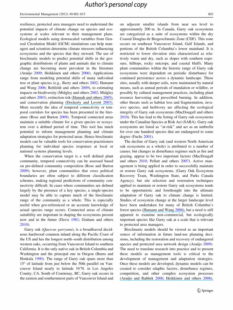
resilience, protected area managers need to understand the

potential impacts of climate change on species and eco-

systems at scales relevant to their management plans.

Ecological models using downscaled variables from Gen-

eral Circulation Model (GCM) simulations can help man-

agers and scientists determine climate stressors influencing

ecosystems and the species that they steward. The use of

bioclimatic models to predict potential shifts in the geo-

graphic distributions of plants and animals due to climate

change are becoming more prevalent in the literature

(Araujo 2009; Heikkinen and others 2006). Applications

range from modeling potential shifts of many individual

tree or plant species (e.g., Berry and others 2002; Hamann

and Wang 2006; Rehfeldt and others 2009), to estimating

impacts on biodiversity (Midgley and others 2002; Midgley

and others 2003), extinction risk (Hannah and others 2005),

and conservation planning (Dockerty and Lovett 2003).

More recently the idea of temporal connectivity or tem-

poral corridors for species has been presented in the liter-

ature (Rose and Burton 2009). Temporal connected areas

maintain a suitable climate for a given species or ecosys-

tem over a defined period of time. This tool has much

potential to inform management planning and climate

adaptation strategies for protected areas. Hence bioclimatic

models can be valuable tools for conservation practitioners

planning for individual species responses at local or

national systems planning levels.

When the conservation target is a well defined plant

community, temporal connectivity can be assessed based

on pre-defined community composition (Rose and Burton

2009); however, plant communities that cross political

boundaries are often subject to different classification

schemes, making regional predictions of community con-

nectivity difficult. In cases where communities are defined

largely by the presence of a key species, a single-species

model may be able to capture much of the bioclimatic

range of the community as a whole. This is especially

useful when geo-referenced or an accurate knowledge of

actual species range occurs. Connected areas of climate

suitability are important in shaping the ecosystems present

now and in the future (Davis 1981; Graham and others

2010).

Garry oak (Quercus garryana), is a broadleaved decid-

uous hardwood common inland along the Pacific Coast of

the US and has the longest north–south distribution among

western oaks, occurring from Vancouver Island to southern

California. It is the only native oak in British Columbia and

Washington and the principal one in Oregon (Burns and

Honkala 1990). The range of Garry oak spans more than

15� of latitude from just below the 50th parallel on Van-

couver Island nearly to latitude 34�N. in Los Angeles

County, CA. South of Courtenay, BC, Garry oak occurs in

the eastern and southernmost parts of Vancouver Island and

on adjacent smaller islands from near sea level to

approximately 200 m. In Canada, Garry oak ecosystems

are categorized as a suite of ecosystems within the dry

Coastal Douglas-fir Biogeoclimatic Zone (CDF). This zone

occurs on southeast Vancouver Island, Gulf Islands, and

portions of the British Columbia’s lower mainland. It is

restricted to lower elevation sites characterized as rela-

tively warm and dry, such as slopes with southern expo-

sure, hilltops, rocky outcrops, and coastal bluffs. Many

plant communities within the historic range of Garry oak

ecosystems were dependent on periodic disturbance for

continued persistence across a dynamic landscape. These

sites, usually with deeper soils, were maintained by natural

means, such as annual periods of inundation or wildfire, or

possibly by cultural management practices, including plant

resource harvesting and prescribed burning. In addition,

other threats such as habitat loss and fragmentation, inva-

sive species, and herbivory are affecting the ecological

integrity of Garry oak ecosystems (MacDougall and others

2010). This has lead to the listing of Garry oak ecosystems

under the Canadian Species at Risk Act (SARA). Garry oak

ecosystems are listed as ‘‘at-risk’’ and act as an umbrella

for over one hundred species that are endangered to some

degree (Fuchs 2001).

The decline of Garry oak (and western North American

oak ecosystems as a whole) is attributed to a number of

causes, but changes in disturbance regimes such as fire and

grazing, appear to be two important factors (MacDougall

and others 2010; Pellatt and others 2007). Active man-

agement is being applied in order to successfully maintain

or restore Garry oak ecosystems, (Garry Oak Ecosystem

Recovery Team, Washington State, and Parks Canada

Agency), but site selection and restoration techniques

applied to maintain or restore Garry oak ecosystems tends

to be opportunistic and forethought into the ultimate

adaptation of Garry oak to climate change is limited.

Studies of ecosystem change at the larger landscape level

have been undertaken for many of British Columbia’s

forest species (Hamann and Wang 2006), but a need is still

apparent to examine non-commercial, but ecologically

important species like Garry oak at a scale that is relevant

to protected area managers.

Bioclimatic models should be viewed as an important

source of information in future land-use planning deci-

sions, including the restoration and recovery of endangered

species and protected area network design (Araujo 2009).

The need to translate research into practice and to present

these models as management tools is critical to the

development of management and adaptation strategies.

Once these models are developed, dynamic models can be

created to consider edaphic factors, disturbance regimes,

competition, and other complex ecosystem processes

(Araujo and Rahbek 2006; Heikkinen and others 2006).

Environmental Management (2012) 49:802–815 803

123

Author's personal copy

The bioclimatic models presented in this paper are to be

included in protected area management plans. These plans

will inform species recovery groups about possible climate

change impacts on Garry oak ecosystems and provide

direction for ecosystem restoration projects that use best

practices by including climate change adaptation of Garry

oak into the planning process. This information is partic-

ularly important because the rate of expected climate

change may well be unprecedented during the Holocene

resulting in climates and ecosystems with no modern or

past analogue (Froyd and Willis 2008; Williams and others

2007).

The objectives of this study are to build upon and refine

work by Bodtker and others (2009) and apply it to the

question of protected area planning under changing climate

scenarios that are projected until the end of the 21st century.

Garry oak ecosystems are one of the most endangered

ecosystems in Canada and the Parks Canada Agency has

established the Gulf Island National Park Reserve (GINPR)

in a region where these ecosystems occur. Under Canada’s

Species at Risk Act (SARA), Parks Canada is the lead

federal agency responsible for the recovery of Garry oak

ecosystems, so obvious interest exists in the long term via-

bility of the national park reserve in the protection of these

ecosystems. Fully realizing that international, provincial,

and local cooperation is needed to maintain, restore, and

allow for future adaptation of at-risk species in Garry oak

ecosystems, we evaluate the level of protection of Garry oak

at present and then forecast how well protected areas in the

Pacific Northwest of North America encompass climatically

suitable Garry oak habitat in the future. We then identify the

areas that are predicted to maintain climatic suitability in all

temporal scenarios that we examine. Most importantly we

generate scenarios examining temporally connected areas

that persist throughout the 21st century for Garry oak as well

as how well existing protected areas overlap these tempo-

rally connected regions.

Data and Methods

Study Area

To build a quantitative model of the relationship between a

species or ecosystem and the total range of current climatic

values, the complete global distribution of the species

should ideally be considered (Dockerty and Lovett 2003).

In this case we felt an exception was warranted. Although

Garry oak extends as far south as 35�North (Fig. 1), the

composition of Garry oak-related ecosystems in the region

south of Oregon is significantly different from those to the

north (Fuchs 2001) so we did not include California in the

study area. Based on biogeographic and ecological

characteristics of Garry oak ecosystems in North America

and our knowledge of future climate scenarios, we included

areas to the north and east of the current Garry oak range,

defining a study area extending from 42�–51� North lati-

tude and 119�–129� West longitude, an area encompassing

southwestern British Columbia, Washington, and Oregon

(Fig. 1).

Climate Data

Climate Data for Model Building

In order to develop a bioclimate envelope model at a

suitable spatial scale for our objectives, a resolution

1 9 1 km was used. The 1 9 1 km resolution for the study

area resulted in a raster size of 660 9 1,168 grid cells, of

which 428,592 were on land. To generate the 33 down-

scaled climate variables at the 1 9 1 km resolution used in

this study, a bilinear interpolation/polynomial regression-

based lapse rate upsampling algorithm was applied to a

merged 4 km US/Canada Parameter Regression on Inde-

pendent Slopes Model (PRISM) (Daly and others 1994,

1997) 1961–1990 climate normal dataset following Wang

and others (2006). Using climatologically-aided interpola-

tion (Willmott and Robeson 1995), Global Climate Model

(GCM) scenarios were generated by superimposing future

Fig. 1 Study area and present extent of Garry oak in British

Columbia, Washington, and Oregon. Red represents actual occurrence

of Garry oak. Green represents the location of protected areas

804 Environmental Management (2012) 49:802–815

123

Author's personal copy

GCM climate anomalies relative to the 1961–1990 period

overtop the 1 9 1 km downscaled climate normals

(Table 1).

Climate Data for Scenario Development

In this study we develop a presence/absence (P/A) model

for Garry oak under various future climate scenarios pre-

dicted by four GCMs (CCSRNIES, CSIRO, CGCM2 and

the HADCM3). Each model uses GCM data to predict

conditions driven by two future emissions scenarios: Sce-

nario A2 is driven by a continuously growing world pop-

ulation with regionally oriented economic development

and slow technological advancement. Scenario B2 is driven

by continuous population growth at a lower rate than sce-

nario A2 with emphasis on local solutions to economic,

social and environmental stability, and thus, overall lower

CO2 concentrations than the A2 scenario.

For the development of Garry oak climate suitability

scenarios, we constructed two parallel models using output

from four GCMs. This was done because confidence in

precipitation values modelled using GCMs are generally

lower than for temperature variables. The first model uses a

number of climate parameters selected for their ecological

relevance including temperature and precipitation vari-

ables, the second uses only temperature variables

(Table 2).

We chose to use outputs from four GCMs in an effort to

compare outputs across a range of possible future scenar-

ios. Individual GCM models share some assumptions about

climatological phenomena, but differ in the full suite of

assumptions and also in the mechanics of the model, often

resulting in variable outputs, especially at longer time-

scales (Salathe and others 2007). Prior analysis by Salathe

and others (2007) in the Pacific Northwest indicates that

the models vary both in their expressions of modern cli-

mate normals and in their expressions of future climate

change (Table 3). Since the outcomes from these four

models broadly represent anticipated model outcomes for

the region we believe that they are appropriate for our P/A

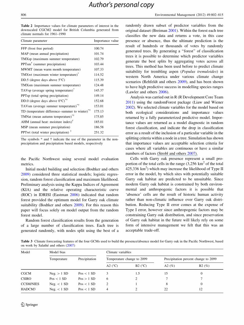
modeling. Importance values for the Garry oak models

indicate that P/A is most strongly determined by winter

precipitation, mean summer precipitation and the annual

heat:moisture index (Table 2).

Model Building

The P/A model for Garry oak is generated using random

forest (Breiman 2001), based on downscaled modern cli-

mate normals (1961–1990; Wang and others 2006) and the

geo-referenced distribution of Garry oak in the Pacific

Northwest region of North America (Chappell and others

2003, Ecological Society of America 2006, Harrington

2003, Klinkenberg 2004). Preliminary work on the

assessment and comparison of downscaled climate models,

different GCMs, and statistical models to develop a bio-

climatic envelope model for Garry oak was undertaken by

Bodtker and others (2009) who were able to show that

random forest (Breiman 2001) models provide the best

predictive accuracy of modern Garry oak distributions in

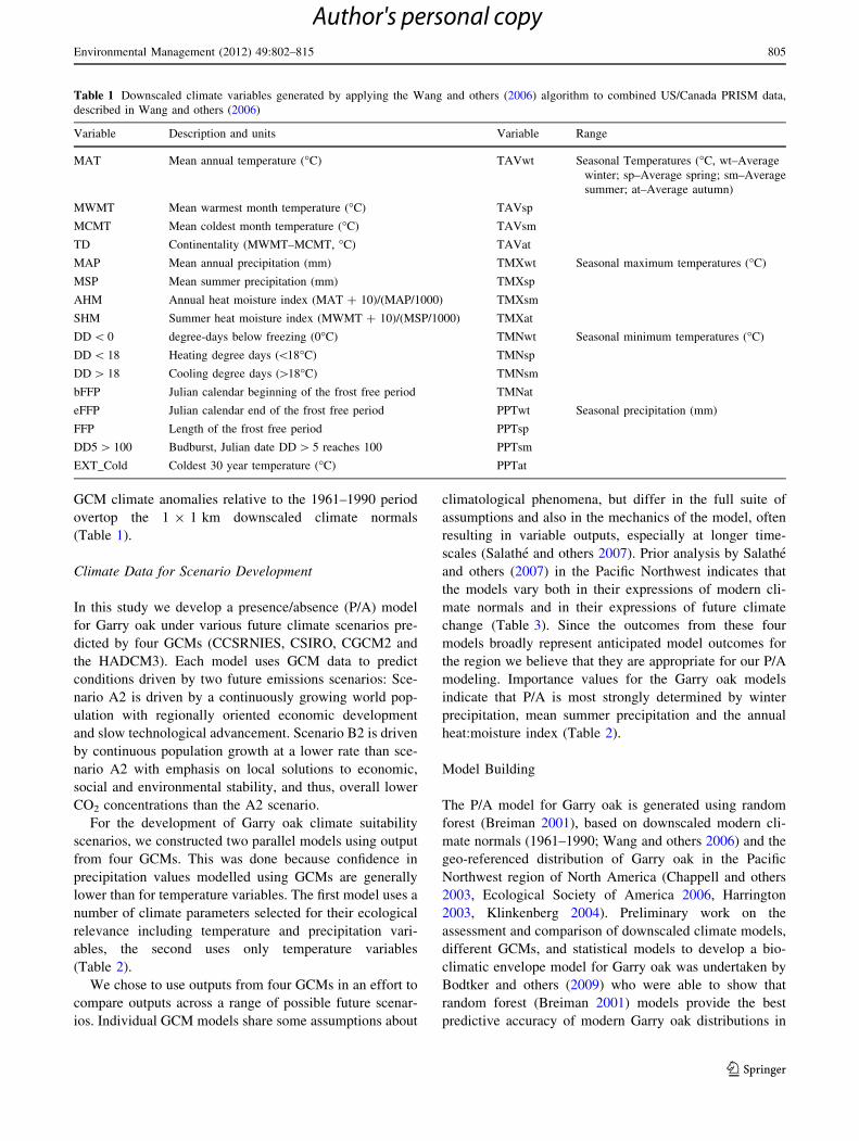
Table 1 Downscaled climate variables generated by applying the Wang and others (2006) algorithm to combined US/Canada PRISM data,

described in Wang and others (2006)

Variable Description and units Variable Range

MAT Mean annual temperature (�C) TAVwt Seasonal Temperatures (�C, wt–Average

winter; sp–Average spring; sm–Average

summer; at–Average autumn)

MWMT Mean warmest month temperature (�C) TAVsp

MCMT Mean coldest month temperature (�C) TAVsm

TD Continentality (MWMT–MCMT, �C) TAVat

MAP Mean annual precipitation (mm) TMXwt Seasonal maximum temperatures (�C)

MSP Mean summer precipitation (mm) TMXsp

AHM Annual heat moisture index (MAT ? 10)/(MAP/1000) TMXsm

SHM Summer heat moisture index (MWMT ? 10)/(MSP/1000) TMXat

DD \ 0 degree-days below freezing (0�C) TMNwt Seasonal minimum temperatures (�C)

DD \ 18 Heating degree days (\18�C) TMNsp

DD [ 18 Cooling degree days ([18�C) TMNsm

bFFP Julian calendar beginning of the frost free period TMNat

eFFP Julian calendar end of the frost free period PPTwt Seasonal precipitation (mm)

FFP Length of the frost free period PPTsp

DD5 [ 100 Budburst, Julian date DD [ 5 reaches 100 PPTsm

EXT_Cold Coldest 30 year temperature (�C) PPTat

Environmental Management (2012) 49:802–815 805

123

Author's personal copy

the Pacific Northwest using several model evaluation

metrics.

Initial model building and selection (Bodtker and others

2009) considered three statistical models; logistic regres-

sion, random forest classification and maximum likelihood.

Preliminary analysis using the Kappa Indices of Agreement

(KIA) and the relative operating characteristic curve

(ROC) in IDRISI (Eastman 2006) indicated that random

forest provided the optimum model for Garry oak climate

suitability (Bodtker and others 2009). For this reason this

paper will focus solely on model output from the random

forest model.

Random forest classification results from the generation

of a large number of classification trees. Each tree is

generated randomly, with nodes split using the best of a

randomly drawn subset of predictor variables from the

original dataset (Breiman 2001). Within the forest each tree

classifies the new data and returns a vote, in this case

presence or absence, thus the ultimate prediction is the

result of hundreds or thousands of votes by randomly

generated trees. By generating a ‘‘forest’’ of classification

trees it is possible to determine which predictor variables

generate the best splits by aggregating votes across all

trees. This method has been used before to predict climate

suitability for trembling aspen (Populus tremuloides) in

western North America under various climate change

scenarios (Rehfeldt and others 2009), and has been shown

to have high predictive success in modelling species ranges

(Lawler and others 2006).

Analysis was carried out in R (R Development Core Team

2011) using the randomForest package (Liaw and Wiener

2002). We selected climate variables for the model based on

both ecological considerations and importance values

returned by a fully parameterized predictive model. Impor-

tance values are returned as a model diagnostic in random

forest classification, and indicate the drop in classification

error as a result of the inclusion of a particular variable in the

splitting criteria within a node in a tree. Simulation has shown

that importance values are acceptable selection criteria for

cases where all variables are continuous or have a similar

numbers of factors (Strobl and others 2007).

Cells with Garry oak presence represent a small pro-

portion of the total cells in the range (3,256 km2 of the total

425,336 km2) which may increase the likelihood of Type II

error in the model, by which sites with potentially suitable

Garry oak habitat are predicted to be unsuitable. Since

modern Garry oak habitat is constrained by both environ-

mental and anthropogenic factors it is possible that

‘absence’ cells are the result of historic human activity

rather than non-climatic influence over Garry oak distri-

bution. Reducing Type II error comes at the expense of

Type I error, however since anthropogenic factors may be

constraining Garry oak distribution, and since preservation

of Garry oak habitat in the future will likely rely on some

form of intensive management we felt that this was an

acceptable trade-off.

Table 3 Climate forecasting features of the four GCMs used to build the presence/absence model for Garry oak in the Pacific Northwest, based

on work by Salathe and others (2007)

Model Model bias Climate variables

Temperature Precipitation Temperature change to 2099 Precipitation percent change to 2099

A2 (�C) B2 (�C) A2 (%) B2 (%)

CGCM Neg. [ 1 SD Pos \ 1 SD 3 1.5 15 0

CSIRO Pos \ 1 SD Pos [ 1 SD 6 2 7 7

CCSM/NIES Neg. \ 1 SD Pos \ 1 SD 2 1 8 0

HADCM3 Neg. \ 1 SD Pos \ 1 SD 4 2 22 12

Table 2 Importance values for climate parameters of interest in the

downscaled CGCM2 model for British Columbia generated from

climate normals for 1961–1990

Climate parameter Importance value

FFP (frost free period) 100.74

MAP (mean annual precipitation) 101.74

TMXsp (maximum summer temperature) 102.79

PPTsm� (summer precipitation) 103.44

MWMT (mean warm month temperature) 107.33

TMXwt (maximum winter temperature)* 114.52

DD.5 (degree days above 5�C) 115.39

TMXsm (maximum summer temperature) 124.48

TAVsp (average spring temperature)* 145.37

PPTsp (total spring precipitation) 149.14

DD.0 (degree days above 0�C)*� 152.68

TAVsm (average summer temperature)*� 153.01

TD (temperature difference–summer to winter)*� 175.13

TMNat (mean autumn temperature)*� 175.85

AHM (annual heat: moisture index)� 185.01

MSP (mean summer precipitation) 186.58

PPTwt (total winter precipitation) � 251.32

The symbols * and � indicate the use of the parameter in the non-

precipitation and precipitation based models, respectively

806 Environmental Management (2012) 49:802–815

123

Author's personal copy

To reduce Type II error we built the model using only

terrestrial cells within 40 km of a cell with known Garry

oak presence rather than the entire study region. Reducing

the total number of cells in this way increased the per-

centage of Garry oak cells to 2.1% of the total dataset.

Since we are more interested in regions that may be suit-

able for Garry oak in the future we wanted to give greater

weight to Garry oak cells. To do this we then constructed

the models by sub-sampling the absence cells, so that they

equalled the number of Garry oak cells. Because the

selection of absence cells was likely to affect the model we

repeated this procedure 100 times, generating 100 separate

P/A predictions for Garry oak, each time re-sampling

the absence cells so that they were equal in number to the

presence cells. We report presence as any site for which the

model predicts presence in more than 50% of the cases.

Protected Area Networks

The ultimate goal of this work is to assess scenarios gen-

erated for Garry oak climate suitability for the network of

protected areas in British Columbia, Washington, and

Oregon over the 21st century. Of particular interest are

areas that maintain continual climate suitability for Garry

oak ecosystems. These results can then assist in regional

planning for Garry oak ecosystem conservation in the

foreseeable future.

A network of protected areas exists through the study

region with a total area of 169,904 km2. Protected areas

range in size from 25 m2 (part of the WA state land trust)

to 50,447 km2 (Oregon, Bureau of Land Management).

The distribution of area values is highly skewed; the

average area is 27 km2 while the median is 0.18 km2. For

the purpose of this study we define protected areas as all

lands protected as parks, various forms of ecological

reserves, experimental forests, or recreation areas by fed-

eral, state or provincial governments. This includes lands

managed by the Parks Canada Agency, the British

Columbia Ministry of the Environment, the United States

Forest Service, the Bureau of Land Management, and the

United States National Parks Service. In practice this land

may currently be under management for resource extrac-

tion, however our objective is to demonstrate the extent of

the landscape upon which management practices may

result in preservation or expansion of suitable habitat and

so our definition of what may constitute protected areas is

broad since we believe that the larger the number of

stakeholders, the greater the possibility that some will

change management practices to accommodate Garry oak

ecosystem adaptation.

The spatial data for the United States was obtained from

the Protected Areas Database (The Conservation Biology

Institute. May 2010. PAD-US 1.1 (CBI Edition). Corvallis,

Oregon) while Canadian data was obtained through

Geogratis (http://geogratis.cgdi.gc.ca). Because of admin-

istrative differences between the United States and Canada,

the extent of managed land in Canada is underreported.

Much of the land base is retained by the Government of

British Columbia and is leased to resource users. This

means that there is land in British Columbia that may have

the potential for the active management of Garry oak that is

currently undergoing resource extraction. Protected areas

in the US are defined as all locations with an IUCN con-

servation ranking based on the PAD-US dataset. Within

British Columbia all protected areas administered by

municipal, provincial, or federal authorities (i.e., National

and Provincial parks, wildlife reserves, conservation areas

and regional parks) jurisdiction are considered as protected.

Much original Garry oak habitat has been lost due to

development and many of the ecological processes neces-

sary for Garry oak persistence have been altered (Lea 2007;

Pellatt and others 2007; Vellend and others 2008; Mac-

Dougall and others 2010). The extent of development

around deep-soiled sites that are presumed to be central to

Garry oak habitat means that changes in habitat suitability

may place serious pressures on the ability of Garry oak to

again reach equilibrium with a changing climate. The

extent of development may also affect our ability to predict

suitable habitat, since much of the original habitat extent

may be lost. This may be offset in part by our grid reso-

lution. The presence of a single Garry oak tree within a

1 km2 grid cell will result in that cell being classified as

indicating presence. However, for this reason we will

principally be investigating the changes in habitat suit-

ability among the region’s protected areas.

Results

Model Output

The fully parameterized (FPm) model using climate nor-

mals from 1961–1990 had a bootstrapped (n = 100) error

of 9.2 ± 0.3%. The smaller model (Pm) including precip-

itation and temperature values (Table 2, parameters indi-

cated by dagger) had an error that was not significantly

different than the model using only temperature-based

variables (NPm; t = -4.01, df = 195.6, P \ 0.001). The

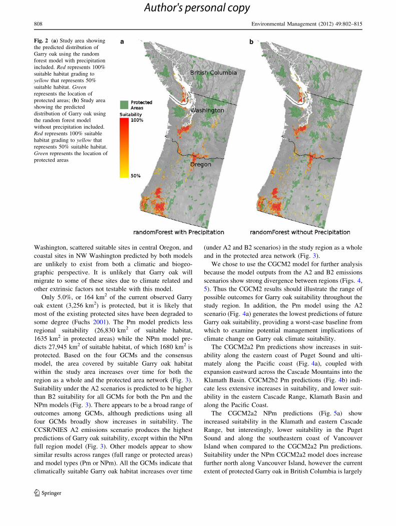
extent of suitable Garry oak sites predicted by the modern

models is broader than the current Garry oak extent, and

Garry oak suitability is predicted in regions that do not

currently support Garry oak populations. The NPm model

predicts a broader extent for Garry oak suitability, specif-

ically indicating broader suitability on the mid-Oregon

coast and along the northern edge of the Olympic Peninsula

in Washington (Fig. 2a, b). The populations in central

Environmental Management (2012) 49:802–815 807

123

Author's personal copy

Washington, scattered suitable sites in central Oregon, and

coastal sites in NW Washington predicted by both models

are unlikely to exist from both a climatic and biogeo-

graphic perspective. It is unlikely that Garry oak will

migrate to some of these sites due to climate related and

other extrinsic factors not testable with this model.

Only 5.0%, or 164 km2 of the current observed Garry

oak extent (3,256 km2) is protected, but it is likely that

most of the existing protected sites have been degraded to

some degree (Fuchs 2001). The Pm model predicts less

regional suitability (26,830 km2 of suitable habitat,

1635 km2 in protected areas) while the NPm model pre-

dicts 27,945 km2 of suitable habitat, of which 1680 km2 is

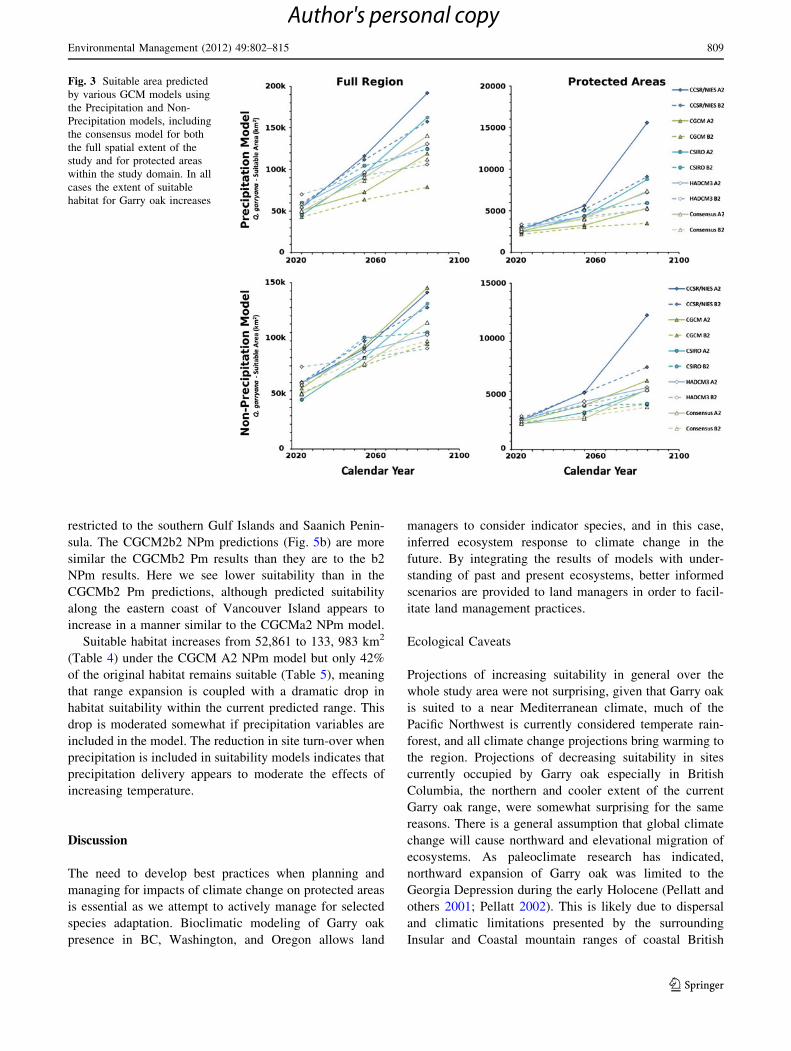
protected. Based on the four GCMs and the consensus

model, the area covered by suitable Garry oak habitat

within the study area increases over time for both the

region as a whole and the protected area network (Fig. 3).

Suitability under the A2 scenarios is predicted to be higher

than B2 suitability for all GCMs for both the Pm and the

NPm models (Fig. 3). There appears to be a broad range of

outcomes among GCMs, although predictions using all

four GCMs broadly show increases in suitability. The

CCSR/NIES A2 emissions scenario produces the highest

predictions of Garry oak suitability, except within the NPm

full region model (Fig. 3). Other models appear to show

similar results across ranges (full range or protected areas)

and model types (Pm or NPm). All the GCMs indicate that

climatically suitable Garry oak habitat increases over time

(under A2 and B2 scenarios) in the study region as a whole

and in the protected area network (Fig. 3).

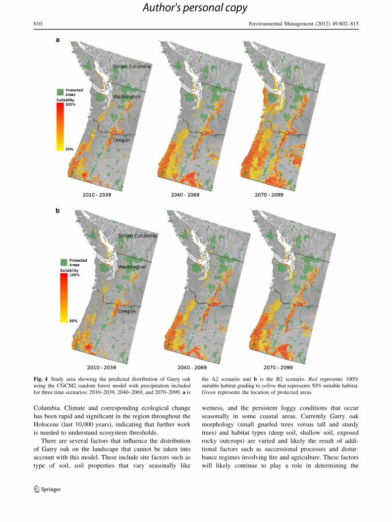
We chose to use the CGCM2 model for further analysis

because the model outputs from the A2 and B2 emissions

scenarios show strong divergence between regions (Figs. 4,

5). Thus the CGCM2 results should illustrate the range of

possible outcomes for Garry oak suitability throughout the

study region. In addition, the Pm model using the A2

scenario (Fig. 4a) generates the lowest predictions of future

Garry oak suitability, providing a worst-case baseline from

which to examine potential management implications of

climate change on Garry oak climate suitability.

The CGCM2a2 Pm predictions show increases in suit-

ability along the eastern coast of Puget Sound and ulti-

mately along the Pacific coast (Fig. 4a), coupled with

expansion eastward across the Cascade Mountains into the

Klamath Basin. CGCM2b2 Pm predictions (Fig. 4b) indi-

cate less extensive increases in suitability, and lower suit-

ability in the eastern Cascade Range, Klamath Basin and

along the Pacific Coast.

The CGCM2a2 NPm predictions (Fig. 5a) show

increased suitability in the Klamath and eastern Cascade

Range, but interestingly, lower suitability in the Puget

Sound and along the southeastern coast of Vancouver

Island when compared to the CGCM2a2 Pm predictions.

Suitability under the NPm CGCM2a2 model does increase

further north along Vancouver Island, however the current

extent of protected Garry oak in British Columbia is largely

Fig. 2 (a) Study area showing

the predicted distribution of

Garry oak using the random

forest model with precipitation

included. Red represents 100%

suitable habitat grading to

yellow that represents 50%

suitable habitat. Greenrepresents the location of

protected areas; (b) Study area

showing the predicted

distribution of Garry oak using

the random forest model

without precipitation included.

Red represents 100% suitable

habitat grading to yellow that

represents 50% suitable habitat.

Green represents the location of

protected areas

808 Environmental Management (2012) 49:802–815

123

Author's personal copy

restricted to the southern Gulf Islands and Saanich Penin-

sula. The CGCM2b2 NPm predictions (Fig. 5b) are more

similar the CGCMb2 Pm results than they are to the b2

NPm results. Here we see lower suitability than in the

CGCMb2 Pm predictions, although predicted suitability

along the eastern coast of Vancouver Island appears to

increase in a manner similar to the CGCMa2 NPm model.

Suitable habitat increases from 52,861 to 133, 983 km2

(Table 4) under the CGCM A2 NPm model but only 42%

of the original habitat remains suitable (Table 5), meaning

that range expansion is coupled with a dramatic drop in

habitat suitability within the current predicted range. This

drop is moderated somewhat if precipitation variables are

included in the model. The reduction in site turn-over when

precipitation is included in suitability models indicates that

precipitation delivery appears to moderate the effects of

increasing temperature.

Discussion

The need to develop best practices when planning and

managing for impacts of climate change on protected areas

is essential as we attempt to actively manage for selected

species adaptation. Bioclimatic modeling of Garry oak

presence in BC, Washington, and Oregon allows land

managers to consider indicator species, and in this case,

inferred ecosystem response to climate change in the

future. By integrating the results of models with under-

standing of past and present ecosystems, better informed

scenarios are provided to land managers in order to facil-

itate land management practices.

Ecological Caveats

Projections of increasing suitability in general over the

whole study area were not surprising, given that Garry oak

is suited to a near Mediterranean climate, much of the

Pacific Northwest is currently considered temperate rain-

forest, and all climate change projections bring warming to

the region. Projections of decreasing suitability in sites

currently occupied by Garry oak especially in British

Columbia, the northern and cooler extent of the current

Garry oak range, were somewhat surprising for the same

reasons. There is a general assumption that global climate

change will cause northward and elevational migration of

ecosystems. As paleoclimate research has indicated,

northward expansion of Garry oak was limited to the

Georgia Depression during the early Holocene (Pellatt and

others 2001; Pellatt 2002). This is likely due to dispersal

and climatic limitations presented by the surrounding

Insular and Coastal mountain ranges of coastal British

Fig. 3 Suitable area predicted

by various GCM models using

the Precipitation and Non-

Precipitation models, including

the consensus model for both

the full spatial extent of the

study and for protected areas

within the study domain. In all

cases the extent of suitable

habitat for Garry oak increases

Environmental Management (2012) 49:802–815 809

123

Author's personal copy

Columbia. Climate and corresponding ecological change

has been rapid and significant in the region throughout the

Holocene (last 10,000 years), indicating that further work

is needed to understand ecosystem thresholds.

There are several factors that influence the distribution

of Garry oak on the landscape that cannot be taken into

account with this model. These include site factors such as

type of soil, soil properties that vary seasonally like

wetness, and the persistent foggy conditions that occur

seasonally in some coastal areas. Currently Garry oak

morphology (small gnarled trees versus tall and sturdy

trees) and habitat types (deep soil, shallow soil, exposed

rocky outcrops) are varied and likely the result of addi-

tional factors such as successional processes and distur-

bance regimes involving fire and agriculture. These factors

will likely continue to play a role in determining the

Fig. 4 Study area showing the predicted distribution of Garry oak

using the CGCM2 random forest model with precipitation included

for three time scenarios: 2010–2039, 2040–2069, and 2070–2099. a is

the A2 scenario and b is the B2 scenario. Red represents 100%

suitable habitat grading to yellow that represents 50% suitable habitat.

Green represents the location of protected areas

810 Environmental Management (2012) 49:802–815

123

Author's personal copy

distribution of Garry oak at a fine scale in areas where it is

climatically suitable.

Since deglaciation (last *12,000 years) climate has

been the primary driver of Garry oak distribution in the

Pacific Northwest of North America (Pellatt and others

2001, 2007). Even with the ever increasing pressure of

habitat loss, climate change impacts will likely deleteri-

ously affect Garry oak ecosystems; rapid change in eco-

system structure due to climate change, invasive species,

species migration, suppression of natural disturbance

regimes, and habitat fragmentation should be expected to

affect Garry oak and associated ecosystems (Shafer and

others 2001; Pellatt and others 2007).

Protected Areas

Protected areas represent a long-term commitment to the

conservation of species, ecological processes and, in many

Fig. 5 Study area showing the predicted distribution of Garry oak

using the CGCM2 random forest model without precipitation

included for three time scenarios: 2010–2039, 2040–2069, and

2070–2099. a is the A2 scenario and b is the B2 scenario. Redrepresents 100% suitable habitat grading to yellow that represents

50% suitable habitat. Green represents the location of protected areas

Environmental Management (2012) 49:802–815 811

123

Author's personal copy

cases, associated cultural values and resources. They are

often accorded legal recognition, have agreed-upon man-

agement and governance approaches, and are supported by

management planning and capacity. It is these qualities that

make investments in protected area establishment and

management cost-effective in the context of climate change

adaptation. There will be pressure to reconsider what the

perceived function of a protected area is as the ecosystems

within it begin to change. The need to critically assess the

purpose of a particular area may serve to determine if it

will remain relevant to the public. We have moved from a

single species approach to an ecosystem-based approach to

protected area management, but still we need to consider

ecosystems in the context of a larger temporal framework.

The paucity of protected areas in locations critical for

the protection of Garry oak ecosystems, now, and in future

climatically suitable areas, appears to be the greatest

challenge for conservation of the species when considering

future global change.

Temporal Connectivity

Although climatically suitable Garry oak habitat will

increase somewhat, primarily in the USA, this habitat will

not be well represented in IUCN Classes I through V

Protected Areas (5.6–7.3%). The distribution of protected

areas in relation to temporally connected climatically

suitable areas between 2010 and 2099 is shown in Fig. 6a

(CGCM2a2), b (CGCM2b2). Of the protected area that

currently contains suitable Garry oak habitat, our models

indicate that between 6.6 and 7.3% will be ‘‘temporally

connected’’ between 2010 and 2099. The CGCM2

Table 4 Change in Garry oak habitat suitability based on the CGCM2–A2 model for climate change. The size of the area of interest is

428,592 km2. Precipitation (PPT)

2010–2039 2040–2069 2070–2099

With PPT

(km2)

Without PPT

(km2)

With PPT

(km2)

Without PPT

(km2)

With PPT

(km2)

Without PPT

(km2)

CGCMa2

Total Region

Predicted suitable habitat 51,947 52,861 84,687 80,737 137,053 133,983

Protected area network 20,548 22,392 37,250 37,255 59,931 60,343

Canada

Predicted suitable habitat 1528 1328 1258 4345 3575 9933

Protected area network 265 108 344 714 985 1435

CGCMb2

Total Region

Predicted suitable habitat 42,376 52,942 69,175 65,398 81,841 83,367

Protected area network 16,057 20,686 29,803 30,733 37,133 38,085

Canada

Predicted suitable habitat 2701 1885 1889 2616 1443 5934

Protected area network 512 166 471 297 380 937

Table 5 Overlap between Garry oak suitable habitat across time-steps using models for the CGCM2a2 and CGCM2b2 climate change models

2010–2039 2040–2069 2070–2099

With PPT (%) Without PPT (%) With PPT (%) Without PPT (%) With PPT (%) Without PPT (%)

CGCMa2

Modern 20.00 20.20 30.40 26.40 45.90 42.20

2010–2039 – – 85.60 62.80 84.40 72.40

2040–2069 – – – – 90.20 79.30

CGCMb2

Modern 17.10 20.20 25.70 22.40 29.70 26.80

2010–2039 – – 75.00 57.10 72.60 56.20

2040–2069 – – – – 90.60 80.60

Each value is calculated as the percentage of the total area predicted by the model at the time indicated by the row heading still covered at the

column heading

812 Environmental Management (2012) 49:802–815

123

Author's personal copy

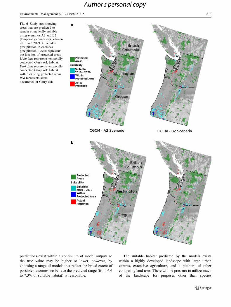
predictions exist within a continuum of model outputs so

the true value may be higher or lower, however, by

choosing a range of models that reflect the broad extent of

possible outcomes we believe the predicted range (from 6.6

to 7.3% of suitable habitat) is reasonable.

The suitable habitat predicted by the models exists

within a highly developed landscape with large urban

centres, extensive agriculture, and a plethora of other

competing land uses. There will be pressure to utilize much

of the landscape for purposes other than species

Fig. 6 Study area showing

areas that are predicted to

remain climatically suitable

using scenarios A2 and B2

(temporally connected) between

2010 and 2099. a includes

precipitation. b excludes

precipitation. Green represents

the location of protected areas.

Light blue represents temporally

connected Garry oak habitat.

Dark Blue represents temporally

connected Garry oak habitat

within existing protected areas.

Red represents actual

occurrence of Garry oak

Environmental Management (2012) 49:802–815 813

123

Author's personal copy

conservation hence selecting ‘‘critical habitat’’ identified as

climatically and ecologically suitable in the future will be

essential for the adaptation of Garry oak and its associated

ecosystems. There will likely be increased pressure to

reconsider what the perceived function of a protected area

is as the ecosystems within in it begin to change, and best

practices that will help maintain ecosystems that are more

resistant to invasive species and other stressors exacerbated

by climate change will be essential. We believe that

understanding the temporal connectivity of climatically

suitable habitat for species is a component of these best

practices. Temporal connectivity of suitable climate is

critical to the formation of ecosystems. In the past these are

represented by dynamic refugia, for example, glacial

refugia and climatically suitable migration corridors

throughout the Holocene and deep time (Davis 1981;

Graham and others 2010). There can be no question that

these climatically suitable corridors and refugia will be key

factors in the conservation of biodiversity and ecosystems,

now, and in the future.

Acknowledgments The Climate Change Action Fund (Project

A718), Interdepartmental Recovery Fund (Project 733), Parks Can-

ada—Western and Northern Service Centre, and the Natural Science

and Engineering Research Council of Canada (NSERC) provided

financial support for the project to M.G. Pellatt. S. Goring is sup-

ported by a NSERC RC PGS-D3 scholarship. We would like to thank

D. Peter and C. Harrington of the US. Department of Agriculture

Forest Service, C. Chappell of the Washington Department of Natural

Resources, Ted Lea, the British Columbia Ministry of the Environ-

ment, VegBank (NatureServe), E-Flora (UBC), and D.Hrynyk (Parks

Canada) for data contributions. We would also like to extend our

appreciation to three anonymous reviewers whose positive comments

helped improve the manuscript.

References

Araujo MB (2009) Climate change and spatial conservation planning.

In: Moilenen A, Wilson KA, Possingham HP (eds) Spatial

conservation prioritization: quantitative methods and computa-

tional tools. Oxford University Press, New York

Araujo MB, Rahbek C (2006) How does climate change affect

biodiversity? Science 313:1396–1397

Berry PM, Dawson TP, Harrison PA, Pearson RG (2002) Modelling

potential impacts of climate change on the bioclimatic envelope

of species in Britain and Ireland. Global Ecology & Biogeog-

raphy 11:453–462

Bodtker KM, Pellatt MG, Cannon AJ (2009) A bioclimatic model to

assess the impact of climate change on ecosystems at risk and

inform land management decisions. Report for the Climate

Change Impacts and Adaptation Directorate, CCAF Project

A718. Western and Northern Service Centre, Vancouver

Breiman L (2001) Random Forests. Machine Learning 45:5–32

Burns RM, Honkala BH (1990) Silvics of North America: 1. Conifers;

2. Hardwoods Agriculture Handbook 654, vol 2. US Department

of Agriculture, Forest Service, Washington, DC

Chappell CB, Gee MS, Stephens B (2003) A geographic information

system map of existing grasslands and oak woodlands in the

Puget lowland and Willamette valley ecoregions, Washington.

Washington Natural Heritage Program, Washington Department

of Natural Resources, Olympia (http://www.dnr.wa.gov/nhp/

refdesk/gis/oakgrsld.html)

Daly C, Neilson RP, Phillips DL (1994) A statistical-topographic

model for mapping climatological precipitation over mountain-

ous terrain. Journal of Applied Meteorology 33:140–158

Daly C, Taylor G, Gibson W (1997) The PRISM approach to mapping

precipitation and temperature, 10th Conference on Applied

Climatology. American Meteorological Society, Reno NV,

pp 10–12

Davis MB (1981) Quaternary history and the stability of forest

communities. In:West DC, Shugart HH, Botkin DB (eds) Forest

succession concepts and application. Springer Verlag, New

York, pp 132–153

Dockerty T, Lovett A (2003) A location-centred, GIS-based meth-

odology for estimating the potential impacts of climate change

on nature reserves. Transactions in GIS 7:345–370

Eastman JR (2006) IDRISI Andes. Clark University, Worcester

Ecological Society of America (2006) VegBank on-line database.

http://vegbank.org/cite/VB.Ob.17196.INW28670, VB.Ob.18019.

INW29518, VB.Ob.18020.INW29519, VB.Ob.18021.INW29520,

VB.Ob.18023.INW29522, VB.Ob.18032.INW29531, VB.Ob.180

33.INW29532, VB.Ob.18034.INW29533, VB.Ob.18037.INW29

536, VB.Ob.18040.INW29539, VB.Ob.18046.INW29545, VB.O-

b.18052.INW29551, VB.Ob.18053.INW29552, VB.Ob.18055.

INW29554, VB.Ob.18056.INW29555, VB.Ob.18059.INW29558,

VB.Ob.18061.INW29560, VB.Ob.18062.INW29561, VB.Ob.180

67.INW29566, VB.Ob.18069.INW29568, VB.Ob.18081.INW29

580, VB.Ob.18093.INW29592, VB.Ob.18101.INW29600, VB.O-

b.18112.INW29611, VB.Ob.18136.INW29635, VB.Ob.18266.

INW29767, VB.Ob.21620.INW32492, VB.Ob.21621.INW32493,

VB.Ob.21688.INW32567, VB.Ob.21689.INW32568, VB.Ob.216

90.INW32569, VB.Ob.21691.INW32570, VB.Ob.21696.INW32

575, VB.Ob.21703.INW32582, VB.Ob.23237.INW33646, VB.O-

b.23386.INW33800, VB.Ob.23387.INW33801

Froyd CA, Willis KJ (2008) Emerging issues in biodiversity &

conservation management: the need for a palaeoecological

perspective. Quaternary Science Reviews 27:1723–1732

Fuchs MA (2001) Towards a Recovery Strategy for Garry Oak and

Associated Ecosystems in Canada: Ecological Assessment and

Literature Review. Technical Report GBEI/EC-00-030. Environ-

ment Canada, Canadian Wildlife Service, Pacific and Yukon Region

Graham CH, VanDerWal J, Phillips SJ, Moritz C, Williams SE (2010)

Dynamic refugia and species persistence: tracking spatial shifts

in habitat through time. Ecography 33:1062–1069

Hamann A, Wang T (2006) Potential effects of climate change on

ecosystem and tree species distribution in British Columbia.

Ecology 87:2773–2786

Hannah L, Midgley G, Hughes G, Bomhard B (2005) The view from

the Cape: extinction risk, protected areas, and climate change.

Bioscience 55:231–242

Harrington CA (2003) The 1930s survey of forest resources in

Washington and Oregon. General Technical Report, PNW-GTR-

584. Portland, OR. US Department of Agriculture, Forest Service,

Pacific Northwest Research Station. 123 p. [plus CD-ROM]

Heikkinen RK, Luoto M, Araujo MB, Virkkala R, Thuiller W, Sykes

MT (2006) Methods and uncertainties in bioclimatic envelope

modelling under climate change. Progress in Physical Geogra-

phy 30:751–777

Klinkenberg B (2004) E-Flora BC: Electronic Atlas of the plants of

British Columbia [www.eflora.bc.ca]. Lab for Advanced Spatial

Analysis, Department of Geography, University of British

Columbia, Vancouver

Lawler JJ, White D, Neilson RP, Blaustein AR (2006) Predicting

climate-induced range shifts: model differences and model

reliability. Global Change Biology 12:1568–1584

814 Environmental Management (2012) 49:802–815

123

Author's personal copy

Lea T (2007) Historical Garry oak ecosystems of Vancouver Island,

British Columbia, pre-European contact to the present. Davidso-

nia 17:34–50

Liaw A, Wiener M (2002) Classification and regression by random

forest. Rnews 2:18–22

MacDougall AS, Duwyn A, Jones NT (2010) Consumer-based

limitations drive oak recruitment failure. Ecology 9:2092–2099

Midgley GF, Hannah L, Millar D, Rutherford MC, Powrie LW (2002)

Assessing the vulnerability of species richness to anthropogenic

climate change in a biodiversity hotspot. Global Ecology &

Biogeography 11:445–451

Midgley GF, Hannah L, Millar D, Thuiller W, Booth A (2003)

Developing regional and species-level assessments of climate

change impacts on biodiversity in the Cape Floristic Region.

Biological Conservation 112:87–97

Pellatt MG (2002) The role of paleoecology in understanding

ecological integrity: an example from a highly fragmented

landscape in the Strait of Georgia Lowlands. In: Bondrop-

Nielson S, Munro N, Nelson G, Willison JHM, Herman T,

Eagles P (eds) Managing protected areas in a changing world,

Proceedings of the fourth international conference on science

and management of protected areas. SAMPAA, Wolfville,

pp 384–397

Pellatt MG, Hebda RJ, Mathewes RW (2001) High-resolution Holo-

cene vegetation history and climate from Hole 1034B, ODP leg

169S, Saanich Inlet, Canada. Marine Geology 174:211–226

Pellatt MG, Gedalof Z, McCoy M, Bodtker K, Canon A, Smith S,

Beckwith B, Mathewes RW, Smith D (2007) Fire History and

Ecology of Garry Oak and Associated Ecosystems in British

Columbia. Final Report for the Interdepartmental Recovery Fund

Project 733. WNSC Publication. Vancouver, BC

R Development Core Team (2011) R: A language and environment for

statistical computing. R Foundation for Statistical Computing,

Vienna, Austria. ISBN 3-900051-07-0, http://www.R-project.org

Rehfeldt GE, Ferguson DE, Crookston NL (2009) Aspen, climate, and

sudden decline in western USA. Forest Ecology and Manage-

ment 258:2353–2364

Rose NA, Burton PJ (2009) Using bioclimate envelopes to identify

temporal corridors in support of conservation planning in a

changing climate. Forest Ecology and Management 258S:S64–

S74

Salathe EP Jr, Motea PW, Wiley MW (2007) Review of scenario

selection and downscaling methods for the assessment of climate

change impacts on hydrology in the United States pacific

northwest. International Journal of Climatology 27:1611–1621

Shafer SL, Bartlein PJ, Thompson RS (2001) Potential changes in the

distributions of western North America tree and shrub taxa under

future climate scenarios. Ecosystems 4:200–215

Strobl C, Boulesteix A, Zeileis A, Hothorn T (2007) Bias in random

forest variable importance measures: illustrations, sources and a

solution. BMC Bioinformatics 8:25

Vellend M, Bjorkman AD, McConchie A (2008) Environmentally

biased fragmentation of oak savanna habitat on southeastern

Vancouver Island, Canada. Biological Conservation 141:

2576–2584

Wang T, Hamann A, Spittlehouse DL, Aitken SN (2006) Develop-

ment of scale-free climate data for Western Canada for use in

resource management. International Journal of Climatology

26:383–397

Williams JW, Jackson ST, Kutzbach JE (2007) Projected distributions

of novel and disappearing climates by 2100 AD. Proceedings of

the National Academy of Sciences 104:5738–5742

Willmott CJ, Robeson SM (1995) Climatologically aided interpola-

tion (CAI) of terrestrial air temperature. International Journal of

Climatology 15:221–229

Environmental Management (2012) 49:802–815 815

123

Author's personal copy