Use of the Singular Value Decomposition in Regression …marianar/MI602/material extra/svd...Use of the Singular Value Decomposition in Regression Analysis JOHN MANDEL* Principal component

Use of the Singular Value Decomposition in Regression AnalysisAuthor(s): John MandelSource: The American Statistician, Vol. 36, No. 1 (Feb., 1982), pp. 15-24Published by: American Statistical AssociationStable URL: http://www.jstor.org/stable/2684086 .Accessed: 19/04/2011 07:36

Your use of the JSTOR archive indicates your acceptance of JSTOR's Terms and Conditions of Use, available at .http://www.jstor.org/page/info/about/policies/terms.jsp. JSTOR's Terms and Conditions of Use provides, in part, that unlessyou have obtained prior permission, you may not download an entire issue of a journal or multiple copies of articles, and youmay use content in the JSTOR archive only for your personal, non-commercial use.

Please contact the publisher regarding any further use of this work. Publisher contact information may be obtained at .http://www.jstor.org/action/showPublisher?publisherCode=astata. .

Each copy of any part of a JSTOR transmission must contain the same copyright notice that appears on the screen or printedpage of such transmission.

JSTOR is a not-for-profit service that helps scholars, researchers, and students discover, use, and build upon a wide range ofcontent in a trusted digital archive. We use information technology and tools to increase productivity and facilitate new formsof scholarship. For more information about JSTOR, please contact [email protected].

American Statistical Association is collaborating with JSTOR to digitize, preserve and extend access to TheAmerican Statistician.

http://www.jstor.org

Use of the Singular Value Decomposition in Regression Analysis JOHN MANDEL*

Principal component analysis, particularly in the form of singular value decomposition, is a useful technique for a number of applications, including the analysis of two-way tables, evaluation of experimental design, em- pirical fitting of functions, and regression. This paper is a discussion in expository form of the use of singular value decomposition in multiple linear regression, with special reference to the problems of collinearity and near collinearity.

KEY WORDS: Collinearity; Multiple linear regres- sion; Principal component regression; Singular value decomposition.

INTRODUCTION

While multiple linear least squares regression has been in use for a long time as the major statistical tech- nique for "fitting equations to data," the full implica- tions, limitations, and inherent problems associated with it have been treated in the literature only recently. In addition to clarifying the issues, much recent work has also provided modifications of the technique aimed at increasing its reliability as a data-analytic tool.

Undoubtedly, the greatest source of difficulties in using least squares is the existence of "collinearity" in many sets of data, and most of the modifications of the ordinary least squares approach are attempts to deal with the problem of collinearity. Among these mod- ifications one can cite principal components regression (Draper and Smith 1981; Hocking, Speed, and Lynn 1976), latent root regression (Webster, Gunst, and Ma- son 1974), shrinkage (Hocking, Speed, and Lynn 1976; Stein 1960), ridge regression (Chatterjee and Price 1977; Draper and Smith 1981; Hocking, Speed, and Lynn 1976; Hoerl and Kennard 1970; Marquardt 1970; Marquardt and Snee 1975; Snee 1973), and a number of variants of these techniques.

The present paper does not attempt to discuss all these techniques, or to compare their relative merits. Its purpose is rather to present the nature of the problems through a careful exposition of the pertinent mathe- matical and conceptual aspects. It is almost indispens- able, in order to achieve this purpose, to use matrix notation and to resort to the method of principal com- ponents or to related techniques. We use the technique known as singular value decomposition (SVD) (Rao 1973, p. 42) of the design matrix, a technique closely related to the method of principal components, to eluci-

date the problem of collinearity, and we attempt to explain this technique mainly through graphical inter- pretations.

This paper is of an expository type, and we do not claim completeness in our treatment. For a more com- prehensive and more advanced treatment, to which this paper may serve as a useful introduction, the reader is referred to a recent book by Belsley, Kuh, and Welsch (1980). Another general reference dealing with this top- ic is the new edition of Draper and Smith (1981).

THE MODEL

We assume that the model is known and of the form

Y=Xr3+e, (1)

where Y and e are vectors of N elements each, X is an N x p matrix of elements xij and ,B a vector of p ele- ments. The matrix X, consisting of nonstochastic ele- ments, is given. The Y vector consists of the mea- surements yi, each of which is the sum of two terms, the expected value

E(y,) = >x4j3j,

and the error term ei. The errors e, are assumed to be uncorrelated, of zero mean and constant variance a2, the value of which is not known. The vector of ei is represented by the term e in (1). The general ideas in this paper will be illustrated for the artificial data dis- played in Table 1, in which N = 8 and p = 3. There are in this case three regressor variables, xi, x2, and x3, of which the first is equal to unity for all i. The regression equation is

yi = r3Xi1 + f2Xi2 + 3Xi3 + ei,

but since xi, 1, the equation becomes

Yi = i + r32xi2 + rB3Xi3 + ei,

with an "independent term" ,B,. Inclusion of such an independent term is a common practice in regression work. Its usefulness is apparent when one considers regressors that can be expressed in linearly related, but nonproportional units. For example, if the regressor x2 is temperature, a conversion from Celsius to Fahrenheit units would be impossible within the assumed model if no allowance had been made for an independent term.

Many practitioners of regression analysis perform a "standardization" on all regressor variables other than the independent term, prior to analysis. The standard- ization of regressor xj consists in replacing it in the regression equation by

XI = Xj + sit], where,x; is the average, and sj is the standard deviation, of the elements x,1 in column x;. The regression is now

*John Mandel is Statistical Consultant, National Measurement Laboratory, National Bureau of Standards, Washington, D.C. 20234.

? The American Statistician, February 1982, Vol. 36, No. 1 15

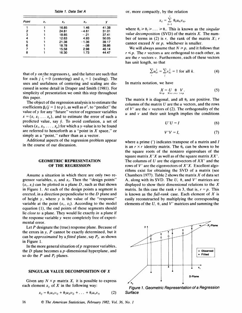
Table 1. Data Set A

Point xI x2 X3 y

1 1 16.85 1.46 41.38 2 1 24.81 -4.61 31.01 3 1 18.85 -.21 37.41 4 1 12.63 4.93 50.05 5 1 21.38 -1.36 39.17 6 1 18.78 -.08 38.86 7 1 15.58 2.98 46.14 8 1 16.30 1.73 44.47

that of y on the regressors tj, and the latter are such that for each j tj = 0 (centering) and st, = 1 (scaling). The uses and usefulness of centering and scaling are dis- cussed in some detail in Draper and Smith (1981). For simplicity of presentation we omit this step throughout this paper.

The object of the regression analysis is to estimate the coefficients r1(ij = 1 to p ), as well as u2, to "predict" the value of y for any "future" vector of regressor variables x = (xI x2 ... xp), and to estimate the error of such a predicted value, say y. To avoid confusion, a set of values (xi, x2, . .. , xp) for which a y-value is to be found are referred to henceforth as a "point in X space," or simply as a "point," rather than as a vector.

Additional aspects of the regression problem appear in the course of our discussion.

GEOMETRIC REPRESENTATION OF THE REGRESSION

Assume a situation in which there are only two re- gressor variables, xi and x2. Then the "design points" (xI, x2) can be plotted in a plane D, such as that shown in Figure 1. At each of the design points a segment is erected, in a direction perpendicular to the D plane and of height y, where y is the value of the "response" variable at the point (xI, x2). According to the model equation (1), the end points of these segments should lie close to a plane. They would lie exactly in a plane if the response variable y were completely free of experi- mental error.

Let P designate the (true) response plane. Because of the errors in y, P cannot be exactly determined, but it can be approximated by a fitted plane, say Pf, as shown in Figure 1.

In the more general situation of p regressor variables, the D plane becomes a p -dimensional hyperplane, and so do the P and Pf planes.

SINGULAR VALUE DECOMPOSITION OF X

Given any N x p matrix X, it is possible to express each element x,1 of X in the following way:

Xi1 = O, u, V ,1 + O2U2iV21 + . .. + OrllriVrj (2)

or, more compactly, by the relation

X >. OkUkiVk1, k = I

where 01 - 0, ... O or. This is known as the singular value decomposition (SVD) of the matrix X. The num- ber of terms in (2) is r, the rank of the matrix X; r cannot exceed N or p, whichever is smaller.

We will always assume that N - p, and it follows that r S p. The r vectors u are orthogonal to each other, as are the r vectors v. Furthermore, each of these vectors has unit length, so that

Uk= Vk = 1 for all k. (4)

In matrix notation, we have

X= U 0 V. (5) Nxp Nxr rxr 'rxp

The matrix 0 is diagonal, and all ok are positive. The columns of the matrix U are the u vectors, and the rows of V' are the v vectors of (2). The orthogonality of the u and v and their unit length implies the conditions

U'U =I (6)

V'V =1, (7)

where a prime (') indicates transpose of a matrix and I is an r x r identity matrix. The ok can be shown to be the square roots of the nonzero eigenvalues of the square matrix X'X as well as of the square matrix XX'. The columns of U are the eigenvectors of XX' and the rows of V' are the eigenvectors of X'X. Excellent algo- rithms exist for obtaining the SVD of a matrix (see Chambers 1977). Table 2 shows the matrix X of data set A, along with its SVD. The U, 0, and V' matrices are displayed to show their dimensional relations to the X matrix. In this case the rank r is 3, that is, r = p. This is known as the full-rank case. Each element of X is easily reconstructed by multiplying the corresponding elements of the U, 0, and V' matrices and summing the

9 I

o Observed * Fitted

D-Plane

Figure 1. Geometric Representation of a Regression Surface

16 ? The American Statistician, February 1982, Vol. 36, No. 1

Table 2. SVD of the X Matrix of Data Set A

x U U1 U2 U3

1 16.85 1.46 .322575 .176104 .193765 1 24.81 -4.61 .473864 -.603455 .049884 1 18.85 -.21 .360574 - .038169 .333727 1 12.63 4.93 .242392 .621398 - .036214 1 21.38 -1.36 .408731 -.186949 -.659192 1 18.78 -.08 .359251 -.021580 .241838 1 15.58 2.98 .298488 .370545 - .453637 1 16.30 1.73 .312108 .210988 .385321

VI ~~~~0 vI .053067 .998579 .004786 52.347807 0 0 V2 .067340 -.008360 .997695 0 7.853868 0 V3 .996317 -.052622 - .067688 0 0 .055690

terms. For example, the element 4.93 in the fourth row and third column is equal to:

[.004786 x 52.347807 x .2423921

+ [.997695 x 7.853868 x .6213981

+ [(-.067688) x .055690 x (-.036214)].

GEOMETRIC INTERPRETATION OF SVD

To simplify the exposition, we consider an example with only two regressor variables. Table 3 shows the X matrix, consisting of five points, as well as the two u- vectors, the two v-vectors, and the diagonal 0 matrix. Each row of the X matrix consists of two numbers xi, x2. We can interpret these as a "point" in 2-dimensional space, with coordinates xi and x2 (see Fig. 2). The vec- tor joining the origin to that point can also be used to represent that point, and we will therefore not hesitate to refer to any such set of two numbers as a vector as well as a point. Thus the X-matrix is represented by five points, or five vectors.

Similarly, the rows labeled v, and v2 also represent one point each or one vector each. The coordinates of the point v1, for example, are the numbers .7309 and .6825. First, we note that the distance of the origin to that point is unity, and that the same holds for vector v2. Thus, the vectors v1 and v2 have unit length. Second, it is easily verified that these two vectors are perpendic- ular (or "orthogonal") to each other (just as the original coordinate axes are perpendicular to each other). This follows from the fact that the sum of products of corre- sponding terms in v, and v2 is zero.

Therefore, the two vectors v, and v2 can be consid- ered as an alternative set of orthogonal coordinate axes. If we now refer any one of the five points of X to these new axes, for example the second point (4.2, 2.8), the new "coordinates" of this point (i.e., the projections of the point on the v,, v2 axes) will be given by 0, u, and 02 u2, in this case by (19.8360) (.2511) and (1.6040) (- .5113), or 4.9808 and - .8201.

The relative sizes of these two numbers are not coin-

Table 3. SVD of an X Matrix of Two Variables

X-Matrix U-Matrix Xi X2 U1 U2

1.3 1.2 .1202 .4037 4.2 2.8 .2511 -.5113 6.3 7.4 .4867 .6912 8.0 7.1 .5391 -.1689 9.4 8.2 .6285 -.2634

VI 0-Matrix V1 .7309 .6825 19.8360 0 V2 -.6825 .7309 0 1.6040

cidental; the projections of the points on the v1-axis cover a wider range than those on the v2-axis. In other words, the five points of the design matrix fall predom- inantly "along" the v,-axis, and less along the v2-axis. Note that if we had 02 = 0, the coordinate of each of the five points on the v2-axis would be zero; in that case, all five points would lie on the v,-line (the line that is per- pendicular to v2 at the origin). We see that the purpose accomplished by the SVD is to reorient the coordinate axes in such a way as to make them follow more closely the pattern made by the points of the X matrix them- selves. The SVD helps us understand the structure of the X matrix.

An entirely analogous interpretation holds for Table 2, but here the vector space of the design variables is three-dimensional. If in Table 2 03 were exactly zero, all the points would lie in the vI, v2 plane, that is, in the plane that is perpendicular to v3 at the origin. Since, for data set A, 03 is actually close to zero, the points lie close to the v,, v2 plane, rather than in this plane.

PRINCIPAL COMPONENTS REGRESSION

The main objective of this paper can now be stated in more precise terms. Having introduced the SVD of the matrix X, we now propose to demonstrate the advan-

x2

. -

Figure 2. Geometric Interpretation of Singular Value Decomposition in the Case of Two Regressor Variables

? The American Statistician, February 1982, Vol. 36, No. 1 17

tages of replacing X by its SVD in carrying out the regression of Y on X. This procedure is called principal components regression. We will see that while this tech- nique can be used in every regression situation covered by (1) as defined above, it is particularly illuminating in the case of collinearity or near collinearity. These terms will be explained below.

Introducing (5) into (1), we obtain

Y= UOV'13+e. (8)

Written in this form, the model is referred to as the principal components regression model.

Equation (8) can be written as

Y = U(OV'3) + e (9)

where OV'13 is a r x 1 matrix, that is, a vector of r elements. Let us denote this vector by a. Then

a= OV'r (10)

and

Y = Uot +e. (1 1) The vector Y and the matrix U are known. The least squares solution for the unknown coefficients a is ob- tained by the usual matrix equation,

ai = (U'U)-IU'Y,

which, as a result of (6), becomes

& = U' Y. (12)

This equation is easily solved since oj is simply the inner product of the vector Y with the jth vector uj.

Through application of (12) we obtain, for the data set A using the U matrix shown in Table 2,

(111. 285635\ (x U'Y 136.565303 .

\ .018803 It follows from (11) and (12) that

d = U' (Uo + e) = o + U'e or

d(.- ot = U'e. (13)

It follows that

E(dij- otj) = 0

or

E (ot) =otj. (14)

Thus, 6t& is unbiased. Furthermore, the variance of &j is

var(dtj) = E(dtj1 - otj)

= E[Euij uj e,e,] It

= (EU72) u2 =(a2

Hence,

var(& ) =a2. (15)

It is also easily shown that the (Xj are mutually un- correlated. Note that whereas the number of elements

of ,B is p, that of a is r, which may be less than p. Now the relation between ,B and a is given by (10), which also holds for the least squares estimates of a and 3,

ci=OV'13. (16)

In (16), OV' has the dimensions r x p. Thus, given the r values of &, the matrix relation (16) represents r equa- tions in the p unknown parameter estimates ,B. If r = p, (the full-rank case), the solution is possible and unique.

In this case V' is a p X p orthogonal matrix (see (7)). Hence, the solution is given by

= V'-0-'i = V 0-'. (17) Note that 0-'& is a p x 1 vector, obtained by dividing each &j by the corresponding Oj. Applying (17) to data set A, using the SVD of X of Table 2, we obtain at once

(,B,\ 1.053067 .067340 .996317 l32} = l.998579 -.008360 - .052622 \,2, .004786 .997695 -.067688/

(&1/52.3478070 x &2I7.853868 )(18)

631/.055690 An important use of (17), apart from its supplying the estimates of ,B as functions of the &, is the ready calcu- lation of the variances of the 1,. We will illustrate this calculation in terms of the numerical relations (18). Thus, we obtain from (18)

053067) ' ? (.067340) d2 3 = (.053067) 52.347807 7.853868

(.996317) 053690

In general notation this equation is written as P

= Vjk (19) k=l Ok

Since the &j are mutually orthogonal and have all vari- 2 ance ua, we see that

var(Ij ) = (f V-)2 (20) k=i ok

Applied to our data, for ,B,, (20) becomes

(A (. 053067)2 + (.067340)2 + (.996317)2 ( j) =(52. 347807)2 (7. 853868)2 (.055690)2)

x u2. (20a)

The numerators in each term are the squares of the elements in the first row of the V matrix, that is, values between 0 and 1. But the denominators are the squares of O0. Now, we note that 03 is considerably smaller than 0O and 02, so that the third term in (20) contributes an unduly large portion to the variance of ,B, (and also to the variances of 12 and 3). In fact, we find from (20a)

var(,B) = [(1. 03 x 10-6) + (74. 4 x 10-') + (320)] U2. (21)

The reason for this unfavorable state of affairs is the very small value of 03 (as compared to those of 0, and 02). We see that the use of the SVD technique allows us to pinpoint the cause or causes for the large variances found for some coefficients. In our example, the value

18 (D The American Statistician, February 1982, Vol. 36, No. 1

of 03 may be considered, for all practical purposes, to be equal to zero. But, a 0-value equal to zero has impor- tant consequences for the interpretation of regression results, as we will see shortly. We therefore interrupt the discussion of our numerical example to explore the consequences of a zero or near-zero value of 0.

COLLINEARITY AND ITS EFFECTS ON REGRESSION

Since the 0's are the square roots of the eigenvalues of the X'X matrix, a zero 0 value implies a zero eigen- value. This in turn implies that a linear relationship exists between at least some of the p x-vectors of the X matrix. A near-zero 0-value consequently implies an approximate linear relationship between at least some of these p x-vectors.

Figure 3 shows that an approximate linear relation, namely

15xi, - . 75xi2 - xi3 0 for all i, (22)

holds among the columns of X (recall xi1 - 1). We have therefore discovered the relation that causes

the very small value for 03. This can, however, also be accomplished without making graphs.

First we observe that the meaning of (22) is more readily grasped if we consider a Euclidean space in three dimensions, with axes labeled xl, x2, and x3. For each i, the triplet (xl, X2, X3) represents a point in this space. (See Figure 2 for a two-dimensional analog.) Equation (22) simply means that all N points lie in a single plane (just as a linear relation between two x- variables indicates that all points lie on a straight line). They are therefore coplanar, an extension of the con- cept of collinearity (points on the same line). The exis- tence of a linear relation such as (22) is however always referred to as collinearity (which is thus used as a ge- neric term, including a generalization of the more lim- ited case of points on the same line).

To study the effects of collinearity on the regression analysis, we introduce a second set of data, labeled data set B, which is shown in Table 4. Set B is merely a modified form of set A (Table 1): the relation between x2 and X3 is now an exact straight line.

The SVD of the X matrix of data set B is shown in Table 5. The value of 03 is now exactly zero, so that the rank of the matrix is 2, rather than 3. We now have the case r <p.

X3

.

4

.

2

0~~~~~~~~

5 10 15 20 25 X2

-2

-4

-6

Figure 3. Near Collinearity for Three Regressor Vari- ables X1, X2, and X3 When x, =1. The (X2, x3) Points Fall Close to a Straight Line

Using (12), we can calculate a which now consists of only two values:

&, = 11.252(23) (=(35.628363).(3

Even though there are only two a-values, there still are three 3-values, one for each of the three x-vectors. We try to obtain estimates for these ,B-values by using (10). Writing

(OV')r3=a, (24)

Table 4. Data Set B

Point x, x2 X3 y

1 1 16.85 2.3625 41.38 2 1 24.81 -3.6075 31.01 3 1 18.85 .8625 37.41 4 1 12.63 5.5275 50.05 5 1 21.38 -1.0350 39.17 6 1 18.78 .9150 38.86 7 1 15.58 3.3150 46.14 8 1 16.30 2.7750 44.47

X3= 15 x, - .75 X2

Table 5. SVD of X Matrix of Data Set B; X = UOV'

.323879 .193143 / .469906 -.598138

.360569 -.005670 x = .246463 .612642 52.406330 0 .053074 .997433 .048047

.406982 -.257171 0 8.036461 .063871 - .051408 .996633

.359285 .001287

.300581 .319391

.313789 .247817

C) The American Statistician, February 1982, Vol. 36, No. 1 19

we obtain

(2.781414 52.271803 2.517967( (: .513297 -.413138 8.009402 3

111.5245620 = 35.628363! (25)

Equation (25) represents two equations in three un- knowns, and does not yield a unique solution for the (3. However, it allows us to exprmss any two of the three ,B-values as a function of the third.

To treat the general case, let us denote the r X p matrix (OV') by Z,

Z-OV', (26) and partition Z into ZA and ZB, the dimensions of which are respectively r x r and r x (p - r). Partition- ing the vector (3 accordingly, into r x 1 and (p - r) x 1, we have

(ZA ZB) D)( (27) which can be written

ZA OA + ZB B =() . (28)

For the data in (25), this equation becomes

(2.781414 52.271803 ( (3 + (2.517967 k.513297 -.413138J (32' +8.009402,

(111.524562) . (29)

Premultiplying both sides of (28) by Z - (the inverse of an r x r nonsingular matrix), we obtain

(3A+ZAZ,ZB4BZA .t (30)

Equation (30) shows that, once a value for (B has been arbitrarily selected, PA is uniquely determined for this selection. Thus, in (29), (3I and (2 are uniquely determined for any arbitrarily selected value of (3. We could of course also have chosen either (,3 or (2 as the arbitrarily selected parameter.

PREDICTION IN THE CASE OF COLLINEARITY

Continuing with our quest for the consequences of collinearity, let us consider a "new" point x, for which we wish to estimate 9. We have

y=x , (31)

or, introducing the partitioning of ,

y x( ) (32)

Since A is of dimensions r x 1, and x has the dimen- sions 1 x p, we partition x, accordingly, into XA (Of dimensions 1 x r) and XB (of dimensions 1 x (p - r)). Thus,

Y=(XA XB) ( 13) or

Y=XA3A + XB(3R. (33)

Introducing (30) into (33), we obtain

9=XAZA a-ZA ZB OR + XBX,B or

YXA (ZA ) + (XB XAZAZB)B (34)

Recall that B cannot be determined by the data, but is arbitrary. In order for (34) to make sense, then, we must insist that the value of 9 be unchanged for any arbitrary value of ,B. This implies that

XB -XAZA'ZB = . (35) It is easily seen that ZAIZB = (VA)-IVB where V' is partitioned analogously to Z. (note that VA is not an orthogonal matrix.) Thus, this product does not involve the 0 matrix, and (35) can be written as

XB = XA [VA 'VB] (35a) If (35) is fulfilled, the solution is

Y =XA(ZA ?i) . (36) It is important to realize that (34) yields two relations: the condition-(35)-and the solution-(36). But the solution is valid only when the condition is fulfilled.

For data set B we have

Z -I = 68. 206904)(7 ZA = _1.49577zj (37)

ZAZB = (750)0 (38)

Thus, the condition becomes

X3= 15x, - 0. 75x2 (39)

and the solution, subject to (39), is

9 = 68.207x1 - 1.496x2 which, as a result of (39), can be written as

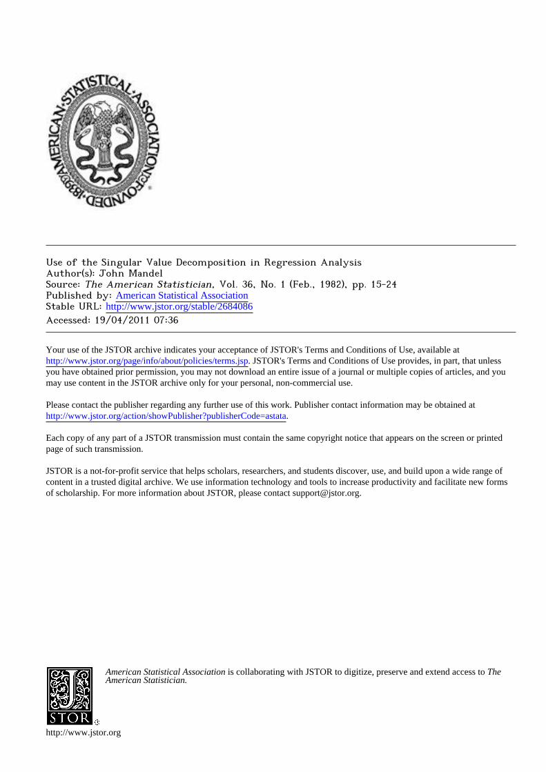
y=1.9144x2 + 4.5471x3 . (40) Since xl 1, (39) is the graph of a straight-line rela-

tion between x2 and x3. A schematic plot of X3 versus x2, using the data of Table 4, is shown in Figure 4 and exhibits this relationship. But our derivation of (39)

y

x2

D-Plane

X3

Figure 4. Effect of Co/linearity on the PRegression Surface

20 (D The American Statistician, February 1982, Vol. 36, No. I

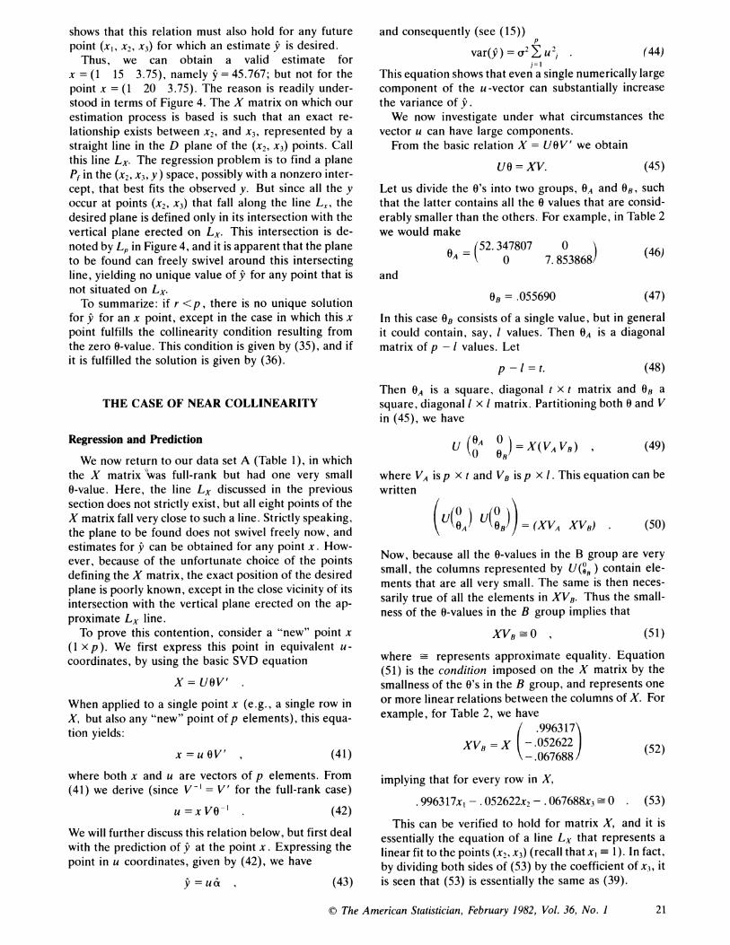
shows that this relation must also hold for any future point (xI, X2, X3) for which an estimate y' is desired.

Thus, we can obtain a valid estimate for x = (1 15 3.75), namely y = 45.767; but not for the point x = (1 20 3.75). The reason is readily under- stood in terms of Figure 4. The X matrix on which our estimation process is based is such that an exact re- lationship exists between x2, and X3, represented by a straight line in the D plane of the (X2, X3) points. Call this line Lx. The regression problem is to find a plane Pf in the (X2, X3, y) space, possibly with a nonzero inter- cept, that best fits the observed y. But since all the y occur at points (X2, X3) that fall along the line Lx, the desired plane is defined only in its intersection with the vertical plane erected on Lx. This intersection is de- noted by Lp in Figure 4, and it is apparent that the plane to be found can freely swivel around this intersecting line, yielding no unique value of j for any point that is not situated on LX.

To summarize: if r <p, there is no unique solution for g for an x point, except in the case in which this x point fulfills the collinearity condition resulting from the zero 0-value. This condition is given by (35), and if it is fulfilled the solution is given by (36).

THE CASE OF NEAR COLLINEARITY

Regression and Prediction

We now return to our data set A (Table 1), in which the X matrix \vas full-rank but had one very small 0-value. Here, the line LX discussed in the previous section does not strictly exist, but all eight points of the X matrix fall very close to such a line. Strictly speaking, the plane to be found does not swivel freely now, and estimates for 9 can be obtained for any point x. How- ever, because of the unfortunate choice of the points defining the X matrix, the exact position of the desired plane is poorly known, except in the close vicinity of its intersection with the vertical plane erected on the ap- proximate LX line.

To prove this contention, consider a "new" point x (1 x p). We first express this point in equivalent u- coordinates, by using the basic SVD equation

X= U0v'

When applied to a single point x (e.g., a single row in X, but also any "new" point of p elements), this equa- tion yields:

x = u OV' , (41)

where both x and u are vectors of p elements. From (41) we derive (since V-' = V' for the full-rank case)

u = xVO -l . (42)

We will further discuss this relation below, but first deal with the prediction of 9 at the point x. Expressing the point in u coordinates, given by (42), we have

9=u&, (43)

and consequently (see (15)) p

var(9) = u2 > u 2j (44) 1=1

This equation shows that even a single numerically large component of the u-vector can substantially increase the variance of j.

We now investigate under what circumstances the vector u can have large components.

From the basic relation X = U0V' we obtain

Uo = XV. (45)

Let us divide the 0's into two groups, OA and 08, such that the latter contains all the 0 values that are consid- erably smaller than the others. For example, in Table 2 we would make

A = (52.347807 7 3 ) (46)

and

OB = .055690 (47)

In this case OB consists of a single value, but in general it could contain, say, I values. Then OA is a diagonal matrix of p - I values. Let

p-l=t. (48)

Then OA is a square, diagonal t x t matrix and OB a square, diagonal I x l matrix. Partitioning both 0 and V in (45), we have

u (OA )= X(VA VB) , (49)

where VA is p x t and VB iS P X 1. This equation can be written

((OA) O(HB)) = (XVA XVB) . (50)

Now, because all the 0-values in the B group are very small, the columns represented by U((8, ) contain ele- ments that are all very small. The same is then neces- sarily true of all the elements in XVB. Thus the small- ness of the 0-values in the B group implies that

XVB - , . (51)

where - represents approximate equality. Equation (51) is the condition imposed on the X matrix by the smallness of the 0's in the B group, and represents one or more linear relations between the columns of X. For example, for Table 2, we have

.996317

XVB =X ~-I067688 (52)

implying that for every row in X,

.996317x,- .052622x2- .067688x3 - 0. (53)

This can be verified to hold for matrix X, and it is essentially the equation of a line Lx that represents a linear fit to the points (X2, X3) (recall that xl--1). In fact, by dividing both sides of (53) by the coefficient of xX, it is seen that (53) is essentially the same as (39).

? The American Statistician, February 1982, Vol. 36, No. 1 21

Returning now to the problem of predicting y for a new point x, we write equation (42) in the form

U = (XVA XVB)0f' (54)

or

U = (XVA XVB) ( 0 (55)

The last I elements of u arise from the product

and because each 0 in 0B is very small and its reciprocal 0-' consequently very large, these elements of u will be very large, causing the variance of 9 to be very large, unless XVB- 0, that is, unless (cf. (52)) the new point x satisfies the near-collinearity condition of the X matrix. The further the new point x lies from the Lx line, the larger will be the variance of 9, that is, the poorer will be the precision of the predicted value. This is really the heart of the collinearity problem, when viewed from the standpoint of usability of the estimated regression for prediction purposes.

If the near-collinearity condition is exactly fulfilled for the point x, we have from (55) that

XVB =O, and u =xVA (OA ) ' (56)

which implies that the last I elements of u are zero, and

9 = Uld +... + U,d, . (57)

In this equation, only the first t a-values are involved, the others having zero-multipliers.

For data set A (Table 1), the near-collinearity condi- tion is given by Eq. (53), and the predicted 9 for x satisfying (53) (considered as an equality) is

9 = Ua = X(VA) ( )a

(.053067 .067340\ 1 .998579 - .008360 .004786 .997695

_____ 0 111.524562~ (52.347807 1

0 7.853868 36.628363 7 .418452\

2X 2089422 (58) \4. 536091!(8

To summarize: The near-collinear case is characterized by one or more very small (though nonzero) 0-values. The rank of X is p; hence predictions can in principle be made for any x-point for which the basic model is known (or assumed) to be valid. However, the precision of the predicted value becomes poorer and poorer as the x-point departs more and more from the near- collinearity condition given by the equation

XVB -? . (59)

When the equality sign holds exactly, the predicted 9 for an x-point satisfying this condition is

9 = XVA (0A)c ) (60)

The poorer the approximation in (59), the poorer is the precision of 9 at that point.

An important remark must be made at this point. If the 0-values in group B are very small, the correspond- ing portion of the V matrix, namely VB, will be known with very poor numerical precision and (59) may then contain very large rounding errors. In that case, it is far better to act as though 0B were exactly equal to zero and to express the near-collinearity condition through the use of (35). Using data set A as an illustration (though in this case (59) was adequate), we obtain, by ignoring 03 and the third row of V',

z-'z ( {14. 7193) ZA -. 7774J and consequently, applying (35), we obtain the col- linearity condition

X3= 14. 7193x -.7774x2

which is equivalent to (53).

Biased Estimation

We have seen that in the case of near-collinearity the variance of 9 increases drastically for x -points that are appreciably removed from the subspace of X in which the points of the design matrix essentially lie (the sub- space defined by the collinearity condition). This condi- tion has led to various attempts to obtain more precise estimates by sacrificing the condition of unbiasedness of the 9 estimator. The proposed procedures are therefore known as "biased estimation." We will deal with only one of the proposed methods: that directly associated with the principal components regression technique. Our discussion will however suffice to reveal the basic nature of the problem and of the proposed solutions.

Principal Components Regression

In the following, we assume that we have a near- collinear X matrix. According to (56) and (57), if a point x satisfies the condition XVB = 0, the estimate of y corresponding to this point is given by the first t terms in 9 = 1.ujgi, where

u =xV0-'

While this estimate of y yields the correct least squares solution for points satisfying XVB = 0, it is not the least squares solution for x -points that do not satisfy this condition, that is, for points that do not lie in the subspace defined by the collinearity condition.

Let us, however, denote by y the quantity

9=>u1ci1, (61)

regardless of whether the condition XVB = 0 iS or is not satisfied. Equation (61) is often called the biased prin- cipal component prediction equation. The reason for

22 ?) The American Statistician, February 1982, Vol. 36, No. I

considering such an estimate is of course the reduction of variance it accomplishes. We have

p p

var() =var( =ujj) =2>uj2 , (62) j=1 j=1

var(j) = var( uj A) = u72 . (63) j=l j=I

For data set A, making t = 2, and considering as an example the point x = (1 23 -6), we have

u=x(V0-1)=(.439 -.778 3.450)

and consequently

var(y) = [(.439)2 + (-.778)2 + (3. 45)2]o.2 = 12.70lo2 ,

var(j9) = [(439)2 + (-. 778)2Ju2 = .7980o&

In this case, then, the reduction in the variance of the estimate of y is very large.

On the other hand the estimator 9 is unbiased, while y is a biased estimator. We have

E()=E(y) , (64) p

E(y) = E(y) - I ujo, (65) j=t+I

Hence p

Bias (9) = EW ) - E(y) =- uja, (66) j=1+I

Denoting by MSE the mean squared error, defined by

MSE = Variance + (Bias)2 , (67)

we have p

MSE(y) = 2 > U ,2 (68) j=1

p

MSE(y)= uj+(- Ujj)2 (69) j=1 j=t+I

By using y in the place of 9, we actually "trade" the reduction in variance, equal to U2 P t+1 uj, for the in- troduction of a (bias)2 equal to ( iit

Let us examine the case where t = p - 1 (occurring when only one 0-value is very small). Then the reduc- tion in variance is u2up and the (bias)2 = 2p2 . Thus, y will have a smaller MSE than 9 if, and only if, (bias)2 < variance reduction, that is if

u 2a2< 2 2 p p UP

or

at 2<oa2 (70)

Unfortunately, both aop and a are unknown parameters, for which only estimates are available. The estimate for a,, is of course ap, and the estimate for a2 is the residual variance after fitting &g, &2, and &3. We have, from least squares theory, N

(E W, - 92)

a='(N -p) ' (71)

which, when using the a estimators, becomes ( N p

,Zdy 9)2) (Y2 _

,2) 6- -- (72 ^2 i=l i=l j=l 7n

(N -p) (N -p) (72

For data set 1, we have (p = 3)

a3= .018803,

/13729.3041 - 13721.5143 = V 8-3 =~~~1.248

Undoubtedly, in this case, d3 <&, but this does not necessarily imply that a3 < a. Indeed, the standard er- ror of a3 is a (cf. (15)); if &3 is of the same order of magnitude as a, it will be virtually impossible to decide, on the basis of the data alone, whether condition (70) is satisfied. To decide whether y is preferable to 9, that is whether MSE(9) < MSE(9), it is therefore often neces- sary to make further assumptions. For example, if we assume that a3 = 0, then the y estimator is obviously the one to use. The hypothesis a3 = Ocan be tested in principal component regression using Student's t test,

t a3-a3 - a3 (73 t ~~~~~~~~(73) which, for the hypothesis a3 =0, becomes

at3 t = a^3, (74) For data set 1, we obtain

t 0

i088 0151 t1.248-05 The hypothesis a3 = 0 cannot be rejected, but this does not allow us to infer that condition (70) is satisfied.

From the viewpoint of the philosophy of experi- mentation, another important matter deserves consid- eration. Our problem involves both an assumption of a linear model, (1), and a set of data. In a "good" experi- ment, the data themselves generally provide some diag- nostic means for testing the model. In the case of near collinearity, these diagnostic means are totally confined to the close vicinity of the subspace defined by the near collinearity. Thus, even if we knew that condition (70) is fulfilled, we would still be uncertain about the validity of the model for points with large u3-values, that is points far removed from the (vI,v2) plane, in the V3

direction. Our analysis has led us to the conclusion that linear

model inferences based on near-collinear X matrices should be made with great caution.

OTHER APPLICATIONS OF THE SVD TECHNIQUE

We have seen that the detection and treatment of collinearity and near collinearity is greatly facilitated through the use of the singular value decomposition. This interesting technique has other important uses in data analysis, such as in the study of the structure of two-way tables (Bradu and Gabriel 1978; Mandel 1971), the evaluation of experimental designs in re- gression (Hahn, Meeker, and Feder 1976), and the em-

? The American Statistician, February 1982, Vol. 36, No. 1 23

pirical fitting of functions of two or more arguments (Mandel 1981).

SUMMARY AND CONCLUSION

We have presented algebraic and geometric aspects of multiple linear regression, based primarily on the singular value decomposition technique, and shown that difficulties of interpretation arise when constraints (such as exact or approximate linear relations) exist between the regressor variables. Linear constraints are known as collinearity. Near collinearity manifests itself in the form of one or more very small singular values.

Under linear constraints, the true coefficients of the relation between the response and the regressor vari- ables cannot be estimated unambiguously without in- troducing additional assumptions. Nevertheless, it is possible to make valid predictions of the response, pro- vided that the point for which the prediction is made lies in the same subspace as the points on which the re- gression calculations were based.

Even though the coefficients of the regression equa- tion cannot be estimated precisely when applying the least squares technique to the case of collinearity, or near collinearity, certain linear combinations of the co- efficients can be estimated with confidence.

[Received August 1980. Revised July 1981.

REFERENCES

BELSLEY, D. A.; KUH, E.; and WELSCH, R. E. (1980), Identi- fying Influential Data and Sources of Collinearity, New York: John Wiley.

BRADU, D., and GABRIEL, K. R. (1978), "The Biplot as a Diag- nostic Tool for Models of Two-Way Tables," Technometrics, 20, 47-68.

CHAMBERS, J. M. (1977), Computational Methods for Data Anal- ysis, New York: John Wiley.

CHATTERJEE, S., and PRICE, B. (1977), Regression Analysis by Example, New York: John Wiley.

DRAPER, N. R., and SMITH, H. (1981), Applied Regression Anal- ysis (2nd ed.), New York: John Wiley.

HAHN, G. J.; MEEKER, W. Q. Jr.; and FEDER, P. I. (1976), "The Evaluation and Comparison of Experimental Design for Fitting Regression Relationships," Journal of Quality Technology, 8, 140-157.

HOCKING, R. R.; SPEED, F. M.; and LYNN, M. J. (1976), "A Class of Biased Estimators in Linear Regression," Technometrics, 18, 425-437.

HOERL, A. E., and KENNARD, R. W. (1970), "Ridge Regression: Biased Estimation for Nonorthogonal Problems," Technometrics, 12, 55-67.

MANDEL, J. (1971), "A New Analysis of Variance Model for Non- Additive Data," Technometrics, 13, 1-18.

(1981), "Fitting Curves and Surfaces with Monotonic and Non-Monotonic Four Parameter Equations," Journal of Research of the National Bureau of Standards, 86(1), 1-25.

MARQUARDT, D. W. (1970), "Generalized Inverses, Ridge Re- gression, Biased Linear Estimation, and Nonlinear Estimation," Technometrics, 12, 591-612.

MARQUARDT, D. W., and SNEE, R. D. (1975), "Ridge Re- gression in Practice," The American Statistician, 29, 3-20.

RAO, C. R. (1973), Linear Statistical Inference and Its Applications, New York: John Wiley.

SNEE, R. D. (1973), "Some Aspects of Nonorthogonal Data Anal- ysis, Part 1. Developing Prediction Equations," Journal of Quality Technology, 5, 67-79.

STEIN, C. M. (1960), "Multiple Regression Contributions to Proba- bility and Statistics," in Essays in Honor of Harold Hotelling, ed. I. Olkin, Stanford: Stanford University Press, 424-443.

WEBSTER, J. T.; GUNST, R. F.; and MASON, R. L. (1974), "Latent Root Regression Analysis," Technometrics, 16, 513-522.

24 ?) The American Statistician, February 1982, Vol. 36, No. I