Use of Geocell in Pavement Design: Final Report

Use of Geocell in Pavement Design: Final Report

Technical Report 0-6833-1 Cooperative Research Program

CENTER FOR TRANSPORTATION INFRASTRUCTURE SYSTEMS THE UNIVERSITY OF TEXAS AT EL PASO

EL PASO, TX 79968

in cooperation with the Federal Highway Administration and the

Texas Department of Transportation

Technical Report Documentation Page

1. REPORT NO.

FHWA/TX-21/0-6833-1 2. GOVERNMENT ACCESSION NO. 3. RECIPIENTS CATALOG NO.

4. TITLE AND SUBTITLE

Use of Geocell in Pavement Design: Final Report 5. REPORT DATE

November 11, 2018 Published: November 2021 6. PERFORMING ORGANIZATION CODE

7. AUTHOR(S)

Sundeep Inti, Ph.D. https://orcid.org/0000-0002-8631-446X Megha Sharma, Ph.D. Cesar Tirado, Ph.D. Vivek Tandon, Ph.D. https://orcid.org/0000-0003-2469-2956

8. PERFORMING ORGANIZATION REPORT No.

0-6833-1

9. PERFORMING ORGANIZATION NAME AND ADDRESS

Center for Transportation Infrastructure Systems The University of Texas at El Paso 500 W. University Ave. El Paso, Texas 79968

10. WORK UNIT NO.

11. CONTRACT OR GRANT NO.

0-6833

12. SPONSORING AGENCY NAME AND ADDRESS

Texas Department of Transportation Research and Technology Implementation Division 125 E. 11th Street Austin, TX 78701

13. TYPE OF REPORT AND PERIOD COVERED

Final Report September 2014 – August 2017 14. SPONSORING AGENCY CODE

15. SUPPLEMENTARY NOTES

Project performed in cooperation with the Texas Department of Transportation and the Federal Highway Administration.

16. ABSTRACT

This study focused on identifying mechanisms responsible for improved bearing capacity and benefits derived from geocell. The study performed Finite Element Analyses (FEA) and verified the results by performing laboratory tests. In addition, the study developed a design system and performed Life Cycle Cost Analysis to identify the benefits of geocell reinforcement and provided construction guidelines. Based on the FEA and laboratory evaluation, the study identified that the geocell is beneficial when construction needs to be performed with a lower/marginal base and subgrade material is available.

17. KEYWORDS

Geocell, Base, Subgrade, Finite Element, Strain, Stress

18. DISTRIBUTION STATEMENT

No restrictions. This document is available to the public through the National Technical Information Service, Springfield, Virginia, 22161; www.ntis.gov

19. SECURITY CLASSIF. (OF THIS REPORT)

Unclassified

20. SECURITY CLASSIF. (OF THIS PAGE)

Unclassified

21. NO. OF PAGES

238

22. PRICE

https://orcid.org/0000-0002-8631-446X

https://orcid.org/0000-0003-2469-2956

https://www.ntis.gov

Use of Geocell in Pavement Design Final Report

Conducted for

Texas Department of Transportation

By

Sundeep Inti, Ph.D. Megha Sharma, Ph.D.

Cesar Tirado, Ph.D. Vivek Tandon, Ph.D

Research Report 0-6833-1

November 2018 Published November 2021

Department of Civil Engineering The University of Texas at El Paso

El Paso, TX 79968 (915) 747-6924

Authors’ Disclaimer: The contents of this report reflect the view of the authors, who are responsible for the facts and the accuracy of the data presented herein. The contents do not necessarily reflect the official views or policies of the Texas Department of Transportation (TxDOT) or the Federal Highway Administration (FHWA). This report does not constitute a standard, specification, or regulation.

NOT INTENDED FOR CONSTRUCTION, BIDDING, OR PERMIT PURPOSES

Sundeep Inti., Ph.D. Megha Sharma, Ph.D. Cesar Tirado, Ph.D. Vivek Tandon, Ph.D.

ACKNOWLEDGMENTS

The successful progress of this project could not have happened without the valuable assistance from several TxDOT personnel. The authors acknowledge Mr. Mark McDaniel, Mr. Wade Blackmon, and Mr. Boon Thian for their valuable guidance, input, and support. The authors would also like to acknowledge Mr. Brett Haggerty, Mr. Aldo Madrid, and Mr. Richard Williammee for facilitating collaboration with TxDOT Districts. In addition, the authors would like to acknowledge Mr. Jose Luis Arias, Mr. Armando Esquivel, Mr. Angel Rodarte, Mr. Rafael Silva, and Ms. Sofia Martin for their assistance in performing tests. In the end, the authors would like to thank Ms. Sonya Badgley of RTI for her support.

vii

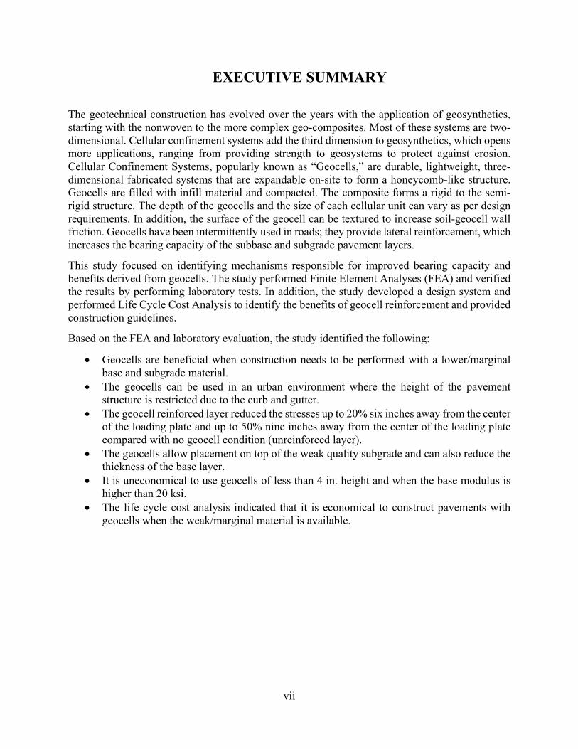
EXECUTIVE SUMMARY

The geotechnical construction has evolved over the years with the application of geosynthetics, starting with the nonwoven to the more complex geo-composites. Most of these systems are two‐dimensional. Cellular confinement systems add the third dimension to geosynthetics, which opens more applications, ranging from providing strength to geosystems to protect against erosion. Cellular Confinement Systems, popularly known as “Geocells,” are durable, lightweight, three-dimensional fabricated systems that are expandable on‐site to form a honeycomb‐like structure. Geocells are filled with infill material and compacted. The composite forms a rigid to the semi‐rigid structure. The depth of the geocells and the size of each cellular unit can vary as per design requirements. In addition, the surface of the geocell can be textured to increase soil‐geocell wall friction. Geocells have been intermittently used in roads; they provide lateral reinforcement, which increases the bearing capacity of the subbase and subgrade pavement layers.

This study focused on identifying mechanisms responsible for improved bearing capacity and benefits derived from geocells. The study performed Finite Element Analyses (FEA) and verified the results by performing laboratory tests. In addition, the study developed a design system and performed Life Cycle Cost Analysis to identify the benefits of geocell reinforcement and provided construction guidelines.

Based on the FEA and laboratory evaluation, the study identified the following:

• Geocells are beneficial when construction needs to be performed with a lower/marginal base and subgrade material.

• The geocells can be used in an urban environment where the height of the pavement structure is restricted due to the curb and gutter.

• The geocell reinforced layer reduced the stresses up to 20% six inches away from the center of the loading plate and up to 50% nine inches away from the center of the loading plate compared with no geocell condition (unreinforced layer).

• The geocells allow placement on top of the weak quality subgrade and can also reduce the thickness of the base layer.

• It is uneconomical to use geocells of less than 4 in. height and when the base modulus is higher than 20 ksi.

• The life cycle cost analysis indicated that it is economical to construct pavements with geocells when the weak/marginal material is available.

viii

ix

TABLE OF CONTENTS Page EXECUTIVE SUMMARY ........................................................................................................ vii LIST OF TABLES ..................................................................................................................... xiii LIST OF FIGURES .................................................................................................................... xv

1. PROJECT OUTLINE .......................................................................................................... 1

1.1 NATURE OF THE PROBLEM ........................................................................................ 1

1.2 TECHNICAL OBJECTIVES ............................................................................................ 1

1.3 RESEARCH PLAN AND REPORT ORGANIZATIONS .............................................. 1

2. LITERATURE REVIEW .................................................................................................... 3

2.1 GENESIS ............................................................................................................................. 3

2.1.1 Construction with Geocell .......................................................................................... 4

2.1.2 Load Support Mechanism .......................................................................................... 4

3. FINITE ELEMENT MODELING (FEM) AND ANALYSIS OF RESULTS ............... 25

3.1 PARAMETRIC STUDY .................................................................................................. 25

3.2 INFLUENCE OF BASE MODULUS (BOTH INFILL AND COVER LAYERS WITH SIMILAR MODULUS VALUES) ....................................................................... 29

3.3 INFLUENCE OF COVER THICKNESS ....................................................................... 30

3.4 INFLUENCE OF COVER BASE MATERIAL............................................................. 39

3.5 INFLUENCE OF SUBGRADE MODULUS .................................................................. 39

3.6 INFLUENCE OF GEOCELL LAYER THICKNESS OR GEOCELL HEIGHT ..... 40

4. SELECTION OF MATERIAL, EXPERIMENTAL DESIGN, AND LABORATORY EVALUATION ...................................................................................... 51

4.1 EXPERIMENTAL DESIGN ........................................................................................... 51

4.2 LABORATORY EVALUATION .................................................................................... 51

4.3 MATERIAL SELECTION .............................................................................................. 54

4.3.1 Geocell ........................................................................................................................ 54

4.3.2 Base and Subgrade Selection ................................................................................... 54

4.4 LABORATORY EVALUATION PROCESS ................................................................ 56

4.4.1 Laboratory Set-Up .................................................................................................... 56

4.5 DATA REDUCTION AND CLEANING........................................................................ 61

4.5.1 Noise Removal from Zero Reading (Datum) .......................................................... 61

4.5.2 Noise Removal from Actual Data and Data Reduction ......................................... 62

4.5.3 Presentation of Data ................................................................................................. 64

4.5.4 Summary of Data ...................................................................................................... 67

x

5. CRITICAL EVALUATION OF EXISTING DESIGN METHODS ............................. 71

5.1 TEXAS PAVEMENT DESIGN PROCEDURE ............................................................. 71

5.1.1 Geosynthetics in Pavement Structure ..................................................................... 72

5.1.2 Geosynthetics for Geotechnical Reinforcement ..................................................... 72

5.2 LOW VOLUME ROAD DESIGN AASHTO ................................................................. 72

5.2.1 Aggregate-Surface Roads ......................................................................................... 73

5.3 DESIGN METHODS FOR LOW VOLUME UNPAVED ROADS WITH GEOCELL REINFORCEMENT ....................................................................... 86

5.3.1 PRESTO GEOSYSTEM Design Method ............................................................... 86

5.3.2 Design Method Presto Geosystems for Low Volume Roads – Unpaved Roads (Pokharel 2010) ............................................................................. 91

5.3.3 Example ..................................................................................................................... 93

5.3.4 Conclusions ................................................................................................................ 94

6. MODEL DEVELOPMENT, STATISTICAL ANALYSIS, AND VALIDATION ....... 97

6.1 PATH TO DEVELOPMENT OF MODEL .................................................................... 97

6.2 DATA FOR DEVELOPING MODEL ............................................................................ 97

6.3 DEVELOPMENT AND VALIDATION OF MODEL FOR ESTIMATING BENEFIT OF GEOCELL REINFORCED LAYER .......................... 98

6.4 MULTILINEAR REGRESSION MODEL AND VERIFICATION OF ASSUMPTIONS ......................................................................................................... 99

6.4.1 Initial Model .............................................................................................................. 99

6.4.2 Linear Relationship ................................................................................................ 101

6.4.3 Variation in Residuals Same for Large and Small ŷ Values ............................... 102

6.4.4 Distribution of Residuals ........................................................................................ 103

6.4.5 Multicollinearity ...................................................................................................... 103

6.4.6 Independent Observations ..................................................................................... 105

6.5 MODEL DEVELOPMENT USING CROSS-VALIDATION TECHNIQUES ........ 108

6.5.1 Full cross-validation or leave-one-out validation method (LOOV) ................... 110

6.5.2 KK-FOLD Cross-Validation .................................................................................. 111

6.5.3 Bootstrapping Cross-Validation ............................................................................ 112

6.6 SUMMARY OF MODELS ............................................................................................ 113

7. LIFE CYCLE COST ANALYSIS ................................................................................... 115

7.1. DETERMINISTIC APPROACH ................................................................................. 115

7.1.1 Establish alternative pavement design strategies for the analysis period ......... 115

xi

7.1.2 Compute Net Present Worth (NPW) or Equivalent Uniform Annual Costs (EUAC) .......................................................................................................... 117

7.1.3 Analyze Results ....................................................................................................... 118

7.1.4 Reevaluate Design Strategies ................................................................................. 118

7.2. ESTIMATION OF GEOCELL LAYER MODULUS ................................................ 119

7.2.1 Comparison of Geocell vs. No Geocell .................................................................. 119

7.3. ESTIMATION OF COST OF GEOCELL REINFORCED LAYER ....................... 125

7.3.1 Design 1: FM 55 Ellis County of Dallas District .................................................. 126

7.3.2 Design 1: US 83 Uvalde County, San Antonio District ........................................ 131

7.3.3 Design 1: US 67 at FM 1001 Titus County, Atlanta District ............................... 134

8. CLOSURE ......................................................................................................................... 137

8.1 SUMMARY ..................................................................................................................... 137

8.2 CONCLUSION ............................................................................................................... 137

8.3 RECOMMENDATION .................................................................................................. 139

9. REFERENCES .................................................................................................................. 141

A. APPENDIX A: SITE INSTRUMENTATION ............................................................... 145

A.1 INTRODUCTION .......................................................................................................... 145

A.2 SITE LOCATION AND MATERIAL PROPERTIES .............................................. 145

A.2.1 Site Location ........................................................................................................... 145

A.2.2 Soil Classification ................................................................................................... 146

A.3 INSTRUMENTATION ................................................................................................. 152

A.4 CONSTRUCTION OF REINFORCED AND UNREINFORCED SECTIONS ...... 156

A.5 DATA COLLECTION AND ANALYSIS ................................................................... 161

B. APPENDIX B- FINITE ELEMENT MODEL DEVELOPMENT ............................... 167

B.1 SOIL MODELS .............................................................................................................. 168

B.1.1 Linear Elastic .......................................................................................................... 168

B.1.2 Mohr-Coulomb ....................................................................................................... 168

B.1.3 FHWA Soil Constitutive Model ............................................................................ 170

B.2 SHELL ELEMENT TYPE FOR GEOCELL MODELING ...................................... 172

B.2.1 Shell Element .......................................................................................................... 172

B.2.2 Thick Shell Element (TSHELL)............................................................................ 173

B.2.3 Geocell Dimensions and Properties ...................................................................... 173

B.3 CONTACT MODEL ...................................................................................................... 174

B.3.1 Automatic Single Surface Contact ........................................................................ 174

xii

B.3.2 Discrete Beam Element Interface ......................................................................... 175 B.4 NODE COMPATIBILITY FROM GEOCELL AND GEOMATERIAL AT LAYER INTERFACE ............................................................................................ 176

B.5 BOUNDARY CONDITIONS ........................................................................................ 177

B.6 LEVEL OF SOPHISTICATION OF FINITE ELEMENT MODELS ..................... 178

B.6.1 Simplified Single Layer FE Model ........................................................................ 178

B.6.2 Pavement with Single Cell ..................................................................................... 179

B.6.3 Geocell-Reinforced Pavement with Geocell Panel Modeled Using Rhomboidal Pattern............................................................................................... 180

B.6.4 Geocell-Reinforced Pavement with Geocell Panel Modeled Using Pseudo-Sinusoidal Pattern .................................................................................... 183

B.7 SELECTION OF LOADING CONDITIONS: PLATE SIZE AND LOCATION ... 184

B.8 RESULTS FROM PRELIMINARY INVESTIGATION: EVALUATION OF SOIL MODELS AND SHELL ELEMENT TYPE FOR MODELING THE GEOCELL ............................................................................................................ 185

B.8.1 Geocell-Reinforced Pavement with Geocell Panel Modeled Using Pseudo-Sinusoidal Pattern ......................................................................... 185

B.8.2 Comparison to University of Kansas Model ........................................................ 190

B.8.3 Preliminary Evaluation of Contact ....................................................................... 190

B.8.4 Evaluation of Geocell Shape: Geocell Panel Simulated with Rhomboidal Pattern............................................................................................... 191

B.8.5 Evaluation of Element Type for Modeling the Geocell ....................................... 192

B.8.6 Use of Shell Elements (SHELL) for Modeling Geocell and Automatic Surface Contact Type ............................................................................................ 192

B.8.7 Use of Thick Shell Elements for Modeling Geocell and Automatic Surface Contact Type ............................................................................................ 193

B.9 EVALUATION OF CONTACT TYPE FOR SOIL-GEOCELL INTERFACE ...... 196

B.9.1 Assessment of Contact Type Using Simplified Single-Layer Model ................. 196

B.9.2 Evaluation of Contact Type Using Single-Cell 3-D FE Model ........................... 198

C. APPENDIX C- GEOCELL INFORMATION ............................................................... 201

D. APPENDIX D .................................................................................................................... 209

D.1 PAIRED T-TEST ........................................................................................................... 217

D.1.1 Procedure ................................................................................................................ 217

D.2 PEARSON CORRELATION ....................................................................................... 218

xiii

LIST OF TABLES Page

Table 1-1 List of Tasks and Associated Chapters. .......................................................................... 2 Table 2-1 Various Studies Performed on Use of Geocells. ............................................................ 8 Table 2-2 Test Setups Developed for Evaluation of Geocell. ...................................................... 14 Table 2-3 Numerical Modeling of Geocell-Reinforced Layer. .................................................... 17 Table 2-4 Finite Element Modeling Geocell Reinforced Layer and Contact Models. ................. 19 Table 2-5 Existing Pavement Design Methods of Geocell-Reinforced Layers ............................ 22 Table 2-6 Summary of Research Performed at Kansas State University ..................................... 24 Table 4-1 Experimental Test Plan ................................................................................................. 53 Table 4-2 Geocell Selection and Properties .................................................................................. 54 Table 4-3 Test Procedures for Evaluation of Base and Subgrade Material .................................. 54 Table 4-4 Measured Engineering Properties of Base and Subgrade Materials ............................ 55 Table 4-5 Factors Evaluated in Laboratory .................................................................................. 56 Table 4-6 Strain Gauges................................................................................................................ 59 Table 4-7 Vertical Deformation (below loading plate) ................................................................. 68 Table 4-8 Stresses Measured on Top of Subgrade (below loading plate) .................................... 68 Table 4-9 Vertical Deformation (below loading plate) ................................................................. 69 Table 4-10 Hoop Strain (cell below loading plate) ....................................................................... 69 Table 4-11 Summary of Measured Stress and Strain with 12” Loading Plate ............................. 70 Table 5-1 Geosynthetic Application (Pavements in Texas). ........................................................ 72 Table 5-2 Suggested Seasons Length (Months) for the Six U.S. Climatic Regions. .................... 75 Table 5-3 Suggested Seasonal Roadbed Soil Resilient Moduli, MR (psi), as a Function of the Relative Quality of the Roadbed Material. ................................................................................... 75 Table 5-4 Effective Roadbed Soil Resilient Modulus Values, MR (psi) that may be used in the Design of Flexible Pavements for Low-Volume Roads. Suggested Values Depend on the U.S. Climatic Region and the Relative Quality of the Roadbed Soil. .................................................. 75 Table 5-5 Chart for Computing Total Pavement Damage (for both Serviceability and Rutting Criteria) Based on a Trial Aggregate Base Thickness. ................................................................. 78 Table 5-6 Computation of Total Pavement Damage (for both Serviceability and Rutting Criteria) Based on Trial Aggregate Base Layer. ......................................................................................... 80 Table 5-7 Computation of Total Pavement Damage (for both Serviceability and Rutting Criteria) Based on 10” Aggregate Base Layer. ........................................................................................... 82 Table 5-8 Chart for Computing Total Pavement Damage (for both Serviceability and Rutting Criteria) Based on a Trial Aggregate Base Thickness. ................................................................. 86 Table 5-9 Methodology for Designing Gravel Roads (Unreinforced) .......................................... 87 Table 5-10 Correlation of Subgrade Soil Strength Parameters for Cohesive (Fine-Grained) Soils....................................................................................................................................................... 87 Table 5-11 Methodology for Designing Gravel Roads with Geocell Reinforced Base ............... 88 Table 5-12 Recommended Peak Friction Angle Ratio (Presto Geosystems) ............................... 89 Table 5-13 Recommended Peak Friction Angle Ratio (Presto Geosystems) for Design ............. 92 Table 6-1 Range of Input Variables Used for Developing the Model .......................................... 98 Table 6-2 Correlation Matrix ...................................................................................................... 105 Table 6-3 Variance Inflation Factors (VIF) ................................................................................ 105 Table 6-4 Verification of Assumptions in Multiple Regression ................................................ 106

xiv

Table 6-5 Multiple Linear Regression Model Parameters for Reduced Model (LOOV) ... 110 Table 6-6 Multiple Linear Regression Model Parameters for Reduced Model (KK-FOLD) 111

Table 6-7 Multiple Linear Regression Model Parameters for Reduced Model (Bootstrapping CV) ............................................................................................................................................. 112 Table 6-8 Summary of Models Developed Using Cross-Validation Techniques ....................... 114 Table 7-1 Cost of Base Materials Considered in this Study ....................................................... 126 Table 7-2 Inputs for Pavement Design (Ellis County, Dallas District) ...................................... 127 Table 7-3 Cost Estimate for Geocell Reinforced Layer (Ellis County, Dallas District) ............. 129 Table 7-4 Input Data for Pavement Design (Uvalde County, San Antonio District) ................ 131 Table 7-5 Cost Estimate of Geocell-Reinforced Layer (Uvalde County, San Antonio District) 133 Table 7-6 Input Data for Pavement Design (Titus County, Atlanta District) ............................. 134 Table 7-7 Cost Estimate of Geocell-Reinforced Layer (Titus County, Atlanta District) ........... 136 Table A-1 Stress at Different Confinements (Subgrade soil) ..................................................... 149 Table A-2 Average Stresses at Different Confinements ............................................................. 151 Table A-3 Strain Gauges ............................................................................................................. 152 Table A-4 Results of MODULUS Software ............................................................................... 163 Table A-5 Results of Field Testing and Bisar Modeling ............................................................ 163 Table B-1 Material Properties Used for Linear-Elastic Model. .................................................. 169 Table B-2 Material Properties Used for Mohr-Coulomb Material Model. ................................. 170 Table B-3 Soil Properties Used for Modeling Base and Subgrade Used for Parametric Study and for Evaluation of Geocell Element Types and Contact .............................................................. 171 Table B-4 FHWA Soil Material Properties Used for Evaluation of the University of Kansas Study (after Yang. 2010) ....................................................................................................................... 172 Table B-5 Geocell Dimensions and Properties. .......................................................................... 173 Table B-6 Dimensions of Single Cell FE Model. ....................................................................... 180 Table B-7 Dimensions and Properties of Geocell-Reinforced Pavement FE Model with Geocell Panel Simulated Using Rhomboidal Shaped Cells. .................................................................... 181 Table B-8 Dimensions and Properties of Geocell-Reinforced Pavement FE Model with Geocell Panel Simulated Using Pseudo-Sinusoidal Shaped Cells. .......................................................... 184 Table B-9 Summary of Numerical Models Used for Evaluating Contact Types. ...................... 197 Table B-10 Summary of Longitudinal and Vertical Stress at the Mid-Height of Model Observed at the Edge of Cell#1, at the Geocell, and at the Edge of Cell#2 in contact with the Geocell. .... 198 Table D-1 Raw Data ................................................................................................................... 209 Table D-2 Training Data Set LOOV-CV .................................................................................... 211 Table D-3 Testing Data Set LOOV-CV ...................................................................................... 212 Table D-4 Training Data Set KK FOLD CV .............................................................................. 213 Table D-5 Testing Data Set KK FOLD CV ................................................................................ 214 Table D-6 Training Data Set Bootstrapping CV ......................................................................... 215 Table D-7 Testing Data Set Bootstrapping CV .......................................................................... 216

xv

LIST OF FIGURES Page

Figure 2-1 Geocell Supplied. .......................................................................................................... 3 Figure 2-2 Application of Geocell (US Army Corps). ................................................................... 4 Figure 2-3 Geocell Construction Sequence. ................................................................................... 5 Figure 2-4 Mechanics of Geocell Reinforcement. .......................................................................... 5 Figure 3-1 Quarter Model used in the Parametric Study. ............................................................. 28 Figure 3-2 Locations of Output Evaluated from FEA. ................................................................. 28 Figure 3-3 Comparison of Compressive Stress at 6” from Loading Center

of Loading Plate (Geocell vs. No Geocell). ................................................................ 28 Figure 3-4 Stress Distribution (Geocell vs. No Geocell) along the Subgrade. ............................. 29 Figure 3-5 Strain Distribution (Geocell vs. No Geocell) along the Subgrade. ............................. 30 Figure 3-6 Stress Distribution (Geocell 4” and 6” vs. No Geocell)along the Subgrade

(Influence of Infill Modulus). ..................................................................................... 31 Figure 3-7 Strain Distribution (Geocell 4” and 6” vs. No Geocell) along the Subgrade

(Influence of Infill Modulus). ..................................................................................... 32 Figure 3-8 Vertical Deformation (Geocell 4” and 6” vs. No Geocell)

(Influence of Infill Modulus). ..................................................................................... 33 Figure 3-9 Hoop Strains on Geocell 4” and 6” (Influence of Infill Modulus). ............................. 33 Figure 3-10 Strain Distribution (Geocell 4” and 6” vs. No Geocell) along the Subgrade

(Influence of Cover Thickness). ................................................................................ 34 Figure 3-11 Vertical Deformation (Geocell 4” and 6” vs. No Geocell)

(Influence of Cover Thickness). ............................................................................... 35 Figure 3-12 Hoop Strain on Geocell 4” and 6” vs. No Geocell

(Influence of Cover Thickness). ............................................................................... 35 Figure 3-13 Stress Distribution (Geocell 3”, 4” and 6” vs. No Geocell) along the Subgrade

(Influence of Good Cover and Poor Infill). .............................................................. 36 Figure 3-14 Strain Distribution (Geocell 3”, 4” and 6” vs. No Geocell) along the Subgrade

(Influence of Good Cover and Poor Infill). .............................................................. 37 Figure 3-15 Vertical Deformation (Geocell 3”, 4” and 6” vs. No Geocell)

(Influence of Good Cover and Poor Infill). ............................................................. 38 Figure 3-16 Hoop Strains on Geocell 3”, 4” and 6” vs. No Geocell

(Influence of Good Cover and Poor Infill). .............................................................. 38 Figure 3-17 Stress Distribution (Geocell 3” vs. No Geocell) along the Subgrade

(Influence of Subgrade Modulus). ............................................................................ 41 Figure 3-18 Strain Distribution (Geocell 3” vs. No Geocell) along the Subgrade

(Influence of Subgrade Modulus). ............................................................................ 42 Figure 3-19 Vertical Deformation (Geocell 3” vs. No Geocell)

(Influence of Subgrade Modulus). ............................................................................ 43 Figure 3-20 Hoop Strain on Geocell 3” (Influence of Subgrade Modulus). ................................. 43 Figure 3-21 Stress Distribution (Geocell 4” vs. No Geocell) along the Subgrade


(Influence of Subgrade Modulus). ............................................................................ 45

xvi

Figure 3-23 Vertical Deformation (Geocell 4” vs. No Geocell) (Influence of Subgrade Modulus). ............................................................................ 46

Figure 3-24 Hoop Strain on Geocell 4” (Influence of Subgrade Modulus). ................................. 46 Figure 3-25 Stress Distribution (Geocell 6” vs. No Geocell) along the Subgrade


(Influence of Subgrade Modulus). ............................................................................ 48 Figure 3-27 Vertical Deformation (Geocell 6” vs. No Geocell)

(Influence of Subgrade Modulus). ............................................................................ 49 Figure 3-28 Hoop Strains on Geocell 6” (Influence of Subgrade Modulus). ............................... 49 Figure 4-1 Photo of Fabricated Box.............................................................................................. 56 Figure 4-2 Sample Preparation Using Vibratory Compactor ....................................................... 57 Figure 4-3 Applied Load Cycle .................................................................................................... 58 Figure 4-4 Locations of Stress and Strains Measurement Transducers ........................................ 58 Figure 4-5 Half Bridge Vs. Quarter Bridge Strain Gauge Circuits............................................... 59 Figure 4-6 Photo of Earth Pressure Cell ....................................................................................... 60 Figure 4-7 a) MTS Data Acquisition System, b) LMS Data Acquisition System ........................ 61 Figure 4-8 Noise removal from pressure cell readings ................................................................. 62 Figure 4-9 a) Pressure Cell 1 (Original Data), b) Pressure Cell 2 (Original Data),

c) Pressure Cell 3 (Original Data), d) Pressure Cell 3 (Kernel Regression). .............. 63 Figure 4-10 A) Strain gauge (Original Data), B) Strain gauge (Kernel Regression) ................... 64 Figure 4-11 Vertical Deformation A) Geocell, B) No Geocell. ................................................... 65 Figure 4-12 Vertical Stresses on Subgrade a) Geocell, b) No Geocell. ........................................ 65 Figure 4-13 a) Location and Direction of Strain Gauges b) Vertical Strain Observed

in the Center Geocell. ............................................................................................... 66 Figure 4-14 Hoop Strains on Geocell. .......................................................................................... 66 Figure 5-1 The Six Climatic Regions in the United States (AASHTO, 1993). ............................ 74 Figure 5-2 Design Chart for Aggregate-Surfaced Roads Considering Allowable

Serviceability Loss (AASHTO, 1993). ....................................................................... 76 Figure 5-3 Design Chart for Aggregate-Surfaced Roads Considering Allowable Rutting

(AASHTO, 1993) ........................................................................................................ 77 Figure 5-4 Example Growth of Total Damage Versus Base Layer Thickness for Both

Serviceability and Rutting Criteria. ............................................................................ 81 Figure 5-5 Chart to Convert a Portion of the Aggregate Base Layer Thickness

to an Equivalent Thickness of Subbase (AASHTO, 1993)......................................... 81 Figure 5-6 Design Chart for Aggregate-Surfaced Roads Considering Allowable

Serviceability Loss (Geocell Reinforced Layer Calculations). (AASHTO, 1993) ..... 83 Figure 5-7 Design Chart for Aggregate-Surfaced Roads Considering Allowable Rutting

(Geocell Reinforced Layer Calculations) (AASHTO, 1993). .................................... 84 Figure 5-8 Chart to Convert a Portion of the Aggregate Base Layer Thickness to an

Equivalent Thickness of Subbase (Geocell Reinforced Layer Calculations) (AASHTO, 1993) ........................................................................................................ 85

Figure 5-9 Design Calculation Geocell Reinforced and Unreinforced Unpaved Roads (Presto Geosystems).................................................................................................... 90

Figure 6-1 Summary of Initial Regression Model (Full Model) ................................................. 100 Figure 6-2 Linear Relationship Between Independent Variable and Dependent Variables. ...... 102

xvii

Figure 6-3 Residuals vs. Estimated (fitted) Values .................................................................... 103 Figure 6-4 Verification of Distribution of Residuals .................................................................. 104 Figure 6-5 Summary of Reduced Model. ................................................................................... 107 Figure 6-6 Example of Leave One Out Validation. .................................................................... 109 Figure 6-7 Example of KK-fold Segmented Cross-Validation. .................................................. 109 Figure 6-8 Example of Bootstrapping......................................................................................... 110 Figure 6-9 Predicted Data vs. Measured Data on Training and Testing Data Sets .................... 111 Figure 6-10 Predicted Data vs. Measured Data on Training and Testing Data Sets .................. 112 Figure 6-11 Predicted Data vs. Measured Data on Training and Testing Data Sets .................. 113 Figure 7-1 Cash flow diagram for a pavement ........................................................................... 117 Figure 7-2 Cash flow diagram for NPW and EUAC .................................................................. 118 Figure 7-3 Pavement Section Evaluated in the Laboratory ........................................................ 120 Figure 7-4 Stress Distribution a) Geocell and b) No Geocell ..................................................... 120 Figure 7-5 Benefit of Geocell in Reduction of Stress (Laboratory Results) ............................... 121 Figure 7-6 Comparison of unreinforced section with BISAR equivalent Section (Laboratory Results) ................................................................................................. 121 Figure 7-7 Comparison of geocell reinforced section with BISAR equivalent Section (Laboratory Results) ................................................................................................. 122 Figure 7-8 Stress Distribution a) Geocell and b) No Geocell ..................................................... 123 Figure 7-9 Benefit of Geocell in Reduction of Stress (FEM) ..................................................... 124 Figure 7-10 Equivalent Modulus Calculation (FEM) ................................................................. 124 Figure 7-11 Estimated Geocell Layer Modulus with Various Infills (4inch Geocell) ............... 125 Figure 7-12 Alternative Designs Developed Using FPS 21 and Geocell Reinforced Layer (Ellis County, Dallas) ................................................................................... 128 Figure 7-13 Estimated Geocell Reinforced Layer Costs using Probabilistic LCCA (Ellis County, Dallas). ................................................................................. 130 Figure 7-14 Alternative Designs Developed Using FPS 21 and Geocell Reinforced Layer for Uvalde County, San Antonio District. .................................................... 132 Figure 7-15 Estimated Geocell Reinforced Layer Costs using Probabilistic LCCA (Uvalde County, San Antonio). .............................................................................. 132 Figure 7-16 Alternative Designs Developed Using FPS 21 and Geocell Reinforced Layer for Titus County, Atlanta District. ................................................................ 135 Figure 7-17 Estimated Geocell Reinforced Layer Costs using Probabilistic LCCA (Titus County, Atlanta). .......................................................................................... 135 Figure A-1 Lamar County, Paris TX Site Location. (Source: Wikipedia). ................................ 145 Figure A-2 Test Site Location (Source: ArcMAP). .................................................................... 146 Figure A-3 Mech. Sieve Soil Classification. .............................................................................. 147 Figure A-4 Liquid Limit. ............................................................................................................ 147 Figure A-5 Subgrade Mohr's Circles. ......................................................................................... 148 Figure A-6 MD Curve Subgrade Soil. ........................................................................................ 148 Figure A-7 MD Curve of Flexbase Material. .............................................................................. 150 Figure A-8 Flex-Base Mohr Circles. .......................................................................................... 150 Figure A-9 Flex base classification ............................................................................................. 151 Figure A-10 Photo of Earth Pressure Cell. ................................................................................. 152 Figure A-11 Pavement Section of Geocell-Reinforced at Testing Site. ..................................... 153 Figure A-12 Pavement Section of FM 906 at Testing Site. ........................................................ 153

xviii

Figure A-13 Cross Section and Instrumentation of FM 906 at Testing Site for Unreinforced Section. ....................................................................................... 154 Figure A-14 Wiring Arrangement at FM 906 at Testing Site for Unreinforced Section. ........... 154 Figure A-15 Cross Section and Instrumentation of FM 906 at Testing Site for Geocell Reinforced Section. ................................................................................................ 155 Figure A-16 Wiring Arrangement at FM 906 at Testing Site for Geocell Reinforced Section. . 155 Figure A-17 LMS Data Acquisition System. .............................................................................. 156 Figure A-18 Marked Sensor Location for Unreinforced Section. .............................................. 157 Figure A-19 Installation of Pressure Cells. ..................................................................................158 Figure A-20 Installation of Geosynthetics. ..................................................................................159 Figure A-21 Installation of Instrumented Geocells. ....................................................................160 Figure A-22 Geocell Construction Sequence. .............................................................................161 Figure A-23 Example of pressure cell result from one FWD drop. ............................................ 162 Figure A-24 Comparison of Pressure Cell Response between Non-Geocell and Geocell Sites. ......................................................................................................... 164 Figure A-25 FWD Geophone Response of Non-Geocell and Geocell Spot 3. ........................... 165 Figure A-26 FWD Geophone Response of Non-Geocell and Geocell Spot 5. ........................... 165 Figure B-1 Geocell and Infill Material. ...................................................................................... 167 Figure B-2 Stress-Strain Relationship for Linear Elastic Material Model. ................................ 169 Figure B-3 Stress-Strain Relationship with Plastic Behavior. .................................................... 169 Figure B-4 Comparison of Mohr-Coulomb Yield Surfaces in Shear Stress-Pressure Space. .... 171 Figure B-5 Representation of (a) Four-Node (quad) BLT Shell Element with 5 Local DOFs, 1 Integration Point in the Plane and 5 Through-Thickness Integration Points, and (b) Eight Node Thick Shell Element with 5 Local DOFs, Single (green) or Reduced (red) Integration Points in the Plane and 5 Through-Thickness Integration Points. .................................................................................................... 173 Figure B-6 Automatic Single Surface Contact to Model Geocell Soil Interface ........................ 174 Figure B-7 Contact Using Discrete Beams (Spring with Normal and Tangential Components). .......................................................................................... 175 Figure B-8 (a) Unreinforced Pavement Indicating Location Where Geocell must be Inserted and (b) Mesh Transition at the Layer interface from Thick Shell (TSHELL) Elements to Solid Elements. .............................................. 176 Figure B-9 Side View of FE Model Showing Boundary Conditions, Shown as Triangles, with Base Layer with no Restrained Conditions to Allow for Expansion. .............. 177 Figure B-10 Simplified Single Layer FEM with Soil Cells of Base Material Separated with (a) BLT Shell (SHELL) Element Types, and (b) Thick Shell (TSHELL) Element Types. ....................................................................................................... 178 Figure B-11 Loading Cycles Used for Simplified FE Model. .................................................... 179 Figure B-12 (a) Laboratory Setup, (b) FE Model of Laboratory Setup, and (c) Setup of Strain Gauges on Geocell for Evaluating Soil-Geocell Interaction. ...................... 179 Figure B-13 Cyclic Loading with Constant Peak Pressure. ........................................................ 180 Figure B-14 Finite Element Model of Pavement Structure with Geocell Panel Simulated using Rhomboidal Shape Cells: (a) Top View Highlighting Quarter Model and (b) Embedding of Geocell Reinforcement in Base Material. .......................... 181 Figure B-15 Cyclic Loading Increase from 0 to 80 psi. ............................................................. 182 Figure B-16 Monotonically Increasing Static Load. ................................................................... 182

xix

Figure B-17 Finite Element Model of Pavement Structure with Geocell Panel Simulated using Pseudo-Sinusoidal Shaped Cells: (a) Top View Highlighting Quarter Model and (b) Embedding of Geocell Reinforcement in Base Material. .............. 183 Figure B-18 Position of Load in the FE Model at (a) Center of Geocell and (b) Joint of Geocell. ............................................................................................... 184 Figure B-19 Vertical Deflection along the Depth of the Pavement Structure. ........................... 185 Figure B-20 Vertical Stress (z-direction) in (a) Geocell-Reinforced (b) Unreinforced Sections. ..................................................................................... 186 Figure B-21 Vertical Deflection with Respect to Depth at Peak Load of First Cycle for a Two-Layer Pavement System Consisting of Subgrade-1 (E=1.74 ksi, c=1.45 psi, φ=15°) and Different Base Properties. ............................ 187 Figure B-22 Percentage Reduction in Surface Deformation with respect to Base Modulus for a Pavement with Subgrade-1 (E=1.74 ksi, c=1.45 psi, φ =15°) Material. ....... 188 Figure B-23 Permanent Deformation for Geocell-Reinforced and Unreinforced Pavement Sections using FHWA Soil Model Properties: Kansas River Sand base (E=0.48 ksi, c=0, φ=41°) and Clay Subgrade (E=1.5 ksi, c=15.2 psi, φ =0°) and Repeated 80 psi Loading. ................................................................................ 188 Figure B-24 Permanent Deformation for Geocell-Reinforced and Unreinforced Pavement Sections using FHWA Soil Model Properties: Kansas River Sand base (E=0.48 ksi, c=0, φ=41°) and Clay Subgrade (E=1.5 ksi, c=15.2 psi, φ =0°) and Increasing Repeated Loading Reaching 80 psi Followed by 80 psi Repeated Loads. ...................................................................................................... 189 Figure B-25 Impact of Ramp Loading on Permanent Deformation for Geocell-Reinforced and Unreinforced Pavement Sections using Kansas River Sand Base and Clay Subgrade. ....................................................................................................... 189 Figure B-26 Pressure to Surface Displacement Curves for Unreinforced and Geocell-Reinforced Sections using (a) FHWA Constitutive Soil Model and (b) Duncan Chang Constitutive Model used in the University of Kansas Study (after Yang, 2010). ..................................................... 190 Figure B-27 Node Penetration and Overlapping of Element at the Joints. ................................. 191 Figure B-28 (a) Top View of FE Model Showing Nodal Unbonding to Accommodate Geocell and (b) Zoomed in View at Joint Showing Infill Material and Geocell Modeled using Shell Elements. ................................................................. 191 Figure B-29 Stresses Developed at the Edges of the Model. ...................................................... 192 Figure B-30 Longitudinal Displacement (dx) at 10th Loading Cycle after FE model with Geocell using Shell Elements and Automatic Single Surface Contact Element. ... 193 Figure B-31 Vertical Stress (Δx) at 10th Loading Cycle after FE Model with Geocell using Shell Elements and Automatic Single Surface Contact Element. .......................... 193 Figure B-32 Longitudinal Displacement (dx) at 1st Loading Cycle after FE Model with Geocell using Thick Shell Elements and Automatic Single Surface Contact Element. ..................................................................................................... 194 Figure B-33 Vertical Stress (σx) at 1st Loading Cycle after FE Model with Geocell using Thick Shell Elements and Automatic Single Surface Contact Element. ...... 194 Figure B-34 Time Step Size as Reported by the d3hsp Output File Required for the Analysis of Simplified FE Model using (a) Shell Elements and (b) TSHELL Elements. .......................................................................................... 195

xx

Figure B-35 Time Required for 1 Second of Analysis for 480 Element FE model with Different Number of 1.65 GHz Processors. .................................................... 195 Figure B-36 Simplified FE Model with Highlighted Elements used for Evaluating theStress Transfer Through Contact and Geocell. .................................................. 197 Figure B-37 Hoop Strains at Edge of Geocell for (a) Laboratory and (b) FEM. ........................ 199 Figure B-38 Hoop Strains at Mid-Geocell for (a) Laboratory and (b) FEM. ............................. 199 Figure B-39 Strains at Center of Geocell for (a) Laboratory and (b) FEM. ............................... 200 Figure C-1 Tenax Geocell Properties. ........................................................................................ 201 Figure C-2 Presto Geocell Properties. ........................................................................................ 203 Figure C-3 Strain Gauge Specifications. .................................................................................... 205 Figure C-4 Pressure Cell Specifications. .................................................................................... 207 Figure C-5 Data Smoothing: Kernel Regression vs. Moving Average. ..................................... 208

1

1. PROJECT OUTLINE

1.1 NATURE OF THE PROBLEM

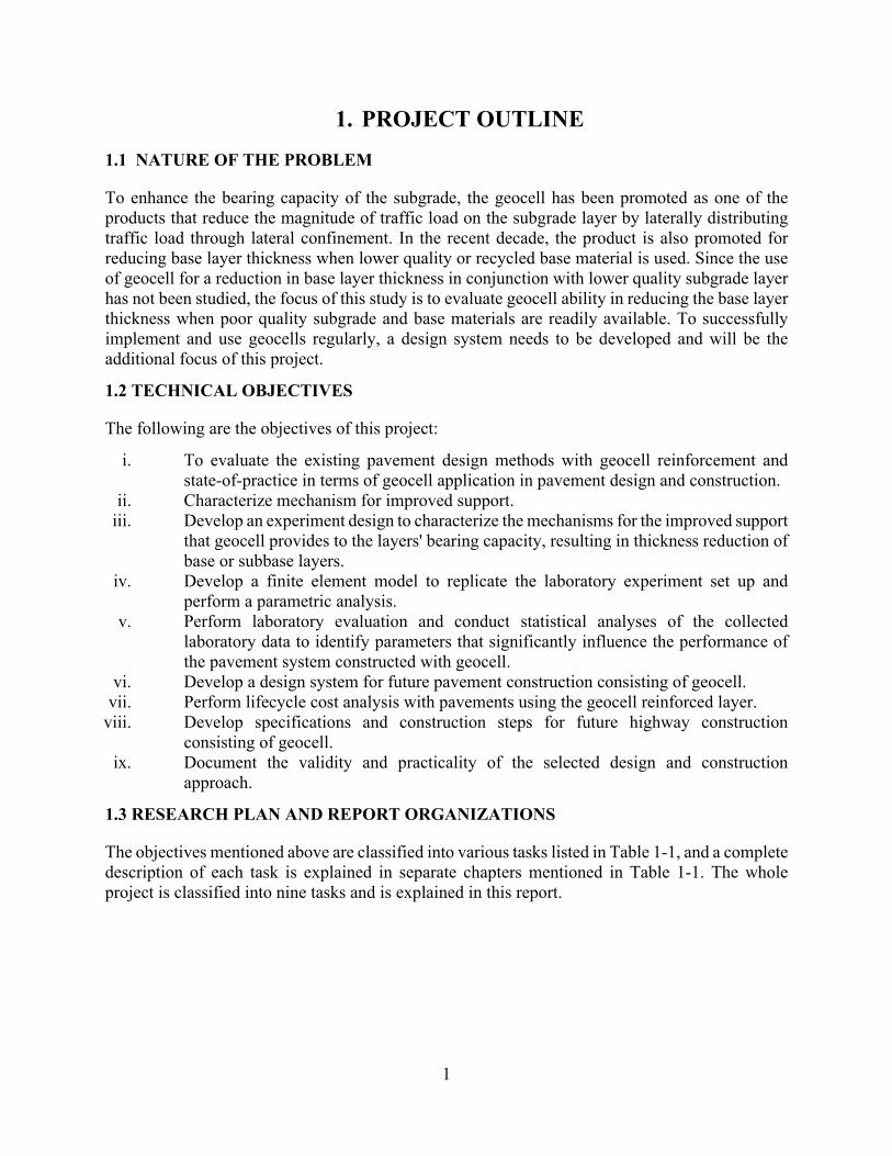
To enhance the bearing capacity of the subgrade, the geocell has been promoted as one of the products that reduce the magnitude of traffic load on the subgrade layer by laterally distributing traffic load through lateral confinement. In the recent decade, the product is also promoted for reducing base layer thickness when lower quality or recycled base material is used. Since the use of geocell for a reduction in base layer thickness in conjunction with lower quality subgrade layer has not been studied, the focus of this study is to evaluate geocell ability in reducing the base layer thickness when poor quality subgrade and base materials are readily available. To successfully implement and use geocells regularly, a design system needs to be developed and will be the additional focus of this project.

1.2 TECHNICAL OBJECTIVES

The following are the objectives of this project:

i. To evaluate the existing pavement design methods with geocell reinforcement and state-of-practice in terms of geocell application in pavement design and construction.

ii. Characterize mechanism for improved support. iii. Develop an experiment design to characterize the mechanisms for the improved support

that geocell provides to the layers' bearing capacity, resulting in thickness reduction of base or subbase layers.

iv. Develop a finite element model to replicate the laboratory experiment set up and perform a parametric analysis.

v. Perform laboratory evaluation and conduct statistical analyses of the collected laboratory data to identify parameters that significantly influence the performance of the pavement system constructed with geocell.

vi. Develop a design system for future pavement construction consisting of geocell. vii. Perform lifecycle cost analysis with pavements using the geocell reinforced layer.

viii. Develop specifications and construction steps for future highway construction consisting of geocell.

ix. Document the validity and practicality of the selected design and construction approach.

1.3 RESEARCH PLAN AND REPORT ORGANIZATIONS

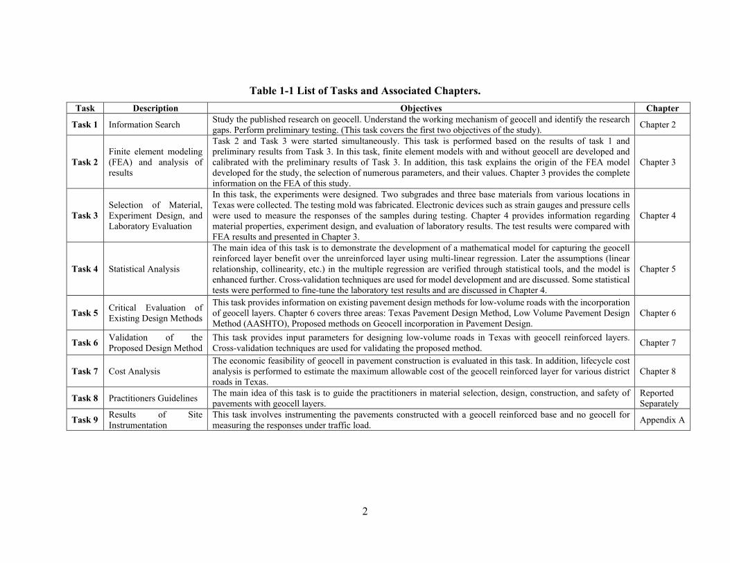
The objectives mentioned above are classified into various tasks listed in Table 1-1, and a complete description of each task is explained in separate chapters mentioned in Table 1-1. The whole project is classified into nine tasks and is explained in this report.

2

Table 1-1 List of Tasks and Associated Chapters.

Task Description Objectives Chapter

Task 1 Information Search Study the published research on geocell. Understand the working mechanism of geocell and identify the research gaps. Perform preliminary testing. (This task covers the first two objectives of the study). Chapter 2

Task 2 Finite element modeling (FEA) and analysis of results

Task 2 and Task 3 were started simultaneously. This task is performed based on the results of task 1 and preliminary results from Task 3. In this task, finite element models with and without geocell are developed and calibrated with the preliminary results of Task 3. In addition, this task explains the origin of the FEA model developed for the study, the selection of numerous parameters, and their values. Chapter 3 provides the complete information on the FEA of this study.

Chapter 3

Task 3 Selection of Material, Experiment Design, and Laboratory Evaluation

In this task, the experiments were designed. Two subgrades and three base materials from various locations in Texas were collected. The testing mold was fabricated. Electronic devices such as strain gauges and pressure cells were used to measure the responses of the samples during testing. Chapter 4 provides information regarding material properties, experiment design, and evaluation of laboratory results. The test results were compared with FEA results and presented in Chapter 3.

Chapter 4

Task 4 Statistical Analysis

The main idea of this task is to demonstrate the development of a mathematical model for capturing the geocell reinforced layer benefit over the unreinforced layer using multi-linear regression. Later the assumptions (linear relationship, collinearity, etc.) in the multiple regression are verified through statistical tools, and the model is enhanced further. Cross-validation techniques are used for model development and are discussed. Some statistical tests were performed to fine-tune the laboratory test results and are discussed in Chapter 4.

Chapter 5

Task 5 Critical Evaluation of Existing Design Methods

This task provides information on existing pavement design methods for low-volume roads with the incorporation of geocell layers. Chapter 6 covers three areas: Texas Pavement Design Method, Low Volume Pavement Design Method (AASHTO), Proposed methods on Geocell incorporation in Pavement Design.

Chapter 6

Task 6 Validation of the Proposed Design Method

This task provides input parameters for designing low-volume roads in Texas with geocell reinforced layers. Cross-validation techniques are used for validating the proposed method. Chapter 7

Task 7 Cost Analysis The economic feasibility of geocell in pavement construction is evaluated in this task. In addition, lifecycle cost analysis is performed to estimate the maximum allowable cost of the geocell reinforced layer for various district roads in Texas.

Chapter 8

Task 8 Practitioners Guidelines The main idea of this task is to guide the practitioners in material selection, design, construction, and safety of pavements with geocell layers.

Reported Separately

Task 9 Results of Site Instrumentation

This task involves instrumenting the pavements constructed with a geocell reinforced base and no geocell for measuring the responses under traffic load. Appendix A

3

2. LITERATURE REVIEW

The pavement construction has evolved over the years with the inclusion of geosynthetic material, starting with the simpler non‐woven to the more complex geocomposites. Technological advancement modified geosynthetic from two‐dimensional to cellular confinement systems that added a third dimension to geosynthetic. The Cellular Confinement Systems are popularly known as “Geocell.” Geocell is a durable, lightweight, three-dimensional fabricated system that is expandable on‐site to form a honeycomb‐like structure (Figure 2-1). Geocell is filled with the soil and compacted to enhance the bearing capacity of the subgrade layer. The depth of the geocell, as well as the size of each cellular unit, typically varies depending on the supplier as well as design requirements. The infill material can be non-cohesive recycled material as the geocell provides confinement and friction (geocell wall texture).

Figure 2-1 Geocell Supplied. 2.1 GENESIS

The development of geocell can be credited to the US Corps of Engineers for evaluating the feasibility of constructing bridge approach roads over the soft ground in 1975. Geocell was extensively used during the Vietnam War and the Gulf operations in the late 1980s (Figure 2-2). In the civilian sector, geocell was first used for load support systems in the early 1980s in the US, followed by slope erosion control and channel lining in 1984 in the US, and earth retention in Canada in 1986. Today applications are many and broadly include:

• Load support systems: o The increased bearing capacity of the foundation layer. o Reinforcement and support systems for embankments on the weak ground; o Reduction in pavement sections for all types of roads, laydown areas, and parking

lots. • Gravity walls for earth retention and surcharge load support. • Erosion control:

4

o Embankment slopes and natural slopes; o Water channel and water bondage linings.

Figure 2-2 Application of Geocell (US Army Corps). 2.1.1 Construction with Geocell

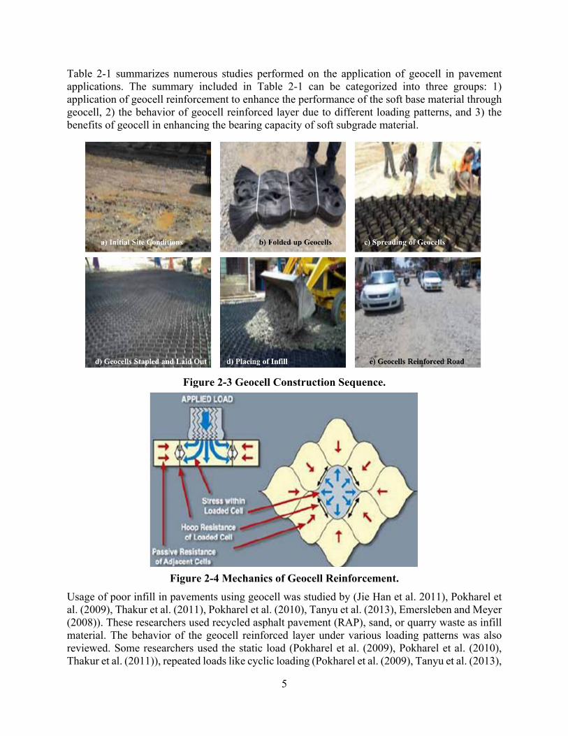
The sequence of construction is illustrated in Figure 2-3. The subgrade layer is leveled and compacted before the placement of geocell. Initially, the geocell was spread on top of the subgrade. However, a geomembrane layer is placed on top of the subgrade to minimize contamination. The spreading of geocell and interconnection of geocell is performed manually using ties and metal anchors or wooden stakes. The spread open geocell is in‐filled using a loader or similar equipment and compacted using a roller compactor. An additional layer of infill material is placed on top to provide a smoother ride.

2.1.2 Load Support Mechanism

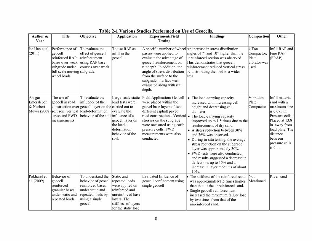
The proposed mechanics of geocell, as a load-carrying system, is illustrated in Figure 2-4. The moving traffic imparts vertical as well as lateral stresses in the base and subgrade layers. The geocell walls counteract the induced lateral stresses as its movement is restricted by adjacent cells. If q₀ is the vertical pressure, the lateral stresses generated along the walls of the individual cells would be K₀q₀ where K₀ is the coefficient of earth pressure “at rest.” The K₀ depends on the angle of internal friction (φ) of the infill soil. This increases the shear strength of the confined infill, which distributes the applied load over a wider area. This horizontal stress acting normal to the cell wall increases the vertical frictional resistance between the infill and the geocell wall, reducing the stresses induced on the layer below the geocell. This phenomenon allows transferring relatively heavy vertical loads onto relatively weak soils.

A detailed literature review was performed to identify the state-of-the-art and research gaps to be bridged to achieve this study's objectives. The literature review aimed to understand numerous factors in the published studies like the study's objective, laboratory setup, numerical modeling, and design. The comprehensive examination of published studies supported developing the laboratory setup, experimental design and proposed a design procedure for low volume roads with geocell. Although reviewed literature identified various applications of geocell, the literature relevant to pavements is summarized and tabulated in the following pages.

5

Table 2-1 summarizes numerous studies performed on the application of geocell in pavement applications. The summary included in Table 2-1 can be categorized into three groups: 1) application of geocell reinforcement to enhance the performance of the soft base material through geocell, 2) the behavior of geocell reinforced layer due to different loading patterns, and 3) the benefits of geocell in enhancing the bearing capacity of soft subgrade material.

Figure 2-3 Geocell Construction Sequence.

Figure 2-4 Mechanics of Geocell Reinforcement. Usage of poor infill in pavements using geocell was studied by (Jie Han et al. 2011), Pokharel et al. (2009), Thakur et al. (2011), Pokharel et al. (2010), Tanyu et al. (2013), Emersleben and Meyer (2008)). These researchers used recycled asphalt pavement (RAP), sand, or quarry waste as infill material. The behavior of the geocell reinforced layer under various loading patterns was also reviewed. Some researchers used the static load (Pokharel et al. (2009), Pokharel et al. (2010), Thakur et al. (2011)), repeated loads like cyclic loading (Pokharel et al. (2009), Tanyu et al. (2013),

6

accelerated pavement testing using wheel loads in the lab (Pokharel et al. 2009), field evaluation either using falling weight deflectometer or truck load (Emersleben and Meyer (2008), Imad L.Al Qadi & John J Hughes (2000), Ofer Jieft et al. (2011))

Jie Han et al. (2011) observed that the stress distribution angle increased due to the geocell reinforcement and less stress on top of the subgrade. Emersleben and Meyer (2008) evaluated geocell of different heights (4”, 6” and 8”) in the field as well as in the laboratory. They concluded that the geocell reinforcement decreases deflection due to an increase in reinforced layer modulus. Additionally, the study identified that increase in geocell height from 4” to 8” enhances the performance of the pavement, which was also observed by Pokharel et al. (2009). Al Qadi & John J Hughes (2000) observed that the resilient modulus of the infill material doubled due to the geocell reinforcement. An increase of base resilient modulus by 40-50% was witnessed by Tanyu et al. (2013). Ofer Jieft et al. (2011) perceived that the modulus of infill increased 2.75 times through the field, laboratory, and finite element evaluation.

Table 2-2 summarizes the laboratory setups of various research projects. Five parameters were identified to be summarized in this table: 1) the dimensions of the pavement tested, 2) the geocell material and height, 3) the thickness of the layer(s), 4) the load type, magnitude, and size of the plate for performing tests, and 5) test parameters and transducers for measuring response due to applied loads.

Dimensions: To minimize the end effect, the researchers fabricated boxes to evaluate geocell in the laboratory; however, the box size differed from one study to the other. For example, Emersleben and Meyer (2008) fabricated a box of 6.6’ x 6.6’ x 6.6’ whereas Tanyu et al. 2013 fabricated a box of 9.8’ x 9.8’ x 11.5’ size. Pokharel et al. (2009) constructed a pavement section of 10’ x 8’ x 6’ for performing accelerated testing at Kansas State University. Even though the box dimension varied between studies, the built structure can hold more than one layer of pavement section, and dimensions were large enough to minimize the end effect.

Geocell Type and Size: The literature review identified two types of material used in geocell production: High-density-polyethylene (HDPE) and Novel-polymeric-alloy (NPA). Three different geocell heights were studies: 4”, 6”, and 8.” Although different geocell have different openings (major and minor diameter), Emersleben and Meyer (2008) were the only ones evaluating the influence of geocell opening on performance.

Layer Thicknesses: Since the initial focus of the geocell was to enhance the bearing capacity of subgrade, most of the laboratory studies used a poor performing subgrade over which either geocell reinforced or unreinforced layer was placed followed by a cover layer. However, the thickness of the reinforced layer, unreinforced layer, and cover layer varied across studies. Tanyu et al. (2013) used expanded polystyrene (EPS), and Emersleben and Meyer (2008) used the Glyben to simulate the weak subgrade to minimize preparation time.

Load: Type, Magnitude, and Shape of Plate: The load applied for evaluation varied between studies ranging from static to repeated loads to moving loads. In repeated load tests, the majority of studies targeted 80 psi which resembles the truck tire load. For example, Jie Han et al. (2011), Pokharel et al. (2009), and Emersleben and Meyer (2008) targeted 80 psi that simulated a truck tire load. Emersleben and Meyer (2008), in the field evaluation, used a heavy truck weighing 41 tons traveling at a speed of 25 mph. The load magnitude used by Tanyu et al. (2013) is different from other studies. They classified load into two classes: 1) Construction load (load on the geocell

7

layer during the construction phase, a higher load but fewer number cycles), 2) Traffic load (load that comes with the base layer during regular traffic, a lower load but higher number of cycles). Tanyu et al. (2013) applied 100 psi to simulate construction load and 20 psi to simulate traffic load. The size of the loading plate varied between studies as well. Emersleben and Meyer (2008) used a 12” diameter plate, Tanyu et al. (2013) used a 10” diameter plate, and Pokharel (2009) and Thakur et al. (2011) used a 6” diameter plate. Even though the static and preliminary testing in Kansas studies used a 6” and 9” loading plates, the later studies (repeated load cycle) used a 12” diameter plate. The reasoning behind the larger diameter plate was not mentioned in the literature.

Test Parameters and Transducers: Jie Han et al. (2011) used pressure cells to monitor the vertical stress on the subgrade. The purpose of the pressure cell was to record the change in stress distribution angle due to the geocell reinforcement. Pokharel (2009) recorded the rut depths for specific wheel loads, vertical stress on the subgrade, and strains on geocells. Tanyu et al. (2013) measured strains in geocell and vertical deformations. It is noted that the researchers used three electronic transducer types: pressure cell to record vertical stress on the subgrade, strain gauges to record the strains on the geocell, linear variable differential transformer (LVDT), or dial gauges to measure the vertical deformations.

Tables 2-3 and 2-4 summarize studies exclusively on numerical and finite element modeling of geocell reinforced layers. Table 2-3 focuses on the published research on numerical modeling of the geocell reinforced layer. This table includes literature from the geocell application in roads and building foundations. Additionally, the table summarizes information on how the geocell reinforced layer was modeled and how the material was characterized to identify the influence of geocell. Most of the researchers, mentioned in this table, modeled geocell and infill material together as a composite material and characterized its behavior either using Drucker-Prager Model (Mhaiskar and Mandal, 1996), Duncan-Chang (Evan et al., 1994; Bathurst and Knight, 1998; Madhavi Latha and Rajagopal, 2008; Madhavi Latha and Rajagopal, 2009; and Madhavi Latha and Somwanshi, 2009) or Mohr-Coulomb Model ((Madhavi Latha and Rajagopal, 2007; and Han et al., 2008).

Modeling the geocell and infill as a composite material leads to lesser computational effort than modeling them separately. However, if the geocell and infill material needs to be modeled separately, the contact between the surfaces plays a vital role in the model. Hence, studies conducted to evaluate performance models are summarized in Table 2-4. The outcomes from Table 2-3 and Table 2-4 guided selecting the element type, meshing, contact models, material models. The complete details of the model developed for this study are discussed in the next chapter, “Finite Element Modeling.”

The existing pavement design methods using geocell reinforced layers are included in Table 2-5. Currently, two design methods are available 1) proposed by Pokharel (2009) that is a modification of Giroud & Han (2004) for Geogrid reinforced pavements, and 2) the second method is proposed by Presto Geosystems (2008). The design methods are for unpaved roads (no asphalt layer) and are empirical (based on the laboratory and field test results). A complete analysis of these two methods is presented in the chapter “Critical Evaluation of Existing Design Methods.”

There are multiple studies performed on geocell by various researchers of Kansas University that can be considered a torchbearer for studying the usage of geocell in pavements. Hence, a summary of all the studies performed at Kansas University is summarized in Table 2-6.

8

Table 2-1 Various Studies Performed on Use of Geocells. Author &

Year Title Objective Application Experiment/Field

Testing Findings Compaction Other

Jie Han et al. (2011)

Performance of geocell reinforced RAP bases over weak subgrade under full scale moving wheel loads

To evaluate the effect of geocell reinforcement using RAP base courses over weak subgrade.

To use RAP as infill in the geocell.

A specific number of wheel passes were applied to evaluate the advantage of geocell reinforcement on rut depth. In addition, the angle of stress distribution from the surface to the subgrade interface was evaluated along with rut depth.

An increase in stress distribution angles of 7° and 10° higher than the unreinforced section was observed. This demonstrates that geocell reinforcement reduced vertical stress by distributing the load to a wider area.

4 Ton Compactor. Plate vibrator was used.

Infill RAP and Fine RAP (FRAP)

Ansgar Emersleben & Norbert Meyer (2008)

The use of geocell in road construction over soft soil: vertical stress and FWD measurements

To evaluate the influence of the geocell layer on the load-deformation behavior of the soil

Large-scale static load tests were carried out to evaluate the influence of a geocell layer on the load-deformation behavior of the soil.

Field Application: Geocell were placed within the gravel base layers of two different asphalt paved road constructions. Vertical stresses on the subgrade were measured using earth pressure cells. FWD measurements were also conducted.

• The load-carrying capacityincreased with increasing cellheight and decreasing celldiameter.

• The load-carrying capacityimproved up to 1.5 times due to thereinforcement of dry sand.

• A stress reduction between 30%and 36% was observed.

• During in-situ testing, the averagestress reduction on the subgradelayer was approximately 30%.

• FWD tests were also conducted,and results suggested a decrease indeflections up to 15% and anincrease in layer modulus of about10%.

Vibration Plate Compactor

Infill material sand with a maximum size is 0.075 in. Pressure cells: Placed at 13.8 in. away from load plate. The distance between pressure cells is 6 in.

Pokharel et al. (2009)

Behavior of geocell reinforced granular bases under static and repeated loads

To understand the behavior of geocell reinforced bases under static and repeated loads by using a single geocell

Static and repeated loads were applied on reinforced and unreinforced base layers. The stiffness of layers for the static load

Evaluated Influence of geocell confinement using single geocell

• The stiffness of the reinforced sandwas approximately1.5 times higherthan that of the unreinforced sand.

• Single geocell reinforcementincreased the maximum failure loadby two times from that of theunreinforced sand.

Not Mentioned

River sand

9

Author & Year

Title Objective Application Experiment/Field Testing

Findings Compaction Other

was calculated. Elastic deformation and plastic deformations were calculated per each cycle of repeated loading.

• Single geocell reinforcement reduced plastic deformation and increased the percent of elastic deformation under repeated loading. It took 10 cycles to reach 80% or more of elastic deformation. The elastic deformation reached 95% of the total deformation at the end of 150 loading cycles.


Experimental study on bearing capacity of geocell reinforced bases


Static and repeated loads were applied on reinforced and unreinforced base layers.

The layer stiffness due to static load was calculated. Elastic and plastic deformations were calculated per each cycle of repeated loading.


• Under static loading, the improvement factor (ratio of the slope of an initial portion of the load-displacement curve for reinforced and unreinforced base) for geocell-reinforced sand was 1.75 in terms of ultimate bearing capacity and 1.5 in terms of stiffness.

• Permanent deformation reduced to 1.5 times of unreinforced base (quarry waste).

• Reinforced quarry waste had a higher percentage of elastic deformation. At the same time, reinforcing river sand had a lower percentage of elastic deformation compared to unreinforced sand. The inferior quality of sand was cited as a reason for higher deformation.

Not Mentioned

River sand & quarry waste

Giroud & Jie Han (2004)

Design Method for geogrid reinforced unpaved Roads. I. Development of design Method

The proposed method for calculating the thickness of the base layer of unpaved roads.

This design method can be used for geogrid reinforced unpaved roads.

The theoretical study only (Assumed proportionality between rut depth and bearing capacity mobilization factor. Tension membrane effect is not considered.)

Proposed a method for calculating base course thickness for a reinforced unpaved road is calculated using a different equation.

NA NA

10

Author & Year




Design Method for geogrid reinforced unpaved roads. II. Calibration and Applications

Calibrate the design method using field wheel load tests and laboratory cyclic plate loading tests on an unreinforced and reinforced base layer.

This design method can be used for geogrid reinforced unpaved roads.

The theoretical study only (Data for calibrating the models was taken from other researchers. Details of data were not discussed in this paper)

• The calibrated design proposed in the above paper using field and laboratory data.

• Analyzed test data for three case studies.

Thakur et al. (2011)

Creep deformation of unreinforced and geocell reinforced recycled asphalt pavements

Permanent deformation or rutting due to creep deformation is one of the concerns of RAP usage in base courses. Confinement due to Geocell can reduce the creep.

Using RAP as a base layer with geocell reinforcement


• Confinement of RAP significantly increased its strength.

• NPA geocell significantly reduced the initial deformation and the rate of creep of the RAP.

The material in geocell is compacted in three layers 2 in., 2 in., 0.8 in—95% of MDD.

Infill RAP

Imad L.Al Qadi & John J Hughes (2000)

Field evaluation of geocell use in flexible pavements

Analysis of a pavement performance constructed with geocell and geosynthetics on the weak subgrade.

Various pavement sections were constructed using geocell, geogrids, and geosynthetics on a high-traffic road.

FWD tests were performed periodically for up to 3 years. FWD measurements were used to calculate the surface modulus and back-calculate the resilient modulus of the subgrade based on known thicknesses and reasonably assumed resilient moduli of pavement layers based on material testing and field experience.

• In sections where 4” thick geocell were used, the resilient modulus of the aggregate layer increased almost twofold due to the material confinement.

• The aggregate confinement provided by the geocell and the subgrade-subbase separation provided by the geotextile improved the performance of pavement constructed on a weak subgrade for a heavily trafficked pavement.

• In this study combination of geocell, geogrid, and geosynthetic were used. So, specific benefit due to geocell was difficult to evaluate.

Material backfilled using backhoe and movement of equipment over geocell was discussed

Infill subbase material.

11

Author & Year





Rutting due to creep deformation is one of the concerns of RAP usage in base courses. Confinement due to Geocell can reduce the creep deformation of RAP.

Using of RAP as a base layer with geocell reinforcement

Three laboratory tests were conducted in a test box (100 in. by 100 in. by 6 in. high) to investigate the role of lateral confinement in reducing creep deformation of RAP. Creep tests were conducted at a room temperature of 77°C. Each test lasted for 7 to 10 days.

• Confinement of RAP significantly increased its strength.

• NPA geocell significantly reduced the initial deformation and therate of creep of the RAP.

The material in geocell compacted in three layers 2in., 2 in., 0.8 in—95% of MDD. Compaction method not mentioned.

NPA geocell Used


Accelerated pavement testing of geocell reinforced unpaved roads over weak subgrade

The objective was to evaluate the effectiveness of geocells as reinforcement for granular base courses over weak subgrade.

Assess the influence of infill materials on geocell performance

Laboratory tests on 20 ft. by 16 ft. by 5.9 ft. pavement trial area divided into four sections. Analyzed four different types of pavement sections.

• Reinforced geocell with Quarrywaste performed poorly.

• Geocell with aggregate as infillperformed better.

• RAP as infill performance is betterthan aggregate

• Welds of geocell were broken underwheel loads.

• Geocell layer reduced the verticalstress by dispersing the load to awide area (12” regular base ≈ 6.5”Geocell layer)

Vibratory compactor

Infill Materials; Crushed Limestone, Quarry Waste, and RAP


Investigation of factors influencing the behavior of single geocell reinforced bases under static loading

This study experimentally investigated the factors influencing the behavior (stiffness and bearing capacity) of single geocell-reinforced bases, including shape, type, embedment, the height of


Repeatability of test method was verified in the study and later confirmed the test set up yields similar results (repeated test)

• Elastic modulus of geocell is anessential factor

• Unconfined geocell had a lowerstiffness but a higher ultimate loadcapacity than the confined geocell

• Performance of geocell depends oninfill material. Cohesionless infillmaterial behaved well than cohesive

• Single geocell reinforce base had alower stiffness and bearing capacitythan the multiple geocell reinforcedbases.

River sand compacted to 70% of relative density and quarry waste to 95% MDD.

Infill Materials: 1) River Sand2) Quarry

Waste

12

Author & Year



geocells, and quality of infill materials.

• A thinner unreinforced or geocell-reinforced base on a firm subgrade had a higher bearing capacity than the thicker unreinforced or geocell-reinforced base, respectively.

Emersleben & Meyer (2008)

Bearing capacity improvement of gravel base layers in road constructions using Geocells

To evaluate the influence of a geocell layer on the load-deformation behavior of soil. Geocell made with different materials, with various cell heights and different cell diameters.

Model tests were performed in the laboratory with various geocell parameters and applied to a trial section in the field.

Prepared and tested geocell using a box size of 6.6 ft3. Different geocell heights were tested (4”, 6”, and 8”). Different Geocell diameters were tested (6.3”, 9”, and 12”). Earth Pressure cells with a diameter of 2” were used to measure the vertical earth pressure on the subgrade. Pressure cells were placed within the sand.

• The decrease in cell diameter reduced rutting and vertical stress.

• Increase in cell height reduced rutting and vertical stress.

• Geocell layer increased the bearing capacity by reducing 30% or more vertical stress on to subgrade.

• The deflections on asphalt surface were reduced by 15%, and back-calculated layer modulus increased by 10%

Sand infill

Tanyu et al. (2013)

Laboratory evaluation of geocell reinforced gravel subbase over poor subgrades

Strain gauges (bonded metallic foil) were used to measure strains of geocell. Vertical deflections in the test pit were measures using position transducers. CR9000 data logger was used to acquire data from position transducers and strain gauges.

The presence of geocells reduced the elastic deflection of the working platforms by 30-50%, improved the resilient modulus of the subbase by 40-50%, and the modulus of subgrade reaction by more than two times.

90% of relative compaction is based on a standard proctor. The material in the geocell compacted with the vibratory compactor.

Subbase material.

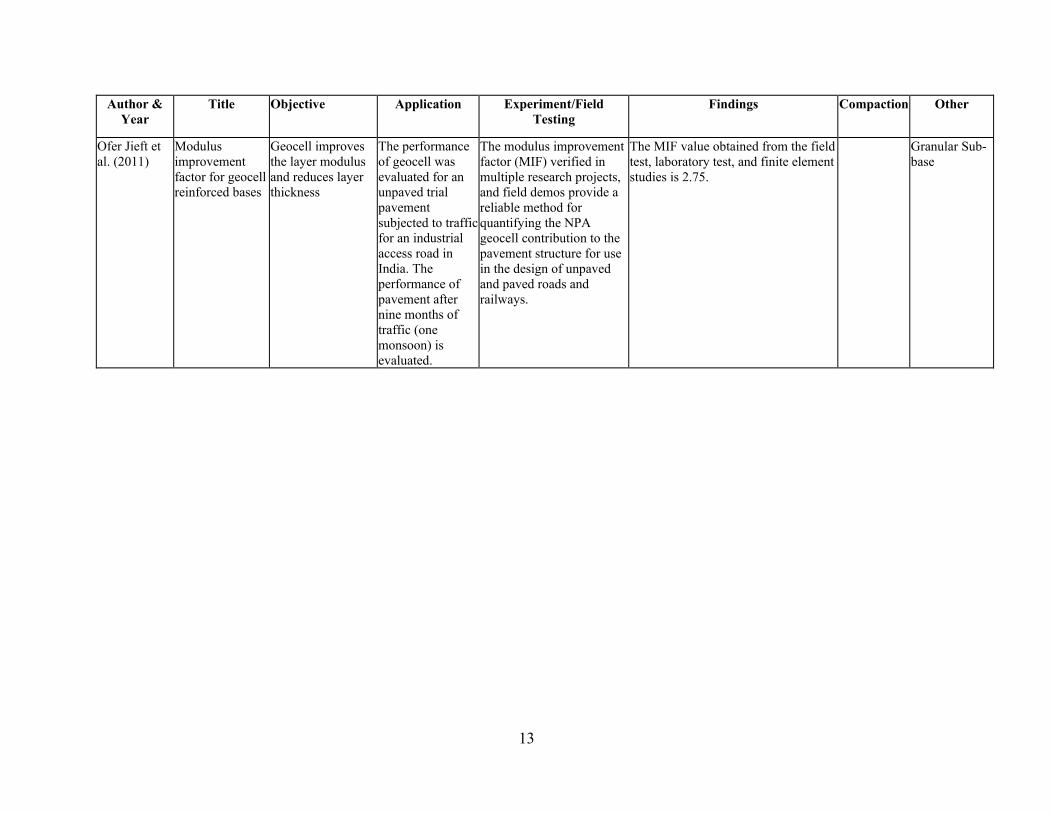
13

Author & Year



Ofer Jieft et al. (2011)

Modulus improvement factor for geocell reinforced bases

Geocell improves the layer modulus and reduces layer thickness

The performance of geocell was evaluated for an unpaved trial pavement subjected to traffic for an industrial access road in India. The performance of pavement after nine months of traffic (one monsoon) is evaluated.

The modulus improvement factor (MIF) verified in multiple research projects, and field demos provide a reliable method for quantifying the NPA geocell contribution to the pavement structure for use in the design of unpaved and paved roads and railways.

The MIF value obtained from the field test, laboratory test, and finite element studies is 2.75.

Granular Sub-base

14

Table 2-2 Test Setups Developed for Evaluation of Geocell. Author and Year

Title Specimen Size

Geocell Size Layer Thickness Load Type Load Magnitude and shape

Loading Plate

Test Parameters and Means



Test section size was 20’ by 16’ by 5.9’. Divided into four sections

Geocell used were in three heights 3”, 4”, and 6” high. Single Geocell dimensions 8.2” long and 10” wide

Seven different sections 1) 12” RAP over Subgrade 2) 16” geocell reinforced RAP 3) 4” geocell reinforced RAP 4) 2 layers of 4” geocell reinforced RAP separated by 1.2” RAP cover. The top cover is 2.8” thick 5) 10” unreinforced FRAP 6) 1 layer 4” geocell reinforced FRAP over 4” unreinforced FRAP. 2” FRAP cover. 7) 3” geocell reinforced FRAP. 4” unreinforced FRAP. 3” FRAP Cover

Tests were carried out for 15000-wheel passes. Tests stopped for a rut depth of 3.”

42’-long reaction frame and an 18 KN single axle load with dual tires Wheel Load—Tire Pressure 80 psi. The frequency of the moving wheel was 0.167 Hz (i.e., 6 s/Pass), and the wheels were run at a speed of 11.3 km/h within the test pit.

NA Rut Depth, Vertical Stress on subgrade, stress distribution angle, maximum recorded tensile strain

Ansgar Emersleben & Norbert Meyer (2008)

The use of geocell in road construction over soft soil: vertical stress and FWD measurements

6.6’ x 6.6’ x 6.6’

1) HDPE 8.3” long and 9.8” wide. Heights 4”, 6” and 8”. Cell walls perforated with 0.4” diameter holes. 2) Thermally solidified non-woven geosynthetic. With diameters 6.3”, 8.7” and 11.8”. Height 8”.

Laboratory Set Up: Glyben used as a subgrade (4” thick). It is compacted as 10cms layers. The non-woven material is used to separate the subgrade and infill material. Field Set-Up: 6” Gravel layer over subgrade. 8” geocell thick layers. With little cover and a 4” Asphalt layer

Static Load. Field Test: Heavy Truck

Vertical load up to 150KN. Circular Steel plate used for applying load. Field Setup: Heavy Truck with five axles and a weight of approximately 41 tons crossed the road at different speeds.

12” (dia)

Lab Set-Up: Load Carrying Factor: Ratio of footing pressure between reinforced and unreinforced soil for the same settlement; Vertical Stresses. Field Set-Up: Stresses on subgrade were measured during vehicle passes. FWD measurements were taken after the road was subjected to traffic.

15

Author and Year

Title Specimen Size


Loading Plate



Experimental study on bearing capacity of geocell reinforced bases

2’ x 2’ in plan

Single-cell 4” height, 8” diameter with two perforations of 0.155 in.2 each on both sides. NPA geocell

Filled sand in geocell in three layers. Two 2” and one 0.75” layer. 70% relative density is the compaction. In case quarry waste as fill material compacted to 95% of MDD

Static and repeated load

Static Load: Applied until geocell reinforced sand failed (72.5 psi). Repeated Load: The repeated load test was only conducted on the reinforced sand at an applied pressure of 50 psi (70% of static failed pressure). 1 cycle/minute. 150 Cycles. On quarry waste, the cyclic load is 80 psi

6” (dia) The stiffness of the unreinforced and reinforced sands using pressure displacement curves. Repeated Load: % Elastic Deformation (Elastic displacement to the total displacement induced by each load cycle)



2’ x 2’x 0.5’

4” high geocell 4.75” and 4” high geocell with 1” cover. No subgrade was used in this study.

Static Creep Behavior Analysis: 40 psi on reinforced & unreinforced for ten days. For Comparison purposes, wholly confined RAP (RAP compacted in a compaction mold) was also tested for the same pressure seven days and measured axial strains with time.

6” (dia) Deformations in two perpendicular transverse directions were measured with three digital dial gauges mounted on the loading plate, and averages of three were used for calculation. (5 Minute Interval)


Accelerated pavement testing of geocell reinforced unpaved roads over weak subgrade

20’ X 16’ X 6’ (Divided into four sections for 4 analyzing 4 sections)

6.7” thick geocell. 6” geocell + 0.75” cover

Four pavement sections were tested. 1) Unreinforced base 12” aggregate layer over weak subgrade. 2) 3 sections had 6.7” NPA geocell reinforced sections over the weak subgrade

Single axle dual tire-wheel loading

Tire pressure applied 80 psi. Wheels are running at 7 mph with a frequency of 6s per pass. Tests terminated after 305 passes as the rut depth in one section is more than 5”.

21.6” width of dual tire

Rut depths for specific wheel passes and the angle of stress distribution from the surface to the base course-subgrade interface using pressure cells.

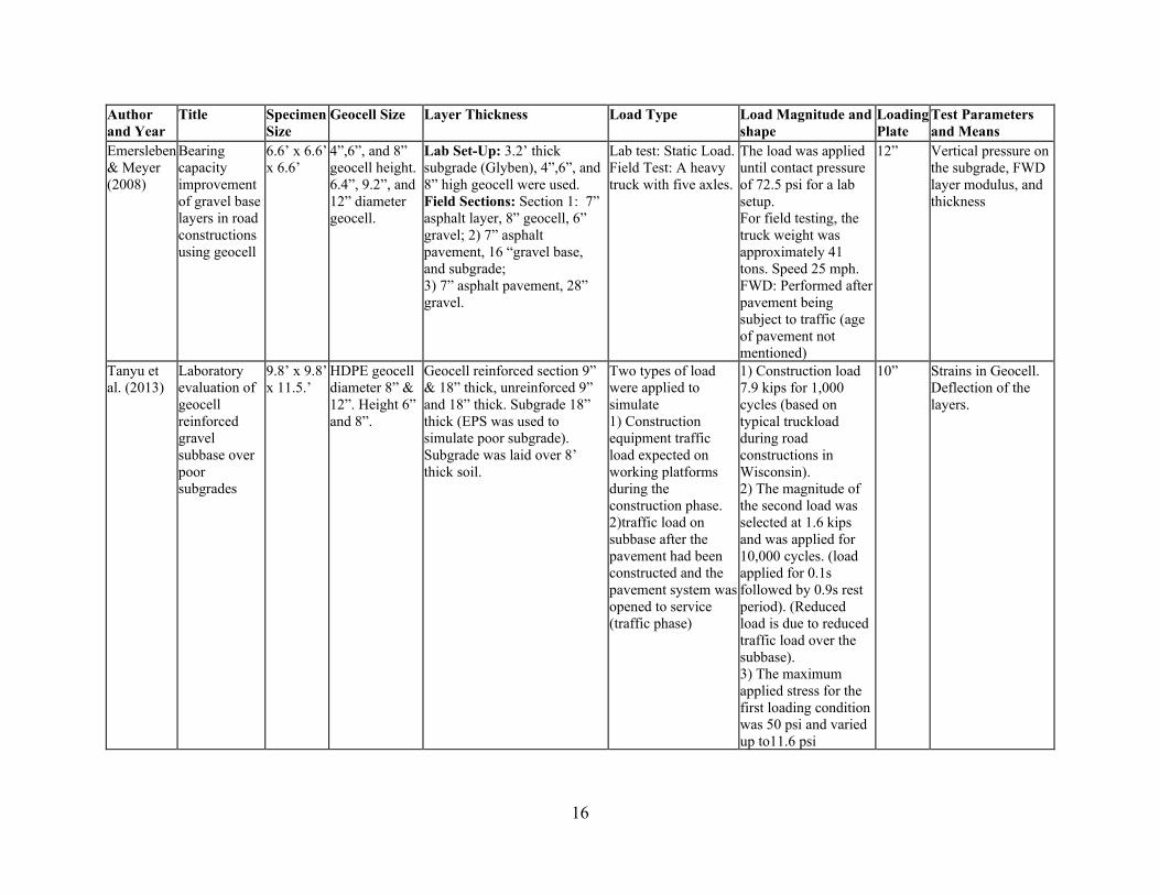
16

Author and Year

Title Specimen Size


Loading Plate


Emersleben & Meyer (2008)

Bearing capacity improvement of gravel base layers in road constructions using geocell

6.6’ x 6.6’ x 6.6’

4”,6”, and 8” geocell height. 6.4”, 9.2”, and 12” diameter geocell.

Lab Set-Up: 3.2’ thick subgrade (Glyben), 4”,6”, and 8” high geocell were used. Field Sections: Section 1: 7” asphalt layer, 8” geocell, 6” gravel; 2) 7” asphalt pavement, 16 “gravel base, and subgrade; 3) 7” asphalt pavement, 28” gravel.

Lab test: Static Load. Field Test: A heavy truck with five axles.

The load was applied until contact pressure of 72.5 psi for a lab setup. For field testing, the truck weight was approximately 41 tons. Speed 25 mph. FWD: Performed after pavement being subject to traffic (age of pavement not mentioned)

12” Vertical pressure on the subgrade, FWD layer modulus, and thickness

Tanyu et al. (2013)

Laboratory evaluation of geocell reinforced gravel subbase over poor subgrades

9.8’ x 9.8’ x 11.5.’

HDPE geocell diameter 8” & 12”. Height 6” and 8”.

Geocell reinforced section 9” & 18” thick, unreinforced 9” and 18” thick. Subgrade 18” thick (EPS was used to simulate poor subgrade). Subgrade was laid over 8’ thick soil.

Two types of load were applied to simulate 1) Construction equipment traffic load expected on working platforms during the construction phase. 2)traffic load on subbase after the pavement had been constructed and the pavement system was opened to service (traffic phase)

1) Construction load 7.9 kips for 1,000 cycles (based on typical truckload during road constructions in Wisconsin). 2) The magnitude of the second load was selected at 1.6 kips and was applied for 10,000 cycles. (load applied for 0.1s followed by 0.9s rest period). (Reduced load is due to reduced traffic load over the subbase). 3) The maximum applied stress for the first loading condition was 50 psi and varied up to11.6 psi

10” Strains in Geocell. Deflection of the layers.

17

Table 2-3 Numerical Modeling of Geocell-Reinforced Layer. Author and Year

Title Model Software Program

Geocell Model & Infill Soil Model Mesh

Evan et al. (1994)

Geocell mattress effects on the embankment settlements, vertical and horizontal deformations of foundations and embankments: settlement

Geocell reinforced sand on top of soft subgrade supporting an embankment load

SSTIPG/2-D Duncan-Chang model, equivalent linearly elastic planar reinforcement

Mhaiskar and Mandal (1996)

Investigations on soft clay subgrade strengthening using geocells

Geocell reinforced sand on top of clay subgrade, supporting a rectangular footing

ANSYS/3-D Geocell reinforced soil was modeled as a composite material using Drucker-Prager Model

Bathurst and Knight (1998)

Analysis of geocell reinforced soil covers over large span conduits

Geocell reinforced sand over a steel conduit

GEOFEM/2-D Geocell reinforced soil was modeled as a composite material using Duncan-Chang Model

Madhavi Latha and Rajagopal (2007)

Parametric finite element analyses of Geocell Supported Embankment

Geocell reinforced sand on top of clay subgrade supporting an embankment load

GEOFEM/2-D Geocell reinforced soil was modeled as a composite material using the Mohr-Coulomb model

3 Node triangles within each rectangle

Han et al. (2008)

The behavior of geocell reinforced sand under a vertical load

Single-cell reinforced sand supporting the rectangular footing

FLAC/3-D Mohr-Coulomb Model/Linearly elastic membrane


Equivalent continuum simulations of geocell reinforced sand beds supporting strip footings

Geocell reinforced sand supporting a strip footing



Numerical simulation of the behavior of geocell reinforced sand in foundations

Geocell reinforced sand supporting a strip footing


Madhavi Latha and Somwanshi (2009)

Effect of reinforcement form on the bearing capacity of square footings on sand

Geocell reinforced sand supporting a square footing

FLAC/3-D (Fast Lagrangian Analysis of Continua)

Geocell reinforced soil was modeled as a composite material using Duncan-Chang Model

18

Author and Year

Title Model Software Program

Geocell Model & Infill Soil Model Mesh

Xiaoming Yang (2010)

Numerical analyses of geocell reinforced granular soils under static and repeated loads

Characterize the performance of the geocell reinforced soil under static and repeated loads

FLAC-3D (finite difference program)

Infill material is modeled using Duncan Chang Model; geocell was modeled using a linear elastic plate model. A Mechanistic empirical model was developed for Geocell reinforced soil under repeated loads based on stress-dependent response model in MEPDG

The geocell pockets were modeled in a diamond shape

Mehdipour et al. (2013)

Numerical study on the stability of geocell reinforced slopes by considering the bending effect

Behavior of geocell reinforced slopes

FLAC-2D The Young's modulus of geocell encased soil was obtained from the elastic modulus of the unreinforced soil and the tensile modulus of the geocell reinforcement using an empirical equation proposed by Madhavilatha(2007). The interface shear stress-strain relationship between the geocell and the foundation soil was modeled based on the Mohr-Coulomb sliding criterion

19

Table 2-4 Finite Element Modeling Geocell Reinforced Layer and Contact Models. Title Objectives Findings Contact Model Geocell Model & Infill Soil Model

Numerical Modeling of behavior of railway ballasted structure with geocell confinement / Ben Leshchinsky, Hoe I Ling (2013)

Perform a parametric study to investigate the effects of geocell confinement on ballasted embankments when encountering a soft subgrade, weaker ballast, or varying reinforcement stiffnesses.

• Geocell confinement was very effective in reducing vertical deformations, primarily when the low-quality material was used.

• Geocell assists in redistributing the stresses more evenly, possibly preventing the development of high shear strains and failure, especially on softer subgrades.

• Lateral spreading along the slope of the railroad substructure was greatly reduced.

• More uniform subgrade stress distribution. Also, the magnitudes of stresses were reduced significantly, in turn mobilizing more of the subgrade's shear strength and preventing shear failure.

The interaction between the surrounding ballast/sub-ballast and the geocell was modeled with contact elements having "hard” normal contact (no penetration), and tangential contact was modeled as 2/3 of the tangent of the friction angle (45), which was applied using penalty friction algorithm.

Infill ballast was modeled as non-associative elastic-plastic material, obeying 3D Drucker Prager Yield Criterion. The foundation was modeled as an elastic material to demonstrate the effects of a compressible, soft soil without considering any time-dependent behavior. The geocell was modeled as an elastic material. The shape of the geocell was modeled with a rhomboidal shape instead of the actual pseudo sinusoidal shape used in the tests. This prevented meshing issues that could occur due to the complex nature of the mesh under 3D configurations.

3-Dimensional numerical modeling of geocell reinforced sand beds/ A Hegde and T.G.Sitharam (2015)

This paper presents a more realistic modeling approach to model geocell in the 3D framework. 3D simulations were performed by the actual 3D honeycomb shape of geocell using the FLAC3D.

It was found that the geocells distribute the load laterally and to a relatively shallow depth as compared to the unreinforced case and the geogrid reinforced case. Therefore, the performance of the foundation bed was directly influenced by the modulus and the height of the geocell.

The geocell and the soil interfaces were linearly modeled with Mohr-Coulomb Yield Criterion (FLAC 3D).

The elastic-perfectly plastic Mohr-Coulomb model was used to simulate the behavior of the foundation and the infill soil. The geocell was modeled using the geogrid structural element. The Linear elastic model was used to simulate the behavior of the geocell.

20

Title Objectives Findings Contact Model Geocell Model & Infill Soil Model

Numerical study on the stability of geocell reinforced slopes by considering the bending effect/ Iman Mehdipour, Mahmoud Ghazavi, Reza Ziaie Moayed (2013)

Behavior of geocell reinforced slopes

The interface shear stress-strain relationship between the geocell and the foundation soils was modeled based on the Mohr-Coulomb sliding criterion (FLAC 2D)

Joint Strength and Wall Deformation Characteristics of a Single-cell Geocell Subjected to Uniaxial Compress/ A Hegde and T.G.Sitharam (2014)

The current study discusses the joint strength and the wall deformation characteristics of a single cell when subjected to uniaxial compression.

The results of the experimental study revealed that the deformation of the geocell wall decrease with the increase in the friction angle of the infill material. The experiment and the numerical results were found to be in good agreement with each other. A simple analytical model based on the theory of thin cylinders is also proposed to calculate the accumulated strain of the geocell wall.

The interface behavior of the geogrid element used in FLAC3D can be numerically represented at each geogrid node by a rigid attachment in the normal direction and a spring slider in the tangent plane to the geogrid surface. The orientation of the spring slider changes concerning relative shear displacement between the geogrid and the soil. The shear behavior of the geogrid soil interface is cohesive and frictional and controlled by the parameters, namely, interface shear modulus, interface cohesive strength, and interface friction angle. A partially rigid interface with interface coefficient R(inter)=0.7 was assumed between the soil and the geocell material. The interface coefficient relates the strength of the soil to the strength of the interfaces. (FLAC 3D)

Elastic perfectly plastic Mohr-Coulomb criterion was used to model the behavior of the soil. Geocell material was modeled using the simplistic linear elastic model. The shape of the Geocell is modeled using the quarter symmetry, assuming the shape of the geocell is cylindrical.

21

Title Objectives Findings Contact Model Geocell Model & Infill Soil Model

Accelerated Pavement Testing of Low Volume Paved Roads with Geocell Reinforcement. Brandon Bortz, Mustaque Hossain (2015)

To test a geocell design with different infill materials and a thin HMA layer under simulated full-scale traffic on a marginal subgrade, using accelerated pavement testing (APT). To develop a finite element model for the geocell reinforced paved roads considering the quality of the infill material to study the design of such pavements.

Trial sections with a 50 mm HMA layer reached the failure criteria of 12.5 mm rut depth after 10,000 passes due to excessive stress in the subgrade. The redesigned sections with 100 mm HMA layer carried 1.2 million passes without reaching 12.5 mm failure rut depth. The geocells with marginal materials as infills appear to be viable in low volume paved road applications.

Geocells were meshed doubly curved thin or thick shell. An embedded region was used to place the geocells in the base layer. Embedded regions are a group of elements that are within a "host" region. The response of the host elements constrained embedded elements; therefore, no contact friction could be attributed to the geocell wall. (Abaqus)

The base material was modeled with Mohr-Coulomb plasticity. HMA layers were considered linear elastic. Geocell as linear elastic.

Numerical analyses of geocell reinforced granular soils under static and repeated loads Xiaoming Yang (2010)

Characterize the performance of the geocell reinforced soil under static and repeated loads

Mohr-Coulomb yield criterion (FLAC 3D)

Infill material is modeled using Duncan Chang Model; geocell was modeled using a linear elastic plate model. A Mechanistic empirical model was developed for Geocell reinforced soil under repeated loads based on stress-dependent response model in MEPDG

22

Table 2-5 Existing Pavement Design Methods of Geocell-Reinforced Layers Author

and Year Title Properties

Measured Model Used Modification Factors Design Thickness Approach



Rutting and stress distribution angle

NPA geocell reinforcement increased the life of unpaved roads compared with an unreinforced section by 1.8 times with one layer of 10 cm high geocell. Geocell higher than 10 cm may be beneficial, but it makes compaction more difficult.


Behavior of geocell reinforced granular bases under static and repeated loads

Stiffness of reinforced layer and % Elastic deformation in total deformation

The high percent of elastic deformation is beneficial to the service life of the road.


Design Method for Geogrid Reinforced Unpaved Roads. 1. Development of Design Method

Distribution of stress, the strength of base course material, the interlock between geosynthetic and base course material, geosynthetic in-plane stiffness.

Design Method was developed based on 1) stresses at the base course/subgrade soil interface. 2) determining the rut depth as a function of the stresses at the base course/subgrade soil interface and the bearing capacity of the subgrade soil.

1)Base course is characterized by its CBR. Resilient modulus is estimated by using CBR. 2) Subgrade characterized by CBR & Undrained cohesion. Resilient modulus is estimated by using CBR. 3) Geogrid is characterized by Aperture Stability modulus.

Developed an equation to calculate the thickness based on normal stress pi at the interface between base course and subgrade soil combined with subgrade soil needs with three unknowns 1) bearing capacity mobilization coefficient, 2) bearing capacity factor, 3) distribution angle.

1) Assumed the bearing capacity factor 3.14 for unreinforced bases and 5.71 for reinforced bases with geogrid, whereas 5.14 for geotextile reinforced unpaved roads. 3) Proposed an equation for calculating bearing capacity mobilization coefficient. The equation has three unknown parameters that need to calibrate with experimental data. 4) Explained that the geogrid properties will influence the stress distribution angle. Higher aperture stability modulus increases the distribution angle. As well as the thickness of the base layer has a positive influence on the distribution angle.


Accelerated pavement testing of geocell reinforced

Rut depth and stress distribution angle

Calculated the stress distribution angle under wheel loads for various sections. The calculated stress angle can be used to calibrate the design.

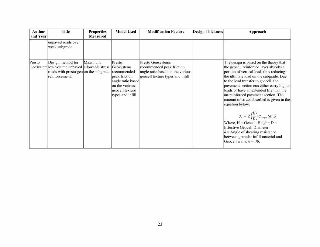
23

Author and Year

Title Properties Measured

Model Used Modification Factors Design Thickness Approach

unpaved roads over weak subgrade

Presto Geosystem

Design method for low volume unpaved roads with presto geo reinforcement.

Maximum allowable stress on the subgrade

Presto Geosystems recommended peak friction angle ratio based on the various geocell texture types and infill

Presto Geosystems recommended peak friction angle ratio based on the various geocell texture types and infill

The design is based on the theory that the geocell reinforced layer absorbs a portion of vertical load, thus reducing the ultimate load on the subgrade. Due to the load transfer to geocell, the pavement section can either carry higher loads or have an extended life than the un-reinforced pavement section. The amount of stress absorbed is given in the equation below.

𝜎𝜎𝑟𝑟 = 2 �𝐻𝐻𝐷𝐷�𝜎𝜎𝑎𝑎𝑎𝑎𝑎𝑎𝑎𝑎𝑡𝑡𝑡𝑡𝑡𝑡𝑡𝑡

Where, H = Geocell Height; D = Effective Geocell Diameter δ = Angle of shearing resistance between granular infill material and Geocell walls; δ = rΦ;

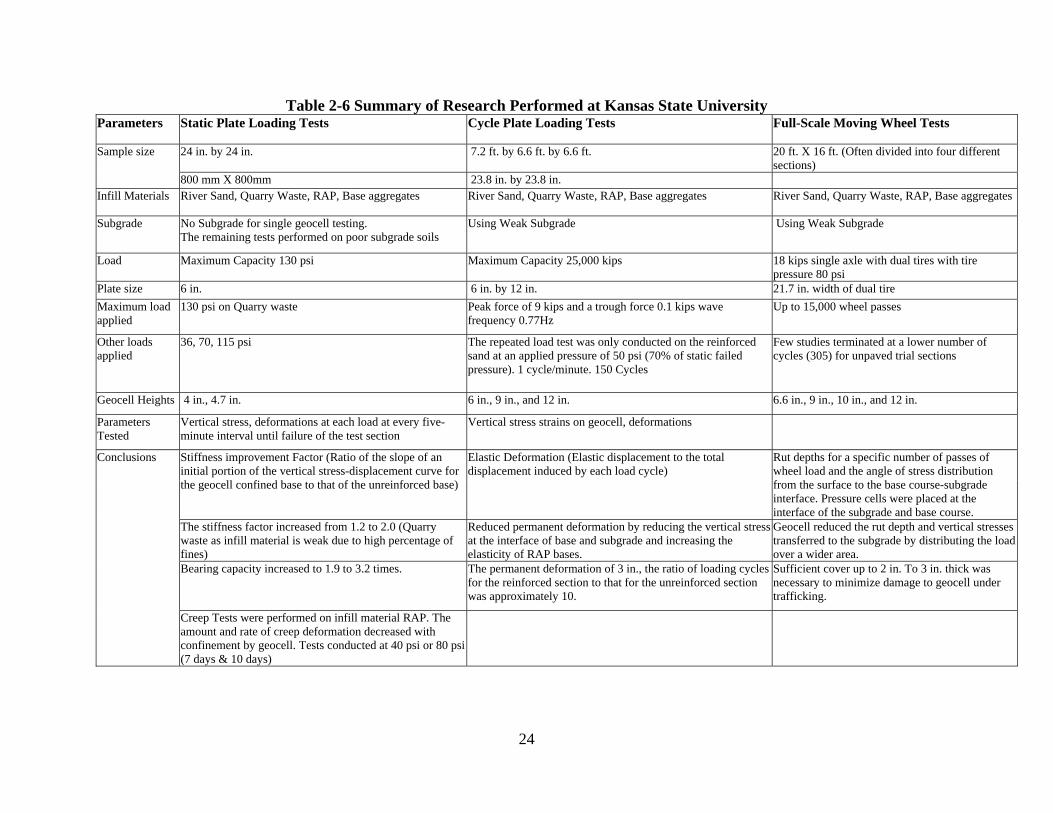
Table 2-6 Summary of Research Performed at Kansas State University Parameters Static Plate Loading Tests Cycle Plate Loading Tests Full-Scale Moving Wheel Tests

Sample size 24 in. by 24 in. 7.2 ft. by 6.6 ft. by 6.6 ft. 20 ft. X 16 ft. (Often divided into four different sections)

800 mm X 800mm 23.8 in. by 23.8 in. Infill Materials River Sand, Quarry Waste, RAP, Base aggregates River Sand, Quarry Waste, RAP, Base aggregates River Sand, Quarry Waste, RAP, Base aggregates

Subgrade No Subgrade for single geocell testing. The remaining tests performed on poor subgrade soils

Using Weak Subgrade Using Weak Subgrade

Load Maximum Capacity 130 psi Maximum Capacity 25,000 kips 18 kips single axle with dual tires with tire pressure 80 psi

Plate size 6 in. 6 in. by 12 in. 21.7 in. width of dual tire Maximum load applied

130 psi on Quarry waste Peak force of 9 kips and a trough force 0.1 kips wave frequency 0.77Hz

Up to 15,000 wheel passes

Other loads applied

36, 70, 115 psi The repeated load test was only conducted on the reinforced sand at an applied pressure of 50 psi (70% of static failed pressure). 1 cycle/minute. 150 Cycles

Few studies terminated at a lower number of cycles (305) for unpaved trial sections

Geocell Heights 4 in., 4.7 in. 6 in., 9 in., and 12 in. 6.6 in., 9 in., 10 in., and 12 in.

Parameters Tested

Vertical stress, deformations at each load at every five-minute interval until failure of the test section

Vertical stress strains on geocell, deformations

Conclusions Stiffness improvement Factor (Ratio of the slope of an initial portion of the vertical stress-displacement curve for the geocell confined base to that of the unreinforced base)

Elastic Deformation (Elastic displacement to the total displacement induced by each load cycle)

Rut depths for a specific number of passes of wheel load and the angle of stress distribution from the surface to the base course-subgrade interface. Pressure cells were placed at the interface of the subgrade and base course.

The stiffness factor increased from 1.2 to 2.0 (Quarry waste as infill material is weak due to high percentage of fines)

Reduced permanent deformation by reducing the vertical stress at the interface of base and subgrade and increasing the elasticity of RAP bases.

Geocell reduced the rut depth and vertical stresses transferred to the subgrade by distributing the load over a wider area.

Bearing capacity increased to 1.9 to 3.2 times. The permanent deformation of 3 in., the ratio of loading cycles for the reinforced section to that for the unreinforced section was approximately 10.

Sufficient cover up to 2 in. To 3 in. thick was necessary to minimize damage to geocell under trafficking.

Creep Tests were performed on infill material RAP. The amount and rate of creep deformation decreased with confinement by geocell. Tests conducted at 40 psi or 80 psi (7 days & 10 days)

24

25

3. FINITE ELEMENT MODELING (FEM) AND ANALYSISOF RESULTS

This chapter provides information relevant to the 3-D FEM developed to analyze geocell-reinforced pavement structures for studying the behavior of the geocell-reinforced pavement structure subjected to repeated loading simulating laboratory testing and traffic loading conditions. A summary of selected model components is included herein, while the details relevant to the model and selection of each component are included in Appendix B.

Although FE analyses (FEA) can identify the level of reinforcement provided by the geocell, the generation of a mesh for FEA is complicated due to several factors like the interaction between geocell and adjacent soil, transfer of load, and confinement provided by the geocell, among others. Additionally, the modeling of geocell required a significant number of elements and nodes to model the honeycomb shape of geocell, which requires significant computational time. Therefore, to develop a 3-D FE model (FEM) that better addresses the needs imposed by the characteristics of the geocell-reinforced pavement, distinctive FEMs with different levels of sophistication were developed before the development of the final 3-D model. These models were developed to evaluate the following aspects:

• Soil material model• Boundary conditions of reinforced-layer• Shape of geocell• Shell element type• Geocell-soil interaction

To perform FEA, a general-purpose finite element program LS-DYNA was selected because this program allows dynamic FEA and includes a comprehensive list of material and contact models/algorithms. Moreover, the program can also be installed on the High-Performance Cluster (HPC), a computer system that groups class Linux clusters and symmetric shared-memory multiprocessor systems that significantly improve simulation program speed performance. The HPC allows executing parallel programs or multiple instances of the same program, each driven by a different parameter set. Based on the analysis detailed in Appendix B, the developed model used for the parametric analysis is summarized in Table 3-1.

3.1 PARAMETRIC STUDY

The following five parameters were selected for evaluating the influence of geocell reinforced layer on pavement performance:

1) cover thickness (layer on top of the geocell reinforced layer),2) the thickness of the geocell reinforced layer,3) modulus of infill material,4) subgrade modulus, and5) modulus of the cover material (high and low modulus material on top of the geocell

reinforced layer).

26

Table 3-2 displays the plan for performing the parametric study. It also shows the properties of the materials, layer, and cover thicknesses. For comparing the effectiveness of geocell, all the cases shown in Table 3-2 are also performed with no geocell. Base 1 and Base 2 were selected as per the laboratory evaluation plan discussed in Section 4. Base 3 and Base 4 used in FEA were considered part of the parametric study.

The following four pavement performance criteria were used for evaluating the influence of geocell reinforced layer:

1. vertical stress distribution on subgrade top2. vertical strain distribution on subgrade top3. vertical deformation in the top layer (base)4. hoop strains on geocell

Figure 3-1 displays the typical quarter model used for the study and the various layers in the model. Each model consists of a cover layer above the geocell reinforced layer and a 24-in. subgrade layer below the reinforced layer. The legend depicting properties evaluated consists of cover thickness and modulus followed by geocell height and infill material modulus, and the last legend indicates subgrade modulus {e.g., COVER4” (12 ksi)_GEOCELL4”(12 ksi)_SUBG(4.5 ksi)}.

Table 3-1 Dimension and Properties of Geocell-Reinforced Pavement FE Model with Geocell Panel Simulated Using Pseudo-Sinusoidal Shaped Cells.

Pavement Structure Thickness Layers Geocell Reinforced

Pavement Structure Unreinforced

Pavement Structure

Top Base Layer (in.) Varying 1, 2, 3 and 4 Varying 1, 2, 3, and 4 Geocell Reinforced Base (in.) Varying 3, 4 and 6 Varying 3, 4 and 6 Subgrade (in.) 24 24

Finite Element Model Properties (Quarter Model) Number of Solid Elements 45,344 45,344 Number of Thick Shell Elements (Geocell) 1120 - Number of Discrete Beams 2568 - Total Number of Elements 49,032 45,344 Total Number of Nodes 52,547 52,547

Finite Element Model Size (Quarter Model) Longitudinal Dimension, x-axis (in.) 24 Transversal Dimension, y-axis (in.) 22

Figure 3-2 shows the location of various outputs evaluated in the study. Instead of measuring the output on a single element, an average of three elements (nearby) was considered. All the model combinations in the parametric research are run for twenty load cycles using a ten-inch load plate. Figure 3-3 illustrates the stresses measured on subgrade at six inches from the center of loading plate for twenty load cycles for both geocell and no geocell model for COVER4” (12 ksi) _GEOCELL4” (12 ksi)_SUBG(4.5 ksi). It is observed that there is no significant change in stresses with load cycles.

27

Table 3-2 Parametric Study Plan.

Geocell 3" Geocell 4" Geocell 6"

Base Modulus Base Modulus Base Modulus

Cover Thickness

Cover Quality Subgrade High

(15 ksi) Marginal (12 ksi)

Low (2 ksi)

High (15 ksi)

Marginal (12 ksi)

Marginal (7 ksi)

Low (2 ksi)

High (15 ksi)

Marginal (12 ksi)

Marginal (7 ksi) Low

(2 ksi)

1"

Same as Infill

Good (4.5 ksi)

A A

Stiff (30 ksi) B, D A, D A, D, B

2"

Same as Infill A A


3"

Same as Infill A A


4"

Same as Infill Good

(4.5 ksi)

B, E B, E B, E B, C, E A, B, C, D, E C B, C, E A, B,

C, E A, B, C,

D, E C B, C, E

Stiff (30 ksi) D D A

6"

Same as Infill Good

(4.5 ksi)

E E E E E, A E E, A, D E

Stiff (30 ksi) B, D B, D B, D

Same as Infill

Poor (2 ksi) A, D A, D

A Evaluate the effect of the cover thickness (only for 4" and 6" height geocells, BASE 2 (Marginal) properties) B Evaluate geocell height (base thickness) C Evaluate base infill material (modulus) D Evaluate the influence of low and high modulus cover material E Evaluate subgrade modulus

28

Figure 3-1 Quarter Model used in the Parametric Study.

Figure 3-2 Locations of Output Evaluated from FEA.

Figure 3-3 Comparison of Compressive Stress at 6” from Loading Center of Loading Plate (Geocell vs. No Geocell).

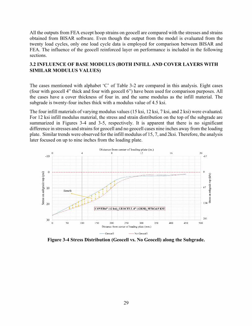
29

All the outputs from FEA except hoop strains on geocell are compared with the stresses and strains obtained from BISAR software. Even though the output from the model is evaluated from the twenty load cycles, only one load cycle data is employed for comparison between BISAR and FEA. The influence of the geocell reinforced layer on performance is included in the following sections.

3.2 INFLUENCE OF BASE MODULUS (BOTH INFILL AND COVER LAYERS WITH SIMILAR MODULUS VALUES)

The cases mentioned with alphabet ‘C’ of Table 3-2 are compared in this analysis. Eight cases (four with geocell 4” thick and four with geocell 6”) have been used for comparison purposes. All the cases have a cover thickness of four in. and the same modulus as the infill material. The subgrade is twenty-four inches thick with a modulus value of 4.5 ksi.

The four infill materials of varying modulus values (15 ksi, 12 ksi, 7 ksi, and 2 ksi) were evaluated. For 12 ksi infill modulus material, the stress and strain distribution on the top of the subgrade are summarized in Figures 3-4 and 3-5, respectively. It is apparent that there is no significant difference in stresses and strains for geocell and no geocell cases nine inches away from the loading plate. Similar trends were observed for the infill modulus of 15, 7, and 2ksi. Therefore, the analysis later focused on up to nine inches from the loading plate.

Figure 3-4 Stress Distribution (Geocell vs. No Geocell) along the Subgrade.

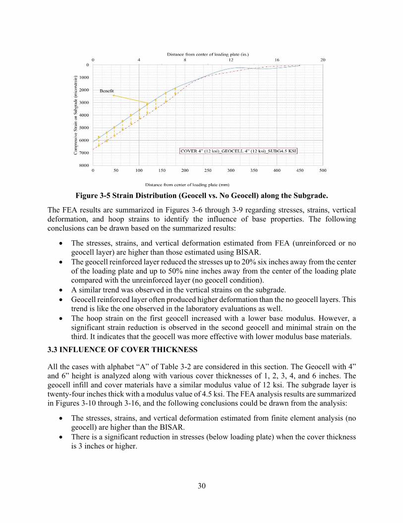
30

Figure 3-5 Strain Distribution (Geocell vs. No Geocell) along the Subgrade.

The FEA results are summarized in Figures 3-6 through 3-9 regarding stresses, strains, vertical deformation, and hoop strains to identify the influence of base properties. The following conclusions can be drawn based on the summarized results:

• The stresses, strains, and vertical deformation estimated from FEA (unreinforced or nogeocell layer) are higher than those estimated using BISAR.

• The geocell reinforced layer reduced the stresses up to 20% six inches away from the centerof the loading plate and up to 50% nine inches away from the center of the loading platecompared with the unreinforced layer (no geocell condition).

• A similar trend was observed in the vertical strains on the subgrade.• Geocell reinforced layer often produced higher deformation than the no geocell layers. This

trend is like the one observed in the laboratory evaluations as well.• The hoop strain on the first geocell increased with a lower base modulus. However, a

significant strain reduction is observed in the second geocell and minimal strain on thethird. It indicates that the geocell was more effective with lower modulus base materials.

3.3 INFLUENCE OF COVER THICKNESS

All the cases with alphabet “A” of Table 3-2 are considered in this section. The Geocell with 4” and 6” height is analyzed along with various cover thicknesses of 1, 2, 3, 4, and 6 inches. The geocell infill and cover materials have a similar modulus value of 12 ksi. The subgrade layer is twenty-four inches thick with a modulus value of 4.5 ksi. The FEA analysis results are summarized in Figures 3-10 through 3-16, and the following conclusions could be drawn from the analysis:

• The stresses, strains, and vertical deformation estimated from finite element analysis (nogeocell) are higher than the BISAR.

• There is a significant reduction in stresses (below loading plate) when the cover thicknessis 3 inches or higher.

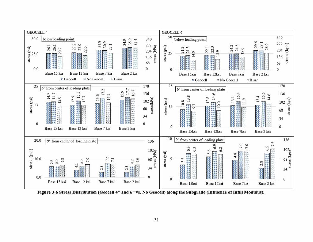
31

Figure 3-6 Stress Distribution (Geocell 4” and 6” vs. No Geocell) along the Subgrade (Influence of Infill Modulus).

32

Figure 3-7 Strain Distribution (Geocell 4” and 6” vs. No Geocell) along the Subgrade (Influence of Infill Modulus).

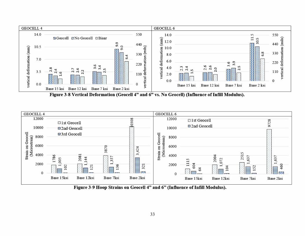
33

Figure 3-8 Vertical Deformation (Geocell 4” and 6” vs. No Geocell) (Influence of Infill Modulus).

Figure 3-9 Hoop Strains on Geocell 4” and 6” (Influence of Infill Modulus).

34

Figure 3-10 Strain Distribution (Geocell 4” and 6” vs. No Geocell) along the Subgrade (Influence of Cover Thickness).

35

Figure 3-11 Vertical Deformation (Geocell 4” and 6” vs. No Geocell) (Influence of Cover Thickness).

Figure 3-12 Hoop Strain on Geocell 4” and 6” vs. No Geocell (Influence of Cover Thickness).

36

Figure 3-13 Stress Distribution (Geocell 3”, 4” and 6” vs. No Geocell) along the Subgrade (Influence of Good Cover and Poor Infill).

37

Figure 3-14 Strain Distribution (Geocell 3”, 4” and 6” vs. No Geocell) along the Subgrade (Influence of Good Cover and Poor Infill).

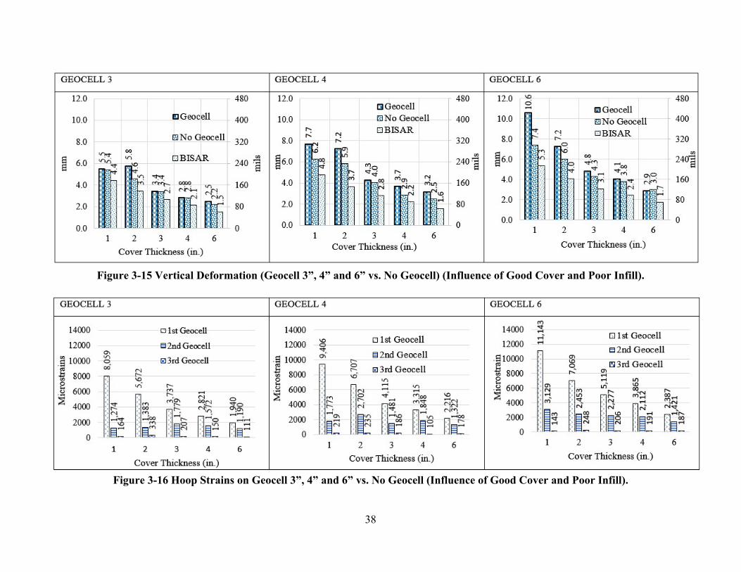
38

Figure 3-15 Vertical Deformation (Geocell 3”, 4” and 6” vs. No Geocell) (Influence of Good Cover and Poor Infill).

Figure 3-16 Hoop Strains on Geocell 3”, 4” and 6” vs. No Geocell (Influence of Good Cover and Poor Infill).

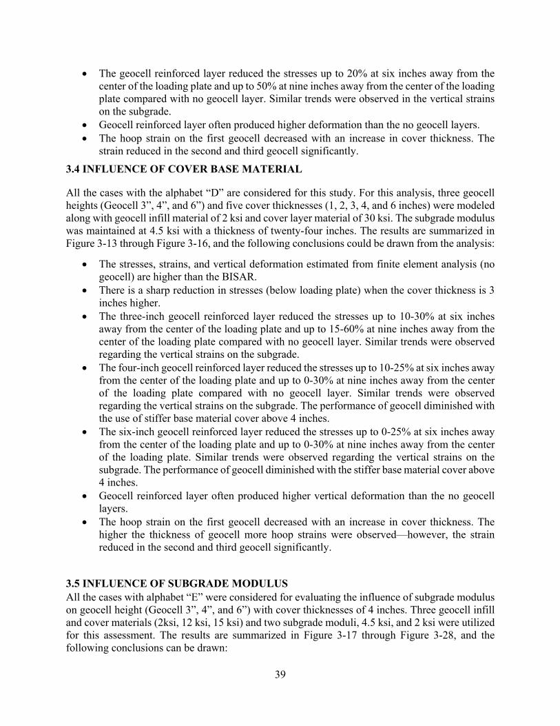
39

• The geocell reinforced layer reduced the stresses up to 20% at six inches away from thecenter of the loading plate and up to 50% at nine inches away from the center of the loadingplate compared with no geocell layer. Similar trends were observed in the vertical strainson the subgrade.

• Geocell reinforced layer often produced higher deformation than the no geocell layers.• The hoop strain on the first geocell decreased with an increase in cover thickness. The

strain reduced in the second and third geocell significantly.3.4 INFLUENCE OF COVER BASE MATERIAL

All the cases with the alphabet “D” are considered for this study. For this analysis, three geocell heights (Geocell 3”, 4”, and 6”) and five cover thicknesses (1, 2, 3, 4, and 6 inches) were modeled along with geocell infill material of 2 ksi and cover layer material of 30 ksi. The subgrade modulus was maintained at 4.5 ksi with a thickness of twenty-four inches. The results are summarized in Figure 3-13 through Figure 3-16, and the following conclusions could be drawn from the analysis:

• The stresses, strains, and vertical deformation estimated from finite element analysis (nogeocell) are higher than the BISAR.

• There is a sharp reduction in stresses (below loading plate) when the cover thickness is 3inches higher.

• The three-inch geocell reinforced layer reduced the stresses up to 10-30% at six inchesaway from the center of the loading plate and up to 15-60% at nine inches away from thecenter of the loading plate compared with no geocell layer. Similar trends were observedregarding the vertical strains on the subgrade.

• The four-inch geocell reinforced layer reduced the stresses up to 10-25% at six inches awayfrom the center of the loading plate and up to 0-30% at nine inches away from the centerof the loading plate compared with no geocell layer. Similar trends were observedregarding the vertical strains on the subgrade. The performance of geocell diminished withthe use of stiffer base material cover above 4 inches.

• The six-inch geocell reinforced layer reduced the stresses up to 0-25% at six inches awayfrom the center of the loading plate and up to 0-30% at nine inches away from the centerof the loading plate. Similar trends were observed regarding the vertical strains on thesubgrade. The performance of geocell diminished with the stiffer base material cover above4 inches.

• Geocell reinforced layer often produced higher vertical deformation than the no geocelllayers.

• The hoop strain on the first geocell decreased with an increase in cover thickness. Thehigher the thickness of geocell more hoop strains were observed—however, the strainreduced in the second and third geocell significantly.

3.5 INFLUENCE OF SUBGRADE MODULUS All the cases with alphabet “E” were considered for evaluating the influence of subgrade modulus on geocell height (Geocell 3”, 4”, and 6”) with cover thicknesses of 4 inches. Three geocell infill and cover materials (2ksi, 12 ksi, 15 ksi) and two subgrade moduli, 4.5 ksi, and 2 ksi were utilized for this assessment. The results are summarized in Figure 3-17 through Figure 3-28, and the following conclusions can be drawn:

40

• It is observed that the 3" geocell height has no significant influence on the reduction ofstresses at the top of the subgrade. In contrast, the 4" geocell height reduced stresses up to30-45% at 9" away from the loading point. The 6" geocell performed better by reducingthe stresses about 10% at 6" away from loading point and around 50% at 9" away from theloading point.

• The hoop strains on the geocell were minimally influenced by a change in subgrademodulus (4.5 ksi and 2.0 ksi).

• The vertical strains and deformation for the 2.0 ksi subgrade (for all geocell) are higherthan the 4.5 ksi subgrade.

3.6 INFLUENCE OF GEOCELL LAYER THICKNESS OR GEOCELL HEIGHT All the cases with the alphabet “B” were considered to evaluate the influence of geocell height. Three geocell heights (Geocell 3”, 4”, and 6”), three geocell infills, and cover materials (2 ksi, 12 ksi, 15 ksi) were used in this assessment with a cover thickness of 4 in. The results are summarized in Figure 3-17 through Figure 3-28, and the following conclusions can be drawn from the analysis:

• In terms of geocell height, the geocell 3" performance is inferior to other geocell heights as itonly reduced stresses up to 10% at 6" from the loading plate and 20% at 9" from the loadingplate, whereas geocell 4" and 6" reduced the stresses around 20% at 6" and 40-50% at 9" fromloading plate.

• Geocell 3" has minimal influence in the presence of weak subgrade material.

Based on the overall evaluation, the observed trends have been summarized in Table 3-3, and the benefits of geocell height are summarized in Table 3-4. The summarized results indicate that 4” and 6” geocell heights provide the benefit of using geocell. In addition, the benefit of geocell reduces with an increase in base modulus (same material for infill and cover) as observed by various researchers and laboratory evaluation results. The test results also indicate that stress on top of the subgrade should be used to design pavements constructed with geocell.

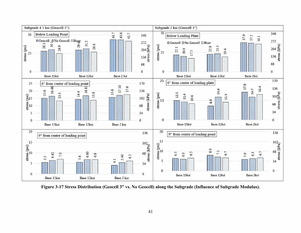
41

Figure 3-17 Stress Distribution (Geocell 3” vs. No Geocell) along the Subgrade (Influence of Subgrade Modulus).

42

Figure 3-18 Strain Distribution (Geocell 3” vs. No Geocell) along the Subgrade (Influence of Subgrade Modulus).

43

Figure 3-19 Vertical Deformation (Geocell 3” vs. No Geocell) (Influence of Subgrade Modulus).

Figure 3-20 Hoop Strain on Geocell 3” (Influence of Subgrade Modulus).

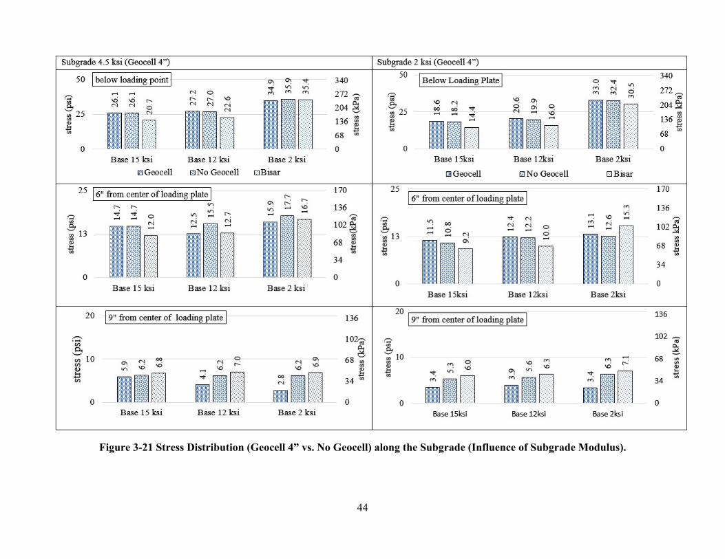
44


45


46


Figure 3-24 Hoop Strain on Geocell 4” (Influence of Subgrade Modulus).

47


48


49


Figure 3-28 Hoop Strains on Geocell 6” (Influence of Subgrade Modulus).

50

Table 3-3 Observed Performance Trends for Various Parameters

Increase of Infill

Modulus

Cover Thickness

Good Cover and Poor

Infill

Decrease in Subgrade Modulus

Increase in Geocell Depth

Stress on Subgrade Decrease

Strain on Subgrade Increase

Vertical Deformation No Clear Trend

Hoop Strain on geocell

Table 3-4 Performance of Three Geocell for Various Parameters

Parameter

GEOCELL 2 7 12 15 Above 15

1" 2" 3" 4" 6" 2 4.5 1" 2" 3" 4" 6"

Geocell 3" 7 7 7 7 0 7 7 10 10 10 0 7 10 10 10 7 7

Geocell 4" 10 10 10 7 0 7 7 10 10 10 7 10 10 10 10 7 0

Geocell 6" 10 10 10 10 0 7 7 10 10 10 10 10 10 10 7 7 0

1070

Poor infill material (2 ksi) and good cover material (30 ksi)

Good PerformanceAverage Performance

No Influence

Infill Modulus (ksi) Cover Thickness (in.) (same as infill)Subgrade

Modulus (ksi)

51

4. SELECTION OF MATERIAL, EXPERIMENTAL DESIGN,AND LABORATORY EVALUATION

This chapter provides information regarding the selection of material, experimental design, and laboratory evaluation process. One of the key objectives of this project is to develop pavement design inputs for geocell reinforced layers. To accomplish the above objective, the performance of the geocell reinforced layer is assessed by modeling the geocell reinforced pavement system in finite element software and comparing the test results obtained from laboratory testing. Furthermore, cyclic load with a rest period (typically used in resilient modulus evaluation) was applied in laboratory testing and finite element modeling to simulate traffic loading.

4.1 EXPERIMENTAL DESIGN

Based on published literature, various parameters that contribute to the performance of pavement reinforced with geocell were identified for evaluation laboratory and FEA analysis (discussed in chapter 3).

The literature and preliminary investigation identified the following four parameters that influence performance:

1) Cover thickness (layer over geocell) and quality of cover material,2) Geocell layer thickness,3) Infill material (in geocell) modulus, and4) Subgrade modulus.

Since the focus of this study was on low-volume roads, it was decided not to include an asphalt concrete surface layer in the analysis. Therefore, the modeling analysis included (bottom to top) a subgrade layer placed at the bottom followed by a geocell reinforced layer (geocell layer with infill base material). At the end (at the top), a layer consisting of either poor quality infill or better-quality base material was placed on top of the geocell infill material and referred to as a cover layer.

To document the benefit of geocell reinforcement, the analysis was also performed for pavement systems without geocell reinforcement by placing a layer of similar thickness without geocell. Although the geocell placement protocol suggests placing fabric between the geocell and subgrade to avoid contamination, it was not followed because of computational constraints in this study. Additionally, initial finite element analysis consisted of a loading plate of 10 inches; however, the design analysis suggested that a 12-in. diameter loading plate would be a better option. Therefore, additional analysis was performed using a 12 in. plate. Finally, the influence of geocell was evaluated by measuring the following performance parameters:

1) Vertical stress and strain distribution below the base layer or at the top of subgrade,2) Vertical deformation below the base layer or at the top of subgrade, and3) Hoop strains on the side of geocell.

4.2 LABORATORY EVALUATION

Like the finite element analysis, the laboratory evaluation was performed for evaluating the performance of the geocell reinforced layer with one exception (quality of cover material). The

52

reason for using the same quality material (for geocell infill and cover layer) was to avoid contamination because we were reusing the material for testing.

The range of parameters selected and the overall laboratory assessment plan are summarized in Table 4-1. To document the benefit of geocell reinforcement, the analysis was also performed for pavement systems without geocell reinforcement by placing a layer of similar thickness without geocell. The initial laboratory test plan consisted of a loading plate of 10 inches; however, the design analysis suggested that a 12-in. diameter loading plate would be a better option. There are three reasons that the 12” plate is used in the testing:

• The input modulus in Texas pavement design software FPS 19 or 21 was based on fallingweight deflector (FWD) back-calculated modulus. According to the test procedurepresented in the report “The Falling Weight Deflectometer for Nondestructive Evaluationof Rigid Pavements (1985) by CTR UT Austin, the diameter of the loading plate is (11.8”).

• The equivalent diameter of each cell in the geocell mattress is around 11” <GeocellDiameter<12.5”. The preliminary testing is performed with a 10” which fitted into the cell.Vertical stresses are concentrated in a single geocell rather than distributed across themattress. The vertical stress distribution on the subgrade top due to 10” loading plate wasappalling, like higher vertical stresses (compared with unreinforced base) below the centerof loading plate and significant drop moving away from the center of loading. So, the actualbenefit of geocell reinforcement is hard to comprehend. But using a 12” loading plate(larger than the single geocell diameter opening), the vertical stress on subgrade rightbelow the loading plate was dropped compared with the unreinforced layer, and a smoothreduction in vertical stresses away from the center of the loading plate.

• Based on the literature, “Experimental Study on Geocell Reinforced Bases under Static andDynamic Loading” (Sanat Kumar Pokharel, 2010) from Kansas in large-scale testing (likethe tank testing and type of geocells used in this study) used a 12” loading plate (for cyclicloading). In the same report, the preliminary testing (static loading) was performed using asmaller diameter plate (6” plate), the reason for shifting to higher diameter plate was notmentioned.

Therefore, additional analysis was performed using 12 in. plate. The influence of geocell was evaluated by measuring the following performance parameters:

• Vertical stress and strain distribution below the base layer or at the top of subgrade,• Vertical deformation below the base layer or at the top of the subgrade• Hoop strains on the side of geocell.

53

Table 4-1 Experimental Test Plan

Tests with Geocell and No Geocell (58)

Tests Not Required

54

4.3 MATERIAL SELECTION

4.3.1 Geocell Although several geocell manufacturers were contacted, only two (Presto and Tenax) provided geocell for this study. Presto provided geocell of 4.25” and 6” height geocell, while Tenax provided 3” and 4” height geocell, as summarized in Table 4-2. Although the main difference from the pavement system point of view is only the height, the geocell has different joints, thickness, construction, etc. Therefore, the details provided by the manufacturers are included in Appendix B – Figure B-1 and Figure B-2. Other than height, the manufacturer-provided specifications were considered in the finite element analysis. In addition, the dimensions of the geocell (width and length of each geocell opening) and thickness of geocell are measured in the laboratory for verification purposes.

Table 4-2 Geocell Selection and Properties Geocell Height Manufacturer Properties

3” and 4” Tenax Appendix C 4.25” and 6” Presto Appendix C

4.3.2 Base and Subgrade Selection As per the tentative plan of the study, three base materials and two subgrades with fair to inferior quality are needed. The needed materials were selected from various locations in Texas with the help of the project management committee.

The base materials were obtained from Dallas (Collin County), San Antonio (La Hoya Quarry), and El Paso Districts. Similarly, the subgrades were obtained from Paris and El Paso District. To perform testing in the laboratory, approximately five tons of each material was obtained from either plant or field. The obtained material was stored in labeled barrels to minimize cross-contamination and accidental use of the wrong material. The following tests were performed to measure properties needed for finite element analysis and design of pavement system. The test procedures followed are included in Table 4-3, while the measured engineering properties are included in Table 4-4.

Table 4-3 Test Procedures for Evaluation of Base and Subgrade Material

Material Property Test Procedure Maximum Dry Density (MDD) and Optimum Moisture Content (OMC) Tex-114-E Particle Size Analysis (Gradation) Tex-110-E Plastic Limit of Soils Tex-105-E Liquid Limit of Soils Tex-104-E Triaxial Compression for Disturbed Soils and Base Materials Tex-117-E In-Place Density of Soils and Base Materials (Sand Cone Method) Tex-115-E Resilient Modulus AASHTO T-307

55

Table 4-4 Measured Engineering Properties of Base and Subgrade Materials

Mat

eria

l

Loc

atio

n

MD

D (P

CF)

OM

C (%

)

Gradation

PI

Φ

C

T

UC

S, p

si

Res

ilien

t Mod

ulus

(K

SI)

Ela

stic

Mod

ulus

(K

SI) e

stim

ated

us

ing

the

Port

able

Se

ism

ic P

avem

ent

Ana

lyze

r

50m

m<

G <

4.

75m

m

4.75

mm

<S<

0.00

75m

m

Pass

ing

75

mic

rons

(Silt

or

Cla

y)

Base 1

FM 545-Collin

County-Dallas District

125.70 6.10 45.80 53.70 0.50 NP 39.10 11.23 3.00 25 28 15

Base 2

La Hoya Quarry, San

Antonio Texas

130.00 6.00 54.10 28.50 2.50 NP 36.90 2.00 4.30 15 23 12

Base 3 El Paso (Jobe Plant) 106.00 16.70 17.00 78.00 5.00 3.00 0.00 8.70 6.90 6 6 5

Subgrade 1

El Paso (Jobe Plant) 130.00 6.70 32.40 65.20 2.50 NP 33.80 7.90 3.90 24 20 4.5

Subgrade 2

Between Commerce and Paris of

Texas

88.00 16.00 0.00 88.70 11.30 8.00 0.00 7.20 6.20 13 Too Soft 2.5

MDD: Maximum Dry Density, OMC: Optimum Moisture Content, PI - Plasticity Index, Φ- Angle of Internal Friction, C – Cohesion (psi), T = Triaxial Classification, UCS = Unconfined Compressive Strength (psi), G-Gravel, S-Sand.

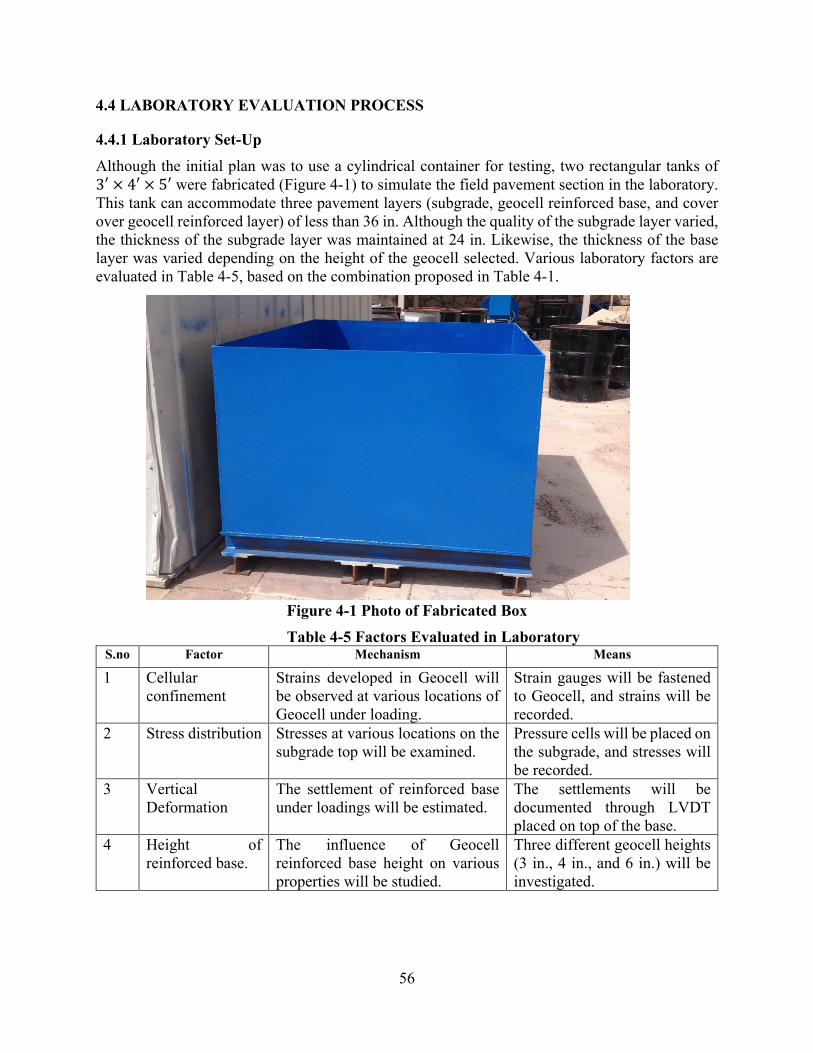
56

4.4 LABORATORY EVALUATION PROCESS

4.4.1 Laboratory Set-Up Although the initial plan was to use a cylindrical container for testing, two rectangular tanks of 3′ × 4′ × 5′ were fabricated (Figure 4-1) to simulate the field pavement section in the laboratory. This tank can accommodate three pavement layers (subgrade, geocell reinforced base, and cover over geocell reinforced layer) of less than 36 in. Although the quality of the subgrade layer varied, the thickness of the subgrade layer was maintained at 24 in. Likewise, the thickness of the base layer was varied depending on the height of the geocell selected. Various laboratory factors are evaluated in Table 4-5, based on the combination proposed in Table 4-1.

Figure 4-1 Photo of Fabricated Box Table 4-5 Factors Evaluated in Laboratory

S.no Factor Mechanism Means

1 Cellular confinement

Strains developed in Geocell will be observed at various locations of Geocell under loading.

Strain gauges will be fastened to Geocell, and strains will be recorded.

2 Stress distribution Stresses at various locations on the subgrade top will be examined.

Pressure cells will be placed on the subgrade, and stresses will be recorded.

3 Vertical Deformation

The settlement of reinforced base under loadings will be estimated.

The settlements will be documented through LVDT placed on top of the base.

4 Height of reinforced base.

The influence of Geocell reinforced base height on various properties will be studied.

Three different geocell heights (3 in., 4 in., and 6 in.) will be investigated.

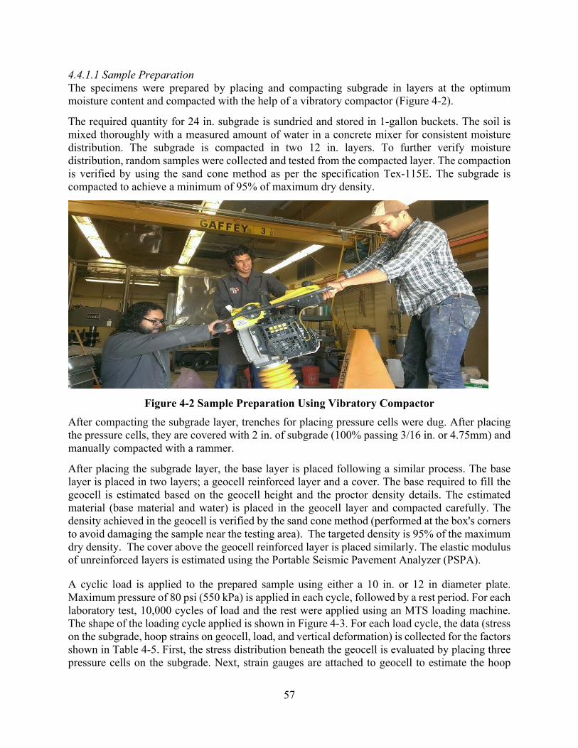
57

4.4.1.1 Sample Preparation The specimens were prepared by placing and compacting subgrade in layers at the optimum moisture content and compacted with the help of a vibratory compactor (Figure 4-2).

The required quantity for 24 in. subgrade is sundried and stored in 1-gallon buckets. The soil is mixed thoroughly with a measured amount of water in a concrete mixer for consistent moisture distribution. The subgrade is compacted in two 12 in. layers. To further verify moisture distribution, random samples were collected and tested from the compacted layer. The compaction is verified by using the sand cone method as per the specification Tex-115E. The subgrade is compacted to achieve a minimum of 95% of maximum dry density.

Figure 4-2 Sample Preparation Using Vibratory Compactor After compacting the subgrade layer, trenches for placing pressure cells were dug. After placing the pressure cells, they are covered with 2 in. of subgrade (100% passing 3/16 in. or 4.75mm) and manually compacted with a rammer.

After placing the subgrade layer, the base layer is placed following a similar process. The base layer is placed in two layers; a geocell reinforced layer and a cover. The base required to fill the geocell is estimated based on the geocell height and the proctor density details. The estimated material (base material and water) is placed in the geocell layer and compacted carefully. The density achieved in the geocell is verified by the sand cone method (performed at the box's corners to avoid damaging the sample near the testing area). The targeted density is 95% of the maximum dry density. The cover above the geocell reinforced layer is placed similarly. The elastic modulus of unreinforced layers is estimated using the Portable Seismic Pavement Analyzer (PSPA).

A cyclic load is applied to the prepared sample using either a 10 in. or 12 in diameter plate. Maximum pressure of 80 psi (550 kPa) is applied in each cycle, followed by a rest period. For each laboratory test, 10,000 cycles of load and the rest were applied using an MTS loading machine. The shape of the loading cycle applied is shown in Figure 4-3. For each load cycle, the data (stress on the subgrade, hoop strains on geocell, load, and vertical deformation) is collected for the factors shown in Table 4-5. First, the stress distribution beneath the geocell is evaluated by placing three pressure cells on the subgrade. Next, strain gauges are attached to geocell to estimate the hoop

58

strains developed in the geocell wall. Finally, the vertical deformation is estimated on the top of the base layer (beneath the load plate) using the LVDT. The location of strain gauges and pressure cells in the testing are also shown in Figure 4-4. The specifications of the electronics used in the experiments are discussed in the later sections.

Figure 4-3 Applied Load Cycle

Figure 4-4 Locations of Stress and Strains Measurement Transducers

4.4.1.2 Strain Gauge In this study, the deformations are measured using the strain gauges due to the loading cycle and converted to estimate induced strains. The strain gauges were selected based on their sensitivity and suitability with the data acquisition system. A half bridge strain gauge circuit was selected because of better sensitivity. The sensitivity of the bridge can be doubled in a half bridge

59

configuration compared to a quarter bridge. Figure 4-5 shows the difference between the quarter bridge and half bridge gauge circuits.

Each strain gauge is glued to geocell and adequately protected. Table 4-6 shows the model of strain gauge used and protection means. Despite employing the precautions in gluing the strain gauges and protecting them, they are occasionally damaged during compaction. Therefore, the working condition of strain gauges before and after compaction of the sample is verified for each test. In some cases, if one of the strain gauges on the half bridge is broken, then the circuit is converted (wiring) into a quarter bridge, and the strains are recorded for the quarter bridge. More details on the strain gauges used in the study are presented in Figure B-3 in Appendix B.

Figure 4-5 Half Bridge vs. Quarter Bridge Strain Gauge Circuits

Table 4-6 Strain Gauges Item Description

Strain Gauge KFH-6-120-C1-11L1M3R (6mm strain gauge, 120Ω, three pre-wired)

Glue (to glue strain gauge to geocell)

Ethyl based cyanoacrylate

Protection of strain gauge Performix Plasti Dip (flexible protection) Protection of strain gauge wires PVC Tubing

4.4.1.3 Earth Pressure Cells

For estimating stress on the subgrade layer, the pressure cells were placed on top of the subgrade. Geokon Model 3500 series (2.5 MPa and 600 kPa) were selected for evaluation, and the specifications of the pressure cells are included in Appendix B Figure B-4. Each pressure cell is a semiconductor strain gauge earth pressure cell (circular 9”), with the thermistor in SS housing, 0-5 VDC output as shown in Figure 4-6.

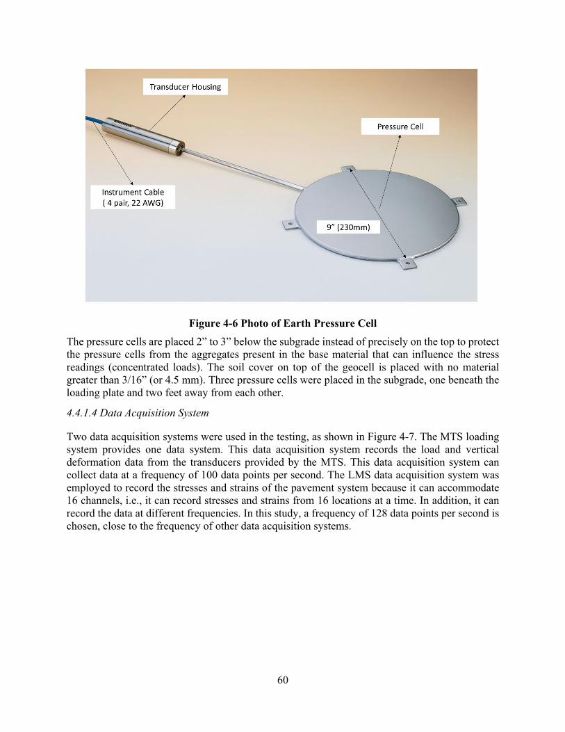
60

Figure 4-6 Photo of Earth Pressure Cell The pressure cells are placed 2” to 3” below the subgrade instead of precisely on the top to protect the pressure cells from the aggregates present in the base material that can influence the stress readings (concentrated loads). The soil cover on top of the geocell is placed with no material greater than 3/16” (or 4.5 mm). Three pressure cells were placed in the subgrade, one beneath the loading plate and two feet away from each other.

4.4.1.4 Data Acquisition System

Two data acquisition systems were used in the testing, as shown in Figure 4-7. The MTS loading system provides one data system. This data acquisition system records the load and vertical deformation data from the transducers provided by the MTS. This data acquisition system can collect data at a frequency of 100 data points per second. The LMS data acquisition system was employed to record the stresses and strains of the pavement system because it can accommodate 16 channels, i.e., it can record stresses and strains from 16 locations at a time. In addition, it can record the data at different frequencies. In this study, a frequency of 128 data points per second is chosen, close to the frequency of other data acquisition systems.

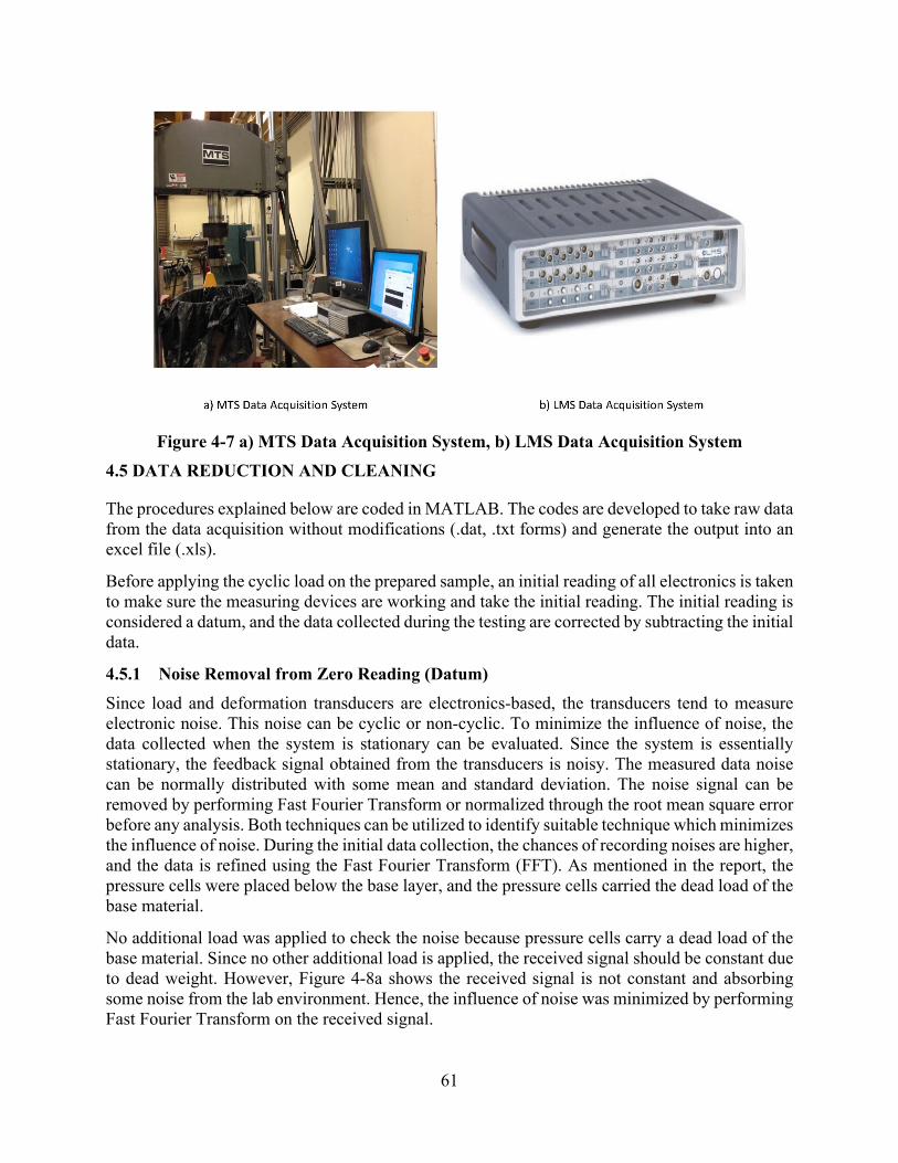
61

Figure 4-7 a) MTS Data Acquisition System, b) LMS Data Acquisition System 4.5 DATA REDUCTION AND CLEANING

The procedures explained below are coded in MATLAB. The codes are developed to take raw data from the data acquisition without modifications (.dat, .txt forms) and generate the output into an excel file (.xls).

Before applying the cyclic load on the prepared sample, an initial reading of all electronics is taken to make sure the measuring devices are working and take the initial reading. The initial reading is considered a datum, and the data collected during the testing are corrected by subtracting the initial data.

4.5.1 Noise Removal from Zero Reading (Datum) Since load and deformation transducers are electronics-based, the transducers tend to measure electronic noise. This noise can be cyclic or non-cyclic. To minimize the influence of noise, the data collected when the system is stationary can be evaluated. Since the system is essentially stationary, the feedback signal obtained from the transducers is noisy. The measured data noise can be normally distributed with some mean and standard deviation. The noise signal can be removed by performing Fast Fourier Transform or normalized through the root mean square error before any analysis. Both techniques can be utilized to identify suitable technique which minimizes the influence of noise. During the initial data collection, the chances of recording noises are higher, and the data is refined using the Fast Fourier Transform (FFT). As mentioned in the report, the pressure cells were placed below the base layer, and the pressure cells carried the dead load of the base material.

No additional load was applied to check the noise because pressure cells carry a dead load of the base material. Since no other additional load is applied, the received signal should be constant due to dead weight. However, Figure 4-8a shows the received signal is not constant and absorbing some noise from the lab environment. Hence, the influence of noise was minimized by performing Fast Fourier Transform on the received signal.

62

For example, the pressure cell's zero reading (no additional load applied apart from dead load) is shown in Figure 4-8. The raw data collected was ranged from 7350 to 7700 Pa (1.06 to 1.11 psi). The data was refined by removing the noise using the Fast Fourier Transform (FFT), and the actual reading from the pressure cells was 7650 Pa (1.11 psi). Therefore, theoretically, the pressure cell was placed below 12 inches of base (Base 1), and around 3 inches into subgrade (Base 2), the stress on the pressure cell was approximately 1.10 psi. The noise minimized signal shows the input as 1.11 psi close to the expected value.

The test data (during load) was corrected using a correction factor of -7650 Pa (for this case, only on pressure cell 1).

Figure 4-8 Noise removal from pressure cell readings 4.5.2 Noise Removal from Actual Data and Data Reduction Each test is performed for 10,000 load cycles, and each load cycle is around 1.3 seconds. Based on the data recorded frequency, around 1.7 million data points from each channel (strain gauges, pressure cells, load cell, and LVDT) are collected from each test. The data needs to reduce to perform further assessments. In addition to the reduction of data, the quality of data also needs to be evaluated.

The data recorded through pressure cells, LVDT, strain gauges, and load cells follow the waveform of the applied load (cyclic pulse). Earlier, some researchers used moving average techniques that may not suit this analysis (might manipulate the waveform). In this study, we used nonparametric regression to minimize the data and remove the noise from the readings. Nonparametric regression provides an effective means by which complex displacement/pressure patterns occurring over a wide range of values can be captured without the constraint of an assumed functional form. Therefore, kernel regression (nonparametric regression) or kernel smoothing is used in this study. Kernel smoothing generally utilizes locally weighted averages of the data defined by a kernel. The use of 95% confidence interval and root mean square with Kernel smoothing should minimize the

63

influence of noise and identify minimum levels of magnitudes that can be measured with pressure cells and strain gauges such that erroneous conclusions will not be drawn from the collected data.

The 1.7 million data points can be refined by removing the noise. The data can be reduced to the required number of data points (150,000 considered in this study) without impacting the observed waveform. It is observed that the pressure cells (closer to the loading plate), load cells, LVDT are not impacted by noise during testing. The noise is observed from the test data on the strain gauges and pressure cell 3 (2 feet away from the loading plate). Figure 4-9 shows the data observed during the testing. Pressure cell 3 (Figure 4-9c) has some noise in the readings refined by Kernel regression (Figure 4-9d). Similarly, Figure 4-10 shows the effectiveness of Kernel regression from the noise from the strain gauge data and reducing the data points without impacting the waveform.

Kernel regression smoothens the data by reducing the influence of noise. It is different from the averaging data or moving average, as Kernel regression follows the signal waveform. Thus, averaging may shift the data. To clarify, comparisons of Kernel regression and moving average are shown in Appendix C Figure C-5.

Figure 4-9 a) Pressure Cell 1 (Original Data), b) Pressure Cell 2 (Original Data), c) Pressure Cell 3 (Original Data), d) Pressure Cell 3 (Kernel Regression).

64

Figure 4-10 A) Strain gauge (Original Data), B) Strain gauge (Kernel Regression) 4.5.3 Presentation of Data Instead of presenting the data in waveforms, it is presented as the readings during loading (when the load is maximum in the cycle as shown in load cycle Figure 4-3) and rest (when the load is minimum in the load cycle). The following figures present the data for the laboratory test performed on geocell of 4 in. height, cover thickness of 6”, subgrade modulus of 2.5 ksi, and base modulus of 5 ksi (for both geocell reinforced and unreinforced sections): a) Figure 4-11 shows the vertical deformation, b) Figure 4-12 shows the stresses on the subgrade, c) Figure 4-13 shows the vertical strains on the geocell, and d) Figure 4-14 shows the hoop strains observed on the geocell. All the data is refined and reduced using Kernel regression.

4.5.3.1 Vertical Deformation Figure 4-11 shows the vertical deformation on the surface top measured using an LVDT attached to the loading frame. Again, both reinforced and unreinforced bases produced a similar deformation. The results observed in other test samples also followed a similar trend.

4.5.3.2 Vertical Stress Distribution on Subgrade Figure 4-12 shows the vertical stress captured on three pressure cells (PC1, PC2, and PC3) along the subgrade. It is observed that the stresses on the subgrade are reduced on PC1 and PC2 locations significantly by placing a geocell reinforced layer. The stresses observed on the PC3 are almost negligible in both reinforced and unreinforced sections.

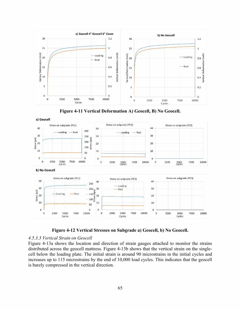
65

Figure 4-11 Vertical Deformation A) Geocell, B) No Geocell.

Figure 4-12 Vertical Stresses on Subgrade a) Geocell, b) No Geocell. 4.5.3.3 Vertical Strain on Geocell Figure 4-13a shows the location and direction of strain gauges attached to monitor the strains distributed across the geocell mattress. Figure 4-13b shows that the vertical strain on the single-cell below the loading plate. The initial strain is around 90 microstrains in the initial cycles and increases up to 115 microstrains by the end of 10,000 load cycles. This indicates that the geocell is barely compressed in the vertical direction.

66

4.5.3.4 Hoop Strains on Geocell Figure 4-14 shows the hoop strain distribution across the cells from the center of the loading plate. The first and second cells show higher strains compared with the third cell. This indicates that the cell below the loading is expanding and transferring the load in the lateral direction (to the second cell). After the second cell, the load distribution is almost negligible.

Figure 4-13 a) Location and Direction of Strain Gauges b) Vertical Strain Observed in the

Center Geocell.

Figure 4-14 Hoop Strains on Geocell.

67

4.5.4 Summary of Data The test results obtained from the laboratory testing for 10 in. and 12 in. loading plates are summarized in Tables 4.7 through 4.11. In addition, the stress and strain measured with the 10 in. loading plate are included in Tables 4.7 through 4.10, while Table 4.11 has results summarized for 12 in. loading plate. Initially, the laboratory and FEM applied load using a 10 in. loading plate. However, the pavement design required a 12 in. loading plate because of FPS-21; therefore, some analysis was performed in the laboratory using a 12 in. loading plate to verify finite element results obtained using a 12 in. loading plate.

The measured vertical deformation below the loading plate is summarized in Table 4.7, obtained from the LVDT of the MTS system. The results indicate an increase in vertical deformation with a reduction in the base modulus. However, the measured vertical deformation was lower in the absence of geocell than those measured with the geocell reinforcement. This can be attributed to lower compaction levels obtained within the individual cells of geocell. Researchers from the University of Kansas also observed this pattern.

68

Table 4-7 Vertical Deformation (below loading plate)

Good Marginal Poor Good Marginal Poor Good Marginal Poor Good Marginal Poor Good Marginal Poor(15 ksi) (12 ksi) (5 ksi) (15 ksi) (12 ksi) (5 ksi) (15 ksi) (12 ksi) (5 ksi) (15 ksi) (12 ksi) (5 ksi) (15 ksi) (12 ksi) (5 ksi)

Subgrade (4.5 ksi)Subgrade(2.5 ksi)Subgrade (4.5 ksi) 1153 886 437 1261

Subgrade(2.5 ksi)

186 132Cover 4”

182 190 1154

Vertical Deformation, milsGeocell 1 (Presto 6") Geocell 2 (Presto 4") Geocell 3 (Tenax 4") Geocell 4 (Tenax 3") No Geocell

Base Base Base Base Base

137 323

609 593 1142 732 1035 1240 587 535 947 469 189 327 454 754

1358 331 244 1467 166187 182 389

692

693

Cover 6”

205 387 1078 205 413 1238 153 413 482 121 1053 1026 453 753

Table 4-8 Stresses Measured on Top of Subgrade (below loading plate)


Subgrade (4.5 ksi)Subgrade(2.5 ksi)Subgrade (4.5 ksi) 26.4 19.0 19.3 37.2 18.4

Subgrade(2.5 ksi) 14.9 25.6 18.4

Pressure Cell Reading (Below Load Plate), psi

14.9 25.6 18.436.2 35.0

Cover 6”

12.2 16.1 15.1 15.5

34.3 33.8 31.9 30.6

19.2

21.7 28.7 29.5 29.7

20.515.715.5 22.220.5 20.7 13.0

22.1 29.1 22.7

31.2 34.6

Geocell 1 (Presto 6") Geocell 2 (Presto 4") Geocell 3 (Tenax 4") Geocell 4 (Tenax 3")

Cover 4”

25.0 17.6 22.7 30.3 34.5 27.8 16.3 18.0 27.2

13.9 19.3 17.7

No Geocell BaseBase Base Base Base

69

Table 4-9 Vertical Deformation (below loading plate)


Subgrade (4.5 ksi)Subgrade(2.5 ksi)Subgrade (4.5 ksi) 13.34 77.89 66.4 27.39

Subgrade(2.5 ksi) NA NA NA

Vertical Compressive Strain (Cell below loading plate), microstrain

NA NA NABroken 32.04

Cover 6”

7.62 36.32 14.35 7.62

278 89.3 Broken 15.6

8.69

16.43 4.17 112.9 21.2

10.729.05 10.84 8.69 20.25 10.6 11.91

3.93 30.25 6.43

11.79 15.72

Geocell 1 Geocell 2 Geocell 3 Geocell 4

Cover 4”

27.15 22.62 13.34 13.5766 45.02 2.86 NA NA NA

50.49 30.96 54.66

Base Base Base BaseNo Geocell

Base

Table 4-10 Hoop Strain (cell below loading plate)


Subgrade (4.5 ksi)Subgrade(2.5 ksi)Subgrade (4.5 ksi) 611.304 1197 Broken 363 123.38 881.65

Subgrade(2.5 ksi) NA NA NA

Hoop Strain (Cell below loading plate), microstrain

NA NA NA152.8 102.78

Cover 6”

15.24 509.24 44.54 15.24

498 98.8 2.73 74.43

144.8

89.44 165.9 Broken 84.68

182.81735 103.97 144.82 40.7 56.09 27.75

41.5 68.48 681.93

Broken 478

Geocell 1 Geocell 2 Geocell 3 Geocell 4

Cover 4”

70.2651 186.9 1197 57.284 306.95 133 NA NA NA

Broken 719.8 171.85

Base Base Base BaseNo Geocell

Base

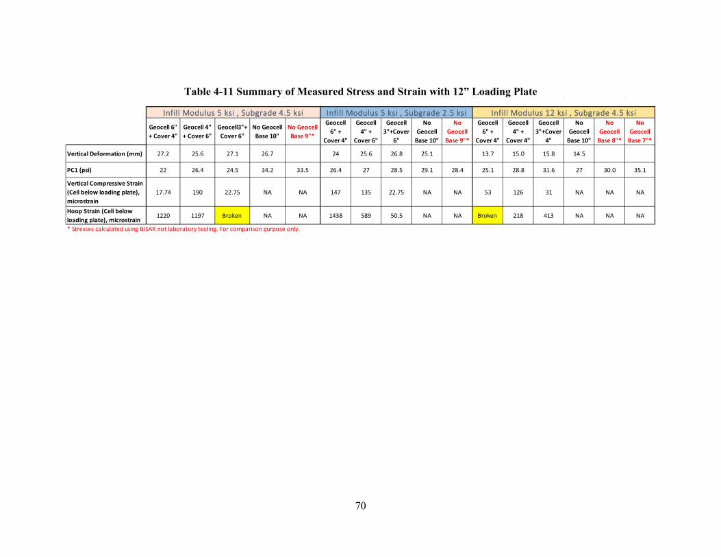
70

Table 4-11 Summary of Measured Stress and Strain with 12” Loading Plate

Geocell 6" + Cover 4"

Geocell 4" + Cover 6"

Geocell3"+Cover 6"

No GeocellBase 10"

No Geocell Base 9"*

Geocell 6" +

Cover 4"

Geocell 4" +

Cover 6"

Geocell 3"+Cover

6"

No Geocell

Base 10"

No Geocell

Base 9"*

Geocell 6" +

Cover 4"

Geocell 4" +

Cover 4"

Geocell 3"+Cover

4"

No Geocell

Base 10"

No Geocell

Base 8"*

No Geocell

Base 7"*

Vertical Deformation (mm) 27.2 25.6 27.1 26.7 24 25.6 26.8 25.1 13.7 15.0 15.8 14.5

PC1 (psi) 22 26.4 24.5 34.2 33.5 26.4 27 28.5 29.1 28.4 25.1 28.8 31.6 27 30.0 35.1

Vertical Compressive Strain(Cell below loading plate), microstrain

17.74 190 22.75 NA NA 147 135 22.75 NA NA 53 126 31 NA NA NA

Hoop Strain (Cell below loading plate), microstrain

1220 1197 Broken NA NA 1438 589 50.5 NA NA Broken 218 413 NA NA NA

* Stresses calculated using BISAR not laboratory testing. For comparison purpose only.

Infill Modulus 5 ksi , Subgrade 4.5 ksi Infill Modulus 12 ksi , Subgrade 4.5 ksiInfill Modulus 5 ksi , Subgrade 2.5 ksi

71

5. CRITICAL EVALUATION OF EXISTING DESIGNMETHODS

Currently, there are no pavement design methods for pavements consisting of the geocell reinforced layer. To design pavements reinforced with geocell, this study focused on the following: 1) Texas Pavement Design Method, 2) Low Volume Pavement Design Method (AASHTO), and3) Proposed methods on Geocell incorporation in Pavement Design. Since laboratory experimentsand finite element analysis (FEA) were performed with no asphalt layer on top, more emphasis isplaced on evaluating low-volume unpaved road design methods in practice.

5.1 TEXAS PAVEMENT DESIGN PROCEDURE In Texas, low-volume flexible pavements are designed using the Flexible Pavement System software (FPS-21). The program uses a “District Temperature Constant” that assigns a cold region multiplier to those areas of the state more susceptible to thermal cracking as the only environmental input. However, the current recommendation is to nullify this parameter by assigning a value of “31” corresponding to the climate in Central Texas.

The program uses a “confidence level” approach to account for in-place subgrade stiffness variability, construction variability, and traffic growth. A multiplier is assigned to the cumulative traffic loading as the desired level of confidence or reliability increases. As a result, the system can generate designs that may fail under occasional heavy wheel loads. This circumstance is particularly acute for designs that have low cumulative loading in regions with a poor subgrade. For this reason, designs obtained from the program must be checked with the “Modified Texas Triaxial Design Method,” which is included in FPS-21 in the post-design check module. In addition, a mechanistic design check is provided to evaluate the expected fatigue life of the HMAC layers and full-depth rut life of the structure with options to use several strain-based performance models.

FPS-21 uses back-calculated modulus to characterize the pavement layer strength (stiffness) based on Falling Weight Deflectometer (FWD) deflection measurements, which is different from the resilient modulus used in the AASHTO design procedure. However, the elastic modulus of pavement layers is the essential input for finding the pavement structure's layer thickness. Therefore, it is incumbent upon the designer to have a current set of deflection data for the project under consideration from which moduli can be generated and institutional knowledge of material moduli when virgin or recycled materials are incorporated in the design.

Design Confidence Level: This parameter is meant to address variability in material quality, construction processes, and forecasted traffic as a means of assuring the structure performs as desired. It does not account for premature failures that may occur due to inadequate construction quality controls. An overall multiplier to the cumulative traffic loading is applied and can be modified if more confidence is desired. FPS-21 uses an alphabetic code tied to a reliability or confidence level: A-80%, B-90%, C-95%, D-99%, E-99.9%. A confidence level as low as level ‘A’ can be considered for designs below 1 million equivalent single axles loads (ESALs); level ‘B’ is recommended for 1 to 5 million ESALs; and level ‘C’ for above 5 million ESALs.

Each material layer used in the structure requires a modulus value characterizing the average stiffness of that material. The construction process, inherent material variability (initially and over service life), and environment and traffic loading effects will typically introduce considerable

72

variance. Overestimating this material property can reduce the service life while underestimating can result in the uneconomical pavement.

Usage of the geocell reinforced layer in pavements is not incorporated in the Texas pavement design guide. However, the following information includes planar geosynthetic (geogrid and geotextile) in the pavement.

5.1.1 Geosynthetics in Pavement Structure According to the pavement design guide of Texas, a geosynthetic is defined as “A manmade material that consists of one or more products used to provide added benefit to the infrastructure,” Applications of geosynthetics have been in asphalt concrete overlays of existing asphalt concrete and hydraulic (Portland) cement concrete surfaces, unbound (flexible) base, soft subgrade, drainage, and encapsulation. The two geosynthetics primarily used are geotextiles and geogrids. The applications of geosynthetics in Texas roads are shown in Table 5-1.

Table 5-1 Geosynthetic Application (Pavements in Texas). Application Name Description

1 Pavement Surface Layer Reinforcement

The first application should be separated and not confused with any other application in a pavement structure. This application is specific to hot-mix asphalt concrete.

2 Geotechnical Reinforcement

Refers to pavement layers only inclusive of subgrades and subbases

3 Drainage and Moisture Control

Drainage and moisture control are features of the pavement structure, not reinforcements. Their functions are to enhance and lengthen pavement performance by reducing the influence of moisture.

5.1.2 Geosynthetics for Geotechnical Reinforcement Many geosynthetics have multiple uses and can serve more than one function. For instance, geogrids are often used in a way to restrain base material during compaction or loading. Still, they also serve as a separation layer to prevent excessive migration and intermingling of pavement layers at interfaces.

Current usage in Texas has been for both restraints of pavement materials and separation of materials. The department acknowledges the benefit of geosynthetics in pavement layers; however, there has been insufficient conclusive research to develop guidance about the reinforcement of unbound materials in pavement structures now. As a result, usage of geosynthetics is limited to separation and restraint and is not accounted for pavement design using FPS-21 design.

5.2 LOW VOLUME ROAD DESIGN AASHTO According to AASHTO, pavement structural design for low-volume roads is divided into three categories

1. Flexible Pavements, 2. Rigid Pavements, and 3. Aggregate-surfaced roads.

73

For designing low-volume roads, the recommended reliability level is 50 percent. However, the user may design for higher reliability levels of 60 to 80 percent, depending on the actual projected level of traffic and the feasibility of rehabilitation, the importance of corridor, etc. The following section describes the design procedure for low-volume unpaved or aggregate surfaced roads.

5.2.1 Aggregate-Surface Roads Unlike flexible or rigid design procedures, the design procedure for aggregate-surfaced roads requires a graphical solution. It is important to note that the effective modulus of the roadbed soil developed for flexible pavement design should not be used instead of the procedure described here.

Because the primary basis for all rational pavement performance prediction methods is cumulative heavy axle load applications, using the 18-kip equivalent single axle load (ESAL) design approach for low-volume roads is necessary. For the aggregate-surfaced (gravel) roads, the maximum traffic level considered is 100,000 18-kip ESAL applications, while the practical minimum level (during a single performance period) is 10,000.

The primary design requirements for aggregate surface roads include:

1) The predicted future traffic, W18 for the period 2) The lengths of the seasons 3) Seasonal resilient moduli of the roadbed soil 4) Elastic modulus, EBS (psi) of an aggregate base layer 5) Elastic modulus ESB (psi) of an aggregate subbase layer 6) Design serviceability loss, ΔPSI 7) Allowable rutting, RD (inches), in the surface layer, and 8) Aggregate loss, GL (inches), of the surface layer

Figure 5-1 provides a map showing six different climatic regions of the United States and the environmental characteristics associated with each. Based on these regional characteristics, Table 5-2 can be used to define the season lengths needed for determining the adequate roadbed soil resilient modulus for flexible pavement design or the effective modulus of subgrade reaction for rigid pavement design.

Table 5-3 provides roadbed soil resilient modulus values that may be used for low-volume road design if the user can classify the general quality of the roadbed material as a foundation for the pavement structure. Based on the suggested season lengths identified in the previous section, effective roadbed soil resilient modulus values (for flexible pavement design only) can be generated for each of the six U.S. climatic regions. These MR values are presented in Table 5-4.

The design procedure is explained through a numerical example (fabricated case study). An aggregate surface road is needed to withstand the traffic of 35,000 ESALs in zone V of Figure 5-1 (zone V covers most regions in Texas). Two types of pavement materials base material with 30,000 psi and subbase with 15,000 psi moduli are available for construction. The existing subgrade is weak, with a modulus of 5,000 psi. The design procedure is explained stepwise in Table 5-5.

An alternative pavement needs to be designed using the geocell reinforced layer. A six in. geocell layer is considered for demonstration purposes. The equivalent modulus of the geocell reinforced layer is taken as 40,000 psi (the actual modulus might vary) using a 15,000-psi modulus material as an infill.

74

Figure 5-1 The Six Climatic Regions in the United States (AASHTO, 1993).

75

Table 5-2 Suggested Seasons Length (Months) for the Six U.S. Climatic Regions. U.S. Climatic

Region Season (Roadbed Soil Moisture Condition)

Winter (Roadbed Frozen)

Spring-Thaw (Roadbed Saturated)

Spring/Fall (Roadbed Wet)

Summer (Roadbed Dry)

I 0.0 0.0 7.5 4.5 II 1.0 0.5 7.0 3.5 III 2.5 1.5 4.0 4.0 IV 0.0 0.0 4.0 8.0 V 1.0 0.5 3.0 7.5 VI 3.0 1.5 3.0 4.5

Table 5-3 Suggested Seasonal Roadbed Soil Resilient Moduli, MR (psi), as a Function of the Relative Quality of the Roadbed Material.

U.S. Climatic Region

Season (Roadbed Soil Moisture Condition) Winter

(Roadbed Frozen)

Spring-Thaw (Roadbed Saturated)

Spring/Fall (Roadbed Wet)

Summer (Roadbed Dry)

Very Good 20,000 2,500 8,000 20,000 Good 20,000 2,000 6,000 10,000 Fair 20,000 2,000 4,500 6,500 Poor 20,000 1,500 3,300 4,900

Very Poor 20,000 1,500 2,500 4,000

Table 5-4 Effective Roadbed Soil Resilient Modulus Values, MR (psi) that may be used in the Design of Flexible Pavements for Low-Volume Roads. Suggested Values Depend on the

U.S. Climatic Region and the Relative Quality of the Roadbed Soil. U.S. Climatic

Region Relative Quality of Roadbed Soil

Very Poor Poor Fair Good Very Good I 2,800 3,700 5,000 6,800 9,500 II 2,700 3,400 4,500 5,500 7,300 III 2,700 3,000 4,000 4,400 5,700 IV 3,200 4,100 5,600 7,900 11,700 V 3,100 3,700 5,000 6,000 8,200 VI 2,800 3,100 4,100 4,500 5,700

76

Figure 5-2 Design Chart for Aggregate-Surfaced Roads Considering Allowable Serviceability Loss (AASHTO, 1993).

77

Figure 5-3 Design Chart for Aggregate-Surfaced Roads Considering Allowable Rutting (AASHTO, 1993).

78

Table 5-5 Chart for Computing Total Pavement Damage (for both Serviceability and Rutting Criteria) Based on a Trial Aggregate Base Thickness.

STEPS Description Referred Tables, Figures

Step 1 Select different base thicknesses, DBS, which should bound the probable solution. Three base layer thicknesses 8”, 10”, and 12” are selected for demonstration purposes. The data for three bases is shown in Table 5-6. The details of the data are explained in the following steps.

Table 5-6

Step 2 Select the serviceability and rutting criteria for the design. A serviceability index of 3 and rutting depth of 3 inches is considered for demonstration.

Step 3 Enter the approximate seasonal resilient moduli of the roadbed (MR) and the aggregate base material, EBS (psi), in columns 2 and 3, respectively, of Table 5-6. For demonstration purposes, the weak quality of subgrade (5000 psi) as shown in Table 3.2 is considered for various seasons. In addition, the season lengths are considered for Zone V (as Figure 5-1 for Texas) from Figure 5-2.

Figure 5-1, Table 5-2, Table 5-3, Table 5-4

Step 4 Enter the seasonal 18-kip ESAL traffic in Column 4 of Table 5-6. If truck traffic is distributed evenly throughout the year, the lengths of the seasons should be used to proportion the total projected 18-kip ESAL traffic for each season. However, if the road is load-zoned (restricted) during specific critical periods, the total traffic may be distributed only among those seasons when truck traffic is allowed.

Table 5-6

Step 5 Within each of the tables (for each base thickness), estimate the allowable 18-kip ESAL traffic for each of the four seasons using the serviceability-based nomograph (Figure 5-2), and enter in column 5. For example, if the resilient modulus of the roadbed soil (during the cold season) is such that the allowable traffic exceeds the upper limit of the nomograph, assume a practical value of 500,000 18-kip ESAL. In Figure 5-2, an example for an 8” thick base layer is displayed with arrows.

Figure5-2, Table 5-6

Step 6 Each table estimates the allowable 18-kip ESAL traffic for each of the four seasons using the rutting-based nomograph in Figure 5-3 (Figure 5-3, an example for 8” thick base layer is shown with arrows) and enter in column 7. Again, if the resilient modulus of the roadbed soil is such that the allowable traffic exceeds the upper limit of the nomograph, assume a practical value of 500,000 18-kip ESAL

Figure 5-3 Table 5-6

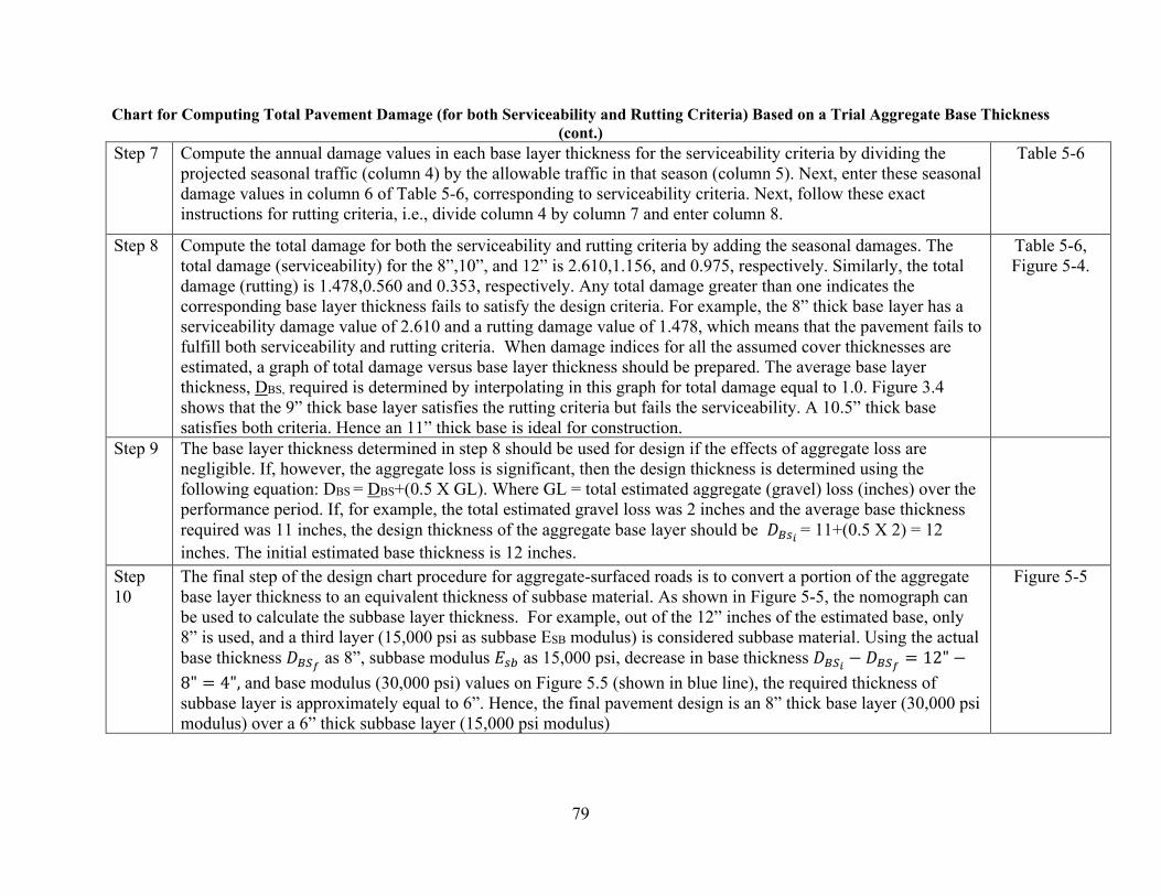
79

Chart for Computing Total Pavement Damage (for both Serviceability and Rutting Criteria) Based on a Trial Aggregate Base Thickness (cont.)

Step 7 Compute the annual damage values in each base layer thickness for the serviceability criteria by dividing the projected seasonal traffic (column 4) by the allowable traffic in that season (column 5). Next, enter these seasonal damage values in column 6 of Table 5-6, corresponding to serviceability criteria. Next, follow these exact instructions for rutting criteria, i.e., divide column 4 by column 7 and enter column 8.

Table 5-6

Step 8 Compute the total damage for both the serviceability and rutting criteria by adding the seasonal damages. The total damage (serviceability) for the 8”,10”, and 12” is 2.610,1.156, and 0.975, respectively. Similarly, the total damage (rutting) is 1.478,0.560 and 0.353, respectively. Any total damage greater than one indicates the corresponding base layer thickness fails to satisfy the design criteria. For example, the 8” thick base layer has a serviceability damage value of 2.610 and a rutting damage value of 1.478, which means that the pavement fails to fulfill both serviceability and rutting criteria. When damage indices for all the assumed cover thicknesses are estimated, a graph of total damage versus base layer thickness should be prepared. The average base layer thickness, DBS, required is determined by interpolating in this graph for total damage equal to 1.0. Figure 3.4 shows that the 9” thick base layer satisfies the rutting criteria but fails the serviceability. A 10.5” thick base satisfies both criteria. Hence an 11” thick base is ideal for construction.

Table 5-6, Figure 5-4.

Step 9 The base layer thickness determined in step 8 should be used for design if the effects of aggregate loss are negligible. If, however, the aggregate loss is significant, then the design thickness is determined using the following equation: DBS = DBS+(0.5 X GL). Where GL = total estimated aggregate (gravel) loss (inches) over the performance period. If, for example, the total estimated gravel loss was 2 inches and the average base thickness required was 11 inches, the design thickness of the aggregate base layer should be 𝐷𝐷𝐵𝐵𝐵𝐵𝑖𝑖 = 11+(0.5 X 2) = 12 inches. The initial estimated base thickness is 12 inches.

Step 10

The final step of the design chart procedure for aggregate-surfaced roads is to convert a portion of the aggregate base layer thickness to an equivalent thickness of subbase material. As shown in Figure 5-5, the nomograph can be used to calculate the subbase layer thickness. For example, out of the 12” inches of the estimated base, only 8” is used, and a third layer (15,000 psi as subbase ESB modulus) is considered subbase material. Using the actual base thickness 𝐷𝐷𝐵𝐵𝐵𝐵𝑓𝑓 as 8”, subbase modulus 𝐸𝐸𝐵𝐵𝑠𝑠 as 15,000 psi, decrease in base thickness 𝐷𝐷𝐵𝐵𝐵𝐵𝑖𝑖 − 𝐷𝐷𝐵𝐵𝐵𝐵𝑓𝑓 = 12" −8" = 4", and base modulus (30,000 psi) values on Figure 5.5 (shown in blue line), the required thickness of subbase layer is approximately equal to 6”. Hence, the final pavement design is an 8” thick base layer (30,000 psi modulus) over a 6” thick subbase layer (15,000 psi modulus)

Figure 5-5

80

Table 5-6 Computation of Total Pavement Damage (for both Serviceability and Rutting Criteria) Based on Trial Aggregate Base Layer.

Trial Base (in.)

(1) Season (RoadbedMoisture Condition)

(2) Roadbed Resilient Modulus, MR (psi)

(3) BaseElasticModulus,EBS (psi)

(4) Projected 18-kipESALTraffic,W18

(5) Allowable 18-kipESALTraffic,(W18) PSI

(6) Seasonal Damage,

𝑾𝑾𝟏𝟏𝟏𝟏

(𝑾𝑾𝟏𝟏𝟏𝟏)𝑷𝑷𝑷𝑷𝑷𝑷

(7) Allowable 18- kipESALTraffic,(W18) RUT

(8) Seasonal Damage

𝒘𝒘𝟏𝟏𝟏𝟏

(𝑾𝑾𝟏𝟏𝟏𝟏)𝑹𝑹𝑹𝑹𝑹𝑹

8” Winter (Frozen) 20,000 30,000 8,750 400,000 0.022 130000 0.067 Spring/Thaw (Saturated) 1,500 30,000 4,375 4,900 0.893 8400 0.521

Spring/Fall (Wet) 3,300 30,000 8,750 10000 0.875 20000 0.438 Summer (Dry) 4,900 30,000 13,125 16000 0.820 29000 0.453

Total Traffic 35,000 Total

Damage 2.610 Total Damage 1.478

10” Winter (Frozen) 20,000 30,000 8,750 400,000 0.022 250000 0.035 Spring/Thaw (Saturated) 1,500 30,000 4,375 9,000 0.486 20000 0.219

Spring/Fall (Wet) 3,300 30,000 8,750 32000 0.273 50000 0.175 Summer (Dry) 4,900 30,000 13,125 35000 0.375 100000 0.131



12” Winter (Frozen) 20,000 30,000 8,750 500,000 0.018 400,000 0.022 Spring/Thaw(Saturated) 1,500 30,000 4,375 15,000 0.292 28000 0.156 Spring/Fall (Wet) 3,300 30,000 8,750 22000 0.398 100000 0.088 Summer (Dry) 4,900 30,000 13,125 35000 0.375 100000 0.131



81

Figure 5-4 Example Growth of Total Damage Versus Base Layer Thickness for Both Serviceability and Rutting Criteria.

Figure 5-5 Chart to Convert a Portion of the Aggregate Base Layer Thickness to an Equivalent Thickness of Subbase (AASHTO, 1993).

82

5.2.1.1 Aggregate-Surface Roads using Geocell Reinforced Layer Initially, a design with a 10-inch-thick layer is developed, and later it is adjusted to a 6-inch reinforced layer and subbase layer based on pavement damage calculations shown in Table 5-7. The values shown in column 5 of Table 5-7 are estimated as shown in Figure 5-6, and the values in column 7 are estimated as shown in Figure 5-7. The total damage values for serviceability and rutting are less than 1. Hence, the design is acceptable. Since only 6 out of 10 inches of the base is reinforced, the final step is to convert a portion of the 4” aggregate base layer (unreinforced) thickness to an equivalent thickness of subbase material. The nomograph as shown in Figure 5-8, can be used to calculate the subbase layer thickness. Out of 10” inches of the estimated base only 6” is considered as a base and a third layer (15,000 psi as subbase ESB modulus) is considered as a subbase material. Using the actual base thickness 𝐷𝐷𝐵𝐵𝐵𝐵𝑓𝑓 as 6”, subbase modulus 𝐸𝐸𝐵𝐵𝑠𝑠 as 15,000 psi, decrease in base thickness 𝐷𝐷𝐵𝐵𝐵𝐵𝑖𝑖 − 𝐷𝐷𝐵𝐵𝐵𝐵𝑓𝑓 = 10" − 6" = 4", and base modulus (40,000 psi) values on Figure 5-6 (shown in blue line), the required thickness of the subbase layer is approximately equal to 7”. Hence, the final pavement design is 6” thick geocell reinforced base layer (40,000 psi modulus) over 7” thick subbase layer (15,000 psi modulus). A comparison of the unreinforced and geocell reinforced layer is shown in Table 5-8.

Table 5-7 Computation of Total Pavement Damage (for both Serviceability and Rutting Criteria) Based on 10” Aggregate Base Layer.

Trial Base (in.)

(1) Season(RoadbedMoistureCondition)

(2) Roadbed Resilient Modulus, MR (psi)

(3) BaseElasticModulus, EBS (psi)

(4) Projected 18-kipESALTraffic,W18

(5) Allowable 18-kipESALTraffic,(W18)PSI

(6) Seasonal Damage,

𝑊𝑊18

(𝑊𝑊18)𝑃𝑃𝐵𝐵𝑃𝑃

(7) Allowable 18- kipESALTraffic,(W18)RUT

(8) SeasonalDamage

𝑤𝑤18(𝑊𝑊18)𝑅𝑅𝑅𝑅𝑅𝑅

10” Winter (Frozen) 20,000 40,000 8,750 500,000 0.02 500,000 0.018

Spring/Thaw (Saturated)

1,500 40,000 4,375 14,000 0.31 50,000 0.088

Spring/Fall (Wet) 3,300 40,000 8,750 26000 0.34 150,000 0.058

Summer (Dry) 4,900 40,000 13,125 39000 0.34 210,000 0.063



83

Figure 5-6 Design Chart for Aggregate-Surfaced Roads Considering Allowable Serviceability Loss (Geocell Reinforced Layer Calculations) (AASHTO, 1993).

84

Figure 5-7 Design Chart for Aggregate-Surfaced Roads Considering Allowable Rutting (Geocell Reinforced Layer Calculations) (AASHTO, 1993).

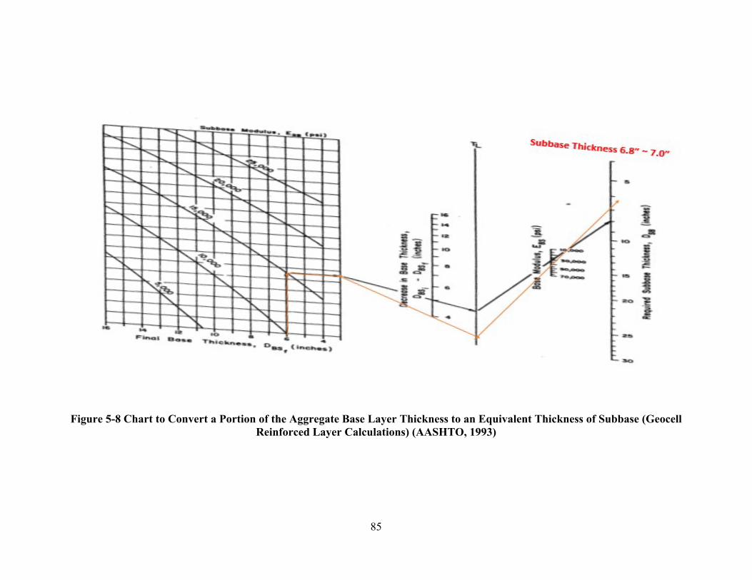
85

Figure 5-8 Chart to Convert a Portion of the Aggregate Base Layer Thickness to an Equivalent Thickness of Subbase (Geocell Reinforced Layer Calculations) (AASHTO, 1993)

86

Table 5-8 Chart for Computing Total Pavement Damage (for both Serviceability and Rutting Criteria) Based on a Trial Aggregate Base Thickness.

Pavement Type Thickness Modulus (ksi)

Base Subbase Total Base Modulus Subbase Modulus

Unreinforced Section 8" 6" 14" 30 15

Geocell Reinforced 6"* 7" 13" 40** 15

* Geocell Height** Equivalent Modulus of Geocell layer is considered as 40 ksi with an infill material of 15 ksi

5.3 DESIGN METHODS FOR LOW VOLUME UNPAVED ROADS WITH GEOCELL REINFORCEMENT

5.3.1 PRESTO GEOSYSTEM Design Method Conventional flexible pavement design methods are based on historical performance data collected from either full-scale road tests or ongoing testing and monitoring of pavement performance within various geographical areas. Federal and local agencies have determined structural values of conventional road construction materials based on years of in-service performance history. While many new materials (Stabilizers, geosynthetics, etc.) have been introduced in recent years to enhance the structural value of conventional construction materials, it isn't easy. It can take several years to obtain structural values for these components to use with existing design methods. For this reason, there are no agency-accepted structural values or equivalencies that can be used with current pavement design methods for the geocell system.

The design of geocell confined granular pavements over soft soils is relatively straightforward and has been well documented for general design purposes. The design method outlined by Presto is for the low-volume roads where minor deformations are tolerable or for the design of pavement subbase layers over soft soils. They are not intended for the design of flexible pavement structures with paved surfaces. The calculations are only valid for granular pavement design over cohesive subgrade soils with CBR values less than 5.

Empirically derived bearing capacity coefficients are first used to determine the maximum allowable stress on a subgrade with either known or estimated shear strength. The maximum allowable stress is the stress that would cause the subgrade's local punching/shear failure under sustained loading conditions. The maximum allowable stress is the limiting stress for design purposes. Next, the Boussinesq theory is used to determine the required depth of granular cover beneath the design wheel load to ensure that the maximum allowable stress is not exceeded.

5.3.1.1 Design for Unreinforced Base layers (Unpaved Surface Layer) Table 5-9 shows the estimation of base layer thickness (height) for unpaved roads using Boussinesq theory. The thickness of the base layer is a factor of the design load, loaded area, and bearing capacity of the subgrade. Table 5-10 displays the close correlation between California Bearing Ratio (CBR), shear strength, and Standard Penetration Testing (SPT). The values of shear strength can be considered from this table if no test data is available.

.

87

Table 5-9 Methodology for Designing Gravel Roads (Unreinforced) A: Design of Unreinforced Pavement (No paved surface layer) Step Description Equation A1 Determine the maximum

allowable stress on the subgrade

𝑞𝑞𝑎𝑎 = 𝑁𝑁𝑐𝑐𝑐𝑐𝑢𝑢 Where: Nc Bearing capacity coefficient- based on design traffic

Cu Subgrade shear strength; The typical values of shear strength for various subgrades are shown in Table 2.2

A2 Determine the required thickness of the granular pavement, Zu

𝑍𝑍𝑢𝑢 =𝑅𝑅

�1

(1 − 𝑞𝑞𝑎𝑎𝑝𝑝 )2/3

− 1

𝑅𝑅 = �𝑃𝑃𝑝𝑝𝑝𝑝

Where R= Radius of loaded area (i.e., the effective radius of single or dual tires); p=Contact Pressure; P= Design wheel load

Table 5-10 Correlation of Subgrade Soil Strength Parameters for Cohesive (Fine-Grained) Soils

Cal

iforn

ia

Bea

ring

Rat

io

CB

R (%

)

Und

rain

ed

Shea

r Stre

ngth

C

u k

Pa(p

si)

SPT

(blo

ws/

ft)

Fiel

d Id

entif

icat

ion

<0.4 <11.7 (1.7) <2 Very Soft (extruded between fingers when squeezed) 0.4-0.8 11.7-24.1

(1.7)-(3.5) 2-4 Soft (molded by light finger pressure)

0.8-1.6 24.1-47.6 (3.5)-(6.9)

4-8 Medium (molded by strong finger pressure)

1.6-3.2 47.6-95.8 (6.9)-(13.9)

8-15 Stiff (readily indented by thumb but penetrated with great effort)

3.2-6.4 95.8-191 (13.9)-(27.7)

15-30 Very stiff (readily indented by thumbnail)

>6.4 > 191 (27.7) > 30 Hard (indented with difficulty by thumbnail)

5.3.1.2 Design for Geocell Reinforced Base layers (Unpaved Surface Layer) The design procedure for the geocell reinforced base layer is shown stepwise in Table 5-11. The design is based on the theory that the geocell reinforced layer absorbs a portion of vertical load, thus reducing the ultimate load on the subgrade. Due to the load transfer to geocell, the pavement section can either carry higher loads or have an extended life than the unreinforced pavement section.

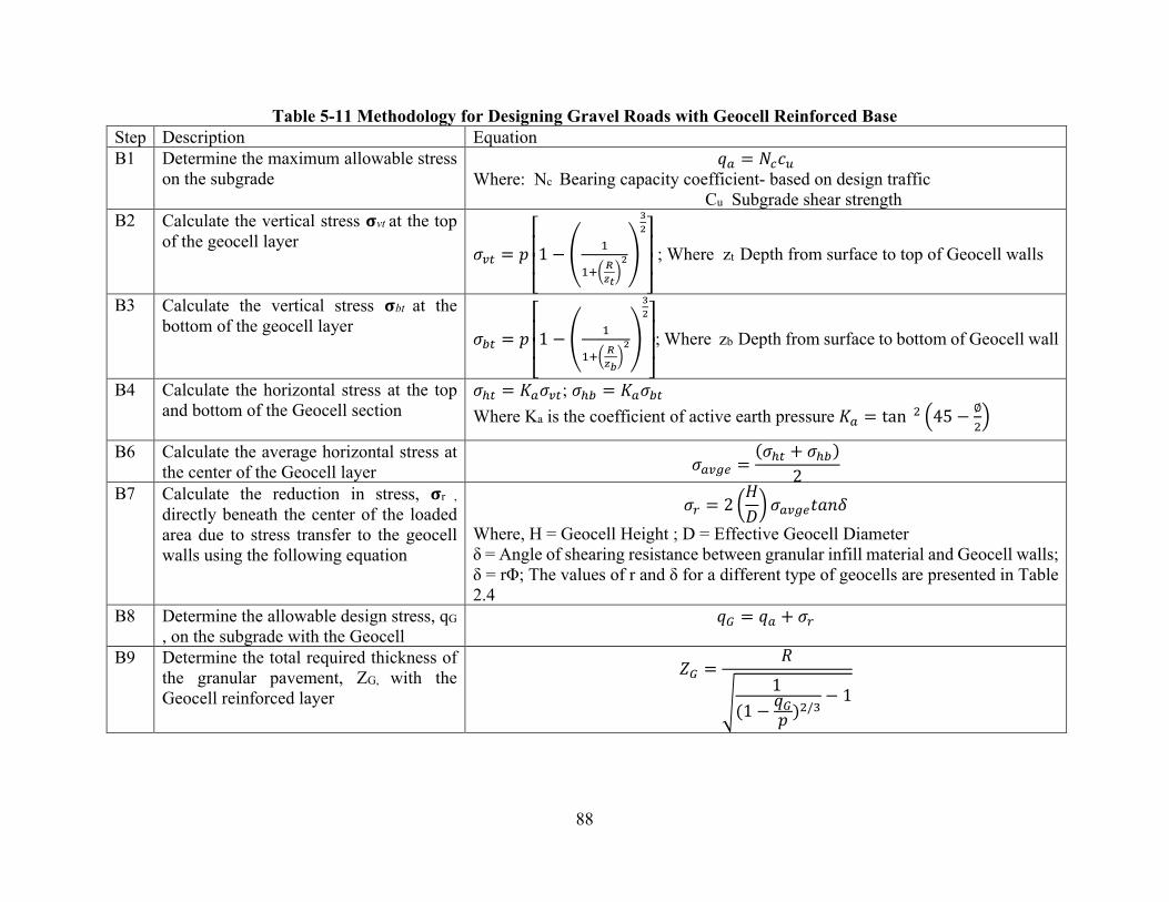
88

Table 5-11 Methodology for Designing Gravel Roads with Geocell Reinforced Base Step Description Equation B1 Determine the maximum allowable stress

on the subgrade 𝑞𝑞𝑎𝑎 = 𝑁𝑁𝑐𝑐𝑐𝑐𝑢𝑢

Where: Nc Bearing capacity coefficient- based on design traffic Cu Subgrade shear strength

B2 Calculate the vertical stress 𝛔𝛔vt at the top of the geocell layer

𝜎𝜎𝑎𝑎𝑣𝑣 = 𝑝𝑝

⎣⎢⎢⎡1 − � 1

1+�𝑅𝑅𝑧𝑧𝑡𝑡�2�

32

⎦⎥⎥⎤

; Where zt Depth from surface to top of Geocell walls

B3 Calculate the vertical stress 𝛔𝛔bt at the bottom of the geocell layer

𝜎𝜎𝑠𝑠𝑣𝑣 = 𝑝𝑝

⎣⎢⎢⎡1 − � 1

1+� 𝑅𝑅𝑧𝑧𝑏𝑏�2�

32

⎦⎥⎥⎤; Where zb Depth from surface to bottom of Geocell wall

B4 Calculate the horizontal stress at the top and bottom of the Geocell section

𝜎𝜎ℎ𝑣𝑣 = 𝐾𝐾𝑎𝑎𝜎𝜎𝑎𝑎𝑣𝑣; 𝜎𝜎ℎ𝑠𝑠 = 𝐾𝐾𝑎𝑎𝜎𝜎𝑠𝑠𝑣𝑣 Where Ka is the coefficient of active earth pressure 𝐾𝐾𝑎𝑎 = tan 2 �45 − ∅

2�

B6 Calculate the average horizontal stress at the center of the Geocell layer 𝜎𝜎𝑎𝑎𝑎𝑎𝑎𝑎𝑎𝑎 =

(𝜎𝜎ℎ𝑣𝑣 + 𝜎𝜎ℎ𝑠𝑠)2

B7 Calculate the reduction in stress, 𝛔𝛔r ,

directly beneath the center of the loaded area due to stress transfer to the geocell walls using the following equation

𝜎𝜎𝑟𝑟 = 2 �𝐻𝐻𝐷𝐷�

𝜎𝜎𝑎𝑎𝑎𝑎𝑎𝑎𝑎𝑎𝑡𝑡𝑡𝑡𝑡𝑡𝑡𝑡 Where, H = Geocell Height ; D = Effective Geocell Diameter δ = Angle of shearing resistance between granular infill material and Geocell walls; δ = rΦ; The values of r and δ for a different type of geocells are presented in Table 2.4

B8 Determine the allowable design stress, qG

, on the subgrade with the Geocell 𝑞𝑞𝐺𝐺 = 𝑞𝑞𝑎𝑎 + 𝜎𝜎𝑟𝑟

B9 Determine the total required thickness of the granular pavement, ZG, with the Geocell reinforced layer

𝑍𝑍𝐺𝐺 =𝑅𝑅

�1

(1 − 𝑞𝑞𝐺𝐺𝑝𝑝 )2/3

− 1

89

The amount of stress absorbed is:

𝝈𝝈𝒓𝒓 = 𝟐𝟐 �𝑯𝑯𝑫𝑫�𝝈𝝈𝒂𝒂𝒂𝒂𝒂𝒂𝒂𝒂𝒕𝒕𝒂𝒂𝒕𝒕𝒕𝒕 5-1

where, H = geocell Height; D = effective geocell diameter, and δ = angle of shearing resistance between granular infill material and geocell walls; δ = rΦ;

Table 5-12 shows typical values of angle of shearing resistance between geocell infill and wall for various types of geocell texture and infill material. The reduction of vertical stress is a function of the angle of shearing resistance between infill material and geocell walls, the aspect ratio (H/D), and the average horizontal stress on the center of geocell

Table 5-12 Recommended Peak Friction Angle Ratio (Presto Geosystems) Granular Infill Material Cell Wall Type r=δ/Φ

Coarse Sand/Gravel Smooth 0.71 Textured 0.88

Textured-Perforated 0.90

#40 Silica Sand Smooth 0.78 Textured 0.90


Crushed Stone Smooth 0.72 Textured 0.72


5.3.1.3 Angle of Shearing Resistance between Infill Material and Geocell Walls The friction between the infill material and the geocell wall is one of the key inputs in the design method proposed by Presto. The friction between the geocell and infill material is typically less than the internal friction of infill material. Table 5-12 shows the recommended friction angle between geocell surface type and infill material as a ratio of reduction of internal friction angle of infill material. As per the table, textured-perforated geocell generates the highest shearing resistance, and silica sand is the most effective infill material.

5.3.1.4 Aspect Ratio The aspect ratio is the ratio between the height of the geocell to the equivalent diameter of the geocell opening. Therefore, the higher aspect ratio indicates more geocell material in the reinforced base.

5.3.1.5 Average Horizontal Stress on the Center of Geocell As per the equation, the reduction in vertical stress is proportional to the horizontal stress coming onto the center of the geocell. It suggests that the higher the horizontal stress, the more significant is the benefit of geocell. Higher horizontal stress can be achieved if the geocell is placed near the loading point. The efficiency decreases with the increase in the geocell placement depth from the applied load. Figure 5-9 shows an example of the design of a low-volume road with and without geocell. A 6-inch geocell with a 4-inch cover is used for the analysis. Infill base and subgrade properties are shown in Figure 5-9. In unreinforced conditions, a 12-inch-thick base is required, whereas a 10-inch-thick (6-inch geocell layer + 4-inch cover) base is required for the use of geocell reinforcement. The geocell reinforcement reduces the base thickness by 2 inches.

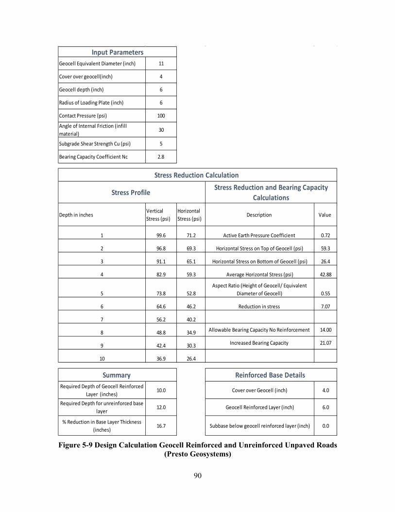
90

Cover over Geocell (inch) 4.0

Geocell Reinforced Layer (inch) 6.0

Subbase below geocell reinforced layer (inch) 0.0

Reinforced Base Details

Figure 5-9 Design Calculation Geocell Reinforced and Unreinforced Unpaved Roads (Presto Geosystems)

Geocell Equivalent Diameter (inch) 11

Cover over geocell(inch) 4

Geocell depth (inch) 6

Radius of Loading Plate (inch) 6

Contact Pressure (psi) 100

Angle of Internal Friction (infill material)

30

Subgrade Shear Strength Cu (psi) 5

Bearing Capacity Coefficient Nc 2.8

Input Parameters

Depth in inches Vertical Stress (psi)

Horizontal Stress (psi)

Description Value

1 99.6 71.2 Active Earth Pressure Coefficient 0.72

2 96.8 69.3 Horizontal Stress on Top of Geocell (psi) 59.3

3 91.1 65.1 Horizontal Stress on Bottom of Geocell (psi) 26.4

4 82.9 59.3 Average Horizontal Stress (psi) 42.88

5 73.8 52.8Aspect Ratio (Height of Geocell/ Equivalent

Diameter of Geocell) 0.55

6 64.6 46.2 Reduction in stress 7.07

7 56.2 40.2

8 48.8 34.9 Allowable Bearing Capacity No Reinforcement 14.00

9 42.4 30.3 Increased Bearing Capacity 21.07

10 36.9 26.4

Stress Reduction Calculation

Stress Profile Stress Reduction and Bearing Capacity

Calculations

Required Depth of Geocell Reinforced Layer (inches)

10.0

Required Depth for unreinforced base layer

12.0

% Reduction in Base Layer Thickness (inches)

16.7

Summary

91

5.3.2 Design Method Presto Geosystems for Low Volume Roads – Unpaved Roads (Pokharel 2010)

In this study, the design method developed by Giroud and Han (2004 a and b) for planar geosynthetic-reinforced (geotextile and geogrid) unpaved roads is modified to accommodate geocell reinforcement. The complete methodology for the design of the unpaved road is shown in Table 5-13. In addition, Gabr (2001) and Pokharel et al. (2010) observed that geocell reinforcement reduces the stress distribution angle. This phenomenon is attributed to the geocell confinement of the base course to increase and maintain the modulus of the base course.

A modulus improvement factor was proposed by Han et al. (2007) to account for this benefit:

𝐼𝐼𝑓𝑓 = �𝐸𝐸𝑠𝑠𝑐𝑐(𝑟𝑟𝑎𝑎𝑟𝑟𝑟𝑟𝑓𝑓𝑟𝑟𝑟𝑟𝑐𝑐𝑎𝑎𝑟𝑟)

𝐸𝐸𝑠𝑠𝑐𝑐(𝑢𝑢𝑟𝑟𝑟𝑟𝑎𝑎𝑟𝑟𝑟𝑟𝑓𝑓𝑟𝑟𝑟𝑟𝑐𝑐𝑎𝑎𝑟𝑟)�

5-2

where Ebc(reinforced) is the modulus of the reinforced base, and Ebc(unreinforced) is the modulus of the unreinforced base. According to Pokharel et al. (2010), the modulus improvement factor is between 1.7 to 2.0 based on the infill material. Regular base material and sand have an improvement factor of 2, which means geocell reinforcement increases the infill modulus by two times. If recycled asphalt pavement (RAP) is used as an infill, a value of 1.7 is proposed.

The design equation proposed by Pokharel et al. (2010) is shown in the equation below (Each parameter in the equation is defined in Table 3.1)

ℎ =(0.868 + 0.52 �𝑟𝑟ℎ�

1.5𝑙𝑙𝑙𝑙𝑙𝑙𝑁𝑁)

𝜂𝜂{1 + 0.204[𝑅𝑅𝐸𝐸 − 1]} × ��𝑃𝑃

𝑝𝑝𝑟𝑟2𝑚𝑚𝑁𝑁𝑐𝑐𝑐𝑐𝑢𝑢− 1�𝑟𝑟

5-3

In the Giroud and Han (2004 a and b) design, the modulus ratio (RE) for unreinforced and planar geosynthetic-reinforced unpaved roads is limited to 5. They recommended this limit, considering that base courses cannot be well compacted over soft subgrade. The three-dimensional confinement by geocell can overcome this problem and help the base course reach and maintain its higher modulus.

Han et al. (2007) reported that the geocell-reinforced bases had modulus ratios ranging from 4.8 to 10. However, their study's calculated modulus ratios from cyclic plate loading tests and accelerated moving wheel tests ranged from 3.4 to 7.6. Therefore, Pokharel (2010) kept the maximum limit of the modulus ratio to 7.6 for Novel Polymeric Alloy (NPA) geocell. The modulus ratio can be calculated based on the equation shown in step 3 of Table 5-13.

In general, it is proposed to use a nonwoven geotextile as a separation between the geocell reinforced layer and the underlying soft subgrade. Since a nonwoven geotextile sheet is commonly used below geosynthetic reinforced bases, the bearing capacity factor (Nc) for geocell-reinforced unpaved roads can be reasonably assumed to be equal to 5.14. Therefore, in the unreinforced base scenario, the recommended value is 3.14.

The proposed methodology is demonstrated through an example in the following section.

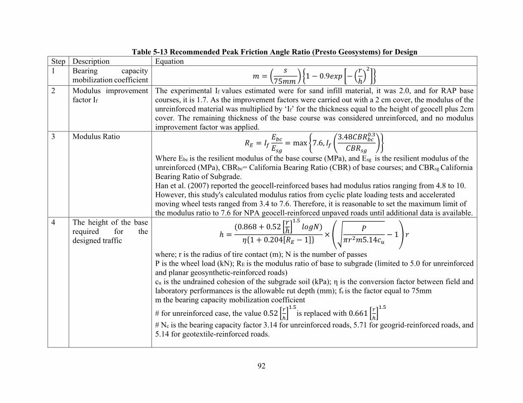
92

Table 5-13 Recommended Peak Friction Angle Ratio (Presto Geosystems) for Design Step Description Equation 1 Bearing capacity

mobilization coefficient 𝑚𝑚 = �𝑠𝑠

75𝑚𝑚𝑚𝑚� �1 − 0.9𝑒𝑒𝑒𝑒𝑝𝑝 �− �𝑟𝑟ℎ�2��

2 Modulus improvement factor If

The experimental If values estimated were for sand infill material, it was 2.0, and for RAP base courses, it is 1.7. As the improvement factors were carried out with a 2 cm cover, the modulus of the unreinforced material was multiplied by ‘If’ for the thickness equal to the height of geocell plus 2cm cover. The remaining thickness of the base course was considered unreinforced, and no modulus improvement factor was applied.

3 Modulus Ratio 𝑅𝑅𝐸𝐸 = 𝐼𝐼𝑓𝑓

𝐸𝐸𝑠𝑠𝑐𝑐𝐸𝐸𝐵𝐵𝑎𝑎

= max �7.6, 𝐼𝐼𝑓𝑓 �

3.48𝐶𝐶𝐶𝐶𝑅𝑅𝑠𝑠𝑐𝑐0.3

𝐶𝐶𝐶𝐶𝑅𝑅𝐵𝐵𝑎𝑎��

Where Ebc is the resilient modulus of the base course (MPa), and Esg is the resilient modulus of the unreinforced (MPa), CBRbc= California Bearing Ratio (CBR) of base courses; and CBRsg California Bearing Ratio of Subgrade. Han et al. (2007) reported the geocell-reinforced bases had modulus ratios ranging from 4.8 to 10. However, this study's calculated modulus ratios from cyclic plate loading tests and accelerated moving wheel tests ranged from 3.4 to 7.6. Therefore, it is reasonable to set the maximum limit of the modulus ratio to 7.6 for NPA geocell-reinforced unpaved roads until additional data is available.

4 The height of the base required for the designed traffic

ℎ =(0.868 + 0.52 �𝑟𝑟ℎ�


𝜂𝜂{1 + 0.204[𝑅𝑅𝐸𝐸 − 1]} × ��𝑃𝑃

𝑝𝑝𝑟𝑟2𝑚𝑚5.14𝑐𝑐𝑢𝑢− 1�𝑟𝑟

where; r is the radius of tire contact (m); N is the number of passes P is the wheel load (kN); RE is the modulus ratio of base to subgrade (limited to 5.0 for unreinforced and planar geosynthetic-reinforced roads) cu is the undrained cohesion of the subgrade soil (kPa); η is the conversion factor between field and laboratory performances is the allowable rut depth (mm); fs is the factor equal to 75mm m the bearing capacity mobilization coefficient

# for unreinforced case, the value 0.52 �𝑟𝑟ℎ�1.5

is replaced with 0.661 �𝑟𝑟ℎ�1.5

# Nc is the bearing capacity factor 3.14 for unreinforced roads, 5.71 for geogrid-reinforced roads, and 5.14 for geotextile-reinforced roads.

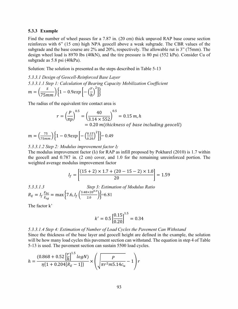
93

5.3.3 Example Find the number of wheel passes for a 7.87 in. (20 cm) thick unpaved RAP base course section reinforces with 6” (15 cm) high NPA geocell above a weak subgrade. The CBR values of the subgrade and the base course are 2% and 20%, respectively. The allowable rut is 3” (75mm). The design wheel load is 8970 lbs (40kN), and the tire pressure is 80 psi (552 kPa). Consider Cu of subgrade as 5.8 psi (40kPa).

Solution: The solution is presented as the steps described in Table 5-13

5.3.3.1 Design of Geocell-Reinforced Base Layer 5.3.3.1.1 Step 1: Calculation of Bearing Capacity Mobilization Coefficient

𝑚𝑚 = �𝑠𝑠

75𝑚𝑚𝑚𝑚 � �1 − 0.9𝑒𝑒𝑒𝑒𝑝𝑝 �−�

𝑟𝑟ℎ�2��

The radius of the equivalent tire contact area is

𝑟𝑟 = �𝑃𝑃𝑝𝑝𝑝𝑝�

0.5

= �40

3.14 × 552�0.5

= 0.15 𝑚𝑚, ℎ

= 0.20 𝑚𝑚(𝑡𝑡ℎ𝑖𝑖𝑐𝑐𝑖𝑖𝑡𝑡𝑒𝑒𝑠𝑠𝑠𝑠 𝑙𝑙𝑜𝑜 𝑏𝑏𝑡𝑡𝑠𝑠𝑒𝑒 𝑖𝑖𝑡𝑡𝑐𝑐𝑙𝑙𝑢𝑢𝑢𝑢𝑖𝑖𝑡𝑡𝑙𝑙 𝑙𝑙𝑒𝑒𝑙𝑙𝑐𝑐𝑒𝑒𝑙𝑙𝑙𝑙)

𝑚𝑚 = � 7575𝑚𝑚𝑚𝑚

� �1 − 0.9𝑒𝑒𝑒𝑒𝑝𝑝 �− �0.150.20

�2��= 0.49

5.3.3.1.2 Step 2: Modulus improvement factor If The modulus improvement factor (If) for RAP as infill proposed by Pokharel (2010) is 1.7 within the geocell and 0.787 in. (2 cm) cover, and 1.0 for the remaining unreinforced portion. The weighted average modulus improvement factor

𝐼𝐼𝑓𝑓 = �(15 + 2) × 1.7 + (20 − 15 − 2) × 1.0

20 � = 1.59

5.3.3.1.3 Step 3: Estimation of Modulus Ratio

𝑅𝑅𝐸𝐸 = 𝐼𝐼𝑓𝑓𝐸𝐸𝑏𝑏𝑏𝑏𝐸𝐸𝑠𝑠𝑠𝑠

= max �7.6, 𝐼𝐼𝑓𝑓 �

3.48×200.3

2.0��=6.81

The factor k’

𝑖𝑖′ = 0.5 �0.150.20

�1.5

= 0.34

5.3.3.1.4 Step 4: Estimation of Number of Load Cycles the Pavement Can Withstand Since the thickness of the base layer and geocell height are defined in the example, the solution will be how many load cycles this pavement section can withstand. The equation in step 4 of Table 5-13 is used. The pavement section can sustain 5500 load cycles.

ℎ =(0.868 + 0.52 �𝑟𝑟ℎ�


𝜂𝜂{1 + 0.204[𝑅𝑅𝐸𝐸 − 1]} × ��𝑃𝑃


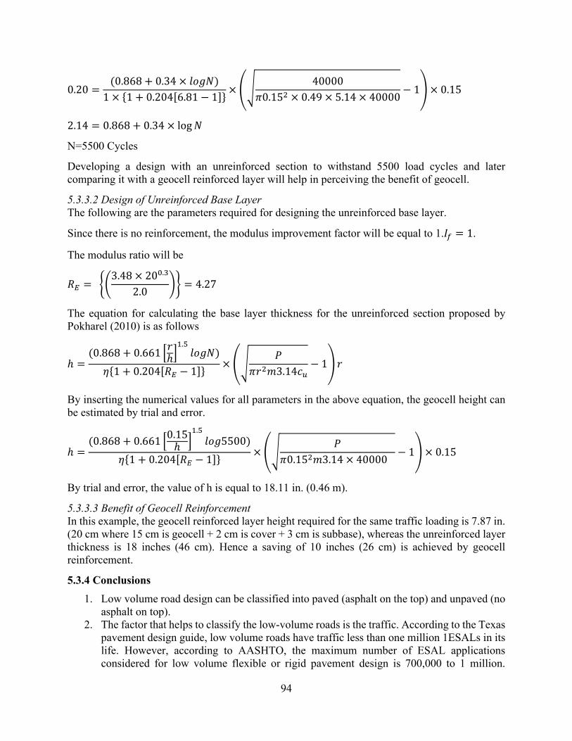
94

0.20 =(0.868 + 0.34 × 𝑙𝑙𝑙𝑙𝑙𝑙𝑁𝑁)

1 × {1 + 0.204[6.81 − 1]} × ��40000

𝑝𝑝0.152 × 0.49 × 5.14 × 40000− 1� × 0.15

2.14 = 0.868 + 0.34 × log𝑁𝑁

N=5500 Cycles

Developing a design with an unreinforced section to withstand 5500 load cycles and later comparing it with a geocell reinforced layer will help in perceiving the benefit of geocell.

5.3.3.2 Design of Unreinforced Base Layer The following are the parameters required for designing the unreinforced base layer.

Since there is no reinforcement, the modulus improvement factor will be equal to 1.𝐼𝐼𝑓𝑓 = 1.

The modulus ratio will be

𝑅𝑅𝐸𝐸 = ��3.48 × 20

0.3

2.0�� = 4.27

The equation for calculating the base layer thickness for the unreinforced section proposed by Pokharel (2010) is as follows

ℎ =(0.868 + 0.661 �𝑟𝑟ℎ�


𝜂𝜂{1 + 0.204[𝑅𝑅𝐸𝐸 − 1]} × ��𝑃𝑃


By inserting the numerical values for all parameters in the above equation, the geocell height can be estimated by trial and error.

ℎ =(0.868 + 0.661 �0.15

ℎ �1.5𝑙𝑙𝑙𝑙𝑙𝑙5500)

𝜂𝜂{1 + 0.204[𝑅𝑅𝐸𝐸 − 1]} × ��𝑃𝑃

𝑝𝑝0.152𝑚𝑚3.14 × 40000− 1� × 0.15

By trial and error, the value of h is equal to 18.11 in. (0.46 m).

5.3.3.3 Benefit of Geocell Reinforcement In this example, the geocell reinforced layer height required for the same traffic loading is 7.87 in. (20 cm where 15 cm is geocell + 2 cm is cover + 3 cm is subbase), whereas the unreinforced layer thickness is 18 inches (46 cm). Hence a saving of 10 inches (26 cm) is achieved by geocell reinforcement.

5.3.4 Conclusions 1. Low volume road design can be classified into paved (asphalt on the top) and unpaved (no

asphalt on top).2. The factor that helps to classify the low-volume roads is the traffic. According to the Texas

pavement design guide, low volume roads have traffic less than one million 1ESALs in itslife. However, according to AASHTO, the maximum number of ESAL applicationsconsidered for low volume flexible or rigid pavement design is 700,000 to 1 million.

95

Therefore, the practical minimum traffic level that can be considered for any flexible or rigid pavement during a given performance period is about 50,000 ESAL applications.

3. The design procedure suggested for low-volume paved roads by AASHTO and TxDOT islike the design procedure for regular pavements. However, the main difference is thereliability or confidence level. A low confidence level is suggested for designing low-volume roads. TxDOT recommended a confidence level as low as ‘An (80%)’ for designsbelow 1 million ESALs. The level of reliability recommended by AASHTO for low-volume road design is 50 percent. The user may design for higher levels of 60 to 80 percentdepending on the importance of the project.

4. AASHTO aggregate surface low volume road method is a graph-based design. A detailedexplanation of the existing method and incorporation of the geocell reinforced base ispresented through an example.

5. Two proposed design methods for unpaved roads with the geocell reinforced base areexamined. One method is proposed by PRESTO GEOSYSTEM (2008), and the other isdesigned by Pokharel (2010). However, these methods are not in practice.

6. The theory behind the PRESTO GEOSYSTEM design is that the geocell reinforced layertransfers load laterally, and a lower load is transmitted to the subgrade. Three main criteriathat benefit the geocell reinforced layer are:

I. the higher aspect ratio (Height of Geocell/ Diameter of Geocell)II. the texture of the geocell (perforated geocell wall with the textured wall is more

efficient than smooth geocell)III. placement of geocell (closer to the loading point highly efficient)

7. Pokharel's (2010) design method is a modification of unpaved roads design with planargeosynthetics proposed by Giroud and Han (2004 a and b). The design philosophy is basedon the experimental results, which showed that the geocell reinforced layer increases themodulus of the infill material, and increased modulus is considered in the design. Themodulus improvement through geocell is in the range of 1.7 to 2.0 times.

8. PRESTO GEOSYSTEM (2008) and Pokharel (2010) design methods revealed a significantbenefit of using geocell reinforcement for pavements with a poor subgrade. However, boththe methods have limitations like:a. Pokharel's (2010) design method is based on a limited test result (geocell from one

manufacturer and four base materials), and its applicability on a different type ofmaterials (other than tested) is questionable. For example, the design proceduredeveloped by Pokharel (2010) is valid only for NPA geocell; no recommendations areproposed for HDPE geocell.

b. The PRESTO GEOSYSTEM (2008) design method does not consider the quality ofthe infill material. The primary design criteria friction angle between the infill andgeocell wall considers the classification of infill (sand, silt, stone) but not the qualityof the infill base. It is observed in both our laboratory testing and FEA that with higherquality (high modulus) infill reduces the benefit of geocell, but PRESTOGEOSYSTEM design ignores this parameter.

96

97

6. MODEL DEVELOPMENT, STATISTICAL ANALYSIS,AND VALIDATION

The main idea of this chapter is to show the developing mathematical model for capturing the geocell reinforced layer benefit over the unreinforced layer using multilinear regression. Later the assumptions (linear relationship, collinearity, etc.) in the multiple regression are verified through statistical tools, and the model is enhanced further. Finally, cross-validation techniques for model development are discussed. The developed model is later employed in the design of pavements with geocell reinforced layer and will be reported in the subsequent chapter “ Design Method for Pavements Consisting of Geocells.” Some statistical tests (removal of noise for laboratory tests) are discussed in Chapter Four and are omitted.

6.1 PATH TO DEVELOPMENT OF MODEL The laboratory test results and FEA indicated that the geocell performance is a function of geocell height, infill modulus, cover thickness, and subgrade modulus (Table 3-3). Since the combination of geocell layered infill materials and existing subgrade conditions vary within geographical parts of Texas, a mathematical model will be helpful in the pavement design process followed within Texas. In addition, the developed model will help provide the information needed by the pavement designers.

The primary step in the model development is identifying the performance factor to be modeled. It is observed from the FEA and laboratory testing that the geocell reinforced layer reduced the vertical stresses on the subgrade, which is due to an increase in stiffness (modulus) of the base layer (geocell reinforced base). Since stress on top of the subgrade is the criteria for design, it was decided to develop a model that predicts a percent reduction (%Red. stress). The percentage of vertical stress reduction on subgrade depended on the combination of geocell height, infill material, cover thickness, and subgrade modulus. Therefore, the percentage vertical stress reduction due to the geocell reinforced layer on the subgrade can be a possible parameter that can be modeled to represent the performance of the geocell layer. The probable model is shown in the following equation:

%𝑹𝑹𝒂𝒂𝑹𝑹.𝑷𝑷𝒕𝒕𝒓𝒓𝒂𝒂𝑺𝑺𝑺𝑺 = 𝒇𝒇(𝑮𝑮𝒂𝒂𝑮𝑮𝑮𝑮𝒂𝒂𝑮𝑮𝑮𝑮 𝑯𝑯𝒂𝒂𝑯𝑯𝒂𝒂𝑯𝑯𝒕𝒕,𝑪𝑪𝑮𝑮𝒂𝒂𝒂𝒂𝒓𝒓 𝑹𝑹𝑯𝑯𝑯𝑯𝑮𝑮𝑻𝑻𝒕𝒕𝒂𝒂𝑺𝑺𝑺𝑺, 𝑷𝑷𝒕𝒕𝒇𝒇𝑯𝑯𝑮𝑮𝑮𝑮 𝒂𝒂𝒕𝒕𝑹𝑹 𝑷𝑷𝑺𝑺𝑺𝑺𝒂𝒂𝒓𝒓𝒂𝒂𝑹𝑹𝒂𝒂 𝑴𝑴𝑮𝑮𝑹𝑹𝑺𝑺𝑮𝑮𝑺𝑺𝑺𝑺) 6-1

Based on the percentage stress reduction, the equivalent modulus due to geocell reinforcement can be back-calculated using BISAR. Sample calculation of vertical stress reduction on subgrade due to geocell reinforced layer and back-calculation of equivalent modulus is shown in the LCCA calculations section (Section 7).

6.2 DATA FOR DEVELOPING MODEL The percentage of stress reduction due to the geocell reinforced layer is calculated for the various input variables ranges shown in Table 6-1. The complete details of combinations of tests are provided in Table 3- and Table 4-1. The parametric study in FEA used subgrades of 2 ksi, 4.5 ksi, 6 ksi, 9 ksi, and 15 ksi. The base properties evaluated include 2 ksi, 3 ksi, 5 ksi, 7 ksi, 9 ksi, 12 ksi, 15 ksi, 20 ksi, and 30 ksi modulus material. Even though the proposed test plan consisted of only testing two subgrades and four base materials, additional tests were performed to develop an appropriate model suitable for Texas (five subgrades and nine bases). It should be noted that the

98

additional tests were performed not only with geocell reinforced layers but also with unreinforced layers for estimating the benefit of the geocell layer.

Table 6-1 Range of Input Variables Used for Developing the Model Parameter Range Remarks

Base Modulus 2 ksi to 30 ksi Base as infill as well as cover material. Geocell Height 3”,4”, and 6” Three geocell are used in the FEA. Subgrade Modulus 2 ksi to 15 ksi Tested from very poor subgrade to good subgrade Cover Thickness 4” and 6” Only two cover thicknesses were considered.

6.3 DEVELOPMENT AND VALIDATION OF MODEL FOR ESTIMATING BENEFIT OF GEOCELL REINFORCED LAYER

In developing the model, this study proposes using multiple regression analysis, a statistical tool for investigating relationships between variables (Sykes 1993). The main advantage of regression analysis is that the analyst can assess the statistical significance of the estimated relationships. The statistical significance provides the degree of confidence that the actual relationship is close to the expected relationship. One form of regression analysis that is widely used is multi-linear regression analysis, which finds the linear relationships between variables. The multilinear regression analysis is often of the following form:

𝒚𝒚 = 𝜷𝜷𝟎𝟎 + 𝜷𝜷𝟏𝟏𝒙𝒙𝟏𝟏 + … … . . + 𝜷𝜷𝒕𝒕𝒙𝒙𝒕𝒕 + 𝝐𝝐

6-2where: 𝑦𝑦 = 𝑢𝑢𝑒𝑒𝑝𝑝𝑒𝑒𝑡𝑡𝑢𝑢𝑒𝑒𝑡𝑡𝑡𝑡 𝑣𝑣𝑡𝑡𝑟𝑟𝑖𝑖𝑡𝑡𝑏𝑏𝑙𝑙𝑒𝑒 (𝑝𝑝𝑟𝑟𝑒𝑒𝑢𝑢𝑖𝑖𝑐𝑐𝑡𝑡𝑖𝑖𝑡𝑡𝑙𝑙) 𝑒𝑒𝑟𝑟 = 𝑖𝑖𝑡𝑡𝑢𝑢𝑒𝑒𝑝𝑝𝑒𝑒𝑡𝑡𝑢𝑢𝑒𝑒𝑡𝑡𝑡𝑡 𝑣𝑣𝑡𝑡𝑟𝑟𝑖𝑖𝑡𝑡𝑏𝑏𝑙𝑙𝑒𝑒 𝐶𝐶𝑟𝑟 = 𝑟𝑟𝑒𝑒𝑙𝑙𝑟𝑟𝑒𝑒𝑠𝑠𝑠𝑠𝑖𝑖𝑙𝑙𝑡𝑡 𝑐𝑐𝑙𝑙𝑒𝑒𝑜𝑜𝑜𝑜𝑖𝑖𝑐𝑐𝑖𝑖𝑒𝑒𝑡𝑡𝑡𝑡 𝜖𝜖 = 𝑒𝑒𝑟𝑟𝑟𝑟𝑙𝑙𝑟𝑟

The regression coefficient explains the correlation between the independent variable and the dependent variable. Although multi-linear regression analysis is commonly used, the main limitation of this method is that there is no sure mechanism for the connected variables. Therefore, this study considers a multiple linear regression analysis as a starting point for the model development and modifies the model further to fit the testing data.

Thus, the model will be developed in three stages (explained in later sections) as follows:

a. Identify the parameters contributing towards the estimation of the benefit of geocellreinforced layer,

b. Develop a suitable approach for developing a model, andc. Perform statistical tests on the established model to verify its performance.

99

6.4 MULTILINEAR REGRESSION MODEL AND VERIFICATION OF ASSUMPTIONS The raw data (nearly sixty data points) for developing the model is shown in Table C-1; as discussed earlier, the model is developed using multiple regression. There are certain underlying assumptions in the multiple regression that needs to be verified.

It is essential to know that the validity of the statistical global and individual tests rely on several assumptions. So, if the assumptions are inaccurate, the results might be biased or misleading. However, even if the values in the multiple regression equations are “off” slightly, our estimates using a multiple regression equation will be closer than any that could be made otherwise. The following are the assumptions for multiple regressions:

1. There is a linear relationship.2. The variation in the residuals is the same for both large and small values of ŷ.3. The residuals follow the normal probability distribution.4. The independent variables should not be correlated.5. The residuals are independent.

Assumptions and statistical tools used for verification are demonstrated in the following sections.

6.4.1 Initial Model Using the raw data shown in Appendix C, a multilinear regression model is developed. The dependent variable is the % vertical stress reduction on the subgrade top, whereas geocell height, infill base modulus, subgrade modulus, and cover thickness are independent variables. The summary of the model is shown in Figure 6-1. The figure shows the regression statistics and analysis of variance. The r-squared value of the model is 0.622, and the adjusted r-square is 0.593, which indicates a functional association between independent and dependent variables.

6.4.1.1 Analysis of Variance (ANOVA) The question that arises is, can the dependent variable be estimated without relying on the independent variables? The test used to check this condition is the “global test,” which tests whether all the independent variables may have zero regression coefficients. The null hypothesis and the alternate hypothesis statements need to be defined as below in testing the hypothesis.

Null Hypothesis 𝐻𝐻0: 𝛽𝛽1 = 𝛽𝛽2 = 𝛽𝛽3 = 𝛽𝛽4 = 0

The Alternative Hypothesis 𝐻𝐻1: 𝑁𝑁𝑙𝑙𝑡𝑡 𝑡𝑡𝑙𝑙𝑙𝑙 𝑡𝑡ℎ𝑒𝑒 𝛽𝛽𝑗𝑗′𝑠𝑠 𝑡𝑡𝑟𝑟𝑒𝑒 0

If the hypothesis test fails to reject the null hypothesis, it implies that the regression coefficients are all zero and, logically, are of no value in estimating the dependent variable. Therefore, f distribution is employed at a significance level of 0.05 (95%) to test the null hypothesis that the multiple regression coefficients are zero.

Testing the null hypothesis is typically based on a p-value. The p-value is defined as the probability of observing an F-value as significant or more significant than the F test statistic, assuming the null hypothesis is true. If the p-value is less than the selected significance level, then the null hypothesis can be rejected.

The ANOVA in Figure 6-1 shows that the F-statistics p-value for all dependent variables except subgrade modulus is less than the selected significance level; hence the null hypothesis that all the coefficients are all zero is rejected.

100

Figure 6-1 Summary of Initial Regression Model (Full Model)

Multiple R-Square 0.622

Adjusted R-Square 0.593

P-value 2.71E-10

Residual Standard Error 5.133

Observations 59

dfSum of Squares

(SS)

Mean Square

(MS)F Significance

Geocell Height 1 1143.54 1143.54 43.398 0.000***

Infill Modulus 1 808.1 808.1 30.669 0.000***

Subgrade Modulus 1 1.15 1.15 0.044 0.83

Cover Thickness 1 262.91 262.91 9.978 0.002***

Significance Codes : 0'***', 0.001 '**', 0.01'*', 0.05 '.'

Coefficients Standard

Error t stat P-Value

Intercept -9.09 4.624 -1.967 0.054

Geocell Height 4.46 0.574 7.776 0.000***

Infill Modulus -0.511 0.0983 -5.198 0.000***

Subgrade Modulus -0.023 0.22 -0.109 0.91

Cover Thickness 2.203 0.697 3.159 0.003**


Regression Statistics

Summary of Model

Analysis of Variance (ANOVA)

Regression Coefficients

101

6.4.1.2 Evaluating Individual Regression Coefficients The next step is to test the independent variables individually to determine which regression coefficients may be zero or non-zero. The strategy is to use four sets of hypotheses: one for geocell height, infill modulus, subgrade modulus, and cover thickness. The null and alternative hypotheses are shown below.

Geocell Height Infill Modulus Subgrade Modulus Cover Thickness 𝑯𝑯𝟎𝟎:𝜷𝜷𝟏𝟏 = 𝟎𝟎 𝐻𝐻0:𝛽𝛽1 = 0 𝐻𝐻0:𝛽𝛽1 = 0 𝐻𝐻0:𝛽𝛽1 = 0 𝑯𝑯𝟏𝟏:𝜷𝜷𝟏𝟏 ≠ 𝟎𝟎 𝐻𝐻1:𝛽𝛽1 ≠ 0 𝐻𝐻1:𝛽𝛽1 ≠ 0 𝐻𝐻1:𝛽𝛽1 ≠ 0

These hypotheses are again tested at 0.05 significance level, using Student’s t distribution. If the p-value is less than the selected significance level, then the null hypothesis can be rejected. The ANOVA in Figure 6 -1 shows that the t-statistic’s p-value for all dependent variables except subgrade modulus is less than the selected significance level; hence the null hypothesis that all the coefficients are all zero is rejected for geocell height, infill modulus, and cover thickness. Since the value of t-statistic’ p-value for subgrade modulus is 0.91, which is higher than the considered significance level 0.05, the null hypothesis is correct that the coefficient of subgrade modulus is 0. That means the subgrade modulus does not correlate with the dependent variable.

The following sections show the verification of multiple regression assumptions.

6.4.2 Linear Relationship The scatter diagrams or residual plots are used to verify that the relationship between the independent variables and the dependent variable is linear.

6.4.2.1 Scatter Diagrams Evaluating multiple regression equations requires a scatter diagram that plots the dependent variable against each independent variable. These graphs help us visualize the relationships and provide initial information about the direction (positive or negative), linearity, and relationship strength. Figure 6-2 shows the scatter plots for all the independent variables with the dependent variables. Geocell height has a positive correlation, indicating that the vertical stress reduction on the subgrade is higher by increasing the geocell depth. Infill modulus has a negative relation that indicates that by increasing the infill base modulus, the effectiveness of the geocell reinforced layer is reducing. The relation between the cover thickness and vertical stress reduction is barely a linear relationship. Even though the statistical tests performed on the coefficient of cover thickness showed an independent variable, the scatter plots suggest no relationship between them. The remedial action in such a scenario will be transforming the independent variable into the logarithmic or polynomial function. Since only two cover thicknesses (4 inches and 6 inches) are considered in the parametric study, the transformation will also yield the same relation. Increasing the range of cover thicknesses in the raw data might improve the linear relationship assumption. As identified in the ANOVA and student t-test, the subgrade modulus has no significant influence on the dependent variable. This is further strengthened by the absence of a linear relationship shown in Figure 6-2.

102

Figure 6-2 Linear Relationship Between Independent Variable and Dependent Variables.

6.4.2.2 Residual Plots Plots of the residuals can help us evaluate the linearity of the multiple regression equations. To investigate, the residuals (the difference between actual data and estimated data using a model) are plotted on the vertical axis against the predicted variable, ŷ. The linearity assumption is valid if the points are scattered and there is no apparent pattern. However, if the graph shows a non-linear pattern of the results, the relationship is probably not linear. In that case, different transformations of the variables in the equation are required. Figure 6-3 shows the residuals vs. fitted plot that indicates no pattern (red dotted line), and hence the linearity assumption is fulfilled.

6.4.3 Variation in Residuals Same for Large and Small ŷ Values This requirement indicates that the variation in the residuals is constant, regardless of whether the predicted values are large or small. To check for homoscedasticity, the residuals are plotted against ŷ. This is the same graph that we used to evaluate the assumption of linearity. Based on the scatter diagram, it is reasonable to conclude that this assumption has not been violated. Figure 6-3 shows the residuals vs. fitted plot, indicating that the estimated values are scattered irrespective of whether the fitted values are small or large.

103

Figure 6-3 Residuals vs. Estimated (fitted) Values

-15

-10

-5

0

5

10

15

20

0 5 10 15 20 25

Res

idua

ls

Fitted Values

Residuals vs. Fitted

6.4.4 Distribution of Residuals The distribution of residuals is evaluated to ensure that the inferences made in the global and individual hypothesis tests are valid. Ideally, the residuals should follow a normal probability distribution and is shown as a normal probability plot. If the plotted points are close to a straight line drawn from the lower left to the upper right of the graph, the normal probability plot supports the assumption of normally distributed residuals. For example, both the plots in Figure 6-4 satisfy the requirement of residual distribution as a normal distribution. Therefore, this plot supports the assumption of normally distributed residuals.

6.4.5 Multicollinearity Multicollinearity exists when independent variables are correlated. Correlated independent variables make it difficult to make inferences about the individual regression coefficients and their individual effects on the dependent variable. In practice, it is nearly impossible to select entirely unrelated variables. However, a general understanding of the issue of multicollinearity is essential.

Firstly, multicollinearity does not affect a multiple regression equation’s abilities to predict the dependent variable. However, multicollinearity may show unexpected results when the relationship between independent and dependent variables is evaluated.

104

Figure 6-4 Verification of Distribution of Residuals

A second reason to avoid correlated independent variables is that they may lead to erroneous results in the hypothesis tests. Several clues that indicate problems with multicollinearity:

1. An independent variable known to be a vital predictor has a regression coefficient that is not significant.

2. A regression coefficient that should have a positive sign turns out to be negative, or vice versa.

3. When an independent variable is added or removed, there is a drastic change in the values of the remaining regression coefficients.

Table 6-2 shows the correlation matrix where the relationship between all the variables (both dependent and independent) is summarized. The correlation between dependent variables is highlighted in italic font. The values indicate that there is some relationship between the dependent variable(s). For example, the infill modulus and subgrade modulus has a correlation of 0.34. The question arises is, does this correlation is significant in influencing the model predictions?

A general rule is that if the correlation between two independent variables is between -0.70 and 0.70, there is likely no problem using both independent variables. However, a more precise test is to use the variance inflation factor (VIF). The value of VIF can be found as follows:

𝑉𝑉𝐼𝐼𝑉𝑉 =1

1 − 𝑅𝑅𝑗𝑗2

6-3

The term 𝑅𝑅𝑗𝑗2 refers to the coefficient of determination, where the selected independent variable is used as a dependent variable, and the remaining independent variables are used as independent variables. A VIF greater than 8 is considered unsatisfactory, indicating that the independent variable should be removed from the analysis. Before performing VIF, eigenvalues of the correlation matrix and a ratio of maximum eigenvalue to minimum eigenvalue are used to identify collinearity existence.

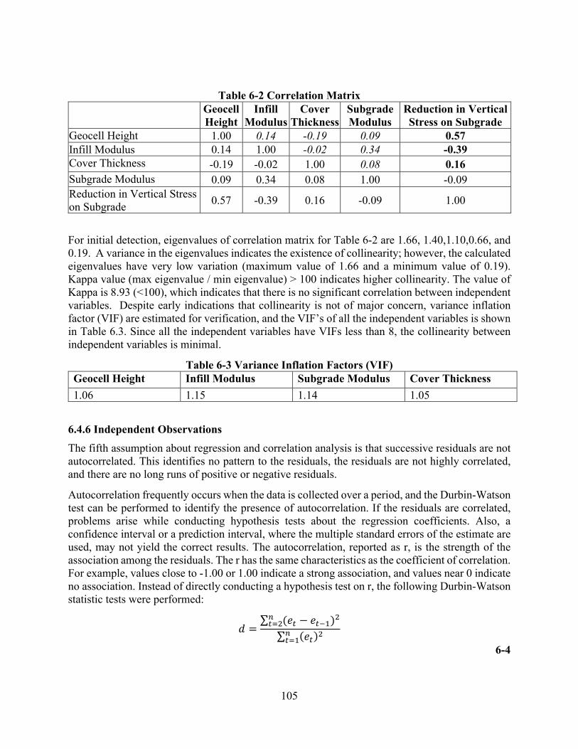
105

Table 6-2 Correlation Matrix Geocell

Height Infill

Modulus Cover

Thickness Subgrade Modulus

Reduction in Vertical Stress on Subgrade

Geocell Height 1.00 0.14 -0.19 0.09 0.57 Infill Modulus 0.14 1.00 -0.02 0.34 -0.39 Cover Thickness -0.19 -0.02 1.00 0.08 0.16 Subgrade Modulus 0.09 0.34 0.08 1.00 -0.09 Reduction in Vertical Stress on Subgrade 0.57 -0.39 0.16 -0.09 1.00

For initial detection, eigenvalues of correlation matrix for Table 6-2 are 1.66, 1.40,1.10,0.66, and 0.19. A variance in the eigenvalues indicates the existence of collinearity; however, the calculated eigenvalues have very low variation (maximum value of 1.66 and a minimum value of 0.19). Kappa value (max eigenvalue / min eigenvalue) > 100 indicates higher collinearity. The value of Kappa is 8.93 (<100), which indicates that there is no significant correlation between independent variables. Despite early indications that collinearity is not of major concern, variance inflation factor (VIF) are estimated for verification, and the VIF’s of all the independent variables is shown in Table 6.3. Since all the independent variables have VIFs less than 8, the collinearity between independent variables is minimal.

Table 6-3 Variance Inflation Factors (VIF) Geocell Height Infill Modulus Subgrade Modulus Cover Thickness 1.06 1.15 1.14 1.05

6.4.6 Independent Observations The fifth assumption about regression and correlation analysis is that successive residuals are not autocorrelated. This identifies no pattern to the residuals, the residuals are not highly correlated, and there are no long runs of positive or negative residuals.

Autocorrelation frequently occurs when the data is collected over a period, and the Durbin-Watson test can be performed to identify the presence of autocorrelation. If the residuals are correlated, problems arise while conducting hypothesis tests about the regression coefficients. Also, a confidence interval or a prediction interval, where the multiple standard errors of the estimate are used, may not yield the correct results. The autocorrelation, reported as r, is the strength of the association among the residuals. The r has the same characteristics as the coefficient of correlation. For example, values close to -1.00 or 1.00 indicate a strong association, and values near 0 indicate no association. Instead of directly conducting a hypothesis test on r, the following Durbin-Watson statistic tests were performed:

𝑢𝑢 =∑ (𝑒𝑒𝑣𝑣 − 𝑒𝑒𝑣𝑣−1)2𝑟𝑟𝑣𝑣=2∑ (𝑒𝑒𝑣𝑣)2𝑟𝑟𝑣𝑣=1

6-4

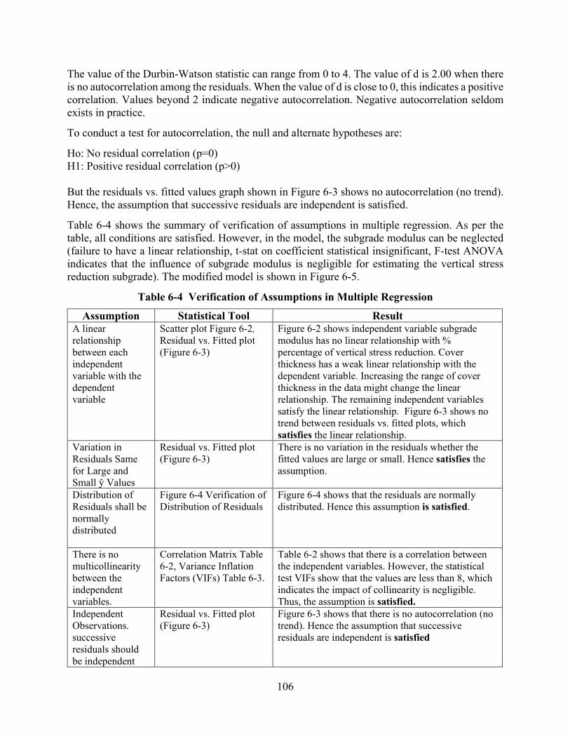
106

The value of the Durbin-Watson statistic can range from 0 to 4. The value of d is 2.00 when there is no autocorrelation among the residuals. When the value of d is close to 0, this indicates a positive correlation. Values beyond 2 indicate negative autocorrelation. Negative autocorrelation seldom exists in practice.

To conduct a test for autocorrelation, the null and alternate hypotheses are:

Ho: No residual correlation (p=0) H1: Positive residual correlation (p>0) But the residuals vs. fitted values graph shown in Figure 6-3 shows no autocorrelation (no trend). Hence, the assumption that successive residuals are independent is satisfied.

Table 6-4 shows the summary of verification of assumptions in multiple regression. As per the table, all conditions are satisfied. However, in the model, the subgrade modulus can be neglected (failure to have a linear relationship, t-stat on coefficient statistical insignificant, F-test ANOVA indicates that the influence of subgrade modulus is negligible for estimating the vertical stress reduction subgrade). The modified model is shown in Figure 6-5.

Table 6-4 Verification of Assumptions in Multiple Regression

Assumption Statistical Tool Result A linear relationship between each independent variable with the dependent variable

Scatter plot Figure 6-2, Residual vs. Fitted plot (Figure 6-3)

Figure 6-2 shows independent variable subgrade modulus has no linear relationship with % percentage of vertical stress reduction. Cover thickness has a weak linear relationship with the dependent variable. Increasing the range of cover thickness in the data might change the linear relationship. The remaining independent variables satisfy the linear relationship. Figure 6-3 shows no trend between residuals vs. fitted plots, which satisfies the linear relationship.

Variation in Residuals Same for Large and Small ŷ Values

Residual vs. Fitted plot (Figure 6-3)

There is no variation in the residuals whether the fitted values are large or small. Hence satisfies the assumption.

Distribution of Residuals shall be normally distributed

Figure 6-4 Verification of Distribution of Residuals

Figure 6-4 shows that the residuals are normally distributed. Hence this assumption is satisfied.

There is no multicollinearity between the independent variables.

Correlation Matrix Table 6-2, Variance Inflation Factors (VIFs) Table 6-3.

Table 6-2 shows that there is a correlation between the independent variables. However, the statistical test VIFs show that the values are less than 8, which indicates the impact of collinearity is negligible. Thus, the assumption is satisfied.

Independent Observations. successive residuals should be independent

Residual vs. Fitted plot (Figure 6-3)

Figure 6-3 shows that there is no autocorrelation (no trend). Hence the assumption that successive residuals are independent is satisfied

107

Figure 6-5 Summary of Reduced Model.

Multiple R-Square 0.622

Adjusted R-Square 0.601

P-value 4.69E-11

Residual Standard Error 5.084

Observations 59

dfSum of Squares

(SS)

Mean Square

(MS)F Significance

Geocell Height 1 1143.54 1143.54 44.24 0.000***

Infill Modulus 1 808.1 808.1 31.263 0.000***

Cover Thickness 1 262.91 262.91 10.204 0.002***


Coefficients Standard

Error t stat P-Value

Intercept -9.149 4.55 -2.011 0.049

Geocell Height 4.46 0.567 7.859 0.000***

Infill Modulus -0.514 0.0919 -5.601 0.000***

Cover Thickness 2.196 0.687 3.194 0.002**


Summary of Model Regression Statistics

Analysis of Variance (ANOVA)

Regression Coefficients

108

6.5 MODEL DEVELOPMENT USING CROSS-VALIDATION TECHNIQUES Statistically, the best course of action would be to use all the data for model building and statistical methods to get reasonable error estimates. However, when a model is developed using all data, one of the fundamental problems is “Overfitting.” Overfitting occurs when a model inappropriately picks up trends in the total data that do not generalize to a new data set. When this occurs, the model based on the initial data set doesn’t estimate the dependent variable. Even from a non-statistical perspective, users of the developed models emphasize the need for an untouched set of samples to evaluate performance. Although it is highly desirable to have a test set of data to verify the developed model, it is often difficult to get real-life data in the model development stage. One of the ways to alleviate the problem stated above (overfitting and lack of test data) is to use the cross-validation technique. Cross-validation maximizes the value of the available limited data and allows the identification of the model's accuracy with new data.

There are two types of cross-validation techniques 1) full cross-validation or leave-one-out validation method (LOOV) and 2) segment (KK-fold and Bootstrapping) cross-validation. A detailed discussion of each method is included in Appendix C.

1) Full cross-validation or leave-one-out validation method (LOOV) is done when sufficient data is unavailable to satisfy statistical requirements. With this technique, the same number of models as data size is developed. One data point (one set of independent variables) is removed in each iteration, and the model is developed with the remaining data set. The validity of the developed model is evaluated using the removed data set and estimating the dependent variable. This process is repeated for the remaining data set by eliminating one data set at a time. After each test, the model's accuracy is verified through a metric (such as coefficient of determination, root means square error, etc.). The model which performed better is considered as the final model. Figure 6-6 shows an example of how this validation technique is applied. The full cross-validation method is known to be one of the best validation tests. Although some researchers suggest that full cross-validation is not an ideal test because the tests are made each time but using the “same data.”

2) Segmented cross-validation method is a good validation test that is used when there is enough data. For this test, the data is segmented into samples of different sizes or percentages. The model is developed on one sample data and tested on the other. Multiple iterations can be performed by randomly picking the samples. The size of the segments could vary depending on the data size and user choice.

There are various approaches for performing segmented cross-validation. K-fold or KK-fold cross-validation (CV) is one such technique. First, the samples are randomly partitioned into kk sets (called folds) of roughly equal size in their basic KK-fold CV. Next, a model is fitted using all the samples of the first subset. Then, the prediction error of the fitted model is calculated using the held-out samples. Finally, the sample operation is repeated for each fold, and the model’s performance is calculated by averaging the error across all folds. This process can be repeated numerous times (iterations). Thus, many performance estimates can be done using KK-fold CV, unlike LOOV, where the number of tests will be fixed. The schematic of k-fold cross-validation is presented in Figure 6-7.

Another type of CV that is widely used is “BOOTSTRAPPING.” Bootstrapping takes a random sample with replacement. Some data is selected for testing the model, and the gap

109

created by moving testing data is replaced with the existing data. So, there are chances that each sample is used more than once in each test. This replacement helps to keep the size of model data constant. The process is repeated multiple times (50-75 times). This procedure yields low variance compared to LOOV and KK-fold CV. Figure 6-8 shows a simple example of how Bootstrapping works.

Figure 6-6 Example of Leave One Out Validation.

Figure 6-7 Example of KK-fold Segmented Cross-Validation.

Data 1 2 3 4 5 6 7 8 9 10

Model Test Data

Test 1 2 3 4 5 6 7 8 9 10 1

Test 2 1 3 4 5 6 7 8 9 10 2

Test 3 1 2 4 5 6 7 8 9 10 3

Test 4 1 2 3 5 6 7 8 9 10 4

Test 5 1 2 3 4 6 7 8 9 10 5

Test 6 1 2 3 4 5 7 8 9 10 6

Test 7 1 2 3 4 5 6 8 9 10 7

Test 8 1 2 3 4 5 6 7 9 10 8

Test 9 1 2 3 4 5 6 7 8 10 9

Test 10 1 2 3 4 5 6 7 8 9 10

Model Training Data

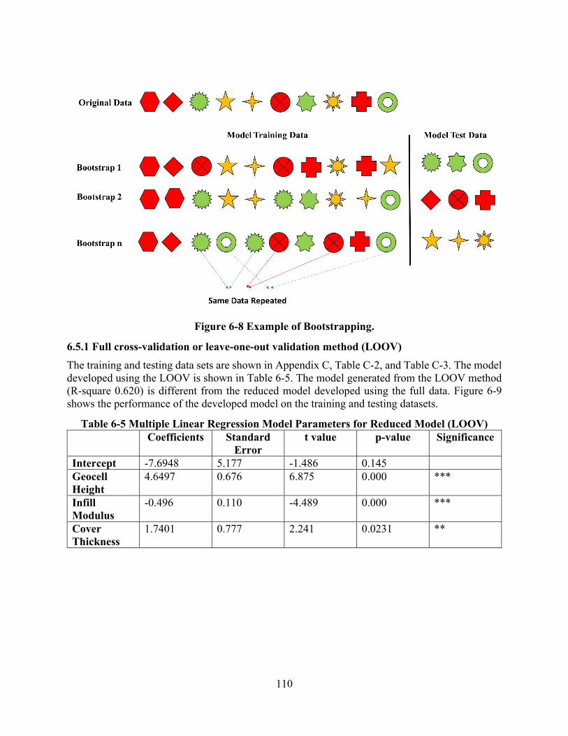
110

Figure 6-8 Example of Bootstrapping.

6.5.1 Full cross-validation or leave-one-out validation method (LOOV) The training and testing data sets are shown in Appendix C, Table C-2, and Table C-3. The model developed using the LOOV is shown in Table 6-5. The model generated from the LOOV method (R-square 0.620) is different from the reduced model developed using the full data. Figure 6-9 shows the performance of the developed model on the training and testing datasets.

Table 6-5 Multiple Linear Regression Model Parameters for Reduced Model (LOOV) Coefficients Standard

Error t value p-value Significance

Intercept -7.6948 5.177 -1.486 0.145 Geocell Height

4.6497 0.676 6.875 0.000 ***

Infill Modulus

-0.496 0.110 -4.489 0.000 ***

Cover Thickness

1.7401 0.777 2.241 0.0231 **

111

Figure 6-9 Predicted Data vs. Measured Data on Training and Testing Data Sets (Model Developed by LOOV Methodology).

6.5.2 KK-FOLD Cross-Validation In the KK-fold CV method, the training data is segmented into four groups. The model is developed on three segments and tested on the 4th one. This process is repeated 25 times. The training data set and testing data sets are shown in Appendix C, Table C-4, and Table C-5. The model developed using the KK-fold is shown in Table 6-6. The model generated from the KK-fold method (R-square 0.60) is different from the reduced model developed using the full data. Figure 6-10 shows the prediction capability of the developed model on the training and testing datasets.

Table 6-6 Multiple Linear Regression Model Parameters for Reduced Model (KK-FOLD) Coefficients Standard

Error t value p-value Significance


4.566 0.671 6.802 0.000 ***

Infill Modulus

-0.502 0.107 -4.705 0.000 ***

Cover Thickness

2.088 0.823 2.536 0.015 **

112

Figure 6-10 Predicted Data vs. Measured Data on Training and Testing Data Sets

(Model Developed by KK FOLD CV Methodology)

6.5.3 Bootstrapping Cross-Validation The training data set and testing data sets are shown in Appendix C, Table C-6, and Table C-7. The model developed using bootstrapping is shown in Table 6-7. The model generated from the bootstrapping method (R-square 0.570) is different from the reduced model developed using the full data. Figure 6-11 shows the prediction capability of the developed model on the training and testing datasets.

Table 6-7 Multiple Linear Regression Model Parameters for Reduced Model (Bootstrapping CV)

Coefficients Standard Error

t value p-value Significance


4.6424 0.6988 6.644 0.000 ***

Infill Modulus -0.5287 0.1101 -4.802 0.000 *** Cover Thickness

1.9325 0.8223 2.350 0.0238 **

113

Figure 6-11 Predicted Data vs. Measured Data on Training and Testing Data Sets (Model Developed by Bootstrapping Methodology)

6.6 SUMMARY OF MODELS Each cross-validation technique explained in Appendix C has advantages over another method. For this study, the three cross-validation techniques were employed, and the technique which generated the best model will be considered for validation. In all the CV techniques explained below, only 75% of data is used (training data set), and 25% (testing dataset) is kept for testing. Furthermore, only significant variables found in the previous analysis are considered in the model development, i.e., the influence of subgrade modulus is ignored in the model.

The performance of the developed model on testing data is statistically measured using the paired t-tests and Pearson correlation. Pearson’s correlation coefficient measures the strength of the linear relationship between two sets of variables. The paired t-test is a statistical analysis used to test a hypothesis about the mean population difference between paired (predicted vs. measured) observations. Pearson’s correlation coefficient measures the strength of the linear relationship between two sets of variables.

The details of the paired t-test and Pearson correlation are given in Appendix C (C.1).

The three cross-validation techniques generated different models. The most appropriate model among the three was selected based on their performance (analyzed using paired t-test and Pearson correlation) on the testing data. The summary of the models and statistical tests are presented in Table 6-8. For paired t-test, the following hypothesis is considered:

Null Hypothesis: 𝜇𝜇𝑟𝑟 = 0

Alternative Hypothesis: 𝜇𝜇𝑟𝑟 ≠ 0

where 𝜇𝜇𝑟𝑟 𝑖𝑖𝑠𝑠 the true difference in population values, and D is hypothesized value.

114

The results in Table 6.8 show that the models developed using CV’s supports (p-value > 0.05) the alternative hypothesis that the true difference in predicted vs. measured values of the testing data set are not equal to zero. It is to be noted that the D value in the hypothesis is considered zero (no difference between predicted and measured). Therefore, the results might change if an allowance is considered (D>0) in the hypothesis. Based on the 95% confidence levels, the model developed using LOOV-CV generated better results (less spread of predictions) and had a Pearson correlation of 0.82. Hence, the most appropriate model of this data is achieved through LOOV-CV, and the model is below:

%𝑅𝑅𝑒𝑒𝑢𝑢.𝐵𝐵𝑣𝑣𝑟𝑟𝑎𝑎𝐵𝐵𝐵𝐵 = −7.69 + 4.65 × 𝐺𝐺𝑒𝑒𝑙𝑙𝑐𝑐𝑒𝑒𝑙𝑙𝑙𝑙 𝐻𝐻𝑒𝑒𝑖𝑖𝑙𝑙ℎ𝑡𝑡 − 0.50 × 𝐼𝐼𝑡𝑡𝑜𝑜𝑖𝑖𝑙𝑙𝑙𝑙 𝑀𝑀𝑙𝑙𝑢𝑢𝑢𝑢𝑙𝑙𝑢𝑢𝑠𝑠+ 1.74 × 𝐶𝐶𝑙𝑙𝑣𝑣𝑒𝑒𝑟𝑟 𝑡𝑡ℎ𝑖𝑖𝑐𝑐𝑖𝑖𝑡𝑡𝑒𝑒𝑠𝑠𝑠𝑠

6-5

Hence the model shows that the geocell depth (height) is the major influencing factor, followed by the cover thickness and infill modulus. Remember that the model developed is based on the input ranges shown in Table 6-1. Since the cover thickness showed a vague linear relationship with the dependent variable additional testing is required to expand the range of cover thickness.

Table 6-8 Summary of Models Developed Using Cross-Validation Techniques

Typ

e of

M

odel

ing

Coefficients

R-S

quar

e

paired t-test *

Pear

son

corr

elat

ion

Inte

rcep

t

Geo

cell

Hei

ght

Infil

l Mod

ulus

Cov

er

Thi

ckne

ss

Sign

ifica

nce

(p-v

alue

)

Hyp

othe

sis

95% Confidence

Levels

Lower Upper

Without Cross Validation (CV) -9.15 4.46 -0.514 2.19 0.62 Na Na Na Na Na

LOOV - CV -7.69 4.65 -0.50 1.74 0.62 0.12 Alternative -0.66 4.81 0.82 KK-FOLD CV -8.98 4.56 -0.50 2.09 0.60 0.19 Alternative -0.90 3.89 0.85 Bootstrapping CV -8.85 4.64 -0.53 1.93 0.56 0.16 Alternative -3.87 0.75 0.88

*paired t-test performed by implementing the model developed using training data on the testingdata.

115

7. LIFE CYCLE COST ANALYSIS

This chapter provides information on the procedure of life cycle cost analysis of pavements. Life cycle cost analysis (LCCA) is a data-driven tool that provides a detailed account of the total costs of a project over its expected life. The purpose of performing LCCA is to provide necessary information to the decision-makers in selecting the best design. Therefore, LCCA needs to estimate the various costs in a pavement life cycle like initial construction, maintenance, user, etc., and discount the anticipated costs to present worth.

There are presently two methodologies being in use for LCCA.

1) Deterministic Approach to LCCA applies procedures and techniques without regard for the variability of the inputs. The primary disadvantage of this traditional approach is that it does not account for the variability associated with the LCCA input parameters.

2) Risk Analysis Approach (or Probabilistic Approach) characterizes uncertainty. The Interim Technical Bulletin on LCCA by the FHWA (J. W. Smith 1998) advocates this approach because it combines probability descriptions of analysis inputs with computer simulations to generate the entire range of outcomes and the likelihood of occurrence.

Currently, the deterministic approach is widely used in many states of the US. Still, the risk analysis approach is recommended by Rangaraju et al., 2008 based on research conducted to evaluate LCCA practices among state highway agencies for pavement selection. According to the study, 81 percent of agencies (17 out of 21) are still using a deterministic approach, 14 percent (3 out of 21) use a combination of deterministic and probabilistic approaches, and only one state is using a probabilistic approach. However, the risk analysis approach is not in practice due to complexity in considering the inputs required for analysis. Therefore, if the deterministic approach is used, a sensitivity analysis of LCCA results is recommended to accompany LCCA results.

7.1. DETERMINISTIC APPROACH The following are the procedural steps involved in conducting a life-cycle cost analysis (LCCA).

1. Establish alternative pavement design strategies for the analysis period 2. Determine performance periods and activity timing 3. Estimate agency costs 4. Estimate user costs 5. Develop expenditure stream diagrams 6. Compute Net Present Worth (NPW) or Equivalent Uniform Annual Costs

(EUAC) 7. Analyze results 8. Reevaluate design strategies

7.1.1 Establish alternative pavement design strategies for the analysis period 7.1.1.1 Analysis period It is the period used to evaluate the total investment required to build and maintain the pavement at an agreed-upon quality level. Although FHWA’s LCCA Policy Statement recommends an analysis period of at least 35 years for all pavement projects (including new or total reconstruction projects as well as rehabilitation, restoration, and resurfacing projects), an analysis period range of 30 to 40 years is also acceptable (J. W. Smith 1998). In Norway, an analysis period is reduced to

116

10 to 20 years because 40 years’ analysis is considered an extended period. According to Scheving (2011), an analysis of more than 20 years will not be suitable because of changes in the economic situation, traffic, and technology.

7.1.1.2 Alternate Pavement Designs Develop alternate designs or different maintenance preservation strategies that perform well during the desired analysis period. Alternate design implies that each design will perform equally, provide a similar level of service over the same performance period, and have similar life-cycle costs (Stephanos November 2008). 7.1.1.3 Determine performance periods and activity timing After selecting the analysis period and alternate pavement design, the next step is to determine the timing and performance of each maintenance activity. This step also involves determining the maintenance duration and how the ongoing traffic will be managed during maintenance.

7.1.1.4 Estimate Agency Costs Agency costs include all costs incurred directly by the agency over the life of a pavement. Although numerous activities are conducted during the construction, reconstruction, or major pavement rehabilitation, only those specific to a pavement alternative should be included in the agency costs (VDOT 2002). As the present study is focused on comparing various pavement designs, costs typical to all alternatives cancel out; these cost factors are generally noted and excluded from LCCA calculations (J. W. Smith 1998). Agency costs include initial preliminary engineering, contract administration, construction supervision, and construction costs, as well as future routine and preventive maintenance, resurfacing and rehabilitation cost, and the associated administrative cost. Preliminary engineering and other administrative costs were not contemplated in this study.

The first step in estimating the agency costs is to calculate the quantities and unit prices. The quantities were calculated based on the structural design and maintenance. The quantities were estimated typically for one mile of a highway. In this study, the unit prices are taken from the average low bid prices published by the Texas Department of Transportation (TxDOT) (“Average Low Bid Unit Prices” 2016).

At the end phase of the pavement life cycle, salvage value will be assigned to the pavement, resulting in a negative cost (savings). Salvage value is considered rather than demolition of pavement based on the practicability issues. Therefore, salvage value represents the value of an investment alternative at the end of the analysis period.

7.1.1.5 Estimate User Costs In the simplest sense, user costs are expenses incurred by the highway user over the project's life. User costs are an aggregation of three separate cost components: vehicle operating costs (VOC), user delay costs, and crash costs.

7.1.1.6 Develop Expenditure Stream Diagrams or Cash Flow Diagrams A cash flow diagram is a pictorial representation of a financial problem that portrays the timing of the cash flows and their character (either cost or saving). Thus, a cash flow diagram helps to comprehend the entire investment quickly. For example, figure 7-1 shows a typical cash flow diagram for a highway project.

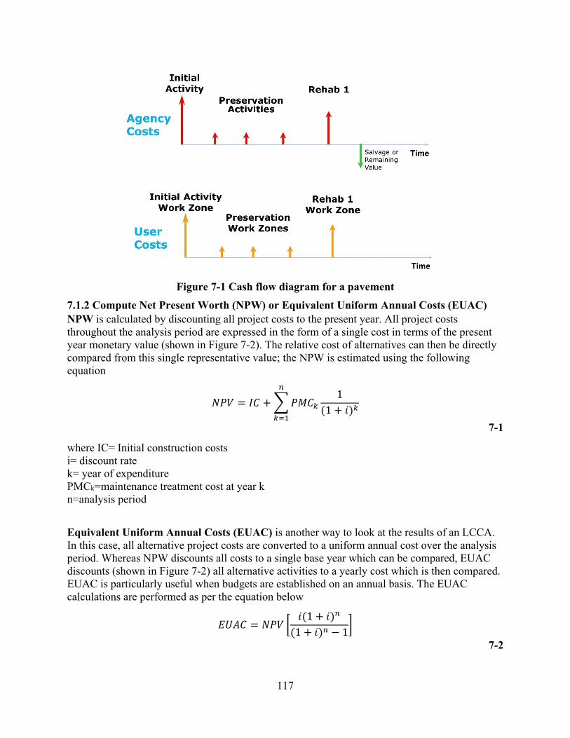
117

Figure 7-1 Cash flow diagram for a pavement 7.1.2 Compute Net Present Worth (NPW) or Equivalent Uniform Annual Costs (EUAC) NPW is calculated by discounting all project costs to the present year. All project costs throughout the analysis period are expressed in the form of a single cost in terms of the present year monetary value (shown in Figure 7-2). The relative cost of alternatives can then be directly compared from this single representative value; the NPW is estimated using the following equation

𝑁𝑁𝑃𝑃𝑉𝑉 = 𝐼𝐼𝐶𝐶 + �𝑃𝑃𝑀𝑀𝐶𝐶𝑘𝑘1

(1 + 𝑖𝑖)𝑘𝑘

𝑟𝑟

𝑘𝑘=17-1

where IC= Initial construction costs i= discount rate k= year of expenditure PMCk=maintenance treatment cost at year k n=analysis period

Equivalent Uniform Annual Costs (EUAC) is another way to look at the results of an LCCA. In this case, all alternative project costs are converted to a uniform annual cost over the analysis period. Whereas NPW discounts all costs to a single base year which can be compared, EUAC discounts (shown in Figure 7-2) all alternative activities to a yearly cost which is then compared. EUAC is particularly useful when budgets are established on an annual basis. The EUAC calculations are performed as per the equation below

𝐸𝐸𝐸𝐸𝐸𝐸𝐶𝐶 = 𝑁𝑁𝑃𝑃𝑉𝑉 �𝑖𝑖(1 + 𝑖𝑖)𝑟𝑟

(1 + 𝑖𝑖)𝑟𝑟 − 1�

7-2

118

Figure 7-2 Cash flow diagram for NPW and EUAC 7.1.3 Analyze Results The next step is to analyze the estimated costs. Since LCCA requires they guide more inputs and the accuracy of the analysis, more scrutiny on the inputs is needed. Sensitivity analysis is one such tool that assists decision-makers in understanding the likelihood of results happening. A sensitivity analysis is recommended as a minimum to study the impact of the individual inputs on LCCA results.

7.1.4 Reevaluate Design Strategies If required, the whole design strategies can be reevaluated, and new design strategies can be developed. Once the new designs are generated, the LCCA can be repeated, as explained in the previously mentioned steps.

In this study, instead of performing LCCA on geocell reinforced layered pavements, we used LCCA to estimate the unit cost for constructing the geocell reinforced layer.

The calculated unit cost will help to decide the viability of using geocell in pavement construction. This approach is chosen for two reasons:

1) The market price of geocell varies among manufacturers. However, none of themanufacturers disclosed the actual price of the delivered product, which restricted LCCA(due to lack of geocell layer price) calculations.

2) The requirement of geocell is primarily dependent on the quality of pavement layermaterials (subgrade, base) and traffic. Through the proposed approach, this studycalculated the possible unit price of the geocell layer for pavements at differentgeographical locations such as Dallas, Paris, Fort Worth, Atlanta, and San Antonio.

The following section describes how this study estimated the modulus of the geocell reinforced layer by using the outputs from both laboratory testing and finite element modeling. The subsequent steps describe the use of the estimated geocell layer modulus in pavement design and LCCA analysis.

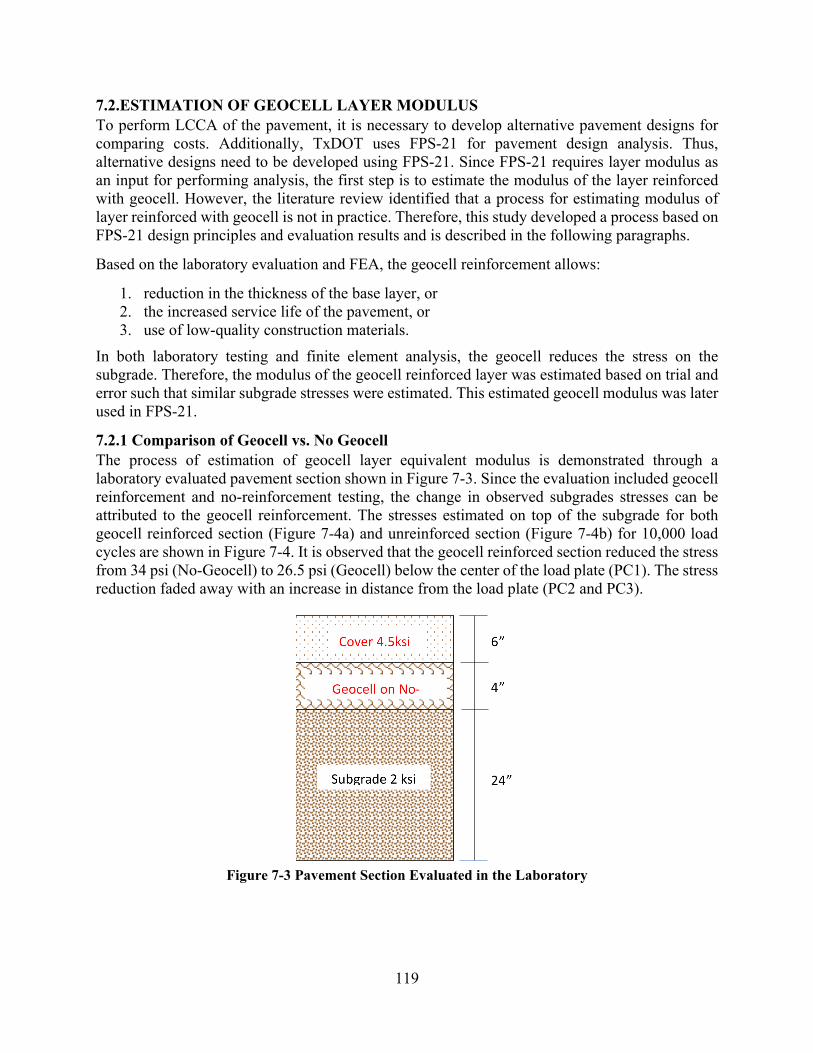
119

7.2.ESTIMATION OF GEOCELL LAYER MODULUS To perform LCCA of the pavement, it is necessary to develop alternative pavement designs for comparing costs. Additionally, TxDOT uses FPS-21 for pavement design analysis. Thus, alternative designs need to be developed using FPS-21. Since FPS-21 requires layer modulus as an input for performing analysis, the first step is to estimate the modulus of the layer reinforced with geocell. However, the literature review identified that a process for estimating modulus of layer reinforced with geocell is not in practice. Therefore, this study developed a process based on FPS-21 design principles and evaluation results and is described in the following paragraphs.

Based on the laboratory evaluation and FEA, the geocell reinforcement allows:

1. reduction in the thickness of the base layer, or 2. the increased service life of the pavement, or 3. use of low-quality construction materials.

In both laboratory testing and finite element analysis, the geocell reduces the stress on the subgrade. Therefore, the modulus of the geocell reinforced layer was estimated based on trial and error such that similar subgrade stresses were estimated. This estimated geocell modulus was later used in FPS-21.

7.2.1 Comparison of Geocell vs. No Geocell The process of estimation of geocell layer equivalent modulus is demonstrated through a laboratory evaluated pavement section shown in Figure 7-3. Since the evaluation included geocell reinforcement and no-reinforcement testing, the change in observed subgrades stresses can be attributed to the geocell reinforcement. The stresses estimated on top of the subgrade for both geocell reinforced section (Figure 7-4a) and unreinforced section (Figure 7-4b) for 10,000 load cycles are shown in Figure 7-4. It is observed that the geocell reinforced section reduced the stress from 34 psi (No-Geocell) to 26.5 psi (Geocell) below the center of the load plate (PC1). The stress reduction faded away with an increase in distance from the load plate (PC2 and PC3).

Figure 7-3 Pavement Section Evaluated in the Laboratory

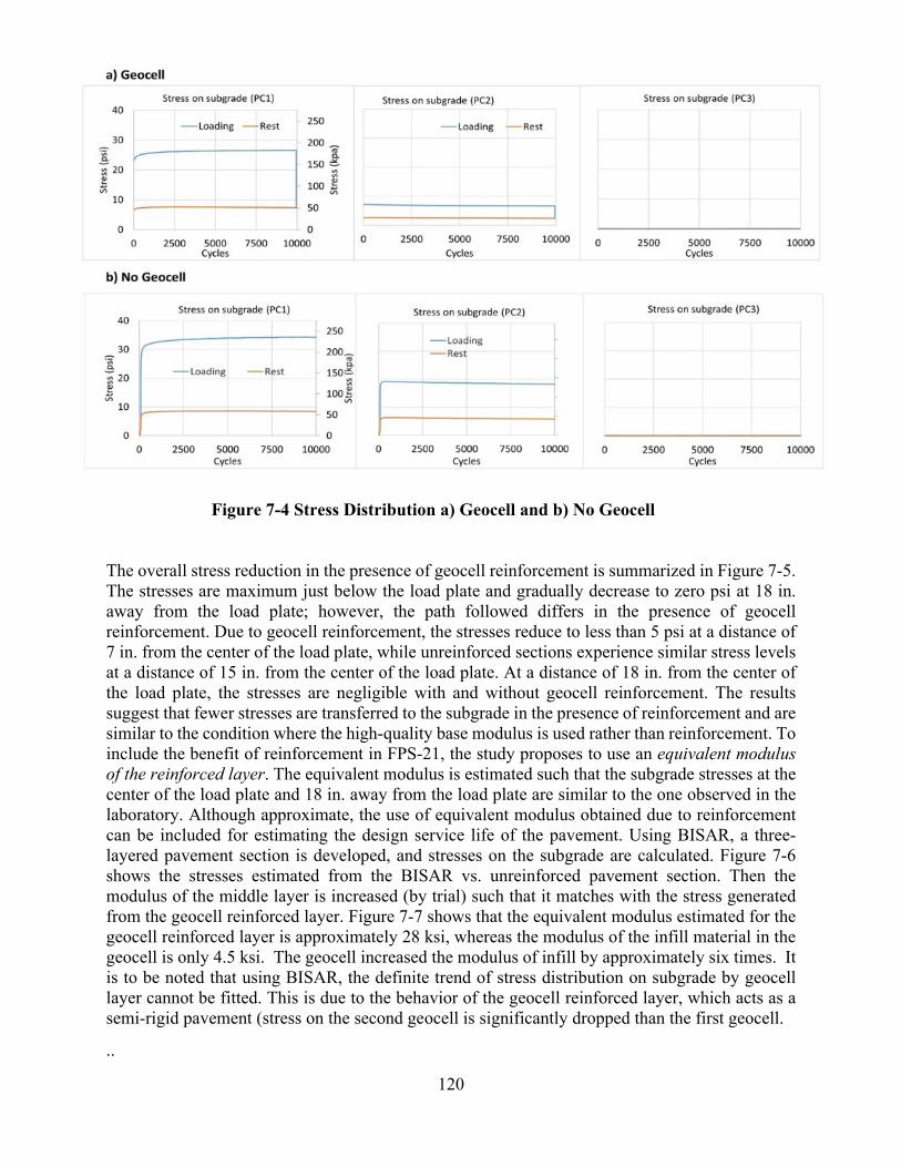
120

The overall stress reduction in the presence of geocell reinforcement is summarized in Figure 7-5. The stresses are maximum just below the load plate and gradually decrease to zero psi at 18 in. away from the load plate; however, the path followed differs in the presence of geocell reinforcement. Due to geocell reinforcement, the stresses reduce to less than 5 psi at a distance of 7 in. from the center of the load plate, while unreinforced sections experience similar stress levels at a distance of 15 in. from the center of the load plate. At a distance of 18 in. from the center of the load plate, the stresses are negligible with and without geocell reinforcement. The results suggest that fewer stresses are transferred to the subgrade in the presence of reinforcement and are similar to the condition where the high-quality base modulus is used rather than reinforcement. To include the benefit of reinforcement in FPS-21, the study proposes to use an equivalent modulus of the reinforced layer. The equivalent modulus is estimated such that the subgrade stresses at the center of the load plate and 18 in. away from the load plate are similar to the one observed in the laboratory. Although approximate, the use of equivalent modulus obtained due to reinforcement can be included for estimating the design service life of the pavement. Using BISAR, a three-layered pavement section is developed, and stresses on the subgrade are calculated. Figure 7-6 shows the stresses estimated from the BISAR vs. unreinforced pavement section. Then the modulus of the middle layer is increased (by trial) such that it matches with the stress generated from the geocell reinforced layer. Figure 7-7 shows that the equivalent modulus estimated for the geocell reinforced layer is approximately 28 ksi, whereas the modulus of the infill material in the geocell is only 4.5 ksi. The geocell increased the modulus of infill by approximately six times. It is to be noted that using BISAR, the definite trend of stress distribution on subgrade by geocell layer cannot be fitted. This is due to the behavior of the geocell reinforced layer, which acts as a semi-rigid pavement (stress on the second geocell is significantly dropped than the first geocell.

..

Figure 7-4 Stress Distribution a) Geocell and b) No Geocell

121

Figure 7-5 Benefit of Geocell in Reduction of Stress (Laboratory Results)

Figure 7-6 Comparison of unreinforced section with BISAR equivalent Section (Laboratory Results)

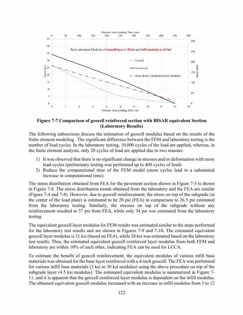
122

Figure 7-7 Comparison of geocell reinforced section with BISAR equivalent Section (Laboratory Results)

The following subsections discuss the estimation of geocell modulus based on the results of the finite element modeling. The significant difference between the FEM and laboratory testing is the number of load cycles. In the laboratory testing, 10,000 cycles of the load are applied, whereas, in the finite element analysis, only 20 cycles of load are applied due to two reasons:

1) It was observed that there is no significant change in stresses and/or deformation with moreload cycles (preliminary testing was performed up to 400 cycles of load).

2) Reduce the computational time of the FEM model (more cycles lead to a substantialincrease in computational time).

The stress distribution obtained from FEA for the pavement section shown in Figure 7-3 is shown in Figure 7-8. The stress distribution trends obtained from the laboratory and the FEA are similar (Figure 7-4 and 7-8). However, due to geocell reinforcement, the stress on top of the subgrade (at the center of the load plate) is estimated to be 28 psi (FEA) in comparison to 26.5 psi estimated from the laboratory testing. Similarly, the stresses on top of the subgrade without any reinforcement resulted in 37 psi from FEA, while only 34 psi was estimated from the laboratory testing.

The equivalent geocell layer modulus for FEM results was estimated similar to the steps performed for the laboratory test results and are shown in Figures 7-9 and 7-10. The estimated equivalent geocell layer modulus is 31 ksi (based on FEA), while 28 ksi was estimated based on the laboratory test results. Thus, the estimated equivalent geocell reinforced layer modulus from both FEM and laboratory are within 10% of each other, indicating FEA can be used for LCCA.

To estimate the benefit of geocell reinforcement, the equivalent modulus of various infill base materials was obtained for the base layer reinforced with a 4-inch geocell. The FEA was performed for various infill base materials (3 ksi to 30 ksi modulus) using the above procedure on top of the subgrade layer (4.5 ksi modulus). The estimated equivalent modulus is summarized in Figure 7-11, and it is apparent that the geocell reinforced layer modulus is dependent on the infill modulus. The obtained equivalent geocell modulus increased with an increase in infill modulus from 3 to 12

123

ksi; however, an increase in infill modulus reduced the effectiveness of geocell reinforcement. For instance, the infill modulus of 12 ksi provided an equivalent geocell modulus of 48 ksi, indicating a four times increase. In comparison, only 37.5 ksi equivalent geocell modulus was obtained for infill material with 30 ksi modulus. The analysis is consistent with published literature indicating that the effectiveness of geocell reinforcement reduced with an increase in the quality of infill material.

Figure 7-8 Stress Distribution a) Geocell and b) No Geocell

124

Figure 7-9 Benefit of Geocell in Reduction of Stress (FEM)

Figure 7-10 Equivalent Modulus Calculation (FEM)

125

Figure 7-11 Estimated Geocell Layer Modulus with Various Infills (4inch Geocell)

7.3. ESTIMATION OF COST OF GEOCELL REINFORCED LAYER Although the use of geocell has been documented, the cost of geocell and geocell installation has not been documented. Since one of the project's tasks was to calculate and perform LCCA, the cost calculations were performed to identify the installation cost of the geocell reinforced layer that will provide service life similar to that of the conventional base material. Also, this study made two assumptions for estimating the cost of the geocell reinforced layer:

1) The cost of the stabilized base is higher than the flexible base, and2) The cost of a higher modulus base is higher than the lower modulus base.

Thus, the viable cost of the geocell reinforced layer is back-calculated using LCCA. The cost estimation and viability of geocell reinforcement are documented through three pavement designs: a) Ellis county of Dallas district, b) Titus county of Atlanta district, and c) Ulvade county of SanAntonio district. For the pavement design, the geocell reinforced layer modulus is considered tobe 48 ksi, which assumes an infill modulus of 12 ksi (Figure 3.20). The respective districtsprovided the pavement designs, and geocell reinforcement was incorporated using FPS 21pavement design software. The unit prices for various districts are taken from Average Low BidUnit Prices from the Texas Department of Transportation. Since the prices for similar materialsvaried within the district, the cost of the geocell reinforced layer is estimated by including costvariability. The base material cost considered in this study is included in Table 7-1. Each basematerial's cost is considered a triangular probability distribution with minimum, mean, andmaximum values. The mean cost of the stabilized base is assumed to be $60 per cubic yard for allfour districts. Geocell reinforced layer cost is estimated using the mean values (deterministicLCCA) and the costs' variability (probabilistic LCCA).

126

Table 7-1 Cost of Base Materials Considered in this Study

District Costs Probability Distribution

Good Base (Base with modulus greater than 35 ksi)

Average Base (< 35 ksi, >20 ksi) Stabilized Base

Atlanta Triangular

(Minimum, Mean, Maximum)

$45, $50, $55 $35, $40, $45 $55, $60, $65 Paris $50, $57, $62 $45, $52, $56 $65, $75, $85

San Antonio $20, $30, $40 $12, $25, $35 $55, $60, $65 Dallas $38, $45, $56 $30, $40, $46 $55, $60, $65

For the probabilistic approach, the Monte Carlo Simulation (Latin Hypercube Sampling) was performed by varying the base prices of Table 7-1 and performing 5,000 simulations. The following sections show the estimated costs of a geocell reinforced layer providing similar service life for various districts. The following assumptions were made for LCCA analysis:

1. A discount rate of 4% is assumed for estimating net present worth.2. The salvage value of pavement is not considered because of a lack of data on the

reusability of geocell reinforced layers.3. The unit prices for the pavement layers need to be verified according to each county.

7.3.1 Design 1: FM 55 Ellis County of Dallas District The data for performing LCCA for FM 55 is shown in Table 7-2, including the design criteria, traffic, and construction data (from 0.14 Miles South of Nash Howard Road to US 77). Based on the data provided, three alternative pavement designs were developed (Figure 7-12) and evaluated for 40 years of service life. Alternative 1 is the district's typical pavement design, including a stabilized base (35 ksi) and a good quality base (40 ksi). The Alternative 2 pavement design is based on the lowest base quality (25 ksi) that can provide service life similar to Alternative 1. Finally, alternative 3 is the pavement designed with geocell reinforcement.

The designs Alternatives 2 and 3 were developed based on discussion with district personnel and FPS-21 constraints. Alternatives 1 and 2 have a subgrade of 200 in. while Alternative 3 has a subgrade of 196 in. Since the subgrade is of lower quality, the top of 4 in. of the subgrade is typically scarified and mixed with lime to stabilize the layer. As a result, construction equipment can move on top of the surface with minimal damage to the layer. Traditionally, the design doesn’t include stabilized subgrade layer because lime eventually washes away with rainwater. Thus, Alternative 3 evaluates a design where the top 4 in. of the subgrade is replaced with a geocell reinforced layer. Alternative 2 assumes that only locally available base material of mediocre quality is available, and the layer is not stabilized. In this situation, the thickness of the base layer and asphalt layer needs to be modified to meet the service life. In comparison, the total pavement thickness is minimal for Alternative 3, indicating that the base thickness can be reduced even with the inferior base material is used to infill geocell.

The cost estimates for three alternatives are summarized in Table 7-3. In terms of Alternatives 1 and 2, the cost of Alternative 2 is higher because of the increase in the HMA layer from 2 to 3 in. Overall, the cost of Alternative 1 turns out to be $601,593, while the cost is $697,319 for Alternative 2. Since the construction cost of the geocell reinforced layer is unavailable, the cost without the geocell layer is calculated, which is $423,769. Based on the difference between the

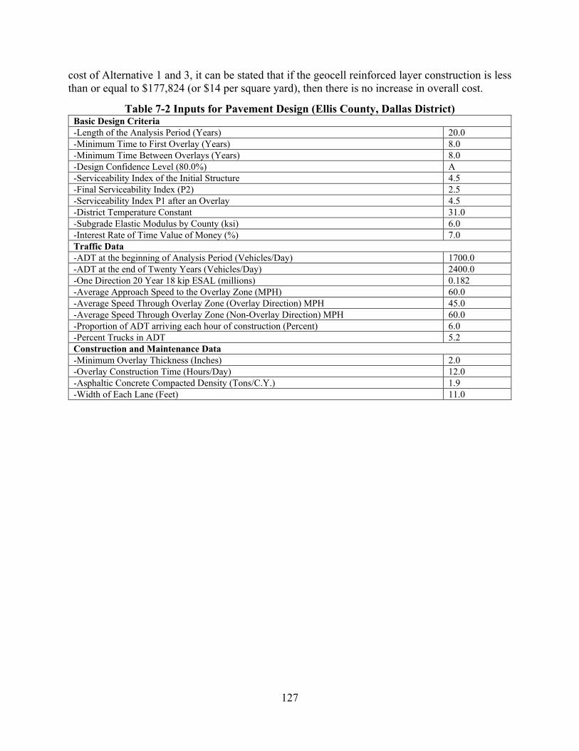
127

cost of Alternative 1 and 3, it can be stated that if the geocell reinforced layer construction is less than or equal to $177,824 (or $14 per square yard), then there is no increase in overall cost.

Table 7-2 Inputs for Pavement Design (Ellis County, Dallas District) Basic Design Criteria -Length of the Analysis Period (Years) 20.0 -Minimum Time to First Overlay (Years) 8.0 -Minimum Time Between Overlays (Years) 8.0 -Design Confidence Level (80.0%) A -Serviceability Index of the Initial Structure 4.5 -Final Serviceability Index (P2) 2.5 -Serviceability Index P1 after an Overlay 4.5 -District Temperature Constant 31.0 -Subgrade Elastic Modulus by County (ksi) 6.0 -Interest Rate of Time Value of Money (%) 7.0 Traffic Data -ADT at the beginning of Analysis Period (Vehicles/Day) 1700.0 -ADT at the end of Twenty Years (Vehicles/Day) 2400.0 -One Direction 20 Year 18 kip ESAL (millions) 0.182 -Average Approach Speed to the Overlay Zone (MPH) 60.0 -Average Speed Through Overlay Zone (Overlay Direction) MPH 45.0 -Average Speed Through Overlay Zone (Non-Overlay Direction) MPH 60.0 -Proportion of ADT arriving each hour of construction (Percent) 6.0 -Percent Trucks in ADT 5.2 Construction and Maintenance Data -Minimum Overlay Thickness (Inches) 2.0 -Overlay Construction Time (Hours/Day) 12.0 -Asphaltic Concrete Compacted Density (Tons/C.Y.) 1.9 -Width of Each Lane (Feet) 11.0

128

Figure 7-12 Alternative Designs Developed Using FPS 21 and Geocell Reinforced Layer (Ellis County, Dallas)

HMA 500 KSI 2"

HMA 500 KSI 2"

Alternative 1 Alternative 2 Alternative 3

10"

4"

196"

8"

10"

FLEXIBLE BASE 25 KSI

HMA 500 KSI 3"

SUBGRADE 6 KSI SUBGRADE 6 KSI SUBGRADE 6 KSI

CEMENT TREATED BASE 35 KSI


GEOCELL BASE 48 KSI


200"

20"

200"

129

Table 7-3 Cost Estimate for Geocell Reinforced Layer (Ellis County, Dallas District) Alternative 1 Actual Design

Description Units Unit Price

No of Lanes

Thickness (in)

Width (feet)

Length (miles)

Quantity (Cu.Yd.)

Total Cost

Hot Mix Asphalt (500 ksi) CY 115 2 2 11 1 717 $82,459 Flexible Base (40 ksi) CY 56 2 8 11 1 2868 $160,616 Cement Treated Base (35 ksi) CY 60 2 10 11 1 3585 $215,111 Subgrade (6 ksi) CY 2 2 200 11 1 71704 $143,407

Alternative 1 Cost $601,593

Alternative 2 Modified Design with Poor Base Material


No of Lanes

Thickness (in)

Width (feet)

Length (miles)

Quantity (Cu.Yd.)

Total Cost

Hot Mix Asphalt (500 ksi) CY 115 2 3 11 1 1076 $123,689 Flexible Base (20 ksi) CY 40 2 30 11 1 10756 $430,223 Subgrade (6 ksi) CY 2 2 200 11 1 71704 $143,408

Alternative 2 Cost $697,319

Alternative 3 With Geocell


No of Lanes

Thickness (in)

Width (feet)

Length (miles)

Quantity (Cu.Yd.)

Total Cost

Hot Mix Asphalt (500 ksi) CY 115 2 2 11 1 717 $82,459 Flexible Base (40 ksi) CY 56 2 10 11 1 3585 $200,771 Geocell Base CY ? 2 4 11 1 1434 ? Subgrade (4.5 ksi) CY 2 2 196 11 1 70270 $140,539

Alternative 3 Cost $423,769 Difference $177,824

Geocell Cost Per Square Yard $14

130

The cost of the geocell reinforced layer using the Monte Carlo Simulation is shown in Figure 7-13. The mean estimated cost based on 5,000 simulations is $14.33 with a standard deviation of $1.42. Thus, the minimum cost is $10.11, and the maximum cost is $18.86, and 90% of the time, the cost of the geocell layer is estimated to be between $11.92 and $16.69. Thus, the construction of the geocell reinforced layer is faster than the other base reinforcement techniques (cement or lime stabilized). However, these LCCA calculations are based on the assumption that there is no time difference between the alternatives.

Figure 7-13 Estimated Geocell Reinforced Layer Costs using Probabilistic LCCA (Ellis

County, Dallas). Similarly, the cost estimates were performed for Uvalde County of San Antonio District (Table 7-4 design data, Figure 7-14 alternative designs, and Table 7-5 cost estimates). In this design, the maintenance cost was also included in LCCA. This design requires maintenance (overlay) after 11 years of service. Hence, the Net Present Worth is calculated as discussed in Section 2 of this report. The optimal construction cost for a geocell reinforced layer is estimated to be $ 15 per square yard. The estimated cost can be interpreted as if the cost of the geocell layer is less than or equal to $15; then there is no cost increase due to the use of geocell. The cost of the geocell reinforced layer using the Monte Carlo Simulation is shown in Figure 7-15. The mean estimated cost based on 5,000 simulations is $15.01, with a standard deviation of $1.55. The minimum cost is $9.59, and the maximum cost is $20.08, and 90% of the time, the cost of the geocell layer is estimated to be between $12.45 and $17.57.

The cost estimate for Titus county of Atlanta District are included in Table 7-6 (design data), Figure 7-16 (alternative designs), and Table 7-7 (cost estimate). The unit cost for geocell is estimated at $ 12 per square yard. This design requires maintenance (overlay) after 14.7 years of service. Hence, the Net Present Worth is calculated as discussed in Section 2 of this report. A discount rate of 4% is considered in the net present worth estimation. The optimal construction cost for a geocell reinforced layer is estimated to be $ 12 per square yard. The estimated cost can be interpreted as if the cost of the geocell layer is less than or equal to $12. Then there is no cost increase due to the use of geocell. The cost of the geocell reinforced layer using the Monte Carlo Simulation is shown in Figure 7-17. The mean estimated cost based on 5,000 simulations is $12.46 with a standard deviation of $0.62. The minimum cost is $10.71, and the maximum cost is $14.17, and 90% of the time, the cost of the geocell layer is estimated to be between $11.43 and $13.49.

131

7.3.2 Design 1: US 83 Uvalde County, San Antonio District Table 7-4 Input Data for Pavement Design (Uvalde County, San Antonio District)

Basic Design Criteria Length of the Analysis Period (Years) 20.0 Minimum Time to First Overlay (Years) 8.0 Minimum Time Between Overlays (Years) 8.0 Design Confidence Level (80.0%) C Serviceability Index of the Initial Structure 4.5 Final Serviceability Index (P2) 2.5 Serviceability Index P1 after an Overlay 4.2 District Temperature Constant 31.0 Subgrade Elastic Modulus by County (ksi) 14.9 Interest Rate of Time Value of Money (%) 7.0 Traffic Data ADT at the beginning of Analysis Period (Vehicles/Day) 2800.0 ADT at the end of Twenty Years (Vehicles/Day) 3800.0 One Direction 20 Year 18 kip ESAL (millions) 2.672 Average Approach Speed to the Overlay Zone (MPH) 70.0 Average Speed Through Overlay Zone (Overlay Direction) MPH 65.0 Average Speed Through Overlay Zone (Non-Overlay Direction) MPH 70.0 Proportion of ADT arriving each hour of construction (Percent) 5.0 Percent Trucks in ADT 22.3 Construction and Maintenance Data Minimum Overlay Thickness (Inches) 2.0 Overlay Construction Time (Hours/Day) 10.0 Asphaltic Concrete Compacted Density (Tons/C.Y.) 1.9 Width of Each Lane (Feet) 12.0

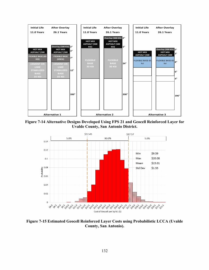
132

Figure 7-14 Alternative Designs Developed Using FPS 21 and Geocell Reinforced Layer for Uvalde County, San Antonio District.

Initial Life After Overlay Initial Life After Overlay Initial Life After Overlay

11.0 Years 26.1 Years 11.0 Years 26.1 Years 11.0 Years 26.1 Years

Overlay (500 KSI) 2"

Overlay (500 KSI) 2"Overlay (500 KSI) 2"

FLEXIBLE BASE

30 KSI24"

HOT MIX ASPHALT (500

KSI) 5"

FlEXIBLE BASE (65 KSI)



FlEXIBLE BASE (65KSI)

3"

7"FLEXIBLE

BASE 30 KSI


KSI)

CEMENT OR LIME

STABILIZED BASE

35 KSI

CEMENT OR LIME

STABILIZED BASE

35 KSI

12" FLEXIBLE BASE 30 KSI

FLEXIBLE BASE 65 ksi



FLEXIBLE BASE 65 ksi


6"

8"

3"

GEOCELL BASE 48 KSI

GEOCELL BASE 48 KSI

4"

Alternative 1 Alternative 2 Alternative 3

SUBGRADE 14.9 KSI

200" SUBGRADE 14.9KSI

SUBGRADE 14.9KSI

196"SUBGRADE

14.9 KSISUBGRADE

14.9 KSI200"

SUBGRADE 14.9 KSI

Figure 7-15 Estimated Geocell Reinforced Layer Costs using Probabilistic LCCA (Uvalde County, San Antonio).

133

Table 7-5 Cost Estimate of Geocell-Reinforced Layer (Uvalde County, San Antonio District) Alternative 1 Actual Design Initial Construction


No of Lanes

Thickness (in)

Width (feet)

Length (miles)

Quantity (Cu.Yd.)

Total Cost

Dense Graded HMA (500 ksi) CY 115 2 3 12 1 1173 $134,933 Flexible Base (65 ksi) CY 30 2 7 12 1 2738 $82,133 Lime (Cement) Stabilized (35 ksi) CY 60 2 12 12 1 4693 $281,600 Subgrade (14.9 ksi) CY 2 2 200 12 1 78222 $156,444 Maintenance (11 Years)

Overlay CY 115 2 2.5 12 1 978 $112,444 Net Present Worth $728,152



No of Lanes

Thickness (in)

Width (feet)

Length (miles)

Quantity (Cu.Yd.)

Total Cost

Dense Graded HMA (500 ksi) CY 115 2 5 12 1 1956 $224,889 Flexible Base (30 ksi) CY 25 2 24 12 1 9387 $234,666 Subgrade (14.9 ksi) CY 2 2 200 12 1 78222 $156,444 Maintenance (11 Years)



No of Lanes

Thickness (in)

Width (feet)

Length (miles)

Quantity (Cu.Yd.)

Total Cost

Dense Graded HMA (500 ksi) CY 115 2 3 12 1 1173 $134,933 Flexible Base (65 ksi) CY 30 2 8 12 1 3129 $93,867 Flexible Base (30 ksi) CY 25 2 6 12 1 2347 $58,667 Geocell CY ? 2 4 12 1 1564 ? Subgrade (14.9 ksi) CY 2 2 200 12 1 78222 $156,444 Maintenance (11 Years)


Difference Compared with Alternative 1 $211,200

Geocell Cost Per

Square Yard $15

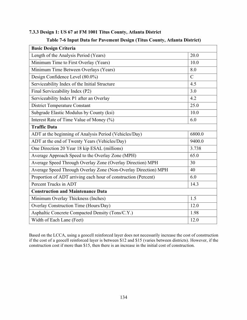
134

7.3.3 Design 1: US 67 at FM 1001 Titus County, Atlanta District Table 7-6 Input Data for Pavement Design (Titus County, Atlanta District)

Basic Design Criteria Length of the Analysis Period (Years) 20.0 Minimum Time to First Overlay (Years) 10.0 Minimum Time Between Overlays (Years) 8.0 Design Confidence Level (80.0%) C Serviceability Index of the Initial Structure 4.5 Final Serviceability Index (P2) 3.0 Serviceability Index P1 after an Overlay 4.2 District Temperature Constant 25.0 Subgrade Elastic Modulus by County (ksi) 10.0 Interest Rate of Time Value of Money (%) 6.0 Traffic Data ADT at the beginning of Analysis Period (Vehicles/Day) 6800.0 ADT at the end of Twenty Years (Vehicles/Day) 9400.0 One Direction 20 Year 18 kip ESAL (millions) 3.738 Average Approach Speed to the Overlay Zone (MPH) 65.0 Average Speed Through Overlay Zone (Overlay Direction) MPH 30 Average Speed Through Overlay Zone (Non-Overlay Direction) MPH 40 Proportion of ADT arriving each hour of construction (Percent) 6.0 Percent Trucks in ADT 14.3 Construction and Maintenance Data Minimum Overlay Thickness (Inches) 1.5 Overlay Construction Time (Hours/Day) 12.0 Asphaltic Concrete Compacted Density (Tons/C.Y.) 1.98 Width of Each Lane (Feet) 12.0

Based on the LCCA, using a geocell reinforced layer does not necessarily increase the cost of construction if the cost of a geocell reinforced layer is between $12 and $15 (varies between districts). However, if the construction cost if more than $15, then there is an increase in the initial cost of construction.

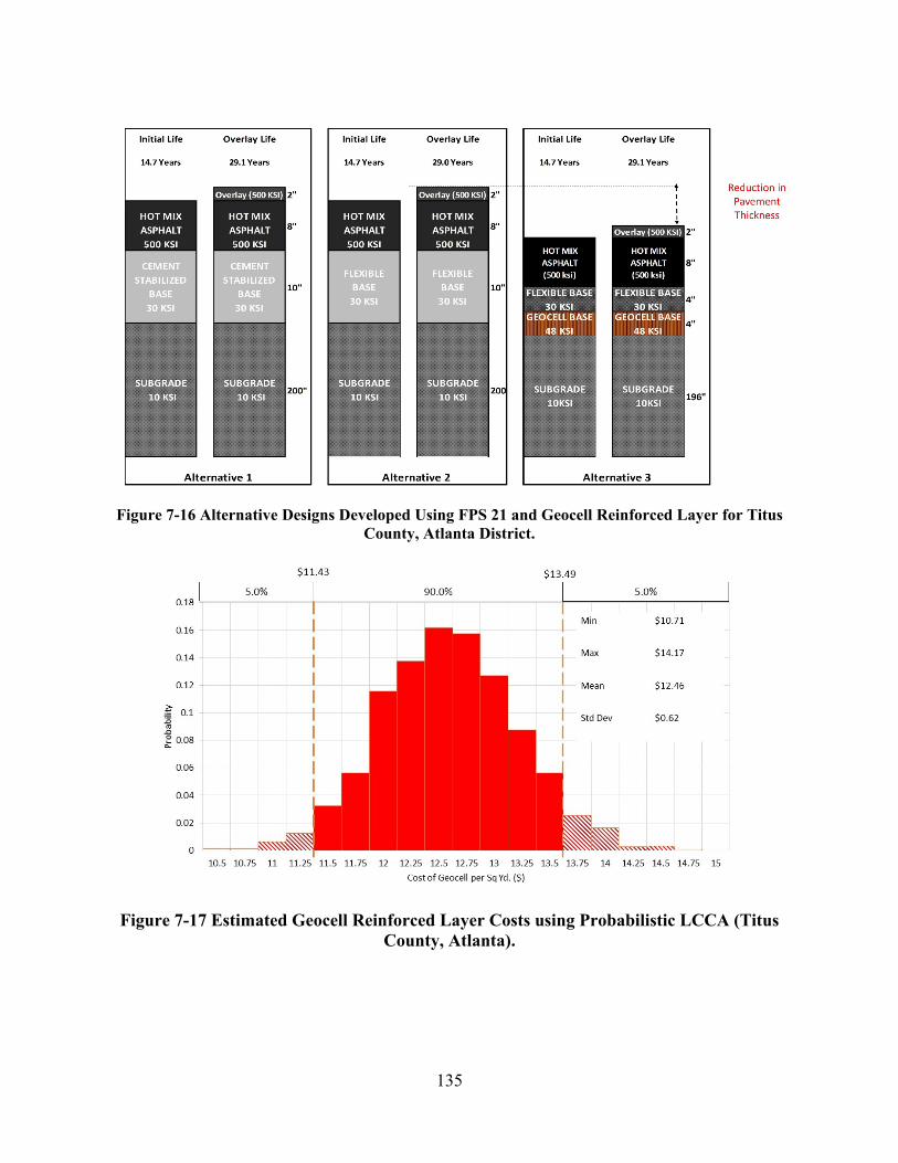
135

Figure 7-16 Alternative Designs Developed Using FPS 21 and Geocell Reinforced Layer for Titus County, Atlanta District.

Figure 7-17 Estimated Geocell Reinforced Layer Costs using Probabilistic LCCA (Titus County, Atlanta).

136

Table 7-7 Cost Estimate of Geocell-Reinforced Layer (Titus County, Atlanta District) Alternative 1 Actual Design


No of Lanes

Thickness (in.)

Width (feet)

Length (miles) Quantity (Cu.Yd.) Total Cost

Dense Graded HMA (500 ksi) CY 115 4 8 12 1 6258 $719,644 Cement Stabilized Subgrade (30 ksi) CY 60 4 10 12 1 7822 $469,333 Subgrade (10 ksi) CY 2 4 200 12 1 156444 $312,889 Maintenance (14.7 Years)

Overlay CY 115 4 2 12 1 1564 $179,911 Alternative 1 Cost $1,602,946



No of Lanes

Thickness (in.)

Width (feet)


Dense Graded HMA (500 ksi) CY 115 4 8 12 1 6258 $719,644 Flexible Base (30 ksi) CY 40 4 10 12 1 7822 $312,889 Subgrade (10 ksi) CY 2 4 200 12 1 156444 $312,889 Maintenance (14.7 Years) Overlay (500 ksi) CY 115 4 2 12 1 1564 $179,911

Alternative 2 Cost $1,446,501 Alternative 3 Modified Design with Geocell Layer


No of Lanes

Thickness (in.)

Width (feet)


Dense Graded HMA (500 ksi) CY 115 4 8 12 1 6258 $719,644 Flexible Base (30 ksi) CY 40 4 4 12 1 3129 $125,155 Geocell CY ? 4 4 12 1 3129 ? Subgrade (14.9 ksi) CY 2 4 196 12 1 153315 $306,631 Maintenance (14.7 Years)

Overlay CY 115 4 2 12 1 1564 $179,911 Alternative 3 Cost $1,252,510

Difference Compared with Alternative 1 $350,435 Geocell Cost Per

Square Yard $12

137

8. CLOSURE

8.1 SUMMARY Cellular Confinement Systems, popularly known as “Geocell,” are durable, lightweight, three-dimensional fabricated systems that are expandable on‐site to form a honeycomb‐like structure. Geocell filled with infill material and compacted to form a rigid to the semi‐rigid layer. The height of the geocell and the size of each cellular unit vary between manufacturers. Some geocell surface has been textured to increase soil‐geocell wall friction. In this study, the mechanism for improved bearing capacity and benefits derived from geocell were evaluated. Also, the influence of in-fill material quality on the performance of geocell has been evaluated, which is a critical issue when only lower/marginal quality material is available. Since geocell provides lateral reinforcement, the possibility of reducing the layer thickness to achieve similar performance levels to the one expected from the thicker base and sub-base systems was also evaluated. The economic feasibility of geocell use in pavements is also evaluated using LCCA. This study also provides a guideline for practitioners in selecting materials, design, construction, and safety of pavements with geocell cell layers. Finally, the conclusion is drawn, and the recommendation of this study is explained in the following sections.

8.2 CONCLUSION I. The following conclusions can be drawn from FEA:

1. Influence of Base Modulus a. The geocell reinforced layer reduced the stresses up to 20% six inches away from

the center of the loading plate and up to 50% nine inches away from the center of the loading plate compared with no geocell condition (unreinforced layer).

b. Similar trends were observed in the vertical strains on the subgrade. c. The hoop strain on the loaded geocell increased with a lower base modulus.

However, a significant strain reduction is observed in the next geocell and minimal strain on the third. Overall, the geocell was more efficient with lower modulus base materials.

2. Influence of Cover Layer Thickness: a. The stress (below loading plate) magnitude reduced significantly with a cover

thickness of 3 in. or higher. b. The hoop strain on the loaded geocell decreased with an increase in cover thickness.

Similar to the base modulus, the strain reduced significantly reduced in adjacent geocell.

c. The benefit of geocell diminished with a stiffer base cover of more than 4 inches. 3. Influence of Geocell-Reinforced Layer Thickness:

Since the thickness of the geocell reinforce layer depended on the height of the geocell, the following conclusions are based on geocell height: a. The three-inch geocell reinforced layer reduced the stresses up to 10-30% at six

inches away from the center of the loading plate and up to 15-60% at nine inches away from the center of the loading plate compared with no geocell layer.

b. The four-inch geocell reinforced layer reduced the stresses up to 10-25% at six inches away from the center of the loading plate and up to 0-30% at nine inches away from the center of the loading plate compared with no geocell layer.

138

c. The six-inch geocell reinforced layer reduced the stresses up to 0-25% at six inches away from the center of the loading plate and up to 0-30% at nine inches away from the center of the loading plate.

d. Comparing the three geocell, the geocell 3" performance is inferior to other geocell heights as it only reduced stresses up to 10% at 6" from the loading plate and 20% at 9" from the loading plate, whereas geocell 4" and 6" reduced the stresses around 20% at 6" and 40-50% at 9" from loading plate.

e. Geocell 3" has minimal influence in the presence of weak subgrade material. 4. Influence of Subgrade Modulus:

a. It is observed that geocell of 3 in. height has no significant influence on reducing stresses at the top of subgrade in the presence of lower quality subgrade (4.5 and 2 ksi).

b. The hoop strains on the geocell were minimally influenced by a change in subgrade modulus (4.5 ksi and 2.0 ksi).

c. The vertical strains and deformation for the 2.0 ksi subgrade (for all geocell) are higher than the 4.5 ksi subgrade

The FEA results indicate that 4” and 6” geocell heights will be more effective than 3” geocell. Although the geocell reinforcement increases the modulus of a reinforced layer, the increase in infill modulus beyond 12 ksi is not as pronounced compared to the infill modulus of 12 ksi or lower.

II. The following conclusion can be drawn from the Laboratory Evaluation: 1. Vertical Deformation: The magnitude of deformation was similar regardless of reinforced

and unreinforced base layers. 2. Vertical stress distribution on subgrade: The stress magnitude and pattern estimated from

the laboratory tests is similar to that obtained from FEA. 3. The vertical strain on geocell: the strain on geocell increased from 90 to 115 microstrains

by the end of 10,000 cycles indicating that the geocell is barely compressed in the vertical direction.

4. Geocell Hoop Strains: The geocell below the loading is expanding and transferring the load in the lateral direction (to the adjacent), and beyond that, the load distribution is almost negligible.

The FEM and laboratory test results showed similar trends. A maximum difference of 10% (vertical stress on top of the subgrade) was observed between them, indicating that FEM analysis can be performed for any new material selected for analysis.

III. The laboratory results indicated similar performance for geocell obtained from two sources.

IV. Summary of models used for Cross-validation Techniques is shown in the figure below:

V. The performed LCCA resulted in the following: a. Suppose the geocell reinforced layer cost is between $12 and $15 (depending on

District) per square yard. In that case, the initial construction cost will be lower

139

while providing a similar service life to the conventional design due to a reduced base layer thickness.

8.3 RECOMMENDATION The recommendation of this study are as follows:

1. This study recommends using geocell, especially in the weak quality base material (modulus of 12 ksi or less).

2. Cover thickness (layer over geocell) and quality of cover material; geocell layer thickness; infill material (in geocell) modulus; and subgrade modulus are four factors that influence the performance of geocell reinforced pavements. Therefore, this study recommends:

a. A minimum cover thickness of 4 in. is recommended. b. A minimum of 4” geocell height should be used to optimize the benefits provided

by geocell reinforcement. c. A cover thickness of 6” is recommended to maximize performance.

3. A site has been instrumented in Paris District, and future performance data will be collected to evaluate long-term performance.

4. Two to four sites should be constructed and monitored before routine use of geocell can be recommended.

5. Since the top four inches of the subgrade is scarified and stabilized with lime in districts with the weak subgrade, the geocell can be placed on top of the scarified surface and infilled with the recovered material will reduce the thickness of the base layer or required quality of base layer and will reduce the construction cost.

140

9. REFERENCES

1. AASHTO (1993), “AASHTO Guide for Design of Pavement Structures,” AASHTO, Washington, D.C.

2. Allison, P. D. D. (1999). Multiple regression: A primer. Thousand Oaks, CA: SAGE Publications.

3. Al-Qadi, I. L., and Hughes, J. J. (2000). "Field evaluation of geocell use in flexible pavements." Transportation Research Record: Journal of Transportation Research Board, 1709, 26-35.

15th,4. “Average Low Bid Unit Prices.” 2016. Accessed December 2016. http://www.txdot.gov/business/letting-bids/average-low-bid-unit-prices.html.

5. Bathurst, R. J., and Knight, M. A. (1998). “Analysis of geocell reinforced-soil covers over large span conduits.” Computers and Geotechnics, 22(3), 205–219.

6. Bortz, B., and Hossain, M. (2015). Accelerated pavement testing of low-volume paved Roads with geocell reinforcement. Final Report FHWA-KS-14-14, Manhattan, KS.

7. Emerslebn, A. and Meyer, N. (2008). “The use of geocells in road constructions over soft soil: vertical stress and falling weight deflectometer measurements.” EuroGeo4 paper number 132, 8 pgs.

8. EN ISO 13426-1 (2003). “Geotextiles and geotextile-related products- strength of internal structural junctions, Part 1: Geocells.” 13 pgs.

9. Esbensen, K., Guyot, D., Westad, F., & Houmoller, L. P. (1994). Multivariate data analysis: in practice: an introduction to multivariate data analysis and experimental design. Oslo, Norway: CAMO.

10. Evans, M. D. (1994). Geocell mattress effects on embankment settlements. Vertical and Horizontal Deformations of Foundations and Embankments, ASCE.

11. Feicheng Sanjie Engineering Materials Co., Ltd., China. “Geocell for road construction specification.” Retrieved April 18, 2011, from http://www.tasanjie.com/english/cp-15.htm.

12. Han, J., Pokharel, S.K., Yang, X., Manandhar, C., Leshchinsky, D., Halahmi, I., and Parsons, R.L. (2011). “Performance of geocell-reinforced RAP bases over weak subgrade under full-scale moving wheel loads.” ASCE Journal of Materials in Civil Engineering accepted.

13. Han, J., Yang, X., Leshchinsky, D., and Parsons, R. (2008). “Behavior of geocell-reinforced sand under a vertical load.” Transportation Research Record: Journal of the Transportation Research Board, 2045, 95–101.

14. Haufe, A., Schweizerhof, K., and DuBois, P. (2013). “Properties and Limits: Review of Shell Element Formulations.” LS-DYNA Developer Forum 2013, DYNAmore GmbH, Filderstadt, Germany.

15. Hegde, A., and Sitharam, T. G. (2014). “Joint strength and wall deformation characteristics of a single-cell geocell subjected to uniaxial compression.” International Journal of Geomechanics, 4014080.

16. Henry, K. S., Olson, J. P., Farrington, S. P., and Lens, J. (2005). "Improved Performance of Unpaved Roads During Spring Thaw." USACE ERDC/CRREL TR-05-1, Engineer Research and Development Center, Cold Region Research and Engineering Laboratory, Hanover, NH.

141

http://www.txdot.gov/business/letting-bids/average-low-bid-unit-prices.html

http://www.tasanjie.com/english/cp-15.htm

17. James Walls, and Michael R Smith. 1998. “Life Cycle Cost Analysis in Pavement Design- Interim Technical Bulletin.” FHWA-SA-98-079. Federal Highway Administration.

18. Klisiński, M. (1985). “Degradation and Plastic Deformation of Concrete.” Polish Academy of Sciences, Institute of Fundamental Technology Research (IFTR) Report 38.

19. Latha, G. M., Dash, S. K., and Rajagopal, K. (2009). “Numerical Simulation of the Behavior of Geocell-Reinforced Sand in Foundations.” American Society of Civil Engineers.

20. Latha, G. M., and Somwanshi, A. (2009). “Effect of reinforcement form on the bearing capacity of square footings on sand.” Geotextiles and Geomembranes, 27(6), 409–422.

21. Lewis, B. A. (2004). Manual for LS-DYNA Soil Material Model 147. FHWA-HRT-04-095, McLean, VA.

22. Long, S. J., & Freese, J. (2006). Regression models for categorical dependent variables using Stata (2nd ed.)

23. LSTC. (2016). LS-DYNA Theory Manual. Livermore Software Technology Corporation, Livermore, CA.

24. Mehdipour, I., Ghazavi, M., and Moayed, R. Z. (2013). “Numerical study on stability analysis of geocell reinforced slopes by considering the bending effect.” Geotextiles and Geomembranes, 37, 23–34.

25. Mengelt, M. J., Edil, T. B., and Benson, C. H. (2000). "Reinforcement of Flexible Pavements Using Geocells." Geo Engineering Report No. 00-04, University of Wisconsin-Madison, Madison, WN.

26. Mengelt, M.J., Edil, T.B., and Benson, C.H. (2006). “Resilient modulus and plastic deformation of soil confined in a geocell.” Geosynthetic International, 13 (5), 195-205.

27. Mhaiskar, S.Y. and Mandal, J.N. (1992a). “Comparison of geocell and horizontal inclusion for paved road structure.” Earth Reinforcement Practice, Ochiai, Hayashi, and Otani. Balkema, Rotterdam.

28. Mhaiskar, S.Y. and Mandal, J.N. (1992b). “Subgrade stabilization using geocells.” ASCE Geotechnical Special Publication, 2 (30), 1092-1103.

29. Mhaiskar, S. Y., and Mandal, J. N. (1994). "Three-dimensional geocell structure: performance under repetitive loads." 5th International Conference on Geotextiles, Geomembranes, and Related Products, Singapore, 155-158.

30. Mhaiskar, S. Y., and Mandal, J. N. (1996). “Investigations on soft clay subgrade strengthening using geocells.” Construction and Building Materials, 10(4), 281–286.

31. Neher, H. P., and Lachler, A., “Numerical modeling of a diaphragm wall production process in Rotterdam compared to monitoring data,” 6th European Conf. on Numerical Methods in Geotechnical Eng., Graz, Austria, pp. 417-22, 2006.

32. Pokharel, S.K., Han, J., Leshchinsky, D., Parsons, R.L., and Halahmi, I. (2009a). “Experimental evaluation of influence factors for single geocell-reinforced sand.” Transportation Research Board 88th annual meeting, January 11-15, 2009, Washington, DC.

33. Pokharel, S.K., Han, J., Leshchinsky, D., Parsons, R.L., and Halahmi, I. (2009b). “Behavior of geocell-reinforced granular bases under static and repeated loads.” International Foundation Congress & Equipment Expo 2009, March 15-19, 2009, Orlando, Florida.

142

34. Pokharel, S.K., Han, J., Parsons, R.L., Qian, Y., Leshchinsky, D., and Halahmi, I. (2009c). “Experimental study on bearing capacity of geocell-reinforced bases.” 8th International Conference on Bearing Capacity of Roads, Railways and Airfields, June 29 - July 2, 2009, Champaign, Illinois.

35. Pokharel, S.K., Han, J., Leshchinsky, D., Parsons, R.L., and Halahmi, I. (2010). “Investigation of factors influencing behavior of single geocell-reinforced bases under static loading.” Journal of Geotextile and Geomembrane, 28 (6), 570-578.

36. Pokharel, S.K. (2010). Experimental Study on Geocell-Reinforced Bases under Static and Dynamic Loadings. Ph.D. dissertation, CEAE Department, the University of Kansas

37. Pokharel, S.K., Han, J., Manandhar, C., Yang, X.M., Leshchinsky, D., Halahmi, I., and Parsons, R.L. (2011). “Accelerated pavement testing of geocell-reinforced unpaved roads over weak subgrade.” Journal of the Transportation Research Board, No. 2204, Low-Volume Roads, Vol. 2, Proceedings of the 10th International Conference on Low-Volume Roads, July 24–27, Lake Buena Vista, Florida, USA, 67-75.

38. PRS Mediterranean Ltd., Israel. Stabilizing an unstable world, Neoloy based nanoweb, Paving the way for tomorrow’s roads. Retrieved on September 20, 2011, from http://www.prs-med.com/.

39. Presto Geosystems, USA. Retrieved on August 11, 2011, from http://www.prestogeo.com/. 40. Presto Geosystems (2007). “Geoweb load support system, Technical overview,” 19 pgs. 41. Rangaraju, Prasada Rao, Serji N. Amirkhanian, Zeynep Guven, and South Carolina. 2008.

“Life Cycle Cost Analysis for Pavement-Type Selection.” South Carolina Department of Transportation. http://www.clemson.edu/t3s/scdot/pdf/projects/spr656final.pdf.

42. Russel Lenz.W. 2011. “Pavement Design Guide.” Pavement Design Guide. Texas Department of Transportation.

43. Reid, J. D., Coon, B. A., Lewis, B. A., Sutherland, S. H., and Murray, Y. D. (2004). Evaluation of LS-DYNA Soil Material Model 147. FHWA-HRT-04-094.

44. Saleh, M., and Edwards, L. (2011). “Application of a Soil Model in the Numerical Analysis of Landmine Interaction with Protective Structures.” Ballistics 2011: 26th International Symposium, E. Baker and D. Templeton, eds., DEStech Publications, Inc., Miami, FL, 256– 275.

45. Schumacher, M., Holländer, N., & Sauerbrei, W. (1997). Resampling and cross-validation techniques: a tool to reduce bias caused by model building? Statistics in Medicine, 16(24), 2813-2827.

46. Sharma, M., Inti, S., Tirado, C., & Tandon, V. (2016). Evaluating the Benefits of Geocell Reinforcement of the Base Course in Flexible Pavement Structures Using 3-D Finite Element Modeling. In International Conference on Transportation and Development 2016 (pp. 728-739).

47. Thakur, J.K., Han, J., Leshchinky, D., Halahmi, I., and Parasons, R.L. (2011). “Creep deformation of unreinforced and geocell-reinforced recycled asphalt pavements.” Accepted for publication at the GeoFrontier International Conference 2010, March 13-16, Dallas, Texas, USA.

48. Thakur, J.K. (2010). Experimental Study on Geocell-Reinforced Recycled Asphalt Pavement (RAP) Bases under Static and Cyclic Loadings. M.S. Thesis, CEAE Department, the University of Kansas.

143

http://www.prs-med.com/

http://www.prestogeo.com/

https://www.scdot.scltap.org/wp-content/uploads/2017/05/SPR656Final.pdf

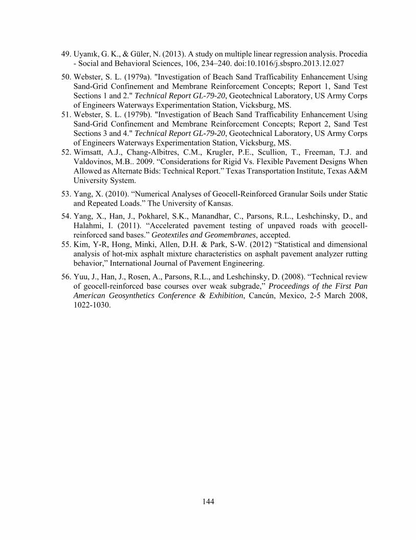
49. Uyanık, G. K., & Güler, N. (2013). A study on multiple linear regression analysis. Procedia - Social and Behavioral Sciences, 106, 234–240. doi:10.1016/j.sbspro.2013.12.027

50. Webster, S. L. (1979a). "Investigation of Beach Sand Trafficability Enhancement Using Sand-Grid Confinement and Membrane Reinforcement Concepts; Report 1, Sand Test Sections 1 and 2." Technical Report GL-79-20, Geotechnical Laboratory, US Army Corps of Engineers Waterways Experimentation Station, Vicksburg, MS.

51. Webster, S. L. (1979b). "Investigation of Beach Sand Trafficability Enhancement Using Sand-Grid Confinement and Membrane Reinforcement Concepts; Report 2, Sand Test Sections 3 and 4." Technical Report GL-79-20, Geotechnical Laboratory, US Army Corps of Engineers Waterways Experimentation Station, Vicksburg, MS.

52. Wimsatt, A.J., Chang-Albitres, C.M., Krugler, P.E., Scullion, T., Freeman, T.J. and Valdovinos, M.B.. 2009. “Considerations for Rigid Vs. Flexible Pavement Designs When Allowed as Alternate Bids: Technical Report.” Texas Transportation Institute, Texas A&M University System.

53. Yang, X. (2010). “Numerical Analyses of Geocell-Reinforced Granular Soils under Static and Repeated Loads.” The University of Kansas.

54. Yang, X., Han, J., Pokharel, S.K., Manandhar, C., Parsons, R.L., Leshchinsky, D., and Halahmi, I. (2011). “Accelerated pavement testing of unpaved roads with geocell-reinforced sand bases.” Geotextiles and Geomembranes, accepted.

55. Kim, Y-R, Hong, Minki, Allen, D.H. & Park, S-W. (2012) “Statistical and dimensional analysis of hot-mix asphalt mixture characteristics on asphalt pavement analyzer rutting behavior,” International Journal of Pavement Engineering.

56. Yuu, J., Han, J., Rosen, A., Parsons, R.L., and Leshchinsky, D. (2008). “Technical review of geocell-reinforced base courses over weak subgrade,” Proceedings of the First Pan American Geosynthetics Conference & Exhibition, Cancún, Mexico, 2-5 March 2008, 1022-1030.

144

145

APPENDIX A: SITE INSTRUMENTATION

A.1 INTRODUCTION

An additional task was added to the project to instrument a portion of FM 906 in Lamar County ( Paris, Texas) constructed using geocells. The purpose of instrumentation was to document the benefits of geocell in pavements. The pavement instrumented included two sections a) no geocell (NGC) and b) constructed with geocell (GC). In addition, falling Weight Deflectometer (FWD) testing was performed at the end of the construction to ensure that the instruments were working correctly. The location of the test section and pertinent information related to construction is included in this appendix.

A.2 SITE LOCATION AND MATERIAL PROPERTIES

A.2.1 Site Location

The project site for geocell installation is a local road located in Lamar County, Paris, TX, a low-volume road (FM 906). The location of the road within Texas is shown in Figure A-1, while Figure A-2 shows the exact location of the test section.

Figure A-1 Lamar County, Paris TX Site Location (Source: Wikipedia).

146

Figure A-2 Test Site Location (Source: ArcMAP).

A.2.2 Soil Classification

At the construction time, subgrade and base material were collected and tested in the laboratory for soil classification, and results are included in the following sections.

Subgrade Soil Classification:

Subgrade soil was classified using the procedure proposed in Tex-142-E (Laboratory Classification of Soils for Engineering Purposes). A 500 g sample was used for the soil classification. The gradation chart is shown in Figure A-3 as represented by a particle–size distribution curve. Based on the gradation, the soil was classified as a poorly graded soil SP. The sample classified consisted of 4% gravel, 69% sand, and 27% fines. In addition, Tex-104-E, Tex-105-E, and Tex-106-E determined Atterberg Limits. The soil's liquid limit (LL) and plastic limit(PL) were 21 and 0, respectively, having a plastic limit (PL) of 21 (Figure A-4). Therefore, the soilis classified as poorly graded sand with clay (SP-SC).

147

Figure A-3 Mech. Sieve Soil Classification.

Figure A-4 Liquid Limit.

Texas Tri-axial Test:

Subgrade Material:

Subgrade material was prepared as per Tex-114-E (Part III) and tested by the Accelerated Method for Triaxial Compression of Soils in Tex-117-E (Part II). A total of 6 specimens at an optimum moisture content of 10.3% and maximum dry density of 112.7 pcf (Figure A-5) were tested. All 6 specimens were 4 in. in diameter and 6 in. in height. Specimen were prepared for capillary wetting for 24 hours, after which the 6 specimens were tested at a single lateral pressure of 0 psi, 3 psi, 5 psi, 10 psi, 15 psi, and 20 psi. In addition, Mohr’s diagram and failure envelope were produced for shear strength evaluation (Figure A-6).

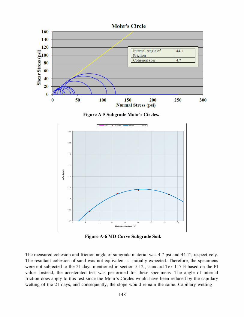
148

Figure A-5 Subgrade Mohr's Circles.

The measured cohesion and friction angle of subgrade material was 4.7 psi and 44.1°, respectively. The resultant cohesion of sand was not equivalent as initially expected. Therefore, the specimens were not subjected to the 21 days mentioned in section 5.12., standard Tex-117-E based on the PI value. Instead, the accelerated test was performed for these specimens. The angle of internal friction does apply to this test since the Mohr’s Circles would have been reduced by the capillary wetting of the 21 days, and consequently, the slope would remain the same. Capillary wetting

Figure A-6 MD Curve Subgrade Soil.

149

reduced the shear stresses for Mohr’s Circles and reduced the y-intercept of the Coulomb failure envelope line (Cohesion).

The resulting data are summarized in Table A-1, as shown below. For example, at 0 psi lateral pressure, the resulting normal stress comes out to 3.83 psi, and the shear stress at 8.98 psi. At 5 psi lateral pressure, the failure normal and shear stresses were calculated to be 11.08 psi and 14.24 psi, respectively. Finally, at a maximum lateral pressure of 20 psi, the resulting failure normal and shear stresses were estimated to be 36.29 psi and 38.15 psi, respectively. Thus, with an increase in lateral pressure, both normal stress and shear stress increased linearly.

Table A-1 Stress at Different Confinements (Subgrade soil) Failure Stresses

Lateral Stress (psi)

Normal Stress (psi)

Shear Stress (psi)

0 3.83 8.98 0 3.83 8.98 3 8.91 13.84 3 8.10 11.95 5 11.08 14.24

10 20.40 24.36 15 29.36 33.63 20 36.29 38.15

Flexbase material:

The Texas Triaxial Test determined the shear strength of the flexible base material following the accelerated method (Tex-117-E, Part II). A total of 9, 6”x8” cylinders were prepared for three different lateral confining pressures. Three prepared specimens were tested under zero confining pressure, three at 3.0 psi confining pressure, and the remaining three were tested under a 15 psi confining pressure. These samples were prepared in accordance with Test Method Tex-113-E, using a Soil Compactor Analyzer (SCA). Specimens were intended to be mold at their Optimum Moisture Content (OMC) of 6.1% and a maximum dry density of 132.5 pcf (Figure A-7). Once the material was molded, extruded, and allowed to sit for 24 hours while monitoring moisture travel from the specimen to the porous stones, if any. Based on Mohr circles results (Figure A-8), the flex base classification, internal friction angle (ϕ), and cohesion were found. Therefore, flex base classification was classified under Class 1 (Figure A-9).

Figure A-7 MD Curve of Flexbase Material.

Figure A-8 Flex-Base Mohr Circles.

150

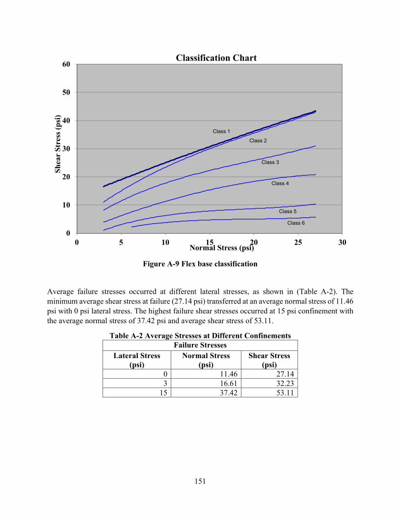
151

Figure A-9 Flex base classification

0

10

20

30

40

50

60

0 5 10 15 20 25 30

Shea

r St

ress

(psi

)

Normal Stress (psi)

Classification Chart

Class 1

Class 2

Class 3

Class 4

Class 5

Class 6

Average failure stresses occurred at different lateral stresses, as shown in (Table A-2). The minimum average shear stress at failure (27.14 psi) transferred at an average normal stress of 11.46 psi with 0 psi lateral stress. The highest failure shear stresses occurred at 15 psi confinement with the average normal stress of 37.42 psi and average shear stress of 53.11.

Table A-2 Average Stresses at Different Confinements Failure Stresses

Lateral Stress (psi)

Normal Stress (psi)

Shear Stress (psi)

0 11.46 27.14 3 16.61 32.23

15 37.42 53.11

152

A.3 INSTRUMENTATION

Geocell: The geocell manufacturer used in this study is Presto 4.25” geocell. The properties of the selected geocell are shown in Appendix B (Figure B-2).

Strain Gauge: The strain gauges are used to measure the deformation occurring due to loading and are converted to estimate the induced strains. Each strain gauge is glued to geocell and adequately protected. Table A-3 shows the strain gauge model and protection means. The specification of the strain gauge is mentioned in Appendix B (Figure B-3).

Table A-3 Strain Gauges Item Description Strain Gauge KFH-6-120-C1-11L1M3R (6mm strain gauge, 120Ω,

3 pre-wired) Glue (to glue strain gauge to geocell)

Ethyl based cyanoacrylate

Protection of strain gauge Performix Plasti Dip (flexible protection) Protection of strain gauge wires PVC Tubing

Earth Pressure Cells: The pressure cells were placed on the top of the subgrade to estimate the stresses at the subgrade level. Geokon Model 3500 series (2.5 MPa and 600 kPa) pressure cell was selected for evaluation, and the specifications of these pressure cells are illustrated in Appendix B (Figure B-4). Each pressure cell is a semiconductor strain gauge earth pressure cell (circular 10”), with the thermistor in SS housing, 0-5 VDC output as shown in Figure A-10.

Figure A-10 Photo of Earth Pressure Cell.

A trench of 1’ x 1’ x 3” is required to fit the front portion of the pressure cell and 3” to 5” along the road for keeping the wiring safe.

Pavement Section: The FM 906 constructed with geocell and pavement profile is shown in Figures A-11 and A12, respectively. The pavement profile consisted of subgrade, 2.0 in. of the salvaged base, and 8 in. of the cement-treated base. In addition, a portion of FM 906 eastbound

153

was left untreated. Approximately 125 ft. of the untreated section was constructed without geocell, while another 250 ft. was constructed with geocell reinforcement. To maintain a similar profile, the unreinforced section consisted of 10 in. of the flexible base. In contrast, the reinforced section consisted of 4 geocells filled and covered (6 in.) with the flexible base material.

Figure A-11 Pavement Section of Geocell-Reinforced at Testing Site.

Figure A-12 Pavement Section of FM 906 at Testing Site.

The location of sensors for the unreinforced section is shown in Figure A-13, while Figure A-14 shows the wiring arrangement in the test section. The placement of the pressure cell at the unreinforced section is shown in Figure A-13c.

154

Figure A-13 Cross Section and Instrumentation of FM 906 at Testing Site for Unreinforced Section.

Figure A-14 Wiring Arrangement at FM 906 at Testing Site for Unreinforced Section.

Figure A-15 represents the cross-section of the geocell reinforced section of the pavements at the test site. The pressure cell and strain gauge placement at the geocell reinforced section is shown in Figure A-15c. Figure A-16 shows the wiring arrangement in the test section.

155

Figure A-15 Cross Section and Instrumentation of FM 906 at Testing Site for Geocell Reinforced Section.

Figure A-16 Wiring Arrangement at FM 906 at Testing Site for Geocell Reinforced Section.

Data Acquisition System: For recording the stresses and strains of the pavement system, the LMS data acquisition system was employed because the system can accommodate 16 channels, i.e., it can record stresses and strains from 16 locations at a time. In addition, it can record the data at different frequencies (Figure A-17). In this study, a frequency of 128 data points per second is chosen, close to the frequency of other data acquisition systems.

156

Figure A-17 LMS Data Acquisition System.

A.4 CONSTRUCTION OF REINFORCED AND UNREINFORCED SECTIONS

Before the instrumentation of sites and construction, the site was visited, and a plan for placement was developed based on the discussion in the previous section. The UTEP research team arrived and left the construction site on July 10th and July 13th, respectively. On the first day of arrival, the site was surveyed to identify and mark sensor locations. In addition to location marking, the construction process was also discussed with the contractors.

Instrumentation of Unreinforced Section: On July 11th, the contractor provided the traffic control and started removing the un-stabilized flexible base material to a depth of 10 in. from the surface and placed the removed material on the westbound lane for the movement of traffic. After material removal, the sensor locations were marked (Figure A-18), and a trencher was employed to dig a trench to place pressure cells and wiring. The pressure cells were placed on the well-compacted leveled surface and covered with playground sand (Figure A-19) before placing flexible base material. To ensure proper contact, the surface below the pressure cell was compacted using a sledgehammer and leveled to minimize settlement of pressure cells due to compaction, thus, minimizing damage to the pressure cell.

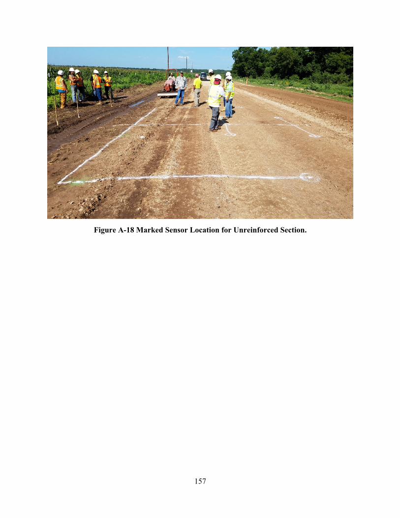
157

Figure A-18 Marked Sensor Location for Unreinforced Section.

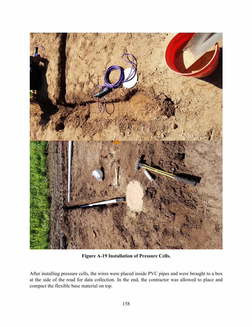
158

After installing pressure cells, the wires were placed inside PVC pipes and were brought to a box at the side of the road for data collection. In the end, the contractor was allowed to place and compact the flexible base material on top.

Figure A-19 Installation of Pressure Cells.

159

Instrumentation of Geocell-Reinforced Section: On July 12th, the placement of the geocell reinforced section was performed. The construction sequence similar to the unreinforced was followed for the placement of pressure cells. After the placement of pressure cells, a geosynthetic fabric (Figure A-20) was placed on top of the pressure cells to minimize the migration of material. After placement of geosynthetic, the instrumented geocells were placed on top, as shown in Figure A-21. The geocells came in panel form (Figure A-20) that can be stretched and connected (FigureA-21). Since geocells were placed in half road width, the standard panels were cut and connectedto the standard panel. The connection of geocells is simple using the Atrakey provided by thesupplier and requires minimal connection time. To make sure that the geocells were stretched, thegeocells were stretched, and rebar was placed on maintaining the stretched condition. After placinginstrumented and non-instrumented geocells, the strain gauges wires were placed inside the pipesand moved towards the control box together with pressure cell wires.

Figure A-20 Installation of Geosynthetics.

160

Figure A-21 Installation of Instrumented Geocells.

161

After the placement of geocells, the rebars were removed, and pegs were placed to maintain the width of geocells. Next, the contractor started moving material and filling geocells closer to the median and continued till it reached the shoulder (Figure A-22).

Figure A-22 Geocell Construction Sequence.

A.5 DATA COLLECTION AND ANALYSIS

After construction and compaction of the geocell reinforced layer, the UTEP research team went to the site on July 13th to verify the working of pressure cells and strain gauges. For verification, Falling Weight Deflectometer (FWD) was requested by the Paris District office. The FWD testing was performed on top of the geocell reinforced, unreinforced, and cement-treated sections. The purpose of FWD tests was to measure the response of pressure cells and strain gauges and obtain a section profile (of three pavement sections). To measure profile, the FWD tests were performed at every 20 or 25 ft. by dropping two seating loads and two drops for measurement. To measure the response of pressure cells and strain gauges, the tests were performed by placing the FWD load plate on top of the pressure cell. To ensure the FWD load plate is placed on top of the pressure cells, the pressure cells locations were marked on the surfaces, and the FWD operator was guided to place the load plate on top of the pressure cells as close as possible. Although efforts were made, the FWD load plate was not precisely aligned on top of the pressure cells at many locations. Each FWD test included two seating drops and two measurements with approximately 9,000 lbs. of the load. Additionally, the FWD tests on the top of the sensors were repeated by moving and

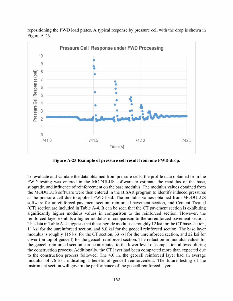
162

repositioning the FWD load plates. A typical response by pressure cell with the drop is shown in Figure A-23.

Figure A-23 Example of pressure cell result from one FWD drop.

To evaluate and validate the data obtained from pressure cells, the profile data obtained from the FWD testing was entered in the MODULUS software to estimate the modulus of the base, subgrade, and influence of reinforcement on the base modulus. The modulus values obtained from the MODULUS software were then entered in the BISAR program to identify induced pressures at the pressure cell due to applied FWD load. The modulus values obtained from MODULUS software for unreinforced pavement section, reinforced pavement section, and Cement Treated (CT) section are included in Table A-4. It can be seen that the CT pavement section is exhibiting significantly higher modulus values in comparison to the reinforced section. However, the reinforced layer exhibits a higher modulus in comparison to the unreinforced pavement section. The data in Table A-4 suggests that the subgrade modulus is roughly 12 ksi for the CT base section, 11 ksi for the unreinforced section, and 8.0 ksi for the geocell reinforced section. The base layer modulus is roughly 115 ksi for the CT section, 33 ksi for the unreinforced section, and 22 ksi for cover (on top of geocell) for the geocell reinforced section. The reduction in modulus values for the geocell reinforced section can be attributed to the lower level of compaction allowed during the construction process. Additionally, the CT layer had been compacted more than expected due to the construction process followed. The 4.0 in. the geocell reinforced layer had an average modulus of 76 ksi, indicating a benefit of geocell reinforcement. The future testing of the instrument section will govern the performance of the geocell reinforced layer.

163

Table A-4 Results of MODULUS Software Modulus, psi

Cement Treated Unreinforced Geocell Reinforced

10 in. Base Subgrade 10 in. Base Subgrade 6 in. Cover

4 in. Geocell Subgrade

Average 115,068 12,328 32,657 10,809 22,124 75,696 7,877

Minimum 105,980 11,697 8,073 9,807 17,144 55,061 5,946

Maximum 122,973 12,614 48,407 11,624 27,954 91,886 10,854

To estimate pressure experienced by the pressure cell at the subgrade level due to FWD load, the BISAR software was used. The base modulus of 33 ksi and subgrade modulus of 11 ksi was assumed to calculate the pressure values. The pavement structure in Bisar software was set as 10-inch of the top layer and 200-inch of subgrade, and the stress on pressure cell was assumed to be buried 3.0 in. below the base layer. Thus, the pavement layer on top of the pressure cell was assumed to be 13 in. The top layer and subgrade layer Poisson’s ratio was assumed to be 0.33 and 0.35, respectively. The FWD load plate was assumed to be 10.82 in., and load values were entered as per the collected data. The results of the BISAR output and pressure measured from pressure cells are summarized in Table A-5 indicate that the pressure cells are working as expected while some of the strain gauges are not functioning because of damage during the construction process. In some instances, pressure cells estimated higher, lower, or similar results to the estimated pressures obtained from BISAR. The lower values can be attributed to misalignment of the FWD plate; the higher values can be attributed to construction equipment passing by while FWD testing was performed. Additionally, the compaction of layers was also occurring due to the movement of construction equipment which further contributed to the discrepancy. Based on the results, it can be concluded that the pressure cells and strain gauges are functioning with few exceptions.

Table A-5 Results of Field Testing and Bisar Modeling ID NGPC (psi) GPC (psi) GSG (µε) Bisar (psi) 6-1 11.34 4.76 - 19.63 6-2 9.04 1.42 - 18.23 5-1 48.82 3.68 112.60 18.23 5-2 44.80 11.53 351.27 16.74 4-1 22.96 13.22 63.78 18.42 4-2 12.87 13.67 235.75 17.12 3-1 31.57 2.10 179.89 18.89 3-2 23.51 13.47 188.05 17.67 2-1 45.39 76.75 85.21 17.86 2-2 28.82 83.58 85.99 17.12 1-1 4.34 28.67 133.50 18.79 1-2 3.28 31.01 169.00 17.11

Note NGPC-Non-Geocell Pressure Cell; GPC-Geocell Pressure Cell; GSG-Geocell Strain Gauge; “-” means the data was unavailable.

164

A comparison between no geocell and geocell reinforced n the comparison of pressure cell response; as shown in Figure A-24, most of the pressure cells of Geocell sites had lower stress response than the Non-Geocell sites except pressure cells 1 and 2. Although reported, some numbers are significantly higher and impossible because the applied pressure was around 80 psi on top and is expected to be lower 13 in. below the surface. The possible reason for discrepancy can be attributed to interference caused by construction equipment. The deflections measured near pressure cells 3 and 5 for the geocell, reinforced section, and the unreinforced section are summarized in Figures A-25 and A-26, respectively. The overall results suggest that the magnitude of deflections is lower in the presence of geocell reinforcement. However, future performance will provide a better indicator of the benefit of geocells.

Figure A-24 Comparison of Pressure Cell Response between Non-Geocell and Geocell Sites.

0102030405060708090

PC 6

-1

PC 6

-2

PC 5

-1

PC 5

-2

PC 4

-1

PC 4

-2

PC 3

-1

PC 3

-2

PC 2

-1

PC 2

-2

PC 1

-1

PC 1

-2

Pres

sure

Cel

l Res

pons

e (P

si) Vertical Stress

Non-Geocell Site

Geocell Site

165

Figure A-25 FWD Geophone Response of Non-Geocell and Geocell Spot 3.

-90

-80

-70

-60

-50

-40

-30

-20

-10

0D1 D2 D3 D4 D5 D6 D7

Def

lect

ion

(mils

)Deflection of Spot 3

Non-Geocell

Geocell

Figure A-26 FWD Geophone Response of Non-Geocell and Geocell Spot 5.

-70

-60

-50

-40

-30

-20

-10

0D1 D2 D3 D4 D5 D6 D7

Def

lect

ion

(mils

)

Deflection of Spot 5

Non-Geocell

Geocell

166

167

APPENDIX B: FINITE ELEMENT MODELDEVELOPMENT

The Finite Element (FE) numerical analysis method was used to study the behavior of geocell-reinforced pavement structures under traffic loading. The finite element analysis of geocell reinforced soils requires truly three-dimensional models because of the all-around confinement of soil by geocell pockets. For this purpose, a 3-D FE model was developed to address better the geometry of geocell panels that expand into a honeycomb formation when placed on-site, as shown in Figure B-1.

Figure B-1 Geocell and Infill Material. Although FE analyses (FEA) can identify the level of reinforcement provided by the geocell, the generation of a mesh for FEA is complicated due to several factors like the interaction between geocell and adjacent soil, transfer of load, and confinement provided by the geocell, among others. Additionally, the modeling of geocell required a significant number of elements and nodes to model the honeycomb shape of geocell, which requires significant computational time. Therefore, to develop a 3-D FE model (FEM) that better addresses the needs imposed by the characteristics of the geocell-reinforced pavement, distinctive FEMs with different levels of sophistication were developed before the development of the final 3-D model. These models were developed to evaluate the following aspects:

• Soil material model• Boundary conditions of reinforced-layer• Shape of geocell• Shell element type• Geocell-soil interaction

To perform FEA, a general-purpose finite element program LS-DYNA was selected because this program allows dynamic FEA and includes a comprehensive list of material and contact models/algorithms. Moreover, the program can also be installed on the High-Performance Cluster (HPC), a computer system that groups class Linux clusters and symmetric shared-memory multiprocessor systems that significantly improve simulation program speed performance. The

168

HPC allows executing parallel programs or multiple instances of the same program, each driven by a different parameter set.

B.1 SOIL MODELS

Many researchers modeled the geocell and infill material as a composite material using FEM or finite difference methods (Bathurst and Knight 1998; Latha et al. 2009; Latha and Somwanshi 2009; Mhaiskar and Mandal 1996), but very few have modeled them as a separate material (Bortz and Hossain 2015; Evans 1994; Han et al. 2008; Yang 2010). In the geocell reinforced base layer, the infill material (linear elastic or plastic) and geocell (elastic) respond simultaneously to loading, but the working mechanism of each material is different. Therefore, to model a geocell reinforced base layer more precisely, the behavior of each material (infill and geocell) needs to be evaluated separately and was utilized in this study.

The mechanical behavior of geomaterials may be modeled at various degrees of accuracy. Hooke's law of linear elasticity, the most straightforward stress-strain relationship, may not provide adequate responses to represent soil behavior under traffic loading adequately. Researchers have proposed many constitutive models to describe various aspects of soil behavior. However, the more sophisticated a soil model is, the more input parameters are necessary, requiring additional laboratory tests. A limited number of models use parameters obtained from traditional laboratory tests. Among these, material models like Mohr-Coulomb and Duncan-Chang models have been used by researchers to simulate permanent deformation under repeated loading and require standard tri-axial soil tests (Han et al., 2008; Yang 2010). To simulate the behavior of geomaterials, three soil models were selected based on their compatibility with LS-DYNA software.

B.1.1 Linear Elastic

The linear elastic model is used to describe materials that behave as follows:

1. The strain in the material is minor (linear).2. The stress is proportional to the strain, σ ∝ ε (linear).3. When the loads are removed, the material returns to its original shape, and the unloading

path is the same as the loading path (elastic).4. There is no dependence on the rate of loading or straining (elastic).

The stress-strain (loading and unloading) curve for the linear elastic is shown in Figure B-2. Finite element programs only require the modulus of elasticity and Poisson’s ratio as input for mechanical properties.

The properties considered for the parametric study for both the base and subgrade materials are shown in Table B-1. In all cases, the base material properties were kept the same for both the top unreinforced base material and the infill material of the geocell-reinforced layer.

B.1.2 Mohr-Coulomb

With the increase in loads, the soil behavior changes from linear to non-linear, as shown in Figure B-3. The Mohr-Coulomb model is a well-known and straightforward linear elastic-perfectly plasticmodel, which can be used as a first approximation of soil behavior. The linear elastic part of theMohr-Coulomb model is based on Hooke’s law of isotropic elasticity. The perfectly plastic part is

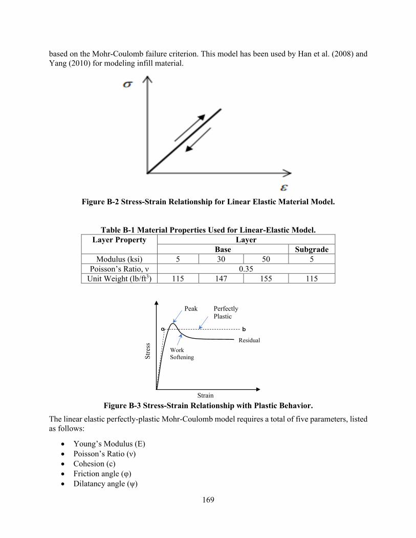
169

based on the Mohr-Coulomb failure criterion. This model has been used by Han et al. (2008) and Yang (2010) for modeling infill material.

Figure B-2 Stress-Strain Relationship for Linear Elastic Material Model.

Table B-1 Material Properties Used for Linear-Elastic Model. Layer Property Layer

Base Subgrade Modulus (ksi) 5 30 50 5

Poisson’s Ratio, ν 0.35 Unit Weight (lb/ft3) 115 147 155 115

Figure B-3 Stress-Strain Relationship with Plastic Behavior.

Stre

ss Work Softening

Perfectly Plastic

Peak

Residual ba

Strain

The linear elastic perfectly-plastic Mohr-Coulomb model requires a total of five parameters, listed as follows:

• Young’s Modulus (E)• Poisson’s Ratio (ν)• Cohesion (c)• Friction angle (φ)• Dilatancy angle (ψ)

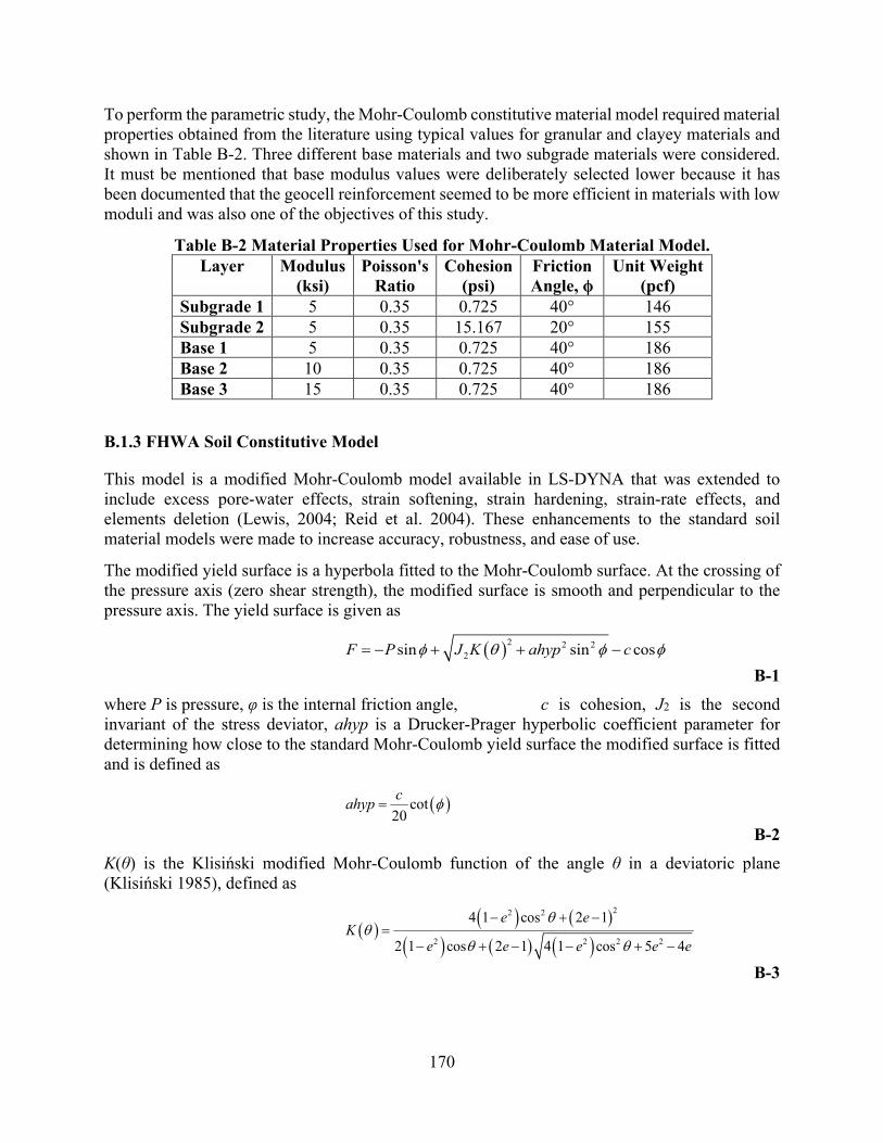
170

To perform the parametric study, the Mohr-Coulomb constitutive material model required material properties obtained from the literature using typical values for granular and clayey materials and shown in Table B-2. Three different base materials and two subgrade materials were considered. It must be mentioned that base modulus values were deliberately selected lower because it has been documented that the geocell reinforcement seemed to be more efficient in materials with low moduli and was also one of the objectives of this study.

Table B-2 Material Properties Used for Mohr-Coulomb Material Model. Layer Modulus

(ksi) Poisson's

Ratio Cohesion

(psi) Friction Angle, ϕ

Unit Weight (pcf)

Subgrade 1 5 0.35 0.725 40° 146 Subgrade 2 5 0.35 15.167 20° 155 Base 1 5 0.35 0.725 40° 186 Base 2 10 0.35 0.725 40° 186 Base 3 15 0.35 0.725 40° 186

B.1.3 FHWA Soil Constitutive Model

This model is a modified Mohr-Coulomb model available in LS-DYNA that was extended to include excess pore-water effects, strain softening, strain hardening, strain-rate effects, and elements deletion (Lewis, 2004; Reid et al. 2004). These enhancements to the standard soil material models were made to increase accuracy, robustness, and ease of use.

The modified yield surface is a hyperbola fitted to the Mohr-Coulomb surface. At the crossing of the pressure axis (zero shear strength), the modified surface is smooth and perpendicular to the pressure axis. The yield surface is given as

( )2 2 22sin sin cosF P J K ahyp cφ θ φ φ= − + + −

B-1where P is pressure, φ is the internal friction angle, c is cohesion, J2 is the second invariant of the stress deviator, ahyp is a Drucker-Prager hyperbolic coefficient parameter for determining how close to the standard Mohr-Coulomb yield surface the modified surface is fitted and is defined as

( )cot20cahyp φ=

B-2K(θ) is the Klisiński modified Mohr-Coulomb function of the angle θ in a deviatoric plane (Klisiński 1985), defined as

( ) ( ) ( )( ) ( ) ( )

22 2

2 2 2 2

4 1 cos 2 1

2 1 cos 2 1 4 1 cos 5 4

e eK

e e e e e

θθ

θ θ

− + −=

− + − − + −

B-3

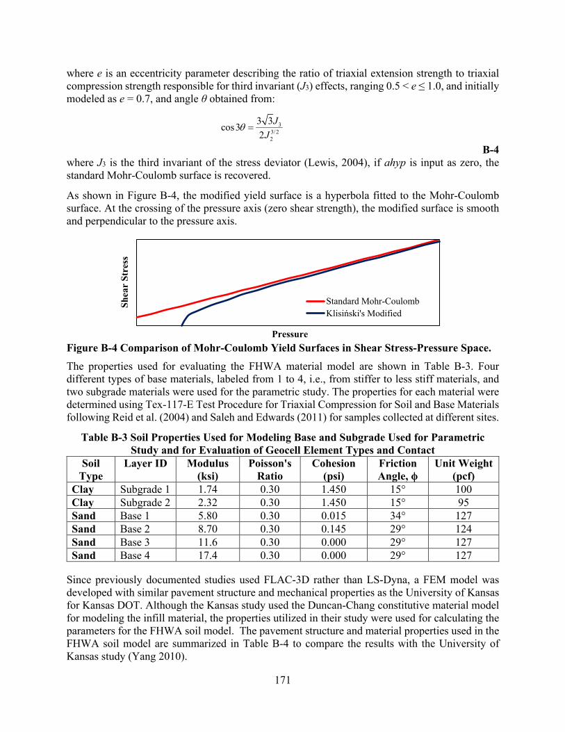
171

where e is an eccentricity parameter describing the ratio of triaxial extension strength to triaxial compression strength responsible for third invariant (J3) effects, ranging 0.5 < e ≤ 1.0, and initially modeled as e = 0.7, and angle θ obtained from:

33/22

3 3cos32

JJ

θ =

B-4where J3 is the third invariant of the stress deviator (Lewis, 2004), if ahyp is input as zero, the standard Mohr-Coulomb surface is recovered.

As shown in Figure B-4, the modified yield surface is a hyperbola fitted to the Mohr-Coulomb surface. At the crossing of the pressure axis (zero shear strength), the modified surface is smooth and perpendicular to the pressure axis.

Figure B-4 Comparison of Mohr-Coulomb Yield Surfaces in Shear Stress-Pressure Space. The properties used for evaluating the FHWA material model are shown in Table B-3. Four different types of base materials, labeled from 1 to 4, i.e., from stiffer to less stiff materials, and two subgrade materials were used for the parametric study. The properties for each material were determined using Tex-117-E Test Procedure for Triaxial Compression for Soil and Base Materials following Reid et al. (2004) and Saleh and Edwards (2011) for samples collected at different sites.

Table B-3 Soil Properties Used for Modeling Base and Subgrade Used for Parametric Study and for Evaluation of Geocell Element Types and Contact

Soil Type

Layer ID Modulus (ksi)

Poisson's Ratio

Cohesion (psi)

Friction Angle, ϕ

Unit Weight (pcf)

Clay Subgrade 1 1.74 0.30 1.450 15° 100 Clay Subgrade 2 2.32 0.30 1.450 15° 95 Sand Base 1 5.80 0.30 0.015 34° 127 Sand Base 2 8.70 0.30 0.145 29° 124 Sand Base 3 11.6 0.30 0.000 29° 127 Sand Base 4 17.4 0.30 0.000 29° 127

Since previously documented studies used FLAC-3D rather than LS-Dyna, a FEM model was developed with similar pavement structure and mechanical properties as the University of Kansas for Kansas DOT. Although the Kansas study used the Duncan-Chang constitutive material model for modeling the infill material, the properties utilized in their study were used for calculating the parameters for the FHWA soil model. The pavement structure and material properties used in the FHWA soil model are summarized in Table B-4 to compare the results with the University of Kansas study (Yang 2010).

Shea

r St

ress

Pressure

Standard Mohr-CoulombKlisiński's Modified

172

B.2 SHELL ELEMENT TYPE FOR GEOCELL MODELING

One of the problems encountered while modeling the geocell and geomaterials is the element aspect ratio or the computational constraints. Although geomaterials can be modeled as solid elements of any shape and size, the geocell can be modeled in specific shapes and sizes because of their thickness. It is entirely possible to create FEM of both geocell as well as geomaterials of the same thickness. However, this will significantly increase the number of elements which will require a significant computational time. On the other hand, if geomaterial element and geocell element thicknesses are different, the compatibility of two different element types and transference of deformation between the two materials must be evaluated and understood. To model thin geocell, various thin element types available in LS-DYNA were explored. The available elements can be categorized as per their behavior to be: as a membrane and as a plate (or shell) elements. Shell elements can sustain loading using bending stresses, unlike membrane elements. LS-DYNA has several formulations for shell elements that meet this requirement. Since some formulations of thin and thick shell elements meet the model's needs, two were selected for evaluation.

Table B-4 FHWA Soil Material Properties Used for Evaluation of the University of Kansas Study (after Yang. 2010)

Layer Soil Type

Thickness (in.)

Modulus (ksi)

Poisson's Ratio, ν

Cohesion (psi)

Friction Angle,

ϕ

Unit Weight

(pcf) Top Base (Unreinforced)

AB-3 3.5 5.8 0.35 0.682 47.2° 142

Bottom Base (Reinforced)

Kansas River Sand

6.0 0.48 0.35 0 41.1° 114

Subgrade Clay 40 1.5 0.35 15.2 0° 124

B.2.1 Shell Element

Among the list of thin shell element types available in LS-DYNA, the Belytschko-Lin-Tsay Shell (BLT) formulation is recommended as it is more computationally efficient (faster) than the Hughes-Liu shell element formulation (LSTC 2016). The BLT formulation is based on the Reissner-Mindlin kinematic assumption, which combines co-rotational and velocity-strain formulation. The BLT element formulation is suitable for four nodes (quad) shell elements and offers a single-point integration with hourglass control. Each element has five local degrees of freedom (DOF) per node (dx, dy, dz, rx, ry) and two (through-thickness) integration points by default (Figure B-5a). In addition, they have a bi-linear nodal interpolation.

173

Figure B-5 Representation of (a) Four-Node (quad) BLT Shell Element with 5 Local DOFs, 1 Integration Point in the Plane and 5 Through-Thickness Integration Points, and (b) Eight Node Thick Shell Element with 5 Local DOFs, Single (green) or Reduced (red) Integration

Points in the Plane and 5 Through-Thickness Integration Points. B.2.2 Thick Shell Element (TSHELL)

The other shell formulation evaluated was the thick shell elements (TSHELL). Unlike thin shell elements, thick shell elements, also called isoparametric solid-shell elements, consist of eight-noded elements like solid brick elements (see Figure B-5b) that have enhancements based on the Hughes-Liu and the BLT shell types formulations. Like BLT elements, they also have 5 local DOF per node (dx, dy, dz, rx, ry, rz) and can have a one-point quadrature (used as default) or selected reduced integration in the shell plane, and two through shell integration points used as default. Three-dimensional constitutive material models can be applied directly to these types of elements.

B.2.3 Geocell Dimensions and Properties

Three types of geocell were simulated in the parametric study with different heights. Table B-5 shows the dimensions and material properties corresponding to the geocell types evaluated. Geocell were modeled as linear elastic materials.

Table B-5 Geocell Dimensions and Properties. Geocell Type Presto

GW20V Tenax 3/200

and 4/200 Tenax 6/200

Geocell Dimensions Longitudinal Length (in.)

9.2 8.0 8.0

Transversal Length (in.)

7.9 8.0 8.0

Height (in.) 4.0 and 6.0 3.0 and 4.0 6.0 Thickness (in.) 0.040 0.040 0.040

Material Properties Density (lb/ft3) 59.3 59.3 59.3 Modulus (ksi) 60.0 60 60 Poisson’s Ratio 0.45 0.45 0.45

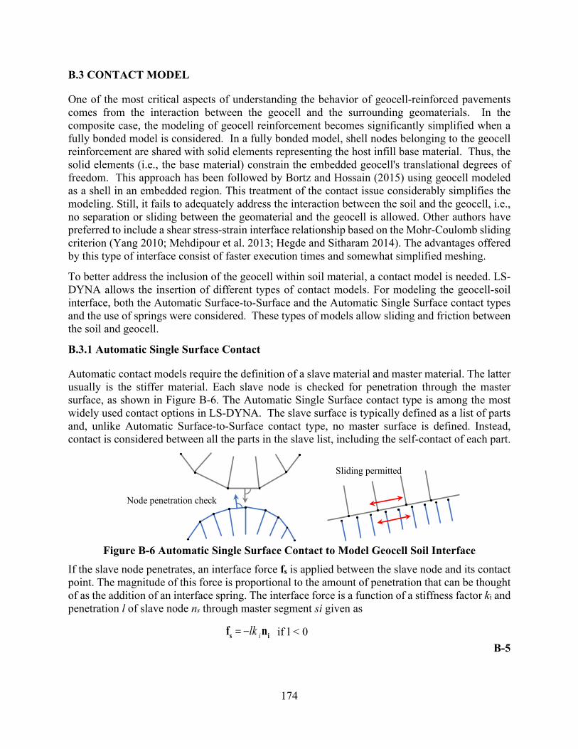
174

B.3 CONTACT MODEL

One of the most critical aspects of understanding the behavior of geocell-reinforced pavements comes from the interaction between the geocell and the surrounding geomaterials. In the composite case, the modeling of geocell reinforcement becomes significantly simplified when a fully bonded model is considered. In a fully bonded model, shell nodes belonging to the geocell reinforcement are shared with solid elements representing the host infill base material. Thus, the solid elements (i.e., the base material) constrain the embedded geocell's translational degrees of freedom. This approach has been followed by Bortz and Hossain (2015) using geocell modeled as a shell in an embedded region. This treatment of the contact issue considerably simplifies the modeling. Still, it fails to adequately address the interaction between the soil and the geocell, i.e., no separation or sliding between the geomaterial and the geocell is allowed. Other authors have preferred to include a shear stress-strain interface relationship based on the Mohr-Coulomb sliding criterion (Yang 2010; Mehdipour et al. 2013; Hegde and Sitharam 2014). The advantages offered by this type of interface consist of faster execution times and somewhat simplified meshing.

To better address the inclusion of the geocell within soil material, a contact model is needed. LS-DYNA allows the insertion of different types of contact models. For modeling the geocell-soil interface, both the Automatic Surface-to-Surface and the Automatic Single Surface contact types and the use of springs were considered. These types of models allow sliding and friction between the soil and geocell.

B.3.1 Automatic Single Surface Contact

Automatic contact models require the definition of a slave material and master material. The latter usually is the stiffer material. Each slave node is checked for penetration through the master surface, as shown in Figure B-6. The Automatic Single Surface contact type is among the most widely used contact options in LS-DYNA. The slave surface is typically defined as a list of parts and, unlike Automatic Surface-to-Surface contact type, no master surface is defined. Instead, contact is considered between all the parts in the slave list, including the self-contact of each part.

Figure B-6 Automatic Single Surface Contact to Model Geocell Soil Interface If the slave node penetrates, an interface force fs is applied between the slave node and its contact point. The magnitude of this force is proportional to the amount of penetration that can be thought of as the addition of an interface spring. The interface force is a function of a stiffness factor ki and penetration l of slave node ns through master segment si given as

ilk= −s if n if l < 0 B-5

Sliding permitted

Node penetration check

175

where ni is normal to the master segment at the contact point. Stiffness ki for master segment si is defined as

For brick elements 2

si i ii

i

f K AkV

=

B-6For shell elements

max( )si i i

idiag

f K Akl

=

B-7where Ki is the bulk modulus, Vi is volume, Ai is the face area of the element in si, ldiag is the shell diagonal length, and fsi is a scale factor for the interface stiffness (normally fsi = 0.10) (LSTC 2016).

Friction is based on a Coulomb formulation. The model implements a friction algorithm that makes use of an elastic-plastic spring. The algorithm is based on an iterative process that starts by calculating the yield force based on the friction and the normal force, followed by the calculation of the incremental movement of the slave node to update the interface force and check yield condition. Finally, an exponential interpolation function smooths the transition between the static and dynamic coefficients of friction based on the relative velocity between the slave node and the master, as described in the LS-DYNA theory manual (LSTC 2016).

B.3.2 Discrete Beam Element Interface

The use of discrete beam elements for establishing a geocell-soil interface was also considered. For the implementation of springs, spring elements that consider normal and tangential components are needed. i.e., the normal component dn, and two other orthogonal components ds and dt, as shown in Figure B-7. For this purpose, discrete elements can be used. These elements are point-to-point physical connections between deformable bodies. As springs (discrete elements) have only one DOF, i.e., a normal component, discrete beams were used instead as they have up to 6 DOFs. Resultant forces and moments of a discrete beam are output in the local (r,s,t) coordinate system. Moreover, the length of a discrete beam may be zero or nonzero.

Figure B-7 Contact Using Discrete Beams (Spring with Normal and Tangential Components).

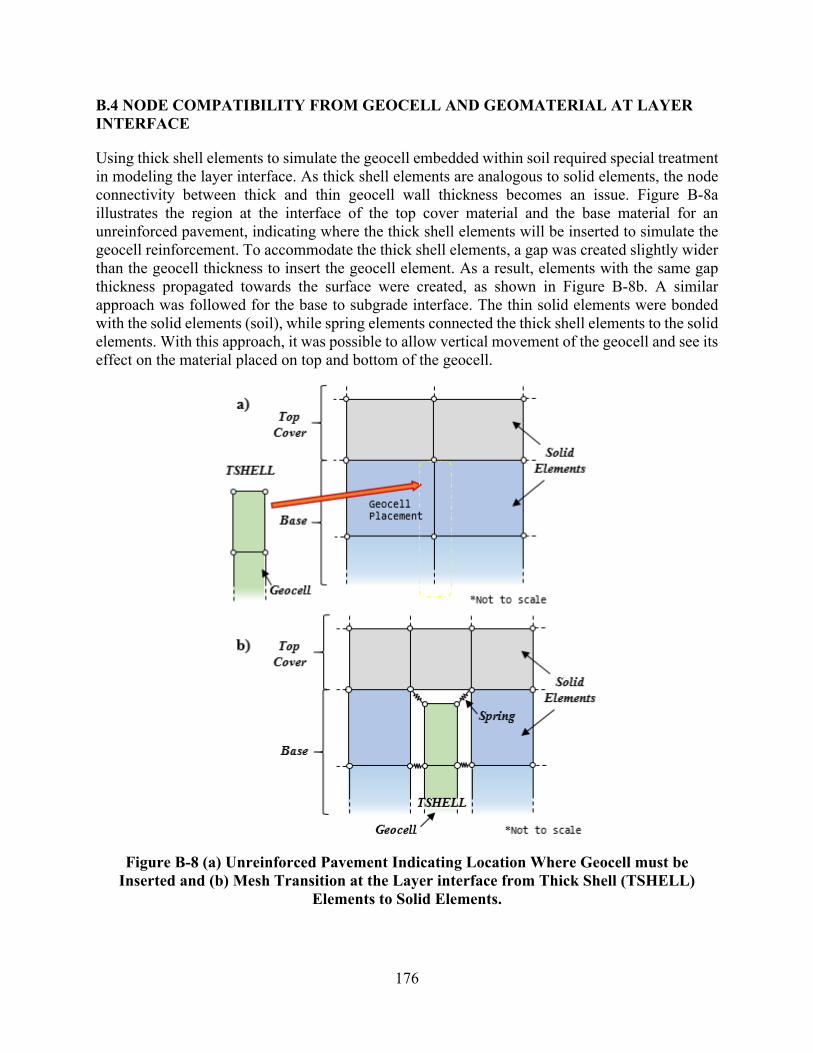
176

B.4 NODE COMPATIBILITY FROM GEOCELL AND GEOMATERIAL AT LAYERINTERFACE

Using thick shell elements to simulate the geocell embedded within soil required special treatment in modeling the layer interface. As thick shell elements are analogous to solid elements, the node connectivity between thick and thin geocell wall thickness becomes an issue. Figure B-8a illustrates the region at the interface of the top cover material and the base material for an unreinforced pavement, indicating where the thick shell elements will be inserted to simulate the geocell reinforcement. To accommodate the thick shell elements, a gap was created slightly wider than the geocell thickness to insert the geocell element. As a result, elements with the same gap thickness propagated towards the surface were created, as shown in Figure B-8b. A similar approach was followed for the base to subgrade interface. The thin solid elements were bonded with the solid elements (soil), while spring elements connected the thick shell elements to the solid elements. With this approach, it was possible to allow vertical movement of the geocell and see its effect on the material placed on top and bottom of the geocell.

Figure B-8 (a) Unreinforced Pavement Indicating Location Where Geocell must be Inserted and (b) Mesh Transition at the Layer interface from Thick Shell (TSHELL)

Elements to Solid Elements.

177

B.5 BOUNDARY CONDITIONS

A preliminary study was performed to evaluate the effect of boundary conditions on geocell reinforcement behavior and whether the change in boundary conditions would destabilize FEA under repeated loading conditions. For this purpose, a mesh optimization was conducted to ensure the model's limits, i.e., boundary conditions were placed far enough where stress and deflection values were less than 10% of the peak values obtained under the load. The identified location was 18 in. away from the point of application of the load. Though models with wider dimensions could be developed, the model must be constrained in size due to a large number of nodes and elements generated since the size of the elements on the pavement layers is determined by the size of the elements along the geocell. About 15 elements were used along the geocell along the half-sine-shaped outline, i.e., from joint to joint, causing many elements to be generated within the infill material, all adapted to the size of the elements on the geocell. The number of nodes and elements used in the three-dimensional models is described in the sections referring to the developed models.

In addition, it was desired to design the FE model with a reinforced layer that allows the expansion of the geocell panels. For this purpose, boundary conditions were removed just for the geocell-reinforced base layer, while the other layers were restrained from lateral movement. A representation of the boundaries conditions is shown in Figure B-9. While evaluating the material constitutive models for simulating the geomaterials, it was found that no instability occurred due to the removal of lateral constraints on the nodes at the edge of the base layer.

Figure B-9 Side View of FE Model Showing Boundary Conditions, Shown as Triangles, with Base Layer with no Restrained Conditions to Allow for Expansion.

178

B.6 LEVEL OF SOPHISTICATION OF FINITE ELEMENT MODELS

Three different levels of sophistication of the FEM were developed. First, a simplified 3-D FEM was developed consisting of a single layer to evaluate the most appropriate shell element and contact model for modeling the geocell embedded in geomaterial. A second 3-D FEM was developed consisting of a pavement section with a single reinforced cell to evaluate the contact type compared to the responses observed in the laboratory after a shell element type was selected from the first simplified model. Finally, an extension of this latter model was developed to simulate pavements reinforced with the honeycomb-type geocell reinforcement. This model was used to carry a parametric study to evaluate the behavior of geocell reinforcement in different pavements.

B.6.1 Simplified Single Layer FE Model

The 3-D model was reduced to a 2-D (one-thick element wide) single-layer model to identify the most appropriate contact model. Additionally, this model was also used for identifying the type of shell element that best addresses the behavior and interaction of the geocell with geomaterial. This model was developed to check the efficiency of the shell elements for transferring the stress from one cell to the adjacent one.

The model consisted of a single layer with properties of base course material, divided into three infill cell pockets separated by the geocell reinforcement, as shown in Figure B-10. The model consisted of 480 elements, divided into three parts representing the cells, and loaded with a 6-in. diameter, 40 psi pressure load directly applied to Cell #1. Symmetry conditions were applied on the left boundary to account for a half-model. The applied pressure of 80 psi was selected to reproduce the pressure conditions experienced by the reinforced base layer when placed underneath a 4-in. cover of the base material. Ten loading cycles were simulated, each of them consisting of a 0.10 sec loading period followed by a 0.90 sec rest period, as shown in Figure B-11. All cells were modeled using material properties of Base 4 material, described in Table B-1.

Figure B-10 Simplified Single Layer FEM with Soil Cells of Base Material Separated with (a) BLT Shell (SHELL) Element Types, and (b) Thick Shell (TSHELL) Element Types.

179

Figure B-11 Loading Cycles Used for Simplified FE Model.

0

10

20

30

40

50

0 1 2 3 4 5 6 7 8 9 10

Loa

d (p

si)

Number of cycles

Two shell element types were evaluated: thin Belytschko-Lin-Tsay Shell (BLT) and thick shell elements (TSHELL). Both element types were assigned linear elastic material properties corresponding to Presto GW20V, as shown in Table B-5.

B.6.2 Pavement with Single Cell

This model was developed for evaluating the soil-geocell interface behavior. The 3-D FE model was developed for simulating a laboratory test consisting of a 3 ft diameter cylindrical tank filled with a 24-in. thick compacted subgrade, as shown in Figure B-12. A single geocell was placed on top of the compacted subgrade and filled with infill material. In the laboratory, a 6-in. diameter and 0.80 in. thick circular steel plate was placed at the center of the geocell pocket and loaded with an MTS load frame was analogous to the laboratory testing, consisting of Subgrade 1 material and Base 1 for cell infill, whose properties are described in Table B-3.

Figure B-12 (a) Laboratory Setup, (b) FE Model of Laboratory Setup, and (c) Setup of Strain Gauges on Geocell for Evaluating Soil-Geocell Interaction.

180

The FE model was developed with these dimensions and loaded with a 6-in. diameter, 80 psi pressure load applied directly at the center of the cell to simulate these conditions. In addition, symmetry conditions were applied on boundaries to account for a quarter-model to reduce the number of elements. Similarly, loading cycles were simulated, each of them consisting of a 0.10 s loading period followed by a 0.90 s rest period, as shown in Figure B-13.

For comparison to unreinforced pavements in the parametric study, a model without geocell was developed by removing the shell elements and discrete beams from the FE models of geocell-reinforced structures and then merging nodes that were in contact. Properties for this model are shown in Table B-4 as well. Table B-6 summarizes the properties of the FE model; Shell elements, both thin BLT and TSHELL, used for modeling the geocell and geocell-soil interaction was simulated using discrete beams (springs).

Figure B-13 Cyclic Loading with Constant Peak Pressure.

020406080

100

0 2 4 6 8 10

Loa

d (p

si)

Number of cycles

Table B-6 Dimensions of Single Cell FE Model. Layer Thickness

Geocell Reinforced Base (in.) 4 Subgrade (in.) 24

Finite Element Model Properties (Quarter Model) Number of Solid Elements 2376 Number of Shell Elements (Geocell) 72 Number of Discrete Beams 91 Total Number of Elements 2539 Total Number of Nodes 3011

B.6.3 Geocell-Reinforced Pavement with Geocell Panel Modeled Using Rhomboidal Pattern

A three-layered pavement structure was developed simulating a geocell-reinforced pavement structure with a geocell expanded panel modeled using a rhomboidal (diamond-shaped) mesh pattern (Figure B-14). Modeling the geocell using a rhomboidal pattern is less complicated than the pseudo-sinusoidal honeycomb pattern used in different studies (Yang 2010; Leshchinsky and Ling 2013). The structure consisted of geocell-reinforced base material on top of the subgrade. In addition, a base material (cover) was placed on top of the geocell reinforced base for protection of the geocell. Finally, a quarter model was simulated to reduce the number of elements by taking advantage of the symmetry. For this model, dimensions and characteristics, such as the number of nodes and elements, are shown in Table B-7.

181

Figure B-14 Finite Element Model of Pavement Structure with Geocell Panel Simulated using Rhomboidal Shape Cells: (a) Top View Highlighting Quarter Model and (b)

Embedding of Geocell Reinforcement in Base Material. Table B-7 Dimensions and Properties of Geocell-Reinforced Pavement FE Model with

Geocell Panel Simulated Using Rhomboidal Shaped Cells. Pavement Structure Thickness

Layers Geocell Reinforced Pavement Structure

Unreinforced Pavement Structure

Top Base Layer (in.) 4 4 Geocell Reinforced Base (in.) 4 4 Subgrade (in.) 40 40

Finite Element Model Properties (Quarter Model) Number of Solid Elements 113,280 113,280 Number of Shell Elements (Geocell) 2400 - Number of Discrete Beams 2568 - Total Number of Elements 115,680 113,280 Total Number of Nodes 118,373 118,373


This model was developed as a preliminary model before developing a more complex model that involved modeling the geocell mat using a pseudo-sinusoidal pattern. The purpose was to verify whether this model could capture the behavior of the geocell reinforced pavement to traffic loading without incurring instabilities of the model to avoid using the more complex modeling of the pseudo-sinusoidal mesh pattern.

The loading consisted of multiple haver-sine cyclic loads of 80 psi (550 kPa), each with a loading period of 0.1 sec and a rest period of 0.9 sec, as shown in Figure B-13. The load was applied at the center of the geocell using a 10 in. diameter plate.

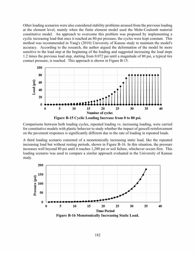
182

Other loading scenarios were also considered stability problems aroused from the previous loading at the element level, mainly when the finite element model used the Mohr-Coulomb material constitutive model. An approach to overcome this problem was proposed by implementing a cyclic increasing load that once it reached an 80-psi pressure, the cycles were kept constant. This method was recommended in Yang's (2010) University of Kansas study to maintain the model's accuracy. According to the research, the author argued the deformation of the model be more sensitive to the load step at the beginning of the loading and suggested increasing the load steps 1.2 times the previous load step, starting from 0.072 psi until a magnitude of 80 psi, a typical tire contact pressure, is reached. This approach is shown in Figure B-15.

Figure B-15 Cyclic Loading Increase from 0 to 80 psi. Comparisons between both loading cycles, repeated loading vs. increasing loading, were carried for constitutive models with plastic behavior to study whether the impact of geocell-reinforcement on the pavement responses is significantly different due to the rate of loading in repeated loads.

A third loading scenario consisted of a monotonically increasing static load, like the repeated increasing load but without resting periods, shown in Figure B-16. In this situation, the pressure increases well beyond 80 psi until it reaches 1,200 psi or soil failure, whichever occurs first. This loading scenario was used to compare a similar approach evaluated in the University of Kansas study.

Figure B-16 Monotonically Increasing Static Load.

183

B.6.4 Geocell-Reinforced Pavement with Geocell Panel Modeled Using Pseudo-SinusoidalPattern

A three-layered pavement structure was developed simulating a geocell-reinforced pavement structure used in the parametric study. The structure consisted of geocell-reinforced base material on top of the subgrade. Base material was placed on top of the geocell reinforced base as recommended for protection of the geocell. This model was modified to simulate different heights of the geocell and top cover for the parametric analysis. Geocell infill pockets were modeled using pseudo-sinusoidal curve shapes of the geocell honeycomb structure, as shown in Figure B-17. To model the geocell, shell elements were used while solid elements were implemented to model the soil of unreinforced layers and the infill soil material.

A quarter model was used to reduce the total number of elements, as symmetry conditions exist in the finite element model, as shown in Figure B-17a. The 8-node constant stress solid elements were selected for the modeling of the base and subgrade structures. These solid elements use one-point integration, and hourglass control was included. Considering the lattice pattern of geocell and its soil embedment in the base layer, proper element arrangement, and nodal connectivity are required to adjust to the geocell lattice pattern and avoid node penetration between the two different materials parts. The resulting mesh consisted of quad elements representing the geocell and a mix of solid hexahedral and prisms elements for the soil. As the reinforced layer was developed first, while the top unreinforced layer and subgrade were developed later, the element pattern of the geocell and infill material propagated through the upper and bottom layers, as seen in Figure B-17b. Dimensions of properties of the FE model are provided in Table B-8.

Figure B-17 Finite Element Model of Pavement Structure with Geocell Panel Simulated using Pseudo-Sinusoidal Shaped Cells: (a) Top View Highlighting Quarter Model and (b)

Embedding of Geocell Reinforcement in Base Material.

Both subgrade and base layers were modeled using the FHWA soil model, using the properties shown in Table 3-1 for the parametric study. In the parametric study, a haversine cyclic load of 80 psi (550 kPa), as shown in Figure B-13, was applied at the center of the geocell using a 10 in. diameter plate.

184

Table B-8 Dimensions and Properties of Geocell-Reinforced Pavement FE Model with Geocell Panel Simulated Using Pseudo-Sinusoidal Shaped Cells.

Pavement Structure Thickness Layers Geocell Reinforced

Pavement Structure Unreinforced

Pavement Structure

Top Base Layer (in.) Varying 1, 2, 3 and 4 Varying 1, 2, 3, and 4 Geocell Reinforced Base (in.) Varying 3, 4 and 6 Varying 3, 4 and 6 Subgrade (in.) 24 24

Finite Element Model Properties (Quarter Model) Number of Solid Elements 45,344 45,344 Number of Thick Shell Elements (Geocell) 1120 - Number of Discrete Beams 2568 - Total Number of Elements 49,032 45,344 Total Number of Nodes 52,547 52,547


B.7 SELECTION OF LOADING CONDITIONS: PLATE SIZE AND LOCATION

In all 3-D FE simulations shown in the parametric study are presented in Section 4. The cases used for developing and improving the model were applied at the center of the geocell, as shown in Figure B-18a. However, as per the TxDOT request, the load applied at the joint of the geocells, as shown in Figure 3-18b, has also been taken into consideration, and the analysis of the FE simulations with this type of loading arrangement will be shared with TxDOT after the analysis of the results is completed and summarized. In addition, different sizes of the load plates, i.e., 6 in., 9 in., and 12 in., were evaluated during the development of the model. Nevertheless, the FE models used for the parametric study presented in the “Parametric Study” later in this chapter for evaluating the benefit of geocell simulated a 9-in. diameter plate.

Figure B-18 Position of Load in the FE Model at (a) Center of Geocell and (b) Joint of Geocell.

185

B.8 RESULTS FROM PRELIMINARY INVESTIGATION: EVALUATION OF SOILMODELS AND SHELL ELEMENT TYPE FOR MODELING THE GEOCELL

B.8.1 Geocell-Reinforced Pavement with Geocell Panel Modeled Using Pseudo-SinusoidalPattern

B.8.1.1 Linear Elastic Model

The initial investigation consisted of modeling the base and subgrade layers as linear elastic materials. The geocell-reinforced infill material, consisting of base material, was modeled as linear elastic with properties shown in Table B-1. The FEM is simulating a geocell-reinforced pavement with geocell panel modeled using a rhomboidal pattern, as shown in Figure B-14 and with properties shown in Table B-7, was used for analyzing the behavior of the pavement layers.

Only one loading cycle was attempted in the linear elastic FE analysis, as other cycles would yield identical results as no plastic deformation occurs. The cycles, as mentioned previously, consisted of a loading period of 0.1 sec and a rest period of 0.9 sec, reaching a peak pressure of 80 psi, as shown in Figure B-13. Pavement responses were compared to those of unreinforced pavements with similar loading conditions.

The initial attempt using linear elastic material models failed to exhibit any significant difference in the responses between the geocell-reinforced pavements and their respective unreinforced cases. For instance, the plot is shown in Figure B-19 for a 5 ksi base layer and 5 ksi subgrade, and 6-in. diameter load plate applying a pressure of 80 ksi at the center of the cell no significant difference regarding deflection with respect to depth. Similar responses were obtained for all other loading scenarios and pavement distresses.

Figure B-19 Vertical Deflection along the Depth of the Pavement Structure. In addition to finding no significant effect of the geocell reinforcement, this model could not capture plastic deformation. This behavior was consistent with the findings previously carried in other numerical simulation studies using linear elastic materials where minimal or no significant

186

changes in distresses are observed when geocell reinforcement is included. Consequently, other material models were selected to accommodate plastic responses.

B.8.1.2 Mohr-Coulomb Material Model

As previously described, the Mohr-Coulomb is the best-known soil material model that can address the soil’s plastic behavior. Unlike the linear elastic model, the use of this model incites the inclusion of multiple loading cycles into the analysis to allow permanent deformation responses to occur in the soil. The properties used for evaluating this constitutive model are shown in Table B-2. The FE model of a geocell-reinforced pavement with a geocell panel modeled using arhomboidal pattern was used as the linear elastic model. The Mohr-Coulomb material modelprovided different soil responses when geocell reinforcement was included, as shown in Figure B-20. This figure shows the vertical stress of both pavements, geocell-reinforced and unreinforced,loaded with 12 in. diameter plates and a pavement structure comprised of a 5-ksi base and 5-ksisubgrade layers, both with the cohesion of 0.72 psi and friction angle of 40°. Fringe contours areset equal in both figures for better comparison purposes, and stress is expressed in Pascals (Pa).Significant higher stresses develop in the reinforced base that covers a wider area than in theunreinforced case. Lower stresses occur at the top of the subgrade in the reinforced pavement whencompared to the unreinforced one.

Figure B-20 Vertical Stress (z-direction) in (a) Geocell-Reinforced (b) Unreinforced Sections.

However, the use of this model became unstable after a few loading cycles, resulting in an abrupt termination of the analysis due to the excessive deformation. The number of cycles before the error depended heavily on the properties used in the analysis, with less stiff and more cohesive materials failing earlier. No material could resist failure beyond ten loading cycles. Figure B-20 shows indications of the elements prone to become unstable, mainly seen in the regions in darker blue along the surface of the soil, which by the way happen to be unloaded. In addition to this problem, large deformations occurred that seemed excessive when compared to other studies.

The problem encountered with this material model in LS-DYNA made its implementation unsuccessful. An attempt was made with ABAQUS to replicate the model. Despite apparent

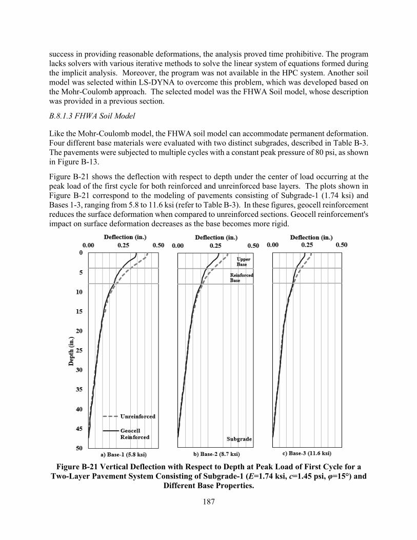
187

success in providing reasonable deformations, the analysis proved time prohibitive. The program lacks solvers with various iterative methods to solve the linear system of equations formed during the implicit analysis. Moreover, the program was not available in the HPC system. Another soil model was selected within LS-DYNA to overcome this problem, which was developed based on the Mohr-Coulomb approach. The selected model was the FHWA Soil model, whose description was provided in a previous section.

B.8.1.3 FHWA Soil Model

Like the Mohr-Coulomb model, the FHWA soil model can accommodate permanent deformation. Four different base materials were evaluated with two distinct subgrades, described in Table B-3. The pavements were subjected to multiple cycles with a constant peak pressure of 80 psi, as shown in Figure B-13.

Figure B-21 shows the deflection with respect to depth under the center of load occurring at the peak load of the first cycle for both reinforced and unreinforced base layers. The plots shown in Figure B-21 correspond to the modeling of pavements consisting of Subgrade-1 (1.74 ksi) and Bases 1-3, ranging from 5.8 to 11.6 ksi (refer to Table B-3). In these figures, geocell reinforcement reduces the surface deformation when compared to unreinforced sections. Geocell reinforcement's impact on surface deformation decreases as the base becomes more rigid.

Figure B-21 Vertical Deflection with Respect to Depth at Peak Load of First Cycle for a Two-Layer Pavement System Consisting of Subgrade-1 (E=1.74 ksi, c=1.45 psi, φ=15°) and

Different Base Properties.

188

Figure B-22 shows the decrease in surface deformation in terms of percent reduction between the unreinforced and reinforced sections with respect to the base modulus. As the modulus of the base layer improves, the effect of geocell reinforcement diminishes. The benefit of using a geocell-reinforced base layer was not evident when a good base quality material was used.

Figure B-22 Percentage Reduction in Surface Deformation with respect to Base Modulus for a Pavement with Subgrade-1 (E=1.74 ksi, c=1.45 psi, φ =15°) Material.

The implementation of the FHWA soil model proved to be successful in terms of reasonable deformations compared to the Mohr-Coulomb responses and considerably more stable too. The model is also prone to encounter issues with respect to element stability after several loading cycles. However, in some instances, the model behaved reasonably well up to 200 cycles, where just one element located right under the center of the load suffered excessive deformation that caused an error in the execution. Despite this issue, the model provided enough cyclic responses to visualize the permanent deformation behavior of the pavement. To overcome the problem arising from the instability of the elements, a ramp-like increasing repeated loading until a pressure of 80 psi is reached, as shown in Figure B-15, was adopted and compared to the repeated loading with no change in the loading pattern and magnitude.

To see the effect of the loading condition on the permanent response behavior of the pavement structure due to these two different loading cycles, a pavement with weak mechanical properties like those used in the University of Kansas, as shown in Table B-4, was modeled. The permanent deformation due to the first loading scenario (Figure B-13), which consisted of the repeated 80 psi loads, is shown in Figure B-23. In contrast, the permanent deformation of the second loading scenario (Figure B-15) is shown in Figure B-24 for both reinforced and unreinforced sections.

Figure B-23 Permanent Deformation for Geocell-Reinforced and Unreinforced Pavement Sections using FHWA Soil Model Properties: Kansas River Sand base (E=0.48 ksi, c=0, φ=41°) and Clay Subgrade (E=1.5 ksi, c=15.2 psi, φ =0°) and Repeated 80 psi Loading.

-0.40

-0.30

-0.20

-0.10

0.000 1 2 3 4 5 6 7 8 9 10

Perm

anen

t D

efor

mat

ion

(in.)

Number of Cycles

Geocell ReinforcedUnreinforced

189

Figure B-24 Permanent Deformation for Geocell-Reinforced and Unreinforced Pavement Sections using FHWA Soil Model Properties: Kansas River Sand base (

-0.40

-0.30

-0.20

-0.10

0.000 5 10 15 20 25 30 35 40

Perm

anen

t Def

orm

atio

n (in

.)

Number of Cycles

Geocell Reinforced

Unreinforced

E=0.48 ksi, c=0, φ=41°) and Clay Subgrade (E=1.5 ksi, c=15.2 psi, φ =0°) and Increasing Repeated Loading

Reaching 80 psi Followed by 80 psi Repeated Loads. The results summarized in Figure B-23 indicate that higher permanent deformation is observed within the initial cycles (first two cycles) when a constant repeated load of 80 psi (Figure B-13) is applied to the pavement. However, the benefit of geocell reinforcement is observed after the application of three or more cyclic loads. On the other hand, the increasing repeated load (Figure B-15) indicates that the permanent deformation is independent of reinforcement (Figure B-24).

For further comparison, the permanent deformation data for both loading scenarios are summarized in Figure 3-25. In this figure, the surface displacements during the earlier cycles are not comparable, as the increasing cyclic loading already amounted to given permanent deformation of about 0.30 in. However, after a few 80 psi cycles, the responses of both loading scenarios approach each other, indicating that there is no need to initiate the loading cycles from low magnitudes but instead start with an 80-psi magnitude. Furthermore, no evidence was found that ramping the repeated loads made the model more stable by extending the analysis in cycles before reaching an error termination due to excessive element deformation. Moreover, and most importantly, time is saved as the ramping to reach a pressure of 80 psi (about 30 cycles) requires analyses times of about 30 hours using the HPC system. Additional discussion about execution times and problems encountered during the modeling are provided in a later section.

Figure B-25 Impact of Ramp Loading on Permanent Deformation for Geocell-Reinforced and Unreinforced Pavement Sections using Kansas River Sand Base and Clay Subgrade.

-0.40

-0.30

-0.20

-0.10

0.000 1 2 3 4 5 6 7 8 9 10

Perm

anen

t D

efor

mat

ion

(in.)

Number of Cycles

Geocell reinforced_increasing loadUnreinforced_increasing loadGeocell reinforced_constant loadUnreinforced_contant load

190

B.8.2 Comparison to University of Kansas Model

A complete comparison of the responses using the FHWA soil model with those of the numerical modeling developed at the University of Kansas was carried to check the behavior of our model with respect to the Duncan-Chang model used in their study. The properties used in their model, shown in Table B-4, were adapted to the FHWA constitutive soil model. Following similar loading conditions, a monotonically increasing load was applied to our model.

For comparison, the pressure to surface displacement curves for both unreinforced and geocell-reinforced sections was developed and are shown in Figure B-26. From Figure B-26a, showing the surface displacements for the FHWA soil model, a significant difference in surface displacements between the reinforced and unreinforced section can be seen after the pressure of 500 kPa (72 psi) is reached. This behavior occurs earlier, at about 200 kPa (29 psi), when the Duncan-Chang model is used (Figure B-26b). However, both responses agree on the benefit of using geocell reinforcement for very weak unbound aggregate materials. Both responses are not similar, and the reason behind this is due to the different soil models used and possibly to distinct rates of loading. SI units are shown in Figure B-26, as the results provided in Yang (2010) used this unit system.

Figure B-26 Pressure to Surface Displacement Curves for Unreinforced and Geocell-Reinforced Sections using (a) FHWA Constitutive Soil Model and (b) Duncan Chang

Constitutive Model used in the University of Kansas Study (after Yang, 2010). B.8.3 Preliminary Evaluation of Contact

The development of the 3-D FE model of the geocell-reinforced pavement used to evaluate the most appropriate constitutive model for simulating the permanent deformation of geomaterials described in the previous section brought forth different problems during the simulation. Some of the issues were related to the contact between the geocell simulated with shell elements and the infill material simulated with solid elements.

One of the conditions required by LS-DYNA for modeling the contact between the shell and solid elements is the need to have an offset between the shell and the solid elements to avoid overlapping nodes between the two types of elements. This implies that two nodes cannot share the same coordinate and that a gap must be considered to account for the shell thickness provided by the user. This helps the contact model's search algorithm find nodes' penetrations and establish contact between nodes. If the user does not correct this, LS-DYNA will automatically adjust the nodes by

191

changing the coordinates before the analysis, leading to overlapping the elements at the contact. This issue is seen markedly at the joints in our preliminary finite element models, as shown in Figure B-27.

Figure B-27 Node Penetration and Overlapping of Element at the Joints. To correct this problem, a gap was included between the soil infill and the geocell on both sides of the geocell, as shown in Figure B-28a. In addition, a separation between the cell infill material was modeled to accommodate a 1 mm thick geocell modeled using shell elements, as shown in Figure B-28b.

Figure B-28 (a) Top View of FE Model Showing Nodal Unbonding to Accommodate Geocell and (b) Zoomed in View at Joint Showing Infill Material and Geocell Modeled

using Shell Elements. B.8.4 Evaluation of Geocell Shape: Geocell Panel Simulated with Rhomboidal Pattern

During the evaluation of the most appropriate constitutive model for modeling the base and subgrade materials, the geocell panel was modeled using a rhomboidal pattern with an automatic surface to surface contact model between the infill soil and the geocell. In addition, a tied contact interface was provided between the geocell and the interfaced above and below the geocell reinforced base, i.e., the top cover and the subgrade, respectively. The rationale to use a tied contact interface between layers was to allow full transfer of stress from the upper to the lower soil layer. After some load cycles, the geocell tarted to experience an unstable behavior, which varied

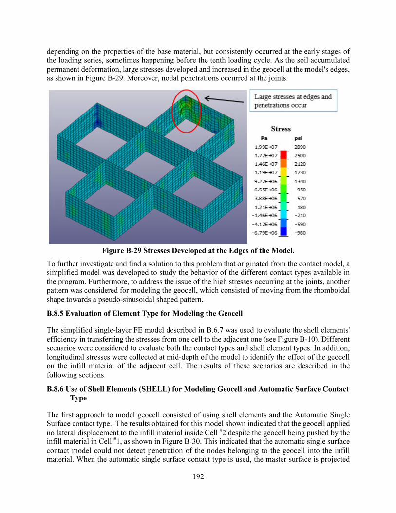
192

depending on the properties of the base material, but consistently occurred at the early stages of the loading series, sometimes happening before the tenth loading cycle. As the soil accumulated permanent deformation, large stresses developed and increased in the geocell at the model's edges, as shown in Figure B-29. Moreover, nodal penetrations occurred at the joints.

Figure B-29 Stresses Developed at the Edges of the Model. To further investigate and find a solution to this problem that originated from the contact model, a simplified model was developed to study the behavior of the different contact types available in the program. Furthermore, to address the issue of the high stresses occurring at the joints, another pattern was considered for modeling the geocell, which consisted of moving from the rhomboidal shape towards a pseudo-sinusoidal shaped pattern.

B.8.5 Evaluation of Element Type for Modeling the Geocell

The simplified single-layer FE model described in B.6.7 was used to evaluate the shell elements' efficiency in transferring the stresses from one cell to the adjacent one (see Figure B-10). Different scenarios were considered to evaluate both the contact types and shell element types. In addition, longitudinal stresses were collected at mid-depth of the model to identify the effect of the geocell on the infill material of the adjacent cell. The results of these scenarios are described in the following sections.

B.8.6 Use of Shell Elements (SHELL) for Modeling Geocell and Automatic Surface ContactType

The first approach to model geocell consisted of using shell elements and the Automatic Single Surface contact type. The results obtained for this model shown indicated that the geocell applied no lateral displacement to the infill material inside Cell #2 despite the geocell being pushed by the infill material in Cell #1, as shown in Figure B-30. This indicated that the automatic single surface contact model could not detect penetration of the nodes belonging to the geocell into the infill material. When the automatic single surface contact type is used, the master surface is projected

193

based on normal nodal vectors; thus, the algorithm of the contact type was unable to detect node penetration in the direction opposite to the normal vector of the shell elements. Therefore, no longitudinal stresses developed on Cell #2 or Cell #3, as shown in Figure B-31. The Automatic Surface-to-Surface contact type has similar limitations and runs into the same problem. The use of shell elements and automatic surface contact types proved inadequate for modeling geocell reinforcement embedded in soil material when solid elements constrain the two sides of the shell elements.

Figure B-30 Longitudinal Displacement (dx) at 10th Loading Cycle after FE model with Geocell using Shell Elements and Automatic Single Surface Contact Element.

Figure B-31 Vertical Stress (Δx) at 10th Loading Cycle after FE Model with Geocell using Shell Elements and Automatic Single Surface Contact Element.

B.8.7 Use of Thick Shell Elements for Modeling Geocell and Automatic Surface ContactType

The second approach to model geocell reinforcement consisted of using thick shell elements, identified by LS-DYNA as TSHELL, and the Automatic Surface to Surface contact type. In this case, lateral displacement transferred from Cell #1 to Cell #2 through the geocell and Cell #2 to Cell #3 to a lesser extent, as shown in Figure B-32. Likewise, stresses transferred through the geocell from Cell #1 to Cell #2, as shown in Figure B-33. For this purpose, TSHELL proved to provide meaningful results in conjunction with the Automatic Surface to the Surface contact type.

194

Figure B-32 Longitudinal Displacement (dx) at 1st Loading Cycle after FE Model with Geocell using Thick Shell Elements and Automatic Single Surface Contact Element.

Figure B-33 Vertical Stress (σx) at 1st Loading Cycle after FE Model with Geocell using Thick Shell Elements and Automatic Single Surface Contact Element.

With similar results, thick shell elements could be used with both automatic surface to surface or automatic single surface contact types. However, a disadvantage in using thick shell elements is that the analysis time increases considerably as thick shells are more computationally expensive than traditional ones. The critical time steps Δte,crit for shells and thick shells are provided in Equations 3.8 and 3.9, respectively as:

For shell elements

,max

e crits

Atc l

∆ =

B-8For thick shell elements

,ele,max

elee crit

b

Vtc A

∆ =

B-9

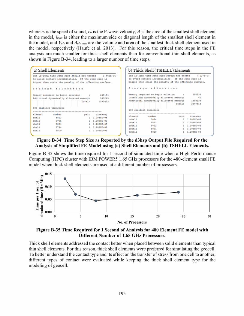
195

where cs is the speed of sound, cb is the P-wave velocity, A is the area of the smallest shell element in the model, lmax is either the maximum side or diagonal length of the smallest shell element in the model, and Vele and Aele,max are the volume and area of the smallest thick shell element used in the model, respectively (Haufe et al. 2013). For this reason, the critical time steps in the FE analysis are much smaller for thick shell elements than for conventional thin shell elements, as shown in Figure B-34, leading to a larger number of time steps.

Figure B-34 Time Step Size as Reported by the d3hsp Output File Required for the Analysis of Simplified FE Model using (a) Shell Elements and (b) TSHELL Elements.

Figure B-35 shows the time required for 1 second of simulated time when a High-Performance Computing (HPC) cluster with IBM POWER5 1.65 GHz processors for the 480-element small FE model when thick shell elements are used at a different number of processors.

Figure B-35 Time Required for 1 Second of Analysis for 480 Element FE model with Different Number of 1.65 GHz Processors.

0:00

0:05

0:10

0:15

0 5 10 15 20 25 30

Tim

e pe

r 1

sec.

of

sim

ulat

ed ti

me

(Hr:

Min

)

No. of Processors

Thick shell elements addressed the contact better when placed between solid elements than typical thin shell elements. For this reason, thick shell elements were preferred for simulating the geocell. To better understand the contact type and its effect on the transfer of stress from one cell to another, different types of contact were evaluated while keeping the thick shell element type for the modeling of geocell.

196

B.9 EVALUATION OF CONTACT TYPE FOR SOIL-GEOCELL INTERFACE

B.9.1 Assessment of Contact Type Using Simplified Single-Layer Model

To better address the behavior and interaction of the geocell with soil, several contact types were evaluated using the same small FE model described in the previous section. This model was developed to check the efficiency of the contact type on transferring the stresses from one cell to the adjacent one through the geocell. Likewise, as shown in Figure B-11, ten loading cycles were simulated with a peak pressure load of 40 psi on a 6-in. diameter load, and the soil had properties of sand as described in Table B-1. To evaluate the contact type and geocell on the infill material of the adjacent cell, longitudinal and vertical stresses were collected at mid-depth of the model, as shown in Figure B-10.

Three contact types were evaluated:

a) Automatic Surface-to-Surface Contact,b) Automatic Single Surface Contact, andc) Springs (discrete beam elements).

The responses obtained at the specified locations for the simplified models with these types of contacts were compared to those obtained by other simplified models with no geocell reinforcement (no implementation of shell elements) and different contact scenarios. In addition, the responses using the BISAR computer program based on layer elastic theory are provided for comparison purposes. The following FE models were used for comparing the responses of the geocell reinforced material.

A linear elastic model based on the relationships developed by Boussinesq and implemented in BISAR. All FE models are based on three individual infill cells separated by geocell, as shown in Figure B-36. Contact type and element used for modeling geocell vary depending on the following conditions: a) FHWA Soil: FEM simulates only soil material with no geocell separating the infill cells. No

interaction of geocell to soil is required. FHWA soil model is used.b) Automatic Surface Contact Soil to Soil: an FE unreinforced model using FHWA soil model for

the base material, simulating three individual infill cells (no geocell) connected only with anautomatic surface-to-surface contact type (automatic single surface offers identical results).

c) SOLID Geocell + Automatic Single Surface: FEM simulates three individual infill cellsseparated by geocell simulated with brick elements (instead of shell elements) and connectedwith an automatic single surface contact type (automatic surface-to-surface offers identicalresults).

d) TSHELL Geocell + Fully Bonded: a geocell-reinforced FE model with fully bonded conditionsbetween geocell and soil. Geocell simulated using thick shell (TSHELL) elements.

e) TSHELL Geocell + Automatic Single Surface: FEM simulates three individual infill cellsseparated by geocell simulated with thick shell elements (TSHELL) and connected with anautomatic single surface contact type (automatic surface-to-surface offers identical results).

f) Spring: kn = 57 lb/in, kt = 5.7 lb/in FE model simulating three individual infill cells separatedby geocell simulated with the thick shell (TSHELL) elements and connected with springs withnormal stiffness kn = 57 lb/in and tangential stiffness kt = 5.7 lb/in.

197

g) Spring: kn = 570 lb/in, kt = 5.7 lb/in FE model simulating three individual infill cells separatedby geocell simulated with thick shell (TSHELL) elements and connected with springs withnormal stiffness kn = 570 lb/in and tangential stiffness kt = 5.7 lb/in.

These models are summarized along with their characteristics in Table B-9.

Figure B-36 Simplified FE Model with Highlighted Elements used for Evaluating the Stress Transfer Through Contact and Geocell.

Table B-9 Summary of Numerical Models Used for Evaluating Contact Types.

Type of Model Analysis Type Geocell Geocell-Soil Interaction

Layer Elastic Theory

Finite Element Element Type Contact Type

1. Linear Elastic (BISAR) - - 2. FHWA Soil No No

3. Aut. Surf. Contact Soil to Soil* No Automatic Surface to Surface

4. SOLID Geocell + Automatic Single Surf. * Brick (Solid) Automatic Surface to Surface

5. TSHELL Geocell + Fully Bonded Thick Shell No 6. TSHELL Geocell + Automatic SingleSurf. * Thick Shell Automatic Surface to

Surface 7. Spring: kn = 57 lb/in, kt = 5.7 lb/in Thick Shell Spring 8. Spring: kn = 570 lb/in, kt = 5.7 lb/in Thick Shell Spring * Automatic Surface to Surface contact type yielded similar results to Automatic Single Surface.

Table B-10 summarizes the soil responses regarding the longitudinal stress, σx, and vertical stress, σy, at mid-height of the base layer as reported by the analysis of the simplified FE models and linear elastic theory at the locations:

• Edge of Cell#1 in contact with geocell• Edge of Cell#2 in contact with geocell (see Figure B-36).• This table shows that the inclusion of geocell caused a decrease in stress at the elements

adjacent to the cells compared to the values obtained from the FE model with no geocell.Moreover, the magnitude of the stress of the elements adjacent to the geocell when thegeocell is modeled as a thick shell is somewhat like those obtained after the geocell ismodeled as a solid element. The use of geocell also caused a decrease in magnitude instress at the element belonging to the second cell, and vertical stress decreased in theelement belonging to Cell #1, next to the geocell.

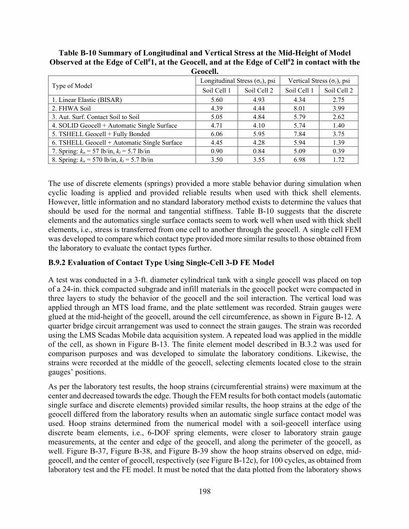
198

Table B-10 Summary of Longitudinal and Vertical Stress at the Mid-Height of Model Observed at the Edge of Cell#1, at the Geocell, and at the Edge of Cell#2 in contact with the

Geocell.

Type of Model Longitudinal Stress (σx), psi Vertical Stress (σz), psi Soil Cell 1 Soil Cell 2 Soil Cell 1 Soil Cell 2

1. Linear Elastic (BISAR) 5.60 4.93 4.34 2.75 2. FHWA Soil 4.39 4.44 8.01 3.99 3. Aut. Surf. Contact Soil to Soil 5.05 4.84 5.79 2.62 4. SOLID Geocell + Automatic Single Surface 4.71 4.10 5.74 1.40 5. TSHELL Geocell + Fully Bonded 6.06 5.95 7.84 3.75 6. TSHELL Geocell + Automatic Single Surface 4.45 4.28 5.94 1.39 7. Spring: kn = 57 lb/in, kt = 5.7 lb/in 0.90 0.84 5.09 0.39 8. Spring: kn = 570 lb/in, kt = 5.7 lb/in 3.50 3.55 6.98 1.72

The use of discrete elements (springs) provided a more stable behavior during simulation when cyclic loading is applied and provided reliable results when used with thick shell elements. However, little information and no standard laboratory method exists to determine the values that should be used for the normal and tangential stiffness. Table B-10 suggests that the discrete elements and the automatics single surface contacts seem to work well when used with thick shell elements, i.e., stress is transferred from one cell to another through the geocell. A single cell FEM was developed to compare which contact type provided more similar results to those obtained from the laboratory to evaluate the contact types further.

B.9.2 Evaluation of Contact Type Using Single-Cell 3-D FE Model

A test was conducted in a 3-ft. diameter cylindrical tank with a single geocell was placed on top of a 24-in. thick compacted subgrade and infill materials in the geocell pocket were compacted in three layers to study the behavior of the geocell and the soil interaction. The vertical load was applied through an MTS load frame, and the plate settlement was recorded. Strain gauges were glued at the mid-height of the geocell, around the cell circumference, as shown in Figure B-12. A quarter bridge circuit arrangement was used to connect the strain gauges. The strain was recorded using the LMS Scadas Mobile data acquisition system. A repeated load was applied in the middle of the cell, as shown in Figure B-13. The finite element model described in B.3.2 was used for comparison purposes and was developed to simulate the laboratory conditions. Likewise, the strains were recorded at the middle of the geocell, selecting elements located close to the strain gauges’ positions.

As per the laboratory test results, the hoop strains (circumferential strains) were maximum at the center and decreased towards the edge. Though the FEM results for both contact models (automatic single surface and discrete elements) provided similar results, the hoop strains at the edge of the geocell differed from the laboratory results when an automatic single surface contact model was used. Hoop strains determined from the numerical model with a soil-geocell interface using discrete beam elements, i.e., 6-DOF spring elements, were closer to laboratory strain gauge measurements, at the center and edge of the geocell, and along the perimeter of the geocell, as well. Figure B-37, Figure B-38, and Figure B-39 show the hoop strains observed on edge, mid-geocell, and the center of geocell, respectively (see Figure B-12c), for 100 cycles, as obtained from laboratory test and the FE model. It must be noted that the data plotted from the laboratory shows

199

only the responses at peak loading, while the FE model data shows the responses at the peak and rest period as well.

The measured strains at the edge of geocell observed were in the range of 240 μɛ. The FEM model generated strains in the range of 290 με during loading and 180 με during the rest period. The key difference in the results was the elastic strain in the FEM model, which was higher than the laboratory results. The difference in responses could be attributed to the impossibility of achieving zero loads during unloading in the lab testing for each cycle and geocell characterized as a perfectly elastic material in the FE model. Similar behavior can be observed in the responses at mid-geocell and the center of geocell.

Based on the similarity of the results provided by the geocell in the single-cell FEM with the laboratory results, it was decided to use to expand this model to simulate the honeycomb pattern of the geocell. This suggests that the discrete elements were used as a contact type, thick shell elements were used to simulate the geocell, and a pseudo-sinusoidal pattern was used for modeling the geocell panel, as shown in Figure B-17. The resulting model is described in Table B-8 and was used for carrying a parametric study for evaluating the effect of geocell on the pavement responses.

Figure B-37 Hoop Strains at Edge of Geocell for (a) Laboratory and (b) FEM.

0

200

400

600

800

0 20 40 60 80Cycles

0

200

400

600

800

0 20 40 60 80Cycles

Stra

in (µ

ε)

Stra

in (µ

ε)

b) a)

0

200

400

600

0 20 40 60 80Cycles

Stra

in (µ

ε)

a)

0

200

400

600

0 20 40 60 80Cycles

Stra

in (µ

ε)

b)

Figure B-38 Hoop Strains at Mid-Geocell for (a) Laboratory and (b) FEM.

200

Figure B-39 Strains at Center of Geocell for (a) Laboratory and (b) FEM.

0

200

400

600

0 20 40 60 80Cycles

0

200

400

600

0 20 40 60 80

Stra

in (µ

ε)

Stra

in (µ

ε)

Cycles

b) a)

201

APPENDIX C: GEOCELL INFORMATION

Figure C-1 Tenax Geocell Properties.

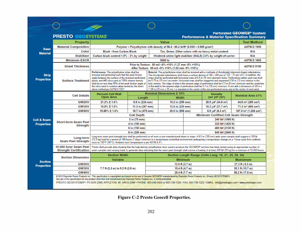
https://www.tenax.net/wp-content/uploads/2017/11/Data_Sheet_TENAX_TENWEB_e.pdf

202

Figure C-2 Presto Geocell Properties.

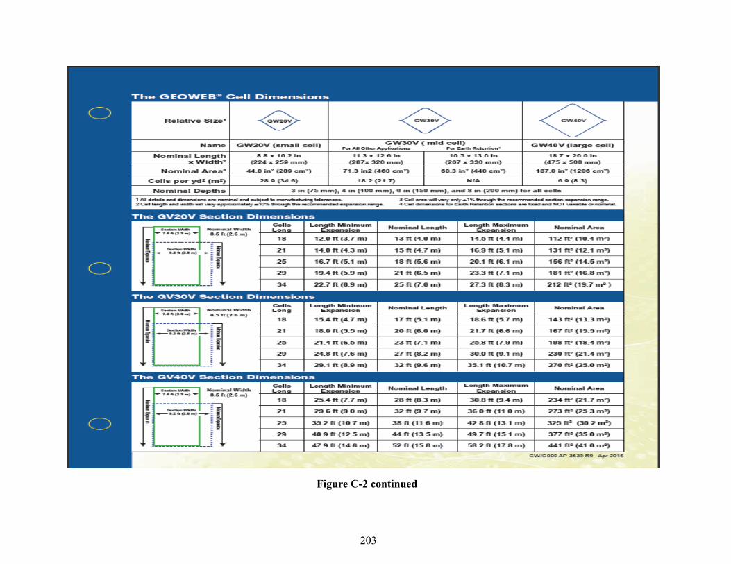
https://www.prestogeo.com/design/soil-stabilization/geoweb-general-design/

Figure C-2 continued

203

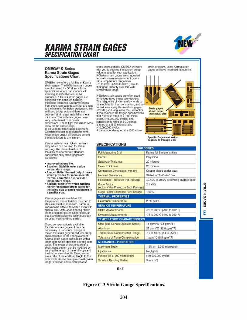
204

Figure C-3 Strain Gauge Specifications.

https://in.omega.com/techref/pdf/STRAIN_GAGE_TECHNICAL_DATA.pdf

205

Figure C-3 continued.

206

Figure C-4 Pressure Cell Specifications.

207

Figure C-4 continued.

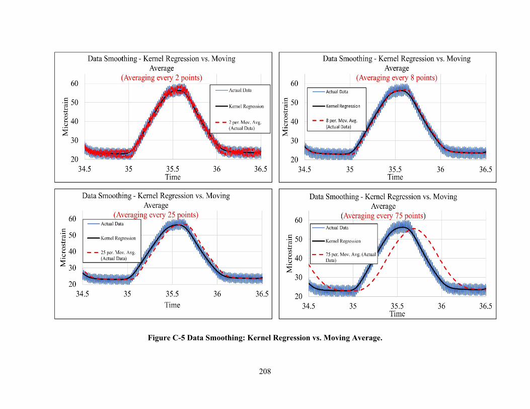
208

Figure C-5 Data Smoothing: Kernel Regression vs. Moving Average.

209

APPENDIX D

Table D-1 Raw Data Geocell Height (in.)

Infill Modulus (ksi)

Cover Thickness (in.)

Subgrade Modulus (ksi)

Percentage Reduction of Vertical Stress on Subgrade Top Below the Center of Loading Plate

4 3 6 4.5 16 4 5 6 4.5 19 4 7 6 4.5 11 4 9 6 4.5 20 4 12 6 4.5 24 4 15 6 4.5 11 4 30 6 4.5 4 6 3 4 4.5 39 6 5 4 4.5 30 6 7 4 4.5 21 6 9 4 4.5 20 6 12 4 4.5 21 6 15 4 4.5 20 4 7 6 6 15 4 12 6 6 17 4 15 6 6 17 4 20 6 6 9 4 30 6 6 27 4 12 6 9 20 4 15 6 9 17 4 20 6 9 15 4 30 6 9 4 4 15 6 15 20 4 20 6 15 14 4 30 6 15 22 3 3 4 4.5 2 3 9 4 4.5 5 3 15 4 4.5 4 3 30 4 4.5 2 4 12 6 8 20 4 12 6 3 17 4 12 2 4.5 21 6 7 4 6 22

210

6 12 4 6 18 6 15 4 6 19 6 20 4 6 9 6 30 4 6 12 6 12 4 9 21 6 15 4 9 15 6 30 4 9 5 6 15 4 12 11 6 20 4 12 11 6 30 4 12 14 3 5 4 2.5 1 3 7 4 2.5 5 3 12 4 2.5 13 3 15 4 2.5 7 3 20 4 2.5 2 3 7 4 6 5 3 12 4 6 14 3 15 4 6 8 3 12 4 9 1 3 15 4 9 3 3 20 4 9 5 3 15 4 15 3 3 20 4 15 3 6 30 4 4.5 9 6 20 4 9 17

211

Table D-2 Training Data Set LOOV-CV Sample no Geocell

Height (in.) Infill Modulus (ksi)


% Reduction in Stress

1 4 3 6 16 3 4 7 6 11 4 4 9 6 20 5 4 12 6 24 6 4 15 6 11 7 4 30 6 4 8 6 3 4 39 9 6 5 4 30

11 6 9 4 20 12 6 12 4 21 14 4 7 6 15 15 4 12 6 17 17 4 20 6 9 18 4 12 6 20 20 4 20 6 15 21 4 30 6 4 22 4 15 6 20 23 4 20 6 14 25 3 9 4 5.3 26 3 15 4 3.9 27 3 30 4 1.8 28 4 12 6 20 29 4 12 6 17 30 4 12 2 21 31 6 7 4 22 32 6 12 4 18 33 6 15 4 19 35 6 30 4 12 37 6 15 4 15 39 6 15 4 11 40 6 20 4 11 41 6 30 4 14 42 3 5 4 1 43 3 7 4 5 44 3 12 4 13 47 3 7 4 5 48 3 12 4 14 49 3 15 4 8 50 3 12 4 1 51 3 15 4 3 52 3 20 4 5 53 3 15 4 3 54 3 20 4 3 56 6 20 4 17

212

Table D-3 Testing Data Set LOOV-CV

Sample no Geocell Height (in.)




2 4 5 6 19 10 6 7 4 21 13 6 15 4 20 16 4 15 6 17 19 4 15 6 17 24 3 3 4 2 34 6 20 4 9 36 6 12 4 21 38 6 30 4 5 45 3 15 4 7 46 3 20 4 2 55 6 30 4 9 2 4 5 6 19 10 6 7 4 21 13 6 15 4 20

213

Table D-4 Training Data Set KK FOLD CV

Sample no Geocell Height (in.)




1 4 3 6 16 2 4 5 6 19 5 4 12 6 24 6 4 15 6 11 7 4 30 6 4 8 6 3 4 39 9 6 5 4 30

11 6 9 4 20 12 6 12 4 21 13 6 15 4 20 14 4 7 6 15 16 4 15 6 17 19 4 15 6 17 20 4 20 6 15 21 4 30 6 4 22 4 15 6 20 23 4 20 6 14 24 3 3 4 2 25 3 9 4 5.3 26 3 15 4 3.9 27 3 30 4 1.8 28 4 12 6 20 29 4 12 6 17 30 4 12 2 21 31 6 7 4 22 33 6 15 4 19 34 6 20 4 9 35 6 30 4 12 36 6 12 4 21 37 6 15 4 15 39 6 15 4 11 40 6 20 4 11 41 6 30 4 14 42 3 5 4 1 43 3 7 4 5 44 3 12 4 13 46 3 20 4 2 47 3 7 4 5 48 3 12 4 14 49 3 15 4 8 51 3 15 4 3 52 3 20 4 5 53 3 15 4 3 55 6 30 4 9

214

Table D-5 Testing Data Set KK FOLD CV Sample no Geocell Height

(in.) Infill Modulus (ksi)



3 4 7 6 11 4 4 9 6 20 10 6 7 4 21 15 4 12 6 17 17 4 20 6 9 18 4 12 6 20 32 6 12 4 18 38 6 30 4 5 45 3 15 4 7 50 3 12 4 1 54 3 20 4 3 56 6 20 4 17 3 4 7 6 11 4 4 9 6 20 10 6 7 4 21

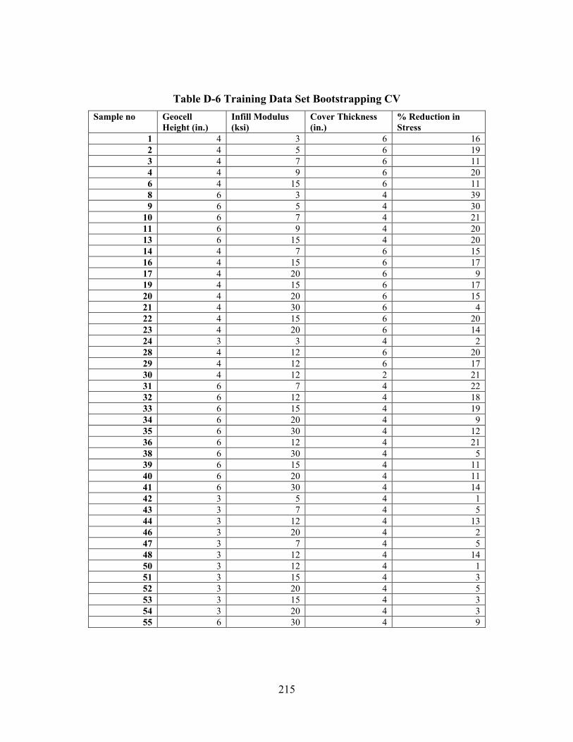
215

Table D-6 Training Data Set Bootstrapping CV Sample no Geocell

Height (in.) Infill Modulus (ksi)



1 4 3 6 16 2 4 5 6 19 3 4 7 6 11 4 4 9 6 20 6 4 15 6 11 8 6 3 4 39 9 6 5 4 30

10 6 7 4 21 11 6 9 4 20 13 6 15 4 20 14 4 7 6 15 16 4 15 6 17 17 4 20 6 9 19 4 15 6 17 20 4 20 6 15 21 4 30 6 4 22 4 15 6 20 23 4 20 6 14 24 3 3 4 2 28 4 12 6 20 29 4 12 6 17 30 4 12 2 21 31 6 7 4 22 32 6 12 4 18 33 6 15 4 19 34 6 20 4 9 35 6 30 4 12 36 6 12 4 21 38 6 30 4 5 39 6 15 4 11 40 6 20 4 11 41 6 30 4 14 42 3 5 4 1 43 3 7 4 5 44 3 12 4 13 46 3 20 4 2 47 3 7 4 5 48 3 12 4 14 50 3 12 4 1 51 3 15 4 3 52 3 20 4 5 53 3 15 4 3 54 3 20 4 3 55 6 30 4 9

216

Table D-7 Testing Data Set Bootstrapping CV Sample no Geocell Height

(in.) Infill Modulus (ksi)



5 4 12 6 24 7 4 30 6 4

12 6 12 4 21 15 4 12 6 17 18 4 12 6 20 25 3 9 4 5.3 26 3 15 4 3.9 27 3 30 4 1.8 37 6 15 4 15 45 3 15 4 7 49 3 15 4 8 56 6 20 4 17

217

D.1 PAIRED T-TEST Use the paired t-test to determine whether the difference between sample means for paired data is significantly different from the hypothesized difference between population means.

Null Hypothesis: 𝜇𝜇𝑟𝑟 = 𝐷𝐷

Alternative Hypothesis: 𝜇𝜇𝑟𝑟 ≠ 𝐷𝐷

Where 𝜇𝜇𝑟𝑟 𝑖𝑖𝑠𝑠 the true difference in population values, and D is hypothesized value.

D.1.1 Procedure Using sample data, find the standard deviation, standard error, degrees of freedom, test statistic, and the P-value associated with the test statistic.

Step 1: Compute the standard deviation (sd) of the differences computed from n matched pairs.

sd = sqrt [ (Σ(di - d)2 / (n - 1) ] D-1

where di is the difference for pair i, d is the sample mean of the differences, and n is the number of paired values.

Step 2: Standard error. Compute the standard error (SE) of the sampling distribution of d.

SE = sd * sqrt{ ( 1/n ) * [ (N - n) / ( N - 1 ) ] } D-2

where sd is the standard deviation of the sample difference, N is the number of matched pairs in the population, and n is the number of matched pairs. When the population size is much larger (at least 20 times larger) than the sample size, the standard error can be approximated by: SE = sd/sqrt ( n )

Degrees of freedom. The degree of freedom (DF) is DF = n - 1.

Step 3: Test statistics. The test statistic is a t-statistic (t) defined by the following equation.

t = [ (x1 - x2) - D ] / SE = (d - D) / SE D-3

where x1 is the mean of sample 1, x2 is the mean of sample 2, d is the mean difference between paired values in the sample, D is the hypothesized difference between population means, and SE is the standard error.

Step 4: The P-value is the probability of observing a sample statistic as extreme as the test statistic. Since the test statistic is a t-statistic, use the t Distribution Calculator to assess the probability associated with the t statistic, having the degrees of freedom computed above. Interpret Results

218

Step 5: If the sample findings are unlikely, given the null hypothesis, the researcher rejects the null hypothesis. Typically, this involves comparing the P-value to the significance level and rejecting the null hypothesis when the P-value is less than the significance level.

D.2 PEARSON CORRELATION Pearson’s correlation coefficient measures the strength of the linear relationship between two sets of variables. Correlation coefficient:

𝑟𝑟 = ∑(𝑒𝑒 − �̅�𝑒)(𝑦𝑦 − 𝑦𝑦�)

(𝑡𝑡 − 1)𝑠𝑠𝑥𝑥𝑠𝑠𝑦𝑦

D-4

Characteristics:

1. Shows the direction and strength of the linear relationship between two variables 2. Can assume any value from -1.00 to +1.00 3. When 𝑟𝑟 = 0, this indicates there is no linear relationship between the variables. 4. When 𝑟𝑟 ≈ 0, this indicates a weak linear relationship between the variables. 5. When 𝑟𝑟 ≈ 1, this indicates a direct or positive linear relationship between the variables. 6. When 𝑟𝑟 ≈ −1, this indicates an inverse or negative linear relationship between the

variables.

http://stattrek.com/Help/Glossary.aspx?Target=Significance%20level

Use of Geocell in Pavement Design: Final Report

Documents