Use of computational fluid dynamics as a tool for …€¦ · Use of Computational Fluid Dynamics as a Tool for Establishing Process Design Space for Mixing in a Bioreactor A. S.

Use of Computational Fluid Dynamics as a Tool for Establishing Process Design

Space for Mixing in a Bioreactor

A. S. Rathore, C. Sharma, and A. PersadDept. of Chemical Engineering, Indian Institute of Technology, Hauz Khas, New Delhi, India

DOI 10.1002/btpr.745Published online November 14, 2011 in Wiley Online Library (wileyonlinelibrary.com).

The concept of ‘‘design space’’ plays an integral part in implementation of quality bydesign for pharmaceutical products. ICH Q8 defines design space as ‘‘the multidimensionalcombination and interaction of input variables (e.g., material attributes) and process param-eters that have been demonstrated to provide assurance of quality. Working within thedesign space is not considered as a change. Movement out of the design space is consideredto be a change and would normally initiate a regulatory post-approval change process.Design space is proposed by the applicant and is subject to regulatory assessment and ap-proval.’’ Computational fluid dynamics (CFD) is increasingly being used as a tool for mod-eling of hydrodynamics and mass transfer. In this study, a laboratory-scale aeratedbioreactor is modeled using CFD. Eulerian-Eulerian multiphase model is used along withdispersed k–e turbulent model. Population balance model is incorporated to account forbubble breakage and coalescence. Multiple reference frame model is used for the rotatingregion. We demonstrate the usefulness of CFD modeling for evaluating the effects of typicalprocess parameters like impeller speed, gas flow rate, and liquid height on the mass transfercoefficient (kLa). Design of experiments is utilized to establish a design space for the abovementioned parameters for a given permissible range of kLa. VVC 2011 American Institute ofChemical Engineers Biotechnol. Prog., 28: 382–391, 2012Keywords: computational fluid dynamics, mixing, bioreactor, stirred tank, mass-transfercoefficient, agitation, design space, QbD, design of experiments

Introduction

Aerated stirred reactors are the most common type of bio-reactors used for performing microbial fermentation or mam-malian cell culture unit operations for production ofbiological therapeutics like vaccines, hormones, proteins, andantibodies.1 Optimum mixing in bioreactors is conducive forefficient transfer of oxygen, for removal of carbon dioxide,and for maintaining uniformity of concentrations of the ana-lytes and the cell mass. However, excess mixing leads tohigh shear stress and may cause cell damage, in particularwith shear sensitive cells such as the Chinese Hamster Ovary(CHO) cells that are commonly used in mammalian cell cul-tures. Maldistribution with respect to energy dissipation,bubble size, and oxygen within the bioreactor has beenshown to significantly impact both the mass transfer withinthe bioreactor and the cell damage.2–6

Bioreactors have increasingly been studied using computa-tional fluid dynamics (CFD) for modeling of local hydrody-namic conditions including fluid flow, gas-fluid mixing,agitation, and mass transfer inside the bioreactor. CFD notonly helps in understanding these conditions at a micro scalebut also equips us to evaluate the effect of any of the opera-tional process parameters on the hydrodynamics of the bio-reactor and thereby optimization of the process.7 CFD has

been used as a tool to assist with scaling-up of bioreactorssuch that the shear environment can be maintained similarvia control of the process parameters.8,9 CFD applicationsalso include improvement of bioreactor design and character-ization with respect to tissue growth models, scaffolds, andmatrices.10 CFD models in these applications have been usedfor estimation of the various output parameters of interestincluding the shear stress, oxygen concentration, Sauter-mean diameter, and mass-transfer coefficient.11

Quality by design (QbD) started gaining momentum in the

biotechnology industry after publication of the FDA’s PAT—

A Framework for Innovative Pharmaceutical Manufacturing

and Quality Assurance.12 Global acceptance of these princi-

ples is reflected in the contents of the International Confer-

ence on Harmonization (ICH) guidelines: ICH Q8

Pharmaceutical Development,13 ICH Q9 Quality Risk Man-

agement,14 and ICH Q10 Pharmaceutical Quality System.15 A

lot of recent publications have attempted to elucidate a path

forward for implementation of QbD and resolving the various

issues that otherwise serve as detriments to successful imple-

mentation.16–18 QbD framework gives emphasis to identifying

critical process parameters and then prescribing a design

space to ensure a consistent product quality.19

In this article, we wish to demonstrate an approach forestablishing design space for mixing in a bioreactor utilizingCFD simulations and the principles of design of experiments(DOE).

Correspondence concerning this article should be addressed to A. S.Rathore at [email protected].

382 VVC 2011 American Institute of Chemical Engineers

Theory

Quality by design

Quality by design is defined in the ICH Q8 guideline as‘‘a systematic approach to development that begins with pre-defined objectives and emphasizes product and processunderstanding and process control, based on sound scienceand quality risk management.’’13,16 Key steps of QbD imple-mentation are identification of the product attributes that areof significant importance to the product’s safety and/or effi-cacy (target product profile and critical quality attributes);design of the process to deliver these attributes; a robustcontrol strategy to ensure consistent process performance;validation and filing of the process demonstrating the effec-tiveness of the control strategy; and finally, ongoing monitor-ing to ensure robust process performance over the life cycleof the product.16–18 Furthermore, risk assessment and man-agement, raw material management, use of statisticalapproaches, and process analytical technology (PAT) pro-vides a foundation to these activities.

Defining process design space

The concept of ‘‘design space’’ plays a key role in imple-mentation of QbD for biopharmaceutical products. ICH Q8defines design space as ‘‘The multidimensional combinationand interaction of input variables (e.g., material attributes)and process parameters that have been demonstrated to pro-vide assurance of quality. Working within the design spaceis not considered as a change. Movement out of the designspace is considered to be a change and would normally initi-ate a regulatory post-approval change process. Design spaceis proposed by the applicant and is subject to regulatoryassessment and approval.’’13 The concept of process designspace is well understood concept in the biotechnology indus-try.18,19 Key steps include performing risk analysis to iden-tify parameters for process characterization; design studiesusing DOE and perform using qualified scale-down models;and finally, execute the studies and analyze the results todefine the design space. It should be emphasized that a com-bination of acceptable ranges based on univariate experimen-tation do not constitute a design space and for achieving thelatter the acceptable ranges must be based on multivariateexperimentation that take into account the main effects aswell as interactions of the process variables. This articlefocuses on use of CFD in establishing process design space.

Design of experiments

DOE is a structured and organized method for experimen-tally determining the relationships between outputs of theprocess (also called as responses) and the inputs of the pro-cess (also called as factors). The experiments are designedsuch that all the factors are systematically varied. The objec-tive of such a study could be one or more of the following:identification of optimal conditions, identification of factorsthat have significant impact on the responses vs. those thatdo not, and finally understanding of interactions between thedifferent factors. DOE can perform all these three tasksmore efficiently than the traditional one factor a time experi-mental approaches. The output of a DOE study is a statisti-cal model in the form of a mathematical equation thatpredicts a given response variable as a function of the fac-tors. Since a typical biotechnology unit operation consists of

10–20 unit operation in series with 5–15 input parametersand 5–10 output parameters, quality of a biotechnology prod-uct can be impacted by 30–100 parameters and their interac-tions. This article uses a combination of DOE and CFD todefine mixing design space for a fermenter.

Eulerian–Eulerian multiphase model

In this model, equations for conservation of mass and mo-mentum are derived for both liquid and gas phases and aresolved simultaneously. Eulerian–Eulerian multiphase modelinvolves solving the Navier-Stokes equations assuming con-stant density (q) and viscosity (l) of both phases. Mass andmomentum conservation equations for each phase, i, aregiven in volume-averaged form as follows:

@

@tðqiaiÞ þ r:ðaiqiUiÞ ¼ 0 (1)

@

@tðqiaiUiÞ þ r:ðqiaiUiUiÞ ¼ �airp þr:sef þ Ri þ Fi þ aiqig

(2)

where, qi, ai, and Ui represent the density, volume fraction,and mean velocity of phase i (liquid or gas), respectively.Pressure is denoted by p with terms Ri and Fi representingmomentum exchange and centrifugal forces in the rotatingframe. Further, sef is the Reynolds stress tensor and g is theacceleration due to gravity. Sum of the volume fractions ofboth phases remains unity in each cell domain:

aL þ aG ¼ 1 (3)

Drag model

The drag force caused by the relative motion between thetwo phases acts on the gas bubbles.

Drag coefficient (CD) is calculated using Schiller-Nau-mann correlation20 as a function of Reynolds number (Rep).The correlation is as follows:

CD ¼24 1þ 0:15Re0:687p

� �Rep

Rep�1000 (4)

CD ¼ 0:44 Rep > 1000 (5)

This model is applicable to bubbles in a still liquid. For tur-bulent liquid, a modified law is used and the expression forthe Reynolds number has a modified viscosity term as shownbelow21:

Rep ¼ qLðUG � ULÞdlL þ Clt;L

(6)

Where, C is the model parameter that accounts for the effectof turbulence in reducing slip velocity and has been assigneda value of 0.3.22

Turbulence model

It is assumed that concentration of gas in the continuousliquid phase is low (verified later from results of the model).Hence, the dispersed k–e turbulence model is used. The liq-uid phase viscosity is given as:

Biotechnol. Prog., 2012, Vol. 28, No. 2 383

lt;L ¼ qLClk2LiqeL

(7)

The turbulent kinetic energy (k) and the energy dissipationrate (e) are calculated from the respective equations of con-servation:

@ðqLaLkLiqÞ@t

þr:ðaLqLULkLipÞ ¼ r: aLlt;Lrk

rkLiq

� �

þ aLGkL � aLqLeL þ aLqLPkL ð8Þ

@ðqLaLeLÞ@t

þr:ðaLqLULeLÞ ¼ r: aLlt;Lre

reL

� �

þ aLeLkLiq

ðC1eGkL � C2eqLeLÞ þ aLqLPeL ð9Þ

where GkL is the rate of production of turbulent kineticenergy and PkL and PeL account for the influence of dis-persed phase on the continuous phase.23 Further Cl, C1e, C2e,rk, and re are model parameters having values equal to 0.09,1.44, 1.92, 1.0, and 1.3, respectively.24

Population balance model

Single bubble size models are often used as they requirelesser computational time.25,26 While such models are simpler,the real situation in the bioreactor is quite different. While thebubbles are of a uniform diameter coming out of the spargerhole, they undergo breakup and coalescence due to movementof the primary liquid phase. Thus, instead of a single bubblesize, a wide spectrum of bubble sizes and shapes exists.Breakup occurs when the surface tension of the bubbles isovercome by the disruptive forces within the liquid. Coales-cence occurs when the collisions between bubbles are strongenough to break the liquid thin film. Models using populationbalance equations (PBE) require higher amount of computa-tion but do provide more accurate information on the second-ary phase.7,27,28 There are several methods used for solvingpopulation balance equations (PBE) such as method of classes(discrete method) and the standard method of moments andquadrature method of moments.29 In our study, method ofclasses29,30 is used for solving population balance equationsfor which the population balance equation can be written as:

qðqGniÞ@t

þr:ðqGGniÞ ¼ qGðBiC � DiC þ BiB � DiBÞ (10)

where ni is the number of particles (bubbles) in the ith bub-ble class. BiB and BiC are the birth rates due to breakage andcoalescence, respectively, and DiB and DiC are the corre-sponding death rates. The breakage and coalescence termsare modeled as functions of bubble volumes,29 V:

BiC ¼ 1

2

Z V

0

aðV � V0;V0ÞnðV � V0; tÞnðV0; tÞdV0 (11)

DiC ¼Z a

0

aðV;V0ÞnðV; tÞnðV0; tÞdV0 (12)

BiB ¼Z a

V

mðV0ÞbðV0ÞpðV;V0ÞnðV0; tÞdV0 (13)

DiB ¼ bðVÞnðV; tÞ (14)

Where, a(V,V0) is the coalescence rate between bubbles ofsize V and V0, b(V0) is the breakage rate of bubble with sizeV, m(V0) denotes the number of daughter bubbles formeddue to breakage of size V0, n(V, t) denotes the number ofbubbles of volume V at time t and p(V, V0) is the probabilitydensity function for bubbles of size V, generated from bub-ble of size V0.

Volume fraction of bubble size, i, is defined as:

ai ¼ niVi (15)

A new variable (fi) is defined as the ratio of the volume frac-tion of the i group bubbles and the total gas volume fraction:

fi ¼ aiaG

(16)

such that Xifi ¼ 1 (17)

This term is directly used as a specific value boundary con-dition when discrete method is applied while using FLU-ENT. Equation 10 can now be written in terms of the Eqs.15 and 16 as:

@ðqGfiaGÞ@t

þr:ðqGUGaGfiÞ ¼ qGViðBiC � DiC þ BiB � DiBÞ(18)

To couple population balance model with the fluid dynamics,Sauter mean diameter (d32) is used as the input bubble diam-eter29 and is defined as:

d32 ¼P

i nid3iP

i nid2i

(19)

Bubble breakage and coalescence model

The breakup model proposed by Luo and Svendsen is usedin this study.31 Isotropic turbulence in stirred tanks and binarybreakage having a stochastic breakage volume fraction hasbeen assumed. Breakage of bubbles occurs when turbulenteddies with energy higher than bubble surface energy hit thebubbles. Only eddies of length scale smaller or comparablewith the bubble size break the bubbles while larger eddiesjust convect the bubbles. This model gives the breakage rateof bubble size, Vj, into two bubbles of sizes, Vi and Vj � Vi:

XBðVj;ViÞ ¼ C2

d2j

� �12Z 1

nmin

ð1þ nÞ2n113

exp � 12cfr

b2qL223d

53

jn113

0@

1Adn

(20)

where Cf is the increase in surface area due to breakage. k isthe arriving eddy size and k is the dimensionless eddy sizegiven by:

n ¼ kdj

(21)

The coalescence rate is written as a function of collision rate(yij) and coalescence frequency (PC)

32:

384 Biotechnol. Prog., 2012, Vol. 28, No. 2

aðVi;VjÞ ¼ hijPC (22)

where yij for bubbles per unit volume is given by:

hij ¼ p4ninjðdi þ djÞ2e1sðd

23

i þ d23

j Þ12 (23)

where d and n stand for bubble diameters and number den-sities of two classes i and j. In general, coalescence can becaused by collision due to turbulence, buoyancy, and laminarshear.33 In our model, turbulence is taken as the dominantphenomena that causes coalescence and the other two factorsare neglected.

Bioreactor Specifications and CFD Modeling

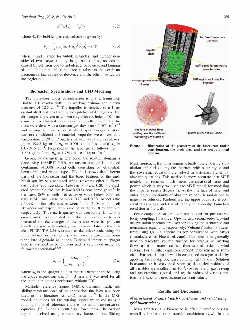
The bioreactor under consideration is a 3 L BrunswickBioFlo 110 reactor with 2 L working volume and a tankdiameter of 12.5 cm.34 The impeller is attached to a 1 cmcentral shaft and has three blades pitched at 45 degrees. Theair sparger is present as a 4 cm ring with six holes of 0.1-cmdiameter, each located 5 cm under the impeller. Earlier simula-tions were done with a constant gas flow rate of 10�5 m3 s�1

and an impeller rotation speed of 600 rpm. Energy equationwas not considered and material properties were taken at atemperature of 20�C. Properties of water used are as follows:qL ¼ 998.2 kg m�3, lL ¼ 0.001 kg m�1 s�1, and rL ¼0.0719 N m�1. Properties of air used are as follows: qG ¼1.225 kg m�3 and lG ¼ 1.7894 � 10�5 kg m�1 s�1.

Geometry and mesh generation of the solution domain isdone using GAMBIT 2.4.6. An unstructured grid is createdcontaining 843,008 hybrid cells consisting of tetrahedral,hexahedral, and wedge types. Figure 1 shows the differentparts of the bioreactor and the basic features of the grid.Mesh quality was analyzed using skewness criteria. Skew-ness value (equisize skew) between 0.50 and 0.80 is consid-ered acceptable and that below 0.50 is considered good.35 Inour case, 86% of cells had equisize value below 0.50 andonly 0.74% had value between 0.70 and 0.80. Aspect ratioof 99% of the cells was between 1 and 2. Maximum cellskewness and aspect ratio were found to be 0.78 and 2.2,respectively. Thus mesh quality was acceptable. Initially, acoarse mesh was created and the number of cells wasincreased till the changes in the results were insignificant(results on grid independency are presented later in the arti-cle). FLUENT 6.3.26 was used as the solver code using thefinite volume method to discretize various governing equa-tions into algebraic equations. Bubble diameter at spargerhole is assumed to be uniform and is calculated using thefollowing correlation33,36:

db ¼ 6rdhgðqL � qGÞ

� �13

(24)

where dh is the sparger hole diameter. Diameter found usingthe above expression was d ¼ 3 mm and was used for allthe initial simulations performed without PBE.

Multiple reference frames (MRF), dynamic mesh, andsliding mesh are some of the approaches that have also beenused in the literature for CFD modeling.24 In the MRFmodel, equations for the rotating region are solved using arotating frame of reference and the momentum conservationequation (Eq. 2) has a centrifugal force term. The outsideregion is solved using a stationary frame. In the Sliding

Mesh approach, the inner region actually rotates during sim-ulation and slides along the interface with outer region andthe governing equations are solved in stationary frame forabsolute quantities. This method is more accurate than MRFmodel, but requires much more computational time andpower which is why we used the MRF model for modelingthe impeller region (Figure 1). At the interface of inner andouter region, continuity of absolute velocity is maintained tomatch the solution. Furthermore, the upper boundary is con-stituted as a gas outlet while applying a no-slip boundarycondition at the walls.

Phase-coupled SIMPLE algorithm is used for pressure-ve-locity coupling. First-order Upwind and second-order Upwinddiscretization schemes are used for solving the turbulence andmomentum equations, respectively. Volume fraction is discre-tized using QUICK scheme as per consultation with Ansys(manufacturer of Fluent software). This scheme is generallyused to discretize volume fraction for rotating or swirlingflows as it is more accurate than second order Upwindscheme. For all other equations, second order scheme is suffi-cient. Further, the upper wall is constituted as a gas outlet byapplying the no-slip boundary condition at the wall. Solutionis assumed to be converged when (a) the scaled residuals ofall variables are smaller than 10�4, (b) the rate of gas leavingand gas entering is equal, and (c) the values of various cus-tom field functions used assume constant values.

Results and Discussions

Measurement of mass transfer coefficient and establishinggrid independency

Mass transfer in a bioreactor is often quantified via theoverall volumetric mass transfer coefficient (kLa). In this

Figure 1. Illustration of the geometry of the bioreactor underconsideration, the mesh used and the computationaldomain.

Biotechnol. Prog., 2012, Vol. 28, No. 2 385

article, Higbie’s penetration model is used for the calculationof kLa. According to this model, a series of short chanceencounters take place between the two phases at the inter-face resulting in unsteady molecular diffusion. Then, kLa isobtained from the product of local liquid mass transfer coef-ficient (kL) and the interfacial area available for mass trans-fer (a). The equations are as follows:

kL ¼ 2

p

ffiffiffiffiffiffiffiffiDO2

p eqLlL

� �14

(25)

a ¼ 6aGd32

(26)

where the diffusion coefficient of oxygen, DO2, is taken as1.97 � 10�9 m2 s�1.27 These equations are written as customfield functions in FLUENT to predict local and average kLain the whole computational domain.

Simulations were initially done with a coarse mesh for asingle bubble diameter throughout the domain. The numberof cells was increased to test for grid independency. Figure 2

shows that at a total cell count of 0.85 million cells results,kLa, is independent of the grid size. Hence, further simula-tions were performed using 0.85 million cells and the kLawas found to be 0.042 s�1.

Figure 3 shows contours of kLa along a diametricplane x ¼ 0.0625 along the centerline. As is to beexpected, the highest value of kLa is found near theimpeller where turbulent dissipation rate is the highest.The value of kLa for a single bubble size (0.042 s�1) isfound to be significantly different from the experimentalresults (0.0169 s�1).32 This is because, as per discussionabove, the single bubble model does not account forbreakage and coalescence of bubbles. Gas volume frac-tion contours shown in Figure 4 suggest that the rotatingimpeller is not able to disperse the gas toward the tankwalls and buoyancy forces the gas toward the tank topalong the central shaft.

Population balance and model validation

To improve upon the accuracy of the simulation, popula-tion balance equations (Eqs. 10–19) are applied and methodof classes is used. Different number of bins were tried in themodel and based on the results, 13 bins were selected withthe minimum bin size equal to 0.00075 m. Smaller number

Figure 2. Plot of kLa as a function of mesh size.

The plot shows that grid independency is achieved at 0.85 mil-lion cells.

Figure 3. Contours of mass transfer coefficient kLa along x 50.0625 plane for model without using population bal-ance equations (PBE).

Figure 4. Contours of gas volume fraction along x 5 0.0625plane for model without using population balanceequations (PBE).

Table 1. Bubble Sizes for all 13 Bins Obtained by Using Method

of Classes (Discrete Model) to Solve Population Balance

Equations (PBE)

Bin Number Size (m)

Bin-0 0.012Bin-1 0.00952Bin-2 0.00755Bin-3 0.006Bin-4 0.00476Bin-5 0.00377Bin-6 0.003Bin-7 0.00238Bin-8 0.00188Bin-9 0.0015Bin-10 0.00119Bin-11 0.000944Bin-12 0.00075

386 Biotechnol. Prog., 2012, Vol. 28, No. 2

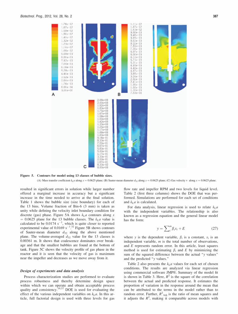
resulted in significant errors in solution while larger numberoffered a marginal increase in accuracy but a significantincrease in the time needed to arrive at the final solution.Table 1 shows the bubble size (size boundary) for each ofthe 13 bins. Volume fraction of Bin-6 (3 mm) is taken asunity while defining the velocity inlet boundary condition fordiscrete (gas) phase. Figure 5A shows kLa contours along x¼ 0.0625 plane for the 13 bubble classes. The kLa value iscalculated to be 0.0174 s�1, which is quite closer to reportedexperimental value of 0.0169 s�1.32 Figure 5B shows contoursof Sauter-mean diameter d32 along the above mentionedplane. The volume-averaged d32 value for the 13 classes is0.00361 m. It shows that coalescence dominates over break-age and that the smallest bubbles are found at the bottom oftank. Figure 5C shows the velocity profile of gas phase in thereactor and it is seen that the velocity of gas is maximumnear the impeller and decreases as we move away from it.

Design of experiments and data analysis

Process characterization studies are performed to evaluateprocess robustness and thereby determine design spacewithin which we can operate and obtain acceptable processquality and consistency.19,37 DOE is used for evaluating theeffect of the various independent variables on kLa. In this ar-ticle, full factorial design is used with three levels for gas

flow rate and impeller RPM and two levels for liquid level.Table 2 (first three columns) shows the DOE that was per-formed. Simulations are performed for each set of conditionsand kLa is calculated.

For data analysis, linear regression is used to relate kLawith the independent variables. The relationship is alsoknown as a regression equation and the general linear modelhas the form:

y ¼Xm

ibixi þ E (27)

where y is the dependent variable, bi is a constant, xi is anindependent variable, m is the total number of observations,and E represents random error. In this article, least squaresmethod is used for estimating bi and E by minimizing thesum of the squared difference between the actual ‘‘y values’’and the predicted ‘‘y values.’’

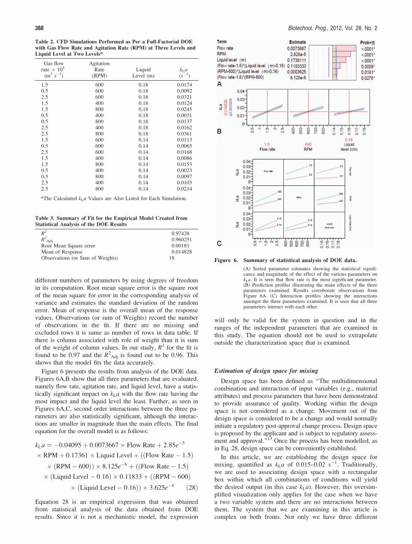
Table 2 also presents the kLa values for each set of chosenconditions. The results are analyzed via linear regressionusing commercial software JMPVR . Summary of the model fitis shown in Table 3. Here, R2 is the square of the correlationbetween the actual and predicted response. It estimates theproportion of variation in the response around the mean thatcan be attributed to the terms in the model rather than torandom error. Further, R2

Adj is the ratio of mean squares andit adjusts the R2, making it comparable across models with

Figure 5. Contours for model using 13 classes of bubble sizes.

(A) Mass transfer coefficient kLa along x ¼ 0.0625 plane; (B) Sauter-mean diameter d32 along x ¼ 0.0625 plane; (C) Gas velocity v along x ¼ 0.0625 plane.

Biotechnol. Prog., 2012, Vol. 28, No. 2 387

different numbers of parameters by using degrees of freedomin its computation. Root mean square error is the square rootof the mean square for error in the corresponding analysis ofvariance and estimates the standard deviation of the randomerror. Mean of response is the overall mean of the responsevalues. Observations (or sum of Weights) record the numberof observations in the fit. If there are no missing andexcluded rows it is same as number of rows in data table. Ifthere is column associated with role of weight than it is sumof the weight of column values. In our study, R2 for the fit isfound to be 0.97 and the R2

Adj is found out to be 0.96. Thisshows that the model fits the data accurately.

Figure 6 presents the results from analysis of the DOE data.Figures 6A,B show that all three parameters that are evaluated,namely flow rate, agitation rate, and liquid level, have a statis-tically significant impact on kLa with the flow rate having themost impact and the liquid level the least. Further, as seen inFigures 6A,C, second order interactions between the three pa-rameters are also statistically significant, although the interac-tions are smaller in magnitude than the main effects. The finalequation for the overall model is as follows:

kLa ¼ �0:04095þ 0:0073667� Flow Rateþ 2:85e�5

� RPMþ 0:17361� Liquid Levelþ ððFlow Rate� 1:5Þ� ðRPM� 600ÞÞ � 8:125e�6 þ ððFlow Rate� 1:5Þ

� ðLiquid Level� 0:16Þ � 0:11833þ ððRPM� 600Þ� ðLiquid Level� 0:16ÞÞ � 3:625e�4 ð28Þ

Equation 28 is an empirical expression that was obtainedfrom statistical analysis of the data obtained from DOEresults. Since it is not a mechanistic model, the expression

will only be valid for the system in question and in theranges of the independent parameters that are examined inthis study. The equation should not be used to extrapolateoutside the characterization space that is examined.

Estimation of design space for mixing

Design space has been defined as ‘‘The multidimensionalcombination and interaction of input variables (e.g., materialattributes) and process parameters that have been demonstratedto provide assurance of quality. Working within the designspace is not considered as a change. Movement out of thedesign space is considered to be a change and would normallyinitiate a regulatory post-approval change process. Design spaceis proposed by the applicant and is subject to regulatory assess-ment and approval.’’13 Once the process has been modelled, asin Eq. 28, design space can be conveniently established.

In this article, we are establishing the design space formixing, quantified as kLa of 0.015–0.02 s�1. Traditionally,we are used to associating design space with a rectangularbox within which all combinations of conditions will yieldthe desired output (in this case kLa). However, this oversim-plified visualization only applies for the case when we havea two variable system and there are no interactions betweenthem. The system that we are examining in this article iscomplex on both fronts. Not only we have three different

Table 2. CFD Simulations Performed as Per a Full-Factorial DOE

with Gas Flow Rate and Agitation Rate (RPM) at Three Levels and

Liquid Level at Two Levels*

Gas flowrate � 105

(m3 s�1)

AgitationRate(RPM)

LiquidLevel (m)

kLa(s�1)

1.5 600 0.18 0.01740.5 600 0.18 0.00922.5 600 0.18 0.03211.5 400 0.18 0.01241.5 800 0.18 0.02450.5 400 0.18 0.00310.5 800 0.18 0.01372.5 400 0.18 0.01622.5 800 0.18 0.03611.5 600 0.14 0.01130.5 600 0.14 0.00652.5 600 0.14 0.01681.5 400 0.14 0.00861.5 800 0.14 0.01530.5 400 0.14 0.00230.5 800 0.14 0.00972.5 400 0.14 0.01032.5 800 0.14 0.0214

*The Calculated kLa Values are Also Listed for Each Simulation.

Table 3. Summary of Fit for the Empirical Model Created from

Statistical Analysis of the DOE Results

R2 0.97428R2

Adj 0.960251Root Mean Square error 0.00181Mean of Response 0.014828Observations (or Sum of Weights) 18 Figure 6. Summary of statistical analysis of DOE data.

(A) Sorted parameter estimates showing the statistical signifi-cance and magnitude of the effect of the various parameters onkLa. It is seen that flow rate is the most significant parameter.(B) Prediction profiler illustrating the main effects of the threeparameters examined. Results corroborate observations fromFigure 6A. (C) Interaction profiles showing the interactionsamongst the three parameters examined. It is seen that all threeparameters interact with each other.

388 Biotechnol. Prog., 2012, Vol. 28, No. 2

variables that are significantly impacting kLa but also theirinteractions are significant.

The easiest way to envision design space in a case such asours is by deciding on an acceptable range for one of thethree parameters and then using the model to establish designspace for the remaining two parameters. In our case, thedesign space for liquid level (the least significant parameter)is assumed to be 0.16–0.17 m. Figure 7A illustrates the varia-tion in kLa at liquid level of 0.16 m when varying the remain-ing two parameters, agitation rate, and flow rate. It is seenthat infinite number of ranges can be chosen for each of thetwo parameters (infinite rectangles can be drawn within thewhite space in Figure 7A). One such design space is given inTable 4 (flow rate 1.5–1.9 � 10�5 m3 s�1 and agitation rate600–660 rpm). This is also shown as the filled box in Figure7A. It must be emphasized again that any number of suchcombinations can be chosen to meet the overall requirementof kLa. Also, it is evident that greater flexibility in one param-eter will result in narrower range for the other parameters.For example, for the illustration in Figure 7A, if greater flexi-bility in flow rate is desired (say 1.5–2.1 � 10�5 m3 s�1)then the agitation rate can only vary between 600–620 rpm(shown as an empty box in Figure 7A).

Figure 7B illustrates the same information as in Figure 7Abut at the liquid level of 0.17 m. Once again, many combi-

nations of flow rate and agitation rate can yield a kLabetween 0.015 and 0.02 s�1. One such combination is listedin Table 4 (flow rate 1.3–1.6 � 10�5 m3 s�1 and agitationrate 600–670 rpm). Based on the chosen set of ranges in Ta-ble 4, an overall design space can be established for liquidflow (0.16–0.17 m), flow rate (1.5–1.6 � 10�5 m3 s�1), andagitation rate (600–660 rpm). Operating anywhere withinthis cube will result in a kLa of 0.015–0.02 s�1. It can beseen that the chosen design space is a bit more restrictive onflow rate and liquid flow and more liberal on the agitationrate. As mentioned earlier, a different combination can bechosen if greater flexibility is desired in one parameter vs.others.

Conclusions

We have demonstrated the usefulness of CFD both formodeling of complex applications such as mixing in a bio-reactor and for evaluating the effect of the different input pa-rameters on the mixing. In combination with statisticalconcepts of design of experiments, design space can beestablished for the input parameters. Chosen experiments canthen be performed (at edges of the model) to validate theresults and if successfully validated, considerable savingscan be realized in comparison with the traditional approachwhere 18 experiments (as per Table 2) would be otherwiseneeded to generate the same process knowledge. We hopethat the article encourages other scientists in academia andindustry to adopt CFD for solving complex problems thatare so often faced in biotechnology process development.

Acknowledgments

The authors thank Mr. Shitalkumar Joshi and Mr. Sravanku-mar Nallamothu from Ansys-Fluent India for technical helpand discussions.

Notation

Ui ¼ mean velocity of i (liquid or gas) phase (m s�1)p ¼ pressure (N m�2)Ri ¼ momentum exchange in rotating frame (N m�3)Fi ¼ centrifugal forces in rotating frame (N m�3)g ¼ acceleration due to gravity (9.81 m s�2)

CD ¼ drag coefficientReP ¼ Reynolds number

d ¼ bubble diameter (m)C ¼ model parameter accounting for effect of turbu-

lence in slip velocity; assigned value of 0.3k ¼ turbulent kinetic energy (m2 s�3)

Figure 7. Contour profilers showing the design space for flowrate and agitation rate for achieving kLa of 0.015–0.02 s

21.

The filled rectangles show the defined design space. (A) Designspace at liquid level of 0.16 m. (B) Design space at liquid levelof 0.17 m.

Table 4. Example of a Design Space for Achieving kLa of

0.015–0.02 s21

AgitationRate (RPM)

FlowRate �105

(m3 s�1)

Design space corresponding toliquid level of 0.16 m

600–660 1.5–1.9

Design space corresponding toliquid level of 0.17 m

600–670 1.3–1.6

Final design space Liquid level0.16–0.17 m,Flow rate

1.5–1.6 � 10�5 m3 s�1,and agitation rate600–660 rpm.

Biotechnol. Prog., 2012, Vol. 28, No. 2 389

GkL ¼ rate of production of turbulent kinetic energy(m2 s�4)

Cl, C1e,C2e, rk, re

¼ model parameters having values equal to 0.09,1.44, 1.92, 1.0, and 1.3, respectively

ni ¼ number of bubbles in the ith bubble classdi ¼ diameter of bubbles in the ith bubble class (m)

BiB ¼ birth rate due to breakage (m3 s�1)BiC ¼ birth rate due to coalescence (m3 s�1)DiB ¼ death rate due to breakage (m3 s�1)DiC ¼ death rate due to coalescence (m3 s�1)

a(V,V0) ¼ coalescence rate between bubbles of size V and V0(s�1)

b(V0) ¼ breakage rate of bubble with size V (s�1)m(V0) ¼ number of daughter bubbles formed due to break-

age of size V0n(V, t) ¼ number of bubbles of size V at time tp(V,V0) ¼ probability density function for bubbles of size V,

generated from bubble of size V0fi ¼ ratio of volume fraction of ith group bubbles and

total gas volume fractiond32 ¼ Sauter mean diameter (m)Cf ¼ increase in surface area due to breakagePc ¼ coalescence frequencydB ¼ bubble diameter used while performing simulation

without PBE (3 mm)dH ¼ sparger hole diameter (m)kL ¼ local liquid mass transfer coefficient (m s�1)a ¼ interfacial area available for mass transfer (m2)

DO2 ¼ diffusion coefficient of oxygen (1.97 � 10�9

m2 s�1)y ¼ dependent variable in linear regression equationxi ¼ independent variable in linear regression equationm ¼ total number of observations taken for linear

regressionE ¼ random error in linear regression equation

Greek letters

ai ¼ volume fraction of i (liquid or gas) phasebi ¼ constant used in linear regression equatione ¼ turbulent dissipation energy (m2 s�3)

yij ¼ collision rate function (m3 s�1)k ¼ arriving eddy size (m)

lG ¼ viscosity of air (1.7894 � 10�5 kg m�1 s�1)lL ¼ viscosity of water (0.001 kg m�1 s�1)lt,L ¼ liquid phase viscosity (kg m�1 s�1)k ¼ dimensionless eddy size

PkL andPeL

¼ terms accounting for influence of continuous phaseon dispersed phase

qi ¼ density of i (liquid or gas) phase (kg m�3)rL ¼ surface tension of water (0.0719 N m�1)sef ¼ stress tensor (kg m�1 s�2)

XB(Vj, Vi) ¼ breakage rate of bubble size Vj in bubbles of sizeVi and Vj � Vi (m

3 s�1)

Literature Cited

1. Chu L, Robinson DK. Industrial choices for protein productionby large-scale cell culture. Curr Opin Biotechnol. 2001;12:180–187.

2. Zhu MM, Goyal A, Rank DL, Gupta SK, Boom TV, Lee SS.Effect of elevated pCO2 and osmolality on growth of CHO cellsand production of antibody-fusion protein B1: a case study. Bio-technol Prog. 2005;21:70–77.

3. deZengotita, VM, Roy M, William M. Effects of CO2 and os-molality on hybridoma cells: growth, metabolism and monoclo-nal antibody production. Cytotechnology. 1998;28:213–227.

4. Ozturk SS, Riley MR, Palsson BO. Effects of ammonia and lac-tate on hybridoma growth, metabolism, and antibody produc-tion. Biotechnol Bioeng. 1992;39:418–431.

5. Koynov A, Tryggvason G. Characterization of the localizedhydrodynamic shear forces and dissolved oxygen distribution insparged bioreactors. Biotechnol Bioeng. 2007;97:317–331.

6. Nyberg G, Green K, Hashimura Y, Rathore AS. Modeling ofbiopharmaceutical processes-part 1: microbial and mammalianunit operations. BioPharm Int. 2008;21:56–85.

7. Zhang H, Zhang K, Fan S. CFD simulation coupled with popu-lation balance equations for aerated stirred bioreactors. Eng LifeSci. 2009;9:421–430.

8. LaRoche RD, Mohan LS. Mammalian Cell Bioreactor Scale-UpUsing Fluid Mixing Analysis and Computational Fluid Dynam-ics. 232nd ACS National Meeting. San Francisco, USA; 2006.Available at: http://eps.fluent.com/5852/900041266/20061006/acs2006-sf-biot102.pdf.

9. Dhanasekharan K. Design and scale-up of bioreactors usingcomputer simulations. BioProcess Int. 2006;4:1–4.

10. Hutmacher DW, Singh H. Computational fluid dynamics forimproved bioreactor design and 3D culture. Trends Biotechnol.2008;26:166–172.

11. Kelly WJ. Using computational fluid dynamics to characterizeand improve bioreactor performance. Biotechnol Appl Biochem.2008;49:225–238.

12. PAT Guidance for Industry—A Framework for Innovative Phar-maceutical Development, Manufacturing and Quality Assurance,US Department of Health and Human Services, Food and DrugAdministration (FDA), Center for Drug Evaluation andResearch (CDER), Center for Veterinary Medicine (CVM),Office of Regulatory Affairs (ORA). September, 2004.

13. Guidance for Industry: Q8 Pharmaceutical Development, USDepartment of Health and Human Service, Food and DrugAdministration (FDA). May, 2006. Q8 Annex PharmaceuticalDevelopment, Step 3, November, 2007.

14. Guidance for Industry: Q9 Quality Risk Management, USDepartment of Health and Human Service, Food and DrugAdministration (FDA). June, 2006.

15. Guidance for Industry: Q10 Quality Systems Approach to Phar-maceutical CGMP Regulations, US Department of Health andHuman Service, Food and Drug Administration (FDA). Septem-ber, 2006.

16. Rathore AS, Winkle H. Quality by design for pharmaceuticals:regulatory perspective and approach. Nat Biotechnol.2009;27:26–34.

17. Kozlowski S, Swann P. Considerations for Biotechnology Prod-uct Quality by Design, in Quality by Design for Biopharmaceut-icals: Principles and Case Studies. In: Rathore AS, Mhatre R,editors. Wiley Interscience; 2009:9–30.

18. Rathore AS, Roadmap A. Implementation of quality by design(QbD) for biotechnology products, Trends Biotechnol. 2009;27:546–553.

19. Harms J, Wang X, Kim T, Yang X, Rathore AS. Defining pro-cess design space for biotech products: case study of pichia pas-toris fermentation. Biotechnol Prog. 2008;24:655–662.

20. Ishii M, Zuber N. Drag coefficient and relative velocity in bubbly,droplet or particulating flows. AICHE J. 1979;25:843–855.

21. Bakker A, Van Den Akker HEA. A computational model forthe gas-liquid flow in stirred reactors. Chem Eng Res Design.1994;72(A4):594–606.

22. Kerdouss F, Bannari A, Proulx P. CFD modeling of gas disper-sion and bubble size in a double turbine stirred tank. Chem EngSci. 2006;61:3313–3322.

23. Rizk MA, Elgobashi SE. A two-equation turbulence model fordispersed dilute confined two-phase flows. Int J MultiphaseFlow. 1989;15:119–133.

24. FLUENT. User’s Manual. Centrera Resource Park, 10 Cav-endish Court, Lebanon, USA: Fluent Inc; 2006.

25. Khopkar AR, Rammohan, Ranade VV, Dudukovic MP. Gas-liq-uid flow generated by a Rushton turbine in a stirred vessel:CARPT/CT measurements and CFD simulations. Chem Eng Sci.2005;60:2215–2229.

26. Deen NG, Solberg T, Hjertager BH. Flow generated by an aer-ated Rushton impeller: two-phase PIV experiments and numeri-cal simulations. Can J Chem Eng. 2002;80:1–15.

27. Dhanasekharan K, Sanyal J, Jain A, Haidari A. A generalizedapproach to model oxygen transfer in bioreactors using popula-tion balances and computational fluid dynamics. Chem Eng Sci.2005;60:213–218.

390 Biotechnol. Prog., 2012, Vol. 28, No. 2

28. Venneker BCH, Derksen JJ, Van Den Akker HEA. Populationbalance modeling of aerated stirred vessels based on CFD.AICHE J. 2002;48:673–684.

29. FLUENT 12 (2009). Population Balance Manual. Centrera

Resource Park, 10 Cavendish Court, Lebanon, USA: Fluent Inc.30. Sanyal J, Marchisio DL, Fox RO, Dhanasekharan K. On the

comparison between population models for CFD simulation of

bubble columns. Ind Eng Chem Res. 2005;44:5063–5072.31. Luo H, Svendsen HF. Theoretical model for drop and bubble

breakup in turbulent dispersions. AICHE J. 1996;42:1225–1233.

32. Saffman PG, Turner JS. On the collision of drops in turbulentclouds. J Fluid Mech. 1956;1:16–30.

33. Prince MJ, Blanch HW. Bubble coalescence and break-up inair-sparged bubble columns. AICHE J. 1990;36:1485–1499.

34. Kerdouss F, Bannari A, Proulx P, Bannari R, Skrga M, LabrecqueY. Two-phase mass transfer coefficient prediction in stirred vesselwith a CFD model. Comput Chem Eng. 2008;32:1943–1955.

35. Bakker A. Mesh Generation. 2002. Fluent Inc. Available at:http://www.bakker.org/dartmouth06/engs150/07-mesh.pdf.

36. Panneerselvem R, Savithri S, Surender GD. CFD modeling ofgas-liquid-solid mechanically agitated contactor. Chem Eng ResDesign. 2008;86:1331–1344.

37. Van Hoek P, Harms J, Wang J, Rathore AS. Case Study onDefinition of Design Space for a Microbial Fermentation Step,in Quality by Design for Biopharmaceuticals: Principles andCase Studies. In: Rathore AS, Mhatre R. Wiley Interscience;2009:85–109.

Manuscript received July 11, 2011, and revision received Oct. 14, 2011.

Biotechnol. Prog., 2012, Vol. 28, No. 2 391

Copyright of Biotechnology Progress is the property of Wiley-Blackwell and its content may not be copied or

emailed to multiple sites or posted to a listserv without the copyright holder's express written permission.

However, users may print, download, or email articles for individual use.