U.S Geological Survey – Connecticut SANDY LiDAR Report Produced for U.S. Geological Survey USGS Contract: G10PC00013 Task Order: G14PD00241 Report Date: 2/6/2015 SUBMITTED BY: Dewberry 1000 North Ashley Drive Suite 801 Tampa, FL 33602 813.225.1325 SUBMITTED TO: U.S. Geological Survey 1400 Independence Road Rolla, MO 65401 573.308.3810

Welcome message from author
This document is posted to help you gain knowledge. Please leave a comment to let me know what you think about it! Share it to your friends and learn new things together.
Transcript

U.S Geological Survey – Connecticut SANDY LiDAR Report Produced for U.S. Geological Survey USGS Contract: G10PC00013
Task Order: G14PD00241
Report Date: 2/6/2015
SUBMITTED BY:
Dewberry 1000 North Ashley Drive Suite 801 Tampa, FL 33602 813.225.1325 SUBMITTED TO:
U.S. Geological Survey 1400 Independence Road Rolla, MO 65401 573.308.3810

Connecticut SANDY LiDAR TO# G14PD00241 February 6, 2015 Page 2 of 70
Table of Contents Executive Summary ........................................................................................................................ 4
The Project Team ......................................................................................................................... 4
Survey Area .................................................................................................................................. 4
Date of Survey .............................................................................................................................. 4
Datum Reference ......................................................................................................................... 4
LiDAR Vertical Accuracy ............................................................................................................. 5
Project Deliverables ..................................................................................................................... 5
Project Tiling Footprint ............................................................................................................... 6
LiDAR Acquisition Report ...............................................................................................................7
LiDAR Acquisition Details............................................................................................................7
LiDAR Control ..............................................................................................................................7
Airborn GPS Kinematic ............................................................................................................... 8
Generation and Calibration of Laser Points (raw data) .............................................................. 8
Boresight and Relative accuracy .................................................................................................. 9
Final Swath Vertical Accuracy Assessment ................................................................................10
LiDAR Processing & Qualitative Assessment ................................................................................ 11
Data Classification and Editing .................................................................................................. 11
Qualitative Assessment .............................................................................................................. 13
Analysis ....................................................................................................................................... 15
Survey Vertical Accuracy Checkpoints ......................................................................................... 22
LiDAR Vertical Accuracy Statistics & Analysis ............................................................................. 25
Background ................................................................................................................................ 25
Vertical Accuracy Test Procedures ............................................................................................ 26
FVA ......................................................................................................................................... 26
CVA ......................................................................................................................................... 26
SVA ......................................................................................................................................... 26
Vertical Accuracy Testing Steps ................................................................................................ 27
Vertical Accuracy Results .......................................................................................................... 29
Breakline Production & Qualitative Assessment Report .............................................................. 32
Breakline Production Methodology .......................................................................................... 32
Breakline Qualitative Assessment ............................................................................................. 32
Breakline Topology Rules .......................................................................................................... 32
Breakline QA/QC Checklist ....................................................................................................... 33
Data Dictionary ............................................................................................................................. 37
Horizontal and Vertical Datum ................................................................................................. 37

Connecticut SANDY LiDAR TO# G14PD00241 February 6, 2015 Page 3 of 70
Coordinate System and Projection ............................................................................................ 37
Inland Streams and Rivers ........................................................................................................ 37
Description ............................................................................................................................. 37
Table Definition ..................................................................................................................... 37
Feature Definition .................................................................................................................. 37
Inland Ponds and Lakes ............................................................................................................ 39
Description ............................................................................................................................. 39
Table Definition ..................................................................................................................... 39
Feature Definition .................................................................................................................. 39
Tidal Waters ............................................................................................................................... 41
Description .............................................................................................................................. 41
Table Definition ...................................................................................................................... 41
Feature Definition ................................................................................................................... 41
DEM Production & Qualitative Assessment ................................................................................. 42
DEM Production Methodology ................................................................................................. 42
DEM Qualitative Assessment .................................................................................................... 43
DEM Vertical Accuracy Results ................................................................................................. 44
DEM QA/QC Checklist .............................................................................................................. 46
Appendix A: Survey Report .......................................................................................................... 48
Appendix B: Complete List of Delivered Tiles ............................................................................... 61
Connecticut SANDY LiDAR TO# G14PD00241 February 6, 2015 Page 4 of 70
Executive Summary The primary purpose of this project was to develop a consistent and accurate surface elevation dataset derived from high-accuracy Light Detection and Ranging (LiDAR) technology for the USGS Connecticut SANDY LiDAR Project Area. The LiDAR data were processed to a bare-earth digital terrain model (DTM). Detailed breaklines and bare-earth Digital Elevation Models (DEMs) were produced for the project area. Data was formatted according to tiles with each tile covering an area of 1500m by 1500m. A total of 1,974 tiles were produced for the project encompassing an area of approximately 1,526 sq. miles.
THE PROJECT TEAM
Dewberry served as the prime contractor for the project. In addition to project management, Dewberry was responsible for LAS classification, all LiDAR products, breakline production, Digital Elevation Model (DEM) production, and quality assurance. Dewberry Consultants LLC completed ground surveying for the project and delivered surveyed checkpoints. Their task was to acquire surveyed checkpoints for the project to use in independent testing of the vertical and horizontal accuracy of the LiDAR-derived surface model. They also verified the GPS base station coordinates used during LiDAR data acquisition to ensure that the base station coordinates were accurate. Please see Appendix A to view the separate Survey Report that was created for this portion of the project. Leading Edge Geomatics (LEG) completed LiDAR data acquisition and data calibration for the project area.
SURVEY AREA
The project area addressed by this report falls within the Connecticut counties of Fairfield, New Haven, Litchfield, Hartford, Middlesex, and New London.
DATE OF SURVEY
The LiDAR aerial acquisition was conducted from April 27, 2014 thru May 29, 2014.
DATUM REFERENCE
Data produced for the project were delivered in the following reference system. Horizontal Datum: The horizontal datum for the project is North American Datum of 1983 (NAD 83) 2011 Vertical Datum: The Vertical datum for the project is North American Vertical Datum of 1988 (NAVD88) Coordinate System: UTM Zone 18N Units: Horizontal units are in meters, Vertical units are in meters. Geiod Model: Geoid12A (Geoid 12A was used to convert ellipsoid heights to orthometricheights).

Connecticut SANDY LiDAR TO# G14PD00241 February 6, 2015 Page 5 of 70
LIDAR VERTICAL ACCURACY
For the Connecticut SANDY LiDAR Project, the tested RMSEz of the classified LiDAR data for checkpoints in open terrain equaled 0.068 m compared with the 0.0925 m specification; and the FVA of the classified LiDAR data computed using RMSEz x 1.9600 was equal to 0.133 m, compared with the 0.181 m specification. For the Connecticut SANDY LiDAR Project, the tested CVA of the classified LiDAR data computed using the 95th percentile was equal to 0.190 m, compared with the 0.269 m specification. Additional accuracy information and statistics for the classified LiDAR data, raw swath data, and bare earth DEM data are found in the following sections of this report.
PROJECT DELIVERABLES
The deliverables for the project are listed below.
1. Raw Point Cloud Data (Swaths) 2. Classified Point Cloud Data (Tiled) 3. Bare Earth Surface (Raster DEM – IMG Format) 4. Intensity Images (8-bit gray scale, tiled, GeoTIFF format) 5. Breakline Data (File GDB and shapefiles) 6. Control & Accuracy Checkpoint Report & Points 7. Metadata 8. Project Report (Acquisition, Processing, QC) 9. Project Extents, Including a shapefile derived from the LiDAR Deliverable

Connecticut SANDY LiDAR TO# G14PD00241 February 6, 2015 Page 6 of 70
PROJECT TILING FOOTPRINT
One thousand nine-hundred and seventy-four (1,974) tiles were delivered for the project. Each tile’s extent is 1,500 meters by 1,500 meters (see Appendix B for a complete listing of delivered tiles).
Figure 1. Project Map

Connecticut SANDY LiDAR TO# G14PD00241 February 6, 2015 Page 7 of 70
LiDAR Acquisition Report LEG provided high accuracy, calibrated multiple return LiDAR for roughly 1,526 square miles around the west-central, CT area. Data was collected and delivered in compliance with the “U.S. Geological Survey National Geospatial Program LiDAR Base Specification Version 1.0.” In addition to the Specification Requirements, this task order shall meet NEEA QL2.
LIDAR ACQUISITION DETAILS
LIDAR acquisition began on April 27, 2014 (julian day 117) and was completed on May 29, 2014 (julian day 149). A total of 40 survey missions were flown to complete the project. LEG utilized a Riegl 680i (SN: 9998328) for the acquisition. The project required 428 flight lines rather than the 418 flight lines planned to complete it. There were no unusual occurrences during the acquisition and the sensor performed within specifications.
Laser Firing Rate: 50000 Altitude (mtr. AGL):1000 Swath Overlap (%): 50 Approx. Ground Speed (kts): 100 Scan Rate (Hz): 76 Scan Angle (°±): 60 Computed Along Track Spacing (mtr): 1.5 Computed Cross Track Spacing (mtr): 1.5 Computed Swath Width (mtr): 1155 Number of Lines Required: 65 Line Spacing (mtr): 0.67
LIDAR CONTROL
The project used TOPCON TOPnext active network. When it was not possible to use the active network, an NGS monument was used. The coordinates of all used base stations are provided in the table below. Before processing, all base stations were adjusted to the CORS network.
Name Easting (m) Northing (m) Ellipsoid Ht (m) Orthometric Ht (m)
CTGU - CORS 304720.2 4573504.2 -18.04 25.515
CTNE - CORS 309751.2 4616053.5 41.812 82.684
BPRT - LEG 349977 4558245.3 -20.900 20.998
DNBY - LEG 372296.1 4582356.5 115.533 155.281
E82 - LEG 305565.6 4591888 70.785 113.364
MDTN - LEG 304520.9 4604655.6 -14.621 27.156
Nail_2 - LEG 338589.6 4601794.8 109.779 150.291
Nail_3 -LEG 364674.4 4586047.1 115.097 155.082
Nail_5 - LEG 304515.6 4624219.1 -23.458 16.856
Nail_6 - LEG 332106.3 4638336.4 89.674 128.181
NHVN – LEG 322166.5 4578107.2 -17.674 24.817
OXFD – LEG 344403.6 4591943.1 168.762 209.456
PRATT – LEG 287567.3 4585243.1 38.571 82.482
PUGLISI - LEG 309691.9 4616313.9 8.931 49.705

Connecticut SANDY LiDAR TO# G14PD00241 February 6, 2015 Page 8 of 70
SPFD - LEG 296484.5 4669040.8 41.708 78.679
WTFD - LEG 263039.8 4586977.2 45.837 90.431
Table 1 – Base Stations used to control LiDAR acquisition
AIRBORN GPS KINEMATIC
Airborne GPS data was processed using the POSPac 5.4 SP2 Trajectory Software. Flights were flown with a PDOP of better than 4. Distances from base station to aircraft were kept to a maximum of 40km.
GENERATION AND CALIBRATION OF LASER POINTS (RAW DATA)
The initial step of calibration is to verify availability and status of all needed GPS and Laser data against field notes and compile any data if not complete. Subsequently the mission points are output using Riegl RiProcess. The software uses plane matching to resolve bore site differences and misalignment. Multiple planes are generated and then used to resolve the difference in the swaths in roll, pitch, and yaw. The initial point generation for each mission calibration is verified within Microstation/Terrascan for calibration errors. If a calibration error greater than specification is observed within the mission, the roll, pitch and scanner scale corrections that need to be applied are calculated. The missions with the new calibration values are regenerated and validated internally once again to ensure quality. Data collected by the LiDAR unit is reviewed for completeness, acceptable density and to make sure all data is captured without errors or corrupted values. In addition, all GPS, aircraft trajectory, mission information, and ground control files are reviewed and logged into a database. On a project level, a supplementary coverage check is carried out to ensure no data voids unreported by Field Operations are present.

Connecticut SANDY LiDAR TO# G14PD00241 February 6, 2015 Page 9 of 70
Figure 2. LiDAR Swath output showing complete coverage.
BORESIGHT AND RELATIVE ACCURACY
The initial points for each mission calibration are inspected for flight line errors, flight line overlap, slivers or gaps in the data, point data minimums, or issues with the LiDAR unit or GPS. Roll, pitch and scanner scale are optimized during the calibration process until the relative accuracy is met. Relative accuracy and internal quality are checked. Vertical differences between ground surfaces of each line are displayed. Color scale is adjusted so that errors greater than the specifications are flagged. Cross sections are visually inspected across each block to validate point to point, flight line to flight line and mission to mission agreement.

Connecticut SANDY LiDAR TO# G14PD00241 February 6, 2015 Page 10 of 70
For this project the specifications used are as follow: Relative accuracy <= 7cm RMSEZ within individual swaths and <=10 cm RMSEZ or within swath overlap (between adjacent swaths).
Figure 3 – Profile views showing correct roll and pitch adjustments.
FINAL SWATH VERTICAL ACCURACY ASSESSMENT
Once Dewberry received the calibrated swath data from LEG, Dewberry tested the vertical accuracy of the open terrain swath data prior to additional processing. Dewberry tested the vertical accuracy of the swath data using the twenty open terrain independent survey check points. The vertical accuracy is tested by comparing survey checkpoints in open terrain to a triangulated irregular network (TIN) that is created from the raw swath points. Only checkpoints in open terrain can be tested against raw swath data because the data has not undergone classification techniques to remove vegetation, buildings, and other artifacts from the ground surface. Checkpoints are always compared to interpolated surfaces from the LiDAR point cloud because it is unlikely that a survey checkpoint will be located at the location of a discrete LiDAR point. Project specifications require a FVA of 0.181 m based on the RMSEz (0.0925 m) x 1.96. The dataset for the Connecticut SANDY LiDAR Project satisfies this criteria. The raw LiDAR swath data tested 0.175 m vertical accuracy at 95% confidence level in open terrain, based on RMSEz (0.089m) x 1.9600. The table below shows all calculated statistics for the raw swath data.
100 % of Totals
RMSEz (m) Open Terrain
Spec=0.0925m
FVA –Fundamental
Vertical Accuracy (RMSEz x 1.9600)
Spec=0.181m
Mean (m)
Median (m)
Skew Std Dev (m)
# of Points
Min (m)
Max (m)
Open Terrain
0.089 0.175 0.075 0.065 0.637 0.050 20 0.004 0.188
Table 2: FVA at 95% Confidence Level for Raw Swaths

Connecticut SANDY LiDAR TO# G14PD00241 February 6, 2015 Page 11 of 70
LiDAR Processing & Qualitative Assessment
DATA CLASSIFICATION AND EDITING
LiDAR mass points were produced to LAS 1.2 specifications, including the following LAS classification codes:
Class 1 = Unclassified, used for all other features that do not fit into the Classes 2, 7, 9, or 10, including vegetation, buildings, etc.
Class 2 = Bare-Earth Ground
Class 7 = Noise, low and high points
Class 9 = Water, points located within collected breaklines
Class 10 = Ignored Ground due to breakline proximity. The data was processed using GeoCue and TerraScan software. The initial step is the setup of the GeoCue project, which is done by importing a project defined tile boundary index encompassing the entire project area. The acquired 3D laser point clouds, in LAS binary format, were imported into the GeoCue project and tiled according to the project tile grid. Once tiled, the laser points were classified using a proprietary routine in TerraScan. This routine classifies any obvious outliers in the dataset to class 7. After points that could negatively affect the ground are removed from class 1, the ground layer is extracted from this remaining point cloud. The ground extraction process encompassed in this routine takes place by building an iterative surface model. This surface model is generated using three main parameters: building size, iteration angle and iteration distance. The initial model is based on low points being selected by a "roaming window" with the assumption that these are the ground points. The size of this roaming window is determined by the building size parameter. The low points are triangulated and the remaining points are evaluated and subsequently added to the model if they meet the iteration angle and distance constraints. This process is repeated until no additional points are added within iterations. A second critical parameter is the maximum terrain angle constraint, which determines the maximum terrain angle allowed within the classification model. The following fields within the LAS files are populated to the following precision: GPS Time (0.000001 second precision), Easting (0.003 meter precision), Northing (0.003 meter precision), Elevation (0.003 meter precision), Intensity (integer value - 12 bit dynamic range), Number of Returns (integer - range of 1-4), Return number (integer range of 1-4), Scan Direction Flag (integer - range 0-1), Classification (integer), Scan Angle Rank (integer), Edge of flight line (integer, range 0-1), User bit field (integer - flight line information encoded). The LAS file also contains a Variable length record in the file header that defines the projection, datums, and units. Once the initial ground routine has been performed on the data, Dewberry creates Delta Z (DZ) orthos to check the relative accuracy of the LiDAR data. These orthos compare the elevations of LiDAR points from overlapping flight lines on a 1 meter pixel cell size basis. If the elevations of points within each pixel are within 10 cm of each other, the pixel is colored green. If the elevations of points within each pixel are between 10 cm and 15 cm of each other, the pixel is colored yellow, and if the elevations of points within each pixel are greater than 15 cm in difference, the pixel is colored red. Pixels that do not contain points from overlapping flight lines are colored according to their intensity values. DZ orthos can be created using the full point cloud or ground only points and are used to review and verify the calibration of the data is acceptable. Some areas are expected

Connecticut SANDY LiDAR TO# G14PD00241 February 6, 2015 Page 12 of 70
to show sections or portions of red, including terrain variations, slope changes, and vegetated areas or buildings if the full point cloud is used. However, large or continuous sections of yellow or red pixels can indicate the data was not calibrated correctly or that there were issues during acquisition that could affect the usability of the data. The DZ orthos for Connecticut SANDY showed that several swaths in the initial data were not calibrated correctly and needed to be adjusted. LEG recalibrated these swaths and returned them to Dewberry, where a new set of DZ orthos were created. These DZ orthos demonstrated that the data was now calibrated correctly with no issues that would affect its usability. The figures below show an example of the DZ orthos before and after the swath recalibration.
Figure 4 - DZ orthos created from the full point cloud. The swath in the center of the image has yellow and red pixels because the DZ between this swath and the surrounding swaths is greater than 10 cm. Pixels are red along embankments, sloped terrain, and in vegetated land cover, as expected.
Figure 5 - DZ orthos created after the data was recalibrated by LEG. The swath in the center is now green in areas of flat, open terrain, indicating a DZ value under 10 cm. Red pixels are visible along embankments, sloped terrain, and in vegetated land cover, as expected. Open, flat areas are green
indicating the calibration and relative accuracy of the data is acceptable.
Once the calibration and relative accuracy of the data was confirmed, Dewberry utilized a variety of software suites for data processing. The LAS dataset was imported into GeoCue task management software for processing in Terrascan. Each tile was imported into Terrascan and a surface model was created to examine the ground classification. Dewberry analysts visually reviewed the ground surface model and corrected errors in the ground classification such as vegetation, buildings, and bridges that were present following the initial processing conducted by

Connecticut SANDY LiDAR TO# G14PD00241 February 6, 2015 Page 13 of 70
Dewberry. Dewberry analysts employ 3D visualization techniques to view the point cloud at multiple angles and in profile to ensure that non-ground points are removed from the ground classification. After the ground classification corrections were completed, the dataset was processed through a water classification routine that utilizes breaklines compiled by Dewberry to automatically classify hydro features. The water classification routine selects ground points within the breakline polygons and automatically classifies them as class 9, water. The final classification routine applied to the dataset selects ground points within a specified distance of the water breaklines and classifies them as class 10, ignored ground due to breakline proximity.
QUALITATIVE ASSESSMENT Dewberry’s qualitative assessment utilizes a combination of statistical analysis and interpretative methodology to assess the quality of the data for a bare-earth digital terrain model (DTM). This process looks for anomalies in the data and also identifies areas where man-made structures or vegetation points may not have been classified properly to produce a bare-earth model. Within this review of the LiDAR data, two fundamental questions were addressed:
Did the LiDAR system perform to specifications?
Did the vegetation removal process yield desirable results for the intended bare-earth terrain product?
Mapping standards today address the quality of data by quantitative methods. If the data are tested and found to be within the desired accuracy standard, then the data set is typically accepted. Now with the proliferation of LiDAR, new issues arise due to the vast amount of data. Unlike photogrammetrically-derived DEMs where point spacing can be eight meters or more, LiDAR nominal point spacing for this project is 1 point per 0.7 square meters. The end result is that millions of elevation points are measured to a level of accuracy previously unseen for traditional elevation mapping technologies and vegetated areas are measured that would be nearly impossible to survey by other means. The downside is that with millions of points, the dataset is statistically bound to have some errors both in the measurement process and in the artifact removal process. As previously stated, the quantitative analysis addresses the quality of the data based on absolute accuracy. This accuracy is directly tied to the comparison of the discreet measurement of the survey checkpoints and that of the interpolated value within the three closest LiDAR points that constitute the vertices of a three-dimensional triangular face of the TIN. Therefore, the end result is that only a small sample of the LiDAR data is actually tested. However there is an increased level of confidence with LiDAR data due to the relative accuracy. This relative accuracy in turn is based on how well one LiDAR point "fits" in comparison to the next contiguous LiDAR measurement, and is verified with DZ orthos. Once the absolute and relative accuracy has been ascertained, the next stage is to address the cleanliness of the data for a bare-earth DTM. By using survey checkpoints to compare the data, the absolute accuracy is verified, but this also allows us to understand if the artifact removal process was performed correctly. To reiterate the quantitative approach, if the LiDAR sensor operated correctly over open terrain areas, then it most likely operated correctly over the vegetated areas. This does not mean that the entire bare-earth was measured; only that the elevations surveyed are most likely accurate (including elevations of treetops, rooftops, etc.). In the event that the LiDAR pulse filtered through the vegetation and was able to measure the true surface (as well as measurements on the surrounding

Connecticut SANDY LiDAR TO# G14PD00241 February 6, 2015 Page 14 of 70
vegetation) then the level of accuracy of the vegetation removal process can be tested as a by-product. To fully address the data for overall accuracy and quality, the level of cleanliness (or removal of above-ground artifacts) is paramount. Since there are currently no effective automated testing procedures to measure cleanliness, Dewberry employs a combination of statistical and visualization processes. This includes creating pseudo image products such as LiDAR orthos produced from the intensity returns, Triangular Irregular Network (TIN)’s, Digital Elevation Models (DEM) and 3-dimensional models. By creating multiple images and using overlay techniques, not only can potential errors be found, but Dewberry can also find where the data meets and exceeds expectations. This report will present representative examples where the LiDAR and post processing had issues as well as examples of where the LiDAR performed well.

Connecticut SANDY LiDAR TO# G14PD00241 February 6, 2015 Page 15 of 70
ANALYSIS Dewberry utilizes GeoCue software as the primary geospatial process management system. GeoCue is a three tier, multi-user architecture that uses .NET technology from Microsoft. .NET technology provides the real-time notification system that updates users with real-time project status, regardless of who makes changes to project entities. GeoCue uses database technology for sorting project metadata. Dewberry uses Microsoft SQL Server as the database of choice. Specific analysis is conducted in Terrascan and QT Modeler environments. Following the completion of LiDAR point classification, the Dewberry qualitative assessment process flow for the Connecticut SANDY LiDAR project incorporated the following reviews:
1. Format: The LAS files are verified to meet project specifications. The LAS files for the Connecticut SANDY LiDAR project conform to the specifications outlined below.
- Format, Echos, Intensity
o LAS format 1.2
o Point data record format 1
o Multiple returns (echos) per pulse
o Intensity values populated for each point
- ASPRS classification scheme
o Class 1 – Processed, but unclassified
o Class 2 – Bare-earth ground
o Class 7 – Noise
o Class 9 – Water
o Class 10 – Ignored Ground due to breakline proximity
- Projection
o Datum – North American Datum 1983 (2011)
o Projected Coordinate System – UTM Zone 18
o Linear Units – Meters
o Vertical Datum – North American Vertical Datum 1988, Geoid 12A
o Vertical Units - Meters
- LAS header information:
o Class (Integer)
o Adjusted GPS Time (0.0001 seconds)
o Easting (0.003 meters)
o Northing (0.003 meters)
o Elevation (0.003 meters)
o Echo Number (Integer 1 to 4)
o Echo (Integer 1 to 4)
o Intensity (8 bit integer)
o Flight Line (Integer)
o Scan Angle (Integer degree)
2. Data density, data voids: The LAS files are used to produce Digital Elevation Models using the commercial software package “QT Modeler” which creates a 3-dimensional data model
Connecticut SANDY LiDAR TO# G14PD00241 February 6, 2015 Page 16 of 70
derived from Class 2 (ground points) in the LAS files. Grid spacing is based on the project density deliverable requirement for un-obscured areas. For the Connecticut SANDY LiDAR project it is stipulated that the minimum post spacing in un-obscured areas should be 1 point per 0.7 square meters.
a. Acceptable voids (areas with no LiDAR returns in the LAS files) that are present in the majority of LiDAR projects include voids caused by bodies of water. These are considered to be acceptable voids. No unacceptable voids are present in Connecticut SANDY LiDAR project.
3. Bare earth quality: Dewberry reviewed the cleanliness of the bare earth to ensure the
ground has correct definition, meets the project requirements, there is correct classification of points, and there are less than 5% residual artifacts.
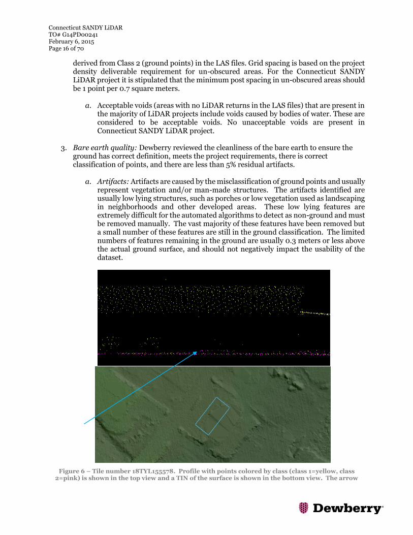
a. Artifacts: Artifacts are caused by the misclassification of ground points and usually
represent vegetation and/or man-made structures. The artifacts identified are usually low lying structures, such as porches or low vegetation used as landscaping in neighborhoods and other developed areas. These low lying features are extremely difficult for the automated algorithms to detect as non-ground and must be removed manually. The vast majority of these features have been removed but a small number of these features are still in the ground classification. The limited numbers of features remaining in the ground are usually 0.3 meters or less above the actual ground surface, and should not negatively impact the usability of the dataset.
Figure 6 – Tile number 18TYL155578. Profile with points colored by class (class 1=yellow, class 2=pink) is shown in the top view and a TIN of the surface is shown in the bottom view. The arrow
Connecticut SANDY LiDAR TO# G14PD00241 February 6, 2015 Page 17 of 70
identifies building or porch points. A limited number of these small features are still classified as ground but do not impact the usability of the dataset.
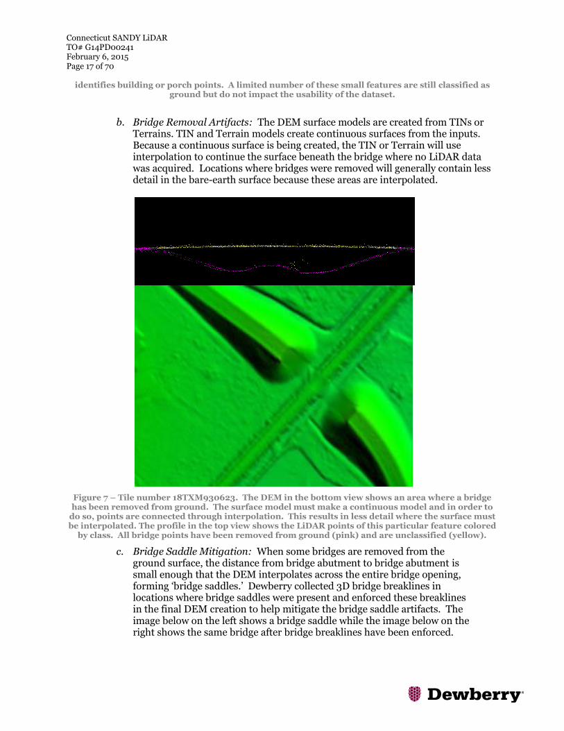
b. Bridge Removal Artifacts: The DEM surface models are created from TINs or
Terrains. TIN and Terrain models create continuous surfaces from the inputs. Because a continuous surface is being created, the TIN or Terrain will use interpolation to continue the surface beneath the bridge where no LiDAR data was acquired. Locations where bridges were removed will generally contain less detail in the bare-earth surface because these areas are interpolated.
Figure 7 – Tile number 18TXM930623. The DEM in the bottom view shows an area where a bridge has been removed from ground. The surface model must make a continuous model and in order to
do so, points are connected through interpolation. This results in less detail where the surface must be interpolated. The profile in the top view shows the LiDAR points of this particular feature colored
by class. All bridge points have been removed from ground (pink) and are unclassified (yellow).
c. Bridge Saddle Mitigation: When some bridges are removed from the ground surface, the distance from bridge abutment to bridge abutment is small enough that the DEM interpolates across the entire bridge opening, forming ‘bridge saddles.’ Dewberry collected 3D bridge breaklines in locations where bridge saddles were present and enforced these breaklines in the final DEM creation to help mitigate the bridge saddle artifacts. The image below on the left shows a bridge saddle while the image below on the right shows the same bridge after bridge breaklines have been enforced.

Connecticut SANDY LiDAR TO# G14PD00241 February 6, 2015 Page 18 of 70
Figure 8-Tile number 18TXM975642. The DEM on the left shows a bridge saddle artifact while the DEM on the right shows the same location after bridge breaklines have been enforced.
d. Culverts and Bridges: Bridges have been removed from the bare earth surface while culverts remain in the bare earth surface. In instances where it is difficult to determine if the feature is a culvert or bridge, such as with some small bridges, Dewberry erred on assuming they would be culverts especially if they are on secondary or tertiary roads. Below is an example of a culvert that has been left in the ground surface.

Connecticut SANDY LiDAR TO# G14PD00241 February 6, 2015 Page 19 of 70
Figure9– Tile number 18TYL155578. Profile with points colored by class (class 1=yellow, class 2=pink) is shown in the top view and the DEM is shown in the bottom view. This culvert remains in
the bare earth surface. Bridges have been removed from the bare earth surface and classified to class 1.

Connecticut SANDY LiDAR TO# G14PD00241 February 6, 2015 Page 20 of 70
e. Dirt Mounds: Irregularities in the natural ground exist and may be misinterpreted as artifacts that should be removed. Small hills and dirt mounds are present throughout the project area. These features are correctly included in the ground.
Figure 10 - Tile 18TXL540599. Profile with the points colored by class (class 1=yellow, class 2=pink) is shown in the top view and a DEM of the surface is shown in the bottom view. These features are
correctly included in the ground classification.

Connecticut SANDY LiDAR TO# G14PD00241 February 6, 2015 Page 21 of 70
f. Elevation Change Within Breaklines: While water bodies are flattened in the
final DEMs, other features such as linear hydrographic features can have significant changes in elevation within a small distance. In linear hydrographic features, this is often due to the presence of a structure that affects flow such as a dam or spillway. Dewberry has reviewed the DEMs to ensure that changes in elevation are shown from bank to bank. These changes are often shown as steps to reduce the presence of artifacts while ensuring consistent downhill flow. An example is shown below.
Figure 11 – Tile number 18TYL185579. Elevation change has been stair stepped. The steps are flat from bank to bank and flow consistently downhill.

Connecticut SANDY LiDAR TO# G14PD00241 February 6, 2015 Page 22 of 70
g. Flight line Ridges: Ridges occur when there is a difference between the
elevations of adjoining flight lines or swaths. Some flight line ridges are visible in the final DEMs but they do not exceed the project specifications and the overall relative accuracy requirements for the project area have been met. An example of a visible ridge that is within tolerance is shown below.
Figure 12– Tile number 18TXM585636. The flight line ridge is less than 10 cm. Overall, the Connecticut SANDY LiDAR data meets the project specifications for 10 cm RMSE relative accuracy.
Survey Vertical Accuracy Checkpoints All checkpoints surveyed for vertical accuracy testing purposes are listed in the following table. A total of one hundred and four (104) checkpoints were surveyed for the Connecticut SANDY LiDAR Project.
Point ID NAD83 UTM Zone 18N NAVD88
Easting X (m) Northing Y (m) Z-Survey (m)
OT-02 672618.271 4648799.471 367.501

Connecticut SANDY LiDAR TO# G14PD00241 February 6, 2015 Page 23 of 70
OT-03 691109.575 4654195.459 70.506
OT-04 669456.981 4636499.092 107.434
OT-05 688620.629 4638253.268 53.489
OT-06 683810.468 4629005.03 136.368
OT-07 668529.58 4625256.056 247.485
OT-08 680963.687 4619282.443 128.57
OT-09 696501.999 4609374.897 11.952
OT-10 690365.149 4597099.522 68.856
OT-11 706399.271 4592305.703 52.672
OT-12 713390.064 4580272.751 24.442
OT-13 666052.337 4613927.52 182.934
OT-14 662750.702 4596346.139 61.326
OT-15 663379.426 4583150.468 104.365
OT-16 654935.14 4578031.399 155.627
OT-17 644895.515 4585480.195 94.708
OT-18 627258.405 4588849.438 185.89
OT-19 628821.058 4602864.123 214.061
OT-20 640490.207 4597178.923 72.204
OT-21 652300.432 4605412.023 131.955
BLT-01 625240.084 4568556.72 216.206
BLT-02 623414.216 4583032.937 161.826
BLT-03 635952.35 4584014.647 139.963
BLT-04 651756.574 4583372.976 59.012
BLT-05 656999.596 4574726.8 129.194
BLT-06 658217.507 4590472.925 219.177
BLT-07 636362.43 4596887.148 166.603
BLT-08 643508.016 4595374.752 202.664
BLT-09 642805.092 4604858.332 289.812
BLT-10 656267.285 4604116.148 195.168
BLT-11 668438.124 4605363.094 157.738
BLT-12 674852.555 4618390.972 99.733
BLT-13 683247.983 4609195.674 52.098
BLT-14 696338.012 4598053.148 96.785
BLT-15 718511.202 4583865.847 0.53
BLT-16 674026.642 4628066.527 118.169
BLT-17 694747.429 4637180.212 17.091
BLT-19 679447.559 4646168.472 106.872
BLT-18 695004.912 4652220.739 60.955
BLT-20 665614.732 4651231.284 316.187

Connecticut SANDY LiDAR TO# G14PD00241 February 6, 2015 Page 24 of 70
BLT-21 659330.731 4634569.343 326.691
FO-01 622647.965 4572804.812 259.227
FO-02 624724.634 4587783.805 230.319
FO-03 625296.465 4603791.846 136.342
FO-04 645280.902 4601265.448 287.502
FO-05 637191.589 4592451.795 128.55
FO-06 640948.318 4582523.204 172.986
FO-07 648109.177 4585961.576 171.368
FO-08 662323.604 4573296.977 56.511
FO-09 650391.184 4593243.767 106.937
FO-10 655038.081 4598970.65 220.066
FO-11 666669.669 4589140.296 206.25
FO-12 663879.716 4609788.606 150.45
FO-13 682419.425 4605771.609 86.389
FO-14 690993.791 4592573.401 86.408
FO-15 702750.301 4594425.231 146.116
FO-16 680904.336 4626852.815 47.879
FO-17 668758.277 4643402.668 196.918
FO-18 687083.722 4646501.688 81.766
FO-19 673445.756 4651650.804 362.696
FO-20 664635.932 4645556.034 144.201
FO-21 657973.198 4650400.706 352.815
GWC-01 725192.098 4576710.64 6.484
GWC-02 709091.698 4585862.772 73.227
GWC-03 702632.641 4600681.1 63.903
GWC-04 692803.454 4588219.549 75.247
GWC-05 689106.758 4607743.908 74.443
GWC-06 678293.615 4621378.387 50.992
GWC-07 685747.152 4637243.808 68.889
GWC-08 685656.61 4649302.395 71.553
GWC-09 674829.863 4642945.061 303.76
GWC-10 662881.599 4648195.598 161.522
GWC-11 655257.033 4647347.551 351.326
GWC-12 662532.615 4641824.276 209.425
GWC-13 670402.542 4632251.878 150.176
GWC-14 668493.467 4608012.327 253.091
GWC-15 655635.392 4609465.948 221.467
GWC-16 637205.806 4602285.475 169.295

Connecticut SANDY LiDAR TO# G14PD00241 February 6, 2015 Page 25 of 70
GWC-17 625102.243 4599452.025 219.265
GWC-18 632484.57 4596265.7 67.797
GWC-19 623392.506 4578055.461 234.985
GWC-20 639085.317 4586613.684 192.829
GWC-21 654042.179 4588798.189 98.705
UT-01 719137.663 4574911.846 4.848
UT-02 711167.133 4586203.724 44.212
UT-03 693527.8 4593996.75 53.003
UT-04 696368.196 4603217.016 9.866
UT-05 684748.481 4615610.685 53.559
UT-06 694332.718 4625088.355 5.972
UT-07 692860.141 4642959.85 47.57
UT-08 690351.433 4651414.309 60.501
UT-09 660613.314 4642529.709 214.128
UT-10 667666.829 4638384.265 116.704
UT-11 668743.923 4626267.465 264.687
UT-12 671570.889 4617043.05 120.309
UT-13 657097.54 4607513.162 148.464
UT-14 663220.934 4601580.398 78.93
UT-15 661969.606 4584668.679 54.008
UT-16 659055.594 4567960.076 15.645
UT-17 649364.986 4600543.502 82.384
UT-18 632028.475 4602211.898 89.668
UT-19 626489.933 4591560.913 190.722
UT-20 630651.566 4584343.593 117.668
UT-21 625784.958 4571969.295 197.372
Table 3: USGS – Connecticut SANDY LiDAR surveyed accuracy checkpoints
LiDAR Vertical Accuracy Statistics & Analysis
BACKGROUND
Dewberry tests and reviews project data both quantitatively (for accuracy) and qualitatively (for usability). For quantitative assessment (i.e. vertical accuracy assessment), one hundred-four (104) check points were surveyed for the project and are located within bare earth/open terrain, urban, tall weeds/crops, brush lands/tress, and forested/fully grown land cover categories. The checkpoints

Connecticut SANDY LiDAR TO# G14PD00241 February 6, 2015 Page 26 of 70
were surveyed for the project using RTK survey methods. Please see appendix A to view the survey report which details and validates how the survey was completed for this project. Checkpoints were evenly distributed throughout the project area so as to cover as many flight lines as possible using the “dispersed method” of placement.
VERTICAL ACCURACY TEST PROCEDURES FVA (Fundamental Vertical Accuracy) is determined with check points located only in the open terrain (grass, dirt, sand, and/or rocks) land cover category, where there is a very high probability that the LiDAR sensor will have detected the bare-earth ground surface and where random errors are expected to follow a normal error distribution. The FVA determines how well the calibrated LiDAR sensor performed. With a normal error distribution, the vertical accuracy at the 95% confidence level is computed as the vertical root mean square error (RMSEz) of the checkpoints x 1.9600. For the Connecticut Sandy LiDAR project, vertical accuracy must be 0.1813 meters or less based on an RMSEz of 0.0925 meters x 1.9600. CVA (Consolidated Vertical Accuracy) is determined with all checkpoints in all land cover categories combined where there is a possibility that the LiDAR sensor and post-processing may yield elevation errors that do not follow a normal error distribution. CVA at the 95% confidence level equals the 95th percentile error for all checkpoints in all land cover categories combined. The Connecticut SANDY LiDAR Project CVA standard is 0.269 meters based on the 95th percentile. The CVA is accompanied by a listing of the 5% outliers that are larger than the 95th percentile used to compute the CVA; these are always the largest outliers that may depart from a normal error distribution. Here, Accuracyz differs from CVA because Accuracyz assumes elevation errors follow a normal error distribution where RMSE procedures are valid, whereas CVA assumes LiDAR errors may not follow a normal error distribution in vegetated categories, making the RMSE process invalid. SVA (Supplemental Vertical Accuracy) is determined for each land cover category other than open terrain. SVA at the 95% confidence level equals the 95th percentile error for all checkpoints in each land cover category. The Connecticut SANDY LiDAR Project SVA target is 0.269 meters based on the 95th percentile. Target specifications are given for SVA’s as one individual land cover category may exceed this target value as long as the overall CVA is within specified tolerances. Again, Accuracyz differs from SVA because Accuracyz assumes elevation errors follow a normal error distribution where RMSE procedures are valid, whereas SVA assumes LiDAR errors may not follow a normal error distribution in vegetated categories, making the RMSE process invalid. The relevant testing criteria are summarized in Table 4.
Quantitative Criteria Measure of Acceptability
Fundamental Vertical Accuracy (FVA) in open terrain only using RMSEz *1.9600
0.1813 meters (based on RMSEz (0.0925 meters) * 1.9600)
Consolidated Vertical Accuracy (CVA) in all land cover categories combined at the 95% confidence level
0.269 meters (based on combined 95th percentile)
Supplemental Vertical Accuracy (SVA) in each land cover category separately at the 95% confidence level
0.269 meters (based on 95th percentile for each land cover category)
Table 4 ― Acceptance Criteria

Connecticut SANDY LiDAR TO# G14PD00241 February 6, 2015 Page 27 of 70
VERTICAL ACCURACY TESTING STEPS The primary QA/QC vertical accuracy testing steps used by Dewberry are summarized as follows: 1. Dewberry’s team surveyed QA/QC vertical checkpoints in accordance with the project’s
specifications. 2. Next, Dewberry interpolated the bare-earth LiDAR DTM to provide the z-value for every
checkpoint. 3. Dewberry then computed the associated z-value differences between the interpolated z-value
from the LiDAR data and the ground truth survey checkpoints and computed FVA, CVA, and SVA values.
4. The data were analyzed by Dewberry to assess the accuracy of the data. The review process examined the various accuracy parameters as defined by the scope of work. The overall descriptive statistics of each dataset were computed to assess any trends or anomalies. This report provides tables, graphs and figures to summarize and illustrate data quality.

Connecticut SANDY LiDAR TO# G14PD00241 February 6, 2015 Page 28 of 70
The figure below shows the location of the QA/QC checkpoints within the project area.
Figure 13 – Location of QA/QC Checkpoints
Connecticut SANDY LiDAR TO# G14PD00241 February 6, 2015 Page 29 of 70
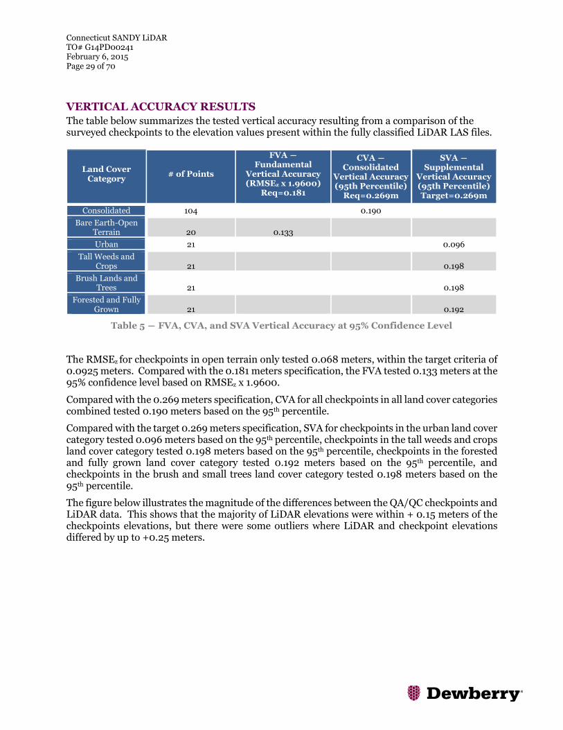
VERTICAL ACCURACY RESULTS
The table below summarizes the tested vertical accuracy resulting from a comparison of the surveyed checkpoints to the elevation values present within the fully classified LiDAR LAS files.
Land Cover Category
# of Points
FVA ― Fundamental
Vertical Accuracy (RMSEz x 1.9600)
Req=0.181
CVA ― Consolidated
Vertical Accuracy (95th Percentile)
Req=0.269m
SVA ― Supplemental
Vertical Accuracy (95th Percentile) Target=0.269m
Consolidated 104 0.190
Bare Earth-Open Terrain 20 0.133
Urban 21 0.096
Tall Weeds and Crops 21 0.198
Brush Lands and Trees 21 0.198
Forested and Fully Grown 21 0.192
Table 5 ― FVA, CVA, and SVA Vertical Accuracy at 95% Confidence Level
The RMSEz for checkpoints in open terrain only tested 0.068 meters, within the target criteria of 0.0925 meters. Compared with the 0.181 meters specification, the FVA tested 0.133 meters at the 95% confidence level based on RMSEz x 1.9600.
Compared with the 0.269 meters specification, CVA for all checkpoints in all land cover categories combined tested 0.190 meters based on the 95th percentile.
Compared with the target 0.269 meters specification, SVA for checkpoints in the urban land cover category tested 0.096 meters based on the 95th percentile, checkpoints in the tall weeds and crops land cover category tested 0.198 meters based on the 95th percentile, checkpoints in the forested and fully grown land cover category tested 0.192 meters based on the 95th percentile, and checkpoints in the brush and small trees land cover category tested 0.198 meters based on the 95th percentile.
The figure below illustrates the magnitude of the differences between the QA/QC checkpoints and LiDAR data. This shows that the majority of LiDAR elevations were within + 0.15 meters of the checkpoints elevations, but there were some outliers where LiDAR and checkpoint elevations differed by up to +0.25 meters.

Connecticut SANDY LiDAR TO# G14PD00241 February 6, 2015 Page 30 of 70
Figure 14 – Magnitude of elevation discrepancies per land cover category
Table 6 lists the 5% outliers that are larger than the 95th percentile.
Point ID
NAD83 UTM Zone 15 NAVD88
LiDAR Z (m)
Delta Z AbsDeltaZ
Easting X (m) Northing Y (m) Survey Z (m)
BLT-19 679447.559 4646168.472 106.872 107.07 0.198 0.198
FO-14 690993.791 4592573.401 86.408 86.6 0.192 0.192
GWC-R10 662881.599 4648195.598 161.522 161.72 0.198 0.198
GWC-R8 685656.61 4649302.395 71.553 71.79 0.237 0.237
FO-R18 687083.722 4646501.688 81.766 82 0.234 0.234
BLT-R6 658217.507 4590472.925 219.177 219.39 0.213 0.213
Table 6 ― 5% Outliers
-0.150
-0.100
-0.050
0.000
0.050
0.100
0.150
0.200
0.250
0.300
Brush Land/Trees
Open Terrain
Forest
Grass/Weeds/Crops
Urban

Connecticut SANDY LiDAR TO# G14PD00241 February 6, 2015 Page 31 of 70
Table 7 provides overall descriptive statistics.
100 % of Totals
RMSEz (m) Open Terrain
Spec=0.0925m Mean (m)
Median (m)
Skew Std Dev (m)
Kurtosis Min (m)
Max (m)
Consolidated 0.079 0.076 0.164 0.064 0.067 -
0.105 0.237
Open Terrain 0.068 0.050 0.041 0.397 0.047 -1.431 -
0.012 0.124
Brush Lands and Trees 0.104 0.094 0.025 0.062 -0.276
-0.033 0.213
Forested and Fully Grown 0.101 0.100 -0.307 0.070 0.138
-0.042 0.234
Urban 0.045 0.040 0.186 0.036 -1.056 -
0.010 0.114
Grass, Weeds, and Crops 0.095 0.094 -0.680 0.073 1.920
-0.105 0.237
Table 7 ― Overall Descriptive Statistics
The figure below illustrates a histogram of the associated elevation discrepancies between the QA/QC checkpoints and elevations interpolated from the LiDAR triangulated irregular network (TIN). The frequency shows the number of discrepancies within each band of elevation differences. The histogram shows that the majority of the discrepancies are skewed on the positive side. The majority of points are within the ranges of 0.0 meters to +0.15 meters.
0
5
10
15
20
25
30
35
40
-0.25 -0.2 -0.15 -0.1 -0.05 0 0.05 0.1 0.15 0.2 0.25
Freq
uen
cy
Errors in Meters
Checkpoints Error Distribution

Connecticut SANDY LiDAR TO# G14PD00241 February 6, 2015 Page 32 of 70
Figure 15 ― Histogram of Elevation Discrepancies with errors in meters
Based on the vertical accuracy testing conducted by Dewberry, the LiDAR dataset for the USGS Connecticut SANDY LiDAR Project satisfies the project’s pre-defined vertical accuracy criteria.
Breakline Production & Qualitative Assessment Report
BREAKLINE PRODUCTION METHODOLOGY
Dewberry used GeoCue software to develop LiDAR stereo models of the Connecticut SANDY LiDAR Project area so the LiDAR derived data could be viewed in 3-D stereo using Socet Set softcopy photogrammetric software. Using LiDARgrammetry procedures with LiDAR intensity imagery, Dewberry used the stereo models developed by Dewberry to stereo-compile the three types of hard breaklines in accordance with the project’s Data Dictionary. All drainage breaklines are monotonically enforced to show downhill flow. Water bodies and tidal waters are reviewed in stereo and the lowest elevation is applied to the entire waterbody or tidal feature.
BREAKLINE QUALITATIVE ASSESSMENT Dewberry completed breakline qualitative assessments according to a defined workflow. The following workflow diagram represents the steps taken by Dewberry to provide a thorough qualitative assessment of the breakline data.
Hydro
Automated checks for
Connectivity,
Monotonicity
Elevation
Check vertices elevation
accuracy against TIN created
from the Lidar points
Completeness
Perform visual
Qualitative Assessment
Breaklines
Format
Geodatabase conformity (schema, attributes,
projection, topology, right hand rule)
Data
received?
Geocue tracked
steps at Dewberry
Data pass?
Validate and Log edit
calls
Major task
Tasks
Dewberry
Legend
Data delivery
BREAKLINE TOPOLOGY RULES
Automated checks are applied on hydro features to validate the 3D connectivity of the feature and the monotonicity of the hydrographic breaklines. Dewberry’s major concern was that the hydrographic breaklines have a continuous flow downhill and that breaklines do not undulate. Error points are generated at each vertex not complying with the tested rules and these potential edit calls are then visually validated during the visual evaluation of the data. This step also helped

Connecticut SANDY LiDAR TO# G14PD00241 February 6, 2015 Page 33 of 70
validate that breakline vertices did not have excessive minimum or maximum elevations and that elevations are consistent with adjacent vertex elevations. The next step is to compare the elevation of the breakline vertices against the elevation extracted from the ESRI Terrain built from the LiDAR ground points, keeping in mind that a discrepancy is expected because of the hydro-enforcement applied to the breaklines and because of the interpolated imagery used to acquire the breaklines. A given tolerance is used to validate if the elevations differ too much from the LiDAR. Dewberry’s final check for the breaklines was to perform a full qualitative analysis. Dewberry compared the breaklines against LiDAR intensity images to ensure breaklines were captured in the required locations. The quality control steps taken by Dewberry are outlined in the QA Checklist below.
BREAKLINE QA/QC CHECKLIST
Project Number/Description: TO G14PD00241 USGS Connecticut SANDY LiDAR Date:______ 1/26/2015____ Overview
All Feature Classes are present in GDB
All features have been loaded into the geodatabase correctly. Ensure feature classes with
subtypes are domained correctly.
The breakline topology inside of the geodatabase has been validated. See Data Dictionary
for specific rules
Projection/coordinate system of GDB is accurate with project specifications
Perform Completeness check on breaklines using either intensity or ortho imagery Check entire dataset for missing features that were not captured, but should be to meet
baseline specifications or for consistency (See Data Dictionary for specific collection
rules). Features should be collected consistently across tile bounds within a dataset as well
as be collected consistently between datasets.
Check to make sure breaklines are compiled to correct tile grid boundary and there is full
coverage without overlap
Check to make sure breaklines are correctly edge-matched to adjoining datasets if
applicable. Ensure breaklines from one dataset join breaklines from another dataset that
are coded the same and all connecting vertices between the two datasets match in X,Y, and
Z (elevation). There should be no breaklines abruptly ending at dataset boundaries and
no discrepancies of Z-elevation in overlapping vertices between datasets.

Connecticut SANDY LiDAR TO# G14PD00241 February 6, 2015 Page 34 of 70
Compare Breakline Z elevations to LiDAR elevations
Using a terrain created from LiDAR ground points and water points, drape breaklines on
terrain to compare Z values. Breakline elevations should be at or below the elevations of
the immediately surrounding terrain. This should be performed before other breakline
checks are completed.
Perform automated data checks using ESRI’s Data Reviewer The following data checks are performed utilizing ESRI’s Data Reviewer extension. These checks allow automated validation of 100% of the data. Error records can either be written to a table for future correction, or browsed for immediate correction. Data Reviewer checks should always be performed on the full dataset.
Perform “adjacent vertex elevation change check” on the Inland Ponds feature class
(Elevation Difference Tolerance=.001 meters). This check will return Waterbodies whose
vertices are not all identical. This tool is found under “Z Value Checks.”
Perform “unnecessary polygon boundaries check” on Inland Ponds and Lakes, Tidal
Waters, and Islands (if delivered as a separate feature class) feature classes. This tool is
found under “Topology Checks.”
Perform “different Z-Value at intersection check” (Inland Streams and Rivers to Inland
Streams and Rivers), (Ponds and Lakes to Ponds and Lakes), (Tidal Waters to Tidal
Waters), (Streams and Rivers to Ponds and Lakes), (Streams and Rivers to Tidal
Waters), (Ponds and Lakes to Tidal Waters), (Island to Inland Ponds and Lakes), (Island
to Tidal Waters), (Island to Island),and (Islands to Inland Streams and Rivers)
(Elevation Difference Tolerance= .01 feet Minimum, 600 feet Maximum, Touches). This
tool is found under “Z Value Checks.”
Perform “duplicate geometry check” on (Inland Streams and Rivers to Inland Streams and
Rivers), (Inland Ponds and Lakes to Inland Ponds and Lakes), (Tidal Waters to Tidal
Waters), (Islands to Islands-if delivered as a separate shapefile), (Inland Streams and
Rivers to Inland Ponds and Lakes), (Inland Streams and Rivers to Tidal Waters), (Inland
Ponds and Lakes to Tidal Waters), (Islands to Tidal Waters), and (Islands to Inland Ponds
and Lakes). Attributes do not need to be checked during this tool. This tool is found under
“Duplicate Geometry Checks.”
Perform “geometry on geometry check” (Inland Streams and Rivers to Inland Ponds and
Lakes), (Inland Streams and Rivers to Tidal Waters), (Inland Ponds and Lakes to Tidal
Waters), (Inland Streams and Rivers to Inland Streams and Rivers), (Inland Ponds and
Lakes to Inland Ponds and Lakes), (Tidal waters to Tidal waters), (Islands to Tidal
Waters), and (Islands to Inland Ponds and Lakes), (Islands to Islands). Spatial
relationship is crosses, attributes do not need to be checked. This tool is found under
“Feature on Feature Checks.”

Connecticut SANDY LiDAR TO# G14PD00241 February 6, 2015 Page 35 of 70
Perform “geometry on geometry check (Tidal Waters to Islands), and (Inland Ponds and
Lakes to Islands), (Inland Streams and Rivers to Islands). Spatial relationship is
contains, attributes do not need to be checked. This tool is found under “Feature on
Feature Checks.”
Perform “geometry on geometry check” (Inland Streams and Rivers to Inland Ponds and
Lakes), (Inland Streams and Rivers to Tidal Waters), (Inland Ponds and Lakes to Tidal
Waters), (Inland Streams and Rivers to Inland Streams and Rivers), (Inland Ponds and
Lakes to Inland Ponds and Lakes), (Tidal waters to Tidal waters), (Islands to Tidal
Waters), and (Islands to Inland Ponds and Lakes), (Islands to Islands). Spatial
relationship is intersect, attributes do not need to be checked. This tool is found under
“Feature on Feature Checks.”
Perform “polygon overlap/gap is sliver check” on (Tidal Waters to Tidal Waters), (Island
to Island), (Island to Inland Ponds and Lakes) and (Inland Ponds and Lakes to Inland
Ponds and Lakes), (Inland Ponds and Lakes to Tidal Waters). Maximum Polygon Area is
not required. This tool is found under “Feature on Feature Checks.”
Perform Dewberry Proprietary Tool Checks
Perform monotonicity check on (Inland Streams and Rivers) and (Tidal Waters to Tidal
Waters if they are not a constant elevation) using “A3_checkMonotonicityStreamLines.”
This tool looks at line direction as well as elevation. Features in the output shapefile
attributed with a “d” are correct monotonically, but were compiled from low elevation to
high elevation. These features are ok and can be ignored. Features in the output
shapefile attributed with an “m” are not correct monotonically and need elevations to be
corrected. Input features for this tool need to be in a geodatabase and must be a line. If
features are a polygon they will need to be converted to a line feature. Z tolerance is 0.01
meters.
Perform connectivity check between (Inland Streams and Rivers to Inland Streams and
Rivers), (Ponds and Lakes to Ponds and Lakes), (Tidal Waters to Tidal Waters), (Streams
and Rivers to Ponds and Lakes), (Streams and Rivers to Tidal Waters), (Ponds and Lakes
to Tidal Waters), (Island to Inland Ponds and Lakes), (Island to Tidal Waters), (Island to
Island),and (Islands to Inland Streams and Rivers) using the tool
“07_CheckConnectivityForHydro.” The input for this tool needs to be in a geodatabase.
The output is a shapefile showing the location of overlapping vertices from the polygon
features and polyline features that are at different Z-elevation.
Metadata
Each XML file (1 per feature class) is error free as determined by the USGS MP tool

Connecticut SANDY LiDAR TO# G14PD00241 February 6, 2015 Page 36 of 70
Metadata content contains sufficient detail and all pertinent information regarding source
materials, projections, datums, processing steps, etc. Content should be consistent across
all feature classes.
Completion Comments: Complete – Approved

Connecticut SANDY LiDAR TO# G14PD00241 February 6, 2015 Page 37 of 70
Data Dictionary
HORIZONTAL AND VERTICAL DATUM
The horizontal datum shall be North American Datum of 1983 (2011), Units in Meters. The vertical datum shall be referenced to the North American Vertical Datum of 1988 (NAVD 88), Units in Meters. Geoid12A shall be used to convert ellipsoidal heights to orthometric heights.
COORDINATE SYSTEM AND PROJECTION All data shall be projected to UTM Zone 18N, Horizontal Units in Meters and Vertical Units in Meters.
INLAND STREAMS AND RIVERS Feature Dataset: BREAKLINES Feature Class: STREAMS_AND_RIVERS Feature Type: Polygon Contains M Values: No Contains Z Values: Yes Annotation Subclass: None XY Resolution: Accept Default Setting Z Resolution: Accept Default Setting XY Tolerance: 0.003 Z Tolerance: 0.001
Description This polygon feature class will depict linear hydrographic features with a width greater than 100 feet.
Table Definition
Field Name Data Type Allow Null
Values
Default Value
Domain Precision Scale Length
Responsibility
OBJECTID Object ID Assigned by
Software
SHAPE Geometry Assigned by
Software
SHAPE_LENGTH Double Yes 0 0 Calculated by
Software
SHAPE_AREA Double Yes 0 0 Calculated by
Software
Feature Definition
Description Definition Capture Rules
Streams and Rivers
Linear hydrographic features such as streams, rivers, canals, etc. with an average width greater than 100 feet. In the case of embankments, if the feature forms a natural dual line channel, then capture it consistent with the capture rules. Other natural or manmade embankments will not qualify for this project.
Capture features showing dual line (one on each side of the feature). Average width shall be greater than 100 feet to show as a double line. Each vertex placed should maintain vertical integrity. Generally both banks shall be collected to show consistent downhill flow. There are exceptions to this rule where a small branch or offshoot of the stream or river is present. The banks of the stream must be captured at the same elevation to ensure flatness of the water feature. If the elevation of the banks appears to be different see the task manager or PM for further guidance.

Connecticut SANDY LiDAR TO# G14PD00241 February 6, 2015 Page 38 of 70
Breaklines must be captured at or just below the elevations of the immediately surrounding terrain. Under no circumstances should a feature be elevated above the surrounding LiDAR points. Acceptable variance in the negative direction will be defined for each project individually. These instructions are only for docks or piers that follow the coastline or water’s edge, not for docks or piers that extend perpendicular from the land into the water. If it can be reasonably determined where the edge of water most probably falls, beneath the dock or pier, then the edge of water will be collected at the elevation of the water where it can be directly measured. If there is a clearly-indicated headwall or bulkhead adjacent to the dock or pier and it is evident that the waterline is most probably adjacent to the headwall or bulkhead, then the water line will follow the headwall or bulkhead at the elevation of the water where it can be directly measured. If there is no clear indication of the location of the water’s edge beneath the dock or pier, then the edge of water will follow the outer edge of the dock or pier as it is adjacent to the water, at the measured elevation of the water. Every effort should be made to avoid breaking a stream or river into segments. Dual line features shall break at road crossings (culverts). In areas where a bridge is present the dual line feature shall continue through the bridge. Islands: The double line stream shall be captured around an island if the island is greater than 1 acre. In this case a segmented polygon shall be used around the island in order to allow for the island feature to remain as a “hole” in the feature.

Connecticut SANDY LiDAR TO# G14PD00241 February 6, 2015 Page 39 of 70
INLAND PONDS AND LAKES Feature Dataset: BREAKLINES Feature Class: PONDS_AND_LAKES Feature Type: Polygon Contains M Values: No Contains Z Values: Yes Annotation Subclass: None XY Resolution: Accept Default Setting Z Resolution: Accept Default Setting XY Tolerance: 0.003 Z Tolerance: 0.001
Description This polygon feature class will depict closed water body features that are at a constant elevation.
Table Definition
Field Name Data Type
Allow Null
Values
Default Value
Domain Precision Scale Length
Responsibility
OBJECTID Object ID Assigned by
Software
SHAPE Geometry Assigned by
Software
SHAPE_LENGTH Double Yes 0 0 Calculated by
Software
SHAPE_AREA Double Yes 0 0 Calculated by
Software
Feature Definition
Description Definition Capture Rules
Ponds and Lakes
Land/Water boundaries of constant elevation water bodies such as lakes, reservoirs, ponds, etc. Features shall be defined as closed polygons and contain an elevation value that reflects the best estimate of the water elevation at the time of data capture. Water body features will be captured for features 2 acres in size or greater. “Donuts” will exist where there are islands within a closed water body feature.
Water bodies shall be captured as closed polygons with the water feature to the right. The compiler shall take care to ensure that the z-value remains consistent for all vertices placed on the water body. Breaklines must be captured at or just below the elevations of the immediately surrounding terrain. Under no circumstances should a feature be elevated above the surrounding LiDAR points. Acceptable variance in the negative direction will be defined for each project individually. An Island within a Closed Water Body Feature that is 1 acre in size or greater will also have a “donut polygon” compiled. These instructions are only for docks or piers that follow the coastline or water’s edge, not for docks or piers that extend perpendicular from the land into the water. If it can be reasonably determined where the edge of water most probably falls, beneath the dock or pier, then the edge of water will be collected at the elevation of the water where it can be directly measured. If there is a clearly-indicated headwall or bulkhead adjacent to the dock or pier and it is evident that the waterline is most probably adjacent to the headwall or bulkhead, then the water line

Connecticut SANDY LiDAR TO# G14PD00241 February 6, 2015 Page 40 of 70
will follow the headwall or bulkhead at the elevation of the water where it can be directly measured. If there is no clear indication of the location of the water’s edge beneath the dock or pier, then the edge of water will follow the outer edge of the dock or pier as it is adjacent to the water, at the measured elevation of the water.

Connecticut SANDY LiDAR TO# G14PD00241 February 6, 2015 Page 41 of 70
TIDAL WATERS Feature Dataset: BREAKLINES Feature Class: TIDAL_WATERS Feature Type: Polygon Contains M Values: No Contains Z Values: Yes Annotation Subclass: None XY Resolution: Accept Default Setting Z Resolution: Accept Default Setting XY Tolerance: 0.003 Z Tolerance: 0.001
Description This polygon feature class will outline the land / water interface at the time of LiDAR acquisition.
Table Definition
Field Name Data Type
Allow Null
Values
Default Value
Domain Precision Scale Length
Responsibility
OBJECTID Object ID Assigned by
Software
SHAPE Geometry Assigned by
Software
SHAPE_LENGTH Double Yes 0 0 Calculated by
Software
SHAPE_AREA Double Yes 0 0 Calculated by
Software
Feature Definition
Description Definition Capture Rules
TIDAL_WATERS
The coastal breakline will delineate the land water interface using LiDAR data as reference. In flight line boundary areas with tidal variation the coastal shoreline may show stair stepping as no feathering is allowed. Stair stepping is allowed to show as much ground as the collected data permits.
The feature shall be extracted at the apparent land/water interface, as determined by the LiDAR intensity data, to the extent of the tile boundaries. Differences caused by tidal variation are acceptable and breaklines delineated should reflect that change with no feathering. Breaklines must be captured at or just below the elevations of the immediately surrounding terrain. Under no circumstances should a feature be elevated above the surrounding LiDAR points. Acceptable variance in the negative direction will be defined for each project individually. If it can be reasonably determined where the edge of water most probably falls, beneath the dock or pier, then the edge of water will be collected at the elevation of the water where it can be directly measured. If there is a clearly-indicated headwall or bulkhead adjacent to the dock or pier and it is evident that the waterline is most probably adjacent to the headwall or bulkhead, then the water line will follow the headwall or bulkhead at the elevation of the water where it can be directly measured. If there is no clear indication of the location of the water’s edge beneath the dock or pier, then the edge of water will follow the outer edge of the dock or pier as it is adjacent to the water, at the measured elevation of the water. Breaklines shall snap and merge seamlessly with linear hydrographic features.

Connecticut SANDY LiDAR TO# G14PD00241 February 6, 2015 Page 42 of 70
DEM Production & Qualitative Assessment
DEM PRODUCTION METHODOLOGY
Dewberry utilized ESRI software and Global Mapper for the DEM production and QC process. ArcGIS software is used to generate the products and the QC is performed in both ArcGIS and Global Mapper.
1. Classify Water Points: LAS point falling within hydrographic breaklines shall be classified to ASPRS class 9 using TerraScan. Breaklines must be prepared correctly prior to performing this task.
2. Classify Ignored Ground Points: Classify points in close proximity to the breaklines from Ground to class 10 (Ignored Ground). Close proximity will be defined as no more than 1x the nominal point spacing on the landward side of the breakline.
3. Terrain Processing: A Terrain will be generated using the Breaklines and LAS data that has been imported into Arc as a Multipoint File.
4. Create DEM Zones for Processing: Create DEM Zones that are buffered around the edges. Zones should be created in a logical manner to minimize the number of zones without creating zones too large for processing. Dewberry will make zones no larger than 200 square miles (taking into account that a DEM will fill in the entire extent not just where

Connecticut SANDY LiDAR TO# G14PD00241 February 6, 2015 Page 43 of 70
LiDAR is present). Once the first zone is created it must be verified against the tile grid to ensure that the cells line up perfectly with the tile grid edge.
5. Convert Terrain to Raster: Convert Terrain to raster using the DEM Zones created in step 4. In the environmental properties set the extents of the raster to the buffered Zone. For each subsequent zone, the first DEM will be utilized as the snap raster to ensure that zones consistently snap to one another.
6. Perform Initial QAQC on Zones: During the initial QA process anomalies will be identified and corrective polygons will be created.
7. Correct Issues on Zones: Dewberry will perform corrections on zones following Dewberry’s correction process.
8. Extract Individual Tiles: Dewberry will extract individual tiles from the zones utilizing a Dewberry proprietary tool.
9. Final QA: Final QA will be performed on the dataset to ensure that tile boundaries are seamless.
DEM QUALITATIVE ASSESSMENT
Dewberry performed a comprehensive qualitative assessment of the bare earth DEM deliverables to ensure that all tiled DEM products were delivered with the proper extents, were free of processing artifacts, and contained the proper referencing information. This process was performed in ArcGIS software with the use of a tool set Dewberry has developed to verify that the raster extents match those of the tile grid and contain the correct projection information. The DEM data was reviewed at a scale of 1:5000 to review for artifacts caused by the DEM generation process and to review the hydro-flattened features. To perform this review Dewberry creates HillShade models and overlays a partially transparent colorized elevation model to review for these issues. All corrections are completed using Dewberry’s proprietary correction workflow. Upon completion of the corrections, the DEM data is loaded into Global Mapper for its second review and to verify corrections. Once the DEMs are tiled out, the final tiles are again loaded into Global Mapper to ensure coverage, extents, and that the final tiles are seamless. The images below show an example of a bare earth DEM.

Connecticut SANDY LiDAR TO# G14PD00241 February 6, 2015 Page 44 of 70
Figure 16- The bare earth DEM of Tile 18TXM810645.
Figure 17-Tile 18TXM810645. 3D Profile view of the bare earth DEM.
DEM VERTICAL ACCURACY RESULTS
The same 104 checkpoints that were used to test the vertical accuracy of the LiDAR were used to validate the vertical accuracy of the final DEM products as well. Accuracy results may vary

Connecticut SANDY LiDAR TO# G14PD00241 February 6, 2015 Page 45 of 70
between the source LiDAR and final DEM deliverable. DEMs are created by averaging several LiDAR points within each pixel which may result in slightly different elevation values at each survey checkpoint when compared to the source LAS, which does not average several LiDAR points together but may interpolate (linearly) between two or three points to derive an elevation value. Table 8 summarizes the tested vertical accuracy results from a comparison of the surveyed checkpoints to the elevation values present within the final DEM dataset.
Land Cover Category
# of Points
FVA ― Fundamental
Vertical Accuracy (RMSEz x 1.9600)
Req=0.1813m
CVA ― Consolidated
Vertical Accuracy (95th Percentile)
Req=0.269m
SVA ― Supplemental
Vertical Accuracy (95th Percentile) Target=0.269m
Consolidated 104 0.201
Bare Earth-Open Terrain 20 0.137
Urban 21 0.098
Tall Weeds and Crops 21 0.192
Brush Lands and Trees 21 0.215
Forested and Fully Grown 21 0.203
Table 8 ― FVA, CVA, and SVA Vertical Accuracy at 95% Confidence Level
The RMSEz for checkpoints in open terrain tested 0.07 meters, within the target criteria of 0.0925 meters. Compared with the 0.181 m specification, the FVA tested 0.137 meters at the 95% confidence level based on RMSEz x 1.9600.
Compared with the 0.269 meters specification, CVA for all checkpoints in all land cover categories combined tested 0.201 meters based on the 95th percentile.
Compared with the target 0.269 meters specification, SVA for checkpoints in the tall weeds and crops land cover category tested 0.192 meters based on the 95th percentile, checkpoints in the forested and fully grown land cover category tested 0.203 meters based on the 95th percentile, checkpoints in the brush and small trees land cover category tested 0.215 meters based on the 95th percentile, and checkpoints in the urban land cover category tested 0.098 meters based on the 95th percentile.
Table 9 lists the 5% outliers that are larger than the 95th percentile.
Point ID NAD83 UTM Zone 18N NAVD88
DeltaZ AbsDeltaZ Easting X (m) Northing Y (m) Z-Survey (m) Z-LiDAR (m)
GWC-8 685656.61 4649302.395 71.553 71.793 0.240 0.240
FO-17 668758.277 4643402.668 196.918 197.121 0.203 0.203
FO-18 687083.722 4646501.688 81.766 81.995 0.229 0.229
BLT-07 636362.43 4596887.148 166.603 166.842 0.239 0.239
BLT-15 718511.202 4583865.847 0.530 0.745 0.215 0.215
BLT-19 679447.559 4646168.472 106.872 107.077 0.205 0.205
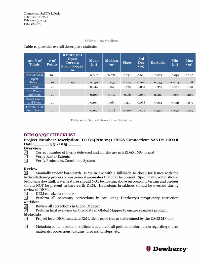
Connecticut SANDY LiDAR TO# G14PD00241 February 6, 2015 Page 46 of 70
Table 9 ― 5% Outliers
Table 10 provides overall descriptive statistics.
100 % of Totals
# of Points
RMSEz (m) Open
Terrain Spec=0.0925
m
Mean (m)
Median (m)
Skew Std Dev (m)
Kurtosis Min (m)
Max (m)
Consolidated 104 0.082 0.071 0.291 0.066 -0.021 -0.099 0.240
Open Terrain 20 0.070 0.050 0.034 0.474 0.050 -1.333 -0.014 0.128
Urban 21 0.044 0.043 0.179 0.037 -0.355 -0.018 0.120
Tall Weeds and Crops 21 0.100 0.102 -0.781 0.069 2.724 -0.099 0.240
Brush Lands and Trees 21 0.105 0.089 0.371 0.068 -0.314 -0.031 0.239
Forested and Fully Grown 21 0.107 0.108 -0.209 0.071 -0.557 -0.035 0.229
Table 10 ― Overall Descriptive Statistics
DEM QA/QC CHECKLIST
Project Number/Description: TO G14PD00241 USGS Connecticut SANDY LiDAR Date:______1/31/2015 _____ Overview
Correct number of files is delivered and all files are in ERDAS IMG format Verify Raster Extents Verify Projection/Coordinate System
Review
Manually review bare-earth DEMs in Arc with a hillshade to check for issues with the hydro-flattening process or any general anomalies that may be present. Specifically, water should be flowing downhill, water features should NOT be floating above surrounding terrain and bridges should NOT be present in bare-earth DEM. Hydrologic breaklines should be overlaid during review of DEMs.
DEM cell size is 1 meter Perform all necessary corrections in Arc using Dewberry’s proprietary correction
workflow. Review all corrections in Global Mapper Perform final overview on tiled data in Global Mapper to ensure seamless product.
Metadata Project level DEM metadata XML file is error free as determined by the USGS MP tool
Metadata content contains sufficient detail and all pertinent information regarding source
materials, projections, datums, processing steps, etc.

Connecticut SANDY LiDAR TO# G14PD00241 February 6, 2015 Page 47 of 70
Completion Comments: Complete – Approved

Connecticut SANDY LiDAR TO# G14PD00241 February 6, 2015 Page 48 of 70
Appendix A: Survey Report 1.1 Project Summary Dewberry Consultants, LLC is under contract to the United States geological Survey to provide 105 Check Points for USGS in the State of Connecticut. Under the above referenced USGS Task Order, Dewberry is tasked to complete the quality assurance of high resolution LiDAR-derived elevation products. As part of this work Dewberry staff will complete checkpoint surveys that will be used to evaluate vertical accuracy on the bare-earth terrain derived from the LiDAR. Existing NGS Control Points were located and surveyed to check the accuracy of the RTK/GPS survey equipment with the results shown in Section 2.4 of this Report. As an internal QA/QC procedure and to verify that the LiDAR Check Points meet the 95% confidence level approximately 50% of the points were re-observed and are shown in Section 5 of this report. Final horizontal coordinates are referenced to UTM Zone 18, NAD83 in meters. Final Vertical elevations are referenced to NAVD88 in meters using Geoid model 2012A (Geoid12A). 1.2 Points of Contact Questions regarding the technical aspects of this report should be addressed to: Dewberry Consultants LLC Gary Simpson, L.S. Senior Associate 10003 Derekwood Lane Suite 204 Lanham, Maryland 20706 (301) 364-1855 direct (301) 731-0188 fax 1.3 Project Areas

Connecticut SANDY LiDAR TO# G14PD00241 February 6, 2015 Page 49 of 70

Connecticut SANDY LiDAR TO# G14PD00241 February 6, 2015 Page 50 of 70
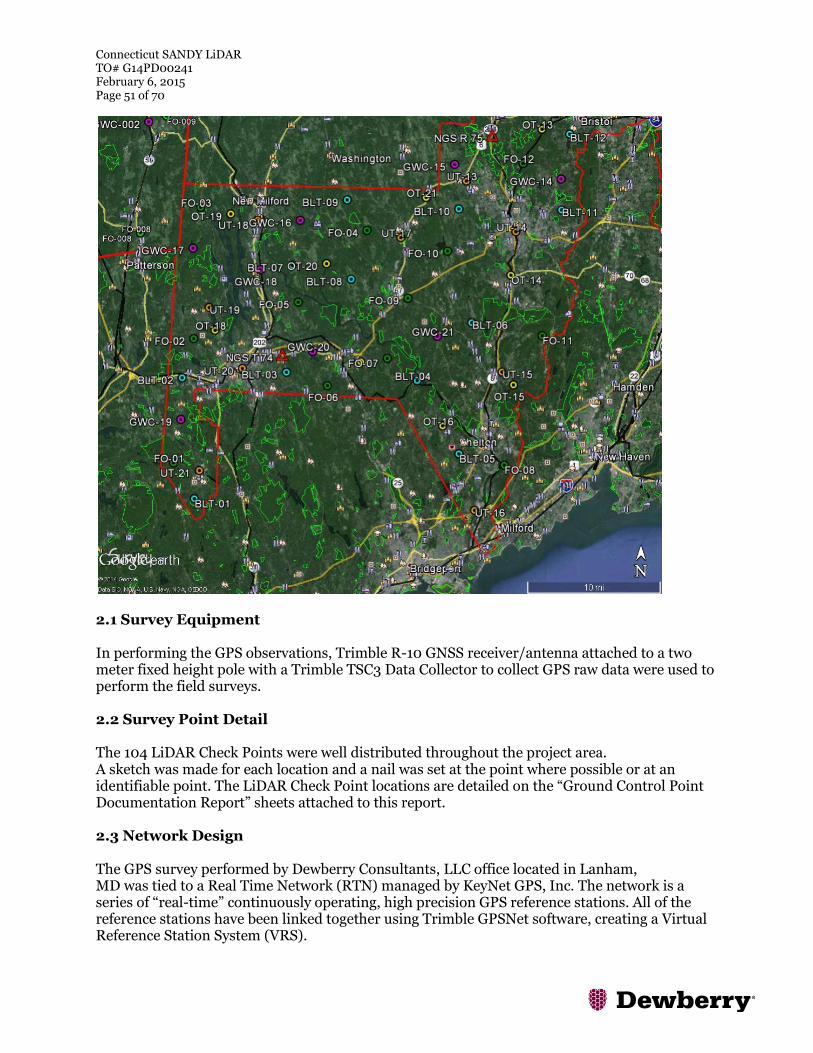
Connecticut SANDY LiDAR TO# G14PD00241 February 6, 2015 Page 51 of 70
2.1 Survey Equipment In performing the GPS observations, Trimble R-10 GNSS receiver/antenna attached to a two meter fixed height pole with a Trimble TSC3 Data Collector to collect GPS raw data were used to perform the field surveys. 2.2 Survey Point Detail The 104 LiDAR Check Points were well distributed throughout the project area. A sketch was made for each location and a nail was set at the point where possible or at an identifiable point. The LiDAR Check Point locations are detailed on the “Ground Control Point Documentation Report” sheets attached to this report. 2.3 Network Design The GPS survey performed by Dewberry Consultants, LLC office located in Lanham, MD was tied to a Real Time Network (RTN) managed by KeyNet GPS, Inc. The network is a series of “real-time” continuously operating, high precision GPS reference stations. All of the reference stations have been linked together using Trimble GPSNet software, creating a Virtual Reference Station System (VRS).

Connecticut SANDY LiDAR TO# G14PD00241 February 6, 2015 Page 52 of 70
The Trimble NetR5 Reference Station is a multi-channel, multi-frequency GNSS (Global Navigation Satellite System) receiver designed for use as a stand-alone reference station or as part of a GNSS infrastructure solution. Trimble R-Track technology in the NetR5 receiver supports the modernized GPS L2C and L5 signals as well as GLONASS L1/L2 signals. 2.4 Field Survey Procedures and Analysis Dewberry field surveyors used Trimble R-8 GNSS receivers, which is a geodetic quality dual frequency GPS receiver, to collect data at each surveyed location. All locations were occupied once with approximately 50% of the locations being reobserved. All re-observations matched the initially derived station positions within the allowable tolerance of ± 5cm or within the 95% confidence level. Each occupation which utilized the VRS network was occupied for approximately three (3) minutes in duration and measured to 180 epochs. Each occupation which utilized OPUS (if used) was occupied between 18 and 20 minutes. Field GPS observations are detailed on the “Ground Control Point Documentation Reports” submitted as part of this report. Two (4) existing NGS monument listed in the NSRS database were located as an additional QA/QC method to check the accuracy of the VRS network as well as being the primary project control monuments designated as PID LX3066, LX7346, LX2363 and LX3162. The results are as follows:
NGS PT. ID As Surveyed (M) Published (M) Differences (M)
Northing(M) Easting(M) Elev.(M) Northing(M) Easting(M) Elev.
(M) Δ N Δ E Δ Elev.
NGS-D-92 4604658.028 698169.622 9.397 4604658.026 698169.606 9.435 0.002 0.016 0.038
NGS-DENNIS
HILL 4645639.340 649303.162 495.853 4645639.355 649303.167 495.9 0.015 0.005 0.047
NGST74 4586046.306 635375.010 145.954 4586046.315 635375.032 145.944 0.009 0.022 0.010
NGS-W-91 4616360.003 690299.165 37.797 4616360.006 690299.125 37.8 0.003 0.040 0.047
The above results indicate that the VRS network is providing positional values within the 5cm parameters for this survey. 2.5 Adjustment The survey data was collected using Virtual Reference Stations (VRS) methodology within a Virtual Reference System (VRS). The system is designed to provide a true Network RTK performance, the RTKNet software enables high-accuracy positioning in real time across a geographic region. The RTKNet software package uses real-time data streams from the GPSNet system user and generates correction models for high-accuracy RTK GPS corrections throughout the network. Therefore, corrections were applied to the points as they were being collected, thus negating the need for a post process adjustment.
Connecticut SANDY LiDAR TO# G14PD00241 February 6, 2015 Page 53 of 70
2.6 Data Processing Procedures After field data is collected the information is downloaded from the data collectors into the office software. The Software program used is called TBC or Trimble Business Center. Downloaded data is run through the TBC program to obtain the following reports; points report, point comparison report and a point detail report. The reports are reviewed for point accuracy and precision. After review of the point data an “ASCII” or “txt” file which is the industry standard is created. Point files are loaded into our CADD program (Carlson Survey 2014) to make a visual check of the point data (Pt. #, Coordinates, Elev. and Description). The data can now be imported into the final product. Final Coordinates
POINT # NORTHING (M) EASTING (M) ELEV. (M)
Open Terrain
OT-02 4648799.471 672618.271 367.501
OT-03 4654195.459 691109.575 70.506
OT-04 4636499.092 669456.981 107.434
OT-05 4638253.268 688620.629 53.489
OT-06 4629005.030 683810.468 136.368
OT-07 4625256.056 668529.580 247.485
OT-08 4619282.443 680963.687 128.570
OT-09 4609374.897 696501.999 11.952
OT-10 4597099.522 690365.149 68.856
OT-11 4592305.703 706399.271 52.672
OT-12 4580272.751 713390.064 24.442
OT-13 4613927.520 666052.337 182.934
OT-14 4596346.139 662750.702 61.326
OT-15 4583150.468 663379.426 104.365
OT-16 4578031.399 654935.140 155.627
OT-17 4585480.195 644895.515 94.708
OT-18 4588849.438 627258.405 185.890
OT-19 4602864.123 628821.058 214.061
OT-20 4597178.923 640490.207 72.204
OT-21 4605412.023 652300.432 131.955
OT-02 4648799.471 672618.271 367.501
Brush/Low Trees Terrain
BLT-01 4568556.720 625240.084 216.206
BLT-02 4583032.937 623414.216 161.826
BLT-03 4584014.647 635952.350 139.963
BLT-04 4583372.976 651756.574 59.012

Connecticut SANDY LiDAR TO# G14PD00241 February 6, 2015 Page 54 of 70
BLT-05 4574726.800 656999.596 129.194
BLT-06 4590472.925 658217.507 219.177
BLT-07 4596887.148 636362.430 166.603
BLT-08 4595374.752 643508.016 202.664
BLT-09 4604858.332 642805.092 289.812
BLT-10 4604116.148 656267.285 195.168
BLT-11 4605363.094 668438.124 157.738
BLT-12 4618390.972 674852.555 99.733
BLT-13 4609195.674 683247.983 52.098
BLT-14 4598053.148 696338.012 96.785
BLT-15 4583865.847 718511.202 0.530
BLT-16 4628066.527 674026.642 118.169
BLT-17 4637180.212 694747.429 17.091
BLT-18 4652220.739 695004.912 60.955
BLT-19 4646168.472 679447.559 106.872
BLT-20 4651231.284 665614.732 316.187
BLT-21 4634569.343 659330.731 326.691
Forest Terrain
FO-01 4572804.812 622647.965 259.227
FO-02 4587783.805 624724.634 230.319
FO-03 4603791.846 625296.465 136.342
FO-04 4601265.448 645280.902 287.502
FO-05 4592451.795 637191.589 128.550
FO-06 4582523.204 640948.318 172.986
FO-07 4585961.576 648109.177 171.368
FO-08 4573296.977 662323.604 56.511
FO-09 4593243.767 650391.184 106.937
FO-10 4598970.65 655038.081 220.066
FO-11 4589140.296 666669.669 206.250
FO-12 4605771.609 682419.425 86.389
FO-13 4605793.834 682602.063 76.858
FO-14 4592573.401 690993.791 86.408
FO-15 4594425.231 702750.301 146.116
FO-16 4626852.815 680904.336 47.879
FO-17 4643402.668 668758.277 196.918
FO-18 4646501.688 687083.722 81.766
FO-19 4651650.804 673445.756 362.696
FO-20 4645556.034 664635.932 144.201
FO-21 4650400.706 657973.198 352.815
Grass/Weeds/Crops Terrain
GWC-01 4576710.640 725192.098 6.484
GWC-02 4585862.772 709091.698 73.227

Connecticut SANDY LiDAR TO# G14PD00241 February 6, 2015 Page 55 of 70
GWC-03 4600681.100 702632.641 63.903
GWC-04 4588219.549 692803.454 75.247
GWC-05 4607743.908 689106.758 74.443
GWC-06 4621378.387 678293.615 50.992
GWC-07 4637243.808 685747.152 68.889
GWC-08 4649302.395 685656.61 71.553
GWC-09 4642945.061 674829.863 303.76
GWC-10 4648195.598 662881.599 161.522
GWC-11 4647347.551 655257.033 351.326
GWC-12 4641824.276 662532.615 209.425
GWC-13 4632251.878 670402.542 150.176
GWC-14 4608012.327 668493.467 253.091
GWC-15 4609465.948 655635.392 221.467
GWC-16 4602285.475 637205.806 169.295
GWC-17 4599452.025 625102.243 219.265
GWC-18 4596265.700 632484.570 67.797
GWC-19 4578055.461 623392.506 234.985
GWC-20 4586613.684 639085.317 192.829
GWC-21 4588798.189 654042.179 98.705
Urban Terrain
UT-01 4574911.846 719137.663 4.848
UT-02 4586203.724 711167.133 44.212
UT-03 4593996.750 693527.800 53.003
UT-04 4603217.016 696368.196 9.866
UT-05 4615610.685 684748.481 53.559
UT-06 4625088.355 694332.718 5.972
UT-07 4642959.850 692860.141 47.570
UT-08 4651414.309 690351.433 60.501
UT-09 4642529.709 660613.314 214.128
UT-10 4638384.265 667666.829 116.704
UT-11 4626267.465 668743.923 264.687
UT-12 4617043.050 671570.889 120.309
UT-13 4607513.162 657097.540 148.464
UT-14 4601580.398 663220.934 78.930
UT-15 4584668.679 661969.606 54.008
UT-16 4567960.076 659055.594 15.645
UT-17 4600543.502 649364.986 82.384
UT-18 4602211.898 632028.475 89.668
UT-19 4591560.913 626489.933 190.722
UT-20 4584343.593 630651.566 117.668
UT-21 4571969.295 625784.958 197.372

Connecticut SANDY LiDAR TO# G14PD00241 February 6, 2015 Page 56 of 70
GPS Observations
POINT ID OBSERV.
DATE JULIAN DATE
TIME OF DAY
RE-OBSERV. DATE
RE-OBSERV. TIME
Open Terrain
OT-02 6/26/2014 177 13:17 N/A N/A
OT-03 6/25/2014 176 18:21 6/26/2014 7:13
OT-04 6/26/2014 177 11:28 N/A N/A
OT-05 6/26/2014 177 7:05 N/A N/A
OT-06 6/26/2014 177 7:46 N/A N/A
OT-07 6/25/2014 176 19:31 N/A N/A
OT-08 6/25/2014 176 20:38 N/A N/A
OT-09 6/25/2014 176 11:16 N/A N/A
OT-10 6/24/2014 175 15:28 6/25/2014 6:13
OT-11 6/24/2014 175 18:46 6/25/2014 8:16
OT-12 6/25/2014 176 9:42 N/A N/A
OT-13 6/25/2014 176 18:12 N/A N/A
OT-14 6/25/2014 176 17:27 N/A N/A
OT-15 6/22/2014 173 14:23 6/23/2014 8:48
OT-16 6/22/2014 173 13:20 6/23/2014 7:02
OT-17 6/23/2014 174 11:39 6/24/2014 5:46
OT-18 6/24/2014 175 10:38 6/25/2014 7:29
OT-19 6/24/2014 175 16:14 6/25/2014 6:13
OT-20 6/25/2014 176 8:55 6/26/2014 5:31
OT-21 6/25/2014 176 13:09 6/26/2014 5:58
Brush/Low Trees Terrain
BLT-01 6/23/2014 174 18:18 6/24/2014 8:30
BLT-02 6/23/2014 174 15:57 6/24/2014 7:16
BLT-03 6/23/2014 174 14:53 6/24/2014 6:32
BLT-04 6/22/2014 173 17:48 6/23/2014 6:39
BLT-05 6/22/2014 173 13:01 6/23/2014 7:23
BLT-06 1/22/2015 22 7:50
BLT-07 6/24/2014 175 13:19 6/25/2014 9:33
BLT-08 6/25/2014 176 9:20 N/A N/A
BLT-09 6/24/2014 175 17:39 6/25/2014 9:48
BLT-10 6/25/2014 176 12:45 N/A N/A
BLT-11 1/22/2015 22 9:00 N/A N/A
BLT-12 1/22/2015 22 10:40 N/A N/A
BLT-13 6/25/2014 176 13:17 N/A N/A

Connecticut SANDY LiDAR TO# G14PD00241 February 6, 2015 Page 57 of 70
BLT-14 6/24/2014 175 17:22 6/25/2014 9:22
BLT-15 6/25/2014 176 9:19 N/A N/A
BLT-16 1/22/2015 22 11:30 N/A N/A
BLT-17 6/25/2014 176 3:45 6/26/2014 5:48
BLT-18 1/22/2015 22 13:30 N/A N/A
BLT-19 6/26/2014 177 12:55 N/A N/A
BLT-20 1/22/2015 22 14:50 N/A N/A
BLT-21 6/26/2014 177 10:29 N/A N/A
Forest Terrain
FO-01 6/23/2014 174 17:11 6/24/2014 7:49
FO-02 6/24/2014 175 9:57 6/25/2014 7:48
FO-03 1/22/2015 22 17:30 N/A N/A
FO-04 6/24/2014 175 18:09 6/25/2014 5:13
FO-05 6/24/2014 175 11:50 6/25/2014 7:59
FO-06 6/23/2014 174 12:29 6/24/2014 6:03
FO-07 6/23/2014 174 10:38 6/24/2014 5:31
FO-08 1/22/2015 22 7:00 N/A N/A
FO-09 6/25/2014 176 10:04 N/A N/A
FO-10 1/22/2015 22 8:20 N/A N/A
FO-11 6/22/2014 173 15:07 6/23/2014 9:09
FO-12 6/25/2014 176 15:19 N/A N/A
FO-13 1/22/2015 22 9:30 N/A N/A
FO-14 6/24/2014 175 14:42 6/25/2014 6:49
FO-15 6/24/2014 175 17:55 6/25/2014 9:02
FO-16 6/26/2014 177 8:30 N/A N/A
FO-17 6/26/2014 177 11:25 N/A N/A
FO-18 1/22/2015 22 13:05 N/A N/A
FO-19 1/22/2015 22 14:20 N/A N/A
FO-20 6/26/2014 177 10:49 N/A N/A
FO-21 6/26/2014 177 9:29 N/A N/A
Grass/Weeds/Crops Terrain
GWC-01 6/25/2014 176 8:46 N/A N/A
GWC-02 6/25/2014 176 10:07 N/A N/A
GWC-03 6/24/2014 175 16:53 6/25/2014 5:49
GWC-04 6/24/2014 175 14:00 6/25/2014 7:11
GWC-05 6/25/2014 176 12:09 N/A N/A
GWC-06 1/22/2015 22 11:00 N/A N/A
GWC-07 1/22/2015 22 12:10 N/A N/A

Connecticut SANDY LiDAR TO# G14PD00241 February 6, 2015 Page 58 of 70
GWC-08 1/22/2015 22 14:00 N/A N/A
GWC-09 1/22/2015 22 12:40 N/A N/A
GWC-10 1/22/2015 22 15:10 N/A N/A
GWC-11 6/26/2014 177 12:17 N/A N/A
GWC-12 1/22/2015 22 15:56 N/A N/A
GWC-13 6/26/2014 177 9:48 N/A N/A
GWC-14 6/25/2014 176 16:05 6/26/2014 6:26
GWC-15 6/25/2014 176 14:03 N/A N/A
GWC-16 6/24/2014 175 17:11 6/25/2014 5:39
GWC-17 1/22/2015 22 18:00 N/A N/A
GWC-18 6/24/2014 175 12:50 6/25/2014 9:16
GWC-19 6/23/2014 174 16:27 6/25/2014 8:23
GWC-20 6/23/2014 174 13:22 6/24/2014 6:16
GWC-21 6/22/2014 173 16:44 6/23/2014 6:13
Urban Terrain
UT-01 6/25/2014 176 8:21 N/A N/A
UT-02 6/24/2014 175 19:07 6/25/2014 8:35
UT-03 6/24/2014 175 15:04 6/25/2014 6:29
UT-04 6/24/2014 175 16:06 6/25/2014 5:32
UT-05 6/25/2014 176 13:52 N/A N/A
UT-06 6/25/2014 176 15:12 N/A N/A
UT-07 6/25/2014 176 12:24 6/26/2014 6:11
UT-08 6/25/2014 176 18:09 N/A N/A
UT-09 6/26/2014 177 11:52 N/A N/A
UT-10 6/26/2014 177 11:15 N/A N/A
UT-11 6/25/2014 176 19:47 6/26/2014 6:59
UT-12 6/25/2014 176 19:01 N/A N/A
UT-13 6/25/2014 176 13:39 N/A N/A
UT-14 6/25/2014 176 17:09 N/A N/A
UT-15 6/22/2014 173 13:56 6/23/2014 8:31
UT-16 6/22/2014 173 10:29 6/23/2014 7:51
UT-17 6/25/2014 176 12:11 N/A N/A
UT-18 6/24/2014 175 16:39 6/25/2014 5:59
UT-19 6/24/2014 175 11:08 6/25/2014 7:09
UT-20 6/23/2014 174 15:27 6/24/2014 6:49
UT-21 6/23/2014 174 17:55 6/24/2014 8:13
Connecticut SANDY LiDAR TO# G14PD00241 February 6, 2015 Page 59 of 70
Point Comparison
POINT ID POINT CK DELTA NORTH
(M) DELTA EAST (M) VERT. DIFF (M)
Open Terrain
OT-03 OT-03CK 0.002 0.005 0.028
OT-10 OT-10CK 0.000 0.001 0.003
OT-11 OT-11CK 0.001 0.002 0.011
OT-15 OT-15CK 0.005 0.005 0.005
OT-16 OT-16CK 0.001 0.002 0.010
OT-17 OT-17CK 0.020 0.009 0.027
OT-18 OT-18CK 0.006 0.002 0.030
OT-19 OT-19CK 0.007 0.002 0.004
OT-20 OT-20CK 0.000 0.002 0.023
OT-21 OT-21CK 0.002 0.007 0.001
Brush/Low Trees Terrain
BLT-01 BLT-01CK 0.003 0.001 0.000
BLT-02 BLT-02CK 0.001 0.002 0.011
BLT-03 BLT-03CK 0.011 0.004 0.025
BLT-04 BLT-04CK 0.004 0.018 0.015
BLT-05 BLT-05CK 0.009 0.002 0.001
BLT-06 BLT-06CK 0.002 0.008 0.006
BLT-07 BLT-07CK 0.000 0.002 0.010
BLT-09 BLT-09CK 0.003 0.007 0.017
BLT-14 BLT-14CK 0.002 0.001 0.012
BLT-17 BLT-17CK 0.008 0.020 0.065
BLT-18 BLT-18CK 0.002 0.005 0.017
Forest Terrain
FO-01 FO-01CK 0.007 0.005 0.014
FO-02 FO-02CK 0.001 0.003 0.003
FO-03 FO-03CK 0.011 0.004 0.005
FO-04 FO-04CK 0.002 0.005 0.017
FO-05 FO-05CK 0.020 0.001 0.004
FO-06 FO-06CK 0.009 0.013 0.031
FO-07 FO-07CK 0.002 0.004 0.015
FO-08 FO-08CK 0.011 0.004 0.005
FO-11 FO-13CK 0.001 0.009 0.002
FO-14 FO-14CK 0.023 0.012 0.006
FO-15 FO-15CK 0.016 0.004 0.028

Connecticut SANDY LiDAR TO# G14PD00241 February 6, 2015 Page 60 of 70
Grass/Weeds/Crops Terrain
GWC-03 GWC-03CK 0.020 0.001 0.004
GWC-04 GWC-04CK 0.001 0.007 0.002
GWC-08 GWC-08CK 0.006 0.016 0.006
GWC-14 GWC-14CK 0.001 0.002 0.008
GWC-16 GWC-16CK 0.012 0.005 0.019
GWC-18 GWC-18CK 0.001 0.002 0.005
GWC-19 GWC-19CK 0.002 0.004 0.018
GWC-20 GWC-20CK 0.004 0.004 0.026
GWC-21 GWC-21CK 0.005 0.002 0.039
Urban Terrain
UT-02 UT-02CK 0.000 0.002 0.008
UT-03 UT-03CK 0.001 0.001 0.020
UT-04 UT-04CK 0.000 0.005 0.017
UT-07 UT-07CK 0.004 0.023 0.040
UT-11 UT-11CK 0.005 0.000 0.003
UT-15 UT-15CK 0.004 0.000 0.003
UT-16 UT-16CK 0.001 0.004 0.004
UT-18 UT-18CK 0.005 0.003 0.010
UT-19 UT-19CK 0.015 0.009 0.028
UT-20 UT-20CK 0.006 0.005 0.001
UT-21 UT-21CK 0.003 0.006 0.006

Connecticut SANDY LiDAR TO# G14PD00241 February 6, 2015 Page 61 of 70
Appendix B: Complete List of Delivered Tiles
18TXL195572 18TXL570581 18TXM555651 18TXM735653 18TXM915606
18TXL210569 18TXL570582 18TXM555653 18TXM735654 18TXM915608
18TXL210570 18TXL570584 18TXM555654 18TXM735656 18TXM915609
18TXL210572 18TXL570585 18TXM555656 18TXM750612 18TXM915611
18TXL210573 18TXL570587 18TXM570600 18TXM750614 18TXM915612
18TXL210575 18TXL570588 18TXM570602 18TXM750615 18TXM915614
18TXL210576 18TXL570590 18TXM570603 18TXM750617 18TXM915615
18TXL210578 18TXL570591 18TXM570605 18TXM750618 18TXM915617
18TXL210579 18TXL570593 18TXM570606 18TXM750620 18TXM915618
18TXL210581 18TXL570594 18TXM570608 18TXM750621 18TXM915620
18TXL210582 18TXL570596 18TXM570609 18TXM750623 18TXM915621
18TXL210584 18TXL570597 18TXM570611 18TXM750624 18TXM915623
18TXL210585 18TXL570599 18TXM570612 18TXM750626 18TXM915624
18TXL210587 18TXL585561 18TXM570614 18TXM750627 18TXM915626
18TXL210588 18TXL585563 18TXM570615 18TXM750629 18TXM915627
18TXL210590 18TXL585564 18TXM570633 18TXM750630 18TXM915629
18TXL210591 18TXL585566 18TXM570635 18TXM750632 18TXM915630
18TXL210593 18TXL585567 18TXM570636 18TXM750633 18TXM915632
18TXL210594 18TXL585569 18TXM570638 18TXM750635 18TXM915633
18TXL210596 18TXL585570 18TXM570639 18TXM750636 18TXM915635
18TXL210597 18TXL585572 18TXM570641 18TXM750638 18TXM915636
18TXL225567 18TXL585573 18TXM570642 18TXM750639 18TXM915638
18TXL225569 18TXL585575 18TXM570644 18TXM750641 18TXM915639
18TXL225570 18TXL585576 18TXM570645 18TXM750642 18TXM915641
18TXL225572 18TXL585578 18TXM570647 18TXM750644 18TXM915642
18TXL225573 18TXL585579 18TXM570648 18TXM750645 18TXM915644
18TXL225575 18TXL585581 18TXM570650 18TXM750647 18TXM915645
18TXL225576 18TXL585582 18TXM570651 18TXM750648 18TXM915647
18TXL225578 18TXL585584 18TXM570653 18TXM750650 18TXM915648
18TXL225579 18TXL585585 18TXM570654 18TXM750651 18TXM915650
18TXL225581 18TXL585587 18TXM570656 18TXM750653 18TXM915651
18TXL225582 18TXL585588 18TXM585600 18TXM750654 18TXM915653
18TXL225584 18TXL585590 18TXM585602 18TXM750656 18TXM915654
18TXL225585 18TXL585591 18TXM585603 18TXM765614 18TXM915656
18TXL225587 18TXL585593 18TXM585605 18TXM765615 18TXM930600
18TXL225588 18TXL585594 18TXM585606 18TXM765617 18TXM930602
18TXL225590 18TXL585596 18TXM585608 18TXM765618 18TXM930603
18TXL225591 18TXL585597 18TXM585609 18TXM765620 18TXM930605

Connecticut SANDY LiDAR TO# G14PD00241 February 6, 2015 Page 62 of 70
18TXL225593 18TXL585599 18TXM585611 18TXM765621 18TXM930606
18TXL225594 18TXL600561 18TXM585612 18TXM765623 18TXM930608
18TXL225596 18TXL600563 18TXM585614 18TXM765624 18TXM930609
18TXL225597 18TXL600564 18TXM585615 18TXM765626 18TXM930611
18TXL225599 18TXL600566 18TXM585632 18TXM765627 18TXM930612
18TXL240566 18TXL600567 18TXM585633 18TXM765629 18TXM930614
18TXL240567 18TXL600569 18TXM585635 18TXM765630 18TXM930615
18TXL240569 18TXL600570 18TXM585636 18TXM765632 18TXM930617
18TXL240570 18TXL600572 18TXM585638 18TXM765633 18TXM930618
18TXL240572 18TXL600573 18TXM585639 18TXM765635 18TXM930620
18TXL240573 18TXL600575 18TXM585641 18TXM765636 18TXM930621
18TXL240575 18TXL600576 18TXM585642 18TXM765638 18TXM930623
18TXL240576 18TXL600578 18TXM585644 18TXM765639 18TXM930624
18TXL240578 18TXL600579 18TXM585645 18TXM765641 18TXM930626
18TXL240579 18TXL600581 18TXM585647 18TXM765642 18TXM930627
18TXL240581 18TXL600582 18TXM585648 18TXM765644 18TXM930629
18TXL240582 18TXL600584 18TXM585650 18TXM765645 18TXM930630
18TXL240584 18TXL600585 18TXM585651 18TXM765647 18TXM930632
18TXL240585 18TXL600587 18TXM585653 18TXM765648 18TXM930633
18TXL240587 18TXL600588 18TXM585654 18TXM765650 18TXM930635
18TXL240588 18TXL600590 18TXM585656 18TXM765651 18TXM930636
18TXL240590 18TXL600591 18TXM600600 18TXM765653 18TXM930638
18TXL240591 18TXL600593 18TXM600602 18TXM765654 18TXM930639
18TXL240593 18TXL600594 18TXM600603 18TXM765656 18TXM930641
18TXL240594 18TXL600596 18TXM600605 18TXM780602 18TXM930642
18TXL240596 18TXL600597 18TXM600606 18TXM780603 18TXM930644
18TXL240597 18TXL600599 18TXM600608 18TXM780611 18TXM930645
18TXL240599 18TXL615563 18TXM600609 18TXM780612 18TXM930647
18TXL255566 18TXL615564 18TXM600611 18TXM780614 18TXM930648
18TXL255567 18TXL615566 18TXM600612 18TXM780615 18TXM930650
18TXL255569 18TXL615567 18TXM600614 18TXM780617 18TXM930651
18TXL255570 18TXL615569 18TXM600615 18TXM780618 18TXM930653
18TXL255572 18TXL615570 18TXM600630 18TXM780620 18TXM930654
18TXL255573 18TXL615572 18TXM600632 18TXM780621 18TXM930656
18TXL255575 18TXL615573 18TXM600633 18TXM780623 18TXM945600
18TXL255576 18TXL615575 18TXM600635 18TXM780624 18TXM945602
18TXL255578 18TXL615576 18TXM600636 18TXM780626 18TXM945603
18TXL255579 18TXL615578 18TXM600638 18TXM780627 18TXM945605
18TXL255581 18TXL615579 18TXM600639 18TXM780629 18TXM945606
18TXL255582 18TXL615581 18TXM600641 18TXM780630 18TXM945608
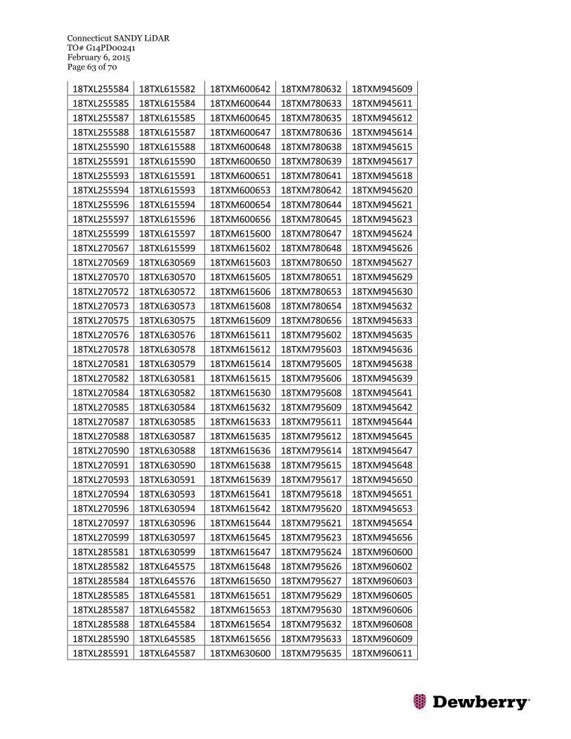
Connecticut SANDY LiDAR TO# G14PD00241 February 6, 2015 Page 63 of 70
18TXL255584 18TXL615582 18TXM600642 18TXM780632 18TXM945609
18TXL255585 18TXL615584 18TXM600644 18TXM780633 18TXM945611
18TXL255587 18TXL615585 18TXM600645 18TXM780635 18TXM945612
18TXL255588 18TXL615587 18TXM600647 18TXM780636 18TXM945614
18TXL255590 18TXL615588 18TXM600648 18TXM780638 18TXM945615
18TXL255591 18TXL615590 18TXM600650 18TXM780639 18TXM945617
18TXL255593 18TXL615591 18TXM600651 18TXM780641 18TXM945618
18TXL255594 18TXL615593 18TXM600653 18TXM780642 18TXM945620
18TXL255596 18TXL615594 18TXM600654 18TXM780644 18TXM945621
18TXL255597 18TXL615596 18TXM600656 18TXM780645 18TXM945623
18TXL255599 18TXL615597 18TXM615600 18TXM780647 18TXM945624
18TXL270567 18TXL615599 18TXM615602 18TXM780648 18TXM945626
18TXL270569 18TXL630569 18TXM615603 18TXM780650 18TXM945627
18TXL270570 18TXL630570 18TXM615605 18TXM780651 18TXM945629
18TXL270572 18TXL630572 18TXM615606 18TXM780653 18TXM945630
18TXL270573 18TXL630573 18TXM615608 18TXM780654 18TXM945632
18TXL270575 18TXL630575 18TXM615609 18TXM780656 18TXM945633
18TXL270576 18TXL630576 18TXM615611 18TXM795602 18TXM945635
18TXL270578 18TXL630578 18TXM615612 18TXM795603 18TXM945636
18TXL270581 18TXL630579 18TXM615614 18TXM795605 18TXM945638
18TXL270582 18TXL630581 18TXM615615 18TXM795606 18TXM945639
18TXL270584 18TXL630582 18TXM615630 18TXM795608 18TXM945641
18TXL270585 18TXL630584 18TXM615632 18TXM795609 18TXM945642
18TXL270587 18TXL630585 18TXM615633 18TXM795611 18TXM945644
18TXL270588 18TXL630587 18TXM615635 18TXM795612 18TXM945645
18TXL270590 18TXL630588 18TXM615636 18TXM795614 18TXM945647
18TXL270591 18TXL630590 18TXM615638 18TXM795615 18TXM945648
18TXL270593 18TXL630591 18TXM615639 18TXM795617 18TXM945650
18TXL270594 18TXL630593 18TXM615641 18TXM795618 18TXM945651
18TXL270596 18TXL630594 18TXM615642 18TXM795620 18TXM945653
18TXL270597 18TXL630596 18TXM615644 18TXM795621 18TXM945654
18TXL270599 18TXL630597 18TXM615645 18TXM795623 18TXM945656
18TXL285581 18TXL630599 18TXM615647 18TXM795624 18TXM960600
18TXL285582 18TXL645575 18TXM615648 18TXM795626 18TXM960602
18TXL285584 18TXL645576 18TXM615650 18TXM795627 18TXM960603
18TXL285585 18TXL645581 18TXM615651 18TXM795629 18TXM960605
18TXL285587 18TXL645582 18TXM615653 18TXM795630 18TXM960606
18TXL285588 18TXL645584 18TXM615654 18TXM795632 18TXM960608
18TXL285590 18TXL645585 18TXM615656 18TXM795633 18TXM960609
18TXL285591 18TXL645587 18TXM630600 18TXM795635 18TXM960611

Connecticut SANDY LiDAR TO# G14PD00241 February 6, 2015 Page 64 of 70
18TXL285593 18TXL645588 18TXM630602 18TXM795636 18TXM960612
18TXL285594 18TXL645590 18TXM630603 18TXM795638 18TXM960614
18TXL285596 18TXL645591 18TXM630605 18TXM795639 18TXM960615
18TXL285597 18TXL645593 18TXM630606 18TXM795641 18TXM960617
18TXL285599 18TXL645594 18TXM630608 18TXM795642 18TXM960618
18TXL300581 18TXL645596 18TXM630609 18TXM795644 18TXM960620
18TXL300582 18TXL645597 18TXM630611 18TXM795645 18TXM960621
18TXL300584 18TXL645599 18TXM630612 18TXM795647 18TXM960623
18TXL300585 18TXL660581 18TXM630614 18TXM795648 18TXM960624
18TXL300587 18TXL660582 18TXM630615 18TXM795650 18TXM960626
18TXL300588 18TXL660584 18TXM630617 18TXM795651 18TXM960627
18TXL300590 18TXL660585 18TXM630618 18TXM795653 18TXM960629
18TXL300591 18TXL660587 18TXM630629 18TXM795654 18TXM960630
18TXL300593 18TXL660588 18TXM630630 18TXM795656 18TXM960632
18TXL300594 18TXL660590 18TXM630632 18TXM810602 18TXM960633
18TXL300596 18TXL660591 18TXM630633 18TXM810603 18TXM960635
18TXL300597 18TXL660593 18TXM630635 18TXM810605 18TXM960636
18TXL300599 18TXL660594 18TXM630636 18TXM810606 18TXM960638
18TXL315581 18TXL660596 18TXM630638 18TXM810608 18TXM960639
18TXL315582 18TXL660597 18TXM630639 18TXM810609 18TXM960641
18TXL315584 18TXL660599 18TXM630641 18TXM810611 18TXM960642
18TXL315585 18TXL675584 18TXM630642 18TXM810612 18TXM960644
18TXL315587 18TXL675585 18TXM630644 18TXM810614 18TXM960645
18TXL315588 18TXL675588 18TXM630645 18TXM810615 18TXM960647
18TXL315590 18TXL675590 18TXM630647 18TXM810617 18TXM960648
18TXL315591 18TXL675591 18TXM630648 18TXM810618 18TXM960650
18TXL315593 18TXL675593 18TXM630650 18TXM810620 18TXM960651
18TXL315594 18TXL675594 18TXM630651 18TXM810621 18TXM960653
18TXL315596 18TXL675596 18TXM630653 18TXM810623 18TXM960654
18TXL315597 18TXL675597 18TXM630654 18TXM810624 18TXM960656
18TXL315599 18TXL675599 18TXM630656 18TXM810626 18TXM975600
18TXL330581 18TXL690588 18TXM645600 18TXM810627 18TXM975602
18TXL330582 18TXL690590 18TXM645602 18TXM810629 18TXM975603
18TXL330584 18TXL690591 18TXM645603 18TXM810630 18TXM975605
18TXL330585 18TXL690593 18TXM645605 18TXM810632 18TXM975606
18TXL330587 18TXL690594 18TXM645606 18TXM810633 18TXM975608
18TXL330588 18TXL690596 18TXM645608 18TXM810635 18TXM975609
18TXL330590 18TXL690597 18TXM645609 18TXM810636 18TXM975611
18TXL330591 18TXL690599 18TXM645611 18TXM810638 18TXM975612
18TXL330593 18TXL705593 18TXM645612 18TXM810639 18TXM975614

Connecticut SANDY LiDAR TO# G14PD00241 February 6, 2015 Page 65 of 70
18TXL330594 18TXL705594 18TXM645614 18TXM810641 18TXM975615
18TXL330596 18TXL870588 18TXM645615 18TXM810642 18TXM975617
18TXL330597 18TXL870590 18TXM645617 18TXM810644 18TXM975618
18TXL330599 18TXL870593 18TXM645618 18TXM810645 18TXM975620
18TXL345581 18TXL870594 18TXM645621 18TXM810647 18TXM975621
18TXL345582 18TXL870596 18TXM645623 18TXM810648 18TXM975623
18TXL345584 18TXL870597 18TXM645624 18TXM810650 18TXM975629
18TXL345585 18TXL870599 18TXM645626 18TXM810651 18TXM975630
18TXL345587 18TXL885587 18TXM645627 18TXM810653 18TXM975632
18TXL345588 18TXL885588 18TXM645629 18TXM810654 18TXM975633
18TXL345590 18TXL885590 18TXM645630 18TXM810656 18TXM975635
18TXL345591 18TXL885591 18TXM645632 18TXM825603 18TXM975636
18TXL345593 18TXL885593 18TXM645633 18TXM825605 18TXM975638
18TXL345594 18TXL885594 18TXM645635 18TXM825606 18TXM975639
18TXL345596 18TXL885596 18TXM645636 18TXM825608 18TXM975641
18TXL345597 18TXL885597 18TXM645638 18TXM825609 18TXM975642
18TXL345599 18TXL885599 18TXM645639 18TXM825611 18TXM975644
18TXL360581 18TXL900587 18TXM645641 18TXM825612 18TXM975645
18TXL360582 18TXL900588 18TXM645642 18TXM825614 18TXM975647
18TXL360584 18TXL900590 18TXM645644 18TXM825615 18TXM975648
18TXL360585 18TXL900591 18TXM645645 18TXM825617 18TXM975650
18TXL360587 18TXL900593 18TXM645647 18TXM825618 18TXM975651
18TXL360588 18TXL900594 18TXM645648 18TXM825620 18TXM975653
18TXL360590 18TXL900596 18TXM645650 18TXM825621 18TXM975654
18TXL360591 18TXL900597 18TXM645651 18TXM825623 18TXM975656
18TXL360593 18TXL900599 18TXM645653 18TXM825624 18TXM990600
18TXL360594 18TXL915585 18TXM645654 18TXM825626 18TXM990602
18TXL360596 18TXL915587 18TXM645656 18TXM825627 18TXM990603
18TXL360597 18TXL915588 18TXM660600 18TXM825629 18TXM990605
18TXL360599 18TXL915590 18TXM660602 18TXM825630 18TXM990606
18TXL375581 18TXL915591 18TXM660603 18TXM825632 18TXM990608
18TXL375582 18TXL915593 18TXM660605 18TXM825633 18TXM990609
18TXL375584 18TXL915594 18TXM660606 18TXM825635 18TXM990611
18TXL375585 18TXL915596 18TXM660608 18TXM825636 18TXM990614
18TXL375587 18TXL915597 18TXM660609 18TXM825638 18TXM990615
18TXL375588 18TXL915599 18TXM660611 18TXM825639 18TXM990617
18TXL375590 18TXL930585 18TXM660612 18TXM825641 18TXM990618
18TXL375591 18TXL930587 18TXM660614 18TXM825642 18TXM990620
18TXL375593 18TXL930588 18TXM660615 18TXM825644 18TXM990621
18TXL375594 18TXL930590 18TXM660617 18TXM825645 18TXM990623

Connecticut SANDY LiDAR TO# G14PD00241 February 6, 2015 Page 66 of 70
18TXL375596 18TXL930591 18TXM660618 18TXM825647 18TXM990632
18TXL375597 18TXL930593 18TXM660620 18TXM825648 18TXM990633
18TXL375599 18TXL930594 18TXM660621 18TXM825650 18TXM990635
18TXL390581 18TXL930596 18TXM660623 18TXM825651 18TXM990636
18TXL390582 18TXL930597 18TXM660624 18TXM840602 18TXM990638
18TXL390584 18TXL930599 18TXM660626 18TXM840603 18TXM990639
18TXL390585 18TXL945587 18TXM660627 18TXM840605 18TXM990641
18TXL390587 18TXL945588 18TXM660629 18TXM840606 18TXM990647
18TXL390588 18TXL945590 18TXM660630 18TXM840608 18TXM990648
18TXL390590 18TXL945591 18TXM660632 18TXM840609 18TXM990650
18TXL390591 18TXL945593 18TXM660633 18TXM840611 18TXM990651
18TXL390593 18TXL945594 18TXM660635 18TXM840612 18TXM990653
18TXL390594 18TXL945596 18TXM660636 18TXM840614 18TXM990654
18TXL390596 18TXL945597 18TXM660638 18TXM840615 18TYL005588
18TXL390597 18TXL945599 18TXM660639 18TXM840617 18TYL005590
18TXL390599 18TXL960590 18TXM660641 18TXM840618 18TYL005591
18TXL405581 18TXL960591 18TXM660642 18TXM840620 18TYL005593
18TXL405582 18TXL960593 18TXM660644 18TXM840621 18TYL005594
18TXL405584 18TXL960594 18TXM660645 18TXM840623 18TYL005596
18TXL405585 18TXL960596 18TXM660647 18TXM840624 18TYL005597
18TXL405587 18TXL960597 18TXM660648 18TXM840626 18TYL005599
18TXL405588 18TXL960599 18TXM660650 18TXM840627 18TYL020588
18TXL405590 18TXL975590 18TXM660651 18TXM840629 18TYL020590
18TXL405591 18TXL975591 18TXM660653 18TXM840630 18TYL020591
18TXL405593 18TXL975593 18TXM660654 18TXM840632 18TYL020593
18TXL405594 18TXL975594 18TXM660656 18TXM840633 18TYL020594
18TXL405596 18TXL975596 18TXM675600 18TXM840635 18TYL020596
18TXL405597 18TXL975597 18TXM675602 18TXM840636 18TYL020597
18TXL405599 18TXL975599 18TXM675603 18TXM840638 18TYL020599
18TXL420581 18TXL990588 18TXM675605 18TXM840639 18TYL035587
18TXL420582 18TXL990590 18TXM675606 18TXM840641 18TYL035588
18TXL420584 18TXL990591 18TXM675608 18TXM840642 18TYL035590
18TXL420585 18TXL990593 18TXM675609 18TXM840644 18TYL035591
18TXL420587 18TXL990594 18TXM675611 18TXM840645 18TYL035593
18TXL420588 18TXL990596 18TXM675612 18TXM840647 18TYL035594
18TXL420590 18TXL990597 18TXM675614 18TXM840648 18TYL035596
18TXL420591 18TXL990599 18TXM675615 18TXM840650 18TYL035597
18TXL420593 18TXM225600 18TXM675617 18TXM840651 18TYL035599
18TXL420594 18TXM225602 18TXM675618 18TXM840653 18TYL050584
18TXL420596 18TXM225603 18TXM675620 18TXM840654 18TYL050585

Connecticut SANDY LiDAR TO# G14PD00241 February 6, 2015 Page 67 of 70
18TXL420597 18TXM225605 18TXM675621 18TXM840656 18TYL050587
18TXL420599 18TXM240600 18TXM675623 18TXM855602 18TYL050588
18TXL435581 18TXM240602 18TXM675624 18TXM855603 18TYL050590
18TXL435582 18TXM240603 18TXM675626 18TXM855605 18TYL050591
18TXL435584 18TXM240605 18TXM675627 18TXM855606 18TYL050593
18TXL435585 18TXM255600 18TXM675629 18TXM855608 18TYL050594
18TXL435587 18TXM255602 18TXM675630 18TXM855609 18TYL050596
18TXL435588 18TXM255603 18TXM675632 18TXM855611 18TYL050597
18TXL435590 18TXM255605 18TXM675633 18TXM855612 18TYL065579
18TXL435591 18TXM270600 18TXM675635 18TXM855614 18TYL065581
18TXL435593 18TXM270602 18TXM675636 18TXM855615 18TYL065582
18TXL435594 18TXM270603 18TXM675638 18TXM855617 18TYL065584
18TXL435596 18TXM270605 18TXM675639 18TXM855618 18TYL065585
18TXL435597 18TXM285600 18TXM675641 18TXM855620 18TYL065587
18TXL435599 18TXM285602 18TXM675642 18TXM855621 18TYL065588
18TXL450581 18TXM285603 18TXM675644 18TXM855623 18TYL065590
18TXL450582 18TXM285605 18TXM675645 18TXM855624 18TYL065591
18TXL450584 18TXM300600 18TXM675647 18TXM855626 18TYL065593
18TXL450585 18TXM300602 18TXM675648 18TXM855627 18TYL065594
18TXL450587 18TXM300603 18TXM675650 18TXM855629 18TYL065596
18TXL450588 18TXM300605 18TXM675651 18TXM855630 18TYL065597
18TXL450590 18TXM315600 18TXM675653 18TXM855632 18TYL080578
18TXL450591 18TXM315602 18TXM675654 18TXM855633 18TYL080579
18TXL450593 18TXM315603 18TXM675656 18TXM855635 18TYL080581
18TXL450594 18TXM315605 18TXM690600 18TXM855636 18TYL080582
18TXL450596 18TXM330600 18TXM690602 18TXM855638 18TYL080584
18TXL450597 18TXM330602 18TXM690603 18TXM855639 18TYL080585
18TXL450599 18TXM330603 18TXM690605 18TXM855641 18TYL080587
18TXL465581 18TXM330605 18TXM690606 18TXM855642 18TYL080588
18TXL465582 18TXM345600 18TXM690608 18TXM855644 18TYL080590
18TXL465584 18TXM345602 18TXM690609 18TXM855645 18TYL080591
18TXL465585 18TXM345603 18TXM690611 18TXM855647 18TYL080593
18TXL465587 18TXM345605 18TXM690612 18TXM855648 18TYL080594
18TXL465588 18TXM360600 18TXM690614 18TXM855650 18TYL080596
18TXL465590 18TXM360602 18TXM690615 18TXM855651 18TYL095576
18TXL465591 18TXM360603 18TXM690617 18TXM855653 18TYL095578
18TXL465593 18TXM360605 18TXM690618 18TXM855654 18TYL095579
18TXL465594 18TXM375600 18TXM690620 18TXM855656 18TYL095581
18TXL465596 18TXM375602 18TXM690621 18TXM870600 18TYL095582
18TXL465597 18TXM375603 18TXM690623 18TXM870602 18TYL095584

Connecticut SANDY LiDAR TO# G14PD00241 February 6, 2015 Page 68 of 70
18TXL465599 18TXM375605 18TXM690624 18TXM870603 18TYL095585
18TXL480579 18TXM390600 18TXM690626 18TXM870605 18TYL095587
18TXL480581 18TXM390602 18TXM690627 18TXM870606 18TYL095588
18TXL480582 18TXM390603 18TXM690629 18TXM870608 18TYL095590
18TXL480584 18TXM390605 18TXM690630 18TXM870609 18TYL095591
18TXL480585 18TXM405600 18TXM690632 18TXM870611 18TYL095593
18TXL480587 18TXM405602 18TXM690633 18TXM870612 18TYL095594
18TXL480588 18TXM405603 18TXM690635 18TXM870614 18TYL110576
18TXL480590 18TXM405605 18TXM690636 18TXM870615 18TYL110578
18TXL480591 18TXM420600 18TXM690638 18TXM870617 18TYL110579
18TXL480593 18TXM420602 18TXM690639 18TXM870618 18TYL110581
18TXL480594 18TXM420603 18TXM690641 18TXM870620 18TYL110582
18TXL480596 18TXM420605 18TXM690642 18TXM870621 18TYL110584
18TXL480597 18TXM435600 18TXM690644 18TXM870623 18TYL110585
18TXL480599 18TXM435602 18TXM690645 18TXM870624 18TYL110587
18TXL495578 18TXM435603 18TXM690647 18TXM870626 18TYL110588
18TXL495579 18TXM435605 18TXM690648 18TXM870627 18TYL110590
18TXL495581 18TXM450600 18TXM690650 18TXM870629 18TYL110591
18TXL495582 18TXM450602 18TXM690651 18TXM870630 18TYL110593
18TXL495584 18TXM450603 18TXM690653 18TXM870632 18TYL110594
18TXL495585 18TXM450605 18TXM690654 18TXM870633 18TYL125576
18TXL495587 18TXM465600 18TXM690656 18TXM870635 18TYL125578
18TXL495588 18TXM465602 18TXM705600 18TXM870636 18TYL125579
18TXL495590 18TXM465603 18TXM705602 18TXM870638 18TYL125581
18TXL495591 18TXM465605 18TXM705603 18TXM870639 18TYL125582
18TXL495593 18TXM480600 18TXM705605 18TXM870641 18TYL125584
18TXL495594 18TXM480602 18TXM705606 18TXM870642 18TYL125585
18TXL495596 18TXM480603 18TXM705608 18TXM870644 18TYL125587
18TXL495597 18TXM480605 18TXM705611 18TXM870645 18TYL125588
18TXL495599 18TXM495600 18TXM705612 18TXM870647 18TYL125590
18TXL510575 18TXM495602 18TXM705614 18TXM870648 18TYL125591
18TXL510576 18TXM495603 18TXM705615 18TXM870650 18TYL140576
18TXL510578 18TXM495605 18TXM705617 18TXM870651 18TYL140578
18TXL510579 18TXM495645 18TXM705618 18TXM870653 18TYL140579
18TXL510581 18TXM495647 18TXM705620 18TXM870654 18TYL140581
18TXL510582 18TXM495648 18TXM705621 18TXM870656 18TYL140582
18TXL510584 18TXM495651 18TXM705623 18TXM885600 18TYL140584
18TXL510585 18TXM495653 18TXM705624 18TXM885602 18TYL140585
18TXL510587 18TXM495654 18TXM705626 18TXM885603 18TYL140587
18TXL510588 18TXM495656 18TXM705627 18TXM885605 18TYL140588

Connecticut SANDY LiDAR TO# G14PD00241 February 6, 2015 Page 69 of 70
18TXL510590 18TXM510600 18TXM705629 18TXM885606 18TYL140590
18TXL510591 18TXM510602 18TXM705630 18TXM885608 18TYL155576
18TXL510593 18TXM510603 18TXM705632 18TXM885609 18TYL155578
18TXL510594 18TXM510605 18TXM705633 18TXM885611 18TYL155579
18TXL510596 18TXM510644 18TXM705635 18TXM885612 18TYL155581
18TXL510597 18TXM510645 18TXM705636 18TXM885614 18TYL155582
18TXL510599 18TXM510647 18TXM705638 18TXM885615 18TYL155584
18TXL525572 18TXM510648 18TXM705639 18TXM885617 18TYL155585
18TXL525573 18TXM510650 18TXM705641 18TXM885618 18TYL155587
18TXL525575 18TXM510651 18TXM705642 18TXM885620 18TYL155588
18TXL525576 18TXM510653 18TXM705644 18TXM885621 18TYL170572
18TXL525578 18TXM510654 18TXM705645 18TXM885623 18TYL170573
18TXL525579 18TXM510656 18TXM705647 18TXM885624 18TYL170575
18TXL525581 18TXM525600 18TXM705648 18TXM885626 18TYL170576
18TXL525582 18TXM525602 18TXM705650 18TXM885627 18TYL170578
18TXL525584 18TXM525603 18TXM705651 18TXM885629 18TYL170579
18TXL525585 18TXM525605 18TXM705653 18TXM885630 18TYL170581
18TXL525587 18TXM525606 18TXM705654 18TXM885632 18TYL170582
18TXL525588 18TXM525608 18TXM705656 18TXM885633 18TYL170584
18TXL525590 18TXM525609 18TXM720612 18TXM885635 18TYL170585
18TXL525591 18TXM525611 18TXM720614 18TXM885636 18TYL170587
18TXL525593 18TXM525612 18TXM720615 18TXM885638 18TYL185572
18TXL525594 18TXM525614 18TXM720617 18TXM885639 18TYL185573
18TXL525596 18TXM525641 18TXM720618 18TXM885641 18TYL185575
18TXL525597 18TXM525642 18TXM720620 18TXM885642 18TYL185576
18TXL525599 18TXM525644 18TXM720621 18TXM885644 18TYL185578
18TXL540570 18TXM525645 18TXM720623 18TXM885645 18TYL185579
18TXL540572 18TXM525647 18TXM720624 18TXM885647 18TYL185581
18TXL540573 18TXM525648 18TXM720626 18TXM885648 18TYL185582
18TXL540575 18TXM525650 18TXM720627 18TXM885650 18TYL185584
18TXL540576 18TXM525651 18TXM720629 18TXM885651 18TYL185585
18TXL540578 18TXM525653 18TXM720630 18TXM885653 18TYL200575
18TXL540579 18TXM525654 18TXM720632 18TXM885654 18TYL200576
18TXL540581 18TXM525656 18TXM720633 18TXM885656 18TYL200578
18TXL540582 18TXM540600 18TXM720635 18TXM900600 18TYL200579
18TXL540584 18TXM540602 18TXM720636 18TXM900602 18TYL200581
18TXL540585 18TXM540603 18TXM720638 18TXM900603 18TYL200582
18TXL540587 18TXM540605 18TXM720639 18TXM900605 18TYL200584
18TXL540588 18TXM540606 18TXM720641 18TXM900606 18TYL215576
18TXL540590 18TXM540608 18TXM720642 18TXM900608 18TYL215578

Connecticut SANDY LiDAR TO# G14PD00241 February 6, 2015 Page 70 of 70
18TXL540591 18TXM540609 18TXM720644 18TXM900609 18TYL215579
18TXL540593 18TXM540611 18TXM720645 18TXM900611 18TYL215581
18TXL540594 18TXM540612 18TXM720647 18TXM900612 18TYL215582
18TXL540596 18TXM540614 18TXM720648 18TXM900614 18TYL215584
18TXL540597 18TXM540641 18TXM720650 18TXM900615 18TYL230575
18TXL540599 18TXM540642 18TXM720651 18TXM900617 18TYL230576
18TXL555567 18TXM540644 18TXM720653 18TXM900618 18TYL230578
18TXL555569 18TXM540645 18TXM720654 18TXM900620 18TYL230579
18TXL555570 18TXM540647 18TXM720656 18TXM900621 18TYL230581
18TXL555572 18TXM540648 18TXM735612 18TXM900623 18TYL245573
18TXL555573 18TXM540650 18TXM735614 18TXM900624 18TYL245575
18TXL555575 18TXM540651 18TXM735615 18TXM900626 18TYL245576
18TXL555576 18TXM540653 18TXM735617 18TXM900627 18TYL245578
18TXL555578 18TXM540654 18TXM735618 18TXM900629 18TYL245579
18TXL555579 18TXM540656 18TXM735620 18TXM900630 18TYL260573
18TXL555581 18TXM555600 18TXM735621 18TXM900632 18TYL260575
18TXL555582 18TXM555602 18TXM735623 18TXM900633 18TYL260576
18TXL555584 18TXM555603 18TXM735624 18TXM900635 18TYL260578
18TXL555585 18TXM555605 18TXM735626 18TXM900636 18TYL260579
18TXL555587 18TXM555606 18TXM735627 18TXM900638 18TYL275573
18TXL555588 18TXM555608 18TXM735629 18TXM900639 18TYL275575
18TXL555590 18TXM555609 18TXM735630 18TXM900641 18TYL275576
18TXL555591 18TXM555611 18TXM735632 18TXM900642 18TYL275578
18TXL555593 18TXM555612 18TXM735633 18TXM900644 18TYL290573
18TXL555594 18TXM555614 18TXM735635 18TXM900645 18TYL290575
18TXL555596 18TXM555633 18TXM735636 18TXM900647 18TYM005600
18TXL555597 18TXM555635 18TXM735638 18TXM900648 18TYM005602
18TXL555599 18TXM555636 18TXM735639 18TXM900650 18TYM005603
18TXL570564 18TXM555638 18TXM735641 18TXM900651 18TYM005618
18TXL570566 18TXM555639 18TXM735642 18TXM900653 18TYM005620
18TXL570567 18TXM555641 18TXM735644 18TXM900654 18TYM020600
18TXL570569 18TXM555642 18TXM735645 18TXM900656 18TYM020602
18TXL570570 18TXM555644 18TXM735647 18TXM915600 18TYM020603
18TXL570572 18TXM555645 18TXM735648 18TXM915602 18TYM035600
18TXL570573 18TXM555647 18TXM735650 18TXM915603 18TYM035602
18TXL570575 18TXM555648 18TXM735651 18TXM915605 18TYM035603
18TXL570576 18TXM555650 18TXL570578 18TXL570579

LiDAR Check Point Survey Report
“CONNECTICUT SANDY LiDAR” USGS Contract: G10PC00013
Task Order Number: G14PD00241
Prepared for: United States Geological Survey
Prepared By:
Dewberry Consultants LLC
10003 Derekwood Lane, Suite 204 Lanham, Maryland, 20706
Phone (301)364-1855 Fax (301)731-0188
Dewberry “CONNECTICUT SANDY LiDAR” 50065310
2 of 19
TABLE OF CONTENTS
1. Introduction
1.1 Project Summary ...................................................................................... 3
1.2 Points of Contact(s) .................................................................................. 3
1.3 Project Area ……………………………………………………………..4-6
2. Project Details
2.1 Survey Equipment………………………………………………………...7
2.2 Survey Point Details……………………………………………………....7
2.3 Network Design…………………………………………………………...7
2.4 Field Survey Procedures and Analysis……………………………………8
2.5 Adjustment………………………………………………………………..9
2.6 Data processing Procedures………………………………………………9
3. Final Coordinates…………………………………………...………….……10-14
4. GPS Observation & Re-Observation Schedule……………………..………15-17
5. Point Comparison Report…………………………………………….….....18-19
6. Deliverables……………………………………………Sent via Electronic Transfer
Including: a) Point Documentation Report & Photos of Survey Points
b) Final Coordinate List in Excel Format
c) NGS Data Sheets for Project Controls

Dewberry “CONNECTICUT SANDY LiDAR” 50065310
3 of 19
1. INTRODUCTION
1.1 Project Summary
Dewberry Consultants, LLC is under contract to the United States geological Survey to
provide 104 Check Points for USGS in the State of Connecticut. Under the above referenced
USGS Task Order, Dewberry is tasked to complete the quality assurance of high resolution
LiDAR-derived elevation products. As part of this work Dewberry staff will complete
checkpoint surveys that will be used to evaluate vertical accuracy on the bare-earth terrain
derived from the LiDAR.
Existing NGS Control Points were located and surveyed to check the accuracy of the
RTK/GPS survey equipment with the results shown in Section 2.4 of this Report.
As an internal QA/QC procedure and to verify that the LiDAR Check Points meet the
95% confidence level approximately 50% of the points were re-observed and are shown in
Section 5 of this report.
Final horizontal coordinates are referenced to UTM Zone 18, NAD83 in meters. Final
Vertical elevations are referenced to NAVD88 in meters using Geoid model 2012A (Geoid12A).
1.2 Points of Contact
Questions regarding the technical aspects of this report should be addressed to:
Dewberry Consultants LLC
Gary Simpson, L.S.
Senior Associate
10003 Derekwood Lane
Suite 204
Lanham, Maryland 20706
(301) 364-1855 direct
(301) 731-0188 fax

Dewberry “CONNECTICUT SANDY LiDAR” 50065310
4 of 19
1.3 Project Areas

Dewberry “CONNECTICUT SANDY LiDAR” 50065310
5 of 19

Dewberry “CONNECTICUT SANDY LiDAR” 50065310
6 of 19
USGS – CONNECTICUT SANDY LiDAR
Dewberry “CONNECTICUT SANDY LiDAR” 50065310
7 of 19
PROJECT DETAILS
2.1 Survey Equipment
In performing the GPS observations, Trimble R-10 GNSS receiver/antenna attached to a
two meter fixed height pole with a Trimble TSC3 Data Collector to collect GPS raw data were
used to perform the field surveys.
2.2 Survey Point Detail
The 104 LiDAR Check Points were well distributed throughout the project area.
A sketch was made for each location and a nail was set at the point where possible or at
an identifiable point. The LiDAR Check Point locations are detailed on the “Ground Control
Point Documentation Report” sheets attached to this report.
2.3 Network Design
The GPS survey performed by Dewberry Consultants, LLC office located in Lanham,
MD was tied to a Real Time Network (RTN) managed by KeyNet GPS, Inc. The network is a
series of “real-time” continuously operating, high precision GPS reference stations. All of the
reference stations have been linked together using Trimble GPSNet software, creating a Virtual
Reference Station System (VRS).
The Trimble NetR5 Reference Station is a multi-channel, multi-frequency GNSS (Global
Navigation Satellite System) receiver designed for use as a stand-alone reference station or as
part of a GNSS infrastructure solution. Trimble R-Track technology in the NetR5 receiver
supports the modernized GPS L2C and L5 signals as well as GLONASS L1/L2 signals.

Dewberry “CONNECTICUT SANDY LiDAR” 50065310
8 of 19
2.4 Field Survey Procedures and Analysis
Dewberry field surveyors used Trimble R-8 GNSS receivers, which is a geodetic quality
dual frequency GPS receiver, to collect data at each surveyed location.
All locations were occupied once with approximately 50% of the locations being re-
observed. All re-observations matched the initially derived station positions within the allowable
tolerance of ± 5cm or within the 95% confidence level. Each occupation which utilized the VRS
network was occupied for approximately three (3) minutes in duration and measured to 180
epochs.
Each occupation which utilized OPUS (if used) was occupied between 18 and 20
minutes.
Field GPS observations are detailed on the “Ground Control Point Documentation
Reports” submitted as part of this report.
Two (4) existing NGS monument listed in the NSRS database were located as an additional
QA/QC method to check the accuracy of the VRS network as well as being the primary project
control monuments designated as PID LX3066, LX7346, LX2363 and LX3162. The results are
as follows:
NGS PT. ID
As Surveyed (M) Published (M) Differences (M)
Northing(M) Easting(M) Elev.(M) Northing(M) Easting(M)
Elev.
(M) ∆ N ∆ E ∆ Elev.
NGS-D-92 4604658.028 698169.622 9.397 4604658.026 698169.606 9.435 0.002 0.016 0.038
NGS-DENNIS HILL 4645639.340 649303.162 495.853 4645639.355 649303.167 495.9 0.015 0.005 0.047
NGST74 4586046.306 635375.010 145.954 4586046.315 635375.032 145.944 0.009 0.022 0.010
NGS-W-91 4616360.003 690299.165 37.797 4616360.006 690299.125 37.8 0.003 0.040 0.047
The above results indicate that the VRS network is providing positional values within the
5cm parameters for this survey.

Dewberry “CONNECTICUT SANDY LiDAR” 50065310
9 of 19
2.5 Adjustment
The survey data was collected using Virtual Reference Stations (VRS) methodology
within a Virtual Reference System (VRS).
The system is designed to provide a true Network RTK performance, the RTKNet
software enables high-accuracy positioning in real time across a geographic region. The RTKNet
software package uses real-time data streams from the GPSNet system user and generates
correction models for high-accuracy RTK GPS corrections throughout the network. Therefore,
corrections were applied to the points as they were being collected, thus negating the need for a
post process adjustment.
2.6 Data Processing Procedures
After field data is collected the information is downloaded from the data collectors into
the office software. The Software program used is called TBC or Trimble Business Center.
Downloaded data is run through the TBC program to obtain the following reports; points
report, point comparison report and a point detail report. The reports are reviewed for point
accuracy and precision.
After review of the point data an “ASCII” or “txt” file which is the industry standard is
created. Point files are loaded into our CADD program (Carlson Survey 2014) to make a visual
check of the point data (Pt. #, Coordinates, Elev. and Description). The data can now be
imported into the final product.

Dewberry “CONNECTICUT SANDY LiDAR” 50065310
10 of 19
3. FINAL COORDINATES______________________________________
POINT # NORTHING (M) EASTING (M) ELEV. (M)
Open Terrain
OT-02 4648799.471 672618.271 367.501
OT-03 4654195.459 691109.575 70.506
OT-04 4636499.092 669456.981 107.434
OT-05 4638253.268 688620.629 53.489
OT-06 4629005.030 683810.468 136.368
OT-07 4625256.056 668529.580 247.485
OT-08 4619282.443 680963.687 128.570
OT-09 4609374.897 696501.999 11.952
OT-10 4597099.522 690365.149 68.856
OT-11 4592305.703 706399.271 52.672
OT-12 4580272.751 713390.064 24.442
OT-13 4613927.520 666052.337 182.934
OT-14 4596346.139 662750.702 61.326
OT-15 4583150.468 663379.426 104.365
OT-16 4578031.399 654935.140 155.627
OT-17 4585480.195 644895.515 94.708
OT-18 4588849.438 627258.405 185.890
OT-19 4602864.123 628821.058 214.061
OT-20 4597178.923 640490.207 72.204
OT-21 4605412.023 652300.432 131.955
Brush/Low Trees Terrain
BLT-01 4568556.720 625240.084 216.206
BLT-02 4583032.937 623414.216 161.826

Dewberry “CONNECTICUT SANDY LiDAR” 50065310
11 of 19
BLT-03 4584014.647 635952.350 139.963
BLT-04 4583372.976 651756.574 59.012
BLT-05 4574726.800 656999.596 129.194
BLT-06 4590472.925 658217.507 219.177
BLT-07 4596887.148 636362.430 166.603
BLT-08 4595374.752 643508.016 202.664
BLT-09 4604858.332 642805.092 289.812
BLT-10 4604116.148 656267.285 195.168
BLT-11 4605363.094 668438.124 157.738
BLT-12 4618390.972 674852.555 99.733
BLT-13 4609195.674 683247.983 52.098
BLT-14 4598053.148 696338.012 96.785
BLT-15 4583865.847 718511.202 0.530
BLT-16 4628066.527 674026.642 118.169
BLT-17 4637180.212 694747.429 17.091
BLT-18 4652220.739 695004.912 60.955
BLT-19 4646168.472 679447.559 106.872
BLT-20 4651231.284 665614.732 316.187
BLT-21 4634569.343 659330.731 326.691
Forest Terrain
FO-01 4572804.812 622647.965 259.227
FO-02 4587783.805 624724.634 230.319
FO-03 4603791.846 625296.465 136.342
FO-04 4601265.448 645280.902 287.502
FO-05 4592451.795 637191.589 128.550
FO-06 4582523.204 640948.318 172.986
FO-07 4585961.576 648109.177 171.368

Dewberry “CONNECTICUT SANDY LiDAR” 50065310
12 of 19
FO-08 4573296.977 662323.604 56.511
FO-09 4593243.767 650391.184 106.937
FO-10 4598970.65 655038.081 220.066
FO-11 4589140.296 666669.669 206.250
FO-12 4605771.609 682419.425 86.389
FO-13 4605793.834 682602.063 76.858
FO-14 4592573.401 690993.791 86.408
FO-15 4594425.231 702750.301 146.116
FO-16 4626852.815 680904.336 47.879
FO-17 4643402.668 668758.277 196.918
FO-18 4646501.688 687083.722 81.766
FO-19 4651650.804 673445.756 362.696
FO-20 4645556.034 664635.932 144.201
FO-21 4650400.706 657973.198 352.815
Grass/Weeds/Crops Terrain
GWC-01 4576710.640 725192.098 6.484
GWC-02 4585862.772 709091.698 73.227
GWC-03 4600681.100 702632.641 63.903
GWC-04 4588219.549 692803.454 75.247
GWC-05 4607743.908 689106.758 74.443
GWC-06 4621378.387 678293.615 50.992
GWC-07 4637243.808 685747.152 68.889
GWC-08 4649302.395 685656.61 71.553
GWC-09 4642945.061 674829.863 303.76
GWC-10 4648195.598 662881.599 161.522
GWC-11 4647347.551 655257.033 351.326
GWC-12 4641824.276 662532.615 209.425

Dewberry “CONNECTICUT SANDY LiDAR” 50065310
13 of 19
GWC-13 4632251.878 670402.542 150.176
GWC-14 4608012.327 668493.467 253.091
GWC-15 4609465.948 655635.392 221.467
GWC-16 4602285.475 637205.806 169.295
GWC-17 4599452.025 625102.243 219.265
GWC-18 4596265.700 632484.570 67.797
GWC-19 4578055.461 623392.506 234.985
GWC-20 4586613.684 639085.317 192.829
GWC-21 4588798.189 654042.179 98.705
Urban Terrain
UT-01 4574911.846 719137.663 4.848
UT-02 4586203.724 711167.133 44.212
UT-03 4593996.750 693527.800 53.003
UT-04 4603217.016 696368.196 9.866
UT-05 4615610.685 684748.481 53.559
UT-06 4625088.355 694332.718 5.972
UT-07 4642959.850 692860.141 47.570
UT-08 4651414.309 690351.433 60.501
UT-09 4642529.709 660613.314 214.128
UT-10 4638384.265 667666.829 116.704
UT-11 4626267.465 668743.923 264.687
UT-12 4617043.050 671570.889 120.309
UT-13 4607513.162 657097.540 148.464
UT-14 4601580.398 663220.934 78.930
UT-15 4584668.679 661969.606 54.008
UT-16 4567960.076 659055.594 15.645
UT-17 4600543.502 649364.986 82.384
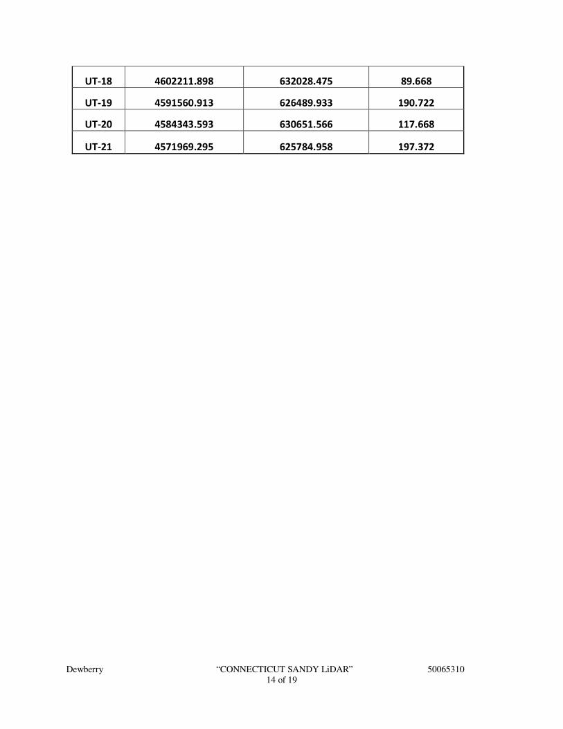
Dewberry “CONNECTICUT SANDY LiDAR” 50065310
14 of 19
UT-18 4602211.898 632028.475 89.668
UT-19 4591560.913 626489.933 190.722
UT-20 4584343.593 630651.566 117.668
UT-21 4571969.295 625784.958 197.372

Dewberry “CONNECTICUT SANDY LiDAR” 50065310
15 of 19
4. GPS OBSERVATIONS_______________________________________
POINT ID
OBSERV.
DATE
JULIAN
DATE
TIME OF
DAY
RE-OBSERV.
DATE
RE-OBSERV.
TIME
Open Terrain
OT-02 6/26/2014 177 13:17 N/A N/A
OT-03 6/25/2014 176 18:21 6/26/2014 7:13
OT-04 6/26/2014 177 11:28 N/A N/A
OT-05 6/26/2014 177 7:05 N/A N/A
OT-06 6/26/2014 177 7:46 N/A N/A
OT-07 6/25/2014 176 19:31 N/A N/A
OT-08 6/25/2014 176 20:38 N/A N/A
OT-09 6/25/2014 176 11:16 N/A N/A
OT-10 6/24/2014 175 15:28 6/25/2014 6:13
OT-11 6/24/2014 175 18:46 6/25/2014 8:16
OT-12 6/25/2014 176 9:42 N/A N/A
OT-13 6/25/2014 176 18:12 N/A N/A
OT-14 6/25/2014 176 17:27 N/A N/A
OT-15 6/22/2014 173 14:23 6/23/2014 8:48
OT-16 6/22/2014 173 13:20 6/23/2014 7:02
OT-17 6/23/2014 174 11:39 6/24/2014 5:46
OT-18 6/24/2014 175 10:38 6/25/2014 7:29
OT-19 6/24/2014 175 16:14 6/25/2014 6:13
OT-20 6/25/2014 176 8:55 6/26/2014 5:31
OT-21 6/25/2014 176 13:09 6/26/2014 5:58
Brush/Low Trees Terrain
BLT-01 6/23/2014 174 18:18 6/24/2014 8:30
BLT-02 6/23/2014 174 15:57 6/24/2014 7:16
BLT-03 6/23/2014 174 14:53 6/24/2014 6:32
BLT-04 6/22/2014 173 17:48 6/23/2014 6:39
BLT-05 6/22/2014 173 13:01 6/23/2014 7:23
BLT-06 1/22/2015 22 7:50
BLT-07 6/24/2014 175 13:19 6/25/2014 9:33
BLT-08 6/25/2014 176 9:20 N/A N/A
BLT-09 6/24/2014 175 17:39 6/25/2014 9:48
BLT-10 6/25/2014 176 12:45 N/A N/A
BLT-11 1/22/2015 22 9:00 N/A N/A
BLT-12 1/22/2015 22 10:40 N/A N/A
BLT-13 6/25/2014 176 13:17 N/A N/A
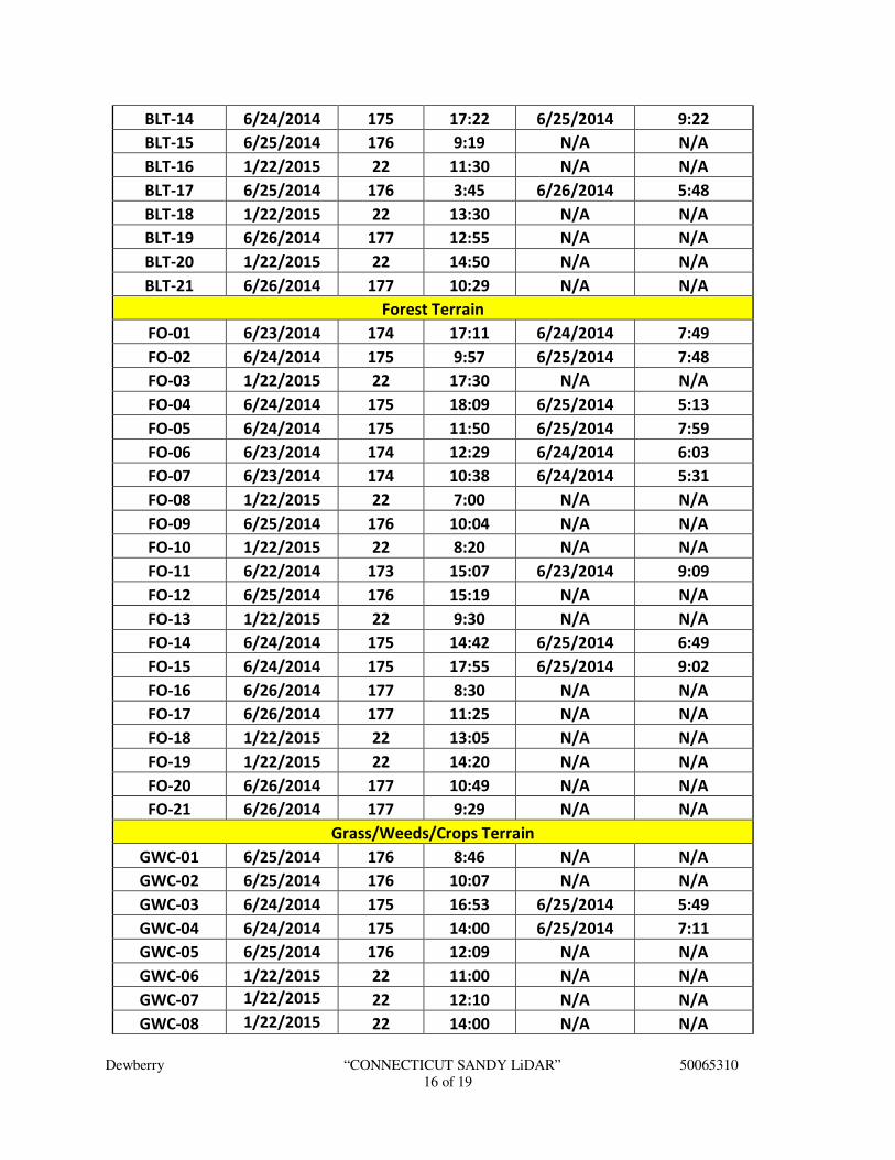
Dewberry “CONNECTICUT SANDY LiDAR” 50065310
16 of 19
BLT-14 6/24/2014 175 17:22 6/25/2014 9:22
BLT-15 6/25/2014 176 9:19 N/A N/A
BLT-16 1/22/2015 22 11:30 N/A N/A
BLT-17 6/25/2014 176 3:45 6/26/2014 5:48
BLT-18 1/22/2015 22 13:30 N/A N/A
BLT-19 6/26/2014 177 12:55 N/A N/A
BLT-20 1/22/2015 22 14:50 N/A N/A
BLT-21 6/26/2014 177 10:29 N/A N/A
Forest Terrain
FO-01 6/23/2014 174 17:11 6/24/2014 7:49
FO-02 6/24/2014 175 9:57 6/25/2014 7:48
FO-03 1/22/2015 22 17:30 N/A N/A
FO-04 6/24/2014 175 18:09 6/25/2014 5:13
FO-05 6/24/2014 175 11:50 6/25/2014 7:59
FO-06 6/23/2014 174 12:29 6/24/2014 6:03
FO-07 6/23/2014 174 10:38 6/24/2014 5:31
FO-08 1/22/2015 22 7:00 N/A N/A
FO-09 6/25/2014 176 10:04 N/A N/A
FO-10 1/22/2015 22 8:20 N/A N/A
FO-11 6/22/2014 173 15:07 6/23/2014 9:09
FO-12 6/25/2014 176 15:19 N/A N/A
FO-13 1/22/2015 22 9:30 N/A N/A
FO-14 6/24/2014 175 14:42 6/25/2014 6:49
FO-15 6/24/2014 175 17:55 6/25/2014 9:02
FO-16 6/26/2014 177 8:30 N/A N/A
FO-17 6/26/2014 177 11:25 N/A N/A
FO-18 1/22/2015 22 13:05 N/A N/A
FO-19 1/22/2015 22 14:20 N/A N/A
FO-20 6/26/2014 177 10:49 N/A N/A
FO-21 6/26/2014 177 9:29 N/A N/A
Grass/Weeds/Crops Terrain
GWC-01 6/25/2014 176 8:46 N/A N/A
GWC-02 6/25/2014 176 10:07 N/A N/A
GWC-03 6/24/2014 175 16:53 6/25/2014 5:49
GWC-04 6/24/2014 175 14:00 6/25/2014 7:11
GWC-05 6/25/2014 176 12:09 N/A N/A
GWC-06 1/22/2015 22 11:00 N/A N/A
GWC-07 1/22/2015 22 12:10 N/A N/A
GWC-08 1/22/2015 22 14:00 N/A N/A
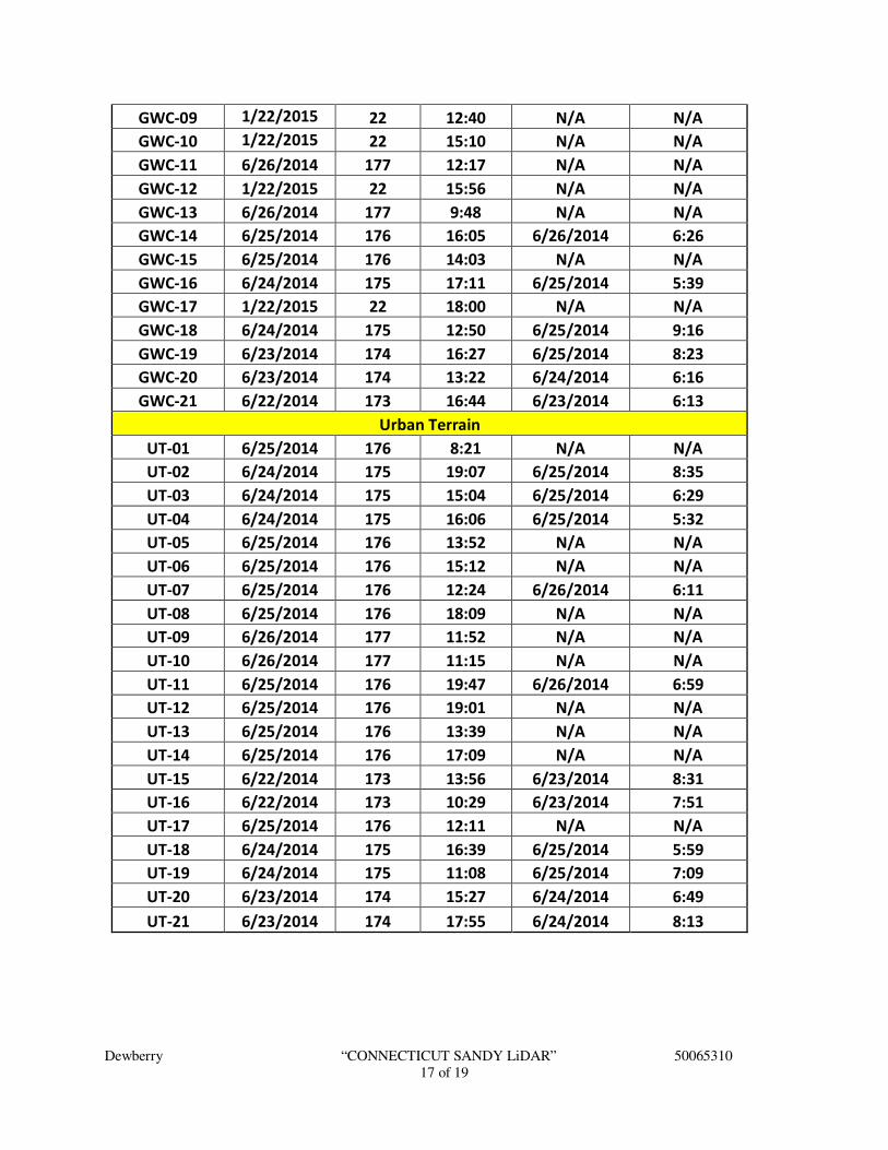
Dewberry “CONNECTICUT SANDY LiDAR” 50065310
17 of 19
GWC-09 1/22/2015 22 12:40 N/A N/A
GWC-10 1/22/2015 22 15:10 N/A N/A
GWC-11 6/26/2014 177 12:17 N/A N/A
GWC-12 1/22/2015 22 15:56 N/A N/A
GWC-13 6/26/2014 177 9:48 N/A N/A
GWC-14 6/25/2014 176 16:05 6/26/2014 6:26
GWC-15 6/25/2014 176 14:03 N/A N/A
GWC-16 6/24/2014 175 17:11 6/25/2014 5:39
GWC-17 1/22/2015 22 18:00 N/A N/A
GWC-18 6/24/2014 175 12:50 6/25/2014 9:16
GWC-19 6/23/2014 174 16:27 6/25/2014 8:23
GWC-20 6/23/2014 174 13:22 6/24/2014 6:16
GWC-21 6/22/2014 173 16:44 6/23/2014 6:13
Urban Terrain
UT-01 6/25/2014 176 8:21 N/A N/A
UT-02 6/24/2014 175 19:07 6/25/2014 8:35
UT-03 6/24/2014 175 15:04 6/25/2014 6:29
UT-04 6/24/2014 175 16:06 6/25/2014 5:32
UT-05 6/25/2014 176 13:52 N/A N/A
UT-06 6/25/2014 176 15:12 N/A N/A
UT-07 6/25/2014 176 12:24 6/26/2014 6:11
UT-08 6/25/2014 176 18:09 N/A N/A
UT-09 6/26/2014 177 11:52 N/A N/A
UT-10 6/26/2014 177 11:15 N/A N/A
UT-11 6/25/2014 176 19:47 6/26/2014 6:59
UT-12 6/25/2014 176 19:01 N/A N/A
UT-13 6/25/2014 176 13:39 N/A N/A
UT-14 6/25/2014 176 17:09 N/A N/A
UT-15 6/22/2014 173 13:56 6/23/2014 8:31
UT-16 6/22/2014 173 10:29 6/23/2014 7:51
UT-17 6/25/2014 176 12:11 N/A N/A
UT-18 6/24/2014 175 16:39 6/25/2014 5:59
UT-19 6/24/2014 175 11:08 6/25/2014 7:09
UT-20 6/23/2014 174 15:27 6/24/2014 6:49
UT-21 6/23/2014 174 17:55 6/24/2014 8:13
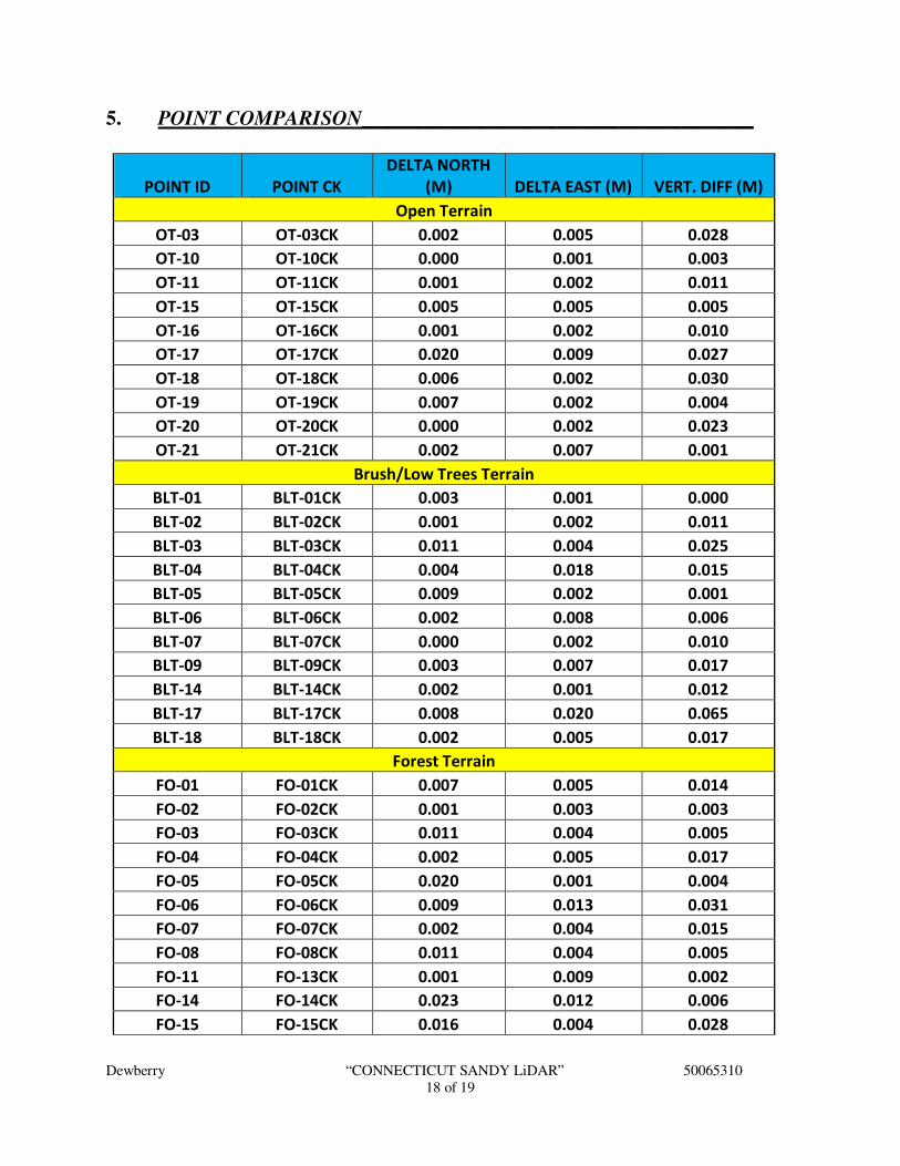
Dewberry “CONNECTICUT SANDY LiDAR” 50065310
18 of 19
5. POINT COMPARISON______________________________________
POINT ID POINT CK
DELTA NORTH
(M) DELTA EAST (M) VERT. DIFF (M)
Open Terrain
OT-03 OT-03CK 0.002 0.005 0.028
OT-10 OT-10CK 0.000 0.001 0.003
OT-11 OT-11CK 0.001 0.002 0.011
OT-15 OT-15CK 0.005 0.005 0.005
OT-16 OT-16CK 0.001 0.002 0.010
OT-17 OT-17CK 0.020 0.009 0.027
OT-18 OT-18CK 0.006 0.002 0.030
OT-19 OT-19CK 0.007 0.002 0.004
OT-20 OT-20CK 0.000 0.002 0.023
OT-21 OT-21CK 0.002 0.007 0.001
Brush/Low Trees Terrain
BLT-01 BLT-01CK 0.003 0.001 0.000
BLT-02 BLT-02CK 0.001 0.002 0.011
BLT-03 BLT-03CK 0.011 0.004 0.025
BLT-04 BLT-04CK 0.004 0.018 0.015
BLT-05 BLT-05CK 0.009 0.002 0.001
BLT-06 BLT-06CK 0.002 0.008 0.006
BLT-07 BLT-07CK 0.000 0.002 0.010
BLT-09 BLT-09CK 0.003 0.007 0.017
BLT-14 BLT-14CK 0.002 0.001 0.012
BLT-17 BLT-17CK 0.008 0.020 0.065
BLT-18 BLT-18CK 0.002 0.005 0.017
Forest Terrain
FO-01 FO-01CK 0.007 0.005 0.014
FO-02 FO-02CK 0.001 0.003 0.003
FO-03 FO-03CK 0.011 0.004 0.005
FO-04 FO-04CK 0.002 0.005 0.017
FO-05 FO-05CK 0.020 0.001 0.004
FO-06 FO-06CK 0.009 0.013 0.031
FO-07 FO-07CK 0.002 0.004 0.015
FO-08 FO-08CK 0.011 0.004 0.005
FO-11 FO-13CK 0.001 0.009 0.002
FO-14 FO-14CK 0.023 0.012 0.006
FO-15 FO-15CK 0.016 0.004 0.028
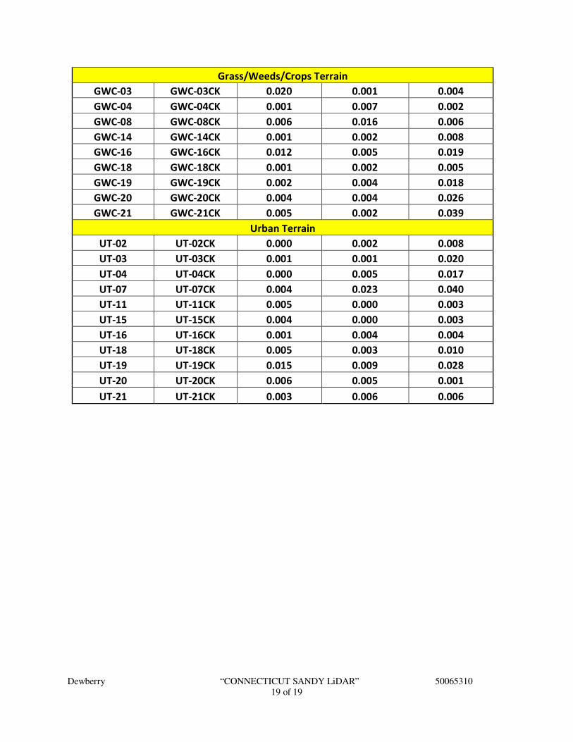
Dewberry “CONNECTICUT SANDY LiDAR” 50065310
19 of 19
Grass/Weeds/Crops Terrain
GWC-03 GWC-03CK 0.020 0.001 0.004
GWC-04 GWC-04CK 0.001 0.007 0.002
GWC-08 GWC-08CK 0.006 0.016 0.006
GWC-14 GWC-14CK 0.001 0.002 0.008
GWC-16 GWC-16CK 0.012 0.005 0.019
GWC-18 GWC-18CK 0.001 0.002 0.005
GWC-19 GWC-19CK 0.002 0.004 0.018
GWC-20 GWC-20CK 0.004 0.004 0.026
GWC-21 GWC-21CK 0.005 0.002 0.039
Urban Terrain
UT-02 UT-02CK 0.000 0.002 0.008
UT-03 UT-03CK 0.001 0.001 0.020
UT-04 UT-04CK 0.000 0.005 0.017
UT-07 UT-07CK 0.004 0.023 0.040
UT-11 UT-11CK 0.005 0.000 0.003
UT-15 UT-15CK 0.004 0.000 0.003
UT-16 UT-16CK 0.001 0.004 0.004
UT-18 UT-18CK 0.005 0.003 0.010
UT-19 UT-19CK 0.015 0.009 0.028
UT-20 UT-20CK 0.006 0.005 0.001
UT-21 UT-21CK 0.003 0.006 0.006

Dewberry Response to USGS Review of the Connecticut SANDY LiDAR Project
Produced for U.S. Geological Survey
USGS Contract: G10PC00013
Task Order:G14PD00241
Report Date: 6/5/2015
SUBMITTED BY:
Dewberry
1000 North Ashley Drive Suite 801 Tampa, FL 33602 813.225.1325 SUBMITTED TO:
U.S. Geological Survey 1400 Independence Road Rolla, MO 6540 573.308.3810

Connecticut LiDAR Response TO# G14PD00241 June 5, 2015 Page 2 of 8
Table of Contents
Executive Summary ............................................................................................................................................. 3
Project area ...................................................................................................................................................... 4
Edit Calls .............................................................................................................................................................. 5
Metadata ........................................................................................................................................................... 5
Artifacts ............................................................................................................................................................ 5
Elevation Transitions at Dams ........................................................................................................................ 6
Elevation Transitions....................................................................................................................................... 6
Breakline adjustments ..................................................................................................................................... 7
Summary of Edit Calls ......................................................................................................................................... 8

Connecticut LiDAR Response TO# G14PD00241 June 5, 2015 Page 3 of 8
Executive Summary The primary purpose of this project was to develop a consistent and accurate surface elevation dataset derived from high-accuracy Light Detection and Ranging (LiDAR) technology for the USGS Connecticut SANDY LiDAR Project Area. The LiDAR data were processed to a bare-earth digital terrain models (DTM). Detailed breaklines and bare-earth digital elevation Models (DEMs) were produced for the project area. Deliverables for this project included raw point cloud data, classified point cloud data, bare earth hydro enforced digital elevation models, intensity images, breaklines, control points, metadata, project report, and project extent shapefiles. The USGS second review of these deliverables resulted in one call to remove building points, four calls to clean up elevation transitions at dams, six calls to modify the elevation transitions in stream and river hydro features, and two calls to modify existing hydro features.

Connecticut LiDAR Response TO# G14PD00241 June 5, 2015 Page 4 of 8
PROJECT AREA
Data was formatted according to tiles with each tile covering an area of 1500m by 1500m. A total of 1,974 tiles were produced for the project encompassing an area of approximately 1,526 sq. miles.
Figure 1- Project Map
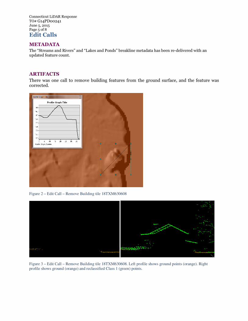
Connecticut LiDAR Response TO# G14PD00241 June 5, 2015 Page 5 of 8
Edit Calls
METADATA The “Streams and Rivers” and “Lakes and Ponds” breakline metadata has been re-delivered with an updated feature count.
ARTIFACTS
There was one call to remove building features from the ground surface, and the feature was corrected.
Figure 2 – Edit Call – Remove Building tile 18TXM630608
Figure 3 – Edit Call – Remove Building tile 18TXM630608. Left profile shows ground points (orange). Right
profile shows ground (orange) and reclassified Class 1 (green) points.

Connecticut LiDAR Response TO# G14PD00241 June 5, 2015 Page 6 of 8
ELEVATION TRANSITIONS AT DAMS USGS identified several issues with elevation transitions and in four instances those issues were caused by dams. The example below shows a waterbody that was digging deeply into the surrounding ground. USGS called out two possible dams and Dewberry added these features to the breaklines.
Figure 4 – Tile 18TXM630608 – The two dam features within this waterbody (now river) allow the water level to drop from over 138 meters to under 126 meters at the appropriate locations.
ELEVATION TRANSITIONS USGS identified six areas in which the elevation transitions in streams and rivers were too abrupt. The specification for elevation transitions is that they must be no greater than 0.3 meters. Dewberry has reduced the transitions at the flagged locations to 0.15 meters.

Connecticut LiDAR Response TO# G14PD00241 June 5, 2015 Page 7 of 8
Figure 5 – Tile 18TXM975654. This elevation transition was corrected. The upper image shows the original DEM, the lower image shows the corrected DEM. The elevation transition was modified from one 25cm step to several 5
and 10 cm steps.
BREAKLINE ADJUSTMENTS There were two locations where USGS identified areas where the breaklines should be removed. After reviewing the LiDAR, Dewberry confirmed that there were significant ground features in those areas and the breaklines were adjusted; one stream was adjusted and one pond was removed.
Connecticut LiDAR Response TO# G14PD00241 June 5, 2015 Page 8 of 8
Figure 6 – Tile 18TXM555602 – A pond breakline was removed from the DEM and the LiDAR was reclassified to
ground.
Summary of Edit Calls
• There were 13 calls in total. All calls were fixed.
Related Documents


