ANNALS OF ECONOMICS AND FINANCE 4, 275–341 (2003) Urbanization and Economic Development J. Vernon Henderson Brown University This paper provides a survey and guide to the literature relevant to urban- ization and economic development. The paper starts with some basic facts and trends about urbanization worldwide. It then reviews the traditional two- sector urban-rural model, but focuses on the modern version, Krugman’s core- periphery model. However, two sector models do not capture the notion of an economy composed of many cities; nor do they represent modern agglomera- tion economies. Models and empirical evidence on agglomeration economies are reviewed. Then the paper turns to empirical evidence on the evolution of the size distribution of cities. It reviews the large literature on systems of cities models, focusing on an endogenous growth version. This part of paper concludes with a review of recent work integrating systems of cities models with the new economic geography. The final section reviews urbanization in China, focusing on policy issues such as migration, under-agglomeration and spatial biases in the FDI policy. c 2003 Peking University Press Key Words : Urbanization; China reginal development; Systems od cities. JEL Classification Numbers : O0, R0. 1. INTRODUCTION Urbanization occurs as countries switch sectoral composition away from agriculture into industry and as technological advances in domestic agri- culture release labor from agriculture to migrate to cities. Given this well accepted process, the study of urbanization with development focuses on three issues. For each of these, this paper will review key empirical facts and evidence and explain the key theoretical models used in analysis. In the last section, I turn to China, using the impacts of China’s urbanization policies, to illustrate aspects of the first three sections. The first issue concerns whether the urbanization process involving rural to urban migration within countries is reasonably efficient, or whether it is subject to forms of market failure or distortionary government policies. Part of the literature on the subject looks at the basic overall rural-urban 275 1529-7373/2002 Copyright c 2003 by Peking University Press All rights of reproduction in any form reserved.

Welcome message from author
This document is posted to help you gain knowledge. Please leave a comment to let me know what you think about it! Share it to your friends and learn new things together.
Transcript
ANNALS OF ECONOMICS AND FINANCE 4, 275–341 (2003)
Urbanization and Economic Development
J. Vernon Henderson
Brown University
This paper provides a survey and guide to the literature relevant to urban-ization and economic development. The paper starts with some basic factsand trends about urbanization worldwide. It then reviews the traditional two-sector urban-rural model, but focuses on the modern version, Krugman’s core-periphery model. However, two sector models do not capture the notion of aneconomy composed of many cities; nor do they represent modern agglomera-tion economies. Models and empirical evidence on agglomeration economiesare reviewed. Then the paper turns to empirical evidence on the evolutionof the size distribution of cities. It reviews the large literature on systems ofcities models, focusing on an endogenous growth version. This part of paperconcludes with a review of recent work integrating systems of cities modelswith the new economic geography. The final section reviews urbanization inChina, focusing on policy issues such as migration, under-agglomeration andspatial biases in the FDI policy. c© 2003 Peking University Press
Key Words: Urbanization; China reginal development; Systems od cities.JEL Classification Numbers: O0, R0.
1. INTRODUCTION
Urbanization occurs as countries switch sectoral composition away fromagriculture into industry and as technological advances in domestic agri-culture release labor from agriculture to migrate to cities. Given this wellaccepted process, the study of urbanization with development focuses onthree issues. For each of these, this paper will review key empirical factsand evidence and explain the key theoretical models used in analysis. Inthe last section, I turn to China, using the impacts of China’s urbanizationpolicies, to illustrate aspects of the first three sections.
The first issue concerns whether the urbanization process involving ruralto urban migration within countries is reasonably efficient, or whether itis subject to forms of market failure or distortionary government policies.Part of the literature on the subject looks at the basic overall rural-urban
2751529-7373/2002
Copyright c© 2003 by Peking University PressAll rights of reproduction in any form reserved.
276 J. VERNON HENDERSON
divide to ask whether countries are over- or under-urbanized. That par-ticular narrow question is not what the recent economics literature hasfocused on, for reasons we will see. Rather the literature has focused onthe form that urbanization takes. In some writings form means the devel-opment and then perhaps subsequent reversal of a core-periphery spatial,or regional structure. In other writings, it means the development andthen subsequent reversal of a high degree of urban primacy, or the degreeof dominance of one city over other cities in a region. How does spatialconcentration, in terms of, say, the share of the core region or primate cityin the economy evolve with development? What are the efficiency implica-tions of more or less, or of too much or too little spatial concentration?
The second issue concerns why industrialization involves urbanization.What market and non-market interactions lead economic activity to spa-tially cluster, or agglomerate into entities we call cities? There are a varietyof papers which model the form of localized scale externalities such as infor-mation spillovers in output and input markets and backward and forwardlinkages which lead to agglomeration; and there is a large body of empir-ical work trying to measure the nature and extent of scale externalities.Finally there is a more recent literature examining dynamic externalitiesand localized knowledge spillovers.
The third issue concerns how cities form and interact with each other,in an urban system in both static and dynamic contexts. Rather thana simple core-periphery regional structure an economy is composed of anendogenous and potentially large number of cities of different sizes andtypes. The country’s urban system can be viewed as a whole, or therecan be core and periphery regions each with their own system of cities.Empirical evidence shows that over long periods of time within countriesthere tends to be a “wide” and very stable relative size distribution of cities.The natural questions then are what is the role of big versus small cities ina country – i.e., in what do they tend to specialize and how do they interactwith each other? Second, what is the inter-relationship between nationaleconomic growth and growth of both individual cities and the overall urbansystem? The theory papers attempt to model all these questions, and theunderlying facts about urban systems. Apart from providing a link betweennational and city growth, from a development perspective this literatureindicates how national urban development evolves. This has implicationsfor national policy governing the spatial allocation of public infrastructureinvestments, fiscal decentralization, internal migration policies and the like.
2. URBANIZATION AND ITS FORM
Urbanization, or the shift of population from rural to urban environ-ments, is a transitory process, albeit one that is socially and culturally

URBANIZATION AND ECONOMIC DEVELOPMENT 277
traumatic. It moves populations from traditional-cultural environmentswith informal political and economic institutions to the relative anonymityand more formal institutions of urban settings. It spatially separates fami-lies, particularly intergenerationally as the young migrate to cities and theold stay behind. By upper middle income ranges countries become “fully”urbanized, with 60-90% of the national population living in cities, with theactual percent urbanized varying with geography, role of agriculture, andnational definitions of urban.
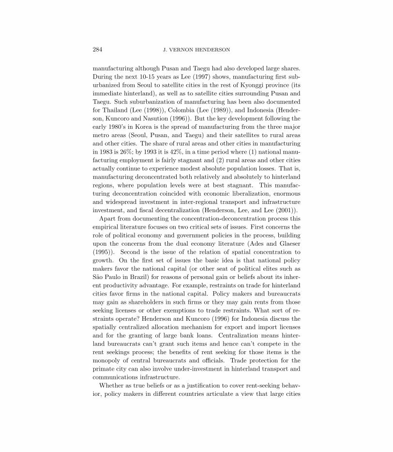
The idea that urbanization is a transitory phenomenon is born out bythe simple statistics in Figure 1, comparing different regions of the world in1960 versus 1995. While urbanization increased in all regions of the worldover those 35 years, among developed countries there is little change since1975. Soviet bloc and Latin American countries have almost converged todeveloped country urbanization levels.
Despite this notion of urbanization being a transitory phenomenon, wedon’t actually have a good conceptual model of the dynamic transitoryprocess. Models of urbanization per se are, oddly, static. The traditionalversions focus on the question of urban “bias”, or the effect of governmentpolicies on the urban-rural divide, or the efficient rural-urban allocation ofpopulation at a point in time. These models are the long-standing dualeconomy models, that date back to Lewis (1954). They are two sectormodels with an exogenously given sophisticated urban sector and a “back-ward” rural sector (Rannis and Fei (1961), Harris and Todaro (1970) andothers as now well exposited in textbooks (e.g., Ray (1998)).
Dual sector models presume an exogenously given situation where theproductivity of labor in the urban sector exceeds that in the rural sector.Arbitrage in terms of labor migration is limited by inefficient labor alloca-tion rules such as farm workers being paid average rather than marginalproduct or artificially limited absorption in the urban sector (e.g., formalsector minimum wages). The literature focuses on the effect on migrationfrom the rural to urban sector of policies such as rural-urban terms of trade,migration restrictions, wage subsidies, and the like.
The final and most complex version of the models are the Kelley andWilliamson (1998) and the Becker, Mills, and Williamson (1984), whichare CGE models which introduce dynamic elements. They have savingsbehavior and capital accumulation, population growth, and multiple eco-nomic sectors in the urban and rural regions. Labor markets within sectorand across regions are allowed to clear. The multiple economic sectors allowconsideration of the effects of a wider array of policy instruments, includ-ing sector specific trade or capital market policies for housing, industry,services and the like. However the starting point is again an exogenouslygiven initial urban-rural productivity gap sustained initially by migrationcosts and exogenous skill acquisition. On-going urbanization is the result

278 J. VERNON HENDERSON
FIG. 1. Share of Urban Population in Total Population.
(a) Average over Countries
0.0
0.1
0.2
0.3
0.4
0.5
0.6
0.7
0.8
60 65 70 75 80 85 90 95 Year
urban population share
Sub-Saharan Africa Asia Soviet Bloc Middle East & N. Af Latin America Developed World
(b) Weighted Average, Using Country Population.
0.0
0.1
0.2
0.3
0.4
0.5
0.6
0.7
0.8
0.9
60 65 70 75 80 85 90 95 Year
urban populationshare
Sub-Saharan Afr Asia Soviet Bloc Middle East & N. Afr Latin America Developed World

URBANIZATION AND ECONOMIC DEVELOPMENT 279
of exogenous forces – technological change favoring the urban sector orchanges in the terms of trade favoring the urban sector.
As models of urbanization, these dual economy ones were a critical stepbut they suffer obvious defects, apart from their rather static nature. Firsthow the dual starting point arises is never modeled. Second, and related tothe first as we will see, there are no forces for agglomeration that would nat-urally foster industrial concentration in the urban sector. Finally althoughthe models have two sectors there is really little spatial or regional aspectto the problem. There is a new generation of two-sector models, the core-periphery models, which attempt to address to differing degrees these threedefects. However core-periphery models are not really about urbanizationper se, since in many versions including Krugman’s (1991a) initial piecethe agricultural population is fixed. The models ask under what conditionsin a two-region country, both regions versus only one region industrializesor urbanizes. In application to the development process, I interpret thesemodels as starting to analyze the form urbanization takes. Before turningto these models, I review the limited empirical evidence first on urban-ization and then on the form of urbanization in terms of core-peripherystructures. Then I turn to the theoretical literature in economic geographyon core-periphery structures.
2.1. What Do We Know About Urbanization and Its Form?There are several important facts that we know about the urbanization
process. We briefly review these and then turn to the bulk of the literaturedevoted to the form that urbanization takes. That literature leads to thecore-periphery models.
2.1.1. Urbanization
The dual-economy models typically take as given the desirability of on-going urbanization. They then ask what types of market failures or gov-ernment policies work to hinder the needed migration. The focus has beenon “urban bias”. Renaud (1981) makes the simple point that, in general,government policies bias, or influence urbanization through their effect onnational sectoral composition. So policies affecting the terms of trade be-tween agriculture and modern industry or between traditional small townindustry (textiles, food processing) and high tech large city industry affectthe rural-urban or small-big city allocation of population. Such policiesinclude tariffs, and price controls and subsidies, and are analyzed in thesystem of cities models discussed in section 3.
The idea that (1) urbanization reflects changes in sector composition and(2) government policies affect urbanization primarily through their effecton sector composition is a key point of empirical studies of urbanization

280 J. VERNON HENDERSON
by Fay and Opal (1999) and Davis and Henderson (2001). These studiesargue that urbanization which occurs in the early and middle stages ofdevelopment is determined largely by changes in national economic sectorcomposition and government policies tend to affect urbanization indirectlythrough their effect on sector composition. Of course it is also possible thatwith or without sector distortions, migration from rural to urban areas canbe influenced by wage policies as in the dual-economy literature or bymigration restrictions, as in former planned economies such as China (Auand Henderson (2002)).
A second point about urbanization is that writers such as Gallup, Sacksand Mellinger (1999) suggest that urbanization may “cause” economicgrowth, rather than emerge as part of the growth, sectoral change process.The limited evidence so far suggests urbanization doesn’t cause growth.Henderson (2002a) finds no econometric evidence linking the extent of ur-banization to either economic or productivity growth or levels, per se. Thatis if a country increases its degree of urbanization per se, typically it doesn’tgrow faster. In a more refined version of growth and urbanization links,so far we have been unable to quantify for different levels of development,the “optimal” degree of urbanization. For each level of development thereshould be an optimal degree of urbanization where either over- or under-urbanization detract from growth. While that may make sense, econo-metric evidence doesn’t support the idea, perhaps because the data areproblematical or because in sub-Saharan Africa, rapid urbanization overthe last thirty years is correlated with negative or zero economic growth.
Finally there is an informal notion (World Bank (2000)) that urbaniza-tion follows the same stages as population growth (the “demographic” tran-sition between falling death rates and falling fertility rates) – an S-shapedrelationship where population growth is slow at low levels of development,then there is a period of rapid acceleration in intermediate stages, followedby a slowing of growth. These differential growth population rates implyan S-shaped relationship between population levels and GDP per capita.These ideas do not seem to carry over to the urbanization process. Davisand Henderson (2001) find a simple concave relationship between the levelof urban population and GDP per capita (with or without controlling fornational population), at least over the last 35 years. Urbanization is mostrapid at low income levels, tapering off from there until a country is fullyurbanized.
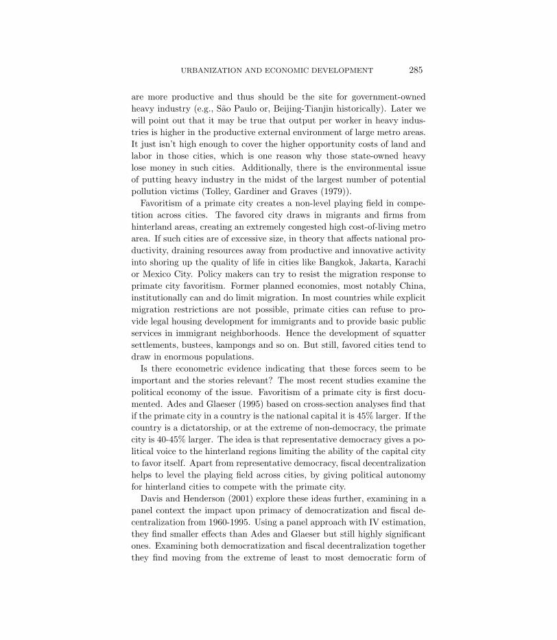
Figure 2 illustrates where the percent urban is a concave function ofincome per capita. In Figure 3 a similar relationship is posited. Therethe relationship between total national urban population and income per

URBANIZATION AND ECONOMIC DEVELOPMENT 281
FIG. 2. Percent Urban and Development Level, 1965-95
urban population s
real GDP per capita 257 19976.4
.016667
.969981
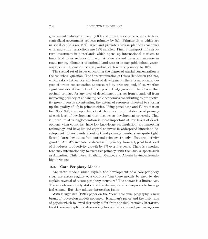
FIG. 3. Partial Correlation Between ln(urban population) and ln(real GDP percapita), Controlling for ln(national population).
ln(urban population)
ln(real GDP per ca -2.23971 2.18817
-2.67718
1.2868
capita is explored after parcelling out the effect of national population,or country size. In Figure 3 the log of national urban population is anincreasing concave function of the log of income per capita, so nationalurban population will generally also be a concave function of income percapita.
282 J. VERNON HENDERSON
2.1.2. The Form of Urbanization: The Degree of Spatial Concentration
In 1965, Williamson published a key paper based on cross-sectional anal-ysis of 24 countries in which he argued that national economic developmentis characterized by an initial phase of internal regional divergence, followedby a phase of later convergence. That is, a few regions initially experi-ence accelerated growth relative to other (peripheral) regions, but later theperipheral regions start to catch up. Barro and Sala-i-Martin (1991 and1992 present extensive evidence on this for the USA, Western Europe, andJapan, by examining the evolution of inter-regional differences in per capitaincomes. While inter-regional out-migration from poorer regions plays arole in catch-up, it may not be critical. In fact for Japan, the authors arguethat later convergence of backward regions occurred in the absence of a realrole for migration. Instead, productivity improved in backward regions.
The urban version of this divergence-convergence phenomenon looks aturban primacy. Following Ades and Glaeser (1995), conceptually the urbanworld is collapsed into two regions – the primate city versus the rest of thecountry, or at least the urban portion thereof. Like dual sector modelsthe focus is on how government policies and institutions affect primacy,with strong political-economy considerations. The basic question concernsto what extent urbanization is confined to one (or a few) major metroareas, relative to being spread more evenly across a variety of cities. Thatis, to what extent is urbanization concentrated? Primacy is the simplestmeasure, where a common measure of primacy is the ratio of the populationof the largest metro area to all urban population in the country (Ades andGlaeser (1995), Junius (1999), and Davis and Henderson (2001)). A morecomprehensive measure might use a Hirschman-Herfindal index [HHI] fromthe industrial organization literature, which is the sum of squared sharesin national urban population of every metro area. That is a tremendousdata gathering exercise, so far attempted only by Wheaton and Shishido(1981) for a single year.
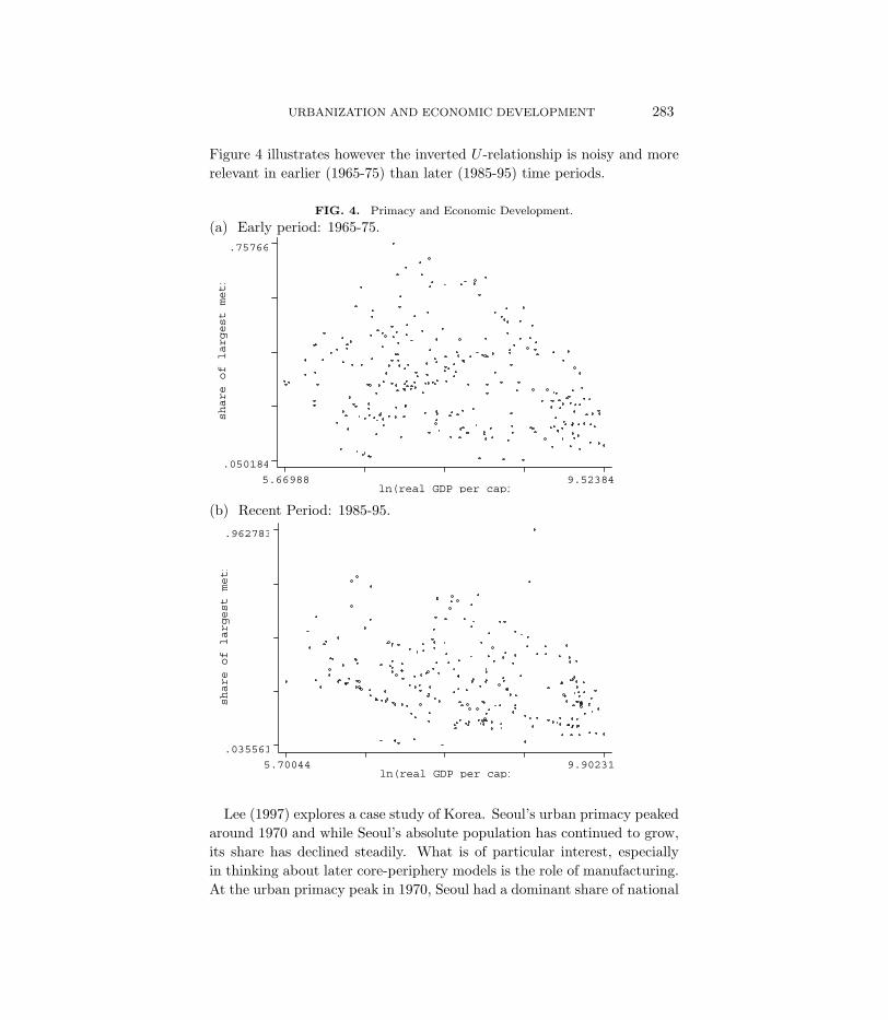
What these papers find is an inverted U -shape relationship where urban-concentration first increases, peaks, and then declines with economic devel-opment. Despite different concentration measures and methods, Wheatonand Shishido (1981) examining a HHI using cross-section non-linear OLSand Davis and Henderson (2001) examining primacy using panel data meth-ods and IV estimation find that urban primacy rises, peaks in the $2000-4000 range (1985 PPP dollars), and then declines. Junius (1999) finds apeak at somewhat higher income levels, but still the inverted U−shape. As
URBANIZATION AND ECONOMIC DEVELOPMENT 283
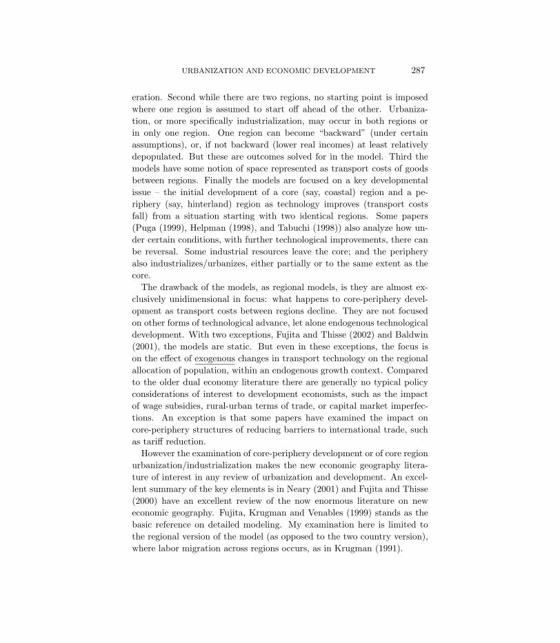
Figure 4 illustrates however the inverted U -relationship is noisy and morerelevant in earlier (1965-75) than later (1985-95) time periods.
FIG. 4. Primacy and Economic Development.
(a) Early period: 1965-75.
share of largest metr
ln(real GDP per capi 5.66988 9.52384
.050184
.75766
(b) Recent Period: 1985-95.
share of largest metr
ln(real GDP per capi 5.70044 9.90231
.035561
.962783
Lee (1997) explores a case study of Korea. Seoul’s urban primacy peakedaround 1970 and while Seoul’s absolute population has continued to grow,its share has declined steadily. What is of particular interest, especiallyin thinking about later core-periphery models is the role of manufacturing.At the urban primacy peak in 1970, Seoul had a dominant share of national
284 J. VERNON HENDERSON
manufacturing although Pusan and Taegu had also developed large shares.During the next 10-15 years as Lee (1997) shows, manufacturing first sub-urbanized from Seoul to satellite cities in the rest of Kyonggi province (itsimmediate hinterland), as well as to satellite cities surrounding Pusan andTaegu. Such suburbanization of manufacturing has been also documentedfor Thailand (Lee (1998)), Colombia (Lee (1989)), and Indonesia (Hender-son, Kuncoro and Nasution (1996)). But the key development following theearly 1980’s in Korea is the spread of manufacturing from the three majormetro areas (Seoul, Pusan, and Taegu) and their satellites to rural areasand other cities. The share of rural areas and other cities in manufacturingin 1983 is 26%; by 1993 it is 42%, in a time period where (1) national manu-facturing employment is fairly stagnant and (2) rural areas and other citiesactually continue to experience modest absolute population losses. That is,manufacturing deconcentrated both relatively and absolutely to hinterlandregions, where population levels were at best stagnant. This manufac-turing deconcentration coincided with economic liberalization, enormousand widespread investment in inter-regional transport and infrastructureinvestment, and fiscal decentralization (Henderson, Lee, and Lee (2001)).
Apart from documenting the concentration-deconcentration process thisempirical literature focuses on two critical sets of issues. First concerns therole of political economy and government policies in the process, buildingupon the concerns from the dual economy literature (Ades and Glaeser(1995)). Second is the issue of the relation of spatial concentration togrowth. On the first set of issues the basic idea is that national policymakers favor the national capital (or other seat of political elites such asSao Paulo in Brazil) for reasons of personal gain or beliefs about its inher-ent productivity advantage. For example, restraints on trade for hinterlandcities favor firms in the national capital. Policy makers and bureaucratsmay gain as shareholders in such firms or they may gain rents from thoseseeking licenses or other exemptions to trade restraints. What sort of re-straints operate? Henderson and Kuncoro (1996) for Indonesia discuss thespatially centralized allocation mechanism for export and import licensesand for the granting of large bank loans. Centralization means hinter-land bureaucrats can’t grant such items and hence can’t compete in therent seekings process; the benefits of rent seeking for those items is themonopoly of central bureaucrats and officials. Trade protection for theprimate city can also involve under-investment in hinterland transport andcommunications infrastructure.
Whether as true beliefs or as a justification to cover rent-seeking behav-ior, policy makers in different countries articulate a view that large cities
URBANIZATION AND ECONOMIC DEVELOPMENT 285
are more productive and thus should be the site for government-ownedheavy industry (e.g., Sao Paulo or, Beijing-Tianjin historically). Later wewill point out that it may be true that output per worker in heavy indus-tries is higher in the productive external environment of large metro areas.It just isn’t high enough to cover the higher opportunity costs of land andlabor in those cities, which is one reason why those state-owned heavylose money in such cities. Additionally, there is the environmental issueof putting heavy industry in the midst of the largest number of potentialpollution victims (Tolley, Gardiner and Graves (1979)).
Favoritism of a primate city creates a non-level playing field in compe-tition across cities. The favored city draws in migrants and firms fromhinterland areas, creating an extremely congested high cost-of-living metroarea. If such cities are of excessive size, in theory that affects national pro-ductivity, draining resources away from productive and innovative activityinto shoring up the quality of life in cities like Bangkok, Jakarta, Karachior Mexico City. Policy makers can try to resist the migration response toprimate city favoritism. Former planned economies, most notably China,institutionally can and do limit migration. In most countries while explicitmigration restrictions are not possible, primate cities can refuse to pro-vide legal housing development for immigrants and to provide basic publicservices in immigrant neighborhoods. Hence the development of squattersettlements, bustees, kampongs and so on. But still, favored cities tend todraw in enormous populations.
Is there econometric evidence indicating that these forces seem to beimportant and the stories relevant? The most recent studies examine thepolitical economy of the issue. Favoritism of a primate city is first docu-mented. Ades and Glaeser (1995) based on cross-section analyses find thatif the primate city in a country is the national capital it is 45% larger. If thecountry is a dictatorship, or at the extreme of non-democracy, the primatecity is 40-45% larger. The idea is that representative democracy gives a po-litical voice to the hinterland regions limiting the ability of the capital cityto favor itself. Apart from representative democracy, fiscal decentralizationhelps to level the playing field across cities, by giving political autonomyfor hinterland cities to compete with the primate city.
Davis and Henderson (2001) explore these ideas further, examining in apanel context the impact upon primacy of democratization and fiscal de-centralization from 1960-1995. Using a panel approach with IV estimation,they find smaller effects than Ades and Glaeser but still highly significantones. Examining both democratization and fiscal decentralization togetherthey find moving from the extreme of least to most democratic form of
286 J. VERNON HENDERSON
government reduces primacy by 8% and from the extreme of most to leastcentralized government reduces primacy by 5%. Primate cities which arenational capitals are 20% larger and primate cities in planned economieswith migration restrictions are 18% smaller. Finally transport infrastruc-ture investment in hinterlands which opens up international markets tohinterland cities reduces primacy. A one-standard deviation increase inroads per sq. kilometer of national land area or in navigable inland water-ways per sq. kilometer, ceteris paribus, each reduce primacy by 10%.
The second set of issues concerning the degree of spatial concentration isthe “so-what” question. The first examination of this is Henderson (2002a),which asks whether, for any level of development, there is an optimal de-gree of urban concentration as measured by primacy, and, if so, whethersignificant deviations detract from productivity growth. The idea is thatoptimal primacy for any level of development derives from a trade-off fromincreasing primacy of enhancing scale economies contributing to productiv-ity growth versus accentuating the extent of resources diverted to shoringup the quality of life in primate cities. Using panel data and IV estimationfor 1960-1990, the paper finds that there is an optimal degree of primacyat each level of development that declines as development proceeds. Thatis, initial relative agglomeration is most important at low levels of devel-opment when countries have low knowledge accumulation, are importingtechnology, and have limited capital to invest in widespread hinterland de-velopment. Error bands about optimal primacy numbers are quite tight.Second, large deviations from optimal primacy strongly affect productivitygrowth. An 33% increase or decrease in primacy from a typical best levelof .3 reduces productivity growth by 3% over five years. There is a modesttendency internationally to excessive primacy, with the usual suspects suchas Argentina, Chile, Peru, Thailand, Mexico, and Algeria having extremelyhigh primacy.
2.2. Core-Periphery Models
Are there models which explain the development of a core-peripherystructure across regions of a country? Can these models be used to alsoexplain reversal of a core-periphery structure? The answer is a limited yes.The models are mostly static and the driving force is exogenous technolog-ical change. But they address interesting issues.
With Krugman’s (1991) paper on the “new” economic geography, a newbrand of two-region models appeared. Krugman’s paper and the multitudeof papers which followed distinctly differ from the dual-economy literature.First there are explicit scale economy forces that foster endogenous agglom-
URBANIZATION AND ECONOMIC DEVELOPMENT 287
eration. Second while there are two regions, no starting point is imposedwhere one region is assumed to start off ahead of the other. Urbaniza-tion, or more specifically industrialization, may occur in both regions orin only one region. One region can become “backward” (under certainassumptions), or, if not backward (lower real incomes) at least relativelydepopulated. But these are outcomes solved for in the model. Third themodels have some notion of space represented as transport costs of goodsbetween regions. Finally the models are focused on a key developmentalissue – the initial development of a core (say, coastal) region and a pe-riphery (say, hinterland) region as technology improves (transport costsfall) from a situation starting with two identical regions. Some papers(Puga (1999), Helpman (1998), and Tabuchi (1998)) also analyze how un-der certain conditions, with further technological improvements, there canbe reversal. Some industrial resources leave the core; and the peripheryalso industrializes/urbanizes, either partially or to the same extent as thecore.
The drawback of the models, as regional models, is they are almost ex-clusively unidimensional in focus: what happens to core-periphery devel-opment as transport costs between regions decline. They are not focusedon other forms of technological advance, let alone endogenous technologicaldevelopment. With two exceptions, Fujita and Thisse (2002) and Baldwin(2001), the models are static. But even in these exceptions, the focus ison the effect of exogenous changes in transport technology on the regionalallocation of population, within an endogenous growth context. Comparedto the older dual economy literature there are generally no typical policyconsiderations of interest to development economists, such as the impactof wage subsidies, rural-urban terms of trade, or capital market imperfec-tions. An exception is that some papers have examined the impact oncore-periphery structures of reducing barriers to international trade, suchas tariff reduction.
However the examination of core-periphery development or of core regionurbanization/industrialization makes the new economic geography litera-ture of interest in any review of urbanization and development. An excel-lent summary of the key elements is in Neary (2001) and Fujita and Thisse(2000) have an excellent review of the now enormous literature on neweconomic geography. Fujita, Krugman and Venables (1999) stands as thebasic reference on detailed modeling. My examination here is limited tothe regional version of the model (as opposed to the two country version),where labor migration across regions occurs, as in Krugman (1991).

288 J. VERNON HENDERSON
In Krugman (1991) there are two regions, each with an identical num-ber of farmers who are completely immobile and who each produce a fixedamount of farm output. Only manufacturing and the fixed population ofmanufacturing workers are mobile across regions. National scale economiesarise from Dixit-Stiglitz (1977) diversity in manufacture’s output, givenfirm level scale economies (fixed costs). Relative to the traditional loca-tion literature, Krugman’s key insight is that when manufacturing firmschoose a location, they employ workers who reside and consume at thelocation, creating local backward and forward linkages. The more work-ers in a region, the more varieties result, and real incomes rise, and moreworkers are attracted to the region – a “virtuous” circle. Rather thanpresenting the Krugman model per se, I outline the structure of Puga’s(1999) variant, since it has a key element of interest – possible reversalof the core-periphery structure – and its assumptions are perhaps morepalatable. Puga allows for inter-sectoral (farming-manufacturing) as wellas inter-regional labor mobility; and, building on Venables (1996), he alsoallows for national scale economies in the production process, as well as inconsumption.
Here I present the primitives and key relationships of a core-peripherymodel, discuss the key analytical tool, discuss the key insights about ag-glomeration versus dispersal forces, and present basic core-periphery re-sults. I do not do full derivations given the limited space and the fact thata number of good reviews and summaries already exist. The idea is toarticulate the forces at work.
There are two regions, each endowed with an equal amount of land, Ki
for region i. Agricultural output in region i, yi is produced with land andlabor in agriculture in region i, LAi so
yi = K1−θi LθAi (1)
The agricultural sector is perfectly competitive, its output is transportedcostlessly across regions (a very weird assumption made throughout thisliterature), and consequently the numeraire is usually the price of agricul-tural products.
Preferences exhibit Dixit-Stiglitz (1977) returns from varieties of manu-facture’s x, so for any individual
U = y1−γxγ (2a)
URBANIZATION AND ECONOMIC DEVELOPMENT 289
x =
[M∑k=1
(x(k))(σ−1)/σ
]σ/(σ−1)
(2b)
whereM is the number of manufacturing varieties nationally (given a closedeconomy). The elasticity of substitution σ > 1. As σ falls to 1 havingvarieties is increasingly important since they are less substitutable in con-sumption. Under this formulation, at equal resource cost (which is not thecase with scale economies to firms), consumers would always prefer anothervariety to more of a given variety. National returns to scale in populationarise since a larger economy, as we will see, can support a greater numberof varieties.
Given (2), the indirect utility of a worker in region i may be written as
Vi = qγi wi (3)
where wi is the wage in region i and qi is a price index for the compositeof manufactures for a person in region i, imposing symmetry (which is anendogenous outcome) in manufacture’s output and pricing decisions. Giventhe functional form in (2b) for the composite good, the corresponding priceindex, qi, from standard Dixit-Stiglitz results has the form
qi =
Ni∑k=1
(pi(k))1−σ +Nj∑d=1
(pj(d)τ)1−σ
11−σ
where with symmetry
qi = (p1−σi Ni + (τpj)1−σNj)
11−σ (4)
Ni and Nj are the number of varieties produced in regions i and j. pi andpj are the local prices of a variety in respectively regions i and j. But itemsshipped from j to i are subject to transport costs; τ > 1 is the numberof units of a good needed to be shipped from j in order for a one unitto arrive in i. With this form of iceberg transport costs, producers in oneregion would never choose to duplicate varieties offered in other regions.Note given σ > 1, qi is increasing in p and decreasing in varieties N .
Manufacturers have identical technologies for each variety and by as-sumption each produce only one variety sold under monopolistic competi-tion. Manufacturers employ labor and the composite of all manufacturedproducts. For simplicity that composite has the same form as (2b), with a

290 J. VERNON HENDERSON
production relationship Axulu = α+ βxk, where x is a composite, l labor,and xk the output of variety k. We get the following total cost function(with appropriate normalization of A) for a firm in region i
TCi = qui w1−ui (α+ βxi) (5)
where xi is output of any single firm in region i. Note the fixed cost α playsa critical role. Firm scale economies limit the efficient and/or equilibriumnumber of firms in an economy. Increasing the population of the economyallows it to pay more α’s and have more firms and varieties. That, per se,increases per resident welfare as an economy’s size grows.
The rest is standard. Firms mark-up over marginal cost βqui w1−ui by
σ/(σ− 1) under monopolistic competition and under zero profits with freeentry produce x = α(σ − 1)/β. Demand for output of any firm in region iproducing variety k is
x(k) = pi(k)−σ[eiq(σ−1)i + ejq
(σ−1)j τ (1−σ))] (6)
ei and ej are the demand bases for any variety (total expenditures on manu-factures) in regions i and j. This base, e, is the share of x in consumption,γ, times all local income (wage, land rents, and profits if any) plus theproducer share parameter for manufactures, u, times total costs of all lo-cal manufactures. Market clearing conditions are threefold. First demandequals supply. Second workers move to equalize utility across regions andthird firms relocate until profits are equal (to zero) in both regions. Withfree inter-regional firm and labor mobility, in the literature, either workersalways have equal utility across regions (q−γi wi = q−γj wj) with instant mi-gration and firms move across regions and change in number according todifferential profits; or firms adjust instantly so profits remain zero every-where and workers adjust through inter-regional migration to inter-regionalutility differences.
The key point in these models is always the following. If regions areof equal size, then a symmetric outcome with identical regions will alwayssolve the first order and market clearing conditions. However is such acandidate for an equilibrium actually an equilibrium? In particular is itstable (or in other contexts is it a Nash equilibrium in location choice)?That is, if a new firm is added to region j (or moves from i to j) willfirm profits in j then exceed those in i, inducing further agglomerationinto j, with the typical final outcome being complete agglomeration ofmanufacturing in region j? What are the forces at work?
URBANIZATION AND ECONOMIC DEVELOPMENT 291
First is a force promoting stability of a symmetric outcome. An extrafirm in j lowers the price index in that region, which lowers (eq. (6))the demand facing each firm for any variety. That is a competition effect.There are two forces promoting instability of a symmetric outcome, or pro-moting a core-periphery structure. First are demand or backward linkages,increasing profitability for existing firms. The new firm in hiring in the la-bor and manufacturing input markets increases demand for labor directlyand indirectly, which induces in-migration. Thus the demand for any lo-cal variety in the home market is increased (relative to the other region)due to more labor income and increased demand for inputs. Second arecost and forward linkages. An extra firm lowers qj by providing more va-rieties, which in turn lowers input costs for firms. With qj declining, realwages rise inducing in-migration to equalize real wages, which causes nom-inal wages to decline, lowering production costs. The question is what isthe net effect of these three forces.
In general, for any values of σ, γ, and u, there are three regions of param-eter space corresponding to different values of transport costs τ . The size ofthese regions vary as σ, γ, and u vary; but the key experiment is to alwaysvary τ . In the first region of parameter space with relatively high valuesof τ , only a symmetric equilibrium is stable. Farming satisfies the Inadaconditions so there is farming in both regions for any parameter values inequilibrium. With high τ , if we start from a symmetric equilibrium, if afirm moves to j, the competition forces dominate and profits decline. Sincecompetition is mostly in the local own market given protection offered bytransport costs, local competition effects are enhanced and firms can’t gainby moving from i to j, so symmetry is maintained. With high τ , if westart from a core-periphery structure, if a firm moves from the core to theperiphery, it increases its profits, given its market is protected by transportcosts (i.e., demand effects dominate). That induces more firms to move,causing the core-periphery structure to fall apart and a symmetric outcometo occur. Of course intuitively the point is simple. With high transportcosts, manufacturers locate in both regions to sell to farmers.
At the other extreme with very low transport costs, we can have onlya core-periphery structure. A symmetric outcome is unstable, becausewith low transport costs, backward and forward linkages dominate (eventhough they weaken as transport costs fall) to ensure (1) agglomerationof all manufacturing in the core and (2) relative agglomeration of farmingin the core. The fall in transport cost so weakens the protection of localmarkets, that local production disappears in one region.

292 J. VERNON HENDERSON
At intermediate values of τ , there are multiple equilibria. Symmetricequilibria are stable, as are core-periphery structures.
The development twist is to view changes in τ as technological progress.As technology improves so τ falls, a country moves from a symmetric out-come to a core-periphery outcome. To this Krugman-type result, Pugaadds an interesting twist, which raises the potential for reversal of a core-periphery structure. If, instead of being mobile, labor is immobile acrossregions as τ declines, we still progress from a symmetric to core-peripheryoutcome. However now when τ gets very low, firms will leave the core tomove back to the periphery with its low wage costs (given a “surplus” oflabor in the periphery). Once trade become minimally expensive, linkageeffects no longer work to ensure the core’s dominance. This of course isthe typical suggested scenario. Core-periphery structures start to reversethemselves once transport costs fall, so firms can utilize cheap hinterlandlabor. In Puga, the reversal can be partial with more manufacturing inthe core than the periphery or it can be complete with again a symmet-ric outcome. Puga gets this result under a special case with forced laborimmobility across regions. However one could then conceive of a situationwith limited labor mobility where as technology improves (τ falls) we movethrough the various regions of parameter space with some agglomerationof labor in the core. However the importance of the core for manufactur-ing could first become almost exclusive, followed by decentralization in thelatter stages, where industry moves back to employ the remaining cheaplabor in the hinterland.
There are easier modeling ways to get the core-periphery reversal, asnoted by Helpman (1998), Junius (1999), and Tabuchi (1998), while main-taining (some) labor mobility. Tabuchi (1998), for example, follows theKrugman structure of immobile agricultural workers but perfectly inter-regionally mobile manufacturing workers. The key element of reversal iscongestion, represented in Tabuchi and Helpman as rising housing costs,either because there is commuting or fixed land for housing. In this con-text we have the same stages where as transport costs fall from very highlevels a core-periphery structure develops.1 But then when transport costsare very low, linkage effects in the Dixit-Stiglitz model become unimpor-tant. From a core-periphery structure, firms move to the periphery wherewage costs are low because housing costs are low, resulting in industrialdispersion.
1Tabuchi (1998) as well as others (Fujita and Thisse (2002)) note that even withhigh transport costs we can have a core-periphery structure if manufacturing’s share inconsumption is very high.

URBANIZATION AND ECONOMIC DEVELOPMENT 293
2.2.1. Extensions of the Core-Periphery Model
Two extensions of the core-periphery model are of interest to the develop-ment-growth literature. First is the reformulation of the model in a growthcontext, by Baldwin and Forslid (2000), Baldwin (2001), and Fujita andThisse (2002). We start with the Fujita-Thisse version, where there aretwo regions, three economic sectors and two types of workers. Immobileunskilled workers are employed in the traditional and modern sectors; mo-bile (at a cost) skilled workers are employed in the innovative sector; andthere is an international capital market where the two regions face an ex-ogenously given cost of capital. The core-periphery structure depends onthe migration decisions of skilled workers and agglomeration in the inno-vative sector. Overall scale economies are in the modern sector, where thenumber of consumer varieties equals the number of (infinite length) patentsin the innovative sector. Consumers have infinite horizons in a continuoustime model.
The productivity of skilled workers equals the knowledge capital in eachregion; and the number of patents developed in a region each instant is pro-portional to the knowledge capital in that region. Knowledge capital in aregion is the sum of all human capital of skilled workers in that region plusknowledge spillovers proportional to the human capital of skilled workersin the other region. Finally human capital of any worker is proportional tothe number of patents in the country (not region). If knowledge spilloversacross regions are limited, then that becomes a powerful force for agglom-eration, since knowledge capital nationally, which determines the level ofpatent development and hence the rate of human capital, increases withagglomeration.
The authors consider several situations, which differ by whether modernfirms (and the patent they each hold) are mobile across regions (equalizingprofits in the modern sector). Assuming firm mobility, again the issue iswhether a core-periphery structure emerges for different exogenous values ofthe cost of transporting modern goods across regions. The results do differfrom the static model since limited knowledge spillovers across regions meanthe innovating sector is always agglomerated, if firms (and hence issuedpatents) are perfectly mobile. Thus for high transport costs, the innovativesector is in the core and the variety demands by those skilled workers inthe core draw in a disproportionate share of modern sector firms. But forhigh transport costs some modern sector activity exists in the peripheryto serve the demands of unskilled workers there. As transport costs fall atsome point, the modern sector agglomerates entirely in the core, given the
294 J. VERNON HENDERSON
transport cost of serving the periphery from the core is low enough.2 Thisanalysis of the role of transport costs is not really different than in thestatic core-periphery models, especially given the “technological change”– drop in transport costs – is exogenous. However there is an aspect ofgrowth of interest – evolving spatial inequality.
Because unskilled workers are immobile, a core-periphery structure gen-erates inequality between core-periphery workers. However Fujita andThisse show that if overall growth is fast enough, periphery workers willbe absolutely better off under a core-periphery structure than an (unsta-ble) symmetrical structure. Agglomeration in the innovative sector spursdevelopment of varieties nationally and if the rate of variety expansion issufficient, periphery workers are absolutely better off.
Baldwin and Forslid (2000) have a simpler model – non-forward lookingworkers and two rather than three explicit sectors. But they focus less onthe role of transport costs and more on growth. In their framework inter-regional knowledge spillovers are a force encouraging a non-core-peripherystructure in the sense that as knowledge flows more freely that reduces thecosts of a symmetric outcome and permits stable symmetric outcomes overa larger range of (relatively high) transport costs of trade.
The core-periphery model has also been used to analyze the impact onperipheral, or hinterland regions of “globalization”, or reduced barriers tointernational trade (Krugman and Venables (1995), Krugman and Livas(1996), Puga and Venables (1999)). This literature argues that global-ization helps peripheral regions (at least in certain regions of parameterspace) either because it redefines the focal points in the economy awayfrom the traditional core to border regions or because it opens up marketsfor hinterland producers. While peripheral producers may be relativelynon-competitive in domestic markets, once international markets open tothe whole country, the relative competitive advantage of the core over theperiphery in distant international market may be quite modest.
2.2.2. Urbanization and the Core-Periphery Model
As a regional model, the core-periphery model suffers often cited limi-tations. The location-resource bound good – agriculture – has no trans-port costs; surely the cost of transporting agricultural products from fertilehinterland regions (e.g., U.S. mid-West) is a force for dispersion, as welldocumented historically (see section on geography below). The assumption
2If firms and patents are not perfectly mobile, stable symmetric equilibria exist forhigh values of transport costs.
URBANIZATION AND ECONOMIC DEVELOPMENT 295
of iceberg transport costs are also a force against dispersion. With lineartransport costs, at some distance trade ceases and peripheral regions needto produce their own varieties (potentially duplicating coastal varieties).But these are details, reflecting choices on essential modeling ingredients.
More critically the core-periphery model is sufficiently complex that todate almost no welfare and policy analysis has been carried out with it.Part of the reason is that we know little about the welfare properties of theequilibria that can result. Policy analysis would be in an n-best contextand one in which the role of government has not been modeled. As notedearlier, the first generation dual economy models were completely policyfocused, examining the impact of input and output market distortions.Since much of development economics focuses on policy issues, this is asevere limitation. Second, to date with the exception of work by Hanson(1996, 2000) and Holmes and Stevens (2002), little empirical work has beendone to test the core-periphery model and its key aspects.
However, the key issue in terms of urbanization is that the core-peripherymodel is more a regional model, with limited urban implications. What arethe key distinctions? Urban models are focused on the city formation pro-cess, where economies are composed of numerous cities, in which both thenumber and sizes of cities are endogenous. An important issue is the extentof market completeness in the national land market in which cities form andthe role of land developers, city governments and inter-city competition inthat formation process. A second key distinction is that there are distinctcity “types”, where within a region there is a wide size distribution of cities.Each city type is relatively specialized in a particular product or range ofproducts, so one research question is the inter-relationship between, say,large more diverse metro areas and smaller more specialized metro areas.A third distinction as we will see involves a focus on welfare, policy, andinstitutional issues.
Finally the details differ. Urban models utilize Marshall’s scale exter-nalities such as localized information spillovers, as well as local knowledgeaccumulation as the basis of agglomeration, rather than market linkages.As we will see that becomes a basis to link urban and national economicgrowth. Urban models also account for the internal structure of cities wherecommuting and congestion and other negative externalities associated withcrowding are a force for dispersion. Finally while urban models can incor-porate an agricultural sector, they de-emphasize the role of agriculturegiven in developed countries such as the USA only 2-3% of the local forceis actively engaged in agriculture. The focus is on footloose production.
296 J. VERNON HENDERSON
3. SCALE ECONOMIES
In this section, we examine the forces for agglomeration that are intrinsicto urban model. We examine models of the micro-foundations of scaleeconomies in the urban literature and review the empirical evidence on thesubject. Understanding the nature of scale externalities which in a moderneconomy are viewed as the key spatial agglomerating force is important tounderstanding the inter-relations across cities and the production structureof cities. Since these scale externalities are also the basis of endogenousgrowth theory, it is useful to see how they play at the sub-national levelin cities, where close spatial proximity makes the idea of spillovers mostrelevant.
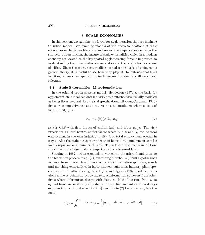
3.1. Scale Externalities: Microfoundations
In the original urban systems model (Henderson (1974)), the basis foragglomeration is localized own industry scale externalities, usually modeledas being Hicks’ neutral. In a typical specification, following Chipman (1970)firms are competitive, constant returns to scale producers where output offirm i in city j is
xij = A(Nj)x(kij , nij) (7)
x(·) is CRS with firm inputs of capital (kij) and labor (nij). The A(·)function is a Hicks’ neutral shifter factor where A
′ � 0 and Nj can be totalemployment in the own industry in city j, or total employment overall incity j. Also the scale measure, rather than being local employment, can belocal output or local number of firms. The relevant arguments in A(·) arethe subject of a large body of empirical work, discussed later.
Starting in 1982, urban economists worked on the micro-foundations tothe block-box process in eq. (7), examining Marshall’s (1890) hypothesizedurban externalities such as (in modern words) information spillovers, searchand matching externalities in labor markets, and intra-industry plant spe-cialization. In path-breaking piece Fujita and Ogawa (1982) modelled firmsalong a line as being subject to exogenous information spillovers from otherfirms where information decays with distance. If the line runs from b1 tob2 and firms are uniformly distributed on the line and information decaysexpotentially with distance, the A (·) function in (7) for a firm at y has theform
A(y) =∫ b2
b1
e−α|y−s|ds =12[2− e−α(y−b1) − e−α(b2−y)] (8)
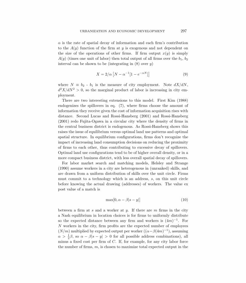
URBANIZATION AND ECONOMIC DEVELOPMENT 297
α is the rate of spatial decay of information and each firm’s contributionto the A(y) function of the firm at y is exogenous and not dependent onthe size of the operations of other firms. If firm output x(y) is simplyA(y) (times one unit of labor) then total output of all firms over the b1, b2interval can be shown to be (integrating in (8) over y)
X = 2/α[N − α−1[1− e−αN ]
](9)
where N ≡ b2 - b1 is the measure of city employment. Note dX/dN ,d2X/dN2 > 0, so the marginal product of labor is increasing in city em-ployment.
There are two interesting extensions to this model. First Kim (1988)endogenizes the spillovers in eq. (7), where firms choose the amount ofinformation they receive given the cost of information acquisition rises withdistance. Second Lucas and Rossi-Hansberg (2001) and Rossi-Hansberg(2001) redo Fujita-Ogawa in a circular city where the density of firms inthe central business district is endogenous. As Rossi-Hansberg shows thisraises the issue of equilibrium versus optimal land use patterns and optimalspatial structure. In equilibrium configurations, firms don’t recognize theimpact of increasing land consumption decisions on reducing the proximityof firms to each other, thus contributing to excessive decay of spillovers.Optimal land use configurations tend to be of higher overall density, or in amore compact business district, with less overall spatial decay of spillovers.
For labor market search and matching models, Helsley and Strange(1990) assume workers in a city are heterogenous in (unranked) skills, andare drawn from a uniform distribution of skills over the unit circle. Firmsmust commit to a technology which is an address, s, on this unit circlebefore knowing the actual drawing (addresses) of workers. The value expost value of a match is
max[0, α− β|s− y|] (10)
between a firm at s and a worker at y. If there are m firms in the citya Nash equilibrium in location choices is for firms to uniformly distributeso the expected distance between any firm and workers is (4m)−1. ForN workers in the city, firm profits are the expected number of employees(N/m) multiplied by expected output per worker ((α−β(4m)−1), assumingα > 1
2β, so α − β|s − y| > 0 for all possible address combinations), allminus a fixed cost per firm of C. If, for example, for any city labor forcethe number of firms, m, is chosen to maximize total expected output in the

298 J. VERNON HENDERSON
city, or N(α− β(4m)−1)− Cm, then we can show total city output is
X = αN − β12C
12N
12 (11)
where again dX/dN , d2X/dN2 > 0 or the marginal product of labor in-creases with city sizes.
Other models include ones based on Dixit-Stiglitz diversity of interme-diate inputs which are non-traded across cities or relatedly on local intra-industry specialization. These are extreme versions of linkages where eachcity must produce its own varieties. So, for example, following Abdel-Rahman and Fujita (1990), suppose y is firm output of the city’s exportgood (say, computers) produced by CRS competitive firms with labor nyand varieties of intermediate inputs x, according to
y = nαy (n∑i=1
xρi )(1−α)/ρ (12)
Then under the usual cost function for any variety N ix = f + cXi and a full
employment constraint, if for simplicity m and Xi are chosen optimally, wecan show3 that total city output is
Y = C0N1−α+αρ
ρ (13)
where again dY/αN, d2Y/dN2 > 0, for N total city employment and C0
a constant. Similar to this model Becker and Henderson (2000) adaptthe Becker and Murphy (1992) model of Adam Smith specialization wherefirms specialize in sets of contiguous heterogenous tasks needed for industryoutput to result. Again the marginal product of labor is increasing in urbanscale.
Note that all these micro-foundation models have a reduced “black-box”form with rising marginal product of labor to the city (but not firm). Scaleimproves productivity, but the reasons could be quite different, as the dif-ferent models indicate. These are models of “static externalities” – infor-mation spillovers today increasing local industry efficiency today. Thereare also specifications in dynamic contexts, but these are also black-boxones. The shift factor A(·) in equation (7) can be made to depend on thelocal stock of knowledge (say, local human capital) or the level of local
3Given full employment, symmetry and aggregation in the CRS Y sector, N = Ny +mNx. Given the cost function for X, then Ny = N−m(f+cX). Substituting for Ny intoY = Nα
y (mXρ)(1−α)/ρ and optimizing with respect to X and m and then substitutingback into the Y function yields (13).

URBANIZATION AND ECONOMIC DEVELOPMENT 299
industry activity in the past (Nj/(t − 1)) contributing to a stock of localtrade secrets, or growth in A(·) can be made to depend on the local stockof knowledge. We will examine such formulations in both the review ofempirical evidence and the presentation of the endogenous growth model.
3.2. Scale Externalities: Evidence
The tradition issue in evaluating scale externalities concerns the rele-vant arguments in the A(·) function in eq. (7) for particular industries.We consider both “static” externalities and the more recent literature on“dynamic” externalities.
3.2.1. Static Externalities
For some industries such as standardized manufacturing, the literaturestarting with Hoover (1948) argues that scale economies are ones oflocalization, meaning they are strictly internal to the own industry anddependent on scale of the own industry locally. Jacobs (1969) on the otherhand argues that, for some industries where innovation and marketing areimportant, what is relevant is the overall scale and diversity of the localenvironment. In static form such economies are ones of urbanization, wherescale externalities depend on the overall size or potential diversity of thelocal environment.
Early empirical work (e.g., Sveikauskas (1975, 1978), Nakamura (1985)and Henderson (1986, 1988)) examined the effect on productivity at the2-3-digit (SIC) industry level of various scale measures estimating eithera primal or dual (cost) form to eq. (7). Work was cross-sectional andindustry-specific data were aggregated to the metropolitan area level, sothe unit of observation was the city-industry. Despite different approachesand data sets (USA, Brazil and Japan), these three sets of studies concludedthere are significant degrees of localization economies in most manufactur-ing industries such as primary metals, machinery, apparel, textiles, pulpand paper, food processing, electrical machinery, and transport equipment,and little evidence of urbanization economies. Below I will argue that scaleeconomies being ones of localization, or internal to the own industry, helpspromote urban specialization. Only in industries such as high fashion ap-parel or glossy publishing did strong evidence of urbanization economiesemerge. However since these studies focus on productivity of manufactur-ing plants, they leave open the question that urbanization economies applyto situations envisioned by Jacobs (1969), such as R&D and perhaps theservice sector. Locational evidence in Fujita and Ishii (1994) in electronics

300 J. VERNON HENDERSON
suggests that R&D activities are drawn to large, diverse metro areas, whilestandardized production is decentralized to smaller cities.
These early productivity studies, even in their own terms face three ma-jor issues. First are location “fixed effects” or relatively time invariantunmeasured aspects of the local environment that affect both productivityand right-hand side variables such as industry scale or the capital to laborratio, resulting in OLS estimates being biased. Such omitted variables in-clude local human capital variables, infrastructure measures, and the localregulatory environment. Second, there is a selection problem. Firms andplants are heterogenous. Perhaps high (or low) productivity plants are dis-proportionately drawn to locations where there are relatively large clustersof own industry firms. Finally firms may be subject to a contemporane-ous locational shock affecting both productivity and inputs, including localindustry scale.
The early literature attempted to deal with the first and third problemsthrough IV estimation, but as always with aggregate cross-section datathere is the issue of valid instruments – ones not affecting productivity butstill (in some conceptual framework) influencing right-hand side covariates.More recent work using panel city-industry data on Korea (Henderson, Lee,Lee (2001)) attempts to deal with the first problem by use of city fixedeffects; and has the same findings as the older literature – scale externalitiesin manufacturing production are ones of localization.
Recent work on this issue has two innovations. First is the use of plantlevel data. Second is investigating what types of plants benefit from scaleexternalities. Third is a start on investigating the nature of spatial decayof externalities. Henderson (2002b) uses plant level productivity data ina panel context to difference out both city fixed effects and a plant unob-served heterogeneity term (that operates as a Hicks’ neutral shift factor)to try to deal with both selectivity and fixed effects. He finds that hightech industries benefit more from localization externalities than traditionalmachinery industries. Plants in single plant firms benefit more than plantsof multi-plant firms, who have a corporate information network to rely on.Finally externalities appear to derive from the number of own industryplants locally representing, say, the count of sources of local informationspillovers, rather than total local employment in the own industry. This lastitem could indicate that information spillovers are the underlying force forexternalities, rather than, say, labor market and search externalities. Butnone of this empirical literature delves into the micro-foundations of scaleexternalities to effectively distinguish information spillover, labor marketexternalities, intra-industry specialization, and the like.

URBANIZATION AND ECONOMIC DEVELOPMENT 301
On the extent of spatial externalities, Ciccone and Hall (1996) using ag-gregate cross-section data argue that density of local activity is important.Henderson (2001) argues that scale effects are internal to the own countyand don’t result from activity in nearby counties. But the most directwork is that of Rosenthal and Strange (2002) who look at how localizationscale effects decay with distance, although their work is based on indirectproductivity inferences from birth patterns. They have data by zip codeson births and argue that relative to adding plants within a 1 mile radius,adding plants in a 1-5 mile radius improves productivity by only 7-50% asmuch depending on the industry, with effects generally dying out at tenmiles. Small plants benefit more than big plants from these localizationeffects.
These studies still face problems with controlling for contemporaneouslocation shocks which influence both productivity and hence scale. Hen-derson (2002b) and Rosenthal and Strange (2002) try controlling for time-metro area fixed effects (i.e., contemporaneous metro area shocks) whileinvestigating scale effects at a more detailed geographic level (county or zipcode). However that leaves open doors – what about zip code or countyshocks. A potential solution to find good instruments for local scale mea-sures involves looking at a location decision framework to model agglomer-ation (Arthur (1990)). There potential instruments for local country scale,would be (exogenous to own county) attributes of competitor counties. Im-proved attributes in those counties draw plants away from the own countywithout directly affecting own county productivity (Bayer and Timmins(2001)).
3.2.2. Dynamic Externalities
There appear to be two sets of working definitions of dynamic exter-nalities. First is that either the history of economic activity in a locationaffects productivity levels today or base period variables affect productiv-ity growth. The second set concerns the effect of “knowledge” (rather thaninformation) spillovers on productivity levels. Knowledge is typically mea-sured by average education and the issue is whether average education ina city affects productivity. It isn’t clear this is a dynamic effect per se. Itcould be static in the sense that average education could simply enhancestatic productivity levels (but not on-going growth rates of productivity),but as we will see later that is sufficient to enhance overall urban scale andpromote endogenous growth.

302 J. VERNON HENDERSON
For the knowledge accumulation framework, Rauch (1993a) estimatesthat average education in a city enhances individual wages, although he hasno control for location effects, sorting effects, or contemporaneous shocksaffecting both wages and education. Moretti (1999) in an important piecemerges plant level productivity data for 1982 and 1992 with individual edu-cation data from the Population Census (PUMS) for 1980 and 1990 to testwhether average educational attainment outside the own industry affectsplant level productivity, controlling for own industry education. Control-ling for overall location fixed effects, he finds that a 1-year increase inaverage education in the city outside the own industry increases plant pro-ductivity by 5%. He also finds that the effect for multi-plant firms is zero,while for single plant firms it is 7.7%. This is very suggestive work. Clearlyit would be interesting to combine an analysis of knowledge accumulationwith scale externalities.
For the productivity growth framework, there is a growing empirical liter-ature on city-industry growth, dating to Glaeser, Khalil, Scheinkman, andShleifer (1992), with a variant in Henderson, Kuncoro, and Turner (1995).The idea is that base period variables such as local own industry scaleor diversity of the local industrial environment encourage local industrygrowth, by promoting local productivity growth which attracts more firmsto a city. Glaeser et al. (1992) find evidence of “dynamic” diversity effectswhich they call Jacobs economies. Henderson et al. (1995) find these forhigh tech industries but find only “dynamic” locationalization economies,called MAR (Marshall-Arrow-Romer) externalities in traditional capitalgoods industries. There is a lot of controversy about what these estima-tions really say especially since issues of endogeneity (to location fixedeffects) are typically overlooked. Looking at net growth of employment ofplants combines two processes, plant births and plant deaths. Davis, Halti-wanger and Schuh (1996) present convincingly evidence that deaths tend tobe related to plant and firm idiosyncratic shocks, rather than location at-tributes. Thus the typical location literature analyzes patterns of births tomake inferences about profit functions and scale effects(Carleton (1983)).Another issue is that, while diversity affects location choices it may notaffect productivity (as Henderson (2002b) finds in looking at lagged diver-sity or own industry scale effects on productivity). So diversity may affect,say, the price, availability, and quality of intermediate inputs drawing firmsinto a city without affecting scale externalities. While industries co-locateto “trade” (reduce transport costs of intermediate inputs) so that growthin industry B at a location is correlated with growth of support industriesX to Z, that doesn’t mean the degree of diversity of X to Z affects pro-
URBANIZATION AND ECONOMIC DEVELOPMENT 303
ductivity in the sense of affecting the A(·) function in eq. (7). Another keyissue concerns how to put all this in a framework of agglomeration overtime, with stochastic components Arthur (1989). As we will note below,individual industry agglomerations at a location tend to change quicklyover time. We have no developed model of that.
4. ECONOMIES COMPOSED OF CITIES
This section examines empirical evidence and models for larger countriesor regions with urban systems comprising dozens or even hundreds of cities.There is an emerging set of well documented facts about the size distribu-tion, production patterns, evolution of the sizes and numbers of cities overtime, and the role of geography in urban systems. Once we have examinedthe empirical evidence, we will turn to modeling systems of cities, with afocus on city specialization and trade patterns and the growth in sizes andnumbers of cities over time. Finally we will examine very recent theoreti-cal work focused on the role of large metro areas versus smaller ones in aneconomy and how to integrate traditional urban systems models with keyaspects of the new economic geography.
4.1. Empirical Facts About Urban Economic Geography
In this section, we examine the evolution of the size distribution of citiesin countries, accounting for city size growth and entry of new cities. We ex-amine patterns of specialization in production by cities. Finally we turn toattempts to account for explicit geographic factors on urban development.
4.1.1. The Size Distribution of Cities and Its Evolution
Work by Eaton and Eckstein (1997) on France and Japan and by Dobkinsand Ioannides (2001) on the USA with later work by Black and Henderson(2002) and Ioannides and Overman (2001) on the USA establish some basicfacts about the development of urban systems in France, Japan, and theUSA over the last century or so. In general, there is a wide size distri-bution of cities in any large economy, where relative size distributions areremarkably stable over time. In this sub-section we examine facts aboutthe evolution of the size distribution of cities and city growth. In the nextwe ask why there is a wide size distribution, where relatively big and smallcities coexist indefinitely.
The empirical work looks at the decade by decade development of urbansystems. In doing so, there are critical choices researchers must make whenassembling data. First is to define what is described by the all-purpose term
304 J. VERNON HENDERSON
“city”. The usual definition is the “metro area” where from a conceptualpoint of view one is trying to capture all contiguous urban economic activ-ity around an urban core, or central city. Large metro areas like Chicagocomprise over 100 municipalities, or local political units, and are definedto cover the entire metro area labor market and to geographically coverall contiguous manufacturing, service and residential activity radiating outfrom the Loop (Chicago city center) until activity peters out into farm landor very low density development. Of course many problems arise, such ashow to treat two or more neighboring and expanding metro areas that atsome point start to overlap. A second problem concerns how to do thesedefinitions over time. One approach is to use whatever contemporaneousdefinition the country census/statistical bureau uses but one problem withthat is that metro area (vs. municipality) concepts only start to be ap-plied after World War II. Another approach is to take current metro areadefinitions and follow the same geographic areas back in time, focusing onnon-agricultural activity.
A third problem concerns how to define “consistently” when an agglomer-ation becomes a city, or metro area over time, especially since the economicnature, population density, and spatial development of metro areas havechanged so much over time. Some authors use an absolute cut-off point(e.g., urban population of 50,000 or more); some use a relative cut-off point(e.g., the minimum size city included in the sample should be .15 mean citysize); and others look at a set number (e.g., 50 or 100) of the largest cities.For these three issues whatever choices researchers make can strongly affectspecific results. Nevertheless a variety of findings emerge that qualitativelyare consistent across studies.
In the research, an initial focus was on studying the evolution of thesize distribution of cities, applying techniques utilized by Quah (1993) inexamining cross-country growth patterns. Cities in each decade are dividedby relative size into 5-6 discrete categories, with fixed relative size cut-offpoints for each cell (e.g., <.22 of mean size, .22 to .47 of mean size, ... >2.2 mean size). A first order Markov process is assumed and a transitionmatrix calculated. Typically stationarity of the matrix over decades can’tbe rejected, so cell transition probabilities are based on all transitions overtime. If M is the transition matrix, i the average rate of entry of newcities in each decade (in a context where in practice there is no exit), Z the(stationary) distribution across cells of entrants (typically concentrated onthe lowest cell), and f the steady-state distribution, then
f = [I− (1− i)M]−1iZ (14)

URBANIZATION AND ECONOMIC DEVELOPMENT 305
In the data decade relative size distributions are remarkably stable overtime and steady-state distributions tend to be close to the most recent dis-tributions. Most critically there is no tendency of distributions to collapseand concentrate in one cell, or for all cities to converge to mean size; norgenerally is there a tendency for distributions to become bipolar. Plots ofrelative size distributions for the U.S.A. in 1900 versus 1990 look almostidentical as Figure 5 illustrates; and Lorenz curves for Japan (1925-1985)and France (1876-1990) in Eaton and Eckstein (1997) almost overlap. InFigure 5 the relative size distribution of cities is plotted for 1900 and 1990,where relative size is actual size divided by mean size in the correspondingtime period. The density functions for 1900 and 1990 almost coincide.
FIG. 5. Density Functions for MSA Size Distributions
. . ..
.
.
.
.
.
...
.
.
.
.. .
... . . .
.
.
.
..... . . . . .
.
.
.
.. . . . . . . . . . . .
. .. . . .
..... . . . . . . . . . . . . .
. .. . . . . . . . . . . . .
. . . . . . . .
Log Relative to Mean Urban MSA Population
Pro
babi
lity
Den
sity
Est
imat
e
-2 0 2 4
0.0
0.1
0.2
0.3
0.4
0.5
oooooo
o
o
o
o
o
o
o
o
oooo
o
o
o
o
oooo
ooooo
ooooooooooooooooo
ooooooooooo
ooooooooooooooooooooooooooooooooooooooooo
. 1900o 1990
A
B
C
Another finding is that, for larger cities, over time there is little changein relative size rankings. In Japan and France, the 39-40 largest citiesin 1925 and 1876 respectively all remain in the top 50 in 1985 and 1990respectively; and, at the top, absolute rankings are unchanged. The USAdisplays more mobility due to substantial entry of new cities. However,while smaller cities do move up and down in rank, the biggest cities tendto remain big over time. So, for example, cities in the top decile of rankingstay in that decile indefinitely, with newer cities joining that decile as thetotal number of cities expands. Alternatively viewed based on the Markov
306 J. VERNON HENDERSON
transition process, the mean first passage time for a city to move from thebottom cell to the top cell is typically 1/10 of the mean first passage timeto go from the top to the bottom , where in Black and Henderson (2002)the later mean first passage time is 545 decades, beyond any horizon of thedata.
Why do big cities stay big? A common answer, in part modeled inHenderson and Ioannides (1981), is physical infrastructure. Large citieshave a huge historical capital stock of streets, buildings, sewers, watermains and parks that are cheaply maintained and almost infinitely livedin, that gives them a persistent comparative advantage over cities withoutthat built-up stock. A second answer is modeled in Arthur (1990) andRauch (1993b) where, with localized scale externalities in production, largecities with an existing fertile externality environment for a particular set ofindustries have a comparative advantage in attracting new firms over citieswith small representation of those industries. We will return to this issuebelow.
Within these relative size distributions of cities, as urbanization andgrowth proceed, both the absolute sizes and numbers of cities have tendedto grow historically, as a country urbanizes and grows in total population.City sizes in the USA, Japan, and France over the past century have grownat average annual rates of 1.2 - 1.5%, depending on countries and samplechoices, rates which involve city sizes rising 3.3 - 4.5 fold every century. Asmall city today which is 250,000 would have been a major center in 1900.In the USA there has also been a large increase in the number of cities.Over 1900-90, using a relative cut-off point to define city entry (minimumsize is .14 of mean size), Black and Henderson (2002) find a 50% increasein the number of cities, while under an absolute cut-off point (50,000) inDobkins and Ioannides (2001) the number of cities triples.
However we count cities, it is clear they have grown in population onan on-going basis over the last century, even in developed countries. Thenext section will model this as related to technological change inducedby knowledge accumulation. Glaeser, Scheinkman, and Shleifer (1995) ina cross-section city growth framework estimate that controlling for 1960population, cities in 1990 are 7% larger if they have a one-standard devi-ation increase in median years of schooling. Black and Henderson (1999)place the issue in a panel context for 1940-1990 controlling for city fixedeffects and examining the impact of percent college educated (which hasenormous time variation). They find a one-standard deviation increase inpercent college educated increases city size by 20%.
URBANIZATION AND ECONOMIC DEVELOPMENT 307
Zipf’s Law. In considering the size distribution of cities, especially in across-sectional context, there is an enormous literature on what is termedZipf’s Law (Rosen and Resnick (1980), Clark and Stabler (1991), Mills andHamilton (1994), Ioannides and Overman (2001)). City sizes are postulatedto follow a Pareto distribution, where if R is rank from smallest, r, tolargest, 1, and n is size
R(n) = An−a (15)
Under Zipf’s Law a = 1, or we have the rank size rule where, for everycity, rank times size is a constant, A. Putting (15) in log-linear form,empirical work produces a’s that vary across countries, samples, and timesbut are “close” to one (ranging, say, from .7 to 1.3) and equations with veryhigh explanatory power. This empirical regularity has drawn considerableattention. While Black and Henderson (2002) show that, with (15) in logs,(1) a < 1 and (2) a quadratic in ln(n) better fits the data for the USAfor 1900-90, so that the relationship does not precisely follow a Paretodistribution, the rank size rule may be a good first approximation.
Where would such a relationship come from? Urban economists have notfocused on that issue, but in a major development, Gabaix (1999a, 1999b)starts to formalize the underlying stochastic components which might leadto such a relationship, building on Simon (1955). Gabaix shows that if citygrowth rates obey Gibiat’s Law where growth rates are random draws fromthe same distribution,4 so growth rates are independent of current size,Zipf’s Law emerges as the limiting size distribution. Growth is scale invari-ant, so the final distribution is and we have a power law with exponent 1.Gabaix sketches an illustrative model. Cities face on-going amenity shocks(bounded away from zero) in an overlapping generations model where onlythe fraction of people who are young are mobile. The young move to equal-ize utility which is real income multiplied by the (scale invariant) amenityshock. Real income is subject to local scale (dis)economies which net tozero in large cities. This formulation leads to Zipf’s Law for the size dis-tribution of cities.
In a recent draft paper, Duranton (2002) illustrates a similar process ina more developed model. He has “first nature” (immobile given naturalresource location) production and “second nature” (mobile, or footloose)production in m cities. There are n (m >> n) products, in a Grossman-Helpman (1991) product quality ladder model. Investment in innovationto try to move the next step up in the ladder in industry k, can also
4Actually the requirement is that they face the same mean and variance in the drawing.
308 J. VERNON HENDERSON
lead to the next step up in a different industry – i.e., there can be cross-industry innovation. To partake of a winning innovation occurring forindustry k in city i, requires industry k production to locate in city i forfootloose industries, which underlies the stochastic process. The result isa approximation (quadratic form to ln(R) in ln(n) in (15)) to Zipf’s Law.
Duranton’s formulation has the advantage over Gabaix’s as an urbanframework in that cities have patterns of production specialization whichchange over time (see next sub-section). Second the paper starts to tryto more explicitly add urban agglomeration benefits and crowding costs.Both papers pass over issues of city formation and economic growth, aswell as issues of stability of static allocation.5
While Gibrat’s Law is a neat underlying stochastic process, does it holdup empirically? Black and Henderson (2002) test whether in the relation-ship, lnnit− lnnit−1 = a+δt+α lnnit−1+εit, α = 0 as hypothesized underthe Law. The Law requires εit to be i.i.d., so simple OLS suffices. Black andHenderson find α < 0 under a variety of circumstance and sub-samples, un-der appropriate statistical criteria, which rejects Gibrat’s Law. Ioannidesand Overman (2001) examine the issue in a more non-parametric fash-ion, characterizing the mean and variance of the distribution from whichgrowth rates are drawn. The mean and variance of growth rates do seemto vary with city size but bootstrapped confidence intervals are fairly widegenerally, allowing for the possibility of (almost) equal means.
4.1.2. Geographic Concentration and Urban Specialization
Geographic concentration refers to the extent to which an industry k isconcentrated at a particular location or, more generally concentrated ata few versus many locations nationally. The measure of concentration ofindustry k at location i might be lik = Xik/
∑iXik. Xik is location i’s
employment or output of industry k. Thus lik is location i’s share of, say,national employment in industry k. On the other hand specialization refersto how much of a location’s total employment is found in industry k, orsik = Xik/
∑kXik. As Overman, Redding and Venables (2001) demon-
strate, if we normalize lik by location i’s share of national employment(sik ≡
∑kXik/
∑k
∑iXik) and sik by industry k’s share of national em-
ployment (sk ≡∑iXik/
∑k
∑iXik) we get the same measure – a location
5With scale effects and, say, an inverted U−shape to city real income in urban scale,equalized utilities can occur on upward and downward sloping portions of the U−shape– only the later are stable, or are Nash equilibria in population location decisions (seebelow).

URBANIZATION AND ECONOMIC DEVELOPMENT 309
quotient, or
qkik = Xik(∑k
∑iXik)∑
kXik
∑iXik
(16)
The distribution of qik across industries, k, compared over time for a citywould tell us about how city i’s specialization patterns are changing overtime. And the distribution of qik across locations, i, over time would tellus whether industry k is becoming more or less concentrated over time.As Overman et al. (2001) point out, in a practical application looking atmany industries and cities over time or across countries, the issue concernshow to produce summary measures to describe how overall concentrationfor one industry compares with another or how one city’s degree of spe-cialization compares with another. Another issue concerns how to accountin measuring specialization or concentration for different forces that causethese phenomena. The literature uses a variety of approaches.
Evidence on a variety of countries such as Brazil, U.S.A., Korea, andIndia (Henderson (1988), and Lee (1997)) indicate that cities are relativelyspecialized. The traditional urban specialization literature going back toBergsman, Greenston and Healy (1972) uses cluster analysis to group citiesinto categories based on similarity of production patterns – correlations (orminimum distances) in the shares of different industries in local employ-ment, Sik. Cluster analysis is an “art form” in the sense that there is nooptimal set of clusters, and it is up to the researcher to define how fineor how broad the clusters should be and there are a variety of clusteringalgorithms.
Using 1990 data on the U.S.A. Black and Henderson (2002) group 317metro areas into 55 clusters, “defining” 55 city types based on patterns ofspecialization for 80 2-digit industries. They define textile, primary met-als, machinery, electronics, oil and gas, transport equipment, health ser-vices, insurance, entertainment, diversified market center, and so on typecities, where anywhere from 5-33% of local employment is typically foundin just one industry. They show that production patterns across the typesare statistically different and that average cities and educational levels bytype differ significantly across many of the types. Specialization especiallyamong smaller cities tends to be absolute. At a 3-digit level many citieshave absolutely zero employment in a variety of categories. So in 1992 formajor industries like computers, electronic components, aircraft, instru-ments, metal working machinery, special machinery, construction machin-ery, and refrigeration machinery and equipment, respectively, of 317 metro
310 J. VERNON HENDERSON
areas 40%, 17%, 42%, 15%, 77%, 15%, 14% and 24% have absolutely zeroemployment in these industries.
Kim (1995) in looking at the USA examines how patterns of special-ization have changed over time, by comparing for pairs (i, j) of locations∑k |sik− sjk| and by estimating locational Gini’s for industry concentra-
tion (Krugman (1991b). He finds that states are substantially less spe-cialized in 1987 than in 1860, but that localization, or concentration hasincreased over time. For Korea, as part of the deconcentration processnoted earlier, Henderson, Lee, and Lee (2001) find that from 1983 to 1993,city specialization as measured by a normalized Hirschman-Herfindahl in-dex
gj =∑k
(sjk − sj)2 (17)
rises in manufacturing, while a provincial level index declines. Cities be-come more specialized and provinces less so. Clearly the geographic unit ofanalysis matters as do the concepts. City specialization as exposited in themodels presented below is consistent with regional diversity, when regionsare composed of a large number of cities.
Henderson (1997) for the USA and Lee (1997) for Korea show that thegj index of specialization in manufacturing declines with metro area size.Smaller cities are much more specialized than larger cities in their man-ufacturing production. More generally, Kolko (1999) demonstrates thatlarger cities are more service oriented and smaller ones more manufactur-ing oriented. For six size categories (over 2.5 million, 1 - 2.5 million, ...< .25 million, non-metro counties) he shows that the ratio of manufactur-ing to business service activity rises from .68 to 2.7 as size declines, wheremanufacturing and business services account for 35% of local private em-ployment. The other 65% of local employment is in “non-traded” activitywhose shares don’t vary across cities – consumer services, retail, wholesale,construction, utilities.
What about concentration of industry – the extent to which a partic-ular industry is found in a few versus many locations? In an extremelyimportant paper Ellison and Glaeser (1997) model the problem using USAdata, to determine to what extent there is clustering of plants within anindustry due to either industry-specific natural advantages (e.g., access toraw materials) or spillovers among plants, where plants locate across spaceso as to maximize profits and profits depend on area specific natural ad-vantage, spillovers, and an i.i.d. drawing from Weibul distribution. The
URBANIZATION AND ECONOMIC DEVELOPMENT 311
idea is to explain the joint importance of spillovers and natural advantagein geographic concentration.
Geographic concentration for industry j is Gj =∑i(sji − xi)2, where
sji is the share of industry j in employment in location i and xi is locationi’s share in total national employment (to standardize for location size).Where 0 ≤ γna ≤ 1 represents the importance of natural advantage (wherethe variance in relative profitability of a location is proportional to γna)and γS represents the fraction of pairs of firms in an industry betweenwhich a spillover exists, Ellison and Glaeser show that
E[Gj ] = (1−∑i
x2i )(γj + (1− γj)Hj) (18)
γ ≡ γna + γs − γsγna
where Hj is the standard Hirschman-Herfindahl index of plant industrialconcentration in industry j. So E[Gj ] equals γj adjusted for variations inlocation size (1−
∑x2i ) and industry concentration H. The empirical part
calculates γj for all 3- or 4-digit manufacturing industries across states andcountries. They show for 4-digit industries that G > (1 −
∑x2i )H in 446
of 459 industries, where G ≤ (1 −∑x2)H only if γ ≤ 0. That is almost
all industries display some degree of spatial concentration due to eithernatural advantage or spillovers. Second they argue that 25% of industriesare highly concentrated ( γ > .05) and 43% are not highly concentrated (γ < .02). In a later article, Ellison and Glaeser (1999) argue that, based oneconometric results relating location choices to natural advantage measures,10-20% of γ is accounted for by natural advantage. The rest is due to intra-industry spillovers, a rather critical finding in urban analysis indicating theimportance of understanding the nature of scale externalities.
4.1.3. Geography
A variety of recent studies have examined the role of geography, primar-ily natural features, in the spatial configuration of production and growthof cities. Rappaport and Sacks (2001) building on Sacks’ general geographyprogram herald the role of coastline location in the U.S.A., as a factor pro-moting city growth. In a related but more comprehensive study, Beeson,DeJong and Troeskan (2001) look at USA counties from 1840-1990. Theyshow that iron deposits, other mineral deposits, river location, ocean loca-tion, river confluence, heating degree days, cooling degree days, mountainlocation, and precipitation all affect 1840 county population significantly.However for 1840-1990 growth in county population, only ocean location,
312 J. VERNON HENDERSON
mountain location, precipitation, and river confluence matter, controllingfor 1840 population. That is, first nature items strongly affected 1840 andhence indirectly 1990 populations; but growth from 1840-1990 is indepen-dent of many first nature influences. Ocean location as Sacks’ suggests haspersistent growth effects.
Both these studies ignore the geography of markets and the role of neigh-bors in influencing city evolution. Dobkins and Ioannides (2001) show thatgrowth of neighboring cities influence own city growth and cities with neigh-bors are generally larger than isolated cities. Black and Henderson (2002)put neighbor and geographic effects together. They calculate normalizedmarket potential variables (sum of distance discounted populations of allother counties in each decade, normalized across decades).They find climateand coast affect relative city growth rates; but market potential has big ef-fects as well, although they are non-linear. Bigger markets provide morecustomers, but also more competition, so marginal market potential effectsdiminish as market potential increases. Market potential helps explain whyNorth-East cities in the USA maintain reasonable growth given it is themost densely populated area from history, despite the natural advantagesof the West.
Introducing market potential brings us full circle to the Krugman (1991)model exposited earlier. There is little empirical work on the model, withHanson’s work being a notable exception. Hanson (2000) examines wagerelations across USA counties in an explicit Krugman monopolistic compe-tition model, where scale derives from diversity of final consumption goods.By examining the effect on county wages and employment of surroundingeconomic activity, or market potential, by imposing the structure of theKrugman model, Hanson infers (1) that prices exceed marginal cost by10-20%, (2) demand shocks attenuate quickly and disappear at about 400miles, and (3) scale effects (diversity) are very strong relative to transporteffects in driving geographic concentration.
4.2. Systems of Cities Models
Systems of cities models date back to Henderson (1974), with a vari-ety of substantial contributors to further development (Hochman (1977),Kanemoto (1980), Henderson and Ioannides (1981), Abdel-Rahman andFujita (1990), Helsley and Strange (1990), and Duranton and Puga (2002),to name a few). Here I outline the model in Black and Henderson (1999)which is an endogenous growth model of cities, that will thus lead directlyto the growth-urban connection. The analysis is broken into two parts.The first examines the traditional static model, focused on city formation

URBANIZATION AND ECONOMIC DEVELOPMENT 313
and the determination of the sizes, numbers, and industrial composition ofcities in an economy at a point in time. The second adds on the growthpart.
4.2.1. The System of Cities at a Point in Time
Consider a large economy composed of two types of cities, where thereare many cities of each type and each type is specialized in the produc-tion of a specific type of traded good. We will show why (when) there isspecialization momentarily and the generalization to many types of goodsand cities is straightforward. To simplify the growth story, each firm iscomposed of a single worker. In a city type 1, in any period, the output offirm i in a type 1 city is
X1i = D1(nδ11 hψ11 )hθ11i 0 < δ1 <
12
(19)
h1i is the human capital of the worker and is his given input in the produc-tion process. A firm/worker is subject to two local externalities. First isown industry localization economies, the level of which depend on the to-tal number of worker-firms, n1, in this representative type 1 city. n1 couldrepresent the total volume of local spillover communications as in eq. (9),where δ1 is the elasticity of firm output with respect to n1. The restrictionδ1 <
12 ensures a unique solution in an economy composed of many type
1 cities. The second externality, h1, is the average level of human capitalin the city and represents local knowledge spillovers, as in section 2.2.2.hψ1
1 could be thought of as the richness of information spillovers nδ11 .Given this simple formulation the wage of worker i is simply
W1i = X1i (20)
In an economy of identical individual workers in type 1 cities, individualswill all have the same human capital level (either exogenously in a staticcontext, or endogenously in a growth context). Thus total city output willsimply be
X1 = D1hσ1+ψ11 n1+δ1
1 (21)
Equilibrium City Sizes.Equations (19) and (21) embody the scale benefits of increases in local
employment, where output per worker is an increasing function of localown industry employment. Determinant city sizes arise because of scale
314 J. VERNON HENDERSON
diseconomies in city living, including per capita infrastructure costs, pollu-tion, accidents, crime, and commuting costs. In Henderson (1974) those arecaptured in a general cost of housing function, but most urban models con-sider an explicit internal spatial structure of cities. All production occursat a point – the center of the city. Surrounding the center in equilibrium inlocal land markets is a circle of residents each on a lot of unit size. Peoplecommute back and forth at a constant cost per unit (return) distance ofτ . That cost can be from working time, or here an out-of-pocket cost paidin units of X1. Equilibrium in the land market is characterized by a lin-ear rent gradient, declining from the center to zero at the city edge whererents (in agriculture) are normalized to zero. Standard analysis dating toMohring (1961) gives us expressions for total city commuting and rents, interms of city population where6
total commuting costs = bn3/21 (22)
total land rents =12bn
3/21 (23)
b ≡ 2/3π−12 τ.
Equation (22) are the critical resource costs, where the marginal commut-ing costs of increasing city size are increasing in city population. Rents areincome to, potentially, a city developer.
How do cities form and how are sizes determined? There are an unex-hausted supply of identical city sites in the economy, each owned by aland developer in a nationally competitive urban land development mar-ket. A developer for an occupied city collects local land rents, specifiescity population (but there is free migration in equilibrium), and offers anyinducements to firms or people to locate in that city, in competition withother cities. Population is freely mobile. Helsley and Strange (1990) spec-ify the city development game to determine how many cities will form and
6An equilibrium in residential markets requires all residents (living on equalize sizelots) to spend the same amount on rent, R(u), plus commuting costs, τu, for any distanceu from the CBD. Any consumer then has the same amount left over to invest or spendon all other goods. At the city edge at a radius of u, rent plus commuting costs areτu1 since R(u1) = 0; elsewhere they are R(u) + τu. Equating those at the city edgewith those amounts elsewhere yields the rent gradient R(u) = τ(u1 − u). From this, wecalculate total rents in the city to be
∫ u10 2πuR(u)du (given lot sizes of one so that each
“ring” 2πudu contains that many residents) or 1/3πτu1. Total commuting costs are∫ u10 2πu(τu)du = 2/3πτu3
1. Given a city population of n and lot sizes of one, n1 = τu21
or u1 = π−12 n
12 . Substitution gives us eqs. (20) and (21).
URBANIZATION AND ECONOMIC DEVELOPMENT 315
what their sizes will be. Given this game, Henderson and Becker (2001)show that resulting solutions (with multiple factors of production) are (1)Pareto efficient, (2) the only coalition proof equilibria in the economy, (3)unique under appropriate parameters (see below), and (4) free mobilityones where the developer specified populations are self-enforcing. Theyalso show under appropriate conditions such outcomes arise (1) in a self-organized economy with no developers where city governments can excluderesidents (“no-growth” restrictions) to maximize the welfare of the repre-sentative local voter, (2) in a growing economy where developers form newcities and old cities are governed by (even passive) local governments. Notefor developing countries the key ingredients: either national land marketsmust be competitive with developers free to form new cities or atomisticsettlements can arise freely and local autonomous governments can limittheir populations as they grow. Without such institutions if, for example,cities only form through “self-organization”, the result is enormously over-sized cities (Henderson (1974), Henderson and Becker (2001)) where all netscale benefits are totally dissipated so the population is no better in citiesthan doing home production.7
In this context, the developer of a representative city chooses city popula-tion (or equivalently number of firms) and subsidies to locating firms/workersto maximize profits, or
maxn1,T1
π1 =12bn
3/21 − T1n1 (24)
subject to W1 + T1 − 3/2bn121 = I1
where T1 is the per firm subsidy (e.g., in practice in a model with localpublic goods, a tax exemption). I1 is the real income per worker availablein equilibrium in national labor markets under free mobility, which a singledeveloper takes as given. In the constraint, I1 equals wages in (20) and(19), plus the subsidy, less per worker rents plus commuting costs paid.Maximizing with respect to T1 and n1 and imposing perfect competitionin national land markets so π1 = 0 ex post, yields
T1 =12bn
121 (25)
7At the limit city sizes are so large with such enormous diseconomies that the popula-tion is indifferent between being in a rural settlement of size 1 (the size of a communityformed by a defecting migrant) and an enormous oversized city. As we will see with aninverted-U shape to real income I1, self organization has cities at the right of the peakat n where I1(n = 1) = I1(n = n) rather than where I1 is maximized.
316 J. VERNON HENDERSON
n∗ = (δ12b−1D1)2/(1−2δ1)h2ε11 (26)
ε1 =θ1 + ψ1
1− 2δ1(27)
This solution has a variety of properties heralded in the urban litera-ture. First it reflects the Henry George Theorem (Flatters, Henderson, andMieszkowski (1974), Stiglitz (1977)), where the transfer per worker/firm ex-actly equals the gap (δ1W1) between social and private marginal of laborto the city, and that externality subsidy is exactly financed out of collectedland rents. That is, total land rents cover the cost of subsidies need toensure Pareto efficient outcomes, as well as the costs of local public goodsin a model where good goods are added in. Second the efficient size in (26)is the point where real income, I1, peaks as an inverted U -shape functionof city size (where I1 = W1 + 1
2bn121 − 3/2bn
121 , where 3/2 bn
121 is per worker
rents plus commuting costs and 12bn
121 is per worker share in local land
rents). If δ1 < 12 , we can show that I1 is a single-peaked function of n1, so
n∗1 is the unique efficient size. If δ1 > 12 , in essence there will only be one
type 1 city in the economy, because net scale economies are unbounded.Given n∗1 is the size where I1 peaks, n∗1 is a free mobility equilibrium – aworker moving to another city would lower real income in that city and beworse off. Finally city size, n∗1 is increasing in technology improvements: τdeclining, δ1 rising, D1 rising, or local knowledge accumulation (h1) rising.
Other City Types and Specialization.In Black and Henderson, X1 of city type 1 is an input into production
of the single final good in the economy, X2 (from which, hence in a growthcontext human capital is also “produced”). In many models all outputs ofspecialized city types are final consumption goods. Here X2 is produced intype 2 cities where the output for worker/firm j is correspondingly
X2j = D2(nδ22 hψ22 )hθ22jX
1−α1j (28)
Here per worker output is also subject to own industry local scale external-ities (nδ22 ) and to local knowledge spillovers (hψ2
2 ). However now there isan intermediate input, X1j , which is the numeraire good with X2j pricedat P in national markets. The analysis of city sizes and formation for type2 cities proceeds as for city type 1, with corresponding expressions otherthan the addition of an expression for P in n∗2 and I2 and a restriction foran inverted U−shape to I2 that δ2 < α/2.
Two basic issues arise. Why do cities specialize and how are the equilib-rium numbers of cities of each type and relative prices P determined. On
URBANIZATION AND ECONOMIC DEVELOPMENT 317
specialization, in this model there are no costs of inter-city trade: no costsof shippingX1 as inputs toX2 types and shippingX2 back as retail goods inX1 type cities. All transport costs are internal to the city, given the relativegreater importance of commuting costs in modern economies. Given thatand given scale economies are internal to the industry, any specialized cityout-competes any mixed city. The heuristic argument is simple. Considerany mixed city with n1 and n2 workers in industry 1 and 2. Split that cityinto two specialized cities, one with just n1 people and the other with justn2. Scale economies are undiminished (nδ11 and nδ22 in both cases in indus-tries 1 and 2 respectively) but per worker commuting costs are lower in thespecialized cities compared to the old larger mixed cities, so real incomesare higher in each specialized city compared to the old city. The rigor-ous argument is a little more subtle in the growth context where humancapital levels, h1 and h2, differ endogenously across industries and affectincomes.8 Having localization economies is a sufficient but not necessarycondition for specialization. Industries can have urbanization economiesso scale depends on total local employment. However if the degree of ur-banization economies differs across industries (the corresponding δ1 6= δ2)then each industry has a different efficient local scale and is better off in adifferent size specialized city than any mixed city. In fact mixed cities aremore likely to emerge if each good has localization economies multipliedby separate spillovers from the other industry or sharing of some commonpublic infrastructure (Abdel-Rahman (2000)).
A basic problem in the pre-economic geography urban models is thelack of nuance on transport costs. Either transport costs of goods acrosscities is zero (X1 and X2) or infinite (housing, and potentially other non-tradeables). A recent innovation is to have generalized transport costs(without a specific geography) where the cost of transporting a unit of X1
to an X2 city is t1 and the cost of shipping X2 back to an X1 city is t2, aninnovation due to Abdel-Rahman (1996) in a model similar to the static oneused here (one intermediate and one final good) and then generalized byXiong (1998) and Anas and Xiong (2001). Now specialization as opposedto diversified cities depends on the level of t1 and t2. At appropriate pointsas t1 or t2 or both rise from zero, X1 and X2 will collocate (in developer runcities). More generally with a spectrum of, say, final products, we wouldexpect that some products have low enough t’s to always be produced inspecialized cities, some high enough t’s to be in all cities, and some in
8It raises issues of low education types potentially benefiting from high education typeexternalities, in a context where separation is desirable but a separating equilibriumcostly to maintain (Black (2002)). See later.
318 J. VERNON HENDERSON
middle range t’s are produced in some cities (ones with bigger markets)but not others (with smaller markets). No one has yet simulated this morecomplex outcome.
The second issue concerns how to close the model in a static context andsolve for P the relative price of X2 and m1 and m2 the number of citiesof each type. In a large economy integer problems are ignored and a fullemployment constraint imposed so
m1n1 +m2n2 = N (29)
where N is national population. The second equation (to solve the 3 un-knowns P , m1, and m2) equates real incomes across cities (I1 = I2) only instatic context. That is in a static context individual workers move acrosscities to equalize real incomes. Finally there is an equation where nationaldemand equals supply in either the X1 or X2 market (i.e., the supply,m1X1, equals the demand for X1 as an intermediate input, m2n2x1, andfor producing commuting costs m1(bn
3/21 ) +m2(bn
3/22 ) from eq. (20)). In
this specific model that will yield values of m1, m2 and P that are functionsof parameters and h1 and h2. In a static context of identical workers, onewould impose h = h1 = h2. We will discuss momentarily the solution forh1 and h2 and the model in the growth context.
In the static context where labor mobility requires I1 = I2, in the largertype of city, say type 1, commuting and land rent costs will be higher. Thus,if real incomes are equalized, W1 > W2 as a compensating differential forhigher living costs. Firms in type 1 cities are willing to pay higher wagesbecause type 1 cities offer them greater scale benefits. Empirical evidenceshows as cities increase from a small size (say, 50,000) to very large metroareas, both the cost-of-living and real wages double (Henderson (1988)).
In a static context, at the national level there are constant returns toscale or replicability. If we double national population, the numbers ofcities of each type and national output of each good simply double, withindividual city sizes and real incomes unchanged.9 With two goods andtwo factors basic international trade theorems (Rybczynski, factor priceequalization, and Stolper-Samuelson) hold (Hochman (1977), Henderson(1988)).
Policy in a System of Cities. The insight that large urbanizedeconomies are replicable with CRS is important, since it simplifies pol-
9Here with h1 and h2 yet to be solved we would need to double the numbers of peoplewith h1 and h2 respectively. Below we will see the solution with growth to h1 and h2 isnational scale invariant.
URBANIZATION AND ECONOMIC DEVELOPMENT 319
icy analysis. Policy analysis of system of cities is not a focus of recentwork, but Henderson (1988) considers the effects of a variety of policies.For example trade protection policies favoring industry X produced in rel-atively large size cities will alter national output composition towards Xproduction and increase the number of large relative to small cities. Na-tional urban concentration will rise. Similarly subsidizing an input such ascapital for a high tech product, X, again, say, produced in a larger type ofcity will cause the numbers of that type of city to increase and raise urbanconcentration. As another example, national minimum wage policies maynot bite in large high wage cities but will bite in smaller low wage cities.In general cities subject to binding minimum wages will increase in size,but their numbers and overall production will decline. In order to pay thelegislated higher wages, relative prices of those products rise (as supplydeclines) and greater city sizes generate greater local scale effects.
Another issue is that policy makers may favor large cities because theyview them as “more productive”. Indeed for an industry found in smallertowns, it may be that the A(·) they face in eq. (7), their technology levelincluding whatever externalities, may be higher in a larger city. Howeverthat doesn’t mean they locate there. Although the A(·) may be higher, inorder for them to locate there, it must be sufficiently relatively higher toafford the higher wage and land rents, compared to a smaller city. If not,their profit maximizing or cost minimizing location is the smaller city.
4.2.2. Growth in a System of Cities
Black and Henderson (1999) specify a dynastic growth model where dy-nastic families grow in numbers at rate g over time starting from size 1.If c is per person family consumption, the objective function is∫∞0
( c(t)1−σ−11−σ )e−(ρ−g)tdt where ρ(> g) is the discount rate. Dynasties can
splinter (as long as they share their capital stock on an equal per capitabasis) and the problem can be put in an overlapping generations contextwith equivalent results (Black (2000)), under a Galor and Zeira (1993) “joyof giving” bequest motive.
The only capital is human capital and as such there is no market for it.Intra-family behavior substitutes for a capital market. Specifically familiesallocate their total stock of human capital (H) and members across cities,where Z proportion of family members go to type 1 cities (taking Zh1e
gt ofthe H with them) and (1−Z) go to type 2 cities taking (1−Z) h2e
gt withthem). Additions to the family stock come from the equation of motionwhere the cost of additions, PH, equals family income (ZegtI1 + (1 −
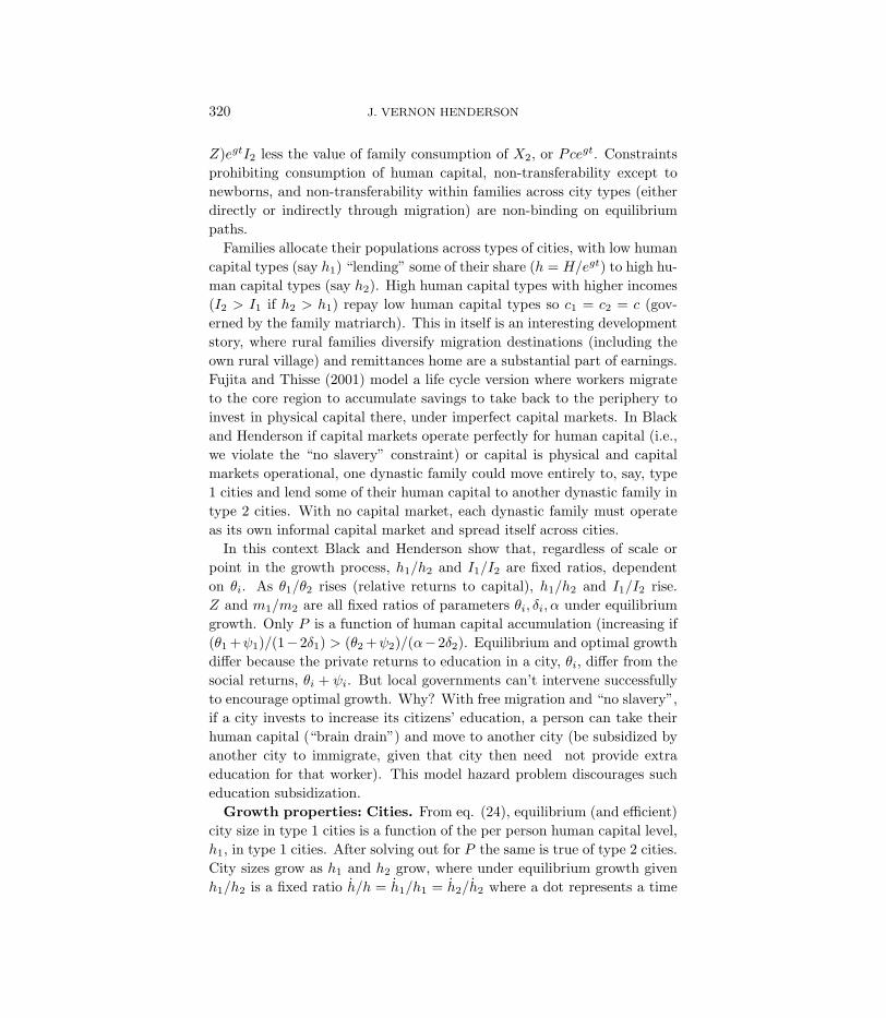
320 J. VERNON HENDERSON
Z)egtI2 less the value of family consumption of X2, or Pcegt. Constraintsprohibiting consumption of human capital, non-transferability except tonewborns, and non-transferability within families across city types (eitherdirectly or indirectly through migration) are non-binding on equilibriumpaths.
Families allocate their populations across types of cities, with low humancapital types (say h1) “lending” some of their share (h = H/egt) to high hu-man capital types (say h2). High human capital types with higher incomes(I2 > I1 if h2 > h1) repay low human capital types so c1 = c2 = c (gov-erned by the family matriarch). This in itself is an interesting developmentstory, where rural families diversify migration destinations (including theown rural village) and remittances home are a substantial part of earnings.Fujita and Thisse (2001) model a life cycle version where workers migrateto the core region to accumulate savings to take back to the periphery toinvest in physical capital there, under imperfect capital markets. In Blackand Henderson if capital markets operate perfectly for human capital (i.e.,we violate the “no slavery” constraint) or capital is physical and capitalmarkets operational, one dynastic family could move entirely to, say, type1 cities and lend some of their human capital to another dynastic family intype 2 cities. With no capital market, each dynastic family must operateas its own informal capital market and spread itself across cities.
In this context Black and Henderson show that, regardless of scale orpoint in the growth process, h1/h2 and I1/I2 are fixed ratios, dependenton θi. As θ1/θ2 rises (relative returns to capital), h1/h2 and I1/I2 rise.Z and m1/m2 are all fixed ratios of parameters θi, δi, α under equilibriumgrowth. Only P is a function of human capital accumulation (increasing if(θ1 +ψ1)/(1−2δ1) > (θ2 +ψ2)/(α−2δ2). Equilibrium and optimal growthdiffer because the private returns to education in a city, θi, differ from thesocial returns, θi + ψi. But local governments can’t intervene successfullyto encourage optimal growth. Why? With free migration and “no slavery”,if a city invests to increase its citizens’ education, a person can take theirhuman capital (“brain drain”) and move to another city (be subsidized byanother city to immigrate, given that city then need not provide extraeducation for that worker). This model hazard problem discourages sucheducation subsidization.
Growth properties: Cities. From eq. (24), equilibrium (and efficient)city size in type 1 cities is a function of the per person human capital level,h1, in type 1 cities. After solving out for P the same is true of type 2 cities.City sizes grow as h1 and h2 grow, where under equilibrium growth givenh1/h2 is a fixed ratio h/h = h1/h1 = h2/h2 where a dot represents a time

URBANIZATION AND ECONOMIC DEVELOPMENT 321
derivative. Then
n2
n2=n1
n1= 2ε1
h
h(30)
where ni/ni is the growth rate of efficient sizes n∗i .For the number of cities, the issue is whether growth in individual sizes
absorbs the national population growth, or
m1
m1=m2
m2= g − ni
ni= g − 2ε1
h
h(31)
The numbers of cities grow if g > ni/ni. Note growth in numbers and sizesof cities is “parallel” by type, so the relative size distribution of cities isconstant over time.
Growth properties: Economy. Ruling out explosive or divergentgrowth, there are two types of growth equilibria. Either the economyconverges to a steady state level (where γc ≡ c/c = 1
σ (Ahε−1 − ρ)), orit experiences endogenous steady-state growth. Convergence to a level oc-curs if ε ≡ ε1(1−(γ−2δ2))+ε2(γ−2δ2) < 1, where ε is a weighted averageof the individual city type εi. In that case at the steady-state h, ni/ni = 0and mi/mi = g, or only the numbers but not sizes of cities grow just like inexogenous growth (Kanemoto (1980), Henderson and Ioannides (1981)). Ifε = 1 then there is steady-state growth, where γh = h/h = A−ρ
σ (where thetransversality conditions require A > ρ). In that case ni/ni = 2ε1(A−ρσ ),or cities grow at a constant rate. and their numbers also increase ifg > 2ε1(A−ρσ ).
4.2.3. Extensions
There are two major extensions to the basic systems of cities models.First people may differ in terms of inherent productivity or in terms of en-dowments. Second, while we have discussed the issue of city specializationversus diversification we haven’t really developed any insights into a morenuanced role of small highly specialized cities versus large diversified metroareas in an economy.
Turning to the first extension, Henderson (1974) had physical capital asa factor of production owned by capitalists who needn’t reside in cities.Then equilibrium city size reflects a market trade-off between the interestsof city workers who have an inverted U−shape to utility as a function ofthe size of the city they live in and capitalists whose returns to capital riseindefinitely with city size (for the same capital to labor ratio). There is apolitical economy story there where capitalists collectively in an economy

322 J. VERNON HENDERSON
have an incentive to limit the number of cities, thus forcing larger citysizes. Helsley and Strange (1991) and then Becker and Henderson (2000)have matching models between the attributes of entrepreneurs and workers,as noted earlier. But again the two class model yields a market resolvedconflict between what is the city size that maximizes the welfare of oneversus another group.
In a different approach Abdel-Rahman and Wang (1997) (see also Abdel-Rahman (2000) for a synthesis) and later (Black (2000) look at high and lowskill workers who are used in differing proportions in production of differentgoods. Black has a low skill traded production good and a second tradedgood produced with high skill workers and inputs of a low skill non-tradedgood, where high skill workers generate production externalities in the formof knowledge spillovers for all traded goods. In Black, urban specializationwith high skill workers concentrated in one type of city is efficient, but aseparating equilibrium, where low skill workers and low tech productionstays in its own type of city (rather than trying to cluster with high techproduction) is not easy to sustain. Black characterizes conditions underwhich a separating equilibrium will emerge.
Abdel-Rahman and Wang (1997) impose an urban core-periphery struc-ture where a high tech good can only be produced by heterogeneous skilledworkers but the low tech good by either those workers or homogeneousunskilled workers. Urban scale economies arise in public infrastructureprovision as well as better matching of heterogeneous skilled workers. Thelow tech good is assumed to be produced in a system of hinterland (pe-ripheral) cities and the high tech good in the core region metropolis. Thefocus is on determinants of income inequality, although much of the workrevolves around the Nash bargaining process in the matching process be-tween heterogeneous skilled workers and the firms which hire them, andless on endogenous properties of systems of cities.
It is important to note that there is a much more developed literature oninequality induced by neighborhood selection, where the characteristics ofneighbors affect skill acquisition (e.g. family background of the class affectsindividual student performance). That leads to segregation of talented orwealthier families by neighborhood (Benabou (1993), Durlauf (1996)) andcan help transmit economic status across generations, promoting inter-generational income inequality.
Metro Areas. Simple indices of urban diversity indicate that smallercities are very specialized and larger cities highly diversified. So the ques-tion is what is the role of large metro areas in an economy and their rela-tionship to smaller cities. Henderson (1988) and Duranton (2002) have a

URBANIZATION AND ECONOMIC DEVELOPMENT 323
first nature - second nature world, where every city has a first nature eco-nomic base and footloose industries cluster in these different first naturecities. Large metro areas are at the top of an urban hierarchy in Hen-derson (1988), with first nature activity benefiting most from local scaleexternalities and with the greatest varieties of footloose activity clusteredin the metro area. The smallest cities are engaged in specialized first natureactivity with minimal scale externalities, where the local market doesn’t at-tract much footloose production. But it seems that today few metro areashave an economic base of first nature activity. Accordingly recent litera-ture has focused on the role of large metro areas as centers of innovation,headquarters, and business services (Kolko (1999)).
The Dixit-Stiglitz model opened up an avenue to look at large metroareas as having a base of diversified intermediate service inputs, whichgenerate scale-diversity benefits for local final goods producers. That initialidea was developed in Abdel-Rahman and Fujita (1990). That idea has ledto a set of papers focused on the general issue of what activities, under whatcircumstances are out-sourced. Theory and empirical evidence (Holmes(1999) and Ono (2000)) suggests that as local market scale increases, finalproducers will in-house less of their service functions and out-source themmore. That out-sourcing encourages competition and diversify in the localbusiness service market, encouraging further out-sourcing.
In terms of incorporating this into the role of metro areas versus smallercities, Davis (2000) has a two-region model, a coastal exporting regionand an interior natural resource rich region. There are specialized man-ufacturing activities which, for production and final sale, require businessservice activities, summarized as headquarters functions. Headquarterspurchase local Dixit-Stiglitz intermediate services such as R&D, market-ing, financing, exporting, and so on. Headquarters activity is in port citiesin the coastal region. The issue is whether manufacturing activities arealso in these ports versus in specialized coastal hinterland cities versus inspecialized interior cities. Scale economies in manufacturing and headquar-ters activities are different and independent of each other, so that, basedon scale considerations, these activities would be in separate specializedcities. However if the costs of interaction (shipping manufactured goods toport and transactions costs of headquarters-production facility communi-cation) between headquarters and manufacturing functions are extremelyhigh, then both manufacturing and headquarters activities can be foundtogether in coastal port cities. Otherwise they will be in separate types ofcities. In that case, manufacturing cities will be in coastal hinterlands ifcosts of headquarters-manufacturing interaction are high relative to ship-

324 J. VERNON HENDERSON
ping natural resources to the coast. However if natural resource shippingcosts are relatively high, then manufacturing cities will be found in theinterior.
Duranton and Puga (2001) have developed an entirely different and stim-ulating view of large metro areas. In an economy there are m types ofworkers who have skills each specific to producing one of m products. Spe-cialized cities have 1 type of worker producing the standardized productfor that type of worker subject to localization economies. Diversified citieshave some of all types of workers. Existing firms at any instant die atan exogenously given rate; and, in a steady-state, new firms are their re-placement. New firms don’t know “their type” – what types of workersthey match best with and hence what final product they would be best offproducing. To find their type they need to experiment by trying the differ-ent technologies (and hence trying different kinds of workers). New firmshave a choice. They can locate in a diversified city with low localizationeconomies in any one sector. In a diversified city they can experiment witha new process each period until they find their ideal process. At that pointthey relocate to a city specialized in that product, with thus high localiza-tion economies for that product. Alternatively new firms can experimentby moving from specialized city to specialized city with high localizationeconomies, but face a relocation cost each time. If relocation costs arehigh, the advantage during their experimental period is to be in a diversi-fied city. This leads to an urban configuration of experimental diversifiedmetro areas and other cities which are specialized in different standardizedmanufacturing products.
The Duranton and Puga model captures a key role of large diversifiedmetro areas consistent with the data. They are incubators where new prod-ucts are born and where new firms learn. Once firms have matured thenthey typically do relocate to more specialized cities. This also capturesthe product-life cycle for firms in terms of location patterns. Fujita andIshii (1994) document the location patterns of Japanese and Korean elec-tronics plants and headquarters. In a spatial hierarchy mega-cities househeadquarters activities (out-sourcing business services) and experimentalactivity. Smaller Japanese or Korean towns house specialized, more stan-dardized high tech production processes and low tech activity is off-shore.
5. URBAN ISSUES IN CHINA
In this last section I turn to a specific application of the urbanizationand economic geography models to China. Chinese urbanization has some

URBANIZATION AND ECONOMIC DEVELOPMENT 325
special features driven by historical and current policies affecting urbaniza-tion. I first discuss features of Chinese urbanization and key policies. ThenI turn to a review of analyses of the impacts of these policies on production,growth and efficiency of Chinese cities.
5.1. Some Key Features and Policies of the Chinese Urban Sys-tem5.1.1. Low Urban Concentration
Chinese cities are relatively small and equal sized, compared to mostcountries. The UN puts the population of Shanghai metro area, the largestcity, at 12.3m in 2000, well below the populations of the 10 largest metroareas in the world. More critically is that China only has 9 metro areas withpopulations over 3 million while it has another 125 or so metro areas withpopulations from 1-3 million; – a ratio of .072, compared to the worldwideratio for the same size categories of .27 (Henderson (2002c)). To give a morecommon frame of reference for comparisons, we examine spatial Gini’s.
For 1657 metro areas with populations over 200,000 in 2000 for the world,the spatial Gini is .564. The Gini is the usual one: rank cities from small-est to largest and plot the Lorenz curve of their accumulated share of totalpopulation for the sample (world cities in this case). The Gini is the shareof area below the 45◦ line that lies between the 45◦ line and the Lorenzcurve. China’s Gini is .43 in 2000, way below the world, and compares to.65, .65,.61 ,.60, .60, .60, .59, .58, .56, .54 and .52 for other large coun-tries respectively of Brazil, Japan, Indonesia, UK, Mexico, Nigeria, France,India, Germany, USA and Spain. Only former Soviet bloc countries havesimilarly low Gini’s, Russia with .45 and Ukraine with .40.
In the second part of this section, we will argue that Chinese cities ingeneral are too small, leading to significant efficiency losses. In fact wewill argue more generally that there is insufficient spatial agglomerationthroughout, in both the urban and rural sector.
5.1.2. The Hukou System
In China, the geographic-urban dispersion of population is maintainedby strong migration restrictions, under the hukou system. Migration re-strictions play such a strong role in the society and economy, it is critical todescribe them. The hukou system in China is similar to an internal pass-port system (see Chan (1994) for a detailed description). A person’s local“citizenship” and residence is initially defined for a child as a birth right,traditionally by the mother’s place of legal residence. The entitlements anddetails of the system differ for urban and rural residents. Legal residence
326 J. VERNON HENDERSON
in a city entitles one to local access to permanent jobs, regular housing,public schooling, and public health care (where almost all health care ispublic) in that city. Until the early 1990’s, it also entitled urban people to“grain rations” – rations of essentials such as grain and kerosene.
Legal residence in a village or rural township entitles residents to land forfarming, township housing, job opportunities in rural industrial enterprises,and access to local health and schooling facilities in their town. Residentsalso have some degree of “ownership” in local enterprises; although dis-tributed profits all go to the local public budget, which may be used tofinance township housing and infrastructure. Again, until recent years,legal residence in a township also entitled a “peasant” to some share inlocally produced (or allocated from the outside) grain and other essentials.
How does a person change their local citizenship? There are severalcommon mechanisms. First is education. A smart rural youth may persistthrough the competitive school system to go to a college and then be hiredinto an urban job, with an urban hukou. Second, the state at times canopen the gates, permitting factories to hire permanent workers from ruralareas, permitting family reunification, or permitting legal migration fromrural areas to nearby small cities. However the official changes in residenceor hukou status average about 18 million (in under 1.3% of the population)a year over the last 20 years with little annual variation (Chan (2000)).
People can migrate to an area without local hukou, or an official changeof residence “citizenship”, either illegally (“unregistered”) or legally as atemporary worker or as a “permanent resident” on a long-term permit. Forexample, a rural person may be hired as a “contract worker” in industryor services, for a term of three years. People may move illegally, withoutregistering in the new location, and work in the informal sector for low pay,under poor conditions, with risk of deportation. Despite these possibilitiesand despite some recent relaxations of restrictions in particular provinces,the restrictions in migration remain tight.
Temporary migrants to larger cities typically have no, or very high pricedaccess to health care and schooling facilities and regular, “legal” housing.In fact cities have strict national guidelines on conversion of agriculture tourban land; and institutional difficulties in housing markets in expandingsupply makes it particularly difficult for migrants to find decent housing.All this means living and social conditions for migrants and their familiesare extremely difficult, since children face no or very high priced access toschooling and health care. But there are other restrictions. Legal tempo-rary migration requires getting a permit from the city of in-migration andcities can impose various hurdles to getting a permit – permission from

URBANIZATION AND ECONOMIC DEVELOPMENT 327
the home location, proof of a guaranteed job and specific housing, and thelike. Cities have also published job lists, citing jobs for which migrantsare not eligible; in 2000, Beijing listed over 100 occupants as non-eligibleones. Migrants may still have to pay taxes to their rural home village forservices they don’t consume and on land left fallow. Finally migrants havetraditionally faced direct fees (Cai (2000)). There is a license fee to workoutside the home township paid to the township that can be equivalentto several months’ wages. At the destination there can be fees for citymanagement, for being a “foreign” worker, for city construction, for crimefighting, for temporary residence, and even for family planning if the mi-grant is female. All these restrictions sharply reduce the benefits and raisethe costs of migration, particularly into large cities. Migration is limitedand most migration is short-term, or “return” migration, as we will detailwith data below. Overall the hukou system holds 100’s of millions of peo-ple in locations where they are not exploiting their earning potential, aswe will detail below.
5.1.3. Aspects of Urban Policy Since 1978
As defined in part by the 1982 Sixth 5-Year Plan, as well as the Seventh5-Year Plan, the post-Mao period has a set of initially defined urbaniza-tion policies that persist today. Good sources on aspects of these policiesinclude Chan (1994), Kojima (1996), Fujita and Hu (2001), and Wei andWu (2001). First urban population was to expand, but through the rapidgrowth of smaller cities relaxing hukou transfers at the level, while con-taining the sizes of larger cities. The 1990’s witnessed the rapid growth innumber of cities, as many places were recognized as having passed 100,000urban population mark. However China’s spatial Gini and degree of urbanconcentration remains very low by world standards and even lower in 2000than in 1960 (.42 versus.47). General urban population expansion has alsobeen fueled by rapid growth, particularly in coastal towns, of township pop-ulations, always pushing these towns towards (or past) the 100,000 markto be a city (Ma and Fan 1994).
In the Sixth and Seventh 5-year plans there is a sense of hierarchy, playedout both in governance structures and in economic policy. Larger cities areto lead smaller ones and rural areas; the coast is to lead the center and west.“Leading” has many dimensions. Larger cities focus on newer production –initially high tech and light industry and then business service developmentin recent years. Large cities receive new technologies and hand-down tra-ditional activities to their hinterlands, in particular contracting-out parts

328 J. VERNON HENDERSON
and components production to small cities, towns, and rural areas, andrelocating heavy, polluting production to their ex-urban areas.
Another aspect of urbanization policy, implicit and as part of big citiesleading the rest, is played out in the development of rural industry – thetown and village enterprise sector [TVE’s]. The rapid productivity growthin agriculture after 1978, coupled with prior restrained urbanization, meanta vast surplus of labor in agriculture. Given the desire to continue to re-strain urbanization (although at a much higher rate after the 15 or so yearsbefore 1978), a policy of “leave the land but not the village” was crafted.So the rural sector was to industrialize, but generally not spatially ag-glomerate. TVE development was constrained by under-capitalization, aninability to spatially agglomerate, and in the 1980’s policies restraining itscompetition with SOE’s (followers are not supposed to out-compete lead-ers!).10 However, TVE growth was rapid: starting from an initial minisculelevel, by 1997 VA in the TVE sector was twice that in remaining SOE’s(independent accounting units). TVE’s had hard budget constraints, fewerregulations, and greater ability to respond to input (hiring and promotion,choice of sellers of intermediate inputs) and output (product demand) mar-ket conditions. By the early 1990’s, Jefferson and Singhe (1999) documenthow TVE total factor productivity exceeded SOE’s, ascribing that to thegreater operational freedom and hard budget constraint of TVE’s.
Still TVE sector development was constrained by the under-capitalizationof the rural sector that has been a feature of modern China. Based on microdata, Jefferson and Singhe show that the rate of return on physical capitalin the TVE sector in 1997 exceeded that of SOE’s by 25%. In addition thehigher wage and compensation returns to labor in the urban sector com-bined with college education being the key to permanent migration fromrural to urban areas, means the more educated population is funneled intocities. An area of investigation is the very high social returns to educationin the rural sector, improving township allocation decisions of resourcesbetween agricultural, animal husbandry and TVE activities (Yang and Au(1997)).
In addition to these policies governing rural-urban (and big city-smallcity) allocation of capital and labor there are other much more explicitpolicies with a spatial bias (Chan (1994), Naughton (2002), Fujita and Hu(2001)). While they have some big city-small city/town flavor, they alsohave a coastal versus rest of the country flavor. Arguably the key element
10Usually shifting restrictions on products that could be produced by TVE’s were thecompetition restraint. Success by a TVE in competition could lead to its product linebeing terminated (Henderson (1988)).

URBANIZATION AND ECONOMIC DEVELOPMENT 329
is initial policies that directed FDI and trade to certain coastal cities. Inthe early (1979) reforms, 4 coastal special economic zones, centered on 4prefecture level cities were created to encourage free market experimen-tation, an inflow of FDI, and development of international trade. In themid-1980’s, 14 more coastal cities were declared as open cities to foreigninvestors, with 2 more coastal cities added by 1990. In addition 10 cities(half overlapping with open status) were given separately listed status –economic decision making powers equal to the provincial cities of Beijing,Tianjin, and Shanghai.
Fujita and Hu (2001) show that 14 open cities and 4 spatial economiczones accounted for 42% of national FDI from 1984-1994. In 1990, the 24“special status” cities (special economic zones, open, and separately listed)plus Beijing accounted for 65% of all FDI in prefecture level cities, whileaccounting for only 36% of value-added in non-agricultural production ofprefecture level cities. This initial advantage persists, despite opening ofthe entire economy. For example, these 25 cities account for 63% of all FDIaccumulated from 1990-1997 in all prefecture (or provincial) level cities.
Fujita and Hu (2001) argue persuasively that the agglomeration of elec-tronics and light manufacturing in coastal areas such as the region aroundGuangzhou is due to these initial policies promoting FDI and trade inthese favored coastal areas. The effect is reflected in the ratio of invest-ment occurring in coastal versus interior regions: in 1984 the ratio is 1.12while 10 years later it is 1.93 (see also Naughton, 2002). These policiesand their impacts are deliberate spatial policies of the Sixth and Seventh5-year plans, favoring development in a spatial hierarchy of the coastal re-gion. On a more positive note, Wei and Wu (2001) do show the expandingtrade within these favored regions, tended to reduce rural-urban incomeinequality, because trade helped the TVE sector in the urban fringe (rural)areas.
An entirely different aspect of this spatial policy bias involves trans-portation. On a world scale, China has an anemic road system. Its ratiosof national roads to land, roads to population, or paved roads to land or topopulation in 1995 are very low by international standards. For example,its ratio of roads to population (which is better than using land as thenormalization or looking at paved roads) in 1995 is 1.2, to be compared to2.1 for India, 1.5 for Pakistan, 1.9 for Indonesia, or 2.7 for Mexico. Half ofthese roads are paved in India but only 15% in China. For a country withfar-flung populations, this places hinterlands at great disadvantage in theirability to secure inputs and truck products to coastal and international

330 J. VERNON HENDERSON
markets. Only now is a highway being built to link Chengdu, Sichuan’scapital, and the 100m. people in the Sichuan region to the coast.
The final aspect of spatial bias involves governance and fiscal relations.Fiscal rules and inter-governmental relations in China are not well definedand transparent. Revenue redistribution contracts send monies comingfrom the center back to provinces and cities; up to the mid-1990’s theseappeared to favor bigger and richer cities. But much official public expen-diture is extra-budgetary – local revenues retained within localities (Jinand Zou (2002)). What is retained and the specifics of a city’s fiscal alloca-tions from above, whatever the rules, are in part the result of bargaining.And in the hierarchy of big city versus small or coast versus interior, thebigger and the coastal have greater bargaining power. Actual results de-pend on the personalities and power of local leaders, with an interestingliterature on China documenting this (Cheung, Chung, and Lin (1998)).Bigger cities have more effective fiscal autonomy and more control overkey appointments (e.g., heads of local state-owned banks which become asource of funds and subsidies of local industries). Cities compared to ruralareas are favored with the ability to offer lower tax rates on FDI firms. Theissue is a difficult one and there has emerged no clear way to quantify thefiscal advantage of one city or set of cities over others. But the spatial biasand lack of transparency is a key feature of China’s urban sector.
5.2. Some Effects of Policy
This section focuses on agglomeration economies and city sizes in China– the extent to which cities in China may be too small. It examines thewelfare losses from under-sized cities and the extent of rural-urban migra-tion that is actually occurring . At the end we will turn to the issue ofspatial bias and history of pro-coastal policies.
5.2.1. Under-agglomeration in Cities
Using data for 1996 and 1997, Au and Henderson (2002) estimate cityproduction functions for 212 prefecture level (or above) cities. Output isvalue-added per worker in the non-agricultural sector of the city proper.Determinants include the capital stock to labor ratio, share of accumulatedFDI in capital stock, distance to the coast, education and scale measures.With respect to the last item, real output per worker following traditionalsystems of cities analysis outlined in section 3 is postulated to be an invertedU-shape function of local scale, as measured by total local non-agriculturalemployment. At low scale, the marginal benefits in terms of increased pro-ductivity of increased local scale from enhanced scale externalities and local

URBANIZATION AND ECONOMIC DEVELOPMENT 331
TABLE 1.
Efficient City Sizes
A. City Employment at Peak of VA per Worker
manufacturing
to service ratio .6 .8 1.0 1.2 1.4 1.6 1.8 2.0
L∗ 2730 2380 2030 1670 1320 970 620 270
95% confidence
interval
- lower 1880 1680 1420 1090 670 180
- upper 3590 3080 2630 2260 1980 1760 1580 1430
B. Gain from moving to L∗ipercent current
size is below peak 50 40 30 20
percent gain in 35% 20% 9.5% 4.1%
V A per worker
backward and forward linkages outweigh the marginal costs from increasedcongestion and commuting costs and environmental degradation. So at lowcity scale, real value-added per worker is increasing in scale, then at somecity size it peaks, and after that declines with further increases in city scale.
However cities are in an economic “hierarchy” where cities relatively andabsolutely specialize in different products. In general in that context, themanufacturing to service ratio of cities declines as city scale rises, or citiesmove up the hierarchy. To capture this, Au and Henderson (2002) postulatethat the inverted U-shape shifts right as the manufacturing to service ratiodrops. They estimate a relationship for city i where
ln(V Ai/Li) = βXi + α1Li + α2L2i + α3Li ·MSi (32)
In (32), Xi are controls on technology, capital-labor ratio, access and thelike. V Ai is value-added; Li is total (non-agricultural) employment, andMSi is the manufacturing to service V A ratio (seconday to tertiary sectorV A). In eq. (32) output per worker peaks where
L∗i =α1 + α3MSi
−2α2(33)
where α2 < 0, α1 > 0, α1 +α3MS1 > 0 and α3 < 0. The last reflectsthe economic hierarchy idea: bigger cities are more service oriented, so L∗ideclines as MSi rises.
Estimation of (32) in Au and Henderson (2002) is by instrumental vari-ables using 1990 (planning period) variables as instruments. Estimation
332 J. VERNON HENDERSON
produces a tight fit with excellent specification test results. Table 1A showsrelevant manufacturing to service ratios, the peak points (L∗i ). where value-added per workers is maximized and the 95% confidence interval for peakscale. Note scale is in thousands of workers. Most Chinese cities (85%)lie to the left of their peak points and 43% are below the 95% confidenceinterval on L∗i . That is, 43% of cities are significantly to the left of L∗i ,or significantly undersized. Table 1B shows the percent gain in V A perworker from moving below the peak to the peak. About 50% of cities are50% or more below their peak size, with resulting large productivity losses.
For county-level cities, Au and Henderson are unable to quantify aninverted-U, instead finding unbounded scale effects (for these smaller citysizes). Similarly for TVE’s across provinces, local scale economies (averagetownship TVE employment by province over three years) are unboundedand very large – a 10% increase in local scale increases value-added byworker by 3%. This is the same order of magnitude found by Jefferson andSinghe (1999) to TVE scale, using micro data.
The conclusion is that throughout China there is under-agglomeration,held in place by the hukou system, and also property right issues in ruralareas. For the latter, there is no ability to readily transfer TVE ownershipand location, for township residents to sell their “shares” in local TVE’s soas to liquidate and relocate, or for township residents to shift location toanother town. That makes rural agglomeration difficult. However here wefocus more on rural-urban migration. But free migration in China wouldchange the landscape – some prefecture and county-level cities would ex-perience huge population inflows over a period of years. Some townshipswould also experience huge inflows and transform into major cities. Con-versely, these flows imply some cities and towns would experience largepopulation losses.
5.2.2. Extent of Actual Rural-Urban Migration
In the popular press, there is sometimes a sense that there is alreadyenormous migration in China, with the transformation well underway.Certainly a transformation is underway, and may be more advanced inprovinces such as Guangdong; but the issue is the extent of overall popula-tion movements. In 1998, the commonly accepted number for the “floating”population – those currently outside their town of residence for more than1-3 days – was about 100m of 1.2b or so people. From Chan (2000), severalfactors are apparent concerning these 100m. First the number of annualpermanent residence changes has been constant at about 18m for the prior

URBANIZATION AND ECONOMIC DEVELOPMENT 333
15 years. About 15% of the population relocates every 10 years, including,as we will suggest, a substantial portion of rural-rural and urban-urbanmoves. Second, in general, most temporary migration in China is returnmigration – migrants move for a few months or years and then return home,rather than remaining as temporary migrants in a destination indefinitely.Third, most of even this temporary migration is short distance.
TABLE 2.
Migration in China
A. Stocks of the Population
floating population (outside of township of residence ) 100m (estimated)
temporary migrants (outside of township of residence for 62.4 m
more than 6 months) in 1998
percent of temporary migrants living outside home county (1995) 59%
B. Flows of Population 1990-1995 Rural/Urban (origin −→ destination) Percent
U−→U 35.4
U−→R 4.8
R−→R 23.8
R−→U 36.0
Out-of Province destination 32.1%
Source: Abstracted from Chan (2000).
Table 2 covers this short distance aspect, as well as an overview of tem-porary migration. Of the 100m floating population in 1998, only 62.4m hadbeen out of residence for over 6 months. Of these (based on 1995 surveyresults), 41% moved just within their home county. So in 1998 only about37m people had been living outside their official county of residence formore than 6 months. For these, what about rural versus urban destina-tions?
Based on flows for 1990-1995, for migrants moving for over 6 months,40% of moves involve urban residents and 60% rural. For these 60% rural,60% go to cities, as opposed to other rural areas. Finally for all moverswith 6+ months stay, only 32% move outside of province. If we applythese numbers to 1998 and assume urban and rural movers have equal outof province propensities, in 1998 of the 62.4m temporary migrants, only12m were rural folks moving out of province (62.4m * 32 *.6). Of the 12mtemporary long distance rural migrants only some portion (60% suggestedin Table 2) go to cities.

334 J. VERNON HENDERSON
Whatever the exact numbers and the fact that we are past 1998, theanalysis suggests that the permanent urban populations are only modestlysupplemented with rural migrants on a nationwide basis. Table 2B suggestsof the 62.4 temporary migrants, under 15m (62.4 *.36) involve rural-urbanmigration, both within and outside provinces. Even if we triple that num-ber to adjust for increased migration and to add in some of the floatingpopulation staying less than 6 months, that still means only 10% of theofficial 450m urban residents are temporary migrants from rural areas.
5.2.3. Spatial Discrimination and The Coast Versus The Hinterlands
China has subsidized FDI (through tax breaks) in prefecture level citiesand encouraged FDI and trade development in certain coastal cities, aspart of a general program emphasizing coastal development, over hinter-land development. The question is whether the FDI policy is efficient. Onthe subsidization question, the argument is that FDI brings in technologytransfer, as well as creating job opportunities for low cost Chinese labor.The counter-argument is that FDI is not particularly high tech, comparedeven to more sophisticated domestic production, and FDI may discourage,or divert funds from local R&D. The evidence is not conclusive. For exam-ple Au and Henderson (2002) find that, ceteris paribus (same total capitalto labor ratio) that cities with a one-standard deviation higher FDI/capitalratio have 8% higher output per worker. In Henderson (2002), FDI alsoenhances city growth rates. And in Fujita and Hu (2001) as noted earlier,FDI is associated with coastal agglomeration.
Assessing the issue of the efficiency of coastal versus hinterland develop-ment is less straightforward. On FDI, in Au and Henderson (2002), thereis no evidence that FDI interacts with distance to the coast or city size –returns to FDI occur in the same degree for all cities regardless of size orlocation. But there is a more general question of coastal versus hinterlanddevelopment. The Rappaport and Sacks (2001) story is that hinterlandsare inherently inferior locations for economic development, compared tocoastal locations. Demurger, Sacks, Woo, et al (2002) amend the storyfor China to argue that favored provinces tend to be coastal provinces sothat the faster growth of coastal provinces is explained by a combinationof policy-bias and inherent advantage.
A limitation in the analysis of coastal advantage is the failure to controlfor market potential of cities, a control fundamental in the analysis of eco-nomic geography (Overman, Redding and Venables (2001)). Statisticallythe issue is that in many countries (e.g. USA), historically populations have
URBANIZATION AND ECONOMIC DEVELOPMENT 335
agglomerated on coasts (including in Rappaport and Sacks for the USA theGreat Lakes). So access to the coast captures both greater domestic mar-ket potential effects, and pure coast effects. In Au and Henderson (2002),distance to the coast on its own in eq. (1) significantly reduces produc-tivity. However introduction of market potential eliminates the effect ofaccess to the coast, and produces large significant effects for market po-tential. Similarly in Henderson (2002) access to the coast is not associatedwith higher growth per se, once FDI and market potential differentials areaccounted for. If we consider Sichuan in Western China, its 100m residentshave enormous market potential. With proper modern highway links to thecoast, it in some sense will become “coast”, with easier access to the coast.While coastal provinces still have better access to international markets,Sichuan may be domestically competitive, relatively specializing in domes-tic products. Its “disadvantage” may reflect policy disadvantage in termsof transport development, FDI, and loosening of planning constraints, morethan an inherent disadvantage of hinterland location.
REFERENCESAbdel-Rahman, H., 1996, When do cities specialize in production. Regional Scienceand Urban Economics 26, 1-22.
Abdel-Rahman, H., 2000, City systems: General equilibrium approaches. In: J-M Hu-riot and J-F Thisse (eds.), Economics of Cities: Theoretical Perspectives, CambridgeUniversity Press, 109-37.
Abdel-Rahman, H. and M. Fujita, 1990, Product variety, marshallan externalities,and city sizes. Journal of Regional Science 30, 165-85.
Abdel-Rahman, H. and P. Wang, 1997, Social welfare and income inequality in asystem of cities. Journal of Urban Economics 41, 462-83.
Ades, A.F. and E.L. Glaeser, 1995, Trade and circuses: Explaining urban giants.Quarterly Journal of Economics 110, 195-227.
Anas, A. and K. Xiong, The formation and growth of specialized cities. Mimeo. StateUniversity of New York at Buffalo.
Arthur, 1990, Silicon valley locational clusters: When do increasing returns to scaleimply monopoly. Mathematical Social Sciences 19, 235-51.
Au, C.C. and J.V. Henderson, 2002, How migration restrictions limit agglomerationand productivity in China. NBER Working Paper No. 8707.
Baldwin, R.E., 2001, Core-Periphery model with forward-looking expectations. Re-gional Science and Urban Economics 31, 21-49.
Baldwin, R.E. and R. Forslid, 2000, The Core-Periphery model and endogenousgrowth: Stabilizing and de-stabilizing integration. Economica 67, 307-42.
Barro, R. and X. Sala-i-Martin, 1991, Convergence scross states and regions. Brook-ings Papers on Economic Activity 1, 107-82.
Barro R. and X. Sala-i-Martin, 1992, Regional growth and migration: A Japan-USAcomparison. Journal of Japanese and International Economics 6, 312-46.

336 J. VERNON HENDERSON
Bayer, P. and C. Timmins, 2001, Identifying social interactions in endogenous sortingmodels. Yale University mimeo.
Becker, G., E. Mills, and J.G. Williamson, 1992, Indian Urbanization and EconomicGrowth since 1960. Johns Hopkins Press.
Becker, G. and K. Murphy, 1992, The division of labor, coordination cost, and knowl-edge. Quarterly Journal of Economics 107, 1137-60.
Becker, R. and J.V. Henderson, 2000, Intra-industry specialization and urban de-velopment. In: J-M Huriot and J-F Thisse (eds.), Economics of Cities, CambridgeUniversity Press, 138-66.
Beeson, P.E., D.N. DeJong, and W. Troeskan, 2001, Population growth in US coun-ties, 1840-1990. Regional Science and Urban Economics 31, 669-700.
Benabou, R., 1993, Workings of a city: Location, education, and production. Quar-terly Journal of Economics 108, 619-52.
Bergsman, J., P. Greenston, and R. Healy, 1972, The agglomeration process in urbangrowth. Urban Studies 9, 263-88.
Black, D., 2000, Local knowledge spillovers and inequality. Mimeo. University of Cal-ifornia Irvine.
Black, D. and J.V. Henderson, 1999, A theory of urban growth. Journal of PoliticalEconomy 107, 252-84.
Black, D. and J.V. Henderson, 2002, Urban evolution in the USA. Journal of Eco-nomic Geography, forthcoming.
Cai, Fang, 2000, The Mobile Population Problem in China. Henan People’s PublishingHouse: Zhengzhou.
Carleton, D., 1983, The location and employment choices of new firms: An economicmodel with discrete and continuous endogenous variables. Review of Economics andStatistics 65, 440-49.
Chan, K.W., 1994, Cities With Invisible Walls. Oxford University Press: Hong Kong.
Chan, K.W., 2000, Internal migration in China: Trends, determiation, and scenarios.University of Washington. Report prepared for World Bank (April).
Cheung, Peter T.Y., J.H. Chung, and Z. Lin (eds.), 1998, Provincial Strategies ofEconomic Reform in Post-Mao China: Leadership, Politics, and Implementation.Armonk, N.Y.: M.E. Sharpe.
Chipman, J.S., 1970, External economies of scale and competitive equilibrium. Quar-terly Journal of Economics 85, 347-85.
Ciccone A., and R.E. Hall, 1996, Productivity and the density of economic activity.American Economic Review 86, 54-70.
Clark, J.S. and J.C. Stabler, 1991, Gibrat’s law and the growth of Canadian cities.Urban Studies 28, 635-39.
Davis, James, 2000, Headquarter service and factory urban specialization with trans-port costs. Brown University.
Davis, S., J. Haltiwanger, and S. Schuh, 1996, Job Creation and Destruction. MITPress.
Davis, J. and J.V. Henderson, 2001, Evidence on the Political Economy of the Ur-banization Process. Mimeo. Journal of Urban Economics. Forthcoming.
Demurger, S., J.D. Sacks, W.T. Woo, S. Bao, G. Chang, and A. Mellinger, 2001,Geography, economic policy, and regional development. Asian Economic Papers 1,forthcoming.
URBANIZATION AND ECONOMIC DEVELOPMENT 337
Dixit A. and J. Stiglitz, 1977, Monopolistic competition and optimum product diver-sity. American Economic Review 67, 297-308.
Dobkins, L.H. and Y.M. Ioannides, 2001, Spatial interactions among U.S. cities: 1900-1990. Regional Science and Urban Economics 31, 701-32.
Duranton, G., 2002, City size distribution as a consequence of the growth process.LSE Mimeo.
Duranton, G. and D. Puga, 2001, Nursery cities: Urban diversity process innovation,and the life cycle of products. American Economic Review 91, 1454-77.
Durlauf, S.N., 1996, A theory of persistent income inequality. Journal of EconomicGrowth 1, 75-93.
Eaton, J. and Z. Eckstein, 1997, Cities and growth: Evidence from France and Japan.Regional Science and Urban Economics 27, 443-74.
Ellison, G. and E. Glaeser, 1999, The geographic concentration of US manufacturing:A dartboard approach. Journal of Political Economy 105, 889-927.
Ellison, G. and E. Glaeser, 1999, The geographic concentration of industry: Doesnatural advantage explain agglomeration. American Economic Association Papersand Proceedings 89, 311-16.
Fay, M. and C. Opal, 1999, Urbanization without growth: Understanding an Africanphenomenon. Mimeo. World Bank.
Flatters, F., J.V. Henderson, and P. Mieszkowski, 1974, Public goods, efficiency, andregional fiscal equalization. Journal of Public Economics 3, 99-112.
Fujita, M. and H. Ogawa, 1982, Multiple equilibria and structural transition of non-monocentric configurations. Regional Science and Urban Economics 12, 161-96.
Fujita, J., P. Krugman, and A.J. Venables, 1999, The Spatial Economy: Cities, Re-gions, and International Trade. MIT Press.
Fujita, M. and T. Ishii, 1994, Global location behavior and organization dynamics ofJapanese electronic firms and their impact on regional economies. Paper presentedfor Prince Bertil Symposium on the Dynanmic Firm, Stockholm.
Fujita, M. and J-F Thisse, 2000, The formation of economic agglomerations. In: J-MHuriot and J-F Thisse (eds.) Economies of Cities, NY, Cambridge University Press.
Fujita, M. and J-F Thisse, 2001, Agglomeration and growth with migration andknowledge externalities. Kyoto University Institute for Economic Research WP#531.
Fujita, M. and D. Hu, 2001, Regional disparity in China 1995-1994: The effects ofglobalization and economic liberalization. The Annals of Regional Science 35, 3-37.
Fujita, M. and J-F Thisse, 2002, Economics of Agglomeration. Cambridge UniversityPress.
Gabaix, X., 1999a, Zipf’s law and the growth of cities. American Economic Associ-ation and Proceedings 89, 129-32.
Gabaix, X., 1999b, Zipf’s law for cities: An explanation. Quarterly Journal of Eco-nomics 114, 739-67.
Gallup, J.L., J.D. Sacks, and A. Mellinger, 1999, Geography and economic develop-ment. International Regional Science Review 22, 179-232.
Galor, O. and J. Zeira, 1993, Income distribution and macro economics. Review ofEconomic Studies 60, 35-52.
338 J. VERNON HENDERSON
Glaeser, E. H. Khalil, J. Scheinkman, and A. Shleifer, 1992, Growth in cities. Journalof Political Economy 100, 1126-52.
Glaeser, E., J. Scheinkman, and A. Schelifer, 1995, Economic growth in a cross-sectionof cities. Journal of Monetary Economics 36, 117-34.
Grossman, G. and E. Helpman, 1991, Quality ladders in the theory of growth. Reviewof Economic Studies 58, 43-61.
Hanson, G., 1996, Localization economies, vertical organization, and trade. AmericanEconomic Review 86, 1266-75.
Hanson, G., 2000, Market potential, increasing returns, and geographic concentration.Mimeo. University of Michigan (November).
Harris, J. and M. Todaro, 1970, Migration, unemployment, and development: A twosector analysis. American Economic Review 40, 126-42.
Helpman, E.,1998, The size of regions. In: D. Pines, E. Sadka and I. Zilcha (eds.),Topics in Public Economics: Theoretical and Applied Analysis, Cambridge UniversityPress, 33-54.
Helsley, R. and W. Strange, 1990, Matching and agglomeration economies in a systemof cities. Regional Science and Urban Economics 20, 189-212.
Henderson, J.V., 1974, The sizes and types of cities. American Economic Review 61,640-56.
Henderson, J.V., 1986, Efficiency of resource usage and city size. Journal of UrbanEconomics 19, 47-70.
Henderson, J.V., 1988, Urban Development: Theory, Fact and Illusion. Oxford Uni-versity Press.
Henderson, J.V., 1997, Medium size cities. Regional Science and Urban Economics27, 583-612.
Henderson, J.V., 2002a, The urbanization process and economic growth: The so-whatquestion. Journal of Economic Growth. Forthcoming.
Henderson, J.V., 2002b, Marshall’s scale economies. Journal of Urban Economics.Forthcoming.
Henderson, J.V., 2002c, City growth, worldwide 1960-2000. Mimeo. Brown University.
Henderson, J.V. and R. Becker, 2001, Political economy of city sizes and formation.Journal of Urban Economics 48, 453-84.
Henderson, J.V. and Y. Ioannides, 1981, Aspects of growth in a system of cities.Journal of Urban Economics 10, 117-39.
Henderson, J.V., A. Kuncoro, and M. Turner, 1995, Industrial development in cities.Journal of Political Economy 103, 167-90.
Henderson, J.V. and A. Kuncoro, 1996, Industrial centralization in Indonesia. WorldBank Economic Review 10, 513-40.
Henderson, J.V., A. Kuncoro, and P. Nasution, 1996, Dynamic development in Jab-otabek. Indonesian Bulletin of Economic Studies 32, 71-96.
Henderson, J.V., T. Lee, and J.Y. Lee, 2001, Scale externalities in Korea. Journal ofUrban Economics 49, 479-504.
Hochman, O., 1977, A two factor three sector model of an economy with cities. Mimeo.
Holmes, T., 1999, Localization of industry and vertical disintegration. Review of Eco-nomics and Statistics 81, 314-25.
URBANIZATION AND ECONOMIC DEVELOPMENT 339
Holmes, T. and J.J. Stevens, 2002, Geographic concentration and establishment scale.Review of Economics and Statistics, forthcoming.
Hoover, E.M., 1948, The Location of Economic Activity. NY: McGraw-Hill.
Ioannides, Y.M. and H.G. Overman, 2001, Zipf’s law for cities: An empirical exami-nation. Mimeo. Tufts University.
Jacobs, J., 1969, The Economy of Cities. NY: Random House.
Jefferson, G. and I. Singhe, 1999, Enterprise Reform in China: Ownership Transitionand Performance. Oxford University Press: New York.
Jin, J. and H-F. Zou, 2002, Soft budget constraint on local governments in China.Mimeo. World Bank.
Junius, K., 1999, Primacy and economic development: Bell shaped or parallel growthof cities. Journal of Economic Development 24(1), 1-22.
Kanemoto, Y., 1980, Theories of Urban Externalities. Amsterdam: North-Holland.
Kelly, A.C. and J.G. Williamson, 1984, What Drives Third World City Growth? ADynamic General Equilibrium Approach. Princeton University Press.
Kim, H.S., 1988, Optimal and equilibrium land use pattern in a City: A non-parametric approach. Ph.D. Thesis. Brown University.
Kim, S., 1995, Expansion of markets and the geographic distribution of economicactivities: The trends in US manufacturing structure, 1860-1987. Quarterly Journalof Economics 95, 881-908.
Kojima, R., 1996, Breakdown of China’s policy of restricting population movement.The Developing Economies 34, 370-401.
Kolko, J., 1999, Can I get some service here? Information technology service indus-tries, and the future of cities. Mimeo Harvard University.
Krugman, P., 1991a, Increasing returns and economic geography. Journal of PoliticalEconomy 99, 483-99.
Krugman, P., 1991b, Geography and Trade. MIT Press, Cambridge.
Krugman, P. and E, Livas, 1996, Trade policy and the third world metropolis. Journalof Development Economics 49, 137-50.
Krugman, P. and A.J. Venables, 1995, Globalization and the inequality of nations.Quarterly Journal of Economics 110, 857-80.
Lee, K.S., 1988, Infrastructure constraints on industrial growth in Thailand. WorldBank INURD Working Paper No. 88-2.
Lee, K.S., 1989, The Location of Jobs in a Developing Metropolis. Oxford UniversityPress.
Lee, T.C., 1997, Industry decentralization and regional specialization in Korean man-ufacturing. Ph.D. Thesis. Brown University .
Lewis, W.A., 1954, Economic development with unlimited supplies of labor. Manch-ester School of Economic and Social Studies 22, 139-91.
Lucas, R.E., 1988, On the mechanics of economic development. Journal of MonetaryEconomics 12, 3-42.
Lucas, R.E. and E. Rossi-Hansberg, 2001, On the internal structure of cities. Econo-metrica. Forthcoming.
Ma, L. and M. Fan, 1994, Urbanization from below: The growth of towns in Jiangsu,China. Urban Studies 31, 10, 1625-1645.

340 J. VERNON HENDERSON
Marshall, A., 1890, Principles of Economics. London: MacMillan.
Mills, E. and B. Hamilton, 1994, Urban Economics. Scott-Foresman.
Mohring, H., 1961, Land values and measurement of highway benefits. Journal ofPolitical Economy 49, 236-49.
Moretti, E., 1999, Worker education, externalities, and technology adoption: Evidencefrom plant-level production functions. University of California Berkeley Center forLabor Economics, WP No. 21.
Nakamura, R., 1985, Agglomeration economies in urban manufacturing industries: Acase study of Japanese cities. Journal of Urban Economics 17, 108-24.
Naughton, G., 2002, Provincial economic growth in China: Causes and consequencesof regional differentiation. Mimeo. University of California, San Diego.
Neary, J.F., 2001, Of hype and hyperbolas: Introducing the new economic geography.Journal of Economic Literature 49, 536-61.
Ono, Y., 2000, Outsourcing business service and the scope of local markets. CESDiscussion Paper CES 00-14.
Overman, H., S. Redding, and A. Venables, 2001, The economic geography of trade,production, and income: A survey of empirics. Mimeo. London School of Economics.
Puga, D., 1999, The rise and fall of regional inequalities. European Economic Review43, 303-34.
Quah, D., 1993, Empirical cross section dynamics and economic growth. EuropeanEconomic Review 37, 426-34.
Rannis, G. and J. Fei, 1961, A theory of economic development. American EconomicReview 51, 533-65.
Rappaport, J. and D. Sacks, 2001, The US as a coastal nation. Mimeo, RWP 01-11.Federal Reserve Bank of Kansas City.
Rauch, J.E., 1993a, Productivity gains from geographical concentration of humancapital: Evidence from the cities. Journal of Urban Economics 34, 380-400.
Rauch, J.E., 1993b, Does history matter only when it matters a little? The case ofcity-industry location. Quarterly Journal of Economics 108, 843-67.
Ray, D., 1998, Development Economics. Princeton: Princeton University Press.
Renaud, B., 1981, National Urbanization Policy in Developing Countries. OxfordUniversity Press.
Rosen, K. and M. Resnick, 1980, The size distribution of cities: An examination ofthe Pareto law and primacy. Journal of Urban Economics 81, 165-86.
Rosenthal, S. and W. Strange, 2002, Geography, industrial organization, and agglom-eration. Review of Economics and Statistics, forthcoming.
Rossu-Hansberg, E., 2001, Optimal urban land use and zoning. Mimeo, November.University of Chicago.
Simon, H., 1995, On a class of skew distribution functions. Biometrika 44, 425-40.
Stiglitz, J., 1977, The theory of local public goods. In: M.S. Feldstein and R.P. Inman(eds.), The Economics of Public Services, London: MacMillan, 273-334.
Sveikauskas, L., 1975, The productivity of cities. Quarterly Journal of Economics 89,393-413.
Sveikauskas, L., 1978, The Productivity of cities. U.S. Bureau of Labor Statistics,mimeo. J-94.
URBANIZATION AND ECONOMIC DEVELOPMENT 341
Tabuchi, T., 1998, Urban agglomeration and dispersion: A synthesis of Alonso andKrugman. Journal of Urban Economics 44, 333-?.
Tolley, G. J. Gardner, and P Graves, 1979, Urban Growth Policy in a Market Econ-omy. NY: Academic Press.
Venables, A.J., 1996, Equilibrium locations of vertically linked industries. Interna-tional Economic Review 37, 341-59.
Wei, S-J. and Y. Wu, Globalization and inequality: Evidence from China. CEPRdiscussion paper No. 3088.
Wheaton, W. and H. Shishido, 1981, Urban concentration, agglomeration economies,and the level of economic development. Economic Development and Cultural Change30, 17-30.
Williamson, J., 1965, Regional inequality and the process of national development.Economic Development and Cultural Change June, 3-45.
World Bank, 2000, Entering the 21st Century: World Development Report1999/2000. Oxford University Press.
Xiong, K., 1998, Intercity and intracity externalities in a system of cities: Equilibrium,transient dynamics, and welfare analysis. Ph.D. Thesis. State University of New Yorkat Buffalo.
Yang, D.T. and M. Y. An, 1997, Human, capital entrepreneurship, and farm house-hold earnings. Mimeo. Duke University.
Related Documents


