Urban land classification and its uncertainties using principal component and cluster analyses: A case study for the UK West Midlands

Seediscussions,stats,andauthorprofilesforthispublicationat:https://www.researchgate.net/publication/222823472

Urbanlandclassificationanditsuncertaintiesusingprincipalcomponentandclusteranalyses:AcasestudyfortheUKWest...

ArticleinLandscapeandUrbanPlanning·November2006

DOI:10.1016/j.landurbplan.2005.11.002

CITATIONS

42

READS

46

7authors,including:

Someoftheauthorsofthispublicationarealsoworkingontheserelatedprojects:

ContributionsofgasflaringemissionstoambientaerosolpollutionViewproject

surveyofvegetationinlinearfeaturesanddisturbedvegetationinEstoniaViewproject

A.R.Mackenzie

UniversityofBirmingham

141PUBLICATIONS1,991CITATIONS

SEEPROFILE

R.G.H.Bunce

EstonianUniversityofLifeSciences

210PUBLICATIONS5,113CITATIONS

SEEPROFILE

RossaGerardDonovan

16PUBLICATIONS417CITATIONS

SEEPROFILE

C.NicholasHewitt

LancasterUniversity

260PUBLICATIONS11,298CITATIONS

SEEPROFILE

AllcontentfollowingthispagewasuploadedbyA.R.Mackenzieon29November2016.

Theuserhasrequestedenhancementofthedownloadedfile.Allin-textreferencesunderlinedinblue

arelinkedtopublicationsonResearchGate,lettingyouaccessandreadthemimmediately.

1

Urban land classification and its uncertainties using principal component and 1

cluster analyses: a case study for the UK West Midlands 2

S.M. Owena, A.R. MacKenzie

a, R.G.H. Bunce

b, H.E. Stewart

a, R.G. Donovan

a, G. 3

Starkb and C.N. Hewitt

a 4

Corresponding author: S.M. Owen, CREAF, Edifici C, Universitat Autònoma de 5

Barcelona, 08193 BELLATERRA (Barcelona), SPAIN, [email protected]; phone: 6

+34 93 581 13 12; fax: +34 93 581 41 51 7

8

aInstitute of Environmental and Natural Sciences, Lancaster University, Lancaster LA1 9

4YQ.

10

bCentre for Ecology and Hydrology, Lancaster Environment Centre, Lancaster 11

University, LA1 4YQ.

12

2

Urban land classification and its uncertainties using principal component and 1

cluster analyses: a case study for the UK West Midlands 2

3

4

ABSTRACT 5

An urban land-cover classification of the 900 km2 comprising the UK West Midland 6

metropolitan area was generated for the purpose of facilitating stratified environmental 7

survey and sampling. The classification grouped the 900 km2 into eight urban land-8

cover classes. Input data to the classification algorithms were derived from spatial land 9

cover data obtained from the UK Centre for Ecology and Hydrology, and from the UK 10

Ordnance Survey. These data provided a description of each km2 in terms of the 11

contributions to the land-cover of 25 attributes (e.g. open land, urban, villages, 12

motorway, etc). The dimensionality of the land-cover dataset was reduced using 13

principal component analysis, and eight urban classes were derived by cluster analysis 14

using an agglomeration technique on the extracted components. The resulting urban 15

land-cover classes reflected groupings of 1 km2 pixels with similar urban land 16

morphology. Uncertainties associated with this agglomerative classification were 17

investigated in detail using fuzzy-type analyses. Our study is the first report of a 18

quantitative investigation of uncertainty associated with a classification of this type. The 19

resulting classification for the UK West Midland metropolitan area offers an impartial 20

basis for a wide range of environmental and ecological surveys. The methods used can 21

be adapted readily to other metropolitan areas where generic urban features (e.g. roads, 22

housing density) are gridded. 23

24

3

KEY WORDS 1

Land classification, stratified sampling and surveys, fuzzy analysis of uncertainty, urban 2

land-cover. 3

4

1. INTRODUCTION 5

Urban land classification introduction 6

Land classification is essential for geographers, planners, and, increasingly, for 7

environmental scientists. Lofvenhaft et al. (2002) remind us that there is “no single 8

correct way to describe reality and solve practical questions” regarding the classification 9

of land-cover, and that all classifications are subjective. Thus the quality of the 10

classification depends on the skill of the interpreter even with globally applicable 11

classification methods, such as the Food and Agriculture Organization of the United 12

Nations (FAO, 2000) Land Cover Classification System (LCCS). 13

In the urban context, land classification is useful in a wide range of applications 14

such as the study of urban land changes, urban ecology, illegal building development, 15

urban expansion, etc. Around 49% of the world’s population live in metropolitan areas 16

(FAOSTAT, 2004), and in some countries, a much higher percent of the population are 17

concentrated in towns and cities, e.g. ~80% for England (Seymour, 2001) and 93% for 18

Australia (FAOSTAT, 2004). The analysis of urban environments is therefore of direct 19

relevance to a large proportion of the world’s population. 20

Many urban land classification systems have been based on interpretation of 21

satellite imagery, which at one time was inadequate for urban applications, but has 22

undergone rapid and sophisticated improvement in recent years (e.g. Karathanassi et al., 23

2000; Barr and Barnsley, 2000; Zhang and Foody, 1998; Hepner et al., 1998; Xiao et al., 24

2004; Lo and Choi, 2004). There are also reports of detailed urban classification from 25

4

aerial photography. For example, Lofvenhaft et al. (2002) present a model to investigate 1

the spatial aspects of biodiversity in urban planning for Stockholm, Sweden, based on the 2

interpretation of colour infrared aerial photographs and laborious ground truthing. 3

Lofvenhaft et al. (2002) conclude that urban planners sometimes have to deal with rapid 4

and large-scale changes, so their basis for planning (for example an urban land-use 5

classification) must be easy to use, and can never be regarded as complete. Modern 6

satellite and aerial images can give very high resolution detail of urban land cover, but for 7

applications requiring stratified sampling, aerial- and satellite-derived classifications need 8

to be processed further to provide integrated information. Stratified sampling is 9

commonly used to obtain samples more representative of a population than simple 10

random sampling (e.g. Kaur et al., 1996). 11

In the UK, there have been regular reviews of urban land-use by the UK 12

government environmental departments: the Department of the Environment (DoE), the 13

Department of the Environment, Transport and the Regions (DETR), and now the 14

Department of the Environment, Food and Rural Affairs (DEFRA; 2001-present) (e.g. 15

Coppock and Gebbett, 1978; Stamp, 1947; DETR, 2000). However, as far as we are 16

aware, there has been no urban classification system designed for stratified sampling at 1 17

km2 resolution which attempts to describe the morphological characteristics of urban land 18

within that 1 km2 pixel. Bunce and Heal (1984) estimated that about 10% of land in Great 19

Britain (GB) was “urban”, but they made no analysis of the nature of different urban land 20

cover. They identified a need for stratified sampling strategies to improve databases for 21

environmental description at national level, and suggested an approach for such a strategy 22

based on work by Bunce and Smith (1978). This was developed by Bunce et al. (1996a), 23

who described the land classification derived by the Institute of Terrestrial Ecology (ITE) 24

(now Centre for Ecology and Hydrology (CEH)) of all 1 km-squares in Great Britain. 25

5

Although this was a successful tool for classifying the GB rural land cover for botanical 1

survey (Bunce et al., 1996a), there were no detailed urban strata in the resulting 2

classification. Therefore the method of Bunce et al. (1996a) was adapted in this study to 3

classify the urban land comprising the UK West Midlands (UKWM) using land cover 4

data stored as a raster dataset with Ordnance Survey coordinates. 5

The classification process used principal component analysis to reduce 6

dimensionality of the input database and extract the dominant relationships between land-7

use variables, followed by cluster analysis to aggregate 1 km2 pixels into classes. The 8

classification that we generate differentiates between different grades of urbanisation, 9

grouping together the most closely related 1 km2 pixels in the same class. These classes 10

(grades) of urbanisation then provide the basis for a range of applications that are not 11

directly measurable from aloft. For example, a particular stratified class may give 12

information about the amount of open space, open forest space and dwellings within any 13

1 km2 pixel belonging to that class. This relationship inherent within all pixels of the 14

same class is not captured with non-stratified classification, and is important for a range 15

of applications, eg effects of different tree species on air quality or effects of urban 16

environment on child health. Similarly, there are several applications where it is 17

important to classify urban land beyond a single “urban” definition, for example in 18

boundary-layer atmospheric chemistry, where there are steep gradients in air pollutants 19

between heavy-industrial and suburban regions. 20

The aims and objectives of this paper are to develop a classification system for 21

the UKWM region, and characterise it as fully as possible by (1) interpreting the principal 22

components, (2) testing the robustness of the classification, and (3) exploring thoroughly 23

the uncertainties associated with the classification process. This work was carried out as 24

6

part of Lancaster University’s contribution to the NERC Urban Regeneration and the 1

Environment (URGENT) programme 2

3

2. METHODS 4

2.1 Generation of urban classification for the UK West Midlands Metropolitan 5

area 6

The method used to generate the urban classification was adapted from that used to 7

generate a classification of the whole of GB (Bunce et al., 1996a), which was used for 8

the CEH Countryside Information System (CIS) (http://www.cis-web.org.uk/). An 9

overview of the methodology is shown in Figure 1. Quantitative spatial data were 10

available at 1 km2 resolution for each of the 900 km-squares comprising the West 11

Midlands Metropolitan area in the UK (Table I; hereafter, km-square = “pixel”). These 12

data were extracted from published sources (Crown Copyright Ordnance Survey; Fuller 13

et al., 1994; and Wyatt et al., 1994.) and stored as tables in an EXCEL spreadsheet. 14

Each 1 km2 pixel occupied one row. The data consisted of 27 variables (“attributes”) 15

which occupied columns of the spreadsheet, with a value for each attribute for each of 16

the 900 pixels. Twenty-five of the 27 attributes described land-cover (e.g. “urban”, 17

“motorways”, etc; Table I). The remaining two of the 27 attributes did not contribute to 18

land cover of the pixels, but were included as diagnostic attributes in the PCA. One of 19

these was the first axis output from the CEH mean PCA values for the individual Land 20

Classes of the GB land classification (“CIS axis 1”). This was used as an integrated 21

environmental attribute for the urban land classification. The second diagnostic attribute 22

“slope” described the gradient of land within the pixel was obtained from CEH data 23

sources, and was included in case this physical parameter affected type of urban 24

development (e.g. housing rather than heavy industry). The 25 land-cover attributes 25

7

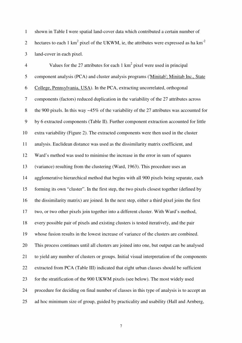
shown in Table I were spatial land-cover data which contributed a certain number of 1

hectares to each 1 km2 pixel of the UKWM, ie, the attributes were expressed as ha km

-2 2

land-cover in each pixel. 3

Values for the 27 attributes for each 1 km2 pixel were used in principal 4

component analysis (PCA) and cluster analysis programs ('Minitab'; Minitab Inc., State 5

College, Pennsylvania, USA). In the PCA, extracting uncorrelated, orthogonal 6

components (factors) reduced duplication in the variability of the 27 attributes across 7

the 900 pixels. In this way ~45% of the variability of the 27 attributes was accounted for 8

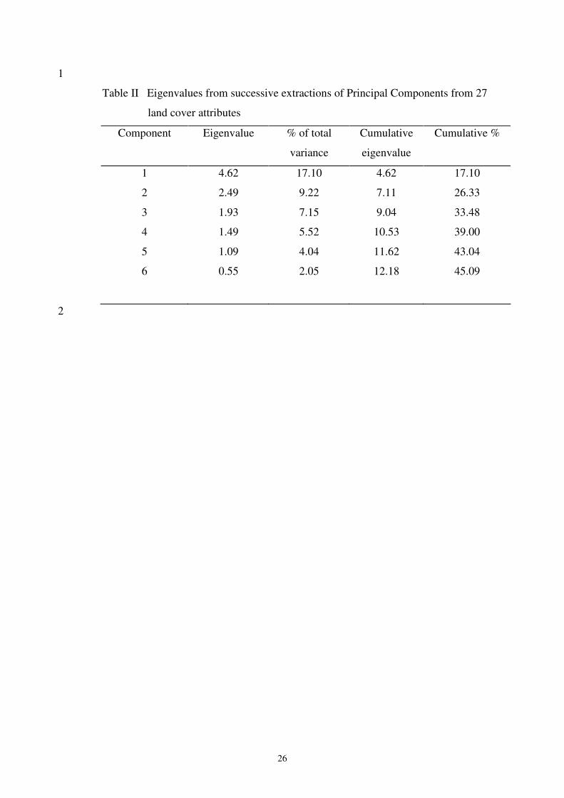
by 6 extracted components (Table II). Further component extraction accounted for little 9

extra variability (Figure 2). The extracted components were then used in the cluster 10

analysis. Euclidean distance was used as the dissimilarity matrix coefficient, and 11

Ward’s method was used to minimise the increase in the error in sum of squares 12

(variance) resulting from the clustering (Ward, 1963). This procedure uses an 13

agglomerative hierarchical method that begins with all 900 pixels being separate, each 14

forming its own “cluster”. In the first step, the two pixels closest together (defined by 15

the dissimilarity matrix) are joined. In the next step, either a third pixel joins the first 16

two, or two other pixels join together into a different cluster. With Ward’s method, 17

every possible pair of pixels and existing clusters is tested iteratively, and the pair 18

whose fusion results in the lowest increase of variance of the clusters are combined. 19

This process continues until all clusters are joined into one, but output can be analysed 20

to yield any number of clusters or groups. Initial visual interpretation of the components 21

extracted from PCA (Table III) indicated that eight urban classes should be sufficient 22

for the stratification of the 900 UKWM pixels (see below). The most widely used 23

procedure for deciding on final number of classes in this type of analysis is to accept an 24

ad hoc minimum size of group, guided by practicality and usability (Hall and Arnberg, 25

8

2002; Bunce et al., 1996b). The minimum and maximum number of squares in this 1

UKWM classification were 7 and 218, respectively. Classes with large numbers could 2

not be usefully subdivided, as they represented the extensive and homogenous farmland 3

and open light suburban areas of the region (section 3.1). Similar use of PCA and 4

cluster analyses have been reported by Huang et al. (2001) who classified energy flows 5

in an urban region, reducing dimensionality of their input datasets from 19 variables to 6

four factors. Cifaldi et al. (2004) performed PCA on two contrasting regions, one 7

agricultural and one urban, to examine spatial patterns in land cover. The reduced the 8

dimensionality of their data-sets of 25 variables to 5 extracted components which 9

accounted for a large proportion of the variability in their original data. 10

11

2.2 Validating the method of generating urban classes using principal component 12

and cluster analyses 13

The methodology was checked using different PCA and cluster analysis programs in 14

two further software packages, “Clustan” (Clustan Ltd., Edinburgh, Scotland) and 15

“Statistica” (Statsoft Inc., Tulsa, Oklahoma, USA). Clustan is a Fortran program 16

running on a UNIX operating system. “Statistica” is a package available for Windows 17

PC (StatSoft inc). Statistica was unable to run with the complete original 900-line 18

dataset; therefore a subset of 300 lines was taken from the data file by extracting the 19

first, then every third line of data. PCA and cluster analysis programs were run to 20

produce eight classes from the subset of data, using Minitab and Statistica, with 21

Euclidean distance and Ward’s linkage. Minitab software generated the classification 22

system directly, with eight classes and six components defined for the output. Statistica 23

output produced a cluster dendrogram, and an amalgamation schedule from which eight 24

classes were extracted. The data for the dendrogram indicated the linkage distance of 25

9

the clusters that would result in 8 classes. Because the default dissimilarity coefficient 1

for Clustan is squared Euclidean distance, a program was included in the Clustan syntax 2

to define Euclidean distance as the dissimilarity coefficient. After processing output 3

data, identical classifications were obtained using Minitab, Clustan and Statistica. 4

5

2.3 Analysis of uncertainty associated with the classification 6

All land cover data contributing to the analysis of a region the size of the UKWM is 7

likely to carry uncertainties, irrespective of its source. When integrating land cover data 8

to provide information at larger scales, more uncertainty is introduced as detail becomes 9

sacrificed to average. When applications demand ground-truthing, surveying or 10

sampling within a very large area, with view to extrapolating from the sampling domain 11

to the entire study domain, uncertainties can become very large indeed. With this in 12

mind, we undertook a rigorous analysis of uncertainty to make transparent the 13

unavoidable and inherent sources of error when using a stratified sampling system. 14

2.3.1 Calculating fuzzy membership of each urban land class for each pixel

15

The vector of attribute values for any particular pixel will have some degree of 16

similarity with all 8 urban class centroid properties, and therefore have some degree of 17

membership to each of the 8 urban classes. To estimate the degree of membership of 18

each pixel in each of the 8 urban classes, the Euclidean distance (dE) between the pixel 19

attribute vector, x, and that of each urban class mean (µc; Table IV) was calculated 20

using: 21

( ) ( )∑=

−=n

j

cjjcE xxd1

2, µµ …………………………………………………………..(1) 22

where dE(x,µc) is the “distance” between pixel x and the class centroid µc for class c, (xj-23

µcj) is the distance between pixel and class centroid for attribute j, and n = number of 24

10

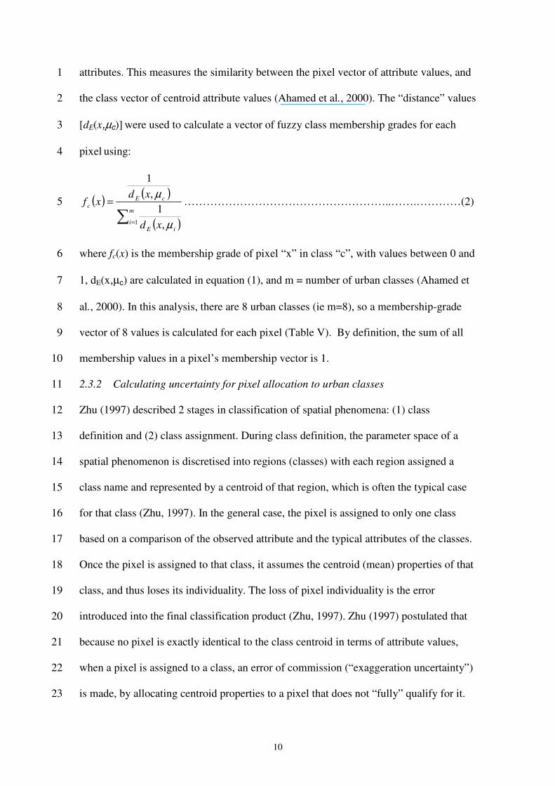
attributes. This measures the similarity between the pixel vector of attribute values, and 1

the class vector of centroid attribute values (Ahamed et al., 2000). The “distance” values 2

[dE(x,µc)] were used to calculate a vector of fuzzy class membership grades for each 3

pixel using: 4

( )( )

( )∑ =

=m

iiE

cE

c

xd

xdxf

1 ,

1

,

1

µ

µ………………………………………………..…….…………(2) 5

where fc(x) is the membership grade of pixel “x” in class “c”, with values between 0 and 6

1, dE(x,µc) are calculated in equation (1), and m = number of urban classes (Ahamed et 7

al., 2000). In this analysis, there are 8 urban classes (ie m=8), so a membership-grade 8

vector of 8 values is calculated for each pixel (Table V). By definition, the sum of all 9

membership values in a pixel’s membership vector is 1. 10

2.3.2 Calculating uncertainty for pixel allocation to urban classes 11

Zhu (1997) described 2 stages in classification of spatial phenomena: (1) class 12

definition and (2) class assignment. During class definition, the parameter space of a 13

spatial phenomenon is discretised into regions (classes) with each region assigned a 14

class name and represented by a centroid of that region, which is often the typical case 15

for that class (Zhu, 1997). In the general case, the pixel is assigned to only one class 16

based on a comparison of the observed attribute and the typical attributes of the classes. 17

Once the pixel is assigned to that class, it assumes the centroid (mean) properties of that 18

class, and thus loses its individuality. The loss of pixel individuality is the error 19

introduced into the final classification product (Zhu, 1997). Zhu (1997) postulated that 20

because no pixel is exactly identical to the class centroid in terms of attribute values, 21

when a pixel is assigned to a class, an error of commission (“exaggeration uncertainty”) 22

is made, by allocating centroid properties to a pixel that does not “fully” qualify for it. 23

11

Similarly, by allocating a pixel to a class, similarities between it and the other classes 1

are ignored, thus introducing an error of omission (“ignorance uncertainty”). 2

The classification method employed here does not pre-define class centroid properties, 3

but generates them in the process of agglomeration. The centroid properties are then 4

defined as the class means of the attributes, and the fuzzy membership functions 5

described above are based on this process-derived centroid definition for each of the 8 6

urban classes. 7

2.3.3 Exaggeration Uncertainties 8

Zhu (1997) describes exaggeration uncertainty as inversely related to the membership 9

saturation in the class to which an object is assigned. Here we define an exaggeration 10

uncertainty vector for a pixel’s possible assignation to each of the 8 urban classes. For 11

any pixel x, possible allocation to class c with centroid µc, carries an exaggeration 12

uncertainty which we define as: 13

[ ]( )

( )[ ]cE

cE

ccxd

xdxE

µ

µµ

,max

,, = ……………………...……..…….………………………(3) 14

where Ec [ ]cx µ, is a measure of exaggeration uncertainty with values ranging between 0 15

and 1, dE(x,µc) are calculated in equation (1) and max[dE(x,µc)] is the maximum value 16

of the distance dE(x,µc) from the centroid µc for pixels previously calculated to be in that 17

class. By calculating E for possible assignation to each of the 8 urban classes, a vector 18

of class exaggeration uncertainty values was generated for each pixel (Table VI). 19

2.3.4 Ignorance Uncertainties 20

The uncertainty associated with ignoring the similarities between a pixel and the classes 21

to which it was not allocated is related to the fuzziness of the pixel compared with the 22

definition of the class centroids (Zhu, 1997). The fuzzier a pixel’s relationship to the 23

classes, the more evenly distributed is the membership in the vector and the greater is 24

12

the ignorance uncertainty. Ignorance uncertainty can be defined in several ways, but a 1

method adopted by Zhu (1997) is based on the level of membership of a pixel in classes 2

to which it was not assigned. The sum of values in a pixel’s membership vector is 1 3

(section 2.3.1 and equation (2)), therefore we define a measure of ignorance uncertainty 4

( ) ( )xfxI c−= 1 ……………………………………………….……………………….(4) 5

where fc(x) is the membership value for the class to which a pixel x is assigned. Ι(x) was 6

calculated for each pixel, and the mean (Ic) and standard deviation calculated for each 7

class (Table VII). 8

9

3. RESULTS 10

3.1 The urban land classification 11

The distribution of Eigenvalues derived from the PCA is presented in Figure 2. 12

Eigenvalues represent the relative contribution of each component to total variation in 13

the data. Figure 2 shows clearly that most of the variation in the data was accounted for 14

by the first six components. The percentage of total variation explained by each 15

component is calculated as (eigenvalue x 100/number of attributes). Thus ~45% of the 16

variability was accounted for by successive extraction of the first six components (Table 17

II). Eigenvectors are sets of scores representing the weighting of each of the original 18

land-cover attributes on each extracted component (Table III). The Eigenvector scores 19

give information for the interpretation of the principal component analysis (Cifaldi et 20

al., 2004). The first component (or factor) describes a gradient between (a) built-up and 21

(b) non built-up areas; the second component distinguishes between (a) wooded areas 22

/heathland, and (b) farmed land; the third component, between (a) water/bare ground, 23

and (b) suburban built-up areas; the fourth component, between (a) urban built-up 24

areas/major transport corridors, and (b) suburban areas/minor transport corridors; the 25

13

fifth, between (a) wooded areas, and (b) heathland countryside; and the sixth between 1

(a) less dense built-up areas, and (b) major transport corridors (Table III). The extracted 2

components’ spectra of attribute weightings suggested, therefore, that eight classes 3

would be an optimum number of classes to specify in the output from the cluster 4

analysis, and that the classes would broadly reflect wooded areas, water, transport 5

corridors, urban built-up areas, different density suburban built-up areas, open land, and 6

farmland. Cluster analysis was then used to generate the classes, and class centroids 7

were found by calculating the mean hectare-age of each of the 25 land-cover attributes 8

in each urban class (Table IV). The distribution and brief interpretation of urban classes 9

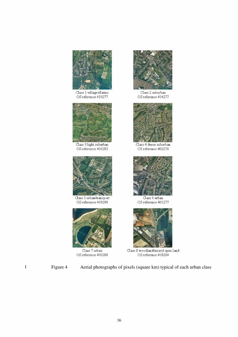
in the UKWM region is shown in the maps in Figure 3. The classes generated were 10

named subjectively according to their dominant centroid attributes (Figure 3; class 1 – 11

villages/farms; class 2 –suburban; class 3 – light suburban; class 4 – dense suburban; 12

class 5 – urban/transport; class 6 – urban; class 7 – light urban/open water; class 8 – 13

woodland/open land). Representative aerial view photographs of pixels representative of 14

each land class are shown in Figure 4 (Cities Revealed (R) photography © 1998 The 15

Geoinformation Group (R) Ltd). The interpretation of each class was confirmed by 16

visual inspection of OS maps (1:50000, nos. 139 and 140). 17

18

3.2 Fuzzy analysis of uncertainty of the urban land-cover classification 19

3.2.1 Fuzzy membership of each urban land class for each pixel

20

Mean membership grade vectors for each class are presented in Table V. Figures in bold 21

depict the mean membership value in the membership-grade vectors (fc) for the class to 22

which the member pixels are allocated. For example, the average membership value of 23

class 1 pixels for class 1 is 0.32±0.10, which is higher than the average membership 24

values of these pixels for the other classes (Table V). 25

3.2.2 Exageration uncertainties 26

14

Mean exaggeration uncertainties are presented in Table VI. The bold figures describe 1

the exaggeration uncertainty of allocating pixels to their own class, and the non-bold 2

figures describe the exaggeration uncertainty of allocating pixels to other classes. Thus, 3

for the pixel members of class 1, the mean exaggeration uncertainty associated with 4

assuming class 1 pixels possess the class 1 centroid properties is 0.20±0.11. 5

3.2.3 Ignorance Uncertainties 6

Table VII lists the ignorance uncertainties for each class. For example, the mean 7

uncertainty associated with lost information about an individual pixel allocated to class 8

1 is 0.68±0.10. This is lower than the mean exaggeration uncertainties associated with 9

allocating these pixels to any other class. 10

11

4. DISCUSSION 12

4.1 The classification system 13

The classification procedure reduced the number of input variables to the principal 14

component analysis from 25 land-cover types to 6 factors, resulting in 8 urban 15

morphology classes. The classification was robust in that different software packages 16

generated identical classifications based on the same input data. Mean class 17

characteristics were derived by interpreting the principal components (Table IV). While 18

the characteristics of most classes are distinct, there is at first glance a close similarity 19

between classes 5 and 6. However, the distinction between class 5 and 6 is real. Class 5 20

is characterised by high density of transport corridors in an urban, rather than suburban 21

or rural environment. Class 6 is high density urban with few transport corridors. This 22

type of distinction is important if we are considering eg communication, ecology 23

corridors for encouraging biodiversity, linear sources of anthropogenic pollutant gases, 24

tree planting, etc. 25

15

1

4.2 Fuzzy membership of each urban land class for each pixel

2

As described above, the vector of attribute values for any particular km2 “pixel” will 3

have some degree of similarity with all 8 urban class centroid properties, and therefore 4

have some degree of membership to each of the 8 urban classes. In theory, the largest 5

fuzzy class membership grade of the 8 urban classes for any individual pixel should 6

correspond to the urban class allocated to that pixel. In fact, there is a satisfactory 65% 7

correspondence for all pixels, between allocated class and largest value in the class 8

membership vector. The remaining 35% non-correspondence highlights the difference 9

between the original clustering process (in which the mean properties of the cluster 10

change as the cluster forms), and a post-hoc test using the final cluster-mean properties. 11

In joining a new pixel to a growing class, it is possible that the pixel that minimizes 12

overall variance at that point in the agglomerative clustering process is not necessarily 13

the pixel whose attribute values are nearest to the final class centroid. 14

Except for class 7, the highest membership value in the average membership-15

grade vectors (fc) is for the class to which the member pixels are allocated (Table V). 16

The membership values in the average vector for class 7 are all very similar, indicating 17

a very high degree of membership fuzziness for these pixels. These pixels were 18

clustered together in the analysis on the strength of the large area of inland water land-19

cover which these pixels share, but apart from inland water, their land-cover attribute 20

composition is similar to that of other classes. Figure 5A illustrates how a pixel can 21

have different degrees of membership in more than one class. 22

23

4.3 Exaggeration Uncertainties 24

16

Individual pixel exaggeration uncertainties associated with allocating each pixel to its 1

urban class ranged from 0.04 to 1.00. The fuzzy class vectors of the mean and standard 2

deviation of the exaggeration uncertainties for each class ranged from 0.11±0.05 to 3

0.50±0.13 (bold type, Table VI). Surprisingly, allocation of a mean class-5 pixel to its 4

own class carries slightly higher mean exaggeration uncertainty than allocating the pixel 5

to class 6 (0.30±0.15 cf 0.29±0.17). Similarly, allocating a mean class 7 pixel to its own 6

class carries exaggeration uncertainty (0.50±0.13) equivalent to the exaggeration 7

uncertainty associated with allocating this square to some of the other classes. The 8

values of the mean class exaggeration uncertainty vectors are a relative measure of how 9

much each pixel is different from the centroid of its allocated class compared with how 10

much the same pixel is different from the centroids of other classes (Figures 5A, 5B). 11

Assuming that a feature we wish to ascribe to a class (e.g. biogenic emission rates, see 12

below) varies linearly with dE, exaggeration uncertainty can be interpreted as the extra 13

false pixel information acquired as each pixel in a class assumes the identity of the class 14

centroid. This could be up to 50% (Table VI). Exaggeration uncertainties reflect the 15

complex nature and broad scope of land-cover within each class. 16

17

4.4 Ignorance Uncertainties 18

Individual mean class ignorance uncertainties range from 0.65±0.11 to 0.87±0.04 (Table 19

VII) and the overall average ignorance uncertainty is 0.73±0.11. As for the exaggeration 20

uncertainties, ignorance uncertainty values are not absolute measures of uncertainty, but 21

indicate the amount of information lost when classifying pixels using the agglomerative 22

cluster analysis methodology, and assigning each pixel to a single class (Figures 5A, 23

5B). Again, this assumes a linear relationship between some feature assigned to the 24

class and pixels’ dE values. Although the results of the uncertainty analysis appear to be 25

17

cause for concern, all comparable systems of stratification, whether in ecology, social 1

science or environmental studies, have comparable problems. The most important 2

feature to emerge from the analysis of uncertainty of the classification described here, is 3

that the allocation of pixels to classes is satisfactory for practical purposes, even for 4

those pixels with very fuzzy membership grade vectors. However, the cluster test with fc 5

(equation 2) broadly justifies the classes that have been formed using PCA and cluster 6

techniques, but indicates that categorical statements regarding class membership, class 7

behaviour and properties should be avoided. 8

9

4.5 Specific Applications 10

The classification can now be used as a structure for surveys and sampling, to answer 11

questions such as “What is the total tree cover in the UK metropolitan region and what 12

are the uncertainties associated with the estimates?”; “How much space is available for 13

future tree planting in the UKWM?”; “What is the effect of the present and possible 14

future tree populations on air quality in the UKWM?”. Given that the classification 15

methodology can be applied to other metropolitan areas where gridded data is available, 16

the same kind of questions may be addressed in metropolitan areas around the world. 17

The classification described here has already been used in a desk study to 18

estimate biogenic volatile organic compound (BVOC) emissions from the UKWM 19

conurbation (Owen et al., 2003). It has also been used in a field survey study to estimate 20

tree cover and tree biomass for the UKWM conurbation (Donovan, 2004), and in a 21

modelling study to investigate the effect of pollutant deposition and biogenic VOC 22

emissions on air quality in the UKWM (Donovan et al, 2005). In the field study 23

(Donovan, 2004), a survey of trees in the UKWM was undertaken by stratified 24

recording of all individual trees in sample plots in randomly selected 1 km2 pixels. A 25

18

total of 22 pixels were surveyed, the number of squares sampled for each of the eight 1

urban land-cover classes was proportional to the area occupied by each class in the 900 2

pixels comprising the UKWM. Data for each urban land-class pixel were extrapolated 3

to the total area of each of the classes in the UKWM to obtain an integrated estimate for 4

the tree population for the whole region based on the survey work, rather than on 5

previously published tree data (c.f. Owen et al., 2003). Because the sampling was 6

stratified, i.e. based upon the urban classification, there was compensation for the 7

relatively small percentage of the total region that it was possible to sample with the 8

available time and manpower. 9

10

4.6 Wider Applications 11

This type of urban land classification could facilitate first estimates of: 12

• overall land resources of an urban region. This would be useful for features 13

that are not recorded on a systematic basis by other agencies and that are not a 14

simple linear sum or difference of standard recorded features, e.g. area occupied 15

by transport corridors, commercial land suitable for tree planting. 16

• the distribution of land resources throughout urban classes. For example, 17

urban land class 5 is designated “urban/transport” here, and each UKWM pixel 18

which is classified as “urban/transport” has a mean of ~20 ha km-2

19

grassland/open land. This information could be of interest to planners, recreation 20

and amenity officers and conservation bodies, to conduct more detailed survey 21

of each pixel according to the application of interest (e.g. housing, creation of 22

playing fields, new woodland planting etc) and to identify, for example, those 23

“urban/transport” squares whose proportion of open space is detrimentally low. 24

19

• land-use potential. Survey work based on the classification can identify further 1

land-use attributes for sample survey pixels (for example, future tree planting 2

potential, derelict sites, sites suitable for recreational development etc.), which 3

can be extrapolated to the whole UKWM region. 4

• changes in the urban infrastructure. For example, removal of railway lines 5

from a pixel in class 5 (urban transport) will result in re-classification of that 6

square, bringing it into a class with less railway, but with other attributes similar 7

to class 5 (e.g. class 2; Table IV), and therefore subject to monitoring or policies 8

for the new class. Of course, when pixel re-classification exceeds some 9

threshold (e.g.10%), then the basis of the original classification becomes 10

obsolete and the region should be re-classified. The procedure described here 11

ensures that updating the classification is a straightforward and time-efficient 12

process. 13

• policy options. For example, the classification provides an estimate of the 14

spatial distribution of high-density transport corridors (i.e. class 5 squares). It is 15

therefore possible to make a first estimate of the concentration of associated 16

features and potential facilities (e.g. lighting, street tree planting, pollutant 17

emissions), and their costs, without resorting to detailed survey in the first 18

instance. 19

• assessment and costings for scaling-up policies. Classification of urban land-20

use for all major cities would assist planners and policy-makers in the task of 21

larger-scale assessments and costings. 22

These are examples of the wide range of potential applications for an urban land-cover 23

classification system, of interest and use to Local Authority planners, property 24

developers, environmental researchers, utility companies and policy makers. The 25

20

classification system described here is “robust enough”, and useful for stratified 1

sampling and extrapolation where time and resources are scarce. It is easy to apply to 2

other UK conurbations, and indeed to any region for which there exists a spatial dataset 3

consisting of attribute data to describe the component land-covers of each pixel. It is 4

also easy to reapply using updated datasets, to monitor land-use changes at pixel and 5

regional scales. 6

7

5. CONCLUSIONS 8

We generated a successful classification system for the UKWM region using land cover 9

data stored as a raster dataset with Ordnance Survey coordinates. Our approach is 10

supported by other workers who have also used PCA and cluster analyses to generate a 11

classification relevant to urban land-cover (e.g. Huang et al., 2001; Cifaldi et al., 2004). 12

We believe that this is the first time that an attempt to quantify uncertainties has 13

been presented alongside an agglomerative land-cover classification. The same analysis 14

of uncertainty could be applied to any application of PCA and clustering in landscape 15

science, with similar uncertainty results. In view of the process of agglomeration and 16

the associated errors, we expected a very large degree of uncertainty associated with the 17

classification and therefore the results of the uncertainty analyses were encouraging. 18

The methodology is statistically robust and reproducible and enables standard 19

errors to be estimated. By including a posteriori tests of the classification, its limits 20

become more clearly defined, and the tendency to make categorical statements based on 21

the classes is reduced. The statistical procedures used can vary according to the 22

availability of algorithms in PCA packages. Even though the decision about the number 23

of classes to allow the cluster analysis to generate is subjective, the principal feature of 24

our approach is the use of objective procedures to construct the classification, and to 25

21

facilitate subsequent estimation of environmental parameters. Similar data for the 1

generation of an urban land classification are available in most European countries so 2

that the approach could be adapted to many other situations. 3

4

ACKNOWLEDGEMENTS 5

We acknowledge the Natural Environment Research Council (NERC) for funding the 6

research as part of the NERC program “Urban Regeneration and the Environment 7

(URGENT)”. 8

9

REFERENCES 10

Ahamed, T.R.N., Rao, K.G. and Murthy, J.S.R., 2000. GIS-based fuzzy membership 11

model for crop- land suitability analysis. Agric. syst., 63(2), 75-95. 12

Barr, S. and Barnsley, M., 2000. Reducing structural clutter in land cover classifications 13

of high spatial resolution remotely-sensed images for urban land use mapping, Comput. 14

Geosci., 26(4), 433-449. 15

Bunce, R.G.H. and Smith, R.S., 1978. An ecological survey of Cumbria, Structure Plan 16

Working paper no 4. Cumbria County Council, Kendal. 17

Bunce, R.G.H. and Heal, O.W., 1984. Landscape evaluation and the impact of changing 18

land-use on the rural environment: the problem and an approach. In R.D. Roberts and 19

T.M.Roberts (Editors). Planning and Ecology. Chapman and Hall, London, pp 164-221. 20

Bunce, R.G.H., Barr, C.J., Clarke, R.T., Howard, D.C. and Lane, A.M.J., 1996a. ITE 21

Merlewood Land Classification of Great Britain. J. Biogeogr., 23(5), 625-634. 22

Bunce, R.G.H., Barr, C.J., Clarke, R.T., Howard, D.C., and Lane, A.M.J., 1996b. Land 23

classification for strategic ecological survey. J. Environ. Manage., 47, 37-60. 24

22

Cifaldi, R.L., Allan, J.D., Duh, J.D. and Brown, D.G., 2004. Spatial patterns in land 1

cover of exurbanizing watersheds in southeastern Michigan. Landscape and Urban 2

Planning. 66 (2), 107-123. 3

Coppock, J.T. and Gebbett, L.F., 1978. Land use and town and country planning: 4

Reviews of UK statistical sources 8. Pergamon Press, London. 5

DETR, 2000. Rural England: A Discussion Document. Our towns and cities: the future 6

– delivering an urban renaissance (Urban White Paper) Cm 4911, ISBN 0-10-14912-3. 7

Donovan R.G., 2004. The development of an urban tree air quality score and its 8

application in a case study. Ph.D. Thesis, Lancaster University. 9

Donovan, R.G., Stewart, H.E., Owen, S.M., MacKenzie, A.R. and Hewitt, C.N. 10

Development and application of an Urban Tree Air Quality Score (UTAQS) for 11

photochemical pollution episodes using the Birmingham UK area as a case study. 12

Environ. Sci. Technol. In press. 13

FAO (2000) Land Cover Classification System (LCCS) 14

http://www.fao.org/documents/show_cdr.asp?url_file=/DOCREP/003/X0596E/X0596e15

00.htm last accessed April 5th 2005 16

FAOSTAT, 2004 http://faostat.fao.org/faostat/ last accessed April 5th

2005. 17

Fuller, R.M., Groom, G.B., and Jones, A.R., 1994. The Land Cover Map of Great 18

Britain: an automated classification of Landsat Thematic Mapper data. Photogramm. 19

Eng. Remote Sensing, 60, 553-562. 20

Hall, O. and Arnberg, W., 2002. A method for landscape regionalization based on fuzzy 21

membership signatures. Landscape and Urban Planning, 59(4), 227-240. 22

Hepner, G.F., Houshmand, B., Kulikov, I. and Bryant, N., 1998. Investigation of the 23

integration of AVIRIS and IFSAR for urban analysis. Photogramm. Eng. Remote 24

Sensing, 64(8), 813-820. 25

23

Huang, S.L., Lai, H.Y., Lee, C.L., 2001.Energy hierarchy and urban landscape system. 1

Landscape and Urban Planning, 53(1-4), 145-161. 2

Karathanassi, V., Iossifidis, C., and Rokos, D., 2000. A texture-based classification 3

method for classifying built areas according to their density. Int. J. Remote Sens., 21(9), 4

1807-1823. 5

Kaur, A., Patil, G.P., Shirk, S.J., and Taillie, C., 1996 Environmental sampling with a 6

concomitant variable, A comparison between ranked set sampling and stratified simple 7

random sampling. J. Appl. Stat. 23 (2-3), 231-255. 8

Lo, C.P. and Choi, J. 2004. A hybrid approach to urban land use/cover mapping using 9

Landsat 7 Enhanced Thematic Mapper Plus (ETM+) images. Int. J. Remote Sens., 10

25(14), 2687-2700. 11

Lofvenhaft, K., Bjorn, C., Ihse, M. 2002. Biotope patterns in urban areas: a conceptual 12

model integrating biodiversity issues in spatial planning. Landscape and Urban Planning 13

58(2-4), 223-240. 14

Owen, S.M., MacKenzie, A.R., Stewart, H.E., Donovan, R. and Hewitt, C.N., 2003. 15

Biogenic volatile organic compound (VOC) flux estimates from a Metropolitan region: 16

the UK West Midlands urban tree canopy as a case study. Ecol. Appl., 13(4), 927-938. 17

Seymour, S., 2001. Rural Sustainability and Countryside Change. In DEFRA, Drivers 18

of Countryside Change – Final Report, 2001. 19

Stamp, L. D., 1947. The land of Britain: The final report of the Land Utilisation Survey 20

of Britain. London Geographical Publications. 21

Ward, J.H. Jr., 1963. Hierarchical grouping to optimize an objective function. J. Am. 22

Stat. Assoc., 58, 236-244. 23

24

Wyatt, B.K., Greatorex-Davies, N.G., Bunce, R.G.H., Fuller, R.M. and Hill, M.O., 1

1994. Comparison of land cover definitions. Countryside 1990 Series: Volume 3 2

London Department of the Environment. 3

Xiao, Q., Ustin, S.L., McPherson, E.G., 2004; Using AVIRIS data and multiple-4

masking techniques to map urban forest tree species. Int. J. Remote Sens., 25 (24), 5

5637-5654. 6

Zhang, J. and Foody, G.M., 1998. A fuzzy classification of sub-urban land cover from 7

remotely sensed imagery. Int. J. Remote Sens., 19(14), 2721-2738. 8

Zhu, A.X., 1997. Measuring uncertainty in class assignment for natural resource maps 9

under fuzzy logic. Photogramm. Eng. Remote Sensing, 63(10), 1195-1202. 10

11

25

1

Table I Attributes used in the principal component analysis to generate eight urban 2

classes 3

From ITE land cover database: From OS data:

urban OS A roads

suburban OS B roads

tilled land OS towns

managed grassland OS villages

rough grassland OS canals

bracken OS minor roads

heath grassland OS motorway

open heathland OS open countryside

dense heathland OS railway

coniferous woodland OS rivers

inland bare ground OS inland waters

inland water OS woodland

deciduous woodland

slope CIS Axis 1*

* First axis scores (upland/lowland weighting) of the principal

component analysis used to generate the CIS land classes.

4

26

1

Table II Eigenvalues from successive extractions of Principal Components from 27

land cover attributes

Component Eigenvalue % of total

variance

Cumulative

eigenvalue

Cumulative %

1 4.62 17.10 4.62 17.10

2 2.49 9.22 7.11 26.33

3 1.93 7.15 9.04 33.48

4 1.49 5.52 10.53 39.00

5 1.09 4.04 11.62 43.04

6 0.55 2.05 12.18 45.09

2

27

Table III Eigenvector scores for each of the urban land-cover attributes 1

Component (factor)1

1 2 3 4 5 6

Slope -0.001 0.064 0.058 -0.05 -0.079 -0.473

Bracken 0.04 0.084 0.05 -0.002 0.324 -0.212

Inland bare -0.001 -0.088 -0.181 0.165 -0.045 -0.153

OS2 village 0.05 -0.047 0.007 0.023 -0.048 -0.123

Urban -0.125 -0.02 -0.189 0.212 0.09 -0.119

OS2 canals -0.047 -0.038 -0.113 0.176 0.14 -0.078

OS2 open country 0.187 -0.094 -0.026 0.071 0.034 -0.049

OS2 B road -0.044 0.053 0.041 -0.015 -0.02 -0.046

Heath grass 0.106 0.166 0.102 -0.04 0.31 -0.045

OS2 A road -0.086 -0.017 -0.083 0.155 0.111 -0.032

Deciduous wood 0.077 0.279 -0.039 0.072 -0.03 -0.017

Managed grass 0.163 -0.091 0.053 -0.012 0.048 -0.009

Rough grass 0.038 -0.003 0.029 0.033 0.226 0.016

Inland water 0.02 0.023 -0.374 -0.324 0.06 0.017

OS2 inland water 0.018 0.027 -0.37 -0.328 0.06 0.018

OS2 rail -0.064 0.026 -0.141 0.177 0.175 0.02

Tilled land 0.12 -0.165 -0.029 0.048 -0.12 0.022

Dense heath 0.054 0.24 -0.063 0.074 -0.083 0.04

OS2 minor road 0.059 -0.061 0.102 -0.18 -0.146 0.043

OS2 towns -0.189 0.079 0.066 -0.074 -0.013 0.048

Open heath 0.042 0.237 0.074 -0.044 0.17 0.069

OS2 wood 0.052 0.184 -0.105 0.16 -0.305 0.07

Coniferous wood 0.043 0.128 -0.114 0.149 -0.317 0.07

Suburban -0.155 0.058 0.157 -0.172 -0.076 0.093

OS2 motorway 0.004 -0.03 -0.073 0.146 0.162 0.228

OS2 rivers 0.052 -0.018 0.012 0.064 0.131 0.316

CIS axis13 -0.005 -0.013 0.003 0.016 0.041 0.549

1component 1=built-up (-ve scores) vs non-built up (+ve scores); 2=farmed land (-ve scores) vs wooded 2

and heathland (+ve scores); 3=urban built-up, water and wooded areas (-ve scores) vs suburban built-up 3 (+ve scores); 4=suburban built-up and water (-ve scores) vs major transport, built-up urban and wooded 4 areas (+ve scores); 5=wooded areas and farmland (-ve scores) vs heathland countryside and transport 5 corridors (+ve scores); 6=less dense built-up (-ve scores) vs major transport corridors (+ve scores). Bold 6 type indicates high scores contributing to interpreting components;

2OS Ordnance Survey data; other 7

attributes from ITE database (see text); 3

First axis scores (upland/lowland weighting) of the principal 8 component analysis used to generate the CIS land classes. 9

28

1

Table IV Mean cover (ha km-2

) of 25 attributes in each of eight urban classes*

Class 1 2 3 4 5 6 7 8

total pixels 216 218 37 155 71 183 13 7

CIS land cover (LC) attributes

urban 2.6±5.4 5.7±6.6 3.6±5.0 6.3±6.7 39.6±22.7 27.6±15.0 8.8±8.6 3.7±8.1

suburban 15.5±10.6 50.5±12.4 32.7±12.3 71.1±10.3 38.1±11.5 51.2±11.0 33.2±22.0 7.2±5.8

tilled 30.2±16.2 14.4±8.8 9.9±5.9 9.3±5.0 10.1±6.4 9.7±5.2 19.8±13.2 10.8±14.9

managed grassland 41.4±18.3 19.5±11.6 23.5±13.4 9.8±6.3 8.2±12.1 7.0±6.2 19.0±13.0 15.5±15.0

rough grassland 0.1±0.3 0.02±0.08 0.4±1.0 0.01±0.06 0.03±0.11 0.01±0.09 0.01±0.04 0.1±0.1

bracken 0.01±0.03 0.00±0.02 0.1±0.3 0.00±0.00 0.00±0.00 0.00±0.01 0.01±0.04 0.04±0.09

heath grassland 2.6±2.3 2.1±1.8 7.7±6.9 0.8±0.8 0.4±0.7 0.5±0.7 1.1±1.8 5.0±5.1

open heath 1.2±1.2 2.1±2.3 7.2±5.2 0.9±1.1 0.5±0.8 0.7±0.7 1.2±2.2 6.0±5.0

dense heath 0.2±0.6 0.2±0.4 0.9±1.1 0.05±0.3 0.02±0.08 0.03±0.1 0.2±0.5 7.1±7.6

coniferous wood 0.1±0.3 0.1±0.2 0.1±0.2 0.02±0.1 0.04±0.2 0.01±0.04 0.1±-.3 4.6±4.1

inland bare ground 1.4±2.4 0.9±1.1 0.4±0.6 0.4±0.5 1.8±1.5 1.2±1.2 1.8±2.0 1.2±2.6

inland water 0.1±0.4 0.1±0.6 0.2±0.6 0.01±0.1 0.2±0.5 0.05±0.2 10.2±14.2 0.9±1.5

deciduous wood 4.3±4.9 4.3±4.5 13.0±8.6 1.3±1.6 1.1±1.7 2.0±3.0 4.2±7.2 37.9±22.3

OS attributes

A roads 0.5±1.0 0.8±1.1 0.8±1.0 0.9±1.1 2.9±2.2 2.1±1.7 1.0±1.6 0.1±0.2

B roads 0.2±0.4 0.3±0.7 0.5±0.7 0.6±0.9 0.4±0.6 0.5±0.7 0.4±0.7 0.6±0.6

towns 6.4±13.8 65.0±22.9 48.5±31.3 90.6±9.3 73.4±26.5 87.3±14.3 41.0±37.1 6.4±11.8

villages 3.8±9.7 0.1±1.0 0.00±0.00 0.00±0.02 0.04±0.3 0.00±0.00 0.00±0.00 1.7±4.6

canals 0.2±0.4 0.1±0.3 0.1±0.2 0.1±0.2 0.8±0.6 0.4±0.5 0.2±0.4 0.00±0.00

minor roads 1.0±0.8 0.9±0.8 0.6±0.6 1.0±0.8 0.2±0.3 0.5±0.6 0.9±0.9 0.4±0.4

motorways 0.3±1.0 0.1±0.5 0.1±0.7 0.1±0.5 1.8±2.2 0.2±0.8 0.3±0.9 0.00±0.00

open countryside 86.4±16.1 32.0±22.5 48.4±31.1 6.7±9.0 19.5±26.2 8.6±14.1 41.0±33.8 58.9±17.1

railways 0.1±0.3 0.1±0.3 0.3±0.4 0.1±0.2 0.9±0.7 0.5±0.5 0.2±0.5 0.2±0.3

rivers 0.4±0.5 0.3±0.5 0.4±0.5 0.2±0.4 0.5±0.6 0.2±0.4 0.5±0.5 0.3±0.4

inland waters 0.02±0.2 0.2±1.1 0.2±1.0 0.01±0.1 0.1±0.3 0.00±0.00 14.5±17.4 1.2±1.9

woodland 0.7±3.4 0.00±0.02 0.3±1.6 0.03±0.4 0.00±0.00 0.00±0.00 0.4±1.5 30.5±18.8

*attributes slope and CIS axis1 did not contribute to “land cover” (see text) 2

29

Table V Mean class membership vectors

Allocated to class:-

1 2 3 4 5 6 7 8

Mean membership fc(x)

of class:-

1 0.32±0.10 0.09±0.02 0.12±0.03 0.07±0.02 0.08±0.02 0.07±0.02 0.12±0.02 0.12±0.02

2 0.07±0.05 0.20±0.09 0.14±0.06 0.16±0.10 0.11±0.02 0.13±0.06 0.13±0.04 0.06±0.02

3 0.12±0.09 0.14±0.04 0.19±0.08 0.10±0.06 0.10±0.02 0.10±0.05 0.14±0.03 0.09±0.04

4 0.04±0.01 0.14±0.06 0.08±0.02 0.35±0.11 0.10±0.02 0.17±0.05 0.08±0.01 0.04±0.01

5 0.08±0.06 0.13±0.04 0.11±0.04 0.12±0.03 0.19±0.06 0.19±0.08 0.11±0.04 0.07±0.02

6 0.05±0.02 0.13±0.05 0.08±0.03 0.19±0.10 0.17±0.05 0.26±0.09 0.08±0.03 0.05±0.01

7 0.15±0.11 0.14±0.07 0.12±0.03 0.13±0.11 0.11±0.04 0.13±0.07 0.13±0.04 0.10±0.05

8 0.15±0.05 0.10±0.01 0.13±0.01 0.07±0.01 0.09±0.01 0.08±0.01 0.13±0.01 0.25±0.04

30

1

Table VI Mean class exaggeration uncertainties

Allocated to class:-

1 2 3 4 5 6 7 8

Member of class:-

1 0.20±0.11 0.78±0.16 0.62±0.14 0.84±0.13 0.81±0.14 0.83±0.14 0.64±0.13 0.48±0.07

2 0.58±0.19 0.28±0.14 0.39±0.16 0.31±0.17 0.38±0.10 0.32±0.15 0.42±0.15 0.64±0.14

3 0.46±0.22 0.43±0.20 0.36±0.20 0.50±0.22 0.50±0.17 0.48±0.21 0.45±0.17 0.52±0.16

4 0.83±0.09 0.37±0.10 0.62±0.11 0.11±0.05 0.38±0.07 0.22±0.05 0.65±0.11 0.86±0.08

5 0.71±0.23 0.48±0.17 0.58±0.20 0.40±0.14 0.30±0.15 0.29±0.17 0.59±0.19 0.74±0.17

6 0.80±0.12 0.39±0.12 0.59±0.13 0.23±0.11 0.26±0.07 0.16±0.09 0.61±0.13 0.81±0.10

7 0.51±0.25 0.52±0.25 0.54±0.14 0.51±0.30 0.53±0.23 0.50±0.29 0.50±0.13 0.59±0.18

8 0.45±0.15 0.80±0.11 0.63±0.11 0.81±0.08 0.78±0.09 0.79±0.08 0.68±0.12 0.27±0.05

31

Table VII Mean Class Ignorance uncertainties (Ic) 1

class

1 0.68±0.10

2 0.80±0.09

3 0.81±0.08

4 0.65±0.11

5 0.81±0.06

6 0.74±0.09

7 0.87±0.04

8 0.75±0.04

32

Figure 1 Schematic presentation of urban land classification methodology 1

2

Figure 2 Results of extracting principal components from 27 urban land-cover 3

attributes. Columns represent the relative contribution of each 4

component to total variation in the land cover data (Eigenvalue) 5

6

Figure 3 Distribution of urban land classes in the West Midlands 7

8

Figure 4 Aerial photographs of pixels (square km) typical of each urban class 9

10

Figure 5A Allocating urban class membership to a pixel 11

Figure 5B Exaggeration and Ignorance uncertainties in terms of centroid and pixel 12

attributes 13

33

1

EXPLORATION OF DATASET

PRINCIPAL COMPONENT ANALYSIS (PCA)

• Extracting “best fit” components from the attribute values

for each pixel.

• Confirms that the data are classifiable

• Indicates possible class characteristics

900 squares (pixels),

each 1 km x 1 km.

Pixels are described

in terms of a total

of 27 attributes Att 4

Att1 Att 3

Att 2

RAW DATA

GENERATING 8 URBAN LAND-COVER CLASSES

CLUSTER ANALYSES

Extracted components for each pixel are used to cluster the 900

pixels into 8 “urban land-cover classes”

VALIDATING CLASSIFICATION

• Visual inspection to compare features of OS map

squares with their class centroid values.

• Estimating the amount of variability accounted for in the

extracted components in PCA.

• Exaggeration and Ignorance uncertainty estimates

CHARACTERISING CLASSES

Calculate “centroid” (mean) values of 25 land-cover

attributes for all pixels contributing to each class

For UK West Midlands

Figure 1 Schematic presentation of urban land classification methodology

34

1

2

3

4

5

6

7

8

9

10

11

0.0

0.5

1.0

1.5

2.0

2.5

3.0

3.5

4.0

4.5

5.0

1 2 3 4 5 6 7 8 9 10 11 12 13 14 15

Component (axis)

Eig

enval

ue

Figure 2 Results of extracting principal components from 27 urban land-cover

attributes. Columns represent the relative contribution of each component to

total variation in the land cover data (Eigenvalue)

35

1

2

3

4

5

6

7

8

9

10

11

12

13

14

15

16

17

18

19

20

21

22

23

24

25

Class 1 villages/farms Class 2 suburban

Class 3 light suburban Class 4 dense suburban

Class 5 urban/transport Class 6 urban

Class 7 light urban/open water Class 8 woodland/open land

Figure 3 Distribution of urban land classes in the West Midlands

36

1 Figure 4 Aerial photographs of pixels (square km) typical of each urban class

37

1

2

3

4

5

6

7

8

9

10

11

12

13

14

15

16

17

18

19

20

21

22

23

24

25

26

27

28

29

30

31

32

33

34

35

36

37

38

39

40

Figure 5A Allocating urban class membership to a pixel. pixels; class centroids.

Pixel X has attribute values that are close to those of the centroids of class 1 (µ1)

and class 2 (µ2). During the process of clustering, it is likely that the pixel will be

allocated to class 2, whose centroid is “closer” to the pixel. However, pixel X

may be allocated to class 1 if, early in the clustering process, it is linked with

nearby pixels which form a cluster which is nearer to µ1, than to µ2 (small cluster

delineated within dashed line). All pixels have some degree of membership in

each of the generated urban classes. Generally, a pixel is allocated to the class

whose centroid is closest. After allocating to a class, the pixel assumes the

characteristics of the class centroid. This results in an exaggeration uncertainty

due to false pixel information acquired (solid arrows), and an ignorance

uncertainty due to loss of individual pixel information (dashed arrows). Further

explanation of these uncertainties is illustrated in Figure 5B below.

µ1

A1

B1

C1

D1

E1

F1

G1

µ2

A2

B2

C2

D2

E2

F2

G2

X

A1

B1

c

d

E2

F2

G2

Figure 5B Exaggeration and Ignorance uncertainties in terms of centroid and pixel

attributes. A – G represent different attributes for class 1 and class 2 centroids

(µ1 and µ2, respectively), and pixel X. Pixel X has similar values to µ1 for

attributes A and B, and similar values to µ2 for attributes E, F and G.

Exaggeration uncertainties associated with allocating pixel X to classes 1 and

2, respectively, are represented by the attribute values enclosed in the solid line

boxes. Ignorance uncertainties associated with allocating pixel X to classes 1

and 2, respectively, are represented by the pixel X attribute values enclosed in

the dashed line box (for class 1 allocation ) and in the dot-dash line box (for

class 2 allocation).

Class 1 Class 2

µ1

µ2 X

38

Author biographies: 1

Susan (Sue) M. Owen is interested in the effects of environmental stress and land-use 2

change on trace gas emissions from man-made and natural vegetation canopies. With 3

several publications on emissions from Mediterranean and urban ecosystems, she 4

completed a NERC Research Fellow at Lancaster University, UK studying emissions 5

from tropical habitats. She is now working at CREAF, University Autonoma de 6

Barcelona, to investigate the effects of biotic and abiotic stresses on isoprenoid 7

emissions from urban and natural vegetation. Robert (Bob) G.H. Bunce is a “retired” 8

senior scientist (CEH Merlewood). A major contributor to the CEH land classification 9

and Countryside Information System, he is now engaged in a large European land 10

classification program based in the Netherlands. Hope E. Stewart was a post-doctoral 11

researcher at Lancaster, and is now an Atmospheric Scientist with the UK Environment 12

Agency. R. Donovan was a NERC-funded PhD student at Lancaster, studying the effect 13

of urban trees on air quality, and is now a Research Fellow at Birmingham University 14

studying the benefit of greening cities. R.A. MacKenzie is a senior lecturer in 15

atmospheric chemistry studying stratospheric processes, and C.N. Hewitt is Professor of 16

atmospheric chemistry at Lancaster University investigating a wide range of biosphere-17

atmosphere interactions. 18

19

39

1

2

3

4

5