Urban configuration, accessibility and property prices - HKU ...

1

Urban configuration, accessibility and property prices: a case study of Cardiff, Wales

Yang Xiaoa, Scott Orfordb*, Chris Websterc

a: College of Architecture and Urban Planning, Tongji University,1239 Siping Road, Shanghai, 200092, China b: School of City and Regional Planning, Cardiff University, Glamorgan Building,King Edward VII Avenue, Cardiff, Wales, CF10 3WA c: Faculty of Architecture, The University of Hong Kong, 4/F, Knowles Building, Pokfulam Road, Hong Kong

* Corresponding author: Dr. Scott Orford, [email protected],02920875272.

2

Abstract

The specification of locational attributes in hedonic house price models has traditionally been

problematic. Whilst many studies use similar sets of structural attributes the range of locational

attributes can be diverse and inconsistent both in their identification and in their measurement. To

address this problem, studies have adopted concepts relating to urban configuration such as the

monocentric city and the access‐space trade‐off model, and later multi‐centric and multiple

accessibility models, to structure their enquiry. This has lead to issues relating to a priori variable

specification using geometrically defined accessibility measures that can also lead to problems such

as spatial auto‐correlation. In this research, we investigate the use of network accessibility metrics in

hedonic house price research using Cardiff, Wales as a case study. We hypothesize that a network

modelling approach to measuring accessibility will improve performance compared to conventional

geometrical specifications. We find that estimating centrality variables across a variety of spatial

scales allows the impact on property prices of urban configuration to be more accurately modelled.

The research shows that not all dimensions of accessibility can be adequately captured by network

measures and that conventional geometric measures of accessibility can add additional explanatory

power in certain circumstances. The research also demonstrates the importance of modelling urban

configuration at the individual property level to prevent the loss of information when using

aggregated data.

Keywords: network analysis, space syntax, locational externalities, urban configuration,

accessibility, hedonic house price models

3

1. Introduction

Neo‐classical micro‐economic theory (Alonso, 1964), which developed classical Ricardian value

theory, emphasises the ‘access‐space’ trade‐off as a fundamental urban law. In this tradition, at

equilibrium, land‐users are indifferent to location because higher transport costs balance lower land

costs in less accessible parts of the city. This insight has fed through into housing research, with the

understanding that land and accessibility are substitute hedonic factors in determining house prices

( (McDonald, 1987, Richardson et al., 1990, Heikkila et al., 1989, Waddell et al., 1993, Orford, 2000,

Orford, 2002).

The specification of locational attributes in hedonic house price models has traditionally been

problematic as, unlike structural attributes (Follain and Jimenez, 1985, Sirmans et al., 2005), their

effects on property prices are less tangible and less understood. They are difficult to conceptualise

and measure; they can operate at various spatial scales; and they are influenced by many inter‐

related external factors (Orford, 2002). As a result, whilst many hedonic house price studies use

similar sets of structural attributes, the range of locational attributes can be diverse and inconsistent

both in their identification and in their measurement. To address this problem, studies have adopted

concepts relating to urban configuration to structure their enquiry. In early studies, accessibility to

the CBD was typically the major determinant of location‐specific land values and site rents in this

class of model. These early studies are considered seminal in urban theory but have given way to

more nuanced studies that better capture the multi‐centric and network geometry and topology of

urban configuration and locational advantage (McDonald, 1987). A variety of accessibility measuring

devices has been adopted more recently to capture the locational externality effect more sensitively

than the purely Euclidean distance (Niedercorn and Ammari, 1987, Hoch and Waddell, 1993).

Specific approaches include studies specifying accessibility indexed by travel time(Landau et al.,

1981), job accessibility (Osland and Thorsen, 2008), railway infrastructure improvement (Debrezion

et al., 2011), and systemic street network connectivity (Matthews and Turnbull, 2007, Enström and

Netzell, 2008).

One characteristic of studies that measure accessibility to specific points of benefits and disbenfits is

that the specific configuration of the study area is used to help frame and design the model

specification. The locational externalities hypothesized to be influential are identified and their

functional relationships with property prices (such as their distance decay) are specified a priori. In a

multi‐centric conceptualisation of urban configuration, this requires multiple variables capturing

each externality effect and this can cause problems of multi‐collinearity if the variables are

correlated across space leading to violation of the model’s assumptions; for instance, if multiple

4

distance measures are used to capture externality effects. Moreover, the exact nature of urban

configuration in relation to the housing market and its impact on property process is often not know

a priori and hence it is often impossible to theorize which of the many possible locational

externalities are important and how they should be specified. Even if it is possible to specify a priori

the likely specific locational influences on house prices, the researcher must make an arbitrary

decision about which ones to measure.

In this paper we take an approach to resolving these issues by exploring the intuitive hypothesis that

important information about urban configuration is contained in the urban street network and can

be captured from accessibility metrics measured from a topological network model of the street

layout. Most hedonic models fail to take note of essential spatial information in the street layout:

network connectivity, network distance, angular distance and so on, which in turn, have been shown

to have a strong influence on pedestrian behaviour, congestion and other influences on property

price (Porta et al., 2006a, Porta et al., 2009, Porta et al., 2012, Chiaradia et al., 2012). One way of

looking at this is that street network connectivity metrics are a proxy for the multiple dimensions of

human interactions that produce value in a city. They measure general accessibility rather than

specific accessibility and may be supposed to be more powerful predictors of locational valuations as

a result (Webster, 2010).

We test this hypothesis using the Welsh capital city of Cardiff as the study area. A sub‐set of the

Cardiff street network is modelled using space syntax methodology and various measurements of

network accessibility are taken from the model to form locational variables in a hedonic model of

house prices, which is used to test the following hypotheses:

1. Accessibility metrics derived from a topological network model improves hedonic model

performance compared to conventional geometrical measures of accessibility, in respect of:

a. Measures of explanatory power

b. A reduction in multicollinearity, heteroscedasticity and spatial autocorrelation

c. Improved accessibility coefficient estimates in terms of reducing counter‐intuitive

sign and statistical insignificance

2. Accessibility metrics derived from a topological network model better capture the

complexity of the access‐space trade‐off model of property prices compared to conventional

geometrical measures in respect of multi‐scaled, multi‐centric urban areas

5

The paper is divided into five sections. In section two we provide a brief review of previously

published work relating to the specification and measurement of accessibility in hedonic research.

The case study area, data, methods of constructing accessibility measures and the hedonic model

specification are presented in section three. Results are presented in section four, where we estimate

three models using individual property level data. Section five summarizes the findings and

concludes with a discussion of network approaches to modelling urban configuration in hedonic

house prices models compared to more conventional geometrical approaches.

2. Accessibility measures in hedonic research

Conventional geometric measures

In access‐space trade‐off models, transportation costs are traded off against land rents.

Improvements in transportation infrastructure are assumed to reduce commuting costs, releasing

more from a household budget to spend on land rent (Alonso, 1964, Muth, 1969, Mills, 1972).

However, Alonso’s (1964) monocentric model is clearly one pertaining to a particular historical phase

in a city’s evolution and does not adequately capture accessibility value where workplaces are not

solely located in the city center (McDonald, 1987), or where trips to work form a declining share of

overall household travel. The multi‐centric nature of many housing‐market areas makes one‐

dimensional separation measures like physical distance and travel time from a distinctly defined

center problematic. The presence of multiple‐worker households and multiple workplaces motivated

the search for alternative separation measures. Heikkila et al (1989) found distance to the CBD to be

insignificant, with the estimated coefficient having a counter‐intuitive positive sign in a property

price hedonic model of Los Angeles in 1980. They concluded that the impact of workplace

accessibility has been overemphasized. Richardson et al. (1990) note that the effect of distance to

the CBD may have declined, findings that the distance coefficient for Los Angeles CBD was significant

and negative in a dataset from 1970. Waddell et al. (1993) emphasized the importance of including

distance to secondary employment centres, and found both a strong and significant asymmetric CBD‐

gradient and strong local effects from non‐CBD employment centres. Orford (2002) specified a

multilevel hedonic model to evaluate locational externalities, examining a range of locational effects

on property prices. In terms of property‐level externalities, the research used distance to the CBD,

motorway exits, railway stations, shopping centres, and suburban employment centres. It also

considered proximity to non‐residential land uses such as parks, schools, industry, commercial, local

shops, recreational centres and cultural and educational centres. The results showed a complex

6

geography of locational externality effects, with areas of positive and negative externalities in

juxtaposition across highly localised areas.

Researchers have experimented with a wide variety of alternative measures. On approach has been

to measure transport costs more accurately (the traditional distance to CBD measure is a simple

approximation of travel cost). Gibbons and Machin (2005) explored the effects on property prices of

a transport innovation for households in London in the late 20th century. They defined rail access in

two ways: distance to a station and service frequency at the nearest station. Distance changes

induced by the transport innovation were associated with price changes and the price effect was

large compared to the monetary valuation of other local amenities. Adair et al. (2000) examined the

relationship of housing price and accessibility in Belfast urban area, adopting a gravity model and

calculating an accessibility index for locations to various opportunities by different types of vehicle.

The measure was a weak but significant predictor of house prices. Osland and Thorsen (2008),

utilized a hedonic model to confirm that gravity‐based labour‐market accessibility contributes to

property prices. Significantly, they found that labour‐market accessibility is not an adequate

alternative to distance from the CBD. Woo and Webster (2013) examined the trade‐off between

publicly provided and privately provided civic goods in determining condominium prices in Seoul,

testing the hypothesis that the club‐goods within condominium developments are a substitute for

open access public goods and therefore a substitute for centrality as conventionally modelled. They

found strong evidence of a substitution effect for some types of goods, including local green space

and concluded that a ‘city of residential clubs’ has significantly different locational dynamics

compared to the conventional city in which public goods are supplied by the state.

Matthews and Turnbull (2007) examined how street layout affects property value using network

centrality derived from a network analysis of east and west Washington. They found network

centrality measured within a 1400 feet walking distance radius to be significantly correlated with

house price in both west and east samples, but the coefficient signs were opposite in the two

samples. They concluded that the portion of house value contributed by street layout critically

depends upon the context of the surrounding development pattern. Enström and Netzell (2008)

examined urban street layout impact on commercial office rents in Stockholm and found that it had a

positive impact on office rent. Empirical evidence of the association between property prices and

street network connectivity are limited; hence the focus of our paper, which attempts to take this

tradition of spatial analysis of housing markets a step further.

7

Network measures of accessibility

Stewart (1947) firstly used the concept of graph theory defining gravitational potential as the

weighted sum of forces. Hansen (1959) started with a graph theory view of the spatial system,

identifying accessibility as a key element in spatial interaction; while Haggett and Chorley (1969)

established a centrality analysis approach to analysing spatial relationships.

Recently, Batty (2009) summarized three mainly types of accessibility in mainstream urban

scholarship. First concerns potential `opportunities' (Hanson 1959, Osland and Thorsen 2008),

measuring the size of the opportunities at a location and inversely moderating this with the distance

or time taken to access those opportunities. The second type of accessibility is normally applied in

traffic models and measures the sum of the shortest routes in a planar graph connecting a location

to all other locations (Debrezion et al. 2011). High accessibility is normally associated with minimum

distance, travel time and travel cost. It is noted that such metric geographical network analysis,

nodes or vertices are defined as the intersection or junction of streets, while the links or edges are

street segments linking two intersections, which is widely accepted as the prime approach. By

contrast, a third type of accessibility is based on the dual approach, which defines road intersections

as links and street segments as node (Hillier and Hanson, 1984, Porta et al., 2006b, Porta et al., 2009,

Jiang and Claramunt, 2002, Jiang and Claramunt, 2004).

The use of the dual approach as applied in the Space Syntax network analysis software has come

under criticism. For example, Ratti (2004) finds several inconsistencies in the ‘axial maps’ that are

used in Space Syntax to model the urban spatial structure. They are, he suggests, not objective,

consistent or unique and suffer from “cross‐error”, which means the value could shift when the

system changes. Furthermore, Steadman (2004) points out that the space syntax method seems to

be problematic at the large urban scale. Movement along a straight but congested urban street is

slow and requires the expenditure of energy. The urban traveller might be expected to choose the

shortest metric distance for lower energy cost rather the fewest changes of direction.

In response to these criticism, Hillier and Penn (2004) suggest that a metric radii search

measurement imposed on the topological analysis will ease the cross‐error of Ratti (2004). This

position is also accepted in the studies of Porta et al (2006, 2009). Turner et al. (2005) proposed an

algorithmic solution to the objectivity criticism of Ratti, by demonstrating the possibility of a unique

axial line map. Turner (2007) also found that using standard road‐centre lines instead of lines of

sight, an

connect

study, w

informat

separati

In this st

these ar

network

on how

destinat

as shops

destinat

is also te

In graph

space sy

Space s

destinat

other ro

(1):

Closene

Where N

between

The thr

(Freema

degree o

which m

indicate

the road

from tw

nd angular s

ivity and ob

we follow Tu

tion contain

on (we aggre

tudy, we use

re based on

k; selecting a

easy is it to

tions on this

s. The betwe

tion, and sco

ermed the th

h‐theoretic t

yntax) and m

syntax Integ

tions within

oad segment

ss for a road

N is the tot

n road segme

ough‐movem

an, 1979). Th

of potential f

measures th

s how often

d network w

wo points on

separation a

bserved veh

rner’s (2007

ned in street

egating the d

ed two metr

two trip‐cho

a destination

get to a des

measure are

eenness mea

ores more hig

hrough‐move

terminology,

measures the

ration analy

network rad

s along the s

d segment i i

al number o

ent i and j.

ment potent

his is Route

for moveme

he relative

people are

will be the b

n the netwo

s a friction

icular flows

7) approach,

t layout‐cen

degrees of tu

ics of netwo

oice criteria

n and selectin

tination, also

e more likely

asure the pl

ghly those p

ement comp

, the to‐mo

e ease with

ysis models

ius R. It mea

shortest dista

s defined as

of road segm

tial is captu

Choice (or C

nt through a

ease of rea

likely to pass

usiest. Space

ork along th

8

measure gav

than the c

using the r

trality. We

urn along a r

ork centrality

that an indiv

ng a route to

o termed the

y to be selec

aces that an

parts of the n

ponent

ovement pot

which a des

the mean

asures the e

ance of the s

:

∑

ments in the

ured by the

Choice) in th

a segment of

aching pote

s through a p

e syntax cho

he shortest

ve a strong

onventional

oad central

measure the

route).

y: closeness

vidual has to

o get to the

e to‐movem

ted as locati

n individual h

network whe

tential is te

stination may

distance b

xtent to whi

street netwo

1

1;

e network, a

e graph‐theo

he space syn

f the road ne

ntial destin

particular ro

oice analysis

path based

er correlatio

space synta

line (ITN) to

e fiction of

and between

o make while

destination.

ent compon

ons for high

has to pass t

ere more peo

rmed 'close

y be accesse

etween orig

ich a road se

ork and is for

and is th

oretic measu

ntax literatur

etwork. In co

ations, the

ute and ther

assumes th

on topolog

on between

ax measures

o capture th

distance by

nness. Beha

e traversing

The former

nent. More a

er activity u

through the

ople pass th

ness' (integ

ed within a

gin and all

egment is clo

rmalised by

(Eq

he shortest d

ure of betw

re and meas

ontrast to int

betweenne

refore which

hat people w

gical distanc

network

s. In our

he spatial

y angular

viourally,

the road

is based

ccessible

ses, such

get to a

hrough. It

ration in

network.

possible

ose to all

equation

uation 1)

distances

weenness

sures the

egration,

ss index

h parts of

will travel

e‐“turn”.

Choice a

segment

central,

connect

Where

number

3.

The stud

authors’

form to

an area

(Figure 1

Edwardi

houses i

some ne

carriage

the divi

previous

at radius R

ts in the ne

and thus ha

ing it to the

is the n

of these sho

Study area a

dy area is the

’ knowledge

other UK cit

6 km by 4

1). This area

an terraces

in the subur

ew build on t

way (A48) w

sion display

s property pr

measures th

etwork with

as more pot

network. Be

number of s

ortest paths

and data ass

e Welsh capi

of the Card

ties, allowing

km stretchin

a is represen

of the inne

rbs. It includ

the edge of t

which divides

ying different

rice research

he number o

a maximum

tential for th

tweenness f

shortest pat

that contain

semblage

ital city of Ca

iff housing m

g for the pos

ng from the

tative of the

r city and th

es recent inf

the city. From

s the study

t social and

h (Orford, 20

[F

9

of shortest

m length of

hrough traff

for a road se

1

1 2

ths between

segment i.

ardiff. Cardiff

market and t

ssibility of ge

north of Ca

e housing sto

he inter‐war

fill developm

m the perspe

area into th

d built‐form

00, Orford, 2

IGURE 1 HER

paths by tu

the path be

fic, the large

egment i is d

∑ 1; 1;

n road segm

f was chosen

the fact that

eneralising th

ardiff city ce

ock in Cardif

r and post‐w

ment of flats

ective of urb

e inner‐city

characterist

2010, Orford

RE]

rns connect

eing R. A roa

er the numb

efined as:

ment j and

n because of

Cardiff is ve

he results. Th

ntre to the

ff and includ

war semi‐det

in the inne

ban configura

and suburbs

ics. The are

, 2002).

ting all pairs

ad segment

ber of shorte

(Eq

k, and

f data availab

ery similar in

he study is li

edge of the

des the Victo

tached and d

r‐city area a

ation, there

s, with each

ea has been

s of road

is more

est paths

uation 2)

is the

bility, the

size and

imited to

suburbs

orian and

detached

s well as

is a dual‐

h sised of

used in

10

Property price data comes from the England and Wales Land Registry and a service license was

acquired to use the following data: full address of the property, price paid, sale date, property type

(detached, semi‐detached, terraced, Flat/Maisonette), whether it was new‐build and tenure

(freehold or leasehold). These data were acquired for 16,297 properties sold in the study area for the

period from 2001 to 2007 (an average of 2000 transactions per year) and were attached to Ordnance

Survey (OS) Mastermap Address Layer that provides grid co‐ordinates for each property to a

resolution of less than 1 metre. Given the paucity of Land Registry data (and structural attribute data

for individual properties in England and Wales), floor area was estimated for each property in the

property price database using a methodology described in Orford (2010) and briefly outlined here.

The building footprints for all the properties in the study area were extracted from OS Mastermap

topographic layer and linked to the address layer. Heights of each property was obtained using

Environment Agency LIDAR data that uses airborne laser scanning to create a digital surface model of

the study area. The height data allowed the number of stories of each building to be calculated and

this information was used with the building footprint data to estimate the floor area of the property.

The estimated floor area data were calibrated against a sample of properties where the actual floor

area had been obtained from estate agent surveys and was referenced to property type. This showed

a close correspondence between the estimated floor area and the actual measures of floor areas in

the sample of properties, although there were some differences reported for flats, principally due to

conversions and sub‐divisions of larger properties. Floor area is perhaps the most important

structural attributes in determining house price (Sirmans et al., 2006), and tends to be highly

correlated with other structural attributes such as number of rooms, size of garden etc. and so its

inclusion will mitigate, to some degree, these missing structural attribute variables. The Office of

National Statistics (ONS) Output Area Classification (OAC) data was used to capture small area

demographic and socio‐economic characteristics (Vickers and Rees, 2007). The OAC classifies each

census Output Area (OA) into one of seven groups: blue collar communities, city living, countryside,

prosperous suburbs, constrained by circumstances, typical traits and multicultural. An OA is the

smallest census unit and corresponds to approximately 125 people and 40 households and there

were 332 OAs in the study area.

Constructing accessibility variables

11

Two distinct sets of accessibility variables were constructed for the research. The first set pertain to

traditional geometric measures of accessibility and, following the housing price studies of Cardiff by

Orford (2000; 2002), these were calculated using the natural log of network distance from each

property to the city centre, to Cardiff Bay and to significant local amenities including the main city

park (Bute Park), the University Heath hospital and a suburban park located in the study area (Roath

Park). The second set pertains to network accessibility metrics, using street centre line from

Ordnance Survey Mastermap ITN and the confeego 1.0 network analysis software

(www.spacesyntax.org). Network accessibility values were calculated for each street network

segment, measuring closeness and betweenness at the following radii: 400m, 800m, 1200m, 1600m,

2000m, 2500m, 3000m, 4000m, 5000m, 6000m, 7000m, 8000m, 10000m and global Nm (the entire

study area). These can be associated with different uses of the road network, for example, 400m ‐

1200m is walking scale and 1600m‐2000m is cycling or running scale, while above 2500m is car scale.

Through testing the different choice radii on housing price in our study area, we can estimate what

kind of network scales affect property prices.

In total, fifty‐five variables were prepared for the hedonic models: twenty‐one dummy variables and

twenty‐four continuous variables (summarized in Table 1). Very few properties are new build and

four‐fifths are freehold tenure. Terraced houses make up the largest portion (53%) of properties in

the sample, with semi‐detached houses the second largest portion (21%), followed by flats (17%).

Only 5% of the OAs in the study area are classified as ‘constrained by circumstances’ in contrast to

28% which are in the ‘typical traits’ and ‘living in the city’ categories. Between 11 – 15% of properties

in the sample are recorded as having been sold in each of the years, with the exception of 2008,

which represents only 1% of sales in the sample due to the large downturn in the housing market

that occurred in that year.

[TABLE 1 HERE]

Hedonic model specification

The hypothesis being tested in this study is that the precise geometric and topological structure of

the urban road network affects residential property prices and by testing their impact at various

spatial scales we can begin to model the effect of urban configuration on those prices. We measure

urban configuration using the network accessibility metrics described above and test their influence

on property price, controlling for other structural and locational attributes of housing.

12

The hedonic price model employed in this study is specified in the following general form:

Pi= αi + β1Si + β2Ci + β3Ti + β4Di + β5Xi + εi (Equation 3)

Where:

Pi= Transaction price of residential property;

Si= Vector of property structural attributes;

Ci= Classification of OA;

Ti= Year of transacted property price;

Di= Vector of geometric accessibility variables;

Xi= Vector of spatial network accessibility metrics at different radii;

εi = Random error term

As is common in hedonic property price research, the log of the dependent variable is used

(Malpezzi, 2003). This allows the interpretation of the coefficients to be in terms of percentage

change of the housing attribute on the price of the property. It also reduces heteroscedasticity in the

error terms (Diewert, 2003). The model was estimated in three forms: (a) classical hedonic house

price variables plus conventional geometric accessibility variables (b) classic hedonic variables plus a

full set of network accessibility variables (c) classic hedonic variables plus conventional geometric

and network accessibility variables. As many hedonic house price researchers fail to report the

results of diagnostic econometrics test we have performed a number of tests (Belsley et al., 2005) to

ensure the assumptions of the hedonic model are not violated including: tests on leverage points

and outliers (Cook’s D, DFFITS), multicollinearity amongst the independent variables using the

Variance Inflation Factor (VIF), a White test used to detect heteroscedasticity and Moran’s I test (Cliff

and Ord, 1981) to assess spatial autocorrelation in the error terms.

4. Analysis and discussion

Three models were estimated in order to investigate the impact of street‐network morphology on

property prices. The first of the three individual level data models (Model I) was estimated using the

structural and neighbourhood variables and the geometric accessibility variables found in

conventional hedonic property price research. As is typical in such research, strong correlation

13

existed between the five accessibility variables and they were also moderately correlated with the

neighbourhood variables. As a result, two of the five accessibility variables (log distance to Bute park

and log distance to Cardiff Bay) were statistically insignificant at the 5% level when included

simultaneously in the model. Therefore only three accessibility variables were retained with the final

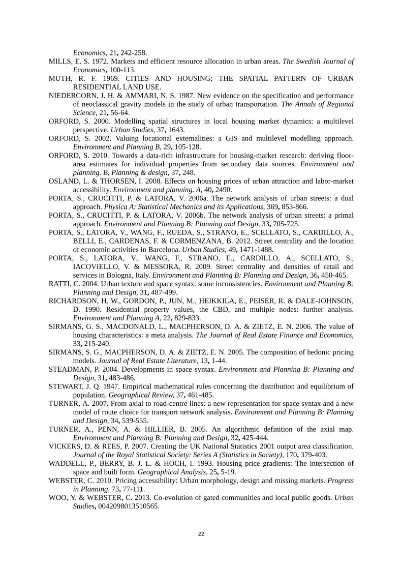
model reported in Table 4.1. The log likelihood is ‐5783, the corrected Akaike Information Criterion

(AIC) is ‐34635, and the F‐statistic is significant at the 1% level or less, all indicating that the model

fits the data well and that each independent variable is significantly linear. The adjusted R‐square

statistic is 0.63 which is typical of hedonic house price models. All the independent variables are

statistically significant at the 1% level or less and the VIFs indicate that multicollinearity is not a

problem. However, the White test reveals the presence of strong heteroscedasticity in the error

terms and so the prediction of the model is poor and Moran’s I also reveals significant positive

autocorrelation, suggesting that the coefficient estimates are unreliable, leading to over estimation.

[TABLE 2 HERE]

As theory suggests, property prices are found in this model to increase as floor area increases; new

build properties are found to have a premium; and terraced, semi‐detached and detached houses

are increasingly more expensive than the omitted property type dummy ‘flat’. Freehold tenure

commands a premium over leasehold tenure. The premiums for living in the different

neighbourhoods are in comparison to the omitted neighbourhood type dummy ‘multicultural

communities’. Hence properties in ‘blue collar’ and ‘constrained by circumstances’ neighbourhoods

are slightly cheaper than in ‘multicultural community’ neighbourhoods whilst properties in

‘prosperous suburbs’ are substantially more expensive. There is very little difference in the premiums

for properties in neighbourhood characterized by ‘typical traits’ or ‘living in the city’. The year

variables reveal continuous property price inflation since 2000 (the omitted dummy variable), the

substantial increase in prices between 2002 and 2004 and the flattening off and start of property

price decline in 2008. In terms of accessibility, log distance to the city centre has a negative

relationship with property prices as predicted by the access‐space theory of land‐values.

Accessibility to Roath Park and to the Heath Hospital has the anticipated negative relationship with

property prices, indicating that they act as positive externalities. The log‐log specification means that

the relationship between property price and accessibility can be interpreted as the price elasticity of

distance. Hence a 1% change in distance to the CBD is associated with a 0.101% decline in property

price or, alternatively, a doubling of distance from the CBD is associated with a 10% decline in

property price. The percentage change is slightly larger for Roath Park, suggesting that it has a

14

stronger affect on property price in the study area, and slightly smaller for Heath Hospital suggesting

a weaker affect on property prices. These findings make intuitive sense to those familiar with the

local housing market.

Model II was estimated using the network accessibility variables rather than the planar geometry

variables. Here, closeness and betweenness measures are investigated at different radii in order to

discover the spatial scale at which any network accessibility effects are most poweerful. The three

planar accessibility variables were removed from the model and pairs of choice and betweenness

variables for the fourteen spatial scales (radii) were entered one at a time into the model, the model

was estimated, and the pair removed before repeating the process for each spatial scale. We used

two statistical tests to help guide us in this process; the t‐statistic and the corrected AIC statistic.

Following Fotheringham et al. (2003) and their use of the t‐statistic in geographically weighted

regression (GWR) modelling, we use t‐statistic values in excess of 2 here purely as an indicator of

where potentially interesting relationships might occur rather than a test of statistical significance.

This is because we are estimating a number of regression models and hence we are undertaking

multiple hypothesis tests when we estimate the significance of the t‐statistics. These tests are not

independent either, as they re‐use the same data for tests which are spatially close to each other.

This will affect the probability of whether the t‐statistic is significant at random and so the

conventional approach of considering only the parameter estimates where the T‐statistic is greater /

less than 1.96 is not appropriate here (Byrne et al., 2009). A similar issue occurs with the estimation

of GWR models, thus the adoption of the GWR approach to modelling here.

The AIC statistic is a goodness of fit measure that corrects for model complexity and can be used to

compare the models with the same dependent variable and different independent variable subsets;

it provides a measure of the information distance between the model which has been fitted and the

unknown true model. The model with the lowest AIC is the one with the best predictive

performance. In addition, and in the spirit of Fotheringham, et al (2003) who used AIC to determine

the optimal bandwidth of kernel density estimates in GWR, we have used the AIC to check if the

network accessibility variables in models estimated at consecutive spatial scales are equivalent and

therefore add equivalent amounts of information (and thus the two models and hence the network

variables are not statistically different). As a rule of thumb, models having their AIC within 3 are said

to be equivalent. The differences in AICs in consecutive models are a lot greater than 3 suggesting

that the network variables in consecutive models are not equivalent and are therefore statistically

different.

15

For brevity, Table 3 summaries the coefficient estimates and t‐statistics for each pair of choice and

integration variables for each spatial scale in the fourteen versions of the model, but not the other

variables which had similar coefficient estimates to those in Model I. The AIC statistics, the White

test statistics and the Moran I statistics are presented below the t‐statistics and give an indication of

the goodness of fit of the model and whether heteroskedasticty and spatial autocorrelation are

present in the model’s error terms. The adjusted R‐square statistic is the same in all models and is

similar to Model I and the VIF scores (not presented) are within the desired range.

The choice and integration measures are statistically significant at the 1% level or less at each spatial

scale and the closeness coefficients have substantially larger T‐statistics than the respective

betweenness coefficients.

[TABLE 3 HERE]

Betweenness has a negative and closeness a positive relationship with property price. This is as

expected, as betweenness indicates likelihood of congestion and closeness indicates ease of access

to opportunities. In this way, the two network metrics neatly differentiate positive and negative

network externalities. The radially unconstrained (city‐wide) model for closeness is 0.001 (T‐statistic

33.12) and for betweenness is ‐0.016 (T‐statistic 10.98). The betweenness coefficients are

substantially larger than the closeness coefficients for each spatial scale with betweenness varying

between ‐0.013 (5000m) and ‐0.019 (2000m) with an average of ‐0.016 and closeness varying

between less than 0.001 (6000m) and 0.003 (400m) with an average 0f 0.001. Indeed, the closeness

coefficients become smaller the larger the spatial scale whereas there is a trend for the betweenness

coefficients to get larger with an increase in spatial scale.

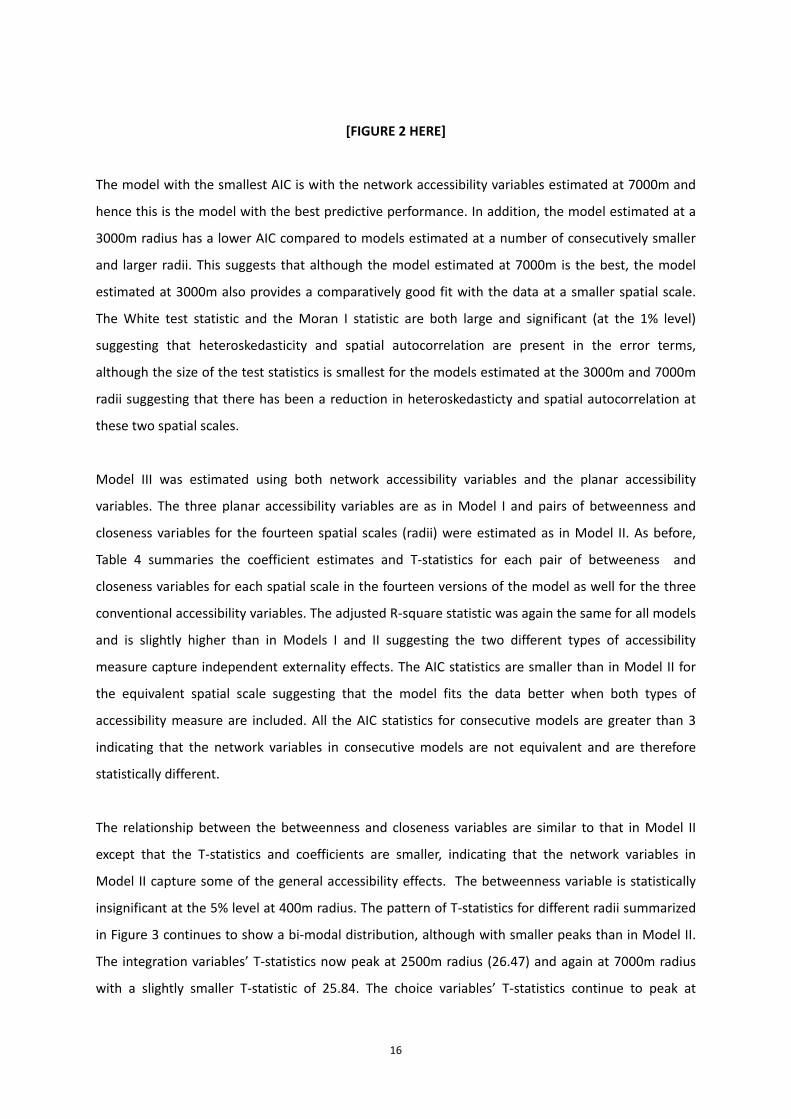
Further insight comes from examining the pattern of T‐statistics for different radii summarized in

Figure 2. This reveals a bi‐modal distribution with the T‐statistics for closeness rising from 10.35 at

400m radius to a peak of 37.05 at 3000m radius before declining and then rising to a slightly larger

peak of 40.49 at a 7000m radius before falling to 36.69 at 10,000m radius. A similar trend of T‐

statistics is observed for betweenness, but with a negative sign reflecting the relationship of

betwenness with property price, with a peak of ‐9.87 at 2000m before declining and rising to a

slightly larger peak of ‐10.93 at 7000m before falling to ‐10.15 at 10,000m radius.

16

[FIGURE 2 HERE]

The model with the smallest AIC is with the network accessibility variables estimated at 7000m and

hence this is the model with the best predictive performance. In addition, the model estimated at a

3000m radius has a lower AIC compared to models estimated at a number of consecutively smaller

and larger radii. This suggests that although the model estimated at 7000m is the best, the model

estimated at 3000m also provides a comparatively good fit with the data at a smaller spatial scale.

The White test statistic and the Moran I statistic are both large and significant (at the 1% level)

suggesting that heteroskedasticity and spatial autocorrelation are present in the error terms,

although the size of the test statistics is smallest for the models estimated at the 3000m and 7000m

radii suggesting that there has been a reduction in heteroskedasticty and spatial autocorrelation at

these two spatial scales.

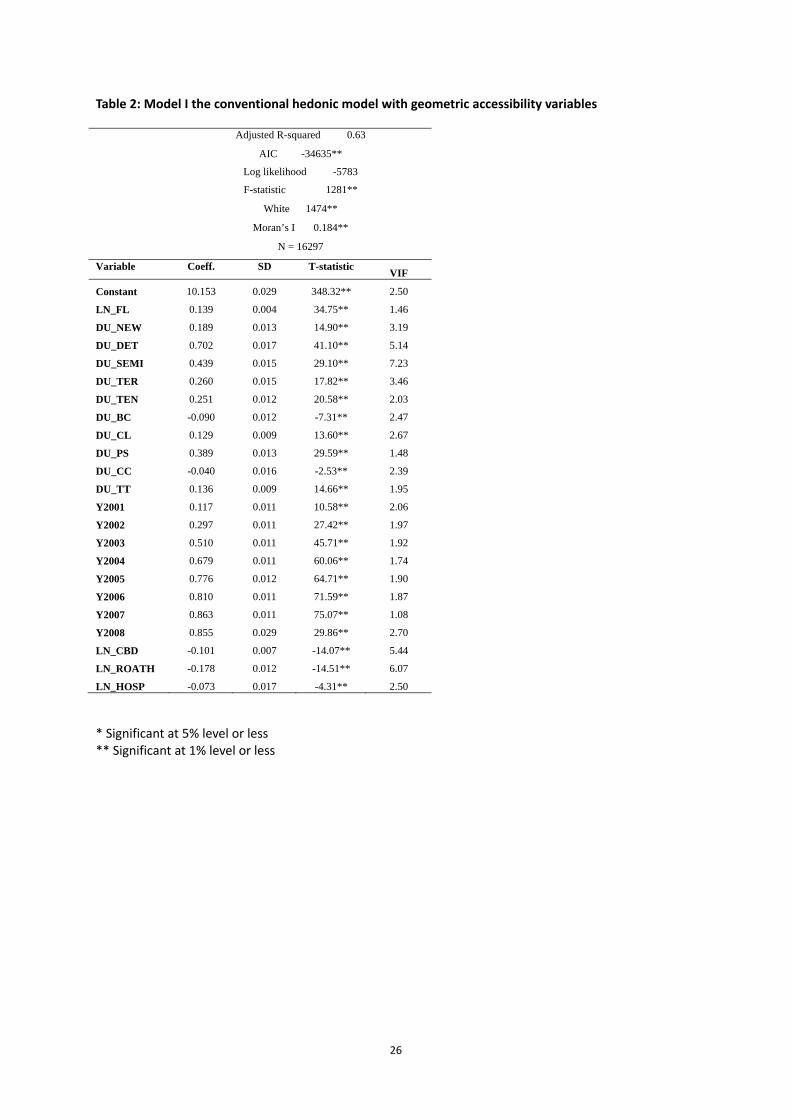
Model III was estimated using both network accessibility variables and the planar accessibility

variables. The three planar accessibility variables are as in Model I and pairs of betweenness and

closeness variables for the fourteen spatial scales (radii) were estimated as in Model II. As before,

Table 4 summaries the coefficient estimates and T‐statistics for each pair of betweeness and

closeness variables for each spatial scale in the fourteen versions of the model as well for the three

conventional accessibility variables. The adjusted R‐square statistic was again the same for all models

and is slightly higher than in Models I and II suggesting the two different types of accessibility

measure capture independent externality effects. The AIC statistics are smaller than in Model II for

the equivalent spatial scale suggesting that the model fits the data better when both types of

accessibility measure are included. All the AIC statistics for consecutive models are greater than 3

indicating that the network variables in consecutive models are not equivalent and are therefore

statistically different.

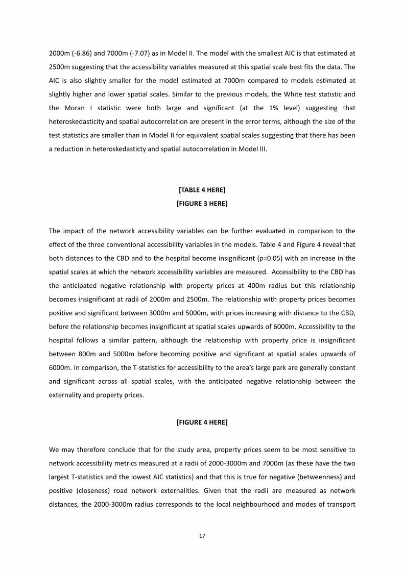
The relationship between the betweenness and closeness variables are similar to that in Model II

except that the T‐statistics and coefficients are smaller, indicating that the network variables in

Model II capture some of the general accessibility effects. The betweenness variable is statistically

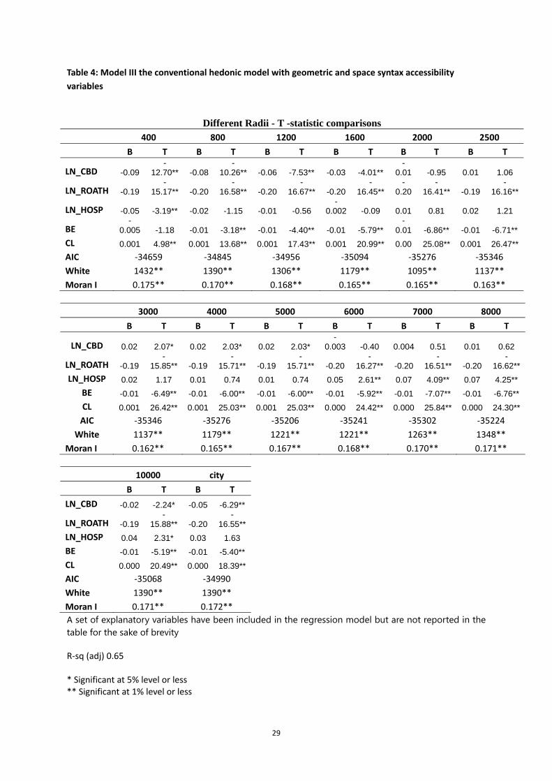
insignificant at the 5% level at 400m radius. The pattern of T‐statistics for different radii summarized

in Figure 3 continues to show a bi‐modal distribution, although with smaller peaks than in Model II.

The integration variables’ T‐statistics now peak at 2500m radius (26.47) and again at 7000m radius

with a slightly smaller T‐statistic of 25.84. The choice variables’ T‐statistics continue to peak at

17

2000m (‐6.86) and 7000m (‐7.07) as in Model II. The model with the smallest AIC is that estimated at

2500m suggesting that the accessibility variables measured at this spatial scale best fits the data. The

AIC is also slightly smaller for the model estimated at 7000m compared to models estimated at

slightly higher and lower spatial scales. Similar to the previous models, the White test statistic and

the Moran I statistic were both large and significant (at the 1% level) suggesting that

heteroskedasticity and spatial autocorrelation are present in the error terms, although the size of the

test statistics are smaller than in Model II for equivalent spatial scales suggesting that there has been

a reduction in heteroskedasticty and spatial autocorrelation in Model III.

[TABLE 4 HERE]

[FIGURE 3 HERE]

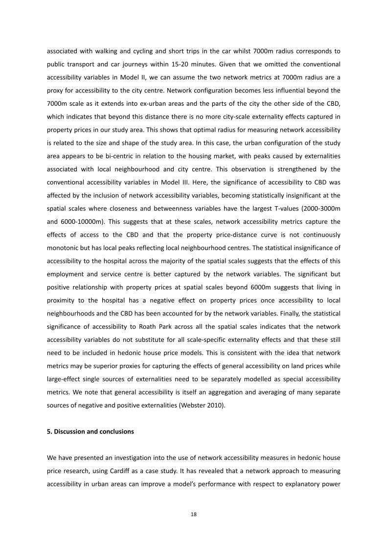
The impact of the network accessibility variables can be further evaluated in comparison to the

effect of the three conventional accessibility variables in the models. Table 4 and Figure 4 reveal that

both distances to the CBD and to the hospital become insignificant (p=0.05) with an increase in the

spatial scales at which the network accessibility variables are measured. Accessibility to the CBD has

the anticipated negative relationship with property prices at 400m radius but this relationship

becomes insignificant at radii of 2000m and 2500m. The relationship with property prices becomes

positive and significant between 3000m and 5000m, with prices increasing with distance to the CBD,

before the relationship becomes insignificant at spatial scales upwards of 6000m. Accessibility to the

hospital follows a similar pattern, although the relationship with property price is insignificant

between 800m and 5000m before becoming positive and significant at spatial scales upwards of

6000m. In comparison, the T‐statistics for accessibility to the area’s large park are generally constant

and significant across all spatial scales, with the anticipated negative relationship between the

externality and property prices.

[FIGURE 4 HERE]

We may therefore conclude that for the study area, property prices seem to be most sensitive to

network accessibility metrics measured at a radii of 2000‐3000m and 7000m (as these have the two

largest T‐statistics and the lowest AIC statistics) and that this is true for negative (betweenness) and

positive (closeness) road network externalities. Given that the radii are measured as network

distances, the 2000‐3000m radius corresponds to the local neighbourhood and modes of transport

18

associated with walking and cycling and short trips in the car whilst 7000m radius corresponds to

public transport and car journeys within 15‐20 minutes. Given that we omitted the conventional

accessibility variables in Model II, we can assume the two network metrics at 7000m radius are a

proxy for accessibility to the city centre. Network configuration becomes less influential beyond the

7000m scale as it extends into ex‐urban areas and the parts of the city the other side of the CBD,

which indicates that beyond this distance there is no more city‐scale externality effects captured in

property prices in our study area. This shows that optimal radius for measuring network accessibility

is related to the size and shape of the study area. In this case, the urban configuration of the study

area appears to be bi‐centric in relation to the housing market, with peaks caused by externalities

associated with local neighbourhood and city centre. This observation is strengthened by the

conventional accessibility variables in Model III. Here, the significance of accessibility to CBD was

affected by the inclusion of network accessibility variables, becoming statistically insignificant at the

spatial scales where closeness and betweenness variables have the largest T‐values (2000‐3000m

and 6000‐10000m). This suggests that at these scales, network accessibility metrics capture the

effects of access to the CBD and that the property price‐distance curve is not continuously

monotonic but has local peaks reflecting local neighbourhood centres. The statistical insignificance of

accessibility to the hospital across the majority of the spatial scales suggests that the effects of this

employment and service centre is better captured by the network variables. The significant but

positive relationship with property prices at spatial scales beyond 6000m suggests that living in

proximity to the hospital has a negative effect on property prices once accessibility to local

neighbourhoods and the CBD has been accounted for by the network variables. Finally, the statistical

significance of accessibility to Roath Park across all the spatial scales indicates that the network

accessibility variables do not substitute for all scale‐specific externality effects and that these still

need to be included in hedonic house price models. This is consistent with the idea that network

metrics may be superior proxies for capturing the effects of general accessibility on land prices while

large‐effect single sources of externalities need to be separately modelled as special accessibility

metrics. We note that general accessibility is itself an aggregation and averaging of many separate

sources of negative and positive externalities (Webster 2010).

5. Discussion and conclusions

We have presented an investigation into the use of network accessibility measures in hedonic house

price research, using Cardiff as a case study. It has revealed that a network approach to measuring

accessibility in urban areas can improve a model’s performance with respect to explanatory power

19

and a reduction in heteroscedasticity, spatial autocorrelation and multi‐collinearity compared to

conventional geometrical measures of accessibility. Further improvements to model specification

such as additional structural and locational attribute variables and weighting and spatial lag variables

may reduce and remove the heteroscedasticity and spatial autocorrelation that currently exists in the

models. By estimating network accessibility variables across a variety of spatial scales, we have

demonstrated that the study area displays a bi‐centric urban configuration with respect to property

prices that corresponds to local and city‐wide externalities. This makes theoretical sense for a city

such as Cardiff that has a clearly identifiable CBD and more localised centres of employment, retail

and commercial activity and strong city‐wide amenity green space attractions. This may not be the

case for larger British cities that have a more polycentric urban configuration.

Possibly our most novel finding is that the two network accessibility measures of closeness and

betweenness, respectively capture positive and negative intra‐urban externalities in a broad sense.

This is all the more significant since (a) the two measures are systemic measures and (b) they can

differentiate micro market areas created by many local negative externality effects.

The research has shown that such variables can be a better substitute for some conventional

geometric measures of general accessibility such as distance to the CBD; but that geometric

measures to more specific locational externalities, such as a major park, are still required. Moreover,

analysing the influence of the city’s major hospital on property prices in the final individual level

model we find that the interaction of network and conventional accessibility variables can unpack

both the positive and negative externality effects of specific locational attributes that occur at

different spatial scales without having to specify this functional relationship a priori. This, we suggest

is another important and novel finding.

In future research in this area we intend to apply the techniques to larger cities with more complex

urban configuration to see if it is possible to identify multiple peaks in the closeness and betweeness

coefficients at various spatial scales relating to a polycentric urban form. It is also important to begin

to better understand the precise nature of betweenness and closeness variables in terms of the

specific locational externalities that they are capturing at different spatial scales. This will involve

exploring spatial correlations of the network variables with conventional accessibility variables across

the different spatial scales and across the city to determine when network accessibility variables

make a good substitute for the conventional measures of locational externalities and when they do

not.

20

Finally, by bringing two genre of spatial analysis together (network analysis of street layouts comes

from both an architectural and transport planning tradition, while CBD‐accessibility and similar, come

from urban economics), it will be possible to develop a deeper understanding of the relationships

between urban configuration and design, locational externalities and property prices. New network

analysis software tools such as Spatial Domain Network Analysis (SDNA)

(http://www.cardiff.ac.uk/sdna/) provide a platform for the scientific study of associations between

urban design and configuration on the one hand all manner of urban performance indicators such as

land values, individual health and environmental quality and risk.

21

References ADAIR, A., MCGREAL, S., SMYTH, A., COOPER, J. & RYLEY, T. 2000. House prices and

accessibility: The testing of relationships within the Belfast urban area. Housing studies, 15, 699-716.

ALONSO, W. 1964. Location and land use: Toward a general theory of land rent. Publication of the Joint Center for Urban Studies. Harvard University Press.

BATTY, M. 2009. Accessibility: in search of a unified theory. Environment and Planning B: Planning and Design, 36, 191-194.

BELSLEY, D. A., KUH, E. & WELSCH, R. E. 2005. Regression diagnostics: Identifying influential data and sources of collinearity, John Wiley & Sons.

BYRNE, G., CHARLTON, M. & FOTHERINGHAM, S. Multiple dependent hypothesis tests in geographically weighted regression. 10th International conference on geocomputation. UNSW, Sydney November–December, 2009.

CHIARADIA, A., HILLIER, B., SCHWANDER, C. & WEDDERBURN, M. 2012. Compositional and urban form effects on centres in Greater London. Proceedings of the ICE-Urban Design and Planning, 165, 21-42.

CLIFF, A. D. & ORD, J. K. 1981. Spatial processes: models & applications, Pion London. DEBREZION, G., PELS, E. & RIETVELD, P. 2011. The Impact of Rail Transport on Real Estate

Prices An Empirical Analysis of the Dutch Housing Market. Urban studies, 48, 997-1015. DIEWERT, W. E. Hedonic regressions: a review of some unresolved issues. 2003. 29. ENSTR M, R. & NETZELL, O. 2008. Can space syntax help us in understanding the intraurban office

rent pattern? Accessibility and rents in downtown Stockholm. The Journal of Real Estate Finance and Economics, 36, 289-305.

FOLLAIN, J. R. & JIMENEZ, E. 1985. Estimating the demand for housing characteristics: a survey and critique. Regional science and urban economics, 15, 77-107.

FOTHERINGHAM, A. S., BRUNSDON, C. & CHARLTON, M. 2003. Geographically weighted regression: the analysis of spatially varying relationships, John Wiley & Sons.

FREEMAN, L. C. 1979. Centrality in social networks conceptual clarification. Social networks, 1, 215-239.

GIBBONS, S. & MACHIN, S. 2005. Valuing rail access using transport innovations. Journal of Urban Economics, 57, 148-169.

HAGGETT, P. & CHORLEY, R. J. 1969. Network analysis in geography. Edward Arnold (London). HANSEN, W. G. 1959. How accessibility shapes land use. Journal of the American Institute of

Planners, 25, 73-76. HEIKKILA, E., GORDON, P., KIM, J. I., PEISER, R. B., RICHARDSON, H. W. & DALE-

JOHNSON, D. 1989. What happened to the CBD-distance gradient? Land values in a policentric city. Environment and Planning A, 21, 221-232.

HILLIER, B. & HANSON, J. 1984. The social logic of space, Cambridge University Press Cambridge.

HILLIER, B. & PENN, A. 2004. Rejoinder to Carlo Ratti. Environment and Planning B: Planning and Design, 31, 501-511.

HOCH, I. & WADDELL, P. 1993. Apartment rents: another challenge to the monocentric model. Geographical Analysis, 25, 20-34.

JIANG, B. & CLARAMUNT, C. 2002. Integration of space syntax into GIS: new perspectives for urban morphology. Transactions in GIS, 6, 295-309.

JIANG, B. & CLARAMUNT, C. 2004. Topological analysis of urban street networks. Environment and Planning B, 31, 151-162.

LANDAU, U., PRASHKER, J. N. & HIRSH, M. 1981. The effect of temporal constraints on household travel behavior. Environment and Planning A, 13, 435-448.

MALPEZZI, S. 2003. Hedonic pricing models: a selective and applied review. Section in Housing Economics and Public Policy: Essays in Honor of Duncan Maclennan.

MATTHEWS, J. W. & TURNBULL, G. K. 2007. Neighborhood street layout and property value: the interaction of accessibility and land use mix. The Journal of Real Estate Finance and Economics, 35, 111-141.

MCDONALD, J. F. 1987. The identification of urban employment subcenters. Journal of Urban

22

Economics, 21, 242-258. MILLS, E. S. 1972. Markets and efficient resource allocation in urban areas. The Swedish Journal of

Economics, 100-113. MUTH, R. F. 1969. CITIES AND HOUSING; THE SPATIAL PATTERN OF URBAN

RESIDENTIAL LAND USE. NIEDERCORN, J. H. & AMMARI, N. S. 1987. New evidence on the specification and performance

of neoclassical gravity models in the study of urban transportation. The Annals of Regional Science, 21, 56-64.

ORFORD, S. 2000. Modelling spatial structures in local housing market dynamics: a multilevel perspective. Urban Studies, 37, 1643.

ORFORD, S. 2002. Valuing locational externalities: a GIS and multilevel modelling approach. Environment and Planning B, 29, 105-128.

ORFORD, S. 2010. Towards a data-rich infrastructure for housing-market research: deriving floor-area estimates for individual properties from secondary data sources. Environment and planning. B, Planning & design, 37, 248.

OSLAND, L. & THORSEN, I. 2008. Effects on housing prices of urban attraction and labor-market accessibility. Environment and planning. A, 40, 2490.

PORTA, S., CRUCITTI, P. & LATORA, V. 2006a. The network analysis of urban streets: a dual approach. Physica A: Statistical Mechanics and its Applications, 369, 853-866.

PORTA, S., CRUCITTI, P. & LATORA, V. 2006b. The network analysis of urban streets: a primal approach. Environment and Planning B: Planning and Design, 33, 705-725.

PORTA, S., LATORA, V., WANG, F., RUEDA, S., STRANO, E., SCELLATO, S., CARDILLO, A., BELLI, E., CARDENAS, F. & CORMENZANA, B. 2012. Street centrality and the location of economic activities in Barcelona. Urban Studies, 49, 1471-1488.

PORTA, S., LATORA, V., WANG, F., STRANO, E., CARDILLO, A., SCELLATO, S., IACOVIELLO, V. & MESSORA, R. 2009. Street centrality and densities of retail and services in Bologna, Italy. Environment and Planning B: Planning and Design, 36, 450-465.

RATTI, C. 2004. Urban texture and space syntax: some inconsistencies. Environment and Planning B: Planning and Design, 31, 487-499.

RICHARDSON, H. W., GORDON, P., JUN, M., HEIKKILA, E., PEISER, R. & DALE-JOHNSON, D. 1990. Residential property values, the CBD, and multiple nodes: further analysis. Environment and Planning A, 22, 829-833.

SIRMANS, G. S., MACDONALD, L., MACPHERSON, D. A. & ZIETZ, E. N. 2006. The value of housing characteristics: a meta analysis. The Journal of Real Estate Finance and Economics, 33, 215-240.

SIRMANS, S. G., MACPHERSON, D. A. & ZIETZ, E. N. 2005. The composition of hedonic pricing models. Journal of Real Estate Literature, 13, 1-44.

STEADMAN, P. 2004. Developments in space syntax. Environment and Planning B: Planning and Design, 31, 483-486.

STEWART, J. Q. 1947. Empirical mathematical rules concerning the distribution and equilibrium of population. Geographical Review, 37, 461-485.

TURNER, A. 2007. From axial to road-centre lines: a new representation for space syntax and a new model of route choice for transport network analysis. Environment and Planning B: Planning and Design, 34, 539-555.

TURNER, A., PENN, A. & HILLIER, B. 2005. An algorithmic definition of the axial map. Environment and Planning B: Planning and Design, 32, 425-444.

VICKERS, D. & REES, P. 2007. Creating the UK National Statistics 2001 output area classification. Journal of the Royal Statistical Society: Series A (Statistics in Society), 170, 379-403.

WADDELL, P., BERRY, B. J. L. & HOCH, I. 1993. Housing price gradients: The intersection of space and built form. Geographical Analysis, 25, 5-19.

WEBSTER, C. 2010. Pricing accessibility: Urban morphology, design and missing markets. Progress in Planning, 73, 77-111.

WOO, Y. & WEBSTER, C. 2013. Co-evolution of gated communities and local public goods. Urban Studies, 0042098013510565.

Figure 1All right

1: The city ofts reserved)

f Cardiff, Waales and the

23

e case study area (Ordnaance Surveyy ©Crown Co

opyright.

24

Table 1: Description of the variables (property level)

Variables Description Type Min Max Mean SDev

LN_FL Natural log of floor area Continuous 1.793 9.595 4.903 1.071

LN_CBD Natural log of distance to City Centre Continuous -0.66 1.79 0.76 0.62

LN_BAY Natural log of distance to Cardiff bay Continuous 0.93 2.18 1.6 0.29

LN_ROATH Natural log of distance to Roath Park Continuous -3.19 1.52 0.72 0.52

LN_HOSP Natural log of distance to Heath hospital Continuous -0.42 1.82 0.99 0.48

LN_BUTE Natural log of distance to Bute Park Continuous -1.03 1.64 0.95 0.39

BE_R400M Betweenness value at radius 400m Continuous 0 3.183 1.483 0.923













BE_N Betweenness value for city wide Continuous 0 7.567 3.834 2.337

CL_R400M Closeness value at radius 400m Continuous 0 95.898 29.479 16.135

CL_R800M Closeness value at radius 800m Continuous 0 194.551 68.402 40.154

CL_R1200M Closeness value at radius 1200m Continuous 11.928 350.988 120.269 67.933











CL_N Closeness value for city wide Continuous 858.122 2150.76 1521.65 245.688

Variables Description Type Code 0 (%)

Code 1 (%)

Mean SDev

DU_NEW New Build Dummy 92.9 7.1 0.080 0.268 DU_DET Detached House Dummy

91.2 8.8 0.100 0.300 DU_SEMI Semidetached House Dummy

79.2 20.8 0.210 0.407 DU_TER Terrace house Dummy

46.6 53.4 0.520 0.500 DU_FLAT Flat Dummy

83 17.0 0.170 0.375 DU_TEN Tenure ( Freehold=1 Leasehold =0) Dummy

21.7 78.3 0.790 0.411 DU_BC OAC Blue collar communities Dummy

89.1 10.9 0.110 0.310 DU_CL OAC Living in the city Dummy

72 28.0 0.270 0.446

25

DU_PS OAC Prosperous suburbs Dummy 87 13.0 0.150 0.354

DU_CC OAC Constrained by Circumstances Dummy 95.5 4.5 0.050 0.208

DU_TT OAC Typical traits Dummy 71.7 28.3 0.280 0.449

DU_MU OAC Multicultural Dummy 84.7 15.3 0.150 0.353

Y2000 Transactions in 2000 Dummy 89.3 10.7 0.110 0.309


Y2002 Transactions in 2002 Dummy 85 15.0 0.150 0.359







26

Table 2: Model I the conventional hedonic model with geometric accessibility variables

* Significant at 5% level or less ** Significant at 1% level or less

Adjusted R-squared 0.63

AIC -34635**

Log likelihood -5783

F-statistic 1281**

White 1474**

Moran’s I 0.184**

N = 16297

Variable Coeff. SD T-statistic VIF

Constant 10.153 0.029 348.32** 2.50

LN_FL 0.139 0.004 34.75** 1.46

DU_NEW 0.189 0.013 14.90** 3.19

DU_DET 0.702 0.017 41.10** 5.14

DU_SEMI 0.439 0.015 29.10** 7.23

DU_TER 0.260 0.015 17.82** 3.46

DU_TEN 0.251 0.012 20.58** 2.03

DU_BC -0.090 0.012 -7.31** 2.47

DU_CL 0.129 0.009 13.60** 2.67

DU_PS 0.389 0.013 29.59** 1.48

DU_CC -0.040 0.016 -2.53** 2.39

DU_TT 0.136 0.009 14.66** 1.95

Y2001 0.117 0.011 10.58** 2.06

Y2002 0.297 0.011 27.42** 1.97

Y2003 0.510 0.011 45.71** 1.92

Y2004 0.679 0.011 60.06** 1.74

Y2005 0.776 0.012 64.71** 1.90

Y2006 0.810 0.011 71.59** 1.87

Y2007 0.863 0.011 75.07** 1.08

Y2008 0.855 0.029 29.86** 2.70

LN_CBD -0.101 0.007 -14.07** 5.44

LN_ROATH -0.178 0.012 -14.51** 6.07

LN_HOSP -0.073 0.017 -4.31** 2.50

Coe

T

AIC

Whi

Mora

Coe

T

AIC

Whi

Mora

Table 3:

400

BE

ef -0.018

-4.22**

C -33

ite 143

an I 0.17

400

BE

ef -0.014

-8.83**

C -342

ite 109

an I 0.16

A set of table for R‐sq (adj * Signific** Signif Figure 2:scales

Model II the

0M

CL B

0.003 -0.

10.35** -5.5

123

2**

75**

00M

CL B

0.001 -0.

35.61** -8.6

272

95**

67**

explanatory r the sake of

j) 0.63

cant at 5% levficant at 1% le

: T‐statistics o

conventiona

800M

BE CL

016 0.002

58** 19.77**

-33432

1306**

0.174**

5000M

BE CL

013 0.001

61** 35.24**

-34248

1137**

0.168**

variables habrevity

vel or less evel or less

of the space

al hedonic mo

Differ

1200M

BE C

-0.017 0

-7.14** 25

-33668

1221**

0.173**

6000M

BE C

-0.014 0

-9.70** 38

-34437

1179**

0.168**

ave been incl

syntax acces

27

odel with spa

rent Radii - T -st

1

CL BE

0.002 -0.018

.16** -8.86*

-

1

0

7

CL BE

0.001 -0.016

.06** -10.93*

-

1

0

luded in the

ssibility varia

ace syntax ac

tatistic comparis

1600M

CL

8 0.001

* 30.05**

-33931

1179**

0.171**

7000M

CL

6 0.001

** 40.49**

-34612

1221**

0.171**

regression m

bles estimat

ccessibility va

sons

2000M

BE C

-0.019 0.0

-9.87** 34.8

-34223

1095**

0.168**

8000M

BE C

-0.015 0.0

-10.75** 39.5

-34537

1263**

0.172**

model but are

ed in Model

ariables

2

CL BE

001 -0.017

83** -9.65**

-3

1

0.

10

CL BE

001 -0.014

55** -10.15**

-3

1

0.

re not report

II for differen

500M

CL

0.001

* 36.77**

34355

137**

.168**

0000M

CL

0

* 36.69**

34338

306**

.173**

ed in the

nt spatial

3000M

BE C

-0.016 0.0

-9.38** 37.0

-34371

1095**

0.165**

City-wide

BE C

-0.016 0.0

-10.98** 33.1

-34092

1306**

0.173**

L

00

05

L

00

12

28

29

Table 4: Model III the conventional hedonic model with geometric and space syntax accessibility

variables

Different Radii - T -statistic comparisons 400 800 1200 1600 2000 2500

B T B T B T B T B T B T

LN_CBD -0.09 -

12.70** -0.08 -

10.26** -0.06 -7.53** -0.03 -4.01**-

0.01 -0.95 0.01 1.06

LN_ROATH -0.19 -

15.17** -0.20 -

16.58** -0.20-

16.67** -0.20-

16.45**-

0.20 -

16.41** -0.19-

16.16**

LN_HOSP -0.05 -3.19** -0.02 -1.15 -0.01 -0.56 -

0.002 -0.09 0.01 0.81 0.02 1.21

BE -

0.005 -1.18 -0.01 -3.18** -0.01 -4.40** -0.01 -5.79**-

0.01 -6.86** -0.01 -6.71**

CL 0.001 4.98** 0.001 13.68** 0.001 17.43** 0.001 20.99** 0.00 25.08** 0.001 26.47**

AIC ‐34659 ‐34845 ‐34956 ‐35094 ‐35276 ‐35346

White 1432** 1390** 1306** 1179** 1095** 1137**

Moran I 0.175** 0.170** 0.168** 0.165** 0.165** 0.163**

3000 4000 5000 6000 7000 8000

B T B T B T B T B T B T

LN_CBD 0.02 2.07* 0.02 2.03* 0.02 2.03* -

0.003 -0.40 0.004 0.51 0.01 0.62

LN_ROATH -0.19 -

15.85** -0.19 -

15.71** -0.19-

15.71** -0.20-

16.27** -0.20 -

16.51** -0.20-

16.62**

LN_HOSP 0.02 1.17 0.01 0.74 0.01 0.74 0.05 2.61** 0.07 4.09** 0.07 4.25**

BE -0.01 -6.49** -0.01 -6.00** -0.01 -6.00** -0.01 -5.92** -0.01 -7.07** -0.01 -6.76**

CL 0.001 26.42** 0.001 25.03** 0.001 25.03** 0.000 24.42** 0.000 25.84** 0.000 24.30**

AIC ‐35346 ‐35276 ‐35206 ‐35241 ‐35302 ‐35224

White 1137** 1179** 1221** 1221** 1263** 1348**

Moran I 0.162** 0.165** 0.167** 0.168** 0.170** 0.171**

10000 city

B T B T

LN_CBD -0.02 -2.24* -0.05 -6.29**

LN_ROATH -0.19 -

15.88** -0.20 -

16.55**

LN_HOSP 0.04 2.31* 0.03 1.63

BE -0.01 -5.19** -0.01 -5.40**

CL 0.000 20.49** 0.000 18.39**

AIC ‐35068 ‐34990

White 1390** 1390**

Moran I 0.171** 0.172**

A set of explanatory variables have been included in the regression model but are not reported in the table for the sake of brevity R‐sq (adj) 0.65 * Significant at 5% level or less ** Significant at 1% level or less

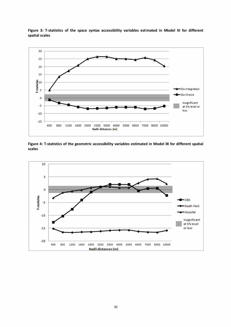
Figure 3spatial s

Figure 4scales

3: T‐statisticscales

: T‐statistics

s of the spac

of the geom

ce syntax ac

metric accessi

30

ccessibility v

ibility variabl

variables esti

les estimated

mated in M

d in Model II

Model III for

II for differen

different

nt spatial

31

List of Tables Table 1: Description of the variables (property level)

Table 2: Model I the conventional hedonic model with geometric accessibility variables

Table 3: Model II the conventional hedonic model with space syntax accessibility variables

Table 4: Model III the conventional hedonic model with geometric and space syntax accessibility variables

List of Figures

Figure 1: The city of Cardiff, Wales and the case study area (Ordnance Survey ©Crown Copyright. All rights reserved) Figure 2: T‐statistics of the space syntax accessibility variables estimated in Model II for different spatial scales Figure 3: T‐statistics of the space syntax accessibility variables estimated in Model III for different spatial scales Figure 4: T‐statistics of the geometric accessibility variables estimated in Model III for different spatial scales

Urban configuration, accessibility and property prices - HKU ...

Documents