Upper limits on gravitational wave bursts in LIGO's second science run

arX

iv:g

r-qc

/050

5029

v1 6

May

200

5

Upper limits on gravitational wave bursts in LIGO’s second science runLIGO-P040040-07-R

to be submitted for publication to Phys Rev D

B. Abbott,12 R. Abbott,15 R. Adhikari,13 A. Ageev,20, 27 B. Allen,39 R. Amin,34 S. B. Anderson,12 W. G. Anderson,29

M. Araya,12 H. Armandula,12 M. Ashley,28 F. Asiri,12, a P. Aufmuth,31 C. Aulbert,1 S. Babak,7 R. Balasubramanian,7

S. Ballmer,13 B. C. Barish,12 C. Barker,14 D. Barker,14 M. Barnes,12, b B. Barr,35 M. A. Barton,12 K. Bayer,13 R. Beausoleil,26, c

K. Belczynski,23 R. Bennett,35, d S. J. Berukoff,1, e J. Betzwieser,13 B. Bhawal,12 I. A. Bilenko,20 G. Billingsley,12

E. Black,12 K. Blackburn,12 L. Blackburn,13 B. Bland,14 B. Bochner,13, f L. Bogue,12 R. Bork,12 S. Bose,40 P. R. Brady,39

V. B. Braginsky,20 J. E. Brau,37 D. A. Brown,39 A. Bullington,26 A. Bunkowski,2, 31 A. Buonanno,6, g R. Burgess,13 D. Busby,12

W. E. Butler,38 R. L. Byer,26 L. Cadonati,13 G. Cagnoli,35 J. B. Camp,21 C. A. Cantley,35 L. Cardenas,12 K. Carter,15

M. M. Casey,35 J. Castiglione,34 A. Chandler,12 J. Chapsky,12, b P. Charlton,12, h S. Chatterji,13 S. Chelkowski,2, 31 Y. Chen,6

V. Chickarmane,16, i D. Chin,36 N. Christensen,8 D. Churches,7 T. Cokelaer,7 C. Colacino,33 R. Coldwell,34 M. Coles,15, j

D. Cook,14 T. Corbitt,13 D. Coyne,12 J. D. E. Creighton,39 T. D. Creighton,12 D. R. M. Crooks,35 P. Csatorday,13 B. J. Cusack,3

C. Cutler,1 E. D’Ambrosio,12 K. Danzmann,31,2 E. Daw,16, k D. DeBra,26 T. Delker,34, l V. Dergachev,36 R. DeSalvo,12

S. Dhurandhar,11 A. Di Credico,27 M. Diaz,29 H. Ding,12 R. W. P. Drever,4 R. J. Dupuis,35 J. A. Edlund,12, b P. Ehrens,12

E. J. Elliffe,35 T. Etzel,12 M. Evans,12 T. Evans,15 S. Fairhurst,39 C. Fallnich,31 D. Farnham,12 M. M. Fejer,26 T. Findley,25

M. Fine,12 L. S. Finn,28 K. Y. Franzen,34 A. Freise,2, m R. Frey,37 P. Fritschel,13 V. V. Frolov,15 M. Fyffe,15 K. S. Ganezer,5

J. Garofoli,14 J. A. Giaime,16 A. Gillespie,12, n K. Goda,13 G. Gonzalez,16 S. Goßler,31 P. Grandclement,23, o A. Grant,35

C. Gray,14 A. M. Gretarsson,15 D. Grimmett,12 H. Grote,2 S. Grunewald,1 M. Guenther,14 E. Gustafson,26, p R. Gustafson,36

W. O. Hamilton,16 M. Hammond,15 J. Hanson,15 C. Hardham,26 J. Harms,19 G. Harry,13 A. Hartunian,12 J. Heefner,12

Y. Hefetz,13 G. Heinzel,2 I. S. Heng,31 M. Hennessy,26 N. Hepler,28 A. Heptonstall,35 M. Heurs,31 M. Hewitson,2 S. Hild,2

N. Hindman,14 P. Hoang,12 J. Hough,35 M. Hrynevych,12, q W. Hua,26 M. Ito,37 Y. Itoh,1 A. Ivanov,12 O. Jennrich,35, r

B. Johnson,14 W. W. Johnson,16 W. R. Johnston,29 D. I. Jones,28 L. Jones,12 D. Jungwirth,12, sV. Kalogera,23 E. Katsavounidis,13

K. Kawabe,14 S. Kawamura,22 W. Kells,12 J. Kern,15, t A. Khan,15 S. Killbourn,35 C. J. Killow,35 C. Kim,23 C. King,12 P. King,12

S. Klimenko,34 S. Koranda,39 K. Kotter,31 J. Kovalik,15, b D. Kozak,12 B. Krishnan,1 M. Landry,14 J. Langdale,15 B. Lantz,26

R. Lawrence,13 A. Lazzarini,12 M. Lei,12 I. Leonor,37 K. Libbrecht,12 A. Libson,8 P. Lindquist,12 S. Liu,12 J. Logan,12, u

M. Lormand,15 M. Lubinski,14 H. Luck,31, 2 T. T. Lyons,12, u B. Machenschalk,1 M. MacInnis,13 M. Mageswaran,12

K. Mailand,12 W. Majid,12, b M. Malec,2, 31 F. Mann,12 A. Marin,13, v S. Marka,12, w E. Maros,12 J. Mason,12, x K. Mason,13

O. Matherny,14 L. Matone,14 N. Mavalvala,13 R. McCarthy,14 D. E. McClelland,3 M. McHugh,18 G. Mendell,14 R. A. Mercer,33

S. Meshkov,12 E. Messaritaki,39 C. Messenger,33 V. P. Mitrofanov,20 G. Mitselmakher,34 R. Mittleman,13 O. Miyakawa,12

S. Miyoki,12, y S. Mohanty,29 G. Moreno,14 K. Mossavi,2 G. Mueller,34 S. Mukherjee,29 P. Murray,35 J. Myers,14 S. Nagano,2

T. Nash,12 R. Nayak,11 G. Newton,35 F. Nocera,12 J. S. Noel,40 P. Nutzman,23 T. Olson,24 B. O’Reilly,15 D. J. Ottaway,13

A. Ottewill,39, z D. Ouimette,12, s H. Overmier,15 B. J. Owen,28 Y. Pan,6 M. A. Papa,1 V. Parameshwaraiah,14

C. Parameswariah,15 M. Pedraza,12 S. Penn,10 M. Pitkin,35 M. Plissi,35 R. Prix,1 V. Quetschke,34 F. Raab,14 H. Radkins,14

R. Rahkola,37 M. Rakhmanov,34 S. R. Rao,12 K. Rawlins,13 S. Ray-Majumder,39 V. Re,33 D. Redding,12, b M. W. Regehr,12, b

T. Regimbau,7 S. Reid,35 K. T. Reilly,12 K. Reithmaier,12 D. H. Reitze,34 S. Richman,13, aaR. Riesen,15 K. Riles,36 B. Rivera,14

A. Rizzi,15, bb D. I. Robertson,35 N. A. Robertson,26,35 L. Robison,12 S. Roddy,15 J. Rollins,13 J. D. Romano,7 J. Romie,12

H. Rong,34, n D. Rose,12 E. Rotthoff,28 S. Rowan,35 A. Rudiger,2 P. Russell,12 K. Ryan,14 I. Salzman,12 V. Sandberg,14

G. H. Sanders,12, cc V. Sannibale,12 B. Sathyaprakash,7 P. R. Saulson,27 R. Savage,14 A. Sazonov,34 R. Schilling,2

K. Schlaufman,28 V. Schmidt,12, dd R. Schnabel,19 R. Schofield,37 B. F. Schutz,1, 7 P. Schwinberg,14 S. M. Scott,3 S. E. Seader,40

A. C. Searle,3 B. Sears,12 S. Seel,12 F. Seifert,19 A. S. Sengupta,11 C. A. Shapiro,28, eeP. Shawhan,12 D. H. Shoemaker,13

Q. Z. Shu,34, ff A. Sibley,15 X. Siemens,39 L. Sievers,12, b D. Sigg,14 A. M. Sintes,1, 32 J. R. Smith,2 M. Smith,13 M. R. Smith,12

P. H. Sneddon,35 R. Spero,12, b G. Stapfer,15 D. Steussy,8 K. A. Strain,35 D. Strom,37 A. Stuver,28 T. Summerscales,28

M. C. Sumner,12 P. J. Sutton,12 J. Sylvestre,12, gg A. Takamori,12 D. B. Tanner,34 H. Tariq,12 I. Taylor,7 R. Taylor,35 R. Taylor,12

K. A. Thorne,28 K. S. Thorne,6 M. Tibbits,28 S. Tilav,12, hh M. Tinto,4, b K. V. Tokmakov,20 C. Torres,29 C. Torrie,12

G. Traylor,15 W. Tyler,12 D. Ugolini,30 C. Ungarelli,33 M. Vallisneri,6, ii M. van Putten,13 S. Vass,12 A. Vecchio,33 J. Veitch,35

C. Vorvick,14 S. P. Vyachanin,20 L. Wallace,12 H. Walther,19 H. Ward,35 B. Ware,12, b K. Watts,15 D. Webber,12 A. Weidner,19

U. Weiland,31 A. Weinstein,12 R. Weiss,13 H. Welling,31 L. Wen,12 S. Wen,16 J. T. Whelan,18 S. E. Whitcomb,12 B. F. Whiting,34

S. Wiley,5 C. Wilkinson,14 P. A. Willems,12 P. R. Williams,1, jj R. Williams,4 B. Willke,31 A. Wilson,12 B. J. Winjum,28, e

W. Winkler,2 S. Wise,34 A. G. Wiseman,39 G. Woan,35 R. Wooley,15 J. Worden,14 W. Wu,34 I. Yakushin,15 H. Yamamoto,12

S. Yoshida,25 K. D. Zaleski,28 M. Zanolin,13 I. Zawischa,31, kk L. Zhang,12 R. Zhu,1 N. Zotov,17 M. Zucker,15 and J. Zweizig12

(The LIGO Scientific Collaboration, http://www.ligo.org)

http://arXiv.org/abs/gr-qc/0505029v1

http://www.ligo.org

2

1Albert-Einstein-Institut, Max-Planck-Institut fur Gravitationsphysik, D-14476 Golm, Germany2Albert-Einstein-Institut, Max-Planck-Institut fur Gravitationsphysik, D-30167 Hannover, Germany

3Australian National University, Canberra, 0200, Australia4California Institute of Technology, Pasadena, CA 91125, USA

5California State University Dominguez Hills, Carson, CA 90747, USA6Caltech-CaRT, Pasadena, CA 91125, USA

7Cardiff University, Cardiff, CF2 3YB, United Kingdom8Carleton College, Northfield, MN 55057, USA

9Fermi National Accelerator Laboratory, Batavia, IL 60510,USA10Hobart and William Smith Colleges, Geneva, NY 14456, USA

11Inter-University Centre for Astronomy and Astrophysics, Pune - 411007, India12LIGO - California Institute of Technology, Pasadena, CA 91125, USA

13LIGO - Massachusetts Institute of Technology, Cambridge, MA 02139, USA14LIGO Hanford Observatory, Richland, WA 99352, USA

15LIGO Livingston Observatory, Livingston, LA 70754, USA16Louisiana State University, Baton Rouge, LA 70803, USA

17Louisiana Tech University, Ruston, LA 71272, USA18Loyola University, New Orleans, LA 70118, USA

19Max Planck Institut fur Quantenoptik, D-85748, Garching,Germany20Moscow State University, Moscow, 119992, Russia

21NASA/Goddard Space Flight Center, Greenbelt, MD 20771, USA22National Astronomical Observatory of Japan, Tokyo 181-8588, Japan

23Northwestern University, Evanston, IL 60208, USA24Salish Kootenai College, Pablo, MT 59855, USA

25Southeastern Louisiana University, Hammond, LA 70402, USA26Stanford University, Stanford, CA 94305, USA27Syracuse University, Syracuse, NY 13244, USA

28The Pennsylvania State University, University Park, PA 16802, USA29The University of Texas at Brownsville and Texas Southmost College, Brownsville, TX 78520, USA

30Trinity University, San Antonio, TX 78212, USA31Universitat Hannover, D-30167 Hannover, Germany

32Universitat de les Illes Balears, E-07122 Palma de Mallorca, Spain33University of Birmingham, Birmingham, B15 2TT, United Kingdom

34University of Florida, Gainesville, FL 32611, USA35University of Glasgow, Glasgow, G12 8QQ, United Kingdom

36University of Michigan, Ann Arbor, MI 48109, USA37University of Oregon, Eugene, OR 97403, USA

38University of Rochester, Rochester, NY 14627, USA39University of Wisconsin-Milwaukee, Milwaukee, WI 53201, USA

40Washington State University, Pullman, WA 99164, USA( RCS Revision: 1.23 ; compiled 4 February 2008)

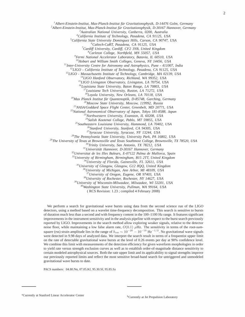
We perform a search for gravitational wave bursts using datafrom the second science run of the LIGOdetectors, using a method based on a wavelet time-frequencydecomposition. This search is sensitive to burstsof duration much less than a second and with frequency content in the 100–1100 Hz range. It features significantimprovements in the instrument sensitivity and in the analysis pipeline with respect to the burst search previouslyreported by LIGO. Improvements in the search method allow exploring weaker signals, relative to the detectornoise floor, while maintaining a low false alarm rate,O(0.1) µHz. The sensitivity in terms of theroot-sum-square(rss) strain amplitude lies in the range ofhrss ∼ 10−20

− 10−19 Hz−1/2. No gravitational wave signalswere detected in 9.98 days of analyzed data. We interpret thesearch result in terms of a frequentist upper limiton the rate of detectable gravitational wave bursts at the level of 0.26 events per day at 90% confidence level.We combine this limit with measurements of the detection efficiency for given waveform morphologies in orderto yield rate versus strength exclusion curves as well as to establish order-of-magnitude distance sensitivity tocertain modeled astrophysical sources. Both the rate upperlimit and its applicability to signal strengths improveour previously reported limits and reflect the most sensitive broad-band search for untriggered and unmodeledgravitational wave bursts to date.

PACS numbers: 04.80.Nn, 07.05.Kf, 95.30.Sf, 95.85.Sz

aCurrently at Stanford Linear Accelerator Center bCurrently at Jet Propulsion Laboratory

3

I. INTRODUCTION

The Laser Interferometer Gravitational wave Observatory(LIGO) is a network of interferometric detectors aiming tomake direct observations of gravitational waves. Construc-tion of the LIGO detectors is essentially complete, and muchprogress has been made in commissioning them to (a) bringthe three interferometers to their final optical configuration,(b) reduce the interferometers’ noise floors and improve thestationarity of the noise, and (c) pave the way toward long-term science observations. Interleaved with commissioning,four “science runs” have been carried out to collect data un-der stable operating conditions for astrophysical gravitationalwave searches, albeit at reduced sensitivity and observationtime relative to the LIGO design goals. The first science run,called S1, took place in the summer of 2002 over a period of17 days. S1 represented a major milestone as the longest andmost sensitive operation of broad-band interferometersin co-incidenceup to that time. Using the S1 data from the LIGOand GEO600 interferometers [1], astrophysical searches forfour general categories of gravitational wave source types—binary inspiral [2], burst-like [3], stochastic [4] and continu-ous wave [5]—were pursued by the LIGO Scientific Collabo-ration (LSC). These searches established general methodolo-

cPermanent Address: HP LaboratoriesdCurrently at Rutherford Appleton LaboratoryeCurrently at University of California, Los AngelesfCurrently at Hofstra UniversitygPermanent Address: GReCO, Institut d’Astrophysique de Paris (CNRS)hCurrently at La Trobe University, Bundoora VIC, AustraliaiCurrently at Keck Graduate InstitutejCurrently at National Science FoundationkCurrently at University of SheffieldlCurrently at Ball Aerospace CorporationmCurrently at European Gravitational ObservatorynCurrently at Intel Corp.oCurrently at University of Tours, FrancepCurrently at Lightconnect Inc.qCurrently at W.M. Keck ObservatoryrCurrently at ESA Science and Technology CentersCurrently at Raytheon CorporationtCurrently at New Mexico Institute of Mining and Technology /MagdalenaRidge Observatory InterferometeruCurrently at Mission Research CorporationvCurrently at Harvard UniversitywPermanent Address: Columbia UniversityxCurrently at Lockheed-Martin CorporationyPermanent Address: University of Tokyo, Institute for Cosmic Ray ResearchzPermanent Address: University College DublinaaCurrently at Research Electro-Optics Inc.bbCurrently at Institute of Advanced Physics, Baton Rouge, LAccCurrently at Thirty Meter Telescope Project at CaltechddCurrently at European Commission, DG Research, Brussels, BelgiumeeCurrently at University of Chicagoff Currently at LightBit CorporationggPermanent Address: IBM Canada Ltd.hhCurrently at University of Delawareii Permanent Address: Jet Propulsion Laboratoryjj Currently at Shanghai Astronomical ObservatorykkCurrently at Laser Zentrum Hannover

gies to be followed and improved upon for the analysis of datafrom future runs. In 2003 two additional science runs of theLIGO instruments collected data of improved sensitivity withrespect to S1, but still less sensitive than the instruments’ de-sign goal. The second science run (S2) collected data in early2003 and the third science run (S3) at the end of the same year.Several searches have been completed or are underway usingdata from the S2 and S3 runs [6, 7, 8, 9, 10, 11, 12, 13]. Afourth science run, S4, took place at the beginning of 2005.

In this paper we report the results of a search for gravita-tional wave bursts using the LIGO S2 data. The astrophys-ical motivation for burst events is strong; it embraces catas-trophic phenomena in the universe with or without clear sig-natures in the electromagnetic spectrum like supernova explo-sions [14, 15, 16], the merging of compact binary stars as theyform a single black hole [17, 18, 19] and the astrophysicalengines that power the gamma ray bursts [20]. Perturbed oraccreting black holes, neutron star oscillation modes and in-stabilities as well as cosmic string cusps and kinks [21] arealso potential burst sources. The expected rate, strength andwaveform morphology for such events is not generally known.For this reason, our assumptions for the expected signals areminimal. The experimental signatures on which this searchfocused can be described as burst signals of short duration (≪1 second) and with enough signal strength in the LIGO sensi-tive band (100–1100 Hz) to be detected in coincidence in allthree LIGO instruments. The triple coincidence requirementis used to reduce the false alarm rate (background) to muchless than one event over the course of the run, so that evena single event candidate would have high statistical signifi-cance.

The general methodology in pursuing this search followsthe one we presented in the analysis of the S1 data [3] withsome significant improvements. In the S1 analysis the ring-ing of the pre-filters limited our ability to perform tight time-coincidence between the triggers coming from the three LIGOinstruments. This is addressed by the use of a new searchmethod that does not require strong pre-filtering. This newmethod also provides an improved event parameter estima-tion, including timing resolution. Finally, a waveform con-sistency test is introduced for events that pass the time andfrequency coincidence requirements in the three LIGO detec-tors.

This search examines 9.98 days of live time and yields onecandidate event in coincidence among the three LIGO detec-tors during S2. Subsequent examination of this event revealsan acoustic origin for the signal in the two Hanford detectors,easily eliminated using a “veto” based on acoustic power in amicrophone. Taking this into account, we set an upper limit onthe rate of burst events detectable by our detectors at the levelof 0.26 per day at an estimated 90% confidence level. We haveusedad hocwaveforms (sine-Gaussians and Gaussians) to es-tablish the sensitivity of the S2 search pipeline and to interpretour upper limit as an excluded region in the space of signalrate versus strength. The burst search sensitivity in termsofthe root-sum-square(rss) strain amplitude incident on Earthlies in the rangehrss ∼ 10−20 − 10−19 Hz−1/2. Both the up-per limit (rate) and its applicability to signal strengths (sensi-

4

tivity) reflect significant improvements with respect to ourS1result [3]. In addition, we evaluate the sensitivity of the searchto astrophysically motivated waveforms derived from modelsof stellar core collapse [14, 15, 16] and from the merger ofbinary black holes [17, 18].

In the following sections we describe the LIGO instru-ments and the S2 run in more detail (section II) as well asan overview of the search pipeline (section III). The proce-dure for selecting the data that we analyze is described in sec-tion IV. We then present the search algorithm and the wave-form consistency test used in the event selection (section V)and discuss the role of vetoes in this search (section VI). Sec-tion VII describes the final event analysis and the assignmentof an upper limit on the rate of detectable bursts. The effi-ciency of the search for various target waveforms is presentedin section VIII. Our final results and discussion are presentedin sections IX and X.

II. THE SECOND LIGO SCIENCE RUN

LIGO comprises three interferometers at two sites: an in-terferometer with 4 km long arms at the LIGO LivingstonObservatory in Louisiana (denoted L1) and interferometerswith 4 km and 2 km long arms in a common vacuum sys-tem at the LIGO Hanford Observatory in Washington (de-noted H1 and H2). All are Michelson interferometers withpower recycling and resonant cavities in the two arms to in-crease the storage time (and consequently the phase shift) forthe light returning to the beam splitter due to motions of theend mirrors [22]. The mirrors are suspended as pendulumsfrom vibration-isolated platforms to protect them from exter-nal noise sources. A detailed description of the LIGO detec-tors as they were configured for the S1 run may be found inref. [1].

A. Improvements to the LIGO detectors for S2

The LIGO interferometers [1, 23] are still undergoing com-missioning and have not yet reached their final operating con-figuration and sensitivity. Between S1 and S2 a number ofchanges were made which resulted in improved sensitivity aswell as overall instrument stability and stationarity. Themostimportant of these are summarized below.

The mirrors’ analog suspension controller electronics onthe H2 and L1 interferometers were replaced with digital con-trollers of the type installed on H1 before the S1 run. Theaddition of a separate DC bias supply for alignment relievedthe range requirement of the suspensions’ coil drivers. This,combined with flexibility of a digital system capable of co-ordinated switching of analog and digital filters, enabled thenew coil drivers to operate with much lower electronics out-put noise. In particular, the system had two separate modes ofoperation: acquisition mode with larger range and noise, andrun mode with reduced range and noise. A matched pair of fil-ters was used to minimize noise in the coil current due to thediscrete steps in the digital to analog converter (DAC) at the

output of the digital suspension controller: a digital filter be-fore the DAC boosted the high-frequency component relativeto the low-frequency component, and an analog filter after theDAC restored their relative amplitudes. Better filtering, betterdiagonalization of the drive to the coils to eliminate length-to-angle couplings and more flexible control/sequencing featuresalso contributed to an overall performance improvement.

The noise from the optical lever servos that damp the angu-lar excitations of the interferometer optics was reduced. Themechanical support elements for the optical transmitter andreceiver were stiffened to reduce low frequency vibrationalexcitations. Input noise to the servo due to the discrete stepsin the analog to digital converter (ADC) was reduced by a fil-ter pair surrounding the ADC: an analog filter to whiten thedata going into the ADC and a digital filter to restore it to itsfull dynamic range.

Further progress was made on commissioning the wave-front sensing (WFS) system for alignment control of the H1interferometer. This system uses the main laser beam to sensethe proper alignment for the suspended optics. During S1, allinterferometers had two degrees of freedom for the main inter-ferometer (plus four degrees of freedom for the mode cleaner)controlled by their WFS. For S2, the H1 interferometer had 8out of 16 alignment degrees of freedom for the main interfer-ometer under WFS control. As a result, it maintained a muchmore uniform operating point over the run than the other twointerferometers, which continued to have only two degrees offreedom under WFS control.

The high frequency sensitivity was increased by operatingthe interferometers with higher effective power. Two mainfactors enabled this power increase. Improved alignment tech-niques and better alignment stability (due to the optical leverand wavefront sensor improvements described above) reducedthe amount of spurious light at the anti-symmetric port, whichwould have saturated the photodiode if the laser power hadbeen increased in S1. Also, a new servo system to cancel theout-of-phase (non-signal) photocurrent in the anti-symmetricphotodiode was added. This amplitude of the out-of-phasephotocurrent is nominally zero for a perfectly aligned andmatched interferometer, but various imperfections in the in-terferometer can lead to large low frequency signals. The newservo prevents these signals from causing saturations in thephotodiode and its RF preamplifier. During S2, the inter-ferometers operated with about1.5 W incident on the modecleaner and about40 W incident on the beam splitter.

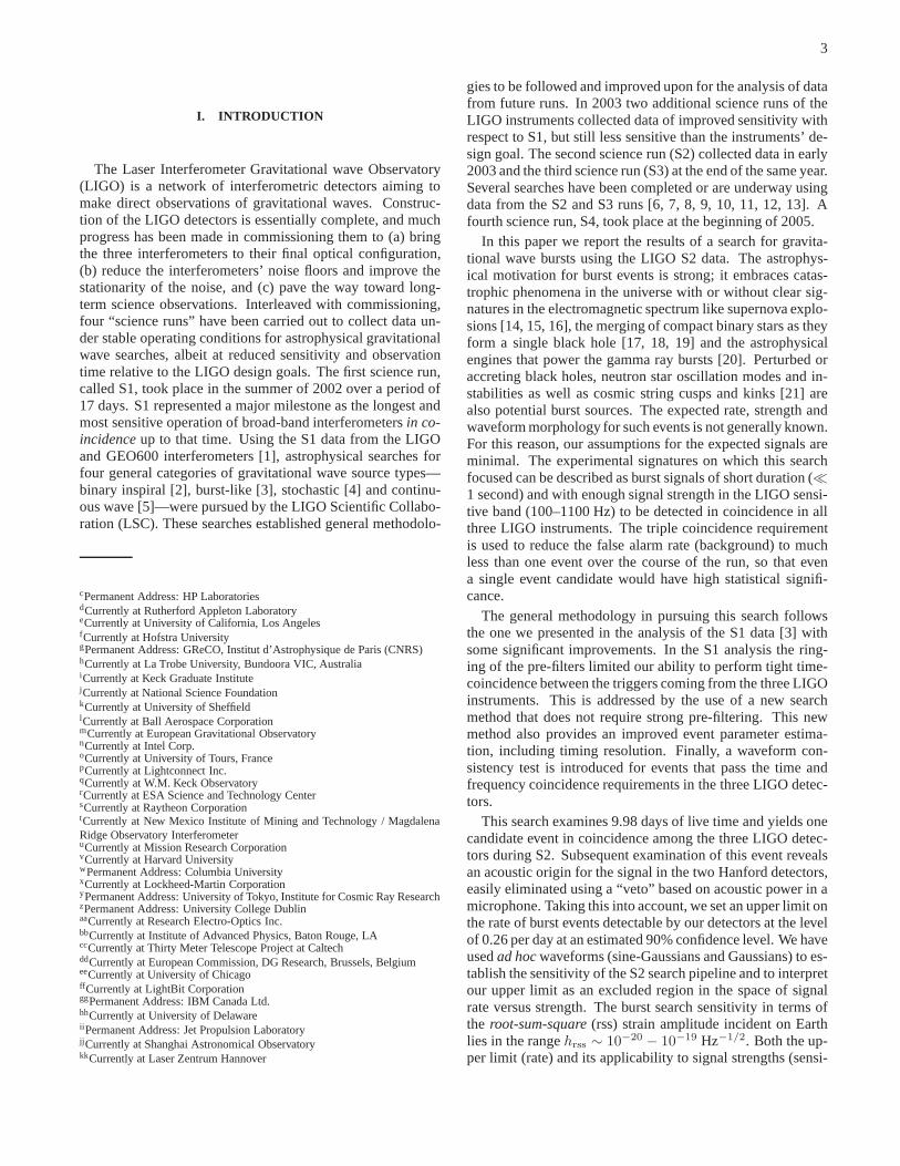
These changes led to a significant improvement in detec-tor sensitivity. Figure 1 shows typical spectra achieved bythe LIGO interferometers during the S2 run compared withLIGO’s S1 and design sensitivity. The differences among thethree LIGO S2 spectra reflect differences in the operating pa-rameters and hardware implementations of the three instru-ments, which were in various stages of reaching the final de-sign configuration.

5

102

103

10−23

10−22

10−21

10−20

10−19

10−18

frequency(Hertz)

stra

in/ √

Hz

S1: L1 (9 Sept ’02)S2: L1 (1 March ’03)S2: H1 (8 April ’04)S2: H2 (11 April ’04)

FIG. 1: Typical LIGO strain sensitivities in units of Hz−1/2 duringthe second science run (S2), compared to the most sensitive detector(L1) during the S1 science run. The solid line denotes the designgoal for the 4 km instruments.

B. Data from the S2 run

The data analyzed in this paper were taken during LIGO’ssecond science run (S2), which spanned 59 days from Febru-ary 14 to April 14, 2003. During this time, operators andscientific monitors worked to maintain continuous low noiseoperation of the LIGO instruments. The duty cycles for theindividual interferometers, defined as the fraction of the totalrun time when the interferometer was locked (i.e., all interfer-ometer control servos operating in their linear regime) andinits low noise configuration, were approximately 74% for H1,58% for H2 and 37% for L1; the triple coincidence duty cy-cle (i.e., the time during which all three interferometers weresimultaneously in lock and in low-noise configuration) was22%. The longest continuous locked stretch for any interfer-ometer during S2 was 66.2 hours for H1. The main sourcesof lost time were high microseismic motion at both sites dueto storms, and anthropogenic noise in the vicinity of the Liv-ingston Observatory.

Improved monitoring and automated alarms instituted afterS1 gave the operators and scientific monitors better warningsof out-of-nominal operating conditions for the interferome-ters. As a result, the fraction of time lost to high noise orto missing calibration lines (both major sources of unanalyz-able data during the S1 run) was greatly reduced. Thus, eventhough the S2 run was less than a factor of four longer thanthe S1 run and the duty cycle for triple interferometer coinci-dence was in fact marginally lower (23.4% for S1 vs. 22.0%for S2), the total amount ofanalyzabletriple coincidence datawas 305 hours compared to 34 hours for S1.

The signature of a gravitational wave is a differentialchange in the lengths of the two interferometer arms rela-tive to the nominal lengths established by the control system,s(t) = [∆Lx(t)−∆Ly(t)]/L , whereL is the average length

of thex andy arms. As in S1, this time series was derivedfrom the error signal of the feedback loop used to differen-tially control the lengths of the interferometer arms in orderto keep the optical cavities on resonance. To calibrate the er-ror signal, the effect of the feedback loop gain was measuredand divided out. Although more stable than during S1, theresponse functions varied over the course of the S2 run dueto drifts in the alignment of the optical elements. These weretracked by injecting fixed-amplitude sinusoidal signals (cali-bration lines) into the differential arm control loop, and moni-toring the amplitudes of these signals at the measurement (er-ror) point [24].

The S2 run also involved coincident running with theTAMA interferometer [25]. TAMA achieved a duty cycleof 81% and had a sensitivity comparable to LIGO’s above∼ 1 kHz, but had poorer sensitivity at lower frequencieswhere the LIGO detectors had their best sensitivity. In addi-tion, the location and orientation of the TAMA detector differssubstantially from the LIGO detectors, which further reducedthe chance of a coincident detection at low frequencies. Forthese reasons, the joint analysis of LIGO and TAMA data fo-cused on gravitational wave frequencies from 700–2000 Hzand will be described in a separate paper [10]. In this paper,we report the result of a LIGO-only search for signals in therange 100–1100 Hz. The overlap between these two searches(700–1100 Hz) serves to ensure that possible sources with fre-quency content spanning the two searches will not be missed.The GEO600 interferometer [26], which collected data simul-taneously with LIGO during the S1 run, was undergoing com-missioning at the time of the S2 run.

III. SEARCH PIPELINE OVERVIEW

The overall burst search pipeline used in the S2 analysisfollows the one we introduced in our S1 search [3]. First, dataselection criteria are applied in order to define periods whenthe instruments are well behaved and the recorded data can beused for science searches (section IV).

A wavelet-based algorithm called WaveBurst [27, 28] (sec-tion V) is then used to identify candidate burst events. Ratherthan operating on the data from a single interferometer, Wave-Burst analyzes simultaneously the time series coming from apair of interferometers and incorporates strength thresholdingas well as time and frequency coincidence to identify tran-sients with consistent features in the two data streams. Toreduce the false alarm rate, we further require that candidategravitational wave events occur effectively simultaneously inall three LIGO detectors (section V B). Besides requiringcompatible WaveBurst event parameters, this involves a wave-form consistency test, ther-statistic [29] (section V C), whichis based on forming the normalized linear correlation of theraw time series coming from the LIGO instruments. This testtakes advantage of the fact that the arms of the interferome-ters at the two LIGO sites are nearly co-aligned, and thereforea gravitational wave generally will produce correlated timeseries. The use of WaveBurst and ther-statistic are the majorchanges in the S2 pipeline with respect to the pipeline used

6

for S1 [3].When candidate burst events are identified, they can be

checked against veto conditions based on the many auxiliaryread-back channels of the servo control systems and physi-cal environment monitoring channels that are recorded in theLIGO data stream (section VI).

The background in this search is measured by artificiallyshifting in time the raw time series of one of the LIGO in-struments, L1, and repeating the analysis as for the un-shifteddata. The time-shifted case will often be referred to as “time-lag” data and the unshifted case as “zero-lag” data. We willdescribe the background estimation in more detail in sec-tion VII.

We have relied on hardware and software signal “injec-tions” in order to establish the efficiency of the pipeline. Sim-ulated signals with various morphologies [30] were added tothe digitized raw data time series at the beginning of our anal-ysis pipeline and were used to establish the fraction of de-tected events as a function of their strength (section VIII).The same analysis pipeline was used to analyze raw (zero-lag), time-lag, and injection data samples.

We maintain a detailed list with a number of checks to per-form for any zero-lag event(s) surviving the analysis pipelineto evaluate whether they could plausibly be gravitational wavebursts. This “detection check-list” is updated as we learn moreabout the instruments and refine our methodology. A majoraspect is the examination of environmental and auxiliary in-terferometric channels in order to identify terrestrial distur-bances that might produce a candidate event through somecoupling mechanism. Any remaining events are comparedwith the background and the experiment’s live time in orderto establish a detection or an upper limit on the rate of burstevents.

IV. DATA SELECTION

The selection of data to be analyzed was a key first step inthis search. We expect a gravitational wave to appear in allthree LIGO instruments, although in some cases it may be ator below the level of the noise. For this search, werequirea signal above the noise baseline in all three instruments inorder to suppress the rate of noise fluctuations that may fakeastrophysical burst events. In the case of a genuine astrophys-ical event this requirement will not only increase our detectionconfidence but it will also allow us to extract in the best possi-ble way the signal and source parameters. Therefore, for thissearch we have confined ourselves to periods of time whenall three LIGO interferometers were simultaneously lockedinlow noise mode with nominal operating parameters (nominalservo loop gains, nominal filter settings, etc.), marked by amanually set bit (“science mode”) in the data stream. Thisproduced a total of 318 hours of potential data for analysis.This total was reduced by the following data selection cuts:

• A minimum duration of 300 seconds was required fora triple coincidence segment to be analyzed for thissearch. This cut eliminated0.9% of the initial data set.

• Post-run re-examination of the interferometer configu-ration and status channels included in the data streamidentified a small amount of time when the interferom-eter configuration deviated from nominal. In additionwe identified short periods of time when the timing sys-tem for the data acquisition had lost synchronization.These cuts reduced the data set by0.2%.

• It was discovered that large low frequency excitationsof the interferometer could cause the photodiode at theanti-symmetric port to saturate. This caused bursts ofexcess noise due to nonlinear up-conversion. These pe-riods of time were identified and eliminated, reducingthe data set by 0.3%.

• There were occasional periods of time when the cal-ibration lines either were absent or were significantlyweaker than normal. Eliminating these periods reducedthe data set by approximately 2%.

• The H1 interferometer had a known problem with amarginally stable servo loop, which occasionally led tohigher than normal noise in the error signal for the dif-ferential arm length (the channel used in this search forgravitational waves). A data cut was imposed to elim-inate periods of time when the RMS noise in the 200–400 Hz band of this channel exceeded a threshold valuefor 5 consecutive minutes. The requirement for 5 con-secutive minutes was imposed to prevent a short burst ofgravitational waves (the object of this search) from trig-gering this cut. This cut reduced the data set by 0.4%.

These data quality cuts eliminated a total of 13 hours fromthe original 318 hours of triple coincidence data, leaving a“live-time” of 305 hours. The fraction of data surviving thesequality cuts (96%) is a significant improvement over the expe-rience in S1 when only 37% of the data passed all the qualitycuts.

The trigger generation software used in this search (to bedescribed in the next section) processed data in fixed 2-minutetime intervals, requiring good data quality for the entire inter-val. This constraint, along with other constraints imposedbyother trigger generation methods which were initially usedtodefine a common data set, led to a net loss of 41 hours, leaving264 hours of triple coincidence data actually searched.

The search for bursts in the LIGO S2 data used roughly10% of the triple coincidence data set in order to tune thepipeline (as described below) and establish event selection cri-teria. This data set was chosen uniformly across the acquisi-tion time and constituted the so-called “playground” for thesearch. The rate bound calculated in Sec. VII reflects only theremaining∼90% of the data, in order to avoid bias from thetuning procedures.

V. METHODS FOR EVENT TRIGGER SELECTION

An accurate knowledge of gravitational wave burst wave-forms would allow the use ofmatched filtering[31] along the

7

lines of the search for binary inspirals [2, 8]. However, manydifferent astrophysical systems may give rise to gravitationalwave bursts, and the physics of these systems is often verycomplicated. Even when numerical relativistic calculationshave been carried out, as in the case of core collapse super-novae, they generally yield roughly representative waveformsrather than exact predictions. Therefore, our present searchesfor gravitational wave bursts use general algorithms whicharesensitive to a wide range of potential signals.

The first LIGO burst search [3] used two Event TriggerGenerator (ETG) algorithms: a time-domain method designedto detect a large “slope” (time derivative) in the data streamafter suitable filtering [32, 33], and a method calledTFCLUS-TERS [34] which is based on identifying clusters of excesspower in time-frequency spectrograms. Several other burst-search methods have been developed by members of the LIGOScientific Collaboration. For this paper, we have chosen to fo-cus on a single ETG called WaveBurst which identifies clus-ters of excess power once the signal is decomposed in thewavelet domain, as described below. Other methods whichwere applied to the S2 data includeTFCLUSTERS; the ex-cess power statistic of Andersonet al. [35]; and the “Block-Normal” time-domain algorithm [36]. In preliminary studiesusing S2 playground data, these other methods had sensitiv-ities comparable to WaveBurst for the target waveforms de-scribed in section VIII, but their implementations were lessmature at the time of this analysis.

An integral part of our S2 search and the final event trig-ger selection is to perform a consistency test among the datastreams recorded by the different interferometers at each trig-ger time identified by the ETG. This is done using ther-statistic [29], a time-domain cross-correlation method sensi-tive to the coherent part of the candidate signals, described insubsection C below.

A. WaveBurst

WaveBurst is an ETG that searches for gravitational wavebursts in the wavelet time-frequency domain. It is described ingreater detail in [27, 28]. The method uses wavelet transfor-mations in order to obtain the time-frequency representationof the data. Bursts are identified by searching for regions inthe wavelet time-frequency domain with an excess of power,coincident between two or more interferometers, that is incon-sistent with stationary detector noise.

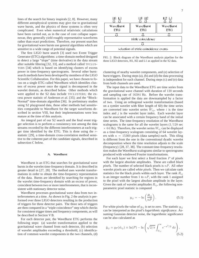
WaveBurst processes gravitational wave data from two in-terferometers at a time. As shown in Fig. 2 the analysis is per-formed over three LIGO detectors resulting in the productionof triggers for three detector pairs. The three sets of triggersare then compared in a “triple coincidence” step which checksfor consistent trigger times and frequency components, as willbe described in Section V B.

For each detector pair, the WaveBurst ETG performs thefollowing steps: (a) wavelet transformation applied to thegravitational wave channel from each detector, (b) selectionof wavelet amplitudes exceeding a threshold, (c) identifica-tion of common wavelet components in the two channels, (d)

FIG. 2: Block diagram of the WaveBurst analysis pipeline forthethree LIGO detectors, H1, H2 and L1 as applied in the S2 data.

clustering of nearby wavelet components, and (e) selectionofburst triggers. During steps (a), (b) and (d) the data processingis independent for each channel. During steps (c) and (e) datafrom both channels are used.

The input data to the WaveBurst ETG are time series fromthe gravitational wave channel with duration of120 secondsand sampling rate of16384 Hz. Before the wavelet trans-formation is applied the data are downsampled by a factorof two. Using an orthogonal wavelet transformation (basedon a symlet wavelet with filter length of 60) the time seriesare converted into wavelet seriesWij , wherei is the timeindex andj is the wavelet layer index. Each wavelet layercan be associated with a certain frequency band of the initialtime series. The time-frequency resolution of the WaveBurstscalograms is the same for all the wavelet layers (1/128 sec× 64 Hz). Therefore, the wavelet seriesWij can be displayedas a time-frequency scalogram consisting of 64 wavelet lay-ers withn = 15360 pixels (data samples) each. This tilingis different from the one in the conventional dyadic waveletdecomposition where the time resolution adjusts to the scale(frequency) [28, 37, 38]. The constant time-frequency resolu-tion makes the WaveBurst scalograms similar to spectrogramsproduced with windowed Fourier transformations.

For each layer we first select a fixed fractionP of pixelswith the largest absolute amplitudes. These are calledblackpixels. The number of selected black pixels isnP . All otherwavelet pixels are calledwhite pixels. Then we calculate rankstatistics for the black pixels within each layer. The rankRij

is an integer number from 1 tonP , with the rank 1 assignedto the pixel with the largest absolute amplitude in the layer.Given the rank of wavelet amplitudesRij , the following non-parametric pixel statistic is computed

yij = − ln

(

Rij

nP

)

. (5.1)

For white pixels the value ofyij is set to zero. The statisticyij

can be interpreted as the pixel’slogarithmic significance. As-suming Gaussian detector noise, the logarithmic significancecan be also calculated as

yij = gP (wij) ≡ ln(P ) − ln

(

√

2/π

∫ ∞

wij

e−x2/2 dx

)

,

(5.2)

8

wherewij is the absolute value of the pixel amplitude in unitsof the noise standard deviation. In practice, the LIGO detec-tor noise is not Gaussian and its probability distribution func-tion is not determineda priori. Therefore, we use the non-parametric statisticyij , which is a more robust measure ofthe pixel significance thanyij . Using the inverse function ofgP with yij as an argument, we introduce thenon-parametricamplitude

wij = g−1P (yij), (5.3)

and theexcess power ratio

ρij = w2ij − 1, (5.4)

which characterizes the pixel excess power above the averagedetector noise.

After the black pixels are selected, we require their time-coincidence in the two channels. Given a black pixel of sig-nificanceyij in the first channel, this is accepted if the signif-icance of neighboring (in time) pixels in the second channel(y′ij) satisfies

y′(i−1)j + y′ij + y′(i+1)j > η, (5.5)

whereη is the coincidence threshold. Otherwise, the pixelis rejected. This procedure is repeated for all the black pix-els in the first channel. The same coincidence algorithm isapplied to pixels in the second channel. As a result, a con-siderable number of black pixels in both channels producedby fluctuations of the detector noise are rejected. At the sametime, black pixels produced by gravitational wave bursts havea high acceptance probability because of the coherent excessof power in two detectors.

After the coincidence procedure is applied to both channelsa clustering algorithm is applied jointly to the two channelpixel maps. As a first step, we merge (OR) the black pixelsfrom both channels into one time-frequency plane. For eachblack pixel we define neighbors (either black or white), whichshare a side or a vertex with the black pixel. The white neigh-bors are calledhalo pixels. We define a cluster as a group ofblack and halo pixels which are connected either by a side ora vertex. After the cluster reconstruction, we go back to theoriginal time-frequency planes and calculate the cluster pa-rameters separately for each channel. Therefore, there areal-ways two clusters, one per channel, which form a WaveBursttrigger.

The cluster parameters are calculated using black pixelsonly. For example, the cluster sizek is defined as the num-ber of black pixels. Other parameters which characterize thecluster strength are the cluster excess power ratioρ and theclusterlogarithmic likelihoodY . Given a clusterC, these areestimated by summing over the black pixels in the cluster:

ρ =∑

ij∈C

ρij , Y =∑

ij∈C

yij . (5.6)

Given the timesti of individual pixels, the cluster center timeis calculated as

T =∑

ij∈C

ti w2ij /

∑

ij∈C

w2ij . (5.7)

As configured for this analysis, WaveBurst initially generatedtriggers with frequency content between 64 Hz and 4096 Hz.As we will see below, the cluster size, likelihood, and excesspower ratio can be used for the further selection of triggers,while the cluster time and frequency span are used in a coin-cidence requirement. The frequency band of interest for thisanalysis, 100–1100 Hz, is selected during the later stages ofthe analysis.

There are two main WaveBurst tunable input parameters:the black pixel fractionP which is applied to each frequencylayer, and the coincidence thresholdη. The purpose of theseparameters is to control the average black pixel occupancyO(P, η), the fraction of black pixels over the entire time-frequency scalogram. To ensure robust cluster reconstruction,the occupancy should not be greater than1%. For white Gaus-sian detector noise the functional form ofO(P, η) can be cal-culated analytically. This can be used to set a constraint onPandη for a given targetO(P, η). If P is set too small (lessthen a few percent), noise outliers due to instrumental glitchesmay monopolize the limited number of available black pixelsand thus allow gravitational wave signals to remain hidden.To avoid this domination of instrumental glitches, we run theanalysis withP equal to 10%. This value ofP together withthe occupancy targetO(P, η) of 0.7% defines the coincidencethresholdη at 1.5.

All the tuning of the WaveBurst method was performed onthe S2 playground data set (Section IV). For the selected val-ues ofP andη, the average trigger rate per LIGO instrumentpair was approximately6 Hz, about twice the false alarm rateexpected for white Gaussian detector noise. The trigger ratewas further reduced by imposing cuts on the excess power ra-tio ρ. For clusters of sizek greater than1 we requiredρ to begreater than6.25 while for single pixel clusters (k = 1) weused a more restrictive cut ofρ greater than9. This selectionon the event parameters further reduced the counting rates perLIGO instrument pair to∼ 1 Hz. The times and reconstructedparameters of WaveBurst events passing these criteria werewritten onto disk. This allowed the further processing and se-lection of these events without the need to re-analyze the fulldata stream, a process which is generally time and CPU inten-sive.

B. Triple coincidence

Further selection of WaveBurst events proceeds by identi-fying triple coincidences. The output of the WaveBurst ETGis a set of coincident triggers for a selected interferometerpairA,B. Each WaveBurst trigger consists of two clusters,one inA and one inB. For the three LIGO interferometersthere are three possible pairs: (L1,H1), (H1,H2) and (H2,L1).In order to establish triple coincidence events, we requireatime-frequency coincidence of the WaveBurst triggers gener-ated for these three pairs. To evaluate the time coincidencewe first constructTAB = (TA + TB)/2, i.e., the averagecentral time of theA andB clusters for the trigger. Threesuch combined central times are thus constructed:TL1H1,TH1H2, andTH2L1. We then require that all possible dif-

9

ferences of these combined central times fall within a timewindowTw = 20 ms. This window is large enough to accom-modate the maximum difference in gravitational wave arrivaltimes at the two detector sites (10 ms) and the intrinsic timeresolution of the WaveBurst algorithm which has an rms onthe order of3 ms as discussed in section VIII.

We apply a loose requirement on the frequency consistencyof the WaveBurst triggers. First, we calculate the minimum(fmin) and maximum (fmax) frequency for each interferome-ter pair(A,B)

fmin = min(fAlow, f

Blow), fmax = max(fA

high, fBhigh),

(5.8)whereflow andfhigh are the low and high frequency bound-aries of theA andB clusters. Then, the trigger frequencybands are calculated asfmax − fmin for all pairs. For the fre-quency coincidence, the bands of all three WaveBurst triggersare required to overlap. An average frequency is then calcu-lated from the clusters, weighted by signal-to-noise ratio, andthe coincident event candidate is kept for this analysis if thisaverage frequency is above 64 Hz and below 1100 Hz.

The final step in the coincidence analysis of the WaveBurstevents involves the construction of a single measure of theircombined significance. As we described already, triple coin-cidence events consist of three WaveBurst triggers involving atotal of six clusters. Each cluster has its parameters calculatedon a per-interferometer basis. Assuming white detector noise,the variableY for a cluster of sizek follows a Gamma prob-ability distribution. This motivates the use of the followingmeasure of thecluster significance:

Z = Y − ln

(

k−1∑

m=0

Y m

m!

)

, (5.9)

which is derived from the logarithmic likelihoodY of a clusterC and from the numberk of black pixels in that cluster [27,28]. Given the significance of the six clusters, we compute thecombined significanceof the triple coincidence event as

ZG =(

ZL1L1H1 Z

H1L1H1 Z

H2H2L1 Z

L1H2L1 Z

H1H1H2 ZH2

H1H2

)1/6,

(5.10)whereZA

AB (ZBAB) is the significance of theA (B) cluster for

the(A,B) interferometer pair.In order to evaluate the rate of accidental coincidences, we

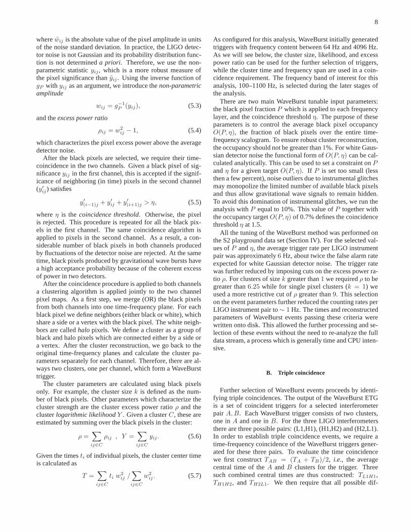
have repeated the above analysis on the data after introduc-ing an unphysical time shift (“lag”) in the Livingston datastream relative to the Hanford data streams. The Hanforddata streams are not shifted relative to one another, so anynoise correlations from the local environment are preserved.Figure 3 shows the distribution of cluster significance (equa-tion 5.9) from the three individual detectors, and the com-bined significance (equation 5.10), over the entire S2 data set,for both zero-lag and time-lag coincidences. Using 46 suchtime-lag instances of the S2 playground data we have set thethreshold onZG for this search in order to yield a targetedfalse alarm rate of10 µHz. Without significantly compromis-ing the pipeline sensitivity, this threshold was selected to beln(ZG) > 1.7. In the 64–1100 Hz frequency band, the result-

ing false alarm rate in the S2 playground analysis was approx-imately15 µHz. The coincident events selected by WaveBurstin this way are then checked for their waveform consistencyusing ther-statistic.

L1Entries 2845Mean 2.615RMS 1.926

significance1 10

even

ts

1

10

210 L1Entries 2845Mean 2.615RMS 1.926

H1Entries 2845Mean 2.603RMS 1.7

significance1 10

even

ts

1

10

210H1

Entries 2845Mean 2.603RMS 1.7

H2Entries 2845Mean 2.572RMS 1.826

significance1 10

even

ts1

10

210 H2Entries 2845Mean 2.572RMS 1.826

L1xH1xH2Entries 2845Mean 2.235RMS 0.9299

significance

even

ts

1

10

210L1xH1xH2


FIG. 3: The significance distribution of the triple coincident Wave-Burst events for individual detectors (L1, H1, H2) and the combinedsignificance of their triple coincidences (L1xH1xH2) for the S2 dataset. Solid histograms reflect the zero-lag events, while thepointsrepresent background (time-lag) events as produced with unphysicaltime shifts between the Livingston and Hanford detectors (and nor-malized to the S2 live-time). The change in the significance distri-bution for the individual detectors around significance equal to fouris attributed to the onset of single pixel clusters (for which a higherthreshold was applied).

C. r-statistic test

Ther-statistic test [29] is applied as the final step of search-ing for gravitational wave event candidates. This test re-analyzes the raw (unprocessed) interferometer data aroundthetimes of coincident events identified by the WaveBurst ETG.

The fundamental building block in performing this wave-form consistency test is ther-statistic, or the normalized lin-ear correlation coefficient of two sequences,{xi} and{yi} (inthis case, the two gravitational wave signal time series):

r =

∑

i(xi − x)(yi − y)√∑

i(xi − x)2√∑

i(yi − y)2, (5.11)

10

wherex and y are their respective mean values. This quan-tity assumes values between−1 for fully anti-correlated se-quences and+1 for fully correlated sequences. For uncorre-lated white noise, we expect ther-statistic values obtained forarbitrary sets of points of lengthN to follow a normal distri-bution with zero mean andσ = 1/

√N . Any coherent com-

ponent in the two sequences will causer to deviate from theabove normal distribution. As a normalized quantity, ther-statistic does not attempt to measure the consistency betweenthe relative amplitudes of the two sequences. Consequently,it offers the advantage of being robust against fluctuationsofdetector amplitude response and noise floor. A similar methodbased on this type of time-domain cross-correlation has beenimplemented in a LIGO search for gravitational waves asso-ciated with a GRB [7, 39] and elsewhere [40].

As will be described below, the final output of ther-statistictest is a combined confidence statistic which is constructedfrom r-statistic values calculated for all three pairs of inter-ferometers. For each pair, we use only the absolute value ofthe statistic,|r|, rather than the signed value. This is becausean astrophysical signal can produce either a correlation orananticorrelation in the interferometers at the two LIGO sites,depending on its sky position and polarization. In fact, ther-statistic analysis was done using whitened (see below) butotherwise uncalibrated data, with an arbitrary sign convention.A signed correlation test using calibrated data would be ap-propriate for the H1-H2 pair, but all three pairs were treatedequivalently in the present analysis.

The number of pointsN considered in calculating thestatistic in Eq. (5.11), or equivalently theintegration timeτ ,is the most important parameter in the construction of ther-statistic. Its optimal value depends in general on the durationof the signal being considered for detection. Ifτ is too long,the candidate signal is “washed out” by the noise when com-putingr. On the other hand, if it is too short, then only part ofthe coherent signal is included in the integration. Simulationstudies have shown that most of the short-lived signals of in-terest to the LIGO burst search can be identified successfullyusing a set of three discrete integration times with lengthsof20, 50 and 100 ms.

Within its LIGO implementation, ther-statistic analysisfirst performs data “conditioning” to restrict the frequencycontent of the data to LIGO’s most sensitive band and to sup-press any coherent lines and instrumental artifacts. Each datastream is first band-pass filtered with an 8th-order Butterworthfilter with corner frequencies of 100 Hz and 1572 Hz, thendown-sampled to a 4096 Hz sampling rate. The upper fre-quency of 1572 Hz was chosen in order to have 20 dB suppres-sion at 2048 Hz and thus avoid aliasing. The lower frequencyof 100 Hz was chosen to suppress the contribution of seismicnoise; it also defines the lower edge of the frequency bandfor this gravitational wave burst search, since it is above thelower frequency limit of 64 Hz for WaveBurst triggers. Theband-passed data are then whitened with a linear predictor er-ror filter with a 10 Hz resolution trained on a 10 second periodbefore the event start time. The filter removes predictable con-tent, including lines that were stationary over a 10 second timescale. It also has the effect of suppressing frequency bands

with large stationary noise, thus emphasizing transients [38].The next step in ther-statistic analysis involves the con-

struction of all the possibler coefficients given the number ofinterferometer pairs involved in the trigger, their possible rel-ative time-delays due to their geographic separation, and thevarious integration times being considered. Relative timede-lays up to±10 ms are considered for each detector pair, cor-responding to the light travel time between the Hanford andLivingston sites. Future analyses will restrict the time delay toa much smaller value when correlating data from the two Han-ford interferometers, to allow only for time calibration uncer-tainties. Furthermore, in the case of WaveBurst triggers withreported durations greater than the integration timeτ , mul-tiple integrationwindowsof that length are considered, off-set from the reported start time of the trigger by multiples ofτ/2. For a given integration window indexed byp (containingNp data samples), ordered pair of instruments indexed byl,m(l 6= m), and relative time delay indexed byk, ther-statisticvalue |rk

plm| is calculated. For eachp lm combination, thedistribution of |rk

plm| for all values ofk is compared to thenull hypothesis expectation of a normal distribution with zeromean andσ = 1/

√

Np using the Kolmogorov-Smirnov test.If these are statistically consistent at the 95% level, thenthealgorithm assigns no significance to any apparent correlationin this detector pair. Otherwise, a one-sided significance andits associated logarithmic confidence are calculated from themaximumvalue of |rk

plm| for any time delay, compared towhat would be expected if there were no correlation. Con-fidence values for all ordered detector pairs are then averagedto define the combined correlation confidence for a given in-tegration window. The final result of ther-statistic test,Γ, isthe maximum of the combined correlation confidence over allof the integration windows being considered. Events with avalue ofΓ above a given threshold are finally selected.

Ther-statistic implementation, filter parameters, and set ofintegration times were chosen based on their performance forvarious simulated signals. The single remaining parameter,the threshold onΓ, was tuned primarily in order to ensurethat much less than one background event was expected in thewhole S2 run, corresponding to a rate of O(0.1) µHz. Sincethe rate of WaveBurst triggers was approximately15 µHz, asmentioned in Section V B, a rejection factor of around 150was required.

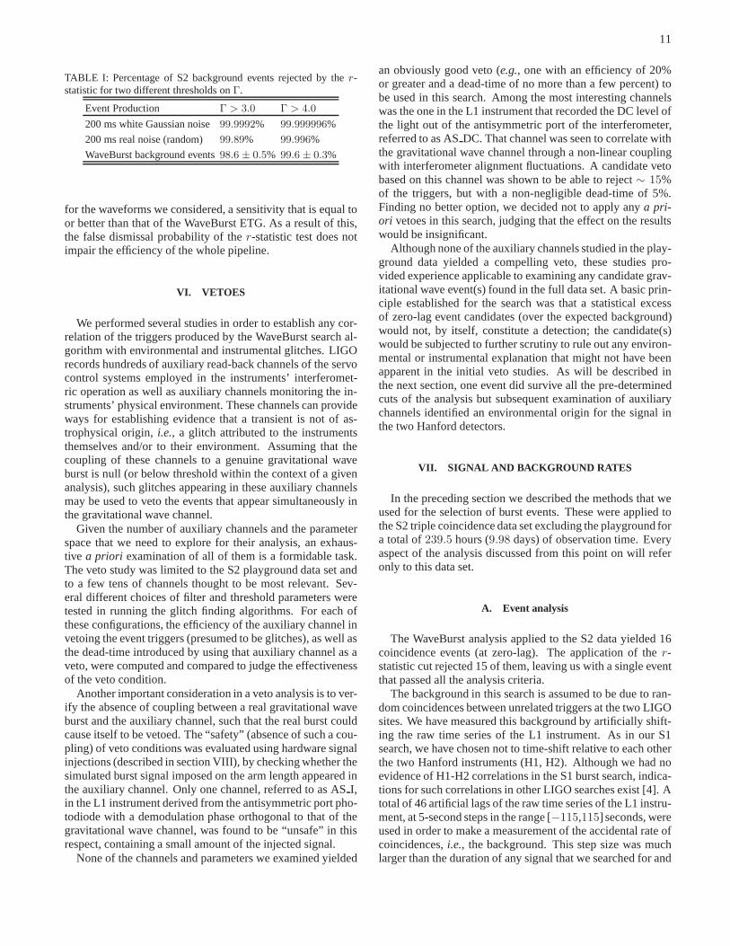
Table I shows the rejection efficiency of ther-statistic testfor two thresholds onΓ when the test is applied to white Gaus-sian noise (200 ms segments), to real S2 interferometer noiseat randomly selected times (200 ms segments), and to the dataat the times of time-lag (i.e., background) WaveBurst triggersin the S2 playground. In the first two cases, 200 ms of datawas processed by ther-statistic algorithm, whereas in the lat-ter case, the amount of data processed was determined by thetrigger duration reported by WaveBurst. The table shows thatrandom detector noise rarely produced aΓ value above3.0,but the rejection factor for WaveBurst triggers was not highenough. AΓ threshold of4.0 was ultimately chosen for thisanalysis, yielding an estimated rejection factor of∼ 250 forWaveBurst triggers. As we will discuss in Section VIII, ther-statistic waveform consistency test withΓ > 4.0 represents,

11

TABLE I: Percentage of S2 background events rejected by ther-statistic for two different thresholds onΓ.

Event Production Γ > 3.0 Γ > 4.0

200 ms white Gaussian noise99.9992% 99.999996%

200 ms real noise (random) 99.89% 99.996%

WaveBurst background events98.6 ± 0.5% 99.6 ± 0.3%

for the waveforms we considered, a sensitivity that is equaltoor better than that of the WaveBurst ETG. As a result of this,the false dismissal probability of ther-statistic test does notimpair the efficiency of the whole pipeline.

VI. VETOES

We performed several studies in order to establish any cor-relation of the triggers produced by the WaveBurst search al-gorithm with environmental and instrumental glitches. LIGOrecords hundreds of auxiliary read-back channels of the servocontrol systems employed in the instruments’ interferomet-ric operation as well as auxiliary channels monitoring the in-struments’ physical environment. These channels can provideways for establishing evidence that a transient is not of as-trophysical origin,i.e., a glitch attributed to the instrumentsthemselves and/or to their environment. Assuming that thecoupling of these channels to a genuine gravitational waveburst is null (or below threshold within the context of a givenanalysis), such glitches appearing in these auxiliary channelsmay be used to veto the events that appear simultaneously inthe gravitational wave channel.

Given the number of auxiliary channels and the parameterspace that we need to explore for their analysis, an exhaus-tive a priori examination of all of them is a formidable task.The veto study was limited to the S2 playground data set andto a few tens of channels thought to be most relevant. Sev-eral different choices of filter and threshold parameters weretested in running the glitch finding algorithms. For each ofthese configurations, the efficiency of the auxiliary channel invetoing the event triggers (presumed to be glitches), as well asthe dead-time introduced by using that auxiliary channel asaveto, were computed and compared to judge the effectivenessof the veto condition.

Another important consideration in a veto analysis is to ver-ify the absence of coupling between a real gravitational waveburst and the auxiliary channel, such that the real burst couldcause itself to be vetoed. The “safety” (absence of such a cou-pling) of veto conditions was evaluated using hardware signalinjections (described in section VIII), by checking whether thesimulated burst signal imposed on the arm length appeared inthe auxiliary channel. Only one channel, referred to as ASI,in the L1 instrument derived from the antisymmetric port pho-todiode with a demodulation phase orthogonal to that of thegravitational wave channel, was found to be “unsafe” in thisrespect, containing a small amount of the injected signal.

None of the channels and parameters we examined yielded

an obviously good veto (e.g., one with an efficiency of 20%or greater and a dead-time of no more than a few percent) tobe used in this search. Among the most interesting channelswas the one in the L1 instrument that recorded the DC level ofthe light out of the antisymmetric port of the interferometer,referred to as ASDC. That channel was seen to correlate withthe gravitational wave channel through a non-linear couplingwith interferometer alignment fluctuations. A candidate vetobased on this channel was shown to be able to reject∼ 15%of the triggers, but with a non-negligible dead-time of 5%.Finding no better option, we decided not to apply anya pri-ori vetoes in this search, judging that the effect on the resultswould be insignificant.

Although none of the auxiliary channels studied in the play-ground data yielded a compelling veto, these studies pro-vided experience applicable to examining any candidate grav-itational wave event(s) found in the full data set. A basic prin-ciple established for the search was that a statistical excessof zero-lag event candidates (over the expected background)would not, by itself, constitute a detection; the candidate(s)would be subjected to further scrutiny to rule out any environ-mental or instrumental explanation that might not have beenapparent in the initial veto studies. As will be described inthe next section, one event did survive all the pre-determinedcuts of the analysis but subsequent examination of auxiliarychannels identified an environmental origin for the signal inthe two Hanford detectors.

VII. SIGNAL AND BACKGROUND RATES

In the preceding section we described the methods that weused for the selection of burst events. These were applied tothe S2 triple coincidence data set excluding the playgroundfora total of239.5 hours (9.98 days) of observation time. Everyaspect of the analysis discussed from this point on will referonly to this data set.

A. Event analysis

The WaveBurst analysis applied to the S2 data yielded 16coincidence events (at zero-lag). The application of ther-statistic cut rejected 15 of them, leaving us with a single eventthat passed all the analysis criteria.

The background in this search is assumed to be due to ran-dom coincidences between unrelated triggers at the two LIGOsites. We have measured this background by artificially shift-ing the raw time series of the L1 instrument. As in our S1search, we have chosen not to time-shift relative to each otherthe two Hanford instruments (H1, H2). Although we had noevidence of H1-H2 correlations in the S1 burst search, indica-tions for such correlations in other LIGO searches exist [4]. Atotal of 46 artificial lags of the raw time series of the L1 instru-ment, at 5-second steps in the range [−115,115] seconds, wereused in order to make a measurement of the accidental rate ofcoincidences,i.e., the background. This step size was muchlarger than the duration of any signal that we searched for and

12

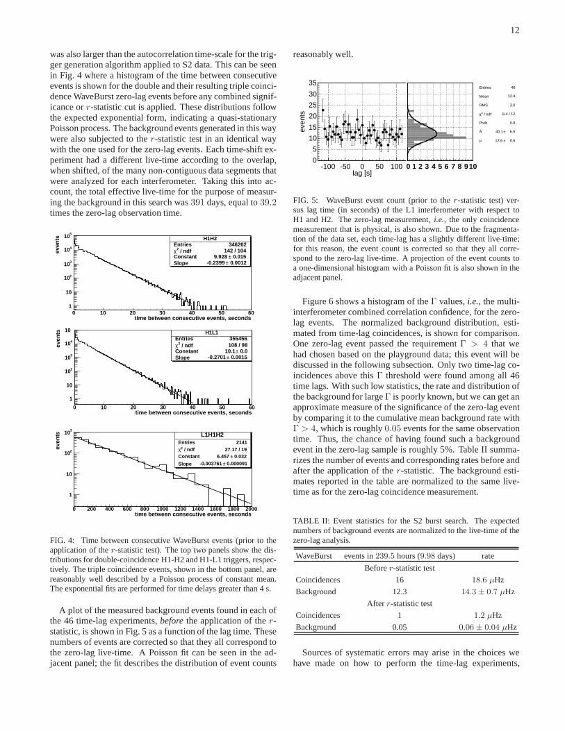
was also larger than the autocorrelation time-scale for thetrig-ger generation algorithm applied to S2 data. This can be seenin Fig. 4 where a histogram of the time between consecutiveevents is shown for the double and their resulting triple coinci-dence WaveBurst zero-lag events before any combined signif-icance orr-statistic cut is applied. These distributions followthe expected exponential form, indicating a quasi-stationaryPoisson process. The background events generated in this waywere also subjected to ther-statistic test in an identical waywith the one used for the zero-lag events. Each time-shift ex-periment had a different live-time according to the overlap,when shifted, of the many non-contiguous data segments thatwere analyzed for each interferometer. Taking this into ac-count, the total effective live-time for the purpose of measur-ing the background in this search was391 days, equal to39.2times the zero-lag observation time.

H1H2Entries 346262

/ ndf 2χ 142 / 104Constant 0.015± 9.928 Slope 0.0012± -0.2399

time between consecutive events, seconds0 10 20 30 40 50 60

even

ts

1

10

210

310

410

510 H1H2Entries 346262


H1L1Entries 355456


time between consecutive events, seconds0 10 20 30 40 50 60

even

ts

1

10

210

310

410

10 H1L1Entries 355456


L1H1H2Entries 2141

/ ndf 2χ 27.17 / 19Constant 0.032± 6.457

Slope 0.000091± -0.003761

time between consecutive events, seconds0 200 400 600 800 1000 1200 1400 1600 1800 2000

even

ts

1

10

210

310 L1H1H2Entries 2141

/ ndf 2χ 27.17 / 19Constant 0.032± 6.457

Slope 0.000091± -0.003761

FIG. 4: Time between consecutive WaveBurst events (prior totheapplication of ther-statistic test). The top two panels show the dis-tributions for double-coincidence H1-H2 and H1-L1 triggers, respec-tively. The triple coincidence events, shown in the bottom panel, arereasonably well described by a Poisson process of constant mean.The exponential fits are performed for time delays greater than 4 s.

A plot of the measured background events found in each ofthe 46 time-lag experiments,beforethe application of ther-statistic, is shown in Fig. 5 as a function of the lag time. Thesenumbers of events are corrected so that they all correspond tothe zero-lag live-time. A Poisson fit can be seen in the ad-jacent panel; the fit describes the distribution of event counts

reasonably well.

lag [s]-100 -50 0 50 100

even

ts

0

5

10

15

20

25

30

35

0 1 2 3 4 5 6 7 8 910

Entries 46

Mean 12.4

RMS 3.0

/ ndf 2χ 8.4 / 12

Prob 0.8

A 6.5± 40.1

µ 0.6± 12.6

FIG. 5: WaveBurst event count (prior to ther-statistic test) ver-sus lag time (in seconds) of the L1 interferometer with respect toH1 and H2. The zero-lag measurement,i.e., the only coincidencemeasurement that is physical, is also shown. Due to the fragmenta-tion of the data set, each time-lag has a slightly different live-time;for this reason, the event count is corrected so that they allcorre-spond to the zero-lag live-time. A projection of the event counts toa one-dimensional histogram with a Poisson fit is also shown in theadjacent panel.

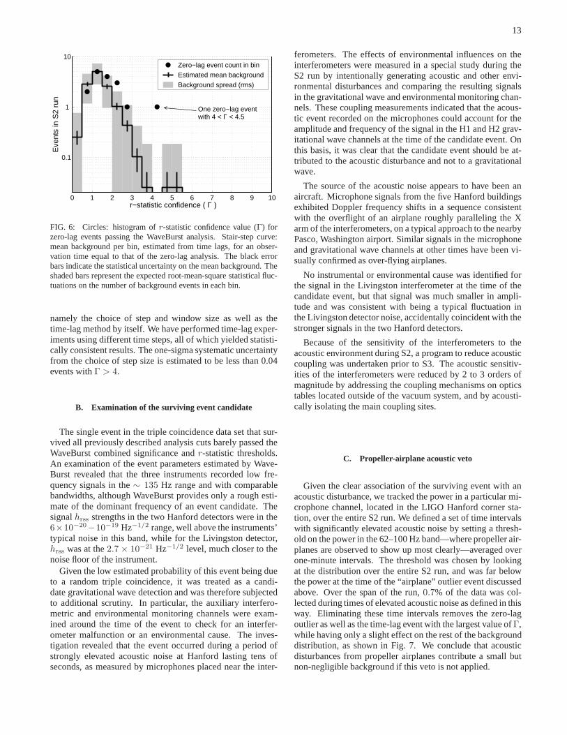
Figure 6 shows a histogram of theΓ values,i.e., the multi-interferometer combined correlation confidence, for the zero-lag events. The normalized background distribution, esti-mated from time-lag coincidences, is shown for comparison.One zero-lag event passed the requirementΓ > 4 that wehad chosen based on the playground data; this event will bediscussed in the following subsection. Only two time-lag co-incidences above thisΓ threshold were found among all 46time lags. With such low statistics, the rate and distribution ofthe background for largeΓ is poorly known, but we can get anapproximate measure of the significance of the zero-lag eventby comparing it to the cumulative mean background rate withΓ > 4, which is roughly0.05 events for the same observationtime. Thus, the chance of having found such a backgroundevent in the zero-lag sample is roughly 5%. Table II summa-rizes the number of events and corresponding rates before andafter the application of ther-statistic. The background esti-mates reported in the table are normalized to the same live-time as for the zero-lag coincidence measurement.

TABLE II: Event statistics for the S2 burst search. The expectednumbers of background events are normalized to the live-time of thezero-lag analysis.

WaveBurst events in239.5 hours (9.98 days) rate

Beforer-statistic test

Coincidences 16 18.6 µHz

Background 12.3 14.3 ± 0.7 µHz

After r-statistic test

Coincidences 1 1.2 µHz

Background 0.05 0.06 ± 0.04 µHz

Sources of systematic errors may arise in the choices wehave made on how to perform the time-lag experiments,

13

0 1 2 3 4 5 6 7 8 9 10

0.1

1

10

r−statistic confidence ( Γ )

Eve

nts

in S

2 ru

nZero−lag event count in bin

Estimated mean background

Background spread (rms)

One zero−lag eventwith 4 < Γ < 4.5

FIG. 6: Circles: histogram ofr-statistic confidence value (Γ) forzero-lag events passing the WaveBurst analysis. Stair-step curve:mean background per bin, estimated from time lags, for an obser-vation time equal to that of the zero-lag analysis. The blackerrorbars indicate the statistical uncertainty on the mean background. Theshaded bars represent the expected root-mean-square statistical fluc-tuations on the number of background events in each bin.

namely the choice of step and window size as well as thetime-lag method by itself. We have performed time-lag exper-iments using different time steps, all of which yielded statisti-cally consistent results. The one-sigma systematic uncertaintyfrom the choice of step size is estimated to be less than 0.04events withΓ > 4.

B. Examination of the surviving event candidate

The single event in the triple coincidence data set that sur-vived all previously described analysis cuts barely passedtheWaveBurst combined significance andr-statistic thresholds.An examination of the event parameters estimated by Wave-Burst revealed that the three instruments recorded low fre-quency signals in the∼ 135 Hz range and with comparablebandwidths, although WaveBurst provides only a rough esti-mate of the dominant frequency of an event candidate. Thesignalhrss strengths in the two Hanford detectors were in the6×10−20−10−19 Hz−1/2 range, well above the instruments’typical noise in this band, while for the Livingston detector,hrss was at the2.7 × 10−21 Hz−1/2 level, much closer to thenoise floor of the instrument.

Given the low estimated probability of this event being dueto a random triple coincidence, it was treated as a candi-date gravitational wave detection and was therefore subjectedto additional scrutiny. In particular, the auxiliary interfero-metric and environmental monitoring channels were exam-ined around the time of the event to check for an interfer-ometer malfunction or an environmental cause. The inves-tigation revealed that the event occurred during a period ofstrongly elevated acoustic noise at Hanford lasting tens ofseconds, as measured by microphones placed near the inter-

ferometers. The effects of environmental influences on theinterferometers were measured in a special study during theS2 run by intentionally generating acoustic and other envi-ronmental disturbances and comparing the resulting signalsin the gravitational wave and environmental monitoring chan-nels. These coupling measurements indicated that the acous-tic event recorded on the microphones could account for theamplitude and frequency of the signal in the H1 and H2 grav-itational wave channels at the time of the candidate event. Onthis basis, it was clear that the candidate event should be at-tributed to the acoustic disturbance and not to a gravitationalwave.

The source of the acoustic noise appears to have been anaircraft. Microphone signals from the five Hanford buildingsexhibited Doppler frequency shifts in a sequence consistentwith the overflight of an airplane roughly paralleling the Xarm of the interferometers, on a typical approach to the nearbyPasco, Washington airport. Similar signals in the microphoneand gravitational wave channels at other times have been vi-sually confirmed as over-flying airplanes.

No instrumental or environmental cause was identified forthe signal in the Livingston interferometer at the time of thecandidate event, but that signal was much smaller in ampli-tude and was consistent with being a typical fluctuation inthe Livingston detector noise, accidentally coincident with thestronger signals in the two Hanford detectors.

Because of the sensitivity of the interferometers to theacoustic environment during S2, a program to reduce acousticcoupling was undertaken prior to S3. The acoustic sensitiv-ities of the interferometers were reduced by 2 to 3 orders ofmagnitude by addressing the coupling mechanisms on opticstables located outside of the vacuum system, and by acousti-cally isolating the main coupling sites.

C. Propeller-airplane acoustic veto

Given the clear association of the surviving event with anacoustic disturbance, we tracked the power in a particular mi-crophone channel, located in the LIGO Hanford corner sta-tion, over the entire S2 run. We defined a set of time intervalswith significantly elevated acoustic noise by setting a thresh-old on the power in the 62–100 Hz band—where propeller air-planes are observed to show up most clearly—averaged overone-minute intervals. The threshold was chosen by lookingat the distribution over the entire S2 run, and was far belowthe power at the time of the “airplane” outlier event discussedabove. Over the span of the run,0.7% of the data was col-lected during times of elevated acoustic noise as defined in thisway. Eliminating these time intervals removes the zero-lagoutlier as well as the time-lag event with the largest value of Γ,while having only a slight effect on the rest of the backgrounddistribution, as shown in Fig. 7. We conclude that acousticdisturbances from propeller airplanes contribute a small butnon-negligible background if this veto is not applied.

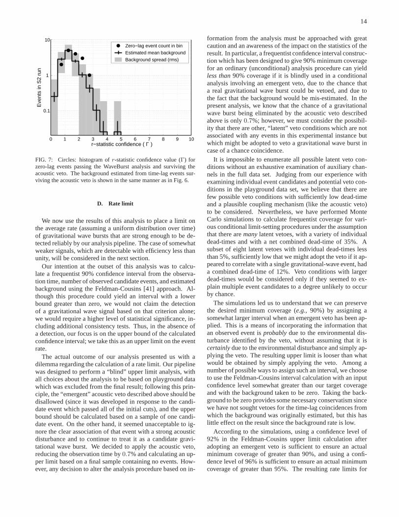
14

0 1 2 3 4 5 6 7 8 9 10

0.1

1

10

r−statistic confidence ( Γ )

Eve

nts

in S

2 ru

nZero−lag event count in bin

Estimated mean background

Background spread (rms)

FIG. 7: Circles: histogram ofr-statistic confidence value (Γ) forzero-lag events passing the WaveBurst analysis and surviving theacoustic veto. The background estimated from time-lag events sur-viving the acoustic veto is shown in the same manner as in Fig.6.

D. Rate limit

We now use the results of this analysis to place a limit onthe average rate (assuming a uniform distribution over time)of gravitational wave bursts that are strong enough to be de-tected reliably by our analysis pipeline. The case of somewhatweaker signals, which are detectable with efficiency less thanunity, will be considered in the next section.

Our intention at the outset of this analysis was to calcu-late a frequentist 90% confidence interval from the observa-tion time, number of observed candidate events, and estimatedbackground using the Feldman-Cousins [41] approach. Al-though this procedure could yield an interval with a lowerbound greater than zero, we would not claim the detectionof a gravitational wave signal based on that criterion alone;we would require a higher level of statistical significance,in-cluding additional consistency tests. Thus, in the absenceofa detection, our focus is on the upper bound of the calculatedconfidence interval; we take this as an upper limit on the eventrate.

The actual outcome of our analysis presented us with adilemma regarding the calculation of a rate limit. Our pipelinewas designed to perform a “blind” upper limit analysis, withall choices about the analysis to be based on playground datawhich was excluded from the final result; following this prin-ciple, the “emergent” acoustic veto described above shouldbedisallowed (since it was developed in response to the candi-date event which passed all of the initial cuts), and the upperbound should be calculated based on a sample of one candi-date event. On the other hand, it seemed unacceptable to ig-nore the clear association of that event with a strong acousticdisturbance and to continue to treat it as a candidate gravi-tational wave burst. We decided to apply the acoustic veto,reducing the observation time by0.7% and calculating an up-per limit based on a final sample containing no events. How-ever, any decision to alter the analysis procedure based on in-

formation from the analysis must be approached with greatcaution and an awareness of the impact on the statistics of theresult. In particular, a frequentist confidence interval construc-tion which has been designed to give 90% minimum coveragefor an ordinary (unconditional) analysis procedure can yieldless than90% coverage if it is blindly used in a conditionalanalysis involving an emergent veto, due to the chance thata real gravitational wave burst could be vetoed, and due tothe fact that the background would be mis-estimated. In thepresent analysis, we know that the chance of a gravitationalwave burst being eliminated by the acoustic veto describedabove is only0.7%; however, we must consider the possibil-ity that there are other, “latent” veto conditions which arenotassociated with any events in this experimental instance butwhich might be adopted to veto a gravitational wave burst incase of a chance coincidence.

It is impossible to enumerate all possible latent veto con-ditions without an exhaustive examination of auxiliary chan-nels in the full data set. Judging from our experience withexamining individual event candidates and potential veto con-ditions in the playground data set, we believe that there arefew possible veto conditions with sufficiently low dead-timeand a plausible coupling mechanism (like the acoustic veto)to be considered. Nevertheless, we have performed MonteCarlo simulations to calculate frequentist coverage for vari-ous conditional limit-setting procedures under the assumptionthat there aremanylatent vetoes, with a variety of individualdead-times and with a net combined dead-time of 35%. Asubset of eight latent vetoes with individual dead-times lessthan 5%, sufficiently low that we might adopt the veto if it ap-peared to correlate with a single gravitational-wave event, hada combined dead-time of 12%. Veto conditions with largerdead-times would be considered only if they seemed to ex-plain multiple event candidates to a degree unlikely to occurby chance.

The simulations led us to understand that we can preservethe desired minimum coverage (e.g., 90%) by assigning asomewhat larger interval when an emergent veto has been ap-plied. This is a means of incorporating the information thatan observed event isprobablydue to the environmental dis-turbance identified by the veto, without assuming that it iscertainlydue to the environmental disturbance and simply ap-plying the veto. The resulting upper limit is looser than whatwould be obtained by simply applying the veto. Among anumber of possible ways to assign such an interval, we chooseto use the Feldman-Cousins interval calculation with an inputconfidence level somewhat greater than our target coverageand with the background taken to be zero. Taking the back-ground to be zero provides some necessary conservatism sincewe have not sought vetoes for the time-lag coincidences fromwhich the background was originally estimated, but this haslittle effect on the result since the background rate is low.

According to the simulations, using a confidence level of92% in the Feldman-Cousins upper limit calculation afteradopting an emergent veto is sufficient to ensure an actualminimum coverage of greater than 90%, and using a confi-dence level of 96% is sufficient to ensure an actual minimumcoverage of greater than 95%. The resulting rate limits for

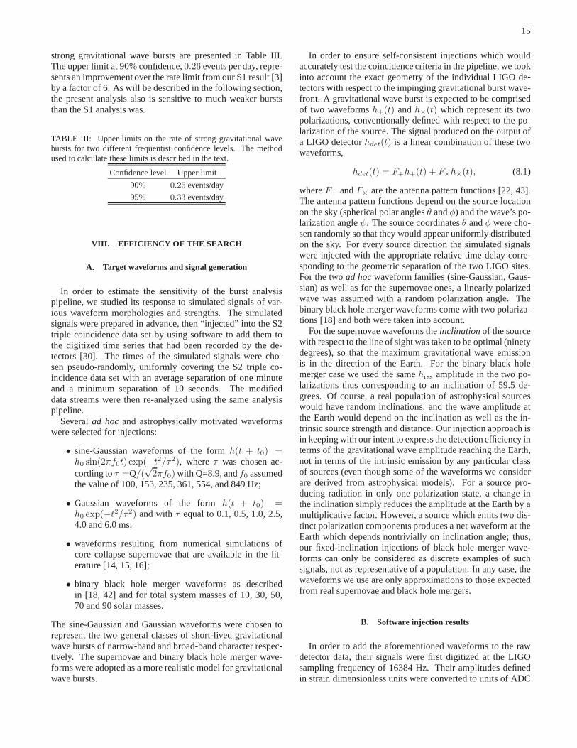
15

strong gravitational wave bursts are presented in Table III.The upper limit at 90% confidence,0.26 events per day, repre-sents an improvement over the rate limit from our S1 result [3]by a factor of 6. As will be described in the following section,the present analysis also is sensitive to much weaker burststhan the S1 analysis was.

TABLE III: Upper limits on the rate of strong gravitational wavebursts for two different frequentist confidence levels. Themethodused to calculate these limits is described in the text.

Confidence level Upper limit

90% 0.26 events/day

95% 0.33 events/day

VIII. EFFICIENCY OF THE SEARCH

A. Target waveforms and signal generation

In order to estimate the sensitivity of the burst analysispipeline, we studied its response to simulated signals of var-ious waveform morphologies and strengths. The simulatedsignals were prepared in advance, then “injected” into the S2triple coincidence data set by using software to add them tothe digitized time series that had been recorded by the de-tectors [30]. The times of the simulated signals were cho-sen pseudo-randomly, uniformly covering the S2 triple co-incidence data set with an average separation of one minuteand a minimum separation of 10 seconds. The modifieddata streams were then re-analyzed using the same analysispipeline.

Severalad hocand astrophysically motivated waveformswere selected for injections:

• sine-Gaussian waveforms of the formh(t + t0) =h0 sin(2πf0t) exp(−t2/τ2), whereτ was chosen ac-cording toτ =Q/(

√2πf0) with Q=8.9, andf0 assumed

the value of 100, 153, 235, 361, 554, and 849 Hz;

• Gaussian waveforms of the formh(t + t0) =h0 exp(−t2/τ2) and withτ equal to 0.1, 0.5, 1.0, 2.5,4.0 and 6.0 ms;

• waveforms resulting from numerical simulations ofcore collapse supernovae that are available in the lit-erature [14, 15, 16];

• binary black hole merger waveforms as describedin [18, 42] and for total system masses of 10, 30, 50,70 and 90 solar masses.

The sine-Gaussian and Gaussian waveforms were chosen torepresent the two general classes of short-lived gravitationalwave bursts of narrow-band and broad-band character respec-tively. The supernovae and binary black hole merger wave-forms were adopted as a more realistic model for gravitationalwave bursts.

In order to ensure self-consistent injections which wouldaccurately test the coincidence criteria in the pipeline, we tookinto account the exact geometry of the individual LIGO de-tectors with respect to the impinging gravitational burst wave-front. A gravitational wave burst is expected to be comprisedof two waveformsh+(t) andh×(t) which represent its twopolarizations, conventionally defined with respect to the po-larization of the source. The signal produced on the output ofa LIGO detectorhdet(t) is a linear combination of these twowaveforms,

hdet(t) = F+h+(t) + F×h×(t), (8.1)

whereF+ andF× are the antenna pattern functions [22, 43].The antenna pattern functions depend on the source locationon the sky (spherical polar anglesθ andφ) and the wave’s po-larization angleψ. The source coordinatesθ andφ were cho-sen randomly so that they would appear uniformly distributedon the sky. For every source direction the simulated signalswere injected with the appropriate relative time delay corre-sponding to the geometric separation of the two LIGO sites.For the twoad hocwaveform families (sine-Gaussian, Gaus-sian) as well as for the supernovae ones, a linearly polarizedwave was assumed with a random polarization angle. Thebinary black hole merger waveforms come with two polariza-tions [18] and both were taken into account.

For the supernovae waveforms theinclinationof the sourcewith respect to the line of sight was taken to be optimal (ninetydegrees), so that the maximum gravitational wave emissionis in the direction of the Earth. For the binary black holemerger case we used the samehrss amplitude in the two po-larizations thus corresponding to an inclination of 59.5 de-grees. Of course, a real population of astrophysical sourceswould have random inclinations, and the wave amplitude atthe Earth would depend on the inclination as well as the in-trinsic source strength and distance. Our injection approach isin keeping with our intent to express the detection efficiency interms of the gravitational wave amplitude reaching the Earth,not in terms of the intrinsic emission by any particular classof sources (even though some of the waveforms we considerare derived from astrophysical models). For a source pro-ducing radiation in only one polarization state, a change inthe inclination simply reduces the amplitude at the Earth byamultiplicative factor. However, a source which emits two dis-tinct polarization components produces a net waveform at theEarth which depends nontrivially on inclination angle; thus,our fixed-inclination injections of black hole merger wave-forms can only be considered as discrete examples of suchsignals, not as representative of a population. In any case,thewaveforms we use are only approximations to those expectedfrom real supernovae and black hole mergers.

B. Software injection results

In order to add the aforementioned waveforms to the rawdetector data, their signals were first digitized at the LIGOsampling frequency of 16384 Hz. Their amplitudes definedin strain dimensionless units were converted to units of ADC

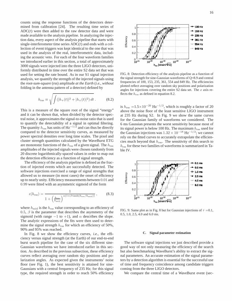
16

counts using the response functions of the detectors deter-mined from calibration [24]. The resulting time series ofADC(t) were then added to the raw detector data and weremade available to the analysis pipeline. In analyzing the injec-tion data, every aspect of the analysis pipeline that startswithsingle-interferometer time series ADC(t) and ends with a col-lection of event triggers was kept identical to the one that wasused in the analysis of the real, interferometric data, includ-ing the acoustic veto. For each of the four waveform familieswe introduced earlier in this section, a total of approximately3000 signals were injected into the three LIGO detectors, uni-formly distributed in time over the entire S2 data set that wasused for setting the rate bound. As in our S1 signal injectionanalysis, we quantify the strength of the injected signals usingtheroot-sum-square(rss) amplitudeat the Earth(i.e., withoutfolding in the antenna pattern of a detector) defined by

hrss ≡√

∫

(|h+(t)|2 + |h×(t)|2) dt . (8.2)

This is a measure of the square root of the signal “energy”and it can be shown that, when divided by the detector spec-tral noise, it approximates the signal-to-noise ratio thatis usedto quantify the detectability of a signal in optimal filtering.The quantityhrss has units of Hz−1/2 and can thus be directlycompared to the detector sensitivity curves, as measured bypower spectral densities over long time scales. The pixel andcluster strength quantities calculated by the WaveBurst ETGare monotonic functions of thehrss of a given signal. Thehrss

amplitudes of the injected signals were chosen randomly from20 discrete logarithmically-spaced values in order to map outthe detection efficiency as a function of signal strength.

The efficiency of the analysis pipeline is defined as the frac-tion of injected events which are successfully detected. Thesoftware injections exercised a range of signal strengths thatallowed us to measure (in most cases) the onset of efficiencyup to nearly unity. Efficiency measurements between0.01 and0.99 were fitted with an asymmetric sigmoid of the form

ǫ(hrss) =1

1 +(

hrss

hmid

)α(1+β tanh(hrss/hmid)), (8.3)

wherehmid is thehrss value corresponding to an efficiency of0.5, β is the parameter that describes the asymmetry of thesigmoid (with range−1 to +1), andα describes the slope.The analytic expressions of the fits were then used to deter-mine the signal strengthhrss for which an efficiency of 50%,90% and 95% was reached.

In Fig. 8 we show the efficiency curves,i.e., the effi-ciency versus signal strength (at the Earth) of our end-to-endburst search pipeline for the case of the six different sine-Gaussian waveforms we have introduced earlier in this sec-tion. As described in the previous subsection, these efficiencycurves reflect averaging over random sky positions and po-larization angles. As expected given the instruments’ noisefloor (see Fig. 1), the best sensitivity is attained for sine-Gaussians with a central frequency of 235 Hz; for this signaltype, the required strength in order to reach 50% efficiency

]Hz [strain/rssh

-2110 -2010 -1910 -1810 -1710]Hz [strain/rssh

-2110 -2010 -1910 -1810 -1710

Effi

cien

cy

0

0.2

0.4

0.6

0.8

1 100 Hz

153 Hz

235 Hz

361 Hz

554 Hz

849 Hz

100 Hz

153 Hz

235 Hz

361 Hz

554 Hz

849 Hz

100 Hz

153 Hz

235 Hz

361 Hz

554 Hz

849 Hz

100 Hz

153 Hz

235 Hz

361 Hz

554 Hz

849 Hz

100 Hz

153 Hz

235 Hz

361 Hz

554 Hz

849 Hz

100 Hz

153 Hz

235 Hz

361 Hz

554 Hz

849 Hz

FIG. 8: Detection efficiency of the analysis pipeline as a function ofthe signal strength for sine-Gaussian waveforms of Q=8.9 and centralfrequencies of 100, 153, 235, 361, 554 and 849 Hz. The efficienciesplotted reflect averaging over random sky positions and polarizationangles for injections covering the entire S2 data set. Thex axis re-flects thehrss as defined in equation 8.2.

is hrss =1.5×10−20 Hz−1/2, which is roughly a factor of 20above the noise floor of the least sensitive LIGO instrumentat 235 Hz during S2. In Fig. 9 we show the same curvesfor the Gaussian family of waveforms we considered. The6 ms Gaussian presents the worst sensitivity because most ofits signal power is below 100 Hz. The maximumhrss used forthe Gaussian injections was1.32× 10−18 Hz−1/2; we cannotrely on the fitted curves to accurately extrapolate the efficien-cies much beyond thathrss. The sensitivity of this search tohrss for these two families of waveforms is summarized in Ta-ble IV.

]Hz [strain/rssh

-2110 -2010 -1910 -1810 -1710]Hz [strain/rssh

-2110 -2010 -1910 -1810 -1710

Effi

cien

cy

0

0.2

0.4

0.6

0.8

1 0.1 ms

0.5 ms

1.0 ms

2.5 ms

4.0 ms

6.0 ms

0.1 ms

0.5 ms

1.0 ms

2.5 ms

4.0 ms

6.0 ms

0.1 ms

0.5 ms

1.0 ms

2.5 ms

4.0 ms

6.0 ms

0.1 ms

0.5 ms

1.0 ms

2.5 ms

4.0 ms

6.0 ms

0.1 ms

0.5 ms

1.0 ms

2.5 ms

4.0 ms

6.0 ms

0.1 ms

0.5 ms

1.0 ms

2.5 ms

4.0 ms

6.0 ms

FIG. 9: Same plot as in Fig. 8 but for Gaussian injections ofτ =0.1,0.5, 1.0, 2.5, 4.0 and 6.0 ms.

C. Signal parameter estimation

The software signal injections we just described provide agood way of not only measuring the efficiency of the searchbut also benchmarking WaveBurst’s ability to extract the sig-nal parameters. An accurate estimation of the signal parame-ters by a detection algorithm is essential for the successful useof time and frequency coincidence among candidate triggerscoming from the three LIGO detectors.

We compare the central time of a WaveBurst event (sec-

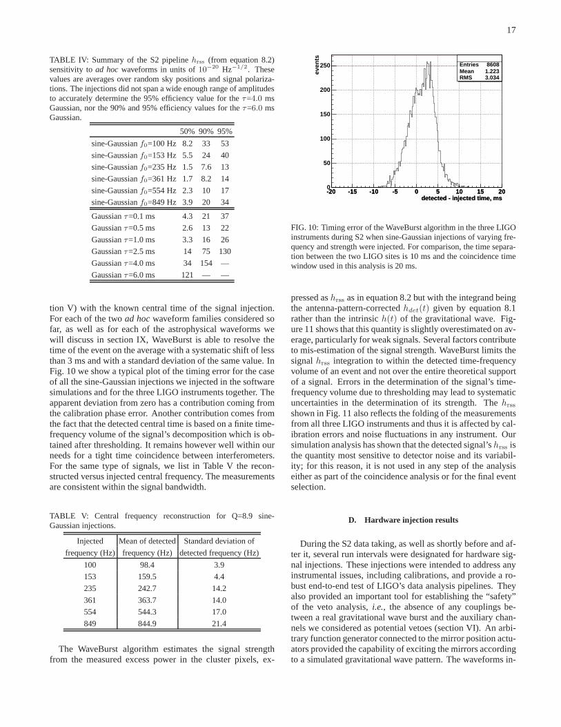
17

TABLE IV: Summary of the S2 pipelinehrss (from equation 8.2)sensitivity toad hocwaveforms in units of10−20 Hz−1/2. Thesevalues are averages over random sky positions and signal polariza-tions. The injections did not span a wide enough range of amplitudesto accurately determine the 95% efficiency value for theτ=4.0 msGaussian, nor the 90% and 95% efficiency values for theτ=6.0 msGaussian.

50% 90% 95%

sine-Gaussianf0=100 Hz 8.2 33 53


sine-Gaussianf0=235 Hz 1.5 7.6 13

sine-Gaussianf0=361 Hz 1.7 8.2 14



Gaussianτ=0.1 ms 4.3 21 37



Gaussianτ=2.5 ms 14 75 130

Gaussianτ=4.0 ms 34 154 —

Gaussianτ=6.0 ms 121 — —

tion V) with the known central time of the signal injection.For each of the twoad hocwaveform families considered sofar, as well as for each of the astrophysical waveforms wewill discuss in section IX, WaveBurst is able to resolve thetime of the event on the average with a systematic shift of lessthan 3 ms and with a standard deviation of the same value. InFig. 10 we show a typical plot of the timing error for the caseof all the sine-Gaussian injections we injected in the softwaresimulations and for the three LIGO instruments together. Theapparent deviation from zero has a contribution coming fromthe calibration phase error. Another contribution comes fromthe fact that the detected central time is based on a finite time-frequency volume of the signal’s decomposition which is ob-tained after thresholding. It remains however well within ourneeds for a tight time coincidence between interferometers.For the same type of signals, we list in Table V the recon-structed versus injected central frequency. The measurementsare consistent within the signal bandwidth.

TABLE V: Central frequency reconstruction for Q=8.9 sine-Gaussian injections.

Injected Mean of detected Standard deviation of

frequency (Hz) frequency (Hz) detected frequency (Hz)

100 98.4 3.9

153 159.5 4.4

235 242.7 14.2

361 363.7 14.0

554 544.3 17.0

849 844.9 21.4

The WaveBurst algorithm estimates the signal strengthfrom the measured excess power in the cluster pixels, ex-

detected - injected time, ms-20 -15 -10 -5 0 5 10 15 20


detected - injected time, ms-20 -15 -10 -5 0 5 10 15 20

even

ts

0

50

100

150

200

250 Entries 8608Mean 1.223RMS 3.034

FIG. 10: Timing error of the WaveBurst algorithm in the threeLIGOinstruments during S2 when sine-Gaussian injections of varying fre-quency and strength were injected. For comparison, the timesepara-tion between the two LIGO sites is 10 ms and the coincidence timewindow used in this analysis is 20 ms.

pressed ashrss as in equation 8.2 but with the integrand beingthe antenna-pattern-correctedhdet(t) given by equation 8.1rather than the intrinsich(t) of the gravitational wave. Fig-ure 11 shows that this quantity is slightly overestimated onav-erage, particularly for weak signals. Several factors contributeto mis-estimation of the signal strength. WaveBurst limitsthesignalhrss integration to within the detected time-frequencyvolume of an event and not over the entire theoretical supportof a signal. Errors in the determination of the signal’s time-frequency volume due to thresholding may lead to systematicuncertainties in the determination of its strength. Thehrss

shown in Fig. 11 also reflects the folding of the measurementsfrom all three LIGO instruments and thus it is affected by cal-ibration errors and noise fluctuations in any instrument. Oursimulation analysis has shown that the detected signal’shrss isthe quantity most sensitive to detector noise and its variabil-ity; for this reason, it is not used in any step of the analysiseither as part of the coincidence analysis or for the final eventselection.

D. Hardware injection results

During the S2 data taking, as well as shortly before and af-ter it, several run intervals were designated for hardware sig-nal injections. These injections were intended to address anyinstrumental issues, including calibrations, and providea ro-bust end-to-end test of LIGO’s data analysis pipelines. Theyalso provided an important tool for establishing the “safety”of the veto analysis,i.e., the absence of any couplings be-tween a real gravitational wave burst and the auxiliary chan-nels we considered as potential vetoes (section VI). An arbi-trary function generator connected to the mirror position actu-ators provided the capability of exciting the mirrors accordingto a simulated gravitational wave pattern. The waveforms in-

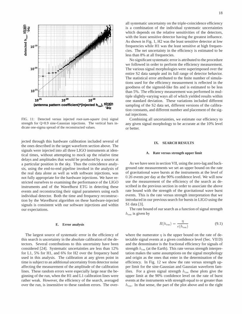
18

Hzstrain), rss(antenna pattern coefficient)*(injected h

-2110 -2010 -1910

Hzstrain), rss(antenna pattern coefficient)*(injected h

-2110 -2010 -1910

Hz

stra

in,

rss

det

ecte

d h

-2110

-2010

-1910

FIG. 11: Detected versus injectedroot-sum-square(rss) signalstrength for Q=8.9 sine-Gaussian injections. The verticalbars in-dicate one-sigma spread of the reconstructed values.

jected through this hardware calibration included severalofthe ones described in the target waveform section above. Thesignals were injected into all three LIGO instruments at iden-tical times, without attempting to mock up the relative timedelays and amplitudes that would be produced by a source ata particular position in the sky. Thus the coincidence analy-sis, using the end-to-end pipeline invoked in the analysis ofthe real data alone as well as with software injections, wasnot fully appropriate for the hardware injections. We have re-stricted ourselves to examining the performance of the LIGOinstruments and of the WaveBurst ETG in detecting theseevents and reconstructing their signal parameters using eachindividual detector. Both the time and frequency reconstruc-tion by the WaveBurst algorithm on these hardware-injectedsignals is consistent with our software injections and withinour expectations.

E. Error analysis

The largest source of systematic error in the efficiency ofthis search is uncertainty in the absolute calibration of the de-tectors. Several contributions to this uncertainty have beenconsidered [24]. Systematic uncertainties are less than 12%for L1, 5% for H1, and 6% for H2 over the frequency bandused in this analysis. The calibration at any given point intime is subject to an additional uncertainty from detector noiseaffecting the measurement of the amplitude of the calibrationlines. These random errors were especially large near the be-ginning of the run, when the H1 and L1 calibration lines wererather weak. However, the efficiency of the search, averagedover the run, is insensitive to these random errors. The over-

all systematic uncertainty on the triple-coincidence efficiencyis a combination of the individual systematic uncertaintieswhich depends on the relative sensitivities of the detectors,with the least sensitive detector having the greatest influence.As shown in Fig. 1, H2 was the least sensitive detector at lowfrequencies while H1 was the least sensitive at high frequen-cies. The net uncertainty in the efficiency is estimated to beless than 8% at all frequencies.

No significant systematic error is attributed to the procedurewe followed in order to perform the efficiency measurement.The various signal morphologies were superimposed over theentire S2 data sample and its full range of detector behavior.The statistical error attributed to the finite number of simula-tions used for the efficiency measurement is reflected in thegoodness of the sigmoid-like fits and is estimated to be lessthan 5%. The efficiency measurement was performed in mul-tiple slightly-varying ways all of which yielded results withinone standard deviation. These variations included differentsampling of the S2 data set, different versions of the calibra-tion constants, and different number and placement of the sig-nal injections.

Combining all uncertainties, we estimate our efficiency toany given signal morphology to be accurate at the 10% levelor better.

IX. SEARCH RESULTS

A. Rate versus strength upper limit

As we have seen in section VII, using the zero-lag and back-ground rate measurements we set an upper bound on the rateof gravitational wave bursts at the instruments at the levelof0.26 events per day at the 90% confidence level. We will nowuse the measurement of the efficiency of the search as de-scribed in the previous section in order to associate the aboverate bound with the strength of the gravitational wave burstevents. This is the rate versus strength interpretation that weintroduced in our previous search for bursts in LIGO using theS1 data [3].

The rate bound of our search as a function of signal strengthhrss is given by

R(hrss) =η

ǫ(hrss)(9.1)

where the numeratorη is the upper bound on the rate of de-tectable signal events at a given confidence level (Sec. VII D)and the denominator is the fractional efficiency for signalsofstrengthhrss (at the Earth). This rate versus strength interpre-tation makes the same assumptions on the signal morphologyand origin as the ones that enter in the determination of theefficiency. In Fig. 12 we show the rate versus strength up-per limit for the sine-Gaussian and Gaussian waveform fam-ilies. For a given signal strengthhrss these plots give theupper limit at the 90% confidence level on the rate of burstevents at the instruments with strength equal to or greater thanhrss. In that sense, the part of the plot above and to the right

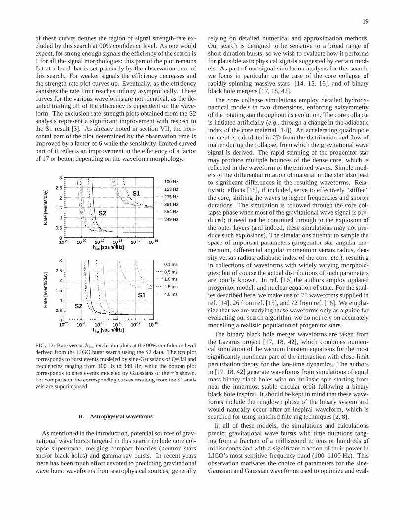
19

of these curves defines the region of signal strength-rate ex-cluded by this search at 90% confidence level. As one wouldexpect, for strong enough signals the efficiency of the search is1 for all the signal morphologies: this part of the plot remainsflat at a level that is set primarily by the observation time ofthis search. For weaker signals the efficiency decreases andthe strength-rate plot curves up. Eventually, as the efficiencyvanishes the rate limit reaches infinity asymptotically. Thesecurves for the various waveforms are not identical, as the de-tailed trailing off of the efficiency is dependent on the wave-form. The exclusion rate-strength plots obtained from the S2analysis represent a significant improvement with respect tothe S1 result [3]. As already noted in section VII, the hori-zontal part of the plot determined by the observation time isimproved by a factor of 6 while the sensitivity-limited curvedpart of it reflects an improvement in the efficiency of a factorof 17 or better, depending on the waveform morphology.

]Hz [strain/rssh

-2110 -2010 -1910 -1810 -1710 -1610]Hz [strain/rssh

-2110 -2010 -1910 -1810 -1710 -1610

Rat

e [e

vent

s/da

y]

0

0.5

1

1.5

2

2.5

3100 Hz

153 Hz

235 Hz

361 Hz

554 Hz

849 Hz

S1

S2

]Hz [strain/rssh

-2110 -2010 -1910 -1810 -1710 -1610]Hz [strain/rssh

-2110 -2010 -1910 -1810 -1710 -1610

Rat

e [e

vent

s/da

y]

0

0.5

1

1.5

2

2.5

30.1 ms

0.5 ms

1.0 ms

2.5 ms

4.0 msS1

S2

FIG. 12: Rate versushrss exclusion plots at the 90% confidence levelderived from the LIGO burst search using the S2 data. The top plotcorresponds to burst events modeled by sine-Gaussians of Q=8.9 andfrequencies ranging from 100 Hz to 849 Hz, while the bottom plotcorresponds to ones events modeled by Gaussians of theτ ’s shown.For comparison, the corresponding curves resulting from the S1 anal-ysis are superimposed.

B. Astrophysical waveforms

As mentioned in the introduction, potential sources of grav-itational wave bursts targeted in this search include core col-lapse supernovae, merging compact binaries (neutron starsand/or black holes) and gamma ray bursts. In recent yearsthere has been much effort devoted to predicting gravitationalwave burst waveforms from astrophysical sources, generally

relying on detailed numerical and approximation methods.Our search is designed to be sensitive to a broad range ofshort-duration bursts, so we wish to evaluate how it performsfor plausible astrophysical signals suggested by certain mod-els. As part of our signal simulation analysis for this search,we focus in particular on the case of the core collapse ofrapidly spinning massive stars [14, 15, 16], and of binaryblack hole mergers [17, 18, 42].

The core collapse simulations employ detailed hydrody-namical models in two dimensions, enforcing axisymmetryof the rotating star throughout its evolution. The core collapseis initiated artificially (e.g., through a change in the adiabaticindex of the core material [14]). An accelerating quadrupolemoment is calculated in 2D from the distribution and flow ofmatter during the collapse, from which the gravitational wavesignal is derived. The rapid spinning of the progenitor starmay produce multiple bounces of the dense core, which isreflected in the waveform of the emitted waves. Simple mod-els of the differential rotation of material in the star alsoleadto significant differences in the resulting waveforms. Rela-tivistic effects [15], if included, serve to effectively “stiffen”the core, shifting the waves to higher frequencies and shorterdurations. The simulation is followed through the core col-lapse phase when most of the gravitational wave signal is pro-duced; it need not be continued through to the explosion ofthe outer layers (and indeed, these simulations may not pro-duce such explosions). The simulations attempt to sample thespace of important parameters (progenitor star angular mo-mentum, differential angular momentum versus radius, den-sity versus radius, adiabatic index of the core,etc.), resultingin collections of waveforms with widely varying morpholo-gies; but of course the actual distributions of such parametersare poorly known. In ref. [16] the authors employ updatedprogenitor models and nuclear equation of state. For the stud-ies described here, we make use of 78 waveforms supplied inref. [14], 26 from ref. [15], and 72 from ref. [16]. We empha-size that we are studying these waveforms only as a guide forevaluating our search algorithm; we do not rely on accuratelymodelling a realistic population of progenitor stars.

The binary black hole merger waveforms are taken fromthe Lazarus project [17, 18, 42], which combines numeri-cal simulation of the vacuum Einstein equations for the mostsignificantly nonlinear part of the interaction with close-limitperturbation theory for the late-time dynamics. The authorsin [17, 18, 42] generate waveforms from simulations of equalmass binary black holes with no intrinsic spin starting fromnear the innermost stable circular orbit following a binaryblack hole inspiral. It should be kept in mind that these wave-forms include the ringdown phase of the binary system andwould naturally occur after an inspiral waveform, which issearched for using matched filtering techniques [2, 8].

In all of these models, the simulations and calculationspredict gravitational wave bursts with time durations rang-ing from a fraction of a millisecond to tens or hundreds ofmilliseconds and with a significant fraction of their power inLIGO’s most sensitive frequency band (100–1100 Hz). Thisobservation motivates the choice of parameters for the sine-Gaussian and Gaussian waveforms used to optimize and eval-

20

uate the efficiency for our search pipeline, as discussed in sec-tion VIII. After tuning our pipeline algorithms using theseadhoc waveforms, we evaluate the efficiency for our search todetect the waveforms predicted from the astrophysical simu-lations. The amplitudes of these waveforms are predicted bythe simulations, so that in addition to evaluating the efficiencyas a function ofhrss (at the Earth), we can also present themas a function of distance to the source (for a particular sourceinclination). We have evaluated the efficiency versus actualdistance, averaged over source directions and polarizations,assuming an isotropic distribution in source direction. Thisassumption becomes invalid for supernova progenitors in theGalactic disk, when the LIGO detectors become sensitive tosupernovae at distances greater than the disk thickness (ontheorder of 150 pc). It is also invalid for extra-galactic binaryblack hole mergers, since the distribution of nearby galaxiesis far from isotropic at the 1 Mpc scale. This evaluation of theefficiency as a function of distance is only to “set the scale”for the current and future astrophysical searches.

For the case of core collapse supernovae we consideredthe collections of waveforms from the three studies discussedabove [14, 15, 16]. There are 176 such supernovae wave-forms. They are generally broad-band in frequency; for 115 ofthem their central frequency is within the sensitive band ofthissearch (100–1100 Hz) and for them we established strengthand distance sensitivities. Sources were uniformly distributedover the whole sky with random polarization and fixed, opti-mal inclination. For detecting these waveforms,hrss ampli-tudes of a few times10−20 Hz−1/2 corresponding to sourcedistances of the order of 100 pc were required. Such close-bysupernovae are, of course, quite rare. In Fig. 13 we show theexpectedhrss (at the detectors) and the central frequency foreach of the 176 supernovae waveforms assuming they origi-nate from a core collapse supernovae that is optimally orientedand polarized and is located at 100 pc from the detectors. Su-perimposed, we show the sensitivity of the LIGO instrumentsduring S2.

Frequency [Hz]10

210

3

Frequency [Hz]10

210

3

h(f)

[1/r

tHz]

10-22

10-21

10-20

10-19

10-18

10-17

10-16

10-15

LLO-4km

ZM 100 pc

DFM 100 pc

OBLW 100 pc

FIG. 13: Signal strengthhrss at the detectors versus central frequencyfor the 176 supernovae waveforms from the three models describedin references [14, 15, 16]: the hydrodynamical model of ref.[14],labeled “ZM”, the relativistic effects considered in ref. [15] and la-beled “DFM”, and finally the hydrodynamical model employingre-alistic nuclear equation of state of ref. [16], labeled “OBLW”. In allcases, the supernova events are positioned in optimal orientation andpolarization at 100 pc from the detectors. The strain sensitivity of theL1 detector during the S2 run is shown for comparison.

For the case of binary black hole mergers, we have consid-ered systems of black hole mass in the range of 10-90M⊙.The characteristic frequency of the resulting waveform is in-versely proportional to the mass of the system and thus fivedifferent masses of 10, 30, 50, 70 and 90M⊙ were chosen inorder to span the nominal frequency band of this search,i.e.,the 100–1100 Hz band. Moreover, the waveforms of thesesystems [17, 18, 42] come with two polarizations and theythus offered a check of the robustness of the waveform consis-tency test, ther-statistic, against complex morphologies. Theefficiency is calculated over the whole sky considering the twopolarization waveforms and a fixed inclination angle. The bestperforming mass system corresponds to 50M⊙: the charac-teristic frequency of this system corresponds to the best oper-ating point of the LIGO instruments,i.e., close to 250 Hz. Onthe contrary, the two worst performing mass systems reflectfrequencies at the two ends of the LIGO instrument’s sensitiv-ities relevant to this search,i.e., 100 Hz and 1100 Hz. As withthe supernova waveforms, the black-hole simulations provideus with order-of-magnitude estimates of the distance to whichour detectors were sensitive to such astrophysical systemsdur-ing the S2 run. For the Lazarus black-hole mergers ourhrss

amplitudes of a few times10−20 Hz−1/2 correspond to dis-tances of order 1 Mpc.

All four waveform families we have considered for our sim-ulations, eitherad hocor astrophysically motivated, have fre-quency content that ranges over the entire band of our search.Within each of these families, signal strengths in order toreach fixed efficiency (e.g., 50%) range over approximatelyan order of magnitude; this is primarily a manifestation of thedifferent frequency content of each waveform and the fact thatthe LIGO detectors’ frequency response is not flat (and variesby an order of magnitude or more over the 100–1100 Hz band,as shown in Fig. 1). We are in the process of augmentingthe waveform library to be considered in future LIGO burstsearches. This will give us further opportunities to test the ro-bustness of our methods and the use ofhrss as a measure ofthe signal strength relevant to burst detection in LIGO.

X. SUMMARY AND DISCUSSION

We have presented a search for gravitational wave burstsusing the data the three LIGO detectors collected duringtheir second science run. Transients with sufficient energyinLIGO’s most sensitive band during the S2 run, 100–1100 Hz,were searched for. A search for gravitational wave bursts withfrequency content above the 1100 Hz range is being pursuedin coincidence with the TAMA [25] detector and will be de-scribed in a separate publication [10]. Our analysis yieldeda single candidate event which was subsequently determinedto be terrestrial in origin and was vetoed retroactively. Incor-porating this into a frequentist statistical approach, we set anupper limit on the rate of strong gravitational wave bursts of0.26 events per day at the 90% confidence level. This ratelimit is a factor of 6 below our previously published value [3],due primarily to the longer duration of the S2 run and to betterdata quality.

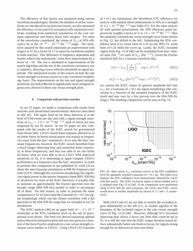
21

The efficiency of this search was measured using variouswaveform morphologies. Besides the families ofad hocwave-forms we introduced in our previous search, we also measuredthe efficiency of our search to astrophysically motivated wave-forms resulting from numerical simulations of the core col-lapse supernovae and binary black hole mergers. For mostof the waveforms considered, the values ofhrss at 50% effi-ciency lie in the10−20 − 10−19 Hz−1/2 range. The sensi-tivity attained by this search represents an improvement withrespect to S1 by a factor of 17 or more for waveforms studiedin both searches. This difference is frequency dependent andmainly reflects the instruments’ noise floor improvement by afactor of∼10. The rest is attributed to improvements of thesearch algorithm and the use of the waveform consistency test(r-statistic), allowing a lower effective threshold on signal am-plitude. The interpreted results of this search include therateversus strength exclusion curves on a per waveform morphol-ogy basis. The improvements on the rate and signal strengthsensitivity are both reflected in significantly more stringent re-gions now allowed in these rate versus strength plots.

A. Comparison with previous searches

In our S1 paper, we made a comparison with results fromsearches with broad-band interferometric detectors describedin [44, 45]. The upper limit set by these detectors is at thelevel of 0.94 events per day and with a signal strength sensi-tivity of hrss = 5.9 × 10−18 Hz−1/2, both of which are nowsurpassed by our S2 search. In our S1 paper we also com-pared with the results of the IGEC search for gravitationalwave bursts [46]. LIGO’s broad band response allowed us toset better limits on bursts whose power was mainly at frequen-cies away from the bars’ resonances. At or near the bars’ res-onant frequencies, however, the IGEC search benefited froma much longer observing time and somewhat better sensitiv-ity at those frequencies, and thus was able to set rate limitsfar below what we were able to do in LIGO. With improvedsensitivity in S2, it is interesting to again compare LIGO’sperformance at a frequency near the bars’ resonance. In orderto perform this comparison in our published S1 work [3] wechose the sine-Gaussian simulations at 849 Hz frequency andwith Q=8.9. Although this waveform morphology has signifi-cant signal power in the narrow frequency band (895–930 Hz)of sensitivity for most of the IGEC detectors, it actually failsto maintain an approximately flat Fourier spectrum over thebroader range (694–930 Hz) needed in order to encompassall of them. For this reason, in order to perform the samecomparison in S2 we have used the Gaussian ofτ=0.1 ms sig-nal morphology which was the closest waveform with a flatspectrum in the 694–930 Hz range that we included in our S2simulations.

The IGEC analysis [46] set an upper limit of∼ 4 × 10−3

events/day at the 95% confidence level on the rate of gravi-tational wave bursts. The limit was derived assuming optimalsource direction and polarization and was also given as a func-tion of the burst Fourier amplitude in a rate versus strengthex-clusion curve similar to LIGO’s. Using LIGO’s S2 Gaussian

of τ=0.1 ms simulations, the WaveBurst ETG efficiency forsources with random linear polarizations is 50% at a strengthof 4.3 × 10−20 Hz−1/2 (see Table IV). For the same sourcesall with optimal polarizations, the 50% efficiency point im-proves by roughly a factor of 3, to1.6× 10−20 Hz−1/2. Thusthe optimally oriented rate versus strength curve looks similarto Fig. 12, but shifted to the left. Substituting the 95% con-fidence level (CL) event limit of0.33 for the 90% CL eventlimit of 0.26 shifts the curve up. Lastly, the IGEC excludedregion from Fig. 13 of [46] can be translated from bars’ natu-ral units (Hz−1) to units ofhrss (Hz−1/2). Given the Fouriertransform h(f) for a Gaussian waveform h(t),

h(t) = hrss

(

2

πτ2

)1/4

exp (−t2/τ2) (10.1)

h(f) = hrss

(

2πτ2)1/4

exp (−π2τ2f2), (10.2)

we convert the IGEC values of spectral amplitude h(f) intohrss for a Gaussian ofτ=0.1 ms signal morphology (the con-version is a function of the assumed frequency of the IGECresult and may vary by a few percent over the 694–930 Hzrange.) The resulting comparison can be seen in Fig. 14.

FIG. 14: Rate versushrss exclusion curves at the 95% confidencelevel for optimally oriented Gaussians ofτ=0.1 ms. The solid curvedisplays the 95% confidence level measurement obtained by LIGOwith this search. The IGEC exclusion region is shown shaded and itis adapted from Fig. 13 of [46]. If the comparison were performedusing Q=8.9, 849 Hz sine-Gaussians, the LIGO and IGEC curveswould move to smaller amplitudes by factors of 1.1 and∼3, respec-tively.

With LIGO and S2 we are able to stretch the excluded re-gion substantially to the left (i.e., to weaker signals) of theboundary of the excluded region in the rate versus strengthcurve of Fig. 13 in [46]. However, although S2’s increasedobserving time allows a lower rate limit than could be set inS1, it is still the case that the IGEC longer duration search al-lows substantially better rate limits to be set, for signalsstrongenough for its detectors to have seen them.

22

Furthermore, we are interested in a comparison with the re-sults reported from the analysis of the EXPLORER and NAU-TILUS 2001 data. In their 2002 paper [47] the Rome groupthat analyzes the data of and operates these two resonant massdetectors reported a slight excess of events seen in siderealhours between 3 and 5. The events seen in concidence bythe two detectors are of an average temperature of approx-imately 120mK which according to the authors correspondsto an optimally oriented gravitational wave burst Fourier am-plitude of 2.7 × 10−21Hz−1 (equation 4 from ref. [47]).The rate of such events is of order 200 events/year (or 0.55events/day) [47, 48]. Given the amplitude of the observedevents by the resonant mass detectors, the correspondinghrss

of the hypothetical events in our LIGO instruments will gener-ally depend on the signal morphology. As with our aforemen-tioned IGEC analysis, we considered the case of a Gaussianof τ=0.1 ms, for which the Fourier amplitude of the observedevents at the detectors’ average resonance frequency impliesan hrss of 1.9 × 10−19 Hz−1/2. Keeping in mind that thesuggestedhrss values refer to optimal orientation, we can seefrom Fig. 14 that for this event strength the LIGO S2 searchset an upper bound to their flux at roughly0.4 events per dayat the 95% CL. It should be noted, though, that depending onthe assumptions of signal waveform (for example a single cy-cle of a 914 Hz sinusoid or a narrow-band sine-Gaussian sig-nal centered on the same frequency) or considering the rangeof event strengths recorded by EXPLORER and NAUTILUS(rather than their average value only) the correspondinghrss atthe LIGO detectors may come nearer to the threshold of oursensitivity and thus make our rate limits poorer. The signalstrength and rate of the 2001 Rome results come with enoughuncertainties that given the LIGO S2 sensitivity and exposurewe cannot make a definitive comparison. The significant im-provements in sensitivity and longer observation times that weexpect in new LIGO searches in the near future will enable usto move in this direction.

B. Discussion and future directions

The search for gravitational wave bursts in LIGO’s S2 runhas seen significant improvements introduced in the searchmethodology and interpretation with respect to S1. This in-cluded the introduction of the waveform consistency cut andthe use of astrophysically motivated waveforms as part of thesearch interpretation. Additional improvements are currentlyunder way. We expect them to bring stronger suppressionof the background via the use of a burst amplitude consis-tency test between the LIGO detectors as well as new ways

of performing our event analysis within the context of a dis-tributional analysis of their strength. Moreover, we plan tomake use of data taking periods corresponding to the doublecoincidence of the instruments that are not part of the triplecoincidence dataset. We will continue investigating the opti-mization of search algorithms for specific types of waveformsand adding stronger astrophysical context in our search by in-voking source population models or targeting plausible pointsources. Among the lessons learned in the S2 search has beenthe importance of the follow-up investigations dictated byco-incident triggers revealed by the pipeline. As expected, withthe detector performance nearing design sensitivity, potentialcouplings from the environment and the instrument itself willbecome apparent and will need to be identified and vetoed out.Our on-going work for vetoes will become more prominenttogether with the need to define rigorous criteria and proce-dures for following up on such events. LIGO’s subsequentruns have already collected data of comparable duration andimproved sensitivity with respect to S2 and they will presentthe next milestone of the search for bursts where a good num-ber of these improvements will be exercised.

The software used in this analysis is available inthe LIGO Scientific Collaboration’s CVS archives athttp://www.lsc-group.phys.uwm.edu/cgi-bin/cvs/viewcvs.cgi/?cvsroot=lscsoft under theS2 072704 tag for WaveBurst inLAL andLALWRAPPERandrStat-1-2 tag forr-statistic inMATAPPS.

Acknowledgments

The authors gratefully acknowledge the support of theUnited States National Science Foundation for the construc-tion and operation of the LIGO Laboratory and the ParticlePhysics and Astronomy Research Council of the United King-dom, the Max-Planck-Society and the State of Niedersach-sen/Germany for support of the construction and operation ofthe GEO600 detector. The authors also gratefully acknowl-edge the support of the research by these agencies and by theAustralian Research Council, the Natural Sciences and Engi-neering Research Council of Canada, the Council of Scientificand Industrial Research of India, the Department of Scienceand Technology of India, the Spanish Ministerio de Educa-cion y Ciencia, the John Simon Guggenheim Foundation, theLeverhulme Trust, the David and Lucile Packard Foundation,the Research Corporation, and the Alfred P. Sloan Foundation.

This document has been assigned LIGO Laboratory docu-ment number LIGO-P040040-07-R.

[1] B. Abbott et al. (LIGO Scientific Collaboration), Nucl. Instr.Meth. A 517, 154 (2004).

[2] B. Abbott et al. (LIGO Scientific Collaboration), Phys. Rev. D69, 122001 (2004).




[6] B. Abbott et al. (LIGO Scientific Collaboration),Limits on thegravitational wave strength from isolated radio pulsars using

http://www.lsc-group.phys.uwm.edu/cgi-bin/

23

data from the second science run of LIGO, to appear in Phys.Rev. Lett., gr-qc/0410007.

[7] B. Abbott et al. (LIGO Scientific Collaboration),A searchfor gravitational waves associated with the gamma ray burstGRB030329 using the LIGO detectors, submitted to Phys. Rev.D, gr-qc/0501068.

[8] LIGO Scientific Collaboration,Search for gravitational wavesfrom galactic and extra-galactic binary neutron stars, in prepa-ration (2005).

[9] LIGO Scientific Collaboration,Search for gravitational wavesfrom primordial black hole binary coalescence in the galactichalo, in preparation (2005).

[10] TAMA and LIGO Scientific Collaborations,Upper limits fromthe LIGO and TAMA detectors on the rate of gravitational wavebursts, in preparation (2005).

[11] LIGO Scientific Collaboration,All-sky search for continuouswave signals in LIGO data using the Hough transform, in prepa-ration (2005).

[12] LIGO Scientific Collaboration,LIGO search for gravitationalwaves from binary black hole mergers, in preparation (2005).

[13] LIGO Scientific Collaboration,Upper limits on a stochasticbackground of gravitational waves, in preparation (2005).

[14] T. Zwerger and E. Muller, Astron. Astrophys.320, 209 (1997).[15] H. Dimmelmeier, J. A. Font, and E. Muller, Astrophys. J. Lett.

560, L163 (2001).[16] C. D. Ott, A. Burrows, E. Livne, and R. Walder, Astrophys. J.

600, 834 (2004).[17] J. Baker, M. Campanelli, C. O. Lousto, and R. Takahashi,Phys.

Rev. D69, 027505 (2004).[18] J. Baker, M. Campanelli, C. O. Lousto, and R. Takahashi,Phys.

Rev. D65, 124012 (2002).[19] E. E. Flanagan and S. A. Hughes, Phys. Rev. D57, 4535 (1998).[20] B. Zhang and P. Meszaros, Int. J. Mod. Phys. A19, 2385 (2003).[21] T. Damour and A. Vilenkin, Phys. Rev. D71, 063510 (2005).[22] P. R. Saulson,Fundamentals of Interferometric Gravitational

Wave Detectors(World Scientific Pub. Co., 1994).[23] D. Sigg, Class. Quant. Grav.21, S409 (2004).[24] G. Gonzalez, M. Landry, and B. O’Reilly, LIGO Tech-

nical Document LIGO-T040060-00-D (2004), URLhttp://www.ligo.caltech.edu/docs/T/T040060-00.pdf.

[25] R. Takahashi et al. (TAMA Collaboration), Class. Quant. Grav.21, S403 (2004).

[26] B. Willke et al., Class. Quant. Grav.21, S417 (2004).

[27] S. Klimenko, I. Yakushin, M. Rakhmanov, and G. Mitsel-makher, Class. Quant. Grav.21, S1685 (2004).

[28] S. Klimenko and G. Mitselmakher, Class. Quant. Grav.21,S1819 (2004).

[29] L. Cadonati, Class. Quant. Grav.21, S1695 (2004).[30] S. Klimenko, M. Rakhmanov, and I. Yakushin, LIGO Technical

Document LIGO-T040042-00-Z (2004).[31] L. A. Wainstein and V. D. Zubakov,Extraction of signals from

noise(Prentice-Hall, Englewood Cliffs, NJ, 1962).[32] N. Arnaud, F. Cavalier, M. Davier, and P. Hello, Phys. Rev. D

59, 082002 (1999).[33] T. Pradier, N. Arnaud, M. Bizouard, F. Cavalier, M. Davier, and

P. Hello, Phys. Rev. D63, 42002 (2001).[34] J. Sylvestre, Phys. Rev. D66, 102004 (2002).[35] W. G. Anderson, P. R. Brady, J. D. E. Creighton, andE. E.

Flanagan, Phys. Rev. D63, 042003 (2001).[36] J. W. C. McNabb et al., Class. Quant. Grav.21, S1705 (2004).[37] I. Daubechies,Ten Lectures on Wavelets(SIAM, Philadelphia,

1992).[38] S. Chatterji, L. Blackburn, G. Martin, and E. Katsavounidis,

Class. Quant. Grav.21, S1809 (2004).[39] S. D. Mohanty et al., Class. Quant. Grav.21, S1831 (2004).[40] P. Astone et al., Phys. Rev. D66, 102002 (2002).[41] G. J. Feldman and R. D. Cousins, Phys. Rev. D57, 3873 (1998).[42] These binary black hole waveforms appear in fig. 36 of [18]

and correspond to the “QC-3” case worked by the authors. Adigitized version of these waveforms with their early part re-moved is available through theASTROGRAVS project’s webpage at http://astrogravs.gsfc.nasa.gov/ maintained by the Lab-oratory for High Energy Astrophysics at NASA’s GSFC. It isthe ASTROGRAVS version of the waveforms that we used inour simulations.

[43] K. S. Thorne, in300 Years of Gravitation, edited by S. Hawkingand W. Israel (Cambridge University Press, Cambridge, 1987),chap. 9, pp. 330–458.

[44] D. Nicholson et al., Phys. Lett.A218, 175 (1996).[45] R. L. Forward, Phys. Rev.D17, 379 (1978).[46] P. Astone et al. (International Gravitational Event Collabora-

tion), Phys. Rev. D68, 022001 (2003).[47] P. Astone et al., Class. Quant. Grav.19, 5449 (2002).[48] E. Coccia, F. Dubath, and M. Maggiore, Phys. Rev. D70,

084010 (2004).

http://www.ligo.caltech.edu/docs/T/T040060-00.pdf

http://astrogravs.gsfc.nasa.gov/

Upper limits on gravitational wave bursts in LIGO's second science run

Documents