Upper Bounds on the Noise Threshold for Fault-Tolerant Quantum Computing

arX

iv:0

802.

1464

v1 [

quan

t-ph

] 1

1 Fe

b 20

08

Upper Bounds on the Noise Threshold for Fault-tolerant Quantum

Computing

Julia Kempe∗ Oded Regev† Falk Unger‡ Ronald de Wolf§

February 11, 2008

Abstract

We prove new upper bounds on the tolerable level of noise in a quantum circuit. We considercircuits consisting of unitary k-qubit gates each of whose input wires is subject to depolarizingnoise of strength p, as well as arbitrary one-qubit gates that are essentially noise-free. Weassume that the output of the circuit is the result of measuring some designated qubit in thefinal state. Our main result is that for p > 1−Θ(1/

√k), the output of any such circuit of large

enough depth is essentially independent of its input, thereby making the circuit useless. For theimportant special case of k = 2, our bound is p > 35.7%. Moreover, if the only allowed gateon more than one qubit is the two-qubit CNOT gate, then our bound becomes 29.3%. Thesebounds on p are notably better than previous bounds, yet are incomparable because of thesomewhat different circuit model that we are using. Our main technique is the use of a Paulibasis decomposition, which we believe should lead to further progress in deriving such bounds.

1 Introduction

The field of quantum computing faces two main tasks: to build a large-scale quantum computer,and to figure out what it can do once it exists. In general the first task is best left to (experimental)physicists and engineers, but there is one crucial aspect where theorists play an important role, andthat is in analyzing the level of noise that a quantum computer can tolerate before breaking down.

The physical systems in which qubits may be implemented are typically tiny and fragile (elec-trons, photons and the like). This raises the following paradox: On the one hand we want to isolatethese systems from their environment as much as possible, in order to avoid the noise caused byunwanted interaction with the environment—so-called “decoherence”. But on the other hand we

∗School of Computer Science, Tel-Aviv University, Tel-Aviv 69978, Israel. Supported by the European Commissionunder the Integrated Project Qubit Applications (QAP) funded by the IST directorate as Contract Number 015848,by an Alon Fellowship of the Israeli Higher Council of Academic Research and by an Individual Research Grant ofthe Israeli Science Foundation.

†School of Computer Science, Tel-Aviv University, Tel-Aviv 69978, Israel. Supported by the Binational ScienceFoundation, by the Israel Science Foundation, and by the European Commission under the Integrated Project QAPfunded by the IST directorate as Contract Number 015848.

‡Partially supported by the European Commission under the Integrated Project Qubit Applications (QAP) fundedby the IST directorate as Contract Number 015848.

§Partially supported by a Veni grant from the Netherlands Organization for Scientific Research (NWO), and bythe European Commission under the Integrated Project Qubit Applications (QAP) funded by the IST directorate asContract Number 015848.

1

need to manipulate these qubits very precisely in order to carry out computational operations. Acertain level of noise and errors from the environment is therefore unavoidable in any implementa-tion, and in order to be able to compute one would have to use techniques of error correction andfault tolerance.

Unfortunately, the techniques that are used in classical error correction and fault tolerance donot work directly in the quantum case. Moreover, extending these techniques to the quantum worldseems at first sight to be nearly impossible due to the continuum of possible quantum states anderror patterns. Indeed, when the first important quantum algorithms were discovered [6, 27, 26, 13],many dismissed the whole model of quantum computing as a pipe dream, because it was expectedthat decoherence would quickly destroy the necessary quantum properties of superposition andentanglement.

It thus came as a great surprise when, in the mid-1990s, quantum error correcting codes weredeveloped by Shor and Steane [24, 28], and these ideas later led to the development of schemes forfault-tolerant quantum computing [25, 18, 15, 1, 14, 12]. Such schemes take any quantum algorithmdesigned for an ideal noiseless quantum computer, and turn it into an implementation that isrobust against noise, as long as the amount of noise is below a certain threshold, known as thefault-tolerant threshold. The overhead introduced by the fault-tolerant schemes is typically quitemodest (a polylogarithmic factor in the total running time of the algorithm).

The existence of fault-tolerant schemes turns the problem of building a quantum computer intoa hard but possible-in-principle engineering problem: if we just manage to store our qubits andoperate upon them with a level of noise below the fault-tolerant threshold, then we can performarbitrarily long quantum computations. The actual value of the fault-tolerant threshold is far fromdetermined, but will have a crucial influence on the future of the area—the more noise a quantumcomputer can tolerate in theory, the more likely it is to be realized in practice.1

The first fault-tolerant schemes were only able to tolerate noise on the order of 10−6, which isway below the level of accuracy that experimentalists can hope to achieve in the foreseeable future.These initial schemes have been substantially improved in the past decade. In particular, Knillhas recently developed various schemes which, according to numerical calculations, seem to be ableto tolerate more than 1% noise [17, 16]. If we insist on provable constructions, the best knownthreshold is on the order of 0.1% [4, 3, 2, 21].

Constructions of fault-tolerant schemes provide a lower bound on the fault-tolerant threshold.A very interesting question, which is the topic of the current paper, is whether one can proveupper bounds on the fault-tolerant threshold. Such bounds give an indication on how far away weare from finding optimal fault-tolerant schemes. They can also give hints as to how one should goabout constructing improved fault-tolerant schemes. Such upper bounds are statements of the form“any quantum computation performed with noise level higher than p is essentially useless”, where“essentially useless” is usually some strong indication that interesting quantum computations areimpossible in such a model. For instance, Buhrman et al. [9] quantify this by giving a classicalsimulation of such noisy quantum computation, and Razborov [19] shows that if the computationis too long, the output of the circuit is essentially independent of its input.

The best known upper bounds on the threshold are 50% by Razborov [19] and 45.3% byBuhrman et al. [9]. (These bounds are incomparable because they work in different models; Seethe end of this section for more accurate statements.) As one can see, there are still about two

1The “fault-tolerant threshold” is actually not a universal constant, but rather depends on the details of the circuitmodel (allowed set of gates, type of noise, etc.). A more precise discussion will be given later.

2

orders of magnitude between our best upper and lower bounds on the fault-tolerant threshold. Thisleaves experimentalists in the dark as to the level of accuracy they should try to achieve in theirexperiments. In this paper, we somewhat reduce this gap. So far, much more work has been spenton lower bounds than on upper bounds. Our approach will be the less-trodden road from above,hoping to bring new techniques to bear on this problem.

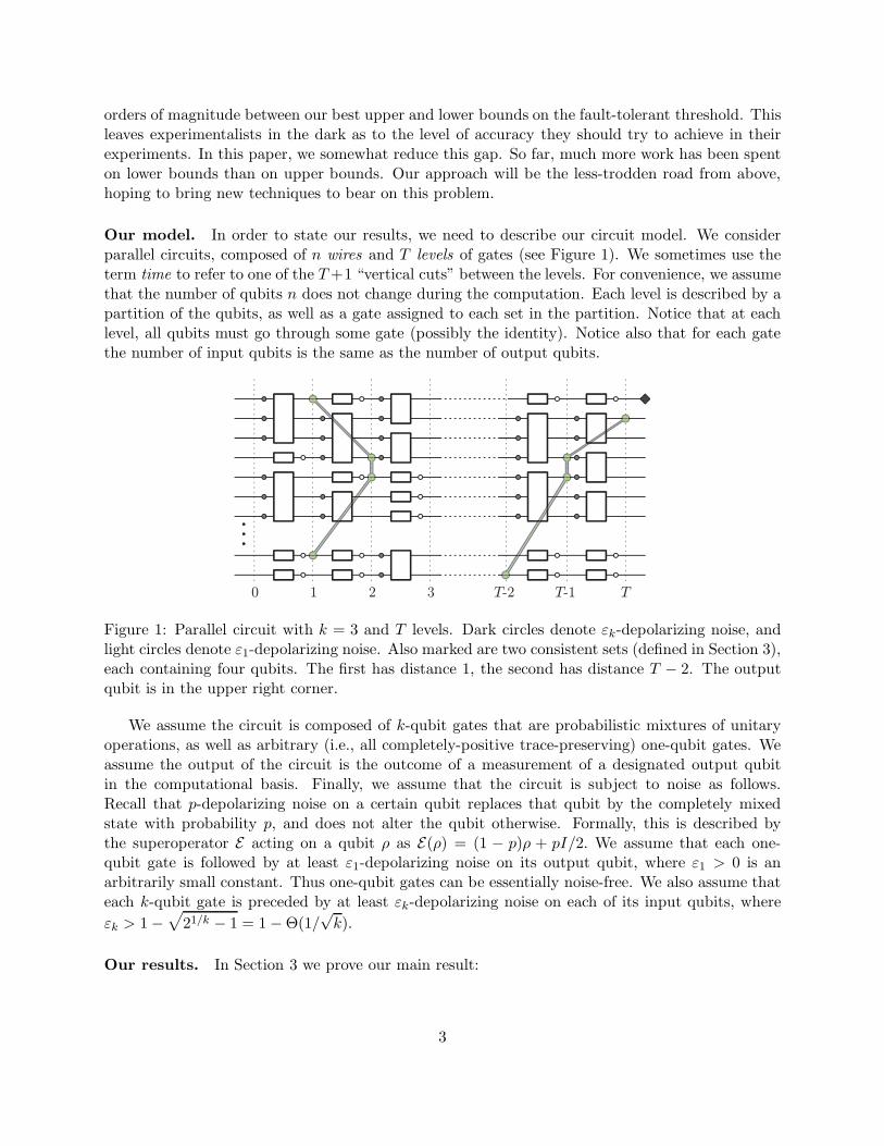
Our model. In order to state our results, we need to describe our circuit model. We considerparallel circuits, composed of n wires and T levels of gates (see Figure 1). We sometimes use theterm time to refer to one of the T +1 “vertical cuts” between the levels. For convenience, we assumethat the number of qubits n does not change during the computation. Each level is described by apartition of the qubits, as well as a gate assigned to each set in the partition. Notice that at eachlevel, all qubits must go through some gate (possibly the identity). Notice also that for each gatethe number of input qubits is the same as the number of output qubits.

0 1 2 3 T-2 T-1 T

Figure 1: Parallel circuit with k = 3 and T levels. Dark circles denote εk-depolarizing noise, andlight circles denote ε1-depolarizing noise. Also marked are two consistent sets (defined in Section 3),each containing four qubits. The first has distance 1, the second has distance T − 2. The outputqubit is in the upper right corner.

We assume the circuit is composed of k-qubit gates that are probabilistic mixtures of unitaryoperations, as well as arbitrary (i.e., all completely-positive trace-preserving) one-qubit gates. Weassume the output of the circuit is the outcome of a measurement of a designated output qubitin the computational basis. Finally, we assume that the circuit is subject to noise as follows.Recall that p-depolarizing noise on a certain qubit replaces that qubit by the completely mixedstate with probability p, and does not alter the qubit otherwise. Formally, this is described bythe superoperator E acting on a qubit ρ as E(ρ) = (1 − p)ρ + pI/2. We assume that each one-qubit gate is followed by at least ε1-depolarizing noise on its output qubit, where ε1 > 0 is anarbitrarily small constant. Thus one-qubit gates can be essentially noise-free. We also assume thateach k-qubit gate is preceded by at least εk-depolarizing noise on each of its input qubits, where

εk > 1 −√

21/k − 1 = 1 − Θ(1/√

k).

Our results. In Section 3 we prove our main result:

3

Theorem 1. Fix any T -level quantum circuit as above. Then for any two states ρ and τ , the

probabilities of obtaining measurement outcome 1 at the output qubit starting from ρ and starting

from τ , respectively, differ by at most 2−Ω(T ).

In other words, for any η > 0, the probability of measuring 1 at the output qubit of a circuitrunning for T = O(log(1/η)) levels is (up to ±η) independent of the input. This makes the outputessentially independent of the starting state, and renders long computations “essentially useless”.

Of special interest from an experimental point of view is the case k = 2, for which our boundbecomes about 35.7%. Furthermore, for the case in which the only allowed two-qubit gate is theCNOT gate, we can improve our bound further to about 29.3%, as we show in Section 4. This caseis interesting both theoretically and experimentally. Note also that the CNOT gate together withall one-qubit gates forms a universal set [5].

Significance of results. Here we comment on the significance of our results and of our model.First, it is known that fault-tolerant quantum computation is impossible (for any positive noise

level) without a source of fresh qubits. Our model takes care of this by allowing arbitrary one-qubitgates—in particular, this includes gates that take any input, and output a fixed one-qubit state,for instance the classical state |0〉. This justifies our assumption that the number of qubits in thecircuit remains the same throughout the computation: all qubits can be present from the start,since we can reset them to whatever we want whenever needed.

Second, our assumption that all k-qubit gates are mixtures of unitaries does slightly restrictgenerality. Not every completely-positive trace-preserving map can be written as a mixture ofunitaries. However, we believe that it is a reasonable assumption. As one indication of this, tothe best of our knowledge, all known fault-tolerant constructions can be implemented using suchgates (in addition to arbitrary one-qubit gates). Moreover, all known quantum algorithms gaintheir speed-up over classical algorithms by using only unitary gates.

A slightly more severe restriction is the assumption that the output consists of just one qubit.However, we believe that in many instances this is still a reasonable assumption. For instance, thisis the case whenever the circuit is required to solve a decision problem. Moreover, our results canbe easily extended to deal with the case in which a small number of qubits are used as an output.

By allowing essentially noise-free one-qubit gates, our model addresses the fact that gates onmore than one qubit are generally much harder to implement. It should also be noted that theexact value of the constant ε1 is inessential and can be chosen arbitrarily small, as this just affectsthe constant in the Ω(·) of Theorem 1. In fact, ε1 > 0 is only necessary because otherwise it wouldbe possible to let ρ := |0〉〈0| ⊗ ρ′ and τ := |1〉〈1| ⊗ τ ′, do nothing for T levels (i.e., apply noise-freeone-qubit identity gates on all wires) and then measure the first qubit. The resulting differencebetween output probabilities is then 1. Instead of assuming an ε1 > 0 amount of noise, we couldalternatively deal with this issue by requiring that every path from the input to the output qubitgoes through enough k-qubit gates. Our proof can be easily adapted to this case.

Note that since our theorem applies to arbitrary starting states, it in particular applies to thecase that the initial state is encoded in some good quantum error-correcting code, or that it is somesort of “magic state” [7, 20]. In all these cases, our theorem shows that the computation becomesessentially independent of the input after sufficiently many levels.

Finally, it is interesting to note that our bound on the threshold behaves like 1−Θ(1/√

k). Thismatches what is known for classical circuits [10, 11], and therefore probably represents the correctasymptotic behavior. Previous bounds only achieved an asymptotic behavior of 1 − Θ(1/k) [19].

4

Techniques. We believe that a main part of our contribution is introducing a new technique forobtaining upper bounds on the fault-tolerant threshold. Namely, we use a Pauli basis decompositionin order to track the state of the computation. We believe this framework will be useful also forfurther analysis of quantum fault-tolerance. A finer analysis of the Pauli coefficients might improvethe bounds we achieve here, and possibly obtain bounds that are tailored to other computationalmodels.

Related work. The work most closely related to ours is that of Razborov [19]. There, he provesan upper bound of εk = 1− 1/k on the fault-tolerant threshold. On one hand, his result is strongerthan ours as it allows arbitrary k-qubit gates and not just mixtures of unitaries. Razborov also hasa second result, namely the trace distance between the two states obtained by applying the circuitto starting states ρ and τ , respectively, goes down as n2−Ω(T ) with the number of levels T . Henceeven the results of an arbitrary n-qubit measurement on the full final state become essentiallyindependent of the initial state after T = O(log n) levels. On the other hand, the value of ourbound is better for all values of k, and we also allow essentially noise-free one-qubit gates. Hencethe two results are incomparable. Razborov’s proof is based on tracking how the trace distanceevolves during the computation. Our proof is similar in flavor, but instead of working with thetrace distance, we work with the Frobenius distance (since it can be easily expressed in terms ofthe Pauli decomposition).

Buhrman et al. [9] show that classical circuits can efficiently simulate any quantum circuit thatconsists of perfect, noise-free stabilizer operations (meaning Clifford gates (Hadamard, phase gate,CNOT), preparations of states in the computational basis, and measurements in the computationalbasis) and arbitrary one-qubit unitary gates that are followed by 45.3% depolarizing noise. Hencesuch circuits are not significantly more powerful than classical circuits.2 This result is incomparableto ours: the noise models and the set of allowed gates are different (and we feel ours is more realistic).In particular, in our case noise hits the qubits going into the k-qubit gates but barely affects theone-qubit gates, while in their case the noise only hits the non-Clifford one-qubit unitaries.

Another related result is by Virmani et al. [29]. Instead of depolarizing noise, they consider“dephasing noise”. This models phase-errors only: while we can view depolarizing noise of strengthp as applying one of four possible operations (I,X,Y,Z), each with probability p/4, dephasing noiseof strength p applies one of two possible operations, I or Z, each with probability p/2. Virmani etal. [29] show, among other results, that any quantum circuit consisting of perfect stabilizer opera-tions, and one-qubit unitary gates that are diagonal in the computational basis and are followed bydephasing noise of strength 29.3%, can be efficiently simulated classically. Their result is incompa-rable to ours for essentially the same reasons as why the Buhrman et al. result is incomparable: adifferent noise model and a different statement about the resulting power of their noisy quantumcircuits.

Finally, it is known that it is impossible to transmit quantum information through a p-depolarizingchannel for p > 1/3 [8]. This seems to suggest that quantum computation over and above classicalcomputation is impossible with depolarizing noise of strength greater than 1/3, but there is noproof that this is indeed the case.

2The 45.3%-bound of [9] is in fact tight if one additionally allows perfect classical control (i.e., the ability tocondition future gates on the earlier classical measurement outcomes): circuits with perfect stabilizer operations andarbitrary one-qubits gates suffering from less than 45.3% noise, can simulate perfect quantum circuits. See [22] and [9,Section 5]. These assumptions are not very realistic, however. In particular the assumption that one can implementperfect, noise-free CNOTs is a far cry from experimental practice.

5

2 Preliminaries

Let P = I,X, Y, Z be the set of one-qubit Pauli matrices,

I =

(1 00 1

), X =

(0 11 0

), Y =

(0 −ii 0

), Z =

(1 00 −1

).

and let P∗ = X,Y,Z. We use Pn to denote the set of all tensor products of n one-qubit Paulimatrices. For a Pauli matrix S ∈ Pn we define its support, denoted supp(S), to be the qubits onwhich S is not identity. We sometimes use superscripts to indicate the qubits on which certainoperators act. Thus IA denotes the identity operator applied to the qubits in set A.

The set of all 2n × 2n Hermitian matrices forms a 4n-dimensional real vector space. On thisspace we consider the Hilbert-Schmidt inner product, given by 〈A,B〉 := Tr(A†B) = Tr(AB). Notethat for any S, S′ ∈ Pn, Tr(SS′) = 2n if S = S′ and 0 otherwise, and hence Pn is an orthogonalbasis of this space. It follows that we can uniquely express any Hermitian matrix δ in this basis as

δ =1

2n

∑

S∈Pn

δ(S)S

where δ(S) := Tr(δS) are the (real) coefficients.We now state some easy observations which will be used in the proof of our main result. First,

by the orthogonality of Pn, it follows that for any δ,

Tr(δ2) =1

2n

∑

S∈Pn

δ(S)2.

This easily leads to the following observation.

Observation 2 (Unitary preserves sum of squares). For any unitary matrix U and any Hermitian

matrix δ, if we denote δ′ = UδU †, then

∑

S∈Pn

δ′(S)2 = 2nTr(δ′2) = 2nTr(UδU †UδU †) = 2nTr(δ2) =∑

S∈Pn

δ(S)2.

This also shows that the operation of conjugating by a unitary matrix, when viewed as a linearoperation on the vector of Pauli coefficients, is an orthogonal transformation.

Observation 3 (Tracing out qubits). Let δ be some Hermitian matrix on a set of qubits W . For

V ⊆ W , let δV = TrW\V (δ). Then,

δ(SIW\V ) = Tr(δ · SIW\V ) = Tr(δV · S) = δV (S).

Observation 4 (Noise in the Pauli basis). Applying a p-depolarizing noise E to the j-th qubit of

Hermitian matrix δ changes the coefficients as follows:

E(δ)(S) =

δ(S) if Sj = I

(1 − p)δ(S) if Sj 6= I

In other words, E “shrinks” by a factor 1−p all coefficients that have support on the j-th coordinate.

6

Observation 5. Let ρ and τ be two one-qubit states and let δ = ρ − τ . Consider the two proba-

bility distributions obtained by performing a measurement in the computational basis on ρ and τ ,

respectively. Then the variation distance between these two distributions is 12 |δ(Z)|.

Proof: Since there are only two possible outcomes for the measurements, the variation distancebetween the two distributions is exactly the difference in the probabilities of obtaining the outcome0, which is given by

|Tr((ρ − τ) · |0〉〈0|)| =

∣∣∣∣Tr

(δ · I + Z

2

)∣∣∣∣ =1

2|Tr(δ · Z)| =

1

2|δ(Z)|,

where we have used Tr(δ) = 0.

Our final observation follows immediately from the convexity of the function x2.

Observation 6 (Convexity). Let pi be any probability distribution, and δi a set of Hermitian

matrices. Let δ =∑

i piδi. Then

∑

S∈Pn

δ(S)2 ≤∑

i

pi

∑

S∈Pn

δi(S)2.

3 Proof of Theorem 1

In this section we prove Theorem 1. The rough idea is the following. Fix two arbitrary initial statesρ and τ . Our goal is to show that after applying the noisy circuit, the state of the output qubitis nearly the same with both starting states. Equivalently, we can define δ = ρ − τ and show thatafter applying the noisy circuit to δ, the “state” of the output qubit is essentially 0 (notice thatwe can view the noisy circuit as a linear operation, and hence there is no problem in applying itto δ, which is the difference of two density matrices). In order to show this, we will examine howthe coefficients of δ in the Pauli basis develop through the circuit. Initially we might have manylarge coefficients. Our goal is to show that the coefficients of the output qubit are essentially 0.This is established by analyzing the balance between two opposing forces: noise, which shrinkscoefficients by a constant factor (as in Observation 4), and gates, which can increase coefficients.As we saw in Observation 2, unitary gates preserve the sum of squares of coefficients. They can,however, “concentrate” several small coefficients into one large coefficient. One-qubit operationsneed not preserve the sum of squares (a good example is the gate that resets a qubit to the |0〉state), but we can still deal with them by using a known characterization of one-qubit gates. Thischaracterization allows us to bound the amount by which one-qubit gates can increase the Paulicoefficients, and very roughly speaking shows that the gate that resets a qubit to |0〉 is “as bad asit gets”.

Before continuing with the proof, we introduce some terminology. From now on we use theterm qubit to mean a wire at a specific time, so there are (T + 1)n qubits (although during theproof we will also consider qubits that are located between a gate and its associated noise). Wesay that a set of qubits V is consistent if we can meaningfully talk about a “state of the qubitsof V ” (see Figure 1). More formally, we define a consistent set as follows. The set of all qubitsat time 0 and all its subsets are consistent. If V is some consistent set of qubits, which containsall input qubits IN of some gate (possibly a one-qubit identity gate), then also (V \ IN) ∪ OUT

7

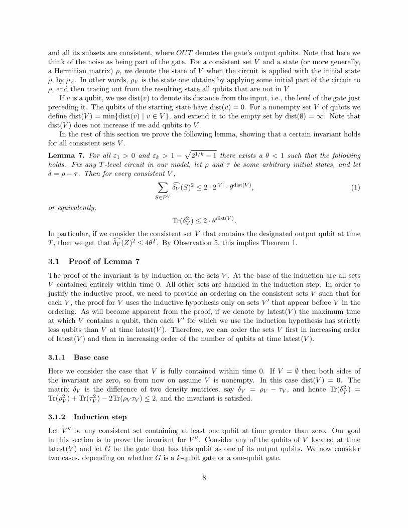
and all its subsets are consistent, where OUT denotes the gate’s output qubits. Note that here wethink of the noise as being part of the gate. For a consistent set V and a state (or more generally,a Hermitian matrix) ρ, we denote the state of V when the circuit is applied with the initial stateρ, by ρV . In other words, ρV is the state one obtains by applying some initial part of the circuit toρ, and then tracing out from the resulting state all qubits that are not in V

If v is a qubit, we use dist(v) to denote its distance from the input, i.e., the level of the gate justpreceding it. The qubits of the starting state have dist(v) = 0. For a nonempty set V of qubits wedefine dist(V ) = mindist(v) | v ∈ V , and extend it to the empty set by dist(∅) = ∞. Note thatdist(V ) does not increase if we add qubits to V .

In the rest of this section we prove the following lemma, showing that a certain invariant holdsfor all consistent sets V .

Lemma 7. For all ε1 > 0 and εk > 1 −√

21/k − 1 there exists a θ < 1 such that the following

holds. Fix any T -level circuit in our model, let ρ and τ be some arbitrary initial states, and let

δ = ρ − τ . Then for every consistent V ,∑

S∈PV

δV (S)2 ≤ 2 · 2|V | · θdist(V ), (1)

or equivalently,

Tr(δ2V ) ≤ 2 · θdist(V ).

In particular, if we consider the consistent set V that contains the designated output qubit at timeT , then we get that δV (Z)2 ≤ 4θT . By Observation 5, this implies Theorem 1.

3.1 Proof of Lemma 7

The proof of the invariant is by induction on the sets V . At the base of the induction are all setsV contained entirely within time 0. All other sets are handled in the induction step. In order tojustify the inductive proof, we need to provide an ordering on the consistent sets V such that foreach V , the proof for V uses the inductive hypothesis only on sets V ′ that appear before V in theordering. As will become apparent from the proof, if we denote by latest(V ) the maximum timeat which V contains a qubit, then each V ′ for which we use the induction hypothesis has strictlyless qubits than V at time latest(V ). Therefore, we can order the sets V first in increasing orderof latest(V ) and then in increasing order of the number of qubits at time latest(V ).

3.1.1 Base case

Here we consider the case that V is fully contained within time 0. If V = ∅ then both sides ofthe invariant are zero, so from now on assume V is nonempty. In this case dist(V ) = 0. Thematrix δV is the difference of two density matrices, say δV = ρV − τV , and hence Tr(δ2

V ) =Tr(ρ2

V ) + Tr(τ2V ) − 2Tr(ρV τV ) ≤ 2, and the invariant is satisfied.

3.1.2 Induction step

Let V ′′ be any consistent set containing at least one qubit at time greater than zero. Our goalin this section is to prove the invariant for V ′′. Consider any of the qubits of V located at timelatest(V ) and let G be the gate that has this qubit as one of its output qubits. We now considertwo cases, depending on whether G is a k-qubit gate or a one-qubit gate.

8

Case 1: G is a k-qubit gate. Here we consider the case that G is a probabilistic mixtureof k-qubit unitaries. First note that by Observation 6 it suffices to prove the invariant for k-qubit unitaries. So assume G is a k-qubit unitary acting on the qubits A = A1, . . . , Ak. LetA′ = A′

1, . . . , A′k be the qubits after the εk-noise but before the gate G and A′′ = A′′

1 , . . . , A′′k

the qubits after G (see Figure 2). By our choice of G, A′′ ∩ V ′′ 6= ∅. Define V ′ = (V ′′ \ A′′) ∪ A′

and V = (V ′′ \ A′′) ∪ A. Note that V and its subsets are consistent sets with strictly fewer qubitsthan V ′′ at time latest(V ′′), and hence we can apply the induction hypothesis to them.

G

A1

A2

A1

A2

'

'

'

'

'

'

A1

A2

Figure 2: An example showing the sets V , V ′, and V ′′ for a two-qubit gate G.

Recall that our goal is to prove the invariant Eq. (1) for V ′′. To begin with, using Observation 3,

∑

S∈PV ′′

δV ′′(S)2 ≤∑

S∈PV ′′∪A′′

δV ′′∪A′′(S)2. (2)

Because G (which maps δV ′ to δV ′′∪A′′) is unitary, it preserves the sum of squares of δ-coefficients(see Observation 2), so the right hand side of (2) is equal to

∑

S∈PV ′

δV ′(S)2 =∑

S∈PV ′\A′

∑

R∈PA′

δV ′(RS)2.

Since the only difference between δV and δV ′ is noise on the qubits A1, . . . , Ak, using Observation4 and denoting µ = 1 − εk, we get that the above is at most

∑

S∈PV \A

∑

R∈PA

µ2|supp(R)|δV (RS)2

=∑

S∈PV \A

∑

a⊆A

µ2|a|(1 − µ2)k−|a|∑

R∈Pa⊗IA\a

δV (RS)2,

where the equality follows by noting that for any fixed S and any R ∈ PA, the term δV (RS)2,which appears with coefficient µ2|supp(R)| on the left hand side, appears with the same coefficient

9

∑a⊇supp(R) µ2|a|(1− µ2)k−|a| = µ2|supp(R)| on the right hand side. By rearranging and using Obser-

vation 3 we get that the above is equal to

∑

a⊆A

µ2|a|(1 − µ2)k−|a|∑

S∈P(V \A)∪a

δ(V \A)∪a(S)2

≤∑

a⊆A

µ2|a|(1 − µ2)k−|a|2 · 2|(V \A)∪a| · θdist((V \A)∪a)

where we used the inductive hypothesis. Note that dist((V \ A) ∪ a) ≥ dist(V ), so the above is

≤ 2 · 2|V \A| · θdist(V )∑

a⊆A

2|a|µ2|a|(1 − µ2)k−|a|

= 2 · 2|V \A| · θdist(V )((1 − µ2) + 2µ2)k

= 2 · 2|V \A| · θdist(V )(1 + µ2)k. (3)

Note that |V \ A| ≤ |V ′′| − 1 and dist(V ′′) − 1 ≤ dist(V ), so the right hand side is bounded by

≤ 2 · 2|V ′′|−1 · θdist(V ′′)−1(1 + µ2)k.

Since εk > 1 −√

21/k − 1, we have that (1 + µ2)k ≤ 2θ if θ is close enough to 1, so we can finallybound the last expression by

≤ 2 · 2|V ′′| · θdist(V ′′)

which proves the invariant for V ′′.

Case 2: G is a one-qubit gate. Before proving the invariant, we need to prove the followingproperty of completely-positive trace-preserving (CPTP) maps on one qubit.

Lemma 8. For any CPTP map G on one qubit there exists a β ∈ [0, 1] such that the following

holds. For any Hermitian matrix δ, if we let δ′ denote the result of applying G to δ, then we have

δ′(X)2 + δ′(Y )2 + δ′(Z)2 ≤ (1 − β) · δ(I)2 + β · (δ(X)2 + δ(Y )2 + δ(Z)2).

Proof: The proof is based on the characterization of trace-preserving completely-positive mapson one qubit due to Ruskai, Szarek, and Werner [23, Sections 1.2 and 1.3]. This characterizationimplies that any one-qubit gate G can be written as a convex combination of gates of the formU1 J U2. Here U1 and U2 are one-qubit unitaries (acting on the density matrix by conjugation),and J is a one-qubit map that in the Pauli basis has the form

J =

1 0 0 00 λ1 0 00 0 λ2 0t 0 0 λ1λ2

for some λ1, λ2 ∈ [−1, 1] and t = ±√

(1 − λ21)(1 − λ2

2).First observe that by the convexity of the square function, it suffices to prove the lemma for G

of the form U1 J U2 (with the resulting β being the appropriate average of the individual β’s).Next note that since U1 and U2 are unitary, they act on the vector of coefficients (δ(X), δ(Y ), δ(Z))

10

as an orthogonal transformation, and hence leave the sum of squares invariant. This shows that itsuffices to prove the lemma for a map J as above. For this map,

δ′(X)2 + δ′(Y )2 + δ′(Z)2 = λ21δ(X)2 + λ2

2δ(Y )2 + (tδ(I) + λ1λ2δ(Z))2.

Assume without loss of generality that λ21 ≥ λ2

2. Applying Cauchy-Schwarz to the two 2-dimensionalvectors (±

√1 − λ2

1a, λ1b) and (√

1 − λ22, λ2), we get that for any a, b ∈ R, (ta + λ1λ2b)

2 ≤ (1 −λ2

1)a2 + λ2

1b2. Hence the above expression is upper bounded by

λ21δ(X)2 + λ2

1δ(Y )2 + (1 − λ21)δ(I)2 + λ2

1δ(Z)2

and we complete the proof by choosing β = λ21.

Let A be the qubit G is acting on, and recall that our goal is to prove the invariant for the setV ′′. Denote by A′ the qubit of G after the gate but before the ε1 noise, and by A′′ the qubit afterthe noise. As before, by our choice of G, we have A′′ ∈ V ′′. Let A = A, A′ = A′, A′′ = A′′.Define V ′ = (V ′′ \ A′′) ∪ A′ and V = (V ′′ \ A′′) ∪ A and notice that |V | = |V ′| = |V ′′|. By usingLemma 8, we obtain a β ∈ [0, 1] such that

∑

S∈PV ′′

δV ′′(S)2 ≤∑

S∈PV ′\A′

(δV ′(IS)2 + (1 − ε1)

2∑

R∈PA′∗

δV ′(RS)2

)

≤∑

S∈PV \A

((1 + (1 − ε1)

2(1 − 2β))δV (IS)2 + (1 − ε1)2β

∑

R∈PA

δV (RS)2

).

By applying the induction hypothesis to both V \ A and V , we can upper bound the above by

(1 + (1 − ε1)2(1 − 2β)) · 2 · 2|V |−1 · θdist(V \A) + (1 − ε1)

2β · 2 · 2|V | · θdist(V )

≤ 1 + (1 − ε1)2

2θ· 2 · 2|V ′′| · θdist(V ′′)

where we used that |V | = |V ′′|, and dist(V ′′) − 1 ≤ dist(V ) ≤ dist(V \ A). Hence the invariantremains valid if we choose θ < 1 such that 1 + (1 − ε1)

2 ≤ 2θ.

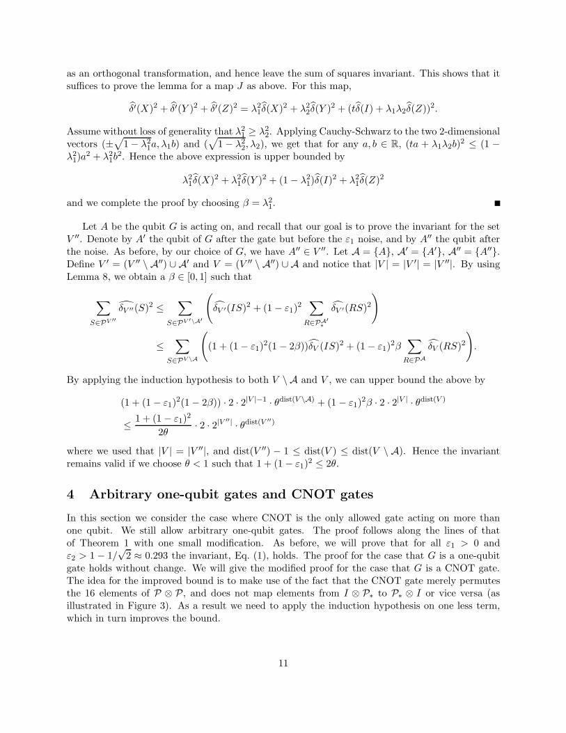
4 Arbitrary one-qubit gates and CNOT gates

In this section we consider the case where CNOT is the only allowed gate acting on more thanone qubit. We still allow arbitrary one-qubit gates. The proof follows along the lines of thatof Theorem 1 with one small modification. As before, we will prove that for all ε1 > 0 andε2 > 1 − 1/

√2 ≈ 0.293 the invariant, Eq. (1), holds. The proof for the case that G is a one-qubit

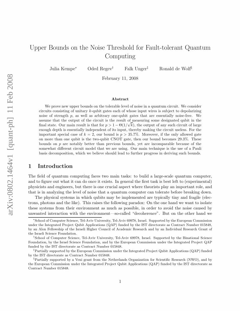
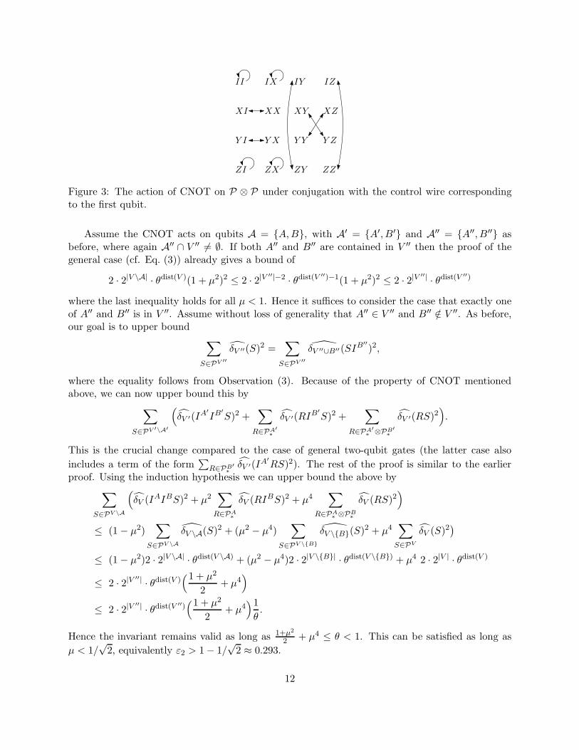
gate holds without change. We will give the modified proof for the case that G is a CNOT gate.The idea for the improved bound is to make use of the fact that the CNOT gate merely permutesthe 16 elements of P ⊗ P, and does not map elements from I ⊗ P∗ to P∗ ⊗ I or vice versa (asillustrated in Figure 3). As a result we need to apply the induction hypothesis on one less term,which in turn improves the bound.

11

II IX IY IZ

XI XX XY XZ

Y I Y X Y Y Y Z

ZI ZX ZY ZZ

Figure 3: The action of CNOT on P ⊗ P under conjugation with the control wire correspondingto the first qubit.

Assume the CNOT acts on qubits A = A,B, with A′ = A′, B′ and A′′ = A′′, B′′ asbefore, where again A′′ ∩ V ′′ 6= ∅. If both A′′ and B′′ are contained in V ′′ then the proof of thegeneral case (cf. Eq. (3)) already gives a bound of

2 · 2|V \A| · θdist(V )(1 + µ2)2 ≤ 2 · 2|V ′′|−2 · θdist(V ′′)−1(1 + µ2)2 ≤ 2 · 2|V ′′| · θdist(V ′′)

where the last inequality holds for all µ < 1. Hence it suffices to consider the case that exactly oneof A′′ and B′′ is in V ′′. Assume without loss of generality that A′′ ∈ V ′′ and B′′ /∈ V ′′. As before,our goal is to upper bound

∑

S∈PV ′′

δV ′′(S)2 =∑

S∈PV ′′

δV ′′∪B′′(SIB′′)2,

where the equality follows from Observation (3). Because of the property of CNOT mentionedabove, we can now upper bound this by

∑

S∈PV ′\A′

(δV ′(IA′

IB′S)2 +

∑

R∈PA′∗

δV ′(RIB′S)2 +

∑

R∈PA′∗ ⊗PB′

∗

δV ′(RS)2).

This is the crucial change compared to the case of general two-qubit gates (the latter case also

includes a term of the form∑

R∈PB′∗

δV ′(IA′RS)2). The rest of the proof is similar to the earlier

proof. Using the induction hypothesis we can upper bound the above by∑

S∈PV \A

(δV (IAIBS)2 + µ2

∑

R∈PA∗

δV (RIBS)2 + µ4∑

R∈PA∗ ⊗PB

∗

δV (RS)2)

≤ (1 − µ2)∑

S∈PV \A

δV \A(S)2 + (µ2 − µ4)∑

S∈PV \B

δV \B(S)2 + µ4∑

S∈PV

δV (S)2)

≤ (1 − µ2)2 · 2|V \A| · θdist(V \A) + (µ2 − µ4)2 · 2|V \B| · θdist(V \B) + µ4 2 · 2|V | · θdist(V )

≤ 2 · 2|V ′′| · θdist(V )(1 + µ2

2+ µ4

)

≤ 2 · 2|V ′′| · θdist(V ′′)(1 + µ2

2+ µ4

)1

θ.

Hence the invariant remains valid as long as 1+µ2

2 + µ4 ≤ θ < 1. This can be satisfied as long as

µ < 1/√

2, equivalently ε2 > 1 − 1/√

2 ≈ 0.293.

12

Acknowledgment

We thank Mary Beth Ruskai for a pointer to [23] and for sharing her insights on the characterizationof one-qubit operations. We thank Peter Shor for a discussion on entanglement breaking channelswhich is related to the discussion of [8] at the end of Section 1.

References

[1] D. Aharonov and M. Ben-Or. Fault tolerant quantum computation with constant error. InProceedings of 29th ACM STOC, pages 176–188, 1997. quant-ph/9611025.

[2] P. Aliferis. Level Reduction and the Quantum Threshold Theorem. PhD thesis, Caltech, 2007.quant-ph/0703264.

[3] P. Aliferis. Threshold lower bounds for Knill’s Fibonacci scheme. quant-ph/0709.3603, 22 Sep2007.

[4] P. Aliferis, D. Gottesman, and J. Preskill. Accuracy threshold for postselected quantum com-putation. Quantum Information and Computation, 8(3):181–244, 2008. quant-ph/0703264.

[5] A. Barenco, C.H. Bennett, R. Cleve, D.P. DiVincenzo, N. Margolus, P. Shor, T. Sleator,J. Smolin, and H. Weinfurter. Elementary gates for quantum computation. Physical Review

A, 52:3457–3467, 1995. quant-ph/9503016.

[6] E. Bernstein and U. Vazirani. Quantum complexity theory. SIAM Journal on Computing,26(5):1411–1473, 1997. Earlier version in STOC’93.

[7] S. Bravyi and A. Kitaev. Universal quantum computation with ideal Clifford gates and noisyancillas. Physical Review A, 71(022316), 2005. quant-ph/0403025.

[8] D. Bruss, D. DiVincenzo, A. Ekert, C. Fuchs, C. Macchiavello, and J. Smolin. Optimaluniversal and state-dependent quantum cloning. Physical Review A, 43:2368–2378, 1998.

[9] H. Buhrman, R. Cleve, M. Laurent, N. Linden, A. Schrijver, and F. Unger. New limits onfault-tolerant quantum computation. In Proceedings of 47th IEEE FOCS, pages 411–419, 2006.quant-ph/0604141.

[10] W. S. Evans and L. J. Schulman. Signal propagation and noisy circuits. IEEE Trans. Inform.

Theory, 45(7):2367–2373, 1999.

[11] W. S. Evans and L. J. Schulman. On the maximum tolerable noise of k-input gates for reliablecomputation by formulas. IEEE Trans. Inform. Theory, 49(11):3094–3098, 2003.

[12] D. Gottesman. Stabilizer Codes and Quantum Error Correction. PhD thesis, Caltech, 1997.quant-ph/9702052.

[13] L. K. Grover. A fast quantum mechanical algorithm for database search. In Proceedings of

28th ACM STOC, pages 212–219, 1996. quant-ph/9605043.

[14] A. Yu. Kitaev. Quantum computations: Algorithms and error correction. Russian Mathemat-

ical Surveys, 52(6):1191–1249, 1997.

13

[15] E. Knill, R. Laflamme, and W. H. Zurek. Resilient quantum computation. Science,279(5349):342–345, 1998.

[16] M. Knill. Fault-tolerant postselected quantum computation: Threshold analysis. quant-ph/0404104, 19 Apr 2004.

[17] M. Knill. Quantum computing with realistically noisy devices. Nature, 434:39–44, 2005.

[18] M. Knill, R. Laflamme, and W. Zurek. Accuracy threshold for quantum computation. quant-ph/9610011, 15 Oct 1996.

[19] A. Razborov. An upper bound on the threshold quantum decoherence rate. Quantum Infor-

mation and Computation, 4(3):222–228, 2004. quant-ph/0310136.

[20] B. Reichardt. Quantum universality from Magic States Distillation applied to CSS codes.Quantum Information Processing, 4:251–264, 2005.

[21] B. Reichardt. Error-Detection-Based Quantum Fault Tolerance Against Discrete Pauli Noise.PhD thesis, UC Berkeley, 2006. quant-ph/0612004.

[22] B. Reichardt. Quantum universality by distilling certain one- and two-qubit states with sta-bilizer operations. quant-ph/0608085, 2006.

[23] M. B. Ruskai, S. Szarek, and E. Werner. An analysis of completely-positive trace-preservingmaps on M2. Linear Algebra and its Applications, 347:159–187, 2002. quant-ph/0101003.

[24] P. W. Shor. Scheme for reducing decoherence in quantum memory. Physical Review A, 52:2493,1995.

[25] P. W. Shor. Fault-tolerant quantum computation. In Proceedings of 37th IEEE FOCS, pages56–65, 1996.

[26] P. W. Shor. Polynomial-time algorithms for prime factorization and discrete logarithms on aquantum computer. SIAM Journal on Computing, 26(5):1484–1509, 1997. Earlier version inFOCS’94. quant-ph/9508027.

[27] D. Simon. On the power of quantum computation. SIAM Journal on Computing, 26(5):1474–1483, 1997. Earlier version in FOCS’94.

[28] A. Steane. Multiple particle interference and quantum error correction. In Proceedings of the

Royal Society of London, volume A452, pages 2551–2577, 1996. quant-ph/9601029.

[29] S. Virmani, S. Huelga, and M. Plenio. Classical simulability, entanglement breaking, andquantum computation thresholds. Physical Review A, 71(042328), 2005. quant-ph/0408076.

14