Update to limits to growth - Interest.co.nz

DOI: 10.1111/jiec.13084

R E S E A RCH AND ANA LY S I S

Update to limits to growthComparing theWorld3model with empirical data

GayaHerrington

KPMG LLP, Los Angeles, California

Correspondence

GayaHerrington (néeBranderhorst), KPMG

LLP, 550SouthHopeStreet, LosAngeles,CA

90071,USA.

Email: [email protected]

EditorManagingReview:HeinzSchandl

Abstract

In the 1972 bestseller Limits to Growth (LtG), the authors concluded that, if global soci-

ety kept pursuing economic growth, it would experience a decline in food produc-

tion, industrial output, and ultimately population, within this century. The LtG authors

used a system dynamics model to study interactions between global variables, vary-

ing model assumptions to generate different scenarios. Previous empirical-data com-

parisons since then by Turner showed closest alignment with a scenario that ended

in collapse. This research constitutes a data update to LtG, by examining to what

extent empirical data alignedwith four LtGscenarios spanning a rangeof technological,

resource, and societal assumptions. The research benefited from improved data avail-

ability since the previous updates and included a scenario and two variables that had

not been part of previous comparisons. The two scenarios aligning most closely with

observed data indicate a halt in welfare, food, and industrial production over the next

decade or so, which puts into question the suitability of continuous economic growth

as humanity’s goal in the twenty-first century. Both scenarios also indicate subsequent

declines in these variables, but only one—where declines are caused by pollution—

depicts a collapse. The scenario that aligned most closely in earlier comparisons was

not amongst the two closest aligning scenarios in this research. The scenario with the

smallest declines aligned leastwith empirical data; however, absolute differenceswere

often not yet large. The four scenarios diverge significantly more after 2020, suggest-

ing that the window to align with this last scenario is closing.

KEYWORDS

collapse, industrial ecology, limits to growth, system dynamics modeling, systems thinking,World3

1 INTRODUCTION

1.1 Limits to growth

In the 1972 bestseller Limits to Growth (LtG), the authors concluded that if humanity kept pursuing economic growth without regard for environ-

mental and social costs, global society would experience a sharp decline (i.e., collapse) in economic, social, and environmental conditions within

the twenty-first century. They used a model calledWorld3 to study key interactions between variables for global population, birth rate, mortality,

industrial output, food production, health and education services, non-renewable natural resources, and pollution. The LtG team generated differ-

entWorld3 scenarios by varying assumptions about technological development, amounts of non-renewable resources, and societal priorities. The

Journal of Industrial Ecology 2020;1–13. © 2020 by Yale University 1wileyonlinelibrary.com/journal/jiec

2 HERRINGTON

few comparisons of empirical data with the scenarios since then, most recently from 2014 (Turner), indicated that the world was still following the

“business as usual” (BAU) scenario. BAU showed a halt in the hitherto continuous increase in welfare indicators around the present day and a sharp

decline starting around 2030.

This article describes the research into whether humanity was still following BAU and whether there seemed opportunity left to change course

to becomemore alignedwith another LtG scenario, perhaps one in which collapse is avoided.World3 scenarios were quantitatively comparedwith

empirical data. The research thus constitutes an update to previous comparisons but also adds to them in several ways. Earlier data comparisons

used scenarios from the 1972 LtG book. The scenarios in this research were created with the latest, revised and recalibrated,World3 version. This

data comparison also included a scenario and two variables that had not been part of such research before, and benefited from better empirical

proxies thanks to improved data availability.

1.2 Limits to growth message

TheLtGmessagewas that continuous growth in industrial output cannot be sustained indefinitely (Meadows,Meadows, Randers, &Behrens, 1972).

Effectively, humanity can either choose its own limit or at some point reach an imposed limit, at which time a decline in human welfare will have

become unavoidable. An often missed, but key point in the LtGmessage is the plural of “limits” (Meadows &Meadows, 2007; Meadows, Meadows,

& Randers, 2004). In an interconnected system like our global society, a solution to one limit inevitably causes interactions with other parts of the

system, giving rise to a new limit which then becomes the binding constraint to growth (Meadows & Meadows, 2007). To illustrate this point, the

LtG authors created various scenarios with World3. World3 was based on the work of Forrester (1971, 1975), the founder of system dynamics: a

modeling approach for interactions between objects in a system, often characterized by non-linear behavior like delays, feedback loops, and expo-

nential growth or decline. The LtG scenarios were thus not meant to produce point predictions, but rather to help us understand the behavior of

systems in the world over time.

1.3 LtG publications

The first book (Meadows et al., 1972) was commissioned by the Club of Rome and introducedWorld3 together with 12 scenarios. Themost widely

discussed scenario has been the BAU. It maintained parameters at historic levels from the latter part of the twentieth century, without imposing

any additional assumptions. In BAU, standards of living would at some point stop rising along with industrial growth once the accompanying deple-

tion of non-renewable resources had started to render these a limiting factor in industrial and agricultural production. Continuation of standard

economic operation without adapting to the constraint of growing resource scarcity would then require increasingly more industrial capital to be

diverted toward extracting non-renewable resources. This would leave less for food production, citizen services and industrial re-investment, caus-

ing declines in these factors and, subsequently, in population (Meadows et al., 1972).

There were 11 other scenarios in the first book, including “comprehensive technology” (CT) and “stabilized world” (SW). CT assumes a range

of technological solutions, including reductions in pollution generation, increases in agricultural land yields, and resource efficiency improvements

that are significantly abovehistoric averages (Meadowset al., 1972, p. 147). TheSWscenario assumes that in addition to the technological solutions,

global societal priorities changed from a certain year onward (Meadows et al., 1972). A change in values and policies translates into, amongst other

things, low desired family size, perfect birth control availability, and a deliberate choice to limit industrial output and prioritize health and education

services. SWwas the only scenario in which declines were avoided.

The second book, Beyond the Limits, was published in 1992 (Meadows, Meadows, & Randers). The LtG team had recalibrated World3 to two

decades of additional data. The authors concluded thatwhile humankind had had the opportunity to act during the 20 years after the first LtG book,

society had now reached overshoot (i.e., exceeds the earth’s carrying capacity).

The third and last book, Limits to Growth: The 30-Year Update, dates from2004 (Meadows et al.). It described 10 new scenarios whichwere similar

to those from the first two books in assumptions, butmadewith a revisedWorld3model:World3-03. Themodel revisions included incorporation of

twonewvariables: the humanecological footprint (EF) and humanwelfare. The assumptions regarding technological progresswere also intensified,

going above historic rates even further, making the CT scenario more optimistic compared to its 1972 version.

1.4 Criticism

The LtG books andWorld3 received much criticism at the time (e.g., Bardi, 2011; Norgard, Peet, & Ragnarsdóttir, 2010). Much of this was focused

on the economic and technological assumptions underlying the World3 model. Additionally, there was technical criticism of World3 and the new

modeling technique (system dynamics) itself. There were also misconceptions about the scenarios and LtG message, some of which have proven

HERRINGTON 3

persistent and influential in the public debate. An example is the claim that the first book predicted resource depletion by 1990 (Passell, Roberts,

& Ross, 1972). This misconception spread to the point of being repeated by organizations like the United Nations Environment Programme (2002).

It was actively revived by analysts (“Plenty of Gloom”, 1997; Bailey, 1989; Lomborg & Olivier, 2009), who subsequently dismissed LtG because

depletion and collapse had not taken place. Reversal points lie beyond 2000 in all the scenario graphs in the LtG books, however.

CriticismonWorld3’s underlying assumptions focusedmostlyon those concerning technological progress andmarket correction. Someregarded

the absence of a corrective pricemechanism as a fatal flaw, contending that increased priceswould spur substitutions between resources and other

technological solutions (Kaysen, 1972; Solow, 1973). Economist Solow (1973), for example, argued that increased scarcity would drive up prices

of non-renewable resources, and also that pollution externalities would drive more regulation and higher taxes. Research by the Organisation for

Economic Co-operation and Development (OECD, 2017, 2018), amongst others, suggests; however, that the social costs of pollution and natural

resource depletion are currently not fully reflected in taxes. Fossil fuels alone still carry large indirect after-tax government subsidies (Coady, Parry,

Le, & Shang, 2019), totaling 6.4% of global gross domestic product (GDP). Others argued in a reaction to the first LtG book thatWorld3 did not give

enoughcredence tohumanity’s ability to invent technological solutions toenvironmental challenges (Cole, Freeman, Jahoda,&Pavitt, 1973;Kaysen,

1972). The LtG authors have since pointed out (Meadows et al., 2004;Meadows et al., 1992) that their books contained several scenarios other than

the BAU, which were based on assumptions about technological innovation and adoption that are significantly higher than historic averages. These

optimistic assumptions on humankind’s ingenuity andwillingness to share technological solutions do not prevent declines in an LtG scenario, unless

it is paired with societal value and policy changes (as in SW).

Technical criticism included the claim that World3 model can be sensitive; relatively small parameter changes will in some cases significantly

alter a scenario’s trajectory (Castro, 2012; de Jongh, 1978; Vermeulen & de Jongh, 1976). Recreation of runs with the same parameter changes as

in these critical studies confirmed that finding, although it also showed that the parameter changes did not avoid an overshoot and collapse pattern

(Turner, 2013). A 1973 review of World3 by Cole, Freeman, Jahoda, & Pavitt, concluded that the model was inadequate from the perspective of

linear modeling. Sterman (2000) has since pointed out that adequacy as a linear model is not the right criterion for a system dynamics model.

1.5 Updates to LtG

Several qualitative reviews of the LtG publications have described how dynamics inWorld3 could be observed in the real world (Bardi, 2014; Jack-

son & Weber, 2016; Simmons, 2000). One such review was from LtG author Randers (2000). Around 1990, it became clear that non-renewable

resources, particularly fossil fuels, had turned out to be more plentiful than assumed in the 1972 BAU scenario. Randers therefore postulated that

not resource scarcity, but pollution, especially from greenhouse gases, would cause the halt in growth. This aligns with the second scenario in the

LtG books. This scenario has the same assumptions as the BAU, except that it assumes double the amount of non-renewable resources. This sce-

nario is referred to asBAU2, and receivedmore focus than theBAUscenario in the second and third LtGbooks.More natural resources do not avoid

collapse inWorld3; the cause changes from resource depletion to a pollution crisis.

BAU2 was quantitatively assessed in a 2015 recalibration study of World3-03 (Pasqualino, Jones, Monasterolo, & Phillips, 2015). Results indi-

cated that society had investedmore to abate pollution, increase food productivity, and invest in services compared to BAU2. However, the authors

did not compare their calibration with SW, nor did they use their recalibrated version of World3 to run the scenario beyond the present to see

if collapse was avoided. Thus, their findings could not be taken as an indication that humanity had done enough to avoid declines, as the authors

themselves made sure to point out.

Quantitative comparisons between LtG scenarios and empirical data were conducted by Turner (2008, 2012, 2014). He compared global

observed data for the LtG variables with 3 of the 12 scenarios from the first book: BAU, CT, and SW. Turner concluded that world data compared

favorably to key features of BAU, andmuchmore so than for the other two scenarios.

1.6 This research: A data comparison to LtG

In this research, data available in 2019 was compared with the recalibrated World3-03 to examine whether this produced the same outcomes as

Turner had found. Because he used the 1972 variables, Turner did not include the two that were added in 2004, human welfare and EF. Another

open question therefore was to what extent these variables aligned with their real-world counterparts. Lastly, given the attention that BAU2 had

received and that its pollution crisis can be interpreted as depicting climate change (i.e., collapse fromgreenhouse gas pollution), this scenario ought

to be included in a comparison.

The research goal was to determine to what extent empirical data aligned with selected scenarios of World3-03 (henceforth called “World3”).

Data was compiled from various official databases, as indicators for what the following 10 variables represented: population, fertility (birth rate),

mortality (death rate), industrial output per capita (p.c.), food p.c., services p.c., non-renewable resources, persistent pollution, human welfare, and

4 HERRINGTON

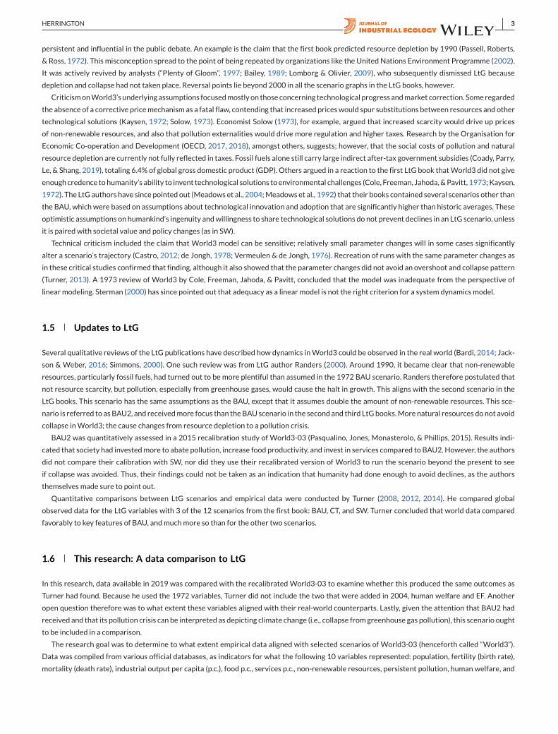
F IGURE 1 The BAU, BAU2, CT, and SW scenarios. Adapted from Limits to Growth: The 30-Year Update (p. 169, 173, 219, 245), byMeadows, D.H., Meadows, D. L., and Randers, J., 2004, Chelsea Green Publishing Co. Copyright 2004 byDennisMeadows. Adaptedwith permission

TABLE 1 Description and cause of halt in growth and/or decline per scenario

Scenario Description Cause

BAU No assumptions added to historic averages Collapse due to natural resource depletion.

BAU2 Double the natural resources of BAU Collapse due to pollution (climate change equivalent).

CT BAU2+ exceptionally high technological development and

adoption rates

Rising costs for technology eventually cause declines, but no

collapse.

SW CT+ changes in societal values and priorities Population stabilizes in the twenty-first century, as does human

welfare on a high level.

ecological footprint (EF). This data was plotted along with fourWorld3 scenarios: BAU, BAU2, CT, and SW. These were the 2004 LtG book equiva-

lents of the three scenarios in Turner’s earlier work, plus BAU2.

Figure 1 shows how some of the LtG variables behave in each of these four scenarios. It should be noted that the numerical scales of theWorld3

output differ widely between variables. They are scaled in Figure 1 (as in the LtG books) to fit in one plot. This means that relative positions to each

other on the y-axis have no meaning whatsoever. What is relevant is the movement of the variables over time in each of the four scenarios. These

movements together depict the storyline of that scenario, which unfolds based on the specific scenario assumptions.

The assumptions underlying each scenario differ in technological, social, or resource conditions. The cause of decline, varying from a temporary

dip to societal collapse, also differs for each scenario (Table 1).

2 METHODS

2.1 Scenario data

BAU, BAU2, CT, and SW, correspond to scenarios 1, 2, 6, and 9 in the 2004 LtG book. This means that for the SW scenario, policy changes are

assumed to start in 2002. To create the scenarios, the original CD-ROMthat camewith the 2004 bookwas used. TheCD-ROMcontains simulations

of the scenarios andnumerical output of thevariables. A zip file ofWorld3-03 is also available fromMetaSD (2020) and it canbe runon free software

fromVensim (2020).

HERRINGTON 5

2.2 Determination of accuracy

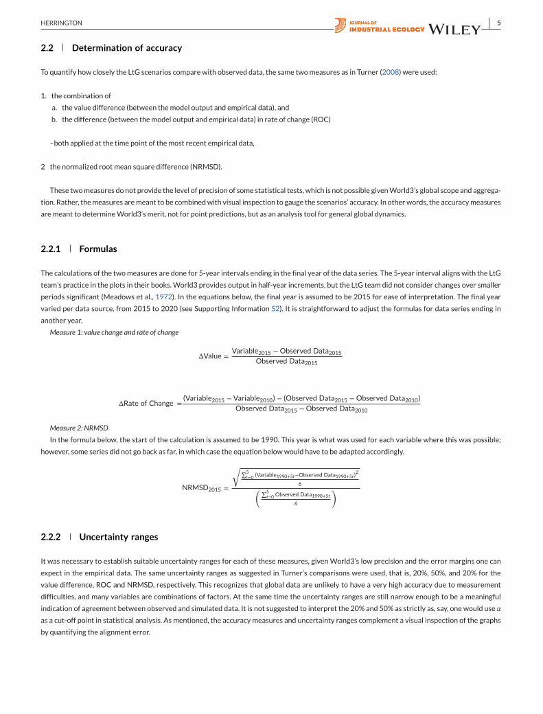
To quantify how closely the LtG scenarios compare with observed data, the same twomeasures as in Turner (2008) were used:

1. the combination of

a. the value difference (between themodel output and empirical data), and

b. the difference (between themodel output and empirical data) in rate of change (ROC)

–both applied at the time point of themost recent empirical data,

2 the normalized root mean square difference (NRMSD).

These twomeasures do not provide the level of precision of some statistical tests, which is not possible givenWorld3’s global scope and aggrega-

tion. Rather, themeasures aremeant to be combinedwith visual inspection to gauge the scenarios’ accuracy. In otherwords, the accuracymeasures

aremeant to determineWorld3’s merit, not for point predictions, but as an analysis tool for general global dynamics.

2.2.1 Formulas

The calculations of the twomeasures are done for 5-year intervals ending in the final year of the data series. The 5-year interval aligns with the LtG

team’s practice in the plots in their books.World3 provides output in half-year increments, but the LtG team did not consider changes over smaller

periods significant (Meadows et al., 1972). In the equations below, the final year is assumed to be 2015 for ease of interpretation. The final year

varied per data source, from 2015 to 2020 (see Supporting Information S2). It is straightforward to adjust the formulas for data series ending in

another year.

Measure 1: value change and rate of change

ΔValue =Variable2015 −Observed Data2015

Observed Data2015

ΔRate of Change =(Variable2015 − Variable2010) − (Observed Data2015 −Observed Data2010)

Observed Data2015 −Observed Data2010

Measure 2: NRMSD

In the formula below, the start of the calculation is assumed to be 1990. This year is what was used for each variable where this was possible;

however, some series did not go back as far, in which case the equation belowwould have to be adapted accordingly.

NRMSD2015 =

√∑5t=0 (Variable1990+5t−Observed Data1990+5t)

2

6(∑5t=0 Observed Data1990+5t

6

)

2.2.2 Uncertainty ranges

It was necessary to establish suitable uncertainty ranges for each of these measures, given World3’s low precision and the error margins one can

expect in the empirical data. The same uncertainty ranges as suggested in Turner’s comparisons were used, that is, 20%, 50%, and 20% for the

value difference, ROC and NRMSD, respectively. This recognizes that global data are unlikely to have a very high accuracy due to measurement

difficulties, and many variables are combinations of factors. At the same time the uncertainty ranges are still narrow enough to be a meaningful

indication of agreement between observed and simulated data. It is not suggested to interpret the 20% and 50% as strictly as, say, one would use αas a cut-off point in statistical analysis. As mentioned, the accuracy measures and uncertainty ranges complement a visual inspection of the graphs

by quantifying the alignment error.

6 HERRINGTON

2.3 Closest fit count

Apart from a measure of absolute fit, the above-mentioned uncertainty range, it was also necessary to distinguish amongst the four scenarios in

terms of relative fit. This can be donewith a simple tally over the variables for each scenario. A scenario was counted as a closest fit when it aligned

more closely than other scenarios and at least one of that variable’s proxieswaswithin the uncertainty bounds for both accuracymeasures. Another

option would have been to count a scenario as a closest fit if either measure 1 ormeasure 2was within the uncertainty range for at least one proxy.

The choice to only count a scenario when both accuracymeasures were within range wasmade because it’s more conservative.When all scenarios

were outside of uncertainty bounds for at least onemeasure, they were counted as inconclusive. For cases where two or more scenarios aligned to

the same extent, they were all counted.

2.4 Data sources

Below follows a list of the source(s) of empirical data used for each variable in this comparison. Reliability of each source is briefly discussed in

Supporting Information S1.

Somevariables requiredproxies because thevariable inWorld3 is not directly observable or quantifiable in the realworld. The samedata sources

as Turner were often chosen; however, in several cases it was possible to improve on previous proxies thanks to new or recently enhanced indices

and databases. When empirical data was expressed in different units than the LtG scenarios, they were normalized to the 1990 scenario value,

because that is the year thatWorld3was recalibrated to last (Meadows et al., 1992).

2.4.1 Population

Figures from the Population Division of the United Nations Department of Economic & Social Affairs (UNDESA PD, 2019) were used for this vari-

able. Their population series includes estimates for 2020, whichwere compared against the LtG 2020 values. Annual population figures can also be

found on theWorld Bank Open Data website (WB, 2019a). Both sites mention national agencies and international organizations as their sources,

such as Eurostat, the US Census Bureau, and census publications from national statistical offices.

2.4.2 Fertility and mortality (two variables)

The data series from the WB Open Data site (2019b, 2019c) were used for both of these variables. The WB mentions as its sources the same

organizations and publications as for its population series.

2.4.3 Food per capita

Total energy available per person per daywas used to approximate this variable. The daily caloric value per capita can be found in the Food Balance

Sheets on FAOSTAT (2019), the database of the Food and Agriculture Organization of the UN.

2.4.4 Industrial output per capita

The industrial output p.c. variable represented citizens’ material and technological standard of living andwas a factor in theWorld3 society’s ability

to grow food anddeliver services (Meadows et al., 2004). The index of industrial production (IIP) and gross fixed capital formation (GFCF)were used

as proxies. Both proxy series were divided by population to arrive at per capita numbers.

IIP is a standardized macroeconomic indicator of an economy’s real output in manufacturing, mining, and energy (e.g., Moles & Terry, 1997).

Unlike GDP, IIP excludes retail and professional services, making it a useful proxy for industrial output. The IIP series can be retrieved as “INSTAT2”

on the data portal of the UN Industrial Development Organization (UNIDO, 2019a). UNIDO does not provide a global IIP, so one was created with

a weighted average of country IIPs. National manufacturing value added, also sourced fromUNIDO (2019b), was used for weighting.

The WB (2019d) provides a global GFCF series. GFCF includes land improvements (e.g., fences and drains), infrastructure (e.g., roads), build-

ings and construction (e.g., schools, offices, hospitals, and industrial buildings), machinery, and equipment purchases. This aligns closely with the

definition of the industrial output variable inWorld3, especially as it relates to a society’s ability to deliver services and grow food.

HERRINGTON 7

2.4.5 Services per capita

InWorld3, services p.c. represents education and health services (Meadows et al., 2004). The Education Index (EI), spending on health, and spending

on education were used as proxies.

The EI is constructed by the UN Development Programme (UNDP, 2019a). It is calculated using mean years of schooling and expected years of

schooling (UNDP, 2019b). These two figures can be quite different, especially in developing countries, and combined thus provide a good indication

of currently available education services (UNDP, 2019c).

The WB provides global figures for both government spending on education (2019e) and health expenditure (2019f). The two series are

expressed as a percentage of GDP. The LtG authors described several collapse patterns as resources being diverted away from these citizen ser-

vices to industrial capital in order to keep extracting natural resources, abate pollution, and/or produce food. Fraction ofGDP is an indication of how

resources are allocated toward something on a macro level, as expressed by the WB’s statement that a “high percentage to GDP suggests a high

priority for education” (2019e). Therefore, tracking the fraction of global GDP spent on education or health can help reveal whether themechanism

described by LtG is indeed observable.

2.4.6 Pollution

World3 assumes pollution to be globally distributed, persistent, and damaging to human health and agricultural production. CO2 concentrations

and plastic production were used as proxies.

Atmospheric CO2 data (Tans & Keeling, 2019) were obtained from the National Oceanic & Atmospheric Administration (NOAA). The 1900 CO2

level of 297 parts per million (Etheridge et al., 1996) was subtracted from the NOAA data, because the LtG scenarios put pollution at 0 in 1900.

Although CO2 is not the only persistent pollutant—NOx, SOx, heavymetals, and ozone-depleting substances are other examples—it is an adequate

proxy because of the global impacts that climate change brings for human health, the environment, and our ability to grow food, and because there

exist accurate time series data.

Global plastic production data was sourced fromGeyer, Jambeck, and Law (2017). The data was adjusted downwards to the share of plastic that

gets discarded, which reportedly went from 100% in 1980 to 55% in 2015 (Geyer et al., 2017). Not all plastic is considered pollution; however,

plastic‘s persistence and ubiquity in today’s society, and documented impacts on human health, aligns withWorld3’s assumptions on the pollution

variable. Various kinds of plastics can be found throughout the entire consumer product and food supply chain, from oceans and marine wildlife

(Smillie, 2017; vanSebille et al., 2015) to tapwater (Kosuth,Wattenberg,Mason, Tyree,&Morrison, 2017), fromagricultural land (Nizzetto, Langaas,

& Futter, 2016) to dietary components and the air we breathe (Wright & Kelly, 2017a), prompting a growing body of scientific literature on a wide

range of possible negative human health effects (Halden, 2010;Wright & Kelly, 2017b).

2.4.7 Non-renewable resources

Twoproxieswereused for this variable, bothbasedondifferent expert estimatesof fossil fuel resources. Full substitutionbetweenenergy resources

is assumed, which is conservative given the current state of technology (Brathwaite, Horst, & Iacobucci, 2010; Driessen, Henckens, van Ierland, &

Worrell, 2016; Graedel, Harper, Nassar, & Reck, 2015). The proxy data series were not normalized to 1990 values because they represent fractions

(i.e., they run on a scale from1 to 0) and so scaling themwould distort the comparison. Because BAUandBAU2differed only in amount of resources

and these were set to 1 at 1900, the two scenarios show the same curve.

Both fossil energy proxies consisted of estimates of remaining coal, natural gas, and oil. The first fossil fuel proxy was the same as in Turner’s

earlier work. His 2008 paper lists all the sources he used to determine high and low expert estimates for fossil energy resources in 1900. Annual

production of each resource was sourced from the World Watch Institute, which in turn had compiled the data from organizations including the

UN, British Petroleum (BP), and the US Energy Information Administration. Turner’s series were updated with production data from BP’s Statisti-

cal Review of World Energy (2019) and summed over the three fossil resources to arrive at the total annual production series. These production

data were cumulatively subtracted from the total high and low resource estimates, resulting in an upper and lower bound for the fraction of non-

renewable resources remaining over time. The second proxy was constructed using the same method, but with fossil energy resource estimates

from a Geochemical Perspective (GP) publication (Sverdrup & Ragnarsdóttir, 2014), and production data from the World Bank (WB) (2019g). For

that reason, this proxy is indicated with “WB” at the end in the results.

8 HERRINGTON

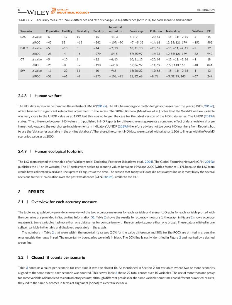
TABLE 2 Accuracymeasure 1: Value difference and rate of change (ROC) difference (both in %) for each scenario and variable

Scenario Population Fertility Mortality Food p.c.

Industrial

output p.c. Services p.c. Pollution Natural cap Welfare EF

BAU Δ value −6 −17 15 −15 −11; 3 5; 8; 9 −20; 64 −15;−11;−2; 15 −4 15

ΔROC −42 55 −12 −342 −107;−90 −7;−5; 33 −14; 68 12; 55; 121; 179 −152 593

BAU2 Δ value −5 −10 8 −14 −7; 13 10; 11; 13 −20; 65 −15;−11;−2; 15 −2 19

ΔROC −28 −4 −6 −279 −64; 5 57; 85; 97 −14; 73 12; 55; 121; 179 −62 940

CT Δ value −5 −10 6 −12 −6; 13 10; 11; 13 −20; 64 −15;−11;−2; 16 −1 18

ΔROC −25 −3 −7 −193 −62; 8 57; 86; 97 −14; 69 7; 50; 113; 166 −40 841

SW Δ value −11 −22 11 −10 −9; 2 18; 20; 22 −19; 68 −15;−11;−2; 16 −1 13

ΔROC −52 −61 −9 −275 −108;−95 22; 32; 68 −8; 78 −3; 39; 97; 143 −67 247

2.4.8 Human welfare

TheHDI data series can be found on thewebsite of UNDP (2019a). TheHDI has undergonemethodological changes over the years (UNDP, 2019d),

which have led to significant retroactive adjustment to the series. The 2004 LtG book (Meadows et al.) notes that the World3 welfare variable

was very close to the UNDP value as at 1999, but this was no longer the case for the latest version of the HDI data series. The UNDP (2019d)

states: “The difference between HDI values (. . . ) published in HD Reports for different years represents a combined effect of data revision, change

inmethodology, and the real change in achievements in indicators”. UNDP (2019d) therefore advises not to source HDI numbers from Reports, but

to use the “data series available in the on-line database”. Therefore, the current HDI datawere scaledwith a factor 1.106 to line upwith theWorld3

scenarios value as at 2000.

2.4.9 Human ecological footprint

The LtG team created this variable after Wackernagels’ Ecological Footprint (Meadows et al., 2004). The Global Footprint Network (GFN, 2019a)

publishes the EF on its website. The EF series were scaled to scenario values between 1990 and 2000 (with a factor of 1.17), because the LtG team

would have calibratedWorld3 to line upwith EF figures at the time. The reason that today’s EF data did not exactly line up is most likely the several

revisions to the EF calculation over the past two decades (GFN, 2019b), similar to the HDI.

3 RESULTS

3.1 Overview for each accuracy measure

The table and graph below provide an overview of the two accuracymeasures for each variable and scenario. Graphs for each variable plotted with

the scenarios are provided in Supporting Information S1. Table 2 shows the results for accuracy measure 1, the graph in Figure 2 shows accuracy

measure 2. Some variables had more than one data series for comparison with the scenario (i.e., more than one proxy). These data are listed in one

cell per variable in the table and displayed separately in the graph.

The numbers in Table 2 that were within the uncertainty ranges (20% for the value difference and 50% for the ROC) are printed in green, the

ones outside the range in red. The uncertainty boundaries were left in black. The 20% line is easily identified in Figure 2 and marked by a dashed

green line.

3.2 Closest fit counts per scenario

Table 3 contains a count per scenario for each time it was the closest fit. As mentioned in Section 2, for variables where two or more scenarios

aligned to the same extent, each scenario was counted. This is why Table 3 shows 22 total counts over 10 variables. The use of more than one proxy

for some variables did not lead to contradictory counts; although different proxies for the same variable sometimes had different numerical results,

they led to the same outcomes in terms of alignment (or not) to a certain scenario.

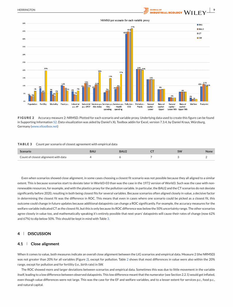
HERRINGTON 9

F IGURE 2 Accuracymeasure 2: NRMSD. Plotted for each scenario and variable proxy. Underlying data used to create this figure can be foundin Supporting Information S2. Data visualization was aided by Daniel’s XL Toolbox addin for Excel, version 7.3.4, by Daniel Kraus,Würzburg,Germany (www.xltoolbox.net)

TABLE 3 Count per scenario of closest agreement with empirical data

Scenario BAU BAU2 CT SW None

Count of closest alignment with data 4 6 7 3 2

Even when scenarios showed close alignment, in some cases choosing a closest fit scenario was not possible because they all aligned to a similar

extent. This is because scenarios start to deviate later inWorld3-03 than was the case in the 1972 version ofWorld3. Such was the case with non-

renewable resources, for example, andwith the plastics proxy for the pollution variable. In particular, the BAU2 and theCT scenarios do not deviate

significantly before 2020, resulting in both being closest fits for several variables. Because scenarios often aligned closely in value, a decisive factor

in determining the closest fit was the difference in ROC. This means that even in cases where one scenario could be picked as a closest fit, this

outcome could change in future updates because additional datapoints can change a ROC significantly. For example, the accuracymeasures for the

welfare variable indicatedCTas the closest fit, but this is only because its ROCdifferencewasbelow the50%uncertainty range. Theother scenarios

agree closely in value too, and mathematically speaking it’s entirely possible that next years’ datapoints will cause their rates of change (now 62%

and 67%) to dip below 50%. This should be kept in mindwith Table 3.

4 DISCUSSION

4.1 Close alignment

When it comes to value, both measures indicate an overall close alignment between the LtG scenarios and empirical data. Measure 2 (the NRMSD)

was not greater than 20% for all variables (Figure 2), except for pollution. Table 2 shows that most differences in value were also within the 20%

range, except for pollution and for fertility (i.e., birth rate) in SW.

The ROC showed more and larger deviations between scenarios and empirical data. Sometimes this was due to little movement in the variable

itself, leading to a lowdifference between observed datapoints. This lowdifferencemeant that the numerator (see Section 2.2.1) would get inflated,

even though value differences were not large. This was the case for the EF and welfare variables, and to a lesser extent for services p.c., food p.c.,

and natural capital.

10 HERRINGTON

4.2 The end of growth

Despite all scenarios showing a relatively close track in value, there were differences between them for some variables. Unlike previous compar-

isons, this research did not reveal the BAU scenario aligning with empirical data more closely than the others. Like in Turner’s work, however, the

lowest count for closest fit was for SW, the scenario that the LtG work models as eventually following a sustainable path. When it was possible to

distinguish between scenarios, the CT and BAU2 aligned closest most often. BAU2 and CT scenarios show a halt in growth within a decade or so

fromnow. Both scenarios thus indicate that continuing business as usual, that is, pursuing continuous growth, is not possible. Evenwhenpairedwith

unprecedented technological development and adoption, business as usual asmodeled by LtGwould inevitably lead to declines in industrial capital,

agricultural output, andwelfare levelswithin this century. These forecasts put in perspective the recent loweconomic predictions (e.g.,OECD, 2020;

WB, 2019h), and talks from organizations like the IMF about a “synchronized slowdown” of global growth (Lawder, 2019) and “uncertain recovery”

from the COVID-19 pandemic (IMF, 2020).

4.3 Collapse?

The CT and BAU2 scenarios show distinctly different decline patterns, and one cannot simply “take the midway” between two scenarios produced

by a complex, non-linear model likeWorld3. Although the steepness of a scenario’s decline cannot be used for predictive purposes (Meadows et al.,

2004), it canbe said thatBAU2showsa clear collapsepattern,whereasCT suggests thepossibility of futuredeclines being relatively soft landings, at

least for humanity in general. Themoderate declines inCTwould alignwith a global forecastmade in 2012by LtGauthorRanders. Randers’ forecast

(2012) was made with a different model thanWorld3 and so it cannot be compared with CT in most ways. However, the overall developments are

not dissimilar, as the forecast includes consumption and GDP stagnation around the middle of the century followed by declines but not a collapse

pattern.

4.4 About tipping points

The BAU2 and CT scenarios seem to align quite closely not just with observed data, but also with contemporary debate. On one hand, the BAU2

scenario resonates with messages from climate scientists that we currently might be at the “climate tipping point” (Cai, Lenton, & Lontzek, 2016;

Intergovernmental Panel onClimate Change, 2019; Lenton et al., 2019; Pearce, 2019). On the other hand, CT is the scenario of thosewho believe in

humanity’s ingenuity to innovate ourselves out of any limit. The assumptions underlying CT are highly optimistic given historic figures. For example,

CT assumes technological progress rates of 4% a year which, amongst other things, should lead to reductions in pollution emissions of 10% from

their 2000 values by 2020 and 48% by 2040. Given the rising trend in global CO2 emissions so far, halving these within the next 20 years seems

unrealistic. However, the technologist could argue that history is full of “technological tipping points” (Montresor, 2014; World Economic Forum,

2015), where innovations disrupted trends and revolutionized society beyondwhat conventional wisdom deemed possible.

Detailing this discussion goes beyond the scope of this article. More important, the findings and LtGwork indicate an altogether different ques-

tion to ask than whether society could be following the CT. Two best fit scenarios that marginally align closer than the other two, point to the fact

that it’s not yet too late for humankind to purposefully change course to significantly alter the trajectory of future data points. The fact that the SW

scenario shows the smallest declines, suggests that if we are to bet our future on the possibility of tipping points, rather than just the technological

ones,we should also aim for the “social tipping points” (David Tàbara et al., 2018;Otto et al., 2020;Westley et al., 2011): A transformation of societal

priorities which, together with technological innovations specifically aimed at furthering these new priorities, can bring humanity back on the path

of the SW scenario.

5 CONCLUSION

Empirical world data was compared against scenarios from the last LtG book, created by the World3 model. The data comparison, which used

the latest World3 version, included four scenarios: BAU, BAU2, CT, and SW. Empirical data showed a relatively close fit for most of the variables.

This was true to some extent for all scenarios, because in several cases the scenarios do nott significantly diverge until 2020. When scenarios had

started to diverge, the ones that aligned closest with empirical data most often were BAU2 and CT. This result is different to previous comparisons

that used the earlierWorld3 version, andwhich indicatedBAUas themost closely followed scenario. The scenario that depicts the smallest declines

in economic output, SW, is also the one that aligned least closely with observed data. Furthermore, the two closest aligning scenarios BAU2 and CT,

respectively, predict a collapse pattern andmoderate decline in output. At this point therefore, the datamost alignswith theCTandBAU2 scenarios

which indicate a slowdown and eventual halt in growth within the next decade or so, butWorld3 leaves open whether the subsequent decline will

HERRINGTON 11

constitute a collapse. World3 also indicates the possibility, for now, of limiting declines to less than in the CT. Although SW tracks least closely,

a deliberate trajectory change brought about by society turning toward another goal than growth is still possible. The LtG work implies that this

window of opportunity is closing fast.

ACKNOWLEDGMENTS

This research was based on my Master of Liberal Arts thesis in Sustainability at Harvard University Extension School, graduation March 2020

(Branderhorst 2020). I am grateful to Graham Turner for sharing his previous work with me and giving me his support. It was a pleasure and honor

to discussmy researchwith him. I would like to thank EstherG. Naikal andGiovanni Ruta from theWorld Bank for providingmewith the underlying

data on natural capital calculations. I am also very appreciative of John Sterman for meeting with me at short notice in January 2019 while he was

on sabbatical. That talk in hisMIT office providedmewith exactly the right insights to nudgemy research in the right direction.

CONFLICT OF INTEREST

The author declares no conflict of interest.

ORCID

GayaHerrington https://orcid.org/0000-0002-9284-9129

REFERENCES

Bailey, R. (1989). Dr. Doom. Forbes, 144, 44.Bardi, U. (2011). Cassandra’s curse: How “the limits to growth” was demonized. Retrieved from https://www.resilience.org/stories/2011-09-15/cassandras-

curse-how-limits-growth-was-demonized/

Bardi, U. (2014). Extracted: How the quest for mineral wealth is plundering the planet. White River Junction, Vermont: Chelsea Green Publishing Co.

Branderhorst, G. (2020).Update to limits to growth: Comparing theWorld3model with empirical data (Master’s thesis, Harvard Extension School). Retrieved from

https://dash.harvard.edu/handle/1/37364868

Brathwaite, J., Horst, S., & Iacobucci, J. (2010). Maximizing efficiency in the transition to a coal-based economy. Energy Policy, 38(10), 6084–6091.British Petroleum (BP). (2019). Statistical review of world energy. Retrieved from https://www.bp.com/en/global/corporate/energy-economics/statistical-

review-of-world-energy.html

Cai, Y., Lenton, T.M., & Lontzek, T. S. (2016). Risk ofmultiple interacting tipping points should encourage rapid CO2 emission reduction.Nature Climate Change,6(5), 520–525.

Castro, R (2012). Arguments on the imminence of global collapse are premature when based on simulationmodels.GAIA, 21, 271–273.Coady, D., Parry, I., Le, N.-P., & Shang, B. (2019).Global fossil fuel subsidies remain large: An update based on country-level estimates. Retrieved from https://www.

imf.org/en/Publications/WP/Issues/2019/05/02/Global-Fossil-Fuel-Subsidies-Remain-Large-An-Update-Based-on-Country-Level-Estimates-46509

Cole, H. S. D., Freeman, C., Jahoda,M., & Pavitt, K. L. R. (1973).Models of doom: A critique of the limits to growth. New York: Universe Publishing.

David Tàbara, J., Frantzeskaki, N., Hölscher, K., Pedde, S., Kok, K., Lamperti, F., . . . Berry, P. (2018). Positive tipping points in a rapidly warming world. CurrentOpinion in Environmental Sustainability, 31(C), 120–129.

de Jongh, D. C. (1978). Structural parameter sensitivity of the limits to growthworldmodel. AppliedMathematical Modelling, 2, 77–80.Driessen, P. P. J., Henckens, M. L. C. M., van Ierland, E. C., &Worrell, E. (2016). Mineral resources: Geological scarcity, market price trends, and future genera-

tions. Resources Policy, 49, 102–111. https://doi.org/10.1016/j.resourpol.2016.04.012Etheridge, D. M., Steele, L. P., Langenfelds, R. L., Francey, R. J., Barnola, J.-M., & Morgan, V. I. (1996). Natural and anthropogenic changes in atmospheric CO2

over the last 1000 years from air in Antarctic ice and firn. Journal of Geophysical Research, 101(D2), 4115–4128.FAOSTAT. (2019). Food balance sheets. Retrieved from http://www.fao.org/faostat/en/#data/FBS

Forrester, J.W. (1971).World dynamics. Cambridge,MA:Wright-Allen Press.

Forrester, J.W. (1975). Collected papers. Waltham,MA: Pegasus Communications.

Geyer, R., Jambeck, J. R., & Law, K. L. (2017). Production, use, and fate of all plastics ever made. Science Advances, 3(7), e1700782.Global Footprint Network (GFN). (2019a). Country trends. Retrieved from http://data.footprintnetwork.org/#/countryTrends?cn=5001&type=earth

Global Footprint Network (GFN). (2019b). FAQs. Retrieved from https://www.footprintnetwork.org/faq/

Graedel, T. E., Harper, E. M., Nassar, N. T., & Reck, B. K. (2015). On the materials basis of modern society. Proceedings of the National Academy of Sciences, 112,6295. https://doi.org/10.1073/pnas.1312752110

Halden, R. U. (2010). Plastics and health risks. Annual Review of Public Health, 31(7), 179–194.Intergovernmental Panel on Climate Change. (2019). IPCC special report on the ocean and cryosphere in a changing climate. Retrieved from https://www.ipcc.ch/

srocc/

International Monetary Fund (IMF). (2020).World economic outlook update. Retrieved from https://www.imf.org/en/Publications/WEO/Issues/2020/06/24/

WEOUpdateJune2020

Jackson, T., &Weber, R. (2016). Limits revisited: A review of the limits to growth debate. Retrieved from http://limits2growth.org.uk/revisited

Kaysen, C. (1972). The computer that printed outW*O*L*F*. Foreign Affairs, 50, 660–668. https://doi.org/10.2307/20037939.Kosuth, M., Wattenberg, E. V., Mason, S. A., Tyree, C., &Morrison, D. (2017). Synthetic polymer contamination in global drinking water.Orb Media. Retrieved

from https://orbmedia.org/stories/Invisibles_final_report/multimedia

Lawder, D. (2019). New IMF chief Georgieva warns of “synchronized slowdown” in global growth.Nasdaq. Retrieved from https://www.nasdaq.com/articles/

new-imf-chief-georgieva-warns-of-synchronized-slowdown-in-global-growth-2019-10-08

Lenton, T., Rockström, J., Gaffney, O., Rahmstorf, S., Richardson, K., Steffen, W., & Schellnhuber, H. (2019). Climate tipping points – Too risky to bet against.

Nature, 575(7784), 592–595.

12 HERRINGTON

Lomborg, B., & Olivier, R. (2009). The dustbin of history: Limits to growth. Foreign Policy, 103, 34–48. Retrieved from https://foreignpolicy.com/2009/11/09/

the-dustbin-of-history-limits-to-growth/

Meadows, D. H., &Meadows, D. L. (2007). The history and conclusions of the limits to growth. SystemDynamics Review, 23, 191–197. https://doi.org/10.1002/sdr.371

Meadows, D. H., Meadows, D. L., & Randers, J. (1992). Beyond the limits: Confronting global collapse, envisioning a sustainable future. White River Junction, VT:

Chelsea Green Publishing Co.

Meadows, D. H., Meadows, D. L., & Randers, J. (2004). The limits to growth: The 30-year update. White River Junction, VT: Chelsea Green Publishing Co.

Meadows, D. H., Meadows, D. L., Randers, J., & Behrens,W.W. (1972). The limits to growth: A report for the Club of Rome’s project on the predicament of mankind.New York: Universe Books.

MetaSD. (2020).World3-03. Retrieved from https://metasd.com/tag/world3/

Moles, P., & Terry, N. (1997). The handbook of international financial terms. Oxford: Oxford University Press.

Montresor, F. (2014, August 14). 14 tech predictions for our world in 2020. Retrieved from https://www.weforum.org/agenda/2014/08/14-technology-

predictions-2020/

Nizzetto, L., Langaas, S., & Futter, M. (2016). Pollution: Domicroplastics spill on to farm soils?Nature, 537, 488. https://doi.org/10.1038/537488bNorgard, J., Peet, J., & Ragnarsdóttir, K. (2010). The history of limits to growth. Solutions, 1(2), 59–63. Retrieved from https://www.thesolutionsjournal.com/

article/the-history-of-the-limits-to-growth/

Organisation for Economic Co-operation and Development (OECD). (2017). Environmental fiscal reform: Progress, prospects, and pitfalls. Retrieved from http:

//www.oecd.org/tax/tax-policy/environmental-fiscal-reform-progress-prospects-and-pitfalls.htm

Organisation for Economic Co-operation and Development (OECD). (2018). Effective carbon rates 2018: Pricing carbon emissions through taxes and emissionstrading. Paris: OECDPublishing. https://doi.org/10.1787/9789264305304-en.

Organisation for Economic Co-operation and Development (OECD). (2020).OECD economic outlook, interim report March 2020. Retrieved from https://www.

oecd-ilibrary.org/economics/oecd-economic-outlook/volume-2019/issue-2_7969896b-en

Otto, I., Donges, J., Cremades, R., Bhowmik, A., Hewitt, R., Lucht,W., . . . Schellnhuber, H. (2020). Social tipping dynamics for stabilizing Earth’s climate by 2050.

Proceedings of the National Academy of Sciences of the United States of America, 117(5), 2354–2365.Passell, P., Roberts,M., &Ross, L. (1972). The limits to growth.TheNewYork Times. Retrieved fromhttps://www.nytimes.com/1972/04/02/archives/the-limits-

to-growth-a-report-for-the-club-of-romes-project-on-the.html

Pasqualino, R., Jones, A.,Monasterolo, I., & Phillips, A. (2015). Understanding global systems today—A calibration of theWorld3-03model between 1995 and

2012. Sustainability, 7, 9864–9889. https://doi.org/10.3390/su7089864Pearce, F. (2019). As climate change worsens, a cascade of tipping points looms. Retrieved from https://e360.yale.edu/features/as-climate-changes-worsens-a-

cascade-of-tipping-points-looms

Plenty of gloom. (1997, December 18). The Economist. Retrieved from https://www.economist.com/christmas-specials/1997/12/18/plenty-of-gloom

Randers, J. (2000). From limits to growth to sustainabledevelopmentor SD (sustainabledevelopment) in a SD (systemdynamics) perspective. SystemDynamicsReview, 16, 213–224.

Randers, J. (2012). 2052: A global forecast for the next forty years. White River Junction, VT: Chelsea Green Publishing Co.

Simmons, M. R. (2000). Revisiting the limits to growth: Could the Club of Rome have been correct, after all? Eugene, OR: Mud City Press. Retrieved from http:

//www.mudcitypress.com/PDF/clubofrome.pdf

Smillie, S. (2017). From sea to plate: Howplastic got into our fish. The Guardian. Retrieved from https://www.theguardian.com/lifeandstyle/2017/feb/14/sea-

to-plate-plastic-got-into-fish

Solow, R.M. (1973). Is the end of the world at hand? Challenge, 16, 39–50. https://doi.org/10.1080/05775132.1973.11469961Sterman, J. (2000). Business dynamics: Systems thinking andmodeling for a complex world. Boston,MA: Irwin/McGraw-Hill.

Sverdrup, H., & Ragnarsdóttir, K. (2014). Natural resources in a planetary perspective. Geochemical Perspectives, 3, 129–341. Retrieved from https://doi.org/

10.7185/geochempersp.3.2

Tans, P., & Keeling, R. (2019). Globally averaged marine surface annual mean data [Data file]. Retrieved from https://www.esrl.noaa.gov/gmd/ccgg/trends/data.

html

Turner, G.M. (2008). A comparison of the limits to growthwith 30 years of reality.Global Environmental Change, 18, 397–411.Turner, G. M. (2012). On the cusp of global collapse? Updated comparison of the limits to growth with historical data. GAIA, 21(2), 116–124.

Retrieved from https://www.ethz.ch/content/dam/ethz/special-interest/usys/ites/ecosystem-management-dam/documents/EducationDOC/Readings_

DOC/Turner_2012_GAIA_LimitsToGrowth.pdf

Turner, G. (2013). The limits to growth model is more than a mathematical exercise: Reaction to R. Castro. 2012. Arguments on the imminence of global

collapse are premature when based on simulationmodels. GAIA, 21/4: 271–274.GAIA, 22, 18–19.Turner, G. (2014). Is global collapse imminent? Parkville, VIC: Melbourne Sustainable Society Institute, The University of Melbourne. Retrieved from http:

//sustainable.unimelb.edu.au/sites/default/files/docs/MSSI-ResearchPaper-4_Turner_2014.pdf

United Nations Department of Economic & Social Affairs, Population Division (UN DESA PD). (2019). Total population – Both sexes [Datafile].

Retrieved fromhttps://population.un.org/wpp/Download/Files/1_Indicators%20(Standard)/EXCEL_FILES/1_Population/WPP2019_POP_F01_1_TOTAL_

POPULATION_BOTH_SEXES.xlsx

United Nations Development Programme (UNDP). (2019a).Human development data (1990–2017). Retrieved from http://hdr.undp.org/en/data

United Nations Development Programme (UNDP). (2019b). Education index (1990–2017). Retrieved from http://hdr.undp.org/en/content/education-index

United Nations Development Programme (UNDP). (2019c). Technical notes. (Human development indices and indicators: 2018 statistical update). Retrieved

from http://hdr.undp.org/sites/default/files/hdr2018_technical_notes.pdf

United Nations Development Programme (UNDP). (2019d). Frequently asked questions – Human development index (HDI). Retrieved from http://hdr.undp.org/

en/faq-page/human-development-index-hdi#t292n2872

United Nations Environment Programme. (2002). Global environment outlook 3. Retrieved from https://www.unenvironment.org/resources/global-

environment-outlook-3

United Nations Industrial Development Organization (UNIDO). (2019a). Selected database: INDSTAT 2 2019, ISIC Revision 3. Retrieved from https://stat.

unido.org/database/INDSTAT%202%202019,%20ISIC%20Revision%203

HERRINGTON 13

United Nations Industrial Development Organization (UNIDO). (2019b). Selected database: MVA 2019, manufacturing. Retrieved from https://stat.unido.org/

database/MVA%202019,%20Manufacturing

van Sebille, E., Wilcox, C., Lebreton, L., Maximenko, N., Hardesty, B. D., van Franeker, J. A., . . . Law, K. L. (2015). A global inventory of small floating plastic

debris. Environmental Research Letters, 10(12), 124006.Vensim. (2020). Free downloads. Retrieved from https://vensim.com/free-download/

Vermeulen, P. J., & de Jongh,D. C. J. (1976). “Dynamics of growth in a finiteworld” –Comprehensive sensitivity analysis. IFAC Proceedings Volumes,9, 133–145.Retrieved from https://www.sciencedirect.com/science/article/pii/S1474667017673336

Westley, F., Olsson, P., Folke, C., Homer-Dixon, T., Vredenburg, H., Loorbach, D., . . . Leeuw, S. (2011). Tipping toward sustainability: Emerging pathways of

transformation. AMBIO, 40(7), 762–780.World Bank (WB). (2019a). Population, total. Retrieved from https://data.worldbank.org/indicator/SP.POP.TOTL

World Bank (WB). (2019b). Birth rate, crude (per 1,000 people). Retrieved from https://data.worldbank.org/indicator/SP.DYN.CBRT.IN

World Bank (WB). (2019c).Death rate, crude (per 1,000 people). Retrieved from https://data.worldbank.org/indicator/SP.DYN.CDRT.IN

World Bank (WB). (2019d).Gross fixed capital formation (constant 2010 US$). Retrieved from https://data.worldbank.org/indicator/NE.GDI.FTOT.KD

World Bank (WB). (2019e).Government expenditure on education, total (% of GDP). Retrieved from https://data.worldbank.org/indicator/SE.XPD.TOTL.GD.ZS

World Bank (WB). (2019f).Government expenditure on health, total (% of GDP). Retrieved from https://data.worldbank.org/indicator/SH.XPD.CHEX.GD.ZS

World Bank (WB). (2019g).Unpublished Excel files [Data files]. Retrievable fromWorld Bank at request.

World Bank (WB). (2019h). Global economic prospects: Slow growth, policy challenges. Retrieved from https://www.worldbank.org/en/publication/global-

economic-prospects#overview

World Economic Forum. (2015). Deep shift: Technology tipping points and societal impact. Retrieved from http://www3.weforum.org/docs/WEF_GAC15_

Technological_Tipping_Points_report_2015.pdf

Wright, S. L., & Kelly, F. J. (2017a). Plastic and human health: A micro issue? Environmental Science & Technology, 51, 6634–6647. https://doi.org/10.1021/acs.est.7b00423pmid:28531345

Wright, S. L., &Kelly, F. J. (2017b). Threat to human health fromenvironmental plastics.BMJ,358(4334), j4334. Retrieved fromhttps://doi-org.ezp-prod1.hul.

harvard.edu/10.1136/bmj.j4334

SUPPORTING INFORMATION

Additional supporting informationmay be found online in the Supporting Information section at the end of the article.

How to cite this article: Herrington G. Update to limits to growth: Comparing the world3model with empirical data. J Ind Ecol. 2020;1–13.

https://doi.org/10.1111/jiec.13084