Upasana Kashyap - University of Houston

Morita equivalence of dual operator algebras

A Dissertation

Presented to

the Faculty of the Department of Mathematics

University of Houston

In Partial Fulfillment

of the Requirements for the Degree

Doctor of Philosophy

By

Upasana Kashyap

December 2008

MORITA EQUIVALENCE OF DUAL

OPERATOR ALGEBRAS

Upasana Kashyap

APPROVED:

Dr. David P. Blecher, Chairman

Dr. Vern I. Paulsen

Dr. David Pitts

Dr. Mark Tomforde

Dr. John L. Bear

Dean, College of Natural Sciences

and Mathematics

ii

ACKNOWLEDGMENTS

I would like to thank my advisor David Blecher for his tremendous help and support.

He has been very kind and generous to me. I appreciate his constant availability

to clear my doubts and motivate me in every situation. I must say he has inspired

me to pursue mathematics as a professional career. I am deeply grateful for all his

help, support, and guidance. I would like to thank Dinesh Singh for providing me

the opportunity and inspiring me to do a Ph.D. in mathematics. I would also like

to thank Mark Tomforde for his generous help and support during the last year of

my graduate studies. I want to express my sincere gratitude to my other committee

members, Vern Paulsen and David Pitts. Last, but certainly not least, I thank my

family and friends for their love, support, and encouragement.

iii

MORITA EQUIVALENCE OF DUAL

OPERATOR ALGEBRAS

An Abstract of a Dissertation

Presented to

the Faculty of the Department of Mathematics

University of Houston

In Partial Fulfillment

of the Requirements for the Degree

Doctor of Philosophy

By

Upasana Kashyap

December 2008

iv

ABSTRACT

In this thesis, we present some new notions of Morita equivalence appropriate to

weak∗ closed algebras of Hilbert space operators. We obtain new variants, appropri-

ate to the dual (weak∗ closed) algebra setting, of the basic theory of strong Morita

equivalence due to Blecher, Muhly, and Paulsen. We generalize Rieffel’s theory of

Morita equivalence for W ∗-algebras to non-selfadjoint dual operator algebras. Our

theory contains all examples considered up to this point in the literature of Morita-

like equivalence in a dual (weak∗ topology) setting. Thus, for example, our notion of

equivalence relation for dual operator algebras is coarser than the one defined recently

by Eleftherakis.

In addition, we give a new dual Banach module characterization of W ∗-modules,

also known as selfdual Hilbert C∗-modules over a von Neumann algebra. This leads

to a generalization of the theory of W*-modules to the setting of non-selfadjoint

algebras of Hilbert space operators which are closed in the weak∗ topology. That

is, we find the appropriate weak∗ topology variant of the theory of rigged modules

due to Blecher. We prove various versions of the Morita I, II, and III theorems for

dual operator algebras. In particular, we prove that two dual operator algebras are

weak∗ Morita equivalent in our sense if and only if they have equivalent categories

of dual operator modules via completely contractive functors which are also weak∗

continuous on appropriate morphism spaces. Moreover, in a fashion similar to the

operator algebra case, we characterize such functors as the module normal Haagerup

tensor product with an appropriate weak∗ Morita equivalence bimodule.

v

Contents

1 Introduction 1

1.1 Morita equivalence: selfadjoint setting . . . . . . . . . . . . . . . . . 1

1.2 Morita equivalence: non-selfadjoint setting . . . . . . . . . . . . . . . 4

2 Background and preliminary results 9

2.1 Operator spaces and operator algebras . . . . . . . . . . . . . . . . . 9

2.2 Dual operator spaces and dual operator algebras . . . . . . . . . . . . 12

2.3 Operator modules and dual operator modules . . . . . . . . . . . . . 15

2.4 Some tensor products . . . . . . . . . . . . . . . . . . . . . . . . . . . 17

3 Morita equivalence of dual operator algebras 26

3.1 Introduction . . . . . . . . . . . . . . . . . . . . . . . . . . . . . . . . 26

3.2 Morita contexts . . . . . . . . . . . . . . . . . . . . . . . . . . . . . . 28

3.3 Representations of the linking algebra . . . . . . . . . . . . . . . . . . 47

3.4 Morita equivalence of generated W ∗-algebras . . . . . . . . . . . . . . 53

4 A characterization and a generalization of W ∗-modules 57

4.1 Introduction . . . . . . . . . . . . . . . . . . . . . . . . . . . . . . . . 57

4.2 W ∗-modules . . . . . . . . . . . . . . . . . . . . . . . . . . . . . . . . 59

4.3 Some theory of w∗-rigged modules . . . . . . . . . . . . . . . . . . . . 67

vi

4.3.1 Basic constructs . . . . . . . . . . . . . . . . . . . . . . . . . . 67

4.3.2 The weak linking algebra, and its representations . . . . . . . 72

4.3.3 Tensor products of w∗-rigged modules . . . . . . . . . . . . . . 73

4.3.4 The W ∗-dilation . . . . . . . . . . . . . . . . . . . . . . . . . 74

4.3.5 Direct sums . . . . . . . . . . . . . . . . . . . . . . . . . . . . 75

4.4 Equivalent definitions of w∗-rigged modules . . . . . . . . . . . . . . . 78

4.5 Examples . . . . . . . . . . . . . . . . . . . . . . . . . . . . . . . . . 82

5 A Morita theorem for dual operator algebras 85

5.1 Introduction . . . . . . . . . . . . . . . . . . . . . . . . . . . . . . . . 85

5.2 Dual operator modules over a generated W ∗-algebra and W ∗-dilations 87

5.3 Morita equivalence and W ∗-dilation . . . . . . . . . . . . . . . . . . . 97

5.4 The main theorem . . . . . . . . . . . . . . . . . . . . . . . . . . . . 104

5.5 W ∗-restrictable equivalences . . . . . . . . . . . . . . . . . . . . . . . 113

Bibliography 117

vii

Chapter 1

Introduction

1.1 Morita equivalence: selfadjoint setting

One of the important and well-known perspectives of study of an algebraic object

is the study of its category of representations. For example, for rings, modules are

viewed as their representations, and hence rings are commonly studied in terms of

their modules. Once we view an algebraic object in terms of its category of rep-

resentations, it is natural to compare such categories. This leads to the notion of

Morita equivalence. The notion of Morita equivalence of rings arose in pure algebra

in the 1960’s. Two rings are defined to be Morita equivalent if and only if they have

equivalent categories of modules. A fundamental Morita theorem says that two rings

A and B have equivalent categories of modules if and only if there exists a pair of

bimodules X and Y such that X ⊗B Y ∼= A and Y ⊗A X ∼= B as bimodules. Morita

equivalence is an equivalence relation and preserves many ring theoretic properties.

It is a powerful tool in pure algebra and it has inspired similar notions in operator

algebra theory.

In the 1970’s Rieffel introduced and developed the notion of Morita equivalence for

C∗-algebras and W ∗-algebras [40], [41]. Rieffel defined strong Morita equivalence in

1

terms of Hilbert C∗-modules, which may be thought of as a generalization of Hilbert

space in which the positive definite inner product is C∗-algebra valued. A Hilbert

C∗-module can also be viewed as the noncommutative generalization of a vector

bundle. The dual (weak∗ topology) version of a C∗-module is called a W ∗-module.

These objects are fundamental tools in operator algebra theory, and they play an

important role in noncommutative geometry, being intimately related to Connes’

correspondences.

We recall some basic definitions of the theory. By a C∗-algebra A, we mean that A

is an involutive Banach algebra satisfying the C∗-identity ‖a∗a‖ = ‖a‖2 for all a ∈ A,

where a 7→ a∗ denotes the involution (adjoint) on A.

A right C∗-module over a C∗-algebra B is a right B-module X endowed with

B-valued sesquilinear map 〈·, ·〉B : X×X → B such that the following conditions are

satisfied:

1. 〈·, ·〉B is conjugate linear in the second variable.

2. 〈x, x〉B is a positive element in B for all x ∈ X.

3. 〈x, x〉B = 0 if and only if x = 0 for all x ∈ X.

4. 〈x, y〉∗B = 〈y, x〉B for all x, y ∈ X.

5. 〈x, yb〉B = 〈x, y〉Bb for all x, y ∈ X, b ∈ B.

6. X is complete in the norm ‖x‖ = ‖〈x, x〉‖ 12 .

A left C∗-module is defined analogously. Here X is a left module over a C∗-algebra

A, the A-valued inner product A〈., .〉 : X ×X → A is linear in the first variable, and

condition (5) in the above is replaced by A〈ax, y〉 = aA〈x, y〉, for x, y ∈ X, a ∈ A.

If X is an A-B-bimodule, then we say X is an equivalence bimodule, if X is a right

C∗-module over B, and a left C∗-module over A, such that

2

1. A〈x, y〉z = x〈y, z〉B for all x, y, z ∈ X.

2. The linear span of {A〈x, y〉 | x, y ∈ X}, which is a two-sided ideal, in A is dense

in A; likewise {〈x, y〉B | x, y ∈ X} spans a dense two-sided ideal in B.

If there exists such an equivalence bimodule, we say that A and B are strongly

Morita equivalent.

Let X be X with the conjugate actions of A and B, and for x ∈ X, write x when

x is viewed as an element in X. Thus bx = xb∗ and xa = a∗x. Then X becomes a B-

A-equivalence bimodule with inner products B〈x, y〉 = 〈x, y〉∗B and 〈x, y〉A = A〈x, y〉∗.

In fact, X and X are operator spaces.

The collection of matrices

L =

a x

y b

: a ∈ A, b ∈ B, x ∈ X, y ∈ X

,

may be endowed with a norm making it a C∗-algebra with multiplicationa1 x1

y1 b1

a2 x2

y2 b2

=

a1a2 +A 〈x1, y2〉 a1x1 + x1b2

y1a2 + b1y2 〈y1, x2〉B + b1b2

and involution a x

y b

∗ =

a∗ y

x b∗

.

The C∗-algebra L is called the linking algebra of A and B determined by X.

A W ∗-algebra is a C∗-algebra that has a Banach space predual; and in this case

the Banach space predual is unique. We say that a right C∗-module X over a C∗-

algebra A is selfdual if every bounded A-module map u : X → A is of the form u(·) =

A〈z, ·〉 for some z ∈ X. By a theorem of Zettl and Effros-Ozawa-Ruan [42], [24], [15,

Theorem 8.5.6] this condition is equivalent to the fact that X has a predual. We say

that X is a right W ∗-module if X is a selfdual right C∗-module over a W ∗-algebra.

3

For W ∗-algebras M and N , W ∗-equivalence M-N-bimodules are defined similarly

as the equivalence bimodules for C∗-algebras, with the term C∗-module replaced with

W ∗-module, and the ranges of the inner products span weak∗-dense ideals in M and

N . If there exists such a bimodule over M and N , then we say M and N are weakly

Morita equivalent. In the case of weak Morita equivalence the linking algebra turns

out to be a W ∗-algebra. A fundamental theorem in the theory states that weakly

Morita equivalent W ∗-algebras have equivalent normal (weak∗ continuous) Hilbert

space representations. For references, see [40], [41], [15, Chapter 8].

1.2 Morita equivalence: non-selfadjoint setting

With the arrival of operator space theory in the 1990s, Blecher, Muhly, and Paulsen

generalized Rieffel’s C∗-algebraic notion of strong Morita equivalence to non-selfadjoint

operator algebras [18]. The theory of Morita equivalence developed by Blecher, Muhly,

and Paulsen focused on the category of Hilbert modules and the category of operator

modules over an operator algebra. Because the appropriate morphisms in the category

of operator spaces are completely bounded or completely contractive maps (defined

in Section 2.1), the module operations are assumed to be completely contractive.

Let A and B be operator algebras. Let X be an operator A-B-bimodule and let Y

be an operator B-A-bimodule (that is, the module actions are completely contractive).

We fix a pair of completely contractive balanced (i.e., (xa, y) = (x, ay) for all x, y ∈ X

and a ∈ A) bilinear bimodule maps (·, ·) : X × Y → A, and [·, ·] : Y × X → B.

The system (A,B,X, Y, (·, ·), [·, ·]) satisfying the above hypotheses is called a Morita

context for A and B in the case the following conditions hold:

(A) (x1, y)x2 = x1[y, x2], for x1, x2 ∈ X, y ∈ Y .

[y1, x]y2 = y1(x, y2), y1, y2 ∈ Y x ∈ X.

4

(G) The bilinear map (., .) : X×Y → A induces a completely isometric isomorphism

between the balanced Haagerup tensor product X ⊗hB Y and A.

(P) The bilinear map [., .] : Y ×X → B induces a completely isometric isomorphism

between the balanced Haagerup tensor product Y ⊗hA X and B.

Two C∗-algebras are Morita equivalent in the sense of Blecher, Muhly, and Paulsen

if and only if they are C∗-algebraically strongly Morita equivalent in the sense of

Rieffel, and moreover the equivalence bimodules are the same.

In [6], Blecher developed a theory of rigged modules over non-selfadjoint operator

algebras that generalizes the theory of Hilbert C∗-modules. Let A be an operator

algebra with a contractive approximate identity and let Y be a right operator A-

module. That is, Y is an operator space equipped with anA-module action Y×A→ Y

that is completely contractive when Y ⊗ A is endowed with the Haagerup tensor

product. Let Cn(A) denote the first column of the matrix space Mn(A). Then Y

is called a (right) A-rigged module if there is a net of positive integers n(β) and

completely contractive right A-module maps φβ : Y → Cn(β)(A) and ψβ : Cn(β)(A)→

Y such that ψβφβ → IdY strongly on Y (i.e., for all y ∈ Y , ψβ(φβ(y))→ y in Y ). A

basic building block example in the theory of rigged modules over an operator algebra

A is Cn(A). Each Hilbert C∗-module has a natural operator space structure. It turns

out that the class of Hilbert C∗-modules coincides with the class of rigged modules

over a C∗-algebra. Again, operator space techniques and completely bounded maps

are used extensively in this theory.

In [10], Blecher proved that two operator algebras are Morita equivalent if and only

if they have equivalent categories of operator modules. The functors implementing

the categorical equivalences are characterized as the module Haagerup tensor product

with an appropriate strong Morita equivalence bimodule.

In this thesis, we have develop a weak∗ version of Morita equivalence for operator

5

algebras that are closed in the weak∗ topology. These operator algebras are called dual

operator algebras, and they are the non-selfadjoint version of von Neumann algebras.

In parallel with the selfadjoint setting, one can prove that an operator algebra is closed

in the weak∗-topology if and only if it has an operator space predual if and only if it

is equal to its double commutant in a certain universal representation (e.g., see [16],

[21]). In this dissertation we give a formulation of Morita equivalence for dual operator

algebras, which generalizes Rieffel’s Morita equivalence for von Neumann algebras.

That is, two W ∗-algebras are Morita equivalent in our sense if and only if they are

W ∗-algebraically Morita equivalent in the sense of Rieffel, and moreover the weak∗

equivalence bimodules are the same. This work can be viewed as a weak∗ version of

the Morita equivalence for operator algebras of Blecher, Muhly, and Paulsen. This is

analogous to Rieffel’s von Neumann algebraic Morita equivalence, which is the weak∗

version of strong Morita equivalence for selfadjoint operator algebras.

The weak∗ Morita equivalence that we develop contains all examples considered up

to this point in the literature of Morita-like equivalence in the dual (weak∗ topology)

setting. Thus, our notion of equivalence relation for dual operator algebras is coarser

than the one recently defined by Eleftherakis.

Also our contexts represent a natural setting for the Morita equivalence of dual

algebras. It is one to which the earlier theory of Morita equivalence (from, e.g., [18]

[17]) transfers in a very clean manner; indeed it may in some sense be summarized as

‘just changing the tensor product’ involved to one appropriate to the weak∗ topology.

We also give a new dual Banach module characterization of W ∗-modules. This leads

to a generalization of the theory of W ∗-modules in the setting of dual operator alge-

bras. That is, we find the appropriate weak∗ topology variant of the theory of rigged

modules due to Blecher, see [6].

We prove variants of Morita’s celebrated fundamental theorems (known as Morita

6

I, Morita II, and Morita III) appropriate to dual operator algebras. For example, we

prove that two dual operator algebras are weak∗ Morita equivalent in our sense if and

only if they have equivalent categories of dual operator modules via completely con-

tractive functors which are also weak∗-continuous on appropriate morphism spaces.

Moreover, in a fashion similar to the operator algebra case, such functors are char-

acterized as a suitable tensor product (namely, the module normal Haagerup tensor

product) with an appropriate weak∗ Morita equivalence bimodule.

Our notion of Morita equivalence focuses on the category of normal Hilbert mod-

ules (weak∗ continuous Hilbert space representations) and the category of dual op-

erator modules over a dual operator algebra. The appropriate tensor product in

our setting of weak∗ topology is the module version of the normal Haagerup tensor

product, recently introduced by Eleftherakis and Paulsen in [31]. In Section 2.4 we

developed some more properties of this tensor product.

We now discuss a brief outline of this thesis. In Chapter 2 we give the necessary

background and preliminary results. In Chapter 3, we define our variants of Morita

equivalence and present some consequences. We prove various versions of the Morita I

theorems. For example, if two dual operator algebras are Morita equivalent in our

sense then they have equivalent categories of dual operator modules and normal

Hilbert modules. Another interesting result is that if two dual operator algebras M

and N are weak∗ Morita equivalent then the von Neumann algebras generated by M

and N are Morita equivalent in Rieffel’s W ∗-algebraic sense.

In Chapter 4, we present a new characterization of W ∗-modules. This leads to

a generalization of the theory of W ∗-modules to the setting of non-selfadjoint weak∗

closed algebras of Hilbert space operators. This is the dual variant of the earlier

theory of rigged module due to Blecher. Chapter 3 and Chapter 4 are mostly joint

work with D. P. Blecher, and much of it also appears in [13] and [14] respectively.

7

In Chapter 5, we prove a Morita II theorem, which characterizes module category

equivalences as tensoring with an invertible bimodule. We also develop the general

theory of the W ∗-dilation, which connects the non-selfadjoint dual operator algebra

with the W ∗-algebraic framework. In the case of weak∗ Morita equivalence, this W ∗-

dilation is a W ∗-module over a von Neumann algebra generated by the non-selfadjoint

dual operator algebra. The theory of the W ∗-dilation is a key part of the proof of our

main theorem. The contents of Chapter 5 appear in [33].

8

Chapter 2

Background and preliminary

results

2.1 Operator spaces and operator algebras

By an operator space, we mean a norm closed subspace X of B(H) for some Hilbert

space H. Besides a vector space structure, an operator space has some hidden norm

structure. The space of n × n matrices over X, denoted by Mn(X) inherits a dis-

tinguished norm ‖.‖n via the identification Mn(X) ⊆ Mn(B(H)) ∼= B(H(n)) iso-

metrically, where H(n) denotes the Hilbert space direct sum of n copies of H. The

appropriate morphisms in this category are the completely bounded maps, which are

defined as follows: Suppose T : X → Y is a linear map between operator spaces. For

n ∈ N, define Tn : Mn(X) → Mn(Y ) by Tn([xij]) = [T (xij)], for [xij] ∈ Mn(X). We

say that T is completely bounded if ‖T‖cbdef= supn‖Tn‖ is finite. We say that T is a

complete contraction if ‖T‖cb ≤ 1, and T is a complete isometry if Tn is an isometry

for each n ∈ N. Similarly T is a complete quotient map if each Tn is a quotient map.

Operator space theory can be thought of as a noncommutative generalization

9

of Banach space theory. This is regarded as the suitable category to study many

problems of operator algebras and operator theory. In particular, operator theoretic

and operator algebraic problems motivated by classical Banach space theory and pure

algebra are often studied in the setting of operator spaces. Long before the subject

of operator spaces was developed, the completely bounded maps were used to study

many problems in C∗-algebras and von Neumann algebras, see [1], [36]. With the

arrival of the operator space theory, it has now become clear that many features of

operator algebras are best understood in this general setting. Basics on operator

spaces may be found in [15], [26], [36], [39].

A fundamental theorem in the subject of operator space is Ruan’s Theorem, which

gives an abstract characterization of operator spaces.

Theorem 2.1.1. Suppose that X is a vector space, and that for each n ∈ N we are

given a norm ‖·‖n on Mn(X). Then X is linearly completely isometrically isomorphic

to a linear subspace of B(H), for some Hilbert space H, if and only if condition (R1)

and (R2) below hold:

(R1) ‖αxβ‖n ≤ ‖α‖‖x‖n‖β‖, for all n ∈ N and all α, β ∈Mn, and x ∈Mn(X).

(R2) For all x ∈Mm(X) and y ∈Mn(X), we have

∥∥∥∥∥∥x 0

0 y

∥∥∥∥∥∥m+n

= max{‖x‖m, ‖y‖n}.

Turning to notation, if E and F are sets of operators in B(H), then EF denotes

the norm closure of the span of products xy for x ∈ E and y ∈ F . For cardinals or

sets I, J , we use the symbol MI,J(X) for the operator space of I×J matrices over X,

whose ‘finite submatrices’ have uniformly bounded norm. Such a matrix is normed by

the supremum of the norms of its finite submatrices. We write KI,J(X) for the norm

closure of these finite submatrices. Then CwJ (X) = MJ,1(X), Rw

J (X) = M1,J(X), and

CJ(X) = KJ,1(X) and RJ(X) = K1,J(X). If I = ℵ0 we simply denote these spaces

10

by for e.g., M(X), Rw(X), Cw(X). We sometimes write MI(X) for MI,I(X). If X

and Y are operator spaces, we denote by CB(X, Y ) the space of completely bounded

linear maps from X to Y .

By a concrete operator algebra we mean a norm closed subalgebra of B(H) for

some Hilbert space H. Note that this subalgebra is not necessarily selfadjoint. With

the arrival of operator space theory in the past few decades, there have been many new

developments in the theory of general operator algebras, which are not necessarily

selfadjoint. The theory in the non-selfadjoint case is not as well developed as the

selfadjoint case (C∗-algebra case), but it is still necessary and worthwhile to look at

non-selfadjoint operator algebras because there are many interesting non-selfadjoint

examples (e.g., upper triangular matrices, nest algebras, the disc algebra A(D), the

bounded analytic function on the disc H∞(D), operator algebras arising in operator

function theory). When studying non-selfadjoint operator algebras, many of the

techniques from the selfadjoint setting do not work, and new approaches and tools

have to be developed. Recently, operator space theory has started to provide necessary

tools to study non-selfadjoint operator algebras; see [15], [36].

We study operator algebras from an operator space point of view. An abstract

operator algebra A is an operator space that is also a Banach algebra for which there

exists a Hilbert space H and a completely isometric homomorphism π : A→ B(H).

We say that an operator algebra A is unital if it has an identity of norm 1.

We mostly consider operator algebras that are approximately unital; that is, which

possess a contractive approximate identity (cai). A contractive approximate identity

is a net (et) ⊂ A, ‖et‖ ≤ 1 such that eta→ a and aet → a for all a ∈ A. Since every

C∗-algebra possesses a cai, the class of approximately unital operator algebras is very

large, including all C∗-algebras. By a representation of an operator algebra A, we

mean a completely contractive homomorphism π : A→ B(H) for some Hilbert space

11

H.

The following theorem, known as the BRS theorem, due to Blecher, Ruan, and

Sinclair, is a fundamental result that gives a criteria for a unital (or more generally

an approximately unital) Banach algebra with an operator space structure, to be

an operator algebra [19]. This characterizes operator algebras at least for unital or

approximately unital algebras. This theorem uses Haagerup tensor product ⊗h which

is defined in Section 2.4.

Theorem 2.1.2. Let A be an operator space that is also an approximately unital

Banach algebra. Let m : A ⊗ A → A denote the multiplication on A. The following

are equivalent:

(i) The mapping m : A⊗h A→ A is completely contractive.

(ii) For any n ≥ 1, Mn(A) is a Banach algebra.

(iii) A is an operator algebra; that is, there exist a Hilbert space H and a completely

isometric homomorphism π : A→ B(H).

2.2 Dual operator spaces and dual operator alge-

bras

For any operator space X, its Banach space dual X∗ is again an operator space in the

following way. We assign Mn(X∗) the norm pulled back via the canonical algebraic

isomorphism Mn(X∗) ∼= CB(X,Mn) (e.g., see Section 1.4 in [15]). We call, X∗ with

this matrix norm structure, the operator space dual of X. We say that X is a dual

operator space if X is completely isometric to the operator space dual Y ∗, for an

operator space Y . Dual operator spaces and weak∗ closed subspaces of B(H), are

essentially the same thing. See [15, Section 1.4], [16] for references.

12

Lemma 2.2.1. Any weak∗ closed subspace X of B(H) is a dual operator space. Con-

versely, any dual operator space is completely isometrically isomorphic, via a home-

omorphism for the weak∗ topologies, to a weak∗ closed subspace of B(H), for some

Hilbert space H.

We will often abbreviate ‘weak*’ to ‘w∗’. For a dual space X, let X∗ denote its

predual.

We will be using the following variant of the Krein-Smulian theorem very often.

Theorem 2.2.2. ( Krein-Smulian)

1. If T ∈ B(E,F ), where E and F are dual Banach spaces, then T is w∗-continuous

if and only if whenever xt → x is a bounded net converging in the w∗-topology

on E, then T (xt)→ T (x) in the w∗-topology.

2. Let E and F be dual Banach spaces, and T : E → F a w∗-continuous isometry.

Then T has w∗-closed range, and u is a w∗-w∗-homeomorphism onto Ran(T).

By a concrete dual operator algebra, we mean a unital weak∗ closed algebra of

operators on a Hilbert space which is not necessarily selfadjoint. By Lemma 2.2.1,

any concrete dual operator algebra is a dual operator space. In order to view dual

operator algebras from an abstract point of view, let M be an operator algebra

together with a weak∗ topology given by some predual for M . Then M is said to be

an abstract dual operator algebra, if there exist a Hilbert space H and a w∗-continuous

completely isometric homomorphism π : M → B(H). By the Krein-Smulian theorem,

π is a w∗-homeomorphism onto its range which is w∗-closed. Hence π(M) is a concrete

dual operator algebra acting on H, which may be identified with M in every sense.

A normal representation of a dual operator algebra M is a w∗-continuous unital

completely contractive representation π : M → B(H).

13

We take all dual operator algebras to be unital, that is we assume they each

possess an identity of norm 1. We reserve the symbol M and N for dual operator

algebras.

One can view a concrete dual operator algebra as a non-selfadjoint analogue of a

von Neumann algebra and abstract dual operator algebra as a non-selfadjoint ana-

logue of a W ∗-algebra. A W∗-algebra is a C∗-algebra which is a dual Banach space.

By a famous theorem of Sakai, any W ∗-algebra can be represented as a von Neu-

mann algebra on some Hilbert space via a w∗-continuous isometric ∗-isomorphism.

In this case the Banach space predual of W ∗-algebra is unique. The following is a

non-selfadjoint version of Sakai’s theorem, due to Blecher, Magajna, and Le Merdy,

which gives an abstract characterization of dual operator algebras. A dual operator

algebra is characterized as a unital operator algebra which is also a dual operator

space (see Section 2.7 in [15]).

Theorem 2.2.3. Let M be an operator algebra that is a dual operator space. Then M

is a dual operator algebra. That is, there exists a Hilbert space H and a w∗-continuous

completely isometric homomorphism π : M → B(H).

The product on a dual operator algebra is separately weak∗ continuous since the

product on B(H) is separately w∗-continuous. We will use this fact very often in

subtle ways.

IfM is a dual operator algebra, then aW ∗-cover ofM is a pair (A, j) consisting of a

W ∗-algebra A and a completely isometric w∗-continuous homomorphism j : M → A,

such that j(M) generates A as a W ∗-algebra. By the Krein-Smulian theorem j(M)

is a w∗-closed subalgebra of A. The maximal W ∗-cover W ∗max(M) is a W ∗-algebra

containing M as a w∗-closed subalgebra, which is generated by M as a W ∗-algebra,

and which has the following universal property: any normal representation π : M →

B(H) extends uniquely to a (unital) normal ∗-representation π : W ∗max(M)→ B(H)

14

(see [21]).

A normal representation π : M → B(H) of a dual operator algebra M , or the

associated space H viewed as an M -module, will be called normal universal, if any

other normal representation is unitarily equivalent to the restriction of a ‘multiple’ of

π to a reducing subspace (see [21]).

Lemma 2.2.4. A normal representation π : M → B(H) of a dual operator algebra

M is normal universal if and only if its extension π to W ∗max(M) is one-to-one.

Proof. The (⇐) direction is stated in [21]. Thus there does exist a normal universal

π whose extension π to W ∗max(M) is one-to-one. It is observed in [21] that any other

normal universal representation θ is quasiequivalent to π. It follows that the extension

θ to W ∗max(M) is quasiequivalent to π, and it follows from this that θ is one-to-one.

2.3 Operator modules and dual operator modules

A concrete left operator module over an operator algebra A is a subspace X ⊂ B(H)

such that π(A)X ⊂ X for a completely contractive representation π : A → B(H).

An abstract operator A-module is an operator space X which is also an A-module,

such that X is completely isometrically isomorphic, via an A-module map, to a con-

crete operator A-module. Similarly for right modules and bimodules. Most of the

interesting modules over operator algebras are operator modules, such as Hilbert C∗-

modules and Hilbert modules. By a Hilbert module over an operator algebra A, we

mean a pair (H, π), where H is a (column) Hilbert space (see e.g. 1.2.23 in [15]), and

π : A → B(H) is a representation of A. That is, Hilbert modules over an operator

algebra are nothing but the Hilbert space representations of an operator algebra.

Let X be a left operator module over an operator algebra A. Then the module

action on X is completely contractive; i.e., the spaces Mn(X) are left Banach Mn(A)-

15

modules in the canonical way for every n ∈ N. That is, ‖ax‖n ≤ ‖a‖n‖x‖n, for all

n ∈ N, a ∈ Mn(A), x ∈ Mn(X). A similar statement is true for right modules or

bimodules.

The following theorem is a variation on a theorem due to Christensen, Effros, and

Sinclair. We often refer to this theorem as the ‘CES theorem’.

Theorem 2.3.1. Let A and B be approximately unital operator algebras. Let X be

an operator space that is a nondegenerate A-B-bimodule such that the module actions

are completely contractive. Then there exist Hilbert spaces H and K, a completely

isometric linear map φ : X → B(K,H), and completely contractive nondegenerate

representations θ : A→ B(H), and π : B → B(K), such that

θ(a)φ(x) = φ(ax) and φ(x)π(b) = φ(xb)

for all a ∈ A, b ∈ B and x ∈ X. Thus X is completely isometric to the concrete

operator A-B-bimodule φ(X) via an A-B-bimodule map.

Let M and N be dual operator algebras. A concrete dual operator M-N-bimodule

is a w∗-closed subspace X of B(K,H) such that θ(M)Xπ(N) ⊂ X, where θ and π

are normal representations of M and N on H and K respectively. An abstract dual

operator M-N-bimodule is defined to be a nondegenerate operator M -N -bimodule X,

which is also a dual operator space, such that the module actions are separately weak*

continuous. Such spaces can be represented completely isometrically as concrete dual

operator bimodules (see e.g., [15, 16, 25]). A similar statement is true for one sided

modules (the case M or N equals C).

We shall write MR for the category of left dual operator modules over M . The

morphisms in MR are the w∗-continuous completely bounded M -module maps.

An important example of a left dual operator module over a dual operator algebra

M , is the normal Hilbert M-module. By this we mean a pair (H, π), where H is a

16

(column) Hilbert space (see 1.2.23 in [15]) and π : M → B(H) is a normal represen-

tation of M . The module action is expressed through the equation m · ζ = π(m)ζ.

We denote the category of normal Hilbert M -modules by MH. The morphisms are

bounded linear transformation between Hilbert spaces that intertwine the represen-

tations; i.e., if (Hi, πi), i = 1, 2, are objects of the category MH, then the space of

morphisms is defined as: BM(H1, H2) = {T ∈ B(H1, H2) : Tπ1(m) = π2(m)T for all

m ∈M}.

If X and Y are dual operator spaces, we denote by CBσ(X, Y ) the space of

completely bounded w∗-continuous linear maps from X to Y . Similarly if X and Y

are left dual operator M -modules, then CBσM(X, Y ) denotes the space of completely

bounded w∗-continuous left M -module maps from X to Y .

The category of operator spaces and completely bounded maps is the appropriate

setting to study the Morita equivalence for operator algebras [18]. Similarly, the

category of dual operator spaces and weak∗ continuous completely bounded maps is

the appropriate setting to study the Morita equivalence for dual operator algebras.

2.4 Some tensor products

Before we begin our discussion of tensor products, we need to introduce the notions

of completely bounded and completely contractive bilinear maps. Suppose that X,

Y , and W are operator spaces, and that u : X × Y → W is a bilinear map. For

n, p ∈ N, define a bilinear map Mn,p(X)×Mp,n(Y )→Mn(W ) by

(x, y) 7→

[p∑

k=1

u(xik, ykj)

]i,j

, (2.4.1)

where x = [xij] ∈ Mn,p(X) and y = [yij] ∈ Mp,n(Y ). Recall that a bilinear map

T : X×Y → Z is bounded if there exists a constant C such that ‖T (x, y)‖ ≤ C‖x‖‖y‖,

for all x ∈ X, y ∈ Y . The norm ‖T‖ is defined as the least such C. If the norms

17

of these bilinear maps defined by (2.4.1) are uniformly bounded over p, n ∈ N, then

we say that u is completely bounded, and we write the supremum of these norms as

‖u‖cb. These classes of bilinear maps were introduced by Christensen and Sinclair.

Suppose X and Y are two operator spaces. Define ‖z‖n for z ∈Mn(X ⊗ Y ) as:

‖z‖n = inf {‖a‖‖b‖ : z = a� b, a ∈Mnp(X), b ∈Mpn(Y ), p ∈ N}.

Here a � b stands for the n × n matrix whose i, j -entry is∑p

k=1 aik ⊗ bkj. The

algebraic tensor product X ⊗ Y with this sequence of matrix norms is an operator

space. The completion of this operator space in the above norm is called the Haagerup

tensor product, and is denoted by X ⊗h Y . The completion of an operator space is

an operator space, and hence X ⊗h Y is an operator space. The reason completely

bounded bilinear maps and the Haagerup tensor product are intimately related is the

well-known universal property of the Haagerup tensor product: the Haagerup tensor

product linearizes completely bounded bilinear maps (see 1.5.4 in [15]).

If X and Y are respectively right and left operator A-modules, then the module

Haagerup tensor product X⊗hAY is defined to be the quotient of X⊗hY by the closure

of the subspace spanned by terms of the form xa � y − x � ay, for x ∈ X, y ∈ Y ,

a ∈ A. Let X be a right and Y be a left operator A-module where A is an operator

algebra. We say that a bilinear map ψ : X×Y → W is balanced if ψ(xa, y) = ψ(x, ay)

for all x ∈ X, y ∈ Y and a ∈ A. The module Haagerup tensor product linearizes

balanced bilinear maps which are completely contractive (or completely bounded).

We state this important fact in the following theorem. Its proof may be found in [18].

Theorem 2.4.1. Let X be a right operator A-module and let Y be a left operator

A-module. Up to a complete isometric isomorphism, there is a unique pair (V,⊗A),

where V is an operator space and ⊗A : X×Y → V is a completely contractive balanced

bilinear map whose range densely spans V , with the following universal property:

Given any operator space W and a completely bounded bilinear balanced map ψ :

18

X × Y → W , there is a unique completely bounded linear map ψ : V → W , with

‖ψ‖cb = ‖ψ‖cb, such that ψ ◦ ⊗A = ψ(x, y). We write X ⊗hA Y for V , and we write

x⊗A y for ⊗A(x, y).

If X and Y are two operator spaces, then the extended Haagerup tensor product

X ⊗eh Y may be defined to be the subspace of (X∗ ⊗h Y ∗)∗ corresponding to the

completely bounded bilinear maps from X∗ × Y ∗ → C which are separately weak∗

continuous. If X and Y are dual operator spaces, with preduals X∗ and Y∗, then

this coincides with the weak∗ Haagerup tensor product defined earlier in [20], and

indeed by 1.6.7 in [15], X ⊗eh Y = (X∗⊗h Y∗)∗. The normal Haagerup tensor product

X ⊗σh Y is defined to be the operator space dual of X∗ ⊗eh Y∗. The canonical maps

are complete isometries

X ⊗h Y → X ⊗eh Y → X ⊗σh Y.

The normal Haagerup tensor product was first studied by Effros and Ruan. See [27]

for more details. We establish some new results about this tensor product.

Lemma 2.4.2. For any dual operator spaces X and Y , Ball(X ⊗h Y ) is w∗-dense in

Ball(X ⊗σh Y ).

Proof. Let x ∈ Ball(X ⊗σh Y ) \ Ball(X ⊗h Y )w∗

. By the geometric Hahn-Banach

theorem, there exists a φ ∈ (X ⊗σh Y )∗, and t ∈ R, such that Re φ(x) > t >

Re φ(y) for all y ∈ Ball(X ⊗h Y ). Note that φ can be viewed as a map φ : X ⊗h

Y → C corresponding to a completely contractive bilinear map from X × Y → C

which is separately w∗-continuous. It follows that Re φ(x) > t > |φ(y)| for all y ∈

Ball(X ⊗h Y ), which implies that ‖φ‖ ≤ t. Thus |Re φ(x)| ≤ ‖φ‖ ‖x‖ ≤ t, which is

a contradiction.

19

Lemma 2.4.3. The normal Haagerup tensor product is associative. That is, if X,

Y , Z are dual operator spaces then (X ⊗σh Y ) ⊗σh Z = X ⊗σh (Y ⊗σh Z) as dual

operator spaces.

Proof. Consider (X ⊗σh Y )⊗σh Z ∼= ((X∗⊗eh Y∗)⊗eh Z∗)∗ ∼= (X∗⊗eh (Y∗⊗eh Z∗))∗ ∼=

X ⊗σh (Y ⊗σh Z) using associativity of the extended Haagerup tensor product (e.g.,

see [27]).

We now turn to the module version of the normal Haagerup tensor product in-

troduced in [31], and review some facts from [31]. Let X be a right dual operator

M -module and Y be a left dual operator M -module. Let (X ⊗hM Y )∗σ denote the

subspace of (X ⊗h Y )∗ corresponding to the completely bounded bilinear maps from

ψ : X × Y → C which are separately weak∗ continuous and M -balanced (that is,

ψ(xm, y) = ψ(x,my)). Define the module normal Haagerup tensor product X ⊗σhM Y

to be the operator space dual of (X ⊗hM Y )∗σ. Equivalently, X ⊗σhM Y is the quotient

of X⊗σhY by the weak∗-closure of the subspace spanned by terms of the form xm⊗y

− x ⊗my, for x ∈ X, y ∈ Y , m ∈ M . The module normal Haagerup tensor prod-

uct linearizes completely contractive, separately weak∗ continuous, balanced bilinear

maps:

Proposition 2.4.4. [31, Proposition 2.2] If X, Y , and Z are dual operator spaces,

and φ : X×Y → Z is a completely bounded separately w∗-continuous balanced bilinear

map then there exists a w∗-continuous and completely bounded map φ : X⊗σhN Y → Z

such that φ(x ⊗N y) = φ(x, y) for all x ∈ X, y ∈ Y . In fact the map φ 7→ φ is a

complete isometry and onto.

We now prove some new results about the module normal Haagerup tensor prod-

uct. These results are used throughout this thesis.

20

Lemma 2.4.5. Let X1, X2, Y1, Y2 be dual operator spaces. If u : X1 → Y1 and

v : X2 → Y2 are w∗-continuous, completely bounded, linear maps, then the map

u ⊗ v extends to a well defined w∗-continuous, linear, completely bounded map from

X1 ⊗σh X2 → Y1 ⊗σh Y2, with ‖u⊗ v‖cb ≤ ‖u‖cb‖v‖cb.

Proof. Since u⊗v = (u⊗I) ◦ (I⊗v), we may by symmetry reduce the argument to the

case that X2 = Y2 and v = IX2 . The map u∗ : (Y1)∗ → (X1)∗ is completely contractive

where (u∗)∗ = u. By the functoriality of extended Haagerup tensor product u∗ ⊗ I :

(Y1)∗ ⊗eh (X2)∗ → (X1)∗ ⊗eh (X2)∗ is completely contractive. Hence (u∗ ⊗ I)∗ :

X1 ⊗σh X2 → Y1 ⊗σh X2 is a w∗-continuous, completely bounded, linear map. It is

easy to check that (u∗ ⊗ I)∗ = u⊗ I.

Corollary 2.4.6. Let N be a dual operator algebra, let X1 and Y1 be dual operator

spaces which are right N-modules, and let X2, Y2 be dual operator spaces which are left

N-modules. If u : X1 → X2 and v : Y1 → Y2 are completely bounded, w∗-continuous,

N-module maps, then the map u⊗ v extends to a well defined linear, w∗-continuous,

completely bounded map from X1 ⊗σhN Y1 → X2 ⊗σhN Y2, with ‖u⊗ v‖cb ≤ ‖u‖cb ‖v‖cb.

Proof. By Lemma 2.4.5, we obtain a w∗-continuous, completely bounded, linear map

X1 ⊗σh Y1 → X2 ⊗σh Y2 taking x ⊗ y to u(x) ⊗ v(y). Composing this map with the

w∗-continuous, quotient map X2 ⊗σh Y2 → X2 ⊗σhN Y2, we obtain a w∗-continuous,

completely bounded map X1 ⊗σh Y1 → X2 ⊗σhN Y2. It is easy to see that the kernel of

the last map contains all terms of form xn⊗N y−x⊗N ny, with n ∈ N, x ∈ X1, y ∈ Y1.

Thus we obtain a map X1 ⊗σhN Y1 → X2 ⊗σhN Y2 with the required properties.

Lemma 2.4.7. If X is a dual operator M-N-bimodule and if Y is a dual operator

N-L-bimodule, then X ⊗σhN Y is a dual operator M-L-bimodule.

Proof. To show X ⊗σhN Y is a left dual operator M -module for example, use the

21

canonical maps

M ⊗h (X ⊗σh Y )→M ⊗σh (X ⊗σh Y )→ (M ⊗σh X)⊗σh Y → X ⊗σh Y.

Composing the map M ⊗σh (X ⊗σh Y ) → X ⊗σh Y above with the canonical map

M×(X⊗σhY )→M⊗σh (X⊗σhY ), one sees the action of M on X⊗σhY is separately

weak∗ continuous (see also [31]). That (a1a2)z = a1(a2z) for ai ∈ M , z ∈ X ⊗σh Y ,

follows from the weak∗ density of X ⊗ Y , and since this relation is true if z is finite

rank. It follows from 3.3.1 in [15], that X ⊗σh Y is a (dual) operator M -module. By

3.8.8 in [15], X⊗σhN Y is a dual operator M -module. (See also Lemma 2.3 in [31].)

There is clearly a canonical map X ⊗hM Y → X ⊗σhM Y , with respect to which:

Corollary 2.4.8. For any dual operator M-modules X and Y , the image of Ball(X⊗hM

Y ) is w∗-dense in Ball(X ⊗σhM Y ).

Proof. Consider the canonical w∗-continuous quotient map q : X ⊗σh Y → X ⊗σhM Y

as in [31, Proposition 2.1]. If z ∈ X ⊗σhM Y with ‖z‖ < 1, then there exists z′ ∈

X ⊗σh Y with ‖z′‖ < 1 such that q(z′) = z. By Lemma 2.4.2, there exists a net (zt)

in Ball(X ⊗h Y ) such that ztw∗→ z′. Thus q(zt)

w∗→ q(z′) = z.

Lemma 2.4.9. For any dual operator M-modules X and Y , and m,n ∈ N, we have

Mmn(X ⊗σhM Y ) ∼= Cm(X)⊗σhM Rn(Y ) completely isometrically and weak* homeomor-

phically. This is also true with m,n replaced by arbitrary cardinals: MIJ(X ⊗σhM Y )

∼= CI(X)⊗σhM RJ(Y ).

Proof. We just prove the case that m,n ∈ N, the other being similar (or can be

deduced easily from Proposition 2.4.11). First we claim that Mmn(X ⊗σh Y ) ∼=

Cm(X)⊗σhRn(Y ). Using facts from [27] and basic operator space duality, the predual

22

of the latter space is

Cm(X)∗ ⊗eh Rn(Y )∗ ∼= (Rm ⊗h X∗)⊗eh (Y∗ ⊗h Cn)

∼= (Rm ⊗eh X∗)⊗eh (Y∗ ⊗eh Cn)

∼= Rm ⊗eh (X∗ ⊗eh Y∗)⊗eh Cn

∼= Rm ⊗h (X∗ ⊗eh Y∗)⊗h Cn

∼= (X∗ ⊗eh Y∗)_⊗ (Mmn)∗.

We have used for example, 1.5.14 in [15], 5.15 in [27], and associativity of the extended

Haagerup tensor product [27]. The latter space is the predual of Mmn(X ⊗σh Y ), by

e.g., 1.6.2 in [15]. This gives the claim. If θ is the ensuing completely isometric

isomorphism Cm(X) ⊗σh Rn(Y ) → Mmn(X ⊗σh Y ), it is easy to check that θ takes

[x1 x2 . . . xm]T ⊗ [y1 y2 . . . yn] to the matrix [xi ⊗ yj]. Now Cm(X) ⊗σhM Rn(Y ) =

Cm(X)⊗σhRn(Y )/N where N = [xt⊗y−x⊗ ty]−w∗

with x ∈ Cm(X), y ∈ Rn(Y ), t ∈

M . Let N ′ = [xt ⊗ y − x ⊗ ty]−w∗

where x ∈ X, y ∈ Y, t ∈ M , then clearly θ(N) =

Mmn(N ′). Hence

Cm(X)⊗σh Rn(Y )/N ∼= Mmn(X ⊗σh Y )/θ(N) = Mmn(X ⊗σh Y )/Mnm(N ′),

which in turn equals Mmn(X ⊗σh Y/N ′) = Mmn(X ⊗σhM Y ).

Corollary 2.4.10. For any dual operator M-modules X and Y , and m,n ∈ N, we

have that Ball(Mmn(X ⊗hM Y )) is w∗-dense in Ball (Mmn(X ⊗σhM Y )).

Proof. If η ∈ Ball (Mmn(X⊗σhM Y )), then by Lemma 2.4.9, η corresponds to an element

η′ ∈ Cm(X)⊗σhMRn(Y ). By Corollary 2.4.8, there exists a net (ut) in Cm(X)⊗hMRn(Y )

such that utw∗→ η′. By 3.4.11 in [15], ut corresponds to u′t ∈ Ball(Mmn(X ⊗hM Y ))

such that u′tw∗→ η.

23

Proposition 2.4.11. The normal module Haagerup tensor product is associative.

That is, if M and N are dual operator algebras, if X is a right dual operator M-

module, if Y is a dual operator M-N-bimodule, and Z is a left dual operator N-

module, then (X⊗σhM Y )⊗σhN Z is completely isometrically isomorphic to X⊗σhM (Y ⊗σhNZ).

Proof. We define X⊗σhM Y ⊗σhN Z to be the quotient of X⊗σhY ⊗σhZ by the w∗-closure

of the linear span of terms of the form xm⊗y⊗z−x⊗my⊗z and x⊗yn⊗z−x⊗y⊗nz

with x ∈ X, y ∈ Y, z ∈ Z,m ∈M,n ∈ N . By extending the arguments of Proposition

2.2 in [31] to the threefold normal module Haagerup tensor product, one sees that

X⊗σhM Y ⊗σhN Z has the following universal property: If W is a dual operator space and

u : X ×Y ×Z → W is a separately w∗-continuous, completely contractive, balanced,

trilinear map, then there exists a w∗-continuous and completely contractive, linear

map u : X⊗σhM Y ⊗σhN Z → W such that u(x⊗M y⊗N z) = u(x, y, z). We will prove that

(X⊗σhM Y )⊗σhN Z has the above universal property defining X⊗σhM Y ⊗σhN Z. Let u : X×

Y ×Z → W be a separately w∗-continuous, completely contractive, balanced, trilinear

map. For each fixed z ∈ Z, define uz : X × Y → W by uz(x, y) = u(x, y, z). This

is a separately w∗-continuous, balanced, bilinear map, which is completely bounded.

Hence we obtain a w∗-continuous completely bounded linear map u′z : X ⊗σhM Y → W

such that u′z(x⊗M y) = uz(x, y). Define u′ : (X ⊗σhM Y )×Z → W by u′(a, z) = u′z(a),

for a ∈ X ⊗σhM Y . Then u′(x ⊗M y, z) = u(x, y, z), and it is routine to check that

u′ is bilinear and balanced over N . We will show that u′ is completely contractive

on (X ⊗hM Y )× Z, and then the complete contractivity of u′ follows from Corollary

2.4.10. Let a ∈ Mnm(X ⊗hM Y ) with ‖a‖ < 1 and z ∈ Mmn(Z) with ‖z‖ < 1. We

want to show ‖u′n(a, z)‖ < 1. It is well known that we can write a = x �M y where

x ∈ Mnk(X) and y ∈ Mkm(Y ) for some k ∈ N, with ‖x‖ < 1 and ‖y‖ < 1. Hence

‖u′n(a, z)‖ = ‖un(x, y, z)‖ ≤ ‖x‖‖y‖‖z‖ < 1, proving u′ is completely contractive.

24

By Proposition 2.2 in [31], we obtain a w∗-continuous, completely contractive, linear

map u : (X ⊗σhM Y ) ⊗σhN Z → W such that u((x ⊗M y) ⊗N z) = u′(x ⊗M y, z) =

u(x, y, z). This shows that (X ⊗σhM Y ) ⊗σhN Z has the defining universal property of

X⊗σhM Y ⊗σhN Z. Therefore (X⊗σhM Y )⊗σhN Z is completely isometrically isomorphic and

w∗-homeomorphic to X⊗σhM Y ⊗σhN Z. Similarly X⊗σhM (Y ⊗σhN Z) = X⊗σhM Y ⊗σhN Z.

Lemma 2.4.12. If X is a left dual operator M-module then M ⊗σhM X is completely

isometrically isomorphic to X.

Proof. As in Lemma 3.4.6 in [15], or follows from the universal property.

25

Chapter 3

Morita equivalence of dual

operator algebras

3.1 Introduction

In this chapter, we introduce some notions of Morita equivalence appropriate to dual

operator algebras. We obtain new variants, appropriate to the dual algebra setting, of

the basic theory of strong Morita equivalence due to Blecher, Muhly, and Paulsen, and

new non-selfadjoint analogues of aspects of Rieffel’s W ∗-algebraic Morita equivalence.

That is, we generalize Rieffel’s variant of W ∗-algebraic Morita equivalence to dual

operator algebras.

Another notion of Morita equivalence for dual operator algebras was considered in

[28] and is called ∆-equivalence. In [31] it was shown that the ∆-equivalence implies

weak∗ Morita equivalence in our sense. That is, any of the equivalences of [28] is one

of our weak∗ Morita equivalences. Both the theories have different advantages. For

example, the equivalence considered in [28] is equivalent to the very important notion

of weak∗ stable isomorphism. On the other hand, our theory contains all examples

26

considered up to this point in the literature of Morita-like equivalence in a dual (weak∗

topology) setting. Thus our notion of equivalence relation for dual operator algebras

is coarser than Eleftherakis’ ∆-equivalence. There are certain important examples

that do not seem to be contained in the other theory but are weak∗ Morita equivalent

in our sense. For example, in the selfadjoint setting the second dual of strongly

Morita equivalent C∗-algebras are Morita equivalent in Rieffel’s W ∗-algebraic sense.

In the non-selfadjoint case, the second dual of strongly Morita equivalent operator

algebras in the sense of Blecher, Muhly and Paulsen are weak∗ Morita equivalent in

our sense. Also, a beautiful example from [30]: two ‘similar’ separably acting nest

algebras are Morita equivalent in our sense (using Davidson’s similarity theorem).

However, it is shown in [30] that these algebras are not ∆-equivalent and hence they

are not weak∗ stably isomorphic [31]. Thus, Eleftherakis’ ∆-equivalence and our

notions of Morita equivalence are distinct. Eleftherakis’ Morita contexts contain a

W ∗-algebraic Morita context (that is, his bimodules contain a bimodule implementing

a W ∗-algebraic Morita equivalence). Our contexts are contained in a W ∗-algebraic

Morita context (see Section 3.4). Also our contexts represent a natural setting for

the Morita equivalence of dual algebras in the sense that the earlier theory of Morita

equivalence (from e.g., [18] [17]) transfers in a very clean manner, indeed which may

be in some sense be summarized as ‘just changing the tensor product’ involved to one

appropriate to weak∗ topology.

In Section 3.2, we define our variant of Morita equivalence, and present some of

its consequences. Section 3.3 is centered on the weak linking algebra, the key tool for

dealing with most aspects of Morita equivalence. In Section 3.4 we prove that if M

and N are weak* Morita equivalent dual operator algebras, then the von Neumann

algebras generated by M and N are Morita equivalent in Rieffel’s W ∗-algebraic sense.

27

3.2 Morita contexts

We now define two variants of Morita equivalence for unital dual operator algebras,

the first being more general than the second. There are many equivalent variants of

these definitions, some of which we shall see later.

Throughout this section, we fix a pair of unital dual operator algebras, M and N ,

and a pair of dual operator bimodules X and Y ; X will always be a M -N -bimodule

and Y will always be an N -M -bimodule.

Definition 3.2.1. We say that M is weak* Morita equivalent to N , if there exist a

pair of dual operator bimodules X and Y as above such that M ∼= X ⊗σhN Y as dual

operator M-bimodules (that is, completely isometrically, w∗-homeomorphically, and

also as M-bimodules), and similarly N ∼= Y ⊗σhM X as dual operator N-bimodules.

We call (M,N,X, Y ) a weak* Morita context in this case.

In this section, we will also fix separately weak∗ continuous completely contractive

bilinear maps (·, ·) : X × Y →M , and [·, ·] : Y ×X → N , and we will work with the

6-tuple, or context (M,N,X, Y, (·, ·), [·, ·]).

Definition 3.2.2. We say that M is weakly Morita equivalent to N , if there exist

w∗-dense approximately unital operator algebras A and B in M and N respectively,

and there exists a w∗-dense operator A-B-submodule X′

in X, and a w∗-dense B-A-

submodule Y′

in Y , such that the ‘subcontext’ (A,B,X′, Y

′, (·, ·), [·, ·]) is a (strong)

Morita context in the sense of [18, Definition 3.1]. In this case, we call (M,N,X, Y )

(or more properly the 6-tuple above the definition), a weak Morita context.

Remark. Some authors use the term ‘weak Morita equivalence’ for a quite different

notion, namely to mean that the algebras have equivalent categories of Hilbert space

representations.

28

Weak Morita equivalence, as we have just defined it, is really nothing more than

the ‘weak∗ closure of’ a strong Morita equivalence in the sense of [18]. This defini-

tion includes all examples considered up to this point in the literature of Morita-like

equivalence in a dual (weak∗ topology) setting.

Examples:

1. We shall see in Corollary 3.2.4 that every weak Morita equivalence is an example

of weak* Morita equivalence.

2. We shall see in Section 3.3 that every weak Morita equivalence arises as follows:

Let A,B be subalgebras of B(H) and B(K) respectively, for Hilbert spaces

H,K, and let X ⊂ B(K,H), Y ⊂ B(H,K), such that the associated subset

L =

A X

Y B

of B(H ⊕K) is a subalgebra of B(H ⊕K), for Hilbert spaces

H,K. This is the same as specifying a list of obvious algebraic conditions, such

as XY ⊂ A. Assume in addition that A possesses a cai (et) with terms of the

form xy, for x ∈ Ball(Rn(X)) and y ∈ Ball(Cn(Y )), and B possessing a cai with

terms of a similar form yx (dictated by symmetry). Taking the weak* (that is,

σ-weak) closure of all these spaces clearly yields a weak Morita equivalence of

Aw∗

and Bw∗

.

3. Every weak* Morita equivalence arises similarly to the setting in (2). The main

difference is that A, B are unital, and (et) is not a cai, but et → 1A weak*, and

similarly for the net in B.

4. Von Neumann algebras which are Morita equivalent in Rieffel’s W ∗-algebraic

sense from [40], are clearly weakly Morita equivalent. We state this in the

language of TROs. We recall that a TRO is a subspace Z ⊂ B(K,H) with

ZZ∗Z ⊂ Z. Rieffel’s W ∗-algebraic Morita equivalence of W ∗-algebras M and

29

N is essentially the same (see e.g. [15, Section 8.5] for more details) as having

a weak* closed TRO (that is, a WTRO) Z, with ZZ∗ weak* dense in M and

Z∗Z weak* dense in N . Recall that Z∗Z denotes the norm closure of the

span of products z∗w for z, w ∈ Z. Here (ZZ∗, ZZ∗, Z, Z∗) is the weak* dense

subcontext.

5. More generally, the tight Morita w∗-equivalence of [16, Section 5], is easily seen

to be a special case of weak Morita equivalence. In this case, the equivalence

bimodules X and Y are selfdual. Indeed, this selfduality is the great advantage

of the approach of [16, Section 5].

6. The second duals of strongly Morita equivalent operator algebras are weakly

Morita equivalent. Recall that if A and B are approximately unital operator

algebras, then A∗∗ and B∗∗ are unital dual operator algebras, by 2.5.6 in [15].

If X is a non-degenerate operator A-B-bimodule, then X∗∗ is a dual operator

A∗∗-B∗∗-bimodule in a canonical way. Let (·, ·) be a bilinear map from X×Y to

A that is balanced over B and is an A-bimodule map. Then notice that by 1.6.7

in [15], there is a unique separately w∗-continuous extension from X∗∗× Y ∗∗ to

A∗∗, which we still call (·, ·). Now the weak Morita equivalence follows easily

from Goldstine Theorem.

7. Any unital dual operator algebra M is weakly Morita equivalent to MI(M),

for any cardinal I. The weak* dense strong Morita subcontext in this case

is (M,KI(M), RI(M), CI(M)), whereas the equivalence bimodules X and Y

above are RwI (M) and Cw

I (M) respectively.

8. TRO equivalent dual operator algebrasM andN , or more generally ∆-equivalent

algebras, in the sense of [28, 29], are weakly Morita equivalent. If M ⊂ B(H)

and N ⊂ B(K), then TRO equivalence means that there exists a TRO Z ⊂

30

B(H,K) such that M = [Z∗NZ]w∗

and N = [ZMZ∗]w∗. Eleftherakis shows that

one may assume that Z is a WTRO and 1Nz = z1M = z for z ∈ Z. Define X

and Y to be the weak* closures of MZ∗N and NZM respectively. Define A and

B to be, respectively, Z∗NZ and ZMZ∗. Define X ′ and Y ′ to be, respectively,

the norm closures of Z∗Y Z∗ and ZXZ. Since Z is a TRO, Z∗Z is a C∗-algebra,

and so it has a contractive approximate identity (et) where et =∑n(t)

k=1 xtky

tk for

some ytk ∈ Z, and xtk = (ytk)∗. It is easy to check that (et) is a cai for A, and a

similar statement holds for B. Indeed it is clear that (A,B,X ′, Y ′) is a weak∗

dense strong Morita subcontext of (M,N,X, Y ). Hence M and N are weakly

Morita equivalent.

9. Examples of weak and weak* Morita equivalence may also be easily built as at

the end of [11, Section 6], from a weak* closed subalgebra A of a von Neumann

algebra M , and a strictly positive f ∈ M+ satisfying a certain ‘approximation

in modulus’ condition. Then the weak linking algebra of such an example is

Morita equivalent in the same sense to A (see Section 3.3), but again, it seems

unlikely that these are always weak* stably isomorphic.

10. An example from [30], two similar separably acting nest algebras are clearly

weakly Morita equivalent by the facts presented around [30, Theorem 3.5]

(Davidson’s similarity theorem). Indeed in this case the Morita subcontext

equals the context. However, Eleftherakis shows they need not be ∆−equivalent

(that is, weak∗ stably isomorphic [31]).

In the theory of strong Morita equivalence, and also in our setting, it is very

important that N has some kind of approximate identity (fs) of the form

fs =ns∑i=1

[ysi , xsi ], ‖[ys1, · · · , ysns ]‖‖[x

s1, · · · , xsns ]

T‖ < 1, (3.2.1)

31

and similarly that M has some kind of approximate identity (et) of form

et =mt∑i=1

(xti, yti), ‖[xt1, · · · , xtmt ]‖‖[y

t1, · · · , ytmt ]

T‖ < 1. (3.2.2)

Here xsi , xti ∈ X, ysi , yti ∈ Y . This clearly follows from Corollary 2.4.8.

In what follows, we say that (·, ·) is a bimodule map if m(x, y) = (mx, y) and

(x, y)m = (x, ym) for all x ∈ X, y ∈ Y,m ∈M .

Theorem 3.2.3. (M,N,X, Y ) is a weak* Morita context if and only if the following

conditions hold: there exists a separately weak∗ continuous completely contractive

M-bimodule map (·, ·) : X × Y → M which is balanced over N , and a separately

weak∗ continuous completely contractive N-bimodule map [·, ·] : Y × X → N which

is balanced over M , such that (x, y)x′ = x[y, x′] and y′(x, y) = [y′, x]y for x, x′ ∈

X, y, y′ ∈ Y ; and also there exist nets (fs) in N and (et) in M of the form in (3.1.1)

and (3.1.2) above, with fs → 1N and et → 1M weak*.

Proof. (⇐) Under these conditions, we first claim that if π : X ⊗σhN Y → M is the

canonical (w∗-continuous) M -M -bimodule map induced by (·, ·), then π(u)x⊗N y =

u(x, y) for all x ∈ X, y ∈ Y , and u ∈ X ⊗σhN Y . To see this, fix x ⊗N y ∈ X ⊗σhN Y .

Define f, g : X ⊗σhN Y → X ⊗σhN Y : f(u) = u(x, y) and g(u) = π(u)x ⊗N y where u

∈ X ⊗σhN Y . We need to show that f = g. Since X ⊗hN Y is w∗-dense in X ⊗σhN Y ,

and f, g are w∗-continuous, it is enough to check that f = g on X ⊗hN Y . For u =

x′ ⊗N y′, we have

u(x, y) = x′⊗N y′(x, y) = x′⊗N [y′, x]y = x′[y′, x]⊗N y = (x′, y′)x⊗N y = π(u)x⊗N y,

as desired in the claim.

To see that M ∼= X ⊗σhN Y , we shall show that π above is a complete isometry.

Since M = Span(·, ·)−w∗, it will follow from the Krein-Smulian theorem that π maps

onto M . Choose an approximate identity (et) for M of the form in (3.2.2). Define

32

ρt : M → X ⊗σhN Y : ρt(m) =∑nt

i=1mxti ⊗N yti . For [ujk] ∈Mn(X ⊗σhN Y ), we have by

the last paragraph that

ρt ◦ π([ujk]) = [nt∑i=1

π(ujk)xti ⊗N yti ] = [

nt∑i=1

ujk(xti, y

ti)] = [ujket]

w∗→ [ujk],

the convergence by [31, Lemma 2.3]. Since ρt is completely contractive, we have

‖[ujket]‖ = ‖(ρt ◦ π)([ujk])‖ ≤ ‖π([ujk])‖.

As [ujk] is the w∗-limit of the net ([ujket])t, by Alaoglu’s theorem we deduce that

‖[ujk]‖ ≤ ‖π([ujk])‖. Similarly, N ∼= Y ⊗σhM X.

(⇒) The existence of the nets (fs) and (et) follows from Corollary 2.4.8. Let f

and g be the pair of completely isometric w∗-homeomorphic bimodule isomorphisms

f : X ⊗σhM Y → M and g : Y ⊗σhM X → N . We write (x, y) = f(x ⊗M y) and

[y, x] = g(y⊗N x) for x ∈ X, y ∈ Y . These maps have all the desired properties except

the relations (x, y)x′ = x[y, x′] and y′(x, y) = [y′, x]y for x, x′ ∈ X and y, y′ ∈ Y . We

will show that f and g may be chosen so that the following two diagram commutes

which will prove the desired relations.

X ⊗σhN Y ⊗σhM Xf⊗1X//

1X⊗g��

M ⊗σhM X

canon

��

Y ⊗σhM X ⊗σhN Yg⊗1Y //

1Y ⊗f��

//

��

N ⊗σhN Y

canon

��

X ⊗σhN Ncanon // X Y ⊗σhM M

canon // Y

Let a : M ⊗σhM X → X and b : X ⊗σhN N → X be the canonical maps. Each arrow

in the first diagram is a completely isometrically isomorphic and w∗-homeomorphic

M -N -module map. Hence there exists a w∗-continuous completely isometric M -N -

bimodule map u : X → X such that b(1⊗g) = ua(f⊗1). By the Corollary 2.4.6, T =

u⊗IY : X⊗σhN Y → X⊗σhN Y is a w∗-continuous M -M -bimodule map of X⊗σhN Y . Using

X ⊗σhN Y ∼= M , CBσM(M) ∼= M and following similar technique as in Proposition 1.3

in [10] , one can show that T is a w∗-continuous unitary map in the C∗-algebra

33

sense of that term. Now replace f by Tf , which is still a completely isometric w∗-

homeomorphic M -M -isomorphism from X ⊗σhN Y → M . Now the standard algebraic

argument (e.g., see 12.12.3 in [32]) shows that both diagrams commute.

Corollary 3.2.4. Every weak Morita context is a weak* Morita context.

Proof. Let (M,N,X, Y, (·, ·), [·, ·]) be a weak Morita context with strong Morita sub-

context (A,B,X ′, Y ′). If (fs) is a cai for B it is clear that fs → 1N weak*. Indeed if a

subnet fsα → f in the weak∗ topology in N , then bf = b for all b ∈ B. By weak∗ den-

sity it follows that bf = b for all b ∈ N . Similarly fb = b. Thus f = 1N . By Lemma

2.9 in [18] we may choose (fs) of the form (3.2.1), and similarly A has a cai (et) of

form in (3.2.2). That (x, y)x′ = x[y, x′] and y′(x, y) = [y′, x]y for x, x′ ∈ X, y, y′ ∈ Y ,

follows by weak* density, and from the fact that the analogous relations hold in X ′

and Y ′. Similarly by weak∗ density arguments, one sees that the bilinear maps are

balanced bimodule maps.

A key point for us, is that the condition involving (3.2.1) in Theorem 3.2.3 becomes

a powerful tool when expressed in terms of an asymptotic factorization of IY through

spaces of the form Cn(N) (or Cn(B) in the case of a weak Morita equivalence).

Indeed, define ϕs(y) to be the column [(xsj , y)]j in Cns(N), for y in Y , and define

ψs([bj]) =∑

j ysjbj for [bj] in Cns(N). Then ψs(ϕs(y)) = fsy → y in the weak*

topology if y ∈ Y (or in norm if y ∈ Y ′, in the case of a weak Morita equivalence,

in which case we can replace Cns(N) by Cn(B)). Similarly, the condition involving

(3.2.2) may be expressed, for example, in terms of an asymptotic factorization of IX

through spaces of the form Rn(N) (or Rn(B) in the weak Morita case), or through

Cn(M) (or Cn(A)).

Henceforth in this section, let (M,N,X, Y, (·, ·), [·, ·]) be as in Theorem 3.2.3. We

will also refer to this 6-tuple as the weak* Morita context.

34

In the literature of Morita equivalence of rings in pure algebra, there is popular

collection of theorems known as Morita I, II, III. Morita I may be described as the

consequences of a pair of bimodules being mutual inverses (X⊗BY ∼= A and Y ⊗AX ∼=

B). For example, one of the Morita I theorem says that such pairs of inverse bimodules

give rise, by tensoring, to module category equivalences (e.g., see 12.10 in [32]). We

prove this Morita I theorem below. A version of the Morita II theorem will be proved

in Chapter 5.

Theorem 3.2.5. Weak* Morita equivalent dual operator algebras have equivalent

categories of dual operator modules.

Proof. Recall that MR denotes the category of left dual operator modules over M .

The morphisms are the weak∗ continuous completely bounded M -module maps. If

Z ∈ NR and if F(Z) = X ⊗σhN Z, then F(Z) is a left dual operator M -module by

Lemma 2.4.7. That is, F(Z) ∈ MR. Further, if T ∈ CBσN(Z,W ), for Z,W ∈ NR,

and if F(T ) is defined to be I⊗N T : F(Z)→ F(W ), then by the functoriality of the

normal module Haagerup tensor product we have F(T ) ∈ CBσM(F(Z),F(W )), and

‖F(T )‖cb ≤ ‖T‖cb. Thus F is a contractive functor from NR to MR. Similarly, we

obtain a contractive functor G from MR to NR. Namely, G(W ) = Y ⊗σhM W , for W ∈

MR, and G(T ) = I ⊗M T for T ∈ CBσM(W,Z) with W,Z ∈ MR. Similarly, it is easy

to check that these functors are completely contractive; for example, T 7→ F(T ) is a

completely contractive map on each space CBσN(Z,W ) of morphisms. If we compose

F and G, we find that for Z ∈ NR we have G(F(Z)) ∈ NR. By Proposition 2.4.11

and Lemma 2.4.12, we have

G(F(Z)) ∼= Y ⊗σhM (X ⊗σhN Z) ∼= (Y ⊗σhM X)⊗σhN Z ∼= N ⊗σhN Z ∼= Z.

where the isomorphisms are completely isometric. The rest of the proof follows as in

Theorem 3.9 in [18].

35

We shall adopt the convention from algebra of writing maps on the side opposite

the one on which the ring acts on the module. For example a left A-module map will

be written on the right and a right A-module map will be written on the left. The

pairings and actions arising in the weak Morita context give rise to eight maps:

RN : N → CBM(X,X), xRN(b) = x · b

LN : N → CB(Y, Y )M , LN(b)y = b · y

RM : M → CBN(Y, Y ), yRM(a) = y · a

LM : M → CB(X,X)N , LM(a)x = a · x

RM : Y → CBM(X,M), xRM(y) = (x, y)

LN : Y → CB(X,N)N , LN(y)x = [y, x]

RN : X → CBN(Y,N), yRM(x) = [y, x]

LM : X → CB(Y,M)M , LM(x)y = (x, y)

The first four maps are completely contractive since module actions are completely

contractive. Also the maps LN and LM are homomorphisms and RN and RM are anti-

homomorphisms. Similar proofs to the analogous results in [18] show that RM , LN ,

RN , and LM are completely contractive.

Theorem 3.2.6. If (M,N,X, Y, (·, ·), [·, ·]) is a weak* Morita context, then each of the

maps RM , RN , LM and LN is a weak* continuous complete isometry. The range of

RM is CBσM(X,M), with similar assertions holding for RN , LM and LN . The map

LN (resp. RN) is a w∗-continuous completely isometric isomorphism (resp. anti-

isomorphism) onto the w∗-closed left (resp. right) ideal CBσ(Y )M (resp. CBσM(X)).

The latter also equals the left multiplier algebra (see [15, Chapter 4]) M`(Y ) (resp.

Mr(X)). Similar results hold for LM and RM .

36

Proof. Most of this can be proved directly, as in [18, Theorem 4.1]. For example,

firstly we will show that LN is a complete isometry. Choose a net (et) for M as in

(3.2.2). As we said earlier, yet → y in the weak∗ topology for all y ∈ Y . Thus from

Alaoglu’s theorem we deduce that ‖y‖ ≤ supt ‖yet‖. However

‖yet‖ = ‖nt∑i=1

y(xti, yti)‖

= ‖nt∑i=1

[y, xti]yti‖

≤ ‖[[y, xt1], [y, xt2], · · · , [y, xtnt ]]‖‖[yt1, y

t2, · · · , ytnt ]

T‖

≤ ‖LN(y)‖cb.

Now take the supremum on the left hand side, to conclude that LN is an isometry.

The matricial version is similar. Now we will show that LN is a complete isometry.

Choose a net (fs) for N as in (3.2.1). By the Theorem 3.2.3, fs → 1N in the w∗-

topology of N . Note that for b ∈ N we have bfs =∑ns)

i=1[LN(b)ysi , xsi ]. Thus

‖bfs‖ ≤ ‖[LN(b)(ys1), LN(b)(ys2), · · · , LN(b)(ysns))]‖‖[xs1, x

s2, · · · , xsns ]

T‖

≤ ‖LN(b)‖cb.

As bfs→ b in the weak∗ topology in N , it follows from the above that ‖b‖ ≤ ‖LN(b)‖cb

which proves that LN is isometric. A similar calculation shows that LN is a complete

isometry. To see that LN maps onto CBσ(Y )M , let T ∈ CBσ(Y )M . With notation as

in (3.2.1), consider the net with terms∑ns

i=1[T (ysi ), xsi ] is bounded, and so by Alaoglu’s

theorem has a weak* convergent subnet converging to η, say, in the w∗-topology of N .

We may assume that the subnet is the entire net. Then, since LN is w∗-continuous,

37

for y ∈ Y we have

LN(η)(y) = w∗ limns∑i=1

[T (ysi ), xsi ]y

= w∗ limns∑i=1

T (ysi )(xsi , y)

= w∗ limns∑i=1

T (ysi (xsi , y))

= w∗ limns∑i=1

T ([ysi , xsi ]y)

= w∗ limT (ns∑i=1

[ysi , xsi ]y)

= T (y).

Similar arguments work for the other seven maps.

We can also deduce the above theorem from the functoriality (Theorem 3.2.5).

For example, because of the equivalence of categories via the functor F = Y ⊗σhM −,

we have completely isometrically

M ∼= CBσM(M) ∼= CBσ

N(F(M)) ∼= CBσN(Y ),

and the composition of these maps is easily seen to be RM . Thus RM is a complete

isometry. Similar proofs work for the other seven maps. To see that LN is w∗-

continuous, for example, let (bt) be a bounded net in N converging in the w∗-topology

of N to b ∈ N . Then LN(bt) is a bounded net in CB(Y )M . As the module action is

separately w∗-continuous, it is easy to see that LN(bt) converges to LN(b) in the w∗-

topology. Thus LN is a w∗-continuous isometry with w∗-closed range, by the Krein-

Smulian theorem. To see that its range is a left ideal simply use the weak∗ density of

the span of terms [y, x] in N , and the equation TLN([y, x])(y′) = LN [Ty, x](y′) for T

∈ CB(Y, Y )M , y′ ∈ Y . The variants for the other maps follow similarly.

To see the assertions involving multiplier algebras, note that we have obvious

38

completely contractive maps

N −→M`(Y ) −→ CBσ(Y )M .

The first of these arrows arises since Y is a left operator N -module (see [15, Theorem

4.6.2]). The second arrow always exists by general properties (see e.g., [15, Chapter

4], or Theorem 4.1 in [16]) of the left multiplier algebra of a dual operator module.

Both arrows are weak* continuous by e.g., Theorem 4.7.4 (ii) and 1.6.1 in [15]. Since

N ∼= CBσ(Y )M completely isometrically and w∗-homeomorphically, we deduce that

these spaces coincide with M`(Y ) too.

Remark. Note that in the case of weak Morita equivalence, CBA(X ′) is an operator

algebra ([18], Theorem 4.9). It is not true in general that CBM(X) is an operator

algebra. Nonetheless, the above shows that CBσM(X) is a dual operator algebra

(∼= N). The following example, suggested by David Blecher, shows that in general

CBM(X) is not an operator algebra.

Example. Let M ⊂M2(B(H)) be the algebra of matrices of the form

λIH T

0 µIH

,

where T ∈ B(H) and λ, µ ∈ C. Let N= M(M), X = Rw(M) and Y = Cw(M). Ma-

trix multiplication define pairings (·, ·) from X × Y into M and [·, ·] from Y ×X into

N . From Example (7) it follows that (M,N,X, Y, (·, ·), [·, ·]) is a weak Morita context.

From simple calculations we have that, CB(Cw(M),M)M is the space of com-

pletely bounded right M -module maps f : Cw(M) → M that takes

λ1 T1

0 µ1

λ2 T2

0 µ2

......

7→

39

~λ.~w ~r.~µ+ g(~T )

0 ~µ.~ν + ϕ(~T )

where λi, µi ∈ C, Ti ∈ B(H), ~r ∈ Rw(B(H)), g : Cw(B(H)) →

B(H) is completely bounded and g|C(B(H)) = ~w.− and ~w ∈ l2 , ~ν ∈ l2, ϕ ∈ Cw(B(H))∗,

ϕ ⊥ C(B(H)).

Lemma 3.2.7. Let f and ϕ be as above. If f is w∗-continuous, so is ϕ.

Proof. Let ~ct → ~c in the w∗-topology of Cw(B(H)). Let xt =

0 ~ct

0 0

, x =

0 ~c

0 0

.

Then xt → x in the w∗-topology of Cw(M) which implies f(xt) → f(x) in the w∗-

topology in M . Hence the (2− 2) entry of f(xt) converges to 2-2 entry of f(x) in the

w∗-topology, which implies ϕ(~ct) → ϕ(~c).

Lemma 3.2.8. There exists f ∈ CB(Cw(M),M)M , and T ∈ CB(Cw(M), Cw(M))M

which are not w∗-continuous.

Proof. Choose ϕ ∈ Cw(B(H))∗ which is not w∗-continuous, and ϕ ⊥ C(B(H)). Then

define f ∈ CB(Cw(M),M)M by f

λ1 T1

0 µ1

λ2 µ2

0 µ2

......

=

0 0

0 ϕ(

T1

T2

...

)

.

If f were w∗-continuous, then so is ϕ by above Lemma, which is false. Similarly if

we define T

m1

m2

...

=

f

m1

m2

...

0

0

...

where mi ∈M . Then T is not w∗-continuous

as f is not.

40

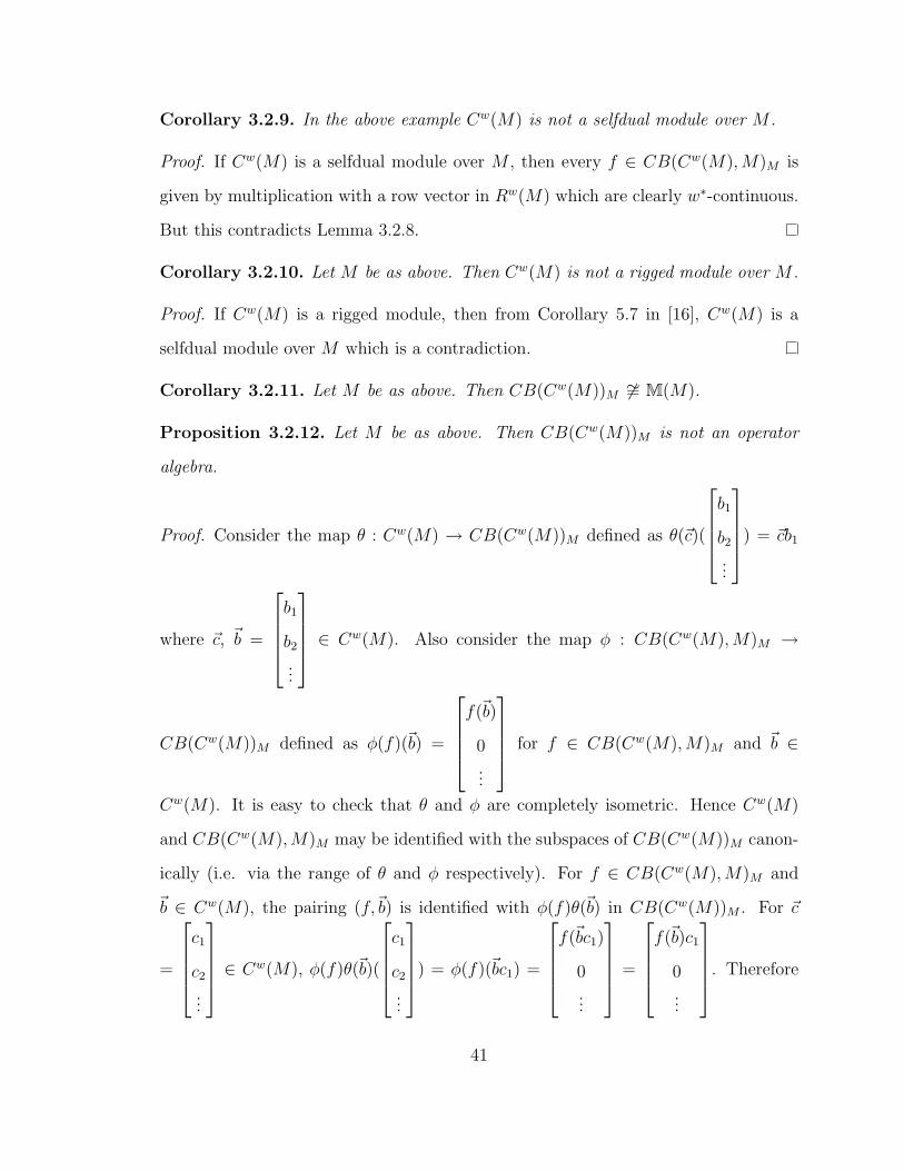
Corollary 3.2.9. In the above example Cw(M) is not a selfdual module over M .

Proof. If Cw(M) is a selfdual module over M , then every f ∈ CB(Cw(M),M)M is

given by multiplication with a row vector in Rw(M) which are clearly w∗-continuous.

But this contradicts Lemma 3.2.8.

Corollary 3.2.10. Let M be as above. Then Cw(M) is not a rigged module over M .

Proof. If Cw(M) is a rigged module, then from Corollary 5.7 in [16], Cw(M) is a

selfdual module over M which is a contradiction.

Corollary 3.2.11. Let M be as above. Then CB(Cw(M))M 6∼= M(M).

Proposition 3.2.12. Let M be as above. Then CB(Cw(M))M is not an operator

algebra.

Proof. Consider the map θ : Cw(M) → CB(Cw(M))M defined as θ(~c)(

b1

b2

...

) = ~cb1

where ~c, ~b =

b1

b2

...

∈ Cw(M). Also consider the map φ : CB(Cw(M),M)M →

CB(Cw(M))M defined as φ(f)(~b) =

f(~b)

0

...

for f ∈ CB(Cw(M),M)M and ~b ∈

Cw(M). It is easy to check that θ and φ are completely isometric. Hence Cw(M)

and CB(Cw(M),M)M may be identified with the subspaces of CB(Cw(M))M canon-

ically (i.e. via the range of θ and φ respectively). For f ∈ CB(Cw(M),M)M and

~b ∈ Cw(M), the pairing (f,~b) is identified with φ(f)θ(~b) in CB(Cw(M))M . For ~c

=

c1

c2

...

∈ Cw(M), φ(f)θ(~b)(

c1

c2

...

) = φ(f)(~bc1) =

f(~bc1)

0

...

=

f(~b)c1

0

...

. Therefore

41

φ(f)θ(~b) can be identified with f(~b) in M . Therefore, if CB(Cw(M))M is an oper-

ator algebra then the canonical map π : CB(Cw(M),M)M ⊗h Cw(M) → M that

takes the pairing (f,~b) to f(~b) where f ∈ CB(Cw(M),M)M and ~b ∈ Cw(M) will

be completely contractive. As Cw(B(H))∗ ⊆ CB(Cw(M),M)M completely isomet-

rically, therefore the restriction π : Cw(B(H))∗ ⊗h Cw(B(H)) → C that takes the

pairing (f,~b) to f(~b) where f ∈ Cw(B(H))∗ and ~b ∈ Cw(B(H)), is completely con-

tractive too. Let N = C(B(H)) which is a closed subspace of Cw(B(H)). As the map

π : N⊥⊗hCw(B(H))→ C is completely contractive, by a well known consequence of

the factorization theorem for completely bounded bilinear functionals (see Corollary

9.4.2 in [10]) there exists a Hilbert space K and completely contractive mappings

ψ : N⊥ → Kc and ϕ : Cw(B(H))→ (Kc)∗ such that π(f, b) = ψ(f)ϕ(b) = f(b) for f

∈ N⊥ and b ∈ Cw(B(H)). From this it is easy to check that ϕ∗ψ : N⊥ → Cw(B(H))∗

is the identity map, hence ψ is completely isometric. Thus N⊥ is a column Hilbert

space, hence Cw(B(H))/C(B(H)) is a column Hilbert space too. Let J be any set or

cardinal. Without loss of generality let H = l2J . Then B(H) ∼= MJ and S∞(H) ∼= KJ .

Define a map from MJ → Cw(MJ)/C(MJ) that takes an infinite matrix (aij)i,j∈J

to A + C(MJ), where A is an infinite column with each entry an infinite matrix

supported in only one row (which is a row of (aij)i,j∈J). This is a completely isomet-

ric map with kernel KJ , hence MJ/KJ ↪→ Cw(MJ)/C(MJ) completely isometrically.

This implies that the Calkin algebra B(H)/S∞(H) is a column Hilbert space, which

is a contradiction since the Calkin algebra is a C∗-algebra.

Theorem 3.2.13. If M and N are weak* Morita equivalent dual operator algebras,

then their centers are completely isometrically isomorphic via a w∗-homeomorphism.

Proof. By Theorem 3.2.6 there is a w∗-continuous complete isometry RM : M →

CBσN(Y ). The restriction of RM to the center Z(M) of M maps into CBσ(Y )M ∼= N ,

and so we have defined a w∗-continuous completely isometric homomorphism θ :

42

Z(M) → N . One easily sees that θ(a)(y) = ya, for a ∈ Z(M). It is also easy to see

that this implies that θ maps into Z(N), and to argue, by symmetry, that θ must be

an isomorphism.

Lemma 3.2.14. Suppose that T : E∗ → F ∗ is a contractive, one-one, surjection

between dual Banach spaces, such that T−1 is weak∗ continuous, and such that T−1

restricts to an isometry on a subspace Y of F ∗. Suppose also that the unit ball of Y

is weak∗ dense in the unit ball of F ∗. Then T is an isometry.

Proof. Suppose that ‖T (x)‖ ≤ δ < 1, where ‖x‖ = 1. Then there exists a net (yλ) ∈

Y with ‖yλ‖ ≤ δ such that yλw∗→ T (x). Since T−1 is weak∗ continuous, T−1(yλ)

w∗→ x,

and ‖T−1(yλ)‖ = ‖yλ‖ ≤ δ. This implies that ‖x‖ ≤ δ which is a contradiction.

Lemma 3.2.15. In the case of weak Morita equivalence, if Z is a left dual operator

N-module, then the canonical map Y ′⊗hB Z → Y ⊗σhN Z is completely isometric, and

it maps the ball onto a w∗-dense set in Ball(Y ⊗σhN Z).

Proof. The canonical map here is completely contractive, let us call it θ. On the other

hand, let ϕs, ψs be as defined just below Corollary 3.2.4, with ψs(ϕs(y)) = fsy → y.

Then for u ∈Mn(Y ′ ⊗B Z), we have

‖θn(u)‖ ≥ ‖(ϕs ⊗ I)n(θn(u))‖ = ‖(ϕs ⊗ I)n(u)‖ ≥ ‖fsu‖.

Taking a limit over s, gives ‖θn(u)‖ ≥ ‖u‖.

Let u ∈ Ball(Y ⊗σhN Z). By Corollary 2.4.8, there exists a net (ut) in the image of

Ball(Y ⊗hN Z) such that utw∗→ u. We rewrite (3.1.1) and the lines below it, namely

write each fs in the form [y, x] (in suggestive notation), for y ∈ Ball(Rm(Y ′)) and

x ∈ Ball(Cm(X ′)).

Note, w � z is the weak* limit of terms fsw � z, and etw � z = y � v, where v is

a column with kth entry∑

j[xk, wj]zj. It is easy to check that ‖v‖ ≤ 1.

43

Proposition 3.2.16. Weak∗ Morita equivalence is an equivalence relation.

Proof. This follows the usual lines, for example the transitivity follows from associa-

tivity of the normal module Haagerup tensor product and Lemma 2.4.12.

Remark. Concerning transitivity of weak Morita equivalence, it is convenient to

consider Definition 3.2.2 as defining an equivalence between pairs (M,A) and (N,B),

as opposed to just between M and N . That is we also consider the weak∗ dense

operator subalgebras, in the relation discussed in the next proposition.

Proposition 3.2.17. Weak Morita equivalence is an equivalence relation.

Proof. Reflexivity is a consequence of the Example (7) : In the notation there, take

X = R1(A), Y = C1(A), and B = M1(A), with both (·, ·) and [·, ·] given by multipli-

cation in A. Symmetry is evident. The only thing that requires work is transitivity.

Suppose that L is weakly Morita equivalent to M and M is weakly Morita equiva-

lent to N . Let (L,M,X, Y, (·, ·)1, [·, ·]1) and (M,N,W,Z, (·, ·)2, [·, ·]2) be weak Morita

contexts with weak∗-dense strong Morita sub-contexts (A,B,X ′, Y ′, (·, ·)1, [·, ·]1) and

(B,C,W ′, Z ′, (·, ·)2, [·, ·]2) respectively. Set U ′ = X ′ ⊗hB W ′ and V ′ = Z ′ ⊗hB Y ′.

Define (·, ·) : U ′ × V ′ → A by the formula ((x′ ⊗B w′), (z′ ⊗B y′)) = (x′, (w′, z′)2y′)1

= (x′(w′, z′)2, y′)1. Similarly define [·, ·] : V ′×U ′ → by the formula [z′⊗By′, x′⊗Bw′]=

[z′, [y′, x′]1w′]2 = [z′[y′, x′]1, w

′]2. Then by Proposition 3.7 in [18], (A,C, U ′, V ′, (·, ·), [·, ·])

is a strong Morita context. Define U = X⊗σhM W and V = Z⊗σhM Y , then by Corollary

2.4.8, U ′ and V ′ are w∗-dense in U and V respectively. From Proposition 2.4.3, there is

a completely contractive map from U⊗σhN V = X⊗σhMW⊗σhN Z⊗σhM Y → X⊗σhMM⊗σhM Y

∼= X ⊗σhM Y → L. By Proposition 2.2 in [31], this gives rise to a separately w∗-

continuous, completely contractive, N -balanced, bilinear map (·, ·) : U × V → L.

Similarly there is a separately w∗-continuous, completely contractive, L-balanced, bi-

linear map [·, ·] : V × U → N . Thus (L,N,U, V, (·, ·), [·, ·]) is a weak Morita context,

which proves transitivity.

44

We would like to thank G. Pisier for the following Lemma.

Lemma 3.2.18. (Pisier) An operator space E is a Hilbert column space if and only

if E ⊗h Cn ∼= Cn(E) isometrically via the canonical map, for all n ∈ N.

Theorem 3.2.19. Weak Morita equivalent dual operator algebras have equivalent

categories of normal Hilbert modules. Moreover, the equivalence preserves the subcat-

egory of modules corresponding to completely isometric normal representations.

Proof. Suppose that H is a Hilbert space on which M is normally represented. We

claim that Y ⊗σhM Hc is a column Hilbert space. By Lemma 3.2.18, it suffices to show

that the canonical map Cn(Y ⊗σhM Hc) → (Y ⊗σhM Hc) ⊗h Cn is isometric for all n ∈

N . Now Cn(Y ⊗σhM Hc) ∼= Cn(Y ) ⊗σhM Hc, and (Y ⊗σhM Hc) ⊗h Cn ∼= Y ⊗σhM Cn(Hc).

Thus we need to show that the canonical map Cn(Y ) ⊗σhM Hc → Y ⊗σhM Cn(Hc) is

isometric. Define a map θ : (Cn(Y )⊗hM Hc)∗σ → (Y ⊗hM Cn(Hc))∗σ by θ(T )(y, (ni)) =∑ni=1 T (yi, ni), where yi is an n-tuple with y in the ith coordinate and otherwise

zero. It is easy to check that θ is contractive. Define φ : (Y ⊗hM Cn(Hc))∗σ →

(Cn(Y ) ⊗hM Hc)∗σ by φ(T )([y1 y2 · · · yn]t, η) =∑n

i=1 T (yi, ηi), where ηi is an n-tuple

with ζ in the ith coordinate and otherwise zero. Again it is easy to check that φ is

bounded, and θ = φ−1. Dualizing the map θ, we get a contractive, one-one, surjective

map ρ = θ∗ : Y ⊗σhM Cn(Hc) → Cn(Y ) ⊗σhM Hc with ρ−1 = φ∗. Hence ρ and ρ−1 are

weak∗ continuous. Since by Theorem 3.10 in [18], Y ′⊗hAHc is a Hilbert space, Lemma

3.2.18 will yield, analogously to the above, that Y ′ ⊗hA Cn(Hc) = Cn(Y ′) ⊗hA Hc

isometrically. That is, ρ−1 is an isometry when restricted to Cn(Y ′)⊗hAHc. Now the

above claim follows from Lemma 3.2.15 and Lemma 3.2.14.

To see that N is normally represented on the Hilbert space Y ⊗σhM Hc, suppose

that (nt) is a net in N converging in the w∗-topology to an element n ∈ N . Then

nty → ny in the w∗-topology of Y , for any y ∈ Y . By Proposition 2.1 in [31], nty⊗M η

→ ny⊗M η for all η ∈ Hc in the w∗-topology of K. Since for Hilbert spaces the weak

45

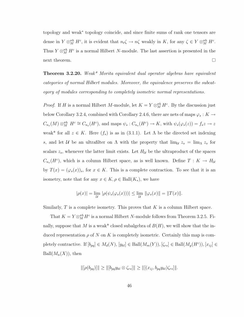
topology and weak∗ topology coincide, and since finite sums of rank one tensors are

dense in Y ⊗σhM Hc, it is evident that ntζ → nζ weakly in K, for any ζ ∈ Y ⊗σhM Hc.

Thus Y ⊗σhM Hc is a normal Hilbert N -module. The last assertion is presented in the

next theorem.

Theorem 3.2.20. Weak* Morita equivalent dual operator algebras have equivalent

categories of normal Hilbert modules. Moreover, the equivalence preserves the subcat-

egory of modules corresponding to completely isometric normal representations.

Proof. If H is a normal Hilbert M -module, let K = Y ⊗σhM Hc. By the discussion just

below Corollary 3.2.4, combined with Corollary 2.4.6, there are nets of maps ϕs : K →

Cns(M)⊗σhM Hc ∼= Cns(Hc), and maps ψs : Cns(H

c)→ K, with ψs(ϕs(z)) = fsz → z

weak* for all z ∈ K. Here (fs) is as in (3.1.1). Let Λ be the directed set indexing

s, and let U be an ultrafilter on Λ with the property that limU zs = limΛ zs for

scalars zs, whenever the latter limit exists. Let HU be the ultraproduct of the spaces

Cns(Hc), which is a column Hilbert space, as is well known. Define T : K → HU

by T (x) = (ϕs(x))s, for x ∈ K. This is a complete contraction. To see that it is an

isometry, note that for any x ∈ K, ρ ∈ Ball(K∗), we have

|ρ(x)| = limU|ρ(ψs(ϕs(x)))| ≤ lim

U‖ϕs(x)‖ = ‖T (x)‖.

Similarly, T is a complete isometry. This proves that K is a column Hilbert space.

That K = Y ⊗σhM Hc is a normal Hilbert N -module follows from Theorem 3.2.5. Fi-

nally, suppose that M is a weak* closed subalgebra of B(H), we will show that the in-

duced representation ρ of N on K is completely isometric. Certainly this map is com-

pletely contractive. If [bpq] ∈Md(N), [ykl] ∈ Ball(Mm(Y )), [ζrs] ∈ Ball(Mg(Hc)), [xij] ∈

Ball(Mn(X)), then

‖[ρ(bpq)]‖ ≥ ‖[bpqykl ⊗ ζrs]‖ ≥ ‖[(xij, bpqykl)ζrs]‖.

46

Taking the supremum over all such [ζrs], gives

‖[ρ(bpq)]‖ ≥ sup{‖[(xij, bpqykl)]‖ : [xij] ∈ Ball(Mn(X))} = ‖[bpqykl]‖,

by Theorem 3.2.6. Taking the supremum over all such [ykl] ∈ Ball(Mm(Y )) gives

‖[ρ(bpq)]‖ ≥ ‖[bpq]‖, by Theorem 3.2.6 again.

We summarize: the last result shows that weak* Morita equivalent operator alge-

bras have equivalent categories of normal representations. It would be interesting to

characterize when two operator algebras have equivalent categories of normal repre-

sentations.

Corollary 3.2.21. If H ∈ MH then Y ⊗σhM Hc = Y ⊗hM Hc = Y_⊗M Hc completely

isometrically. These are column Hilbert spaces. Here_⊗M is as in 3.4.2 of [15]. In

the case of weak Morita equivalence, these also equal Y ′ ⊗hA Hc = Y ′_⊗A Hc.

Proof. By Lemma 3.2.15 and Corollary 2.4.8, Y ⊗hMHc = Y ⊗σhM Hc. Note that since

− ⊗h Hc = −_⊗ Hc (see e.g. [26, Proposition 9.3.2]), we may replace ⊗hM here by

_⊗M ( where

_⊗M is the module projective tensor product e.g., see 3.4.2 of [15]). The

assertions involving Y ′ follow in a similar way, by Lemma 3.2.15. Note that in this

case, if η ∈ H [AH] and (et) is a cai for A, then

〈η, η〉 = limt〈etη, η〉 = 0.

Thus A acts nondegenerately on H.

3.3 Representations of the linking algebra

In this section again, (M,N,X, Y, (·, ·), [·, ·]) is a weak* Morita context. Suppose that

M is represented as a weak∗-closed nondegenerate subalgebra of B(H), for a Hilbert

space H. Then by Corollary 3.2.21, K = Y ⊗σhM Hc is a column Hilbert space. Define

47

a right M -module map Φ : Y → B(H,K) by Φ(y)(ζ) = y ⊗M ζ where y ∈ Y and

ζ ∈ H. It is easy to see that Φ is a completely contractive N -M -bimodule map. It is

weak∗ continuous, since if we have a bounded net yt → y weak∗ in Y , and if ζ ∈ H,

then yt ⊗M ζ → y ⊗M ζ weakly by [31]. That is, Φ(yt) → Φ(y) in the WOT, and

it follows that Φ is weak∗ continuous. If ‖Φ(y)‖ ≤ 1, and if ζ ∈ Ball(H(n)), and

[xij] ∈ Ball(Mn(X)), then

‖[(xij, y)]ζ‖ = ‖[xij ⊗ Φ(y)]ζ‖‖ ≤ ‖Φ(y)‖.

Taking the supremum over such ζ, and then over such [xij], we obtain from The-

orem 3.2.6 that ‖y‖ ≤ 1. Thus Φ is an isometry, and a similar but more tedious

argument shows that Φ is a complete isometry. By the Krein-Smulian theorem we

deduce that the range of Φ is weak∗ closed. A lengthy but similar argument, shows

that the map Ψ : X → B(K,H), defined by Ψ(x)(y⊗ ζ) = (x, y)ζ, is a w∗-continuous

completely isometric M -N -bimodule map. As we said in Theorem 3.2.20, the induced

normal representation N → B(K) is completely isometric.

We use the above to define the direct sum M ⊕c Y as follows. For specificity, we

want to take H to be a universal normal representation of M , that is the restriction

to M of a one-to-one normal representation of W ∗max(M). Define a map θ : M⊕cY →

B(H,K ⊕ H) by θ((m, y))(ζ) = (mζ, y ⊗M ζ), for y ∈ Y,m ∈ M, ζ ∈ H. One can

quickly check that θ is a one-to-one, M -module map, and that θ is a weak∗ continuous

complete isometry when restricted to each of Y and M . Also, W= Ran(θ) is easily

seen to be weak∗ closed. We norm M ⊕c Y by pulling back the operator space

structure from W via θ. Thus M ⊕c Y may be identified with the weak∗ closed right

M -submodule W of B(H,H ⊕K); and hence it is a dual operator M -module. In a

similar way, we define M ⊕rX to be the canonical weak∗ closed left M -submodule of

B(H ⊕K,H).

48

We next define the ‘weak linking algebra’ of the context, namely

Lw =

a x

y b

: a ∈M, b ∈ N, x ∈ X, y ∈ Y

,

with the multiplication with the given by the formula

a x

y b

a′ x′

y′b′

=

aa′ + (x, y′) ax

′+ xb

′

ya′+ by

′[y, x

′] + bb

′

As in [18, Lemma 5.6], one easily sees that there is at most one possible sensible

dual operator space structure on this linking algebra. Indeed if Λ is the set indexing

t in the net in (3.2.2), and if β, t ∈ Λ, then define θβ,t on the linear space Lw to

be the map θβ in [18, p. 45], but with all the yβi replaced by yti . Then a simple

modification of the argument in [18, p. 50-51], and using semicontinuity of the norm

in the weak* topology, yields that any ‘sensible’ norm assigned to Lw must agree with

supβ,t ‖θβ,t(·)‖.

That such a dual operator space structure does exist, one only need view Lw as a

subalgebra R of B(H⊕K), using the obvious pairings X×K → H (induced by (·, ·)),

Y ×H → K, and N ×K → K (this is the induced representation of N on K from

Theorem 3.2.20). It is easy to check that (M,R,M ⊕r X,M ⊕c Y ) is also a weak*

Morita context (this follows from norm equalities of the kind in e.g., the centered

equations in [18, Theorem 5.12]). This all may be most easily visualized by picturing

both contexts as 3× 3-matrices, namely as subalgebras of B(H ⊕H ⊕K). Theorem

3.2.6 gives R ∼= CBσ(M ⊕c Y )M completely isometrically and w∗-homeomorphically.

Note that in a weak Morita situation, the linking operator algebra of the strong

Morita context (A,B,X ′, Y ′) can be identified completely isometrically as the obvious

49

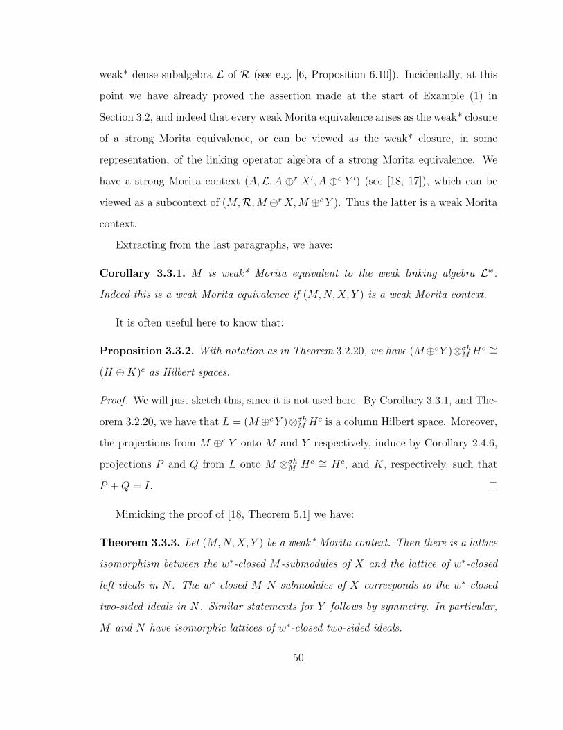
weak* dense subalgebra L of R (see e.g. [6, Proposition 6.10]). Incidentally, at this

point we have already proved the assertion made at the start of Example (1) in

Section 3.2, and indeed that every weak Morita equivalence arises as the weak* closure

of a strong Morita equivalence, or can be viewed as the weak* closure, in some

representation, of the linking operator algebra of a strong Morita equivalence. We

have a strong Morita context (A,L, A ⊕r X ′, A ⊕c Y ′) (see [18, 17]), which can be

viewed as a subcontext of (M,R,M ⊕rX,M ⊕c Y ). Thus the latter is a weak Morita

context.

Extracting from the last paragraphs, we have:

Corollary 3.3.1. M is weak* Morita equivalent to the weak linking algebra Lw.

Indeed this is a weak Morita equivalence if (M,N,X, Y ) is a weak Morita context.

It is often useful here to know that:

Proposition 3.3.2. With notation as in Theorem 3.2.20, we have (M⊕cY )⊗σhM Hc ∼=

(H ⊕K)c as Hilbert spaces.

Proof. We will just sketch this, since it is not used here. By Corollary 3.3.1, and The-

orem 3.2.20, we have that L = (M⊕cY )⊗σhM Hc is a column Hilbert space. Moreover,

the projections from M ⊕c Y onto M and Y respectively, induce by Corollary 2.4.6,

projections P and Q from L onto M ⊗σhM Hc ∼= Hc, and K, respectively, such that

P +Q = I.

Mimicking the proof of [18, Theorem 5.1] we have:

Theorem 3.3.3. Let (M,N,X, Y ) be a weak* Morita context. Then there is a lattice

isomorphism between the w∗-closed M-submodules of X and the lattice of w∗-closed

left ideals in N . The w∗-closed M-N-submodules of X corresponds to the w∗-closed

two-sided ideals in N . Similar statements for Y follows by symmetry. In particular,

M and N have isomorphic lattices of w∗-closed two-sided ideals.

50

Proof. Suppose the linking algebra has concrete representation on Hilbert space. All

products which follows are products of operators on this Hilbert space. If U is a

w∗-closed M -submodule of X, let IU = Y.Uw∗

. Since Y.Xw∗

= N we see that IU is a

w∗-closed left idea of N . If I is a w∗-closed left ideal in N let UI = X.Iw∗

, which is a

w∗-closed M -submodule X. Clearly U 7→ IU and I 7→ UI are inverse to each other,

and are lattice isomorphisms, which establishes the first result. If U is a w∗-closed

M,N -submodule, then IU is a w∗-closed two-sided ideal in N . Conversely, if I is

a w∗-closed two sided ideal in N then UI is a w∗-closed M -N -submodule. The last

statement follows by symmetry.

We next show, analogously to [18, Section 6], that if M and N are W ∗-algebras,

then they are Morita equivalent in Rieffel’s sense if and only if they are weakly (or

equivalently, weak*) Morita equivalent in our sense. Indeed we already have remarked

(Example (4) in Section 3.2) that Rieffel’s Morita equivalence is an example of our

weak Morita equivalence. The following gives the converse, and more:

Theorem 3.3.4. Let (M,N,X, Y ) be a weak* Morita context where N is a W ∗-

algebra. Then M is a W ∗-algebra, and there is a completely isometric isomorphism

i : X → Y such that X becomes a W ∗-equivalence M-N-bimodule (see e.g. 8.5.12 in

[15] with inner products defined by the formulas M〈x1, x2〉 = (x1, i(x2)) and 〈x1, x2〉N

= [i(x1), x2].

Proof. First we represent the linking algebra on a Hilbert space H ⊕ K as above.

We rechoose the net (et) such that et → IH strongly, so that e∗t et → IH thus weak*,

and similarly for the net (fs). To accomplish this, note that the WOT-closure of

the convex hull of the (et) equals the SOT-closure, by elementary operator theory.

However it is easy to see that the form in (3.2.1) is preserved if we replace es by

convex combinations of the et. Now one can follow the proof of [18, Theorem 6.2]

to deduce that the adjoint of any y ∈ Y is a limit of terms in X. That is Y ⊂ X∗.

51

Similarly, X ⊂ Y ∗. So X = Y ∗, and so it follows that M is a W ∗-algebra, and X is

a WTRO (this term was defined in the list of examples in Section 3.2) setting up a

W ∗-algebra Morita equivalence.

The following is the non-selfadjoint analogue of a theorem of Rieffel. A special

case of it is mentioned, with a proof sketch, at the end of [16].

Theorem 3.3.5. Let (M,N,X, Y ) be a weak∗ Morita context. Let H be a universal

normal representation for M , and let K be the induced representation of N as in

Theorem 3.2.20. Then M ′ ∼= N ′; that is there is a completely isometric w∗-continuous

isomorphism θ : BM(H) ∼= BN(K). Writing R for either of these commutants,

we have X ∼= BR(K,H) and Y ∼= BR(H,K) completely isometrically and as dual

operator bimodules.

Proof. One uses the equivalence of categories to see that BM(H) ∼= BN(F(H)) =

BN(K) completely isometrically, in the notation of Theorem 3.2.5. That is, M ′ ∼= N ′

as asserted, and it is easy to argue that if θ is this isomorphism then Φ(y)T =

θ(T )Φ(y) for all y ∈ Y, T ∈ M ′. Here Φ is as in the discussion at the start of

Section 3.3. Now mimic the proof of 8.5.32 and 8.5.37 in [15]. The main point to

bear in mind is that since M is weak* Morita equivalent to the weak linking algebra

Lw, the induced representation of Lw is also a universal normal representation, by

easy category theoretic arguments. Thus by [21] it satisfies the double commutant

theorem. Carefully computing the first, and then the second, commutants of Lw as

in 8.5.32 in [15], and using the double commutant theorem, gives the result.

Example. If M and N are finite dimensional then weak* Morita equivalence equals

strong Morita equivalence, and coincides also with the equivalence considered in [28,

29], that is, weak* stable isomorphism [31]. Indeed if (M,N,X, Y ) is a weak* Morita

context, then it is clearly a strong Morita context, and by [18, Lemma 2.8] we can

52

actually factor the identity map IY through Cn(M) for some n ∈ N, so that Y is

finite dimensional. Similarly, X is finite dimensional. To see that this implies that M

and N are weak* stably isomorphic, note that in this situation, since M ∼= X ⊗σhN Y ,

there is a norm 1 element in X ⊗h Y mapping to 1M . Similarly for 1N , and then it is

easy to argue that one has what is called a ‘quasi-unit of norm 1’ in [18, Section 7].

By [18, Corollary 7.9], M and N are stably isomorphic, and taking second duals and

using e.g. (1.62) in [15], we see that they are weak* stably isomorphic. In the infinite

dimensional case however, all these notions are distinct (e.g. see the Introduction 3.1).

3.4 Morita equivalence of generated W ∗-algebras

From [17] or [6], we know that a strong Morita equivalence of operator algebras in

the sense of [18] ‘dilates’ to, or is a subcontext of, a strong Morita equivalence in the

sense of Rieffel, of containing C∗-algebras. This happens in a very tidy way. More

particularly, suppose that (A,B,X, Y ) is a strong Morita context of operator algebras

A and B. Then any C∗-algebra C generated by A induces a C∗-algebra D generated

by B, and C and D are strongly Morita equivalent in the sense of Rieffel [40], with

equivalence bimodule the C∗-dilation (see [8]) C⊗hAX. Moreover the linking algebra

for A and B is (completely isometrically) a subalgebra of the linking C∗-algebra for

C and D. We see next that all of this, and the accompanying theory, will extend to

our present setting. Although one may use any W ∗-cover in the arguments below,

for specificity, the maximal W ∗-algebra W ∗max(M) from [21] will take the place of C

above, and the maximal W ∗-dilation W ∗max(M) ⊗σhM X will play the role of the C∗-

dilation. In Chapter 5, we will develop the theory for this W ∗-dilation in a general

setting analogously to [8, 17]. We will however state that just as in [8], any (left,

say) dual operator M -module is completely isometrically embedded in its maximal

W ∗-dilation, via the M -module map x 7→ 1⊗ x, which is weak* continuous.

53

Throughout this section again, (M,N,X, Y ) is a weak* Morita context. In this

case, we shall show that the left and right W ∗-dilations coincide, and constitutes a

bimodule implementing the W ∗-algebraic Morita equivalence between W ∗max(M) and

W ∗max(N).

Theorem 3.4.1. The W ∗-dilation Y⊗σhM W ∗max(M) is a right C∗-module over W ∗

max(M).

Proof. With H a normal universal Hilbert M -module as usual, we may view W ∗max(M)

as the von Neumann algebra R generated by M in B(H). Let K = Y ⊗σhM Hc as

usual, and let Z = Y ⊗σhM W ∗max(M). Note that

Z ⊗σhW ∗max(M) Hc ∼= Y ⊗σhM W ∗

max(M)⊗σhW ∗max(M) Hc ∼= Y ⊗σhM Hc = K.

This allows us to define a completely contractive weak∗ continuous φ : Z → B(H,K)

given by φ(y ⊗ a)(ζ) = y ⊗ aζ, for y ∈ Y, a ∈ R, ζ ∈ H. Note that φ restricted to

the copy of Y is just the map Φ at the start of Section 3.3. We are following the

ideas of [7, p. 286-288]. It is clear that φ is a R-module map. By the discussion

just below Corollary 3.2.4, combined with Corollary 2.4.6, there are nets of maps

ϕs ⊗ I : Z → Cns(M) ⊗σhM W ∗max(M) ∼= Cns(W

∗max(M)), and maps ψs ⊗ I, with

(ψs ⊗ I)(ϕs ⊗ I)(z) = fsz → z weak* for all z ∈ Z. Here (fs) is as in (3.2.1),

and the last convergence follows from e.g., [31, Lemma 2.3]. We have ‖[fszij]‖ ≤

‖[(ϕs ⊗ I)(zij)]‖ ≤ ‖[φ(zij)]‖. This follows, as in [7, p. 287], from the fact that there

is a sequence of weak* continuous complete contractions

B(H,K)→ B(H,Cnt(M)⊗σhM W ∗max(M)⊗σhW ∗max(M) H

c) ∼= B(H,Cnt(Hc))

that maps φ(y ⊗ a) to ϕs(y)a, for y ∈ Y, a ∈ R, and hence maps φ(z) for z ∈ Z, to

(ϕs ⊗ I)(z). As in [7, p. 287], we can deduce from these facts that φ is a complete

isometry.

Define 〈z, w〉 = φ(z)∗φ(w) for z, w ∈ Z. To see that this is a R-valued inner

product on Z, we will use von Neumann’s double commutant theorem. Note that if

54

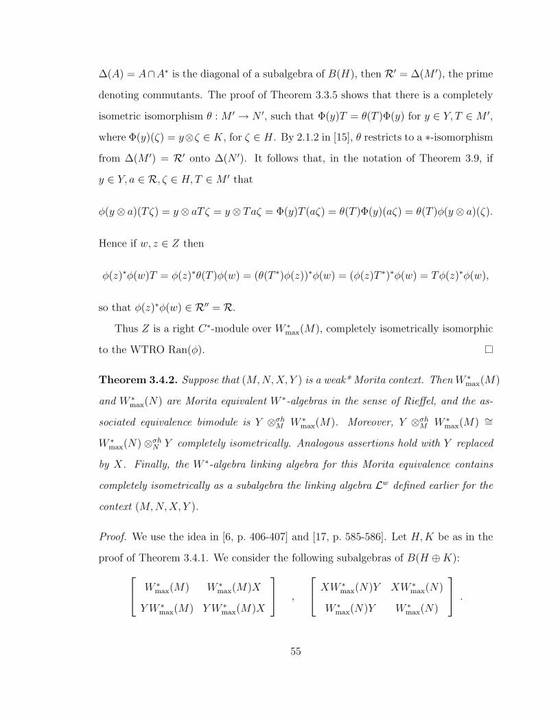
∆(A) = A∩A∗ is the diagonal of a subalgebra of B(H), then R′ = ∆(M ′), the prime

denoting commutants. The proof of Theorem 3.3.5 shows that there is a completely

isometric isomorphism θ : M ′ → N ′, such that Φ(y)T = θ(T )Φ(y) for y ∈ Y, T ∈M ′,

where Φ(y)(ζ) = y⊗ζ ∈ K, for ζ ∈ H. By 2.1.2 in [15], θ restricts to a ∗-isomorphism

from ∆(M ′) = R′ onto ∆(N ′). It follows that, in the notation of Theorem 3.9, if

y ∈ Y, a ∈ R, ζ ∈ H,T ∈M ′ that

φ(y⊗ a)(Tζ) = y⊗ aTζ = y⊗ Taζ = Φ(y)T (aζ) = θ(T )Φ(y)(aζ) = θ(T )φ(y⊗ a)(ζ).

Hence if w, z ∈ Z then

φ(z)∗φ(w)T = φ(z)∗θ(T )φ(w) = (θ(T ∗)φ(z))∗φ(w) = (φ(z)T ∗)∗φ(w) = Tφ(z)∗φ(w),

so that φ(z)∗φ(w) ∈ R′′ = R.

Thus Z is a right C∗-module over W ∗max(M), completely isometrically isomorphic

to the WTRO Ran(φ).

Theorem 3.4.2. Suppose that (M,N,X, Y ) is a weak* Morita context. Then W ∗max(M)

and W ∗max(N) are Morita equivalent W ∗-algebras in the sense of Rieffel, and the as-

sociated equivalence bimodule is Y ⊗σhM W ∗max(M). Moreover, Y ⊗σhM W ∗

max(M) ∼=

W ∗max(N)⊗σhN Y completely isometrically. Analogous assertions hold with Y replaced

by X. Finally, the W ∗-algebra linking algebra for this Morita equivalence contains

completely isometrically as a subalgebra the linking algebra Lw defined earlier for the

context (M,N,X, Y ).

Proof. We use the idea in [6, p. 406-407] and [17, p. 585-586]. Let H,K be as in the

proof of Theorem 3.4.1. We consider the following subalgebras of B(H ⊕K): W ∗max(M) W ∗

max(M)X

YW ∗max(M) YW ∗

max(M)X

,

XW ∗max(N)Y XW ∗

max(N)

W ∗max(N)Y W ∗

max(N)

.

55

Let L1 and L2 denote the weak* closures of these two subalgebras. These are dual

operator algebras which are the linking algebras for a Morita equivalence. Thus by

Theorem 3.3.4, they are actually selfadjoint. Moreover, both of these can now be

seen to equal the von Neumann algebra generated by Lw, and so they are equal

to each other. Now it is clear that, for example, the weak* closures of YW ∗max(M)

and W ∗max(N)Y coincide, and this constitutes an equivalence bimodule (or WTRO)

setting up a W ∗-algebraic Morita equivalence between W ∗max(M) and W ∗

max(N). The

W ∗-algebraic linking algebra here is just L1 = L2, and this clearly contains the

algebra we called R in the discussion in the beginning of Section 3.3, that is, Lw, as

a subalgebra.

Finally, notice that the map φ in the proof of the last theorem is a completely

isometric W ∗max(M)-module map from Z = Y ⊗σhM W ∗

max(M) onto the weak* closure

W of YW ∗max(M) in B(H,K). Similar considerations, or symmetry, shows that V =

W ∗max(N) ⊗σhN Y agrees with the weak* closure of W ∗

max(N)Y , which by the above

equals W , and thus agrees with Z. Similarly for the modules involving X.

Remark. Theorems 4 and 5 of [17] have obvious variants valid in our setting,

with arbitrary W ∗-dilations in place of W ∗max(M). We will present this in Chapter 5.

Similarly, as in [17], we will show later in Chapter 5 that W ∗max(Lw) = L1.

56

Chapter 4

A characterization and a

generalization of W ∗-modules

4.1 Introduction

In this chapter, we give a new dual Banach module characterization of W ∗-modules,

also known as selfdual Hilbert C∗-modules, over a von Neumann algebra. This leads

to a generalization of the notion, and the theory, of W ∗-modules, to the setting where

the operator algebras are weak∗ closed algebras of operators on a Hilbert space. That

is, we find the appropriate weak* topology variant of the theory of rigged modules [6],

which in turn generalizes the notion of Hilbert C∗-modules. The ensuing modules,

the w∗-rigged modules, do not necessarily give rise to a weak* Morita equivalence in

the sense of Chapter 3. Nonetheless, w∗-rigged modules have canonical ‘envelopes’

which are W ∗-modules. Indeed, w∗-rigged modules may be defined to be a subspace

of a W ∗-module possessing certain properties.

A W ∗-module is a Hilbert C∗-module over a von Neumann algebra which is selfd-

ual, or, equivalently, which has a predual (see e.g., [42, 24, 16]). These objects were

57

first studied by Paschke, and then by Rieffel [37, 40] (see also [15, Section 8.7] for an

account of their theory). They are by now fundamental objects in C∗-algebra theory

and noncommutative geometry, being intimately related to Connes’ correspondences

(see, e.g., [3] for the relationship). W ∗-modules have many characterizations; the

one mentioned in the title of this chapter characterizes them in the setting of Banach

modules in a new way. This in turn leads into a generalization of the notion of W ∗-

module to the setting where the operator algebra is a dual operator algebra. We also

develop the basic theory of this new class of modules, which we call w∗-rigged mod-

ules. The theory of the space of left multipliers M`(X) of an operator space X (see

e.g., [15, Chapter 4]), plays a role in this process. Unlike the W ∗-module situation,

w∗-rigged modules do not necessarily give rise to a weak* Morita equivalence in the

sense of Chapter 3. Thus there is limited overlap between Chapter 3 and Chapter 4.

However, weak* Morita equivalence bimodules are w∗-rigged modules and there are

strong connections between the two theories. Also, each w∗-rigged module has a

canonical W ∗-module envelope, called the W ∗-dilation, and thus w∗-rigged modules

give new examples of W ∗-modules. This dilation is an important tool in our the-

ory. Indeed, a w∗-rigged modules may be defined to be a subspace of a W ∗-module

possessing certain properties.

Much of Section 4.2 (on W ∗-modules) is closely related to a paper of Blecher [4].

The main point of the this paper is that W ∗-modules fall comfortably into a dual

operator module setting; for example, their usual tensor product (sometimes called

composition of W ∗-correspondences), agrees with a certain operator space tensor

product studied by Magajna. This has certain advantages, for example new results

about this tensor product (see also [23]). Here we show that this tensor product

also equals the normal module Haagerup tensor product recently introduced in [31],

and studied further by in this thesis (see, Section 2.4). In Section 4.3 we find the

58

variant for w∗-rigged modules of the basic theory of rigged modules from [6] (and to

a lesser extent, [18]). In Section 4.4 we give several alternative equivalent definitions

of w∗-rigged modules. In Section 4.5 we give examples of w∗-rigged modules.

In a couple proofs, we use multipliers of an operator space X (see, [15, Chapter

4]). We recall that the left multiplier algebra M`(X) of X is a collection of certain

operators on X, which are weak* continuous if X is a dual operator space [16].

4.2 W ∗-modules

We begin this section with a useful lemma:

Lemma 4.2.1. Let {Hα} be a collection of Hilbert spaces (resp. column Hilbert spaces)

indexed by a directed set. Let Y be a dual Banach space (resp. dual operator space).

Suppose there exist w∗-continuous contractive (resp. completely contractive) linear

maps φα : Y → Hα, ψα : Hα → Y , such that ψα(φα(y))w∗→ y for each y ∈ Y . Then

Y is a Hilbert space (resp. column Hilbert space) with inner product given by 〈y, z〉=

limα 〈φα(y), φα(z)〉, for y, z ∈ Y .

Proof. The proof that Y is a Hilbert space (respectively column Hilbert space) follows

by the ultraproduct argument in Theorem 3.2.20. For the last assertion, we will

show first that ‖φα(y)‖2 → ‖y‖2. Then by the polarization identity, it follows that

〈y, z〉= limα〈φα(y), φα(z)〉 as desired. Suppose there exists a subnet (φαt(y)) such

that ‖φαt(y)‖2 → β. We need to prove that β = ‖y‖2. Clearly β ≤ ‖y‖2. If

β < K < ‖y‖2, then there exists a t0, such that, ‖φαt(y)‖2 ≤ K for all t ≥ t0. This

implies that ‖ψαtφαt(y)‖2 ≤ ‖φαt(y)‖2 ≤ K for all t ≥ t0. Since ψαtφαt(y)w∗→ y, by

Alaoglu’s theorem we deduce that ‖y‖2 ≤ K, which is a contradiction.

We now generalize the notion of W ∗-modules to the setting where the operator

algebras are σ-weakly closed algebras of operators on a Hilbert space. The following

59

is the weak* variant of the notion of a rigged module studied in [6, 18, 5, 12]. The

paper [12] has the most succinct definition of these objects, and [5] is a survey. In

Section 4.4 there are several equivalent, but quite different looking, definitions of

w∗-rigged modules.

Definition 4.2.2. Suppose that Y is a dual operator space and a right module over a

dual operator algebra M . Suppose that there exists a net of positive integers (n(α)),

and w∗-continuous completely contractive M-module maps φα : Y → Cn(α)(M) and

ψα : Cn(α)(M) → Y , with ψα(φα(y)) → y in the w∗-topology on Y , for all y ∈ Y .

Then we say that Y is a right w∗-rigged module over M .

An argument similar to that in the last few lines of the proof of Lemma 4.2.1, and

using basic operator space duality principles, shows that for a w∗-rigged module Y ,

‖[yij]‖Mn(Y ) = supα‖[φα(yij)]‖, [yij] ∈Mn(Y ). (4.2.1)

Theorem 4.2.3. If Y is a right w∗-rigged module over a dual operator algebra M ,

then CBσ(Y )M =M`(Y ) completely isometrically isomorphically, and this is a weak*

closed subalgebra of CB(Y )M . Hence CBσ(Y )M is a dual operator algebra, and Y is

a left dual CBσ(Y )M -module.

Proof. By facts in the theory of multipliers of an operator space (see e.g., [15, Chapter

4] or [16]), the identity map is a weak* continuous completely contractive homomor-

phism M`(Y ) → CB(Y ), which maps into CBσ(Y )M . If CBσ(Y )M is an operator

algebra, and if Y is a left operator CBσ(Y )M -module (with the canonical action),

then by the aforementioned theory there exists a completely contractive homomor-

phism π : CBσ(Y )M → M`(Y ) with π(T )(y) = T (y) for all y ∈ Y, T ∈ CBσ(Y )M .

That is, π(T ) = T . Thus CBσ(Y )M =M`(Y ), and it is clear from the Krein-Smulian

theorem and [15, Theorem 4.7.4 (2)] that CB(Y )M is weak* closed in CB(Y ).

60

We now show that CBσ(Y )M is an operator algebra by appealing to the abstract

characterization of operator algebras [15, Theorem 2.3.2]. If S = [Sij], T = [Tij] ∈

Mn(CBσ(Y )M), then one may use the idea in [6, Theorem 2.7] or [18, Theorem 4.9]

to write the matrix a = [∑

k SikTkj(ypq)] as an iterated weak* limit of a product of

three matrices. The norm of this last product is dominated by ‖[Sij]‖‖[Tij]‖‖[ypq]‖.

It follows by Alaoglu’s theorem that ‖a‖ ≤ ‖S‖‖T‖‖[ypq]‖, and thus ‖ST‖ ≤ ‖S‖‖T‖

as desired.

A similar argument shows that Y is a left operator CBσ(Y )M -module: If T is as

above, and y = [yij] ∈Mn(Y ), then z = [∑

k Tik(ykj)] may be written as a weak* limit

of a product of two matrices, the latter product having norm ≤ ‖T‖‖y‖. Applying

Alaoglu’s theorem gives ‖z‖ ≤ ‖T‖‖y‖, as desired.

The final assertion now follows from [15, Lemma 4.7.5].

Theorem 4.2.4. Suppose that Y is a right w∗-rigged module over a dual operator

algebra M . Suppose that H is a Hilbert space, and that θ : M → B(H) is a normal

representation. Then Y ⊗σhM Hc is a column Hilbert space. Moreover, the finite rank

tensors Y ⊗Hc are norm dense in the Y ⊗σhM Hc.

Proof. Let eα = φαψα (notation as in Definition 4.2.2). By Lemma 2.4.7 and The-

orem 4.2.3, Y ⊗σhM Hc is a left dual M`(Y )-module. By the functoriality of the

module normal Haagerup tensor product, we obtain a net of complete contractions

φα⊗ IH : Y ⊗σhM Hc → Cn(α)(M)⊗σhM Hc and ψα⊗ IH : Cn(α)(M)⊗σhM Hc → Y ⊗σhM Hc.

Their composition (φα ⊗ IH)(ψα ⊗ IH) = eα ⊗ IH may be regarded as the canonical

left action of eα ∈ M`(Y ) on Y ⊗σhM Hc mentioned at the start of the proof. Since

the action is separately weak* continuous, the composition converges to the identity

map on Y ⊗σhM Hc in the w∗-topology (i.e., point-weak∗ on Y ⊗σhM Hc). However, for

any m, we have from the facts in Section 2.4 that

Cm(M)⊗σhM Hc ∼= (Cm⊗σhM)⊗σhM Hc ∼= Cm⊗σh (M⊗σhM Hc) ∼= Cm⊗σhHc ∼= Cm(Hc),

61

and Cm(Hc) is a column Hilbert space. Thus by Lemma 4.2.1, Y ⊗σhM Hc is a column

Hilbert space. The last assertion follows from Section 2.4 in Chapter 2 and Mazur’s

theorem that the norm closure of a convex set equals its weak closure. But for a

Hilbert space, weak closure equals its weak∗ closure by using the reflexivity of Hilbert

spaces.

Henceforth in this section, we stick to the case that M is a W ∗-algebra.

Part (ii) (and (iii)) of the following is the Banach-module characterization of W ∗-

modules promised in our title. The result may be compared with e.g., [15, Corollary

8.5.25].

Theorem 4.2.5. Let M be a W ∗-algebra.

(i) An operator M-module Y is w∗-rigged if and only if Y is a W ∗-module, and

the matrix norms for Y coincide with the W ∗-module’s canonical operator space

structure.

(ii) If Y is a dual Banach space and a right M-module, then Y is a W ∗-module if

and only if Y satisfies the condition involving nets in Definition 4.2.2 but with

the maps φα, ψα contractive as opposed to completely contractive.

(iii) If the conditions in (i) or (ii) hold, and if φα is as in Definition 4.2.2 or (ii),

then for y, z ∈ Y , the weak∗ limit w∗-limα φα(y)∗φα(z) exists in M , and equals

the W ∗-module inner product.

Proof. If Y is a W ∗-module then the existence of the nets in (i) or (ii) follow easily

from, e.g., Paschke’s result [15, Corollary 8.5.25] or [4, Theorem 2.1].

For the other direction in (i), we follow the proof on p. 286–287 in [7]. Let φα

and ψα be as in Definition 4.2.2. We write the kth coordinate of φα as xαk , where

xαk is a w∗-continuous module map from Y → M , and we write the kth entry of

62

ψα as yαk ∈ Y . By hypothesis we have∑n(α)

k=1 yαk xαk (y)

w∗→ y for every y ∈ Y . Let

H be a Hilbert space on which M is normally and faithfully represented. Then by

Lemma 4.2.4, K = Y ⊗σhM H is a column Hilbert space. Define two canonical maps

Φ : Y → B(H,K) and Ψ : CBσM(Y,M) → B(K,H), given respectively by Φ(y)(ζ)

= y ⊗ ζ and Ψ(f)(y ⊗ ζ) = f(y)ζ. Then it is easily checked (or see Subsection 4.3.1

for this in a more general setting), that Φ and Ψ are weak* continuous complete

isometries.

Let eα =∑n(α)

k=1 Φ(yαk )Ψ(xαk ). It is easy to check that eαΦ(y) = Φ(ψαφαy) hence

eαΦ(y)w∗→ Φ(y) for all y ∈ Y . Hence eα(y⊗ζ)→ y⊗ζ weak* in K for all y ∈ Y, ζ ∈ H.

It follows by the last assertion of Theorem 4.2.4 that eα → IK in the WOT for B(K).

By a argument similar to that of the proof of Theorem 3.3.4, we can rechoose the net

(eα) such that eα → I strongly on K. Continuing to follow the proof in [7], one can

deduce by a small modification of the argument there, that the adjoint of any Φ(y)

∈ Φ(Y ) is a weak∗ limit of terms in Ψ(CBM(Y,M)). Thus for z ∈ Y , we have that

Φ(y)∗Φ(z) is a weak∗ limit of terms in Ψ(CBσM(Y,M))Φ(Y ), and hence is in M , being

a weak∗ limit of terms in M .

Define 〈y, z〉 = Φ(y)∗Φ(z) for y, z ∈ Y . As in [7], Y is a C∗-module over M and

the canonical C∗-module matrix norms coincide with the operator space structure of

Y , since Φ is a complete isometry on Y . Since Φ is w∗-continuous, it follows that

the inner product on Y is separately w∗-continuous. Hence Y is a W ∗-module, by

Lemma 8.5.4 in [15].

The assertions (ii) and (iii) follow from (i) and (4.2.1), as in [7], replacing limits

by weak* limits. Note that (4.2.1) corresponds to an isometric embedding of Y in

⊕∞α Cnα(M), which is easily seen to be weak* continuous and hence a weak* homeo-

morphism by Krein-Smulian. Thus (4.2.1) will induce a dual operator space structure

on Y .

63

By a weak* approximate identity in a unital dual Banach algebra M , we mean a

net {et} in M such that etw∗→ 1. A weak* iterated approximate identity for M is a

doubly indexed net {e(α,β)} (where β and the directed set indexing β may possibly

depend on α), such that for each fixed α, the weak∗ limit w∗-limβ e(α,β) exists, and

w∗-limαw∗-limβ e(α,β) = 1.

Lemma 4.2.6. A weak* iterated approximate identity for a dual Banach algebra may

be reindexed to become a weak* approximate identity.

Proof. Suppose that {e(α,β)} is a weak iterated approximate identity for a dual Banach

algebra M . For each a ∈ M and fixed α, define xα(a) = w∗-limβe(α,β)a and yα(a)

= w∗-limβae(α,β). We also define a new indexing set τ which consist of the set of

5-tuples γ = (α, β, V,M∗, ε), where V is a finite subset of M , and ε > 0 such that

|f(e(α,β)a)− f(xα(a))| < ε and |f(ae(α,β))− f(yα(a))| < ε for all a ∈ V and f ∈ M∗.

One can check that τ is a directed set with ordering (α, β, V,M∗, ε)≤ (α′, β′, V ′,M∗, ε′)

if and only if α ≤ α′, V ⊂ V ′ and ε′ ≤ ε. We say eγ = e(α,β) if γ = (α, β, V,M∗, ε).

Let ε > 0 and a ∈M be given. Choose α0 such that for α ≥ α0, |f(xα(a))− f(a)|

< ε and |f(yα(a)) − f(a)| < ε. Choose β0 in such a way that γ0 = (α0, β0, a,M∗, ε)

∈ τ . If γ = (α, β, V,M∗, ε) ≥ γ0 then |f(eγa) − f(a)| ≤ |f(e(α,β)a) − f(xα(a))| +

|f(xα(a))− f(a)| < ε′ + ε = 2ε. Hence {eγ}γ∈τ is a left weak∗ approximate identity.

Similarly it is right weak∗ approximate identity.

Theorem 4.2.7. Let {Yi} be a collection of W ∗-modules over a W ∗-algebra M , in-

dexed by a directed set. Let Y be a dual Banach space (resp. dual operator space)

and a right module over M . Suppose that there exist w∗-continuous contractive (resp.

completely contractive) M-module maps φi : Y → Yi and ψi : Yi → Y , such that

ψi(φi(y))w∗→ y in Y , for y ∈ Y . Then Y is a W ∗-module (resp. a W ∗-module with its

canonical dual operator space structure). For y, z ∈ Y , the limit w∗-limi〈φi(y), φi(z)〉

exists in M and equals the W ∗-module inner product 〈y, z〉.

64

Proof. As in Theorem 4.2.5, one can focus on the operator space version. For each

i choose nets φiαi , ψiαi

for Yi as in the last theorem. Let φ′i,αi = φiαi ◦ φi, and ψ′i,αi =

ψi ◦ ψiαi . By Lemma 4.2.6, reindex the net {φ′i,αi , ψ′i,αi}, so that the weak∗ limit of

ψ′i,αiφ′i,αi

in CBσ(Y )M over the new directed set coincides with the iterated weak∗ limit

w∗-limi w∗-limαi ψ

′i,αiφ′i,αi , which equals IY . This gives a new asymptotic factorization

of IY through spaces of form Cn(M) with respect to which Y is w∗-rigged. Hence by

Theorem 4.2.5, Y is a W ∗-module, with the inner product

〈y, z〉 = w∗lim 〈φiαi(φi(y)), φiαi(φi(z))〉

where the limit is taken over the new directed set. Carefully inspecting the directed

set used in Lemma 4.2.6 (a variant of the one used in [6, Lemma 2.1]), it is easy to

argue that the last inner product equals w∗- limi 〈φi(y), φi(z)〉.

Remark. The same proof as the above establishes the analogue of the last result,

but for a dual operator module Y over a unital dual operator algebra M , taking

the Yi to be w∗-rigged modules over M , and the φi, ψi completely contractive (the

conclusion being that Y is w∗-rigged).

Theorem 4.2.8. If Y is a right W ∗-module over M , and if Z is a left (resp. right)

dual operator module over M , then Y ⊗σhM Z ∼= CBσM(Y , Z) = CBM(Y , Z) completely

isometrically and w∗-homeomorphically (resp. Z⊗σhM Y ∼= CBσ(Y, Z)M = CB(Y, Z)M

completely isometrically and w∗-homeomorphically).

Proof. We will use facts and routine techniques from [25] or [15, 1.2.26, 1.6.3, Section

3.8]. If T ∈ B(Y, Z)M , and if (eα)α∈I is an orthonormal basis for Y (see [37] or [15,

8.5.23]), note that by [25, Theorem 4.2 and remark after it] we have

T (y) = T (∑α

eα〈eα, y〉) =∑α

T (eα)〈eα, y〉 = ag(y), y ∈ Y,

65

where a is the row with αth entry T (eα), and g : Y → CI(M) has αth entry the

function 〈eα, ·〉. Thus T is the composition of left multiplication by a ∈ RI(Z) and

g, both of which are weak* continuous (see e.g., the proof of [15, Corollary 8.5.25]).

Thus CBσM(Y, Z) = CBM(Y, Z).

That Z ⊗σhM Y ∼= CBσM(Y, Z) is generalized later in Theorem 4.3.4.

Corollary 4.2.9. In the situation of the last theorem, the tensor products ⊗σhM coin-

cide with Magajna’s extended module Haagerup tensor product ⊗hM used in [4].

It follows that in all of the results in [4], all occurrences of the extended module

Haagerup tensor product ⊗hM may be replaced by the normal module Haagerup

tensor product ⊗σhM . This is very interesting because in many of these results this

tensor product also coincides with the most important and commonly used tensor

product for W ∗-modules, the composition tensor product Y⊗θZ. Thus our results

gives a new way to treat this famous composition tensor product (see also [23]). Both

tensor product descriptions have their own advantages: ⊗hM allows one to concretely

write elements as infinite sums of a nice form, whereas ⊗σhM has many useful general

properties (see [31], Section 2.4).

We state just a couple of the many tensor product results from [4], adapted to

our setting:

Corollary 4.2.10. Let Y , Z be right W ∗-modules over M and N respectively, and

suppose that θ : M → B(Z) is a normal ∗-homomorphism. Then the ‘composition

tensor product’ Y⊗θZ equals Y ⊗σhM Z. Also, CB(Y⊗θZ)N ∼= Y ⊗σhM CB(Z)N ⊗σhM Y

completely isometrically and weak* homeomorphically.

Proof. The first assertion is discussed above (following from Theorem 4.2.8 and [4]).

For the second, just as in the proof of this result from [4], Theorem 4.2.8 gives

CB(Y⊗θZ)N ∼= (Y⊗θZ)⊗σhN (Y⊗θZ)− ∼= (Y ⊗σhM Z)⊗σhN (Z ⊗σhM Y ),

66

which equals Y⊗σhM (Z ⊗σhN Z) ⊗σhM Y ∼= Y⊗σhM B(Z)N⊗σhM Y (see [13, 31]).

A similar proof, using Theorem 4.2.8 twice and associativity of the tensor product,

gives:

Corollary 4.2.11. Let M,N be W ∗-algebras, let Y be a right W ∗-module over M ,

and let W (resp. Z) be a dual operator N-M-bimodule (resp. dual right operator N-

module). Then CB(Y, Z⊗σhN W )M ∼= Z⊗σhN CB(Y,W )M completely isometrically and

weak* homeomorphically.

4.3 Some theory of w∗-rigged modules

4.3.1 Basic constructs

We begin with some notation and important constructs which will be used throughout.

For a w∗-rigged module Y over a dual operator algebra M , define Y = CBσ(Y,M)M .

Let φα and ψα be as in Definition 4.2.2. We write the kth coordinate of φα as xαk ,

where xαk is a w∗-continuous module map from Y to M , and we write kth entry of ψα

as yαk ∈ Y . By hypothesis we have∑n(α)

k=1 yαk xαk (y)

w∗→ y for every y ∈ Y .

We sometimes write Y as X, and use (·, ·) to denote the canonical pairing Y ×

Y → M . This is completely contractive, as one may see using the idea in the proof

of Theorem 4.2.3 (the crux of the matter being that for f ∈ Y , y ∈ Y we have

(f, y) = w∗-limα

∑n(α)k=1 f(yαk )xαk (y), a limit of a product in M).

Let H be a Hilbert space on which M is normally and faithfully (completely

isometrically) represented. Then by Lemma 4.2.4, K = Y ⊗σhM H is a column Hilbert

space. Define two canonical maps Φ : Y → B(H,K) and Ψ : Y → B(K,H), given

respectively by Φ(y)(ζ) = y ⊗ ζ and Ψ(f)(y ⊗ ζ) = f(y)ζ. By the argument at

the beginning of Section 3.3 in Chapter 3, Φ is weak* continuous. In view of the

canonical map Y ×Hc → K being completely contractive, a routine argument gives

67

Φ completely contractive. By the argument on p. 287 in [7], Φ is a complete isometry:

one obtains, as in that calculation, that

‖[φα(yij)]‖ ≤ ‖[Φ(yij)]‖,

so in the limit, by (4.2.1), ‖[yij]‖ ≤ ‖[Φ(yij)]‖. The canonical weak* continuous

complete contraction

Y ⊗σh Kc ∼= (Y ⊗σh Y )⊗σhM Hc →M ⊗σhM Hc → Hc,

corresponds to a separately weak* continuous complete contraction Y × Kc → Hc.

The map Ψ is precisely the induced weak* continuous complete contraction Y →

B(K,H). As before, Ψ is a complete isometry.

We define the direct sum M ⊕c Y as in Section 3.3. Namely, θ : M ⊕ Y →

B(H,K ⊕ H) defined by θ((m, y))(ζ) = (mζ, y ⊗M ζ), for y ∈ Y,m ∈ M, ζ ∈ H, is

a one-to-one M -module map, which is a weak∗ continuous complete isometry when

restricted to each of Y and M . We norm M ⊕c Y by pulling back the operator

space structure via θ, then M ⊕c Y may be identified with the weak∗ closed right M -

submodule Ran(θ) of B(H,H⊕K); and hence M ⊕c Y is a dual operator M -module.

Lemma 4.3.1. If Y is a right w∗-rigged module over M , then M ⊕c Y is a left w∗-

rigged module over M . Also, (M ⊕c Y ) ⊗σhM Hc ∼= (H ⊕ K)c as Hilbert spaces, for

H,K as above.

Proof. Define φ′α : M ⊕c Y → Cn(α)+1(M) and ψ′α : Cn(α)+1(M) → M ⊕c Y , to

be IM ⊕ φα and IM ⊕ ψα respectively. We also view M ⊂ B(H), identify Y and

Φ(Y ), and write n(α) = n. One may then view φ′α(m, y), for m ∈ M, y ∈ Y , as

the matrix product of the (n+ 1)× 2 matrix IH ⊕Ψn,1([xαk ]) (viewed as an operator

H⊕K → H(n+1)), and the 2×1 matrix with entries m and Φ(y) (viewed as an operator

H → H ⊕K). Thus it is clear that φ′α is completely contractive. Similarly, we view

68

ψ′α(m, [mk]), for m ∈ M, [mk] ∈ Cn(M), as the matrix product of the 2 × (n + 1)

matrix IH ⊕Φ1,n([yαk ]) (viewed as an operator H(n+1) → H ⊕K) and the (n+ 1)× 1

matrix with entries m and mk (viewed as an operator H → H(n+1)). Thus it is clear

that ψ′α is completely contractive. It is easy to see that φ′αφ′α → I weak* on M ⊕c Y .

So M ⊕c Y is w∗-rigged.

The last assertion follows just as in Section 3.3.

Lemma 4.3.2. If Y is a right w∗-rigged module over M , then Y is a weak* closed

subspace of CB(Y,M)M . Indeed, Y is a left w∗-rigged module over M , which is also a

dual right module over CBσ(Y ). The canonical map (·, ·) : Y ×Y →M is completely

contractive and separately weak* continuous.

Proof. Let P and Q be the canonical projections from M ⊕c Y onto Y and M re-

spectively; and let i and j be the canonical inclusions of Y and M , respectively, into

M ⊕c Y . Then Θ(T ) = jQTiP defines a weak* continuous completely contractive

projection on M`(M ⊕c Y ) = CBσ(M ⊕c Y )M . Thus the range of θ is weak* closed.

However, this range is easily seen to be completely isometric to CBσ(Y,M)M . Thus

the latter becomes a dual operator space, in which, from [15, Theorem 4.7.4(2)], a

bounded net converges in the associated weak* topology if and only if the net con-

verges point weak*. It follows easily that Y is a weak* closed subspace of CB(Y,M)M

(by the Krein-Smulian theorem, or by using the fact thatM`(M⊕cY ) is weak* closed

in CB(M ⊕c Y ) (see Theorem 4.2.3)).

Define nets of weak* continuous maps f 7→ [f(yαk )] ∈ Rn(α)(M), and [mk] 7→∑k mkx

αk ∈ Y , then it is easy to see that with respect to these, Y satisfies the left

module variant of Definition 4.2.2. Since CBσ(M⊕cY )M is a dual operator algebra, it

is easy to see that its 1-2-corner Y is a dual right module over its 2-2-corner CBσ(Y ).

We have already essentially seen the last part.

69

Corollary 4.3.3. We have Y ∼= CBσM(Y ,M) completely isometrically, and as right

M-modules. That is, ˜Y = Y . Also a bounded net yt → y weak* in Y if and only if

(x, yt)→ (x, y) weak* in M for all x ∈ Y .

Proof. This is straightforward, using the Lemma above and the ideas in [6, 18], and

routine weak* topology principles.

We say that T : Y → Z between w∗-rigged modules over M is adjointable if there

exists S : Z → Y such that (w, Ty) = (S(w), y) for all y ∈ Y,w ∈ Z. The properties

of adjointables in the first three paragraphs of p. 389 of [6] hold in our setting too,

and moreover it is easy to see that T is adjointable if and only if T ∈ CBσ(Y, Z)M .

For any dual operator modules Y, Z, set B(Y, Z) = CBσ(Y, Z)M and set B(Y ) =

CBσ(Y )M . So Y = B(Y,M). We also set N = Y ⊗σhM Y . Using the canonical

completely contractive and separately weak* continuous map (·, ·) : Y ×Y →M , one

obtains by the facts in Section 2.4, a weak* continuous completely contractive map

N ⊗σh N ∼= Y ⊗σhM (Y ⊗σh Y )⊗σhM Y → Y ⊗σhM M ⊗σhM Y ∼= N.

This endows N = Y ⊗σhM Y with a separately weak* continuous completely contractive

product, so that by [15, Theorem 2.7.9], we have that N is a dual operator algebra.

We now show that N is unital. As in [18, 6], the elements vα =∑n(α)

k=1 yαk ⊗ xαk are in

Ball(N), and for any y ∈ Y, x ∈ Y we have in the product above the theorem,

vα(y ⊗ x) = ψα(φα(y))⊗ x → y ⊗ x

weak* in N . If vαt → v is a weak* convergent subnet, then by the above formula we

have v(y⊗x) = y⊗x, and it follows that vu = u for all u ∈ N . Similarly uv = u. We

deduce from this that N has an identity of norm 1. Since such an identity is unique,

we must have vα → 1N weak*.

70

Theorem 4.3.4. If Y is a right w∗-rigged module over M , and Z is a right dual

operator M-module, then B(Y, Z) is weak* closed in CB(Y, Z). Moreover, B(Y, Z) ∼=

Z⊗σhM Y completely isometrically and weak* homeomorphically. In particular, B(Y ) ∼=

Y ⊗σhM Y as dual operator algebras, equipping the last space with the product mentioned

above.

Proof. As in the second paragraph after Corollary 4.3.3, by the facts in Section 2.4,

we have canonical weak* continuous complete contractions

(Z ⊗σhM Y )⊗σhM Y ∼= Z ⊗σhM (Y ⊗σhM Y )→ Z ⊗σhM M ∼= Z.

This induces a canonical completely contractive w∗-continuous linear map θ : Z ⊗σhMY → CB(Y, Z)M , which satisfies θ(z⊗ x)(y) = z(x, y), and which actually maps into

B(Y, Z)M .

In the notation we introduced prior to Theorem 4.3.4, N = Y ⊗σhM Y is a unital

dual operator algebra. Set W = Z ⊗σhM Y . The canonical weak* continuous maps

W ⊗σh (Y ⊗σhM Y ) ∼= Z ⊗σhM (Y ⊗σh Y )⊗σhM Y → Z ⊗σhM M ⊗σhM Y ∼= W,

induces a separately weak* continuous complete contraction m : W ×N → W . Note

that m(z ⊗ x, 1N) = z ⊗ x for z ∈ Z, x ∈ Y , since m(z ⊗ x, vα) = z ⊗ xψαφα → z ⊗ x

weak*. Thus m(u, 1N) = u for any u ∈ W , and so m(u, vα)→ u weak*.

Now define µα : CB(Y, Z)M → W : T 7→∑n(α)

k=1 T (yαk ) ⊗ xαk . This is a weak*

continuous complete contraction. We have µα(θ(z⊗x)) = z⊗xψαφα = m(z⊗x, vα)→

z ⊗ x weak* for any z ∈ Z, x ∈ Y . From the equality in the last line, and weak*

density, we have for all u ∈ W that µα(θ(u)) = m(u, vα). The latter, by the fact at

the end of the last paragraph, converges to u. Since ‖µα(θ(u))‖ ≤ ‖θ(u)‖ it follows

from Alaoglu’s theorem that θ is an isometry. Similarly, θ is a complete isometry.

Since it is weak* continuous, by Krein-Smulian θ has weak* closed range, and is a

weak* homeomorphism. Since θ(µα(T )) → T weak* if T ∈ B(Y, Z), we have now

71

proved that Ran(θ) = B(Y, Z). Note that in the case when Z = Y we have that θ is

a homomorphism, because it is so on the weak∗ dense subalgebra Y ⊗ Y .

As one immediate application of this, as on p. 391 in [6], one can argue that for

any cardinals or sets I, J we have MI,J(B(Y, Z)) ∼= B(CwJ (Y ), Cw

I (Z)) completely iso-

metrically and weak* homeomorphically. This uses the fact that CwJ (Y ) = Rw

I (Y ) ∼=

Y ⊗σh RI .

4.3.2 The weak linking algebra, and its representations

If Y is a w∗-rigged module over M , with Y , set

Lw =

a x

y b

: a ∈M, b ∈ B(Y ), x ∈ Y , y ∈ Y

,

with the obvious multiplication. As in Section 3.3, one may easily adapt the proof of

the analogous fact in [18], that there is at most one possible sensible dual operator

space structure on this linking algebra, and so the linking algebra with this structure

must coincide with B(M ⊕c Y ). Another description proceeds as follows. Let H

be any Hilbert space on which M is normally completely isometrically represented,

and set K = Y ⊗σhM Hc. We saw at the start of Section 4.3 the canonical maps

Φ : Y → B(H,K) and Ψ : Y → B(K,H).

Lemma 4.3.5. The weak* closure in B(K) of Φ(Y )Ψ(Y ) is completely isometrically

isomorphic, via a weak* homeomorphism, to B(Y ).

Proof. Let N be this weak* closure, which is a weak* closed operator algebra. Clearly

NΦ(Y ) ⊂ Φ(Y ), so that by 4.6.6 in [15] we have a completely contractive homomor-

phism µ : N → M`(Y ). Conversely, since Y is a dual left operator M`(Y )-module

by Theorem 4.2.3, so is K by Lemma 2.4.7. Thus by the proof of [15, Theorem 4.7.6],

there is a normal representation θ : M`(Y ) → B(K). If y ⊗ f denotes the obvious

72

operator in CBσ(Y ), for y ∈ Y , and f ∈ Y , then θ(y ⊗ f)(y′ ⊗ ζ) = yf(y′) ⊗ ζ =

Φ(y)Ψ(f)(y′ ⊗ ζ) for all y′ ∈ Y, ζ ∈ H. Thus θ(y ⊗ f) = Φ(y)Ψ(f) ∈ N . However, it

is easy to see from the fact that Tψαφα → IY weak*, that the span of such y ⊗ f is

weak* dense in CBσ(Y )M , and it follows that θ maps into a weak* dense subset of

N . Clearly µ(θ(y⊗ f)) = y⊗ f , and so µ ◦ θ = I. Thus θ is a complete isometry, and

the proof is completed by an application of the Krein-Smulian theorem.

Thus the linking algebra Lw of the w∗-rigged module may also be taken to be the

subalgebra of B(H ⊕K) with ‘four corners’ Φ(Y ),Ψ(Y ),M , and the weak* closure

in B(K) of Φ(Y )Ψ(Y ).

4.3.3 Tensor products of w∗-rigged modules

If Y is a right w∗-rigged module over M , if Z is a right w∗-rigged module over a dual

operator algebra R, and if Z is a also left dual operator M -module, then Y ⊗σhM Z is

a right dual operator R-module (see Section 2.4). As in the proof of Theorem 4.2.4,

we obtain a net of completely contractive right R-module maps φα⊗ IZ : Y ⊗σhM Z →

Cn(α)(M) ⊗σhM Z ∼= Cn(α)(Z), and ψα ⊗ IZ : Cn(α)(Z) → Y ⊗σhM Z, such that the

composition (φα ⊗ IZ)(ψα ⊗ IZ) = eα ⊗ IZ converges weak* to the identity map on

Y ⊗σhM Z. Thus by the remark after Theorem 4.2.7, Y ⊗σhM Z is a w∗-rigged module

over R. In particular, if R is a W ∗-algebra then Y ⊗σhM Z is a W ∗-module over R by

Theorem 4.2.5 (i).

In the setting of the last paragraph (and R possibly non-selfadjoint again),

(Y ⊗σhM Z)˜ = CBσ(Y ⊗σhM Z,R)R ∼= Z ⊗σhM Y , (4.3.1)

completely isometrically and weak* homeomorphically. We give one proof of this

(another route is to use the method on p. 402–403 in [6]). Note that the canonical

73

weak* continuous complete contractions

(Z ⊗σhM Y )⊗σh (Y ⊗σhM Z)→ Z ⊗σhM M ⊗σhM Z → Z ⊗σhM Z → R,

induce a weak∗ continuous complete contraction σ : Z ⊗σhM Y → CBσ(Y ⊗σhM Z,R)R.

On the other hand, the complete contraction from the operator space projective

tensor product to Y ⊗σhM Z, induces a complete contraction CBσ(Y ⊗σhM Z,R)R →

CB(Y,CB(Z,R)) that is easily seen to map into CB(Y, Z), and in fact into CBσ(Y, Z)M .

Now it is easy to check that this map CBσ(Y ⊗σhM Z,R)R → CBσ(Y, Z)M is also

weak∗-continuous. By Theorem 4.3.4, we have constructed a weak∗-continuous com-

plete contraction ρ : CBσ(Y ⊗σhM Z,R)R → Z⊗σhM Y . It is easy to check that ρσ = Id,

thus σ is completely isometric, and by Krein-Smulian σ has weak* closed range. Any

f ∈ CBσ(Y ⊗σhM Z,R)R is a weak* limit of f ◦ (ψαφα ⊗ IZ). The latter function is

easily checked to lie in Ran(σ), using the fact that for any y ∈ Y the map f(y⊗ ·) on

Z is in Z. Hence σ has weak* dense range, and hence is surjective, proving (4.3.1).

Just as in the proof of Corollary 4.2.10, one may deduce from (4.3.1) the relation

B(Y ⊗σhM Z) ∼= Y ⊗σhM B(Z)R ⊗σhM Y .

In fact the weak* variants of all the theorems in Section 6 of [6] are valid. In next

subsection, we merely focus on Section 6.8 from that paper, which we shall need at

the end of the next section.

4.3.4 The W ∗-dilation

This important tool is a canonical W ∗-module envelope of a w∗-rigged module Y over

M . If R is a W ∗-algebra containing M as a weak* closed subalgebra with 1R = 1M ,

then E = Y ⊗σhM R is a W ∗-module over R, and it is called a W ∗-dilation of Y . We

may identify Y with Y ⊗ 1. This is a completely isometric weak* homeomorphic

74

identification, since by (4.2.1) we have for [yij] ∈Mn(Y ) that

‖[yij ⊗ 1]‖Mn(E) = supα‖[(ψα ⊗ IZ)(yij ⊗ 1)]‖ = sup

α‖[ψα(yij)]‖ = ‖[yij]‖Mn(Y ).

Thus every w∗-rigged module over M is a weak* closed M -submodule of a W ∗-module

over R. Usually we assume R is generated as a W ∗-algebra by M .

Similarly, it is easy to see that Y is a weak* closed left M -submodule of R⊗σhM Y .

By (4.3.1) above, R⊗σhM Y = E, which in turn is just the conjugate C∗-module (see

e.g. [15, 8.1.1 and 8.2.3(2)]) E of E. We claim that B(Y ) may be regarded as a weak*

closed subalgebra of B(E) having a common identity element. By a principle we have

met several times now (e.g., in the proof of Lemma 4.3.5), there is a canonical weak*

continuous completely contractive unital homomorphism B(Y ) → B(E). However,

since Y ∼= Y ⊗ 1 ⊂ E as above, it is easy to see that the last homomorphism is a

completely isometric weak* homeomorphism. Thus we have established the variant

in our setting of [6, Theorem 6.8].

The W ∗-dilation is discussed in a more general setting in Chapter 5.

4.3.5 Direct sums

If Y is a w∗-rigged module over M , and if P ∈ B(Y ) is a contractive idempotent,

then it is easy to see from the remark after Theorem 4.2.7, that P (Y ) is a w∗-rigged

module over M , called an orthogonally complemented submodule of Y .

As in the discussion at the top of p. 409 of [6], if {Yk}k∈I is a collection of w∗-

rigged modules over M , and if Ek = Yk ⊗σhM R is the W ∗-dilation of Yk, for a W ∗-

algebra R containing M , then we can define the column direct sum ⊕ck∈I Yk, to be

⊕ck∈I Yk = {(yk) ∈ ⊕ck∈I Ek : yk ∈ Yk for all k ∈ I}, where ⊕ck∈I Ek is the W ∗-module

direct sum (see [37] or [15, 8.5.26]). A key principle, which is used all the time when

working with this direct sum, is the following. Consider the directed set of finite

subsets ∆ of I, and for z ∈ ⊕ck∈I Ek, write z∆ for the tuple z, but with entries zk

75

switched to zero if k /∈ ∆. Then (z∆)∆ is a net indexed by ∆, which converges weak*

to z. For example, it follows from this principle that ⊕ck∈I Yk is the weak* closure

inside ⊕ck∈I Ek of the finitely supported tuples (yk) with yk ∈ Yk for all k.

Theorem 4.3.6. If {Yk : k ∈ I} is a collection of w∗-rigged modules over M , then

⊕ck∈I Yk is again a w∗-rigged module over M .

Proof. We first observe that this holds if I is finite. For simplicity, we just want to

consider the case of two modules, which is similar to the proof of Lemma 4.3.1. In

fact one may use Definition 4.4.5 below in Section 4.4 to see quickly that Y1 ⊕c Y2

is w∗-rigged if Y1 and Y2 are: note that if E = E1 ⊕c E2 in the notation of the last

paragraph, and if (z1, z2) ∈ E is such that 〈(z1, z2)|(y1, y2)〉 = 〈z1|y1〉 + 〈z2|y2〉 ∈ M

for all y1, y2 ∈ Y , then z∗k ∈ Xk = Yk by Definition 4.4.5. One can then see that the

conditions of Definition 4.4.5 are satisfied, so that Y1 ⊕c Y2 is w∗-rigged.

If I is infinite we proceed as follows. In the notation of the paragraph above

the theorem, we have that ⊕ck∈∆ Yk is w∗-rigged by the last paragraph. There are

canonical maps φ∆ and ψ∆ between Y = ⊕ck∈I Yk and ⊕ck∈∆ Yk. Namely, φ∆ is

essentially the map z 7→ z∆, and ψ∆ is the inclusion, indeed φ∆ ◦ ψ∆ = Id. It is easy

to see that these maps are completely contractive and weak* continuous, since when

one tensors them with IR they have these properties. Also, ψ∆ ◦ φ∆ → IY weak*,

using the principle above the theorem that z∆ → z. It follows from the remark after

Theorem 4.2.7, that Y is w∗-rigged.

The following universal property shows that the direct sum ⊕ck∈I Yk does not

dependent on the specific construction of it above:

Theorem 4.3.7. Suppose that {Yk}k∈I is a collection of dual operator modules over

M , that Y is a fixed w∗-rigged module over M , and that there exist weak* continuous

contractive M-module maps ik : Yk → Y , πk : Y → Yk with πk ◦ im = δkmIdYm

76

for all k,m. Here δkm is the Kronecker delta. Then each Yk is w∗-rigged, and Y is

completely isometrically weak* homeomorphically M-isomorphic to the column direct

sum Z⊕c (⊕ckYk) defined above, where Z is a submodule of Y which is also w∗-rigged.

If∑

k∈I ikπk = IY in the weak*-topology of B(Y ), then Z = (0).

Proof. The ranges ik(Yk) are orthogonally complemented submodules of Y , and hence

they are w∗-rigged, and so is Yk. The sum R =∑

k ikπk is a increasing net of con-

tractive projections in the dual operator algebra B(Y ), indexed by the finite subsets

of I directed upwards by inclusion. Hence it converges in the weak* topology in

B(Y ) to a contractive projection R ∈ B(Y ). Let Z = Ran(I − R), which again is

w∗-rigged. Define Z ⊕c (⊕ck Yk) as above the theorem, a weak* closed M -submodule

of the W ∗-module direct sum (Z ⊗σhM R) ⊕c (⊕ck (Yk ⊗σhM R)). Tensoring all maps

with IR we obtain maps back and forth between Yk⊗σhM R and Y ⊗σhM R, and between

Z ⊗σhM R and Y ⊗σhM R, satisfying the hypotheses of [4, Theorem 2.2]. Note that

ikπk ∈ B(Y )M , and Y ⊗σhM R is a left dual operator B(Y )M -module (since Y is). It

follows that∑

k (ikπk ⊗ IR) = R ⊗ IR, so that∑

k (ikπk ⊗ IR) + (I − R) ⊗ IR = I.

From [4, Theorem 2.2], it follows that the canonical map is a completely isometric

weak* homeomorphic, R-isomorphism between (Z ⊗σhM R) ⊕c (⊕ck (Yk ⊗σhM R)) and

Y ⊗σhM R. The restriction of this isomorphism to the copy of Z⊕(⊕wnYn) is the desired

map.

As in [6, Section 7] it follows that the column direct sum is associative and com-

mutative. We also have the obvious variant of [6, Theorem 7.4] valid in our setting,

concerning the direct sum ⊕k Tk of maps Tk ∈ B(Yk, Zk). Again, the proof of this is

now familiar: apply the W ∗-module case of this result to the maps Tk ⊗ IR between

the W ∗-dilations, and then restrict to the appropriate subspace. Also, we obtain

from Theorem 4.3.7 and functoriality of the tensor product ⊗σhM , as in [6, p. 411],

both left and right distributivity of this tensor product ⊗σhM over column direct sums

77

of w∗-rigged modules:

(⊕ck Yk)⊗σhM Z ∼= ⊕ck (Yk ⊗σhM Z),

and

Y ⊗σhM (⊕ck Zk) ∼= ⊕ck (Y ⊗σhM Zk).

All spaces in these formulae are right w∗-rigged modules, and the Z and Zk are

also left dual operator M -modules. For the last formula, for infinitely many Zk, one

needs to use the fact that if Tt → T weak* in B(Z)M , then IY ⊗Tt → I ⊗T weak* in

B(Y ⊗σhM Z). Indeed, if we have a weak* convergent subnet IY ⊗Ttµ → S ∈ B(Y ⊗σhM Z),

then S(y⊗ z) = y⊗ T (z) for y ∈ Y, z ∈ Z. Since finite rank tensors are weak* dense,

we have S = I ⊗ T , and it follows that IY ⊗ Tt → I ⊗ T weak*.

Remark. Theorem 4.3.7 also shows that our definition at the start of Section 4.3

of M ⊕c Y , agrees with the column direct sum in the present subsection. Thus the

last relation in Lemma 4.3.1 is a very simple special case of the second last centered

formula.

4.4 Equivalent definitions of w∗-rigged modules

4.4.1 One may prefer some of the following four descriptions of w∗-rigged modules,

each of which involves a pair X, Y of modules. In each case, the first paragraph of

the subsection constitutes the alternative definition. One must show that every w∗-

rigged module Y satisfies (or is completely isometrically, weak* homeomorphically,

M -isomorphic to a module which satisfies) the given alternative description; and that

conversely any Y satisfying the description is w∗-rigged, and that moreover X ∼= Y .

We will be a little informal in this section, as the objectives here are quite clear —

we are just adapting four theorems from [6, Section 5] to the present setting of weak*

topology.

78

4.4.2 Second definition of a w∗-rigged module

Fix two unital dual operator algebras M and N , and two dual operator bimodules

X and Y , with X an M -N -bimodule and Y an N -M -bimodule. We also assume

there exists a separately weak∗-continuous completely contractive M -bimodule map

(·, ·) : X × Y → M which is balanced over N , and a separately weak∗ continuous

completely contractive N -bimodule map [·, ·] : Y × X → N which is balanced over

M , such that (x, y)x′ = x[y, x′] and y′(x, y) = [y′, x]y for x, x′ ∈ X, y, y′ ∈ Y ; and

such that [·, ·] induces a weak* continuous quotient map Y ⊗σh X → N .

As in [6, Section 5], any w∗-rigged module in the earlier sense of Definition 4.2.2,

satisfies the conditions in the last paragraph, with N = B(Y ) (or N = Y ⊗σhM Y ), and

X = Y , by our earlier results. Conversely, given the conditions in the last paragraph,

suppose that u ∈ Ball(Y ⊗σh X) maps to 1N , and that (fs) is a net of finite rank

tensors in Ball(Y ⊗h X) which converges weak* to u (using Corollary 2.4.8). The

image of fs in N converges weak* to 1N . From this it is easy to see that Y satisfies

Definition 4.2.2, following similar assertions in [6] (see the bottom of p. 384 of [6]).

Moreover, a by-now-routine modification of the last two paragraphs of the proof of

[18, Theorem 4.1], one sees that the canonical map X → CBσ(Y,M)M is a weak*

continuous surjective complete isometry. That is X ∼= Y as dual operator M -modules.

We have a canonical weak* continuous complete quotient map θ : Y ⊗σhM Y → N .

A simple modification of the last paragraph of the proof of Theorem 4.3.4, which is

essentially the proof of (⇐) in Theorem 3.2.3, shows that θ is a complete isometry,

so that [·, ·] induces a weak* homeomorphic complete isometry Y ⊗σhM Y ∼= N .

4.4.3 Third definition of a w∗-rigged module

A pair consisting of a dual left M -module X, and a dual right M -module Y , with a

separately weak* continuous completely contractive pairing (·, ·) : X × Y →M , such

79

that if we equip N = Y ⊗σhM X with the canonical separately weak* continuous com-

pletely contractive product induced by (·, ·), as in the discussion above Theorem 4.3.4,

then this (dual operator) algebra has an identity of norm 1. We also assume that the

canonical actions of N on Y and on X are non-degenerate (that is, 1Ny = y, x1N = x

for y ∈ Y, x ∈ X).

Again, clearly any w∗-rigged module in the earlier sense, satisfies the conditions in

the last paragraph, by Theorem 4.3.4 and the remarks above it. Conversely, suppose

that X, Y , (·, ·) are as in the last paragraph. We shall verify the conditions of

Definition 4.4.2 above. It is by now routine to see that X, Y are dual operator modules

over N . To see that (·, ·) is N -balanced, follows by showing that for x ∈ X, y ∈ Y ,

the two weak* continuous functions (x, · y) and (x · , y) on N , are equal on the weak*

dense subset Y ⊗X of N . The rest is straightforward.

4.4.4 Fourth description of w∗-rigged modules

Let M,N be weak* closed unital subalgebras of B(H) and B(K) respectively, for

Hilbert spaces H,K, and let X ⊂ B(K,H), Y ⊂ B(H,K) be weak* closed subspaces,

such that the associated subset L of B(H⊕K) is a subalgebra of B(H⊕K), for Hilbert

spaces H,K. This is the same as specifying a list of obvious algebraic conditions, such

as XY ⊂M . Assume in addition that the weak* closure N in B(K) of Y X, possesses

a net (et) with terms of the form yx, for x ∈ Ball(Cn(X)) and y ∈ Ball(Rn(Y )), such

that et → 1N weak*.

That every w∗-rigged module Y is essentially of this form, follows by replacing Y

by Φ(Y ), Y by X = Ψ(Y ), and looking at the weak linking algebra Lw at the end of

Section 4.2. As in the proof of Theorem 4.2.5, one sees that the net (et) defined there

converges to IK weak*, which gives the condition in the last paragraph. Conversely,

given the setup in the last paragraph, we will verify the conditions of Definition 4.4.2

80

above. The canonical map θ : Y ⊗σh X → N is completely contractive and weak*

continuous, we need to show it is a quotient map. If T ∈ Ball(N), and if we write

the x and y in the last paragraph as x = [xk], y = [yk], then ut =∑

k Tyk ⊗ xk ∈

Ball(Y ⊗σhX). Consider a weak* convergent subnet utβ → u ∈ Ball(Y ⊗σhX). Then

θ(utβ) → θ(u). On the other hand, θ(utβ) = Tetβ → T weak*. So T = θ(u), so that

θ is a quotient map.

4.4.5 Fifth definition of a w∗-rigged module

Let R be a W ∗-algebra containing M as a weak*-closed subalgebra with 1R = 1M ,

and suppose that Z is a right W ∗-module over R, and that Y is a weak* closed

M -submodule of Z. Define W = {z ∈ Z : 〈z|y〉 ∈ M}, and set N to be the weak*

closure in B(Z)R of the span of terms of the form |y〉〈w| for y ∈ Y,w ∈ W . Here

we are using bra-ket notation, |y〉〈w| is the rank one operator on Z (see e.g., [15,

8.1.7]). Suppose that there is a net (et) converging to IZ weak* in B(Z), with terms

of the form et =∑n

k=1 |yk〉〈wk|, where yk ∈ Y,wk ∈ W with∑n

k=1 |yk〉〈yk| ≤ 1 and∑nk=1 |wk〉〈wk| ≤ 1.

We claim that under the hypotheses in the last paragraph, Y is w∗-rigged, Y ∼= W ,

and B(Y )M ∼= N . To see this, we follow the proof of [6, Theorem 5.10], working inside

the linking W ∗-algebra Lw(Z) for Z, where all inner products and module actions

become concrete operator multiplication. Note first that W is a weak* closed right

M -submodule of Z, and hence X = W ∗ is a weak* closed left M -submodule of Z∗.

The subspace of Lw(Z) with four corners M,X, Y,N , is a weak* closed subalgebra,

and one can see that the criteria of the Definition 4.4.4 above are met for these

subspaces of Lw(Z). Hence the criteria of Definition 4.4.4 above are met, and we are

done by facts from there.

Conversely, to see that every w∗-rigged module Y is essentially of this form, set

81

Z = Y ⊗σhM R, which we saw in 4.3.4 is a W ∗-module over R, containing Y as a weak*

closed M -submodule. Also we saw there that Y ⊂ Z (resp. B(Y )M ⊂ B(Z)R) as a

weak* closed M -submodule (resp. weak* closed subalgebra with a common identity).

Now apply a simple variant of the argument in the last paragraph of [6, p. 405].

4.5 Examples

(1) As we saw in Section 4.2, W ∗-modules are w∗-rigged. Thus so are WTROs,

where a WTRO is a weak* closed space Z of Hilbert space operators with

ZZ∗Z ⊂ Z (see [15, 8.5.11 and 8.5.18]).

(2) For finite dimensional modules over a finite dimensional operator algebra M , the

notions of rigged and w∗-rigged coincide, as is easily seen from Definition 4.2.2.

(3) By Definition 4.4.2 and Theorem 3.2.3, every weak* Morita equivalence bimod-

ule in the sense of Chapter 3 is w∗-rigged. In Section 3.2, a long list of examples

of these bimodules is given. Indeed, a weak* Morita equivalence bimodule is

essentially the same thing as a left-right symmetric variant of second definition

(that is, we also assume there that (·, ·) induces a weak* continuous quotient

map X ⊗σh Y →M).

There are simple examples of w∗-rigged modules which give rise to no kind of

weak* Morita equivalence (in contrast to the W ∗-module case). For example,

consider Y = R2, a right w∗-rigged module over the upper triangular 2 × 2

matrices. A partial result in the positive direction here: if Y is a w∗-rigged M -

module which is w∗-full, that is the span of the range of (·, ·) is weak* dense in

M , and ifR is a W ∗-algebra generated by M , then the W ∗-dilation E = Y ⊗σhMR

gives a von Neumann algebraic Morita equivalence (see [40] or [15, Section 8.7])

between R and B(E). This will follow if E is w∗-full over R (see [15, 8.5.12]).

82

To this end, note E = E = R⊗σhM Y by (4.3.1). Thus Y Y , and therefore also

M , is contained in the weak* closure of EE. So E is w∗-full, since the latter is

an ideal of R, and because M generates R.

(4) The second dual of a rigged module over an operator algebra A is w∗-rigged over

A∗∗. This is evident by taking the second dual of all objects in the definition

of a rigged module from [12] (note that Cn(A)∗∗ = Cn(A∗∗) by basic operator

space duality).

(5) If P is a weak*-continuous completely contractive idempotent M -module map

on CwI (M), for a cardinal or set I, then Ran(P ) is a w∗-rigged module (see

Section 4.3.5).

(6) Examples of w∗-rigged may be built analogously to the rigged modules in [11]

(see the end of Section 6 of [11]).

(7) There is a stronger variant of ‘w∗-rigged’ which we call ‘weakly rigged’. The

distinction between this notion and w∗-rigged, is exactly like the difference

between the notions we called weak and weak* Morita equivalence in Chapter 3.

Indeed one definition of ‘weakly rigged’ is just as in Definition 3.2.2 of Chapter

3, but replacing the phrase ‘(strong) Morita context’ by ‘(P)-context’ (see [18,

p. 20]). An adaption of the proof of Corollary 3.2.4 shows that weakly rigged

modules are w∗-rigged. One may then show that any weakly rigged module

pair (Y,X) arises as a weak* closure of a rigged module situation, just as in

Example (2) after Definition 3.2.2 of Chapter 3, but dropping the requirement

on the cai for A there. This proceeds by showing that the linking algebra for the

‘subcontext’ is a weak* dense subalgebra of the weak linking algebra for (Y,X)

(this uses 6.10 in [6], see the argument above Corollary 3.3.1 in Chapter 3).

(8) Let Z be any WTRO (see Example (1)), and suppose that Z∗Z is contained in

83

a dual operator algebra M . Then Y = ZMw∗

is a w∗-rigged M -module. We

call this example a WTRO-rigged module. We also have Y ∼= MZ∗w∗

. To see

this, denote the last space by X, and set N to be the weak* closure of ZMZ∗, a

dual operator algebra containing ZZ∗. If (et) is the usual approximate identity

for ZZ∗ with terms of the form∑n

k=1 zkz∗k, then it is routine to see that (et)

converges weak* to an identity 1N for N . One can check that M,Y,X,N satisfy

Definition 4.4.4, and we are done.

We remark that the above is a generalization of Eleftherakis’ recent notion of

TRO-equivalence (see e.g., [29, 31]). Indeed, a WTRO-rigged module gives a

TRO-equivalence of M and N iff the identity e of the weak* closure of Z∗Z

is 1M . For the most difficult part of this, note that if the latter holds, and if

fs → e weak* with fs ∈ Z∗Z, then any m ∈ M is an iterated weak* limit of

the fsmfs′ , and it follows that M equals the weak* closure of Z∗NZ.

(9) The selfdual rigged modules over a dual operator algebra M , considered at the

start of the last section in [16], together with their unique dual space structure

making (·, ·) separately weak* continuous (see [16, Lemma 5.1]), are w∗-rigged.

Indeed one can see from the last mentioned continuity that Definition 4.2.2 is

satisfied.

84

Chapter 5

A Morita theorem for dual

operator algebras

5.1 Introduction

In this chapter, we prove that two dual operator algebras are weak∗ Morita equivalent

in our sense if and only if they have equivalent categories of dual operator modules

via completely contractive functors which are also weak∗ continuous on appropriate

morphism spaces. Moreover, in a fashion similar to the operator algebra case, we

characterize such functors as the module normal Haagerup tensor product with an

appropriate weak∗ Morita equivalence bimodule. We also develop the theory of the

W ∗-dilation, which connects the non-selfadjoint dual operator algebra with the W ∗-

algebraic framework. In the case of weak∗ Morita equivalence, this W ∗-dilation is

a W ∗-module over a von Neumann algebra generated by the non-selfadjoint dual

operator algebra.

In the literature on Morita equivalence in pure algebra, there is a popular collection

of theorems known as Morita I, II and III. Morita I deals with the consequences of a

85

pair of bimodules being mutual inverses (X ⊗N Y ∼= M and Y ⊗M X ∼= N). For dual

operator algebras, most of the appropriate version of Morita I is proved in Chapter 3

(Section 3.2). Morita II characterizes module category equivalences as tensoring with

an invertible bimodule, and our main theorem here is a Morita II theorem for dual

operator algebras. The Morita III theorem states that there is a bijection between the

set of isomorphism classes of invertible bimodules and the set of equivalence classes

of category equivalences; its appropriate version for dual operator algebras follows as

in pure algebra.

In Chapter 3, we proved that two dual operator algebras which are weak∗ Morita

equivalent in our sense have equivalent categories of dual operator modules. In this

chapter, we prove the converse, a Morita II theorem: if two dual operator alge-

bras have equivalent categories of dual operator modules then they are weak∗ Morita

equivalent in our sense. The functors implementing the categorical equivalences are

characterized as the module normal Haagerup tensor product with an appropriate

weak∗ Morita equivalence bimodule. In Section 5.2, we develop the theory of the

W ∗-dilation, which connects the non-selfadjoint dual operator algebra with the W ∗-

algebraic framework. In particular, we use the maximal W ∗-algebra C generated by a

dual operator algebra M . Every dual operator M -module dilates to a dual operator

module over C, which is called the maximal dilation. We show that every dual oper-

ator module is a weak∗ closed submodule of its maximal dilation. Indeed, in the case

of weak∗ Morita equivalence this maximal dilation turns out to be a W ∗-module over

C as we saw in Chapter 3. The theory of the W ∗-dilation is a key part of the proof

of our main theorem. In Section 5.3, we discuss some weak∗ Morita equivalence and

W ∗-dilation results. In Section 5.4 and 5.5, we prove our main theorem.

Many of the techniques and ideas in this chapter are taken from [8], [10], [9],

[17]. In some places we just need to modify the arguments in the present setting of

86

weak∗-topology, or merely change the tensor product. However, we need to develop

new techniques to deal with a number of subtleties that arise in the weak∗ topology

setting.

In Chapter 3, we showed that weak∗ Morita equivalent dual operator algebra

have equivalent categories of normal Hilbert space representations (also known as

normal Hilbert modules). However, the converse of this is still an open problem. The

characterization theorem in [28] is in terms of equivalence of categories of normal

Hilbert modules which intertwines not only the representations of the dual operator

algebras, but also their restrictions to the diagonals.

In this chapter, we refer to Rieffel’s W ∗-algebraic Morita equivalence [40] as ‘weak

Morita equivalence’ for W ∗-algebras, and the associated equivalence bimodules as

‘W ∗-equivalence-bimodules’ (see Section 8.5 in [15]).

5.2 Dual operator modules over a generated W ∗-

algebra and W ∗-dilations

We begin this section with a weak∗ topology version of Theorem 3.1 in [8].

Theorem 5.2.1. Let D be a W ∗-algebra, B a Banach algebra which is also a dual

Banach space, and θ : D → B a unital w∗-continuous contractive homomorphism.

Then the range of θ is w∗-closed, and possesses an involution with respect to which θ

is a ∗-homomorphism and the range of θ is a W ∗-algebra.

Proof. It is known that (see Theorem A.5.9 in [15]) the range of a contractive homo-

morphism between a C∗-algebra and a Banach algebra is a C∗-algebra and moreover

such homomorphisms are ∗-homomorphisms. To see that the range of θ is w∗-closed,

consider the quotient map D/ker(θ)→ B which is an isometry, and apply the Krein-

Smulian theorem.

87

Thus if X is a left dual operator module over a W ∗-algebra D, and if we let

θ : D → CB(X) be the associated unital w∗-continuous contractive (equivalently

completely contractive by Proposition 1.2.4 in [15]) homomorphism, then the range

of θ is a W ∗-algebra.

Theorem 5.2.2. Suppose that X is a left dual operator module over a dual operator

algebra M . Let θ : M → CB(X) be the associated completely contractive homomor-

phism. Suppose that D is any W ∗-algebra generated by M . Then the M-action on X

can be extended to a D-action with respect to which X is a dual operator D-module

if and only if θ is the restriction to M of a w∗-continuous contractive (equivalently

completely contractive) homomorphism φ : D → CB(X). This extended D-action, or

equivalently the homomorphism φ, is unique if it exists.

Proof. If θ is the restriction to M of a w∗-continuous completely contractive homo-

morphism φ : D → CB(X) then the M -action on X can be extended to a D-action

via d·x = φ(d)·x. Note that the D-module action x 7→ dx on X, for x ∈ X and d ∈ D,

is a multiplier (see e.g., Section 4.5 in [15]), hence it is weak∗ continuous by Theorem

4.1 in [16]. The D-module action on X is separately w∗-continuous and completely

contractive. Hence X is a dual operator D-module. The converse is obvious. To

see the uniqueness assertion, suppose that φ1 and φ2 are two w∗-continuous contrac-

tive homomorphisms D → CB(X), extending θ. By Theorem 5.2.1, the ranges E1

and E2, of φ1 and φ2 respectively, are each W ∗-algebras, but with possibly different

involutions and weak∗ topologies. We will write these involutions as ? and # respec-

tively. With respect to these involutions φ1 and φ2 are ∗-homomorphisms. Note that

CB(X) is a unital Banach algebra and E1 and E2 may be viewed as unital subalgebras

of CB(X) with the same unit. Let a ∈ M and f be a state on CB(X). Then f |Ei

is a state on Ei for i = 1, 2. Thus f(φ1(a)?) = f(φ1(a)) = f(φ2(a)) = f(φ2(a)#).

Thus u = φ1(a)? − φ2(a)# is a Hermitian element in CB(X) with numerical ra-

88

dius 0, and hence u = 0. This implies that φ1(a∗) = φ2(a∗), since φ1 and φ2 are

∗-homomorphisms. Hence φ1 equals φ2 on the ∗-subalgebra generated by M in D.

By weak∗-density, it follows that φ1 = φ2 on D.

This immediately gives the following:

Corollary 5.2.3. Let D be a W ∗-algebra generated by a dual operator algebra M . If

X1 and X2 are two dual operator D-modules, and if T : X1 → X2 is a w∗-continuous

completely isometric and surjective M-module map, then T is a D-module map.

Corollary 5.2.4. Let D be a W ∗-algebra generated by a dual operator algebra M .

Then the category DR of dual operator modules over D is a subcategory of the category

MR of dual operator modules over M . Similarly, DH is a subcategory of MH.

Next we discuss the W ∗-dilation which we call the D-dilation of a dual operator

M -module X, where D is a W ∗-algebra generated by M . Strictly speaking, it should

be called the W ∗-D-dilation, but for brevity we will use the shorter term.

Definition 5.2.5. A pair (E, i) is said to be a D-dilation of a left dual operator

M-module X if the following hold:

1. E is a left dual operator D-module and i : X → E is a w∗-continuous completely

contractive M-module map.

2. For any left dual operator D-module X ′, and any w∗-continuous completely

bounded M-module map T : X → X ′, there exists a unique w∗-continuous

completely bounded D-module map T : E → X ′ such that T ◦ i = T , and also

‖T‖cb = ‖T‖cb.

Some authors also use the terminology D-adjunct for D-dilation (see [8]).

89

The assertion in (2) above implies that i(X) generates E as a dual operator D-

module. To see this, let E ′ = Di(X)w∗

, and consider the quotient map q : E → E/E ′.

Then E/E ′ is a left dual operator D-module such that q ◦ i = 0. Hence the assertion

in (2) in the above definition implies that the map q = 0. Thus E = E ′.

Up to a complete isometric module isomorphism there is a unique pair (E, i)

satisfying (1) and (2) in the above definition. To see this, let (E ′, i′) be any other pair

satisfying (1) and (2), then there exists a unique w∗-continuous completely contractive

D-module linear maps ρ : E → E ′ and φ : E ′ → E such that ρ ◦ i = i′ and φ ◦ i′

= i. One concludes that ρ ◦ φ is the identity map on i′(X) and φ ◦ ρ is the identity

map on i(X). Since i(X) and i′(X) generate E as a dual operator D-module, and

since φ and ρ are w∗-continuous complete contractions, this implies that φ and ρ are

complete isometries.

Remark 5.2.6. From the above it is clear that the D-dilation (E, i) is the unique

pair satisfying (1), and such that for all dual operator D-modules X ′, the canonical

map i∗ : CBσD(E,X ′) → CBσ

M(X,X ′), given by composition with i, is an isometric

isomorphism. Note that by using (1.7) and Corollary 1.6.3 in [15], it is easy to see

that Mn(CBσ(X, Y )) ∼= CBσ(X,Mn(Y )) completely isometrically for dual operator

spaces X and Y . If X is a left dual operator M -module, then Mn(X) is also a left dual

operator M -module via m · [xij] = [m · xij] = In⊗m · [xij], where In⊗m denotes the

diagonal matrix in Mn(M) with diagonal entries m. Indeed, if X is a dual operator

M -module, the above module action is completely contractive and by Corollary 1.6.3

in [15], this action is separately w∗-continuous. This proves that Mn(X) is a dual

operator M -module if X is a dual operator M -module. Since i∗ is an isometry for all

dual operator D-modules X ′, it follows that CBσD(E,Mn(X ′)) ∼= CBσ

M(X,Mn(X ′))

for all dual operator D-modules X ′, which implies that i∗ is a complete isometry.

90

Thus the D-dilation E of X satisfies:

CBσD(E,X ′) ∼= CBσ

M(X,X ′) (5.2.1)

completely isometrically.

By the dual operator module version of Christensen-Effros-Sinclair theorem (see

Theorem 3.3.1 in [15]), X ′ in Definition 5.2.5 can be taken to be B(H,K), where K

is a normal Hilbert D-module and H is a Hilbert space. In fact, by a modification of

Theorem 3.8 in [8], we may take X ′ = K. We are going to prove this important fact

in the next theorem but before that we need to recall some tensor product facts.

For operator spaces X, Y and Z, we let CB(X × Y, Z) denotes the space of

completely bounded bilinear maps from X × Y → Z (in the sense of Christensen

and Sinclair). It is well known that CB(X × Y, Z) ∼= CB(X ⊗h Y, Z) completely

isometrically (see 1.5.4 in [15]).

If X and Y are two dual operator spaces, we use (X⊗hY )∗σ to denote the subspace

of (X⊗hY )∗ corresponding to the completely bounded bilinear maps from X×Y → C

which are separately w∗-continuous. Recall that the normal Haagerup tensor product

X ⊗σh Y is then defined to be the operator space dual of (X ⊗h Y )∗σ. If Z is another

dual operator space, we denote by CBσ(X × Y, Z) the space of completely bounded

bilinear maps from X ×Y → Z which are separately w∗-continuous. By the matrical

version of (5.22) in [25], CBσ(X×Y, Z) ∼= CBσ(X⊗σhY, Z) completely isometrically.

Suppose X is a right dual operator M -module and Y is a left dual operator M -

module. We let (X⊗hM Y )∗σ denote the subspace of (X⊗hM Y )∗ corresponding to the

completely bounded balanced bilinear maps from X × Y → C that are separately

w∗-continuous, where ⊗hM denotes the module Haagerup tensor product. Recall, by

Proposition 2.1 in [31], the module normal Haagerup tensor product X ⊗σhM Y may be

defined to be the operator space dual of (X ⊗hM Y )∗σ. If Z is another dual operator

space, we denote by CBMσ(X × Y, Z) the space of completely bounded balanced

91

separately w∗-continuous bilinear maps. By Proposition 2.2 in [31], CBMσ(X×Y, Z)

∼= CBσ(X ⊗σhM Y, Z) completely isometrically.

In order to prove the next lemma, we will introduce some notation. Let CBSσ(X_⊗

Y, Z) denote the subspace of CB(X_⊗ Y, Z) consisting of completely bounded maps

from X_⊗ Y to Z that are induced by the jointly completely bounded bilinear maps

from X × Y → Z which are separately w∗-continuous, where_⊗ denotes the operator

space projective tensor product (see e.g. 1.5.11 in [15]). In the case, when Z = C, we

denote CBSσ(X_⊗ Y,C) by (X

_⊗ Y )∗σ.

Lemma 5.2.7. For any Hilbert spaces H and K and dual operator space X, CBσ(X,B(H,K))

∼= CBσ(X ⊗σh Hc, Kc) ∼= (Kr ⊗σh X ⊗σh Hc)∗ completely isometrically.

Proof. For any dual operator space X, we have the following isometries:

CBσ(X ⊗σh Hc, Kc) ∼= CBσ(X ×Hc, Kc)

∼= CBSσ(X_⊗ Hc, Kc)

∼= CBσ(X,CB(Hc, Kc)

∼= CBσ(X,B(H,K))

using Proposition 1.5.14 (1) and (1.50) from [15]. Consider

CBσ(X ⊗σh Hc, Kc) ∼= (Kr _⊗ (X ⊗σh Hc))∗σ

∼= (Kr ⊗h (X ⊗σh Hc))∗σ

∼= (Kr ⊗σh (X ⊗σh Hc))∗

∼= (Kr ⊗σh X ⊗σh Hc)∗,

using (1.51) and Proposition 1.5.14 (1) in [15], and associativity of the normal Haagerup

tensor product.

Similarly we have the module version of the above lemma:

92

Lemma 5.2.8. Let X be a left dual operator M-module and K be a normal Hilbert

M-module. Then for any Hilbert space H, CBσM(X,B(H,K)) ∼= CBσ

M(X⊗σhHc, Kc)

∼= (Kr ⊗σhM X ⊗σh Hc)∗ completely isometrically.

Proof. The first isomorphism follows as above with completely bounded maps re-

placed with module completely bounded maps. Consider

CBσM(X ⊗σh Hc, Kc) ∼= (K

r _⊗M (X ⊗σh Hc))∗σ

∼= (Kr ⊗hM (X ⊗σh Hc))∗σ

∼= (Kr ⊗σhM (X ⊗σh Hc))∗

∼= (Kr ⊗σhM X ⊗σh Hc)∗,

using Corollary 3.5.10 in [15], Kr ⊗hM − = Kr_⊗M − and a variant of Proposi-

tion 2.4.11.

We would like to thank David Blecher for the proof of the following lemma.

Lemma 5.2.9. Let S : X → Y be a w∗-continuous linear map between dual operator

spaces. The following are equivalent:

(i) S is a complete isometry and surjective.

(ii) For some Hilbert space H, S⊗ IH : X⊗σhHc → Y ⊗σhHc is a complete isometry

and surjective.

Proof. Firstly, suppose S is a completely isometric and w∗-homeomorphic map. Then,

by the functoriality of the normal Haagerup tensor product S ⊗ IH and S−1⊗ IH are

completely contractive w∗-continuous maps, where IH denotes the identity map on

H. Also (S−1 ⊗ IH) ◦ (S ⊗ IH) = Id on a weak∗ dense subset X ⊗H. By w∗-density,

(S−1⊗ IH)◦ (S⊗ IH) = Id on X⊗σhHc. Similarly, (S⊗ IH)◦ (S−1⊗ IH) = Id. Thus

S ⊗ IH is a completely isometric and w∗-homeomorphic map.

93

Conversely, suppose (ii) holds. Fix a η ∈ H with ‖η‖ = 1. Let v : X → X ⊗σh η :

x 7→ x⊗η. SinceX ⊆ X⊗hHc completely isometrically via v, andX⊗hHc ⊆ X⊗σhHc

completely isometrically, this implies that v is a complete isometry. If S ⊗ IH is a

complete isometry, then S⊗IH restricted to X⊗σhη is a complete isometry. Similarly,

let u : Y → Y ⊗σh η : y 7→ y⊗ η. Thus, S = u−1 ◦ (S⊗ IH) ◦ v is a complete isometry.

To see S is onto, suppose for the sake of contradiction that it is not. Then by the

Krein-Smulian theorem G = Ran(S) is a weak∗ closed proper subspace of Y . Let

ϕ ∈ G⊥ and ϕ 6= 0. Consider a map r : Y ⊗σh Hc → C ⊗σh Hc : y ⊗ ζ 7→ ϕ(y) ⊗ ζ.

Then r ◦ (S ⊗ IH) = 0, since this vanishes on a w∗-dense subset Y ⊗Hc. So r = 0.

Hence ϕ(y) ⊗ ζ = 0 for all ζ ∈ H and y ∈ Y . This implies ϕ = 0, which is a

contradiction.

Theorem 5.2.10. Suppose E is a left dual operator D-module and i : X → E is a

w∗-continuous completely contractive M-module map. Then (E, i) is the D-dilation

of X if and only if the canonical map i∗ : CBσD(E,K) → CBσ

M(X,K) as defined

above is a complete isometric isomorphism, for all normal Hilbert D-modules K. It

is sufficient to take K to be the normal universal representation of D or any normal

generator for DH in the sense of [21], [40].

Proof. Consider the following sequence of complete contractions:

Kr ⊗σhM X

id⊗i−→ Kr ⊗σhM E ∼= K

r ⊗σhD D ⊗σhM E → Kr ⊗σhD E

where the last map in the sequence comes from the multiplication D × E → E.

Taking the composition of the above maps, we get a complete contraction S : Kr⊗σhM

X → Kr ⊗σhD E. Tensoring S with the identity map on H, we get a w∗-continuous,

completely contractive linear map S1 = S⊗idH : Kr⊗σhM X⊗σhHc → K

r⊗σhD E⊗σhHc

by Lemma 2.4.5. From a well known weak∗ topology fact, S1 = T ∗ for some T :

(Kr⊗σhD E⊗σhHc)∗ → (K

r⊗σhM X⊗σhHc)∗. From Lemma 5.2.8, and standard weak∗

94

density arguments, it follows that T equals i∗, as defined earlier. Indeed, we use the

duality pairing, namely, 〈ψ ⊗ x ⊗ η, T 〉 = 〈T (x)(η), ψ〉, for T ∈ CBσM(X,B(H,K)),

x ∈ X, η ∈ H, ψ ∈ K∗, to check that (i∗)∗ = S1 on the weak∗ dense subset

Kr⊗X⊗Hc. Then by weak∗ density, it follows that (i∗)∗ = S1 = T ∗, so i∗ = T . Hence,

i∗ is an isometric isomorphism if and only if S1 is an isometric isomorphism if and only

if S is an isometric isomorphism by Lemma 5.2.9. Note that with H = C in Lemma

5.2.8, CBσM(X,Kc) = (K

r⊗σhM X)∗. From Lemma 5.2.8, it is clear that CBσD(E,Kc) ∼=

CBσM(X,Kc) if and only if CBσ

D(E⊗σhHc, Kc) ∼= CBσM(X⊗σhHc, Kc) for all normal

Hilbert D-modules K. For the last assertion, note that every nondegenerate normal

Hilbert D-module K is a complemented submodule of a direct sum of I copies of the

normal universal representation or normal generator, for some cardinal I (see [21]).

Therefore we need to show that if CBσD(E,K) ∼= CBσ

M(X,K) completely isometrically

then CBσD(E,KI) ∼= CBσ

M(X,KI) completely isometrically as well, where KI denotes

the Hilbert space direct sum of I-copies of K. This follows from the operator space

fact that CBσM(X, Y I) ∼= MI,1(CBσ

M(X, Y )) completely isometrically for any dual

operator spaces X and Y which are also M -modules (see p. 156 in [27]). Here MI,1(X)

denotes the operator space of columns of length I with entries in X, whose finite

subcolumns have uniformly bounded norm.

The following lemma shows the existence of the D-dilation. The normal module

Haagerup tensor product D ⊗σhM X (which is a dual operator D-module by Lemma

2.4.7) acts as the D-dilation of X. We note that, since by Lemma 2.4.12 M ⊗σhM X

∼= X, there is a canonical w∗-continuous completely contractive M -module map i :

X → D ⊗σhM X taking x 7→ 1⊗M x.

Lemma 5.2.11. For any left dual operator module X over M , the dual operator

D-module E = D ⊗σhM X is the D-dilation of X.

Proof. If T : X → X ′ is as in Definition 5.2.5, then by the functoriality of the

95

normal module Haagerup tensor product, ID ⊗ T : D ⊗σhM X → D ⊗σhM X ′ is w∗-

continuous completely bounded. Composing this with the w∗-continuous module

action D ⊗σhM X ′ → X ′ gives the required map T . It is routine to check that T has

the required properties.

Lemma 5.2.12. If X is a left dual operator M-module, and if D is a W ∗-algebra

generated by M , then the following are equivalent:

1. There exists a dual operator D-module X ′ and a completely isometric w∗-continuous

M-module map j : X → X ′.

2. The canonical w∗-continuous M-module map i : X → D ⊗σhM X, is a complete

isometry.

Proof. The direction (2) implies (1) is obvious. For the other direction, suppose that

m is the module action on X ′. Then we have the following sequence of canonical

w∗-continuous completely contractive M -module maps:

Xi−→ D ⊗σhM X

I⊗j−→ D ⊗σhM X ′m−→ X ′.

The composition of these maps equals j, which is a complete isometry. This forces i

to be a complete isometry, which proves the assertion.

In the case that D = C = W ∗max(M), we call C ⊗σhM X the maximal W ∗-dilation or

maximal dilation. This is the key point in proving our main theorem (Section 5.4).

The reason we work mostly with maximal dilation instead of any arbitrary dilation

is the following result.

Corollary 5.2.13. For any left dual operator M-module X, the canonical M-module

map i : X → C ⊗σhM X is a w∗-continuous complete isometry.

Proof. This follows from the previous result, the Christensen-Effros-Sinclair repre-

sentation theorem for dual operator modules, and the fact that every normal Hilbert

96

M -module is a normal Hilbert C-module for the maximal W ∗-algebra generated by

M (i.e., the universal property of C).

Hence, we may regard X as a w∗-closed M -submodule of C ⊗σhM X. There is

a similar notion of W ∗-dilation for right dual operator modules or dual operator

bimodules. The results in this section carry through analogously to these cases.

5.3 Morita equivalence and W ∗-dilation

In this section, M and N are again dual operator algebras. We reserve the symbols

C and D for the maximal W ∗-algebras W ∗max(M) and W ∗

max(N) generated by M and

N respectively.

We begin with the following normal Hilbert module characterization ofW ∗-algebras

which is proved in Proposition 7.2.12 in [15].

Proposition 5.3.1. Let M be a dual operator algebra. Then M is a W ∗-algebra if

and only if for every completely contractive normal representation π : M → B(H),

the commutant π(M)′ is selfadjoint.

Corollary 5.3.2. Suppose M and N are dual operator algebras such that the cate-

gories MH and NH are completely isometrically equivalent; i.e., there exist completely

contractive functors F : MH → NH and G : NH → MH, such that FG ∼= Id and

GF ∼= Id completely isometrically, then

1. If M is a W ∗-algebra then so is N .

2. Also CH and DH are completely isometrically equivalent.

Proof. Suppose F : MH → NH and G : NH → MH, are functors as in the statement

of the corollary. If M is a W ∗-algebra, then for H ∈ MH, BM(H) is a W ∗-algebra

by Proposition 5.3.1. The map T 7→ F (T ) from BM(H) to BN(F (H)) is a surjective

97

isometric homomorphism (see Lemma 2.2 in [10] or Lemma 5.4.4 below). Hence

by Theorem A.5.9 in [15], this is a ∗–homomorphism if M is a W ∗-algebra, and

consequently its range BN(F (H)) is a W ∗-algebra. Thus, if M is a W ∗-algebra, then

BN(H) is a W ∗-algebra for all normal Hilbert N -modules H. From Proposition 5.3.1,

it follows that N is a W ∗-algebra. For H ∈ MH, we have BC(H) is a subalgebra of

BM(H). The proof that F restricts to a functor from CH to DH and similar assertion

for G, follows identically to the C∗-algebra case (see Proposition 5.1 in [8]).

Definition 5.3.3. 1. Suppose that E and F are weakly Morita equivalent W ∗-

algebras in the sense of Rieffel [40], and that Z is a W ∗-equivalence F-E-

bimodule (see 8.5.12 in [15]), and that W = Z is the conjugate E-F- bimodule

of Z. Then we say that (E ,F ,W, Z) is a W ∗-Morita context (or W ∗-context

for short).

2. Suppose that M and N are dual operator algebras, and suppose that E and F

are W ∗-algebras generated by M and N respectively. Suppose that (E ,F ,W, Z)

is a W ∗-Morita context, X is a w∗-closed M-N-submodule of W , and Y is a

w∗-closed N-M-submodule of Z. Suppose that the natural pairings Z×W → F

and W × Z → E restrict to maps Y × X → N , and X × Y → M respec-

tively, both with w∗-dense range. Then we say (M,N,X, Y ) is a subcontext of

(E ,F ,W, Z). If further, E and F are maximal W ∗-covers of M and N respec-

tively, then we say that (M,N,X, Y ) is a maximal subcontext .

3. A subcontext (M,N,X, Y ) of a W ∗-Morita context (E ,F ,W, Z) is left dilatable

if W is the left E-dilation of X, and Z is the left F-dilation of Y . In this case

we say that M and N are left weakly subequivalent and (M,N,X, Y ) is a left

subequivalence context.

98

There is a similar definition and symmetric theory where we replace the word ‘left’

by ‘right’ or ‘two-sided’.

Remark 5.3.4. Note that (2) in the above definition implies that X and Y are non-

degenerate dual operator modules over M and N .

Write Lw for the set of 2× 2 matrices

Lw =

a x

y b

: a ∈M, b ∈ N, x ∈ X, y ∈ Y

.

Write L′ for the same set, but with entries from the W ∗-context (E ,F ,W, Z). It is

well known that L′ is canonically a W ∗- algebra, called the linking W ∗-algebra of

the W ∗-context (E ,F ,W, Z) (see e.g., 8.5.10 in [15]). Saying that (M,N,X, Y ) is a

subcontext of (E ,F ,W, Z) implies that Lw is a w∗-closed subalgebra of L′. Thus a

subcontext gives a linking dual operator algebra Lw. Clearly Lw has a unit. We shall

see that Lw generates L′ as a W ∗-algebra.

The proof of the following theorem is similar to the proof of Theorem 3.4.2 with

an arbitrary W ∗-dilation in place of W ∗max(M) and hence we omit it.

Theorem 5.3.5. Suppose that dual operator algebras M and N are linked by a

weak∗Morita context (M,N,X, Y ) in our sense. Suppose that M is represented nor-

mally and completely isometrically as a subalgebra of B(H) nondegenerately, for some

Hilbert space H, and let E be the W ∗-algebra generated by M in B(H). Then Y ⊗σhM E

is a right W ∗-module over E. Also (as in the proof of Theorem 3.4.2) Y ⊗σhM E ∼= Y Ew∗

completely isometrically and w∗-homeomorphically and hence Y ⊗σhM E contains Y as

a w∗-closed M-submodule completely isometrically. Also, via this module, E is weakly

Morita equivalent (in the sense of Rieffel) to the W ∗-algebra F generated by the com-

pletely isometric induced normal representation of N on Y ⊗σhM H.

99

If C is a W ∗-algebra generated by M , then we shall write F(C) for Y ⊗σhM C⊗σhM X.

By an obvious modification of Theorem 3.4.2, we have that F(C) is a W ∗-algebra

containing a copy of N , which is ∗-isomorphic and w∗-homeomorphic to (Y CX)−w∗.

The copy of N may be identified with (YMX)−w∗. Thus, Theorem 5.3.5 tells us that

C is weakly Morita equivalent to F(C) as W ∗-algebras.

Similarly, if D is a W ∗-algebra generated by N , then we write G(D) for X ⊗σhND ⊗σhN Y . Again G(D) ∼= (XDY )−w∗ ∗-isomorphically and w∗-homeomorphically.

By associativity of the module normal Haagerup tensor product and Lemma 2.4.12,

G(F(C)) ∼= C, and F(G(D)) ∼= D ∗-isomorphically. One can think of F as a mapping

between W ∗-covers of M and N . There is a natural ordering of W ∗-covers of a dual

operator algebra. If (A, j) and (A′, j′) are W ∗-covers of M , we then define (A, j)

≤ (A′, j′) if and only if there is a w∗-continuous ∗-homomorphism π : A′ → A such

that π ◦ j′ = j. It is an easy exercise (using that the range of π is w∗-closed) to check

that π is surjective.

Theorem 5.3.6. The correspondence C 7→ F(C) is bijective and order preserving.

Proof. From the above discussion, the bijectivity is clear. Suppose φ : C1 → C2 is a

w∗-continuous quotient ∗-homomorphism between two W ∗-algebras generated by M ,

such that φ|M = IdM . Then by Corollary 2.4.6, φ = IdY ⊗φ⊗IdX : Y ⊗σhM C1⊗σhM X →

Y ⊗σhM C2⊗σhM X is a w∗-continuous completely contractive map with w∗-dense range,

which equals the identity when restricted to the copy of N . It is easy to check that

φ is a homomorphism on the w∗-dense subset Y ⊗ C1 ⊗X. Therefore by w∗-density,

φ is a homomorphism. Hence by Proposition A.5.8 in [15], φ is a ∗-homomorphism

and is onto. Hence, φ is order preserving.

Corollary 5.3.7. If Lw is the linking dual operator algebra for a weak∗ Morita equiv-

alence of dual operator algebras M and N , and if L′ is the corresponding linking W ∗-

algebra of the weak Morita equivalence of W ∗-algebras W ∗max(M) and W ∗

max(N), then

100

W ∗max(Lw) = L′.

Proof. Suppose W ∗max(M) is normally and faithfully represented on B(H) for some

Hilbert space H. Then, by Lemma 2.2.4, H is a normal universal Hilbert M -module.

Also M is weak∗ Morita equivalent to Lw, via the dual bimodule M ⊕c Y (see Corol-

lary 3.3.1). By Theorem 3.2.20, this induces a normal representation of Lw on the

Hilbert space (M ⊕c Y )⊗σhM Hc. By Proposition 3.3.2 we have that

(M ⊕c Y )⊗σhM Hc ∼= (H ⊕K)c

unitarily, where K = Y ⊗σhM Hc and K is also a normal universal Hilbert N -module

(see the remark on p. 6 in [21]). As in the proof of Theorem 3.4.2, W ∗max(Lw) may be

taken to be the W ∗-algebra generated by Lw in B(H ⊕K), which is L′.

The above corollary has a variant valid for arbitrary W ∗-covers. That is, if L′

is the corresponding linking W ∗-algebra of the weak Morita equivalence of arbitrary

W ∗-covers then L′ is a W ∗-cover of Lw.

Proposition 5.3.8. If (M,N,X, Y ) is a subcontext of a W ∗-Morita context (E ,F ,W, Z),

then

1. X and Y generate W and Z respectively as left dual operator modules; i.e., W is

the smallest w∗-closed left E-submodule of W containing X. Similar assertions

hold as right dual operator modules, by symmetry.

2. The linking algebra L of (M,N,X, Y ) generates the linking W ∗-algebra L′ of

(E ,F ,W, Z).

3. If M or N is a W ∗-algebra, then (M,N,X, Y ) = (E ,F ,W, Z).

Proof. Since the pairing [·, ·] : Y × X → N has w∗-dense range, we can pick a net

et in N which is a sum of terms of the form [y, x], for y ∈ Y , x ∈ X, such that

101

etw∗→ 1N . Hence wet

w∗→ w for all w ∈ W . Thus, sums of terms of the form w[y, x],

for w ∈ W,x ∈ X, y ∈ Y are w∗-dense in W . However, w[y, x] = (w, y)x ∈ EX

which shows that EX is w∗-dense in W . Thus, X generates W as a left dual operator

E-module. Assertions (2) and (3) follow from (1). For example, if M is a W ∗-algebra,

then clearly X = W . Since Y generates Z as a right dual operator module, we have

Z = Y Ew∗ = YMw∗

= Y . Since the ranges of the natural pairings Z ×W → F and

Y ×X → N are weak∗ dense, this implies that F = N .

Theorem 5.3.9. If (M,N,X, Y ) is a weak∗ Morita context which is a subcontext of

a W∗-Morita context (E ,F ,W, Z), then it is a dilatable subcontext.

Proof. By Proposition 5.3.8, X and Y generate W and Z, respectively, as left dual

operator modules. Hence we have a w∗-continuous complete contraction E⊗σhMX → W

with w∗-dense range. On the other hand,

W ∼= W ⊗σhN N ∼= W ⊗σhN Y ⊗σhM X ∼= (W ⊗σhN Y )⊗σhM X

completely isometrically and w∗-homeomorphically. However, the pairing (·, ·) :

W × Y → E determines a w∗-continuous complete contraction W ⊗σhM Y → E , and so

we obtain a w∗-continuous complete contraction W → E ⊗σhM X. Recall from Chap-

ter 3 that N has an ‘approximate identity’ of the form∑nt

i=1[yti , xti]. Under the above

identifications,

w 7→ w ⊗N 1N 7→ w ⊗N w∗-limt

∑nti=1 y

ti ⊗M xti 7→ w∗-limt

∑nti=1(w ⊗N yti)⊗M xti

7→ w∗-limt

∑nti=1(w, yti)x

ti 7→ w∗-limt

∑nti=1w[yti , x

ti] = w.

Hence, the composition of these maps

E ⊗σhM X → W → E ⊗σhM X

102

is the identity map, from which it follows that W ∼= E ⊗σhM X. Similarly Z is the

dilation of Y .

Theorem 5.3.10. If (M,N,X, Y ) is a left dilatable maximal subcontext of a W∗-

context, then M and N are weak∗ Morita equivalent dual operator algebras. Indeed,

it also follows that (M,N,X, Y ) is a weak∗ Morita context. Conversely, every weak∗

Morita equivalence of dual operator algebras occurs in this way. That is, every weak∗

Morita context is a left dilatable maximal subcontext of a W∗-Morita context.

Proof. Every weak∗ Morita context is a left dilatable maximal subcontext of a W∗-

Morita context is proved in Theorem 3.4.2 in Chapter 3. For the converse, let C and D

be the usual maximal W ∗-algebras of M and N respectively, and let (M,N,X, Y ) be

a left dilatable subcontext of (C,D,W, Z). Using Corollary 5.2.13 and Lemma 5.2.11,

we have

Y ⊗σhM X ⊂ (D ⊗σhN Y )⊗σhM X ∼= Z ⊗σhM X ∼= (Z ⊗σhC C)⊗σhM X ∼= Z ⊗σhC W ∼= D,

complete isometrically and w∗-homeomorphically. On the other hand, we have the

canonical w∗-continuous complete contraction

Y ⊗σhM X → N ⊂ D

coming from the restricted pairing in Definition 5.3.3 (2). It is easy to check that

the composition of maps in these two sequences agree. Thus the canonical map

Y ⊗σhM X → N is a w∗-continuous completely isometric isomorphism. Similarly,

X ⊗σhN Y → M is a w∗-continuous completely isometric isomorphism. Hence by the

Krein-Smulian theorem, X ⊗σhN Y ∼= M and Y ⊗σhM X ∼= N completely isometrically

and w∗-homeomorphically. Thus M and N are weak∗ Morita equivalent dual operator

algebras.

103

5.4 The main theorem

Definition 5.4.1. Two dual operator algebras M and N are (left) dual operator

Morita equivalent if there exist completely contractive functors F : MR → NR and

G : NR → MR which are weak∗ continuous on morphism spaces (see below), such

that FG ∼= Id and GF ∼= Id completely isometrically. Such F and G will be called

dual operator equivalence functors.

Note that by Corollary 3.5.10 in [15], CBM(V,W ) for V,W ∈ MR is a dual

operator space, but CBσM(V,W ) is not a w∗-closed subspace of CBM(V,W ). In

the above definition, by the functor F being w∗-continuous on morphism spaces,

we mean that if (ft) ⊆ CBσM(V,W ), ft

w∗→ f in CBM(V,W ), and if f also lies in

CBσM(V,W ), then F (ft)

w∗→ F (f) in CBN(F (V ), F (W )). Similarly for the functor G.

We also assume that the natural transformations coming from GF ∼= Id and FG ∼= Id

are weak∗ continuous in the sense that for all V ∈ MR, the natural transformation

wV : GF (V ) → V is a weak∗ continuous map. A similar statement is true for

FG ∼= Id.

There is an obvious analogue to right dual operator Morita equivalence, where we

are concerned with right dual operator modules. Throughout, we write C and D for

W ∗max(M) and W ∗

max(N) respectively.

We now state our main theorem:

Theorem 5.4.2. Two dual operator algebras are weak∗ Morita equivalent if and only

if they are left dual operator Morita equivalent if and only if they are right dual oper-

ator Morita equivalent. Suppose that F and G are the left dual operator equivalence

functors, and set Y = F (M) and X = G(N). Then X is a weak∗ Morita equiva-

lence M-N-bimodule. Similarly Y is a weak∗ Morita equivalence N-M-bimodule; that

is, (M,N,X, Y ) is a weak∗ Morita context. Moreover, F (V ) ∼= Y ⊗σhM V completely

isometrically and weak∗ homeomorphically (as dual operator N-modules) for all V ∈

104

MR. Thus, F ∼= Y ⊗σhM − and G ∼= X ⊗σhN − completely isometrically. Also F and

G restrict to equivalences of the subcategory MH with NH, the subcategory CH with

DH, and the subcategory CR with DR.

One direction of the main theorem (i.e., the weak∗ Morita equivalent dual opera-

tor algebras are left dual operator Morita equivalent) is proved in Chapter 3 (Theo-

rem 3.2.5) with the exception that the functors implementing the categorical equiv-

alences are weak∗ continuous in the sense described above. See [14] for the proof of

this part.

We will use techniques similar to those of [9] and [10] to prove our main theorem.

Mostly this involves the change of tensor product and modification of arguments in

the present setting of weak∗ topology.

The following lemmas will be very useful to us. Their proofs are almost identical

to analogous results in [9] and therefore are omitted.

Lemma 5.4.3. Let V ∈ MR. Then v 7→ rv where rv(m) = mv, is a w∗-continuous

complete isometry of V onto CBM(M,V ). In this case, CBM(M,V ) = CBσM(M,V );

i.e., V ∼= CBσM(M,V ) completely isometrically and w∗-homeomorphically.

Lemma 5.4.4. If V , V ′ ∈ MR then the map T 7→ F (T ) gives a completely isometric

surjective linear isomorphism CBσM(V, V ′) ∼= CBσ

N(F (V ), F (V ′)). If V = V ′, then

this map is a completely isometric surjective homomorphism.

Lemma 5.4.5. For any V ∈ MR, we have F (Rm(V )) ∼= Rm(F (V )) and F (Cm(V ))

∼= Cm(F (V )) completely isometrically.

Lemma 5.4.6. The functors F and G restrict to a completely isometric functorial

equivalence of the subcategories MH and NH.

Proof. Let H ∈ MH. Recall that H with its column Hilbert space structure Hc is a

left dual operator M -module. We need to show that K = F (Hc) ∈ NH or equivalently

105

F (Hc) is a column Hilbert space. For any dual operator space X and m ∈ N, we

have X ⊗h Cm = X ⊗σh Cm. Hence by Proposition 2.4 in [9], it suffices to show that

the identity map K ⊗min Cm → K ⊗σh Cm is a complete contraction for all m ∈ N.

Since all operator space tensor products coincide for Hilbert column spaces, we have

Cm(Hc) ∼= Hc ⊗min Cm ∼= Hc ⊗h Cm ∼= Hc ⊗σh Cm. Thus

K ⊗min Cm ∼= Cm(F (Hc))

∼= F (Cm(Hc))

∼= F (Hc ⊗σh Cm)

∼= F (G(K)⊗σh Cm)

using Lemma 5.4.5 and G(K) ∼= Hc. Also, using Lemma 5.4.3 and Lemma 5.4.4 we

have

G(K) ∼= CBM(M,G(K))

∼= CBσN(Y, FG(K))

∼= CBσN(Y,K).

By Lemma 2.4.5, we get a complete contraction G(K)⊗σhCm → CBσN(Y,K)⊗σhCm.

Now CBσN(Y,K) ⊗σh Cm → CBσ

N(Y,K ⊗σh Cm) : T ⊗ z 7→ y 7→ T (y) ⊗ z for T ∈

CBσN(Y,K) and z ∈ Cm, is a complete contraction. Again using Lemma 5.4.3 and

Lemma 5.4.4, we have CBσN(Y,K⊗σhCm) ∼= CBσ

M(M,G(K⊗σhCm)) ∼= G(K⊗σhCm).

Taking the composition of above maps gives a complete contraction G(K)⊗σhCm →

G(K ⊗σh Cm). Applying F to this map, we get a complete contraction F (G(K)⊗σh

Cm) → K ⊗σh Cm. This together with K ⊗min Cm ∼= F (G(K) ⊗σh Cm) gives the

required complete contraction K ⊗min Cm → K ⊗σh Cm.

Corollary 5.4.7. The functors F and G restrict to a completely isometric equivalence

of CH and DH.

106

The above is Corollary 5.3.2 proved earlier. Also, this restricted equivalence is a

normal ∗-equivalence in the sense of Rieffel [40], and so C and D are weak Morita

equivalent in the sense of Definition 7.4 in [40].

Lemma 5.4.8. For a dual operator M-module V , the canonical map τV : Y ⊗ V →

F (V ) given by y⊗ v 7→ F (rv)(y) is separately w∗-continuous and extends uniquely to

a completely contractive map on Y ⊗σhM V . Moreover, this map has w∗-dense range.

Proof. Since the functor F is w∗-continuous on morphism spaces, it is easy to check

that τV : Y × V → F (V ) is a separately w∗-continuous bilinear map. To see

that τV has w∗-dense range, suppose the contrary. Let Z = F (V )/N where N

= Range(τV )w∗

and let Q : F (V ) → Z be the nonzero w∗-continuous quotient

map. Then G(Q) : G(F (V )) → G(Z) is nonzero. Thus there exists v ∈ V such

that G(Q)w−1V rv 6= 0 as a map on M , where wV is the w∗-continuous completely

isometric natural transformation GF (V ) → V coming from GF ∼= Id. Hence

FG(Q)F (w−1V )F (rv) 6= 0, and thus QTF (rv) 6= 0 for some w∗-continuous module

map T : F (V ) → F (V ) since w−1V is w∗-continuous by the Krein-Smulian theorem.

By Lemma 5.4.4, T = F (S) for some w∗-continuous module map S : V → V , so

that QF (rv′) 6= 0 for v′ = S(v) ∈ V . Hence Q ◦ τV 6= 0, which is a contradiction.

Again as in the proof of Lemma 2.6 in [10], τV is a complete contraction. Thus, τV is

a separately w∗-continuous completely contractive bilinear map. The result follows

from the universal property of Y ⊗σhM V .

Let (M,N, C,D, F,G,X, Y ) be as above. We let H ∈ MH be the Hilbert space

of the normal universal representation of C and let K = F (H). By Lemma 5.4.6

and Corollary 5.4.7, F and G restrict to equivalences of MH with NH, and restrict

further to normal ∗-equivalences of CH with DH. By Proposition 1.3 in [40] , D acts

faithfully on K. Hence, we can regard D as a subalgebra of B(K). Define Z = F (C)

and W = G(D).

107

From Lemma 5.4.8, with V = M , it follows that Y is a right dual operator M -

module with module action y ·m = F (rm)(y), for y ∈ Y , m ∈ M and rm : M → M

: c 7→ cm is simply right multiplication by m. Similarly, X is a right dual operator

N -module, and Z and W are dual operator N -C- and M -D-bimodules respectively.

The inclusion i of M in C induces a completely contractive w∗-continuous inclusion

F (i) of Y in Z. One can check that F (i) is a N -M -module map. By Lemma 5.4.9

below and its proof, it is easy to see that F (i) is a complete isometry. Hence we may

regard Y as a w∗-closed N -M -submodule of Z and similarly X may be regarded as a

w∗-closed M -N -submodule of W .

With V = X in Lemma 5.4.8, there is a left N -module map Y ⊗ X → F (X)

defined by y ⊗ x 7→ F (rx)(y). Since F (X) = FG(N) ∼= N , we get a left N -module

map [.] : Y ⊗ X → N . In a similar way we get a module map (.) : X ⊗ Y → M .

In what follows we use the same notation for the unlinearized bilinear maps, so for

example we use the symbol [y, x] for [y ⊗ x]. These maps (.) and [.] have natural

extensions to Y ⊗W → D and X⊗Z → C respectively, which we denote by the same

symbols. Namely, [y, w] is defined via τW for y ∈ Y and w ∈ W . By Lemma 5.4.8,

these maps have weak∗ dense ranges.

Lemma 5.4.9. The canonical maps X → CBσN(Y,N) and Y → CBσ

M(X,M), in-

duced by [.] and (.) respectively, are completely isometrically isomorphic. Similarly,

the extended maps W → CBσN(Y,D) and Z → CBσ

M(X, C) are complete isometries.

Proof. By Lemma 5.4.3 and Lemma 5.4.4, we haveX ∼= CBσM(M,X)∼= CBσ

N(Y, F (X))

∼= CBσN(Y,N) completely isometrically. Taking the composition of these maps shows

that x ∈ X corresponds to the map y 7→ [y, x] in CBσN(Y,N). Similarly for the other

maps.

Next consider maps φ : Z → B(H,K), and ρ : W → B(K,H) defined by φ(z)(ζ)

= F (rζ)(z), and ρ(w)(η) = ωHG(rη)(w), for ζ ∈ H and η ∈ K where ωH : GF (H)→

108

H is the w∗-continuous M -module map coming from the natural transformation GF

∼= Id. Again rζ : C → H and rη : D → K are the obvious right multiplications. As

ωH is an isometric onto map between Hilbert spaces, ωH is unitary and hence also a

C-module map by Corollary 5.2.3. One can check that:

ρ(x)φ(z) = (x, z) and φ(y)ρ(w) = [y, w]V (5.4.1)

for all x ∈ X, y ∈ Y , z ∈ Z, w ∈ W and where V ∈ B(K) is a unitary operator in D′

composed of two natural transformations. A calculation similar to that in Lemma 4.3

in [10], shows that the unitary V is in the center of D, hence φ(y)ρ(w) ∈ D for all

y ∈ Y and w ∈ W .

Lemma 5.4.10. The map φ (respectively ρ) is a completely isometric w∗-continuous

N-C-module map (respectively, M-D-module map). Moreover, φ(z1)∗φ(z2) ∈ C for all

z1, z2 ∈ Z, and ρ(w1)∗ρ(w2) ∈ D, for all w1, w2 ∈ W .

Proof. We will prove that the maps φ and ρ are w∗-continuous. The rest of the

assertions follow as in Lemma 4.2 in [10] and by von Neumann’s double commutant

theorem. To see that φ is w∗-continuous, let (zt) be a bounded net in Z such that

ztw∗→ z in Z. For ζ ∈ H, we have F (rζ) ∈ CBσ

N(Z,K). Hence F (rζ)(zt) → F (rζ)(z)

weakly. That is, φ(zt)→ φ(z) in the WOT and it follows that φ is weak∗ continuous.

A similar argument works for ρ.

We will follow the approach of [9] to prove the selfadjoint analogue of our main

theorem, which involves a change of the tensor product. Nonetheless, for completeness

we will give the proof.

Theorem 5.4.11. Two W ∗-algebras A and B are weakly Morita equivalent in the

sense of Rieffel if and only if they are dual operator Morita equivalent in the sense of

Definition 5.4.1. Suppose that F and G are the dual operator equivalence functors,

109

and set Z = F (A) and W = G(B). Then, W is a W ∗-equivalence A-B-bimodule,

Z is a W ∗-equivalence B-A-bimodule, and Z is unitarily and w∗-homeomorphically

isomorphic to the conjugate W ∗-bimodule W of W . Moreover, F (V ) ∼= Z ⊗σhA V

completely isometrically and weak∗ homeomorphically (as dual operator B-modules)

for all V ∈ AR. Thus F ∼= Z ⊗σhA − and G ∼= W ⊗σhB − completely isometrically.

Also F and G restrict to equivalences of the subcategory AH with BH.

Proof. In Chapter 3 we saw that the weakly Morita equivalent W ∗-algebras (in the

sense of Rieffel) are weak∗ Morita equivalent. Hence by Theorem 3.2.5, they have

equivalent categories of dual operator modules and the assertion about the form of

the functors also holds.

For the other direction, observe that by Corollary 5.4.6, the functors F and G

restrict to a completely isometric equivalence of AH and BH. Hence, by Definition 7.4

in [40], A and B are weakly Morita equivalent in the sense of Rieffel. We will follow

[9] to prove the rest of the assertions.

By the polarization identity and Lemma 5.4.10, W is a right C∗-module over B

with inner product 〈w1, w2〉B = ρ(w1)∗ρ(w2), for w1, w2 ∈ W . Similarly, W is a left

C∗-module over A by setting A〈w1, w2〉 = ρ(w1)ρ(w2)∗. To see that this inner product

lies in A, note that, since the range of (.) is w∗-dense in A, we can choose a net in

A of the form eα =∑n(α)

k=1 (wk, zk) =∑n(α)

k=1 ρ(wk)φ(zk) where zk ∈ Z and wk ∈ W ,

such that eαw∗→ 1A. Then, e∗α

w∗→ 1A. Since ρ is a weak∗ continuous A-module map,

ρ(w)∗ = w∗-limα ρ(e∗αw)∗ = w∗-limα ρ(w)∗eα, it follows that ρ(w)ρ(w)∗ is a weak∗

limit of finite sums of terms of the form ρ(w)(ρ(w)∗ρ(wk))φ(zk) = ρ(w)φ(bzk) =

(w, bzk) ∈ A, where b = ρ(w)∗ρ(wk) ∈ B. Thus ρ(w)ρ(w)∗ ∈ A. By the polarization

identity ρ(w1)ρ(w2)∗ ∈ A. Similarly, Z is both a left and a right C∗-module. To see

that Z is a w∗-full right C∗-module over A, rechoose a net in A of the form eα =∑n(α)k=1 ρ(wk)φ(zk) such that eα → IH strongly, so that e∗αeα → IH weak∗ as done in

110

Theorem 3.3.4. However e∗αeα =∑

k,l φ(zk)∗bklφ(zl) where bkl = ρ(wk)

∗ρ(wl) ∈ B.

Since P = [bkl] is a positive matrix, it has a square root R = [rij], with rij ∈ B.

Thus e∗αeα =∑

k φ(zαk )∗φ(zαk ) where zαk =∑

j rkjzj. From this one can easily deduce

that the A-valued inner product on Z has w∗-dense range. Similarly Z is a weak∗ full

left C∗-module over B. Similarly for W . Since ρ and φ are w∗-continuous, the inner

products are separately w∗-continuous. Hence, by Lemma 8.5.4 in [15], W and Z are

W ∗-equivalence bimodules, implementing the weak Morita equivalence of A and B.

Note that by Corollary 8.5.8 in [15], CBA(W,A) = CBσA(W,A). Thus by (8.18) in

[15] and Lemma 5.4.9, Z ∼= W completely isometrically.

Let V ∈ AR. By Lemma 5.4.3, Lemma 5.4.4, Theorem 4.2.8, and the fact that

Z ∼= W , we have the following sequence of isomorphisms:

F (V ) ∼= CBσB(B,F (V )) ∼= CBσ

A(W,V ) ∼= Z ⊗σhA V

as left dual operator B-modules. Thus the conclusions of the theorem hold.

Now we will come back to the setting where M and N are dual operator algebras

and C and D are maximal W ∗-algebras generated by M and N respectively.

Theorem 5.4.12. The W ∗-algebras C and D are weakly Morita equivalent. In fact Z,

which is a dual operator N-C-bimodule, is a W ∗-equivalence D-C-bimodule. Similarly,

W is a W ∗-equivalence C-D-bimodule, and W is unitarily and w∗-homeomorphically

isomorphic to the conjugate W ∗-bimodule Z of Z (and as dual operator bimodules).

Proof. By Lemma 5.4.10, it follows that ρ(W ) is a w∗-closed TRO (a closed subspace

Z ⊂ B(K,H) with ZZ∗Z ⊂ Z). Hence, by 8.5.11 in [15] and Lemma 5.4.10, W

(or equivalently ρ(W )) is a right W ∗-module over D with inner product 〈w1, w2〉D =

ρ(w1)∗ρ(w2). Since ρ is a complete isometry, the induced norm on W coming from

the inner product coincides with the usual norm. Similarly Z is a right W ∗-module

over C. Also, W (or equivalently ρ(W )) is a w∗-full left W ∗-module over E = weak∗

111

closure of ρ(W )ρ(W )∗, with the obvious inner product E〈w1, w2〉 = ρ(w1)ρ(w2)∗. We

will show that E = C. Analogous statements hold for D and φ. It will be understood

that whatever a property is proved for W , by symmetry, the matching assertions for

Z hold.

Let Lw be the linking W ∗-algebra for the right W ∗-module W , viewed as a weak∗

closed subalgebra of B(H ⊕K). We let A equal the weak∗ closure of ρ(W )φ(Y ). It

is easy to check, using the fact that φ(Y )ρ(W ) ∈ D (see above Lemma 5.4.10) and

Lemma 5.4.10, that A is a dual operator algebra. By the last assertion of Lemma 5.4.8

and (5.4.1), M = ρ(X)φ(Y )w∗⊆ A and the identity of M is an identity of A. We

let U be the weak∗ closure of Dφ(Y ), and we define L to be the following subset of

B(H ⊕K) A ρ(W )

U D

.Using (5.4.1) and Lemma 5.4.10, it is easy to check that L is a subalgebra of B(H⊕K).

By explicit computation and Cohen’s factorization theorem, LwL = L and LLw = Lw.

Indeed, by Lemma 5.4.10 and the fact that ρ(W ) is a TRO, it follows that LwL ⊆ L.

Again by using (5.4.1), Lemma 5.4.10 and the fact that ρ(W )∗ is a left W ∗-module

over D, it follows that LLw ⊆ Lw. As ρ(W ) is a right W ∗-module over D so ρ(W )

is a nondegenerate D-module (see 8.1.3 in [15]), hence ρ(W ) = ρ(W )D by Cohen’s

factorization theorem (A.6.2 in [15]). For the same reason, ρ(W ) = ρ(W )ρ(W )∗ρ(W ).

Now one can easily check that L ⊆ LwL and similarly Lw ⊆ LLw. Hence LwL = L

and LLw = Lw. Therefore, we conclude that Lw = L. Comparing corners of these

algebras gives E = A and U = ρ(W )∗. Thus, M ⊆ E , from which it follows that C ⊆

E , since C is the W ∗-algebra generated by M in B(H). Thus ρ(W ) is a left C-module,

so W can be made into a left C-module in a unique way (by Theorem 5.2.2). Also

by Corollary 5.2.3, ρ is a left C-module map. By symmetry, Z is a left D-module

and φ is a D-module map, so that ρ(W )∗ = U = Dφ(Y )w∗

⊂ φ(Z). By symmetry,

112

φ(Z)∗ ⊂ ρ(W ), so that ρ(W )∗ = φ(Z). Since, φ(Z) = Dφ(Y )w∗

, by symmetry,

ρ(W ) = Cρ(X)w∗

. Also, ρ(W )φ(Y ) ⊂ Cρ(X)φ(Y )w∗

⊂ C and thus E = A ⊂ C.

Thus E = A = C, and that D = φ(Z)φ(Z)∗w∗

= ρ(W )∗ρ(W )w∗

. This proves the

theorem.

5.5 W ∗-restrictable equivalences

Definition 5.5.1. We say that a dual operator equivalence functor F is W ∗-restrictable,

if F restricts to a functor from CR into DR.

We prove our main theorem under the assumption that the functors F and G

are W ∗-restrictable. Later we will prove that this condition is automatic; i.e., the

functors F and G are automatically W ∗-restrictable.

Remark 5.5.2. The canonical equivalence functors coming from a given weak∗ Morita

equivalence are W ∗-restrictable. Suppose that M and N are weak∗ Morita equivalent

and let (M,N,X, Y ) be a weak∗ Morita context. Then from Theorem 3.4.2 we know

that C and D are weakly Morita equivalent W ∗-algebras, with W ∗-equivalence D-C-

bimodule Z = Y ⊗σhM C. From Theorem 3.2.5, F (V ) = Y ⊗σhM V , for V a dual operator

M -module. However, if V is a dual operator C-module, Y ⊗σhM V ∼= Y ⊗σhM C ⊗σhC V

∼= Z ⊗σhC V . Hence, F restricted to CR is equivalent to Z ⊗σhC −, and thus F is

W ∗-restrictable.

Theorem 5.5.3. Suppose that the dual operator equivalence functors F and G are

W ∗-restrictable. Then the conclusions of the Theorem 5.4.2 all hold.

Proof. Clearly, F and G give a dual operator Morita equivalence of CR and DR when

restricted to these subcategories. Set Y = F (M), Z = F (C), X = G(N), and W

113

= G(D) as before. By Theorem 5.4.11, C and D are weakly Morita equivalent von

Neumann algebras with Z and W as W ∗-equivalence bimodules. From the discussion

above Lemma 5.4.9, Y is a right dual operator M -module and X is a right dual

operator N -module. Also Y is a w∗-closed N -M -submodule of Z and X is a w∗-

closed M -N -submodule of W .

For any left dual operator C-module X ′, we have the following sequence of canon-

ical complete isometries by Lemma 5.4.3 and Lemma 5.4.4:

CBσM(X,X ′) ∼= CBσ

N(N,F (X ′))

∼= F (X ′)

∼= CBσD(D, F (X ′))

∼= CBσC (W,X ′).

Hence, by the discussion following Definition 5.2.5, and by Lemma 5.2.11, we have

W ∼= C ⊗σhM X completely isometrically and as C-modules. It can be checked that this

isometry is a right N -module map. Similarly, Z ∼= D ⊗σhN Y .

For any dual operator M -module V , we have, Y ⊗σhM V ⊂ (D ⊗σhN Y ) ⊗σhM V ∼=

Z ⊗σhM V completely isometrically, since any dual operator module is contained in

its maximal dilation. On the other hand, using Lemma 5.4.8, Lemma 5.4.4, and

Theorem 5.4.11, we have the following sequence of canonical completely contractive

N -module maps:

Y ⊗σhM V → F (V )→ F (C ⊗σhM V ) ∼= Z ⊗σhC (C ⊗σhM V ) ∼= Z ⊗σhC V .

The composition of the maps in this sequence coincides with the the composition

of complete isometries in the last sequence. Hence, the canonical map Y ⊗σhM V →

F (V ) is a w∗-continuous complete isometry. Since this map has w∗-dense range,

by the Krein-Smulian theorem it is a complete isometric isomorphism. Thus F (V )

∼= Y ⊗σhM V , and similarly G(U) ∼= X ⊗σhN U . Finally, M ∼= GF (M) ∼= X ⊗σhN Y ,

114

using Lemma 2.4.12 and similarly N ∼= Y ⊗σhM X completely isometrically and w∗-

homeomorphically.

Corollary 5.5.4. Dual operator equivalence functors are W ∗-restrictable.

Proof. Firstly, we will show that W is the maximal dilation of X, and Z is the

maximal dilation of Y . In Theorem 5.4.12, we saw that the set U equals Z. This

implies that Y generates Z as a left dual operator D-module. Similarly, X generates

W as a left dual operator C-module.

By Lemma 5.4.3 and Lemma 5.4.4, we have the following sequence of maps

CBσM(X,H) ∼= CBσ

N(N,K) ∼= K ∼= CBσD(D, K)→ CBσ

M(W,H).

One can check that η ∈ K corresponds under the last two maps in the sequence to

the map w 7→ ρ(w)(η), which lies in CBσC (W,H), since ρ is a left C-module map.

Thus, the composition R of the maps in the above sequence has range contained in

CBσC (W,H). Also, R is an inverse to the restriction map CBσ

C (W,H)→ CBσM(X,H).

Thus CBσC (W,H) ∼= CBσ

M(X,H). Since H is a normal universal representation of C

(see the paragraph below Lemma 5.4.8), it follows from Theorem 5.2.10, that W is

the maximal dilation of X. Similarly Z is the maximal dilation of Y .

Let V ∈ CR. By Lemma 5.4.3, Lemma 5.4.4, Definition 5.2.5, Theorem 4.2.8,

and Theorem 5.4.12, we have the following sequence of isomorphisms

F (V ) ∼= CBσN(N,F (V )) ∼= CBσ

M(X, V ) ∼= CBσC (W,V ) ∼= Z ⊗σhC V ,

as left dual operator N -modules. Since Z ⊗σhC V is a left dual operator D-module, we

see that F (V ) is a left dual operator D-module and by Theorem 5.2.2, this D-module

action is unique. Also by Corollary 5.2.3 the map Z ⊗σhC V → F (V ) coming from the

composition of the above isomorphisms is a D-module map. This map Z ⊗σhC V →

115

F (V ) is defined analogously to the map τV defined in Lemma 5.4.8. One can check

that if T : V1 → V2 is a morphism in CR, then the following diagram commutes:

Z ⊗σhC V1//

IZ⊗T��

F (V1)

F (T )

��

Z ⊗σhC V2// F (V2)

By Corollary 2.4.6, IZ⊗T is a w∗-continuous D-module map and both the horizon-

tal arrows above are w∗-continuous D-module maps. Hence F (T ) is a w∗-continuous

D-module map; that is, F (T ) is a morphism in DR. Thus F is W ∗-restrictable. By

Theorem 5.5.3, our main theorem is proved.

116

Bibliography

[1] W. B. Arveson, Subalgebras of C∗-algebras, Acta Math. 123 (1969), 141–224.

[2] W. B. Arveson, Subalgebras of C∗-algebras II, Acta Math. 128 (1972), 271–308.

[3] M. Baillet, Y. Denizeau, and J-F. Havet, Indice d’une esperance conditionelle,

Compositio Math. 66 (1988), 199–236.

[4] D. P. Blecher, On selfdual Hilbert modules, Operator algebras and their applica-

tions, pp. 65–80, Fields Inst. Commun., 13, Amer. Math. Soc., Providence, RI,

1997.

[5] D. P. Blecher, Some general theory of operator algebras and their modules, p.113-

144 in “Operator Algebras and Applications”, Ed. A. Katavolos, Nato ASI Series,

Series C - Vol. 495, Kluwer (1997).

[6] D. P. Blecher, A generalization of Hilbert modules, J. Funct. Anal. 136 (1996),

365–421.

[7] D. P. Blecher, A new approach to Hilbert C∗-modules, Math. Ann. 307 (1997),

253–290.

[8] D. P. Blecher, Modules over operator algebras and the maximal C∗-dilation, J.

Funct. Anal. 169 (1999), 251-288.

117

[9] D. P. Blecher, On Morita’s fundamental theorem for C∗-algebras, Math. Scand.

88 (2001), 137–153.

[10] D. P. Blecher, A Morita theorem for algebras of operators on Hilbert space, J.

Pure Appl. Algebra 156 (2001), 153–169.

[11] D. P. Blecher and K. Jarosz, Isomorphisms of function modules, and generalized

approximation in modulus, Trans. Amer. Math. Soc. 354 (2002), 3663–3701.

[12] D. P. Blecher, D. M. Hay, and M. Neal, Hereditary subalgebras of operator alge-

bras, to appear J. Operator Theory (ArXiv: math.OA/0512417).

[13] D. P. Blecher and U. Kashyap, Morita equivalence of dual operator algebras, to

appear J. Pure Appl. Algebra (ArXiv:0709.0757).

[14] D. P. Blecher and U. Kashyap, A characterization and a generalization of W ∗-

modules, preprint, December 2007 (ArXiv:0712.1236).

[15] D. P. Blecher and C. Le Merdy, Operator Algebras and their Modules—an Oper-

ator Space Approach, London Mathematical Society Monographs, Oxford Univ.

Press, Oxford, 2004.

[16] D. P. Blecher and B. Magajna, Duality and operator algebras: automatic weak∗

continuity and applications, J. Funct. Anal. 224 (2005), 386–407.

[17] D. P. Blecher, P. S. Muhly, and Q. Na, Morita equivalence of operator algebras

and their C∗-envelopes, Bull. London Math. Soc. 31 (1999), 581–591.

[18] D. P. Blecher, P. S. Muhly, and V. I. Paulsen, Categories of operator modules

(Morita equivalence and projective modules), Mem. Amer. Math. Soc. 143 (2000),

no. 681.

118

[19] D. P. Blecher, Z-J. Ruan, and A. M. Sinclair, A characterization of operator

algebras, J. Funct. Anal. 89 (1990), 188–201.

[20] D. P. Blecher and R. R. Smith, The dual of the Haagerup tensor product, J.

London Math. Soc. (2) 45 (1992), 126–144.

[21] D. P. Blecher and and B. Solel, A double commutant theorem for operator alge-

bras, J. Operator Theory 51 (2004), 435–453.

[22] J. B. Conway, A Course in Functional Analysis, Graduate Texts in Mathematics,

96, Springer-Verlag, New York, 1990.

[23] Y. Denizeau and J-F. Havet, C orrespondances d’indice fini I: Indice d’un vecteur,

J. Operator Theory 32 (1994), 111–156.

[24] E. G. Effros, N. Ozawa, and Z-J. Ruan, On injectivity and nuclearity for operator

spaces, Duke Math. J. 110 (2001), 489–521.

[25] E. G. Effros and Z-J. Ruan, Representations of operator bimodules and their

applications, J. Operator Theory 19 (1988), 137–157.

[26] E. G. Effros and Z-J. Ruan, Operator Spaces, London Mathematical Society

Monographs, Oxford Univ. Press, New York, 2000.

[27] E. G. Effros and Z-J. Ruan, Operator space tensor products and Hopf convolution

algebras, J. Operator Theory 50 (2003), 131–156.

[28] G. K. Eleftherakis, A Morita type equivalence for dual operator algebras, to ap-

pear J. Pure Appl. Algebra (ArXiv: math.OA/0607489).

[29] G. K. Eleftherakis, TRO equivalent algebras, preprint, (ArXiv:

math.OA/0607488).

119

[30] G. K. Eleftherakis, Morita type equivalences and reflexive algebras, preprint,

(ArXiv: math.OA/0709.0600).

[31] G. K. Eleftherakis, V. I. Paulsen, Stably isomorphic dual operator algebras, to

appear Math. Annalen (ArXiv: math.OA/0705.2921v1).

[32] C. Faith, Algebra I: Rings, Modules and Categories, Springer, Berlin, 1981.

[33] U. Kashyap, A Morita Theorem for Dual Operator Algebras, preprint,

(ArXiv:0806.2704).

[34] T. Y. Lam, Lectures on Modules and Rings, Springer-Verlag, 1998.

[35] B. Magajna, Strong operator modules and the Haagerup tensor product, Proc.

London Math. Soc. 74 (1997), 201–240.

[36] V. I. Paulsen, Completely Bounded Maps and Operator Algebras, Cambridge

University Press, 2002.

[37] W. L. Paschke, Inner product modules over B∗-algebras, Trans. Amer. Math.

Soc. 182 (1973), 443–468.

[38] G. K. Pedersen, Analysis Now, Graduate Texts in Mathematics, Springer-Verlag,

New York, 1988.

[39] G. Pisier, Introduction to Operator Space Theory, Cambridge University Press,

2003.

[40] M. A. Rieffel, Morita equivalence for C∗-algebras and W ∗-algebras, J. Pure Appl.

Algebra 5 (1974), 51–96.

[41] M. A. Rieffel, Morita equivalence for operator algebras. Operator algebras and

applications, pp. 285–298, Proc. Sympos. Pure Math., 38, Amer. Math. Soc.,

Providence, R.I., 1982.

120

[42] H. Zettl, A characterization of ternary rings of operators, Adv. in Math. 48

(1983), 117–143.

121