
Welcome message from author
This document is posted to help you gain knowledge. Please leave a comment to let me know what you think about it! Share it to your friends and learn new things together.
Transcript


To the memory of my father

i
ZusammenfassungDiese Arbeit stellt eine Multiskalenmethode fur die Interaktion von Rissen in einemFestkorper vor, basierend auf der Idee von LOEHNERT & BELYTSCHKO (2007a). Die Mo-tivation fur dieses Thema besteht darin, dass in vielen Materialien Mikrorisse auftreten. Dadiese Mikrorisse das Rissfortschrittsverhalten eines Makrorisses stark beeinflussen, spielensie eine große Rolle bezuglich der allgemeinen Tragfahigkeit eines Materials. Da die Betra-chtung von Mikrorissen jedoch eine sehr feine Netzauflosung erfordert, ist es aufgrund desdaraus resultierenden hohen numerischen Aufwands nicht sinnvoll, diese Art von Problemenauf einer einzigen Skala zu behandeln. Angesichts dessen, dass Mikrorisse nur in der Naheder Makrorissfront berucksichtigt werden mussen, stellt eine Multiskalenmethode fur dieseArt von Problemen eine elegante und effiziente Alternative dar.Die vorgestellt Multiskalenmethode ist im Rahmen der dreidimensionalen ”eXtended Fi-nite Element Method” (XFEM) implementiert. Die XFEM berucksichtigt Risse implizit,indem bekannte Losungseigenschaften in Form von anwendungsspezifischen Ansatzfunk-tionen und entsprechenden Freiheitsgraden einbezogen werden. Auf diese Weise wird derstandardmaßige Finite-Element-Ansatz erweitert, um seine Einschrankungen zu umgehenund gleichzeitig seine Starken zu nutzen.Die Robustheit und Genauigkeit der XFEM wird durch spezielle Maßnahmen verbessert.Die so genannte korrigierte XFEM, die in dieser Arbeit fur den dreidimensionalen Fall en-twickelt wird, dient als Abhilfe fur das Problem, dass in Elementen, die sowohl angereicherteals auch nicht angereicherte Knoten beinhalten, die Summe der Ansatzfunktionen nicht anjeder Stelle Eins ist. Ein Netzregularisierungsverfahren sorgt dafur, dass von jedem XFEM-Element ein hinreichend großer Volumenanteil abgeschnitten wird. So kann eine schlechtkonditionierte Koeffizientenmatrix aufgrund naherungsweiser linearer Abhangigkeit zwis-chen Standard- und Anreicherungsfreiheitsgraden verhindert werden, ohne dass die Rissge-ometrie geandert werden muss. Dieses Verfahren wird durch eine besondere Vorgehensweisebei der numerischen Integration von XFEM-Elementen erganzt. Eine Formulierung fur denKontakt von Rissflanken sorgt schließlich dafur, dass sich Rissflanken nicht durchdringenkonnen, und stellt so physikalisch sinnvolle Ergebnisse sicher.Die von LOEHNERT & BELYTSCHKO (2007a) vorgestellte Multiskalenmethode wird unterBerucksichtigung der vorgeschlagenen Veranderungen der XFEM fur dreidimensionaleAnwendungen erweitert. Insbesondere wird dabei sichergestellt, dass die Geometrien derMikrorisse unverandert bleiben, wenn auf der Makroskala das Netzregularisierungsver-fahren angewendet wird.
Schlagworte: XFEM, 3d, Multiskalenmethode, Risse, Rissflankenkontakt

ii
iii
AbstractThis work presents a multiscale method for the interaction of cracks in a solid material,based on the idea of LOEHNERT & BELYTSCHKO (2007a). The motivation for this topic isthat many materials exhibit micro cracks, which strongly influence the propagation behaviorof macro cracks, and thus are vitally important for the overall load-carrying capacity of amaterial. However, using a singlescale analysis for this class of problems is not feasible, asthe incorporation of micro cracks requires a very fine discretization, which results in a highcomputational effort. Considering the fact that micro cracks only need to be accounted forin the vicinity of a macro crack front, applying a multiscale approach is more elegant andefficient than a brute force singlescale analysis.The proposed multiscale method is implemented in context of the three-dimensional eX-tended Finite Element Method (XFEM). Within the XFEM, cracks are considered implicitlyby incorporating known solution properties by means of application-specific ansatz func-tions and corresponding degrees of freedom. Thus, the standard displacement finite elementformulation is enriched to circumvent its restrictions, while its powerfulness is exploited.Special measures are taken to improve robustness and accuracy of the XFEM. The correctedXFEM is implemented for the three-dimensional case as a remedy to the partition of unitynot being fulfilled in elements which contain enriched as well as nonenriched nodes. A meshregularization scheme ensures that a sufficient volume fraction of each XFEM element iscut off by a crack. Thereby, ill-conditioning of the coefficient matrix due to near linear de-pendence of standard and enriched degrees of freedom is avoided, while the crack geometryis maintained. This scheme is complemented by a special numerical integration techniquefor cracked elements. Finally, a crack face contact formulation is proposed, which preventsthe faces of a crack from penetrating each other and thus provides for physically meaningfulresults.The multiscale method presented by LOEHNERT & BELYTSCHKO (2007a) is then extendedto the three-dimensional case, allowing for the proposed modifications to the XFEM. Specif-ically, it is ensured that the micro crack geometries, which are defined during pre-processing,are maintained when the macro scale mesh is modified by the mesh regularization scheme.
Keywords: XFEM, 3d, multiscale method, fracture, crack face contact

iv
v
Acknowledgements
This thesis is the result of my research work under the guidance of Prof. Dr. Peter Wriggersat the Institute of Mechanics and Computational Mechanics (IBNM) and the Institute ofContinuum Mechanics (IKM) at the Leibniz Universitat Hannover.
I would like to thank my advisor and principal referee Prof. Dr. Peter Wriggers for histrust and the freedom to implement my own ideas, while he always helped with advice andencouragement whenever I needed it. Furthermore, I would like to thank him for supportingmy plans to study at the University of Colorado as well as giving me the opportunity ofparticipating in the DAAD project “PPP Kroatien”. From both experiences, I profitedextraordinarily.
Also, I would like to thank my second referee Prof. Dr. Nicolas Moes for his interest inmy work and the effort he invested in reading my thesis, writing the report and traveling toHannover. During my stay in Nantes, I greatly appreciated the friendly welcome and theinteresting discussions.
The joint project with Prof. Dr. Lovre Krstulovic-Opara and Prof. Dr. Matej Vesenjak gaveme valuable insight into experimental mechanics and often provided me with inspirationand motivation for my research. I would like to thank them for unforgettable stays in Splitand Maribor.
My sincere thanks also go to my colleagues at the IBNM and IKM, who were alwayswilling to discuss ideas, answer questions and encourage me in difficult project phases. Inparticular, I am grateful to Dr. Stefan Lohnert, who shared his extensive knowledge with me,introduced me to the XFEM and helped me to make my ideas compatible to FEAP. WithCorinna Prange and Matthias Holl, I shared not only the daily ups and downs of research,but many enjoyable hours in and out of the office.
Furthermore, I would like to thank my friends for their support and providing me withdistraction whenever I needed it, especially Dr. Jana Friedrichs, Prof. Dr. Timm Eichenbergand Jens Mußigbrodt. Above all, my thanks go to Prof. Dr. Eiris Schulte-Bisping, whointroduced me to research and always treated me on equal terms while being her researchassistant. I am incredibly glad about the friendship which resulted from our time at theIBNM.
Finally, I would like to thank my family for unconditionally supporting my dreams andbelieving in me during all my life, especially my aunt, Anne-Susanne Guler, and my mother,Dr. Nina Muller-Hoeppe.
Above all, I would like to thank Nils Pfullmann for his constant patience and support andfor always believing in me. You have enriched my life immensely and make me incrediblyhappy.
Hannover, April 2012 Dana Muller-Hoeppe

vi
Contents
1 Introduction 11.1 Motivation . . . . . . . . . . . . . . . . . . . . . . . . . . . . . . . . . . 11.2 Background and state of the art . . . . . . . . . . . . . . . . . . . . . . . 21.3 Structure of this work . . . . . . . . . . . . . . . . . . . . . . . . . . . . 4
2 Continuum solid mechanics 72.1 Kinematics . . . . . . . . . . . . . . . . . . . . . . . . . . . . . . . . . . 7
2.1.1 Deformation . . . . . . . . . . . . . . . . . . . . . . . . . . . . . 72.1.2 Strains . . . . . . . . . . . . . . . . . . . . . . . . . . . . . . . . 10
2.2 Conservation laws . . . . . . . . . . . . . . . . . . . . . . . . . . . . . . 122.2.1 Conservation of mass . . . . . . . . . . . . . . . . . . . . . . . . 122.2.2 Conservation of linear and angular momentum . . . . . . . . . . . 132.2.3 Conservation of energy . . . . . . . . . . . . . . . . . . . . . . . 152.2.4 Entropy inequality . . . . . . . . . . . . . . . . . . . . . . . . . . 16
2.3 Constitutive equations . . . . . . . . . . . . . . . . . . . . . . . . . . . . 172.3.1 Mechanical principles . . . . . . . . . . . . . . . . . . . . . . . . 182.3.2 Isotropic elasticity . . . . . . . . . . . . . . . . . . . . . . . . . . 192.3.3 Isotropic hyper elasticity . . . . . . . . . . . . . . . . . . . . . . . 202.3.4 Examples of hyper elastic isotropic materials . . . . . . . . . . . . 21
2.4 Variational forms . . . . . . . . . . . . . . . . . . . . . . . . . . . . . . . 242.4.1 Weak form of equilibrium . . . . . . . . . . . . . . . . . . . . . . 24
3 Analytical fracture mechanics 273.1 Reasons and natures of fracture . . . . . . . . . . . . . . . . . . . . . . . 27
3.1.1 Fracture types . . . . . . . . . . . . . . . . . . . . . . . . . . . . . 283.1.2 Crack propagation . . . . . . . . . . . . . . . . . . . . . . . . . . 28
3.2 Linear fracture mechanics . . . . . . . . . . . . . . . . . . . . . . . . . . 293.2.1 Crack tip fields . . . . . . . . . . . . . . . . . . . . . . . . . . . . 293.2.2 Crack propagation criteria . . . . . . . . . . . . . . . . . . . . . . 31
3.3 Nonlinear fracture mechanics . . . . . . . . . . . . . . . . . . . . . . . . . 34
4 Finite Element Method 354.1 A three-dimensional displacement FE formulation . . . . . . . . . . . . . 35
4.1.1 Isoparametric concept . . . . . . . . . . . . . . . . . . . . . . . . 364.1.2 Discretized weak form of equilibrium . . . . . . . . . . . . . . . . 38
vii
viii CONTENTS
4.1.3 Numerical integration . . . . . . . . . . . . . . . . . . . . . . . . 39
5 Numerical methods for fracture mechanics 415.1 Boundary Element Method . . . . . . . . . . . . . . . . . . . . . . . . . . 425.2 Cohesive elements . . . . . . . . . . . . . . . . . . . . . . . . . . . . . . 445.3 Strong Discontinuity Approach . . . . . . . . . . . . . . . . . . . . . . . . 445.4 Element-free Galerkin Method . . . . . . . . . . . . . . . . . . . . . . . . 455.5 Partition of Unity Method . . . . . . . . . . . . . . . . . . . . . . . . . . . 465.6 EXtended Finite Element Method . . . . . . . . . . . . . . . . . . . . . . 475.7 Particle methods . . . . . . . . . . . . . . . . . . . . . . . . . . . . . . . . 485.8 Arbitrary Langrangian-Eulerian methods . . . . . . . . . . . . . . . . . . . 49
6 EXtended finite element method 516.1 Representation of discontinuities by level sets . . . . . . . . . . . . . . . . 516.2 Enrichment functions . . . . . . . . . . . . . . . . . . . . . . . . . . . . . 52
6.2.1 Standard XFEM enrichment functions . . . . . . . . . . . . . . . . 536.2.2 Corrected XFEM enrichment functions . . . . . . . . . . . . . . . 56
6.3 Discretized weak form of equilibrium for the XFEM . . . . . . . . . . . . 616.3.1 Small deformation theory . . . . . . . . . . . . . . . . . . . . . . 616.3.2 Finite deformation theory . . . . . . . . . . . . . . . . . . . . . . 61
6.4 Improvement of accuracy . . . . . . . . . . . . . . . . . . . . . . . . . . . 646.4.1 XFEM mesh regularization . . . . . . . . . . . . . . . . . . . . . 656.4.2 Numerical integration of cracked elements . . . . . . . . . . . . . 67
6.5 Contact of crack faces . . . . . . . . . . . . . . . . . . . . . . . . . . . . 736.5.1 Contact formulation . . . . . . . . . . . . . . . . . . . . . . . . . 746.5.2 Contact surface discretization . . . . . . . . . . . . . . . . . . . . 766.5.3 Contact element implementation . . . . . . . . . . . . . . . . . . 786.5.4 Numerical studies of crack face contact . . . . . . . . . . . . . . . 80
7 Multiscale approach 857.1 Existent multiscale methods . . . . . . . . . . . . . . . . . . . . . . . . . 85
7.1.1 General multiscale methods . . . . . . . . . . . . . . . . . . . . . 867.1.2 Multiscale methods for fracture mechanics . . . . . . . . . . . . . 86
7.2 XFEM multiscale projection method . . . . . . . . . . . . . . . . . . . . . 877.2.1 Basic assumptions and variational formulation . . . . . . . . . . . 877.2.2 Discretization . . . . . . . . . . . . . . . . . . . . . . . . . . . . 897.2.3 Projection of boundary conditions . . . . . . . . . . . . . . . . . . 907.2.4 Solution procedure . . . . . . . . . . . . . . . . . . . . . . . . . . 91
7.3 Numerical studies of the multiscale method . . . . . . . . . . . . . . . . . 927.3.1 Parallel micro cracks . . . . . . . . . . . . . . . . . . . . . . . . . 937.3.2 Inclined micro cracks above and below the macro crack front . . . . 977.3.3 Inclined micro cracks in front of the macro crack . . . . . . . . . . 100
7.4 Performance of the multiscale projection method . . . . . . . . . . . . . . 102

CONTENTS ix
8 Numerical examples 1038.1 Crack face contact in a multiscale setting . . . . . . . . . . . . . . . . . . 1038.2 Influence of micro cracks on the macro crack propagation behavior . . . . 1058.3 The multiscale method as an XFEM boundary condition application tool . 107
9 Conclusions 111
Bibliography 114
CURRICULUM VITAE 134

x CONTENTS
Chapter 1
Introduction
1.1 MotivationThe collapse of buildings like Terminal 2E of CHARLES DE GAULLE airport and the failureof structural components like in the case of the ICE train WILHELM CONRAD RONTGEN
or the space shuttle Challenger show that, in spite of advances in engineering, fracture stillplays an essential role in structural safety. Apart from issues concerning the safety of people,cracks in industrial goods like e.g. circuit boards cause huge financial losses every year.As analytical approaches in fracture mechanics need rather strong assumptions, especiallyregarding the size, distance and arrangement of cracks, the Finite Element Method (FEM)developed by R.W. CLOUGH and coworkers at BOEING (TURNER ET AL. (1956)), basedon the works of RITZ and GALERKIN, was soon applied to fracture problems. However, itwas immediately discovered that standard finite elements are not capable of capturing thematerial behavior in the vicinity of a crack front accurately, which is important to predict thepropagation path of a crack. For this reason, and with the advance of computational mechan-ics in general as well as increasing computer power, a wide range of numerical methods forfracture mechanics has been developed in the last forty years. Nevertheless, the analysis ofstructures containing multiple cracks and general crack geometries is still challenging, suchthat there is a continuing demand for accurate, flexible and efficient algorithms for fracturemechanics problems.This need is confirmed by the fact that in many safety-relevant contexts, like maintenanceof airplane turbines, the decision whether a component needs to be overhauled or exchangedis still based on practical experience of individual engineers, rather than on scientificallyfounded methods. Given that e.g. blades in high-performance turbines consist of expensivematerials and pass through sophisticated manufacturing processes, significant cost arises ifdecisions are too conservative.Within the field of fracture analysis, imaging methods like X-ray computed tomographyshow that many materials, like e.g. ceramics, contain micro cracks, which strongly influencethe material behavior in the vicinity of a macro crack front, and thus its propagation behavior.Therefore, it is desirable to include these micro cracks in the numerical analysis of the zonearound a macro crack front. However, as undistinguished numerical treatment of macro- andmicro cracks is not feasible regarding computational effort, multiscale methods need to bedeveloped for this class of problems.
1
2 CHAPTER 1. INTRODUCTION
1.2 Background and state of the artDue to the incapability of analytical approaches to treat general fracture mechanics problems,the Finite Element Method was applied in this area soon after its development. However,even in the first publications regarding this topic, as e.g. CHAN ET AL. (1970), it is pointedout that standard finite elements fail to capture the stress singularity at a crack front and thecorresponding high stress gradients in the surrounding area, unless extreme mesh refinementis used in the vicinity of a crack front.As a consequence, a multitude of numerical methods for fracture mechanics has been de-veloped to this day. Although approaches originating from different motivations naturallyexhibit different priorities, objectives in general are
• accuracy of the near crack front field, also for relatively coarse meshes
• correct representation of the underlying physics
• efficiency
• robustness and stability
• capability to handle general crack geometries with nonplanar crack surfaces
• capability to consider multiple cracks.
Most of these requirements are obvious and seem to be easy to meet. However, especiallyin the three-dimensional case, a surprisingly large number of publications shows restrictionsregarding the quantity and geometry of cracks used in the numerical examples – the goalswhich at first glance appear to be the easiest to achieve.In the early 1990s, focus in numerical fracture mechanics more and more shifted from im-proving finite element formulations such that they can handle the crack front singularity todeveloping numerical methods especially suited to fracture mechanics applications. Some ofthese methods showed insufficient generality or, although being theoretically feasible, led tosevere numerical problems, and consequently are hardly used nowadays. Nevertheless, somealso served as a starting point for the development of new approaches, like the Partition ofUnity Method (PUM) presented by BABUSKA & MELENK (1997).For general fracture mechanics problems, three widely used methods are cohesive elements,the strong discontinuity approach (SDA) and the eXtended Finite Element Method (XFEM).Cohesive elements, first introduced by NEEDLEMAN (1987), follow the notion that from anatomistic point of view, fracture is a gradual phenomenon, where a cohesive zone is formedat the crack front and a crack is introduced if complete debonding is detected. This approachavoids the crack front singularity and naturally accounts for crack nucleation, propagation,coalescence and branching, see XU & NEEDLEMAN (1994). Numerical modeling withinthe context of the FEM is done by placing line elements in the two-dimensional and surfaceelements in the three-dimensional case, respectively, between standard finite elements. Thesecohesive elements contain a cohesive interface potential. As the a crack can only propagatealong element boundaries, the crack path depends on the initial mesh. Remedies to thisproblem are presented e.g. in MERGHEIM ET AL. (2005) and REMMERS ET AL. (2008).
1.2. BACKGROUND AND STATE OF THE ART 3
The strong discontinuity approach, originally introduced by SIMO ET AL. (1993) and firstapplied to fracture problems by OLIVER (1995), follows a different idea. Here, a discontinu-ity is represented by combining the HEAVISIDE step function with a C0-continuous function,which has an arbitrary value in the vicinity of the discontinuity, while it is zero on one side ofthe discontinuity and one on the other side. This function is treated as an ansatz for an incom-patible mode in terms of SIMO & RIFAI (1990). Thus, the displacement jump is accountedfor as an enhanced variable in terms of an enhanced assumed strain (EAS) finite element. Incontrast to the introduction of cohesive elements, remeshing in case of crack propagation canbe avoided, see OLIVER ET AL. (2002a, 2004) for details. The method is extended to threedimensions in WELLS & SLUYS (2001a,c). Recent research is mainly focused on improvingrobustness (OLIVER & HUESPE (2004b); OLIVER ET AL. (2006)).
The widely used eXtended Finite Element Method (BELYTSCHKO & BLACK (1999); MOES
ET AL. (1999); SUKUMAR ET AL. (2000)) is based on the PUM, which never became populardue to its high computational effort and insufficient convergence behavior. The analyticalsolution for specific problem types, where approximation by polynomials is unsatisfactory,is used to formulate enrichment functions and introduce corresponding degrees of freedomin addition to the standard finite element ansatz functions and degrees of freedom, see DAUX
ET AL. (2000). In contrast to the PUM, only a small part of the domain is enriched, thusgreatly improving robustness and computational efficiency. The beauty of the method is thatthe flexibility of the FEM can be utilized, while its main drawbacks, namely incapabilityto correctly represent the crack front singularity and the remeshing issue in case of crackpropagation, are avoided. Especially since SUKUMAR ET AL. (2001) exploited the levelset method to express enrichment functions in terms of level set values, crack geometriescan be elegantly described independently of the finite element mesh. The current challengein context of the XFEM is to improve solution accuracy in the vicinity of the crack front(FRIES (2008)) and subsequently find a precise crack propagation criterion, in combinationwith static as well as dynamic propagation algorithms for the three-dimensional case, seeCOMBESCURE ET AL. (2008), ELGUEDJ ET AL. (2009) and SONG ET AL. (2008).
At the same time as research on numerical methods for fracture mechanics became increas-ingly popular, the desire developed to adequately model fine scale features like micro crackswithout having to resort to a brute force single scale analysis. This resulted in a wideningrange of multiscale methods. However, as pointed out by GEERS ET AL. (2010), most ofthese methods are not suitable for localization phenomena like fracture. A large numberof multiscale methods is based on homogenization techniques, meaning that the homoge-nized material behavior of representative volume elements (RVEs), which contain fine scalefeatures, is considered to be representative for the entire structure. Of course, this conceptbreaks down in case of localization, as then, the homogenized material behavior is stronglyinfluenced by the presence or absence of cracks within the chosen RVE. Consequently, sev-eral multiscale approaches specifically developed for fracture applications have been intro-duced in the last couple of years, see e.g. GUIDAULT ET AL. (2008); MERGHEIM (2009);BEN DHIA & JAMOND (2010). In particular, LOEHNERT & BELYTSCHKO (2007a) pro-posed a multiscale method in context of the two-dimensional XFEM.
More details on numerical fracture mechanics and multiscale methods are given in the cor-responding chapters of this work.
4 CHAPTER 1. INTRODUCTION
1.3 Structure of this work
The first part of this thesis briefly introduces the theoretical background and specifies thenotation. To this end, the basic continuum mechanics are presented in chapter 2, namely thekinematics describing the motion of a material body, conservation laws, constitutive relationsrelevant for this work and the most common variational principles. Chapter 3 focuses onanalytical fracture mechanics, introducing the basic concepts of fracture before giving a briefsummary of linear and nonlinear fracture mechanics. In this context, the analytical cracktip field is established, which is used as a basis for the XFEM enrichment functions. Thesecond ingredient to the XFEM as implemented in this work, a displacement finite elementformulation for an eight node brick element, is presented in chapter 4.The second part begins with an overview of numerical methods for fracture mechanics inchapter 5. These methods try to overcome the limitations of standard finite elements regard-ing the treatment of cracks in a solid body. The review is given in chronological order, tryingto point out how methods evolved out of each other, lost importance due to more sophisti-cated approaches and interacted with each other. The summary for each method lines outits basic ideas, often arising from a specific application, as well as major achievements inthe development of the method, advantages and limitations. In chapter 6, the XFEM as themethod of choice within this work is presented. First, the representation of discontinuitieslike cracks or material interfaces by means of level set functions, nearly independent of thefinite element mesh, is established. Then, the enrichment functions incorporating knowledgeabout the analytical solution into the finite element formulation are introduced. The standardenrichment functions as presented by MOES ET AL. (1999) lead to undesired terms in partlyenrichment elements, thus impairing accuracy and convergence behavior of the numericalsolution. As a remedy, the corrected XFEM for quadrilaterals by FRIES (2008) is extendedto the three-dimensional case. The resulting XFEM ansatz is then used to adjust the standarddiscretized weak form of equilibrium presented in chapter 4, where small as well as finitedeformation theory is considered. Generally, the convergence behavior of XFEM problemssuffers if only a small portion of an element is cut off by a crack, as then the standard andenriched shape functions are almost linearly dependent. In order to circumvent this issue, acrack can be easily moved onto the closest element node, however, this does not maintainthe original crack geometry. As an alternative, a mesh regularization algorithm is proposed.Further improvement of accuracy can be achieved by an efficient numerical integration tech-nique which accounts for the presence of a crack within one finite element. Finally, chapter 6deals with the often neglected problem that the XFEM does not automatically prevent un-physical crack closure. Consequently, a normal contact formulation for crack faces withinan eight node brick element is presented.In the third part, chapter 7, the two-dimensional XFEM multiscale method proposed inLOEHNERT & BELYTSCHKO (2007a) is extended to the three-dimensional case, after givinga brief review of common multiscale methods. The basic assumptions are revisited beforeadopting the discretization such that the mesh regularization scheme introduced in chapter 6is accounted for. Then, the projection of displacement boundary conditions onto the mi-cro scale computational domain is discussed, where care has to be taken to avoid a singularcoefficient matrix.

1.3. STRUCTURE OF THIS WORK 5
All methods developed to improve and extend the standard XFEM and the multiscale pro-jection method are accompanied by suitable numerical tests. In contrast, the numerical ex-amples presented in chapter 8 do not aim to provide quantitative results showing the perfor-mance of single components of this work. Instead, its goal is to combine the achievementsof chapters 6 and 7 and show the power of the proposed methods as well as their limitations.Finally, chapter 9 concludes the results of this work and indicates possible future improve-ments and extensions.

6 CHAPTER 1. INTRODUCTION
Chapter 2
Continuum solid mechanics
Continuum solid mechanics is concerned with deformation of and stresses in solid bodies.The analysis is simplified by disregarding the molecular structure of the matter and assumingit to be continuous. Also, it is supposed that all mathematical functions entering the theoryare continuous except at a finite number of interior surfaces. These assumptions lead to thefact that not all observable material properties can be accounted for. However, continuummechanics used in combination with empirical information or molecular theories proves tobe a powerful tool for the treatment of a multitude of applications (MALVERN (1969)).In the following, the continuum mechanical background for solids is briefly summarized.The fundamental equations of kinematics, balance laws and constitutive equations as wellas variational principles are presented and the notation employed in the subsequent chaptersis introduced. Detailed introductions to continuum mechanics can be found e.g. in TRUES-DELL & TOUPIN (1960), TRUESDELL & NOLL (1965), MALVERN (1969), OGDEN (1984),MARSDEN & HUGHES (1994), ALTENBACH & ALTENBACH (1994), CHADWICK (1999),HOLZAPFEL (2000) and HAUPT (2002).
2.1 Kinematics
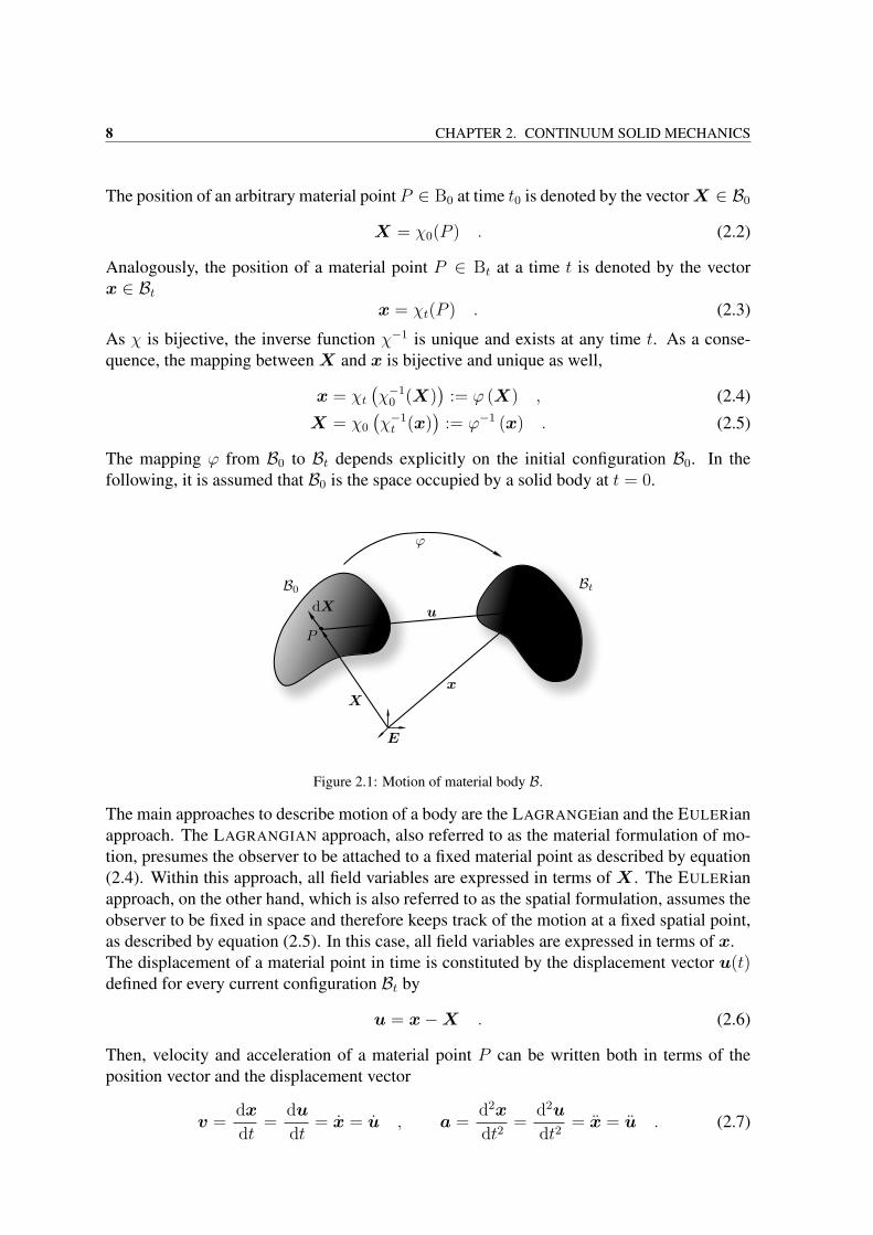
Kinematics describes the motion and deformation of a body in time as depicted in figure 2.1.This section introduces the concept of bodies, their motion and deformation as well as thecorresponding deformation and strain tensors.
2.1.1 Deformation
A material body B is constituted of a set of material points P . Each material point can beidentified uniquely at each point in time t. Furthermore, coherence of all material pointsduring the deformation of the body is assumed. To describe the motion and deformation ofa material body B, each material point P is mapped onto a corresponding point defined ina region B of the EUCLIDian vector space E3. Thus, the material body B is mapped onto aconfiguration of points P by
χ : B 7−→ B . (2.1)
7
8 CHAPTER 2. CONTINUUM SOLID MECHANICS
The position of an arbitrary material point P ∈ B0 at time t0 is denoted by the vectorX ∈ B0
X = χ0(P ) . (2.2)
Analogously, the position of a material point P ∈ Bt at a time t is denoted by the vectorx ∈ Bt
x = χt(P ) . (2.3)
As χ is bijective, the inverse function χ−1 is unique and exists at any time t. As a conse-quence, the mapping betweenX and x is bijective and unique as well,
x = χt(χ−1
0 (X))
:= ϕ (X) , (2.4)
X = χ0
(χ−1t (x)
):= ϕ−1 (x) . (2.5)
The mapping ϕ from B0 to Bt depends explicitly on the initial configuration B0. In thefollowing, it is assumed that B0 is the space occupied by a solid body at t = 0.
•
•
Figure 2.1: Motion of material body B.
The main approaches to describe motion of a body are the LAGRANGEian and the EULERianapproach. The LAGRANGIAN approach, also referred to as the material formulation of mo-tion, presumes the observer to be attached to a fixed material point as described by equation(2.4). Within this approach, all field variables are expressed in terms of X . The EULERianapproach, on the other hand, which is also referred to as the spatial formulation, assumes theobserver to be fixed in space and therefore keeps track of the motion at a fixed spatial point,as described by equation (2.5). In this case, all field variables are expressed in terms of x.The displacement of a material point in time is constituted by the displacement vector u(t)defined for every current configuration Bt by
u = x−X . (2.6)
Then, velocity and acceleration of a material point P can be written both in terms of theposition vector and the displacement vector
v =dx
dt=
du
dt= x = u , a =
d2x
dt2=
d2u
dt2= x = u . (2.7)
2.1. KINEMATICS 9
In addition to describing the displacement of a material point P in EUCLIDian vector space,the formulation of its position and movement also facilitates the specification of the defor-mation imposed on an infinitesimal line element attached to P . The mapping of such aninfinitesimal line element in B0, denoted by dX , onto the corresponding infinitesimal lineelement in the current configuration Bt, denoted by dx, is performed by the material defor-mation gradient F
dx = F · dX , F =∂x
∂X= 1 +
∂u
∂X= 1 +H , (2.8)
where both dX and dx are shown in figure 2.1. Here, 1 denotes the second order unittensor, while H is called the displacement gradient. The material deformation gradient is atwo-point tensor
F = Fijei ⊗Ej , (2.9)
which is in general non-symmetric. Its components are Fij , given in the Cartesian basis ofthe current and initial configuration, ei and Ej , respectively. Due to these properties, F canbe used to transform a tensor from the initial to the current configuration (push forward)as well as vice versa (pull back). The non-singularity of F is mathematically equivalent tothe existence of the inverse mapping of a deformed infinitesimal line element dx onto thecorresponding infinitesimal line element dX in the initial configuration. The determinant ofF
J = det(F ) > 0 (2.10)
is called the JACOBIan J . The property stated in equation (2.10) is valid for all motions ofB. Its physical interpretation is that material is not allowed to penetrate itself.Every deformation of a body can be decomposed into rigid body translation, rigid bodyrotation and deformation. Rigid body translation is not contained in F , in contrast to rigidbody rotation and deformation. Accordingly, there exists a multiplicative split of the materialdeformation gradient in terms of
F = R ·U = V ·R . (2.11)
Here,R is a proper orthogonal rotation tensor, while the positive definite, symmetric tensorsU and V are the right and left stretch tensor, respectively. The spectral decomposition of Uand V
U =3∑i=1
λiN i ⊗N i , V =3∑i=1
λini ⊗ ni (2.12)
is useful for the description of some material models, where the principal stretches λi arethe eigenvalues of U or V , N i are the eigenvectors of U and ni are the eigenvectors of V .Then, the material deformation gradient can be written in terms of
F =3∑i=1
λini ⊗N i (2.13)
and the rotation tensor in terms of
R =3∑i=1
ni ⊗N i . (2.14)
10 CHAPTER 2. CONTINUUM SOLID MECHANICS
Apart from transforming infinitesimal line elements between the initial and the current con-figuration, F also maps infinitesimal surface elements with the aid of NANSON’s formula
n da = JF−T ·N dA . (2.15)
Please note, that here, N and n are not eigenvectors but outward unit normal vectors ofthe surface element in the initial and the current configuration, and dA and da are the cor-responding infinitesimal surface areas, respectively. Finally, the mapping of infinitesimalvolume elements is accomplished by applying the JACOBIan
dv = J dV . (2.16)
2.1.2 StrainsAs mentioned in section 2.1.1, the material deformation gradient F uniquely describes thedeformation of an infinitesimal volume element, including rigid body rotations. However,especially when knowledge about strains and stresses is necessary, it is usually not a conve-nient deformation measure for several reasons. First of all, strains and stresses should not beinfluenced by rigid body rotations. This means that, for the same deformation in another di-rection, F might have a different sign. In addition, F is non-symmetric and thus not alwayspractical.In order to circumvent these drawbacks of the material deformation gradient, the GREEN-LAGRANGE strain tensor E is introduced by interpreting strains as infinitesimal lengthchanges
|| dx||22 − || dX||22 = dx · dx− dX · dX
= dX · F T · F · dX − dX · 1 · dX
= dX ·(F T · F − 1
)· dX
= dX · 2E · dX . (2.17)
The basis of the GREEN-LAGRANGE strain tensor E is given in the initial configuration.Analogously, the EULER-ALMANSI strain tensor e is defined in the current configuration by
|| dx||22 − || dX||22 = dx · dx− dX · dX
= dx · 1 · dx− dx · F−T · F−1 · dx
= dx ·(1− F−T · F−1
)· dx
= dx · 2 e · dx . (2.18)
Other convenient measures are the right CAUCHY-GREEN tensor C defined in the initialconfiguration
C = F T · F = U 2 , (2.19)
as well as the left CAUCHY-GREEN tensor e defined in the current configuration
b = F · F T = V 2 . (2.20)
2.1. KINEMATICS 11
As can be seen from equations (2.17) and (2.18), the right and left CAUCHY-GREEN tensorscan be used to express the GREEN-LAGRANGE and EULER-ALMANSI strain tensors
E =1
2(C − 1) , e =
1
2(1− b−1) . (2.21)
Writing the GREEN-LAGRANGE tensor E in terms of the displacement gradient H , it caneasily be seen that E can be additively decomposed into a linear and a non-linear part
E =1
2
(H +HT +HT ·H
). (2.22)
If small deformations are considered, linearized strain measures can be used. The linearizedstrain tensor ε is obtained by the linearization of E or e
ε = [LIN [E]]u=0 = [LIN [e]]u=0 =1
2
(∂u
∂X+
(∂u
∂X
)T)=
1
2
(H +HT
), (2.23)
which is also reflected in equation (2.22).
Strain rates
In theory of elasticity, hyper elasticity is generally assumed, see section 2.3.3 for details.This means that the actual stress-strain path that is taken to achieve a certain deformation isconsidered irrelevant for the stress-strain relation. If, however, phenomena like viscosity orplasticity are taken into account, the history of the deformation has to be followed, see e.g.MALVERN (1969).Important tensors are the rate-of-deformation tensor d and the spin tensor w. In order todefine them, the material velocity gradient
F =∂x
∂X(2.24)
is introduced in terms of the material time derivative of the deformation gradient F .The spatial velocity gradient l is given by
l =∂x
∂x= F · F−1 . (2.25)
It can be expressed in terms of the above mentioned rate-of-deformation or spatial strainvelocity d
d =1
2
(F · F−1 + F−T · F T
)(2.26)
and the spin tensor
w =1
2
(F · F−1 − F−T · F T
), (2.27)
such thatl = d+w . (2.28)
12 CHAPTER 2. CONTINUUM SOLID MECHANICS
Here, it is easy to see that d andw constitute the symmetric and the skew symmetric part ofthe spatial velocity gradient.The pull back of d finally yields the material time derivative of the GREEN-LAGRANGE
strain tensor EE = F T · d · F =
1
2C . (2.29)
2.2 Conservation lawsAll solid as well as fluid mechanics, independently of the material model used, are based onconservation laws, see e.g. KUNDU & COHEN (2004). They form a set of axiomatic equa-tions and inequalities based on physical observations. For solid mechanics, the conservationof mass, conservation of linear and angular momentum, conservation of energy and entropyinequality are mostly focused on.These laws can be written in integral form for an extended region or in differential (local)form at a point.
2.2.1 Conservation of massThe mass of a body B is independent of motion and deformation
d
dtm(B) = 0 . (2.30)
The definition of mass density of a material point P at time t is given by
ρ(x, t) =dm
dv, (2.31)
where v denotes the volume in the current configuration. Together with equation (2.16), themass of a body B at time t can then be written as a function of the mass density in the initialas well as in the current configuration
m(B, t) =
∫Bt
ρ dv =
∫B0
Jρ dV =
∫B0
ρ0 dV , (2.32)
also defining the relation between the initial mass density field ρ0 and the current mass den-sity field ρ
ρ0 = Jρ . (2.33)
Using this relation, equation (2.30) can be written in terms of the current mass density,yielding the integral form of mass conservation
d
dtm =
∫B0
d
dt(Jρ) dV =
∫B0
(ρ+ ρ div x) J dV =
∫Bt
(ρ+ ρ div x) dv = 0 . (2.34)
As stated in section 2.2, equation (2.34) has to hold for an arbitrary volume, thus leading tothe local form of mass conservation
ρ+ ρ div x = 0 . (2.35)
2.2. CONSERVATION LAWS 13
2.2.2 Conservation of linear and angular momentum
A body’s linear momentum I is defined by
I =
∫Bt
ρx dv . (2.36)
Providing that NEWTON’s third law (”actio = reactio”) holds for internal forces, the changeof linear momentum equals the sum of all applied external forces. It is given by
d
dtI =
∫Bt
ρ b dv +
∫∂Bt
t da . (2.37)
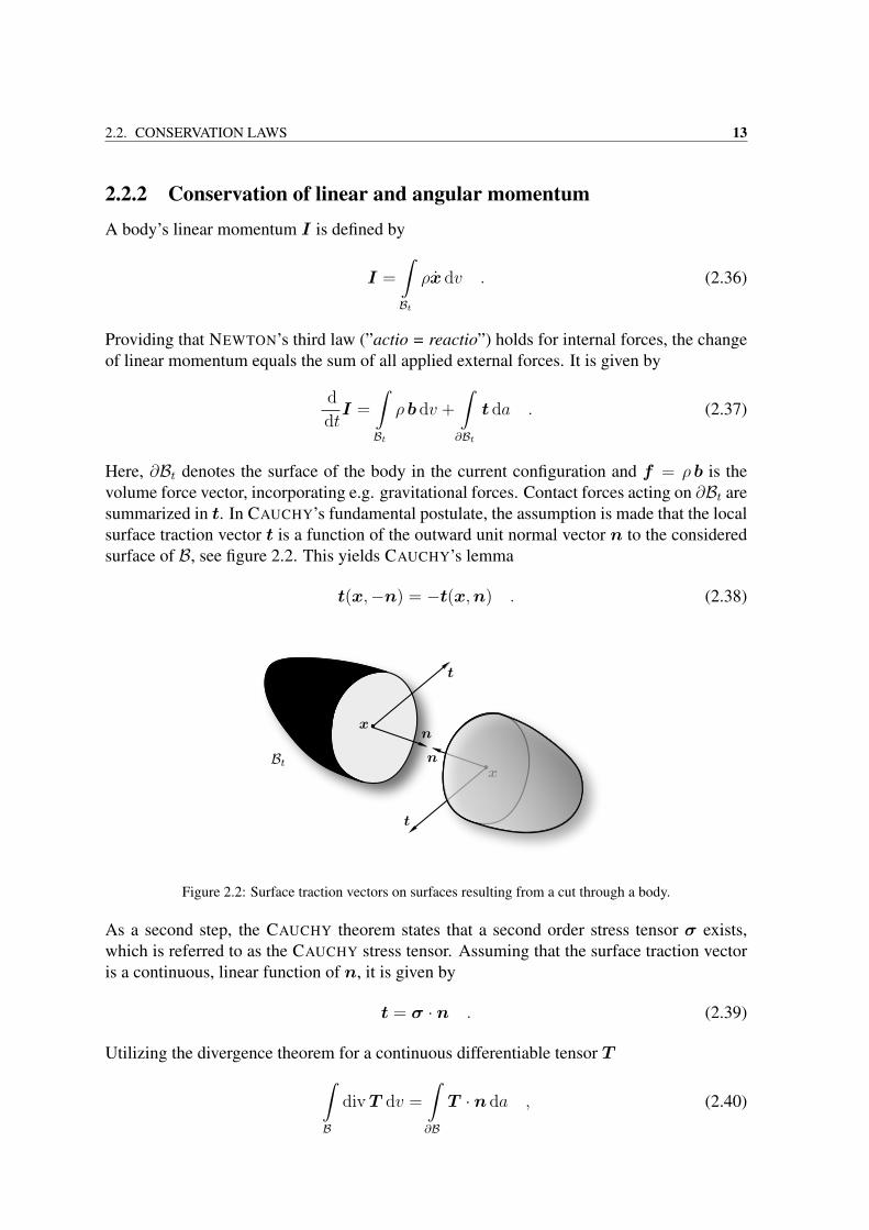
Here, ∂Bt denotes the surface of the body in the current configuration and f = ρ b is thevolume force vector, incorporating e.g. gravitational forces. Contact forces acting on ∂Bt aresummarized in t. In CAUCHY’s fundamental postulate, the assumption is made that the localsurface traction vector t is a function of the outward unit normal vector n to the consideredsurface of B, see figure 2.2. This yields CAUCHY’s lemma
t(x,−n) = −t(x,n) . (2.38)
•
•
Figure 2.2: Surface traction vectors on surfaces resulting from a cut through a body.
As a second step, the CAUCHY theorem states that a second order stress tensor σ exists,which is referred to as the CAUCHY stress tensor. Assuming that the surface traction vectoris a continuous, linear function of n, it is given by
t = σ · n . (2.39)
Utilizing the divergence theorem for a continuous differentiable tensor T∫B
divT dv =
∫∂B
T · n da , (2.40)
14 CHAPTER 2. CONTINUUM SOLID MECHANICS
the CAUCHY theorem and the conservation of mass as given in equation (2.34) in combi-nation with the change of linear momentum as expressed in equation (2.37), the change oflinear momentum in integral form can be written as∫
Bt
(divσ + f − ρ x) dv = 0 . (2.41)
The local form of the conservation of linear momentum, which is also known as CAUCHY’sfirst law of motion, follows as
divσ + f − ρ x = 0 . (2.42)
Neglecting the acceleration term in case of statics, the local static equilibrium equation re-sults in terms of
divσ + f = 0 . (2.43)
The angular momentum of a body B is defined by
L =
∫Bt
ρ (x− x0)× x dv , (2.44)
its change in time is equal to the sum of all external forces acting on B
d
dtL =
∫Bt
ρ ((x− x0)× b) dv +
∫∂Bt
((x− x0)× t) da . (2.45)
Applying the CAUCHY theorem (2.39), the divergence theorem (2.40) and the balance oflinear momentum (2.42) to equation (2.45), the symmetry of the CAUCHY stress tensor canbe proved
σ = σT . (2.46)
As already indicated by equation (2.38), the CAUCHY stress tensor is defined in the currentconfiguration.If a traction force t in the current configuration is related to the outward unit normalN in theinitial configuration with aid of CAUCHY’s theorem (2.39) and NANSON’s formula (2.15)
t da = σ · n da = Jσ · F−T ·N dA = P ·N dA , (2.47)
the 1st PIOLA-KIRCHHOFF stress tensor P can be defined. It is a two-point tensor with onebasis in the initial and one basis in the current configuration and thus maps a vector from theinitial onto the current configuration. As can be seen from equation (2.47), the 1st PIOLA-KIRCHHOFF stress tensor is generally non-symmetric
P 6= P T . (2.48)
Now, writing equation (2.37) in terms of the initial volume and surface of the body andapplying the divergence theorem (2.40), the equilibrium equation is obtained in terms of the
2.2. CONSERVATION LAWS 15
1st PIOLA-KIRCHHOFF stress tensor and the volume force vector f 0 = ρ0 b in the currentconfiguration related to the volume in the initial configuration
DivP + f 0 = 0 . (2.49)
As the characteristics of P , namely its non-symmetry, make it an inconvenient choice formany applications, the 2nd PIOLA-KIRCHHOFF stress tensor S is introduced in terms of
S = F−1 · P = JF−1 · σ · F−T . (2.50)
The 2nd PIOLA-KIRCHHOFF stress tensor is completely defined in the initial configurationand symmetric, as can be seen from equation (2.50)
S = ST . (2.51)
In contrast to the CAUCHY stress tensor and the 1st PIOLA-KIRCHHOFF stress tensor, the2nd PIOLA-KIRCHHOFF stress tensor has no direct physical meaning. It is solely defined forconvenience, especially regarding the derivation of constitutive equations, see section 2.3.3.
2.2.3 Conservation of energyThe first law of thermodynamics constitutes that the energy in a closed system remains con-stant. The energy E of a body can be additively decomposed into the internal energy U andthe kinetic energy K
E = U +K . (2.52)
Here, the internal energy is the sum of the strain energy due to elastic strains and the thermalenergy. They are expressed in terms of the specific internal energy u. The internal energy Uis then given by
U =
∫Bt
ρu dv . (2.53)
As the internal energy is an unknown quantity, it has to be related to other state variableswith aid of constitutive equations (MALVERN (1969)). Specific constitutive equations arepresented in section 2.3.4.The kinetic energy of a body can be expressed by
K =1
2
∫Bt
ρ x · x dv (2.54)
and is due to the body’s observable motion in time.The change of energy in time for a body B is given in terms of the external power input Pand the thermal power supply Q
E = P +Q . (2.55)
Specifically, the external power input P is the rate at which the body forces ρ b and surfacetractions t are doing work on the body
P =
∫Bt
ρ b · x dv +
∫∂Bt
t · x da , (2.56)
16 CHAPTER 2. CONTINUUM SOLID MECHANICS
while the thermal power supply is caused by a distributed internal heat source of strength ras well as heat flux in terms of the heat flux vector q through the surface of the body
Q =
∫Bt
ρr dv −∫∂Bt
q · n da . (2.57)
Then, inserting the definitions of the internal (2.53) and kinetic energy (2.54) as well as theexternal power input (2.56) and the thermal power supply (2.57) into equation (2.55), theconservation of energy of a body Bt in integral form is given by
d
dt
∫Bt
ρ
(u+
1
2x · x
)dv =
∫Bt
ρ (r + b · x) dv +
∫∂Bt
(t · x− q · n) da . (2.58)
Applying the definition of the symmetric part of the velocity gradient (2.26), the CAUCHY
theorem (2.39), the local balance of linear momentum (2.42) and the symmetry of theCAUCHY stress tensor (2.46), the integral form of the conservation of energy of a bodyin the current configuration can be expressed in terms of∫
Bt
ρu dv =
∫Bt
(σ : d+ ρr − div q) dv . (2.59)
The local form of the conservation of energy in the current configuration is given by
ρu = σ : d+ ρr − div q . (2.60)
2.2.4 Entropy inequalityApart from the observation that no energy can be created or lost in a closed system, thedirection of a thermomechanical process is naturally given. For example, it has never beenobserved in nature that a cold body transfers heat to a warmer body without applying work– a process that the first law of thermodynamics allows for. Obviously, a restriction on thefirst law of thermodynamics is necessary. This restriction is given by the second law ofthermodynamics. To facilitate its formulation, the entropy S in terms of a mass specificentropy density s is introduced
S =
∫Bt
ρs dv . (2.61)
Entropy is a measure for the direction of a physical process. It is often explained with theaid of statistical mechanics, where it is found that changes of state are more likely to occurin the direction of greater disorder. For an illustrative example, see MALVERN (1969).The change of entropy of a body in time equals the entropy input due to internal heat sourcesas denoted by the first term, the entropy due to heat flux through the surface of the bodyas stated by the second term as well as entropy production inside the body by means ofdissipative mechanical processes as given by the third term of the entropy balance
d
dtS =
∫Bt
ρr
θdv −
∫∂Bt
1
θq · n da+
∫Bt
ρσ dv . (2.62)
2.3. CONSTITUTIVE EQUATIONS 17
Here, θ is the absolute temperature and σ denotes the specific entropy production due todissipative mechanical processes. It can be observed that the entropy production cannot benegative, such that
σ ≥ 0 . (2.63)
If no entropy is generated (σ = 0), a process is called reversible. Otherwise, a process iscalled irreversible. This observation yields the CLAUSIUS-DUHEM inequality in the integralform
d
dt
∫Bt
ρs dv ≥∫Bt
ρr
θdv −
∫∂Bt
1
θq · n da . (2.64)
Applying the divergence theorem (2.40), the conservation of energy (2.59) and the definitionof the HELMHOLTZ free energy
ψ = u− s θ , (2.65)
the local form of the CLAUSIUS-DUHEM inequality in the current configuration can be writ-ten as
−ρ(ψ + s θ
)+ σ : d− 1
θq · grad θ ≥ 0 . (2.66)
The HELMHOLTZ free energy is the part of the internal energy which is available for doingwork at a constant temperature. It is an energy per unit mass, as can be seen e.g. fromequation (2.53). The CLAUSIUS-DUHEM inequality in the initial configuration is given by
−ρ0
(ψ + s θ
)+ S : E − 1
θQ ·Grad θ ≥ 0 , (2.67)
whereQ is the heat flux vector in the initial configuration.As mentioned above, the CLAUSIUS-DUHEM inequality is fulfilled with equality in case ofreversible processes. A process is called isothermal if the temperature remains constant inspace and time. Then, the HELMHOLTZ free energy is equal to the elastic strain energydensity of a body. Thus, the second law of thermodynamics acts as a restriction to the choiceof strain energy density functions and therefore plays an important role for the developmentof constitutive equations.
2.3 Constitutive equationsConstitutive equations describe the idealized behavior of a material due to its intrinsic inter-nal constitution. Different constitutive models are used for different types of material. Afterfirst over-simplifying and thus over-idealizing a material, the trend from the 1950s on hasbeen to develop very general constitutive relations which are specialized as late and littleas possible, not to overlook e.g. coupling effects (MALVERN (1969)). Together with theconservation laws introduced in section 2.2, they form a set of equations connecting con-stitutively independent variables such as deformation and temperature to variables whichdepend on the specific material, such as stress and heat flux. Mathematically, they providethe equations needed in addition to the balance laws to determine all unknowns in a physicalproblem. Fundamental principles for the systematic development of constitutive models goback to NOLL (1955), FLORY (1961), TRUESDELL & NOLL (1965), HILL (1970), OGDEN
(1984) and CHADWICK (1999).
18 CHAPTER 2. CONTINUUM SOLID MECHANICS
2.3.1 Mechanical principlesApart from satisfying the balance laws, a number of principles have to be observed whendeveloping constitutive relations to avoid physically unreasonable material models. Here,only the principles of material causality, determinism, material objectivity and material sym-metry are addressed. For more details or other mechanical principles see NOLL (1955) andCIARLET (1994).
Principle of material causality
The principle of material causality states that the motion x = χ(P, t) and the temperatureθ = Θ(P, t) are the only constitutively independent, measurable variables. All other vari-ables which cannot be directly determined from x and θ are constitutively dependent vari-ables. As only isothermal processes are considered in the following, the only independentvariable remaining is the motion x.
Principle of determinism
The principle of determinism states that the values of the thermodynamic functions (σ, q, uand s) at a material point P at time t are determined by the history of motion and temperatureof all material points. This allows e.g. for material aging. At the same time, it is ascertainedthat material behavior is not coincidental.
Principle of material objectivity
The principle of material objectivity states that qualitative and quantitative descriptions ofphysical phenomena have to remain unchanged even if any changes of the point of view fromwhich they are observed are made (HOLZAPFEL (2000)). Thus, all constitutive equations, asthe mathematical representation of these physical phenomena, have to be observer invariant.To this end, suppose that an observer O records a motion x and the resulting CAUCHY stressσ at point P and time t specified by
x = ϕ(X, t) , σ(x, t) = Z(X, t) . (2.68)
A second observer O records the corresponding motion x and CAUCHY stress σ
x = ϕ(X, t) , σ(x, t) = Z(X, t) . (2.69)
The observer transformation is given in terms of the proper rotation tensor Q and arbitrarytranslation vector c. Then, in order to be objective, a scalar ψ, a vector a and a tensor Thave to transform according to
ψ = ψ (2.70)a = Q · a (2.71)
T = Q · T ·QT . (2.72)
2.3. CONSTITUTIVE EQUATIONS 19
Although the material deformation gradient F and the 1st PIOLA-KIRCHHOFF stress tensorP transform like a vector by
F = Q · F (2.73)
P = Q · P , (2.74)
they are objective because as two-point tensors, one of their basis is given in terms of theinitial configuration, which is intrinsically observer independent. Accordingly, with bothbasis given in terms of the initial configuration, the 2nd PIOLA-KIRCHHOFF stress tensor Ssimply transforms by
S = S , (2.75)
while the CAUCHY stress tensor, being completely given in terms of x, has to transform by
σ = Q · σ ·QT . (2.76)
Principle of material symmetry
The principle of material symmetry states that a constitutive equation has to be independentof certain rotations applied to the material coordinates of a body before it is subjected to adeformation. In other words, the stresses resulting from the deformation have to remain thesame, independently of the rotation expressed in terms of the proper rotation tensorQ∗,
σ(F ·Q∗) = σ(F ) . (2.77)
However, the rotation tensor Q∗ can in general not be chosen arbitrarily. It depends on thespecific type of material and can only be chosen from the symmetry group inherent to thismaterial. If a material is symmetric with respect to Q∗, the material coordinates can berotated by Q∗ before applying the deformation without changing the resulting stresses. Forthe case of isotropy, as assumed in the following,Q∗ can be any proper orthogonal tensor.
2.3.2 Isotropic elasticity
A material is called CAUCHY-elastic if, for each material point P of a body B, the stressfield at time t depends only on the deformation and temperature but not on the deformationand temperature history. Then, the second law of thermodynamics is fulfilled in equilibriumassuming a reversible, non-dissipative deformation process. In this case, the CAUCHY stresstensor σ for an isothermal process can be expressed in terms of the material deformationgradient F
σ = σ(F (X, t)) , (2.78)
where the principle of material objectivity poses the requirement that σ is in fact a functionof the stretches U alone.Although the stress of a CAUCHY-elastic material is independent of the deformation path,the work performed by the stress in general is not.
20 CHAPTER 2. CONTINUUM SOLID MECHANICS
2.3.3 Isotropic hyper elasticityIn contrast to CAUCHY-elastic materials, hyper elastic or GREEN-elastic materials satisfy theadditional requirement that the work done by the stress is independent of the deformationpath. This requirement is equivalent to the existence of a specific strain energy densityfunction Ψ in the form of a potential. It is given as an energy per unit volume in terms of thedensity ρ of the material and the HELMHOLTZ free energy ψ
Ψ = ρψ . (2.79)
For a reversible, non-dissipative, isothermal process, inserting equation (2.79) into theCLAUSIUS-DUHEM inequality (2.67) immediately leads to
S : E − Ψ = 0 . (2.80)
Since equation (2.78) yields that the strain energy density function Ψ depends only on E
Ψ =∂Ψ
∂E: E , (2.81)
equation (2.80) can be rewritten as(S − ∂Ψ
∂E
): E = 0 . (2.82)
Then, the relation between strain and stress for a hyper elastic material is finally given interms of
S =∂Ψ
∂E= 2
∂Ψ
∂C. (2.83)
The corresponding fourth-order elasticity tensor in the initial configuration is given by
C =∂2Ψ
∂E∂E= 4
∂2Ψ
∂C∂C. (2.84)
The strain energy density function Ψ has to take into account several restrictions. First, inthe undeformed state, which is equivalent to F = 1, the strain energy as well as the stresseshave to vanish. If a material behaves isotropic, Ψ can be expressed in terms of the threeindependent principal invariants IC , IIC and IIIC or, alternatively, in terms of the principalstretches λ1, λ2 and λ3
Ψ = Ψ (IC , IIC , IIIC) (2.85)Ψ = Ψ (λ1, λ2, λ3) . (2.86)
The invariants and the principal stretches are functions of the right CAUCHY-GREEN tensorC. They do not depend on the coordinate system in which the components of C wereinitially given and are thus invariant w.r.t. to solid body rotations (MALVERN (1969)). Theprincipal stretches are defined by a spectral decomposition of C
C =3∑i=1
λ2iN i ⊗N i (2.87)
2.3. CONSTITUTIVE EQUATIONS 21
and the invariants of C as well as their connection to the principal stretches are given by
IC = trC = λ21 + λ2
2 + λ23 (2.88)
IIC =1
2
(tr 2C − trC2
)= λ2
1λ22 + λ2
2λ23 + λ2
3λ21 (2.89)
IIIC = detC = λ21λ
22λ
23 . (2.90)
Then, using the isotropic tensor function properties and applying CAYLEY-HAMILTON’stheorem, equation (2.83) for a general isotropic hyper elastic material can be expressed by
S = 2
((∂Ψ
∂IC+ IC
∂Ψ
∂IIC
)1− ∂Ψ
∂IICC +
∂Ψ
∂IIICIIIC C
−1
). (2.91)
Details regarding the derivation can be found e.g. in HOLZAPFEL (2000). Using equation(2.50), the CAUCHY stress tensor for a general isotropic hyper elastic material is given by
σ =2
J
(∂Ψ
∂IIICIIIC 1 +
(∂Ψ
∂IC+ IC
∂Ψ
∂IIC
)b− ∂Ψ
∂IICb2
). (2.92)
Finally, a strain energy density function needs to be poly convex. Regarding it as a functionof F , adjF and detF , Ψ is poly convex if it is convex in its arguments. The poly convexityrequirement provides for the existence of a deformation which globally minimizes the strainenergy under a given external load. Also, it ensures ellipticity of the partial differentialequation, which guarantees that the wave speed within the material remains real. The latterproperty is also known as the LEGENDRE-HADAMARD condition, which is fulfilled if theacoustic tensorA with
A = N · ∂2Ψ
∂F ∂F·N , Aik =
∂2Ψ
∂Fij∂FklNjNl (2.93)
is positive definite for all deformations,
n ·A · n > 0 . (2.94)
Here, N is an arbitrary vector in the initial configuration and n is an arbitrary vector in thecurrent configuration, whereN and n are both non-zero vectors. It has to be noted that polyconvexity of the strain energy density function is not a sufficient criterion for stability. Forfurther details on stability, see REESE (1994).
2.3.4 Examples of hyper elastic isotropic materialsAs mentioned in section 2.3, a wide range of constitutive equations has been developed tomodel a multitude of materials. In the following, the non-linear Neo-HOOKE and the linearHOOKE material model are introduced, as these are the only constitutive equations used inthe remainder of this work. For both material models, the strain energy density function aswell as the corresponding stresses and elasticity tensors are presented. An extensive overviewof constitutive equations as well as their respective application ranges is given in OGDEN
(1984).
22 CHAPTER 2. CONTINUUM SOLID MECHANICS
Neo-Hooke material
The strain energy density function for the Neo-HOOKE material was introduced byTRELOAR (1943a) for the general and by TRELOAR (1943b) for the incompressible case.Here, it is given applying the volumetric-deviatoric split as first introduced by FLORY (1961).Within the concept of the volumetric-deviatoric split, the strain energy density function isadditively divided into a part resulting from volumetric and a part resulting from isochoricdeformation. Thus, the different material behavior for volumetric and deviatoric deforma-tions can be reflected. Also, the numerical treatment of incompressible or inelastic materialsis simplified by the decoupled strain energy density function, see SIMO & HUGHES (1998).The strain energy density function for a Neo-HOOKE material is then given by
Ψ(F ) =µ
2
(J−2/3 trC − 3
)+ g(J) , (2.95)
where µ is the shear modulus and g(J) is the volumetric function. As it is a function of Jonly, its influence is restricted to compressible materials. For incompressible materials withJ = 1,
g(J) ≡ 0 . (2.96)
For compressible materials, g(J) has to be a convex function and the conditions
limJ→0
g(J)→∞ , limJ→+∞
g(J)→∞ (2.97)
have to be fulfilled, to be theoretically able to create an unlimited amount of energy for thesecases. Additionally, no energy should be created in case of no deformation, resulting in
g(J = 1) ≡ 0 ,∂g(J)
∂J
∣∣∣∣J=1
≡ 0 . (2.98)
In the mathematical context, equation (2.97) is important for proving the existence anduniqueness of solutions, see e.g. MARSDEN & HUGHES (1994). Some widely used vol-umetric functions are
g(J) =
K
2(J − 1)2
K
4
((J − 1)2 + ln2 J
)K
β2
(J−β − 1 + β ln J
)K (J − 1− ln J)
, (2.99)
where K is the bulk modulus and β is a material parameter accounting for different types ofvolumetric response. Obviously, the function given in equation (2.99a) does not fulfill therequirement that the strain energy density goes to infinity for the volume approaching zero.For an overview, see WRIGGERS (2008) and literature cited therein.
2.3. CONSTITUTIVE EQUATIONS 23
The 2nd PIOLA-KIRCHHOFF stress tensor for the Neo-HOOKE material is then given by
S = µJ−2/3
(1− 1
3trCC−1
)+ J
∂g(J)
∂JC−1 , (2.100)
where
∂g(J)
∂J=
K (J − 1)
K
2
(J − 1 + J−1 ln J
)K
β
(J−1 − J−(β+1)
)K (1− J−1)
. (2.101)
The material tangent in the initial configuration is
C =2
3µJ−2/3
(−1⊗C−1 −C−1 ⊗ 1 +
1
3trCC−1 ⊗C−1 − trC J
)+J
(∂g(J)
∂J+ J
∂2g(J)
∂J2
)C−1 ⊗C−1 + 2J
∂g(J)
∂JJ (2.102)
withJijst = −C−1
ik IklstC−1lj . (2.103)
Here, I is the fourth order unit tensor, which is given in index notation by
Iklst =1
2(δksδlt + δktδls) (2.104)
with the KRONECKER-delta identity
δij =
1 if i = j0 if i 6= j
. (2.105)
The second derivatives of the volumetric functions introduced in equation (2.99) are
∂2g(J)
∂J2=
K
K
2
(1− J−2 ln J + J−2
)K
β
((β + 1) J−(β+2) − J−2
)KJ−2
. (2.106)
Linear Hooke material
For the linear HOOKE material, small deformations and rotations and thus coincidence ofthe initial and current configuration are assumed. Therefore, the corresponding strain energy
24 CHAPTER 2. CONTINUUM SOLID MECHANICS
density function is given in terms of the linear strain tensor ε introduced in equation (2.23)by
Ψ =1
2
(K − 2
3µ
)tr 2ε+ µ tr ε2 . (2.107)
In linear theory, all stress tensors coincide, leading to
σ = 2µ ε+
(K − 2
3µ
)tr ε1 . (2.108)
The elasticity tensor for the linear HOOKE material is given by
Cijkl = 2µ Iijkl +
(K − 2
3µ
)δijδkl , (2.109)
where the fourth order unit tensor Iijkl has been introduced in equation (2.104). In contrast tothe elasticity tensor for the Neo-HOOKE material, the linear elasticity tensor is independentof the deformation.
2.4 Variational formsIn the preceding sections, the equations for describing the boundary value problem for themotion of a body were introduced. The boundary value problem, which is generally referredto as the strong form, is constituted by a coupled system of partial differential equationscomprising the kinematic equation (2.8) and (2.21a), the local form of equilibrium for linearmomentum (2.43) and (2.49) and the stress-strain relation (2.83) as well as boundary condi-tions. The strong form can be written in terms of the initial as well as the current configura-tion. Apart from the conservation of linear momentum, conservation of mass is fulfilled byusing ρ0 = Jρ. Conservation of angular momentum is fulfilled implicitly by considering theCAUCHY stress tensor σ to be symmetric. Entropy inequality is fulfilled implicitly as wellby choice or construction of an appropriate constitutive equation, as elaborated in section2.3.Analytical solutions to the strong form only exist for very simple cases, which are not suffi-cient to describe real life continuum solid mechanics problems with arbitrary boundary con-ditions. However, an approximation of the solution can be obtained using numerical methodswhich are often based on variational methods. To this end, the local form of equilibrium forisothermal processes is transformed to a variational form in the following.
2.4.1 Weak form of equilibriumThe principle of virtual displacements uses the local form of conservation of linear momen-tum in the mixed (2.49) or current (2.43) configuration to achieve a formulation, which ismathematically equivalent, but serves as a point of departure to obtain the so-called weakform of equilibrium. For this purpose, the local form of the balance equation (2.49) or (2.43)is multiplied by an arbitrary but non-zero vector valued virtual displacement function δu.This function is also called the test function or weight function and often referred to as η
2.4. VARIATIONAL FORMS 25
instead of δu. The test function has to be zero at DIRICHLET boundaries. The resultingexpression is integrated over the entire domain, thus leading to a term which fulfills the localbalance of linear momentum in a volume average sense. Using the conservation of linearmomentum in the mixed configuration (2.49), multiplication with the virtual displacementvector and subsequent integration over the entire domain yields∫
B0
DivP · δu dV +
∫B0
f 0 · δu dV = 0 , (2.110)
while using the conservation of linear momentum in the current configuration (2.43) leads to∫Bt
divσ · δu dv +
∫Bt
f · δu dv = 0 , (2.111)
where the respective boundary conditions are given by
u0 = u0 on ∂B0u , t0 = P ·N = t0 on ∂B0σ (2.112)
andu = u on ∂Btu , t = σ · n = t on ∂Btσ . (2.113)
Here, ∂B0u and ∂Btu are the DIRICHLET boundaries in the initial and current configuration,respectively, where the displacements are prescribed. On the NEUMANN boundary in theinitial configuration ∂B0σ and the current configuration ∂Btσ the tractions are prescribed.Also, as mentioned above, the respective test function has to fulfill
δu = 0 on ∂B0u , δu = 0 on ∂Btu . (2.114)
Using partial integration, the divergence theorem (2.40) as well as the boundary conditions(2.112), equation (2.110) can be written as
G (u, δu) =
∫B0
P : Grad δu dV −∫B0
f 0 · δu dV −∫∂B0
t0 · δu dA = 0 , (2.115)
which is referred to as the weak form of equilibrium in the mixed configuration. Equation(2.115) is called the weak form of equilibrium because in contrast to equation (2.110), wherethe divergence operator introduces a second derivative of the displacements, only the firstderivative of the displacement remains. Thus, the continuity demands on the displacementfield are weaker than for the strong form of equilibrium.The weak form of equilibrium in the mixed configuration can be transferred into the initialconfiguration by replacing the 1st PIOLA-KIRCHHOFF stress tensor P by the 2nd PIOLA-KIRCHHOFF stress tensor S = F−1 · P and by identifying Grad δu as the variation of thedeformation gradient F . This results in the weak form of equilibrium in the initial configu-ration
G (u, δu) =
∫B0
S : δE dV −∫B0
f 0 · δu dV −∫∂B0
t0 · δu dA = 0 , (2.116)
26 CHAPTER 2. CONTINUUM SOLID MECHANICS
withδE =
1
2
(F T ·Grad δu+ Grad T δu · F
). (2.117)
The weak form of equilibrium in the current configuration is generally obtained from theweak form of equilibrium in the initial configuration (2.116) by using the volume transfor-mation (2.16), the relation between the mass density fields (2.33) and a push forward of the2nd PIOLA-KIRCHHOFF stress tensor S, yielding
g (u, δu) =
∫Bt
σ : grad δu dv −∫Bt
f · δu dv −∫∂Bt
t · δu da = 0 . (2.118)
Chapter 3
Analytical fracture mechanics
Fracture mechanics is concerned with the influence of cracks in a solid body on the body’smechanical behavior, including crack initialization and propagation. Generally, fracture canbe seen as the partitioning of an originally intact body into two or more parts (GROSS &SEELIG (2007)). Its mechanisms are manifold and strongly depend on the considered ma-terial, consequently, a large number of mathematical models exists for fracture mechanicsphenomena. In the following, common reasons and natures of fracture are presented beforeintroducing analytical approaches for linear as well as nonlinear fracture mechanics. Foran overview on fracture mechanics, the reader is referred e.g. to KNOTT (1973), HELLAN
(1984), SANFORD (2003), JANSSEN ET AL. (2004), ANDERSON (2005), GROSS & SEELIG
(2007) and KUNDU (2008).
3.1 Reasons and natures of fracture
The reasons for fracture as well as the nature of fracture behavior in a material strongly de-pend on the material’s microscopic characteristics. However, as argued in chapter 2, contin-uum mechanics does not account for material properties on the nanometer level. It neglectsthe fracture process zone, which defines the part of a body where debonding on the atomisticlevel occurs. Thus, if continuum mechanics is applied to fracture problems, the fracture pro-cess zone has to be sufficiently small compared to the size of the body and cracks (GROSS
& SEELIG (2007)).
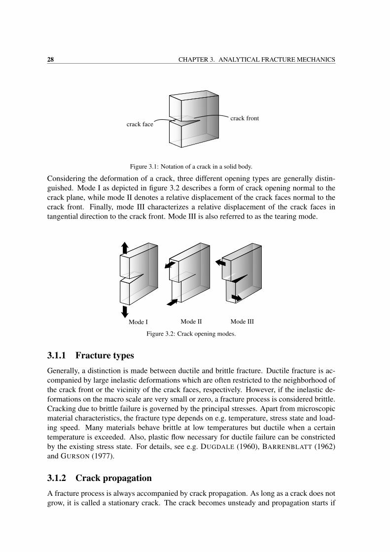
As the focus of this work is on the macroscopic aspects of fracture, only the most importantmacroscopic classifications resulting from processes on the molecular scale are introduced inthe following. Here, crack initiation is not considered, as on the macroscopic level, a body isconsidered a continuum which contains cracks a priori. A crack is regarded as a cut througha body with crack faces and a crack front as depicted in figure 3.1, where the crack faces areusually assumed to be traction free.
27
28 CHAPTER 3. ANALYTICAL FRACTURE MECHANICS
Figure 3.1: Notation of a crack in a solid body.
Considering the deformation of a crack, three different opening types are generally distin-guished. Mode I as depicted in figure 3.2 describes a form of crack opening normal to thecrack plane, while mode II denotes a relative displacement of the crack faces normal to thecrack front. Finally, mode III characterizes a relative displacement of the crack faces intangential direction to the crack front. Mode III is also referred to as the tearing mode.
Figure 3.2: Crack opening modes.
3.1.1 Fracture typesGenerally, a distinction is made between ductile and brittle fracture. Ductile fracture is ac-companied by large inelastic deformations which are often restricted to the neighborhood ofthe crack front or the vicinity of the crack faces, respectively. However, if the inelastic de-formations on the macro scale are very small or zero, a fracture process is considered brittle.Cracking due to brittle failure is governed by the principal stresses. Apart from microscopicmaterial characteristics, the fracture type depends on e.g. temperature, stress state and load-ing speed. Many materials behave brittle at low temperatures but ductile when a certaintemperature is exceeded. Also, plastic flow necessary for ductile failure can be constrictedby the existing stress state. For details, see e.g. DUGDALE (1960), BARRENBLATT (1962)and GURSON (1977).
3.1.2 Crack propagationA fracture process is always accompanied by crack propagation. As long as a crack does notgrow, it is called a stationary crack. The crack becomes unsteady and propagation starts if
3.2. LINEAR FRACTURE MECHANICS 29
a certain, material dependent load is exceeded. Then, a distinction is made between stableand unstable crack growth. If the external load has to be increased in order to achieve fur-ther crack propagation, crack growth is referred to as stable, while spontaneous crack growthwithout additional loading implies instable crack growth. Similar to brittle and ductile frac-ture, the type of crack propagation does not only depend on material properties but also onthe type of loading as well as the geometry of the body and possible further cracks.An additional distinction is made regarding the speed of crack propagation. Slow crack prop-agation where inertia does not play a role is called quasi-static, while fast crack propagationin the range of the speed of sound is called dynamic. Here, inertia has to be considered. Inmany engineering situations, very slow cracking due to cyclic loading and unloading can beobserved, which is referred to as fatigue cracking.
3.2 Linear fracture mechanics
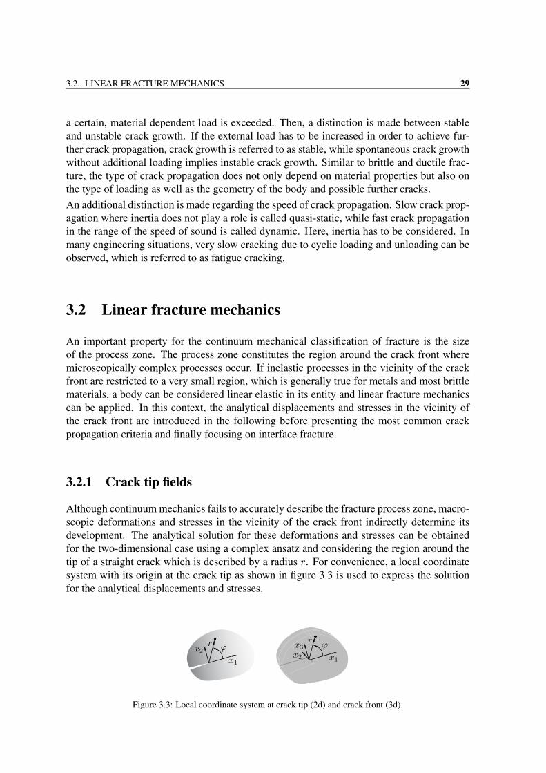
An important property for the continuum mechanical classification of fracture is the sizeof the process zone. The process zone constitutes the region around the crack front wheremicroscopically complex processes occur. If inelastic processes in the vicinity of the crackfront are restricted to a very small region, which is generally true for metals and most brittlematerials, a body can be considered linear elastic in its entity and linear fracture mechanicscan be applied. In this context, the analytical displacements and stresses in the vicinity ofthe crack front are introduced in the following before presenting the most common crackpropagation criteria and finally focusing on interface fracture.
3.2.1 Crack tip fields
Although continuum mechanics fails to accurately describe the fracture process zone, macro-scopic deformations and stresses in the vicinity of the crack front indirectly determine itsdevelopment. The analytical solution for these deformations and stresses can be obtainedfor the two-dimensional case using a complex ansatz and considering the region around thetip of a straight crack which is described by a radius r. For convenience, a local coordinatesystem with its origin at the crack tip as shown in figure 3.3 is used to express the solutionfor the analytical displacements and stresses.
• •
Figure 3.3: Local coordinate system at crack tip (2d) and crack front (3d).
30 CHAPTER 3. ANALYTICAL FRACTURE MECHANICS
The displacements u and stresses σ for a pure mode I deformation in a homogeneous linearelastic medium, following the notation by ANDERSON (2005), then read
[u1
u2
]=KI
2µ
√r
2π
cos(ϕ
2
)(κ− 1 + 2 sin2
(ϕ2
))sin(ϕ
2
)(κ+ 1− 2 cos2
(ϕ2
)) (3.1)
and
σ11
σ22
σ12
=KI√2πr
cos(ϕ
2
)
1− sin(ϕ
2
)sin
(3
2ϕ
)1 + sin
(ϕ2
)sin
(3
2ϕ
)sin(ϕ
2
)cos
(3
2ϕ
)
, (3.2)
respectively, for the two-dimensional case. For mode II displacements, they are given by
[u1
u2
]=KII
2µ
√r
2π
sin(ϕ
2
)(κ+ 1 + 2 cos2
(ϕ2
))cos(ϕ
2
)(κ− 1 + 2 sin2
(ϕ2
)) (3.3)
and
σ11
σ22
σ12
=KII√2πr
− sin
(ϕ2
)(2 + cos
(ϕ2
)cos
(3
2ϕ
))sin(ϕ
2
)cos(ϕ
2
)cos
(3
2ϕ
)cos(ϕ
2
)(1− sin
(ϕ2
)sin
(3
2ϕ
))
(3.4)
whereκ = 3− 4ν , σ33 = ν (σ11 + σ22) (3.5)
for plane strain and
κ =3− ν1 + ν
, σ33 = 0 (3.6)
for plane stress. Here, ν denotes POISSON’s ratio, whose relation to the bulk modulus K andthe shear modulus µ is given by
ν =3K − 2µ
6K + 2µ. (3.7)
The stress intensity factors KI and KII are a measure of the magnitude of the crack tip field,they depend on the geometry of the body as well as the external loads. From equation (3.2)and (3.4) it can be seen that the stresses at the crack tip contain a singularity of order r−1/2. Itcan be shown that singular stresses are necessary within a continuum description of fractureto predict nonzero separation work (HELLAN (1984)).If the complete three-dimensional stress field is to be obtained, three-dimensional character-istics of a fracture process have to be accounted for. It can be shown that the two-dimensional
3.2. LINEAR FRACTURE MECHANICS 31
solution for the crack tip field can be applied for the three-dimensional case as well, wherefor mode I and mode II, plane strain has to be considered and the mode III displacementsand stresses in the crack front region are given by
u2 =2KIII
µ
√r
2πsin(ϕ
2
)(3.8)
and (σ23
σ31
)=
KIII√2πr
− cos(ϕ
2
)sin(ϕ
2
) . (3.9)
Here, all displacements and stresses not listed explicitly are zero. To achieve the crack tipfields for mixed mode cracking, superposition can be applied due to linear elasticity.The analytical displacements and stresses listed above do not hold for cracks along interfacesbetween two dissimilar solids as depicted in figure 3.4. For the sake of brevity, the reader isreferred to RICE (1988) for details.
•
Figure 3.4: Interface crack between two dissimilar solids.
3.2.2 Crack propagation criteriaIn the case of crack propagation, criteria if, for how much and in which direction a crackpropagates need to be established. Apart from the stress intensity factors already mentionedin section 3.2.1, the energy release rate and the J-integral are frequently used as crack growthcriteria, while the maximum hoop stress criterion is a prevalent criterion for mixed modeloading.
Stress intensity factors
As can be seen from equations (3.1) and (3.2) for mode I, equations (3.3) and (3.4) for modeII and equations (3.8) and (3.9) for mode III loading, the stress intensity factors K, as ameasure of the stress singularity, characterize the displacements and stresses in the vicinity ofthe crack front. However, the crack tip field fails to describe processes very close to the crackfront, which are dominated by inelastic material behavior. Also, the formally existing stresssingularity at the crack front is a contradiction to the assumption of linear elasticity, whichstates that the strains are to remain small. Thus, the region dominated by the stress intensityfactors possesses an outer as well as an inner bound. However, the inelastic zone close tothe crack front and the fracture process zone are assumed to be sufficiently small such thatprocesses there are dominated by the behavior of the zone where the stress intensity factors
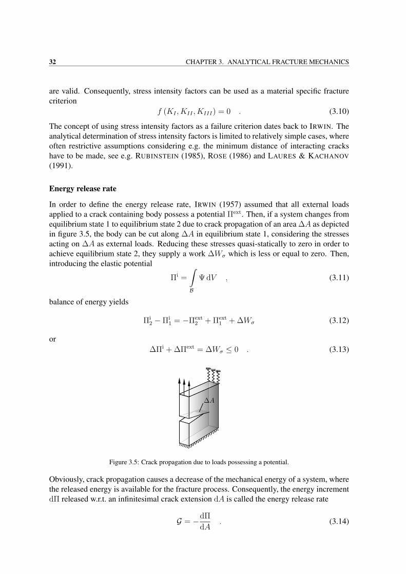
32 CHAPTER 3. ANALYTICAL FRACTURE MECHANICS
are valid. Consequently, stress intensity factors can be used as a material specific fracturecriterion
f (KI , KII , KIII) = 0 . (3.10)
The concept of using stress intensity factors as a failure criterion dates back to IRWIN. Theanalytical determination of stress intensity factors is limited to relatively simple cases, whereoften restrictive assumptions considering e.g. the minimum distance of interacting crackshave to be made, see e.g. RUBINSTEIN (1985), ROSE (1986) and LAURES & KACHANOV
(1991).
Energy release rate
In order to define the energy release rate, IRWIN (1957) assumed that all external loadsapplied to a crack containing body possess a potential Πext. Then, if a system changes fromequilibrium state 1 to equilibrium state 2 due to crack propagation of an area ∆A as depictedin figure 3.5, the body can be cut along ∆A in equilibrium state 1, considering the stressesacting on ∆A as external loads. Reducing these stresses quasi-statically to zero in order toachieve equilibrium state 2, they supply a work ∆Wσ which is less or equal to zero. Then,introducing the elastic potential
Πi =
∫B
Ψ dV , (3.11)
balance of energy yields
Πi2 − Πi
1 = −Πext2 + Πext
1 + ∆Wσ (3.12)
or∆Πi + ∆Πext = ∆Wσ ≤ 0 . (3.13)
Figure 3.5: Crack propagation due to loads possessing a potential.
Obviously, crack propagation causes a decrease of the mechanical energy of a system, wherethe released energy is available for the fracture process. Consequently, the energy incrementdΠ released w.r.t. an infinitesimal crack extension dA is called the energy release rate
G = −dΠ
dA. (3.14)
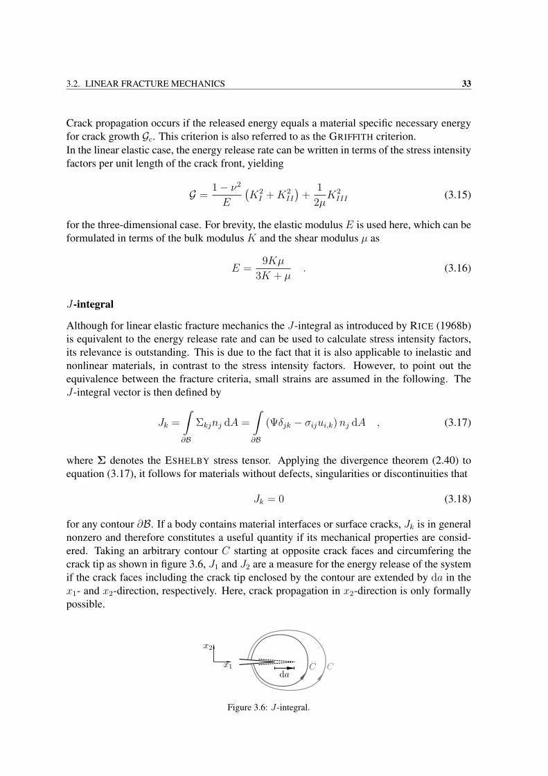
3.2. LINEAR FRACTURE MECHANICS 33
Crack propagation occurs if the released energy equals a material specific necessary energyfor crack growth Gc. This criterion is also referred to as the GRIFFITH criterion.In the linear elastic case, the energy release rate can be written in terms of the stress intensityfactors per unit length of the crack front, yielding
G =1− ν2
E
(K2I +K2
II
)+
1
2µK2III (3.15)
for the three-dimensional case. For brevity, the elastic modulus E is used here, which can beformulated in terms of the bulk modulus K and the shear modulus µ as
E =9Kµ
3K + µ. (3.16)
J-integral
Although for linear elastic fracture mechanics the J-integral as introduced by RICE (1968b)is equivalent to the energy release rate and can be used to calculate stress intensity factors,its relevance is outstanding. This is due to the fact that it is also applicable to inelastic andnonlinear materials, in contrast to the stress intensity factors. However, to point out theequivalence between the fracture criteria, small strains are assumed in the following. TheJ-integral vector is then defined by
Jk =
∫∂B
Σkjnj dA =
∫∂B
(Ψδjk − σijui,k)nj dA , (3.17)
where Σ denotes the ESHELBY stress tensor. Applying the divergence theorem (2.40) toequation (3.17), it follows for materials without defects, singularities or discontinuities that
Jk = 0 (3.18)
for any contour ∂B. If a body contains material interfaces or surface cracks, Jk is in generalnonzero and therefore constitutes a useful quantity if its mechanical properties are consid-ered. Taking an arbitrary contour C starting at opposite crack faces and circumfering thecrack tip as shown in figure 3.6, J1 and J2 are a measure for the energy release of the systemif the crack faces including the crack tip enclosed by the contour are extended by da in thex1- and x2-direction, respectively. Here, crack propagation in x2-direction is only formallypossible.
Figure 3.6: J-integral.
34 CHAPTER 3. ANALYTICAL FRACTURE MECHANICS
The energetic interpretation of the J-integral shows its equivalence to the energy release ratefor crack propagation,
J = J1 = G . (3.19)
For linear material behavior, equation (3.15) additionally yields
J =1− ν2
E
(K2I +K2
II
)+
1
2µK2III (3.20)
for the plane strain case. As the contour is arbitrary, the J-integral is a popular crack propa-gation criterion in numerical fracture mechanics. Application of the J-integral to the three-dimensional case with variable loading along the crack front is accomplished by integratingover a slice of width ∆l formed by the contour C along the crack front. If ∆l is approachingzero, the contour integral remains. However, this concept is only applicable in the three-dimensional case if a planar crack with a straight crack front is considered.
Maximum hoop stress criterion
The maximum hoop stress criterion was first introduced by ERDOGAN & SIH (1963). Itassumes that a crack propagates in radial direction from the crack tip, perpendicular to themaximum hoop stress σϕmax, if σϕmax at a distance rc from the crack tip reaches the samecritical value as in pure mode I. Thus, the crack deflection angle ϕ0 is given by the condition
∂σϕ∂ϕ
∣∣∣∣ϕ0
= 0 . (3.21)
3.3 Nonlinear fracture mechanicsThe application of linear elastic fracture mechanics might not be sufficient for specific mate-rials typically exhibiting finite strain response, like e.g. if fracture in rubber-like materials isconsidered. Also, the large strains around a crack front violate a basic assumption of linearelasticity, even for materials which usually can be described by small strain theory. Conse-quently, RICE (1968a), RICE & ROSENGREN (1968) and HUTCHINSON (1968), introduce anonlinear constitutive relation but retain the kinematic assumption of small deformations.The crack tip field for a fully nonlinear analysis was derived by KNOWLES & STERN-BERG (1973), KNOWLES & STERNBERG (1974) and KNOWLES (1977). In GEUBELLE
& KNAUSS (1994), it is specified for an incompressible generalized Neo-HOOKE material.
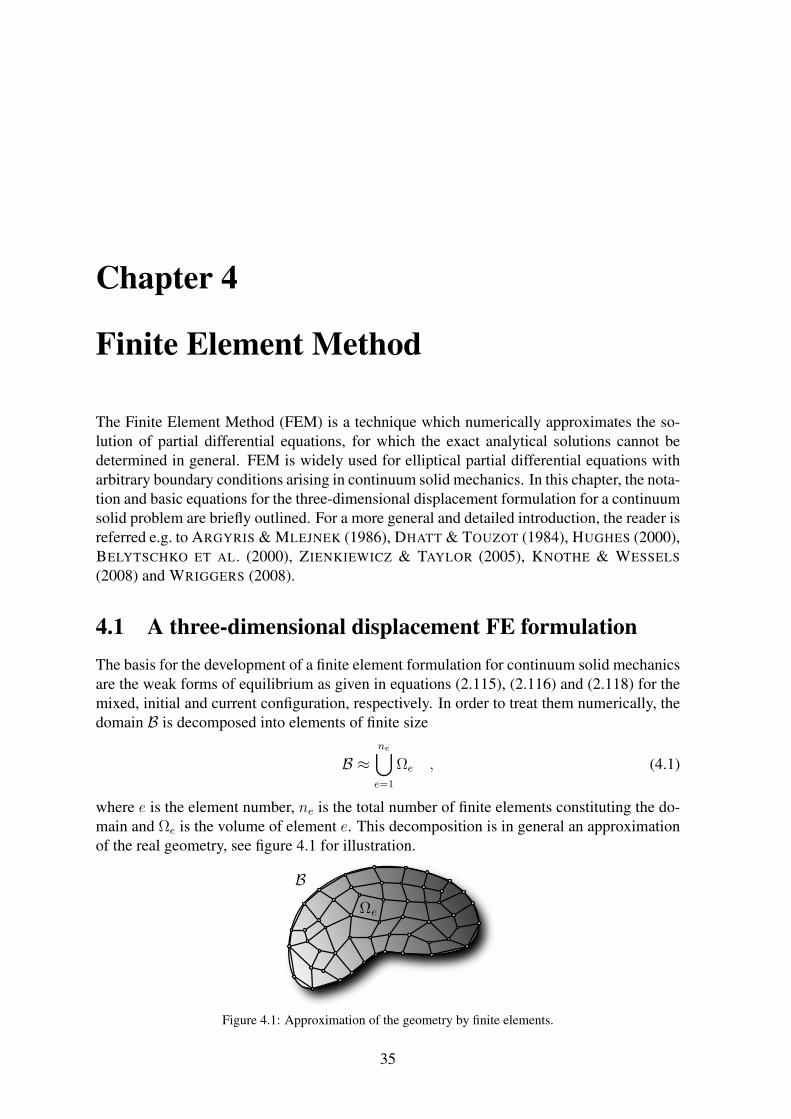
Chapter 4
Finite Element Method
The Finite Element Method (FEM) is a technique which numerically approximates the so-lution of partial differential equations, for which the exact analytical solutions cannot bedetermined in general. FEM is widely used for elliptical partial differential equations witharbitrary boundary conditions arising in continuum solid mechanics. In this chapter, the nota-tion and basic equations for the three-dimensional displacement formulation for a continuumsolid problem are briefly outlined. For a more general and detailed introduction, the reader isreferred e.g. to ARGYRIS & MLEJNEK (1986), DHATT & TOUZOT (1984), HUGHES (2000),BELYTSCHKO ET AL. (2000), ZIENKIEWICZ & TAYLOR (2005), KNOTHE & WESSELS
(2008) and WRIGGERS (2008).
4.1 A three-dimensional displacement FE formulationThe basis for the development of a finite element formulation for continuum solid mechanicsare the weak forms of equilibrium as given in equations (2.115), (2.116) and (2.118) for themixed, initial and current configuration, respectively. In order to treat them numerically, thedomain B is decomposed into elements of finite size
B ≈ne⋃e=1
Ωe , (4.1)
where e is the element number, ne is the total number of finite elements constituting the do-main and Ωe is the volume of element e. This decomposition is in general an approximationof the real geometry, see figure 4.1 for illustration.
Figure 4.1: Approximation of the geometry by finite elements.
35
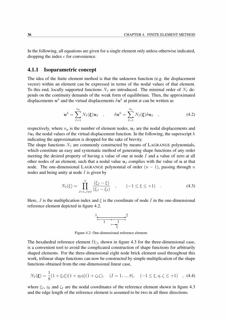
36 CHAPTER 4. FINITE ELEMENT METHOD
In the following, all equations are given for a single element only unless otherwise indicated,dropping the index e for convenience.
4.1.1 Isoparametric conceptThe idea of the finite element method is that the unknown function (e.g. the displacementvector) within an element can be expressed in terms of the nodal values of that element.To this end, locally supported functions NI are introduced. The minimal order of NI de-pends on the continuity demands of the weak form of equilibrium. Then, the approximateddisplacements uh and the virtual displacements δuh at point x can be written as
uh =
np∑I=1
NI(ξ)uI , δuh =
np∑I=1
NI(ξ)δuI , (4.2)
respectively, where np is the number of element nodes, uI are the nodal displacements andδuI the nodal values of the virtual displacement function. In the following, the superscript hindicating the approximation is dropped for the sake of brevity.The shape functions NI are commonly constructed by means of LAGRANGE polynomials,which constitute an easy and systematic method of generating shape functions of any ordermeeting the desired property of having a value of one at node I and a value of zero at allother nodes of an element, such that a nodal value uI complies with the value of u at thatnode. The one-dimensional LAGRANGE polynomial of order (n − 1), passing through nnodes and being unity at node I is given by
NI(ξ) =n∏
J=1,J 6=I
(ξJ − ξ)(ξJ − ξI)
, (−1 ≤ ξ ≤ +1) . (4.3)
Here, J is the multiplication index and ξ is the coordinate of node I in the one-dimensionalreference element depicted in figure 4.2.
Figure 4.2: One-dimensional reference element.
The hexahedral reference element Ω, shown in figure 4.3 for the three-dimensional case,is a convenient tool to avoid the complicated construction of shape functions for arbitrarilyshaped elements. For the three-dimensional eight node brick element used throughout thiswork, trilinear shape functions can now be constructed by simple multiplication of the shapefunctions obtained from the one-dimensional linear case,
NI(ξ) =1
8(1 + ξIξ)(1 + ηIη)(1 + ζIζ), (I = 1, ..., 8), (−1 ≤ ξ, η, ζ ≤ +1) , (4.4)
where ξI , ηI and ζI are the nodal coordinates of the reference element shown in figure 4.3and the edge length of the reference element is assumed to be two in all three directions.
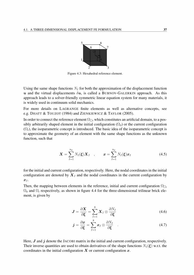
4.1. A THREE-DIMENSIONAL DISPLACEMENT FE FORMULATION 37
Figure 4.3: Hexahedral reference element.
Using the same shape functions NI for both the approximation of the displacement functionu and the virtual displacements δu, is called a BUBNOV-GALERKIN approach. As thisapproach leads to a solver-friendly symmetric linear equation system for many materials, itis widely used in continuum solid mechanics.
For more details on LAGRANGE finite elements as well as alternative concepts, seee.g. DHATT & TOUZOT (1984) and ZIENKIEWICZ & TAYLOR (2005).
In order to connect the reference element Ω, which constitutes an artificial domain, to a pos-sibly arbitrarily shaped element in the initial configuration (Ω0) or the current configuration(Ωt), the isoparametric concept is introduced. The basic idea of the isoparametric concept isto approximate the geometry of an element with the same shape functions as the unknownfunction, such that
X =
np∑I=1
NI(ξ)XI , x =
np∑I=1
NI(ξ)xI (4.5)
for the initial and current configuration, respectively. Here, the nodal coordinates in the initialconfiguration are denoted by XI and the nodal coordinates in the current configuration byxI .
Then, the mapping between elements in the reference, initial and current configuration Ω,Ω0 and Ωt respectively, as shown in figure 4.4 for the three-dimensional trilinear brick ele-ment, is given by
J =∂X
∂ξ=
8∑I=1
XI ⊗∂NI
∂ξ(4.6)
j =∂x
∂ξ=
8∑I=1
xI ⊗∂NI
∂ξ. (4.7)
Here, J and j denote the JACOBI matrix in the initial and current configuration, respectively.Their inverse quantities are used to obtain derivatives of the shape functions NI(ξ) w.r.t. thecoordinates in the initial configurationX or current configuration x.
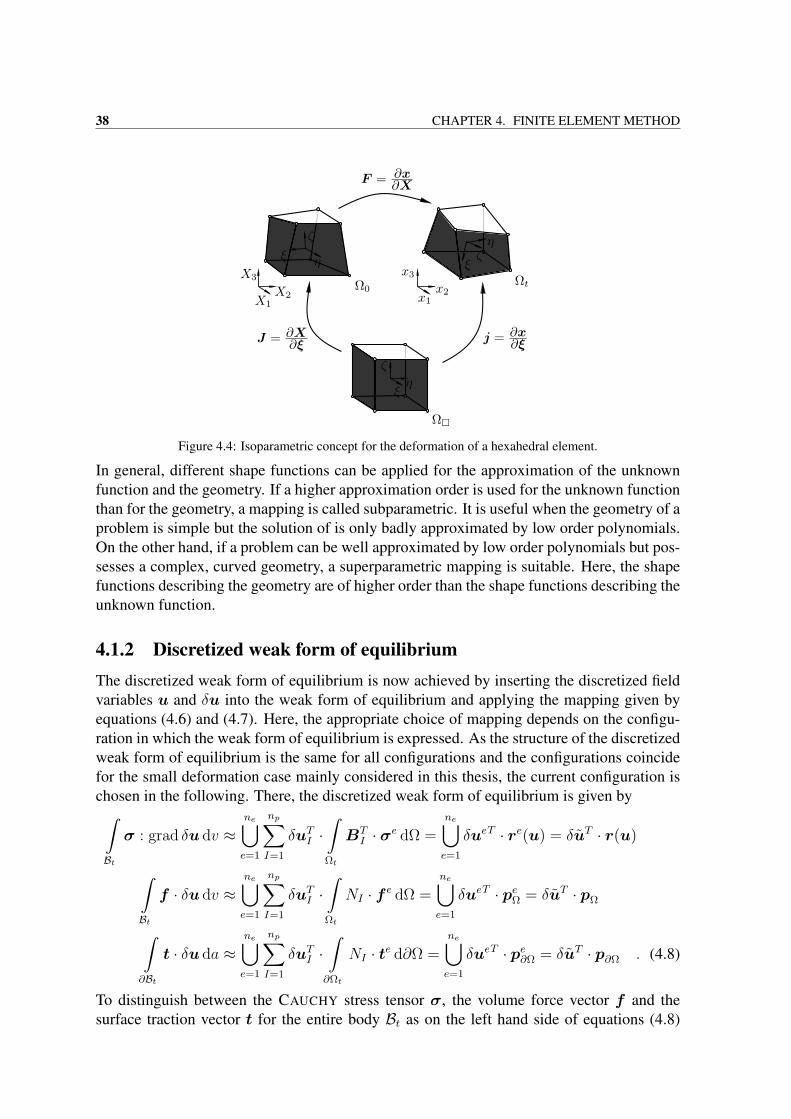
38 CHAPTER 4. FINITE ELEMENT METHOD
Figure 4.4: Isoparametric concept for the deformation of a hexahedral element.
In general, different shape functions can be applied for the approximation of the unknownfunction and the geometry. If a higher approximation order is used for the unknown functionthan for the geometry, a mapping is called subparametric. It is useful when the geometry of aproblem is simple but the solution of is only badly approximated by low order polynomials.On the other hand, if a problem can be well approximated by low order polynomials but pos-sesses a complex, curved geometry, a superparametric mapping is suitable. Here, the shapefunctions describing the geometry are of higher order than the shape functions describing theunknown function.
4.1.2 Discretized weak form of equilibriumThe discretized weak form of equilibrium is now achieved by inserting the discretized fieldvariables u and δu into the weak form of equilibrium and applying the mapping given byequations (4.6) and (4.7). Here, the appropriate choice of mapping depends on the configu-ration in which the weak form of equilibrium is expressed. As the structure of the discretizedweak form of equilibrium is the same for all configurations and the configurations coincidefor the small deformation case mainly considered in this thesis, the current configuration ischosen in the following. There, the discretized weak form of equilibrium is given by∫Bt
σ : grad δu dv ≈ne⋃e=1
np∑I=1
δuTI ·∫Ωt
BTI · σe dΩ =
ne⋃e=1
δueT · re(u) = δuT · r(u)
∫Bt
f · δu dv ≈ne⋃e=1
np∑I=1
δuTI ·∫Ωt
NI · f e dΩ =ne⋃e=1
δueT · peΩ = δuT · pΩ
∫∂Bt
t · δu da ≈ne⋃e=1
np∑I=1
δuTI ·∫∂Ωt
NI · te d∂Ω =ne⋃e=1
δueT · pe∂Ω = δuT · p∂Ω . (4.8)
To distinguish between the CAUCHY stress tensor σ, the volume force vector f and thesurface traction vector t for the entire body Bt as on the left hand side of equations (4.8)
4.1. A THREE-DIMENSIONAL DISPLACEMENT FE FORMULATION 39
and the respective quantities for each finite element, the element measures are denoted bythe superscript e. The matrix BI contains the derivatives of shape function NI w.r.t. thecoordinates in the current configuration x in order to construct the gradient operator. Thevector δu contains the assembled virtual displacements δue of each element, which are fixedas well as arbitrary but nonzero. Finally, the vector pΩ is the vector of nodal volume forcesacting in B and the vector p∂Ω is the vector of nodal traction forces acting on ∂Bt. Thevector r(u) is usually called vector of internal nodal forces and depends on the unknownnodal displacements u. Assuming the forces acting on the body Bt to be conservative andintroducing the global vector of external forces
pEXT = pΩ + p∂Ω , (4.9)
the discretized form of equation (2.118) can be written in terms of
g(u) = r(u)− pEXT = 0 . (4.10)
Here, g(u) is called the residual vector. If the dependence of the vector of internal nodalforces r(u) on the displacements u is linear, as for small deformation theory and linearelasticity, equation (4.10) yields a linear system of equations. If the dependence of r(u) onthe displacements is nonlinear, as e.g. for a Neo-HOOKE material, a NEWTON-RAPHSON
scheme can be used to solve (4.10). Prerequisite is that the initial guess for the unknownfunction u is close to the exact solution and certain other restrictions are met, see DHATT &TOUZOT (1984) and WRIGGERS (2008) for details. Application of a NEWTON-RAPHSON
scheme yields
g(uk+1) = g(uk) +∂g(u)
∂u
∣∣∣∣u=uk
· (uk+1 − uk) = 0 (4.11)
for the iteration in k to obtain the converged solution of u. Generally, the discretized form
of∂g(u)
∂u
∣∣∣∣u=uk
is called the tangent stiffness matrixK.
Further details on the nonlinear finite element method can be found e.g. in CRISFIELD (1997)and WRIGGERS (2008).
4.1.3 Numerical integration
The discretized weak form of equilibrium given in equations (4.8) contains integrals overeach element domain, which in general cannot be solved analytically. Different methods forthe numerical evaluation of these integrals such as the trapezoidal rule and the SIMPSON
rule exist, see e.g. DHATT & TOUZOT (1984) for an overview. A very popular choice isthe GAUSS integration scheme, as it yields the minimal number of integration points for agiven polynomial order, making it very efficient. Here, a function f , which is continuous,differentiable and sufficiently smooth in the element Ωt, is first mapped onto a referenceelement Ω, as described for the isoparametric concept in section 4.1.1. Then, integration inthe reference element is substituted by a summation of the values of f at the coordinates ξgp
40 CHAPTER 4. FINITE ELEMENT METHOD
of the ngp GAUSS integration points multiplied by a specific weight factor wgp, yielding∫Ωt
f dΩt =
∫Ω
f det j dΩ ≈ngp∑gp=1
f(ξgp)wgp det jgp . (4.12)
The number and position of GAUSS integration points depends on the dimension of theproblem and the polynomial order of f . Applying a sufficient number of GAUSS integrationpoints, polynomials can be integrated numerically exact. However, for arbitrarily shapedfinite elements, the mapping onto the reference configuration might result in the integrand notbeing a polynomial. Also, for nonpolynomial shape functions, GAUSS integration cannot beexpected to yield numerically exact results. Although for many cases the integration error isnegligible compared to the approximation error, applying GAUSS integration to inappropriatecases can lead to a substantial decrease of accuracy.Using a reduced number of GAUSS integration points is a frequent measure to reduce thecomputational effort and a remedy to the locking phenomenon, where the chosen shapefunctions are of insufficient order for a specific problem, and thus lead to an artificially stiffbehavior. Reduced integration, however, can lead to rank deficiency of the stiffness matrix,resulting in unphysical displacements. This numerical problem is also called hourglassingeffect.
Chapter 5
Numerical methods for fracturemechanics
As a consequence of the development of the FEM and the restrictions imposed by analyticalsolutions, first attempts to use the FEM for fracture applications were made in the early1970s, see CHAN ET AL. (1970).Standard displacement formulations cannot capture the singularity at a crack tip, as alreadydiscussed by CHAN ET AL. (1970). Consequently, first efforts concentrated on improvingthe solution at the crack tip by incorporating the singularity into the ansatz functions. The re-sulting formulations are commonly referred to as singularity elements, see BYSKOV (1970),BENZLEY (1974) and AKIN (1976) for two-dimensional and BLACKBURN & HELLEN
(1977) for three-dimensional approaches. However, special efforts have to be taken withthese elements to ensure compatibility with the surrounding standard elements, as presentedin BENZLEY (1974), AKIN (1976) and BLACKBURN & HELLEN (1977). Also, these ele-ments generally fail the patch test and therefore do not provide optimal convergence.A different approach was independently followed by HENSHELL & SHAW (1975) and BAR-SOUM (1976), who construct the singularity by moving nodes at the center of element edgestowards the singular crack tip point. These elements, which can be further improved bycollapsing nodes at the singularity, are known as quarter-point elements. As was shown byBARSOUM (1977), the elastic singularity is achieved if the same displacements are enforcedat the collapsed nodes, while leaving the nodes independent yields the plastic singularity.Crack propagation was first considered in the context of dynamics. First attempts for crackpropagation modeling can be found e.g. in KOBAYASHI ET AL. (1976), where a simple nodalrelease technique along a predefined crack path for a two-dimensional example is used, notsurprisingly resulting in spurious oscillations. A moving singular element is introduced inNISHIOKA & ATLURI (1980), which follows the crack tip through the finite element mesh.Nodal data of moved or newly introduced nodes is interpolated using information from theold mesh. In the context of quarter-point elements, SWENSON & INGRAFFEA (1988) movethe crack tip point until the mesh is sufficiently distorted, and then delete the elements aroundthe crack tip and remesh this area using data from the old mesh as an interpolation basis.However, in some cases this process has to be manually controlled. In contrast, MURTHY
& MUKHOPADHYAY (2000) use an error-controlled automatic mesh generator and NISH-IOKA ET AL. (2002) model dynamic crack branching problems by employing a remeshing
41
42 CHAPTER 5. NUMERICAL METHODS FOR FRACTURE MECHANICS
technique based on DELAUNAY triangulation. Cutting elements in the course of crack propa-gation is another option, see e.g. MEYER ET AL. (2006) for a very efficient method involvinga hierarchical data structure, which is not destroyed during crack propagation and thus fa-cilitates the use of hierarchical preconditioners. However, due to the many possible crackplanes in three dimensions this approach can become very cumbersome, see e.g. DHONDT
(1998).Obviously, modeling fracture with standard finite elements is not straightforward, especiallyin terms of mesh generation and remeshing in case of crack propagation. To circumventthis problem, an element doubling technique was developed by HANSBO & HANSBO
(2002) and applied to a simple two-dimensional fracture mechanics example in HANSBO
& HANSBO (2004). This approach is also known as the phantom node method. The basicidea is to double elements intersected by a crack and use two independent copies of thestandard shape functions. Each set of shape functions is attached to one side of the crack,shape functions corresponding to nodes on the respective other crack side are set to zero.This actually results in a linear combination of the standard XFEM basis. However, noadditional degrees of freedom need to be introduced, which makes this approach easier toimplement in existing commercial finite element programs. The element doubling conceptwas subsequently extended to linear elastic cohesive fracture by MERGHEIM ET AL. (2005)including crack propagation, where a nonlocal principal stress criterion is used. As theauthors point out, the main drawback of this method is that for very coarse meshes, themaximum reaction force is overestimated. Also, oscillations due to element-wise failureoccur unless sufficient mesh refinement is used, as a crack cannot end within one element.This issue was examined by RABCZUK ET AL. (2008), who extended the proposed method,such that cracks can end within one element. The application to dynamic fracture is givenby SONG ET AL. (2006), showing that for coarse meshes the crack tip speed is overesti-mated. An extension to three-dimensional, finite deformation, planar crack applications isintroduced in MERGHEIM ET AL. (2007). Similarly to the strong discontinuity approach,the main challenge is to track the surface of nonplanar cracks. Local tracking algorithms arereviewed in JAGER ET AL. (2008a) and JAGER ET AL. (2008b), coming to the conclusionthat a global tracking algorithm is more promising, see also JAGER ET AL. (2009).
Although more or less standard finite elements have been used for numerical fracture me-chanics for more than forty years now, they are by no means the only way to numericallytreat this class of problems. In the following, the most common methods, finite elementbased and not finite element based, are shortly revisited. A rough historical order is chosento point out how they influenced each other and in some cases led to the flourishing of newmethods.
5.1 Boundary Element MethodThe main idea of the Boundary Element Method (BEM) is to convert domain integrals ofthe considered problem into boundary integrals by means of GREEN’s second identity. Byinserting the fundamental solution of the governing equation, the boundary integral equationfor a domain point is obtained. Then, the limit case of this point approaching the boundary
5.1. BOUNDARY ELEMENT METHOD 43
is considered and the fundamental solution is evaluated at the boundary point. The numer-ical treatment is to discretize the boundary by choosing a finite number of points and thensequentially employing each node as a load point, which results in a system of equations.Finally, the solution inside the domain can be computed by moving the load point to the spotwhere the domain data is to be calculated.
Compared to the standard FEM, the advantage of the BEM for fracture mechanics appli-cations is obvious. The crack can be treated as an interior boundary, no sophisticated dis-cretization of the domain, resulting in many degrees of freedom, is necessary. However,special measures like e.g. domain subdivision are needed for the standard BEM to allowfor crack modeling, as the presence of two boundaries (crack faces) with the same geome-try leads to a singular system of equations. For the sake of brevity, the focus here lies onmethods which do not need domain subdivision.
In LUTZ ET AL. (1992), a temporary closure surface inside the volume is constructed totransform the singular integral over the crack surface patch into an equivalent nonsingularintegral. Another effective remedy to this problem is the dual boundary element method. Itwas introduced by PORTELA ET AL. (1992) for two-dimensional and by MI & ALIABADI
(1992) for three-dimensional applications, who use both the displacement and the tractionboundary integral equation and apply one to each side of the crack to avoid a singular systemof equations. An extension to dynamic problems is given in FEDELINSKI ET AL. (1993) andWEN ET AL. (1998). Linear plasticity problems are considered in LEITAO ET AL. (1995a),LEITAO ET AL. (1995b) and CISILINO ET AL. (1998), where domain discretization is nec-essary wherever plastic material behavior is expected. Crack propagation is examined byPORTELA ET AL. (1993) for two-dimensional applications including a predictor-correctorscheme in combination with stress intensity factors. MI & ALIABADI (1994) consider three-dimensional cases using a strain energy density criterion for crack growth as well as thepropagation direction and increment. Multiple cracks are considered by CHEN & CHEN
(1995) following the approach by LUTZ ET AL. (1992), as well as by DENDA & DONG
(1997), who compute multiple straight cracks in two dimensions. To facilitate the compu-tation of multiple curvilinear cracks, DENDA & MARANTE (2004) locally apply singularcrack tip elements.
As already mentioned, the BEM leads to less degrees of freedom compared to the FEM, asonly the boundaries need to be discretized unless plasticity is considered. Therefore, the pre-processing is simplified as e.g. data input from CAD can be used directly. In contrast to theFEM, the BEM also allows for improved accuracy in stress concentration problems and isthus well suited for fracture applications. The simple and accurate treatment of infinite andsemi-infinite domains is obvious. However, the nature of the approach requires knowledgeof a suitable fundamental solution. Also, it is limited to linear problems with a homoge-neous material unless domain decomposition with appropriate coupling is used. Concerningfracture problems, the resulting singular integrals need complicated algebraic manipulationsto avoid a singular system matrix. The main drawback of the BEM is that it leads to a non-symmetric, fully populated system of equations. Consequently, fast solution algorithms havebeen a main focus recently (see e.g. KOLK ET AL. (2005) and BENEDETTI ET AL. (2008)),especially for crack propagation, see WEBER & KUHN (2008).
44 CHAPTER 5. NUMERICAL METHODS FOR FRACTURE MECHANICS
5.2 Cohesive elementsFollowing the notion of DUGDALE (1960), BARRENBLATT (1962) and RICE (1968a),among others, that fracture is essentially a gradual phenomenon, where a cohesive zoneis formed at the crack tip, cohesive elements were introduced in NEEDLEMAN (1987),NEEDLEMAN (1990a) and NEEDLEMAN (1990b) to study debonding at interfaces. Withinthis approach, line and surface elements in the two- and three-dimensional case, respectively,are inserted between standard elements. They constitute a cohesive interface potential, spec-ified in terms of an interfacial strength and a work of separation, which are determined byexperiments. A smooth transition between a continuum and a crack can be modeled, avoidinga singularity at the crack tip by introducing a characteristic separation distance. This separa-tion distance defines a fully developed displacement discontinuity and a cohesive zone at thecrack tip. The cohesive element model naturally incorporates crack nucleation, propagation,coalescence and branching for a wide range of material models, if cohesive elements areplaced in the zones of interest (XU & NEEDLEMAN (1994)) and can be easily implementedinto commercial finite element codes.Research emanating from this work primarily focuses on the further development of cohe-sive potentials (TVERGAARD & HUTCHINSON (1992), LIU ET AL. (2008) and SETTGAST
& RASHID (2009)), fatigue cracking (YANG ET AL. (2001) and NGUYEN ET AL. (2001)) anddynamic crack growth and fragmentation (XU & NEEDLEMAN (1996) and MILLER ET AL.(1999)). Here, CAMACHO & ORTIZ (1996) insert cohesive elements only where a criticaltraction is attained between two elements to avoid the costly procedure of placing cohesiveelements everywhere in the domain, as in XU & NEEDLEMAN (1994). Additionally, a datastructure to account for the dynamics of fragmented pieces is introduced and further devel-oped for both two- and three-dimensional fragmentation (PANDOLFI & ORTIZ (1998), OR-TIZ & PANDOLFI (1999), RUIZ ET AL. (2001) and PANDOLFI & ORTIZ (2001)). However,by abruptly introducing cohesive elements, numerical problems occur. Also, none of theapproaches mentioned above addresses the inherent problem that the crack path depends onthe initial mesh, as a crack can only propagate along element boundaries. This is pointed outby means of several examples in ZHOU & MOLINARI (2004). There, the problem of meshdependency is reduced but not solved using a modified weakest link WEIBULL distributionto determine the initial strength of the interfaces. An alternative is to use the HEAVISIDE en-richment of the XFEM to allow for a discontinuous displacement field within one element, asin REMMERS ET AL. (2003), DE BORST (2003) and REMMERS ET AL. (2008). The elementdoubling technique for cohesive fracture presented by MERGHEIM ET AL. (2005), which isequivalent to the XFEM, can also be seen as a remedy in this context.
5.3 Strong Discontinuity ApproachThe Strong Discontinuity Approach (SDA) was originally introduced by SIMO ET AL. (1993)to incorporate dislocations into a standard continuum model, and applied to shear bands anddamage as examples for inelastic constitutive models exhibiting strain softening. The mainidea of the SDA is to represent a discontinuity by a combination of the HEAVISIDE stepfunction and a C0-continuous function that is arbitrary in the vicinity of the dislocation,
5.4. ELEMENT-FREE GALERKIN METHOD 45
zero on one side of the dislocation and one on the other. This function, being an ansatzfor an incompatible mode in terms of SIMO & RIFAI (1990), is then used to develop finiteelements in the context of enhanced assumed strains. In this framework, the displacementjump within an element is treated as the enhanced variable. In elements where the enhancedvariable remains zero, no dislocation occurs. Thus, the SDA is the first attempt in terms ofthe FEM to avoid cumbersome remeshing as a remedy to crack path dependence on the finiteelement mesh by simply incorporating the discontinuity into the element formulation itself.The SDA was applied to fracture problems in OLIVER (1995) and subsequently extendedin this context, strongly focussing on local as well as global crack tracking algorithms, seee.g. OLIVER (1996a), OLIVER (1996b), OLIVER ET AL. (1999), OLIVER ET AL. (2002b),FEIST & HOFSTETTER (2006a) and FEIST & HOFSTETTER (2006b). Fracture was speciallyconsidered in OLIVER ET AL. (2002a) and OLIVER ET AL. (2004), with a focus on the prop-agation of multiple cracks, while LINDER & ARMERO (2009) incorporate crack branchingwithin one element. An extension for three-dimensional problems is given in WELLS &SLUYS (2001c) and WELLS & SLUYS (2001a), while the topic of finite deformations istreated e.g. in OLIVER ET AL. (2003a). In OLIVER & HUESPE (2004a) and REESE (2007),combination of material and geometrical failure is studied, where REESE (2007) uses thediscontinuity bandwidth as a crack propagation criterion. Mixed and enhanced assumedstrain elements are introduced in OLIVER ET AL. (2003b) as a remedy to the stress lockingphenomenon. MOSLER & MESCHKE (2003) compute the displacement jump at the materialinstead of the element level to meet the same ends and thus also improve the robustness of thesolution scheme. The issue of robustness is also addressed by OLIVER & HUESPE (2004b)and OLIVER ET AL. (2006). DIAS-DA-COSTA ET AL. (2009) and RADULOVIC ET AL.(2011) avoid stress locking by incorporating the discontinuity like an interface element.While the SDA is mesh-independent as well as independent of the element alignment, itsmain drawbacks are that a crack cannot end within one element and that the singularity atthe crack front cannot be represented, as pointed out by BELYTSCHKO & BLACK (1999).
5.4 Element-free Galerkin MethodIn contrast to the FEM and similar to the BEM, the element-free GALERKIN method (EFG)does not require a mesh and element connectivities, but only nodes and a description of theexternal and internal boundaries as well as interfaces of the model. Moving least-squares(MLS) are used as trial and test functions at each node. An underlying cell structure or finiteelement mesh is used for numerical integration, which can be refined at crack tips and othersmall details (BELYTSCHKO ET AL. (1995a)). This method was originally introduced as thediffuse element method by NAYROLES ET AL. (1992) and first applied to two-dimensionalfracture mechanics by BELYTSCHKO ET AL. (1994b), who called it EFG. It was extendedto three-dimensional applications by BELYTSCHKO ET AL. (1996b) and SUKUMAR ET AL.(1997).The obvious advantage of the EFG is that as there is no mesh, no costly remeshing with itsdisadvantages such as data projection, but only an adaption of the boundary description isnecessary in case of crack propagation. In zones of interest like the vicinity of a crack tip,a closer spacing of nodes can be easily accomplished, which can be moved along with the
46 CHAPTER 5. NUMERICAL METHODS FOR FRACTURE MECHANICS
crack tip in case of crack propagation (BELYTSCHKO ET AL. (1994a, 1995a,b)). This leadsto high convergence rates. Also, due to the naturally smooth gradient field, no smoothing ofstresses etc. is necessary.However, there are several drawbacks to the EFG. A major problem is that, as theKRONECKER-δ-property is not fulfilled, the trial functions do not satisfy the DIRICHLET
boundary conditions. Several remedies to this problem were introduced, like imposing theDIRICHLET boundary conditions by means of LAGRANGE multipliers, see BELYTSCHKO
ET AL. (1994b). A modified variational principle, which is less accurate but yields easier tosolve systems of equations, is another option (LU ET AL. (1994)), as well as penalty meth-ods or coupling with a layer of finite elements (KRONGAUZ & BELYTSCHKO (1996)). Apartfrom the difficulties regarding boundary conditions, another issue is that discontinuous trialfunctions in the continuous displacement field around the crack tip are possible, which wasshown by BELYTSCHKO ET AL. (1996b). This is due to the requirement that for the com-putation of the trial functions, no information on the other side of a discontinuity should betaken. Apart from using enriched trial functions (FLEMING ET AL. (1997)), smoothing tech-niques have been developed to circumvent this problem (KRYSL & BELYTSCHKO (1997)).However, these lead to ”baroque shape functions” (BELYTSCHKO ET AL. (1996b)) involvinghigher order quadrature, which makes this procedure rather expensive (BELYTSCHKO ET AL.(1996a,b)). Independent of the application, neighborhood relations between the points haveto be established, and care has to be taken that there is a sufficient amount of points in theneighborhood to avoid artificial singularities. This makes a N2 algorithm unavoidable. Inorder to reduce computational effort, an idea was to couple EFG and FEM, using FEM inregions without cracks. This process combines the efficiency of the FEM with the accuracyand flexibility concerning cracks of the EFG (BELYTSCHKO ET AL. (1995c)).The review given in RAJAGOPAL & GUPTA (2011) shows that many of the above mentionedproblems are still subject to active research, which explains a popularity decrease of meshlessmethods in recent years.
5.5 Partition of Unity MethodThe basic idea of the Partition of Unity Method (PUM) presented in BABUSKA & MELENK
(1997) and MELENK & BABUSKA (1996) is to use analytic knowledge about the local be-havior of the exact solution for specific problem types where the approximation by polyno-mials is unsatisfactory, as in the case of singularities. These enrichment functions (knowna priori and therefore not resulting in a system of equations like meshless methods, wherecoefficients for the MLS interpolants have to be computed) describing the analytic behaviorare multiplied by the SHEPARD function, thus forming a partition of unity.However, as for the PUM the entire domain has to be enriched, it may suffer from linear de-pendencies resulting in ill-conditioned stiffness matrices, see BABUSKA & MELENK (1997).This was also observed in context of the XFEM using a fixed enrichment zone around a cracktip (LABORDE ET AL. (2005) and BECHET ET AL. (2005)), although there only a small partof the domain is enriched in comparison to the PUM. Another drawback of the PUM isthat the computational effort increases significantly due to the additional degrees of freedomintroduced globally, as pointed out in FRIES & BELYTSCHKO (2006).
5.6. EXTENDED FINITE ELEMENT METHOD 47
5.6 EXtended Finite Element Method
The eXtended Finite Element Method (XFEM) is a direct offspring of the partition ofunity method and nowadays essentially the same as the generalized finite element method(GFEM). The idea is the same as in the partition of unity method, however, only a smallpart of the domain is enriched. In case of fracture mechanics applications, these are usuallyfinite element nodes whose support is cut by the discontinuity. The goal of the XFEM is toexploit the flexibility of the finite element method and avoid one of its major drawbacks incrack applications, the (re)meshing issue, by modeling the crack independently of the mesh.By incorporating a priori known solution properties into the approximation space (FRIES
(2008)), the finite element method is thus extended to special applications like e.g. fractureproblems. The WESTERGAARD asymptotic crack tip field is used for all nodes whose sup-port is cut by the crack in BELYTSCHKO & BLACK (1999). As this involves mapping theenriched field w.r.t. the crack tip coordinate system for curved cracks, MOES ET AL. (1999)propose to use a modified HEAVISIDE function to represent the jump in the displacementfield away from the crack tip. An extension to the three-dimensional case is given by SUKU-MAR ET AL. (2000). The development of suitable enrichment functions for branching andintersecting cracks is considered by DAUX ET AL. (2000) and for very short cracks by BEL-LEC & DOLBOW (2003). Both approaches are introduced for two-dimensional problems.As LOEHNERT & BELYTSCHKO (2007a) show, the interaction of a macro crack with microcracks indeed greatly influences the behavior of the macro crack.Usually, triangles and quadrilaterals constitute two-dimensional meshes and tetrahedronsand hexahedrons are used for three-dimensional meshes, although TABARRAEI & SUKU-MAR (2008) proposed a very interesting alternative in terms of arbitrary polygons for twodimensions. After representing cracks as a sequence of line segments and triangles, the levelset method quickly became very popular for this purpose, see SUKUMAR ET AL. (2001).Here, the crack geometry is given implicitly by storing the signed distance to the crack foreach node where it is necessary. Usually, a linear isoparametric interpolation is used. Curvedcracks can be modeled with higher-order elements, however, using these also to enforce thepartition of unity of the enrichment functions is not feasible (STAZI ET AL. (2003)). An issuewithin the level set concept is not to change the crack geometry accidentally in case of crackpropagation (STOLARSKA ET AL. (2001)). Several remedies are presented e.g. in DUFLOT
(2007). Vector level sets are another option to describe the crack geometry, see VENTURA
ET AL. (2003) and BUDYN ET AL. (2004) for details.Several publications deal with crack propagation for the three-dimensional case (DUARTE
ET AL. (2001)), where a strong focus lies on accurate computation of the stress intensityfactors (MOES ET AL. (2002a)) and the level set update (MOES ET AL. (2002b), SUKU-MAR ET AL. (2003) and CHOPP & SUKUMAR (2003)). Crack initiation and propagation isconsidered in AREIAS & BELYTSCHKO (2005) as well as GASSER & HOLZAPFEL (2005).Especially for planar cracks in a mode I environment, adequate results can be achieved, how-ever, mode II and most of all mode III applications are still challenging. This is mostly dueto the inability of current methods to accurately compute the stress intensity factors in thesecases.Approaches to include more material properties than plain linear elasticity into the XFEM
48 CHAPTER 5. NUMERICAL METHODS FOR FRACTURE MECHANICS
emerged soon after its introduction by means of cohesive cracks (WELLS & SLUYS (2001b)and MOES & BELYTSCHKO (2002)), where ZI & BELYTSCHKO (2003) present a newenrichment such that a crack can end within an element without employing the crack tipfield. Appropriate enrichment functions for confined plasticity based on the HUTCHINSON-RICE-ROSENGREN fields are developed by ELGUEDJ ET AL. (2006) for the two-dimensionalcase. The plastic crack closure effect in case of crack propagation is modeled in ELGUEDJ
ET AL. (2007). Finite strain problems in terms of a Neo-HOOKE material are consideredin LEGRAIN ET AL. (2005) in a two-dimensional and by LOEHNERT ET AL. (2011) in athree-dimensional setting.Dynamic crack propagation has recently become a topic of increased interest. It was firstregarded by BELYTSCHKO ET AL. (2003), who use loss of hyperbolicity as a crack propa-gation criterion. Current focus lies on improving the accuracy in terms of level set update(PRABEL ET AL. (2007)), energy conservation (RETHORE ET AL. (2005) and COMBES-CURE ET AL. (2008)) and lumping strategies (MENOUILLARD ET AL. (2008) and ELGUEDJ
ET AL. (2009)). LIU ET AL. (2011) use higher-order XFEM to reduce numerical oscilla-tions. However, many methods in general do not yield satisfactory results comparing themto a range of experiments. It is suggested by SONG ET AL. (2008) that this is due to a lackof understanding and thus adequately modeling dynamic fracture processes.In order to avoid ill-conditioning of the stiffness matrix and an accurate integration of thenonpolynomial crack tip field, standard GAUSS integration is not sufficient for the XFEM.This was first observed by MOES ET AL. (1999), who apply triangulation considering thecrack geometry of cracked elements for integration purposes. Since then, more elaboratetechniques have been developed for the two-dimensional case, see section 6.4.2 for details.Another problem of the XFEM is that, for a wide range of enrichment functions, includingthe crack tip enrichment, the partition of unity is not fulfilled in elements which are onlypartly enriched, compromising accuracy and convergence (CHESSA ET AL. (2003)). Severalremedies are possible, like e.g. using the intrinsic XFEM (FRIES & BELYTSCHKO (2006))or direct treatment of the affected elements. An overview is given in section 6.2.2. Also,BECHET ET AL. (2005) observe that to achieve optimal convergence rates, the same geo-metrical zone should be enriched for all meshes. However, this leads to an ill-conditionedsystem of equations. If a problem includes enriched boundary nodes, imposing DIRICHLET
boundary conditions is not straightforward. In order to gain proper boundary conditions, theenrichment functions can be shifted, as e.g. done by FRIES (2008). A different concept isnot to change the enrichment function but apply boundary conditions by aid of LAGRANGE
multipliers (MOES ET AL. (2006)) or in a least-squares sense by making use of the multiscalemethod presented by LOEHNERT & BELYTSCHKO (2007b).Recently, DE LUYCKER ET AL. (2011) proposed to combine the XFEM with isogeometricanalysis and thus benefit from advantages of both methods.
5.7 Particle methodsParticle methods, which are popular for the simulations of granular materials, have beenapplied to fracture problems in geotechnics in the last couple of years. Here, rigid elementsinteracting with neighboring elements according to interaction rules, which are applied at
5.8. ARBITRARY LANGRANGIAN-EULERIAN METHODS 49
points of contact, are used in the context of the Discrete Element Method (DEM) to discretizea material. Although a variety of shapes is possible (LILLIE (2007)), circles and spheresfor two- and three-dimensional computations are mostly used, as the speed of the contactalgorithm strongly depends on the shape of the element.In TAVAREZ & PLESHA (2007), a failure criterion which is a function and thus independentof the discrete element size is developed, in contrast to POTYONDY & CUNDALL (2004),where the failure criterion does depend on the element size. It is argued that fracture is a nat-ural outcome of the DEM, however, several problems arise. First, applying particle methodsto quasi-static problems is cumbersome, as a time-marching procedure is used to solve theequation of motion for each particle. Therefore, a static problem has to be made dynamicartificially, resulting in the need for special loading algorithms (ZHAO ET AL. (2007, 2009))and calibration of algorithmic parameters to imitate quasi-static behavior in the system (TU
& ANDRADE (2008)). Also, a crack can only initiate and grow between particles, whichmakes the method inherently mesh-dependent. A very large number of particles is necessaryto allow a high number of possible crack paths. A multiscale approach was developed inANDRADE & TU (2009), however, this method does not consider the fact that homogeniza-tion is not applicable to localization effects. Another alternative to reduce computationaleffort is to use discrete elements only in zones of interest. These zones are then coupled tothe remaining domain, which is modeled with finite elements, see e.g. CALEYRON ET AL.(2011) and WELLMANN (2011).
5.8 Arbitrary Langrangian-Eulerian methodsIn order to automatically optimize a mesh for a specific problem, THOUTIREDDY & OR-TIZ (2004) and MOSLER & ORTIZ (2006) vary the strain energy with respect to both thedisplacement and the nodal position in the reference configuration. This method is also re-ferred to as r-adaptivity. Here, the goal is to automatically concentrate the mesh density inareas where a finer mesh is useful, e.g. around a crack tip. Different methods like changingthe element connectivity are employed to restrict mesh distortion. However, a nonconvexminimization problem with a singular coefficient matrix results. By formulating the dis-placements as a function of the nodal positions, SCHERER ET AL. (2007) regularize thecoefficient matrix.A slightly different argumentation is put forward by MUELLER ET AL. (2004), who usethe spurious configurational forces resulting from the finite element approximation as anindicator for mesh quality and refine the mesh where high configurational forces occur. Theypoint out that, especially at singularities, refinement leads only to moderate error reductionin the material force balance.Another way to look at configurational forces is to view them as the driving force in thekinetics of defects like e.g. crack propagation (MUELLER ET AL. (2002)) and consequentlydevelop an algorithm for crack propagation based on configurational forces (MUELLER &MAUGIN (2002)). A method for finite deformation crack propagation is presented in MIEHE
& GUERSES (2007), where the mesh is adapted around the crack tip such that crack propaga-tion is possible along the line of the configurational force at the crack tip. Here, the criterionfor crack propagation is given by the length of the configurational force vector, which corre-
50 CHAPTER 5. NUMERICAL METHODS FOR FRACTURE MECHANICS
sponds to the value of the J-integral. An overview is given in STEINMANN ET AL. (2009).Studying crack kinking for the two- and three-dimensional case, respectively, MIEHE ET AL.(2007) and GUERSES & MIEHE (2009) observe that only smooth crack kinking is possible.A transfer of the concept to the XFEM for fracture mechanics without incorporation of thecrack tip enrichment is given in FAGERSTROEM & LARSSON (2006). Here, a mesh depen-dence especially of the magnitude of the configurational forces is observed. By incorporatingthe crack tip field, HAUSLER ET AL. (2011) reduce this effect.The obvious advantage of applying configurational forces to fracture mechanics is that theissue of mesh refinement around the crack tip is a natural outcome, as well as a fracturecriterion and the direction of crack propagation. However, as the configurational forces arealso a measure of mesh quality, the question remains which part of a configurational forceconstitutes the driving force of a crack and which part is spurious, especially close to a cracktip (MUELLER ET AL. (2004)). The fact that only smooth kinking is possible indicates thatthe fracture process is not captured adequately.
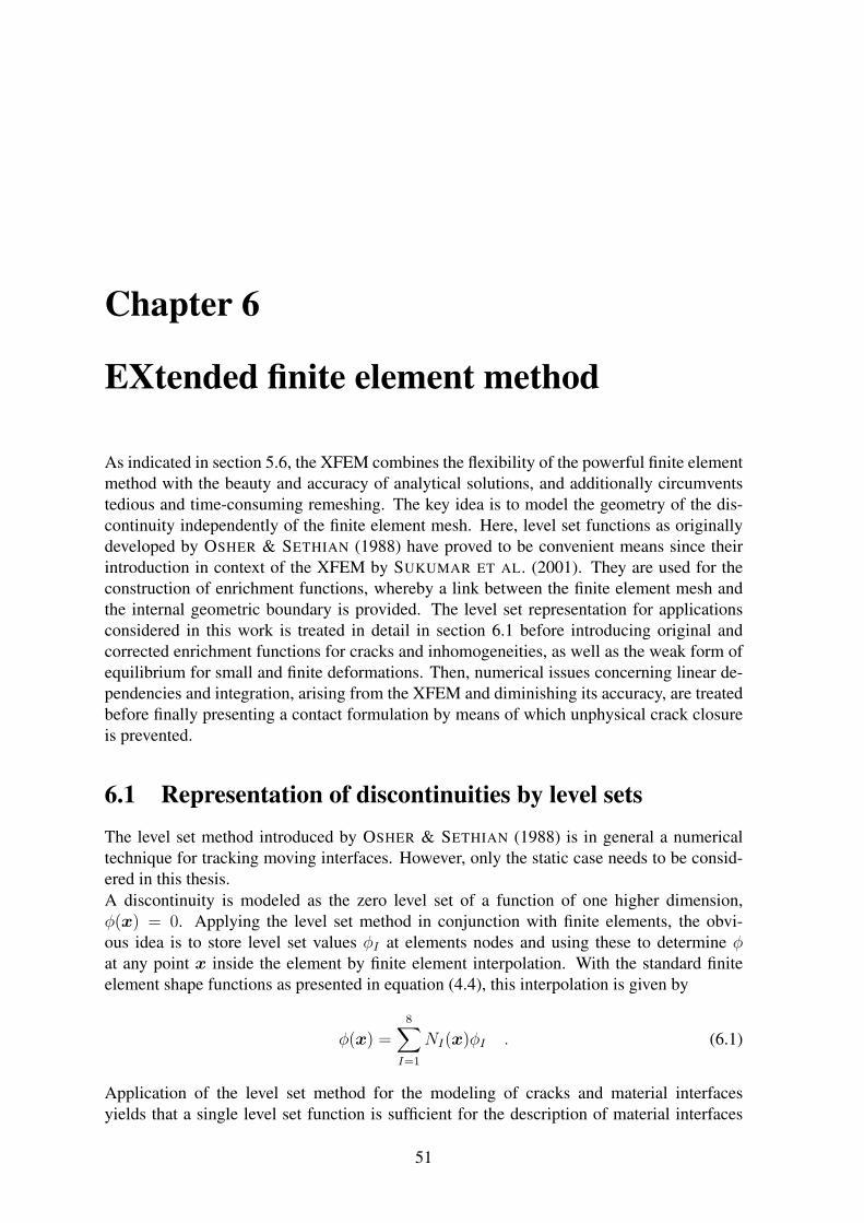
Chapter 6
EXtended finite element method
As indicated in section 5.6, the XFEM combines the flexibility of the powerful finite elementmethod with the beauty and accuracy of analytical solutions, and additionally circumventstedious and time-consuming remeshing. The key idea is to model the geometry of the dis-continuity independently of the finite element mesh. Here, level set functions as originallydeveloped by OSHER & SETHIAN (1988) have proved to be convenient means since theirintroduction in context of the XFEM by SUKUMAR ET AL. (2001). They are used for theconstruction of enrichment functions, whereby a link between the finite element mesh andthe internal geometric boundary is provided. The level set representation for applicationsconsidered in this work is treated in detail in section 6.1 before introducing original andcorrected enrichment functions for cracks and inhomogeneities, as well as the weak form ofequilibrium for small and finite deformations. Then, numerical issues concerning linear de-pendencies and integration, arising from the XFEM and diminishing its accuracy, are treatedbefore finally presenting a contact formulation by means of which unphysical crack closureis prevented.
6.1 Representation of discontinuities by level setsThe level set method introduced by OSHER & SETHIAN (1988) is in general a numericaltechnique for tracking moving interfaces. However, only the static case needs to be consid-ered in this thesis.A discontinuity is modeled as the zero level set of a function of one higher dimension,φ(x) = 0. Applying the level set method in conjunction with finite elements, the obvi-ous idea is to store level set values φI at elements nodes and using these to determine φat any point x inside the element by finite element interpolation. With the standard finiteelement shape functions as presented in equation (4.4), this interpolation is given by
φ(x) =8∑I=1
NI(x)φI . (6.1)
Application of the level set method for the modeling of cracks and material interfacesyields that a single level set function is sufficient for the description of material interfaces
51
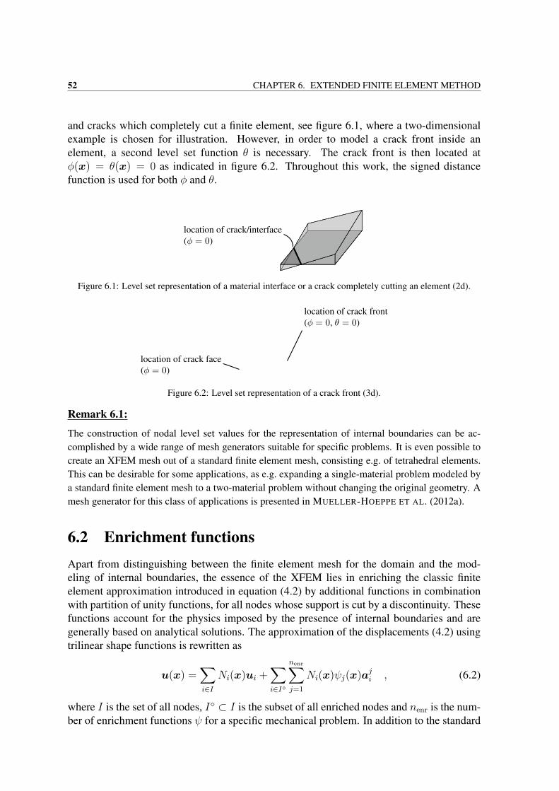
52 CHAPTER 6. EXTENDED FINITE ELEMENT METHOD
and cracks which completely cut a finite element, see figure 6.1, where a two-dimensionalexample is chosen for illustration. However, in order to model a crack front inside anelement, a second level set function θ is necessary. The crack front is then located atφ(x) = θ(x) = 0 as indicated in figure 6.2. Throughout this work, the signed distancefunction is used for both φ and θ.
Figure 6.1: Level set representation of a material interface or a crack completely cutting an element (2d).
Figure 6.2: Level set representation of a crack front (3d).
Remark 6.1:
The construction of nodal level set values for the representation of internal boundaries can be ac-complished by a wide range of mesh generators suitable for specific problems. It is even possible tocreate an XFEM mesh out of a standard finite element mesh, consisting e.g. of tetrahedral elements.This can be desirable for some applications, as e.g. expanding a single-material problem modeled bya standard finite element mesh to a two-material problem without changing the original geometry. Amesh generator for this class of applications is presented in MUELLER-HOEPPE ET AL. (2012a).
6.2 Enrichment functionsApart from distinguishing between the finite element mesh for the domain and the mod-eling of internal boundaries, the essence of the XFEM lies in enriching the classic finiteelement approximation introduced in equation (4.2) by additional functions in combinationwith partition of unity functions, for all nodes whose support is cut by a discontinuity. Thesefunctions account for the physics imposed by the presence of internal boundaries and aregenerally based on analytical solutions. The approximation of the displacements (4.2) usingtrilinear shape functions is rewritten as
u(x) =∑i∈I
Ni(x)ui +∑i∈I
nenr∑j=1
Ni(x)ψj(x)aji , (6.2)
where I is the set of all nodes, I ⊂ I is the subset of all enriched nodes and nenr is the num-ber of enrichment functions ψ for a specific mechanical problem. In addition to the standard
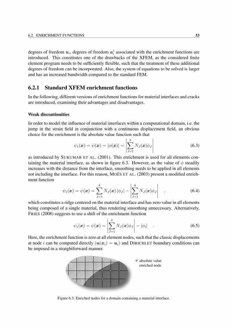
6.2. ENRICHMENT FUNCTIONS 53
degrees of freedom ui, degrees of freedom aji associated with the enrichment functions areintroduced. This constitutes one of the drawbacks of the XFEM, as the considered finiteelement program needs to be sufficiently flexible, such that the treatment of these additionaldegrees of freedom can be incorporated. Also, the system of equations to be solved is largerand has an increased bandwidth compared to the standard FEM.
6.2.1 Standard XFEM enrichment functionsIn the following, different versions of enrichment functions for material interfaces and cracksare introduced, examining their advantages and disadvantages.
Weak discontinuities
In order to model the influence of material interfaces within a computational domain, i.e. thejump in the strain field in conjunction with a continuous displacement field, an obviouschoice for the enrichment is the absolute value function such that
ψ1(x) = ψ(x) = |φ(x)| =∣∣∣∣∣
8∑J=1
NJ(x)φJ
∣∣∣∣∣ (6.3)
as introduced by SUKUMAR ET AL. (2001). This enrichment is used for all elements con-taining the material interface, as shown in figure 6.3. However, as the value of φ steadilyincreases with the distance from the interface, smoothing needs to be applied in all elementsnot including the interface. For this reason, MOES ET AL. (2003) present a modified enrich-ment function
ψ1(x) = ψ(x) =8∑
J=1
NJ(x) |φJ | −∣∣∣∣∣
8∑J=1
NJ(x)φJ
∣∣∣∣∣ , (6.4)
which constitutes a ridge centered on the material interface and has zero value in all elementsbeing composed of a single material, thus rendering smoothing unnecessary. Alternatively,FRIES (2008) suggests to use a shift of the enrichment function
ψ1(x) = ψ(x) =
∣∣∣∣∣8∑
J=1
NJ(x)φJ
∣∣∣∣∣− |φi| . (6.5)
Here, the enrichment function is zero at all element nodes, such that the classic displacementsat node i can be computed directly (u(xi) = ui) and DIRICHLET boundary conditions canbe imposed in a straightforward manner.
Figure 6.3: Enriched nodes for a domain containing a material interface.
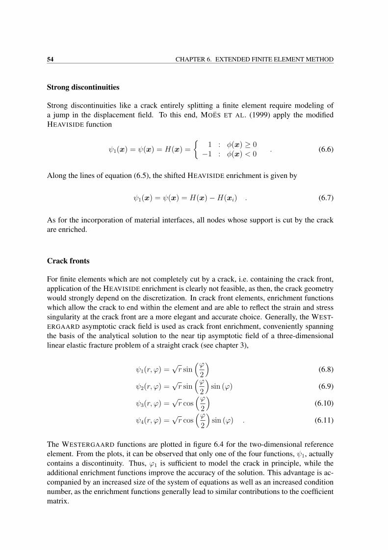
54 CHAPTER 6. EXTENDED FINITE ELEMENT METHOD
Strong discontinuities
Strong discontinuities like a crack entirely splitting a finite element require modeling ofa jump in the displacement field. To this end, MOES ET AL. (1999) apply the modifiedHEAVISIDE function
ψ1(x) = ψ(x) = H(x) =
1 : φ(x) ≥ 0−1 : φ(x) < 0
. (6.6)
Along the lines of equation (6.5), the shifted HEAVISIDE enrichment is given by
ψ1(x) = ψ(x) = H(x)−H(xi) . (6.7)
As for the incorporation of material interfaces, all nodes whose support is cut by the crackare enriched.
Crack fronts
For finite elements which are not completely cut by a crack, i.e. containing the crack front,application of the HEAVISIDE enrichment is clearly not feasible, as then, the crack geometrywould strongly depend on the discretization. In crack front elements, enrichment functionswhich allow the crack to end within the element and are able to reflect the strain and stresssingularity at the crack front are a more elegant and accurate choice. Generally, the WEST-ERGAARD asymptotic crack field is used as crack front enrichment, conveniently spanningthe basis of the analytical solution to the near tip asymptotic field of a three-dimensionallinear elastic fracture problem of a straight crack (see chapter 3),
ψ1(r, ϕ) =√r sin
(ϕ2
)(6.8)
ψ2(r, ϕ) =√r sin
(ϕ2
)sin (ϕ) (6.9)
ψ3(r, ϕ) =√r cos
(ϕ2
)(6.10)
ψ4(r, ϕ) =√r cos
(ϕ2
)sin (ϕ) . (6.11)
The WESTERGAARD functions are plotted in figure 6.4 for the two-dimensional referenceelement. From the plots, it can be observed that only one of the four functions, ψ1, actuallycontains a discontinuity. Thus, ϕ1 is sufficient to model the crack in principle, while theadditional enrichment functions improve the accuracy of the solution. This advantage is ac-companied by an increased size of the system of equations as well as an increased conditionnumber, as the enrichment functions generally lead to similar contributions to the coefficientmatrix.
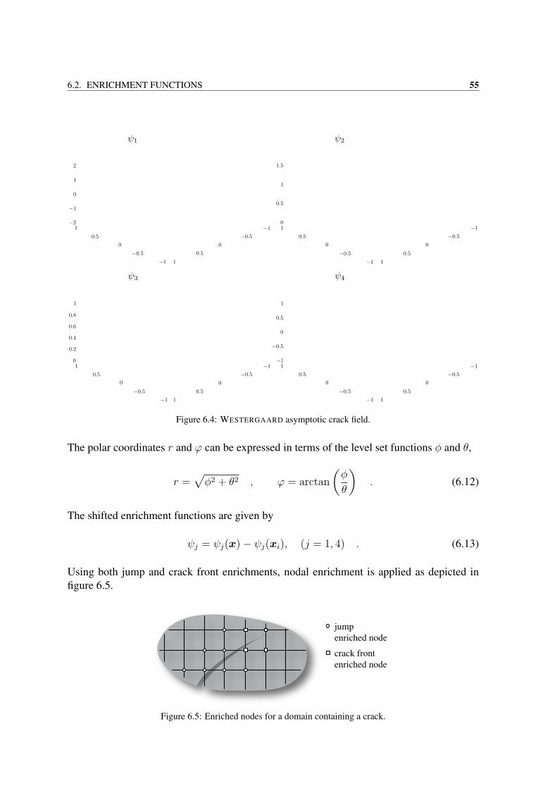
6.2. ENRICHMENT FUNCTIONS 55
Figure 6.4: WESTERGAARD asymptotic crack field.
The polar coordinates r and ϕ can be expressed in terms of the level set functions φ and θ,
r =√φ2 + θ2 , ϕ = arctan
(φ
θ
). (6.12)
The shifted enrichment functions are given by
ψj = ψj(x)− ψj(xi), (j = 1, 4) . (6.13)
Using both jump and crack front enrichments, nodal enrichment is applied as depicted infigure 6.5.
Figure 6.5: Enriched nodes for a domain containing a crack.
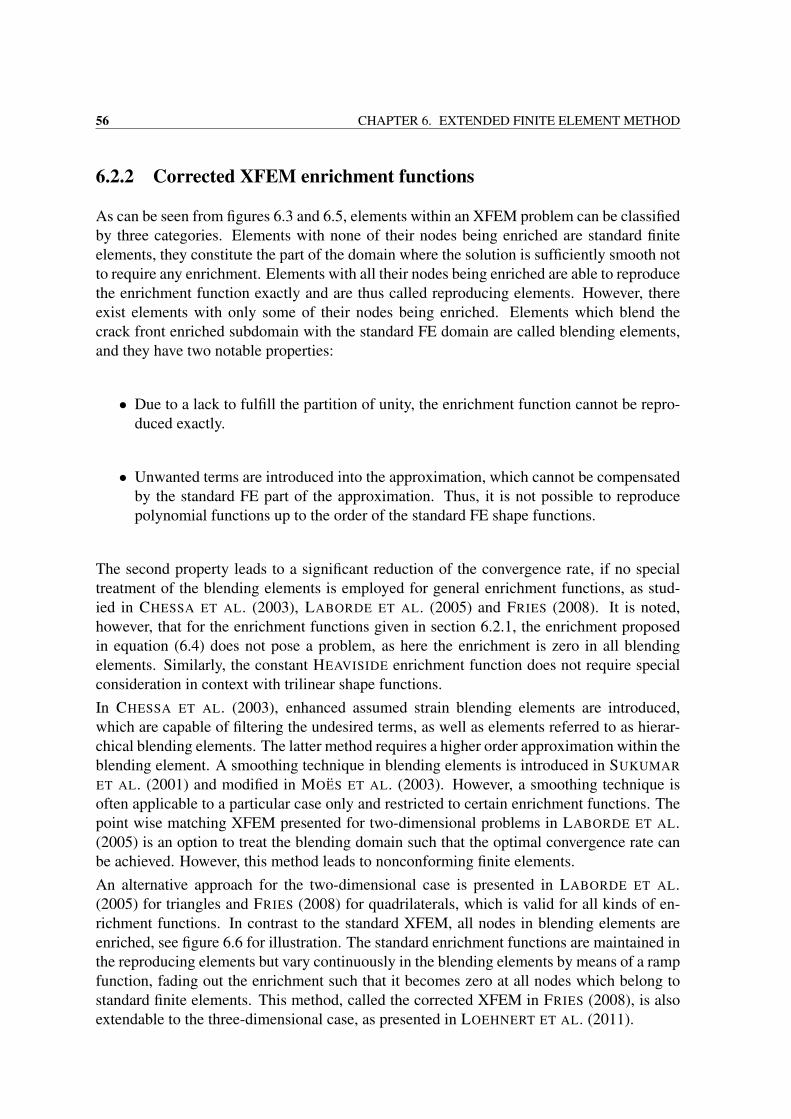
56 CHAPTER 6. EXTENDED FINITE ELEMENT METHOD
6.2.2 Corrected XFEM enrichment functions
As can be seen from figures 6.3 and 6.5, elements within an XFEM problem can be classifiedby three categories. Elements with none of their nodes being enriched are standard finiteelements, they constitute the part of the domain where the solution is sufficiently smooth notto require any enrichment. Elements with all their nodes being enriched are able to reproducethe enrichment function exactly and are thus called reproducing elements. However, thereexist elements with only some of their nodes being enriched. Elements which blend thecrack front enriched subdomain with the standard FE domain are called blending elements,and they have two notable properties:
• Due to a lack to fulfill the partition of unity, the enrichment function cannot be repro-duced exactly.
• Unwanted terms are introduced into the approximation, which cannot be compensatedby the standard FE part of the approximation. Thus, it is not possible to reproducepolynomial functions up to the order of the standard FE shape functions.
The second property leads to a significant reduction of the convergence rate, if no specialtreatment of the blending elements is employed for general enrichment functions, as stud-ied in CHESSA ET AL. (2003), LABORDE ET AL. (2005) and FRIES (2008). It is noted,however, that for the enrichment functions given in section 6.2.1, the enrichment proposedin equation (6.4) does not pose a problem, as here the enrichment is zero in all blendingelements. Similarly, the constant HEAVISIDE enrichment function does not require specialconsideration in context with trilinear shape functions.In CHESSA ET AL. (2003), enhanced assumed strain blending elements are introduced,which are capable of filtering the undesired terms, as well as elements referred to as hierar-chical blending elements. The latter method requires a higher order approximation within theblending element. A smoothing technique in blending elements is introduced in SUKUMAR
ET AL. (2001) and modified in MOES ET AL. (2003). However, a smoothing technique isoften applicable to a particular case only and restricted to certain enrichment functions. Thepoint wise matching XFEM presented for two-dimensional problems in LABORDE ET AL.(2005) is an option to treat the blending domain such that the optimal convergence rate canbe achieved. However, this method leads to nonconforming finite elements.An alternative approach for the two-dimensional case is presented in LABORDE ET AL.(2005) for triangles and FRIES (2008) for quadrilaterals, which is valid for all kinds of en-richment functions. In contrast to the standard XFEM, all nodes in blending elements areenriched, see figure 6.6 for illustration. The standard enrichment functions are maintained inthe reproducing elements but vary continuously in the blending elements by means of a rampfunction, fading out the enrichment such that it becomes zero at all nodes which belong tostandard finite elements. This method, called the corrected XFEM in FRIES (2008), is alsoextendable to the three-dimensional case, as presented in LOEHNERT ET AL. (2011).
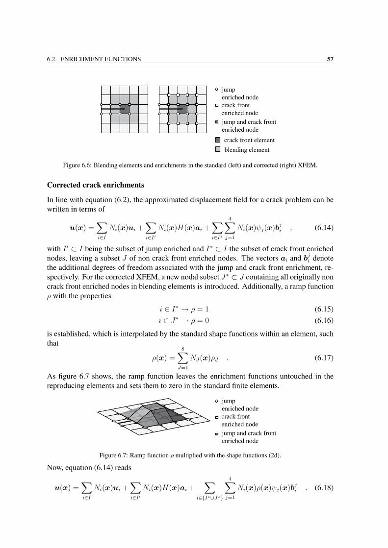
6.2. ENRICHMENT FUNCTIONS 57
Figure 6.6: Blending elements and enrichments in the standard (left) and corrected (right) XFEM.
Corrected crack enrichments
In line with equation (6.2), the approximated displacement field for a crack problem can bewritten in terms of
u(x) =∑i∈I
Ni(x)ui +∑i∈I′
Ni(x)H(x)ai +∑i∈I∗
4∑j=1
Ni(x)ψj(x)bji , (6.14)
with I ′ ⊂ I being the subset of jump enriched and I∗ ⊂ I the subset of crack front enrichednodes, leaving a subset J of non crack front enriched nodes. The vectors ai and bji denotethe additional degrees of freedom associated with the jump and crack front enrichment, re-spectively. For the corrected XFEM, a new nodal subset J∗ ⊂ J containing all originally noncrack front enriched nodes in blending elements is introduced. Additionally, a ramp functionρ with the properties
i ∈ I∗ → ρ = 1 (6.15)i ∈ J∗ → ρ = 0 (6.16)
is established, which is interpolated by the standard shape functions within an element, suchthat
ρ(x) =8∑
J=1
NJ(x)ρJ . (6.17)
As figure 6.7 shows, the ramp function leaves the enrichment functions untouched in thereproducing elements and sets them to zero in the standard finite elements.
Figure 6.7: Ramp function ρ multiplied with the shape functions (2d).
Now, equation (6.14) reads
u(x) =∑i∈I
Ni(x)ui +∑i∈I′
Ni(x)H(x)ai +∑
i∈I∗∪J∗
4∑j=1
Ni(x)ρ(x)ψj(x)bji . (6.18)
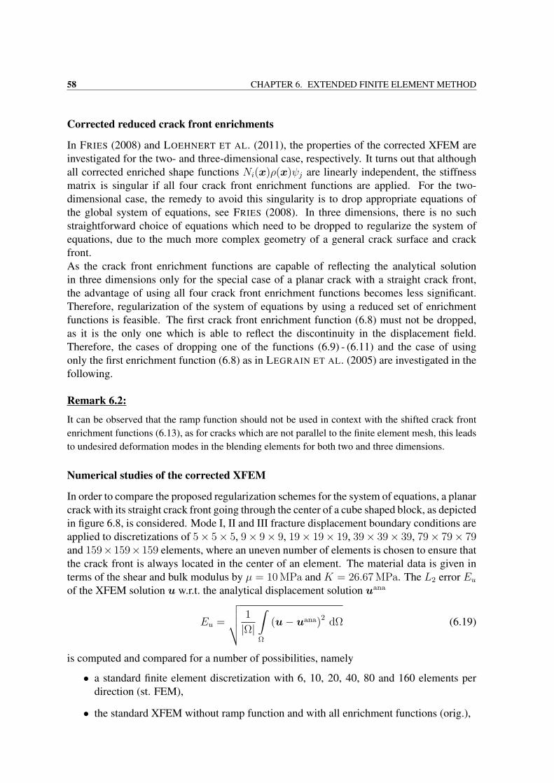
58 CHAPTER 6. EXTENDED FINITE ELEMENT METHOD
Corrected reduced crack front enrichments
In FRIES (2008) and LOEHNERT ET AL. (2011), the properties of the corrected XFEM areinvestigated for the two- and three-dimensional case, respectively. It turns out that althoughall corrected enriched shape functions Ni(x)ρ(x)ψj are linearly independent, the stiffnessmatrix is singular if all four crack front enrichment functions are applied. For the two-dimensional case, the remedy to avoid this singularity is to drop appropriate equations ofthe global system of equations, see FRIES (2008). In three dimensions, there is no suchstraightforward choice of equations which need to be dropped to regularize the system ofequations, due to the much more complex geometry of a general crack surface and crackfront.As the crack front enrichment functions are capable of reflecting the analytical solutionin three dimensions only for the special case of a planar crack with a straight crack front,the advantage of using all four crack front enrichment functions becomes less significant.Therefore, regularization of the system of equations by using a reduced set of enrichmentfunctions is feasible. The first crack front enrichment function (6.8) must not be dropped,as it is the only one which is able to reflect the discontinuity in the displacement field.Therefore, the cases of dropping one of the functions (6.9) - (6.11) and the case of usingonly the first enrichment function (6.8) as in LEGRAIN ET AL. (2005) are investigated in thefollowing.
Remark 6.2:
It can be observed that the ramp function should not be used in context with the shifted crack frontenrichment functions (6.13), as for cracks which are not parallel to the finite element mesh, this leadsto undesired deformation modes in the blending elements for both two and three dimensions.
Numerical studies of the corrected XFEM
In order to compare the proposed regularization schemes for the system of equations, a planarcrack with its straight crack front going through the center of a cube shaped block, as depictedin figure 6.8, is considered. Mode I, II and III fracture displacement boundary conditions areapplied to discretizations of 5× 5× 5, 9× 9× 9, 19× 19× 19, 39× 39× 39, 79× 79× 79and 159×159×159 elements, where an uneven number of elements is chosen to ensure thatthe crack front is always located in the center of an element. The material data is given interms of the shear and bulk modulus by µ = 10 MPa and K = 26.67 MPa. The L2 error Euof the XFEM solution u w.r.t. the analytical displacement solution uana
Eu =
√√√√ 1
|Ω|
∫Ω
(u− uana)2 dΩ (6.19)
is computed and compared for a number of possibilities, namely
• a standard finite element discretization with 6, 10, 20, 40, 80 and 160 elements perdirection (st. FEM),
• the standard XFEM without ramp function and with all enrichment functions (orig.),
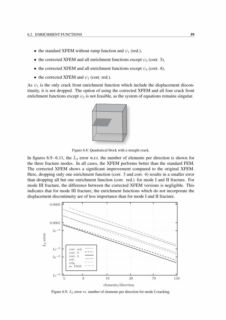
6.2. ENRICHMENT FUNCTIONS 59
• the standard XFEM without ramp function and ψ1 (red.),
• the corrected XFEM and all enrichment functions except ψ3 (corr. 3),
• the corrected XFEM and all enrichment functions except ψ4 (corr. 4),
• the corrected XFEM and ψ1 (corr. red.).
As ψ1 is the only crack front enrichment function which include the displacement discon-tinuity, it is not dropped. The option of using the corrected XFEM and all four crack frontenrichment functions except ψ2 is not feasible, as the system of equations remains singular.
Figure 6.8: Quadratical block with a straight crack.
In figures 6.9 - 6.11, the L2 error w.r.t. the number of elements per direction is shown forthe three fracture modes. In all cases, the XFEM performs better than the standard FEM.The corrected XFEM shows a significant improvement compared to the original XFEM.Here, dropping only one enrichment function (corr. 3 and corr. 4) results in a smaller errorthan dropping all but one enrichment function (corr. red.) for mode I and II fracture. Formode III fracture, the difference between the corrected XFEM versions is negligible. Thisindicates that for mode III fracture, the enrichment functions which do not incorporate thedisplacement discontinuity are of less importance than for mode I and II fracture.
elements/direction
L2
erro
r
corr. 3corr. 4red.
st. FEM
corr. red.
orig.
1e−6
5e−5
0.0001
0.0005
5 9 19 39 79 159
1e−5
5e−6
Figure 6.9: L2 error vs. number of elements per direction for mode I cracking.
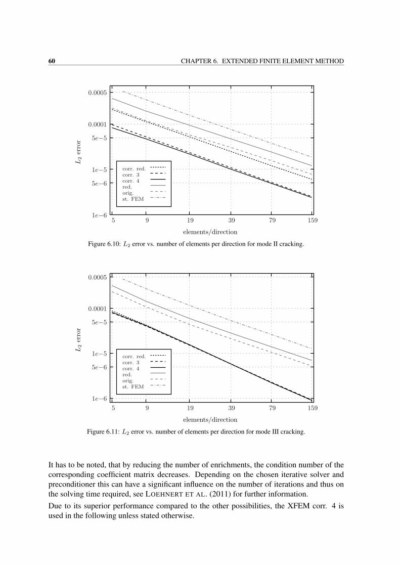
60 CHAPTER 6. EXTENDED FINITE ELEMENT METHOD
elements/direction
L2
erro
r
corr. 3corr. 4red.
st. FEM
corr. red.
orig.
1e−6
5e−6
1e−5
5e−5
0.0001
0.0005
9 19 39 795 159
Figure 6.10: L2 error vs. number of elements per direction for mode II cracking.
elements/direction
L2
erro
r
corr. 3corr. 4red.
st. FEM
corr. red.
orig.
5e−6
1e−5
0.0001
0.0005
5 9 19 39 79 159
5e−5
1e−6
Figure 6.11: L2 error vs. number of elements per direction for mode III cracking.
It has to be noted, that by reducing the number of enrichments, the condition number of thecorresponding coefficient matrix decreases. Depending on the chosen iterative solver andpreconditioner this can have a significant influence on the number of iterations and thus onthe solving time required, see LOEHNERT ET AL. (2011) for further information.Due to its superior performance compared to the other possibilities, the XFEM corr. 4 isused in the following unless stated otherwise.
6.3. DISCRETIZED WEAK FORM OF EQUILIBRIUM FOR THE XFEM 61
6.3 Discretized weak form of equilibrium for the XFEM
To accommodate the additional degrees of freedom, the discrete form of equilibrium has tobe slightly modified for the XFEM. In order to retain the original structure, it is feasible toreformulate the vectors containing the nodal values of the test function and the nodal degreesof freedom introduced in section 4.1.2, as well as the corresponding vector of enriched shapefunctions such that
δui =
δui
δai
δb1i
δb2i
δb3i
δb4i
, ui =
ui
ai
b1i
b2i
b3i
b4i
, N i(x) =
Ni(x)
Ni(x)H(x)
Ni(x)ρ(x)ψ1(x)
Ni(x)ρ(x)ψ2(x)
Ni(x)ρ(x)ψ3(x)
Ni(x)ρ(x)ψ4(x)
. (6.20)
For the reformulated B-matrix, the definition Bi = grad symN i is used, resulting in a stan-dard 6 × 3 matrix for nonenriched nodes, a 6 × 6 matrix for jump enriched nodes, a 6 × 15matrix for crack front enriched nodes and a 6×18 matrix for jump and front enriched nodes.
6.3.1 Small deformation theory
Now, the discretized weak form of equilibrium, specified for eight node brick elements, canbe expressed as in equation (4.8),
ne⋃e=1
8∑I=1
δuTI
∫Ω
BT
I · σe dΩ−∫Ω
N I · f e dΩ−∫∂Ω
N I · te d∂Ω
= 0 , (6.21)
where enriched degrees of freedom are blocked for nonenriched nodes by setting appropriatedisplacement boundary conditions.
6.3.2 Finite deformation theory
In LEGRAIN ET AL. (2005), fracture of rubber-like materials is investigated for the two-dimensional case by means of a Neo-HOOKE material. Only the first crack front enrichmentfunction is used, arguing that, as the basis for the analytical solution to a straight and planarcrack in three dimensions cannot be given in an explicit form (KNOWLES & STERNBERG
(1973, 1974)), the other three enrichment functions can be neglected. As the analytical solu-tion for a generally curved crack front and nonplanar crack surface in the three-dimensionalcase has not been found yet, this strategy is adopted for the three-dimensional case as well.The strain energy density function given in equation (2.95) with the volumetric part (2.99c)is used to model the material behavior.
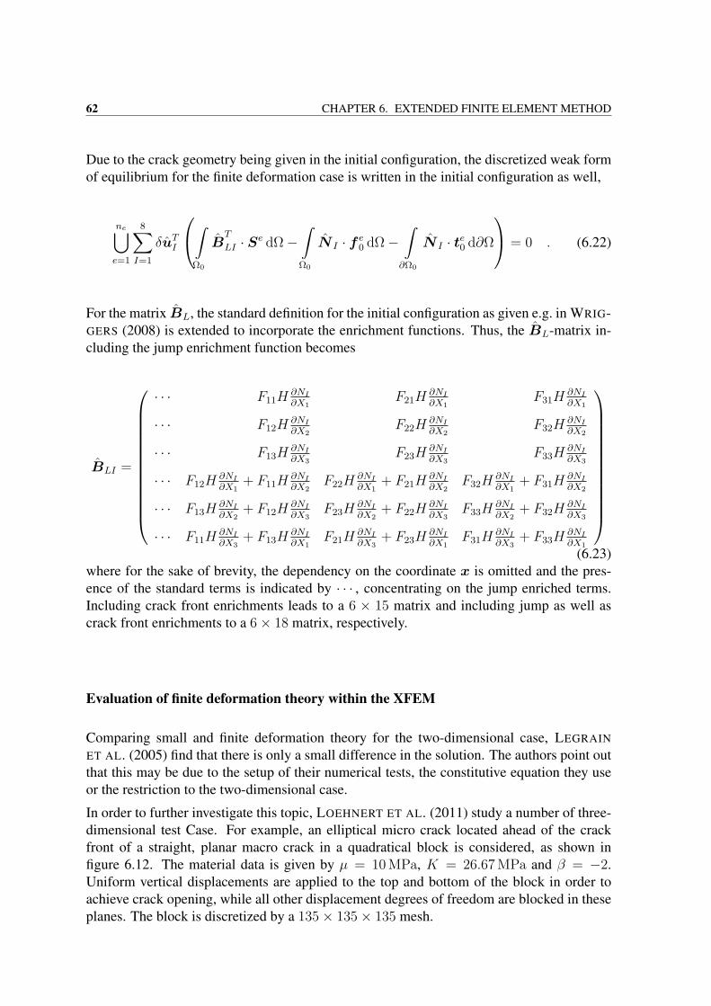
62 CHAPTER 6. EXTENDED FINITE ELEMENT METHOD
Due to the crack geometry being given in the initial configuration, the discretized weak formof equilibrium for the finite deformation case is written in the initial configuration as well,
ne⋃e=1
8∑I=1
δuTI
∫Ω0
BT
LI · Se dΩ−∫Ω0
N I · f e0 dΩ−∫∂Ω0
N I · te0 d∂Ω
= 0 . (6.22)
For the matrix BL, the standard definition for the initial configuration as given e.g. in WRIG-GERS (2008) is extended to incorporate the enrichment functions. Thus, the BL-matrix in-cluding the jump enrichment function becomes
BLI =
· · · F11H∂NI∂X1
F21H∂NI∂X1
F31H∂NI∂X1
· · · F12H∂NI∂X2
F22H∂NI∂X2
F32H∂NI∂X2
· · · F13H∂NI∂X3
F23H∂NI∂X3
F33H∂NI∂X3
· · · F12H∂NI∂X1
+ F11H∂NI∂X2
F22H∂NI∂X1
+ F21H∂NI∂X2
F32H∂NI∂X1
+ F31H∂NI∂X2
· · · F13H∂NI∂X2
+ F12H∂NI∂X3
F23H∂NI∂X2
+ F22H∂NI∂X3
F33H∂NI∂X2
+ F32H∂NI∂X3
· · · F11H∂NI∂X3
+ F13H∂NI∂X1
F21H∂NI∂X3
+ F23H∂NI∂X1
F31H∂NI∂X3
+ F33H∂NI∂X1
(6.23)
where for the sake of brevity, the dependency on the coordinate x is omitted and the pres-ence of the standard terms is indicated by · · · , concentrating on the jump enriched terms.Including crack front enrichments leads to a 6 × 15 matrix and including jump as well ascrack front enrichments to a 6× 18 matrix, respectively.
Evaluation of finite deformation theory within the XFEM
Comparing small and finite deformation theory for the two-dimensional case, LEGRAIN
ET AL. (2005) find that there is only a small difference in the solution. The authors point outthat this may be due to the setup of their numerical tests, the constitutive equation they useor the restriction to the two-dimensional case.
In order to further investigate this topic, LOEHNERT ET AL. (2011) study a number of three-dimensional test Case. For example, an elliptical micro crack located ahead of the crackfront of a straight, planar macro crack in a quadratical block is considered, as shown infigure 6.12. The material data is given by µ = 10 MPa, K = 26.67 MPa and β = −2.Uniform vertical displacements are applied to the top and bottom of the block in order toachieve crack opening, while all other displacement degrees of freedom are blocked in theseplanes. The block is discretized by a 135× 135× 135 mesh.
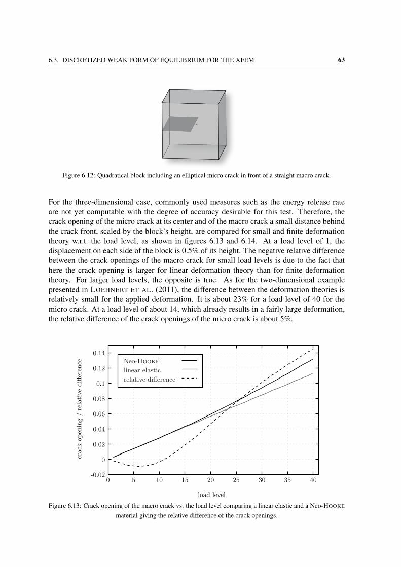
6.3. DISCRETIZED WEAK FORM OF EQUILIBRIUM FOR THE XFEM 63
Figure 6.12: Quadratical block including an elliptical micro crack in front of a straight macro crack.
For the three-dimensional case, commonly used measures such as the energy release rateare not yet computable with the degree of accuracy desirable for this test. Therefore, thecrack opening of the micro crack at its center and of the macro crack a small distance behindthe crack front, scaled by the block’s height, are compared for small and finite deformationtheory w.r.t. the load level, as shown in figures 6.13 and 6.14. At a load level of 1, thedisplacement on each side of the block is 0.5% of its height. The negative relative differencebetween the crack openings of the macro crack for small load levels is due to the fact thathere the crack opening is larger for linear deformation theory than for finite deformationtheory. For larger load levels, the opposite is true. As for the two-dimensional examplepresented in LOEHNERT ET AL. (2011), the difference between the deformation theories isrelatively small for the applied deformation. It is about 23% for a load level of 40 for themicro crack. At a load level of about 14, which already results in a fairly large deformation,the relative difference of the crack openings of the micro crack is about 5%.
0.14
0.12
0.1
0.08
0.06
0.04
0.02
0
-0.020 5 10 15 20 25 30 35 40
crac
kop
enin
g/
rela
tive
diffe
renc
e
load level
linear elasticrelative difference
Neo-Hooke
Figure 6.13: Crack opening of the macro crack vs. the load level comparing a linear elastic and a Neo-HOOKE
material giving the relative difference of the crack openings.
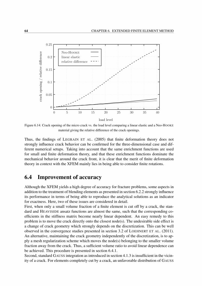
64 CHAPTER 6. EXTENDED FINITE ELEMENT METHOD
load level
crac
kop
enin
g/
rela
tive
diffe
renc
e
linear elasticrelative difference
Neo-Hooke
0
0.05
0.1
0.15
0.2
0.25
0 5 10 15 20 25 30 35 40
Figure 6.14: Crack opening of the micro crack vs. the load level comparing a linear elastic and a Neo-HOOKE
material giving the relative difference of the crack openings.
Thus, the findings of LEGRAIN ET AL. (2005) that finite deformation theory does notstrongly influence crack behavior can be confirmed for the three-dimensional case and dif-ferent numerical setups. Taking into account that the same enrichment functions are usedfor small and finite deformation theory, and that these enrichment functions dominate themechanical behavior around the crack front, it is clear that the merit of finite deformationtheory in context with the XFEM mainly lies in being able to consider finite rotations.
6.4 Improvement of accuracyAlthough the XFEM yields a high degree of accuracy for fracture problems, some aspects inaddition to the treatment of blending elements as presented in section 6.2.2 strongly influenceits performance in terms of being able to reproduce the analytical solutions as an indicatorfor exactness. Here, two of these issues are considered in detail.First, when only a small volume fraction of a finite element is cut off by a crack, the stan-dard and HEAVISIDE ansatz functions are almost the same, such that the corresponding co-efficients in the stiffness matrix become nearly linear dependent. An easy remedy to thisproblem is to move the crack directly onto the closest node(s). The undesirable side effect isa change of crack geometry which strongly depends on the discretization. This can be wellobserved in the convergence studies presented in section 3.2 of LOEHNERT ET AL. (2011).An alternative, maintaining the crack geometry independently of the discretization, is to ap-ply a mesh regularization scheme which moves the node(s) belonging to the smaller volumefraction away from the crack. Thus, a sufficient volume ratio to avoid linear dependence canbe achieved. This procedure is presented in section 6.4.1.Second, standard GAUSS integration as introduced in section 4.1.3 is insufficient in the vicin-ity of a crack. For elements completely cut by a crack, an unfavorable distribution of GAUSS
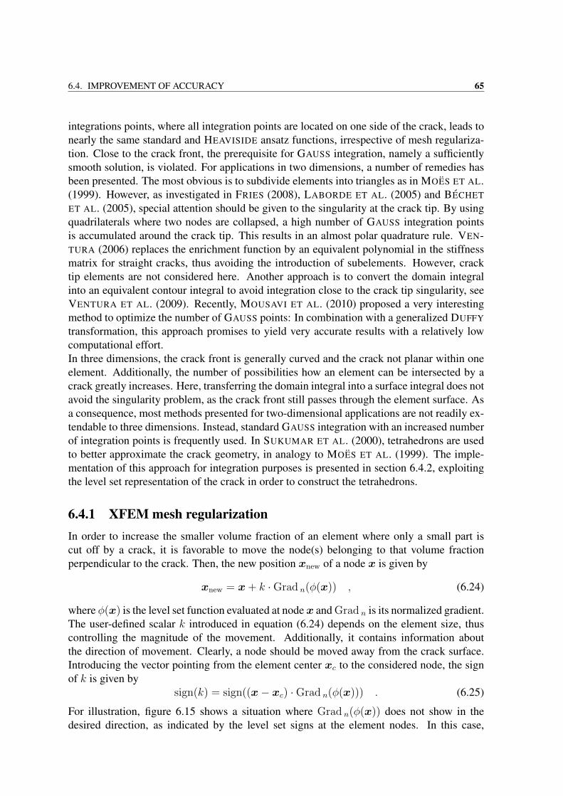
6.4. IMPROVEMENT OF ACCURACY 65
integrations points, where all integration points are located on one side of the crack, leads tonearly the same standard and HEAVISIDE ansatz functions, irrespective of mesh regulariza-tion. Close to the crack front, the prerequisite for GAUSS integration, namely a sufficientlysmooth solution, is violated. For applications in two dimensions, a number of remedies hasbeen presented. The most obvious is to subdivide elements into triangles as in MOES ET AL.(1999). However, as investigated in FRIES (2008), LABORDE ET AL. (2005) and BECHET
ET AL. (2005), special attention should be given to the singularity at the crack tip. By usingquadrilaterals where two nodes are collapsed, a high number of GAUSS integration pointsis accumulated around the crack tip. This results in an almost polar quadrature rule. VEN-TURA (2006) replaces the enrichment function by an equivalent polynomial in the stiffnessmatrix for straight cracks, thus avoiding the introduction of subelements. However, cracktip elements are not considered here. Another approach is to convert the domain integralinto an equivalent contour integral to avoid integration close to the crack tip singularity, seeVENTURA ET AL. (2009). Recently, MOUSAVI ET AL. (2010) proposed a very interestingmethod to optimize the number of GAUSS points: In combination with a generalized DUFFY
transformation, this approach promises to yield very accurate results with a relatively lowcomputational effort.In three dimensions, the crack front is generally curved and the crack not planar within oneelement. Additionally, the number of possibilities how an element can be intersected by acrack greatly increases. Here, transferring the domain integral into a surface integral does notavoid the singularity problem, as the crack front still passes through the element surface. Asa consequence, most methods presented for two-dimensional applications are not readily ex-tendable to three dimensions. Instead, standard GAUSS integration with an increased numberof integration points is frequently used. In SUKUMAR ET AL. (2000), tetrahedrons are usedto better approximate the crack geometry, in analogy to MOES ET AL. (1999). The imple-mentation of this approach for integration purposes is presented in section 6.4.2, exploitingthe level set representation of the crack in order to construct the tetrahedrons.
6.4.1 XFEM mesh regularizationIn order to increase the smaller volume fraction of an element where only a small part iscut off by a crack, it is favorable to move the node(s) belonging to that volume fractionperpendicular to the crack. Then, the new position xnew of a node x is given by
xnew = x+ k ·Grad n(φ(x)) , (6.24)
where φ(x) is the level set function evaluated at nodex and Grad n is its normalized gradient.The user-defined scalar k introduced in equation (6.24) depends on the element size, thuscontrolling the magnitude of the movement. Additionally, it contains information aboutthe direction of movement. Clearly, a node should be moved away from the crack surface.Introducing the vector pointing from the element center xc to the considered node, the signof k is given by
sign(k) = sign((x− xc) ·Grad n(φ(x))) . (6.25)
For illustration, figure 6.15 shows a situation where Grad n(φ(x)) does not show in thedesired direction, as indicated by the level set signs at the element nodes. In this case,
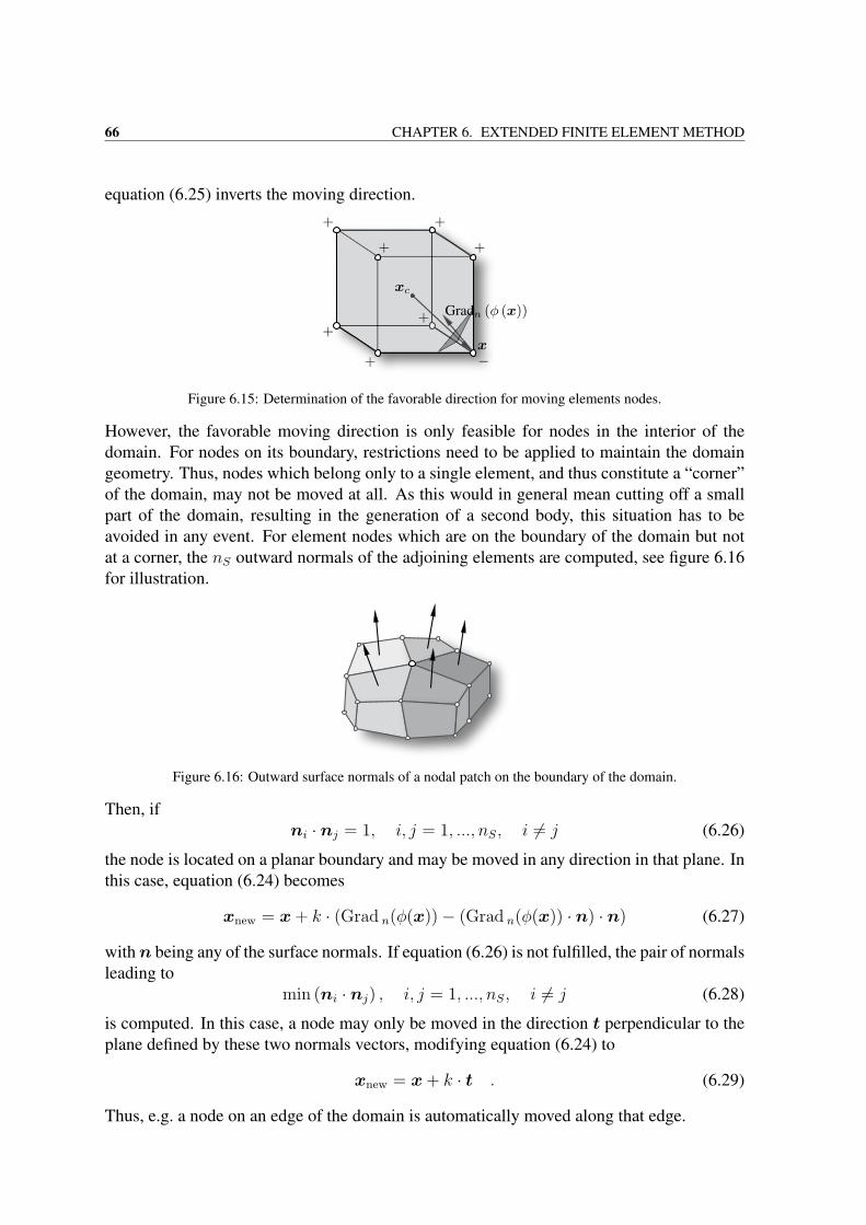
66 CHAPTER 6. EXTENDED FINITE ELEMENT METHOD
equation (6.25) inverts the moving direction.
Figure 6.15: Determination of the favorable direction for moving elements nodes.
However, the favorable moving direction is only feasible for nodes in the interior of thedomain. For nodes on its boundary, restrictions need to be applied to maintain the domaingeometry. Thus, nodes which belong only to a single element, and thus constitute a “corner”of the domain, may not be moved at all. As this would in general mean cutting off a smallpart of the domain, resulting in the generation of a second body, this situation has to beavoided in any event. For element nodes which are on the boundary of the domain but notat a corner, the nS outward normals of the adjoining elements are computed, see figure 6.16for illustration.
Figure 6.16: Outward surface normals of a nodal patch on the boundary of the domain.
Then, ifni · nj = 1, i, j = 1, ..., nS, i 6= j (6.26)
the node is located on a planar boundary and may be moved in any direction in that plane. Inthis case, equation (6.24) becomes
xnew = x+ k · (Grad n(φ(x))− (Grad n(φ(x)) · n) · n) (6.27)
withn being any of the surface normals. If equation (6.26) is not fulfilled, the pair of normalsleading to
min (ni · nj) , i, j = 1, ..., nS, i 6= j (6.28)
is computed. In this case, a node may only be moved in the direction t perpendicular to theplane defined by these two normals vectors, modifying equation (6.24) to
xnew = x+ k · t . (6.29)
Thus, e.g. a node on an edge of the domain is automatically moved along that edge.
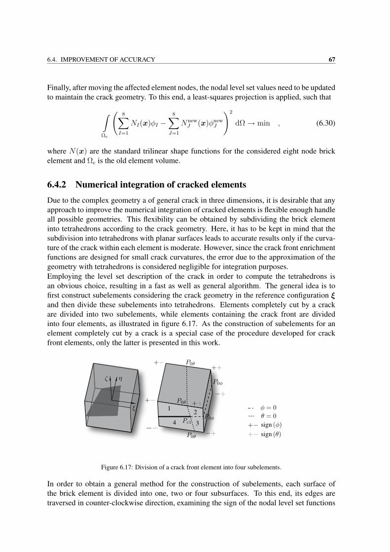
6.4. IMPROVEMENT OF ACCURACY 67
Finally, after moving the affected element nodes, the nodal level set values need to be updatedto maintain the crack geometry. To this end, a least-squares projection is applied, such that
∫Ωe
(8∑I=1
NI(x)φI −8∑
J=1
NnewJ (x)φnew
J
)2
dΩ→ min , (6.30)
where N(x) are the standard trilinear shape functions for the considered eight node brickelement and Ωe is the old element volume.
6.4.2 Numerical integration of cracked elementsDue to the complex geometry a of general crack in three dimensions, it is desirable that anyapproach to improve the numerical integration of cracked elements is flexible enough handleall possible geometries. This flexibility can be obtained by subdividing the brick elementinto tetrahedrons according to the crack geometry. Here, it has to be kept in mind that thesubdivision into tetrahedrons with planar surfaces leads to accurate results only if the curva-ture of the crack within each element is moderate. However, since the crack front enrichmentfunctions are designed for small crack curvatures, the error due to the approximation of thegeometry with tetrahedrons is considered negligible for integration purposes.Employing the level set description of the crack in order to compute the tetrahedrons isan obvious choice, resulting in a fast as well as general algorithm. The general idea is tofirst construct subelements considering the crack geometry in the reference configuration ξand then divide these subelements into tetrahedrons. Elements completely cut by a crackare divided into two subelements, while elements containing the crack front are dividedinto four elements, as illustrated in figure 6.17. As the construction of subelements for anelement completely cut by a crack is a special case of the procedure developed for crackfront elements, only the latter is presented in this work.
Figure 6.17: Division of a crack front element into four subelements.
In order to obtain a general method for the construction of subelements, each surface ofthe brick element is divided into one, two or four subsurfaces. To this end, its edges aretraversed in counter-clockwise direction, examining the sign of the nodal level set functions
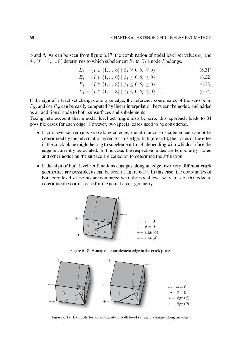
68 CHAPTER 6. EXTENDED FINITE ELEMENT METHOD
φ and θ. As can be seen from figure 6.17, the combination of nodal level set values φI andθI , (I = 1, ..., 8) determines to which subelement E1 to E4 a node I belongs,
E1 = I ∈ 1, ..., 8 | φI ≥ 0, θI ≤ 0 (6.31)E2 = I ∈ 1, ..., 8 | φI ≥ 0, θI ≥ 0 (6.32)E3 = I ∈ 1, ..., 8 | φI ≤ 0, θI ≥ 0 (6.33)E4 = I ∈ 1, ..., 8 | φI ≤ 0, θI ≤ 0 . (6.34)
If the sign of a level set changes along an edge, the reference coordinates of the zero pointP0φ and / or P0θ can be easily computed by linear interpolation between the nodes, and addedas an additional node to both subsurfaces and subelements.Taking into account that a nodal level set might also be zero, this approach leads to 81possible cases for each edge. However, two special cases need to be considered.
• If one level set remains zero along an edge, the affiliation to a subelement cannot bedetermined by the information given for this edge. In figure 6.18, the nodes of the edgein the crack plane might belong to subelement 1 or 4, depending with which surface theedge is currently associated. In this case, the respective nodes are temporarily storedand other nodes on the surface are called on to determine the affiliation.
• If the sign of both level set functions changes along an edge, two very different crackgeometries are possible, as can be seen in figure 6.19. In this case, the coordinates ofboth zero level set points are compared w.r.t. the nodal level set values of that edge todetermine the correct case for the actual crack geometry.
Figure 6.18: Example for an element edge in the crack plane.
Figure 6.19: Example for an ambiguity if both level set signs change along an edge.
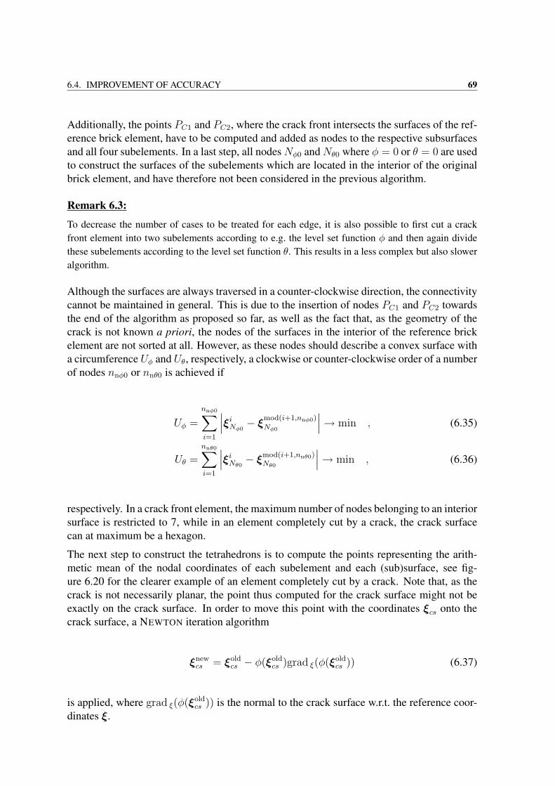
6.4. IMPROVEMENT OF ACCURACY 69
Additionally, the points PC1 and PC2, where the crack front intersects the surfaces of the ref-erence brick element, have to be computed and added as nodes to the respective subsurfacesand all four subelements. In a last step, all nodesNφ0 andNθ0 where φ = 0 or θ = 0 are usedto construct the surfaces of the subelements which are located in the interior of the originalbrick element, and have therefore not been considered in the previous algorithm.
Remark 6.3:
To decrease the number of cases to be treated for each edge, it is also possible to first cut a crackfront element into two subelements according to e.g. the level set function φ and then again dividethese subelements according to the level set function θ. This results in a less complex but also sloweralgorithm.
Although the surfaces are always traversed in a counter-clockwise direction, the connectivitycannot be maintained in general. This is due to the insertion of nodes PC1 and PC2 towardsthe end of the algorithm as proposed so far, as well as the fact that, as the geometry of thecrack is not known a priori, the nodes of the surfaces in the interior of the reference brickelement are not sorted at all. However, as these nodes should describe a convex surface witha circumference Uφ and Uθ, respectively, a clockwise or counter-clockwise order of a numberof nodes nnφ0 or nnθ0 is achieved if
Uφ =
nnφ0∑i=1
∣∣∣ξiNφ0− ξmod(i+1,nnφ0)
Nφ0
∣∣∣→ min , (6.35)
Uθ =
nnθ0∑i=1
∣∣∣ξiNθ0 − ξmod(i+1,nnθ0)Nθ0
∣∣∣→ min , (6.36)
respectively. In a crack front element, the maximum number of nodes belonging to an interiorsurface is restricted to 7, while in an element completely cut by a crack, the crack surfacecan at maximum be a hexagon.
The next step to construct the tetrahedrons is to compute the points representing the arith-metic mean of the nodal coordinates of each subelement and each (sub)surface, see fig-ure 6.20 for the clearer example of an element completely cut by a crack. Note that, as thecrack is not necessarily planar, the point thus computed for the crack surface might not beexactly on the crack surface. In order to move this point with the coordinates ξcs onto thecrack surface, a NEWTON iteration algorithm
ξnewcs = ξold
cs − φ(ξoldcs )grad ξ(φ(ξold
cs )) (6.37)
is applied, where grad ξ(φ(ξoldcs )) is the normal to the crack surface w.r.t. the reference coor-
dinates ξ.
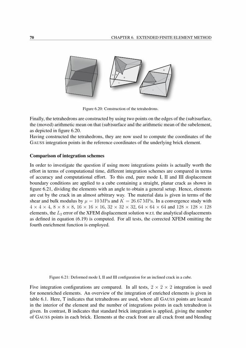
70 CHAPTER 6. EXTENDED FINITE ELEMENT METHOD
Figure 6.20: Construction of the tetrahedrons.
Finally, the tetrahedrons are constructed by using two points on the edges of the (sub)surface,the (moved) arithmetic mean on that (sub)surface and the arithmetic mean of the subelement,as depicted in figure 6.20.Having constructed the tetrahedrons, they are now used to compute the coordinates of theGAUSS integration points in the reference coordinates of the underlying brick element.
Comparison of integration schemes
In order to investigate the question if using more integrations points is actually worth theeffort in terms of computational time, different integration schemes are compared in termsof accuracy and computational effort. To this end, pure mode I, II and III displacementboundary conditions are applied to a cube containing a straight, planar crack as shown infigure 6.21, dividing the elements with an angle to obtain a general setup. Hence, elementsare cut by the crack in an almost arbitrary way. The material data is given in terms of theshear and bulk modulus by µ = 10 MPa and K = 26.67 MPa. In a convergence study with4 × 4 × 4, 8 × 8 × 8, 16 × 16 × 16, 32 × 32 × 32, 64 × 64 × 64 and 128 × 128 × 128elements, the L2 error of the XFEM displacement solution w.r.t. the analytical displacementsas defined in equation (6.19) is computed. For all tests, the corrected XFEM omitting thefourth enrichment function is employed.
Figure 6.21: Deformed mode I, II and III configuration for an inclined crack in a cube.
Five integration configurations are compared. In all tests, 2 × 2 × 2 integration is usedfor nonenriched elements. An overview of the integration of enriched elements is given intable 6.1. Here, T indicates that tetrahedrons are used, where all GAUSS points are locatedin the interior of the element and the number of integrations points in each tetrahedron isgiven. In contrast, B indicates that standard brick integration is applied, giving the numberof GAUSS points in each brick. Elements at the crack front are all crack front and blending
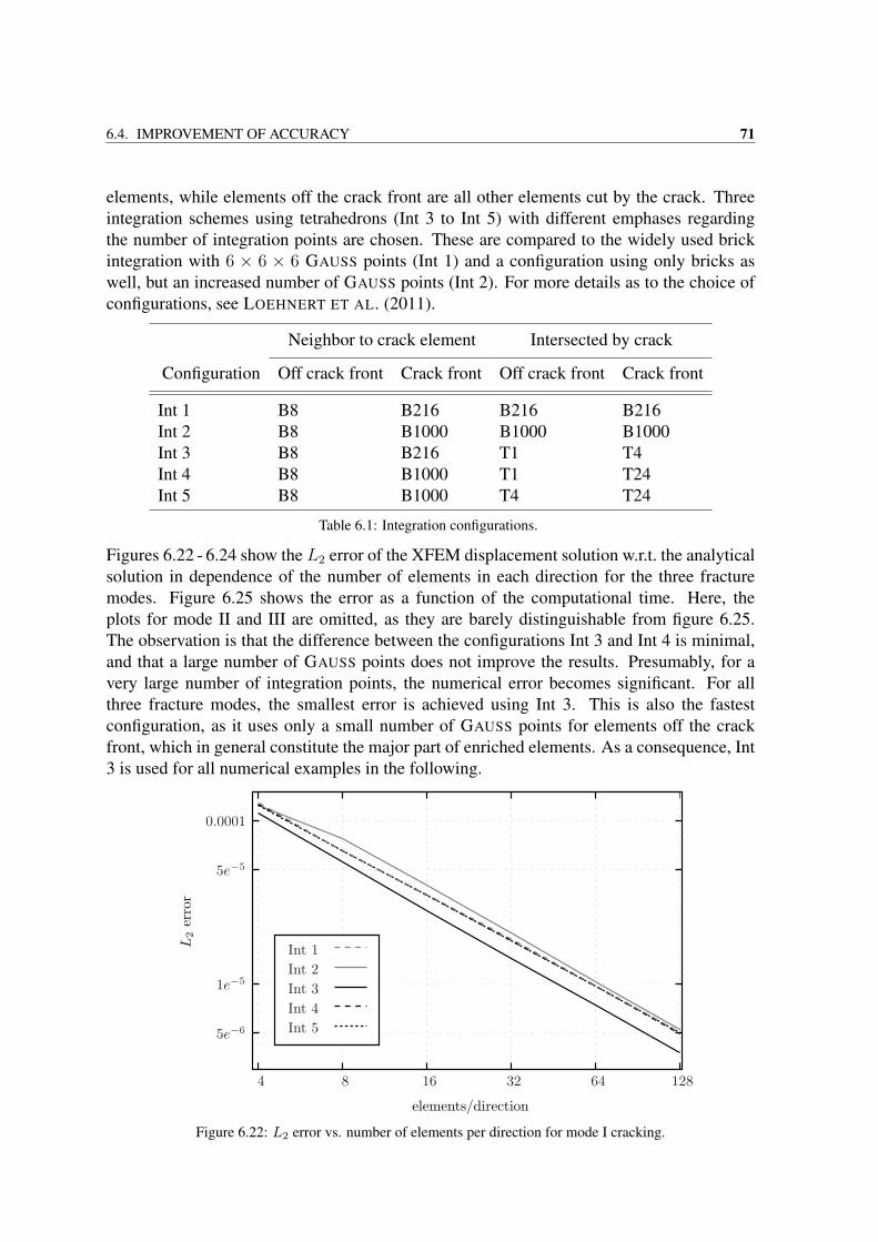
6.4. IMPROVEMENT OF ACCURACY 71
elements, while elements off the crack front are all other elements cut by the crack. Threeintegration schemes using tetrahedrons (Int 3 to Int 5) with different emphases regardingthe number of integration points are chosen. These are compared to the widely used brickintegration with 6 × 6 × 6 GAUSS points (Int 1) and a configuration using only bricks aswell, but an increased number of GAUSS points (Int 2). For more details as to the choice ofconfigurations, see LOEHNERT ET AL. (2011).
Neighbor to crack element Intersected by crack
Configuration Off crack front Crack front Off crack front Crack front
Int 1 B8 B216 B216 B216Int 2 B8 B1000 B1000 B1000Int 3 B8 B216 T1 T4Int 4 B8 B1000 T1 T24Int 5 B8 B1000 T4 T24
Table 6.1: Integration configurations.
Figures 6.22 - 6.24 show the L2 error of the XFEM displacement solution w.r.t. the analyticalsolution in dependence of the number of elements in each direction for the three fracturemodes. Figure 6.25 shows the error as a function of the computational time. Here, theplots for mode II and III are omitted, as they are barely distinguishable from figure 6.25.The observation is that the difference between the configurations Int 3 and Int 4 is minimal,and that a large number of GAUSS points does not improve the results. Presumably, for avery large number of integration points, the numerical error becomes significant. For allthree fracture modes, the smallest error is achieved using Int 3. This is also the fastestconfiguration, as it uses only a small number of GAUSS points for elements off the crackfront, which in general constitute the major part of enriched elements. As a consequence, Int3 is used for all numerical examples in the following.
elements/direction
L2
erro
r
Int 1Int 2Int 3Int 4Int 55e−6
1e−5
5e−5
0.0001
4 8 16 32 64 128
Figure 6.22: L2 error vs. number of elements per direction for mode I cracking.
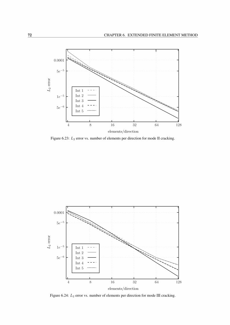
72 CHAPTER 6. EXTENDED FINITE ELEMENT METHOD
elements/direction
L2
erro
r
Int 1Int 2Int 3Int 4Int 5
5e−5
0.0001
4 8 16 32 64 128
5e−6
1e−5
Figure 6.23: L2 error vs. number of elements per direction for mode II cracking.
elements/direction
L2
erro
r
Int 1Int 2Int 3Int 4Int 5
1e−5
5e−5
4 8 16 32 64 128
0.0001
5e−6
Figure 6.24: L2 error vs. number of elements per direction for mode III cracking.
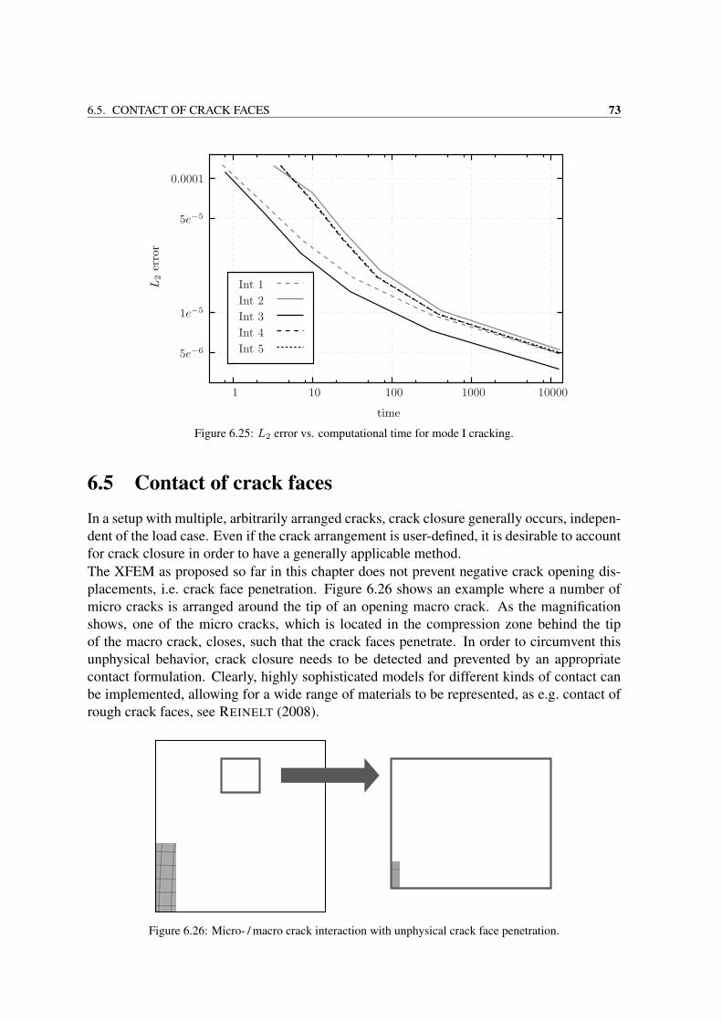
6.5. CONTACT OF CRACK FACES 73
L2
erro
r
time
Int 1Int 2Int 3Int 4Int 55e−6
1e−5
5e−5
0.0001
1 10 100 1000 10000
Figure 6.25: L2 error vs. computational time for mode I cracking.
6.5 Contact of crack facesIn a setup with multiple, arbitrarily arranged cracks, crack closure generally occurs, indepen-dent of the load case. Even if the crack arrangement is user-defined, it is desirable to accountfor crack closure in order to have a generally applicable method.The XFEM as proposed so far in this chapter does not prevent negative crack opening dis-placements, i.e. crack face penetration. Figure 6.26 shows an example where a number ofmicro cracks is arranged around the tip of an opening macro crack. As the magnificationshows, one of the micro cracks, which is located in the compression zone behind the tipof the macro crack, closes, such that the crack faces penetrate. In order to circumvent thisunphysical behavior, crack closure needs to be detected and prevented by an appropriatecontact formulation. Clearly, highly sophisticated models for different kinds of contact canbe implemented, allowing for a wide range of materials to be represented, as e.g. contact ofrough crack faces, see REINELT (2008).
Figure 6.26: Micro- / macro crack interaction with unphysical crack face penetration.
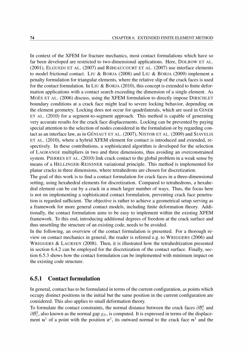
74 CHAPTER 6. EXTENDED FINITE ELEMENT METHOD
In context of the XFEM for fracture mechanics, most contact formulations which have sofar been developed are restricted to two-dimensional applications. Here, DOLBOW ET AL.(2001), ELGUEDJ ET AL. (2007) and RIBEAUCOURT ET AL. (2007) use interface elementsto model frictional contact. LIU & BORJA (2008) and LIU & BORJA (2009) implement apenalty formulation for triangular elements, where the relative slip of the crack faces is usedfor the contact formulation. In LIU & BORJA (2010), this concept is extended to finite defor-mation applications with a contact search exceeding the dimension of a single element. AsMOES ET AL. (2006) discuss, using the XFEM formulation to directly impose DIRICHLET
boundary conditions at a crack face might lead to severe locking behavior, depending onthe element geometry. Locking does not occur for quadrilaterals, which are used in GINER
ET AL. (2010) for a segment-to-segment approach. This method is capable of generatingvery accurate results for the crack face displacements. Locking can be prevented by payingspecial attention to the selection of nodes considered in the formulation or by regarding con-tact as an interface law, as in GENIAUT ET AL. (2007), NISTOR ET AL. (2009) and SIAVELIS
ET AL. (2010), where a hybrid XFEM element for contact is introduced and extended, re-spectively. In these contributions, a sophisticated algorithm is developed for the selectionof LAGRANGE multipliers in two and three dimensions, thus avoiding an overconstrainedsystem. PIERRES ET AL. (2010) link crack contact to the global problem in a weak sense bymeans of a HELLINGER-REISSNER variational principle. This method is implemented forplanar cracks in three dimensions, where tetrahedrons are chosen for discretization.The goal of this work is to find a contact formulation for crack faces in a three-dimensionalsetting, using hexahedral elements for discretization. Compared to tetrahedrons, a hexahe-dral element can be cut by a crack in a much larger number of ways. Thus, the focus hereis not on implementing a sophisticated contact formulation, preventing crack face penetra-tion is regarded sufficient. The objective is rather to achieve a geometrical setup serving asa framework for more general contact models, including finite deformation theory. Addi-tionally, the contact formulation aims to be easy to implement within the existing XFEMframework. To this end, introducing additional degrees of freedom at the crack surface andthus unsettling the structure of an existing code, needs to be avoided.In the following, an overview of the contact formulation is presented. For a thorough re-view on contact mechanics in general, the reader is referred e.g. to WRIGGERS (2006) andWRIGGERS & LAURSEN (2008). Then, it is illustrated how the tetrahedrization presentedin section 6.4.2 can be employed for the discretization of the contact surface. Finally, sec-tion 6.5.3 shows how the contact formulation can be implemented with minimum impact onthe existing code structure.
6.5.1 Contact formulation
In general, contact has to be formulated in terms of the current configuration, as points whichoccupy distinct positions in the initial but the same position in the current configuration areconsidered. This also applies to small deformation theory.To formulate the contact constraints, the normal distance between the crack faces ∂B1
c and∂B2
c , also known as the normal gap gN , is computed. It is expressed in terms of the displace-ment u1 of a point with the position x1, its outward normal to the crack face n1 and the
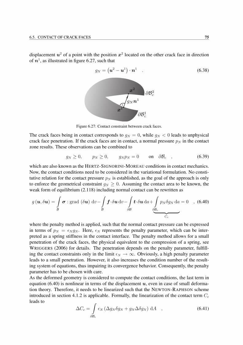
6.5. CONTACT OF CRACK FACES 75
displacement u2 of a point with the position x2 located on the other crack face in directionof n1, as illustrated in figure 6.27, such that
gN =(u2 − u1
)· n1 . (6.38)
•
•
Figure 6.27: Contact constraint between crack faces.
The crack faces being in contact corresponds to gN = 0, while gN < 0 leads to unphysicalcrack face penetration. If the crack faces are in contact, a normal pressure pN in the contactzone results. These observations can be combined to
gN ≥ 0, pN ≥ 0, gNpN = 0 on ∂Bc , (6.39)
which are also known as the HERTZ-SIGNORINI-MOREAU conditions in contact mechanics.Now, the contact conditions need to be considered in the variational formulation. No consti-tutive relation for the contact pressure pN is established, as the goal of the approach is onlyto enforce the geometrical constraint gN ≥ 0. Assuming the contact area to be known, theweak form of equilibrium (2.118) including normal contact can be rewritten as
g (u, δu) =
∫B
σ : grad (δu) dv−∫B
f ·δu dv−∫∂B
t·δu da+
∫∂Bc
pNδgN da
︸ ︷︷ ︸Cc
= 0 , (6.40)
where the penalty method is applied, such that the normal contact pressure can be expressedin terms of pN = εNgN . Here, εN represents the penalty parameter, which can be inter-preted as a spring stiffness in the contact interface. The penalty method allows for a smallpenetration of the crack faces, the physical equivalent to the compression of a spring, seeWRIGGERS (2006) for details. The penetration depends on the penalty parameter, fulfill-ing the contact constraints only in the limit εN → ∞. Obviously, a high penalty parameterleads to a small penetration. However, it also increases the condition number of the result-ing system of equations, thus impairing its convergence behavior. Consequently, the penaltyparameter has to be chosen with care.As the deformed geometry is considered to compute the contact conditions, the last term inequation (6.40) is nonlinear in terms of the displacement u, even in case of small deforma-tion theory. Therefore, it needs to be linearized such that the NEWTON-RAPHSON schemeintroduced in section 4.1.2 is applicable. Formally, the linearization of the contact term Ccleads to
∆Cc =
∫∂Bc
εN (∆gNδgN + gN∆δgN) dA , (6.41)
76 CHAPTER 6. EXTENDED FINITE ELEMENT METHOD
which depends on the discretization of the contact surface and the desired convergence be-havior of the NEWTON-RAPHSON method.
6.5.2 Contact surface discretizationFor the contact surface discretization, the obvious approach is to employ the tetrahedrizationof cracked elements as introduced in section 6.4.2, as here, the crack surface is discretizedalong the way of constructing the tetrahedrons. For nonplanar cracks, this approach onlyyields an approximation of the crack geometry, however, the triangles can be refined if de-sired.Based on this crack surface discretization, an established contact formulation like node-to-segment contact can be applied. Thus, numerical problems which are apparently XFEM-related, like the locking behavior observed in MOES ET AL. (2006), can be avoided. Ad-ditionally, the formulation is kept flexible for the incorporation of more advanced contactmodels.Here, node-to-segment (NTS) contact as examined in detail in WRIGGERS (2006) is used.In contrast to standard contact mechanics, where two distinct bodies (master and slave) areconsidered, only one single body exists in case of crack face contact. Thus, instead of defin-ing a master and a slave body, a master and a slave crack face are defined, where the choiceis arbitrary. Based on this definition, contact of a slave node with coordinates x2 to a mastertriangle defined by the points x1
1, x12 and x1
3 is considered, as depicted in figure 6.28. Op-posed to the definition of the normal gap given in equation (6.38), the outward normal at theslave node is employed, such that
gN =(u1 − u2
)· n2 . (6.42)
In the converged state, both definitions yield the same result.
•
•
Figure 6.28: Node-to-segment contact.
The slave nodes are simply given by the points defining the triangles discretizing the cracksurface. It has to be noted that, as the continuum equations imply contact at the crack front,care has to be taken not to include points located at the crack front into the contact formu-lation. Applying contact constraints at the crack front would overdetermine the mechanicalsystem and thus lead to a singular system of equations.Then, for all slave nodes i which are not located at the crack front, the outward normal tothe crack face n2
i is computed as the average of the normals of the nS adjoining trianglesdiscretizing the crack surface,
n2i =
1
nS
nS∑j=1
nj . (6.43)
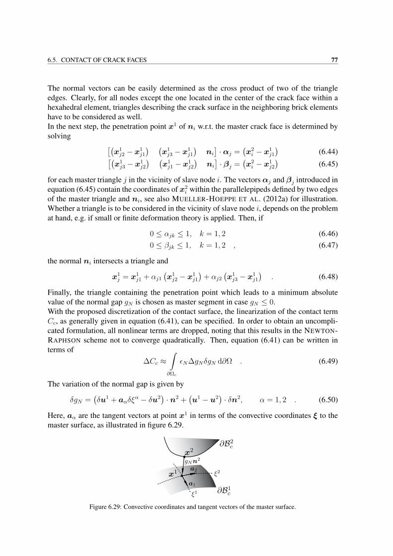
6.5. CONTACT OF CRACK FACES 77
The normal vectors can be easily determined as the cross product of two of the triangleedges. Clearly, for all nodes except the one located in the center of the crack face within ahexahedral element, triangles describing the crack surface in the neighboring brick elementshave to be considered as well.In the next step, the penetration point x1 of ni w.r.t. the master crack face is determined bysolving [(
x1j2 − x1
j1
) (x1j3 − x1
j1
)ni]·αj =
(x2i − x1
j1
)(6.44)[(
x1j3 − x1
j2
) (x1j1 − x1
j2
)ni]· βj =
(x2i − x1
j2
)(6.45)
for each master triangle j in the vicinity of slave node i. The vectorsαj and βj introduced inequation (6.45) contain the coordinates of x2
i within the parallelepipeds defined by two edgesof the master triangle and ni, see also MUELLER-HOEPPE ET AL. (2012a) for illustration.Whether a triangle is to be considered in the vicinity of slave node i, depends on the problemat hand, e.g. if small or finite deformation theory is applied. Then, if
0 ≤ αjk ≤ 1, k = 1, 2 (6.46)0 ≤ βjk ≤ 1, k = 1, 2 , (6.47)
the normal ni intersects a triangle and
x1j = x1
j1 + αj1(x1j2 − x1
j1
)+ αj2
(x1j3 − x1
j1
). (6.48)
Finally, the triangle containing the penetration point which leads to a minimum absolutevalue of the normal gap gN is chosen as master segment in case gN ≤ 0.With the proposed discretization of the contact surface, the linearization of the contact termCc, as generally given in equation (6.41), can be specified. In order to obtain an uncompli-cated formulation, all nonlinear terms are dropped, noting that this results in the NEWTON-RAPHSON scheme not to converge quadratically. Then, equation (6.41) can be written interms of
∆Cc ≈∫∂Ωc
εN∆gNδgN d∂Ω . (6.49)
The variation of the normal gap is given by
δgN =(δu1 + aαδξ
α − δu2)· n2 +
(u1 − u2
)· δn2, α = 1, 2 . (6.50)
Here, aα are the tangent vectors at point x1 in terms of the convective coordinates ξ to themaster surface, as illustrated in figure 6.29.
Figure 6.29: Convective coordinates and tangent vectors of the master surface.
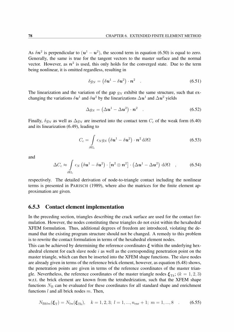
78 CHAPTER 6. EXTENDED FINITE ELEMENT METHOD
As δn2 is perpendicular to (u1 − u2), the second term in equation (6.50) is equal to zero.Generally, the same is true for the tangent vectors to the master surface and the normalvector. However, as n2 is used, this only holds for the converged state. Due to the termbeing nonlinear, it is omitted regardless, resulting in
δgN =(δu1 − δu2
)· n2 . (6.51)
The linearization and the variation of the gap gN exhibit the same structure, such that ex-changing the variations δu1 and δu2 by the linearizations ∆u1 and ∆u2 yields
∆gN =(∆u1 −∆u2
)· n2 . (6.52)
Finally, δgN as well as ∆gN are inserted into the contact term Cc of the weak form (6.40)and its linearization (6.49), leading to
Cc =
∫∂Ωc
εNgN(δu1 − δu2
)· n2 d∂Ω (6.53)
and
∆Cc ≈∫∂Ωc
εN(δu1 − δu2
)·[n2 ⊗ n2
]·(∆u1 −∆u2
)d∂Ω , (6.54)
respectively. The detailed derivation of node-to-triangle contact including the nonlinearterms is presented in PARISCH (1989), where also the matrices for the finite element ap-proximation are given.
6.5.3 Contact element implementation
In the preceding section, triangles describing the crack surface are used for the contact for-mulation. However, the nodes constituting these triangles do not exist within the hexahedralXFEM formulation. Thus, additional degrees of freedom are introduced, violating the de-mand that the existing program structure should not be changed. A remedy to this problemis to rewrite the contact formulation in terms of the hexahedral element nodes.This can be achieved by determining the reference coordinates ξ within the underlying hex-ahedral element for each slave node i as well as the corresponding penetration point on themaster triangle, which can then be inserted into the XFEM shape functions. The slave nodesare already given in terms of the reference brick element, however, as equation (6.48) shows,the penetration points are given in terms of the reference coordinates of the master trian-gle. Nevertheless, the reference coordinates of the master triangle nodes ξTk; (k = 1, 2, 3)w.r.t. the brick element are known from the tetrahedrization, such that the XFEM shapefunctions NB can be evaluated for these coordinates for all standard shape and enrichmentfunctions l and all brick nodes m. Then,
NBklm(ξT) = Nlm(ξTk), k = 1, 2, 3; l = 1, ..., nenr + 1; m = 1, ..., 8 . (6.55)
6.5. CONTACT OF CRACK FACES 79
These shape functions are combined with the standard shape functions for a linear triangleas depicted in figure 6.30, given by
NT1(ξ1) = 1− ξ − η (6.56)
NT2(ξ1) = ξ (6.57)
NT2(ξ1) = η . (6.58)
The reference coordinates of the penetration point in terms of the triangle ξ1 are calculatedfrom the parameters α1 and α2 used in equation (6.47). This finally results in the XFEMbrick shape functions evaluated for the penetration point being
NBlm(ξ1) =3∑
k=1
NBklm(ξT)NTk(ξ1), l = 1, ..., nenr + 1; m = 1, ..., 8 . (6.59)
Figure 6.30: Reference linear triangle.
The discretized versions of the weak form given in equation (6.53) and the linearization givenin equation (6.54) can be expressed in terms of
Cc ≈ δˆuT εNgNAˆN (6.60)
∆Cc ≈ δˆuT εNAˆN ˆNT∆ˆu (6.61)
for each slave node on the crack surface which is in contact. Here, the area of the mastertriangle containing the penetration point is denoted by A. Similarly to standard node-to-segment contact formulations, the vectors δˆu and ∆ˆu comprise the variation and lineariza-tion, respectively, of the nodal degrees of freedom for the hexahedral element in which themaster triangle is located, as well as the nodal degrees of freedom for the hexahedral elementin which the slave node is located. The shape function vector is given by
ˆN =
(NIi(ξ
1)n2
−NJj(ξ2)n2
),
I = 1, ..., 8; i = 1, ..., nenr(I) + 1; J = 1, ..., 8; j = 1, ..., nenr(J) + 1 . (6.62)
Without any restrictions like small deformation contact, this formulation results in a 16 nodecontact element. For the special case that contact occurs within one hexahedral element,the nodal sets I and J are the same. Thus, the proposed element is able to handle contactbetween any two underlying brick elements, which is essential for an application to finitedeformation theory.
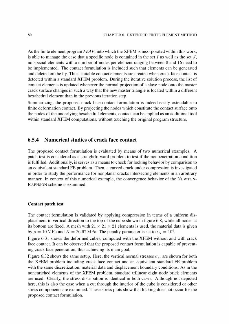
80 CHAPTER 6. EXTENDED FINITE ELEMENT METHOD
As the finite element program FEAP, into which the XFEM is incorporated within this work,is able to manage the case that a specific node is contained in the set I as well as the set J ,no special elements with a number of nodes per element ranging between 8 and 16 need tobe implemented. The contact formulation is included such that elements can be generatedand deleted on the fly. Thus, suitable contact elements are created when crack face contact isdetected within a standard XFEM problem. During the iterative solution process, the list ofcontact elements is updated whenever the normal projection of a slave node onto the mastercrack surface changes in such a way that the new master triangle is located within a differenthexahedral element than in the previous iteration step.Summarizing, the proposed crack face contact formulation is indeed easily extendable tofinite deformation contact. By projecting the nodes which constitute the contact surface ontothe nodes of the underlying hexahedral elements, contact can be applied as an additional toolwithin standard XFEM computations, without touching the original program structure.
6.5.4 Numerical studies of crack face contact
The proposed contact formulation is evaluated by means of two numerical examples. Apatch test is considered as a straightforward problem to test if the nonpenetration conditionis fulfilled. Additionally, is serves as a means to check for locking behavior by comparison toan equivalent standard FE problem. Then, a curved crack under compression is investigatedin order to study the performance for nonplanar cracks intersecting elements in an arbitrarymanner. In context of this numerical example, the convergence behavior of the NEWTON-RAPHSON scheme is examined.
Contact patch test
The contact formulation is validated by applying compression in terms of a uniform dis-placement in vertical direction to the top of the cube shown in figure 6.8, while all nodes atits bottom are fixed. A mesh with 21 × 21 × 21 elements is used, the material data is givenby µ = 10 MPa and K = 26.67 MPa. The penalty parameter is set to εN = 104.Figure 6.31 shows the deformed cubes, computed with the XFEM without and with crackface contact. It can be observed that the proposed contact formulation is capable of prevent-ing crack face penetration, thus achieving its main goal.Figure 6.32 shows the same setup. Here, the vertical normal stresses σzz are shown for boththe XFEM problem including crack face contact and an equivalent standard FE problemwith the same discretization, material data and displacement boundary conditions. As in thenonenriched elements of the XFEM problem, standard trilinear eight node brick elementsare used. Clearly, the stress distribution is identical in both cases. Although not depictedhere, this is also the case when a cut through the interior of the cube is considered or otherstress components are examined. These stress plots show that locking does not occur for theproposed contact formulation.
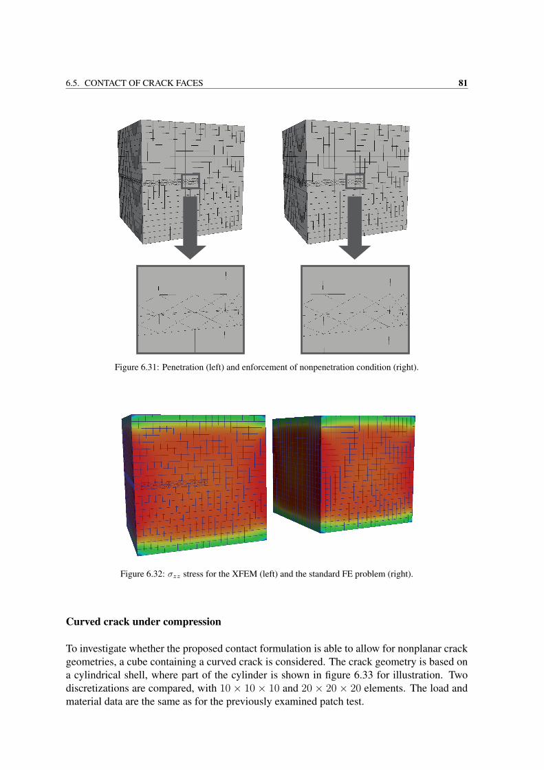
6.5. CONTACT OF CRACK FACES 81
Figure 6.31: Penetration (left) and enforcement of nonpenetration condition (right).
Figure 6.32: σzz stress for the XFEM (left) and the standard FE problem (right).
Curved crack under compression
To investigate whether the proposed contact formulation is able to allow for nonplanar crackgeometries, a cube containing a curved crack is considered. The crack geometry is based ona cylindrical shell, where part of the cylinder is shown in figure 6.33 for illustration. Twodiscretizations are compared, with 10 × 10 × 10 and 20 × 20 × 20 elements. The load andmaterial data are the same as for the previously examined patch test.
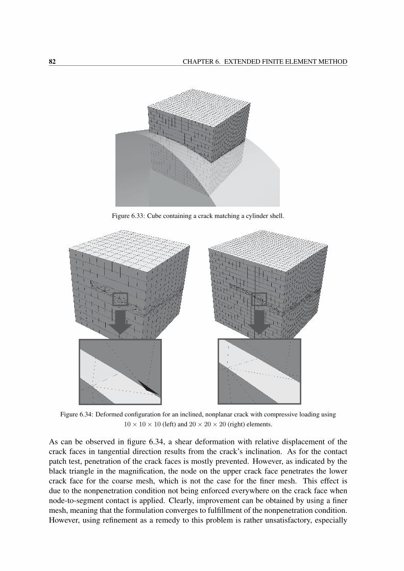
82 CHAPTER 6. EXTENDED FINITE ELEMENT METHOD
Figure 6.33: Cube containing a crack matching a cylinder shell.
Figure 6.34: Deformed configuration for an inclined, nonplanar crack with compressive loading using10× 10× 10 (left) and 20× 20× 20 (right) elements.
As can be observed in figure 6.34, a shear deformation with relative displacement of thecrack faces in tangential direction results from the crack’s inclination. As for the contactpatch test, penetration of the crack faces is mostly prevented. However, as indicated by theblack triangle in the magnification, the node on the upper crack face penetrates the lowercrack face for the coarse mesh, which is not the case for the finer mesh. This effect isdue to the nonpenetration condition not being enforced everywhere on the crack face whennode-to-segment contact is applied. Clearly, improvement can be obtained by using a finermesh, meaning that the formulation converges to fulfillment of the nonpenetration condition.However, using refinement as a remedy to this problem is rather unsatisfactory, especially
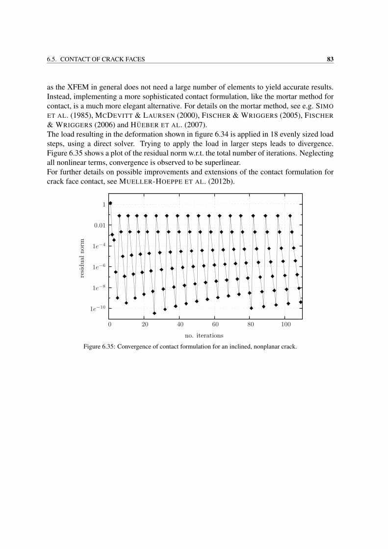
6.5. CONTACT OF CRACK FACES 83
as the XFEM in general does not need a large number of elements to yield accurate results.Instead, implementing a more sophisticated contact formulation, like the mortar method forcontact, is a much more elegant alternative. For details on the mortar method, see e.g. SIMO
ET AL. (1985), MCDEVITT & LAURSEN (2000), FISCHER & WRIGGERS (2005), FISCHER
& WRIGGERS (2006) and HUEBER ET AL. (2007).The load resulting in the deformation shown in figure 6.34 is applied in 18 evenly sized loadsteps, using a direct solver. Trying to apply the load in larger steps leads to divergence.Figure 6.35 shows a plot of the residual norm w.r.t. the total number of iterations. Neglectingall nonlinear terms, convergence is observed to be superlinear.For further details on possible improvements and extensions of the contact formulation forcrack face contact, see MUELLER-HOEPPE ET AL. (2012b).
1e−10
1e−6
0.01
1
0 20 40 60 80 100
1e−8
1e−4
no. iterations
resi
dual
norm
Figure 6.35: Convergence of contact formulation for an inclined, nonplanar crack.

84 CHAPTER 6. EXTENDED FINITE ELEMENT METHOD
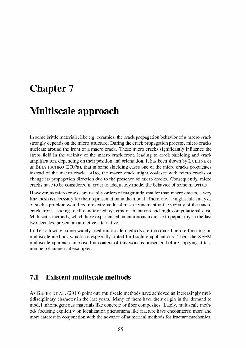
Chapter 7
Multiscale approach
In some brittle materials, like e.g. ceramics, the crack propagation behavior of a macro crackstrongly depends on the micro structure. During the crack propagation process, micro cracksnucleate around the front of a macro crack. These micro cracks significantly influence thestress field in the vicinity of the macro crack front, leading to crack shielding and crackamplification, depending on their position and orientation. It has been shown by LOEHNERT
& BELYTSCHKO (2007a), that in some shielding cases one of the micro cracks propagatesinstead of the macro crack. Also, the macro crack might coalesce with micro cracks orchange its propagation direction due to the presence of micro cracks. Consequently, microcracks have to be considered in order to adequately model the behavior of some materials.
However, as micro cracks are usually orders of magnitude smaller than macro cracks, a veryfine mesh is necessary for their representation in the model. Therefore, a singlescale analysisof such a problem would require extreme local mesh refinement in the vicinity of the macrocrack front, leading to ill-conditioned systems of equations and high computational cost.Multiscale methods, which have experienced an enormous increase in popularity in the lasttwo decades, present an attractive alternative.
In the following, some widely used multiscale methods are introduced before focusing onmultiscale methods which are especially suited for fracture applications. Then, the XFEMmultiscale approach employed in context of this work is presented before applying it to anumber of numerical examples.
7.1 Existent multiscale methods
As GEERS ET AL. (2010) point out, multiscale methods have achieved an increasingly mul-tidisciplinary character in the last years. Many of them have their origin in the demand tomodel inhomogeneous materials like concrete or fiber composites. Lately, multiscale meth-ods focusing explicitly on localization phenomena like fracture have encountered more andmore interest in conjunction with the advance of numerical methods for fracture mechanics.
85
86 CHAPTER 7. MULTISCALE APPROACH
7.1.1 General multiscale methodsDuring the 1990s, increasing computer power led to the desire to adequately model finescale features important to the overall behavior of a structure, and at the same time circum-vent the problem that a brute force singlescale analysis was (and is) in general not possible,and due to the large data output might not even be desirable, as pointed out in ZOHDI &WRIGGERS (2001). This resulted in different multiscale concepts based on separation ofscales between the structure and its fine scale properties. Examples are variational multi-scale methods, where the near field and far field solution are coupled by a variational for-mulation as in HUGHES (1995), and which have been extended to be able to deal with awide range of applications like nonlinear problems, see e.g. TERADA & KIKUCHI (2001)and MIEHE & BAYREUTHER (2007). In order to save computational effort, ZOHDI ET AL.(1996) and ODEN & ZOHDI (1997) estimate the error when homogenized material proper-ties are used, and only compute the more accurate fine scale material properties if the localerror is above a certain limit. The FE2 method introduced by FEYEL & CHABOCHE (2000)follows a different focus regarding computational effort. Here, a finite element problemwith microscopic features is solved at each macroscopic GAUSS point, such that no macro-scopic material model is necessary. Although parallel computing is an obvious approach inthis case, significant computational resources are required. Domain decomposition methodsfollow another principle. The computational domain is subdivided, such that finer meshesor different models can be used in regions of special interest and then glued to the modelwhich is used for the overall structure e.g by LAGRANGE multipliers (FARHAT (1991)) orthe ARLEQUIN method (BEN DHIA & RATEAU (2005)). Recently, the coupling of atomisticto continuum models within a multiscale context has received increasing interest (XIAO &BELYTSCHKO (2004) and CHEN & FISH (2006a,b)), as well as the treatment of structureswithout scale separation. Here, extensions of the above mentioned methods are exploited, ase.g. in FEYEL (2003) and KOUZNETSOVA ET AL. (2002) or ZOHDI & WRIGGERS (2001),who perform statistical studies on micro heterogeneous materials. Also, new approachesare introduced, see e.g. MIEHE & BAYREUTHER (2007) for a multigrid method or FISH &YUAN (2005) for enrichment of the coarse scale with fine scale features.An overview highlighting the benefits and limitations of general classes of multiscale meth-ods is given in GEERS ET AL. (2010).
7.1.2 Multiscale methods for fracture mechanicsAs indicated by GEERS ET AL. (2010), many of the multiscale methods introduced in sec-tion 7.1.1 are not suitable for fracture applications. This is due to the fact that they are basedon standard homogenization techniques using a representative volume element (RVE). TheRVE has to be chosen such that it is large enough to be statistically representative, but atthe same time has to be orders of magnitude smaller than the structure. This concept breaksdown in case of localizing phenomena, since the averaging of deformation and stress mea-sures smears the localizing effect, making the RVE behavior strongly dependent on the aver-aging domain and its size. Therefore, representativeness of the RVE cannot be maintained,as pointed out by LOEHNERT & MUELLER-HOEPPE (2008). Generally, this coincides withloss of material stability. Unfortunately, the limitations of RVE-based multiscale methods
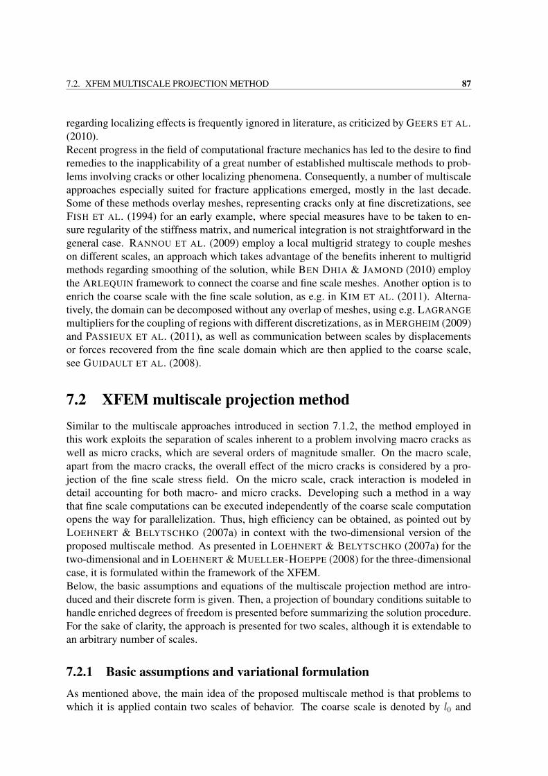
7.2. XFEM MULTISCALE PROJECTION METHOD 87
regarding localizing effects is frequently ignored in literature, as criticized by GEERS ET AL.(2010).Recent progress in the field of computational fracture mechanics has led to the desire to findremedies to the inapplicability of a great number of established multiscale methods to prob-lems involving cracks or other localizing phenomena. Consequently, a number of multiscaleapproaches especially suited for fracture applications emerged, mostly in the last decade.Some of these methods overlay meshes, representing cracks only at fine discretizations, seeFISH ET AL. (1994) for an early example, where special measures have to be taken to en-sure regularity of the stiffness matrix, and numerical integration is not straightforward in thegeneral case. RANNOU ET AL. (2009) employ a local multigrid strategy to couple mesheson different scales, an approach which takes advantage of the benefits inherent to multigridmethods regarding smoothing of the solution, while BEN DHIA & JAMOND (2010) employthe ARLEQUIN framework to connect the coarse and fine scale meshes. Another option is toenrich the coarse scale with the fine scale solution, as e.g. in KIM ET AL. (2011). Alterna-tively, the domain can be decomposed without any overlap of meshes, using e.g. LAGRANGE
multipliers for the coupling of regions with different discretizations, as in MERGHEIM (2009)and PASSIEUX ET AL. (2011), as well as communication between scales by displacementsor forces recovered from the fine scale domain which are then applied to the coarse scale,see GUIDAULT ET AL. (2008).
7.2 XFEM multiscale projection methodSimilar to the multiscale approaches introduced in section 7.1.2, the method employed inthis work exploits the separation of scales inherent to a problem involving macro cracks aswell as micro cracks, which are several orders of magnitude smaller. On the macro scale,apart from the macro cracks, the overall effect of the micro cracks is considered by a pro-jection of the fine scale stress field. On the micro scale, crack interaction is modeled indetail accounting for both macro- and micro cracks. Developing such a method in a waythat fine scale computations can be executed independently of the coarse scale computationopens the way for parallelization. Thus, high efficiency can be obtained, as pointed out byLOEHNERT & BELYTSCHKO (2007a) in context with the two-dimensional version of theproposed multiscale method. As presented in LOEHNERT & BELYTSCHKO (2007a) for thetwo-dimensional and in LOEHNERT & MUELLER-HOEPPE (2008) for the three-dimensionalcase, it is formulated within the framework of the XFEM.Below, the basic assumptions and equations of the multiscale projection method are intro-duced and their discrete form is given. Then, a projection of boundary conditions suitable tohandle enriched degrees of freedom is presented before summarizing the solution procedure.For the sake of clarity, the approach is presented for two scales, although it is extendable toan arbitrary number of scales.
7.2.1 Basic assumptions and variational formulationAs mentioned above, the main idea of the proposed multiscale method is that problems towhich it is applied contain two scales of behavior. The coarse scale is denoted by l0 and
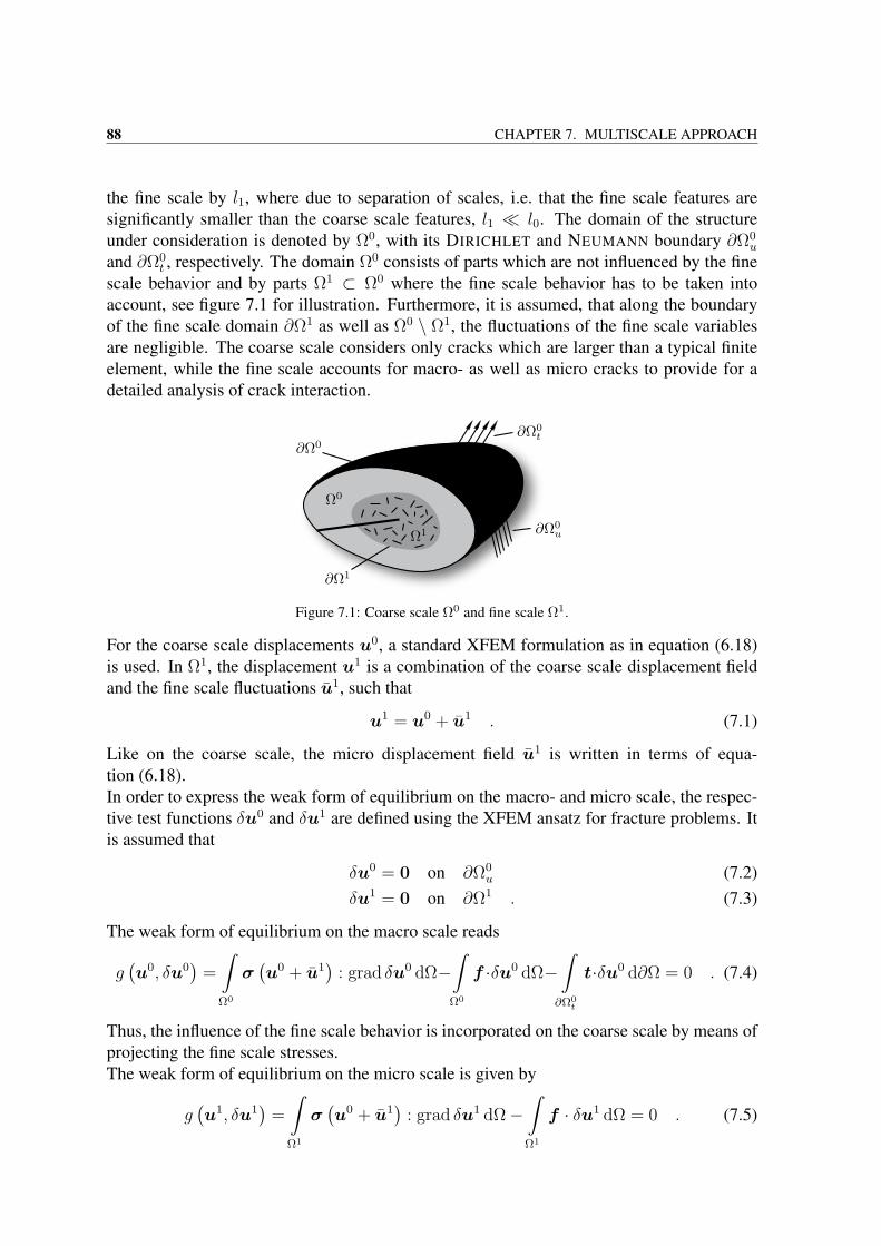
88 CHAPTER 7. MULTISCALE APPROACH
the fine scale by l1, where due to separation of scales, i.e. that the fine scale features aresignificantly smaller than the coarse scale features, l1 l0. The domain of the structureunder consideration is denoted by Ω0, with its DIRICHLET and NEUMANN boundary ∂Ω0
u
and ∂Ω0t , respectively. The domain Ω0 consists of parts which are not influenced by the fine
scale behavior and by parts Ω1 ⊂ Ω0 where the fine scale behavior has to be taken intoaccount, see figure 7.1 for illustration. Furthermore, it is assumed, that along the boundaryof the fine scale domain ∂Ω1 as well as Ω0 \ Ω1, the fluctuations of the fine scale variablesare negligible. The coarse scale considers only cracks which are larger than a typical finiteelement, while the fine scale accounts for macro- as well as micro cracks to provide for adetailed analysis of crack interaction.
Figure 7.1: Coarse scale Ω0 and fine scale Ω1.
For the coarse scale displacements u0, a standard XFEM formulation as in equation (6.18)is used. In Ω1, the displacement u1 is a combination of the coarse scale displacement fieldand the fine scale fluctuations u1, such that
u1 = u0 + u1 . (7.1)
Like on the coarse scale, the micro displacement field u1 is written in terms of equa-tion (6.18).In order to express the weak form of equilibrium on the macro- and micro scale, the respec-tive test functions δu0 and δu1 are defined using the XFEM ansatz for fracture problems. Itis assumed that
δu0 = 0 on ∂Ω0u (7.2)
δu1 = 0 on ∂Ω1 . (7.3)
The weak form of equilibrium on the macro scale reads
g(u0, δu0
)=
∫Ω0
σ(u0 + u1
): grad δu0 dΩ−
∫Ω0
f ·δu0 dΩ−∫∂Ω0
t
t·δu0 d∂Ω = 0 . (7.4)
Thus, the influence of the fine scale behavior is incorporated on the coarse scale by means ofprojecting the fine scale stresses.The weak form of equilibrium on the micro scale is given by
g(u1, δu1
)=
∫Ω1
σ(u0 + u1
): grad δu1 dΩ−
∫Ω1
f · δu1 dΩ = 0 . (7.5)
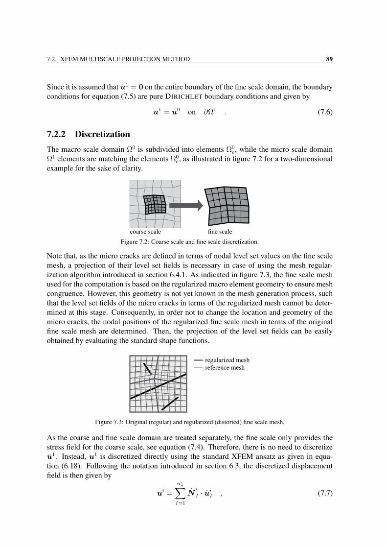
7.2. XFEM MULTISCALE PROJECTION METHOD 89
Since it is assumed that u1 = 0 on the entire boundary of the fine scale domain, the boundaryconditions for equation (7.5) are pure DIRICHLET boundary conditions and given by
u1 = u0 on ∂Ω1 . (7.6)
7.2.2 DiscretizationThe macro scale domain Ω0 is subdivided into elements Ω0
e, while the micro scale domainΩ1 elements are matching the elements Ω0
e, as illustrated in figure 7.2 for a two-dimensionalexample for the sake of clarity.
Figure 7.2: Coarse scale and fine scale discretization.
Note that, as the micro cracks are defined in terms of nodal level set values on the fine scalemesh, a projection of their level set fields is necessary in case of using the mesh regular-ization algorithm introduced in section 6.4.1. As indicated in figure 7.3, the fine scale meshused for the computation is based on the regularized macro element geometry to ensure meshcongruence. However, this geometry is not yet known in the mesh generation process, suchthat the level set fields of the micro cracks in terms of the regularized mesh cannot be deter-mined at this stage. Consequently, in order not to change the location and geometry of themicro cracks, the nodal positions of the regularized fine scale mesh in terms of the originalfine scale mesh are determined. Then, the projection of the level set fields can be easilyobtained by evaluating the standard shape functions.
Figure 7.3: Original (regular) and regularized (distorted) fine scale mesh.
As the coarse and fine scale domain are treated separately, the fine scale only provides thestress field for the coarse scale, see equation (7.4). Therefore, there is no need to discretizeu1. Instead, u1 is discretized directly using the standard XFEM ansatz as given in equa-tion (6.18). Following the notation introduced in section 6.3, the discretized displacementfield is then given by
ui =
nin∑I=1
Ni
I · uiI , (7.7)
90 CHAPTER 7. MULTISCALE APPROACH
where i indicates the scale, nin is the number of nodes on each scale and the vectors Ni
I anduiI contain the shape functions and degrees of freedom for each node on scale i, respectively.The discretized weak form of equilibrium on the macro scale then reads
n0e⋃
e=1
8∑I=1
δu0I
T
∫Ω0e
B0I
T
· σe(u0 + u1
)dΩ−
∫Ω0e
N0
I · f e dΩ−∫∂Ω0
e
N0
I · te d∂Ω
= 0 .
(7.8)Here, in the domain Ω0 \ Ω1 the stresses only depend on the macro displacement field dueto the assumption u1 !
= 0. In the domain Ω0 ∩ Ω1 the stresses depend on the fine scaledisplacement field, which is obtained from the discretized weak form of equilibrium on themicro scale
n1e⋃
e=1
8∑I=1
δu1I
T
∫Ω1e
B1I
T
· σe(u1)
dΩ−∫Ω1e
N1
I · f e dΩ
= 0 , (7.9)
where the traction term is dropped, as only DIRICHLET boundary conditions are applied tothe fine scale problem.In the domain Ω0 \ Ω1 of the macro scale problem, the integration scheme presented insection 6.4.2 is used. For all parts of the structure Ω0 ∩ Ω1 containing a micro domain, thecongruence of the finite element meshes is exploited by using∫
Ω0e
(·) dΩ =
n1e∑
j=1
∫Ω1je
(·) dΩ , (7.10)
where for the fine scale the proposed XFEM integration scheme is applied as well. In order tospeed up the integration process on the macro scale, it is feasible to use averaged quantitiesfor each micro scale element instead of considering each micro scale GAUSS integrationpoint.
7.2.3 Projection of boundary conditionsAs stated in equation (7.6), the boundary conditions for the fine scale domain are given bythe coarse scale displacement field, such that
u1 = u0 on ∂Ω1 (7.11)
in the discrete form. Even though the meshes on the macro- and micro scale are congruent,the enrichment functions of the coarse and fine scale displacement fields vary. Therefore, thenodal displacement boundary conditions on the fine scale domain cannot be determined byaid of the standard shape functions in general. Instead, a least-squares projection is used tocompute the proper nodal displacements, which is given by∫
Ω1
n1n∑
I=1
N1
I · u1I −
n0n⊂n1
n∑J=1
N0
J · u0J
· n1
n∑M=1
N1
M · δu1M
dΩ = 0 . (7.12)
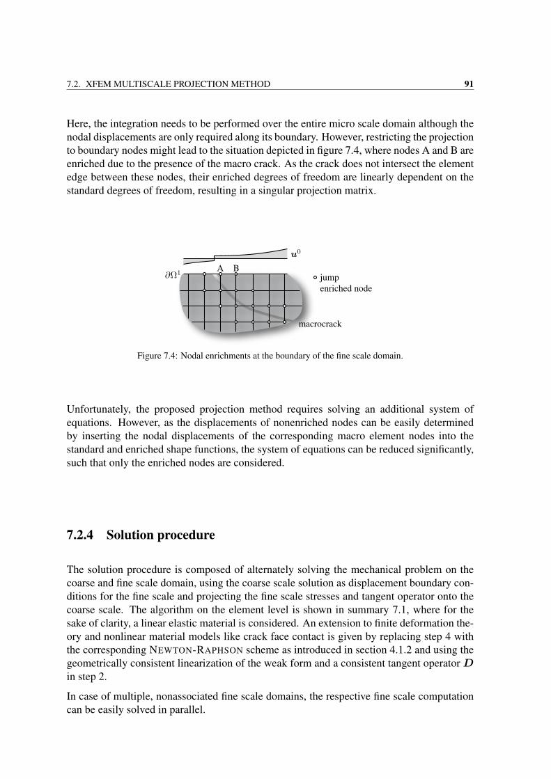
7.2. XFEM MULTISCALE PROJECTION METHOD 91
Here, the integration needs to be performed over the entire micro scale domain although thenodal displacements are only required along its boundary. However, restricting the projectionto boundary nodes might lead to the situation depicted in figure 7.4, where nodes A and B areenriched due to the presence of the macro crack. As the crack does not intersect the elementedge between these nodes, their enriched degrees of freedom are linearly dependent on thestandard degrees of freedom, resulting in a singular projection matrix.
Figure 7.4: Nodal enrichments at the boundary of the fine scale domain.
Unfortunately, the proposed projection method requires solving an additional system ofequations. However, as the displacements of nonenriched nodes can be easily determinedby inserting the nodal displacements of the corresponding macro element nodes into thestandard and enriched shape functions, the system of equations can be reduced significantly,such that only the enriched nodes are considered.
7.2.4 Solution procedure
The solution procedure is composed of alternately solving the mechanical problem on thecoarse and fine scale domain, using the coarse scale solution as displacement boundary con-ditions for the fine scale and projecting the fine scale stresses and tangent operator onto thecoarse scale. The algorithm on the element level is shown in summary 7.1, where for thesake of clarity, a linear elastic material is considered. An extension to finite deformation the-ory and nonlinear material models like crack face contact is given by replacing step 4 withthe corresponding NEWTON-RAPHSON scheme as introduced in section 4.1.2 and using thegeometrically consistent linearization of the weak form and a consistent tangent operatorDin step 2.
In case of multiple, nonassociated fine scale domains, the respective fine scale computationcan be easily solved in parallel.
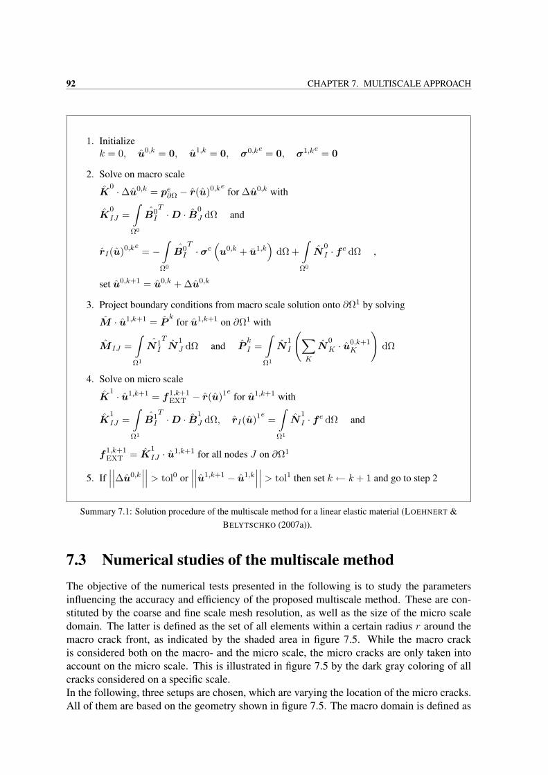
92 CHAPTER 7. MULTISCALE APPROACH
1. Initializek = 0, u0,k = 0, u1,k = 0, σ0,ke = 0, σ1,ke = 0
2. Solve on macro scale
K0 ·∆u0,k = pe∂Ω − r(u)0,ke for ∆u0,k with
K0IJ =
∫Ω0
B0I
T·D · B0
J dΩ and
rI(u)0,ke = −∫Ω0
B0I
T· σe
(u0,k + u1,k
)dΩ +
∫Ω0
N0I · f e dΩ ,
set u0,k+1 = u0,k + ∆u0,k
3. Project boundary conditions from macro scale solution onto ∂Ω1 by solving
M · u1,k+1 = Pk
for u1,k+1 on ∂Ω1 with
M IJ =∫Ω1
N1I
TN
1J dΩ and P
kI =
∫Ω1
N1I
(∑K
N0K · u0,k+1
K
)dΩ
4. Solve on micro scale
K1 · u1,k+1 = f1,k+1
EXT − r(u)1e for u1,k+1 with
K1IJ =
∫Ω1
B1I
T·D · B1
J dΩ, rI(u)1e =∫Ω1
N1I · f e dΩ and
f1,k+1EXT = K
1IJ · u1,k+1 for all nodes J on ∂Ω1
5. If∣∣∣∣∣∣∆u0,k
∣∣∣∣∣∣ > tol0 or∣∣∣∣∣∣u1,k+1 − u1,k
∣∣∣∣∣∣ > tol1 then set k ← k + 1 and go to step 2
Summary 7.1: Solution procedure of the multiscale method for a linear elastic material (LOEHNERT &BELYTSCHKO (2007a)).
7.3 Numerical studies of the multiscale methodThe objective of the numerical tests presented in the following is to study the parametersinfluencing the accuracy and efficiency of the proposed multiscale method. These are con-stituted by the coarse and fine scale mesh resolution, as well as the size of the micro scaledomain. The latter is defined as the set of all elements within a certain radius r around themacro crack front, as indicated by the shaded area in figure 7.5. While the macro crackis considered both on the macro- and the micro scale, the micro cracks are only taken intoaccount on the micro scale. This is illustrated in figure 7.5 by the dark gray coloring of allcracks considered on a specific scale.In the following, three setups are chosen, which are varying the location of the micro cracks.All of them are based on the geometry shown in figure 7.5. The macro domain is defined as
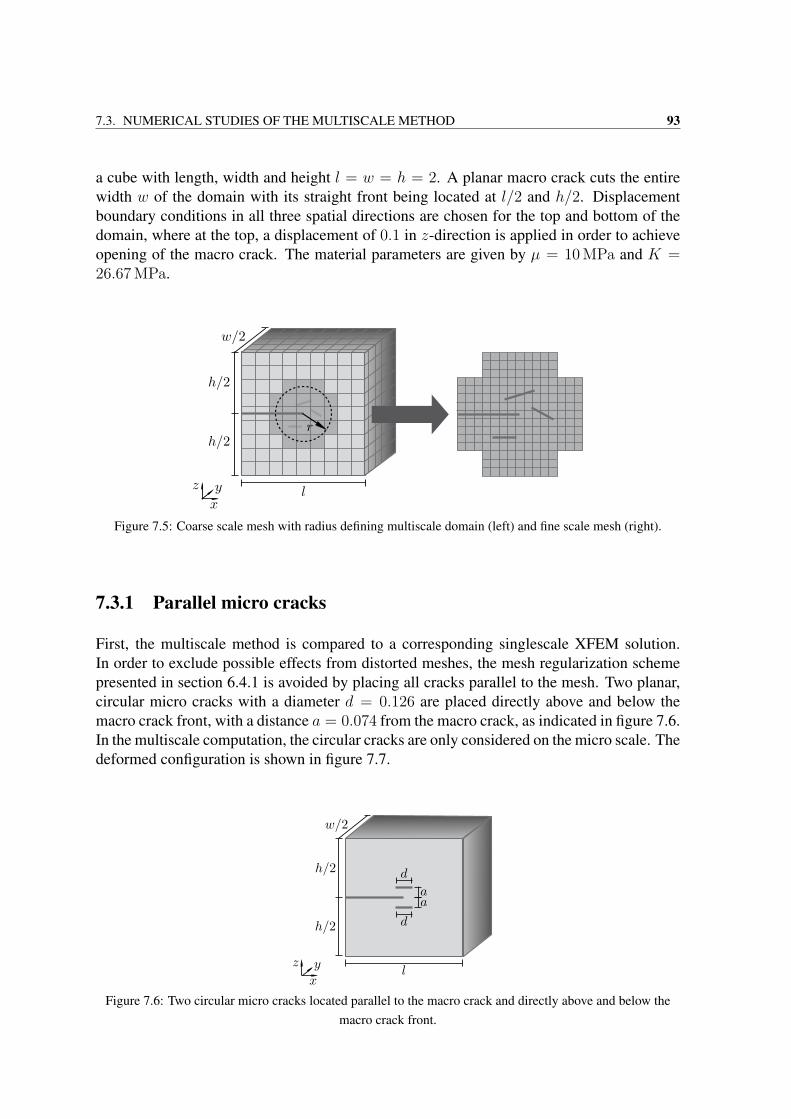
7.3. NUMERICAL STUDIES OF THE MULTISCALE METHOD 93
a cube with length, width and height l = w = h = 2. A planar macro crack cuts the entirewidth w of the domain with its straight front being located at l/2 and h/2. Displacementboundary conditions in all three spatial directions are chosen for the top and bottom of thedomain, where at the top, a displacement of 0.1 in z-direction is applied in order to achieveopening of the macro crack. The material parameters are given by µ = 10 MPa and K =26.67 MPa.
Figure 7.5: Coarse scale mesh with radius defining multiscale domain (left) and fine scale mesh (right).
7.3.1 Parallel micro cracks
First, the multiscale method is compared to a corresponding singlescale XFEM solution.In order to exclude possible effects from distorted meshes, the mesh regularization schemepresented in section 6.4.1 is avoided by placing all cracks parallel to the mesh. Two planar,circular micro cracks with a diameter d = 0.126 are placed directly above and below themacro crack front, with a distance a = 0.074 from the macro crack, as indicated in figure 7.6.In the multiscale computation, the circular cracks are only considered on the micro scale. Thedeformed configuration is shown in figure 7.7.
Figure 7.6: Two circular micro cracks located parallel to the macro crack and directly above and below themacro crack front.
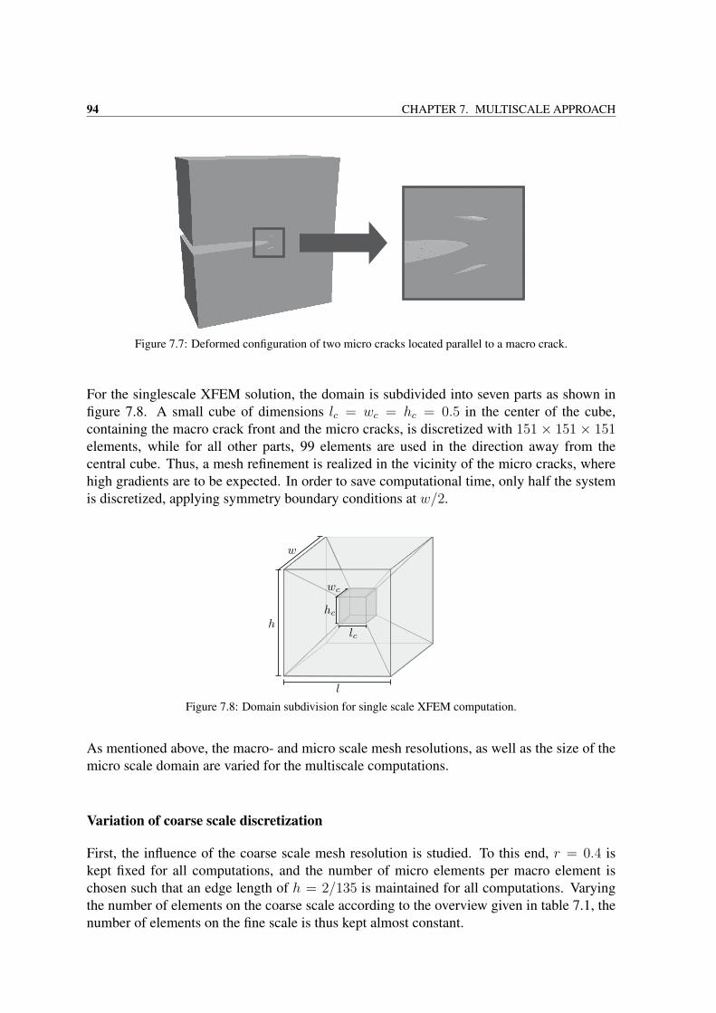
94 CHAPTER 7. MULTISCALE APPROACH
Figure 7.7: Deformed configuration of two micro cracks located parallel to a macro crack.
For the singlescale XFEM solution, the domain is subdivided into seven parts as shown infigure 7.8. A small cube of dimensions lc = wc = hc = 0.5 in the center of the cube,containing the macro crack front and the micro cracks, is discretized with 151 × 151 × 151elements, while for all other parts, 99 elements are used in the direction away from thecentral cube. Thus, a mesh refinement is realized in the vicinity of the micro cracks, wherehigh gradients are to be expected. In order to save computational time, only half the systemis discretized, applying symmetry boundary conditions at w/2.
Figure 7.8: Domain subdivision for single scale XFEM computation.
As mentioned above, the macro- and micro scale mesh resolutions, as well as the size of themicro scale domain are varied for the multiscale computations.
Variation of coarse scale discretization
First, the influence of the coarse scale mesh resolution is studied. To this end, r = 0.4 iskept fixed for all computations, and the number of micro elements per macro element ischosen such that an edge length of h = 2/135 is maintained for all computations. Varyingthe number of elements on the coarse scale according to the overview given in table 7.1, thenumber of elements on the fine scale is thus kept almost constant.
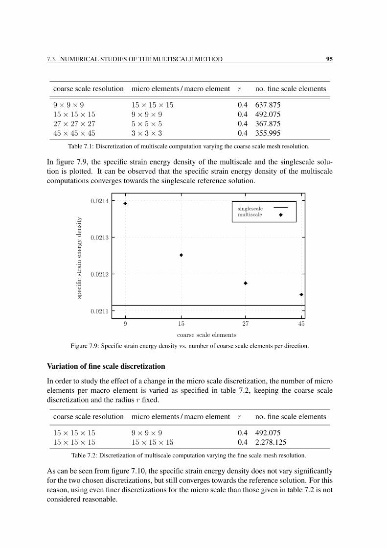
7.3. NUMERICAL STUDIES OF THE MULTISCALE METHOD 95
coarse scale resolution micro elements / macro element r no. fine scale elements
9× 9× 9 15× 15× 15 0.4 637.87515× 15× 15 9× 9× 9 0.4 492.07527× 27× 27 5× 5× 5 0.4 367.87545× 45× 45 3× 3× 3 0.4 355.995
Table 7.1: Discretization of multiscale computation varying the coarse scale mesh resolution.
In figure 7.9, the specific strain energy density of the multiscale and the singlescale solu-tion is plotted. It can be observed that the specific strain energy density of the multiscalecomputations converges towards the singlescale reference solution.
coarse scale elements
spec
ific
stra
inen
ergy
dens
ity
0.0212
0.0213
0.0214
9 15 27 45
0.0211
multiscalesinglescale
Figure 7.9: Specific strain energy density vs. number of coarse scale elements per direction.
Variation of fine scale discretization
In order to study the effect of a change in the micro scale discretization, the number of microelements per macro element is varied as specified in table 7.2, keeping the coarse scalediscretization and the radius r fixed.
coarse scale resolution micro elements / macro element r no. fine scale elements
15× 15× 15 9× 9× 9 0.4 492.07515× 15× 15 15× 15× 15 0.4 2.278.125
Table 7.2: Discretization of multiscale computation varying the fine scale mesh resolution.
As can be seen from figure 7.10, the specific strain energy density does not vary significantlyfor the two chosen discretizations, but still converges towards the reference solution. For thisreason, using even finer discretizations for the micro scale than those given in table 7.2 is notconsidered reasonable.
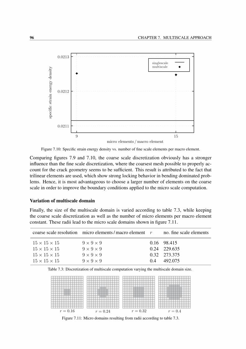
96 CHAPTER 7. MULTISCALE APPROACH
micro elements / macro element
spec
ific
stra
inen
ergy
dens
ity
0.0211
0.0212
0.0213
9 15
multiscalesinglescale
Figure 7.10: Specific strain energy density vs. number of fine scale elements per macro element.
Comparing figures 7.9 and 7.10, the coarse scale discretization obviously has a strongerinfluence than the fine scale discretization, where the coarsest mesh possible to properly ac-count for the crack geometry seems to be sufficient. This result is attributed to the fact thattrilinear elements are used, which show strong locking behavior in bending dominated prob-lems. Hence, it is most advantageous to choose a larger number of elements on the coarsescale in order to improve the boundary conditions applied to the micro scale computation.
Variation of multiscale domain
Finally, the size of the multiscale domain is varied according to table 7.3, while keepingthe coarse scale discretization as well as the number of micro elements per macro elementconstant. These radii lead to the micro scale domains shown in figure 7.11.
coarse scale resolution micro elements / macro element r no. fine scale elements
15× 15× 15 9× 9× 9 0.16 98.41515× 15× 15 9× 9× 9 0.24 229.63515× 15× 15 9× 9× 9 0.32 273.37515× 15× 15 9× 9× 9 0.4 492.075
Table 7.3: Discretization of multiscale computation varying the multiscale domain size.
Figure 7.11: Micro domains resulting from radii according to table 7.3.
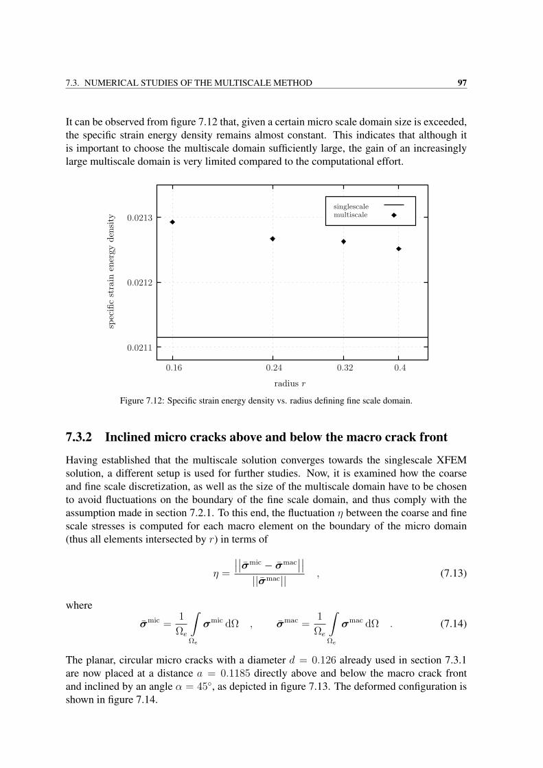
7.3. NUMERICAL STUDIES OF THE MULTISCALE METHOD 97
It can be observed from figure 7.12 that, given a certain micro scale domain size is exceeded,the specific strain energy density remains almost constant. This indicates that although itis important to choose the multiscale domain sufficiently large, the gain of an increasinglylarge multiscale domain is very limited compared to the computational effort.
radius r
spec
ific
stra
inen
ergy
dens
ity
0.0212
0.16 0.24 0.32 0.4
0.0213
0.0211
multiscalesinglescale
Figure 7.12: Specific strain energy density vs. radius defining fine scale domain.
7.3.2 Inclined micro cracks above and below the macro crack front
Having established that the multiscale solution converges towards the singlescale XFEMsolution, a different setup is used for further studies. Now, it is examined how the coarseand fine scale discretization, as well as the size of the multiscale domain have to be chosento avoid fluctuations on the boundary of the fine scale domain, and thus comply with theassumption made in section 7.2.1. To this end, the fluctuation η between the coarse and finescale stresses is computed for each macro element on the boundary of the micro domain(thus all elements intersected by r) in terms of
η =
∣∣∣∣σmic − σmac∣∣∣∣
||σmac|| , (7.13)
where
σmic =1
Ωe
∫Ωe
σmic dΩ , σmac =1
Ωe
∫Ωe
σmac dΩ . (7.14)
The planar, circular micro cracks with a diameter d = 0.126 already used in section 7.3.1are now placed at a distance a = 0.1185 directly above and below the macro crack frontand inclined by an angle α = 45, as depicted in figure 7.13. The deformed configuration isshown in figure 7.14.
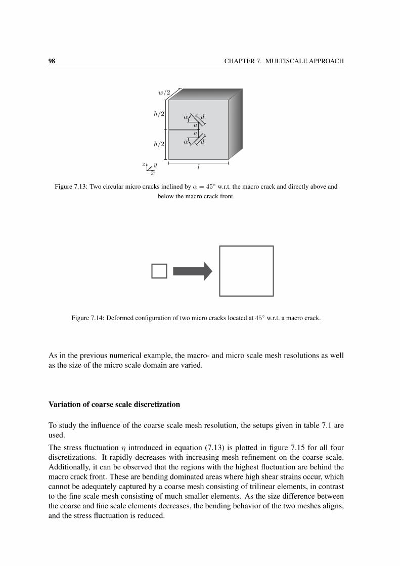
98 CHAPTER 7. MULTISCALE APPROACH
Figure 7.13: Two circular micro cracks inclined by α = 45 w.r.t. the macro crack and directly above andbelow the macro crack front.
Figure 7.14: Deformed configuration of two micro cracks located at 45 w.r.t. a macro crack.
As in the previous numerical example, the macro- and micro scale mesh resolutions as wellas the size of the micro scale domain are varied.
Variation of coarse scale discretization
To study the influence of the coarse scale mesh resolution, the setups given in table 7.1 areused.
The stress fluctuation η introduced in equation (7.13) is plotted in figure 7.15 for all fourdiscretizations. It rapidly decreases with increasing mesh refinement on the coarse scale.Additionally, it can be observed that the regions with the highest fluctuation are behind themacro crack front. These are bending dominated areas where high shear strains occur, whichcannot be adequately captured by a coarse mesh consisting of trilinear elements, in contrastto the fine scale mesh consisting of much smaller elements. As the size difference betweenthe coarse and fine scale elements decreases, the bending behavior of the two meshes aligns,and the stress fluctuation is reduced.
7.3. NUMERICAL STUDIES OF THE MULTISCALE METHOD 99
Figure 7.15: Stress fluctuation η varying the coarse scale discretization.
Variation of fine scale discretization
Using the examples introduced in table 7.2, the stress fluctuation varying the fine scale dis-cretization is investigated.
Figure 7.16 shows the stress fluctuation η for the two setups considered. As in section 7.3.1,the difference between the configurations is negligible, emphasizing that choosing an ade-quate coarse scale discretization is of much higher importance than using a very fine meshon the micro scale.
Figure 7.16: Stress fluctuation η varying the number of micro elements per macro element.
Variation of multiscale domain
As in the previous example, the influence of the micro scale domain size is examined byvarying the radius according to table 7.3.
The stress fluctuation η depicted in figure 7.17 shows that the bending dominated area behindthe crack front is the source of fluctuation. For r = 0.16, this area is not reached, while forr = 0.24, the boundary of the fine scale domain coincides with this high shear stress zone,leading to a high fluctuation. For larger radii, the fluctuation decreases and remains almostconstant, while the bending dominated area is still the main source of stress fluctuation.
100 CHAPTER 7. MULTISCALE APPROACH
Figure 7.17: Stress fluctuation η varying the micro scale domain size.
7.3.3 Inclined micro cracks in front of the macro crackAs a final example, the setup shown in figure 7.18 is chosen to study whether the behavior ofthis system is similar to the system investigated in section 7.3.2. Again, the stress fluctuationη defined in equation (7.13) is used as a measure for the quality of the coarse and fine scalediscretization and the size of the micro scale domain.In this case, the planar, circular micro cracks with diameter d = 0.126 are placed at a distancea = 0.1185 in the z-direction above and below the macro crack front and at the same distancea in the x-direction in front of the macro crack. The inclination is given by the angle α = 45,as indicated in figure 7.18. The deformed configuration is shown in figure 7.19.
Figure 7.18: Two circular micro cracks inclined by α = 45 w.r.t. the macro crack at a distance a from themacro crack front.
Figure 7.19: Deformed configuration of two micro cracks located at 45 w.r.t. the macro crack and in front ofthe macro crack.
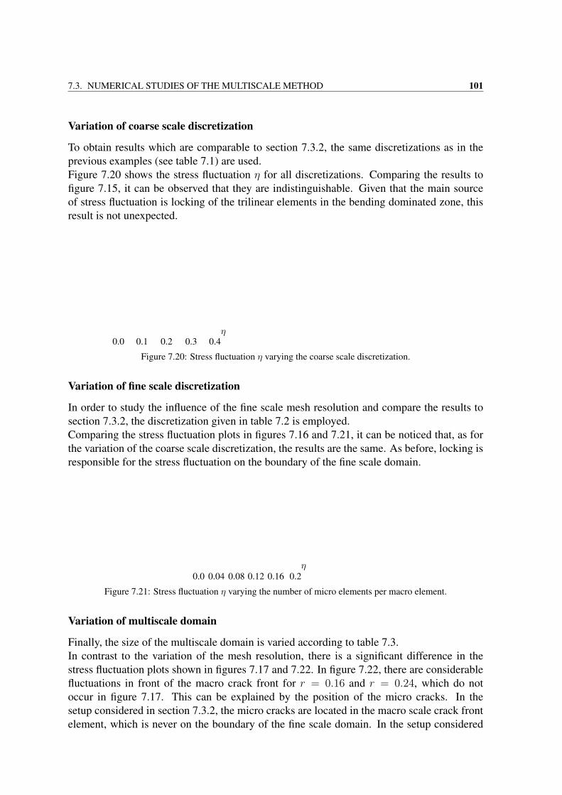
7.3. NUMERICAL STUDIES OF THE MULTISCALE METHOD 101
Variation of coarse scale discretization
To obtain results which are comparable to section 7.3.2, the same discretizations as in theprevious examples (see table 7.1) are used.Figure 7.20 shows the stress fluctuation η for all discretizations. Comparing the results tofigure 7.15, it can be observed that they are indistinguishable. Given that the main sourceof stress fluctuation is locking of the trilinear elements in the bending dominated zone, thisresult is not unexpected.
Figure 7.20: Stress fluctuation η varying the coarse scale discretization.
Variation of fine scale discretization
In order to study the influence of the fine scale mesh resolution and compare the results tosection 7.3.2, the discretization given in table 7.2 is employed.Comparing the stress fluctuation plots in figures 7.16 and 7.21, it can be noticed that, as forthe variation of the coarse scale discretization, the results are the same. As before, locking isresponsible for the stress fluctuation on the boundary of the fine scale domain.
Figure 7.21: Stress fluctuation η varying the number of micro elements per macro element.
Variation of multiscale domain
Finally, the size of the multiscale domain is varied according to table 7.3.In contrast to the variation of the mesh resolution, there is a significant difference in thestress fluctuation plots shown in figures 7.17 and 7.22. In figure 7.22, there are considerablefluctuations in front of the macro crack front for r = 0.16 and r = 0.24, which do notoccur in figure 7.17. This can be explained by the position of the micro cracks. In thesetup considered in section 7.3.2, the micro cracks are located in the macro scale crack frontelement, which is never on the boundary of the fine scale domain. In the setup considered
102 CHAPTER 7. MULTISCALE APPROACH
in this section, the micro cracks are located in macro scale elements which constitute theboundary of the fine scale domain for r = 0.16 and r = 0.24. Increasing the fine scaledomain beyond a radius r = 0.24, it can be observed that the influence of the micro crackson the stress fluctuation rapidly decreases.
Figure 7.22: Stress fluctuation η varying the micro scale domain size.
7.4 Performance of the multiscale projection methodThe numerical examples presented above show that varying the three parameters of the mul-tiscale method, i.e. coarse scale mesh resolution, fine scale mesh resolution and size of themultiscale domain, two main points greatly influence its performance.In all cases, the result is greatly improved by refining the coarse scale mesh, as thus, lockingowing to the trilinear ansatz functions can be reduced. However, this is not a specific problemof the proposed multiscale projection method, but of all computations using trilinear finiteelements.Another important aspect is the size of the multiscale domain. Here, it can be observedthat, beyond a certain size, no increase of accuracy can be obtained by further increasingthe multiscale domain. However, below that threshold, the multiscale domain size has asignificant effect on the results. Also, comparing figures 7.17 and 7.22, the position of themicro cracks strongly influences the required multiscale domain size.Considering that the influence of the micro cracks additionally depends on the applied load,as well as the position and orientation of the macro crack, it is clear that the results pre-sented in section 7.3 can only be perceived as a guideline. To efficiently apply the multiscaleprojection method, the parameters studied above should be chosen based on error estimation.
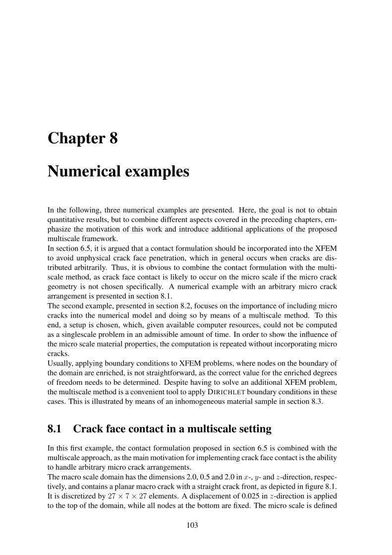
Chapter 8
Numerical examples
In the following, three numerical examples are presented. Here, the goal is not to obtainquantitative results, but to combine different aspects covered in the preceding chapters, em-phasize the motivation of this work and introduce additional applications of the proposedmultiscale framework.In section 6.5, it is argued that a contact formulation should be incorporated into the XFEMto avoid unphysical crack face penetration, which in general occurs when cracks are dis-tributed arbitrarily. Thus, it is obvious to combine the contact formulation with the multi-scale method, as crack face contact is likely to occur on the micro scale if the micro crackgeometry is not chosen specifically. A numerical example with an arbitrary micro crackarrangement is presented in section 8.1.The second example, presented in section 8.2, focuses on the importance of including microcracks into the numerical model and doing so by means of a multiscale method. To thisend, a setup is chosen, which, given available computer resources, could not be computedas a singlescale problem in an admissible amount of time. In order to show the influence ofthe micro scale material properties, the computation is repeated without incorporating microcracks.Usually, applying boundary conditions to XFEM problems, where nodes on the boundary ofthe domain are enriched, is not straightforward, as the correct value for the enriched degreesof freedom needs to be determined. Despite having to solve an additional XFEM problem,the multiscale method is a convenient tool to apply DIRICHLET boundary conditions in thesecases. This is illustrated by means of an inhomogeneous material sample in section 8.3.
8.1 Crack face contact in a multiscale settingIn this first example, the contact formulation proposed in section 6.5 is combined with themultiscale approach, as the main motivation for implementing crack face contact is the abilityto handle arbitrary micro crack arrangements.The macro scale domain has the dimensions 2.0, 0.5 and 2.0 in x-, y- and z-direction, respec-tively, and contains a planar macro crack with a straight crack front, as depicted in figure 8.1.It is discretized by 27 × 7 × 27 elements. A displacement of 0.025 in z-direction is appliedto the top of the domain, while all nodes at the bottom are fixed. The micro scale is defined
103
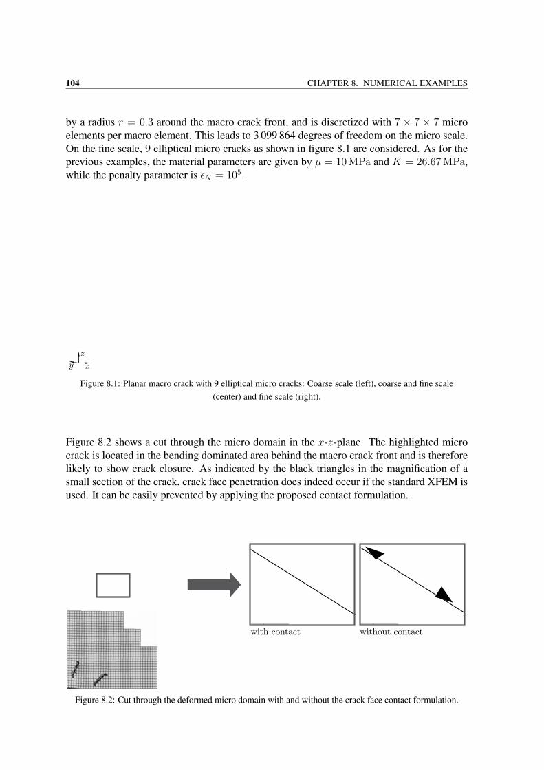
104 CHAPTER 8. NUMERICAL EXAMPLES
by a radius r = 0.3 around the macro crack front, and is discretized with 7 × 7 × 7 microelements per macro element. This leads to 3 099 864 degrees of freedom on the micro scale.On the fine scale, 9 elliptical micro cracks as shown in figure 8.1 are considered. As for theprevious examples, the material parameters are given by µ = 10 MPa and K = 26.67 MPa,while the penalty parameter is εN = 105.
Figure 8.1: Planar macro crack with 9 elliptical micro cracks: Coarse scale (left), coarse and fine scale(center) and fine scale (right).
Figure 8.2 shows a cut through the micro domain in the x-z-plane. The highlighted microcrack is located in the bending dominated area behind the macro crack front and is thereforelikely to show crack closure. As indicated by the black triangles in the magnification of asmall section of the crack, crack face penetration does indeed occur if the standard XFEM isused. It can be easily prevented by applying the proposed contact formulation.
Figure 8.2: Cut through the deformed micro domain with and without the crack face contact formulation.
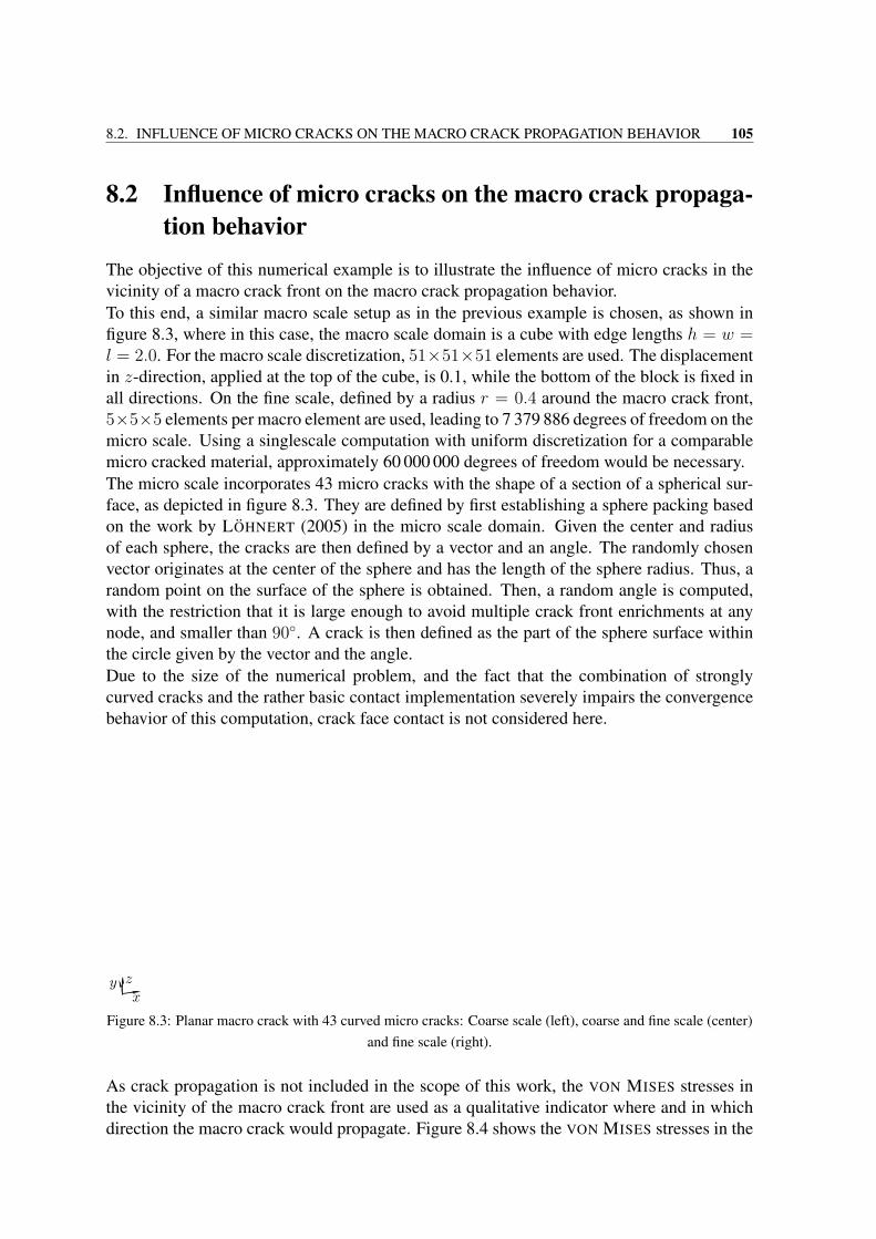
8.2. INFLUENCE OF MICRO CRACKS ON THE MACRO CRACK PROPAGATION BEHAVIOR 105
8.2 Influence of micro cracks on the macro crack propaga-tion behavior
The objective of this numerical example is to illustrate the influence of micro cracks in thevicinity of a macro crack front on the macro crack propagation behavior.To this end, a similar macro scale setup as in the previous example is chosen, as shown infigure 8.3, where in this case, the macro scale domain is a cube with edge lengths h = w =l = 2.0. For the macro scale discretization, 51×51×51 elements are used. The displacementin z-direction, applied at the top of the cube, is 0.1, while the bottom of the block is fixed inall directions. On the fine scale, defined by a radius r = 0.4 around the macro crack front,5×5×5 elements per macro element are used, leading to 7 379 886 degrees of freedom on themicro scale. Using a singlescale computation with uniform discretization for a comparablemicro cracked material, approximately 60 000 000 degrees of freedom would be necessary.The micro scale incorporates 43 micro cracks with the shape of a section of a spherical sur-face, as depicted in figure 8.3. They are defined by first establishing a sphere packing basedon the work by LOHNERT (2005) in the micro scale domain. Given the center and radiusof each sphere, the cracks are then defined by a vector and an angle. The randomly chosenvector originates at the center of the sphere and has the length of the sphere radius. Thus, arandom point on the surface of the sphere is obtained. Then, a random angle is computed,with the restriction that it is large enough to avoid multiple crack front enrichments at anynode, and smaller than 90. A crack is then defined as the part of the sphere surface withinthe circle given by the vector and the angle.Due to the size of the numerical problem, and the fact that the combination of stronglycurved cracks and the rather basic contact implementation severely impairs the convergencebehavior of this computation, crack face contact is not considered here.
Figure 8.3: Planar macro crack with 43 curved micro cracks: Coarse scale (left), coarse and fine scale (center)and fine scale (right).
As crack propagation is not included in the scope of this work, the VON MISES stresses inthe vicinity of the macro crack front are used as a qualitative indicator where and in whichdirection the macro crack would propagate. Figure 8.4 shows the VON MISES stresses in the
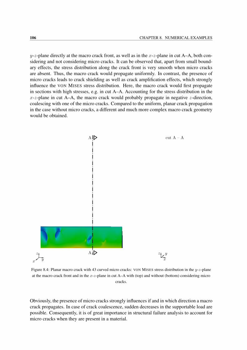
106 CHAPTER 8. NUMERICAL EXAMPLES
y-z-plane directly at the macro crack front, as well as in the x-z-plane in cut A–A, both con-sidering and not considering micro cracks. It can be observed that, apart from small bound-ary effects, the stress distribution along the crack front is very smooth when micro cracksare absent. Thus, the macro crack would propagate uniformly. In contrast, the presence ofmicro cracks leads to crack shielding as well as crack amplification effects, which stronglyinfluence the VON MISES stress distribution. Here, the macro crack would first propagatein sections with high stresses, e.g. in cut A–A. Accounting for the stress distribution in thex-z-plane in cut A–A, the macro crack would probably propagate in negative z-direction,coalescing with one of the micro cracks. Compared to the uniform, planar crack propagationin the case without micro cracks, a different and much more complex macro crack geometrywould be obtained.
Figure 8.4: Planar macro crack with 43 curved micro cracks: VON MISES stress distribution in the y-z-planeat the macro crack front and in the x-z-plane in cut A–A with (top) and without (bottom) considering micro
cracks.
Obviously, the presence of micro cracks strongly influences if and in which direction a macrocrack propagates. In case of crack coalescence, sudden decreases in the supportable load arepossible. Consequently, it is of great importance in structural failure analysis to account formicro cracks when they are present in a material.
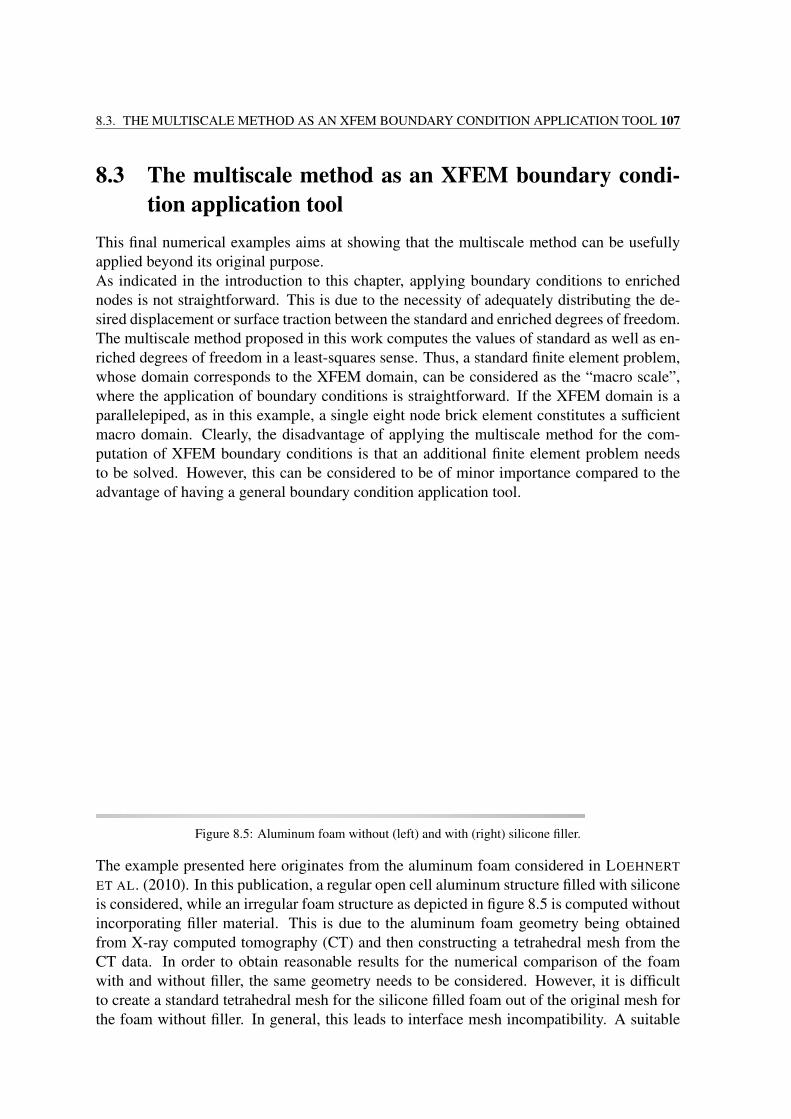
8.3. THE MULTISCALE METHOD AS AN XFEM BOUNDARY CONDITION APPLICATION TOOL 107
8.3 The multiscale method as an XFEM boundary condi-tion application tool
This final numerical examples aims at showing that the multiscale method can be usefullyapplied beyond its original purpose.As indicated in the introduction to this chapter, applying boundary conditions to enrichednodes is not straightforward. This is due to the necessity of adequately distributing the de-sired displacement or surface traction between the standard and enriched degrees of freedom.The multiscale method proposed in this work computes the values of standard as well as en-riched degrees of freedom in a least-squares sense. Thus, a standard finite element problem,whose domain corresponds to the XFEM domain, can be considered as the “macro scale”,where the application of boundary conditions is straightforward. If the XFEM domain is aparallelepiped, as in this example, a single eight node brick element constitutes a sufficientmacro domain. Clearly, the disadvantage of applying the multiscale method for the com-putation of XFEM boundary conditions is that an additional finite element problem needsto be solved. However, this can be considered to be of minor importance compared to theadvantage of having a general boundary condition application tool.
Figure 8.5: Aluminum foam without (left) and with (right) silicone filler.
The example presented here originates from the aluminum foam considered in LOEHNERT
ET AL. (2010). In this publication, a regular open cell aluminum structure filled with siliconeis considered, while an irregular foam structure as depicted in figure 8.5 is computed withoutincorporating filler material. This is due to the aluminum foam geometry being obtainedfrom X-ray computed tomography (CT) and then constructing a tetrahedral mesh from theCT data. In order to obtain reasonable results for the numerical comparison of the foamwith and without filler, the same geometry needs to be considered. However, it is difficultto create a standard tetrahedral mesh for the silicone filled foam out of the original mesh forthe foam without filler. In general, this leads to interface mesh incompatibility. A suitable
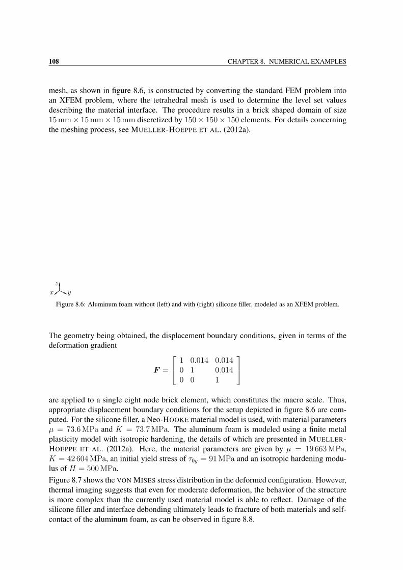
108 CHAPTER 8. NUMERICAL EXAMPLES
mesh, as shown in figure 8.6, is constructed by converting the standard FEM problem intoan XFEM problem, where the tetrahedral mesh is used to determine the level set valuesdescribing the material interface. The procedure results in a brick shaped domain of size15 mm× 15 mm× 15 mm discretized by 150× 150× 150 elements. For details concerningthe meshing process, see MUELLER-HOEPPE ET AL. (2012a).
Figure 8.6: Aluminum foam without (left) and with (right) silicone filler, modeled as an XFEM problem.
The geometry being obtained, the displacement boundary conditions, given in terms of thedeformation gradient
F =
1 0.014 0.0140 1 0.0140 0 1
are applied to a single eight node brick element, which constitutes the macro scale. Thus,appropriate displacement boundary conditions for the setup depicted in figure 8.6 are com-puted. For the silicone filler, a Neo-HOOKE material model is used, with material parametersµ = 73.6 MPa and K = 73.7 MPa. The aluminum foam is modeled using a finite metalplasticity model with isotropic hardening, the details of which are presented in MUELLER-HOEPPE ET AL. (2012a). Here, the material parameters are given by µ = 19 663 MPa,K = 42 604 MPa, an initial yield stress of τ0y = 91 MPa and an isotropic hardening modu-lus of H = 500 MPa.Figure 8.7 shows the VON MISES stress distribution in the deformed configuration. However,thermal imaging suggests that even for moderate deformation, the behavior of the structureis more complex than the currently used material model is able to reflect. Damage of thesilicone filler and interface debonding ultimately leads to fracture of both materials and self-contact of the aluminum foam, as can be observed in figure 8.8.
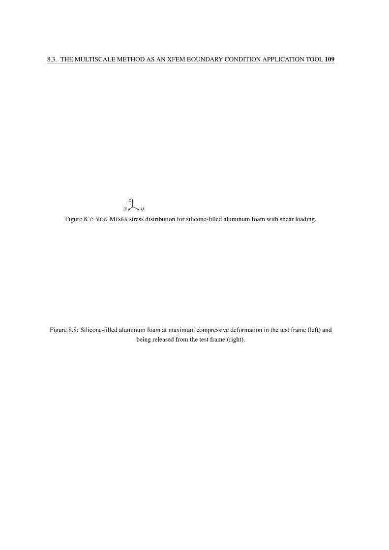
8.3. THE MULTISCALE METHOD AS AN XFEM BOUNDARY CONDITION APPLICATION TOOL 109
Figure 8.7: VON MISES stress distribution for silicone-filled aluminum foam with shear loading.
Figure 8.8: Silicone-filled aluminum foam at maximum compressive deformation in the test frame (left) andbeing released from the test frame (right).

110 CHAPTER 8. NUMERICAL EXAMPLES
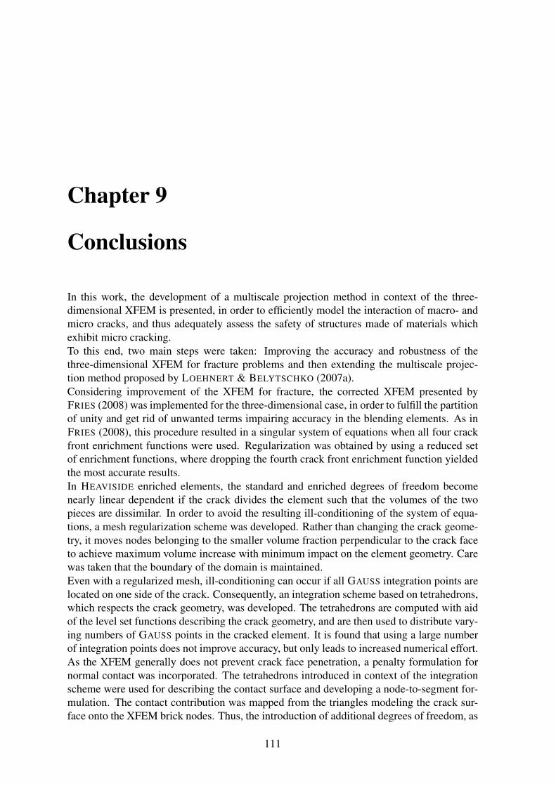
Chapter 9
Conclusions
In this work, the development of a multiscale projection method in context of the three-dimensional XFEM is presented, in order to efficiently model the interaction of macro- andmicro cracks, and thus adequately assess the safety of structures made of materials whichexhibit micro cracking.To this end, two main steps were taken: Improving the accuracy and robustness of thethree-dimensional XFEM for fracture problems and then extending the multiscale projec-tion method proposed by LOEHNERT & BELYTSCHKO (2007a).Considering improvement of the XFEM for fracture, the corrected XFEM presented byFRIES (2008) was implemented for the three-dimensional case, in order to fulfill the partitionof unity and get rid of unwanted terms impairing accuracy in the blending elements. As inFRIES (2008), this procedure resulted in a singular system of equations when all four crackfront enrichment functions were used. Regularization was obtained by using a reduced setof enrichment functions, where dropping the fourth crack front enrichment function yieldedthe most accurate results.In HEAVISIDE enriched elements, the standard and enriched degrees of freedom becomenearly linear dependent if the crack divides the element such that the volumes of the twopieces are dissimilar. In order to avoid the resulting ill-conditioning of the system of equa-tions, a mesh regularization scheme was developed. Rather than changing the crack geome-try, it moves nodes belonging to the smaller volume fraction perpendicular to the crack faceto achieve maximum volume increase with minimum impact on the element geometry. Carewas taken that the boundary of the domain is maintained.Even with a regularized mesh, ill-conditioning can occur if all GAUSS integration points arelocated on one side of the crack. Consequently, an integration scheme based on tetrahedrons,which respects the crack geometry, was developed. The tetrahedrons are computed with aidof the level set functions describing the crack geometry, and are then used to distribute vary-ing numbers of GAUSS points in the cracked element. It is found that using a large numberof integration points does not improve accuracy, but only leads to increased numerical effort.As the XFEM generally does not prevent crack face penetration, a penalty formulation fornormal contact was incorporated. The tetrahedrons introduced in context of the integrationscheme were used for describing the contact surface and developing a node-to-segment for-mulation. The contact contribution was mapped from the triangles modeling the crack sur-face onto the XFEM brick nodes. Thus, the introduction of additional degrees of freedom, as
111
112 CHAPTER 9. CONCLUSIONS
well as locking, both common phenomena of crack face contact within XFEM formulations,was avoided.Finally, extending the linear elastic XFEM to a Neo-HOOKE material model and compar-ing both formulations numerically showed negligible difference in the results. Thus, it wasconcluded that for fracture problems, the decisive factor is the crack front field and not thematerial model. Therefore, the merit of using a finite deformation approach lies in the abilityto model large rotations.After these measures to enhance accuracy and robustness, the multiscale projection methodwas extended to the three-dimensional case. Here, special care was taken to maintain the mi-cro crack geometry during the mesh regularization process on the macro scale by projectingthe nodal level set values defining the micro cracks onto the distorted mesh. Numerical stud-ies concerning the discretization of macro- and micro scale, as well as the size of the microdomain showed that, while a micro discretization which is able to accommodate the typicalsize of a micro crack is sufficient, the macro discretization is of great importance. Addition-ally, the size of the micro domain strongly influences the results. No recommendation couldbe given, as the ideal size of the micro domain is controlled by the size and position of themicro cracks and is thus problem-dependent.Having studied each component of this work where it was introduced, three numerical exam-ples were presented, which incorporated all developed features. First, the crack face contactimplementation was combined with the multiscale method. Thus, an arbitrary arrangementof micro cracks, often occurring in multiscale settings and generally leading to crack facepenetration, could be treated properly. Second, a similar macro scale setup was studied with-out micro cracks and with a large number of curved micro cracks. This test showed thatthe presence of micro cracks strongly influences the stress distribution in the vicinity of themacro crack front, and consequently the crack propagation behavior of the macro crack. Fi-nally, it was demonstrated by means of a silicone-filled aluminum foam, that the proposedmultiscale method is also useful for the appropriate application of boundary conditions toenriched nodes.The numerical examples in particular showed that many extensions and improvements arepossible, both to certain aspects of the three-dimensional XFEM for fracture and the multi-scale projection method.Regarding the contact formulation, it is desirable to improve convergence behavior by addingthe nonlinear terms to the coefficient matrix, which currently is restricted to the linear term.Also, the formulation should be extended to account for tangential contact. Regarding tan-gential contact and sliding of crack faces, many micro mechanical properties like rough crackfaces could be incorporated. Finally, the node-to-segment approach could be substituted bya more sophisticated contact formulation, like e.g. the mortar method.The case of the silicone-filled aluminum foam shows that no realistic numerical model offracture processes can be complete without accounting for damage and crack nucleation. Ifinhomogeneous materials are to be considered, debonding as a primary stage of cracking isalso an issue. For this class of applications, another necessity is an XFEM formulation whichcombines fracture and material interfaces, such that cracks can run through the structure inan arbitrary manner and are not restricted to material interfaces.Concerning the multiscale projection method, it is desirable to automatically determine the
113
choice of the discretization on both scales, as well as the micro domain size, in an error-controlled procedure instead of the current user-defined, experience-based process. For anextension which is able to model crack propagation, an accurate crack propagation criterionand a crack coalescence algorithm need to be developed.Finally, a specific mesh generator is developed for each application at present. This is ex-tremely time-consuming and still, only rather academic examples are modeled. In order toapply the presented methods to more general, real-life examples, it is unavoidable to imple-ment mesh generators based on CAD or CT data.

114 CHAPTER 9. CONCLUSIONS
Bibliography
AKIN J. The generation of elements with singularities. International Journal for NumericalMethods in Engineering, 10 (1976): 1249–1259.
ALTENBACH J. & ALTENBACH H. Einfuhrung in die Kontinuumsmechanik. Teubner, 1994.
ANDERSON T. Fracture mechanics: Fundamentals and applications. Taylor & Francis,2005.
ANDRADE J. & TU X. Multiscale framework for behavior prediction in granular media.Mechanics of Materials, 41 (2009): 652–669.
AREIAS P. & BELYTSCHKO T. Analysis of three-dimensional crack initiation and prop-agation using the extended finite element method. International Journal for NumericalMethods in Engineering, 63 (2005): 760–788.
ARGYRIS J. & MLEJNEK H.P. Die Methode der Finiten Elemente in der elementaren Struk-turmechanik. Band 1: Verschiebungsmethoden in der Statik. Viewig, 1986.
BABUSKA I. & MELENK J. The partition of unity method. International Journal for Nu-merical Methods in Engineering, 40 (1997): 727–758.
BARRENBLATT G. The mathematical theory of equilibrium of cracks in brittle fracture.Advances in Applied Mechanics, 7 (1962): 55–129.
BARSOUM R. On the use of isoparametric finite elements in linear fracture mechanics.International Journal for Numerical Methods in Engineering, 10 (1976): 25–37.
BARSOUM R. Triangular quarter-point elements as elastic and perfectly-plastic crack tipelements. International Journal for Numerical Methods in Engineering, 11 (1977): 85–98.
BECHET E., MINNEBO H., MOES N. & BURGARDT B. Improved implementation androbustness study of the x-fem for stress analysis around cracks. International Journal forNumerical Methods in Engineering, 64 (2005): 1033–1056.
BELLEC J. & DOLBOW J. A note on enrichment functions for modelling crack nucleation.Communications in Numerical Methods in Engineering, 19 (2003): 921–932.
BELYTSCHKO T. & BLACK T. Elastic crack growth in finite elements with minimal remesh-ing. International Journal for Numerical Methods in Engineering, 45 (1999): 601–620.
115
116 BIBLIOGRAPHY
BELYTSCHKO T., CHEN H., XU J. & ZI G. Dynamic crack propagation based on loss ofhyperbolicity and a new discontinuous enrichment. International Journal for NumericalMethods in Engineering, 58 (2003): 1873–1905.
BELYTSCHKO T., GU L. & LU Y. Fracture and crack growth by element free Galerkinmethods. Modelling and Simulations in Materials Science and Engineering, 2 (1994a):519–534.
BELYTSCHKO T., KRONGAUZ Y., FLEMING M., ORGAN D. ET AL. Smoothing and accel-erated computations in the element free Galerkin method. Journal of Computational andApplied Mathematics, 74 (1996a): 111–126.
BELYTSCHKO T., KRONGAUZ Y., ORGAN D., FLEMING M. ET AL. Meshless methods:An overview and recent developments. Computer Methods in Applied Mechanics andEngineering, 2 (1996b): 519–534.
BELYTSCHKO T., LIU W. & MORAN B. Nonlinear Finite Elements for Continua and Struc-tures. Wiley, 2000.
BELYTSCHKO T., LU Y. & GU L. Element-free Galerkin methods. International Journalfor Numerical Methods in Engineering, 37 (1994b): 229–256.
BELYTSCHKO T., LU Y. & GU L. Crack propagation by element-free Galerkin methods.Engineering Fracture Mechanics, 51 (1995a): 295–315.
BELYTSCHKO T., LU Y., GU L. & TABBARA M. Element-free Galerkin methods for staticand dynamic fracture. International Journal of Solids and Structures, 32 (1995b): 2547–2570.
BELYTSCHKO T., ORGAN D. & KRONGAUZ Y. A coupled finite element – element-freeGalerkin method. Computational Mechanics, 17 (1995c): 186–195.
BEN DHIA H. & JAMOND O. On the use of XFEM within the Arlequin framework for thesimulation of crack propagation. Computer Methods in Applied Mechanics and Engineer-ing, 199 (2010): 1403–1414.
BEN DHIA H. & RATEAU G. The Arlequin method as a flexible engineering design tool.International Journal for Numerical Methods in Engineering, 62 (2005): 1442–1462.
BENEDETTI I., ALIABADI M. & DAVI G. A fast 3d dual boundary element method basedon hierarchical matrices. International Journal of Solids and Structures, 45 (2008): 2355–2376.
BENZLEY S. Representation of singularities with isoparametric finite elements. Interna-tional Journal for Numerical Methods in Engineering, 8 (1974): 537–545.
BLACKBURN W. & HELLEN T. Calculation of stress intensity factors in three dimensionsby finite element methods. International Journal for Numerical Methods in Engineering,11 (1977): 211–229.
BIBLIOGRAPHY 117
DE BORST R. Numerical aspects of cohesive-zone models. Engineering Fracture Mechan-ics, 70 (2003): 1743–1757.
BUDYN E., ZI G., MOES N. & BELYTSCHKO T. A method for multiple crack growthin brittle materials without remeshing. International Journal for Numerical Methods inEngineering, 61 (2004): 1741–1770.
BYSKOV E. The calculation of stress intensity factors using the finite element method withcracked elements. International Journal of Fracture Mechanics, 6 (1970): 159–167.
CALEYRON F., CHUZEL-MARMOT Y. & COMBESCURE A. Modeling of reinforced con-crete through sph-fe coupling and its application to the simulation of a projectile’s impactonto a slab. International Journal for Numerical Methods in Biomedical Engineering, 27(2011): 882–898.
CAMACHO G. & ORTIZ M. Computational modelling of impact damage in brittle materials.International Journal of Solids and Structures, 33 (1996): 2899–2938.
CHADWICK P. Continuum mechanics: Concise theory and problems. Dover, 1999.
CHAN S., TUBA I. & WILSON W. On the finite element method in linear elastic fracturemechanics. Engineering Fracture Mechanics, 2 (1970): 1–17.
CHEN W. & CHEN T. An efficient dual boundary element technique for a two-dimensionalfracture problem with multiple cracks. International Journal for Numerical Methods inEngineering, 38 (1995): 1739–1756.
CHEN W. & FISH J. A generalized space-time mathematical homogenization theory forbridging atomistic and continuum scales. International Journal for Numerical Methods inEngineering, 67 (2006a): 253–271.
CHEN W. & FISH J. A mathematical homogenization perspective of virial stress. Interna-tional Journal for Numerical Methods in Engineering, 67 (2006b): 189–207.
CHESSA J., WANG H. & BELYTSCHKO T. On the construction of blending elements for lo-cal partition of unity enriched finite elements. International Journal for Numerical Meth-ods in Engineering, 57 (2003): 1015–1038.
CHOPP D. & SUKUMAR N. Fatigue crack propagation of multiple coplanar cracks withthe coupled extended finite element / fast marching method. International Journal ofEngineering Science, 41 (2003): 845–869.
CIARLET P. Mathematical elasticity I: Three dimensional elasticity. North-Holland, 1994.
CISILINO A., ALIABADI M. & OTEGUI J. A three-dimensional boundary element formula-tion for the elastoplastic analysis of cracked bodies. International Journal for NumericalMethods in Engineering, 42 (1998): 237–256.
118 BIBLIOGRAPHY
COMBESCURE A., GRAVOUIL A., GREGOIRE D. & RETHORE J. X-FEM a good candidatefor energy conservation in simulation of brittle dynamic propagation. Computer Methodsin Applied Mechanics and Engineering, 197 (2008): 309–318.
CRISFIELD M. Non-linear Finite Element Analysis of Solids and Structures. Volume 2:Advanced topics. Wiley, 1997.
DAUX C., MOES N., DOLBOW J., SUKUMAR N. ET AL. Arbitrary branched and intersect-ing cracks with the extended finite element method. International Journal for NumericalMethods in Engineering, 48 (2000): 1741–1760.
DE LUYCKER E., BENSON D., BELYTSCHKO T., BAZILEVS Y. ET AL. X-FEM in iso-geometric analysis for linear fracture mechanics. International Journal for NumericalMethods in Engineering, 87 (2011): 541–565.
DENDA M. & DONG Y. Complex variable approach to the BEM for multiple crack prob-lems. Computer Methods in Applied Mechanics and Engineering, 141 (1997): 247–264.
DENDA M. & MARANTE M. Mixed mode BEM analysis of multiple curvilinear cracks inthe general anisotropic solids by the crack tip singular element. International Journal ofSolids and Structures, 41 (2004): 1473–1489.
DHATT G. & TOUZOT G. The Finite Element Method Displayed. Wiley, 1984.
DHONDT G. Cutting of a 3-d finite element mesh for automatic mode I crack propagationcalculations. International Journal for Numerical Methods in Engineering, 42 (1998):749–772.
DIAS-DA-COSTA D., ALFAIATE J., SLUYS L. & JULIO E. A discrete strong discontinuityapproach. Engineering Fracture Mechanics, 76 (2009): 1176–1201.
DOLBOW J., MOES N. & BELYTSCHKO T. An extended finite element method for mod-eling crack growth with frictional contact. Computer Methods in Applied Mechanics andEngineering, 190 (2001): 6825–6846.
DUARTE C., HAMZEH O., LISZKA T. & TWORZYDLO W. A generalized finite elementmethod for the simulation of three-dimensional dynamic crack propagation. ComputerMethods in Applied Mechanics and Engineering, 190 (2001): 2227–2262.
DUFLOT M. A study of the representation of cracks with level sets. International Journalfor Numerical Methods in Engineering, 70 (2007): 1261–1302.
DUGDALE D. Yielding of steel sheets containing slits. Journal of the Mechanics and Physicsof Solids, 8 (1960): 100–104.
ELGUEDJ T., GRAVOUIL A. & COMBESCURE A. Appropriate extended functions for X-FEM simulation of plastic fracture mechanics. Computer Methods in Applied Mechanicsand Engineering, 195 (2006): 501–515.
BIBLIOGRAPHY 119
ELGUEDJ T., GRAVOUIL A. & COMBESCURE A. A mixed augmented Lagrangian-extendedfinite element method for modelling elastic-plastic fatigue crack growth with unilateralcontact. International Journal for Numerical Methods in Engineering, 71 (2007): 1569–1597.
ELGUEDJ T., GRAVOUIL A. & MAIGRE H. An explicit dynamics extended finite elementmethod. Part 1: Mass lumping for arbitrary enrichment functions. Computer Methods inApplied Mechanics and Engineering, 198 (2009): 2297–2317.
ERDOGAN F. & SIH G. On the crack extension in plates under plane loading and transverseshear. Journal of Basic Engineering, 85 (1963): 519–527.
FAGERSTROEM M. & LARSSON R. Theory and numerics for finite deformation fracturemodelling using strong discontinuities. International Journal for Numerical Methods inEngineering, 66 (2006): 911–948.
FARHAT C. A Lagrange multiplier based divide and conquer finite element algorithm. Com-puter Systems in Engineering, 2 (1991): 149–156.
FEDELINSKI P., ALIABADI M. & ROOKE D. The dual boundary element method in dy-namic fracture mechanics. Engineering Analysis with Boundary Elements, 12 (1993):203–210.
FEIST C. & HOFSTETTER G. An embedded strong discontinuity model for cracking ofplain concrete. Computer Methods in Applied Mechanics and Engineering, 195 (2006a):7115–7138.
FEIST C. & HOFSTETTER G. Three-dimensional fracture simulations based on the SDA. In-ternational Journal for Numerical and Analytical Methods in Geomechanics, 31 (2006b):189–212.
FEYEL F. A multilevel finite element method (FE2) to describe the response of highly non-linear structures using generalized continua. Computer Methods in Applied Mechanicsand Engineering, 192 (2003): 3233–3244.
FEYEL F. & CHABOCHE J.L. FE2 multiscale approach for modelling the elastoviscoplas-tic behaviour of long fibre SiC/Ti composite materials. Computer Methods in AppliedMechanics and Engineering, 183 (2000): 309–330.
FISCHER K. & WRIGGERS P. Frictionless 2D contact formulations for finite deformationsbased on the mortar method. Computational Mechanics, 36 (2005): 226–244.
FISCHER K. & WRIGGERS P. Mortar based frictional contact formulation for higher orderinterpolations using the moving friction cone. Computer Methods in Applied Mechanicsand Engineering, 195 (2006): 5020–5036.
FISH J., MARKOLEFAS S., GUTTAL R. & NAYAK P. On adaptive multilevel superposi-tion of finite element meshes for linear elastostatics. Applied Numerical Mathematics, 14(1994): 135–164.
120 BIBLIOGRAPHY
FISH J. & YUAN Z. Multiscale enrichment based on partition of unity. International Journalfor Numerical Methods in Engineering, 62 (2005): 1341–1359.
FLEMING M., CHU Y., MORAN B. & BELYTSCHKO T. Enriched element-free Galerkinmethods for crack tip fields. International Journal for Numerical Methods in Engineering,40 (1997): 1483–1504.
FLORY P. Thermodynamic relations for high elastic materials. Transactions of the FaradaySociety, 57 (1961): 829–838.
FRIES T.P. A corrected XFEM approximation without problems in blending elements. In-ternational Journal for Numerical Methods in Engineering, 75 (2008): 503–532.
FRIES T.P. & BELYTSCHKO T. The intrinsic XFEM: A method for arbitrary discontinuitieswithout additional unknowns. International Journal for Numerical Methods in Engineer-ing, 68 (2006): 1358–1385.
GASSER T. & HOLZAPFEL G. Modeling 3d crack propagation in unreinforced concreteusing PUFEM. Computer Methods in Applied Mechanics and Engineering, 194 (2005):2859–2896.
GEERS M., KOUZNETSOVA V. & BREKELMANS W. Multi-scale computational homog-enization: Trends and challenges. Journal of Computational and Applied Mathematics,234 (2010): 2175–2182.
GENIAUT S., MASSIN P. & MOES N. A stable 3D contact formulation using X-FEM.European Journal of Computational Mechanics, 16 (2007): 259–275.
GEUBELLE P. & KNAUSS W. Finite strains at the tip of a crack in a sheet of hyperelasticmaterial: I. Homogeneous case. Journal of Elasticity, 35 (1994): 61–98.
GINER E., TUR M., TARANCON J. & FUENMAYOR F. Crack face contact in X-FEM usinga segment-to-segment approach. International Journal for Numerical Methods in Engi-neering, 82 (2010): 1424–1449.
GROSS D. & SEELIG T. Bruchmechanik. Springer, 2007.
GUERSES E. & MIEHE C. A computational framework of three-dimensionalconfigurational-force-driven brittle crack propagation. Computer Methods in Applied Me-chanics and Engineering, 198 (2009): 1413–1428.
GUIDAULT P.A., ALLIX O., CHAMPANEY L. & CORNUAULT C. A multiscale extendedfinite element method for crack propagation. Computer Methods in Applied Mechanicsand Engineering, 197 (2008): 381–399.
GURSON A. Continuum theory of ductile rupture by void nucleation and growth; Part I:Yield criterion and flow rules for porous ductile materials. Journal of Engineering Mate-rials and Technology, 99 (1977): 2–15.
BIBLIOGRAPHY 121
HANSBO A. & HANSBO P. An unfitted finite element method, based on Nitsche’s method,for elliptic interface problems. Computer Methods in Applied Mechanics and Engineering,191 (2002): 5537–5552.
HANSBO A. & HANSBO P. A finite element method for the simulation of strong and weakdiscontinuities in solid mechanics. Computer Methods in Applied Mechanics and Engi-neering, 193 (2004): 3523–3540.
HAUPT P. Continuum mechanics and theory of materials. Springer, 2002.
HAUSLER S., LINDHORST K. & HORST P. Combination of material force concept and theextended finite element method for mixed mode crack growth simulations. InternationalJournal for Numerical Methods in Engineering, 85 (2011): 1522–1542.
HELLAN K. Introduction to fracture mechanics. McGraw-Hill, 1984.
HENSHELL R. & SHAW K. Crack tip finite elements are unnecessary. International Journalfor Numerical Methods in Engineering, 9 (1975): 495–507.
HILL R. Constitutive inequalities for isotropic elastic solids under finite strain. Proceedingsof the Royal Society of London, A 314 (1970): 457–472.
HOLZAPFEL G. Nonlinear solid mechanics. Wiley, 2000.
HUEBER S., MATEI A. & WOHLMUTH B. Efficient algorithms for problems with friction.SIAM Journal on Scientific Computing, 29 (2007): 70–92.
HUGHES T. Multiscale phenomena: Green’s functions, the Dirichlet-to-Neumann formu-lation, subgrid scale methods, bubbles and the origins of stabilized methods. ComputerMethods in Applied Mechanics and Engineering, 127 (1995): 387–401.
HUGHES T. The Finite Element Method. Dover, 2000.
HUTCHINSON J. Singular behavior at the end of a tensile crack in a hardening material.Journal of the Mechanics and Physics of Solids, 16 (1968): 13–31.
IRWIN G. Analysis of stresses and strains near the end of a crack traversing a plate. Journalof Applied Mechanics, 24 (1957): 361–364.
JAGER P., STEINMANN P. & KUHL E. Modeling three-dimensional crack propagation– a comparison of crack path tracking strategies. International Journal for NumericalMethods in Engineering, 76 (2008a): 1328–1352.
JAGER P., STEINMANN P. & KUHL E. On local tracking algorithms for the simulation ofthree-dimensional discontinuities. Computational Mechanics, 42 (2008b): 395–406.
JAGER P., STEINMANN P. & KUHL E. Towards the treatment of boundary conditions forglobal crack path tracking in three-dimensional brittle fracture. Computational Mechanics,45 (2009): 91–107.
122 BIBLIOGRAPHY
JANSSEN M., ZUIDEMA J. & WANHILL R. Fracture mechanics. Taylor & Francis, 2004.
KIM D.J., DUARTE C. & SOBH N. Parallel simulations of three-dimensional cracks usingthe generalized finite element method. Computational Mechanics, 47 (2011): 265–282.
KNOTHE K. & WESSELS H. Finite Elemente. Springer, 2008.
KNOTT J. Fundamentals of fracture mechanics. Butterworths, 1973.
KNOWLES J. The finite anti-plane shear field near the tip of a crack for a class of incom-pressible materials. International Journal of Fracture, 13 (1977): 611–639.
KNOWLES J. & STERNBERG E. An asymptotic finite-deformation analysis of the elasto-static field near the tip of a crack. Journal of Elasticity, 3 (1973): 67–107.
KNOWLES J. & STERNBERG E. Finite-deformation analysis of the elastostatic field near thetip of a crack: Reconsideration and higher-order results. Journal of Elasticitiy, 4 (1974):201–233.
KOBAYASHI A., EMERY A. & MALL S. Dynamic-finite-element and dynamic-photoelasticanalyses of two fracturing homalite-100 plates. Experimental Mechanics, 16 (1976): 321–328.
KOLK K., WEBER W. & KUHN G. Investigation of 3d crack propagation problems via fastBEM formulations. Computational Mechanics, 37 (2005): 32–40.
KOUZNETSOVA V., GEERS M. & BREKELMANS W. Multi-scale constitutive modellingof heterogeneous materials with a gradient-enhanced computational homogenizationscheme. International Journal for Numerical Methods in Engineering, 54 (2002): 1235–1260.
KRONGAUZ Y. & BELYTSCHKO T. Enforcement of essential boundary conditions in mesh-less approximations using finite elements. Computer Methods in Applied Mechanics andEngineering, 131 (1996): 133–145.
KRYSL P. & BELYTSCHKO T. Element-free Galerkin method: Convergence of the contin-uous and discontinuous shape functions. Computer Methods in Applied Mechanics andEngineering, 148 (1997): 257–277.
KUNDU P. & COHEN I. Fluid mechanics. Elsevier, 2004.
KUNDU T. Fundamentals of fracture mechanics. Taylor & Francis, 2008.
LABORDE P., POMMIER J., RENARD Y. & SALAUN M. High-order extended finite elementmethod for cracked domains. International Journal for Numerical Methods in Engineer-ing, 64 (2005): 354–381.
LAURES J.P. & KACHANOV M. Three-dimensional interactions of a crack front with arraysof penny-shaped microcracks. International Journal of Fracture, 48 (1991): 255–279.
BIBLIOGRAPHY 123
LEGRAIN G., MOES N. & VERRON E. Stress analysis around crack tips in finite strainproblems using the extended finite element method. International Journal for NumericalMethods in Engineering, 63 (2005): 290–314.
LEITAO V., ALIABADI M. & ROOKE D. The dual boundary element formulation for elasto-plastic fracture mechanics. International Journal for Numerical Methods in Engineering,38 (1995a): 315–333.
LEITAO V., ALIABADI M. & ROOKE D. Elastoplastic simulation of fatigue crack growth:Dual boundary element formulation. International Journal of Fatigue, 17 (1995b): 353–363.
LILLIE C. Dreidimensionales Diskrete Elemente Modell fur Superellipsoide. Ph.D. thesis,Leibniz Universitat Hannover (2007).
LINDER C. & ARMERO F. Finite elements with embedded branching. Finite Elements inAnalysis and Design, 45 (2009): 280–293.
LIU F. & BORJA R. A contact algorithm for frictional crack propagation with the extendedfinite element method. International Journal for Numerical Methods in Engineering, 76(2008): 1489–1512.
LIU F. & BORJA R. An extended finite element framework for slow-rate frictional fault-ing with bulk plasticity and variable friction. International Journal for Numerical andAnalyical Methods in Geomechanics, 33 (2009): 1535–1560.
LIU F. & BORJA R. Finite deformation formulation for embedded frictional crack with theextended finite element method. International Journal for Numerical Methods in Engi-neering, 82 (2010): 773–804.
LIU X., LI S. & SHENG N. A cohesive finite element for quasi-continua. ComputationalMechanics, 42 (2008): 543–553.
LIU Z., MENOUILLARD T. & BELYTSCHKO T. An XFEM/Spectral element method fordynamic crack propagation. International Journal of Fracture, 169 (2011): 183–198.
LOEHNERT S. & BELYTSCHKO T. Crack shielding and amplification due to multiple mi-crocracks interacting with a macrocrack. International Journal of Fracture, 145 (2007a):1–8.
LOEHNERT S. & BELYTSCHKO T. A multiscale projection method for macro / microcracksimulations. International Journal for Numerical Methods in Engineering, 71 (2007b):1466–1482.
LOEHNERT S., KRSTULOVIC-OPARA L., VESENJAK M. & MUELLER-HOEPPE D. Ho-mogenization principle based multi-scale modeling of cellular structures. Journal of theSerbian Society for Computational Mechanics, 4 (2010): 97–109.
124 BIBLIOGRAPHY
LOEHNERT S. & MUELLER-HOEPPE D. Multiscale methods for fracturing solids. InREDDY B., ed., IUTAM Symposium on Theoretical, Computational and Modelling As-pects of Inelastic Media, pages 79–87. 2008.
LOEHNERT S., MUELLER-HOEPPE D. & WRIGGERS P. 3d corrected XFEM approach andextension to finite deformation theory. International Journal for Numerical Methods inEngineering, 86 (2011): 431–452.
LOHNERT S. Computational homogenization of microheterogeneous materials. Ph.D. thesis,Leibniz Universitat Hannover (2005).
LU Y., BELYTSCHKO T. & GU L. A new implementation of the element free Galerkinmethod. Computer Methods in Applied Mechanics and Engineering, 113 (1994): 397–414.
LUTZ E., INGRAFFEA A. & GRAY L. Use of ’simple solutions’ for boundary integralmethods in elasticity and fracture analysis. International Journal for Numerical Methodsin Engineering, 35 (1992): 1737–1751.
MALVERN L. Introduction to the Mechanics of a Continuous Medium. Prentice-Hall, 1969.
MARSDEN J. & HUGHES T. Mathematical foundations of elasticity. Dover, 1994.
MCDEVITT T. & LAURSEN T. A mortar-finite element formulation for frictional contactproblems. International Journal for Numerical Methods in Engineering, 48 (2000): 1525–1547.
MELENK J. & BABUSKA I. The partition of unity finite element method: Basic theoryand applications. Computer Methods in Applied Mechanics and Engineering, 139 (1996):289–314.
MENOUILLARD T., RETHORE J., MOES N., COMBESCURE A. ET AL. Mass lumpingstrategies for X-FEM explicit dynamics: Application to crack propagation. InternationalJournal for Numerical Methods in Engineering, 74 (2008): 447–474.
MERGHEIM J. A variational multiscale method to model crack propagation at finite strains.International Journal for Numerical Methods in Engineering, 80 (2009): 269–289.
MERGHEIM J., KUHL E. & STEINMANN P. A finite element method for the computationalmodelling of cohesive cracks. International Journal for Numerical Methods in Engineer-ing, 63 (2005): 276–289.
MERGHEIM J., KUHL E. & STEINMANN P. Towards the algorithmic treatment of 3d strongdiscontinuities. Communications in Numerical Methods in Engineering, 23 (2007): 97–108.
MEYER A., RABOLD F. & SCHERZER M. Efficient finite element simulation of crackpropagation using adaptive iterative solvers. Communications in Numerical Methods inEngineering, 22 (2006): 93–108.
BIBLIOGRAPHY 125
MI Y. & ALIABADI M. Dual boundary element method for three-dimensional fracturemechanics analysis. Engineering Analysis with Boundary Elements, 10 (1992): 161–171.
MI Y. & ALIABADI M. Three-dimensional crack growth simulation using BEM. Computers& Structures, 52 (1994): 871–878.
MIEHE C. & BAYREUTHER C. On multiscale FE analyses of heterogeneous structures:From homogenization to multigrid solvers. International Journal for Numerical Methodsin Engineering, 71 (2007): 1135–1180.
MIEHE C. & GUERSES E. A robust algorithm for configurational-force-driven brittle crackpropagation with r-adaptive mesh alignment. International Journal for Numerical Meth-ods in Engineering, 72 (2007): 127–155.
MIEHE C., GUERSES E. & BIRKLE M. A computational framework of configurational-force-driven brittle fracture based on incremental energy minimization. InternationalJournal of Fracture, 145 (2007): 245–259.
MILLER O., FREUND L. & NEEDLEMAN A. Modeling and simulation of dynamic frag-mentation in brittle materials. International Journal of Fracture, 96 (1999): 101–125.
MOES N., BECHET E. & TOURBIER M. Imposing Dirichlet boundary conditions in theextended finite element method. International Journal for Numerical Methods in Engi-neering, 67 (2006): 1641–1669.
MOES N. & BELYTSCHKO T. Extended finite element method for cohesive crack growth.Engineering Fracture Mechanics, 69 (2002): 813–833.
MOES N., CLOIREC M., CARTRAUD P. & REMACLE J.F. A computational approach tohandle complex microstructural geometries. Computer Methods in Applied Mechanicsand Engineering, 192 (2003): 3163–3177.
MOES N., DOLBOW J. & BELYTSCHKO T. A finite element method for crack growth with-out remeshing. International Journal for Numerical Methods in Engineering, 46 (1999):131–150.
MOES N., GRAVOUIL A. & BELYTSCHKO T. Non-planar 3d crack growth by the extendedfinite element and level sets – Part I: Mechanical model. International Journal for Numer-ical Methods in Engineering, 53 (2002a): 2549–2568.
MOES N., GRAVOUIL A. & BELYTSCHKO T. Non-planar 3d crack growth by the extendedfinite element and level sets – Part II: Level set update. International Journal for Numeri-cal Methods in Engineering, 53 (2002b): 2569–2586.
MOSLER J. & MESCHKE G. 3d modelling of strong discontinuities in elastoplastic solids:Fixed and rotating localization formulations. International Journal for Numerical Meth-ods in Engineering, 57 (2003): 1553–1576.
126 BIBLIOGRAPHY
MOSLER J. & ORTIZ M. On the numerical implementation of variational arbitraryLangrangian-Eulerian (VALE) formulations. International Journal for Numerical Meth-ods in Engineering, 67 (2006): 1272–1289.
MOUSAVI S., XIAO H. & SUKUMAR N. Generalized Gaussian quadrature rules on arbitrarypolygons. International Journal for Numerical Methods in Engineering, 82 (2010): 99–113.
MUELLER R., GROSS D. & MAUGIN G. Use of material forces in adaptive finite elementmethods. Computational Mechanics, 33 (2004): 421–434.
MUELLER R., KOLLING S. & GROSS D. On configurational forces in the context of thefinite element method. International Journal for Numerical Methods in Engineering, 53(2002): 1557–1574.
MUELLER R. & MAUGIN G. On material forces and finite element discretizations. Compu-tational Mechanics, 29 (2002): 52–60.
MUELLER-HOEPPE D., LOEHNERT S., CLASEN H., KRSTULOVIC-OPARA L. ET AL. Nu-merical aspects of the comparison of metal foams with and without filler material com-puted using the XFEM. Submitted to Computer Methods in Applied Mechanics and Engi-neering, (2012a).
MUELLER-HOEPPE D., WRIGGERS P. & LOEHNERT S. Crack face contact fora hexahedral-based XFEM formulation. Computational Mechanics, (2012b): DOI10.1007/s00 466–012–0701–2.
MURTHY K. & MUKHOPADHYAY M. Adaptive finite element analysis of mixed-mode crackproblems with automatic mesh generator. International Journal for Numerical Methodsin Engineering, 49 (2000): 1087–1100.
NAYROLES B., TOUZOT G. & VILLON P. Generalizing the finite element method: Diffuseapproximation and diffuse elements. Computational Mechanics, 10 (1992): 307–318.
NEEDLEMAN A. A continuum model for void nucleation by inclusion debonding. Journalof Applied Mechanics, 54 (1987): 525–531.
NEEDLEMAN A. An analysis of decohesion along an imperfect plane. International Journalof Fracture, 42 (1990a): 21–40.
NEEDLEMAN A. An analysis of tensile decohesion along an interface. Journal of the Me-chanics and Physics of Solids, 38 (1990b): 289–324.
NGUYEN O., REPETTO E., ORTIZ M. & RADOVITZKY R. A cohesive model of fatiguecrack growth. International Journal of Fracture, 110 (2001): 351–369.
NISHIOKA T. & ATLURI S. Numerical modeling of dynamic crack propagation in finitebodies, by moving singular elements. Journal of Applied Mechanics, 47 (1980): 570–582.
BIBLIOGRAPHY 127
NISHIOKA T., FURUTUKA J., TCHOUIKOV S. & FUJIMOTO T. Generation-phase simula-tion of dynamic crack bifurcation phenomenon using moving finite element method basedon Delaunay automatic triangulation. Computer Modeling in Engineering & Sciences, 3(2002): 129–145.
NISTOR I., GUITON M., MASSIN P., MOES N. ET AL. An X-FEM approach for largesliding contact along discontinuities. International Journal for Numerical Methods inEngineering, 78 (2009): 1407–1435.
NOLL W. Die Herleitung der Grundgleichungen der Thermomechanik der Kontinua aus derStatistischen Mechanik. Journal of Rational Mechanics and Analysis, 4 (1955): 627–646.
ODEN J. & ZOHDI T. Analysis and adaptive modeling of highly heterogeneous elasticstructures. Computer Methods in Applied Mechanics and Engineering, 148 (1997): 367–391.
OGDEN R. Non-linear elastic deformations. Dover, 1984.
OLIVER J. Continuum modelling of strong discontinuities in solid mechanics using damagemodels. Computational Mechanics, 17 (1995): 49–61.
OLIVER J. Modelling strong discontinuities in solid mechanics via strain softening consti-tutive equations. Part 1: Fundamentals. International Journal for Numerical Methods inEngineering, 39 (1996a): 3575–3600.
OLIVER J. Modelling strong discontinuities in solid mechanics via strain softening con-stitutive equations. Part 2: Numerical simulation. International Journal for NumericalMethods in Engineering, 39 (1996b): 3601–3623.
OLIVER J., CERVERA M. & MANZOLI O. Strong discontinuities and continuum plasticitymodels: The strong discontinuity approach. International Journal of Plasticity, 15 (1999):319–351.
OLIVER J. & HUESPE A. Continuum approach to material failure in strong discontinuitysettings. Computer Methods in Applied Mechanics in Engineering, 193 (2004a): 3195–3220.
OLIVER J. & HUESPE A. Theoretical and computational issues in modelling material failurein strong discontinuity scenarios. Computer Methods in Applied Mechanics in Engineer-ing, 193 (2004b): 2987–3014.
OLIVER J., HUESPE A., BLANCO S. & LINERO D. Stability and robustness issues in nu-merical modeling of material failure with the strong discontinuity approach. InternationalJournal for Numerical Methods in Engineering, 195 (2006): 7093–7114.
OLIVER J., HUESPE A., PULIDO M. & CHAVES E. From continuum mechanics to frac-ture mechanics: The strong discontinuity approach. Engineering Fracture Mechanics, 69(2002a): 113–136.
128 BIBLIOGRAPHY
OLIVER J., HUESPE A., PULIDO M. & SAMANIEGO E. On the strong discontinuity ap-proach in finite deformation settings. International Journal for Numerical Methods inEngineering, 56 (2003a): 1051–1082.
OLIVER J., HUESPE A. & SAMANIEGO E. A study on finite elements for capturing strongdiscontinuities. International Journal for Numerical Methods in Engineering, 56 (2003b):2135–2161.
OLIVER J., HUESPE A., SAMANIEGO E. & CHAVES E. On strategies for tracking strongdiscontinuities in computational failure mechanics. 5th World Congress on ComputationalMechanics, Vienna, Austria, Conference Proceedings, (2002b).
OLIVER J., HUESPE A., SAMANIEGO E. & CHAVES E. Continuum approach to the numer-ical simulation of material failure in concrete. International Journal for Numerical andAnalytical Methods in Geomechanics, 28 (2004): 609–632.
ORTIZ M. & PANDOLFI A. Finite-deformation irreversible cohesive elements for three-dimensional crack-propagation analysis. International Journal for Numerical Methods inEngineering, 44 (1999): 1267–1282.
OSHER S. & SETHIAN J. Fronts propagating with curvature-dependent speed: Algorithmsbased on Hamilton-Jacobi formulations. Journal of Computational Physics, 79 (1988):12–49.
PANDOLFI A. & ORTIZ M. Solid modeling aspects of three-dimensional fragmentation.Engineering with Computers, 14 (1998): 287–308.
PANDOLFI A. & ORTIZ M. An efficient adaptive procedure for three-dimensional fragmen-tation simulations. Engineering with Computers, 18 (2001): 148–159.
PARISCH H. A consistent tangent stiffness matrix for three-dimensional non-linear contactanalysis. International Journal for Numerical Methods in Engineering, 28 (1989): 1803–1812.
PASSIEUX J., GRAVOUIL A., RETHORE J. & BAIETTO M. Direct estimation of generalizedstress intensity factors using a three-scale concurrent multigrid X-FEM. InternationalJournal for Numerical Methods in Engineering, 85 (2011): 1648–1666.
PIERRES E., BAIETTO M., GRAVOUIL A. & MORALES-ESPEJEL G. 3d two scale X-FEMcrack model with interfacial frictional contact: Application to fretting fatigue. TribologyInternational, 43 (2010): 1831–1841.
PORTELA A., ALIABADI M. & ROOKE D. The dual boundary element method: Effec-tive implementation for crack problems. International Journal for Numerical Methods inEngineering, 33 (1992): 1269–1287.
PORTELA A., ALIABADI M. & ROOKE D. Dual boundary element incremental analysis ofcrack propagation. Computers & Structures, 46 (1993): 237–247.

BIBLIOGRAPHY 129
POTYONDY D. & CUNDALL P. A bonded-particle model for rock. International Journal ofRock Mechanics and Mining Sciences, 41 (2004): 1329–1364.
PRABEL B., COMBESCURE A., GRAVOUIL A. & MARIE S. Level set X-FEM non-matching meshes: Application to dynamic crack propagation in elastic-plastic media. In-ternational Journal for Numerical Methods in Engineering, 69 (2007): 1553–1569.
RABCZUK T., ZI G., GERSTENBERGER A. & WALL W. A new crack tip element for thephantom-node method with arbitrary cohesive cracks. International Journal for NumericalMethods in Engineering, 75 (2008): 577–599.
RADULOVIC R., BRUHNS O. & MOSLER J. Effective 3d failure simulations by combin-ing the advantages of embedded strong discontinuity approaches and classical interfaceelements. Engineering Fracture Mechanics, 78 (2011): 2470–2485.
RAJAGOPAL S. & GUPTA N. Meshfree modelling of fracture – a comparative study ofdifferent methods. Meccanica, 46 (2011): 1145–1185.
RANNOU J., GRAVOUIL A. & BAIETTO-DUBOURG M. A local multigrid X-FEM strategyfor 3-d crack propagation. International Journal for Numerical Methods in Engineering,77 (2009): 581–600.
REESE S. Theorie und Numerik des Stabilitatsverhaltens hyperelastischer Festkorper. Ph.D.thesis, Technische Hochschule Darmstadt (1994).
REESE S. Adaptive methods for continuous and discontinuous damage modeling in fractur-ing solids. Ph.D. thesis, Leibniz Universitat Hannover (2007).
REINELT J. Frictional contact of elastomer materials on rough rigid surfaces. Ph.D. thesis,Leibniz Universitat Hannover (2008).
REMMERS J., DE BORST R. & NEEDLEMAN A. A cohesive segments method for thesimulation of crack growth. Computational Mechanics, 31 (2003): 69–77.
REMMERS J., DE BORST R. & NEEDLEMAN A. The simulation of dynamic crack propaga-tion using the cohesive segments method. Journal of the Mechanics and Physics of Solids,56 (2008): 70–92.
RETHORE J., GRAVOUIL A. & COMBESCURE A. An energy-conserving scheme for dy-namic crack growth using the extended finite element method. International Journal forNumerical Methods in Engineering, 63 (2005): 631–659.
RIBEAUCOURT R., BAIETTO-DUBOURG M.C. & GRAVOUIL A. A new fatigue frictionalcontact crack propagation model with the coupled X-FEM / LATIN method. ComputerMethods in Applied Mechanics and Engineering, 196 (2007): 3230–3247.
RICE J. Fracture, chapter Mathematical analysis in the mechanics of fracture. AcademicPress, 1968a.

130 BIBLIOGRAPHY
RICE J. A path independent integral and the approximate analysis of strain concentration bynotches and cracks. Journal of Applied Mechanics, 35 (1968b): 379–386.
RICE J. Elastic fracture mechanics concepts for interfacial cracks. Journal of Applied Me-chanics, 55 (1988): 98–103.
RICE J. & ROSENGREN G. Plane strain deformation near a crack tip in a power-law hard-ening material. Journal of the Mechanics and Physics of Solids, 16 (1968): 1–12.
ROSE L. Microcrack interaction with a main crack. International Journal of Fracture, 31(1986): 233–242.
RUBINSTEIN A. Macrocrack interaction with semi-infinite microcrack array. InternationalJournal of Fracture, 27 (1985): 113–119.
RUIZ G., PANDOLFI A. & ORTIZ M. Three-dimensional cohesive modeling of dynamicmixed-mode fracture. International Journal for Numerical Methods in Engineering, 52(2001): 97–120.
SANFORD R. Principles of fracture mechanics. Prentice Hall, 2003.
SCHERER M., DENZER R. & STEINMANN P. Energy-based r-adaptivity: A solution strategyand applications to fracture mechanics. International Journal of Fracture, 147 (2007):117–132.
SETTGAST R. & RASHID M. Continuum coupled cohesive zone elements for analysis offracture in solid bodies. Engineering Fracture Mechanics, 76 (2009): 1614–1635.
SIAVELIS M., MASSIN P., GUITON M., MAZET S. ET AL. Robust implementation of con-tact under friction and large sliding with the eXtended finite element method. EuropeanJournal of Computational Mechanics, 19 (2010): 189–203.
SIMO J. & HUGHES T. Computational inelasticity. Springer, 1998.
SIMO J., OLIVER J. & ARMERO F. An analysis of strong discontinuities induced by strain-softening in rate-independent inelastic solids. Computational Mechanics, 12 (1993): 277–296.
SIMO J. & RIFAI M. A class of mixed assumed strain methods and the method of incom-patible modes. International Journal for Numerical Methods in Engineering, 29 (1990):1595–1638.
SIMO J., WRIGGERS P. & TAYLOR R. A perturbed Langrangian formulation for the fi-nite element solution of contact problems. Computer Methods in Applied Mechanics andEngineering, 50 (1985): 163–180.
SONG J.H., AREIAS P. & BELYTSCHKO T. A method for dynamic crack and shear bandpropagation with phantom nodes. International Journal for Numerical Methods in Engi-neering, 67 (2006): 868–893.
BIBLIOGRAPHY 131
SONG J.H., WANG H. & BELYTSCHKO T. A comparative study on finite element methodsfor dynamic fracture. Computational Mechanics, 42 (2008): 239–250.
STAZI F., BUDYN E., CHESSA J. & BELYTSCHKO T. An extended finite element methodwith higher-order elements for curved cracks. Computational Mechanics, 31 (2003): 38–48.
STEINMANN P., SCHERER M. & DENZER R. Secret and joy of configurational mechanics:From foundations in continuum mechanics to applications in computational mechanics.Zeitschrift fur Angewandte Mathematik und Mechanik, 89 (2009): 614–630.
STOLARSKA M., CHOPP D., MOES N. & BELYTSCHKO T. Modelling crack growth bylevel sets in the extended finite element method. International Journal for NumericalMethods in Engineering, 51 (2001): 943–960.
SUKUMAR N., CHOPP D., MOES N. & BELYTSCHKO T. Modeling holes and inclusions bylevel sets in the extended finite-element method. Computer Methods in Applied Mechanicsand Engineering, 190 (2001): 6183–6200.
SUKUMAR N., CHOPP D. & MORAN B. Extended finite element method and fast marchingmethod for three-dimensional fatigue crack propagation. Engineering Fracture Mechan-ics, 70 (2003): 29–48.
SUKUMAR N., MOES N., MORAN B. & BELYTSCHKO T. Extended finite element methodfor three-dimensional crack modelling. International Journal for Numerical Methods inEngineering, 48 (2000): 1549–1570.
SUKUMAR N., MORAN B., BLACK T. & BELYTSCHKO T. An element-free Galerkinmethod for three-dimensional fracture mechanics. Computational Mechanics, 20 (1997):170–175.
SWENSON D. & INGRAFFEA A. Modeling mixed-mode dynamic crack propagation usingfinite elements: Theory and applications. Computational Mechanics, 3 (1988): 381–397.
TABARRAEI A. & SUKUMAR N. Extended finite element method on polygonal and quadtreemeshes. Computer Methods in Applied Mechanics and Engineering, 197 (2008): 425–438.
TAVAREZ F. & PLESHA M. Discrete element method for modelling solid and particulatematerials. International Journal for Numerical Methods in Engineering, 70 (2007): 379–404.
TERADA K. & KIKUCHI N. A class of general algorithms for multi-scale analyses of hetero-geneous media. Computer Methods in Applied Mechanics and Engineering, 190 (2001):5427–5464.
THOUTIREDDY P. & ORTIZ M. A variational r-adaption and shape-optimization method forfinite-deformation elasticity. International Journal for Numerical Methods in Engineer-ing, 61 (2004): 1–21.
132 BIBLIOGRAPHY
TRELOAR L. The elasticity of a network of long-chain molecules – I. Transactions of theFaraday Society, 39 (1943a): 36–41.
TRELOAR L. The elasticity of a network of long-chain molecules – II. Transactions of theFaraday Society, 39 (1943b): 241–246.
TRUESDELL C. & NOLL W. The non-linear field theories of mechanics. Springer, 1965.
TRUESDELL C. & TOUPIN R. The classical field theories. Springer, 1960.
TU X. & ANDRADE J. Criteria for static equilibrium in particulate mechanics computations.International Journal for Numerical Methods in Engineering, 75 (2008): 1581–1606.
TURNER M., CLOUGH R., MARTIN H. & TOPP L. Stiffness and deflection analysis ofcomplex structures. Journal of the Aeronautical Sciences, 23 (1956): 805–823.
TVERGAARD V. & HUTCHINSON J. The relation between crack growth resistance andfracture process parameters in elastic-plastic solids. Journal of the Mechanics and Physicsof Solids, 40 (1992): 1377–1397.
VENTURA G. On the elimination of quadrature subcells for discontinuous functions in theextended finite-element method. International Journal for Numerical Methods in Engi-neering, 66 (2006): 761–795.
VENTURA G., BUDYN E. & BELYTSCHKO T. Vector level sets for description of propagat-ing cracks in finite elements. International Journal for Numerical Methods in Engineering,58 (2003): 1571–1592.
VENTURA G., GRACIE R. & BELYTSCHKO T. Fast integration and weight function blend-ing in the extended finite element method. International Journal for Numerical Methodsin Engineering, 77 (2009): 1–29.
WEBER W. & KUHN G. An optimized predictor–corrector scheme for fast 3d crack growthsimulations. Engineering Fracture Mechanics, 75 (2008): 452–460.
WELLMANN C. A two-scale model of granular materials using a coupled DE-FE approach.Ph.D. thesis, Leibniz Universitat Hannover (2011).
WELLS G. & SLUYS L. Analysis of slip planes in three-dimensional solids. ComputerMethods in Applied Mechanics and Engineering, 190 (2001a): 3591–3606.
WELLS G. & SLUYS L. A new method for modelling cohesive cracks using finite elements.International Journal for Numerical Methods in Engineering, 50 (2001b): 2667–2682.
WELLS G. & SLUYS L. Three-dimensional embedded discontinuity model for brittle frac-ture. International Journal of Solids and Structures, 38 (2001c): 897–913.
WEN P., ALIABADI M. & ROOKE D. Cracks in three dimensions: A dynamic dual boundaryelement analysis. Computer Methods in Applied Mechanics and Engineering, 167 (1998):139–151.
BIBLIOGRAPHY 133
WRIGGERS P. Computational Contact Mechanics. Springer, 2006.
WRIGGERS P. Nonlinear Finite Element Methods. Springer, 2008.
WRIGGERS P. & LAURSEN T. Computational Contact Mechanics. Springer, 2008.
XIAO S. & BELYTSCHKO T. A bridging domain method for coupling continua with molec-ular dynamics. Computer Methods in Applied Mechanics and Engineering, 193 (2004):1645–1669.
XU X.P. & NEEDLEMAN A. Numerical simulations of fast crack growth in brittle solids.Journal of the Mechanics and Physics of Solids, 42 (1994): 1397–1434.
XU X.P. & NEEDLEMAN A. Numerical simulations of dynamic crack growth along aninterface. International Journal of Fracture, 74 (1996): 289–324.
YANG B., MALL S. & RAVI-CHANDAR K. A cohesive zone model for fatigue crack growthin quasibrittle materials. International Journal of Solids and Structures, 38 (2001): 3927–3944.
ZHAO C., HOBBS B., ORD A., HORNBY P. ET AL. Particle simulation of spontaneouscrack generation problems in large-scale quasi-static systems. International Journal forNumerical Methods in Engineering, 69 (2007): 2302–2329.
ZHAO C., PENG S., LIU L., HOBBS B. ET AL. Effective loading algorithm associated withexplicit dynamic relaxation method for simulating static problems. Journal of CentralSouth University of Technology, 16 (2009): 125–130.
ZHOU F. & MOLINARI J. Dynamic crack propagation with cohesive elements: A method-ology to address mesh dependency. International Journal for Numerical Methods in En-gineering, 59 (2004): 1–24.
ZI G. & BELYTSCHKO T. New crack-tip elements for XFEM and applications to cohesivecracks. International Journal for Numerical Methods in Engineering, 57 (2003): 2221–2240.
ZIENKIEWICZ O. & TAYLOR R. The Finite Element Method for Solids and StructuralMechanics. Elsevier Butterworth-Heinemann, 2005.
ZOHDI T., ODEN J. & RODIN G. Hierarchical modeling of heterogeneous bodies. ComputerMethods in Applied Mechanics and Engineering, 138 (1996): 273–298.
ZOHDI T. & WRIGGERS P. Computational micro-macro material testing. Archives of Com-putational Methods in Engineering, 8 (2001): 131–228.
134
Curriculum vitae
Dana Susanne Leonore Ulrike Muller-Hoeppeborn December 14, 1981 in Hannover, Germany
Professional Experience
since 04.2008 Research assistant at the Institute of Continuum Mechanics,Leibniz Universitat Hannover
06.2007 - 03.2008 Research assistant at the Institute of Mechanicsand Computational Mechanics, Leibniz Universitat Hannover
Education
06.2006 - 05.2007 Leibniz Universitat HannoverCivil Engineering
Focus: Computational MechanicsDegree: M. Sc. (with distinction)
08.2005 - 05.2006 University of Colorado, Boulder, CO, USAAerospace Engineering
Focus: Computational Mechanics, Fluid Mechanics
10.2001 - 07.2005 Leibniz Universitat HannoverCivil Engineering
Degree: B. Sc.
1988 - 2001 Elementary education at the Grundschule Vinnhorst,Orientierungsstufe Entenfangweg andSecondary education at the Lutherschule, Hannover
Awards and Scholarships
06.2008 Niedersachsischer Wissenschaftspreis
01.2008 Award for outstanding academic achievements bythe Stiftung der Bauindustrie Niedersachsen-Bremen
01.2006 Victor-Rizkallah Award for the best Bachelor degreeat the Department of Civil Engineering ofthe Leibniz Universitat Hannover in 2005
08.2005 - 05.2006 Scholarship of the Fulbright Program for nondegree studiesat the University of Colorado in Boulder, CO, USA
08.2003 - 05.2007 Scholarship of the German National Academic Foundation(Studienstiftung des deutschen Volkes)

CURRICULUM VITAE 135


Related Documents
![Hydroinformatik II [1ex] ''Prozesssimulation und ... · Hydroinformatik II ”Prozesssimulation und Systemanalyse” Grundlagen Kontinuumsmechanik Olaf Kolditz *Helmholtz Centre for](https://static.cupdf.com/doc/110x72/5f04223f7e708231d40c7b03/hydroinformatik-ii-1ex-prozesssimulation-und-hydroinformatik-ii-aprozesssimulation.jpg)


![(UNTITLED) []...Title (UNTITLED) Subject (UNTITLED)](https://static.cupdf.com/doc/110x72/5e75d9c1b01cbe739756294f/-untitled-title-untitled-subject-untitled.jpg)
![Untitled-1 []€¦ · Title: Untitled-1 Created Date: 20140217113650Z](https://static.cupdf.com/doc/110x72/60d0fe286b308346f174d731/untitled-1-title-untitled-1-created-date-20140217113650z.jpg)
![(UNTITLED) [] file(UNTITLED)](https://static.cupdf.com/doc/110x72/5af0b7bc7f8b9a8b4c8dcf22/untitled-untitled.jpg)


![Untitled-1 []€¦ · Potenzfunktionen mit negativen Exponenten Untitled-1.nb . 4 Untitled-1.nb. Untitled-1.nb 5](https://static.cupdf.com/doc/110x72/605b197ad57d6d08187081fc/untitled-1-potenzfunktionen-mit-negativen-exponenten-untitled-1nb-4-untitled-1nb.jpg)
![(UNTITLED) []...Title (UNTITLED) Subject (UNTITLED) Keywords](https://static.cupdf.com/doc/110x72/5e9b61cb57896228d3155fa7/-untitled-title-untitled-subject-untitled-keywords.jpg)