Unsteady Operation of the Francis Turbine By NG, Tzuu Bin, B.E. (Hons.) School of Engineering Submitted in fulfillment of the requirements for the Degree of Doctor of Philosophy University of Tasmania June 2007

Welcome message from author
This document is posted to help you gain knowledge. Please leave a comment to let me know what you think about it! Share it to your friends and learn new things together.
Transcript
Unsteady Operation of the Francis Turbine
By
NG, Tzuu Bin, B.E. (Hons.)
School of Engineering
Submitted in fulfillment of the
requirements for the Degree of
Doctor of Philosophy
University of Tasmania
June 2007

Statement of originality and authority of access
This thesis contains no material that has been accepted for the award of a degree or a
diploma by the University or any other institutions, except by way of background
information and duly acknowledged in this thesis. To the author's best knowledge
and belief, the thesis contains no material previously published or written by another
person, except where due reference is made in the text.
This thesis may be made available for loan and limited copying in accordance with
the Copyright Act 1968.
0 µk, Tzuu Bin NG
16/6/2007
Abstract 1
ABSTRACT
Increasing interconnection of individual power systems into major grids has imposed
more stringent quality assurance requirements on the modelling of hydroelectric
generating plant. This has provided the impetus for the present study in which existing
industry models used to predict the transient behaviour of the Francis-turbine plants are
reviewed. Quasi-steady flow models for single- and multiple-turbine plants developed
in MATLAB Simulink are validated against field test results collected at Hydro
Tasmania's Mackintosh and Trevallyn power stations. Nonlinear representation of the
Francis-turbine characteristics, detailed calculation of the hydraulic model parameters,
and inclusion of the hydraulic coupling effects for multiple-machine station are found to
significantly improve the accuracy of predictions for transient operation. However, there
remains a noticeable phase lag between measured and simulated power outputs that
increases in magnitude with guide vane oscillation frequency. The convective lag effect
in flow establishment through the Francis-turbine draft tube is suspected as a major
contributor to this discrepancy, which is likely to be more important for hydro power
stations with low operating head and short waterway conduits.
To further investigate these effects, the steady flow in a typical Francis-turbine draft
tube without swirl is analysed computationally using the commercial finite volume code
ANSYS CFX. Experimental studies of a scale model draft tube using air as the working
medium are conducted to validate and optimise the numerical simulation. Surprisingly,
numerical simulations with a standard k-£ turbulence model are found to better match
experimental results than the steady-flow predictions of more advanced turbulence
models. The streamwise pressure force on the draft tube is identified as a quantity not
properly accounted for in current industry models of hydro power plant operation.
Transient flow effects in the model draft tube following a sudden change in discharge
are studied computationally using the grid resolution and turbulence model chosen for
the steady-flow analysis. Results are compared with unsteady pressure and thermal
anemometry measurements. The three-dimensional numerical analysis is shown to
predict a longer response time than the one-dimensional hydraulic model currently used
as the power industry standard. Convective lag effects and fluctuations in the draft tube
pressure loss coefficient are shown to largely explain the remaining discrepancies in
current quasi-steady predictions of transient hydro power plant operation.

Acknow ledgments ii
ACKNOWLEGMENTS
The work described in this thesis was carried out at School of Engineering, University
of Tasmania. This project has always been an interesting and challenging experience.
The author has been accompanied and supported by many people and organizations
throughout the process. In particular, the scholarship and financial support from
University of Tasmania and Hydro Tasmania are gratefully acknowledged.
The author is highly indebted to Dr. G.J. Walker for being an excellent supervisor and
outstanding professor. His constant support, frequent encouragement, and creative
suggestions have made this work successful. It is amazing of how much the author can
still learn from him after all these years of research. The author is very grateful to Dr.
J.E. Sargison for her constructive comments, and for providing useful guidance during
the experimental testing. The author wishes to express his gratitude to Dr. M.P.
Kirkpatrick for sharing his knowledge and experience on CFD calculation of transient
flow. The author would also like to thank his industrial ad visors P. Rayner and K.
Caney of Hydro Tasmania for their expert advice on technical matters and for offering
opportunity to participate in their power plant testing. Many discussions and
interactions with engineers from various departments of Hydro Tasmania had a direct
impact on the final form and quality of this thesis.
The author would like to acknowledge all of the technical staff from the University
(especially R. Le Fevre, N. Smith, P. Seward, J. McCulloch, B. Chenery, S. Avery, and
G. Mayhew) who kindly spared their time to provide endless workshop support for
preparing the experimental model in the laboratory. Special thanks are due to Dr. P.A.
Brandner for sharing the equipment used for unsteady pressure measurements, F.
Sainsbury for his excellent IT support, and AD. Henderson for his friendship and
frequent advice on the use of UNIX-based machines. The author wishes to acknowledge
with appreciation the provision of academic licenses from ANSYS for CFX software.
On the home front, the author is deeply indebted to his parents and sisters for their love
and support. Their confidence in the author's ability to overcome the many hurdles that
the author had faced during his academic life had been a crucial driving force in the
pursuit of his goals.
iii
TABLE OF CONTENTS
Abstract i
Acknowledgements ii
List of Figures ix
List of Tables xxvi
Nomenclature xxviii
1. Introduction 1
1.1 General Introduction of the Francis-Turbine Power Plant . . . . . . . . . . . . . . . . . . . . . 1
1.2 Motivation of the Investigations.. . . . . . . . . . . . . . . . . . . . . . . . . . . . . . . . . . . . . . . . . . . . . . . . . . 2
1.3 Scope of the Study................................................................... 4
1.4 Thesis Outline........................................................................ 6
2. Literature Review 7
2.1 Principles for governing the Francis-Turbine Power Plant...................... 7
2.2 Transient Modelling of Francis-turbine Power Plant............................ 9
2.3 Flow in the Francis-Turbine Draft tube ............................................ 13
2.4 Experimental Testing ................................................................. 18
2.5 Computational Fluid Dynamics ..................................................... 21
3. Field Tests for Francis-Turbine Power Plants 30
3 .1 Overview ............................................................................... 30
3.2 Instrumentation ........................................................................ 31
3.2.1 Data Acquisition ............................................................. 31
3.2.2 Water Temperature .......................................................... 31
3.2.3 Turbine Rotational Speed ................................................... 32
3.2.4 Static Pressure ................................................................ 32
3.2.5 Main Servo Position ......................................................... 33
3.2.6 Electric Power. ............................................................... 34
3.2.7 Mechanical Power. ........................................................... 35
3.2.8 Control of the Main Servo Position ........................................ 38
iv
3.3 Staged Tests of the Francis-Turbine Power Plants ............................... 39
3.3.1 Steady-State Measurement.. ................................................ 40
3.3.2 Frequency Deviation Tests .................................................. 41
3.3.3 Nyquist Tests ................................................................ 43
3.4 Multiple-Machine Tests .............................................................. 46
3.5 Discussion .............................................................................. 48
3.5.1 Estimation of Instantaneous Flow Rate ................................... 48
3.5.2 Transmission Time Lag ...................................................... 50
3.5.3 Stability Analysis of a Hydro Power Plant.. .............................. 51
3.6 Conclusions ............................................................................. 55
4. Hydraulic Modelling of a Single-Machine Power Plant 56
4.1 Overview ............................................................................... 56
4.2 Basic Arrangement of the Studied Power Station............................... 57
4.3 Nonlinear Modelling of the Power Plant's Waterway Conduit. ............... 58
4.3.1 Inelastic Waterway Model. ................................................. 59
4.3.2 Elastic Waterway Model... .................................................. 63
4.3.3 Model Comparison and Selection .......................................... 66
4.4 Nonlinear Modelling of Francis Turbine Characteristics ....................... 67
4.5 Linearised Model of the Single-Machine Power Plant.. ........................ 72
4.6 Transient Analysis of the Single-Machine Power Plant. ....................... 75
4.6.1 Model Structure and Formulation ......................................... 75
4.6.2 Evaluation of Hydraulic Model Parameters .............................. 76
4.6.2.1 Rated Parameters Used in the Per-Unit System .............. 77
4.6.2.2 Total Available Static Pressure Head ......................... 78
4.6.2.3 Water Starting Time Constant................................. 78
4.6.2.4 Head Loss Coefficient........................................... 79
4.6.2.5 Inlet Dynamic Pressure Head Coefficient.. .................. 81
4.6.2.6 Draft Tube Static Pressure Force Coefficient ................ 81
4.6.2.7 Turbine Characteristics .......................................... 82
4.6.2.8 Nonlinear Guide Vane Function .............................. 84
4.6.2.9 Coefficient for Flow Non-uniformity ......................... 86
4.6.3 Simulation of Time Response for Single-Machine Station ............ 86
4.6.4 Simulation of Frequency Response for Single-Machine Station ...... 89
4.7 Discussion and Conclusions ........................................................ 94
v
5. Hydraulic Modelling of a Multiple-Machine Power Plant 97 5.1 Overview ............................................................................... 97
5.2 Basic Arrangement of the Studied Power Station ................................ 98
5.3 Modelling of a Turbine & Waterway System with Multiple Penstocks ...... 99
5.4 Nonlinear Modelling of Surge Tank .............................................. 102
5 .5 Transient Analysis of the Multiple-Machine Power Plant. ..................... 104
5.5.1 Model Structure and Formulation .......................................... 104
5. 5 .2 Evaluation of Hydraulic Model Parameters .............................. 109
5.5.2.1 Rated Parameters Used in the Per-Unit System .............. 109
5.5.2.2 Total Available Static Pressure Head ......................... 109
5 .5 .2.3 Water Starting Time Constant. ................................ 110
5.5.2.4 Head Loss Coefficients .......................................... 111
5.5.2.5 Inlet Dynamic Pressure Head Coefficient. .................... 112
5.5.2.6 Draft Tube Static Pressure Force Coefficient ................ 112
5.5.2.7 Coefficient for Flow Non-uniformity ......................... 112
5.5.2.8 Turbine Characteristics .......................................... 113
5.5.2.9 Nonlinear Guide Vane Function .............................. 113
5.5.2.10 Storage Constant and Orifice Loss Coefficient of Surge Tank ... 115
5.5.3 Time Response Simulation of the Multiple-Machine Station .............. 116
5.5.4 Frequency Response Simulation of the Multiple-Machine Station .......... 121
5.6 Discussion ............................................................................. 127
5 .6.1 Influence of Hydraulic Coupling Effects on Control Stability ........ 127
5.6.2 Travelling Wave Effects of Waterway Conduit ......................... 128
5.6.3 Model Inaccuracies .......................................................... 129
5.7 Conclusions ............................................................................ 130
6. Research Methodologies for Modelling of the Draft Tube Flow 131
6.1 Overview ............................................................................... 131
6.2 Experimental Model Testing ......................................................... 131
6.2.1 Experimental Model. ......................................................... 132
6.2.1.1 Draft Tube Model Specification ............................... 133
6.2.1.2 General Description of the Air Flow Control Systems ...... 136
6.2.2 Instrumentation .............................................................. 139
6.2.2.1 Data Acquisition ................................................. 139
6.2.2.2 Ambient Condition Monitoring ................................ 139
6.2.2.3 Draft Tube Temperature Measurement. ....................... 140
Vl
6.2.2.4 Steady-Flow Measurement ...................................... 141
6.2.2.4.1 Micromanometer and Scanivalve .................. 141
6.2.2.4.2 Four-Hole Probe ...................................... 143
6.2.2.4.3 Hot-Wire Anemometry .............................. 145
6.2.2.4.4 Preston Tube .......................................... 146
6.2.2.5 Transient-Flow Measurement ................................... 146
6.2.2.5.1 Unsteady Wall Pressure Transducer. .............. 146
6.2.2.5.2 Hot-Wire Anemometry .............................. 148
6.2.2.5.3 Optical Encoder. ...................................... 148
6.2.2.5.4 Motor Frequency Transducer. ....................... 149
6.2.3 Experimental Techniques ................................................... 149
6.2.3. l Inlet Boundary Layer Measurement. .......................... 149
6.2.3.2 Static Pressure Survey ............................................ 151
6.2.3.3 Hot-Wire Anemometry ........................................... 153
6.2.3.3.1 Hot-Wire Calibration ................................ 154
6.2.3.3.2 Hot-Wire Mounting .................................. 156
6.2.3.3.3 Hot-Wire Accuracy ................................... 157
6.2.3.4 Four-Hole Probe Measurement... ............................... 159
6.2.3.5 Skin Friction Measurement ...................................... 160
6.2.3.6 Flow Visualisation ................................................ 161
6.2.3.7 Unsteady Flow Measurement ................................... 162 6.3 Numerical Flow Modelling ......................................................... 168
6.3.1 Code Description ............................................................ 168
6.3.2 Geometry and Flow Domain ............................................... 169
6.3.3 Mesh Generation ............................................................ 170
6.3.3.1 Mesh Type and Topology ........................................ 172
6.3.3.2 Mesh Quality ....................................................... 174
6.3.3.3 Grid Convergence Study .......................................... 176
6.3.4 Boundary Condition Modelling ........................................... 178
6.3.4.1 Inflow Plane ........................................................ 179
6.3.4.2 Outflow Plane ...................................................... 179
6.3.4.3 Wall Boundary ...................................................... 181
6.3 .5 Turbulence and Near Wall Modelling .................................... 181
6.3.5.1 Eddy-Viscosity Model. ........................................... 182
6.3.5.2 Differential Reynolds Stress Model... .......................... 184 6.3.5.3 Near-Wall Treatment... ............................................ 185
6.3.6 Initial Condition Modelling ................................................ 186
6.3.7 Transient Flow Modelling .................................................. 187
6.3.8 Convergence Criteria for a Simulation ................................... 188
6.3.9 Post Processing .............................................................. 190
vii
7. Steady-Flow Analysis of the Draft Tube Model 191 7.1 Overview............................................................................ 191
7.2 Experiments ............................................................................ 191
7.2.1 Inlet Boundary Layer Analysis .............................................. 191 7.2.2 Static Pressure Distributions ............................................... 195
7.2.3 Mean Velocity Distributions ................................................ 198
7.2.4 Turbulence Profiles ........................................................... 204 7.2.5 Skin Friction Distributions ................................................... 205
7 .2.6 Flow Visualisation ............................................................ 206
7.3 Computational Fluid Dynamics (CFD) ............................................ 207
7.3.1 Verification ................................................................... 207
7.3.1.1 Mesh Resolution ................................................... 207
7.3.1.2 Turbulence Models ................................................ 210
7.3.1.3 Inlet Boundary Condition ......................................... 217
7.3.1.4 Outlet Boundary Condition ........................................ 219
7.3.2 Validation ..................................................................... 220
7 .3.2.1 Static Pressure Distributions ..................................... 221
7.3.2.2 Velocity Traverses ................................................. 221
7.3.2.3 Turbulence Profiles ................................................. 222
7 .3 .2.4 Skin Friction Distributions ........................................ 223
7 .4 Discussion ............................................................................. 235
7.4.1 Reynolds Number Effects ................................................... 235
7.4.2 Flow Separation .............................................................. 236
7.4.3 Inlet Swirl. ..................................................................... 238
7.4.4 Flow Asymmetries ........................................................... 241
7.4.5 Flow Unsteadiness ........................................................... 242
7.4.6 Effects of the Stiffening Pier ................................................ 246
7 .5 Conclusions ............................................................................ 246
8. Transient Analysis of the Draft Tube Model 247 8 .1 Overview.... . .. . . . . . . .. . .. .. . . .. .. . . . . . .. . . . . . .. .. . . . . . . . . . . . . . . . . . .. . . . . . . . . . . .. . . . 24 7
8.2 Experiments ............................................................................ 247
8.3 Mathematical Flow Modelling ...................................................... 252
8.3.1 Three-dimensional CFD Model. ........................................... 252
8.3.2 Two-dimensional Unsteady Stall Model.. ............................... 257 8.3.3 One-dimensional Momentum Theory ..................................... 261
8.4 Analysis of Convective Lag Response for the Draft Tube Flow ............... 263
8.4.1 Convective Time Lag ......................................................... 263 8.4.2 Influence of Flow Non-uniformity ........................................ 265
8.4.3 Effects of Pressure Oscillation Frequency ............................... 268
8.4.4 Effects of Inlet Swirl on the Transient Phenomena of a Draft Tube ..... 269
viii
8.5 Analysis of Transient Draft Tube Forces and Loss Coefficients ............... 270
8.6 Practical Application of Transient Analysis for Power Plant Modelling ..... 273
8.7 Conclusions ............................................................................ 277
9. Conclusions 278 9.1 Summary .............................................................................. 278
9.2 Recommendations for Future Study ............................................... 282
9 .2.1 Full-Scale Field Tests of the Francis-Turbine Power Plants .......... 282
9 .2.2 Hydraulic Modelling of Francis-Turbine Power Plants ................ 282
9.2.3 Experimental Model Testings of the Turbine Draft Tube ............. 283
9 .2.4 CFD Simulations of Turbine Draft Tube ................................. 284
Appendix: Drawings for the Experimental Model Tests 285
Bibliography 289

List of Figures
LIST OF FIGURES
1.1 The schematic layout and the basic hydraulic components of a typical Francis turbine hydro power plant (adapted from references [17] and [112]) 1
2.1 Hydraulic servomechanism and governor control systems of a typical Francis turbine hydro power plant (adapted from reference [86]) 7
2.2 Simplified block diagrams showing typical stabilising elements of the turbine governors [ 45] 8
2.3 Functional block diagram showing the complete model of a hydroelectric power system 9
2.4 Simplified block diagram representing the 1992 nonlinear IEEE turbine and waterway model [141] 11
2.5 Different types of draft tube geometries used in the hydro power plants (adapted from reference [136]) 13
3.1 Locations and types of instrumentation used in the field tests of a Francis-turbine power plant 30
3.2 WaveBook data acquisition system (one WBK16 signal conditioning model and two WBKlOA analogue expansion modules) used for simultaneous data sampling at Trevallyn power station 31
3.3 Block diagram of the DATAFORTH DSCA45 frequency input module connected to a generator bus-bias at Trevallyn power station. The current output from DSCA45 will then be converted to an analogue voltage signal using a 200.Q precision resistor 32
3.4 Druck PTX industrial pressure sensor used to measure the static pressure at entry of the spiral case and draft tube of a Francis turbine 33
3.5 PSI-Tronix displacement transducer (left) and GEC-Alston C651B servomotor position feedback transducer (right) used to measure the position of the main servo that control the opening of turbine guide vanes 33
ix
List of Figures
3.6 Simplified block diagram of TorqueTrak TT9000 strain gauge system used to measure the mechanical power generated from a Francis turbine. The system consists of a transmitting circuit and a receiving circuit [16] 35
3.7 Strain gauge is bonded to the turbine shaft of machine no.3 at Trevallyn power station and it is connected to the transmitter via a cable. The battery-powered digital radio telemetry transmitter strapped on the shaft transmits the millivolt data signal wirelessly from the strain gauge to the data receiver 36
3.8 Comparison of mechanical and electrical power outputs generated from machine 3 at Trevallyn power plant during a load acceptance. The mechanical output is measured by the strain gauge while the electrical power is measured by the wattmeter connected to the generator bus (All values are normalised by rated values 37
3.9 HP33120A waveform generator (left), a power amplifier, and a 1:2 transformer (right) used to produce a 50 Hz 110 V AC injected frequency signal to the turbine governor that control the motion of the main servo link. A handheld oscilloscope is used to check the frequency signal from HP33120A 38
3 .10 Typical test result of a steady-state measurement conducted at a Francis-turbine power plant (All units expressed in the diagram are normalised by the rated values when the machine is running at full output) 40
3.11 Typical frequency-deviation test result for a Francis-turbine power plant subjected to a load rejection (All units expressed in the diagram are normalised by the rated ~~ a
3.12 Typical frequency-deviation test result for a Francis-turbine power plant under a load acceptance case (All units expressed in the diagram are normalised by the rated values) 43
3.13 Typical Nyquist test result for a Francis-turbine power plant with guide vanes operated sinusoidally at the lowest test frequency of 0.01 Hz (All units expressed in the diagram are normalised by the rated values) 44
3.14 Typical Nyquist test result for a Francis-turbine power plant with guide vanes operated sinusoidally at the highest test frequency of 0.5 Hz (All units expressed in the diagram are normalised by the rated values) 45
3.15 Typical field test results collected at Trevallyn power station, showing four machines supplying a constant load and the event of shedding the power output at one of the units (All units expressed in the diagram are normalised by the rated values) 47
x

List of Figures
3.16 Bode diagram of the Mackintosh power station. Open-loop frequency-response characteristics of the plant are obtained from Nyquist test data where guide vane is oscillating at high initial load 51
3 .17 Bode diagram for Machine 3 at Trevallyn power station, comparing the open-loop frequency-response characteristics of the machine running at high and low initial loads 53
3.18 Bode diagram for Machine 3 of the Trevallyn power station, showing the openloop frequency-responses of the machine when running in single- or multiplemachine modes 54
4.1 Geographical location of the Mackintosh power station (adapted from reference [112]). The plant has been operated by Hydro Tasmania since 1982 57
4.2 Schematic layout of the Hydro Tasmania's Mackintosh power station (Source: Hydro Tasmania Inc.) 58
4.3 Comparison between linearised and nonlinear plant models using inelastic waterway column theory for a given load acceptance in Mackintosh station (Dotted line indicates main servo position and solid Imes represent power output of the machine) 74
4.4 Simulink block diagram showing the nonlinear turbine and inelastic waterway model for Mackintosh power plant 75
4.5 Steady-state measurement of Mackintosh power plant to characterise the Francis-turbine performance (H ""60 m) 82
4.6 Turbine characteristic curve relating normalised turbine efficiency llTurb /T]Turb-rated
to the dimensionless flow coefficient CQ 83
4.7 Characteristic curve showing nonlinear guide vane function versus main servo position for Mackintosh power plant 85
4.8 Comparison of the simulated and measured power outputs when the machine is operated at an initial load of 0.2 p.u. (Dotted line indicates main servo position and solid lines represent power output of the machine) 87
4.9 Comparison of the simulated and measured power outputs when the machine is operated at an initial load of 0.4 p.u. (Dotted line indicates main servo position and solid lines represent power output of the machine) 87
xi

List of Figures
4.10 Comparison of the simulated and measured power outputs when the machine is operated at an initial load of 0.6 p.u. (Dotted line indicates main servo position and solid lines represent power output of the machine) 88
4.11 Comparison of the simulated and measured power outputs when the machine is operated at an initial load of 0.8 p.u. (Dotted line indicates main servo position and solid lines represent power output of the machine) 88
4.12 Comparison of the simulated and measured power outputs when the machine is operated at an initial load of 0.9 p.u. (Dotted line indicates main servo position and solid lines represent power output of the machine) 89
4.13 Comparison of the simulated and measured power outputs when the turbine guide vanes are oscillating at a test frequency of 0.01 Hz for a given high initial load 90
4.14 Comparison of the simulated and measured power outputs when the turbine guide vanes are oscillating at a test frequency of 0.02 Hz for a given high mitial load 90
4.15 Comparison of the simulated and measured power outputs when the turbine guide vanes are oscillating at a test frequency of 0.03 Hz for a given high initial load 91
4.16 Comparison of the simulated and measured power outputs when the turbine guide vanes are oscillating at a test frequency of 0.05 Hz for a given high initial load 91
4.17 Comparison of the simulated and measured power outputs when the turbine guide vanes are oscillating at a test frequency of 0.07 Hz for a given high initial load 92
4.18 Comparison of the simulated and measured power outputs when the turbine guide vanes are oscillating at a test frequency of 0.10 Hz for a given high initial load 92
4.19 Comparison of the simulated and measured power outputs when the turbine guide vanes are oscillating at a test frequency of 0.20 Hz for a given high initial load 93
4.20 Comparison of the simulated and measured power outputs when the turbine guide vanes are oscillating at a test frequency of 0.30 Hz for a given high initial load 93
4.21 Bode plot showing the simulated and measured frequency response of the Mackintosh power plant 94
5.1 Simplified layout of the Trevallyn waterway system (Not to scale). The water is drawn from the Trevallyn Lake and discharged into the Tamar River through a tailrace (see reference [112]) 98
xii
List of Figures
5.2 Location of the Trevallyn power station and its waterway conduits (Source: Hydro Tasmania Inc.) 98
5.3 Common tunnel supplying a manifold from which individual penstocks branch out to each turbine 100
5.4 Simplified geometry of the surge tank used for Trevallyn power station 102
5.5 Main block diagram of the four-machine hydraulic model for Trevallyn multiple-machine plant 106
5.6 Details of the "Upper Tunnel, Lower Tunnel and Surge Tank" block in Figure 5.5 107
5.7 Details of the "Equivalent Head" block in Figure 5.5. Note that the value of K will change as the number of units online changes. A decision block will be added to cater for this change 107
5.8 Details of the "Penstock and Turbine 1-4" blocks as shown in Figure 5.5 108
5.9 Turbine characteristic curve relating the normalised efficiency to the dimensional flow coefficient of Trevallyn station 113
5.10 The nonlinear GV characteristic curves for the machines at Trevallyn power station (the machine number follows the arrangement as shown in Figure 5.1) 115
5.11 Worst-case comparison between single-machine model and the measured outputs for Trevallyn machine 3 117
5.12 Best-case comparison between single-machine model and the measured outputs for Trevallyn machine 3 117
5.13 Worst-case comparison between two-machine model and the measured outputs for Trevallyn machines 1 and 3 118
5.14 Best-case comparison between two-machine model and the measured outputs for Trevallyn machines 1 and 3 118
5.15 Worst-case comparison between three-machme model and the measured outputs for Trevallyn machines 1, 3, and 4 119
xiii
List of Figures
5 .16 Best-case comparison between three-machine model and the measured outputs for Trevallyn machines 1, 3, and 4 119
5.17 Worst-case comparison between four-machine model and the measured outputs for Trevallyn machines 1, 2, 3, and 4 120
5.18 Best-case comparison between four-machine model and the measured outputs for Trevallyn machines 1, 2, 3, and 4 120
5.19 Nyquist-test for a single machine operating at Trevallyn plant. Machine 3 is running at high initial load and its guide vanes are moving at the highest test frequency of 0.3 Hz 122
5.20 Nyquist-test for a single machine operating at Trevallyn plant. Machine 3 is running at low initial load and its guide vanes are moving at the highest test frequency of 0.3 Hz 122
5.21 Nyquist-test for two machines operating at Trevallyn plant. Machine 3 is running at high initial load and its guide vanes are moving at the highest test frequency of 0.3 Hz 123
5.22 Nyquist-test for two machines operating at Trevallyn plant. Machine 3 is running at low imtial load and its guide vanes are moving at the highest test frequency of 0.3 Hz 123
5.23 Nyquist-test for three machines operating at Trevallyn plant. Machine 3 is running at high initial load and its guide vanes are moving at the highest test frequency of 0.3 Hz 124
5.24 Nyquist-test for three machines operating at Trevallyn plant. Machine 3 is running at low initial load and its guide vanes are moving at the highest test frequency of 0.3 Hz 124
5.25 Nyquist-test for four machines operating at Trevallyn plant. Machine 3 is running at high initial load and its guide vanes are moving at the highest test frequency of 0.3 Hz 125
5.26 Nyquist-test for four machines operating at Trevallyn plant. Machine 3 is running at low initial load and its guide vanes are moving at the highest test frequency of 0.3 Hz 125
5.27 Bode plot showing the frequency characteristics of the Trevallyn machine 3 when it is running at low and high initial loads 126
xiv

List of Figures
5.28 Bode plot showing the frequency characteristics of the Trevallyn machine 3 when it is running in a single- and multiple-machine mode 126
6.1 General view of the experimental test rig. Airflow in the system is supplied by the centrifugal fan system and the flow rate is controlled by a pneumatic actuated butterfly valve at outlet 132
6.2 Geometry characteristics and centreline profile of the full-scale draft tube employed in the Mackintosh power plant (All Dimensions in mm) 133
6.3 Close-up view of the draft tube scale model used for experimental testing in the laboratory 134
6.4 Comparison of the designed and actual centreline profiles for the experimental draft tube scale model 135
6.5 Overview of the pneumatic-actuated valve system used to control the flow rates of the draft tube 136
6.6 Valve characteristic curve showing the relationship between the amount of valve opening and the average inlet flow velocity measured by the bellmouth nozzle 137
6.7 Basic layout of the Festo positioning control system used to monitor the flow rate inside the model 137
6.8 Calibration curve and residual plot of Temtrol thermocouple for draft tube temperature measurement 140
6.9 Furness Controls micromanometer and the computer-controlled 48J9 Scanivalve for static pressure measurements 141
6.10 Calibration curve and residual error plot of Furness Control FC014 micromanometer used for static pressure measurements 142
6.11 The geometry and the associated dimensions of the Oxford four-hole pyramid probe (reference [127]) 143
6.12 Calibration results of the Oxford four-hole pyramid probe (calibrated by Tsang, University of Oxford, UK, November 2002). Left picture: variations of yaw and pitch angles with pitch and yaw coefficients. Right picture: variation of head coefficient with pitch and yaw coefficients (reference [127]) 144
xv

List of Figures
6.13 Dantec 55Pl 1 single-sensor hotwire probe used in the current investigation 145
6.14 Overview of the DISA 55M10 constant temperature anemometer system 145
6.15 Kulite XCS-190 differential pressure transducer 146
6.16 Location of the Kulite XCS-190 pressure transducer and the static pressure tapping used for calibration 147
6.17 Calibration curve showing relationship between amplified signal and applied static pressure 147
6.18 Location of the HP rotary encoder and its output signals used to determine the direction of rotation 148
6.19 2mm-diameter Pitot tube used to measure the velocity profiles and boundary layers at the inlet pipe 150
6.20 Digital oscilloscope output showing the result of a square wave test used to determine the frequency response of a DISA 55Pl 1 probe. The right picture shows the typical optimised response of the square wave test 154
6.21 In-situ calibration of a Dantec 55Pl 1 hotwire probe. Probe is located 560mm above the draft tube inlet 156
6.22 Briiel and Kjrer accelerometer used to check the vibrational effect on the pressure transducer output signal 164
6.23 Pressure fluctuations due to acceleration effects of the Kulite transducer during a transient 165
6.24 Typical effect of ensemble averaging to reduce the random noise in unsteady pressure data 167
6.25 Typical effect of the Savitzky-Golay approach for smoothing out noisy signals measured by the Kulite pressure transducer 167
6.26 Flow domain of the draft tube model used in the CFD simulations (image is obtained from ANSYS CFX-Pre) 169
6.27 Visualisat10n of surface mesh elements for the draft tube geometry (image extracted from ANSYS CFX-Post with medium mesh size as specified in Table 6.1) 174
xvi
List of Figures
6.28 Visualisation of hexahedral mesh elements on various cross-sectional planes along the draft tube geometry (image taken from ICEM CPD 10 with medium mesh size as specified in Table 6.1) 175
6.29 Residual plots of typical steady and transient simulations showing "good" converging behaviour of a calculation (image extracted from ANSYS CFX-Solver Mm~~ 1~
7.1 Total pressure profiles measured by Pitot tube at the pipe inlet and 190 mm (1.3 pipe diameters) below pipe entrance for two valve positions: 78% (top) and 44% (bottom) of the valve opening. Error bars show the root-mean-square variations of the total pressures 193
7.2 Velocity profiles at the pipe inlet and 190 mm (1.3 pipe diameters) below pipe entrance for two valve positions: 78% (top) and 44% (bottom) of the valve opening 194
7.3 Definitions and locations of the top, bottom, left, and right centrelines on the draft tube model 196
7.4 Wall static pressure distributions for various Reynolds numbers along the top centrelme of the model 196
7.5 Wall static pressure distributions for various Reynolds numbers along the bottom centreline of the model 197
7.6 Wall static pressure distributions for various Reynolds numbers along the left and right centrelines of the model 197
7. 7 Circumferential wall static pressure distributions for various Reynolds numbers at the draft tube inlet and outlet 198
7.8 Measurement locations of the mean velocity profiles for both hotwire and fourhole pressure probes. All dimensions are in mm (blue lines indicate the extent of horizontal probe traverses, red lines define the extent of vertical probe traverses, blue dots represent the Stations for horizontal probe traverses, red dots represent the Stations for vertical probe traverses) 199
7 .9 Vertical hotwire traverse for mean velocity profiles at various locations of the draft tube (ReINLET = 2.51 x ](f) 200
7 .10 Vertical hotwire traverse for mean velocity profiles at various locations of the draft tube (Re!NLET = 1.06 x J(f) 200
xvii

List of Figures
7 .11 Horizontal hotwire traverse for mean velocity profiles at vanous locations of the draft tube (ReINLET = 2.51 x la5) 201
7.12 Horizontal hotwire traverse for mean velocity profiles at various locations of the draft tube (ReINLEr = 1.06 x la5) 201
7.13 Comparisons of the hotwire and four-hole probe measurements for vertical probe traverse at various locations of the draft tube model (Re INLET= 2.51 x 1 a5) 202
7.14 Comparisons of the hotwire and four-hole probe measurements for vertical probe traverse at various locations of the draft tube model (ReINLET =l.06 x HY) 202
7.15 Comparisons of the hotwire and four-hole probe measurements for horizontal probe traverse at various locations of the draft tube model (ReINLET = 2.51 x }(Y) 203
7.16 Comparisons of the hotwire and four-hole probe measurements for horizontal probe traverse at various locations of the draft tube model (ReINLET = 1.06 x la5) 203
7 .17 Horizontal hotwire traverse for turbulence profiles at various locations of the draft tube model (ReINLET = 2.51 x la5) 204
7 .18 Horizontal hotwire traverse for turbulence profiles at various locations of the draft tube model (ReINLET = 1.06 x la5) 204
7.19 Skin friction distribution for various inlet Reynolds numbers along the bottom centreline of the draft tube model 205
7 .20 Skin friction distribution for various inlet Reynolds numbers along the right centreline of the draft tube model 206
7.21 Predicted streamline pattern along the geometric symmetry plane of the draft tube model using different grid sizes and turbulence models (left: coarse-mesh solution, middle: medium-mesh solution, right: fine-mesh solution) 209
7 .22 CFD Result for standard k-e. model and a mesh size of 1176000 nodes (Left: Axial Velocity Contours, Right: Secondary Velocity Vectors) 211
7.23 CFD Result for RNG k-e. model and a mesh size of 1176000 nodes (Left: Axial Velocity Contours, Right: Secondary Velocity Vectors) 212
xviii
List of Figures
7.24 CFD Result for Wilcox's k-ro model and a mesh size of 1176000 nodes (Left: Axial Velocity Contours, Right: Secondary Velocity Vectors) 213
7.25 CFD Result for SST k-ro model and a mesh size of 1176000 nodes (Left: Axial Velocity Contours, Right: Secondary Velocity Vectors) 214
7.26 CFD Result for LRR Reynolds Stress model and a mesh size of 1176000 nodes (Left: Axial Velocity Contours, Right: Secondary Velocity Vectors) 215
7.27 CFD Result for SSG Reynolds Stress model and a mesh size of 1176000 nodes (Left: Axial Velocity Contours, Right: Secondary Velocity Vectors) 216
7 .28 Comparisons of the experimental and computed velocity profiles at pipe entrance 218
7.29 Comparisons of the experimental and computed velocity profiles at 1.3 pipe diameters below pipe entrance 219
7.30 Comparison of experimental measurement and CFD prediction of wall static pressure distribution along the bottom centreline of the model at inlet Reynolds number of2.51x105 (mesh size: 1176000 nodes) 224
7. 31 Comparison of experimental measurement and CFD prediction of wall static pressure distribution along the bottom centreline of the model at inlet Reynolds number of 1.06 x 10⁵ (mesh size: 1176000 nodes) 224
7 .32 Comparison of experimental measurement and CPD prediction of wall static pressure distribution along the top centreline of the model at inlet Reynolds number of2.51x105 (mesh size: 1176000 nodes) 225
7 .33 Comparison of experimental measurement and CFD prediction of wall static pressure distribution along the top centreline of the model at inlet Reynolds number of 1.06 x 10⁵ (mesh size: 1176000 nodes) 225
7.34 Comparison of experimental measurement and CPD prediction of wall static pressure distribution along the right/left centreline of the model at inlet Reynolds number of 2.51 x 10⁵ (mesh size: 1176000 nodes) 226
7.35 Comparison of experimental measurement and CPD prediction of wall static pressure distribution along the right/left centreline of the model at inlet Reynolds number of 1.06 x 10⁵ (mesh size: 1176000 nodes) 226
xix
List of Figures
7.36 Comparison of experimental and predicted velocity profiles for vertical traverse along the centre plane of the model at inlet Reynolds numbers of 2.51 x 10⁵ (left) and 1.06 x 10⁵ (right) (mesh size: 1176000 nodes, turbulence model: standard k-8 Model) 227
7.37 Comparison of experimental and predicted velocity profiles for vertical traverse along the centre plane of the model at inlet Reynolds numbers of 2.51 x 10⁵ (left) and 1.06 x 10⁵ (right) (mesh size. 1176000 nodes, turbulence model: RNG k-8 Model) 227
7 .38 Comparison of experimental and predicted velocity profiles for vertical traverse along the centre plane of the model at inlet Reynolds numbers of 2.51 x 10⁵ (left) and 1.06 x 10⁵ (right) (mesh size: 1176000 nodes, turbulence model: Wilcox k-OJ Model) 227
7.39 Comparison of experimental and predicted velocity profiles for vertical traverse along the centre plane of the model at inlet Reynolds numbers of 2.51 x 10⁵ (left) and 1.06 x 10⁵ (right) (mesh size: 1176000 nodes, turbulence model: SST k-OJ Model) 228
7.40 Comparison of experimental and predicted velocity profiles for vertical traverse along the centre plane of the model at inlet Reynolds numbers of 2.51 x 10⁵ (left) and 1.06 x 10⁵ (right) (mesh size: 1176000 nodes, turbulence model: LRR Reynolds Stress Model) 228
7.41 Comparison of experimental and predicted velocity profiles for vertical traverse along the centre plane of the model at inlet Reynolds numbers of 2.51 x 10⁵ (left) and 1.06 x 10⁵ (right) (mesh size: 1176000 nodes, turbulence model: SSG Reynolds Stress Model) 228
7.42 Comparison of experimental and predicted velocity profiles for horizontal traverse along the duct centre at inlet Reynolds numbers of 2.51 x 10⁵ (left) and 1.06 x 10⁵
(right) (mesh size: 1176000 nodes, turbulence model: standard k-8Model) 229
7.43 Comparison of experimental and predicted velocity profiles for horizontal traverse along the duct centre at inlet Reynolds numbers of 2.51 x 10⁵ (left) and 1.06 x 10⁵
(right) (mesh size: 1176000 nodes, turbulence model: RNG k-sMode[) 229
7 .44 Comparison of experimental and predicted velocity profiles for horizontal traverse along the duct centre at inlet Reynolds numbers of 2.51 x 10⁵ (left) and 1.06 x 10⁵
(right) (mesh size: 1176000 nodes, turbulence model: Wilcox k-OJ Model) 229
7.45 Companson of experimental and predicted velocity profiles for horizontal traverse along the duct centre at inlet Reynolds numbers of 2.51 x 10⁵ (left) and 1.06 x 10⁵
(right) (mesh size: 1176000 nodes, turbulence model: SST k-OJModel) 230
xx
List of Figures
7.46 Comparison of experimental and predicted velocity profiles for horizontal traverse along the duct centre at inlet Reynolds numbers of 2.51 x 10⁵ (left) and 1.06 x 10⁵ (right) (mesh size: 1176000 nodes, turbulence model: LRR Reynolds Stress Model) 230
7.47 Comparison of experimental and predicted velocity profiles for horizontal traverse along the duct centre at inlet Reynolds numbers of 2.51x10⁵ (left) and 1.06 x 10⁵ (right) (mesh size: 1176000 nodes, turbulence model: SSG Reynolds Stress Model) 230
7.48 Comparison of experimental and predicted turbulence (normal stress) profiles for horizontal traverse along the duct centre at inlet Reynolds numbers of 2.51 x 10⁵
(left) and 1.06 x 10⁵ (right) (mesh size: 1176000 nodes, turbulence model: standard k-8 Mode[) 231
7.49 Comparison of experimental and predicted turbulence (normal stress) profiles for horizontal traverse along the duct centre at inlet Reynolds numbers of 2.51 x 10⁵
(left) and 1.06 x 10⁵ (right) (mesh size: 1176000 nodes, turbulence model: RNG kc Model) 231
7.50 Comparison of experimental and predicted turbulence (normal stress) profiles for horizontal traverse along the duct centre at inlet Reynolds numbers of 2.51 x 10⁵
(left) and 1.06 x 10⁵ (right) (mesh size: 1176000 nodes, turbulence model: Wilcox k-OJ Model) 231
7.51 Comparison of experimental and predicted turbulence (normal stress) profiles for horizontal traverse along the duct centre at inlet Reynolds numbers of 2.51 x 10⁵
(left) and 1.06 x 10⁵ (right) (mesh size: 1176000 nodes, turbulence model: SST k-w Model) 232
7.52 Comparison of experimental and predicted turbulence (normal stress) profiles for horizontal traverse along the duct centre at inlet Reynolds numbers of 2.51 x 10⁵
(left) and 1.06 x 10⁵ (right) (mesh size: 1176000 nodes, turbulence model: LRR Reynolds Stress Model) 232
7.53 Comparison of experimental and predicted turbulence (normal stress) profiles for horizontal traverse along the duct centre at inlet Reynolds numbers of 2.51 x 10⁵
(left) and 1.06 x 10⁵ (right) (mesh size: 1176000 nodes, turbulence model: SSG Reynolds Stress Model) 232
7 .54 Comparison of experimental measurement and CFD prediction of skin friction distribution along the bottom centreline of the model at inlet Reynolds number of 2.51 x 10⁵ (mesh size: 1176000 nodes) 233
xxi
List of Figures
7.55 Comparison of experimental measurement and CFD prediction of skin friction distribution along the bottom centreline of the model at inlet Reynolds number of 1.06 x 10⁵ (mesh size: 1176000 nodes) 233
7.56 Comparison of experimental measurement and CFD prediction of skin friction distribution along the right centreline of the model at inlet Reynolds number of 2.51x10⁵ (mesh size: 1176000 nodes) 234
7.57 Comparison of experimental measurement and CFD prediction of skin friction distribution along the right centreline of the model at inlet Reynolds number of 1.06 x 10⁵ (mesh size: 1176000 nodes) 234
7.58 Numerical flow visualisation of skin friction lines predicted by various turbulence models at inlet Reynolds number of 2.51 x 10⁵ (example of the saddle point and the focus points are shown in the top left diagram) 237
7 .59 Numencal flow visuahsation of skin friction lines predicted by standard k-c model and the identical mesh size of 1176000 nodes for cases with and without inlet swrrl 239
7.60 CFD Result for standard k-E model with swirling flow at draft tube inlet. see Figure 7.22 for comparions of the case without inlet swirl (Left: Axial Velocity Contours, Right: Secondary Velocity Vectors) 240
7.61 Instantaneous static pressure recovery factor predicted by unsteady RANS simulation using SSG Reynolds stress model and the mesh size of 1176000 nodes. Boundary conditions remain unchanged during the simulation 242
7.62 Instantaneous streamline pattern on the centre plane of the draft tube model. Unsteady RANS simulation is run over a period of 0.1 second and the solution is based on the SSG Reynolds stress model and the mesh size of 1176000 nodes 243
7.63 Skin Friction lines viewing from the topside of the draft tube model. Unsteady RANS simulation is run over a period of 0.1 second and the solution is based on the SSG Reynolds stress model and the mesh size of 1176000 nodes 244
7.64 Skin Friction lines viewing from the bottom side of the draft tube model. Unsteady RANS simulation is run over a period of 0.1 second and the solution is based on the SSG Reynolds stress model and the mesh size of 1176000 nodes 245
8.1 Measurement locations of the transient wall static pressures and velocity for the model draft tube (Blue dots represent stations for transient pressure measurements along the sidewall of the model while red dots indicate stations for transient pressure measurements along the top wall of the model) 248
xxii
List of Figures
8.2 Expenmental result of the transient flow in the draft tube for a step increase in the valve position (from 44% to 78% valve opening) 250
8.3 Experimental result of the transient flow in the draft tube for a step decrease in the valve position (from 78% to 44% valve opening) 250
8.4 Experimental result of the transient flow in the draft tube following a sinusoidal valve movement (between 78% and 44% valve opening) conducted at the oscillation frequency of 1.2 Hz 251
8.5 Experimental result of the transient flow in the draft tube following a sinusoidal valve movement (between 78% and 44% valve opening) conducted at the oscillation frequency of 0.6 Hz 251
8.6 Comparisons between the inlet flow speed and outlet static pressure at two oscillation frequencies. Both transient static pressure and velocity are normalised with their initial values at 78% valve opening 252
8.7 A portion of the experimental outlet static pressure (at Station T4) that will be used as the outflow boundary condition in ANSYS CFX (left: step increase in draft tube flow; Right: step decrease in draft tube flow) 253
8.8 Comparisons between the CFD solution and experimental data for the velocity at the draft tube inlet when the valve is step-increased from 44% to 78% valve opening (Velocity is normalised with the steady-state value measured at 78% valve opening) 254
8.9 Comparisons between the CFD solution and experimental data for the velocity at the draft tube inlet when the valve is step-decreased from 78% to 44% valve opening (Velocity is normalised with the steady-state value measured at 78% valve opening) 254
8.10 Comparisons of the CFD solutions performed at three different time steps for a step increase in the draft tube flow (Velocity is normalised with the steady-state value measured at 78% valve opening) 255
8.11 Comparisons of the CFD solutions performed at three different time steps for a step decrease in the draft tube flow (Velocity is normalised with the steady-state value measured at 78% valve opening) 255
8.12 Comparisons of the CFD solutions performed at three different time steps for an instantaneous step increase in the draft tube flow (Velocity is normalised with the steady-state value measured at 78% valve opening) 256
xxili

List of Figures
8.13 Comparisons of the CFD solutions performed at three different time steps for an instantaneous step decrease in the draft tube flow (Velocity is normalised with the steady-state value measured at 78% valve opening) 256
8.14 Transitory stall occurred m a typical diffusing flow passage (adapted from reference [81]) 257
8.15 Power spectrum analysis of the wall static pressure at the inlet of the draft tube model. The oscillation frequency calculated from the unsteady stall model matches the local peak of the pressure spectrum 260
8.16 Comparisons between three-dimensional CFD model and one-dimensional momentum theory for the flow subjected to an instantaneous step decrease in outlet static pressure 264
8.17 Comparisons between three-dimensional CFD model and one-dimensional momentum theory for the flow subjected to an instantaneous step increase in outlet static pressure 265
8 .18 Geometry of a simple waterway conduit used to investigate the effect of flow non-uniformity 265
8.19 Comparisons between the mlet flow speed and outlet static pressure at three different oscillation frequencies. Both transient static pressure and velocity are normalised with their initial values 269
8.20 A portion of the draft tube model used for the analysis of draft tube forces 270
8.21 Computed unsteady pressure loss coefficient of the draft tube model following an instantaneous step decrease in the outlet static pressure (corresponds to load acceptance) 271
8.22 Computed unsteady pressure loss coefficient of the draft tube model following an instantaneous step increase in the outlet static pressure (corresponds to load rejection) 271
8.23 Computed transient pressure force coefficient for the draft tube model following an instantaneous step decrease in the outlet static pressure (corresponds to load acceptance) 272
8.24 Computed transient pressure force coefficient for the draft tube model following an instantaneous step increase in the outlet static pressure (corresponds to load rejection) 272
xxiv

List of Figures
8.25 Simulink block diagram showing the nonlinear turbine and inelastic waterway model for Mackintosh power plant. The effects transient draft tube forces are included in this model (Compared with Figure 4.4) 274
8.26 Comparison of the simulated and measured power outputs for load acceptance when the machine is operated at an initial load of 0.2 p.u. (Dotted line indicates main servo position) 274
8.27 Comparison of the simulated and measured power outputs for load acceptance when the machine is operated at an initial load of 0.4 p.u. (Dotted line indicates main servo position) 275
8.28 Comparison of the simulated and measured power outputs for load acceptance when the machine is operated at an initial load of 0.6 p.u. (Dotted line indicates main servo position) 275
8.29 Comparison of the simulated and measured power outputs for load acceptance when the machine is operated at an initial load of 0.8 p.u. (Dotted line indicates main servo position) 276
8.30 Comparison of the simulated and measured power outputs for load acceptance when the machine is operated at an initial load of 0.9 p.u. (Dotted line indicates main servo position) 276
A.1 Overview of the experimental test rig for draft tube flow investigation 285
A.2 Steel support frame for the experimental draft tube model (All dimensions in mm) 285
A.3 Details of the experimental model used for draft tube flow investigation (All dimensions in mm) 286
A.4 Inlet pipe holder connecting the 750mm pipe and the draft tube model (All dimensions in mm) 287
A.5 Contraction cone at the outlet of the extension box (All dimensions in mm) 288
xxv

List of Tables
LIST OF TABLES
3.1 Combinations of machine operation during the field tests conducted at Trevallyn power station 46
4.1 Rated parameters used in the per-unit based simulation of transient operat10ns of the Mackintosh power plant 77
4.2 Steady-flow head loss coefficients for Mackintosh hydraulic system (Loss coefficients are expressed in per-unit base) 81
5.1 The rated parameters used in the per-unit based simulation of Trevallyn multiple-machine station 109
5.2 The water starting time for the Trevallyn power station. Note that the water time constant at the upper tunnel and the lower tunnel increase as the number of machines in operation increases 111
5.3 Steady-flow head loss coefficient for the Trevallyn hydraulic system. Note that the head loss is expressed in the per-unit base and the branch loss for the individual penstocks is assumed positive for all machines 111
5.4 Identified parameters (C,) used to determine the nonlinear guide vane functions for the Trevallyn machines 114
5.5 The storage time constant of the surge tank at Trevallyn power station. The mean sea water level (MSL) at Bass Strait is set as the reference in measuring the surge tank level 116
6.1 Quality criteria of the hexahedral meshes (3 grid resolutions) employed for CPD simulations 176
7.1 Measured boundary layer properties at the pipe inlet and 190 mm (l.3 pipe diameters) below pipe entrance for two valve positions: 78% and 44% of the valve opening 194
7.2 Measured static pressure recovery factors for various valve pos1t:J.ons. The evaluation is based on the circumferentially averaged static pressures measured from the wall pressure tappings installed at the inlet and outlet planes of the draft tube model 198
xxvi
List of Tables
7.3 Grid convergence studies showing results of various turbulence models applied for a CFD calculation with identical boundary conditions and convergence criteria 208
7.4 Estimated values of pressure recovery factor and loss coefficient at zero grid scale (within 90% confidence level) 209
7.5 Predicted boundary layer properties at entrance to the inlet pipe. Results of various turbulence models using the same mesh with 1176000 nodes are presented 218
7.6 Predicted boundary layer properties at 1.3 pipe diameters below the pipe entrance. Results of various turbulence models using the same mesh with 1176000 nodes are presented 218
7.7 Effect of the distance of passage elongation (L) from the draft tube exit. The solution is based on the standard k-& model and identical mesh size within the draft tube 220
7.8 Starting location of the flow separation along the top centreline of the model for inlet Reynolds number of 2.51 x 10⁵
: CFD predictions based on diminishing wall shear stress and experimental observations based on mini-tuft flow visualisation 236
7.9 Effects of adding a constant swirl (rotating in clockwise direction) at the draft tube inlet. Solutions are based on the standard k-& model and the identical mesh size of 117 6000 nodes 239
7 .10 Predicted instantaneous static pressure recovery factor at various time instant. Unsteady RANS simulation is run over a period of 0.1 second and the solutions are based on the SSG Reynolds stress model and the mesh size of 1176000 nodes 243
8.1 Phase lag and gain between the inlet flow speed and outlet static pressure of the draft tube model for two different oscillation frequencies: 0.6 and 1.2 Hz 252
8.2 Time response of the draft tube flow when subjected to an instantaneous change in outlet static pressure 263
8.3 Effects of flow non-uniformity on the change of flow per initial flow rate. Flow is becoming more uniform with increasing value of n 268
8.4 Phase lag and gain between the inlet flow speed and outlet static pressure of the draft tube model calculated by the three-dimensional CFD model and onedimensional inertia model 268
A.1 Geometry details (from draft tube inlet to outlet) of the 1:27.1 scale model draft tube (All dimensions in mm) 286
xxvii

Nomenclature
NOMENCLATURE
a
Ac
A,
AIN
As
Ar
c cd-o
Cn
Cnyn
CJ
CF-dt
CH
Cp
CP1tch
Cp1deal
Cprecovery
Cpstat1c
Cs
Craw
CQ
CFD
d
E
E
pressure wave speed I flow acceleration
gmde-vane opening area
cross-sectional area of conduit section i
cross-sectional area at the entrance of the waterway conduit
cross-sectional area of the surge tank
turbine gain factor
tuning parameter I calibration coefficient
surge tank discharge coefficient
turbine discharge coefficient
head coefficient
skin friction coefficient
draft tube static pressure force coefficient
dimensionless head coefficient
dimensionless power coefficient
pitch coefficient
ideal static pressure coefficient
static pressure recovery factor
static pressure coefficient
surge tank storage constant
yaw coefficient
dimensionless flow coefficient
computational fluid dynamics
Pitot tube diameter
hot wire diameter
speed-damping factor (Chapter 4)
conduit diameter
equivalent diameter for non-circular geometry
inlet diameter of the draft tube
turbine diameter
conduit wall thickness
Young's modulus of elasticity (Chapters 4 and 5)
fractional error of a grid (Chapters 6 and 7)
xxviii

Nomenclature
f !zt fo
fq
fp
fut
fv
F
Fs
g
G
GCI
hrated
H
Hout/et
I
IEEE
k
k1
k,
k1oss
knu
Kdt
KIN
bulk modulus of elasticity of water (Chapters 4 and 5)
measured bridge voltage from the hotwire anemometer (Chapter 6)
friction factor (Chapters 4-7) I frequency of oscillation (Chapter 8)
pressure loss coefficient for the lower tunnel
surge tank loss coefficient
quasi-steady part of the friction factor
pressure loss coefficient for the penstock
pressure loss coefficient for the upper tunnel
valve oscillation frequency
static pressure force
support I safety factor
gravitational acceleration
guide vane position
grid convergence index
rated head
static head at turbine admission or turbine net head I momentum shape factor
sum of the conduit head losses, inlet dynamic head and draft tube static head
static head acting on the turbine draft tube
equivalent head at penstockjunction
conduit head losses due to friction and fittings
inlet dynamic pressure head for the waterway conduit
local height of a draft tube section
static head between reservoir and tailrace
draft tube outlet height
static head in the surge tank
static head at the end of upper tunnel (Chapter 5)
total available static head (Chapter 4)
turbulence intensity
Institution of Electrical and Electronic Engineers
Brunone friction coefficient
air thermal conductivity
loss coefficient for individual component I
total pressure loss coefficient of the draft tube
factor accounting for flow non-uniformity
factor accounting for inertia force on fluid in the turbine draft tube
factor accounting for inlet dynamic pressure head
xxix
Nomenclature
krurb
m
N
N.
Nrated
Nu
p
p
Parm
Ps
Protal
r
Rmlet
Re
Re INLET
s
Sscale
turbulence kinetic energy
inlet pipe length
average length of the draft tube
length of the conduit i
hot wire sensor length
mass of the fluid
turbine I fan rotational speed
specific speed
rated turbine rotational speed
Nusselt number
order of convergence (Chapters 6 and 7) I static pressure (Chapter 8)
power output of the turbine (Chapters 4 and 5) I pressure (Chapters 7 and 8)
atmospheric pressure
dynamic pressure
electrical power output of a machine
mechanical power output of the turbine shaft
wall static pressure
total pressure
radial position from duct centre
grid refinement ratio
radius of draft tube inlet
Reynolds number
Reynolds number based on draft tube inlet diameter
probe resistance of the hot wire
inlet pipe radius
total resistance of the hot wire
surface distance along a conduit
draft tube inlet swirl number
scalling factor for the transmitter gain of turbine shaft
time
T mechanical torque generated by turbine shaft
Ta atmospheric temperature
Tdr draft tube air temperature
Te elastic water time constant
Tm mean flow temperature
Trared rated mechanical torque generated by turbine shaft
T. settling time
xxx

Nomenclature
Wiocal
Wr
z
z a
fJ
T/Turb
T/Gen
µ
Jlt
v
OJ
1fallmg
'CJD-p
water starting time constant
turbine flow rate
flow at the lower tunnel (Chapter 5)
no-load flow
flow at peak turbine efficiency
rated flow rate
flow in the surge chamber (Chapter 5)
flow at the upper tunnel (Chapter 5)
flow velocity
main servo position
output signal from micromanometer
amplified signal from temperature transducer
dimensionless head coefficient
local width for a draft tube section
dimensionless torque coefficient
elevation head
hydraulic surge impedance
pitch angle
yaw angle
surface roughness I grid error I turbulence dissipation rate
turbine efficiency
generator efficiency
dynamic viscosity
turbulent viscosity
Poisson ratio
air kinematic viscosity
guide vane I valve oscillation frequency
boundary layer thickness
boundary layer displacement thickness
angle of operating zone (Chapter 4) I valve position (Chapter 6)
boundary layer momentum thickness (Chapter 7)
mechanical torque angle of the rotor (Chapter 2)
air density
convective time lag of the draft tube
time interval between falling-edge pulses of the frequency transducer
inertia time constant for inlet pipe
xxxi

Nomenclature
'rw-dc inertia time constant for draft tube
i;. wall shear stress
OJ speed or frequency
Superscript
Subscript
0
a
coarse
dt
fine
in
ini
final
lt
nl
peak
rated
rms
st
per-unit quantity (Chapters 4 and 5) I mean value (Chapters 7 and 8)
complex amplitude
reference position I reference plane I initial state
axial direction I airflow I ambient condition
coarse mesh
draft tube
fine mesh
draft tube inlet
initial condition
final condition
lower tunnel
no-load condition
operating condition corresponding to peak efficiency
rated condition
root-mean-square
surge tank
t turbine
tot total
ut upper tunnel
w hotwire
BE best efficiency condition
Dyn dynamic
xxxii
IN inlet to waterway conduit (Chapters 4 and 5) I inlet to bellmouth nozzle (Chapter 7)
Gen generator
Turb turbine
oo free stream condition

C hapter I Introduction
CHAPTER 1
INTRODUCTION
1.1 General Introduction of the Francis-Turbine Power Plant
Hydroelectricity has been widely used as a renewable energy source for decades.
M osonyi [83] pro vides a comprehensive introducti on of the hydroe lectric generating
plant, inc luding a brief historical survey from the first inventi on of the radia l-outflow
water wheel in 1827 to the establishment of the Franc is turbines in 1850 ' as an
accepted and re liable method of hydropower generation; and beyond to the recent
hydropower developments around the world . Mosonyi [83] also discu es vari ous types
of power plant configurations and the design of various Franc is turbine co mponents to
account for di ffe rent geographic and economic constraints.
The number of F rancis turbine units to be employed in the power plant depends on the
operating cost, load fluctuation, and the fl ow avai labili ty in the reservoir [1 36). In most
cases, a hydro power plant with a single high-capacity machine has lower operating cost
and higher e ffi c iency than a stati on using multiple machines of smaller s izes. The
multiple-machine configuration is required when the fl ow ava il ability is subjec t to large
variation (run-of-ri ver type) or when the electricity demand is highl y fluctuating [I 36).
The present work focu es on the study of transient operati on fo r the Franc is- turbine
power pl ants. Part icular attention will be given to unsteady fl ow effects in a s ingle
machine stati on with a relati ve ly short waterway conduit.
Dam Powerhouse
Intake c~:I Penstock Turbine
Figure I. I : The schematic layout and the basic hydraulic components of a typica l Francis turbine hydro power plan t (adapted from references [ 17] and [ I 12])
Chapter 1 Introduction 2
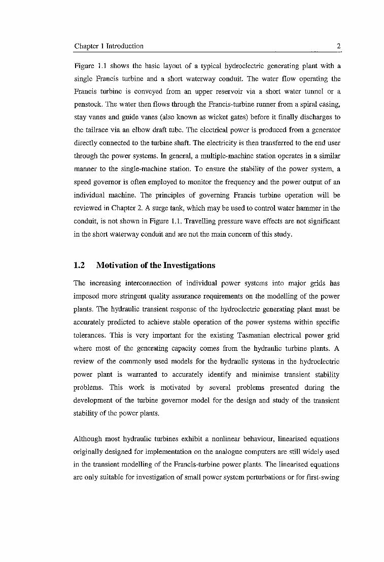
Figure 1.1 shows the basic layout of a typical hydroelectric generating plant with a
single Francis turbine and a short waterway conduit. The water flow operating the
Francis turbine is conveyed from an upper reservoir via a short water tunnel or a
penstock. The water then flows through the Francis-turbine runner from a spiral casing,
stay vanes and guide vanes (also known as wicket gates) before it finally discharges to
the tailrace via an elbow draft tube. The electrical power is produced from a generator
directly connected to the turbine shaft. The electricity is then transferred to the end user
through the power systems. In general, a multiple-machine station operates in a similar
manner to the single-machine station. To ensure the stability of the power system, a
speed governor is often employed to monitor the frequency and the power output of an
individual machine. The principles of governing Francis turbine operation will be
reviewed in Chapter 2. A surge tank, which may be used to control water hammer in the
conduit, is not shown in Figure 1.1. Travelling pressure wave effects are not significant
in the short waterway conduit and are not the main concern of this study.
1.2 Motivation of the Investigations
The increasing interconnection of individual power systems into major grids has
imposed more stringent quality assurance requirements on the modelling of the power
plants. The hydraulic transient response of the hydroelectric generating plant must be
accurately predicted to achieve stable operation of the power systems within specific
tolerances. This is very important for the existing Tasmanian electrical power grid
where most of the generating capacity comes from the hydraulic turbine plants. A
review of the commonly used models for the hydraulic systems in the hydroelectric
power plant is warranted to accurately identify and minimise transient stability
problems. This work is motivated by several problems presented during the
development of the turbine governor model for the design and study of the transient
stability of the power plants.
Although most hydraulic turbines exhibit a nonlinear behaviour, linearised equations
originally designed for implementation on the analogue computers are still widely used
in the transient modelling of the Francis-turbine power plants. The linearised equations
are only suitable for investigation of small power system perturbations or for first-swing
Chapter 1 Introduction 3
stability studies. The turbine characteristics vary nonlinearly with the speed, flow and
the net head of the turbine. Such nonlinearities make the governing of the Francis
turbine operation a nontrivial task, as the turbine governors designed for a particular
operating condition may not work at all under other conditions. There is no guarantee
that the closed-loop system will remain stable at all operating conditions and exhaustive
stability analyses are needed if the linearised turbine models are utilised. However,
simplifications of the nonlinear behaviour for the Francis turbines are no longer
necessary with modern computing power. The present research seeks to improve the
accuracy of existing industrial models for hydroelectric generating plant through the
numerical and experimental flow modelling of the unsteady operation of the typical
Francis-turbine draft tube, and more accurate representation of overall turbine
performance characteristics. The hydraulic transient response of both single- and
multiple-machine power plants will be analysed and described in detail in this thesis.
While extensive introduction on the steady-flow operation of the hydraulic turbines is
currently available, relatively little is known about the transient-flow phenomena. The
unsteady flow behaviour in the draft tube could easily affect the transient stability of the
Francis-turbine power plant and modelling of the draft tube flow is therefore desirable
in order to fully examine the dynamic behaviour of the hydro power plant. However,
there remain great challenges in the simulation, visualization and analysis of the flow in
the draft tube. The complex nature of the draft tube flow has hampered detailed flow
investigations by both experimental measurement and numerical analysis. The swirl
introduced at the draft tube inlet, streamline curvature, flow unsteadiness and
separation, and the adverse pressure gradient caused by the diffusion and changing
cross-sectional shape have complicated the study of draft tube flow behaviour. Each of
these characteristics alone is known to be difficult to predict and measure accurately.
Although some recent publications [6, 7, 75, 92, 105, 107, 109, 118, 132] have started
to investigate the unsteady-flow behaviour of the Francis-turbine draft tube, these
studies are limited to the numerical simulations of the self-excited unsteadiness caused
by the vortex rope and little effort has been applied to probe the externally-excited
unsteadiness that results from the changes in the guide vane settings or the turbine
operating conditions. Much effort is still needed to verify and validate the numerical
solutions of the draft tube flow, even for a simpler steady-state calculation. This study
Chapter 1 Introduction 4
attempts to develop a more comprehensive data bank suitable for the analysis of the
time-dependent draft tube flow near the best-efficiency operating condition. The
prediction capacity of an existing commercial CFD (Computational Fluid Dynamics)
code with different turbulence models will also be evaluated in this work. Attention is
focused on the analysis of the transient fluid losses and the convective time lag in flow
establishment through the draft tube, which are thought to be critical for the study of
transient operation for the Francis-turbine power plants.
This research also aims to provide data for future plant refurbishments to improve the
machine efficiency and the operating stability of a large number of ageing hydraulic
turbine installations. The current refurbishment process that concentrates only on the
redesign of the turbine guide vane and runner is insufficient, as unfavourable flow
behaviour may occur if the new runner design and the draft tube are unsuitably
matched. The deregulated energy market in Australia has called for the power plant
operators to run their hydraulic machines more frequently at off-design conditions. The
off-design performance of hydraulic turbines is strongly influenced by the unsteady
flow behaviour of the draft tube. Although most hydraulic turbines are reasonably
efficient, efficiency improvements of only a few tenths of a percent from the draft tube
design can still generate substantially increased profits. This thesis therefore aims to
gain further insights into the transient operation of the draft tube flow and its influence
on the design and control of the hydro power plant.
1.3 Scope of the Study
This research commenced with an investigation of the deficiency in the existing
industry model used to describe the hydraulic behaviour of Hydro Tasmania's
Mackintosh power plant. Full scale measurement and computational modelling of the
overall hydroelectric system were performed. The unsteady behaviour of the turbine
draft tube and the pressure forces acting on it were later found to be the important
factors affecting the accuracy of the existing model. To further examine this issue, a
balanced approach consisting of both experimental and numerical modelling of the
unsteady draft tube flow was carried out. Particular attention was paid to the transient
operation of the single-machine station with a short waterway conduit. The improved
plant model was developed based on transient analysis of the draft tube model, and was
Chapter 1 Introduction 5
validated against the Mackintosh test results. This single-machine model was also
extended into multiple-machine model, which was validated against the full scale test
results of the Hydro Tasmania's Trevallyn plant. This study had been bounded by
several constraints, including:
• Modelling of Francis-turbine power plants in MATLAB Simulink [124] only. The
complete analysis of the transient plant operation should incorporate both
hydraulic and electrical models of the power plant and the results should be
compared to various simulation codes in common industrial use. The full
investigations of the entire power system and plant operation are performed by
Hydro Tasmania and the study herein will only focus on the improvement in the
hydraulic model of the Francis turbine plant.
• Experimental and numerical testing of the turbine draft tube only. The influences
of the waterway conduit and the tailrace are not being considered in the modelling
of the draft tube flow. Instead, the flow conditions without swirl are imposed at
the draft tube inlet. Ideally the model should include the spiral case, stay vanes,
guide vanes, and the runner as the impacts of the inlet swirl and the rotor-stator
interactions could be essential for the analysis of the draft tube flow.
• Experimental and numerical testing of the draft tube with a predetermined
geometry only. The chosen geometry models the Mackintosh power plant used in
field studies. The effects of stiffening rib, the cross sectional shapes and the
diffusing angle on the transient behaviour of the draft tube flow are not fully
examined due to time constraints.
• Scaling effect of the model. Air is used as the working fluid in the experiments to
facilitate measurements, but the model Reynolds number is about 100 times
smaller than the full scale. Water model testing would have allowed operation at
higher Reynolds numbers (around 12 times larger with similar flow rates) and
given some indication of the magnitude of scale effects. The water models are
required to observe cavitation effects in the draft tube, and also facilitate the
observation of unsteady vortex rope phenomenon. However, logistical
considerations and current resources preclude this.
Chapter 1 Introduction 6
• Limited computing resources. Approximately 12 million nodes are estimated to
achieve the grid-independent solutions for the draft tube geometry used herein.
This requires massive amounts of computing times and resources. Transient
simulations with such numerical grids can easily take more than a month to finish,
even though parallel solvers with multiple CPUs are adopted here. The majority of
the computer simulations are therefore carried out with larger time steps and
coarser grid.
1.3 Thesis Outline
The objectives and scope of the study have been stated earlier in this Chapter. A
background survey of the literature relevant to this research is presented in Chapter 2.
Transient operation of the Francis-turbine power plant is discussed and analysed in
three separate Chapters. Chapter 3 details full-scale field testing of Francis-turbine
power plants including the field-test procedures and the instruments used for both
single- and multiple-machine tests. Chapter 4 examines the transient modelling of
hydraulic components in a single-machine station. The computer model is validated
against the full-scale test results conducted in the Mackintosh power station operated by
Hydro Tasmania. Chapter 5 discusses the transient modelling of a hydro power plant
with multiple machines in operation. The multiple-machine model is validated against
the field test results collected in Hydro Tasmania's Trevallyn power station.
Phase lag problems identified in the above transient modelling exercises for Francis
turbine power plants have led to further detailed investigation of the unsteady flow
effects of the turbine draft tube. Both experimental and numerical flow modelling of a
Francis-turbine draft tube have been carried out. Chapter 6 summarises the experimental
and numerical research methodologies used for the draft tube flow modelling.
Experimental and numerical results are then presented in two separate Chapters.
Chapter 7 contains the results of the steady-state operation that will be used as the initial
conditions for the transient simulation of the draft tube flow. Chapter 8 gives the results
of the unsteady draft tube flow under various transient operating conditions similar to
the actual power plant operation at best efficiency with zero inlet swirl. Conclusions are
drawn and recommendations for future studies are suggested in Chapter 9. Drawings of
the experimental test rig can be found in the Appendix.
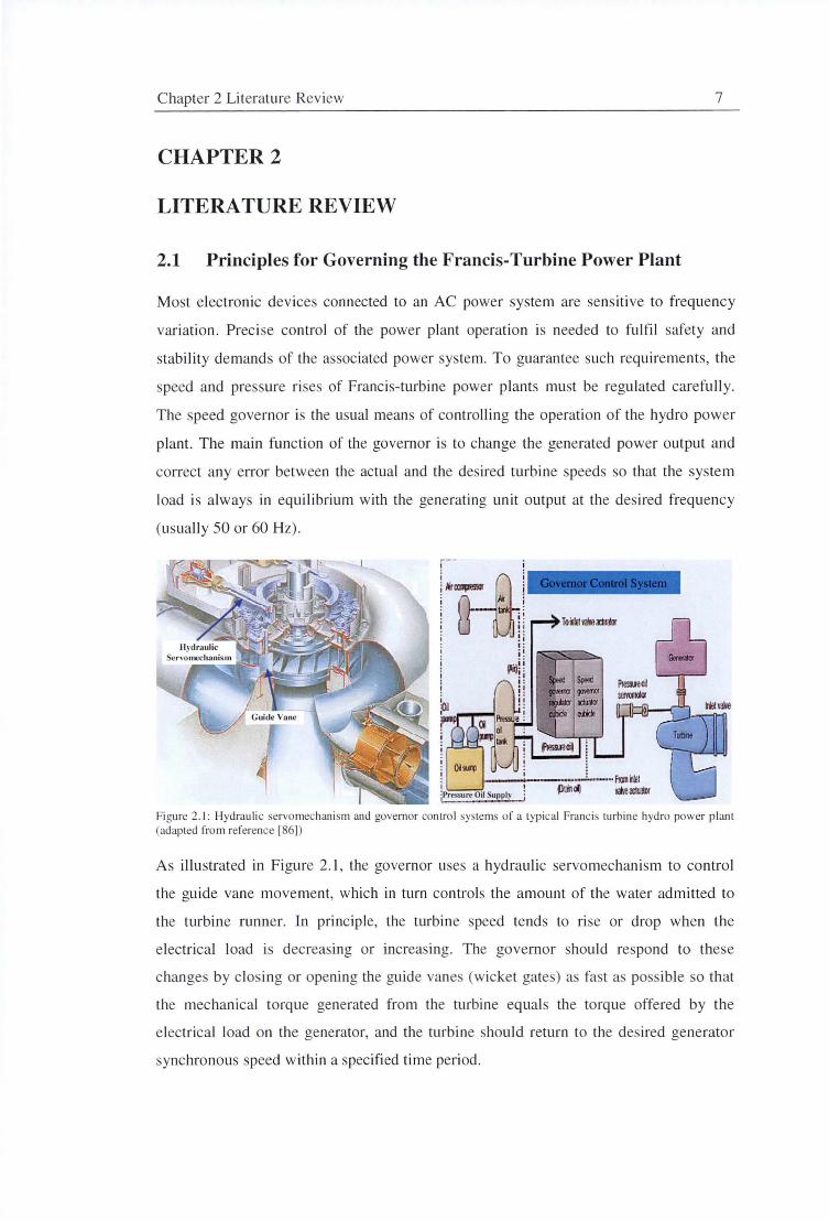
Chapter 2 Literature Rev iew 7
CHAPTER2
LITERATURE REVIEW
2.1 Principles for Governing the Francis-Turbine Power Plant
Most electronic devices connected to an AC power system are sens itive to frequency
variation . Precise control of the power plant operation is needed to fulfil safety and
stability demand of the assoc iated power system. To guarantee such requirements, the
speed and pressure ri se of Francis-turbine power plants must be regulated carefully.
The speed governor is the usual means of controlling the operation of the hydro power
plant. The main func tion of the governor is to change the generated power output and
correct any error between the actual and the des ired turbine speeds so that the system
load is always in equilibrium with the generating unit output at the des ired frequency
(usually 50 or 60 Hz) .
I
"'ffii It i i! i i p ·'
Figure 2 .1 : Hydraulic servomechan ism and governor contro l systems of a typical Francis turbine hydro power p lant (adapted from reference [86])
As illustrated in Figure 2.1 , the governor uses a hydraulic servomechani sm to control
the guide vane movement, which in turn controls the amount of the water admitted to
the turbine runner. In principle, the turbine speed tends to rise or drop when the
e lectrical load is decrea ing or increas ing. The governor should respond to these
changes by c lo ing or openi ng the guide vanes (wicket gates) as fast as possibl e so that
the mechanical torque generated from the turbine equals the torque offered by the
e lectrical load on the generator, and the turbine should return to the desired generator
synchronous speed within a specified time period.
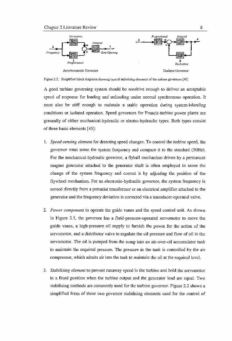
Chapter 2 Literature Review 8
De11vat1ve
3 4
l 2 Prop01 t1011a/ Derivaflve
Accelerometric Governor Dashpot Governor
Figure 2.2. Simplified block diagrams showmg typical stabilising elements of the turbme governors [ 45]
A good turbine governing system should be sensitive enough to deliver an acceptable
speed of response for loading and unloading under normal synchronous operation. It
must also be stiff enough to maintain a stable operation during system-islanding
conditions or isolated operation. Speed governors for Francis-turbine power plants are
generally of either mechanical-hydraulic or electro-hydraulic types. Both types consist
of three basic elements [ 45]:
1. Speed-sensing element for detecting speed changes. To control the turbine speed, the
governor must sense the system frequency and compare it to the standard (50Hz).
For the mechanical-hydraulic governor, a flyball mechanism driven by a permanent
magnet generator attached to the generator shaft is often employed to sense the
change of the system frequency and correct it by adjusting the position of the
flywheel mechanism. For an electronic-hydraulic governor, the system frequency is
sensed directly from a potential transformer or an electrical amplifier attached to the
generator and the frequency deviation is corrected via a transducer-operated valve.
2. Power component to operate the guide vanes and the speed control unit. As shown
in Figure 2.1, the governor has a fluid-pressure-operated servomotor to move the
guide vanes, a high-pressure oil supply to furnish the power for the action of the
servomotor, and a distributor valve to regulate the oil pressure and flow of oil in the
servomotor. The oil is pumped from the sump into an air-over-oil accumulator tank
to maintain the required pressure. The pressure in the tank is controlled by the air
compressor, which admits air into the tank to maintain the oil at the required level.
3. Stabilising element to prevent runaway speed in the turbine and hold the servomotor
in a fixed position when the turbine output and the generator load are equal. Two
stabilising methods are commonly used for the turbine governor. Figure 2.2 shows a
simplified form of these two governor stabilising elements used for the control of
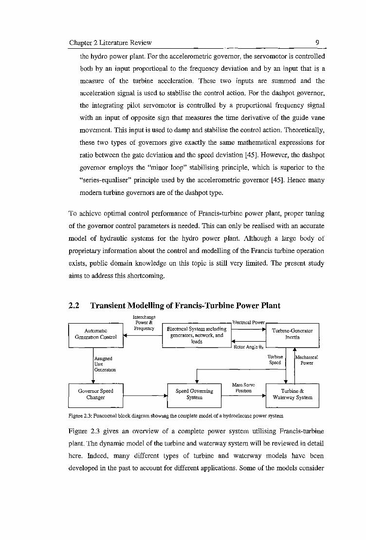
Chapter 2 Literature Review 9
the hydro power plant. For the accelerometric governor, the servomotor is controlled
both by an input proportional to the frequency deviation and by an input that is a
measure of the turbine acceleration. These two inputs are summed and the
acceleration signal is used to stabilise the control action. For the dashpot governor,
the integrating pilot servomotor is controlled by a proportional frequency signal
with an input of opposite sign that measures the time derivative of the guide vane
movement. This input is used to damp and stabilise the control action. Theoretically,
these two types of governors give exactly the same mathematical expressions for
ratio between the gate deviation and the speed deviation [ 45]. However, the dashpot
governor employs the "minor loop" stabilising principle, which is superior to the
"series-equaliser" principle used by the accelerometric governor [ 45]. Hence many
modern turbine governors are of the dashpot type.
To achieve optimal control performance of Francis-turbine power plant, proper tuning
of the governor control parameters is needed. This can only be realised with an accurate
model of hydraulic systems for the hydro power plant. Although a large body of
proprietary information about the control and modelling of the Francis turbine operation
exists, public domain knowledge on this topic is still very limited. The present study
aims to address this shortcoming.
2.2 Transient Modelling of Francis-Turbine Power Plant
Automatic ~
Generat10n Control ~
Assigned Umt Generauon
,
Governor Speed Changer
Interchange p & ow er
Frequency
~
r
Electncal System mcluding generators, network, and
loads
L Speed Governing
System
ec c El tn a!P ow er ~
r Turbme-Generator Inertia
~
Rotor Angle eR ~
Turbme Mechamcal Speed Power
' Mam Servo Pos1t1on Turbine&
~
~ Waterway System
Figure 2.3: Functional block diagram showmg the complete model of a hydroelectnc power system
Figure 2.3 gives an overview of a complete power system utilising Francis-turbine
plant. The dynamic model of the turbine and waterway system will be reviewed in detail
here. Indeed, many different types of turbine and waterway models have been
developed in the past to account for different applications. Some of the models consider
Chapter 2 Literature Review 10
surge chamber effects or hydraulic coupling effects in multiple-turbine plants, others
take into account either elastic or inelastic water columns, and many configurations
include travelling pressure wave effects.
Chaudhry [21] and Streeter & Wylie [123] were among the first to develop a computer
code simulating the hydraulic operation of a Francis-turbine power plant. The simplest
hydraulic network (a turbine connecting to a reservoir via a pipe network) is modelled
in their code but the electrical system is not considered in their models. The codes are
designed only for a single case study and have not been thoroughly validated against the
full turbine operation. Brekke and Li [18], on the other hand, use the structural matrix
approach and a set of linearised equations to construct a more generalised model for a
hydroelectric generating plant. This method has been used extensively for the
investigation of small power system perturbations and has been applied to first swing
stability studies (or frequency domain analysis). Ramey and Skooglund [96], 1973 IEEE
Committee Report [47], Ye et al. [150], Malik et al. [71], and Kundur [59] investigate
the dynamic behaviour of the hydro power plants with an ideal turbine and inelastic
water columns. They all use the classical linearised turbine models, which relate the
mechanical power deviation with the gate opening deviation at a particular operating
condition, to represent the whole turbine performance. Sanathanan [111] develops an
important method to obtain reduced order models for hydraulic turbines with long
waterway conduits, and demonstrates that the first-order linearised turbine models are
faulty, as they always show a stable and strongly damped transient behaviour even
though the real system exhibits undesirable oscillations.
Jones [51] extends the application of the linearised model to the analysis of multiple
machine operation, concluding that single-machine operation has quite different
hydraulic characteristics from the multiple-machine configuration. He suggests that the
governor parameters must be tuned according to the number of operating machines in
order to achieve the optimal control performance from a hydroelectric generating plant.
The frequency response of the power station, which is important for the governor
stability design, can be evaluated by injecting a sinusoidal signal into the transfer
function of the linearised model [98]. The field test procedure designed to study the
transient performance of such operation in the hydro power plant (Nyquist test) has
been described in some detail by Rayner [99].
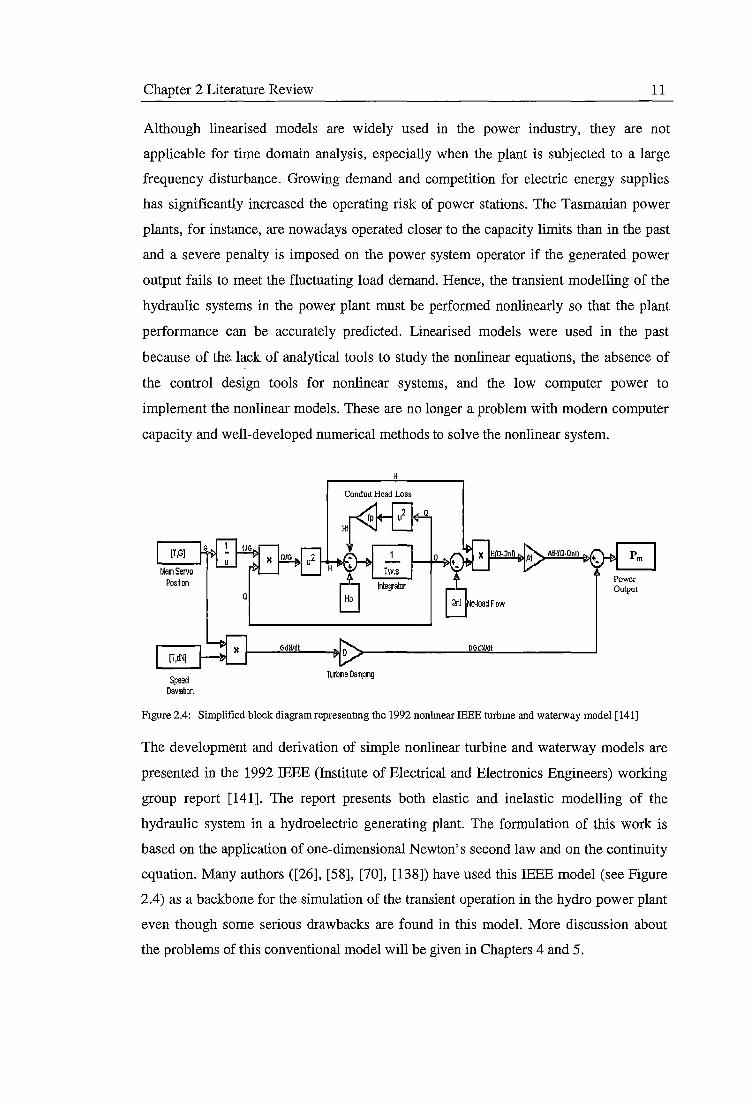
Chapter 2 Literature Review 11
Although linearised models are widely used in the power industry, they are not
applicable for time domain analysis, especially when the plant is subjected to a large
frequency disturbance. Growing demand and competition for electric energy supplies
has significantly increased the operating risk of power stations. The Tasmanian power
plants, for instance, are nowadays operated closer to the capacity limits than in the past
and a severe penalty is imposed on the power system operator if the generated power
output fails to meet the fluctuating load demand. Hence, the transient modelling of the
hydraulic systems in the power plant must be performed nonlinearly so that the plant
performance can be accurately predicted. Linearised models were used in the past
because of the, lack of analytical tools to study the nonlinear equations, the absence of
the control design tools for nonlinear systems, and the low computer power to
implement the nonlinear models. These are no longer a problem with modern computer
capacity and well-developed numerical methods to solve the nonlinear system.
[T,G]
Mam Servo Posl1on
[T,dN]
Speed Deviation
Conduit Head Loss
Turbine Dampmg
Figure 2.4: Simplified block diagramrepresentmg the 1992 nonhnear IEEE turbme and waterway model [141]
The development and derivation of simple nonlinear turbine and waterway models are
presented in the 1992 IEEE (Institute of Electrical and Electronics Engineers) working
group report [141]. The report presents both elastic and inelastic modelling of the
hydraulic system in a hydroelectric generating plant. The formulation of this work is
based on the application of one-dimensional Newton's second law and on the continuity
equation. Many authors ([26], [58], [70], [138]) have used this IEEE model (see Figure
2.4) as a backbone for the simulation of the transient operation in the hydro power plant
even though some serious drawbacks are found in this model. More discussion about
the problems of this conventional model will be given in Chapters 4 and 5.
Chapter 2 Literature Review 12
Nonlinear modelling is generally very useful for control and stability study of plant
operation such as system islanding, excessive load shedding, and black start after power
system restoration where large changes in power output or system frequency are
expected [138]. Modelling of the electromechanical speed governor is usually well
tested and is unlikely to cause any significant accuracy problem in the modelling of
large system disturbance cases. Effective control of such operations will therefore rely
heavily on the accuracy of the turbine and waterway model. Little information is
available to validate this model, as large changes in the system rarely happen.
Nicolet et al. [85] indicate that the hydraulic model of Francis-turbine power plant can
be improved by considering a pressure source driven by the hydraulic characteristic of
the turbine instead of the pure resistance commonly used in the power-engineering
domain to model turbine operation. The latest works of Nicolet et al. [85] attempt to
include the unsteady vortex rope effect in the draft tube and the similitude of the
pressure field along the draft tube extension in their in-house power plant simulation
code SIMSEN. A linearised electrical analogy is still being used to illustrate the
hydraulic components in their plant models. Two parameters are proposed to account
for the wall deformation and water compressibility and for the vortex rope compliance
[85]. Unfortunately, no simulation results have been given to validate this approach and
more efforts are needed to evaluate the data transposed from scale model to prototype.
Up to the present time, no publications have considered the effects of unsteady turbine
operation on the accuracy of the power system simulation. Although the influence of the
unsteady flow behaviour has been recognised in the IEEE working group report [141],
no further development has taken place to ensure the proper inclusion of this effect in
the model. Vaughan [130] reports a significant phase lag between the simulated and
measured power outputs from a single-machine power plant when the guide vane is
oscillating at high speed. Travelling pressure wave effects should not be the cause of
this observed phase lag since the waterway conduit is relatively short in this case.
fustead, the transient flow behaviour of the Francis turbine is likely to be the source of
this problem. The present work is the first step in an attempt to study the unsteady
effects of the draft tube flow on the transient modelling of the Francis-turbine power
plant using both experimental and computational fluid dynamic techniques.
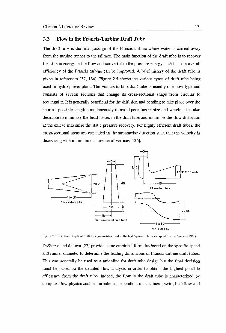
Chapter 2 Literature Review 13
2.3 Flow in the Francis-Turbine Draft Tube
The draft tube is the final passage of the Francis turbine where water is carried away
from the turbine runner to the tailrace. The main function of the draft tube is to recover
the kinetic energy in the flow and convert it to the pressure energy such that the overall
efficiency of the Francis turbine can be improved. A brief history of the draft tube is
given in references [37, 136]. Figure 2.5 shows the various types of draft tube being
used in hydro power plant. The Francis turbine draft tube is usually of elbow type and
consists of several sections that change its cross-sectional shape from circular to
rectangular. It is generally beneficial for the diffusion and bending to take place over the
shortest possible length simultaneously to avoid penalties in size and weight. It is also
desirable to minimise the head losses in the draft tube and minimise the flow distortion
at the exit to maximise the static pressure recovery. For highly efficient draft tubes, the
cross-sectional areas are expanded in the streamwise direction such that the velocity is
decreasing with minimum occurrence of vortices [136].
Conical draft tube
Vertical conical draft tube
I 1.330 X 30 wide _J
~--------11 1-----40----1.
Elbow draft tube
"S" Draft tube
Figure 2.5· Different types of draft tube geometries used in the hydro power plants (adapted from reference [136])
DeSiervo and deLeva [27] provide some empirical formulas based on the specific speed
and runner diameter to determine the leading dimensions of Francis turbine draft tubes.
This can generally be used as a guideline for draft tube design but the final decision
must be based on the detailed flow analysis in order to obtain the highest possible
efficiency from the draft tube. Indeed, the flow in the draft tube is characterized by
complex flow physics such as turbulence, separation, unsteadiness, swirl, backflow and

Chapter 2 Literature Review 14
curved flow. All the flow phenomena present in the bend and straight diffuser will occur
in the elbow draft tube, but will normally exist in a rather more extreme form [81].
Conversion of dynamic pressure to static pressure is therefore more difficult in an elbow
draft tube than in a straight diffuser. An understanding of the draft tube flow physics
will be helpful for the precise control and modelling of the power plant operation.
Fox and Kline [35] report a wide-ranging investigation of curved diffusing flow. The
details of stall inception patterns for the axisymmetric curved diffuser are examined as a
function of NIW1 (axial length normalised on the throat width), fi(turning angle) and 28
(total wall divergence angle) [35]. Secondary flow in the form of a long helical roller is
observed in curved diffusers with turning angles of more than 40°, and reasonable
variations of the inlet velocity profile are found to have only a slight effect on the
location of first appreciable stall [35]. The flow regime data of Fox and Kline [35]
provide considerable insight into the fundamental problems associated with draft tube
design, as the pressure recovery for the draft tube is closely related to its flow regime
[35]. However, the effect of flow separation on the performance of curved diffuser is
not detailed in this study.
Sagi and Johnston [110] present a systematic approach to the analysis of a two
dimensional diffusing bend. The streamline curvature is found to greatly affect the wall
potential-flow velocity distribution and the existence of the secondary flow, as well as
turbulent mixing near the wall (see also Parsons and Hill [93]). Sagi and Johnston [110]
suggest that performance of a curved diffusing channel should be evaluated based on
the potential-flow pressure distributions along the wall, since large changes in the
secondary flow and turbulent mixing effects are usually difficult to obtain for a fixed
geometry. A simple potential flow method is proposed for the design of a curved
diffusing channel. Early designs of turbine draft tubes are mostly founded on the
empirical data and findings given in Fox and Kline [35], and Sagi and Johnston [110].
The performance of a 90°-cascade diffusing bend with an area ratio of 1.45:1 for an
aircraft duct system is studied in Friedman and Westphal [36]. Five different inlet
boundary layers are used to examine the effect of inlet-boundary-layer shape and
thickness on the performance of the diffusing bend [36]. Tests are made at Mach
Chapter 2 Literature Review 15
numbers up to 0.41 and a cascade of airfoils are used to control the boundary layer at
the bend. Results indicate that increasing the inlet boundary layer thickness will
adversely affect the total pressure losses and static pressure recovery [36]. Increasing
inlet Mach number is also shown to adversely affect the performance of the cascade in
the diffusing bend. V aned bends, however, are seldom used in water turbine draft tubes
due to manufacturing difficulties, pressure forces and the possibility of cavitation in
such applications.
The above publications neglect the strong curvature effects and the impacts of
substantial variation in cross-sectional aspect ratio on the flow behaviour inside a
diffusing bend. To understand the flow developments in such extreme geometry (which
is the case for most draft tube geometries), Yaras [145, 146] has conducted a series of
investigations for the strongly curved diffusing bend. Several aspects including the
effect of flow turning on diffusion performance, the dominant structures influencing the
flow development in such geometry and the effect of the inlet boundary conditions are
examined [145]. The three-dimensional velocity distribution at the exit is found to be
sensitive to circumferentially uniform alterations to the inlet boundary layer, while
static-pressure recovery and total-pressure losses are observed to be relatively
insensitive to variations of the inlet boundary layer [145].
Yaras [146] also mentions that the flow pattern within a strongly curved diffusing bend
is similar to the one occurring in the constant-area bend. The secondary flows induced
by a pair of counter-rotating vortices are found to reach maximum strength at about 30°
into the diffusing bend and are significantly stronger for the case with a thinner
boundary layer and lower free-stream turbulence intensity at inlet [146]. The difference
between the actual and ideal static pressure distributions along the diffusing bend is
primarily due to the total pressure losses with a thick inlet boundary layer, whereas the
flow distortion and loss generation influence the streamwise static pressure distribution
by comparable amounts for the thin boundary layer case [146].
Simonsen [119] performs a detailed flow survey in an axial-to-radial axisymmetric bend
diffuser for a gas turbine system, concluding that the bend has an important influence on
the flow in the diffuser and should not be neglected in the diffuser design as it can easily
lead to poor performance or damage to the downstream equipment if not treated
Chapter 2 Literature Review 16
properly. The boundary layer and the turbulent flow properties (particularly the
development of Reynolds stress components) are examined in detail in Simonsen's
research. The difference between the turbulence levels on the inner and outer wall
perimeters is found to cause the wall normal mean velocity to be directed from the inner
perimeter towards the outer perimeter of the diffuser [119]. This cross-stream flow is
kept alive throughout most of the diffuser until turbulent diffusion has equalised the
cross-sectional turbulence profiles [119]. The findings have been used to improve the
boundary layer condition along inner perimeter so that flow separation is avoided. The
flow in Simonsen' s diffuser is generally less complex than that for Francis turbine draft
tube because the flow is axisymmetric and the diffusion happens only after the bend.
Wahl [133] investigates experimentally the phenomenon of draft tube surge (see also
Hosoi [44], Skotak [118]) and attempts to correlate the hill chart of the Francis turbine
with different modes of draft tube vortex surging observed in experimental tests. The
main objective is to identify the critical operating points where synchronous pressure
pulsations, which cause severe vibrations, noise, fatigue failure and power swings in the
power plants, may occur. A dimensionless swirl parameter (mDruri!pQ2) has been used
as an indicator for the existence of the twin vortex, which is an excitation source for the
draft tube surging. However, Wahl [133] points out that the surge behaviour in the
overload region is significantly different from that in part-load operation and the draft
tube swirl parameter is still unable to fully explain the behaviour of the draft tube surge
over the complete operating range of the Francis turbine.
Ruprecht et al. [108] examine numerically and experimentally the unsteady vortex rope
behaviour in a draft tube under part load conditions. This causes oscillations in the
waterway conduit and a discharge variation at the turbine admission (see also Dorfler
[30], Vu et al. [132]). Dynamic behaviour of the waterway systems is taken into account
using the one-dimensional method of characteristics [108]. Pressure at the draft tube
inlet is averaged at each time step of the numerical simulation and this value is then fed
into the one-dimensional model of the waterway system as a boundary condition [108].
The new discharge value obtained from the waterway model is used to update the inlet
boundary condition of the draft tube in the numerical simulation [108]. Ruprecht et al.
[108] indicate that a synchronous pressure oscillation of approximately 3% will cause
about 1 % variation in the turbine discharge. This case study assumes that the waterway
Chapter 2 Literature Review 17
conduit is not in resonance with the draft tube surge. Otherwise, more severe pressure
and velocity oscillations may result in the power plant [108].
Mauri [73, 75] explores the flow behaviour of a Francis-turbine draft tube from a
different perspective. The mean flow field of the draft tube is analysed numerically and
experimentally but the turbulence profiles are not fully examined. Mauri [73, 75]
suggests using the topological structure of flow field to show the bifurcation with the
flow rate as a parameter leading to a Werle-Legendre separation, which can reduce the
draft tube performance over an operating range [73]. The pressure recovery factor is
found to be sensitive to the flow rate, which behaves in a similar way as the machine
efficiency (i.e. the pressure recovery factor peaks at the full flow condition and then
drops at overload operating conditions). A self-sustained time-dependent vortex
shedding is observed numerically in some cases even though the boundary conditions
remain unchanged. The mean flow field is not affected by this phenomenon [73].
At this stage, few studies have actually considered the unsteady flow effects at the draft
tube. Mauri [75] presents a case of forced time-dependent draft tube flow where the
fluctuations are caused by the runner rotation. A quick damping of the fluctuations,
which is caused by an error in the prediction of the phase shift between velocity and
pressure fluctuations, is observed numerically [75]. These fluctuations are however
recognised to quickly disappear at the cone outlet during experiment. Similar statements
are also made by Yang et al. [144]. Mauri [75] argues that computational error is mainly
caused by the poor prediction of the flow unsteadiness and not the problems of
turbulence modelling. This statement is questionable, since no detailed investigation is
performed in his study to compare the turbulence quantities obtained from numerical
calculations and experiments.
Y aras and Orsi [147, 149] conduct several tests to study the effects of the periodic
inflow unsteadiness on the flow development in a fishtail-shaped diffusing bend of
strong curvature for gas turbine operation. When inflow oscillation condition is
compared to the design operating condition, the time-averaged velocity field is found to
be very similar to that obtained under steady inflow conditions with comparable inlet
boundary-layer thickness [147]. A strong flow asymmetry caused by the difference in
strengths of two counter-rotating streamwise vortices is also detected when the
Chapter 2 Literature Review 18
frequency of the inflow velocity fluctuat10ns is decreased. Furthermore, the transients in
the ensemble-averaged velocity distribution at the diffuser exit are observed to decrease
to negligible levels if a three- to fourfold increase in the frequency is imposed for the
inflow unsteadiness [147, 149].
To the author's best knowledge, little or no study has been carried out on the unsteady
flow effects of a Francis-turbine draft tube due to changes in flow operating condition.
Most of the papers (including Mauri [75], Ruprecht et al. [108], Skotak [118], Vu et al.
[132], Yaras & Orsi [147, 149]) that investigate the transient flow behaviour in the draft
tube either concentrate on the self-excited unsteadiness caused by the turbulent motion,
vortex shedding (Karman vortex street), and unsteady vortex rope in the draft tube, or
focus on the externally forced unsteadiness resulting from changes of the inlet domain
due to runner rotation. Although rotor-stator interactions in the turbine have been the
subject of research for years, they are usually studied individually without taking the
existence of draft tube into consideration. The moving-mesh technique for numerical
computation is still at its early stage of development and is only usable when a very
simple motion is applied on the geometry. Much effort is needed to make the solution
more realistic. Applying transient boundary conditions is therefore the most effective
method for such analysis. This thesis investigates numerically and experimentally the
unsteady operations of the draft tube caused by changes of the turbine discharge.
Emphasis is put on determining the time lag required to establish a new steady state in
the draft tube after a change in inlet flow condition.
2.4 Experimental Testing
Although it has long been recognised that the flow in the hydraulic turbine is
predominantly three-dimensional and unsteady, the approach to the design and
development of Francis turbine power plant ignores most of these flow features. This
approach is no longer appropriate for today's operating environments due to growing
complexity of the power systems, which call for more precise control of the turbine
operation. Such requirements can only be fulfilled through the more detailed flow
modelling of the Francis turbine components. There are two basic approaches to model
the unsteady flow effects in the Francis turbine draft tube, namely experimental testing
and numerical modelling (CFD).
Chapter 2 Literature Review 19
While numerical modelling offers the ability to study the evolution of the pressure and
velocity fields inside the draft tube at less cost than the conventional experimental
testing, experimental data for CFD validation is generally required. Mehta [77] defines
validation as "an essential process of assessing the credibility of the simulation model,
within its domain of applicability, by determining whether the right simulation model is
developed and by estimating the degree to which the model is an accurate representation
of reality ... ". Experimental testing may also reveal flow phenomena present in the
actual flow for which the numerical model has no mechanism for prediction. Van Wie
and Rice [129] also point out that "it becomes difficult to separate the validation of the
measurement procedure from the validation of the analysis procedure. In this situation,
the experimental and analytical techniques are intertwined in a single process".
Yaras [146, 147, 149] details the experimental model testing for a strongly curved
diffusing bend (including both steady and unsteady flow measurements). The model
with an area ratio of 3.42:1 is manufactured using CNC machining and an open-circuit
wind tunnel provides the flow source for the tests. The boundary layer thickness at the
inlet is established by adjusting the length of the entry pipe [146]. The steady-state flow
field is measured via a miniature non-nulling seven-hole pressure probe (2.1 mm
diameter) and a capacitive-type pressure transducer while the instantaneous velocity
field is measured using a miniature hotwire probe with four tungsten sensors (of 1 mm
long and 5 µm diameter) and a constant-temperature anemometer. A perforated plate
mounted on a radial spoke in an alternating pattern is employed to generate the periodic
inflow unsteadiness at various frequencies [147].
Simonsen [119] undertakes scaled model tests on an axisymmetric bend-diffuser
geometry used for gas turbine operation. The model is made out of transparent
plexiglass and the air is used as the working fluid in his experiments. Most of his
measurements use the hotwire technique and the Reynolds number effects on the flow
properties are investigated. The Reynolds stress components and the mean flow
velocities at various sections of the diffuser are obtained using either 2.5 µm single-wire
platinum-rhodium sensors or 5 µm cross-wire tungsten sensors. The static and total
pressures are measured via linear response pressure transducers, while the skin friction
measurements are performed using a surface Pitot tube. All the tests are accomplished at
constant flow speed and no transient measurements are obtained in these experiments.
Chapter 2 Literature Review 20
Andersson and Karlsson [2] discuss the experimental methods for the flow
measurement in a 1:11 scale sharp-heel draft tube. Inlet boundary-layer control is not
necessary in their case as the whole Kaplan runner is also included in the model. Water
is used as the working fluid for the tests. The tangential and axial velocities at the draft
tube inlet (and outlet) are obtained via Laser-Doppler Anemometry (LDA) but the radial
velocity is not measured due to hardware limitations. The water is seeded with nylon
particles to improve the LDA signal quality. The centreline wall pressures are obtained
using a differential pressure gauge. Fluorescent dye is injected at various positions of
the draft tube for flow visualisation. The model test results of Andersson [3] have been
used extensively for CFD validation (Turbine 99 workshops [37]) but these do not
include transient flow measurements.
Arpe and Avellan [6], Berca et al. [12], Vu et al. [132] and Mauri et al. [73] have
investigated various aspects of the draft tube flow phenomena in the same Francis
turbine model (1: 10 scale) at the laboratory of EPFL. The model consists of stay vanes,
guide vanes, runner and the draft tube (with transparent inlet cone). However, the
waterway conduit and the tailrace are not included in their test facility. Laser-Doppler
anemometry (LDA) and particle image velocimetry (PN) are used to measure the
velocity and turbulence fields at draft tube inlet and outlet. The water is seeded with
spherical silver coated glass particles of 10 µm diameter to reduce the LDA acquisition
time. A miniature five-hole pressure probe is employed for instantaneous velocity
surveys at other locations of the draft tube. Unsteady wall pressure measurements are
carried out using fast response pressure transducers (frequency response up to 51.2 kHz)
while wall friction measurements are performed with a hot-film probe. Although
unsteady flow measurements are conducted in their laboratory, the transient flow effects
generated by the changes in the guide vane positions are not investigated at all and the
tests are completed at fixed guide vane settings.
Wahl [133] tests a 1:40.3 scale model, consisting of the penstock, guide vanes, runner,
draft tube and the tailrace. Although the complete hydraulic system is modelled in
Wahl' s experiments, no detailed pressure and velocity surveys are carried out in his
tests. The amplitude and frequency of the pressure fluctuations at the draft tube inlet
under different operating conditions are the only data being recorded [133]. The
Chapter 2 Literature Review 21
analyses are centred on the visualisation of the vortices in the fibreglass draft tube.
Wahl [133] points out that the results obtained from this water model are essentially
identical to those from the air model (conducted by his predecessors). The study gives
some fundamental insights into the complex nature of the draft tube flow and illustrates
the difficulties in performing accurate measurements for such a large-scale facility.
Rayner [99] details the field test procedure (including the governor response test) to
examine the transient behaviour in a full-scale Francis turbine power plant. The lack of
suitable fast-response pressure transducers for the full-scale machine and the complexity
involved in the installation of new pressure tappings on an existing draft tube preclude
detailed flow surveys during the field tests. Although some wall pressure measurements
at the draft tube inlet are recorded, the data may not be suitable for transient flow
analysis as the frequency response of the pressure transducer used in the tests is quite
low. Hence, the present study that employs wind-tunnel based experimentation using a
scaled draft tube model and the pneumatically controlled vane systems are thought to be
a more realistic and efficient approach to examine the unsteady flow effects in a Francis
turbine power plant.
2.5 Computational Fluid Dynamics (CFD)
Computational Fluid Dynamics (CPD) methods have been widely used in the power
generation industry for decades. Extensive literature on CPD studies of the hydraulic
turbine draft tube can be found in numerous fluid mechanics publications (e.g. A vellan
[9], Bergstrom [15], Drtina et al. [31], Engstrom et al. [33], Gebart et al. [37], Mauri
[75], Rudolf and Skotak [105], Ruprecht [108], Shyy and Braaten [114], Vu et al. [132],
Yang et al. [144] and Yuan and Schilling [151]). Large eddy simulation (LES) and
Reynolds-averaged Navier-Stokes (RANS) code are two general numerical approaches
used for such application. Three-dimensional viscous and turbulent solvers are often
employed in these studies, as the potential flow analysis (or Euler codes) fail to fully
describe the complex behaviour of the draft tube flow.
Gebart et al. [37] organised the first ERCOFTAC workshop to systematically
investigate the limitations and the problems faced in the steady-flow simulation of a
standard draft tube at a particular operating condition using different codes and
Chapter 2 Literature Review 22
techniques. Many insights can be gained from this workshop, even though only the
steady flow calculations are reported here. The experimental inlet velocity profiles
(tangential and axial components) and the outlet wall pressures have been supplied as
the boundary conditions for the simulation. The contributions to the workshop are based
on simulations with nine different commercial and three different in-house CPD codes.
The methods include finite element, structured multi-block finite-volume and
unstructured finite-volume methods. Some useful findings from these simulations are
summarised as follows:
• Bergstrom [15] uses the block-structured code CFX-4.2 with the Reynolds stress
model for the simulation. The grid error is evaluated using the general Richardson
extrapolation method (see also Avellan [9]) while the iterative error is assessed
through the investigation of the residuals for all flow variables. However, the
attempt to use pure Richardson extrapolation is unsuccessful in this case since the
asymptotic range is not reached for the grid sequence used. The coarse grid and the
poor iterative convergence for the Reynolds stress are thought to be the reasons for
not reaching the asymptotic range. Bergstrom [15] recommends that a transient
simulation should be carried out for further investigation and the unknown radial
velocity (and its fluctuation) at the inlet should be resolved in order to get a more
realistic solution.
• Kim et al. [54] and Lai and Patel [62] use the same grid with two different finite
volume codes (Fluent and U2RANS) and they obtain almost identical results from
the simulations. A mesh dependency test is performed through the visual inspection
of the flow field at a particular section of the draft tube (after the bend) [62]. A mesh
size of about 708000 cells is selected for the final calculation since no obvious
changes in the flow features are observed for this mesh. The numerical results are
found to be insensitive to the exit location. However, this is not always true as the
outlet boundary location may affect the convergence and stability of a numerical
solution when the strongly recirculating flow occurs at the outlet. No significant
difference is found in the prediction of flow field inside the draft tube for both k-E
and k-m turbulence models tested (except for slightly higher pressure recovery and
energy losses predicted by k-E turbulence model).
Chapter 2 Literature Review 23
• Page and Giroux [91] find that the results generated from the finite element
(FIDAP) and finite volume (CFX-TASCflow) codes are quite different even though
the same turbulence model (standard k-&) and the same grid size are applied in the
simulation. The grid error is examined by comparing the centreline velocity profiles
at different sections of the draft tube using two different mesh densities. The steady
flow solution is observed to be sensitive to the radial velocity distribution (which
can increase the pressure recovery factor by 15% if included in the inlet boundary
condition), while the turbulence dissipation at the inlet and the discretization scheme
are found to affect the "shape" of the centreline velocity profile noticeably.
• Longatte et al. [67] compare results using the finite-element (N3S) and the finite
volume (Fluent-UNS) codes. Unstructured tetrahedral meshes with different grid
sizes are employed (but a grid sensitivity test is not performed) and the predicted
flow fields from these two codes are found to be quite different. The variation is
thought to be caused by different approaches used for the near-wall treatment.
Longatte et al. [67] also check the impacts of the outlet boundary location by adding
a tank at the draft tube outlet, concluding that the outlet conditions have little
influence on the steady-flow solution for the draft tube.
• Komminaho and Bard [57] perform unsteady calculations with different time steps
using Fluent-5 and a realisable k-& model, and conclude that an unsteady vortex in
the inlet region can cause convergence problems in the steady-flow solution. Staubli
and Meyer [122] conduct similar quasi-unsteady simulations using CFX-TASCflow
and a standard k-& model. Their attempt to study Reynolds number effects fails, as
the inlet boundary layers of the prototype are different and not known in this case.
The impacts of the unsteady flow behaviour on the draft tube performance are not
discussed in detail in these papers and the transient simulation is conducted merely
to explain the possible causes of the poor convergence in the solution when steady
flow solvers are used.
• Lorstad and Fuchs [68] estimate, based on physical arguments, the grid size
necessary for a satisfactory LES simulation of the draft tube flow in a finite-element
program SPECTRUM. A mesh size of about 4 million and a time step of around
Chapter 2 Literature Review 24
0.002 second are necessary to properly resolve all length scales of LES [68].
However, no attempt has been made to perform a serious LES based on these
estimates due to the lack of adequate computational resources. Three different
combinations of inflow boundary conditions are tested and the Reynolds number
dependency is investigated. However, no firm conclusions can be made at this stage
due to large variations of the results, the unknown fluctuating part of the inflow
boundary conditions and the relatively coarse mesh being applied in this analysis.
Similar problems are reported by Yang et al. [144].
• Clerides and Jones [22], Grotjans [39], Komminaho and Bard [57], Kurosawa et al.
[60], Lorstad and Fuchs [68], Ma et al. [69], Skotak [117], Skare et al. [116], Staubli
and Meyer [122] and Thakur et al. [125] discuss their results based on single-grid
calculations. Although the importance of grid convergence is constantly cited in
these papers, none actually undertake a grid sensitivity analysis. It is difficult to
draw any general conclusions under such situation of what turbulence model is most
suitable for draft tube simulation and which boundary condition is most stable when
no proper grid sensitivity analysis has been carried out. Grid convergence study
should be standard practice in all CPD analyses and are required, for instance, by
ASME Journal of Fluids Engineering, International Journal for Numerical Methods
in Fluids, and AIAA journals. It is no longer adequate to publish results performed
on a single fixed grid (Wilcox [140], Roache [103]). Rumsey and Vatsa [106] state
that "mesh refinement. .. can sometimes lead to dramatically different results,
particularly for 3-D separated flow " (one of the important flow phenomena in the
draft tube). Grid improvements are usually required to accurately model the surface
shear stress, which is another important variable used to study the losses in a turbine
draft tube.
• It has been demonstrated in the First ERCOFTAC workshop [37] that small
alterations (especially the inlet boundary condition, turbulence model and the mesh
density) in the numerical set-up could lead to large discrepancies in the final results.
Different users solving the identical problem with the same numerical code can
easily end up with varying results. User experience still plays an important role in
the CPD simulation. A remark taken directly from Roache [103] is probably worth
repeating here. "No one believes the CPD results except the one who performed the
Chapter 2 Literature Review 25
calculation, and everyone believes the experimental results except the one who
performed the experiment". This statement clearly emphasizes the need for
extensive verification and validation for both numerical and experimental modelling
of the draft tube flow.
To provide more consistent reporting of the results for numerical simulation of the draft
tube flow, the grid and the material models are fixed in the second ERCOFTAC
workshop organised by Engstrom et al. [33]. Several interesting findings from the
workshop participants are listed below:
• Belanger [11] uses the commercial code PowerFLOW for large eddy simulations.
The approach is based on the kinetic energy of gases and the special discretization
of the Boltzmann equation (instead of solving the RANS equations). The boundary
condition at the wall is realised via a flux formulation according to the kinetic
process while the RNG based k-c model is used to represent the dynamics of sub
grid turbulence in the flow [11]. Simulations with two different grid sizes are
performed but no details are given to show the grid convergent solution.
• Cervantes and Engstrom [20] employ the finite-volume code CFX-4 and the
standard k-c model to evaluate the influence and the interaction of the surf ace
roughness, the inlet radial velocity and the inlet dissipation length scale on the
important flow variables used for draft tube analysis. The inlet radial velocity
distribution is found to be the most critical parameter influencing the pressure
recovery and energy loss coefficient of the draft tube, while the dissipation rate at
the inlet changes the flow variables only slightly. The surface roughness is observed
to affect the total losses in the draft tube, but not the pressure recovery factor (22%
change in the loss coefficient but only 3.3% for the pressure recovery factor if
surface roughness increases from 0 to 200 µm). Hence, the near-wall flow should be
carefully modelled to ensure an accurate prediction of draft tube losses.
• Jonzen et al. [50] use the unstructured finite-volume code Fluent 6 and the standard
k-c model to investigate the influence of wall adjacent cells (or y+ value) on the
steady-flow calculations. A 1.8% variation of y+ value at the inlet wall is observed

Chapter 2 Literature Review 26
to significantly increase the static pressure and wall shear stress at the inlet, but the
effects are gradually decreased towards the outlet of the draft tube (and thereby
generate a distinct pressure recovery factor). Apart from this, no major difference is
found between the flow patterns for varying sizes of the wall adjacent cells used in
the simulation.
• Shimmei et al. [ 115] compare the results of different turbulence models (standard k
c model, Speziale' s quadratic nonlinear k-c model, Suga' s cubic nonlinear k-c model
and LES) based on the single grid calculation. The nonlinear k-c models are found
to generate similar solutions if compared with the time-averaging results of LES,
which is expected as the turbulence in the draft tube is highly anisotropic. However,
it is impossible to tell if the numerical error is caused by the isotropic assumption of
the turbulence models or insufficient grid resolution as a grid convergence study is
not conducted in the simulation.
Hellstrom [43] use CFD to redesign the shape of an existing draft tube in order to
improve the pressure recovery factor. Both steady and transient simulations are
performed in CFX 5.7 with the standard k-cand SST turbulence models. A maximum of
6.2 million unstructured tetrahedral cells generated by ICEM CFD is used for the
numerical investigation. Computational analysis of the modified geometry by Hellstrom
[43] indicates that the improvement in pressure recovery between the original and the
modified geometry is small, which does not agree with experimental results. However,
he points out that his grid quality is questionable (mesh sensitivity test are not
performed) and the simulations using the Shear Stress Transport (SST) turbulence
model are not converged even though many different numerical settings are tried. This
is in line with the current author's experience for ICEM CFD and CFX 5. 7. ICEM CFD
employs an Octree unstructured meshing algorithm that does not work well with
geometry having sliver surfaces and small angles, while the CFX mesher is unable to
cope well with the "bumpy" surface mesh generated in this case. The use of
unstructured hexahedral mesh should overcome this problem.
Rudolf and Skotak [105] conduct a numerical investigation of the unsteady self-excited
vortex flow in an elbow draft tube using Fluent-5.4. Both inviscid and Reynolds stress

Chapter 2 Literature Review 27
models have been used to examine the effect of dissipation on the draft tube vortex
flow. The inviscid model is shown to predict the vortex rope dynamics fairly well in the
region of inlet cone, but the solution becomes unrealistic downstream of the elbow due
to the lack of the damping offered by the inviscid model. Hence, Rudolf and Skotak
[105] comment that "using Reynolds stress model (RSM) appeared to be the best
approach to simulation of turbulent unsteady flow in draft tube, although it was very
time consuming". However, no details for verification of the calculations are given to
show the effects of the varying boundary conditions and turbulence models. Time step
and grid sensitivity tests are not mentioned at all in their works, which calls into
question their statements that "the pressure pulsations at the draft tube inlet are not
smooth sine waves but a superposition of two sine waves". Identical problems are also
found in the work of Vu et al. [132]
Shyy and Braaten [114] examine numerically the effects of inlet swirl on draft tube
performance, concluding that the strength of the inlet swirl will affect the overall
pressure recovery factors and increase the non-uniformity of the exit velocity profiles.
Two discretization schemes (hybrid and second-order upwind) are studied in detail with
two different grid densities. Drtina et al. [31] employ a similar grid to investigate the
impact of a stiffening rib in the draft tube. Although two different grid systems are used
in the simulations, they do not discuss the influence of the grid densities at all, but only
state that "many of the salient features observed on the fine grid system are smeared out
on the coarse grid system". The lack of measurement data for turbulent quantities to
validate the numerical calculations also limits the credibility of the results in this case.
Simonsen [119] undertakes both grid sensitivity analysis and experimental validation of
numerical flow modelling for an axisymmetric curved diffuser using Fluent-6. The inlet
and outlet boundary locations are extended some distances away from the original
geometry to avoid the influence of the upstream bend effects and downstream reversed
flow effects on the numerical solutions. Three different (hexahedral) grid densities are ,
tested in conjunction with different turbulent models (Spalart-Almaras, standard k-£,
RNG based k-£, realisable k-£, and Reynolds stress models). A grid convergent solution
is obtained via inspection of the variation of outlet velocity profiles caused by changing
grid sizes. The Reynolds stress model is found to predict the pressure recovery factor
and the turbulent kinetic energy most accurately but the model performs less well in the
Chapter 2 Literature Review 28
predicting the skin friction distribution and the "shape" of the mean flow velocity
profiles if compared to RNG based k-& or realisable k-& models. Simonsen [119] is
unable to clearly explain the cause of this problem, but points out that the inlet
boundary conditions (Reynolds stress components and the turbulence dissipation) and
the near-wall treatment could well affect the accuracy of the Reynolds stress model.
Paik et al. [92] use an in-house CPD code to compare the solutions generated from
unsteady Reynolds-averaged Navier-Stokes (URANS) simulations and detached-eddy
simulations (DES). They conclude that the flow in the draft tube is highly unsteady even
without imposing any kind of explicit unsteady forcing at the inlet. Significant
discrepancies between the DES and URANS predictions of the turbulence statistics are
observed in the straight downstream diffuser. Both URANS and DES predictions
capture the onset of complex large-scale flow instabilities in the draft tube and yield
mean velocity profiles in reasonable agreement with measurements. However, mesh
dependency tests are not performed in their work and further detailed flow measurement
is required to fully assess the performance of various unsteady statistical turbulence
modelling strategies.
To the best of the present author's knowledge, no papers on the CPD analysis of draft
tube flow have given a clear approach to the systematic refinement of near-wall
elements. Most authors determine their grid independent solutions based on a fixed Y
plus value or a constant wall distance. Although Bergstrom [15] and Mauri [74, 75]
have both utilized the Grid Convergence Index (CGI) and Richardson extrapolation
methods to systematically refine the mesh and uniformly report the grid convergent
solution, they do not detail the methods of refining the near-wall mesh when the wall
function is also used in the simulation. In fact, the use of wall functions actually
prevents the grid from being refined uniformly and systematically near the wall. The
current study finds that refining the near-wall mesh can easily produce a huge difference
in the solution and should therefore be considered in the grid sensitivity analysis.
In summary, CPD solutions of the draft tube flow are significantly affected by many
factors such as boundary conditions, turbulence models, grid densities and the
numerical approaches used in the flow modelling. The current study uses the total
pressure rather than the experimentally derived velocity profiles (which have been

Chapter 2 Literature Review 29
implemented by most of the papers found) as the inlet boundary condition in the
numerical modelling of the draft tube flow. Extensive verification and validation must
be performed before the results can be used with confidence in the design process. This
is particularly true in the present work, as no papers have been found to address the
issues of verification and validation for the transient flow simulation of the draft tube.

Chapter 3 Field Tests for Francis-turbine Power Plants
CHAPTER3
FIELD TESTS PLANTS
3.1 Overview
FOR FRANCIS-TURBINE
30
POWER
A fi eld test program was developed for the single-machine testing conducted at Hydro
Tasmania's Mackintosh power station as well as the multiple-machine testing
performed at Trevallyn power station. The main objective was to investigate
experimentally the transient response of the Francis-turbine power plants when the
system frequency or the electrical load is fluctuating. The tests provided useful data to
validate the hydraulic models , to identify the model parameters for individual power
plants, and to investigate the stability of a power plant. The major component of the
fi eld test program were steady-state measurement, frequency deviation tests and the
Nyquist tests. Thi s Chapter describes the general instrumentation and test procedures
used for both single- and multiple-machine tests. Figure 3. 1 shows a schematic of the
locations and types of instrumentation used in the field tests of a Francis-turbine power
plant. The analysis of te t re ults and their comparison with simulation results generated
from MATLAB Simulink will be covered in Chapters 4 and 5.
G Data Acquisition Tools 0 Generator Frequency Tra nsducer
@ Pressure Transducer 0 Servomotor Position Feedbac k
@ Three-phase Wattmeter © Strain -Gauge Torque Sensor
Figure 3.1: Locations and types of in trumentation used in the field tests of a Franc is- turbine power plant
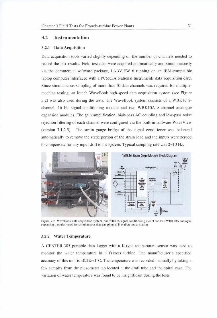
Chapter 3 Field Tests fo r Francis-turbine Power P lants 3 1
3.2 Instrumentation
3.2.1 Data Acquisition
Data acquisition tools vari ed s li ght ly depending on the number of channels needed to
record the test results. Field test data were acquired automaticall y and simultaneously
via the commercia l software package, LAB VIEW 6 running on an IBM-co mpatib le
laptop computer interfaced with a PCMCIA National Instruments data acquisition card.
Since simu ltaneous sampling of more than 10 data channels was required fo r mul tipl e
machine testing, an Iotech W aveBook high-speed data acqui siti on system (see Figure
3.2) was also used during the tests. The WaveBook system consists of a WBK1 6 8-
channel, 16 bit s igna l-conditioning module and two WBK JOA 8-channel analogue
ex pansion modul es. The gain amplification , high-pass AC coupling and low-pass noise
rej ection filtering of each channel were configured via the built-in software Wave View
(version 7.1.2.5). The strain gauge bridge of the signal cond itioner was balanced
automaticall y to remove the static porti on of the strain load and the inputs were zeroed
to compensate fo r any input drift to the system. Typical sampling rate was 2- 10 Hz.
• : I : WBK16 Strain Gage Module Block Diagram
"" ~ ,-------------~"-~-~---- - --- - -- -:z_,
~ ; .
b >T--1-r+-i:
Figure 3.2 : WaveBoo k data acquisition system (one WB Kl 6 signal conditionin g model and two WB KI OA analogue ex pansion modules) used fo r simul taneous data samp li ng at Trevall yn power station
3.2.2 Water Temperature
A CENTER-305 portable data logger with a K-type temperature sensor was used to
monitor the water temperature in a Franc is turbine. The manufacturer' s spec ified
accuracy of thi s unit is ±0.2%+ I °C. The temperature was recorded manuall y by tak ing a
few samples fro m the piezometer tap located at the draft tube and the spi ral case. The
variation of water temperature was fo und to be insignificant during the tests.
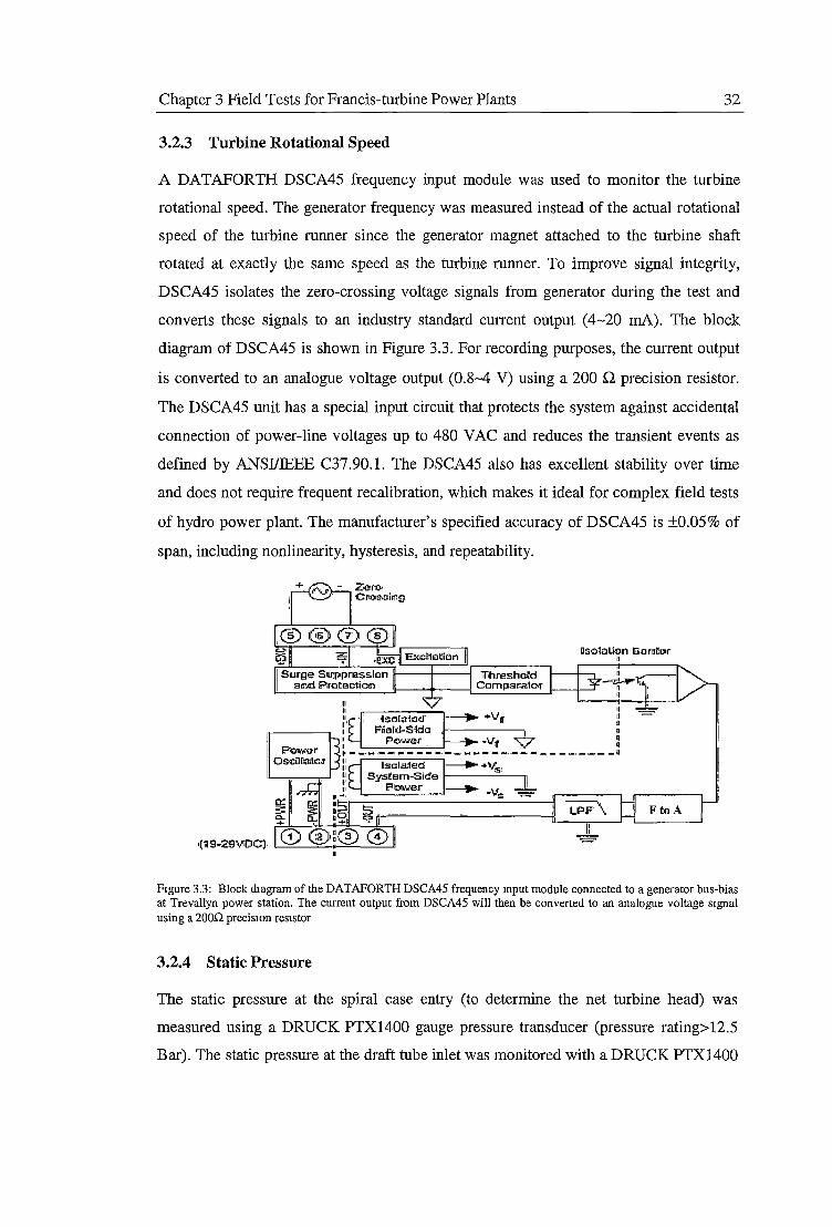
Chapter 3 Field Tests for Francis-turbine Power Plants 32
3.2.3 Turbine Rotational Speed
A DATAFORTH DSCA45 frequency input module was used to monitor the turbine
rotational speed. The generator frequency was measured instead of the actual rotational
speed of the turbine runner since the generator magnet attached to the turbine shaft
rotated at exactly the same speed as the turbine runner. To improve signal integrity,
DSCA45 isolates the zero-crossing voltage signals from generator during the test and
converts these signals to an industry standard current output (4-20 mA). The block
diagram of DSCA45 is shown in Figure 3.3. For recording purposes, the current output
is converted to an analogue voltage output (0.8-4 V) using a 200 .Q precision resistor.
The DSCA45 unit has a special input circuit that protects the system against accidental
connection of power-line voltages up to 480 VAC and reduces the transient events as
defined by ANSI/JEEE C37.90.l. The DSCA45 also has excellent stability over time
and does not require frequent recalibration, which makes it ideal for complex field tests
of hydro power plant. The manufacturer's specified accuracy of DSCA45 is ±0.05% of
span, including nonlinearity, hysteresis, and repeatability.
Thresh a!\::! Compall'ator
~=lnlion Eilamor II
Figure 3.3: Block diagram of the DATAFORTH DSCA45 frequency mput module connected to a generator bus-bias at Trevallyn power station. The current output from DSCA45 will then be converted to an analogue voltage signal using a 200.Q precis10n resistor
3.2.4 Static Pressure
The static pressure at the spiral case entry (to determine the net turbine head) was
measured using a DRUCK PTX1400 gauge pressure transducer (pressure rating>12.5
Bar). The static pressure at the draft tube inlet was monitored with a DRUCK PTX1400
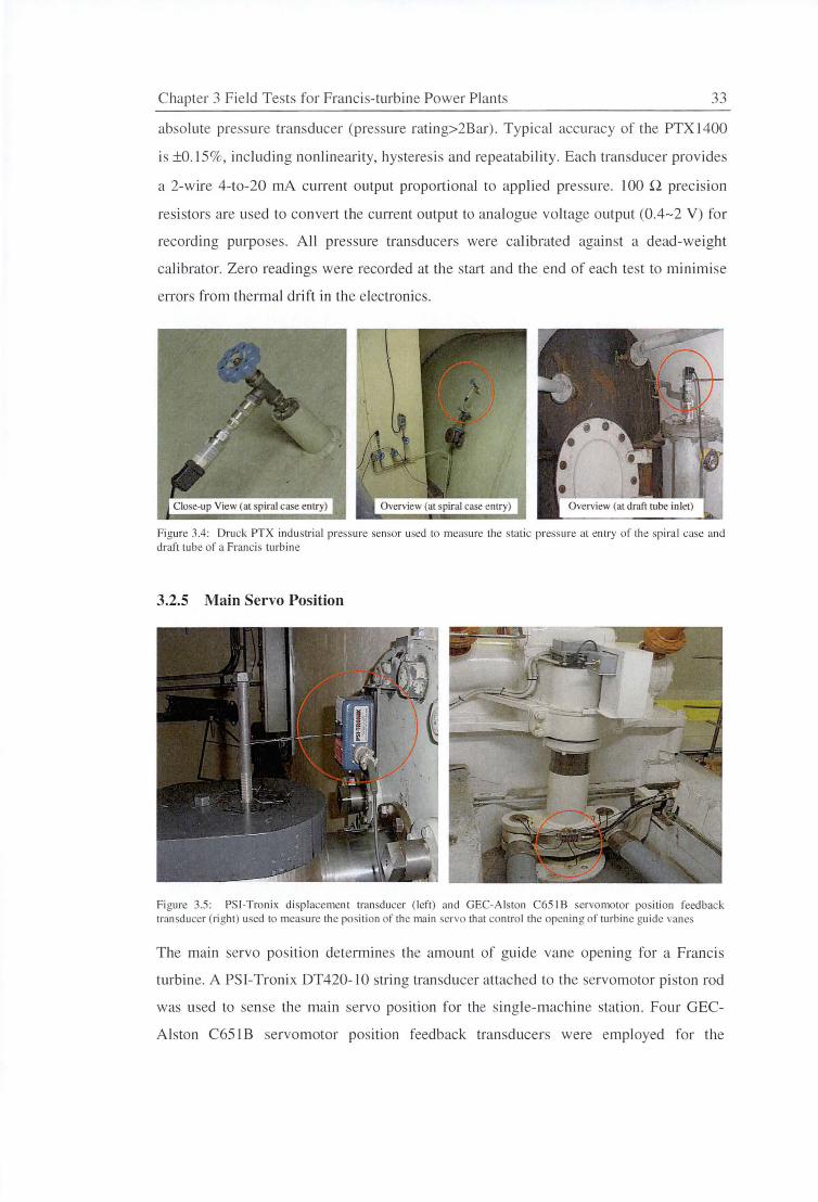
Chapter 3 Field Tests for Francis-turbine Power Plants 33
abso lute pressure transducer (pressure ratin g>2Bar). Typical accuracy of the PTX1400
is ±0.15%, including nonlinearity, hysteresi and repeatability. Each transducer provides
a 2-wire 4-to-20 mA current output proportional to applied pressure. I 00 Q precision
resistors are used to convert the current output to analogue vo ltage output (0.4-2 V) for
recording purposes. All pressure transducers were calibrated against a dead-weight
calibrator. Zero readings were recorded at the start and the end of each te t to minimise
errors from thermal drift in the electronics.
Figure 3.4: Druck PTX industrial pressure sensor used to measure the static pressure at entry of the sp iral case and draft tube of a Francis turbine
3.2.5 Main Servo Position
Figure 3.5: PSl-Tronix displacement transducer (left) and GEC-Alston C65 I B servomotor position feedback transducer (right) used to measure the position of the main servo that control the opening of turbine guide vanes
The main servo position determines the amount of guide vane opening for a Francis
turbine. A PSI-Tronix DT420-10 string transducer attached to the ervomotor piston rod
was used to sense the main servo position for the single-machine station. Four GEC
Alston C65 I B servomotor po ition feedback transducers were employed for the
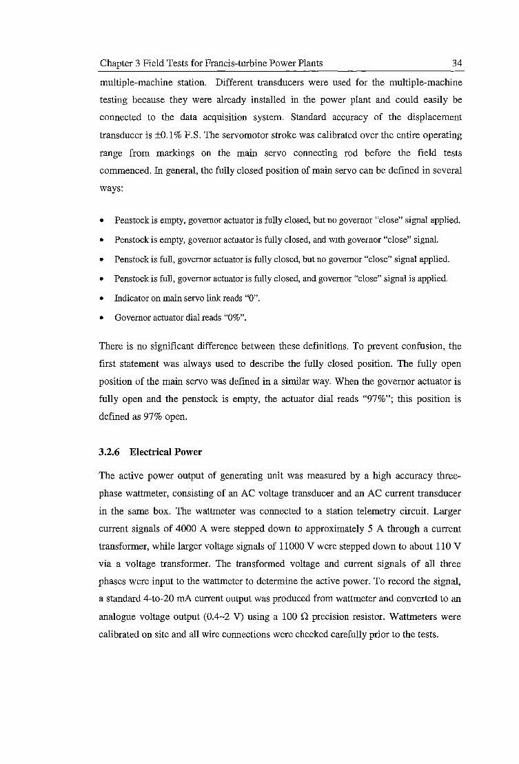
Chapter 3 Field Tests for Francis-turbine Power Plants 34
multiple-machine station. Different transducers were used for the multiple-machine
testing because they were already installed in the power plant and could easily be
connected to the data acquisition system. Standard accuracy of the displacement
transducer is ±0.1 % F.S. The servomotor stroke was calibrated over the entire operating
range from markings on the main servo connecting rod before the field tests
commenced. In general, the fully closed position of main servo can be defined in several
ways:
• Penstock is empty, governor actuator is fully closed, but no governor "close" signal applied.
• Penstock is empty, governor actuator is fully closed, and with governor "close" signal.
• Penstock is full, governor actuator is fully closed, but no governor "close" signal applied.
• Penstock is full, governor actuator is fully closed, and governor "close" signal is applied.
• Indicator on main servo link reads "O".
• Governor actuator dial reads "0%".
There is no significant difference between these definitions. To prevent confusion, the
first statement was always used to describe the fully closed position. The fully open
position of the main servo was defined in a similar way. When the governor actuator is
fully open and the penstock is empty, the actuator dial reads "97%"; this position is
defined as 97% open.
3.2.6 Electrical Power
The active power output of generating unit was measured by a high accuracy three
phase wattmeter, consisting of an AC voltage transducer and an AC current transducer
in the same box. The wattmeter was connected to a station telemetry circuit. Larger
current signals of 4000 A were stepped down to approximately 5 A through a current
transformer, while larger voltage signals of 11 OOO V were stepped down to about 110 V
via a voltage transformer. The transformed voltage and current signals of all three
phases were input to the wattmeter to determine the active power. To record the signal,
a standard 4-to-20 mA current output was produced from wattmeter and converted to an
analogue voltage output (0.4-2 V) using a 100 n precision resistor. Wattmeters were
calibrated on site and all wire connections were checked carefully prior to the tests.
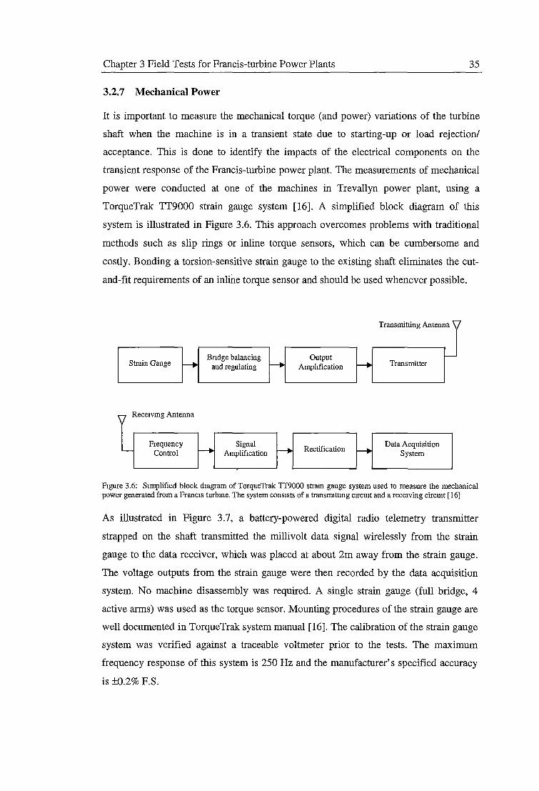
Chapter 3 Field Tests for Francis-turbine Power Plants 35
3.2. 7 Mechanical Power
It is important to measure the mechanical torque (and power) variations of the turbine
shaft when the machine is in a transient state due to starting-up or load rejection/
acceptance. This is done to identify the impacts of the electrical components on the
transient response of the Francis-turbine power plant. The measurements of mechanical
power were conducted at one of the machines in Trevallyn power plant, using a
TorqueTrak: TT9000 strain gauge system [16]. A simplified block diagram of this
system is illustrated in Figure 3.6. This approach overcomes problems with traditional
methods such as slip rings or inline torque sensors, which can be cumbersome and
costly. Bonding a torsion-sensitive strain gauge to the existing shaft eliminates the cut
and-fit requirements of an inlille torque sensor and should be used whenever possible.
Strain Gauge
Rece1vmg Antenna
Frequency Control
Bndge balancing and regulating
Signal Amplification
Output Amphfication
Rectification
Transmitting Antenna
Transmitter
Data Acquisition System
Figure 3.6: Simplified block diagram of TorqueTrak TT9000 stram gauge system used to measure the mechanical power generated from a Francis turbme. The system consists of a transIDittmg c1rcmt and a receiving circmt [ 16]
As illustrated in Figure 3.7, a battery-powered digital radio telemetry transmitter
strapped on the shaft transmitted the millivolt data signal wirelessly from the strain
gauge to the data receiver, which was placed at about 2m away from the strain gauge.
The voltage outputs from the strain gauge were then recorded by the data acquisition
system. No machine disassembly was required. A single strain gauge (full bridge, 4
active arms) was used as the torque sensor. Mounting procedures of the strain gauge are
well documented in TorqueTrak system manual [16]. The calibration of the strain gauge
system was verified against a traceable voltmeter prior to the tests. The maximum
frequency response of this system is 250 Hz and the manufacturer's specified accuracy
is ±0.2% F.S.
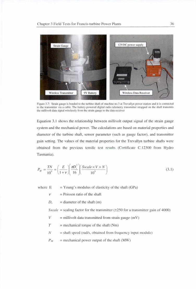
Chapter 3 Field Tests for Franci -turbine Power Plants 36
12YDC power supply
Figure 3.7: Strain gauge is bonded to the turbine shaft of machine no.3 a t Trevallyn power stati on and it is connected to the transmitter via a cab le. The battery-powered digital radio telemetry transmitter strapped on the haft transmits the millivo lt data sign al wirelessly from the strain gauge to the data receiver
Equation 3.1 shows the relationship between millivolt output signal of the strain gauge
system and the mechanical power. The calculations are based on material properties and
diameter of the turbine shaft, sensor parameter (such as gauge factor) , and transmitter
gain setting. The values of the material properties for the Trevallyn turbine shafts were
obtained from the previous tensil e test results (Certificate C . 12300 from Hydro
Tasmania).
p = TN = (__!____)[ nD: )( Sscale x V x N ) M lQ6 l+V 16 106
where E
v
= Young's modulus of elasticity of the shaft (GPa)
= Poisson ratio of the shaft
=diameter of the shaft (m)
(3. I)
Sscale = caling factor for the transmitter (±250 for a transmitter gain of 4000)
V =millivolt data transmitted from strain gauge (mV)
T = mechanical torque of the shaft (Nm)
N =shaft speed (rad/s, obtained from frequency input module)
PM =mechanical power output of the shah (MW)
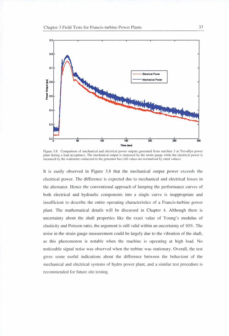
Chapter 3 Field Tests for Francis-turbine Power Plants 37
O.B
0.7
--Electrical Power
]; 0.6 --Mech1nic1I Power
:; ~ 0
I o.s ...
0.4
0.3
!iO 100 150 200 250
Time (Mel
Figure 3 .8: Comparison of mechanica l and elec tri ca l power outputs generated from machine 3 al Trevallyn power plant during a load acceptance. The mechanical outpu t is measured by the strai n gauge while the electrica l power is mea ured by the wattmeter connected to the generator bus (All va lues are normalised by rated va lues)
It is easily observed in Figure 3.8 that the mechanical output power exceeds the
electrical power. The difference is ex pected due to mechanical and electrical losses in
the alternator. Hence the conventional approach of lumping the performance curves of
both electrical and hydraulic components into a single curve is in appropriate and
insufficient to describe the entire operating characteristics of a Francis-turbine power
plant. The mathematical details will be di scussed in Chapter 4. Although there is
uncertai nty about the shaft properties like the exact value of Young's modulus of
elasticity and Poisson ratio, the argument is still valid within an uncertainty of 10%. The
noise in the strain gauge measurement cou ld be largely due to the vibration of the shaft,
as this phenomenon is notab le when the machine is operating at high load. No
noticeab le signal noi se was observed when the turbine was stationary. Overa ll , the test
gives some useful indications about the difference between the behaviour of the
mechanical and e lectrical systems of hydro power plant, and a sim il ar test procedure is
recommended for future site testing.
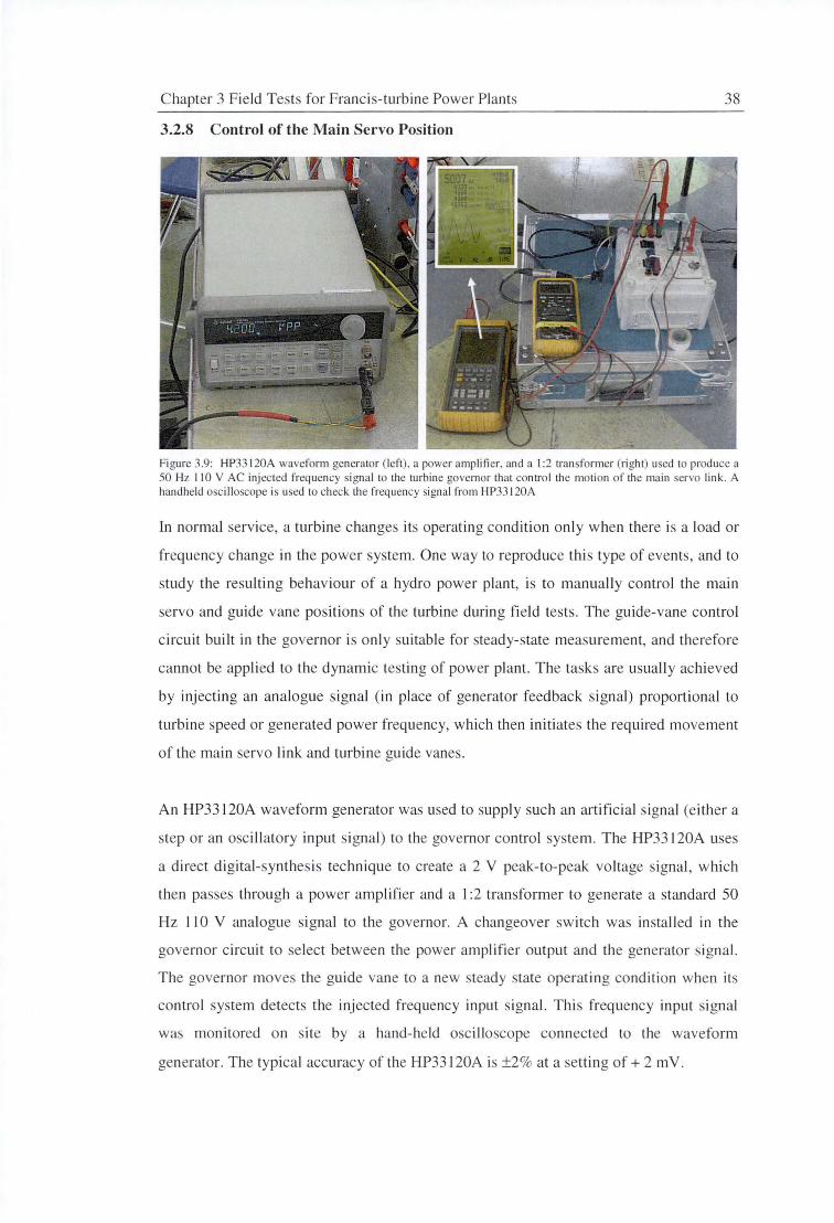
Chapter 3 Field Tests for Francis-turbin e Power Plants 38
3.2.8 Control of the Main Servo Position
Figure 3.9: HP33 120A waveform generator (left), a power amplifier, and a 1:2 tran former (right) used to produce a 50 Hz 110 V AC injec ted frequency signal to the turbine governor that contro l the motion of the main servo link. A handheld oscilloscope is u ed to check the frequency signal from HP33 I 20A
In normal service, a turbine changes its operating condition only when there is a load or
frequency change in the power system. One way to reproduce thi s type of events, and to
study the resulting behaviour of a hydro power plant, is to manually control the main
servo and guide vane positions of the turbine during field tests. The guide-vane control
circuit built in the governor is only suitable for steady-state measurement, and therefore
cannot be applied to the dynamic testing of power plant. The tasks are usually achieved
by injecting an analogue signal (in place of generator feedback signal) proportional to
turbine speed or generated power frequency, which then initiates the required movement
of the main servo link and turbine guide vane .
An HP33 I 20A waveform generator was used to supply such an artificial signal (e ither a
step or an oscillatory input signal ) to the governor control system . The HP33 I 20A uses
a direct digital-synthes is technique to create a 2 Y peak-to-peak vo ltage signal , which
then passes through a power amplifier and a l :2 transformer to generate a standard 50
Hz 110 V analogue signal to the governor. A changeover sw itch was in stalled in the
governor circuit to select between the power amplifier output and the generator signal.
The governor moves the guide vane to a new steady state operating condition when its
control system detects the injected frequency input signal. This frequency input signal
was monitored on site by a hand-held oscilloscope connected to the waveform
generator. The typical accuracy of the HP33 I 20A is ±2% at a setting of+ 2 mV.
Chapter 3 Field Tests for Francis-turbine Power Plants 39
3.3 Staged Tests of the Francis-Turbine Power Plants
Full-scale field tests were carried out to provide information for verifying mathematical
models of power plant operation and to identify key model parameter values. The
hydraulic system tests were always combined with governor response tests because of
the close interaction between turbine and governor performance. All tests were designed
to minimise interruption to plant and system operation, allow ease of simulation of
staged tests, and to reduce the complexity of the parameter derivation problem by
limiting the number of parameters significantly affecting an individual test. Technical
information such as turbine characteristics, equipment drawings, plant layouts, and
previous commissioning test reports were collected and studied before the actual tests.
Measurements of water levels at the upper and lower reservoirs were obtained from the
system control data and recorded regularly during the tests.
The turbine was unresponsive to the system frequency disturbances during the field
tests, since the functions of the guide vanes and governor had been switched to manual
mode. However, the plant and generator protection system remained intact all the time.
An interlock circuit was installed on the machine under test. If the machine circuit
breaker were accidentally tripped, the governor solenoid will be tripped to limit the
machine speed rise. Plant operators were present during the test to assist the control of
the guide vane operation. System dispatchers were also informed when the tests were to
start. No operator adjustments were performed during data recording. The field tests
typically took about a week to finish, including instrumentation set up.
The sequence of test program was carefully designed to facilitate parameter
identification and model verification in a logical order. All tests requiring the turbine to
be in a particular mode of operation were finished before proceeding to the tests
demanding a different mode of operation. The first stage of the tests involved measuring
the steady-state responses of the turbine. This information was used to identify
parameter values that are associated with steady-state operation. The second phase of
tests involved observing the hydraulic transient response of the plant subjected to
various types of disturbances. Step and sinusoidal changes of guide vane position
(Frequency deviation and Nyquist tests) were performed at different loading conditions
during this stage, and the responses were recorded for later analysis.
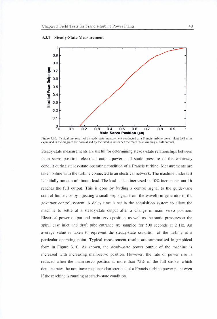
C hapter 3 Fi eld Tests fo r Francis-turb ine Power Plants
3.3.1 Steady-State Measurement
0.9
0 .8
.2. 0 .7 t: ii. = 0 .6
0
I o.5 0
c.. ~ u
·c:: u ~ LU
0.4
0 .3
0 .2
0 .1
0 .1 0 .2 0.3 0.4 0 .5 0.6 Main Servo Position (pu)
40
0.7 0 .8 0.9
Figure 3. 10 : Typica l tes t resul t of a steady-state mea urement cond ucted at a Franc is-tu rb ine power plant (All uni ts expressed in the di agra m are normali sed by the rated va lues when the machine is running at full output)
Steady-state measurements are useful for determining steady-state relationships between
main servo position, e lectrica l output power, and static pressure of the waterway
conduit during steady-state operating condition of a Francis turbine. Measurements are
taken online with the turbine connected to an e lectrical network. The machine under test
is initially run at a minimum load. The load is then increased in 10% increments until it
reaches the fu ll output. This is done by feeding a control signal to the guide-vane
control limiter, or by injecting a small tep signal from the waveform generator to the
governor control system. A delay time is set in the acqui sitio n system to a llow the
machine to settle at a steady-state output after a change in main servo po ition.
El ectrical power output and main servo position, as well as the static pressures at the
spiral case inlet and draft tube entrance are sampl ed for 500 seconds at 2 Hz. A n
average value is taken to represent the steady-state condition of the turbine at a
particular operating point. Typical measurement results are summari sed in graphi cal
form in Figure 3. 10. As shown, the steady- tate power output of the machine is
increased with increas ing main-servo positi on. However, the rate of power ri se is
reduced when the main-servo pos ition is more than 75 % of the full stroke, which
demonstrates the non I inear response characteristic of a Francis-turbine power plant even
if the machine is running at steady-state condition.
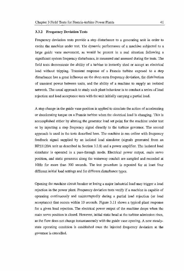
Chapter 3 Field Tests for Francis-turbine Power Plants 41
3.3.2 Frequency Deviation Tests
Frequency deviation tests provide a step disturbance to a generating unit in order to
excite the machine under test. The dynamic performance of a machine subjected to a
large guide vane movement, as would be present in a real situation following a
significant system frequency disturbance, is measured and assessed during the tests. The
field tests demonstrate the ability of a turbine to instantly shed or accept an electrical
load without tripping. Transient response 'of a Francis turbine exposed to a step
disturbance has a great influence on the short-term frequency deviation, the distribution
of transient power between units, and the ability of a machine to supply an isolated
network. The usual approach to study such plant behaviour is to conduct a series of load
rejection and load acceptance tests with the unit initially carrying a partial load.
A step change in the guide vane position is applied to simulate the action of accelerating
or decelerating torque on a Francis turbine when the electrical load is changing. This is
accomplished either by altering the generator load set point for the machine under test
or by injecting a step frequency signal directly to the turbine governor. The second
approach is used in the tests described here. The machine is run online with frequency
feedback signal supplied by an isolated load simulator (signals generated from an
HP33120A unit as described in Section 3.2.8) and a power amplifier. The isolated load
simulator is operated in a pass-through mode. Electrical power output, main servo
position, and static pressures along the waterway conduit are sampled and recorded at
lOHz for more than 300 seconds. The test procedure is repeated for at least four
different initial load settings and for different disturbance types.
Opening the machine circuit breaker or losing a major industrial load may trigger a load
rejection in the power plant. Frequency deviation tests verify if a machine is capable of
operating continuously and uninterruptedly during a partial load rejection (or load
acceptance) that occurs within 10 seconds. Figure 3.11 shows a typical plant response
for a given load rejection. The electrical power output of the machine drops when the
main servo position is closed. However, initial static head at the turbine admission rises,
as the flow does not change instantaneously with the guide vane opening. A new steady
state operating condition is established once the injected frequency deviation at the
governor is cancelled.
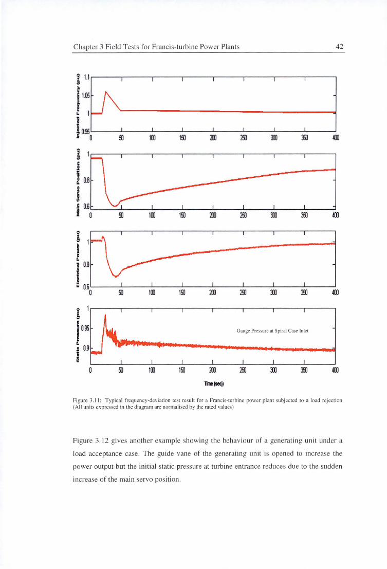
Chapter 3 Field Tests for Francis-turb ine Power Plants 42
i 1.1 .... ~ i 1.05 :i r .. i i ? 0.95
100 1!"il DJ - 0 ... :i a. .... c .2 i 0 O.B II. 0 ; VI c 0.6 i 0 1!"il
... & ....
I 0 II. i O.B II 'C
j Ill 0.6
0 100 1!"il 400
s ! ! I o.95 Gauge Pressure at Spiral Case Inlet
II. II 0.9 i 0
0 100 1!"il DJ
Tme(sec))
Figure 3.11: Typical frequ ency-deviation test result for a Francis-turbine power plant subjected to a load rejection (All uni ts expressed in the diagram are normalised by the rated values)
Figure 3.12 gives another example showing the behaviour of a generating unit under a
load acceptance case. The guide vane of the generating unit is opened to increase the
power output but the initial static pressure at turbine entrance reduces due to the sudden
increase of the main servo position .
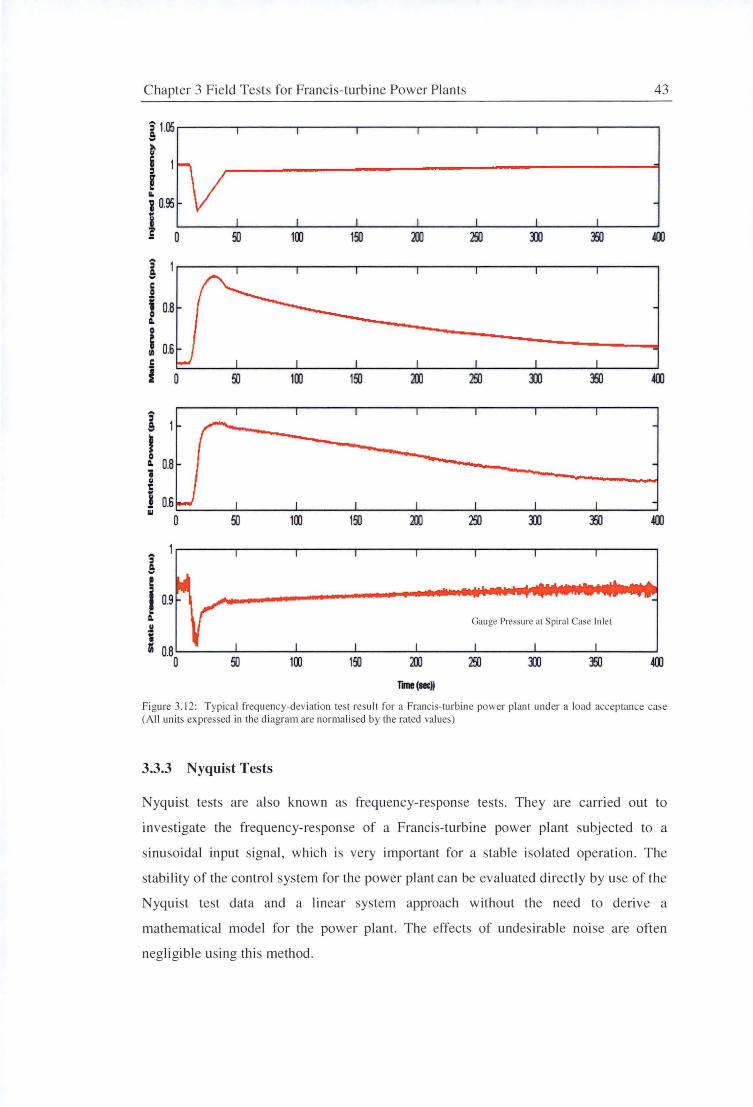
Chapter 3 Field Tests for Francis-turbine Power Plant 43
! 1.~ f :I r II.
i 0.95 i s 0 100 19) :m 350
s a c 0
i 0.8 II. 0
; 0.6 Ill
.e I 100 19) :m
s a ~ 0
O.B II.
i II 'C
j 0.6 Ill
100 19)
s a !
I 0.9 II. II
Gauge Pressure at Spiral Case Inlet
i In 0.8
0 100 1:AJ :m 350
Tme(sec))
Figure 3. 12: Typical frequency-deviation test result for a Francis-turbine power plant under a load acceptance case (All units expressed in the diagram are normalised by the rated values)
3.3.3 Nyquist Tests
Nyquist tests are a lso known as frequency-response tests. They are carried out to
investigate the frequency-response of a Francis-turbine power plant subjected to a
sinusoidal input signal, which is very important for a stable isolated operation. The
stability of the control system for the power plant can be evaluated direct ly by use of the
Nyquist test data and a linear system approach without the need to derive a
mathematical model for the power plant. The effects of undesirable noise are often
negli gibl e using this method .
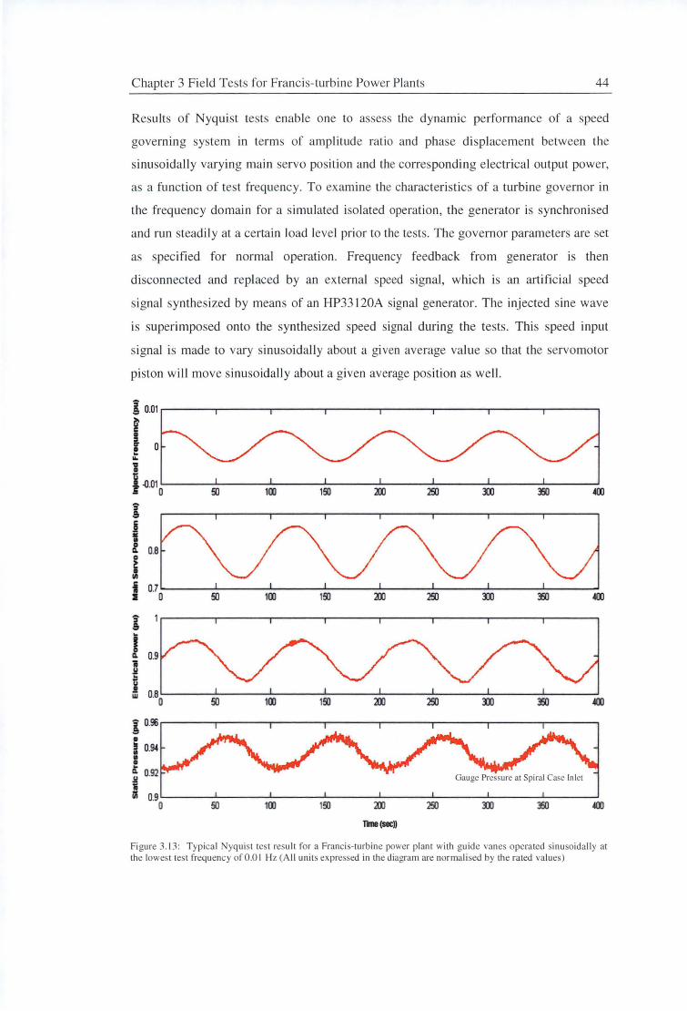
Chapter 3 Field Tests for Francis-turbine Power Plants 44
Results of Nyquist tests enab le one to assess the dynamic performance of a speed
govern in g system in terms of amplitude rat io and phase displacement between the
si nusoidally varying main servo position and the corresponding electrical output power,
as a function of test frequency. To examine the characteristics of a turbine governor in
the frequency domain for a imulated isolated operat ion, the generator is synchroni sed
and run steadi ly at a certai n load level prior to the tests. The governor parameters are set
as specified for normal operation. Frequency feedback from generator is then
disconnected and replaced by an external speed signal, which is an artific ial speed
signal synthes ized by means of an HP33120A signal generator. The inj ected sine wave
is superimposed onto the synthesized speed signal during the tests. This speed input
signal is made to vary sinusoidally about a given average value so that the servomotor
piston will move sinuso idally about a given average position as well.
i 0.01
I 0 ... i i-0.010 50 100 150 :m 350
i ~
I O.B 0
i i :I
i I 0.9 1 .l! .. i w
i 0.$
• I O.~ : &: 0.92 .l! Gauge Pressure at Spiral Case Inlet 1i Iii 0.9
0 50 100 150 200 250 :m 350 ~
rme(sec))
Figure 3. 13: Typical Nyquist te t resu It fo r a Francis-turbine power pl ant with guide vane operated inusoidally at the lowest te t frequency of 0 .0 I Hz (All units expressed in the diagram are normali sed by the rated va lues)
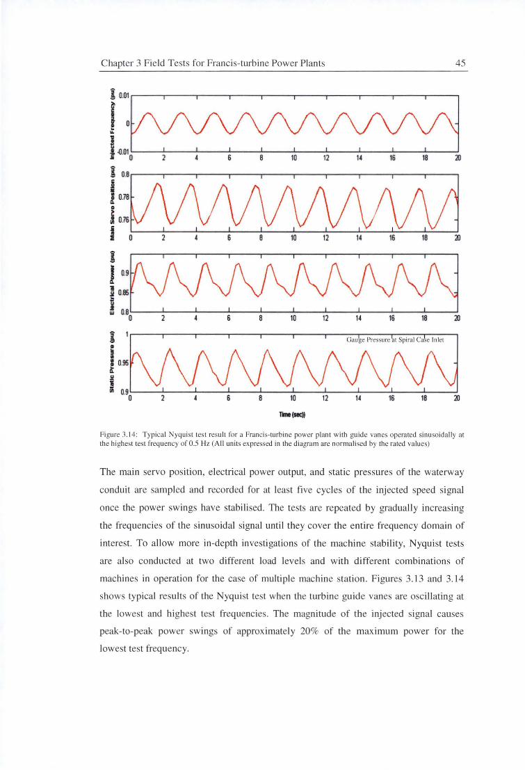
Chapter 3 Field Tests fo r Francis-turbine Power Plants 45
i 0.01 ~--~--~--~--~---~--..------~--~--~--~
I o ... 1 tl f -0.010 2 10
i a.a~--~--..----~--~--~--~--~--~--~--~ j • ~ 0.78 0 ~ ~ 0.76
i I 0 2 4 6 B 10 12 14 16 18 20
Gauge Pressure l Spiral Ca e Inlet
flM(SIC))
Figure 3.1 4: Typica l Nyquis t test result for a Francis-turbine power plant wi th guide vanes operated sinusoidally at the highest te t frequency of 0.5 Hz (A ll units expressed in the diagram are normalised by the rated va lues)
The main servo position, electrical power output, and static pressures of the waterway
conduit are sampled and recorded for at least five cycles of the injected speed signal
once the power swings have stabilised. The tests are repeated by gradually increasing
the frequencies of the sinuso idal signal until they cover the entire frequency domain of
interest. To allow more in-depth investigations of the machine stability, Nyqui st tests
are also conducted at two different load levels and with different combinations of
machine in operation for the case of multiple machine station . Figures 3. 13 and 3. 14
shows typical results of the Nyquist test when the turbine guide vane are oscill ating at
the lowest and highest test frequencies. The magnitude of the injected signal causes
peak-to-peak power swings of approx imate ly 20% of the maximum power for the
lowest test frequency.
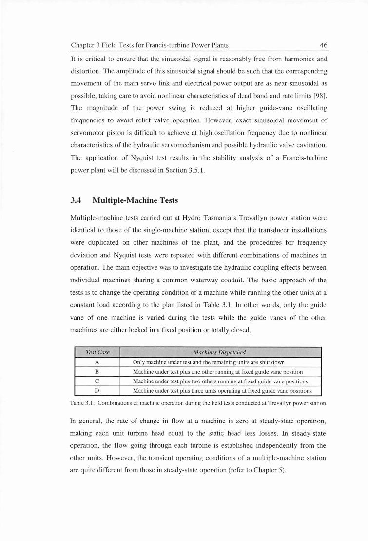
Chapter 3 Field Tests for Francis-turbine Power Plants 46
It is critical to ensure that the sinusoidal signal is reasonably free from harmonics and
distortion. The amplitude of this sinusoidal signal should be such that the corresponding
movement of the main servo link and electrical power output are as near sinusoidal as
possible, taking care to avoid nonlinear characteristics of dead band and rate limits [98].
The magnitude of the power swing is reduced at higher guide-vane oscillating
frequencies to avoid relief valve operation. However, exact sinusoidal movement of
servomotor piston is difficult to achieve at high oscillation frequency due to nonlinear
characteristics of the hydraulic servomechanism and possible hydraulic valve cavitation.
The application of Nyquist test results in the stability analysis of a Francis-turbine
power plant will be discussed in Section 3.5.1.
3.4 Multiple-Machine Tests
Multiple-machine tests carried out at Hydro Tasmania's Trevallyn power station were
identical to those of the single-machine station, except that the transducer installations
were duplicated on other machines of the plant, and the procedures for frequency
deviation and Nyquist tests were repeated with different combinations of machines in
operation. The main objective was to investigate the hydraulic coupling effects between
individual machines sharing a common waterway conduil. Tlie bask approach of the
tests is to change the operating condition of a machine while running the other units at a
constant load according to the plan listed in Table 3.1. In other words, only the guide
vane of one machine is varied during the tests while the guide vanes of the other
machines are either locked in a fixed position or totally closed.
Test Case Machines Dispatched
A Only machine under test and the remaining units are shut down
B Machine under test plus one other running at fixed guide vane position
c Machine under test plus two others running at fixed guide vane positions
D Machine under test plus three units operating at fixed guide vane positions
Table 3.1: Combinations of machine operation during the field tests conducted at Trevallyn power station
In general, the rate of change in flow at a machine is zero at steady-state operation,
making each unit turbine head equal to the static head less losses. In steady-state
operation, the flow going through each turbine is established independently from the
other units. However, the transient operating conditions of a multiple-machine station
are quite different from those in steady-state operation (refer to Chapter 5).
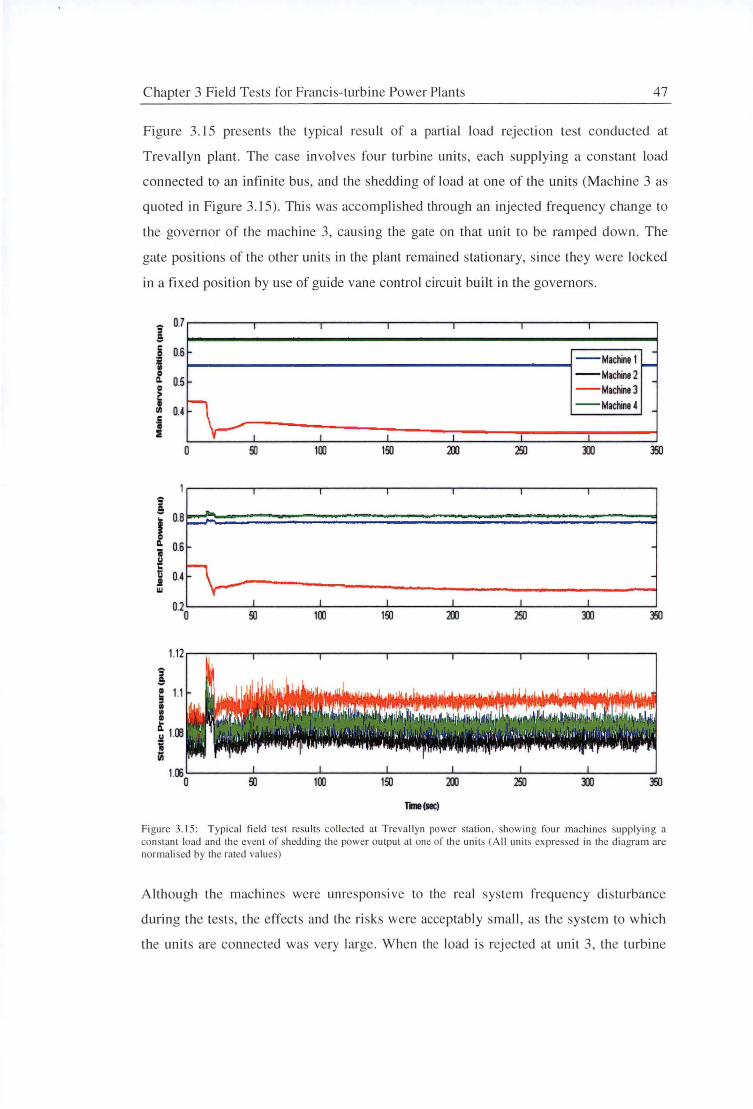
Chapter 3 Field Tests for Francis-turbine Power Plants 47
Figure 3.15 presents the typical result of a partial load rejection test conducted at
Trevallyn plant. The case involves four turbine units, each supplying a constant load
connected to an infin ite bus, and the shedd ing of load at one of the units (Machine 3 as
quoted in Figure 3.15). This was accomplished through an injected frequency change to
the governor of the machine 3, cau ing the gate on that unit to be ramped down. T he
gate positions of the other units in the plant remained stationary, ince they were locked
in a fixed position by use of guide vane contro l circuit bu il t in the governors.
- 0.7 i j 0.6 11 ~ 0.5
j 0.(
.E I + 0
i O.B
~
I Q. 0.6 1 ~
f\--ti 0.4 .I w
0.2 0
1.12
I • 1.1 ! • • • ... Q. Ji! 1 Ill 11 Iii
I I
I I
50 100
I I
I I
50 100
I I I I
---Machine1 ---Machine2 ---Machine3 --Machine( -
I I I I
150 250
I I I I
-
-
I I I I
150 250
Tine(sec)
Figure 3. 15: Typical field test results collected at Trevallyn power station . show ing four machines supplying a constan t load and the even t of shedding the power output at one of the units (All unit expressed in the diagram are normali ed by the rated values)
Although the machines were unresponsive to the real system frequency di sturbance
during the tests , the effects and the ri sks were acceptably small , as the system to which
the units are connected was very large. When the load is rejected at unit 3, the turbine
Chapter 3 Field Tests for Francis-turbine Power Plants 48
head rises, as the guide vane opening is reduced. The initial rise in the turbine head of
this unit results in a decreased flow and at the same time produces an increase in flows
to the other units because the total flow in the common tunnel cannot be changed
instantaneously. For this reason, the power output of the other machines rises initially
when the guide vane opening of unit 3 is reduced. The effect gradually disappears when
the final flow conditions reach a new steady state. Similar behaviours are observed in
the Nyquist tests and for step load changes with two and three machines in operation.
The multiple-machine site testing generally confirmed the expected nonlinear and
multivariable behaviour of this type of power plant. Although this did not constitute a
system verification of the mathematical model for the power plant, it did provide good
evidence for its authenticity and emphasise the importance of considering the hydraulic
coupling effects in modelling a multiple-machine station.
3.5 Discussion
3.5.1 Estimation of Instantaneous Flow Rate
Precise measurement of flow through a Francis turbine is desirable for more detailed
verification of the hydraulic models developed for both single- and multiple-machine
stations. However, factors such as cost, complexity and time involved in the equipment
installation, or the accuracy of the measuring techniques for a large flow rate have
precluded the measurement of instantaneous turbine flow in the current field tests. The
instantaneous flow in the system model (see Chapters 4 and 5) is derived from the
instantarieous turbine head via the orifice head-flow relationship. The system
verification will therefore rely on the measurement of instantaneous power output,
which is proportional to the product of the instantaneous head and flow. It is worthwhile
in this section to review some commonly used measuring techniques that have been
tried successfully by others in the steady-state performance testing of a full-scale
Francis turbine. These techniques may be applied in the future site testing, if time and
budget allow, which will permit direct verification of the instantaneous flow modelling:
• The current-meter method uses a number of propeller-type current meters placed
in turbine inlets or penstocks to measure the local mean velocities simultaneously.
The turbine discharge is estimated by integrating the flow velocities over the
conduit cross section. The method is recommended by IEC publication 41 and
Chapter 3 Field Tests for Francis-turbme Power Plants 49
other codes for measuring flow in a hydraulic turbine [80]. However, to get an
acceptable accuracy, this approach requires a uniform and rectilinear flow over the
cross section of the measuring plane to obtain a favourable velocity distribution.
The penstock must also be emptied for installation of the instrumentation support
frame and related work. This is difficult to implement, particularly when a Francis
turbine is tested in a transient state, and must be operated continuously for
economic purposes. Thus, this method was not applied in the current site testing.
• The Gilson pressure-time method determines the turbine flow indirectly from the
pressure rise between two sections of the penstock during an interruption of flow
caused by closing the turbine guide vanes. The distance between two measurement
sections should be at least 9m or two times the conduit diameter. Moreover, this
method relies on piezometer taps that have been installed during construction of
the power plant [32]. Installing a new pressure taps in existing concrete penstocks
is costly and time consuming. Hence, this method is not being used for transient
flow measurement of the Francis turbine.
• The salt dilution tracer method [32] measures the flow rate by observing the
concentration of a solution of sodium dichromate injected into the main water
flow at points evenly distributed over the cross section of the penstock. The flow
must be perfectly turbulent so that the salt solution is evenly distributed in the
conduit. To get a meaningful result, extreme care is needed when injecting the salt
solution to the water. This is difficult to apply in the typical operating environment
of a hydraulic turbine. Nor does the method guarantee acceptable accuracy when
the machine is running at a transient state. Hence, it is not useful for dynamic
testing of a turbine plant.
• The Pitot tube gauging approach [32] obtains the turbine discharge from local
measurements of flow velocity over the penstock cross section. Although this
method is simple in principle, it is not suitable for large diameter conduits with
relatively high velocities due to stiffness problems of the tube support. The
difficulty of retrofitting tube access ports in existing conduits is also a problem.
• The acoustic method utilises two acoustic transducers installed in a steel penstock
over a distance of about one-half of the penstock diameter. The transducer
Chapter 3 Field Tests for Francis-turbine Power Plants 50
measures the travel time of an acoustic wave in and against the flow direction, and
relates these two travel times to the mean velocity of the water along the acoustic
path. The discharge is determined by integrating the profile of mean velocities
numerically. This approach has the advantages that the transducers can be
installed without the penstock emptied and that it is not necessary to cause a
sudden variation in flow in order to measure it. Dube and Martin [32] report a high
repeatability and an accuracy of 0.5% using the acoustic method in a crossed
plane. The drawback of this approach is that an acoustic transducer is always
expensive.
• The relative discharge method [32] determines the "relative" turbine flow by
means of Winter-Kennedy pressure taps located in the turning section of the spiral
case or through the head loss measurement between two sets of pressure taps. The
discharge is found through the pressure differential caused by different locations
of the pressure taps in the measurement section and due to the centrifugal forces of
the water. The measurement accuracy depends on the accuracy of the pressure
transducer. If the knowledge of absolute flow is required, an index test must be
performed simultaneously; or alternatively, calibration data may be obtained from
model tests. This approach should be tried in the future for stations where Winter
Kennedy pressure taps are already installed in the spiral case.
3.5.2 Transmission Time Lag
The transmission lag of a measuring system is critical in unsteady flow measurements.
The lag can be caused either by the dynamic characteristics of equipment or by
communication delay between Graphical User Interfaces (GUls) used in the LABVIEW
data acquisition program. The time lag generated by a transducer is minimised by use of
an electrical current for signal transmission since the state of change of an electrical
signal occurs with virtually no time losses. The transmission lag due to acquisition
software is reduced by using an external triggering device to make sure that all signals
are send without significant delay. The oscillation period of the pressure wave in the
pressure tubes is estimated to be two order of magnitude less than that of the fastest
oscillation encountered in the Nyquist test and the actual plant verification. Hence, the
pressure wave in the cavity tube is quite unlikely to affect the system measurement here.
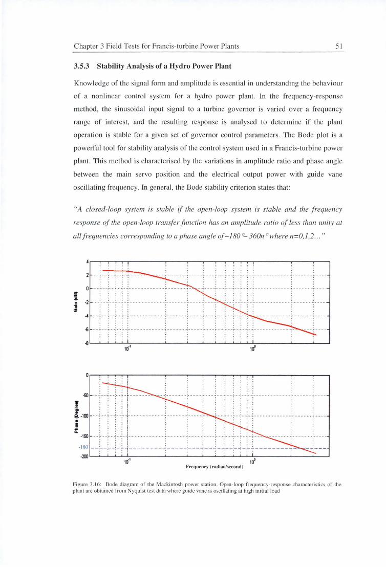
Chapter 3 Field Tests for Francis-turbine Power Plant 51
3.5.3 Stability Analysis of a Hydro Power Plant
Knowledge of the signal form and amplitude is essentia l in understanding the behaviou r
of a nonlinear control system for a hydro power plant. In the frequency-response
method, the sinusoidal input signal to a turbine governor is varied over a frequency
range of intere t, and the resulting response is analysed to determine if the plant
operation is stabl e for a given set of governor control parameters. The Bode plot is a
powerful tool for stability analysis of the control sy tern used in a Francis-turbine power
plant. Thi s method is characterised by the variation s in amplitude ratio and phase angle
between the main servo position and the electrical output power with guide vane
oscillating frequency. In general, the Bode tability criterion states that:
"A closed-loop system is stable if the open-loop system is stable and the frequency
response of the open-loop transfer function has an amplitude ratio of less than unity at
all frequencies corresponding to a phase angle of-180 °- 360n °where n=0, 1,2 ... "
m :!!.
2 ... ······· ···i ........ ;; ... .. ;. ···.··· ··.····.····.··· ···· ····· ········ ·· . .. . \ · ..... . .
0 ......... ....... .. -. ....... .. .. ... .... ..... .. .. . ... -:· .. .... ·:- .... . :· .. · ·: .. . ·: .. ·: .. ·::- ... ........ -........... - ~ -.. .. .... . . . .
-2 . . . . ··-··· ·-··-···· ··· ··················- ··············· ·· ······-·· .. ······ -· ··· ·· ······· ··· ·-·· ····· ····· ·· ············ ········ ·····- ····· . . . . . . . . . .
... . . . . . -4 ····'.····<· ... ; ... ; ... ; ... ..... ... ........... ... ; ....... ....... ;- ......... ; ... .... ; ...... ; ..... ; .. .. ; .. . ,. · ..... ..... .. .... ........ ; ....... ....... ; ....... .
. . . . . . . . . . -6 .. .. , ..... .... . : .... ... , .. . .. ............. --~ .......... ·- .. ' • .. .. . . . .. . . .
~..___.__.__.__._..__~~~~.L-~~'--~.L---L~L..-.L-.L-.Jc......L~~~~--'-~~--'-~--'
10·1 1rf
ai .• i ~ .... T .. . ...... : ..... ~ ..... ~ .... ; ... : ... : . . . . . . . . . . . . . . . . . . . . . . . . . . . . . . . . . . .. ·.· ....... .
;-100 ... , .. .. , 't ................. ..
. -: -~L~~nt~~~~~ ~L~-~-~ -~·~-~ ____ c __ H-~-------------1~ 1rf
Frequency (rad ian/second )
Figure 3.16: Bode diagram of the Mackintosh power stati on. Open-loop frequency-re ponse characteri stics of the plant are obtained from Nyquist test data where gu ide vane is osci llating at high initial load
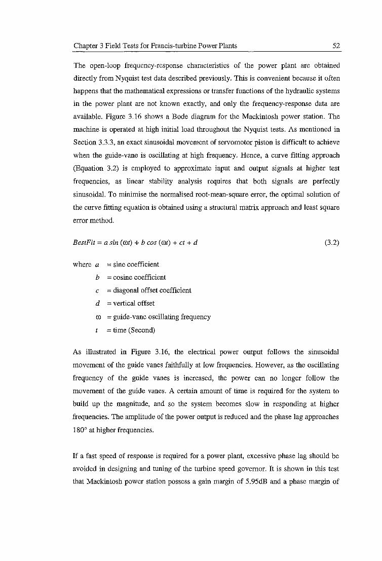
Chapter 3 Field Tests for Francis-turbine Power Plants 52
The open-loop frequency-response characteristics of the power plant are obtained
directly from Nyquist test data described previously. This is convenient because it often
happens that the mathematical expressions or transfer functions of the hydraulic systems
in the power plant are not known exactly, and only the frequency-response data are
available. Figure 3.16 shows a Bode diagram for the Mackintosh power station. The
machine is operated at high initial load throughout the Nyquist tests. As mentioned in
Section 3.3.3, an exact sinusoidal movement of servomotor piston is difficult to achieve
when the guide-vane is oscillating at high frequency. Hence, a curve fitting approach
(Equation 3.2) is employed to approximate input and output signals at higher test
frequencies, as linear stability analysis requires that both signals are perfectly
sinusoidal. To minimise the normalised root-mean-square error, the optimal solution of
the curve fitting equation is obtained using a structural matrix approach and least square
error method.
BestFit = a sin (rot) + b cos (rot) + et + d
where a =sine coefficient
b = cosine coefficient
c = diagonal offset coefficient
d = vertical offset
ro =guide-vane oscillating frequency
t =time (Second)
(3.2)
As illustrated in Figure 3 .16, the electrical power output follows the sinusoidal
movement of the guide vanes faithfully at low frequencies. However, as the oscillating
frequency of the guide vanes is increased, the power can no longer follow the
movement of the guide vanes. A certain amount of time is required for the system to
build up the magnitude, and so the system becomes slow in responding at higher
frequencies. The amplitude of the power output is reduced and the phase lag approaches
180° at higher frequencies.
If a fast speed of response is required for a power plant, excessive phase lag should be
avoided in designing and tuning of the turbine speed governor. It is shown in this test
that Mackintosh power station possess a gain margin of 5.95dB and a phase margin of
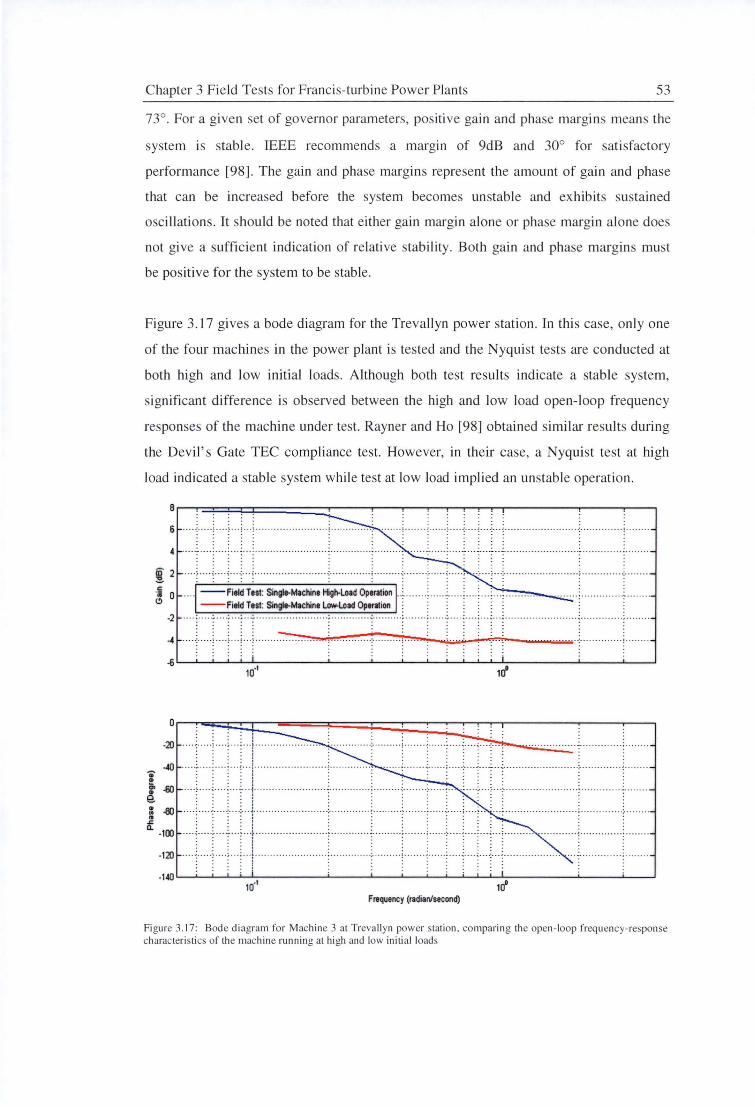
Chapter 3 Fie ld Tests for Francis- turbine Power Plants 53
73°. For a given set of governor parameters, positive gain and phase margins means the
system is stable. IEEE recommends a margin of 9dB and 30° for sati sfactory
performance [98]. The gain and phase margins represent the amount of gain and phase
that can be increased before the system becomes unstable and ex hibits sustai ned
o c ill ations. It hou ld be noted that either ga in margin alone or phase margin a lone does
not give a suffic ient indication of relative stability. Both gain and phase marg ins must
be positive for the system to be stable.
Figure 3.17 gives a bode diagram for the Trevallyn power station. In this case, onl y one
of the four machines in the power plant is tested and the Nyqui st tests are conducted at
both high and low initial loads. Although both test results indicate a stable system,
significant difference is observed between the high and low load open-l oop frequency
responses of the machine under test. Rayner and Ho [98] obtained similar results during
the Devil 's Gate TEC compliance test. However, in their case, a Nyquist test at high
load indicated a stable system while test at low load implied an unstable operation .
6 ..... ,. .... , .... , ... , ... ,. ... • • • • • ••I • • • • • • •: • • • • • • ~ • • • • .. . • • •: • • • ••• • •: • • • • • • • • • • • • • • • • • • • • • • • . . . . . . .
. . .... 4 ..... : .... : .... : . .. : .. . : .... . .. ... ..... .. ...... . , ... ..... .. .. . . , .. ... .... : · ··· ·' ··· ···:····-:-···-··· ·-· · -········ ·· ······ ·· ·· ·····:······ · ······:
. . . . . . . . . . . . . . . . . . . . . . . . . . . . . ;. .... , .... i· .. ·> .. i · ........ . .......... . .... ; . ..... ........ i ..... . .... ; ... .. .. <· ••.•• \ .... ·~ .. ; ..•. :,; .•• ; •...• .•.. .. .• .... .. ...... z .. .....•. . ...• ; .•..•••. . . . . . . . . . . . . . . . . . . . . . . . . .
~ o .... --Field Test: Single-Machine High-Load Operation .. : ...... . : .. ... ; ..... : .... : ... : ... : .......... . --Field Test: Single-Machine Low-Load Operation : :
. ..... ...... .... .... ....... .. .. . . .
-2 ····:· ····'····'··· ' ···'· ······················· ' ······· ····· '. ··········:·······:······:···· :····'. .. : ... ; ..... .... ........ ...... . :······ ········:· ······· . . . . . . . . . . . . . .
--~.;.,.,.,~~~· ~~· ~...;..._..:,· __;·_...;~~--~-..-----4 ..... : . .... , .... , .. , ... , ........ ........ ~ .. . ... ; .. .... .
0
-20 ·······-········· ~---
-CO .. ... ... :· ...... ~- ..... i ..... : .... ~- .. ~ .. ~- ...................... . ·~· ....... ...... ~· ...... .
! . .
"' -SO • 9. . . ~ .. ·:· ....................... -~ ....... .... .. i' ...... .
• -al .. .. ..... ... - ~· ...... ....... ~ - ... ' ... · ·~ ...... ·= ... .. ~-- .. . i .. .. ; .... ··=-· ............ ..... ...... ~ .. ........... ·=· . . .... . .
~ a. -100 .......... ...... ... . : ............. ~ ... ... .... ~ ....... ; .. .... : .. .. . ~- .. . : .. . : ... i ... ....... . ... ..... ... ~- ....... ...... ~ ....... .
. . . . . . . . -120 ....... .... ··· ~ · · ···· · ~·· ·· ··=····~· · ··~····=···~················· · · .. ...
-140
Frequency (radian/second)
Figure 3. 17: Bode diagram for Machine 3 al Trevallyn power station. comparing the open-loop frequency-response characteri sti cs of the machine running at high and low initial loads
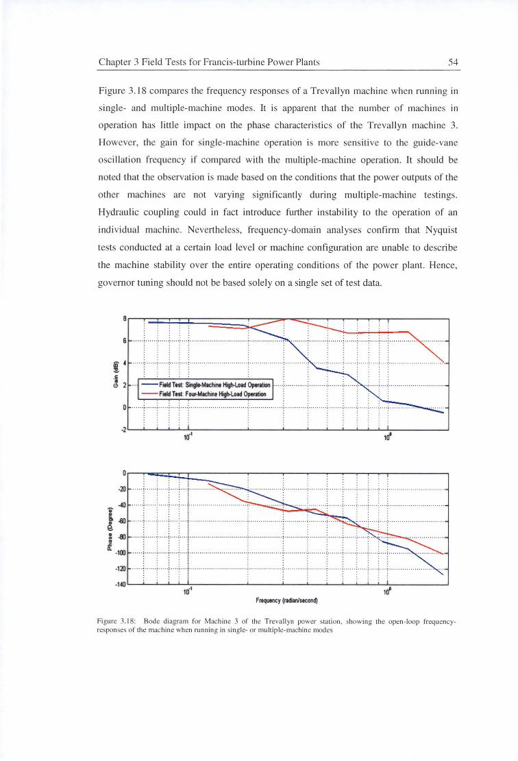
C hapter 3 Fie ld Tests fo r Francis-turbine Power Plants 54
F igure 3. 18 compares the frequency responses of a Trevall yn machine when running in
single- and mul tipl e-machine modes. It is apparent that the number of machines in
operati on has litt le impact on the phase characteri ti es of the Trevall yn machine 3.
However, the gain fo r single- machine operation is more sensitive to the gu ide-vane
oscill ation frequency if compared with the multiple-machine operati on. It should be
noted that the observation is made based on the conditions that the power outputs of the
other machines are not varying significantly during multiple-machine testings.
Hydraulic coupling could in fact introduce further instability to the operation of an
indi vidual machine. Neve1t heless, frequency-domain analyses confi rm that Nyquist
tests conducted at a ce1tain load level or machine configurati on are unable to describe
the machine stability over the entire operating conditions of the power plant. Hence,
govern or tuning should not be based so lely on a single set of test data.
6 . ... ....... ...... . ... . . .... ... .. ... .......... .. ......... . . . .. . . . . . .. . . . #. . . . . . . .. ....... .. .. ........ ... .. . . . . . . . . . . . . . . . . . . Iii' ' .. .. . ,. .. .. ,, ....... . .... ... , ............................ , .......... ....... , ..... . :!!. c ..
e> 2 ... --Fitld Test: Singl•Machine High-Load Operation ..... : ........... ; ......... : .. .. .... : ..... . ;. .; .. . ; .. .. : .. ....... ................. .. --Fitld Test: Four·Machine High-Load Operation
0 .... ......... ...... ..
0
-20 ........... ..... .. ... . : ...... '. ..... ~- .... ; ... ~ . . . ....... ...... ..... ..... .
. : -.40 ..
!
"' .aJ .. e. • -8) .. .. ,;:; 0..
-100
T. T t ; ... .. - ~ ... . -~· ... . ~- ... ~ -· · - ~ ............................. : .... .. ... .... .. .. ; ... · ·······~· ........ : ....... ~ ..... . : .. ... ~- ..
. .... i ...... : .... i .. .. L .. l· ···· ··- ···-··· ·-·· .... ... ... : .... ..... ... ................. l. ....... ; ....... : ... ... f .... .... .. : ... i ....... .... .
-120 .... . , ..... :· · ·· ·~·· · i···· ............. .. ....... ·:··-······"·····-(··· ...... ; ........ ; ...... : .... .. : ... .: ..... , ... : .... ...... . -1.40
10' Frequency (radian/second)
Figure 3. 18: Bode diagram for M achine 3 of the Treva llyn power station, showing the open- loop frequencyresponses of the machine when ru nning in single- or mu ltip le-machine modes
Chapter 3 Field Tests for Francis-turbine Power Plants 55
Although Nyquist tests have been used to determine the stability margins for generators
with Francis turbines, the appropriateness of the test on generators with other types of
turbines is not fully explored. Some tests have been conducted by Hydro Tasmania on a
generator with a Pelton turbine but the test outcome was not encouraging [98]. The
deflector action and the opening (or closing) rate of the spear generate nonlinearities in
power output of the Pelton turbine that invalidate the linear stability analysis of the
power plant. The accuracy of the Nyquist test approach is also greatly affected by the
characteristics of the instrumentation used. The frequency response of the measuring
equipment must have a nearly flat magnitude-versus-frequency curve. Frequency
characteristics of the test instruments used in the current field tests were not fully
calibrated due to time constraints, but they were assumed to behave according to their
manufacturer's specifications.
3.6 Conclusions
A field-test program has been successfully carried out to investigate the dynamic
behaviour of both single- and multiple-machine stations. The techniques and
instrumentation used for field testings are discussed in detail here. The test results show
that the operating characteristics of Francis-turbine power plants are highly nonlinear.
Stability analyses using the Bode diagram indicate that a turbine governor should not be
tuned based solely on a single set of Nyquist test results. Nyquist tests at different
loading conditions and machine configurations must be performed in order to optimise
the governor tuning parameters and to achieve stable operation over the entire operating
range of a power plant. However, this would generally require more time and money to
be invested into the field-testing. Computer simulation provides a low-cost alternative
for predicting the dynamic behaviour of a Francis-turbine power plant. The
development of computer models for hydraulic systems in the Mackintosh and
Trevallyn power plants will be presented in the Chapters 4 and 5 to assist the stability
analysis of these power plants.
Chapter 4 Hydraulic Modelling of Single-Machine Power Plant 56
CHAPTER4
HYDRAULIC MODELLING OF POWER PLANT
4.1 Overview
SINGLE-MACHINE
Computer simulation is a powerful and inexpensive tool for system planning and
development, as well as for optimising the performance of a hydropower plant. For a
typical Francis-turbine installation, transient simulation and analysis are essential, as the
system looping and service connections of the power plant's waterway systems may
amplify hydraulic transient effects and complicate flow control operations of the Francis
turbine. The existing industry model employed for a single-machine power plant is
usually the manufacturer-supplied model or the standard IEEE (Institution of Electrical
& Electronic Engineers) model that has not been thoroughly verified by field tests (see
Chapter 3). An accurate hydraulic modelling can increase the overall power-transfer
capability of a hydraulic turbine plant, whereas an inaccurate simulation model could
result in the power plant being allowed to operate beyond safe margins.
This Chapter presents a case study of modelling the transient behaviour of a single
machine power plant with the commercial simulation package MATLAB Simulink
[124]. Hydro Tasmania's Mackintosh power station was chosen for this transient
analysis due to its relatively simple configuration. The Chapter begins with a brief
introduction of the hydraulic circuit for Mackintosh power station. Nonlinear modelling
of the waterway conduit and Francis turbine are presented in Sections 4.3 and 4.4. The
mathematical assumptions and limitations of the inelastic waterway models will be
discussed in some detail here. The drawbacks of linearising the nonlinear plant model
are then investigated; the need of a nonlinear model to correctly represent the Francis
turbine characteristics is emphasised in Section 4.5. The basic structures and
formulation of the nonlinear Simulink model, as well as identifications of the hydraulic
model parameters, are summarised in Section 4.6. The mathematical model is validated
against field test results previously collected at Mackintosh power station. Possible
sources of errors in modelling the transient operation of the single-machine power plant
are reviewed in Section 4.7.

C hapter 4 Hydraulic Modellin g of S ingle-Machine Power Plant 57
4.2 Basic Arrangement of the Studied Power Station
Transient behav iour of the Hydro Tas mani a ' s Mackintosh power sta ti on is described in
thi s C hapter. T he water fo r power generati on is uppli ed by one of the large t ri vers in
Tas mani a, the Pieman, and its two major tributaries, the Murchi son and the Mackin tosh.
Lake Mackintosh, w hi ch has a max imum volume o f about 2.7x I 08 m3, i the main
storage for the M ackintosh power station (see Figure 4 . 1). The rectangul ar intake
structu re, as shown in F igure 4.2, is designed to eliminate the creation of vortices and
streamlin e the water fl ow into the pressure tunnel. Two sets of gates are located at the
start of the tunne l fo r maintenance work and emergency access. They are ra ised du ring
normal plant operati on. The water is conveyed from intake structure to power station
via a 5.2 m-diameter pressure tunnel, providing a net head of about 6 1 m. The first 149
m of the pressure tunne l is lined with concrete while the remaining 75 m is constructed
with stainl ess steel. The pl ant is equipped with a sing le 79.9 MW Franci s turbine. The
water pass ing through the Francis turbine discharges into Lake Rosebery via an e lbow
draft tube. The maximum flow rate from the turbine is 150 m3/s.
Fi gure 4 .1 : Geographical location of the Mackintosh power stat ion (adapted from reference [ 11 2]). The p lant has been opera ted by Hydro Tasmania since 1982
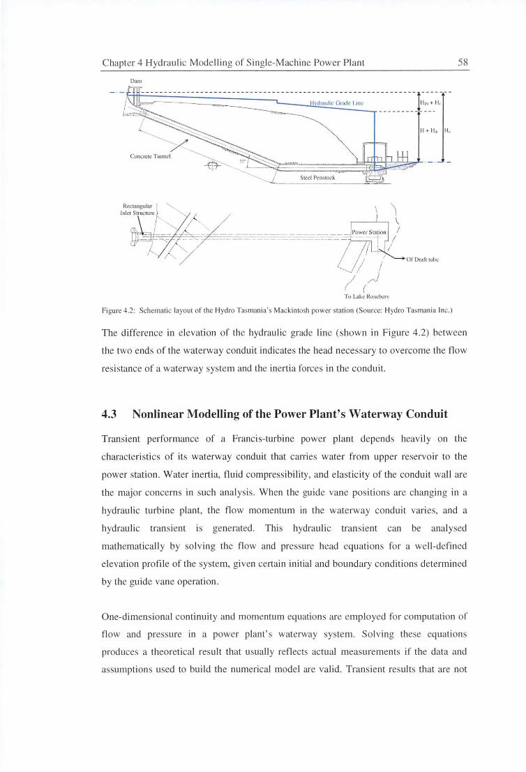
C hapter 4 Hydraulic Modelli ng of Single-Machine Power Pl ant 58
Dam
H draulic Grade Line HIN + H,
H + H~ H0
Steel Penstock
To L1ke Rosebery
Figure 4.2: Schematic layout of the Hydro Tasman ia' s Mackin tosh power station (Source: Hydro Tas mania Inc.)
The difference in elevati on of the hydraulic grade line (show n in Figure 4 .2) between
the two ends o f the waterway conduit indicates the head necessary to overcome the fl ow
res istance of a waterway system and the inertia fo rces in the co nduit.
4.3 Nonlinear Modelling of the Power Plant's Waterway Conduit
Transient performance of a Franci s-turbine power plant depends heavil y on the
characteri sti cs of its waterway conduit that carries water from upper reservoir to the
power station . Water inertia, fluid compress ibility, and e lasticity of the conduit wall are
the major concerns in such ana lys is. When the guide vane pos iti ons are changing in a
hydraulic turbine pl ant, the fl ow momentum in the waterway conduit vari es, and a
hydraulic transient is generated . Thi s hydraulic transient can be analysed
mathematica ll y by solving the fl ow and pressure head equati ons fo r a well-defin ed
elevation profile of the system, given certain initial and boundary conditions determined
by the guide vane operation .
One-dimensional continuity and momentum equations are employed fo r computation of
fl ow and pressure in a power plant 's waterway system. Solving the e equati ons
produces a theoretical result that usually refl ects actual measurements if the data and
assumpti ons used to build the numerical model are valid. T ransient results that are not
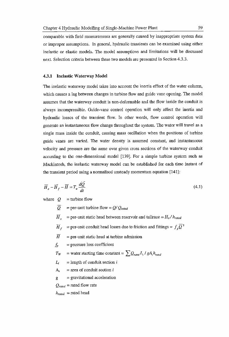

Chapter 4 Hydraulic Modelling of Single-Machine Power Plant 60
Equation 4.1 represents a conventional inelastic waterway model that has been reported
by Institute of Electrical & Electronics (IEEE) and is constantly used in the power
industry to describe the hydraulic transient of the waterway system in a hydroelectric
generating plant with a single turbine and penstock, unrestricted headrace and tailrace,
and no surge tank [141]. The normalised or "per-unit" values of the flow and head (see
also section 4.6.2.1) in Equation 4.1 are obtained by dividing the dimensional flow and
head values by the rated flow and head values, respectively.
This conventional model contains some significant drawbacks. Conduit head losses in
the conventional model are often ignored for simplicity (either linear or nonlinear
models). This simplification is no longer necessary with today's modem computing
power. In fact, conduit losses (modelled as a constant pressure loss coefficient times
flow squared) could easily amount to around 5% of the total available head at rated flow
and are not always constant, even for a simple hydro power plant such as Mackintosh.
Hence the inclusion of the conduit losses is considered desirable and will be carefully
evaluated here.
Another deficiency of the conventional model is that the dynamic pressure at entrance
to the pressure tunnel is neglected. This will cause an overestimate of the flow changes
in the system, and in tum over-predict the transient power output of a hydro power plant
if the guide vane position is changed. To resolve this issue, inlet dynamic pressure head
should be included and modelled in the similar manner to the conduit head losses.
Calculation of the inlet dynamic pressure head and conduit head losses will be
summarised in Sections 4.6.2.4 and 4.6.2.5.
The conventional model also assumes that the flow inside the conduit is one
dimensional and the velocity is uniformly distributed over the cross section of the
waterway conduit. For a hydraulic turbine plant where the flow is always viscous and
non-uniform, the effect of flow non-uniformity could be significant, depending on the
flow profile at the given operating condition. At least 5% difference m acceleration (or
deceleration) can be expected between flows with uniform and non-uniform velocity
distributions. A simple analysis to investigate the effect of flow non-uniformity on
transient behaviour of the Francis-turbine operation is discussed in Chapter 8.
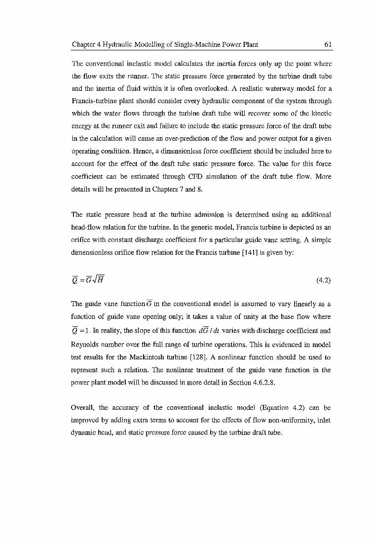
Chapter 4 Hydraulic Modelling of Single-Machine Power Plant 61
The conventional inelastic model calculates the inertia forces only up the point where
the flow exits the runner. The static pressure force generated by the turbine draft tube
and the inertia of fluid within it is often overlooked. A realistic waterway model for a
Francis-turbine plant should consider every hydraulic component of the system through
which the water flows through the turbine draft tube will recover some of the kinetic
energy at the runner exit and failure to include the static pressure force of the draft tube
in the calculation will cause an over-prediction of the flow and power output for a given
operating condition. Hence, a dimensionless force coefficient should be included here to
account for the effect of the draft tube static pressure force. The value for this force
coefficient can be estimated through CFD simulation of the draft tube flow. More
details will be presented in Chapters 7 and 8.
The static pressure head at the turbine admission is determined using an additional
head-flow relation for the turbine. In the generic model, Francis turbine is depicted as an
orifice with constant discharge coefficient for a particular guide vane setting. A simple
dimensionless orifice flow relation for the Francis turbine [141] is given by:
Q=GJli (4.2)
The guide vane function G in the conventional model is assumed to vary linearly as a
function of guide vane opening only; it takes a value of unity at the base flow where
Q = 1. In reality, the slope of this function dG I dt varies with discharge coefficient and
Reynolds number over the full range of turbine operations. This is evidenced in model
test results for the Mackintosh turbine [128]. A nonlinear function should be used to
represent such a relation. The nonlinear treatment of the guide vane function in the
power plant model will be discussed in more detail in Section 4.6.2.8.
Overall, the accuracy of the conventional inelastic model (Equation 4.2) can be
improved by adding extra terms to account for the effects of flow non-uniformity, inlet
dynamic head, and static pressure force caused by the turbine draft tube.
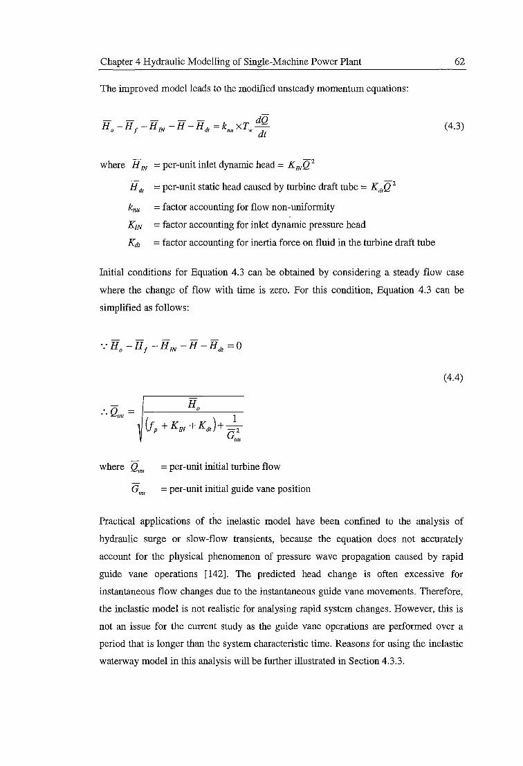
Chapter 4 Hydraulic Modelling of Single-Machine Power Plant
The improved model leads to the modified unsteady momentum equations:
----- dQ Ho -HJ -HIN -H -Hdt = knu xTW
dt
where HIN =per-unit inlet dynamic head= KINQ 2
H dr =per-unit static head caused by turbine draft tube= Ka1Q 2
knu = factor accounting for flow non-uniformity
Km = factor accounting for inlet dynamic pressure head
Kdr = factor accounting for inertia force on fluid in the turbine draft tube
62
(4.3)
Initial conditions for Equation 4.3 can be obtained by considering a steady flow case
where the change of flow with time is zero. For this condition, Equation 4.3 can be
simplified as follows:
(4.4)
. Q -• • 1n1 -
where Q lnl
=per-unit initial turbine flow
G,m =per-unit initial guide vane position
Practical applications of the inelastic model have been confined to the analysis of
hydraulic surge or slow-flow transients, because the equation does not accurately
account for the physical phenomenon of pressure wave propagation caused by rapid
guide vane operations [142]. The predicted head change is often excessive for
instantaneous flow changes due to the instantaneous guide vane movements. Therefore,
the inelastic model is not realistic for analysing rapid system changes. However, this is
not an issue for the current study as the guide vane operations are performed over a
period that is longer than the system characteristic time. Reasons for using the inelastic
waterway model in this analysis will be further illustrated in Section 4.3.3.
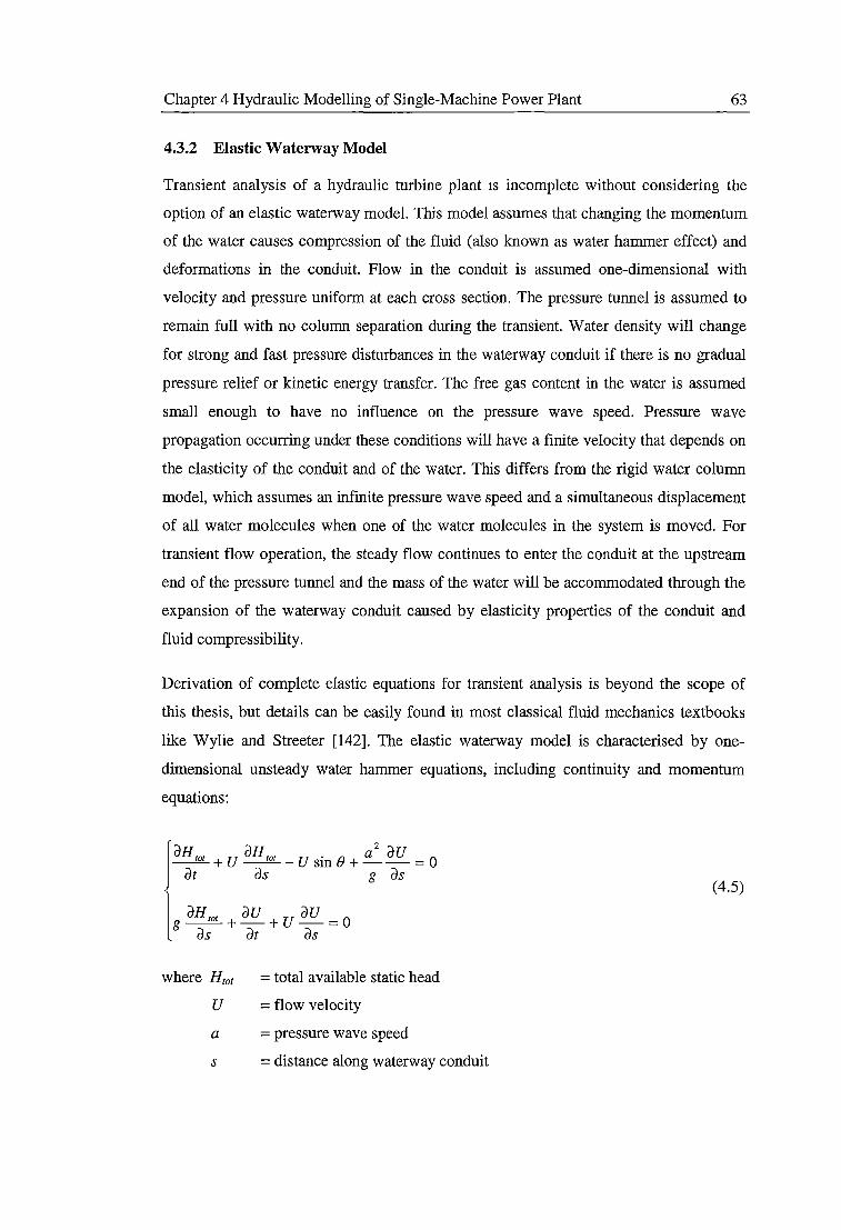
Chapter 4 Hydraulic Modelling of Single-Machine Power Plant 63
4.3.2 Elastic Waterway Model
Transient analysis of a hydraulic turbine plant 1s incomplete without considering the
option of an elastic waterway model. This model assumes that changing the momentum
of the water causes compression of the fluid (also known as water hammer effect) and
deformations in the conduit. Flow in the conduit is assumed one-dimensional with
velocity and pressure uniform at each cross section. The pressure tunnel is assumed to
remain full with no column separation during the transient. Water density will change
for strong and fast pressure disturbances in the waterway conduit if there is no gradual
pressure relief or kinetic energy transfer. The free gas content in the water is assumed
small enough to have no influence on the pressure wave speed. Pressure wave
propagation occurring under these conditions will have a finite velocity that depends on
the elasticity of the conduit and of the water. This differs from the rigid water column
model, which assumes an infinite pressure wave speed and a simultaneous displacement
of all water molecules when one of the water molecules in the system is moved. For
transient flow operation, the steady flow continues to enter the conduit at the upstream
end of the pressure tunnel and the mass of the water will be accommodated through the
expansion of the waterway conduit caused by elasticity properties of the conduit and
fluid compressibility.
Derivation of complete elastic equations for transient analysis is beyond the scope of
this thesis, but details can be easily found in most classical fluid mechanics textbooks
like Wylie and Streeter [142]. The elastic waterway model is characterised by one
dimensional unsteady water hammer equations, including continuity and momentum
equations:
dHrot U dH101 U . () az dU 0 --+ --- sm +--= dt ds g ds
where H,01
u a
s
= total available static head
= flow velocity
= pressure wave speed
= distance along waterway conduit
(4.5)
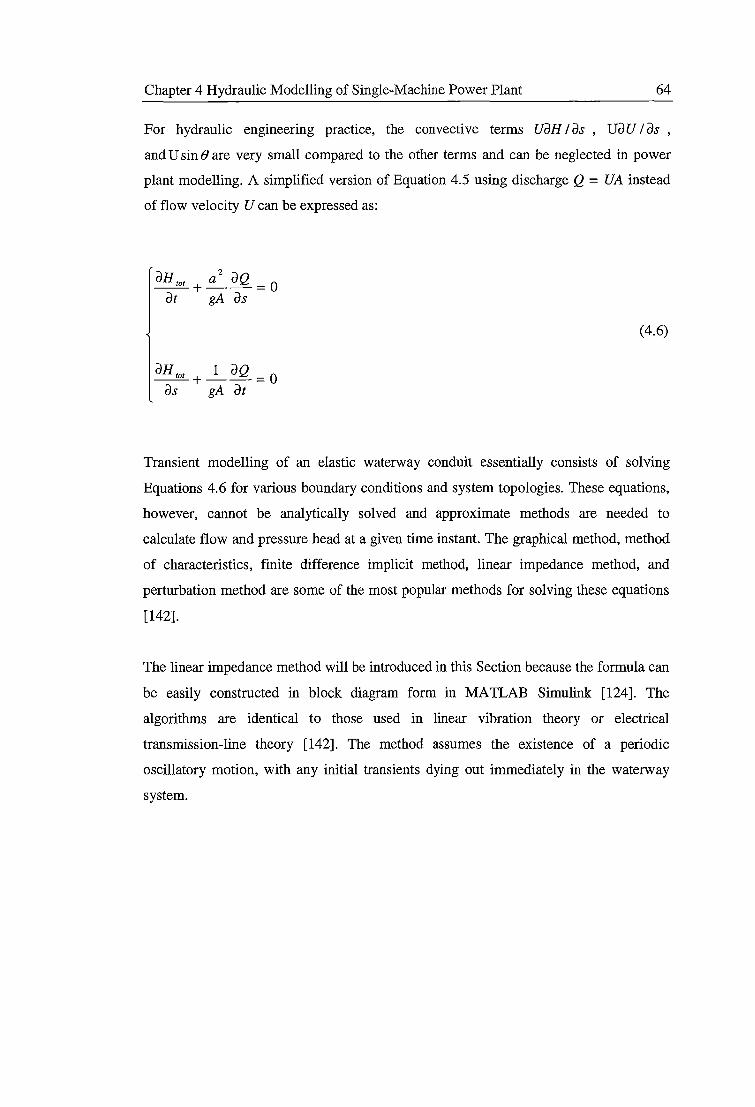
Chapter 4 Hydraulic Modelling of Single-Machine Power Plant 64
For hydraulic engineering practice, the convective terms UoH I OS ' Uo u I OS '
and U sin() are very small compared to the other terms and can be neglected in power
plant modelling. A simplified version of Equation 4.5 using discharge Q = UA instead
of flow velocity U can be expressed as:
(4.6)
oH,o, + _1_ oQ = 0 os gA ot
Transient modelling of an elastic waterway conduit essentially consists of solving
Equations 4.6 for various boundary conditions and system topologies. These equations,
however, cannot be analytically solved and approximate methods are needed to
calculate flow and pressure head at a given time instant. The graphical method, method
of characteristics, finite difference implicit method, linear impedance method, and
perturbation method are some of the most popular methods for solving these equations
[142].
The linear impedance method will be introduced in this Section because the formula can
be easily constructed in block diagram form in MA1LAB Simulink [124]. The
algorithms are identical to those used in linear vibration theory or electrical
transmission-line theory [142]. The method assumes the existence of a periodic
oscillatory motion, with any initial transients dying out immediately in the waterway
system.
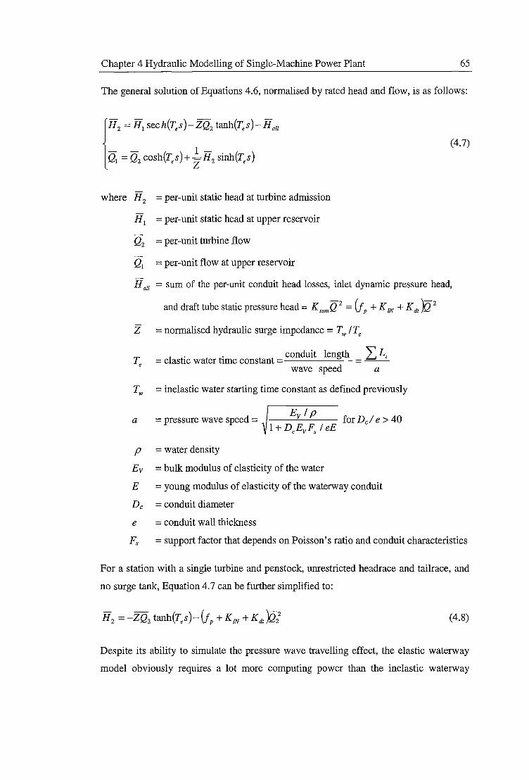
Chapter 4 Hydraulic Modelling of Single-Machine Power Plant 65
The general solution of Equations 4.6, normalised by rated head and flow, is as follows:
{
H, ~ H, sech(T,s )-;Q, tanh(T,s )-H,.,
Q1 = Q2 cosh(Tes)+-=H2 sinh(Tes) z
where H 2 =per-unit static head at turbine admission
H 1 =per-unit static head at upper reservoir
Q2 =per-unit turbine flow
Q1 = per-unit flow at upper reservoir
(4.7)
Hau = sum of the per-unit conduit head losses, inlet dynamic pressure head,
and draft tube static pressure head= KsumQ 2 = (JP +KIN+ Kdr )Q 2
z =normalised hydraulic surge impedance= Tw /Te
. . conduit length I L, = elastic water time constant = = --
wave speed a
=inelastic water starting time constant as defined previously
a = pressure wave speed =
p = water density
Ev = bulk modulus of elasticity of the water
E = young modulus of elasticity of the waterway conduit
De =conduit diameter
e = conduit wall thickness
Fs = support factor that depends on Poisson' s ratio and conduit characteristics
For a station with a single turbine and penstock, unrestricted headrace and tailrace, and
no surge tank, Equation 4. 7 can be further simplified to:
(4.8)
Despite its ability to simulate the pressure wave travelling effect, the elastic waterway
model obviously requires a lot more computing power than the inelastic waterway
Chapter 4 Hydraulic Modelling of Single-Machine Power Plant 66
model, even for a calculation utilising a simplified water hammer equation (Equation
4.8). Vaughan [130] points out that the travelling wave velocity affects only the "shape"
of the time domain response, but not the frequency domain phase response. For power
system stability analyses where more than one turbine plant is usually involved in the
simulation and many different scenarios have to be investigated, computations using the
elastic waterway model may require excessive amounts of computing time and
resources. Clearly, the types of models used in a simulation must been chosen carefully
to achieve a practical balance between the accuracy achieved and the computing time
required.
4.3.3 Model Comparison and Selection
The distinction between elastic and inelastic models can be observed by examining the
pressure changes calculated by each model in an ideal inviscid flow case:
L dQ df>.ne/ast1c oc _.!lJ.__ dPe1as11c adQ
where dPmelastzc = pressure change calculated by inelastic waterway model
dPe1asuc =pressure change calculated by elastic waterway model
(4.9)
As illustrated by Equation 4.9, the guide-vane control movements over a time interval dt
that cause a flow change dQ in the waterway conduit will have significant effect on the
ratio of pressure changes computed using inelastic and elastic waterway models. In the
elastic waterway model, pressure changes depend on the opening or closure time of the
guide vanes (compared to the system characteristic time). When a rapid guide vane
movement occurs (dt-70), head changes calculated by inelastic model will be excessive
and will increase with conduit length L, even for small flow changes. Both models
produce similar results only when dQ-70 or dt-700, which corresponds to a steady-flow
or a very slow transient flow conditions.
The system characteristic time (Ts) for the power plant's waterway conduit, which
defined as 2Va, is the most important criterion used to classify the relative speed of a
guide vane movement and to determine which model is best suited for evaluating a
Chapter 4 Hydraulic Modelling of Single-Machine Power Plant 67
particular hydraulic transient flow case. Guide-vane control operation is "rapid" when it
generates a flow change dQ in a time interval (Top) less than the system characteristic
time (Tc). On the other hand, guide vane movement is considered "slow" when the
operation is carried out over a period longer than the system characteristic time.
While the inelastic waterway model can reasonably predict the pressure variation in
slow transient conditions (Tc << T0p), it generally fails to adequately predict the
discharge when the flow conditions are rapidly varying. The inelastic model is derived
by assuming that the wave speeds of a pressure pulse are infinite. In reality the wave
speeds are always finite, and therefore application of inelastic waterway models is
restricted to hydraulic transients that do not cause significant water compression and
conduit deformation. For the Mackintosh power plant, the highest frequency of guide
vane movement utilised during field test was about 0.5 Hz (Tap "" 2 seconds). This
execution time is 30% larger than the system characteristic time (Tc ::el.4 seconds). For
normal operation, the guide vanes are usually moving at a slower rate of around 0.1 Hz.
Hence, the inelastic waterway model is expected to give reasonably accurate results for
the power plant simulation in the present study. Another important consideration is that
the computational time for an inelastic model is about 4 times faster than the one
employing elastic model (using a desktop computer with Pentium N 1.6 GHz and 256
MB RAM). For these reasons, the inelastic waterway model has been used for transient
modelling of Francis-turbine power plant throughout this project.
4.4 Nonlinear Modelling of Francis Turbine Characteristics
The Francis turbine is a more complicated element to model than the waterway conduit.
Accuracy of the Francis turbine model is the key of the nonlinear simulation of turbine
governing system. The performance of the Francis turbine is affected by many physical
variables including head (H), flow (Q), power output (P), rotational speed (N), turbine
diameter (Drurb), water density (p), and viscosity (µ). Consequently, the accurate
modelling of Francis turbine performance over the whole range of possible operating
conditions is a complex and challenging task.

Chapter 4 Hydraulic Modelling of Single-Machine Power Plant 68
The 1992 IEEE committee report [141] suggests the use of a simple linearised equation
to evaluate the turbine characteristics and power output:
where pm
At
Qnl
D
N
= per-unit electrical power output of a machine
= turbine gain factor
=per-unit no-load flow
= speed-damping factor
=per-unit turbine rotational speed
N rated = per-unit rated turbine rotational speed
(4.10)
The no-load flow Qn1 is used to allow for bearing friction and windage losses in both
the turbine and generator. The turbine gain factor At allows for other internal flow
losses. Separation of losses into two components is not rational. Nor is the assumption
that the turbine characteristic representing by a gain factor At is constant with guide
vane opening, which is quite incorrect for large load disturbances.
The damping factor D is introduced in the IEEE model to allow for efficiency changes
resulting from varied operating conditions. A constant value of D = 0.5 is employed for
Francis turbine modelling. The basis for choosing this value as the speed-damping
factor is not explained in the IEEE report [ 141]. The use of this speed-damping factor is
unrealistic for Francis turbine operation and could lead to significant error when the
change in turbine operating conditions is large. In fact, this equation is incorrect for a
power plant that is governed to maintain a constant runner speed in order to keep the
AC frequency constant within the electrical power grid, in which case the dimensionless
turbine flow coefficient ( c a = Q / ND iurb ) must vary with turbine net head for a fixed
guide vane position. Besides, the power and efficiency changes with speed could be
positive or negative depending on the guide vane position, and their rates of change may
also vary with guide vane position.
Damping effects due to head changes are also completely neglected in Equation 4.10.
As the net head decreases, the Francis turbine becomes relatively more inefficient at
part loads. Changing the turbine net head will change the flow rate of the machine. At a

Chapter 4 Hydraulic Modelling of Single-Machine Power Plant 69
constant turbine speed, this also changes the flow coefficient CQ oc QIN and moves to a
different turbine operating point and efficiency. The probable magnitude of the damping
due to head changes is similar to the speed damping effect and must be taken into
account in the simulation. Vaughan [130] suggests multiplying the turbine gain by a
factor of (H I hrared)312 to correct for damping effects due to head changes. This is
incorrect, as it will result in power output being factored by H 914 through the related
dependence of flow on H 112• Altering the turbine net head while maintaining constant
turbine speed results in a change in flow coefficient, making an exact H312 dependence
of power output impossible.
The only feasible way to correctly represent a Francis turbine characteristic is to use a
dimensionless turbine performance curve. This is done by utilising the model test
information of a scaled down unit and incorporating the empirical data into the real
turbine unit. Dimensional analysis is often employed to handle and extrapolate these
empirical data to the full-scale machine. Four dimensionless groups can be specified
using this approach: flow coefficient ( c 0 = Q J ND iurb ), head coefficient
(c H = gH IN 2 DJ,,,b ), power coefficient (c P =PI pN 3 D:urb ), and Reynolds number
(Re = pND :urb / µ ). These dimensionless quantities however are not all independent,
as power coefficient is the product of head and flow coefficients. Ramos and Almeida
[97] use a rather different set of parameters (known as Suter parameters) to characterise
the dynamic behaviour of a Francis turbine. This approach assumes a homologous
relationship between turbines and pumps. Two parameters can be obtained as follows:
w (B)= T!Trated T (N / Nrated )2 + (Q / Qrated )2
where WH =dimensionless head coefficient
Wr = dimensionless torque coefficient
T = mechanical torque generated by Francis turbine
Trared = rated mechanical torque generated by Francis turbine
B =angle of operating zone= tan-1(N IQ)
(4.11)
Chapter 4 Hydraulic Modelling of Single-Machine Power Plant 70
The Suter parameters described in Equation 4.11 require an enormous effort to
recalculate various parameters listed in the model test report [128] for the Mackintosh
turbine. Two independent variables N and Q are needed to work out a particular turbine
operating condition. Hydraulic turbine engineers always work with the head and power
coefficients, as the flow and mechanical torque are difficult to measure in full-scale
prototype. It should be noted that exact similarities (geometric, kinematic, and dynamic)
in the operation of Francis turbine installations must be achieved so that model test data
can be used correctly for the full-scale turbine. To satisfy geometric similarity, the
turbine model should be tested with identical guide vane settings, same runner design,
and similar draft tube geometry. As meridional velocity Vm in the Francis turbine is
proportional to Q f D ;urb , and the peripheral speed of the turbine runner u is
proportional to NDrurb, it can be seen that kinematic similarity (vml u) requires the flow
coefficient CQ to be constant in order to ensure similar flow patterns or velocity
diagrams at the turbine. Dynamic similarity requires all force components in the same
ratio for both model and prototype, which implies that the head coefficient CH and
Reynolds number must be the same for both installations.
For an incompressible and non-cavitating flow, the turbine operation is accurately
described by the following relation:
Ca= f(CQ, Re) or Cp = f(CQ, Re) (4.12)
Changes in turbine performance with Reynolds number are relatively slow, and for
small variations in Reynolds number, the Francis turbine performance can be
approximated by:
(4.13)
In real cases, the turbine net head will vary due to transients or long period changes in
the supply head. Similar operating conditions (CQ, CH constant) with varying speed
require that Q oc N, H oc N2, and P oc N3 or alternatively N oc H° 5
, Q oc H°5, and P oc
H1s.
Model test data for the Francis turbine are usually presented in a hill chart or in a series
of tables. Finding efficiency data over the whole ranges of turbine operating conditions
is difficult. This is particularly true for an ageing turbine plant. Turbine manufacturers
Chapter 4 Hydraulic Modelling of Single-Machine Power Plant 71
regard such information as proprietary and often publish efficiency data as relative with
a peak relative efficiency for runner set at unity. Nearly all published efficiency data for
full-scale turbines are provided as a curve of efficiency plotted against power. For the
Mackintosh power station, the model test data is published in terms of pseudo
dimensionless groups: unit speed ( N 11 = ND rurb I H 0 5 ), unit discharge
( Q 11 = Q / H 0 5 D Jurb ), and unit power (Pu = p / H 1 5 D Jurb ). However, only data near
the best-efficiency operating conditions are presented in the chart. Information
regarding off-design conditions is not available.
Gordon [38] has developed a generic formula based on empirical data from eight
different Francis turbines to describe the shape of the turbine efficiency curve:
17 q = 17 peak - ~ 17 peak
where 17q = turbine efficiency at flow Q
17peak = peak turbine efficiency
= 0.9187-[( 1998-y)/ 187]3-[(Ns -52)/292]1·017 + dsize
.t117peak = change from peak turbine efficiency
Ye = year when unit was commissioned
dszze = factor accounting for different size of Francis turbine diameter
N 'f' d NQ o s h-o 1s s = SpeCl lC Spee = rated rated
Qpeak = flow at peak turbine efficiency
(4.14)
From an engineering viewpoint, the shape of efficiency curve is approximated by a
parabola with the apex at peak efficiency. Equation 4.14 takes into account three
important characteristics of the Francis turbine's efficiency curve: the peak efficiency
flow (Qpeak) relative to the rated flow (Qrated) changes as the specific speed changes; the
shape of efficiency curve becomes flatter as the specific speed decreases; and the no
load flow relative to rated flow position decreases as the specific speed decreases. The

Chapter 4 Hydraulic Modelling of Single-Machine Power Plant 72
age of the Francis turbine is also being considered in the equation. Higher efficiency
values are expected if the unit has recently been commissioned.
For the Mackintosh power station, a combined technique utilising full-scale steady-state
test data, Gordon's empirical formula, simulations, and turbine model test results is
adopted to form the complete efficiency curve for the Francis turbine. A nonlinear
relation can then be established to calculate the per-unit electrical power output
generated in a hydro power plant:
p - - - HQ & m - 1J Turb 1J Gen ffrurb = J(CQ) (4.15)
No further correction for variation from rated head is required with this arrangement.
More details about the turbine performance curve will be presented in Section 4.6.2.7.
4.5 Linearised Model of the Single-Machine Power Plant
Linearised models originally designed for implementation on analogue computers are
still widely used in the power industry. They are useful only for investigation of small
power system perturbations or for first swing stability studies. The linearised plant
model using inelastic waterway column theory can be obtained by rearranging the basic
equations for waterway and turbine system (Equations 4.2, 4.3 and 4.10). The
formulation is based on small perturbations in flow, head, guide vane opening, and
power output during the operation. To ease the calculation, the linearised model always
assumes that the turbine is ideal, hydraulic losses in the conduit are negligible, flow is
uniform, and other flow effects are minimal for a small change in guide vane position.
The resulting model is expressed by:
~ l-Tw,s ----==- = ----AG l+0.5Tw,s
(4.16)
Readers are referred to Kundur [59] for full derivations of this linearised model.
Equation 4.16 represents a typical "non-minimum phase" system since its zero is
located in the right half of the s-plane1. In other words, the system will always behave
1 A two-dimensional complex space defined by a real-number axis and imaginary-number axis. It is used m control theory to visualise the roots of equation descnbing a system's behaviour. This equation is normally expressed as a polynomial in parameter 's' of the Laplace transform, and hence named s-plane.
Chapter 4 Hydraulic Modelling of Single-Machine Power Plant 73
stably. When knowledge of the frequency response of such a system is reqmred, both
the phase and magnitude of the system must be investigated as it does not possess a
minimum amount of phase shift for a given magnitude plot. This is important if the
system is to manoeuvre at the highest frequency possible. The water starting time
constant T w1 in this case corresponds to the turbine nominal operating condition rather
than the rated condition and must therefore be adjusted according to the variation of the
guide vane opening (Gm,) if the initial operating conditions are changed, according to:
(4.17)
The complete time response of the linearised plant model can be examined by taking the
inverse Laplace transform of Equation 4.16:
(4.18)
For an ideal turbine with a given step increase in guide vane opening, the normalised
power output is bounded within values of [-2, 1]. The initial power surge will be
opposite to the direction of change in guide vane position because of the inertia effect of
the waterway conduit. Applying an elastic waterway model and still assuming an ideal
turbine leads to:
M _m __
!::.G
1-Z tanh(Tes)
1+0.5Z tanh(Tes) (4.19)
Although simplified, Equation 4.19 is still difficult to solve analytically and a reduced
order approach is needed to approximate the hyperbolic tangent:
l-e-"" sT,~ [1 +(~ rJ tanh(Tes) = -ZTs = [ l 1 + e , ~ 2T s z
~ 1 + ( (2n _: l)n-) (4.20)
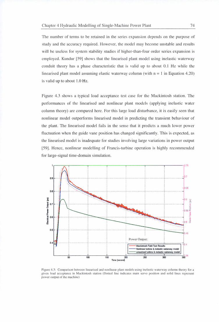
Chapter 4 Hydraulic Modelling of Single-Machine Power Plant 74
The number of terms to be retai ned in the series ex pansion depends on the purpose of
study and the accuracy required . However, the model may become unstable and results
will be useless for system stabi lity stud ies if higher-than-four order series expansion is
employed . Kundur [59] shows that the linearised plant model using inel astic waterway
conduit theory ha a phase characteristic that is valid up to about 0.1 Hz while the
lineari sed plant model assuming elastic waterway column (w ith n = 1 in Equation 4.20)
is valid up to about 1.0 Hz.
Figure 4.3 shows a typical load acceptance test case for the Mackintosh station. The
performances of the linearised and nonlinear plant model s (applying inelastic water
column theory) are compared here. For thi s large load disturbance, it is easily seen that
nonlinear model outperforms lineari sed model in predicting the transient behaviour of
the plant. The linearised model fails in the sense that it predicts a much lower power
fluctuation when the guide vane position has changed sign ificant ly. This is expected, as
the linearised model is inadequate for studies involving large variations in power output
[59] . Hence, nonlinear modelling of Franci s-turbine operation is highly recommended
for large-signal time-domain simulation.
0.9
0.8
x ! 07 0
I Q.
~ 0.6 u .!! w
0.5
O.•
50 100 150 200 Time (second)
c 0
~ 055 ~
ID c
>
Figure 4.3: Comparison between lineari sed and non linear plant models usin g inelasti c waterway column theory for a given load acceptance in Mackintosh station (Dotted line indicates main servo position and so li d lines represent power output of the machine)
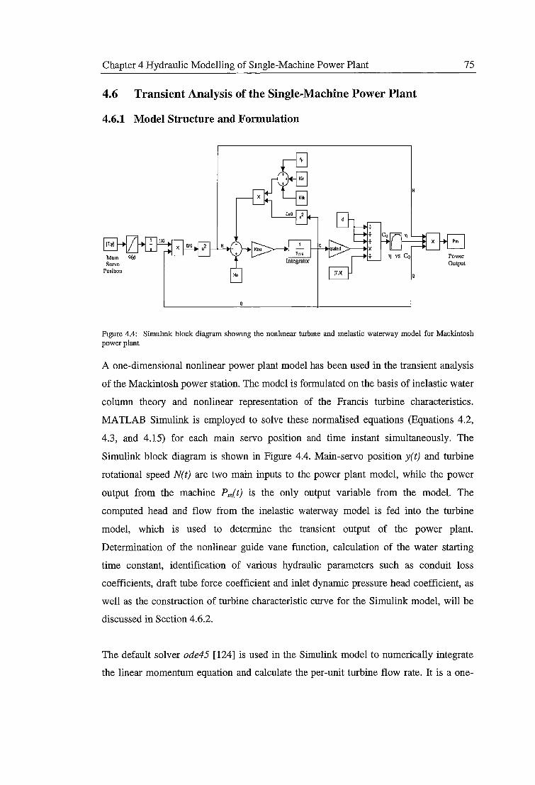
Chapter 4 Hydraulic Modelling of Smgle-Machine Power Plant 75
4.6 Transient Analysis of the Single-Machine Power Plant
4.6.1 Model Structure and Formulation
Figure 4.4: Simulmk block diagram showmg the nonlmear turbme and melastic waterway model for Mackintosh power plant
A one-dimensional nonlinear power plant model has been used in the transient analysis
of the Mackintosh power station. The model is formulated on the basis of inelastic water
column theory and nonlinear representation of the Francis turbine characteristics.
MATLAB Simulink is employed to solve these normalised equations (Equations 4.2,
4.3, and 4.15) for each main servo position and time instant simultaneously. The
Simulink block diagram is shown in Figure 4.4. Main-servo position y(t) and turbine
rotational speed N(t) are two main inputs to the power plant model, while the power
output from the machine Pm(t) is the only output variable from the model. The
computed head and flow from the inelastic waterway model is fed into the turbine
model, which is used to determine the transient output of the power plant.
Determination of the nonlinear guide vane function, calculation of the water starting
time constant, identification of various hydraulic parameters such as conduit loss
coefficients, draft tube force coefficient and inlet dynamic pressure head coefficient, as
well as the construction of turbine characteristic curve for the Simulink model, will be
discussed in Section 4.6.2.
The default solver ode45 [124] is used in the Simulink model to numerically integrate
the linear momentum equation and calculate the per-unit turbine flow rate. It is a one-
Chapter 4 Hydraulic Modelling of Smgle-Machine Power Plant 76
step solver based on the 4/5-order Runge-Kutta formula, the Dormand-Prince pair,
which is designed to handle the initial value problem for systems of differential
equations with the form of y/ = f(y, t). The solver imposes the initial conditions at the
beginning of a calculation and returns the solution evaluated at every integration step.
Only the solution from the immediately preceding time point is needed for each
integration step. This solver algorithm is recommended for power plant simulation
because it requires the smallest number of function evaluations, the minimal number of
floating-point operations, and the least amount of numerical steps to get a converged
solution compared to other solver algorithms built in the MATLAB Simulink [124].
Overall, the model is set up in the way that no algebraic loop will occur in the
simulation. The implications of algebraic loops and the need to avoid them are well
explained in MATLAB user manual [124].
When the guide vanes of a turbine become almost closed and the associated flow rate in
the conduit decreases, the numerical integration of the ordinary differential equation
becomes more difficult due to the assumption of inelastic water column. If the turbine
guide vanes are shut off at some small discharge Q, the value of this turbine flow will
be replaced discontinuously by zero. In this case, the flow rate Q will become less than
a small value L1Q and the mass continuity at the upstream and downstream ends of the
conduit can no longer hold. In fact, the jump in flow rates is incompatible with a strictly
applied inelastic water column assumption. To resolve this issue, a decision block is
added to the model to overcome the discontinuity problem and ensure that simulation
runs smoothly when the guide vanes are almost closed.
4.6.2 Evaluation of Hydraulic Model Parameters
The parameter identification and evaluation process for the Francis-turbine plant model
requires numerous simulations to examine the effects of changing one model parameter
on the overall plant response. For each parameter change, a comparison is made
between response of the model and that recorded from the field tests. This traditional
methodology is highly dependent on the skills of the experienced engineers applying
their knowledge to select the best-suited parameters, perform calculations using those
parameters, and adjust the parameters manually based on difference between measured
and calculated values to improve the fit between model and real-plant response. The

Chapter 4 Hydraulic Modelling of Single-Machine Power Plant 77
task becomes even more tedious if non-linear dynamic interactions are involved in the
power plant modelling. Various important hydraulic model parameters for Simulink
model of the Mackintosh power station will be thoroughly assessed and discussed in the
following subsections.
4.6.2.1 Rated Parameters Used in the Per-Unit System
It is common practice in time-domain simulations of power plant to express the
resulting head, flow rate and the power output of a machine in a normalised way or a
per-unit (pu) base. The advantages of the per-unit system are that it:
• imposes proper scaling, which is good for numerical solution;
• yields valuable relative magnitude information; and
• simplifies searching of erroneous data since the parameters tend to fall in relatively narrow numerical ranges.
For the Mackintosh power plant, the rated flow of the Francis turbine, which
corresponds to the turbine flow when guide vanes are fully opened, is chosen as the base
flow value in the calculation. The base value for static pressure head is defined as the
elevation difference between water levels at Lake Mackintosh and Lake Rosebery when
the machine is operating at the design condition; but the rated power output is related to
the amount of electrical power generated by the machine under the base flow and head
values. The rated turbine efficiency is obtained by dividing the actual turbine output
with the hydraulic power input (pgHQ) of the machine. However, the choices of these
base values are not restricted. Users are free to choose any set of base quantities for
power, head, and flow in the model as long as they are consistent throughout the
calculations . The values of rated parameters used in the present modelling of
Mackintosh power plant are listed in Table 4.1.
Rated Parameters Used in Per-Unit System Base Values
Rated Speed (rpm) 166.7
Rated Head (m) 61
Rated Flow Rate (mj/s) 149.7
Rated Power Output (MW) 79.9
Rated Guide Vane Opening(%) JOO
Rated Turbine Efficiency(%) 89.2
Rated Generator Efficiency(%) 97
Table 4.1: Rated parameters used in the per-unit based simulation of transient operations of the Mackintosh station
Chapter 4 Hydraulic Modelling of Single-Machine Power Plant 78
4.6.2.2 Total Available Static Pressure Head
The total available static head H 0 is defined as the elevation difference between head
and tail water levels. For the Mackintosh power station, the average water levels at Lake
Mackintosh and Lake Rosebery are measured and recorded daily. The full storage level
of Lake Mackintosh is 228.6 m above sea level while the minimum operating level of
Lake Mackintosh is 218.8 m above sea level. The average water level at Lake Rosebery
is 159.3 m above sea level, and is essentially independent of the station flow (only
±0.4 m variation between full- and no-flow operating conditions). The normal operating
head of the Mackintosh power station is approximately 61 m. However, the total static
head increased from 60 to 65 m during the field tests because of the significant rainfall
at that time. The variation of the total available static head must be taken into account in
the transient simulation of the Francis-turbine power plant, as it will affect the accuracy
of the computed turbine flow from the waterway model.
4.6.2.3 Water Starting Time Constant
The water starting time constant T w is defined as the amount of time required to
accelerate the flow from zero to the rated flow under the base head or rated head
(Mansoor [70]). The time constant calculation is based on the geometry of the waterway
system when the machine is operating at rated conditions. Unlike the linearised model
where instantaneous flow and head values are employed, the water starting time of the
nonlinear waterway model does not need to be updated in successive iterations for a
simulation. However, it is essential to ensure that consistent values of rated flow and
rated head are used in the calculation of water starting time constant. For an inelastic
waterway conduit with varying geometries and irregular cross-sectional areas, the water
starting time constant is computed from:
(4.21)
The computation of the water starting time constant for Mackintosh station includes the
entire waterway column from the reservoir to the tailrace, which also incorporates the
flow passage through the Francis turbine and draft tube components. A constant starting
time of 3 .17 seconds is used in the modelling of transient operation for Mackintosh
Chapter 4 Hydraulic Modelling of Single-Machine Power Plant 79
power plant. Vaughan [130] examined the effects of varying the water starting times of
the model based on simplified and detailed waterway columns. Detailed calculation of
the water starting time was found to greatly improve the predicted time-domain
response of the power plant, and to reduce the magnitude of differences between the
measured and simulated results [135]. However, significant phase error is still reported
in Vaughan's simulations.
4.6.2.4 Head Loss Coefficient
The flow in the waterway system is turbulent and highly complex. A portion of the
energy has to be spent to overcome the forces of hydraulic resistance in the conduit.
This analysis is restricted to the computation of steady-flow head loss coefficient. As
little information is available on the flow structure during transients, the quasi-steady
flow assumption has to be made so that the steady-flow loss coefficients can be used.
The overall pressure or head loss can be found by summing the pressure losses of all
individual components along the waterway conduit [81]. This includes head losses due
to friction and other minor losses due to geometrical transitions and turbulence within
the bulk fluid. The formula for conduit head losses on a per unit base is:
where fp = I(4][ Q~ted J A. 2ghrated
(4.22)
The k1 values in Equation 4.22 represent the loss coefficients of individual components
that are determined from given empirical charts or tables. The calculating procedures of
the loss coefficients are well documented in Miller [81] and Idelchik [46].
Friction losses in the conduit are normally represented by a factor depending on the
dimensions and surface roughness of the conduit, fluid viscosity, and flow speed. The
effects of joints, local resistance, blockages, formation of wall deposits, and other
complicating factors may increase the friction losses in the pressure tunnel. In fact,
friction calculations involve an element of judgement in selecting roughness values
[ 46]. It is assumed in the current study that the concrete tunnel has good surface finish
and average joints, while the steel penstock is smooth and without any significant
deterioration on the walls. Numerous formulae are available to relate the friction factor

Chapter 4 Hydraulic Modelling of Single-Machine Power Plant 80
(j) to the Reynolds number (Re) of the flow and the relative roughness (e) of the
conduit. One of the most popular formulae is Colebrook-White equation [139]:
1 _ 21 ( e 2.51 J ---- ogw +---fj 3.7 D,q Refj
(4.23)
The equivalent diameter Deq = A IP is used to account for non-circular cross-section
geometry. Equation 4.23 is solved by iterating through assumed values of friction factor
f until both sides are equal. A quick solution of friction factor can be obtained
graphically from Moody diagram.
For the rectangular intake structure, minor energy losses occur in the entrance and
contraction zone. The entrance loss coefficient is a measure of the efficiency of the inlet
structure to smoothly transport the water flow from the upstream reservoir into the
pressure tunnel; although it does vary with flow, a constant value corresponding to the
full flow condition is used here. The "wing-wall" build at the entrance has the effect of
streamlining the flow into the tunnel and hence can minimise the energy losses.
Moreover, a converging section with a contraction length ratio of 7 is employed to
provide a gradual change in the area and velocity, which has a positive impact on
minimising losses at the inlet.
A 22° bend at the end of the concrete-lined tunnel (see Figure 4.2) will cause a diffuser
effect at the outer (bottom) wall and a bellmouth effect at the inner wall. This generates
a secondary flow along the bend and may lead to flow separation in the penstock. The
bend loss is strongly dependent on the bend curvature, flow Reynolds number, surface
roughness, and the geometry of the connecting tunnels at both ends.
Transition losses for the elbow draft tube are also included in the head loss calculation.
Losses due to the combined turning and diffusion in the draft tube are highly dependent
on the inlet-outlet area ratio, inlet boundary layer thickness, bend angle, and the outlet
conditions. The kinetic energy of flow at exit from the draft tube is always lost to the
system. It is assumed that the exit flow is discharged into an infinitely large reservoir
and therefore the downstream effect will be minimal in this case. More details about the
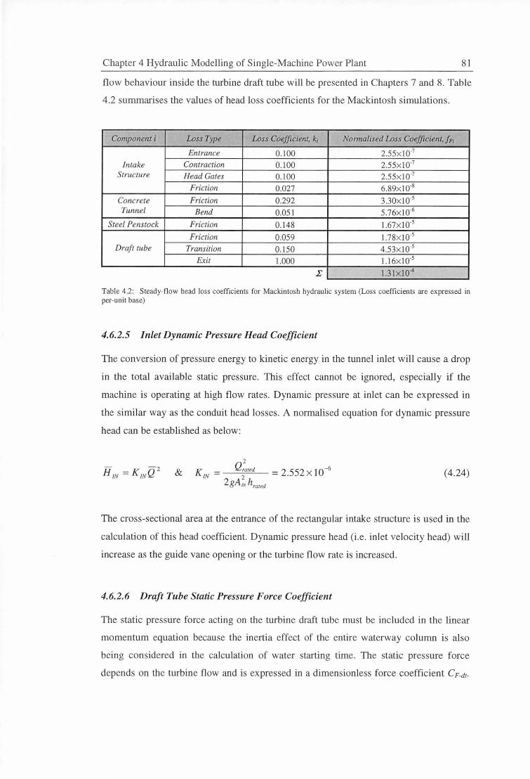
Chapter 4 Hydraulic Modelling of Single-Machine Power Plant 81
fl ow behaviour inside the turbine draft tube will be presented in Chapters 7 and 8. Table
4.2 summarises the values of head loss coefficients for the Mackintosh simulations.
Component i Loss Type Loss Coefficient, k; Normalised Loss Coefficient,fp;
Entrance 0.100 2.55x10·7
Intake Contraction 0.100 2.55x10·7
Structure Head Gates 0.100 2.55x l0'7
Friction 0.027 6.89x10·8
Concrete Friction 0.292 3.30x 10·5
Tunnel Bend 0.051 5.76xl0·6
Steel Penstock Friction 0.148 l.67xl0·5
Friction 0.059 I.78x l0·5
Draft tube Transition 0.150 4.53x10·5
Exit 1.000 l.16x l0-5
I l.3 l x l04
Table 4.2: Steady-flow head loss coefficients for Mackintosh hydraulic system (Loss coefficien ts are expressed in per-unit base)
4.6.2.5 Inlet Dynamic Pressure Head Coefficient
The conversion of pressure energy to kinetic energy in the tunnel inlet will cause a drop
in the total available static pressure. This effect cannot be ignored, especially if the
machine is operating at high flow rates . Dynamic pressure at inlet can be expressed in
the similar way as the conduit head losses. A normalised equation for dynamic pressure
head can be established as below:
2
H IN= K IN Q 2 & K IN= Q;ared = 2.552X 10⁻⁶
2gA IN hrated (4.24)
The cross-sectional area at the entrance of the rectangular intake structure is used in the
calculation of this head coefficient. Dynamic pressure head (i.e. inlet velocity head) will
increase as the guide vane opening or the turbine flow rate is increased.
4.6.2.6 Draft Tube Static Pressure Force Coefficient
The static pressure force acting on the turbine draft tube must be included in the linear
momentum equation because the inertia effect of the entire waterway column is also
being considered in the calculation of water starting time. The static pressure force
depends on the turbine flow and is expressed in a dimensionless force coefficient CF-dr·
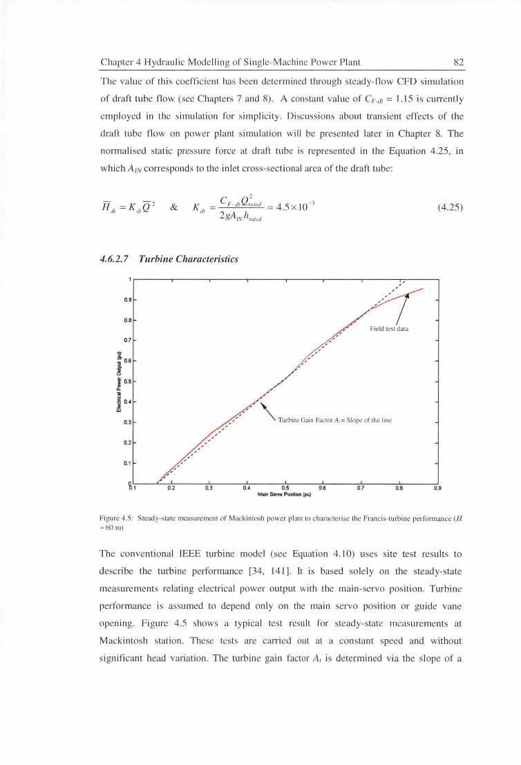
Chapter 4 Hydraulic Modelling of Single-Machine Power Plant 82
The value of thi s coeffic ient has been determined through s teady-flow CFO simulation
of draft tube flow (see Chapters 7 and 8). A con tant value of CF.dr = 1.15 is currently
employed in the simulation for simplicity. Di scussions about transient effects of the
draft tube flow on power plant simul ation will be presented later in Chapter 8. The
normali sed static pressure force at draft tube is represented in the Equation 4.25, in
which AIN corresponds to the inlet cross-sectional area of the draft tube:
&
4.6.2.7 Turbine Characteristics
0.9
O.B
0.7
j; l 0.6
6 I 05 0. ,. .g .i 0.4 w
0.3
0.2
0.1
,
, , ,
,
, , ,
, , , ' Turbine Gain Factor A,= Slope of the line
(4.25)
~.~1~~~0~.2~~~-0~.3~~~0~ .• ~~~-0~.5~~~0~.6~~~-0.~7~~~0~.B~~~-'0.9
Main Serro Posnion (pu)
Figure 4.5: Steady-state measurement of Mackintosh power plant to characterise the Francis-turbine performance (H
= 60 m)
The conventional IEEE turbine model (see Equation 4. I 0) uses s ite test results to
describe the turbine performance [34, 141]. It is based so lely on the steady-state
measurements relating e lectrical power output with the main-servo position . Turbine
performance is assumed to depend only on the main servo position or guide vane
opening. Figure 4.5 shows a typical tes t result for steady-state measurements at
Mackintosh station. These tests are carried out at a constant speed and without
significant head variation . The turbine gain factor A1 is determined via the s lope of a
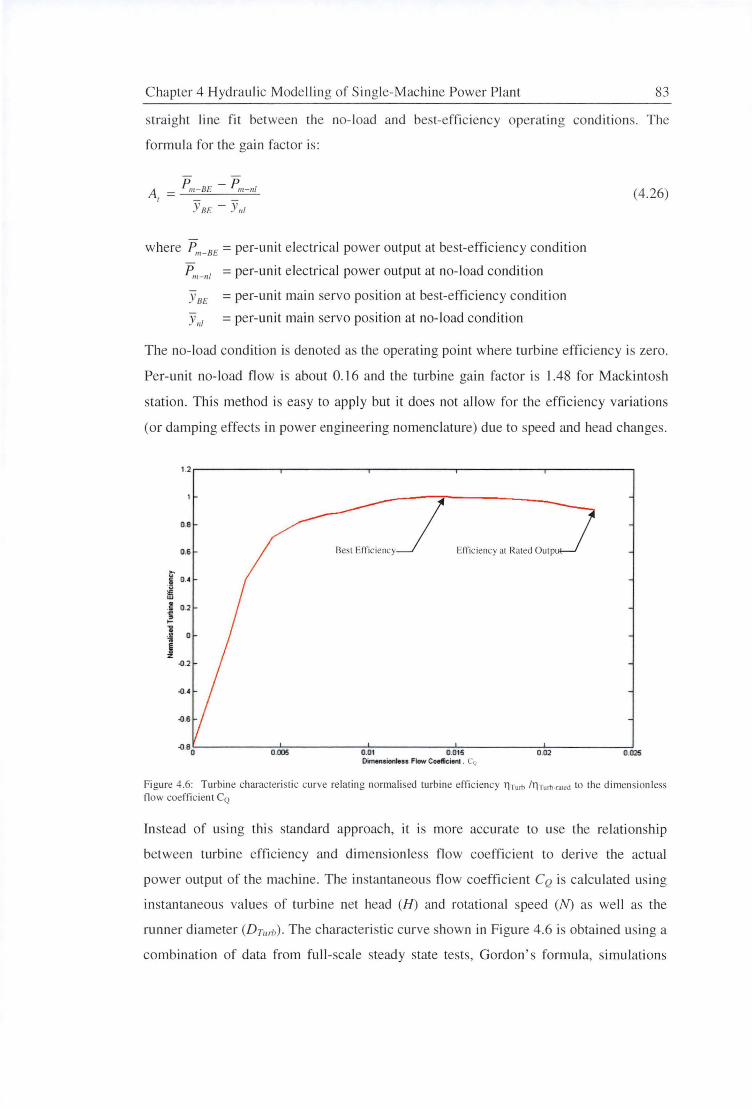
C hapter 4 Hydraulic Modelling of Single-Machine Power Pl ant 83
straight line fi t between the no- load and best-efficiency operating cond itions. The
formul a for the gain factor is:
A, YsE - Y111
where P,n-BE =per-unit electrical power output at best-effi c iency conditi on
Pm_111 = per-unit electrica l power output at no-load condition
y BE = per-uni t main servo position at best-effi ciency condition
y111 =per-unit main servo pos ition at no-load condition
(4.26)
The no- load condition i denoted a the operating point where turbine effi c iency is zero.
Per-unit no-load fl ow is about 0.16 and the turbine gain fac tor is 1.48 fo r Mackintosh
station. This method is easy to apply but it does not allow fo r the effici ency variations
(or damping effects in power engineering nomenclature) due to speed and head changes.
1.2.---------..---------..---------.---- ----.r----- ----.
0.8
0.6
i 0.4
if w I 0.2 .... l: ,: a
j -0.2
-0.4
-0.6
Best Efficiency Efficiency at Rated Outp
-0 .eo~-----o:-:.005~--------=-o.0~1-------,o""'.o.,..,1s,.-------o.02'-:--------o~.025
Dimensionless Flow Coefficienl . Cq
Figure 4 .6: Turbine characteristic curve re la ti ng normalised turbine effi ciency 11Turb hlrum-rat<d to the dimensionless now coefficient CQ
Instead of using thi s standard approach, it is more accurate to use the re lati onship
between turbine efficiency and dimensionless fl ow coeffic ient to derive the actual
power output of the machine. The instantaneous fl ow coeffi cient CQ is calculated using
instantaneous values of turbine net head (H) and rotati onal speed (N) as well as the
runner diameter (DTur!J) . T he characteristic curve shown in Figure 4.6 is obta ined using a
combination of data from full- scale steady state tests, Gordon's fo rmul a, simulati ons
Chapter 4 Hydraulic Modelling of Single-Machine Power Plant 84
and model test results. This approach will automatically take in to account the
efficiency variations due to both speed and head changes, and therefore no further
damping correction for variation from rated head is required. Direct effects of head
change are also incorporated in this method.
Model test results and full-scale measurements of the Mackintosh turbine show that the
efficiency does not vary greatly with the net head. However, only data with flow
coefficient above 0.0048 are presented in the hill chart of the turbine model. To fill the
gap, Gordon's empirical formula, simulation, and steady-state test results were used to
determine the turbine efficiency where the flow coefficient is below 0.0048 (i.e. the first
five data points). The negative efficiency in the curve implies that the power is supplied
to the generator in order to synchronise the machine. The generator is assumed to work
at a constant efficiency of 97% (or 1 in per-unit system) as no relevant information on
the generator efficiency is available in the Hydro Tasmania's database.
4.6.2.8 Nonlinear Guide Vane Function
The guide vane function is the key parameter relating the water flow and the net head of
the Francis turbine. The working principle is very similar to a nozzle orifice. However,
the resulting flow pattern for the Francis turbine is more complicated than the flow in an
orifice meter; and secondary flow, separation, and turbulence effects are more severe
inside a Francis turbine. The amount of head drop across the turbine depends on the
guide vane opening. The head drop decreases as the guide vanes close. The guide vane
function is defined as [26, 76]:
& AG= f(y)
{
G = 0 if guide vanes are fully closed
G = 1 if guide vanes are fully open
(4.27)
where CD =instantaneous discharge coefficient at the given guide-vane opening area Ao
CDo =reference discharge coefficient at full guide-vane opening areaA00
y = instantaneous main servo position
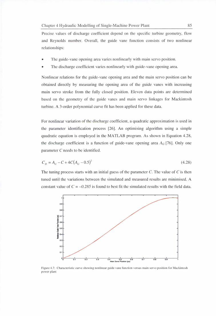
Chapter 4 Hydraulic Modelling of Single-Machine Power Pl ant 85
Precise va lues of di scharge coeffic ient depend on the specific turbine geometry, flow
and Reynolds number. Overall, the guide vane function consists of two nonlinear
re lationships:
• The guide-vane opening area varies nonlinearl y with main servo position .
• The di scharge coefficient varies nonlinearly with guide-vane opening area.
Nonlinear re lation s for the guide-vane open ing area and the main servo position can be
obtained directly by measuring the opening area of the guide vanes with increasing
main servo stroke from the fully closed positi on. Eleven data points are determined
based on the geo metry of the guide vanes and main servo linkages for Mackintosh
turbine. A 3-order pol ynomi al curve fit has been applied for these data.
For nonlinear vari ation of the discharge coefficient, a quadratic approximation is used in
the parameter identification process [26]. An optimising a lgorithm using a simple
quadratic equation is employed in the MATLAB program. As shown in Equation 4.28,
the di scharge coefficient is a function of guide-vane opening area Ac [76]. Only one
parameter C needs to be identified.
(4.28)
The tuning process starts with an initial guess of the parameter C. The value of C is then
tuned until the variation s between the simulated and measured results are minimised . A
constant value of C = - 0.285 is found to best fit the simulated results with the fi e ld data.
0 .9
O.B
A0.7
J 0 .6
J J 0.5
• j a.•
0 .J
O.J 0.A 0.5 0.6 0.7 O.B 0.9 Main SelYCI Position (pu)
Figure 4.7 : Characteristic curve showing non l inear guide vane functi on versus main servo position for Macki ntosh power plant
Chapter 4 Hydraulic Modellmg of Single-Machine Power Plant 86
Figure 4.7 shows the nonlinear guide vane function used in the Simulink model. This
gmde vane function combines both effects of nonlinear discharge coefficient and
nonlinear guide-vane opening area. Weber [138] and De Jaeger et al. implement a
similar parameter optimising procedure for hydro plant modelling. They report a very
good agreement between the measured and simulated dynamic transients. Thus, the
quadratic form of Equation 4.28 appears satisfactory here but in any case, there is
insufficient information available to justify a more complex curve fit at present. A
higher-order term could be used in the identification process when more data are
available in the future.
4.6.2.9 Coefficient for Flow Non-uniformity
The velocity distribution in the waterway conduit has some impacts on flow
acceleration or deceleration. Analysis of the transient flow in the draft tube shows that
flow with a non-uniform axial velocity profile at inlet has faster response time than flow
with a uniform velocity profile for a given initial flow rate and static pressure
fluctuation. This effect is expected to vary nonlinearly with the turbine operating
conditions and will be more significant for conditions where flow separation causes
greater flow non-uniformity. This will be discussed in more details in Chapter 8. Due to
a lack of further information for Mackintosh station, a constant coefficient of knn = 1.05
is currently used to account for the effect of axial velocity non-uniformity in the turbine
and waterway system.
4.6.3 Simulation of Time Response for Single-Machine Station
The time response of a single-machine station subjected to a large frequency
disturbance is simulated and analysed here. The main servo position and the turbine
rotational speed measured during field tests are used as the inputs to the Simulink
model. The total available static head for Mackintosh station is set at a level of 65 m.
Simulated electrical power outputs are compared with the site test results. The
performances of the conventional IEEE (Figure 2.4) and the improved (Figure 4.4)
models are investigated. Load acceptance cases with different initial power outputs are
illustrated in Figures 4.8 to 4.12. These results show that the new model is more
capable of reproducing the transient behaviour of the Mackintosh power station despite
some under-prediction of the magnitude of the transient power at high load. The errors
are largely explained by the transient behaviour of the draft tube flow, and these will
later be discussed in detail in Chapter 8.
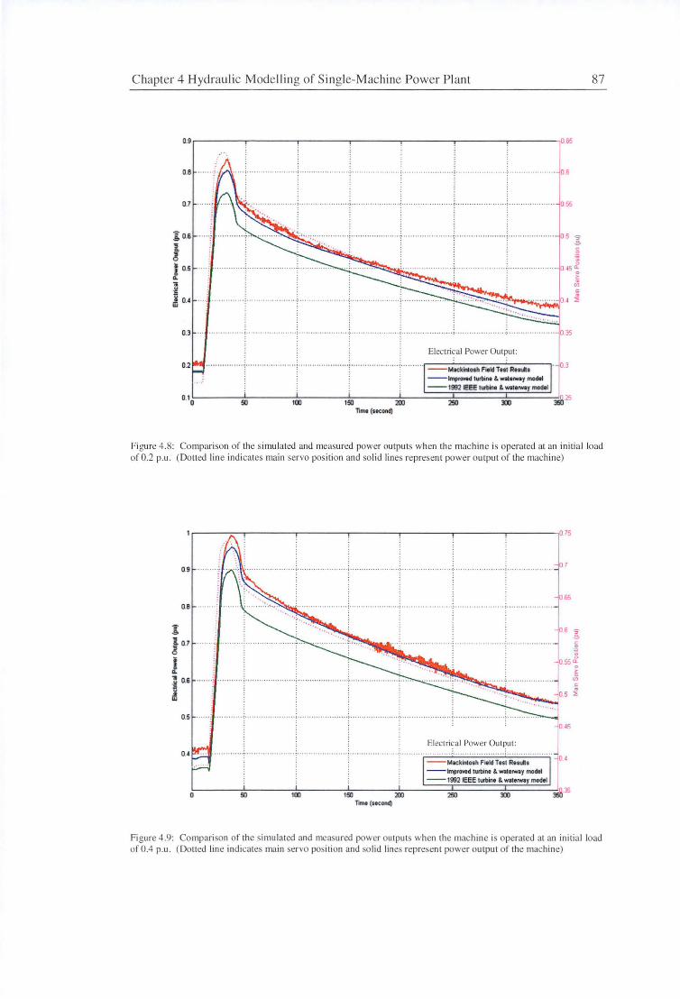
Chapter 4 Hydraulic Model ling of Single-Machine Power Pl ant 87
0.8
0.7
0.3 ...
Electrical Power Output: . . 0.2 --Mackinl:osh Field THI R11uh
--lmprO¥ed turbine & Wlterway modet --1992 IEEE lurbint Lwattrwoy model
5ll 100 151) 200 Time (stcond)
Figure 4.8: Comparison of the simulated and measured power outputs when the machine is operated at an initial load of 0.2 p.u . (Dotted line indicates main servo position and solid lines represent power output of the machine)
0.9
0.8
0.5
o.~
Time (11cond)
'5' .5 ~ 0
~ 055 ~
~ VJ ~
~
Figure 4.9: Compari son of the simulated and measured power outputs when the machine is operated at an initial load of0.4 p.u. (Dolled line indica tes main servo position and solid lines represent power output of the machine)
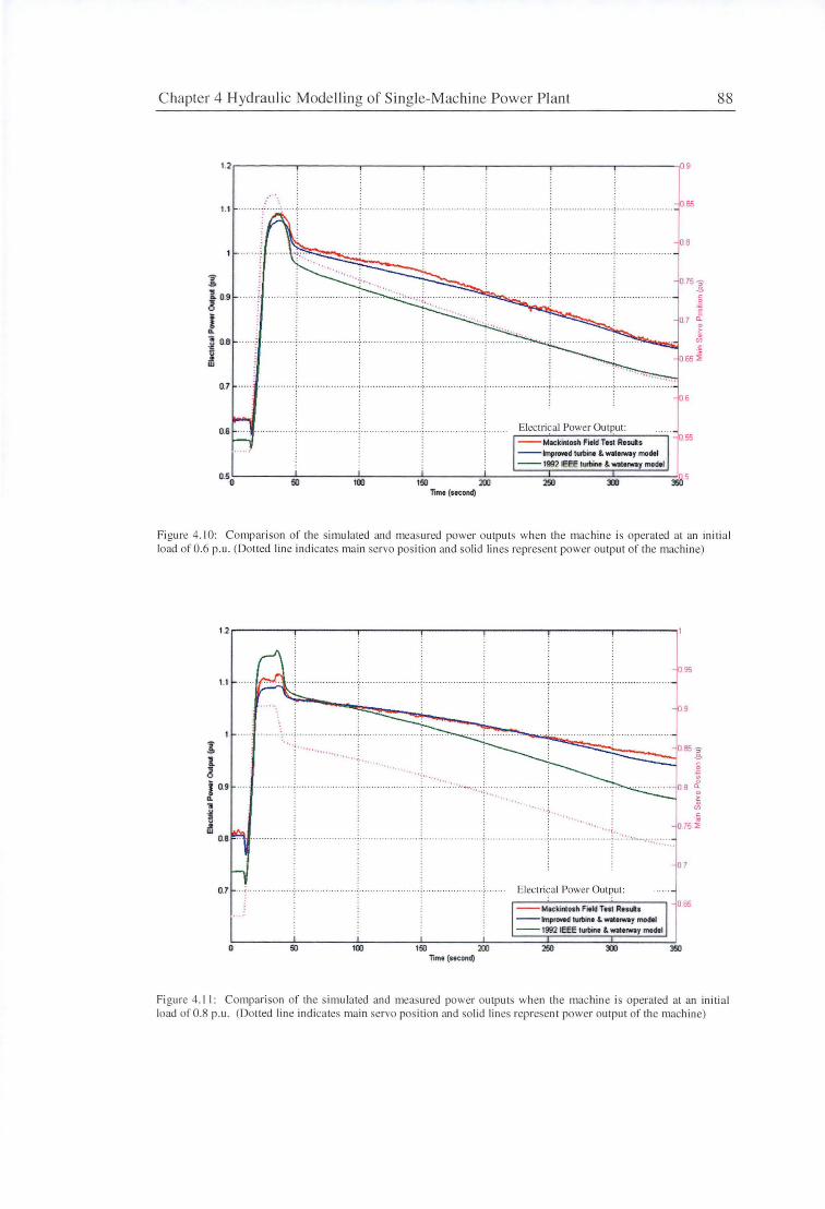
Chapter 4 Hydraulic Modelling of Single-Machine Power Plant
1.1
];
! 09
! ~ 0.8
~
Timt (ucond)
Elec tri~a l Power Out~ut: --Mackintosh Field THI R ..... --lmprowd turbine & waterw1y model --1992 IEEE lurbine & woltrwty modtl
c 0 .. ~ 0
; CJ)
88
Figure 4. 10: Compari son of the simulated and measured power outputs when the machine is operated at an initi al load of 0.6 p.u. (Dotted line indica tes main servo posi ti on and solid lines represent power output of the machine)
l l 6
1.1
! 0.9 ... .. a. 11 ·l!
~
0.7
0 50 100 150 Time (s:econd)
Elec trical Power Output:
--Mackinlosh Fieki Test Res!As -- knprcwed turbine & Wlterway model --1992 IEEE t..t.int L woltrway modtl
200 250
07
c 0
~ a. 0
!'; CJ)
Figure 4.1 I : Comparison of the simulated and mea ured power ou tputs when the machine is operated at an initial load of0.8 p.u. (Dotted line indicates main servo po ition and solid lines represent power ou tput of the machine)
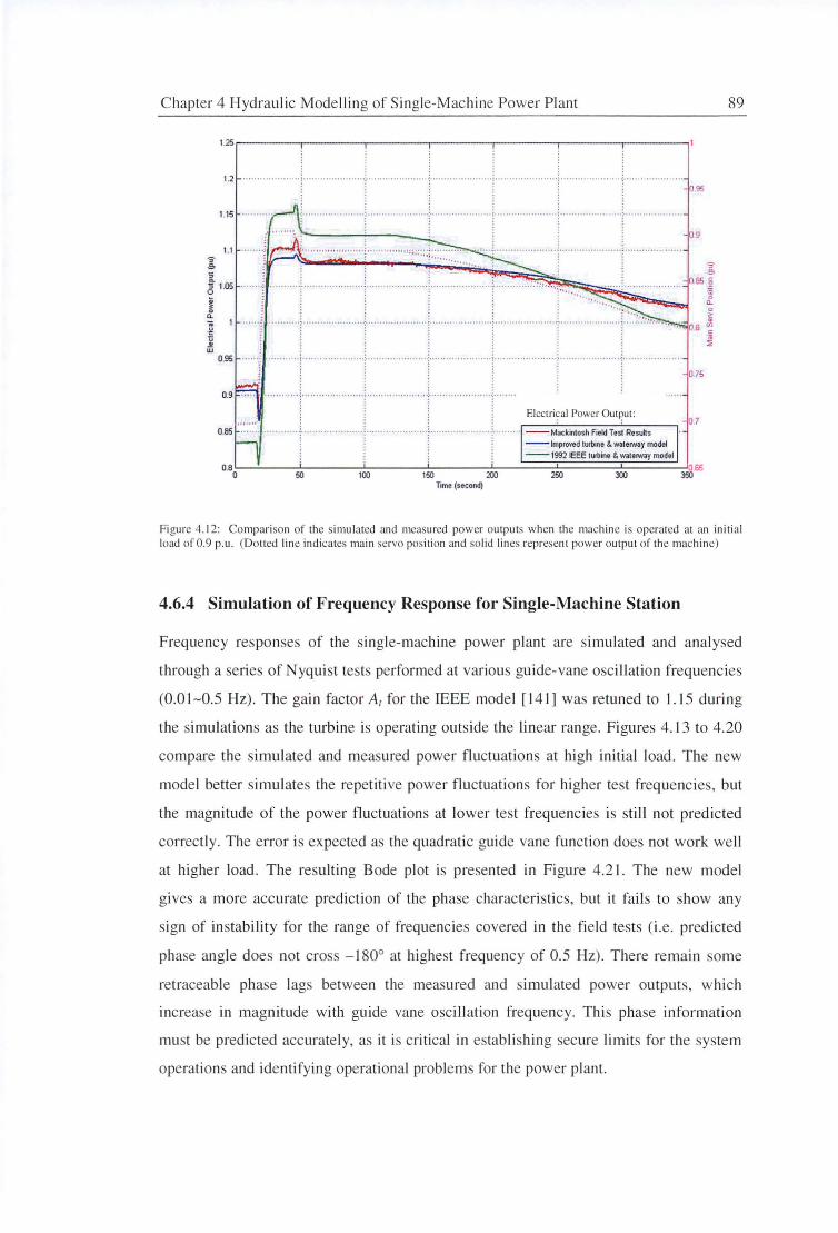
Chapter 4 Hydraulic Modelling of Single-Machine Power Plant 89
1.25~---~------~---~---~---~---~
. : : 1.2 . . . . .... . ... . .... '" l'"" ' . . ..... '' ' ... ' ·~ ... ' ..... " ' . ... ... '' ~ · . . . . .. ... .. ... ' .... ·!• •. ' . . • . ••• . . . •.••.. •)'. ... .. . ..... .. ..... . • ......... .. ... ' ••• '
: : : 0%
1.15 !········· ···· ........ ; .. ............ ·~· ... ... ..... ••••••... •! .. ............. .
0 9
! . ~ . ····· · · ~ ......... ~ ..................... ~ ....... ............ ··~ · ············· · ·······~···· ....... ::::: . ' \'. ·······
····· .. f .... ...... - ~ ....... .......... .... ~- ..... .. .......... .. .. ~ - ........... ..... .
. . . . . .
0.% .. T . . .. m , •••••••• • ••• , ••••••
0 75
- Mackintosh Field Test Results 0.85
....... ····r ..................... r ...................... r··············· .. ····r······· . . . .
.. 1............. . .................. i. : :
Electri~a l Power Out~ut:
. . - Improved turbine & waterway model - 1992 IEEE turbine & waterway model
o.a L_!_ __ L_ __ _ji__ __ _j ___ _l _ __::===::L=======:I=====:'_J 0 50 100 150 200 250
Time (second)
Fi gure 4. 12: Comparison of the simulated and measured power outputs when the machine is operated al an initial load of 0.9 p.u. (Dotted line indicates main servo position and solid lines represent power ou tput of the machine)
4.6.4 Simulation of Frequency Response for Single-Machine Station
Frequency responses of the single-machine power plant are simulated and analysed
through a series of yquist tests performed at various guide-vane oscillation frequencies
(0.0 1-0.5 Hz). The gain factor A1 for the IEEE model [ 141] was retuned to I. 15 during
the simulations as the turbine is operating outside the linear range. Figures 4.13 to 4.20
compare the simulated and mea ured power fluctuations at high initial load. The new
model better simulates the repetitive power fluctuations for higher test frequencies, but
the magnitude of the power fluctuations at lower te t frequencies is still not predicted
correctly. The error is expected as the quadratic guide vane function does not work well
at higher load. The re ulting Bode plot is presented in Figure 4.21. The new model
gives a more accurate prediction of the phase characteristics, but it fails to show any
sign of instability for the range of frequencies covered in the fi eld tests (i.e. predicted
phase angle does not cross -180° at highest frequency of 0.5 Hz). There remai n some
retraceable phase lags between the measured and simulated power outputs, which
increase in magnitude with guide vane osci llation frequency. This phase information
must be predicted accurate ly, as it is critical in estab lishing secure limits for the system
operations and identifying operational problem for the power plant.
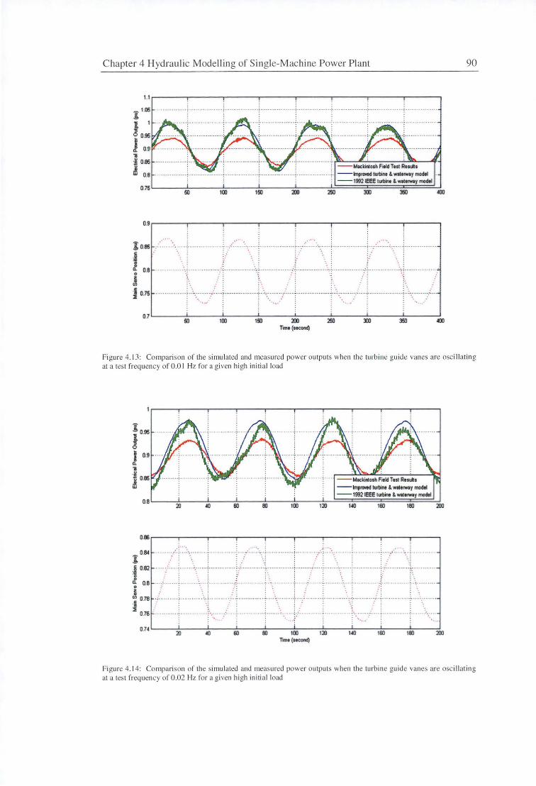
Chapter 4 Hydraulic Modelling of Single-Machine Power Plant
- 1.05 ~ 1 1
6 095
J ~.9 • ·£ 0.85 j w 0.8
--M1ckinlo1h Field THI Ruulta --mprM<I turbine & waterway model --1992 IEEE turbine & woterway model
0.75L_ ___ l_ ___ _L ___ _.L ___ _L ___ _JL.!:::===:m====350====_J«XJ
j; 085
:! !: 0.. 0.8 ~ 0
£ :I 0.75
.... : ...... ~ -
.............. , .:..,. ....... ... : · . .. , ..
.. ····· ···· i
······•·/·:··
. .... ·
•"'·. . .
.. :,,: : ..
\ .. ······ ~
0.7~---~---~i ____ ~i----~---~----~----~·· ---~ 50 100 150 200 250 :m 350
Time (aecond)
90
Figure 4. 13: Comparison of the simulated and measured power outputs when the turbine gui tle vant:s are oscillating at a test frequency of 0.01 Hz for a given high initial load
j; 1 0.95
6 i 0.9 0.. 11 ¥ .i 085 w
- - Meckinlosh Field Toal Results --knprM<l 1urbine & waterway model --1992 IEEE lurbine & woterway model
o.8L __ L_ __ ...L __ _L __ J. __ _J ___ L_....============::....i uo 11i0 1111 200
0.84 j; :~ 0.82 0
0.. 0.8 0
~ (/) 0.78 i :I
0.76
Time (aecond)
Figurt: 4.14: Comparison of the simulated and measured power outputs when the turbine guide vanes are oscillating at a test frequency of 0.02 Hz for a given high initial load
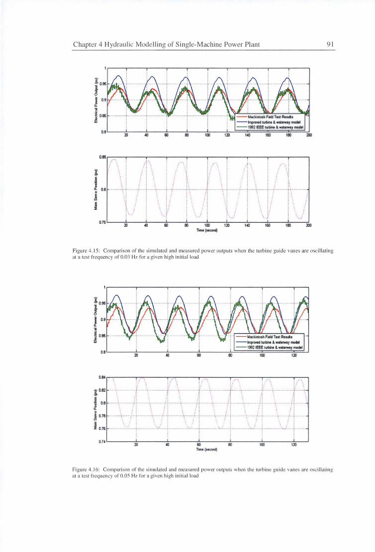
Chapter 4 H ydraul ic Modelling of Single-M achine Power Plant
• . g u 0.85 !JI w
];
~ a. 0.8 ... 0
£ i lE
....... . .
. ... ; -- ~·- ·A ...... · ·~ ·: .......... . . .. , /;
.. : . . .. , o.75~--~20---~«l---~60---~oo~---H~Xl--~,20~---u~o ---160~---,~oo--~
Time (11cond)
91
Figure 4.15: Compari son of the simu lated and measured power outputs when the turbine guide vanes are oscillating at a test frequency of 0.03 Hz for a given high initi al load
]; l 0.95
6 I o.s a. ... . g i 0.85 w
--Mackintosh Fiold Tut Rnuh --1mprOW1d turl>ine & waterway modtt --1992 IEEE turbine & waterway model
0.8 L_ _ _ _ __L ____ _L ____ __J_ ____ __J_..=::==========:'.._J 100 120
0.IM~----~. -.~---~. -.----~~ -:.-.. -,----~,. -_-.. -, ---~,-.. -.. -,---~-. -,~
]; 0.82
:I 0.8 a.
~ 0.78
"' ii lE 0.76
··· ··········· -=··
. . ·· ~ ·· ········ ···J ...... -:, ····· '..·
.. .. ...... :: .. ::. i i i i i
0.74~----20~-----«l~-----60~-----!ll~-----1·00-----,~20--~
Timi (11cond)
Figure 4.16: Compari son of the simulated and measured power outputs when the turbine guide vanes are oscill ating at a test frequency of 0.05 Hz for a given high ini tial load
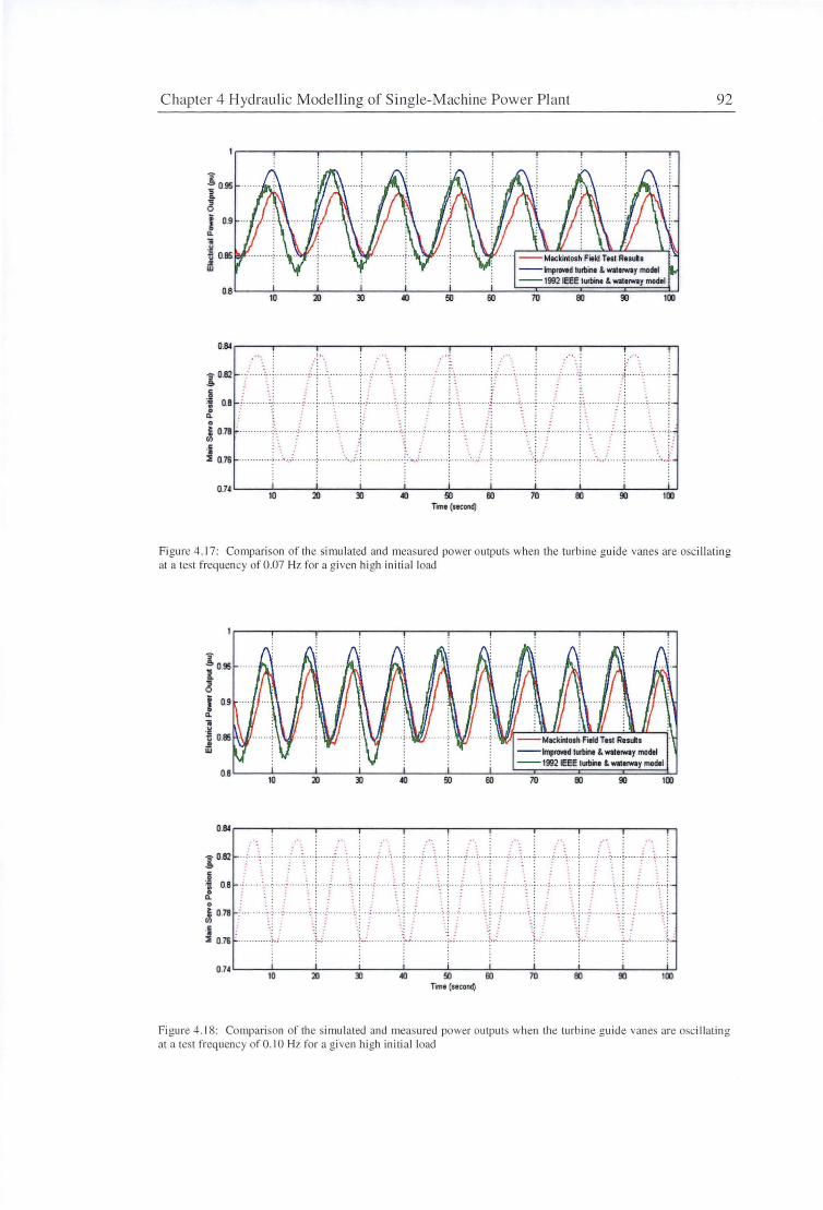
C hapter 4 Hydraulic Modellin g of Single-Machi ne Power P lant
]; 1 0.95
6 l 0.9
lli ·I!! ] 085 w
······ · --Mackinlosh Field T111 R11 .. 1
--1mpr ... d lurbine & waterway model --1992 IEEE lurbint & waterway model
o.8L_J __ _i_ __ _i_ __ _i_ __ _t_ __ _i__-'== ========::::LJ 70 80 90
0.&1.----.. -_ --.----_-.... .-,.-._:----.----.-•. ---..... : _---:.---.... -.. -. ---.---.-.• -._.-: ---.-•. ----.-,
A 0.82 ~ ·;= . . '' '• , . , . '' ' ' ·w · '} ' ' ' ' : _
.i i -·: 0.8 , ........ - .... ...;., ............. :.. . . . 0 :
Q.
£ 0.78 . . "" ' ·.
ii . . :I 0.7li ... ; ... ,,.-.
•• • j~ .... :. ...... ;. ! ··········~ · ·· · ........ .
..... .. ::.,:.: .... : .·...,,·..... . . . . .• . .. ...• ,. . . ·=·... . . . .... . : ~ · (•
. ....... - ... ~ · .
. ' -- ~ · ~ · -
i i i i i i i i i i O.H ~--1~0---20~---3l~---«l~---!i0~---60~---70~---80~---90~---1~00~
Time (second)
92
Figure 4 . 17: Co mparison of the simu lated and measured power output when the turbine guide vane are oscill ati ng at a test frequency of 0 .07 Hz for a given high initi al load
--Meckinlosh Field THI Re ... 1
--lmpr0¥td lurbine & waterway model --1992 IEEE lurbine & wolerwoy model
o.8L _ __L __ _j_ __ .L__ __ l_ __ L__J_-'===========:i.J
1082
:! 0.8 0
Q.
0
~ 0.78 en ·Ii ; :I 0.7li .
. .
. . . -. . ..
.. ;
.. . .. . r .; ........... ~;-;.· ·········· "~- ........... \ f. .......... : .. : ..
70 80 90
.''· : ' ':
.. ;: .
.; .: ········ ~ ~-
······· -=··· ············!·· . . ······'·' ........... ..:..~. .. . ...... .; :
O.H ~--1~0---20~---3l~---«l~---50~--~60~---70~---80~---90~---100~
Time (second)
Fi gure 4. 18: Compari son or the simu lated and measured power outputs when the turbine guide vane are oscill ating at a test frequency of 0 .10 Hz fo r a given high in iti a l load
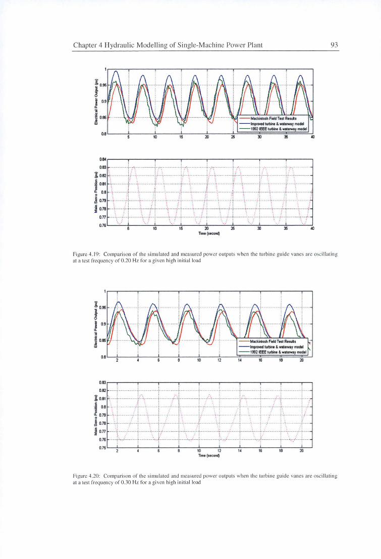
Chapter 4 Hydraulic Modelli ng of Single-Machine Power Plant
]; l 0.95
6 i 0.9 a. 11 .g u 0.85 .!! w
--Mackinlosh Field Tosi RostAs --lmpnwod lulbino & Wllorway model --1992 IEEE lurbino & waterway model
o.9 L __ _L _ _ _ -110 _ _ __ 1Ls ___ _J20 ____ 25~===:Jl'.l====35=====_J«i
0.IM~--~----,.----...----...------r-----,-----.------,
0.83
]; 082
:! 0.81 g a. 0.8 0
£ 079
·i 078 J: .
o.n 0.76~--~---~--~-~---~--~_._---~--~-..._--~~.
Timo (11cond)
93
Figure 4. 19: Compari son of the simulated and measured power outputs when the turbine guide vanes are o ci ll a ling at a tes l frequen cy of 0.20 Hz for a given high initi al load
]; l 0.95
6 i 0.9 a. 11
~ 0.85 .!! w
--Mackinlosh Field T111 R11tA1 --lmprDYtd turbine & Wlltrway model --1992 IEEE turbine & waterway model
o.9L_L __ _J _ _ _ i_ _ _ J_ __ J__ __ _i_ __ ~1::c•===1s===1x::8====-_J
Timo (socond)
Fi gure 4.20: Comparison of the simul ated and measured power outputs when the turbine guide vanes are osc illating at a test frequency of 0 .30 Hz for a given high in itial load
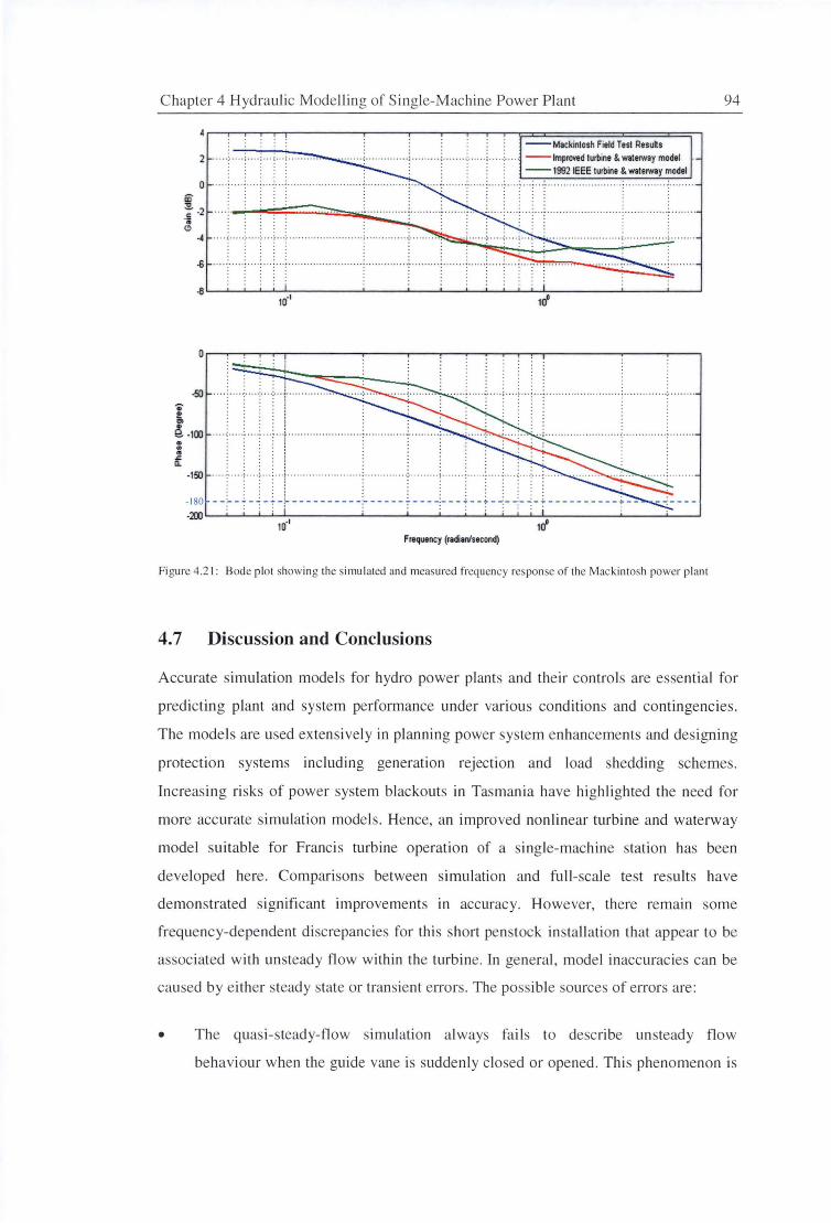
C hapter 4 Hydraulic Modellin g of S ingle-Machine Power Pl ant
... ;.
0 1D ~ -2 'ii
" -4
-6
-50
e. -100 . .. .. .c: a.
-150
- 1 0
--Mackintosh Field Test Results
. ) ;
- ~ ----------:- ----- ----i---4- -~ -~- -~--200 ~_,__,__,_...__.~---~--~-~-......__.__,__._...__. ____ ~--~--'
10~ 1~ Frequency (radian/second)
Figure 4.2 1: Bode plot showing the simulated and measured frequency response of the Mackintosh power plant
4. 7 Discussion and Conclusions
94
Accurate imulation models fo r hydro power plants and the ir controls are essentia l fo r
predicting plant and sy te rn performance under vari ous conditions and contingenci es.
The mode ls are used extensively in pl anning power system enhancements and des igning
protec tion systems including generation rejection and load shedding schemes.
Increasing ri sks of power system blackouts in Tasmania have highlighted the need fo r
more accurate simulati on models. Hence, an improved nonlinear turbine and wate rway
model suitable fo r Francis turbine operatio n of a s ing le-machine station has been
developed here. Comparisons between simu lation and full -scale test results have
demo nstrated significant improvements in accuracy. However, there remain some
frequency-dependent di crepancie fo r this short penstock in stall ation that appear to be
a ociated with unsteady fl ow within the turbine. In general, model inaccurac ies can be
caused by e ither steady state or transient errors. The possible sources of errors are:
• The quasi-steady-flow simulation always fai ls to desc ribe unsteady fl ow
behaviour when the guide vane is suddenl y closed or opened . Thi s phenomenon is

Chapter 4 Hydraulic Modelling of Single-Machine Power Plant 95
well known in the simulation of hydroelectric systems. Pressure changes during
the transient operation will propagate at sonic velocity and pass almost
instantaneously through the machine, but the vortical flow that convects through
the machine at through-flow velocity is a much slower process and therefore the
time lag of the flow establishment in the turbine can be significant for a station
with a relatively short penstock. A constant force coefficient used to represent the
pressure force on the turbine draft tube can also generate some errors, since
unsteady flow effects in the draft tube could be significant for large variations in
the turbine flow condition.
• The turbine characteristic curve used for simulations relies heavily on the model
test data. No change in the turbine design (exact geometric similarity) is assumed
in this case. Turbine efficiency can increase or decrease if a new runner or other
components have been modified or replaced in recent years. A maximum of 2% of
uncertainty due to this factor is expected in the calculations.
• Generator efficiency is assumed independent of the turbine flow conditions. A
constant efficiency of 97% is used for the Mackintosh generators due to a lack of
detailed information. This can be misleading as the generator efficiency may vary
nonlinearly with the machine output. Although the variation could be small, 0.5%
difference in generator efficiency may cause an uncertainty of ±0.5MW for
Mackintosh station. Hence, a steady state variation of 1-2% may occur due to this
assumption.
• The quadratic guide vane function may not give a true representation of the flow
characteristic, especially if machine is running at high load. It is known from
observation that the flow will usually increase very slowly at or near the full gate
opening. The quadratic flow relation may not work very well at this operating
condition and so a larger steady-state error is expected for units initially operating
near or at the full load. This effect, however, can be minimised when more data
are available for tuning in the future.
• Constant water levels are assumed for both upper and lower reservoirs. The
available static head may increase or decrease if the reservoir conditions are
changed. This effect must be considered when the simulation is to be carried out
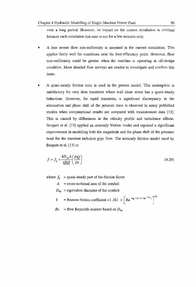
Chapter 4 Hydraulic Modelling of Single-Machine Power Plant 96
over a long period. However, its impact on the current simulation is minimal
because each simulation test case is run for a few minutes only.
• A less severe flow non-uniformity is assumed in the current simulation. This
applies fairly well for conditions near the best-efficiency point. However, flow
non-uniformity could be greater when the machine is operating at off-design
condition. More detailed flow surveys are needed to investigate and confirm this
issue.
• A quasi-steady friction term is used in the present model. This assumption is
satisfactory for very slow transients where wall shear stress has a quasi-steady
behaviour. However, for rapid transients, a significant discrepancy in the
attenuation and phase shift of the pressure trace is observed in many published
studies when computational results are compared with measurement data [13].
This is caused by differences in the velocity profile and turbulence effects.
Bergant et al. [13] applied an unsteady friction model and reported a significant
improvement in modelling both the magnitude and the phase shift of the pressure
head for the transient turbulent pipe flow. The unsteady friction model used by
Bergant et al. [13] is:
where fq = quasi-steady part of the friction factor
A = cross-sectional area of the conduit
Deq = equivalent diameter of the conduit
k = Brunone friction coefficient= 1 . 361 x [Re Jog <14
·3
' Re 0 05
l J o.s
Re =flow Reynolds number based on Deq
(4.29)
Chapter 5 Hydrauhc Modelling of a Multiple-Machine Power Plant 97
CHAPTERS
HYDRAULIC MODELLING OF A MUTIPLE-MACHINE POWER PLANT
5.1 Overview
Large system disturbances impose a serious threat to the stability of power systems.
Many power plant analyses are devoted to improving the defence mechanisms and
preventing disasters caused by large disturbances. Increased competition in the
electricity supply industry, stricter market rules, and the structural changes in generation
capacity have put more pressure on power system security. Accurate modelling of
power plants with a multiple-machine configuration, which is the most common design
for modem power stations, has played a critical role in ensuring satisfactory plant and
system performance. In Chapter 4, a new model for the waterway system and turbine of
a single-machine hydro plant without a shared waterway conduit was developed. This
Chapter will focus on the modelling of transient operations for plants with more than
one turbine unit. In contrast to a single-machine station, the case of a multiple-machine
power plant with a common tunnel supplying a manifold from which individual
penstocks branch out to each turbine will introduce hydraulic coupling effects.
This Chapter extends the application of the inelastic waterway model and nonlinear
turbine characteristics discussed previously into multiple-machine modelling. The
transient behaviour of Hydro Tasmania's Trevallyn power station will be used as a case
study. The hydraulic configuration of the Trevallyn plant is briefly introduced in
Section 5.2. Nonlinear modelling of flow in turbine and waterway conduits with
multiple penstocks is presented in Section 5.3, while modelling of surge tank dynamics
is discussed in Section 5.4. The mathematical assumptions of these models will be
explained in some detail there. The structure of the nonlinear model constructed in
MATLAB Simulink and the parameter evaluations of this hydraulic model are
described in Section 5.5. The mathematical model will be validated against field test
results previously collected at Trevallyn power station. The implication of hydraulic
coupling effects on governor tuning, influence of travelling pressure waves, and
possible sources of model inaccuracies for a multiple-machine station are reviewed in
Section 5.6.
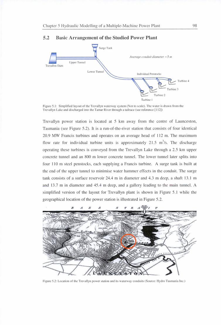
Chapter 5 Hydrau lic Mode ll ing of a Mu ltiple-Mach ine Power P lant
5.2 Basic Arrangement of the Studied Power Plant
Average c:onduir dia111erer = 5 111
Upper Tunnel Treva llvn Dam
Turbine 4
Turbine I
Fi gure 5. 1: Simplified layout of the Trevall yn waterway system (Not to sca le) . The water is drawn from the Trevallyn Lake and di scharged into the Tamar Ri ver through a tailrace (see reference [ 112])
98
Trevallyn power station is located at 5 km away from the centre of Launceston,
Tasmania (see F igure 5.2) . It is a run-of-the- ri ver station that consists of fo ur identical
20.9 MW Franc i turbines and operates on an average head of I 12 m. The max imum
fl ow rate fo r indi vidual turbine units is approx imately 2 1.5 m3/s. The di scharge
operating these turbines is conveyed from the Trevall yn Lake through a 2 .5 km upper
concrete tunne l and an 800 m lower concrete tunnel. The lower tunnel later splits into
fo ur 110 m steel pen stocks, each supplyin g a Francis turbine. A surge tank is built at
the end of the upper tunne l to minimise water hammer effects in the conduit. The surge
tank consists of a surface reservoi r 24.4 m in diameter and 4 .3 m deep, a shaft 13. 1 m
and 13.7 m in diameter and 45 .4 m deep, and a gall ery leadi ng to the main tunne l. A
simplifi ed version of the layout for Trevallyn plant is shown in Figure 5. 1 while the
geographical locati on of the power tati on is illustrated in Figure 5.2.
Fi gure 5.2 : Location o f the Treva ll yn power station and its wa terway conduits (Source: Hydro Tasmania Inc .)

Chapter 5 Hydraulic Modelling of a Multiple-Machine Power Plant 99
5.3 Modelling of a Turbine & Waterway System with Multiple Penstocks
This Section gives an overview of the formulae used to simulate the turbine and
waterway system of a multiple-machine station with four individual machines and
separate penstocks, unrestricted head and tail races, and a surge chamber at the common
tunnel. One-dimensional continuity and momentum equations, as well as the inelastic
water column theory, are employed in this case. The formulation is identical to that of
the single-machine model, except that the waterway conduit is now being divided into
three separate parts: upper tunnel, lower tunnel, and penstocks. Hydraulic transients are
described by the linear momentum equations applied from the reservoir to the end of the
upper tunnel; from the end of the upper tunnel (or the start of the lower tunnel) to the
end of the lower tunnel (or penstock junction); and from the end of the lower tunnel to
each individual machine:
where Q =per-unit flow at the upper tunnel (ut), lower tunnel (lt), and penstock (i)
H 0
=per-unit static head between reservoir and tailrace
H 1
= per-unit static head at the end of the upper tunnel
H eq =per-unit equivalent static head at the penstock junction
H1
=per-unit static head at the turbine admission
HIN =per-unit inlet dynamic head= KINQu;
H f-ur =per-unit head loss at the upper tunnel = furQu;
H 1_11 =per-unit head loss at the lower tunnel = f 11 Q1;
H 1_1
=per-unit head loss at the individual penstock i= f1Q,2
Hd1_
1 =per-unit static head caused by draft tube of machine i= Kd
1_
1Q
1
2
(5.1)
Tw =water starting time for upper tunnel (ut), lower tunnel (lt), and penstock (z)
knu = flow nonumfornuty factor for upper tunnel (ut), lower tunnel (lt), and penstock (i)
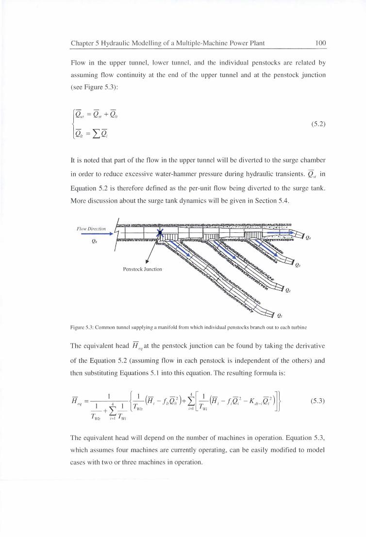
Chapter 5 Hydraulic Modelling of a Mul tiple-Machine Power Plant 100
Flow in the upper tunnel, lower tunnel, and the individual penstocks are related by
assuming fl ow continuity at the end of the upper tunnel and at the penstock juncti on
(see Figure 5.3):
(5.2)
It is noted that part of the flow in the upper tunnel will be diverted to the surge chamber
in order to reduce excessive water-hammer pressure during hydraulic transients. Q,., in
Equation 5.2 is therefore defined as the per-unit fl ow being di verted to the surge tank.
More di cussion about the surge tank dynamics will be given in Section 5.4.
Floll' Direction
Pen stock Junction
Figure 5.3: Common tunnel supplying a mani fo ld from which individual penstocks branch out to each turbine
The equi valent head H,," at the pen stock junction can be found by taking the deri vati ve
of the Equation 5.2 (assuming flow in each penstock is independent of the others) and
then substituting Equations 5.1 into this equation. The resulting formul a is:
(5.3)
The eq ui valent head will depend on the number of machines in operati on. Equation 5.3,
which assumes four machines are currently operating, can be eas ily modifi ed to model
cases with two or three machines in operati on.
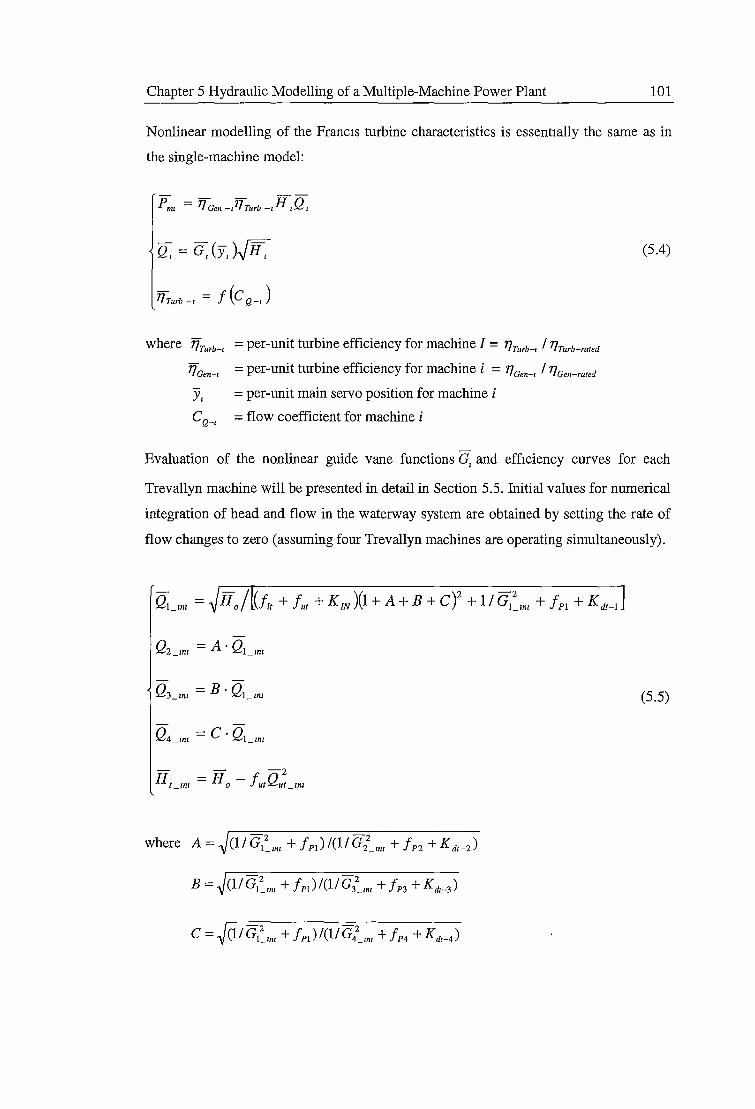
Chapter 5 Hydraulic Modelling of a Multiple-Machine Power Plant 101
Nonlinear modelling of the Francis turbine characteristics is essentially the same as in
the single-machine model:
Pm,= T/oen-1T/Turb-1H,Q,
Q, = G, (y, )jH,
where 'ifrurb-i =per-unit turbine efficiency for machine I= T/rurb-i I T/rurb-rared
'ifoen-• =per-unit turbine efficiency for machine i = T/cen-• I T/cen-rared
y1
=per-unit main servo position for machine i
C Q-• = flow coefficient for machine i
(5.4)
Evaluation of the nonlinear guide vane functions G, and efficiency curves for each
Trevallyn machine will be presented in detail in Section 5.5. Initial values for numerical
integration of head and flow in the waterway system are obtained by setting the rate of
flow changes to zero (assuming four Trevallyn machines are operating simultaneously).
Q =A·Q1 2_rnr rnz
(5.5)
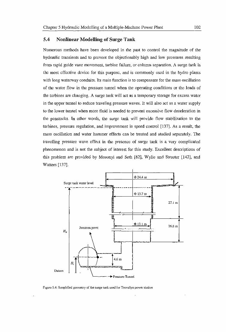
Chapter S Hydraulic Modelling of a Multiple-Machine Power Plant 102
5.4 Nonlinear Modelling of Surge Tank
Numerous methods have been developed in the past to control the magnitude of the
hydraulic transients and to prevent the objectionably high and low pressures resulting
from rapid guide vane movement, turbine failure, or column separation. A surge tank is
the most effective device for this purpose, and is commonly used in the hydro plants
with long waterway conduits. Its main function is to compensate for the mass oscillation
of the water flow in the pressure tunnel when the operating conditions or the loads of
the turbines are changing. A surge tank will act as a temporary storage for excess water
in the upper tunnel to reduce traveling pressure waves. It will also act as a water supply
to the lower tunnel when more fluid is needed to prevent excessive flow deceleration in
the penstocks. In other words, the surge tank will provide flow stabilization to the
turbines, pressure regulation, and improvement in speed control [137]. As a result, the
mass oscillation and water hammer effects can be treated and studied separately. The
travelling pressure wave effect in the presence of surge tank is a very complicated
phenomenon and is not the subject of interest for this study. Excellent descriptions of
this problem are provided by Mosonyi and Seth [82], Wylie and Streeter [142], and
Watters [137].
Surge tank water level
Junction pomt H,,
Datum
et> 24.4 m
________ J ________ _
I et> 13.7 m
46m,J ~· - ~
Pressure Tunnel
Figure 5.4: S1mphfied geometry of the surge tank used for Trevallyn power station
27.l m
26.Sm
Chapter 5 Hydraulic Modelling of a Multiple-Machine Power Plant 103
A simplified view of the surge chamber used in the Trevallyn plant is shown in Figure
5.4. The surge tank is a restricted orifice type. Flow in this type of surge tank can be
obtained by keeping track of the elevation of water surface in the surge tank above the
tunnel through:
= C dH sr & Q,t s dt C,=J(A.)
where H st =per-unit static head in the surge tank
Cs = storage constant of the surge tank
As = cross-sectional area of the surge tank
(5.6)
The flow in the surge tank can then be linked to the static head at the main tunnel by
rearranging and substituting Equation 5.6 into Equation 5.7. This relation is based on
the assumption that the pressure head at entry to the surge tank, and the upper or lower
tunnel endpoints is the same at any instant. The mass is conserved and the velocity
distribution over the cross section of each conduit at the junction is assumed uniform
[139]. The primary and reflected pressure waves emanating from the junction are also
assumed plane-fronted.
Ht = H st - H f-o = d f dQ,tdt - foQs: s
(5.7)
where H 1 _0
=per-unit head losses in the surge tank
f 0
= head loss coefficient due to restricted orifice
A restricted orifice, like many diaphragms, causes concentrated local losses. This head
loss is modelled as the steady-flow loss coefficient times flow squared in the simulation.
An initial value for numerical integration of the surge tank flow can be obtained by
assuming a steady flow conditions at the start of the simulation. The variation of flow
with respect to time will be equal to zero in this case (assuming four Trevallyn
machines in operation):
(5.8)
Chapter 5 Hydraulic Modelling of a Multiple-Machine Power Plant 104
The inclusion of surge tank effects is warranted in cases where transient performance of
the plant is being analysed over a few minutes of "real" time. The surge tank causes a
long-period damped oscillation of flow in the tunnel between the reservoir and the tank
[70]. The oscillation period of the Trevallyn surge tank is 305 seconds, which is about
the total length of simulation time. Hence, adding Equations 5.6 and 5.7 to the model is
expected to generate a more accurate result.
5.5 Transient Analysis of a Multiple-Machine Power Plant
5.5.1 Model Structure and Formulation
The approach used to implement the multiple-machine system is similar to the one used
for the single-machine model, except that the multiple-machine model is now broken
down into smaller subsystems. The system complexity prevents the hydraulic system
from being represented as a single subsystem, and this applies to the electrical system
too [70]. Therefore, three subsystems have been created in MATLAB Simulink for the
following elements:
• individual penstock and turbine;
• upper tunnel, lower tunnel and surge tank; and
• equivalent head.
The first two subsystems of the model are depicted by inelastic water column theory
where conservation of momentum and continuity of flow at the surge chamber junction
apply. The inelastic model is used as it is relatively easy to construct and more efficient
in terms of computational time and resources used. The surge tank alleviates the
travelling wave effects in the lower tunnel. Thus, the use of the inelastic model is
expected to give the accuracy needed for the current power system design process.
Figures 5.5 to 5.8 show the resulting Simulink block diagram of the multiple-machine
model where four units are assumed operating at the same time.
In addition, the multiple-machine model for the Trevallyn plant assumes the lower
tunnel branches into four at one point and models the inertia of the resulting five
segments accordingly. These five pipeline segments are the lower tunnel and the four
branches to each individual machine. In reality, the portion downstream of the surge

Chapter 5 Hydraulic Modelling of a Multiple-Machine Power Plant 105
tank consists of a common tunnel with successive off-takes to each machine (see Figure
5.3). Private communication with Hydro Tasmania's consultant, P. Rayner, indicates
that this portion can be represented more accurately by considering the inertia of seven
segments, which are: the lower tunnel; four individual pipes to each machine; a
common section between pipe to first machine and pipe to second machine; a common
section between pipe to second machine and pipe to third machine. However, this
approach requires a more complex hydraulic model, which implies a more complicated
and time-consuming process for the simulation. The improvement of simulation
accuracy due to this effect would be relatively insignificant in the present case, as the
water starting time constants of the branches are small in the Trevallyn system.
Although the steady-state losses have been calculated in detail, they do not represent the
true nature of the hydraulic system under transient flow conditions. The errors in
estimating the transient flow losses from a quasi-steady model may be more significant
than the errors due to the model topology simplification. The Simulink model presented
in this Section is therefore recommended as providing a good compromise between
modelling accuracy and computational time required.
The effects of hydraulic coupling between the individual machines will be taken into
account in the computation of equivalent head at the penstock junction. As illustrated in
Section 5.3, the formula is based on continuity relations for the flow in the tunnel and
the penstocks. This computed head value is fed back to the models of individual
penstocks and machines (see Figure 5.5).
For gate positions at or near total closure, the inelastic simulations of the turbine head
and penstock flows are no longer applicable, and are replaced by a steady-state
algebraic solution of the penstock. This method is currently used in the simulation to
account for conditions when a machine is operated below 5% of the total guide vane
opening.
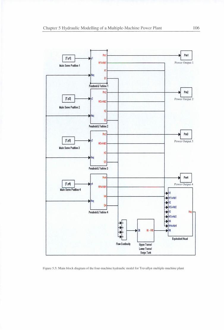
Chapter 5 Hydrau lic Modelling of a M ul tip le-Machine Power Pl ant 106
Pm1 .. Pm1 I [T.y1]
I y 1
y
I Hf1+Hdt1 Power Output I
Main Sel'o'o Position 1
H1 ; Heq
01 ,___
Penslod<& Turbine 1
Pm2 .. I Pm2 I
I I [T,:(l] : 2 Power Output 2 I Hf2tHdi2
Main Sel'o'o Position 2 H2
~ Heq 02 -
Penslod<& Turbine 2
Pm3 .. Pm3 y
I [T.)'31 I ~ 3 Power Out put 3 I Hf3tHdt3
Main Sel'o'o Position 3
H3
~ Heq 03 -
Penslod<& Turbine 3
Pm4 .. Pm4 "'
I [T.y4) I ~ 4 Power Output 4 I Hf4+Hdt4
Main Smo Position 4 f-t> HI
H4 f.+ HfltHdtl ~ Heq ~ H2
04 ,.__ f+ Hf2+Hdt2
Penslod<& Turbine 4 f-t> H3 Heq -
f-+ Hf3+Hdt3 - f+ H4 .....
.... t f+ Hf4+Hdt4
.... t r----t> Olt Ht · Hflt ; Hit
-J t Equivalent Head -
Flow Continuity Upper Tunnel Lower Tunnel
Surge TaM
Figure 5.5 : M a in bloc k di agra m o r the fo ur-machine hyd raulic model fo r Treva ll yn multi ple-mac hine plant
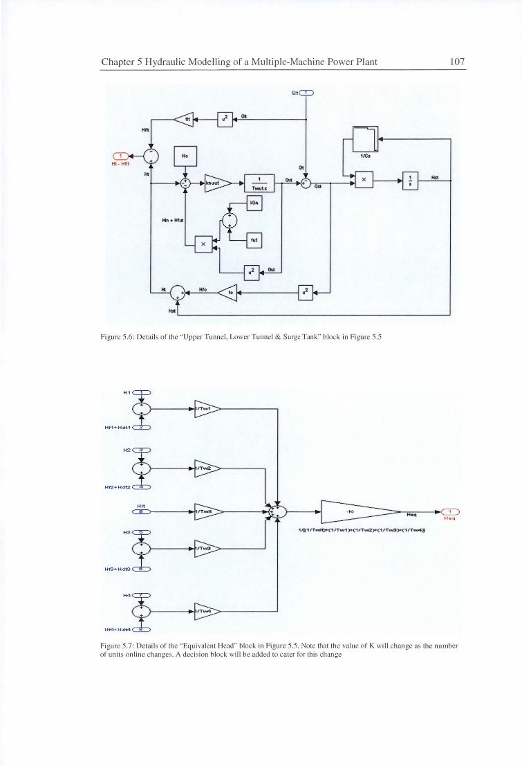
Chapter 5 Hydrau lic Model ling of a Mu ltiple-Machine Power Plant 107
011
Oil
1/Cs
Olt HI
Hst
Figure 5.6: Detail s of the " Upper Tunnel, Lower Tunnel & Surge Tank" block in Figure 5.5
H1
Hf1+Hdt1
H2
H1'2+Hdt2
Hit
Heq Hoq
H 3 1 /k:1 /T~f)+(1 /Tw1 )+(1 /T"""2)+(1 /TIAB)+(1 /Tw4)J
H1'3+Hdt3
H4
Hf4+Hdt4-
Figure 5.7: Details of the " Equi va lent Head'" block in Figure 5.5 . Note that the va lue or K will chan ge as the number of units on line changes. A decision block wi ll be added to ca ter for this change
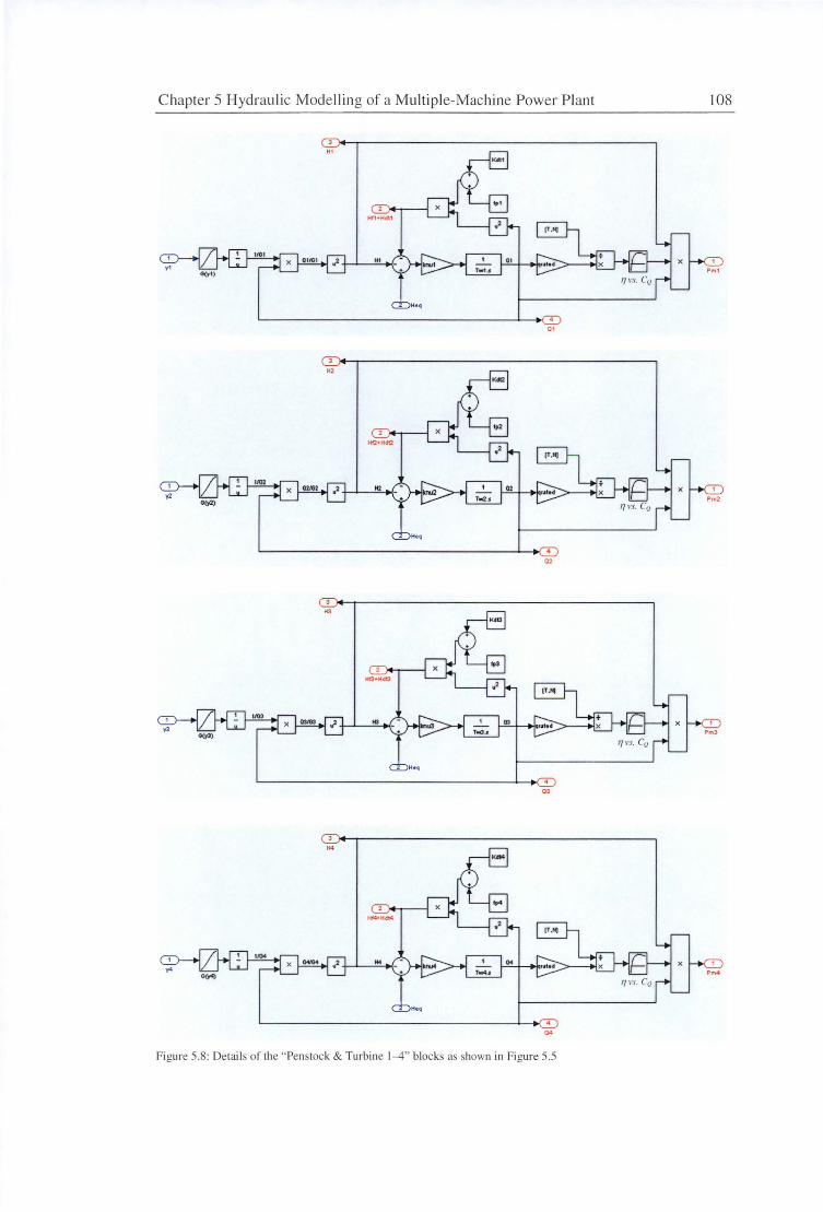
Chapter 5 Hydraulic Mode lling of a Multiple-Machine Power Plant 108
01
Figure 5.8: Details of the ·'Penstock & Turbine 1-4" blocks a shown in Figure 5.5
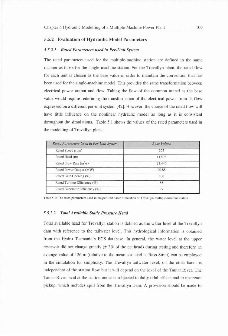
Chapter 5 Hydraulic Modelling of a Multiple-Machine Power Plant 109
5.5.2 Evaluation of Hydraulic Model Parameters
5.5.2.1 Rated Parameters used in Per-Unit System
The rated parameters used for the multiple-machine station are defined in the same
manner as those for the single-machine station. For the Trevallyn plant, the rated flow
for each unit is chosen as the base value in order to maintain the convention that has
been used for the single-machine model. This provides the same transformation between
electrical power output and flow. Taking the flow of the common tunnel as the base
value would require redefining the transformation of the electrical power from its flow
expressed on a different per-unit system [ 42]. However, the choice of the rated flow will
have little influence on the nonlinear hydraulic model as long as it is consistent
throughout the simulations. Table 5.1 shows the values of the rated parameters used in
the modelling of Trevallyn plant.
Rated Parameters Used in Per-Unit System Base Values
Rated Speed (rpm) 375
Rated Head (m) 112.78
Rated Flow Rate (mj/s) 21.446
Rated Power Output (MW) 20.88
Rated Gate Opening(%) 100
Rated Turbine Efficiency (%) 88
Rated Generator Efficiency(%) 97
Table 5.1: The rated parameters used in the per-unit based simulation of Trevallyn multiple-machine station
5.5.2.2 Total Available Static Pressure Head
Total available head for Trevallyn station is defined as the water level at the Trevallyn
dam with reference to the tailwater level. This hydrological information is obtained
from the Hydro Tasmania's ECS database. In general, the water level at the upper
reservoir did not change greatly (± 2% of the net head) during testing and therefore an
average value of 126 m (relative to the mean sea level at Bass Strait) can be employed
in the simulation for simplicity. The Trevallyn tailwater level, on the other hand, is
independent of the station flow but it will depend on the level of the Tamar River. The
Tamar River level at the station outlet is subjected to daily tidal effects and to upstream
pickup, which includes spill from the Trevallyn Dam. A provision should be made to
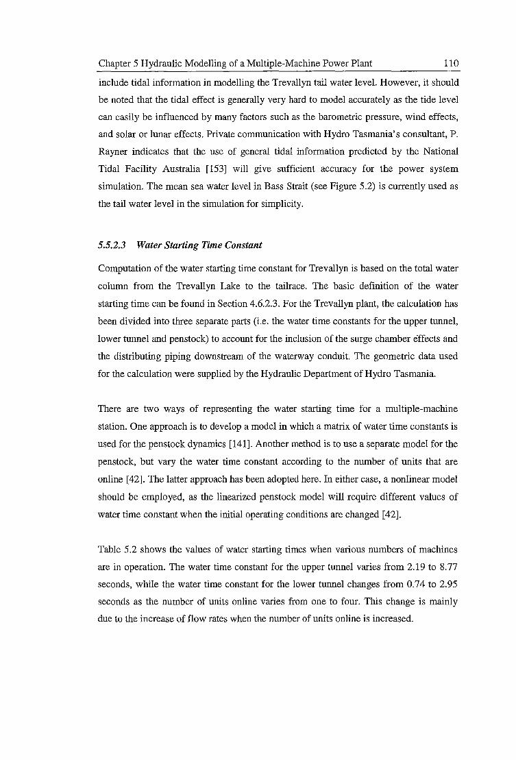
Chapter 5 Hydraulic Modelling of a Multiple-Machine Power Plant 110
include tidal information in modelling the Trevallyn tail water level. However, it should
be noted that the tidal effect is generally very hard to model accurately as the tide level
can easily be influenced by many factors such as the barometric pressure, wind effects,
and solar or lunar effects. Private communication with Hydro Tasmania's consultant, P.
Rayner indicates that the use of general tidal information predicted by the National
Tidal Facility Australia [153] will give sufficient accuracy for the power system
simulation. The mean sea water level in Bass Strait (see Figure 5.2) is currently used as
the tail water level in the simulation for simplicity.
5.5.2.3 Water Starting Time Constant
Computation of the water starting time constant for Trevallyn is based on the total water
column from the Trevallyn Lake to the tailrace. The basic definition of the water
starting time can be found in Section 4.6.2.3. For the Trevallyn plant, the calculation has
been divided into three separate parts (i.e. the water time constants for the upper tunnel,
lower tunnel and penstock) to account for the inclusion of the surge chamber effects and
the distributing piping downstream of the waterway conduit. The geometric data used
for the calculation were supplied by the Hydraulic Department of Hydro Tasmania.
There are two ways of representing the water starting time for a multiple-machine
station. One approach is to develop a model in which a matrix of water time constants is
used for the penstock dynamics [141]. Another method is to use a separate model for the
penstock, but vary the water time constant according to the number of units that are
online [42]. The latter approach has been adopted here. In either case, a nonlinear model
should be employed, as the linearized penstock model will require different values of
water time constant when the initial operating conditions are changed [42].
Table 5.2 shows the values of water starting times when various numbers of machines
are in operation. The water time constant for the upper tunnel varies from 2.19 to 8.77
seconds, while the water time constant for the lower tunnel changes from 0.74 to 2.95
seconds as the number of units online varies from one to four. This change is mainly
due to the increase of flow rates when the number of units online is increased.
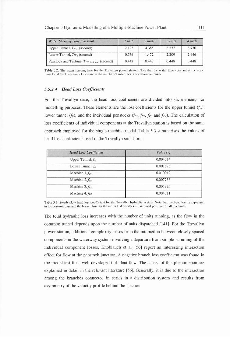
Chapter 5 Hydraulic Modelling of a Multiple-Machine Power Plant 111
Water Starting Time Constant 1 unit 2 units 3 units 4 units
Upper Tunnel, Tw11 t (second) 2.192 4.385 6.577 8.770
Lower Tunnel, Tw1t (second) 0.736 1.472 2.209 2.946
Pen stock and Turbine, Tw;, ; =I to 4 (second) 0.448 0.448 0.448 0.448
Table 5.2: The water starting time for the Trevallyn power station. Note that the water time constant at the upper tunnel and the lower tunnel increase as the number of machines in operation increases
5.5.2.4 Head Loss Coefficients
For the Trevallyn case, the head loss coefficients are divided into six elements for
modelling purposes. These elements are the loss coefficients for the upper tunnel ifu1),
lower tunnel (ft1), and the individual penstocks (jpj, fn. f P3 and f P4). The calculation of
loss coefficients of individual components at the Trevallyn station is based on the same
approach employed for the single-machine model. Table 5.3 summarises the values of
head Joss coefficients used in the Trevallyn simulation .
Head Loss Coefficient Value(-)
Upper Tunnel ,/,,, 0.004714
Lower Tunnel,.fit 0.001876
Machine l ,f PI 0.010012
Machine 2,/n 0.007736
Machine 3,f PJ 0.005975
Machine 4,fp4 0.004311
Table 5.3: Steady-flow head loss coefficient for the Trevallyn hydraulic system. Note that the head loss is expressed in the per-unit base and the branch loss for the individual penstocks is assumed positive for all machines
The total hydraulic loss increases with the number of units running, as the flow in the
common tunnel depends upon the number of units dispatched [141]. For the Trevallyn
power station, additional complexity arises from the interaction between closely spaced
components in the waterway system involving a departure from simple summing of the
individual component losses. Knoblauch et al. [56] report an interesting interaction
effect for flow at the penstock junction. A negative branch loss coefficient was found in
the model test for a well-developed turbulent flow. The causes of this phenomenon are
explained in detail in the relevant literature [56]. Generally, it is due to the interaction
among the branches connected in series in a distribution system and results from
asymmetry of the velocity profile behind the junction.

Chapter 5 Hydraulic Modelling of a Multiple-Machine Power Plant 112
Neglecting the interaction effects among the branches may result in the overall losses at
the individual penstocks being slightly overestimated or underestimated. Hence, a
steady-state offset error between the simulated and the measured results may occur. A
computational study could be carried out in the future to investigate this interaction
effect in the distributing system. However, in the absence of any better information at
present, the branch losses are currently assumed positive and the values used in the
simulation are the same for all four machines.
5.5.2.5 Inlet Dynamic Pressure Head Coefficient
The definition previously applied for the single-machine model is employed in the
multiple-machine modelling. For the Trevallyn plant, the cross-sectional area at
entrance to the upper tunnel is 29.2 m2, which gives a value of the inlet dynamic head
coefficient Km= 2.31x10⁴.
5.5.2.6 Draft tube Static Pressure Force Coefficient
A provision is made in the model to include the static pressure force generated by the
flow in the draft tube and the tailrace water tunnel. However, the values of these force
coefficients are not known exactly at this stage, as the steady-flow CPD simulations
were not conducted for the draft tubes of the Trevallyn station. For this reason, the
coefficients are currently set to zero. This will have little impacts on the overall
accuracy of the model, as the flow through each turbine is relatively small compared to
that of the Mackintosh station.
5.5.2. 7 Coefficient for flow non-uniformity
The factor accounting for flow non-uniformity in the Trevallyn waterway system is
based on the assumption of a fully developed turbulent velocity profile. The non
uniformity effects are expected to be more significant in the common tunnel as the flow
rate is greater in the tunnel than the penstock. Nevertheless, a constant coefficient value
of 1.05 is used for both common tunnel and penstocks, as no information is currently
available to distinguish the effects of flow non-uniformity in these conduits.
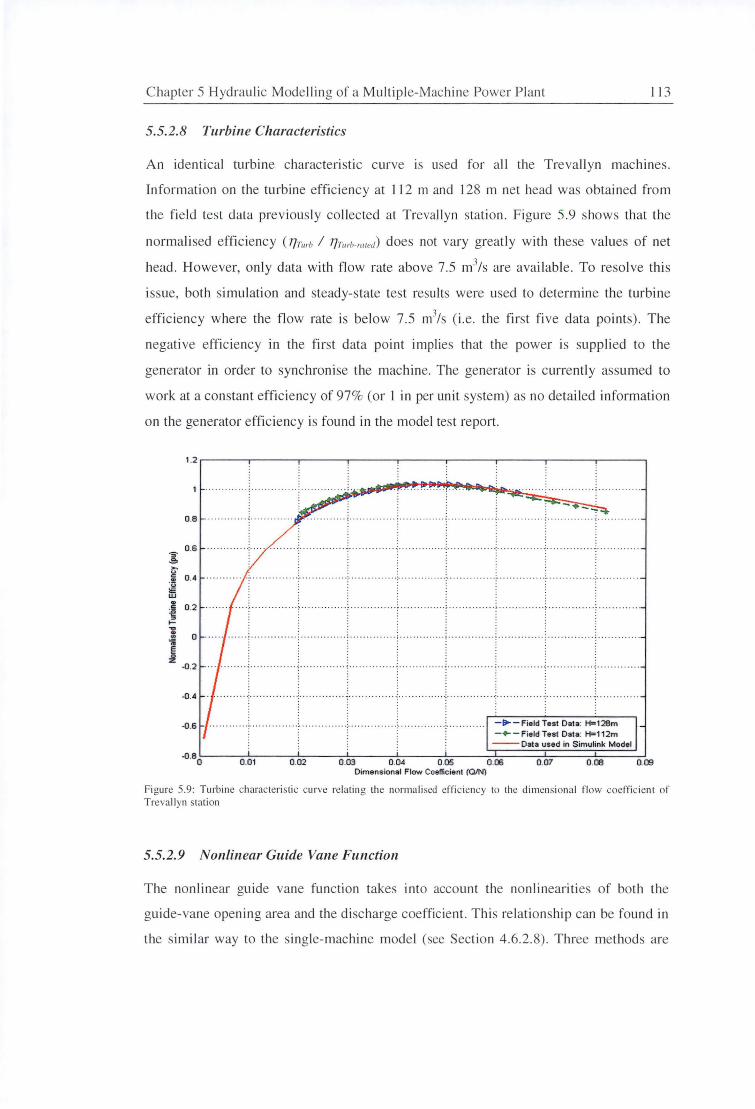
C hapter 5 Hydraulic Modelling of a Multip le-Machine Power P lant 11 3
5.5.2.8 Turbine Characteristics
An identi cal turbine characteri stic curve is used fo r all the Trevall yn machines.
In fo rmation on the turbine effi c iency at 11 2 m and 128 m net head was obtained from
the fi eld test data prev iously collected at Trevallyn stati on. F igure 5.9 shows that the
normali sed effi c iency ( T/rurb I 77rurb-miett) does not vary greatl y with these values of net
head. However, only data with flow rate above 7.5 m3/s are availabl e. To resol ve thi s
issue, both simulation and steady-state test results were used to determine the turbine
effici ency where the flow rate is below 7 .5 m3/s ( i. e. the first fi ve data points). The
negati ve effi ciency in the first data point implies that the power is supplied to the
generator in order to synchronise the machine. The generator is currently assumed to
work at a constant effi c iency of 97% (or I in per unit system) as no detai led information
on the generator e ffici ency i · found in the model test report.
0 .B
0.6
1 ,.. " c 0.4 .!!
~ UJ .. ~
0 .2
>--..., . 0 .. . .
~ § ~
-0.2
-0 .4
0.01
··~· ·· · · · ··· · · · · ·~ ·· · · · · ··· · · · ·~ · ···· ·· ···
···· ···:······ ·· ····· ·:•·•······ ..... .. .. ..... ····; ··· ········· ··; ........ .
·· ···:······ ·· ··· ·· ·:···· ·· · ... ... , ..... .... ····:···· ····· ·· ···· ···· ····· ·· ·= ···· ···· ······:·· ······
........... ~ .... ... .... ... ! ... .. .. .
0.02 0 .03 0.04 0.05 Dimensional Flow Coefficient (QIN)
. . .......... ~ - ... .... ...... ~ .. ...... .. .. .
··:· · ··· ·· ······#······ ··· ·
-II- - Field Test Data: H=12Bm _ .,. - Field Test Data: H=112m --Data used in Simulink Model
0.06 0.07 O.DB
Figure 5.9 : Turb ine characteri sti c curve relati ng the normalised effic iency to the dimensional flow coefficient o f Trevallyn station
5.5.2.9 Nonlinear Guide Vane Function
T he nonlinear gu ide vane function takes into account the nonlineariti es of both the
guide-vane openin g area and the di charge coefficient. This relationship can be fo und in
the imil a.r way to the s ingle-machine mode l (see Section 4.6.2.8). Three methods are
Chapter 5 Hydraulic Modelling of a Multiple-Machine Power Plant 114
proposed in this Section to determine the nonlinear discharge coefficient relation for the
Trevallyn machines:
Using the hill chart data for Trevallyn station. The relationship is found by
processing the head and flow coefficients of the model turbine at different guide
vane positions. The discharge coefficient will be a function of these two variables.
It is assumed that the machines will normally operate well above a head
coefficient of 0.25, and therefore the guide vane function should be insensitive to
variations in the head coefficient. Unfortunately, there is some doubt about the
values of unit speed and unit flow rate presented in the hill chart. Private
communication with K. Caney of Hydro Tasmania indicates that it would be quite
difficult to trace the errors due to lack of detailed documentation for the Trevallyn
station. Thus, this method is not being used here.
Using pressure measurement data from site tests. P. Rayner of Hydro Tasmania
suggests the use of steady-state test results to establish the nonlinear guide vane
function . The values can be found by processing pressure data at the turbine spiral
case and subsequently calculating the corresponding head drop from the no-flow
static head condition. However, due to the equipment limitations, only the
pressure readings of one machine were recorded during the Trevallyn site tests.
Analysis of the test data indicates that each Trevallyn machine may have a slightly
different characteristic, and so the use of one machine characteristic to represent
all may not be appropriate here.
Using a quadratic approximation to identify the nonlinear guide vane function . A
quadratic relation is used for parameter identification because only one parameter
C; needs to be tuned in the equation. The identified parameters for each machine
are listed in Table 5.4 and the resulting nonlinear guide vane functions are
presented in Figure 5.10.
G; =Ac.;- C; + 4C;(Aa.;- 0.5/ Identified Value for Machine i
Machine 1, C1 -0.310
Machine 2, C2 -0.220
Machine 3, C3 -0.253
Machine 4, C4 -0.220
Table 5.4 : Identified parameters (C;) used to determine the nonlinear guide vane functions for the Trevallyn machines
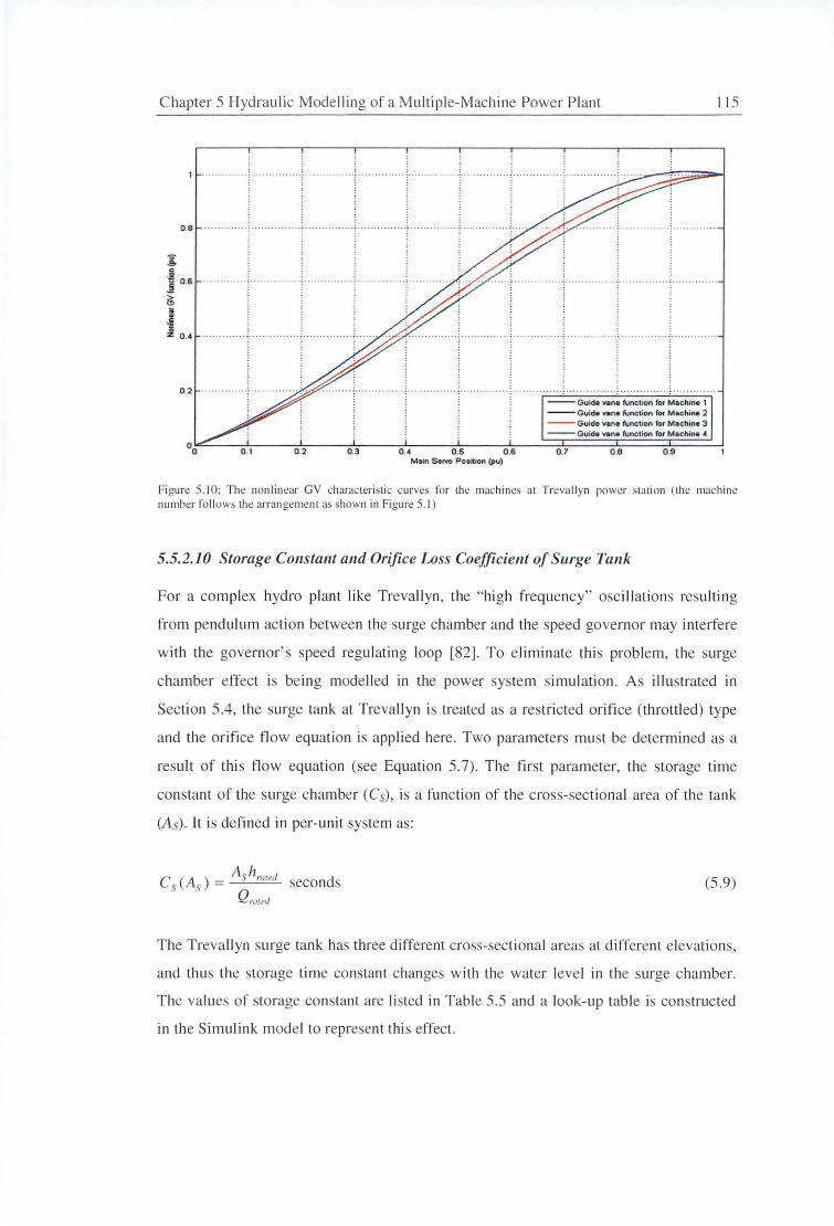
C hapter 5 Hydrau lic Modelli ng of a Mul tiple-Machine Power P lant
]; .i
O.B
] 0 .6
(;
• f z 0 .4
0 .2
0 .1 0 .2
--Guide vane function for Machine 3 -- Guide vane function for M achine _.
0.3 0 .6 0 .7 O.B 0 .9 Main Servo Position (pu)
11 5
Fi gure 5.10: The non linear GV characteristic curves for the machines al Treva llyn power sta tion (the machi ne number follows the arrangement as shown in Figure 5.1)
5.5.2.10 Storage Constant and Orifice Loss Coefficient of Surge Tank
For a complex hydro plant like Trevallyn , the "hi gh frequency" osc illations resulting
from pendulum action between the surge chamber and the speed governor may interfe re
with the governor's speed regul ating loop [82]. To e liminate this pro blem, the surge
chamber effect is being modelled in the power ystem simulation. As illustrated in
Secti on 5.4, the urge tank at Trevall yn is treated a a restricted orifice (throttled) type
and the orifice fl ow equation is applied here. Two parameters must be determined as a
result of thi s fl ow equation (see Equation 5.7). The first parameter, the storage time
constant of the surge chamber (Cs), is a function of the cross-sectional area of the tank
(As). It is defin ed in per-unit system as:
C (A ) - Ashm1ed seconds s s -Q rated
(5 .9)
T he T revall yn surge tank has three di fferent cross-secti onal areas at different elevat ions,
and thus the storage time constant changes with the water level in the surge chamber.
The values of storage constant are listed in Table 5.5 and a look-up table is co nstructed
in the Simulink model to represent thi s effect.
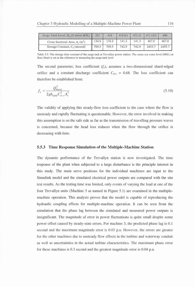
Chapter 5 Hydraulic Modelling of a Multiple-Machine Power Plant 116
Surge Tank Level, H,1 (ft above MSL) 323 418 418.001 471.12 471.1201 486
Cross Sectional Area, A, (m2) 134.9 134.9 141 .3 141.3 467.0 467.0
Storage Constant, Cs (second) 709.5 709.5 742.9 742.9 2455.7 2455.7
Table 5.5: The storage time constant of the surge tank at Trevallyn power station . The mean sea walt:r lt:vt:I (MSL) at Bass Strait is set as the reference in measuring the surge tank level
The second parameter, loss coefficient (j0 ) , assumes a two-dimensional shard-edged
orifice and a constant discharge coefficient C d-o = 0.68. The loss coefficient can
therefore be established from:
2
f. = Q Rared 0 2 2
2ghrared C d-o Ao (5 .10)
The validity of applying this steady-flow loss coefficient to the case where the flow is
unsteady and rapidly fluctuating is questionable. However, the error involved in making
this assumption is on the safe side as far as the transmission of travelling pressure waves
is concerned, because the head loss reduces when the flow through the orifice is
decreasing with time.
5.5.3 Time Response Simulation of the Multiple-Machine Station
The dynamic performance of the Trevallyn station is now investigated. The time
response of the plant when subjected to a large disturbance is the principle interest in
this study. The main servo positions for the individual machines are input to the
Simulink model and the simulated electrical power outputs are compared with the site
test results. As the testing time was limited, only events of varying the load at one of the
four Trevallyn units (Machine 3 as named in Figure 5.1) are examined in the multiple
machine operation . This analysis proves that the model is capable of reproducing the
hydraulic coupling effects for multiple-machine operation. It can be seen from the
simulation that the phase lag between the simulated and measured power outputs is
insignificant. The magnitude of error in power fluctuations is quite small despite some
power offset caused by steady-state errors. For machine 3, the predicted phase lag is 0.1
second and the maximum magnitude error is 0.03 p.u. However, the errors are greater
for the other machines due to unsteady flow effects in the turbine and waterway conduit
as well as uncertainties in the actual turbine characteristics. The maximum phase error
for these machines is 0.3 second and the greatest magnitude error is 0.04 p.u .
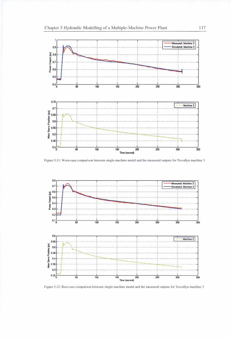
Chapter 5 Hydraulic Modelling of a Mu ltiple-M achine Power P lant
0.75,-----T""-----,~-----,,, -----,------,-----;:::====::::;-1 I - - - Machine 3 I
0.7 5' ~ 065 0
:~ ~ 0.6 a. ~ 0.55 ..
Cl)
""t""'.''\ I \ . .. .. , .. .. ..... .. -...... ~;,.:_·~ .......... ...... . .
f : """~- . .. . J ..... .. .. .. ~tort..- ~ .. ••••• ..•• .•• . •••. ; . ........... .
I .----
··· · ···\ ··
1 ---- ~ ----.; o.5 - .. r ;. . ..... ·.............. . ~":'"."":o."t--~·.;...:.::.._~ ~ .. :::... ·· ·.· ::i; I -------~
··· -
···· -
0.45- .. J· ...... .. .. .. .. ; .. ... .. ...... .. .. .. .. , ........ ; .... ) ......... . ..
] 17
I 0.4 -~
0 I
50 i
100 i
150 i
200 i
250 I
300 350 Time (second)
Figure 5.11: Worst-case comparison between single-machine model and the measured outputs fo r Treva llyn machine 3
O.Br--- ---,-----,------.....,.------,------,-;=:::======i:::=:======:::::;-, 0.7
'S 0.6 .s. l 0.5
6 ~ 0.4
i a. 0.3
0.2
0.6r------.------,,-----,,-----.-------.-----;::::::i::======::;---, I - - - Machine 3 I
0.55 _ .. L-,,
~ t' c 0.5 "" '(" """\ ' ... ;
... . ... ---~~i. '.": .-,.,,,._~-=-·.; .. . -·---
-----~ --~- ,..., __ '*!.._._:.:..:......:. ___ _
.. ... · ~ ... ... ..... . ··· ··-
.2 J - ..... :~ 0.45 .4..... :-:- ..... . a. • ~ o.4 .. . I·· "' I ·i 0.35 ,_ . r··· ····· ::i; •
0.3 - · .~ .. .;
I
Time (second)
Figure 5.12: Best-case comparison between single-machine model and the measu red outputs for Trevallyn machine 3
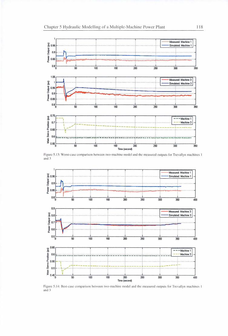
Chapter S Hydrau lic Modelling of a Mu ltipl e-Machine Power Plant 118
]; 0.95 :;
g 0.9
! 085 ll.
'S .5
10.95
8 ~ 0.9
! ll. 0.85
50 100 350
"[ 0.75 -= ---,
I
6 0.7 · ·····I ··' ················ ···• ·· ·· · ········'····· ···
~ ' /~--------~--------1
- - -Machine 1 I ·· ·· ······ ---Machine3 ·-
0 \ ..-"' : --------:---&-.----------------... -- ... ';; 0.65 ... ... ····11 · ......... , ... ..... . ..... ..... ; .... ........ ...... ... .,. ...... . .. .. .... .. ... . . ~ . :
~ 0.6 >;.·.:.:.:. ·.;.;:.:.;;:.,; ·.:.;.:,;.i;,;;.;.;.;;.:.; :.:. ·.;.~-,;.·.;;b..: ·.;.; ;.;.:;,;;~; ;.; ;,;;..; ·,;...;.;;;.;;.;:.:.; ;.: ;.; ·..:.; ;.:.·J :.:. :.;.;.:.;;;.; :.; ·.:.·.:.: :.:.;.; ~;.:;.;.;:.;.;.,; ;;:;,;:.::~;; ·~·.;;.:.;,;;;.:;.;:.;:.;.;.:~ ·.
:1 055 j I i j j . 0 50 100 150 200 250 DJ 350
Time (second)
Figure 5.13: Worst-case comparison between two-machine model and the measured outputs fo r Trevallyn machines I and 3
]; 095 :;
g 0.9
! 085 ll.
]; 0.8 :; g 0.7
! 0.6 ll.
50 100
50 100
150 200 250 350
150 200 250 350
'S0 .65,-~~~-,-~~~~-.-~~~~~~~~-,r-~~~-,-~~~~,-~~-;::==========::;--i
i o.6 ~ ·.:.::.: ·.::;.; ·.:.:;.;. ·L;.: ·.::.;:.:.: ·..:..:.:;.;f ·.:..::.;:;.; ·.:.: ·.::;.; ·.:L;.; ·.:.: ·.:::.;::.::;;.l:.:.: ·.:::.;::.;: .:.: :.:.:.:~.:.;:.:.:.:.;.::..:.::.:;.: ·J ·.:::.:.:;.: ·.:..: · ::: ~:~~:~:~ ~ 0.55 , .. ········· ···· : ... ... .... ...... .. . ......... ,. : ...... ... ... .. .•... ..
~ ' .,;'"":- --- ----~---- ---:----- __ ..... ___ -- - ~ --- ---~-.J-- --~- . ~ 0.5 ·;i..;"' .; .. ... :1 0.45'--~'~~-L~~~~-'-~~~~-'-~~~---''--~~~-'-~~~~-'-~~~~-'-~~~--'
0 50 100 150 200 250 DJ 350 400 Time (second)
Fi gure 5. 14: Best-case compari son between two-machine model and the measured outputs fo r Trevallyn machines and 3
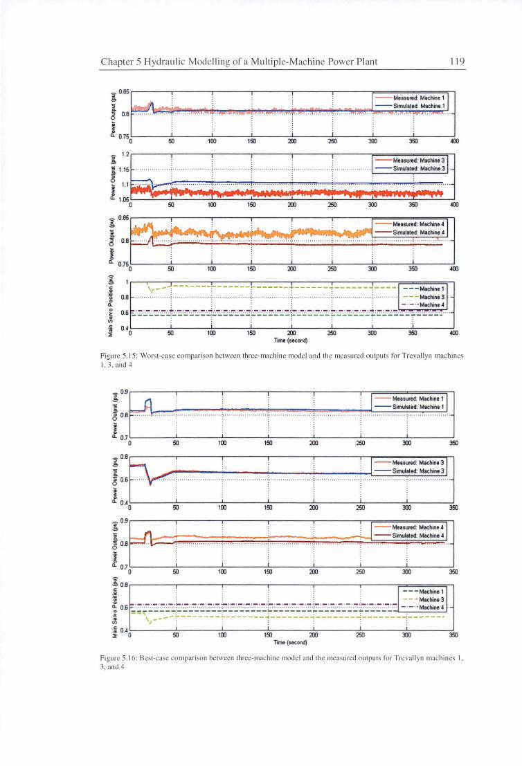
Chapter 5 Hydraulic Modelling of a Multip le-Machine Power P lant
]: 0.85
l 6 !
. . : :
. . . . . . . . . . . . . . .... .... ; ........ .. ...... ... ~ .
50 HIJ 150 200 250 350
--Measured: Machine 4
bf .. tf'lllli.d'l~f\rft~ .. Millrlllffl"9tiimlfll!IPllwf"4~Jllllllfil•'-'illllllllrl~ ---Simulaled: Machine 4 ········ ···· ····
] 19
Cl. 0·75o.__ ____ 50..___ ____ 1_._00 ____ 1_._50 ____ 200_._ ____ 250_..__ ____ :m__._ ____ 350.....__ ___ ~0J
\r_ .. -! --- ------ ~ ------4 ------ ~ ------ ~ ---- - - - Machine 1 o.B- ··· ..... ..... ... : ... .... .... ... .... . ; ··· ··-············ ...... ·.... .. .... ... ........... ---Machine3 ·-
. · - ·- · ·Machine4
0.6 ~=:.:...,.~:: .. =:::.h:.'.:-.:.:-:..::::··i:.:::"".:.:=:.:...,.~::·.:µ-:..:.::·.:·:::-:..::::·;:'-'"!".:.: =·=::.-:: ·±::::..:.::· .: ·:::..:.i'.:·.:..:-:::::::::.:..,....;;::::.:.::::: · i i i i i i i
50 100 150 200 250 :m 350 Time (second)
Fi gure 5.15 : Worst-case compari son between three-machine model and the measured outputs fo r Trevallyn machines I, 3, and 4
'S0.9r-------,-----~-----.------~-----,---;::========i==========;-i .5 :;
g DB
! Cl. 0 .7~----~-----~-----~-----~-----~----~-----~
0 50 100 150 200 250 350
'5"0 .8,------,-----~-----,------~-----.--,-~~~~~~~~....,-,
.5 l 6 0.6
! Cl. 0.4'--------'------'--------'-------...._ _____ .._ ____ __. _____ _,
0 50 100 150 200 250 350
'S0 .9r-------,-----~-----,------~-----.---.====================;-i ,g. --Measured: Machine 4 :; --Simulaled: Machine 4 g 08
! Cl. 0 .7~------'-----~-------'-------~-----~------'-----~
0 50 100 150 200 250 350 'S .50.Br-----r-----r------,,-----,-----,-----;;::=========,-, g 1
---Machine 1 :,o · - - - Machine 3 j 0·
6 :::'{~:?~?f~~?~~:~E~?_:~~=~~:..::=~E-:.~=::~=E~?_~~::_:I::.:~0:=~~~=,~~~:~n:~ ·-.!: 0.4 I i I j I I
~ 0 50 100 150 200 250 :m 350 Time (second)
Fi gure 5.1 6: Best-case comparison between three-machine model and the measured outputs for Trevallyn machin es I . 3, and 4
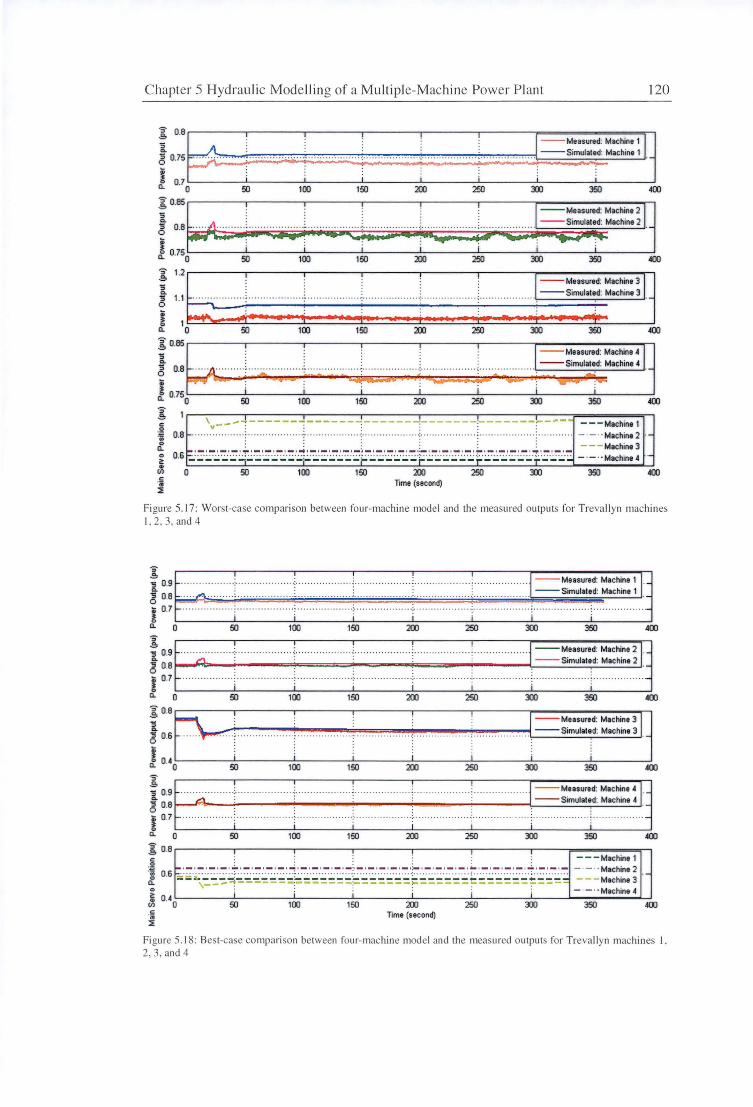
Chapter 5 Hydraulic Modelling of a Multiple-Machine Power P lant 120
~ 0.0,-----.-----r-----r------.------.-----r=~~~~~~~~=r--,
g 0.75 ~;:: .. :·· :::;;::::::~~;::::::::;:::::=:::::::::.::::::i::::::;;:::j;;~~~~~~ J 0.70~~~~~~~~~~~~~~~~~~~~~~~~~~~~~~~~~~~
f ':b; I · :••+·~~ z i·~ ~ .. -v~-.......... -~:.::~:=::~; 1 j Cl.
0·75o 50 100 150 200 250 DJ 350 OJ
F1LJ..:l :J I· J l:~~.:::::::i~ ~ ~ ; •. ~ .. ' - . : ...... ~- ..... · ··~· ..... _,,. J Cl. 0 50 100 150 200 250 DJ 350 OJ
FL. j:, · :.:., B _:.;;, 1•. ~ . J.' ,;__; " ... :.,,,,,,,,,,,,,L ; ; ·· ······!· --. . ~=:= ::::~: IJ ~ ~ -- --. :±-- ~ .. -~ ·~ .. r - <s;:>··: ve;;=J J
Cl. 0
·75o 50 100 150 200 250 DJ 350 OJ
~ c \v __ ..,.. ~ ------ ~---- --:----- --~- ---- --1-------~- .---:! 0.8 .............. .......................... . ··· ·-=·· ···· ···· ·········: ·· ········ ···· ····· :·· ····· ·· ···
- - -Machine 1 - ·-··Machine 2 - - - Machine 3 ~ 0.6 ~=·~"'.';:;:·:;;t;..;: '.:::::-:.:·::$:::·:.::::::~-:-:.:.:·:~-:.:.-::i: . .;;-;;;:::.::::p::.:.:··:::.-:-:.:.t'.:~-;;'.·: - ·- ··Machine 4 -.
(/) 0 50 100 150 200 250 DJ 350 OJ c ..
:l1 Time (second)
Figure 5. 17: Worst-case compari son between fo ur-machine model and the mea ured outpu ts fo r Trevallyn machines I. 2. 3. and 4
'S .5 --Measured: Machine 1 "5 0.9 0. --Simulated: Machine 1 "5 0.8 0
i 0.7 ....... •. .... .. ... .................... . . . . . . . . . . . . . . . . . . . . . . . . . Cl. 0 200 350 OJ 'S .5 --Measured: Machine 2 "5 0.9 0. --Simulalod: M1chin1 2 6 0.8
i 0.7 ... .:-.. ..... ........ ... ~ .. .
Cl. 0 50 100 150 200 250 DJ 350 OJ
~ 0.8 --Measured: M1chin1 3
"5 0. --Simulatod: Machine 3 6 0.6
i 0.40 Cl. 50 100 150 200 250 DJ 350 OJ
I ::5 " I· .. . -1:.. . . .. ·1•, .
1o7 E · . . . J- -.. ~· """"' · 1 ~ . . . --Simulated: Machine 4: T , ........ .
Cl. 0 50 100 150 200 250 DJ 350 4ClJ
~ 0.0.-----.------.-----.-----.-----,1-----,---...,,.~~~~~...--, c ---Machine 1
j o.6 ;.: ;;;.~~~-;;~~:::i-~·~:~:i:·~·;~~;~~~·~;~;·~~-;~:~~-;~·;-~;~;~I·~~-;~ -=.· :::~ ~:~~:~:; ~ ; ; ; 1 1 ; - · - · · Machine 4
(/) 0·4o 50 100 150 200 250 DJ 350 400
Time (second)
Figure 5. 18: Best-case compari son between fo ur- machine model and the measured outputs fo r Treva llyn machines I . 2, 3, and 4

Chapter 5 Hydraulic Modelling of a Multiple-Machine Power Plant 121
5.5.4 Frequency Response Simulation of the Multiple-Machine Station
The frequency responses of the multiple-machine Trevallyn station were studied
through a series of Nyquist tests performed at different guide-vane oscillation
frequencies. This information is very useful in deriving an optimal set of governor
parameters for improving the plant and system performances. The Nyquist criterion, in
general, guarantees the closed loop stability. However, the use of Nyquist tuning rules
to determine the governor parameters in a nonlinear system is still controversial as the
theory is derived mainly for use in the linear systems.
For Mackintosh station, where the waterway conduit is relatively short, a significant
error is found in simulating both the phase and the magnitude of the power output when
the guide vanes are moving at high frequencies. The error is thought to be caused by the
unsteady flow effects in the Francis turbine. This unsteady flow effect, however, is not a
significant problem for the Trevallyn power station. The contradictory result is not
surprising since Trevallyn has a long waterway conduit and its water inertia is relatively
high. Therefore, the inertia effect of the water column is expected to overwhelm the
unsteady flow effects of the Francis turbine operation here.
Figures 5.19 to 5.26 show several Nyquist test cases where the power outputs of
machine 3 are varying at two different initial load levels. To save space, only the results
of the highest test frequency are shown here. The offset between simulated and
measured power outputs is a consequence of the steady-state errors and thus it is not the
main concern for frequency-domain analysis here. Spikes in the high-frequency power
output are observed in both simulation and measurement. They are mainly caused by the
cavitation of machine oil in the control valve of the main servo system. This effect
becomes more obvious, as the guide vanes oscillation frequency is increased. The
presence of this non-sinusoidal power output signals complicates the frequency-domain
analysis, and greater errors for the system gain are expected at high guide-vane
oscillation frequencies. The resulting Bode diagrams are presented in Figures 5.27 and
5.28. As illustrated, the phase and magnitude of the oscillating power outputs are
simulated quite well for Trevallyn station. The phase characteristic of machine 3 is
greatly affected by the initial operating condition, but 1t is insensitive to the number of
machines in operation if power outputs of the other machines are not fluctuating
significant! y.
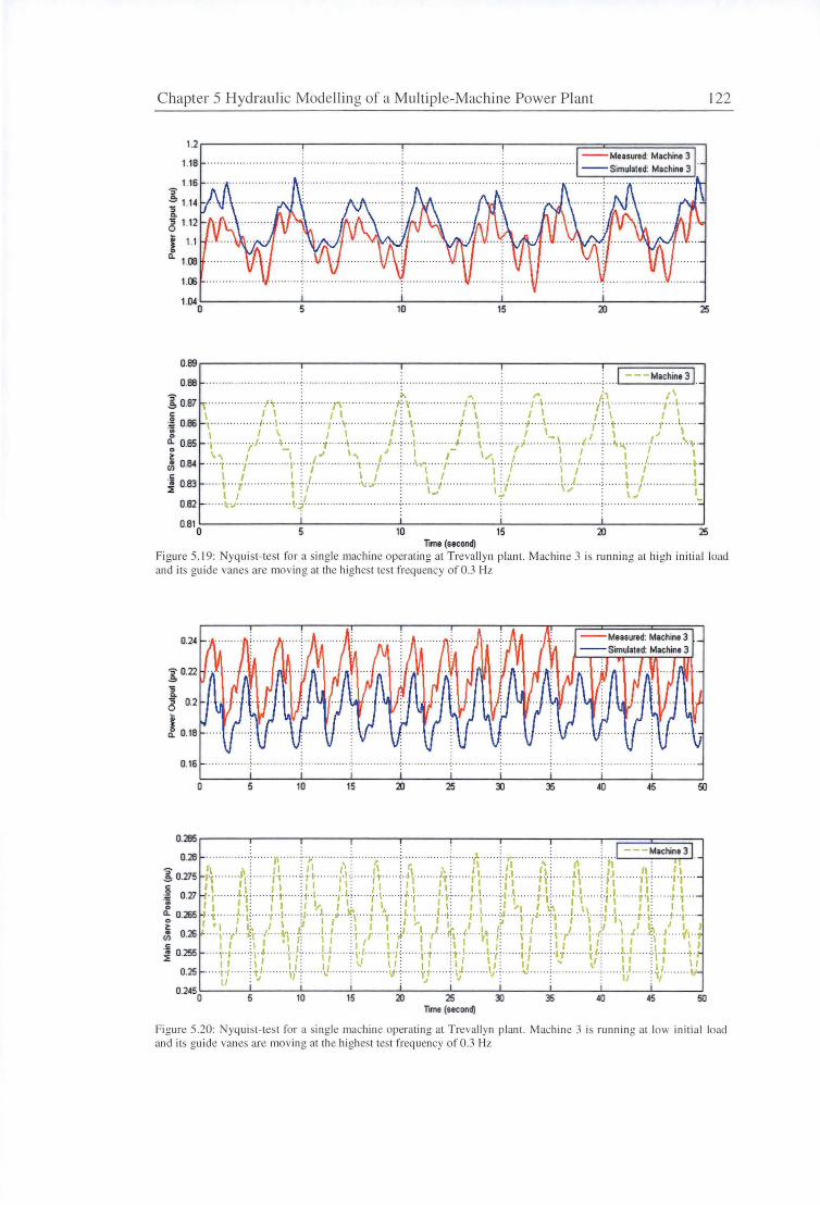
Chapter 5 Hydraulic Modelling of a Mu ltiple-Machine Power Plant
1.2
1.18
1.16 9 .e. 1 u :; . Q.
:; 1.12 0
~ 1.1 tl.
1.00
1.Cl>
5 10 15 20 25
0 .89,--------.--------.-------,,------,-----;::=====~
...................... .. ............... .. ... ....... ~ ... .I -- - t.fachine 31 0.88
~ o.87 ...... ... ....... -J'c .... . .. 1'\ .............. /\ ..... .... .... ... . 1; .. ... ; .... . ..r1 .............. A .. f.\. ... . c: \ f I I I I ; \ I \ : J I f : \ f I
~ :.: r·· ··· ····· t ·t .. ·:·· .... r ·y··········· --:- -:- ·y· ···· ·· ·· -:--··~··· ··r···-r t · ... n -r ··· ·· "J ... \ ...
! 084 :\ .; .. : . 1'::. : :. ~~\ ::;:::~? .. :·:\;l :.:.·;.t .:.·::L.·:::.·/#· "\;:.:. ( .:. ·.~:L.·:t: .. ~ .. _~,y .-:I ....... ::1 l I I : I l J : l I I : , I I I I I
~ 0.83 .... -r·r···· ·········r-/ .. ·· ···b ········:········\·.:t .. ..\f . .... · · · · ··· ~I · .... ; .... ~J ·· ..... ··· ··:. 0.82 ·· · · l;;t ··· · ·· · ··· · ·•··· · \·~ · ... . .. ._. .;. ............. . .... .. ... .. . .. . ..... . .. ... . . . . . .
5 10 15 20 25 Time (second)
122
Figure 5. 19 : Nyquist-test for a single machine operating at Treva ll yn plant. Machine 3 i running at high initial load and its gu ide vanes are moving at the highest test frequen cy of 0.3 Hz
0.24
9 0.22 .. .e. :;
g 0.2
! tl. 0.18
0.16
0 50
0.285 ,---.-----.----,---,----,----,---r---.--;:::====:::::;-1
5 10 15 20 25 35 45 50 Time (second)
Figure 5.20: yqu ist-test for a single machine operating at Trevallyn plant. Machine 3 is running at low initi al load and its guide vanes are moving at the highes t test freq uency of 0 .3 Hz
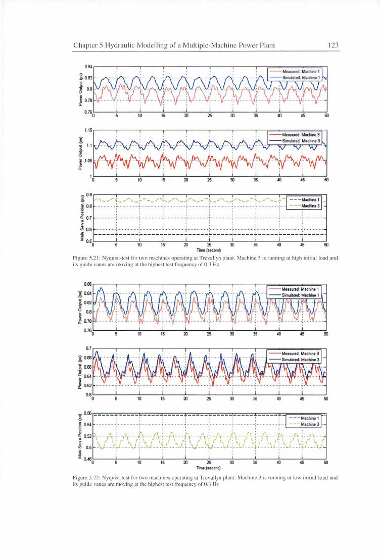
Chapter 5 Hydrau lic Modelling of a Multiple-Machine Power Plant
:; g 0.8
i 0.78 a.
5 10 15 20 25 35 40
1.15
9 .5 :; 1.1 Q.
:; 0
i 1.05
a.
5 10 15 20 25 3J 35 40
9 o.9,--~~-,~~~-r~~~-,.-~~~,.--~~~.--~~-,~~~-.-~~~-,.---;::===========:;--i
..s /"\..._ ,.,.r~ .._,,,.~ '---:-.._._.J'-. ....,_,,,,.r,.._).-'"'-,,-1-~_,-''°'-.,,.~ /'""J',,,.°'!--,.-.__~- ---Machine 1 g O.B ...... .. .... .. , ...... .. ··· ···~···············:··· ...... ... .... ;. ............... ;.··· --- Machine3 :.c .. 0
a. 0.7 0 ~ .
(/) 0.6
' ' ····:-·········· ····-::···· ······· ... .; ............... ,. ···!······ .. ···· ··· :· ' ' ' '
..... -~ .............. ~-.
I -----•-----~----~-----t-----~----~-----~-----~----~-----· :l'
0.50 5 10 15 20 25 35 40 Time (second)
123
Fi gure 5.21: Nyquist-test fo r two machines operatin g at Treva llyn plant. Machine 3 is running at high initial load and its guide vanes are movin g at the highest test frequency of 0 .3 Hz
0.86
]: 08.(
10.82 :; 0 0.8
J 0.78
5 10 15 20 25 3J 35 40 45 50
0.7
]: 068
1066 :; <: 064
l 062
0.6 0 5 10 15 20 25 3J 35 40 45 50
]: 0.5S ----- : ----- . ---- .----- : ----- , ---- ----- ----- - --Machine 1
~ 0.54 ............. ] ............ ... :...... ............... ......... . ........ ---Machine3
~ 0.52 ' ....... p, .. ; . . p ...... .[\ ... . -'·\ : -t\· . .. /\ ... l , .. ; .. {'1" .. .j\ .... f.\, .: .. ,.1\ .. .... \.\ .. />, .. : . . /\ ...... . ~ \ r \ : r '• r ; 1,. ;' I . I I I' : \ t \ · ( \\ I : \\ ,' ~ : f \ /I / I : /' I_ r
c'1 o.5 ... \). ".',_! ...... U .. ~ .... \J.. \!. .... : .. L .\J .... '.';._,f. ...... ..,.1 .. ; .... - . .... I .. ....... \J.. : .. \ .; ...... \ .1 .. .. .. \~ .!:
i 048'--~~~L-~~~L-~~~L-~~~L-~~~L-~~~L-~~~L-~~~.L-~~~.L-~~---' . 0 5 10 15 20 25 3J 35 40 45
Time (second)
Figure 5.22 : yquisl-test for two machines operating at Trevallyn plan t. Machine 3 is running at low initia l load and its guide vanes are moving at the highest tes t frequency of 0.3 Hz
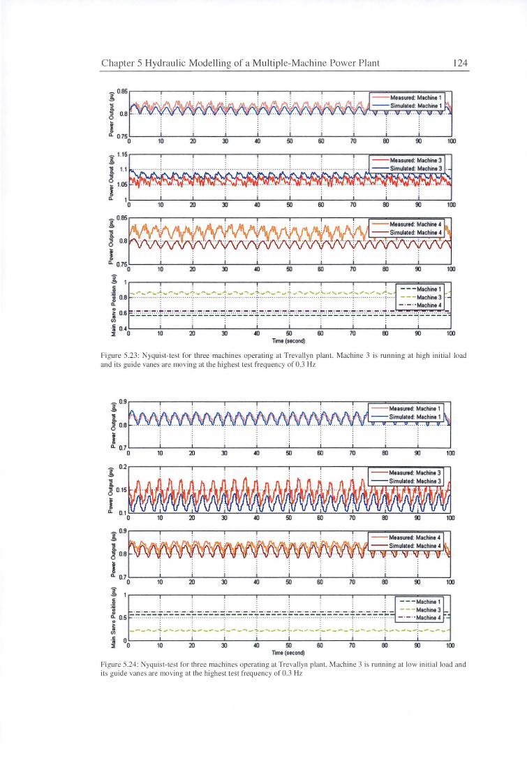
Chapter 5 Hydrau lic Modelling of a M ultipl e-Machine Power P lant
- 0.85 " a :; 0. :; 0.6 0
! a. 0.75
-1.15 " .!!> :; Q.
:; 0
! a.
5' .!!>
1.1
1.05
0 10
10
20 :ll .4() 50 60 70
20 :ll .4() 50 60 70
BO
BO
c I I I I
0 ~'-~~~~r-~-~-----~-~~~-~---~-~-'-'~~-,~~;,,~,~;-:~ 0.6 ....... ... .... ... . ·············;················=··· ··· ·········: ·· ····· ···· ····: ·· ···· ··· ··· ·· ·! ····
124
ro 100
ro 100
- - - Machine 1 - - - Machine3 ·-
a. - ·- ··Machine4
~ 0.6 ~! ;:. ;..;.~.:::::·;~~.:..:.~ '.=~~:..::·= ·=-~-:'. ~~.=:::,;· ::~~+::··=~~~·:.!~~-:..::· :··=*=·~~~··t:.:..~~·::. '.=·.'.:.;t'::.: .. ::~ ·..:..:~~-.:.::~·..:..:..:...~ en c j I i j i i 0· 40'--~~-1~0~~~-20'--~~--':ll~~~-.4CJ-'--~~~50'--~~-60-'--~~~70,__~~--'BO~~~-ro-'--~~--'100
Time (second)
Fi gure 5 .23: Nyquist-tes t fo r three machine operating at Treva ll yn plant. Machine 3 is running at high in it ial load and its guide vanes are moving at the highest test frequency of 0 .3 Hz
5' 0.2.-~~--,.-~~--,~~~--,.-~~--,.-~~~.-~~--,.-~~--,.--,~~~~~~~~~ ..... .!!> :;
go.15
! a.
5' a c 0 :.;: .. 0 a. 0.5 0 ~ .
en c
0 ·;; ::!!: 0
10 20 50 60 70 100
- - -Machine 1
..:::. ~-:-~~·:!.~-:-:..::::: :=.~~.:: :~~~~~~?. ::~-:-+~-.-:::~-:-:..:.:: :~.-:-:-:-..:.:=:~~~ ==. ~'.7?.7.~-:-:..:~:=. -:-:·F - - - Machine 3 - · - ··Machine 4
-----~-~-~-~----~---~-~-~---~-~~~-~----~---'-~-,·--~----. .
10 20 50 60 70 100 Time (second)
Figure 5.24: Nyqui !-test for three machines operating at Trevallyn plant. Machine 3 is running at low initi a l load and its guide vanes are moving at the highest tes t frequency of 0 .3 Hz
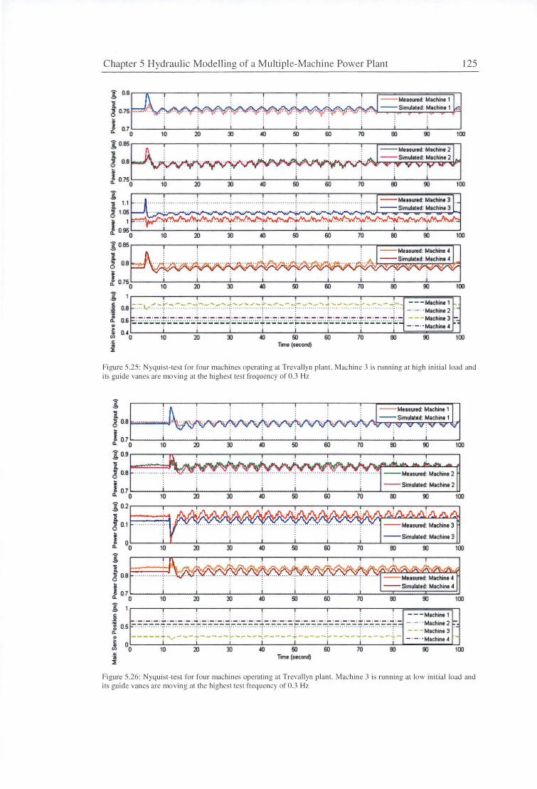
C hapter S Hydrau lic Modelling of a Multip le-M achine Power Plant 125
9
H~ c.
0·95
o 10 20 )J .a 50 60 70 00 9J 100 xo.85.-~~~.-~~~r--~~~.--~~~r--~~~.--~~~.--~~~.--~.-~~~~~~~~..,......,
1 6 0.8
I c. 0.750 10 50 100
~ - - .,,._,;.... ____ ...; __ ~_..- J ..__._,, .... ~ ---- J-_....__ ....... J...__, .... ,.._ l, ____ J_ .... ---M1chin11 ... :~ 0.8 ..... I.,,. ..... . ~ ·· ··· · ···· ····'······· ··· ··· ··~·· ··· ·· ·· ······~· ···· ·· ··· ·· ···;·········· ·· ·· · : ··· ············~ ······ ··· ······ ~ ·· ·· - ·-·· Machine2
~ o.s :::.:;,;-:.;'.;::f;.;-:-.;:: ·=+·::.:-;;.::·~·:.:;:::.;.;-:-F·:;;.-:-~::F~-;;:.: ::{;;.;:. ;_;-:;:;-:· 9:.:.-:-~:·.:~~:.:·: -=-· = ~ ~:~~:~:! :':. UJ
0·4o 10 20 )J .a 50 60 70 00 9J 100
c
i Time (second)
Figure 5.25: yquis t-test for four machines operatin g at Treva llyn plant. Machine 3 is running at high initial load and its guide vanes are moving at the highest tes t frequency of 0 .3 Hz
9 .s 1 6 0.8 ~""""--"""'" j 0.70~~~~~~~~~~~~~~~~~~~~~~~~~~~~~~~~~ ~ 10 20 )J ~ 50 60 70 00 9J 100
f:f l~:E:~:=t::::i c. 0· 70'---~~-1~0~~~20...._~~"'""""JJ'---~~-~'--~~-so-'-~~-so..._.~~ ......... 70~~.__oo~~~-oo~~~_..,100
~0.2~~~~~~~~~~~~~~~~~~~~~~~~~~~~~~~~~~~~~~~~
1 6 0.1
! c.
x '.5 g 08
J 0·70L-~~-1Lo~~~20...L~~_JJJL-~~-.0L..~~-50L..~~-60..l-~~--L7o~~==~ooi:::======ooi::::====::!l100 X c !
:~ o.5 ':,'.:::;:..:.:::,·f..:,,,-:..:..-::.:;.:, ~c.::::::=..:.:::.: .=i:=.-,:. ::: . .::.:,.,-:+.~:; . .:,-:.,:-::..F.:,-::....::=. ·;-;~.::.:=.:..:.:::.: i:::.,:, ~: :=. ~~ :=
c. -----~~ ---~-----~----~-----~-----~----~-----~-~ i /' i i i I i i i c'1 °o 10 20 lJ .a 50 60 70 00
- - - Machine 1 - ·-··Machine2 ":"" - - - Machine 3
- · - · ·Machine~
9J 100 Time (second)
Figure 5.26: yqui s t-test fo r fo ur machines operating a t Treva ll yn plant. Machine 3 is running a t low ini tial load and its guide vanes are mo vin g at the highest test frequency of 0 .3 Hz
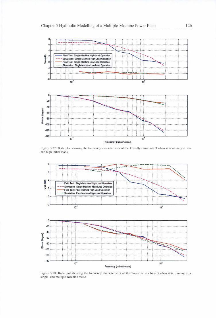
Chapter S Hydraulic Modelling of a Mu ltiple-Machine Power Pl ant
6 ·····:
4
1D 2 ::!:!. .!< ~ 0
-2
--Field Test: Single-Machine Higl>-Load Operation - - - Simulation: Single-Machine Higl>-Load Operation --Field Test: Single-Machine Low-Load Operation - - - Simulation: Single-Machine Low-Load Operalion
-4 ..... , ..... , ... . , ... , . .. .. . ~. : we ; : .94 .41 1"1"\~-~·'" ·~::. . . .
--~. -:- =!
126
. . . . • . . • . • . • . ! . . .
.s ~~~~~~~~~~~~~~~~~~~~~~~~~~~~~~~~~~~~~~~~~~~~~~~
10·1 10°
OIT-:-~~::::::===i===:;;~:::::::::=:::;=::::r::-~~~~--;---i ...... . . -20 .....
";" -40 ., .... ····· i · · ··-:·· ·
e "' -60 .. e. .. -a:J ::
..r:: a_
-100
-120 .. : .... ... : ...... :
-140
Frequency (radian/second)
Figure 5.27: Bode plo t showing the frequency characteristic of 1he T reva llyn machine 3 when it is run ning at low and high in iti al loads
";" e "' .. e. : ..
..r:: a_
8
6
1D 4 ::!:!.
" ... 2 (!)
0
-2
·:· - ~-! -~ .7. ~. T.-~j~ -~~-~~-:~~~~~~~~-~-~ --. . . . .
.. ~ .... . • .... ·:· ... ~ . . . . . . .... ... .... .. .. . . --Field Test: Single-Machine Higl>-Load Operation - - - Simulation: Single-Machine Higl>-Load Operation --Field Ttst: Four-Machint Higl>-Load Optration - - - Simulation: Four-Machint Higl>-Load Operation
.. ;
. ' ' ·· "- ···
' ' '
or--~~~:+::::::=-~--:~~-,--~:-:-~~--:~~~~----i
-20 .: .... -~ ... i-: :
-40
-60
-a:J
... ; ... 1. ...... . . . !
....• , .•.. r•••·········· ····
..... ~
..... ;. ............... . !·· ·
-100 ; . ·- ···- ··: .... ;
-120 ····.· "!' ...... : .... . ;
-140~~~~~~~~~~~~~~~~~~~~~~~~~~~~~~~~~~~~~~~~~~~~
10·' 10° Frequency (radian/second)
Figure 5.28: Bode plo t show ing the frequency characteri stics of the Treva llyn machin e 3 when it s in gle- and multiple- machine mode
running in a
Chapter 5 Hydraulic Modelling of a Multiple-Machine Power Plant 127
5.6 Discussion
5.6.1 Influence of Hydraulic Coupling Effects on Control Stability
Hydraulic coupling in the water supply column is a very well known effect for a
multiple-machine plant [141]. A plant subjected to a large external disturbance has been
studied in this Chapter. The phenomenon is quite important in the governor tuning to
ensure the stable response of the plant for all conditions. Using simplified models that
neglect such effects can lead to errors in control tuning leading to unstable operation
under certain operating scenarios. When an individual unit is tuned through field tests to
verify the adequacy of the governor settings, one may be misled by the testing results.
In fact, a well-tuned response obtained from testing an individual unit does not
necessarily guarantee a well-tuned or even stable response for the entire plant [ 42]. This
scenario is even more critical when units of various sizes are sharing a common
waterway conduit [ 42].
Although little analysis is done on a plant like Trevallyn where units of identical sizes
are used, care must be taken when applying standard tuning rules such as Hovey' s
criteria to set the governor parameters. It is easy to foresee that a counteracting control
of the guide vane is required to reduce the effect of the perturbation caused by any
change in the operating condition of the machines. For stability under islanding or
black start conditions, the governor tuning criteria must be based on the set of units or
the hydro plant as a whole rather than on individual operating units [ 42].
While certain control tuning parameters may be acceptable under open circuit
conditions or when connected to a large system, the case of isolated load operation or
black start under unusual system restoration conditions may be limiting. More
conservative turbine/governor parameters are needed here ([42], [51]). As conservative
setting of the parameters may result in sluggish plant response under normal conditions,
it is wiser to compute in advance the appropriate values for the tuning parameters and
establish a procedure for implementing them when isolated operation or black start
scenarios occur [70]. However, the nature of hydro plant together with the costs, and
indeed risks, associated with carrying out tests on all the machines means that it is not
practical to carry out site testing at the detailed level required to establish the optimum
governor settings over the full range of system and station conditions [70]. Hence, an
accurate turbine and waterway model that captures the hydraulic coupling effects will
play an essential role in the overall system stability study.
Chapter 5 Hydraulic Modelling of a ~ult1ple-Machine Power Plant 128
5.6.2 Travelling Wave Effects of Waterway Conduit
An inelastic waterway model was utilised in this study, as the fastest guide-vane
execution time (3.33 seconds) is longer than the system characteristic time (1.6 second).
Although modelling of hydraulic systems using inelastic water column theory seems to
be adequate in the simulation of Trevallyn plant, the consequences of neglecting
travelling pressure waves or water hammer effects must be carefully investigated to
ensure the stability of the plant under all operating conditions.
Water hammer is the result of flow deceleration or acceleration caused by the sudden
closing or opening of the guide vanes. This phenomenon is characterised by a series of
positive and negative pressure waves, which travel back and forth in the conduit until
they are damped out by friction. The difference between elastic and inelastic solutions is
generally negligible, except for some transient high frequency effects [70].
Even with a throttled surge tank installed in the waterway system, the travelling
pressure wave effects still merit full attention. It would be a dangerous illusion to think
that the surge tank will stop any type of pressure wave. fudeed, it is an established fact
that pressure tunnels have been severely damaged by water hammer in spite of ample
protection provided by the surge tank (Monsonyi & Seth [82]).
Besides, the ability of inelastic model to simulate the total load rejection of a hydro
plant remains in question. No tests have been carried out so far in the Trevallyn station
to investigate the plant behaviour when total load rejection of all four machines occurs.
The costs and the risks of performing such an experiment have prevented it from being
carried out. The effect of travelling waves could be significant here, and there is no
guarantee of the model accuracy or system stability under this circumstance. Hence,
readers must be aware of the assumptions made in the inelastic theory before applying
the model to the power system design.

Chapter 5 Hydraulic Modelling of a Multiple-Machine Power Plant 129
5.6.3 Model Inaccuracies
It is necessary to confirm that the simulated response agrees with the real plant
behaviour before using a simulation to investigate the transient operation of the
hydroelectric generating plant. Simulations using the MATLAB Simulink program
reveal a worst-case accuracy of about 4 percent for the Trevallyn power outputs. The
model inaccuracies are caused by either steady-state or transient errors. The possible
sources of errors are:
• Identical turbine characteristic curves being used to simulate the machine
behaviour at Trevallyn power station. This could have significant impacts because
the efficiency of individual turbines may differ depending on the conditions of the
mechanical parts being used for that unit. The guide vanes of two machines at the
Trevallyn had been replaced just before the field tests, and the guide vanes of
another machine were found badly pitted during the tests. Neglecting these factors
may result in steady-state errors or an offset between the simulated and measured
power outputs.
• Generator efficiency being assumed independent of the turbine flow conditions,
due to lack of any detailed information. A constant efficiency of 97% was used for
the Trevallyn generators. This could be misleading, as the generator efficiency
will vary slightly with the machine output. A steady state variation of 1or2% may
occur.
• The quadratic guide vane function may not be a true representation of the
Trevallyn flow characteristic. A larger steady-state error is expected for units
initially operating near or at the full load.
• Daily tidal effects will have some impacts on the Trevallyn tail water level. It will
change the turbine net head from time to time, which in tum may generate some
steady state errors for the power output simulation if an incorrect value is being
used. This effect must be considered when the testing is to be carried out over a
longer period. The tail water level at the Trevallyn outlet ranges between sea level
+1.8 m and -2.6 mas the tide varies in the Tamar River [154]. The magnitude of
Chapter 5 Hydraulic Modelling of a Multiple-Machine Power Plant 130
this error is still an unknown, as it can either be compensated or amplified by the
errors made in the lake water level measurement. Nevertheless, its impact on the
transient behaviour of the plant is minimal because the simulation is usually run
for a few minutes only.
• A one-dimensional quasi-steady-flow simulation does not capture any unsteady or
three-dimensional flow effects in the Francis turbine. Errors of this type are
generated because of the unsteady Francis turbine operation and the convective
time lag in establishing a new flow pattern in turbine runner and draft tube after
altering the guide vane position.
• A quasi-steady friction term is used in the model. For the Trevallyn plant, the
friction loss is relatively large in magnitude due to its long waterway conduit and
thus an unsteady friction model should be considered to improve accuracy.
5. 7 Conclusions
This Chapter has emphasised the contributions made by the multiple-machine
simulation to improving the accuracy of governor tuning and power system design. The
multiple-machine model successfully captured hydraulic coupling effects observed in
the field tests that parallel single-machine models were unable to predict accurately.
Unsteady flow effects were found to be insignificant for the Trevallyn station, as the
inertia effect of the water column dominated the unsteady flow effects of the Francis
turbine operation. Hence, the unsteady flow studies presented in the later part of this
thesis will focus on operations at power plants with relatively short waterway conduits.
Chapter 6 Research Methodologies for Modelling of the Draft tube Flow 131
CHAPTER6
RESEARCH METHODOLOGIES FOR MODELLING OF THE DRAFT TUBE FLOW
6.1 Overview
Quasi-steady flow analysis for Mackintosh power station reveals that unsteady flow
behaviour in the runner and draft tube could easily affect the operations of a Francis
turbine. The transient effects are thought to be more significant in stations with
relatively short waterway conduits. This has motivated further investigation of unsteady
flow effects in the Francis turbme. Due to time constraints and limited resources, the
current study will only focus on the modelling of the flow inside the Mackintosh's draft
tube with zero inlet swirl. The flow behaviour in the turbine draft tube actually merits
even greater attention, as the stability of a hydraulic power plant is influenced and
restricted by the presence of complex draft tube flow phenomena when the turbine is
operating at off-design conditions. Experimental and numerical procedures for
modelling both steady and transient flow behaviour of the draft tube flow are presented
in details in the following subsections.
6.2 Experimental Model Testing
The experimental program was based on a 1:27.1 scale plexiglass model of the draft
tube component employed in Mackintosh power plant. All experimental tests were
carried out in the Aerodynamics Laboratory of the University of Tasmania. The airflow
in the model was supplied by a centrifugal fan and controlled via a pneumatic-actuated
butterfly valve. Flow visualisation, velocity and turbulence traverses, static pressure
surveys, and skin friction measurements were the main components of the steady-flow
investigations; the transient-flow study involved measurements of instantaneous
velocity at inlet and instantaneous static pressure at outlet. The experimental scale
model and the flow control system are described in Section 6.2.1, while the instruments
and techniques used for the experimental testing are detailed in Sections 6.2.2 and 6.2.3
respectively. The main objectives of this experimental program were to provide an
insight into the physical flow processes of an elbow draft tube; provide quantitative
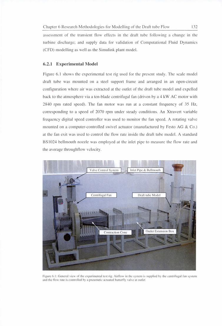
Chapter 6 Research M ethodologies for Modelling of the Draft Lube Flow 132
asse sment of the tran ient flow effects in the draft tube following a change in the
turbine di scharge; and upply data for validation of Computational Fluid Dynamics
(CFD) modelling as well as the Simulink plant model.
6.2.1 Experimental Model
Figure 6. 1 shows the experimental tes t rig used for the present study. The scale model
draft tube was mounted on a steel upport frame and arranged in an open-circuit
configuration where air was extracted at the outlet of the draft tube model and expelled
back to the atmo phere via a ten-blade centrifugal fan (driven by a 4 kW AC motor with
2840 rpm rated speed). The fan motor was run at a constant frequency of 35 Hz,
corre ponding to a speed of 2070 rpm under steady condition . An Xtravert variab le
frequency digital speed controller was used to monitor the fan speed. A rotating valve
mounted on a computer-control led swivel actuator (manufactured by Festo AG & Co.)
at the fan exit was used to control the flow rate in ide the draft tube model. A tandard
BS 1024 bellmouth nozzle was employed at the inlet pipe to measure the flow rate and
the average throughflow velocity.
Centrifugal Fan Draft tube Model
Figure 6.1 : General view or the experimental tes t ri g. A irflow in the system is supplied by the centrifuga l fan sys tem and the fl ow rate is controlled by a pneumatic actuated butterfly va lve at outlet
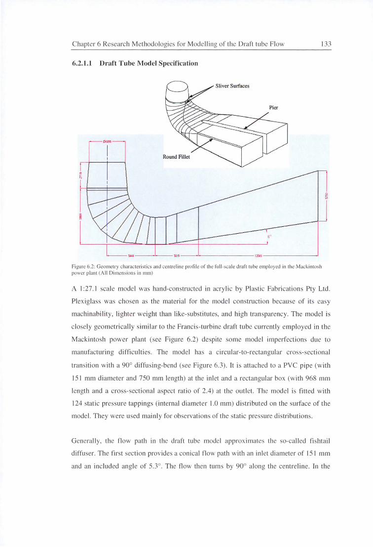
Chapter 6 Research Methodologie fo r Modelling of the Draft tube Flow
6.2.1.1 Draft Tube Model Specification
Sliver Surfaces
~OOO
I I
---5444---'---5'l16---'--------1354 D-------
Figure 6.2: Geometry charac teri stics and ce1iu-eline pro fi le or the full -sca le draft tube employed in the Mackintosh power plant (A ll Dimension in mm)
133
A I :27. 1 cale model was hand-constructed in ac rylic by Plastic Fabrications Pty Ltd .
Plex igla s was chosen as the material for the model constructi on because of its ea y
machinability, lighter weight than like-substitutes, and high transparency. The model is
closely geometrically similar to the Francis- turbine draft tube currentl y employed in the
Mackintosh power pl ant ( ee Figure 6.2) despite some model imperfections due to
manu facturing di ffic ulti es . The model has a circul ar-to-rectangul ar cro s-secti onal
transition with a 90° diffusin g-bend (see Figure 6.3). It is attached to a PVC pipe (with
15 1 mm diameter and 750 mm length) at the inl et and a rectangul ar box (with 968 mm
length and a cross-secti onal aspect rati o of 2.4) at the outl et. The model is fitted with
124 static pressure tappings (internal di ameter 1.0 mm) di stributed on the surface of the
model. They were used mainl y for observati ons of the static pressure di stributions.
Generally, the flow path in the draft tube model approx imates the so-called fis hta il
di ffuser. The first secti on prov ide a coni cal fl ow path with an inlet di ameter of 151 mm
and an included angle of 5.3°. The fl ow then turns by 90° along the centreline. In the
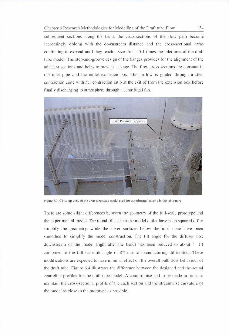
Chapter 6 Research Methodologies for Modelling of the Draft tube F low 134
sub equent secti ons along the bend, the cross-sections of the fl ow path become
increas ingly oblong w ith the downstream distance and the cross-sectional areas
continuing to expand until they reach a size that is 5.1 times the inlet area of the draft
tube model. The step-and-groove des ign of the flanges provide · for the alignment of the
adjacent ections and helps to prevent leakage. The flow cross sections are constant in
the inl et pipe and the outlet extension box . The airflow is guided through a steel
contraction cone with 5: I contraction rat io at the ex it of from the extension box before
finally discharging to atmosphere through a centrifugal fan.
Static Pressure Tappings
Fi gure 6.3: C loe-up view of the draf't tube scale model used for experimen tal testin g in the laboratory
There are some slight differences between the geometry of the full-scale prototype and
the ex perimental model. The round fill ets near the model outlet have been squared off to
simplify the geometry, while the sli ver surfaces below the inlet cone have been
smoothed to simplify the model construction . The tilt angle for the diffuser box
downstream of the model (right after the bend) has been reduced to about 4° ( if
compared to the full-scale tilt angle of 8°) due to manu facturing difficultie . These
modifications are ex pected to have minimal effect on the overall bulk flow behaviour of
the draft tube. Figure 6.4 illustrate the difference between the designed and the actual
centreline profiles for the draft tube model. A compromise had to be made in order to
maintain the cross-sectional profil e of the each secti on and the treamwise curvature of
the model as close to the prototype as possible.
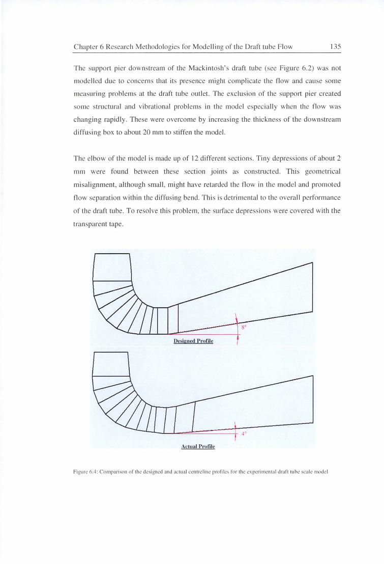
Chapter 6 Research Methodologies for Modelling of the Draft tube Flow 135
The support pi er downstream of the Mackinto h's draft tube (see Figure 6.2) was not
mode ll ed due to concerns that its presence might complicate the flow and cause some
measuring problems at the draft tube out let. The exclusion of the suppo11 pi er created
o me structural and vibrational problems in the model especia ll y when the fl ow was
changing rapidly. These were overcome by increas ing the thickn e s of the downstream
diffusing box to about 20 mm to stiffen the model.
The elbow of the model is made up of 12 different ections. Tiny depress ions of about 2
mm were found between these section joints as constructed. Thi s geo metrical
mi salignment, although small , might have retarded the flow in the model and promoted
flow separation within the diffusing bend. Thi s is detrimental to the overall performance
of the draft tube. To resolve this problem, the surface depress ion were covered with the
transparent tape.
Designed Profile
Actual Profile
Figure 6.4: Comparison of the designed and ac tual centreline profiles for !he experimental draft tube scale model
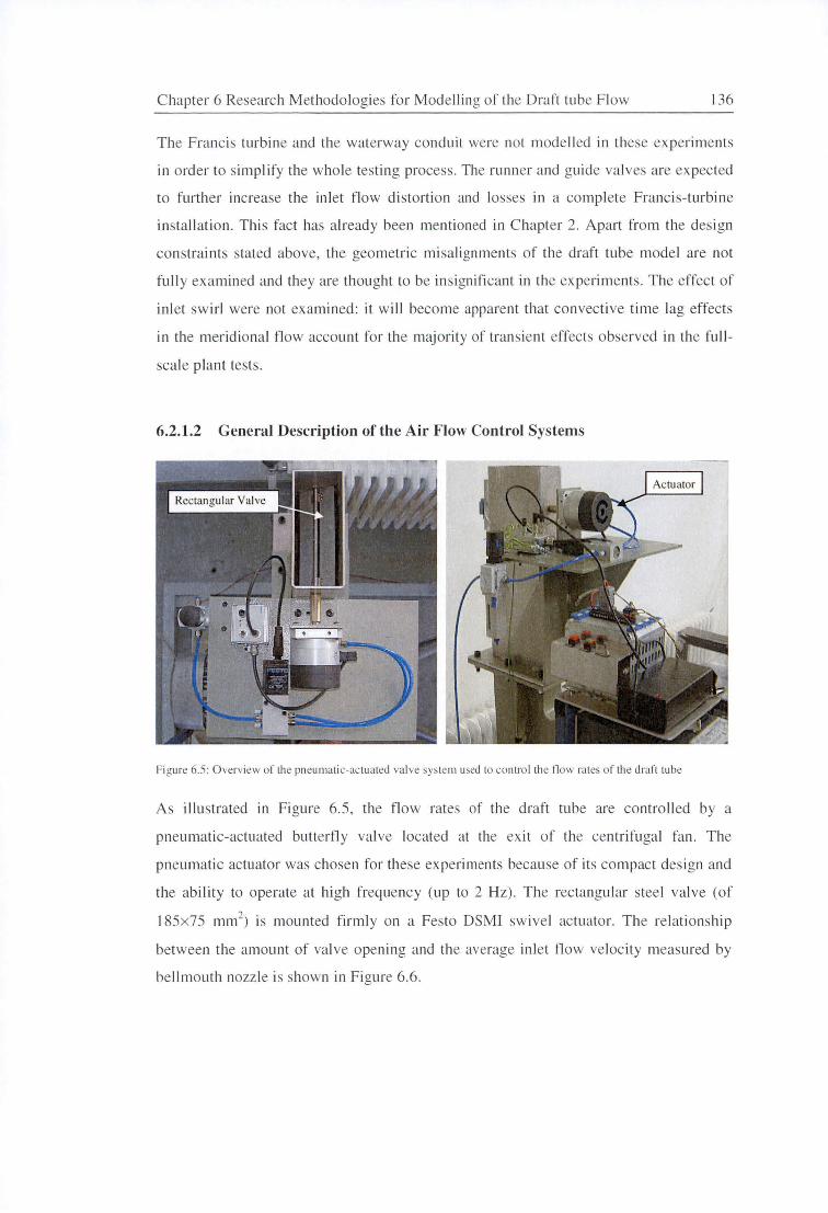
C hapter 6 Research Methodologies fo r Mode lling of the Draft tube F low 136
T he Francis turbine and the waterway conduit were not modelled in these experiments
in o rder to simplify the who le testing process . The runner and guide valves are ex pected
to further increase the inl et fl ow di storti on and losses in a co mpl ete Franci s- turbine
install ation. This fac t has a lready heen mentioned in C hapter 2 . Apart from the des ign
constrain ts stated above, the geometric mi sali gnments of the draft tube mode l are not
full y examined and they are thought to be in signifi cant in the ex periments. The effect of
inl et sw irl were not examined: it w ill become apparent that convecti ve time lag effects
in the meridiona l fl ow account fo r the maj or ity of trans ient effects observed in the full
scale pl ant tests.
6.2.1.2 General Description of the Air Flow Control Systems
Figure 6.5: O verview of the pneumati c-ac tuated valve sys te m used to contro l the tlow rates o f the draft tube
As illustrated in Figure 6.5, the fl ow rates of the d raft tube are controll ed by a
pneumatic-actuated butterfl y va lve located at the ex it o f the centrifugal fa n. The
pneumati c actuato r was chosen for these experiments because of its compact des ign and
the ability to operate at hi gh frequency (up to 2 Hz) . The rectangul ar steel valve (of
I 85x75 mm2) is mounted firml y on a Festo DSMI sw ivel actuato r. The relati onship
between the amount of va lve opening and the average inl et fl ow ve loc ity measured by
bellmouth nozzle is shown in F igure 6 .6 .
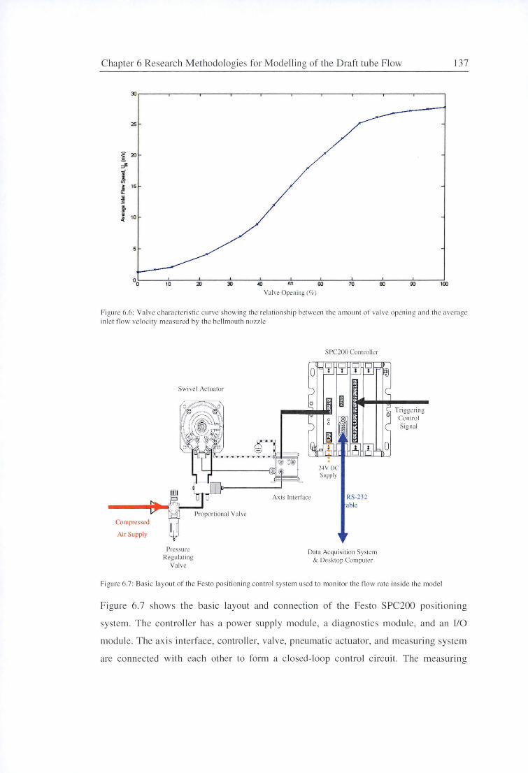
C hapter 6 Research M ethodologies for Modelling o f the D raft tube Flow 137
25
~ 20
~
l (J')
~ 15
• ~ t 10 ~
5
20 30 60 70 00 100
Valve Opening(%)
Figure 6.6: Val ve characteri sti c curve showing the relationship between the amount of valve opening and the average in let fl ow velocity measured by the bellmouth nozzle
SPC200 Contro ller
Swivel Ac tuator
r1~~~~~:~~~, g
~11' @·1 ~'
~ j \.I~ ':/J - "?='
~1 ... A'i-> .:.?' !koJ I ~~ "~ :!f;,7 ··~·-·~
~>m~~-~~( 24V DC Supply ' JD ¥
----.... -~~ _ A xi Interface e- ~-- Proport ional Valve
RS-232 able
Compressed ll Air Supply ,,i
Pressure Regulating
Valve
Data Acquisition System & Desk top Computer
Fi gure 6.7: Basic layout of the Festo posi tioning contro l system used to monitor the flow rate inside the model
Figure 6.7 shows the bas ic layout and connecti on of the Festo SPC200 pos iti oning
system. The cont ro ller has a power supply module, a d iagnosti cs module, and an I/O
modul e. The ax is interface, controll er, valve, pneumatic actuator, and measuring system
are co nnected with each other to fo rm a c losed-l oop contro l c ircuit. The measuring
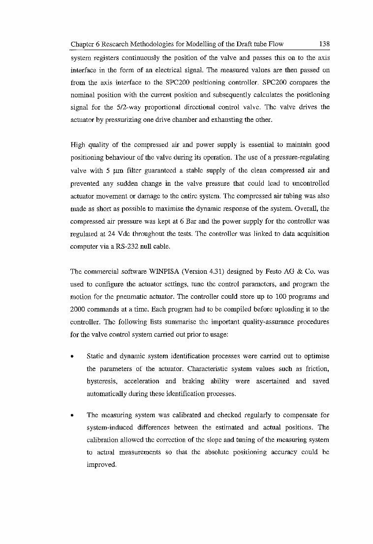
Chapter 6 Research Methodologies for Modelling of the Draft tube Flow 138
system registers continuously the position of the valve and passes this on to the axis
interface in the form of an electrical signal. The measured values are then passed on
from the axis interface to the SPC200 positioning controller. SPC200 compares the
nominal position with the current position and subsequently calculates the positioning
signal for the 5/2-way proportional directional control valve. The valve drives the
actuator by pressurizing one drive chamber and exhausting the other.
High quality of the compressed air and power supply is essential to maintain good
positioning behaviour of the valve during its operation. The use of a pressure-regulating
valve with 5 µm filter guaranteed a stable supply of the clean compressed air and
prevented any sudden change in the valve pressure that could lead to uncontrolled
actuator movement or damage to the entire system. The compressed air tubing was also
made as short as possible to maximise the dynamic response of the system. Overall, the
compressed air pressure was kept at 6 Bar and the power supply for the controller was
regulated at 24 V de throughout the tests. The controller was linked to data acquisition
computer via a RS-232 null cable.
The commercial software WINPISA (Version 4.31) designed by Pesto AG & Co. was
used to configure the actuator settings, tune the control parameters, and program the
motion for the pneumatic actuator. The controller could store up to 100 programs and
2000 commands at a time. Each program had to be compiled before uploading it to the
controller. The following lists summarise the important quality-assurance procedures
for the valve control system carried out prior to usage:
• Static and dynamic system identification processes were carried out to optimise
the parameters of the actuator. Characteristic system values such as friction,
hysteresis, acceleration and braking ability were ascertained and saved
automatically during these identification processes.
• The measuring system was calibrated and checked regularly to compensate for
system-induced differences between the estimated and actual positions. The
calibration allowed the correction of the slope and tuning of the measuring system
to actual measurements so that the absolute positioning accuracy could be
improved.
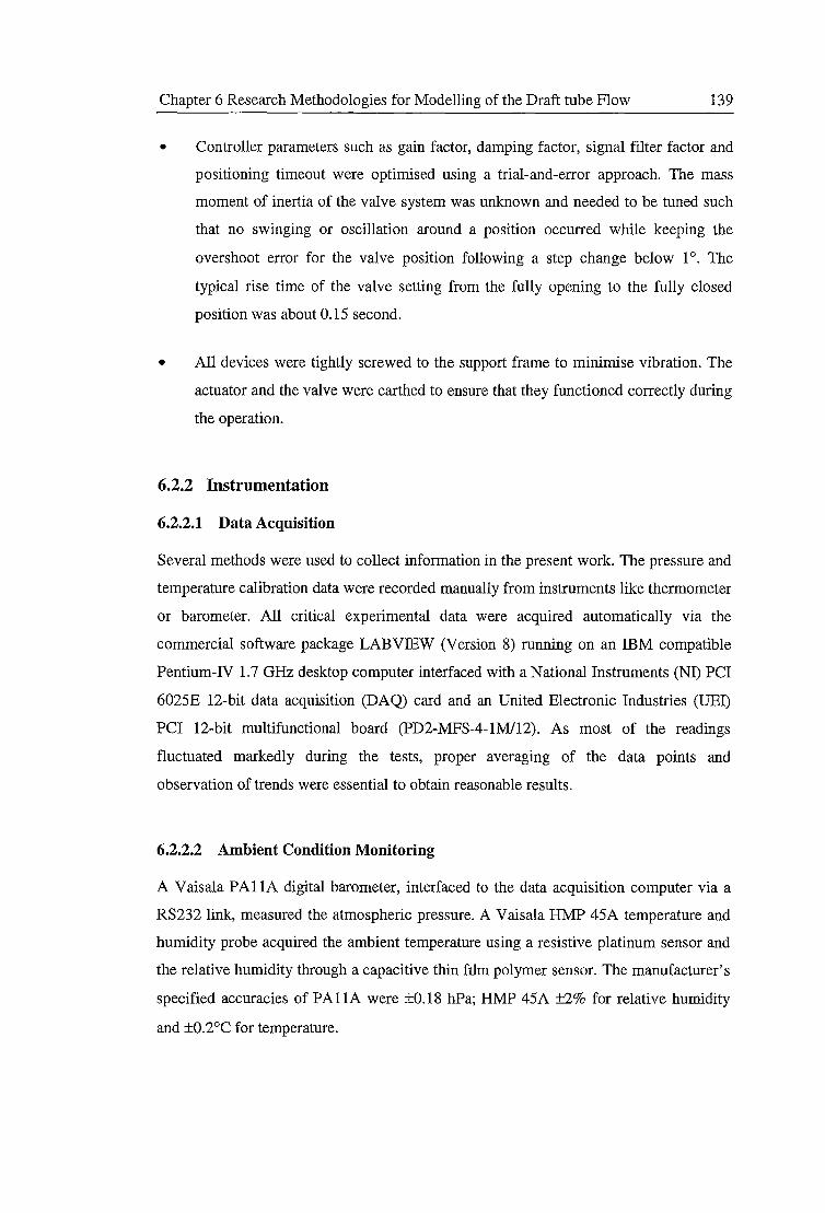
Chapter 6 Research Methodologies for Modelling of the Draft tube Flow 139
• Controller parameters such as gain factor, damping factor, signal filter factor and
positioning timeout were optimised using a trial-and-error approach. The mass
moment of inertia of the valve system was unknown and needed to be tuned such
that no swinging or oscillation around a position occurred while keeping the
overshoot error for the valve position following a step change below 1°. The
typical rise time of the valve setting from the fully opening to the fully closed
position was about 0.15 second.
• All devices were tightly screwed to the support frame to minimise vibration. The
actuator and the valve were earthed to ensure that they functioned correctly during
the operation.
6.2.2 Instrumentation
6.2.2.1 Data Acquisition
Several methods were used to collect information in the present work. The pressure and
temperature calibration data were recorded manually from instruments like thermometer
or barometer. All critical experimental data were acquired automatically via the
commercial software package LABVIEW (Version 8) running on an IBM compatible
Pentium-N 1.7 GHz desktop computer interfaced with a National Instruments (NI) PCI
6025E 12-bit data acquisition (DAQ) card and an United Electronic Industries (UBI)
PCI 12-bit multifunctional board (PD2-MFS-4-1M/12). As most of the readings
fluctuated markedly during the tests, proper averaging of the data points and
observation of trends were essential to obtain reasonable results.
6.2.2.2 Ambient Condition Monitoring
A Vaisala PAllA digital barometer, interfaced to the data acquisition computer via a
RS232 link, measured the atmospheric pressure. A V aisala HMP 45A temperature and
humidity probe acquired the ambient temperature using a resistive platinum sensor and
the relative humidity through a capacitive thin film polymer sensor. The manufacturer's
specified accuracies of PAllA were ±0.18 hPa; HMP 45A ±2% for relative humidity
and ±0.2°C for temperature.
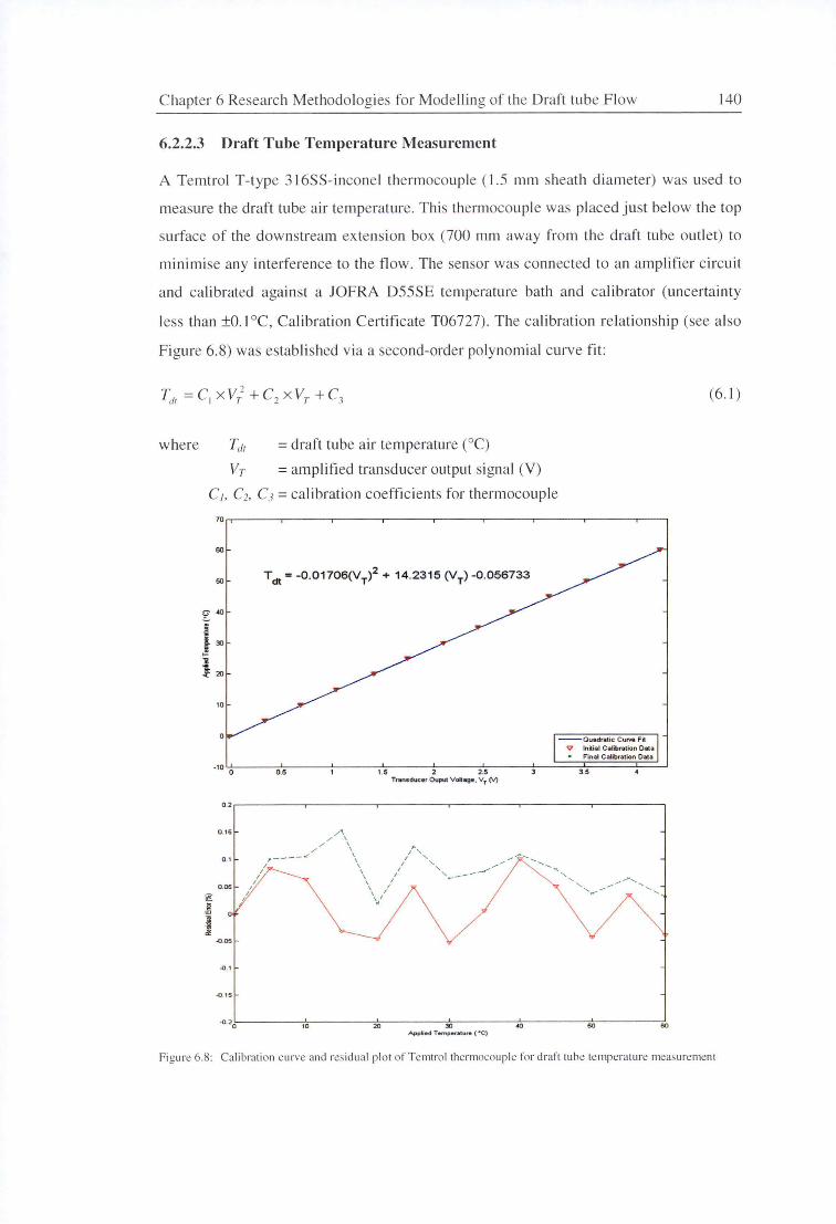
Chapter 6 Research Methodologies for Mod elling of the Draft tube Flow 140
6.2.2.3 Draft Tube Temperature Measurement
A Temtrol T-type 3 l 6SS- inconel thermocouple ( 1.5 mm sheath diameter) was used to
measure the draft tube air temperature. This thermocouple was placed just below the top
surface of the down stream extension box (700 mm away from the draft tube outl et) to
minimise any interfe rence to the fl ow. The sensor was connected to an amplifier c ircuit
and calibrated again st a JOFRA DSSSE temperatu re bath and calibrator (uncertainty
less than ±0.1 °C , Calibrati on Certificate T06727). The calibrati on relationship (see a lso
F igure 6 .8) was estab li shed via a second-order polynomial curve fit:
where = draft tube a ir temperature (0 C)
Vr = amp lifi ed transducer output signa l (V)
C1, C2• C1 =calibration coeffic ients for thermocoupl e
60
50 T dt = -0.01706(VT)2 + 14.2315 (VT) -0 .056733
10
·10 0.5 1.5 2 2.5
Transducer Ouput Voltage, VT M
0 .2
0. 15
0 . 1
0 .05
g
.ll l &
-0.05
-0. •
-0.15
-0.20 10 30 4()
Af:ipli•d Temperatu,. ( • c)
- Quadratic Cul'Vll Fit V Initial Calibr9tion Data • Final Calibration Data
3.5
50
(6. 1)
60
Fi gure 6.8 : Calibration curve and residual pl ot of Temtrol thermocouple for draft tube temperature measurement
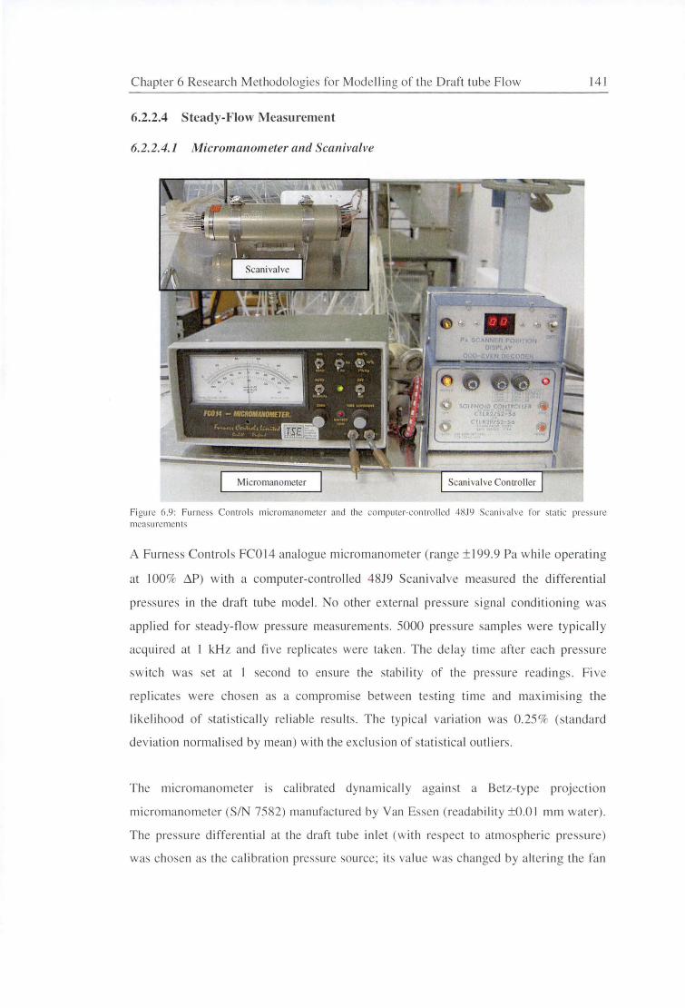
Chapter 6 Research Methodologies fo r Modelling of the D raft tube Flow 141
6.2.2.4 Steady-Flow Measurement
6.2.2.4.1 Micromanometer and Scanivalve
Scanivalve Controller
Figure 6.9: Furness Controls micromanometer and the computer-cont ro lled -18J9 Scan iva lve fo r static pressure measurements
A Furness Controls FC014 analogue micromanometer (range ±199.9 Pa w hil e o perating
at 100% M ) with a computer-controlled 4819 Scanivalve measured the diffe renti a l
pressures in the draft tube model. No other ex terna l pressure signal conditioning was
applied for steady-fl ow pressure measurements. 5000 pressure samples were typica lly
acquired at I kHz and fi ve replicates were taken . The de lay time after each pressure
sw itch was set at 1 second to ensure the stab ility of the pressure readings. Five
rep licates were chosen as a compromise between te ting time and maximis ing the
like lihood of stati sti ca lly reliabl e results. The typ ica l variation was 0.25% (s tandard
dev iati on normali sed by mean) with the exclus ion of stat istical outliers.
The micromanometer is calibrated dynamically against a Betz-type projectio n
micromanometer (SIN 7582) manu factured by Van Essen (readability ±0.0 I mm water).
The pre sure differential at the draft tube inlet (w ith respect to atmospher ic pressure)
was chosen as the calibratio n pressure source; its va lue was changed by altering the fa n
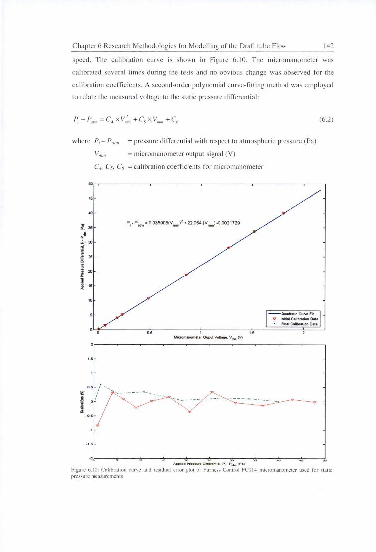
Chapter 6 Research Methodologies for Modelling of the D raft tube F low 142
speed. The ca li bration curve is shown in Figure 6. 10. The micro mano meter was
calibrated several times during the tests and no obv ious change was observed for the
calibration coeffic ients. A second-order polynomial curve-fitting method was e mployed
to re late the measured voltage Lo Lhe static pres ure differential:
P; - P,_11111
= C ~ x v,,;111
+ C 5 x V111111
+ C 6
where P;- Pm111 = pre sure differentia l with respect to atmospheric pressure (Pa)
V,,1111 = micromanometer output s ignal (Y)
C4, C5, C6 =calibration coefficients for micromanometer
45
~ 35
a.• .;_- 30
Ji 1!
ii 25 ~ !!;
~ 20
l 15 ~
10
5
0
2
1 .5
0 .5
~
! 0
l ~
-0.5
-1
-1 5
-20
0
,.. I
I I
I I
P1 - P aim= 0.035908(V mm)2 + 22.054 (V mm) -0.0021729
0.5 1.5 Micromanometer Ouput Vohage, v_ M
' ' ---- ............... __ _
5 10 15 20 25 30 36 Applied Preaaur• 0jff'erenti•1, P1 • P eitm (Pa)
--Quadratic Curve Fit V Initial Calibration Data x Final Calibration Data
2
(6.2)
50
Figure 6. 10: Ca li bration curve a nd residual error plot of Furness Con tro l FCO 14 micromanometer used for static pres ure measurements
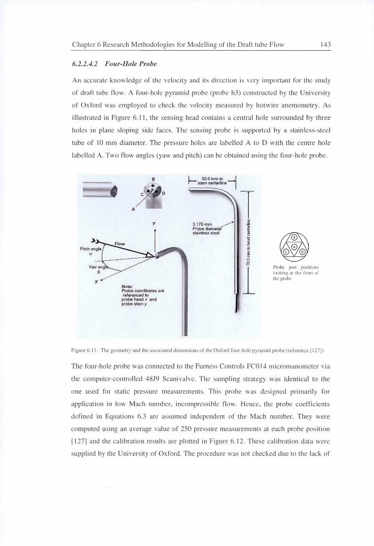
C hapter 6 Research M ethodologies fo r Modelling of the D raft tube F low 143
6.2.2.4.2 Four-Hole Probe
An accurate knowledge of the ve locity and its directi on is very important for the study
of dra ft tube fl ow. A four-hole pyramid probe (probe h3) constructed by the Uni versity
of Oxford was empl oyed to check the veloc ity mea ured by hotwire anemometry. As
illustrated in Figure 6.11 , the sensing head contains a centra l hole surrounded by three
holes in plane s loping s ide faces . The sensing probe is supported by a stainless-steel
tube of lO mm diameter. The pressure holes are labell ed A to D w ith the centre hole
labelled A. Two flow angles (yaw and pitch) can be obtained us ing the four-hole probe.
B
0
A
y
Note: Probe coord inates are referenced to
probe head x and probe stemy
3.175mm ~.., Probe diameter stainless steel
T Probe port pos itions looking a l the front of the probe
Fi gure 6. 11 : The geollletry and the associated dilllensions of the Oxford fou r-hole pyralllid probe (reference [ 127])
The fo ur-hol e probe was connected to the Furness Control s FCO 14 micro manometer via
the co mputer-controll ed 4819 Scani valve. The sampling strategy was identical to the
one used for static pressure measurements. This probe was des igned primaril y for
application in low Mach number, incompress ible fl ow. Hence, the probe coeffi cients
defined in Equati ons 6.3 are assumed independent of the Mach number. They were
computed using an average value of 250 pressure measurements at each probe positi on
[ 127] and the calibration resul ts are plotted in F igure 6.12 . These calibrati on data were
supplied by the Uni versity of Oxford . The procedure was not checked due to the lack of
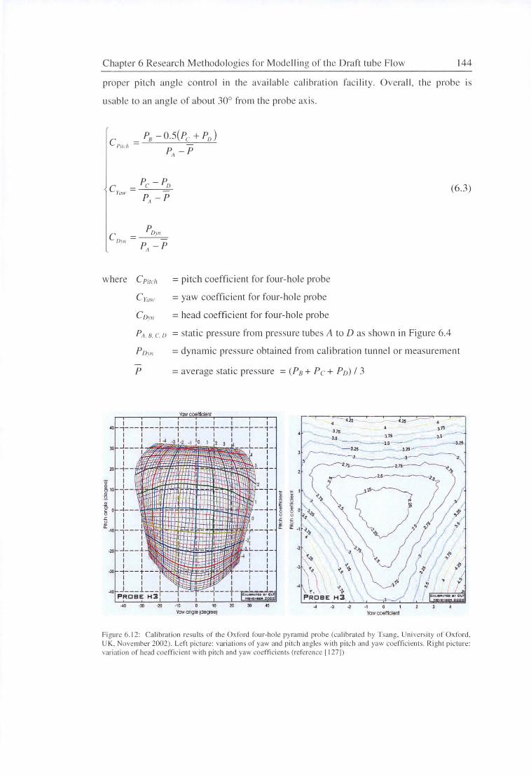
Chapter 6 Research M ethodol ogies for Modelling o f the Draft tube Flow 144
proper pitch ang le control in the avail able calibrati on fac ility. O vera ll , the probe is
usable to an angle of about 30° from the probe ax is.
C Pitt h
CDyn
P8 -0.S(Pc +PD)
PA - P
(6.3)
where C Pirch = pitch coeffi c ient fo r four-hole probe
Cym,· = yaw coeffici ent for four-hole probe
Corn = head coefficient for four-ho le probe
P11 . 8. c. v = stati c pressure from pressure tubes A to D as shown in Figure 6.4
Po.rn =dynamic pressure obtained from calibrati on tunne l or measurement
P =average stat ic pressure = (P8 + Pc + P0 ) I 3
C: I
~ ~ 0 i::: !I
4 ---4.2.5 - - -----.c.25___.;----- 4
J.75 • 3,75
3.5 J,75 J.5 _ --------3.5 _ _ - a.25
- 3.25 - - .25 - -r------J~J~J
2.1s-----i1s____,,.....____<' ~
\
"' , .., I .... I} ~1" ) ..,"!
v ~ 1- I ~~~,.,, PROBE H3 . c--~·~ c•_
... .3 ·2 ·1 0 1
Yow CC<lfficlenl
Figure 6. 12: Calibration results of the Oxford four-hole pyramid probe (calibrated by Tsang. Un ivers ity of Oxford. UK. November 2002). L eft picture: variations of yaw and pitch angles wi th pitch and yaw coefficients. Ri ght picture: variat ion of head coefficien t wi th pitch and yaw coefficients (reference [ 127])
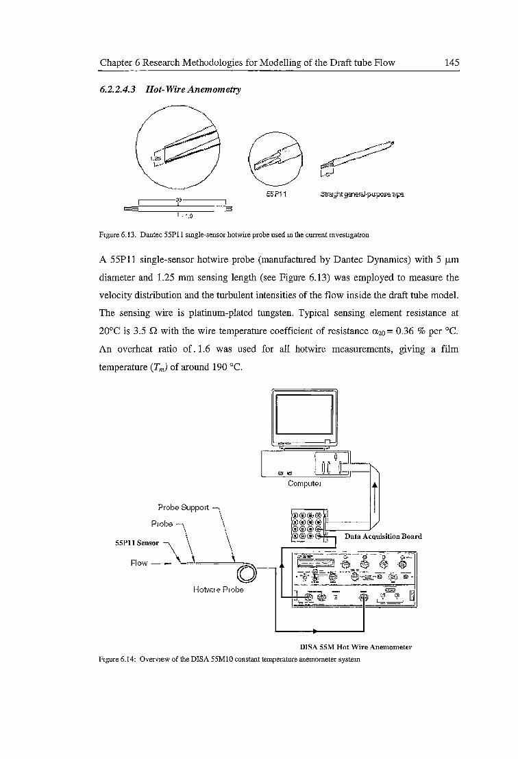
Chapter 6 Research Methodologies for Modelling of the Draft tube Flow 145
6.2.2.4.3 Hot- Wire Anemometry
65?11
b. 1.9
Figure 6.13. Dantec 55Pl 1 smgle-sensor hotwire probe used m the current mvestrgatron
A 55Pl 1 single-sensor hotwire probe (manufactured by Dantec Dynamics) with S µm
diameter and 1.25 mm sensing length (see Figure 6.13) was employed to measure the
velocity distribution and the turbulent intensities of the flow inside the draft tube model.
The sensing wire is platinum-plated tungsten. Typical sensing element resistance at
20°C is 3.5 .Q with the wire temperature coefficient of resistance a.20 = 0.36 % per °C.
An overheat ratio of. 1.6 was used for all hotwire measurements, giving a film
temperature (Tm) of around 190 °C.
D Probe Suppo1t -\
Data Acquisition Board
P1 obe -., \\, "
SSPll Sensor -\ \" .• , \ \.,
Fio"N -- '-=-\=-===~~---,
DISA SSM Hot Wire Anemometer
Figure 6.14: Overview of the DISA 55M10 constant temperature anemometer system

Chapter 6 Research Methodologies for Modelling of the Draft tube Flow 146
As illustrated in Figure 6.14, the signals from SSP I I hotwire sensor are tran sferred to
the DISA SSM Constant Temperature Anemometer (CTA) via a coaxial cable. The
system consists of a SSMOS power pack , SSMO I main unit, and SSM I 0 standard bridge.
The power pack contains circuits to rectify and smooth out AC line voltage as we ll as
voltage limiting and sho1t-circuit protection [28]. The high output voltage at low current
was selected as the default setting for thi s application . The main unit includes amplifiers,
fi lter, square-wave generator, decade res istance, and probe protection circuits [28] . No
other external signal conditioner was employed for these measurements. The bridge
circuit operates at a bridge ratio of 1 :20 and a ratio re istance of 50 Q in the active arm
of the bridge [28]. The resi stance measurement accuracy is estimated to be O. l % ± 0.0 I.
Details of the calibration procedures and measurement accuracy of the hotwire probe
are given in Section 6.2.3.3 .
6.2.2.4.4 Preston Tube
A 2 mm-di ameter Preston tube was used to measure the surface shear stress or skin
friction. The tube was connected to a Furness Controls FCO 14 micromanometer and the
pressure reading is acquired via NI PCI 6025E 12-bit data acquisition (DAQ) card. The
measurement techniques are presented in Section 6.2.3.4.
6.2.2.5 Transient Flow Measurement
6.2.2.5.1 Unsteady Wall Pressure Transducer
1~L M SCREEN OPTIONAL
Fi gure 6.15: Kulite XCS- 190 differential pressure transducer
A miniature high sensiti vity IS® piezoresistive tran sducer XCS-190 (manufactured by
Kulite Semiconductor Products Inc. ) was used for un steady measurements of static
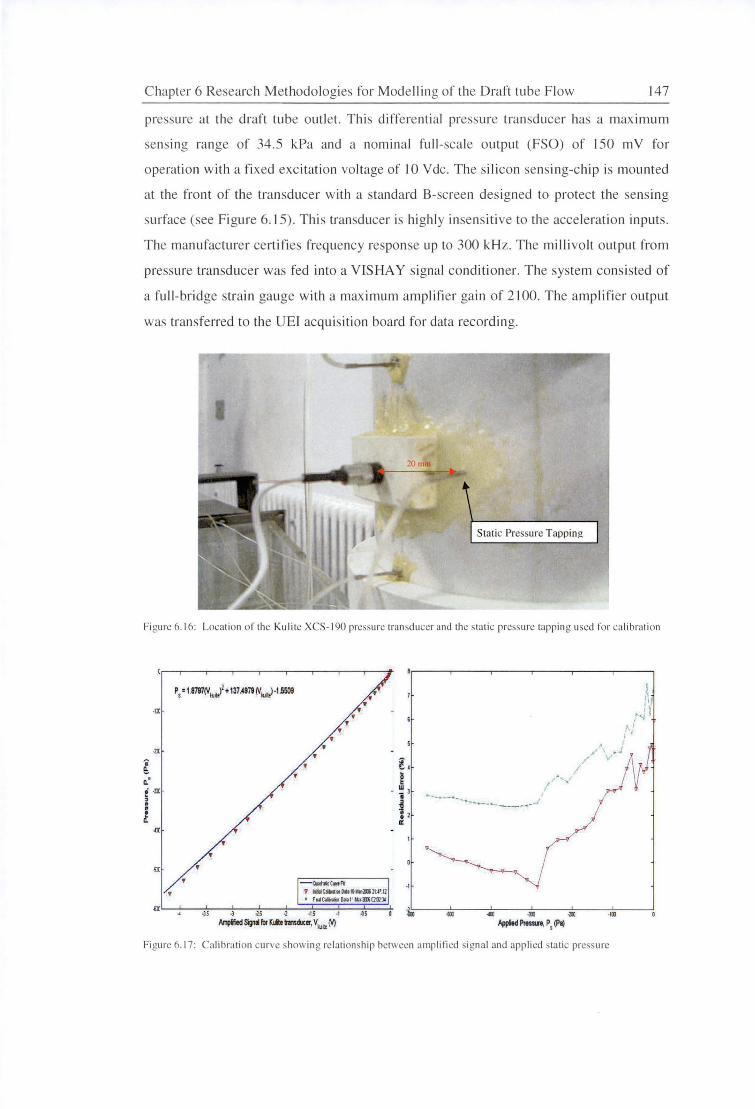
Chapter 6 Research Methodologies for Modelling of the Draft tube Flow 147
pressure at the draft tube outlet. Thi differential pressure transducer ha a maximum
sen ing range of 34.5 kPa and a nominal full-scale output (FSO) of 150 mV for
operation with a fix ed excitation voltage of 10 Vdc. The silicon sensing-chip is mounted
at the front of the transducer with a standard B-screen designed to protect the sensing
surface (see Figure 6.15) . This transducer is highly insensitive to the acceleration inputs.
The manufacturer certifie frequency response up to 300 kHz. The millivolt output from
pressure transducer was fed into a VISHAY signal conditioner. The system consisted of
a full-bridge strain gauge with a maximum amplifier gain of 2100. The amplifier output
was transferred to the UEI acquisition board for data recording.
Static Pressure Tappin.g
Fi gure 6.16: Location of the Kulite XCS- 190 pressure tran sducer and the static pressure tappin g used for ca li brat ion
·IX
-lI
-~lhlitCllfll'tR
• '
v ~CJliAt•IW•ll-W.m2u1.12 • FIAIC*DrCIR1'4ot."m;QQl:ll
I ... _ .. ___ , __ .. . ---... _____ ... , ,·, /
' '
/,
,I 1\1
.,; l I
/\' I I
' I
~~~~~:-,-~~~=-~---,'~,.-~-.~m~~-.m..,__~~
Appitd Prtut.r1, P, (P1)
Figure 6 .1 7: Calibration curve showing re lati onship betwet:n amp lifi ed signal and applied static pressure
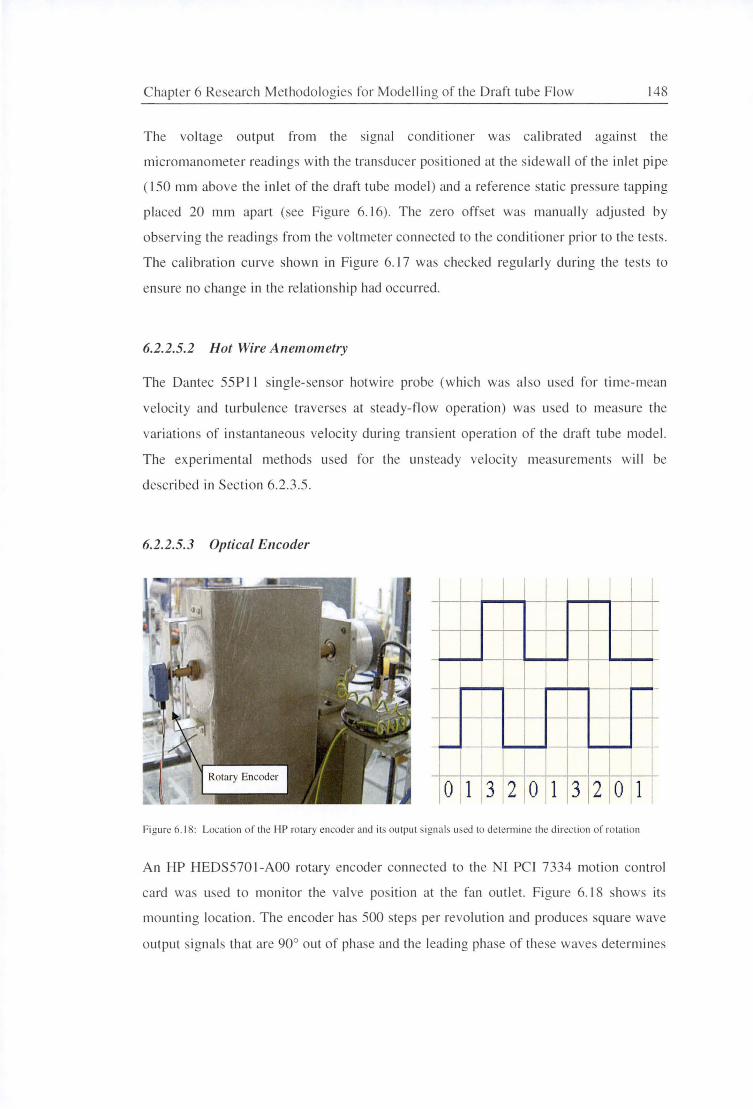
C hapter 6 Research Methodologies fo r Modelli ng of the D raft tube Flow 148
The voltage output from the ignal conditioner wa calibrated aga inst the
micromanorneter readin gs with the transducer posi tioned at the s idewa ll of the inl et pipe
( 150 mm above the inl et of the d raft tube mode l) and a reference sta ti c pres ·ure tapping
pl aced 20 mm apart (see Figure 6. 16). The zero offset was manually adjusted by
observing the readin gs from the voltmeter connected to the conditioner prior to the tests.
The ca lib rati on curve shown in Figure 6. 17 was checked regul ar ly during the tests to
en ure no change in the re lationship had occurred.
6.2.2.5.2 Hot Wire Anemometry
The Dantec 55PI I single-sensor hotwire probe (w hich was al o used fo r time- mean
veloc ity and turbul ence traverses at steady-flow operation) was used to measure the
variations of instantaneous ve loc ity during transient operatio n of the draft tube model.
The ex perimental methods used fo r the un steady ve locity measurements will be
described in Sec tion 6.2.3.5.
6.2.2.5.3 Optical Encoder
tl=I I I I I
I I I I I
0 1 3 2 0 1 3 2 0 1
Figure 6.1 8: Location of the HP ro tary encoder and its output signals used to determi ne the direc tion of rotation
An HP HEDS5701-AOO rotary encoder connected to the NI PCI 7334 moti on control
card was used to monitor the valve po ition at the fa n outle t. Figure 6. 18 shows its
mounting locatio n. The encoder has 500 steps per revolution and produce square wave
output signals that are 90° out of pha e and the leading phase of these waves determines
Chapter 6 Research Methodologies for Modelling of the Draft tube Flow 149
the direction of the rotation. Turning the valve clockwise generates a signal pattern of 0-
1-3-2-0, while rotating the valve counter-clockwise produces a pattern of 0-2-3-1-0. The
encoder compares the old value with the new value to decide the direction of the valve.
An externally mounted protractor reading to 1° was used to establish the fully valve
position.
6.2.2.5.4 Motor Frequency Transducer
A magnetic pickup sensor was placed 15 mm in front of the motor cooling blades to
measure the variation of motor speed during a transient. Four magnets were embedded
into the cooling fan blades 90° apart from each other so that four falling-edge pulses
could be detected in a complete motor revolution. The transducer signal was fed into the
built-in counter of the NI 6025 acquisition card, where the inverse of the time interval
between pulses ( l/4'tranmg) was determined to give the motor speed.
6.2.3 Experimental Techniques
6.2.3.1 Inlet Boundary Layer Measurement
Inlet conditions greatly affect the draft tube performance. Hence, the boundary layer
properties at the entrance of the draft tube model were thoroughly investigated to
guarantee identical inflow conditions for both experimental and numerical models. All
boundary layer measurements were carried out within the inlet pipe (of 151 mm
diameter). The measuring procedures were repeated at two longitudinal positions
located 560 mm and 750 mm above the entrance of the draft tube model. For each
location, data were collected for two different operating conditions: 78% and 44% of the
maximum valve opening. A Pi tot tube (of 2 mm diameter) with wall tapping in the same
plane was used to measure the time-mean boundary layer velocity profile. The tube was
inserted from the opposite wall of the inlet pipe pointing into the oncoming flow. Initial
measurement was taken with the tube tip in contact with pipe wall.
As shown in Figure 6.19, the Pitot tube was secured to a Mitutoyo height gauge adopted
as a traversing rig. This was clamped on the pipe wall, and measurements were taken by
traversing the tube gradually from the wall position to the centre of the inlet pipe. An
identical profile was assumed on the opposite wall. The Pitot tube was connected to the
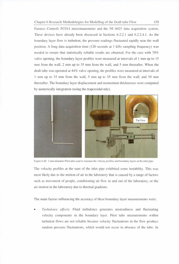
Chapter 6 Research Methodologie fo r Modelli ng of the Draft tube Flow 150
Furness Control FCO 14 mi cromanometer and the NI 6025 data acqui sition system.
These devices have already been di scu sed in Secti ons 6.2.2. 1 and 6.2.2.4. 1. As the
boundary layer fl ow is turbul ent, the pressure readings fluctuated rapidly near the wall
pos ition. A long data acqui ition time ( 120 econds at l kHz sampling frequency) was
needed to ensure that statisticall y reliabl e results are obtained. For the case with 78%
valve opening, the boundary layer profiles were measured at in tervals of I mm up to 15
mm from the wall , 2 mm up to 35 mm from the wall , and 5 mm thereafter. When the
draft tube was operated at 44% valve opening, the profil es were measured at intervals of
I mm up to 15 mm from the wall , 5 mm up to 35 mm from the wall , and I 0 mm
thereafter. The boundary layer di splacement and momentum thi ckne ses were computed
by numeri call y integration (using the trapezo idal rul e) .
Figure 6.20: 2 111111-di arneter Pitot tu be used to measure the ve loc ity profi le
The velocity pro fil es at the start of the inlet pipe exhibited some instability. This was
most li ke ly due to the motion of air in the laboratory that is caused by a range of fac tors
such as movement of people, conditioning air flow in and out of the laboratory, or the
ai r motion in the laboratory due to thermal gradients.
The main fac tors influencing the accuracy of these boundary layer measurements were:
• Turbulence effects: Fluid tu rbulence generates unsteadiness and fluctuating
velocity components in the boundary layer. Pi tot tu be measurements within
turbulent fl ows are not reli able because veloc ity fl uctuati ons in the fl ow produce
random pressure flu ctuations, which would not occur in absence of the tube. In
Chapter 6 Research Methodologies for Modelling of the Draft tube Flow 151
addition, turbulence may also change the level of static pressure across the pipe.
However, its contribution to the wall pressure measurements represents only a
small correction at high frequency and can always be approximated as constant
[87]. The effect is not corrected in the present study, as the turbulence intensity
was quite low in the inlet pipe. However, turbulence effects were more severe
inside the draft tube model and accurate boundary layer measurements were not
possible in that case. Hence, boundary layer analysis was only performed for the
inlet pipe.
• Velocity gradient effect: The effective measurement location is about 65% of the
tube diameter from the low velocity side of the tube. Hence, the smallest distance
from the wall that a 2 mm-diameter tube can effectively reach is 1.4 mm from wall.
• Blockage effect: The presence of Pitot tube in a pipe creates both solid and wake
blockages. These effects may generate some small errors in the measurements.
The effect of solid blockage may be examined by treating the tube as a doublet in
a two-dimensional flow. Wake blockage effect, on the other hand, may be
approximated based on the known drag coefficient for a circular cylinder in
uniform flow. The maximum estimated total blockage correction for the 2 mm
diameter Pitot tube used in these tests was 1.3%.
6.2.3.2 Static Pressure Survey
The static pressure distribution represents one of the most important flow characteristics
of the draft tube, as the performance of the draft tube is closely related to its ability to
recover the kinetic energy at the runner exit by conversion into pressure energy. 124
wall static pressure taps were installed by drilling holes on the model surface and
inserting stainless steel tube (of 1 mm diameter) into the holes, with the tubing
subsequently connected to the Scanivalve and rnicromanometer. Electrical circuits for
pressure devices were energised and allowed to warm up for long enough to ensure
stability of operation after setting up the transducer and making the electrical
connections. Zero readings were recorded before and after each pressure scan to account
for thermal drift during the tests. To reduce the uncertainty, all pressure results were
expressed in terms of pressure coefficients and statistical outliers were excluded from
the data averaging.
Chapter 6 Research Methodologies for Modelling of the Draft tube Flow 152
A tube size of 1 mm diameter was chosen for the wall pressure taps as a compromise
between the acquisition time and measurement accuracy. Errors due to the dimensions
of the static pressure tappings are well documented in reference [8]. Better results are
always obtained for static pressure tappings with smaller diameters. Hole diameters
below 0.5 mm result m large response times, and the holes are easily blocked by dust;
measurements with larger holes are less accurate due to the amount of distortion
introduced into the flow field [8]. For 1 mm-diameter pressure holes, the estimated
uncertainty is about 0.6% of the dynamic head. To reduce the effects of pressure
gradients and surface curvature, the static pressure tapping holes were made as
perpendicular to the surface as possible.
The surface adjacent to each pressure tap was smoothed and squared off to ensure no
disturbance was generated due to surface undulations. Any visible burrs protruding into
the airstream were carefully checked for and removed from the surface. This is critical
because the failure to remove any burrs resulting from drilling a hole onto the surface
may generate a negative error of around 15-20% of the dynamic head [8]. Dirt collected
at the edge of the static pressure hole can have similar effect to burrs. A burr with height
as small as 1/30 of the hole diameter can easily produce errors of about 1 % of dynamic
pressure [8]. To eliminate this problem, the inner surface of the model was thoroughly
cleaned prior to the tests.
Eddies developing in the pressure tapping cavity and fluid turbulence may cause
additional problems in the wall pressure measurement. The shear stress of the boundary
layer passing over the static pressure tap induces recirculating flows in the tube, which
in tum entrains relatively high momentum fluid from the free stream into the static
pressure tap [8]. This results in a static pressure in the tube that is higher than the actual
pressure on the surface. A short tube would have minimised this error, but the tube
length is limited by the thickness of the model. An uncertainty of around 3-5% of the
local dynamic pressure can occur due to this effect. The influence of fluid turbulence,
on the other hand, mainly results from fluctuations of the velocity component
perpendicular to the wall. Irreversibility and nonlinearity of the energy exchange with
the pressure tap may produce an error of around 0.5% of the dynamic head. However,
the error due to turbulence disappears when the hole diameter is smaller than the length
Chapter 6 Research Methodologies for Modelling of the Draft tube Flow 153
scale of the turbulent fluctuations [8], which is likely to be the case in this study. Hence,
no correction for turbulence was applied here.
Finally, any air leaks around the pressure tappings were identified by spraying detergent
liquid on the model surface and then observing bubble development due to flow being
drawn into the model. Any leaks identified were eliminated by applying glue or rubber
tape. Blockages in the pressure tubing were checked for by blowing the air through the
tube. Pressure tubing leaks were identified by blocking the air in the tube and then
connecting it to the micromanometer to observe whether a constant pressure was
maintained. Vacuum grease was applied to all tube connections to reduce leakage
problems.
6.2.3.3 Hot-Wire Anemometry
Velocity and turbulence profiles for steady-flow operation were measured using the
hotwire technique. The probe was traversed horizontally and vertically in several
different planes of the model. The exact measurement positions will be defined later in
Section 7.2.3. For transient-flow operations, the instantaneous velocity at the inlet was
acquired using the same hotwire anemometry techniques. The unsteady flow
measurements will be discussed in Section 6.2.3.7. The following operating procedure
was carried out during the initial set up of the test gear:
• The probe cables were carefully tested to ensure they functioned properly. All
plug-and-socket connections for the hotwire probe were secured tightly to the
anemometer to ensure no change in the probe resistance during the tests. The
condition of the hotwire sensor was investigated using a zoom telescope. Any dirt
on the wire was removed by cleaning before measurements were taken.
• The equipment was continuously powered until all measurements were taken. This
minimised temperature drift in the system and reduced calibration curve shifts
during the tests.
• The overheat ratio of the 55Pl 1 probe was set to 1.6 after proper allowance for the
lead and probe support resistances.
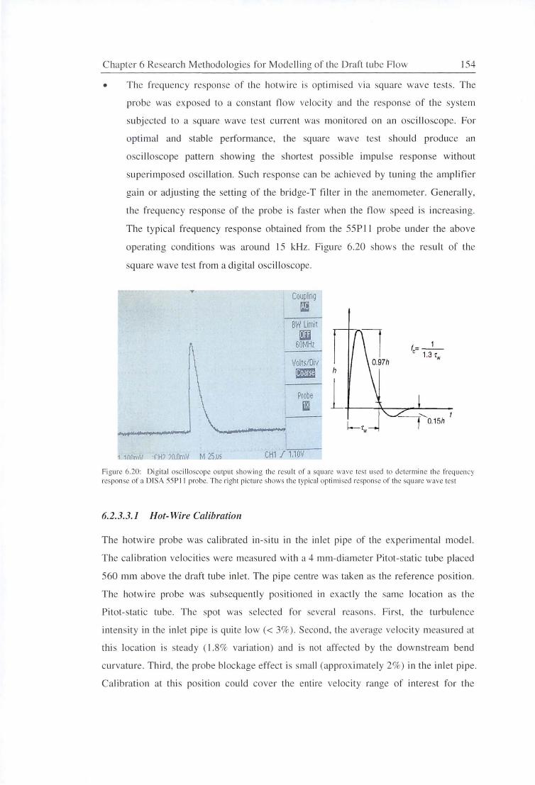
Chapter 6 Re earch Methodologies for Modelling of the Draft tube Flow 154
• The frequency response of the hotw ire is opt imised via square wave tests. The
probe was exposed to a constant flow ve loc ity and the response of the system
subj ected to a square wave test current was monitored on an oscil loscope. For
optimal and stable performance, the square wave test should produce an
osci lloscope pattern showing the hortest possible impul se response without
superimpo ed oscillati on. Such re ponse can be achi eved by tuning the amplifier
gain or adjusting the setting of the bridge-T filter in the anemometer. Generall y,
the frequency response of the probe is faster when the flo w speed is increasing.
The typica l frequency response obtained from the 55PI 1 probe under the above
operat ing conditions was arou nd 15 kHz. Figure 6.20 shows the result of the
square wave test from a di g ital oscilloscope.
Coupling rl
BW Limit w
60MHz
Volt5/0iv -Probe w
1 1 nr1rro'J i H) W.OrnV M 25JJS CH1 f 1.10V
Fi gure 6.20: Digital oscillo cope output showing the result of a square wave res t used to determine the frequ ency respon e of a DISA 55P 11 probe. The right picture shows the typical optimised response of the square wave tes t
6.2.3.3.1 Hot-Wire Calibration
The hotwire probe was calibrated in-situ in the inlet pipe of the experimenta l model.
The calibration ve loc ities were measured with a 4 mm-d iameter Pitot-stati c tube placed
560 mm above the draft tube inl et. The pipe centre was taken as the re ference pos ition.
The hotw ire probe was subsequently positioned in exactly the same locati o n as the
Pitot- tatic tube. The spot wa selected for several reasons. First, the turbulence
intensity in the inlet pipe is quite low(< 3%). Second , the average ve locity measured at
this location i steady ( 1.8% variation) and is not affected by the down tream bend
curvature. Third, the probe blockage effect i small (approximately 2%) in the inl et pipe.
Calibration at this position cou ld cover the entire ve locity range of interest for the
Chapter 6 Research Methodologies for Modelling of the Draft tube Flow 155
highest Reynolds number experiments. Fourth, the risks involved in transferring the
fragile probe to another calibration facility outweigh any inaccuracies caused by the in
situ calibration. All calibrations were performed by gradually increasing the valve
opening at the fan exit from the fully closed to the fully open position to vary the air
velocity.
The calibration procedure of Walker [134] has been employed in this study. It is a
modification of the method of Collis and Williams [25]. A quadratic term was added to
the equation in order to improve the calibration at low velocities. The theory is based on
the heat loss generated from an infinitely long heated cylinder in a cross flow. A non
dimensional data fit was established using Equation 6.4 with the coefficients C7, Cs, and
C9 being determined by the method of least squares.
2 Ev wRp
where Nu = Nusselt number= -2
;rlw!)..TkfRt
Rew = wire Reynolds number= Udw Va
Ev-w = measured bridge voltage (V)
Rp = probe resistance (.Q)
Lw = hotwire sensor length (m)
L1T = temperature difference = Tm - Ta (0 C)
Ta = air temperature (0 C)
T w = wire temperature (0 C)
Tm =mean flow temperature= 0.5(Tw +Ta) (0 C)
kt =air thermal conductivity= 0.0001423 x (Tm+273.15) 0 9138 (W/m.K)
(6.4)
Rt =total resistance including resistances for lead, cable, probe, and bridge (.Q)
U =mean velocity measured by Pitot-static tube (m/s)
dw = hotwire diameter (m)
Va =air kinematic viscosity (m2/s)
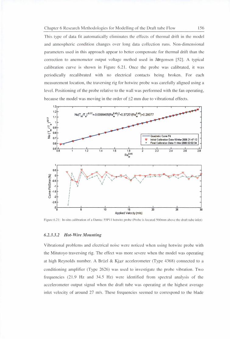
C hapter 6 Research Methodo logies fo r Mode lling of the D raft tube Flow 156
Thi s type of data fit automaticall y e liminates the e ffects of the rmal drift in the mode l
and atmosphe ric condition changes over long data collecti on runs. Non-dimensional
paramete rs used in thi s approach appear to better co mpensate for thermal drift than the
correcti on to anemometer output vo ltage method used in J0rgensen [52 ]. A typical
calibrati on curve is shown in Figure 6.2 1. Once the probe was cali brated, it was
periodi cally recalibrated with no electrical contac ts be ing broken. For each
measurement locati on, the traversing rig for hotwire probe was carefull y a ligned using a
level. Pos iti oning of the probe relati ve to the wall was pe rfo rmed with the fan operating,
because the model was mov ing in the order of ±2 mm due to vibrati onal effects.
1 .3~--~--~--~--~~--~--~--~--~--~--~
1.2
1.1
t:'" 0.9 1-E ~ 0.8 :::> z 0.7
0.6
Nu(T FT r0·17 =-0.0099405(Re0·45)2+0.37251(Re045)+0.28077 m a w w
--Quadratic Cuive Fn V lnnial Calibration Dat•1~Mar-21X6 21 :47:12 x Final Calibration Dat• 11-Mar-21X6 02:02:34
o.5~--~--~--~--~---~--~--~--~--~--~ 0.8 1.2 1.4 1.6
0.5
~ 0
g ~.5
~ -1 iI ~ -1 .5
u -2
-2.5
)
I I r I )
I I
J
1.8 Re0.45
w
2 2.2 2.4 2.6 2.8
~~----~----~-----~----~----~----~ 0 5 10 15 20 25
Applied Velocity (rn/s)
Figure 6.2 1: In-Situ cali brat ion of a Dan tee 55P 11 hot wire probe (Probe is located 560mm above the draft tu be inlet)
6.2.3.3.2 Hot-Wire Mounting
Vibrational pro ble ms and electrical noise were noticed w hen using ho twire probe with
the Mitutoyo traversing ri g. The e ffect was more severe when the mode l was operating
at high Reynolds number. A BrUel & Kj a;r accelero mete r (T ype 4368) connected to a
conditi oning amplifi er (T ype 2626) was used to in vesti gate the probe vibrati on. Two
frequenc ies (2 1.9 Hz and 34.5 Hz) were identified from spectral analys is of the
acce leromete r output signal when the draft tube was operating at the hi ghest average
inlet ve loc ity of around 27 m/s. The e frequencie seemed to correspond to the bl ade
Chapter 6 Research Methodologies for Modelling of the Draft tube Flow 157
passing frequency of the fan. The natural frequency of the probe support was estimated
using Rayleigh's formula and treating the support as a stepped cantilever. The
calculated natural frequency of the support was around 32 Hz, which was quite close to
the problematic frequency zone identified by the accelerometer. These vibrational
problems were overcome by reducing the length of the probe support and making the
traversing rig as close to the measurement location as possible. This shifted the probe
out of the observed vibrational mode. The support frame was stiffened by replacing the
metal stand with a heavier stainless steel bar (using an added mass approach). A
cushioning plate was also added between the support frame and the traversing rig in
order to dampen any vibrations.
In addition to the vibrational effects, some significant electrical noise was initially
observed in the hotwire signal when a metal structure was used for the traversing rig.
Subsequent investigation indicated that this noise arose from the ground loop problems.
These were eliminated by employing rubber plates and plastic bolts to isolate the
traversing rig from the ground, and ensuring that all the electrical loops returned to the
ground connection of the anemometer.
6.2.3.3.3 Hot- Wire Accuracy
Hot-wire measurement is challenging for the current model geometry, as the
uncertainties are difficult to quantify in a highly unsteady and turbulent flow possessing
many small turbulent scales and high velocity gradient. The major factors affecting the
accuracy of the hotwire measurements are summarised as follows:
• Calibration error: Accuracy of the calibration velocities is largely affected by the
pressure readings obtained from Pitot-static tube. The maximum uncertainties
resulting from the Pitot-static tube measurement is around 3%. Five replicates are
taken for bridge voltages at each calibration point, giving an average error of
0.08%. The error due to analogue-to-digital conversion is negligible if compared
to the noise on the data acquisition channel. The temperature measurement error is
around± 0.1 °C, producing an uncertainty of less than 0.3% in Nusselt number.
Chapter 6 Research Methodologies for Modelling of the Draft tube Flow 158
• Probe orientation: Although extreme care was taken to minimise misalignment of
the probe, variations in sensor orientation of up to ±4 ° may have occurred when
moving between different measuring locations.
• Nonlinear cooling effect: Simonsen [119] indicated that this effect was caused by
mean velocity gradients in the flow. Little information is available in the present
study about its impact on the mean velocity distribution. It is believed that a
negative error in mean velocity will occur when measuring in a high velocity
gra~ient flow.
• Turbulence effect: For regions with high turbulence intensities, truncation errors
arise from ignoring the effect of non-measurable velocity components normal to
the probe axis [119]. Moreover, the inability of a hotwire probe to determine the
flow direction will cause rectification errors. This error is significant at the outlet
of the draft tube model, as a strong velocity fluctuation and intermittent flow
reversal can be clearly seen in this region. More details about the velocity and
turbulence distributions will be given in Chapter 7. High measuring accuracy
cannot be expected in these locations.
• Electrical noise: White noise is usually related to the 50 Hz line power in the area
and cannot be reduced except by decreasing the amplifier gain. Electrical noise
was regularly checked during the tests by momentarily turning off the excitation
source and observing the output from the conditioner. Shielded or twisted multi
conductor wire was used for all electrical connections, with the shields grounded
at the input connector and insulated against accidental grounding at the bridge end
to minimise inductive effects. All metal structures were electrically connected to a
common good ground and wiring was kept well clear of magnetic fields caused by
the electric motor.
• Probe support blockage effect: Blockage effects due to the presence of hotwire
probe support may have caused an error of up to 2%. This estimation is based on
the approach described in Section 6.2.3.1.
Chapter 6 Research Methodologies for Modelling of the Draft tube Flow 159
6.2.3.4 Four-Hole Probe Measurement
The major problem of the single-sensor hotwire anemometer described in the previous
Section is the impossibility of detecting the sense of velocity vector [8]. This is of
particular concern when measurements are to be taken in a highly turbulent flow.
Although many solutions to this problem have been suggested, they always lead to a
very complicated probe design that would be extremely difficult to apply in the present
draft tube geometry. Only non-intrusive measurement techniques such Laser-Doppler
Velocimetry (LDV) and Particle Image Velocimetry (PIV) may provide valid
alternatives for this application [48]; but these facilities were not available. A simpler
approach utilising a four-hole pressure probe was therefore implemented at several
locations of the model to double-check the validity of the hotwire measurements. The
four-hole probe is preferred for three-dimensional measurements because no redundant
data is gained and smaller flow disturbance can be achieved due to its more compact
probe size (compared to five- or seven-hole probes).
No precise yaw nulling procedure is needed for the four-hole probe measurements. The
probe was simply oriented with reference to its bottom surface for vertical traverses or
with respect to its side surface for horizontal traverses. The tip was pointed towards the
incoming flow. Only half the flow passage could be traversed with the probe inserted
from the sidewall because of the limited probe support length. The measurement grid
will be shown later in Section 7.2.3. Pressures from the four ports were sampled and
stored sequentially during the experiments. Any statistical outliers were excluded from
averaging.
The flow velocity and angularity were deduced from the probe pressure coefficients (see
Equation 6.3) using calibration lookup tables established by Tsang and Oldfield (127].
Since all calibration data are arranged in matrix form, a simple program is constructed
in MATLAB to linearly interpolate and interpret the measurement data into pitch angle
(a), yaw angle (/J), and dynamic pressure (Pvyn). For each measurement position, the
axial velocity (Ua) perpendicular to the model cross section is computed from:
U, ~~cosacos/) (6.5)
Chapter 6 Research Methodologies for Modelling of the Draft tube Flow 160
The uncertainties of the total pressure, yaw angle, and pitch angle are 5 Pa, 0.8°, and
1.2° respectively. This gives an uncertainty of 0.6 m/s in the velocity magnitude.
Overall, four-hole probe measurements suffer from problems caused by dynamic stall or
vortex shedding effects as well as the limitations of probe geometry. These problems
are significant for an inherently unsteady and turbulent flow fields [8]. Erroneous
measurement data were obtained at several locations along the centreline plane of the
model because the flow angle was unsteady and occasionally fell outside the usable
measurement range of the probe. Rotating the probe into different orientations could
have improved the flow angle measurement, but the procedure would have been tedious
without an automatic probe traversing device and would have required large access slots
in the model walls. Besides, such approach cannot guarantee accurate result if the
velocity profile is highly unsteady.
Reynolds number effects were neglected, due to the pressure coefficients being weakly
dependent on velocity or Reynolds number. Wall proximity effects were also
insignificant for the four-hole probe due to the absence of near-wall measurements as
well as the relatively flat response of the pressure coefficients to wall proximities
greater than 7 mm. The probe diameter and the radiused support bend restricted the
probe from measuring nearer than 20 mm from the wall. Despite its shortcomings, four
hole probe can provide valuable information on measurement locations for which the
hotwire data should be interpreted more cautiously and conservatively.
6.2.3.5 Skin Friction Measurement
Various direct and indirect methods exist for skin friction measurement. Direct
techniques based on floating elements, oil films, and liquid crystal layers have been
developed to measure both magnitude and direction of the local wall shear stress [19].
These methods avoid any assumptions regarding the nature of the boundary layer
responsible for the skin friction. Although powerful, their accuracies are strong affected
by several aspects like sensor alignment, pressure gradient, and head gap effects. Hence,
indirect approaches are still widely employed. These methods are based on measured
parameters such as surface heat flux or impact pressure near the surface, and the
assumed relations between these measured parameters and the skm friction. The Preston
tube is the most popular and inexpensive technique to indirectly determine the local skin
Chapter 6 Research Methodologies for Modelling of the Draft tube Flow 161
frict10n. The attractiveness of the Preston tube lies in its simplicity and manoeuvrability
within the boundary layer and across the wall surface. The dynamic pressure measured
by a simple Pitot tube resting on the surface and facing the flow is correlated with the
boundary shear stress using the law of wall for the boundary layer velocity distribution.
The Preston tube measures the impact pressure imparted by the air across the mouth of
the tube (with diameter d) while a static pressure measurement is simultaneously taken
by an adjacent static pressure tapping. The wall shear stress ( 'ZW) is then calculated from
the pressure differential (&d) measured by the Preston tube and static pressure tapping
using:
(6.6)
The applicability and accuracy of the Preston tube deteriorates in flows with severe
pressure gradients because of the break down of the standard logarithmic velocity law
on which the Preston tube calibration depends. Such shortcomings are exacerbated in
three-dimensional flows. For smooth boundary surfaces, Patel [94] correlates the errors
in the inferred skin friction using a pressure gradient parameter &:
where ur = /r:: ~Pa
(6.7)
For the current investigation, 6-10% uncertainty in the Preston tube measurement is
indicated by the Patel correlation. However, this value should be viewed conservatively
as Patel' s results are derived from a rather simple geometry where three-dimensional
flow effects may not be significant. The error for Preston tube measurements can easily
exceed 10% because of the intrusive nature of the probe and the fluctuating flow
direction caused by three-dimensional unsteady flow effects in the draft tube.
6.2.3.6 Flow Visualisation
The tuft probe technique provides an effective, inexpensive, and fast means of
visualising the flow direction for low speed testing with models of moderate size. A
light and flexible tuft attached to a stainless steel probe (of 2 mm diameter) was used in
Chapter 6 Research Methodologies for Modelling of the Draft tube Flow 162
the present experiment. The probe had a torque-free hinge at its tip and the mini-tuft
consisted of two polyester sewing threads (of 0.2 mm diameter and 40 mm length) that
were glued to the hinge. A red colour was chosen for the tuft material because it gave
excellent visibility inside the plexiglass model. Effects of flow disruption due to the
probe insertion are considered to have been minimal. This technique is very flexible and
does not need any glueing of tufts on the surface, which are always difficult to remove
cleanly when no longer required.
The tuft probe was inserted into the model at various measurement locations when the
fan was operating. Airflow speeds higher than 2 m/s were required to avoid undue
errors arising from stiffness of the tuft and gravitational effects. The flow direction
could be interpreted from the tuft behaviour, as the tuft responds to the flow within a
layer approximately the same thickness as the thread. Streamwise vortices were
indicated by the tuft spinning about its hinge and forming a narrow cone with axis
nearly parallel with the wall. In regions of separating flow, the tuft oscillated and
reversed direction periodically.
Video recording of the tuft behaviour was attempted via a digital video camera but the
tuft images were blurry due to the relatively low resolution and limited zoom function
of the available camera. A more efficient recording technique should be developed in
the future. Due to limited time and resources, these tuft images were not retaken and
they are not shown in this thesis. However, valuable insights about the flow processes in
the draft tube were gained, and the accuracy of the hotwire measurements was better
assessed with the help of these mini-tuft flow visualisations.
6.2.3.7 Unsteady Flow Measurement
Unsteady flow measurements were carried out to study the time evolution of the
transient velocity and pressure fields in the model draft tube. The flow responses of the
draft tube model when subjected to an impulsive change of pressure force were
measured and analysed in this experiment. Transients were created by varying the
amount of valve opening at the outlet of the centrifugal fan. The fan motor frequency
was maintained at a constant value of 35 Hz throughout the tests. The fan speed for
steady operations was about 2070 rpm. Only a slight change of fan speed (±30 rpm) was
detected when the transients occurred.
Chapter 6 Research Methodologies for Modelling of the Draft tube Flow 163
Both step and oscillatory valve motions were investigated in this experiment. For the
step response, the valve position was varied by increasing or decreasing the valve
opening between 44% and 78% of the full opening. A complete opening or closure of
the valve was not carried out because the flow has a rather flat response when the valve
position was less than 40% or greater than 80% of the full opening. The step motion
was usually completed within 0.1 second after the valve started moving. For oscillatory
response, the valve position was changed periodically between 44% and 78% of the full
opening in a roughly sinusoidal manner. Five cycles were recorded at two different
oscillatory frequencies: 0.6 Hz and 1.2 Hz, which corresponded to the full-scale power
plant frequencies of 0.013 Hz and 0.027 Hz respectively. Although motion with a
maximum frequency of 2 Hz was possible for the pneumatic actuator, this frequency
was not used because it would have required retuning of the control parameters to
obtain stable valve operation.
For each transient measurement, the DISA 55M hotwire anemometry system was used
to measure the instantaneous velocity while a Kulite transducer was applied to trace the
instantaneous wall static pressure. The hotwire probe was inserted at the centre of the
inlet pipe 560 mm above the draft tube inlet. The probe was calibrated periodically at
the same location during the tests. Risks of breaking the hotwire were thereby
minimised, as the probe remained fixed in position. Reasons for choosing this
measurement location have already been discussed in Section 6.2.3.3.1. Procedures to
set up the hotwire system are detailed in Section 6.2.3.3.
The Kulite transducer was flush-mounted on a surface that had been carefully cleaned to
ensure no visible burrs were present to corrupt the pressure readings. A rubber fixture
was attached on the transducer so that it could be easily positioned and screwed tightly
to the model. The manner of transducer mounting did not influence its response.
Transient wall pressures at various locations were monitored by systematically moving
the pressure transducer from one location to another.
Techniques for reducing hotwire errors are discussed in Section 6.2.3.3.3. For the
pressure transducer, the major source of errors is the white noise. The low-voltage
unsteady pressure signal was very sensitive to contamination from electric ground loops
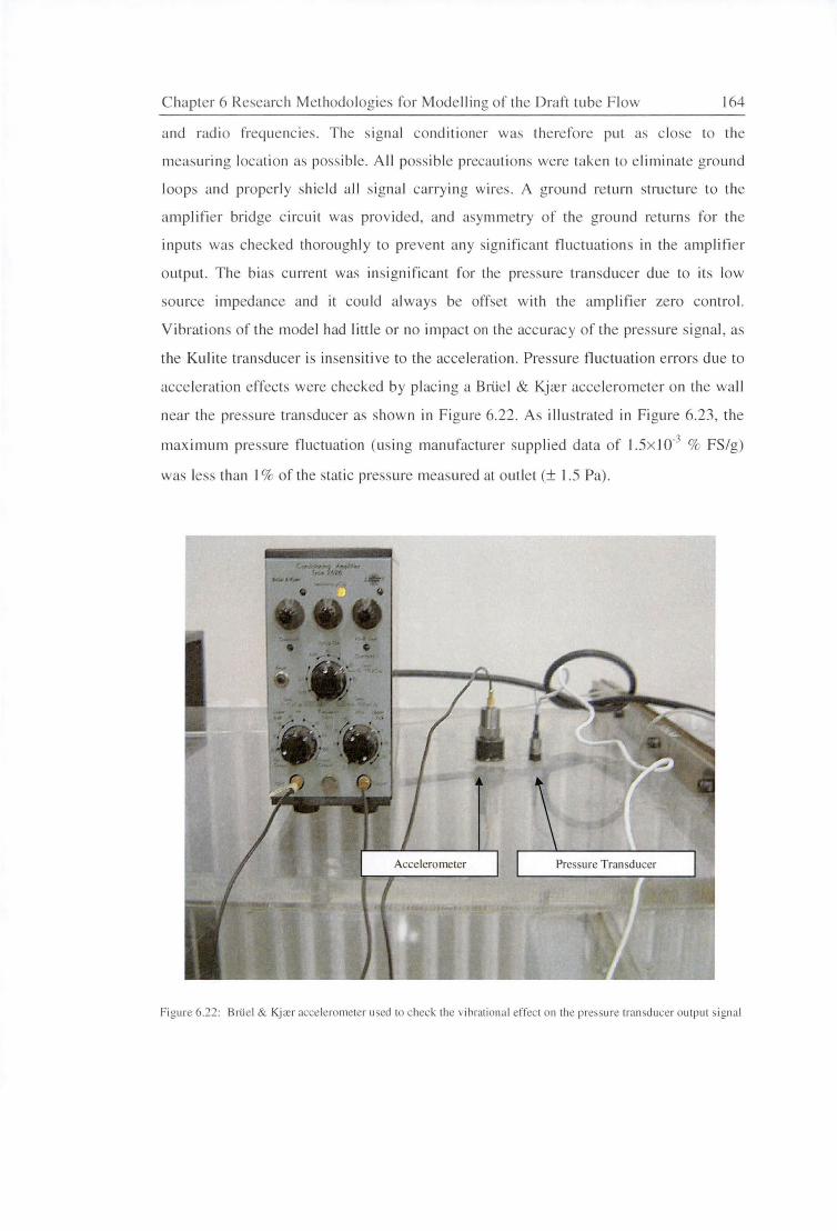
Chapter 6 Re earch Methodologies for Modelling of the Draft tube Flow 164
and radi o frequencies. The ignal conditi oner was therefore put as close to the
measuring locati on as poss ible. All possible precauti ons were taken to eliminate ground
loo ps and properl y shield all signal carrying wire . A ground return structure to the
amplifier bridge circuit was prov ided, and asymmetry of the ground returns fo r the
inputs was checked thoroughl y to prevent any significant fluctuati ons in the amplifier
output. The bias current was insignificant for the pressure transducer due to its low
source impedance and it could always be offset with the amplifier zero cont ro l.
Vibrations of the model had little or no impact on the accuracy of the pressure signal, as
the Kulite transducer is insensitive to the accelerati on. Pressure flu ctuation errors due to
accelerati on effects were checked by pl ac ing a Bri.iel & Kj rer accelerometer on the wall
near the pre sure transducer as shown in Figure 6.22. A illustrated in Figure 6.23, the
max imum pre sure fluctuati on (using manu fac turer supplied data of l.Sx 10-3 % FS/g)
was less than 1 % of the stati c pressure measured at outlet (± 1.5 Pa).
Pres ure T ransducer
Figure 6.22: BrUcl & Kjrer accelerometer used to check the vibrational effect on the pressure transducer output signa l
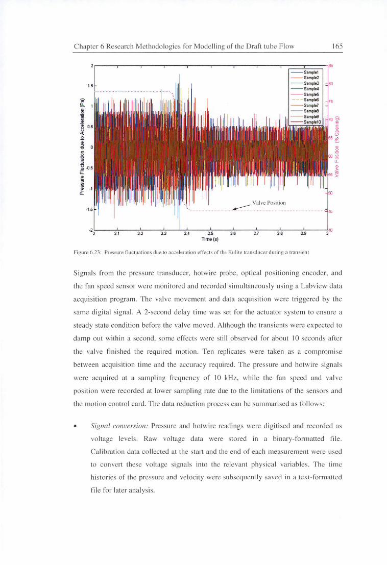
C hapte r 6 Research M ethodologies fo r Modelling of the Draft tube Flow
roQ;;. c: 0 .,,, ~ Cl)
1.5
~ 0.5 u <(
.8 Cl)
-5 a c: 0
·~ OJ ;3 ~ -0.5 u:: ~ :::i
"' ~ -1 0.
·1.5
165
75
·22~~~2~.,~~-2~.2~~-2~.3~~~2 .• ~~~2.~5~~-2~.6~~-2~.7~~-2~.8~~~2.~9~~~3~
Time (s)
Figure 6.23: Pressure flu ctuations due to accelera tion effects of the Kul ite transducer durin g a transient
Signals from the pressure tran sducer, hotwire probe, optical positioning encoder, and
the fan speed sensor were monitored and recorded simu ltaneously us ing a Labview data
acquisiti on program. The valve movement and data acqui siti on were triggered by the
same di gital s ignal. A 2-second de lay time was set fo r the actuator syste m to ensure a
steady state cond ition before the valve moved. Although the transients were expected to
damp out within a second, some effec ts were still observed for about I 0 seconds after
the valve fin ished the required motion. Ten replicates were taken as a compromise
between acqui siti on time and the accuracy required. The pressure and hotwire signa ls
were acquired at a sampling frequency of 10 kHz, while the fan speed and valve
position were recorded at lower sampling rate due to the limitati ons of the sensors and
the moti on control card. The data reducti on process can be summari sed as foll ows:
• Signal conversion: Pressure and hotwire readings were di giti sed and recorded as
vo ltage levels. Raw voltage data were stored in a binary-fo rmatted fil e.
Calibration data co llected at the start and the end of each measurement were used
to convert these voltage s ignals in to the relevant phys ical vari ables . The time
hi stories o f the pressure and ve locity were subsequentl y saved in a tex t- fo rmatted
fil e for later analys is.
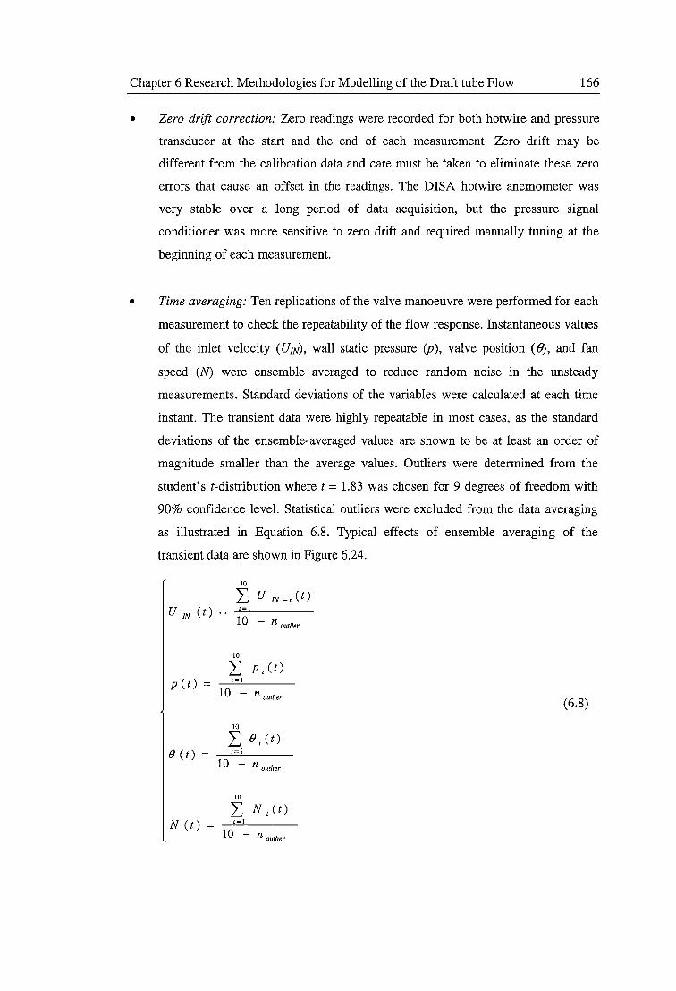
Chapter 6 Research Methodologies for Modelling of the Draft tube Flow 166
• Zero drift correction: Zero readings were recorded for both hotwire and pressure
transducer at the start and the end of each measurement. Zero drift may be
different from the calibration data and care must be taken to eliminate these zero
errors that cause an offset in the readings. The DISA hotwire anemometer was
very stable over a long period of data acquisition, but the pressure signal
conditioner was more sensitive to zero drift and required manually tuning at the
beginning of each measurement.
• Time averaging: Ten replications of the valve manoeuvre were performed for each
measurement to check the repeatability of the flow response. Instantaneous values
of the inlet velocity ( UJN), wall static pressure (p ), valve position ( B), and fan
speed (N) were ensemble averaged to reduce random noise in the unsteady
measurements. Standard deviations of the variables were calculated at each time
instant. The transient data were highly repeatable in most cases, as the standard
deviations of the ensemble-averaged values are shown to be at least an order of
magnitude smaller than the average values. Outliers were determined from the
student's t-distribution where t = 1.83 was chosen for 9 degrees of freedom with
90% confidence level. Statistical outliers were excluded from the data averaging
as illustrated in Equation 6.8. Typical effects of ensemble averaging of the
transient data are shown in Figure 6.24.
10
L UIN-1(t)
U IN (t) = 1=1
10 - n outlier
10
'L p I (t) p ( t) = 1=1
10 - n outlter (6.8)
10
'L fJ,(t) (J ( t) z=l
10 - n outlier
10
'L NI (t) N (t) i=l
10 - n outlier
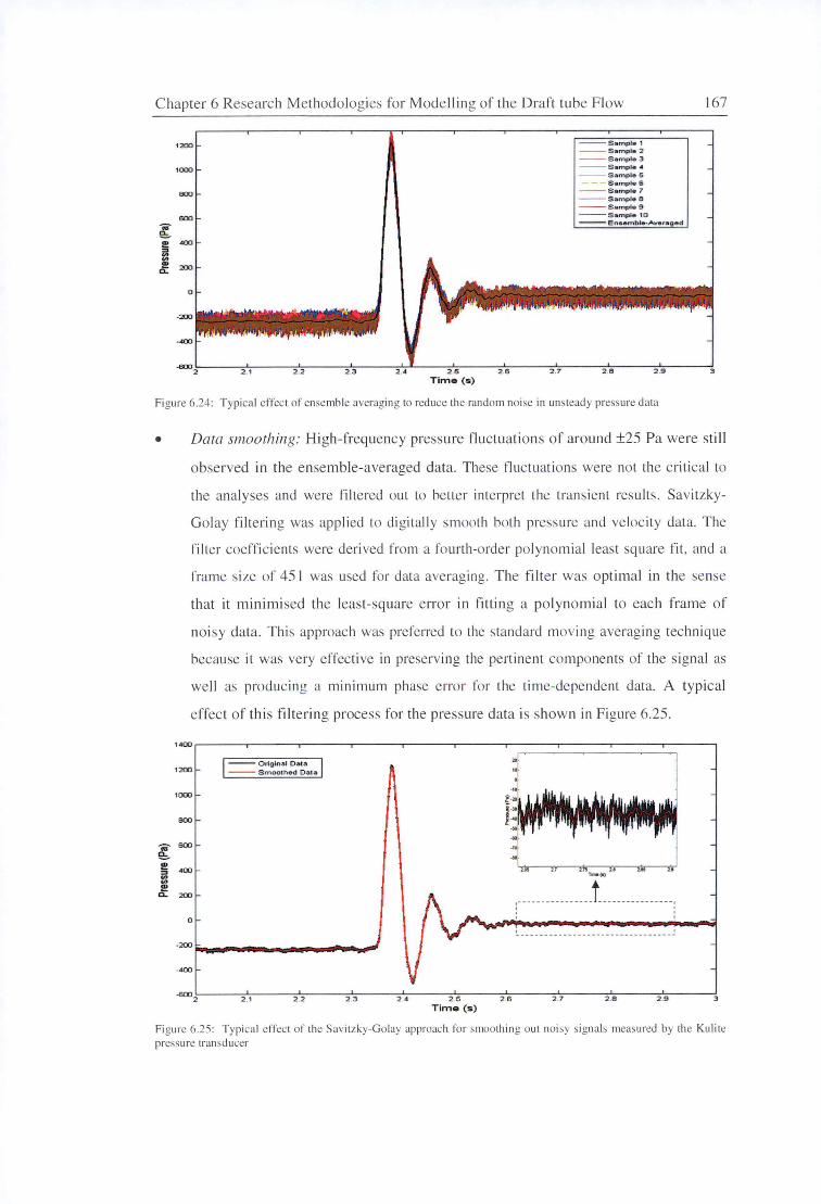
C hapte r 6 Research M ethodo logies for Mode l! ing of the D raft tube Flow
.... e:.. I!! ::>
"' "' ... 0:
1200
1000
OOO
600
400
200
0
-200
-400
2 .4 2 .5 Time (s)
- - S•mpl•1 --S•mple2 - - S•mpl•3 --Sample A
--Sample5 -- Sample 6 --Sample 7 --SampleS --Sample9 --sample 10 -- Ensemble-Averaged
2 .6 2 .7 2 .8 2 .9
Figure 6.24 : Typical effec t of ensemble averaging to red uce the random noise in unsteady pressure data
167
3
• Data smoothing: High-frequency pressure fluctuations of a round ±25 Pa we re still
observed in the ensemble-averaged data . The e fluctuations were not the c riti cal to
the analyses and were filte red out to be tter inte rpret the transient results. Sav itzky
Golay filte ring was app lied to di gitall y smooth both pressure and ve loc ity data. The
filter coeffic ients were derived from a fo urth-order polynomi al least square fit , and a
fra me size of 451 was used fo r data averaging. The filte r was optima l in the sense
that it minimi sed the least-square e rror in fittin g a po lyno mial to each frame of
no isy data . This approach was preferred to the standard moving averag ing technique
because it was very effective in preserving the pertinent co mponents of the s igna l as
we ll as produc in g a minimum phase e rro r fo r the time-dependent data. A typical
effect o f this fi lte ring process for the pressure data is shown in Figure 6.25.
1400
1200 -- Original D ata -- Smoothed Data
1000
OOO
"" 600
e,_ I!! 400 ::>
"' "' I!! a.. 200
0
-200
-400
-6002 2 . 1 2 .2 2 .3 2 .4 2 .5 Time (s)
2 .6
!- -- -- -------- -_ _t_ ----------- -- -;
' ' -- ---- ---- --- -- --- -- -- ---- -- -- --- -
2 .7 2 .B 2 .9 3
Figure 6 .25: Typical effect of the Savitzky-Golay approac h fo r smoothing out noisy signa ls measured by the Kulite pre ure transducer

Chapter 6 Research Methodologies for Modelling of the Draft tube Flow 168
6.3 Numerical Flow Modelling
The three-dimensional flow modelling of the draft tube geometry using Computational
Fluid Dynamics (CPD) techniques is presented here. The Section mcludes a brief
description of the commercial fimte-volume code ANSYS CFX. Issues involved in the
simplification of flow domains, meshing of physical geometry, modelling of fluid
turbulence, selection of appropriate boundary condition, and modelling of transient flow
are discussed in detail. Grid resolution and turbulence models chosen from the best
steady-flow predictions will also be applied in the transient-flow simulations. Steady
flow results for the draft tube model will be given in Chapter 7, while the transient-flow
results will be presented in Chapter 8. CPD solutions for the transient flow operations
will also be evaluated against simple models based on the one-dimensional momentum
equation and two-dimensional unsteady stall analysis.
6.3.1 Code Description
The commercial finite-volume code ANSYS CFX 10 was used to model the draft tube
flow. ANSYS CFX employs an unstructured, coupled implicit, pressure-based
numerical solution strategy. The flow domain is discretised into finite control volumes
and all relevant quantities in the governing equations are integrated and conserved over
each control volume. Rhie and Chow [156] interpolation is applied to overcome the
problem of checkerboard oscillations when the pressure and velocity are collocated. The
diffusion terms in the governing equations are calculated based on an element shape
function, whereas the convection terms are computed using a second-order upwind
differencing scheme. In the unsteady flow simulation, transient terms are approximated
using a fully implicit, second-order backward Euler scheme. The resulting coupled and
non-linear equations are linearised and assembled into a solution matrix using a fully
implicit approach. To improve the convergence rate, the linearised equations are solved
iteratively using an algebraic multi-grid (AMG) accelerated Incomplete Lower Upper
(ILU) factorisation technique. The convergence of the solution is judged from the
normalized residual of each solution variable [4].
All simulations were run in parallel via the Message Passing Interface (MPI) on a
multiple-processor SGI machine. Turbulence closure was achieved by applying the

Chapter 6 Researc h Methodo logies for M ode lli ng of the Draft tube F low 169
s imple eddy-viscos ity or more sophi sticated Reynolds stress model First-order
approx imati on is used for the time de ri vati ve of turbulence quantities to ensure bounded
so lution for a ll turbul ence quantities. Scalable wall functions and a n automatic near
wall treatment that a llows for a smooth shi ft from low-Reynolds numbe r form to the
wal 1 function formulation were e mployed to model the flo w near wall s.
6.3.2 Geometry and Flow Domain
The flow domain for the current CFD study is based on the 1 :27.1-scale laboratory
mode l, a nd the geometric shape of which is closely similar to the ex isting draft tube
used in the Mackinto h power plant. Mode lling of the turbine d raft tube at full- scale
Reynold numbers was not practical for thi s analys is due to large a mounts of
computational time and resources required to get re liable and consistent results. The
difficulty in obtaining detailed measure ment data to validate the CFO mode l in the full
scale fi e ld tes ts was another majo r reason for employing laboratory-s ize model in the
CFO s imulati on. Apart from the scale effects, there are some s light differences between
the shapes of the full- scale prototype and CFO model. The tiny corner fill et in the
rectangular secti on of the draft tube and the sli ver surface below the inlet cone were
not mode ll ed due to meshing difficulti es. The support pier dow nstream of the draft tube
was a lso exc luded for simplicity. The flo w domain has been rotated 4° about the inlet
pl ane to make it identical to the labora tory model. Reasons for thi modificali on we
prev ious ly stated in Section 6.2. l . 1.
Inlet Ex tended Region
~
Draft lube Model
Outnow Oullel Extended Region ~
z
Figure 6.26: Flow domain of the drafl tube model used in the CFO simulations (image is obtained from ANSYS CFX-Pre)

Chapter 6 Research Methodologies for Modelling of the Draft tube Flow 170
As shown in Figure 6.26, the inlet and outlet planes of the draft tube have been
extended to the parallel planes of 5-inlet diameters and 5-outlet heights away from their
original locations to minimise the influence of boundary locations on the solution. The
meshing issues that arose from these boundary extensions are discussed in the next
Section. The entire flow field was calculated even though the physical geometry is
symmetrical about its half plane. This was done to account for any possible flow
asymmetry due to the transient operations or the unsteady flow physics of the draft tube.
6.3.3 Mesh Generation
Mesh generation is an essential first step in numerical flow solutions. A poor quality
mesh can adversely affect the stability and accuracy achieved. Detailed descriptions of
the most popular meshing technologies and their numerical implementations are given
in the books of Liseikin [66] and Thompson et al. [126]. A survey of the recent
development m the mesh generation technologies is presented in references [90, 155].
Significant problems were encountered in the meshing phase of the CPD simulations,
and three different commercial mesh generation packages (ANSYS CFX-Mesher
version 10.0, ICEM CPD version 10.0.1, and Pointwise Gridgen version 15.02) were
tested as a result. ICEM CPD was finally chosen because of its ability to quickly
produce a hexahedral mesh using multi-block strategy and its compatibility with the
current unstructured ANSYS CFX solver code. The integration of CPD analyses with
the present complex geometric model proved a time-consuming and challenging task.
Overall, the meshing problems faced in this work are caused by the complex geometry
and the limitations of the wall distance imposed by ANSYS CFX as part of its
turbulence modelling and near-wall treatment. A three-dimensional model was first
created in the CAD modelling package (Solid Edge version 15) and then imported to
ICEM CPD through an IGES translator. This required extensive geometry cleanups
before a mesh could be created. Sliver surfaces with strong curvature, filleting around
the corners, and the large streamwise variation of the draft tube cross-sectional aspect
ratio create a geometry that is difficult to mesh. Many of the strategies tried for meshing
this flow region were found to be problematic.

Chapter 6 Research Methodologies for Modelling of the Draft tube Flow 171
Bergstrom [15] reports similar meshing problem for a Kaplan-turbine draft tube when
dealing with IGES-based CAD geometry. The restructuring and grouping of the internal
solids into a single block may eliminate this problem. However, this approach was
difficult to apply in the current study due to the complexity of the geometry and the lack
of direct translation between the CAD and meshing software. The built-in geometry
creation tools in the current version of ICEM CPD and ANSYS CFX Mesher are still
insufficient for an accurate solid modelling of the three-dimensional geometry. Besides,
it is essential to divide the domain into several sections in order to correctly capture the
important geometric feature of each draft tube section.
The use of proper wall element size is vitally important for the turbulent flow studied
here. The wall elements may fail to work correctly if their sizes are either too large or
too small. The turbulence model, flow operating conditions, and the availability of the
computational resources all significantly influence the size of the wall elements to be
used in the CPD simulation. The wall element size can be examined via a dimensionless
wall distance Y + and the value is obtained using trial-and-error approach. To correctly
resolve the boundary layer flow and the wall shear stress, relatively thin wall elements
are required.
The extension of the draft tube inlet and outlet planes resulted in a large number
(approximately half) of the elements being placed outside the draft tube. To improve
computational efficiency, the number of extension nodes was reduced by gradually
increasing the mesh sizes through an exponential growth function when the elements
were located away from the inlet and outlet regions. The element volume ratio was kept
below 5 as a compromise between the number of nodes used (computational time is
proportional to the square of the number of nodes) and the stability of the numerical
solution [ 4].

Chapter 6 Research Methodologies for Modelling of the Draft tube Flow 172
6.3.3.l Mesh Type and Topology
Unlike some simple linear geometries, the strong curvature of the draft tube can incur
more adverse pressure gradients in which flow separation may occur. Mesh resolution
will play an important role in correctly modelling the scale of this geometry. Accurate
simulation of the flow phenomena in the draft tube requires computational grids that
simultaneously capture the geometric curvature and discontinuities in the solution [15].
Element type and mesh topology can have a considerable impact on coarse grid
solutions, and may affect the mesh resolution required to achieve a grid-independent
solution [103].
A non-uniform hexahedral mesh generated by ICEM CPD was used for the current
simulations because it is best suited for adequately resolving the near-wall region of the
flow field. Phillipson [95] performed a CPD validation check on the CFX solver using
various mesh types and found that about 4 times as many elements are required to
achieve the same accuracy when a tetrahedral mesh is employed. The discretisation
error is larger for tetrahedral elements because the grid 1s highly non-orthogonal and the
equations need extra terms for tetrahedral mesh. A non-uniform mesh was also found to
outperform a uniform mesh in terms of the computer resources needed to obtain
solutions of the same accuracy [95]. Better results are generally obtained for internal
flow problems when the elements are more distributed around the walls than in the
centre of the flow passage.
Hexahedral elements do not present any significant problem for meshing a non
manifold geometric domain that has small angles on the surfaces. Although a tetrahedral
mesh is relatively easier to generate for a complex geometry than a hexahedral mesh, it
does not always mesh well domains with small angles, especially if these domains are
non-manifold (irrespective of whether Delaunay, Advancing Front, or Octree methods
are used) [113]. In fact, no meshing algorithm up to date can guarantee a triangulation
of a domain without creating any small angles that are not already present in the input
domain [113]. To achieve accurate solutions and good convergence properties on
tetrahedral meshes, special discretisation techniques and a large number of cells are
needed. None of these remedies is optimal. A code is more complicated and difficult to

Chapter 6 Research Methodologies for Modelling of the Draft tube Flow 173
maintain, and the memory and computing time requirements for the simulations are
increased, with the use of tetrahedral meshes.
The Octree meshing method [90] adopted by ICEM CPD tends to deteriorate the
tetrahedral mesh quality when the boundaries are approached. Further mesh smoothing
does not seem to improve the quality, even though many smoothing steps have been
assigned. The advancing front and Delaunay meshing algorithms used in the ANSYS
CFX-Mesher are unable to distribute the nodes uniformly across the non-manifold
surfaces. Thousands of nodes are placed on the smaller surface, and little control has
been offered in the current package to resolve this problem. Another drawback is that
mesh refinement studies cannot be properly conducted for unstructured tetrahedral
meshes because the refined elements are not nested subdivisions of the coarsest mesh (a
property that cannot be guaranteed for meshes generated using unstructured tetrahedral
meshing methods). These limitations resulted in a hexahedral mesh being used for the
current research.
A good blocking strategy is essential for the creation of a hexahedral mesh [152]. A
multi-block 0-grid topology was used to map the elements onto curved sections of the
geometry because it provided optimal skew angles for control volumes around the wall
boundary. The use of multi-block grid arrangement improved the orthogonality of the
hexahedral elements near the curved diffusing bend. Skewed elements must be avoided
as they always cause convergence difficulties and induce errors in the solution. Zhu et
al. [152] identified various issues about blocking strategies for CPD simulations and
concluded that the number of iterations needed for a multi-block grid to converge is
essentially the same as that for single block. The thickness of the near-wall grid was
also found to have significant impact on the solution convergence rate1•
1 Only one paper was found in literature search that discusses the issues of blocking strategy, but the examiner comments that "The finding of Zhu et al. [152] zs not a general observation. Slower convergence has been observed by the examiner's research group when a multz-block grid is used in place of a single-block grid, provided that the geometry of the computatzonal domain is such that the use of a single block instead of multiple blocks does not adversely affect the skewness of the grzd elements. Whzle the computations are typically zmplzcit within each block, the algorithm is explicit at the block level in that the blocks are computed separately (within each outer iteratzon) before data exchange amongst the blocks at the block interfaces is performed. This explicitness tends to reduce the convergence rate."

C hapter 6 Research Methodologies fo r Mode lling of the D raft tube F low 174
6.3.3.2 Mesh Quality
A reas of poor mesh can have a detrimenta l effec t on the overall so lution [41 ]. Qua lity
assessment of the hexahedral grid is a re lati vely stra ightforwa rd task, and two different
methods can be u ed [ 1 O]. The eas iest way is to visua ll y inspect the pl ots of the
hexahedra l mes h on the boundary surface or at various cross-sectiona l planes, a show n
in F igures 6.27 and 6.28. Regions of poor mesh quality can be identified and corrected
by manua ll y adjusting the vertices of the control vo lumes.
Figure 6.27: Visuali sa ti on of surface mesh e lements for the draft tube geometry (image ex trac ted from ANSYS CFX-Post with medium mesh size as specified in Tab le 6. 1)
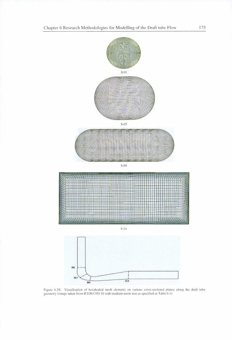
C hapter 6 Research Methodo logies fo r Modelling of the D raft tube Flow 175
s 0 1
s 05
S 09
- -s 14
SOI
S09 Sl4
Figure 6.28: Visuali sation of hexahedral mesh elements on various cross-sec tional planes along the draft tube geometry (image taken from ICEM CFO 10 with medium mesh size as specifi ed in Table 6. 1)
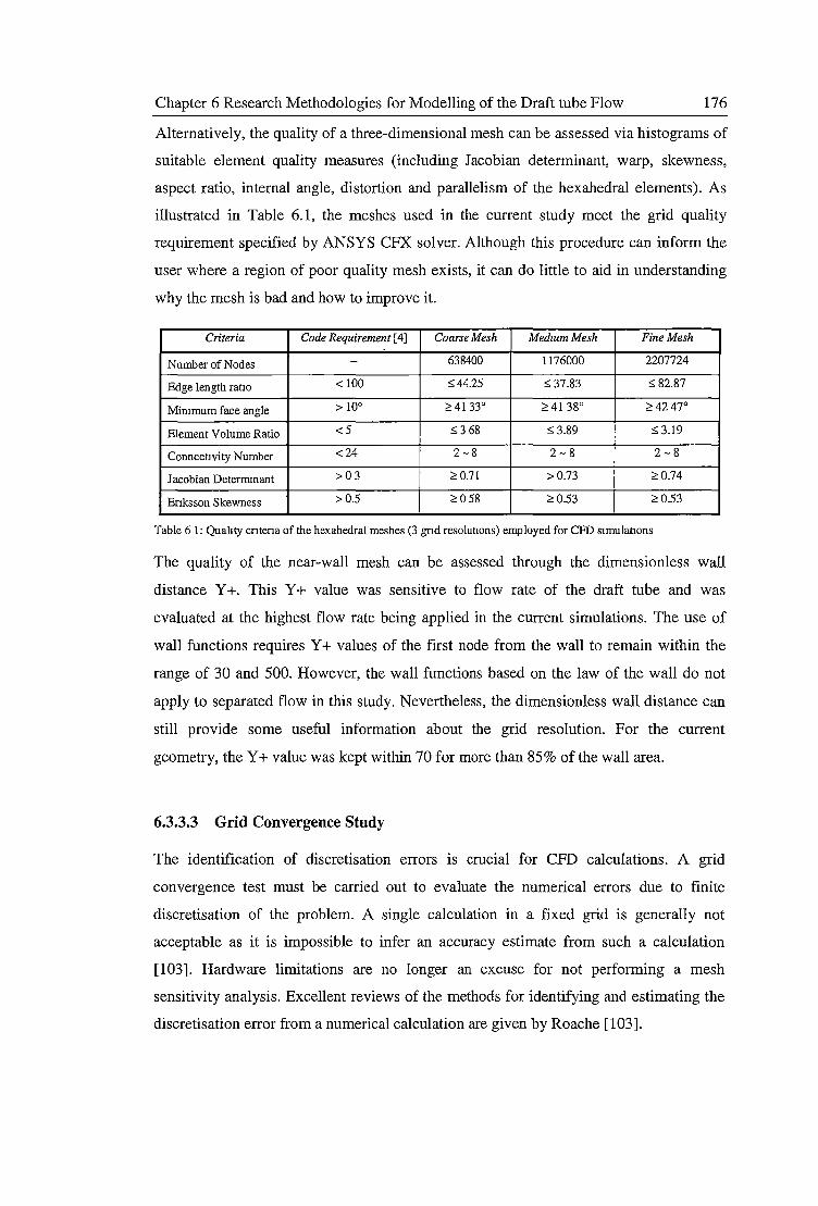
Chapter 6 Research Methodologies for Modelling of the Draft tube Flow 176
Alternatively, the quality of a three-dimensional mesh can be assessed via histograms of
suitable element quality measures (including Jacobian determinant, warp, skewness,
aspect ratio, internal angle, distortion and parallelism of the hexahedral elements). As
illustrated in Table 6.1, the meshes used in the current study meet the grid quality
requirement specified by ANSYS CFX solver. Although this procedure can inform the
user where a region of poor quality mesh exists, it can do little to aid in understanding
why the mesh is bad and how to improve it.
Criteria Code Requirement [ 4] Coarse Mesh MedzumMesh Fine Mesh
Number of Nodes - 638400 1176000 2207724
Edge length rat10 < 100 :::;44.25 :::; 37.83 :::;82.s1
Mimmum face angle > 10° ;:: 41 33° ;:: 41 38° ;::4247°
Element Volume Ratio <5 :::; 3 68 :::; 3.89 :::; 3.19
Connectivity Number <24 2-8 2-8 2-8
Jacobian Determmant >03 ;:: 0.71 >0.73 ;::0.74
Eriksson Skewness > 0.5 ;::o 58 ;::Q.53 ;:: 0.53
Table 6 1: Quahty cntena of the hexahedral meshes (3 gnd resolutions) employed for CPD simulations
The quality of the near-wall mesh can be assessed through the dimensionless wall
distance Y +. This Y + value was sensitive to flow rate of the draft tube and was
evaluated at the highest flow rate being applied in the current simulations. The use of
wall functions requires Y + values of the first node from the wall to remain within the
range of 30 and 500. However, the wall functions based on the law of the wall do not
apply to separated flow in this study. Nevertheless, the dimensionless wall distance can
still provide some useful information about the grid resolution. For the current
geometry, the Y +value was kept within 70 for more than 85% of the wall area.
6.3.3.3 Grid Convergence Study
The identification of discretisation errors is crucial for CPD calculations. A grid
convergence test must be carried out to evaluate the numerical errors due to finite
discretisation of the problem. A single calculation in a fixed grid is generally not
acceptable as it is impossible to infer an accuracy estimate from such a calculation
[103]. Hardware limitations are no longer an excuse for not performing a mesh
sensitivity analysis. Excellent reviews of the methods for identifying and estimating the
discretisation error from a numerical calculation are given by Roache [103].
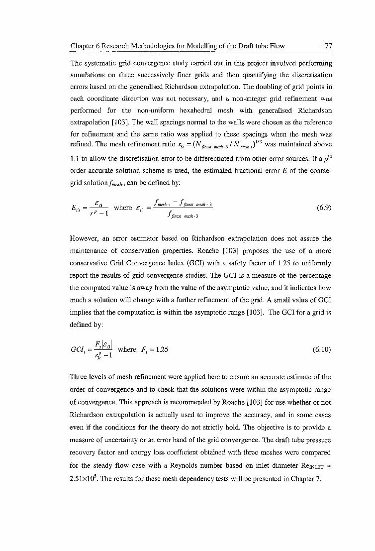
Chapter 6 Research Methodologies for Modelling of the Draft tube Flow 177
The systematic grid convergence study carried out in this project involved performing
simulations on three successively finer grids and then quantifying the discretisation
errors based on the generalised Richardson extrapolation. The doubling of grid points in
each coordinate direction was not necessary, and a non-integer grid refinement was
performed for the non-uniform hexahedral mesh with generalised Richardson
extrapolation [103]. The wall spacings normal to the walls were chosen as the reference
for refinement and the same ratio was applied to these spacings when the mesh was
refined. The mesh refinement ratio r31 = (N finest mesh-3 IN mesh-,)113 was maintained above
1.1 to allow the discretisation error to be differentiated from other error sources. If a pth
order accurate solution scheme is used, the estimated fractional error E of the coarse
grid solution! mesh-1 can be defined by:
E - 813 h - fmesh-1 - !finest mesh- 3 13 - -P-- w ere 8 13 -
r - I !finest mesh-3
(6.9)
However, an error estimator based on Richardson extrapolation does not assure the
maintenance of conservation properties. Roache [103] proposes the use of a more
conservative Grid Convergence Index (GCI) with a safety factor of 1.25 to uniformly
report the results of grid convergence studies. The GCI is a measure of the percentage
the computed value is away from the value of the asymptotic value, and it indicates how
much a solution will change with a further refinement of the grid. A small value of GCI
implies that the computation is within the asymptotic range [ 103]. The GCI for a grid is
defined by:
GCJ = Fsl8131 where F = 1.25
i r.P-I s 31
(6.10)
Three levels of mesh refinement were applied here to ensure an accurate estimate of the
order of convergence and to check that the solutions were within the asymptotic range
of convergence. This approach is recommended by Roache [103] for use whether or not
Richardson extrapolation is actually used to improve the accuracy, and in some cases
even if the conditions for the theory do not strictly hold. The objective is to provide a
measure of uncertainty or an error band of the grid convergence. The draft tube pressure
recovery factor and energy loss coefficient obtained with three meshes were compared
for the steady flow case with a Reynolds number based on inlet diameter ReINLET ""
2.5lx105• The results for these mesh dependency tests will be presented in Chapter 7.
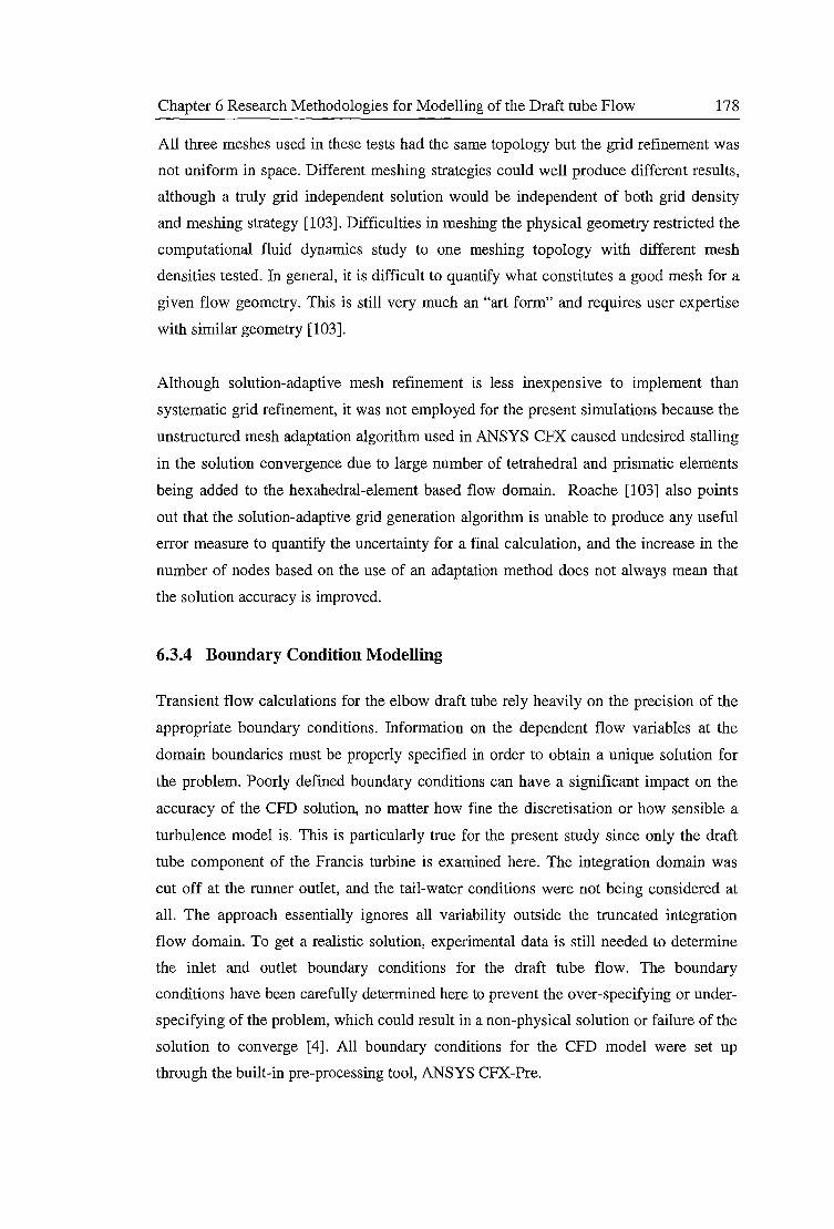
Chapter 6 Research Methodologies for Modelling of the Draft tube Flow 178
All three meshes used in these tests had the same topology but the grid refinement was
not uniform in space. Different meshing strategies could well produce different results,
although a truly grid independent solution would be independent of both grid density
and meshing strategy [103]. Difficulties in meshing the physical geometry restricted the
computational fluid dynamics study to one meshing topology with different mesh
densities tested. In general, it is difficult to quantify what constitutes a good mesh for a
given flow geometry. This is still very much an "art form" and requires user expertise
with similar geometry [103].
Although solution-adaptive mesh refinement is less inexpensive to implement than
systematic grid refinement, it was not employed for the present simulations because the
unstructured mesh adaptation algorithm used in ANSYS CFX caused undesired stalling
in the solution convergence due to large number of tetrahedral and prismatic elements
being added to the hexahedral-element based flow domain. Roache [103] also points
out that the solution-adaptive grid generation algorithm is unable to produce any useful
error measure to quantify the uncertainty for a final calculation, and the increase in the
number of nodes based on the use of an adaptation method does not always mean that
the solution accuracy is improved.
6.3.4 Boundary Condition Modelling
Transient flow calculations for the elbow draft tube rely heavily on the precision of the
appropriate boundary conditions. Information on the dependent flow variables at the
domain boundaries must be properly specified in order to obtain a unique solution for
the problem. Poorly defined boundary conditions can have a significant impact on the
accuracy of the CFD solution, no matter how fine the discretisation or how sensible a
turbulence model is. This is particularly true for the present study since only the draft
tube component of the Francis turbine is examined here. The integration domain was
cut off at the runner outlet, and the tail-water conditions were not being considered at
all. The approach essentially ignores all variability outside the truncated integration
flow domain. To get a realistic solution, experimental data is still needed to determine
the inlet and outlet boundary conditions for the draft tube flow. The boundary
conditions have been carefully determined here to prevent the over-specifying or under
specifying of the problem, which could result in a non-physical solution or failure of the
solution to converge [ 4]. All boundary conditions for the CFD model were set up
through the built-in pre-processing tool, ANSYS CFX-Pre.
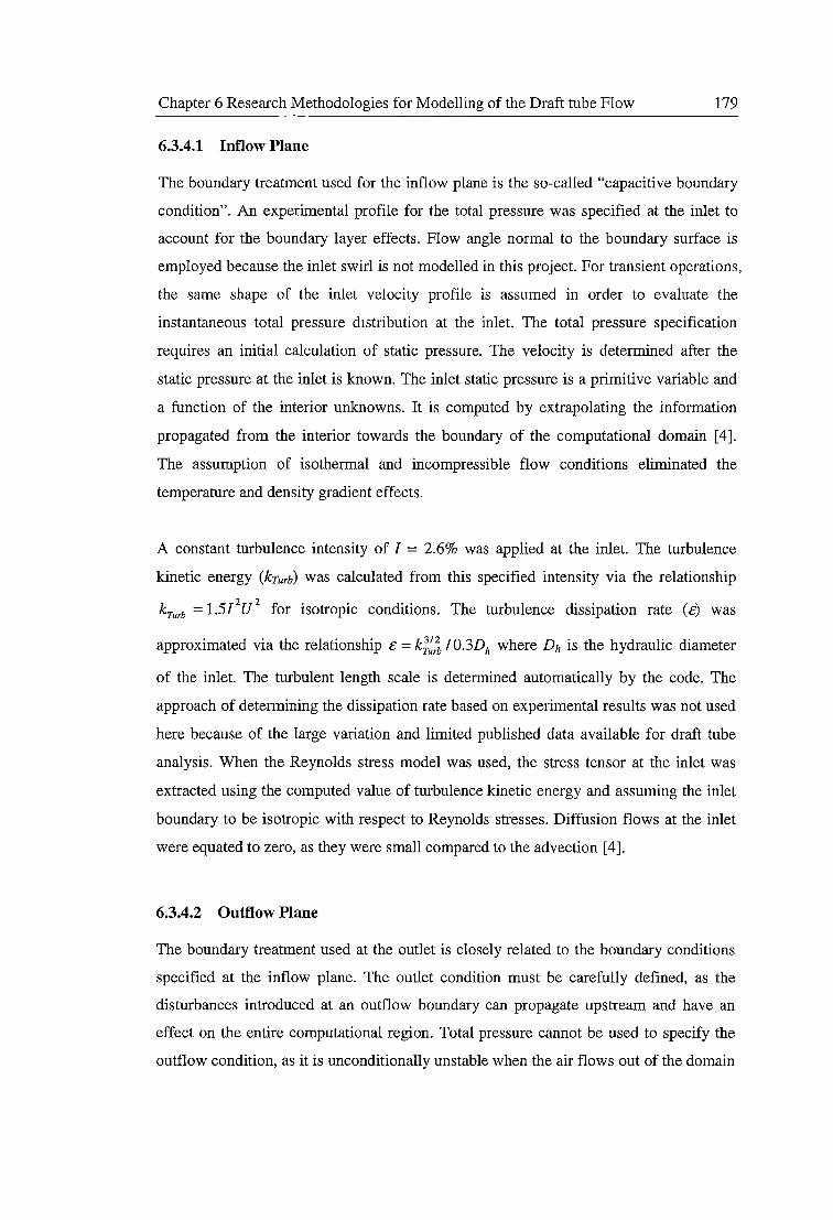
Chapter 6 Research Methodologies for Modelling of the Draft tube Flow 179
6.3.4.1 Inflow Plane
The boundary treatment used for the inflow plane is the so-called "capacitive boundary
condition". An experimental profile for the total pressure was specified at the inlet to
account for the boundary layer effects. Flow angle normal to the boundary surface is
employed because the inlet swirl is not modelled in this project. For transient operations,
the same shape of the inlet velocity profile is assumed in order to evaluate the
instantaneous total pressure distribution at the inlet. The total pressure specification
requires an initial calculation of static pressure. The velocity is determined after the
static pressure at the inlet is known. The inlet static pressure is a primitive variable and
a function of the interior unknowns. It is computed by extrapolating the information
propagated from the interior towards the boundary of the computational domain [ 4].
The assumption of isothermal and incompressible flow conditions eliminated the
temperature and density gradient effects.
A constant turbulence intensity of I = 2.6% was applied at the inlet. The turbulence
kinetic energy (krurb) was calculated from this specified intensity via the relationship
kTurb = l.5/2U
2 for isotropic conditions. The turbulence dissipation rate (£) was
approximated via the relationship £ = ki:,~ I 0.3Dh where Dh is the hydraulic diameter
of the inlet. The turbulent length scale is determined automatically by the code. The
approach of determining the dissipation rate based on experimental results was not used
here because of the large variation and limited published data available for draft tube
analysis. When the Reynolds stress model was used, the stress tensor at the inlet was
extracted using the computed value of turbulence kinetic energy and assuming the inlet
boundary to be isotropic with respect to Reynolds stresses. Diffusion flows at the inlet
were equated to zero, as they were small compared to the advection [4].
6.3.4.2 Outflow Plane
The boundary treatment used at the outlet is closely related to the boundary conditions
specified at the inflow plane. The outlet condition must be carefully defined, as the
disturbances introduced at an outflow boundary can propagate upstream and have an
effect on the entire computational region. Total pressure cannot be used to specify the
outflow condition, as it is unconditionally unstable when the air flows out of the domain
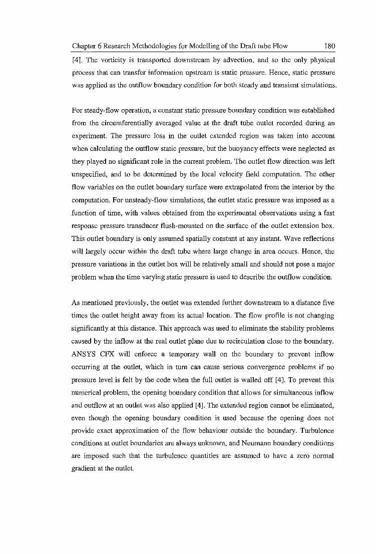
Chapter 6 Research Methodologies for Modelling of the Draft tube Flow 180
[4]. The vorticity is transported downstream by advection, and so the only physical
process that can transfer information upstream is static pressure. Hence, static pressure
was applied as the outflow boundary condition for both steady and transient simulations.
For steady-flow operation, a constant static pressure boundary condition was established
from the circumferentially averaged value at the draft tube outlet recorded during an
experiment. The pressure loss in the outlet extended region was taken into account
when calculating the outflow static pressure, but the buoyancy effects were neglected as
they played no significant role in the current problem. The outlet flow direction was left
unspecified, and to be determined by the local velocity field computation. The other
flow variables on the outlet boundary surface were extrapolated from the interior by the
computation. For unsteady-flow simulations, the outlet static pressure was imposed as a
function of time, with values obtained from the experimental observations using a fast
response pressure transducer flush-mounted on the surface of the outlet extension box.
This outlet boundary is only assumed spatially constant at any instant. Wave reflections
will largely occur within the draft tube where large change in area occurs. Hence, the
pressure variations in the outlet box will be relatively small and should not pose a major
problem when the time varying static pressure is used to describe the outflow condition.
As mentioned previously, the outlet was extended further downstream to a distance five
times the outlet height away from its actual location. The flow profile is not changing
significantly at this distance. This approach was used to eliminate the stability problems
caused by the inflow at the real outlet plane due to recirculation close to the boundary.
ANSYS CFX will enforce a temporary wall on the boundary to prevent inflow
occurring at the outlet, which in turn can cause serious convergence problems if no
pressure level is felt by the code when the full outlet is walled off [ 4]. To prevent this
numerical problem, the opening boundary condition that allows for simultaneous inflow
and outflow at an outlet was also applied [4]. The extended region cannot be eliminated,
even though the opening boundary condition is used because the opening does not
provide exact approximation of the flow behaviour outside the boundary. Turbulence
conditions at outlet boundaries are always unknown, and Neumann boundary conditions
are imposed such that the turbulence quantities are assumed to have a zero normal
gradient at the outlet.
Chapter 6 Research Methodologies for Modelling of the Draft tube Flow 181
6.3.4.3 Wall Boundary
A smooth wall boundary condition was applied at the surfaces of the inlet extension
pipe, draft tube and the outlet extension box. A non-slip adiabatic heat transfer flow
condition was imposed at the wall. The flow immediately next to the wall assumes the
zero wall velocity. The effect of surface roughness was not studied here, even though it
may have some influence on the loss mechanism and the efficiency of the full-scale
draft tube. A logarithmic wall function relating the tangential velocity to the wall shear
stress was employed if using the £-based model for turbulence simulation. The
automatic near-wall treatment in ANSYS CFX was used when an lV-based turbulence
model was applied. Discussion of the near wall flow treatment associated with different
turbulence models will be presented in Section 6.3.5.3.
6.3.5 Turbulence and Near Wall Modelling
Turbulent fluctuations in the draft tube are always three-dimensional and unsteady, and
consist of eddying motion with a wide range of length scales. To predict the effects of
turbulence, the Reynolds Averaged Navier-Stokes (RANS) equations are solved
together with the suitable statistical turbulence models. These models are needed to
resolve the Reynolds stresses resulting from the time-averaging procedure. The use of
turbulence models significantly reduces the amount of computational effort compared to
Direct Numerical Simulation (DNS). Although Large Eddy Simulation (LES) model
and Detached Eddy Simulation (DES) model are also provided in ANSYS CFX, they
were not used in the present study because of the considerable amount of computing
resources required to get reliable results for high Reynolds number flow and
uncertainties in the fluctuating component of the inflow boundary condition [68]. The
statistical turbulence models in ANSYS CFX can be classified into two categories:
eddy-viscosity models and differential Reynolds stress models. Mathematical details of
various turbulence models can be easily found in references [4, 63, 78, 79, 104, 121,
131, 140]. The following subsections briefly highlight some important features of the
turbulence models used in the current simulations.
Chapter 6 Research Methodologies for Modelling of the Draft tube Flow 182
6.3.5.1 Eddy-Viscosity Model
Eddy-viscosity models are based on the assumption that the Reynolds stresses can be
related to the mean velocity gradients and the turbulent viscosity (µt) by the gradient
diffusion (Boussinesq) hypothesis [ 4]. The eddy-viscosity models used in the present
study are of the two-equation type where two separate scalar-transport equations are
solved for velocity and length scale in order to obtain information about the turbulent
viscosity of the flow [ 4]. The zero-equation model was not considered here because the
simple algebraic expression for the mixing length is not feasible for recirculating flow
(with strong convection and diffusion).
Eddy-viscosity models are widely used in the industry because they are relatively easy
and inexpensive to implement in the viscous solver. The extra viscosity aids stability in
the numerical algorithms. However, the anisotropy (i.e. normal stresses are different in
nature) and history effects are always neglected. Only one Reynolds stress can be
represented accurately in this type of model. The standard k-£ model [4], RNG k-£
model [4], Wilcox's k-OJ model [140], and Menter's Shear-Stress-Transport (SST)
model [78] were all examined in the present study. These models were employed in
their standard configurations, with various empirical constants set to values proposed by
their respective developers.
The standard k-Emodel assumes that the turbulent viscosity is linked to the turbulence
kinetic energy k and turbulence dissipation rate £. This model describes the mechanisms
that affect the turbulence kinetic energy of the flow. The values of k and £ are obtained
directly by solving the differential transport equations for the turbulence kinetic energy
and turbulence dissipation rate. A large dissipation rate always occurs when the
production of the turbulence kinetic energy is high. The model has been extensively
validated in CFD simulations and is capable of predicting broad features of the draft
tube flow reasonably well [4]. However, care must be taken while using the k-£ model
as it is well known for its erroneous predictions of the turbulence production in strong
strain fields and its inability due to isotropic assumption to predict secondary motions
that are driven by the difference between the normal stresses [4, 79].
Chapter 6 Research Methodologies for Modelling of the Draft tube Flow 183
The RNG k-s model, which is based on renormalisation group analysis of the Navier
Stokes equations, was proposed to overcome the over-predictions of turbulence
product10n in the standard k-B model. The transport equations for turbulence production
and dissipation are the same as those for standard k-smodel, but the model constants are
different [ 4, 5]. This modification dramatically increases the turbulence dissipation for
rapid distortions, which yields lower levels of turbulence in complex geometries. The
RNG k-s model often actually underestimates the turbulence kinetic energy (less
viscous), but this will sometimes result in more realistic flow features. The trend is in
the right direction but for entirely wrong reasons [5]. It is the production of turbulence
kinetic energy that is overestimated by standard k-s model, and not the level of
dissipation underestimated. However, the changes should indeed be made for better
representation of anisotropy, and essentially of the normal stresses [ 4, 5, 106].
The Wilcox's k-OJ model assumes that the turbulence viscosity is related to the
turbulence kinetic energy k and the turbulence frequency OJ. This model is also known
as the low Reynolds number model. The details associated with its near-wall treatment
method will be discussed in Section 6.3.5.3. The values of k and OJ are obtained via the
transport equations for turbulence kinetic energy and turbulence frequency. In some
cases, the k-OJ model is superior to the k-s model in near wall layers because it does not
involve the complex non-linear damping functions required for the k-s model [ 4, 5, 78].
However, the Wilcox model is very sensitive to free-stream conditions and suffers from
a problematic wall boundary condition (where OJ tends to infinity) [140]. The solution
may vary greatly with changes in turbulent frequency specified at the inlet.
The Menter's Shear Stress Transport (SST) k-OJmodel was developed in an attempt
to resolve the sensitivity problem of the l'.iJ-equation by blending the k-co model near the
surface with the k-c. model in the outer region [4, 78]. The blending functions used in
this model are critical to the success of the method and their formulation is based on the
distance to the nearest surface and on the flow variables [ 4]. The distances of the nodes
to the nearest wall for performing blending between k-co and k-c. models are determined
via the wall-scale equation. Overall, the model has taken into account the transport of
the turbulent shear stress and may give a more accurate prediction of the onset and
amount of flow separation under strong adverse pressure gradients [78, 79]. Detailed
discussion of the SST turbulence model is given in Menter et al. [79].
Chapter 6 Research Methodologies for Modelling of the Draft tube Flow 184
Nonlinear eddy-viscosity models [5] such as the cubic k-£ model have also been
developed to reduce the model deficiency caused by isotropic assumptions, and are
expected to improve the accuracy of predictions for swirling flow. Unfortunately,
ANSYS CFX does not currently include any non-linear eddy-viscosity models, and so
they are not discussed further here.
6.3.5.2 Differential Reynolds Stress Model
The differential Reynolds stress model in ANSYS CFX uses individual differential
transport equations for the Reynolds stresses (rather than the turbulence kinetic energy)
and one transport equation for the turbulence dissipation (which is similar to the one
used for k-£ model). The turbulence transport equation for the Reynolds stress has a
term to describe the rate of change of the Reynolds stress, an advection term, a diffusion
term, a production term that creates energy from the mean flow, a dissipation term due
to viscosity acting on fluctuating velocity gradient, and a redistribution (pressure-strain)
term to transfer energy between stresses via pressure fluctuations [5]. The model does
not use an eddy-viscosity hypothesis, but has included the history-dependent non-local
effects of the flow through convection and viscous diffusion of the Reynolds stresses
[5]. As such, the model contains more turbulence physics, because the rate of
production of Reynolds stresses, advection and production terms are exact in the
equations.
The production term is a function of stress-strain products, which are sensitive to
anisotropy in the flow field (and essential for proper modelling of the streamline
curvature effects, impingement and rotation in the flow) [121]. The diffusion term is
modelled using a General Gradient Diffusion Hypothesis that assumes the rate of
Reynolds stress transport by diffusion is proportional to the gradient of the Reynolds
stress [5]. The assumption of local isotropy is used for the dissipation of the Reynolds
stresses. The model chosen for the pressure-strain correlation can either be the linear
Launder, Reece and Rodi (LRR) model [63] or the quadratic Speziale, Sarkar and
Gatski (SSG) model [121]. The wall reflection part of the pressure-strain correlation has
a net effect in the direction normal to a wall by damping the fluctuations only [5].
However, the application of a wall reflection term into a general complex geometry is
Chapter 6 Research Methodologies for Modelling of the Draft tube Flow 185
difficult, as it includes normal distances to walls. For this reason, the wall reflection
term is omitted in the CFX form of the LRR-model because the published results have
not always shown an improvement of these relatively small contributions; they
sometimes cause a degradation of the model performance [ 4, 5].
Although the Reynolds stress model contains several important features of turbulence
physics, it is seldom used in industry because it is very expensive computationally (as
six stress-transport equations and an equation for turbulence dissipation rate must be
solved). The strong nonlinearities and the lack of a turbulent viscosity in the differential
stress transport equation may degrade the numerical stability and lead to solver failure.
Many important terms in the equations (such as redistribution and dissipation of
turbulence) still require extensive modelling. Furthermore, the Reynolds stress model is
not as widely validated as the eddy-viscosity models and more research is needed to
overcome several modelling issues as stated above. ANSYS CFX also provides {J)-
based Reynolds stress models but they are not considered here due to very fine meshes
required and the inherent numerical instability.
6.3.5.3 Near-Wall Treatment
Near-wall treatment is crucial for modelling the turbulent flow in the draft tube. Non
slip boundary condition is required at the solid surface so that both mean and fluctuating
velocities vanish. This generates a very large flow gradient near the wall and suppresses
the wall-normal fluctuations in high Reynolds number flow. The viscous and turbulent
stresses are of comparable magnitude in this region. The common approach to
overcome turbulent flow problems near the wall surfaces is to use either a wall function
or a low-Reynolds-number turbulence model [4].
For turbulence models using an E-equation, the wall function approach is usually
implemented. The wall function in ANSYS CFX follows the method of Launder and
Spalding [139] by assuming a logarithmic profile between near-wall nodes and the
boundary [ 4]. This function is based on the local equilibrium of fluid turbulence. In
other words, the production and dissipation of turbulence are always assumed balanced.
This approach works well if the equilibrium assumption is reasonable, but fails in
highly non-equilibrium regions such as the recirculating flow. The standard wall
Chapter 6 Research Methodologies for Modelling of the Draft tube Flow 186
function is sensitive to the near-wall meshing, and the near-wall node should optimally
be placed in the region of 30<Y+ <500. Refming a near-wall mesh with a standard wall
function being used will not guarantee a unique solution of increasing accuracy, as the
function is not compatible with the systematic grid refinement technique [103]. For
turbulence models using iv-equations, the wall problem is tackled by solving the
turbulence transport equation right up to the boundary. The effects of molecular
viscosity are included in the coefficients of the eddy-viscosity formula and dissipation
transport equations. However, full resolution of the flow requires the near-wall node to
satisfy the condition of y+ ::; 1. The low Reynolds number model is therefore very
computationally demanding, particularly for high-Reynolds-number flows [4].
Hence, several improvements are made in ANSYS CFX to overcome the potential
problems of both the wall function and low-Reynolds-number models [4]. A scalable
wall function is employed to replace the standard wall function for all turbulence
models using E-equation. The basic idea behind this approach is to limit the value of
dimensionless wall distance Y + used in the logarithmic formulation to 11.06 so that all
mesh points are outside the viscous sub-layer and all fine mesh inconsistencies are
avoided [ 4]. At least 10 nodes are placed in the boundary layer and the upper limit for
dimensionless wall distance is kept below 100 in all cases [ 4]. For the low-Reynolds
number model, an automatic near-wall treatment is used in the code to automatically
switch the low-Reynolds-number formulation to the wall function mode, depending on
the grid resolution [ 4].
6.3.6 Initial Condition Modelling
A good initial guess can improve the convergence of a CPD solution. Initial values for
all solved variables were set as "automatic with value" in the ANSYS CFX-Pre (pre
processing tool) before starting the solver. The ANSYS CFX solver automatically reads
the initial conditions from the initial value file or uses the specified value during the
course of solution. For the steady-flow calculation, the initial variable values give the
solver a flow field from which to start its computation [ 4]. Although the convergence of
the solution is more rapidly achieved 1f sensible imtial guesses are supplied, the
converged results are not affected by the initialisation [ 4]. For transient-flow simulation,
the initial values provide the actual flow field at the instant when the CPD calculation
Chapter 6 Research Methodologies for Modelling of the Draft tube Flow 187
starts. It is essential to apply a proper initial condition for a transient simulation, as the
error may propagate in successive time steps and cause the divergence of a solution.
Hence, validated and converged steady-state solut10ns were used to provide initial
conditions for the transient simulations. The values specified should be the actual flow
field present at the beginning of the time of the simulation [ 4].
An automatic linearly varying initial condition was used to specify the velocity field in
the draft tube domain. It was generated using a weighted average of boundary condition
information from the inlet and outlet. The magnitude of the velocity was set lower than
the inlet velocity, as the flow was decelerating in the draft tube. The initial guess for the
turbulent kinetic energy was obtained using the turbulent intensity of 2.6% and the
initial velocity guess. To prevent zero turbulence kinetic energy in the domain, a
minimum clipping velocity of 0.01 m/s was employed whenever a zero initial velocity
value was found [ 4]. The static pressure was initialised in the same way as the velocity,
but the inlet and outlet pressure values were decreased and increased respectively by
10% of the range of values to avoid creation of walls at the domain inlet and outlet [ 4].
The pressure values were set as the average of the highest value of pressure specified on
the outlet boundary and the lowest value of pressure specified at inlet boundary. This
approach can reduce the likelihood of unrealistic spurious inflow at outlet or outflow at
inlet, which may cause the solver to fail [ 4].
6.3. 7 Transient Flow Modelling
Transient characteristics of the draft tube flow were analysed through transient
simulations that required real time information to determine the time intervals at which
the ANSYS CFX solver calculated the flow field. Transient flow behaviour of the draft
tube is caused by the inherently unsteady nature of the flow and the changing boundary
conditions when the turbine operating condition varies. The boundary conditions used
for transient modelling have already been discussed in Section 6.3.4. Turbulence model
and grid resolution choices were guided by the verification and validation of steady
flow results presented in Chapter 7. In AN SYS CFX, the transient term is discretised
via a first- or second-order Backward Euler scheme. The first-order approach suffers
from the numerical diffusion and the code developer does not recommend the use of a
first-order scheme for production runs [4]. Hence, a second-order method was used in
this study. This approach is a fully imphcit time-stepping scheme and it is second-order
accurate. However, the transient scheme for turbulence quantities remains first-order

Chapter 6 Research Methodologies for Modelling of the Draft tube Flow 188
accurate regardless of the types of transient schemes chosen because the second-order
approach is not monotonic and is unsuitable for calculations of turbulence quantities
that must be bounded in the calculations for stability reasons.
For transient simulations, the time step size and the maximum number of iterations
within a time step are two important variables that must be set properly in order to get
an accurate result within an acceptable time frame. ANSYS CFX will perform several
coefficient iterations until it reaches the specified maximum number of 5 iterations or
the predefined maximum residual tolerance of 5x10⁻⁵ at each simulation time instant.
The solver will continue to compute the solutions until the desired simulation time is
reached [ 4]. Setting an appropriate time step size is very challenging for transient
analyses, as no precise procedure has been established for this practice.
The code supplies information on the Courant number ( CFL = Uiocal Lit I L1x where L1t
represents the time step size and L1x represents the characteristic computational grid
spacing) at each simulation time to help determine if the current time step size is good
enough for the simulation. The Courant number describes the time step size relative to
the spatial discretisation and compares the time step in a calculation to the characteristic
time of moving a fluid element across a control volume. It should be noted that stability
of the transient scheme is not restricted by the Courant number, as the code is fully
implicit. A Courant number greater than unity may be applied in the simulation.
Nevertheless, a time-step dependency test was carried out to check the effect of the time
step size on the accuracy of the results. The simulations were repeated at three different
time steps: 0.005 second, 0.001 second, and 0.0002 second, which in tum gave the
maximum Courant numbers of 4.8, 12.2, and 60.9 for a typical run. Generally, the
solutions were found insensitive to Courant number and so the time step of 0.001
second was used in the transient analyses to ensure the solutions would converge within
five coefficient iterations for any time instant. More details of the transient flow results
will be presented in Chapter 8.
6.3.8 Convergence Criteria for a Simulation
Many factors can affect the convergence of a CPD solution. The preceding discussion
has described efforts to reduce numerical instabilities arising from ill-posed boundary
conditions, poor quality meshes, and inappropriate solver settings. ANSYS CFX uses
the normalised residuals of solution variables to judge convergence. Converging

C hapter 6 Research Methodologies for Mode llin g of the D raft tube Flow 189
res iduals imp ly a decreas ing imbalance in the conservat ion equations being so lved [4].
If the problem is well defined, the solver will run until the spec ified levels of res idua ls
are met. Normalised max imum res iduals of 1-Sx 10-5 were set as the convergence
c ri teri a for the present simulati ons. [t should be noted that the res idua l leve l fo r the
turbul ence transport equations does not constitu te part of the convergence cri teria in
ANS YS CFX [4]. Gl oba l imbalances for the conservati on equations were checked at the
end of a simul ation to ensure that they were well below I% fo r the hydrodyn amic
eq uati ons in all cases .
For steady s imulati ons, osc ill atory convergence behaviour was occas ionall y observed
w hen more advanced turbulence models were used . Thi s could not be e liminated even
though a damping facto r or steady-state time step contro l was appli ed in the calculati ons.
T he root-mean-square (RMS) residual was fo und to be about 100 times smaller than
max imum res idua ls fo r most of steady simulations. Thi s implies that un stable fl ow
behav iour such as separati on and reattachment of the fl ow may occur in the d raft tube,
even though the boundary conditi on does not vary [4]. Ru nni ng these simulations in
tran ient considerabl y reduced the res idual levels of the so lu tion. Figure 6.29 shows the
typ ical res id ua l plots of the s imulati ons where the so lu tions are considered co nverged .
1.oe-01
1.0.--02
1.0.-0S _:_
1.De-07
Steady-Flow Simu lation
100 150 "4:eurdaled lime S1ep
200 2!0
- ~,._Mus - MAX U - Mom - MAX V- htom - MAX W- Mom - MAX 1!- 06n. IC - MAX K-TlrbKI!
· · Unsteady-Flow Simulat ion
o .oe &rnulatlon ,,,_
300
Figure 6.29: Res idua l plots of typica l steady and transient s imulation showing '·good·· converging behaviour of a calculation (image extrac ted from ANSYS CFX-Solver Manager)

Chapter 6 Research Methodologies for Modelling of the Draft tube Flow 190
6.3.9 Post Processing
The majority of post-processing jobs were carried out using the built-in post-processing
tool ANSYS CFX-Post. The area-averaged velocity, area-averaged static pressure
coefficient, and the mass-flow-averaged total pressure coefficient were computed using
the macro function provided in the software. The area averages of the velocity and static
pressure are calculated by integrating the local pressure or velocity values multiplied by
the associated elemental area and divided by the total area over the region. A spatially
dominant quantity will have the greatest impact on an area-averaged result. The mass
flow averaged total pressure, on the other hand, is obtained by integrating the total
pressure value times absolute mass flow divided by the total absolute mass flow over
the region. Mass averaging returns the value that is dominant in the mean flow, and was
applied for the total pressure because that quantity is not spatially conserved. The
absolute value of the mass flow was employed to mimmise adverse effects of flow
recirculation on the averaging process.
For steady-flow analyses, velocity contour and vector plots at different sections of the
draft tube were constructed by specifying the coordinates of the planes and the ranges of
the velocities to be shown in the graph. Hybrid variable values were chosen in these
plots so that the velocities at the wall node were set to their true values of zero, and not
the values averaged over the control volumes at the boundaries. The flow topology was
examined via skin friction lines created using the Runge-Kutta method of vector
variable integration with variable time step control [ 4]. The lines start at nodes
uniformly distributed over the entire wall surface of the model. Two-dimensional plots
used for CFD validation were generated in MATLAB, as the experimental results were
also processed and presented using the MATLAB program. For transient-flow studies,
the pressure and velocity values for each time step at a specified location were evaluated
and exported to a text-formatted file using the CFX Command Language (CCL). The
CCL syntaxes are borrowed directly from the programming language PERL. Structures
such as looping or I/O processing can be easily added to the program to extract the
transient information automatically from a large result file. All transient data were
analysed in MATLAB.
Chapter 7 Steady-Flow Analyses of the Draft tube Model 191
CHAPTER 7
STEADY-FLOW ANALYSES OF THE DRAFT TUBE MODEL
7 .1 Overview
Procedures for experimental model testing and numerical simulation of the draft tube
flow have already been discussed in Chapter 6. In this Chapter, the experimental and
computational results for steady-state operation of the scale model draft tube are
presented. The model is geometrically similar to the one used in Hydro Tasmania's
Mackintosh power station. No significant Reynolds number dependency is observed
over the limited range of the Reynolds numbers tested. Section 7.2 summarises the
experimental results for steady-flow operation. These include inlet boundary layer
analysis, static pressure surveys, turbulence and velocity traverses, skin friction
measurements, and tuft flow visualisation. Section 7.3 covers the verification and
validation of the CFD simulations. Meshing issues, turbulence models, and boundary
conditions are examined and verified in detail. The numerical solutions are also
validated against the experimental results collected at two different Reynolds numbers:
2.5lx105 and l.06xl05. Several important phenomena for the draft tube flow are
reviewed in Section 7.4. The discussion includes Reynolds number effects, flow
separation, inlet swirl, flow asymmetry, flow unsteadiness, and effects of the stiffening
pier. The validated steady-flow results will be used as the initial conditions for the
transient-flow analyses presented in Chapter 8.
7.2 Experiments
7.2.1 Inlet Boundary Layer Analysis
The initial boundary layer thickness has a major influence on the flow development
within the elbow of a draft tube. In this analysis, the boundary layer is assumed
turbulent from the start of the inlet pipe. For an equilibrium turbulent boundary layer,
the local value of the pressure gradient parameter at separation is ( (J IU)(dU/ds) ""-0.004
where B is the local boundary layer momentum thickness and dU/ds is the local free-
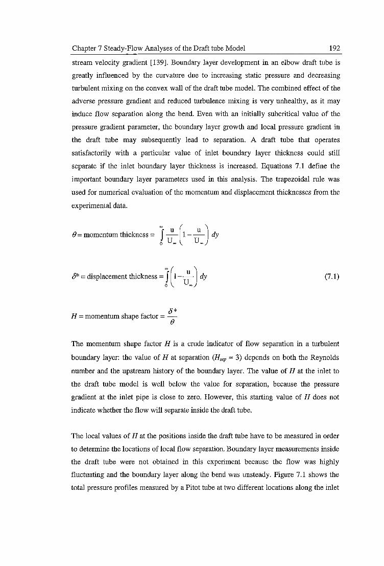
Chapter 7 Steady-Flow Analyses of the Draft tube Model 192
stream velocity gradient [139]. Boundary layer development in an elbow draft tube is
greatly influenced by the curvature due to increasing static pressure and decreasing
turbulent mixing on the convex wall of the draft tube model. The combined effect of the
adverse pressure gradient and reduced turbulence mixing is very unhealthy, as it may
induce flow separation along the bend. Even with an initially subcritical value of the
pressure gradient parameter, the boundary layer growth and local pressure gradient in
the draft tube may subsequently lead to separation. A draft tube that operates
satisfactorily with a particular value of inlet boundary layer thickness could still
separate if the inlet boundary layer thickness is increased. Equations 7.1 define the
important boundary layer parameters used in this analysis. The trapezoidal rule was
used for numerical evaluation of the momentum and displacement thicknesses from the
experimental data.
() = momentum thickness = J ~ (1-~J dy 0 u~ u~
o* =displacement thickness=} (1-~J dy o u~
8* H = momentum shape factor = -
()
(7.1)
The momentum shape factor H is a crude indicator of flow separation in a turbulent
boundary layer: the value of H at separation (Hsep "" 3) depends on both the Reynolds
number and the upstream history of the boundary layer. The value of H at the inlet to
the draft tube model is well below the value for separation, because the pressure
gradient at the inlet pipe is close to zero. However, this starting value of H does not
indicate whether the flow will separate inside the draft tube.
The local values of H at the positions inside the draft tube have to be measured in order
to determine the locations of local flow separation. Boundary layer measurements inside
the draft tube were not obtained in this experiment because the flow was highly
fluctuating and the boundary layer along the bend was unsteady. Figure 7.1 shows the
total pressure profiles measured by a Pitot tube at two different locations along the inlet
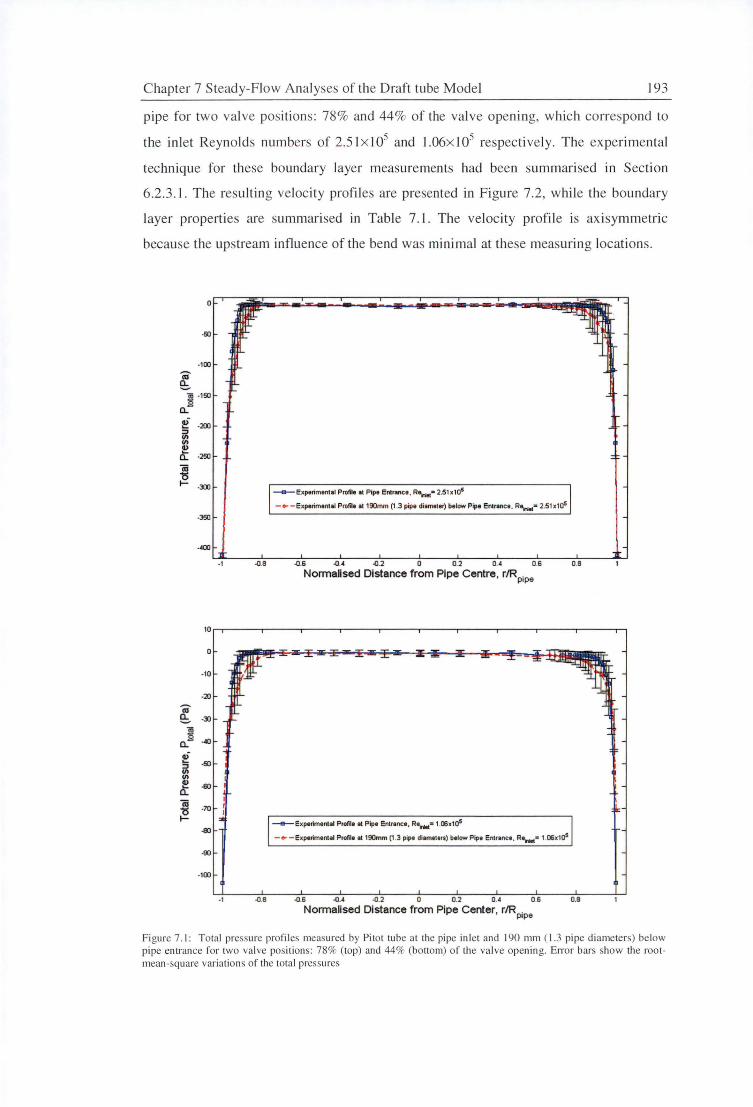
Chapter 7 Steady-Flow Analyses of the Draft tube Model 193
pipe for two valve positions: 78% and 44% of the valve opening, which correspond to
the inlet Reynolds numbers of 2.5 I x l05 and l.06x I 05 respectively. The experimenta l
technique for these boundary layer measurements had been summarised in Section
6.2.3. 1. The re ulting velocity profiles are presented in Figure 7 .2, whi le the boundary
layer properties are summarised in Table 7.J. The velocity profil e is axisymmetric
because the upstream influence of the bend was minimal at these measuring locations.
·50
-100
Iii e:. ~ -150
a.. ~ ·200 ::I VI VI ~ a.. .250
iii "ts I- .300
--a-- Experimental Profile at Pip• Entrance, R-....· 2.5h1c5
- • - E11perimental Profile et 190mm (1 .3 pipe diameter) below Pipe Entrance , Re..._• 2.51 x1c5
.350
.400
·1 -0.B -0.6 -0.4 -0.2 0 0.2 0.4 0.6 O.B
Normalised Distance from Pipe Centre , r/Rpipe
10
-10
-20
Iii e:. -31
111 l;i ~ a..
~ -50 ::I VI VI
~ a.. .SJ
iii -70 "ts
I--8J
~Experimental Profile at Pipe Entrance, R~a 1.C6x105
-•-Experimental Profile at 190mm (1 .3 pipe diameters) below Pipe Entrance, R9tt.1• 1.Clix1 c5
-9J
-100
-1 -0.B -0.6 -0.4 -0.2 0 0.2 0.4 0.6 O.B
Normalised Distance from Pipe Center, r/Rpipe
Figure 7 .1: Total pre sure profiles measured by Pilot tube al the pipe inlet and 190 mm ( 1.3 pipe diameters) below pipe entrance for two va lve pos itions: 78% (top) and 44% (bottom) of the va lve openin g. En-or bars show the rootmean-square variations of the tota l pressures
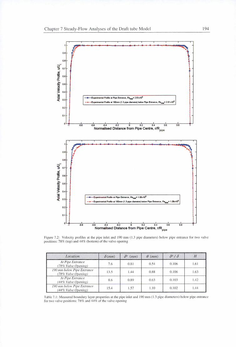
Chapter 7 Steady-Flow Analyses of the Draft tube Model 194
0.9
0.8
<u 0.7 ::J
Q,-
~ 0.6 (l._
.?;- 0.5 ·g Q) > 0.4 (ij
~ 0.3 --e-- Experim1ntal Pro!Ut at Pipt Entrance , R-,..• 2.51x1a5
-•-Exptrimtntal Proilt at 190mm (1 .3 pipe diameter) btklw Pipe Entrance, R9n1et• 2.51x1a5
0.2
0.1
·1 -0.8 -0.6 -0.4 -0.2 0 0.2 0.4 0.6 0.8
Nomialised Distance from Pipe Centre, r/Rpipe
0.9 { , 1
0.8
<u 0.7 ::J
Qf
~ 0.6 (l._
z::. 0.5 '8 Q) > 0.4 (ij
~ 0.3 ~Experim ental Profile 11 Pipe Entrance , R...._• 1.tl5x1a5
- .. - Experimtntaf Profilt at 190rrvn (1 .3 pipe diameter) below Pipe Entrance , R'ni.t• 1.00x1a5
0.2
0.1
0 · 1 -0.B -0.6 -0.4 -0.2 0 0.2 0.4 0.6 0.8
Nomialised Distance from Pipe Centre, r/Rpipe
Figure 7.2: Velocity profi les at the pipe inlet and 190 mm ( 1.3 pipe diameters) below pipe entrance for two valve posi tions: 78% (top) and 44% (bottom) of the va lve opening
Location o (mm) o* (mm) e (mm) 0*1 o H
At Pipe Entrance 7.6 0.81 0 .54 0. 106 1.61
(78 % Valve OpeninR) 190 111111 below Pipe Entrance
13.5 1.44 0 .88 0 .106 1.63 (78 % Valve Openin~)
At Pipe Entrance 8.6 0.89 0.63 0. 103 1.42
(44 % Valve OveninR) 190 mm below Pipe Entrance
15.4 1.57 1.10 0. 102 1.44 (44 % Valve Open.inR)
Table 7. I: Measured boundary layer properti es at the pipe inlet and 190 mm ( 1.3 pipe diameters) below pipe entrance for two va lve positions: 78% and 44% of the valve opening
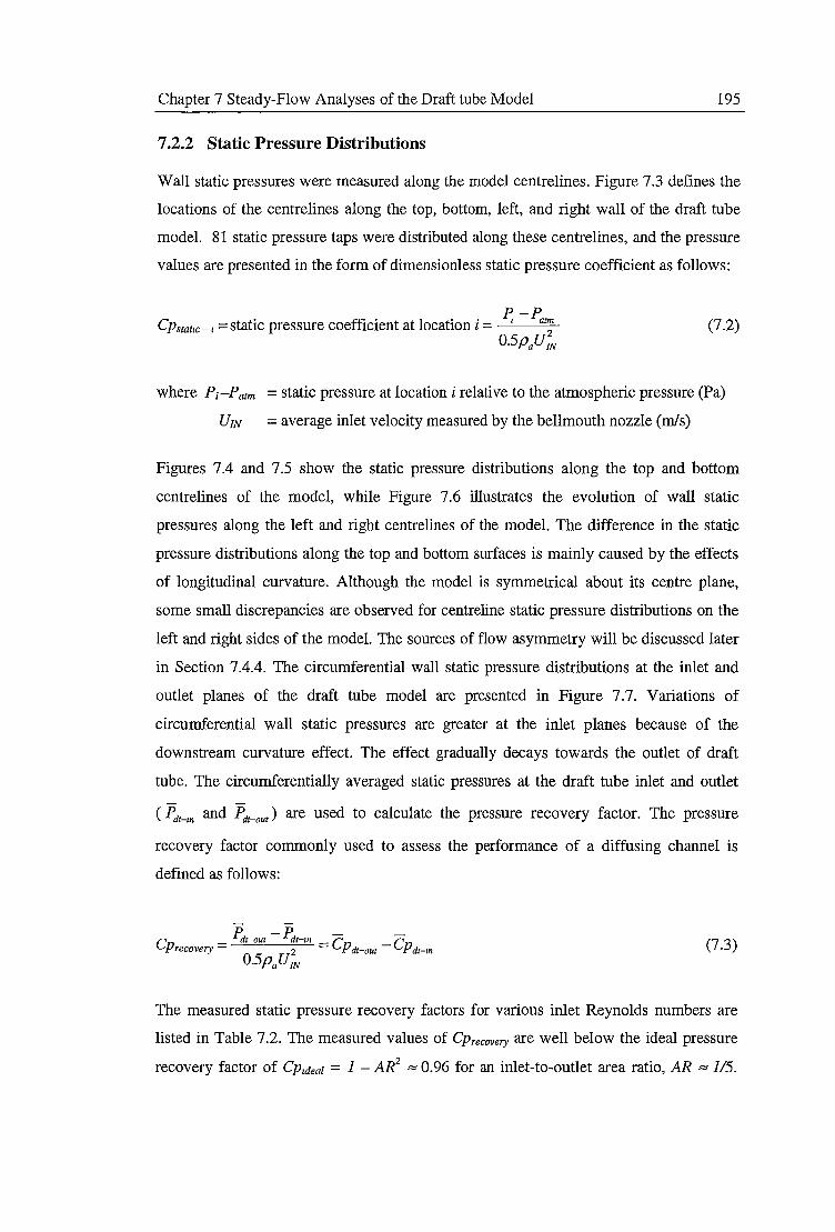
Chapter 7 Steady-Flow Analyses of the Draft tube Model 195
7.2.2 Static Pressure Distributions
Wall static pressures were measured along the model centrelines. Figure 7.3 defines the
locations of the centrelines along the top, bottom, left, and right wall of the draft tube
model. 81 static pressure taps were distributed along these centrelines, and the pressure
values are presented in the form of dimensionless static pressure coefficient as follows:
P-P Cpstatlc-1 =static pressure coefficient at location i = I at;
0.5paUIN (7.2)
where Pi-Parm =static pressure at location i relative to the atmospheric pressure (Pa)
Um = average inlet velocity measured by the bellmouth nozzle (m/s)
Figures 7.4 and 7.5 show the static pressure distributions along the top and bottom
centrelines of the model, while Figure 7.6 illustrates the evolution of wall static
pressures along the left and right centrelines of the model. The difference in the static
pressure distributions along the top and bottom surfaces is mainly caused by the effects
of longitudinal curvature. Although the model is symmetrical about its centre plane,
some small discrepancies are observed for centreline static pressure distributions on the
left and right sides of the model. The sources of flow asymmetry will be discussed later
in Section 7.4.4. The circumferential wall static pressure distributions at the inlet and
outlet planes of the draft tube model are presented in Figure 7. 7. Variations of
circumferential wall static pressures are greater at the inlet planes because of the
downstream curvature effect. The effect gradually decays towards the outlet of draft
tube. The circumferentially averaged static pressures at the draft tube inlet and outlet
( Pdr-m and Pdt-our ) are used to calculate the pressure recovery factor. The pressure
recovery factor commonly used to assess the performance of a diffusing channel is
defined as follows:
C J',it-out - pdt-m C C Precovery = 2 = P dt-out - P dt-m
O.SpaUIN (7.3)
The measured static pressure recovery factors for various inlet Reynolds numbers are
listed in Table 7.2. The measured values of Cprecovery are well below the ideal pressure
recovery factor of Cp1aeat = 1 - AR2 = 0.96 for an inlet-to-outlet area ratio, AR = 115.
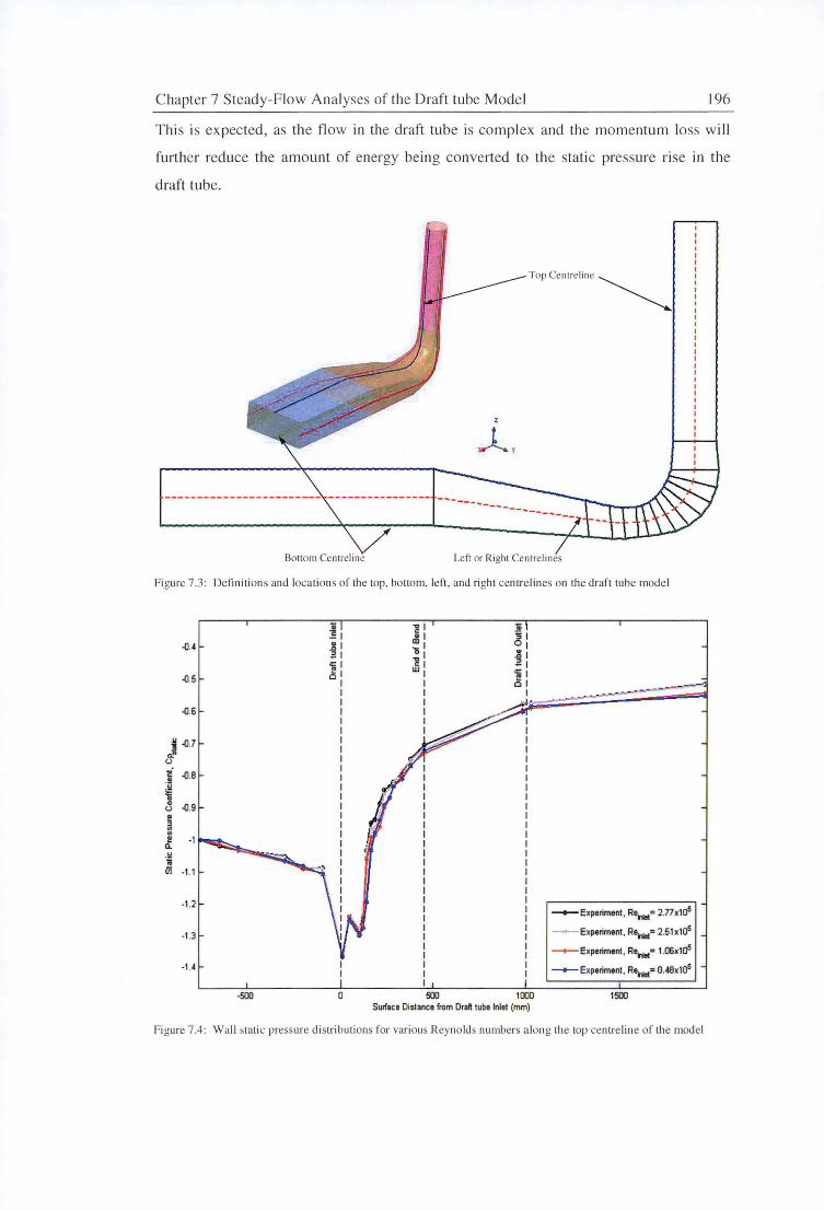
Chapter 7 Steady-Flow Analyses of the Draft tube Model 196
This is expected , as the flow in the draft tube is complex and the momentum loss will
further reduce the amount of energy being converted to the stati c pressure rise in the
draft tube.
Top CentreLine ~
Bottom Centreline Left or Right Centrelines
Figure 7.3 : Defini ti ons and locations of the lop. bottom, left , and ri ght centrelines on the draft tu be model
-0.4
-0.5
-0.6
~ -07 c: ()
~- -0.8
~ 8 -0.9 ! " "' "' ! Q.
-1
.!I 1i Cii -1.1
-1 .2
-1.3
-U
;; £1 1l I 21 <=I c3 I
I I I I I
-500 0
.,, " .. ID
'O ~ w
...,---~~·
-Experiment , ReiWI= 2.77x1a5
- Experiment , Re-= 2.51x1a5
--+-Experiment , R~= 1.llMa5
- Experiment , R~= 0.48x1a5
500 HID 1500 Surface Distance from Ora~ tube Inlet (mm)
Figure 7.4: Wall stati c pressure di stributions for various Reyno lds numbers a long the top cenu·eline of the model
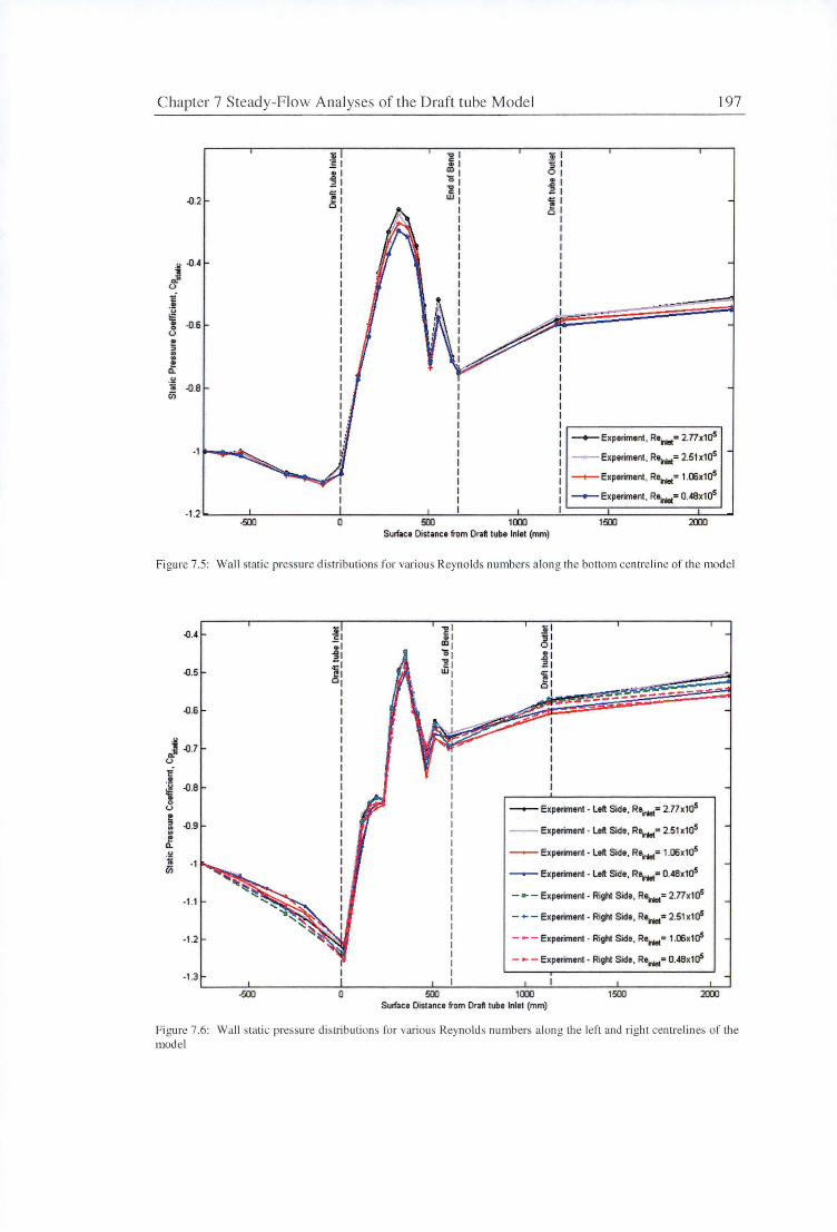
Chapter 7 Steady-Flow Analyses of the Draft tube Model 197
li -g -.; ~I .. s .. 1 ID 0
~I 'o .. -g ...
.:: I ;:? -0.2 !! I w
~ 01 0
~ -04 .. 0
c: • ·;::; ii: • -0.6 0 0 !! ~ .. I! a..
.I! 1i -0.8 iii
-Experiment, Reinlet= 2.nx1a5
- Experiment, Reinlet= 2.51x1a5
---+- Experiment , R8iniet= 1.Cllx1a5
- Experiment, R8iniet= 0.48x1a5
Surface Distance from Draft tube Inlet (mm)
Figure 7.5: Wall stati c pressure di stributions for various Reyno lds numbers along the bottom centreline of the model
-0.4
-0.5
------------0.6
j -0.7 0
<i
i -0.B
0
~ -0.9 I!
-- Experiment· Left Side, Re.riot= 2.77x1a5
-- Experiment · Left Side, Reinlet= 2.51 x10⁵
a.. " ·;;
·1 iii
-- Experiment · Left Side, Re.riot= 1.Cllx1a5
--Experiment· Left Side, R8iniet= 0.48x105
·1 .1 - • - Experiment · Right Side, R8iniet= 2.77x1 a5
- +- - Experiment · Right Side, Reinlet= 2.51 xta5
·1 .2 - - - Experiment · Right Side, Reinlet= 1.06xta5
- - - Experiment • Right Side, Reinlet= 0.48x1 a5
·1 .3
.500 0 500 1CXXJ 1500 2!lXl Surface Distance from Draft tube Inlet (mm)
Figure 7.6: Wall s tati c pressure di stri butions fo r various Reynolds numbers along the left and right centrelin es of the model
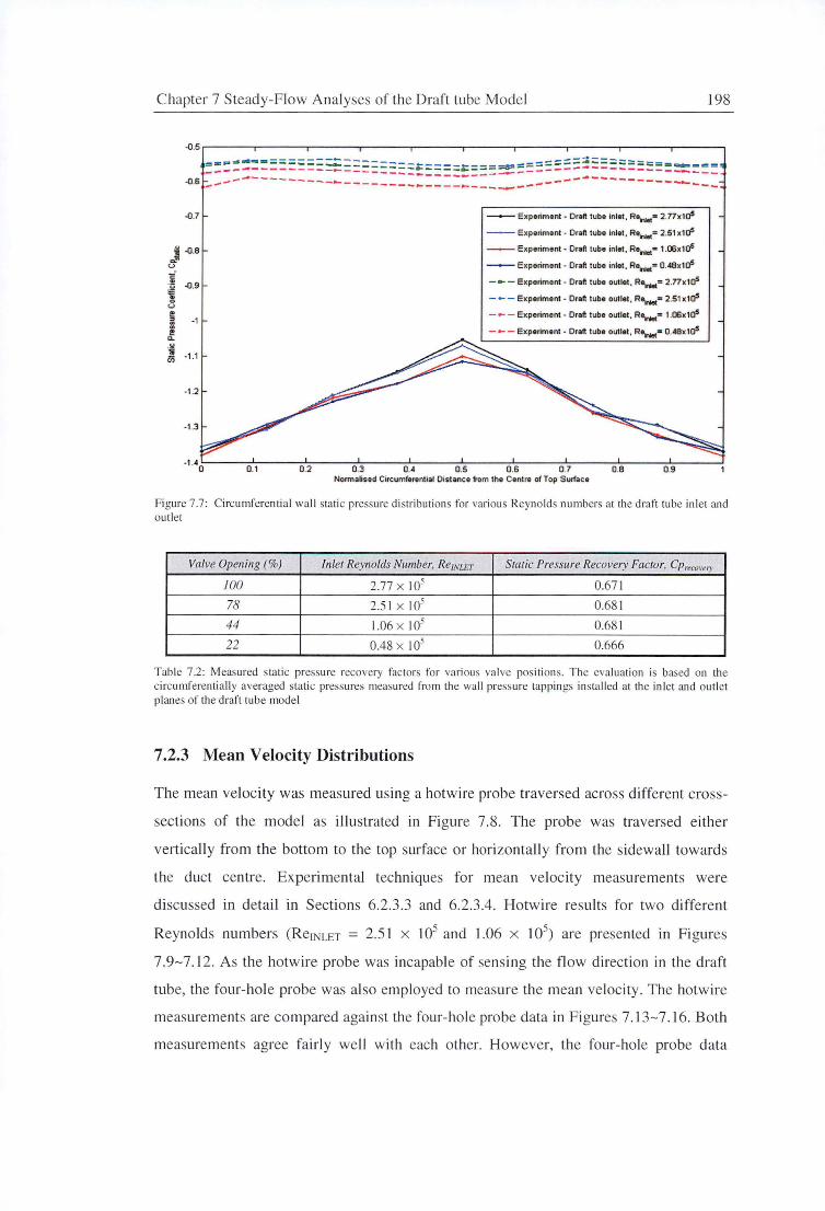
Chapter 7 Steady-Flow Analyses of the Draft tube Model
.Q.7
j .08
<..>
i i -0.9
<..>
-1.2
-1 .3
- E xperiment - Draft tube inlet, R•1n1et• 2.nx1a5
-- E xperiment - Draft tuba inlet, Re.Net= 2 .51 x1a5
- E xperiment - Draft tube inlet, Reinlet• 1.00x1a5
- Experiment - Draft tube inlet, R8ir,w= 0.48x1a5
_.,. - Experiment - Draft tube outlet , R"-= 2.77x1a5
- +- - Experiment - Draft tube outlet, Relnlet• 2 .51 x1 a5
- - - E xperiment - Draft tube outlet, Relrllel• 1.llix1a5
- .... - E xperiment - Draft tube outlet I Reillet• o.~x1 a5
0.9 Normalised Circumferential Distance from the Centre of Top Surface
198
Fi gure 7.7: Circumferentia l wall static pressure di stributions for various Reynolds numbers at the draft tube inlet and ou tl e t
Valve Opening (%) In/er Reynolds Number, RelNl.Ef Static Pressure Recovery Fae/or, Cp,.00,..,y
100 2.77 x 10' 0.671
78 2.5 1 x I O' 0.681
44 1.06 x I O' 0.68 1
22 0.48 x lO' 0.666
Table 7 .2: Measured stati c pressure recovery factors for various valve positions. The evaluation is based on the circumferentia lly averaged static pressures measured from the wa ll pressure tappings in sta lled at the inlet and outl et planes of the draft tube model
7.2.3 Mean Velocity Distributions
The mean velocity was measured using a hotwire probe traversed across different cross
sections of the model as illustrated in Figure 7.8. The probe was traversed either
vert icall y from the bottom to the top surface or horizontally from the sidewall towards
the duct centre. Experimental techniques for mean velocity measurements were
discussed in detail in Sections 6.2.3.3 and 6.2.3.4. Hotwire results for two different
Reynolds numbers (RelNLET = 2.51 x 10⁵ and 1.06 x 10⁵) are presented in Figures
7 .9-7.12 . As the hotwire probe was incapable of sensing the flow direction in the draft
tube, the four-hole probe was also employed to measure the mean velocity. The hotwire
measurements are compared against the four-hole probe data in Figures 7 .13- 7 .16. Both
measurements agree fairly well with each other. However, the four -hole probe data
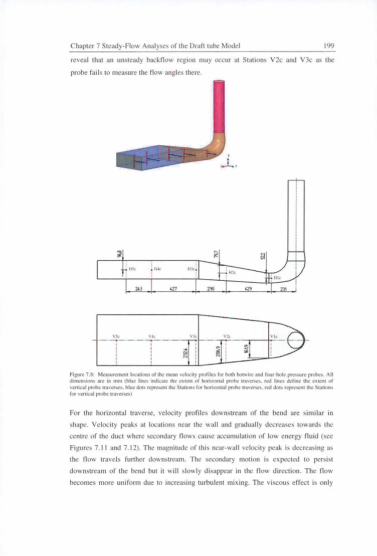
Chapter 7 Steady-Flow Analyse of the Draft tube Model 199
reveal that an unsteady backflow region may occur at Stations V2c and V3c as the
probe fail s to measure the flow angle there.
I
' H5c H4c H3c
243 427 290 429
V5c V4c V3c V2c ----....,,.---·- -__,...---·---..----.1---
1 I I I -.o:
: 8:1 I
Figure 7.8: Measurement locations of the mean velocity profiles for both hotwire and fo ur-hole pressure probes . A ll dimensions are in 111111 (blue lines indicate the extent of horizontal probe traverses. red lines define the ex tent of vertica l probe traverses , blue dots represent the Stations for horizontal probe traverses, red dots represent the Stations for verti ca l probe traverses)
For the horizontal traverse, velocity profiles downstream of the bend are s imil ar in
shape. Velocity peaks at locations near the wall and gradually decreases towards the
centre of the duct where secondary flows cause accumulation of low energy fluid (see
Figures 7.1 I and 7.12). The magnitude of this near-wall velocity peak is decreasing as
the flow travels further dow nstream. The secondary motion is ex pected to persist
downstream of the bend but it will slowly di sappear in the flow direction. The fl ow
becomes more uniform due to increasing turbulent mixing. The viscous effect is only
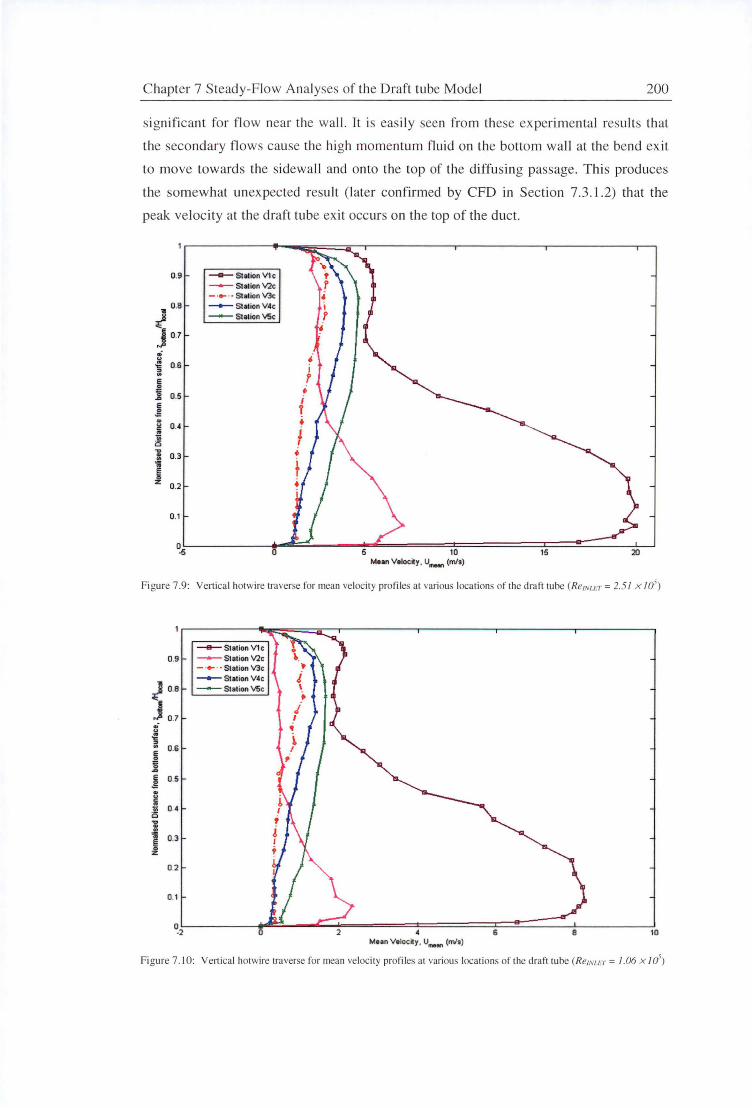
C hapter 7 Steady-Flow Analyses of the Draft tube Model 200
s ignificant fo r fl ow near the wall. It is easil y een from these ex perimental results that
the secondary fl ow cause the high momentum fluid on the botto m wall at the bend exit
to move toward s the sidewall and onto the top of the diffusing passage. This produces
the somewhat unex pected result (l ater confirmed by CFD in Section 7 .3 .1.2) that the
peak velocity at the draft tube ex it occurs on the top of the duct.
0.9 - stetionV1c - stationV2c - ..... · · Station V3c
0.8
.} J 07
-- S1ation V•c - Station V'Sc
.;
~ 0.6 ~
~ :: .8 0.5 E 0 .;
i o.• .ii 0 .... = 0.3
J 0.2
0.1
0-5 0 5 10 15 MHn Vtloc~y , U,,_, (m/s)
Figure 7 .9: Vertical hot wire traver e for mean veloc ity profi les at various locations of the draft tube (Re/Nu.T = 2.51 x t o')
- Station V1c 0.9 ~ Stalion V2c
- ... · · Station V3c --+-- Station V•c
.} 0.8
J 07
- Station V'Sc
{ 0.6
~ j j 0.5
i .. o.• 0
i 0.3
0.2
0.1
Mnn Voloc~y . U....,, (ml•)
Figure 7 .1 0 : Venical hot wire traverse for mean velocity profiles at various locations of the dra ft tu be (Re/Nu._-r = 1.06 x !(/)
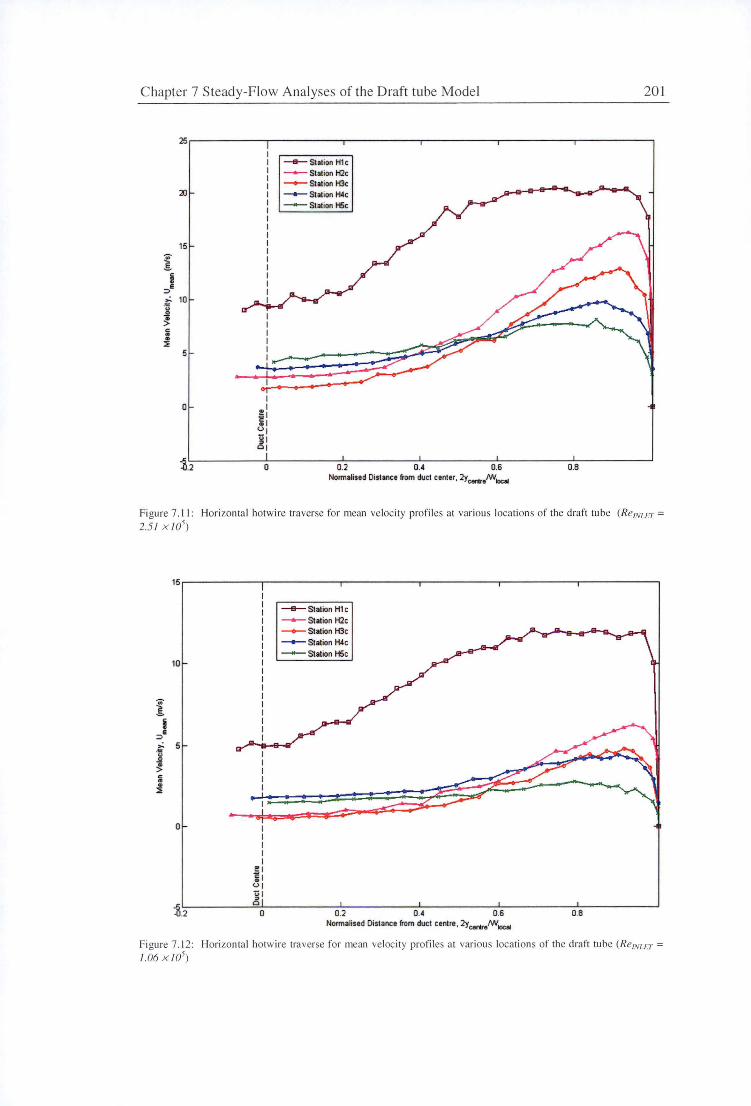
C hapter 7 Steady-F low Analyses of the Draft tube Model 201
- St1tion H1 c - Station H2c - Station H3c
20
15 .... 1 i
-=>e ,.:; 10 ... u .2 ~ " .. :.i
5
0
:g_2 0 0.2 0.4 0.6 0.8 Normolised Distanc1 from duct canter, 2ye«ts/WOc:M
Figure 7.11: Hori zontal hot wire traverse fo r mean veloc ity profi les at various locations of the draft tube (RetNu:r = 2.51 x /05
)
I i E
-=>
.~ u
.S! ~ :i ..
:::;;:
10
5
0 I I I I I
~ I ii 01
~ I 0
-e-- Station H1 c
- Station H2c
--Station H3c -+-- Station H4c
- Station H5c
0.2 O.• 0.6 0.8 Normalised Distance from duct centre , 2ye«tsoNV'ocllA
Figure 7 .1 2: Horizontal hotwire traverse for mean velocity profiles a t various locations of the draft tube (RetNu:r = 1.06 x /05)
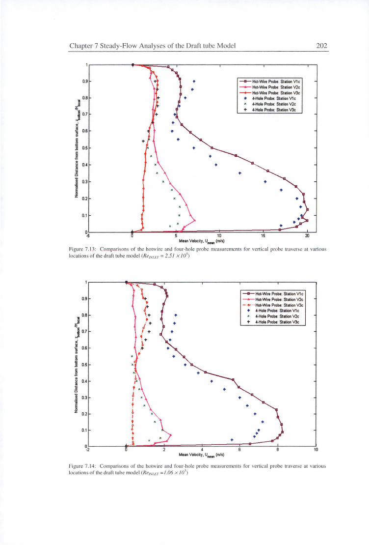
C hapter 7 Steady-Flow Analyses of the Dra ft tube Model 202
0.9 - Hot-Wire Probe: Station V1 c - Hot-Wirt Probe: Station V2c - Hot-Wire Probe: Stllion V3c
0.8
),, + 4-Hole Probe: Station V1 c x 4-Hole Probe: Station V2c + 4-Hole Probe: Station V3c
• " .. 0.6 't:
" .. E 0
'.5 0.5 ..Cl
~ .. " 0.4 c:. .. .. 0 .. .,, .. 0.3 .. • ~
~ .. z
0.2
0.1
• 0 -5 10 15 20
Mean Velocity, U,,_, (m/s)
Fi gure 7 . 13: Compari sons of the hot wire and four-hole probe measurements fo r verti ca l probe u·averse at various location of the draft tube mode l (Re1NtE r = 2.5 I x I 05)
., 'Y • ~ • t
0.9 - Hot-Wirt Probe: Station V1 c - Hot-Wire Probe: Station V2c - ·e- · - Hot-Wire Probe: Station V3c
• 4-Hole Probe: Station V1 c \_+ • • i + •
I + • '
a.a } j 0.7
x 4-Hole Probe: Station V2c + 4-Hole Probe: Station V3c
- + ~ ,,. • " .. 0.6 5 , ..
E 0
x • 15 0.5 ..Cl
j " " 0.4 c:. .. .. 0 .,, " 0.3 .!!! ... e 0 z
0.2
0.1
0 -2 4 6 e 10
Mean Velocity , u......, (m/s)
Figure 7 . 14: Compari sons o f the hotwire and four-hole probe measurements for vertical probe traverse at various locations of the draft tube model (RetNlff =1.06 x 10⁵
)
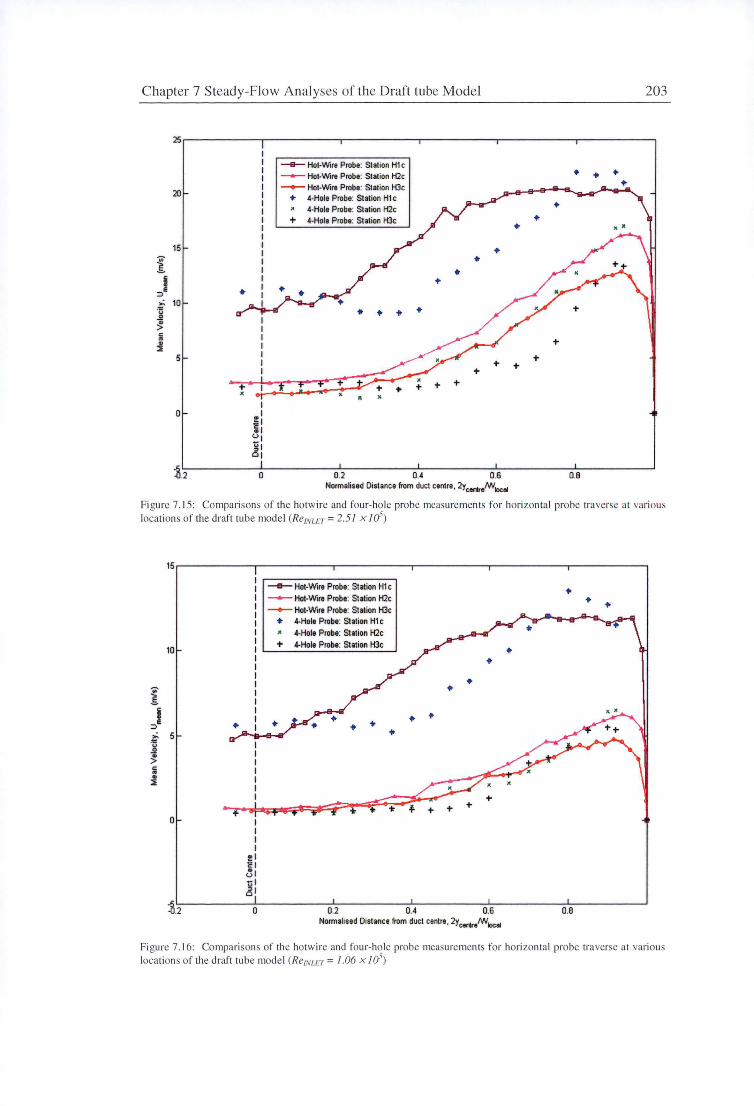
C hapter 7 Steady-Flow Analyses of the Draft tube Model
1 i e
::::> .; .... ~ ~ c: .. ..
:::t
20
15
10
5
0
~.2
•
+ •
0
-e- Hot-Wire Probe: Station H1 c - Hot-Wire Probe: Station H2c -- Hot-Wire Probe: Station H3c
• 4-Hole Probe: Station H1 c 4-Hole Probe: Station H2c
+ 4-Hole Probe: Station H3c
• • • +
+ • •
0.2 0.4
• +
+ +
+
0.6 Normalised Distance from duct centre, 2yt«*/Wbca
203
• •
+
+ +
+
0.8
Figure 7 . 15: Compatisons of the hot wire and fo ur-hole probe mea urements for hori zontal probe traverse at various locations of the draft tube mode l (RetNLET = 2.51 x JO-')
I i
=>I
>o ... ~ ~ ii .
:::;;
10
5
0
~.2
I I I I
!! 1 cl ~ I ti I i~P
0
-e- Hot-Wire Probe: Station H1 c - Hot-Wire Probe: Station H2c --Hot-Wire Probe: Station H3c
• -4-Hole Probe: Station H1 c • -4-Hole Probe: Station H2c + -4-Hole Probe: Station H3c
• • • •
0.2
• •
0.4 0.6 Normalised Distance from duct centre, 2y
0-
8Mlbca
• • •
0.8
Fi gure 7. 16: Compari sons of the hotwire and four-hole probe measurements fo r hori zontal probe o·averse at various locations of the draft tube mode l (RetNLEr = 1.06 x JO-' )
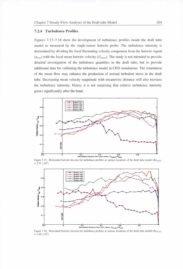
Chapter 7 Steady-Flow Analyses of the Draft tube Mode l 204
7.2.4 Turbulence Profiles
Figures 7.17-7.] 8 show the development of turbulence profiles ins ide the draft tube
model as measured by the single-sensor hotwire probe. The turbulence intensity is
determined by dividing the local fluctuating velocity component from Lhe hotwire s ignal
(ur111.J with the local mean hotwire velocity ( U111e011 ). The study is not intended to provide
detailed inves tigation of the turbulence quantitie in the draft tube, but to provide
additional data for validating the turbulence model in CFD simulations. The retardation
of the mean flow may enhance the production of normal turbulent stress in the draft
tube. Decreasing mean velocity magnitude with streamwise distance will also increase
the turbulence intensity. Hence, it is not surprising that relative turbulence intensity
grows significantly after the bend.
----- St•tion H1c - St•tionH2c - Station H3c
0 .5 - StatlonH4e - StationHSc
I o.• ::
! ,.
i 0 .3
~
j 0 .2
I I I I
"'' 0 .1 l! I <>1
~: I I
.S.2 0 0 .2 O.• 0 .6 0 .8 Normalised Distance from duct centre , 2ycer*•f\Ntit;Jc;eA
Fi gure 7. 17: Hori zonta l hotwire traverse for turbulence profiles at various loca tions of the draft tube model (RetNu:r
= 2.5 I x IO-' )
----- Stal ion H1 c - stalionH2c - Station H3c
0 .5 - S tation H4c - stationHSc
i o.• ::&
i! ,.
i' 0 .3
~ ii
i 0 .2
.. , 0 .1 ...
<>r
~: I I
.S.2 0 0 .2 O.• 0 .6 0 .8 Normaliead Distance from duct canlre , 2Yc.itref\Nkloeal
Figure 7 .18: Horizonta l hotwire traverse fo r turbulence profiles at various locations of the draft tube model (Re/NI.Er
= I.06 x /05)
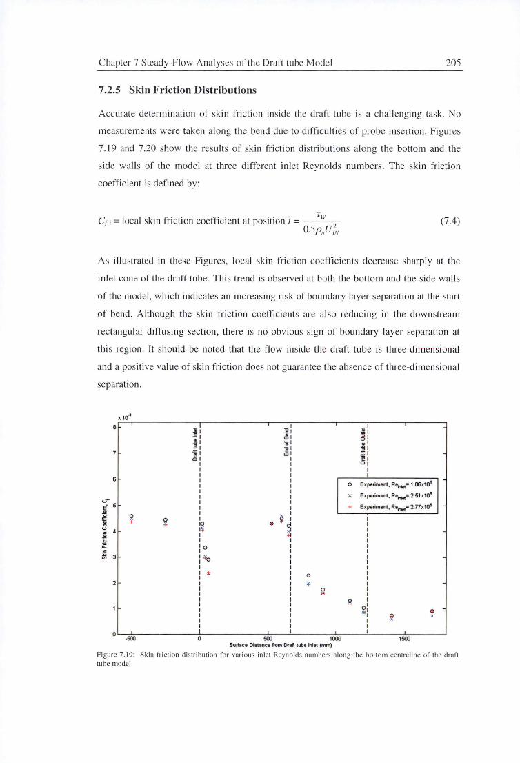
Chapter 7 Steady-Flow Ana lyses of the Draft tube Model 205
7.2.5 Skin Friction Distributions
Accurate determination of skin friction inside the draft tube is a chall enging task . No
measurements were taken along the bend due to difficulties of probe insertion. Figures
7.19 and 7.20 show the results of skin friction distributions along the bottom and the
side walls of the model at three different inlet Reynolds numbers. The skin friction
coefficient is defined by:
'r Cr-; =local skin friction coefficient at position i = w
2 . 0.SpaUtN (7.4)
As illustrated in these Figures, local ski n friction coefficients decrease sharply at the
inlet cone of the draft tube. This trend is observed at both the bottom and the side walls
of the model, which indicates an increasing risk of boundary layer separation at the start
of bend. Although the skin friction coefficients are also reducing in the downstream
rectangular diffusing section, there is no obvious sign of boundary layer separation at
this region . It should be noted that the flow inside the draft tube is three-dimensional
and a positive value of skin friction does not guarantee the absence of three-dimensional
separation.
x 10"
8 I j
7 'ii d
6
u-~- 5
~ ~ 0 ¥ u
4 c .!1 g "-.£
"" 3 en
2
IO 1¥
0
lfo ,.,
0
¥
O Experiment , Reillet• 1.06xla5
x Experiment, R"-• 2.51x1a5
+ Experiment, R8-• 2.77x1a5
I
~ ) ,.,:
I I
4> x
o~~~~~~~~"--~~~~~---'~~"'--~~~-'-~~---'-1 ~~~~~~~~ 500 100'.J 1500
Surface Dislanco from Draft tube Inlet (mm)
Fi gure 7 .19: Skin fri ction distribution fo r vari ous inlet Reynolds numbers along the bottom centreline of the dra ft tube model
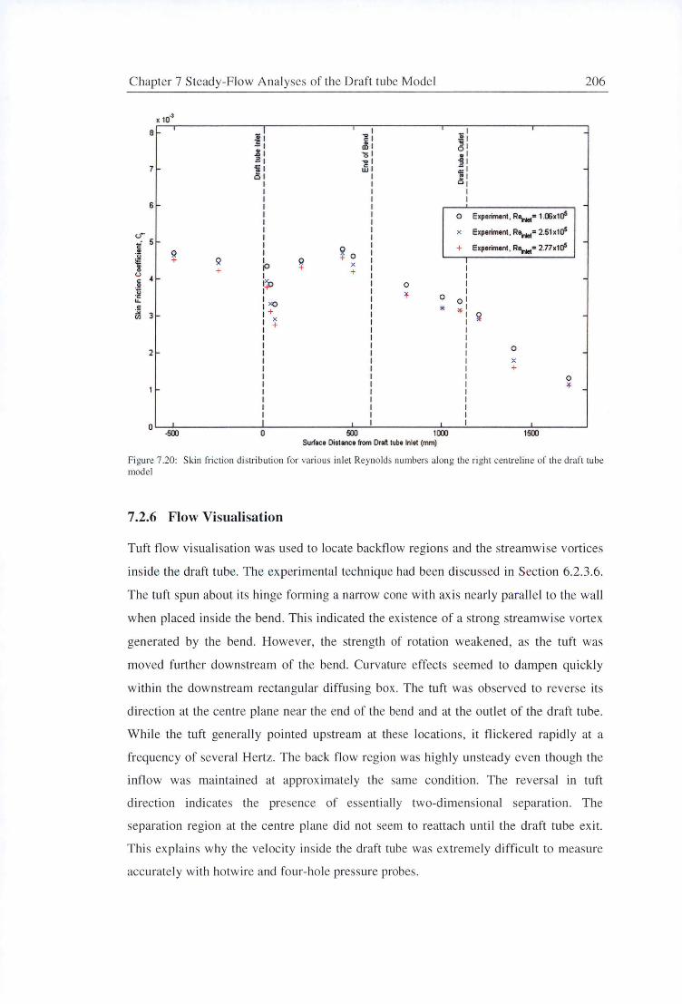
C hapter 7 Steady-Flow Analyses of the Draft tube Model
x 10-3
8 "i ~ .! = 7 ~
6
<.r ti 5 ..
~ ~ 0 ' (j Q ~ "" l '°
x + + u
~ I c: t:p .!2 0 u
"' ·c: u.
XO c: :;;:
3 + en x +
2
-' ..!!f '5 I o, _g I ~: cs,
I I
0 Experiment, R"-s 1.06x1a5
x Experiment, R8r..t= 2.51x1a5
+ Experiment , R"-s 2.77x1a5
I I I I I
o ol
* "' : ~ I I I I I I I I I I I I I
0
x +
0
"'
206
O '----'-~~~~~~-'--~~~~~--'~...;_~~~~-'--~~'~~~~---'-~~~--' .500 0 HXXJ 1500
Surface Distance from Draft tube Inlet (mm)
Fi gure 7 .20: Skin fricLion di stribution for various in let Reynolds numbers along the right centreline of th e draft tube model
7 .2.6 Flow Visualisation
Tuft flow visualisation was used to locate backfl ow regions and the streamwise vortices
inside the draft tube. The experimental technique had been discussed in Section 6.2.3.6.
The tuft spun about its hinge forming a narrow cone with axis nearly parall e l to the wall
when pl aced inside the bend . This indicated the ex istence of a strong streamwise vortex
generated by the bend. However, the strength of rotation weakened , as the tuft was
moved further downstream of the bend. Curvature effects seemed to dampen quickly
w ithin the downstream rectangul ar diffusing box . The tuft was observed to reverse its
direction at the centre plane near the end of the bend and at the outlet of the d raft tube.
While the tuft generally pointed upstream at these locations, it flickered rapidly at a
frequency of several Hertz. The back flow region was highly unsteady even though the
inflow was maintained at approx imately the same condition. The reversal in tuft
d irection indicates the presence of essentially two-dimensional separation . T he
separation region at the centre plane did not seem to reattach until the draft tube ex it.
Thi s explains why the velocity inside the draft tube was extremely difficu lt to measure
accurately with hotwire and four-hole pressure probes.
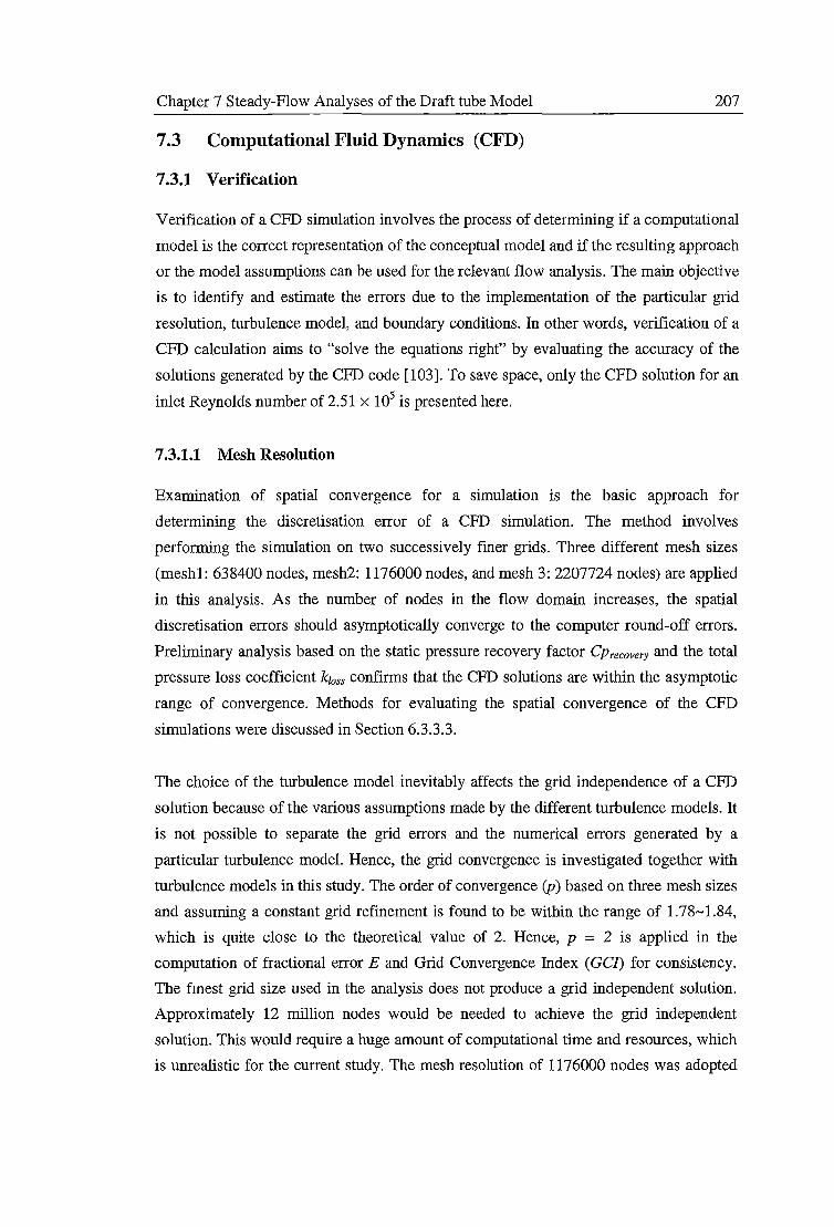
Chapter 7 Steady-Flow Analyses of the Draft tube Model 207
7.3 Computational Fluid Dynamics (CFD)
7.3.1 Verification
Verification of a CFD simulation involves the process of determining if a computational
model is the correct representation of the conceptual model and if the resulting approach
or the model assumptions can be used for the relevant flow analysis. The main objective
is to identify and estimate the errors due to the implementation of the particular grid
resolution, turbulence model, and boundary conditions. In other words, verification of a
CFD calculation aims to "solve the equations right" by evaluating the accuracy of the
solutions generated by the CFD code [103]. To save space, only the CFD solution for an
inlet Reynolds number of 2.51 x 10⁵ is presented here.
7.3.1.1 Mesh Resolution
Examination of spatial convergence for a simulation is the basic approach for
determining the discretisation error of a CFD simulation. The method involves
performing the simulation on two successively finer grids. Three different mesh sizes
(meshl: 638400 nodes, mesh2: 1176000 nodes, and mesh 3: 2207724 nodes) are applied
in this analysis. As the number of nodes in the flow domain increases, the spatial
discretisation errors should asymptotically converge to the computer round-off errors.
Preliminary analysis based on the static pressure recovery factor Cprecovery and the total
pressure loss coefficient ktoss confirms that the CFD solutions are within the asymptotic
range of convergence. Methods for evaluating the spatial convergence of the CFD
simulations were discussed in Section 6.3.3.3.
The choice of the turbulence model inevitably affects the grid independence of a CFD
solution because of the various assumptions made by the different turbulence models. It
is not possible to separate the grid errors and the numerical errors generated by a
particular turbulence model. Hence, the grid convergence is investigated together with
turbulence models in this study. The order of convergence (p) based on three mesh sizes
and assuming a constant grid refinement is found to be within the range of 1.78~1.84,
which is quite close to the theoretical value of 2. Hence, p = 2 is applied in the
computation of fractional error E and Grid Convergence Index (GCJ) for consistency.
The fmest grid size used in the analysis does not produce a grid independent solution.
Approximately 12 million nodes would be needed to achieve the grid independent
solution. This would require a huge amount of computational time and resources, which
is unrealistic for the current study. The mesh resolution of 1176000 nodes was adopted
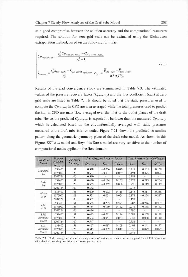
Chapter 7 Steady-Flow Analyses of the Draft tube Model 208
as a good compromise between the solution accuracy and the computational resources
required. The solution for zero grid scale can be estimated using the Richardson
extrapolation method, based on the following formulae:
C _ 13; Cp recovery-mes/13 - Cp recoveiy- mesh2 P re coveiy-esr - 2 l
T32 -
(7 .5)
k = r3; k loss- mesli3 - k/oss-mesh2 where k = P,oral-inlet - P,otal-outlet loss-est 2 l loss 0 5 U 2
~- - ~ m
Results of the grid convergence study are summarised in Table 7.3. The estimated
values of the pressure recovery factor (CPrecovery) and the loss coefficient (k1oss) at zero
grid scale are listed in Table 7.4. It should be noted that the static pressures used to
compute the Cprecovery in CFD are area-averaged while the total pressures used to predict
the k 1oss in CFD are mass-flow-averaged over the inlet or the outlet planes of the draft
tube. Hence, the predicted Cprecovery is expected to be lower than the measured Cprecovery.
which is calculated based on the circumferentially averaged wall static pressures
measured at the draft tube inlet or outlet. Figure 7.21 shows the predicted streamline
pattern along the geometric symmetry plane of the draft tube model. As shown in this
Figure, SST k-{J) model and Reynolds Stress model are very sensitive to the number of
computational nodes applied in the flow domain.
Turbulence Number Refinement Static Pressure Recovery Factor Total Pressure Loss Coefficient
Model of Nodes,
Ratio, r3; Cpr.covery Ep=2 GC/p=2 k1oss Ep=2 GCip=2 Nmuh-i
Standard 638400 l.51 0.548 - 0.056 0 .070 0.219 0.135 0.169
k-£ 1176000 1.23 0.581 - 0.03 1 0.039 0.194 0.075 0.094 2207724 1.00 0.590 - - 0.1 87 - -
RNG 638400 1.51 0.490 - 0.124 0.155 0.273 0.2 13 0.266
k-£ 1176000 1.23 0.562 - 0.069 0.086 0.228 0.119 0. 149 2207724 1.00 0.582 - - 0.215 - -
Wilcox 638400 l.51 0.600 0.092 0.115 0.11 5 - 0.311 0.388
k-(J) 1176000 1.23 0.551 0 .051 0.064 0. 174 - 0.1 74 0.217 2207724 1.00 0.537 - - 0.191 - -
SST 638400 1.51 0.552 0 .233 0.291 0.203 - 0.246 0.307
k-(J) 1176000 1.23 0.454 0 .1 30 0.162 0.276 - 0.1 38 0.1 72 2207724 1.00 0.426 - - 0.296 - -
LRR 638400 1.51 0.483 - 0.091 0.114 0.388 0 .159 0.1 98 Reynolds 11 76000 1.23 0.532 - 0.051 0.063 0.337 0 .088 0.11 0
Stress 2207724 1.00 0.547 - - 0.322 - -SSC 638400 1.51 0.467 - 0.087 0.109 0.404 0.141 0.177
Reynolds 1176000 1.23 0.513 - 0.039 0.049 0.356 0 .079 0.099 Stress 2207724 1.00 0.526 - - 0.342 - -
Table 7.3 : Grid convergence studies showing results of various turbu lence models app lied for a CFD calculation with iden tical boundary conditions and convergence criteria
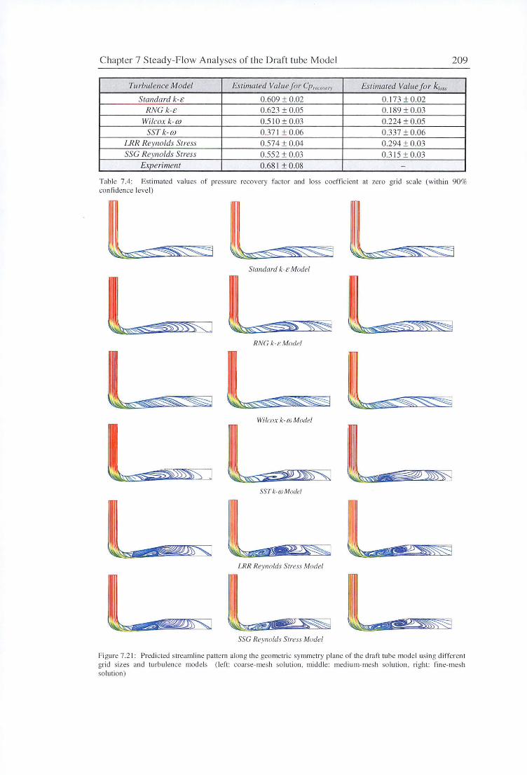
Chapter 7 Steady-Flow Analyses of the Draft tube Model 209
Turbulence Model Estimated Value for Cprecomy Estimated Value for k 1oss
Standard k-t: 0.609 ± 0.02 0.173 ± 0.02 RNC k-t: 0.623 ± 0.05 0.189 ± 0.03
Wilcox k-OJ 0.510 ± 0.03 0.224 ± 0.05 SST k-OJ 0.37 1 ± 0.06 0.337 ± 0.06
LRR Reynolds Stress 0.574 ± 0.04 0.294 ± 0.03 SSC Reynolds Stress 0.552 ± 0.03 0.315 ± 0.03
Experiment 0.68 1 ±0.08 -
Tab le 7 .4: Estimated values of pressure recovery factor and loss coeffi cient at zero grid scale (within 90% confidence level)
Standard k-t: Model
RN(; k-F. MnrlPI
Wilr:nx k-fli M nrfp/
SST k-w Mode/
LRR Reynolds Stress Model
SSC Reynolds Stress Model
Figure 7.21: Predicted streamline pattern along the geometric symmetry pl ane of the draft tube mode l using different grid sizes and turbulence models (left : coarse-mesh so lution, middle: medium-mesh so lution, ri ght : fine-mesh so lution)

Chapter 7 Steady-Flow Analyses of the Draft tube Model 210
7 .3.1.2 Turbulence Models
As noted by Roache [103], "a fundamental difficulty associated with the validation and
verification of turbulence modelling is the essential lack of a universal turbulence
model". Various important features of the turbulence models and the near-wall
treatments employed in ANSYS CFX were discussed in Section 6.3.5. Figures
7 .22~ 7 .27 show the axial velocity contours ( Ua) and the secondary flow velocity vectors
( Ut) predicted by different turbulence models at various cross-sections of the draft tube
model. All CFD solutions presented here are based on the mesh size of 1176000 nodes.
Overall, the predicted flow feature in the draft tube is characterised by a pair of counter
rotating vortices, a feature that is well known in studies of flow in bends. The fluid that
possesses the highest streamwise momentum at the bottom wall will migrate toward the
top surface. Streamwise momentum of the fluid along the bottom wall diminishes with
increasing distance from the wall. These broad features are predicted by all turbulence
models, although differences appear for the engineering quantities. This flow structure
is mainly caused by the well-known imbalance between the centrifugal force and the
radial pressure gradient acting on the relatively slow-moving fluid. A weak radial cross
flow generated in the region along the symmetry plane will carry the fluid toward the
stalled region on the top surf ace.
Although a similar flow structure is predicted by all turbulence models, some significant
differences can still be observed between the solutions. First, the strength of the vortex
pair computed via the eddy-viscosity model is weaker than the one for Reynolds stress
model, which yields a broader low-momentum region at the outlet and a larger pressure
loss. Second, the streamwise momentum is observed to decay and dissipate more slowly
if the eddy-viscosity model is used; this results in a higher peak velocity predicted
inside the draft tube. Third, the Reynolds stress models capture unsteady flow
phenomena that are not predicted by the eddy-viscosity models. The flow asymmetries
found in solutions of the Reynolds stress models are direct consequences of the flow
unsteadiness. Solutions of the eddy-viscosity models are stable even if the unsteady
simulations are performed. The longer detached shear layers predicted by eddy
viscosity models stabilise the recirculating flow inside the draft tube. This explains why
the CFD simulations using eddy-viscosity models are numerically stable in most cases.
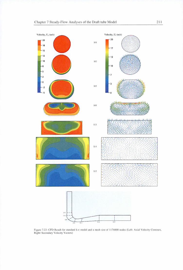
Chapter 7 Steady-Flow Analyses of the Draft tube Model 2 1]
Velocity, U., (m/s)
20 SO I
18
15
12
10 S02
8
3 S05
0
S09
St3
S l4
S l5
SO I
502
505
SO'J SIJ 5 14 S l 5
Figure 7 .22: CFD Result for standard k-e model and a mesh size of 11 76000 nodes (Left: Axial Veloc ity Contours , Ri ght: Secondary Ve locity Vectors)
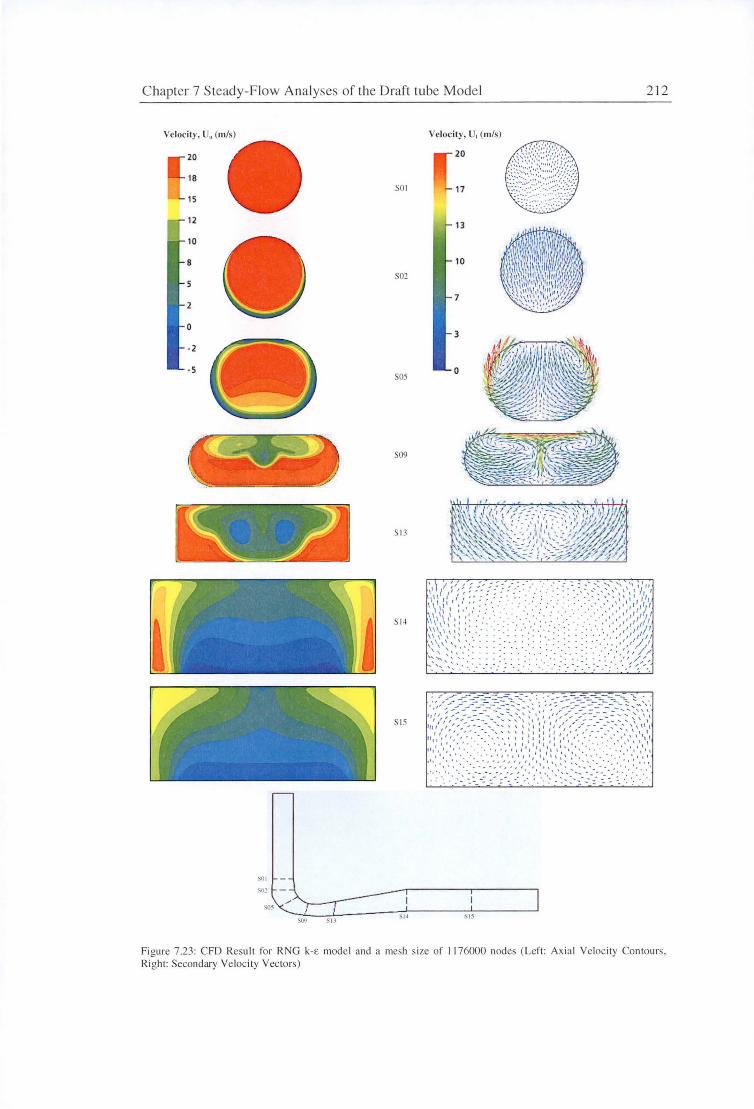
Chapter 7 Steady-Flow Analyses of the Draft tube Model 212
Velocity, U, (rn /s)
20
18 SO I
15
12
10
LJ 8
2
502
10
7
0 3
-2
- 5 0 505
S09
513
s 14
SIS
SOI
SOS SIJ SI S
Figure 7.23: CFO Result for RNG k-E model and a mesh size of 1176000 nodes (Left : Axial Velocity Contours. Right: Secondary Velocity Vectors)
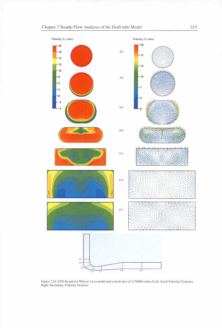
Chapter 7 Steady-Flow Ana lyses of the Draft tube Model 2 13
Velocity, U, (rn/s) Velocity, U, (rn/s)
20
18
15
12
SO I
20
17
• . .
13
10
S02 10
7
3
SOS
S09
SIJ
S 14
S IS
513 SJ5
Figure 7.24: CFD Result for Wilcox's k-ro model and a mesh size of 11 76000 nodes (Left: Ax ial Velocity Contours. Right: Secondary Velocity Vectors)
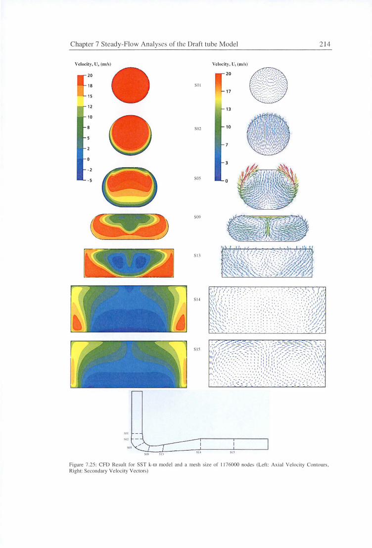
Chapter 7 Steady-Flow Analyses of the Draft tube Model 2 14
Velocity, U, (rn/s)
20
18 SO I
15
12
10
u 8
2
S02
0
- 2
- 5 SOS
S09
Sl3
SI~
S IS
SOI
502
S l4 SIS
Figure 7.25: CFD Result for SST k-ro model and a mesh size of 1176000 nodes (Left: Axial Velocity Contours, Right: Secondary Velocity Vectors)
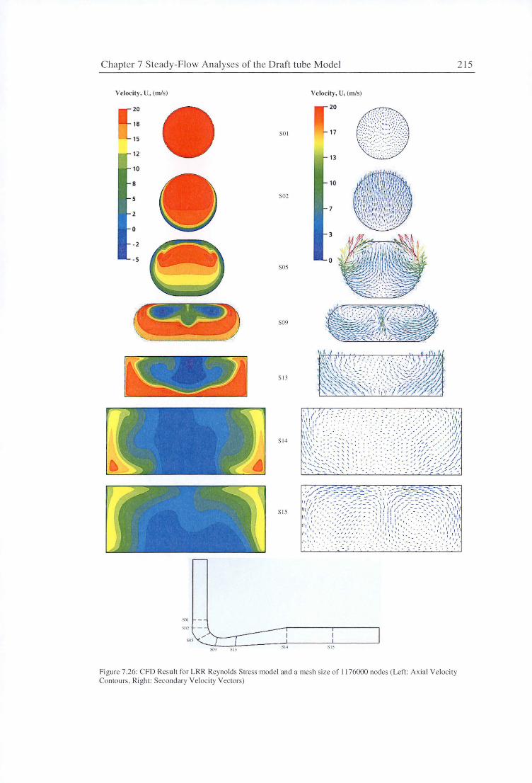
Chapter 7 Steady-Flow Analyses of the Draft tube Model
Velocity, U" (m/s)
20
18
15
12
10
SO I
SOl
SOS
Velocity, U, (m/s)
SO I
13
S02
SOS
509
SIJ
S l4
SIS
S14 S l5
Fi gure 7 .26: C FD Result fo r LRR Reynolds Stress model and a mesh size of 11 76000 nodes (Left: Ax ial Veloc ity Contours, Right: Secondary Velocity Vectors)
215
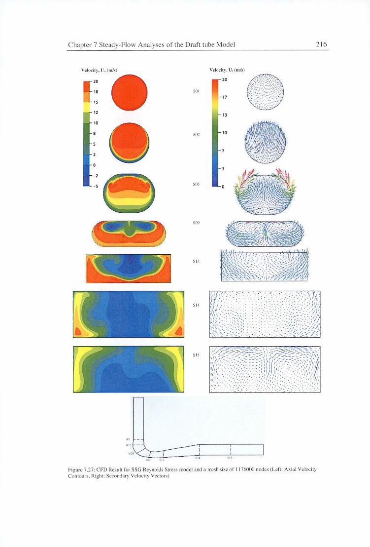
Chapter 7 Steady-Flow Ana lyses of the Draft tube Model 216
Velocity, U .. (m/s) Velocity, U, (m/s)
20
18
15
SOI
• 20
17
12 13
10
8 502 10
7 2
0
· 2
· 5 SOS
S09
S l3
s 14
S IS
SO I
S02
SOS
S l4 S IS
Fi gure 7.27: CFO Result for SSG Reynolds Stress model and a mesh size of 11 76000 nodes (Left: Axial Velocity Contours , Right: Secondary Velocity Vectors)
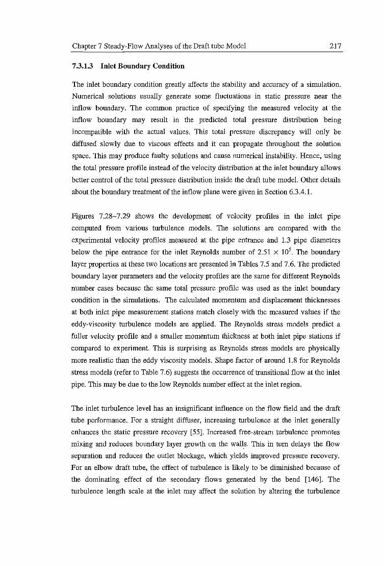
Chapter 7 Steady-Flow Analyses of the Draft tube Model 217
7 .3.1.3 Inlet Boundary Condition
The inlet boundary condition greatly affects the stability and accuracy of a simulation.
Numerical solutions usually generate some fluctuations in static pressure near the
inflow boundary. The common practice of specifying the measured velocity at the
inflow boundary may result in the predicted total pressure distribution being
incompatible with the actual values. This total pressure discrepancy will only be
diffused slowly due to viscous effects and it can propagate throughout the solution
space. This may produce faulty solutions and cause numerical instability. Hence, using
the total pressure profile instead of the velocity distribution at the inlet boundary allows
better control of the total pressure distribution inside the draft tube model. Other details
about the boundary treatment of the inflow plane were given in Section 6.3.4.1.
Figures 7 .28-7 .29 shows the development of velocity profiles in the inlet pipe
computed from various turbulence models. The solutions are compared with the
experimental velocity profiles measured at the pipe entrance and 1.3 pipe diameters
below the pipe entrance for the inlet Reynolds number of 2.51 x 10⁵. The boundary
layer properties at these two locations are presented in Tables 7.5 and 7.6. The predicted
boundary layer parameters and the velocity profiles are the same for different Reynolds
number cases because the same total pressure profile was used as the inlet boundary
condition in the simulations. The calculated momentum and displacement thicknesses
at both inlet pipe measurement stations match closely with the measured values if the
eddy-viscosity turbulence models are applied. The Reynolds stress models predict a
fuller velocity profile and a smaller momentum thickness at both inlet pipe stations if
compared to experiment. This is surprising as Reynolds stress models are physically
more realistic than the eddy viscosity models. Shape factor of around 1.8 for Reynolds
stress models (refer to Table 7.6) suggests the occurrence of transitional flow at the inlet
pipe. This may be due to the low Reynolds number effect at the inlet region.
The inlet turbulence level has an insignificant influence on the flow field and the draft
tube performance. For a straight diffuser, increasing turbulence at the inlet generally
enhances the static pressure recovery [55]. Increased free-stream turbulence promotes
mixing and reduces boundary layer growth on the wal~s. This in tum delays the flow
separation and reduces the outlet blockage, which yields improved pressure recovery.
For an elbow draft tube, the effect of turbulence is likely to be diminished because of
the dominating effect of the secondary flows generated by the bend [146]. The
turbulence length scale at the inlet may affect the solution by altering the turbulence
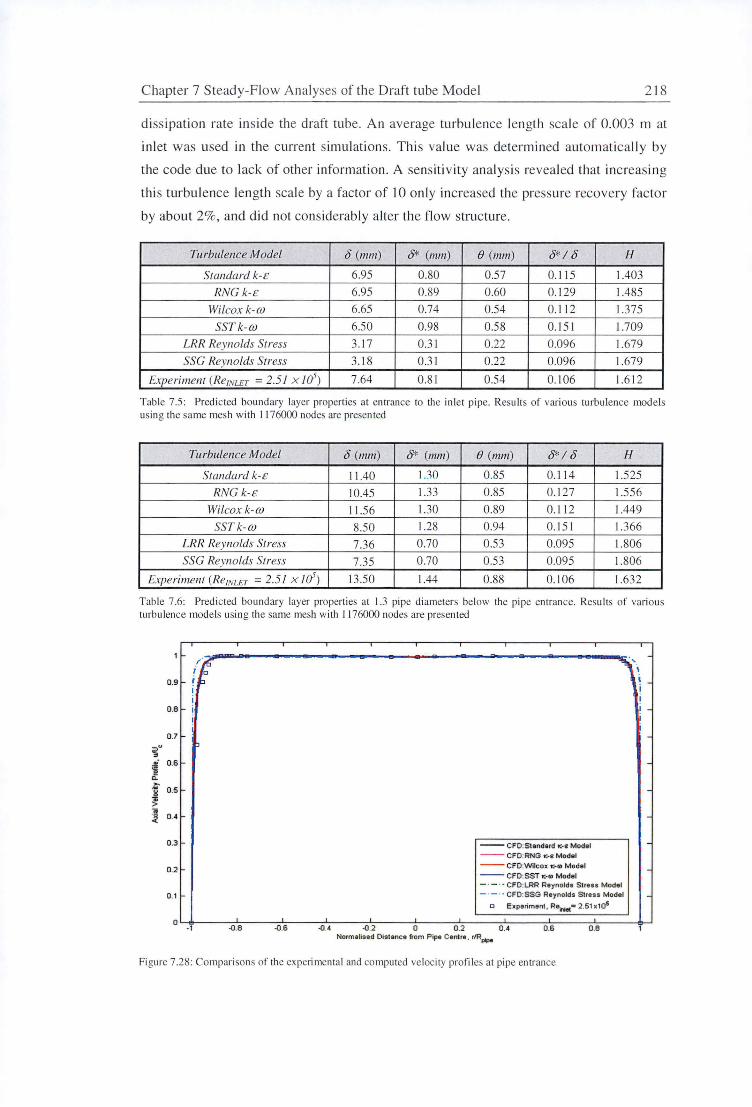
Chapter 7 Steady-Flow Analyses of the Draft tube Model 218
diss ipation rate inside the draft tube. An average turbu lence length sca le of 0.003 m at
inl et was used in the current simu lations. This value was determined automatica ll y by
the code due to lack of other information . A sensitivity analysis revealed that increasing
th is turbulence length scale by a factor of I 0 on ly increased the pressure recovery factor
by about 2%, and did not considerably alter the flow structure.
Turbulence Model t5 (mm) O* (mm) e (mm) o*I o H
Standard k-£ 6.95 0.80 0.57 0.115 1.403
RNC k-£ 6.95 0.89 0.60 0. 129 l.485
Wilcox k-OJ 6.65 0.74 0.54 0.112 1.375
SST k- w 6.50 0.98 0.58 0. 15 1 1.709
LRR Reynolds Stress 3.17 0.31 0.22 0.096 1.679
SSC Reynolds Stress 3. 18 0.3 1 0.22 0.096 1.679
Experiment (Re!NLET = 2.51 x I a5) 7.64 0.81 0.54 0.106 1.6 12
Table 7.5: Predicted boundary layer properties at entrance to the inlet pipe. Results of various turbulence mode ls using the same mesh with 11 76000 nodes are presented
Turbulence Model o (mm) O* (mm) e (mm) 0*1 o H
Standard k-£ 11 .40 1.30 0.85 0.114 1.525
RNC k-£ 10.45 1.33 0.85 0. 127 1.556
Wilcox k-OJ 11.56 1.30 0.89 0. 11 2 1.449
SST k-w 8.50 1.28 0.94 0.151 1.366
LRR Reynolds Stress 7.36 0.70 0.53 0.095 1.806
SSC Reynolds Stress 7.35 0.70 0.53 0.095 1.806
Experiment (ReiNLET = 2.5 1 x Id) 13.50 1.44 0.88 0. 106 1.632
Tab le 7 .6: Predicted boundary layer properti es at 1.3 pipe diameters below the pipe entrance. Results of various turbu lence models using the same mesh with 1176000 nodes are presented
1 ....
f( 0.9 ,... I
i I
0.8 .... j
0.7 ....
:f 'J
~ 0.6 ....
a.
f 0.5 ....
~ 0.4 .... ~
0.3
0 .2
0 .1
0 -1 -0.B -0.6
- - CFO: Standard K-• Model --CFO:RNG >::-•Model -- CFO:Wilcox K-m Mod•I --CFO: SST >::-co Model
~\ i I I
- · - · • CFO:LRR Raynolds Strea:s Model
-
-
- · - · - CFD:SSG Reynolds S1ress Model -
o Experiment, Relriet= 2.51 x1a5
-0.4 -0.2 0 0 .2 0 .4 0 .6 0 .8 Normalised Distance from Pipe Centre, r/Rptpe
Figure 7.28: Comparisons of the experi menta l and computed ve locity profiles at pipe entrance
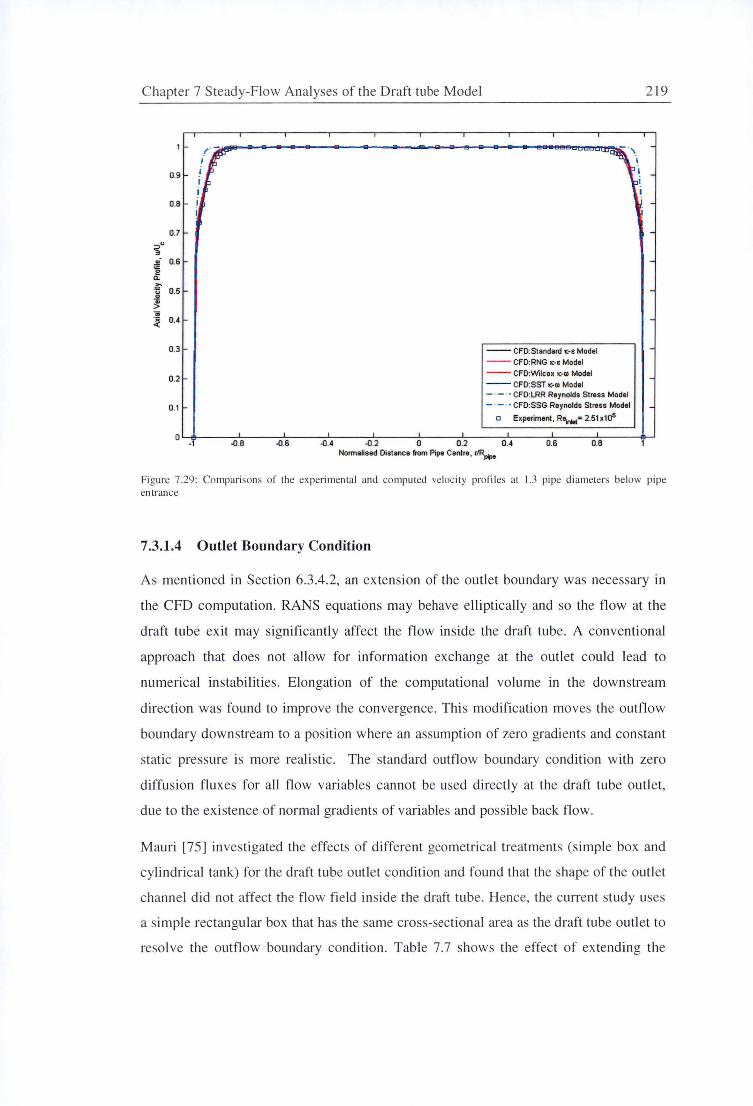
C hapter 7 Steady-Flow Analyses of the Draft tube Model 2 19
0.9
O.B
0.7
~Q
i!. 0.6 E! c. ,.. ·" 0.5 u 0
J .... ~ 0.4
0.3 -- CFO: Standard K-s Modal
--CFD:RNG K-• Modal
0.2 --CFD:Wilcox K-m Model
-- CFD:SSTK-6l Modal - · - · - CFD:LRR Raynolds Stniss Model
0.1 - · - · - CFD:SSG Raynolds Stniss Modal
a Experiment, R.,_= 2.51 x1a5
0 -1 -0.B -0.6 -0.4 -0.2 0 0.2 0.4 0.6 0.8
Normalised Distance from Pipe Cantre , r/Rpipe
Fi gure 7.29: Compari sons of the experimental and computed velocity profi les at 1.3 pipe di ameters below pipe entrance
7.3.1.4 Outlet Boundary Condition
As mentioned in Section 6.3.4.2, an extension of the outl et boundary was necessary in
the CFD computation . RANS equations may behave elliptically and so the flow at the
draft tube ex it may significantly affect the flow in side the draft tube. A conventional
approach that does not allow for information exchange at the outlet could lead to
numerical in stabilities. Elongation of the computational volume in the downstream
direction was found to improve the convergence. Thi s modification moves the outflow
boundary downstream to a positi on where an assumption of zero gradi ents and constant
static pressure is more realistic. The standard outflow boundary condition with zero
diffusion fluxes for all flow variables cannot be used directly at the draft tube outlet,
due to the ex istence of normal gradi ents of variables and possible back flow .
Mauri [75] investigated the effects of different geo metrical treatments (simple box and
cylindrical tank) for the draft tube out let condition and found that the shape of the outlet
channel did not affect the flow fie ld inside the draft tube. Hence, the current study uses
a simple rectangular box that has the same cross-sectional area as the draft tube outlet to
resolve the outflow boundary condition . Table 7.7 shows the effect of ex tending the
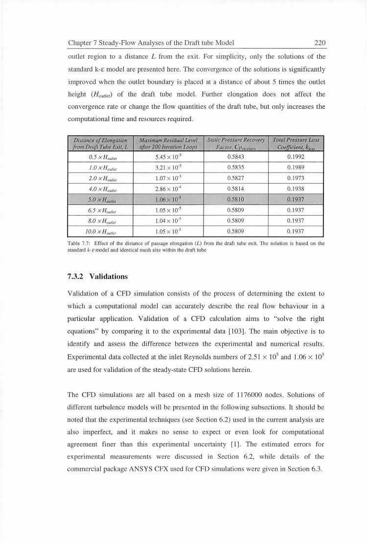
Chapter 7 Steady-Flow Analyses of the Draft tube Model 220
outlet region to a distance L from the exit. For simplicity, only the solutions of the
standard k-£ model are presented here. The convergence of the solutions is significantly
improved when the outlet boundary is placed at a distance of about 5 times the outlet
height (Hout/et) of the draft tube model. Further elongation does not affect the
convergence rate or change the tlow quantities of the draft tube, but only increases the
computational time and resources required.
Distance of Elongation Maximum Residual level Static Pressure Recovery Total Pressure Loss from Drafl Tube Exit, L after 200 Iteration Loops Factor, Cprecoverv Coefficient, ktoss
0.5 X H 01111er 5.45 x 10·3 0.5843 0.1992
1.0 X H our/er 3.21 x 10·3 0.5835 0.1989
2.0 X H 0111ler 1.07 x 10·3 0.5827 0.1973
4.0 xH01111er 2.86 x 10⁻⁴ 0.5814 0.1938
5.0 X H our/er 1.06 x 10⁻⁵ 0.5810 0.1937
6.5 X H owler 1.05 x 10·5 0.5809 0.1937
8.0 X H owler 1.04 x 10·5 0.5809 0.1937
10.0 X H 011rler 1.05 x 10⁻⁵ 0.5809 0.1937
Table 7.7: Effect of the distance of passage elongation (l) from the draft tube exit. The solution is based on the standard k-£ model and identical mesh size within the draft tube
7 .3.2 Validations
Validation of a CFD simulation consists of the process of determining the extent to
which a computational model can accurately describe the real flow behaviour in a
particular application. Validation of a CFD calculation aims to "solve the right
equations" by comparing it to the experimental data [103]. The main objective is to
identify and assess the difference between the experimental and numerical results.
Experimental data collected at the inlet Reynolds numbers of 2.51 x 10⁵ and 1.06 x 10⁵
are used for validation of the steady-state CFD solutions herein.
The CFD simulations are all based on a mesh size of 1176000 nodes . Solutions of
different turbulence models will be presented in the following subsections. It should be
noted that the experimental techniques (see Section 6.2) used in the current analysis are
also imperfect, and it makes no sense to expect or even look for computational
agreement finer than this experimental uncertainty [1]. The estimated errors for
experimental measurements were discussed in Section 6.2, while details of the
commercial package ANSYS CFX used for CFD simulations were given in Section 6.3 .
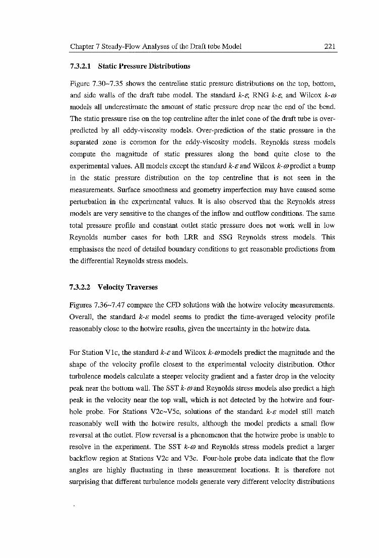
Chapter 7 Steady-Flow Analyses of the Draft tube Model 221
7 .3.2.1 Static Pressure Distributions
Figure 7.30-7.35 shows the centreline static pressure distributions on the top, bottom,
and side walls of the draft tube model. The standard k-c, RNG k-s, and Wilcox k-m
models all underestimate the amount of static pressure drop near the end of the bend.
The static pressure rise on the top centreline after the inlet cone of the draft tube is over
predicted by all eddy-viscosity models. Over-prediction of the static pressure in the
separated zone is common for the eddy-viscosity models. Reynolds stress models
compute the magnitude of static pressures along the bend quite close to the
experimental values. All models except the standard k-c and Wilcox k-OJ predict a bump
in the static pressure distribution on the top centreline that is not seen in the
measurements. Surface smoothness and geometry imperfection may have caused some
perturbation in the experimental values. It is also observed that the Reynolds stress
models are very sensitive to the changes of the inflow and outflow conditions. The same
total pressure profile and constant outlet static pressure does not work well in low
Reynolds number cases for both LRR and SSG Reynolds stress models. This
emphasises the need of detailed boundary conditions to get reasonable predictions from
the differential Reynolds stress models.
7 .3.2.2 Velocity Traverses
Figures 7 .36-7.4 7 compare the CFD solutions with the hotwire velocity measurements.
Overall, the standard k-s model seems to predict the time-averaged velocity profile
reasonably close to the hotwire results, given the uncertainty in the hotwire data.
For Station V le, the standard k-c and Wilcox k-m models predict the magnitude and the
shape of the velocity profile closest to the experimental velocity distribution. Other
turbulence models calculate a steeper velocity gradient and a faster drop in the velocity
peak near the bottom wall. The SST k-mand Reynolds stress models also predict a high
peak in the velocity near the top wall, which is not detected by the hotwire and four
hole probe. For Stations V2c-V5c, solutions of the standard k-c model still match
reasonably well with the hotwire results, although the model predicts a small flow
reversal at the outlet. Flow reversal is a phenomenon that the hotwire probe is unable to
resolve in the experiment. The SST k-m and Reynolds stress models predict a larger
backflow region at Stations V2c and V3c. Four-hole probe data indicate that the flow
angles are highly fluctuating in these measurement locations. It is therefore not
surprising that different turbulence models generate very different velocity distributions
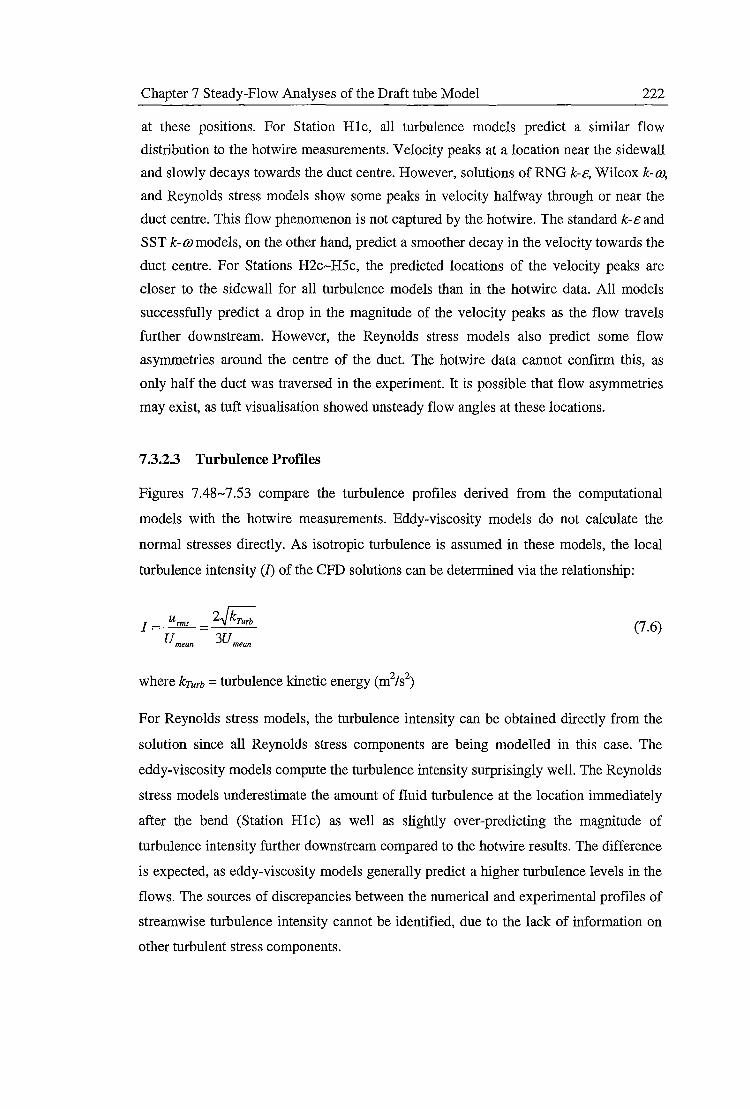
Chapter 7 Steady-Flow Analyses of the Draft tube Model 222
at these positions. For Station Hlc, all turbulence models predict a similar flow
distribution to the hotwire measurements. Velocity peaks at a location near the sidewall
and slowly decays towards the duct centre. However, solutions of RNG k-&, Wilcox k-OJ,
and Reynolds stress models show some peaks in velocity halfway through or near the
duct centre. This flow phenomenon is not captured by the hotwire. The standard k-& and
SST k-mmodels, on the other hand, predict a smoother decay in the velocity towards the
duct centre. For Stations H2c~H5c, the predicted locations of the velocity peaks are
closer to the sidewall for all turbulence models than in the hotwire data. All models
successfully predict a drop in the magnitude of the velocity peaks as the flow travels
further downstream. However, the Reynolds stress models also predict some flow
asymmetries around the centre of the duct. The hotwire data cannot confirm this, as
only half the duct was traversed in the experiment. It is possible that flow asymmetries
may exist, as tuft visualisation showed unsteady flow angles at these locations.
7 .3.2.3 Turbulence Profiles
Figures 7.48~7.53 compare the turbulence profiles derived from the computational
models with the hotwire measurements. Eddy-viscosity models do not calculate the
normal stresses directly. As isotropic turbulence is assumed in these models, the local
turbulence intensity (I) of the CPD solutions can be determined via the relationship:
I = u,ms ::: 2.JC U mean 3U mean
(7.6)
where kTurb =turbulence kinetic energy (m2/s2)
For Reynolds stress models, the turbulence intensity can be obtained directly from the
solution since all Reynolds stress components are being modelled in this case. The
eddy-viscosity models compute the turbulence intensity surprisingly well. The Reynolds
stress models underestimate the amount of fluid turbulence at the location immediately
after the bend (Station Hlc) as well as slightly over-predicting the magnitude of
turbulence intensity further downstream compared to the hotwire results. The difference
is expected, as eddy-viscosity models generally predict a higher turbulence levels in the
flows. The sources of discrepancies between the numerical and experimental profiles of
streamwise turbulence intensity cannot be identified, due to the lack of information on
other turbulent stress components.
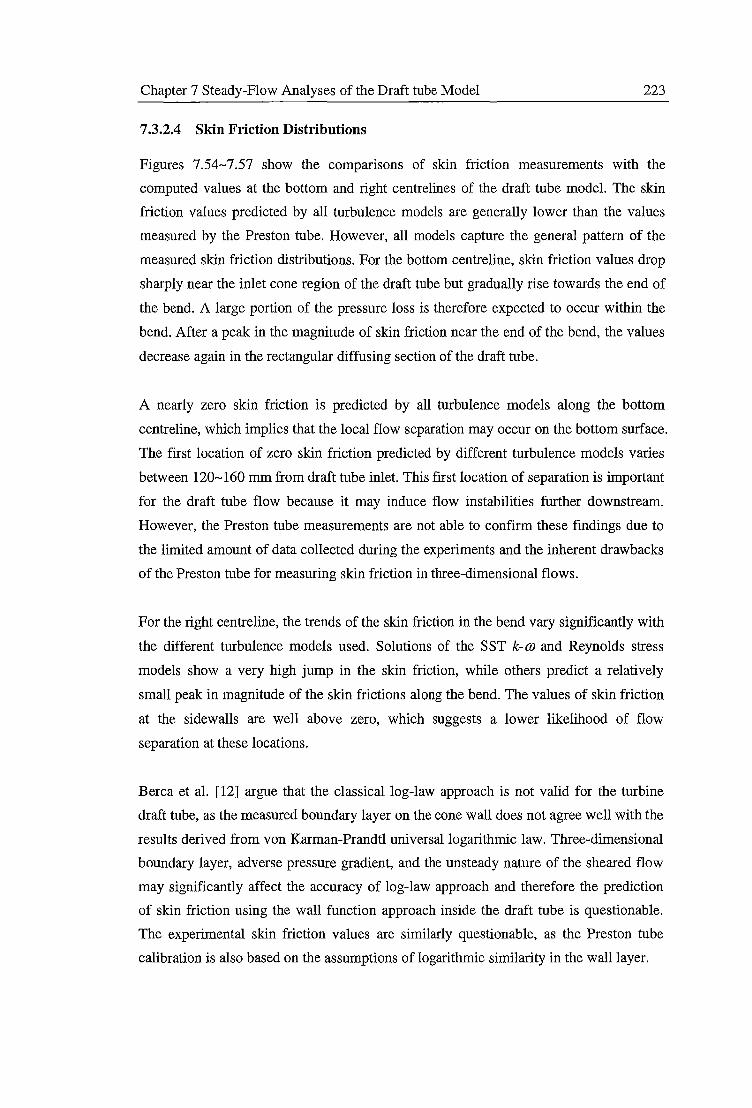
Chapter 7 Steady-Flow Analyses of the Draft tube Model 223
7 .3.2.4 Skin Friction Distributions
Figures 7.54-7.57 show the comparisons of skin friction measurements with the
computed values at the bottom and right centrelines of the draft tube model. The skin
friction values predicted by all turbulence models are generally lower than the values
measured by the Preston tube. However, all models capture the general pattern of the
measured skin friction distributions. For the bottom centreline, skin friction values drop
sharply near the inlet cone region of the draft tube but gradually rise towards the end of
the bend. A large portion of the pressure loss is therefore expected to occur within the
bend. After a peak in the magnitude of skin friction near the end of the bend, the values
decrease again in the rectangular diffusing section of the draft tube.
A nearly zero skin friction is predicted by all turbulence models along the bottom
centreline, which implies that the local flow separation may occur on the bottom surface.
The first location of zero skin friction predicted by different turbulence models varies
between 120-160 mm from draft tube inlet. This first location of separation is important
for the draft tube flow because it may induce flow instabilities further downstream.
However, the Preston tube measurements are not able to confirm these findings due to
the limited amount of data collected during the experiments and the inherent drawbacks
of the Preston tube for measuring skin friction in three-dimensional flows.
For the right centreline, the trends of the skin friction in the bend vary significantly with
the different turbulence models used. Solutions of the SST k- OJ and Reynolds stress
models show a very high jump in the skin friction, while others predict a relatively
small peak in magnitude of the skin frictions along the bend. The values of skin friction
at the sidewalls are well above zero, which suggests a lower likelihood of flow
separation at these locations.
Berca et al. [12] argue that the classical log-law approach is not valid for the turbine
draft tube, as the measured boundary layer on the cone wall does not agree well with the
results derived from von Karman-Prandtl universal logarithmic law. Three-dimensional
boundary layer, adverse pressure gradient, and the unsteady nature of the sheared flow
may significantly affect the accuracy of log-law approach and therefore the prediction
of skin friction using the wall function approach inside the draft tube is questionable.
The experimental skin friction values are similarly questionable, as the Preston tube
calibration is also based on the assumptions of logarithmic similarity in the wall layer.
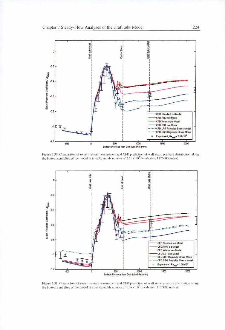
Chapter 7 Steady-Flow Ana lyses of the Draft tube Model
0
-0.2
! ; -{l.6 .. ! a. u
·~
tn -0.8
-1
.!ii E J l: I =1 'i I cs1
I I I I I I I I I I I I I I I I I I I I I I I I I I
I a; I I '§ J
-gl OJ ~I ~I 'QI Z I -cl ii ifi1 cs1
I I I I I I I I I I I I I I I I I I I
.......... _..-I __ ._.--
r--r----
---_ _,, I
--CFO: Standard i::-s Model
--CFO:RNG i::-£ Model
--CFD:Wilcox i::-a> Model
--cFO:SSTi::-Ol Model - · - · -CFO:LRR Reynolds Stress Model
- · - · - CFD:SSG Reynolds Stress Model
o Experiment, Re.not= 2.51 x1D5
Surface Distance from Draft tube Inlet (mm)
224
Fi gure 7.30: Comparison of experimental measurement and CFO prediction of wall static pressure diSU'ibution along the bottom centreline of the model at in Jet Reynolds number of 2.51 x I 05 (mesh size: 1176000 nodes)
0
-0.2
J 0 -0.4 -i .!!
~ 0
0
~ -0.6 ., ., ~ a.
.!.! 1i tii
-0.B
-1
.!ii E J l: I =1 'ii I Ci I
i
-500 0
I 'iii I '§ J
-g1 01 ~I l: I 'QI =1 -.. I 1i I JjJ cs1
--CFD:Standard ic-• Model
--CFD:RNG i::-£ Model
--CFO:Wilcox i::-m Model
--c FD:SSTK-Cll Model - · - · - CFO: LRR Reynolds Streu Model - · - · · CFO: SSG Reynolds Stress Model
o Experiment , Re.not= 1.00x1D5
500 1CXXJ 1500 2CXXJ Surface Distance from Draft tube Inlet (mm)
Fi gure 7.3 1: Compari son of experimental measurement and CFO prediction of wall static pressure distribution along the bottom centreline of the model at inlet Reynolds number of 1.06 x I 05 (mesh size: 1176000 nodes)
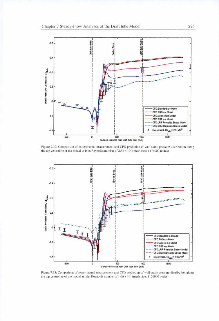
Chapter 7 Steady-Flow Analyses of the Draft tube Model
-0.2
-0.4
.ll
J .()6 (.)
c .!! u :: . 8 -0.B ! ii: .. ! a. .!l ... -1 tii
-1.2
-1 .4
-500
I a; ]! I I ~I .: I -g I 01 1! I O'll 1! I .: I 'QI .: I 'i I -g I '& I al wl al
I I I I
I
:J: 0 500 um
Surface Distance from Draft tube Inlet (mm)
225
--CFO: Standard 1::- s Model --CFO:RNG 1::-s Model --CFD:Wilcox 1::-11 Model --cFD:SST 1'-Q) Model - · - · - CFD:LRR Reynolds Stress Model - · - · - CFD:SSG Raynolds Stress Modal
o Experiment, ReHel= 2.51 x1Cl5
1500
Figure 7.32: Compari son of experimental measurement and CFD prediction of wall static pressure distribution along the top centreline of the model at inlet Reynolds number of 2.5 1 x I 05 (mesh size: 1176000 nodes)
-0.2
-0.4
t -0.6 "' (.)
i . ·c:; E .
-0.B 0 (.)
$ :: ! a. -·-·-. u
-1 -.... 'i I tii :I :I
-1.2
-1 .4
-500
.i I
.: I 1! I .: I <=I ,51
I I I I I I
., ., . 1' -
0
I I
-g I ~I -1 ~I Ji I
I I I I
500
~I 01 .J!l I .: I ii I al
I I
um Surface Distance from Draft tube Inlet (mm)
--CFD:Standard 1::-1 Model --cFO:RNG 1::-• Model --CFD:Wilcox 1::-11 Model --CFO: SST ic-m Model - · - · - CFO: LRR Reynolds Stress Model - · - · - CFO: SSG Reynolds Stress Model
o Experiment , R._= 1.00x1Cl5
1500
Figure 7.33: Comparison of experimental measurement and CFD prediction of wall static pressure distribution along the top centreline of the model at inlet Reynolds number of 1.06 x 10⁵ (mesh size: 11 76000 nodes)
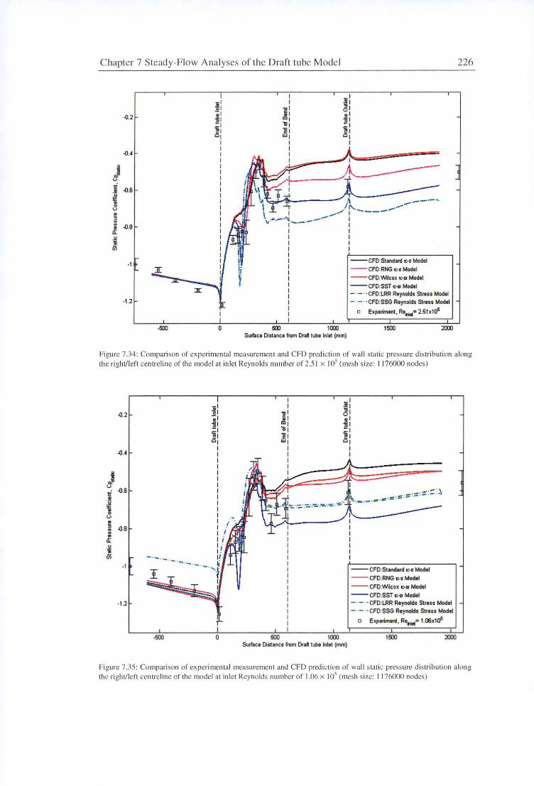
Chapter 7 Steady-Flow A nalyses of the Draft tube Model
-0.2
-O.•
~ "' u i -0.6 .. 'i:l i: " 0 u !! " :: -0.B !!
D. .!I 1i iii
-1
-1 .2
-500 0
'I ___ ,
/J\... _ ..... -1 -----
500 1000 Surface Distance from Draft tube Inlet (mm)
1 I I I I I
--CFO: Standard IC-s Model --CFD:RNG IC-s Model
--CFD:Wilcox IC-Ill Model
--CFD:SST IC-m Modal - · - · - CFD:LRR Reynolds Stress Model - · - · • CFD:SSG Raynolds Stress Modal
o Experiment, Ra,....= 2.51x1a5
1500
226
Figure 7 .34: Comparison of experimental measurement and CFO prediction of wall slatic pressure distribution along the ri ght/left centre line of the model at inlet Reynolds number of 2.51 x I 05 (mesh size: 1176000 nodes)
~ "' u
-0.2
-O.•
c: -0.6 .!! ~ .. 0 u ! : -0.8 ! D. u 1i iii
-1
-1.2
- --· --·-·-·-.
-500 0 500
I I
"2 ' ill' _, 01 °21 w1
I I I I I
1000 Surface Distance from Draft tube Inlet (mm)
I .... ... . , " ·- ·::: :- ·- ·-I :~ ·. -. 1 _ ,_ , ., ! ~ ·· == · - ·
--CFO: Standard IC-• Model --CFD:RNG 1C-s Model
--CFD:Wilcox IC-Ill Model --CFD:SSTIC-lll Model - · - · -CFD:LRR Reynolds Stress Model - · - · - CFD:SSG Raynolds Stress Model
o Experiment , Re,....= 1.06x1a5
1500
Figure 7 .35: Comparison of experi mental measurement and CFO prediction of wall stat ic pressure distribution along the right/left centreline of the model at in let Reynolds number of 1.06 x I 05 (me h size: I 176000 nodes)
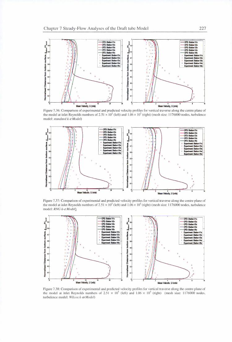
Chapter 7 Steady-Flow Analyses of the Draft tube Model 227
- CFD:SlllionV1c .} .. 1 - CFD:SlllionV2c ;i: •.• - - - ·CFD:SlobVJc
j .. ---- CFD: Slob V4c J .. - CFD:Slob'l5c
3 0 E,.,.-:SllllonV1c .; u
1 ., E,.,.-:-V2• ~
., 0 E,.,.-:SlobVJc ii
E 0.1 . ~SlolionV4c E O.t
i · Slllloo'l5c 0
" .. .8 o.• E E ,g •• ,g . .. ~ ~ ! ., • 1 O.I Q Q
J ., J ., Ii Ii e •• e •• ~ 0 z .,
10 " " 0 . ,
Meen Velociy, U (mls)
.. • 0 • "
0 . 0 \ O o •
•'
0 -,. ,.
)t • • •
l t : r ;
, <Jo i· : ~/ ;
' ~~ : •
Mean Vrk:dy, U (mls)
-CFD:SlolionV1c - CFO: SlationV2c - - - ·CFD:SlationVJc ---- CFD:-.V4c - CFD: Slolion'l5c
o !Jipelinenl:SlllionV1c
• E>qJerimoN: - V2c 0 E>qJerimoN: - VJc
!Jipefinenl: SllliaoV4c !Jipefinenl: Sllliao'l5c
10
Figure 7.36: Compari son of experimental and predicted velocity profi les for verti ca l traverse along the centre plane of the model at in let Reynolds numbers of2.51 x !05 (left) and 1.06 x 10⁵ (right) (mesh size: 1176000 nodes. turbu lence model: srandard k-& Model)
1 ;i: 0.9
Jo. 8 i'' E 0.1
~ .., .. E ,g ~ 0.4
! O.I Q
10.2 Ii
e '·'
- CFD:SlolionV1c - CFD:-.V2c ---·CFD:-VJc ----·CFD:-V4c -CFD:-'15c
o !Jporimool:SlllionV1c ' E,.,.-:SlllionV2c 0 !,.,..-: Slllion VJc • e.i--: SlllionV4c
: Slllion'l5c
~ o,L.~ ....... i._,'1..!.-'-~-'-~fr"-~--,,~, ~~~-.. ~==::::::.~»J,--~~--,1,,.
Mun Vlkd.v. U (mill
~ j A C+ t
T 0.1 .:. ~) *\ 1C:; O OT\ J 0 • 1·
o.t • o• I. o 8 0 .i j 0.7 '
·i ' ~ OI A0 1,1;
l< . } 'ff .! 0.5 ° ~ 1'
~ ~ .jj ~ 0.4 o:.// 8 0 +;; ! OJ ' /i Q '•"/ 1! , , .i OJ f' i 'i / ;'
Z~ 0.1 ! /:i
- CFD:SllliaoV1c - CFD:-.V2c - - - ·CFD:SlolionVJc ---- CFD:SlolionV4c -CFD:Sllliaolr.5c
• !Jipefinenl: SllliaoV1c !Jipefinenl: SllliaoV2c
0 E>qJerimoN: - VJc • !Jipefinenl:SllliaoV4c
S111ion'l5c
;' ;; ; ~,ZL~~--'-+;'"'-~"-'--~~--',~~~.-""'::::::.~-'-~~~~10
Mean Vrk:dy, U (mls)
Figure 7.37: Comparison of experimenta l and predicted veloci ty profi les for vertica l traverse along the cen u·e plane of the model at inlet Reynolds numbers of 2.5 1 x I 05 ( left) and 1.06 x !05 (right) (mesh size: I 176000 nodes. turbu lence model: RNC k- &Modell
~l o. - CFD:-V1c 1 ~··'\
0 0 - CFD:SllliaoV1c
- CFD:SlobV2c ~ O.t ' 0 ... . .,. - CFD:SllliaoV2c
--·CFD:SlobVJc 0 I ~\ ---·CFD:SllllonVJc
Jo. ---- CFD: Sllb V4c
J .1 I ,II~ ----·CFD:SlolionV4c
A -CFD:Slolionlr.5c ' 0 °' 'd - CFD:Slolion'l5c
3 ., 0 !Jporimool;- V1c 8 : b 0 Elq>orimonl:SllliooV1c . j 0.1 . !Jporimool;- V2c j 0.1 H . Elq>orimonl: SllliaoV2c
0 ~: SlolionVJc ' E>qJerimoN: - VJc , ., E 0.1 . ~: SlobV4c
~ 0.1 ' ' ii Elq>orimonl:S111ionV4c , , 0 E,.,.-:-'15c :! · 5111ion'15c
" ~ .8 o.• o.s .q :: j j " if 0.4 •.. ,,
~ ~ °' ! j • 0.3 ! of j 1 ., Q Q ,. if
" OJ l " :4
.I OJ , , • I
Ii • : ,' / e ., e "' !)- J : 0 0 0 :/ i 0 z j z 0
0
$!' ' ., 10 " " 0 • 10 .,
Meen Vtb:fl:t, U (mls) Mean Volocitv. U (mlsl
Fi gure 7.38: Comparison of experimental and predicted ve locity profil es for vertica l traverse along the centre plane of the model at in let Reynolds numbers of 2.5 1 x I 05 ( left) and 1.06 x I 05 (ri ght) (mesh size: I 176000 nodes. turbulence model: Wilcox k-m Model)
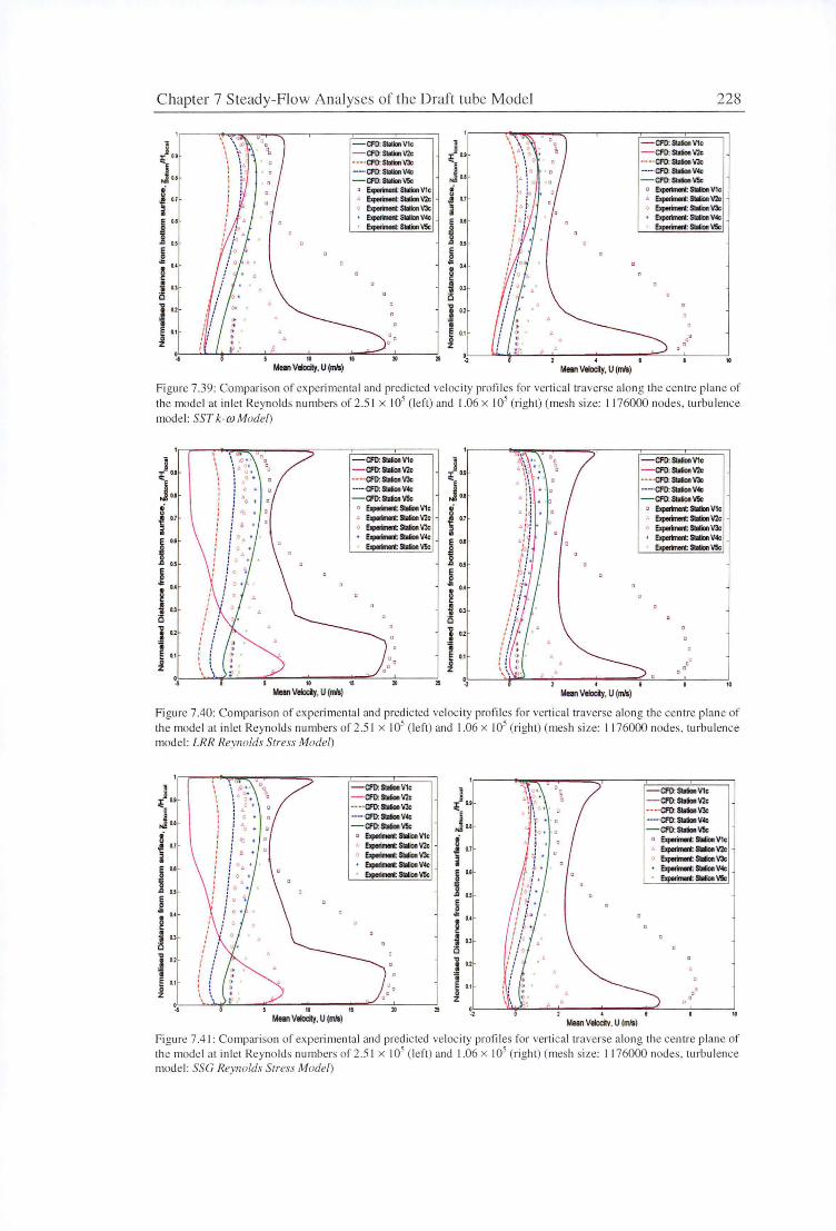
Chapter 7 Steady-Flow Analyses of the Draft tube Model
1 - CFO:stationV1c .,} .. - CfO:SllllonV2c ;i: 0.1 -- - · CfO:SllllonV3c J,. ·····CfO:SllllonVolo J .. -CfO:SlatianV5c
3 a Elperimenl: Sbllion V1c 3 ; 0.7 • Elperimenl: - V2c ; 0.1
0 OperimmC Slolion V3c
i •.. OperimmC Slolion Volo E 0.8
:Slmion V5c 0
... ~ ,, !I ] "' 0.4 0.4
~ ~ ; OJ • 0.) ii i5 i5
1 ., 1 01
g • 0.1 0 g 0.1
0 0 z f1 z
' 10 " .,
" 0, • MNn VeltJciy, U (mll) Man Vrlt:D.y, U (mll)
228
- CfO:StalionV1c - CfO:SlalianVlc --- ·CfO:StaliooV3c --···CfO:SllliooVolo - CfO:SllliooV5c
a Experimlrll: Sllion V1c • Experimlrll:SlollooVZ. o Exporimonl: S1o11oo V3c
Exporimonl: Slolloo Volo E :SlatianV5c
" Figure 7.39: Comparison of expe1imental and predicted velocity profi les for vertical traverse along the centre plane of the model at inlet Reynolds numbers of2.5 1 x 10⁵ (left) and 1.06 x 10⁵ (right) (mesh size: 1176000 nodes, turbulence model: SST k-w Model)
- CfO:SlolionV1c
;i:] .. ;i:1 .. - CfO:SllbVZc - - - ·CFO: SWloo V3c
J .. ··- ·CfO:Slllioo Volo J.. - CfO:SllbV5c
3 0 OperimmC Sllb V1c 3 ; ., . OperimmC Sllb Vlc ; ., 0 OperimmC Sllb V3c
~ OJ . OperimmC Sllb Volo
I •• SWlooV5c
'8 ... •• j j ~
•• ~
•• • OJ ; ii OJ i5 i3
l ., I ., =a
~ •1 0 ~ •1 '
'. " " " " 0 ·2
MNn Vekxty, U (mll)
h \\)
tl\ *~
ti 'W ·4~ ~ b 4
.-. :: d '
.l :d .: .
o, 1) 1
:! ~ I I
;:,/ .. J : + ! :
:'o! :'(/ .. / ,
/ /' ii I ! ' : . . . . I : (t : : ~
\ \ f)
0
4
MNn VeltJciy, U (mll)
- CfO:S1111onV1c - CfO:SllliooVlo -- - CfO: SllliooV3c ·····CfO:SllliooV4c - CfO:StalionV5c
0 Exporimonl:SlobV1c Exporimonl: Slob Vlc
0 Exporimonl: - V3c ' Exporimonl: Slob V4c
SlolionV5c
l 0
" Figure 7.40: Comparison of experimental and predicted velocity profiles for vertical traverse along the centre plane of the model at inlet Reynolds numbers of 2.51 x I 05 (left) and 1.06 x I 05 (right) (mesh size: 1 176000 nodes, turbulence model: LRR Reynolds Stress Model)
1 - CfO:SlobV1c - CfO:SlllionVlc ;i: 0.1 - -- ·CfO:SlllionV3c
J .. ·····CfO:SlllionV4c . 0 - CfO:SllbV5c 0 • • " '
o Elperimenl: SlolionV1c u . ; 0.1 • OperimmC Slolion vz.
Elperimenl: - V3c
I 0.1 OperimmC Slolion Volo
:Slolion V5c
,, j
0.4
~ ; O.l
i5
l 0.2
'i ~ 0.1 0
' z '. 10 "
., Mnn VeltJciy, U (mll)
] ;i: 0.1
J., 3 ; 0.1
I 0.1
'·' ] ~
0.4
; O.l
i5
1 0.2
• g 0.1
z
" 0 ·2
Mean Velocitv. U (mill
- CfO:SllliooV1c - CfO:-Vlc - - - Cf0:-V3c -···CfO:SlllionV4c - Cf0:-V5c
o Experimlrll: -.V1c • Exporimonl:- vz.
Exporimonl:- V3c ~:-V4c
· -V5c
10
Figure 7.41: Comparison of experimental and predicted velocity profiles for verti cal traverse along the centre plane of the model at inlet Reynolds numbers of 2.5 1 x I 05 ( left) and 1.06 x I 05 (right) (mesh size: I 176000 nodes, turbulence model: SSC Reynolds Srress Model)
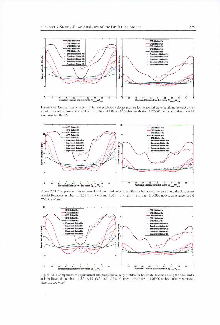
Chapter 7 Steady-Flow Ana lyses of the Draft tube Model 229
,. - CfD:SlaliooH1c - CFD:-H2c ---·Cl'O:-H3c ----·Cl'O:-H-4c - CFD:-H5c
I" D D
D
::>
~ ~ 10
• > c: • i '
~.~-~ ... ~.--.. ~ .• ,--~~.--4~,-~,'---~.,,--.~.-,-,~.-~.~.--'
Nonnolised Oillance Iran duct come, °l'f..,.,.IW ...
,.
"
I" ::>
l" >
l
- CFD: S1oliooH1c - Cl'O:S1oliooH2c --- -Cf0:-H3c ----·CFD:SloliooH-4c - CFD:S1oliooH5c
o ~:-H1c
~:-H2c
~:-H3c i!Jipoftnw11:-H-4c ~-H5c
Figure 7.42: Compari son of experimental and predicted ve locity profiles for horizontal traverse along the duct centre at inlet Reynolds numbers of 2.51 x I 05 (left) and 1.06 x I 05 (right) (mesh size: 1176000 nodes, turbulence model: standa rd k-t: Model)
,. " - Cl'O:-H1c - CfO:StliliorlH1c
- Cl'O:-H2c - Cl'O:-H2c ---·Cl'O:-H3c ---·Cl'O:-IOc ----·Cl'O:-H4c 20 ----·Cl'O:-H-4c - Cl'O:-H5c - Cl'O:-H5c
D ~:-Hie 0 i!Jipoftnw11:-Hlc
I" . l!Jipoftnw11:-.H2c l" . ~:-H2c 0 i!Jipoftnw11:-H3c l!>ip.--:-H3c
::> ~-H4c ::> . ~:-H-4c
flO ~:-H5c
l" ~:-H5c
g DQo DC o OC
coco
> > c: l • i'
Figure 7.43: Comparison of experimental and pred icted ve loc ity profiles for horizontal traverse along the duct centre at inlet Reynolds numbers of 2.5 1 x I 05 (left) and 1.06 x I 05 (right) (mesh size: l 176000 nodes, turbulence model: RNG k-t: Model)
"r-__,,---,--;::::::r:=::::!::=::::c::::;--.--....--,.--.------, - Cl'O:-Hlc
i i.
- Cl'O:-H2c ---Cf0:-H3c ----·Cl'O:-H-4c
20
- Cl'O:-Hlc - Cl'O:-H2c - - - ·Cl'O: - IOc ---Cl'O:-Ho4c - Cl'O:-H5c · ~-Hie - ~-H2c ' ~-toe ~-H-4c ~-H5c
-~.~ -~4J,--.0,C.l,-----,.0L.4-~.0J'---~,--~.,,--,~ .• -,-0LJ-~0.~I _ _,
Noonolised Oillance Iran duct cerm, °l'f _,_IW_
Figure 7.44: Compari son of experimental and predicted veloc ity profi les for horizontal traverse along the duct cenu·e at inlet Reynolds numbers of2.5 1 x 10⁵ (left) and 1.06 x !05 (right) (mesh size: 1176000 nodes, turbulence model: Wilcox k-wMode[)
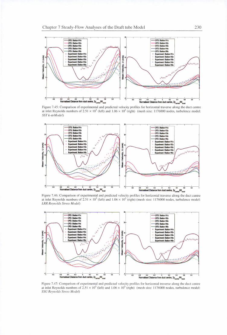
Chapter 7 Steady-Flow Ana lyses of the Draft tube Model 230
" - CFO:-H1c - Cf0:-H2c •• -·CFO: - H3c ···--CFO:-H4c - CfD:-HSc
I" ::> z!. ~ 10 • > c • i '
"
"'
I" ::>
f10 ~ c • i '
- CFD:SlolicnH1c - CFD:SlolicnH2c • · ··CFO: Slolicn H3c ----·CFO: Slolicn Hole - CFO:SlolicnHSc
a Exp1rim1nl: Slolicn H1c Experiment: Slolicn H2c
o Exporimonl: S1a11on HJc
• Exporimori; - H4c Experiment: - H5c
·••,'~~.,~~.-.,~~.~ .• ~:--.-,~~,~~7u:--~,-.,~~,~.~:--,-. ~..-,
Namalised Disllnce from duct cerire, 'l:f _,,IW"'"' Figure 7.45: Comparison of experimental and predicted velocity profi les for hor izontal traverse along the duct centre at inlet Reynolds numbers of 2.5 1 x 10⁵ (left) and 1.06 x 10⁵ (right) (mesh size: 1176000 nodes, turbulence model : SST k-mModel)
f., ~ c • i 5
- Cf0:-H1c - Cf0:-H2c - - ·CfD: Slllion HJc -----Cf0: Slllion H4c -CfD:SlllionHSc
~.,~~~.~ .• ~~.~,~-.-,~~.~,~~,~~~u~~.-,~~,~.~~.~,~~
Namalised Diotance Iran duct cenlnl, 'l:f _.IW"'"'
- CfD:SlolicnH1c - CFO:SlolicnH2c --- ·CfD:SlolicnHJc -----CfD: Slolicn H4c
c
i
~·,·~~~,~~.-,:--~.~,~:--.~,~..-,,,.....~7u:--~,~,~~u,.,-~~,7. ~..-,
Noonatised Diotance from duct cenlrt, 'J:f _IW"'"' Figure 7.46: Comparison of experimental and pred icted velocity profi les for hori zontal traverse along the duct centre at inlet Reynolds numbers of 2.5 1 x 10⁵ (left) and 1.06 x I 05 (right) (mesh size: 1 176000 nodes, turbulence model: LRR Reynolds Stress Model)
- CFO:-H1c - Cf0:-H2c - -- ·CfD:-HJc ----·CFO: - H4c - CfD:-HSc
• Exporimonl:-H1c
• Experiment: - H2c o Exporimon(:-HJc
Exporimori; - H4c Exporimonl:-HSc
0 a
a
"'
- CFD:S111ionH1c - CfD:S111ionH2c - - - ·CfD:S111ionHJc
-----Cl'O: - Hole -CfD:S111ionH5c
• Exporimonl:SlolionH1c Exporimonl:-H2c
0 Exporimonl: - HJc • Exporimonl:- Hole
Experiment: - H5c
~~.~-.7,:--:--.~.~--=.~.~--:.,:--~~,~---,,~,:----:,~,~--:,~.~--:,,~.~-,
Namalised Distance from duct certre, 'l:f _,,IW"'"' Figure 7.47: Comparison of experimental and predicted ve loc ity profi les for horizontal traverse along the duct cen tre at inlet Reynolds numbers of2.5 1 x 10⁵ (left) and 1.06 x 10⁵ (right) (mesh ize: 11 76000 nodes, turbulence model: SSC Reynolds Stress Model)
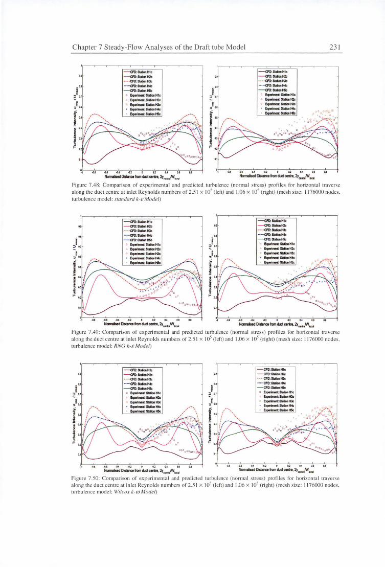
Chapter 7 Steady-Flow Analyses of the Draft tube Model 23 1
.. I o.•
:> 0.7
.} .. i; -~ 0.1
~ • •• 8
i ....
- CfO:SlallonH1c - CfO:SlllianH2c - -- ·CfO:SlllianHJc ----Cf0:-H4c - Cf0:-H5c
0 E,.,..--H1c
• E..,..- - H2c 0 E..,..- - H3c ~-H4c
!Jq>Ononl: - H5c
~ ~ G O U ~ I.I
Nonnliled Diltance from cllCt cnra, 2y _.IW"""' ..
0.1
r: O.I
i '.) ., .,~ I.I ,;
! OJ
~ ~ • "5
~ ....
- CfO:SlllianH1c - Cf0:-H2c - -· ·Cl'O:-HJc ----·CfO:- H4c - Cl'O:SlllionH5c · ~-H1c
• EJpOrimont - H2c 0 ~-HJc
~-H4c
!Jq>Ononl: - H5c
Figure 7.48: Comparison of experimental and predicted turbulence (normal stress) pro files for horizonta l traverse along the duct centre at inlet Reynolds numbers of 2.5 1 x I 05 (left) and 1.06 x I 05 (1i ght) (mesh size: 1176000 nodes, turbulence model : standard k-£ Model)
•• - CfD:SlllionH1c - Cf0:-H2c - - - ·CfO:- H3c - Cf0:-H4c - Cf0:-H5c
a !Jq>Onon!: - H1c • !Jq>Ononl: - H2c 0 L!Jq>orimod:-HJc
!Jq>Ononl: - H4c !Jq>Ononl: - H5c
OJ
, .. i
'.) ., } 0.1
i 0.1
• ~ i i ....
',
- Cf0:-H1c - CfD:SlllionH2c ---CfO:-HJc ---CfO: - H4c - CfO:SlllionH5c
a !Jq>Onon1: S111ion H1c
!Jq>Ononl: - H2c 0 ~-HJc
~-tMc hporimn:- H5c . -,:,r:"!\\
. . '- '<.k:-=·-=-:.-; .-. ~~ 4n;, "'~
.... " L .-.\ ',
..... ,\
-4.1-4.4 ..e..l 0 o.l U U O.I ~14.l ·H.0.4 .. J IJUO.I u NonnMood Diltance rrom OJc:t '**'· 2y_,tw.,,,.. Nom1ailed Diltance from OJc:t '**'· 2'J...,.tw.,,..
Figure 7.49: Compari son of experi mental and pred icted turbulence (normal stress) profi les for horizontal traverse along the duct centre at in let Reynolds number of 2.51 x I 05 (left) and 1.06 x I 05 (right) (mesh ize: 11 76000 nodes. turbu lence model: RNC k- £ Model)
- CFO:StlllonH1c - CR>:-.H2c -- -·Cl'O:-HJc ---·CfO:- H4c - Cf0:-H5c
o !Jq>Onon!: - H1c • E..,..-- H2c
0 !Jq>Ononl: - H3c !Jq>Ononl: - H4c !Jq>Ononl: - H5c
OJ - Cf0:-H1c - Cf0:-H2c ----CFO:- H3c ----·CfO:SllliontMc - CfO:SlllionH5c
o &perimltC: Slllan H1c
, &perimltC: - H2c 0 &perimltC: - H3c
&perimltC: - H4c EJpOrimont - H5c
.~~-',-~--'c~~,_~-',-~~~--',,.-~~~-'c-~-,L~--.
-G.l-G.1.0.4 .0.2 O 02UUU ·14.l ·U .0.4.0J 0 o.lUO.IOJ
NonnlliMd Di1tance from OJc:t cnra. 2y _.tw.,,,.. Normahld Disllnco ~om cllCt c:orlrt. Zy _,IW_ Figure 7.50: Compari son of experimental and predicted turbulence (normal stress) profiles for horizontal traverse along the duct centre at inlet Reynolds numbers of 2.5 1 x I 05 (left) and 1.06 x I 05 (right) (mesh size: 1176000 nodes. turbulence model: Wilcox k-coModel)
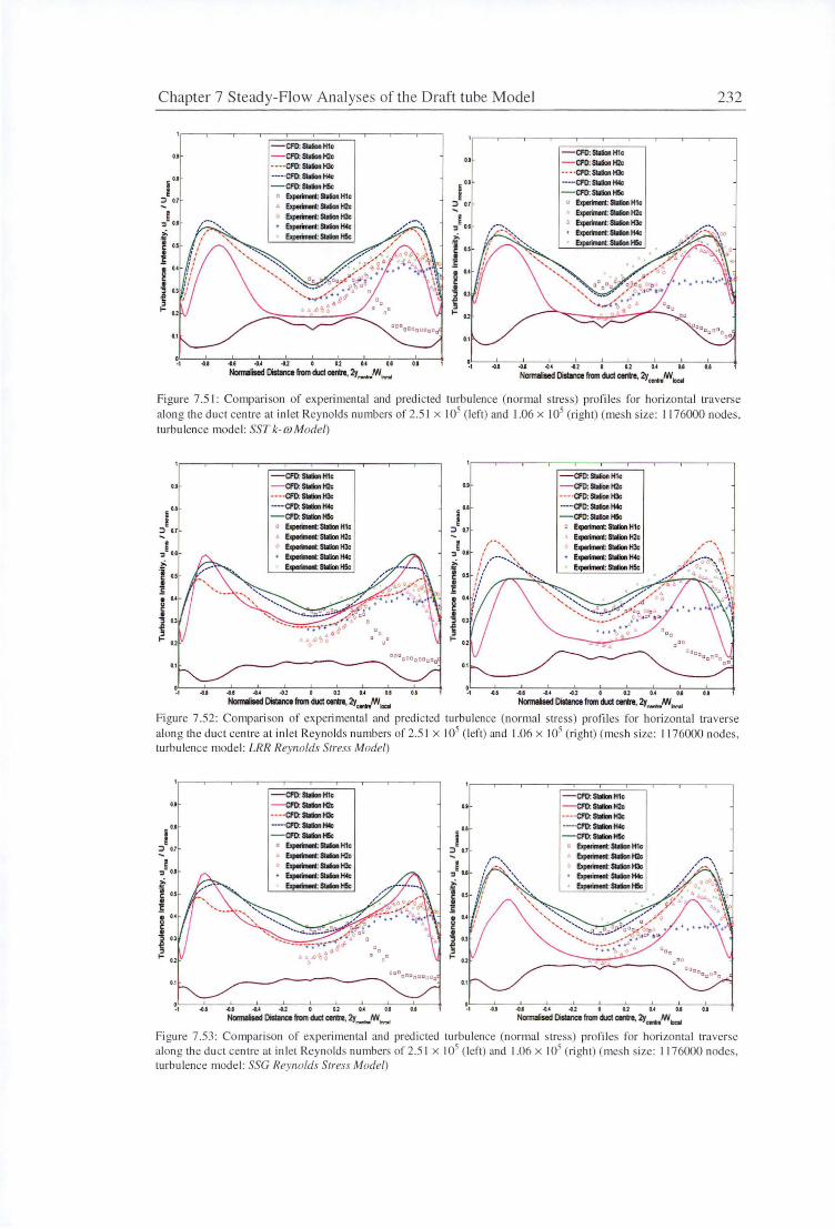
C hapter 7 Steady-Flow Analyses of the Draft tube Model 232
0.1
i 0.1
~ 2 ., ,} .. ,;.
! f ~
i I-
- Cl'O:SlllionH1c - Cl'O:SlllionH2c ·-·Cl'O:SlllionHJc · - · ·Cl'O:SlllionH4c - Cl'O:SlllionH!c
0 Exporimonl: Slllion H1c . Exporimonl: Slolion H2c 0 Exporimonl: - H3c
Exporimonl: - H4c Exporimonl: - H!c
~ ~ a o u u u Normoliud DiUnce flan duct ""*'· 2y ,_.Ml,,,,,,
- Cl'O:SlllionH1c 0.1 - C1D:SlaliooH2c
· ···Cl'D:SlllionHJc
(' ··· - Cl'D:-H4c -Cl'O:SlllionH!c
~ 0.7 0 Exporimonl: - H1c
.} 0.1
0 Upotinwi:- H2c 0 !xporimonl: - H3c
-f Exporimonl: - H4c Exporimonl: - H!c
l: ~
i I-
o~-~-~-~--~-~-~--~-~-~--~ • ~ ~ ~ a o u u u u Nonnaised Dislanoe flan duct ctnlrt, 2y ,_Ml...,
Figure 7.5 1: Comparison of experimenta l and predicted turbulence (normal stress) profi les for horizonta l traverse along the duct centre at in let Reynolds numbers of 2.5 1 x I 05 (left) and 1.06 x !05 (right) (me h ize: 1176000 nodes. turbu lence model: SST k- mModel)
- Cl'O:-H1c OJ - Cl'O:-H2c
· ·· ·Cl'O:-HJc
i •.• ··-·Cl'O:-H4c -Cl'O:S1ollooH!c
~ 0 Exporimonl: Slllion H1c ~ 0.7 . Exporimonl: S1llion H2c
}0.1 0
Exporimonl: - H3c
i' Exporimonl: - H4c Exporimonl: - H!c
c ! .E g • i I-
~ ~ ~ a o u u u u Normoliud DiUnce 1ran duct ""*'· ?t,_m _
Figure 7.52: Comparison of experimental and predicted along the duct centre at inlet Reynolds numbers of 2.5 1 x turbu lence model: LRR Reynolds Stress Model)
0.1
.,~ 0.1
f i I-
- Cl'D:SlolionH1c - Cl'O:-H2c ---Cl'O:-HJc --·Cl'O:-H4c - CPD:-H!c
o Exporimon1: - H1c
Exporimonl: - H2c 0 Exporimonl: - H3c • Exporimonl: - H4c
Exporimonl: - H!c
___ _...---~---------..., 00 0ao ooo o0 c0
0.1
( 2 0.1
.,~ 0.1
,;.
! • ~ ~
i I-
- Cl'O:-H1c - CFO:SlolionH2c ····Cl'O:SlolionHJc ·····Cl'O:SlolionH4c -Cl'D:-H!c
0 Eliplrimori:S111iooH1c . E""'"""'1t-H2• 0
!xporimonl - H3c !xporimonl - H4c !xporimonl - H!c
u ~ ~ a o 02 u u u Nomllioed Dislanoe flan duct ctnlrt, ?I ,_I'll,,_
turbu lence (normal stress) profi les for horizonta l traverse I 05 (left) and 1.06 x I 05 (ri ght) (mesh size: I 176000 nodes,
0.1
..
- Cl'D:-H1c - Cl'D:-H2c · -·Cl'll:-HJc ·--CPD:-H4c - Cl'D:-H!c
o Exporimon1: S1o1ion H1c
" Exporimonl: - H2c 0 ~: SlolionHJc
Exporimonl: - H4c Exporimonl: - H!c
-4.1 ... I -4.4 .. J OJ l4 0.1 U ~!-1 --.-::.I,---,~~-°"•·"°• --.-::,,...--0!--°"02::---0-!:_.--,,LcA-~O.I::----.
Normoiled cm.a from duct c:enre, 'l'/,_.1'11..., Nonnaised Dislanoe from duct cnra, ?t....,.m..., Figure 7.53: Comparison of experimental and predicted turbulence (normal stress) profi les for hori zontal traver e along the duct centre at inlet Reynolds numbers of 2.5 1 x I 05 (left) and 1.06 x !05 (right) (mesh size: 11 76000 nodes, turbu lence model: SSC Reynolds S1ress Model)
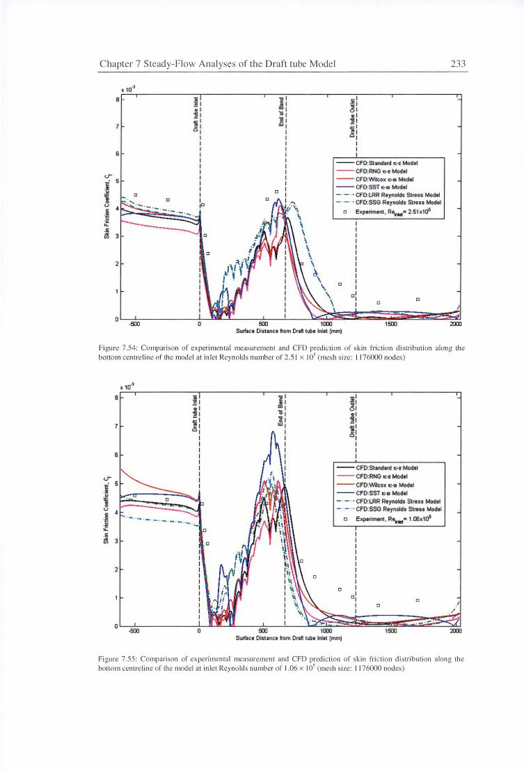
Chapter 7 Steady-Flow Analyses of the Draft tube Model 233
x 10·•
8 l> ... - 1 c ..!!1 E .. .. m 61 .... '15 ..1 ~
~ ~ .g I
7 w ,; I 0 !!I 01
I I
6 I --CFD:Standard IC-• Model --CFD:RNG IC-8 Model
c.r --CFD:Wilcox 1<-m Model ci 5 .!! --CFD:SST 1<-m Model u D
- · - · - CFD:LRR Reynolds Stress Model E . 0 ..... - · - · - CFD:SSG Reynolds Stress Model
0
- ~ -4 r/'\ D Experiment, Rt-= 2.51 x1a5
u \ ·c \ u..
.e \ -" 3 D Vl \
I \ D \ I
2 I \ I
,}\ I I D I \ I \ DI I D I \ I D I J
0 -500 0 500 1CXXJ 1500 200J
Surface Distance from Draft tube Inlet (mm)
Figure 7.54: Compari son of experimental measurement and CFD predicti on of skin fricti on distribution along the bottom centreline of the model at inlet Reynolds number of 2.5 1 x I 05 (mesh size: 11 76000 nodes)
x 10·•
8 -;; i -1 :E ..!!1
• m 61 ~ 'o •I ... ~I <= c
7 !! w o::I 0 !!I 01
I
6 I I
-- CFD:Standard 1<-8 Model
u- --CFD:RNG IC-c Model
c 5 --CFD:Wilcox K-m Model .!! --CFD:SST IC-Ill Model u I: - · - · • CFD:LRR Reynolds Stress Model .. 0
- · - · • CFD:SSG Reynolds Stress Model 0 -4 -~ - ·- ·- ·- ·- D Experiment, R911Wt= 1.00x1a5 u ·-·-·c u.. D I c I :.x 3 I Vl
I I I I
2 I D I
I D I
DI I D I D I
0 -500 0 500 1CXXJ 1500 200J
Surface Distance from Draft tube Inlet (mm)
Figure 7.55: Comparison of experimental measurement and CFD prediction of skin fri ction di stri bution along the bottom centre line of the model al inlet Reynold number of 1.06 x I 05 (mesh size: 11 76000 nodes)
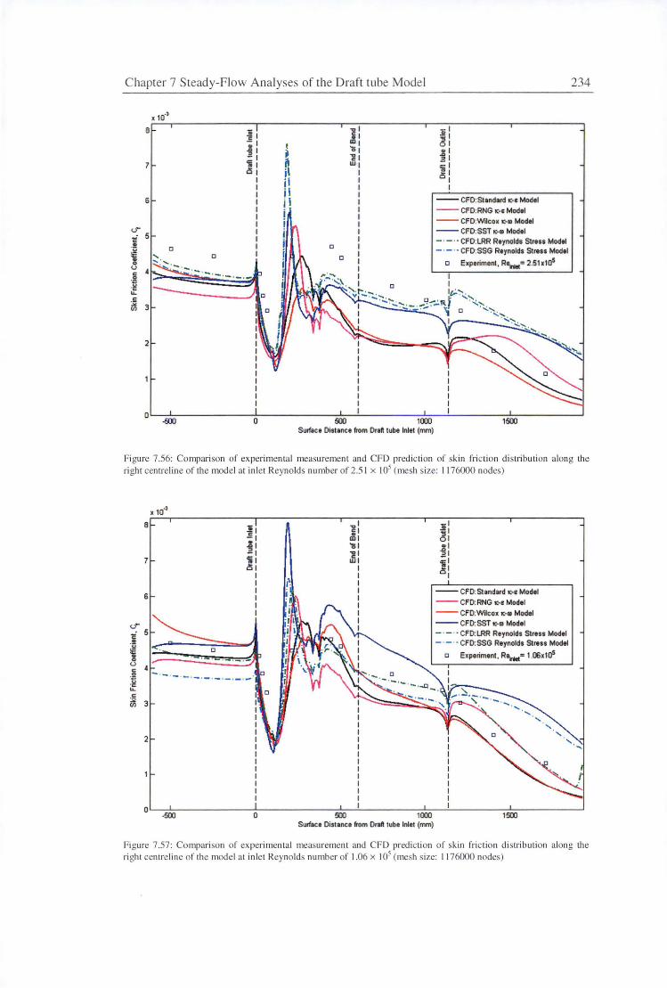
Chapter 7 Steady-Flow Analyses of the Draft tube Model 234
x 10·•
B
7
6
<.:r -i 5 .. ·;:; D
"ii D 0
0 ·-·-·-c .S! u ·c: .._ .!:
"" 3 CJ)
2
ii E .. ... .= = .. c3
D
D
-ol -1 i i ~I IOI cSI ~ I ~1 ~ I -g I w ;: I
!!1 01
I
-- CFO: Standard 1::-1 Model
--CFD:RNG r::-s Modol
--CFD:Wilcox r::-ro Modal
--CFD:SSTr::·m Modtl
- · - · • CFO: LRR Reynolds Stress Modol - · - · • CFO: SSG Reynolds Stress Modtl
o Experiment , R._= 2.51x1a5
Surface Distance from Draft tube Inlet (mm)
Fi gure 7 .56: Comparison of experimental measurement and CFD predicti on of sk in fri ction di su·ibution along the ri ght cen treline of the model at inlet Reynolds number of 2.5 1 x I 05 (mesh size: 11 76000 nodes)
x 10-3
B .. E . ... .=
7 ~
6
o--i .. ·;:; i.: D .. 0 0 • c 0 -·-· - ·- ·- ·- ·- ·- ·- ·- · ·~ ·c .._ c :,.;
3 CJ)
2
.500 0
1'-••
500
..,I <=I ~I '01 1! I wl
Hlll Surface Distance from Dreft tube Inlet (mm)
--CFO: Standard 1::-1 Model
-- CFD:RNG r::-e Modtl
--CFD:Wilcox 1::-11 Model
-- CFO: SST r::-m Model
- · - · • CFD:LRR Reynolds Stress Modtl - · - · • CFD:SSG Reynolds Stress Modtl
o Experiment , Re.riot= 1.00x1a5
1500
Figure 7.57: Comparison of experimental measurement and CFD prediction of sk in friction distribution along the right centreline of the model at inlet Reynolds number of 1.06 x I 05 (mesh size: 1176000 nodes)

Chapter 7 Steady-Flow Analyses of the Draft tube Model 235
7.4 Discussion
7.4.1 Reynolds Number Effects
Investigation of Reynolds number effects is essential for this analysis because the flow
of the Mackintosh Francis-turbine draft tube will operate at Reynolds numbers of about
100 times larger than these in the present experiments or simulations. For the limited
Reynolds numbers tested, no obvious Reynolds number dependency was observed for
the measured wall static pressure distribution along the draft tube. There was a very
weak drop in the pressure recovery with decreasing Reynolds number that could be
explained by the increasing boundary layer momentum thickness at the draft tube entry
as the Reynolds number reduces. The flow losses increased weakly with increasing
Reynolds number but all of the foregoing changes were within the experimental
uncertainty.
For the mean velocity profiles in the draft tube, the Reynolds number effects are
generated by the Reynolds number dependency of the velocity normal to the wall
emerging from the bend [119]. This unmeasurable velocity component enhances the
boundary layer growth on the top wall but delays the boundary layer growth on the
bottom surface. The shift in the peak of the velocity profile towards the top surface as
the flow travels further downstream also supports this argument. This effect will not
change the shapes of the mean velocity profiles substantially. For turbulence intensity,
the Reynolds number effect is also insignificant when the local velocity is used for
scaling. Some differences in behaviour are found at the draft tube exit, where increasing
Reynolds number reduces the turbulence intensity. This behaviour may be related to the
unsteady flow in the recirculation region or the stronger pressure gradients occurring at
lower Reynolds number, which increase the production of normal turbulent stress.
The values of skin friction coefficient in the draft tube generally reduce with increasing
Reynolds number. Larger differences are found near the inlet cone region of the draft
tube, where the skin friction coefficients at low Reynolds number are about twice as
large as the ones at high Reynolds number.
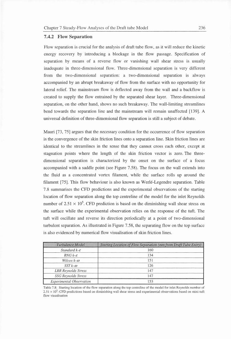
Chapter 7 Steady-Flow Analyses of the Draft tube Model 236
7 .4.2 Flow Separation
Flow separation is crucial for the analysis of draft tube flow, as it will reduce the kinetic
energy recovery by introducing a blockage in the flow passage. Specification of
separation by means of a reverse flow or vanishing wall shear stress is usually
inadequate in three-dimensional flow. Three-dimensional separation is very different
from the two-dimensional separation: a two-dimensional separation is always
accompanied by an abrupt breakaway of flow from the surface with no opportunity for
lateral relief. The mainstream flow is deflected away from the wall and a backflow is
created to supply the flow entrained by the separated shear layer. Three-dimensional
separation, on the other hand, shows no such breakaway. The wall-limiting streamlines
bend towards the separation line and the mainstream will remain unaffected [ 139]. A
universal definition of three-dimensional flow separation is still a subject of debate.
Mauri [73, 75] argues that the necessary condition for the occurrence of flow separation
is the convergence of the skin friction lines onto a separation line. Skin friction lines are
identical to the streamlines in the sense that they cannot cross each other, except at
stagnation points where the length of the skin friction vector is zero. The three
dimensional separation is characterized by the onset on the surface of a focus
accompanied with a saddle point (see Figure 7.58). The focus on the wall extends into
the fluid as a concentrated vortex filament, while the surface rolls up around the
filament [75]. This flow behaviour is also known as Werle-Legendre separation. Table
7 .8 summarises the CFD predictions and the experimental observations of the starting
location of flow separation along the top centreline of the model for the inlet Reynolds
number of 2.51 x 10⁵. CFD prediction is based on the diminishing wall shear stress on
the surface while the experimental observation relies on the response of the tuft. The
tuft will oscillate and reverse its direction periodically at a point of two-dimensional
turbulent separation. As illustrated in Figure 7.58, the separating flow on the top surface
is also evidenced by numerical flow visualisation of skin friction lines.
Turbulence Model StartinR Location of Flow Separation (mmfrom Draft Tube Entry)
Standard k-£ 160
RNGk-£ 134 Wilcox k-w 151
SST k-w 126 LRR Reynolds Stress 147 SSG Reynolds Stress 147
Experimental Observation 153
Table 7 .8: Starting location of the flow separation along the top centreline of the model for inlet Reynolds number of 2.5 1 x I 05
: CFD pred ictions based on diminishing wall shear stress and experimental observations based on mini-tuft flow visualisation
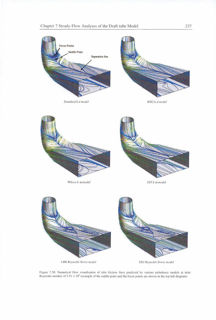
Chapter 7 Steady-Flow Analyses of the Draft tube Model 237
Standard k-£ model RNC k-£ model
Wilcox k-m model SST k-m model
LRR Reynolds Stress model SSC Reynolds Stress model
Figure 7.58: umerica l flow visuali sation of skin fri c tion lines predic1ed by various turbulence mode ls at inle1 Reynolds number of2 .5 I x 105 (example of the sadd le poinl and the focus poinls are shown in lhe lop left diagram)
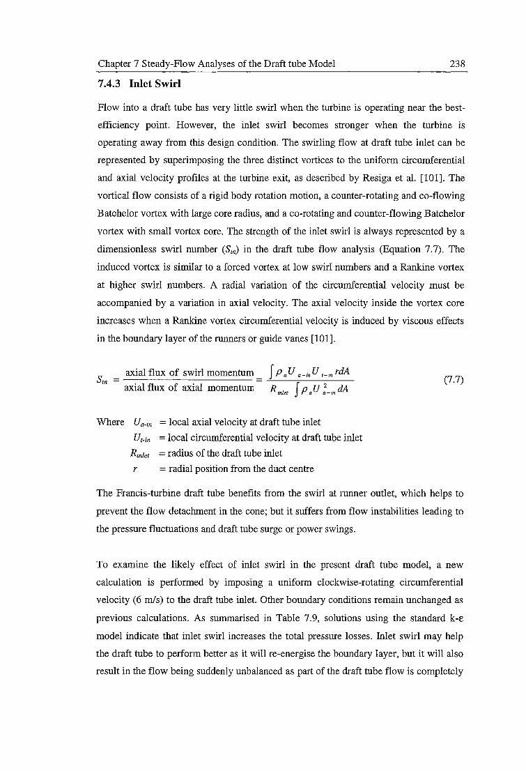
Chapter 7 Steady-Flow Analyses of the Draft tube Model 238
7 .4.3 Inlet Swirl
Flow into a draft tube has very little swirl when the turbine is operating near the best
efficiency point. However, the inlet swirl becomes stronger when the turbine is
operating away from this design condition. The swirling flow at draft tube inlet can be
represented by superimposing the three distinct vortices to the uniform circumferential
and axial velocity profiles at the turbine exit, as described by Resiga et al. [101]. The
vortical flow consists of a rigid body rotation motion, a counter-rotating and co-flowing
Batchelor vortex with large core radius, and a co-rotating and counter-flowing Batchelor
vortex with small vortex core. The strength of the inlet swirl is always represented by a
dimensionless swirl number (Sin) in the draft tube flow analysis (Equation 7.7). The
induced vortex is similar to a forced vortex at low swirl numbers and a Rankine vortex
at higher swirl numbers. A radial variation of the circumferential velocity must be
accompanied by a variation in axial velocity. The axial velocity inside the vortex core
increases when a Rankine vortex circumferential velocity is induced by viscous effects
in the boundary layer of the runners or guide vanes [101].
axial flux of swirl momentum= f Pa U a-in U i-zn rdA
axial flux of axial momentum R J p U 2 d' A inlet a a-rn r1
Where Ua-m = local axial velocity at draft tube inlet
Ur-in = local circumferential velocity at draft tube inlet
Rmlet = radius of the draft tube inlet
r = radial position from the duct centre
(7.7)
The Francis-turbine draft tube benefits from the swirl at runner outlet, which helps to
prevent the flow detachment in the cone; but it suffers from flow instabilities leading to
the pressure fluctuations and draft tube surge or power swings.
To examine the likely effect of inlet swirl in the present draft tube model, a new
calculation is performed by imposing a uniform clockwise-rotating circumferential
velocity (6 m/s) to the draft tube inlet. Other boundary conditions remain unchanged as
previous calculations. As summarised in Table 7.9, solutions using the standard k-£
model indicate that inlet swirl increases the total pressure losses. Inlet swirl may help
the draft tube to perform better as it will re-energise the boundary layer, but it will also
result in the flow being suddenly unbalanced as part of the draft tube flow is completely
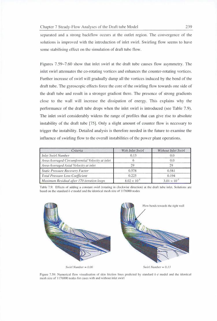
C hapter 7 Steady-Flow Analyse of the Draft tube Model 239
separated and a strong backflow occurs at the outlet region. The convergence of the
solu tions is improved with the in troduction of inlet swirl. Swirling fl ow seems to have
some stabilising effect on the simulation of draft tube fl ow.
F igures 7.59- 7.60 show that inl et swirl at the draft tube causes fl ow asymmetry. T he
in let sw irl attenuates the co-rotating vortices and enhances the counter-rotating vortices .
Further increase of sw irl will gradually damp all the vortices induced by the bend of the
draft tube. The gyroscopic effects fo rce the core of the swirling fl ow towards one side of
the draft tube and result in a stronger gradi ent there. The presence of strong gradients
c lose to the wall will increase the diss ipation of energy. This explains why the
perfo rmance of the draft tube drops when the inlet swirl is introduced (see Table 7.9).
The in let sw irl considerably widen the range of profil es that can give ri se to abso lute
instability of the draft tube [75]. Only a slight amount of counter fl ow is necessary to
trigger the instability. Detail ed analysis is therefore needed in the future to examine the
influence of swirling fl ow to the overall instabilities of the power plant operati ons.
Criteria With Inlet Swirl Without Inlet Swirl
Inlet Swirl Number 0.1 3 0.0
Area-A veraged Circumferential Velocity at inlet 6 0.0
Area-A veraged Axial Velocity at inlet 29 29
Static Pressure Recovery Factor 0.578 0.58 1
Total Pressure Loss Coefficient 0.225 0. 194
Maximum Residual aft er 170 iteration loops 8.02 x 10⁻⁶ 3.0 1x 10·5
Table 7.9: Effects of add ing a constant swirl (rotating in clockwise d irection) at the draft tube inlet. So lu ti ons are based on the standard k-t: model and the identica l mesh size of I 176000 nodes
Flow bends towards the ri ght wa ll
Swirl Number = 0.00 Swirl Number= 0.13
Figure 7. 59: Numerica l fl ow visuali sation of sk in fri ction line predicted by standard k-t: model and the identica l mesh size of 11 76000 nodes fo r ea es with and without inlet swirl
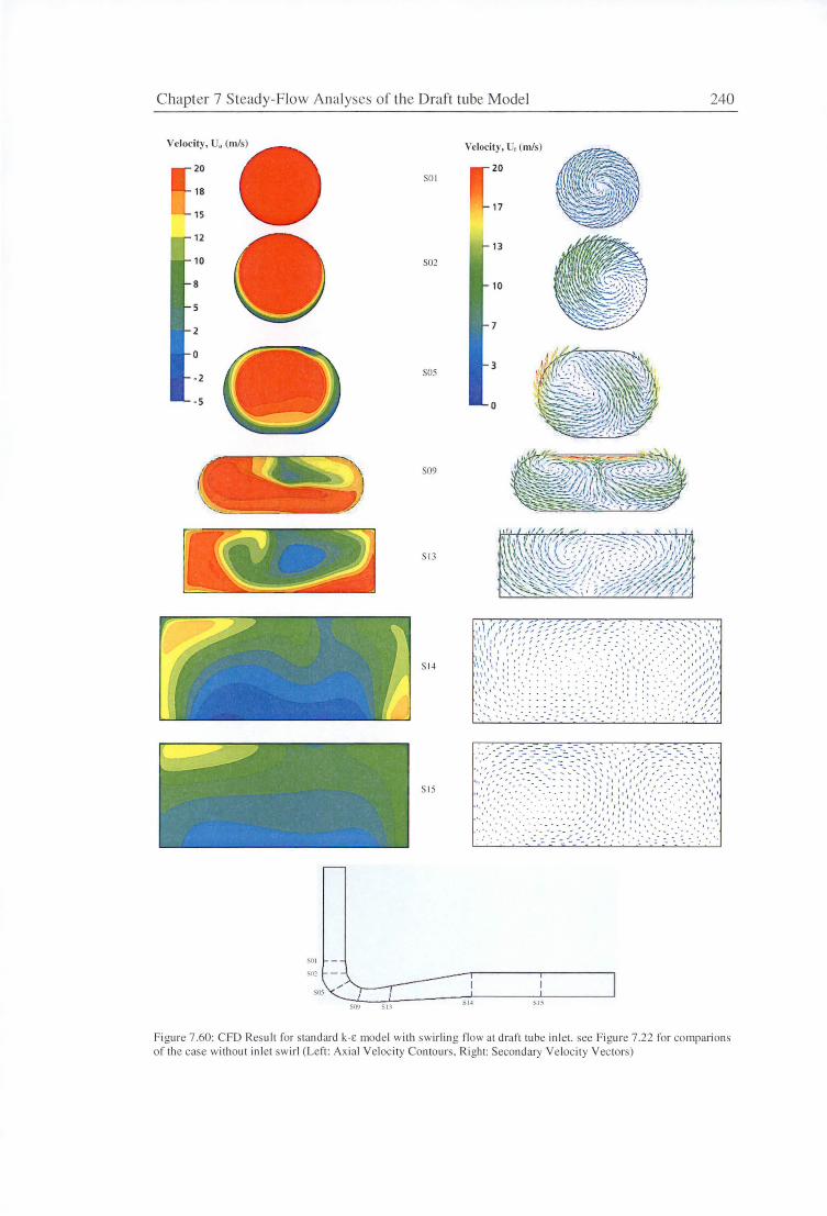
Chapter 7 Steady-Flow Analyses of the Draft tube Model 240
Velocity, U" (m/s) Velocity, U, (m/s)
20 20 SO I
18
17 15
12 13
10 S02
8 10
2 7
0
S05 3
·2
· 5 0
S09
S l3
S I-I
S l5
SO I
'>02
SO>
SIS
Figure 7 .60: CFO Resu It for standard k-E model with swirling fl ow at dra ft tube inlet. see Figure 7 .22 for compari ons of the case without inlet sw irl (Left : Axial Velocity Contours. Ri ght: Secondary Velocity Vectors)

Chapter 7 Steady-Flow Analyses of the Draft tube Model 241
7.4.4 Flow Asymmetries
The experimental wall static pressure distributions at the left and right centrelines of the
model show slight asymmetry. Sotiropoulos and Ventikos [120] suggest that flow
asymmetry observed in an internal flow system is the result of the outer disturbances
from some small but finite imperfections of a non-ideal environment. The flow
asymmetry in the experiments could be caused by many factors such as noise and
vibrations, thermal gradients, model imperfections, proximity of the inlet to a wall, or
small asymmetries at the boundaries. These problems are also common in real turbine
plants. Although asymmetry does not generally emerge from imperfections at the wall,
it is still impossible to exclude this randomness from reality [ 40]. The experimental
model was placed quite close to the wall due to limited space in the laboratory. The
measured surface temperature close to the wall side was usually about 0.5-1°C above
the temperature of the opposite surf ace. Temperature gradients through the thermal
boundary layer may induce a density driven down-flow near the wall and generate some
small discrepancies in the flow behaviour. The presence of the wall (one diameter away
from the draft tube model) may cause asymmetry of the inlet flow and the introduction
of a streamwise vortex originating from the wall surface ("ground vortex").
For numerical simulations, the use of a symmetrical total pressure profile at inlet would
suggest that the solution should also be symmetrical. Although symmetrical solutions
may exist, they will probably never be obtained in the real flow due to unstable
properties of the three-dimensional physics. In general, flow asymmetry in a simulation
may arise from the round-off errors of the coordinates of the nodes as well as the
asymmetries in grid structure, block topology, or CAD geometry. These effects should
be relatively insignificant in the present case, as flow asymmetry is only observed in the
solutions of Reynolds stress models where the unsteady flow behaviour near duct centre
is predicted. Instead, the asymmetric behaviour is thought to be caused by the
instabilities of the symmetric mode that gives rise to an oscillating wave in the flow and
the periodic pressure fluctuations in the draft tube [ 40]. Flow asymmetry is one of the
possible solutions of the nonlinear problem expressed by the unsteady Navier-Stokes
equations. Separated or recirculating flow may break the symmetry of the precedent
flow, adopting a form of lesser symmetry in which dissipative structures arise to absorb
just the amount of excess available energy that the more symmetrical flow can no
longer be able to absorb [ 40].
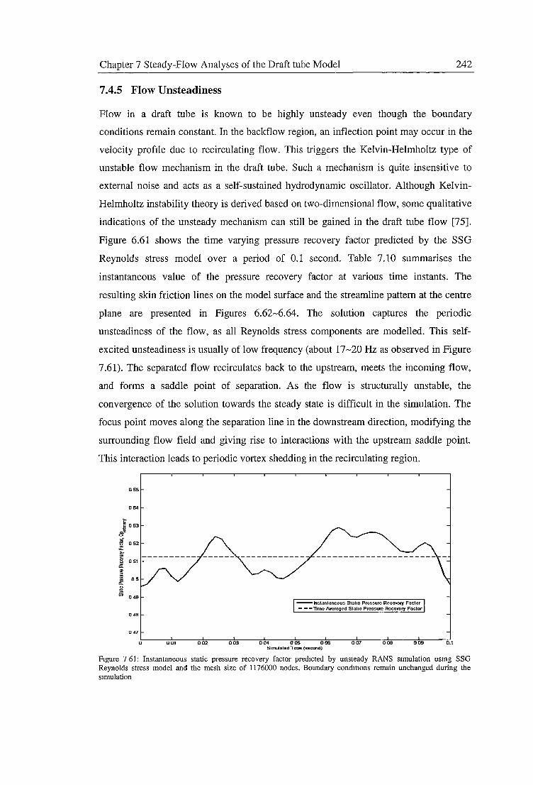
Chapter 7 Steady-Flow Analyses of the Draft tube Model 242
7.4.5 Flow Unsteadiness
Flow in a draft tube is known to be highly unsteady even though the boundary
conditions remain constant. In the backflow region, an inflection point may occur in the
velocity proftle due to recirculating flow. This triggers the Kelvin-Helmholtz type of
unstable flow mechanism in the draft tube. Such a mechanism is quite insensitive to
external noise and acts as a self-sustained hydrodynamic oscillator. Although Kelvin
Helmholtz instability theory is derived based on two-dimensional flow, some qualitative
indications of the unsteady mechanism can still be gained in the draft tube flow [75].
Figure 6.61 shows the time varying pressure recovery factor predicted by the SSG
Reynolds stress model over a period of 0.1 second. Table 7.10 summarises the
instantaneous value of the pressure recovery factor at various time instants. The
resulting skin friction lines on the model surface and the streamline pattern at the centre
plane are presented in Figures 6.62-6.64. The solution captures the periodic
unsteadiness of the flow, as all Reynolds stress components are modelled. This self
excited unsteadiness is usually of low frequency (about 17-20 Hz as observed in Figure
7.61). The separated flow recirculates back to the upstream, meets the incoming flow,
and forms a saddle point of separation. As the flow is structurally unstable, the
convergence of the solution towards the steady state is difficult in the simulation. The
focus point moves along the separation line in the downstream direction, modifying the
surrounding flow field and giving rise to interactions with the upstream saddle point.
This interaction leads to periodic vortex shedding in the recirculating region.
055
0 54
.. J 053
! 0 52
iii'
J 051
~ ;;; 05 a.
~ 0 49
- Instantaneous Static Pressure Recovery Factor - --Time Averaged Static Pressure Recovery Factor
048
047
0 001 002 003 004 005 006 007 008 009 0.1 S1mulaled lime (second)
Figure 7 61: Instantaneous static pressure recovery factor predicted by unsteady RANS simulation usmg SSG Reynolds stress model and the mesh size of 1176000 nodes. Boundary cond1t10ns remain unchanged during the smmlation
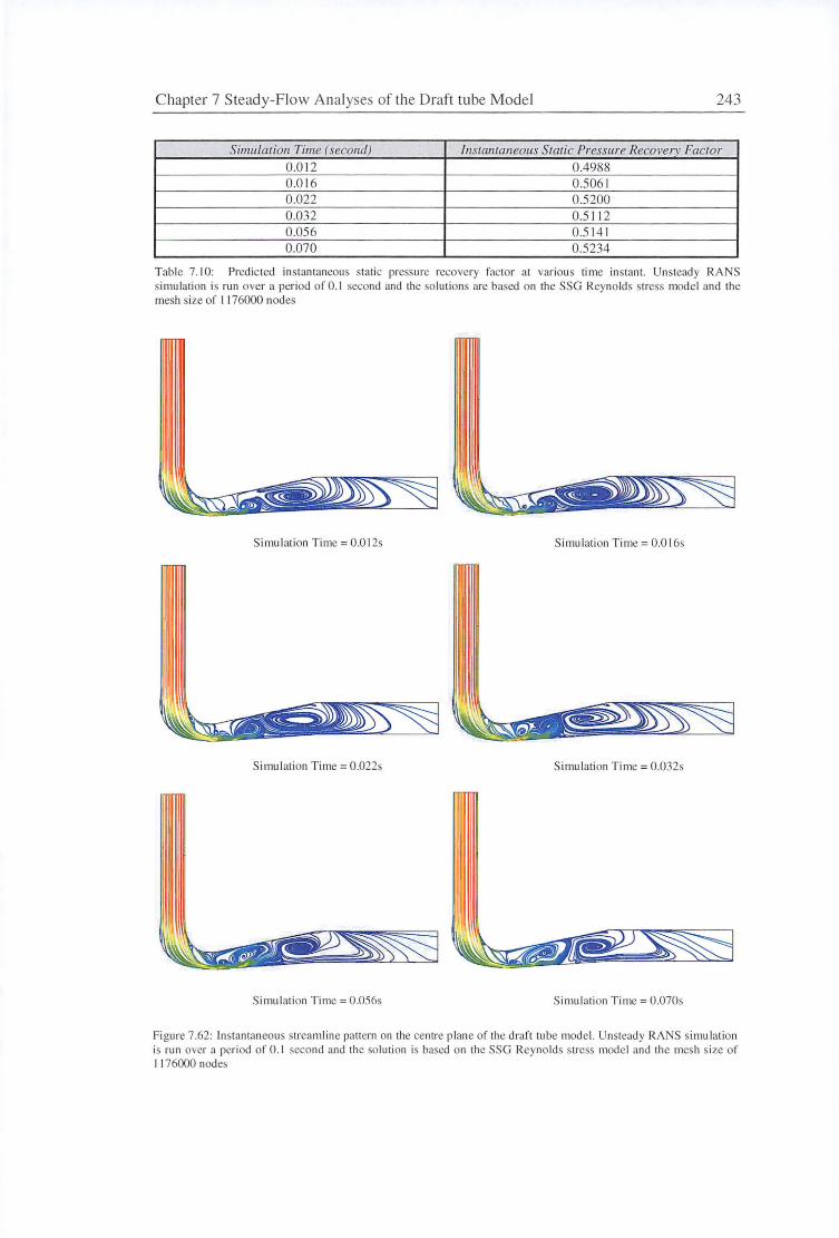
Chapter 7 Steady-Flow Analyses of the Draft tube Model 243
Simulation Time (second) Instantaneous Static Pressure Recovery Factor 0.012 0.4988 0.016 0.5061 0.022 0.5200 0.032 0.5112 0.056 0.5 141 0.070 0.5234
Tab le 7. 10: Predicted instantaneous static pressure recovery fac tor at various time instant. Unsteady RANS simulation is run over a period of 0. 1 second and the solutions are based on the SSG Reynolds stress model and the mesh size of I 176000 nodes
Simulation Time= 0 .0 I 2s Simulati on T ime= 0.016s
Simul ation Time = 0.022s Simulati on Time = 0.032s
Simu lation Time= 0.056s Simu lation Time = 0.070s
Fi gure 7.62: Instantaneous streamline pattern on the centre plane of the draft tu be mode l. Unsteady RANS simulation is run over a period of 0.1 second and the so lution is based on the SSG Reyno lds stress model and the mesh size o f I 176000 nodes
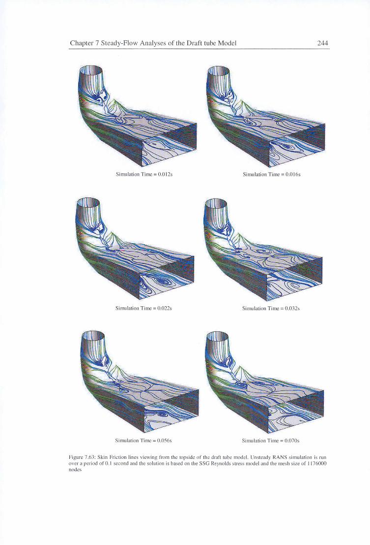
Chapter 7 Steady-Flow Analyses of the Draft tube Model 244
Simulation Time= 0.012s Simulation Time= 0.016s
Simulation Time = 0.022s Simu lation Time = 0.032s
Simulation Time = 0.056s Simulation Time = 0.070s
Figure 7.63: Skin Friction lines viewing from the topside of the draft tube model. Unsteady RANS simulation i run over a period of 0.1 second and the solution is based on the SSG Reynolds stress model and the mesh size of 1176000 nodes
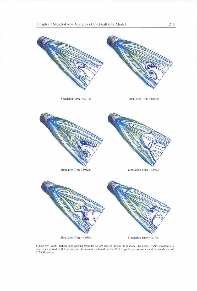
Chapter 7 Steady-Flow Analyses of the Draft tube Model 245
Simulation T ime = 0.01 2s Simu lation Time= 0.016s
Simulation Time= 0.022s Simulation T ime = 0.032s
Simulation Time= 0.056s Simulation Time = 0.070s
Figure 7.64: Skin Friction lines viewing from the bottom side of the draf't tube model. Unsteady RANS simu lation is run over a period of 0.1 second and the solution is based on the SSG Reynolds stress model and the mesh size of I 176000 nodes
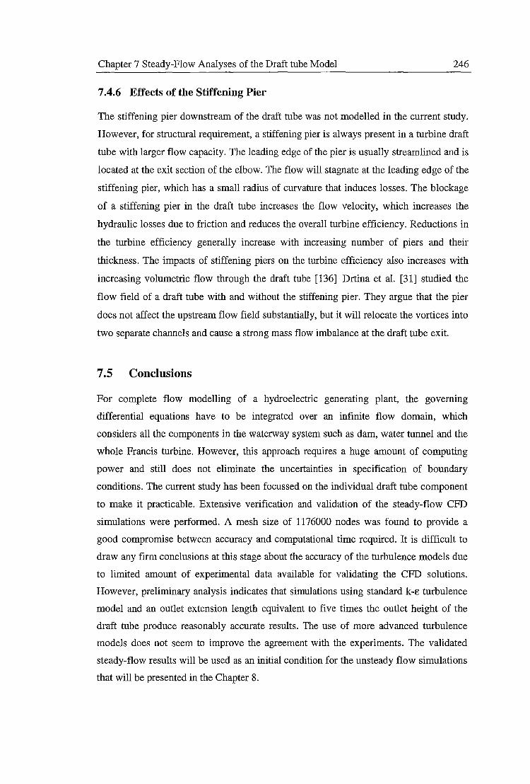
Chapter 7 Steady-Flow Analyses of the Draft tube Model 246
7 .4.6 Effects of the Stiffening Pier
The stiffening pier downstream of the draft tube was not modelled in the current study.
However, for structural requirement, a stiffening pier is always present in a turbine draft
tube with larger flow capacity. The leading edge of the pier is usually streamlined and is
located at the exit section of the elbow. The flow will stagnate at the leading edge of the
stiffening pier, which has a small radius of curvature that induces losses. The blockage
of a stiffening pier in the draft tube increases the flow velocity, which increases the
hydraulic losses due to friction and reduces the overall turbine efficiency. Reductions in
the turbine efficiency generally increase with increasing number of piers and their
thickness. The impacts of stiffening piers on the turbine efficiency also increases with
increasing volumetric flow through the draft tube [136] Drtina et al. [31] studied the
flow field of a draft tube with and without the stiffening pier. They argue that the pier
does not affect the upstream flow field substantially, but it will relocate the vortices into
two separate channels and cause a strong mass flow imbalance at the draft tube exit.
7 .5 Conclusions
For complete flow modelling of a hydroelectric generating plant, the governing
differential equations have to be integrated over an infinite flow domain, which
considers all the components in the waterway system such as dam, water tunnel and the
whole Francis turbine. However, this approach requires a huge amount of computing
power and still does not eliminate the uncertainties in specification of boundary
conditions. The current study has been focussed on the individual draft tube component
to make it practicable. Extensive verification and validation of the steady-flow CFD
simulations were performed. A mesh size of 1176000 nodes was found to provide a
good compromise between accuracy and computational time required. It is difficult to
draw any firm conclusions at this stage about the accuracy of the turbulence models due
to limited amount of experimental data available for validating the CFD solutions.
However, preliminary analysis indicates that simulations using standard k-E turbulence
model and an outlet extension length equivalent to five times the outlet height of the
draft tube produce reasonably accurate results. The use of more advanced turbulence
models does not seem to improve the agreement with the experiments. The validated
steady-flow results will be used as an initial condition for the unsteady flow simulations
that will be presented in the Chapter 8.
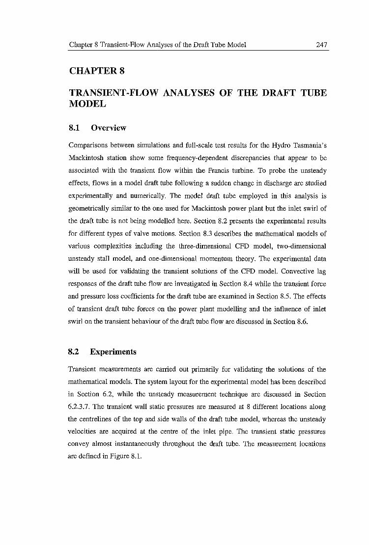
Chapter 8 Transient-Flow Analyses of the Draft Tube Model 247
CHAPTERS
TRANSIENT-FLOW ANALYSES OF THE DRAFT TUBE MODEL
8.1 Overview
Comparisons between simulations and full-scale test results for the Hydro Tasmania's
Mackintosh station show some frequency-dependent discrepancies that appear to be
associated with the transient flow within the Francis turbine. To probe the unsteady
effects, flows in a model draft tube following a sudden change in discharge are studied
experimentally and numerically. The model draft tube employed in this analysis is
geometrically similar to the one used for Mackintosh power plant but the inlet swirl of
the draft tube is not being modelled here. Section 8.2 presents the experimental results
for different types of valve motions. Section 8.3 describes the mathematical models of
various complexities including the three-dimensional CFD model, two-dimensional
unsteady stall model, and one-dimensional momentum theory. The experimental data
will be used for validating the transient solutions of the CFD model. Convective lag
responses of the draft tube flow are investigated in Section 8.4 while the transient force
and pressure loss coefficients for the draft tube are examined in Section 8.5. The effects
of transient draft tube forces on the power plant modelling and the influence of inlet
swirl on the transient behaviour of the draft tube flow are discussed in Section 8.6.
8.2 Experiments
Transient measurements are carried out primarily for validating the solutions of the
mathematical models. The system layout for the experimental model has been described
in Section 6.2, while the unsteady measurement technique are discussed in Section
6.2.3.7. The transient wall static pressures are measured at 8 different locations along
the centrelines of the top and side walls of the draft tube model, whereas the unsteady
velocities are acquired at the centre of the inlet pipe. The transient static pressures
convey almost instantaneously throughout the draft tube. The measurement locations
are defined in Figure 8.1.
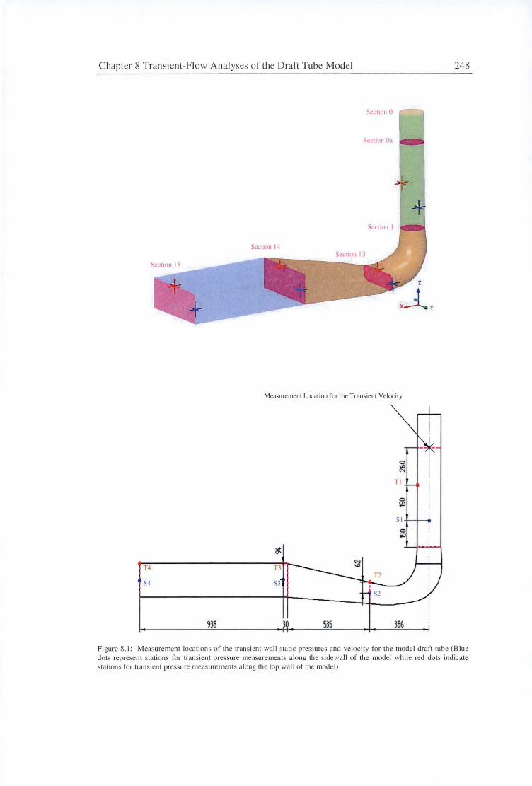
Chapter 8 Transient-Flow Analy es of the Draft Tube Model 248
Sec11on 0
Section Oa
+
Measurement Location for the Transient Veloc it y
0 >IJ N
TI
0 \£!
SI
0 \£!
~
T4 T3
~ S3
938 30 535 386
Fi gure 8. 1: Measurement locations of the tran ient wall stati c pressures and velocity for the model draft tube (Blue dots represent stations for transient pressure measurement along the sidewall of the model whi le red dots indica te stations for transient pressure measuremen t along the top wa ll of the model)
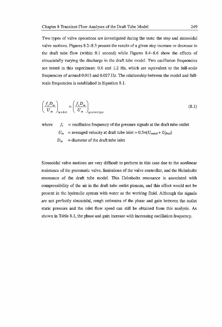
Chapter 8 Transient-Flow Analyses of the Draft Tube Model 249
Two types of valve operations are investigated during the tests: the step and sinusoidal
valve motions. Figures 8.2-8.3 present the results of a given step increase or decrease in
the draft tube flow (within 0.1 second) while Figures 8.4-8.6 show the effects of
sinusoidally varying the discharge in the draft tube model. Two oscillation frequencies
are tested in this experiment: 0.6 and 1.2 Hz, which are equivalent to the full-scale
frequencies of around 0.013 and 0.027 Hz. The relationship between the model and full
scale frequencies is established in Equation 8.1.
where
(8.1)
fv = oscillation frequency of the pressure signals at the draft tube outlet
Um =averaged velocity at draft tube inlet= O.Sx(Umztzat+ UflnaD
Dm = diameter of the draft tube inlet
Sinusoidal valve motions are very difficult to perform in this case due to the nonlinear
resistance of the pneumatic valve, limitations of the valve controller, and the Helmholtz
resonance of the draft tube model. This Helmholtz resonance is associated with
compressibility of the air in the draft tube outlet plenum, and this effect would not be
present in the hydraulic system with water as the working fluid. Although the signals
are not perfectly sinusoidal, rough estimates of the phase and gain between the outlet
static pressure and the inlet flow speed can still be obtained from this analysis. As
shown in Table 8.1, the phase and gain increase with increasing oscillation frequency.
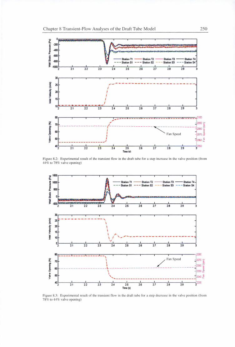
Chapter 8 Transient-Flow Analyses of the Draft Tube Model
.... 0 !!:-
i -200
.. -«Xl ! Q.
.\! .ml 11 Cii -8XI
~ -1000 2 2.1 2.2
3J
I 25 ... ...
20 8 • > • 15 E
10 2 2.1 2.2
2.3
i 23
I I
2.4 2.5
--Station T2 --Station 13 --Station H - - - St1tion S2 - - - Station S3 - - - Station S4
2.6 2.7 2.8 2.9
2.6 2.7 2.8 2.9
250
3
3
Ell...----....,.-----r-----i----.-----~-~-......... ----------~--.---=-~----_.,...,,~---------~-......,..~---~-----~--.--------~-~-~2100 ,.-ro / ~~ 60 -------------------- r ------------------~--------- - -- 2IBl i
f Fan Speed ';l'.)70 ~ 50 I
------------------~' 402 2.1 2.2 2.3 2.4 2.5
Time lsl 2.6 2.7 2.8 2.9
Figure 8.2: Experi menta l result of the transient flow in the draft tube for a step increase in the valve position (fro m 44% to 78% va lve opening)
.,.1&XJ...-----.-----r-----i...-----.----..------.----.----..------.---~
l!:i 1000 .. --Station T2 --Station 13 --Station T4
- - - Station S2 - - - Station S3 - - - Station S4
~ !DJ u 'i
0 Cii
2.1 i -500
2 2.2 2.3 2.4 2.5 2.6 2.7 2.8 2.9 3
:JJ...----....,.-----r-----i...-----.----..------.----.----..------.---~
I 25 .. . - . - . - . - . - . - . - . - . - . - . - . ~·- ... \ -= ;n \ ~
-> 15
• ~ 10
,. . '· _,· ' ·-·' ''""'·-·- ·-·-·-·-·-·-·-·-·-· .. ........ . -·-·-·-·-·-·-·=
I I I V I I I I I I
52 2.1 2.2 2.3 u ll ll v ll ll 3
Ell
l ro r
' \ / Fan Speed
• 60 ... 0 . ~ 50 >
402
-------------------~-----------------------------------
2.1 2.2 2.3
\ I '\
'---------------------------------2.4 2.5
Time (s) 2.6 2.7 2.B 2.9
Figure 8.3: Experimental result of the tran sient fl ow in the draft tube for a step decrease in the va lve position (from 78% to 44% valve opening)
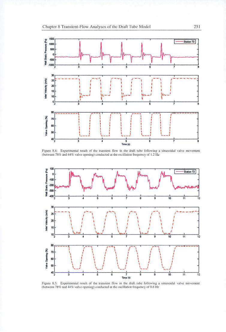
C hapter 8 Transient-Flow Analyses of the Draft Tube Model 25 1
.. 1500 ~
10CXJ ; --Slation T3 . .. 500 !
c.. u 0 'j iii -500
~ -10CXJ 2 3 • 5 6 7 e
30~------~,------~,-----~,------~,-----~,------~
~ · - · - · - · - · - · - · , -·-...·"· . .r·-·-·, "·-·-· .-·-·, ,·-· ..... ·-·-.-· ..... ·-. 25 _ . l I - - l I _
20 I I I i 1
15 i '·' -10 i!•_...,., __ ,
, ; 52 3
80 ---------\ ,.. ~ I I ~ 70 I I
I I I I
l : I I I I '---~
·f 0. 60 0
50
3
- ' !r,,-~ - .i
f,
... I
' I I I I
I I I I
' I
l ' \ ' ___ ,
I I
j I• lj\:\..-.1 ii;,·r·...,· I ~
I I
5 6
I ,.----. I I I l I I I I I I I l I I I I I I I I I l I I I
I : ~ I 1.--- ___ J
5 lime (s)
6
l · , -/l'- ·-· ~
I
7
I I-.---------1 I I I I I I I I I I I I I , __ .J
7
e
B
Figure 8.4: Experimental result of the transient flow in the draft tube fo llowing a sinusoidal va lve movement (between 78% and 44% va lve opening) conducted at lhe osc illation frequency of 1.2 Hz
.. 100r----ir-----,,-----,-----,-----,----.----.----.-;=:==:::::i:======;-, ~ ; 0
r100 .!I -200 .. "-"L_,.,,,,..,....,. iii -300
~--400'--~---'-~~--'-~~......_~~...__~___..__~_._~~--'-~~......__~~-'--~---'
.. 1 ,..., .... u 0
~ li ]
~ .f • 0. 0 . ~ . >
2 3 5 6
30 .r""''"1 I \ I
·- ·- ·- ·'\ r '"" ·- · 25
I i \
': i ' 20 I I
I . I \, \ . . .. ......
5 6
15 ' . . I
102 \..1.,,,,;
3 •
7 B
i.,.,.. . __ . \ I .,
-, i i ..... . _l ....... ..... 7 B
9
,,. .. i ., i \ -,
I
\
9
10
i 10
I I
I
11 12
·"·""·- ·- ·- .,.-..
11 12
Ill ----- --.... ,-' r I I I I \ I
' ,-- ,.. I I \ I
\ ,,..--' I 70
60
50
I \ \ r' I : I I \ I I I \ I 1 I I I \. __ .... , __ ,
-402 3 5 6
\ I \ I \ I I I 1 I I I I I \ I \ I \ I \ I \ : , __ , ...,.. __
7 Torno (s)
B 9
\ I I I \ I I I \ I '- I ...,_..,
10 11 12
Figure 8.5: Experimenta l result of the transient fl ow in the draft tube fo llowing a sinusoidal va lve movement (between 78% and 44% va lve opening) cond ucted at the oscillation frequency of 0.6 Hz
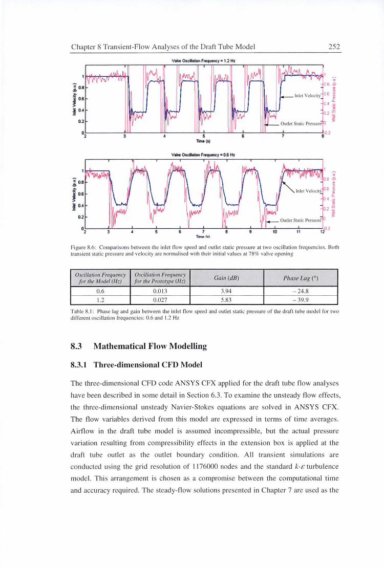
Chapter 8 Transient-Flow Analyses of the Draft Tube Model
; 0.8 ... i 0.6
> I 04
0.2
Valve Oscillation Froquoncy = 1.2 Hz
252
!5 In let Velocity 0.6 ~
u: 0 4 u
ii 02 ~
Outlet Static Pressur 0 ~
o2~----~3~---~~---~~5---~-6~-~~-~----~8-0.2
Tome (s)
; 0.8 ... i 06 > I o.4
0.2
V°"' Oscihtion Froquoncy • 0.6 Hz
!5 06 ~
~ Cl.
04 ~
02 ~
Outlet Static Pressure o ~
'----~---'----'-----'---'---'--............ --_..___._'---'-- - -'-- --'-02 5 6 7 8 9 10 11 12 3
Ttmflt f!i\)
Figure 8.6 : Comparisons between the inlet flow speed and outlet stati c pressure at two osci llation frequencies. Both tran sient stati c pressure and velocity are normalised with their initial va lues at 78% va lve opening
Oscillation Frequency Oscillation Frequency Gain (dB) Phase Lag (0
) for the Model (Hz) for the Prototype (Hz)
0.6 0.0 13 3.94 -24.8
1.2 0.027 5.83 -39.9
Table 8. 1: Phase lag and ga in between the inlet flow speed and ou tl et sta tic pressure of the draft tube model for two different osci llation frequencies: 0.6 and 1.2 Hz
8.3 Mathematical Flow Modelling
8.3.1 Three-dimensional CFD Model
The three-dimensional CFD code ANSYS CFX applied for the draft tube fl ow anal yses
have been described in so me detail in Section 6.3. To examine the unsteady flow effects,
the three-dimensional unsteady Navier-Stokes equations are so lved in ANSYS CFX.
The flow variables derived from this model are ex pressed in terms of time averages.
Airflow in the draft tube model is assumed incompressibl e, but the actual pressure
variation resulting from compressibility effects in the extension box is app lied at the
draft tube outlet as the outlet boundary condition. All transient simulations are
conducted using the grid re olution of 1176000 nodes and the standard k-£ turbu lence
model. This arrangement is chosen as a compromise between the computational time
and accuracy requi red. The steady-flow solutions presented in C hapter 7 are used as the
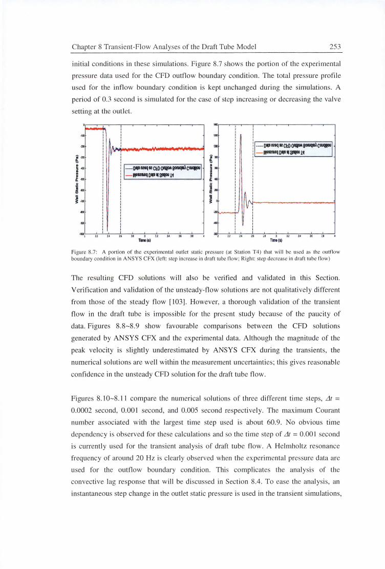
C hapter 8 Transient-Flow Analyses of the Draft Tube Model 253
initia l conditions in these simulat ions. F igure 8.7 shows the portion of the experimental
pressure data used for the CFD outfl ow boundary cond ition. The tota l pressure profi le
used fo r the inflow boundary condition is kept unchanged during the simulations. A
period of 0.3 second is simulated fo r the case of step increasing or decreasing the valve
settin g at the outle L.
' I I
I I ... I I I I I I I I I !\.11 I
~ . - ~ I I v· I I
·"" I I I I I I I
! 1-·--· 0lll nnq R C~D ()Ip~ CGJll!OU I I I I I : - l'f'RIUCI l)lll II 2lll!OU u I I I I I I I I I I I I I I I I I I I I I I I I I I "" I I I I I I I I I I I I
u u u ll l u 14 ll 11 I I ....
Tnlsl
, .. "" llll
~ "' • = "' s a: ., u : "' 'I ~ •
...
...
...,, u ,,
: I I I ' ~~~~~~~~~~
! 1 ·-··00 [)II! nnq R C~D ()Ip~ CGJll!OU I
: . - lllRIUCI Olll II 2lll!OU l • . 1 '--~~~~~~~~--'
I I I
l~v--., --
I u a 1 u ~ ll ~
Tme(s)
Figure 8 .7: A portion of the experimental outlet static pressure (at Station T4) that will be used as the outflow boundary condition in ANSYS CFX (left: tep increa e in draft tube flow; Righ t: step decrease in draft tube flow)
The resulling CFO solutions will also be veri fi ed and validated in thj s Section.
Verification and validation of the un steady- fl ow solutions are not qualitatively different
from those of the steady fl ow [I 03]. However, a thorough validation of the transient
fl ow in the draft tube is impossible fo r the present study because of the paucity of
data. Figures 8.8-8.9 show favourable comparisons between the CFD solutions
generated by ANSYS CFX and the experimental data. Although the magnitude of the
peak velocity is s lightl y underestimated by ANSYS CFX during the trans ients, the
numerical so lutions are well within the measurement uncerta inties; thi gives reasonable
confidence in the unsteady CFO solution for the draft tube fl ow.
Figures 8. l0-8 . l l compare the numerical solutions of three di fferent time steps, Lit = 0.0002 second, 0 .001 second, and 0.005 second respectively. The maximum Courant
number associated with the largest time step used is about 60 .9 . No obvious time
dependency is observed fo r these calculations and so the time step of Lit = 0.00 I second
i currently used for the transient analy is of draft tube flow. A Helmholtz resonance
frequency of arou nd 20 Hz is clearly observed when the experimental pressure data are
used for the outflow boundary condition. This complicates the analys is of the
convective lag response that wi ll be di scussed in Section 8.4. To ease the analys is, an
instantaneou step change in the outlet static pressure is used in the transient simulations,
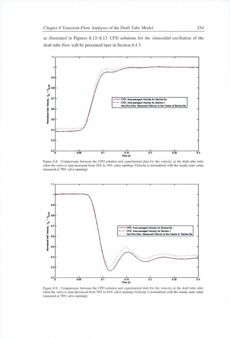
Chapter 8 Transient-Flow Analyses of the Draft Tube Model 254
as illustrated in Figures 8.12-8.13. CPD solutions for the sinusoidal oscill ation of the
draft tube fl ow wi ll be presented later in Section 8.4.3 .
0.9
~ =>J. 0.8
d" ~ 0.7
" ~ ~ 0.6 .,, 1 .. ~ 0.5 z
O.•
0.3
0.20 0.05 0.1
.................... '
..... ...
--CFO: Are•overaged Velocity for Section Oa - · - · · CFO: Are•averaged Velocity for Section 1 · · · · · · · · · Hol-Wiro Oala: Mooaurtd Velocity at the Centro of Soclion Oa
0.15 Tome (s)
0.2 0.25 0.3
Figure 8.8: Comparisons between the CFO solution and expe1imenta l data for the velocity at the draft tube in let when the valve is step- increased from 44% to 78% va lve openi ng (Velocity is normalised with the steady-state va lue measured at 78% va lve openin g)
0.9
d" ~ 0.7
I ! 0.6 .,, . ,: j 0.5
O.•
0.3
0.05 O.t
--CFO: Art•1VOraged Volody for Section Oa - · - · - CFO: Are• ... raged Vtlocily for Section 1 · · ·· · ···· Hot-Wire Dale: MHsurtd Velocity et tht Centro ol Section Oa
"••,
. '····· ····· ····· .. ·· , ........ .
0.15 Time(•)
0.2 0.25 0.3
Figure 8.9 : Comparisons between the CFO solution and experimenta l data for the ve locity at the draft tube inlet when the va lve is step-decreased from 78% to 44% va lve opening (Velocity is normalised with the steady-state va lue measured at 78% va lve opening)
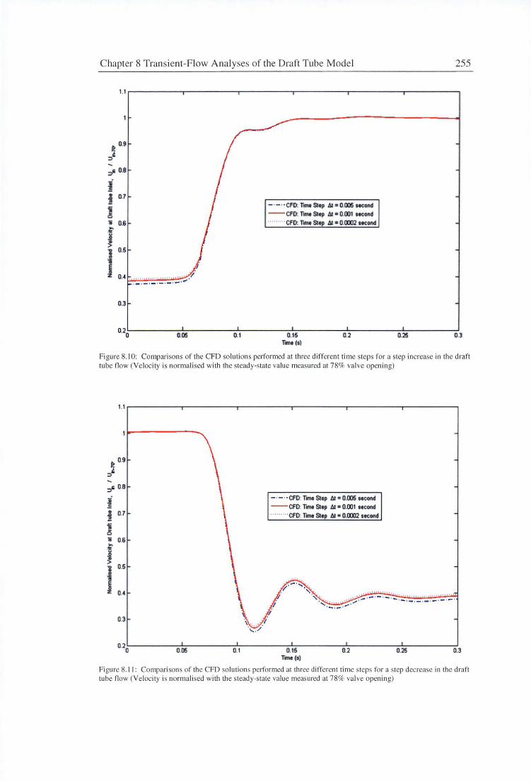
C hapter 8 Transient-Flow Analyses of the Draft Tube Model
b 0.9
":)~
~ 0.8
i ~ 0.7
1i 0.6
0.3
0.05 0.1
- · - · ·CFO: Time Sttp t.I = 0.005 second --CFO: Timt Sttp t.I = 0.001 stcond · · ······· CFO: Tomt Sttp t.I = 0.0002 second
0.15 Tme(s)
0.2
255
0.25 0.3
Figure 8.10: Comparisons or the CFD solutions performed at three different time steps For a step increase in the draft tube flow (Ve locity is normalised with the steady-state va lue measured at 78% valve opening)
b 0.9 ... ":)~
~ 0.8
~-
• 0.7 ~ ii 0 1i 0.6 "' "' CJ .s! . > "i 0.5
i ~ z 0.4
0.3
0.20 0.05 0.1
- · - ·· CFO: Tmt Step t.I = 0.005 second --CFO: Tmt Step t.I • 0.001 second · · ······· CFO: Tmt Step t.I • 0.0002 second
0.15 Tme (s)
0.2
...... ,, ....... .
0.25 0.3
Figure 8.1 1: Comparisons of the CFD solutions performed at three different time steps for a step decrease in the draft tube flow (Ve locity is normalised with the steady-state va lue mea ured at 78% va lve opening)
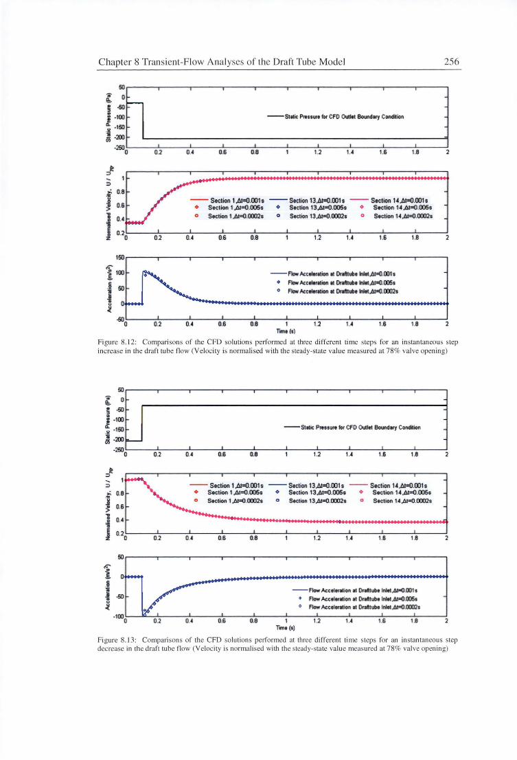
Chapter 8 Transient-Flow Analyses of the Draft Tube Model 256
50.------.- ---...----....----,----.....----.------.-----.----...----, .,.. o~
e,. -i -50 ,_ i! -100 ,_
~ -150~ ! -200 ,_
--Static Pressure for CFO Outlet Boundary Cond~ion
-250~--~·---~·----~·--~·~--~·----·~--~·---~·----~·--~ 0 0.2 0.4 0.6 0.8 1 1.2 1.4 1.6 1.8 2
} ::>
~ O.B .... ]
0.6 ~ 1 0.4
j 0.2
~ 0 0.2
150
1100
c
i 50
• u
:J. -50
0 0.2
-- Section 1 ,ll.t=0.001 s -- Section 13 ,ll.t=0.001s -- Section U ,.M=0.001s
0.4
0.4
+ Sec1ion 1,il.l=0.005s + Section 13,il.l=O.OOSs + Section U,il.l=0.0051
o Section 1 ,il.l=O.IXXJ21
0.6 0.8
0.6 0.8
o Section 13,il.l=O.IXXJ21 o Section 14 ,il.l=O.IXXJ21
1.2 1.6
--Flow Acceleration at Orafttube Inlet ,.lll=O.OOh
• Flow Acceleration at Orafttube Inlet ,.lll=0.005s
° Flow Acceleration at Orafttube Inlet ,.lll=0.0002s
1 T1111e (s)
1.2 1.4 1.6
1.8
1.8
2
2
Fi gure 8. 12: Compari sons of the CFD solu tions performed at three different time steps for an instantaneous step increase in the draft tube flow (Velocity is norma lised with the steady-stale value measured at 78% valve opening)
50 ... 0 ,_ e,. ~
" -50 ~ .. i! -100 ,_
a. -150 ,_ .!I
~ -200 ----250 0
I
0.2
} ::> ~ 0.8 j
0.6 . > ... . 0.4 '5 l 0.2
0 0.2
50
1 0
. ~ 1i J -50 . u
~ -1 000
--Static Pr9SSUr9 for CFO Outlet Boundary Condition
I
0.4 0.6 O.B 1.2 1.6 1.B
-- Section 1 ,ll.t=0.001 s -- Section 13 APQ.001 s -- Section U ,.6.r().001 s
0.4
+ Section 1,il.l=0.005s + Section 13,il.l=O.OOSs + Section U,il.1=0.005s
o Section 1 ,il.l=O.IXXJ2s
0.6 O.B
0.6 0.8
o Section 13~.IXXJ2s o Section 14~.IXXJ2s
1.2 1.6 1.8
--Flow Acceleration at Orafttube Inlet ,41..().0011
1 T1111e (s)
o Flow Acceleration at Orafttube Inlet Al-0.005•
o Flow Acee I- ion at Ordtube Inlet Al=O.CXD2s
1.2 1.6 1.8
-
2
2
2
Fi gure 8. 13: Comparisons of the CFD solutions performed at three different time steps for an in stantaneous step decrease in the draft tube flow (Velocity is normali ed with the steady-sta te value mea ured at 78% valve opening)
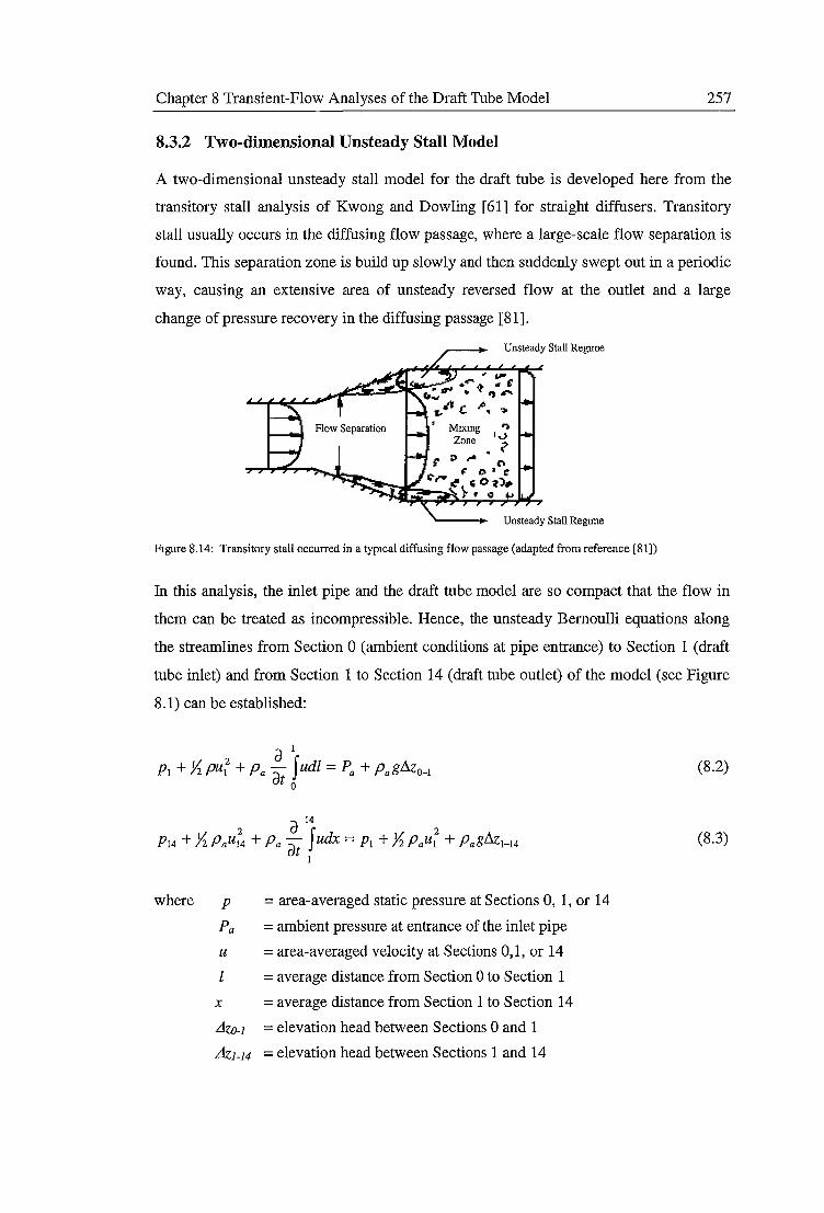
Chapter 8 Transient-Flow Analyses of the Draft Tube Model 257
8.3.2 Two-dimensional Unsteady Stall Model
A two-dimensional unsteady stall model for the draft tube is developed here from the
transitory stall analysis of Kwong and Dowling [61] for straight diffusers. Transitory
stall usually occurs in the diffusing flow passage, where a large-scale flow separation is
found. This separation zone is build up slowly and then suddenly swept out in a periodic
way, causing an extensive area of unsteady reversed flow at the outlet and a large
change of pressure recovery in the diffusing passage [81].
Unsteady Stall Regune
Mixmg -:. Zone IJ . ~
Unsteady Stall Regime
Figure 8.14: Transitory stall occurred in a typical diffusing flow passage (adapted from reference [81))
In this analysis, the inlet pipe and the draft tube model are so compact that the flow in
them can be treated as incompressible. Hence, the unsteady Bernoulli equations along
the streamlines from Section 0 (ambient conditions at pipe entrance) to Section 1 (draft
tube inlet) and from Section 1 to Section 14 (draft tube outlet) of the model (see Figure
8.1) can be established:
where p = area-averaged static pressure at Sections 0, 1, or 14
Pa =ambient pressure at entrance of the inlet pipe
u =area-averaged velocity at Sections 0,1, or 14
= average distance from Section 0 to Section 1
x =average distance from Section 1 to Section 14
L1z0_1 = elevation head between Sections 0 and 1
L1z1_14 =elevation head between Sections 1and14
(8.2)
(8.3)
Chapter 8 Transient-Flow Analyses of the Draft Tube Model 258
On the other hand, the compressibility effects are thought to be quite significant inside
the outlet extension box. The volume of the outlet extension box is relatively large and
the flow inside the extension box may behave like a Helmholtz resonator. Applying the
continuity equation from the draft tube entrance to the exit of the extension box yields:
where = cross-sectional area at draft tube entrance
Aexr = cross-sectional area of the extension box
Uext-ss = steady-state value of the velocity at the exit of the extension box
Vexr = volume of the outlet extension box "" 0.087 m3
Flow Continuity between Section 1 and 14 gives:
where A14 = cross-sectional area at the draft tube outlet = Aexr
UJ4-ss = steady-state value of the velocity at the draft tube outlet "" Uext-ss
C P = draft tube static pressure coefficient
(8.4)
(8.5)
Equation 8.5 applies to the section of flow that is inviscid (i.e. unstalled flow region) in
the draft tube model.
The flow in the draft tube is highly unsteady and the fluctuations in the flow cannot be
altered immediately. A first-order lag equation is established to account for the
convective lag effect inside the draft tube model:
(8.6)
where =convective time lag= U u1
u14 =instantaneous velocity at the draft tube outlet
Chapter 8 Transient-Flow Analyses of the Draft Tube Model 259
Kwong and Dowling [61] apply a similar unsteady stall model to predict the frequency
of oscillation inside a straight diffuser. For linear perturbation of frequency (ro),
Equations 8.2-8.6 can be linearised to:
(8.7)
(8.8)
(8.9)
(8.10)
where L = effectivelengthofthedrafttubemodel = Ldr +0.13[ 4
Ai 05
]
05
n-(1- Cp)
La1 = average length of the draft tube model
Lin = effective length of the inlet pipe= l P + 0.3D P
lp = length of the inlet pipe
Dp = inlet pipe diameter
c =speed of sound at 20°C, latm"" 343.5 m/s
Substituting Equations 8.7-8.9 to 8.10 yields:
where Leq = equivalent length of the inlet pipe and draft tube model
- 05 =0.5Lx[(l-Cp) +l]+Lm
(8.11)
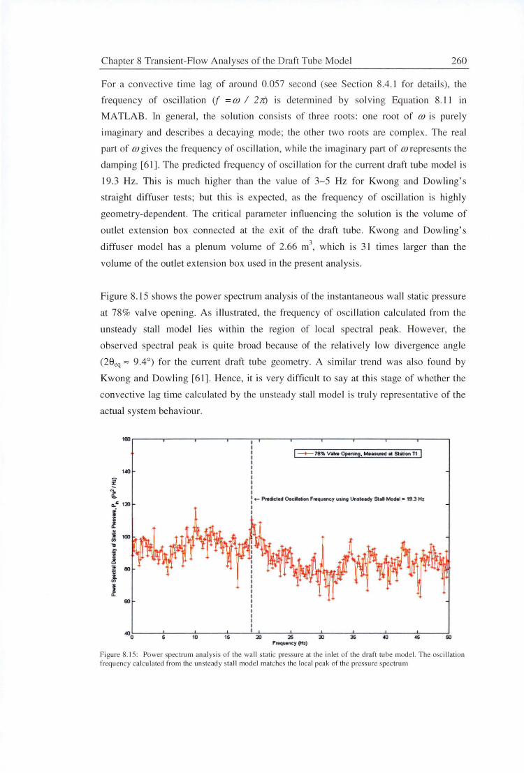
C hapter 8 Transient-Flow Analyses of the Draft Tube Model 260
For a convect ive time lag of around 0.057 econd (see Section 8.4. 1 fo r details), the
frequency of oscillati on (j =OJ I 2Jt) is determined by so lving Equation 8. 11 in
MATLAB . In general , the so lution consists of three roots: one root of {J) is pure ly
imaginary and describes a decaying mode; the other two roots are complex . The real
part of {J) gives the frequency of osc illation, while the imaginary part o f {J) represents the
damping [6 1 ]. The predicted frequency of o c illation fo r the current draft tube model is
19.3 Hz. Thi s is much higher than the value of 3-5 Hz fo r Kwong and Dowling' s
straight diffuser tests; but this is ex pected, as the frequency of osc ill ation is hi ghly
geometry-dependent. The critical parameter influencing the so lution is the volume of
outlet ex tension box connected at the ex it of the draft tube . Kwong and Dowling's
diffuser model has a plenum volume of 2.66 m3, which is 31 times larger than the
volume of the outlet extension box used in the present analys is.
Figure 8. 15 shows the power spectrum analysis of the instantaneous wall static pressure
at 78% valve opening. As illustrated, the frequency of osc ill ation calcul ated from the
unsteady stall model lies within the region of local spectral peak. However, the
observed spectral peak is quite broad because of the relati vely low divergence angle
(28 eq"" 9.4°) fo r the current draft tube geometry. A simil ar trend was also fo und by
Kwong and Dowling [6 l]. Hence, it i very difficult to say at this stage of whether the
convecti ve lag time calcul ated by the unsteady stall model is trul y representati ve of the
actual system behaviour.
I -+-- 78% Va!Ye Opening , MoHU<9d al Station T1 I
uo .... ::c
'1. I!.. o..• 120
+- Predicted Oscilation Frequency using Unsteady Stall Model • 19.3 Hz
l .!,! 11 c;; ,. i" ~
i 80
"' I Cl.
60
.j()o 5 10 15 20 25 30 35 45 50 Frequency (Hz)
Figure 8. 15: Power spectrum ana lys is of the wa ll static pres ure at the inlet of the draft tube model. The oscillation frequency calculated from the unsteady stall model matches the local peak of the pressure spectrum
Chapter 8 Transient-Flow Analyses of the Draft Tube Model 261
8.3.3 One-dimensional Momentum Theory
One-dimensional momentum theory does not take into account the lag time due to
unsteady flow effects but it is useful for comparisons with the three-dimensional CPD
model. The assumptions used in the inelastic waterway model of the power plant will
also be applied in this analysis. The inlet pipe connected to the draft tube is treated like
the waterway conduit of the power plant but the turbine runner is not included here.
Applying the momentum equation between Sections 0 and 1 of the inlet pipe (see
Figure 8.1) gives:
(8.12)
where F = pressure force acting on the inlet pipe
m = mass of the air within the inlet pipe
a = flow acceleration
'riv-p =inertia time constant for the inlet pipe= lp I g
lp = inlet pipe length
h1 = head loss of the inlet pipe due to friction
For the draft tube model, the unsteady Bernoulli equation can be applied between
Sections 1 and 14:
(8.13)
Flow continuity between Sections 0 and 1 as well as Sections 0 and 14 gives:
(8.14)

Chapter 8 Transient-Flow Analyses of the Draft Tube Model 262
Substituting Equation 8.14 in 8.13 and rearranging gives:
= J!.JL - (1 - A12 J u~ + A1 f L x A, + A,+1 duo Pa8 Al~ 2g 2g i=l
1
A, X A,+I dt
(8.15)
_ J!.JL _ C u~ + 't' du 0 - P ideal -dt 2 ID-dt dt
Pa8 g
where 'rJn-di = inertia time constant for the draft tube model
Cp,aeal-dt =ideal pressure recovery factor based on area ratio Ai I Au
The static head term at the pipe entrance can be evaluated from the Bernoulli equation:
.../!.Q__ ~ - u~ Pag Pag 2g
(8.16)
The head loss due to friction (h1) for the inlet pipe can be expressed as:
(8.17)
The friction factor off= 0.015 is assumed based on the Moody diagram with smooth
pipe and a Reynolds number of Ren= 2.5x10⁵. Substituting Equations 8.15-8.17 into
8.12 gives:
::::> Uo = __ 1 __ f{- p3 - pa -[1- Cp,deal + J(Lm + L)l U~ }dt '[ID-dt +Tw-p Pag DP 2g
(8.18)
Equation 8.18 is solved using the MATLAB Simulink. The time response of the flow
subjected to an instantaneous step or a sinusoidal change in outlet static pressure is
analysed and compared with the CPD model in Section 8.4.
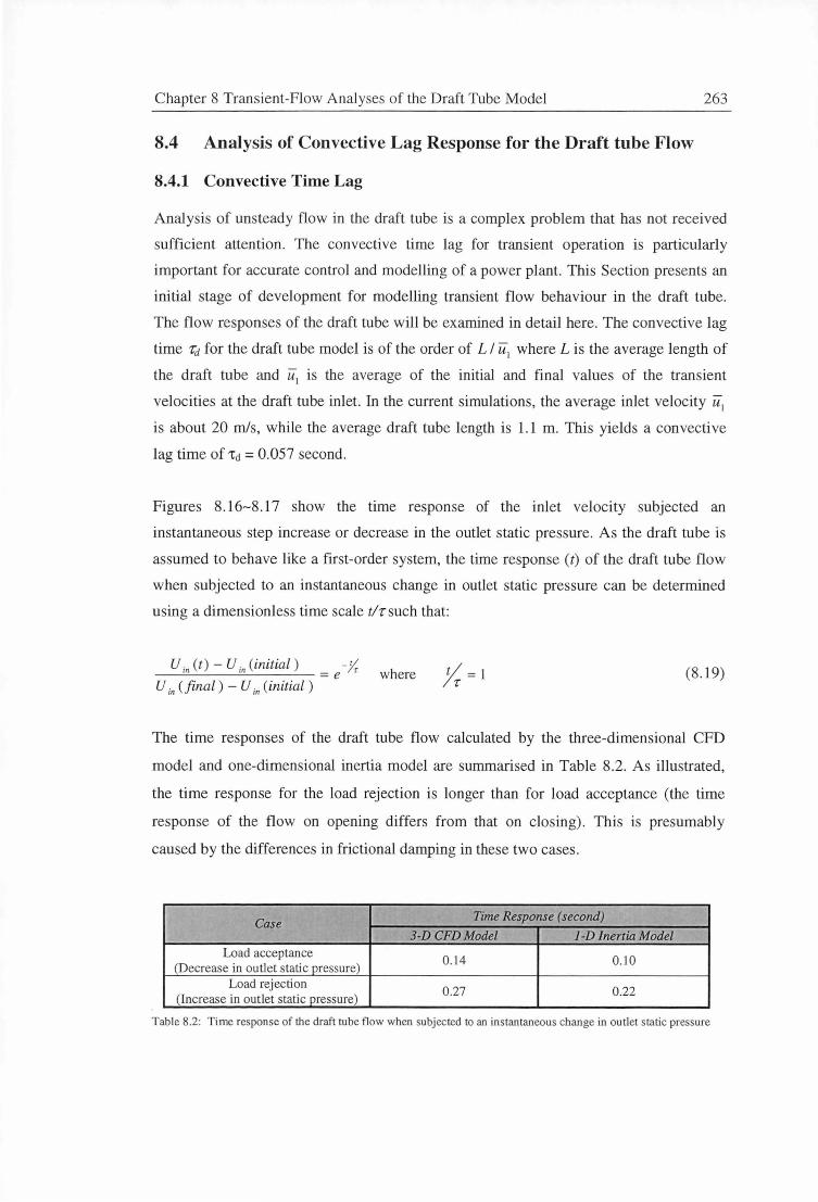
Chapter 8 Transient-Flow Analyses of the Draft Tube Model 263
8.4 Analysis of Convective Lag Response for the Draft tube Flow
8.4.1 Convective Time Lag
Analysis of unsteady flow in the draft tube is a complex problem that has not received
sufficient attention. The convective time lag for transient operation is particularly
important for accurate control and modelling of a power plant. This Section presents an
initial stage of development for modelling transient flow behaviour in the draft tube.
The flow responses of the draft tube will be examined in detail here. The convective lag
time 'rd for the draft tube model is of the order of LI u1 where L is the average length of
the draft tube and u, is the average of the initial and final values of the transient
velocities at the draft tube inlet. In the current simulations, the average inlet velocity u1
is about 20 mls, while the average draft tube length is 1.1 m. This yields a convective
lag time of 'tct = 0.057 second.
Figures 8.16-8.17 show the time response of the inlet velocity subjected an
instantaneous step increase or decrease in the outlet static pressure. As the draft tube is
assumed to behave like a first-order system, the time response (t) of the draft tube flow
when subjected to an instantaneous change in outlet static pressure can be determined
using a dimensionless time scale tlr such that:
U in (t) - U in (initial ) -fr = e '
U in (final) - U in (initial ) where ,% = 1 (8. 19)
The time responses of the draft tube flow calculated by the three-dimensional CFD
model and one-dimensional inertia model are summarised in Table 8.2. As illustrated,
the time response for the load rejection is longer than for load acceptance (the time
response of the flow on opening differs from that on closing). This is presumably
caused by the differences in frictional damping in these two cases.
Case Time Response (second)
3-D CFD Model 1-D Inertia Model Load acceptance
0.14 0.10 (Decrease in outlet static pressure)
Load rejection 0.27 0.22
(Increase in outlet static pressure)
Table 8.2: Time response of the draft tube flow when subjected to an instantaneous change in outlet static pressure
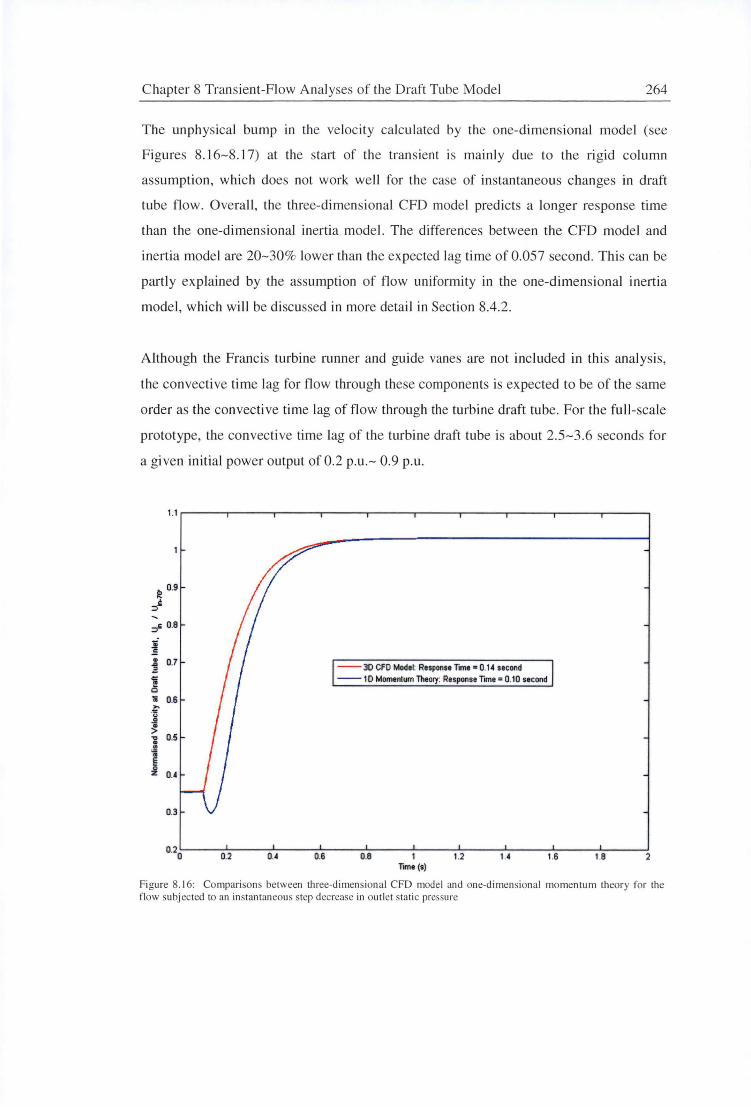
C hapter 8 Transient-Flow Analyses of the Draft Tube Model 264
The unphysical bump in the veloc ity calculated by the one-dimensional model (see
Figures 8. 16-8. 17) at the start of the trans ient is mainl y due to the ri gid column
assumption , which does not work well for the case of instantaneous changes in draft
tube fl ow. Overall, the three-dimensional CFD model predicts a longer response time
than the one-dimensional inertia model. The differences between the CFD model and
inertia model are 20-30% lower than the expected lag time of 0.057 second. This can be
partly explained by the assumption of fl ow uni formity in the one-dimensional inertia
model, which will be di scussed in more detail in Section 8.4.2.
Although the Francis turbine runner and guide vanes are not included in thi analysis,
the convecti ve time lag fo r fl ow through these components is expected to be of the ame
order as the convective time lag of fl ow through the turbine draft tube. For the full- scale
prototype, the convec ti ve time lag of the turbine draft tube is about 2.5-3.6 seconds fo r
a gi ven initial power output of 0.2 p.u.- 0.9 p.u .
b 0.9
"=>~ -~ O.B
~-
• 0.7 .a .a .. I!
0 -; 0.6 >-
] ~ .... • 0.5 .. ~ e :¥. 0.4
0.3
0.2 0 0.2 0.4 0.6
--30 CFO Model: Response Tome• 0.14 second --1 D Momentum Theory: Response Tome= 0.10 second
0.8 1 Tome (s)
1.2 1.6 1.B 2
Figure 8. 16: Co mparisons between three-dimensional CFD model and one-d imensional momentum Lh eory for the flow subj ected to an instantaneous step decrease in outlet static pressure
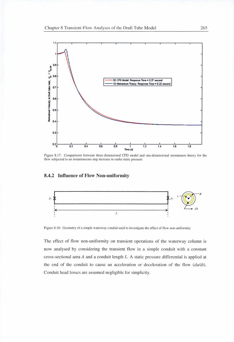
Chapter 8 Transient-Flow Analyses of the Draft Tube Model 265
1.1 ~--~--~---..,------.,...---~--~----..---..,------.,...--~
re o.s J.
::> -="' 0.8 .. ! . 0.7 1 'ii ~ 11 0.6 .., ... ... j ... . 0.5 .. 'i
j 0.4
0.3
0.20 0.2 0.4 0.6
--30 CFO Model: Response Tome • 0.27 aecond --1 D Momentum Theory: R11pont1 Time • 0.22 second
O.B 1 Toma (s)
1.2 1.6 1.8
Figure 8. 17: Comparisons between three-dimensional CFD mode l and one-d imensional momentum theory for the flow subj ected to an instantaneous step increase in outlet static pressure
8.4.2 Influence of Flow Non-uniformity
t t -~·:::-. R '· I \ I
/JI /JO \ ', : : ,_____________________________ \< .. -::: I I
I I tfA
L
Figure 8. 18: Geometry of a simple waterway cond uit used to in vestigate the effect of flow non-uni formity
The effect of flow non-uniformity on transient operations of the waterway column is
now analysed by consideri ng the transient flow in a simple conduit with a constant
cross-sectional area A and a conduit length L. A static pressure differential is applied at
the end of the conduit to cause an acceleration or deceleration of the flow (du/dt).
Conduit head losses are assumed negligible for simplicity.

Chapter 8 Transient-Flow Analyses of the Draft Tube Model 266
Applying the one-dimensional momentum equation across the conduit (between
Sections 1and2 as shown in Figure 8.18) gives:
(8.20)
The change of flow per unit time dq through an elemental area dA1 can be computed as
follows:
The elemental area dA1 is defined as:
dA = ;r[(r +!!.._)2 -(r _!!.._)
2
] I I 2k I 2k
where k = the number of equal elements of the pipe radius
R = radius of the conduit
r1 = radial distance of the element from the centre of the conduit
A power law is used to describe the initial non-uniform velocity distribution qim:
( )
l/n
:~ = 1- ~ where (n + 1)(2n + 1)
u max = 2n2 u,m
. = A = (l -!1._)1'n (n + 1)(2n + 1)
.. q,m-• u, R 2n2 u,m
(8.21)
(8.22)
(8.23)
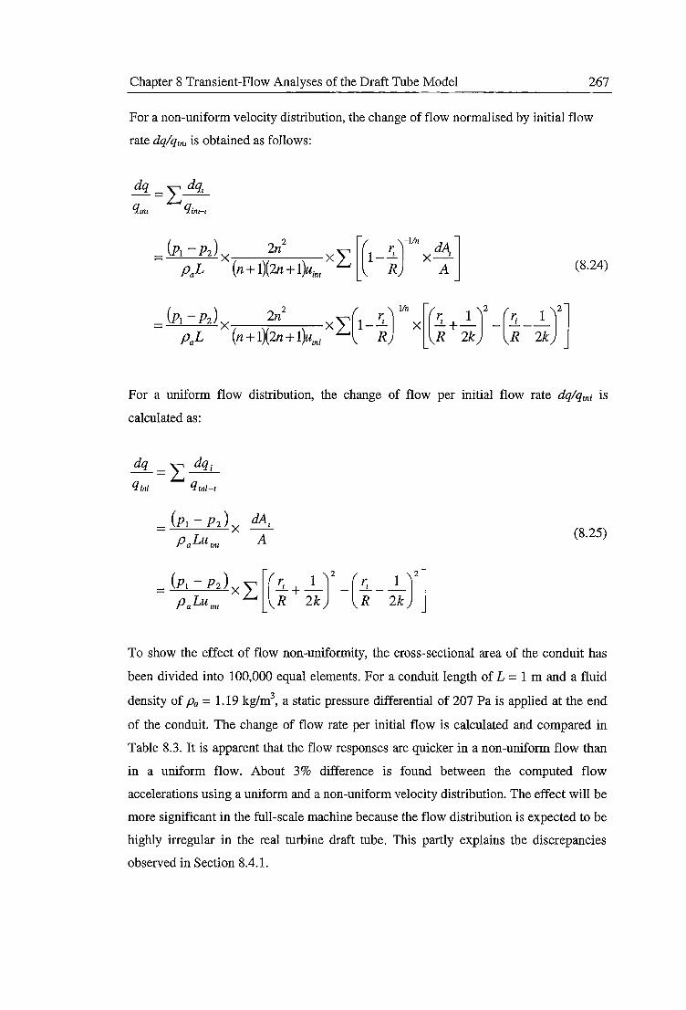
Chapter 8 Transient-Flow Analyses of the Draft Tube Model 267
For a non-uniform velocity distribution, the change of flow normalised by initial flow
rate dqlqrm is obtained as follows:
dq - ""dq, --L.--qml qim-1
- P1 - P2 x 2n x 1-3_ x d4 ( ) 2 [( )-1/n ] - PaL (n + 1)(2n + l)uinr L R A
- P1 - P2 x 2n x 1-3_ x 3_ + J_ - 1i _ J_ ( ) 2 ( )-1/n [( )2 ( )2] - PaL (n+1)(2n+l)umi L R R 2k R 2k
(8.24)
For a uniform flow distribution, the change of flow per initial flow rate dqlqmi is
calculated as:
dq - "" dqi --L.--qini qmi-1
= (P1 - p 2 )x dA,
PaLum, A
= (pi - P2) x I [(3._ + _1 )2 -(3._- _1 )
2 l pa Lu in• R 2k R 2k j
(8.25)
To show the effect of flow non-uniformity, the cross-sectional area of the conduit has
been divided into 100,000 equal elements. For a conduit length of L = 1 m and a fluid
density of Pa = 1.19 kg/m3, a static pressure differential of 207 Pa is applied at the end
of the conduit. The change of flow rate per initial flow is calculated and compared in
Table 8.3. It is apparent that the flow responses are quicker in a non-uniform flow than
in a uniform flow. About 3% difference is found between the computed flow
accelerations using a uniform and a non-uniform velocity distribution. The effect will be
more significant in the full-scale machine because the flow distribution is expected to be
highly irregular in the real turbine draft tube. This partly explains the discrepancies
observed in Section 8.4.1.
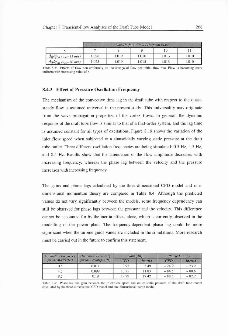
Chapter 8 Transient-Flow Analyses of the Draft Tube Model 268
Non-Uniform Flow I Uniform Flow
n 7 8 9 10 11
dq/q;n; (u;n;=l l mls) 1.026 1.019 1.016 1.013 1.010
dq/q;ni (u;n;=30 mls) 1.025 1.019 1.015 1.013 1.010
Table 8.3 : Effects of flow non-unifonnity on the change of flow per initial flow rate. Flow is becoming more uniform with increasing value of n
8.4.3 Effect of Pressure Oscillation Frequency
The mechanism of the convective time lag in the draft tube with respect to the quasi
steady flow is assumed universal in the present study. This universality may originate
from the wave propagation properties of the vortex flows. In general, the dynamic
response of the draft tube flow is similar to that of a first-order system, and the lag time
is assumed constant for all types of excitations. Figure 8.19 shows the variation of the
inlet flow speed when subjected to a sinusoidally varying static pressure at the draft
tube outlet. Three different oscillation frequencies are being simulated: 0.5 Hz, 4.5 Hz,
and 8.5 Hz. Results show that the attenuation of the flow amplitude decreases with
increasing frequency, whereas the phase lag between the velocity and the pressure
increases with increasing frequency.
The gains and phase lags calculated by the three-dimensional CFD model and one
dimensional momentum theory are compared in Table 8.4. Although the predicted
values do not vary significantly between the models, some frequency dependency can
still be observed for phase lags between the pressure and the velocity. This difference
cannot be accounted for by the inertia effects alone, which is currently observed in the
modelling of the power plant. The frequency-dependent phase lag could be more
significant when the turbine guide vanes are included in the simulations. More research
must be carried out in the future to confirm this statement.
Oscillation Frequency Oscillation Frequency Gain (dB) Phase Lag (0)
for the Model (Hz) for the Prototype (Hz) CFD Inertia CFD Inertia
0.5 0.011 3.95 3.49 -24.9 -23.2
4.5 0.099 13.75 11.83 -84.5 -80.6
8.5 0.19 19.79 17.42 - 88.5 -82.2
Tab le 8.4: Phase lag and gain between the in let flow speed and outlet static pressure of the draft tube model calculated by the three-dimensional CFO model and one-dimensional inertia model
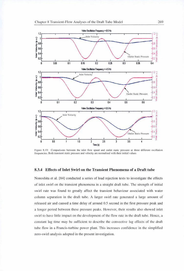
Chapter 8 Transient-Flow Analyses of the Draft Tube Model
Vat.e Oscilation Frequency= 8.5 Hz 1.2~--~-----,.---~---~---~---~---~----, 1 . 2--:
" ; 1 -------11 ~ .. ~ ----~--~~------....... t----------i 5 ~ M M: ~ .. ~ 0.6 060: > ~ i o.• 0.4 ~ c 00 - [2 02-.__ __ __. ___ _,_ ___ _.__ ___ _._ ___ _._ ___ .___ __ ___..__ __ __, · ~
0 0.05 0.1 0.15 0.2 0.25 0.3 0.35 o.•
Vat.e Oscilation Frtquency = 4.5 Hz 1 .2~-------------~---~---------~---,i.2~
"
0.4 ~ 00
02 = ~
0.1 0.2 03 O.• 0.5 0.6
Val'fe OsciUation Frtquency = 0.5 Hz 1 .2~------~------~------~------~---, 1.2 "':'
" 1 ~
~
0.8 ~ .. 0.6 a:
0
04 ~ 00
0.2 ~
0 0.5 1.5 2 2.5 3 3.5 nme (s)
269
Figure 8.19: Compari sons between the inlet flow speed and outlet static pressure at three different oscillation frequ encies. Both transient static pressure and veloci ty are normalised with their initi al values
8.3.4 Effects of Inlet Swirl on the Transient Phenomena of a Draft tube
Nonoshita et al. [84] conducted a series of load rejection tests to in vestigate the effects
of inlet swirl on the transient phenomena in a straight draft tube. The strength of initial
sw irl rate was found to greatly affect the transient behaviour associated with water
column separation in the draft tube. A larger swirl rate generated a large amount of
released air and caused a time delay of around 0.5 second in the first pressure peak and
a longer period between these pressure peaks. However, their results also showed inlet
swirl to have little impact on the development of the flow rate in the draft tube. Hence, a
constant lag time may be sufficient to describe the convective lag effects of the draft
tube flow in a Francis-turbine power pl ant. This increases confidence in the simplifi ed
zero-swirl analysis adopted in the present investigation.
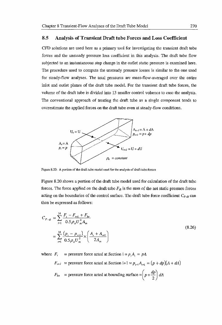
Chapter 8 Transient-Flow Analyses of the Draft Tube Model 270
8.5 Analysis of Transient Draft tube Forces and Loss Coefficient
CPD solutions are used here as a primary tool for investigating the transient draft tube
forces and the unsteady pressure loss coefficient in this analysis. The draft tube flow
subjected to an instantaneous step change in the outlet static pressure is examined here.
The procedure used to compute the unsteady pressure losses is similar to the one used
for steady-flow analyses. The total pressures are mass-flow-averaged over the entire
inlet and outlet planes of the draft tube model. For the transient draft tube forces, the
volume of the draft tube is divided into 13 smaller control volumes to ease the analysis.
The conventional approach of treating the draft tube as a single component tends to
overestimate the applied forces on the draft tube even at steady-flow conditions.
A,=A p,=p
Pa = constant
A1+1= A+ dA P1+1 = p+ dp
Figure 8.20: A portion of the draft tube model used for the analysis of draft tube forces
Figure 8.20 shows a portion of the draft tube model used for calculation of the draft tube
forces. The force applied on the draft tube Fdr is the sum of the net static pressure forces
acting on the boundaries of the control surface. The draft tube force coefficient CF-dt can
then be expressed as follows:
(8.26)
where F 1 = pressure force acted at Section i = p,A, = pA
Fz+J =pressure force acted at Section i+ 1 = P,+1A1+1 = (p + dp )(A+ dA)
Fbs =pressure force acted at bounding surface =(p + ~) dA
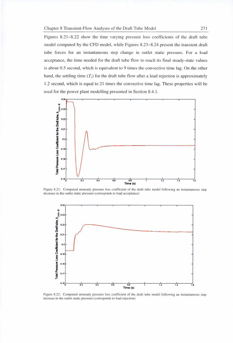
Chapter 8 Transient-Flow Anal yses of the Draft Tube Model 271
Figures 8.21-8.22 show the time varying pressure loss coefficients of the draft tube
model computed by the CFD model , whi le Figures 8.23-8.24 present the tran sient draft
tube forces for an in stantaneous step change in outlet static pressure. For a load
acceptance, the time needed for the draft tube flow to reach its final steady-state values
is about 0 .5 second , wh ich is equival ent to 9 times the convective time lag. On the other
hand, the sett ling time (Ts) for the draft tube flow after a load rejection is approx imate ly
1.2 second, which is equal to 21 times the convective time lag. These properties wi ll be
u ed for the power plant modelling presented in Section 8.4.1.
0.2,
'5
"' .9 0.23 .... • ..0 .a 0.22 .. ~ • 0.21 » a c: ~
0.2
• 0 u 0.19 .. .. 0 -' ! 0.18
"' .. .. I!!
Q.
~ 0.17
I-
0.160 0.6 0.8 1.2 1-' u
Time (s)
Figure 8.2 1: Computed un steady pressure loss coeffi cient of the draft tube model following an instantaneous step decrease in the outlet static pressure (corresponds to load acceptance)
0.2,
'5
"' .9 0.23 .... .! .a 0.22 .. ~ • 0.21 » ~ c: •• 0.2
~ g u 0.19 .. g -' ! 0.18 iii .. ~ ~
0.17
I-
0.160 0.2 0., 0.6 0.8 1.2 u 1.6
Time (s)
Fi gure 8.22: Computed un steady pressure loss coeffic ien t of the draft tube model fo llowin g an instantaneous s tep increase in the outlet static pressure (corresponds to load rejec tion)
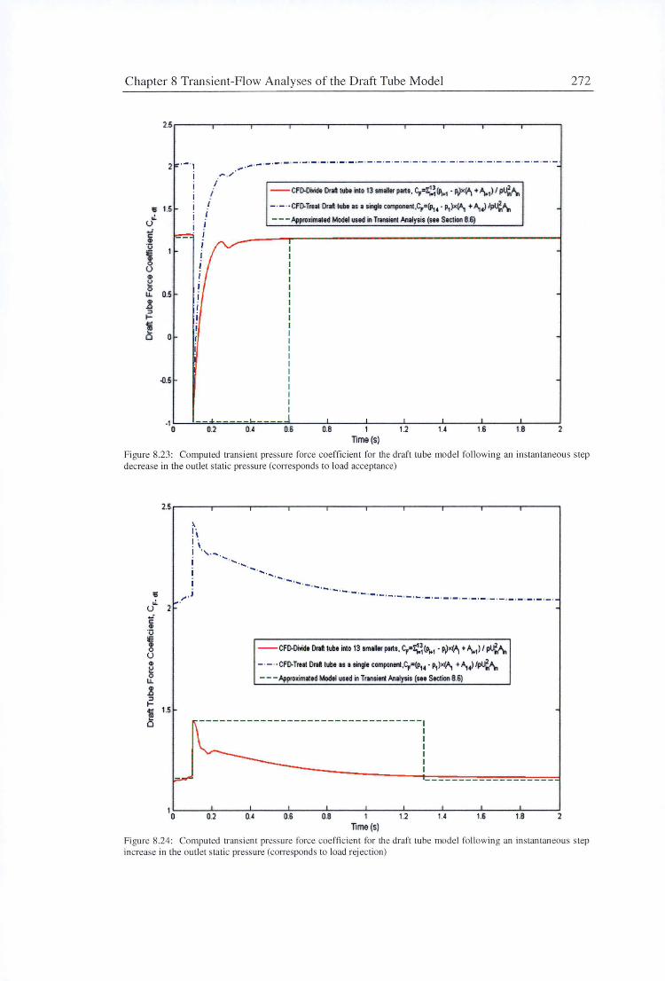
Chapter 8 Transient-Flow Analyses of the Draft Tube Model
9 1.5 .;.
u
-0.5
I I
i i
_. .... - ·- ·- ·- ·- ·- ·- ·- ·- ·- ·- ·- ·- ·- ·- ·- ·- ·- ·- ·- ·- ·- ·- ·- ·- ·- ·- ·- ·- ·- ·- ·- ·- · ,... ,,,
--CFO.Divide Oral tube into t3 smaltr parts, C,=~~1 · Pi)•~ +~1)/p~-\, - · - · · Cf[).Traal Oral tube as a single cornponenl.C,=(p14 • p1)x(A, + A,.J /~-\, - - - .Afproximllod Model uud in TIWlliont Analysis (111 Section B.6)
·1 '----'~-~-:..z.=-~-~-=-=-=-,.....,-=-=-=-~-=-=----'----'-----'----"'-----'-----'-----' 0 0.2 0.4 0.6 O.B 1 1.2 1.4 1.6 1.B 2
Time (s)
272
Figure 8.23: Computed transient pressure fo rce coefficient for the draft tube model fo llowing an instantaneous step decrease in the outlet sta tic pressure (corresponds to load acceptance)
2.5 ..-----.------.----.-----.----,..----.-----.----.----~----.
.;. u 2 E ~ ·c:::;
~ 0 u ~
~ 0 u.. .2l " 1-iii 1.5
0
\ 1· . \ 1 • . ' I ., . .... ......
,,. , J
.... ..... .....
--CFO.Divide Drat tube into 13 smaller parts, C,·~ ~1 • l\)•(-4, + ~1 ) IP~-\,
- · - ·· CF[). Troll Oral tube as a single component .C,•(p14 • p1)x(A, + A,.J Ip~-\, - - - ,Afproximattd !Wldtl used in Transienl Analysis (see Section B.6)
---------------------------------1
0.2 0.4 0.6 0.8 1 Time (s)
1.2
I I I I I I
1.6 1.8 2
Figure 8.24 : Computed transient pressure force coeffic ient for the draft tube model fo llowing an instantaneous step increase in the outlet static pressure (corresponds to load rejection)
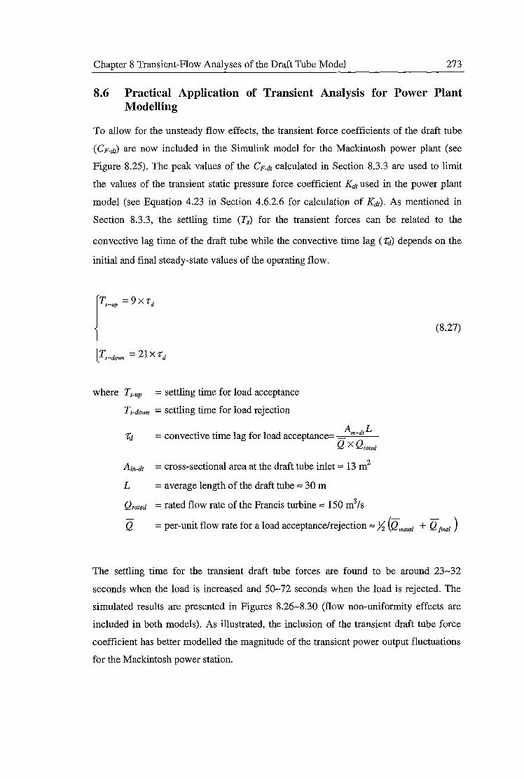
Chapter 8 Transient-Flow Analyses of the Draft Tube Model 273
8.6 Practical Application of Transient Analysis for Power Plant Modelling
To allow for the unsteady flow effects, the transient force coefficients of the draft tube
(CF-di) are now included in the Simulink model for the Mackintosh power plant (see
Figure 8.25). The peak values of the CF-dt calculated in Section 8.3.3 are used to limit
the values of the transient static pressure force coefficient Kdt used in the power plant
model (see Equation 4.23 in Section 4.6.2.6 for calculation of Kd1). As mentioned in
Section 8.3.3, the settling time (Ts) for the transient forces can be related to the
convective lag time of the draft tube while the convective time lag ( 'rd) depends on the
initial and final steady-state values of the operating flow.
Ts-up = 9 X '[d
where Ts-up = settling time for load acceptance
Ts-down = settling time for load rejection
. . 1 ., 1 d Am-dr L = convective time ag 1or oa acceptance Q X Qrated
An-dt = cross-sectional area at the draft tube inlet z 13 m2
L = average length of the draft tube z 30 m
Qrated =rated flow rate of the Francis turbine z 150 m3/s
(8.27)
Q = per-unit flow rate for a load acceptance/rejection z Yz (Qmmat + Q final )
The settling time for the transient draft tube forces are found to be around 23-32
seconds when the load is increased and 50-72 seconds when the load is rejected. The
simulated results are presented in Figures 8.26-8.30 (flow non-uniformity effects are
included in both models). As illustrated, the inclusion of the transient draft tube force
coefficient has better modelled the magnitude of the transient power output fluctuations
for the Mackintosh power station.
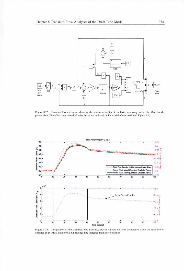
Chapter 8 Transient-Flow Analyses of the Draft Tube Model 274
Figure 8.25: Simulink block d iagram showing the nonlinear tu rbine & inelas ti c waterway mode l for Mackintosh power plant. The effects transient draft tube forces are included in this mode l (Compared with Figure 4.4)
Initial Power Output = 0.2 p.u. 0.9.----..----..----..----..----..----..-----..----..----..------,065
0.8 0 6
.2.0 7 . . ... , ' '• • 055~ 1 . .. ..... "' ., ., ...... , ., . ''" .. . c:
6 0.6 .. .. 0.5 ~
i 0.5 045 ~ ~ 0.4 0 4 ~ " ~ 0.3 .!!
--Field Test Results for Mackintosh Power Plant
w 0.2 ~:::::::=:::~r --Power Plant Model (Transient Drafttube Force) --Power Plant Model (Constant Drafttube Force)
10 20 50 60 70 90
x 10·3
6 ,---,----,c----.----r;;:====================~o.1 ., ::.:: • t[ .! " ~ 2 0 u
' ... . "'' " "• 1 . Main Servo Position = 0.6 s-
····· ····· ····· ·· · · ··· ··~···· · ··· · · ··· ·· ·· · ··· ··· · · ···· ·· · ~ .•••. •. ••.• , .. ,, , , •':!: 0.5 -~ . a.
~ 0 "- ~ a . 4 ~ ;
·2 ~
(/)
" • 0.3 ~
.. 0 10
I I I I
50 20 60 70 90 TKnt (second)
Figure 8.26: Comparison of the simulated and measured power ou tputs for load acceptance when the machine is operated at an initial load of0.2 p.u. (Dotted line indicates main servo position)
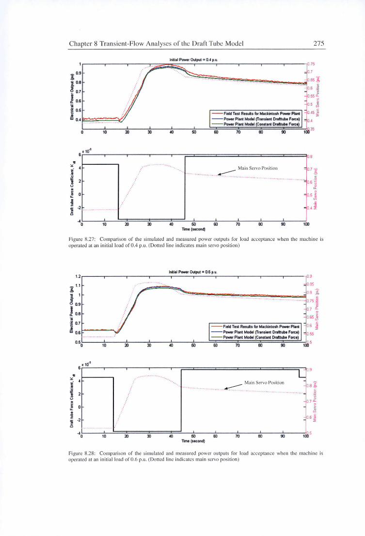
Chapter 8 Transient-Flow Analyses of the Draft Tube Model 275
]; 0.9
l 08
6 0.7
I a. 0.6
~ 0.5 ~ w o.• ~~~:::::::==~'i
0 10 20
ln~ ial Power Oulput = 0.4 p.u.
.... ..... ..... ......... ,,,,, '' ' "'"" .,, .
'II It " '"'""'•"
--field Tesl Resulls for Mackintosh Power Pl1nl --Power Plant Model (Transient Drafttube Force) --Power Plant Model (Constant Drofttube Force)
50 60 70 90
x 10-3 6r-----,,- ----,,----r-,----,,--;:==i::======:::r=======:i:::======c:::====::::::c======:::::io.a ,,
~
1:.-. ~ 2 0
(.) . ~ O>-
~ ~ -2'7 .... ... .. ..... ... .. ... .
.. 0 10
·· ···
20
.... , ...
50 60 70 90 Tome (second)
= 0.7 S' s c:
"' ~ o .s ·~ 0 a. 0
~ 0.5 ~ (/)
c:
• 0.4 ~
100
Figure 8.27 : Comparison of the simulated and measured power outputs fo r load acceptance when the machine is operated at an initial load of0.4 p.u. (Dotted line indicates main servo position )
IMial Power Output• 0.6 p.u. 1 .2~--~---~---~---~---~--~---~---~---~--~o.s
]; 1.1 -s Q.
3 0 0.9
I a. 0.8 .. -~ 0.7
~ 0.61-"'-----...;u
10
6 x 10⁻³
,, ~ • "i . !!
~ 2 . 0
(.) . ~ 0 ... . .a .i!
~ -2
0
...... .. ..... ... .
20
, .... "'"""
085
... , "' " """ " ... ... .... .. .. .. .... ..... .. ... .
--f ield Test Rosuh for Mackintosh Power Pion! --Power Plant Model (Transient Drafttub1 Force) --Power Pl1nl Model (Constant Drafttub1 Force)
50 60 70 90
Main Servo Posilion - S" - ass .... .. ................. ...... ~ ... .. .... ..... ... .. ....... ...... . .. .. ..... ~ c:
0
·u;
-0 7 ~ 0
~ (/)
-0.6 - ~ - ::;:
.. 0 10 L_ __ __J_-====20::c::======3Jt::::=====.l(]::t::=='..__-~L_---l~----7Lo'---~~L..---90~1----1(8·5
Time (socond)
Fi gure 8.28: Comparison of the simulated and measured power outputs for load acceptance when the machine is operated at an initi al load of 0 .6 p.u. (Dotted line indicates main servo position)
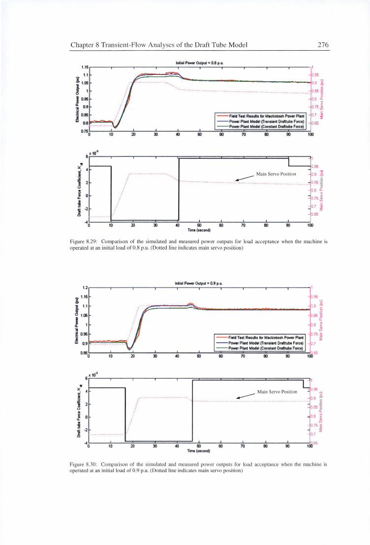
Chapter 8 Transient-Flow Analyses of the Draft Tube Model 276
Initial P-r 01Jtput = 0.8 p.u. 1.15
1.1 0.95 A i. 1.05
.3 1
~--------------------.Jo .9 ]; 0.85 ·~
iii ..... ........ ...... .. '"" .......... ....... .. . ..... ............ ..
I 095 a.
0.9 "'ii ·I!! u 0.95 1
0.6 rt_
0 75 ~ rn
--Fitld Tel1 R11uft1 for Mackintosh Power Plan1 w
0.8 --Power Plant Model (Tr1n1ien1 Dr1fttub1 Force) ,.,,., , ,.,,.,., , --POMr Plant Model (Constant Drafttub1 Force)
0.750 10 so 70 90
6 x 10·)
9 :.:
- 1 I ._ __ ~0.95
.i ~ 2 . 0
.... ................. Main Servo Posi tion = 0.9 ];
---- § ..... .... ......... . .. .. ........ .. .. .... ~ 0 65 -~ <..> . 0
- 0 8 a. ~ 0 ..._ . - ~
- 075 ~
' -2 c -0.7 · ~ - ::;:
.3 ... -065 .. 0 10 20 50 100
I I I I I
so 70 90 T11n1 (second)
Figure 8.29: Comparison of the simulated and meas ured power outputs for load acceptance when the machine is operated al an initial load of0.8 p.u . (Dotted line indicates main servo position)
'S' 1.15 .s 1 1.1
6 1.05
! 1 11 ·I!! 095 j . w o.9 e."" .. == .. "" ... ::: .. == .. =. :i:: ... ;:, .. .: .. :: .. ::::i .. ·
10
ln~ial POMr Output= 0.9 p.u.
095 2~=====~~~=-----------------..J109 f
--Field T111 R11ufts for Mackintosh Power Plant
--Power Plant Model (Transient Dr1fttub1 F orc1) --Power Plant Model (Constant Draft1ube Force)
so 70 90
0.85 ~ a.
08 ~ rn
o 75 -~ ::;:
9 :.:
x 10" s,----,,----,----,--,---r--,---;==c::::=====:::i======::::i:======::::i:======:::t:====~l.__'-::i-1
Main Servo Position : o 95 S' ?!
.!!
i 2 <..> . ~ 0
~ c -2 : .3 ..................... .
"o 10 20 50 Tone (second)
so
---- -09 .!!> '" ' ....... . ..................... . .. .......... . .. .. , ... . . §
70 90
- z - 0 85 · ~
a. <= 0.8 ~
rn -0.75 ·= - i - 0.7
Figure 8.30: Comparison of the simulated and measured power outputs for load acceptance when the machine is operated at an initia l load of 0 .9 p.u. (Dotted li ne indicates main servo position)

Chapter 8 Transient-Flow Analyses of the Draft Tube Model 277
8.7 Conclusions
Unsteady flow effects in the model draft tube following a sudden change in discharge
have been studied computationally using mathematical models of various complexities.
The CFD solutions were validated against the thermal anemometry measurements. The
three-dimensional CFD numerical analysis was shown to predict a longer response time
than the one-dimensional hydraulic model currently used for simulating the operations
of the Mackintosh power station. The inclusion of transient draft tube forces in the
power plant model improved the simulation accuracy for the Mackintosh station.
Convective lag effects and fluctuations in the draft tube pressure force or loss
coefficients were shown to largely explain the remaining discrepancies in current quasi
steady predictions of transient hydro power plant operation.

Chapter 9 Conclusions 278
CHAPTER9
CONCLUSIONS
9.1 Summary
The specific objectives of this thesis were to:
• develop and validate nonlinear quasi-steady flow models for the Francis turbine
and waterway systems of single- and multiple-machine hydroelectric power plants;
• verify and validate the steady- and transient-flow solutions of CPD models for the
turbine draft tube flows using the experimental model tests; and
• evaluate convective lag effects in the draft tube flow as well as the influence of
transient draft tube force and loss coefficient variations during unsteady operation
of a Francis turbine.
These objectives have been carefully investigated and it has been found that nonlinear
modelling of the Francis turbine and waterway systems significantly improves the
simulation accuracy of the power plants. The nonlinear computer models were
developed in MATLAB Simulink for transient stability analysis of power stations
subjected to a large frequency disturbance. Inelastic waterway models that take into
account the inertia effect of the water column were found to perform satisfactorily in the
current simulations. These results also showed that linearised models will underestimate
the magnitude of power fluctuations during a large system disturbance. Overall, the
improved hydraulic models presented in this thesis possess several important
characteristics that can overcome the deficiencies of the existing industry models. These
features include:
• introduction of a nonlinear guide vane function to account for the nonlinear
relation between the turbine flow and gate opening;
• use of the dimensionless turbine performance curves to properly represent the
nonlinear characteristics of the Francis turbine;

Chapter 9 Conclusions 279
• application of a flow non-uniformity factor to correct for the effects of non
uniform velocity distribution in the hydraulic conduits;
• inclusion of the inlet dynamic pressure and draft tube static pressure force terms in
the unsteady momentum equation for the waterway column;
• detailed calculations of the hydraulic model parameters such as water starting time
and pressure loss coefficients for the entire waterway column; and
• consideration of the hydraulic coupling effects for multiple-turbine plant.
Favourable comparisons have been obtained between simulations and full-scale test
results collected at Hydro Tasmania's Mackintosh and Trevallyn power stations. For the
Mackintosh power plant, a noticeable phase lag between the measured and simulated
power outputs, which increases in magnitude with guide vane oscillation frequency, was
observed for this short penstock installation. The well-tested electro-mechanical model
for the governor operation was unlikely to have been a significant cause of error. The
remaining discrepancies were most likely due to the unsteady flow effects in the Francis
turbine. The flow pattern in the Francis turbine does not change instantaneously with
the guide vane movement and thus a time lag in flow establishment through the runner
and draft tube may occur. For the Trevallyn power station, this unsteady flow effect was
found to be relatively insignificant, as this power plant has a relatively long waterway
conduit and high water inertia. The inertia effect of the water column in such cases is
expected to dominate any unsteady flow effects of the Francis turbine operation.
To further examine these effects, the flow in a typical Francis-turbine draft tube without
swirl has been studied experimentally and computationally. The 1:27.1 scale model
draft tube used for these analyses was geometrically similar to the one employed in
Hydro Tasmania's Mackintosh station. Extensive verification and validation of the
simulations using ANSYS CFX were performed. The three-dimensional Reynolds
A veraged Navier-Stokes equations were solved by the code. Grid resolution, turbulence
model, and boundary conditions were identified as the major factors affecting the
accuracy of the numerical solution. Although a mesh-independent solution was not
achieved in these simulations, a mesh size of 1176000 nodes was found to provide a
Chapter 9 Conclusions 280
good compromise between computational time and the accuracy required. No firm
conclusions can be drawn at this stage about the accuracy of the turbulence models used,
due to the scarcity of experimental data for validating the CFD solutions. Preliminary
investigations indicated that simulations using a standard k-E turbulence model
produced reasonably accurate results. The more advanced turbulence models such as
Reynolds stress models did capture the self-excited unsteadiness of the draft tube flow
but they did not seem to improve agreement with steady-state experiments.
Great care was taken in the selection of suitable boundary conditions for the CFD
analysis: experimentally derived boundary conditions were used whenever possible; this
is especially true for the inflow boundary condition. The inlet boundary layer properties
were checked to ensure that the simulations would reflect the actual flow situations. The
outflow boundary of the draft tube was extended to a distance of five times the outlet
height to improve the convergence rate of the solution. Computational studies indicated
that the inlet swirl of the draft tube would greatly affect the flow distribution inside the
draft tube (see Section 7.4.3).
For transient-flow operations, the validated steady-flow solutions were used as the
initial conditions in the unsteady simulations. Three different time steps were used to
check for the time dependency of the solutions. The calculations were found insensitive
to the Courant number of the flow and a time step of 0.001 second was applied for all
transient simulations. Favourable comparisons were obtained between CFD solutions
and thermal anemometry measurements. These provide some confidence for use of CFD
in the transient analysis of the draft tube flow.
Unsteady flow effects in the turbine draft tube were evaluated using a three-dimensional
CFD model, a two-dimensional unsteady stall model, and one-dimensional momentum
theory. The convective time lag of the draft tube depended on the initial and final
steady-state values of the flow. The predicted oscillation frequency using unsteady stall
model seemed to match the experimental data, but the exact determination of convective
lag time using this approach was difficult due to the relatively broad power spectrum of
the experimental static pressure.
Chapter 9 Conclusions 281
The time responses of the draft tube flow when subjected to an instantaneous step
change in outlet static pressure were determined using Equation 8.19. The time response
for the load rejection is longer than for load acceptance. This is presumably caused by
the differences in frictional damping in these two cases. The three-dimensional CFD
analysis was shown to predict a longer response time than the one-dimensional
hydraulic model currently used as the power industry standard. The above difference
was lower than the expected convective time lage of 0.057 second for the draft tube
model. This can be partly explained by the assumption of uniform velocity distribution
used in one-dimensional momentum theory.
The pressure oscillation frequency was found to greatly affect the flow response in the
laboratory model tests. Although frequency dependence of the flow was clearly seen, it
was still very difficult to quantify the impact of the oscillation frequency on the
convective lag time of the flow. The Helmholtz resonance present in the experimental
model tests further complicated the analysis of the frequency-dependent lag between the
outlet static pressure and inlet flow speed. In general, the gain and phase lag between
the inlet flow speed and outlet static pressure of the draft tube both increased with
increasing oscillation frequency.
Transient behaviour was also observed in the calculated static pressure force and loss
coefficients. The settling times of these coefficients when subjected to an instantaneous
step increase and decrease of the flow were about 9 and 21 times the convective time
lag, respectively. Inclusion of the unsteady draft tube forces into the power plant model
of Mackintosh station produced favourable improvements in predicting the magnitude
of power fluctuations. Overall, the convective lag effects as well as the fluctuations in
draft tube pressure force and loss coefficients were shown to largely explain the
remaining discrepancies in current quasi-steady predictions of the transient hydro power
plant operation.
Chapter 9 Conclusions 282
9.2 Recommendations for Future Study
9.2.1 Full-Scale Field Testings of the Francis-Turbine Power Plants
Acoustic methods should be used to measure the full-scale turbine flow during transient
operations. These should provide valuable information for validation of the hydraulic
models and evaluation of the nonlinear guide vane function.
Turbine and generator efficiency should be measured on every full-scale machine
before the dynamic tests are carried out. The ages of the hydraulic components in the
Francis turbine installations were found to influence the efficiency of an individual
machine. A current efficiency test would greatly reduce the uncertainty involved in the
parameter identification process, and increase the modelling accuracy.
The power outputs, guide vane positions, flow rates, speed variations, and static
pressures should be measured and recorded on every machine under test in multiple
machine stations. Effects of simultaneously changing the operating conditions of
turbines sharing a common waterway conduit should be thoroughly investigated to
confirm the effects of hydraulic coupling on the transient stability of a power plant.
Frequency response tests should be carried out at different load levels so that a complete
safe operating zone can be established for the Francis turbine operations.
A continuous data acquisition system should be developed to build the database needed
for validating power plant models. This would provide increased modelling fidelity and
control accuracy of a power plant.
9.2.2 Hydraulic Modelling of Francis-Turbine Power Plants
Simulated results should be verified using different simulation programs. The hydraulic
model should also be validated for power plants possessing a long waterway conduit.
Comparisons with an elastic waterway models would be interesting in this case. The
methods of characteristics commonly used in solving equations for elastic waterways
would provide some flexibility in adding extra equations to account for unsteady
friction losses in the conduits (see Equation 4.27).
Chapter 9 Conclusions 283
Modelling and control strategies based on the concepts of Artificial Intelligence (AI)
should be considered. This approach is now becoming feasible, as Hydro Tasmania has
recently begun its program to continuously acquire the data from its power plants. The
AI modelling procedure is based primarily on the principle of pattern recognition and
the predictive capabilities of the neural networks implemented through a cluster-wise
segmented associative memory scheme. Exhaustive system identification processes can
be eliminated using this approach. Neural-network based controllers should be tried in
the Francis-turbine power plants because they are found to give better damping effects
for the generator oscillations over a wide range of operating conditions [29].
9.2.3 Experimental Model Testings of the Turbine Draft Tube
The use of a water model would be beneficial in determining the magnitude of scale
effects and eliminating the Helmholtz resonance effects presented in the aerodynamic
model. Two-phase flow studies for the turbine draft tube would also be informative in
the transient analysis associated with the water column separation. The effects of inlet
swirl could be examined by adding a ring of guide vanes at the draft tube inlet. A
complete model of the Francis turbine runner and guide vanes would be even more
desirable, as the time lag due to the movement of turbine guide vanes is thought to be of
the same order as the convective time lag of the draft tube.
Due to the extreme combination of streamline curvature, adverse pressure gradients and
secondary flows, experimental measurements of all Reynolds stresses would be
valuable. This information would be particularly useful for the assessment of turbulence
models used in the CFD simulations of draft tube flow. Laser Doppler Anemometry
(LDA) should be used to check for the hot wire measurements, as the hot wire is
incapable of sensing the flow direction in the highly unsteady and recirculating flow
regimes.
Surface flow visualisation should be performed in order to aid the analyses of draft tube
flow. This technique provides a visual image of the skin friction distribution on the
surface and helps better understanding of the unsteady flow phenomena inherent in the
flow. Fluorescent mini-tuft and oil-film methods are most suitable techniques currently

Chapter 9 Conclusions 284
available. While detailed boundary-layer information is not obtainable, general patterns
of flow separation and reattachment are recognisable with surface flow visualisation.
9.2.4 CFD Simulations of Turbine Draft Tube
Impacts of inlet boundary conditions for the draft tube should be carefully examined. In
particular, the effects of swirl on either steady- or unsteady-flow operations of the draft
tube should be thoroughly investigated. The current model is probably unable to
correctly account for all the imposed information. The problems with inlet boundary
condition underline the need to include the whole Francis turbine runner and guide
vanes in the calculations of draft tube flow. This would require millions of additional
nodes for computations. Although an unsteady rotor-stator interface can be easily
modelled in ANSYS CFX, the limitations of turbulence models are still present.
Detached Eddy Simulation (DES) and Large Eddy Simulation (LES) are becoming
feasible with increasing computer power, and it would be interesting to verify the
current RANS approach for the transient prediction of the draft tube flow against these
more realistic models.
Simulation of the transient flow effects due to the movements of turbine guide vanes
would be interesting. Flow modelling for variable guide vane motion is still challenging,
as the moving-mesh techniques developed in ANSYS CFX can only account for very
simple motion such as translation or rotation of a circular cylinder.
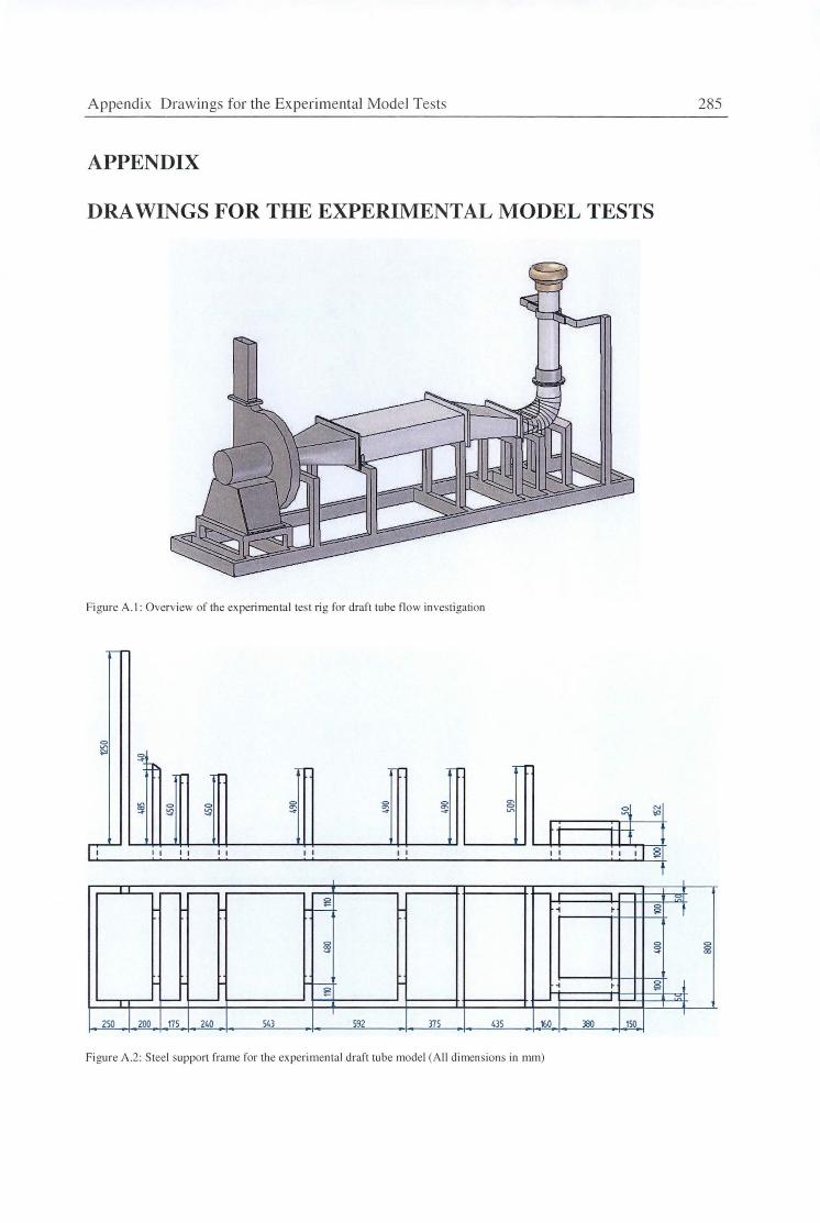
Appendi x Drawings for the Experimental Model Tests 285
APPENDIX
DRAWINGS FOR THE EXPERIMENTAL MODEL TESTS
Fi gure A. I : Overview of the ex perimenta l tes t ri g fo r draft tube fl ow investigation
-
0
~ ~
~ -
~ ~ ~ ~ ~ ~ ~ ~ N
"" h I I
11 t IT ~ I I I I I I I I I I I I I I I I ~
I
,-- - - "'' ~ ~ t - .... ~ ~
~ ~ :;:
.... ~ ~ ~ ~ ~ >--- - - "' '
I 200 I
250 175 240 543 592 375 435 160 380 150
Figure A.2: Steel suppo1t frame for the experimental draft tube model (All dimensions in mm)
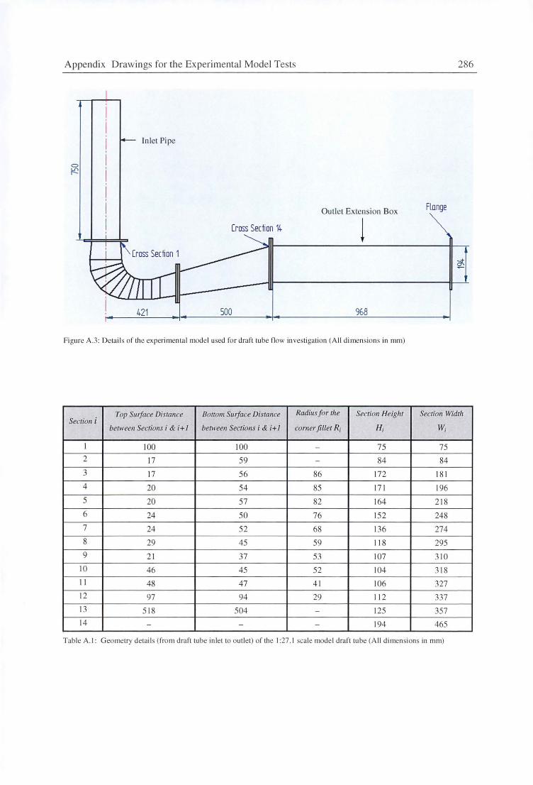
Appendix Drawings for the Experimental Model Te 'ts 286
lnlel Pipe
Oullel Extension Box Flnnge
Cross Section 14. !
4.21 500 968
Fi gure A.3 : Detai ls of the experimental model used for draft tube flow in vestigation (A ll dimensions in mm)
Section i Top Surface Distance Bottom Surface Distance Radiusfor the Section Heighr Section Width
between Sections i & i+ I between Sections i & i+ l corner fillet R; H; W;
I 100 100 - 75 75 2 17 59 - 84 84 3 17 56 86 172 18 1 4 20 54 85 17 1 196 5 20 57 82 164 218 6 24 50 76 152 248 7 24 52 68 136 274 8 29 45 59 118 295 9 21 37 53 107 310
10 46 45 52 104 318 11 48 47 41 106 327 12 97 94 29 112 337 13 518 504 - 125 357 14 - - - 194 465
Table A. I: Geometry details (from draft tu be inle t to outlet) of the I :27 .1 sca le model draft tu be (A ll dimensions in mm)
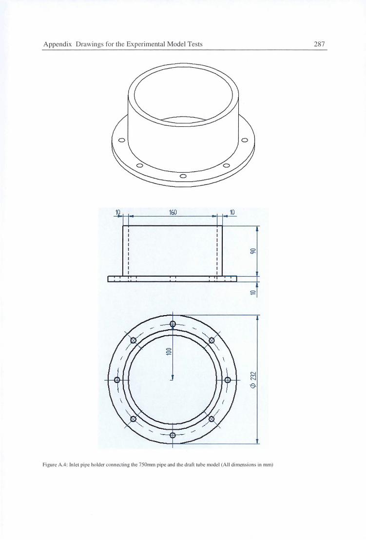
Appendix Drawings fo r the Experimental Model Tests 287
0 0
10 10 I - - I _:: -I I I I I I I I I I I I = I I C7'
I I I I I I I I
I I I I
=
Figure A.4: Inlet pipe holder connecting the 750mm pipe and the draft tube model (A ll dimensions in mm)
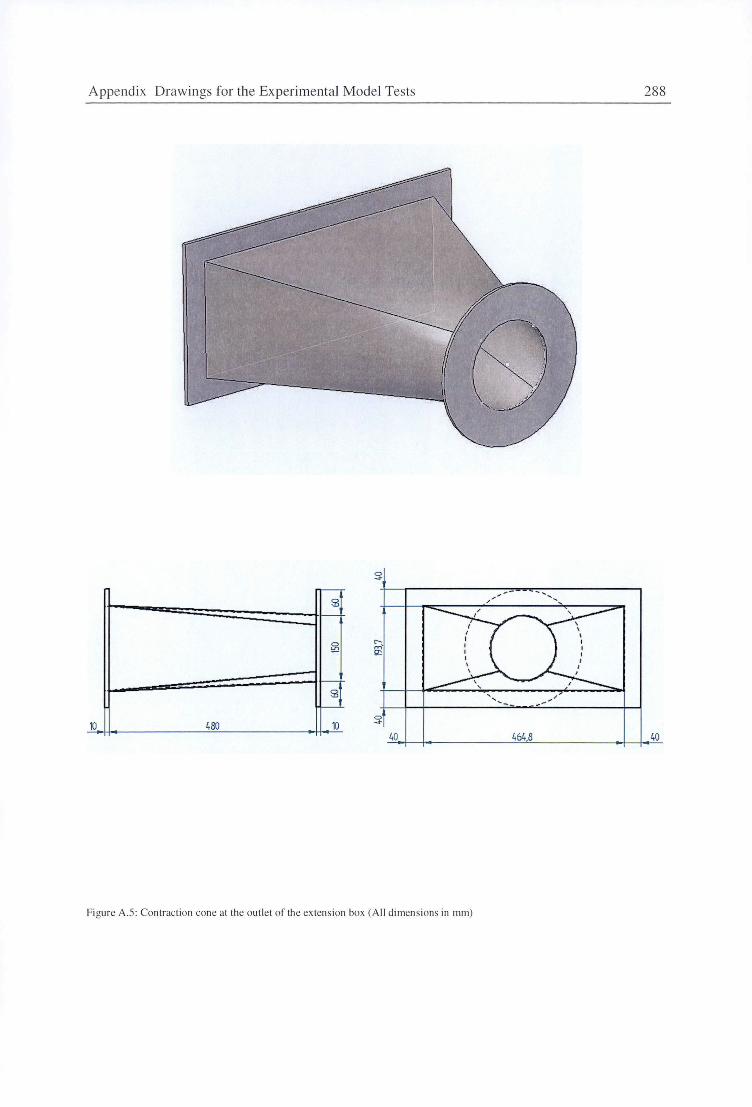
Appendix Drawings for the Experimental Model Tests 288
--' @ '
§l 0-,..., ~
-@ ' ' ~~' --
c:>
10 480 10 .... 40 464,8 40
Fi gure A.5 : Contraction cone at the outlet of the ex tension box (All dimen sions in mm)
Bibliography 289
BIBLIOGRAPHY
[l] Aeschliman, D.P. & Oberkampf, W.L. "Experimental methodology for computational fluid dynamics code validation", AIAA Journal, 1997.
[2] Andersson, U. & Karlsson, R., "Quality aspects of the turbine 99 draft tube experiment", Proceedings of Turbine 99 - workshop on draft tube flow, Porjus, Sweden, June 20-23 1999.
[3] Andersson, U., "Turbine 99 - experiments on draft tube flow (test case T)", Proceedings of Turbine 99 - workshop on draft tube flow, Porjus, Sweden, June 20-23 1999.
[4] ANSYS CFX Inc., "ANSYS CFX release 10.0 user's manual", Waterloo, Ontario, Canada, 2005.
[5] Apsley, D.D., "Lecture notes for computational hydraulics", School of Mechanical, Aerospace and Civil Engineering, University of Manchester, 2005.
[6] Arpe, J.A. & Avellan, F., "Pressure wall measurements in the whole draft tube: steady and unsteady analysis", Proceedings of the XXI IAHR Symposium on Hydraulic Machinery and Systems, Lausanne, September 9-12 2002.
[7] Arpe, J.A., "Experimental investigation of unsteady pressure and velocity field in a draft tube of Francis turbine", PhD Thesis, Department De Genie Mecanique, Ecole Polytechnique Federale De Lausanne, Switzerland, 2003.
[8] Arts, T., Boerrigter, H., Carbonaro, M., Charbonnier, J.M., Degrez, G., Olivari, D., Riethmuller, M.L., & Van den Braembussche, R.A., "Measurement techniques in fluid dynamics: an introduction", von Karman Institute for Fluid Dynamics, 1997.
[9] A vellan, F., "Flow investigation in a Francis draft tube: the Flindt project'', Proceedings of the Hydraulic Machinery and Systems 20th IAHR Symposium, Charlotte, August 7-9, 2000.
[10] Bauer, D., Peikert, R., Sato, M. & Sick, M., "A case study in selective visualisation of unsteady 3D flow", Proceedings of the conference on Visualisation, Boston, Massachusetts, USA, 2002, pp. 525-528.
[11] Belanger, A., "Simulation of the ERCOFTAC draft tube using PowerFlow", Proceedings of Turbine 99 workshop 2, Alvkarleby, Sweden, June 18-20, 2001.
[12] Berca, E.L., Ciocan, G.D. & Avellan, F., "Wall friction and boundary layer development in the cone of a Francis turbine scale model", 22nct IAHR Symposium on Hydraulic Machinery and Systems, Stockholm, Sweden, June 29 -July 2 2004.
Bibliography 290
[13] Bergant, A., Simpson, A.R. & Vftkovsky, J., "Developments in unsteady pipe flow friction modeling", Journal of Hydraulic Research, Vol. 39, No. 3, 2001.
[14] Bergstrom, J. & Gebart, R., "Estimation of numerical accuracy for the flow field in a draft tube", International Journal of Numerical Methods for Heat and Fluid Flow, Vol. 9, No. 4, 1999, pp. 472-486.
[15] Bergstrom, J., "Modelling and numerical simulation of hydro power flows", PhD Thesis, Department of Mechanical Engineering, Division of Fluid Mechanics, LuLea University of Technology, Sweden, 2000.
[16] Binsfeld Engineering Inc., "TorqueTrak 9000 digital telemetry system users manual", MacFarlane Road, Maple City, MI, USA.
[17] Bonsor, K., "How Hydropower Plants Work", retrieved March 4 2006, from internet website: http://people.howstuffworks.com/hydropower-plantl .htm
[18] Brekke, H. & Li, X.X., "The structure matrix method for stability analysis of hydroelectric power plants", Proceedings of 6th International Conference on Pressure Surges, British Hydromechanics Research Association, Cranfield, Bedford, UK, 1990, pp. 297-308.
[19] Buttsworth, D.R., Elston, S.J. & Jones, T.V., "Directional sens1t1v1ty of skin friction measurements using nematic liquid crystal", Measurement Science Technology, No. 9, 1998, pp. 1856-1865.
[20] Cervantes, M.J. & Engstrom, T.F., "Influence of boundary conditions using factorial design", Proceedings of Turbine 99 workshop 2, Alvkarleby, Sweden, June 18-20, 2001.
[21] Chaudhry, M.H., "A nonlinear mathematical model for analysis of transients caused by a governed Francis turbine", Proceedings of 3rd International Conference on Pressure Surges, British Hydro-mechanics Research Association, Canterbury, UK, 1980, pp. 301-314.
[22] Clerides, D. & Jones, P.M., "Flow prediction in a hydroturbine draft tube", Proceedings of Turbine 99 - workshop on draft tube flow, Porjus, Sweden, June 20-23 1999.
[23] Ciocan, G.D., Avellan, F., & Berca, E.L., "Wall friction measurements: application in a Francis turbine cone", Proceedings of 2002 Joint US ASMEEuropean Fluids Engineering Summer Conference, Montreal, Quebec, Canada, July 14-18 2002.
[24] Coldrick, M., Ivey, P., & Wells, R., "Considerations for using 3-D pneumatic probes in high speed axial compressors", ASME Journal of Turbomachinery, Vol. 125, January 2003, pp. 149-154.

Bibliography 291
[25] Collis, D.C. & Williams, M.J., "Two-dimensional convection from heated wires at low Reynolds number", Journal of Fluid Mechanics, No. 6, 1959, pp. 357-384.
[26] De Jaeger, E., Janssens, N., Malfliet, B. & Van De Meulebrooke, F., "Hydro turbine model for system dynamic studies", IEEE Transactions on Power Systems, Vol. 9, No. 4, November 1994, pp. 1709-1715.
[27] DeSiervo, F. & Deleva, F., "Modern trends in selecting and designing Francis turbines'', Water Power and Dam Construction, Vol. 28, No. 8, 1976.
[28] DISA Elektronik A/S, "Description of the DISA 55M Sytem", Herlev, Denmark, October 1971 (Reg. No. 9150A4211).
[29] Djukanovic, M., Novicevic, M., Dobrijevic, D.J. & Babic, B., "Neural-net based coordinated stabilising control for the exciter and governor loops of low head hydropower plants", IEEE Transactions on Energy Conversion, Vol. 10, No. 4, December 1995, pp. 760-767.
[30] Dorfler, P., "Mathematical model of the pulsations in Francis turbines caused by the vortex core at part load", Escher Wyss News, 1980, pp. 101-106.
[31] Drtina, P., Gode, E. & Schachenmann, A., "Three-dimensional turbulent flow simulation for two different hydraulic turbine draft tube", Proceedings of the First European Computational Fluid Dynamics Conference, September 7-11 1992, Brussels, Belgium.
[32] Dube, L. & Martin, C., "Hydro-QUEBEC's experience in on-site testing of hydraulic-turbine efficiency", 14th Inter-Ram Conference for the electric power industry, 1986.
[33] Engstrom, T.F., Gustavsson, L.H. & Karlsson, R.I., "The second ERCOFTAC workshop on draft tube flow'', Proceedings of Turbine 99 - Workshop 2, Alvkarleby, Sweden, June 18-20 2001.
[34] Feltes, J.W., Orero, S., Fardanesh, B., Uzunovic, E., Zelingher, S. & Abi-Samra N., "Deriving model parameters from field test measurements", IEEE Computer Applications in Power, Vol.15, No. 4, October 2002, pp. 30-36.
[35] Fox, R.W. & Kline, S.J., "Flow regimes in curved subsonic diffusers", Journal of Basic Engineering, Vol.84, 1962, pp. 303-316.
[36] Friedman, D. & Westphal, W.R., "Experimental investigation of a 90° cascade diffusing bend with an area ratio of 1.45:1 and with several inlet boundary layers", NACA technical note 2668, Washington, USA, April 1952.
[37] Gebart, B.R., Gustavsson, L.H. & Karlsson, R.I., "Proceedings of turbine - 99 workshop on draft tube flow in Porjus Sweden", Lulea University of Technology, Technical Report 2000: 11, Sweden 2000.
Bibliography 292
[38] Gordon, J.L., "Hydraulic turbine efficiency", Canadian Journal of Civil Engineering, Vol. 28, No. 2, April 2001, pp. 238-252.
[39] Grotjans, H., "Higher order turbulence modelling for draft tube applications'', Proceedings of Turbine 99 - workshop on draft tube flow, Porjus, Sweden, June 20-23 1999.
[40] Gyllenram, W., "Modelling of swirling flow in a conical diffuser", Diploma Thesis, Division of Thermo and Fluid Dynamics, Chalmers University of Technology, Goteborg, Sweden, 2003.
[41] Haimes, R., Connell, S.D. & Vermeersch, S.A., "Visual grid quality assessment for 3D unstructured meshes", AIAA Journal 93-3352, Orlando FL, July 1993.
[42] Hannett, L.N., Feltes, J.W., Fardanesh, B. & Crean, W., "Modelling and control tuning of a hydro station with units sharing a common penstock section" IEEE Transactions on Power Systems, Vol. 14, No.4, November 1999, pp. 1407-1414.
[43] Hellstrom, l.G.J., "Redesign of an existing hydropower draft tube'', MSc Thesis, Department of Applied Physics and Mechanical Engineering, Lulea University of Technology, Sweden, 2005.
[44] Rosio, Y., "Contributions to model tests of draft tube surges of Francis turbine", Proceedings, Joint Symposium on Design and Operation of Fluid Machinery, Fort Collins, Colorado, June 1978, pp. 141-150.
[45] Hydro Tasmania Inc., "Devils Gate power station: ASEA Electro-hydraulic turbine governors - Description and operating instruction", Hydro Tasmania Reference No. F025692.
[46] Idelchik, I.E., "Handbook of hydraulic resistance", 2°d edition, Hemisphere Publishing Corporation, Washington, USA, 1986. ISBN: 0891162844.
[ 4 7] IEEE committee, "Dynamic models for steam and hydro turbines in power system studies," IEEE Transactions on Power Apparatus and Systems, Vol. PAS-92, No. 6, 1973,pp. 1904-1915.
[48] Iliescu, M.S. & Ciocan, G.D., "3D PIV and LDV measurements at the outlet of a Francis turbine draft tube", Proceedings of 2002 joint US ASEM-European Fluids Engineering Summer Conference, Montreal, Quebec, Canada, July 14-18 2002.
[49] Iliescu, M.S. & Ciocan, "2 phase PIV measurements at the runner outlet in a Francis turbine", Proceedings of 4th ASME_JSME Joint Fluids Engineering Conference, Honolulu, Hawaii, USA, July 6-11 2003.
[50] Janzen, S., Hemstrom, B. & Andersson, U., "Turbine 99 - accuracy in CFD simulations on draft tube flow", Proceedings of Turbine 99 workshop 2, Alvkarleby, Sweden, June 18-20, 2001.
Bibliography 293
[51] Jones, DI., "Multivariable control analysis of a hydraulic turbine" Transactions of Institute of Measurement and Control, Vol. 21, No. 2/3, 1999, pp. 122-136.
[52] J0rgensen, F.E., "How to measure turbulence with hot-wire anemometers - a practical guide", DANTEC Dynamics, Skovlunde, Denmark, 2002. (Publication no. 9040U6151)
[53] Jost, D., Lipej, A. & Schweiger, V., "Flow in draft tube and tunnel of high head Francis turbine", 11 th IAHR International Meeting of the Work Group on the Behaviour of Hydraulic Machinery under Steady Oscillatory Conditions, Stuttgart, Germany, October 8-10 2003.
[54] Kim, S.E., Malan, P., Lai, Y.G. & Patel, V.C., "CPD prediction of turbulent flow through a draft tube", Proceedings of Turbine 99 - workshop on draft tube flow, Porjus, Sweden, June 20-23 1999.
[55] Klein, A., "Review: Effects of Inlet Conditions on Conical-Diffuser Performance", ASME Journal of Fluids Engineering, Vol. 103, 1981, pp. 250-257.
[56] Knoblauch, H., Klasinc, R., Heigerth, G. & Sattler, W., "Scale model test for a distributing piping". Proceedings of the XXVII IAHR Congress, 22/8/1999. Graz.
[57] Komminaho, J. & Bard, A., "Calculations on a draft tube with Fluent", Proceedings of Turbine 99 - workshop on draft tube flow, Porjus, Sweden, June 20-23 1999.
[58] Komilov, V.I., Litvinenko, Yu.A. & Pavlov, A.A., "Skin-friction measurements in an incompressible pressure-gradient turbulent boundary layer", 11 th International Conference on Methods of Aerophysical Research, Novosibirsk, Russia, 1-7 July 2002.
[59] Kundur, P., "Power system stability and control", McGraw-Hill, USA, 1994.
[60] Kurosawa, S., Nagafuji, T., Tezuka, K. & Biswas, D., "Navier-stokes simulations with a non-linear eddy viscosity model for the draft tube of a Kaplan turbine", Proceedings of Turbine 99 - workshop on draft tube flow, Porjus, Sweden, June 20-23 1999.
[61] Kwong, A.H.M & Dowling, A.P., "Unsteady flow in diffusers", ASME Journal of Fluid Engineering, Vol. 116, December 1994, pp. 842-847.
[62] Lai, Y.G. & Patel, V.C., "CPD simulation and assessment of the draft tube flow", Proceedings of Turbine 99 - workshop on draft tube flow, Porjus, Sweden, June 20-23 1999.
[63] Launder, B.E., Reece, G.J. & Rodi, W., "Progress in the developments of a Reynolds-stress turbulence closure", Journal of Fluid Mechanics, Vol. 68, 1975, pp.537-566
Bibliography 294
[64] Laurence, D., "Limitations of current RANS models & progress perspectives", QNET CFD, 2nct workshop, Lucerne, May 22, 2002.
[65] Lindenmeyer, D., Moshref, A., Schaeffer, C. & Benge, A., "Simulation of the start-up of a hydro power plant for the emergency power supply of a nuclear power station", IEEE Transactions on Power Systems, Vol. 16, No. 1, February 2001,pp. 163-169.
[66] Liseikin, V.D., "Grid generation methods", Springer-Verlag, Berlin, Heidelberg, New York, 1999.
[67] Longatte, F., Kueny, J.L. & Avellan, F., "Three-dimensional analysis of the flow in the ERCOFTAC draft tube with N3S and Fluent softwares", Proceedings of Turbine 99-workshop on draft tube flow, Porjus, Sweden, June 20-23 1999.
[68] Lorstad, D. & Fuchs, L., "LES of turbulent flow in a draft tube of a water turbine", Proceedings of Turbine 99 - workshop on draft tube flow, Porjus, Sweden, June 20-23 1999.
[69] Ma, Z.Y., Nishi, M. & Yoshida, K., "Numerical flow analysis for elbow draft tubes by finite element method", Proceedings of Turbine 99 - workshop on draft tube flow, Porjus, Sweden, June 20-23 1999.
[70] Mansoor, S.P., "Behaviour and operation of pumped storage hydro plants" PhD Thesis, University of Wales, Bangor, UK, July 2000.
[71] Malik, 0., Hope, G., Hancock, G., Li, Z.H., Ye, L.Q. & Wei, S.P., "Frequency measurement for use with a microprocessor-based water turbine governor'', IEEE Transactions on Energy Conversion, Vol. 6, No. 3, September 1991, pp. 361-366.
[72] Mauri, S., Kueny, J.L. & A vellan, F., "Numerical prediction of the flow in a turbine draft tube influence of the boundary conditions", Proceedings of ASME 2000 Fluids Engineering Division Summer Meeting, Boston, Massachusetts, USA, June 11-15 2000.
[73] Mauri, S., Kueny, J.L. & Avellan, F., "Werle-Legendre separation in a hydraulic machine draft tube", Proceedings of ASME 2002 Fluids Engineering Division Summer Meeting, Montreal, Quebec, Canada, July 14-18 2002.
[74] Mauri, S., Kueny, J.L. & Avellan, F., "Flow simulation in an elbow diffuser: verification and validation'', Proceedings of XXI IAHR Symposium on Hydraulic Machinery and Systems, Lausanne, September 9-12 2002.
[75] Mauri, S., "Numerical simulation and flow analysis of an elbow diffuser'', PhD Thesis, Department De Genie Mecanique, Ecole Polytechnique Federale De Lausanne, Switzerland, 2002.
[76] McPheat, J., "Integrated dynamic modelling of hydro-electric power systems'', MEngSci Thesis, University of Adelaide, Australia, November 1997.

Bibliography 295
[77] Mehta, U., "Guide to credible computational fluid dynamics simulations'', AIAA Journal of Propulsion and Power, Vol. 12, No. 5, October 1996, pp. 940-948.
[78] Menter, F.R., "Two-equation eddy-viscosity turbulence models for engineering applications", AIAA Journal, Vol. 32 No. 8, 1994.
[79] Menter, F.R., Kuntz, M. & Langtry, R., "Ten years of industrial experience with the SST turbulence model", Proceedings of the 4th International Symposium on Turbulence, Heat and Mass Transfer, 2003, pp. 625-632.
[80] Mikhail, A.F. & Knowlton, R.J., "Performance testing of the St. Lawrence power project using current meters", International Group on Hydraulic Efficiency Measurements, July 2000.
[81] Miller, D.S., "Internal flow systems". BHRA Fluid Engineering, Vol. 5, 1978. ISBN 0 900983787.
[82] Monsonyi, E. & Seth H.B.S., "The surge tank - a device for controlling water hammer", Water Power & Dam Construction, February 1975, pp. 69-74.
[83] Mosonyi, E., "Water power development - low head power plants", Volume 1, Akademiai Kiad6, Budapest, Hungary, 1987, ISBN 9630542714.
[84] Nanoshita, T., Matsumoto, Y., Ohashi, H. & Kubota, T., "Water column separation in a straight draft tube", Proceedings of the 3rd ASME/JSME Joint Fluids Engineering Conference, San Francisco, California, USA, July 18-22, 1999.
[85] Nicolet, C., Arpe, J & Avellan, F., "Identification and modelling of pressure fluctuations of a Francis turbine scale model at part load operation", 22nd IAHR Symposium on Hydraulic Machinery and Systems, Stockholm, Sweden, June 29-July 2 2004.
[86] Nilsson, H., "Numerical investigations of turbulent flow in water turbines", PhD Thesis, Division of Thermo and Fluid Dynamics, Chalmers University of Technology, Goteborg, Sweden, 2002. ISBN 9172911875.
[87] Ng, T.B., "Waterjet intake flows", Honours Thesis, Department of Civil & Mechanical Engineering, University of Tasmania, Australia, 2001.
[88] Oberkampf, W.L. & Blattner, F.G. & Aeschliman, D.P., "Methodology for computational fluid dynamics code verification/validation", 26th AIAA Fluid Dynamics Conference, San Diego, California, USA, June 19-22 June 1995.
[89] Orfanidis, S.J., "Introduction to signal processing'', Prentice-Hall, Englewood Cliffs, NJ, 1996.
[90] Owen, S., "A survey of unstructured mesh generation technology'', retrieved March 4 2005, from Carnegie Mellon University, department of Civil & Environ. Eng. website: http://www.andrew.cmu.edu/user/sowen/survey/index.html.
Bibliography 296
[91] Page, M. & Giroux, A.M., "Turbine 99 draft tube flow computation with FIDAP and TASCflow", Proceedings of Turbine 99 - workshop on draft tube flow, Porjus, Sweden, June 20-23 1999.
[92] Paik, J, Sotiropoulos, F., & Sale, M.J., "Numerical simulation of swirling flow in complex hydroturbine draft tube using unsteady statistical turbulence models", Journal of Hydraulic Engineering, Vol.131, 2005, pp. 441-456.
[93] Parsons, D.J. & Hill, P.G., "Effects of curvature on two-dimensional diffuser flow", ASME Journal of Fluid Engineering, Vol. 95, 1973, pp. 349-360.
[94] Patel, V.C., "Calibration of the Preston tube and limitations of its use in pressure gradients", Journal of Fluid Mechanics, Vol. 23, No. 1, 1965, pp. 185-208.
[95] Phillipson, S.J., "Comparison of accuracy for various element types: laminar flow", ANSYS CFX validation report, CFX-VALll/0404, 28 October 2002.
[96] Ramey, D. & Skooglund, J., "Detailed hydrogovernor representation for system stability studies", IEEE Transactions on Power Apparatus and Systems, Vol. PAS-89, January 1970, pp. 106-112.
[97] Ramos, H. & Almeida, A.B., "Parametric analysis of water-hammer effects in small hydro schemes", Journal of Hydraulic Engineering, July 2002, pp. 689-696.
[98] Rayner, P. & Ho, S., "Devils Gate power station - dynamic modelling and Tasmanian electricity code compliance assessment'', Hydro Electric Corporation Internal Report, 18/8/2003. (Report No. 112475 -Report 1).
[99] Rayner, P., "GEN-109168-TP-Ol: Trevallyn power station - testing to verify penstock hydraulic model" Hydro Tasmania Consulting Division, May 2003.
[100] Reddy, H., Seshadri, V. & Kothari, D.P., "Effect of draft tube size on the performance of a cross-flow turbine", Energy Sources, Vol.18, 1996, pp. 143-149.
[101] Resiga, R.S., Ciocan, G.D., Anton, I. & Avellan, F., "Analysis of the swirling flow downstream of a Francis turbine runner", ASME Journal of Fluids Engineering, Vol. 128, January 2006, pp. 177-189.
[102] Ripley, R.C., Whitehouse, D.R., & Lien, F.S., "Effect of mesh topology on shock wave loading computations", Proceedings 11 th Annual Conference of the CFD Society of Canada, Vancouver, Canada, 2003.
[103] Roache, P.J., "Verification and validation in computational science and engineering", Hermosa Publishers, New Mexico, USA, 1998.
[104] Rokni, M. & Sunden, B., "Calculation of turbulent fluid flow and heat transfer in ducts by a full Reynolds stress model", International Journal for Numerical Methods in Fluids, Vol. 42, 2003, pp. 147-162.
Bibliography 297
[105] Rudolf, P. & Skotak, A., "Unsteady flow in the draft tube with elbow part B -numerical investigation", Symposium of the Behaviour of Hydraulic Machines under Steady Oscillatory Conditions, Trondheim, Norway, June 2001.
[106] Rumsey, C.L. & Vatsa, V.N., "A comparison of the predictive capabilities of several turbulence models using upwind and central-difference computer codes", AIAA Journal 93-0192, Reno, NV, January 1993.
[107] Ruprecht, A., Heitele, M., Helmrich, T., Moser, W. & Aschenbrenner, T., "Numerical simulation of a complete Francis turbine including unsteady rotor/stator interactions", 20th IAHR Symposium on Hydraulic Machinery and Systems, Charlotte, August 2000.
[108] Ruprecht, A., Heimrich, T., Aschenbrenner, T. & Scherer, T., "Simulation of vortex rope in a turbine draft tube", Proceedings of the Hydraulic Machinery and Systems 21 81 IAHR Symposium, Lausanne, September 9-12 2002.
[109] Ruprecht, A., "Unsteady flow simulation in hydraulic machinery", Task Quarterly, Vol. 6, No. 1, 2002, pp. 187-208.
[110] Sagi, C.J. & Johnston, J.P., "The design and performance of two-dimensional, curved diffusers", ASME Journal of Basic Engineering, Vol. 89, 1967, pp. 715-731.
[111] Sanathanan, C.K., "Accurate low order model for hydraulic turbine-penstock", IEEE Transactions on Energy Conservation, Vol. EC-2, 1987, pp. 196-200.
[112] Scanlon, A., "Water power", 2nct edition, HEC, Tasmania, Australia 1995, ISBN 0724642315.
[113] Shewchuk, J.R., "Mesh generation for domains with small angles", Proceedings of the Sixteenth Annual Symposium on Computational Geometry, Clear Water Bay, Kowloon, Hong Kong, June 12-14, 2000.
[114] Shyy, W. & Braaten, M.E., "Three-dimensional analysis of the flow in a curved hydraulic turbine draft tube", International Journal for Numerical Methods in Fluids, Vol. 6, 1986, pp. 861-882.
[115] Shimmei, K., Ishii, T. & Niikura, K., "Numerical simulations of flow in Kaplan draft tube Turbine 99 ERCOFTAC workshop on draft tube flows", Proceedings of Turbine 99 workshop 2, Alvkarleby, Sweden, June 18-20, 2001.
[116] Skare, P.E., Dahlhaug, O.G. & Kjeldsen, M., "CFD calculation of a draft tube flow", Proceedings of Turbine 99 - workshop on draft tube flow, Porjus, Sweden, June 20-23 1999.
[117] Skotak, A., "Draft tube flow simulation state-of-the-art approach application", Proceedings of Turbine 99 - workshop on draft tube flow, Porjus, Sweden, June 20-23 1999.
Bibliography 298
[118] Skotak, A., "Unsteady flow in the draft tube with elbow Part A - Experimental investigation", 101
h IAHR International Meeting of the Work Group on the Behaviour of Hydraulic Machinery under Steady Oscillatory Conditions, Tronheim, Norway, June 26-28 2001.
[119] Simonsen, A.J., "Experimental and numerical investigation of a bend-diffuser configuration", PhD Thesis, Department of Energy and Process Engineering, The Norwegian University of Science and Technology, Norway, October 2003.
[120] Sotiropoulos, F. & Ventikos, Y., "The three-dimensional structure of confined swirling flows with vortex breakdown", Journal of Fluid Mechanics, Vol. 426, 2000,pp. 155-175.
[121] Speziale, C.G., Sarkar, S. & Gatski, T.B., "Modelling the pressure-strain correlation of turbulence: an invariant dynamical systems approach", Journal of Fluid Mechanics, Vol. 277, 1991, pp. 245-272.
[122] Staubli, T. & Meyer, D., "Draft tube calculations", Proceedings of Turbine 99 -workshop on draft tube flow, Porjus, Sweden, June 20-23 1999.
[123] Streeter, V.L. & Wylie, E.B., "Fluid mechanics", McGraw-Hill, Toronto, Canada, 1981.
[124] The Math Works Inc., "MATLAB release 14 user's guide", MA, USA, 2004.
[125] Thakur, S., Vu, T., Shyy, W. & Laprise, C., "Computation of fluid flow in a model draft tube", Proceedings of Turbine 99 - workshop on draft tube flow, Porjus, Sweden, June 20-23 1999.
[126] Thompson, J.F., Warsi, Z.U.A. & Mastin, C.W., "Numerical grid generation: Foundations and applications", North-Holland, New York, USA, 1985.
[127] Tsang, C.L.P & Oldfield, M.L.G., "Oxford 4-hole pressure probe (Probe h3)", user manual, University of Oxford, UK, January 1 2003.
[128] Ueda, T. & Kubota, T., "Model test report of hydraulic turbine for Mackintosh & Bastyan power station", Fuji Electric Corporation, Kawasaki, Japan, December 7 1976. (Hydro Tasmania Reference No. 568870)
[129] Van Wie, D.M. & Rice, T., "Quantification of data uncertainties and validation of CFD results in the development of hypersonic airbreathing engines", 27!h AIAA Fluid Dynamics conference, New Orleans, Louisiana, June 17-20 1996.
[130] Vaughan, P., "Bastyan and Mackintosh turbine/ waterway simulations", Memorandum, Hydro Tasmania, 2001.
[131] Versteeg, H.K. & Malalasekera, W., "An introduction to computational fluid dynamics'', Prentice Hall, London, 1995, ISBN 0582218845.
Bibliography 299
[132] Vu, T.C., Nennemann, B., Ciocan, G.D., Iliescu, M.S., Braun, 0. & Avellan, F., "Experimental study and unsteady simulation of the Flindt draft tube rotating vortex rope", Proceedings of the Hydro 2004 Conference, Porto, Portugal, October 16-18, 2004.
[133] Wahl, T.L., "Draft tube surging hydraulic model study", MEngSci Thesis, Department of Civil Engineering, Colorado State University, USA, 1990.
[134] Walker, G.J., "An investigation of the boundary layer behaviour on the blading of a single-stage axial-flow compressors", PhD Thesis, University of Tasmania, 1971.
[135] Walker, G.J. & Sargison, J.E., "Turbine and waterway modelling: investigation and development of improved models stage 1 report", School of Engineering, University of Tasmania, 5/4/2002. (HT Professional Service Contract No. 900831).
[136] Warnick, C.C., Mayo, H.A., Carson, J.L. & Sheldon, L.H., "Hydropower engineering", Prentice Hall, Englewood, NJ, 1984, ISBN 0134484983.
[137] Watters, G.Z., "Modem analysis and control of unsteady flow in pipelines", Ann Arbor Science Publishers Inc., Michigan, USA, 1980, ISBN 0250402289.
[138] Weber, H.W., Prillwitz, F., Hladky, M. & Asal H.P., "Reality oriented simulation models of power plants for restoration studies", Control Engineering Practice 9, 2001, pp. 805-811.
[139] White, F.M., "Viscous fluid flow", McGraw-Hill, USA, 1974. ISBN 0070697108.
[140] Wilcox, D.C., "Turbulence modelling for CFD", DCW Industries Inc., LA Canada, CA, 1993.
[141] Working Group on Prime Mover & Energy Supply Models for System Dynamic Performance Studies, "Hydraulic turbine and turbine control models for system dynamic performance studies", IEEE Transactions on Power System, Vol.7, No.1, February 1992, pp. 167-179.
[142] Wylie, E.B. & Streeter, V.L., "Fluid transients in systems", Prentice Hall, Englewood Cliffs, NJ, 1993.
[143] Wyler, J.S., "Probe blockage effects in free jets and closed tunnels", ASME Journal of Engineering Power, Vol. 97, No. 4, 1975, pp. 509-515.
[144] Yang, J.M., Liu, W.J. & Wu, Y.L., "The large eddy simulation method for computation of 3-D unsteady periodic turbulent flow in draft tube", ShuiLi XueBao, No. 8, August 2001, pp. 79-84 (in Chinese).
[145] Yaras, M.I., "Effects of inlet conditions on the flow in a fishtail curved diffuser with strong curvature", ASME Journal of Fluids Engineering, Vol. 118 No. 4, 1996, pp. 772-778.
Bibliography 300
[146] Yaras, M.I., "Flow measurements in a fi shtail diffuser with strong curvature," ASME Journal of Fluids Engineering, Vol. 121, No. 2, 1999, pp. 410-417.
[147] Yaras, M.I. & Orsi, P., "Measurements of the effects of periodic inflow unsteadiness on the aerodynamics of a fishtail diffuser," ASME Paper GT-2002-30455, 4i11 ASME-IGTI Turbomachinery Conference Proceedings, 2002.
[148] Yaras, M.I. & Grosvenor, A.D., "Evaluation of one- and two-equation turbulence models part I- axisymmetric separating and swirling flows," International Journal for Numerical Methods in Fluids, Vol. 42, 2003, pp. 1293-1319.
[149] Yaras, M.I. & Orsi, P., "Measurements of the transient velocity field in a strongly curved diffusing bend with periodic inflow unsteadiness", Experiments in Fluids, Vol.36, 2004, pp. 363-372.
[150] Ye, L.Q., Wei, S.P., Malik, 0 . & Hope, G., "Variable structure and time-varying parameter control for hydroelectric generating unit", IEEE Transactions on Energy Conversion, Vol.4, No. 3, September 1989, pp. 293-299.
[151] Yuan, W.X. & Schilling, R., "Numerical simulation of the draft tube and tailwater flow interaction", Journal of Hydraulic Research, Vol.40, No. 1, 2002, pp. 73-81.
[152] Zhu, B., Chi, X. & Shih, T.I-P., "Computing aerodynamic performance of 2D iced airfoils: blocking strategy and convergence rate", 20th Applied Aerodynamics Conference, St. Louis, Missouri, USA, June 24-26 2002.
[153] www.ntf.flinders.edu.au (Tidal Information by National Tidal Facility Australia), retrieved in November 2003.
[154] Hydro Tasmania's Trevallyn Plant Drawings: Reference No. A-00818, A-02153, A-01349, A-01395, A-01402, A-01470, A-01529, B-02218, 0-08371, 0 -08768, 0-08769, retrieved in November 2003.
[155] Canann, S.A., Saigal, S. & Owen, S.J., "Special edition on unstructured mesh generation", International Journal for Numerical Methods in Engineering, Vol. 1, No. 49, 2000.
[156] Rhie, C.M. & Chow, W.L., "Numerical study of the turbulent flow past an airfoil with trailing edge separation", Journal of AIAA, Vol. 21, No. 11, 1983, pp. 1525-1532.
Related Documents


![Francis Turbine [Compatibility Mode]](https://static.cupdf.com/doc/110x72/55cf92f8550346f57b9ab6be/francis-turbine-compatibility-mode.jpg)


