Unsteady Aerodynamic Forces: Experiments, Simulations, …faculty.washington.edu/sbrunton/talks/JUP_2011_04_06_Princeton.pdfUnsteady Aerodynamic Forces: Experiments, Simulations, and

Unsteady Aerodynamic Forces: Experiments, Simulations, and Models

Steve Brunton & Clancy RowleyFAA/JUP Quarterly Meeting

April 6, 2011Wednesday, March 28, 2012

FLYIT Simulators, Inc.

Motivation

Predator (General Atomics)

Applications of Unsteady Models

Conventional UAVs (performance/robustness)

Micro air vehicles (MAVs)

Flow control, flight dynamic control

Autopilots / Flight simulators

Gust disturbance mitigation

Need for State-Space Models

Need models suitable for control

Combining with flight models

Daedalus Dakota

Wednesday, March 28, 2012

Flight Dynamic Control

flight dynamics

aerodynamics

coupled model

estimatorcontroller

reference trajectory,wind disturbances

deviation from desired path, or state

position,aerodynamic state

thrust, elevator, aileron, blowing/suction


Stall velocity and size

RQ-1 Predator (27 m/s stall)

Daedalus Dakota (18m/s stall)

Puma AE(10 m/s stall)

Smaller, lower stall velocity

Vstall =�

2ρ

(CLmaxS)−1 W

S

W

L

CL

V

Wing surface area

Aircraft weight

Lift force

Lift coefficient

Velocity of aircraft


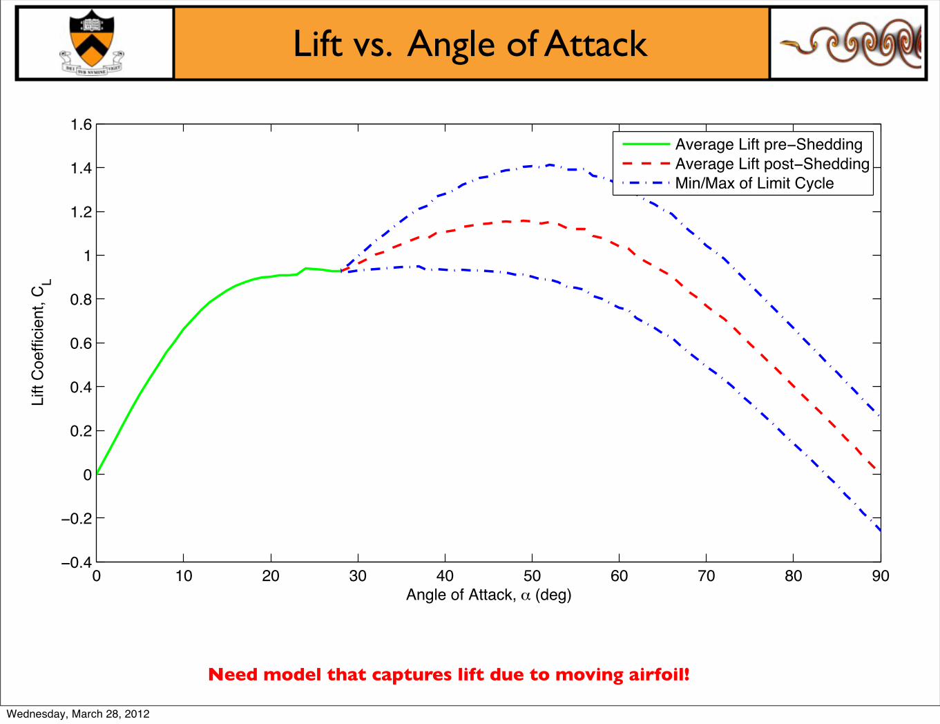
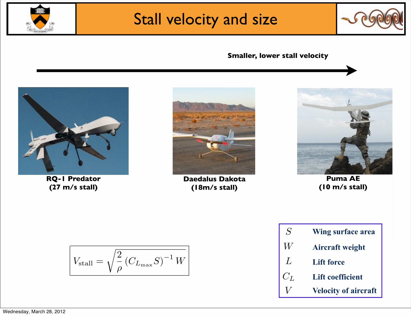
Lift vs. Angle of Attack

0 10 20 30 40 50 60 70 80 900.4

0.2

0

0.2

0.4

0.6

0.8

1

1.2

1.4

1.6

Angle of Attack, (deg)

Lift

Coe

ffici

ent,

C L

Average Lift pre SheddingAverage Lift post SheddingMin/Max of Limit Cycle

Need model that captures lift due to moving airfoil!



0 10 20 30 40 50 60 70 80 900.4

0.2

0

0.2

0.4

0.6

0.8

1

1.2

1.4

1.6


Lift

Coe

ffici

ent,

C L

Average Lift pre SheddingAverage Lift post SheddingMin/Max of Limit CycleSinusoidal (f=.1,A=3)




0 10 20 30 40 50 60 70 80 900.4

0.2

0

0.2

0.4

0.6

0.8

1

1.2

1.4

1.6


Lift

Coe

ffici

ent,

C L

Average Lift pre SheddingAverage Lift post SheddingMin/Max of Limit CycleSinusoidal (f=.1,A=3)Canonical (a=11,A=10)



Lift

Drag

Re = 300

2D Model Problem

α = 32◦

Added-Mass

Periodic Vortex SheddingTransient


Lift

Drag

Re = 300

2D Model Problem

α = 32◦

Added-Mass

Periodic Vortex SheddingTransient


Reduced Order Indicial Response

+ CL

G(s)

!"#$%&$'(#)*+,+#))()+-#$$

.#$'+)*/#-%0$

CL!̈

CL!̇

s

CL!

s2

!̈

Brunton and Rowley, in preparation.

Model Summary

ODE model ideal for control design

Based on experiment, simulation or theory

Linearized about α = 0

Recovers stability derivatives associated with quasi-steady and added-mass

CLα , CLα̇ , CLα̈

quasi-steady and added-mass

Reduced-order model

input

fast dynamics

d

dt

xαα̇

=

Ar 0 00 0 10 0 0

xαα̇

+

Br

01

α̈

CL =�Cr CLα CLα̇

�

xαα̇

+ CLα̈ α̈

CL(t) = CSL(t)α(0) +

� t

0CS

L(t− τ)α̇(τ)dτ



0 10 20 30 40 50 60 70 80 900.4

0.2

0

0.2

0.4

0.6

0.8

1

1.2

1.4

1.6


Lift

Coe

ffici

ent,

C L


Models linearized at α = 0◦+ CL

G(s)

!"#$%&$'(#)*+,+#))()+-#$$

.#$'+)*/#-%0$

CL!̈

CL!̇

s

CL!

s2

!̈


10 2 10 1 100 101 102

40

20

0

20

40

60

Mag

nitu

de (d

B)

10 2 10 1 100 101 102200

150

100

50

0

Frequency (rad U/c)

Phas

e (d

eg)

Indicial ResponseROM, r=3Wagner/TheodorsenDNSROM, r=3 (MIMO)

Bode Plot - Pitch (QC)

Frequency response

Reduced order model with ERA r=3 accurately reproduces Indicial Response

Indicial Response and ROM agree better with DNS than Theodorsen’s model.

output is lift coefficient CL

input is ( is angle of attack)α̈ α

Brunton and Rowley, in preparation.

Pitching at quarter chord

Asymptotes are correct for Indicial Response because it is based on experiment

Model for pitch/plunge dynamics [ERA, r=3 (MIMO)] works as well, for the same order model

Quarter-Chord Pitching



0 10 20 30 40 50 60 70 80 900.4

0.2

0

0.2

0.4

0.6

0.8

1

1.2

1.4

1.6


Lift

Coe

ffici

ent,

C L


Models linearized at α = 0◦+ CL

G(s)

!"#$%&$'(#)*+,+#))()+-#$$

.#$'+)*/#-%0$

CL!̈

CL!̇

s

CL!

s2

!̈


10−2 10−1 100 101 102−40

−20

0

20

40

60Frequency Response Linearized at various !

Mag

nitu

de (d

B)

ERA, !=0DNS, !=0ERA, !=10DNS, !=10ERA, !=20DNS, !=20

10−2 10−1 100 101 102−200

−150

−100

−50

0

Frequency

Phas

e

Bode Plot of Model (-) vs Data (x)

Direct numerical simulation confirms that local linearized models are accurate for small amplitude sinusoidal maneuvers

Brunton and Rowley, AIAA ASM 2011Wednesday, March 28, 2012

PLANTuk u(t) yky(t)

u

u̇

�u

Time

A

T

0

0

(Indicial) Step Response

Previously, models are based on aerodynamic step response

Idea: Have pilot fly aircraft around for 5-10 minutes, back out the Markov parameters, and construct ERA model.


CL(t)

!̈

!̇

!

Random Input Maneuver

Idea: Have pilot fly aircraft around for 5-10 minutes, back out the Markov parameters, and construct ERA model.


Wind Tunnel Setup

NACA 0006 Airfoil (24.6 cm chord)

Push rods and sting

Test section

Servo tubes


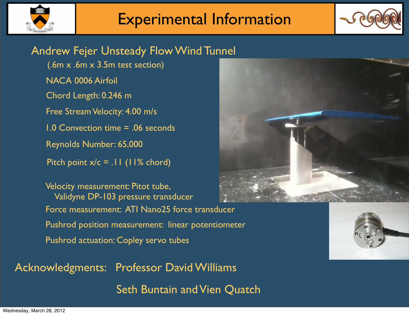
Experimental Information

Free Stream Velocity: 4.00 m/s

Chord Length: 0.246 m

Reynolds Number: 65,000

1.0 Convection time = .06 seconds

Force measurement: ATI Nano25 force transducer

Velocity measurement: Pitot tube, Validyne DP-103 pressure transducer

NACA 0006 Airfoil

Pitch point x/c = .11 (11% chord)

Pushrod position measurement: linear potentiometer

Pushrod actuation: Copley servo tubes

Andrew Fejer Unsteady Flow Wind Tunnel(.6m x .6m x 3.5m test section)

Acknowledgments: Professor David Williams

Seth Buntain and Vien Quatch


0 500 1000 1500 2000 2500 3000 3500 40002

1.5

1

0.5

0

0.5

1

1.5

Convective Time

Phase Averaged Data

940 950 960 970 980 990

1

0.5

0

0.5

1

0 10 20 30 40 50 60 70 80

!0.4

!0.2

0

0.2

0.4

0.6

0.8

1

1.2

Convective Time

Norm

al F

orc

e (

N)

Step!Up, Step!Down, 5 degrees

Phase averaged over 200 cycles


0 10 20 30 40 50 60 70 80 90!10

!8

!6

!4

!2

0

2

4

6

8

10

Convective Times (s=tU/c)

Angle

(degre

es)

Commanded Angle

Measured Angle

Wing Maneuver


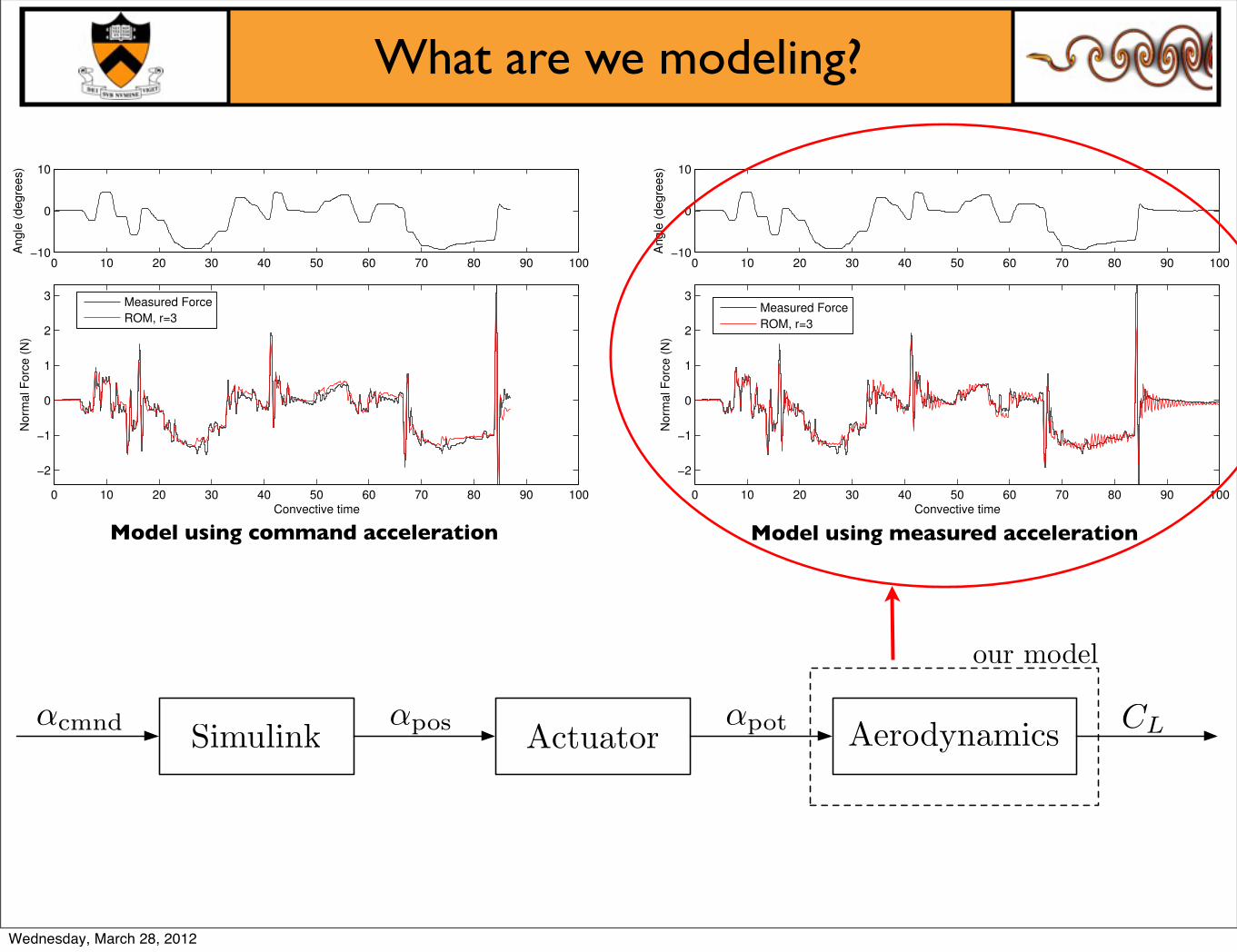
What are we modeling?

0 10 20 30 40 50 60 70 80 90 100!10

0

10

Ang

le (

degre

es)

0 10 20 30 40 50 60 70 80 90 100

!2

!1

0

1

2

3

Convective time

Norm

al F

orc

e (

N)

Measured Force

ROM, r=3

Model using command acceleration

0 10 20 30 40 50 60 70 80 90 100!10

0

10

Ang

le (

degre

es)

0 10 20 30 40 50 60 70 80 90 100

!2

!1

0

1

2

3

Convective time

Norm

al F

orc

e (

N)

Measured Force

ROM, r=3

Model using measured acceleration


What are we modeling?

0 10 20 30 40 50 60 70 80 90 100!10

0

10

Ang

le (

degre

es)

0 10 20 30 40 50 60 70 80 90 100

!2

!1

0

1

2

3

Convective time

Norm

al F

orc

e (

N)

Measured Force

ROM, r=3

Model using command acceleration

0 10 20 30 40 50 60 70 80 90 100!10

0

10

Ang

le (

degre

es)

0 10 20 30 40 50 60 70 80 90 100

!2

!1

0

1

2

3

Convective time

Norm

al F

orc

e (

N)

Measured Force

ROM, r=3


!cmnd !pot CLAerodynamicsActuator

our model

Simulink!pos


0 10 20 30 40 50 60 70 80 90 100!10

0

10

Ang

le (

degre

es)

0 10 20 30 40 50 60 70 80 90 100

!2

!1

0

1

2

3

Convective time

Norm

al F

orc

e (

N)

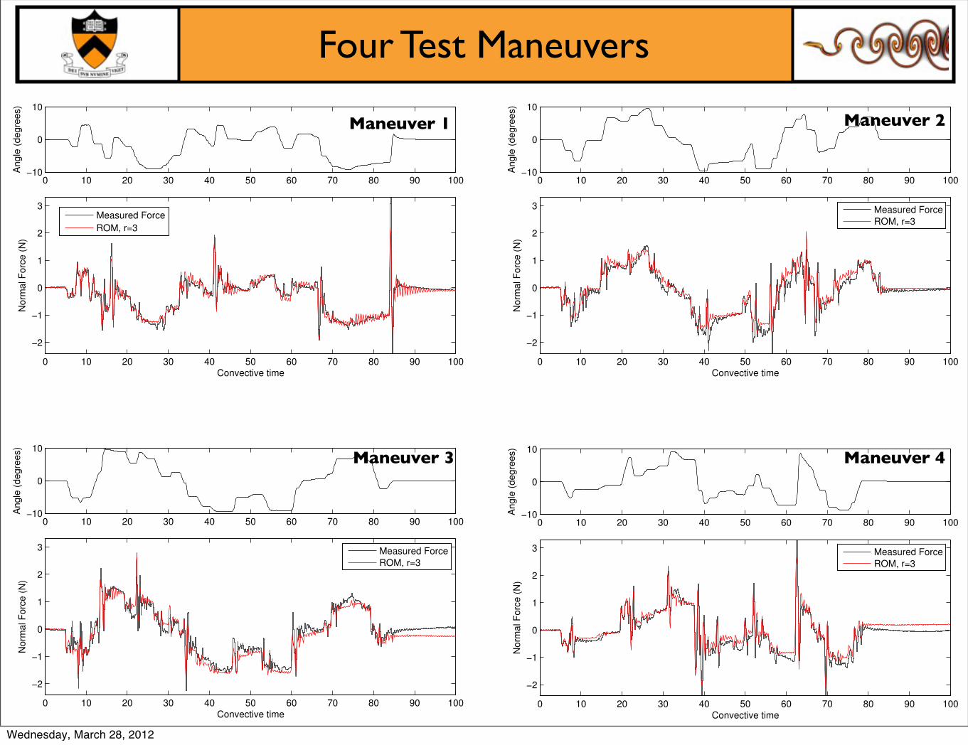
Measured ForceROM, r=3

Four Test Maneuvers

0 10 20 30 40 50 60 70 80 90 100!10

0

10

Angle

(degre

es)

0 10 20 30 40 50 60 70 80 90 100

!2

!1

0

1

2

3

Convective time

Norm

al F

orc

e (

N)


0 10 20 30 40 50 60 70 80 90 100!10

0

10

Ang

le (

degre

es)

0 10 20 30 40 50 60 70 80 90 100

!2

!1

0

1

2

3

Convective time

Norm

al F

orc

e (

N)

Measured Force

ROM, r=3

0 10 20 30 40 50 60 70 80 90 100!10

0

10

Angle

(degre

es)

0 10 20 30 40 50 60 70 80 90 100

!2

!1

0

1

2

3

Convective time

Norm

al F

orc

e (

N)


Maneuver 1 Maneuver 2

Maneuver 3 Maneuver 4


10!2

10!1

100

101

102

103

!60

!40

!20

0

20

40

60M

agnitu

de (

dB

)

10!2

10!1

100

101

102

103

!150

!100

!50

0

Frequency (rad/s ! c/U)

Phase

(degre

es)

maneuver 1

maneuver 2

maneuver 3

maneuver 4

Bode Plots for AoA=0


Idea: lets combine all maneuvers into one large system ID maneuver!


−40−20

020406080

Mag

nitu

de (d

B)

10−2 10−1 100 101 102−180−135−90−45

045

Phas

e (d

eg)

Bode Diagram

Frequency (rad/sec)

0 50 100 150 200 250 300 350 400 450−10

0

10An

gle

(deg

rees

)

0 50 100 150 200 250 300 350 400 450

−2

−1

0

1

2

3

Convective time

Nor

mal

For

ce (N

)


Bode Plot for AoA=0

Resonant peak

Added-mass “bump”


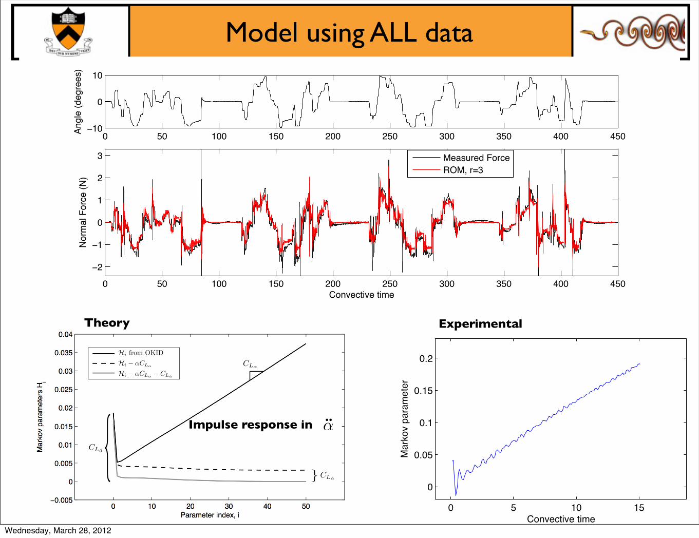
CL!

CL!̇

CL!̈{{

Hi from OKIDHi ! !CL!

Hi ! !CL! ! CL!̇

Impulse response in α̈

0 5 10 15

0

0.05

0.1

0.15

0.2

Mar

kov

para

met

er

Convective time

Model using ALL data

0 50 100 150 200 250 300 350 400 450−10

0

10An

gle

(deg

rees

)

0 50 100 150 200 250 300 350 400 450

−2

−1

0

1

2

3

Convective time

Nor

mal

For

ce (N

)


Theory Experimental


0 10 20 30 40 50 60 70 80

!0.4

!0.2

0

0.2

0.4

0.6

0.8

1

1.2

Convective Time

Norm

al F

orc

e (

N)

Step!Up, Step!Down, 5 degrees

30Hz Mechanical Oscillation


0 10 20 30 40 50 60 70 80 90 100!10

0

10

Angle

(degre

es)

0 10 20 30 40 50 60 70 80 90 100

!2

!1

0

1

2

3

Convective time

Norm

al F

orc

e (

N)

Experiment 4

Model 1

Model 2

Model 3

Model 4

0 10 20 30 40 50 60 70 80 90 100!10

0

10

Angle

(degre

es)

0 10 20 30 40 50 60 70 80 90 100

!2

!1

0

1

2

3

Convective time

Norm

al F

orc

e (

N)

Experiment 3

Model 1

Model 2

Model 3

Model 4

0 10 20 30 40 50 60 70 80 90 100!10

0

10

Ang

le (

degre

es)

0 10 20 30 40 50 60 70 80 90 100

!2

!1

0

1

2

3

Convective time

Norm

al F

orc

e (

N)

Experiment 2

Model 1

Model 2

Model 3

Model 4

0 10 20 30 40 50 60 70 80 90 100!10

0

10

Ang

le (

degre

es)

0 10 20 30 40 50 60 70 80 90 100

!2

!1

0

1

2

3

Convective time

Norm

al F

orc

e (

N)

Experiment 1

Model 1

Model 2

Model 3

Model 4

Models agree with data


0 10 20 30 40 50 60 70 80 90

−2

0

2

Verti

cal P

ositi

on (i

nche

s)

0 10 20 30 40 50 60 70 80 90

−2

−1

0

1

2

3

Convective time

Nor

mal

For

ce (N

)


Model for Plunging

−20

0

20

40

60

Mag

nitu

de (d

B)

10−2 10−1 100 101 1020

45

90

135

180

Phas

e (d

eg)

Bode Diagram

Frequency (rad/sec)


Conclusions

Reduced order model based on indicial response at non-zero angle of attack

- Based on eigensystem realization algorithm (ERA)- Models appear to capture dynamics up to Hopf bifurcation

Observer/Kalman Filter Identification with more realistic input/output data

- Efficient computation of reduced-order models- Ideal for simulation or experimental data

Brunton and Rowley, AIAA ASM 2009-2011

OL, Altman, Eldredge, Garmann, and Lian, 2010

Leishman, 2006.

Wagner, 1925.

Theodorsen, 1935.

Confirmation with experimental data- Tested modeling procedure in Dave Williams’ wind tunnel experiment- Flexible procedure works with various geometry, Reynolds number

Juang, Phan, Horta, Longman, 1991.

Juang and Pappa, 1985.

Ma, Ahuja, Rowley, 2010.


Unsteady Aerodynamic Forces: Experiments, Simulations, …faculty.washington.edu/sbrunton/talks/JUP_2011_04_06_Princeton.pdfUnsteady Aerodynamic Forces: Experiments, Simulations, and

Documents