arXiv:1111.6779v2 [hep-ph] 31 Jul 2014 DESY-THESIS-2011-039 November 2011 Unstable Gravitino Dark Matter Prospects for Indirect and Direct Detection Dissertation zur Erlangung des Doktorgrades des Departments Physik der Universit¨ at Hamburg vorgelegt von Michael Grefe aus L¨ uneburg Hamburg 2011

Welcome message from author
This document is posted to help you gain knowledge. Please leave a comment to let me know what you think about it! Share it to your friends and learn new things together.
Transcript

arX
iv:1
111.
6779
v2 [
hep-
ph]
31
Jul 2
014
DESY-THESIS-2011-039November 2011
Unstable Gravitino Dark Matter
Prospects for Indirect and Direct Detection
Dissertation
zur Erlangung des Doktorgrades
des Departments Physik
der Universitat Hamburg
vorgelegt von
Michael Grefe
aus Luneburg
Hamburg
2011

Gutachter der Dissertation: Prof. Dr. Laura Covi
Prof. Dr. Jan Louis
Prof. Dr. Piero Ullio
Gutachter der Disputation: Prof. Dr. Laura Covi
Prof. Dr. Wilfried Buchmuller
Datum der Disputation: 6. Juli 2011
Vorsitzender des Prufungsausschusses: Prof. Dr. Gunter H. W. Sigl
Vorsitzender des Promotionsausschusses: Prof. Dr. Peter H. Hauschildt
Dekan der Fakultat fur Mathematik,Informatik und Naturwissenschaften: Prof. Dr. Heinrich Graener

Abstract
We confront the signals expected from unstable gravitino dark matter with observa-tions of indirect dark matter detection experiments in all possible cosmic-ray channels.For this purpose we calculate in detail the gravitino decay widths in theories with bilin-ear violation of R parity, particularly focusing on decay channels with three particles inthe final state. Based on these calculations we predict the fluxes of gamma rays, chargedcosmic rays and neutrinos expected from decays of gravitino dark matter. Althoughthe predicted spectra could in principal explain the anomalies observed in the cosmic-ray positron and electron fluxes as measured by PAMELA and Fermi LAT, we findthat this possibility is ruled out by strong constraints from gamma-ray and antiprotonobservations.
Therefore, we employ current data of indirect detection experiments to place strongconstraints on the gravitino lifetime and the strength of R-parity violation. In addition,we discuss the prospects of forthcoming searches for a gravitino signal in the spectrumof cosmic-ray antideuterons, finding that they are in particular sensitive to rather lowgravitino masses. Finally, we discuss in detail the prospects for detecting a neutrino sig-nal from gravitino dark matter decays, finding that the sensitivity of neutrino telescopeslike IceCube is competitive to observations in other cosmic ray channels, especially forrather heavy gravitinos.
Moreover, we discuss the prospects for a direct detection of gravitino dark mattervia R-parity violating inelastic scatterings off nucleons. We find that, although the scat-tering cross section is considerably enhanced compared to the case of elastic gravitinoscattering, the expected signal is many orders of magnitude too small in order to hopefor a detection in underground detectors.


Zusammenfassung
Wir konfrontieren die erwarteten Signale von instabiler Gravitino-Dunkler-Materiemit Beobachtungen von Experimenten zur indirekten Suche nach dunkler Materie inallen moglichen Kanalen kosmischer Strahlung. Zu diesem Zweck berechnen wir in allenEinzelheiten die Gravitinozerfallsbreiten in Theorien mit bilinearer Verletzung der R-Paritat, wobei wir uns insbesondere auf Zerfallskanale mit drei Teilchen im Endzustandkonzentrieren. Auf der Basis dieser Berechnungen sagen wir die Flusse von Gammastrah-len, geladenen kosmischen Strahlen und Neutrinos vorher, die aus Zerfallen Gravitino-Dunkler-Materie erwartet werden. Obwohl die vorhergesagten Spektren prinzipiell diebeobachteten Anomalien in den von PAMELA und Fermi LAT gemessenen Flussen vonPositronen und Elektronen in der kosmischen Strahlung erklaren konnten, beobachtenwir, dass diese Moglichkeit auf Grund starker Einschrankungen aus den Beobachtungenvon Gammastrahlen und Antiprotonen ausgeschlossen ist.
Daher verwenden wir aktuelle Daten von Experimenten zur indirekten Suche nachdunkler Materie um starke Schranken an die Gravitinolebensdauer und die Starke der R-Paritats-Verletzung zu setzen. Des Weiteren diskutieren wir die Erfolgsaussichten kom-mender Suchen nach einem Gravitinosignal im Spektrum von Antideuteronen in derkosmischen Strahlung, wobei wir beobachten, dass sie insbesondere fur niedrige Gravi-tinomassen empfindlich sind. Schließlich erortern wir ausfuhrlich die Erfolgsaussichtenein Neutrinosignal aus Zerfallen Gravitino-Dunkler-Materie zu messen, wobei wir fest-stellen, dass die Sensitivitat von Neutrinoteleskopen wie IceCube insbesondere fur denFall schwerer Gravitinos zu Beobachtungen in anderen Kanalen kosmischer Strahlungkonkurrenzfahig ist.
Daruber hinaus besprechen wir die Erfolgsaussichten fur eine direkte EntdeckungGravitino-Dunkler-Materie uber R-Paritats-verletzende inelastische Streuungen an Nu-kleonen. Wir stellen fest, dass, obwohl der Streuwirkungsquerschnitt gegenuber demFall elastischer Gravitino-Streuungen deutlich erhoht ist, das erwartete Signal um vieleGroßenordnungen zu klein ist als dass man eine Entdeckung in unterirdischen Detekto-ren erhoffen konnte.


Fur Melanie

Contents
Contents i
List of Figures iii
List of Tables vi
1 Introduction 1
2 Cosmology and Dark Matter 6
2.1 Big Bang Cosmology . . . . . . . . . . . . . . . . . . . . . . . . . . . . . 62.2 Evidence for the Existence of Dark Matter . . . . . . . . . . . . . . . . . 152.3 Constraints on Dark Matter Properties . . . . . . . . . . . . . . . . . . . 19
3 Supersymmetry and Supergravity 21
3.1 Supergravity . . . . . . . . . . . . . . . . . . . . . . . . . . . . . . . . . . 223.2 The Minimal Supersymmetric Standard Model . . . . . . . . . . . . . . . 273.3 Bilinear Breaking of R Parity . . . . . . . . . . . . . . . . . . . . . . . . 34
4 Gravitino Decays 42
4.1 The Massive Gravitino and its Interactions . . . . . . . . . . . . . . . . . 424.2 Gravitino Cosmology . . . . . . . . . . . . . . . . . . . . . . . . . . . . . 454.3 Gravitino Decay Channels . . . . . . . . . . . . . . . . . . . . . . . . . . 48
4.3.1 Two-Body Decays . . . . . . . . . . . . . . . . . . . . . . . . . . . 484.3.2 Three-Body Decays . . . . . . . . . . . . . . . . . . . . . . . . . . 524.3.3 Gravitino Branching Ratios . . . . . . . . . . . . . . . . . . . . . 59
4.4 Spectra of Final State Particles from Gravitino Decays . . . . . . . . . . 63
5 Indirect Detection of Gravitino Dark Matter 76
5.1 Indirect Searches for Dark Matter . . . . . . . . . . . . . . . . . . . . . . 765.2 Probing Gravitino Dark Matter with Gamma Rays . . . . . . . . . . . . 825.3 Probing Gravitino Dark Matter with Cosmic-Ray Antimatter . . . . . . . 87
5.3.1 Positrons and Electrons . . . . . . . . . . . . . . . . . . . . . . . 895.3.2 Antiprotons . . . . . . . . . . . . . . . . . . . . . . . . . . . . . . 955.3.3 Antideuterons . . . . . . . . . . . . . . . . . . . . . . . . . . . . . 100
i

Contents
5.3.4 Bounds on the Gravitino Lifetime from Charged Cosmic Rays . . 1035.4 Probing Gravitino Dark Matter with Neutrinos . . . . . . . . . . . . . . 104
5.4.1 Neutrino Fluxes . . . . . . . . . . . . . . . . . . . . . . . . . . . . 1055.4.2 Neutrino and Muon Spectra . . . . . . . . . . . . . . . . . . . . . 1095.4.3 Rates and Bounds . . . . . . . . . . . . . . . . . . . . . . . . . . 117
5.5 Constraints on the Gravitino Dark Matter Parameter Space . . . . . . . 124
6 Direct Detection of Gravitino Dark Matter 128
6.1 Direct Searches for Dark Matter . . . . . . . . . . . . . . . . . . . . . . . 1286.2 Gravitino Dark Matter with Bilinear R-Parity Violation . . . . . . . . . 131
7 Conclusions and Outlook 137
Acknowledgments 141
A Units and Physical Constants 142
B Notation, Conventions and Formulae 144
C Feynman Rules 149
D Kinematics of Scattering and Decay Processes 153
E Calculation of Gravitino Decay Widths 158
E.1 Two-Body Decays . . . . . . . . . . . . . . . . . . . . . . . . . . . . . . . 158E.2 Three-Body Decays . . . . . . . . . . . . . . . . . . . . . . . . . . . . . . 160
E.2.1 ψ3/2 → γ∗/Z∗ ν → f f ν . . . . . . . . . . . . . . . . . . . . . . . 160E.2.2 ψ3/2 → W+∗
ℓ− → f f ′ ℓ− . . . . . . . . . . . . . . . . . . . . . . . 166E.2.3 ψ3/2 → h∗ ν → f f ν . . . . . . . . . . . . . . . . . . . . . . . . . . 170
F Calculation of Gravitino–Nucleon Cross Sections 173
F.1 Inelastic Gravitino–Nucleon Scattering via Higgs Exchange . . . . . . . . 173F.2 Inelastic Gravitino–Nucleon Scattering via Z Exchange . . . . . . . . . . 175F.3 Inelastic Gravitino–Nucleon Scattering via Photon Exchange . . . . . . . 179
Bibliography 181
ii

List of Figures
2.1 Timeline of the thermal early universe. . . . . . . . . . . . . . . . . . . . 10
2.2 BBN predictions of the light element abundances and ΩΛ − Ωm plane ofthe concordance model of cosmology. . . . . . . . . . . . . . . . . . . . . 14
2.3 WMAP 7-year temperature anisotropy map and angular power spectrum. 15
2.4 Rotation curve of the Milky Way and the Bullet cluster. . . . . . . . . . 17
2.5 Energy content of the universe at the time of the CMB emission and today. 19
3.1 Renormalization group evolution of the inverse gauge couplings in thestandard model and in the minimal supersymmetric standard model. . . 22
3.2 Schematic particle content of the minimal supersymmetric standard model. 28
4.1 Branching ratios of the gravitino decay channels in the decoupling limit. 61
4.2 Branching ratios of the gravitino decay channels in the decoupling limitfor the case of a suppressed photon channel. . . . . . . . . . . . . . . . . 63
4.3 Spectra of stable final state particles from gravitino decay in the channelψ3/2 → Zνi. . . . . . . . . . . . . . . . . . . . . . . . . . . . . . . . . . . 67
4.4 Spectra of stable final state particles from gravitino decay in the channelψ3/2 →We. . . . . . . . . . . . . . . . . . . . . . . . . . . . . . . . . . . 68
4.5 Spectra of stable final state particles from gravitino decay in the channelψ3/2 →Wµ. . . . . . . . . . . . . . . . . . . . . . . . . . . . . . . . . . . 69
4.6 Spectra of stable final state particles from gravitino decay in the channelψ3/2 →Wτ . . . . . . . . . . . . . . . . . . . . . . . . . . . . . . . . . . . 70
4.7 Spectra of stable final state particles from gravitino decay in the channelψ3/2 → hνi. . . . . . . . . . . . . . . . . . . . . . . . . . . . . . . . . . . 70
4.8 Fermion spectra from gravitino decay in the channel ψ3/2 → W ∗ℓi → f f ′ ℓi. 72
4.9 Fermion spectra from gravitino decay in the channel ψ3/2 → Z∗νi → f f νi. 73
4.10 Fermion spectra from gravitino decay in the channel ψ3/2 → γ∗/Z∗νi →f f νi. . . . . . . . . . . . . . . . . . . . . . . . . . . . . . . . . . . . . . 74
5.1 Density profiles for different dark matter halo models and angular de-pendence of the line-of-sight integral for dark matter annihilations anddecays. . . . . . . . . . . . . . . . . . . . . . . . . . . . . . . . . . . . . . 79
iii
List of Figures
5.2 Diffuse gamma-ray flux from gravitino dark matter decays compared tothe measured extragalactic gamma-ray background. . . . . . . . . . . . . 84
5.3 Bounds on the gravitino lifetime from gamma-ray observations. . . . . . 86
5.4 Contribution to the cosmic-ray positron fraction from gravitino decayscompared to measurements and the expectation from astrophysical pri-mary and secondary production. . . . . . . . . . . . . . . . . . . . . . . . 92
5.5 Cosmic-ray electron flux from gravitino decays compared to measure-ments and the expectation from astrophysical primary and secondaryproduction. . . . . . . . . . . . . . . . . . . . . . . . . . . . . . . . . . . 94
5.6 Cosmic-ray positron flux from gravitino decays compared to measure-ments and the expectation from astrophysical secondary production. . . . 96
5.7 Cosmic-ray antiproton-to-proton flux ratio from gravitino decays com-pared to measurements and the expected astrophysical background. . . . 98
5.8 Cosmic-ray antiproton flux from gravitino decays compared to measure-ments and the expectation from astrophysical secondary production. . . . 100
5.9 Cosmic-ray antideuteron flux from gravitino decays compared to the ex-pectation from astrophysical secondary production and the sensitivitiesof forthcoming experiments. . . . . . . . . . . . . . . . . . . . . . . . . . 102
5.10 Bounds on the gravitino lifetime from observations of charged cosmic raysand sensitivity of forthcoming antideuteron experiments. . . . . . . . . . 104
5.11 Dependence of the statistical significance of a neutrino signal from darkmatter decays or annihilations on the size of the observed cone around thegalactic center and dependence of the statistical significance of a neutrinosignal from dark matter on the observed cone size around the zenithdirection. . . . . . . . . . . . . . . . . . . . . . . . . . . . . . . . . . . . 108
5.12 Expected neutrino spectrum from the decay of gravitino dark mattercompared to the expected background of atmospheric neutrinos and datafrom neutrino experiments. . . . . . . . . . . . . . . . . . . . . . . . . . . 109
5.13 Event topology of muon neutrino-induced upward through-going muonsand the expected flux of upward through-going muons from gravitino darkmatter decays compared to the atmospheric background. . . . . . . . . . 113
5.14 Event topology of muon neutrino-induced contained muons and the ex-pected spectrum of contained muons from gravitino dark matter decayscompared to the atmospheric background. . . . . . . . . . . . . . . . . . 115
5.15 Event topology of neutrino-induced cascades and the expected spectrumof cascades from gravitino dark matter decays compared to the atmo-spheric background. . . . . . . . . . . . . . . . . . . . . . . . . . . . . . . 117
5.16 Present bounds on the gravitino lifetime from Super-Kamiokande andIceCube-22. . . . . . . . . . . . . . . . . . . . . . . . . . . . . . . . . . . 119
5.17 Neutrino effective areas and prospects for bounds on the gravitino darkmatter lifetime from the IceCube experiment. . . . . . . . . . . . . . . . 122
iv
List of Figures
5.18 Flux of upward through-going muons expected from decaying gravitinodark matter compared to the atmospheric background and the statisticalsignificance of the expected signal. . . . . . . . . . . . . . . . . . . . . . . 123
5.19 Rate of contained muons expected from decaying gravitino dark mattercompared to the atmospheric background and the statistical significanceof the expected signal. . . . . . . . . . . . . . . . . . . . . . . . . . . . . 124
5.20 Rate of cascade events expected from decaying gravitino dark mattercompared to the atmospheric background and the statistical significanceof the expected signal. . . . . . . . . . . . . . . . . . . . . . . . . . . . . 125
5.21 Summarized bounds from indirect dark matter searches on the gravitinodark matter parameter space. . . . . . . . . . . . . . . . . . . . . . . . . 126
v

List of Tables
3.1 The gravity supermultiplet of locally supersymmetric theories. . . . . . . 233.2 The gauge supermultiplets of the minimal supersymmetric standard model. 283.3 The chiral supermultiplets of the minimal supersymmetric standard model. 29
4.1 Branching ratios of the gravitino decay channels in the decoupling limit. 624.2 Multiplicities of stable final state particles from gravitino decay. . . . . . 66
5.1 Cosmic-ray propagation parameters for positrons. . . . . . . . . . . . . . 905.2 Values of the Fisk potential to account for the effect of solar modulation
in the electron and positron data sets. . . . . . . . . . . . . . . . . . . . 935.3 Cosmic-ray propagation parameters for antiprotons. . . . . . . . . . . . . 975.4 Values of the Fisk potential to account for the effect of solar modulation
in the antiproton data sets. . . . . . . . . . . . . . . . . . . . . . . . . . 995.5 Cosmic-ray propagation parameters for antideuterons. . . . . . . . . . . . 1015.6 Neutrino mixing parameters. . . . . . . . . . . . . . . . . . . . . . . . . . 1055.7 Density, proton-number-to-mass-number ratio and approximate muon en-
ergy loss parameters for materials of interest in Cherenkov neutrino de-tectors. . . . . . . . . . . . . . . . . . . . . . . . . . . . . . . . . . . . . . 111
5.8 Rates of upward through-going muon events from the atmospheric neu-trino background and gravitino dark matter decays at contemporary neu-trino experiments. . . . . . . . . . . . . . . . . . . . . . . . . . . . . . . . 121
5.9 Gravitino lifetimes for various gravitino masses corresponding to a fivesigma statistical significance in the most significant energy bin after oneyear of observation in an idealized neutrino detector. . . . . . . . . . . . 125
vi
Chapter 1
Introduction
Almost eighty years after the first evidence for dark matter in the universe1 its existenceis firmly established on the basis of astrophysical and cosmological observations [3–5].However, the question of the nature of dark matter is still one of the biggest unresolvedproblems in modern cosmology. While it has been proposed that the observed gravita-tional effects might be explained by a modification of the theory of gravity [6] or thatthe dark matter could be composed of non-luminous astrophysical objects in the halo ofgalaxies [7, 8], both explanations are strongly disfavored by current experimental data.
The best candidates for the dark matter are new elementary particles that obey allobservational constraints.2 However, no direct evidence for dark matter particles hasbeen found so far on microscopic scales and thus little is known about their propertieslike their mass or their interaction strength. It is even unclear if dark matter particlesare stable or simply very long-lived. Well-motivated particle dark matter candidates canarise from extensions of the standard model of particle physics, the most thoroughlystudied candidates being weakly interacting massive particles. These are particles withweak-scale interactions that are stabilized by a symmetry in the particle physics model.The prototype dark matter candidate of this class is the lightest neutralino in super-symmetric theories that is stabilized in models with conserved R parity [10]. Anotherprominent candidate of this type is the lightest Kaluza–Klein particle in theories withuniversal extra dimensions that is stabilized by the KK parity [11].
An immense experimental effort is undertaken to search for signatures of particledark matter candidates: Depending on the details of the particle physics model distinctsignatures are expected in high-energetic proton-proton collisions at the Large HadronCollider at CERN. In addition, weakly interacting massive particles of the dark halo ofthe Milky Way are expected to elastically scatter off nuclei while traversing the Earth,leading to nuclear recoils that might be observable in low-background underground
1Although Fritz Zwicky is generally accepted to be the first who discovered dark matter (in a studyof radial velocities of galaxies in the Coma cluster in 1933 [1]) the term ’dark matter’ was first used asearly as 1922 by James Jeans to describe the missing mass found in a study of vertical motions of starsclose to the galactic plane [2].
2For recent reviews of the particle explanation for dark matter see for instance [4, 9].
1

Chapter 1. Introduction
detectors. Another strategy is to search for exotic contributions from the annihilationor the decay of dark matter particles in the galactic halo to the spectra of cosmic rays.
Only a combination of evidence for particle dark matter from signals at colliders andfrom astrophysical searches in direct and indirect detection experiments will allow toconnect the cosmological observation of dark matter with a particle physics explanation,finally leading to an unambiguous identification of the particle nature of the dark matterin the universe. A large portion of the neutralino parameter space is already excludedby direct detection experiments and collider searches and it is expected that within thenext decade either neutralino dark matter will be detected or completely excluded.
This is a strong motivation to study more elusive dark matter candidates. In thisthesis we will thus concentrate on the well-motivated case of the gravitino. It arises nat-urally in locally supersymmetric extensions of the standard model as the gauge fermionof supergravity [12, 13]. Depending on the mechanism of supersymmetry breaking, thegravitino can be the lightest supersymmetric particle and thus represent the dark mat-ter of the universe [14]. Due to its extremely weak interactions that are suppressed bythe Planck scale it appears to be one of the most elusive dark matter candidates withrespect to the prospects for its experimental detection.
The existence of the gravitino in the particle spectrum leads to several cosmolog-ical problems, the most severe being that late gravitino decays are in conflict withthe successful predictions of primordial nucleosynthesis for the abundances of light el-ements [15]. Since gravitinos are produced in thermal scatterings after the end of theinflationary phase in the early universe [16], compatibility with big bang nucleosynthesisputs strong upper limits on the reheating temperature of the universe [17]. However, theobservation of small, nonvanishing neutrino masses strongly supports the mechanism ofthermal leptogenesis as the origin of the baryon asymmetry in the universe [18], thusrequiring a high value for the reheating temperature [19]. For this reason, there is anapparent conflict between supersymmetry, predicting the existence of the gravitino, andthe successful predictions of big bang nucleosynthesis, which also require a mechanismfor baryogenesis.
It has been proposed that this problem could be solved if the gravitino is the lightestsupersymmetric particle and thus a stable dark matter candidate [20]. However, strongconstraints arise also from possible late decays of the next-to-lightest supersymmetricparticle which in general still lead to conflicts with big bang nucleosynthesis [21]. Bycontrast, theories with a slight violation of R parity naturally lead to a cosmologicalscenario that is consistent with thermal leptogenesis and all bounds from big bangnucleosynthesis [22]. In this case the next-to-lightest supersymmetric particle decaysmainly via R-parity breaking interactions into standard model particles well before thetime of nucleosynthesis. The decays of the gravitino are then suppressed by the Planckscale and additionally by the small amount of R-parity breaking, predicting a gravitinolifetime that exceeds the age of the universe by many orders of magnitude [23]. Therefore,the gravitino remains a perfectly viable candidate for the dark matter in the universe.
An intriguing feature of this scenario is that the gravitino is not that elusive anymore
2

but in contrast exhibits a rich phenomenology. Since the gravitino is unstable it might beobserved via its decays in the late universe [23]. Due to the large density of dark matterparticles in the universe, which is five times higher than that of ordinary matter, thedecay signal might be strong enough to be observed in the isotropic diffuse flux of gammarays [22–28], in the fluxes of cosmic-ray antimatter [26–29] or in the flux of neutrinos [28,30], irrespective of the extremely long lifetime of the gravitino. In addition, this modelpredicts spectacular observational consequences for collider experiments: Since the decaywidth of the next-to-lightest supersymmetric particle is suppressed by R-parity violatinginteractions, it might be observable as a long-lived particle leading to displaced verticesor, in the specific case of a charged next-to-lightest supersymmetric particle, to a chargedparticle track leaving the detector [31–34].
In particular the field of indirect dark matter searches via cosmic-ray signals hasbeen very active in the past years. Deviations from the expected cosmic-ray spectra fromastrophysical processes have been reported already several years ago for the extragalacticdiffuse gamma-ray signal as derived from EGRET data [35] and for the cosmic-raypositron fraction as measured by the HEAT instrument [36]. These observations led toseveral studies interpreting the anomalous spectra as a hint for dark matter annihilationsor decays [24–26, 29, 37–40].
However, in particular the observation of a steep rise in the positron fraction at ener-gies above 10GeV by PAMELA [41], confirming the result from HEAT, and the precisemeasurement of the absolute cosmic-ray electron plus positron flux by Fermi LAT [42]stimulated a lot of activity in the field. A multitude of studies for annihilating [43–49] anddecaying [27, 47, 50–58] dark matter candidates was published, in many cases trying tosimultaneously explain all deviations from astrophysical background expectations. Oneshould keep in mind, though, that also astrophysical sources like supernova remnants orpulsars could explain the observations [60–65].
On the other hand, recent data from Fermi LAT do not confirm an excess in theextragalactic diffuse gamma-ray spectrum as claimed based on EGRET data [66]. In ad-dition, searches for photon lines in the Fermi LAT data have been negative so far, thusproviding strong limits on dark matter annihilations or decays predicting monoenergeticphotons in the final state [67]. Another interesting channel for the indirect detection ofdark matter are neutrinos as they provide directional information and possibly an inde-pendent confirmation of an exotic contribution to cosmic rays. Several studies of neutrinosignals from annihilating and decaying dark matter candidates have been presented inthe literature [30, 68–74].
In the present work we will therefore employ a multi-messenger approach of indirectsearches and confront the expected signals from unstable gravitino dark matter withindirect detection data in all possible cosmic ray channels. The intention of this strategyis to place strong constraints on the lifetime of the gravitino and also on the amount ofbilinear R-parity breaking. For this purpose we will revisit and extend the calculation ofgravitino decay channels in scenarios with bilinear R-parity violation. As a first step wewill re-evaluate the mixing of leptons with gauginos and higgsinos induced by R-parity
3
Chapter 1. Introduction
violating operators and find new analytical approximate formulae for the mixing param-eters governing the decay of gravitino dark matter particles. Equipped with these resultswe will present a detailed calculation of gravitino decay widths, upgrading previouslyobtained two-body decay results by the addition of a set of Feynman diagrams that wereneglected in earlier calculations. One of the main results of this work is the extensionof the gravitino decay width calculation to include three-body gravitino decay channelsfor gravitino masses below the threshold for the on-shell production of massive gaugebosons. These contributions are important for the phenomenology of low mass gravitinosas first pointed out in [75]. Using the spectra of stable final state particles produced ingravitino decays we will then predict the spectra of gamma rays, positrons, electrons,antiprotons and neutrinos, and compare them to current observations of cosmic rays.
Beyond that, we will study in detail future prospects for the detection of a neutrinosignal from gravitino decays. Neutrinos are not directly observed in neutrino telescopesbut only via their weak interactions with the material inside or close to the detector. Wewill discuss the different event topologies that can arise and predict the correspondingsignal spectra at detector level. Taking into account the energy resolution of differentdetection channels we will argue which of the channels provides the best sensitivity tosignals from gravitino decays.
In addition, we want to discuss for the first time the antideuteron signal expectedfrom gravitino decays. In [76] it was first noted that antideuterons are a convenientcosmic-ray channel for the detection of dark matter signals as the expected astrophysi-cal background can be very low compared to the signal expectation, in particular at thelow-energetic end of the spectrum. In the derivation of the antideuteron spectrum fromgravitino decays we will employ a Monte Carlo treatment as it was found that the con-ventional spherical approximation of the coalescence model for antideuteron formationleads to erroneous results [77]. As no antideuterons have been observed in cosmic raysso far we will present future prospects for the sensitivity of the antideuteron channelbased on the projected sensitivity regions of forthcoming antideuteron experiments.
Moreover, we will shortly discuss the prospects for a direct detection of gravitino darkmatter. In contrast to the case of weakly interacting massive particles, no observablesignal is expected from elastic gravitino–nucleon scatterings due to the Planck-scalesuppression of gravitino couplings to matter. This situation could change in the caseof broken R parity. In this case the gravitino is expected to scatter inelastically offnucleons with a cross section that is considerably enhanced compared to that of elasticscatterings as it is suppressed by a lower order of the Planck scale. In order to study thiseffect quantitatively, we will calculate the gravitino–nucleon cross sections via Higgs andZ boson exchange. In addition, we observe the intriguing feature that the gravitino canscatter off nucleons via photon exchange, a channel that in general is not available forweakly interacting massive particles. We expect that the scattering via photon exchangeleads to a strong enhancement of the cross section due to the massless photon propagator.
Let us summarize the structure of this thesis: In the next chapter we will shortlyreview the basics of big bang cosmology as well as evidence and constraints for dark
4

matter from cosmological observations. In Chapter 3 we will introduce supersymmetryand supergravity and discuss the effects of bilinear R-parity violation. The gravitinowill be discussed in Chapter 4: After a short review of the field-theoretical descriptionof the gravitino, we will summarize its cosmological implications. In the main partof the chapter we will study in detail the decay channels of the unstable gravitino,discuss the branching ratios of the different decay channels and determine the spectra ofstable final state particles produced in gravitino decays. Chapter 5 contains an extensivediscussion of indirect searches for gravitino dark matter, covering the expected signalsof gamma rays, positrons, antiprotons, antideuterons and neutrinos. In Chapter 6 wediscuss the cross sections for inelastic gravitino–nucleon scattering and the prospects ofdetecting gravitino dark matter in direct detection experiments. Finally, we will presentour conclusions and an outlook for future directions of investigating gravitino darkmatter.
The appendices contain supporting material on the calculations in this work: Ap-pendix A summarizes the physical constants used in calculations throughout the presentthesis. Appendix B fixes our notation and contains useful formulae for the calculation ofmatrix elements. In Appendices C and D we present, respectively, the Feynman rules andthe kinematics needed for the calculation of gravitino decays and scattering processes.Appendix E contains the complete calculation of the gravitino decay widths that are dis-cussed in Chapter 5, while Appendix F contains the calculation of the gravitino–nucleonscattering cross sections that are discussed in Chapter 6.
The results for the detection of neutrinos from gravitino dark matter decays presentedin Section 5.4 are based on our study of neutrino signals for generic decay channels ofscalar and fermionic dark matter particles that is published in [78]. Instead of directlypresenting the results of this publication we decided to redo the analysis for the specificcase of unstable gravitino dark matter exactly along the lines of the published work,only updating the analysis to the most recent status of neutrino telescopes and theirobservations.
The discussion of gravitino three-body decays in Section 4.3 and the discussion ofsignals for the indirect detection of gravitino dark matter in Chapter 5, in particularthe prospects for antideuteron searches, are part of an ongoing project in collaborationwith Laura Covi and Gilles Vertongen [79].
Similarly, the discussion of the prospects for a direct detection of gravitino darkmatter in scenarios with bilinear R-parity violation in Chapter 6 is part of an ongoingproject in collaboration with Laura Covi [80].
5
Chapter 2
Cosmology and Dark Matter
In this introductory chapter we want to present the basic picture of big bang cosmo-logy, shortly discuss the astrophysical and cosmological evidence for dark matter andsummarize the constraints on the dark matter properties coming from cosmologicalobservations. More comprehensive reviews on these topics can be found for instancein [4, 81, 82].
2.1 Big Bang Cosmology
In this section we will first discuss the dynamics of our expanding universe and thenhighlight several important stages of its thermal history.
Dynamics of the Universe
The framework for the study of the dynamics of our universe is the theory of generalrelativity [83]. Einstein’s equations,
Rµν −1
2gµν R = 8 πGNTµν + Λ gµν , (2.1)
express the connection of the geometry of space-time and the energy content of the uni-verse. In this expression, Rµν and R are the Ricci tensor and Ricci scalar, respectively,while gµν is the space-time metric, Tµν is the energy-momentum tensor describing theenergy content of the universe and Λ is a cosmological constant. In order to solve thisset of coupled equations it is reasonable to employ symmetries of the universe: Measure-ments of the Cosmic Microwave Background (CMB) show that the universe is highlyisotropic. In addition, galaxy surveys indicate that the universe is homogeneous on largescales (O(100)Mpc).
The most general space-time metric compatible with the isotropy and homogeneityof the universe is the Friedmann–Lemaıtre–Robertson–Walker metric [84–87]. The line
6

2.1. Big Bang Cosmology
element can be written as
gµν dxµ dxν = ds2 = dt2 − a2(t)
[dr2
1− k r2+ r2
(dθ2 + sin2 θ dφ2
)], (2.2)
where a(t) is the scale factor, r, θ and φ are the comoving spatial coordinates and theconstant k characterizes the spatial curvature of the universe: k = −1 corresponds toan open, k = 0 to a flat and k = +1 to a closed universe.
The energy-momentum tensor must be diagonal and have equal spatial componentsin order to be compatible with the symmetries of the universe. The simplest realizationof such an energy-momentum tensor is that of a perfect fluid. In its rest frame it reads
Tµν =
ρ 0 0 00 p 0 00 0 p 00 0 0 p
, (2.3)
where ρ and p are, respectively, the energy density and the isotropic pressure of the fluid.For arbitrary four-velocities vµ of the perfect fluid this expression can be generalized tothe form
Tµν = (ρ+ p) vµvν − p gµν . (2.4)
Solving Einstein’s equations with the above assumptions results in the Friedmannequation [84]
H2 ≡(a
a
)2
=8 πGN
3
∑
i
ρi −k
a2+
Λ
3(2.5)
and the acceleration equation
H +H2 =a
a= −4 πGN
3
∑
i
(ρi + 3 pi) +Λ
3, (2.6)
where a dot denotes a derivative with respect to time. These equations determine theevolution of the scale factor and thus the dynamics of the universe. In these equationswe introduced the Hubble parameter H = a/a that characterizes the expansion rateof the universe.1 The energy of photons and other relativistic particles decreases dur-ing their propagation through the expanding universe and thus the spectra of distantastrophysical objects appear redshifted. This is used to describe the expansion of theuniverse in terms of the redshift parameter z that is defined as
1 + z ≡ λ(t0)
λ(te)=a(t0)
a(te), (2.7)
1The Hubble parameter is named after Edwin Hubble, who first observed the expansion of theuniverse in a study of the relation of distance and redshift of galaxies [88].
7

Chapter 2. Cosmology and Dark Matter
where λ(te) and a(te) are, respectively, the wavelength and scale factor at emission,and λ(t0) and a(t0) are their present-day values. The present-day scale factor is usuallychosen as a(t0) = 1.
From the Friedmann equation one can derive a critical density ρc that correspondsto the energy density of a flat universe:
ρc =3H2
8 πGN≃ 1.05× 10⁻⁵ h2 GeVcm−3, (2.8)
where h is the scaled Hubble parameter that is defined by
H ≡ 100 h km s−1Mpc−1. (2.9)
The critical density can then be used to define a density parameter,
Ωi =ρiρc, (2.10)
that can be employed to rewrite the Friedmann equation in the form of a sum rule:
1 =∑
i
Ωi −k
a2H2≡ Ωtot −
k
a2H2, (2.11)
where the cosmological constant is considered as a part of the total energy density.Written in this form, the notions of an open, a flat and a closed universe correspond,respectively, to Ωtot < 1, Ωtot = 1 and Ωtot > 1. The energy content of the universe canbe composed of several forms of energy, characterized by the equation of state
pi = wi ρi . (2.12)
Relativistic particles and radiation have a pressure that contributes with one third oftheir energy density, thus wr = 1/3, while non-relativistic particles have negligible pres-sure and therefore wm = 0. The cosmological constant Λ can be described as an energycomponent with negative pressure: wΛ = −1.
From the Friedmann equation and the acceleration equation one can derive the con-tinuity equation
ρi + 3H (ρi + pi) = ρi + 3a
aρi (1 + wi) = 0 , (2.13)
which is equivalent to the covariant conservation of the energy-momentum tensor. Byintegration of the continuity equation one can derive the dependence of the energydensity on the redshift parameter:
ρi ∝ a−3(1+wi) = (1 + z)3(1+wi) . (2.14)
The energy density of non-relativistic matter decreases with (1 + z)3 due to the dilutionof its number density during the expansion of the universe. By contrast, the energy
8

2.1. Big Bang Cosmology
density of relativistic matter decreases with an additional factor of (1 + z) because ofthe energy redshift in the expanding universe. The cosmological constant is equivalentto an intrinsic energy of the vacuum and is independent of the dynamics of the universe.These different behaviors lead to a change of the fraction that the individual energy formscontribute to the total energy density with time. Thus the early universe is dominatedby radiation, while at later times the universe is dominated by matter and finally byvacuum energy.2
The History of the Thermal Universe
During the phase of radiation domination the universe is mainly filled with relativisticparticles in thermal equilibrium. From thermodynamics we know that the total energydensity is then given by
ρ =π2
30g∗T
4, (2.15)
where g∗ is the effective number of relativistic degrees of freedom, being defined as
g∗ =∑
bosons
gi
(TiT
)4
+7
8
∑
fermions
gi
(TiT
)4
, (2.16)
and the factors gi are the numbers of degrees of freedom of the individual relativisticboson and fermion species. This energy density determines the Hubble parameter andthus also the expansion rate of the early universe. In an adiabatically expanding universethe conserved quantity is the comoving entropy density:
d(s a3)
dt= 0 , where s =
ρ+ p
T=
2 π2
45g∗ST
3 (2.17)
for relativistic particles. In the definition of the entropy density g∗S is the effectivenumber of relativistic degrees of freedom with respect to entropy:
g∗S =∑
bosons
gi
(TiT
)3
+7
8
∑
fermions
gi
(TiT
)3
. (2.18)
One can then derive that in the thermal universe the temperature is inversely propor-tional to the scale factor as long as g∗S remains constant:
T ∝ g−1/3∗S a−1 = g
−1/3∗S (1 + z) . (2.19)
Whenever a particle species vanishes from the thermal plasma due to annihilation ordecay processes, its entropy is transferred to the remaining particles in the thermal
2The existence of a significant vacuum energy contribution to the total energy density of the universeat late times was first deduced from observations of supernovae indicating an accelerated expansion ofour universe [89, 90].
9
Chapter 2. Cosmology and Dark Matter
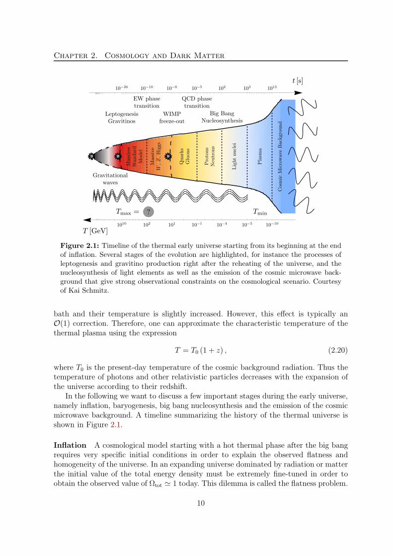
xxxxxxxxxxxxxxxxxxxxxxxxxxxxxxxxxxxxxxxxxxxxxxxxxxxxxxxxxxxxxxxxxxxxxxxxxxxxxxxxxxxxxxxxFigure 2.1: Timeline of the thermal early universe starting from its beginning at the endof inflation. Several stages of the evolution are highlighted, for instance the processes ofleptogenesis and gravitino production right after the reheating of the universe, and thenucleosynthesis of light elements as well as the emission of the cosmic microwave back-ground that give strong observational constraints on the cosmological scenario. Courtesyof Kai Schmitz.
bath and their temperature is slightly increased. However, this effect is typically anO(1) correction. Therefore, one can approximate the characteristic temperature of thethermal plasma using the expression
T = T0 (1 + z) , (2.20)
where T0 is the present-day temperature of the cosmic background radiation. Thus thetemperature of photons and other relativistic particles decreases with the expansion ofthe universe according to their redshift.
In the following we want to discuss a few important stages during the early universe,namely inflation, baryogenesis, big bang nucleosynthesis and the emission of the cosmicmicrowave background. A timeline summarizing the history of the thermal universe isshown in Figure 2.1.
Inflation A cosmological model starting with a hot thermal phase after the big bangrequires very specific initial conditions in order to explain the observed flatness andhomogeneity of the universe. In an expanding universe dominated by radiation or matterthe initial value of the total energy density must be extremely fine-tuned in order toobtain the observed value of Ωtot ≃ 1 today. This dilemma is called the flatness problem.
10
2.1. Big Bang Cosmology
In addition, observations of the cosmic microwave background indicate that the universewas highly isotropic before structure formation although the observed cosmic microwavebackground sky is many orders of magnitude larger than the causal horizon at the time ofphoton decoupling. Thus the homogeneity of the temperature could not be achieved byphysical interactions. Instead, it could only be achieved by extremely fine-tuned initialconditions. This dilemma is known as the horizon problem.
Both problems can be solved by the introduction of an inflationary phase in the earlyuniverse where weff ≃ −1 and therefore the universe is expanding exponentially [91–93]:During inflation, Ωtot = 1 becomes an attractor solution that is approached regardlessof the initial conditions. After the inflationary phase the universe is so close to beingflat that the observed value of the total energy density is very close to one even duringthe phases of radiation and matter domination. The isotropy of the cosmic microwavebackground sky can also be explained by this mechanism: The entire observed universehad initially been contained in a small causally connected region that expanded tremen-dously during the phase of inflation.
Such an inflationary phase can be realized by a scalar inflaton field that enters aso-called slow-roll phase. Apart from solving the above issues, inflation theories predictlarge-scale density perturbations that arise from quantum fluctuations of the inflatonfield. These are observed in the form of temperature anisotropies in the CMB and finallylead to the formation of structures like galaxies and stars in the universe.
After inflation, the density of all particles that initially filled the universe is diluted.However, the decay of the inflaton field at the end of the inflationary phase produces ahot thermal plasma of elementary particles. This process of entropy production is knownas the reheating of the universe, and the equilibrium temperature of the thermal plasmaright after inflation is therefore called the reheating temperature. After this phase theuniverse is described by standard thermal cosmology.
Baryogenesis A fundamental problem in cosmology and particle physics is the originof the baryon asymmetry, i.e. the question why there is more matter than antimatterin the universe. Any initial baryon asymmetry in the universe is diluted by the expo-nential expansion during inflation. Thus it is necessary to generate a baryon asymmetrydynamically after inflation. However, this process of baryogenesis is only possible whenthe three Sakharov conditions are satisfied [94]:
• baryon number (B) violation,
• C-symmetry and CP -symmetry violation,
• departure from thermal equilibrium.
Several models have been proposed for baryogenesis: The first model was the productionof a baryon asymmetry in the out-of-equilibrium decays of superheavy particles in grandunified theories (GUTs) [95, 96]. However, it was found out that the generated baryonasymmetry is washed out by non-perturbative sphaleron processes that are effective at
11

Chapter 2. Cosmology and Dark Matter
temperatures above the electroweak scale and violate the linear combination B + L ofbaryon and lepton number but conserve the combination B − L [97, 98].
This observation led to the proposal of electroweak baryogenesis, where the baryonasymmetry is generated in B + L-violating sphaleron processes [99]. However, this sce-nario is also disfavored since it only works if the electroweak phase transition is of firstorder which is not the case for the standard model of particle physics and most su-persymmetric extensions. One viable model of baryogenesis is based on the coherentproduction of baryons in the decay of scalar supersymmetric partners of leptons andbaryons. This model is known as Affleck–Dine baryogenesis [100].
The currently favored model to solve the problem of baryon asymmetry is baryo-genesis via thermal leptogenesis [18]. In this model a lepton asymmetry is generatedin B − L-violating out-of-equilibrium decays of heavy Majorana neutrinos that is thenpartly transferred into a baryon asymmetry via sphaleron processes. This mechanism isclosely related to the problem of neutrino masses, since heavy Majorana neutrinos canalso explain small nonvanishing masses for the light neutrinos via the seesaw mecha-nism [101,102]. The observation of neutrino oscillations and thus nonvanishing neutrinomasses strongly supports the existence of heavy Majorana neutrinos and therefore alsothe mechanism of thermal leptogenesis. One drawback of this model might be that ahigh reheating temperature of TR & 109GeV is required in the early universe in orderto produce the observed amount of baryon asymmetry [19, 103].
Primordial Nucleosynthesis Big Bang nucleosynthesis (BBN), i.e. the productionof light elements during the first minutes of the cosmological evolution, is one of the besttools to study the early universe since it takes place at temperatures T ≃ 1–0.1MeVand is thus based on well-understood standard model physics [104, 105]. Therefore, upto now BBN provides the deepest reliable probe of the early universe.
At temperatures above roughly 1MeV neutrons and protons are in thermal equilib-rium due to weak interactions. When the temperature falls below this value, the neutronsleave chemical equilibrium and the ratio of the neutron and proton number densities isfixed due to the Boltzmann factor at a value of
nn
np
= exp
(−mn −mp
Tfr
)≃ 1
6. (2.21)
The exact value of the freeze-out time Tfr depends on the number of relativistic degreesof freedom g∗(Tfr) and is therefore sensitive, for instance, to the number of relativisticneutrino species. After chemical decoupling, protons and neutrons could start to formdeuterium. However, as a result of photo-dissociation processes due to the large numberof photons in the thermal plasma, the deuterium production becomes only efficient attemperatures below 0.1MeV. This delay of the production of light elements is known asthe deuterium bottleneck. Once deuterium is efficiently produced, virtually all neutronscombine with protons to form 4He almost independent of the nuclear reaction rates.However, by that time the neutron-to-proton ratio has slightly decreased to about 1/7
12

2.1. Big Bang Cosmology
due to neutron decay. The relative abundance of 4He by weight can then easily beestimated:
Yp ≡ρ4He
ρp + ρ4He
≃ 2nn
np + nn=
2nn/np
1 + nn/np≈ 25% . (2.22)
By contrast, the calculation of the other light element abundances depends on the detailsof nuclear interactions and in particular on the value of the baryon-to-photon ratioη ≡ nb/nγ that determines at which temperature the process of nucleosynthesis canstart after the deuterium bottleneck. The latter is practically the only free parameter ofthe theory of BBN.
The abundances of the light elements predicted for the case of the standard modelof particle physics are in good agreement with data from astrophysical observationsof the 4He abundance in low-metallicity H ii regions and of the deuterium abundancein quasar absorption spectra for a value of the baryon-to-photon ratio in the rangeof 5.1 × 10⁻¹⁰ < η < 6.5 × 10⁻¹⁰, corresponding to an energy density in baryons of0.019 ≤ Ωbh
2 ≤ 0.024. This value is in remarkable agreement with the value determinedfrom observations of the cosmic microwave background (see left panel in Figure 2.2)and thus strongly constrains deviations imposed by physics beyond the standard model.The only drawback of this theory is the significant deviation of observations from thecalculation of the lithium abundance which is not understood so far.
Cosmic Microwave Background The observation of the cosmic microwave back-ground (CMB) radiation [107] is the most compelling evidence for a hot thermal phasein the early universe [108]. Actually, it is a relic from the time of last scattering, whenphotons decoupled from the thermal plasma of electrons and light elements at a tem-perature of T ≃ 0.25 eV corresponding to a redshift z ≃ 1100. The Cosmic BackgroundExplorer (COBE) satellite mission found that the CMB is practically isotropic and cor-responds to an almost perfect black body radiation spectrum with a temperature ofT0 = 2.725K [109, 110]. In addition, the COBE satellite observed slight temperatureanisotropies in the CMB sky map at the level of δT/T ∼ 10−5 [111].
These anisotropies were observed in detail by the Wilkinson Microwave AnisotropyProbe (WMAP) satellite mission and are probably the most valuable probe of the bigbang theory (see left panel of Figure 2.3). Expansion of the temperature anisotropy mapinto spherical harmonics
δT
T(θ, φ) =
∞∑
l=2
l∑
m=−l
alm Ylm(θ, φ) (2.23)
results in the CMB power spectrum l (l + 1)Cl/(2 π) in terms of multipole moments l(roughly corresponding to an angular size θ ∼ 180/l) with
Cl ≡⟨|alm|2
⟩=
1
2 l + 1
l∑
m=−l
|alm|2 . (2.24)
13

Chapter 2. Cosmology and Dark Matter3He/H p
4He
2 3 4 5 6 7 8 9 101
0.01 0.02 0.030.005
CM
B
BB
N
Baryon-to-photon ratio η × 1010
Baryon density Ωbh2
D___H
0.24
0.23
0.25
0.26
0.27
10−4
10−3
10−5
10−9
10−10
2
57Li/H p
Yp
D/H p
0.0 0.5 1.0
0.0
0.5
1.0
1.5
2.0
FlatBAO
CMB
SNe
No Big Bang
Figure 2.2: Left: BBN predictions for the abundances of 4He, deuterium, 3He and 7Li asa function of the baryon-to-photon ratio compared to values deduced from astrophysicalobservations (boxes). There is a remarkable coincidence of the values for the baryon-to-photon ratio derived from BBN and CMB observations. Figure taken from [81]. Right:ΩΛ − Ωm plane of the concordance model of cosmology. The observations of the CMB, ofsupernovae and of baryon acoustic oscillations overlap, and their combination suggests aflat universe with a dark energy density of ΩΛ ≃ 0.74 and a matter density of Ωm ≃ 0.26.Figure taken from [106].
The structure of the CMB power spectrum (see right panel in Figure 2.3) is mainly deter-mined by four effects: Fluctuations in the photon density at the time of last scatteringcorrespond to temperature fluctuations in the CMB sky. Moreover, photons emittedfrom a potential well are redshifted on the way to the observer. The combination ofintrinsic temperature fluctuations and gravitational redshift is called Sachs–Wolfe ef-fect. In addition, the observed photon temperature is affected by a Doppler shift dueto movements of the thermal plasma and by varying potential wells that are crossedby the CMB photons. The latter effect is known as integrated Sachs–Wolfe effect. Onscales smaller than roughly 1, corresponding to the size of the causal horizon at thetime of last scattering, one can observe acoustic oscillations of the thermal plasma thatare driven by the gravitational potential of matter and the pressure of photons.
All these effects are very sensitive to cosmological parameters. One particular ex-
14
2.2. Evidence for the Existence of Dark Matter
Multipole moment l
Angular Size
10
90° 2° 0.5° 0.2°
100 500 1000
Te
mp
era
ture
Flu
ctu
atio
ns [
µK
2]
0
1000
2000
3000
4000
5000
6000
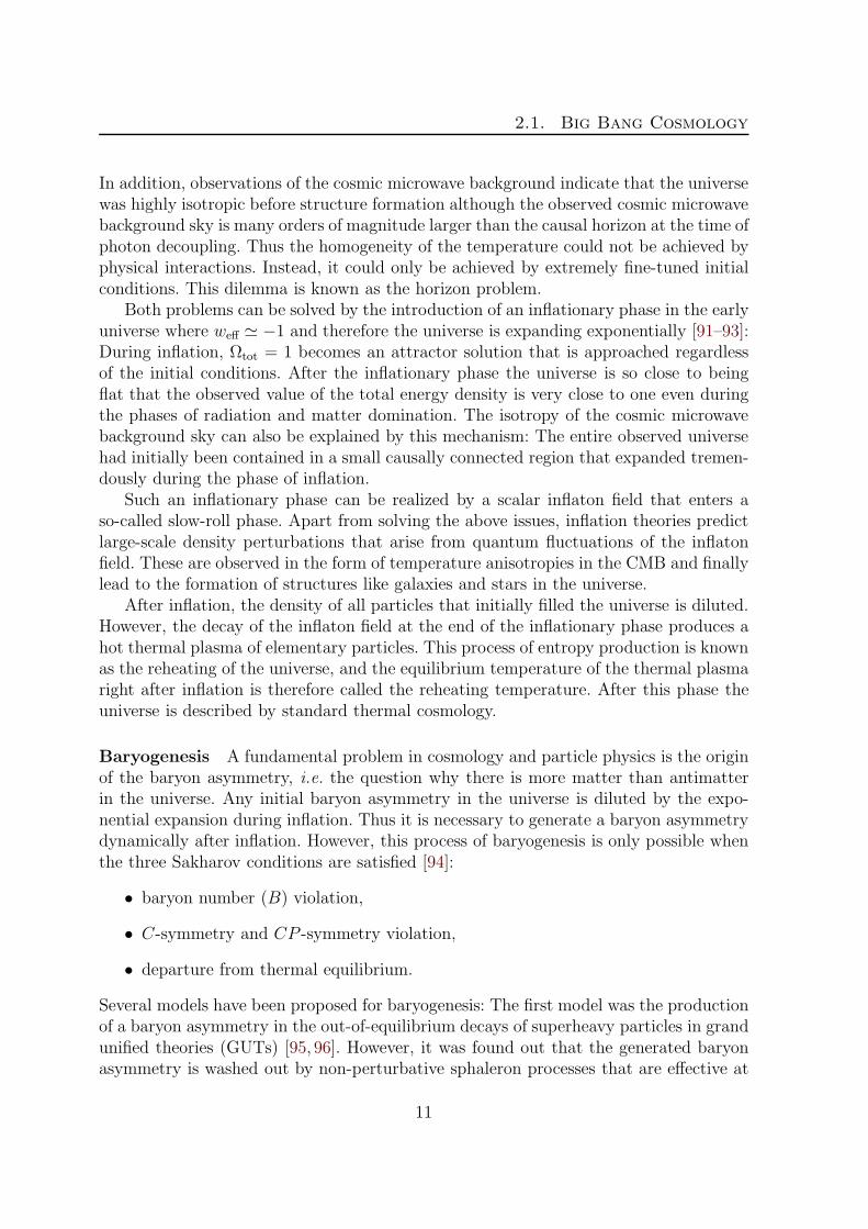
Figure 2.3: WMAP 7-year temperature anisotropy map (left) and the angular powerspectrum of temperature fluctuations from the decomposition of the temperature mapinto spherical harmonics (right) [112]. Image credit: NASA / WMAP Science Team.
ample is the position of the first acoustic peak which shows that we are living in auniverse that is practically spatially flat. The derived cosmological parameters are ingood agreement among various observations and thus one speaks of the concordancemodel of cosmology (see also Figure 2.2).
2.2 Evidence for the Existence of Dark Matter
Various astrophysical observations suggest the existence of dark matter. In this sectionwe want to summarize the evidence from observations on galactic scales up to cosmo-logical scales. All evidence is based on the gravitational effect of dark matter. By now,no evidence for dark matter has been found on microscopic scales. For more extensivereviews on this topic see for instance [4, 5].
Galactic Scales
Rotation Curves of Spiral Galaxies A very convicing evidence for dark matteron galactic scales comes from the observation of rotation curves of spiral galaxies, i.e.the circular velocity distribution of stars and gas as a function of the distance to thegalactic center. In spiral galaxies, stars and gas move on almost circular orbits aroundthe center of their host galaxy. From Newtonian dynamics we know that their circularvelocity is given by
vc(r) =
√GN M(r)
r, (2.25)
where M(r) = 4π∫ r
0dr′ r′2 ρ(r′) is the total mass inside the sphere with radius r. In the
outer regions of a galaxy, beyond the visible disc, one would then expect the velocityto fall off as v ∝ 1/
√r. However, observations of galactic rotation curves show that
15

Chapter 2. Cosmology and Dark Matter
the velocity remains constant even far beyond the luminous disk (see Figure 2.4).3 Thisobservation can be explained by the existence of a spherical dark halo with a densityprofile ρhalo ∝ 1/r2 in the outer regions. Although the existence of a spherical halo of darkmatter is firmly established due to these observations, the situation in the inner partsof galaxies is much less clear. Inside the galactic disc the density is typically dominatedby stars and gas and thus the shape of the density profile of the dark component cannotbe traced well in these regions.
So far, the outer boundary of galactic halos has not been observed and thus the totalmass of galaxies is unknown. Therefore, only a lower limit on the total amount of darkmatter in galaxies can be inferred. This translates to a lower limit ΩDM & 0.1 on thecosmological dark matter density. It has been proposed that part of the galactic darkhalos is composed of non-luminous ordinary matter in the form of Massive CompactHalo Objects (MACHOs) [7,8]. There have been searches for these objects through themicrolensing effect, finding that MACHOs can only contribute a subdominant part ofthe galactic dark halo. Thus non-baryonic dark matter is needed to explain the galacticdynamics.
Velocity Dispersion in Galaxies A method particularly useful to search for darkmatter effects in dwarf galaxies is the observation of their velocity dispersion. Assuminghydrodynamical equilibrium and spherical symmetry of the system, the velocity disper-sion is related to the mass of the galaxy. Typically, very high mass-to-light ratios areobserved in dwarf spheroidal galaxies, indicating that these systems are dominated bya halo of dark matter.
Scale of Galaxy Clusters
Also in galaxy clusters a significant discrepancy between the observed amount of lumi-nous matter in the form of stars or gas and the total cluster mass is observed. In thefollowing we will list a few methods that are used to determine the total cluster mass.
Virial Theorem From the observation of the velocity dispersion of galaxy clusterstheir mass can be determined using the virial theorem which relates the average kineticenergy with the average gravitational potential. This method actually gave the very firstevidence for the existence of dark matter: Fritz Zwicky found in 1933 that the velocities ofgalaxies in the Coma galaxy cluster are almost a factor of ten larger than expected fromthe mass of the luminous galaxies and concluded that the system must be dominatedby a dark matter component [1]. Modern observations of this type are consistent witha total matter density in the range Ωm ≈ 0.2–0.3, thereby clearly exceeding the amountof baryonic matter in the universe as derived from big bang nucleosynthesis.
3A flat rotation curve extending to radii larger than the visible disc of stars was first observed in 1970when Vera Rubin and Kent Ford studied the velocities of H ii regions in the Andromeda galaxy [113].
16

2.2. Evidence for the Existence of Dark Matter
Figure 2.4: Left: Rotation curve of the Milky Way. The solid line shows a fit to dataobtained by the observation of hydrogen gas and the long-dashed, dotted and short-dashedlines show the expected contributions from the luminous disk, the galactic bulge (i.e.the very dense central group of stars in a spiral galaxy) and their sum, respectively. Inaddition, the dash-dotted line shows the required contribution of a dark halo. Figure takenfrom [114]. Right: X-ray image of two galaxy clusters that passed through each other, thesmaller of the two being called the Bullet cluster. The hot gas which makes up the dominantcontribution of the luminous cluster mass was slowed down in the collision and is clearlydisplaced from the gravitational potential lines as mapped by weak gravitational lensing.It is concluded that the cluster masses are dominated by collisionless dark matter. Figureborrowed from [115].
Gravitational Lensing Another method to determine the mass of galaxy clustersis based on the effect of gravitational lensing. A massive galaxy cluster can act as alens that bends the light of distant astrophysical sources in the cluster direction bythe gravitational effect of its potential well. One distinguishes between strong lensing,where the effect of the gravitational lens leads to visible distortions of the image of abackground source, and weak lensing, where the lensing effect leads to slight distortionsof the shapes of background galaxies that can only be observed by a statistical analysisof a large number of these galaxies. However, this method works very well and allows toreconstruct the spatial mass distribution inside the galaxy cluster.
X-Ray Observation of Hot Gas in Galaxy Clusters Yet another method todetermine the mass of a galaxy cluster is based on X-ray observations of the hot gascontained inside the cluster. Under the assumption of hydrostatical equilibrium thereexists a relation between the temperature of the gas and the cluster mass. This methodin addition allows to map the distribution of matter in the cluster. In general one findsthat the gas temperature is much higher than expected from the amount of luminousmatter observed in clusters. Therefore, a dark component is needed to explain the high
17
Chapter 2. Cosmology and Dark Matter
temperature of the contained gas. The results for the dark matter density obtained bythe latter two methods are generally in good agreement with the result deduced fromthe velocity dispersion of galaxy clusters.
Bullet Cluster An even more direct evidence for the existence of dark matter is foundin the Bullet cluster [115] (see right panel in Figure 2.4). This system actually consists oftwo galaxy clusters that passed through each other. Although the hot gas, which makesup the dominant contribution of the luminous cluster mass, is displaced from the galaxiesdue to the collision, the gravitational potential follows the distribution of galaxies. Thiscan only be understood if the cluster mass is dominated by a practically collisionlesscomponent of dark matter. This observation also strongly disfavors alternative theoriesof gravity like Modified Newtonian Dynamics (MOND) [6] that were proposed to explainthe galactic rotation curves without invoking a dark matter component.
Cosmological Scales
Large Scale Structure Although the universe appears to be homogeneous and iso-tropic on the largest scales, a lot of structure is observed on small and large scales. Thisstructure is expected to originate from quantum fluctuations that were amplified duringthe stage of inflation. These density perturbations can only start to grow efficiently withthe beginning of the matter-dominated phase of the universe. However, as baryons arecoupled to the plasma of photons whose pressure counteracts the gravitational collaps,their density perturbations can only start to grow after the decoupling of photons, i.e.after the emission of the CMB. In this case the density fluctuations at photon decouplingwould have needed to be already quite large, corresponding to temperature fluctuationsin the CMB of the order of δT/T ∼ 10−3 in order to explain the observed structure inthe present universe.
This value is much larger than the observed level of fluctuations (δT/T ∼ 10−5) andthus dark matter is needed to explain the amount of structure that we observe today.Since dark matter particles were already decoupled from the thermal plasma, theirdensity perturbations could start to grow from the time of matter-radiation equality(redshift z ∼ 3000) onwards.
The effect of baryon acoustic oscillations can also be observed in the large-scale dis-tribution of galaxies and allows to derive the total density of matter in the universe [116]:Ωm ≃ 0.27. Together with the value for the density of baryonic matter from primordialnucleosynthesis this is a strong evidence for dark matter.
Cosmic Microwave Background As discussed before the temperature fluctuationsin the CMB correspond to the acoustic oscillations of the thermal plasma of photonsand baryons. The power spectrum of temperature anisotropies has been measured inparticular detail by the WMAP experiment. From the shape of the acoustic peaks thedensities of baryons and matter as well as a number of other cosmological parameters
18
2.3. Constraints on Dark Matter Properties
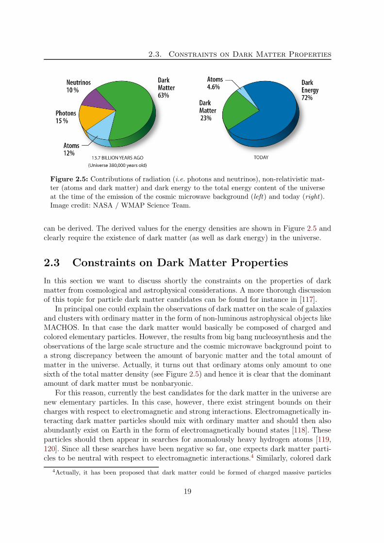
Figure 2.5: Contributions of radiation (i.e. photons and neutrinos), non-relativistic mat-ter (atoms and dark matter) and dark energy to the total energy content of the universeat the time of the emission of the cosmic microwave background (left) and today (right).Image credit: NASA / WMAP Science Team.
can be derived. The derived values for the energy densities are shown in Figure 2.5 andclearly require the existence of dark matter (as well as dark energy) in the universe.
2.3 Constraints on Dark Matter Properties
In this section we want to discuss shortly the constraints on the properties of darkmatter from cosmological and astrophysical considerations. A more thorough discussionof this topic for particle dark matter candidates can be found for instance in [117].
In principal one could explain the observations of dark matter on the scale of galaxiesand clusters with ordinary matter in the form of non-luminous astrophysical objects likeMACHOS. In that case the dark matter would basically be composed of charged andcolored elementary particles. However, the results from big bang nucleosynthesis and theobservations of the large scale structure and the cosmic microwave background point toa strong discrepancy between the amount of baryonic matter and the total amount ofmatter in the universe. Actually, it turns out that ordinary atoms only amount to onesixth of the total matter density (see Figure 2.5) and hence it is clear that the dominantamount of dark matter must be nonbaryonic.
For this reason, currently the best candidates for the dark matter in the universe arenew elementary particles. In this case, however, there exist stringent bounds on theircharges with respect to electromagnetic and strong interactions. Electromagnetically in-teracting dark matter particles should mix with ordinary matter and should then alsoabundantly exist on Earth in the form of electromagnetically bound states [118]. Theseparticles should then appear in searches for anomalously heavy hydrogen atoms [119,120]. Since all these searches have been negative so far, one expects dark matter parti-cles to be neutral with respect to electromagnetic interactions.4 Similarly, colored dark
4Actually, it has been proposed that dark matter could be formed of charged massive particles
19

Chapter 2. Cosmology and Dark Matter
matter particles are expected to form color-neutral bound states together with ordinarymatter [118]. These heavy hadrons could then be identified in searches for heavy nucle-ons [119,120,123,124]. Also in this case all searches have been negative so far and thusone expects dark matter particles to be color-neutral.
The requirement of a successful structure formation introduces another importantconstraint. Dark matter is necessary to explain the observed growth of density perturba-tions after the time of radiation domination but it also needs to have the correct prop-erties in order to match observations. In fact, the observation of small-scale structuresconstrains the free-streaming length of dark matter particles: they must be sufficientlynon-relativistic in order not to wash out small-scale density perturbations. Thus thedominant part of the dark matter in the universe must be in the form of cold darkmatter particles, i.e. particles that became non-relativistic well before the beginning ofstructure formation at the time of matter-radiation equality. In any case, however, thereis also a subdominant contribution of hot dark matter, namely the background of lightstandard model neutrinos.
Another important constraint comes from the requirement that the relic densityof the dark matter particle as predicted by the particle physics model needs to be inaccord with the observed dark matter density in the universe. The current best-fit valuefrom the combination of the seven-year data of WMAP, observations of baryon acousticoscillations and determinations of the present-day Hubble parameter is given by [125]
ΩDMh2 = 0.1126(36) . (2.26)
Of course, an additional constraint is that the dark matter particle candidate is eitherperfectly stable or sufficiently long-lived to explain the dark matter observations. Cos-mological observations alone constrain the dark matter lifetime to be at least one orderof magnitude above the current age of the universe (t0 ≃ 13.7Gyr = 4.3× 10¹⁷ s) [126].We will see later in this work that astrophysical observations are able to set much morestringent constraints on the dark matter lifetime.
There are additional constraints for many particle dark matter candidates from therequirement that the particle physics model leads to a consistent cosmological scenariothat is not in conflict with any cosmological observation. In particular, big bang nu-cleosynthesis is very sensitive to deviations from the standard model particle contentat an early epoch of the cosmological evolution. For instance, the presence of chargedparticles at the time of BBN or the decay of metastable relics during or after the timeof BBN can significantly alter the predicted abundances of light elements and thus leadto conflicts with observations.5
In particular the latter point typically provides strong constraints for supergravitytheories containing a gravitino in the particle spectrum. We will give an overview ofthese constraints and how they can be circumvented in Section 4.2.
(CHAMPS) [121, 122] but these models are strongly constrained.5For a recent review of constraints from big bang nucleosynthesis and further references see [127].
20

Chapter 3
Supersymmetry and Supergravity
Supersymmetry (SUSY) [128] is a generalization of the space-time symmetries of quan-tum field theory that relates bosonic and fermionic degrees of freedom. It introducesnew fermionic generators Q that transform fermions into bosons and vice versa:
Q |boson〉 ≃ |fermion〉 , Q |fermion〉 ≃ |boson〉 .
This represents a nontrivial extension to the Poincare symmetry of ordinary quantumfield theory and its structure is highly constrained by the theorem of Haag, Lopuszanskiand Sohnius [129] which is a generalization of the Coleman–Mandula theorem [130].
The introduction of SUSY predicts the existence of supersymmetric partners for thestandard model particles relating each fermionic degree of freedom with a bosonic one.If SUSY were an exact symmetry of nature, particles and their superpartners wouldbe degenerate in mass. However, since no superpartners have been observed yet, SUSYmust be a broken symmetry.
Although not yet confirmed experimentally, there are several theoretical motiva-tions for interest in this additional symmetry. The first is the hierarchy problem of thestandard model. This problem stems from the huge difference of the electroweak scale(O(100)GeV) and the (reduced) Planck scale
MPl =1√
8 πGN
≃ 2.4× 10¹⁸GeV , (3.1)
where gravitational interactions become comparable in magnitude to gauge interactions.The only scalar particle in the standard model, the Higgs boson, receives quadraticradiative corrections to its mass due to fermion loops. These quadratic divergences areconveniently cancelled by the contributions of the bosonic superpartners to the radiativecorrections. This exact cancellation holds only for unbroken SUSY. However, as long asSUSY is broken softly, no quadratic divergences are reintroduced and the hierarchyproblem can still be solved [131].
A second motivation is the unification of gauge couplings αα = g2α/4π, α = 1, 2, 3,where g1 =
√5/3 g′ and g2 = g are the electroweak coupling constants, and g3 = gs is
21
Chapter 3. Supersymmetry and Supergravity
2 4 6 8 10 12 14 16 18Log10(Q/1 GeV)
0
10
20
30
40
50
60
α−1
α1
−1
α2
−1
α3
−1
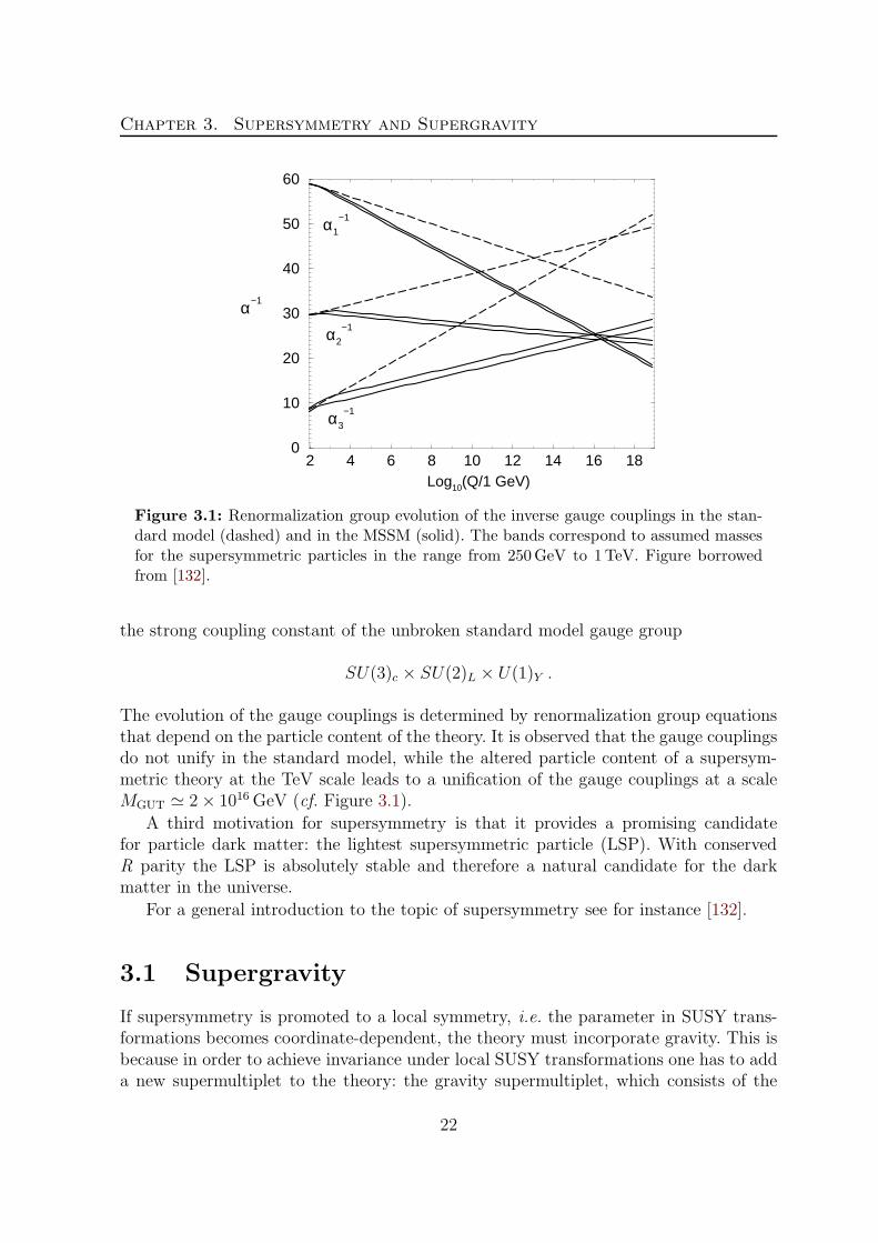
Figure 3.1: Renormalization group evolution of the inverse gauge couplings in the stan-dard model (dashed) and in the MSSM (solid). The bands correspond to assumed massesfor the supersymmetric particles in the range from 250GeV to 1TeV. Figure borrowedfrom [132].
the strong coupling constant of the unbroken standard model gauge group
SU(3)c × SU(2)L × U(1)Y .
The evolution of the gauge couplings is determined by renormalization group equationsthat depend on the particle content of the theory. It is observed that the gauge couplingsdo not unify in the standard model, while the altered particle content of a supersym-metric theory at the TeV scale leads to a unification of the gauge couplings at a scaleMGUT ≃ 2× 10¹⁶GeV (cf. Figure 3.1).
A third motivation for supersymmetry is that it provides a promising candidatefor particle dark matter: the lightest supersymmetric particle (LSP). With conservedR parity the LSP is absolutely stable and therefore a natural candidate for the darkmatter in the universe.
For a general introduction to the topic of supersymmetry see for instance [132].
3.1 Supergravity
If supersymmetry is promoted to a local symmetry, i.e. the parameter in SUSY trans-formations becomes coordinate-dependent, the theory must incorporate gravity. This isbecause in order to achieve invariance under local SUSY transformations one has to adda new supermultiplet to the theory: the gravity supermultiplet, which consists of the
22

3.1. Supergravity
Name Bosons Fermions (SU(3)c , SU(2)L)Y
Graviton, gravitino gµν ψµ (1, 1)0
Table 3.1: The gravity supermultiplet of locally supersymmetric theories. Listed are theparticles together with their quantum numbers with respect to the unbroken standardmodel gauge group.
spin-2 graviton and the spin-3/2 gravitino (see Table 3.1). The resulting locally super-symmetric theory is therefore called supergravity (SUGRA) [12,13]. A short introductionto supergravity can be found for instance in [133]. For more exhaustive discussions ofSUGRA see references therein.
The Supergravity Lagrangian
Supergravity theories are in general described by three functions of the scalar fields inthe theory: The Kahler potential K(φ, φ∗), which is a real function of the scalar fields,the superpotential W (φ), which is a holomorphic function of the scalar fields, and thegauge kinetic function fab(φ), which also is a holomorphic function of the scalar fields.
The bosonic part of the supergravity Lagrangian is of the form [133]
L =√−g[− M2
Pl
2R −Gi(φ, φ
∗)(Dµ φ
i)(Dµφ∗ )− V (φ, φ∗)
− 1
4(Re fab)F
aµνF
bµν +i
4(Im fab)F
aµνF
b µν
],
(3.2)
where g = det gµν is the determinant of the space-time metric. The first part with theRicci scalar R is the usual Einstein–Hilbert term from general relativity. The second partis the kinetic term of the scalar fields that in general is not of canonical form. However,the non-linear sigma model of scalars is not arbitrary since invariance under supergravitytransformations requires that the field space of scalars is a Kahler manifold. The metricof this Kahler manifold is given by a second derivative of the Kahler potential:
Gi(φ, φ∗) =
∂
∂φi
∂
∂φ∗ K(φ, φ∗) . (3.3)
In addition, the covariant derivative of the scalars is of the form
Dµφi = ∂µφ
i − gAaµX
i a = ∂µφi + i gAa
µGi ∂D
a
∂φ∗ , (3.4)
where the X i a are holomorphic Killing vector fields corresponding to isometries of theKahler metric Gi and the Da are the associated Killing potentials. The third term in
23

Chapter 3. Supersymmetry and Supergravity
the Lagrangian is the scalar potential that is given by
V = exp
(K
M2Pl
)((∇iW )Gi (∇W
∗)− 3|W |2M2
Pl
)+
1
2g2(Re fab)
−1DaDb, (3.5)
where the Kahler covariant derivative ∇iW and the real Killing potential Da are, re-spectively, given by
∇iW =∂W
∂φi+
1
M2Pl
∂K
∂φiW and Da = −i ∂K
∂φiX i a. (3.6)
The last two terms are the kinetic terms of gauge bosons expressed in form of thefield strength tensor and its dual. These terms are proportional to the gauge kineticfunction fab. Due to the appearance of non-canonical kinetic terms, supergravity isa nonrenormalizable theory. In addition, the full Lagrangian will contain interactionterms with couplings of negative mass dimension. However, it is usually assumed thatsupergravity is an appropriate low-energy approximation of a more general theory likestring theory.
The most general supergravity Lagrangian including all fermionic terms is usuallyderived using the superspace formalism. A convenient starting point for phenomenolog-ical studies of four-dimensional N = 1 supergravity models is the complete supergravityLagrangian in component fields as given in the book of Wess and Bagger [134]. Herewe want to quote the Lagrangian in a simplified case where fab = δab. In the notationof Wess and Bagger – but restoring the dependence on the reduced Planck mass – theLagrangian reads:
L√−g = −M2Pl
2R −Gi
(Dµ φ
i)(Dµφ∗ )− 1
2g2DaDa − 1
4F aµνF
aµν − iλaσµDµ λa
− i Gi χ σµDµ χ
i + εµνρσψµσνDρ ψσ + i√2 g
∂Da
∂φiχiλa − i
√2 g
∂Da
∂φ∗ χ λa
− 1
MPl
(g
2Daψµ σ
µλa − g
2Daψµ σ
µλa +1√2Gi (Dµ φ
∗ )χiσµ σνψµ
+1√2Gi
(Dµ φ
i)χ σνσµψν −
i
4
(ψµ σ
ρσσµλa + ψµ σρσσµλa
)(F aρσ + F a
ρσ
))
+1
M2Pl
(1
4Gi
(i εµνρσψµσνψρ + ψρ σ
σψρ)χiσσχ
− 3
16λaσµλaλbσµλ
b
− 1
8
(GiGkl − 2M2
PlRikl
)χi χk χ χl +
1
8Gi χ
σµ χi λa σµλa
)(3.7)
− exp
(K
2M2Pl
)(1
M2Pl
(W ∗ψµ σ
µνψν +Wψµ σµνψν
)+
1
MPl
( i√2(∇iW )χiσµψµ
+i√2(∇ıW
∗) χı σµψµ
)+
1
2Di∇jWχi χj +
1
2Dı∇W
∗χı χ
)
− exp
(K
M2Pl
)((∇iW )Gi (∇W
∗)− 3|W |2M2
Pl
),
24
3.1. Supergravity
where
F aµν ≡ F a
µν −i
2MPl
(ψµ σν λ
a + ψµ σν λa − ψν σµ λ
a − ψν σµ λa)
(3.8)
and
σµν ≡ 1
4(σµσν − σν σµ) . (3.9)
The curvature tensor and the connection of the Kahler manifold are, respectively, givenby [134]
Rikl = Gml
∂Γmik
∂φ∗ and Γkij = Gkl ∂Gjl
∂φi. (3.10)
The covariant derivative of the scalars and the Kahler covariant derivative have beenintroduced before. The remaining derivatives are given by [134]:
Dµ χi = ∂µχ
i + χiωµ + Γijk
(Dµ φ
j)χk + i gAa
µ
∂
∂φk
(Gi ∂D
a
∂φ∗
)χj
− 1
4M2Pl
(∂K
∂φjDµ φ
j − ∂K
∂φ∗ Dµ φ∗)χi − i
2M2Pl
gAaµ ImF aχi, (3.11)
Dµ λa = ∂µλ
a + λaωµ − gfabcAbµλ
c
+1
4M2Pl
(∂K
∂φjDµ φ
j − ∂K
∂φ∗ Dµ φ∗)λa +
i
2M2Pl
gAbµ ImF bλa, (3.12)
Dµ ψν = ∂µψν + ψν ωµ +1
4M2Pl
(∂K
∂φjDµ φ
j − ∂K
∂φ∗ Dµ φ∗)ψν
+i
2M2Pl
gAaµ ImF aψν , (3.13)
Di∇jW =∂2W
∂φi ∂φj+
1
M2Pl
(∂2K
∂φi ∂φjW +
∂K
∂φi∇jW +
∂K
∂φj∇iW
)
− 1
M4Pl
∂K
∂φi
∂K
∂φjW − Γk
ij∇kW . (3.14)
In these expressions ωµ is the spin connection and
F a ≡ −i Gi ∂Da
∂φ∗∂K
∂φi+ iDa. (3.15)
If the Kahler potential has a minimal form, i.e. K = φi φ∗ı, the Kahler metric becomes
trivial (Gi = δi) and canonical kinetic terms for the scalars are recovered. In this casethe Kahler connection and curvature are vanishing and the Killing potentials coincidewith the D-terms of the globally supersymmetric theory:
Da = φ∗i T aij φ
j. (3.16)
25
Chapter 3. Supersymmetry and Supergravity
In [135] the supergravity Lagrangian was rewritten up to O(M−1Pl ) in four-component
spinor notation which is convenient for the calculation of matrix elements. Useful ref-erences on the translation from two-component to four-component notation are for in-stance [136] and [137]. In the conventions of [135] the four-component spinors of matterfermions, gauginos and gravitinos are defined as
χiL =
(χi
0
), λa =
(−iλaiλa
)and ψµ =
(−i ψµ
i ψµ
). (3.17)
A definition of the gravitino 4-spinor without the factors of i would lead to a change ofthe relative signs of the gaugino and gravitino masses that might be observable in theinterference terms of different Feynman diagrams.
Supersymmetry Breaking and the Super-Higgs Mechanism
As mentioned in the beginning of this chapter, supersymmetry must be spontaneouslybroken by soft parameters to explain the mass differences of standard model particlesand their superpartners. However, there are no realistic models of spontaneously brokensupersymmetry where the SUSY breaking arises from the particle interactions of theminimal supersymmetric standard model. Therefore, one usually assumes the existenceof a hidden sector where supersymmetry is broken. The effect of supersymmetry breakingis then mediated to the observable sector via suppressed interactions.
Analogous to the Higgs mechanism of electroweak symmetry breaking, in supergrav-ity there exists a super-Higgs mechanism of supersymmetry breaking [139]. Since theSUSY generators are fermionic, the breaking of supersymmetry generates a masslessgoldstone fermion, the goldstino. However, since the Lagrangian of a spontaneously bro-ken supergravity theory contains a gravitino–goldstino mixing mass term, the goldstinois absorbed into the gravitino, which thereby acquires its longitudinal (helicity ±1/2)components and becomes massive. The gravitino mass is then given by [138]
m3/2 ∼〈F 〉MPl
, (3.18)
where 〈F 〉 is the vacuum expectation value of the hidden sector auxiliary field that isresponsible for the spontaneous breaking of supersymmetry. The value of the gravitinomass depends on the particular scheme of SUSY breaking mediation and can range fromthe eV scale to scales beyond many TeV.
Let us shortly mention the two best-known mechanisms for the mediation of super-symmetry breaking.1
Gravity-Mediated Supersymmetry Breaking In gravity mediation it is assumedthat supersymmetry is broken spontaneously in a hidden sector and mediated to the
1For a discussion of various mechanisms of supersymmetry breaking mediation see e.g. [132, 138].
26

3.2. The Minimal Supersymmetric Standard Model
observable sector via non-renormalizable interactions (see for instance [140]). For dimen-sional reasons, in gravity mediation one typically expects soft terms of the order
msoft ∼〈F 〉MPl
∼ m3/2 , (3.19)
as the soft masses need to vanish in the limits 〈F 〉 → 0 and MPl → ∞. Therefore, thegravitino mass is required to be somewhere around the electroweak scale up to the TeVscale in order to solve the hierarchy problem. The scale of supersymmetry breaking israther high in this case:
√〈F 〉 ∼ 1010–1011GeV.
Gauge-Mediated Supersymmetry Breaking In models of gauge mediation [141,142]2 the breaking of supersymmetry is mediated to the visible sector via a sector ofmessenger particles that couple to the MSSM particles via gauge interactions. In thesemodels the soft mass parameters for scalars are generated via loop effects. By dimen-sional analysis one expects:
msoft ∼α
4 π
〈F 〉Mmess
, (3.20)
where α/(4 π) ∼ O(1/100) is a loop factor. As the messenger scale is typically consider-ably below the Planck scale, supersymmetry must be broken at a lower scale comparedto the case of gravity mediation to achieve soft masses between the electroweak scaleand the TeV scale. This leads subsequently to a gravitino mass that is in general muchsmaller than in the case of gravity mediation. Then, the gravitino is always the lightestsupersymmetric particle.
Although the contributions to the soft parameters from gravity mediation are alsopresent in scenarios of gauge-mediated supersymmetry breaking, they are in generalnegligible due to the suppression of the lower supersymmetry breaking scale by thePlanck scale.
3.2 The Minimal Supersymmetric Standard Model
The minimal supersymmetric extension of the standard model (MSSM) introduces su-perpartners to the standard model matter fermions and gauge bosons, and extends theHiggs sector to include two SU(2) doublets and their superpartners (see Figure 3.2). Thestandard model particles and their superpartners are combined into supermultiplets. Thegauge or vector supermultiplets consist of a spin-1 vector boson Aa
µ, a spin-1/2 Majoranafermion λa and a scalar auxiliary field Da, where a labels the gauge group generators. Inparticular, we have the electroweak gauge bosons and the corresponding fermionic gaug-inos as well as the gluons and the fermionic gluinos (see Table 3.2). The table gives thenotation of the particles in Lagrangians and Feynman rules, and their transformationproperties under the standard model gauge group.
2For a review on theories of gauge mediation see also [143].
27

Chapter 3. Supersymmetry and Supergravity
Figure 3.2: Particle content of the minimal supersymmetric standard model. There arethree generations of quarks and leptons along with their scalar superpartners. Similarly,there are gauge bosons corresponding to the standard model gauge group generators (hereshown after electroweak symmetry breaking) and their fermionic superpartners. The Higgssector is represented by a Higgs boson and its fermionic superpartner, the higgsino. ImageCredit: DESY.
Name Gauge bosons Gauginos (SU(3)c , SU(2)L)Y
B boson, bino A(1)µ = Bµ λ(1) = B (1, 1)0
W bosons, winos A(2) aµ =W a
µ λ(2) a = W a (1, 3)0gluons, gluinos A
(3) aµ = Ga
µ λ(3) a = ga (8, 1)0
Table 3.2: The gauge supermultiplets of the minimal supersymmetric standard model.Listed are the different particles together with their quantum numbers with respect to theunbroken standard model gauge group.
Chiral supermultiplets consist of one complex scalar φ, a two-component chiralfermion χ and an auxiliary scalar field F . There are three generations of left-handed andright-handed leptons and quarks, the corresponding scalar sleptons and squarks, and therespective antiparticles. Additionally, there are two Higgs doublets, the fermionic hig-gsinos and their antiparticles (see Table 3.3). The enlarged Higgs sector is needed toguarantee the cancellation of anomalies from the introduction of the higgsino superpart-ners. In addition, the two Higgs doublets are needed to generate masses for ‘up’- and‘down’-type quarks as well as charged leptons after electroweak symmetry breaking.
The Lagrangian of a globally supersymmetric theory is determined by the superpo-tential W , which is a function of the scalar fields. In the MSSM with conserved R paritythe superpotential is given by [144]
WMSSM = µHuHd + λeijHdℓie∗j + λdijHdqid
∗j − λuijHuqiu
∗j . (3.21)
In this expression we implicitly sum over generation indices i, j = 1, 2, 3 and the sup-
28
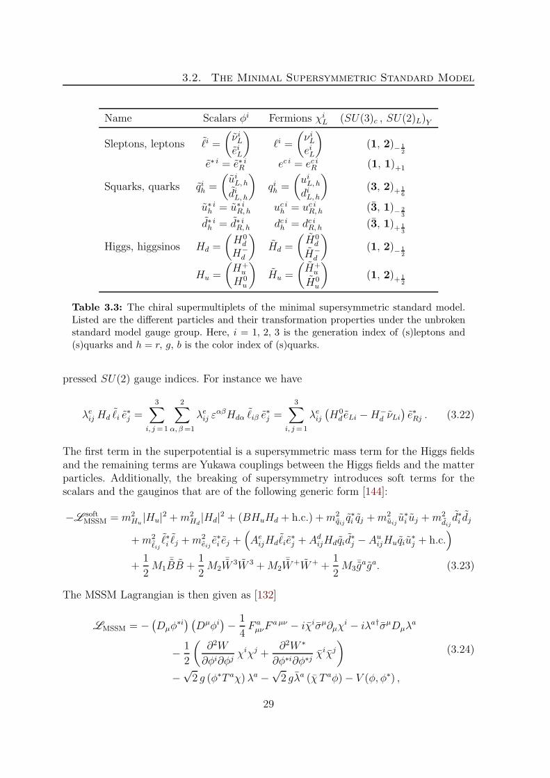
3.2. The Minimal Supersymmetric Standard Model
Name Scalars φi Fermions χiL (SU(3)c , SU(2)L)Y
Sleptons, leptons ℓi =
(νiLeiL
)ℓi =
(νiLeiL
)(1, 2)− 1
2
e∗ i = e∗ iR ec i = ec iR (1, 1)+1
Squarks, quarks qih =
(uiL, hdiL, h
)qih =
(uiL, hdiL, h
)(3, 2)+ 1
6
u∗ ih = u∗ iR, h uc ih = uc iR, h (3, 1)− 23
d∗ ih = d∗ iR, h dc ih = dc iR, h (3, 1)+ 13
Higgs, higgsinos Hd =
(H0
d
H−d
)Hd =
(H0
d
H−d
)(1, 2)− 1
2
Hu =
(H+
u
H0u
)Hu =
(H+
u
H0u
)(1, 2)+ 1
2
Table 3.3: The chiral supermultiplets of the minimal supersymmetric standard model.Listed are the different particles and their transformation properties under the unbrokenstandard model gauge group. Here, i = 1, 2, 3 is the generation index of (s)leptons and(s)quarks and h = r, g, b is the color index of (s)quarks.
pressed SU(2) gauge indices. For instance we have
λeij Hd ℓi e∗j =
3∑
i, j =1
2∑
α, β=1
λeij εαβHdα ℓiβ e
∗j =
3∑
i, j=1
λeij(H0
d eLi −H−d νLi
)e∗Rj . (3.22)
The first term in the superpotential is a supersymmetric mass term for the Higgs fieldsand the remaining terms are Yukawa couplings between the Higgs fields and the matterparticles. Additionally, the breaking of supersymmetry introduces soft terms for thescalars and the gauginos that are of the following generic form [144]:
−LsoftMSSM = m2
Hu|Hu|2 +m2
Hd|Hd|2 + (BHuHd + h.c.) +m2
qijq∗i qj +m2
uiju∗i uj +m2
dijd∗i dj
+m2ℓijℓ∗i ℓj +m2
eije∗i ej +
(Ae
ijHdℓie∗j + Ad
ijHdqid∗j −Au
ijHuqiu∗j + h.c.
)
+1
2M1
¯BB +1
2M2
¯W 3W 3 +M2¯W+W+ +
1
2M3
¯gaga. (3.23)
The MSSM Lagrangian is then given as [132]
LMSSM = −(Dµφ
∗i) (Dµφi)− 1
4F aµνF
aµν − iχiσµ∂µχi − iλa†σµDµλ
a
− 1
2
(∂2W
∂φi∂φjχiχj +
∂2W ∗
∂φ∗i∂φ∗j χiχj
)
−√2 g (φ∗T aχ) λa −
√2 gλa (χ T aφ)− V (φ, φ∗) ,
(3.24)
29

Chapter 3. Supersymmetry and Supergravity
where the scalar potential has the form
V (φ, φ∗) = F iF ∗i +1
2DaDa + L
soft =∂W
∂φi
∂W ∗
∂φ∗i +1
2
∑
a
g2 (φ∗T aφ)2 + Lsoft. (3.25)
Let us now turn to the effects of electroweak symmetry breaking.
Electroweak Symmetry Breaking
As we have stated before, in the MSSM there are two complex Higgs doublets. Elec-troweak symmetry is broken down to electromagnetism,
SU(2)L × U(1)Y → U(1)em ,
dynamically through radiative corrections to the soft Higgs masses mHu and mHd. The
neutral Higgs fields then acquire vacuum expectation values 〈H0u〉 = vu and 〈H0
d〉 = vd.The ratio of the Higgs VEVs is usually denoted as
tan β ≡ vuvd. (3.26)
The VEVs of the Higgs doublets are related to the standard model Higgs VEV v ≃174GeV in the following way:
v2 = v2u + v2d , vu = v sin β and vd = v cos β . (3.27)
The new mass eigenstates after electroweak symmetry breaking are the electrically neu-tral photon Aµ and the electrically neutral Z boson, defined as
(Aµ
Zµ
)=
(cos θW sin θW− sin θW cos θW
)(Bµ
W 3µ
), (3.28)
as well as the electrically charged W± bosons, defined as
W±µ =
1√2
(W 1
µ ∓ iW 2µ
). (3.29)
In these expressions the weak mixing angle θW is defined as
sin θW =g′√
g2 + g′2and cos θW =
g√g2 + g′2
, (3.30)
with the SU(2)L gauge coupling g and the U(1)Y gauge coupling g′. The gauge couplingof the residual symmetry group U(1)em is the elementary charge
e =√4 π α = g sin θW = g′ cos θW . (3.31)
30
3.2. The Minimal Supersymmetric Standard Model
The photon Aµ turns out to be massless, while the other electroweak gauge bosonsacquire masses through the Higgs mechanism. They absorb the three massless degreesof freedom of the two complex Higgs doublets: the Goldstone bosons G and G±. Thesebecome the longitudinal modes of the massive Z and W± gauge bosons whose massesare then given by
mW =g v√2
and mZ =g v√
2 cos θW. (3.32)
The Higgs gauge eigenstates can be expressed in terms of the Higgs mass eigenstates:The neutral gauge eigenstates are decomposed as
(H0
u
H0d
)=
(vuvd
)+
1√2
(cα sα−sα cα
)(hH
)+
i√2
(sβ0 cβ0
−cβ0 sβ0
)(GA
)(3.33)
and the charged gauge eigenstates read
(H+
u
H−∗d
)=
(sβ±
cβ±
−cβ±sβ±
)(G+
H+
). (3.34)
Here and in the following parts we use the abbreviations sα ≡ sinαand cα ≡ cosα forthe mixing angles. In the tree-level approximation one has β0 = β± = β and the massesof the Higgs mass eigenstates are given by
m2h,H =
1
2
(m2
A +m2Z ∓
√(m2
A −m2Z)
2+ 4m2
Z m2A sin2 2 β
),
m2A = 2 |µ|2 +m2
Hu+m2
Hd,
m2H± = m2
A +m2W .
(3.35)
In this case, the mixing angle α is determined by the conditions
sin 2α
sin 2 β= −
(m2
H +m2h
m2H −m2
h
)and
tan 2α
tan 2 β=
(m2
A +m2Z
m2A −m2
Z
), (3.36)
and is usually chosen to be negative.In the decoupling limit [145], i.e. formA ≫ mZ , corresponding to a large µ parameter,
the Higgs particles H , A and H± are very heavy and decouple from the low-energyphenomenology. Only the lightest Higgs particle h stays at the electroweak scale. In thiscase, using the relations (3.36), the mixing angle becomes α ≃ β − π/2 and the lightestHiggs boson h obtains the couplings of the ordinary standard model Higgs boson.
Neutralinos and Charginos
Gauginos and higgsinos mix with each other due to electroweak symmetry breaking. Theneutral gauginos and the neutral higgsinos combine to form the four mass eigenstatescalled neutralinos χ0
α , while the charged gauginos and the charged higgsinos mix to formthe two mass eigenstates called charginos χ±
α .
31
Chapter 3. Supersymmetry and Supergravity
In the gauge eigenstate basis ψ0 = (−iB, −iW 3, H0u, H
0d)
T the neutralino mass partof the Lagrangian is given by
Lneutralino mass = −1
2ψ0TMN ψ
0 + h.c. (3.37)
The entries of the neutralino mass matrix MN can be directly read off from the MSSMLagrangian. The matrix turns out to be symmetric and reads
MN =
M1 0 g′vu√2
−g′vd√2
0 M2 −g vu√2
g vd√2
g′vu√2
−g vu√2
0 −µ−g′vd√
2
g vd√2
−µ 0
. (3.38)
Using an orthogonal matrix that includes equation (3.28), we can change the basisfrom the gauge eigenstates to the supersymmetric partners of the massive gauge bosonsψ0′ = (−iγ, −iZ, H0
u, H0d)
T :
−iγ−iZH0
u
H0d
= R
−iB−iW 3
H0u
H0d
, R =
cW sW 0 0−sW cW 0 00 0 1 00 0 0 1
. (3.39)
The neutralino mass term can then be rewritten in the form
Lneutralino mass = −1
2ψ0′TM ′
N ψ0′ + h.c. , (3.40)
where the neutralino mass matrix in the new basis can be written as
M ′N = RMN R
T =
M1c2W +M2 s
2W (M2 −M1) sW cW 0 0
(M2 −M1) sW cW M1s2W +M2 c
2W −mZ sβ mZ cβ
0 −mZ sβ 0 −µ0 mZ cβ −µ 0
.(3.41)
In this expression we used the relations (3.27), (3.30) and (3.32) to rewrite the contri-butions from Yukawa couplings in terms of the Z boson mass. For the mixing angles weused the abbreviations sW ≡ sin θW , cW ≡ cos θW , sβ ≡ sin β and cβ ≡ cos β.
In a similar way the basis can be changed to the neutralino mass eigenstates. Sym-metric matrices can always be diagonalized by a unitary matrix N and its transposedmatrix in the following way:
N∗M ′NN
† =
mχ01
0 0 0
0 mχ02
0 0
0 0 mχ03
0
0 0 0 mχ04
. (3.42)
32
3.2. The Minimal Supersymmetric Standard Model
The neutralinos are then obtained by the rotation
χ01
χ02
χ03
χ04
= N
−iγ−iZ0
H0u
H0d
. (3.43)
The chargino mass term in the gauge eigenstate basis ψ− = (−iW−, H−d )
T andψ+ = (−iW+, H+
u )T reads
Lchargino mass = −ψ−TMC ψ
+ + h.c. , (3.44)
where the chargino mass matrix MC is given by
MC =
(M2 g vug vd µ
)=
(M2
√2mW sβ√
2mW cβ µ
). (3.45)
For the last equality we employed the relations (3.27) and (3.32). Due to the asymmetricform of the mass matrix, two unitary matrices U and V are required to diagonalize it.This can be done in the following way:
U∗MCV† = VM †
CUT =
(mχ±
10
0 mχ±2
). (3.46)
The matrices U and V also rotate the gauge eigenstates into the basis of left- andright-handed chargino mass eigenstates:
(χ−1
χ−2
)= U
(−iW−
H−d
)and
(χ+1
χ+2
)= V
(−iW+
H+u
). (3.47)
The chargino masses are given as the positive roots of the eigenvalues of M †CMC , since
VM †CMCV
† = U∗MCM†CU
T =
(m2
χ±1
0
0 m2χ±2
), (3.48)
and can be given in an analytical form:
m2χ±1,2
=1
2
(|M2|2 + |µ|2 + 2m2
W
∓√(
|M2|2 + |µ|2 + 2m2W
)2 − 4 |µM2 −m2W sin 2 β|2
).
(3.49)
One should keep in mind, though, that our treatment of the neutralino and charginomass matrices is only valid at tree level and typically gets corrections from higher-ordercontributions.
33

Chapter 3. Supersymmetry and Supergravity
3.3 Bilinear Breaking of R Parity
R Parity
In the standard model of particle physics the baryon number B and the lepton numberL are accidentally conserved quantities. In particular, the difference B − L is evenconserved in nonperturbative sphaleron processes coming from the chiral anomaly ofthe standard model. In the MSSM this conservation of B and L does not genericallyhold. As a consequence one usually introduces an additional parity by hand in order toforbid processes that lead to rapid proton decay [146,147]. This parity is called R parityand is described by a new multiplicative quantum number
Rp = (−1)3(B−L)+2s (3.50)
that is assigned to all particles in the MSSM plus the gravity multiplet according totheir baryon and lepton numbers as well as their spin s. It turns out that all standardmodel particles have even (Rp = +1) and their supersymmetric partners odd R parity(Rp = −1). This imposes that supersymmetric particles can only be produced pairwiseand that they cannot decay into standard model particles only.
Thus, in theories with conserved R parity the lightest supersymmetric particle isabsolutely stable and provides a natural particle candidate for dark matter as long asit is neutral with respect to electromagnetic and strong interactions. Depending on themechanism of supersymmetry breaking, it turns out that in many cases the lightestof the neutralinos discussed above is the lightest supersymmetric particle and thus ithas been thoroughly studied as the prototype candidate for dark matter in the form ofweakly interacting massive particles (WIMPs) [10].
R-Parity Breaking Operators
Despite the typical assumption of a conserved R parity, in general supersymmetric theo-ries contain R-violating terms [148]. In particular, the most general MSSM superpoten-tial contains additional R-parity violating terms that are renormalizable and compatiblewith all gauge symmetries [144]:
W/Rp= µiHuℓi +
1
2λijkℓiℓj e
∗k + λ′ijkℓiqj d
∗k +
1
2λ′′ijku
∗i d
∗j d
∗k . (3.51)
As in the case of the superpotential with conserved R parity, summation over the gen-eration indices i, j, k = 1, 2, 3 and the suppressed gauge indices is assumed. Gaugeinvariance requires that λijk is antisymmetric with respect to its first two indices whileλ′′ijk must be antisymmetric in the last two indices. The factors of one half are typicallyintroduced to avoid factors of two in the calculation of matrix elements. The R-paritybreaking mass parameters µi, and the Yukawa couplings λijk and λ′ijk violate leptonnumber, while the Yukawa couplings λ′′ijk violate baryon number. We want to stressagain that there is in principle no underlying symmetry of the theory that forbids theseterms.
34
3.3. Bilinear Breaking of R Parity
Experimentally, however, the strength of these interactions is strongly constrained:The observed lower limit of the proton lifetime of τp > 2.1 × 1029 years [81] demands,for instance, that either the L-violating or the B-violating couplings vanish, or thatall the couplings are extremely suppressed. In addition, the requirement that a baryonasymmetry produced in the early universe is not erased before the electroweak phasetransition implies constraints on the order of λijk, λ
′ijk < 10−7 [149–152].
In addition to the terms in the superpotential, the most general Lagrangian of asoftly broken supersymmetric theory contains R-parity violating soft terms [144]:
−Lsoft/Rp
= BiHuℓi+m2Hdℓi
H∗d ℓi+
1
2Aijkℓiℓj e
∗k+
1
2A′
ijkℓiqj d∗k+
1
2A′′
ijku∗i d
∗j d
∗k+h.c. (3.52)
From the theoretical point of view, R-parity violation could for instance be connectedto the spontaneous breaking of a B −L symmetry. A model where R-parity breaking isrealized in this way was studied in [22].
Bilinear R-Parity Violation
In this work we want to restrict ourselves to the case of bilinear R-parity breaking,i.e. only the R-parity violating mass terms µi, Bi and m
2Hdℓi
are considered in additionto the MSSM case. In these scenarios proton stability is generically guaranteed as thelisted R-parity breaking terms violate only lepton number while baryon number is stilla conserved quantity.
Once R parity is broken, the sneutrinos acquire a typically nonvanishing vacuumexpectation value vi. In order to determine its value we need to minimize the scalar po-tential that is given by equation (3.25). Taking into account the extended superpotentialand the additional soft terms, and replacing the neutral components of the scalar SU(2)doublets with their respective VEVs we find the following expression for the minimumof the potential:
Vmin = |µ|2(v2d + v2u
)+ (µµ∗
i + µ∗µi) vd vi + |µi|2(v2u + v2i
)+m2
Hdv2d +m2
Huv2u
− (B +B∗) vuvd +m2ℓijv2i − (Bi +B∗
i ) vuvi +(m2
Hdℓi+m∗2
Hdℓi
)vd vi
+1
8
(g2 + g′2
) (v2u − v2d − v2i
)2(3.53)
The parameters B and Bi can always be chosen real by a suitable choice of the phaseof the slepton fields [153]. As long as the R-parity violating parameters are small, theHiggs VEVs are practically the same as in the R-parity conserving case. The VEVs forthe sneutrino fields can then be found by looking at the minimum of the scalar potentialin the sneutrino directions:
0!=
∂V
∂ν∗i
∣∣∣∣min
= µµ∗i vd + |µi|2vi +m2
ℓijvj − Bi vu +m∗2
Hdℓivd
+1
4
(g2 + g′2
) (v2d − v2u + v2i
)vi .
(3.54)
35

Chapter 3. Supersymmetry and Supergravity
The term |µi|2vi can be safely neglected since it is quadratic in the small parameter µi.In addition, v2i does not contribute significantly to the sum of squared VEVs and canbe neglected in the D-term part:
1
4
(g2 + g′2
) (v2d − v2u + v2i
)≃ 1
2m2
Z
(cos2 β − sin2 β
)=
1
2m2
Z cos 2 β . (3.55)
After rearranging equation (3.54) we find the following expression for the VEVs of thesneutrino fields:
vivd
≃Bi tanβ −m∗2
Hdℓi− µµ∗
i
m2ℓij
+ 12m2
Z cos 2 β. (3.56)
Now we want to perform a supersymmetry-preserving rotation of the down-typeHiggs and lepton SU(2) doublets. After the field redefinitions
Hd = H ′d − ǫiℓ
′i , Hd = H ′
d − ǫiℓ′i , ℓi = ℓ′i + ǫiH
′d , and ℓi = ℓ′i + ǫiH
′d , (3.57)
where ǫi = µi/µ, the bilinear R-parity breaking mass term vanishes from the superpo-tential, i.e. µ′
i = 0. However, new R-parity violating Yukawa couplings are generated inthis way:
W ′ = µHuH′d + λeijH
′dℓ
′ie
∗j + λdijH
′dqid
∗j − λuijHuqiu
∗jµ+
1
2λijkℓ
′ie
∗j ℓ
′k + λ′ijkqid
∗j ℓ
′k , (3.58)
whereλijk = ǫk λ
eij − ǫi λ
ekj and λ′ijk = ǫk λ
dij . (3.59)
It is important to note that although this rotation generates new trilinear couplings itdoes not lead to baryon number violation and therefore proton stability is still guaran-teed. In the soft scalar Lagrangian only the R-parity violating mass mixings change atfirst order in the small R-parity breaking parameters:
B′i = Bi − ǫiB and m′2
Hdℓi= m2
Hdℓi+ ǫi
(m2
ℓij−m2
Hd
). (3.60)
In this new basis the VEV of the sneutrino fields turns out to be
vivd
≃Bi tan β −m∗2
Hdℓi
m2ℓij
+ 12m2
Z cos 2 β, (3.61)
where we dropped the primes on the rotated parameters. This expression for the vacuumexpectation values of the sneutrino fields has been used in several works on gravitinodark matter to parametrize the effect of bilinear R-parity violation, see for instance [22,26,30,154]. In some of these works, though, the D-term contribution in the denominatorhas been neglected.
In a different parametrization of bilinear R-parity breaking one can perform an addi-tional rotation of the fields in the scalar sector such that the sneutrino VEV vanishes [33].In that case all effects of bilinear R-parity violation are encoded in the form of R-paritybreaking Yukawa couplings. Of course, there should be no physical consequences of usinga different parametrization of the theory.
36

3.3. Bilinear Breaking of R Parity
Neutralino–Neutrino and Chargino–Charged Lepton Mixing
In models with bilinear R-parity breaking the distinction between down-type Higgs andlepton supermultiplets is lost. Since lepton number is not a conserved quantity any-more, the left-handed neutrinos mix with the neutralinos to form new mass eigenstates.Similarly, the charged leptons mix with the charginos. These mixings lead to decays ofthe lightest supersymmetric particle and they are therefore a crucial ingredient for thecalculation of gravitino dark matter decay channels in this work.
The 4× 4 neutralino mixing matrix in equation (3.38) is extended to a 7× 7 matrixthat also includes mixings with the three flavors of the light neutrinos. In its most generalform this neutralino–neutrino mixing matrix can be written as [144]
M7N =
M1 0 g′vu√2
−g′vd√2
g′vj√2
0 M2 −g vu√2
g vd√2
−g vj√2
g vd√2
−g′vd√2
0 −µ −µj
−g vu√2
g′vu√2
−µ 0 0g′vi√
2−g vi√
2−µi 0 0
, (3.62)
where the basis is given by ψ0i = (−iB, −iW 3, H0
u, H0d , νi)
T . As mentioned in theprevious section, we want to present our results in a parametrization where the bilinearR-parity violating terms in the superpotential are vanishing (µ′
i = 0). Rotating the binoand wino fields into the photino–zino basis and expressing the Higgs VEVs in terms ofthe Z mass, the neutralino–neutrino mixing matrix then reads
M7′N =
M1c2W +M2 s
2W (M2 −M1) sW cW 0 0 0
(M2 −M1) sW cW M1s2W +M2 c
2W −mZ sβ mZ cβ −mZ ξj
0 −mZ sβ 0 −µ 00 mZ cβ −µ 0 00 −mZ ξi 0 0 0
. (3.63)
In this expression we introduced the ratio of the sneutrino VEVs and the Higgs VEVξi = vi/v for a dimensionless parametrization of R-parity violation. This mixing matrixis then diagonalized by a unitary matrix N7 and the mass eigenstates are obtained bythe rotation
χ01
χ02
χ03
χ04
χ04+i
= N7
−iγ−iZ0
H0u
H0d
νi
. (3.64)
Due to the very small mixing via the sneutrino VEV the neutrino eigenstate is practicallynot changed by the rotation. Thus we have
νi ≃ χ04+i (3.65)
37

Chapter 3. Supersymmetry and Supergravity
and mixings between the fields ψ0i and the neutrinos can be simply calculated as
νi = N74+i j ψ
0j = N7
νi jψ0j . (3.66)
If one considers neutrinos and antineutrinos as separate particles one should, however,employ an additional chirality projector in the calculation of matrix elements:
νLi = PL νi = N7νi jPL ψ
0j . (3.67)
Another consequence of the fact that the mixing of neutralinos with the neutrinos is avery small perturbation to the neutralino mass matrix is that it can be described usingthe method of mass insertions that is frequently used in studies of small flavor-violatingeffects [155,156]. Since this method was used in previous treatments of gravitino decaysvia neutrino–neutralino and charged lepton-chargino mass mixings [26, 30] we will alsopresent the connection to the mixing parameters used in those works. In that case themixing of neutralinos with the neutrinos can be expressed in terms of a mixing of thefields ψ0
i into the zino in the standard neutralino sector multiplied with the coupling ofthe zino to the neutrinos:
N74+i 1 = N7
νi γ≃ −ξi UγZ ,
N74+i 2 = N7
νi Z≃ −ξi UZZ ,
N74+i 3 = N7
νi H0u≃ −ξi UH0
uZ,
N74+i 4 = N7
νi H0d≃ −ξi UH0
d Z.
(3.68)
In these expressions the photino–zino, zino–zino and higgsino–zino mixing parametersare defined in the following way:
UγZ = mZ
4∑
i=1
N∗iγNiZ
mχ0i
, (3.69)
UZZ = mZ
4∑
i=1
N∗iZNiZ
mχ0i
, (3.70)
UH0uZ
= mZ
4∑
i=1
N∗iH0
uNiZ
mχ0i
, (3.71)
UH0d Z
= mZ
4∑
i=1
N∗iH0
d
NiZ
mχ0i
. (3.72)
Following the treatment in [33] we now perform a perturbative diagonalization of themixing matrix. Neglecting the off-diagonal elements proportional to the Z mass and thesneutrino VEV the matrix is diagonalized by
N7 =
cW −sW 0 0 0sW cW 0 0 00 0 1√
21√2
0
0 0 − 1√2
1√2
0
0 0 0 0 1
, N7M7′
N N7T =
M1 0 0 0 00 M2 0 0 00 0 −µ 0 00 0 0 µ 00 0 0 0 0
. (3.73)
38

3.3. Bilinear Breaking of R Parity
Starting from this zeroth order approximation, we expand the diagonalizing matrix N7
to leading order in mZ and ξi.3 From the result of this perturbative expansion we find
useful approximate formulae for the mixing parameters:
UγZ ≃ −mZ sin θW cos θWM2 −M1
M1M2, (3.74)
UZZ ≃ mZ
(sin2 θWM1
+cos2 θWM2
), (3.75)
UH0uZ
≃ m2Z cos β
M1 cos2 θW +M2 sin
2 θWM1M2 µ
, (3.76)
UH0d Z
≃ −m2Z sin β
M1 cos2 θW +M2 sin
2 θWM1M2 µ
. (3.77)
Comparing these relations to results from numerical diagonalizations we find that theaccuracy of these formulae is at the percent level as long as M1,M2, µ & mZ . Hencethey are more accurate than the approximations for the mixing parameters previouslypresented in [154]. In addition, we now also have approximate formulae for higgsino–zinomixing that were not available before.
Similar to the case of the neutralino mass matrix, the 2× 2 chargino mixing matrixin equation (3.45) is extended to a 5 × 5 matrix that also includes mixings with thethree flavors of charged leptons. In its most general form this chargino–lepton mixingmatrix can be written as [144]
M5C =
M2 g vu 0g vd µ −λeij vig vi µi λeij vd
, (3.78)
where the basis vectors are ψ− = (−iW−, H−d , ℓ
−i )
T and ψ+ = (−iW+, H+u , e
c+i )T . Also
in this case we rotate away the µi and express the Higgs VEVs in terms of the W massand and the lepton mass:
M5′C =
M2
√2mW sβ 0√
2mW cβ µ −mℓij ξi cβ√2mW ξi 0 mℓij
. (3.79)
This mass matrix is diagonalized by two unitary matrices U5 and V 5 and the masseigenstates are obtained by the rotations
χ−1
χ−2
χ−2+i
= U5
−iW−
H−d
ℓ−i
and
χ+1
χ+2
χ+2+i
= V 5
−iW+
H+u
ec+i
. (3.80)
3A Mathematica package to perform perturbative matrix diagonalizations was kindly provided byJonas Schmidt.
39
Chapter 3. Supersymmetry and Supergravity
Due to the very small mixing via the sneutrino VEV the left- and the right-handed partof the charged lepton eigenstates are practically not changed by the rotation. Thus wehave
ℓ−i ≃ χ−2+i and ec+i ≃ χ+
2+i , (3.81)
and mixings between the fields ψ±i and the charged leptons can be simply calculated as
ℓ−i = U52+i j ψ
−j = U5
ℓi jψ−j and ec+i = V 5
2+i j ψ+j = V 5
eci jψ+j . (3.82)
In the calculation of matrix elements with massive leptons as external particles thisshould be written in the form:
ℓ−i = PL U5ℓi jψ−j + PR V
5∗eci j
ψ+j . (3.83)
The mixing of charginos to the left-handed leptons is a very small perturbation to themass matrix induced by the tiny R-parity violating coupling of the left-handed leptonsto the right-handed wino. Therefore, using the method of mass insertions it decouplesinto a mixing of the fields ψ−
i into the right-handed wino in the standard chargino sectormultiplied with the coupling of the right-handed wino to the charged leptons:
U52+i 1 = U5
ℓi W≃ −
√2 ξi UWW ,
U52+i 2 = U5
ℓi H−d≃ −
√2 ξi UH−
d W .(3.84)
In principle the situation for the right-handed leptons is similar. Their mixing with thecharginos is induced by a tiny R-parity violating coupling to the down-type higgsino.However, in addition it mixes via a detour over the left-handed leptons. In both cases thecoupling is proportional to the lepton mass and thus both mixings contribute at the sameorder. In this case the mixing in the standard chargino sector does not decouple fromthe mixing with the right-handed leptons and thus in cannot be described in a simpleform as written above for the left-handed leptons.4 The wino–wino and higgsino–winomixing parameters are defined in the following way:
UW W = mW
2∑
i=1
UiW−V ∗iW+
mχ±i
, (3.85)
UH−d W = mW
2∑
i=1
UiH−dV ∗iW+
mχ±i
. (3.86)
Similar to the case of neutralino–neutrino mixing we can perform a perturbative diago-nalization of the mixing matrix in order to find approximate formulae for these mixingparameters. Neglecting the off-diagonal elements proportional to the W mass and the
4Actually, also for the left-handed leptons there is an additional contribution to the mixing withthe charginos via a detour over the right-handed leptons. However, this contribution is suppressed byO(m2
ℓi/m2
W ) compared to the dominant contribution and can therefore safely be neglected.
40

3.3. Bilinear Breaking of R Parity
sneutrino VEV the matrix is diagonalized by the identity matrix. Starting from thiszeroth order approximation, we expand the diagonalizing matrices U5 and V 5 to leadingorder in mW and ξi and find the relations:
UW W ≃ mW
M2, (3.87)
UH−d W ≃ −
√2m2
W sin β
M2 µ. (3.88)
Also these formulae are accurate at the percent level as long as M2, µ & mW . The firstrelation has already been found in [154] while the higgsino–wino mixing formula was notavailable before. As mentioned before, the mixing of the charginos with the right-handedleptons is proportional to the lepton mass. Therefore, it turns out that it is suppressedcompared to the mixing of the left-handed leptons by O(mℓi/mW ). Hence we will neglectthe mixing of the charginos with the right-handed leptons due to R-parity breaking inthis work and only consider the dominant mixing of the charginos with the left-handedleptons.
Higgs–Sneutrino Mixing
In addition to the extended mixing in the fermionic sector R-parity violation also in-troduces new mixings in the scalar sector, in particular between the Higgs boson andlepton doublets. In principle there are mixings in the neutral part of the doublets aswell as in the charged part. Here, however, we want to restrict ourselves to the mixingbetween the lightest Higgs boson and the sneutrinos in the decoupling limit. The mixingmatrix has the form
Lhνi = − (h ν∗i )
(m2
h1√2
(Bj sβ −m2
Hdℓicβ)
1√2
(B∗
i sβ −m∗2Hdℓi
cβ)
m2ℓij
+ 12m2
Z ξ2i
)(hνj
). (3.89)
Since we only consider small values for the R-parity breaking parameters, the masses ofthe lightest Higgs boson and the sneutrinos are practically not affected by the mixing.The mixing between the lightest Higgs particle and the sneutrinos can then be expressedin terms of the sneutrino VEV:
Lhνi ≃ m2h h
2 +m2ℓij
|νi|2 +(ξi√2
(m2
ℓij+
1
2m2
Z cos 2 β
)hνi + h.c
). (3.90)
41
Chapter 4
Gravitino Decays
In this chapter we discuss the effects of adding the gravitino to the supersymmetricparticle spectrum. After an introduction of the field-theoretical treatment of the massivegravitino and its interactions, we review the implications of the presence of the gravitinoin the early universe. In the remaining part of this chapter we will present a main resultof this thesis: the calculation of the decay widths of the gravitino lightest supersymmetricparticle in theories with bilinear R-parity breaking including decay processes with threeparticles in the final state. In addition, we discuss the gravitino branching ratios andtheir dependence on the parameters of the theory. Finally, we present the spectra ofstable final state particles produced in different gravitino decay channels.
4.1 The Massive Gravitino and its Interactions
The massive gravitino is described by the following Lagrangian [16]:
L3/2 = −1
2εµνρσψµ γ
5γν ∂ρψσ −1
4m3/2 ψµ [γ
µ, γν ]ψν + Lint . (4.1)
The free gravitino obeys the equations of motion
∂L3/2
∂ψµ
− ∂ν∂L3/2
∂(∂ν ψµ)= −1
2εµνρσγ5γν ∂ρψσ −
1
4m3/2 [γ
µ, γν ]ψν = 0 (4.2)
that finally lead to the Rarita–Schwinger equations [157] for the massive gravitino field:
γµψµ(x) = 0 and(i /∂ −m3/2
)ψµ(x) = 0 . (4.3)
These equations additionally imply the constraint ∂µψµ(x) = 0 . Going to momentumspace there are positive and negative frequency solutions for the Rarita–Schwinger equa-tions:
ψsµ(x) = ψ+ s
µ (p) e−ip·x and ψsµ(x) = ψ− s
µ (p) eip·x, s = ±3
2,±1
2, (4.4)
42

4.1. The Massive Gravitino and its Interactions
where the mode functions ψ+µ and ψ−
µ have to obey the constraints
γµψ+ sµ (p) = 0 , γµψ− s
µ (p) = 0 ,(/p−m3/2
)ψ+ sµ (p) = 0 , and
(/p+m3/2
)ψ− sµ (p) = 0 , (4.5)
pµψ+ sµ (p) = 0 pµψ− s
µ (p) = 0 .
For the calculation of unpolarized matrix elements we will need the gravitino polarizationtensors
P±µν(p) =
∑
s
ψ± sµ (p) ψ± s
ν (p), (4.6)
where the sum is performed over the four helicity states s = ±32,±1
2of the spin-3/2
gravitino. The polarization tensors for a gravitino with four-momentum p are given by
P+µν(p) = −
(/p+m3/2
)Πµν(p)−
1
3Πµσ(p) Πνλ(p) γ
σγλ
= −(/p+m3/2
)Φµν(p) (4.7)
for the positive frequency mode functions and
P−µν(p) = −
(/p−m3/2
)Πµν(p)−
1
3Πµσ(p) Πνλ(p) γ
σγλ
= −(/p−m3/2
)Φµν(p) (4.8)
for the negative frequency mode functions. In the above expressions we use
Πµν(p) =
(gµν −
pµ pνm2
3/2
)and Φµν(p) = Πµν(p)−
1
3Πµσ(p) Πνλ(p) γ
σγλ. (4.9)
For a derivation of these polarization tensors see for instance [154]. Since the gravitinofield is a solution of the Rarita–Schwinger equations of motion, the polarization tensorsobey the relations
γµP±µν(p) = 0 , P±
µν(p) γν = 0 ,
pµP±µν(p) = 0 , and P±
µν(p) pν = 0 , (4.10)(
/p∓m3/2
)P±µν(p) = 0 P±
µν(p)(/p∓m3/2
)= 0 .
These constraints – as well as those in equation (4.5) – can be used to significantlysimplify the calculation of matrix elements including gravitinos.
After this short discussion of the gravitino equations of motion we want to introduceinteractions between the gravitino and the MSSM particles. The interaction part of thegravitino Lagrangian reads [16, 135]
Lint =− i√2MPl
[(D∗
µφi∗) ψνγ
µγνPLχi −(Dµφ
i)χiPRγ
νγµψν
]
− i
8MPlψµ [γ
ν , γρ] γµλ(α) aF (α) aνρ +O(M−2
Pl ) .
(4.11)
43

Chapter 4. Gravitino Decays
In this expression the covariant derivative of scalar fields is given as [135]
Dµφi = ∂µφi + i
3∑
α=1
gαA(α) aµ T
(α)a, ijφj (4.12)
and the field strength tensor for the gauge bosons reads
F (α) aµν = ∂µA
(α) aν − ∂νA
(α) aµ − gαf
(α) abcA(α) bµ A(α) c
ν . (4.13)
The T(α)a, ij with α = 1, 2, 3 are the generators of the standard model gauge groups:
T(1)a, ij = Yi δij , T
(2)a, ij =
1
2σa, ij and T
(3)a, ij =
1
2λa, ij , (4.14)
where Yi is the hypercharge of the chiral supermultiplets as listed in Table 3.3. The Paulimatrices σa are given in equation (B.9) and λa are the eight Gell-Mann matrices whichwill not be needed in this work. The f (α) abc are the totally antisymmetric structureconstants of the corresponding gauge group.
The gravitino Feynman rules have been extracted from the interaction Lagrangianfor instance in [135]. Since the gravitino and the gauginos are Majorana fields for whichexist Wick contractions different from those of Dirac fermions, amplitudes will containcharge conjugation matrices and there may arise ambiguities concerning the relativesign of interfering diagrams. Therefore we employ a notation that introduces a contin-uous fermion flow [158]. The direction of this fermion flow in a process can be chosenarbitrarily if the corresponding Feynman rules are used. Amplitudes are then writtendown in the direction opposite to the continuous fermion flow. This method avoids theappearance of charge conjugation matrices and gives the correct relative signs of differ-ent Feynman diagrams contributing to a single process. A set of Feynman rules that arerelevant for this work is provided in Appendix C.
44
4.2. Gravitino Cosmology
4.2 Gravitino Cosmology
The addition of the gravitino to the supersymmetric particle spectrum leads to severalstrong constraints from the requirement of a consistent cosmological scenario. Thesegeneric problems are therefore called the cosmological gravitino problems.
It was early understood that a population of gravitinos in thermal equilibrium withthe hot plasma in the early universe can have an unacceptably high abundance, by farexceeding the critical density of the universe if the gravitino is stable and not lighter thanO(1) keV [14]. In addition, an unstable gravitino may affect the successful predictionsof primordial nucleosynthesis if it is present during or after the time of BBN [15]. Sincethe gravitino interactions are suppressed by the Planck scale, its lifetime is expected tobe of the order
τ3/2 ∼M2
Pl
m33/2
≈ 3 years
(100GeV
m3/2
)3
. (4.15)
This led to the conclusion that an unstable gravitino should be heavier than O(10) TeVin order to decay before the time of BBN [15]. Another constraint comes from theoverproduction of the stable lightest supersymmetric particle in gravitino decays [159].
These problems can partly be circumvented in an inflationary universe, since duringinflation any initial abundance of gravitinos is diluted due to the exponential expansionof the universe [160]. However, gravitinos can also be abundantly produced after a phaseof inflation, again leading to strong cosmological constraints [161, 162].
In particular, gravitinos are produced in scattering processes in the hot thermalplasma after the reheating of the universe (cf. Figure 2.1). Thermal gravitino productionin a hot plasma is enhanced due to the contribution of the less suppressed interactionsof the goldstino component. The gravitino relic density in that case is proportional tothe reheating temperature TR [163, 164] and is given by [16, 165, 166]
Ω3/2h2 ≃ 0.27
(TR
1010GeV
)(100GeV
m3/2
)( mg
1TeV
)2, (4.16)
where mg is the gluino mass. Late entropy production as well as late electromagneticand/or hadronic cascades from the decay of a metastable gravitino during the time ofBBN can significantly alter the predictions of the light element abundances. In conse-quence this leads to strong constraints on the reheating temperature [17,21,163,167–171].
If the gravitino is assumed to be stable, the requirement that its abundance fromthermal production does not exceed the critical density of the universe gives, dependingon the gravitino mass, also strong constraints on the reheating temperature [164]. Onthe other hand, for reasonable values of the gluino mass and a gravitino mass in theO(100)GeV range, thermally produced gravitinos can amount to the observed darkmatter density, i.e. Ω3/2 ≃ ΩDM. This constrains the reheating temperature to be TR ≈O(1010)GeV, which is compatible with the constraint TR & 109GeV from thermalleptogenesis (cf. Chapter 2). As the gravitino is neutral with respect to all standardmodel gauge interactions, a gravitino with a mass roughly on the order of the electroweak
45

Chapter 4. Gravitino Decays
scale thus appears to be a natural candidate for the cold dark matter in the universe thatis also consistent with the production of the baryon asymmetry via thermal leptogenesis.
In this case an additional contribution to the gravitino abundance arises from thedecay of the next-to-lightest supersymmetric particle (NLSP) [172, 173]:1
Ω3/2h2 =
m3/2
mNLSPΩNLSPh
2. (4.17)
However, since its decay rate into the gravitino and standard model particles is sup-pressed by the Planck scale, the NLSP is expected to be long-lived [132]:
τNLSP ≃48 πM2
Plm23/2
m5NLSP
≈ 9 days( m3/2
10GeV
)2(150GeV
mNLSP
)5
. (4.18)
Thus the late NLSP decays may – depending on its particle nature – spoil the predictionsof standard BBN [21,179]. For instance, the hadronic decays of a neutralino NLSP typi-cally dissociate the primordial light elements [180–183], whereas a long-lived stau NLSPcan form a bound state with 4He and catalyze the production of 6Li [184–187].2 StopNLSPs are also strongly constrained [189], while sneutrino NLSPs affect the standardBBN predictions much less and could lead to a viable scenario [190].
Several solutions to the NLSP decay problem have been proposed in the literature.For instance, the gravitino could be very light, thus leading to a sufficiently short NLSPlifetime [164]. Other options are that the NLSP has additional allowed decay channelsto hidden sector particles [191] or that the number density of the NLSP is diluted by asufficient amount of entropy production before the onset of BBN [186, 192, 193].
However, there is another solution to the gravitino problem: The introduction of asmall amount of R-parity violation at a level λ, λ′ & 10−14 suffices to cause the NLSPto decay into standard model particles before the onset of BBN. The requirement thatthe baryon asymmetry is not washed out imposes an upper limit λ, λ′ . 10−7 (cf.Section 3.3), thus leaving a large allowed range for the R-parity breaking parameters.Due to the double suppression of the gravitino couplings to standard model particlesby the Planck mass and a small R-parity violating parameter, the gravitino remainsvery long-lived with a lifetime exceeding the age of the universe by several orders ofmagnitude [23]. Since the NLSPs in this scenario decay mainly via the R-parity violatinginteractions, no contribution to the gravitino abundance from NLSP decays is expectedand the abundance is given by the thermal production rate.
It is highly nontrivial that the combination of constraints from the requirement of asuccessful baryogenesis via leptogenesis and a sufficiently short NLSP lifetime predict ascenario where the gravitino naturally has the correct relic density and a sufficiently long
1It has been proposed that gravitinos could also be produced in non-thermal processes at the end ofinflation [174–177]. Another recently proposed gravitino production mechanism is the freeze-in mecha-nism [178]. As all these mechanisms are hypothetical, we will not further consider them in this work.
2It has also been proposed that the catalyzed production of 7Li in specific scenarios might explainthe discrepancy between the observed lithium abundance and that predicted by BBN [188].
46

4.2. Gravitino Cosmology
lifetime to constitute the dark matter of the universe. For this reason a slight breakingof R parity is a very attractive solution to the NLSP decay problem.3
Let us shortly summarize the observations: Supergravity theories encounter strongconstraints due to the impact of the gravitino on the cosmological scenario. For instance,in scenarios where the lightest neutralino is the dark matter candidate strong upperlimits on the reheating temperature arise from the requirement that the late gravitinodecay is not in conflict with the predictions of primordial nucleosynthesis. In this casethermal leptogenesis cannot be the mechanism responsible for the generation of thebaryon asymmetry in the universe.
On the other hand, gravitino dark matter leads to cosmological scenario that is natu-rally consistent with big bang nucleosynthesis and baryogenesis via thermal leptogenesisfor gravitino masses roughly above 5GeV and for a small amount of R-parity violationin the range [22]
10−14 . λ, λ′ . 10−7. (4.19)
A similar allowed range is found for the bilinear R-parity breaking parameter ξ from therequirement that the NLSP decays before the time of BBN and that the contribution tothe light neutrino masses from R-parity breaking is consistent with observations [26]:
10−11 . ξ . 10−7. (4.20)
Several models for R-parity breaking have been discussed in the literature that lead toscenarios with very long-lived gravitino dark matter [22, 194–197]. An appealing con-sequence is that these scenarios lead to an interesting and testable phenomenology atcolliders [31–33] and in indirect detection experiments [24,26,29,30]. This is particularlyintriguing as the gravitino is usually considered to be one of the most elusive particleswith respect to experimental detection.
In the main part of this work we will confront the predicted signals from unstablegravitino dark matter with observations of indirect detection experiments in all possiblecosmic-ray channels. For this purpose we will start with a study of the decay channelsof the unstable gravitino assuming that R parity is violated by small bilinear termswithout discussing a specific underlying model.
3An additional motivation for models with a slight violation of R parity is that these scenarios canalso relax cosmological constraints on the axion multiplet and thus lead to a more natural solution forthe strong CP problem [198].
47

Chapter 4. Gravitino Decays
4.3 Gravitino Decay Channels
In this section we want to discuss the decay channels of the gravitino LSP via bilinearR-parity violating terms as introduced in Section 3.3.4 These can be used subsequentlyto calculate the branching ratios of different decay channels and the spectra of finalstate particles in gravitino decays. With these calculations we quantitatively connectthe lifetime of gravitino dark matter to the underlying parameters of supergravity andbilinear R-parity violation. In addition, the spectra predicted for the stable final stateparticles are a crucial input for all phenomenological studies concerning the indirectdetection of gravitino dark matter.
4.3.1 Two-Body Decays
Calculations for the typically dominating two-body gravitino decays have been presentedin several works. The tree-level decay of a gravitino into a photon and a neutrino viaR-parity violating photino–neutrino mixing is described by the Feynman diagram
ψ3/2
γ
γ
νi
and was first calculated in [23]. Above the threshold for the production of W and Zbosons two more decay channels become kinematically allowed: the decay of a gravitinointo aW boson and a charged lepton via wino–charged lepton mixing as well as that intoa Z boson and a neutrino via zino–neutrino mixing. The contributions of the tree-level
4Discussions of gravitino decays via trilinear operators can be found for instance in [34, 199, 200].
48
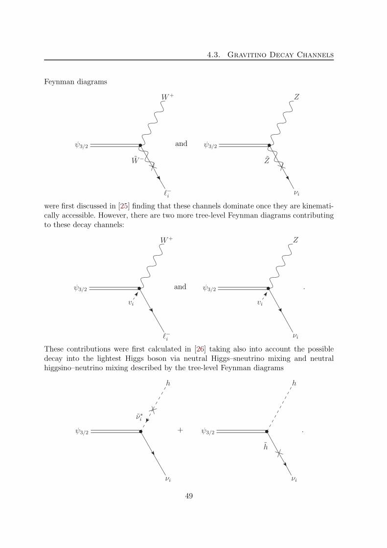
4.3. Gravitino Decay Channels
Feynman diagrams
ψ3/2
W+
W−
ℓ−i
and ψ3/2
Z
Z
νi
were first discussed in [25] finding that these channels dominate once they are kinemati-cally accessible. However, there are two more tree-level Feynman diagrams contributingto these decay channels:
ψ3/2
W+
vi
ℓ−i
and ψ3/2
Z
vi
νi
.
These contributions were first calculated in [26] taking also into account the possibledecay into the lightest Higgs boson via neutral Higgs–sneutrino mixing and neutralhiggsino–neutrino mixing described by the tree-level Feynman diagrams
ψ3/2
h
ν∗i
νi
+ ψ3/2
h
h
νi
.
49

Chapter 4. Gravitino Decays
It was found that the additional channels further decrease the branching ratio for thedecay into a photon and a neutrino, thereby reducing the strength of a monoenergeticsignal of gamma rays from gravitino decays in indirect detection experiments. Assuminga standard model-like lightest Higgs boson, the decay into the Higgs plus neutrino chan-nel contributes at the same level as the Z boson plus neutrino channel if the gravitinomass is sufficiently above the production threshold.
The calculation of all tree-level gravitino decay channels mentioned above has beenrevised in detail in [154] leading to the following results for the decay widths of thegravitino LSP decay channels with two particles in the final state:
Γ(ψ3/2 → γ νi
)≃
ξ2i m33/2
64 πM2Pl
∣∣UγZ
∣∣2 ,
Γ(ψ3/2 → Zνi
)≃ξ2i m
33/2 β
2Z
64 πM2Pl
U2ZZfZ − 8
3
mZ
m3/2
UZZ jZ +1
6hZ
,
Γ(ψ3/2 →W+ℓ−i
)≃ξ2i m
33/2 β
2W
32 πM2Pl
U2W W
fW − 8
3
mW
m3/2
UW W jW +1
6hW
,
Γ(ψ3/2 → h νi
)≃ξ2i m
33/2 β
4h
384 πM2Pl
∣∣∣∣m2
νi
m2νi−m2
h
+ sin β UH0uZ
+ cos β UH0d Z
∣∣∣∣2
,
(4.21)
where ξi ≡ vi/v is the dimensionless number parametrizing the strength of bilinear R-parity breaking and the mixing parameters UγZ , UZZ , UW W , UH0
uZand UH0
d Zare those
defined in Section 3.3. In these expressions the kinematic functions βX , fX , jX and hXare given by
βX = 1− m2X
m23/2
, fX = 1 +2
3
m2X
m23/2
+1
3
m4X
m43/2
,
jX = 1 +1
2
m2X
m23/2
, hX = 1 + 10m2
X
m23/2
+m4
X
m43/2
. (4.22)
The same results hold for the conjugate processes ψ3/2 → γ νi, ψ3/2 → Z νi, ψ3/2 →W−ℓ+i and ψ3/2 → h νi. Indeed, these decay channels represent the complete set ofall possible two-body final states in the decay of the gravitino LSP in theories withbilinear R-parity violation according to the interaction Lagrangian from equation (4.11).All other two-particle final states that one could imagine are kinematically forbidden:Decays into sleptons, squarks, neutralinos, charginos and gluinos are obviously forbiddensince the gravitino represents the lightest supersymmetric particle. But also the decaysinto the heavier neutral Higgs bosons and the charged Higgs bosons are impossible sincetheir masses are in general larger than the corresponding higgsino masses.
Although there are no additional two-particle final states that have been neglected inprevious calculations, it turns out that there are two more tree-level Feynman diagramscontributing to the gravitino decay into a W boson and a charged lepton, and that into
50

4.3. Gravitino Decay Channels
a Z boson and a neutrino. These contributions come from 4-vertex diagrams with aHiggs VEV at one of the legs:
ψ3/2
W+
H−d
vd
ℓ−i
and ψ3/2
Z
H0u, d
vu, d
νi
.
For the calculation of the contribution of these diagrams we refer to Appendix E. Incases where the µ parameter is large compared to the gaugino mass parameters (as in thediscussions in [26,30,154]) these additional diagrams do not contribute significantly sincethe higgsino–gaugino mixing parameters are suppressed in that case (cf. equations (3.76),(3.77) and (3.88)). Since these contributions are of the same form as the diagrams with asneutrino VEV, the final results can be altered in a simple way to include this correction.The complete set of tree-level two-body decay widths is then given by
Γ(ψ3/2 → γ νi
)≃
ξ2i m33/2
64 πM2Pl
∣∣UγZ
∣∣2 ,
Γ(ψ3/2 → Zνi
)≃ξ2i m
33/2 β
2Z
64 πM2Pl
U2ZZfZ +
1
6
∣∣∣1 + sβ UH0uZ
− cβ UH0d Z
∣∣∣2
hZ
−8
3
mZ
m3/2
UZZ
(1 + sβ ReUH0
uZ− cβ ReUH0
d Z
)jZ
, (4.23)
Γ(ψ3/2 →W+ℓ−i
)≃ξ2i m
33/2 β
2W
32 πM2Pl
U2W W
fW +1
6
∣∣∣1−√2 cβ UH−
d W
∣∣∣2
hW
−8
3
mW
m3/2
UWW
(1−
√2 cβ ReUH−
d W
)jW
,
Γ(ψ3/2 → h νi
)≃ξ2i m
33/2 β
4h
384 πM2Pl
∣∣∣∣m2
νi+ 1
2m2
Z cos 2β
m2h −m2
νi
+ 2 sin β UH0uZ
+ 2 cos β UH0d Z
∣∣∣∣2
.
In the result for the Higgs channel we also included a correction since we neglected theD-term contribution to the sneutrino VEV in our previous calculation in [154]. Thisaffected also the mixing that was assumed between the lightest Higgs particle and thesneutrinos (see Section 3.3).
51

Chapter 4. Gravitino Decays
4.3.2 Three-Body Decays
Recently it has been pointed out that below the threshold for the production of themassive electroweak gauge bosons the three-body decays involving virtual gauge bosonshave to be taken into account [75]. The decay widths of the channels ψ3/2 → Z∗ ν → f f νand ψ3/2 → W+∗
ℓ− → f f ′ ℓ− were first calculated in [201]. In this thesis we revise thiscalculation in detail and in addition calculate the contributions from virtual photonsand virtual lightest Higgs bosons, i.e. contributions from the three-body decay diagramsψ3/2 → γ∗ ν → f f ν and ψ3/2 → h∗ ν → f f ν.
ψ3/2 → γ∗/Z∗ ν → f f ν
At tree level there are five diagrams contributing to the decay of a gravitino into afermion-antifermion pair and a neutrino via an intermediate photon or Z boson:
ψ3/2
f
f
γ, Z
γ, Z
νi
+ ψ3/2
f
f
Z
vi
νi
and in addition the diagrams coming from the 4-vertex with a Higgs VEV that werealso discussed for the two-body decay:
ψ3/2
f
f
Z
H0u, d
vu, d
νi
.
Although there are in principle additional interference effects from the virtual exchangeof the lightest Higgs boson, we discuss that process separately. This is justified since the
52

4.3. Gravitino Decay Channels
Higgs exchange process is strongly suppressed below the threshold by the small Higgs–fermion couplings. In addition, there exists an interference for decay into the specificfinal state ℓ+i ℓ
−i νi since it can proceed via the photon, Z and Higgs channels, but also via
the W channel. In the calculation presented here, however, we did not take into accountthis exceptional case.
We present the calculation of the decay width corresponding to the Feynman dia-grams above in detail in Appendix E of this thesis. Here we directly show the resultfor the differential decay width with respect to s and t, where s is the invariant massof the two fermions f and f and t is the invariant mass of the neutrino and one of thefermions. Neglecting the masses of the final state particles we find5
dΓ(ψ3/2 → γ∗/Z∗ νi → f f νi
)
ds dt≃ ξ2i
1536 π3m53/2M
2Pl
[e2Q2
s
∣∣UγZ
∣∣2
×(3m6
3/2
(1 + 2
m2f
s
)+m2
3/2
(s2 + 8 s t+ 6 t2 + 6m2
f
(m2
f − s− 2 t))
− 3m43/2 (s+ 2 t)− s
(s2 + 2 s t+ 2 t2 + 2m2
f (m2f − 2 t)
))
+gZ
(s−m2Z)
2+m2
Z Γ2Z
gZ s U
2ZZ
((CV − CA)
2(3m4
3/2 − s2)
×(m2
3/2 − s− 2 t)+(C2
V + C2A
) (m2
3/2
(2 s2 + 8 s t+ 6 t2
)− 2 s (s+ t)2
) )
− 2 gZ sm3/2mZ UZZ
(1 + sβ ReUH0
uZ− cβ ReUH0
d Z
)
×(− 2CV CA
(3m2
3/2 − s) (m2
3/2 − s− 2 t)
+(C2
V + C2A
) (3m4
3/2 − 2m23/2 (s+ t)− s2 + 2 s t+ 2 t2
))(4.24)
+ 2 gZ m2Z
∣∣∣1 + sβ UH0uZ
− cβ UH0d Z
∣∣∣2 (
− 2m23/2 sCV CA
(m2
3/2 − s− 2 t)
+(C2
V + C2A
) (m4
3/2 (2 s+ t)−m23/2
(2 s2 + 2 s t+ t2
)+ s t (s+ t)
) )
− 2 eQ(ReUγZ
(m2
Z − s)+ ImUγZ mZ ΓZ
)
×(UZZ
(CV
(3m6
3/2 − 3m43/2 (s+ 2 t) +m2
3/2
(s2 + 8 s t+ 6 t2
)
− s(s2 + 2 s t+ 2 t2
) )− CA
(3m4
3/2 − s2) (m2
3/2 − s− 2 t) )
−m3/2mZ
(1 + sβ ReUH0
uZ− cβ ReUH0
d Z
)
×(CV
(3m4
3/2 − 2m23/2 (s+ t)− s2 + 2 s t+ 2 t2
)
5In the case of virtual photon exchange the effect of nonvanishing final state fermion masses cannotbe neglected since that could lead to a divergent propagator. Therefore, we will keep track of fermionmasses for the pure photon channel.
53

Chapter 4. Gravitino Decays
− CA
(3m2
3/2 − s) (m2
3/2 − s− 2 t) ))
],
where gZ ≡ g/ cos θ is the gauge coupling of the Z boson, Q is the charge of the finalstate fermions, and CV and CA are the coefficients of the V −A structure of the Z bosonvertex with two fermions:
CV =1
2T 3 −Q sin2 θW and CA = − 1
2T 3 . (4.25)
After integrating over the kinematically allowed range of t, 0 . t . m23/2 − s, we find
the following differential decay rate:6
dΓ(ψ3/2 → γ∗/Z∗ νi → f f νi
)
ds
≃ξ2i m
33/2 β
2s
768 π3M2Pl
[e2Q2
s
∣∣UγZ
∣∣2 fs
√
1− 4m2
f
s
(1 + 2
m2f
s
)
+gZ
(s−m2Z)
2+m2
Z Γ2Z
gZ U
2ZZs(C2
V + C2A
)fs
− 8
3
mZ
m3/2
gZ UZZ
(1 + sβ ReUH0
uZ− cβ ReUH0
d Z
)s(C2
V + C2A
)js (4.26)
+1
6gZ m
2Z
∣∣∣1 + sβ UH0uZ
− cβ UH0d Z
∣∣∣2 (C2
V + C2A
)hs
+ eQ(ReUγZ
(m2
Z − s)+ ImUγZ mZ ΓZ
)CV
×(2UZZ fs +
8
3
mZ
m3/2
(1 + sβ ReUH0
uZ− cβ ReUH0
d Z
)js
)].
In this expression the kinematic functions βs, fs, js and hs are defined corresponding tothe kinematic functions in the two-body decays (see equation(4.22)):
βs = 1− s
m23/2
, fs = 1 +2
3
s
m23/2
+1
3
s2
m43/2
,
js = 1 +1
2
s
m23/2
, hs = 1 + 10s
m23/2
+s2
m43/2
. (4.27)
The total decay width can be obtained by integrating the above differential decay widthover the invariant mass range 0 ≤ s ≤ m2
3/2.7
6For the pure photon channel we integrate over the range of t given by equation (D.14), onlyneglecting the neutrino mass.
7To avoid a divergent propagator in the case of virtual photon exchange one should integrate overthe range 4m2
f ≤ s ≤ m23/2 in that case (see equation (D.13)).
54
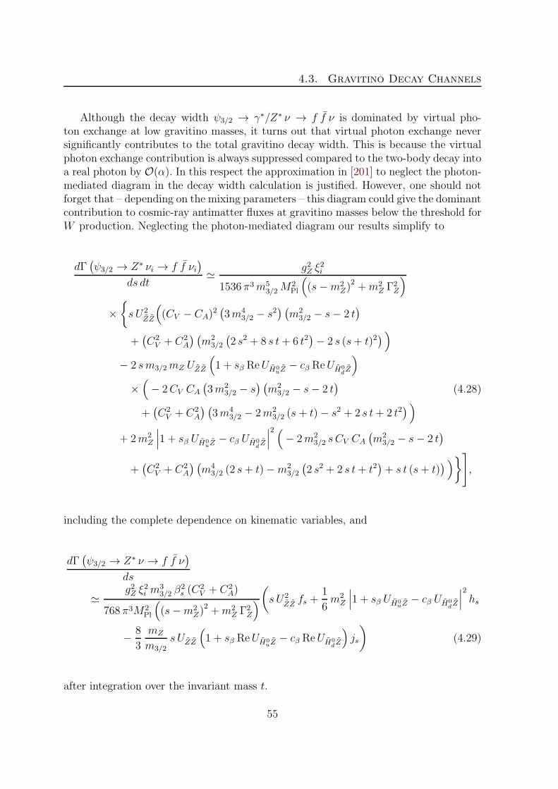
4.3. Gravitino Decay Channels
Although the decay width ψ3/2 → γ∗/Z∗ ν → f f ν is dominated by virtual pho-ton exchange at low gravitino masses, it turns out that virtual photon exchange neversignificantly contributes to the total gravitino decay width. This is because the virtualphoton exchange contribution is always suppressed compared to the two-body decay intoa real photon by O(α). In this respect the approximation in [201] to neglect the photon-mediated diagram in the decay width calculation is justified. However, one should notforget that – depending on the mixing parameters – this diagram could give the dominantcontribution to cosmic-ray antimatter fluxes at gravitino masses below the threshold forW production. Neglecting the photon-mediated diagram our results simplify to
dΓ(ψ3/2 → Z∗ νi → f f νi
)
ds dt≃ g2Z ξ
2i
1536 π3m53/2M
2Pl
((s−m2
Z)2+m2
Z Γ2Z
)
×s U2
ZZ
((CV − CA)
2(3m4
3/2 − s2) (m2
3/2 − s− 2 t)
+(C2
V + C2A
) (m2
3/2
(2 s2 + 8 s t+ 6 t2
)− 2 s (s+ t)2
) )
− 2 sm3/2mZ UZZ
(1 + sβ ReUH0
uZ− cβ ReUH0
d Z
)
×(− 2CV CA
(3m2
3/2 − s) (m2
3/2 − s− 2 t)
(4.28)
+(C2
V + C2A
) (3m4
3/2 − 2m23/2 (s+ t)− s2 + 2 s t+ 2 t2
) )
+ 2m2Z
∣∣∣1 + sβ UH0uZ
− cβ UH0d Z
∣∣∣2 (
− 2m23/2 sCV CA
(m2
3/2 − s− 2 t)
+(C2
V + C2A
) (m4
3/2 (2 s+ t)−m23/2
(2 s2 + 2 s t+ t2
)+ s t (s+ t)
) )],
including the complete dependence on kinematic variables, and
dΓ(ψ3/2 → Z∗ ν → f f ν
)
ds
≃g2Z ξ
2i m
33/2 β
2s (C
2V + C2
A)
768 π3M2Pl
((s−m2
Z)2+m2
Z Γ2Z
)(s U2
ZZfs +
1
6m2
Z
∣∣∣1 + sβ UH0uZ
− cβ UH0d Z
∣∣∣2
hs
− 8
3
mZ
m3/2
s UZZ
(1 + sβ ReUH0
uZ− cβ ReUH0
d Z
)js
)(4.29)
after integration over the invariant mass t.
55

Chapter 4. Gravitino Decays
ψ3/2 →W ∗ ℓ → f f ′ ℓ
At tree level there are three Feynman diagrams contributing to the decay of a gravitinointo two fermions and a charged lepton:
ψ3/2
f
f ′
W+
W−
ℓ−i
+ ψ3/2
f
f ′
W+
vi
ℓ−i
and in addition the diagram coming from the 4-vertex with a down-type Higgs VEVthat was also discussed for the two-body decay:
ψ3/2
f
f ′
W+
H−d
vd
ℓ−i
.
For the detailed calculation of the decay width corresponding to the Feynman diagramsabove we refer to Appendix E of this thesis. Here we directly show the result for thedifferential decay width with respect to s and t, where s is the invariant mass of thetwo fermions f and f ′ and t is the invariant mass of the charged lepton and one of the
56

4.3. Gravitino Decay Channels
fermions. Neglecting the masses of the final state particles we find
dΓ(ψ3/2 →W+∗ ℓ−i → f f ′ ℓ−i
)
ds dt
≃ g2 ξ2i
1536 π3m53/2M
2Pl
((s−m2
W )2+m2
W Γ2W
)
×[s U2
WW
(m2
3/2 − t) (
3m43/2 − 3m2
3/2 (s+ t) + s t)
− 2 sm3/2mW UW W
(1−
√2 cβ ReUH−
d W
)
×(3m4
3/2 −m23/2 (3 s+ 4 t) + t (2 s+ t)
)
+m2W
∣∣∣1−√2 cβ UH−
d W
∣∣∣2
×(m4
3/2 (3 s+ t)−m23/2
(3 s2 + 4 s t+ t2
)+ s t (s+ t)
) ].
(4.30)
After integrating over the kinematically allowed range of t we find the following differ-ential decay rate:
dΓ(ψ3/2 →W+∗ ℓ−i → f f ′ ℓ−i
)
ds
≃g2 ξ2i m
33/2 β
2s
1536 π3M2Pl
((s−m2
W )2+m2
W Γ2W
)(s U2
WWfs (4.31)
− 8
3
mW
m3/2
s UW W
(1−
√2 cβ ReUH−
d W
)js +
1
6m2
W
∣∣∣1−√2 cβ UH−
d W
∣∣∣2
hs
),
where the kinematic functions βs, fs, js and hs are those given in equation (4.27).
ψ3/2 → h∗ ν → f f ν
At tree level there are two Feynman diagrams contributing to the decay of a gravitinointo a fermion–antifermion pair and a neutrino via an intermediate lightest Higgs boson:
ψ3/2
f
f
h
ν∗i
νi
+ ψ3/2
f
f
h
h
νi
.
57

Chapter 4. Gravitino Decays
As for the other decay channels we present the detailed calculation in Appendix E.Neglecting the masses of the final state particles the differential decay width of thisprocess is found to be
dΓ(ψ3/2 → h∗ ν → f f ν
)
ds dt
≃ξ2i m3/2m
2f β
3s s
∣∣∣∣m2
νi+ 1
2m2
Z cos 2β
s−m2νi
+ 2 sin β UH0uZ
+ 2 cos β UH0d Z
∣∣∣∣2
6144 π3M2Pl v
2((s−m2
h)2+m2
h Γ2h
) .
(4.32)
The differential decay width is independent of the invariant mass t and thus the in-tegration over t just results in an additional factor of (m2
3/2 − s) = m23/2 βs leading
to
dΓ(ψ3/2 → h∗ ν → f f ν
)
ds
≃ξ2i m
33/2m
2f β
4s s
∣∣∣∣m2
νi+ 1
2m2
Z cos 2β
s−m2νi
+ 2 sin β UH0uZ
+ 2 cos β UH0d Z
∣∣∣∣2
6144 π3M2Pl v
2((s−m2
h)2+m2
h Γ2h
) .
(4.33)
The conjugate processes ψ3/2 → γ∗/Z∗ νi → f f νi, ψ3/2 → W−∗ℓ+i → f f ′ ℓ+i and
ψ3/2 → h∗ νi → f f νi have identical decay widths.
Discussion
We observe that our results for the three-body decay widths presented in equations (4.28)and (4.30) (neglecting the contributions from higgsino–neutrino mixing) do not coincidewith those presented in [201]. Therefore, we carefully repeated our calculations andadditionally verified that above the thresholds for W±, Z and h boson production ourresults for the decay widths coincide with the two-body decay results of equation (4.23)in the narrow-width approximation (NWA), i.e. we replaced the boson propagator bythe limiting value
limΓX/mX→0
1
(s−m2X)
2+m2
XΓ2X
=π
mX ΓXδ(s−m2
X) (4.34)
and verified that
ΓNWA
(ψ3/2 → Z∗νi → f f νi
)= Γ
(ψ3/2 → Z νi
)× BR
(Z → f f
),
ΓNWA
(ψ3/2 →W+∗
ℓ−i → f f ′ ℓ−i)= Γ
(ψ3/2 →W+ℓ−i
)× BR
(W+ → f f ′) .
(4.35)
Thus we are confident that our calculations are correct. The same holds for the three-body decay via virtual Higgs exchange, where we checked that
ΓNWA
(ψ3/2 → h∗νi → f f νi
)= Γ
(ψ3/2 → h νi
)× BR
(h→ f f
). (4.36)
58

4.3. Gravitino Decay Channels
For a derivation of the results in the narrow-width approximation we refer to Ap-pendix E.
It might thus well be that the details of the final state particle spectra presentedin [201] are not completely correct, although their conclusions for phenomenologicalstudies are not expected to change qualitatively.
Let us shortly comment on additional possible Feynman diagrams for gravitino de-cays into three final state particles. One class of these additional contributions are decaysvia trilinear R-parity breaking Yukawa couplings as induced by the field redefinitions inSection 3.3. As these decays always involve off-shell propagators of sleptons or squarkswe expect their contribution to be negligible compared to the resonantly enhanced two-body decay channels.
In addition, at sufficiently large gravitino masses, the gravitino can decay into an on-shell three-body final state including gauge bosons and leptons, namely ψ3/2 →W+W−νiand ψ3/2 → Z W+ℓ−i . These processes can proceed via the nonabelian 4-vertex includingtwo massive gauge bosons and a gaugino that mixes with the neutrinos or chargedleptons. In addition, various other diagrams involving off-shell propagators contributeto these processes.8 However, also in this case we expect the additional contributions tothe total gravitino decay width to be negligible compared to the resonantly enhancedtwo-body decay channels.
To conclude this section we want to give an estimate of the dependence of thegravitino lifetime on the amount ofR-parity breaking. For this reason we give a numericalresult for the prefactor of the lifetime in two-body decays into a photon and a neutrinoor an antineutrino:
τγ νi/νi3/2 =
32 πM2Pl
ξ2i m33/2
∣∣UγZ
∣∣2 ≃ 3.8× 1026 s
(10−9
ξi
)2(100GeV
m3/2
)31∣∣UγZ
∣∣2 . (4.37)
Thus a gravitino with a mass around the electroweak scale naturally has a lifetimeof the order of 1026–1027 s for an R-parity violating parameter in the center of thecosmologically favored range. This is exactly the order of magnitude of lifetimes leadingto interesting prospects for indirect dark matter searches (see Chapter 5).
4.3.3 Gravitino Branching Ratios
In order to calculate the cosmic-ray signals from gravitino decays we need to know thebranching ratios of the different gravitino decay channels. These can easily be obtainedfrom the decay widths we calculated before by dividing the partial decay widths by thetotal gravitino decay width:
BR (X) =Γ(ψ3/2 → X
)
Γtot, where Γtot =
∑
X
Γ(ψ3/2 → X
). (4.38)
8The diagrams contributing to the process ψ3/2 → W+W−νi have been discussed in a differentcontext in [202].
59

Chapter 4. Gravitino Decays
In the calculation of the gravitino branching ratios the R-parity violating parameter ξidrops out. Therefore, the branching ratios present a general result that can be obtainedwithout knowledge of the exact size of ξi. By contrast, there is a significant dependenceon the mixing parameters that enter in the calculation of decay widths.
Assuming that the gaugino masses are at the same order (M1 ∼ M2 ∼M1/2), we findthe following proportionalities for the mixing parameters from the approximate formulaein equations (3.74) to (3.77), (3.87) and (3.88):
UγZ , UZZ ∝ mZ
M1/2
and UH0uZ, UH0
d Z∝ m2
Z
M1/2 µ(4.39)
for the neutralino–neutrino mixing parameters, and
UW W ∝ mW
M2
and UH−d W ∝ m2
W
M2 µ(4.40)
for the chargino–charged lepton mixing parameters.9 This means that for large gravitinomasses, where the gaugino and Higgs mass parameters are necessarily much larger thanthe gauge boson masses, the Feynman diagrams involving a mass mixing are suppressedcompared to those that do not include mixing parameters. Therefore, the two-bodydecay into a photon and a neutrino will always be suppressed above the threshold forelectroweak gauge boson production. The other decay channels then have the asymptoticdecay widths:
1
2Γ(ψ3/2 →W+ℓ−i
)= Γ
(ψ3/2 → Zνi
)= Γ
(ψ3/2 → h νi
)=
ξ2i m33/2
384 πM2Pl
. (4.41)
In addition, all higgsino mixing parameters are suppressed compared to the gauginomixings by an additional factor of O(mZ/W/µ). Therefore, they typically contributeeven less. In particular, in the decoupling limit, which we employ as our standard setup,these mixings are negligible for all gravitino masses.
We want to fix now a standard choice of parameters for the following phenomenolog-ical studies in this thesis. From mediation mechanisms of supersymmetry breaking likegravity mediation it is expected that the soft mass parameters are proportional to thegravitino mass. Therefore, we choose the gaugino masses to be given by M1 = 1.5m3/2
and M2 = 1.89M1. The latter relation corresponds to the typical assumption of uni-versal gaugino masses at a high unification scale. Similarly, we choose mνi = 2m3/2 forthe masses of sneutrinos. This choice is not very critical as the dependence of the decaywidths on the sneutrino mass is very mild. In addition, we take tan β = 10 and a largeµ parameter. Technically, we set µ = Max
(10mZ , 10m3/2
)in order to guarantee that
we are in the decoupling limit for all choices of the gravitino mass. For the mass of thestandard model-like lightest Higgs boson we assume a low value ofmh = 115GeV, whichis right above the LEP limit and favored by electroweak precision data [81].
9The chargino–charged lepton mixing parameters only depend on the wino mass parameter M2.
60

4.3. Gravitino Decay Channels
ΓΝi
Γ*Z*Νi
Wi
W*i
ZΝi
hΝi
10 100 1000 10000
10-5
10-4
10-3
0.01
0.1
1
Gravitino Mass HGeVL
BranchingRatio
Figure 4.1: Branching ratios of the different gravitino decay channels as a function of thegravitino mass in the decoupling limit for our standard choice of parameters. The dashedlines show the result taking into account only the two-body decays of the gravitino, whilethe solid lines show the full result including three-body decays.
The result for the gravitino branching ratios using this set of parameters is presentedin Figure 4.1 as a function of the gravitino mass and in Table 4.1 for several exemplaryvalues of the gravitino mass. As expected from the calculation in the narrow-widthapproximation, the branching ratios derived from the three-body decay widths agreewell with the two-body decay results above the thresholds for on-shell production of W ,Z and Higgs bosons. In addition, we observe the asymptotic behavior of the branchingratios at large gravitino masses as expected from the discussion of the mixing parametersabove.
Below the thresholds for on-shell boson production we see the effects of the off-shell processes. In particular the virtual W channel can play a role at gravitino massesslightly below theW production threshold. At lower masses, however, it drops fast in thisscenario. In that region actually the virtual photon exchange channel is not completelynegligible. It dominates the decay rate in the channel ψ3/2 → γ∗/Z∗ νi → f f νi in thissetup and is then the only source of different final state particles than the monoenergeticphoton and neutrino. The virtual Higgs channel plays no role at all below the thresholdsince only light fermions are kinematically allowed in the final state and their couplingsto the Higgs boson are suppressed by their small masses.
In [201] it was found that the two-body decay into photon and neutrino could bestrongly suppressed compared to the three-body decays via virtual gauge bosons. This
61
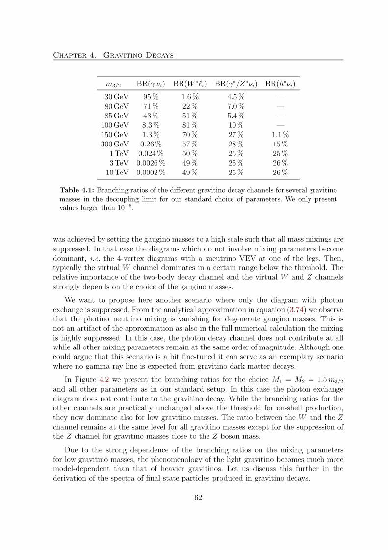
Chapter 4. Gravitino Decays
m3/2 BR(γ νi) BR(W ∗ℓi) BR(γ∗/Z∗νi) BR(h∗νi)
30GeV 95% 1.6% 4.5% —80GeV 71% 22% 7.0% —85GeV 43% 51% 5.4% —100GeV 8.3% 81% 10% —150GeV 1.3% 70% 27% 1.1%300GeV 0.26% 57% 28% 15%
1TeV 0.024% 50% 25% 25%3TeV 0.0026% 49% 25% 26%10TeV 0.0002% 49% 25% 26%
Table 4.1: Branching ratios of the different gravitino decay channels for several gravitinomasses in the decoupling limit for our standard choice of parameters. We only presentvalues larger than 10−6.
was achieved by setting the gaugino masses to a high scale such that all mass mixings aresuppressed. In that case the diagrams which do not involve mixing parameters becomedominant, i.e. the 4-vertex diagrams with a sneutrino VEV at one of the legs. Then,typically the virtual W channel dominates in a certain range below the threshold. Therelative importance of the two-body decay channel and the virtual W and Z channelsstrongly depends on the choice of the gaugino masses.
We want to propose here another scenario where only the diagram with photonexchange is suppressed. From the analytical approximation in equation (3.74) we observethat the photino–neutrino mixing is vanishing for degenerate gaugino masses. This isnot an artifact of the approximation as also in the full numerical calculation the mixingis highly suppressed. In this case, the photon decay channel does not contribute at allwhile all other mixing parameters remain at the same order of magnitude. Although onecould argue that this scenario is a bit fine-tuned it can serve as an exemplary scenariowhere no gamma-ray line is expected from gravitino dark matter decays.
In Figure 4.2 we present the branching ratios for the choice M1 = M2 = 1.5m3/2
and all other parameters as in our standard setup. In this case the photon exchangediagram does not contribute to the gravitino decay. While the branching ratios for theother channels are practically unchanged above the threshold for on-shell production,they now dominate also for low gravitino masses. The ratio between the W and the Zchannel remains at the same level for all gravitino masses except for the suppression ofthe Z channel for gravitino masses close to the Z boson mass.
Due to the strong dependence of the branching ratios on the mixing parametersfor low gravitino masses, the phenomenology of the light gravitino becomes much moremodel-dependent than that of heavier gravitinos. Let us discuss this further in thederivation of the spectra of final state particles produced in gravitino decays.
62
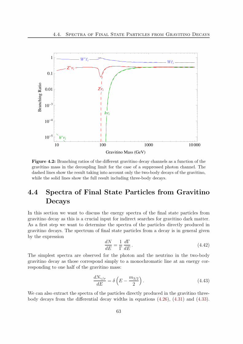
4.4. Spectra of Final State Particles from Gravitino Decays
Z*Νi
WiW*i
ZΝi
hΝi
h*Νi
10 100 1000 10000
10-5
10-4
10-3
0.01
0.1
1
Gravitino Mass HGeVL
BranchingRatio
Figure 4.2: Branching ratios of the different gravitino decay channels as a function of thegravitino mass in the decoupling limit for the case of a suppressed photon channel. Thedashed lines show the result taking into account only the two-body decays of the gravitino,while the solid lines show the full result including three-body decays.
4.4 Spectra of Final State Particles from Gravitino
Decays
In this section we want to discuss the energy spectra of the final state particles fromgravitino decay as this is a crucial input for indirect searches for gravitino dark matter.As a first step we want to determine the spectra of the particles directly produced ingravitino decays. The spectrum of final state particles from a decay is in general givenby the expression
dN
dE=
1
Γ
dΓ
dE. (4.42)
The simplest spectra are observed for the photon and the neutrino in the two-bodygravitino decay as those correspond simply to a monochromatic line at an energy cor-responding to one half of the gravitino mass:
dNγ/ν
dE= δ
(E − m3/2
2
). (4.43)
We can also extract the spectra of the particles directly produced in the gravitino three-body decays from the differential decay widths in equations (4.26), (4.31) and (4.33).
63
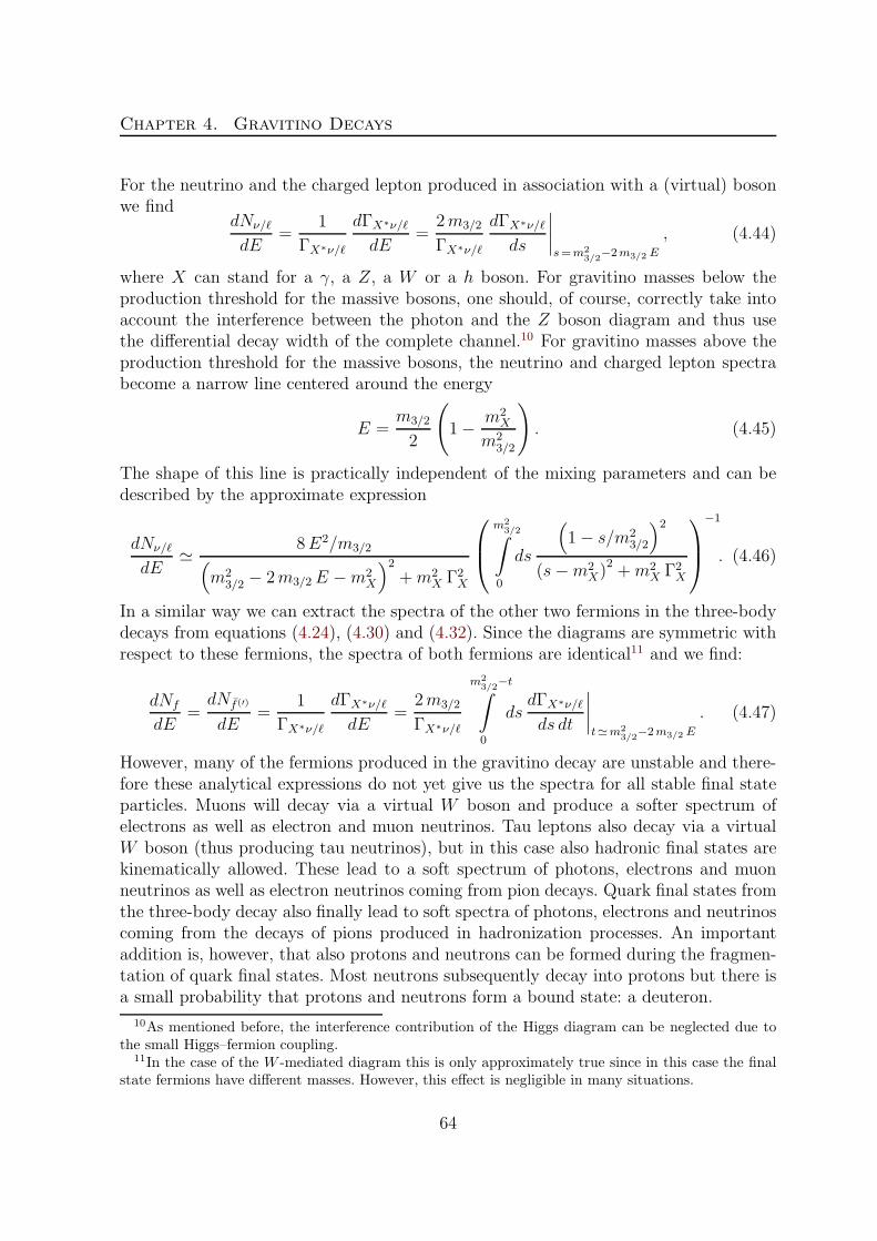
Chapter 4. Gravitino Decays
For the neutrino and the charged lepton produced in association with a (virtual) bosonwe find
dNν/ℓ
dE=
1
ΓX∗ν/ℓ
dΓX∗ν/ℓ
dE=
2m3/2
ΓX∗ν/ℓ
dΓX∗ν/ℓ
ds
∣∣∣∣s=m2
3/2−2m3/2 E
, (4.44)
where X can stand for a γ, a Z, a W or a h boson. For gravitino masses below theproduction threshold for the massive bosons, one should, of course, correctly take intoaccount the interference between the photon and the Z boson diagram and thus usethe differential decay width of the complete channel.10 For gravitino masses above theproduction threshold for the massive bosons, the neutrino and charged lepton spectrabecome a narrow line centered around the energy
E =m3/2
2
(1− m2
X
m23/2
). (4.45)
The shape of this line is practically independent of the mixing parameters and can bedescribed by the approximate expression
dNν/ℓ
dE≃ 8E2/m3/2(
m23/2 − 2m3/2E −m2
X
)2+m2
X Γ2X
m23/2∫
0
ds
(1− s/m2
3/2
)2
(s−m2X)
2+m2
X Γ2X
−1
. (4.46)
In a similar way we can extract the spectra of the other two fermions in the three-bodydecays from equations (4.24), (4.30) and (4.32). Since the diagrams are symmetric withrespect to these fermions, the spectra of both fermions are identical11 and we find:
dNf
dE=dNf(′)
dE=
1
ΓX∗ν/ℓ
dΓX∗ν/ℓ
dE=
2m3/2
ΓX∗ν/ℓ
m23/2
−t∫
0
dsdΓX∗ν/ℓ
ds dt
∣∣∣∣t≃m2
3/2−2m3/2 E
. (4.47)
However, many of the fermions produced in the gravitino decay are unstable and there-fore these analytical expressions do not yet give us the spectra for all stable final stateparticles. Muons will decay via a virtual W boson and produce a softer spectrum ofelectrons as well as electron and muon neutrinos. Tau leptons also decay via a virtualW boson (thus producing tau neutrinos), but in this case also hadronic final states arekinematically allowed. These lead to a soft spectrum of photons, electrons and muonneutrinos as well as electron neutrinos coming from pion decays. Quark final states fromthe three-body decay also finally lead to soft spectra of photons, electrons and neutrinoscoming from the decays of pions produced in hadronization processes. An importantaddition is, however, that also protons and neutrons can be formed during the fragmen-tation of quark final states. Most neutrons subsequently decay into protons but there isa small probability that protons and neutrons form a bound state: a deuteron.
10As mentioned before, the interference contribution of the Higgs diagram can be neglected due tothe small Higgs–fermion coupling.
11In the case of the W -mediated diagram this is only approximately true since in this case the finalstate fermions have different masses. However, this effect is negligible in many situations.
64

4.4. Spectra of Final State Particles from Gravitino Decays
Deuteron and Antideuteron Formation A usual approach to model the forma-tion of deuterons and antideuterons in particle physics processes is the coalescencemodel [203]. In this prescription a deuteron is formed when a proton and a neutroncome sufficiently close in momentum space, i.e. when the absolute value of the differ-ence of their four-momenta is below a threshold coalescence momentum:
|pp − pn| < p0 . (4.48)
We adopt here a value for the coalescence momentum of p0 = 160MeV that was ex-tracted by the authors of [77] to match the data on deuteron and antideuteron productionin hadronic Z decays of the ALEPH experiment at the LEP collider [204].
A common approximation for deuteron formation is that the distributions of neutronsand protons in momentum space are spherically symmetric and uncorrelated. This leadsto an energy distribution of deuterons that can be directly calculated from the spectraof neutrons and protons [77, 205]:
dNd
dTd=
2
3p30
md
mpmn
1√T 2d + 2md Td
dNp
dTp
dNn
dTn, (4.49)
where Tp = Tn = Td/2 are the kinetic energies of protons, neutrons and deuterons. Aspointed out in [77], this approximation is qualitatively wrong and significantly under-estimates the deuteron yield in high-energetic processes. This is due to the fact, thatthe distributions of neutrons and protons are actually neither spherically symmetric noruncorrelated. For instance, in the decay of a gravitino into a Z boson and a neutrinothe probability for the formation of a deuteron in the fragmentation of the Z bosonshould be independent of the gravitino mass. This is due to the fact that the Z bo-son fragmentation process is always the same as viewed from the Z boson rest frame.However, the spherical approximation of the coalescence model gives a lower yield ofdeuterons for larger gravitino masses, since the protons and neutrons are distributedover a larger phase space for higher injection energies. Another qualitatively wrong be-havior of this approximation is the possibility that protons and neutrons from distinctgravitino decays form a deuteron. This is due to the fact that the simply the spectra ofprotons and neutrons are multiplied, while in principle the coalescence condition on thefour-momenta of protons and neutrons should be applied on an event-by-event basis.
This can be achieved in a Monte Carlo simulation of the decay process. For instance,using an event generator like PYTHIA one can simulate the hadronization of massivegauge and Higgs bosons explicitly requiring the neutrons not to decay. One can then ap-ply event by event the coalescence condition on the protons and neutrons. This methodleads to plausible results, e.g. the deuteron yield in the gravitino decay to final statesincludingW , Z or Higgs bosons is independent of the gravitino mass. This method, how-ever, requires a lot of computing time to generate smooth spectra as only one deuteronor antideuteron is produced in O(104) decay processes.
Let us now turn to the discussion of final state particle spectra from the decay ofgravitinos with masses above the threshold for the on-shell production of massive gaugeand Higgs bosons.
65

Chapter 4. Gravitino Decays
Particle type Z νi We Wµ Wτ h νi
γ 17.0 15.0 15.0 16.1 31.5e− + e+ 16.4 15.7 15.7 16.0 28.8p+ p 1.67 1.60 1.60 1.60 2.98νe + νe 16.3 14.5 15.5 15.8 29.5νµ + νµ 29.7 26.5 27.5 28.8 54.1ντ + ντ 0.23 0.22 0.22 1.22 0.23d+ d 1.1× 10⁻⁴ 1.1× 10⁻⁴ 1.1× 10⁻⁴ 1.1× 10⁻⁴ 3.6× 10⁻⁴
Table 4.2: Multiplicities of stable final state particles from gravitino decays after thefragmentation of the different on-shell intermediate particles simulated with PYTHIA.
Two-Body Decay Spectra In cases where the gravitino mass is large enough toproduce on-shell massive bosons, the decay process is well described by a two-bodydecay with subsequent fragmentation of the boson (cf. the discussion in the last section).Since in this case the phase-space distribution is independent of the structure of thesquared matrix element, the whole decay process including the hadronization can bemimicked using the event generator PYTHIA 6.4 [206] although the gravitino is notincluded in that program. We employ a similar treatment of the implementation of thisprocess as described in [154] and simulate O(105) events per decay channel for severalvalues of the gravitino mass to generate the spectra of photons, electrons, positrons,electron neutrinos and antineutrinos, and muon neutrinos and antineutrinos. In orderto generate the spectra of the less abundant protons, antiprotons, and tau neutrinosand antineutrinos, we use a higher statistics of O(106) events. For the generation ofthe spectra of deuterons and antideuterons an even higher statistics of O(107) events isused.12
The resulting particle multiplicities per single gravitino decay for the decay chan-nels ψ3/2 → Z νi, We, Wµ, Wτ and h νi are summarized in Table 4.2. Note that themultiplicities are independent of the gravitino mass. We observe that similar amountsof particles are produced in the Z νi and Wℓi decay channels while the numbers areroughly twice as high for the decay channel into h νi. In addition, the amount of pho-tons, electrons and electron neutrinos is similar for every single decay channel. Thenumber of muon neutrinos is larger by a factor of two compared to the other particles.By contrast, the number of protons is lower by one order of magnitude and the numberof tau neutrinos is low in all channels. As discussed above, the probability for deuteronformation is extremely low.
Several features of these numbers can be understood qualitatively or even quantita-tively: Electrons, electron neutrinos and muon neutrinos are mainly produced in pionand subsequent muon decays and therefore the number of muon neutrinos is a factor of
12The spectra of deuterons and antideuterons from gravitino decay were kindly provided by GillesVertongen.
66

4.4. Spectra of Final State Particles from Gravitino Decays
ΝΤ
ΝΜ
Νe
dH´ 10
3L
p
e
Γ
Ν
e
Νi
Ψ32 ® Z Νi , m32 = 100 GeV
0.01 0.1 1 10 100
0.001
0.01
0.1
1
10
100
Kinetic Energy HGeVL
Spectrum
dNdHlog10TL
ΝΤ
ΝΜ
Νe
dH´ 10
3L
p
e
Γ
Ν
e
Νi
Ψ32 ® Z Νi , m32 = 1 TeV
0.01 0.1 1 10 100 1000
0.001
0.01
0.1
1
10
100
Kinetic Energy HGeVL
Spectrum
dNdHlog10TL
Figure 4.3: Spectra of stable final state particles from the decay of a gravitino with amass of 100GeV (left) or 1TeV (right) in the channel ψ3/2 → Zνi. The features of thesespectra are discussed in the text.
two higher. We expect a factor of two less neutral pions compared to charged pions, thusexplaining that the number of photons is at the same level as the number of electrons.Tau neutrinos are practically only produced in direct decays of gauge bosons and tauleptons. A smaller contribution comes also from B meson decays. The larger particlemultiplicities in the h νi channel are probably due to the dominant Higgs decay intopairs of bottom quarks. Therefore, we expect more hadronic activity compared to theother channels leading to a larger number of final state particles.
The differences between the three Wℓi channels exclusively come from the decay ofthe hard leptons in the respective decay channels. While the electron only contributesa single electron to the final spectrum, the muon decay produces a muon neutrino, anelectron neutrino and an electron. The tau decay is more complicated, but we expect anadditional tau neutrino as well as ∼ 1 e, νe, ∼ 2 νµ and ∼ 1 γ which is in good agreementwith the simulation.
In Figures 4.3–4.7 we present the energy spectra of photons, electrons, protons,deuterons and the different neutrino flavors for the gravitino two-body decay channelsψ3/2 → Z νi, We, Wµ, Wτ and h νi obtained from the PYTHIA simulation. Note thatthe deuteron spectra are multiplied by a factor of 103 to increase their visibility. Itis also important to note that these spectra are independent of the choice of mixingparameters as the phase-space distribution of the final state particles is completely fixedby the on-shell condition. Let us discuss in the following the features of these spectra.
Figure 4.3 shows the spectra from the decay channel ψ3/2 → Z νi for two exemplaryvalues of the gravitino mass: m3/2 = 100GeV and m3/2 = 1TeV. For the lower mass,slightly above the production threshold, there are particularly prominent features close
67

Chapter 4. Gravitino Decays
ΝΤ
ΝΜ
Νe
dH´ 10
3L
p
e
Γ
f
e
Ψ32 ®W e , m32 = 100 GeV
0.01 0.1 1 10 100
0.001
0.01
0.1
1
10
100
Kinetic Energy HGeVL
Spectrum
dNdHlog10TL
ΝΤ
ΝΜ
Νe
dH´ 10
3L
p
e
Γ
f
e
Ψ32 ®W e , m32 = 1 TeV
0.01 0.1 1 10 100 1000
0.001
0.01
0.1
1
10
100
Kinetic Energy HGeVL
Spectrum
dNdHlog10TL
Figure 4.4: Spectra of stable final state particles from the decay of a gravitino with amass of 100GeV (left) or 1TeV (right) in the channel ψ3/2 → We. The features of thesespectra are discussed in the text.
to the high-energy end of the spectrum at E = m3/2/2. In this range the spectra ofelectrons and neutrinos are dominated by the direct decay of the Z boson into theseparticles. For comparison we show the spectra of electrons and neutrinos calculatedaccording to the three-body decay formula in equation (4.47) as light dotted curves. Inaddition we show the prominent spectrum of the hard neutrino produced directly in thegravitino decay in association with the Z boson calculated according to equation (4.44).The soft spectra of photons, electrons and neutrinos are mainly produced from piondecays after the hadronization of quark final states. At the lowest energies there is acontribution to the electron and electron neutrino spectra from neutron decay that leadsto a departure from the factor of one half compared to muon neutrinos. Tau neutrinosare exclusively produced in rather hard processes, so the soft part of their spectrumis suppressed compared to the other particles. Protons are mainly produced in thedecays of heavy baryons and neutrons. The heavy baryons are typically produced earlyduring hadronization thus producing a harder spectrum of protons compared to thoseof particles coming from pion decay.
A gravitino mass of 1TeV represents the typical spectra when threshold effects arenegligible. The hard neutrino forms a narrow line at the end of the spectrum, while thespectra of electrons and neutrinos directly produced in the three-body decay becomesofter due to the larger available phase-space. The soft part of the spectrum comingfrom fragmentation processes is roughly scale invariant.
For the decay channel ψ3/2 → We the situation is similar as the soft part of thespectra is determined by practically the same hadronization processes (see Figure 4.4).The hard part shows prominent features of the hard electron and the electrons and
68

4.4. Spectra of Final State Particles from Gravitino Decays
ΝΤ
ΝΜ
Νe
dH´ 10
3L
p
e
Γ
f
Ψ32 ®W Μ , m32 = 100 GeV
0.01 0.1 1 10 100
0.001
0.01
0.1
1
10
100
Kinetic Energy HGeVL
Spectrum
dNdHlog10TL
ΝΤ
ΝΜ
Νe
dH´ 10
3L
p
e
Γ
f
Ψ32 ®W Μ , m32 = 1 TeV
0.01 0.1 1 10 100 1000
0.001
0.01
0.1
1
10
100
Kinetic Energy HGeVL
Spectrum
dNdHlog10TL
Figure 4.5: Spectra of stable final state particles from the decay of a gravitino with amass of 100GeV (left) or 1TeV (right) in the channel ψ3/2 → Wµ. The features of thesespectra are discussed in the text.
neutrinos directly produced in the three-body decay. For the shape of the electron linewe observe a remarkable agreement of the calculation according to equation (4.44) andthe PYTHIA simulation. One comment is in order in this case: The spectra simulatedin the described way (and also the analytical calculations) do not take into account theeffect of final state radiation. This effect would lead to a softening of the high-energypart of the electron spectrum – in particular of the line features – and at the same timeharden the high-energetic photon spectrum. We plan to include this effect in a futuretreatment of these decay processes.
For the decay channels ψ3/2 →Wµ and Wτ we get a slightly different result coming,respectively, from the decay of the hard muon and the decay of the hard tau lepton (seeFigures 4.5 and 4.6). The muon decay produces a hard contribution to the spectra ofelectrons as well as electron and muon neutrinos close to the position of the muon linefrom the direct decay. For a gravitino mass of 1TeV we clearly observe the enhancementof the lepton spectra compared to the contribution directly from the three-body decayas shown by the curve from the analytical calculation according to equation (4.47). Inthe case of tau decay a prominent hard contribution of tau neutrinos is generated closeto the position of the tau line from the direct decay. Also in this case the enhancement ofthe tau neutrino spectrum at the high-energy end is clearly visible form3/2 = 1TeV. Theeffect on the photon, electron, and electron and muon neutrino spectra is also slightlyvisible.
In Figure 4.7 we show the final state particle spectra for the decay channel ψ3/2 → h νifor gravitino masses of 150GeV and 1TeV. In this case the situation is a bit different.Due to the coupling of the Higgs boson to fermion masses, mainly pairs of bottom quarks
69

Chapter 4. Gravitino Decays
ΝΤ
ΝΜ
Νe
dH´ 10
3L
p
e
Γ
f
Ψ32 ®W Τ , m32 = 100 GeV
0.01 0.1 1 10 100
0.001
0.01
0.1
1
10
100
Kinetic Energy HGeVL
Spectrum
dNdHlog10TL
ΝΤ
ΝΜ
Νe
dH´ 10
3L
p
e
Γ
f
Ψ32 ®W Τ , m32 = 1 TeV
0.01 0.1 1 10 100 1000
0.001
0.01
0.1
1
10
100
Kinetic Energy HGeVL
Spectrum
dNdHlog10TL
Figure 4.6: Spectra of stable final state particles from the decay of a gravitino with amass of 100GeV (left) or 1TeV (right) in the channel ψ3/2 → Wτ . The features of thesespectra are discussed in the text.
ΝΤ
ΝΜ
Νe
dH´ 10
3L
p
e
Γ
Νi
Ψ32 ® h Νi , m32 = 150 GeV
0.01 0.1 1 10 100
0.001
0.01
0.1
1
10
100
Kinetic Energy HGeVL
Spectrum
dNdHlog10TL
ΝΤ
ΝΜ
Νe
dH´ 10
3L
p
e
Γ
Νi
Ψ32 ® h Νi , m32 = 1 TeV
0.01 0.1 1 10 100 1000
0.001
0.01
0.1
1
10
100
Kinetic Energy HGeVL
Spectrum
dNdHlog10TL
Figure 4.7: Spectra of stable final state particles from the decay of a gravitino with amass of 150GeV (left) or 1TeV (right) in the channel ψ3/2 → h νi assuming a mass ofmh = 115GeV for the standard model-like lightest Higgs boson. The features of thesespectra are discussed in the text.
70

4.4. Spectra of Final State Particles from Gravitino Decays
are produced directly in the three-body decay for mh = 115GeV. Therefore, the spectraare generally softer at the high-energy end of the spectrum. There is, however, also acontribution from pairs of tau leptons and virtual W bosons that leads to a relativelyhard spectrum of tau neutrinos.
Three-Body Decay Spectra For gravitino masses below the threshold for gaugeand Higgs boson production, i.e. when the boson propagators are off-shell, the situationis significantly more complicated. Although we can calculate the energy spectra of allparticles directly produced in the gravitino decay, one needs to employ event generatorsto simulate the hadronization of colored final state particles.
In contrast to the two-body decays this situation cannot be easily mimicked in anevent generator like PYTHIA since the kinematic distributions are not solely determinedby phase space but depend explicitly on the matrix element of the process.13 In addition,PYTHIA only treats 2 → 1 and 2 → 2 processes and is not capable of handling thephase space of generic processes with three or more final state particles. Only a limitednumber of specific three-body decay processes like muon decay is explicitly included inPYTHIA [206].
The usual treatment of processes with multiparticle final states is to calculate thematrix element and the phase-space distribution of the process with a matrix elementgenerator like MadGraph/MadEvent [207,208] or WHIZARD [209]. These tools producea table of events where the four-momenta of all particles from the direct decay are listedaccording to the kinematic distribution given by the matrix element and the phase space.This output is subsequently handed over to PYTHIA where the hadronization processesand particle decays are treated.
For this method, of course, the particle physics model needs to be implemented inthe matrix element generator. This is a bit problematic for the case of the gravitinoin models with R-parity violation. Although MadGraph and WHIZARD are able tohandle spin-3/2 particles,14 the violation of R parity leads to changes in the behaviorof the model that cannot be implemented in an easy way by slightly modifying theexisting model files. It is, however, planned to extend the capabilities of Madgraph inthis direction in the future [213].
Another approach could be to implement the model using a Feynman rules generatorlike FeynRules [214] that allows to generate model files for matrix element generatorslike MadGraph and WHIZARD directly from the Lagrangian of the theory. In thiscase, however, there is no publically available implementation of spin-3/2 particles yet,although the authors are working on this topic [215]. Thus one can expect that it will bepossible to treat the phenomenology of R-parity violating gravitino dark matter decayswith the help of automated calculations in the near future.
13In this respect, it is unclear to us how the gravitino three-body decay spectra were derived in [201]using PYTHIA.
14In the case of MadGraph a support for gravitinos and goldstinos has only recently been added [210,211]. For the current status of gravitino implementation in MadGraph see also [212].
71
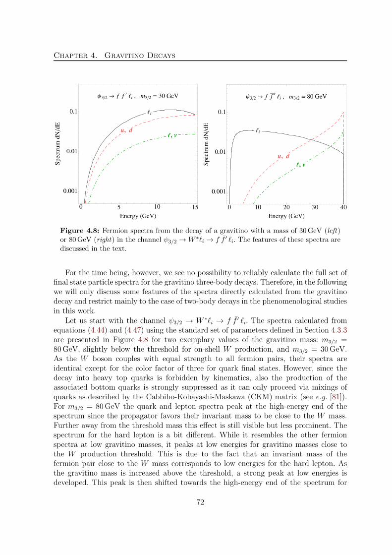
Chapter 4. Gravitino Decays
, Νu, d
i
Ψ32 ® f f¢i , m32 = 30 GeV
0 5 10 15
0.001
0.01
0.1
Energy HGeVL
Spectrum
dNdE
, Ν
u, d
i
Ψ32 ® f f¢i , m32 = 80 GeV
0 10 20 30 40
0.001
0.01
0.1
Energy HGeVL
Spectrum
dNdE
Figure 4.8: Fermion spectra from the decay of a gravitino with a mass of 30GeV (left)or 80GeV (right) in the channel ψ3/2 → W ∗ℓi → f f ′ ℓi. The features of these spectra arediscussed in the text.
For the time being, however, we see no possibility to reliably calculate the full set offinal state particle spectra for the gravitino three-body decays. Therefore, in the followingwe will only discuss some features of the spectra directly calculated from the gravitinodecay and restrict mainly to the case of two-body decays in the phenomenological studiesin this work.
Let us start with the channel ψ3/2 → W ∗ℓi → f f ′ ℓi. The spectra calculated fromequations (4.44) and (4.47) using the standard set of parameters defined in Section 4.3.3are presented in Figure 4.8 for two exemplary values of the gravitino mass: m3/2 =80GeV, slightly below the threshold for on-shell W production, and m3/2 = 30GeV.As the W boson couples with equal strength to all fermion pairs, their spectra areidentical except for the color factor of three for quark final states. However, since thedecay into heavy top quarks is forbidden by kinematics, also the production of theassociated bottom quarks is strongly suppressed as it can only proceed via mixings ofquarks as described by the Cabbibo-Kobayashi-Maskawa (CKM) matrix (see e.g. [81]).For m3/2 = 80GeV the quark and lepton spectra peak at the high-energy end of thespectrum since the propagator favors their invariant mass to be close to the W mass.Further away from the threshold mass this effect is still visible but less prominent. Thespectrum for the hard lepton is a bit different. While it resembles the other fermionspectra at low gravitino masses, it peaks at low energies for gravitino masses close tothe W production threshold. This is due to the fact that an invariant mass of thefermion pair close to the W mass corresponds to low energies for the hard lepton. Asthe gravitino mass is increased above the threshold, a strong peak at low energies isdeveloped. This peak is then shifted towards the high-energy end of the spectrum for
72

4.4. Spectra of Final State Particles from Gravitino Decays
Ν
ud
Νi
Ψ32 ® f f Νi , m32 = 30 GeV
0 5 10 15
0.001
0.01
0.1
Energy HGeVL
Spectrum
dNdE
Ν
u
d
Νi
Ψ32 ® f f Νi , m32 = 80 GeV
0 10 20 30 40
0.001
0.01
0.1
Energy HGeVL
Spectrum
dNdE
Figure 4.9: Fermion spectra from the decay of a gravitino with a mass of 30GeV (left)or 80GeV (right) in the channel ψ3/2 → Z∗νi → f f νi. The features of these spectra arediscussed in the text.
larger gravitino masses (cf. equation (4.45) and Figure 4.4). Note that in all cases thespectrum is suppressed as the energy goes to zero since the phase-space factor βs vanisheswhen the invariant mass of the fermion pair, s, equals the gravitino mass.
Before we discuss the spectra in the channel ψ3/2 → γ∗/Z∗νi → f f νi let us firstdiscuss the case, when the virtual photon contribution is negligible. The correspondingspectra are presented in Figure 4.9. In principle the features of the spectra are thesame as for the previously discussed case, the only difference being that the couplingof the Z boson to fermions is not universal. In fact, it depends on the electromagneticcharge and the third component of the weak isospin of the particles via the coefficientsof the V − A structure of the Z coupling (see equation (4.25)). This leads to slightlydifferent spectra for up- and down-type quarks as well as neutrinos and charged leptons.Another difference to the W channel is that the pair production of bottom quarks is notsuppressed.
In the case where the virtual exchange of a photon contributes, the spectra will besignificantly more complicated. As the decay width depends on the fermion masses dueto the singular behavior of the photon propagator, we expect different spectra for thedifferent fermion generations. The spectra calculated taking into account the dependenceon the fermion masses are presented in Figure 4.10. These spectra are a superpositionof the photon and Z exchange contributions and their interference. However, at a gra-vitino mass of 30GeV the photon channel strongly dominates for our standard choiceof parameters and even at m3/2 = 80GeV the Z channel is subdominant. The mostprominent feature is the strongly peaked spectrum of the hard neutrino at one half ofthe gravitino mass, coming from the preference of a close to massless photon in the
73

Chapter 4. Gravitino Decays
Ν
e
Μ
Τd
s
b
u
c
Νi
Ψ32 ® f f Νi , m32 = 30 GeV
0 5 10 15
0.0001
0.001
0.01
0.1
Energy HGeVL
Spectrum
dNdE
Ν
e
Μ
Τd s
b
u
c
Νi
Ψ32 ® f f Νi , m32 = 80 GeV
0 10 20 30 40
0.001
0.01
0.1
Energy HGeVL
Spectrum
dNdE
Figure 4.10: Fermion spectra from the decay of a gravitino with a mass of 30GeV (left)or 80GeV (right) in the channel ψ3/2 → γ∗/Z∗νi → f f νi. The features of these spectraare discussed in the text.
propagator. In particular for larger gravitino masses, there is a notable contributionfrom the Z channel to the low-energy tail of the neutrino spectrum.
The reason for the rather flat spectra of the other fermions is less obvious, though thecontribution at low energies certainly comes from the fact that a vanishing invariant massof the fermion system is favored. Since the minimal value of the invariant mass stronglydepends on the fermion masses, the spectra of heavier generations are suppressed for allfermion species. Since neutrinos do not couple to the photon, their only contribution –apart from the hard neutrino spectrum directly produced in the gravitino decay – comesfrom the subdominant Z boson exchange and thus their spectrum is strongly suppressedcompared to the other particles. For a gravitino mass closer to the Z threshold, onecan already see the contribution of the Z channel, in particular for down-type quarks(compare the spectra in Figures 4.9 and 4.10).
The phenomenology of these decay processes for low-energetic gravitinos definitelydeserves further treatment in future work, but – as discussed above – at the momentwe see no option but to concentrate on the phenomenology of the two-body decays ofheavier gravitinos.
Gravitino Decay Spectra In real situations the final state spectra cannot be ob-served for the individual decay channels. Thus, in order to study the cosmic-ray signalsfrom gravitino decay in the following chapter, we will need the combined spectrum ofa final state particle X from all gravitino decay channels with particle X in the finalstate. Using the branching ratios of the individual channels the combined spectrum is
74

4.4. Spectra of Final State Particles from Gravitino Decays
given bydNX
dE=∑
i
Γi
Γtot× 1
Γi
dΓi
dEX=∑
i
BRi ×dNi,X
dE. (4.50)
As the flavor structure of the R-parity breaking coupling ξi is not known and since wedo not employ a model that gives a prediction for it, we will assume throughout the restof this thesis that the coupling is equivalent for all flavors. This means, in particular,that equal amounts of hard electron, muon and tau neutrinos, or electrons, muons andtau leptons are produced directly in the gravitino decay.
75

Chapter 5
Indirect Detection of Gravitino
Dark Matter
The method of indirect dark matter detection is based on the observation of cosmicrays. Typically, cosmic rays are either directly produced in astrophysical sources orin spallation processes during the propagation of cosmic rays through the interstellarmedium. However, the annihilation or decay of dark matter particles in the galactichalo or extragalactic structures produces an additional contribution to the spectra ofcosmic rays that might be observable on top of the astrophysical background. In thisintroductory part of the chapter we want to review those aspects of indirect dark mattersearches that are relevant for the case of unstable gravitino dark matter. We also want toelaborate on the differences between the case of a decaying dark matter candidate, likethe gravitino in models with broken R-parity, and annihilating dark matter candidates,like the well-studied case of weakly-interacting massive particles (WIMPs). For moregeneral discussions on the topic of indirect dark matter detection we refer the reader toextensive reviews in the literature [3, 4, 9, 216, 217].
5.1 Indirect Searches for Dark Matter
As we have seen in Section 2.2, there is compelling evidence that dark matter makes upa significant part of the energy density of the universe, actually at a level of five timesthe contribution of baryonic matter. That means that a particle dark matter candidateexplaining this observation will have an average number density of
nDM =ΩDM ρcmDM
≃ 1.1× 10⁻³
(1TeV
mDM
)m−3 (5.1)
on cosmological scales. When these dark matter particles decay, they produce intermedi-ate standard model particles that eventually hadronize and/or decay into a set of stableparticles: electrons, protons, deuterons, neutrinos and their respective antiparticles aswell as gamma rays (cf. Section 4.4). The amount of particles produced per unit volume,
76

5.1. Indirect Searches for Dark Matter
time and energy is described by a source term of the form
QX(E) ≡dNX
dV dt dE=nDM
τDM
dNX
dE, (5.2)
where dNX/dE is the energy spectrum of final state particles X in the decay of the darkmatter particle. These particles will then propagate through the intergalactic mediumand might finally be observed in the fluxes of cosmic rays at the Earth. Neutrinosand gamma rays practically do not suffer deflections while traversing the intergalacticmedium and thus propagate on straight paths. By contrast, charged cosmic rays in theGeV to TeV energy range considered in this work are strongly affected by magnetic fieldsand are thus not expected to reach Earth from extragalactic distances (see Section 5.3for a discussion of the propagation of charged cosmic rays).
We can then determine the flux of gamma rays and neutrinos at the position of theEarth coming from dark matter decays at extragalactic distances. With the term ’flux’we refer here to the number of particles per unit area, time and solid angle:1
Φ ≡ dN
dAdt dΩ. (5.3)
Taking into account that the particles are propagating through an expanding universewe obtain for the differential flux of gamma rays and neutrinos the expression [154]
dΦegγ/ν
dE=
ΩDM ρc
4 π τDMmDMH0Ω1/2m
ymax∫
1
dydNγ/ν
d(y E)
y−3/2
√1 + ΩΛ/Ωm y−3
(5.4)
≃ 2.3× 10⁻⁴ (m2 s sr)−1
(1026 s
τDM
)(1TeV
mDM
) ymax∫
1
dydNγ/ν
d(y E)
y−3/2
√1 + ΩΛ/Ωm y−3
,
where y ≡ 1 + z and ymax = 1 + zdec corresponds to the time when photons/neutrinosdecoupled from the thermal plasma and started to propagate freely.2 For monochro-matic spectra of photons or neutrinos at injection, the redshift integral can be solvedanalytically and results in [22]
dΦegγ/ν
dE=
ΩDM ρc
2 π τDMm2DMH0Ω
1/2m
[1 +
ΩΛ
Ωm
(2E
mDM
)3]−1/2(
2E
mDM
)1/2
θ
(1− 2E
mDM
), (5.5)
1Later in this work, we will also use a more conventional notion of flux, namely the number ofparticles per unit area and time. This quantity will then be denoted as φ in contrast to Φ = dφ/dΩ.
2For photons this statement is not exactly true since they can produce electron pairs in collisions withphotons from the CMB or the intergalactic background light. These processes lead to a nonvanishingoptical depth for high-energy photons [218]. In addition, the expression for the redshift integral is onlyvalid in the late universe when matter and dark energy dominate the energy density of the universe.However, since the contributions from higher redshifts are practically negligible, we will actually performthe integration up to ymax = ∞.
77

Chapter 5. Indirect Detection of Gravitino Dark Matter
where θ(x) denotes the Heaviside step function.In addition to the extragalactic signal, there exists a strong contribution from a
more local source, namely dark matter decays in the Milky Way halo. In contrast tothe isotropic extragalactic signal, the halo signal is anisotropic since the source termdepends on the dark matter distribution in the galactic halo which is anisotropic asviewed from the Earth’s position in the Milky Way:
QX(E, ~l) ≡dNX(~l)
dV dE dt=nDM(~l)
τDM
dNX
dE=
ρhalo(~l)
τDMmDM
dNX
dE, (5.6)
where ~l = (s, b, l) denotes galactic coordinates in terms of the distance s to the Sun,the galactic latitude b and the galactic longitude l. The density profile of the dark halois not precisely known besides the fact that in order to fit galactic rotation curves abehavior ρ ∝ r−2 at larger radii is needed (cf. Section 2.2). The shape in the inner partsof the galaxy, however, is not completely determined by observations.
Fits to observational data, though, tend to favor a cored isothermal profile, i.e. thedensity approaches a constant value in the core of the galaxy [4]:
ρiso(r) = ρloc1 + (R⊙/rs)
2
1 + (r/rs)2 , (5.7)
where the normalization is given by the local dark matter density3 ρloc ≈ 0.3GeVcm−3,R⊙ = 8.4 kpc is the radius of the solar orbit around the galactic center and we adoptrs = 3.5 kpc for the case of the Milky Way halo. By contrast, results from numerical N-body simulations seem to favor cuspy profiles, i.e. halo profiles with a singular behaviorat the galactic center. The best-known example is the Navarro–Frenk–White (NFW)profile [220]:
ρNFW(r) = ρloc(R⊙/rs) (1 +R⊙/rs)
2
(r/rs) (1 + r/rs)2 , (5.8)
where rs = 20 kpc for the case of the Milky Way. More recent simulations, on the otherhand, favor the Einasto profile with a finite central density [221, 222]:
ρEin(r) = ρloc exp
(− 2
α
((r
rs
)α
−(R⊙rs
)α)), (5.9)
where we adopt α = 0.17 and rs = 20 kpc for the case of the Milky Way. A comparisonof the shapes of these halo profiles is presented in the left panel of Figure 5.1. The radiusr in the density profiles is given with respect to the galactic center, so we need to expressit in terms of galactic coordinates in order to calculate the cosmic-ray fluxes from darkmatter decays in the halo:
r(s, b, l) =√s2 +R2
⊙ − 2 sR⊙ cos b cos l . (5.10)
3The determination of the local dark matter density is subject to quite some uncertainty. We willuse in this work the standard value given in the text though recent determinations seem to favor avalue closer to 0.4GeVcm−3 [219].
78

5.1. Indirect Searches for Dark Matter
R
Ρloc
Einasto
NFW
Isothermal
0.01 0.1 1 10 100
0.01
0.1
1
10
100
Distance to the Galactic Center HkpcL
DarkMatterDensityHG
eVcm-3L
average
annihilation
decay
EinastoNFW
Isothermal
-180 ° -90 ° 0 ° 90 ° 180 °
0.1
1
10
Galactic Longitude
Line-
of-
SightIntegralCompared
toitsAverage
Figure 5.1: Left: Shapes of the dark matter halo density profiles listed in the text. All halomodels are normalized to the local dark matter density and reproduce the ρ ∝ r−2 behaviorat larger radii that is needed to explain the observed galactic rotation curve. The Navarro–Frenk–White profile is singular at the galactic center while the Einasto profile finallyapproaches a constant value. The isothermal profile, by contrast, exhibits an extended flatcore. Right: Comparison of the angular dependence of the line-of-sight integrals for thecases of dark matter annihilations and decays. The curves are shown for different haloprofiles and are normalized to the average value for each individual case.
Then, the differential gamma-ray and neutrino fluxes from dark matter decays in thegalactic halo observed in the direction specified by b and l are given by an integrationalong the line of sight:
dΦhaloγ/ν
dE(b, l) =
1
4 π τDMmDM
dNγ/ν
dE
∞∫
0
ds ρhalo(r(s, b, l)) . (5.11)
Due to the linear dependence of the flux on the halo density the anisotropy is not verystrong in the case of decaying dark matter. Thus we will mainly work with an averagedsignal in the following. For the same reason the dependence on the choice of the halomodel is very weak. For definiteness, we will adopt the NFW density profile as ourstandard choice in this work. In this case we can solve the integration over the haloanalytically and obtain the following result for the averaged full-sky flux:
⟨dΦhalo
γ/ν
dE
⟩=
1
4 π
π∫
−π
dl
π/2∫
−π/2
cos b dbdΦhalo
γ/ν
dE(b, l)
79

Chapter 5. Indirect Detection of Gravitino Dark Matter
=ρloc (R⊙ + rs)
4 π τDMmDM
dNγ/ν
dE
(artanh
(1
1 + rsR⊙
)−
ln(R⊙
rs)
rsR⊙
− 1− 1
2ln
(1 + 2
R⊙rs
))
≃ 1.3× 10⁻⁴ (m2 s sr)−1
(1026 s
τDM
)(1TeV
mDM
)dNγ/ν
dE. (5.12)
In the following we want to outline the differences in the indirect detection strategiesfor the cases of dark matter annihilations and decays.
Annihilating and Decaying Dark Matter We have seen before that the flux ex-pected from dark matter decays is proportional to the number density of dark matterparticles and inversely proportional to their lifetime. In the case of dark matter an-nihilations the situation is different: Since a collision of two dark matter particles isrequired, the resulting cosmic-ray flux is proportional to the square of the dark matternumber density. In addition, the annihilation rate depends on the relative velocity ofthe colliding particles and on their annihilation cross section.
Let us first discuss the dependence on the dark matter density: Since the averagepresent-day dark matter density in the universe is rather low in absolute numbers (cf.equation (5.1)) we do not expect a sizable annihilation signal from diffuse extragalacticsources at low redshifts as in the case of dark matter decays. In fact, the expected signalis very sensitive to the actual distribution of dark matter in the universe since overdenseregions significantly enhance the expected total flux. Let us demonstrate this on theexpected differential flux of gamma rays and neutrinos from dark matter annihilationsin the Milky Way halo. It is given by the following integral along the line of sight:
dΦhaloγ/ν
dE(b, l) =
〈σv〉DM
8 πm2DM
dNγ/ν
dE
∞∫
0
ds ρ2halo(r(s, b, l)) , (5.13)
where 〈σv〉DM is the thermally averaged dark matter annihilation cross section anddNγ/ν/dE is the energy spectrum of photons/neutrinos in the annihilation of two darkmatter particles. Due to the dependence on the square of the halo density, the signalfrom annihilating dark matter is strongly enhanced in the direction towards the galacticcenter, especially for cuspy halo profiles. In the right panel of Figure 5.1 we comparethe angular dependencies of the signals expected from dark matter annihilations anddecays for different halo profiles. Clearly visible is the enhancement of the signal in thegalactic center direction where the dark matter density has its maximum. In the case ofdark matter annihilations, however, the signal varies over several orders of magnitudedepending on the line of sight while in the case of decays the signal varies by less thana factor of ten. Thus the expected signal from dark matter annihilations is much moreanisotropic than that from dark matter decays and the observation of the angular de-pendence of gamma-ray or neutrino signals can be used as a strategy to discriminateannihilating and decaying dark matter particles. In addition, we observe that the ex-pected annihilation signal suffers much larger uncertainties from the choice of the haloprofile than the signal expected from decays.
80

5.1. Indirect Searches for Dark Matter
However, not only the galactic center is an important source for signals from darkmatter annihilation. Also other dense structures could emit an observable signal. Amongthese are substructures of the galactic halo that are expected from numerical simulations,the dark matter halos of dwarf galaxies in the neighborhood of the Milky Way and thedark matter concentration in galaxy clusters. But also celestial bodies like the Sun or theEarth could emit an enhanced annihilation signal if dark matter particles are capturedinside their centers by energy losses due to weak elastic scattering processes. In thiscase, however, only neutrinos could leave the dense objects and be observed.
Let us now come to the dependence on the dark matter annihilation cross section:If dark matter exists in the form of weakly interacting massive particles, the observeddark matter density is a relic from the freeze-out of WIMP annihilations in the earlyuniverse [10]. When the temperature in the early universe dropped below the WIMPmass, these particles left thermal equilibrium and efficiently annihilated with each other.However, due to the expansion of the universe their physical number density was dilutedand the annihilation process became inefficient before all WIMPs were destroyed, leavinga relic density of WIMPs that could play the role of dark matter. The annihilations ofWIMPs in the present universe are thus determined by the same annihilation crosssection that is responsible for the production of the correct relic density in the earlyuniverse. This circumstance makes the WIMP scenario very predictive, as the thermallyaveraged WIMP annihilation cross section is required to be 〈σv〉WIMP ≈ 3×10⁻²⁶ cm3 s−1
to match the observed dark matter density [10].
However, as this annihilation cross section is too small to predict observable anoma-lous contributions in cosmic-ray signals, typically a boost factor is introduced to increasethe annihilation signal. A small part of this boost factor could be accommodated byastrophysical effects like halo substructures [223], but in general an additional enhance-ment like the proposed Sommerfeld enhancement of non-relativistic annihilation crosssections is needed (see for instance [224]).
For decaying dark matter, on the other hand, the value of the lifetime is in gen-eral not directly related to the cross section determining the production in the earlyuniverse. Therefore, scenarios with decaying dark matter particles are less constrainedand in principle less predictive, but they do not rely on the assumption of additionalenhancement mechanisms to explain cosmic-ray signatures.
In the specific case of gravitino dark matter no accumulation inside astrophysicalobjects is expected since the gravitational interaction is too weak. Also, the existenceof halo substructures and large scale structures does not significantly change the signalpredictions since the average flux is not affected by inhomogeneities in the dark mat-ter distribution. Thus one can work with a gravitino distribution according to the halodensity profile for the signal from gravitino decays in the Milky Way halo and with theaverage cosmological dark matter density for the signal from gravitino decays at extra-galactic distances. In addition, there is in general no chance to observe the contributionfrom gravitino annihilations, since these are suppressed by higher orders of the Planckscale.
81

Chapter 5. Indirect Detection of Gravitino Dark Matter
In the following sections of this thesis we want to discuss the prospects for the indirectdetection of unstable gravitino dark matter in the spectra of gamma rays, charged cosmicrays and neutrinos.
5.2 Probing Gravitino DM with Gamma Rays
In this section we discuss the gamma-ray signals coming from the decay of gravitino darkmatter. Gamma rays are a very important channel to search for dark matter signals sincethey contain spectral and directional information that can be well measured. Since thegamma-ray signal expected from gravitino decays is a diffuse flux from all directionswith only mild angular dependence, it contributes to the isotropic diffuse gamma-raybackground that is often referred to as the extragalactic gamma-ray background (EGB).This is a diffuse flux of high-energetic photons that is thought to have its origin inunresolved sources like active galactic nuclei, blazars, starburst galaxies, gamma-raybursts or in truly diffuse emission (see for instance [225]). However, it is not clear thatthis flux is completely of extragalactic nature since exotic sources of diffuse emission inthe galactic halo could also contribute.
Another strategy to search for a dark matter signal is to search for gamma-raylines. Gamma rays of astrophysical origin are typically expected to have a spectrumthat follows a power law. Monochromatic signals in the spectrum are a clear sign for aparticle physics origin. Therefore, one can use the good energy resolution of gamma-rayobservatories to constrain the partial lifetime of dark matter two-body decay channelswith at least one photon in the final state.
The signals of gamma rays from the decay of gravitino dark matter in scenarioswith bilinear R-parity violation have already been studied in several works [22–27]. Inthis thesis, however, we want to employ recent data from the Large Area Telescope onthe Fermi Gamma-Ray Space Telescope (Fermi LAT) to constrain the parameters ofgravitino dark matter.
Diffuse Gamma-Ray Flux
The diffuse extragalactic gamma-ray background is overwhelmed by a diffuse componentexpected from galactic gamma-ray emission. Thus it has to be extracted in a complicatedway from gamma-ray observations by subtracting the galactic contribution as modeledby galactic cosmic-ray propagation models. This subtraction of a dominant componentcan, however, lead to large systematical uncertainties on the derived flux.
An isotropic diffuse gamma-ray component on top of the galactic emission was firstobserved by the SAS-2 satellite [226] and has since then been measured in more detail bythe Energetic Gamma Ray Experiment Telescope (EGRET) on the Compton GammaRay Observatory [227] and by Fermi LAT [66]. To reduce the foreground contamination,the galactic disc (corresponding to galactic latitudes −10 ≤ b ≤ 10) is usually excludedfrom the analysis. The extragalactic gamma-ray background amounts to roughly one
82
5.2. Probing Gravitino Dark Matter with Gamma Rays
quarter of the total diffuse flux measured away from the galactic disc.
Here we will compare the expected contribution from gravitino decays to the ex-tragalactic gamma-ray background as recently derived from Fermi LAT data [66]. Noanomalous behavior of the spectrum is observed and the data points are well describedby a power law:
E2dΦEGB
γ
dE≈ 5.5× 10⁻³
(E
GeV
)−0.41
GeV (m2 s sr)−1. (5.14)
For comparison we also show previous results obtained from data of the EGRET ex-periment [35,227]. In the original analysis of the EGRET data a power-law behavior ofthe extragalactic gamma-ray background in the energy range from 50MeV–10GeV wasfound [227]:
E2dΦEGB
γ
dE= 1.37× 10⁻²
(E
GeV
)−0.1
GeV (m2 s sr)−1. (5.15)
An independent analysis using an optimized cosmic-ray propagation model to matchthe observations of the galactic diffuse emission [228] led to a softer power law in theenergy range from 50MeV–2GeV [35]:
E2dΦEGB
γ
dE= 6.8× 10⁻³
(E
GeV
)−0.32
GeV (m2 s sr)−1. (5.16)
However, in this analysis an excess of gamma rays above the power law was observedat energies above 2GeV stimulating the interpretation of this anomaly as a signal fromdark matter annihilations or decays (see for instance [25, 40]). In particular, it wasfound that the gamma-ray signal from gravitino dark matter could explain the excessin the EGRET data for a gravitino mass of roughly 150GeV and a lifetime on the orderof 1026 s [25]. However, as mentioned before, although the new Fermi LAT data areconsistent with the reanalysis of the EGRET data by Strong et al. at low energies theyshow no evidence for the existence of an excess at higher energies and therefore we willuse the data only as an upper limit for the contribution from gravitino decays.
The main dark matter contribution to the diffuse gamma-ray flux at high energiescomes from photons directly produced in the decays of gravitinos. In addition, thereis a contribution from the upscattering of photons due to inverse Compton scatteringof electrons and positrons from gravitino decays on the interstellar radiation field (seee.g. [59, 229, 230]).4 In this work, however, we will only consider the prompt flux for anorder of magnitude estimate of the gamma-ray signal. The averaged gamma-ray fluxfrom gravitino decays in the galactic halo excluding the galactic disk is then calculated
4Actually, the contribution from inverse Compton scatterings dominate the low-energy tail of thegamma-ray spectrum for large gravitino masses [59].
83

Chapter 5. Indirect Detection of Gravitino Dark Matter
ì
ì
ìì ì
ìì
ì ì ì
ìì
ìà
àààà
àà
à
à
àà
æ
æ
æ
æ
æ
ææ
ææ
Τ32 = 1027 s
m32 = 100 GeV 1 TeV 10 TeV
0.1 1 10 100 1000 10000
0.0001
0.0003
0.001
0.003
0.01
0.03
Energy HGeVL
E2´Gam
ma-
Ray
FluxHG
eVm-2s-
1sr-1L
ì EGRET HSreekumar et al.L
à EGRET HStrong et al.L
æ Fermi LAT
Figure 5.2: Diffuse gamma-ray flux from gravitino dark matter decays compared to theextragalactic gamma-ray background as derived from Fermi LAT and EGRET data. Thegravitino signal is shown for a lifetime of 1027 s and gravitino masses of 100GeV, 1TeV and10TeV. The dashed, dotted and dash-dotted lines show the power-law fits to the FermiLAT and EGRET data points.
as
⟨dΦhalo
γ
dE
⟩
|b|> 10
=1
2 π (1− sin π/18)
π∫
−π
dl
π/2∫
π/18
cos b dbdΦhalo
γ
dE(b, l)
≃ 1.2× 10⁻⁸ (cm2 s sr)−1
(1026 s
τ3/2
)(1TeV
m3/2
)dNγ
dE.
(5.17)
In addition, we consider the isotropic extragalactic contribution according to equa-tion (5.4) so that the total diffuse gamma-ray signal expected from gravitino decaysis calculated as
dΦγ
dE=
⟨dΦhalo
γ
dE
⟩
|b|> 10
+dΦeg
γ
dE. (5.18)
In Figure 5.2 we compare the contribution of gamma rays from the decay of gravitinodark matter to the observed extragalactic gamma-ray background as derived from FermiLAT [66] and EGRET data [35, 227]. For the gravitino signal we choose a lifetime of1027 s and three exemplary masses: 100GeV, 1TeV and 10TeV. Additionally, we adopt
84

5.2. Probing Gravitino Dark Matter with Gamma Rays
an energy resolution of σ(E)/E = 10% to estimate the sensitivity of Fermi LAT tospectral features [231]. Technically we apply the energy resolution by a convolution ofthe gamma-ray spectrum with a Gaussian distribution:
dΦGaussγ
dE=
1√2 π σ(E)
∞∫
0
dE ′ exp
(−1
2
(E −E ′
σ(E)
)2)dΦγ
dE ′ . (5.19)
We clearly see the gamma-ray line at the high-energy end of the spectrum for lowgravitino masses. For higher masses, where the gravitino two-body decay into a photonand a neutrino is suppressed, this contribution vanishes practically completely and thegamma-ray flux is dominated by the soft contributions from gauge and Higgs bosonfragmentation. As the Fermi LAT data do not exhibit any spectral features, the gravitinodecay contribution to the flux can only be subdominant. In the following we will presentlimits on the gravitino lifetime obtained from diffuse gamma-ray data and searches forgamma-ray lines.
Lifetime Bound from the Diffuse Flux and from Photon Lines
We estimate a bound on the gravitino lifetime by requiring that the prompt gamma-ray flux from gravitino decays does not overshoot the error bars of the Fermi LATmeasurement of the extragalactic gamma-ray background. This bound is rather conser-vative since we neglect the possible contribution from astrophysical backgrounds in thederivation of the lifetime limit.
In addition, a strong upper limit on the gravitino lifetime can be deduced from asearch for photon lines by the Fermi LAT collaboration [67]. Their analysis covers thefull sky excluding the galactic disc (|b| < 10) but taking also into account a patch of20 × 20 around the galactic center, where a strongly enhanced signal is expected forthe case of annihilating dark matter. We take their limits on the decay width into atwo-photon final state in the energy range 30–200GeV and apply it to the case of thegravitino two-body decay into a photon and a neutrino. In order to calculate a lifetimelimit for the gravitino we multiply with the appropriate branching ratio and rescale theirlifetime limits by a factor of one half since we have a single-photon final state:
τ3/2 ≥ BR(ψ3/2 → γ νi
)× τγγ
2. (5.20)
Recently, in an independent analysis using Fermi LAT data, these limits have beenextended to cover the energy range 1–500GeV [232].5 The authors give separate limitsdeduced from a full-sky analysis excluding the galactic disc and from an analysis usinga region around the galactic center. In addition, the specific case of a decay channelinto a photon and a neutrino is discussed. Thus we derive upper limits on the gravitino
5This energy range has been corrected to 1–300GeV in the published version, but that does notaffect our discussion.
85

Chapter 5. Indirect Detection of Gravitino Dark Matter
excluded by diffuse flux
excluded by line searches
1 10 100 1000 10000
1024
1025
1026
1027
1028
1029
Gravitino Mass HGeVL
GravitinoLifetim
eHsL
Fermi LAT diffuse flux
Vertongen et al. photon line
Fermi LAT photon line
Figure 5.3: Bounds on the gravitino lifetime from observations of the diffuse extragalacticgamma-ray background and from photon line searches.
lifetime in the following way:
τ3/2 ≥ BR(ψ3/2 → γ νi
)× τhaloγν and τ3/2 ≥ BR
(ψ3/2 → γ νi
)× τ centerγν . (5.21)
We will only use the bounds from the full-sky analysis since they are stronger than thebounds from the central region of the Milky Way for decaying dark matter particles. Theresults of the conservative lifetime estimate from the diffuse flux and the limits derivedfrom the photon-line searches are presented in Figure 5.3. For gravitino masses belowthe W boson mass, the branching fraction for the gamma-ray line is close to 100% inour standard gravitino scenario (cf. Section 4.3.3) and a very strong lower limit on thegravitino lifetime on the order of τ3/2 & 5 × 1028 s is obtained from line searches. Atlarger masses the branching ratio for the line drops quickly, reducing the significance ofthe lifetime limit. The comparison of the continuum signal with the diffuse extragalacticgamma-ray background leads to an estimate for the lower limit of the gravitino lifetimeat a constant level around τ3/2 & 3× 1026 s. In our standard scenario this limit becomesmore important than the limit from line searches for gravitino masses above a fewhundred GeV.
If the photon line is suppressed for some reason (see Section 4.3.3), the low gravitinomass region is significantly less constrained since line searches do not provide a lifetimelimit in that case. There will, however, still be a constraint on the continuum gamma-rayflux expected from three-body decays. Thus the lifetime limit derived from the diffuseflux is expected to remain at the same order of magnitude.
86
5.3. Probing Gravitino Dark Matter with Cosmic-Ray Antimatter
5.3 Probing Gravitino Dark Matter with Cosmic-
Ray Antimatter
In this section we want to discuss the signals expected from gravitino dark matterdecays in the spectra of charged cosmic rays. Also in this case, related studies have beenpresented before in the literature [26, 27, 29].
While cosmic-ray particles are abundantly produced in astrophysical sources, an-timatter particles are thought to be practically only produced in spallation processesinvolving high-energetic cosmic rays impinging on the interstellar medium. Therefore,one typically expects a charge-symmetric exotic contribution from dark matter to appearfirst as an anomalous component in the spectra of cosmic-ray antiparticles.
As mentioned earlier in this chapter, the propagation of charged cosmic rays throughthe Milky Way halo is much more complicated than in the case of gamma rays andneutrinos. In order to predict the contributions from gravitino dark matter decays tothe spectra of charged cosmic rays one thus needs to have a detailed understanding ofthe effects of cosmic-ray propagation. In the following we will therefore give a shortoverview of the propagation of charged particles. For a more extensive discussion andfurther references we refer to [216].
Propagation of Charged Cosmic Rays While charged cosmic rays traverse thegalactic halo, they are deflected by Alfven waves, the irregularities of the galactic mag-netic field. In the case of the Milky Way the magnetic turbulence is strong and thus theeffect of multiple deflections can be described by space diffusion with a coefficient
K(E) = K0 β (R/GV)δ , (5.22)
where R = pc/(Ze) and β = v/c are, respectively, the rigidity and the velocity of thecosmic-ray particle, δ is a spectral index, and K0 is a normalization coefficient.6 TheAlfven waves drift inside the Milky Way with the Alfven velocity Va which is typicallyin the range of 20–100 km s−1. This drift of the magnetic irregularities leads to a smalleffect of diffusive reacceleration of cosmic rays due to second-order Fermi acceleration.This effect depends on the strength of space diffusion as well as on the velocity of thecosmic rays and their total energy:
KEE(E) =2
9V 2a
E2β
K(E). (5.23)
In addition, the galactic wind coming from the stars in the galactic disc with a velocityVC in the range of 5–15 km s−1 leads to a drift of cosmic rays away from the galacticdisc.
6It is usually also assumed thatK(E) is constant throughout the diffusive halo, so there is no explicitspatial dependence.
87

Chapter 5. Indirect Detection of Gravitino Dark Matter
The values for the normalization K0 and the spectral index δ of the diffusion co-efficient, the galactic drift velocity VC , and the Alfven velocity Va can be constrainedby studying the spectra of primary cosmic rays produced in astrophysical sources andsecondary cosmic rays produced in spallation processes during propagation. In particu-lar the cosmic-ray boron-to-carbon ratio (B/C) is quite sensitive to the parameters ofcosmic-ray transport and is thus usually employed to determine the free parameters ofthe propagation model [233].
The transport equation for the cosmic-ray number density per unit kinetic energyfX(T ) = dnX/dT has the general form [234]
∂fX∂t
= ~∇ ·(K(T ) ~∇fX − ~VC(~r) fX
)− ∂
∂T
(b(T,~r) fX −KEE(T )
∂fX∂T
)+QX(T,~r) ,
(5.24)where b(T,~r) is a coefficient describing energy losses and QX(T,~r) is a source term thatdescribes particle production and depletion processes. This transport equation holds forall cosmic-ray species as long as the correct source terms and energy loss coefficientsare taken into account. A useful assumption is that the number densities of cosmic-rayparticles are in a steady state, i.e. ∂fX/∂t = 0.
The transport equation can be solved in a semi-analytical two-zone diffusion modelfor the galaxy [233]. In this approach the diffusive halo is modeled as a thick disc thatmatches the circular structure of the Milky Way. The disc of stars and gas with a heightof 2 h = 200 pc and a radius of 20 kpc lies in the middle. Above and beneath the discare confinement layers with a respective height of L = 1–15 kpc where cosmic rays aretrapped by diffusion.
The solution to the transport equation for cosmic rays originating from gravitinodark matter decay can then be expressed in the following form [29]:
fX(T ) =1
m3/2 τ3/2
∞∫
0
dT ′G(T, T ′)dNX
dT ′ , (5.25)
where dNX/dT is the source spectrum of cosmic rays from gravitino decay and G(T, T ′)is a Green’s function that accounts for the propagation through the diffusive halo andincludes all astrophysical parameters like the halo density profile. The differential fluxof cosmic rays coming from gravitino decays in the galactic halo can then be expressedas
dΦDMX
dT=vX4 π
fX(T ) , (5.26)
where vX is the velocity of the cosmic-ray particle.
Solar Modulation An additional complication for the accurate prediction of charged-cosmic-ray spectra as observed by experiments is the effect of solar modulation. Cosmic-ray particles that enter the heliosphere of the solar system are affected by the solar windof charged particles. The plasma of charged particles emitted from the sun mainly has
88
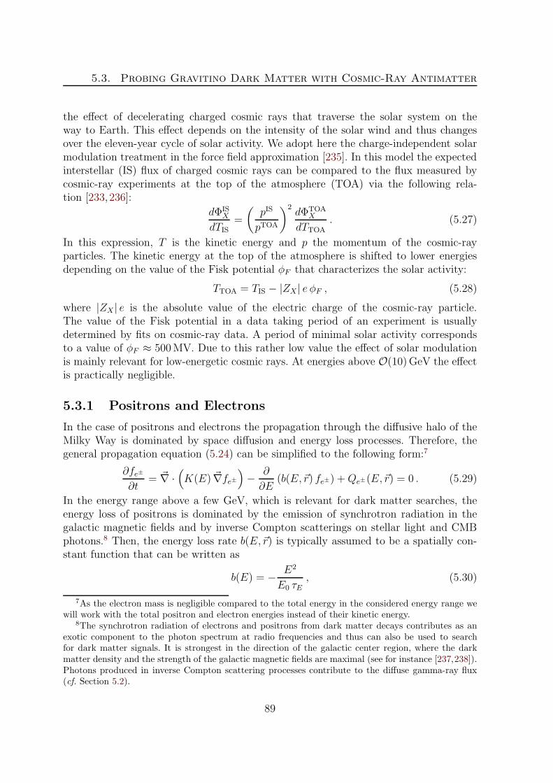
5.3. Probing Gravitino Dark Matter with Cosmic-Ray Antimatter
the effect of decelerating charged cosmic rays that traverse the solar system on theway to Earth. This effect depends on the intensity of the solar wind and thus changesover the eleven-year cycle of solar activity. We adopt here the charge-independent solarmodulation treatment in the force field approximation [235]. In this model the expectedinterstellar (IS) flux of charged cosmic rays can be compared to the flux measured bycosmic-ray experiments at the top of the atmosphere (TOA) via the following rela-tion [233, 236]:
dΦISX
dTIS=
(pIS
pTOA
)2dΦTOA
X
dTTOA. (5.27)
In this expression, T is the kinetic energy and p the momentum of the cosmic-rayparticles. The kinetic energy at the top of the atmosphere is shifted to lower energiesdepending on the value of the Fisk potential φF that characterizes the solar activity:
TTOA = TIS − |ZX | e φF , (5.28)
where |ZX | e is the absolute value of the electric charge of the cosmic-ray particle.The value of the Fisk potential in a data taking period of an experiment is usuallydetermined by fits on cosmic-ray data. A period of minimal solar activity correspondsto a value of φF ≈ 500MV. Due to this rather low value the effect of solar modulationis mainly relevant for low-energetic cosmic rays. At energies above O(10)GeV the effectis practically negligible.
5.3.1 Positrons and Electrons
In the case of positrons and electrons the propagation through the diffusive halo of theMilky Way is dominated by space diffusion and energy loss processes. Therefore, thegeneral propagation equation (5.24) can be simplified to the following form:7
∂fe±
∂t= ~∇ ·
(K(E) ~∇fe±
)− ∂
∂E(b(E,~r) fe±) +Qe±(E,~r) = 0 . (5.29)
In the energy range above a few GeV, which is relevant for dark matter searches, theenergy loss of positrons is dominated by the emission of synchrotron radiation in thegalactic magnetic fields and by inverse Compton scatterings on stellar light and CMBphotons.8 Then, the energy loss rate b(E,~r) is typically assumed to be a spatially con-stant function that can be written as
b(E) = − E2
E0 τE, (5.30)
7As the electron mass is negligible compared to the total energy in the considered energy range wewill work with the total positron and electron energies instead of their kinetic energy.
8The synchrotron radiation of electrons and positrons from dark matter decays contributes as anexotic component to the photon spectrum at radio frequencies and thus can also be used to searchfor dark matter signals. It is strongest in the direction of the galactic center region, where the darkmatter density and the strength of the galactic magnetic fields are maximal (see for instance [237,238]).Photons produced in inverse Compton scattering processes contribute to the diffuse gamma-ray flux(cf. Section 5.2).
89

Chapter 5. Indirect Detection of Gravitino Dark Matter
Model δ K0 (kpc2/Myr) L (kpc) a b
M2 0.55 0.00595 1 −0.9716 −10.012MED 0.70 0.0112 4 −1.0203 −1.4493M1 0.46 0.0765 15 −0.9809 −1.1456
Table 5.1: Parameters of cosmic-ray propagation models that correspond, respectively,to the best fit of cosmic-ray B/C data (MED) as well as the minimal (M2) or maximal(M1) positron flux compatible with cosmic-ray B/C data. Figures taken from [29,239].
where E0 = 1GeV is a reference energy and τE = 1016 s is the typical timescale ofenergy loss processes. Since high-energetic positrons are ultra-relativistic their velocityis practically given by the speed of light and their rigidity is proportional to their totalenergy. Hence, the space diffusion coefficient K(E) can be written in the form
K(E) = K0 (E/GeV)δ . (5.31)
Using equations (5.25) and (5.26) we find that the interstellar positron and electronfluxes in the vicinity of the solar system coming from gravitino dark matter decays inthe galactic halo are given by
dΦDMe±
dE=
c
4 πm3/2 τ3/2
∞∫
0
dE ′Ge±(E,E′)dNe±
dE ′ , (5.32)
where the Green’s function for the propagation of the positrons can be approximated inthe following way [29]:
Ge±(E,E′) ≃ 1016
ǫ2exp
(a + b
(ǫδ−1 − ǫ′δ−1
))θ(E ′ −E) cm−3 s . (5.33)
The energy of electrons and positrons is parametrized in the form ǫ = E/GeV andǫ′ = E ′/GeV, and the parameters a and b are given in Table 5.1 for our choice of aNavarro–Frenk–White dark matter halo density profile and different sets of propagationparameters. In practice the upper limit for the integration over the Green’s function isgiven by the maximal energy of positrons in a gravitino decay: Emax = m3/2/2. Dueto their sizable energy losses during propagation, electrons and positrons observed atEarth are expected to originate from rather local regions of the galactic halo.
Let us now discuss the signal spectra expected from gravitino decays and how theycompare to expected astrophysical backgrounds and experimental observations.
Positron Fraction From the experimental point of view it is convenient to presentmeasurements of cosmic-ray positrons and electrons in form of the positron fraction thatis defined as the ratio of the cosmic-ray positron flux and the sum of cosmic-ray electronand positron fluxes:
e+
e+ + e−≡ Φe+
Φe+ + Φe−. (5.34)
90

5.3. Probing Gravitino Dark Matter with Cosmic-Ray Antimatter
It is generally assumed that systematic uncertainties connected with the measurementmethod (for instance the detection efficiency) are similar for positrons and electrons.Therefore, these effects to a large extent cancel if the results are presented in form ofthe positron fraction (see for instance [41]).
This treatment, however, introduces more uncertainties in the theoretical prediction,since in order to calculate this quantity we will need to take into account the astrophys-ical background fluxes of positrons and electrons in addition to the contribution fromgravitino decays. A background of secondary positrons and electrons is produced bythe spallation of the interstellar medium by impinging high-energetic cosmic rays. Forthe case of electrons one expects an additional primary component directly producedin astrophysical sources. Usually the fluxes of cosmic-ray secondary positrons as well asthose of primary and secondary electrons are obtained from numerical simulations. Inthis work we will employ the parametrization of the background fluxes from [37] for thenumerical result found in [240]:
dΦsece+
dE≃ 4.5 ǫ0.7
1 + 650 ǫ2.3 + 1500 ǫ4.2(GeV cm2 s sr)−1, (5.35)
dΦprime−
dE≃ 0.16 ǫ−1.1
1 + 11 ǫ0.9 + 3.2 ǫ2.15(GeV cm2 s sr)−1, (5.36)
dΦsece−
dE≃ 0.70 ǫ0.7
1 + 110 ǫ1.5 + 600 ǫ2.9 + 580 ǫ4.2(GeV cm2 s sr)−1, (5.37)
where ǫ = E/GeV. Using these expressions we can calculate the differential positronfraction of the astrophysical background as
e+
e+ + e−(E)
∣∣∣∣bkg
=dΦsec
e+ /dE
dΦsece+ /dE + dΦprim
e− /dE + dΦsece−/dE
. (5.38)
In the case of a signal from gravitino decays the exotic contribution to the positronfraction is calculated as
e+
e+ + e−(E)
∣∣∣∣DM
=dΦDM
e+ /dE
2 dΦDMe± /dE + dΦsec
e+ /dE + dΦprime− /dE + dΦsec
e−/dE, (5.39)
where the normalization is modified due to the dark matter contribution to the totalflux of cosmic-ray electrons and positrons.
In Figure 5.4 we compare the contribution of gravitino dark matter decays to thecosmic-ray positron fraction with the expected astrophysical background and the data ofseveral experiments: the balloon-borne Matter Antimatter Superconducting Spectrom-eter (MASS-91) [241], the balloon-borne TS93 experiment [242], the balloon-borne Cos-mic AntiParticle Ring Imaging Cherenkov Experiment (CAPRICE94) [243], the balloon-borne High-Energy Antimatter Telescope (HEAT) [36], the balloon-borne HEAT-pbarexperiment [244], the Alpha Magnetic Spectrometer on Space Shuttle flight STS-91(AMS-01) [245] and the Payload for Antimatter Matter Exploration and Light-nucleiAstrophysics (PAMELA) on the Resurs-DK1 satellite [41].9
9The data tables were partly extracted from the cosmic-ray database of Strong and Moskalenko [246].
91

Chapter 5. Indirect Detection of Gravitino Dark Matter
ª
ª
ª
ª§
§
§
§
¨
¨¨
¨
¨
¨¨
¨
¨
¨
øø
ø
ø
ø
øø
øø
ì
ì
ì
ì
ì
ì
ì
ì
ìçç
ç
æææææææææææ æ
ææ
æ
æ
background
Τ32 = 1026 s
m32 = 100 GeV 1 TeV 10 TeV
1 10 100 1000 10000
0.01
0.03
0.1
0.3
Energy HGeVL
PositronFractione+He++e-L
ª MASS-91
§ TS93
¨ CAPRICE94
ø HEAT
ì AMS-01
ç HEAT-pbar
æ PAMELA
Figure 5.4: Contribution to the cosmic-ray positron fraction from the decay of gravitinodark matter in the MED propagation model compared to measurements of the positronfraction by various experiments and the expectation from astrophysical primary and sec-ondary production. The contribution from gravitino decays is shown for a lifetime of 1026 sand gravitino masses of 100GeV, 1TeV and 10TeV. In order to account for effects of solarmodulation, the data points were demodulated using values for the Fisk potential quotedby the experimental groups (cf. Table 5.2).
Since the gravitino signal and the astrophysical background calculated above cor-respond to the interstellar positron fraction, we need to correct the experimental datafor the effect of solar modulation according to equation (5.27). For flux ratios like thepositron fraction, however, the rescaling with the squared ratio of the interstellar mo-mentum and the the momentum at the top of the atmosphere cancels and only a shiftin the energy scale remains:10
e+
e+ + e−(EIS)
∣∣∣∣IS
=e+
e+ + e−(EIS − e φF )
∣∣∣∣∣
TOA
. (5.40)
The corresponding values of the Fisk potential for the data taking periods of the experi-ments measuring the positron fraction are listed in Table 5.2. We observe from Figure 5.4that the data for the positron fraction from different experiments are in approximateagreement with each other and with the expected astrophysical background, but at low
10In several works in the literature it is, however, erroneously stated that solar modulation effectscompletely cancel in the positron fraction.
92

5.3. Probing Gravitino Dark Matter with Cosmic-Ray Antimatter
Experiment Fisk potential (MV)
PAMELA 600Fermi LAT 550AMS-01 650HEAT 710
Experiment Fisk potential (MV)
BETS 550CAPRICE94 600MASS-91 550
Table 5.2: Values of the Fisk potential to account for the effect of solar modulation inthe electron and positron data sets. The figures are taken from the publications of therespective data sets (see text for the list of references).
energies the PAMELA data significantly deviate from the other experiments, in par-ticular in view of the small error bars of the PAMELA measurement. This raises thequestion if the effect of solar modulation is really independent of the sign of charge [41].Due to this source of uncertainty, data at energies below 10GeV are usually ignored inthe search for exotic contributions.
On the other hand, at energies above 10GeV the PAMELA experiment observes adrastic rise of the positron fraction, thereby supporting earlier hints for a rising positronfraction in the HEAT and AMS-01 data.11 This observation cannot be explained by thebackground of secondary positrons and is a strong indication for a primary source ofcosmic-ray positrons. It has been proposed, for instance, that supernova remnants ornearby pulsars might act as a primary source for electron-positron pairs (see e.g. [60–64]). An intriguing possibility, however, is also that the rise of the positron fractionis a signal of particle dark matter. This has led to a multitude of studies trying toexplain the data by an exotic contribution from dark matter annihilations [44,47–49] ordecays [26, 29, 50, 53–57].
As we see in Figure 5.4 gravitino decays predict a rising contribution in the positronfraction with a cutoff at half of the gravitino mass. For a gravitino mass of 100GeV,slightly above theW boson production threshold, the positron line from the direct decayis displaced from the kinematic endpoint and is visible as a second peak. This spectrumclearly cannot explain the data points. Since the rise is measured up to almost 100GeVa gravitino of at least 200GeV is needed to explain the data. In general, however, itturns out that the gravitino signal does not give a perfect fit to the data as the rise ofthe sum of signal and background contributions is typically too soft. This is due to thesoft contributions to the positron fraction from gravitino decays that comes from thefragmentation of gauge and Higgs bosons and from the decays of muons and tau leptons.This situation is improved if the R-parity breaking coupling is only in the electron flavoras the larger amount of positrons directly produced in gravitino decays leads to a harderspectrum (see also [27, 248]).
However, all explanations of the rise in the positron fraction by unstable gravitino
11The observation of a steep rise of the positron fraction at energies above 10GeV is also supportedby a recent analysis of Fermi LAT data [247].
93

Chapter 5. Indirect Detection of Gravitino Dark Matter
ª
ª
ªªªª
ª
ªª
ªªª
¨
¨¨¨¨
¨
¨¨
¨
¨¨¨
¨
¨¨¨
¨
¨¨
¨
¨
¨
çç
ç ç
ç ç
ç
ç
§
§ §§
§
§ § §
§
§
§
ø
ø
ø
øøøøø
ø
ø
ø
ì
ì
ì
ì
ì
ìììììììì
ììììììììì
ìì
ìì
ôô ô ôôô
ôô ô ô ô ô
ô
ôô
ô
ô
ô
ôô
ô
÷
÷ ÷
÷
÷
óóóóóó
óóó
òò
ò
òò
ò
ò
ò
àààààààààààààààààààààààààààààààààààààààà
à à
ææææææææææææææææ
ææææææææææææ
æ
ææ
æææ
æ
ææææ
background
Τ32 = 1026 s
m32 = 100 GeV 1 TeV 10 TeV
1 10 100 1000 10000
10
100
103
Energy HGeVL
E3´ElectronFluxHG
eV2m-2s-
1sr-1L ÷ PPB-BETS
à Fermi LATæ PAMELA
ô ATICò H.E.S.S. high energyó H.E.S.S. low energy
§ Kobayashi et al.ç BETSì AMS-01
ª MASS-91¨ CAPRICE94ø HEAT
Figure 5.5: Cosmic-ray electron flux expected from the decay of gravitino dark matter inthe MED propagation model compared to measurements of the electron (+ positron) fluxby various experiments and the expectation from astrophysical primary and secondaryproduction. The flux from gravitino decay is shown for a lifetime of 1026 s and gravitinomasses of 100GeV, 1TeV and 10TeV. In order to account for effects of solar modula-tion, the data points were demodulated using values for the Fisk potential quoted by theexperimental groups (cf. Table 5.2).
dark matter require a lifetime of the order of 1026 s that is in conflict with bounds fromsearches for a contribution to the diffuse isotropic gamma-ray flux (cf. Figure 5.3).
Electron and Positron Flux In addition to the positron fraction many experi-ments report results for the total flux of cosmic-ray electrons and positrons. In Fig-ure 5.5 we compare the contribution of gravitino dark matter decays to the cosmic-ray electron spectrum with the expected astrophysical background and the data ofMASS-91 [241], CAPRICE94 [243], HEAT [251], a balloon-borne emulsion-chamber ex-periment by Kobayashi et al. [249], the Balloon-borne Electron Telescope with Scin-tillating fibers (BETS) [252], AMS-01 [250], the balloon-borne Advanced Thin Ion-ization Calorimeter (ATIC) [254], the BETS experiment on the Polar Patrol Balloon(PPB-BETS) [253], the High Energy Stereoscopic System (H.E.S.S.) [255, 256], FermiLAT [257] and PAMELA [258].12
Many of the experiments only use calorimetric information to measure electrons and
12The data tables were partly extracted from the cosmic-ray database of Strong and Moskalenko [246].
94

5.3. Probing Gravitino Dark Matter with Cosmic-Ray Antimatter
thus cannot discriminate between electrons and positrons. In particular, the measure-ments at high energies by Fermi LAT, H.E.S.S., PPB-BETS, ATIC and Kobayashi etal. show only the combined spectrum of electrons and positrons. We observe that notall the data points agree well with each other. In particular at low energies there arestrong discrepancies among the experiments although we already accounted for solarmodulation effects. This could be another hint for the existence of charge-dependentsolar modulation effects. But also at higher energies the results from ATIC and PPB-BETS strongly deviate from other data and from the expected flux of astrophysicalorigin. In particular before the publication of the Fermi LAT results this has led tomany works trying to explain these observations in terms of exotic contributions fromdark matter [248,259–261]. However, also the Fermi LAT data are not compatible withthe power-law behavior of the expected astrophysical background, although at a smallerlevel than the ATIC and PPB-BETS data. Also this deviation has been interpreted asa signal from dark matter [58, 59] but could also be explained by pulsars [65].
Also a gravitino with a mass of the order of 1TeV can lead to an exotic contributionin the correct energy range. In this work, however, we do not try to fit the exoticcontribution from gravitino decays to the Fermi LAT data points as there are strongconstraints on this explanation from bounds on the gravitino lifetime from gamma-raydata.
Let us also comment on measurements of the positron flux. In Figure 5.6 we presentthe absolute flux of positrons expected from gravitino dark matter decays and compareit to the data of the spectrometric measurements of MASS-91 [241], CAPRICE94 [243],HEAT [251] and AMS-01 [250]. Since the signal from gravitino decay is charge-symmetricthe expected positron flux is equivalent to the electron flux presented in Figure 5.5.However, the expected astrophysical positron background is significantly lower than theelectron background and decreases faster with rising energy. Therefore, the backgroundat TeV energies is lower by two orders of magnitude and a dark matter signal thatcontributes visibly to the electron spectrum should be clearly observable in the positronspectrum. But also for smaller contributions, like a gravitino signal compatible withgamma-ray observations, a signature above the background could be observable.
Unfortunately, only measurements at rather low energies are available so far, wherethe effects of solar modulation are important. In addition, the measurements exhibitrather large uncertainties. Looking at the data for the positron fraction, one can, how-ever, expect that a significant deviation from the astrophysical background will be ob-served. It is expected that the PAMELA collaboration will eventually publish data forthe absolute flux of cosmic-ray positrons up to energies of 300GeV [258].
5.3.2 Antiprotons
In contrast to the case of positrons, energy loss processes during propagation are neg-ligible for antiprotons (and protons). Then again, the effect of galactic convection hasto be taken into account in this case and there is an additional negative contributionto the source term that comes from the annihilation of antiprotons with hydrogen and
95
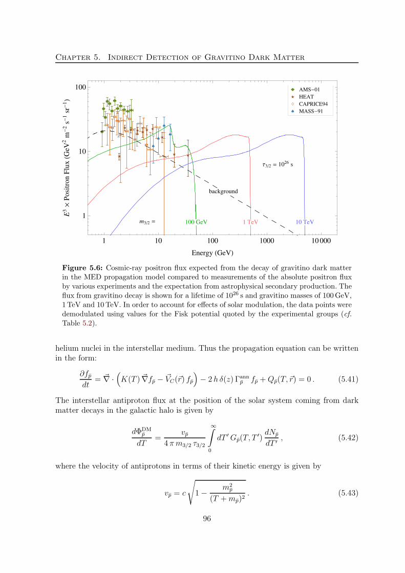
Chapter 5. Indirect Detection of Gravitino Dark Matter
ª
ª
ª
ª
¨¨¨
¨¨
¨
¨
¨
¨
¨
¨
¨
¨
¨
¨
¨
¨
¨ø
øø ø ø
ø ø
ø
ø ø
ì
ì
ì
ìì
ì
ì
ììììì
background
Τ32 = 1026 s
m32 = 100 GeV 1 TeV 10 TeV
1 10 100 1000 10000
1
10
100
Energy HGeVL
E3´PositronFluxHG
eV2m-2s-
1sr-1L
ª MASS-91
¨ CAPRICE94
ø HEAT
ì AMS-01
Figure 5.6: Cosmic-ray positron flux expected from the decay of gravitino dark matterin the MED propagation model compared to measurements of the absolute positron fluxby various experiments and the expectation from astrophysical secondary production. Theflux from gravitino decay is shown for a lifetime of 1026 s and gravitino masses of 100GeV,1TeV and 10TeV. In order to account for effects of solar modulation, the data points weredemodulated using values for the Fisk potential quoted by the experimental groups (cf.Table 5.2).
helium nuclei in the interstellar medium. Thus the propagation equation can be writtenin the form:
∂fpdt
= ~∇ ·(K(T ) ~∇fp − ~VC(~r) fp
)− 2 h δ(z) Γann
p fp +Qp(T,~r) = 0 . (5.41)
The interstellar antiproton flux at the position of the solar system coming from darkmatter decays in the galactic halo is given by
dΦDMp
dT=
vp4 πm3/2 τ3/2
∞∫
0
dT ′Gp(T, T′)dNp
dT ′ , (5.42)
where the velocity of antiprotons in terms of their kinetic energy is given by
vp = c
√1− m2
p
(T +mp)2. (5.43)
96

5.3. Probing Gravitino Dark Matter with Cosmic-Ray Antimatter
Model δ K0 (kpc2/Myr) L (kpc) VC (km/s) x y z
MIN 0.85 0.0016 1 13.5 −0.0537 0.7052 −0.1840MED 0.70 0.0112 4 12 1.8002 0.4099 −0.1343MAX 0.46 0.0765 15 5 3.3602 −0.1438 −0.0403
Table 5.3: Parameters of cosmic-ray propagation models that correspond, respectively,to the best fit of cosmic-ray B/C data (MED) as well as the minimal (MIN) or maximal(MAX) antiproton flux compatible with cosmic-ray B/C data. Figures taken from [29,262].
The Green’s function for the propagation of antiprotons can be approximated by [29]
Gp(T, T′) ≃ 1014 exp
(x+ y ln τ + z (ln τ)2
)δ(T ′ − T ) cm−3 s , (5.44)
where τ = T/GeV. The parameters x, y and z are given in Table 5.3 for the case ofan NFW dark matter halo density profile and different sets of propagation parameters.In practice the upper limit for the integration over the Green’s function is given by themaximal kinetic energy of antiprotons in a gravitino decay: Tmax = m3/2/2−mp .
Antiproton-to-Proton Ratio Similar to the case of the cosmic-ray positron frac-tion, systematic uncertainties of antiproton measurements are reduced if the results arepresented in the form of the ratio of antiproton and proton fluxes:
p
p=
Φp
Φp
. (5.45)
Also in this case a larger theoretical uncertainty is introduced since the astrophysicalbackground of protons needs to be taken into account in addition to that of antiprotons.Even if there are no primary antiprotons expected from astrophysical objects, a back-ground of secondary antiprotons is produced in spallation processes between impingingprimary cosmic rays and the interstellar medium [263]. The dominant contribution comesfrom interactions of cosmic-ray protons and helium nuclei with hydrogen and helium nu-clei in the interstellar medium. For the background of cosmic-ray antiprotons at the topof the atmosphere we use the parametrization from [49] for the numerical result of [264]:
dΦbkg,TOAp
dT=
0.9 τ−0.9
14 + 30 τ−1.85 + 0.08 τ 2.3(GeVm2 s sr)−1, (5.46)
where τ = T/GeV. In the simulation of this spectrum the effect of solar modulation hasbeen taken into account assuming a Fisk potential of 500MV. The main uncertainty onthis background comes from uncertainties in the knowledge of nuclear cross sections andamounts to roughly 25% in the energy range of 100MeV–100GeV [263].
The background flux of cosmic-ray protons is mainly of primary origin. For theexpected flux at the top of the atmosphere we use the parametrization from [49] for the
97

Chapter 5. Indirect Detection of Gravitino Dark Matter
ªª
ó
ó
ó
¨
¨
§
§
§
§
òò
ò
òò
ò
ò
ò
òò
òòò
ø
ø
øø
øøø
ø
ø
øøø
øø
ô
ô
ô
ô
ô
ô
ô
ôô
÷
÷
÷
÷
÷÷
÷
÷
÷
àà
à
àà
à
à
ààà
àà
ç ç
çç
æ
æ
æ
æ
ææ
ææ
ææææææ
æ
æ
æ
ææ æ æ æ
æ
background
Τ32 = 1027 s
m32 = 100 GeV 1 TeV 10 TeV
1 10 100 1000 10000
10-6
10-5
10-4
10-3
Kinetic Energy HGeVL
Antiproton-to-ProtonFluxRatio
pp
ª MASS-91ó IMAX¨ CAPRICE94§ CAPRICE98ç HEAT-pbaræ PAMELA
ò BESS 95+97ø BESS 98ô BESS 99÷ BESS 00à BESS-Polar
Figure 5.7: Cosmic-ray antiproton-to-proton flux ratio expected from the decay of gra-vitino dark matter in the MED propagation model compared to measurements by variousexperiments and the expected astrophysical background. The contribution from gravitinodecays is shown for a lifetime of 1027 s and gravitino masses of 100GeV, 1TeV and 10TeV.In order to account for effects of solar modulation, the data points were demodulated usingvalues for the Fisk potential quoted by the experimental groups (cf. Table 5.4).
numerical result of [265]:
dΦbkg,TOAp
dT=
0.9 τ−1
8 + 1.1 τ−1.85 + 0.8 τ 1.68(GeV cm2 s sr)−1, (5.47)
where τ = T/GeV. In the generation of this spectrum solar modulation has been takeninto account assuming a Fisk potential of 550MV. In order to compare the astrophysicalbackground to the expected interstellar flux originating from gravitino decays, we needto account for solar modulation in a similar way as for the case of the positron fraction:
p
p(T IS)
∣∣∣∣IS
=p
p(T IS − e φF )
∣∣∣∣∣
TOA
. (5.48)
In Figure 5.7 we compare the contribution of gravitino dark matter decays to thecosmic-ray antiproton-to-proton flux ratio with the expected astrophysical backgroundand the data measured by MASS-91 [266], the balloon-borne Isotope Matter Anti-matter Experiment (IMAX) [267], CAPRICE94 [268], CAPRICE98 [269], a series offlights of the Balloon-borne Experiment with a Superconducting Spectrometer (BESS)
98
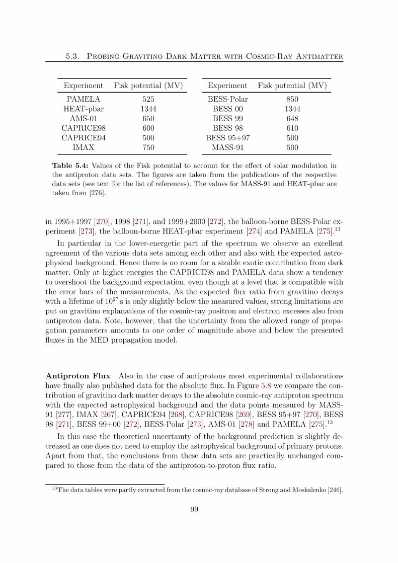
5.3. Probing Gravitino Dark Matter with Cosmic-Ray Antimatter
Experiment Fisk potential (MV)
PAMELA 525HEAT-pbar 1344AMS-01 650
CAPRICE98 600CAPRICE94 500
IMAX 750
Experiment Fisk potential (MV)
BESS-Polar 850BESS 00 1344BESS 99 648BESS 98 610
BESS 95+97 500MASS-91 500
Table 5.4: Values of the Fisk potential to account for the effect of solar modulation inthe antiproton data sets. The figures are taken from the publications of the respectivedata sets (see text for the list of references). The values for MASS-91 and HEAT-pbar aretaken from [276].
in 1995+1997 [270], 1998 [271], and 1999+2000 [272], the balloon-borne BESS-Polar ex-periment [273], the balloon-borne HEAT-pbar experiment [274] and PAMELA [275].13
In particular in the lower-energetic part of the spectrum we observe an excellentagreement of the various data sets among each other and also with the expected astro-physical background. Hence there is no room for a sizable exotic contribution from darkmatter. Only at higher energies the CAPRICE98 and PAMELA data show a tendencyto overshoot the background expectation, even though at a level that is compatible withthe error bars of the measurements. As the expected flux ratio from gravitino decayswith a lifetime of 1027 s is only slightly below the measured values, strong limitations areput on gravitino explanations of the cosmic-ray positron and electron excesses also fromantiproton data. Note, however, that the uncertainty from the allowed range of propa-gation parameters amounts to one order of magnitude above and below the presentedfluxes in the MED propagation model.
Antiproton Flux Also in the case of antiprotons most experimental collaborationshave finally also published data for the absolute flux. In Figure 5.8 we compare the con-tribution of gravitino dark matter decays to the absolute cosmic-ray antiproton spectrumwith the expected astrophysical background and the data points measured by MASS-91 [277], IMAX [267], CAPRICE94 [268], CAPRICE98 [269], BESS 95+97 [270], BESS98 [271], BESS 99+00 [272], BESS-Polar [273], AMS-01 [278] and PAMELA [275].13
In this case the theoretical uncertainty of the background prediction is slightly de-creased as one does not need to employ the astrophysical background of primary protons.Apart from that, the conclusions from these data sets are practically unchanged com-pared to those from the data of the antiproton-to-proton flux ratio.
13The data tables were partly extracted from the cosmic-ray database of Strong and Moskalenko [246].
99

Chapter 5. Indirect Detection of Gravitino Dark Matter
ª
ª
ª
ó
ó
ó
¨
¨§
§
§
§
òò
ò
òòò
ò
ò
òò
òòò
ø
ø
øø
øøø
øø
øø
øøø
ô
ô
ôô
ô
ô
ô
ô
ô
÷
÷
÷
÷÷÷
÷
÷
÷
ààà
à
àà
à
à
ààà
àà
ì
ì
ì
ìì
æ
æ
æ
æ
ææ
ææ
ææææææ
ææææ æ æ
æ æ æ
background
Τ32 = 1027 s
m32 = 100 GeV 1 TeV 10 TeV
1 10 100 1000 10000
10-3
0.01
0.1
1
10
100
Kinetic Energy HGeVL
T3´AntiprotonFluxHG
eV2m-2s-
1sr-1L
ª MASS-91ó IMAX¨ CAPRICE94§ CAPRICE98ì AMS-01æ PAMELA
ò BESS 95+97ø BESS 98ô BESS 99÷ BESS 00à BESS-Polar
Figure 5.8: Cosmic-ray antiproton flux expected from the decay of gravitino dark matterin the MED propagation model compared to measurements by various experiments andthe expectation from astrophysical secondary production. The flux from gravitino decayis shown for a lifetime of 1027 s and gravitino masses of 100GeV, 1TeV and 10TeV. Inorder to account for effects of solar modulation, the data points were demodulated usingvalues for the Fisk potential quoted by the experimental groups (cf. Table 5.4).
5.3.3 Antideuterons
The use of a signal of antideuterons to search for dark matter was first proposed byDonato et al. [76]. It is a particularly convenient dark matter detection channel, sincethe expected astrophysical background at low energies is at a very low level. Therefore,antideuterons allow for an almost background-free search for an exotic dark mattercomponent in certain parameter ranges. In fact, no cosmic-ray antideuterons have beenobserved so far and there exists only an upper bound on the antideuteron flux fromthe BESS experiment [283]. However, several new experiments are currently plannedto improve this situation: The Gaseous Antiparticle Spectrometer (GAPS) is plannedto perform two balloon flights, the Long Duration Balloon flight (LDB) and the Ultra-Long Duration Balloon flight (ULDB) [284]. In addition, the recently launched AMS-02experiment on the International Space Station will greatly improve on the sensitivity tolow antideuteron fluxes [285].
Several studies on antideuteron fluxes from dark matter annihilations or decays canbe found in the literature [76, 205, 279–281]. All of these studies, however, employ thespherical approximation of the coalescence model for antideuteron formation which in
100

5.3. Probing Gravitino Dark Matter with Cosmic-Ray Antimatter
Model δ K0 (kpc2/Myr) L (kpc) VC (km/s) x y z
MIN 0.85 0.0016 1 13.5 −0.3889 0.7532 −0.1788MED 0.70 0.0112 4 12 1.6023 0.4382 −0.1270MAX 0.46 0.0765 15 5 3.1992 −0.1098 −0.0374
Table 5.5: Parameters of cosmic-ray propagation models that correspond, respectively,to the best fit of cosmic-ray B/C data (MED) as well as the minimal (MIN) or maximal(MAX) antideuteron flux compatible with cosmic-ray B/C data. Figures taken from [262,281].
general is insufficient to describe the actual production rate [77]. Only very recent studiesemploy the Monte Carlo approach [77,282]. As discussed in Section 4.4 we also employdecay spectra obtained by this method.
The propagation equation for antideuterons is given in analogy to that for antipro-tons:
∂fddt
= ~∇ ·(K(T ) ~∇fd − ~VC(~r) fd
)− 2 h δ(z) Γann
d fd +Qd(T,~r) = 0 . (5.49)
The interstellar antideuteron flux at the position of the solar system coming from darkmatter decays in the galactic halo is then given by
dΦDMd
d(T/n)=
vd4 πm3/2 τ3/2
∞∫
0
d(T ′/n)Gd(T/n, T′/n)
dNd
d(T ′/n), (5.50)
where the velocity of antideuterons in terms of their kinetic energy is given by
vd = c
√1−
m2d
(T +md)2. (5.51)
We use a numerical approximation of the Green’s function that was found in [281] andis of the same form as the Green’s function for antiproton propagation:
Gd(T/n, T′/n) ≃ 1014 exp
(x+ y ln τ + z (ln τ)2
)δ(T ′/n− T/n) cm−3 s , (5.52)
where the kinetic energy per nucleon is parametrized in the form τ = (T/n)/(GeV/n)and τ ′ = (T ′/n)/(GeV/n). The parameters x, y and z are given in Table 5.5 for thecase of an NFW halo profile. In practice the upper limit for the integration over theGreen’s function is given by the maximal kinetic energy per nucleon of antideuterons ina gravitino decay: (T/n)max = (m3/2/2−md)/2.
As for the case of antiprotons, no primary antideuterons are expected from astro-physical objects and the dominant background for dark matter searches are secondaryantideuterons created in spallation processes of cosmic-ray protons and helium nuclei
101

Chapter 5. Indirect Detection of Gravitino Dark Matter
BESS 97-00
GAPSHLDBL
GAPSHU
LDBL
AMS-02 A
MS-02
background
Τ32 = 1027 s
m32 = 100 GeV 1 TeV 10 TeV
ΦF = 500 MV
0.1 1 10 100 1000
10-10
10-9
10-8
10-7
10-6
10-5
10-4
Kinetic Energy per Nucleon HGeVnL
HTnL´AntideuteronFluxHm-2s-
1sr-1L
Figure 5.9: Cosmic-ray antideuteron flux expected from the decay of gravitino darkmatter in the MED propagation model compared to the expectation from astrophysicalsecondary production and the sensitivities of forthcoming experiments. The flux fromgravitino decay is shown for a lifetime of 1027 s and gravitino masses of 100GeV, 1TeV and10TeV. The effect of solar modulation was taken into account assuming a Fisk potentialof φF = 500MV.
impinging on interstellar hydrogen and helium gas. In order to estimate the backgroundfor the signal from gravitino decay we employ here the astrophysical secondary an-tideuteron flux calculated in [280]. We parametrize their results by assuming a similarfunctional dependence as for the other cosmic-ray backgrounds and find
dΦsecd
d(T/n)≈ 1.08× 10⁻⁷ τ 0.88
1 + 0.041 τ 2.2 + 2.6× 10⁻⁴ τ 4(GeVm2 s sr)−1, (5.53)
where τ = (T/n)/(GeV/n). This spectrum corresponds to the interstellar antideuteronflux where effects of solar modulation are not taken into account.
In Figure 5.9 we present the antideuteron spectrum from gravitino dark matterdecays and compare it to the expected astrophysical background and the flux limitobtained by the BESS experiment [283]. In addition, we present the projected sensitivityregions of the GAPS and AMS-02 experiments. In order to be able to compare theexpected fluxes to the projected sensitivities we take into account the effect of solarmodulation according to equation (5.27) assuming a period at minimal solar activitywith φF = 500MV.
In particular for rather low gravitino masses on the order of 100GeV the signalfrom gravitino decays can dominate the background even for lifetimes as large as 1027 s
102

5.3. Probing Gravitino Dark Matter with Cosmic-Ray Antimatter
that are not yet excluded by gamma-ray and antiproton observations. A signal in thatrange should be observed in forthcoming antideuteron searches practically without abackground of antideuterons from astrophysical secondary production. In this respect itwill also be interesting to see what antideuteron flux could be expected for even lowergravitino masses. We plan to study this region in future work using the spectra obtainedfrom gravitino three-body decays [79].
But also for larger gravitino masses the gravitino signal is at least at the same orderas the background. This was not observed in earlier studies as the signal for large darkmatter masses is artificially suppressed in the spherical approximation of the coalescenceprescription. Therefore, one could argue that there are in principle also good prospectsfor the observation of an exotic component in the higher-energetic part of the spectrum,where currently no experiments are planned.
5.3.4 Bounds on the Gravitino Lifetime from Observations of
Charged Cosmic Rays
Similar to the bounds derived from the diffuse gamma-ray flux, we can estimate con-servative lower limits on the gravitino lifetime from the requirement that the gravitinosignal in charged cosmic rays does not overshoot the error bars of the measurements. Forthis task we will assume a MED propagation model and consider the PAMELA measure-ment of the positron fraction, the measurements of the total electron + positron flux byFermi LAT and H.E.S.S., and the PAMELA measurement of the antiproton flux. Theresulting exclusion regions are presented in Figure 5.10.
As expected, observations of cosmic-ray antiprotons in general lead to the strongestconstraints. The exclusion limit from observations of the positron fraction is weaker dueto the observed excess above the expected astrophysical background. One can see fromthe boundary of the exclusion region that a lifetime of typically 1026 s is required inorder to explain the rise of the positron fraction in terms of a signal from dark matterdecays. On the other hand, we clearly see that this possibility is ruled out for the caseof gravitino dark matter by the strong constraints in the antiproton channel.
In addition, we present an estimate of the sensitivity of forthcoming antideuteronexperiments to the gravitino parameter space. For this task we also employ the MEDpropagation model and require that the expected antideuteron flux from gravitino de-cays is at the lower edge of the sensitivity region of antideuteron experiments. In mostcases the AMS-02 experiment provides the best sensitivity. Only for the lowest gravitinomasses considered, the sensitivity of the GAPS experiment is better. This is due to thedifferent energy ranges in which the experiments are sensitive to antideuterons. AMS-02has a sensitivity region at larger antideuteron energies and is thus more sensitive tosignals from heavier dark matter particles. On the other hand, in particular in the lowmass range the antideuteron channel has the potential to be more sensitive than othercharged cosmic ray channels and this is the region where the GAPS balloon can com-pete. For this reason it would also be very interesting to study the antideuteron signals
103

Chapter 5. Indirect Detection of Gravitino Dark Matter
excluded by
antiproton flux
excluded by electron + positron flux
excluded
by
positron
fraction
antideuteron sensitivity
100 1000 10000
1024
1025
1026
1027
1028
Gravitino Mass HGeVL
GravitinoLifetim
eHsL
PAMELA e+He+ + e
-L
PAMELA p
Fermi LAT H.E.S.S. e+ + e-
Figure 5.10: Bounds on the gravitino lifetime from observations of charged cosmic raysand sensitivity of forthcoming antideuteron experiments.
from gravitino three-body decays at low gravitino masses [79]. It might well be thatthe sensitivity of the antideuteron channel is even higher than that of the gamma-raychannel. Clearly this also depends on the strength of the gamma-ray line from gravitinodecays.
One comment is in order: Of course one should remember that these exclusion andsensitivity regions are only rough estimates as there is quite some uncertainty in theexpected fluxes, for instance due to the choice of the propagation model. In addition,taking into account the expected flux contributions from astrophysical charged particleproduction can lead to much stricter limits on the gravitino parameters. In particularin the case of antiprotons the expected astrophysical background practically perfectlymatches the observations, leaving only little space for an exotic contribution.
5.4 Probing Gravitino Dark Matter with Neutrinos
In this section we present a study on the neutrino signals from gravitino dark mat-ter decays that was performed in analogy to our published phenomenological study ofneutrino signals from generic decay channels of fermionic and scalar dark matter par-ticles [78]. This study is complementary to our previous study on tau neutrino signalsfrom gravitino decays in [30, 154].
104
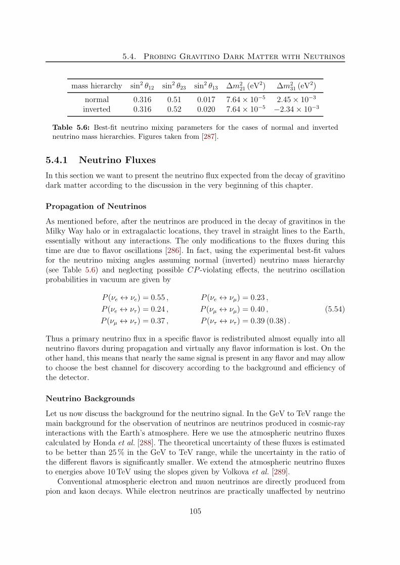
5.4. Probing Gravitino Dark Matter with Neutrinos
mass hierarchy sin2 θ12 sin2 θ23 sin2 θ13 ∆m221 (eV
2) ∆m231 (eV
2)
normal 0.316 0.51 0.017 7.64× 10⁻⁵ 2.45× 10⁻³
inverted 0.316 0.52 0.020 7.64× 10⁻⁵ −2.34× 10⁻³
Table 5.6: Best-fit neutrino mixing parameters for the cases of normal and invertedneutrino mass hierarchies. Figures taken from [287].
5.4.1 Neutrino Fluxes
In this section we want to present the neutrino flux expected from the decay of gravitinodark matter according to the discussion in the very beginning of this chapter.
Propagation of Neutrinos
As mentioned before, after the neutrinos are produced in the decay of gravitinos in theMilky Way halo or in extragalactic locations, they travel in straight lines to the Earth,essentially without any interactions. The only modifications to the fluxes during thistime are due to flavor oscillations [286]. In fact, using the experimental best-fit valuesfor the neutrino mixing angles assuming normal (inverted) neutrino mass hierarchy(see Table 5.6) and neglecting possible CP -violating effects, the neutrino oscillationprobabilities in vacuum are given by
P (νe ↔ νe) = 0.55 , P (νe ↔ νµ) = 0.23 ,
P (νe ↔ ντ ) = 0.24 , P (νµ ↔ νµ) = 0.40 , (5.54)
P (νµ ↔ ντ ) = 0.37 , P (ντ ↔ ντ ) = 0.39 (0.38) .
Thus a primary neutrino flux in a specific flavor is redistributed almost equally into allneutrino flavors during propagation and virtually any flavor information is lost. On theother hand, this means that nearly the same signal is present in any flavor and may allowto choose the best channel for discovery according to the background and efficiency ofthe detector.
Neutrino Backgrounds
Let us now discuss the background for the neutrino signal. In the GeV to TeV range themain background for the observation of neutrinos are neutrinos produced in cosmic-rayinteractions with the Earth’s atmosphere. Here we use the atmospheric neutrino fluxescalculated by Honda et al. [288]. The theoretical uncertainty of these fluxes is estimatedto be better than 25% in the GeV to TeV range, while the uncertainty in the ratio ofthe different flavors is significantly smaller. We extend the atmospheric neutrino fluxesto energies above 10TeV using the slopes given by Volkova et al. [289].
Conventional atmospheric electron and muon neutrinos are directly produced frompion and kaon decays. While electron neutrinos are practically unaffected by neutrino
105

Chapter 5. Indirect Detection of Gravitino Dark Matter
oscillations due to their large oscillation length, muon neutrinos, particularly at lowenergies, can be converted into tau neutrinos and provide the dominant tau neutrinobackground at energies below 1TeV. The conversion probability of muon neutrinos intotau neutrinos is given by [286]
P (νµ → ντ ) = sin2 2 θ23 sin2
(1.27
(∆m213/eV
2) (L/km)
(Eν/GeV)
)
≃ sin2
(3× 10⁻³ (L/km)
(Eν/GeV)
),
(5.55)
where we employed the best-fit neutrino mixing parameters in the second step. In thisexpression, Eν is the neutrino energy and L is their propagation length after beingproduced in the atmosphere, which is given by
L(θ) =√
(R⊕ cos θ)2 + 2R⊕ h+ h2 −R⊕ cos θ (5.56)
as a function of the zenith angle θ, with R⊕ ≃ 6.4 × 10³ km being the Earth’s radiusand h ≃ 15 km the mean altitude at which atmospheric neutrinos are produced [286].
In addition to this conventional atmospheric neutrino flux from pion and kaon decaysthere is a prompt neutrino flux from the decay of charmed particles that are also pro-duced in cosmic-ray collisions with the atmosphere. The prompt neutrinos have a harderspectrum than the conventional ones and therefore dominate the background at higherenergies (roughly above 10TeV for electron neutrinos and above 100TeV for muon neu-trinos). Since these contributions are not well understood and in any case subdominantin the GeV to TeV energy range that is of interest for dark matter searches, we neglectthem in the present study. On the other hand, the prompt flux of tau neutrinos starts todominate around 1TeV (and at even smaller energies for down-going neutrinos). Thuswe include this contribution using the parametrization [290]
log10
[E3 dΦντ
dE
/(GeV2
cm2 s sr
)]= −A+Bx− Cx2 −Dx3, (5.57)
where x = log10 (E/GeV), A = 6.69, B = 1.05, C = 0.150 and D = −0.00820. Thisparametrization is valid in the energy range of 100GeV up to 1PeV. However, we pointout that compared to the conventional atmospheric neutrino flux the prompt flux suffersfrom larger uncertainties.
Other neutrino backgrounds in the considered energy range are neutrinos producedin cosmic-ray interactions with the solar corona [291] and those produced in cosmic-rayinteractions with the interstellar medium of the Milky Way [292,293]. While the formeris subdominant in diffuse searches for all flavors [30,154] and can be excluded from theanalysis by excluding neutrinos from the direction of the Sun, the latter represents anirreducible, ill-understood neutrino background for searches in the galactic disc direc-tion. In fact, the flux of galactic neutrinos is expected to become comparable to theatmospheric electron neutrino background for the galactic disc direction and energies inthe TeV range.
106
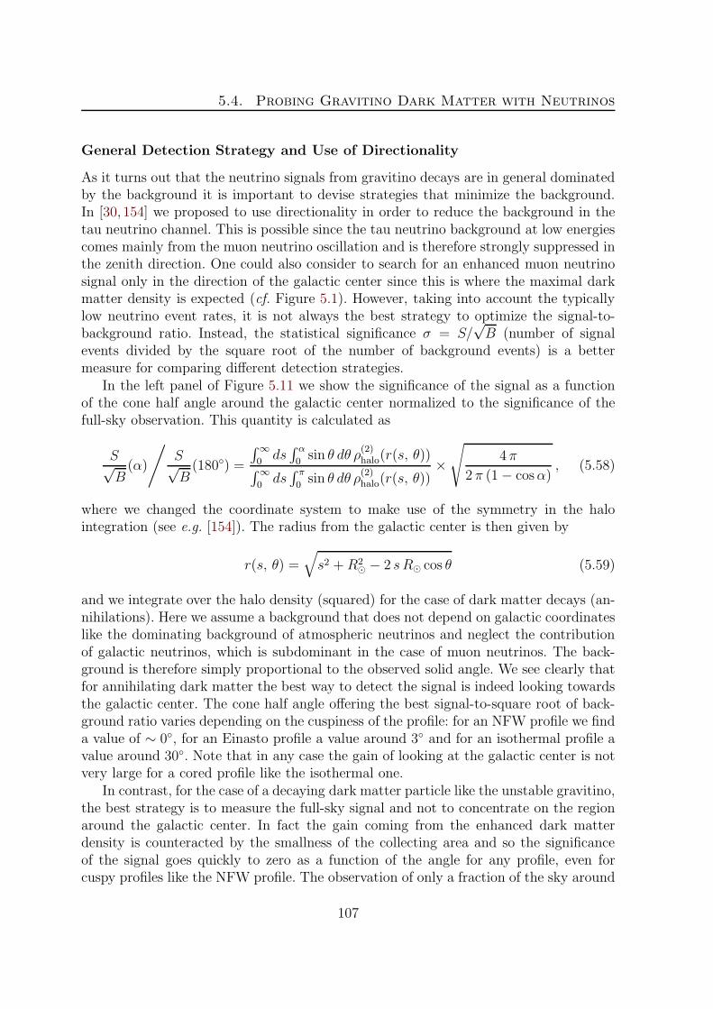
5.4. Probing Gravitino Dark Matter with Neutrinos
General Detection Strategy and Use of Directionality
As it turns out that the neutrino signals from gravitino decays are in general dominatedby the background it is important to devise strategies that minimize the background.In [30, 154] we proposed to use directionality in order to reduce the background in thetau neutrino channel. This is possible since the tau neutrino background at low energiescomes mainly from the muon neutrino oscillation and is therefore strongly suppressed inthe zenith direction. One could also consider to search for an enhanced muon neutrinosignal only in the direction of the galactic center since this is where the maximal darkmatter density is expected (cf. Figure 5.1). However, taking into account the typicallylow neutrino event rates, it is not always the best strategy to optimize the signal-to-background ratio. Instead, the statistical significance σ = S/
√B (number of signal
events divided by the square root of the number of background events) is a bettermeasure for comparing different detection strategies.
In the left panel of Figure 5.11 we show the significance of the signal as a functionof the cone half angle around the galactic center normalized to the significance of thefull-sky observation. This quantity is calculated as
S√B(α)
/S√B(180) =
∫∞0ds∫ α
0sin θ dθ ρ
(2)halo(r(s, θ))∫∞
0ds∫ π
0sin θ dθ ρ
(2)halo(r(s, θ))
×√
4 π
2 π (1− cosα), (5.58)
where we changed the coordinate system to make use of the symmetry in the halointegration (see e.g. [154]). The radius from the galactic center is then given by
r(s, θ) =√s2 +R2
⊙ − 2 sR⊙ cos θ (5.59)
and we integrate over the halo density (squared) for the case of dark matter decays (an-nihilations). Here we assume a background that does not depend on galactic coordinateslike the dominating background of atmospheric neutrinos and neglect the contributionof galactic neutrinos, which is subdominant in the case of muon neutrinos. The back-ground is therefore simply proportional to the observed solid angle. We see clearly thatfor annihilating dark matter the best way to detect the signal is indeed looking towardsthe galactic center. The cone half angle offering the best signal-to-square root of back-ground ratio varies depending on the cuspiness of the profile: for an NFW profile we finda value of ∼ 0, for an Einasto profile a value around 3 and for an isothermal profile avalue around 30. Note that in any case the gain of looking at the galactic center is notvery large for a cored profile like the isothermal one.
In contrast, for the case of a decaying dark matter particle like the unstable gravitino,the best strategy is to measure the full-sky signal and not to concentrate on the regionaround the galactic center. In fact the gain coming from the enhanced dark matterdensity is counteracted by the smallness of the collecting area and so the significanceof the signal goes quickly to zero as a function of the angle for any profile, even forcuspy profiles like the NFW profile. The observation of only a fraction of the sky around
107

Chapter 5. Indirect Detection of Gravitino Dark Matter
Einasto
NFW
Isothermal
annihilation
decay
0.1 ° 1 ° 10 ° 30 ° 180 °0
1
2
3
4
5
Cone Half Angle Towards the Galactic Center
StatisticalSignificance
Compared
toFullSky
Νe
ΝΜ
ΝΤ
0 0.2 0.4 0.6 0.8 10
1
2
3
4
Cosine of Maximal Zenith Angle
StatisticalSignificance
Compared
toFullSky
Figure 5.11: Left: Statistical significance of the neutrino signal as a function of the conehalf angle towards the galactic center normalized to the significance of the full-sky signalfor annihilating/decaying dark matter depending on the different density profiles. Right:Statistical significance of the neutrino signal as a function of the maximal angle observedaround the zenith direction normalized to the significance for the observation of the upperhemisphere. The curves are shown for a neutrino energy of 100GeV.
the galactic center direction leads to an increase in the signal-to-background ratio, butnot of the significance. We therefore conclude that for decaying dark matter there isno advantage in looking only at the galactic center. The full-sky signal offers not onlybetter statistics, but also a higher significance.
Considering the directionality of the atmospheric background instead of the signal,another good strategy might be to exploit the fact that the flux from the zenith andnadir directions is (depending on the neutrino flavor and the energy) a few times smallerthan from the horizontal direction. Assuming a signal that does not depend on the zenithangle, which is practically true for the signal from dark matter decays, the observationof only a fraction of the sky around the zenith (and nadir) direction is again clearlyleading to an increase in the signal-to-background ratio. In the case of muon neutrinosit turns out that the best value for the significance is achieved for a full-sky observa-tion. For electron neutrinos the difference in the background fluxes from the zenith andhorizontal directions is larger and a slight increase of the statistical significance couldbe achieved. As mentioned before, the tau neutrino background is strongly suppressedin the zenith direction since it is only produced from oscillations (cf. equation (5.55)).Thus a large increase of the statistical significance is achieved if only a fraction of theupper hemisphere is observed. We show the dependence on the maximal zenith anglefor an exemplary neutrino energy of 100GeV in the right panel of Figure 5.11.
108

5.4. Probing Gravitino Dark Matter with Neutrinos
ô ôô
ô
ô ô
ô
ò
òò ò
òò
ò
òò
ò
ò
ì
ì
ì
ì
ì
ì
ì
ì
ì
æ
æ
æ
æ
æ
æ
æ
æ
æ
æ
æ
ΝΤΝe
ΝΜ
Τ32 = 1026 s
m32 = 100 GeV 1 TeV 10 TeV
1 10 100 1000 10000 100000
10-4
10-3
0.01
0.1
1
10
100
103
Energy HGeVL
E2´NeutrinoFluxHG
eVm-2s-
1sr-1L
ô Fréjus Νe
ò Fréjus ΝΜ
Super-Kamiokande ΝΜ
AMANDA-II Forward ΝΜ
ì AMANDA-II Unfolding ΝΜ
IceCube-40 ΝΜ
æ IceCube-40 Unfolding ΝΜ
Figure 5.12: Expected combined spectrum of neutrinos and antineutrinos from the decayof gravitino dark matter compared to the combined background of atmospheric neutrinosand antineutrinos and data of neutrino experiments. The expected flux is presented fora gravitino lifetime of 1026 s and gravitino masses of 100GeV, 1TeV and 10TeV. Clearlyvisible are the monochromatic lines at the end of the spectra coming from the two-bodydecay channels with a neutrino in the final state. Due to the steeply falling atmosphericbackground the signal-to-background ratio at the endpoint of the decay spectrum increasessignificantly for larger gravitino masses if the lifetime is kept fixed.
We can therefore conclude that exploiting the directionality of the signal or back-ground, apart from the case of specific flavors like tau neutrinos as discussed in [30,154],is not promising for the first detection of a decaying dark matter candidate like theunstable gravitino. The largest rate and significance is achieved for a full-sky search,and this is the option we will discuss in the following. On the other hand, as discussedin the beginning of this chapter, directionality offers a clear way to disentangle a sig-nal of decaying dark matter from a signal of annihilating dark matter, where lookinginto the galactic center should give an increase in significance. In addition, directionalobservation allows to distinguish the dark matter signal from point sources like dwarfgalaxies, pulsars and supernova remnants.
5.4.2 Neutrino and Muon Spectra
The contributions to the neutrino flux from gravitino decays at extragalactic distancesand in the Milky Way halo are calculated according to equations (5.4) and (5.12) us-
109
Chapter 5. Indirect Detection of Gravitino Dark Matter
ing the neutrino spectra presented in Section 4.4. The result after propagation to theEarth is shown in Figure 5.12 together with the expected atmospheric background assimulated by Honda et al. [288] and the data measured by the Frejus [294], Super-Kamiokande [295], AMANDA-II [296, 297] and IceCube [298, 299] experiments. We seethat for a lifetime of the order of 1026 s the signal always lies below the measured back-ground of muon neutrinos. The best signal-to-background ratio in the neutrino channelis achieved for the high-energy end of the spectrum, which contains information aboutthe gravitino mass.
The neutrino spectra shown in Figure 5.12 look rather distinctive, and an interestingquestion is whether they can be observed in a neutrino detector. In particular it isinteresting to see if the neutrino line leads to an observable signal. However, we have toconsider that neutrino detectors do not really measure neutrinos directly, but only thecorresponding charged leptons or showers produced in interactions of neutrinos with thematter inside and around the detector.
Neutrino Interactions
Since we are mainly interested in neutrino energies much larger than nucleon masseswe only take into account deep inelastic neutrino–nucleon scattering. Neutrino–electronelastic scattering is subdominant in this energy range and will be neglected [286].
The cross sections for deep inelastic scattering of (anti)neutrinos off nucleons at restare given by [286, 300]
dσν p,nCC/NC(Eν , y)
dy≃ 2mp,nG
2F
πEν
(aν p,nCC/NC + bν p,n
CC/NC (1− y)2)
≃ 3.2× 10−38 cm2
GeVEν
(aν p,nCC/NC + bν p,n
CC/NC (1− y)2) (5.60)
with aν p,nCC = 0.15, 0.25, bν p,n
CC = 0.04, 0.06 and aν p,nCC = bν n,p
CC , bν p,nCC = aν n,p
CC for charged-current interactions, and aν p,n
NC = 0.058, 0.064, bν p,nNC = 0.022, 0.019 and aν p,n
NC = bν p,nNC ,
bν p,nNC = aν p,n
NC for neutral-current interactions. The inelasticity y is given by
y = 1− Eℓ
Eνor y ≃ Ehad
Eν, (5.61)
where Eℓ is the energy of the generated lepton and Ehad is the energy of the generatedhadronic shower. For the total neutrino–nucleon cross sections one obtains
σν p,nCC/NC(Eν) ≃
2mp,nG2F
πEν
(aν p,nCC/NC +
1
3bν p,nCC/NC
). (5.62)
As we can see, the total cross section is proportional to the energy of the incomingneutrino in the considered energy range. However, equation (5.60) in principle holdsonly for neutrino energies up to the TeV region where the effect of the massive gaugeboson propagators becomes relevant. Nevertheless, we will employ this parametrization,keeping in mind that at higher energies the cross-sections might be overestimated [286].
110

5.4. Probing Gravitino Dark Matter with Neutrinos
material ρ (g/cm3) 〈Z/A〉 α (GeV cm2/g) β (cm2/g)standard rock 2.650 0.5 2.3× 10⁻³ 4.4× 10⁻⁶
water 1.000 0.55509 2.7× 10⁻³ 3.3× 10⁻⁶
ice 0.918 0.55509 2.7× 10⁻³ 3.3× 10⁻⁶
Table 5.7: Density, proton-number-to-mass-number ratio and approximate muon energyloss parameters for materials of interest in Cherenkov neutrino detectors. The values of thedensity and the average proton-number-to-mass-number ratio are taken from [301, 302].The muon energy loss parameters α and β are best-fit values from a fit of equation (5.64)to the tabulated data in [301,302].
Muon Neutrinos
The charged-current deep inelastic scattering of a muon neutrino off a nucleus producesa hadronic shower and a muon. These track-like events can be clearly identified inCherenkov detectors via the Cherenkov light cone of the relativistic muon.
Through-Going Muons
Since muons are rather long-lived (cτµ = 658.650m), their range is only limited by energyloss during their passage through matter and not by their lifetime. Therefore Cherenkovdetectors can also observe muons that are generated in the surrounding material of thedetector (see left panel of Figure 5.13). This effect enhances the effective detector areafor high-energetic muon neutrinos.
The average rate of muon energy loss can be written as [81]
− dEµ
dx= α(Eµ) + β(Eµ)Eµ , (5.63)
where α(Eµ) describes the ionization energy loss and β(Eµ) takes into account the energyloss due to radiative processes: e+e− pair production, bremsstrahlung and photonuclearcontributions. Both α(Eµ) and β(Eµ) are slowly varying functions of the muon energy.As long as we can approximate α and β as energy-independent, the range after whichthe muon energy drops below a threshold energy Eth
µ is given by
Rµ(Eµ, Ethµ ) =
1
ρ βln
[α + βEµ
α + βEthµ
], (5.64)
where ρ is the density of the medium. Important materials in connection with Cherenkovneutrino detectors are standard rock, water and ice. The relevant parameters for thesematerials are given in Table 5.7. In fact, equation (5.63) only describes the average muonenergy loss and does not account for the stochastic nature of radiative muon energy lossprocesses which start to dominate at TeV energies (Eµ > α/β). Nonetheless, we willemploy equation (5.64) as a useful approximation for the muon range that allows us to
111

Chapter 5. Indirect Detection of Gravitino Dark Matter
determine the initial muon energy as an explicit function of the final muon energy andthe muon range:
E0µ(Eµ, Rµ) = Eµ e
ρ β Rµ +α
β
(eρ β Rµ −1
). (5.65)
The rate of muon neutrino-induced through-going muon events is given by
dN
dt=
∫dΩ
∞∫
0
dEνµ
dΦνµ(Eνµ, θ, φ)
dEνµ
Aeffνµ(Eνµ, θ, φ)
=
∫dΩ
∞∫
Ethµ
dEνµ
Eν∫
Ethµ
dEµ
dΦνµ(Eνµ , θ, φ)
dEνµ
[dσνp
CC(Eνµ, Eµ)
dEµnp + (p→ n)
]
× Rµ(Eµ, Ethµ )Aeff
µ (Eµ, θ, φ) e−σνN (Eνµ )nN L(θ)+(νµ → νµ) ,
(5.66)
where the number density of protons is given by np = ρM−1p NA 〈Z/A〉 and the density
of neutrons by nn = ρM−1n NA(1 − 〈Z/A〉). NA = 6.022 × 10²³mol−1 is the Avogadro
constant, Mp ≃ Mn ≃ 1 gmol−1 is the molar mass of protons and neutrons, ρ is thedensity of the material, and 〈Z/A〉 is the average ratio of the proton number and themass number of the material as given in Table 5.7. Due to the small neutrino–nucleoncross-section the effect of the attenuation term that accounts for the absorption of partof the signal and background neutrino fluxes during the passage of the Earth is negligiblein the considered energy range. However, since the neutrino–nucleon cross section riseswith increasing neutrino energy, this effect becomes non-negligible at neutrino energiesabove 10TeV.
The muon neutrino effective area Aeffνµ is defined as the ratio of the rate of recon-
structed events and the incident neutrino flux. It is calculated using Monte Carlo meth-ods and incorporates the attenuation of the neutrino flux during the passage of theEarth, the neutrino–nucleon cross section, the range of the generated muon and thereconstruction and selection efficiencies. This effective area is usually provided by theexperimental collaborations. The energy dependence of the neutrino effective area comesmainly from the energy dependence of the cross section (roughly ∝ Eν) and the increaseof the muon range with rising energy (roughly ∝ Eν for Eν ≪ α/β ∼ O(1) TeV and∝ lnEν for Eν ≫ O(1) TeV). Notice that the muon effective area Aeff
µ , on the other hand,is defined as the ratio of the rate of reconstructed events and the incident muon flux.This area incorporates only the geometry of the detector and the detection efficiency. Itis roughly equal to the geometrical area but might have a slight energy dependence.
For the calculation of the spectrum of muon neutrino induced muons at the detectorposition we have to take into account the shift to lower energies due to the energy loss
112

5.4. Probing Gravitino Dark Matter with Neutrinos
Upward Through-Going Muons
atmospheric background
Τ32 = 1026 s
m32 = 100 GeV 1 TeV 10 TeV
1 10 100 1000 1000010-3
0.01
0.1
1
10
100
103
104
105
Energy HGeVL
MuonFluxHG
eV-1km-2yr-
1L
Figure 5.13: Left: Event topology of muon neutrino-induced upward through-goingmuons. A muon neutrino that traversed the Earth scatters in a charged-current inter-action on matter surrounding the detector, thus producing a muon that penetrates thedetector. Right: Muon fluxes induced by muon neutrinos from gravitino dark matter de-cays compared to the atmospheric background for upward through-going muons in a neu-trino detector surrounded by standard rock. The flux is computed for gravitino masses of100GeV, 1TeV and 10TeV, and a lifetime of 1026 s, corresponding to the neutrino spectrashown in Figure 5.12.
during muon propagation through matter [303]:
dφµ
dEµ
=
∫dΩ
∞∫
0
dRµ
∞∫
E0µ
dEνµ eρ β RµdΦ(Eνµ, θ, φ)
dEνµ
×[dσνp
CC(Eνµ, E0µ)
dE0µ
np + (p→ n)
]
E0µ=E0
µ(Eµ,Rµ)
+ (νµ → νµ) ,
(5.67)
where we neglected the attenuation term. In this expression the initial muon energyenters as an explicit function of the final muon energy as given by equation (5.65).
Using equation (5.67) we calculate the flux of through-going muons induced by neu-trinos from gravitino dark matter decay and show the results in the right panel of Fig-ure 5.13 for the case of a detector surrounded by standard rock like Super-Kamiokande.However, the result is also applicable for the case of detectors surrounded by wateror ice since the dependence on the density of the material cancels in equation (5.67)and the muon energy loss parameters are roughly similar for the different materials(cf. Table 5.7). Since there is no possibility to veto for the overwhelming backgroundof atmospheric muons, only up-going events and therefore a solid angle of 2π can be
113

Chapter 5. Indirect Detection of Gravitino Dark Matter
used for the analysis. We observe that the deep inelastic scattering transforms the inci-dent neutrino spectrum into a softer muon spectrum. In addition, the energy loss in themuon propagation smooths out the spectrum making the edge corresponding to half thegravitino mass less clear.
Contained Muons
These events are similar to through-going muons but in this case the neutrino–nucleoninteraction takes place inside the instrumented volume (see left panel of Figure 5.14).If the muon track ends inside the detector the events are called contained. If the muontrack leaves the detector one speaks of a partially contained event. The rate of muonneutrino induced contained track-like events per unit detector volume is given by14
dN
dEµ dV dt=
∫dΩ
∞∫
Eµ
dEνµ
dΦνµ(Eνµ, θ, φ)
dEνµ
[dσνp
CC(Eνµ, Eµ)
dEµnp + (p→ n)
]
+ (νµ → νµ) ,
(5.68)
where we also neglected the attenuation term. In this case also the hadronic cascade iscontained in the detector volume and therefore, by measuring the energy of the muon aswell as of the hadronic cascade, it is in principle possible to reconstruct the total energyof the incident muon neutrino. In this case, however, one has to rely on the detectionalso of the hadronic cascade which, as we will discuss later, seems to be challenging.The effective volume of the detector for contained events corresponds roughly to thegeometrical volume (apart from boundary effects and reconstruction efficiency) and itis not enhanced by the muon range, which as we have seen, grows as Eν . Therefore, thestatistics for contained events is lower than for through-going events at large energies.For instance in the case of Super-Kamiokande the event rate above roughly 10GeV isdominated by through-going muons. On the other hand, in the energy range of interestfor dark matter searches the muon range is of the order of one kilometer and therefore theexpected rate of contained muons is comparable to the rate of through-going muons indetectors of cubic kilometer size. Thus these contained events might be equally importantfor dark matter searches at the new generation of neutrino telescopes.
In addition, for downgoing contained muon events there is the interesting possibilityto reduce the background of atmospheric muon neutrinos by the detection of a coincidentmuon that was produced in the same parent meson decay [304]. This strategy couldbe used to increase the signal-to-background ratio for this channel, especially at largeenergies. However, we will not discuss this strategy quantitatively in this work.
In the right panel of Figure 5.14 we show the muon spectra for contained eventscalculated using equation (5.68) for the case of a detector volume filled with ice asin the case of the IceCube experiment. The result for a volume of water can easily beobtained by rescaling the event rate with the slightly higher density of water. In contrast
14We do not discriminate between partially and completely contained events in this analysis.
114

5.4. Probing Gravitino Dark Matter with Neutrinos
Contained Muons
atmospheric background
Τ32 = 1026 s
m32 = 100 GeV 1 TeV 10 TeV
1 10 100 1000 1000010-3
0.01
0.1
1
10
100
103
104
105
106
107
Energy HGeVL
MuonRateHG
eV-1km-3yr-
1L
Figure 5.14: Left: Event topology of muon neutrino-induced contained muons. A muonneutrino scatters in a charged-current interaction on matter inside the detector, thus pro-ducing a muon that traverses the detector. Right: Spectrum of contained muons inducedby muon neutrinos from gravitino dark matter decays compared to the atmospheric back-ground. The event rate per cubic kilometer of detector volume (filled with ice) is computedfor gravitino masses of 100GeV, 1TeV and 10TeV, and a lifetime of 1026 s, correspondingto the neutrino spectra shown in Figure 5.12.
to through-going muons there is no smoothing due to muon energy loss and the edge ofthe spectrum is clearer.
Here we only discussed the case where only the muon is measured since this iswhat can be done by the experiments at the moment. If the hadronic shower is alsomeasured the total energy of the incident muon neutrino could be reconstructed andtherefore in principle the complete spectral information of the neutrino flux as shown inFigure 5.12 would be available for analyses. This is similar to the case of electron andtau neutrinos that is discussed in the next section. However, as will be discussed there,that channel offers a better signal-to-background ratio and a better energy resolutionand will therefore be of more interest once the showers can be measured and used foranalyses.
Electron and Tau Neutrinos
The charged-current deep inelastic scattering of an electron neutrino off a nucleus pro-duces a hadronic shower and an electron that immediately causes an electromagneticshower. The charged-current deep inelastic scattering of a tau neutrino off a nucleusproduces a hadronic shower and a tau lepton. Due to the short lifetime of the tau lep-ton (cττ = 87.11µm), at GeV to TeV energies it decays almost instantly and produces
115

Chapter 5. Indirect Detection of Gravitino Dark Matter
another shower at the interaction point. Thus, at energies below many TeV, neutrino de-tectors like IceCube cannot distinguish electron neutrino from tau neutrino events sinceboth types produce similar showers in the detector [305] (see left panel of Figure 5.15).In these cases, however, the whole neutrino energy is deposited in the detector and there-fore it may be possible in principle to reconstruct better the initial neutrino spectrum.On the other hand, the analysis for cascade-like events is much more difficult than theanalysis for muon tracks [306]. Recently there has been a first study by the IceCubecollaboration [307] searching for atmospheric and extraterrestrial neutrino-induced cas-cades. Only few candidate events at energies above several TeV have been found so far,but the situation will improve in the future with refined analysis methods and higherstatistics of recorded events. However, at this moment we cannot realistically estimatethe sensitivity in shower events that finally will be reached and therefore we study thischannel assuming an ideal detector.
Shower-like events are also characteristic of the neutrino–nucleon neutral-currentinteraction and for this reason probably only a combined analysis of neutral-currentinteractions for all neutrino flavors and charged-current interactions for tau and electronneutrinos will be feasible (see left panel of Figure 5.15). The total rate of neutrino-induced shower-like events per unit detector volume is given by
dN
dEshower dV dt=
∫dΩ
∑
ℓ= e,τ
(dΦνℓ(Eνℓ , θ, φ)
dEνℓ
[σνpCC(Eνℓ)np + (p→ n)]
)
Eνℓ=Eshower
+∑
ℓ= e,µ,τ
∞∫
Eshower
dEνℓ
dΦνℓ(Eνℓ , θ, φ)
dEνℓ
(5.69)
×[dσνp
NC(Eνℓ , Eshower)
dEshowernp + (p→ n)
]+ (νℓ → νℓ) .
We give in the right panel of Figure 5.15 the signal and atmospheric backgroundspectra calculated from equation (5.69) for a detector volume filled with ice as in the caseof the IceCube experiment. Note that in this case the muon neutrinos contribute only viatheir neutral-current interactions which are weaker by a factor of about three comparedto charged-current interactions (cf. equation (5.62)). Still, since the atmospheric muonneutrino flux is a factor of 20 larger than the electron neutrino flux at TeV energies, theatmospheric muon neutrinos provide the dominant background. At the same time thesignal rate is increased by roughly a factor of three. This is because, due to neutrinooscillations, the signal is roughly equal in all neutrino flavors and, therefore, the signalrate from the charged-current interactions of electron and tau neutrinos is the same asfor the muon neutrinos. In addition, the combined neutral-current signal of all flavorscontributes at the same level as the charged-current signal of one flavor. In summary,cascade-like events will offer a signal-to-background ratio that is roughly one order ofmagnitude larger than in the case of through-going muons and, therefore, they appearto be a very promising channel, once they can be measured.
116
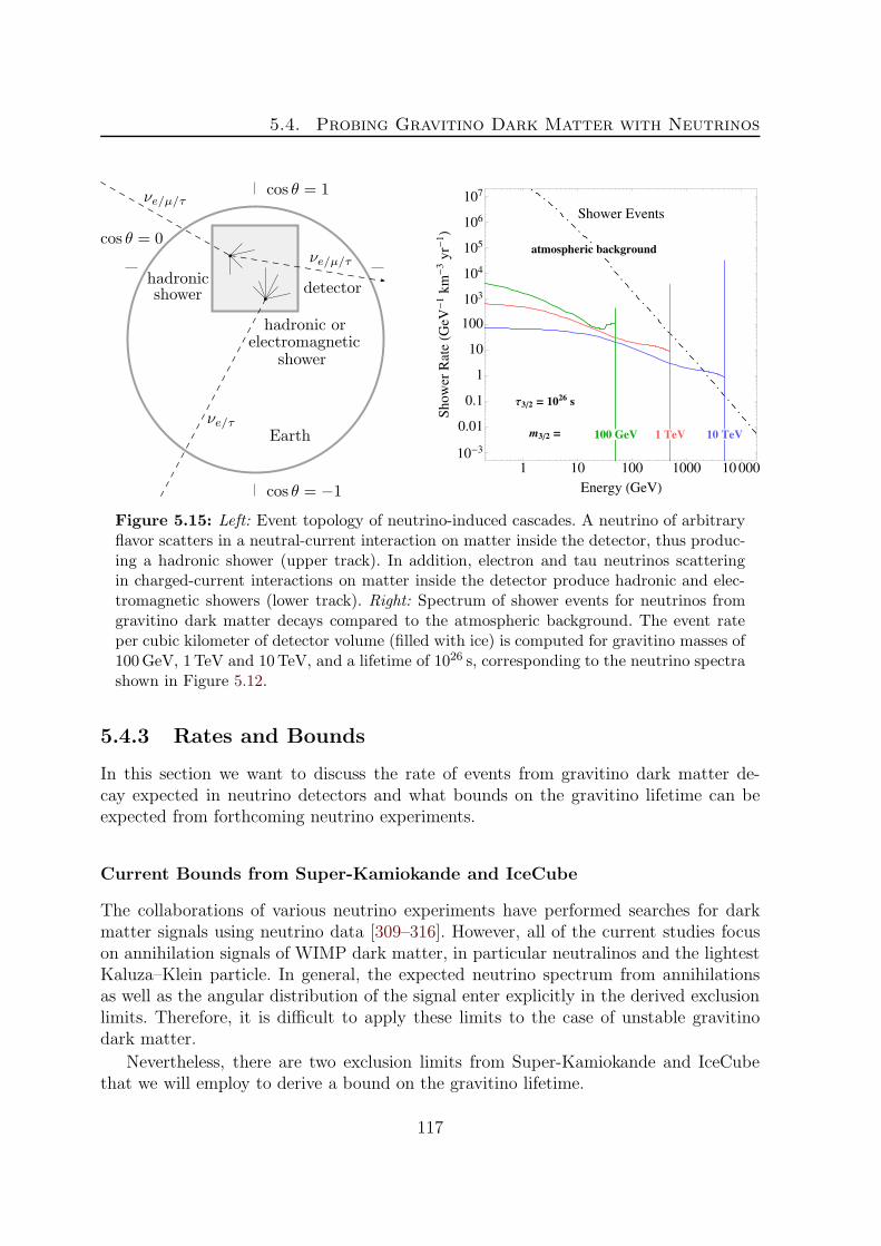
5.4. Probing Gravitino Dark Matter with Neutrinos
Shower Events
atmospheric background
Τ32 = 1026 s
m32 = 100 GeV 1 TeV 10 TeV
1 10 100 1000 1000010-3
0.01
0.1
1
10
100
103
104
105
106
107
Energy HGeVL
Shower
RateHG
eV-1km-3yr-
1L
Figure 5.15: Left: Event topology of neutrino-induced cascades. A neutrino of arbitraryflavor scatters in a neutral-current interaction on matter inside the detector, thus produc-ing a hadronic shower (upper track). In addition, electron and tau neutrinos scatteringin charged-current interactions on matter inside the detector produce hadronic and elec-tromagnetic showers (lower track). Right: Spectrum of shower events for neutrinos fromgravitino dark matter decays compared to the atmospheric background. The event rateper cubic kilometer of detector volume (filled with ice) is computed for gravitino masses of100GeV, 1TeV and 10TeV, and a lifetime of 1026 s, corresponding to the neutrino spectrashown in Figure 5.12.
5.4.3 Rates and Bounds
In this section we want to discuss the rate of events from gravitino dark matter de-cay expected in neutrino detectors and what bounds on the gravitino lifetime can beexpected from forthcoming neutrino experiments.
Current Bounds from Super-Kamiokande and IceCube
The collaborations of various neutrino experiments have performed searches for darkmatter signals using neutrino data [309–316]. However, all of the current studies focuson annihilation signals of WIMP dark matter, in particular neutralinos and the lightestKaluza–Klein particle. In general, the expected neutrino spectrum from annihilationsas well as the angular distribution of the signal enter explicitly in the derived exclusionlimits. Therefore, it is difficult to apply these limits to the case of unstable gravitinodark matter.
Nevertheless, there are two exclusion limits from Super-Kamiokande and IceCubethat we will employ to derive a bound on the gravitino lifetime.
117

Chapter 5. Indirect Detection of Gravitino Dark Matter
Super-Kamiokande Super-Kamiokande is a 50 kt water Cherenkov detector with afiducial mass of 22.5 kt. The muon effective area is 1200m2 (with a slight zenith angledependence due to the cylindrical shape of the detector) and is identical to the geo-metrical area since the reconstruction and selection efficiencies are virtually 100% [318].Super-Kamiokande has been looking for a neutrino signal from WIMP annihilations inthe center of the Sun, the center of the Earth and in the galactic center using 1679.6days of data [308]. No excess has been found so far, and this can also be used to obtaina constraint in the case of decaying dark matter.
We calculate the flux of upward through-going muons induced by muon neutrinosfrom gravitino dark matter decays according to a variation of equation (5.66):15
φµ =
∫dΩ
∞∫
Ethµ
dEµRµ(Eµ, Ethµ )
∞∫
Eµ
dEνµ
dΦ(Eνµ , θ, φ)
dEνµ
×[dσνp
CC(Eνµ , Eµ)
dEµ
np + (p→ n)
]+ (νµ → νµ) .
(5.70)
The Super-Kamiokande detector is surrounded by rock and we employ a detectionthreshold of Eth
µ = 1.6GeV for upgoing muons [308]. We compare the resulting fluxwith the 90% C.L. flux limit of excess neutrino-induced upward through-going muonsprovided by the Super-Kamiokande collaboration for the galactic center [308].16 As dis-cussed in Section 5.4.1, the strongest bounds are obtained for the largest field of view.The exclusion region in the gravitino parameter space derived from the limit in the 30
half-angle cone around the galactic center is given in the left panel of Figure 5.16.
IceCube The IceCube neutrino telescope is a Cherenkov detector consisting of 86strings with optical sensors deployed at depths between 1.5 km and 2.5 km in the ice atthe South Pole [319]. With a surface area of one square kilometer the instrumented vol-ume amounts to one cubic kilometer, a factor of 20 000 larger than Super-Kamiokande.On the other hand, IceCube is much more loosely instrumented compared to Super-Kamiokande and thus has a higher detection threshold of O(100)GeV.
A recent search for neutrino signals from dark matter in the galactic halo has beenperformed using data taken with the IceCube detector on 276 days during a stage ofconstruction when it consisted of 22 strings [317]. In this study the expected angulardistribution of the dark matter signal from the galactic halo was used to constrain thedark matter contribution by comparing the observed event rates from two sky regions:one directed towards the galactic center and one directed away from the galactic center.
15Since we are not interested in the spectrum of muons in this case, we do not need to performan integration over the muon range as in equation (5.67). Thus we can save one step of numericalintegration while still obtaining the correct total muon flux.
16The flux limits from the analyses of the directions towards the Sun and the Earth result in weakerlimits for the case of decaying dark matter.
118

5.4. Probing Gravitino Dark Matter with Neutrinos
excluded by
Super-Kamiokande
10 100 1000 10000
1023
1024
1025
1026
Gravitino Mass HGeVL
GravitinoLifetim
eHsL
excluded by
IceCube-22
100 1000 10000
1023
1024
1025
1026
Gravitino Mass HGeVL
GravitinoLifetim
eHsL
Figure 5.16: Left: 90% C.L. exclusion region in the lifetime vs. mass plane for decayinggravitino dark matter from the non-observation of an excess in the Super-Kamiokande data(cf. text). Right: 90% C.L. exclusion region in the lifetime vs. mass plane for decayinggravitino dark matter from a search for monochromatic neutrinos from the galactic halowith the IceCube-22 detector (cf. text). Both bounds are stronger for larger gravitinomasses since the integrated muon flux increases due to the increasing neutrino–nucleoncross section and the increasing muon range in spite of the decreasing neutrino flux.
An exclusion limit was also presented for the lifetime of a dark matter particle decayinginto two monochromatic neutrinos.
We can use this limit to derive a conservative lower limit on the gravitino lifetimeby taking into account only the neutrino-line contributions from gravitino decays:
τ3/2(m3/2) &1
2
(BR (γ νi)× τνν(m3/2) + BR (Zνi)× τνν
(m3/2
(1− m2
Z
m23/2
))
+ BR (h νi)× τνν
(m3/2
(1− m2
h
m23/2
))).
(5.71)
Our result is presented in the right panel of Figure 5.16.The bounds obtained from the Super-Kamiokande and IceCube analyses become
stronger for larger masses although the neutrino flux is inversely proportional to thegravitino mass for a fixed gravitino lifetime. This is due to the increasing neutrino–nucleon cross section and the increasing muon range. Note, however, that these presentbounds do not have sensitivity to the parameter region preferred by the PAMELA excessyet, which corresponds to a gravitino lifetime of the order of 1026 s and masses largerthan 200GeV.
119

Chapter 5. Indirect Detection of Gravitino Dark Matter
We observe that the current limit from Super-Kamiokande is still stronger thanthe IceCube limit. This is probably due to the longer data-taking period of Super-Kamiokande, the reduced size of the IceCube 22 string configuration compared to thefull IceCube array and the higher detection threshold of IceCube. As we will discuss inthe following, we expect the full IceCube detector to improve these results significantly.
Rates and Bounds for Present and Future Experiments
Assuming decaying gravitino dark matter with a lifetime of 1026 s, we can now com-pute the expected signal rates for present and future experiments. These results canbe easily generalized to arbitrary lifetimes, by recalling that the flux is proportionalto 1/τ3/2. We give the rates for some typical detectors of different sizes, i.e. Super-Kamiokande [320], AMANDA [321], ANTARES [322] and IceCube [319]. The results forSuper-Kamiokande can be easily scaled up to the Hyper-Kamiokande [323] or UNO [324]size by multiplying by a factor 10 or 20 (for a Hyper-Kamiokande mass of 500 kt anda Hyper-Kamiokande/UNO mass of 1Mt, respectively). The result for KM3NeT [325]will be very similar to that expected for IceCube.
We would like to stress here that Super-Kamiokande is still taking data, and thatthe full ANTARES detector was completed in summer 2008 and is also operational. TheAMANDA-II detector was decommissioned in summer 2009, but has since been sub-stituted by the IceCube detector, which has already taken data during various stagesof construction and was completed in late 2010. The other experiments are still inthe planning phase: KM3NeT is a proposed cubic-kilometer sized underwater neutrinotelescope in the Mediterranean Sea, which will probably have an effective volume com-parable to IceCube, but will be able to look at the galactic center, while the proposedHyper-Kamiokande detector and the Underwater Neutrino Observatory (UNO) are wa-ter Cherenkov detectors similar to Super-Kamiokande but of megaton scale.
For the case of IceCube we also take into account the DeepCore subdetector [327].It is designed to lower the energy threshold of the experiment to roughly 10GeV and toincrease the sensitivity at low energies. This detector consists of six additional stringswith less spacing between the digital optical modules compared to IceCube. The com-bination of IceCube and DeepCore can use the outer layers of IceCube as a veto toatmospheric muons and therefore has a 4 π sensitivity for fully and partially containedevents, but a considerably smaller effective volume.
For the calculation of rates of upward through-going muon events we use the neu-trino effective areas for AMANDA, ANTARES and the IceCube 80 strings configurationfrom [326] and integrate over the muon spectrum. For the combined IceCube + Deep-Core detector we amend the effective area in the low-energy range using the neutrinoeffective area given in [327]. The effective areas are reproduced in the left panel of Fig-ure 5.17. In the case of Super-Kamiokande we calculate the rate using equation (5.66)with standard rock as the surrounding material, a muon effective area of 1200m2 and athreshold muon energy of 1.6GeV.
We see from Table 5.8 that a sizable number of muon events is expected for a gravitino
120
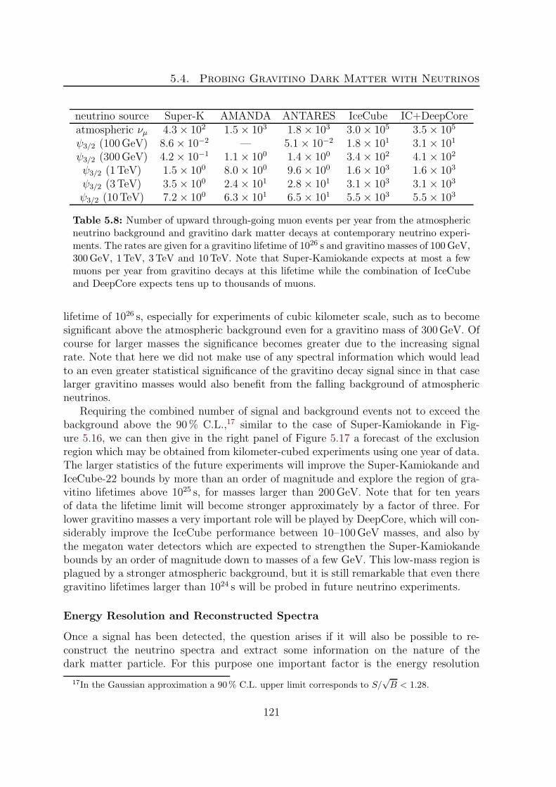
5.4. Probing Gravitino Dark Matter with Neutrinos
neutrino source Super-K AMANDA ANTARES IceCube IC+DeepCoreatmospheric νµ 4.3× 10² 1.5× 10³ 1.8× 10³ 3.0× 10⁵ 3.5× 10⁵
ψ3/2 (100GeV) 8.6× 10⁻² — 5.1× 10⁻² 1.8× 101 3.1× 101
ψ3/2 (300GeV) 4.2× 10⁻¹ 1.1× 100 1.4× 100 3.4× 10² 4.1× 10²
ψ3/2 (1TeV) 1.5× 100 8.0× 100 9.6× 100 1.6× 10³ 1.6× 10³
ψ3/2 (3TeV) 3.5× 100 2.4× 101 2.8× 101 3.1× 10³ 3.1× 10³
ψ3/2 (10TeV) 7.2× 100 6.3× 101 6.5× 101 5.5× 10³ 5.5× 10³
Table 5.8: Number of upward through-going muon events per year from the atmosphericneutrino background and gravitino dark matter decays at contemporary neutrino experi-ments. The rates are given for a gravitino lifetime of 1026 s and gravitino masses of 100GeV,300GeV, 1TeV, 3TeV and 10TeV. Note that Super-Kamiokande expects at most a fewmuons per year from gravitino decays at this lifetime while the combination of IceCubeand DeepCore expects tens up to thousands of muons.
lifetime of 1026 s, especially for experiments of cubic kilometer scale, such as to becomesignificant above the atmospheric background even for a gravitino mass of 300GeV. Ofcourse for larger masses the significance becomes greater due to the increasing signalrate. Note that here we did not make use of any spectral information which would leadto an even greater statistical significance of the gravitino decay signal since in that caselarger gravitino masses would also benefit from the falling background of atmosphericneutrinos.
Requiring the combined number of signal and background events not to exceed thebackground above the 90% C.L.,17 similar to the case of Super-Kamiokande in Fig-ure 5.16, we can then give in the right panel of Figure 5.17 a forecast of the exclusionregion which may be obtained from kilometer-cubed experiments using one year of data.The larger statistics of the future experiments will improve the Super-Kamiokande andIceCube-22 bounds by more than an order of magnitude and explore the region of gra-vitino lifetimes above 1025 s, for masses larger than 200GeV. Note that for ten yearsof data the lifetime limit will become stronger approximately by a factor of three. Forlower gravitino masses a very important role will be played by DeepCore, which will con-siderably improve the IceCube performance between 10–100GeV masses, and also bythe megaton water detectors which are expected to strengthen the Super-Kamiokandebounds by an order of magnitude down to masses of a few GeV. This low-mass region isplagued by a stronger atmospheric background, but it is still remarkable that even theregravitino lifetimes larger than 1024 s will be probed in future neutrino experiments.
Energy Resolution and Reconstructed Spectra
Once a signal has been detected, the question arises if it will also be possible to re-construct the neutrino spectra and extract some information on the nature of thedark matter particle. For this purpose one important factor is the energy resolution
17In the Gaussian approximation a 90% C.L. upper limit corresponds to S/√B < 1.28.
121

Chapter 5. Indirect Detection of Gravitino Dark Matter
ANTARES
AMANDA-II
IceCube H+ DeepCoreL
101 102 103 104 105 106
10-5
10-4
10-3
0.01
0.1
1
10
100
Energy HGeVL
NeutrinoEffectiveAreaHm
2L
exclusion from
through-going muons
after 1 year at IceCube + DeepCore
100 1000 10000
1024
1025
1026
1027
Gravitino Mass HGeVL
GravitinoLifetim
eHsL
Figure 5.17: Left: Neutrino effective areas of the AMANDA-II, ANTARES and IceCube-80 experiments. The increased effective area due to the DeepCore extension of the IceCubedetector is shown as a dashed line (see text for references). Right: 90% C.L. exclusionprospects in the lifetime vs. mass plane for decaying gravitino dark matter from the non-observation of a statistically significant excess in the total rate of neutrino-induced upwardthrough-going muons observed at IceCube + DeepCore in one year.
of the neutrino detectors. We will take here for reference the IceCube detector, forwhich the energy resolution is σ = log10(Emax/Emin) = 0.3–0.4 for track-like events andσ = log10(Emax/Emin) = 0.18 for cascade-like events [328].
Technically we apply the energy resolution by a convolution of the signal spectrumwith a Gaussian distribution in the logarithm of the energy:
dNGauss
dE=
exp (−(σ ln 10)2/2)√2 π σ ln 10
∞∫
0
dE ′ 1
E ′ exp
(−1
2
(log10 E/E
′
σ
)2)dN
dE ′ . (5.72)
In Figures 5.18–5.20 we show the resulting histograms for the signal from gravitinodecays and the atmospheric background using an energy resolution of 0.3 in log10 E andthree bins per decade for upward through-going and contained muons, and an energyresolution of 0.18 in log10E and five bins per decade for shower events. These figurescan be compared to Figures 5.13–5.15 which show the spectra unbinned and withoutfinite energy resolution. Also shown is the significance of the signal over the backgroundin different bins for a lifetime of 1026 s using one year of data assuming an ideal detectorwith an effective area of 1 km2 for upward through-going muons and an effective volumeof 1 km3 for contained muons and cascades.
We see that for nearly all gravitino masses the signal will appear with a large sta-tistical significance in more than a single bin and it is obvious that the neutrino signal
122

5.4. Probing Gravitino Dark Matter with Neutrinos
Upward Through-Going Muons
atmospheric background
Τ32 = 1026 s
m32 = 100 GeV 1 TeV 10 TeV
1 10 100 1000 10000 100000
0.1
1
10
100
103
104
105
Energy HGeVL
MuonFluxHkm-2yr-
1L
Upward Through-Going Muons
Τ32 = 1026s
m32 = 100 GeV 1 TeV 10 TeV
1 10 100 1000 10000 100000
0.01
0.1
1
10
Energy HGeVL
StatisticalSignificance
Figure 5.18: Left: Flux of upward through-going muons expected from decaying gravitinodark matter compared to the atmospheric background. The flux is computed for gravitinomasses of 100GeV, 1TeV and 10TeV, and a lifetime of 1026 s using an energy resolutionof 0.3 in log10E and three bins per decade. Right: Statistical significance (S/
√B) of the
signal of through-going muons as shown in the left panel calculated for every single energybin using one year of data assuming an ideal detector with an effective area of 1 km2.
from gravitino decays is not following a power law like the atmospheric one. Thus it isclear that using spectral information it will be possible to set much stricter limits onthe gravitino parameter space than shown in Figure 5.17. In order to give an idea of thesensitivities that can be obtained using spectral information, we show in Table 5.9 thevalues of the gravitino lifetime for several gravitino masses that correspond to a 5 σ signalin the most significant energy bin after one year of observation for an idealized detectorwith an effective muon area of 1 km2 and an effective volume of 1 km3 for containedmuons and shower events. We observe that the limits from through-going and containedmuons are better but not far from those shown in Figure 5.17, while the shower eventsin principle allow to constrain even one order of magnitude larger lifetimes. Using notonly the dominant energy bin from Figures 5.18 to 5.20 but a combination of severalenergy bins optimized for the expected signal from gravitino decays it will be possibleto set even stronger constraints on the gravitino lifetime.
On the other hand, discriminating the spectra expected from gravitino decay fromthose expected for other dark matter candidates will not be that straightforward, espe-cially if the mass of the decaying particle is unknown (cf. the discussion in [78]). Afterconvolution with the energy resolution, the spectrum expected for gravitino dark matterand those for generic channels of scalar or fermionic dark matter particles appear quitesimilar, especially within their statistical error.
123

Chapter 5. Indirect Detection of Gravitino Dark Matter
Contained Muons
atmospheric background
Τ32 = 1026 s
m32 = 100 GeV 1 TeV 10 TeV
1 10 100 1000 10000 100000
1
10
100
103
104
105
106
Energy HGeVL
MuonRateHkm-3yr-
1L
Contained Muons
Τ32 = 1026s
m32 = 100 GeV 1 TeV 10 TeV
1 10 100 1000 10000 100000
0.01
0.1
1
10
Energy HGeVL
StatisticalSignificance
Figure 5.19: Left: Rate of contained muons per cubic kilometer of detector volume fromdecaying gravitino dark matter compared to the atmospheric background. The rates arecomputed for gravitino masses of 100GeV, 1TeV and 10TeV, and a lifetime of 1026 susing an energy resolution of 0.3 in log10E and three bins per decade. Right: Statisticalsignificance (S/
√B) of the contained muon signal as shown in the left panel calculated for
every single energy bin using one year of data assuming an ideal detector with an effectivevolume of 1 km3.
5.5 Constraints on the Gravitino Dark Matter Pa-
rameter Space
In this final section we want to summarize the limits on the parameter space of decay-ing gravitino dark matter coming from indirect searches in the gamma-ray, positron,antiproton, antideuteron and neutrino channels. While we have presented bounds onthe gravitino lifetime from the different channels in the previous sections, here we wantto use these limits to constrain the amount of bilinear R-parity violation.
The upper limits on the parameter ξ can be calculated from the decay widths pre-sented in Section 4.3 and the lower limits on the gravitino lifetime in the followingway:
ξ ≤(Γtot(m3/2)
ξ2× τ3/2(m3/2)
)−1/2
. (5.73)
Since the gravitino decay width scales like m33/2 one would generically expect a bound
on ξ that scales like m−3/23/2 for a lifetime bound that is independent of the gravitino
mass. Rather flat lifetime bounds are obtained from practically all cosmic ray observa-tions except for neutrinos, where the limits become stronger for larger gravitino masses.However, we also need to take into account the dependence of the mixing parameters on
124

5.5. Constraints on the Gravitino Dark Matter Parameter Space
Shower Events
atmospheric background
Τ32 = 1026 s
m32 = 100 GeV 1 TeV 10 TeV
1 10 100 1000 10000 100000
1
10
100
103
104
105
106
Energy HGeVL
Shower
RateHkm-3yr-
1L
Shower Events
Τ32 = 1026s
m32 = 100 GeV 1 TeV 10 TeV
1 10 100 1000 10000 100000
0.01
0.1
1
10
100
Energy HGeVL
StatisticalSignificance
Figure 5.20: Left: Rate of electromagnetic and hadronic showers per cubic kilometerof detector volume from decaying gravitino dark matter compared to the atmosphericbackground. The rates are computed for gravitino masses of 100GeV, 1TeV and 10TeV,and a lifetime of 1026 s using an energy resolution of 0.18 in log10E and five bins perdecade. Right: Statistical significance (S/
√B) of the shower signal as shown in the left
panel calculated for every single energy bin using one year of data assuming an idealdetector with an effective volume of 1 km3.
gravitino mass through-going muons contained muons shower events100GeV 2.0× 1024 s 8.4× 1024 s 3.6× 1025 s300GeV 8.5× 1024 s 2.3× 1025 s 1.3× 1026 s1TeV 3.1× 1025 s 4.7× 1025 s 3.8× 1026 s3TeV 8.3× 1025 s 9.1× 1025 s 7.3× 1026 s10TeV 2.3× 1026 s 2.0× 1026 s 1.7× 1027 s
Table 5.9: Gravitino lifetimes for various gravitino masses corresponding to a S/√B = 5
significance in the most significant energy bin after one year of observation in an ideal-ized detector with an effective muon area of 1 km2 and an effective volume for containedmuons and showers of 1 km3. Notice that the sensitivity obtained with through-going andcontained muons is quite similar. At larger masses the bound from through-going muonsis stronger since the statistics increases due to the longer muon range at higher energies.However, neglecting reconstruction efficiencies the strongest constraint is obtained fromshower events since that channel offers the best signal-to-background ratio (see discussionin Section 5.4.2).
125

Chapter 5. Indirect Detection of Gravitino Dark Matter
Ξ = 10-7
Ξ = 10-11
1 10 100 1000 10000
10-12
10-11
10-10
10-9
10-8
10-7
Gravitino Mass HGeVL
R-ParityViolatingParam
eterΞ
IceCube ΝΜ prospects
Super-Kamiokande ΝΜ
GAPSAMS-02 d prospects
PAMELA p
Fermi LAT diffuse Γ
Fermi LAT Γ line
Figure 5.21: Summarized bounds from indirect dark matter searches on the gravitinodark matter parameter space. We present the current bounds from cosmic-ray observationsand future prospects for antideuteron and neutrino searches. In addition, we mark theboundaries of the cosmologically preferred range of the R-parity breaking parameter.
the gravitino mass. As we chose the gaugino masses to be proportional to the gravitinomass, the gaugino–neutrino and gaugino–charged lepton mixing parameters scale like1/m3/2 (cf. the discussion in Section 4.3.3). Therefore, we find that the decay width forthe two-body decay into photon and neutrino actually scales like m3/2. For the otherdecay channels the decay width is dominated by diagrams not involving any mixingparameters for larger gravitino masses and it therefore really scales like m3
3/2.
In Figure 5.21 we present the exclusion regions in the ξ − m3/2 parameter spaceobtained via the method described above. At low gravitino masses the dominant boundcomes from photon-line searches. Above m3/2 = 100GeV the bounds from the contin-uum contributions to the gamma-ray and antiproton fluxes provide the most stringentconstraints. The current limits of Super-Kamiokande from the neutrino flux are weakerby almost one order of magnitude. However, future bounds from IceCube are expectedto be competitive to those of gamma rays and antiprotons. Beyond that, using the moresensitive channel of neutrino-induced showers and employing spectral information theneutrino bounds could even dominate the large gravitino mass region.
In scenarios where the photon line is absent an important role is expected to beplayed by observations of charged cosmic rays for low gravitino masses. Since boundsfrom antiprotons rely on background subtractions in an energy range where the effect ofsolar modulation introduces some uncertainty, the almost background-free antideuteron
126

5.5. Constraints on the Gravitino Dark Matter Parameter Space
channel is expected to provide the best exclusion limit in this case.We also show the boundaries of the cosmologically preferred range of the R-parity
breaking parameter ξ. It is quite remarkable that indirect dark matter searches areprobing exactly the allowed region derived from completely different arguments. In par-ticular, for masses above O(1) TeV practically the complete favored range of ξ is alreadyexcluded. It will be interesting to see how future observations or complementary limitsfrom collider searches will further constrain this parameter space.
127

Chapter 6
Direct Detection of Gravitino Dark
Matter
The method of direct dark matter detection is based on the observation of nuclearrecoils in underground detectors due to scattering processes of nuclei with dark matterparticles traversing the Earth. In particular for WIMP dark matter candidates a signalis expected since their interactions with matter should be of the order of weak scaleinteractions.
However, as the interactions of gravitinos are strongly suppressed compared to thestandard WIMP case, typically no observable signal is expected in direct detectionexperiments from gravitino–nucleon scattering. In this chapter we want to discuss quan-titatively how the situation changes for gravitino dark matter in models with broken Rparity. Although the rate for elastic scatterings is not changed by additional R-parityviolating interactions, the slight violation of R parity allows for inelastic scatteringsoff nucleons that could be significantly enhanced in strength compared to the elasticscattering processes.
Let us start the discussion with a very brief overview of the method of direct darkmatter detection. A more extensive review on this topic and further references can befound, for instance, in [10].
6.1 Direct Searches for Dark Matter
As the solar system orbits around the galactic center, it is expected that dark matterparticles from the galactic halo cross the Earth in large numbers. In [329] it was firstproposed to search for signals from scatterings of these dark matter particles in under-ground detectors. The general idea is to observe the recoil of target nuclei induced byelastic scatterings of dark matter particles off those nuclei. Usually, one distinguishesbetween spin-independent and spin-dependent interactions: Spin-dependent interactionsare determined by the coupling of the dark matter particle’s spin and the spin of thetarget nucleus. In many cases this type of interaction dominates in the scattering off
128

6.1. Direct Searches for Dark Matter
a single proton or light nuclei. Spin-independent interactions, on the other hand, havethe advantage that they coherently add up and thus can be significantly enhanced whenscattering off heavy nuclei is considered. In the following we will only consider the lattercase.
The differential recoil rate for spin-independent dark matter–nucleus scattering pro-cesses is given by [10]
dR
dER
=2 ρlocmDM
dσ
d|~k|2v f(v) dv , (6.1)
where ~k is the momentum of the recoiling nucleus and the recoil energy is given by
ER ≃ |~k|22mN
(6.2)
in the non-relativistic case. The elastic scattering of dark matter particles with massesof the order of the electroweak scale typically leads to recoil energies in the range from10 to 100 keV. The four-momentum transfer t of the scattering process is given by
t = (k′ − k)2= 2m2
N − 2mN
√m2
N + |~k|2 ≃ −|~k|2, (6.3)
where k and k′ are the four-momenta of the nucleus before and after the scattering, and~k is the non-relativistic recoil momentum. Thus the differential scattering cross sectionis typically described in terms of |~k|2. The differential scattering cross section of anelastic scattering process can also be written as the product of the cross section at zeromomentum transfer σ0 and a nuclear form factor
dσ
d|~k|2=
σ04µ2 v2
F 2(|~k|) , (6.4)
where the dark matter–nucleus reduced mass is defined as
µ =mN mDM
mN +mDM. (6.5)
In elastic processes there is a relation between the momentum transfer, the relativevelocity and the scattering angle θ∗ in the center-of-momentum frame:
|~k|2 = 2µ2 v2 (1− cos θ∗) so that ER ≃ µ2 v2
mN
(1− cos θ∗) . (6.6)
The expected signal is determined assuming that the dark matter particles are dis-tributed in the halo according to an isothermal profile with a local dark matter densityρloc ≃ 0.3GeVcm−3. In addition, usually a Maxwell–Boltzmann velocity distributionf(v) with a characteristic velocity of v0 ∼ 220 km s−1 is assumed for the dark matter
129

Chapter 6. Direct Detection of Gravitino Dark Matter
particles [10]. The total rate is then determined by integrating over the dark mattervelocity distribution:
dR
dER=
ρσ0 loc
2mDM µF 2(|~k|)
∞∫
vmin
f(v)
vdv , (6.7)
where the minimal velocity is given by the condition vmin =√ERmN/(2µ2). In the
popular case of neutralino WIMP dark matter one expects elastic scattering cross sec-tions of the order of 10−10 to 10−6 pb corresponding to a maximal event rate of aboutone event per kilogram detector material and day [138]. Most recent direct detection ex-periments have excluded spin-independent WIMP elastic scattering cross sections downto a level of 10−7 to 10−8 pb (see for instance [330–332]).
On the other hand, it is claimed that the DAMA experiment observes an annualmodulation signal from dark matter with a significance of more than 8 σ [333, 334].An annual modulation in the rate of dark matter scattering events is a generic signalfrom dark matter particles in the galactic halo. It is expected due to the variation ofthe Earth’s velocity with respect to the halo because of the Earth’s orbit around theSun. The DAMA observation is generally considered as being in conflict with the nullresults of other experiments, although various possibilities to achieve compatibility arediscussed in the literature (see e.g. [335]).
One proposal to reconcile the observations of DAMA with the majority of otherdirect detection experiments is inelastic dark matter [336, 337]. In this framework thedark matter particle is accompanied by an almost degenerate state that is heavier byO(100) keV. Assuming a highly suppressed elastic scattering cross section, an incidentdark matter particle can only inelastically scatter off nuclei, leading to a transition tothe heavier state. This means, however, that not all dark matter particles crossing theEarth can scatter off nuclei but only those with a particular minimal velocity. This effectleads to very a strong suppression of the signal in detectors like CDMS and EDELWEISSusing rather light target nuclei, thereby giving a possible explanation for the compatibil-ity of the DAMA observation using rather heavy iodine nuclei. However, very recentlythis model has been almost completely ruled out by new data of the XENON100 exper-iment [338].
Let us now turn to the case of gravitino dark matter. As the elastic scatteringcross section of gravitinos on nuclei is proportional to 1/M4
Pl there is no chance toobserve these processes in underground detectors. In the case of additional R-parityviolating interactions, however, inelastic scattering processes whose cross sections areonly suppressed by 1/M2
Pl and the amount of R-parity breaking become possible. In thiscase the inelasticity is in the opposite direction as for the framework mentioned above.A gravitino can scatter off nuclei, thereby being transformed into a neutrino. In thisprocess the mass of the gravitino is released as energy and passed over to the neutrinoand the target nucleus. In this respect, one could refer to the gravitino with broken Rparity as anti-inelastic dark matter.
130

6.2. Gravitino Dark Matter with Bilinear R-Parity Violation
6.2 Gravitino Dark Matter with Bilinear R-Parity
Violation
Here we want to discuss the inelastic scattering of gravitino dark matter off targetnucleons in the framework of bilinear R-parity breaking. We separately consider threecases: the exchange of a lightest Higgs boson, the exchange of a Z boson and the exchangeof a photon. In all cases the gravitino is destroyed in the scattering process while aneutrino is generated in the final state. In particular the photon exchange channel mightbe interesting since it is not available for practically all other dark matter candidatesand potentially leads to an enhanced cross section because of the massless propagator.
Inelastic Gravitino–Nucleon Scattering via Higgs Exchange
At tree level there are two Feynman diagrams contributing to the inelastic gravitinoscattering off a nucleon via the exchange of the lightest Higgs boson:
ψ3/2 νi
h
νi
N N
+
h
ψ3/2 νi
h
N N
.
For the coupling of the Higgs boson to the nucleons we need to know the effective massof the quarks inside the nucleon. Typically, this is expressed in the form [10]
〈N |mq q q|N〉 = mN fNTq. (6.8)
For the cases of protons and neutrons the coefficients for the light quarks are givenby [339]
f pTu
= 0.020± 0.004 , fnTu
= 0.014± 0.003 ,
f pTd
= 0.026± 0.005 , fnTd
= 0.036± 0.008 , (6.9)
f pTs
= 0.118± 0.062 , fnTs
= 0.118± 0.062 .
In addition, there is a coupling to the gluon content of the nucleons via heavy quarkloops. This leads to coefficients for the heavy quarks of the form [340]
fNTc, b ,t
=2
27fNTG
with fNTG
= 1− fNTu
− fNTd
− fNTs. (6.10)
131

Chapter 6. Direct Detection of Gravitino Dark Matter
For the cases of protons and neutrons this leads to practically equal coefficients for theheavy quarks:
f pTc, b ,t
≃ 0.062 and fnTc, b ,t
≃ 0.062 . (6.11)
The calculation of the differential scattering cross section is presented in Appendix F.Here we directly present the final result:
dσNdt
=ξ2i m
23/2m
2N
(∑q f
NTq
)2
1536 π v2m4hM
2Pl |~v|
2
∣∣∣∣1 +1
2
m2Z
m2νi
cos 2 β − 2 sin β UH0uZ
− 2 cosβ UH0dZ
∣∣∣∣2
×(1− t
m23/2
)3(1− t
2m2N
). (6.12)
The four-momentum transfer t can be expressed in terms of the scattering angle θbetween the direction of the incoming gravitino and the scattered neutrino:
t = (p′ − p)2 = m23/2 − 2 (E |~p ′| − |~p | |~p ′| cos θ) . (6.13)
Energy conservation requires that the momentum of the final state neutrino is given by
|~p ′| =m2
3/2 + 2mNE
2 (E +mN − |~p | cos θ) . (6.14)
This leads finally to the relation
t = m23/2 −
(E − |~p | cos θ)(m2
3/2 + 2mNE)
mN + E − |~p | cos θ . (6.15)
The limiting values of the four-momentum transfer are then given by
t0 = t(θ = 0) = m23/2 −
(E − |~p |)(m2
3/2 + 2mNE)
mN + E − |~p | (6.16)
and
t1 = t(θ = 180) = m23/2 −
(E + |~p |)(m2
3/2 + 2mNE)
mN + E + |~p | , (6.17)
and the size of the kinematically allowed range is given by
t0 − t1 =2 |~p |mN
(m2
3/2 + 2mNE)
(mN + E − |~p |) (mN + E + |~p |) . (6.18)
The kinematics in this situation strongly differs from the case of elastic WIMP scattering,where the momentum transfer is determined by the velocity of the dark matter particles.
132

6.2. Gravitino Dark Matter with Bilinear R-Parity Violation
Here the momentum transfer is mainly given by the gravitino mass with only a slightdependence on the velocity. Therefore, one needs much lighter gravitino masses to geta recoil signal in the 10–100 keV range probed by current experiments. We then findthat we will need gravitinos with a mass of O(1–100)MeV.1 In this case the gravitinois much lighter than the target nucleon, m3/2 ≪ mN , and the results simplify to
t ≃ −m23/2 (1− 2 |~v| cos θ) and t0 − t1 ≃ 4 |~v|m2
3/2 . (6.19)
Since the differential cross section does not change significantly over the kinematicallyallowed range, the total cross section is approximately given by
σN ≃ξ2i m
43/2m
2N
(∑q f
NTq
)2
48 π v2m4hM
2Pl |~v|
, (6.20)
where we neglected a possible suppression by a nuclear form factor. Numerically we find
σp ≃ 1.2× 10−63 pb
(ξi
10−7
)2 ( m3/2
10MeV
)4(115GeV
mh
)4(220 km s−1
|~v|
)(6.21)
and
σn ≃ 1.3× 10−63 pb
(ξi
10−7
)2 ( m3/2
10MeV
)4(115GeV
mh
)4(220 km s−1
|~v|
)(6.22)
for the cases of gravitino–proton and gravitino–neutron scattering, respectively. Thesevalues are extremely far below the current experimental limits on elastic scattering crosssections which are on the order of 10−8 pb. Therefore, it seems hopeless to detect a signalfrom gravitino dark matter in an underground laboratory, even in the case of largeramounts of R-parity violation. Nevertheless, we also want to consider the remaining twocases.
1A consistent cosmological scenario with a gravitino mass in the MeV range can be constructed inspecific models of gauge mediation [341–344].
133

Chapter 6. Direct Detection of Gravitino Dark Matter
Inelastic Gravitino–Nucleon Scattering via Z Exchange
At tree level there are four diagrams contributing to the inelastic gravitino–nucleonscattering via the exchange of a Z boson:
ψ3/2 νi
Z
Z
N N
+
ψ3/2 νi
Z
N N
vi
+
H0u, d
ψ3/2 νi
Z
N N
vu, d
.
For the coupling of the Z boson to the nucleons we only consider the vector part of theinteraction. In this case only the charges of the valence quarks contribute. The couplingto protons and neutrons is then calculated as
proton:∑
q
CV = 2CV (u) + CV (d) =1
4− sin2 θW ,
neutron:∑
q
CV = CV (u) + 2CV (d) = −1
4.
(6.23)
Since sin2 θW ≈ 1/4, the Z coupling to protons is suppressed compared to the couplingto neutrons. We present the calculation of the differential cross section in Appendix F.The full result is rather lengthy so we directly show the approximate result for the total
134

6.2. Gravitino Dark Matter with Bilinear R-Parity Violation
cross section. Using the same approximations as for the Higgs channel we find
σn ≃ξ2i g
2Z m
23/2
128 πm2Z M
2Pl |~v|
(U2ZZ
m23/2
m2Z
+∣∣∣1 + sβ UH0
uZ− cβ UH0
d Z
∣∣∣2
− 2
3
m3/2
mZUZZ
(1 + sβ ReUH0
uZ− cβ ReUH0
d Z
)).
(6.24)
We observe that the contribution from the 4-vertex dominates the cross section. Ne-glecting the small higgsino–zino mixing parameters, this leads to the following numericalresult for the gravitino–neutron cross section via Z exchange:
σn ≃ 4.7× 10−50 pb
(ξi
10−7
)2 ( m3/2
10MeV
)2(220 km s−1
|~v|
). (6.25)
This value is still far below the reach of detectors but it is thirteen orders of magnitudelarger than the Higgs exchange contribution. Let us now turn to the case of photonexchange.
Inelastic Gravitino–Nucleon Scattering via Photon Exchange
At tree level there is only one diagram contributing to the inelastic gravitino–nucleonscattering via the exchange of a photon:
ψ3/2 νi
γ
γ
N N
.
The photon coupling to the nucleons is also a vector interaction. From the calculationin Appendix F we find the differential cross section
dσNdt
=ξ2i
(∑qQ)2e2∣∣UγZ
∣∣2
192 π tM2Pl |~v|
2
(1− 3
4
m23/2
m2N
− 5E
mN− 3
4
t
m2N
− t
m23/2
− 6E2
m23/2
(6.26)
− t E
mN m23/2
+1
4
t2
m2N m
23/2
+t
m23/2
(2
(E2
m23/2
+t E
mN m23/2
)+
1
4
t2
m2N m
23/2
)).
135

Chapter 6. Direct Detection of Gravitino Dark Matter
In this case the coupling to neutrons vanishes as they are electromagnetically neutral.The coupling to protons is simply given by the elementary charge. We find the approx-imate total cross section
σp ≃ξ2i e
2∣∣UγZ
∣∣2
8 πM2Pl |~v|
=ξ2i α
∣∣UγZ
∣∣2
2M2Pl |~v|
. (6.27)
It is important to note that this result is independent of the masses of the gravitinoand the nucleon. We find the following numerical result for the gravitino–proton crosssection via photon exchange:
σp ≃ 3.4× 10−43 pb
(ξi
10−7
)2(220 km s−1
|~v|
)(∣∣UγZ
∣∣2
0.1
). (6.28)
Although this number is still way to small to hope for a detection in this channel, it isvery interesting that the cross section for the photon exchange channel is roughly sevenorders of magnitude larger than for the Z boson exchange channel and even twentyorders of magnitude larger than for the Higgs exchange channel. This shows that themassless propagator really leads to a significant enhancement of the cross section, evenif – unfortunately – still far below the reach of any proposed underground detector.
136

Chapter 7
Conclusions and Outlook
After several decades of thorough theoretical studies and a multitude of ambitious exper-iments the nature of dark matter still remains one of the greatest unresolved mysteriesin cosmology. A particularly well-motivated particle candidate for the dark matter isthe gravitino in theories with a slight violation of R parity as it naturally leads toa consistent cosmological scenario avoiding all cosmological gravitino problems. Afterinflation the universe is reheated to a very high temperature as required in order togenerate the observed baryon asymmetry via the mechanism of thermal leptogenesis.In this early hot phase gravitinos are produced in scattering processes of the thermalplasma, thus leading to a relic density that is consistent with the observed dark matterdensity for generic values of the particle physics parameters. A tiny amount of R-paritybreaking induces a sufficiently fast decay of the other supersymmetric particles so thatthe particle content of the thermal plasma reduces to that expected from the standardmodel of particle physics well before the onset of primordial nucleosynthesis. Togetherwith the upper limit on the amount of R-parity breaking from the condition that aonce generated baryon asymmetry is not washed out again by lepton number-violatingprocesses, this leads to an allowed range for the gravitino lifetime that is several ordersof magnitude above the current age of the universe.
In this thesis we have studied in detail the phenomenological consequences of unstablegravitino dark matter for indirect and direct detection experiments. We started witha discussion of the effect of R-parity violating mass mixing in the fermionic sector,providing new analytical approximate formulae for the mixing parameters. Equippedwith these tools we presented a detailed calculation of gravitino three-body decay widths,thereby extending and correcting results previously obtained in the literature. Moreover,we extended the results for the gravitino two-body decay widths by adding a set ofFeynman diagrams that were neglected in earlier calculations.
Using the results for the three-body decay widths we determined the gravitinobranching ratios in the decoupling limit for an exemplary choice of parameters and dis-cussed the differences to the two-body results and the implications for indirect searchesfor gravitino dark matter. We also found that there are regions in the parameter spacewhere the two-body decay into a photon and a neutrino is suppressed. This could lead
137

Chapter 7. Conclusions and Outlook
to interesting differences in the phenomenology for light gravitinos. We then discussedthe spectra of particles produced in gravitino decays. For the case of gravitino two-bodydecays we presented the spectra of all possible stable final state particles as obtainedwith the help of PYTHIA including also the spectra for deuterons and antideuterons.1
In the case of gravitino three-body decays we only presented the spectra of particlesdirectly produced in the three-body decay as we were lacking a numerical tool to treatthe subsequent fragmentation processes. This is a point that definitely should be workedout in future studies.
Moreover, we presented an extensive study of the cosmic-ray signals expected fromgravitino dark matter decays, finding that gravitino decays cannot explain the observedrise in the positron fraction as this would lead to gamma-ray and and antiproton signalsovershooting the observed fluxes. Actually, requiring that the gravitino signal does notexceed the observed fluxes, we estimated conservative lower limits on the gravitino life-time at the level of 1026–1027 s. Searches for photon lines lead to significantly strongerlifetime limits reaching almost 1029 s for gravitino masses below 100GeV if the photonline from gravitino decays is not suppressed. We also elaborated on the prospects of fu-ture antideuteron searches, finding that the antideuteron channel potentially allows toput even stronger limits on the gravitino lifetime, especially at low masses. This is due tothe fact that forthcoming experiments are planned to search for antideuterons at low en-ergies where the astrophysical background is small compared to the signal expectation.But also for larger gravitino masses the antideuteron signal from gravitino decays mightbe observable on top of the astrophysical background. This is in contrast to findingsin earlier analyses where the spectrum of high-energetic antideuterons was artificiallysuppressed by the spherical approximation of the antideuteron coalescence prescription.As we were lacking the spectra of final state particles for gravitino three-body decays,we concentrated in these discussions on the case of gravitinos heavier than the W bosonmass. However, since the phenomenology of gravitino three-body decays promises tolead to interesting predictions we plan to perform a study for lighter gravitinos in futurework.
In addition, we presented a detailed analysis of the expected neutrino signals fromgravitino decays, discussing also the different event topologies and the respective ex-pected rates in neutrino detectors. We found that the neutrino channel is particularlyuseful to constrain rather heavy gravitinos since the observed event rates get enhancedat high energies. The most promising detection channel are neutrino-induced showerevents as they provide the best energy resolution and suffer the least background ofatmospheric neutrinos. Finally, we employed the combination of limits on the gravitinolifetime from various cosmic-ray channels to place constraints on the underlying R-parityviolating parameter. Interestingly, indirect dark matter searches exactly probe values forthe strength of R-parity violation that are favored by arguments from cosmology. Actu-ally, we find that about one half of the cosmologically favored parameter range is already
1The deuteron spectra were generated by my collaborator Gilles Vertongen employing a Monte Carloapproach instead of the commonly used spherical coalescence model.
138

excluded by indirect searches over the range of gravitino masses considered in this work.In the last part of this thesis we discussed the prospects for a direct detection of
gravitino dark matter. It is interesting that the violation of R parity allows for inelasticscatterings off nucleons with a significantly enhanced cross section. The kinematics ofthese processes is very different from elastic scatterings and also from the proposedinelastic dark matter models. We find that the momentum transferred to the nucleon ispractically independent of the dark matter velocity distribution in the galactic halo andsimply given by the gravitino mass. This could lead to a spectacular new kind of signalsat dark matter detectors. Additionally, in contrast to other dark matter candidatesthe gravitino can scatter via photon exchange, leading to an enhancement of the crosssection due to the massless propagator. Unfortunately, the suppression by the Planckscale and the small R-parity breaking parameters is still too strong and there seems tobe no hope to ever detect a gravitino scattering signal in an underground detector.
Now is a very exciting time for dark matter studies. Direct detection experimentswill soon completely probe the parameter space for neutralino dark matter and othergeneric weakly interacting massive particles. At the same time the LHC will be ableto test a large portion of the parameter space of softly broken supersymmetric theoriesand might soon deliver a first observation of supersymmetric particles. In particular,the LHC will be able to test scenarios of gravitino dark matter with broken R-parity bysearching for effects of long-lived massive particles. As the decay length of the next-to-lightest supersymmetric particle depends on the strength of bilinear R-parity breaking,the LHC will allow to extend the astrophysical bounds by roughly one order of magnitudefor gravitino masses at the order of the electroweak scale.
Finally, forthcoming indirect detection experiments will allow to search for darkmatter signals with much higher precision. In particular the AMS-02 experiment thatwas successfully launched into space on the last flight of space shuttle Endeavor andsubsequently installed at the International Space Station just a few weeks ago willgreatly improve on the observations of charged cosmic rays in the coming years. It iscapable of measuring positrons and electrons up to energies of almost a TeV. Due toits spectrometric measurement it is able to distinguish positrons from electrons up toenergies of several hundred GeV thus allowing to observe a possible cutoff in the positronspectrum due to an endpoint in the spectrum from dark matter annihilations or decays.In addition, the observation of the spectrum of antiprotons up to almost a TeV willallow to decide if a deviation from the astrophysical background as predicted by heavydark matter explanations of the PAMELA and Fermi LAT data really exists. Last butnot least AMS-02 will be the first experiment to significantly improve on the sensitivityfor antideuterons, thereby possibly allowing for the detection of a low-energetic darkmatter signal practically free from astrophysical backgrounds.
139

Chapter 7. Conclusions and Outlook
Note Added
Last week an analysis appeared on the arXiv that also presents a calculation of thegravitino three-body decay widths [345]. Their analysis confirms that the results for thedecay widths presented in [201] were incorrect. In addition, their formulae seem to be inaccord with our results. The Higgs exchange channel was not considered in this work,but the interference between the photon, Z and W channels for the ℓ+i ℓ
−i νi final state
was taken into account. This part was neglected in our calculation.
140
Acknowledgments
First and foremost I would like to thank my fiancee Melanie who supported me duringall the time I was working on this thesis.
Many thanks go also to my supervisor Laura Covi for many helpful discussions andvaluable advice, and to Jan Louis for acting as second examiner of this thesis.
I am also grateful to Alejandro Ibarra, David Tran and Gilles Vertongen for a fruitfulcollaboration on parts of the topics discussed in this thesis.
In addition, I would like to thank my office colleagues Vladimir Mitev, JasperHasenkamp, Kai Schmitz and Sebastian Schmidt for many helpful discussions and anenjoyable atmosphere in the office.
I would also like to thank Jan Hajer for helpful discussions about bilinear R-paritybreaking, and Kai Schmitz, Gilles Vertongen, my brother Christian and in particularJasper Hasenkamp for helpful suggestions on the manuscript of this thesis.
Finally, many thanks go to the entire DESY theory group for an enjoyable timeduring the years of preparing this thesis.
In addition, I acknowledge the support of the “Impuls- und Vernetzungsfonds” ofthe Helmholtz Association under contract number VH-NG-006 and of the DeutscheForschungsgemeinschaft within the Collaborative Research Centre 676.
141

Appendix A
Units and Physical Constants
In this appendix we summarize the values of all the physical and astrophysical constantsthat are used throughout this thesis. At times we work in units where the reduced Planckconstant, the speed of light and the Boltzmann constant obey ~ = c = k = 1. In thiscase, we have the conversion factors
1 eV = 1.160 4505(20)× 104K ,
1 eV = 1.602 176 487(40)× 10−19 J ,
1GeV = 1.782 661 758(44)× 10−27 kg ,
1GeV−1 = 1.973 269 631(49)× 10−16m ,
1GeV−1 = 6.582 118 99(16)× 10−25 s ,
1GeV−2 = 0.389 379 304(19)mb .
All figures are taken from the The Review of Particle Physics [81]. Numbers in paren-theses represent the one standard deviation uncertainty in the last digits.
Quantity Symbol Value
parsec pc 3.085 6776× 1016mSolar distance from galactic center r⊙ 8.4(4) kpcEarth mean equatorial radius R⊕ 6.378 137× 106mlocal halo density ρloc 0.3GeV cm−3 (within factor 2–3)present-day CMB temperature T0 2.725(1)Knormalized Hubble constant h 0.72(3)critical density ρc 1.053 68(11)× 10−5 h2GeV cm−3
matter density Ωmh2 0.133(6)
baryon density Ωbh2 0.0227(6)
dark matter density ΩDMh2 0.110(6)
dark energy density ΩΛ 0.74(3)total energy density Ωtot 1.006(6)baryon-to-photon ratio η 6.23(17)× 10−10
142

Quantity Symbol Value
barn b 10−28m2
electron mass me 510.998 910(13) keVmuon mass mµ 105.658 367(4)MeVmuon mean life τµ 2.197 034(21)× 10−6 stau mass mτ 1.776 82(16)GeVtau mean life ττ 290.6(1.0)× 10−15 sup quark mass mu 1.7–3.3MeVdown quark mass md 4.1–5.8MeVstrange quark mass ms 101+29
−21MeVcharm quark mass mc 1.27+0.07
−0.09GeVbottom quark mass mb 4.19+0.18
−0.06GeVtop quark mass mt 172.0(0.9)(1.3)GeVW boson mass mW 80.399(23)GeVW boson decay width ΓW 2.085(42)GeVZ boson mass mZ 91.1876(21)GeVZ boson decay width ΓZ 2.4952(23)GeVneutron mass mn 939.565 346(23)MeVneutron mean life τn 885.7(8) sproton mass mp 938.272 013(23)MeVdeuteron mass md 1875.612 793(47)MeVfine-structure constant α 1/137.035 999 679(94)Fermi coupling constant GF 1.116 37(1)× 10−5GeV−2
weak mixing angle sin2 θW (mZ) 0.231 16(13)strong coupling constant αs(mZ) 0.1184(7)gravitational constant GN 6.708 81(67)× 10−39GeV−2
Avogadro constant NA 6.022 141 79(30)× 1023mol−1
The values for the neutrino mixing parameters are taken from the recent analysis in [287].If two values are given, the first is the value assuming normal neutrino mass hierarchyand the second is the value for inverted hierarchy.
Quantity Symbol Value
solar neutrino mixing angle sin2 θ12 0.316(16)atmospheric mixing angle sin2 θ23 0.51(6), 0.52(6)third neutrino mixing angle sin2 θ13 0.017(+7
−9), 0.020(+8−9)
solar neutrino mass difference ∆m221 7.64(+19
−18)× 10−5 eV2
atmospheric mass difference ∆m231 2.45(9)× 10−3 eV2, −2.34(+10
−9 )× 10−3 eV2
143

Appendix B
Notation, Conventions and
Formulae
Four-Vectors and Tensors Lorentz indices are depicted by small Greek letters, e.g.µ = 0, 1, 2, 3. The metric of Minkowski space is chosen to be
gµν = gµν =
+1 0 0 00 −1 0 00 0 −1 00 0 0 −1
. (B.1)
Lorentz indices of four-vectors and higher rank tensors are raised and lowered using thespace-time metric:
aµ = gµν aν and bµ = gµν bν . (B.2)
We use in all cases a sum convention for Lorentz indices:
aµbµ ≡3∑
µ=0
aµbµ . (B.3)
Antisymmetric Symbols The totally antisymmetric tensor εµνρσ is defined such that
ε0123 = +1 . (B.4)
The indices of the totally antisymmetric tensor can be lowered using the space-timemetric:
εµνρσ = gµα gνβ gργ gσδ εαβγδ. (B.5)
The totally antisymmetric tensor in three dimensions, εijk, is chosen such that
ε123 = +1 . (B.6)
144
Gamma Matrices The Dirac gamma matrices are defined to form a Clifford algebrawith the anticommutation relation
γµ, γν = 2 gµν. (B.7)
In most cases it is convenient to suppress the spinor indices of the gamma matrices, sowe do not write them here. We also want to introduce an explicit representation of thegamma matrices. In the Weyl basis (also called chiral basis) the Dirac gamma matricesread
γµ =
(0 σµ
σµ 0
). (B.8)
In this expression the sigma matrices are given by σµ = (1, σi) and σµ = (1,−σi), where
the Pauli matrices are given by
σ1 =
(0 11 0
), σ2 =
(0 −ii 0
), σ3 =
(1 00 −1
), (B.9)
satisfying the identity σi σj = δij + i εijk σk . Using the algebra of the gamma matricesand the explicit form of the space-time metric (B.1) it can be easily seen that
(γ0)2
= 1 and(γi)2
= −1 . (B.10)
Hermitian conjugation of the gamma matrices yields
(γµ)† = γ0γµγ0. (B.11)
The Lorentz indices of gamma matrices are raised and lowered by the metric, just as inthe case of four-vectors. That implies
γ0 = γ0 and γi = −γi. (B.12)
Thus we see that raising and lowering of Lorentz indices is equivalent to hermitianconjugation. In addition to γ0, γ1, γ2, γ3, a fifth gamma matrix can be defined:
γ5 ≡ iγ0γ1γ2γ3 = − i
4!εµνρσγ
µγνγργσ. (B.13)
Using the algebra (B.7) it can be easily shown that γ5 has the following properties:γ5, γµ
= 0 ,
(γ5)2
= 1 ,(γ5)†
= γ5. (B.14)
In the Weyl basis γ5 has the following explicit form:
γ5 =
(−1 00 1
). (B.15)
Using this expression we can define the chirality projection operators
PL ≡ 1
2
(1− γ5
)=
(1 00 0
)and PR ≡ 1
2
(1 + γ5
)=
(0 00 1
). (B.16)
These operators possess the projector properties
P 2L = PL , P 2
R = PR and PLPR = PRPL = 0 . (B.17)
145

Appendix B. Notation, Conventions and Formulae
Identities for Gamma Matrices In the calculation of squared matrix elements weencounter traces of gamma matrices. For these the following identities can be derivedfrom the algebra (B.7):
Tr (1) = 4 ,
Tr (odd number of γs) = 0 ,
Tr (γµγν) = 4 gµν,
Tr (γµγνγργσ) = 4 (gµνgρσ − gµρgνσ + gµσgνρ) ,
Tr(γ5)= 0 ,
Tr(γµγνγ5
)= 0 ,
Tr(γµγνγργσγ5
)= −4 i εµνρσ.
(B.18)
We also encounter contractions of gamma matrices. Using the algebra (B.7), we obtainthe following identities:
γµγµ = 4 ,
γµγνγµ = −2 γν ,
γµγνγργµ = 4 gνρ,
γµγνγργσγµ = −2 γσγργν .
(B.19)
Two-Component and Four-Component Spinors A four-component Dirac spinorψD is made up of two two-component spinors, χα and η†α, in the following way:
ψD =
(χα
η†α
). (B.20)
The two-component spinors χα and η†α are complex, anticommuting objects with twodistinct types of spinor indices, α = 1, 2 and α = 1, 2. The spinor indices are depicted bysmall Greek letters from the beginning of the alphabet. They can be raised and loweredusing the antisymmetric symbols
εαβ, εαβ , εαβ and εαβ , where ε12 = 1 and ε12 = −1. (B.21)
In many places the spinor indices are not written explicitly. Then they can be recon-structed according to the contraction conventions
χ η = χαηα and χ†η† = χ†αη
†α. (B.22)
The Dirac adjoint and the charge conjugate of a Dirac spinor are, respectively, given by
ψD ≡ ψ†Dγ
0 =(ηα χ†
α
), (B.23)
ψcD ≡ CψT
D =
(ηαχ†α
), (B.24)
146

where we introduced the charge-conjugation matrix C with the properties
C† = C−1, CT = −C and CΓi TC† = ηiΓi, (B.25)
and
ηi =
1 for Γi = 1, γµγ5, γ5
−1 for Γi = γµ, σµν . (B.26)
In the above expression we use the definition σµν ≡ i2[γµ, γν ] , µ < ν . Using the
chirality projectors from equation (B.16) we define the left- and right-handed Diracspinors
PLψD =
(χα
0
), PRψD =
(0η†α
). (B.27)
A four-component Majorana spinor ψM is defined to be invariant under charge con-jugation. Thus a Majorana spinor is a Dirac spinor with the condition that η = χ,i.e.
ψM =
(χα
χ†α
)= ψc
M ≡ CψTM . (B.28)
A very common object in theories of particles with half-integral spin is the contractionof gamma matrices with the particle momentum. Therefore, we use the Feynman slashnotation
/p ≡ γµpµ . (B.29)
In order to obtain Lorentz scalars, in the formulation of theories of particles with half-integral spin there occur products of adjoint spinors and spinors. The adjoint spinor andadjoint vector-spinor are, respectively, defined as
ψ ≡ ψ†γ0 and ψµ ≡ ψ†µγ
0. (B.30)
Dirac Spinors Free spin-1/2 fermions are described by the Dirac equation,(i/∂ −m
)ψ(x) = 0 , (B.31)
that has four linearly independent plane-wave solutions:
ψ(x) = us(p) e−ip·x and ψ(x) = vs(p) eip·x, s = ±1
2, (B.32)
where the Dirac spinors u and v have to obey the following constraints:(/p−m
)us(p) = 0 and
(/p+m
)vs(p) = 0 . (B.33)
The polarization sums for spin-1/2 fermions are then given by [346]∑
s
us(p) us(p) = /p +m,
∑
s
vs(p) vs(p) = /p−m,(B.34)
where the sum is performed over the fermion helicity states s = ±12.
147
Appendix B. Notation, Conventions and Formulae
Polarization Vectors Free massless spin-1 particles in the Lorentz gauge (∂µAµ = 0)and free massive spin-1 particles obey the Proca equation [347]
(∂ν∂ν +M2
)Aµ = 0 . (B.35)
This equation has the plane-wave solutions
Aµ = ǫµ(p) e−ip·x, (B.36)
where ǫµ is a polarization vector. The condition ∂µAµ = 0 demands that
pµǫµ = 0 , (B.37)
reducing the number of independent polarization vectors to three. For massless spin-1particles we have the freedom to make the additional gauge transformation
Aµ → A′µ = Aµ + ∂µΛ with ∂µ∂µΛ = 0 . (B.38)
The condition for Λ is required by the Lorentz gauge condition. This additional gaugefreedom reduces the number of independent polarization vectors for massless spin-1particles to two. The polarization sum for massless spin-1 particles is then given by [346]
∑
λ
ǫλ ∗µ (p) ǫλν(p) = −gµν , (B.39)
where the sum is performed over the two polarization states of the massless spin-1particle λ = ±1, and the polarization sum for massive spin-1 particles is given by
∑
λ
ǫλ ∗µ (p) ǫλν(p) = −
(gµν −
pµpνm2
A
), (B.40)
where the sum is performed over the three polarization states of the massive spin-1particle λ = ±1, 0.
148
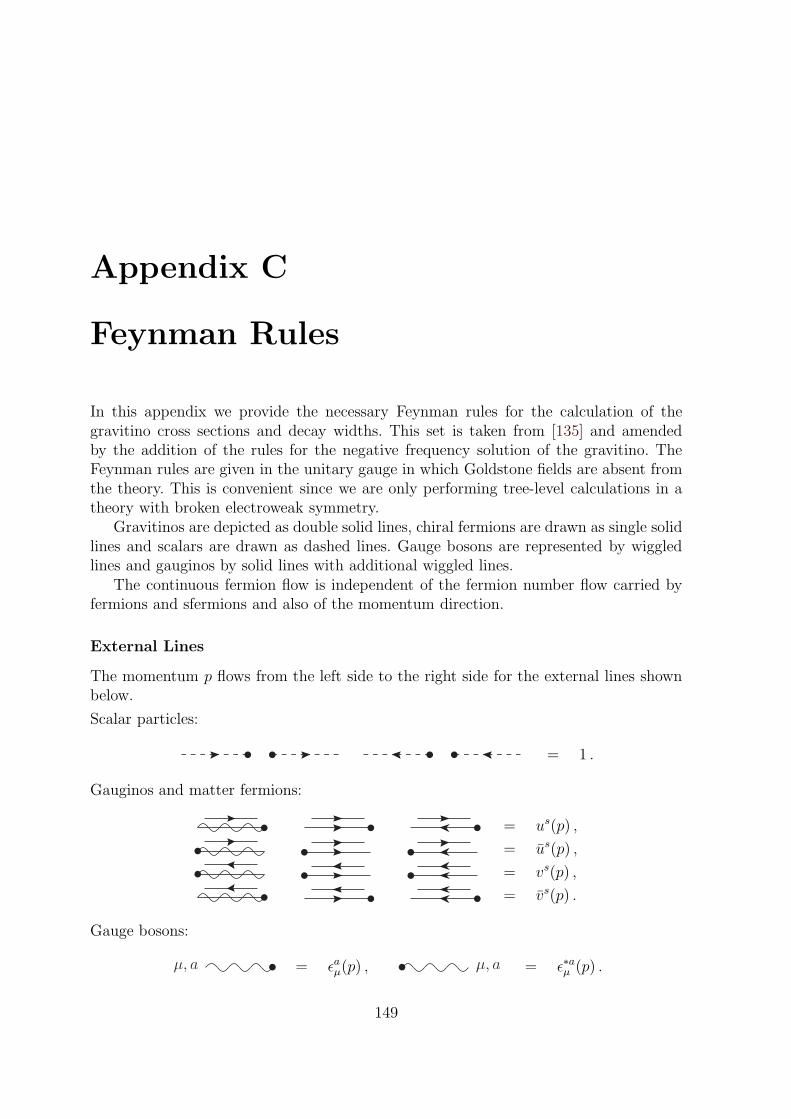
Appendix C
Feynman Rules
In this appendix we provide the necessary Feynman rules for the calculation of thegravitino cross sections and decay widths. This set is taken from [135] and amendedby the addition of the rules for the negative frequency solution of the gravitino. TheFeynman rules are given in the unitary gauge in which Goldstone fields are absent fromthe theory. This is convenient since we are only performing tree-level calculations in atheory with broken electroweak symmetry.
Gravitinos are depicted as double solid lines, chiral fermions are drawn as single solidlines and scalars are drawn as dashed lines. Gauge bosons are represented by wiggledlines and gauginos by solid lines with additional wiggled lines.
The continuous fermion flow is independent of the fermion number flow carried byfermions and sfermions and also of the momentum direction.
External Lines
The momentum p flows from the left side to the right side for the external lines shownbelow.
Scalar particles:
= 1 .
Gauginos and matter fermions:
= us(p) ,
= us(p) ,
= vs(p) ,
= vs(p) .
Gauge bosons:
µ, a = ǫaµ(p) , µ, a = ǫ∗aµ (p) .
149

Appendix C. Feynman Rules
Gravitinos:
µ = ψ+ sµ (p) , µ = ψ+ s
µ (p) ,
µ = ψ− sµ (p) , µ = ψ− s
µ (p) .
Propagators
The momentum p flows from the left side to the right side for the propagators shownbelow.
Scalar particles:
i j =i
p2 −m2φ + imφΓφ
δij .
Matter fermions:
i j =i(/p+mχ
)
p2 −m2χ + imχΓχ
δij ,
i j =i(−/p+mχ
)
p2 −m2χ + imχΓχ
δij .
Gauginos:
a b =i(/p+mλ
)
p2 −m2λ + imλΓλ
δab .
Massless and massive gauge bosons:
a, µ b, ν = −igµνp2
δab ,
a, µ b, ν = − i (gµν − pµpν/m2A)
p2 −m2A + imAΓA
δab .
150

Gravitino Vertices
The momentum p flows into the vertex for the vertices shown below.
µ
i, p
j
= − i√2MPl
δij/pγµPL , µ
i, p
j
= − i√2MPl
δijPLγµ/p ,
µ
i, p
j
= − i√2MPl
δij/pγµPR , µ
i, p
j
= − i√2MPl
δijPRγµ/p ,
a, ρ i
jµ
= − igα√2MPl
T(α)a, ijPLγ
ργµ,
a, ρ i
jµ
= − igα√2MPl
T(α)a, ijPLγ
µγρ,
a, ρ i
jµ
= − igα√2MPl
T(α)a, jiPRγ
ργµ,
a, ρ i
jµ
= − igα√2MPl
T(α)a, jiPRγ
µγρ,
µ
b, ρ, p
a
= − i
4MPlδab[/p, γ
ρ]γµ, µ
b, ρ, p
a
= − i
4MPlδabγ
µ[/p, γ
ρ],
b, ν c, ρ
aµ
= − gα4MPl
f (α) abc [γν , γρ] γµ,
b, ν c, ρ
aµ
= − gα4MPl
f (α) abcγµ [γν , γρ] .
151

Appendix C. Feynman Rules
Gauge Vertices
i
a, µ
j
= −igαT (α)a, ijγ
µPL ,
a
i
j
= −i√2gαT
(α)a, ijPL , a
i
j
= −i√2gαT
(α)a, jiPR .
Yukawa Vertices
fi
h
fj
=imf√2 v
δij .
152

Appendix D
Kinematics of Scattering and Decay
Processes
In this appendix we collect formulae about kinematics that are relevant for the calcu-lation of scattering cross sections and decay widths in this work. Most of the formulaeare taken from [81].
Two-Body Decays
p
p1
p2
In this case the scalar products of the four-momenta can be easily obtained using four-momentum conservation. Starting from
p = p1 + p2 , (D.1)
we multiply by the three different four-momenta to obtain
(p · p) = (p · p1) + (p · p2) ,(p · p1) = (p1 · p1) + (p1 · p2) ,(p · p2) = (p1 · p2) + (p2 · p2) .
(D.2)
153
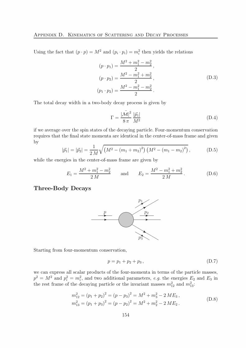
Appendix D. Kinematics of Scattering and Decay Processes
Using the fact that (p · p) =M2 and (pi · pi) = m2i then yields the relations
(p · p1) =M2 +m2
1 −m22
2,
(p · p2) =M2 −m2
1 +m22
2,
(p1 · p2) =M2 −m2
1 −m22
2.
(D.3)
The total decay width in a two-body decay process is given by
Γ =¯|M|28 π
|~p1|M2
(D.4)
if we average over the spin states of the decaying particle. Four-momentum conservationrequires that the final state momenta are identical in the center-of-mass frame and givenby
|~p1| = |~p2| =1
2M
√(M2 − (m1 +m2)
2) (M2 − (m1 −m2)2) , (D.5)
while the energies in the center-of-mass frame are given by
E1 =M2 +m2
1 −m22
2Mand E2 =
M2 −m21 +m2
2
2M. (D.6)
Three-Body Decays
p
p1
p3
p2
Starting from four-momentum conservation,
p = p1 + p2 + p3 , (D.7)
we can express all scalar products of the four-momenta in terms of the particle masses,p2 = M2 and p2i = m2
i , and two additional parameters, e.g. the energies E2 and E3 inthe rest frame of the decaying particle or the invariant masses m2
12 and m213:
m212 = (p1 + p2)
2 = (p− p3)2 =M2 +m2
3 − 2ME3 ,
m213 = (p1 + p3)
2 = (p− p2)2 =M2 +m2
2 − 2ME2 .(D.8)
154

From these expressions we can directly derive all scalar products of the four-momenta:
(p · p3) =M2 +m2
3 −m212
2, (p1 · p2) =
m212 −m2
1 −m22
2,
(p · p2) =M2 +m2
2 −m213
2, (p1 · p3) =
m213 −m2
1 −m23
2, (D.9)
(p · p1) =m2
12 +m213 −m2
2 −m23
2, (p2 · p3) =
M2 +m21 −m2
12 −m213
2.
Alternatively, one can use the following set of scalar products:
(p · p1) =M (M −E2 − E3) , (p · p2) =ME2, (p · p3) =ME3 , (D.10)
and
(p1 · p2) =M2 −m2
1 −m22 +m2
3
2−ME3 ,
(p1 · p3) =M2 −m2
1 +m22 −m2
3
2−ME2 ,
(p2 · p3) =M (E2 + E3)−M2 −m2
1 +m22 +m2
3
2.
(D.11)
When we average over the spin states of the decaying particle, its partial decay widthturns out to be
dΓ
dm212 dm
213
=1
(2 π)3
¯|M|232M3
, (D.12)
where the limiting values of the invariant masses are given by
(m1 +m2)2 ≤ m2
12 ≤ (M −m3)2 (D.13)
and
m213, min/max = m2
1 +m23 +
1
2m212
((m2
12 +m21 −m2
2
) (M2 −m2
12 −m23
)
∓√λ(m2
12, m21, m
22)√λ(M2, m2
12, m23
).
(D.14)
In the last expression we used the abbreviation
λ(x, y, z) = x2 + y2 + z2 − 2 x y − 2 x z − 2 y z . (D.15)
Alternatively, one can write the partial decay width in the form
dΓ
dE2 dE3=
1
(2 π)3
¯|M|28M
. (D.16)
155

Appendix D. Kinematics of Scattering and Decay Processes
Two-Body Reactions
p p′
k′k
For the discussion of two-to-two scattering processes we want to introduce the Lorentz-invariant Mandelstam variables:
s = (p+ k)2 = (p′ + k′)2=M2 +m2 + 2 (p · k) =M ′2 +m′2 + 2 (p′ · k′) ,
t = (p− p′)2= (k − k′)
2=M2 +M ′2 − 2 (p · p′) = m2 +m′2 − 2 (k · k′) ,
u = (p− k′)2= (k − p′)
2=M2 +m′2 − 2 (p · k′) = m2 +M ′2 − 2 (k · p′) ,
(D.17)
where the squared four-momenta are replaced by the particle masses squared (p2 =M2,p′2 =M ′2, k2 = m2 and k′2 = m′2). The Mandelstam variables satisfy the relation
s+ t+ u =M2 +m2 +M ′2 +m′2. (D.18)
We can now write down the six scalar products of the four-momenta in terms of theMandelstam variables and the particle masses:
(p · k) = s−M2 −m2
2, (p′ · k′) = s−M ′2 −m′2
2,
(p · p′) = M2 +M ′2 − t
2, (k · k′) = m2 +m′2 − t
2, (D.19)
(p · k′) = s+ t−M ′2 −m2
2, (k · p′) = s+ t−M2 −m′2
2.
In the last two expressions we replaced u using equation (D.18). The differential crosssection of a two-body reaction is given by
dσ
dt=
|M|2
64 π s |~pcm|2, (D.20)
where the limiting values of t are given by
t0/1 =(M2 −M ′2 −m2 +m′2)
2
4 s− (pcm ∓ p′cm)
2. (D.21)
The particle momenta in the center-of-mass frame are given by
pcm =√E2
cm −M2 and p′cm =√E ′2
cm −M ′2 , (D.22)
156

while the center-of-mass energies read
Ecm =s+M2 −m2
2√s
and E ′cm =
s+M ′2 −m′2
2√s
. (D.23)
In the laboratory frame, where the particle with four-momentum k is at rest, the scat-tering cross section can be rewritten using the relation
|~pcm|2 =|~plab|2m2
s. (D.24)
157

Appendix E
Calculation of Gravitino Decay
Widths
In this appendix we compute the decay channels of the LSP gravitino in the frameworkof bilinear R-parity breaking. The relative magnitude of the decay widths of the differentdecay channels determines the branching ratios for these channels. In addition, the exactshape of the differential decay widths determines the spectra of the final state particles.Therefore, this is a crucial input for the prediction of spectra of gravitino decay products.For a discussion of these topics see Sections 4.3 and 4.4.
E.1 Two-Body Decays
Here we want to calculate the decay widths of the two additional effective 3-vertexdiagrams coming from 4-vertex diagrams with a Higgs VEV at one of the legs:
ψ3/2
p
k
q
Z
H0u, d
vu, d
νi
and ψ3/2
p
k
q
W+
H−d
vd
ℓ−i
.
Using the rotation of the neutral higgsino fields into the neutrino as discussed in Sec-tion 3.3 we find the following decay amplitude for the first Feynman diagram:
iMZ = −ur(q)PR
N7∗
νi H0uvu
(gσ3, 222
cos θW − g′YHu sin θW
)
158

E.1. Two-Body Decays
+N7∗νi H0
dvd
(gσ3, 112
cos θW − g′YHdsin θW
) i√2MPl
γµγρ ψ+ sµ (p) ǫλ ∗
ρ (k)
≃ − i gZ ξi
2√2MPl
vu U
∗H0
uZ− vd U
∗H0
d Z
ur(q)PR γ
µγρ ψ+ sµ (p) ǫλ ∗
ρ (k) (E.1)
= −imZ ξi2MPl
sin β U∗
H0uZ
− cos β U∗H0
d Z
ur(q)PR γ
µγρ ψ+ sµ (p) ǫλ ∗
ρ (k) .
This additional diagram is exactly of the same form as the 4-vertex diagram that wasalready taken into account in previous calculations. Therefore, we can simply alter thepreviously obtained result into the following expression:
Γ(ψ3/2 → Zνi
)≃ξ2i m
33/2 β
2Z
64 πM2Pl
U2ZZfZ +
1
6
∣∣∣1 + sβ UH0uZ
− cβ UH0d Z
∣∣∣2
hZ
−8
3
mZ
m3/2
UZZ
(1 + sβ ReUH0
uZ− cβ ReUH0
d Z
)jZ
.
(E.2)
In order to write down the decay amplitude of the second diagram we need the rotationof the charged down-type higgsino into the left-handed charged leptons. We find
iMW = −ur(q)PRU5∗ℓi H
−dvd
g√2
(σ1, 212
− iσ2, 212
) i√2MPl
γµγρ ψ+ sµ (p) ǫλ ∗
ρ (k)
≃ i g ξi vd√2MPl
U∗H−
d Wur(q)PR γ
µγρ ψ+ sµ (p) ǫλ ∗
ρ (k)
=i√2mW ξi√2MPl
cos β U∗H−
d Wur(q)PR γ
µγρ ψ+ sµ (p) ǫλ ∗
ρ (k) .
(E.3)
This additional diagram is also exactly of the same form as the 4-vertex diagram thatwas already taken into account. Therefore, we can simply alter the previously obtainedresult into the following expression:
Γ(ψ3/2 →W+ℓ−i
)≃ξ2i m
33/2 β
2W
32 πM2Pl
U2W W
fW +1
6
∣∣∣1−√2 cβ UH−
d W
∣∣∣2
hW
−8
3
mW
m3/2
UW W
(1−
√2 cβ ReUH−
d W
)jW
.
(E.4)
We also want to include a small correction for the decay into the lightest Higgs particleand a neutrino. In the previous calculation in [154] we neglected theD-term contributionto the sneutrino VEV. This affected also the mixing that was assumed between thelightest Higgs particle and the sneutrinos. We simply replace this part in the final resultwith the complete expression found in Section 3.3:
Γ(ψ3/2 → h νi
)≃ξ2i m
33/2 β
4h
384 πM2Pl
∣∣∣∣m2
νi+ 1
2m2
Z cos 2 β
m2h −m2
νi
+ 2 sin β UH0uZ
+ 2 cos β UH0d Z
∣∣∣∣2
.(E.5)
159

Appendix E. Calculation of Gravitino Decay Widths
E.2 Three-Body Decays
In this section we calculate in detail the decay widths of the three-body gravitino decayprocesses ψ3/2 → γ∗ ν → f f ν, ψ3/2 → Z∗ ν → f f ν, ψ3/2 → W+∗
ℓ− → f f ′ ℓ− andψ3/2 → h∗ ν → f f ν. The related discussion in the text can be found in Section 4.3.2.
E.2.1 ψ3/2 → γ∗/Z∗ ν → f f ν
At tree level there are five diagrams contributing to the decay of a gravitino into afermion-antifermion pair and a neutrino:
ψ3/2
pk2
k1
q
f
f
γ, Z
γ, Z
νi
+ ψ3/2
pk2
k1
q
f
f
Z
vi
νi
and in addition the diagrams coming from the 4-vertex with a Higgs VEV at one of thelegs that were also discussed for the two-body decay:
ψ3/2
pk2
k1
q
f
f
Z
H0u, d
vu, d
νi
.
We find for the diagram with photon exchange
iMγ = ut(q)PRN7∗νi γ
i
4MPlγµ[/p− /q, γ
ρ]ψ+ sµ (p)
igρν(p− q)2
uq(k1) i Q e γνvr(k2)
≃ i Q e ξi4MPl
gρν(p− q)2
U∗γZut(q)PR γ
µ[/p− /q, γ
ρ]ψ+ sµ (p) uq(k1) γ
νvr(k2)
= −i Q e ξi U
∗γZ
MPl (p− q)2ut(q)PR
(qµγρ − gµρ(/q − /p)
)ψ+ sµ (p) uq(k1) γρ v
r(k2) .
(E.6)
160

E.2. Three-Body Decays
In the last step we used the fact that pµψ+ sµ (p) = 0 (see equation (4.5)) and thus
γµ[/p− /q, γ
ρ]ψ+ sµ (p) = 4
((pµ − qµ)γρ − gµρ(/p− /q)
)ψ+ sµ (p)
= −4(qµγρ − gµρ(/q − /p)
)ψ+ sµ (p) .
(E.7)
The photino–zino mixing parameter UγZ has already been introduced in equation (3.69).The amplitude for the first Z boson exchange diagram reads
iMZ1 = ut(q)PRN7∗νi Z
i
4MPlγµ[/p− /q, γ
ρ]ψ+ sµ (p)
×i(gρν − (pρ−qρ)(pν−qν)
m2Z
)
(p− q)2 −m2Z + imZΓZ
uq(k1)ig
cos θWγν(CV + CAγ
5)vr(k2)
≃ igZ ξi4MPl
gρν − (pρ−qρ)(pν−qν)
m2Z
(p− q)2 −m2Z + imZΓZ
U∗ZZ
(E.8)
× ut(q)PR γµ[/p− /q, γ
ρ]ψ+ sµ (p) uq(k1) γ
ν(CV + CAγ
5)vr(k2)
= −igZ ξiMPl
U∗ZZ
(p− q)2 −m2Z + imZΓZ
× ut(q)PR
(qµγρ − gµρ(/q − /p)
)ψ+ sµ (p) uq(k1) γρ
(CV + CAγ
5)vr(k2) .
Here we used the Z boson coupling constant gZ = g/ cos θW . The zino–zino mixingparameter UZZ has already been introduced in equation (3.70). The coefficients of theV − A structure of the vertex of the Z boson with two fermions were introduced inequation (4.25). The amplitude for the second Z boson exchange diagram is given by
iMZ2 = −ut(q)PRi vi√2MPl
(gσ3, 112
cos θW − g′YνL sin θW
)γµγρψ+ s
µ (p)
×i(gρν − (pρ−qρ)(pν−qν)
m2Z
)
(p− q)2 −m2Z + imZΓZ
uq(k1)ig
cos θWγν(CV + CAγ
5)vr(k2)
=igZ mZ ξi2MPl
gρν − (pρ−qρ)(pν−qν)
m2Z
(p− q)2 −m2Z + imZΓZ
× ut(q)PR γµγρψ+ s
µ (p) uq(k1) γν(CV + CAγ
5)vr(k2)
=igZ mZ ξiMPl
gµρ + qµ(pρ−qρ)
m2Z
(p− q)2 −m2Z + imZΓZ
× ut(q)PR ψ+ sµ (p) uq(k1) γρ
(CV + CAγ
5)vr(k2) .
(E.9)
Here we used the fact that γµψ+ sµ (p) = 0 (see equation (4.5)) and thus
γµγρψ+ sµ (p) = (2 gµρ − γργµ)ψ+ s
µ (p) = 2ψ+ s ρ(p) . (E.10)
161

Appendix E. Calculation of Gravitino Decay Widths
The last two diagrams have the same vertex structure as the previous one. In analogyto the two-body decay amplitude we find
iMZ3 =igZ mZ ξiMPl
sin β U∗
H0uZ
− cos β U∗H0
d Z
gµρ + qµ(pρ−qρ)
m2Z
(p− q)2 −m2Z + imZΓZ
× ut(q)PR ψ+ sµ (p) uq(k1) γρ
(CV + CAγ
5)vr(k2)
= iMZ2 ×sin β U∗
H0uZ
− cos β U∗H0
d Z
.
(E.11)
With these expressions for the individual amplitudes we can now write down the squaredmatrix element:
¯|M|2 = 1
4
∑
s, t, q, r
(iMγ + iMZ1 + iMZ2 + iMZ3) (iMγ + iMZ1 + iMZ2 + iMZ3)∗
=− ξ2i4M2
Pl
[Q2e2
∣∣UγZ
∣∣2
(p− q)4Tr [(/k1 +mf ) γρ (/k2 −mf ) γσ]
× Tr[/qPR
(qµγρ − gµρ(/q − /p)
)/pΦµν(p)
(qνγσ − gνσ(/q − /p)
)]
− 2Qe gZ UZZ
ReUγZ (m2Z − s) + ImUγZ mZ ΓZ
((p− q)2 −m2Z)
2+m2
ZΓ2Z
× Tr[(/k1 +mf ) γρ
(CV + CAγ
5)(/k2 −mf ) γσ
]
× Tr[/qPR
(qµγρ − gµρ(/q − /p)
)/pΦµν(p)
(qνγσ − gνσ(/q − /p)
)]
+g2Z U
2ZZ
((p− q)2 −m2Z)
2+m2
ZΓ2Z
× Tr[(/k1 +mf ) γρ
(CV + CAγ
5)(/k2 −mf )
(CV − CAγ
5)γσ]
× Tr[/qPR
(qµγρ − gµρ(/q − /p)
)/pΦµν(p)
(qνγσ − gνσ(/q − /p)
)]
−2 g2Z m3/2mZ UZZ
(1 + sβ ReUH0
uZ− cβ ReUH0
d Z
)
((p− q)2 −m2Z)
2+m2
ZΓ2Z
(gνσ +
qν(pσ − qσ)
m2Z
)
× Tr[(/k1 +mf ) γρ
(CV + CAγ
5)(/k2 −mf )
(CV − CAγ
5)γσ]
(E.12)
× Tr[/qPR
(qµγρ − gµρ(/q − /p)
)Φµν(p)
]
+ g2Z m2Z
∣∣∣1 + sβ UH0uZ
− cβ UH0d Z
∣∣∣2
(gµρ + qµ(pρ−qρ)
m2Z
)(gνσ + qν(pσ−qσ)
m2Z
)
((p− q)2 −m2Z)
2+m2
ZΓ2Z
× Tr[(/k1 +mf ) γρ
(CV + CAγ
5)(/k2 −mf )
(CV − CAγ
5)γσ]
× Tr[/qPR /pΦµν(p)
]
+ 2Qe gZ m3/2mZ
(1 + sβ ReUH0
uZ− cβ ReUH0
d Z
)
×ReUγZ (m2
Z − s) + ImUγZ mZ ΓZ
((p− q)2 −m2Z)
2+m2
ZΓ2Z
(gνσ +
qν(pσ − qσ)
m2Z
)
162

E.2. Three-Body Decays
× Tr[/qPR
(qµγρ − gµρ(/q − /p)
)Φµν(p)
]
× Tr[(/k1 +mf ) γρ
(CV + CAγ
5)(/k2 −mf ) γσ
]].
A number of traces of gamma matrices appear in this expression. Using the Mathematicapackage Feyn Calc [348] we find that the traces originating from the fermion currentpart of the amplitude are given by
Tr [(/k1 +mf ) γρ (/k2 −mf ) γσ]
= 4[k1ρk2σ + k1σk2ρ − gρσ
(m2
f + (k1 · k2))],
Tr[(/k1 +mf) γρ
(CV + CAγ
5)(/k2 −mf) γσ
]
= 4CV
[k1ρk2σ + k1σk2ρ − gρσ
(m2
f + (k1 · k2))]
+ 4 i CA ερσδλkδ1k
λ2 ,
Tr[(/k1 +mf) γρ
(CV + CAγ
5)(/k2 −mf)
(CV − CAγ
5)γσ]
= 4(C2
V + C2A
) [k1ρk2σ + k1σk2ρ − gρσ
(m2
f + (k1 · k2))]
+ 8C2A gρσm
2f
+ 8 i CV CA ερσδλkδ1k
λ2 ,
(E.13)
while the traces including the gravitino field turn out to be
Tr[/q PR
(qµγρ − gµρ(/q − /p)
)/pΦµν(p)
(qνγσ − gνσ(/q − /p)
)]
=4
3m23/2
[(p · q)
(gρσ(m4
3/2 −m23/2 (p · q) + (p · q)2
)
− pρ(m2
3/2 pσ + qσ (p · q)
) )+ qρ
(m4
3/2 qσ − pσ (p · q)2
)]
+2 i
3m23/2
(m4
3/2 + 2m23/2 (p · q)− 2 (p · q)2
)ερσδλpδ qλ ,
Tr[/qPR
(qµγρ − gµρ(/q − /p)
)Φµν(p)
]
=2
3m23/2
[(p · q)
(δρν(2m2
3/2 − (p · q))+ pν (2 p
ρ + qρ)
+ qν(m2
3/2 qρ + pρ (p · q)
))− i(m2
3/2 + (p · q))gνσ ε
σρδλpδ qλ],
Tr[/qPR /pΦµν(p)
]
=2
3m23/2
[2(m2
3/2 gµν − pµpν)(p · q) + im2
3/2 εµνρσpρ qσ].
(E.14)
In these expressions we already replaced the squared four-momenta with the squaredparticle masses:
p2 = m23/2 , k21 = k22 = m2
f ≃ 0 , q2 = m2ν ≃ 0 . (E.15)
In most cases it is convenient to neglect the masses of the final state particles. Nowwe want to use the complete kinematics of this decay process in order to calculate the
163

Appendix E. Calculation of Gravitino Decay Widths
corresponding decay width. Using equation (D.9) we find
(p · q) ≃m2
3/2 − s
2, (k1 · k2) ≃
s
2,
(p · k2) ≃m2
3/2 − t
2, (k1 · q) ≃
t
2, (E.16)
(p · k1) ≃s+ t
2, (k2 · q) ≃
m23/2 − s− t
2,
where we renamed the invariant masses used to parametrize the kinematics:
s ≡ m212 = (p− q)2 = (k1 + k2)
2, t ≡ m213 = (p− k2)
2 = (k1 + q)2. (E.17)
From equations (D.13) and (D.14) the ranges of the invariant masses are found to be
0 . t . m23/2 − s and 0 . s . m2
3/2 . (E.18)
Using equation (D.12) we can now write down the differential decay width for a gravitinodecaying into a fermion-antifermion pair and a neutrino:
dΓ
ds dt≃ ξ2i
1536 π3m53/2M
2Pl
[e2Q2
s
∣∣UγZ
∣∣2
×(3m6
3/2 − 3m43/2 (s+ 2 t) +m2
3/2
(s2 + 8 s t+ 6 t2
)− s
(s2 + 2 s t+ 2 t2
))
+gZ
(s−m2Z)
2+m2
Z Γ2Z
gZ s U
2ZZ
((CV − CA)
2(3m4
3/2 − s2)
×(m2
3/2 − s− 2 t)+(C2
V + C2A
) (m2
3/2
(2 s2 + 8 s t+ 6 t2
)− 2 s (s+ t)2
))
− 2 gZ sm3/2mZ UZZ
(1 + sβ ReUH0
uZ− cβ ReUH0
d Z
)
×(− 2CV CA
(3m2
3/2 − s) (m2
3/2 − s− 2 t)
+(C2
V + C2A
) (3m4
3/2 − 2m23/2 (s+ t)− s2 + 2 s t+ 2 t2
))(E.19)
+ 2 gZ m2Z
∣∣∣1 + sβ UH0uZ
− cβ UH0d Z
∣∣∣2 (
− 2m23/2 sCV CA
(m2
3/2 − s− 2 t)
+(C2
V + C2A
) (m4
3/2 (2 s+ t)−m23/2
(2 s2 + 2 s t+ t2
)+ s t (s+ t)
) )
− 2 eQ(ReUγZ
(m2
Z − s)+ ImUγZ mZ ΓZ
)
×(UZZ
(CV
(3m6
3/2 − 3m43/2 (s + 2 t) +m2
3/2
(s2 + 8 s t+ 6 t2
)
− s(s2 + 2 s t+ 2 t2
) )− CA
(3m4
3/2 − s2) (m2
3/2 − s− 2 t))
−m3/2mZ
(1 + sβ ReUH0
uZ− cβ ReUH0
d Z
)
164

E.2. Three-Body Decays
×(CV
(3m4
3/2 − 2m23/2 (s+ t)− s2 + 2 s t+ 2 t2
)
− CA
(3m2
3/2 − s) (m2
3/2 − s− 2 t) ))
].
After integrating over the invariant mass t we find as our final result the followingdifferential decay width:
dΓ
ds≃ξ2i m
33/2 β
2s
768 π3M2Pl
[e2Q2
s
∣∣UγZ
∣∣2 fs +gZ
(s−m2Z)
2+m2
Z Γ2Z
gZ U
2ZZs(C2
V + C2A
)fs
− 8
3
mZ
m3/2
gZ UZZ
(1 + sβ ReUH0
uZ− cβ ReUH0
d Z
)s(C2
V + C2A
)js
+1
6gZ m
2Z
∣∣∣1 + sβ UH0uZ
− cβ UH0d Z
∣∣∣2 (C2
V + C2A
)hs (E.20)
+ eQ(ReUγZ
(m2
Z − s)+ ImUγZ mZ ΓZ
)CV
×(2UZZ fs +
8
3
mZ
m3/2
(1 + sβ ReUH0
uZ− cβ ReUH0
d Z
)js
)].
In this case the kinematic functions βs, fs, js and hs are defined corresponding to thekinematic functions in the two-body decays (see equation(4.22)):
βs = 1− s
m23/2
, fs = 1 +2
3
s
m23/2
+1
3
s2
m43/2
,
js = 1 +1
2
s
m23/2
, hs = 1 + 10s
m23/2
+s2
m43/2
. (E.21)
We can now verify that above the threshold for Z boson production and using thenarrow-width approximation (NWA) the part of this result coming from Z boson ex-change coincides with the two-body decay result as given in equation (4.23), i.e.:
ΓNWA
(ψ3/2 → Z∗νi → f f νi
)= Γ
(ψ3/2 → Z νi
)× BR
(Z → f f
). (E.22)
The narrow-width approximation states that in the limit of a vanishing width-to-massratio the propagator can be replaced by a δ-function:
limΓ/m→0
1
(s−m2)2 +m2Γ2=
π
mΓδ(s−m2) . (E.23)
165

Appendix E. Calculation of Gravitino Decay Widths
Using this replacement we find for the three-body decay width
ΓNWA
(ψ3/2 → Z∗νi → f f νi
)=
m23/2∫
0
dsdΓ(ψ3/2 → Z∗νi → f f νi
)
ds
∣∣∣∣NWA
=ξ2i m
33/2 β
2Z
64 πM2Pl
(U2ZZfZ − 8
3
mZ
m3/2
UZZ
(1 + sβ ReUH0
uZ− cβ ReUH0
d Z
)jZ
+1
6
∣∣∣1 + sβ UH0uZ
− cβ UH0d Z
∣∣∣2
hZ
)× Γ
(Z → f f
)
ΓZ
,
(E.24)
which is exactly the equivalence we wanted to verify. In the last expression we used thepartial width of the Z boson decay into a fermion pair (see for instance [81]):
Γ(Z → f f
)=
√2GF m
3Z
3 π
(C2
V + C2A
)=g2Z mZ
12 π
(C2
V + C2A
). (E.25)
E.2.2 ψ3/2 →W+∗
ℓ− → f f ′ ℓ−
At tree level there are three diagrams contributing to the decay of a gravitino into twofermions and a charged lepton:
ψ3/2
pk2
k1
q
f
f ′
W+
W−
ℓ−i
+ ψ3/2
pk2
k1
q
f
f ′
W+
vi
ℓ−i
166

E.2. Three-Body Decays
and in addition the diagram coming from the 4-vertex with a down-type Higgs VEV atone of the legs that was also discussed for the two-body decay:
ψ3/2
pk2
k1
q
f
f ′
W+
H−d
vd
ℓ−i
.
The amplitude for the first diagram is given by
iMW1 = ut(q)PRU5∗ℓi W
i
4MPlγµ[/p− /q, γ
ρ]ψ+ sµ (p)
i(gρν − (pρ−qρ)(pν−qν)
m2W
)
(p− q)2 −m2W + imWΓW
× uq(k1)ig√2γν(σ1, 21
2− i
σ2, 212
)PL v
r(k2)
≃ ig ξi4MPl
U∗W W
gρν − (pρ−qρ)(pν−qν)
m2W
(p− q)2 −m2W + imWΓW
(E.26)
× ut(q)PR γµ[/p− /q, γ
ρ]ψ+ sµ (p) uq(k1) γ
νPL vr(k2)
= −ig ξiMPl
U∗WW
(p− q)2 −m2W + imWΓW
× ut(q)PR
(qµγρ − gµρ(/q − /p)
)ψ+ sµ (p) uq(k1) γρPL v
r(k2) ,
while the amplitude for the second diagram reads
iMW2 = −ut(q)PRi vi√2MPl
g√2
(σ1, 212
− iσ2, 212
)γµγρ ψ+ s
µ (p) (E.27)
×i(gρν − (pρ−qρ)(pν−qν)
m2W
)
(p− q)2 −m2W + imWΓW
uq(k1)ig√2γν(σ1, 21
2− i
σ2, 212
)PL v
r(k2)
≃ ig mW ξi2MPl
gρν − (pρ−qρ)(pν−qν)
m2W
(p− q)2 −m2W + imWΓW
ut(q)PR γµγρ ψ+ s
µ (p) uq(k1) γνPL v
r(k2)
=ig mW ξiMPl
gρν +qρ(pν−qν)
m2W
(p− q)2 −m2W + imWΓW
ut(q)PR ψ+ s ρ(p) uq(k1) γ
νPL vr(k2) .
167

Appendix E. Calculation of Gravitino Decay Widths
The last diagram has the same vertex structure as the previous one. In analogy to thetwo-body decay amplitude we find
iMW3 = −ig mW ξiMPl
√2 cos β U∗
H−d W
gρν +qρ(pν−qν)
m2W
(p− q)2 −m2W + imWΓW
× ut(q)PR ψ+ s ρ(p) uq(k1) γ
νPL vr(k2)
= −iMW2 ×√2 cos β U∗
H−d W
.
(E.28)
Using these individual amplitudes we find the squared matrix element of this process tobe given by
¯|M|2 = 1
4
∑
s,t,q,r
(iMW1 + iMW2 + iMW3) (iMW1 + iMW2 + iMW3)∗
≃ g2ξ2i4M2
Pl
1
((p− q)2 −m2W )
2+m2
WΓ2W
[U2W W
Tr [(/k1 +mf ) γρPL (/k2 −mf ′)PR γσ]
× Tr[(/q +mℓ
)PR
(qµγρ − gµρ(/q − /p)
)P+µν(p)
(qνγσ − gνσ(/q − /p)
)PL
]
− 2mW UW W
(1−
√2 cβ ReUH−
d W
)(gνσ +
qν(pσ − qσ)
m2W
)
× Tr [(/k1 +mf) γρPL (/k2 −mf ′)PR γσ]
× Tr[(/q +mℓ
)PR
(qµγρ − gµρ(/q − /p)
)P+µν(p)PL
]
+m2W
∣∣∣1−√2 cβ UH−
d W
∣∣∣2(gµρ +
qµ(pρ − qρ)
m2W
)(gνσ +
qν(pσ − qσ)
m2W
)(E.29)
× Tr [(/k1 +mf) γρPL (/k2 −mf ′)PR γ
σ] Tr[(/q +mℓ
)PR P
+µν(p)PL
] ]
=− g2ξ2i4M2
Pl
1
((p− q)2 −m2W )
2+m2
WΓ2W
[U2W W
Tr [/k1γρPL/k2γσ]
× Tr[/qPR
(qµγρ − gµρ(/q − /p)
)/pΦµν(p)
(qνγσ − gνσ(/q − /p)
)]
− 2m3/2mW UW W
(1−
√2 cβ ReUH−
d W
)(gνσ +
qν(pσ − qσ)
m2W
)
× Tr [/k1γρPL/k2γσ] Tr[/qPR
(qµγρ − gµρ(/q − /p)
)Φµν(p)
]
+m2W
∣∣∣1−√2 cβ UH−
d W
∣∣∣2(gµρ +
qµ(pρ − qρ)
m2W
)(gνσ +
qν(pσ − qσ)
m2W
)
× Tr [/k1γρPL /k2γ
σ] Tr[/q PR /pΦ
µν(p)] ].
Also in this squared matrix element a number of traces of gamma matrices appear. Thetrace originating from the fermion current part of the amplitude is given by
Tr [/k1γρPL /k2γ
σ] = 2(kρ1k
σ2 + kσ1k
ρ2 − gρσ (k1 · k2)− iερσδλk1 δk2λ
), (E.30)
168

E.2. Three-Body Decays
while the traces including the gravitino field are exactly the same as those given inequation (E.14). In these expressions we already replaced the squared four-momentawith the squared particle masses:
p2 = m23/2 , k21 = m2
f ≃ 0 , k22 = m2f ′ ≃ 0 , q2 = m2
ℓ ≃ 0 . (E.31)
Neglecting the masses of the final state particles the kinematics of this decay processis the same as in the previously discussed decay via photon/Z boson exchange. Usingequation (D.12) we find the following differential decay width for a gravitino decayinginto two fermions and a charged lepton:
dΓ
ds dt≃ g2 ξ2i
1536 π3m53/2M
2Pl
((s−m2
W )2+m2
W Γ2W
)
×[s U2
WW
(m2
3/2 − t) (
3m43/2 − 3m2
3/2 (s+ t) + s t)
− 2 sm3/2mW UW W
(1−
√2 cβ ReUH−
d W
)
×(3m4
3/2 −m23/2 (3 s+ 4 t) + t (2 s+ t)
)
+m2W
∣∣∣1−√2 cβ UH−
d W
∣∣∣2
×(m4
3/2 (3 s+ t)−m23/2
(3 s2 + 4 s t+ t2
)+ s t (s+ t)
) ].
(E.32)
After integrating over the invariant mass t we find as our final result the differentialdecay width
dΓ
ds≃
g2 ξ2i m33/2 β
2s
1536 π3M2Pl
((s−m2
W )2+m2
W Γ2W
)(s U2
W Wfs (E.33)
− 8
3
mW
m3/2
s UWW
(1−
√2 cβ ReUH−
d W
)js +
1
6m2
W
∣∣∣1−√2 cβ UH−
d W
∣∣∣2
hs
),
where the kinematic functions βs, fs, js and hs are those given in equation (4.27). As inthe case of gravitino decays via Z propagator we can verify that above the threshold forW± production and using the narrow-width approximation this result coincides withthe two-body decay result as given in equation (4.23), i.e.:
ΓNWA
(ψ3/2 →W+∗
ℓ−i → f f ′ ℓ−i)= Γ
(ψ3/2 → W+ℓ−i
)× BR
(W+ → f f ′) . (E.34)
169

Appendix E. Calculation of Gravitino Decay Widths
Replacing the propagator according to equation (4.34) we find
ΓNWA
(ψ3/2 →W+∗
ℓ−i → f f ′ ℓ−i)=
m23/2∫
0
dsdΓ(ψ3/2 →W+∗
ℓ−i → f f ′ ℓ−i)
ds
∣∣∣∣NWA
=ξ2i m
33/2 β
2W
32 πM2Pl
(U2W W
fW − 8
3
mW
m3/2
UWW
(1−
√2 cβ ReUH−
d W
)jW
+1
6
∣∣∣1−√2 cβ UH−
d W
∣∣∣2
hW
)× Γ
(W+ → f f ′)
ΓW,
(E.35)
which is exactly the equivalence we wanted to verify. In the last expression we used thepartial width of the W± boson decay into fermions [81]:
Γ(W+ → f f ′) =
√2GF m
3W
12 π=g2mW
48 π. (E.36)
E.2.3 ψ3/2 → h∗ ν → f f ν
At tree level there are two Feynman diagrams contributing to the decay of a gravitinointo a fermion-antifermion pair and a neutrino via an intermediate lightest Higgs boson:
ψ3/2
pk2
k1
q
f
f
h
ν∗i
νi
+ ψ3/2
pk2
k1
q
f
f
h
h
νi
.
The first diagram involves a mixing between the sneutrino and the lightest Higgs bosonand the corresponding amplitude reads
iMh1 = ut(q)PRi√
2MPl
γµ(/p− /q
)ψ+ sµ (p)
i
(p− q)2 −m2νi+ imνiΓνi
× i ξi√2
(m2
νi+
1
2m2
Z cos 2 β
)i
(p− q)2 −m2h + imhΓh
imf√2 v
uq(k1) vr(k2)
≃ imf ξi
v√2MPl
((p− q)2 −m2
h + imhΓh
) m2νi+ 1
2m2
Z cos 2 β
(p− q)2 −m2νi
(E.37)
× ut(q)PR qµ ψ+ s
µ (p) uq(k1) vr(k2) ,
170

E.2. Three-Body Decays
where we used the fact that pµψ+ sµ (p) = γµψ+ s
µ (p) = 0 (see equation (4.5)) and thus
γµ(/p− /q
)ψ+ sµ (p) =
(2 (pµ − qµ) + (/p− /q) γ
µ)ψ+ sµ (p) = −2 qµ ψ+ s
µ (p) . (E.38)
In addition, we assumed that the width of the sneutrino is negligible compared to itsmass. The second diagram involves a mixing between the higgsino partner of the lightestHiggs boson and the neutrino. The amplitude for this diagram is given by
iMh2 = ut(q)PR
√2sin β N7∗
νi H0u+ cos β N7∗
νi H0d
i√2MPl
γµ(/p− /q
)ψ+ sµ (p)
× i
(p− q)2 −m2h + imhΓh
imf√2 v
uq(k1) vr(k2)
≃ imf ξi
v√2MPl
((p− q)2 −m2
h + imhΓh
)(2 sin β U∗
H0uZ
+ 2 cos β U∗H0
d Z
)(E.39)
× ut(q)PR qµ ψ+ s
µ (p) uq(k1) vr(k2) .
The squared matrix element of this process is then given by
¯|M|2 = 1
4
∑
s,t,q,r
(iMh1 + iMh2) (iMh1 + iMh2)∗
= −m2
f ξ2i
8 v2M2Pl
1((p− q)2 −m2
h
)2+m2
hΓ2h
×∣∣∣∣m2
νi+ 1
2m2
Z cos 2 β
s−m2νi
+ 2 sin β UH0uZ
+ 2 cosβ UH0dZ
∣∣∣∣2
× qµ qν Tr[/q PR /pΦµν(p)
]Tr [(/k1 +mf ) (/k2 −mf)] .
(E.40)
The traces appearing in this expression are given by
qµ qν Tr[/q PR /pΦµν(p)
]= − 4
3m23/2
(p · q)3 ,
Tr [(/k1 +mf) (/k2 −mf )] = 4((k1 · k2)−m2
f
),
(E.41)
where we already replaced the squared four-momenta with the squared particle masses:
p2 = m23/2 , k21 = k22 = m2
f ≃ 0 , q2 = m2ν ≃ 0 . (E.42)
The only scalar products appearing in the squared matrix element are given by
(p · q) =m2
3/2 − s
2and (k1 · k2) =
s
2, (E.43)
and thus the differential decay width reads
dΓ
ds dt≃ξ2i m3/2m
2f β
3s s
∣∣∣∣m2
νi+ 1
2m2
Z cos 2β
s−m2νi
+ 2 sinβ UH0uZ
+ 2 cosβ UH0d Z
∣∣∣∣2
6144 π3M2Pl v
2((s−m2
h)2+m2
h Γ2h
) . (E.44)
171

Appendix E. Calculation of Gravitino Decay Widths
The differential decay width is independent of the invariant mass t and thus the in-tegration over t just results in an additional factor of (m2
3/2 − s) = m23/2 βs leading
to
dΓ
ds≃ξ2i m
33/2m
2f β
4s s
∣∣∣∣m2
νi+ 1
2m2
Z cos 2β
s−m2νi
+ 2 sin β UH0uZ
+ 2 cos β UH0d Z
∣∣∣∣2
6144 π3M2Pl v
2((s−m2
h)2+m2
h Γ2h
) . (E.45)
Similar to the other decay channels we can verify that above the threshold for h produc-tion and using the narrow-width approximation this result coincides with the two-bodydecay result as given in equation (4.23), i.e.:
ΓNWA
(ψ3/2 → h∗νi → f f νi
)= Γ
(ψ3/2 → h νi
)× BR
(h→ f f
). (E.46)
Replacing the propagator according to equation (4.34) we find
ΓNWA
(ψ3/2 → h∗νi → f f νi
)=
m23/2∫
0
dsdΓ(ψ3/2 → h∗νi → f f νi
)
ds
∣∣∣∣NWA
(E.47)
=ξ2i m
33/2 β
4h
384 πM2Pl
∣∣∣∣m2
νi+ 1
2m2
Z cos 2 β
m2h −m2
νi
+ 2 sin β UH0uZ
+ 2 cosβ UH0d Z
∣∣∣∣2
× Γ(h→ f f
)
Γh
,
which is exactly the equivalence we wanted to verify. In the last expression we used thepartial width of the Standard Model Higgs boson decay into a pair of fermions [81]:
Γ(h→ f f
)=GF m
2f mh
4 π√2
=m2
f mh
16 π v2. (E.48)
172

Appendix F
Calculation of Gravitino–Nucleon
Cross Sections
In this appendix we compute the scattering cross sections of the LSP gravitino withtarget nucleons in the framework of bilinear R-parity breaking. We separately considerthree cases: the exchange of a lightest Higgs boson, the exchange of a Z boson and theexchange of a photon. For a discussion of this topic see Chapter 6.
F.1 Inelastic Gravitino–Nucleon Scattering via Higgs
Exchange
At tree level there are two Feynman diagrams contributing to the inelastic gravitinoscattering off a nucleon via the exchange of the lightest Higgs boson:
ψ3/2 νi
h
νi
N N
p p′
k k′
+
h
ψ3/2 νi
h
N N
pp′
k k′
.
Similar to the case of gravitino three-body decay the amplitude is given by
iMh1 =∑
q
ut(p′)PRi√
2MPl
γµ(/p− /p
′)ψ+ sµ (p)
i
(p− p′)2 −m2νi+ imνiΓνi
(F.1)
173

Appendix F. Calculation of Gravitino–Nucleon Cross Sections
× i ξi√2
(m2
νi+
1
2m2
Z cos 2 β
)i
(p− p′)2 −m2h + imhΓh
imq√2 v
uq(k′) ur(k)
≃ −∑
q
i ξimN fNTq
v√2m2
hMPl
(1 +
1
2
m2Z
m2νi
cos 2 β
)ut(p′)PR p
′µ ψ+ sµ (p) uq(k′) ur(k) ,
where we need to sum over all quarks and their contribution to the nucleon mass. Inaddition, we only consider the case where (p − p′)2 ≪ m2
h, m2νi
so that the propagatorreduces to a contact interaction. The amplitude for the second diagram is given by
iMh2 =∑
q
ut(p′)PR
√2sin β N7∗
νi H0u+ cos β N7∗
νi H0d
i√2MPl
γµ(/p− /p
′)ψ+ sµ (p)
× i
(p− p′)2 −m2h + imhΓh
imq√2 v
uq(k′) ur(k) (F.2)
≃∑
q
i ξimN fNTq
v√2m2
hMPl
(2 sinβ U∗
H0uZ
+ 2 cosβ U∗H0
d Z
)ut(p′)PR p
′µ ψ+ sµ (p) uq(k′) ur(k) .
The squared matrix element of this process is then given by
¯|M|2 = 1
8
∑
s,t,q,r
(iMh1 + iMh2) (iMh1 + iMh2)∗ (F.3)
= −ξ2i m
2N
(∑q f
NTq
)2
16 v2m4hM
2Pl
∣∣∣∣1 +1
2
m2Z
m2νi
cos 2 β − 2 sinβ UH0uZ
− 2 cos β UH0d Z
∣∣∣∣2
× p′µ p′ν Tr[/p′PR /pΦµν(p)
]Tr[(/k′+mq
)(/k +mq)
].
Neglecting the masses of the individual quarks, the traces appearing in this expressionare given by
p′µ p′ν Tr[/p′PR /pΦµν(p)
]= − 4
3m23/2
(p · p′)3 ,
Tr[(/k′1 +mq
)(/k +mq)
]≃ 4 (k · k′) ,
(F.4)
where we already replaced the squared four-momenta with the squared particle masses:
p2 = m23/2 , p′2 = m2
ν ≃ 0 , k2 = k′2 = m2N . (F.5)
The only scalar products appearing in the squared matrix element are given by (cf.equation (D.19))
(p · p′) =m2
3/2 − t
2and (k · k′) = m2
N − t
2. (F.6)
174

F.2. Inelastic Gravitino–Nucleon Scattering via Z Exchange
Using equation (D.20) we can now write down the differential cross section:
dσ
dt=
¯|M|2
64 π s |~p1cm|2=
¯|M|2
64 π |~p1lab|2m2N
≃¯|M|2
64 πm23/2m
2N |~v|2
=ξ2i m
23/2m
2N
(∑q f
NTq
)2
1536 π v2m4hM
2Pl |~v|
2
∣∣∣∣1 +1
2
m2Z
m2νi
cos 2 β − 2 sin β UH0uZ
− 2 cos β UH0d Z
∣∣∣∣2
×(1− t
m23/2
)3(1− t
2m2N
). (F.7)
F.2 Inelastic Gravitino–Nucleon Scattering via Z
Exchange
At tree level there are four diagrams contributing to the inelastic gravitino–nucleonscattering via the exchange of a Z boson:
ψ3/2 νi
Z
Z
N N
pp′
k k′
+
ψ3/2 νi
Z
N N
p p′
k k′
vi
+
H0u, d
ψ3/2 νi
Z
N N
pp′
k k′
vu, d
.
175
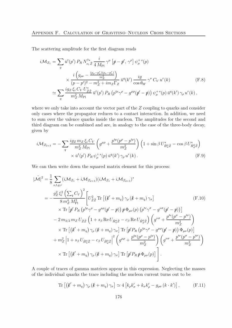
Appendix F. Calculation of Gravitino–Nucleon Cross Sections
The scattering amplitude for the first diagram reads
iMZ1 =∑
q
ut(p′)PRN7∗νi Z
i
4MPlγµ[/p− /p
′, γρ]ψ+ sµ (p)
×i(gρν − (pρ−p′ρ)(pν−p′ν)
m2Z
)
(p− p′)2 −m2Z + imZΓZ
uq(k′)ig
cos θWγν CV u
r(k) (F.8)
≃∑
q
igZ ξi CV U∗ZZ
m2Z MPl
ut(p′)PR
(p′µγρ − gµρ(/p
′ − /p))ψ+ sµ (p) uq(k′) γρ u
r(k) ,
where we only take into account the vector part of the Z coupling to quarks and consideronly cases where the propagator reduces to a contact interaction. In addition, we needto sum over the valence quarks inside the nucleon. The amplitudes for the second andthird diagram can be combined and are, in analogy to the case of the three-body decay,given by
iMZ2+3 = −∑
q
igZ mZ ξiCV
m2Z MPl
(gµρ +
p′µ(pρ − p′ρ)
m2Z
)(1 + sin β U∗
H0uZ
− cos β U∗H0
d Z
)
× ut(p′)PR ψ+ sµ (p) uq(k′) γρ u
r(k) . (F.9)
We can then write down the squared matrix element for this process:
¯|M|2 = 1
8
∑
s,t,q,r
(iMZ1 + iMZ2+3)(iMZ1 + iMZ2+3)∗
= −g2Z ξ
2i
(∑q CV
)2
8m4Z M
2Pl
[U2ZZ
Tr[(/k′+mq
)γρ (/k +mq) γσ
](F.10)
× Tr[/p′ PR
(p′µγρ − gµρ(/p
′ − /p))/pΦµν(p)
(p′νγσ − gνσ(/p
′ − /p))]
− 2m3/2mZ UZZ
(1 + sβ ReUH0
uZ− cβ ReUH0
dZ
)(gνσ +
p′ν(pσ − p′σ)
m2Z
)
× Tr[(/k′+mq
)γρ (/k +mq) γσ
]Tr[/p′PR
(p′µγρ − gµρ(/p
′ − /p))Φµν(p)
]
+m2Z
∣∣∣1 + sβ UH0uZ
− cβ UH0d Z
∣∣∣2(gµρ +
p′µ(pρ − p′ρ)
m2Z
)(gνσ +
p′ν(pσ − p′σ)
m2Z
)
× Tr[(/k′+mq
)γρ (/k +mq) γσ
]Tr[/p′PR /pΦµν(p)
]].
A couple of traces of gamma matrices appear in this expression. Neglecting the massesof the individual quarks the trace including the nucleon current turns out to be
Tr[(/k′+mq
)γρ (/k +mq) γσ
]≃ 4
[kρk
′σ + kσk
′ρ − gρσ (k · k′)
], (F.11)
176
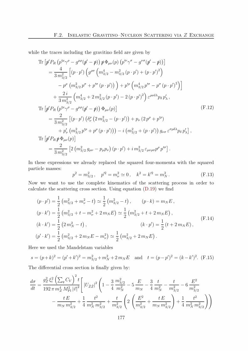
F.2. Inelastic Gravitino–Nucleon Scattering via Z Exchange
while the traces including the gravitino field are given by
Tr[/p′PR
(p′µγρ − gµρ(/p
′ − /p))/pΦµν(p)
(p′νγσ − gνσ(/p
′ − /p))]
=4
3m23/2
[(p · p′)
(gρσ(m4
3/2 −m23/2 (p · p′) + (p · p′)2
)
− pρ(m2
3/2 pσ + p′σ (p · p′)
) )+ p′ρ
(m4
3/2 p′σ − pσ (p · p′)2
)]
+2 i
3m23/2
(m4
3/2 + 2m23/2 (p · p′)− 2 (p · p′)2
)ερσδλpδ p
′λ ,
Tr[/p′PR
(p′µγρ − gµρ(/p
′ − /p))Φµν(p)
]
=2
3m23/2
[(p · p′)
(δρν(2m2
3/2 − (p · p′))+ pν (2 p
ρ + p′ρ)
+ p′ν(m2
3/2 p′ρ + pρ (p · p′)
))− i(m2
3/2 + (p · p′))gνσ ε
σρδλpδ p′λ
],
Tr[/p′PR /pΦµν(p)
]
=2
3m23/2
[2(m2
3/2 gµν − pµpν)(p · p′) + im2
3/2 εµνρσpρ p′σ
].
(F.12)
In these expressions we already replaced the squared four-momenta with the squaredparticle masses:
p2 = m23/2 , p′2 = m2
ν ≃ 0 , k2 = k′2 = m2N . (F.13)
Now we want to use the complete kinematics of the scattering process in order tocalculate the scattering cross section. Using equation (D.19) we find
(p · p′) = 1
2
(m2
3/2 +m2ν − t
)≃ 1
2
(m2
3/2 − t), (p · k) = mNE ,
(p · k′) = 1
2
(m2
3/2 + t−m2ν + 2mNE
)≃ 1
2
(m2
3/2 + t + 2mNE),
(k · k′) = 1
2
(2m2
N − t), (k · p′) = 1
2(t + 2mNE) ,
(p′ · k′) = 1
2
(m2
3/2 + 2mNE −m2ν
)≃ 1
2
(m2
3/2 + 2mNE).
(F.14)
Here we used the Mandelstam variables
s = (p+k)2 = (p′+k′)2 = m23/2+m
2N +2mNE and t = (p−p′)2 = (k−k′)2. (F.15)
The differential cross section is finally given by:
dσ
dt=g2Z ξ
2i
(∑q CV
)2t
192 πm4Z M
2Pl |~v|
2
[|UZZ |
2
(1− 3
4
m23/2
m2N
− 5E
mN
− 3
4
t
m2N
− t
m23/2
− 6E2
m23/2
− t E
mN m23/2
+1
4
t2
m2N m
23/2
+t
m23/2
(2
(E2
m23/2
+t E
mN m23/2
)+
1
4
t2
m2N m
23/2
))
177
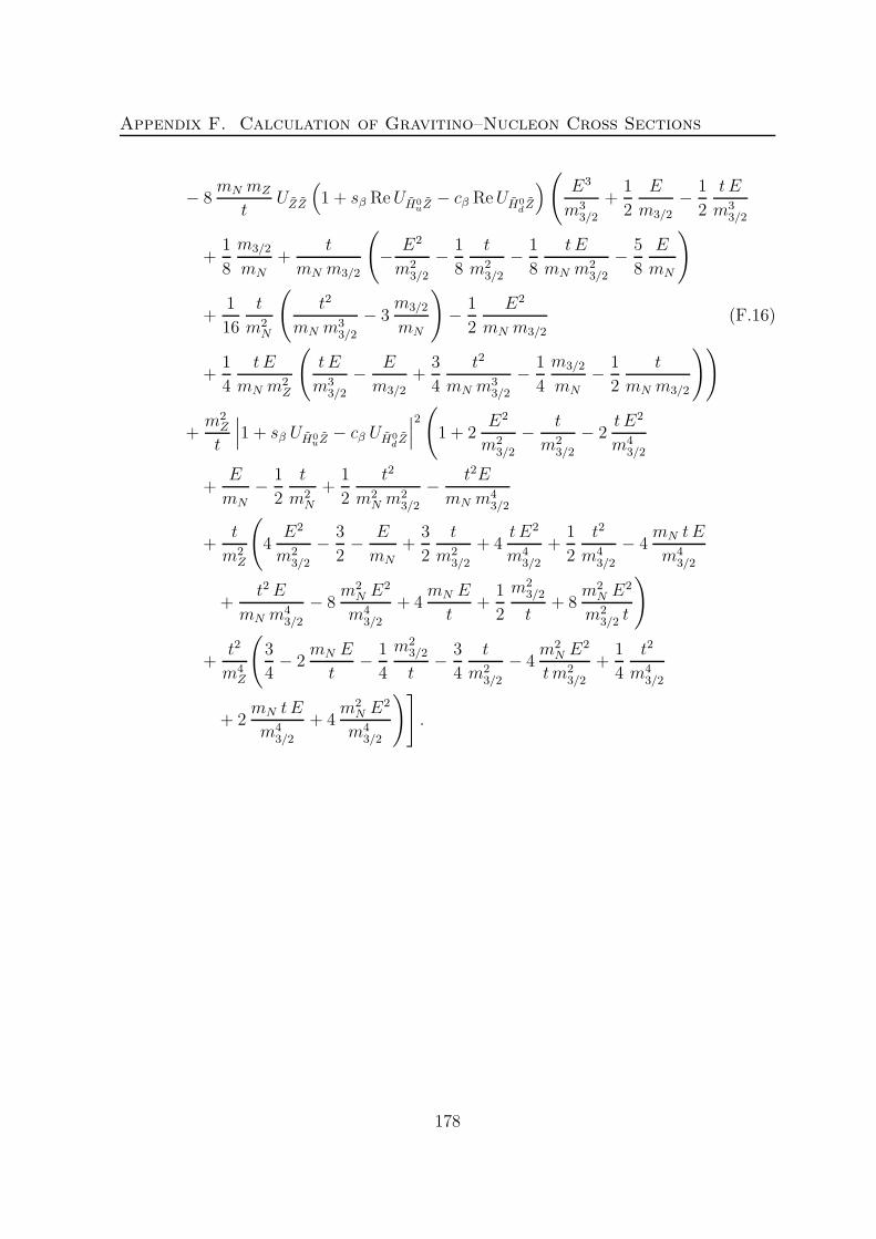
Appendix F. Calculation of Gravitino–Nucleon Cross Sections
− 8mN mZ
tUZZ
(1 + sβ ReUH0
uZ− cβ ReUH0
d Z
)( E3
m33/2
+1
2
E
m3/2
− 1
2
t E
m33/2
+1
8
m3/2
mN
+t
mN m3/2
(− E2
m23/2
− 1
8
t
m23/2
− 1
8
t E
mN m23/2
− 5
8
E
mN
)
+1
16
t
m2N
(t2
mN m33/2
− 3m3/2
mN
)− 1
2
E2
mN m3/2(F.16)
+1
4
t E
mN m2Z
(t E
m33/2
− E
m3/2+
3
4
t2
mN m33/2
− 1
4
m3/2
mN− 1
2
t
mN m3/2
))
+m2
Z
t
∣∣∣1 + sβ UH0uZ
− cβ UH0d Z
∣∣∣2(1 + 2
E2
m23/2
− t
m23/2
− 2t E2
m43/2
+E
mN− 1
2
t
m2N
+1
2
t2
m2N m
23/2
− t2E
mN m43/2
+t
m2Z
(4E2
m23/2
− 3
2− E
mN+
3
2
t
m23/2
+ 4t E2
m43/2
+1
2
t2
m43/2
− 4mN t E
m43/2
+t2E
mN m43/2
− 8m2
N E2
m43/2
+ 4mN E
t+
1
2
m23/2
t+ 8
m2N E
2
m23/2 t
)
+t2
m4Z
(3
4− 2
mN E
t− 1
4
m23/2
t− 3
4
t
m23/2
− 4m2
N E2
tm23/2
+1
4
t2
m43/2
+ 2mN t E
m43/2
+ 4m2
N E2
m43/2
)].
178

F.3. Inelastic Gravitino–Nucleon Scattering via Photon Exchange
F.3 Inelastic Gravitino–Nucleon Scattering via Pho-
ton Exchange
At tree level there is only one diagram contributing to the inelastic gravitino–nucleonscattering via the exchange of a photon:
ψ3/2 νi
γ
γ
N N
pp′
k k′
.
The scattering amplitude for this diagram is similar to the respective three-body decayamplitude and reads
iMγ =∑
q
ut(p′)PRN7∗νi γ
i
4MPlγµ[/p− /p
′, γρ]ψ+ sµ (p)
igρν(p− p′)2
uq(k′) i Q e γνur(k)
≃ −∑
q
i Q e ξi U∗γZ
MPl (p− p′)2ut(p′)PR
(p′µγρ − gµρ(/p
′ − /p))ψ+ sµ (p) uq(k′) γρ u
r(k) ,
(F.17)
where we need to sum over the valence quarks in the nucleon as in the case of scatteringvia Z exchange. We find then the following squared matrix element:
¯|M|2 = 1
8
∑
s,t,q,r
iMγ (iMγ)∗
= −ξ2i
(∑q Q)2e2∣∣UγZ
∣∣2
8M2Pl (p− p′)4
Tr[(/k′+mq
)γρ (/k +mq) γσ
]
× Tr[/p′PR
(p′µγρ − gµρ(/p
′ − /p))/pΦµν(p)
(p′νγσ − gνσ(/p
′ − /p))].
(F.18)
The traces appearing in this matrix element have already been presented in equa-tions (F.11) and (F.12), and the kinematics of this scattering process is the same asfor the case of Z boson and Higgs exchange. This finally leads to the differential cross
179

Appendix F. Calculation of Gravitino–Nucleon Cross Sections
section
dσ
dt=ξ2i
(∑q Q)2e2∣∣UγZ
∣∣2
192 π tM2Pl |~v|
2
(1− 3
4
m23/2
m2N
− 5E
mN
− 3
4
t
m2N
− t
m23/2
− 6E2
m23/2
(F.19)
− t E
mN m23/2
+1
4
t2
m2N m
23/2
+t
m23/2
(2
(E2
m23/2
+t E
mN m23/2
)+
1
4
t2
m2N m
23/2
)).
180

Bibliography
[1] F. Zwicky, “Die Rotverschiebung von extragalaktischen Nebeln,” Helv. Phys. Acta6 (1933) 110.
[2] J. H. Jeans, “The Motions of Stars in a Kapteyn Universe,” Mon. Not. Roy. Astron.Soc. 82 (1922) 122.
[3] L. Bergstrom, “Non-Baryonic Dark Matter: Observational Evidence and DetectionMethods,” Rept. Prog. Phys. 63 (2000) 793 [arXiv:hep-ph/0002126].
[4] G. Bertone, D. Hooper and J. Silk, “Particle Dark Matter: Evidence, Candidatesand Constraints,” Phys. Rept. 405 (2005) 279 [arXiv:hep-ph/0404175].
[5] J. Einasto, “Dark Matter,” arXiv:0901.0632 [astro-ph.CO].
[6] M. Milgrom, “AModification of the Newtonian Dynamics as a Possible Alternativeto the Hidden Mass Hypothesis,” Astrophys. J. 270 (1983) 365.
[7] B. Paczynski, “Gravitational Microlensing by the Galactic Halo,” Astrophys. J.304 (1986) 1.
[8] K. Griest, “Galactic Microlensing as a Method of Detecting Massive CompactHalo Objects,” Astrophys. J. 366 (1991) 412.
[9] J. L. Feng, “Dark Matter Candidates from Particle Physics and Methods of De-tection,” Ann. Rev. Astron. Astrophys. 48 (2010) 495 [arXiv:1003.0904 [astro-ph.CO]].
[10] G. Jungman, M. Kamionkowski and K. Griest, “Supersymmetric Dark Matter,”Phys. Rept. 267 (1996) 195 [arXiv:hep-ph/9506380].
[11] G. Servant and T. M. P. Tait, “Is the Lightest Kaluza-Klein Particle a Viable DarkMatter Candidate?,” Nucl. Phys. B 650 (2003) 391 [arXiv:hep-ph/0206071].
[12] D. Z. Freedman, P. van Nieuwenhuizen and S. Ferrara, “Progress toward a Theoryof Supergravity,” Phys. Rev. D 13 (1976) 3214.
[13] S. Deser and B. Zumino, “Consistent Supergravity,” Phys. Lett. B 62 (1976) 335.
181

Bibliography
[14] H. Pagels and J. R. Primack, “Supersymmetry, Cosmology and New TeV Physics,”Phys. Rev. Lett. 48 (1982) 223.
[15] S. Weinberg, “Cosmological Constraints on the Scale of Supersymmetry Break-ing,” Phys. Rev. Lett. 48 (1982) 1303.
[16] M. Bolz, A. Brandenburg and W. Buchmuller, “Thermal Production of Graviti-nos,” Nucl. Phys. B 606 (2001) 518 [Erratum-ibid. B 790 (2008) 336] [arXiv:hep-ph/0012052].
[17] M. Kawasaki and T. Moroi, “Gravitino Production in the Inflationary Universeand the Effects on Big Bang Nucleosynthesis,” Prog. Theor. Phys. 93 (1995) 879[arXiv:hep-ph/9403364].
[18] M. Fukugita and T. Yanagida, “Baryogenesis without Grand Unification,” Phys.Lett. B 174 (1986) 45.
[19] S. Davidson and A. Ibarra, “A Lower Bound on the Right-Handed Neutrino Massfrom Leptogenesis,” Phys. Lett. B 535 (2002) 25 [arXiv:hep-ph/0202239].
[20] M. Bolz, W. Buchmuller and M. Plumacher, “Baryon Asymmetry and Dark Mat-ter,” Phys. Lett. B 443 (1998) 209 [arXiv:hep-ph/9809381].
[21] M. Kawasaki, K. Kohri, T. Moroi and A. Yotsuyanagi, “Big-Bang Nucleosynthesisand Gravitino,” Phys. Rev. D 78 (2008) 065011 [arXiv:0804.3745 [hep-ph]].
[22] W. Buchmuller, L. Covi, K. Hamaguchi, A. Ibarra and T. Yanagida, “GravitinoDark Matter in R-Parity Breaking Vacua,” JHEP 0703 (2007) 037 [arXiv:hep-ph/0702184].
[23] F. Takayama and M. Yamaguchi, “Gravitino Dark Matter without R-Parity,”Phys. Lett. B 485 (2000) 388 [arXiv:hep-ph/0005214].
[24] G. Bertone, W. Buchmuller, L. Covi and A. Ibarra, “Gamma-Rays from DecayingDark Matter,” JCAP 0711 (2007) 003 [arXiv:0709.2299 [astro-ph]].
[25] A. Ibarra and D. Tran, “Gamma Ray Spectrum from Gravitino Dark MatterDecay,” Phys. Rev. Lett. 100 (2008) 061301 [arXiv:0709.4593 [astro-ph]].
[26] K. Ishiwata, S. Matsumoto and T. Moroi, “High Energy Cosmic Rays from theDecay of Gravitino Dark Matter,” Phys. Rev. D 78 (2008) 063505 [arXiv:0805.1133[hep-ph]].
[27] W. Buchmuller, A. Ibarra, T. Shindou, F. Takayama and D. Tran, “ProbingGravitino Dark Matter with PAMELA and Fermi,” JCAP 0909 (2009) 021[arXiv:0906.1187 [hep-ph]].
182

Bibliography
[28] N. E. Bomark, S. Lola, P. Osland and A. R. Raklev, “Photon, Neutrino andCharged Particle Spectra from R-Violating Gravitino Decays,” Phys. Lett. B 686
(2010) 152 [arXiv:0911.3376 [hep-ph]].
[29] A. Ibarra and D. Tran, “Antimatter Signatures of Gravitino Dark Matter Decay,”JCAP 0807 (2008) 002 [arXiv:0804.4596 [astro-ph]].
[30] L. Covi, M. Grefe, A. Ibarra and D. Tran, “Unstable Gravitino Dark Matter andNeutrino Flux,” JCAP 0901 (2009) 029 [arXiv:0809.5030 [hep-ph]].
[31] W. Buchmuller, K. Hamaguchi, M. Ratz and T. Yanagida, “Supergravity at Col-liders,” Phys. Lett. B 588 (2004) 90 [arXiv:hep-ph/0402179].
[32] J. R. Ellis, A. R. Raklev and O. K. Oye, “Gravitino Dark Matter Scenarios withMassive Metastable Charged Sparticles at the LHC,” JHEP 0610 (2006) 061[arXiv:hep-ph/0607261].
[33] S. Bobrovskyi, W. Buchmuller, J. Hajer, and J. Schmidt, “Broken R-Parity in theSky and at the LHC,” JHEP 1010 (2010) 061 [arXiv:1007.5007 [hep-ph]].
[34] N. E. Bomark, S. Lola, P. Osland and A. R. Raklev, “Gravitino Dark Matter andthe Flavour Structure of R-Violating Operators,” Phys. Lett. B 677 (2009) 62[arXiv:0811.2969 [hep-ph]].
[35] A. W. Strong, I. V. Moskalenko and O. Reimer, “A New Determination of theExtragalactic Diffuse Gamma-Ray Background from EGRET Data,” Astrophys.J. 613 (2004) 956 [arXiv:astro-ph/0405441].
[36] S. W. Barwick et al. [HEAT Collaboration], “Measurements of the Cosmic-RayPositron Fraction from 1 GeV to 50 GeV,” Astrophys. J. 482 (1997) L191[arXiv:astro-ph/9703192].
[37] E. A. Baltz and J. Edsjo, “Positron Propagation and Fluxes from Neutralino An-nihilation in the Halo,” Phys. Rev. D 59 (1998) 023511 [arXiv:astro-ph/9808243].
[38] G. L. Kane, L. T. Wang and J. D. Wells, “Supersymmetry and the Positron Excessin Cosmic Rays,” Phys. Rev. D 65 (2002) 057701 [arXiv:hep-ph/0108138].
[39] E. A. Baltz, J. Edsjo, K. Freese and P. Gondolo, “The Cosmic Ray PositronExcess and Neutralino Dark Matter,” Phys. Rev. D 65 (2002) 063511 [arXiv:astro-ph/0109318].
[40] W. de Boer, C. Sander, V. Zhukov, A. V. Gladyshev and D. I. Kazakov, “EgretExcess of Diffuse Galactic Gamma Rays as Tracer of Dark Matter,” Astron. As-trophys. 444 (2005) 51 [arXiv:astro-ph/0508617].
183

Bibliography
[41] O. Adriani et al. [PAMELA Collaboration], “An Anomalous Positron Abun-dance in Cosmic Rays with Energies 1.5-100 GeV,” Nature 458 (2009) 607[arXiv:0810.4995 [astro-ph]].
[42] A. A. Abdo et al. [The Fermi LAT Collaboration], “Measurement of the Cos-mic Ray e+ + e− Spectrum from 20 GeV to 1 TeV with the Fermi Large AreaTelescope,” Phys. Rev. Lett. 102 (2009) 181101 [arXiv:0905.0025 [astro-ph.HE]].
[43] N. Arkani-Hamed, D. P. Finkbeiner, T. R. Slatyer and N. Weiner, “A Theory ofDark Matter,” Phys. Rev. D 79 (2009) 015014 [arXiv:0810.0713 [hep-ph]];
[44] I. Cholis, D. P. Finkbeiner, L. Goodenough and N. Weiner, “The PAMELAPositron Excess from Annihilations into a Light Boson,” JCAP 0912 (2009) 007[arXiv:0810.5344 [astro-ph]].
[45] Y. Nomura and J. Thaler, “Dark Matter through the Axion Portal,” Phys. Rev.D 79 (2009) 075008 [arXiv:0810.5397 [hep-ph]];
[46] D. Feldman, Z. Liu and P. Nath, “PAMELA Positron Excess as a Signal from theHidden Sector,” Phys. Rev. D 79 (2009) 063509 [arXiv:0810.5762 [hep-ph]];
[47] K. Ishiwata, S. Matsumoto and T. Moroi, “Cosmic-Ray Positron from Superpar-ticle Dark Matter and the PAMELA Anomaly,” Phys. Lett. B 675 (2009) 446[arXiv:0811.0250 [hep-ph]].
[48] P. J. Fox and E. Poppitz, “Leptophilic Dark Matter,” Phys. Rev. D 79 (2009)083528 [arXiv:0811.0399 [hep-ph]].
[49] E. Nezri, M. H. G. Tytgat and G. Vertongen, “e+ and Anti-p from Inert DoubletModel Dark Matter,” JCAP 0904 (2009) 014 [arXiv:0901.2556 [hep-ph]].
[50] P. f. Yin, Q. Yuan, J. Liu, J. Zhang, X. j. Bi and S. h. Zhu, “PAMELAData and Leptonically Decaying Dark Matter,” Phys. Rev. D 79 (2009) 023512[arXiv:0811.0176 [hep-ph]].
[51] C. R. Chen, F. Takahashi and T. T. Yanagida, “High-Energy Cosmic-RayPositrons from Hidden-Gauge-Boson Dark Matter,” Phys. Lett. B 673 (2009)255 [arXiv:0811.0477 [hep-ph]].
[52] K. Hamaguchi, E. Nakamura, S. Shirai and T. T. Yanagida, “Decaying Dark Mat-ter Baryons in a Composite Messenger Model,” Phys. Lett. B 674 (2009) 299[arXiv:0811.0737 [hep-ph]].
[53] A. Ibarra and D. Tran, “Decaying Dark Matter and the PAMELA Anomaly,”JCAP 0902 (2009) 021 [arXiv:0811.1555 [hep-ph]].
184

Bibliography
[54] E. Nardi, F. Sannino and A. Strumia, “Decaying Dark Matter Can Explain theElectron/Positron Excesses,” JCAP 0901 (2009) 043 [arXiv:0811.4153 [hep-ph]].
[55] K. Hamaguchi, S. Shirai and T. T. Yanagida, “Cosmic Ray Positron and ElectronExcess from Hidden-Fermion Dark Matter Decays,” Phys. Lett. B 673 (2009) 247[arXiv:0812.2374 [hep-ph]].
[56] S. L. Chen, R. N. Mohapatra, S. Nussinov and Y. Zhang, “R-Parity Breaking viaType II Seesaw, Decaying Gravitino Dark Matter and PAMELA Positron Excess,”Phys. Lett. B 677 (2009) 311 [arXiv:0903.2562 [hep-ph]].
[57] A. Ibarra, A. Ringwald, D. Tran and C. Weniger, “Cosmic Rays from LeptophilicDark Matter Decay via Kinetic Mixing,” JCAP 0908 (2009) 017 [arXiv:0903.3625[hep-ph]].
[58] S. Shirai, F. Takahashi and T. T. Yanagida, “R-Violating Decay of Wino DarkMatter and Electron/Positron Excesses in the PAMELA/Fermi Experiments,”Phys. Lett. B 680 (2009) 485 [arXiv:0905.0388 [hep-ph]].
[59] A. Ibarra, D. Tran and C. Weniger, “Decaying Dark Matter in Light of thePAMELA and Fermi LAT Data,” JCAP 1001 (2010) 009 [arXiv:0906.1571 [hep-ph]].
[60] D. Hooper, P. Blasi, P. D. Serpico, “Pulsars as the Sources of High Energy CosmicRay Positrons,” JCAP 0901, 025 (2009). [arXiv:0810.1527 [astro-ph]].
[61] S. Profumo, “Dissecting Pamela (and ATIC) with Occam’s Razor: Existing, Well-Known Pulsars Naturally Account for the ’Anomalous’ Cosmic-Ray Electron andPositron Data,” arXiv:0812.4457 [astro-ph].
[62] N. J. Shaviv, E. Nakar and T. Piran, “Natural Explanation for the AnomalousPositron to Electron Ratio with Supernova Remnants as the Sole Cosmic RaySource,” Phys. Rev. Lett. 103 (2009) 111302 [arXiv:0902.0376 [astro-ph.HE]].
[63] P. Blasi and P. D. Serpico, “High-Energy Antiprotons from Old Supernova Rem-nants,” Phys. Rev. Lett. 103 (2009) 081103 [arXiv:0904.0871 [astro-ph.HE]].
[64] V. Barger, Y. Gao, W. Y. Keung, D. Marfatia and G. Shaughnessy, “Dark Matterand Pulsar Signals for Fermi LAT, PAMELA, ATIC, HESS and WMAP Data,”Phys. Lett. B 678 (2009) 283 [arXiv:0904.2001 [hep-ph]].
[65] D. Grasso et al. [FERMI-LAT Collaboration], “On Possible Interpretations ofthe High Energy Electron-Positron Spectrum Measured by the Fermi Large AreaTelescope,” Astropart. Phys. 32 (2009) 140 [arXiv:0905.0636 [astro-ph.HE]].
185

Bibliography
[66] A. A. Abdo et al. [The Fermi-LAT collaboration], “The Spectrum of the IsotropicDiffuse Gamma-Ray Emission Derived from First-Year Fermi Large Area Tele-scope Data,” Phys. Rev. Lett. 104 (2010) 101101 [arXiv:1002.3603 [astro-ph.HE]].
[67] A. A. Abdo et al., “Fermi LAT Search for Photon Lines from 30 to 200 GeV andDark Matter Implications,” Phys. Rev. Lett. 104 (2010) 091302 [arXiv:1001.4836[astro-ph.HE]].
[68] J. Hisano, M. Kawasaki, K. Kohri and K. Nakayama, “Neutrino Signals from An-nihilating/Decaying Dark Matter in the Light of Recent Measurements of CosmicRay Electron/Positron Fluxes,” Phys. Rev. D 79 (2009) 043516 [arXiv:0812.0219[hep-ph]].
[69] J. Liu, P. f. Yin and S. h. Zhu, “Prospects for Detecting Neutrino Signals from An-nihilating/Decaying Dark Matter to Account for the PAMELA and ATIC results,”Phys. Rev. D 79 (2009) 063522 [arXiv:0812.0964 [astro-ph]].
[70] J. Hisano, K. Nakayama and M. J. S. Yang, “Upward Muon Signals at NeutrinoDetectors as a Probe of Dark Matter Properties,” Phys. Lett. B 678 (2009) 101[arXiv:0905.2075 [hep-ph]].
[71] D. Spolyar, M. R. Buckley, K. Freese, D. Hooper and H. Murayama, “High EnergyNeutrinos as a Test of Leptophilic Dark Matter,” arXiv:0905.4764 [astro-ph.CO].
[72] M. R. Buckley, K. Freese, D. Hooper, D. Spolyar and H. Murayama, “High-EnergyNeutrino Signatures of Dark Matter Decaying into Leptons,” Phys. Rev. D 81
(2010) 016006 [arXiv:0907.2385 [astro-ph.HE]].
[73] J. Liu, Q. Yuan, X. Bi, H. Li and X. Zhang, “Neutrino Emission from Dark MatterAnnihilation/Decay in Light of Cosmic e± and p Data,” arXiv:0911.1002 [astro-ph.CO].
[74] S. K. Mandal, M. R. Buckley, K. Freese, D. Spolyar and H. Murayama, “Cas-cade Events at IceCube+DeepCore as a Definitive Constraint on the Dark MatterInterpretation of the PAMELA and Fermi Anomalies,” Phys. Rev. D 81 (2010)043508 [arXiv:0911.5188 [hep-ph]].
[75] K. -Y. Choi, C. E. Yaguna, “New Decay Modes of Gravitino Dark Matter,” Phys.Rev. D82 (2010) 015008. [arXiv:1003.3401 [hep-ph]].
[76] F. Donato, N. Fornengo and P. Salati, “Antideuterons as a Signature of Supersym-metric Dark Matter,” Phys. Rev. D 62 (2000) 043003 [arXiv:hep-ph/9904481].
[77] M. Kadastik, M. Raidal and A. Strumia, “Enhanced Anti-Deuteron Dark Mat-ter Signal and the Implications of PAMELA,” Phys. Lett. B 683 (2010) 248[arXiv:0908.1578 [hep-ph]].
186

Bibliography
[78] L. Covi, M. Grefe, A. Ibarra and D. Tran, “Neutrino Signals from Dark MatterDecay,” JCAP 1004 (2010) 017 [arXiv:0912.3521 [hep-ph]].
[79] L. Covi, M. Grefe and G. Vertongen, in preparation.
[80] L. Covi and M. Grefe, in preparation.
[81] K. Nakamura et al. [Particle Data Group], “Review of Particle Physics,” J. Phys.G 37 (2010) 075021.
[82] M. Trodden and S. M. Carroll, “TASI Lectures: Introduction to Cosmology,”arXiv:astro-ph/0401547.
[83] A. Einstein, “Die Grundlage der allgemeinen Relativitatstheorie,” Annalen Phys.49 (1916) 769-822 [Annalen Phys. 14 (2005) 517].
[84] A. Friedmann, “Uber die Krummung des Raumes,” Z. Phys. 10 (1) (1922) 377-386; A. Friedmann, “Uber die Moglichkeit einer Welt mit konstanter negativerKrummung des Raumes,” Z. Phys. 21 (1924) 326 [Gen. Rel. Grav. 31 (1999)2001].
[85] G. Lemaıtre, “Un Univers Homogene de Masse Constante et de Rayon CroissantRendant Compte de la Vitesse Radiale des Nebuleuses Extra-Galactiques,” An-nales Soc. Sci. Brux. Ser. I, A47 (1927) 49-59.
[86] H. P. Robertson, “Kinematics and World-Structure,” Astrophys. J. 82 (1935) 284-301.
[87] A. G. Walker, “On Milne’s Theory of World-Structure,” Proc. London Math. Soc.2 42 (1) (1937) 90-127.
[88] E. Hubble, “A Relation between Distance and Radial Velocity among Extra–Galactic Nebulae,” Proc. Nat. Acad. Sci. 15 (1929) 168.
[89] A. G. Riess et al. [Supernova Search Team Collaboration], “Observational Ev-idence from Supernovae for an Accelerating Universe and a Cosmological Con-stant,” Astron. J. 116 (1998) 1009 [arXiv:astro-ph/9805201].
[90] S. Perlmutter et al. [Supernova Cosmology Project Collaboration], “Measurementsof Omega and Lambda from 42 High-Redshift Supernovae,” Astrophys. J. 517(1999) 565 [arXiv:astro-ph/9812133].
[91] A. H. Guth, “The Inflationary Universe: A Possible Solution to the Horizon andFlatness Problems,” Phys. Rev. D 23 (1981) 347.
[92] A. Albrecht and P. J. Steinhardt, “Cosmology for Grand Unified Theories withRadiatively Induced Symmetry Breaking,” Phys. Rev. Lett. 48 (1982) 1220.
187

Bibliography
[93] A. D. Linde, “Chaotic Inflation,” Phys. Lett. B 129 (1983) 177.
[94] A. D. Sakharov, “Violation of CP Invariance, C Asymmetry, and Baryon Asym-metry of the Universe,” Pisma Zh. Eksp. Teor. Fiz. 5 (1967) 32 [JETP Lett. 5(1967 SOPUA,34,392-393.1991 UFNAA,161,61-64.1991) 24].
[95] M. Yoshimura, “Unified Gauge Theories and the Baryon Number of the Universe,”Phys. Rev. Lett. 41 (1978) 281 [Erratum-ibid. 42 (1979) 746].
[96] A. Y. Ignatiev, N. V. Krasnikov, V. A. Kuzmin and A. N. Tavkhelidze, “UniversalCP Noninvariant Superweak Interaction and Baryon Asymmetry of the Universe,”Phys. Lett. B 76 (1978) 436.
[97] G. ’t Hooft, “Symmetry Breaking through Bell-Jackiw Anomalies,” Phys. Rev.Lett. 37 (1976) 8.
[98] N. S. Manton, “Topology in the Weinberg-Salam Theory,” Phys. Rev. D 28 (1983)2019.
[99] V. A. Kuzmin, V. A. Rubakov and M. E. Shaposhnikov, “On the AnomalousElectroweak Baryon Number Nonconservation in the Early Universe,” Phys. Lett.B 155 (1985) 36.
[100] I. Affleck and M. Dine, “A New Mechanism for Baryogenesis,” Nucl. Phys. B 249
(1985) 361.
[101] T. Yanagida, “Horizontal Gauge Symmetry and Masses of Neutrinos,” in Proceed-ings of the Workshop on Unified Theories and the Baryon Number of the Universe,ed. O. Sawada and A. Sugamoto, Tsukuba, Japan, 1979. KEK-79-18-95, Feb 1979;Prog. Theor. Phys. 64 (1980) 1103.
[102] M. Gell-Mann, P. Ramond and R. Slansky, “Complex Spinors and Unified The-ories,” in Supergravity, ed. by D. Freedman and P. van Nieuwenhuizen, NorthHolland (1979).
[103] W. Buchmuller, P. Di Bari and M. Plumacher, “Leptogenesis for Pedestrians,”Annals Phys. 315 (2005) 305 [arXiv:hep-ph/0401240].
[104] R. A. Alpher, H. Bethe and G. Gamow, “The Origin of Chemical Elements,” Phys.Rev. 73 (1948) 803.
[105] R. V. Wagoner, W. A. Fowler and F. Hoyle, “On the Synthesis of Elements atVery High Temperatures,” Astrophys. J. 148 (1967) 3.
[106] M. Kowalski et al. [ Supernova Cosmology Project Collaboration ], “ImprovedCosmological Constraints from New, Old and Combined Supernova Datasets,”Astrophys. J. 686 (2008) 749-778. [arXiv:0804.4142 [astro-ph]].
188

Bibliography
[107] A. A. Penzias and R. W. Wilson, “A Measurement of Excess Antenna Temperatureat 4080 Mc/s,” Astrophys. J. 142 (1965) 419.
[108] R. H. Dicke, P. J. E. Peebles, P. G. Roll and D. T. Wilkinson, “Cosmic Black-BodyRadiation,” Astrophys. J. 142 (1965) 414.
[109] J. C. Mather et al., “Measurement of the Cosmic Microwave Background Spectrumby the COBE FIRAS Instrument,” Astrophys. J. 420 (1994) 439.
[110] J. C. Mather, D. J. Fixsen, R. A. Shafer, C. Mosier and D. T. Wilkinson, “Cali-brator Design for the COBE Far Infrared Absolute Spectrophotometer (FIRAS),”Astrophys. J. 512 (1999) 511 [arXiv:astro-ph/9810373].
[111] G. F. Smoot et al., “Structure in the COBE Differential Microwave RadiometerFirst Year Maps,” Astrophys. J. 396 (1992) L1.
[112] D. Larson et al., “Seven-Year Wilkinson Microwave Anisotropy Probe (WMAP)Observations: Power Spectra and WMAP-Derived Parameters,” Astrophys. J.Suppl. 192 (2011) 16 [arXiv:1001.4635 [astro-ph.CO]].
[113] V. C. Rubin and W. K. J. Ford, “Rotation of the Andromeda Nebula from aSpectroscopic Survey of Emission Regions,” Astrophys. J. 159 (1970) 379.
[114] A. Klypin, H. Zhao and R. S. Somerville, “LCDM-Based Models for the MilkyWay and M31 I: Dynamical Models,” Astrophys. J. 573 (2002) 597 [arXiv:astro-ph/0110390].
[115] D. Clowe, M. Bradac, A. H. Gonzalez, M. Markevitch, S. W. Randall, C. Jonesand D. Zaritsky, “A Direct Empirical Proof of the Existence of Dark Matter,”Astrophys. J. 648 (2006) L109 [arXiv:astro-ph/0608407].
[116] D. J. Eisenstein et al. [SDSS Collaboration], “Detection of the Baryon AcousticPeak in the Large-Scale Correlation Function of SDSS Luminous Red Galaxies,”Astrophys. J. 633 (2005) 560 [arXiv:astro-ph/0501171].
[117] M. Taoso, G. Bertone and A. Masiero, “Dark Matter Candidates: A Ten-PointTest,” JCAP 0803 (2008) 022 [arXiv:0711.4996 [astro-ph]].
[118] J. R. Ellis, J. S. Hagelin, D. V. Nanopoulos, K. A. Olive and M. Srednicki, “Su-persymmetric Relics from the Big Bang,” Nucl. Phys. B 238 (1984) 453.
[119] S. Wolfram, “Abundances of Stable Particles Produced in the Early Universe,”Phys. Lett. B 82 (1979) 65.
[120] T. Yamagata, Y. Takamori and H. Utsunomiya, “Search for Anomalously HeavyHydrogen in Deep Sea Water at 4000 m,” Phys. Rev. D 47 (1993) 1231.
189

Bibliography
[121] A. De Rujula, S. L. Glashow and U. Sarid, “Charged Dark Matter,” Nucl. Phys.B 333 (1990) 173.
[122] S. Dimopoulos, D. Eichler, R. Esmailzadeh and G. D. Starkman, “Getting aCharge out of Dark Matter,” Phys. Rev. D 41 (1990) 2388.
[123] C. B. Dover, T. K. Gaisser and G. Steigman, “Cosmological Constraints on NewStable Hadrons,” Phys. Rev. Lett. 42 (1979) 1117.
[124] D. Javorsek, D. Elmore, E. Fischbach, D. Granger, T. Miller, D. Oliver andV. Teplitz, “New Experimental Limits on Strongly Interacting Massive Particlesat the TeV Scale,” Phys. Rev. Lett. 87 (2001) 231804.
[125] E. Komatsu et al. [WMAP Collaboration], “Seven-Year Wilkinson MicrowaveAnisotropy Probe (WMAP) Observations: Cosmological Interpretation,” Astro-phys. J. Suppl. 192 (2011) 18 [arXiv:1001.4538 [astro-ph.CO]].
[126] S. De Lope Amigo, W. Y. Cheung, Z. Huang and S. P. Ng, “Cosmological Con-straints on Decaying Dark Matter,” JCAP 0906 (2009) 005 [arXiv:0812.4016 [hep-ph]].
[127] K. Jedamzik and M. Pospelov, “Big Bang Nucleosynthesis and Particle Dark Mat-ter,” New J. Phys. 11 (2009) 105028 [arXiv:0906.2087 [hep-ph]].
[128] J. Wess and B. Zumino, “Supergauge Transformations in Four-Dimensions,” Nucl.Phys. B 70 (1974) 39.
[129] R. Haag, J. T. Lopuszanski and M. Sohnius, “All Possible Generators of Super-symmetries of the S Matrix,” Nucl. Phys. B 88 (1975) 257.
[130] S. R. Coleman and J. Mandula, “All Possible Symmetries of the S Matrix,” Phys.Rev. 159 (1967) 1251.
[131] L. Girardello and M. T. Grisaru, “Soft Breaking of Supersymmetry,” Nucl. Phys.B 194 (1982) 65.
[132] S. P. Martin, “A Supersymmetry Primer,” arXiv:hep-ph/9709356.
[133] D. G. Cerdeno and C. Munoz, “An Introduction to Supergravity,” Prepared for6th Hellenic School and Workshop on Elementary Particle Physics:, Corfu, Greece,6-26 Sep 1998.
[134] J. Wess and J. Bagger, “Supersymmetry and Supergravity,” Princeton, USA:Univ. Pr. (1992) 259 p
[135] J. Pradler, “Electroweak Contributions to Thermal Gravitino Production,”arXiv:0708.2786 [hep-ph].
190
Bibliography
[136] H. K. Dreiner, H. E. Haber and S. P. Martin, “Two-component Spinor Techniquesand Feynman Rules for Quantum Field Theory and Supersymmetry,” Phys. Rept.494 (2010) 1 [arXiv:0812.1594 [hep-ph]].
[137] H. E. Haber and G. L. Kane, “The Search for Supersymmetry: Probing PhysicsBeyond the Standard Model,” Phys. Rept. 117 (1985) 75.
[138] D. J. H. Chung, L. L. Everett, G. L. Kane, S. F. King, J. D. Lykken andL. T. Wang, “The Soft Supersymmetry-Breaking Lagrangian: Theory and Ap-plications,” Phys. Rept. 407 (2005) 1 [arXiv:hep-ph/0312378].
[139] S. Deser and B. Zumino, “Broken Supersymmetry and Supergravity,” Phys. Rev.Lett. 38 (1977) 1433.
[140] H. P. Nilles, “Supersymmetry, Supergravity and Particle Physics,” Phys. Rept.110 (1984) 1.
[141] M. Dine, A. E. Nelson, Y. Nir and Y. Shirman, “New Tools for Low-EnergyDynamical Supersymmetry Breaking,” Phys. Rev. D 53 (1996) 2658 [arXiv:hep-ph/9507378].
[142] M. Dine, A. E. Nelson and Y. Shirman, “Low-Energy Dynamical SupersymmetryBreaking Simplified,” Phys. Rev. D 51 (1995) 1362 [arXiv:hep-ph/9408384].
[143] G. F. Giudice and R. Rattazzi, “Theories with Gauge-Mediated SupersymmetryBreaking,” Phys. Rept. 322 (1999) 419 [arXiv:hep-ph/9801271].
[144] R. Barbier et al., “R-Parity Violating Supersymmetry,” Phys. Rept. 420 (2005) 1[arXiv:hep-ph/0406039].
[145] J. F. Gunion and H. E. Haber, “The CP Conserving Two Higgs DoubletModel: The Approach to the Decoupling Limit,” Phys. Rev. D 67 (2003) 075019[arXiv:hep-ph/0207010].
[146] P. Fayet, “Spontaneously Broken Supersymmetric Theories of Weak, Electromag-netic and Strong Interactions,” Phys. Lett. B 69 (1977) 489.
[147] G. R. Farrar and P. Fayet, “Phenomenology of the Production, Decay, and Detec-tion of New Hadronic States Associated with Supersymmetry,” Phys. Lett. B 76
(1978) 575.
[148] L. J. Hall and M. Suzuki, “Explicit R-Parity Breaking in Supersymmetric Models,”Nucl. Phys. B 231 (1984) 419.
[149] B. A. Campbell, S. Davidson, J. R. Ellis and K. A. Olive, “Cosmological BaryonAsymmetry Constraints on Extensions of the Standard Model,” Phys. Lett. B 256
(1991) 457.
191
Bibliography
[150] W. Fischler, G. F. Giudice, R. G. Leigh and S. Paban, “Constraints on the Baryo-genesis Scale from Neutrino Masses,” Phys. Lett. B 258 (1991) 45.
[151] H. K. Dreiner and G. G. Ross, “Sphaleron Erasure of Primordial Baryogenesis,”Nucl. Phys. B 410 (1993) 188 [arXiv:hep-ph/9207221].
[152] M. Endo, K. Hamaguchi and S. Iwamoto, “Lepton Flavor Violation and Cosmolog-ical Constraints on R-Parity Violation,” JCAP 1002 (2010) 032 [arXiv:0912.0585[hep-ph]].
[153] J. Hajer, “Gravitino and Scalar Tau-Lepton Decays in Supersymmetric Modelswith Broken R-Parity,” DESY-THESIS-2010-021.
[154] M. Grefe, “Neutrino Signals from Gravitino Dark Matter with Broken R-Parity,”DESY-THESIS-2008-043 [arXiv:1111.6041 [hep-ph]].
[155] L. J. Hall, V. A. Kostelecky and S. Raby, “New Flavor Violations in SupergravityModels,” Nucl. Phys. B 267 (1986) 415.
[156] F. Gabbiani, E. Gabrielli, A. Masiero and L. Silvestrini, “A Complete Analysis ofFCNC and CP Constraints in General SUSY Extensions of the Standard Model,”Nucl. Phys. B 477 (1996) 321 [arXiv:hep-ph/9604387].
[157] W. Rarita, J. Schwinger, “On a Theory of Particles with Half Integral Spin,” Phys.Rev. 60 (1941) 61.
[158] A. Denner, H. Eck, O. Hahn and J. Kublbeck, “Feynman Rules for Fermion Num-ber Violating Interactions,” Nucl. Phys. B 387 (1992) 467.
[159] L. M. Krauss, “New Constraints on Ino Masses from Cosmology. 1. Supersymmet-ric Inos,” Nucl. Phys. B 227 (1983) 556.
[160] J. R. Ellis, A. D. Linde and D. V. Nanopoulos, “Inflation Can Save the Gravitino,”Phys. Lett. B 118 (1982) 59.
[161] D. V. Nanopoulos, K. A. Olive and M. Srednicki, “After Primordial Inflation,”Phys. Lett. B 127 (1983) 30.
[162] M. Y. Khlopov and A. D. Linde, “Is it Easy to Save the Gravitino?,” Phys. Lett.B 138 (1984) 265.
[163] J. R. Ellis, J. E. Kim and D. V. Nanopoulos, “Cosmological Gravitino Regenera-tion and Decay,” Phys. Lett. B 145 (1984) 181.
[164] T. Moroi, H. Murayama and M. Yamaguchi, “Cosmological Constraints on theLight Stable Gravitino,” Phys. Lett. B 303 (1993) 289.
192

Bibliography
[165] J. Pradler and F. D. Steffen, “Thermal Gravitino Production and Collider Testsof Leptogenesis,” Phys. Rev. D 75 (2007) 023509 [arXiv:hep-ph/0608344].
[166] V. S. Rychkov and A. Strumia, “Thermal Production of Gravitinos,” Phys. Rev.D 75 (2007) 075011 [arXiv:hep-ph/0701104].
[167] J. R. Ellis, D. V. Nanopoulos and S. Sarkar, “The Cosmology of Decaying Grav-itinos,” Nucl. Phys. B 259 (1985) 175.
[168] M. H. Reno and D. Seckel, “Primordial Nucleosynthesis: The Effects of InjectingHadrons,” Phys. Rev. D 37 (1988) 3441.
[169] S. Dimopoulos, R. Esmailzadeh, L. J. Hall and G. D. Starkman, “Limits on LateDecaying Particles From Nucleosynthesis,” Nucl. Phys. B 311 (1989) 699.
[170] R. H. Cyburt, J. R. Ellis, B. D. Fields and K. A. Olive, “Updated Nucleosyn-thesis Constraints on Unstable Relic Particles,” Phys. Rev. D 67 (2003) 103521[arXiv:astro-ph/0211258].
[171] K. Kohri, T. Moroi and A. Yotsuyanagi, “Big-Bang Nucleosynthesis with UnstableGravitino and Upper Bound on the Reheating Temperature,” Phys. Rev. D 73
(2006) 123511 [arXiv:hep-ph/0507245].
[172] L. Covi, J. E. Kim and L. Roszkowski, “Axinos as Cold Dark Matter,” Phys. Rev.Lett. 82 (1999) 4180 [arXiv:hep-ph/9905212].
[173] J. L. Feng, A. Rajaraman and F. Takayama, “Superweakly-Interacting MassiveParticles,” Phys. Rev. Lett. 91 (2003) 011302 [arXiv:hep-ph/0302215].
[174] R. Kallosh, L. Kofman, A. D. Linde and A. Van Proeyen, “Gravitino Productionafter Inflation,” Phys. Rev. D 61 (2000) 103503 [arXiv:hep-th/9907124].
[175] G. F. Giudice, I. Tkachev and A. Riotto, “Nonthermal Production of DangerousRelics in the Early Universe,” JHEP 9908 (1999) 009 [arXiv:hep-ph/9907510].
[176] M. Kawasaki, F. Takahashi and T. T. Yanagida, “Gravitino Overproduction inInflaton Decay,” Phys. Lett. B 638 (2006) 8 [arXiv:hep-ph/0603265].
[177] M. Endo, F. Takahashi and T. T. Yanagida, “Inflaton Decay in Supergravity,”Phys. Rev. D 76 (2007) 083509 [arXiv:0706.0986 [hep-ph]].
[178] C. Cheung, G. Elor and L. Hall, “Gravitino Freeze-In,” Phys. Rev. D 84 (2011)115021 [arXiv:1103.4394 [hep-ph]].
[179] K. Jedamzik, “Big Bang Nucleosynthesis Constraints on Hadronically and Elec-tromagnetically Decaying Relic Neutral Particles,” Phys. Rev. D 74 (2006) 103509[arXiv:hep-ph/0604251].
193

Bibliography
[180] J. L. Feng, S. f. Su and F. Takayama, “SuperWIMP Gravitino Dark Matterfrom Slepton and Sneutrino Decays,” Phys. Rev. D 70 (2004) 063514 [arXiv:hep-ph/0404198].
[181] D. G. Cerdeno, K. Y. Choi, K. Jedamzik, L. Roszkowski and R. Ruiz de Austri,“Gravitino Dark Matter in the CMSSM with Improved Constraints from BBN,”JCAP 0606 (2006) 005 [arXiv:hep-ph/0509275].
[182] W. Buchmuller, L. Covi, J. Kersten and K. Schmidt-Hoberg, “Dark Matter fromGaugino Mediation,” JCAP 0611 (2006) 007 [arXiv:hep-ph/0609142].
[183] L. Covi, J. Hasenkamp, S. Pokorski and J. Roberts, “Gravitino Dark Matter andGeneral Neutralino NLSP,” JHEP 0911 (2009) 003 [arXiv:0908.3399 [hep-ph]].
[184] M. Pospelov, “Particle Physics Catalysis of Thermal Big Bang Nucleosynthesis,”Phys. Rev. Lett. 98 (2007) 231301 [arXiv:hep-ph/0605215].
[185] R. H. Cyburt, J. R. Ellis, B. D. Fields, K. A. Olive and V. C. Spanos, “Bound-State Effects on Light-Element Abundances in Gravitino Dark Matter Scenarios,”JCAP 0611 (2006) 014 [arXiv:astro-ph/0608562].
[186] K. Hamaguchi, T. Hatsuda, M. Kamimura, Y. Kino and T. T. Yanagida, “Stau-Catalyzed 6Li Production in Big-Bang Nucleosynthesis,” Phys. Lett. B 650 (2007)268 [arXiv:hep-ph/0702274].
[187] M. Kawasaki, K. Kohri and T. Moroi, “Big-Bang Nucleosynthesis with Long-LivedCharged Slepton,” Phys. Lett. B 649 (2007) 436 [arXiv:hep-ph/0703122].
[188] K. Jedamzik, K. Y. Choi, L. Roszkowski and R. Ruiz de Austri, “Solving theCosmic Lithium Problems with Gravitino Dark Matter in the CMSSM,” JCAP0607 (2006) 007 [arXiv:hep-ph/0512044].
[189] J. L. Diaz-Cruz, J. R. Ellis, K. A. Olive and Y. Santoso, “On the Feasibilityof a Stop NLSP in Gravitino Dark Matter Scenarios,” JHEP 0705 (2007) 003[arXiv:hep-ph/0701229].
[190] T. Kanzaki, M. Kawasaki, K. Kohri and T. Moroi, “Cosmological Constraints onGravitino LSP Scenario with Sneutrino NLSP,” Phys. Rev. D 75 (2007) 025011[arXiv:hep-ph/0609246].
[191] C. Cheung, J. Mardon, Y. Nomura and J. Thaler, “A Definitive Signal of MultipleSupersymmetry Breaking,” JHEP 1007 (2010) 035 [arXiv:1004.4637 [hep-ph]].
[192] W. Buchmuller, K. Hamaguchi, M. Ibe and T. T. Yanagida, “Eluding the BBNConstraints on the Stable Gravitino,” Phys. Lett. B 643 (2006) 124 [arXiv:hep-ph/0605164].
194
Bibliography
[193] J. Hasenkamp and J. Kersten, “Leptogenesis, Gravitino Dark Matter and EntropyProduction,” Phys. Rev. D 82 (2010) 115029 [arXiv:1008.1740 [hep-ph]].
[194] X. Ji, R. N. Mohapatra, S. Nussinov and Y. Zhang, “A Model with DynamicalR-parity Breaking and Unstable Gravitino Dark Matter,” Phys. Rev. D 78 (2008)075032 [arXiv:0808.1904 [hep-ph]].
[195] M. Endo and T. Shindou, “R-Parity Violating Right-Handed Neutrino in GravitinoDark Matter Scenario,” JHEP 0909 (2009) 037 [arXiv:0903.1813 [hep-ph]].
[196] P. Fileviez Perez and S. Spinner, “Spontaneous R-Parity Breaking in SUSYModels,” Phys. Rev. D 80 (2009) 015004 [arXiv:0904.2213 [hep-ph]].
[197] K. Y. Choi, D. E. Lopez-Fogliani, C. Munoz and R. R. de Austri, “Gamma-RayDetection from Gravitino Dark Matter Decay in the mu nu SSM,” JCAP 1003
(2010) 028 [arXiv:0906.3681 [hep-ph]].
[198] J. Hasenkamp and J. Kersten, “Dark and Visible Matter with Broken R-Parity andthe Axion Multiplet,” Phys. Lett. B 701 (2011) 660 [arXiv:1103.6193 [hep-ph]].
[199] G. Moreau and M. Chemtob, “R-parity Violation and the Cosmological GravitinoProblem,” Phys. Rev. D 65 (2002) 024033 [arXiv:hep-ph/0107286].
[200] S. Lola, P. Osland and A. R. Raklev, “Radiative Gravitino Decays from R-ParityViolation,” Phys. Lett. B 656 (2007) 83 [arXiv:0707.2510 [hep-ph]].
[201] K. -Y. Choi, D. Restrepo, C. E. Yaguna, O. Zapata, “Indirect Detection of Gra-vitino Dark Matter Including its Three-Body Decays,” JCAP 1010 (2010) 033.[arXiv:1007.1728 [hep-ph]].
[202] F. Luo, K. A. Olive and M. Peloso, “The Gravitino Coupling to Broken GaugeTheories Applied to the MSSM,” JHEP 1010 (2010) 024 [arXiv:1006.5570 [hep-ph]].
[203] L. P. Csernai and J. I. Kapusta, “Entropy and Cluster Production in NuclearCollisions,” Phys. Rept. 131 (1986) 223.
[204] S. Schael et al. [ALEPH Collaboration], “Deuteron and Anti-Deuteron Productionin e+ e− Collisions at the Z Resonance,” Phys. Lett. B 639 (2006) 192 [arXiv:hep-ex/0604023].
[205] C. B. Brauninger and M. Cirelli, “Anti-Deuterons from Heavy Dark Matter,” Phys.Lett. B 678 (2009) 20 [arXiv:0904.1165 [hep-ph]].
[206] T. Sjostrand, S. Mrenna and P. Skands, “PYTHIA 6.4 Physics and Manual,”JHEP 0605 (2006) 026 [arXiv:hep-ph/0603175].
195

Bibliography
[207] J. Alwall et al., “MadGraph/MadEvent v4: The New Web Generation,” JHEP0709 (2007) 028 [arXiv:0706.2334 [hep-ph]].
[208] J. Alwall, M. Herquet, F. Maltoni, O. Mattelaer and T. Stelzer, “MadGraph 5 :Going Beyond,” JHEP 1106 (2011) 128 [arXiv:1106.0522 [hep-ph]].
[209] W. Kilian, T. Ohl and J. Reuter, “WHIZARD: Simulating Multi-Particle Processesat LHC and ILC,” arXiv:0708.4233 [hep-ph].
[210] K. Hagiwara, K. Mawatari and Y. Takaesu, “HELAS and MadGraph with Spin-3/2 Particles,” Eur. Phys. J. C 71 (2011) 1529 [arXiv:1010.4255 [hep-ph]].
[211] K. Mawatari and Y. Takaesu, “HELAS and MadGraph with Goldstinos,” Eur.Phys. J. C 71 (2011) 1640 [arXiv:1101.1289 [hep-ph]].
[212] See K. Mawatari’s talk “Gravitino Phenomenology with MG/ME at Colliders” atthe MadGraph Spring Meeting 2011, Fermilab, USAhttp://indico.cern.ch/conferenceDisplay.py?confId=125190.
[213] K. Mawatari, private communication.
[214] N. D. Christensen and C. Duhr, “FeynRules - Feynman Rules Made Easy,” Com-put. Phys. Commun. 180 (2009) 1614 [arXiv:0806.4194 [hep-ph]].
[215] See C. Duhr’s talk “FeynRules Status and Plans” at the MadGraph Spring Meeting2011, Fermilab, USA http://indico.cern.ch/conferenceDisplay.py?confId=125190.
[216] P. Salati, F. Donato and N. Fornengo, “Indirect Dark Matter Detection withCosmic Antimatter,” In *Bertone, G. (ed.): Particle dark matter* 521-546[arXiv:1003.4124 [astro-ph.HE]].
[217] T. A. Porter, R. P. Johnson and P. W. Graham, “Dark Matter Searches withAstroparticle Data,” Ann. Rev. Astron. Astrophys. 49 (2011) 155 [arXiv:1104.2836[astro-ph.HE]].
[218] F. W. Stecker, M. A. Malkan and S. T. Scully, “Intergalactic Photon Spectrafrom the Far IR to the UV Lyman Limit for 0 < z < 6 and the Optical Depthof the Universe to High Energy Gamma-Rays,” Astrophys. J. 648 (2006) 774[arXiv:astro-ph/0510449].
[219] R. Catena and P. Ullio, “A Novel Determination of the Local Dark Matter Den-sity,” JCAP 1008 (2010) 004 [arXiv:0907.0018 [astro-ph.CO]].
[220] J. F. Navarro, C. S. Frenk and S. D. M. White, “The Structure of Cold DarkMatter Halos,” Astrophys. J. 462 (1996) 563 [arXiv:astro-ph/9508025].
196
Bibliography
[221] J. F. Navarro et al., “The Inner Structure of LambdaCDM Halos III: Univer-sality and Asymptotic Slopes,” Mon. Not. Roy. Astron. Soc. 349 (2004) 1039[arXiv:astro-ph/0311231].
[222] J. Einasto, “On the Construction of a Composite Model for the Galaxy and onthe Determination of the System of Galactic Parameters,” Trudy Astrophys. Inst.Alma-Ata, 5, 87 (1965).
[223] J. Lavalle, Q. Yuan, D. Maurin and X. J. Bi, “Full Calculation of Clumpiness BoostFactors for Antimatter Cosmic Rays in the Light of ΛCDM N-body SimulationResults,” Astron. Astrophys. 479 (2008) 427 [arXiv:0709.3634 [astro-ph]].
[224] M. Cirelli, A. Strumia and M. Tamburini, “Cosmology and Astrophysics of Mini-mal Dark Matter,” Nucl. Phys. B 787 (2007) 152 [arXiv:0706.4071 [hep-ph]].
[225] C. D. Dermer, “The Extragalactic Gamma Ray Background,” AIP Conf. Proc.921 (2007) 122 [arXiv:0704.2888 [astro-ph]].
[226] C. E. Fichtel, G. A. Simpson and D. J. Thompson, “Diffuse Gamma Radiation,”Astrophys. J. 222 (1978) 833.
[227] P. Sreekumar et al. [EGRET Collaboration], “EGRET Observations of the Ex-tragalactic Gamma Ray Emission,” Astrophys. J. 494 (1998) 523 [arXiv:astro-ph/9709257].
[228] A. W. Strong, I. V. Moskalenko and O. Reimer, “Diffuse Galactic ContinuumGamma Rays. A Model Compatible with EGRET Data and Cosmic-Ray Mea-surements,” Astrophys. J. 613 (2004) 962 [arXiv:astro-ph/0406254].
[229] S. Matsumoto, K. Ishiwata and T. Moroi, “Cosmic Gamma-Ray from InverseCompton Process in Unstable Dark Matter Scenario,” Phys. Lett. B 679 (2009)1 [arXiv:0905.4593 [astro-ph.CO]].
[230] L. Zhang, C. Weniger, L. Maccione, J. Redondo and G. Sigl, “Constraining De-caying Dark Matter with Fermi LAT Gamma-Rays,” JCAP 1006 (2010) 027[arXiv:0912.4504 [astro-ph.HE]].
[231] R. Rando for the Fermi LAT Collaboration, “Post-Launch Performance of theFermi Large Area Telescope,” arXiv:0907.0626 [astro-ph.IM].
[232] G. Vertongen and C. Weniger, “Hunting Dark Matter Gamma-Ray Lines with theFermi LAT,” JCAP 1105 (2011) 027 [arXiv:1101.2610 [hep-ph]].
[233] D. Maurin, F. Donato, R. Taillet and P. Salati, “Cosmic Rays below Z=30 in aDiffusion Model: New Constraints on Propagation Parameters,” Astrophys. J. 555(2001) 585 [arXiv:astro-ph/0101231].
197
Bibliography
[234] V. S. Berezinskii, S. V. Bulanov, V. A. Dogiel, V. L. Ginzburg and V. S. Ptuskin,“Astrophysics of Cosmic Rays,” North Holland (1990) 534 p.
[235] L. J. Gleeson and W. I. Axford, “Solar Modulation of Galactic Cosmic Rays,”Astrophys. J. 154 (1968) 1011.
[236] J. S. Perko, “Solar Modulation of Galactic Antiprotons,” Astron. Astrophys. 184(1987) 119.
[237] K. Ishiwata, S. Matsumoto and T. Moroi, “Synchrotron Radiation from the Galac-tic Center in Decaying Dark Matter Scenario,” Phys. Rev. D 79 (2009) 043527[arXiv:0811.4492 [astro-ph]].
[238] L. Zhang, G. Sigl and J. Redondo, “Galactic Signatures of Decaying Dark Matter,”JCAP 0909 (2009) 012 [arXiv:0905.4952 [astro-ph.GA]].
[239] T. Delahaye, R. Lineros, F. Donato, N. Fornengo and P. Salati, “Positrons fromDark Matter Annihilation in the Galactic Halo: Theoretical Uncertainties,” Phys.Rev. D 77 (2008) 063527 [arXiv:0712.2312 [astro-ph]].
[240] I. V. Moskalenko and A. W. Strong, “Production and Propagation of Cosmic-RayPositrons and Electrons,” Astrophys. J. 493 (1998) 694 [arXiv:astro-ph/9710124].
[241] C. Grimani et al., “Measurements of the Absolute Energy Spectra of Cosmic-RayPositrons and Electrons above 7 GeV,” Astron. Astrophys. 392 (2002) 287.
[242] R. L. Golden et al. [WiZard Collaboration], “Measurement of the Positron toElectron Ratio in the Cosmic Rays above 5 GeV,” Astrophys. J. 457 (1996) L103.
[243] M. Boezio et al. “The Cosmic-Ray Electron and Positron Spectra Measured at 1AU during Solar Minimum Activity,” Astrophys. J. 532 (2000) 653.
[244] J. J. Beatty et al., “New Measurement of the Cosmic-Ray Positron Fraction from5 to 15 GeV,” Phys. Rev. Lett. 93 (2004) 241102 [arXiv:astro-ph/0412230].
[245] M. Aguilar et al. [AMS-01 Collaboration], “Cosmic-Ray Positron Fraction Mea-surement from 1 GeV to 30 GeV with AMS-01,” Phys. Lett. B 646 (2007) 145[arXiv:astro-ph/0703154].
[246] A. W. Strong and I. V. Moskalenko, “A Galactic Cosmic-Ray Database,”arXiv:0907.0565 [astro-ph.HE].
[247] See W. Mitthumsiri’s talk “Cosmic-Ray Positron Measurement with the Fermi-LAT Using the Earth’s Magnetic Field” at the 2011 Fermi Symposium, Rome,Italy, http://fermi.gsfc.nasa.gov/science/symposium/2011/program/.
198

Bibliography
[248] K. Ishiwata, S. Matsumoto and T. Moroi, “High Energy Cosmic Rays from De-caying Supersymmetric Dark Matter,” JHEP 0905 (2009) 110 [arXiv:0903.0242[hep-ph]].
[249] T. Kobayashi et al., “High Energy Cosmic-Ray Electrons beyond 100 GeV,” Pro-ceedings of the 26th International Cosmic Ray Conference. August 17-25, 1999.Salt Lake City, Utah, USA. Under the auspices of the International Union of Pureand Applied Physics (IUPAP). Volume 3. Edited by D. Kieda, M. Salamon, andB. Dingus, p.61.
[250] J. Alcaraz et al. [AMS Collaboration], “Leptons in Near Earth Orbit,” Phys. Lett.B 484 (2000) 10 [Erratum-ibid. B 495 (2000) 440].
[251] M. A. DuVernois et al., “Cosmic Ray Electrons and Positrons from 1 GeV to100 GeV: Measurements with HEAT and their Interpretation,” Astrophys. J. 559(2001) 296.
[252] S. Torii et al., “The Energy Spectrum of Cosmic Ray Electrons from 10 GeV to100 GeV Observed with a Highly Granulated Imaging Calorimeter,” Astrophys.J. 559 (2001) 973.
[253] S. Torii et al. [PPB-BETS Collaboration], “High-Energy Electron Observationsby PPB-BETS Flight in Antarctica,” arXiv:0809.0760 [astro-ph].
[254] J. Chang et al., “An Excess of Cosmic Ray Electrons at Energies of 300-800 GeV,”Nature 456 (2008) 362.
[255] F. Aharonian et al. [H.E.S.S. Collaboration], “The Energy Spectrum ofCosmic-Ray Electrons at TeV Energies,” Phys. Rev. Lett. 101 (2008) 261104[arXiv:0811.3894 [astro-ph]].
[256] F. Aharonian et al. [H.E.S.S. Collaboration], “Probing the ATIC Peak in theCosmic-Ray Electron Spectrum with H.E.S.S,” Astron. Astrophys. 508 (2009)561 [arXiv:0905.0105 [astro-ph.HE]].
[257] M. Ackermann et al. [Fermi LAT Collaboration], “Fermi LAT Observations ofCosmic-Ray Electrons from 7 GeV to 1 TeV,” Phys. Rev. D 82 (2010) 092004[arXiv:1008.3999 [astro-ph.HE]].
[258] O. Adriani et al. [PAMELA Collaboration], “The Cosmic-Ray Electron Flux Mea-sured by the PAMELA Experiment between 1 and 625 GeV,” Phys. Rev. Lett.106 (2011) 201101 [arXiv:1103.2880 [astro-ph.HE]].
[259] B. Kyae, “PAMELA/ATIC Anomaly from the Meta-Stable Extra Dark MatterComponent and the Leptophilic Yukawa Interaction,” JCAP 0907 (2009) 028[arXiv:0902.0071 [hep-ph]].
199

Bibliography
[260] K. Cheung, P. Y. Tseng and T. C. Yuan, “Double-Action Dark Matter, PAMELAand ATIC,” Phys. Lett. B 678 (2009) 293 [arXiv:0902.4035 [hep-ph]].
[261] H. Fukuoka, J. Kubo and D. Suematsu, “Anomaly Induced Dark Matter Decay andPAMELA/ATIC Experiments,” Phys. Lett. B 678 (2009) 401 [arXiv:0905.2847[hep-ph]].
[262] F. Donato, N. Fornengo, D. Maurin and P. Salati, “Antiprotons in Cosmic Raysfrom Neutralino Annihilation,” Phys. Rev. D 69 (2004) 063501 [arXiv:astro-ph/0306207].
[263] F. Donato, D. Maurin, P. Salati, A. Barrau, G. Boudoul and R. Taillet, “Antipro-tons from Spallation of Cosmic Rays on Interstellar Matter,” Astrophys. J. 563(2001) 172 [arXiv:astro-ph/0103150].
[264] T. Bringmann and P. Salati, “The Galactic Antiproton Spectrum at High Ener-gies: Background Expectation vs. Exotic Contributions,” Phys. Rev. D 75 (2007)083006 [arXiv:astro-ph/0612514].
[265] A. M. Lionetto, A. Morselli and V. Zdravkovic, “Uncertainties of Cosmic RaySpectra and Detectability of Antiproton mSUGRA Contributions with PAMELA,”JCAP 0509 (2005) 010 [arXiv:astro-ph/0502406].
[266] M. Hof et al., “Measurement of Cosmic-Ray Antiprotons from 3.7 GeV to 19GeV,” Astrophys. J. 467 (1996) L33.
[267] J. W. Mitchell et al., “Measurement of 0.25–3.2 GeV Antiprotons in the CosmicRadiation,” Phys. Rev. Lett. 76 (1996) 3057.
[268] M. Boezio et al. [WiZard Collaboration], “The Cosmic-Ray Antiproton Flux be-tween 0.62 and 3.19 GeV Measured near Solar Minimum Activity,” Astrophys. J.487 (1997) 415.
[269] M. Boezio et al. [WiZard/CAPRICE Collaboration], “The Cosmic-Ray Antipro-ton Flux between 3 and 49 GeV,” Astrophys. J. 561 (2001) 787 [arXiv:astro-ph/0103513].
[270] S. Orito et al. [BESS Collaboration], “Precision Measurement of Cosmic-Ray An-tiproton Spectrum,” Phys. Rev. Lett. 84 (2000) 1078 [arXiv:astro-ph/9906426].
[271] T. Maeno et al. [BESS Collaboration], “Successive Measurements of Cosmic-RayAntiproton Spectrum in a Positive Phase of the Solar Cycle,” Astropart. Phys. 16(2001) 121 [arXiv:astro-ph/0010381].
[272] Y. Asaoka et al., “Measurements of Cosmic-Ray Low-Energy Antiproton and Pro-ton Spectra in a Transient Period of the Solar Field Reversal,” Phys. Rev. Lett.88 (2002) 051101 [arXiv:astro-ph/0109007].
200

Bibliography
[273] K. Abe et al., “Measurement of Cosmic-Ray Low-Energy Antiproton Spectrumwith the First BESS-Polar Antarctic Flight,” Phys. Lett. B 670 (2008) 103[arXiv:0805.1754 [astro-ph]].
[274] A. S. Beach et al., “Measurement of the Cosmic-Ray Antiproton to Proton Abun-dance Ratio between 4 GeV and 50 GeV,” Phys. Rev. Lett. 87 (2001) 271101[arXiv:astro-ph/0111094].
[275] O. Adriani et al. [PAMELA Collaboration], “PAMELA Results on the Cosmic-Ray Antiproton Flux from 60 MeV to 180 GeV in Kinetic Energy,” Phys. Rev.Lett. 105 (2010) 121101 [arXiv:1007.0821 [astro-ph.HE]].
[276] F. Donato, D. Maurin, P. Brun, T. Delahaye and P. Salati, “Constraints on WIMPDark Matter from the High Energy PAMELA p/p Data,” Phys. Rev. Lett. 102(2009) 071301 [arXiv:0810.5292 [astro-ph]].
[277] G. Basini et al., “The Flux of Cosmic Ray Antiprotons from 3.7 GeV to 24 GeV,”Proceedings of the 26th International Cosmic Ray Conference. August 17-25, 1999.Salt Lake City, Utah, USA. Under the auspices of the International Union of Pureand Applied Physics (IUPAP). Volume 3. Edited by D. Kieda, M. Salamon, andB. Dingus, p.77.
[278] M. Aguilar et al. [AMS Collaboration], “The Alpha Magnetic Spectrometer (AMS)on the International Space Station: Part I – Results from the Test Flight on theSpace Shuttle,” Phys. Rept. 366 (2002) 331 [Erratum-ibid. 380 (2003) 97].
[279] H. Baer and S. Profumo, “Low Energy Antideuterons: Shedding Light on DarkMatter,” JCAP 0512 (2005) 008 [arXiv:astro-ph/0510722].
[280] F. Donato, N. Fornengo and D. Maurin, “Antideuteron Fluxes from DarkMatter Annihilation in Diffusion Models,” Phys. Rev. D 78 (2008) 043506[arXiv:0803.2640 [hep-ph]].
[281] A. Ibarra and D. Tran, “Antideuterons from Dark Matter Decay,” JCAP 0906
(2009) 004 [arXiv:0904.1410 [hep-ph]].
[282] Y. Cui, J. D. Mason and L. Randall, “General Analysis of Antideuteron Searchesfor Dark Matter,” JHEP 1011 (2010) 017 [arXiv:1006.0983 [hep-ph]].
[283] H. Fuke et al., “Search for Cosmic-Ray Antideuterons,” Phys. Rev. Lett. 95 (2005)081101 [arXiv:astro-ph/0504361].
[284] H. Fuke et al., “Current Status and Future Plans for the General AntiparticleSpectrometer (GAPS),” Adv. Space Res. 41 (2008) 2056.
201

Bibliography
[285] V. Choutko and F. Giovacchini “Cosmic Rays Antideuteron Sensitivity for AMS-02 Experiment,” in Proceedings of the 30th International Cosmic Ray Conference,2007, Merida, Yucatan, Mexico. Edited by R. Caballero, J. C. D’Olivo, G. Medina-Tanco, L. Nellen, F. A. Sanchez and J. F. Valdes-Galicia. Universidad NacionalAutonoma de Mexico, Mexico City, Mexico, 2008. Volume 4, p.765-768, see alsohttp://ams.cern.ch/.
[286] A. Strumia, F. Vissani, “Neutrino Masses and Mixings and...,” [hep-ph/0606054].
[287] T. Schwetz, M. Tortola and J. W. F. Valle, “Global Neutrino Data and RecentReactor Fluxes: Status of Three-Flavour Oscillation Parameters,” New J. Phys.13 (2011) 063004 [arXiv:1103.0734 [hep-ph]].
[288] M. Honda, T. Kajita, K. Kasahara, S. Midorikawa and T. Sanuki, “Calculation ofAtmospheric Neutrino Flux Using the Interaction Model Calibrated with Atmo-spheric Muon Data,” Phys. Rev. D 75 (2007) 043006 [arXiv:astro-ph/0611418].
[289] L. V. Volkova and G. T. Zatsepin, “Fluxes of Cosmic Ray Muons and AtmosphericNeutrinos at High Energies,” Phys. Atom. Nucl. 64 (2001) 266 [Yad. Fiz. 64 (2001)313].
[290] L. Pasquali and M. H. Reno, “Tau Neutrino Fluxes from Atmospheric Charm,”Phys. Rev. D 59 (1999) 093003 [arXiv:hep-ph/9811268].
[291] G. Ingelman and M. Thunman, “High Energy Neutrino Production by Cosmic RayInteractions in the Sun,” Phys. Rev. D 54, 4385 (1996) [arXiv:hep-ph/9604288].
[292] H. Athar, F. F. Lee and G. L. Lin, “Tau Neutrino Astronomy in GeV Energies,”Phys. Rev. D 71, 103008 (2005) [arXiv:hep-ph/0407183].
[293] G. Ingelman and M. Thunman, “Particle Production in the Interstellar Medium,”arXiv:hep-ph/9604286.
[294] K. Daum et al. [Frejus Collaboration.], “Determination of the Atmospheric Neu-trino Spectra with the Frejus Detector,” Z. Phys. C 66 (1995) 417.
[295] M. C. Gonzalez-Garcia, M. Maltoni and J. Rojo, “Determination of the Atmo-spheric Neutrino Fluxes from Atmospheric Neutrino Data,” JHEP 0610 (2006)075 [arXiv:hep-ph/0607324].
[296] R. Abbasi et al. [IceCube Collaboration], “Determination of the Atmospheric Neu-trino Flux and Searches for New Physics with AMANDA-II,” Phys. Rev. D 79
(2009) 102005 [arXiv:0902.0675 [astro-ph.HE]].
[297] R. Abbasi et al. [IceCube Collaboration], “The Energy Spectrum of AtmosphericNeutrinos between 2 and 200 TeV with the AMANDA-II Detector,” Astropart.Phys. 34 (2010) 48 [arXiv:1004.2357 [astro-ph.HE]].
202

Bibliography
[298] R. Abbasi et al. [IceCube Collaboration], “Measurement of the Atmospheric Neu-trino Energy Spectrum from 100 GeV to 400 TeV with IceCube,” Phys. Rev. D83 (2011) 012001 [arXiv:1010.3980 [astro-ph.HE]].
[299] R. Abbasi et al. [IceCube Collaboration], “A Search for a Diffuse Flux of Astro-physical Muon Neutrinos with the IceCube 40-String Detector,” Phys. Rev. D 84
(2011) 082001 [arXiv:1104.5187 [astro-ph.HE]].
[300] V. Barger, W. Y. Keung, G. Shaughnessy and A. Tregre, “High Energy Neutri-nos from Neutralino Annihilations in the Sun,” Phys. Rev. D 76 (2007) 095008[arXiv:0708.1325 [hep-ph]].
[301] W. Lohmann, R. Kopp and R. Voss, “Energy Loss of Muons in the Energy Range1 GeV to 10000 GeV,” CERN Report 85-03 (1985).
[302] D. E. Groom, N. V. Mokhov and S. I. Striganov, “Muon Stopping Power andRange Tables 10 MeV to 100 TeV,” Atom. Data Nucl. Data Tabl. 78 (2001) 183.Tables are available at http://pdg.lbl.gov/2010/AtomicNuclearProperties/.
[303] A. E. Erkoca, M. H. Reno and I. Sarcevic, “Muon Fluxes from Dark MatterAnnihilation,” Phys. Rev. D 80 (2009) 043514 [arXiv:0906.4364 [hep-ph]].
[304] S. Schonert, T. K. Gaisser, E. Resconi and O. Schulz, “Vetoing Atmospheric Neu-trinos in a High Energy Neutrino Telescope,” Phys. Rev. D 79 (2009) 043009[arXiv:0812.4308 [astro-ph]].
[305] D. F. Cowen [IceCube Collaboration], “Tau Neutrinos in IceCube,” J. Phys. Conf.Ser. 60 (2007) 227.
[306] M. D’Agostino for the IceCube Collaboration, “A Search for AtmosphericNeutrino-Induced Cascades with IceCube,” arXiv:0910.0215 [astro-ph.HE].
[307] R. Abbasi et al. [IceCube Collaboration], “First Search for Atmospheric and Ex-traterrestrial Neutrino-Induced Cascades with the IceCube Detector,” Phys. Rev.D 84 (2011) 072001 [arXiv:1101.1692 [astro-ph.HE]].
[308] S. Desai et al. [Super-Kamiokande Collaboration], “Search for Dark MatterWIMPs Using Upward Through-Going Muons in Super-Kamiokande,” Phys. Rev.D 70 (2004) 083523 [Erratum-ibid. D 70 (2004) 109901] [arXiv:hep-ex/0404025].
[309] M. Ackermann et al. [AMANDA Collaboration], “Limits to the Muon Flux fromNeutralino Annihilations in the Sun with the AMANDA Detector,” Astropart.Phys. 24 (2006) 459 [arXiv:astro-ph/0508518].
[310] A. Achterberg et al. [AMANDA Collaboration], “Limits on the Muon Flux fromNeutralino Annihilations at The Center of the Earth with Amanda,” Astropart.Phys. 26 (2006) 129.
203

Bibliography
[311] H. Landsman, “IceCube, the World’s Largest Dark Matter Detector,” arXiv:astro-ph/0612239.
[312] G. Lim for the ANTARES Collaboration, “First Results on the Search for DarkMatter in the Sun with the ANTARES Neutrino Telescope,” arXiv:0905.2316[astro-ph.CO].
[313] J. Braun and D. Hubert for the IceCube Collaboration, “Searches for WIMP DarkMatter from the Sun with AMANDA,” arXiv:0906.1615 [astro-ph.HE].
[314] M. Danninger and K. Han for the IceCube Collaboration, “Search for the Kaluza-Klein Dark Matter with the AMANDA/IceCube Detectors,” arXiv:0906.3969[astro-ph.HE].
[315] C. Rott for the IceCube Collaboration, “Search for Dark Matter from the GalacticHalo with IceCube,” arXiv:0912.5183 [astro-ph.HE].
[316] C. de los Heros, “Dark Matter Searches with IceCube,” PoS IDM2010 (2011)064 [arXiv:1012.0184 [astro-ph.HE]].
[317] R. Abbasi et al. [IceCube Collaboration], “Search for Dark Matter from the Galac-tic Halo with the IceCube Neutrino Observatory,” Phys. Rev. D 84 (2011) 022004[arXiv:1101.3349 [astro-ph.HE]].
[318] Y. Fukuda et al. [Super-Kamiokande Collaboration], “Measurement of the Fluxand Zenith-Angle Distribution of Upward Through-Going Muons by Super-Kamiokande,” Phys. Rev. Lett. 82 (1999) 2644 [arXiv:hep-ex/9812014].
[319] A. Karle for the IceCube Collaboration, “IceCube,” arXiv:1003.5715 [astro-ph.HE]; see also http://icecube.wisc.edu/.
[320] Y. Fukuda et al., “The Super-Kamiokande Detector,” Nucl. Instrum. Meth. A 501
(2003) 418; see also http://www-sk.icrr.u-tokyo.ac.jp/sk/index-e.html.
[321] T. DeYoung for the IceCube Collaboration, “Results from Seven Years ofAMANDA-II,” J. Phys. Conf. Ser. 136 (2008) 022046 [arXiv:0810.4513 [astro-ph]].
[322] A. Collaboration, “ANTARES: The First Undersea Neutrino Telescope,”arXiv:1104.1607 [astro-ph.IM]; see also http://antares.in2p3.fr/.
[323] K. Nakamura, “Hyper-Kamiokande: A Next Generation Water Cherenkov Detec-tor,” Int. J. Mod. Phys. A 18 (2003) 4053.
[324] R. J. Wilkes, “UNO,” arXiv:hep-ex/0507097.
[325] U. F. Katz [KM3NeT Collaboration], “The KM3NeT Project,” Nucl. Instrum.Meth. A 626-627 (2011) S57; see also http://km3net.org/.
204
Bibliography
[326] T. Montaruli, “Review on Neutrino Telescopes,” Nucl. Phys. Proc. Suppl. 190(2009) 101 [arXiv:0901.2661 [astro-ph]].
[327] C. Wiebusch for the IceCube Collaboration, “Physics Capabilities of the IceCubeDeepCore Detector,” arXiv:0907.2263 [astro-ph.IM].
[328] E. Resconi for the IceCube Collaboration, “Status and Prospects of the Ice-Cube Neutrino Telescope,” Nucl. Instrum. Meth. A 602 (2009) 7 [arXiv:0807.3891[astro-ph]].
[329] M. W. Goodman and E. Witten, “Detectability of Certain Dark-Matter Candi-dates,” Phys. Rev. D 31 (1985) 3059.
[330] Z. Ahmed et al. [The CDMS-II Collaboration], “Dark Matter Search Resultsfrom the CDMS II Experiment,” Science 327 (2010) 1619 [arXiv:0912.3592 [astro-ph.CO]].
[331] E. Armengaud et al. [EDELWEISS Collaboration], “Final Results of theEDELWEISS-II WIMP Search Using a 4-kg Array of Cryogenic Germanium Detec-tors with Interleaved Electrodes,” Phys. Lett. B 702 (2011) 329 [arXiv:1103.4070[astro-ph.CO]].
[332] E. Aprile et al. [XENON100 Collaboration], “Dark Matter Results from 100 LiveDays of XENON100 Data,” Phys. Rev. Lett. 107 (2011) 131302 [arXiv:1104.2549[astro-ph.CO]].
[333] R. Bernabei et al. [DAMA Collaboration], “Search for WIMP Annual Modula-tion Signature: Results from DAMA / NaI-3 and DAMA / NaI-4 and the GlobalGombined Analysis,” Phys. Lett. B 480 (2000) 23.
[334] R. Bernabei et al. [DAMA Collaboration], “First Results from DAMA/LIBRAand the Combined Results with DAMA/NaI,” Eur. Phys. J. C 56 (2008) 333[arXiv:0804.2741 [astro-ph]].
[335] C. Savage, G. Gelmini, P. Gondolo and K. Freese, “Compatibility ofDAMA/LIBRA Dark Matter Detection with Other Searches,” JCAP 0904 (2009)010 [arXiv:0808.3607 [astro-ph]].
[336] D. Tucker-Smith and N. Weiner, “Inelastic Dark Matter,” Phys. Rev. D 64 (2001)043502 [arXiv:hep-ph/0101138].
[337] D. Tucker-Smith and N. Weiner, “The Status of Inelastic Dark Matter,” Phys.Rev. D 72 (2005) 063509 [arXiv:hep-ph/0402065].
[338] E. Aprile et al. [XENON100 Collaboration], “Implications on Inelastic Dark Mat-ter from 100 Live Days of XENON100 Data,” Phys. Rev. D 84 (2011) 061101[arXiv:1104.3121 [astro-ph.CO]].
205

Bibliography
[339] J. R. Ellis, A. Ferstl and K. A. Olive, “Re-Evaluation of the Elastic Scatter-ing of Supersymmetric Dark Matter,” Phys. Lett. B 481 (2000) 304 [arXiv:hep-ph/0001005].
[340] M. A. Shifman, A. I. Vainshtein and V. I. Zakharov, “Remarks on Higgs BosonInteractions with Nucleons,” Phys. Lett. B 78 (1978) 443.
[341] M. Fujii and T. Yanagida, “Baryogenesis and Gravitino Dark Matter in Gauge-Mediated Supersymmetry Breaking Models,” Phys. Rev. D 66 (2002) 123515[arXiv:hep-ph/0207339].
[342] M. Fujii and T. Yanagida, “Natural Gravitino Dark Matter and Thermal Lepto-genesis in Gauge-Mediated Supersymmetry-Breaking Models,” Phys. Lett. B 549
(2002) 273 [arXiv:hep-ph/0208191].
[343] M. Lemoine, G. Moultaka and K. Jedamzik, “Natural Gravitino Dark Matter inSO(10) Gauge Mediated Supersymmetry Breaking,” Phys. Lett. B 645 (2007) 222[arXiv:hep-ph/0504021].
[344] K. Jedamzik, M. Lemoine and G. Moultaka, “Gravitino Dark Matter in GaugeMediated Supersymmetry Breaking,” Phys. Rev. D 73 (2006) 043514 [arXiv:hep-ph/0506129].
[345] M. A. Diaz, S. G. Saenz and B. Koch, “Gravitino Dark Matter and Neu-trino Masses in Partial Split Supersymmetry,” Phys. Rev. D 84 (2011) 055007[arXiv:1106.0308 [hep-ph]].
[346] M. E. Peskin, D. V. Schroeder, “An Introduction to Quantum Field Theory,”Reading, USA: Addison-Wesley (1995) 842 p.
[347] P. D. B. Collins, A. D. Martin, E. J. Squires, “Particle Physics And Cosmology,”NEW YORK, USA: WILEY (1989) 496p.
[348] R. Mertig, M. Bohm, A. Denner, “Feyn Calc – Computer-Algebraic Calculationof Feynman Amplitudes,” Comput. Phys. Commun. 64 (1991) 345-359.
206
Related Documents