Unravelling the Dynamics of Semidilute Polymer Solutions Using Brownian Dynamics A THESIS SUBMITTED FOR THE DEGREE OF DOCTOR OF PHILOSOPHY by Aashish Jain Department of Chemical Engineering Monash University Clayton, Australia June 28, 2013

Welcome message from author
This document is posted to help you gain knowledge. Please leave a comment to let me know what you think about it! Share it to your friends and learn new things together.
Transcript
Unravelling the Dynamics of SemidilutePolymer Solutions Using Brownian
Dynamics
A THESIS
SUBMITTED FOR THE DEGREE OF
DOCTOR OF PHILOSOPHY
by
Aashish Jain
Department of Chemical Engineering
Monash University
Clayton, Australia
June 28, 2013

This thesis, except with the Graduate Research Committees approval, con-
tains no material which has been accepted for the award of any other degree or
diploma in any university or other institution. I affirm that, to the best of my
knowledge, the thesis contains no material previously published or written by
another person, except where due reference is made in the text of the thesis.
Aashish Jain

In loving memory of my father
and
to my wife, Pallavi
for your love and support,
and your efforts in keeping my spirits up

Acknowledgments
I would like to express my sincere gratitude to Prof. Ravi Prakash Jagadee-
shan, my PhD supervisor, for his constant support, encouragement and advice
throughout my thesis work. Working with him, helped me to get an insight into
the areas of “Polymer physics” and “Brownian dynamics simulations”. I thank
him further for his guidance in writing this thesis. The most effective learn-
ing period of my life became successful because of him, which will stay in my
memories forever.
I am grateful to Prof. Burkhard Dunweg who has been an incredible mentor
for many parts of my research. His excellent hold on theoretical physics helped
my understanding whenever he visited Monash university. It was my pleasure
to attend two very fascinating lecture series given by him at Monash. I am
indebted to Dr. Prabhakar Ranganathan and Dr. P. Sunthar who provided their
insightful comments and valuable suggestions throughout my PhD. I thank Prof.
Billy Todd and Mr. Remco Hartkamp for helping me in understanding the Mixed
Flow algorithm.
I would also like to acknowledge my colleagues and friends without whom
this journey would not have been as fruitful and enjoyable as it has been. A big
thanks to Debadi, Sarah, Sharad, Amo, Andi, Chamath, Emma, Anuja, Chandi
and Gopesh for the several complicated but fascinating technical discussions,
and for all the fun that I had in Molecular Rheology Group meetings. I shall
always cherish the sweet memories attached with Debadi, Parama, Chiranjib
and Mandar for their perpetual and unending support and making my journey
at Monash a memorable one.
I thank the staff at the Department of Chemical Engineering, in particular
Lilyanne Price and Jill Crisfield, for their help on administrative matters. My
i

work would not have been possible without the MGS and IPRS scholarships
from the MIGR, and the Finkel top-up scholarship. Travel grants provided by
the MIGR, Engineering faculty and the department of Chemical Engineering also
enabled me to present at conferences in Adelaide and Lisbon (Portugal).
I take this opportunity to thank the National Computational Infrastructure,
Victorian Life Sciences Computation Initiative and Victorian Partnership for
Advanced Computing for allocations of CPU-time on their supercomputers. I
also thank Philip, Simon and Shahaan from Monash SunGrid facility for their
help and effort in setting-up the computer programs.
Finally, I thank my parents, my brother and my wife for their unconditional
support and encouragement. Without their constant support, it would not have
been possible for me to embark upon this amazing journey.
ii

Abstract
A polymer solution has three concentration regimes: (i) dilute (ii) semidi-
lute and (iii) concentrated. There are a number of contexts involving polymer
solutions, such as in the spinning of nanofibers or in ink jet printing, where in
order to achieve the most optimal outcome the concentration of polymers must
be in the semidilute regime. In many biological contexts as well, such as the
diffusion of protein and other biomolecules, the essential physics occur in the
semidilute regime. Therefore, it is extremely important to understand the be-
havior of semidilute polymer solutions from the fundamental and also from the
technological point of view. A significant amount of research has been carried
out in the dilute and concentrated regimes in the past by means of experiments,
theories and computer simulations. These two regimes have been explored suc-
cessfully because the behavior of polymer solutions in the dilute and concentrated
regimes can be understood by studying the behavior of single molecules. In the
dilute case the motivation for this is obvious, while in the concentrated case, by
treating all the molecules that surround a particular molecule as obstacles that
constrain its motion, the entire problem is reduced to understanding the motion
of a polymer in a tube. This approximation, however, is not valid in the semidi-
lute regime, which lies between the dilute and concentrated regimes, because of
all the many-body interactions, that arise in this regime.
The main focus of this thesis is to develop an optimized Brownian dynam-
ics (BD) simulation algorithm for semidilute polymer solutions at and far from
equilibrium, that is capable of accounting for the many-body interactions. The
goal is to use this algorithm to predict various physical properties for a range
iii

of concentrations and temperatures and to interpret the results in terms of the
blob scaling theory.
The development of a BD simulation algorithm for multi-chain systems re-
quires the consideration of a large system of polymer chains coupled to one
another through excluded volume interactions (which are short-range in space)
and hydrodynamic interactions (which are long-range in space). In the presence
of periodic boundary conditions, long-ranged hydrodynamic interactions are fre-
quently summed with the Ewald summation technique (Beenakker, 1986; Stoltz
et al., 2006). By performing detailed simulations that shed light on the influence
of several tuning parameters involved both in the Ewald summation method, and
in the efficient treatment of Brownian forces, we describe the development of a
BD algorithm in this thesis, in which the computational cost scales as O(N1.8),
where N is the number of monomers in the simulation box. It is also shown
that Beenakker’s original implementation of the Ewald sum, which is only valid
for systems without bead overlap, can be modified so that θ solutions can be
simulated by switching off excluded volume interactions. Comparison of the
predictions by the BD algorithm of the gyration radius, the end-to-end vector,
and the self-diffusion coefficient with the hybrid lattice Boltzmann-Molecular
dynamics (LB-MD) method (Ahlrichs and Dunweg, 1999) shows excellent agree-
ment between the two methods. This study has been published in the paper Jain
et al. (2012).
The behavior of semidilute polymer solutions at equilibrium varies signifi-
cantly with concentration and solvent quality. These effects are reflected in the
concentration driven crossover from the dilute to the concentrated regime, and
in the solvent quality driven crossover from theta solvents to good solvents in the
phase diagram of polymer solutions. This double crossover region for concentra-
tion above the overlap concentration, is explored by Brownian dynamics simula-
iv

tions to map out the universal crossover scaling functions for the gyration radius
and the single-chain diffusion constant. Scaling considerations (Rubinstein and
Colby, 2003), our simulation results, and recently reported experimental data
(Pan, Nguyen, Sunthar, Sridhar & Prakash, Pan et al.) on the polymer contri-
bution to the zero-shear rate viscosity obtained from rheological measurements
on DNA systems support the assumption that there are simple relations between
these functions, such that they can be inferred from one another. This study has
been published in the paper Jain et al. (2012).
Unlike the simulation of equilibrium systems where periodic boundary con-
ditions (PBCs) are used in an orthogonal cell to get rid of wall effects, for the
simulation of far from equilibrium systems, appropriate PBCs need to be used
such that they are compatible with any particular imposed flow. One should
also be able to carry out the simulation for an arbitrary amount of time. Com-
monly, the Lees Edwards PBC (Lees and Edwards, 1972) is used for planar shear
flow and the Kraynik-Reinelt PBC (Kraynik and Reinelt, 1992) is used for planar
elongational flow. These PBCs have been used and tested in molecular dynamics
simulations (Bhupathiraju et al., 1996; Todd and Daivis, 1998) and multi-chain
BD simulations (Stoltz et al., 2006). In this thesis PBCs that can handle a planar
mixed flow (which is a linear combination of planar elongational flow and planar
shear flow) (Hunt et al., 2010) is implemented in a multi-chain BD simulation
algorithm for semidilute polymer solutions. Preliminary results on the validation
of the planar mixed flow algorithm are presented.
v

vi
Contents
Certificate
Acknowledgments i
Abstract iii
List of Figures xii
List of Tables xxi
List of Notations xxiii
1 Introduction 1
1.1 Semidilute Polymer Solutions . . . . . . . . . . . . . . . . . . . . 1
1.2 Mesoscopic Simulations . . . . . . . . . . . . . . . . . . . . . . . . 7
1.3 Far-From-Equilibrium Simulations . . . . . . . . . . . . . . . . . . 9
1.4 Objectives . . . . . . . . . . . . . . . . . . . . . . . . . . . . . . . 10
2 Scaling Theory for Dilute Polymer Solutions Near Equilibrium 13
2.1 Excluded Volume Interactions . . . . . . . . . . . . . . . . . . . . 14
vii

2.2 Hydrodynamic Interactions . . . . . . . . . . . . . . . . . . . . . . 21
2.3 Scaling Theory . . . . . . . . . . . . . . . . . . . . . . . . . . . . 25
3 Scaling Theory for Semidilute Polymer Solutions Near Equilib-
rium 29
4 Governing Equations for the Bead-Spring Chain Model 49
4.1 The Polymer Model . . . . . . . . . . . . . . . . . . . . . . . . . . 49
4.2 The Brownian Dynamics Integrator . . . . . . . . . . . . . . . . . 50
4.3 Bonded Interactions . . . . . . . . . . . . . . . . . . . . . . . . . 52
4.4 Non-bonded Interactions . . . . . . . . . . . . . . . . . . . . . . . 53
4.5 Macroscopic Properties . . . . . . . . . . . . . . . . . . . . . . . 55
4.5.1 Equilibrium properties . . . . . . . . . . . . . . . . . . . . 55
4.5.2 Rheological properties . . . . . . . . . . . . . . . . . . . . 58
5 Development of a Brownian Dynamics Simulation Algorithm for
Semidilute Polymer Solutions 65
5.1 Introduction . . . . . . . . . . . . . . . . . . . . . . . . . . . . . 65
5.2 Ewald Summation Method for Hydrodynamic Interactions . . . . 71
5.2.1 Evaluation of∑
µ Dνµ · Fµ as an Ewald sum . . . . . . . . 71
5.2.2 Modification of the Ewald sum to account for overlapping
beads . . . . . . . . . . . . . . . . . . . . . . . . . . . . . 72
5.2.3 Implementation of the Ewald summation method . . . . . 75
5.3 Validation of∑
µ Dνµ · Fµ Calculations . . . . . . . . . . . . . . . 77
5.3.1 Comparison with single-chain simulations . . . . . . . . . 78
5.3.2 Verification of the prediction of the Madelung constant . . 78
5.3.3 Explicit vs Ewald sum . . . . . . . . . . . . . . . . . . . . 80
5.4 Optimization of the Evaluation of∑
µ Dνµ · Fµ . . . . . . . . . . 83
5.5 Decomposition of the Diffusion Tensor . . . . . . . . . . . . . . . 88
viii

5.6 Optimization of Each Euler Time Step . . . . . . . . . . . . . . 94
5.7 Testing and Verification of the Algorithm . . . . . . . . . . . . . 101
5.7.1 θ solvents . . . . . . . . . . . . . . . . . . . . . . . . . . . 102
5.7.2 Good solvents . . . . . . . . . . . . . . . . . . . . . . . . 105
5.8 Comparison of Computational Cost with LB/MD . . . . . . . . . 108
5.9 Conclusions . . . . . . . . . . . . . . . . . . . . . . . . . . . . . . 111
6 Dynamic Crossover Scaling in Semidilute Polymer Solutions 113
6.1 Introduction . . . . . . . . . . . . . . . . . . . . . . . . . . . . . . 113
6.2 Extrapolation Procedure and the Single Chain Diffusivity . . . . . 114
6.2.1 Comparison with experimental data . . . . . . . . . . . . . 117
6.3 Universal Crossover Scaling Functions . . . . . . . . . . . . . . . . 120
6.4 The Existence of a Single Universal Crossover Scaling Function . . 125
6.5 Conclusions . . . . . . . . . . . . . . . . . . . . . . . . . . . . . . 127
7 Multi-Chain Brownian Dynamics Simulation Algorithm for Pla-
nar Shear, Elongational and Mixed Flows 129
7.1 Introduction . . . . . . . . . . . . . . . . . . . . . . . . . . . . . . 129
7.2 Implementation of Periodic Boundary Conditions . . . . . . . . . 130
7.2.1 Planar shear flow . . . . . . . . . . . . . . . . . . . . . . . 132
7.2.2 Planar elongational flow . . . . . . . . . . . . . . . . . . . 139
7.2.3 Planar mixed flow . . . . . . . . . . . . . . . . . . . . . . . 145
7.3 Modifications in Calculating the Ewald Summation in the Pres-
ence of Flow . . . . . . . . . . . . . . . . . . . . . . . . . . . . . . 152
7.4 Validation Studies . . . . . . . . . . . . . . . . . . . . . . . . . . . 155
7.4.1 Planar shear flow . . . . . . . . . . . . . . . . . . . . . . . 155
7.4.2 Planar elongational flow . . . . . . . . . . . . . . . . . . . 158
7.5 Preliminary Results and Discussion for Planar Mixed Flows . . . 163
ix

7.6 Conclusions . . . . . . . . . . . . . . . . . . . . . . . . . . . . . . 169
8 Conclusions and Future Work 173
8.1 Conclusions . . . . . . . . . . . . . . . . . . . . . . . . . . . . . . 173
8.2 Future Work . . . . . . . . . . . . . . . . . . . . . . . . . . . . . . 175
Appendix 177
A Averaging Methods 177
A.1 The Ensemble Averaging Method . . . . . . . . . . . . . . . . . . 177
A.2 The Sliding Average Method . . . . . . . . . . . . . . . . . . . . . 182
B Ewald Summation of Rotne-Prager-Yamakawa Mobility Tensor185
B.1 Brief introduction to the Ewald Sum for Electrostatic Interactions 185
B.2 Rotne-Prager-Yamakawa (RPY) Tensor and the Lattice Sum . . . 187
B.3 Derivation of the Ewald Sum of RPY Tensor . . . . . . . . . . . . 188
B.3.1 Calculation of M(1)(r) . . . . . . . . . . . . . . . . . . . . 190
B.3.2 Calculation of M(2)(k) . . . . . . . . . . . . . . . . . . . . 194
B.3.3 Calculation of M(2)(r = 0) (self-correction term) . . . . . . 197
B.3.4 Derivation of the form of the additional term in the mod-
ified Ewald sum . . . . . . . . . . . . . . . . . . . . . . . . 200
C Scaling of Computational Cost with Chain Size 203
D Error in the Extrapolated Value at Nb →∞ 207
E Running LB/MD Simulations 209
F Static Structure Factor Calculations 217
F.1 Simulation results . . . . . . . . . . . . . . . . . . . . . . . . . . . 219
x

G Periodic Boundary Condition for Planar Elongational Flow 223
G.1 Introduction . . . . . . . . . . . . . . . . . . . . . . . . . . . . . . 223
G.2 Condition for Reproducibility . . . . . . . . . . . . . . . . . . . . 224
G.3 The Eigenvalue Problem . . . . . . . . . . . . . . . . . . . . . . . 226
G.4 The Strain Period of the Lattice . . . . . . . . . . . . . . . . . . . 228
G.5 Magic Angle and Initial Lattice . . . . . . . . . . . . . . . . . . . 230
G.6 Step-by-Step Implementation for a Square Lattice . . . . . . . . . 233
H Compatibility Condition in Planar Mixed Flow 235
Bibliography 238
xi

xii

List of Figures
1.1 Volume of a sphere of radius Rg can be used as an approximation
for the volume of a polymer chain . . . . . . . . . . . . . . . . . . 4
1.2 State of polymer chains in solutions with different polymer con-
centrations . . . . . . . . . . . . . . . . . . . . . . . . . . . . . . . 5
2.1 Illustration of excluded volume interactions in a polymer molecule 14
2.2 Monomer-solvent interactions affect the structure of a polymer
molecule . . . . . . . . . . . . . . . . . . . . . . . . . . . . . . . . 16
2.3 Experimental data on polymer swelling reproduced from Miyaki and
Fujita (1981): (a) for various temperatures and molecular weights and
(b) collapse of all the data by plotting logα2g as a function of logM?,
where M? is a reduced molecular weight defined by Miyaki and Fujita
(1981). Note that the parameter M? can be related to τu through
M? = cMτ2u , where cM is a chemistry dependent parameter, which is
used to make a shift in the horizontal axis in order to collapse all the
data points onto a master curve. Reprinted (adapted) with permission
from Miyaki and Fujita (1981). Copyright (1981) American Chemical
Society. . . . . . . . . . . . . . . . . . . . . . . . . . . . . . . . . . 19
xiii

2.4 Experimental data for swelling obtained by Miyaki and Fujita
(1981) collapse onto the BD simulation results obtained by Ku-
mar and Prakash (2003). Reprinted (adapted) with permission
from Miyaki and Fujita (1981) and Kumar and Prakash (2003).
Copyright (1981), (2003) American Chemical Society. . . . . . . . 22
2.5 Illustration of long-range hydrodynamic interactions for a polymer
molecule immersed in a pool of solvent . . . . . . . . . . . . . . . 23
2.6 Thermal blobs in dilute solution . . . . . . . . . . . . . . . . . . . 25
2.7 Changing z changes the size of a thermal blob ξT . . . . . . . . . 27
3.1 Phase diagram of a polymer solution in the plane monomer con-
centration c and excluded volume strength z?, as predicted by the
standard blob picture. The θ regime occurs for small z? N−1/2b ,
while z? N−1/2b in the good solvent regime. The overlap con-
centration is given by c?. For concentrations above c??, excluded
volume interactions are completely screened. . . . . . . . . . . . . 30
3.2 Blob picture in a semidilute polymer solution . . . . . . . . . . . 32
3.3 Schematic representation of hydrodynamic screening by surround-
ing chains. . . . . . . . . . . . . . . . . . . . . . . . . . . . . . . . 33
3.4 Same as Fig. 3.1 but now using the scaled concentration c/c?
and the solvent quality z = z?N1/2b as variables. Note that in
this representation the loci of the crossovers do not depend on the
chain length Nb. . . . . . . . . . . . . . . . . . . . . . . . . . . . . 37
xiv

4.1 A schematic illustration of the simulation system in 2-D, showing
an example of a system with box size L, number of chains Nc = 3
and number of beads in a chain Nb = 5. The grey box indicates
the original simulation box while the white boxes are the periodic
images. . . . . . . . . . . . . . . . . . . . . . . . . . . . . . . . . . 50
5.1 Periodic boundary conditions in 2-D: demonstration of the dis-
tance vector between two beads . . . . . . . . . . . . . . . . . . . 73
5.2 Validation of the Ewald sum with the single-chain code . . . . . . 79
5.3 Validation of the Ewald sum with Hasimoto’s solution for the
Madelung constant . . . . . . . . . . . . . . . . . . . . . . . . . . 80
5.4 An example to illustrate the placement of particles in the simula-
tion box in a highly symmetric manner . . . . . . . . . . . . . . . 82
5.5 Execution time scaling for the real space and the Fourier space sums
for: (a) Constant rc (b) Constant L/rc . . . . . . . . . . . . . . . . . 85
5.6 (a) Total execution time vs. exponent x for various N (b) Power law
scaling for TR, TF and Topt at(rE
c
)opt
. . . . . . . . . . . . . . . . . 87
5.7 Scaling of maximum eigen values with N for c = 4.44c?, a = 0.5 and
Nb = 10 (a) Actual and Fixman maximum eigenvalues (b) Ratio of
actual to Fixman maximum eigenvalues as a function of N . . . . . . 93
5.8 Ratio of actual maximum to minimum eigenvalues of the diffusion
tensor . . . . . . . . . . . . . . . . . . . . . . . . . . . . . . . . . 94
5.9 CPU time scalings for (a) HMA (b) LMA. Symbols represent simula-
tions results, and the lines are analytical estimates for the total time. . 98
5.10 Comparison between HMA and LMA for (a) Computer memory re-
quirement (b) CPU time required for a single time step computation . 100
xv

5.11 Validation of static properties under θ-conditions: (a) Mean-square
end-to-end distance 〈R2e〉 (b) Mean-square gyration radius 〈R2
g〉. Sym-
bols indicate simulation data, while solid lines represent the analytical
results given by Eqs. (5.34) and (5.35). . . . . . . . . . . . . . . . . . 104
5.12 Long-time self-diffusion coefficient under θ solvent conditions. Sym-
bols indicate simulation data obtained with the current multi-
chain algorithm, while the solid line represents the value obtained
by simulating the dynamics of a single chain in a dilute solution.
The circle symbol on the y-axis is the value obtained by extrapolat-
ing the finite concentration results to the limit of zero concentration.105
5.13 Comparison of the CPU time required by the LB and BD systems
for a wide range of system sizes N , at concentration c/c? = 1.2,
for the equivalent of one LB time unit. . . . . . . . . . . . . . . . 109
6.1 Universal predictions of the ratio of the single chain diffusion con-
stant D (at a finite concentration c/c?), to its value in the dilute
limit DZ, at two values of the solvent quality z = 0.7 and z = 1.7.
Data accumulated for finite values of chain length Nb (symbols)
for two different values of h? extrapolate to a unique value in the
limit Nb →∞. . . . . . . . . . . . . . . . . . . . . . . . . . . . . . 116
6.2 Extrapolated values of D/DZ are independent of K for z = 1.7
and c/c? = 2.5. . . . . . . . . . . . . . . . . . . . . . . . . . . . . 117
6.3 Comparison of experimentally found D/DZ data with BD simulation
results: (a) Experimental data disagree with simulation results (b)
Shifting the experimental x axis by a factor of 2.5 leads to agreement
between the experimental data and simulation results . . . . . . . . . 119
xvi
6.4 Concentration dependence of the crossover scaling function φR in
the semidilute regime, for different values of solvent quality z,
obtained by Brownian dynamics simulations. The effective expo-
nents νeff have been determined by fitting power laws to the data
φR ∝ (c/c?)−p and requiring p = (2νeff − 1)/(6νeff − 2), according
to Table 3.2 in regime C. . . . . . . . . . . . . . . . . . . . . . . . 122
6.5 Concentration dependence of the crossover scaling functions φD
in the semidilute regime, for different values of solvent quality z,
obtained by Brownian dynamics simulations. Using the values
of effective exponents for φR, lines are drawn according to φD ∝(c/c?)−q with q = (1 − νeff)/(3νeff − 1). φD data for z = 0 are
omitted because of large statistical errors. . . . . . . . . . . . . . 123
6.6 Concentration dependence of the crossover scaling functions φη
in the semidilute regime, for different values of solvent quality z,
obtained from rheological measurements on DNA solutions per-
formed by Pan, Nguyen, Sunthar, Sridhar & Prakash (Pan et al.).
Using the values of effective exponents for φR, lines are drawn ac-
cording to φη ∝ (c/c?)r with r = 1/(3νeff − 1). This experimental
data is reproduced with permission from Pan, Nguyen, Sunthar,
Sridhar & Prakash (Pan et al.). . . . . . . . . . . . . . . . . . . . 124
6.7 Demonstration that the combination (c/c?)1/4 φR φ1/4D = 1 in the
semidilute regime and scales as (c/c?)1/4 in the dilute regime.
Here, z = 0 data are omitted because of large statistical errors. . . 126
6.8 Demonstration that the combination (c/c?)1/3 φR φ−1/6η = 1 in the
semidilute regime and scales as (c/c?)1/6 in the dilute regime. . . . 127
7.1 Demonstration of the necessity for sliding the lattice in planar
shear flow. . . . . . . . . . . . . . . . . . . . . . . . . . . . . . . . 134
xvii

7.2 Demonstration of deforming brick method . . . . . . . . . . . . . 135
7.3 Lattice evolution in planar shear flow (Reproduced from Todd and
Daivis (2007)) . . . . . . . . . . . . . . . . . . . . . . . . . . . . . 137
7.4 Lattice evolution in planar shear flow: 900 to 450 (Todd and
Daivis, 2007) . . . . . . . . . . . . . . . . . . . . . . . . . . . . . 138
7.5 Lattice reproducibility in planar shear flow: Blue indicates initial
lattice, grey indicates lattice after time τp and red indicates lattice
after time 2τp . . . . . . . . . . . . . . . . . . . . . . . . . . . . . 138
7.6 Schematic of a square lattice undergoing planar elongational flow 141
7.7 A reproducible lattice oriented at the magic angle . . . . . . . . . 142
7.8 Lattice reproducibility for planar elongational flow . . . . . . . . . 143
7.9 Axis of extension and contraction in planar mixed flow . . . . . . 147
7.10 A parallelepiped simulation cell . . . . . . . . . . . . . . . . . . . 153
7.11 Mean square end-to-end distance obtained by BD simulations com-
pared with Rouse model predictions, for bead-spring chains with
Nb = 10 beads. . . . . . . . . . . . . . . . . . . . . . . . . . . . . 156
7.12 Comparison of the mean square end-to-end distance 〈R2e〉 and the mean
square gyration radius 〈R2g〉, at various shear rate γ, predicted by the
multi-chain BD algorithm with the results of single-chain BD simula-
tions in the dilute limit. EV interactions are taken into account but
HI is switched off. The parameter values are indicated in the figure. . 157
7.13 Comparison of the viscosity η, at various γ, predicted by the multi-
chain BD algorithm with the results of single-chain BD simulations
in the dilute limit . . . . . . . . . . . . . . . . . . . . . . . . . . . 159
7.14 Illustration of inherent numerical instability in planar elongational
flow simulations . . . . . . . . . . . . . . . . . . . . . . . . . . . . 161
xviii

7.15 Comparison of η1, at various ε, predicted by the multi-chain BD al-
gorithm with the results of single-chain BD simulations in the dilute
limit: (a) for z? = 0 and (b) for z? = 10. . . . . . . . . . . . . . . . . 162
7.16 Mean square end-to-end distance of dumbbells of bp = 50 in PMF at
c/c? = 1: (a) 〈R2e〉 as a function of ε for various values of γ. (b) 〈R2
e〉
as a function of γ for various values of ε. . . . . . . . . . . . . . . . . 166
7.17 Mean square gyration radius of dumbbells of bp = 50 in PMF at c/c? =
1: (a) 〈R2g〉 as a function of ε for various values of γ. (b) 〈R2
g〉 as a
function of γ for various values of ε. . . . . . . . . . . . . . . . . . . 167
7.18 Mixedness parameter χ as function of γ and ε . . . . . . . . . . . 168
7.19 PMF viscosity of a solution of dumbbells of bp = 50 at c/c? = 1: (a) η
as a function of ε for various values of γ. (b) η as a function of γ for
various values of ε. . . . . . . . . . . . . . . . . . . . . . . . . . . . 170
A.1 Demonstration of block averaging method using the Ornstein−Uhlenbeck
process: (a) A typical trajectory in the Ornstein−Uhlenbeck process
(b) The standard deviation reaches a limiting value. . . . . . . . . . . 179
A.2 Illustration of block averaging method to calculate the mean value and
the standard deviation of 〈Re2〉: (a) the mean value along with the
standard deviation (b) the standard deviation does not reach a limiting
value. . . . . . . . . . . . . . . . . . . . . . . . . . . . . . . . . . . 181
A.3 Illustration of ensemble averaging method to calculate the mean value
and the standard deviation of 〈Re2〉: (a) the mean value along with
the standard deviation, showing that the level of confidence increases
as NT increases (b) the standard deviation decreases with NT but does
not reach a limiting value. . . . . . . . . . . . . . . . . . . . . . . . 183
A.4 Illustration of window of times ∆τ in the MSDavg data . . . . . . 184
xix
C.1 CPU time as a function of chain length for Brownian dynamics
simulations carried out at the two state points (z, c/c?) = (0.7, 3)
and (1.7, 2) for two different values of the hydrodynamic interac-
tion parameter (h? = 0.15 and 0.28), on a 156 SGI Altix XE 320
cluster. Symbols represent the various values of chain length Nb
used in the simulations, while the dashed line is drawn with a
slope predicted by the scaling relation Eq. (C.6). . . . . . . . . . 205
F.1 A straight line is fitted to obtain S(k)/Nb in the long-chain limit
by extrapolating finite Nb results at a fix value of kRg = 5.025.
Following parameters are used: z = 1.7, c/c? = 1. . . . . . . . . . 220
F.2 Illustration of extrapolation for S(k)/Nb at z = 1.7 and c/c? = 1 . 221
F.3 Effect of c/c? on structure factor scalings at a fixed value of z = 1.7.222
G.1 Schematic illustration of lattice reproducibility condition for a 2-D
lattice with N11, N12, N21, N22 = 6, 3, 4, 4. . . . . . . . . . . . 225
G.2 A general 2-D lattice with magic angle θ . . . . . . . . . . . . . . 231
H.1 Schematic illustration of how the corners of a simulation box
evolve in the xy plane (reproduced from Hunt et al. (2010)). Blue
indicates the initial simulation box, red indicates the simulation
box at time t and the black dashed lines represent the trajectories
of cell vectors. . . . . . . . . . . . . . . . . . . . . . . . . . . . . . 236
xx
List of Tables
1.1 Scaling predictions for semidilute solutions in theta and good sol-
vents. . . . . . . . . . . . . . . . . . . . . . . . . . . . . . . . . . 6
3.1 Various quantities of the polymer system (thermal blob size ξT ,
overlap blob size ξc, gyration radius Rg, single-chain diffusion con-
stant D, polymer part of the viscosity ηp) in the regimes indicated
in Fig. 3.1, as a function of monomer size b, chain length Nb, ex-
cluded volume interaction strength z?, thermal energy kBT , sol-
vent viscosity ηs, and monomer concentration c, within the frame-
work of scaling theory. Blob sizes are not indicated in cases where
they are irrelevant. Numerical prefactors of order unity have been
ignored. The scaling laws are valid in the asymptotic regimes
sufficiently far away from the crossover boundaries. . . . . . . . . 46
xxi

3.2 Various normalized quantities of the polymer system (thermal blob
size ξT , overlap blob size ξc, gyration radius Rg, single-chain diffu-
sion constant D, polymer part of the viscosity ηp) in the regimes
indicated in Fig. 3.4, in terms of the scaled concentration c/c?
and the solvent quality z = z?N1/2b . Blob sizes are not indicated
in cases where they are irrelevant. Numerical prefactors of order
unity have been ignored. The scaling laws are valid in the asymp-
totic regimes sufficiently far away from the crossover boundaries.
R?g, D
?, η?p denote the values of Rg, D, ηp at c = c?. . . . . . . . . 47
5.1 Comparison of predictions of the radius of gyration, the end-to-
end vector, and the self-diffusion coefficient by the explicit solvent
LB/MD method with the predictions of the implicit solvent BD
method, for a bead-spring chain with Nb = 10 at three different
concentrations, in a good solvent. Note that all properties are
given in BD units, except the box size L, and concentration c,
which are given in LB units when reported for the LB/MD simu-
lations. Both L and c are identical in both methods when reported
in the same unit system. Note that the highest concentration cor-
responds to melt-like conditions. . . . . . . . . . . . . . . . . . . 107
6.1 Some examples of simulation parameters used in obtaining uni-
versal crossover scaling functions. . . . . . . . . . . . . . . . . . . 121
6.2 Values of νeff for various z, found by adjusting the value of ν in
the scaling laws of regime C of Table 3.2 to the observed slope for
φR . . . . . . . . . . . . . . . . . . . . . . . . . . . . . . . . . . . 122
E.1 Choice of LB/MD simulation parameters . . . . . . . . . . . . . . 212
xxii

List of Notations
α Ewald parameter . . . . . . . . . . . . . . . . . . . . . . . . . . . . . . . . . . . . . . . . . . . . .71
αg Swelling of a polymer molecule . . . . . . . . . . . . . . . . . . . . . . . . . . . . . . . 18
〈R2e〉 Mean-square end-to-end distance of a polymer chain . . . . . . . . . 55
⟨R2g
⟩Mean-square gyration radius of a polymer chain . . . . . . . . . . . . . . 56
B 3N × 3N matrix to denote the square root of D . . . . . . . . . . . . . .51
D 3N × 3N diffusion matrix . . . . . . . . . . . . . . . . . . . . . . . . . . . . . . . . . . . . 51
L Cell basis matrix. . . . . . . . . . . . . . . . . . . . . . . . . . . . . . . . . . . . . . . . . . . .153
β The angle between the elongation and contraction axes in PMF
147
σ Stress tensor . . . . . . . . . . . . . . . . . . . . . . . . . . . . . . . . . . . . . . . . . . . . . . . . . 60
δ Unit tensor . . . . . . . . . . . . . . . . . . . . . . . . . . . . . . . . . . . . . . . . . . . . . . . . . . 53
Γ Rate of strain tensor . . . . . . . . . . . . . . . . . . . . . . . . . . . . . . . . . . . . . . . . . 60
κ Transpose of a velocity gradient tensor . . . . . . . . . . . . . . . . . . . . . . . 51
Λ Time evolution matrix for lattice vectors . . . . . . . . . . . . . . . . . . . . 142
xxiii

M(1) Matrix involved in real space part of the Ewald sum. . . . . . . . . .71
M(2) Matrix involved in reciprocal space part of the Ewald sum. . . .71
N Integer matrix used in Kraynik-Reinelt PBC . . . . . . . . . . . . . . . . 143
T Transformation matrix used in PMF . . . . . . . . . . . . . . . . . . . . . . . . 148
χ Mixedness parameter. . . . . . . . . . . . . . . . . . . . . . . . . . . . . . . . . . . . . . . . .62
∆t Time step size . . . . . . . . . . . . . . . . . . . . . . . . . . . . . . . . . . . . . . . . . . . . . . . 51
δ Dirac delta function. . . . . . . . . . . . . . . . . . . . . . . . . . . . . . . . . . . . . . . . . .18
δµν Kronecker delta . . . . . . . . . . . . . . . . . . . . . . . . . . . . . . . . . . . . . . . . . . . . . . 53
ε Elongation rate . . . . . . . . . . . . . . . . . . . . . . . . . . . . . . . . . . . . . . . . . . . . . . 59
Γ Characteristic strain rate. . . . . . . . . . . . . . . . . . . . . . . . . . . . . . . . . . . . .62
γ Shear rate . . . . . . . . . . . . . . . . . . . . . . . . . . . . . . . . . . . . . . . . . . . . . . . . . . . 59
ε Repulsive energy of the enthalpic origin between two monomers
25
η Planar mixed flow viscosity . . . . . . . . . . . . . . . . . . . . . . . . . . . . . . . . . . 63
ηH Generalized viscosity defined by Hounkonnou et al. (1992) . . . .60
ηp Polymer contribution to the viscosity . . . . . . . . . . . . . . . . . . . . . . . . . . 6
ηθp Polymer contribution to the viscosity at theta condition . . . . . . 28
ηs Solvent contribution to the viscosity . . . . . . . . . . . . . . . . . . . . . . . . . . . 6
ηPEF Planar elongational flow viscosity defined by Hunt et al. (2010)61
xxiv

ηPMF Planar mixed flow viscosity defined by Hunt et al. (2010) . . . . . 60
ηPSF Planar shear flow viscosity defined by Hunt et al. (2010). . . . . .61
η?p Polymer contribution to the viscosity at overlap concentration43
λH Characteristic time scale used for nondimensionalizations . . . . . 51
λmax Maximum eigenvalue of D . . . . . . . . . . . . . . . . . . . . . . . . . . . . . . . . . . . 90
λmin Minimum eigenvalue of D . . . . . . . . . . . . . . . . . . . . . . . . . . . . . . . . . . . . 90
NA Avogadro number . . . . . . . . . . . . . . . . . . . . . . . . . . . . . . . . . . . . . . . . . . . 118
µ Index used to indicate a bead . . . . . . . . . . . . . . . . . . . . . . . . . . . . . . . . 18
ν Index used to indicate a bead . . . . . . . . . . . . . . . . . . . . . . . . . . . . . . . . 18
νeff Effective exponent . . . . . . . . . . . . . . . . . . . . . . . . . . . . . . . . . . . . . . . . . . 121
φη Universal crossover scaling function for viscosity . . . . . . . . . . . . . .43
φD Universal crossover scaling function for diffusivity . . . . . . . . . . . . 43
φR Universal crossover scaling function for gyration radius . . . . . . . 43
τ1 The longest relaxation time of the polymer chain . . . . . . . . . . . . . 28
τc Crossover time used in the context of HI screening . . . . . . . . . . . 34
τp Strain period . . . . . . . . . . . . . . . . . . . . . . . . . . . . . . . . . . . . . . . . . . . . . . . 137
τu Universal scaling variable combining T and Mw . . . . . . . . . . . . . . 17
Θ Theta temperature . . . . . . . . . . . . . . . . . . . . . . . . . . . . . . . . . . . . . . . . . . . 17
θs Angle used in planar shear flow . . . . . . . . . . . . . . . . . . . . . . . . . . . . . 136
xxv
bi Basis lattice vector in PEF (i = 1, 2, 3) . . . . . . . . . . . . . . . . . . . . . . 142
bi′ Basis lattice vector in PMF (i = 1, 2, 3) . . . . . . . . . . . . . . . . . . . . . 149
k Wave vector . . . . . . . . . . . . . . . . . . . . . . . . . . . . . . . . . . . . . . . . . . . . . . . . . 71
Li Lattice vector (i = 1, 2, 3) . . . . . . . . . . . . . . . . . . . . . . . . . . . . . . . . . . . 135
n Integer triplet used to account for periodic images . . . . . . . . . . . . 71
rνµ A vector connecting beads ν and µ . . . . . . . . . . . . . . . . . . . . . . . . . . . 18
rcm Center of mass of a polymer chain. . . . . . . . . . . . . . . . . . . . . . . . . . . .56
vν Velocity of the solvent at the bead ν . . . . . . . . . . . . . . . . . . . . . . . . . 80
ξc Size of a concentration blob . . . . . . . . . . . . . . . . . . . . . . . . . . . . . . . . . . . 3
ξH Hydrodynamic screening length . . . . . . . . . . . . . . . . . . . . . . . . . . . . . . 33
ξT Size of a thermal blob . . . . . . . . . . . . . . . . . . . . . . . . . . . . . . . . . . . . . . . . 25
ζ Hydrodynamic friction coefficient associated with a bead . . . . . 51
a Dimensionless bead radius . . . . . . . . . . . . . . . . . . . . . . . . . . . . . . . . . . . 54
b Size of a monomer . . . . . . . . . . . . . . . . . . . . . . . . . . . . . . . . . . . . . . . . . . . 21
bp FENE parameter . . . . . . . . . . . . . . . . . . . . . . . . . . . . . . . . . . . . . . . . . . . . 52
c Monomer concentration . . . . . . . . . . . . . . . . . . . . . . . . . . . . . . . . . . . . . . . 4
c? Overlap concentration . . . . . . . . . . . . . . . . . . . . . . . . . . . . . . . . . . . . . . . . . 5
c?? Concentration to demarcate between the semidilute and the con-
centrated regimes . . . . . . . . . . . . . . . . . . . . . . . . . . . . . . . . . . . . . . . . . . . . 35
xxvi

cp Chebyshev coefficients . . . . . . . . . . . . . . . . . . . . . . . . . . . . . . . . . . . . . . . 89
cM Chemistry dependent parameter . . . . . . . . . . . . . . . . . . . . . . . . . . . . . 18
D Diffusivity . . . . . . . . . . . . . . . . . . . . . . . . . . . . . . . . . . . . . . . . . . . . . . . . . . . 24
D? Diffusivity at overlap concentration . . . . . . . . . . . . . . . . . . . . . . . . . . 43
d? Dimensionless parameter used to measure the range of the ex-
cluded volume interaction . . . . . . . . . . . . . . . . . . . . . . . . . . . . . . . . . . . . 21
Dθ Diffusivity at theta condition. . . . . . . . . . . . . . . . . . . . . . . . . . . . . . . . .28
D0 Diffusivity at infinite dilution . . . . . . . . . . . . . . . . . . . . . . . . . . . . . . . . . 6
Dθ0 Diffusivity at infinite dilution and at theta condition . . . . . . . . . 41
DK Kirkwood diffusivity . . . . . . . . . . . . . . . . . . . . . . . . . . . . . . . . . . . . . . . . . 57
Dmin Minimum lattice spacing . . . . . . . . . . . . . . . . . . . . . . . . . . . . . . . . . . . . 152
Ds Short time diffusivity . . . . . . . . . . . . . . . . . . . . . . . . . . . . . . . . . . . . . . . . 57
DZ Diffusivity in the dilute limit . . . . . . . . . . . . . . . . . . . . . . . . . . . . . . . . 114
E Excluded volume potential . . . . . . . . . . . . . . . . . . . . . . . . . . . . . . . . . . . 18
g Number of monomers in a concentration blob . . . . . . . . . . . . . . . . 38
H Spring constant in a bead-spring chain . . . . . . . . . . . . . . . . . . . . . . . 18
h? Hydrodynamic interaction parameter . . . . . . . . . . . . . . . . . . . . . . . . . 54
kB Boltzmann constant . . . . . . . . . . . . . . . . . . . . . . . . . . . . . . . . . . . . . . . . . .18
Kr Reciprocal space cutoff in the Ewald sum . . . . . . . . . . . . . . . . . . . . 76
xxvii

kz Chemistry dependent parameter . . . . . . . . . . . . . . . . . . . . . . . . . . . . . 21
L Edge length of a cubic simulation box . . . . . . . . . . . . . . . . . . . . . . . . 50
lH Characteristic length scale used for nondimensionalizations . . . 20
M Accuracy parameter used in the Ewald sum method . . . . . . . . . . 76
m Number of thermal blobs within the concentration blob . . . . . . 36
Md The Madelung constant (2.8373) . . . . . . . . . . . . . . . . . . . . . . . . . . . . . 79
Mw Molecular weight of a polymer molecule . . . . . . . . . . . . . . . . . . . . . . . 4
N Total number of beads in a simulation box . . . . . . . . . . . . . . . . . . . 50
n Number of monomers within a thermal blob . . . . . . . . . . . . . . . . . . 25
N? Number of overlapping beads . . . . . . . . . . . . . . . . . . . . . . . . . . . . . . . . 73
Nb Number of beads in a bead-spring chain . . . . . . . . . . . . . . . . . . . . . . 18
Nc Number of polymer chains in a simulation box . . . . . . . . . . . . . . . 50
np Number of polymer chains per unit volume. . . . . . . . . . . . . . . . . . . 60
NCh Number of terms used in the Chebyshev polynomial approxima-
tion . . . . . . . . . . . . . . . . . . . . . . . . . . . . . . . . . . . . . . . . . . . . . . . . . . . . . . . . . . 89
Nrc Number of beads in a sphere of radius rc . . . . . . . . . . . . . . . . . . . . . 83
q0 Maximum stretch of a spring . . . . . . . . . . . . . . . . . . . . . . . . . . . . . . . . . 52
Rg Gyration radius of a polymer molecule . . . . . . . . . . . . . . . . . . . . . . . . 5
R0g Gyration radius at infinite dilution . . . . . . . . . . . . . . . . . . . . . . . . . . . . 6
xxviii
R?g Gyration radius at overlap concentration . . . . . . . . . . . . . . . . . . . . . 43
R0,θg Gyration radius at infinite dilution and at theta condition . . . . 38
Rθg Gyration radius at theta condition . . . . . . . . . . . . . . . . . . . . . . . . . . . 27
rc A cutoff radius in the real space part of the Ewald sum. . . . . . .76
S(k) Static Structure factor at wave number k . . . . . . . . . . . . . . . . . . . . .56
T Temperature . . . . . . . . . . . . . . . . . . . . . . . . . . . . . . . . . . . . . . . . . . . . . . . . . . 4
t Time . . . . . . . . . . . . . . . . . . . . . . . . . . . . . . . . . . . . . . . . . . . . . . . . . . . . . . . . 51
TF CPU cost to calculate the reciprocal space sum. . . . . . . . . . . . . . .83
TR CPU cost to calculate the real space sum. . . . . . . . . . . . . . . . . . . . .83
V Volume of a simulation box . . . . . . . . . . . . . . . . . . . . . . . . . . . . . . . . . . 50
v(T ) Temperature dependent excluded volume parameter . . . . . . . . . . 18
Z Total friction experienced by a polymer chain . . . . . . . . . . . . . . . . 23
z Solvent quality parameter . . . . . . . . . . . . . . . . . . . . . . . . . . . . . . . . . . . . 20
z? Dimensionless strength of the excluded volume interaction. . . .20
(∇v) Velocity gradient tensor . . . . . . . . . . . . . . . . . . . . . . . . . . . . . . . . . . . . . . 51
η1 Conventional definition of planar elongational flow viscosity . . 63
Ω Hydrodynamic interaction tensor . . . . . . . . . . . . . . . . . . . . . . . . . . . . . 53
Bνµ 3 × 3 matrix responsible for multiplicative noise for a fixed pair
of beads µ and ν . . . . . . . . . . . . . . . . . . . . . . . . . . . . . . . . . . . . . . . . . . . . . 51
xxix
Dνµ 3× 3 diffusion matrix for a fixed pair of beads µ and ν . . . . . . . 51
Fc Connector force between two beads . . . . . . . . . . . . . . . . . . . . . . . . . . 52
Fµ Sum of all the non-hydrodynamic forces on bead µ . . . . . . . . . . . 51
Fexvµ Excluded volume force on bead µ . . . . . . . . . . . . . . . . . . . . . . . . . . . . 51
Fsprµ Spring force on bead µ . . . . . . . . . . . . . . . . . . . . . . . . . . . . . . . . . . . . . . . 51
Ω1 RPY function . . . . . . . . . . . . . . . . . . . . . . . . . . . . . . . . . . . . . . . . . . . . . . . . 54
Ω2 RPY function . . . . . . . . . . . . . . . . . . . . . . . . . . . . . . . . . . . . . . . . . . . . . . . . 54
∆W Vector to denote Wiener process . . . . . . . . . . . . . . . . . . . . . . . . . . . . . 51
rν Position vector of a bead ν . . . . . . . . . . . . . . . . . . . . . . . . . . . . . . . . . . . 51
MSD Mean square displacement . . . . . . . . . . . . . . . . . . . . . . . . . . . . . . . . . . . 58
xxx
Chapter 1
Introduction
1.1 Semidilute Polymer Solutions
Polymer molecules are building blocks for manufacturing paints, fibers, films,
glues and many other products. Polymer molecules, when immersed in suitable
solvents, form polymer solutions. Theoretical investigations of polymeric solu-
tions have been extensively carried out for many years because of their interest-
ing physical and chemical properties, and for their technological applications. At
present, we have an excellent understanding of the dynamics of infinitely dilute
polymer solutions, and of concentrated polymer solutions and melts. However,
there is very little known about the vast regime of concentrations that lie in
between; a regime that has, because of its unique behavior, a special name all of
its own, the so-called semidilute concentration regime. Semidilute solutions are
of significant interest in many practical applications and display highly interest-
ing behavior. For example, the flow resistance is quite strong when a semidilute
solution is subjected to an elongational flow. This has potential ramifications
in many applications in which there is a strong elongational component to the
deformation of the solution, including fiber spinning and coating flows. Studies
1
1.1. Semidilute Polymer Solutions
of nanoscale motion such as the diffusion of globular proteins through media
crowded with macromolecules has become an important area of research in cell
biology since in a typical cell proteins function in the crowded cytoplasmic en-
vironment where thirty percent of the space is occupied by polymers of varying
size and nature (Kozer et al., 2007; Mangenota et al., 2003). Obtaining a quan-
titative understanding of semidilute polymer solution dynamics is consequently
not only of fundamental importance, but is also vitally important for a number
of practical applications.
Today, a significant amount of literature can be found on the studies of dilute
and concentrated polymer solutions because in either case, their behavior can
be understood by understanding the behavior of single molecules. In the dilute
case this is obvious since polymer molecules are far apart from each other. In the
concentrated case, the prohibition of lateral motion of any particular molecule
due to the presence of surrounding molecules can be represented as a tube sur-
rounding the chain (Doi and Edwards, 1986). In the vast regime of semidilute
polymer concentrations, the simplifications (of having to deal only with a single
chain) made for dilute and concentrated regime are not afforded because of the
inherently many-body interactions in the problem. It is important to appreciate
that the onset of the semidilute regime occurs at surprisingly low concentrations
because even though the monomer concentration is very low, their being strung
together into polymers that are extended objects in space gives rise to the early
emergence of interactions (Rubinstein and Colby, 2003).
In essence there are only two interactions that are significant. The first is
the excluded volume interaction, which simply states that two monomers cannot
occupy the same place at the same time. While this interaction is short-ranged in
space, it is long-ranged along the backbones of the polymer chains since any two
monomers on any two chains can interact with each other. The other significant
2

1.1. Semidilute Polymer Solutions
interaction is hydrodynamic interaction, which is a solvent-mediated interaction
that is long-ranged in space. When one part of a polymer moves, it disturbs the
solvent close to it, and this disturbance is propagated to all the other chains in the
system, leading to a coupling of all their motions. Any theoretical effort towards
understanding the behavior of semidilute solutions must be able to account for
and satisfactorily treat these two interactions.
Excluded volume and hydrodynamic interactions exist in dilute solutions as
well, therefore it is well known how to incorporate them into molecular theories
(Prabhakar and Prakash, 2004). In this case, however, it is sufficient to account
for only intra-chain interactions because only a single polymer chain is considered.
It is an amazing fact of polymer solution behavior that both excluded volume
and hydrodynamic interactions disappear in concentrated solutions and melts
(Rubinstein and Colby, 2003). As a consequence, one may think of semidilute
solutions as the regime in which excluded volume and hydrodynamic interactions
are gradually screened with increasing concentration.
Current understanding of semidilute solution behavior is mainly due to the
theoretical scaling laws (de Gennes, 1976a,b, 1979; Muthukumar and Edwards,
1982a,b, 1983; Muthukumar, 1984; Richter et al., 1984; Edwards and Muthuku-
mar, 1984; Doi and Edwards, 1986; Shiwa et al., 1988; Fredrickson and Helfand,
1990; R. H. Colby et al., 1994; Rubinstein and Colby, 2003) developed around
the concepts of (i) blobs models (Daoud et al., 1975) and (ii) screening of different
interactions. The blob model is based on identifying physically relevant length
scales, and formulating different scaling laws for different observables using these
length scales. Basically, a semidilute solution is characterized by one such length
scale ξc, representing the size of a concentration blob. Within a concentration
blob, segments on a polymer chain are ignorant of the presence of other chains
and behave as though they are in a dilute solution. As a result, both excluded
3
1.1. Semidilute Polymer Solutions
volume and hydrodynamic interactions are present. On length scales larger than
ξc, both these interactions are screened and the chains behave as though they
are in a concentrated solution or melt. This simple demarcation of a semidilute
solution through the concept of a concentration blob into two known regimes of
dilute and concentrated solution behavior enables the development, particularly
at equilibrium and close to equilibrium, of a number of scaling predictions in
terms of the key independent variables.
The key variables that determine the behavior of a polymer solution at equi-
librium are the molecular weight of the polymer molecule Mw, the monomer
concentration c (which is defined as number of monomers per unit volume), and
the temperature T . Therefore, one must study and understand various physical
properties as functions of these key variables.
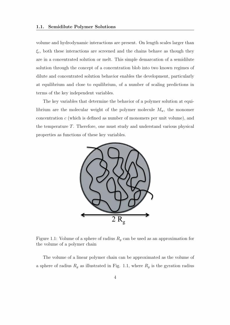
2 Rg
Figure 1.1: Volume of a sphere of radius Rg can be used as an approximation forthe volume of a polymer chain
The volume of a linear polymer chain can be approximated as the volume of
a sphere of radius Rg as illustrated in Fig. 1.1, where Rg is the gyration radius
4

1.1. Semidilute Polymer Solutions
of a polymer molecule. At low polymer concentrations, as shown in Fig. 1.2
(a), these spheres of radius Rg are far apart and do not interact with each other.
Upon increasing the polymer concentration, polymer chains become congested
and interact with each other. At a certain polymer concentration, the monomer
concentration c becomes equal to the so called overlap concentration c?. At
the overlap concentration, individual polymer chains just begin to touch each
other, and the whole volume of the system is filled with spheres of radius Rg, as
depicted in Fig. 1.2 (b). In this scenario, the monomer concentration inside a
sphere is equal to the monomer concentration of the whole system. The onset of
(a) c << c* (b) c ≅ c*
Figure 1.2: State of polymer chains in solutions with different polymer concen-trations
the semidilute solution regime is believed to occur at the overlap concentration
c?. Clearly, the larger the molecular weight, the larger the chain size, and the
smaller the value of c?. In fact, it turns out it is possible to eliminate the explicit
dependence on Mw altogether, and describe the behavior completely in terms of
the scaled variable c/c? (Rubinstein and Colby, 2003).
The dependence on temperature is subtler. At high enough temperatures,
5

1.1. Semidilute Polymer Solutions
Property Theta solvent Good solvent
Gyration radiusRg
R0g
∼( cc?
)0 Rg
R0g
∼( cc?
)−0.125
Zero-shear rate viscosityηpηs∼( cc?
)2 ηpηs∼( cc?
)1.25
Diffusion coefficientD
D0
∼( cc?
)−1 D
D0
∼( cc?
)−0.5
Table 1.1: Scaling predictions for semidilute solutions in theta and good solvents.
the enthalpic interactions between monomers and solvent molecules are favor-
able, so a polymer coil swells to occupy as large a size as is permitted within the
constraints of monomer connectivity. This good solvent regime vanishes as the
temperature is lowered and polymer-solvent interactions become less favorable.
At a unique temperature called the theta temperature, the desire for the polymer
coil to swell due to entropic considerations is just balanced by the unfavorable
enthalpic interactions with the solvent, giving rise to a unique scaling regime
called the theta regime. Using the concept of a concentration blob, scaling pre-
dictions in theta and good solvents can be developed. For instance, the gyration
radius, the zero-shear rate viscosity and the self-diffusion coefficient in semidilute
solutions are predicted to scale with c/c? as shown in Table 1.1. In this Table, R0g
is the gyration radius at infinite dilution, ηp and ηs are the polymer and solvent
contributions to viscosity, and D and D0 are self-diffusion coefficients, with D0
representing the value in a dilute solution at theta condition. These scaling
laws, that govern the static and near-equilibrium dynamic properties, have been
subjected to a wealth of carefully executed experiments (Rubinstein and Colby,
2003; Wiltzius et al., 1984; Ewen and Richter, 1997) and computer simulations
6

1.2. Mesoscopic Simulations
(W. Paul et al., 1991; Muller et al., 2000; Huang et al., 2010; Ahlrichs et al.,
2001).
Unfortunately, these scaling laws are only valid in the limits of the theta
and good solvent regimes, with no predictions available in the large crossover
regime between theta and good solvents (Grosberg and Khokhlov, 1994; Schafer,
1999). Therefore, it is clearly also important to study the crossover driven by
temperature in semidilute solutions in more detail. Indeed there have been only
few investigations (based on scaling theory) that have tried to study the double
crossover driven by both concentration and temperature, in particular when dy-
namic properties are concerned (Daivis and Pinder, 1990). These have not been
examined by any computer simulations either because of the complexity of the
problem.
The aim of this thesis is to explore the universal crossover scaling functions
in the semidilute regime by studying both the concentration driven crossover
and the temperature driven crossover simultaneously, with the help of computer
simulations. In particular, we wish to discover the specific form of these scal-
ing functions, and address the question: do these scaling functions bear any
resemblance to the purely concentration driven crossover scaling functions? We
address this question by developing a mesoscopic Brownian dynamics simulation
algorithm, and examining universal behavior in the long-chain limit.
1.2 Mesoscopic Simulations
In recent years, significant progress in the development of mesoscopic simula-
tion techniques, which allow the exploitation of underlying theories without the
need for approximations, (Ahlrichs et al., 2001; Stoltz et al., 2006; Huang et al.,
2010) has made it possible for the first time to obtain detailed predictions of
7

1.2. Mesoscopic Simulations
equilibrium and nonequilibrium properties that can be compared with experi-
mental observations. The successful implementation of mesoscopic simulations
has been made possible through the use of algorithms that enable an accurate
depiction of the semidilute regime. Essentially, this requires the ability to de-
scribe long polymers that overlap with each other, while maintaining a low seg-
ment density. Further, the segments must be capable of interacting with each
other through solvent mediated hydrodynamic interactions (Kirkwood and Rise-
man, 1948; Freed and Edwards, 1974; de Gennes, 1976b; Bixon, 1976; Ahlrichs
et al., 2001). Three different mesoscopic simulation methods, all of which use
coarse-grained bead-spring chain models for polymer molecules, have been de-
veloped recently that achieve these objectives. Two of these techniques, namely,
the hybrid Lattice Boltzmann/Molecular Dynamics (LB/MD) method (Ahlrichs
and Dunweg, 1999; Dunweg and Ladd, 2009) and the hybrid Multi-particle Colli-
sion Dynamics/Molecular Dynamics (MPCD) method treat the solvent explicitly
(Malevanets and Kapral, 1999; Kapral, 2008; Gompper et al., 2009). As a con-
sequence, hydrodynamic interactions between polymer segments arise naturally
through the exchange of momentum between the beads on a chain and solvent
molecules. In the third approach (Stoltz et al., 2006), which is based on Brown-
ian dynamics (BD) simulations (Ottinger, 1996), the solvent degrees of freedom
are removed completely, but their effect is taken into account through long-range
dynamic correlations in the stochastic displacements of the beads.
The very nature of semidilute polymer solutions, particularly the need to
use periodic boundary conditions to describe homogeneous polymer solutions in
unbounded domains, necessitates the simulation of a large number of particles.
As a result, the computational efficiency of a simulation technique becomes an
important consideration. One of the aim of this thesis is to implement an opti-
mized BD algorithm for semidilute polymer solutions by efficiently treating the
8
1.3. Far-From-Equilibrium Simulations
long-ranged hydrodynamic interactions. Moreover, the BD algorithm developed
by Stoltz et al. (2006) is not applicable when there is particle-particle overlap,
and hence is restricted to the simulation of semidilute solutions in good solvent
conditions. The aim here is to develop a BD algorithm capable of simulating
semidilute solutions at the θ temperature, which is essential in order to study
the temperature driven crossover regime, and also in addressing the question
regarding the form of the crossover scaling functions in the double crossover
regime.
1.3 Far-From-Equilibrium Simulations
While it is important to study the behavior of semidilute polymer solutions at
equilibrium, it is equally important to understand far from equilibrium behav-
ior, because for many practical applications, polymer solutions are processed
under different flow conditions. The great advantage of BD simulations is that
the same algorithm can be used for simulating both equilibrium systems, and
systems subject to flow. In the case of dilute solutions, this is typically ac-
complished by incorporating a term in the stochastic differential equation that
accounts for flow. However, this is highly nontrivial for polymer solutions at finite
concentrations, in particular for infinite systems treated with periodic boundary
conditions. Unlike the simulation of equilibrium system where periodic boundary
conditions (PBCs) are used in an orthogonal cell to get rid of wall effects, for
simulating far from equilibrium systems, appropriate PBCs need to be used such
that the following two requirements are met: (i) The PBCs should be compatible
with any particular flow and (ii) the simulation should be capable of running for
an arbitrary amount of time. PBCs for planar shear flow and planar elonga-
tional flow were developed by Lees and Edwards (1972) and Kraynik and Reinelt
9

1.4. Objectives
(1992), respectively, such that the two requirements mentioned above were ful-
filled. Lees-Edwards and Kraynik-Reinelt PBCs have been used by Bhupathiraju
et al. (1996); Todd and Daivis (1998) in their nonequilibrium molecular dynam-
ics (NEMD) simulation algorithm. Other than NEMD simulations, these PBCs
have also been implemented in a BD algorithm by Stoltz et al. (2006) to simu-
late semidilute polymer solutions undergoing planar shear or planar elongational
flows.
In real flow situations, however, rather than only shear or elongational flow, a
combination of these flows is often observed. Woo and Shaqfeh (2003); Dua and
Cherayil (2003) and Hoffman and Shaqfeh (2007) have simulated dilute polymer
solutions in planar mixed flow using a BD algorithm in which PBCs were not
required. In a recent paper, Hunt et al. (2010) have derived suitable PBCs for
planar mixed flow (which is a linear combination of planar elongational flow
and planar shear flow) and implemented them in their nonequilibrium molecular
dynamics (NEMD) simulation algorithm. To our knowledge, mixed flows of
semidilute polymer solutions have not been studied so far. We aim to implement,
for the first time, PBCs for planar mixed flow (Hunt et al., 2010) in a multi-
chain Brownian dynamics simulation algorithm, which will enable us to simulate
semidilute polymer solutions undergoing different kinds of flows.
1.4 Objectives
The broad objectives of this thesis can be listed as the following set of tasks:
1. Derivation of universal crossover scaling functions based on the blob model.
2. Development of a Brownian dynamics simulation algorithm for semidilute
polymer solutions at equilibrium.
10

1.4. Objectives
3. Verification of the crossover scaling functions predicted by scaling theory
using Brownian dynamics simulations.
4. Implementation of mixed flow in a Brownian dynamics simulation algo-
rithm.
The structure of the thesis is as follows: In order to set the stage for deriving
universal crossover scaling laws for semidilute solutions, various concepts such
as the blob model, excluded volume and hydrodynamic interactions etc . . . are
introduced in Chapter 2. In Chapter 3, these concepts are used to derive scaling
functions for semidilute solutions in the double crossover regime. The governing
equations for the BD simulation algorithm are described in Chapter 4, while
Chapter 5 focuses on the implementation of different terms in the BD simulation
algorithm at equilibrium. Optimization studies that have been carried out to ob-
tain a fast BD simulation algorithm are also discussed in Chapter 5. The various
predictions of scaling theory in the double crossover regime are verified with the
help of BD simulations in Chapter 6. Chapter 7 describes the implementation of
mixed flows in a BD simulation algorithm, and the preliminary results we have
obtained for the viscosity of a semidilute solution under mixed flow conditions
are discussed. Finally, conclusions of the thesis are presented in Chapter 8.
11

1.4. Objectives
12
Chapter 2
Scaling Theory for Dilute
Polymer Solutions Near
Equilibrium
The behavior of dilute polymer solutions near equilibrium has been extensively
studied by experiments, theory and computer simulations, and there are many
monographs that provide an excellent summary of our current understanding
of these systems (Bird et al., 1987; de Gennes, 1979; Doi and Edwards, 1986;
Rubinstein and Colby, 2003). In this chapter, we briefly discuss the scaling theory
used to derive scaling laws for various properties in dilute polymer solutions at
equilibrium. Though we are interested in semidilute solutions, a discussion of
scaling concepts in the context of dilute solutions is required to set up the basic
framework for developing scaling laws in the semidilute regime, presented in
Chapter 3.
Scaling laws for dilute solutions account for two important pieces of physics
that occur on the microscopic scale, namely, excluded volume (EV) interactions
and hydrodynamic interactions (HI) (Bird et al., 1987; de Gennes, 1979; Doi and
13

2.1. Excluded Volume Interactions
Edwards, 1986; Larson, 1988; Prakash and Ottinger, 1999; Prakash, 1999, 2009).
Excluded volume interactions are first briefly discussed in Section 2.1, followed
by a discussion of hydrodynamics interactions in Section 2.2. Finally, scaling
laws for various properties are derived for dilute polymer solutions in Section
2.3.
2.1 Excluded Volume Interactions
Excluded volume interactions play an important role in determining the static
behavior of polymer solutions (de Gennes, 1979; Doi and Edwards, 1986; Ru-
binstein and Colby, 2003). The physics of excluded volume interactions can be
understood as follows. When any two monomers of a polymer molecule come
close to each other, a strong mutual repulsion is felt by them. This repulsion
arises because a monomer cannot occupy space that is already occupied by an-
other monomer of the same polymer molecule at the same time. As seen in Fig.
Ø Short-range interaction along the backbone
Ø Short-range interaction in space
Ø Long-range interaction along the backbone
Ø Short-range interaction in space
Figure 2.1: Illustration of excluded volume interactions in a polymer molecule
14
2.1. Excluded Volume Interactions
2.1, the two black monomers cannot overlap each other because of the repulsive
interaction between them.
In general, the effective interaction between a pair of monomers can be ei-
ther repulsive or attractive, depending on the difference between the strengths
of monomer-monomer and monomer-solvent interactions. When the monomer-
monomer energy is lower than the monomer-solvent energy, monomers like to be
near each other, and this means that the effective interaction between monomers
is attractive. Note that by energy we mean the energy u(r) required to bring
two particles (that can be either monomer or solvent particles) from∞ to within
distance r of each other (Rubinstein and Colby, 2003). On the other hand, when
the energy between monomer and solvent is lower than that between monomer
and monomer, monomers like to be surrounded by solvent molecules, leading to
the effective interaction between monomers being repulsive. This effective inter-
action, which includes the repulsive and attractive parts of monomer-monomer
interaction, is known as excluded volume interaction (Flory, 1953). Excluded
volume interactions are either short-range or long-range along the backbone of a
polymer molecule but they are always short-range in space.
Clearly the structure of a polymer molecule depends on the relative strength
of monomer-monomer and monomer-solvent interactions. For example, the av-
erage size of a polymer molecule tends to increase due to the monomer-monomer
repulsion, but at the same time, this swelling of a molecule is opposed by solvent-
mediated attractions. The thermodynamic state of the solvent plays an impor-
tant role in monomer-solvent interactions, and the temperature is a control-
ling parameter in such interactions (Flory, 1953; Schafer, 1999). For instance,
monomer-solvent interactions are energetically unfavorable at low temperatures,
and the polymer solution is said to be under poor solvent conditions. This leads to
strong enough monomer-monomer attractions that dominate monomer-monomer
15

2.1. Excluded Volume Interactions
repulsions, and the polymer molecule collapses to a globule like structure. Upon
increasing the temperature, the strength of monomer-monomer attractions re-
duces, and therefore, the average size of a polymer molecule increases. The term
good solvent is used to describe a condition where the temperature is high enough
for the repulsive interactions to dominate over attractive interactions. There
exists an intermediate temperature between poor solvent and good solvent con-
ditions, the so called theta temperature, at which the attractive and repulsive
parts of monomer-monomer interactions balance each other. Therefore, at the
theta temperature, the size of a polymer molecule is the same as that of an ideal
polymer molecule (Doi and Edwards, 1986). Depending on the monomer-solvent
interactions, or temperature, three different cases can be visualized as shown in
Fig. 2.2. It is well known that in the theta limit, where polymer configurations
Department of Chemical Engineering
!!"#"! !"$"!
!"#$%&'()*+#,'-
!"#$%#&'()'"&#$*(&'+",)-#&.##")/+012#$)*"3),+04#"&)*$#)($5('*067*4+$*-0#)'"&#$*(&'+",)8 %++3),+04#"&5"7*4+$*-0#)'"&#$*(&'+",)8 /++$),+04#"&
Good solventPoor solvent θ solvent
Figure 2.2: Monomer-solvent interactions affect the structure of a polymermolecule
obey random walk (RW) statistics, the size of a polymer molecule scales as M1/2w .
This power law is also referred to as the Gaussian scaling law for polymer size.
The exponent in this power law is universal and hence is (1/2) for all theta sol-
vents. However, the prefactor depends on the chemistry of the polymer-solvent
system.
16
2.1. Excluded Volume Interactions
In the good solvent limit, on the other hand, the polymer is considered to
follow self avoiding walk (SAW) statistics. In this case, a similar power law gov-
erns the polymer size, but with a nontrivial exponent ν ∼= 3/5, famously known
as the Flory exponent [the precise value is 0.587597 (7) (Clisby, 2010)]. This
exponent is again universal in the good solvent limit and hence is independent
of temperature or chemistry. The size of a polymer molecule in a good solvent,
therefore, scales as Mνw. This power law is referred to as the Kuhnian scaling law
for polymer size. Similar to the theta case, the prefactor in this power law con-
tains all the information regarding chemistry or temperature. This power law is
valid only in the excluded volume limit, when the molecular weight is sufficiently
large, with the effective interaction being repulsive or with the temperature T
being not too close to the theta temperature. The repulsive interaction decreases
as T approaches the theta temperature. In order for the excluded volume power
law to be valid at a lower temperature, the polymer must have an even larger
molecular weight. In other words, the polymer solution departs from the ex-
cluded volume limit if either T is reduced towards the theta temperature at a fix
Mw or Mw is decreased by keeping T fixed.
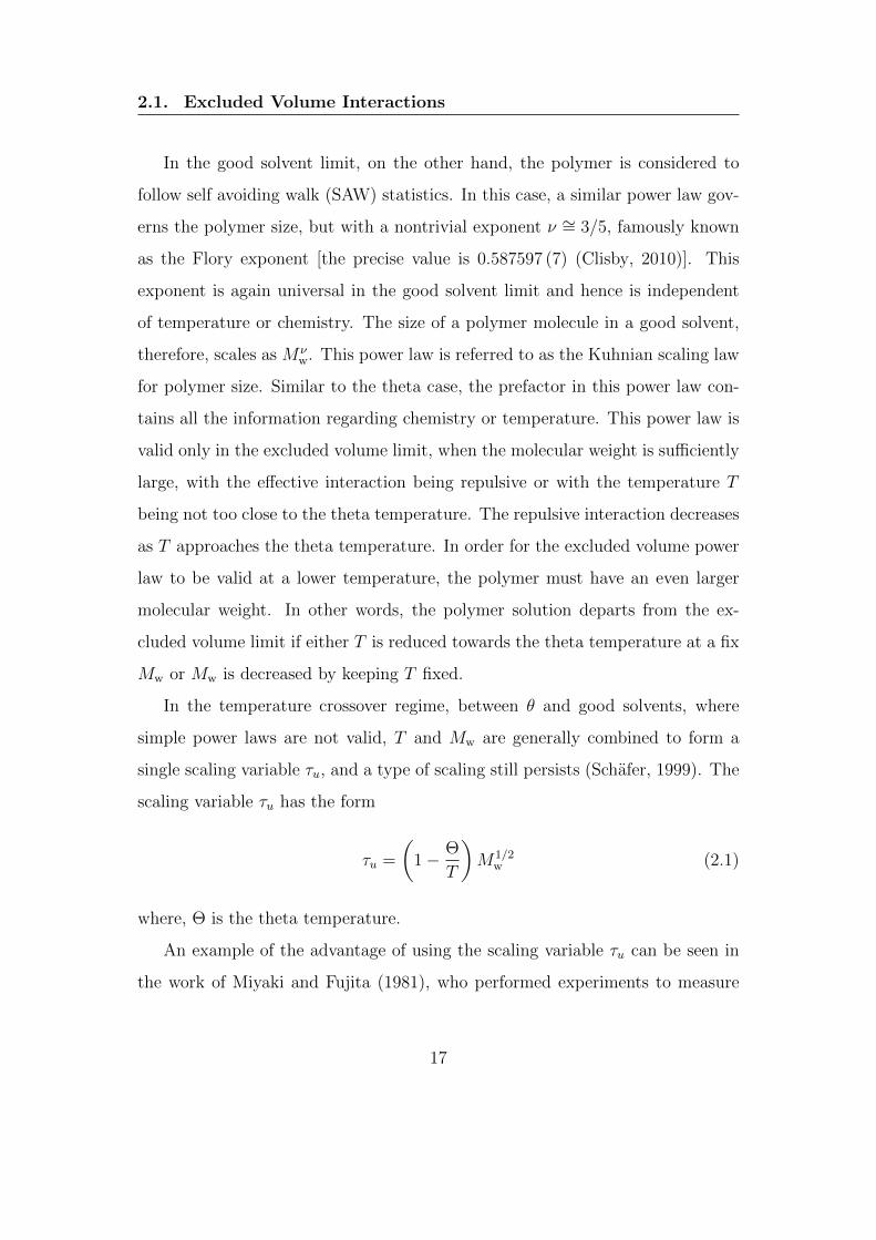
In the temperature crossover regime, between θ and good solvents, where
simple power laws are not valid, T and Mw are generally combined to form a
single scaling variable τu, and a type of scaling still persists (Schafer, 1999). The
scaling variable τu has the form
τu =
(1− Θ
T
)M1/2
w (2.1)
where, Θ is the theta temperature.
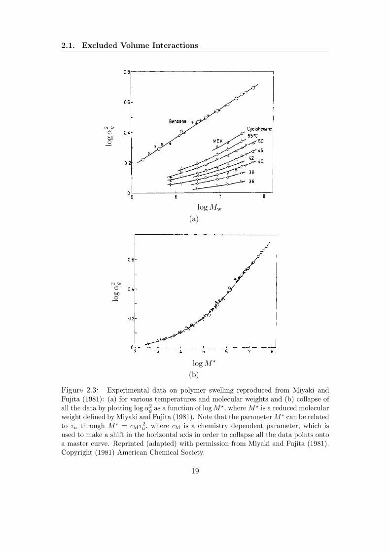
An example of the advantage of using the scaling variable τu can be seen in
the work of Miyaki and Fujita (1981), who performed experiments to measure
17
2.1. Excluded Volume Interactions
the swelling of polystyrene in Benzene at 25 and 300 C, in methyl ethyl ketone
(MEK) at 350 C, and in Cyclohexane at the temperatures indicated in Fig. 2.3
(a). The variable in the y-axis is the swelling of a polymer molecule αg(T,Mw)
defined as the ratio of the polymer size at temperature T to that in a theta
solvent.
When α2g is plotted as a function of M? in a log− log plot, where M? = cMτ
2u
and cM is a chemistry dependent parameter, it can be seen in Fig. 2.3 (b) that
universal behavior can be obtained for all values of Mw and temperature T > Θ,
by merely using proper values of cM (Miyaki and Fujita, 1981).
Universal behavior in the temperature crossover regime has also been ob-
served using theoretical models. For instance, renormalization group (RG) meth-
ods have been applied to successfully predict the entire range of behavior ex-
hibited by static solution properties (Freed, 1987; Schafer, 1999; Cloizeaux and
Jannink, 2010). In these theoretical models, polymer molecules are represented
by a coarse-grained model, such as a bead-spring chain (Bird et al., 1987), con-
sisting of Nb beads connected together by Nb− 1 Hookean springs (with a spring
constant H). Each bead consists of several monomers, and hence Nb is directly
proportional to the molecular weight of a polymer molecule.
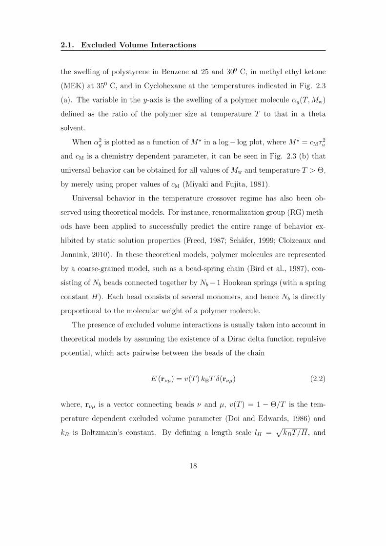
The presence of excluded volume interactions is usually taken into account in
theoretical models by assuming the existence of a Dirac delta function repulsive
potential, which acts pairwise between the beads of the chain
E (rνµ) = v(T ) kBT δ(rνµ) (2.2)
where, rνµ is a vector connecting beads ν and µ, v(T ) = 1 − Θ/T is the tem-
perature dependent excluded volume parameter (Doi and Edwards, 1986) and
kB is Boltzmann’s constant. By defining a length scale lH =√kBT/H, and
18
2.1. Excluded Volume Interactions
logα
2 g
log Mw
(a)Vol. 14, No. 3, May-June 1981
o.81 Testa of Two-Parameter Theory for (P) W d [VI 743
Cyclohexane
0.2-
1 I
6 7 8 log M w
O5
Figure 1. log-log plots of a: vs. M, for polystyrene in benzene at 25 and 30 "C, in methyl ethyl ketone (MEK) at 35 "C, and in cyclohexane at the temperatures indicated. Half-filled circles, from ref 4 and 5. Other symbols, from ref 3 and 6.
generally in favor of this prediction. However, we must note that the existence of a universal relation between a, and a,, is only a necessary condition for eq 1 and 4 to hold. Nonetheless, one might take it as a sufficient condition for the two-parameter theory of [TI, considering eq 1 to be self-evident theoretically. It is imperative for completeneas to verify, in addition to the above-mentioned necessary condition, that either a, or a, is a universal function of z.
Now, to a good approximation, the characteristic ratio ( P ) , / M of a polymer may be treated as a constant except in the region of low M. Further, the binary cluster integral /3 is a function of polymer and solvent condition but not of M. Therefore, to a good approximation, we may write eq 3 as
z = K M I 2 (6) with K a constant for polymer and solvent condition fixed. The subsequent discussion is limited to the case in which eq 6 is valid.
Criterion A. With eq 6 it follows that if eq 1 holds, plots of log a, vs. log M for different combinations of polymer and solvent condition can be superimposed on a single curve by appropriate displacement along the hori- zontal axis.
For a given polymer we choose a relevant solvent con- dition R as the reference state and denote the value of K for R by KW Then, KRf, the K value of the same polymer for another solvent condition R', can be expressed by
(7) if criterion A is obeyed. Here, log U M is the horizontal distance needed to have the log a, vs. log M curve for R' match that for R. We call U M the shift fador for R' relative to R. Since K is proportional to fi for a given polymer, eq 7 is equivalent to
OR' = fiRBR(aM)-'I2 (8)
Hence, when eq 1 holds, /3 can be evaluated from experi- mental determination of the shift factor if one has a means to estimate BR.
Criterion B. With eq 6 it follows that if eq 4 holds, plots of log a? vs. log M for different combinations of polymer and solvent condition can be brought on a single curve when displaced horizontally, and the horizontal distance between the plots of a given polymer for solvent conditions R' and R should be equal to that between the corresponding log a, vs. log M plots.
0.61
0.4
o.2 t 3 4 5 6 7 8
log M* Figure 2. log-log plots of CY: vs. M* (:M,/aM) derived from Figure 1. Symbols are the same as in Figure 1.
0.6 P I 8 1 / I Cyclohexane
log Mw
Figure 3. log-log plots of a: vs. M , for polyisobutylene in cyclohexane at 25 "C, in n-heptane at 25 "C, and in isoamyl isovalerate (IAIV) at the temperatures indicated.
The latter condition is required by the fact that a, and a, are functions of the same variable z.
Radius Expansion Factor Check of Criterion A. Figure 1 shows double-loga-
rithmic plots of a,2 vs. M , (weight-average molecular weight) for narrow-distribution polystyrene samples in benzene at 25 and 30 "C, in methyl ethyl ketone (MEK) at 35 "C, and in cyclohexane at a series of temperatures above the 8 point (307.7 K).
Figure 2 illustrates how accurately the sets of data points for different solvent conditions in Figure 1 can be brought to a single line by horizontal shifting. Here, M* is a re- duced molecular weight defined by Mw/uM, with aM the shift factor relative to 25 O C benzene as the reference state R. We conclude that the polystyrene data in Figure 1 satisfy criterion A.
Figure 3 displays double-logarithmic plots of CY: vs. M, for polyisobutylene in cyclohexane at 25 "C, in n-heptane at 25 OC, and in isoamyl isovalerate (IAIV) at different temperatures above the 8 point (295.3 K). These data were taken from part 4 of this ~e r i e s .~ It is seen that there is little or no range of a,2 in which values of this quantity in different solvents overlap. This condition makes it difficult to check data unambiguously for the superim- posability required by criterion A. However, if the system obeys criterion A, the lines drawn in Figure 3 should be made coincident with the composite curve for polystyrene in Figure 2 by horizontal displacement. Figure 4 demon- strates that this prediction holds. Thus, we can conclude
logα
2 g
log M
(b)
Figure 2.3: Experimental data on polymer swelling reproduced from Miyaki andFujita (1981): (a) for various temperatures and molecular weights and (b) collapse ofall the data by plotting logα2
g as a function of logM?, where M? is a reduced molecularweight defined by Miyaki and Fujita (1981). Note that the parameterM? can be relatedto τu through M? = cMτ
2u , where cM is a chemistry dependent parameter, which is
used to make a shift in the horizontal axis in order to collapse all the data points ontoa master curve. Reprinted (adapted) with permission from Miyaki and Fujita (1981).Copyright (1981) American Chemical Society.
19
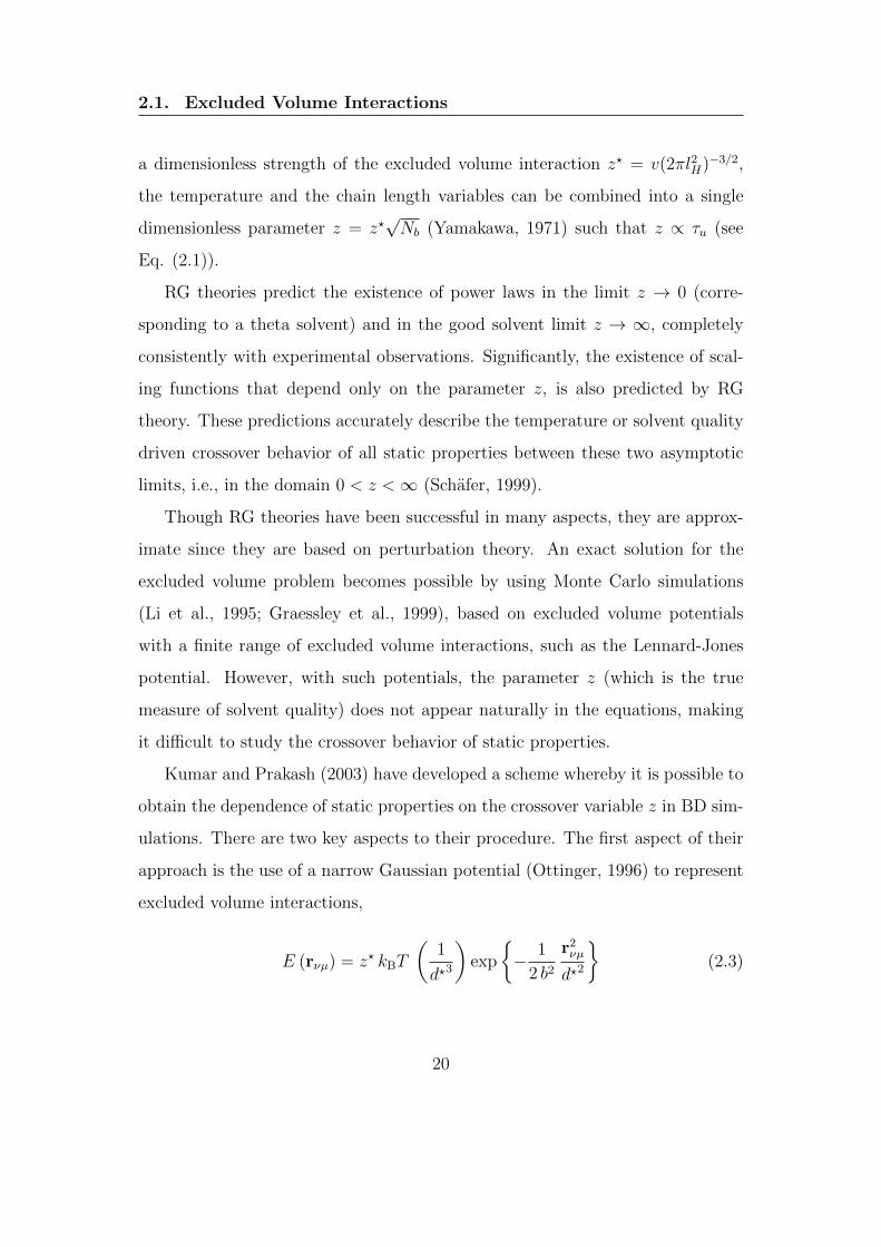
2.1. Excluded Volume Interactions
a dimensionless strength of the excluded volume interaction z? = v(2πl2H)−3/2,
the temperature and the chain length variables can be combined into a single
dimensionless parameter z = z?√Nb (Yamakawa, 1971) such that z ∝ τu (see
Eq. (2.1)).
RG theories predict the existence of power laws in the limit z → 0 (corre-
sponding to a theta solvent) and in the good solvent limit z → ∞, completely
consistently with experimental observations. Significantly, the existence of scal-
ing functions that depend only on the parameter z, is also predicted by RG
theory. These predictions accurately describe the temperature or solvent quality
driven crossover behavior of all static properties between these two asymptotic
limits, i.e., in the domain 0 < z <∞ (Schafer, 1999).
Though RG theories have been successful in many aspects, they are approx-
imate since they are based on perturbation theory. An exact solution for the
excluded volume problem becomes possible by using Monte Carlo simulations
(Li et al., 1995; Graessley et al., 1999), based on excluded volume potentials
with a finite range of excluded volume interactions, such as the Lennard-Jones
potential. However, with such potentials, the parameter z (which is the true
measure of solvent quality) does not appear naturally in the equations, making
it difficult to study the crossover behavior of static properties.
Kumar and Prakash (2003) have developed a scheme whereby it is possible to
obtain the dependence of static properties on the crossover variable z in BD sim-
ulations. There are two key aspects to their procedure. The first aspect of their
approach is the use of a narrow Gaussian potential (Ottinger, 1996) to represent
excluded volume interactions,
E (rνµ) = z? kBT
(1
d?3
)exp
− 1
2 b2
r2νµ
d?2
(2.3)
20

2.2. Hydrodynamic Interactions
where, d? is a dimensionless parameter that measures the range of the excluded
volume interaction, and b is the monomer size. In the limit d? → 0, the narrow
Gaussian potential reduces to δ-function potential, and is consequently a means
of regularizing the δ potential.
The second aspect is their procedure for finding the model’s predictions in
the limit of infinite chain length. In their simulations, data for larger and larger
values of Nb are accumulated, and the infinite chain length limit is then found
by extrapolating the finite chain data to Nb →∞.
Kumar and Prakash (2003) have shown that in this limit, d? is an irrelevant
variable, and that the only relevant variable is the scaling variable z. The results
of their BD simulations for α2g at various values of z are displayed as the solid red
line in Fig. 2.4. The experimental data of Miyaki and Fujita (1981), is plotted
along with the simulation results in Fig. 2.4. By considering z = kzτu, where kz
is a chemistry dependent parameter, all the experimental data can be collapsed
onto the simulation curve by making a simple horizontal shift to the experimental
data. Details of the shifting procedure are given in Kumar and Prakash (2003).
The extended discussion of excluded volume interactions in this section has
served two purposes. Firstly, it helps introduce the solvent quality variable z,
which is used in the scaling theories for dilute and semidilute solutions. Sec-
ondly, it helps to introduce the narrow Gaussian potential and the extrapolation
procedure that we have used subsequently in our simulations.
2.2 Hydrodynamic Interactions
In a polymer chain, each segment experiences a drag force because of friction with
solvent molecules caused by their relative motion. When any one segment of a
polymer chain moves, the velocity field of the solvent near all the other segments
21

2.2. Hydrodynamic Interactions
Figure 2.4: Experimental data for swelling obtained by Miyaki and Fujita (1981)collapse onto the BD simulation results obtained by Kumar and Prakash (2003).Reprinted (adapted) with permission from Miyaki and Fujita (1981) and Kumarand Prakash (2003). Copyright (1981), (2003) American Chemical Society.
are disturbed due to fast diffusive momentum transport by solvent molecules.
This disturbance in the velocity field modifies the drag force on other segments,
which eventually affects the motion of those segments. This interaction is known
as hydrodynamic interaction, and is shown schematically in Fig. 2.5. The phe-
nomenon of hydrodynamic interactions is a long-range effect, which means that a
strong coupling of motions of segments are unavoidable even for those segments
that are far apart along the backbone of the chain, and far apart in space as well.
An example of a dynamic property is the diffusivity of a polymer molecule, D,
which is proportional to the mean squared displacement of the chain with time.
Accurate prediction of diffusivity, through theoretical approach, is obtained only
when HI is included (Zimm, 1956).
22
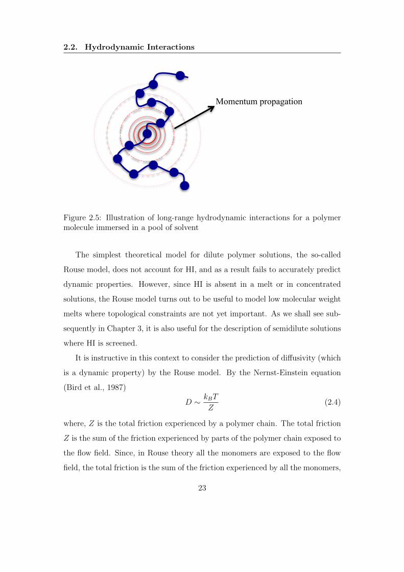
2.2. Hydrodynamic Interactions
Momentum propagation
Figure 2.5: Illustration of long-range hydrodynamic interactions for a polymermolecule immersed in a pool of solvent
The simplest theoretical model for dilute polymer solutions, the so-called
Rouse model, does not account for HI, and as a result fails to accurately predict
dynamic properties. However, since HI is absent in a melt or in concentrated
solutions, the Rouse model turns out to be useful to model low molecular weight
melts where topological constraints are not yet important. As we shall see sub-
sequently in Chapter 3, it is also useful for the description of semidilute solutions
where HI is screened.
It is instructive in this context to consider the prediction of diffusivity (which
is a dynamic property) by the Rouse model. By the Nernst-Einstein equation
(Bird et al., 1987)
D ∼ kBT
Z(2.4)
where, Z is the total friction experienced by a polymer chain. The total friction
Z is the sum of the friction experienced by parts of the polymer chain exposed to
the flow field. Since, in Rouse theory all the monomers are exposed to the flow
field, the total friction is the sum of the friction experienced by all the monomers,
23

2.2. Hydrodynamic Interactions
and as a result Z scales as the molecular weight Mw of the chain. This also implies
that the diffusivity in Rouse theory scales as M−1w . This prediction is contrary
to experimental observations, which suggest that D scales as M−νw .
The introduction by Zimm (1956) of HI in an equilibrium averaged form into
a molecular model for polymer solutions led for the first time to an accurate
description of dynamic properties close to equilibrium. The Zimm theory does
not capture the dynamics of polymer solutions away from equilibrium since it
does not account for fluctuations in HI (Ottinger, 1989; Prakash, 1999). As will
be discussed in Chapter 4, fluctuations in HI can be taken into account in BD
simulations without making any averaging approximations. For the purpose of
scaling theory, however, the Zimm theory is perfectly adequate.
The key result of the Zimm theory is that in dilute solutions, the total friction
of the polymer chain is that experienced by the polymer coil as a whole, and not
that of all the monomers together. In some sense, the monomers inside the
polymer molecule are shielded from the flow (de Gennes, 1979; Rubinstein and
Colby, 2003). As a result Z is proportional to the size of the polymer molecule
Rg, and the diffusivity then takes the form
D ∼ kBT
ηsRg
(2.5)
Since Rg ∼ Mνw, the diffusivity in Zimm theory scales as M−ν
w , in excellent
agreement with experimental observations.
As we shall see in the scaling theory for semidilute solutions developed in
Chapter 3, we use Rouse scaling when HI is screened and Zimm scaling when it
is present. In the next section however, we use the concepts of solvent quality
and Zimm scaling to derive some scaling laws for dilute polymer solutions.
24

2.3. Scaling Theory
2.3 Scaling Theory
The scaling theory for dilute polymer solutions is based on the concept of thermal
blobs (de Gennes, 1979; Rubinstein and Colby, 2003; Grosberg and Khokhlov,
1994). The thermal blob is associated with a balance between thermal energy
and energetic contributions due to excluded volume interactions . The size of the
thermal blob ξT characterizes the length scale at which the energy due to excluded
volume interactions amongst all the monomers lying within a blob becomes equal
to the thermal energy kBT . This implies that the conformations of the chain
inside a thermal blob are unperturbed by excluded volume effects. As a result,
the polymer chain obeys random walk (RW) statistics within a thermal blob. On
the other hand, for length scales greater than ξT , excluded volume interactions
become important and as a result, thermal blobs obey self avoiding walk (SAW)
statistics, as shown schematically in Fig. 2.6.
Thermal blob
ξT (RW )
Rg(SAW )
Figure 2.6: Thermal blobs in dilute solution
The size of the thermal blob ξT can be estimated as follows. Two monomers
are assumed to interact with an energy ε
(1− Θ
T
), where ε (> 0) is the repulsive
energy of enthalpic origin. We assume that there are n monomers within a
thermal blob. Since the number of contacts in a RW are of order n1/2 in three
25

2.3. Scaling Theory
spatial dimensions, it is straightforward to see that the excluded volume energy
due to all the interactions within a thermal blob is of order n1/2 ε
(1− Θ
T
). From
the definition of a thermal blob, this energy must be of the same order as kBT .
Therefore, the condition to find n is
ε
(1− Θ
T
)n1/2 = kBT (2.6)
The excluded volume interaction energy for a pair of monomers, ε
(1− Θ
T
),
nondimensionalized by kBT , can be equated to the dimensionless parameter
z?, which is the parameter in the narrow Gaussian potential which represents
the non-dimensional strength of pair-wise excluded volume interactions (see Eq.
(2.3)). As a result,
z? =ε
kBT
(1− Θ
T
)(2.7)
From Eqs. (2.6) and (2.7), it follows that,
n = (z?)−2 (2.8)
The corresponding blob size is consequently (since RW statistics are obeyed
within a blob)
ξT = bn1/2 = b (z?)−1 (2.9)
Using the definition of the solvent quality parameter, as mentioned in Section
2.1,
z = z?N1/2b (2.10)
the nondimensional blob size in terms of the scaled variable z is,
ξT
bN1/2b
=ξTRθg
= z−1 (2.11)
26

2.3. Scaling Theory
where, Rθg = bN
1/2b is the gyration radius at theta condition. The solvent quality
can be seen to represent the ratio of the size of the chain in a θ solvent to the
size of the thermal blob. Clearly, decreasing z increases ξT , and in the θ limit
The theta solution limit The good solvent limit
z → 0 ⇒ ξT → Rg z → ∞ ⇒ ξT → b
Rg ∼ bN1/2b
Rg ∼ bNνb
Figure 2.7: Changing z changes the size of a thermal blob ξT
the size of the thermal blob becomes larger than the size of a polymer chain. On
the other hand, increasing z decreases ξT , and in the very good solvent limit ξT
becomes equal to the size of a monomer b. This can be visualized as shown in
Fig. 2.7.
The scaling relation for the gyration radius Rg can be derived in terms of
the scaled variable z as follows. Since the chain obeys SAW statistics on length
scales larger than ξT ,
Rg = ξT
(Nb
n
)ν(2.12)
where, (Nb/n) is the number of thermal blobs. Using Eqs. (2.8) and (2.9), leads
to
Rg = bN νb (z?)2ν−1 (2.13)
The scaling relation in terms of scaled variables can be obtained by making use
of Eq. (2.10), and the definition of Rθg
Rg
Rθg
= z2ν−1 (2.14)
27

2.3. Scaling Theory
As discussed earlier, Zimm dynamics are relevant on all length scales in the dilute
regime. Using Zimm’s scaling law for diffusivity from Eq. (2.5) and Rg from Eq.
(2.13), we can write
D =kBT
ηs bN νb (z?)2ν−1
(2.15)
Defining Dθ =kBT
ηsRθg
, it follows from Eq. (2.10) that the ratio of diffusivities is
given in terms of scaled variables by
D
Dθ= z−(2ν−1) (2.16)
Once the expressions for Rg and D are known, the scaling laws for ηp, the polymer
contribution to viscosity, can be derived from the relation
ηp = kBT (c/Nb)τ1 (2.17)
where τ1 is the longest relaxation time of the polymer molecule which can be
expressed as τ1 ∼ R2g/D. Using Eqs. (2.13), (2.15) and (2.17), it follows that the
scaling law for ηp is
ηp = ηscb3N3ν−1
b z?3(2ν−1) (2.18)
Defining ηθp =c
Nb
ηs b3N
3/2b and using Eq. (2.10), the scaling law for the ratio of
viscosities in terms of scaled variables is
ηpηθp
= z3(2ν−1) (2.19)
Using the scaling arguments discussed in this section, and the concepts of
excluded volume and hydrodynamics interactions, we develop the scaling theory
for finite concentration systems in the next chapter.
28

Chapter 3
Scaling Theory for Semidilute
Polymer Solutions Near
Equilibrium
Predicting the behavior of polymer solutions becomes more complicated when
the polymer concentration becomes finite. When the polymer concentration in-
creases to such an extent that the monomer concentration c becomes equal to the
overlap concentration c? (where the total volume is equal to the volume occupied
by polymer chains), the polymer solution becomes semidilute. Although c may
be low, a strong overlap of polymer chains may occur in semidilute solutions be-
cause of the extended size of polymer chains. This chapter attempts to develop
a scaling theory for semidilute polymer solutions that is applicable to both the
static and dynamic crossovers (based on the framework developed in Chapter 2
in the context of dilute polymer solutions).
Depending on the strength of the excluded volume interaction z? and the
monomer concentration c, different regimes on the phase diagram of a polymer
solution (Rubinstein and Colby, 2003) can be drawn as shown in Fig. 3.1. Dilute
29

Excl
uded
vol
ume
inte
ract
ion
z*
semidilute dilute
concentrated
SAW
RW
RW
RW
RW
SAW
RW
isolated RWs
Monomer concentration c
Nb
!12
c*
c**
dilute overlapping
RWs
! - point
A
B C
D/E
Zimm
Zimm
Rouse/Zimm
Rouse/Zimm
Nb
!12
Figure 3.1: Phase diagram of a polymer solution in the plane monomer concen-tration c and excluded volume strength z?, as predicted by the standard blobpicture. The θ regime occurs for small z? N
−1/2b , while z? N
−1/2b in the
good solvent regime. The overlap concentration is given by c?. For concentrationsabove c??, excluded volume interactions are completely screened.
polymer solutions are indicated by regimes A and B for theta and good solvent
regimes, respectively, and the semidilute regime is indicated by regime C. Un-
like dilute solutions where excluded volume and hydrodynamics interactions were
treated as only intra-chain interactions, in semidilute solutions these interactions
are intra-chain as well as inter-chain, which leads to a many-body problem. The
challenge of solving the many-body problem becomes even more difficult due to
the complicated interplay between excluded volume and hydrodynamic interac-
tions. Using the concepts of scaling blobs, Daoud et al. (1975) developed scaling
30
theories to describe the static and dynamic behavior of semidilute polymer solu-
tions at equilibrium. Scaling theory is based on the idea of a separation of length
scales. Apart from the thermal blob (as discussed in Chapter 2), another blob
(or another length scale) called the concentration blob or correlation blob is in-
troduced to felicitate the development of a scaling theory for semidilute polymer
solutions (de Gennes, 1979).
In both static and dynamic scaling theories, the concentration blob size ξc
corresponds to the length scale at which interactions between polymer chains
become significant. On length scales smaller than ξc the interaction is not im-
portant, and the segment inside a concentration blob essentially follows isolated
chain (dilute solution) behavior. Parts of a chain inside the concentration blob
are not aware that the solution is semidilute because these interact mainly with
solvent molecules and with other monomers from the same segment of the chain.
Since the conformations of a polymer chain in a dilute solution in a good solvent
follow self-avoiding walk (SAW) statistics, the conformations of parts of a chain
that lie within a concentration blob obey SAW statistics of thermal blobs as illus-
trated in Fig. 3.2. On length scales larger than the concentration blob size, the
behavior of a semidilute polymer solution is controlled by interactions between
chains. Moreover, since the concentration of polymers in a semidilute solution is
such that the concentration blob volumes are space filling, on length scales larger
than ξc the semidilute solution behaves as a melt of chains whose segments are
concentration blobs. Thus, polymer conformations on these scales are random
walks (RW) of concentration blobs. This static scaling ansatz is shown schemat-
ically in Fig. 3.2. The transition from self-avoiding walk statistics to random
walk statistics on the length scale of the concentration blob occurs due to the
screening of excluded volume interactions by the overlapping chains. On length
scales smaller than ξc excluded volume interactions are strong enough to swell
31

Concentration blobs SAW
RW
ξc
ξT
Thermal blobs RW
Figure 3.2: Blob picture in a semidilute polymer solution
the chain but are not yet screened by the surrounding chains, while on length
scales larger than ξc, as in the case of melts, excluded volume interactions are
screened.
The blob scaling picture has also been adopted to describe the equilibrium
dynamic behavior of semidilute polymer solutions. As discussed in Chapter 2,
polymer dynamics in dilute solutions incorporating hydrodynamic interactions,
can be described by Zimm dynamics. In concentrated solutions, hydrodynamic
interactions are screened (Freed and Edwards, 1974; Shiwa et al., 1988; Richter
et al., 1984; Edwards and Muthukumar, 1984; Fredrickson and Helfand, 1990; R.
H. Colby et al., 1994) similar to the screening of excluded volume interactions. As
a consequence, for short chains that are not entangled, the Rouse model, which
neglects hydrodynamic interactions, has been found to provide an accurate de-
scription of polymer dynamics in the concentrated regime (Doi and Edwards,
1986). In the special case of semidilute solutions, there exists a length scale
ξH (which is often called the hydrodynamic screening length), which separates
32

Figure 3.3: Schematic representation of hydrodynamic screening by surroundingchains.
these two types of dynamics. On length scales shorter than ξH , hydrodynamic
interactions dominate, and the Zimm model describes polymer dynamics. On
length scales larger than ξH , HI is screened, essentially as a result of chain-chain
collisions which tend to randomize the momentum propagation in the system (as
shown schematically in Fig. 3.3) (Ahlrichs et al., 2001), and the Rouse model
describes polymer dynamics. In the dynamic scaling scenario, as a consequence,
the blob size ξH represents the length scale at which a crossover occurs from
Zimm to Rouse dynamics.
In an important paper, de Gennes (1976b) verified the Freed-Edwards theory
(Freed and Edwards, 1974) for the screening of hydrodynamic interactions and
set up the connection between static length scale ξc and the dynamic length scale
or hydrodynamic interaction screening length ξH . de Gennes (1976b) proposed
convincing scaling arguments to suggest that the static and dynamic correlation
lengths should be identical, i.e., ξc = ξH . Experimental results from static and
33
dynamic light scattering studies appear to support de Gennes contention that
hydrodynamic interactions and excluded volume interactions are indeed screened
on similar length scales (Wiltzius and Cannell, 1986; Zhang et al., 1999).
In another important study, Ahlrichs et al. (2001) have revealed an interesting
aspect about the screening of hydrodynamics interactions in semidilute solutions
at equilibrium. They found from their simulations (using a coupled Molecu-
lar Dynamics/Lattice Boltzmann mesoscopic simulation scheme (Ahlrichs and
Dunweg, 1999)) that hydrodynamic screening is not simply a matter of length
scales, but must necessarily be viewed as a dynamic time-dependent phenomenon.
In particular, they found that HI is not screened up to the crossover time τc on
all length scales, after which screening sets in, leading to Rouse-like motion. The
crossover time τc is the Zimm time of a concentration blob, i.e., roughly the time
needed for a blob to move its own size. After τc, the chain will, on average, feel the
constraints by the temporary matrix of other chains. From then on it is unable to
follow the flow, but rather lags behind, and momentum transport occurs mainly
along the chain backbones, due to connectivity forces. The computer simulation
results of Ahlrichs et al. (2001) are in complete accord with the neutron spin
echo measurements on labeled polymer chains by Richter et al. (1984), which
show that hydrodynamic screening is a dynamic effect which becomes relevant
only after the crossover time. However, it should be noted that their findings are
not relevant if we are interested in understanding only long-time dynamics.
The central message of the discussion above is that for c/c? > 1, and at
sufficiently low time scales, screening of both HI and EV interactions occur at
a certain length scale ξc (the size of a concentration blob), beyond which poly-
mer chains obey RW statistics. A semidilute solution (regime C in Fig. 3.1) is
consequently characterized by b ξT ξc Rg, i.e., by only a finite window
of length scales between ξT and ξc where SAW statistics apply. Upon further
34
increasing c, the system enters the concentrated regime c c??, where this
window has shrunk to zero and chains obey RW statistics on all length scales.
The reason the window shrinks to zero is because, (i) ξT is independent of the
monomer concentration, as discussed in Chapter 2, and (ii) ξc decreases by in-
creasing concentration (as will be discussed shortly), and becomes equal to ξT at
c = c?? (Rubinstein and Colby, 2003). As a result, on length scales smaller than
ξc, thermal energy is stronger than the energy of excluded volume interactions,
and on length scales greater than ξc, excluded volume interactions are screened
by overlapping chains. Therefore, ideal chain like behavior is observed at all
length scales when the monomer concentration is equal to or greater than c??
(Rubinstein and Colby, 2003).
The lines drawn in Fig. 3.1 do not indicate sharp phase transitions but rather
smooth crossovers. Clearly, there is a concentration driven crossover from the
dilute regime (SAW statistics) to the concentrated regime (RW statistics) via
the semidilute regime for any given solvent quality. The effect of solvent quality
on the behavior of semidilute solutions can be studied in a similar manner as
was discussed for dilute solutions in Chapter 2. In order to understand the effect
of concentration and solvent quality together on the behavior of semidilute so-
lutions at equilibrium, the blob scaling picture can be applied to regime C, and
scaling relations for ξc, Rg and D can be derived (in terms of concentration and
solvent quality) as discussed below.
Thermal blobs within the concentration blob obey SAW statistics, hence the
size of a concentration blob ξc is given by
ξc = ξT mν (3.1)
35
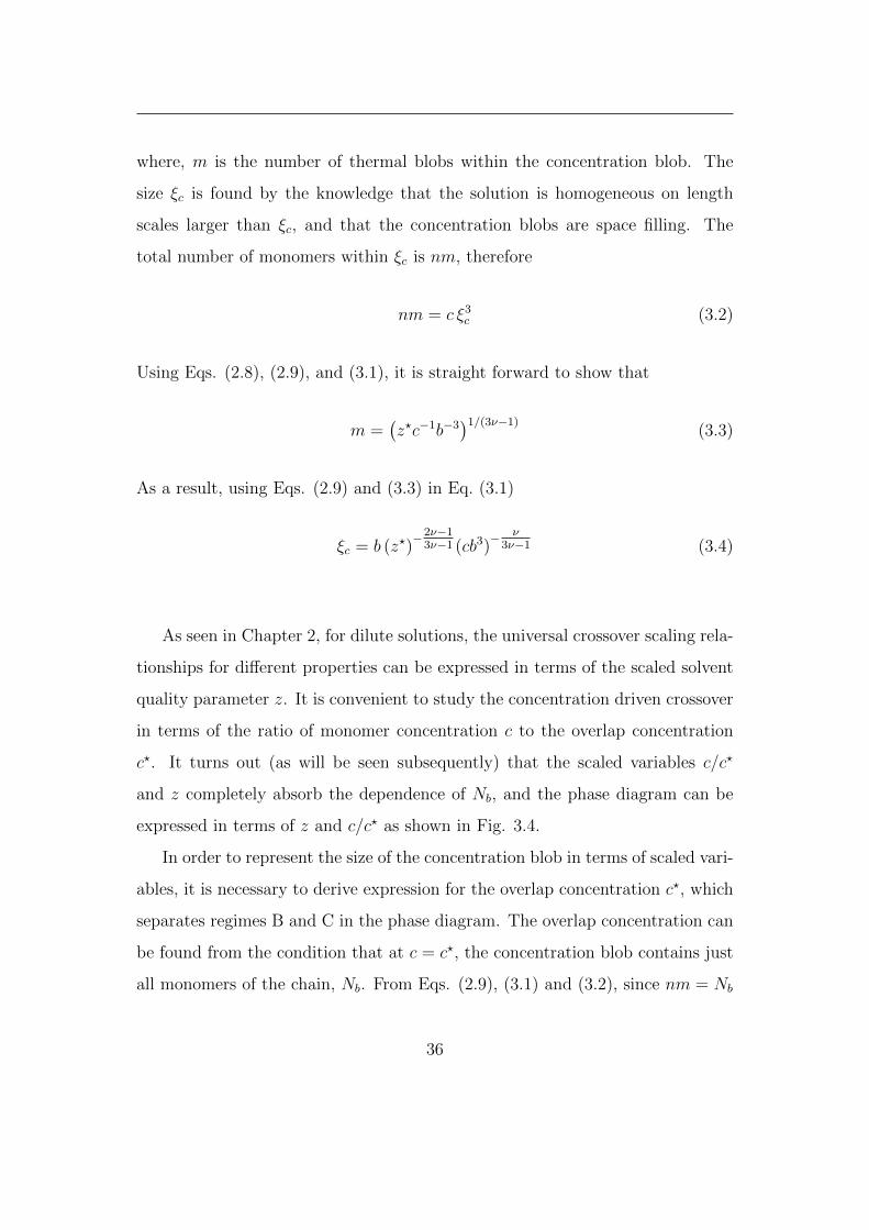
where, m is the number of thermal blobs within the concentration blob. The
size ξc is found by the knowledge that the solution is homogeneous on length
scales larger than ξc, and that the concentration blobs are space filling. The
total number of monomers within ξc is nm, therefore
nm = c ξ3c (3.2)
Using Eqs. (2.8), (2.9), and (3.1), it is straight forward to show that
m =(z?c−1b−3
)1/(3ν−1)(3.3)
As a result, using Eqs. (2.9) and (3.3) in Eq. (3.1)
ξc = b (z?)−2ν−1
3ν−1 (cb3)− ν
3ν−1 (3.4)
As seen in Chapter 2, for dilute solutions, the universal crossover scaling rela-
tionships for different properties can be expressed in terms of the scaled solvent
quality parameter z. It is convenient to study the concentration driven crossover
in terms of the ratio of monomer concentration c to the overlap concentration
c?. It turns out (as will be seen subsequently) that the scaled variables c/c?
and z completely absorb the dependence of Nb, and the phase diagram can be
expressed in terms of z and c/c? as shown in Fig. 3.4.
In order to represent the size of the concentration blob in terms of scaled vari-
ables, it is necessary to derive expression for the overlap concentration c?, which
separates regimes B and C in the phase diagram. The overlap concentration can
be found from the condition that at c = c?, the concentration blob contains just
all monomers of the chain, Nb. From Eqs. (2.9), (3.1) and (3.2), since nm = Nb
36
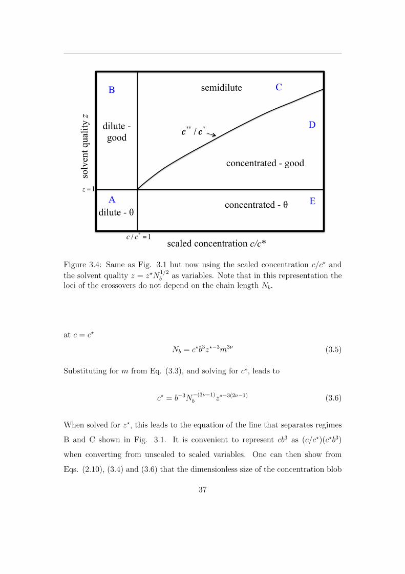
solv
ent q
ualit
y z
semidilute
dilute - good
concentrated - θ
scaled concentration c/c*
c** / c*
dilute - θ A
B C
D
concentrated - good
E
c / c* =1
z =1
Figure 3.4: Same as Fig. 3.1 but now using the scaled concentration c/c? and
the solvent quality z = z?N1/2b as variables. Note that in this representation the
loci of the crossovers do not depend on the chain length Nb.
at c = c?
Nb = c?b3z?−3m3ν (3.5)
Substituting for m from Eq. (3.3), and solving for c?, leads to
c? = b−3N−(3ν−1)b z?−3(2ν−1) (3.6)
When solved for z?, this leads to the equation of the line that separates regimes
B and C shown in Fig. 3.1. It is convenient to represent cb3 as (c/c?)(c?b3)
when converting from unscaled to scaled variables. One can then show from
Eqs. (2.10), (3.4) and (3.6) that the dimensionless size of the concentration blob
37
in terms of scaled variables is
ξc
R0,θg
=( cc?
)−ν/(3ν−1)
z2ν−1 (3.7)
where, R0,θg = bN
1/2b is the gyration radius in dilute solution at θ condition. We
can also derive an expression for ξc in the concentrated regime. Upon system-
atically increasing the monomer concentration c, the concentration blob shrinks
until at a threshold concentration c = c??, ξc = ξT , and there is no longer any
length scale where SAW statistics apply. The locus of points c?? separates regime
C from regimes D and E in the unscaled variables phase diagram. It is straight
forward to calculate c?? by equating Eqs. (2.9) and (3.4)
c?? = b−3 z? (3.8)
In terms of scaled variables, it is similarly straight forward to show by equating
Eqs. (2.11) and (3.7) that
c?? = c? z2(3ν−1) (3.9)
As a result,c??
c?= z2(3ν−1) (3.10)
It is clear that when represented in terms of z and c/c?, the loci of crossover
between the various regimes no longer depend on chain length Nb. In regimes D
and E, where only RW statistics apply, the concentration blob size is given by
ξc = bg1/2 (3.11)
where, g is the number of monomers in a concentration blob. Since the solution
is homogeneous on all length scales larger than ξc, and the concentration blobs
38

are space filling,
c =g
ξ3c
=g
(bg1/2)3(3.12)
which implies
g = (cb3)−2 (3.13)
and as a result
ξc = b (cb3)−1 (3.14)
The expression for c? given by Eq. (3.6) is only valid away from the Θ regime,
i.e., for z? > N−1/2b . On the other hand, in the Θ regime, since at c = c?
the concentration blob contains all the monomers in the chain, which implies
ξc = bN1/2b , Eq. (3.14) leads to
c? = b−3N−1/2b (3.15)
This difference in the expressions for c? makes it necessary to distinguish between
regimes D (where EV effects are important) and E (where EV effects are negli-
gible) when representing the size of the concentration blob (and indeed all other
observables) in terms of scaled variables. Figure 3.4 shows the clear demarcation
between regime D and E. In regime D, Eqs. (2.10), (3.6) and (3.14) imply
ξc
R0,θg
=( cc?
)−1
z3(2ν−1) (3.16)
while in regime E, Eqs. (3.14) and (3.15) imply
ξc
R0,θg
=( cc?
)−1
(3.17)
Once the blob scaling laws for ξT are known in regimes B and C, and those for
ξc are known in regimes C to E, the scaling laws for all other observables in
39
these regimes can be derived. Even though these laws have been derived and
discussed in detail previously (de Gennes, 1979; Grosberg and Khokhlov, 1994;
Rubinstein and Colby, 2003), here, as examples, we derive the scaling laws for
the static chain size Rg, and the single-chain diffusion coefficient D, in order to
represent them in terms of the notation used in this work. Also, as discussed in
Chapter 2, knowing the expressions for Rg and D, the scaling laws for ηp, the
polymer contribution to viscosity, can be derived using Eq. (2.17). The scaling
laws for regime A are not discussed since the conventional notation in this regime
is followed here, and regime B has been discussed in Chapter 2.
Regime C
Since RW statistics are obeyed on length scales larger than ξc
Rg = ξc
(Nb
nm
)1/2
(3.18)
where, (Nb/nm) is the number of concentration blobs in a chain. Using Eqs.
(2.8), (3.3) and (3.4), leads to
Rg = bN1/2b
[z?(cb3)−1
]12
2ν−13ν−1 (3.19)
The scaling relation in terms of scaled variables is obtained by using Eqs. (2.10)
and (3.6)
Rg
R0,θg
=( cc?
)−12
2ν−13ν−1
z2ν−1 (3.20)
Rouse dynamics are obeyed on length scales larger than ξc. Therefore, the total
friction of the chain is the sum of the friction experienced by all the concentration
blobs. This leads to the following expression for the diffusivity
D =kBT
ηs ξc (Nb/nm)(3.21)
40
Using Eqs. (2.8), (3.3) and (3.4), leads to
D =kBT
ηsbNb
(z?)−2
2ν−13ν−1 (cb3)
− 1−ν3ν−1 . (3.22)
The nondimensional diffusivity in terms of scaled variables follows from using
Eqs. (2.10) and (3.6) in Eq. (3.22)
D
Dθ0
= (c/c?)− 1−ν
3ν−1 z−(2ν−1) (3.23)
where, Dθ0 = (kBT/ηsbN
1/2b ) is the diffusivity in the dilute solution at θ condition.
The polymer contribution to the viscosity ηp
(kBT
c
Nb
R2g
D
)can be written as
ηp = ηs(cb3)
13ν−1Nb(z
?)3
2ν−13ν−1 (3.24)
Using Eq. (3.6) and (3.24), the polymer contribution to the viscosity ηp can be
expressed in terms of scaled variables as,
ηp/ηs = (c/c?)1
3ν−1 (3.25)
Regime D
In regime D, RW statistics are obeyed on all length scales, both within the
concentration blob, and by the concentration blobs themselves. As a result
Rg = ξc
(Nb
g
)1/2
= bN1/2b (3.26)
where Eqs. (3.13) and (3.14) have been used for simplification. The nondimen-
sional chain size in this regime is trivially Rg/R0,θg = 1.
41
Rouse dynamics are obeyed on length scales larger than ξc. Using Eq. (3.21)
(with g = nm), and Eqs. (3.13) and (3.14) leads to
D =kBT
ηsbNb
(cb3)−1 (3.27)
The nondimensional diffusivity in terms of scaled variables follows from Eqs.
(2.10) and (3.6)D
Dθ0
=( cc?
)−1
z3(2ν−1) (3.28)
Regime E
In regime E, the scaling relations for Rg and D in terms of unscaled variables are
identical to those in regime D, since in both regimes, RW statistics are obeyed
on all length scales, and Rouse dynamics apply on length scales larger than ξc.
In terms of scaled variables, while the distinction between the two regimes is
irrelevant for the static chain size, the difference in the expression for c? due
to the presence and absence of EV effects, respectively, manifests itself as a
difference in the expression for the nondimensional diffusivity. Using Eqs. (2.10)
and (3.15), Eq. (3.27) reduces in terms of scaled variables to
D
Dθ0
=( cc?
)−1
(3.29)
Table 3.1 summarizes all the unscaled equations derived in this chapter, in-
cluding those for the polymer contribution to viscosity. Table 3.2 summarizes
the equations in terms of scaled variables. As can be seen, in this representation
the dependence on the chain length Nb has been completely absorbed in the Nb
dependence of c? and z, and the only remaining variables are c/c? and z. It is
42

therefore natural to generalize these results to the relations
Rg
R?g
= φR
( cc?, z)
(3.30)
D
D?= φD
( cc?, z)
(3.31)
andηp
η?p= φη
( cc?, z)
(3.32)
where, R?g, D
?, η?p denote the values of Rg, D, ηp at c = c?, and φR, φD, and
φη are universal crossover scaling functions defined on the whole plane of Fig.
3.4, and which, up to numerical prefactors, are known deep in the asymptotic
regimes (these are just the results listed in Table 3.2), but whose behavior needs
to be calculated or measured near the crossover lines.
Finally, an interesting observation can be made when looking at the last two
lines of Table 3.2, i.e.,
(c/c?)1/4 (Rg/R?g
)(D/D?)1/4 =
( cc?
)1/4
in regimes A and B
1 in regimes C, D and E
(3.33)
and
(c/c?)1/3 (Rg/R?g
) (ηp/η
?p
)−1/6=
( cc?
)1/6
in regimes A and B
1 in regimes C, D and E
(3.34)
In all regimes above the overlap concentration, we find that the functions Rg/R?g,
D/D?, and ηp/η?p are not independent, but can be calculated as soon as one of
them is known. It is then natural to assume that the same property also holds
43

in the crossover regimes, i.e. that the relations
(c/c?)1/4φRφ1/4D =
( cc?
)1/4
(3.35)
and
(c/c?)1/3φRφ−1/6η =
( cc?
)1/6
(3.36)
are valid in regimes A and B, while the relations
(c/c?)1/4φRφ1/4D = const. (3.37)
and
(c/c?)1/3φRφ−1/6η = const. (3.38)
are valid in regimes C, D and E.
By carrying out a scaling analysis of the semidilute regime has led to the
following predictions:
1. There exist universal scaling functions φR, φD and φη that depend only on
(c/c?) and z.
2. These functions obey power laws whose specific forms are known away
from the crossover regions, but scaling theory is unable to provide further
information in the crossover regimes.
3. Combinations of the scaling functions assume particularly simple forms
that span several regimes in the phase diagram, suggesting that they are
valid even in the crossover regimes.
4. Equations (3.35) - (3.38) suggest that there is only a single crossover scaling
function and the others can be inferred from them.
44

These predictions of scaling theory can be verified by carrying out BD sim-
ulations. Further, the specific forms of φR, φD and φη in the crossover regimes
can also be ascertained . This is a substantial part of the goals of this thesis. In
Chapters 4 and 5 we develop the BD algorithm and in Chapter 6 we verify the
prediction of scaling theory.
45

regi
me
AB
CD
/E
ξ T–
b(z?)−
1b
(z?)−
1–
ξ c–
–b
(z?)−
2ν−
13ν−
1(cb3
)−ν
3ν−
1b
(cb3
)−1
Rg
bN1/2
bbN
ν b(z?)2ν−
1bN
1/2
b[z?(cb3
)−1]1 2
2ν−
13ν−
1bN
1/2
b
DkBT
η sbN
1/2
b
kBT
η sbN
ν b(z?)2ν−
1
kBT
η sbN
b
(z?)−
22ν−
13ν−
1(cb3
)−1−ν
3ν−
1kBT
η sbN
b
(cb3
)−1
η pη scb
3N
1/2
bη scb
3N
3ν−
1b
(z?)3
(2ν−
1)
η s(cb3
)1
3ν−
1Nb(z?)3
2ν−
13ν−
1η s
(cb3
)2Nb
Tab
le3.
1:V
ario
us
quan
titi
esof
the
pol
ym
ersy
stem
(ther
mal
blo
bsi
zeξ T
,ov
erla
pblo
bsi
zeξ c
,gy
rati
onra
diu
sRg,
singl
e-ch
ain
diff
usi
onco
nst
antD
,p
olym
erpar
tof
the
vis
cosi
tyη p
)in
the
regi
mes
indic
ated
inF
ig.
3.1,
asa
funct
ion
ofm
onom
ersi
zeb,
chai
nle
ngt
hNb,
excl
uded
volu
me
inte
ract
ion
stre
ngt
hz?
,th
erm
alen
ergy
kBT
,so
lven
tvis
cosi
tyη s
,an
dm
onom
erco
nce
ntr
atio
nc,
wit
hin
the
fram
ewor
kof
scal
ing
theo
ry.
Blo
bsi
zes
are
not
indic
ated
inca
ses
wher
eth
eyar
eir
rele
vant.
Num
eric
alpre
fact
ors
ofor
der
unit
yhav
eb
een
ignor
ed.
The
scal
ing
law
sar
eva
lid
inth
eas
ym
pto
tic
regi
mes
suffi
cien
tly
far
away
from
the
cros
sove
rb
oundar
ies.
46

regi
me
AB
CD
E
ξ T/R
0,θg
–z−
1z−
1–
–
ξ c/R
0,θg
––
(c/c?)−
ν3ν−
1z2ν−
1(c/c?)−
1z3
(2ν−
1)
(c/c?)−
1
Rg/R
0,θg
1z2ν−
1(c/c?)−
1 22ν−
13ν−
1z2ν−
11
1
D/D
θ 01
z−(2ν−
1)
(c/c?)−
1−ν
3ν−
1z−
(2ν−
1)
(c/c?)−
1z3
(2ν−
1)
(c/c?)−
1
η p/η
sc/c?
c/c?
(c/c?)
13ν−
1(c/c?)2z−
6(2ν−
1)
(c/c?)2
Rg/R
? g1
1(c/c?)−
1 22ν−
13ν−
1z−
(2ν−
1)
1
D/D
?1
1(c/c?)−
1−ν
3ν−
1(c/c?)−
1z4
(2ν−
1)
(c/c?)−
1
η p/η
? pc/c?
c/c?
(c/c?)
13ν−
1(c/c?)2z−
6(2ν−
1)
(c/c?)2
(c/c?)1/4( R
g/R
? g
) (D/D
?)1/4
(c/c?)1/4
(c/c?)1/4
11
1
(c/c?)1/3( R
g/R
? g
)(η p/η
? p
) −1/6
(c/c?)1/6
(c/c?)1/6
11
1
Tab
le3.
2:V
ario
us
nor
mal
ized
quan
titi
esof
the
pol
ym
ersy
stem
(ther
mal
blo
bsi
zeξ T
,ov
erla
pblo
bsi
zeξ c
,gy
rati
onra
diu
sRg,
singl
e-ch
ain
diff
usi
onco
nst
antD
,p
olym
erpar
tof
the
vis
cosi
tyη p
)in
the
regi
mes
indic
ated
inF
ig.
3.4,
inte
rms
ofth
esc
aled
conce
ntr
atio
nc/c?
and
the
solv
ent
qual
ityz
=z?N
1/2
b.
Blo
bsi
zes
are
not
indic
ated
inca
ses
wher
eth
eyar
eir
rele
vant.
Num
eric
alpre
fact
ors
ofor
der
unit
yhav
eb
een
ignor
ed.
The
scal
ing
law
sar
eva
lid
inth
eas
ym
pto
tic
regi
mes
suffi
cien
tly
far
away
from
the
cros
sove
rb
oundar
ies.R? g,D?,η? p
den
ote
the
valu
esofRg,D
,η p
atc
=c?
.
47

48

Chapter 4
Governing Equations for the
Bead-Spring Chain Model
In this chapter, the polymer model and the basic governing equations of the Brow-
nian dynamics simulation algorithm are discussed in the context of a multi-chain
system. As mentioned earlier in Chapter 2, excluded volume and hydrodynamic
interactions are two important microscopic phenomena that must be incorpo-
rated in order to obtain a realistic model for semidilute solution behavior. We
briefly discuss the treatment of these two interactions in the context of BD simu-
lations in this chapter. Finally, formulae to calculate the mean values of various
equilibrium and rheological properties are presented.
4.1 The Polymer Model
A linear bead-spring chain model (Bird et al., 1987) is used to represent polymers
at the mesoscopic level, with each polymer chain coarse-grained into a sequence
of Nb beads, which act as centers of hydrodynamic resistance, connected by
Nb−1 massless springs that represent the entropic force between adjacent beads.
49

4.2. The Brownian Dynamics Integrator
A semidilute polymer solution is modeled as an ensemble of such bead-spring
chains, immersed in an incompressible Newtonian solvent. A total of Nc chains
are initially enclosed in a cubic and periodic cell of edge length L, giving a total
of N = Nb × Nc beads per cell at a bulk monomer concentration of c = N/V ,
where V = L3 is the volume of the simulation cell. Figure 4.1 schematically
shows a simple example of the simulation system in 2-D.
Periodic Images Original Simulation box
L
Bead-Spring Chains
Figure 4.1: A schematic illustration of the simulation system in 2-D, showingan example of a system with box size L, number of chains Nc = 3 and numberof beads in a chain Nb = 5. The grey box indicates the original simulation boxwhile the white boxes are the periodic images.
4.2 The Brownian Dynamics Integrator
Using the length scale lH =√kBT/H and time scale λH = ζ/4H, where kB
is the Boltzmann’s constant, T is the temperature, H is the spring constant
50
4.2. The Brownian Dynamics Integrator
and ζ is the hydrodynamic friction coefficient associated with a bead, the Euler
integration algorithm for the nondimensional Ito stochastic differential equation
governing the position vector rν(t) of bead ν at time t, is (Stoltz et al., 2006)
rν(t+ ∆t) = rν(t) + [κ · rν(t)] +∆t
4
N∑
µ=1
[Dνµ(t) · Fµ(t)] (4.1)
+1√2
N∑
µ=1
[Bνµ(t) ·∆Wµ(t)]
Here, the 3×3 tensor κ is equal to (∇v)T , with v being the unperturbed solvent
velocity. The dimensionless diffusion tensor Dνµ is a 3×3 matrix for a fixed pair of
beads µ and ν. It is related to the hydrodynamic interaction tensor, as discussed
further subsequently. Fµ incorporates all the non-hydrodynamic forces on bead
µ due to all the other beads. The non-hydrodynamic forces in the model are
comprised of the spring forces Fsprµ and excluded volume interaction forces Fexv
µ ,
i.e., Fµ = Fsprµ +Fexv
µ . The components of the Gaussian noise ∆Wµ are obtained
from a real-valued Gaussian distribution with zero mean and variance ∆t. The
quantity Bνµ is a nondimensional tensor whose presence leads to multiplicative
noise (Ottinger, 1996). Its evaluation requires the decomposition of the diffusion
tensor. Defining the matrices D and B as block matrices consisting of N × Nblocks each having dimensions of 3× 3, with the (ν, µ)-th block of D containing
the components of the diffusion tensor Dνµ, and the corresponding block of B
being equal to Bνµ, the decomposition rule for obtaining B can be expressed as
B ·Bt = D (4.2)
In Eq. (4.1), there are three terms that are challenging to implement efficiently:
(i) the flow term [κ · rν(t)], (ii) the drift term∑N
µ=1 [Dνµ(t) · Fµ(t)], and (iii) the
51

4.3. Bonded Interactions
diffusion term∑N
µ=1 [Bνµ(t) ·∆Wµ(t)]. The implementation and optimization
of the later two terms are presented in Chapter 5, where as the implementation
of the flow term is discussed in Chapter 7. Note that since Chapters 5 and 6
consider only equilibrium systems, the flow term can be ignored for the purpose
of the problems discussed in these two chapters.
The specification of the force term in Eq. (4.1) requires the consideration
of bonded and non-bonded interactions between beads. These interactions are
discussed below.
4.3 Bonded Interactions
Interactions that arise due to the presence of spring forces are labelled here as
bonded interactions. In order to model spring forces, a linear Hookean spring
potential is used in this thesis for nearly all our studies, except for two cases.
The first case involves validation studies where our results are compared with
the Lattice Boltzmann method. In this particular study, a finitely extensible
nonlinear elastic (FENE) potential has been used to model spring forces. The
second case involves the simulation of polymer solutions undergoing either planar
elongational flow or planar mixed flow, and FENE springs are used in this case
as well. The entropic spring force on bead µ due to adjacent beads can be
expressed as Fsprµ = Fc(Qµ) − Fc(Qµ−1) where Fc(Qµ−1) is the force between
the beads µ − 1 and µ, acting in the direction of the connector vector between
the two beads Qµ−1 = rµ − rµ−1. The dimensionless Hookean spring force is
given by Fc(Qµ) = Qµ, while for FENE springs, Fc(Qµ) =Qµ
1− |Qµ|2/bp, where
bp = Hq20/kBT is the dimensionless finite extensibility parameter, and q0 is the
dimensional maximum stretch of a spring.
52

4.4. Non-bonded Interactions
4.4 Non-bonded Interactions
In the present instance, where we are considering the dynamics of neutral poly-
mer solutions, the two non-bonded interactions are hydrodynamic and excluded
volume interactions, respectively. Hydrodynamic interactions are accounted for
through the diffusion tensor (Prabhakar and Prakash, 2004) and as mentioned
earlier, excluded volume interactions are modeled using a narrow Gaussian po-
tential (Prakash and Ottinger, 1999).
The nondimensional diffusion tensor Dνµ in Eq. (4.1) is related to the nondi-
mensional hydrodynamic interaction tensor Ω through
Dµν = δµν δ + (1− δµν)Ω(rµν) (4.3)
where δ and δµν represent a unit tensor and a Kronecker delta, respectively, while
Ω represents the effect of the motion of a bead µ on another bead ν through the
disturbances carried by the surrounding fluid. In above equation, the distance
vector rµν connecting the beads µ and ν is an abbreviation for rν − rµ. The
hydrodynamic interaction tensor Ω is assumed to be given by the Rotne-Prager-
Yamakawa (RPY) regularization of the Oseen function
Ω(r) = Ω1 δ +Ω2rr
r2(4.4)
where for r ≥ 2a, the branch A of the RPY functions Ω1 and Ω2 is given by,
respectively,
Ω1 =3a
4r
(1 +
2a2
3r2
)and Ω2 =
3a
4r
(1− 2a2
r2
)(4.5)
while for 0 < r ≤ 2a, the branch B of the RPY functions Ω1 and Ω2 is given by,
53

4.4. Non-bonded Interactions
respectively,
Ω1 = 1− 9
32
r
aand Ω2 =
3
32
r
a(4.6)
We introduce the notation of the two branchesA and B for facilitating subsequent
discussion in Section 5.2.2. The quantity a has been introduced here as the
nondimensional radius of the bead as an additional independent parameter. It is
related to the conventionally defined (Thurston and Peterlin, 1967; Bird et al.,
1987) hydrodynamic interaction parameter h∗ by a =√πh∗. As is well known
(Beenakker, 1986), the sum∑
µ Dνµ ·Fµ in Eq. (4.1) converges slowly since Dµν
is long-ranged in nature, scaling as 1/r. The problem of slow convergence can
be resolved through the use of the Ewald sum, as discussed in greater detail in
Section 5.2. It is worth noting here that it is sufficient to evaluate∑
µ Dνµ ·Fµ in order to determine the time evolution of rν(t). It is not necessary to
know Dνµ explicitly. Further, as will be seen later in Section 5.5, the evaluation
of∑
µ Bνµ ·∆Wµ using a Chebyshev polynomial approximation for Bνµ, also
requires a repeated evaluation of the Ewald sum.
As in the case of dilute solutions, we treat EV interactions in semidilute
polymer solutions as well with a narrow Gaussian potential which in terms of
non-dimensional variables is given by
E (rνµ) = z?(
1
d?3
)exp
−1
2
r2νµ
d?2
(4.7)
As discussed in Section 2.1, the dimensionless parameter z? is the strength of
excluded volume interactions and d? is a dimensionless parameter that measures
the range of the excluded volume interaction. z? is related to the solvent quality
parameter through z? = z/√Nb (see Section 2.1), and d? is related to z? through
d? = Kz?1/5, where K is an arbitrary parameter which becomes irrelevant in
the long chain limit (Kumar and Prakash, 2003). In the absence of excluded
54

4.5. Macroscopic Properties
volume interactions (when the strength of the potential z? is zero), polymer
chains behave like ideal chains. As z? increases, the solvent quality increases and
hence polymer chains tend to swell.
4.5 Macroscopic Properties
Static and dynamic properties of semidilute polymer solutions at equilibrium can
be calculated once the trajectories of the time evolution of all the beads on all
the chains are obtained using Eq. (4.1). For rheological properties, not only are
bead configurations, but also the forces on them are required. As the simulation
progresses in time, bead configurations and forces are stored simultaneously on
the fly. The following sections briefly describe the expressions used to calculate
the various physical properties considered in this thesis.
4.5.1 Equilibrium properties
Equilibrium physical properties that are independent of time are called static
properties. There are three important static properties for polymer molecules:
(i) the end-to-end distance, (ii) the gyration radius and (iii) the static structure
factor. The mean dimension or the size of a polymer chain is assessed through the
end-to-end distance and the gyration radius (Doi and Edwards, 1986; Rubinstein
and Colby, 2003). The end-to-end distance is defined as the mean square distance
between the first and the last beads on a chain,
⟨R2e
⟩=⟨(rNb − r0)2
⟩(4.8)
where, 〈· · ·〉 represents an ensemble average, and rNb and r0 are position vectors
of the first and the last bead, respectively. The mean square gyration radius,
55

4.5. Macroscopic Properties
which is the mean square distance between the beads and the center of mass rcm
of the chain, written as rcm =1
Nb + 1
∑Nbµ=0 rµ, is defined by
⟨R2g
⟩=
1
Nb + 1
Nb∑
µ=0
⟨(rµ − rcm)2
⟩(4.9)
The static structure factor or form factor is a convenient quantity that describes
the structure of the chains at all length scales (Binder, 1995). It is important to
calculate structure factors not only to quantify the structure of a polymer but
also to check with experimental results because polymer structures are mainly
determined by experimental means. The static structure factor of a polymer
chain is given by (Doi and Edwards, 1986)
S(k) =1
Nb
∑
µν
〈exp (ik · rµν)〉 =1
Nb
∑
µν
⟨sin (krµν)
krµν
⟩(4.10)
where k is the scattering vector and k is the magnitude of k, and rµν is the
magnitude of rµν .
Equations (4.8) to (4.10) refer to the static properties of a single chain at
infinite dilution. For a multi-chain system, these static properties are calculated
for each individual chain and averaged across all the chains in the system.
The output of a Brownian dynamics simulation is basically the time evolution
of the configuration of all the chains in the system. The mean values and the
standard error are obtained in the post-processing stage. First, at a given time,
the values of the static properties of each chain are calculated, and then these
values are averaged across all the chains to obtain a typical average property
which we denote as Schains. Schains is then calculated at all the times and the time
series Schains(t) is obtained. In order to estimate the mean values and the stan-
dard error, the block averaging method is typically used. In this method, blocks
56

4.5. Macroscopic Properties
of different sizes are chosen from the whole time series and the error analysis is
performed with the help of these blocks (see details in Appendix A). However, we
found in our work, that the block averaging method does not lead to satisfactory
results (see the discussion in Appendix A) because of the limitation of running
long time simulations. Therefore, we use an alternative approach, which is a
special case of block averaging, in which only one block is chosen and the size of
the block is equal to the size of a trajectory. In particular, many trajectories are
run simultaneously and the time average of each trajectory is calculated. Next,
an ensemble average of all these mean values is calculated, along with the stan-
dard error of the ensemble average obtained in this process. In this approach the
length of simulation can be small (of the order of 10− 70 relaxation times) but
the number of trajectories need to be large in order to obtain highly accurate
results.
Properties, such as diffusivity, that depend on time are called dynamic prop-
erties. The short-time diffusivity, Ds, of an individual polymer chain can be
calculated via a center-of-mass definition or by the Kirkwood formula (DK),
which are given respectively as
Ds = lim∆t→0
1
6
⟨ |rcm(t+ ∆t)− rcm(t)|2∆t
⟩(4.11)
and
DK =1
3N2b
Nb∑
ν=1
Nb∑
µ=1
(tr〈Dνµ〉) (4.12)
The long-time diffusivity is calculated by tracking the mean-square displacement
of the center-of-mass of each chain,
D = limt→∞
⟨ |rcm(t)− rcm(0)|26t
⟩(4.13)
57

4.5. Macroscopic Properties
In this thesis, only the long-time diffusivity is calculated. For a system of Nc
chains, typically D is calculated for each individual chain and averaged across
all the chains in the system, i.e.,
D(t) = limt→∞
1
Nc
Nc∑
i=1
⟨ |ricm(t)− ricm(0)|26t
⟩(4.14)
Detailes of the approach used to calculate the mean diffusivity and the standard
error are presented in Appendix A. In this approach, the idea is to first calculate
the mean-squared-distance (MSD = 〈|rcm(t)− rcm(0)|2〉) as a function of time.
Next, the slope of the MSD vs. time curve is used to find the diffusivity (note
that D = slope/6). It is important to smooth out short-term fluctuations and
highlight longer-term trends in the time series data of the MSD. Appendix A
discusses an efficient method of doing this with the help of the sliding-average
method.
4.5.2 Rheological properties
The behavior of semidilute polymer solutions, when subjected to an imposed
flow such as shear, elongational or mixed flow, is described in terms of various
material functions. In this work, we have focused our attention on the prediction
of viscosities in these flows. Expressions for viscosities in these various flow
system are presented in this section.
For a planar shear flow (PSF), ∇v is given by
(∇v)PSF =
0 0 0
γ 0 0
0 0 0
58

4.5. Macroscopic Properties
while in planar elongational flow (PEF) it is given by
(∇v)PEF =
ε 0 0
0 −ε 0
0 0 0
where γ and ε are the dimensionless shear rate and elongational rate, respectively.
A planar mixed flow (PMF) is a linear combination of planar shear flow and
planar elongational flow, and Hunt et al. (2010) propose a velocity gradient
tensor for PMF of the following form
(∇v)PMF =
ε 0 0
γ −ε 0
0 0 0
(4.15)
This form is referred to as the canonical form, in which the expanding direc-
tion is along the x axis and the contracting direction is along the y axis, with
elongational field strength ε, while the shear gradient is along the y direction,
with shear field strength γ. Therefore, the expansion axis is always parallel to
the x-axis, but the contraction axis is along the direction of one of the eigen-
vectors of the velocity gradient tensor. Hunt et al. (2010) have shown that the
noncanonical form of the velocity gradient tensor (in which the elongation and
contraction axes are always orthogonal) is equivalent to the canonical form in
a rotated frame of reference. For simplicity, we use the canonical form of the
velocity gradient tensor in this work.
Using κ = (∇v)TPMF in Eq. (4.1), the beads configurations and forces on
them can be computed, and hence the stress tensor can be calculated. In the
absence of external forces, the nondimensional stress tensor for a single chain is
59

4.5. Macroscopic Properties
given by Kramer’s expression (Bird et al., 1987),
σ =
Nb∑
ν=1
〈rνFν〉 (4.16)
For a multi-chain system, the stress tensor can be shown to be (Stoltz, 2006)
σ =1
Nc
N∑
ν=1
〈rνFν〉 (4.17)
Note that σ is a dimensionless stress tensor, which is obtained by nondimension-
alizing the stress tensor by npkBT , where np is number of polymer chains per
unit volume i.e. np = Nc/V .
Once the stress tensor is calculated, the polymer contribution to the viscosity
can be estimated. Hounkonnou et al. (1992) proposed the following expression
for a generalized viscosity ηH for any arbitrary flow gradient tensor (∇v)
ηH =Γ : σ
Γ : Γ(4.18)
where Γ is the rate of strain tensor, defined by Γ = (∇v) + (∇v)T . Using
Eq. (4.18) and considering (∇v) = (∇v)PMF, Hunt et al. (2010) derived an
expression for the planar mixed flow viscosity ηPMF,
ηPMF = −2ε(σxx − σyy) + 2γσxy8ε2 + 2γ2
(4.19)
In the limit of pure planar shear flow (i.e., ε = 0), Eq. (4.19) leads to
ηPSF = −σxyγ
(4.20)
60

4.5. Macroscopic Properties
while in the limit of pure planar elongational flow (i.e., γ = 0), Eq. (4.19)
simplifies to
ηPEF = −σxx − σyy4ε
(4.21)
Clearly, Eq. (4.19) can be rewritten as a linear combination of ηPSF and ηPEF as,
ηPMF =(4ε2ηPEF + γ2ηPSF)
4ε2 + γ2(4.22)
Eqs. (4.20) - (4.22) have been used by Hounkonnou et al. (1992); Baranyai and
Cummings (1995); Todd and Daivis (1998); Daivis et al. (2003) and Hunt et al.
(2010) in their nonequilibrium molecular dynamics (NEMD) simulations for the
viscosity of various fluids.
While the form of the velocity gradient tensor given by (∇v)PMF [Eq. (4.15)]
instinctively separates the shear and elongational flow components, it does not
permit one to easily study the variation in material behavior as the flow changes
smoothly from pure shear to pure elongation or vice versa. Secondly, the elon-
gational viscosity limit of the definition of viscosity in Eq. (4.18), namely ηPEF,
differs from the conventional definition of viscosity in PEF, which is (Bird et al.,
1987)
η1 = −σxx − σyyε
(4.23)
As can be seen by comparing Eqs. (4.21) and (4.23), η1 = 4ηPEF.
An alternative form for (∇v) in PMF proposed by Fuller and Leal (1981)
resolves the first of these issues
(∇v) =
0 Γχ 0
Γ 0 0
0 0 0
(4.24)
61

4.5. Macroscopic Properties
where, Γ is the characteristic strain rate and χ (∈ [−1, 1]) is the mixedness
parameter which measures the relative strength of rotational and elongational
components of a planar mixed flow. It can be shown that this form for (∇v)
reduces to PSF when χ → 0, while the pure PEF limit is recovered when χ →1. Eq. (4.24) is also valid in the limit of χ → −1, which corresponds to the
pure rotational flow limit. In their studies of PMF of dilute polymer solutions,
Hoffman and Shaqfeh (2007) showed that Eq. (4.24) was equivalent to
(∇v) =
Γ√χ 0 0
Γ(1− χ) −Γ√χ 0
0 0 0
(4.25)
in a suitably rotated coordinate system, where they confined their attention to
elongation-dominated mixed flow, for which χ > 0. Clearly, (∇v) and (∇v)PMF
are similar in structure. Comparing Eqs. (4.15) and (4.25), we can express the
shear rate γ and elongational rate ε in terms of Γ and χ as follows
γ = Γ(1− χ) (4.26)
and
ε = Γ√χ (4.27)
Clearly, the velocity gradient defined in this manner approaches the limit of pure
planar shear flow when χ → 0, and pure planar elongation flow when χ → 1.
As a result, it allows us to study the smooth crossover between the pure planar
shear and pure planar elongational flow limits by varying χ between 0 and 1.
In an attempt to address the issue of ηPEF not being equal to η1, we propose
62

4.5. Macroscopic Properties
the following definition of the PMF viscosity
η = − Γ?
: σ?
Γ(4.28)
where Γ?
= Γ/Γ and σ? =1
2(√χ+ 1− χ)
σ. Using Eq. (4.25), Γ can be shown
to be
Γ =
√Γ : Γ
8χ+ 2(1− χ)2(4.29)
while Eq. (4.28) leads to
η = −√χ(σxx − σyy) + (1− χ)σxy
Γ(√χ+ 1− χ)
(4.30)
Clearly, Eq. (4.30) reduces to Eq. (4.20) for planar shear flow in the limit
χ → 0, while for χ → 1, we recover the expression for the planar elongational
flow viscosity η1. η can be related to ηPMF through the expression
η =
[4χ+ (1− χ)2
√χ+ (1− χ)
]ηPMF (4.31)
Equation (4.30) not only allows us to study the crossover of PMF viscosity
smoothly between the pure PSF and pure PEF limits, but also leads to an expres-
sion for the PEF viscosity which is consistent with that reported in the polymer
rheology literature. As we shall see subsequently, defining the PMF viscosity in
this manner allows us to compare our multi-chain simulation results with the BD
simulation results for single polymer chain systems (dilute solutions) obtained
earlier by Prakash (2001b, 2002) and Kumar and Prakash (2003), who used the
conventional definition of the various viscosities.
63

4.5. Macroscopic Properties
64

Chapter 5
Development of a Brownian
Dynamics Simulation Algorithm
for Semidilute Polymer Solutions
5.1 Introduction
This chapter describes the implementation, optimization and validation of a
Brownian dynamics simulation algorithm for semidilute polymer solutions at
equilibrium. This section presents the background related to mesoscopic sim-
ulation algorithm development. As discussed in Section 1.2, one of the major
challenges in algorithm development is to achieve maximum computational ef-
ficiency. It is consequently worth reviewing and comparing the performance of
the different mesoscopic simulations algorithms, mentioned in Section 1.2.
To our knowledge, there has been no systematic investigation to compare the
performance of the different techniques in terms of their computational efficiency
in the semidilute regime. Recently, however, a quantitative comparison of the
predictions of the explicit solvent LB/MD method with the predictions of the
65
5.1. Introduction
implicit solvent BD method for the dynamics of a single chain in a solvent, i.e.
in the dilute regime, has been carried out with a view to compare their com-
putational efficiencies (Pham et al., 2009; Ladd et al., 2009). It was shown in
Pham et al. (2009) that in order to observe the system for the same time span
in physical units, significantly less CPU time is required with BD in comparison
to LB/MD, for bead-spring chains with Nb . 106. The situation, however, is
expected to be quite different in the semidilute regime. For the LB/MD method,
the CPU cost scales linearly with the number of particles, which implies that
the CPU costs grows as L3 since the solvent particles (the calculation of whose
dynamics dominates the CPU cost) are distributed on lattice grid points in a
simulation box of size L. In order to prevent a chain from wrapping over itself
due to spatial restriction and hence altering its static conformation, it is nec-
essary to ensure that L ≥ 2√〈R2
e〉, where 〈R2e〉 is the mean-square end-to-end
distance of the chain. In the dilute case, this leads to the CPU time scaling as
N3νb for the LB/MD method. Using a simple scaling argument based on the blob
picture of semidilute solutions, Pham et al. (2009) suggest that the CPU effort
is even somewhat decreased in semidilute solutions due to the shrinkage of the
chains resulting from the screening of excluded volume interactions (de Gennes,
1979; Doi and Edwards, 1986).
In the case of BD, even though the number of degrees of freedom is signif-
icantly reduced by eliminating the solvent, implementation of pairwise hydro-
dynamic interactions between segments proves to be extremely computationally
expensive. For dilute polymer solutions, the computational cost of evaluating
intramolecular hydrodynamic interactions arises from the need to carry out a
decomposition of the diffusion tensor that appears in Eq. (4.1). A straight-
forward Cholesky decomposition leads to an algorithm that scales like O(N3b ).
Many current implementations of single chain BD simulations, however, mitigate
66

5.1. Introduction
this large CPU cost by using Fixman’s polynomial approximation to this decom-
position, which leads to O(N2.25b ) scaling (Fixman, 1986; Jendrejack et al., 2000;
Kroger et al., 2000; Prabhakar and Prakash, 2004). In the case of semidilute
polymer solutions, both intramolecular and intermolecular hydrodynamic inter-
actions must be taken into account. For a typical segment on a polymer chain,
the use of periodic boundary conditions to imitate bulk systems necessitates the
evaluation of the sum of pairwise hydrodynamic interactions not only between
the particular segment and all other segments within the primary simulation box,
but also with all the other segments in all the periodic images of the box. Be-
cause of the long-range nature of hydrodynamic interactions, which decay only
reciprocally with distance, this sum converges very slowly and only conditionally
(Hasimoto, 1959; Beenakker, 1986). Inspired by its earlier success in summing
electrostatic interactions between charged species (Allen and Tildesley, 1990;
Luty et al., 1994; Toukmaji and Board, 1996; Deserno and Holm, 1998) (which
are also long-ranged in nature), the problem of slow convergence has been re-
solved through the use of the Ewald summation technique (Ewald, 1921) — both
in the context of BD simulations of colloidal suspensions where hydrodynamic
interactions between particles with a finite radius must be taken into account
(Smith et al., 1987; Brady et al., 1988; Rinn et al., 1999; Sierou and Brady, 2001;
Banchio and Brady, 2003), and in the context of BD simulations of semidilute
polymer solutions where the polymer segments are assumed to be point particles
(Stoltz et al., 2006).
Rapid convergence is achieved in the Ewald sum by splitting the slowly con-
verging sum into two sums, one of them in real space and the other in reciprocal
space, both of which converge exponentially. A straightforward implementation
of the Ewald sum, however, is computationally demanding, scaling like O(N2),
where it may be recalled, N = Nc × Nb, is the total number of beads in the
67

5.1. Introduction
primary simulation box with Nc polymer chains. Interestingly, by a suitable
choice of a parameter α in the Ewald sum that tunes the relative weights of the
real space and reciprocal space contributions (consequently splitting the load of
calculating the total sum between the real space and reciprocal space sums), it
is possible to make the computational cost of calculating either the real space
or the reciprocal space sum scale like O(N2), while the remaining sum scales as
O(N). In their recent simulation of semidilute polymer solutions, Stoltz et al.
(2006) have implemented a BD algorithm that leads to the real space sum scal-
ing like O(N2). In the case of colloidal suspensions, accelerated BD algorithms
have been developed by Brady and co-workers with the Ewald sum scaling like
O(N logN) (Sierou and Brady, 2001; Banchio and Brady, 2003). The essential
idea is to retain an O(N) scaling for the real space sum, while reducing the com-
plexity of the reciprocal part of the Ewald sum to O(N logN) with the help of
Fast Fourier Transformation. For confined systems which are non-periodic, and
in which methods based on Fourier transforms are not applicable, the Wisconsin
group have recently successfully introduced a BD simulation technique they term
the “general geometry Ewald-like method”, which achieves O(N logN) scaling
(Hernandez-Ortiz et al., 2007). Analogous to the Ewald method, the technique
is based on splitting the solution to Stokes equation into singular short-ranged
parts and smooth long-ranged parts. Thus, even though a detailed quantitative
comparison of all the currently available mesoscopic simulation techniques is yet
to be carried out, they all appear to scale, in their most efficient versions, roughly
linearly with system size.
In the context of electrostatic interactions, to date broadly two different
classes of schemes have been proposed for the optimization of the Ewald sum
over the Coulomb potential (Allen and Tildesley, 1990; Deserno and Holm, 1998;
Perram et al., 1988; Fincham, 1994). One of these classes of schemes (on which
68

5.1. Introduction
the accelerated BD schemes are modeled), achieves O(N logN) scaling by as-
signing particles to a mesh and then using fast Fourier transform techniques to
evaluate the reciprocal space part of the Ewald sum on this mesh (Luty et al.,
1994; Deserno and Holm, 1998). The other class of schemes (Perram et al., 1988;
Fincham, 1994) achieves O(N1.5) scaling by balancing the computational cost of
evaluating the real space and reciprocal space sums. To our knowledge, the latter
approach has so far not been trialled for summing hydrodynamic interactions.
In the context of hydrodynamic interactions, it is also worth noting that the
BD simulation of semidilute polymer solutions carried out by Stoltz et al. (2006)
differs from BD simulations of colloidal suspensions (Brady et al., 1988; Ban-
chio and Brady, 2003) in the procedure adopted for the calculation of far-field
hydrodynamic interactions, even though both are based on the Ewald summa-
tion technique. While the latter are based on Hasimoto’s solution of the Stokes
equations for flow past a periodic array of point forces (Hasimoto, 1959), the
former is based on Beenakker’s solution (Beenakker, 1986), which generalises
Hasimoto’s treatment to the Rotne-Prager-Yamakawa (RPY) tensor (Rotne and
Prager, 1969; Yamakawa, 1970). The RPY tensor, which is a regularization of the
Oseen-Burgers tensor to account for finite particle radius, is commonly used in
BD simulations of polymer solutions in order to maintain the positive-definiteness
of the diffusion tensor. Essentially, the RPY tensor avoids the singularity of the
Oseen-Burgers tensor for vanishing inter-bead distance by having two branches
depending on the magnitude of the inter-bead distance relative to the parti-
cle diameter. In BD simulations of colloidal suspensions on the other hand,
near-field hydrodynamic interactions are taken into account through short-range
lubrication forces (Brady et al., 1988). Notably, even though Beenakker’s peri-
odic hydrodynamic interaction tensor is based on the RPY tensor, the original
derivation by Beenakker is only valid for the long-ranged branch of the tensor.
69

5.1. Introduction
As a result, it is not applicable to situations where bead overlap might occur.
In their BD simulations of semidilute solutions, Stoltz et al (Stoltz et al., 2006)
avoid bead overlap through the use of an excluded volume potential between
beads. However, one can anticipate that bead overlap can occur in simulations
of semidilute θ-solutions, since θ-solutions are commonly simulated by switching
off excluded volume interactions (Prabhakar and Prakash, 2004; Sunthar and
Prakash, 2005). An extension of Beenakker’s derivation of the periodic RPY
tensor is consequently necessary in order for it to be useful for the treatment of
hydrodynamic interactions in semidilute θ-solutions.
As discussed earlier in Section 4.2, in the absence of flow, there are two major
challenges to integrating the stochastic differential equation (4.1): (i) calculation
of the drift term, which can be done using the Ewald summation method and
(ii) calculation of the diffusion term, which can be done using the Chebyshev
polynomial approximation. Also, since it is required to simulate a large number
of beads, optimization of the algorithm is necessary. The plan of the chapter is
as follows. In Section 5.2, the evaluation and implementation of the Ewald sum
and its modification to handle overlapping beads, are discussed. Sections 5.4,
5.5 and 5.6 consider the optimization of (i) the Ewald sum for hydrodynamic
interactions, (ii) the Chebyshev polynomial approximation for the decomposi-
tion of the diffusion tensor, and (iii) the execution of a single Euler time step,
respectively. The optimized BD algorithm is validated by a variety of different
means, under both θ and good solvent conditions, in Section 5.7. In Section
5.8, its computational cost is compared with that of the LB/MD method at a
concentration that lies in the semidilute regime.
70

5.2. Ewald Summation Method for Hydrodynamic Interactions
5.2 Ewald Summation Method for Hydrody-
namic Interactions
5.2.1 Evaluation of∑
µ Dνµ · Fµ as an Ewald sum
Beenakker’s (Beenakker, 1986) representation of the sum∑
µ Dνµ·Fµ as an Ewald
sum for infinite periodic systems, using the RPY tensor to represent hydrody-
namic interactions, has the form
N∑
µ=1
Dνµ · Fµ =
(1− 6aα√
π+
40a3 α3
3√π
)Fν +
∑
n
′N∑
µ=1
M(1)(rνµ,n) · Fµ
+∑
k 6=0
M(2)(k) ·
cos(k · rν)N∑
µ=1
cos(k · rµ)Fµ − sin(k · rν)N∑
µ=1
sin(k · rµ)Fµ
(5.1)
where the first and the second sums on the right hand side, both of which con-
verge rapidly, are carried out in real and reciprocal space, respectively. The first
term on the RHS is the correction due to self-interactions and does not involve
any summation. A brief introduction to the Ewald summation method and the
detailed derivation of Eq. (5.1) is presented in Appendix B. In Eq. (5.1), the
parameter α determines the manner in which the computational burden is split
between the two sums. The vector rνµ,n is defined by rνµ,n = rν−rµ+nL, where
n = (nx, ny, nz) is the lattice vector with nx, ny, nz being integer numbers (see
Fig. 5.1). The first summation on the RHS of Eq. (5.1) is carried out in the
original simulation box and over all the neighboring periodic images. The prime
on the summation indicates that the lattice vector n = 0 is omitted for ν = µ.
M(1)(r) is a 3× 3 matrix (in real space), which depends on a and α, and M(2)(k)
is also a 3×3 matrix (in reciprocal space), which depends on a, α and the volume
71
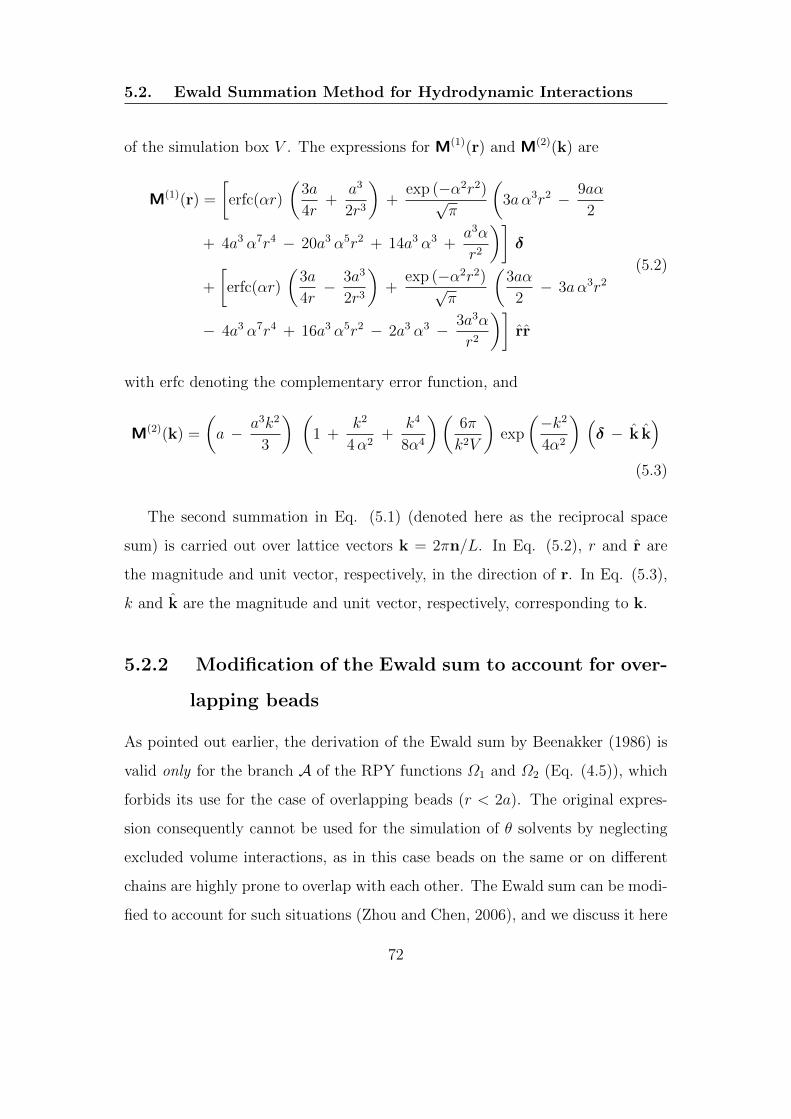
5.2. Ewald Summation Method for Hydrodynamic Interactions
of the simulation box V . The expressions for M(1)(r) and M(2)(k) are
M(1)(r) =
[erfc(αr)
(3a
4r+
a3
2r3
)+
exp (−α2r2)√π
(3aα3r2 − 9aα
2
+ 4a3 α7r4 − 20a3 α5r2 + 14a3 α3 +a3α
r2
)]δ
+
[erfc(αr)
(3a
4r− 3a3
2r3
)+
exp (−α2r2)√π
(3aα
2− 3aα3r2
− 4a3 α7r4 + 16a3 α5r2 − 2a3 α3 − 3a3α
r2
)]rr
(5.2)
with erfc denoting the complementary error function, and
M(2)(k) =
(a − a3k2
3
) (1 +
k2
4α2+
k4
8α4
)(6π
k2V
)exp
(−k2
4α2
) (δ − k k
)
(5.3)
The second summation in Eq. (5.1) (denoted here as the reciprocal space
sum) is carried out over lattice vectors k = 2πn/L. In Eq. (5.2), r and r are
the magnitude and unit vector, respectively, in the direction of r. In Eq. (5.3),
k and k are the magnitude and unit vector, respectively, corresponding to k.
5.2.2 Modification of the Ewald sum to account for over-
lapping beads
As pointed out earlier, the derivation of the Ewald sum by Beenakker (1986) is
valid only for the branch A of the RPY functions Ω1 and Ω2 (Eq. (4.5)), which
forbids its use for the case of overlapping beads (r < 2a). The original expres-
sion consequently cannot be used for the simulation of θ solvents by neglecting
excluded volume interactions, as in this case beads on the same or on different
chains are highly prone to overlap with each other. The Ewald sum can be modi-
fied to account for such situations (Zhou and Chen, 2006), and we discuss it here
72
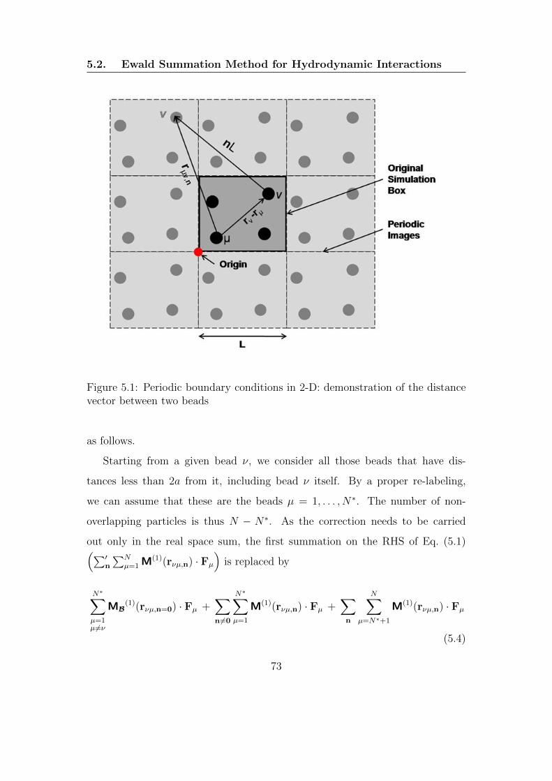
5.2. Ewald Summation Method for Hydrodynamic Interactions
Figure 5.1: Periodic boundary conditions in 2-D: demonstration of the distancevector between two beads
as follows.
Starting from a given bead ν, we consider all those beads that have dis-
tances less than 2a from it, including bead ν itself. By a proper re-labeling,
we can assume that these are the beads µ = 1, . . . , N∗. The number of non-
overlapping particles is thus N − N∗. As the correction needs to be carried
out only in the real space sum, the first summation on the RHS of Eq. (5.1)(∑′n
∑Nµ=1 M(1)(rνµ,n) · Fµ
)is replaced by
N∗∑
µ=1µ6=ν
MB(1)(rνµ,n=0) · Fµ +
∑
n6=0
N∗∑
µ=1
M(1)(rνµ,n) · Fµ +∑
n
N∑
µ=N∗+1
M(1)(rνµ,n) · Fµ
(5.4)
73

5.2. Ewald Summation Method for Hydrodynamic Interactions
where, MB(1) is equivalent to the M(1) matrix, but for branch B of the RPY
tensor given by Eq. (4.6). The summation in the first term is carried out
only over the overlapping particles in the original simulation box (n = 0). The
second summation is carried out over the periodic images of the overlapping
particles (whose distances are more than 2a), and the third summation is similar
to that given in Eq. (5.1) but here it is carried out only over the non-overlapping
particles. Note that the second sum is not carried out in the original box. In
order to make this sum extend over the original box and periodic images, a term
is added and subtracted as follows
N∗∑
µ=1µ 6=ν
MB(1)(rνµ,n=0) · Fµ +
∑
n6=0
N∗∑
µ=1
M(1)(rνµ,n) · Fµ (5.5)
+N∗∑
µ=1µ6=ν
M(1)(rνµ,n=0) · Fµ −N∗∑
µ=1µ6=ν
M(1)(rνµ,n=0) · Fµ
+∑
n
N∑
µ=N∗+1
M(1)(rνµ,n) · Fµ
Note that while the first sum involves branch B of the RPY tensor, the third
sum involves branch A. The second, third and fifth summations of the above
equation together represent the original real space sum in Eq. (5.1). Equation
(5.5) can consequently be rearranged as
(∑
n
′N∑
µ=1
M(1)(rνµ,n) · Fµ
)+
N∗∑
µ=1µ6=ν
[MB
(1)(rνµ,n=0)− M(1)(rνµ,n=0)]· Fµ (5.6)
where the second summation is carried over all overlapping particles in the orig-
inal box. Denoting the second term in Eq. (5.6) by M∗, it is straightforward to
74

5.2. Ewald Summation Method for Hydrodynamic Interactions
show that
M∗(x) = δ
[1− 1
2x3
(3x2
4+ 1
)2]
+ x x
[1
2x3
(3x2
4− 1
)2]
(5.7)
where x = r(νµ,n=0)/a and x is the unit vector in the direction of r(νµ,n=0) (see
Appendix B.3.4). The modified form of the Ewald sum that is valid for arbitrary
inter-particle distance is consequently
N∑
µ=1
Dνµ · Fµ =
(1− 6aα√
π+
40a3 α3
3√π
)Fν +
∑
n
′N∑
µ=1
M(1)(rνµ,n) · Fµ
+∑
k 6=0
M(2)(k) ·
cos (k · rν)N∑
µ=1
cos (k · rµ)Fµ − sin (k · rν)N∑
µ=1
sin (k · rµ)Fµ
+N∗∑
µ=1µ6=ν
M∗(rνµ,n=0) · Fµ (5.8)
5.2.3 Implementation of the Ewald summation method
As discussed earlier, the real space sum is carried out over all the periodic images
while the reciprocal space sum involves particles only in the original simulation
box. There are three parameters which control the accuracy of both the real and
reciprocal space sums: nmax, an integer which defines the range of the real space
sum (governed by the number of periodic images, see Fig. 5.1), kmax, an integer
that defines the summation range in reciprocal space and the Ewald parameter
α. These three parameters are related to each other from the point of view of
accuracy and speed. A large value of α makes the real space sum converge faster
(since a smaller value of nmax is required). However, this leads to the reciprocal
space sum requiring a larger number of wave-vectors kmax. On the other hand,
a small value of α implies an expensive real space sum but a cheaper reciprocal
space sum. The optimal choice of these parameters has been discussed previously
75
5.2. Ewald Summation Method for Hydrodynamic Interactions
by Fincham (1994) in the context of electrostatic interactions. Here, a similar
study is performed for hydrodynamics interactions.
Choice of Ewald parameters
At fixed monomer bulk concentration c, the box size increases as N1/3. As can
be seen from Eqs. (5.1) and (5.2), the convergence of the real space sum depends
on the complementary error function erfc(αr), where r is the distance between a
pair of beads. In practice, the sum is evaluated only for r ≤ rc, where rc denotes
a cutoff radius. The value of α is chosen such that erfc(αrc) is small. At large
values of the argument, erfc(αrc) behaves as exp(−α2rc2). If we specify M such
that exp(−M2) is very small, then
α2rc2 = M2 or α = M/rc (5.9)
Similarly the rate of convergence of the reciprocal space sum is controlled by
the factor exp(−k2/4α2). If it is required (Fincham, 1994) that the accuracy of
the real space sum is roughly equal to that of the reciprocal space sum at the
reciprocal space cutoff, Kr, then using Eq. (5.9) we find
M2 = K2r /(4α
2) or Kr = 2αM = 2M2/rc (5.10)
These relations allow us to specify α and Kr for given values of M and rc,
while the latter parameters control the accuracy and speed of the algorithm, as
discussed subsequently.
The real space and reciprocal space sums
Locating all pairs of beads which are separated by less than the cutoff distance
rc is the first step in evaluating the real space sum. A naive all-pairs neighbor
76
5.3. Validation of∑
µ Dνµ · Fµ Calculations
search results in O(N2) performance and therefore the link-cell method, which is
a cell-based neighbor search method, is used to improve the performance (Hock-
ney et al., 1973; Griebel et al., 2007; Grest et al., 1989). The calculation of the
infinite real space sum is thus reduced to the calculation of the sum locally over
only a small number of neighboring beads. Here, the neighbor search is imple-
mented with cells of side rc/5. The reciprocal space sum is more straightforward
to implement. The major effort is expended in the evaluation of terms of the
form exp(ik · rµ). The method adopted here precomputes the components of
these factors by recursion and stores them (Fincham, 1994). This avoids calling
the complex exponential function repeatedly. However, it involves a substantial
amount of computer memory.
5.3 Validation of∑
µDνµ · Fµ Calculations
Three different approaches have been used to validate the calculations of the
Ewald sum:
1. A single-chain code (developed to simulate a dilute polymer solution) (Prab-
hakar, 2005; Prabhakar and Prakash, 2004) is used to validate the Ewald
sum in the dilute regime
2. Hasimoto’s solution (Hasimoto, 1959) of the Stokes equation of motion for
viscous fluid flow past a periodic array of spherical obstacles is used to
validate the implementation of periodic boundary conditions, again in the
dilute limit.
3. The pairwise summation of hydrodynamic interactions is carried out explic-
itly i.e. without using the Ewald summation and this sum is then compared
with the Ewald sum. This approach enables us to validate the Ewald sum
77

5.3. Validation of∑
µ Dνµ · Fµ Calculations
for finite concentration systems.
Each of these approaches are discussed below in detail.
5.3.1 Comparison with single-chain simulations
In this approach, firstly the values of∑
µ [Dνµ · Fµ] from a single-chain code,
written for dilute polymer solutions (Prabhakar, 2005; Prabhakar and Prakash,
2004), are computed. Thereafter, data for∑
µ [Dνµ · Fµ] for the same set of
parameters (a = 0.1, Nc = 1, Nb = 20, 100) are generated using the current code
for various values of box size L. The element by element difference between the
vector D · F of the single-chain code and the current code is calculated to get
the sum of the square of the error (SSE). As can be seen in Fig. 5.2, the SSE
approaches to ∼ 10−8 as 1/L→ 0, which indicates that at lower concentrations,
the current code agrees with the single-chain code. Note that a tolerance criteria
of 10−8 is used in the current code for the convergence of the Ewald summation.
5.3.2 Verification of the prediction of the Madelung con-
stant
In this approach, the Madelung constant for the motion of a viscous fluid flow-
ing past a periodic array of spherical particles is verified by the current code.
Madelung’s constant was first derived by Hasimoto (1959) by solving the Stokes
equation for the system mentioned above. Note that the Hasimoto solution as-
sumes that the suspension is dilute. By considering a single particle at the centre
of a box and periodic images of that particle, Hasimoto derived an expression
78
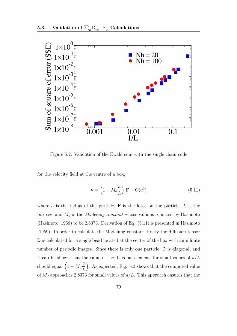
5.3. Validation of∑
µ Dνµ · Fµ Calculations
0.001 0.01 0.11/L
1×10⁻⁸
1×10⁻⁷
1×10⁻⁶
1×10⁻⁵
1×10⁻⁴
1×10⁻³
1×10⁻²
1×10⁻¹
1×100
Sum
of
squar
e of
erro
r (S
SE
)Nb = 20Nb = 100
Figure 5.2: Validation of the Ewald sum with the single-chain code
for the velocity field at the centre of a box,
v =(
1−Mda
L
)F +O(a3) (5.11)
where a is the radius of the particle, F is the force on the particle, L is the
box size and Md is the Madelung constant whose value is reported by Hasimoto
(Hasimoto, 1959) to be 2.8373. Derivation of Eq. (5.11) is presented in Hasimoto
(1959). In order to calculate the Madelung constant, firstly the diffusion tensor
D is calculated for a single bead located at the center of the box with an infinite
number of periodic images. Since there is only one particle, D is diagonal, and
it can be shown that the value of the diagonal element, for small values of a/L
should equal(
1−Mda
L
). As expected, Fig. 5.3 shows that the computed value
of Md approaches 2.8373 for small values of a/L. This approach ensures that the
79

5.3. Validation of∑
µ Dνµ · Fµ Calculations
0.001 0.01 0.1a/L
2.3
2.4
2.5
2.6
2.7
2.8M
adel
ung C
onst
ant M
d = 2.8373
Figure 5.3: Validation of the Ewald sum with Hasimoto’s solution for theMadelung constant
periodic boundary conditions are implemented correctly in the algorithm.
5.3.3 Explicit vs Ewald sum
The velocity of the solvent, vν , at the location of a bead ν, due to forces on all
the other beads in the system, is given by,
vν =∑
n
N∑
µ=1
[Dνµ,n · Fµ] (5.12)
As mentioned earlier, in general, it is not possible to evaluate this sum explicitly
because of the slow and conditional nature of the sum. For a periodic system,
however, as we have seen, the sum can be evaluated using an Ewald summation
technique. It would seem, consequently, that we cannot validate the result of
80

5.3. Validation of∑
µ Dνµ · Fµ Calculations
Ewald summation by comparison with the explicit sum, since the latter cannot
in general be evaluated.
We have found, however, that by constructing a special kind of periodic
system, we can in fact compare the Ewald and explicit sums, and as a result
obtain a validation of our implementation of the Ewald sum for systems at finite
concentrations.
Before we discuss the special periodic arrangement, it is worth making a
few remarks on our observations for a general periodic arrangement of particles,
where they are placed at random in the original simulation box. A converged
value for the velocity vν at an arbitrary location rν in the original simulation
box, for a periodic but random system of particles, was obtained when it was
evaluated using the explicit sum, provided the sum of forces on all the beads was
zero, i.e.,∑
µ=1 Fµ = 0. The converged value was independent of the order in
which summation was carried out, i.e., whether all the particles in the simulation
box were first summed, and then all the sums over the images carried out, or the
sum for each particle over all the images was followed by a sum over all particles
in the original simulation box. However, this converged value of velocity did
not agree with that obtained using the Ewald sum for the same arrangement of
particles.
We are not entirely sure of the reason for this discrepancy. A possible reason
is that while the Ewald sum is strictly valid only for a periodic system the explicit
sum has to in some sense discover the periodicity, and is unable to do so for a
random periodic arrangement of particles. In order to check this hypothesis, we
evaluated the solvent velocity with the explicit sum at locations, one of which
was the periodic image of the other. The only points in the simulation box that
also have a periodic image in the box are points on the walls of the box. As a
result, we placed a particle on one of the walls, and evaluated the velocity vν at
81
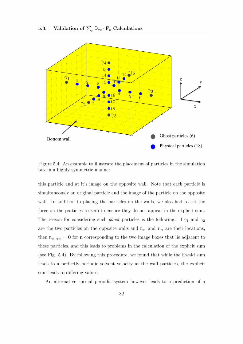
5.3. Validation of∑
µ Dνµ · Fµ Calculations
x
y z
1 2 3 4 5 6 7 8 9 12
34
56
78
9
1
2
3
4
5
6
7
8
9
γ1
γ2
γ3
γ4
γ5
γ6
1 2 3
45 6
78
9
1011
1213
14
15
16
17
18
Ghost particles (6)
Physical particles (18) Bottom wall
Figure 5.4: An example to illustrate the placement of particles in the simulationbox in a highly symmetric manner
this particle and at it’s image on the opposite wall. Note that each particle is
simultaneously an original particle and the image of the particle on the opposite
wall. In addition to placing the particles on the walls, we also had to set the
force on the particles to zero to ensure they do not appear in the explicit sum.
The reason for considering such ghost particles is the following. if γ1 and γ2
are the two particles on the opposite walls and rγ1 and rγ2 are their locations,
then rγ1γ2,n = 0 for n corresponding to the two image boxes that lie adjacent to
these particles, and this leads to problems in the calculation of the explicit sum
(see Fig. 5.4). By following this procedure, we found that while the Ewald sum
leads to a perfectly periodic solvent velocity at the wall particles, the explicit
sum leads to differing values.
An alternative special periodic system however leads to a prediction of a
82

5.4. Optimization of the Evaluation of∑
µ Dνµ · Fµ
periodic solvent velocity by the explicit sum, which also agrees with the value
obtained with the Ewald sum. In this special arrangement, rather than choosing
a random distribution of particles, the particles are placed in a highly symmetric
manner in the original simulation box. A typical example is shown in Fig. 5.4.
Further, the particles are subjected to forces that are also symmetric. Thus, for
instance, particles 1 and 6 in Fig. 5.4 have equal and opposite forces acting on
them. The constraint∑
µ=1 Fµ = 0 is also imposed. Under these conditions, we
find that for a range of values of concentration c, bead radii a, and number of
beads N , the velocities of the solvent at all the particle locations are identical in
the explicit and Ewald sum, within the prescribed tolerance for the convergence
of the sums. This completes the validation of the implementation of the Ewald
sum under a variety of different circumstances.
5.4 Optimization of the Evaluation of∑
µDνµ·Fµ
The Ewald parameter α, which splits the computational burden between the
real space sum and the reciprocal space sum, is related to the real space cutoff
rc by Eq. (5.9). The aim of optimization is to minimize the total execution time
(which is the sum of the real space execution time, TR and the reciprocal space
execution time, TF ), with respect to the real space cutoff rc. Following Fincham
(1994), the execution time TR is calculated as follows. A sphere of cutoff radius
rc contains on average Nrc =4π
3r3
c c beads. Each bead interacts with the Nrc
beads that surround it. Since for symmetry reasons, each pair interaction needs
to be considered only once, the execution time is
TR =1
2N
4π
3r3
c c tr (5.13)
83

5.4. Optimization of the Evaluation of∑
µ Dνµ · Fµ
where tr is a constant parameter with a unit of time, and it depends on the code
architecture and on the execution time to evaluate one interaction. Equation
(5.13) is fit to data obtained by running BD simulations for a range of parameters
on a 156 SGI Altix XE 320 cluster, and the fitted parameter tr is then found to be
0.75µs. The execution time TF is evaluated as follows. Within the cutoff Kr, the
volume of the reciprocal space is4π
3K3r =
4π
3
8M6
r3c
(the latter follows from Eq.
(5.10)). The reciprocal space points are defined by k =2π
L(l,m, n) where l,m, n
are integers and L is the simulation box size. The volume of reciprocal space per
point is, thus, (2π/L)3, and4π
3
8M6
r3c
L3
8π3is the number of points in the cutoff
sphere. Using L3 = N/c to highlight the N dependence at fixed concentration c,
the number of reciprocal space points in the cutoff sphere becomes4π
3
M6
π3
N
cr3c
.
It is worth pointing out that for fixed cutoff radius, the number of k-space points
increases as N , because the concentration of points in reciprocal space increases
with system size. Further, inversion symmetry of reciprocal space halves the
number of reciprocal space points mentioned above. A sum over the N beads
must be performed for each k-space point, so the execution time is
TF =1
2
4π
3
M6
π3
N2
cr3c
tf (5.14)
where tf is a constant parameter with a unit of time, and it depends on the
code architecture and on the execution time to evaluate one term in the sum.
As in the real space instance, Eq. (5.14) is fitted to simulation data to obtain
tf = 0.063µs. The total execution time is consequently
T = TR + TF =1
2
4π
3
[N r3
c c tr +M6
π3
N2
cr3c
tf
](5.15)
Equation (5.15) shows that, for fixed M and rc, TR varies as N , but TF varies
as N2, because of the increasing concentration of points in reciprocal space.
84
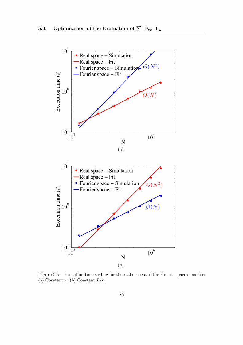
5.4. Optimization of the Evaluation of∑
µ Dνµ · Fµ
103
104
10−1
100
101
Ex
ecuti
on
tim
e (s
)
N
O(N 2)
O(N )
Real space − Simulation
Real space − Fit
Fourier space − Simulation
Fourier space − Fit
(a)
103
104
10−1
100
101
Ex
ecu
tio
n t
ime
(s)
N
O(N 2)
O(N )
Real space − Simulation
Real space − Fit
Fourier space − Simulation
Fourier space − Fit
(b)
Figure 5.5: Execution time scaling for the real space and the Fourier space sums for:(a) Constant rc (b) Constant L/rc
85

5.4. Optimization of the Evaluation of∑
µ Dνµ · Fµ
This behavior is demonstrated for c = 4.44 c? and rc = 10 in Fig. 5.5 (a) for
the simulation data (symbols), which agrees with the expressions given in Eqs.
(5.13) and (5.14) (solid lines). Here c? is the overlap concentration defined by
Nb/
[4π
3(R0
g)3
], where R0
g is the gyration radius of a polymer chain in the dilute
limit. To increase the value of N , we fix the value of beads per chain at Nb = 10
and increase the number of chains Nc. Conversely, if rc is increased as the system
size increases in such a way that rc/L is constant (as in the approach adopted
by Stoltz et al. (2006)), then since c = N/L3, TR varies as N2 but TF varies as
N . Fig. 5.5 (b) displays this behavior for Nb = 10, c = 4.44 c?, M = 3.3 and
L/rc = 3. Once again the simulation data is seen to match the expressions given
in Eqs. (5.13) and (5.14). This suggests that by appropriate choice of parameters
it may be possible to achieve better than N2 behavior in the total time T . For a
given accuracy, the only free parameter is rc, since this determines α and hence
K by Eqs. (5.9) and (5.10). To find the value of rc which minimizes the total
execution time, we set dT/drc = 0. This leads to
(rE
c
)opt
=M√π
(tftr
)1/6N1/6
c1/3(5.16)
Thus the optimal choice of the cutoff radius(rE
c
)opt
increases slowly (1/6th power)
with N . The validity of Eq. (5.16) has been verified by carrying out simulations.
Assuming that the quantityN1/6 in Eq. (5.16) is replaced byNx, various values of
the exponent x are selected in place of the exponent 1/6, and the total execution
time for a given value of N is estimated. Figure 5.6 (a) shows the total execution
time as a function of the exponent x and it is clear that the minimum execution
time is achieved when x = 1/6 as given by Eq. (5.16), for all N . Substituting
86

5.4. Optimization of the Evaluation of∑
µ Dνµ · Fµ
0.05 0.1 0.15 0.2 0.25 0.310
−1
100
101
102
x
Ex
ecu
tio
n t
ime (
s)
N = 1250
N = 2160
N = 3430
N = 5120
N = 7290
N = 10000
(a)
103
104
10−1
100
101
Exec
uti
on t
ime
(s)
N
O(N 1.5)
O(N 1.5)
O(N 1.5)Real space − Simulation
Real space − Fit
Fourier space − Simulation
Fourier space − Fit
Total − Simulation
Total − Fit
(b)
Figure 5.6: (a) Total execution time vs. exponent x for various N (b) Power lawscaling for TR, TF and Topt at
(rE
c
)opt
87

5.5. Decomposition of the Diffusion Tensor
(rE
c
)opt
in Eq. (5.15) we find for the optimal time
Topt = 2TR = 2TF =4π
3N1.5 M3
π1.5
√tr tf (5.17)
Thus, when the total time is optimized, it is equally divided between the real and
reciprocal space parts of the calculation. This is verified in Fig. 5.6 (b), which
displays plots of TR, TF and T as a function of N , at x = 1/6 and for Nb = 10,
c = 4.44c? and M = 3.3. Symbols indicate simulation data and solid lines
correspond to Eq. (5.17) with the appropriate values for the various parameters.
Equation (5.17) also indicates that the real space, reciprocal space and total
time scale as N1.5. Simulation results shown in Fig. 5.6 (b) substantiate this
prediction. These results are similar to those obtained by Fincham (1994) in the
context of electrostatic interactions.
5.5 Decomposition of the Diffusion Tensor
In component form, the decomposition rule (Eq. (4.2)) for obtaining the block
matrix B can be expressed as follows,
N∑
β=1
3∑
q=1
Brqνβ Bsqµβ = Drsνµ (5.18)
where ν, β, µ = 1, . . . , N, r, q, s = 1, 2, 3, and Drsνµ is the ‘rs’th Cartesian
component of the tensor Dνµ. The matrix B is not unique. Assuming that B
is a lower (or upper) triangular matrix leads to its calculation using a Cholesky
decomposition of D, which as mentioned earlier in Section 5.1, requires O(N3)
operations. Fixman’s (Fixman, 1986) approach achieves an attenuation of this
CPU intensity by recognizing that (i) it is sufficient to find B approximately, and
88

5.5. Decomposition of the Diffusion Tensor
(ii) the individual columns of the matrix B are in themselves not of much interest,
only the vector dS = B ·∆W is required, where ∆W is a vector consisting of
the 3N Gaussian noise coordinates ∆W sµ, with µ = 1, . . . , N , and s = 1, 2, 3. By
assuming that B =√D, and using a Chebyshev polynomial approximation for
the square root function, Fixman showed that (Fixman, 1986; Jendrejack et al.,
2000; Kroger et al., 2000; Prabhakar, 2005)
dS =√D ·∆W ≈
NCh−1∑
p=0
cpVp −c0
2∆W (5.19)
where NCh is the number of terms used in the Chebyshev polynomial approxi-
mation, cp are the Chebyshev coefficients, and the vectors Vp are defined by the
recurrence relations
Vp = 2Y · Vp−1 − Vp−2 ; p ≥ 2 (5.20)
with V0 = ∆W and V1 = Y · V0. The linear mapping
Y =
(2
dmax − dmin
)D −
(dmax + dmin
dmax − dmin
)I (5.21)
(where I denotes the 3N × 3N -dimensional identity matrix), ensures that the
eigenvalues of Y lie in the domain [−1, 1] when the eigenvalues of D are within
[dmin, dmax]. This is essential for the validity of the Chebyshev approximation.
It is clear that for a given NCh, the cost of the direct calculation of the 3N -
dimensional vector dS, without the intermediate calculation of B, is proportional
to NCh× [the cost of evaluating Vp]. The number of terms NCh that are required
is determined by the desired accuracy in the estimation of the square root. The
choice of NCh is also affected by the necessity of ensuring that the bounds dmax
and dmin satisfy the following constraints relative to the maximum (λmax) and
89

5.5. Decomposition of the Diffusion Tensor
minimum (λmin) eigenvalues of D, namely, dmax ≥ λmax and dmin ≤ λmin.
The CPU cost involved in adopting Fixman’s procedure for dilute polymer
solutions has been discussed in depth in Jendrejack et al. (2000); Kroger et al.
(2000) and Prabhakar (2005). Here, we briefly summarize the main conclusions:
(i) The cost of evaluating Vp is simply O(N2). (ii) The number of terms in
the Chebyshev approximation is determined using the expression (Kroger et al.,
2000; Prabhakar and Prakash, 2004)
NCh = nint
[(λmax
λmin
) 12
]+ 1 (5.22)
where nint is the nearest integer function. The use of Eq. (5.22) is motivated
by the finding (Fixman, 1986; Jendrejack et al., 2000) that the value of NCh
required to keep the error in the estimation of the square root below a fixed
tolerance, scales as (λmax/λmin)12 . (iii) The limiting eigenvalues λmax and λmin can
be calculated exactly inO(N2) operations using standard software packages—this
procedure was adopted in Jendrejack et al. (2000) with the package ARPACK.
On the other hand, Kroger et al. (2000) and Prabhakar and Prakash (2004) avoid
explicit evaluation of the eigenvalues, but instead obtain approximate estimates
for λmax and λmin. In particular, Prabhakar and Prakash (2004) use the following
expressions based on a suggestion by Fixman (1986)
λFixmanmax =
1
3N(U+ ·D · U+) and λFixman
min =1
3N(U− ·D · U−) (5.23)
where U+ is a 3N -dimensional vector, all of whose elements are equal to 1 and U−
is a 3N -dimensional vector with alternating 1’s and −1’s. Further, the bounds
dmax = 2λFixmanmax and dmin = 0.5λFixman
min were chosen to satisfy the conditions on the
magnitudes of dmax and dmin relative to the maximum and minimum eigenvalues.
Since for dilute polymer solutions, (λmax/λmin) ∼ N0.5 and consequently NCh ∼
90

5.5. Decomposition of the Diffusion Tensor
N1/4, the CPU time requirement for the calculation of dS in Fixman’s method
scales as NChN2 ∼ N9/4.
In the case of semidilute polymer solutions, since determining Vp requires
the recursive evaluation of the product of a linear transformation of the diffusion
tensor with various 3N -dimensional vectors (see Eq. (5.20)), the Ewald sum can
be used for its evaluation, with the force vector Fµ in Eq. (5.1) replaced by
the relevant vector in the Chebyshev recursive relationship Eq. (5.20). Thus
the cost of evaluating Vp is identical to the cost of carrying out the Ewald sum.
With the optimization introduced here, this would imply a cost that scales as
O(N1.5). The issues of determining the number of terms NCh, and the maximum
and minimum eigenvalues of D, must also be addressed before the total cost of
Fixman’s procedure in the context of semidilute solutions can be estimated.
As pointed out earlier, it is not necessary to know the diffusion matrix D
explicitly in order to describe the conformational evolution of polymer molecules
in a semidilute solution. However, since Beenakker (1986) provides an expression
for the periodic diffusion tensor Dνµ in his original derivation, it can used to
determine the exact values of the maximum and minimum eigenvalues, denoted
here by λexactmax and λexact
min . By comparing the values given by Eq. (5.23) with the
exact values (obtained with the gsl eigen symm subroutine of the GNU Scientific
Library), we find that the behavior for our semidilute system is quite different
from what is known for single-chain simulations: While in the latter case, λFixmanmax
is a reasonable approximation to λexactmax (meaning that it scales in the same way
with the number of beads, with a constant ratio of order unity), we here find that
λFixmanmax is essentially independent of N , while λexact
max increases with N , roughly
like N0.6. One such example for these scalings are illustrated in Fig. 5.7 (a). In
other words, Eq. (5.23) provides only a poor approximation. The reason why
the behavior is so different for dilute and semidilute systems is not clear to us;
91

5.5. Decomposition of the Diffusion Tensor
we speculate that it might have to do with the different density distributions
of segments. Nevertheless, we can still use λFixmanmax for estimating the maximum
eigenvalue, since we empirically find, for a range of values of c/c?, a, Nb and Nc,
and for a variety of polymer conformations, the relation
λexactmax = 0.35N0.6 λFixman
max (5.24)
which is therefore used to estimate λmax, assuming that it is valid throughout.
An example showing this scaling is plotted in Fig. 5.7 (b). Similarly, we find
empirically that the lowest exact eigenvalue is essentially independent of the
number of segments, i.e.λexact
max
λexactmin
= C N0.6 (5.25)
where the prefactor C depends on the values of c/c?, a and Nb, increasing with
an increase in a and Nb and decreasing with an increase in c/c?. For instance,
for c = 4.44c?, a = 0.5 and Nb = 10, we find C = 8. The scaling of λexactmax /λ
exactmin
is shown in Fig. 5.8. It follows that in the course of simulations a fairly accurate
estimate of the minimum eigenvalue can be obtained, once λmax is determined, by
using the expression λmin = λmax/(C N0.6). In general, the value of C is obtained
by trial and error. Once λmax and λmin are determined by this procedure, we find
that it is adequate to use the bounds dmax = λmax and dmin = λmin to ensure a
robust implementation of the Chebyshev polynomial approximation.
With regard to the number of Chebyshev terms, we find that for semidilute
solutions, as in the case of dilute solutions, the value of NCh required to keep
the error in the estimation of the square root below a fixed tolerance, scales as
(λmax/λmin)12 . This immediately suggests from Eq. (5.25) that the CPU time
requirement for the calculation of dS for semidilute solutions using Fixman’s
method scales as NChN1.5 ∼ N1.8. Equation (5.22) is used here to provide an
92

5.5. Decomposition of the Diffusion Tensor
1000 2000 3000 40001
5
10
20
50
N
!m
ax
!Fixmanmax
!exactmax
slope = 0.6
(a)
1,000 2000 3000 4000
20
30
40
50
N
!exact
max
!Fixm
an
max
slope = 0.6
!exactmax
!Fixmanmax
= 0.35N 0.6
λexactmax
λFixmanmax
(b)
Figure 5.7: Scaling of maximum eigen values with N for c = 4.44c?, a = 0.5 andNb = 10 (a) Actual and Fixman maximum eigenvalues (b) Ratio of actual to Fixmanmaximum eigenvalues as a function of N
93

5.6. Optimization of Each Euler Time Step
1000 2000 3000 4000
500
750
1000
N
!exact
max
!exact
min
!exactmax
!exactmin
= 8N 0.6
slope = 0.6λexactmax
λexactmin
Figure 5.8: Ratio of actual maximum to minimum eigenvalues of the diffusiontensor
initial guess for NCh, which is then incrementally increased until the relative
error Ef in the estimation of the square root function, given by the following
expression suggested in Jendrejack et al. (2000),
Ef =
( | (B ·∆W) · (B ·∆W)−∆W ·D ·∆W |∆W ·D ·∆W
)1/2
(5.26)
is less than a specified tolerance. In practice we find that the choice of C affects
the efficiency with which the final value of NCh is obtained.
5.6 Optimization of Each Euler Time Step
The implementation of the Euler algorithm used here to determine the configura-
tional evolution of the system requires the estimation of the drift term∑
µ Dνµ·Fµ
94
5.6. Optimization of Each Euler Time Step
and the diffusion term∑
µ Bνµ ·∆Wµ at each time step, since the algorithm pro-
ceeds by evaluating the right hand side of Eq. (4.1) for each bead ν in the original
simulation box. As mentioned earlier, determining the latter sum involves the
repeated invocation of the Ewald sum. Since the spatial configuration of the
system is frozen in a single time step, all terms in the Ewald sum that are either
(i) constant, (ii) only dependent on the reciprocal space vector k, or (iii) only
dependent on the spatial configuration, do not have to be repeatedly evaluated.
As a result, it becomes necessary not only to discuss the optimal evaluation and
scaling with system size of the drift and diffusion terms individually (as we have
in Sections 5.4 and 5.5), but also to consider the overall optimization of each
Euler time step.
It turns out that there are two ways in which this optimization can be carried
out. In order to give a flavor of the issues involved, we only discuss here the treat-
ment of the term involving M(1)(rνµ,n) in the Ewald sum (see Eq. (5.8)). The
remaining terms are either treated similarly, or entail a more straightforward
treatment. Clearly, the term involving M(1)(rνµ,n) is first evaluated when the
drift term∑
µ Dνµ · Fµ is evaluated. Subsequently, it is required that each time
the term D ·Vp ; p = 0, . . . , NCh−1 is evaluated in the Chebyshev polynomial ap-
proximation (see Eqs. (5.20) and (5.21)). For ease of discussion, we denote by Vsµthe 3N components of a typical vector Vp. Then the term involving M(1)(rνµ,n) in
the implementation of the Chebyshev polynomial approximation can be written
as∑′
n
∑Nµ=1
∑3s=1M
rsνµ,nVsµ, where M rs
νµ,n represents the ‘rs’th Cartesian compo-
nent of the tensor M(1)(rνµ,n). Before discussing the two methods of optimization
used here, it is worth noting the following point that is common to both methods.
For each bead ν, in any periodic image n, the sum over the index µ is carried
out only over the nearest neighbors of bead ν, i.e., over the Nrc particles that
lie within a sphere centered at bead ν with cutoff radius rc. The choice of rc,
95

5.6. Optimization of Each Euler Time Step
however, is different in the two schemes, as detailed below.
In the first method of optimization, which we denote here as HMA (for “High
Memory Algorithm”), the 3N × 3N matrix Srsνµ =∑′
nMrsνµ,n is calculated once
and for all and stored in the course of evaluating the drift term∑
µ Dνµ · Fµ.
Note that the cost of evaluating Srsνµ scales as O(N ×Nrc) since in each periodic
image n, only the beads µ whose distance from bead ν is less than a cutoff ra-
dius(rHMA
c
)opt
are considered in the sum over all periodic images. The nature of(rHMA
c
)opt
and the value of Nrc in this context, is discussed in more detail below.
It should be noted that the matrix Srsνµ becomes increasingly sparse when the
system size is increased. While it is therefore possible to save memory by sparse-
matrix techniques (meaning in practice the construction of a Verlet table (Grest
et al., 1989) and making use of indirect addressing), this was not attempted here,
i.e. we stored the matrix with a simple O(N2) implementation. Subsequently,
each time the term D · Vp ; p = 0, . . . , NCh − 1 is calculated in the Chebyshev
polynomial approximation, the O(N2) matrix multiplication∑N
µ=1
∑3s=1 S
rsνµVsµ
is carried out. Again, a sparse matrix implementation might be able to reduce
this computational complexity. Ultimately this term dominates and the total
CPU cost of this scheme scales as O(NCh ×N2). For systems that are not suffi-
ciently large, the CPU cost might lie in the crossover region between O(N ×Nrc)
(the cost for the deterministic drift) and O(NCh ×N2).
The reason that(rHMA
c
)opt
is different from the cutoff radius(rE
c
)opt
(calcu-
lated earlier for just the evaluation of the Ewald sum) is because in the HMA
algorithm a different procedure is used in the repeated evaluation of the Ewald
sum, with certain quantities being calculated once and for all and stored. By re-
peating the procedure adopted earlier for optimizing the bare Ewald sum, namely,
by estimating the total time required to evaluate the various quantities in the
real space and reciprocal space sums, we find for the CPU time for one step in
96
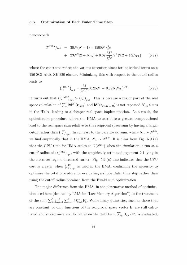
5.6. Optimization of Each Euler Time Step
nanoseconds
THMA/ns = 30N(N − 1) + 1500N r3cc
+ 23N2(2 +NCh) + 0.67M6
r3ccN2 (9.2 + 4.2NCh) (5.27)
where the constants reflect the various execution times for individual terms on a
156 SGI Altix XE 320 cluster. Minimizing this with respect to the cutoff radius
leads to(rHMA
c
)opt
=M
2c1/3[0.25N + 0.12NNCh]1/6 (5.28)
It turns out that(rHMA
c
)opt
>(rE
c
)opt
. This is because a major part of the real
space calculation of∑′
n M(1)(rνµ,n) and M∗(rνµ,n = 0) is not repeated NCh times
in the HMA, leading to a cheaper real space implementation. As a result, the
optimization procedure allows the HMA to attribute a greater computational
load to the real space sum relative to the reciprocal space sum by having a larger
cutoff radius than(rE
c
)opt
. In contrast to the bare Ewald sum, where Nrc ∼ N0.5,
we find empirically that in the HMA, Nrc ∼ N0.7. It is clear from Fig. 5.9 (a)
that the CPU time for HMA scales as O(N2.1) when the simulation is run at a
cutoff radius of(rHMA
c
)opt
, with the empirically estimated exponent 2.1 lying in
the crossover regime discussed earlier. Fig. 5.9 (a) also indicates that the CPU
cost is greater when(rE
c
)opt
is used in the HMA, confirming the necessity to
optimize the total procedure for evaluating a single Euler time step rather than
using the cutoff radius obtained from the Ewald sum optimization.
The major difference from the HMA, in the alternative method of optimiza-
tion used here (denoted by LMA for “Low Memory Algorithm”), is the treatment
of the sum∑′
n
∑Nµ=1
∑3s=1M
rsνµ,nVsµ. While many quantities, such as those that
are constant, or only functions of the reciprocal space vector k, are still calcu-
lated and stored once and for all when the drift term∑
µ Dνµ · Fµ is evaluated,
97
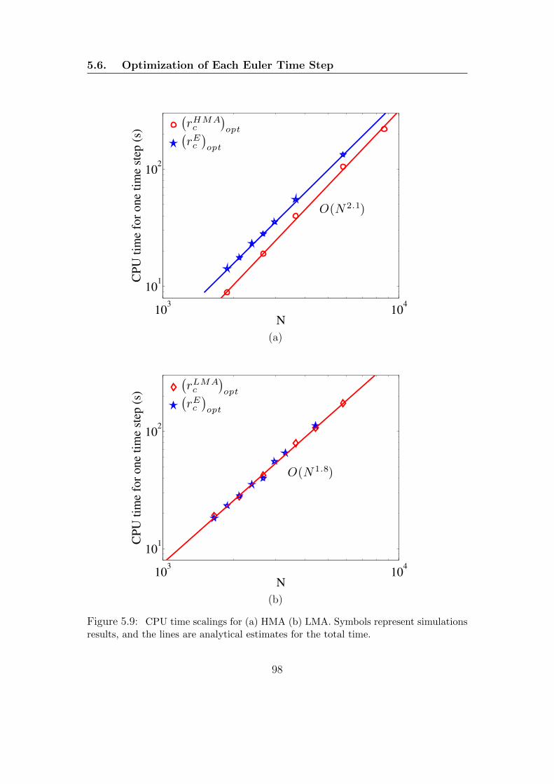
5.6. Optimization of Each Euler Time Step
103
104
101
102
CP
U t
ime
for
on
e ti
me
step
(s)
N
O(N 2.1)
(rHMA
c
)opt(
rEc
)opt
(a)
103
104
101
102
CP
U t
ime
for
on
e ti
me
step
(s)
N
O(N 1.8)
(rLMA
c
)opt(
rEc
)opt
(b)
Figure 5.9: CPU time scalings for (a) HMA (b) LMA. Symbols represent simulationsresults, and the lines are analytical estimates for the total time.
98
5.6. Optimization of Each Euler Time Step
the 3N × 3N matrix Srsνµ is not stored. Instead, the following two steps are
carried out: (i) For a given bead index ν and periodic image n, the quantity
T rν,n =∑N
µ=1
∑3s=1M
rsνµ,nVsµ is evaluated, ensuring that only those beads µ that
lie within a cutoff radius(rLMA
c
)opt
of bead ν are considered in the sum over µ.
Note that for each bead µ, the sum over s involves a simple (3×3)×(3×1) matrix
multiplication. (ii) The sum∑′
n Trν,n over periodic images n is then performed
to obtain the required quantity in the Ewald sum.
Since, even in the LMA, some quantities are stored during the evaluation
of the drift term∑
µ Dνµ · Fµ, we can optimize the entire process involved in
executing one time step in the Euler algorithm by choosing the appropriate cutoff
radius. Adopting the procedure described earlier, we find for the CPU time per
step in nanoseconds
T LMA/ns = 1200 r3ccN(1 +NCh) + 2
M6
r3ccN2 (1.8 + 1.5NCh) (5.29)
(rLMA
c
)opt
=M
2c1/3
[0.18N + 0.15NNCh
1 +NCh
]1/6
(5.30)
Fig. 5.9 (b) compares the CPU cost involved when either the cutoff radius(rLMA
c
)opt
or(rE
c
)opt
is used in the LMA. The reason that(rLMA
c
)opt
and(rE
c
)opt
are nearly equal to each other is because practically all the time consuming parts
of the Ewald sum are calculated repeatedly NCh times in the LMA. As a result,
in contrast to the HMA, the saving achieved by storing some quantities does not
make a significant difference to the choice of cutoff radius. Unlike the HMA,
there is no large storage requirement in the LMA, as shown in Fig. 5.10 (a),
where it is seen to scale as O(N) for sufficiently large N . Further, the CPU
cost scales as O(NCh × N × Nrc), which is identical to the scaling for the basic
Ewald sum, namely, O(N1.8) as can be seen in Fig. 5.10 (b). On the other hand,
since Srsνµ is not stored, the components M rsνµ,n are repeatedly evaluated in each
99

5.6. Optimization of Each Euler Time Step
103
104
102
103
104
Co
mp
ute
r m
emo
ry (
MB
)
N
O(N 2)
O(N )
High Memory Algorithm
Low Memory Algorithm
(a)
103
104
105
101
102
103
104
CP
U t
ime
for
on
e ti
me
step
(s)
N
O(N 1.8)
O(N 2.1)
N ∼ 35000
High Memory Algorithm
Low Memory Algorithm
(b)
Figure 5.10: Comparison between HMA and LMA for (a) Computer memory re-quirement (b) CPU time required for a single time step computation
100
5.7. Testing and Verification of the Algorithm
of the recursive Chebyshev calculations. This extra calculation leads to a large
pre-factor in the scaling of the CPU with N . However, at N ∼ 35000 a crossover
in the CPU cost can be seen to occur, suggesting that it is advisable to use HMA
below a system size of roughly 35000, while the LMA would be cheaper for larger
systems.
5.7 Testing and Verification of the Algorithm
The optimized BD algorithm developed here is validated by testing and verifi-
cation under both θ solvent and good solvent conditions. In the former case,
we first check to see if static equilibrium properties, namely, the gyration radius
and the end-to-end vector, agree with known analytical results. Secondly, the
current implementation of the Ewald sum for hydrodynamic interactions (which
enables its use even in simulations that do not incorporate excluded volume inter-
actions) is tested by comparing the prediction of the infinite dilution equilibrium
self-diffusion coefficient, which is a dynamic property, with the results of a BD
simulation of single chain dynamics. As mentioned in Section 5.1, Pham et al.
(2009) have recently quantitatively compared the predictions of the explicit sol-
vent LB/MD method with the predictions of the implicit solvent BD method
for the dynamics of a single chain under good solvent conditions in the dilute
limit. A natural follow up of the development of the current BD algorithm is to
compare the two methods at finite concentrations under good solvent conditions.
Here we carry out our study by comparing the predictions of the radius of gy-
ration, the end-to-end vector, and the self-diffusion coefficient. This serves both
to verify the predictions of the current algorithm in a regime where there are no
analytical predictions, and to obtain an estimate of the relative computational
costs of the two mesoscopic simulation methods in the semidilute regime.
101
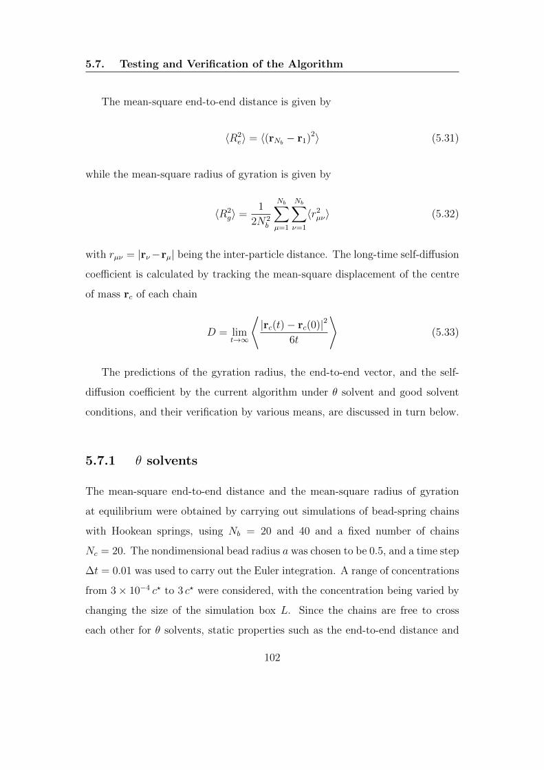
5.7. Testing and Verification of the Algorithm
The mean-square end-to-end distance is given by
〈R2e〉 = 〈(rNb − r1)2〉 (5.31)
while the mean-square radius of gyration is given by
〈R2g〉 =
1
2N2b
Nb∑
µ=1
Nb∑
ν=1
〈r2µν〉 (5.32)
with rµν = |rν−rµ| being the inter-particle distance. The long-time self-diffusion
coefficient is calculated by tracking the mean-square displacement of the centre
of mass rc of each chain
D = limt→∞
⟨|rc(t)− rc(0)|2
6t
⟩(5.33)
The predictions of the gyration radius, the end-to-end vector, and the self-
diffusion coefficient by the current algorithm under θ solvent and good solvent
conditions, and their verification by various means, are discussed in turn below.
5.7.1 θ solvents
The mean-square end-to-end distance and the mean-square radius of gyration
at equilibrium were obtained by carrying out simulations of bead-spring chains
with Hookean springs, using Nb = 20 and 40 and a fixed number of chains
Nc = 20. The nondimensional bead radius a was chosen to be 0.5, and a time step
∆t = 0.01 was used to carry out the Euler integration. A range of concentrations
from 3× 10⁻⁴ c? to 3 c? were considered, with the concentration being varied by
changing the size of the simulation box L. Since the chains are free to cross
each other for θ solvents, static properties such as the end-to-end distance and
102

5.7. Testing and Verification of the Algorithm
the gyration radius are independent of concentration. Further, as is well known,
their dependence on Nb can be shown analytically to be Bird et al. (1987)
〈R2e〉 = 3(Nb − 1) (5.34)
and
〈R2g〉 =
N2b − 1
2Nb
(5.35)
Note that c? can be determined once a choice for Nb is made. Figs. 5.11 (a)
and (b) display the results for 〈R2e〉 and 〈R2
g〉, respectively, for the range of con-
centrations considered here. Symbols indicate simulation data, while solid lines
represent the analytical results given by Eqs. (5.34) and (5.35). Clearly, the
simulated static properties are in good agreement with analytical predictions.
The single chain diffusion coefficient in a dilute solution under θ solvent con-
ditions is used here as the benchmark for verifying the current implementation of
the Ewald sum. The value of the diffusion coefficient for Nb = 20 and a = 0.5 is
displayed as the solid line in Fig. 5.12, obtained here by a conventional BD sim-
ulation algorithm that uses a semi-implicit predictor corrector scheme developed
in our group for simulating a single chain that is not confined in a box (Prab-
hakar and Prakash, 2004). For the same set of input simulation parameters, the
long-time diffusivity is obtained from the current multi-chain BD algorithm for
a range of concentrations. It is clear from Fig. 5.12 that the simulated data
(symbols) for the diffusivity D approaches the single-chain result in the limit of
zero concentration. The value of D at c/c? = 0 was obtained by fitting the values
at c/c? = 0.001, 0.003 and 0.01 with a second order polynomial and extrapolating
to zero concentration.
103
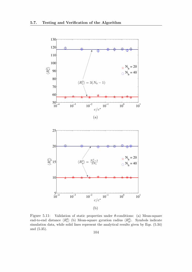
5.7. Testing and Verification of the Algorithm
10−4
10−3
10−2
10−1
100
101
50
60
70
80
90
100
110
120
130
c/c∗
〈R2 e〉
〈R2e〉 = 3(Nb − 1)
Nb = 20
Nb = 40
(a)
10−4
10−3
10−2
10−1
100
101
5
10
15
20
25
c/c∗
〈R2 g〉
〈R2g〉 =
N 2b −1
2Nb
Nb = 20
Nb = 40
(b)
Figure 5.11: Validation of static properties under θ-conditions: (a) Mean-squareend-to-end distance 〈R2
e〉 (b) Mean-square gyration radius 〈R2g〉. Symbols indicate
simulation data, while solid lines represent the analytical results given by Eqs. (5.34)and (5.35).
104

5.7. Testing and Verification of the Algorithm
!" # !" $ !" % !" ! !"" !"!"&"!
"&"%
"&"$
"&"#
"&"'
"&"(
c/c*
)*
+,-./01234,-15,6678,9,:;
<=:>4?@/4:05194/70
D
Figure 5.12: Long-time self-diffusion coefficient under θ solvent conditions. Sym-bols indicate simulation data obtained with the current multi-chain algorithm,while the solid line represents the value obtained by simulating the dynamics ofa single chain in a dilute solution. The circle symbol on the y-axis is the valueobtained by extrapolating the finite concentration results to the limit of zeroconcentration.
5.7.2 Good solvents
In order to carry out a quantitative comparison between the LB/MD and BD
methods, it is necessary to ensure that the underlying polymer model is iden-
tical for both the methods, and to map the input parameters of the hybrid
model onto the input values of the BD model. A detailed discussion of how
this can be achieved in the context of dilute solutions has been given in Pham
et al. (2009). Exactly the same procedure has been adopted here as discussed
in Appendix E. In particular, Appendix E discusses (i) the mapping of different
105
5.7. Testing and Verification of the Algorithm
simulation parameters between BD and LB/MD, and (ii) the procedure to run
LB/MD simulations using an open source software ESPResSo (Extensible Sim-
ulation Package for Research on Soft matter). Essentially, a bead-spring chain
with FENE springs is used, with a Weeks-Chandler-Andersen potential, which
acts between all monomers, employed to model the excluded volume (EV) ef-
fect. While in the LB/MD simulation approach, the Weeks-Chandler-Andersen
parameters are used to define the units of energy, length, and time, the corre-
sponding units in the BD simulations have been discussed earlier in Section 4.2.
Appendix E discusses the details of the length and time unit conversions between
the two methods. The comparison of the two methods proceeds by first picking
the simulation parameters for the LB/MD model, using these for the LB/MD
simulations, then converting them to BD units using the procedure outlined in
Pham et al. (2009) and Appendix E, and finally running the equivalent BD model
obtained in this manner. In other words, the two units systems are maintained
in the respective methods, and a comparison of predicted quantities carried out
a posteriori.
The results of carrying out this procedure for 〈R2e〉, 〈R2
g〉 and D are shown in
Table 5.1 for Nb = 10 at three different concentrations. It is worth noting that,
since EV interactions are short-ranged, we have implemented a neighbor-list in
the current BD algorithm for computing the pairwise summation of EV interac-
tions, with a cutoff radius equal to the range of the Weeks-Chandler-Andersen
potential. All values are reported in BD units, unless specified otherwise.
106

5.7. Testing and Verification of the Algorithm
Nc
Met
hod
Lc
c/c?
〈R2 e〉
〈R2 g〉
D
20B
D24
.152
0.01
420.
546±
0.00
111
1.37±
0.47
18.3
6±
0.04
0.02
72±
6×10−
4
LB
100.
20.
543±
0.00
511
2.93±
0.27
18.2
9±
0.02
0.02
68±
8×10−
4
32B
D21
.737
0.03
111.
199±
0.00
298
.35±
0.43
16.6±
0.04
0.01
62±
6×10−
4
LB
90.
439
1.19
2±
0.01
199
.11±
0.36
16.5
9±
0.03
0.01
51±
4×10−
4
70B
D21
.737
0.06
82.
623±
0.00
476
.07±
0.53
13.3
3±
0.05
0.00
24±
1×
10−
4
LB
90.
962.
607±
0.02
577
.29±
0.35
13.4
2±
0.04
0.00
245±
5×
10−
5
Tab
le5.
1:C
ompar
ison
ofpre
dic
tion
sof
the
radiu
sof
gyra
tion
,th
een
d-t
o-en
dve
ctor
,an
dth
ese
lf-d
iffusi
onco
effici
ent
by
the
explici
tso
lven
tL
B/M
Dm
ethod
wit
hth
epre
dic
tion
sof
the
implici
tso
lven
tB
Dm
ethod,
for
ab
ead-s
pri
ng
chai
nw
ithNb
=10
atth
ree
diff
eren
tco
nce
ntr
atio
ns,
ina
good
solv
ent.
Not
eth
atal
lpro
per
ties
are
give
nin
BD
unit
s,ex
cept
the
box
size
L,
and
conce
ntr
atio
nc,
whic
har
egi
ven
inL
Bunit
sw
hen
rep
orte
dfo
rth
eL
B/M
Dsi
mula
tion
s.B
othL
andc
are
iden
tica
lin
bot
hm
ethods
when
rep
orte
din
the
sam
eunit
syst
em.
Not
eth
atth
ehig
hes
tco
nce
ntr
atio
nco
rres
pon
ds
tom
elt-
like
condit
ions.
107
5.8. Comparison of Computational Cost with LB/MD
We find it convenient to maintain the same absolute concentration in the
two methods rather than the same c/c?, as this would entail an interpolation
procedure. In the BD method, c? is determined from 〈R2g〉 in the dilute limit, by
carrying out a single-chain simulation for parameter values that are identical to
those in the multi-chain BD simulation. In the LB/MD method, simulations are
carried out for three box sizes, L = 12, 17 and 21, with the number of monomers
held fixed (we use Nc = 20 and Nb = 10). As a result, the monomer concentra-
tion decreases with increasing box size. The values of 〈R2g〉 obtained for these
three box sizes are extrapolated to infinite box size in order to determine 〈R2g〉
(and consequently c?) in the dilute limit.
It is clear from Table 5.1, both in the dilute limit, with regard to values of
c/c?, and at all three finite concentrations, with regard to values of 〈R2e〉, 〈R2
g〉and D, that there is excellent agreement between the two mesoscopic simulation
methods, since all properties agree with each other within error bars. This vali-
dates the current algorithm in a regime where there are no analytical solutions.
Further, it demonstrates the robustness of the parameter mapping technique
developed by Pham et al. (2009) for comparing the two simulation methods.
5.8 Comparison of Computational Cost with
LB/MD
Recent comparison by Pham et al. (2009) of the predictions of the explicit solvent
LB/MD method with the predictions of the implicit solvent BD method for the
dynamics of a single chain indicated that in the dilute limit, BD is the method of
choice as it is significantly more efficient than LB/MD. However, Fig. 5.13 sug-
gests that for our current implementation the situation is quite the reverse at the
finite concentration, c/c? = 1.2, at which the simulation data in the figure were
108
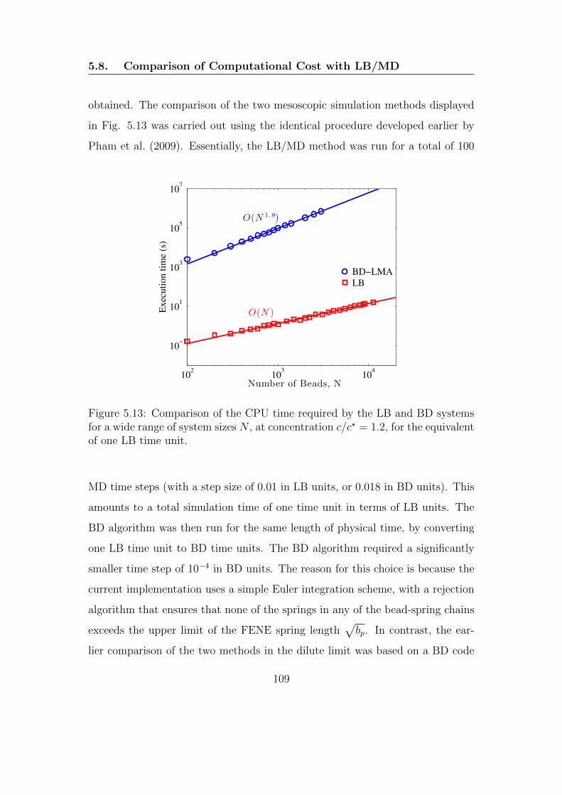
5.8. Comparison of Computational Cost with LB/MD
obtained. The comparison of the two mesoscopic simulation methods displayed
in Fig. 5.13 was carried out using the identical procedure developed earlier by
Pham et al. (2009). Essentially, the LB/MD method was run for a total of 100
102
103
104
10−1
101
103
105
107
Number of Beads, N
Executi
on t
ime (
s)
O(N 1.8)
O(N )
BD−LMA
LB
Figure 5.13: Comparison of the CPU time required by the LB and BD systemsfor a wide range of system sizes N , at concentration c/c? = 1.2, for the equivalentof one LB time unit.
MD time steps (with a step size of 0.01 in LB units, or 0.018 in BD units). This
amounts to a total simulation time of one time unit in terms of LB units. The
BD algorithm was then run for the same length of physical time, by converting
one LB time unit to BD time units. The BD algorithm required a significantly
smaller time step of 10−4 in BD units. The reason for this choice is because the
current implementation uses a simple Euler integration scheme, with a rejection
algorithm that ensures that none of the springs in any of the bead-spring chains
exceeds the upper limit of the FENE spring length√bp. In contrast, the ear-
lier comparison of the two methods in the dilute limit was based on a BD code
109

5.8. Comparison of Computational Cost with LB/MD
that uses a semi-implicit predictor-corrector method, enabling the use of a much
larger step size of 5 × 10⁻³ BD units. The dependence of CPU time on system
size was examined here by increasing the number of chains Nc, while keeping the
number of beads in a chain fixed at Nb = 10. The concentration was maintained
constant at c/c? = 1.2 (or c = 0.031 in BD units) by increasing the box size
L suitably. Since the difference between the HMA and LMA BD algorithms is
insignificant on the scale of the difference between LB/MD and BD, only results
for the LMA are shown in Fig. 5.13.
The CPU time scaling of the LMA algorithm has been established in Sec-
tion 5.6 to be N1.8. From Eqs. (5.29) and (5.30) one immediately sees that
after optimization the CPU time depends only on the particle number N , but is
independent of the concentration c (or the system volume V ):
T LMA(N, V ) = γLMAN1.8 (5.36)
with some proportionality constant γLMA. Conversely, the LB/MD method is
dominated by the CPU effort of the solvent, i.e.
T LB(N, V ) = γLBV = γLBN
c(5.37)
with another constant γLB. Hence
T LMA
T LB=γLMA
γLBcN0.8 (5.38)
From our CPU timings we find a value γLMA/γLB = 1.3×10⁴ in BD units, i.e. our
current implementation of Ewald BD becomes competitive with LB/MD only if
the concentration is below the very small value 7.8× 10⁻⁵ ×N−0.8.
However, it should be noted that the present version is by far not the fastest
110

5.9. Conclusions
conceivable BD code. Firstly, we expect that by implementing an implicit in-
tegrator the time step may be increased by nearly two orders of magnitude.
Secondly, the evaluation of the real space HI should be substantially faster (both
in the LMA and HMA versions) by making use of Verlet tables. Thirdly, the
HMA algorithm could then take advantage of sparse-matrix techniques (see also
the discussion in Section 5.6). Finally, the evaluation of the Fourier part can be
speeded up by making use of Fast Fourier Transformation, which, as shown pre-
viously, gives rise to a complexity of the total algorithm of O(N1.3 logN) (Sierou
and Brady, 2001; Banchio and Brady, 2003). All together, achieving accelera-
tions by up to three orders of magnitude does not seem unrealistic.
5.9 Conclusions
A range of issues related to the development of an optimized BD algorithm for
simulating the dynamics of semidilute solutions in unbounded domains has been
considered here. In particular:
1. It is possible to develop an optimized Ewald method for hydrodynamic
interactions that splits the cost of evaluating the real space and reciprocal
space sums evenly, leading to a CPU cost that scales as N1.5, rather than
the N2 scaling that would result from a straightforward implementation.
2. While Beenakker’s original implementation of the Ewald sum is only valid
for systems without bead overlap, it can be modified to account for bead
overlap, such that θ-solutions can be simulated by switching off excluded
volume interactions.
3. As in the case of dilute solutions, the number of Chebyshev terms required
to maintain a desired accuracy scales as (λmax/λmin)12 , where λmax and λmin
111

5.9. Conclusions
are the maximum and minimum eigenvalues of the diffusion tensor D. It
is shown that this leads to an additional computational load that scales as
N0.3.
4. It is necessary to consider the optimization of the overall time required to
perform one Euler time step, in addition to the individual optimizations of
the Ewald sum and Chebyshev polynomial approximation. In this context,
two different schemes for optimization have been proposed in the form
of the “high memory” (HMA), and the “low memory” (LMA) algorithms.
While the LMA leads to an overall CPU time scaling of N1.8, which appears
better than the N2.1 scaling of the HMA, the large prefactor in the former
makes it preferable only for large systems with more than roughly 35,000
particles.
5. The optimized BD algorithm gives accurate predictions under both θ and
good solvent conditions. In the latter case, BD predictions are compared
with those of the LB/MD method. The parameter mapping scheme devel-
oped by Pham et al. (2009) for dilute solutions is found to be valid and
useful even at a finite concentration in the semidilute regime.
6. In contrast to dilute solutions, where BD was shown to be significantly
more computationally efficient than LB/MD (Pham et al., 2009), exactly
the opposite is true for semidilute solutions. The CPU cost of the BD
method scales as N1.8, while the cost of the LB/MD method scales linearly
with system size. The necessity of carrying out an Ewald sum renders the
BD method developed here significantly more computationally expensive
than LB/MD. Nevertheless, it should be noted that the BD method can
be further refined and dramatically speeded up, as discussed at the end of
Section 5.8.
112

Chapter 6
Dynamic Crossover Scaling in
Semidilute Polymer Solutions
6.1 Introduction
This chapter aims to verify the scaling arguments developed in Chapter 3, using
the Brownian dynamics simulation algorithm discussed in Chapter 5. Broadly,
this chapter attempts to validate the two important conclusions of the scaling
analysis with the help of computer simulations:
1. The existence of universal crossover scaling functions in the solvent quality
driven crossover region.
2. The suggestion that there is only a single crossover scaling function from
which others can be inferred.
These conclusions can be validated by carrying out simulations for the different
crossover scaling functions such as φR and φD for a range of c/c? and z. In order to
perform simulations for these crossover scaling functions for semidilute polymer
solutions and verify their universality, it is necessary to consider sufficiently long
113
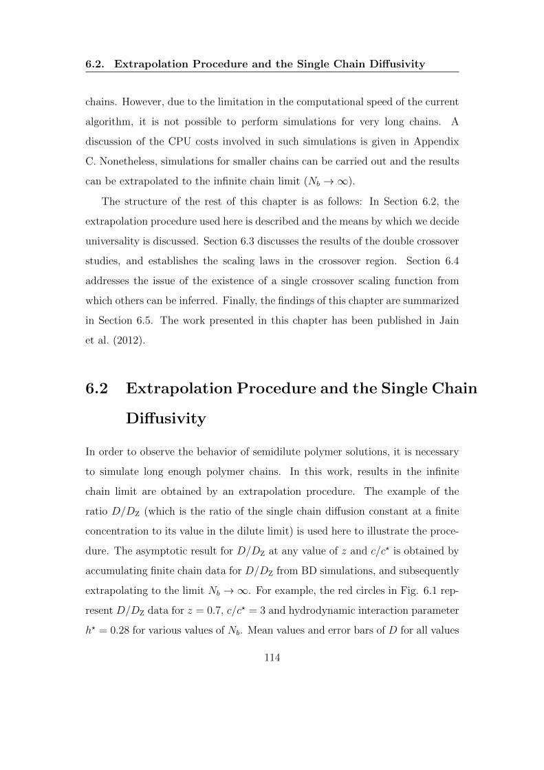
6.2. Extrapolation Procedure and the Single Chain Diffusivity
chains. However, due to the limitation in the computational speed of the current
algorithm, it is not possible to perform simulations for very long chains. A
discussion of the CPU costs involved in such simulations is given in Appendix
C. Nonetheless, simulations for smaller chains can be carried out and the results
can be extrapolated to the infinite chain limit (Nb →∞).
The structure of the rest of this chapter is as follows: In Section 6.2, the
extrapolation procedure used here is described and the means by which we decide
universality is discussed. Section 6.3 discusses the results of the double crossover
studies, and establishes the scaling laws in the crossover region. Section 6.4
addresses the issue of the existence of a single crossover scaling function from
which others can be inferred. Finally, the findings of this chapter are summarized
in Section 6.5. The work presented in this chapter has been published in Jain
et al. (2012).
6.2 Extrapolation Procedure and the Single Chain
Diffusivity
In order to observe the behavior of semidilute polymer solutions, it is necessary
to simulate long enough polymer chains. In this work, results in the infinite
chain limit are obtained by an extrapolation procedure. The example of the
ratio D/DZ (which is the ratio of the single chain diffusion constant at a finite
concentration to its value in the dilute limit) is used here to illustrate the proce-
dure. The asymptotic result for D/DZ at any value of z and c/c? is obtained by
accumulating finite chain data for D/DZ from BD simulations, and subsequently
extrapolating to the limit Nb →∞. For example, the red circles in Fig. 6.1 rep-
resent D/DZ data for z = 0.7, c/c? = 3 and hydrodynamic interaction parameter
h? = 0.28 for various values of Nb. Mean values and error bars of D for all values
114

6.2. Extrapolation Procedure and the Single Chain Diffusivity
of Nb are estimated using the procedure discussed in Appendix A. The reason
for choosing 1/√Nb as the x axis is justified shortly. The finite chain data are
extrapolated to 1/√Nb → 0 limit with the help of a “Least-Squares Fitting” nu-
merical routine, which is discussed in Appendix D. This routine, which accounts
for the error bars at each finite size data point, also reports the error bar on the
extrapolated data.
Kroger et al. (2000); Prakash (2001a); Kumar and Prakash (2003); Sunthar
and Prakash (2005, 2006) found, for a single chain, that the extrapolation of
finite chain data leads not only to asymptotic predictions at constant z, but
also to values independent of the choice of h∗. This independence from the
choice of a microscopic simulation parameter was taken to indicate the existence
of universality. In their extrapolation analysis, they considered the x axis as
1/√Nb, which was motivated by the fact that the leading order corrections to
the infinite chain length limit, of various material properties, is of order 1/√Nb.
A similar behavior appears to hold true for semidilute polymer solutions as
well, by considering the x axis as 1/√Nb. The red asterisks in Fig. 6.1 represent
data for the same values of z = 0.7 and c/c? = 3 but for a different value of
h? = 0.15. As can be seen in Fig. 6.1, the error bars on the extrapolated
values are large because of a conservative estimation of the error (see Appendix
D). However, as the extrapolated data for h? = 0.28 and 0.15 are very close to
each other, we consider the prediction of D/DZ in the infinite chain limit to be
independent of h?. Fig. 6.1 shows another data set for z = 1.7 and c/c? = 2 using
blue symbols, and here also the results in the infinite chain limit are independent
of h?. This clearly indicates that the extrapolated value is a universal value
independent of the choice of the simulation parameter h?.
Apart from the hydrodynamic interaction parameter h?, there is another ar-
bitrary parameter which arises from the use of the narrow Gaussian potential
115

6.2. Extrapolation Procedure and the Single Chain Diffusivity
0 0.05 0.1 0.15 0.2 0.25 0.3 0.35 0.4 0.45
0.2
0.3
0.4
0.5
0.6
N!1/2b
D/D
Z
Extrapolated values
[z, c/c*, h*]
[0.7, 3, 0.28]
[0.7, 3, 0.15]
[1.7, 2, 0.28]
[1.7, 2, 0.15]
Figure 6.1: Universal predictions of the ratio of the single chain diffusion constantD (at a finite concentration c/c?), to its value in the dilute limit DZ, at two valuesof the solvent quality z = 0.7 and z = 1.7. Data accumulated for finite values ofchain length Nb (symbols) for two different values of h? extrapolate to a uniquevalue in the limit Nb →∞.
for excluded volume interactions. For a given value of solvent quality z, the
parameters used in the narrow Gaussian potential are (i) z? = z/√Nb and (ii)
d?. Note that z? is determined once a choice for z and Nb is made. The param-
eter d? can be chosen arbitrarily. For reasons elaborated in Kumar and Prakash
(2003), instead of d?, we choose to pick a value for the constant K, and then
determine d? from the relation d? = Kz?1/5. It has been shown previously by
Kumar and Prakash (2003) that, for a given z, the results extrapolated in the
limit Nb →∞ are independent of the particular choice of K. This finding turns
out to be true for semidilute solutions as well. We carried out simulations for
fixed values of z = 1.7 and c/c? = 2.5, and varied d? according to d? = Kz?1/5,
116

6.2. Extrapolation Procedure and the Single Chain Diffusivity
with three different values of K. It is clear from Fig. 6.2 that the extrapolated
results are essentially independent of K. Therefore, it can be concluded that
0 0.1 0.2 0.3 0.40.2
0.25
0.3
0.35
0.4
N!1/2b
D/D
Z
d! = Kz!1/5
Extrapolated values
K = 1K = 1.5K = 3
Figure 6.2: Extrapolated values of D/DZ are independent of K for z = 1.7 andc/c? = 2.5.
the extrapolation procedure not only provides the result for infinite chains but
also leads to parameter free predictions that can be used to directly compare
with experimental data. In this work, data accumulated for chains ranging from
lengths Nb = 6 to Nb = 20 have been extrapolated to the limit Nb →∞.
6.2.1 Comparison with experimental data
The main advantage of obtaining parameter free predictions in the long chain
limit is that the extrapolated values of D/DZ can be directly compared with ex-
117

6.2. Extrapolation Procedure and the Single Chain Diffusivity
perimental data. The self diffusion coefficientD was first measured by Marmonier
and Leger (1985) for polystyrene in Benzene (good solvent) for different concen-
trations and molecular weights using forced Rayleigh light scattering. They also
measured D at very low concentrations, which corresponds to DZ. As a result,
the ratio D/DZ obtained from BD simulations can be compared with experi-
mental D/DZ data. Fig. 6.3 (a) shows the simulation results for various values
of z, along with the experimental data for a good solvent system for a range of
molecular weights (ranging from 78000− 750000). Colored symbols indicate the
simulation results and black symbols represent experimental data. We conjecture
that the disagreement between simulation results and experimental observations
may be due to two reasons. Firstly, the overlap concentration c? used by Mar-
monier and Leger (1985) is based on the following definition: c? =NmmvsNA (R0
g)3,
where Nm is the number of monomers in a chain, m is the molar weight of a
monomer, vs is the partial specific volume and NA is the Avogadro number.
Marmonier and Leger (1985) deduced the values of vs from Pouyet et al. (1976),
for polystyrene in Benzene for a range of molecular weights. This definition of
c? does not have the factor of 4π/3 in the denominator which is included in the
definition used here for c?.
Secondly, Marmonier and Leger (1985) do not report the values of R0g used
in their paper but rather provide reference to an unpublished PhD thesis. We
are consequently unable to compare with simulation results for R0g. For these
reasons, the value of c/c? reported by Marmonier and Leger (1985) could be
different from simulation values at the same absolute concentration c.
In addition, there is another noteworthy aspect to the experimental data
obtained by Marmonier and Leger (1985). In general, the semidilute regime is
considered to span the range 1 ≤ c/c? < 10 in neutral linear polymer solutions.
According to scaling theory, the diffusivity in the semidilute regime scales as
118
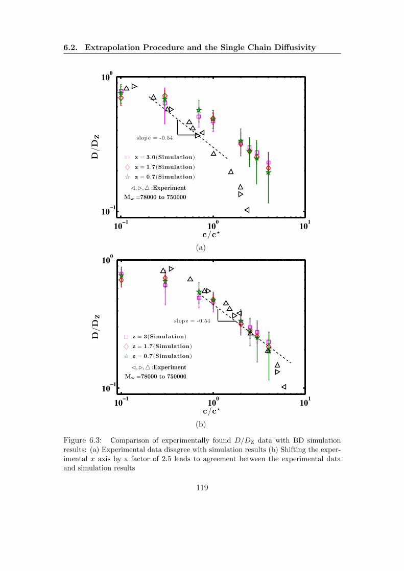
6.2. Extrapolation Procedure and the Single Chain Diffusivity
!" ! !"" !"!!" !
!""
c/c!
D/D
Z
z = 3.0(Simulation)
z = 1.7(Simulation)
z = 0.7(Simulation)
slope = -0.54
,, :Experiment
Mw =78000 to 750000
(a)
!" ! !"" !"!!" !
!""
c/c!
D/D
Z
z = 3(Simulation)
z = 1.7(Simulation)
z = 0.7(Simulation)
slope = -0.54
,, :Experiment
Mw =78000 to 750000
(b)
Figure 6.3: Comparison of experimentally found D/DZ data with BD simulationresults: (a) Experimental data disagree with simulation results (b) Shifting the exper-imental x axis by a factor of 2.5 leads to agreement between the experimental dataand simulation results
119

6.3. Universal Crossover Scaling Functions
(c/c?)−0.54 in good solvents. The experimental data of Marmonier and Leger
(1985) however suggests that the onset of this scaling occurs at a much lower
value of c/c?.
We can bring experimental data and similar results much closer to each other,
as shown in Fig. 6.3 (b) by applying a horizontal shift factor of 2.5 to the
experimental data. Given the uncertainty in the experimental value of c/c?, this
is perhaps not completely unreasonable. It would be worthwhile revisiting the
problem of measuring the diffusivity in semidilute solutions and carrying out
detailed comparisons in the entire crossover regime.
6.3 Universal Crossover Scaling Functions
In this section, the question of the form of the universal scaling function in
the crossover regime is addressed with the help of simulation results for universal
crossover scaling functions φR(c/c?, z) and φD(c/c?, z). These results are obtained
by carrying out a careful Brownian dynamics simulations of short chains and then
extrapolating the short chain results to infinite size chains as discussed in Section
6.2. Simulations to explore the solvent quality crossover have been carried out
by keeping the value of z constant at four different values: 0, 0.7, 1.7, 3, with
z = 0 corresponding to θ-solutions. At each fixed value of z, a range of c/c?
from 0.1 to 4 have been used to sample both the dilute and semidilute regimes.
The overlap concentration c? is calculated from c? = Nb/[(4π/3)R0
g3], where
R0g is computed apriori by running single-chain BD simulations. The box size
L is selected to ensure L ≥ 2Re, in order to prevent a chain from wrapping
over itself. For this purpose, the value of Re at any value of c/c? is estimated
from the blob scaling law Re = R0e (c/c?)(2ν−1)/(2−6ν) where R0
e is the end-to-end
distance of a chain computed in the dilute limit. Typical simulations consist of an
120
6.3. Universal Crossover Scaling Functions
equilibration run for approximately one relaxation time followed by a production
run whose length varies from 10 to 60 relaxation times; here, the relaxation time
τ1 was estimated via τ1 = R2g/(6D). Moreover, data were obtained by averaging
over 30 − 70 independent runs. Some examples of the simulation parameters
used in this study are shown in Table 6.1. The resulting crossover scaling
z c/c? Nb L Nc Simulation length
0.1 10 23.4 28 68.2 τ1
0 1 20 15.1 27 12.9 τ1
4 16 13.4 103 10.2 τ1
0.1 8 24.3 32 44.7 τ1
0.7 1 10 14.9 51 28.7 τ1
4 14 12.2 64 9.8 τ1
0.1 10 30.5 34 20.5 τ1
1.7 1 18 20.4 38 12.8 τ1
4 14 13.5 67 10 τ1
0.1 10 30.1 27 28.3 τ1
3 1 6 10 25 26.7 τ1
4 16 15.8 69 12.7 τ1
Table 6.1: Some examples of simulation parameters used in obtaining universalcrossover scaling functions.
functions φR(c/c?, z) and φD(c/c?, z) are shown in Figs. 6.4 and 6.5, where the
mean polymer size R is Rg. The data are limited to the crossover region where in
principle none of the power laws of Table 3.2 hold. Since the observation regime
is small, it is nevertheless possible to fit a power law to the data (without deeper
theoretical justification). This gives rise to a convenient description in terms of
an effective empirical exponent νeff (see Table 6.2 and Fig. 6.4 for the values of
νeff), which is obtained by adjusting the value of ν in the scaling laws of regime
C of Table 3.2 to the observed slope for φR. Since the crossover scaling functions
are related to each other (see below), each crossover yields the same value for
νeff. For instance, in Fig. 6.5, lines are drawn, on top of φD data, based on the
121

6.3. Universal Crossover Scaling Functions
1 1.5 2 2.5 3 3.5 40.8
0.9
1
c/c!
R/R
!
z = 3, !e! = 0.63 ± 0.03
1 1.5 2 2.5 3 3.5 40.850.90.951
c/c!
R/R
!
z = 1.7, !e! = 0.58 ± 0.03
1 1.5 2 2.5 3 3.5 40.9
0.95
1
c/c!
R/R
!
z = 0.7, !e! = 0.54 ± 0.02
1 1.5 2 2.5 3 3.5 4
0.981
1.02
c/c!
R/R
!
z = 0, !e! = 0.5
1 1.5 2 2.5 3 3.5 4
0.981
1.02
c/c!
R/R
!
z = 0, !e! = 0.5
1 1.5 2 2.5 3 3.5 4
0.981
1.02
c/c!
R/R
!
z = 0, !e! = 0.5
1 1.5 2 2.5 3 3.5 4
0.981
1.02
c/c!
R/R
!
z = 0, !e! = 0.5
1 1.5 2 2.5 3 3.5 4
0.981
1.02
c/c!
R/R
!
z = 0, !e! = 0.5
Figure 6.4: Concentration dependence of the crossover scaling function φR in thesemidilute regime, for different values of solvent quality z, obtained by Browniandynamics simulations. The effective exponents νeff have been determined byfitting power laws to the data φR ∝ (c/c?)−p and requiring p = (2νeff−1)/(6νeff−2), according to Table 3.2 in regime C.
z νeff
0 0.50.7 0.54 ± 0.021.7 0.58 ± 0.033 0.63 ±0.03
Table 6.2: Values of νeff for various z, found by adjusting the value of ν in thescaling laws of regime C of Table 3.2 to the observed slope for φR
122
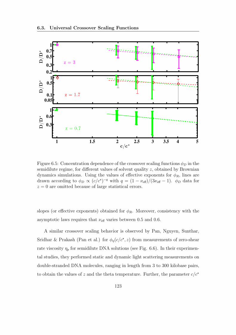
6.3. Universal Crossover Scaling Functions
1 1.5 2 2.5 3 3.5 4 50.20.3
0.50.71
c/c!
D/D
!
z = 3
1 1.5 2 2.5 3 3.5 4 50.050.1
0.51
c/c!
D/D
!
z = 1.7
1 1.5 2 2.5 3 3.5 4 5
0.3
0.61
c/c!
D/D
!
z = 0.7
1 1.5 2 2.5 3 3.5 4 5
0.3
0.61
c/c!
D/D
!
z = 0.7
1 1.5 2 2.5 3 3.5 4 5
0.3
0.61
c/c!
D/D
!
z = 0.7
1 1.5 2 2.5 3 3.5 4 5
0.3
0.61
c/c!
D/D
!
z = 0.7
Figure 6.5: Concentration dependence of the crossover scaling functions φD in thesemidilute regime, for different values of solvent quality z, obtained by Browniandynamics simulations. Using the values of effective exponents for φR, lines aredrawn according to φD ∝ (c/c?)−q with q = (1 − νeff)/(3νeff − 1). φD data forz = 0 are omitted because of large statistical errors.
slopes (or effective exponents) obtained for φR. Moreover, consistency with the
asymptotic laws requires that νeff varies between 0.5 and 0.6.
A similar crossover scaling behavior is observed by Pan, Nguyen, Sunthar,
Sridhar & Prakash (Pan et al.) for φη(c/c?, z) from measurements of zero-shear
rate viscosity ηp for semidilute DNA solutions (see Fig. 6.6). In their experimen-
tal studies, they performed static and dynamic light scattering measurements on
double-stranded DNA molecules, ranging in length from 3 to 300 kilobase pairs,
to obtain the values of z and the theta temperature. Further, the parameter c/c?
123

6.3. Universal Crossover Scaling Functions
1 2 3 4 5 6 71
51020
c/c!
!p/!
! p
z = 0.7
1 2 3 4 5 6 71
51020
c/c!
!p/!
! p
z = 0T4 DNA at 24.5oC" DNA at 35oC
25 kbp DNA at 44.6oC
1 2 3 4 5 6 71
51020
c/c!
!p/!
! p
z = 1.71 2 3 4 5 6 7
1
51020
c/c!
!p/!
! p
z = 3
φη
φη
φη
φη
Figure 6.6: Concentration dependence of the crossover scaling functions φη inthe semidilute regime, for different values of solvent quality z, obtained fromrheological measurements on DNA solutions performed by Pan, Nguyen, Sunthar,Sridhar & Prakash (Pan et al.). Using the values of effective exponents forφR, lines are drawn according to φη ∝ (c/c?)r with r = 1/(3νeff − 1). Thisexperimental data is reproduced with permission from Pan, Nguyen, Sunthar,Sridhar & Prakash (Pan et al.).
defined in their study is identical to the definition used in our simulations. This
allows a decent comparison with simulation results for various values of c/c? and
z.
While we have not obtained predictions of ηp due to computational limita-
124
6.4. The Existence of a Single Universal Crossover Scaling Function
tions, we can still compare our prediction of the scaling in the double crossover
regime with experimental measurements. The lines shown in Fig. 6.6 are based
on νeff obtained from simulations for φR at the corresponding values of z. Clearly,
the predicted scaling at each value of z agrees remarkably well with experimental
observations. As we shall see in the next section, this corroborates the expecta-
tion that there is only one scaling function.
6.4 The Existence of a Single Universal Crossover
Scaling Function
As discussed in Chapter 3, the combination of crossover scaling functions to-
gether in certain specific ways leads to very simple functional dependences in the
(c/c?, z) phase diagram, as displayed in Table 3.2. In this section we validate
these predictions of scaling theory with BD simulations.
Figure 6.7 examines the validity of the scaling prediction that the combination
(c/c?)1/4 φR φ1/4D = 1 in the entire semidilute regime, while it is proportional to
(c/c?)1/4 in the dilute limit. It is clear from the Fig. 6.7 that indeed the functions
φR and φD, which have been obtained by BD simulations in the long-chain limit,
when combined as suggested by scaling theory lead to the predicted functional
dependence in the two regimes, respectively.
Figure 6.8 examines the validity of the scaling prediction that the combination
(c/c?)1/3 φR φ−1/6η = 1 in the semidilute regime, while it scales as (c/c?)1/6 in
the dilute regime. We have obtained φη from the experimental measurements
reported in Pan, Nguyen, Sunthar, Sridhar & Prakash (Pan et al.), and φR from
BD simulations as discussed previously. Clearly in this case as well, the scaling
predictions are well substantiated. The departure of data from the (c/c?)1/4 and
(c/c?)1/6 curves for values of c/c? ≈ 1 in Figs. 6.7 and 6.8 can be attributed to
125
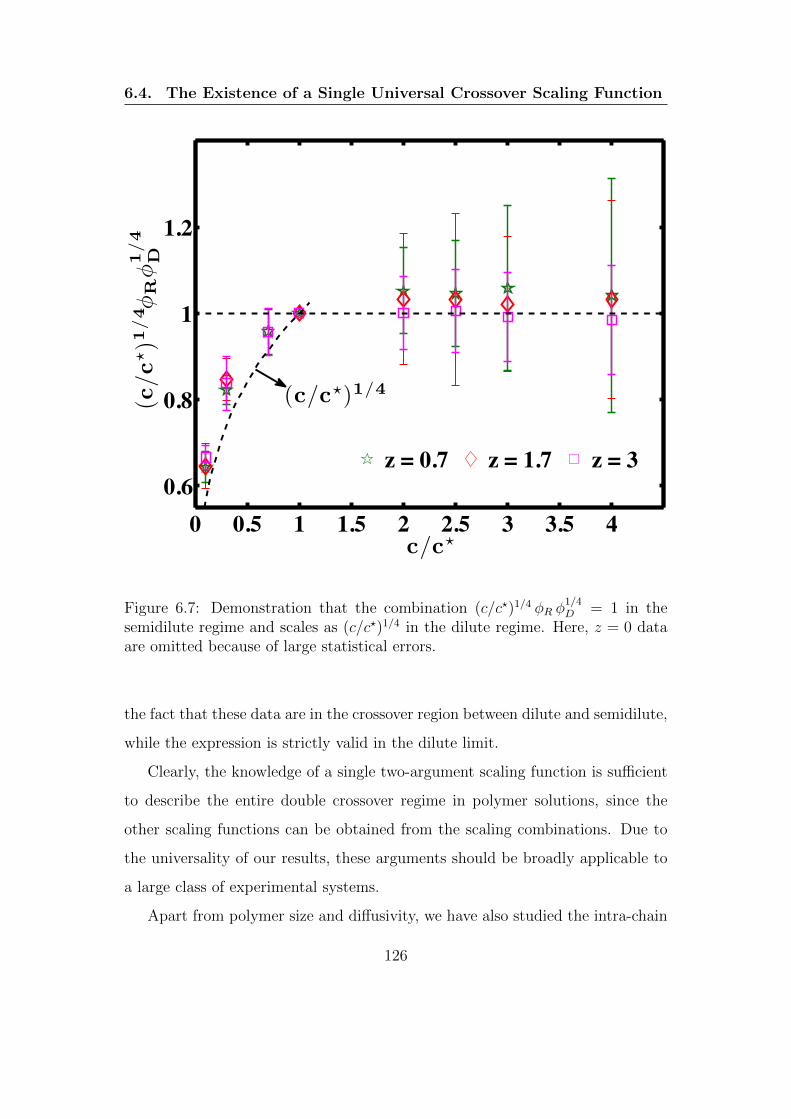
6.4. The Existence of a Single Universal Crossover Scaling Function
0 0.5 1 1.5 2 2.5 3 3.5 40.6
0.8
1
1.2
c/c!
(c/c
!)1
/4!
R!
1/4
D
z = 0.7 z = 1.7 z = 3
(c/c!)1/4
Figure 6.7: Demonstration that the combination (c/c?)1/4 φR φ1/4D = 1 in the
semidilute regime and scales as (c/c?)1/4 in the dilute regime. Here, z = 0 dataare omitted because of large statistical errors.
the fact that these data are in the crossover region between dilute and semidilute,
while the expression is strictly valid in the dilute limit.
Clearly, the knowledge of a single two-argument scaling function is sufficient
to describe the entire double crossover regime in polymer solutions, since the
other scaling functions can be obtained from the scaling combinations. Due to
the universality of our results, these arguments should be broadly applicable to
a large class of experimental systems.
Apart from polymer size and diffusivity, we have also studied the intra-chain
126

6.5. Conclusions
0 0.5 1 1.5 2 2.5 3 3.5 40.6
0.7
0.8
0.9
1
1.1
c/c!
(c/c
!)1
/3!
R!
!1
/6
"
z = 0z = 0.7z = 1.7z = 3
(c/c!)1/6
Figure 6.8: Demonstration that the combination (c/c?)1/3 φR φ−1/6η = 1 in the
semidilute regime and scales as (c/c?)1/6 in the dilute regime.
static structure factor of semidilute polymer solutions for a range of c/c? and z,
which is discussed in Appendix F.
6.5 Conclusions
The double crossover behavior for various physical properties was examined in
semidilute polymer solutions with the help of Brownian dynamics simulations.
Following are the key findings of this study:
127

6.5. Conclusions
1. Because of the high CPU cost, the current algorithm is restricted in simu-
lating chains of up to 20 beads. However, an extrapolation technique can
be used to circumvent the problem.
2. The extrapolation procedure was used to elucidate universal behavior. It
was shown that, in the limit of infinite size chain, parameter free predictions
are obtained that can be directly compared with experimental data.
3. Universal crossover scaling functions φR, φD and φη defined in terms of c/c?
and z were obtained. In particular, the blob scaling relationships, that are
valid only for very good solvents and θ solvents, were shown to be also
applicable in the solvent quality driven crossover regime, with an effective
exponent in place of the Flory exponent.
4. The prediction of scaling theory that there exists only a single universal
crossover scaling function from which others can be inferred, has been ver-
ified by simulations.
128

Chapter 7
Multi-Chain Brownian Dynamics
Simulation Algorithm for Planar
Shear, Elongational and Mixed
Flows
7.1 Introduction
We have achieved a fairly complete description of static and dynamic properties
of semidilute polymer solutions near equilibrium as shown in Chapters 3 and
6. The next challenge is to extend this understanding to the case where the
solution is undergoing flow. Because of time constraints, we have only done the
preliminary work of extending the multi-chain BD algorithm to an algorithm
which is capable of simulating planar shear, elongational and mixed flows. This
chapter discusses the issues pertaining to the implementation of these flows, and
summarizes some preliminary results that we have obtained.
In simulations, periodic boundary conditions (PBC’s) are often used to mimic
129

7.2. Implementation of Periodic Boundary Conditions
real systems, enabling us to compute bulk properties by simulating only a small
number of particles. This chapter discusses the implementation of suitable PBC’s
for planar shear flow, planar elongational flow and planar mixed flow in the multi-
chain Brownian dynamics simulation algorithm for semidilute polymer solutions.
The term [κ · rν(t)] in Eq. (4.1) (in Chapter 4) accounts for the presence
of a homogeneous flow field, where κ is a 3 × 3 tensor and is equal to (∇v)T ,
with v being the unperturbed solvent velocity. While the implementation of the
term [κ · rν(t)] is straightforward, the major challenge is the implementation of
PBC’s. Details of the implementation procedure are discussed in Section 7.2.
Another difficulty that arises in the implementation of various flows is in treat-
ing the diffusion term in Eq. (4.1), which accounts for pairwise hydrodynamic
interactions. As discussed in Section 5.2, the Ewald summation method is used
to compute pairwise summation of hydrodynamic interactions. However, for a
solution undergoing flow, some additional considerations must be taken into ac-
count while calculating the Ewald summation because the simulation cell may
not be cubical. A few important points that need to be considered in calculating
the Ewald sum (Wheeler et al., 1997) are discussed in Section 7.3. Validation
studies for the algorithm in different flow geometries are presented in Section 7.4.
Some preliminary results for a semidilute polymer solution of FENE dumbbells
at finite concentration undergoing planar mixed flow are presented in Section
7.5. Finally, the conclusions of this chapter are given in Section 7.6.
7.2 Implementation of Periodic Boundary Con-
ditions
It is a prerequisite condition for flow simulations with PBCs that the shape of the
simulation box changes with time in accordance with the flow; this way Eq. (4.1)
130

7.2. Implementation of Periodic Boundary Conditions
is in conjunction with suitably compatible PBCs. As the simulation box deforms
with respect to time, there comes a time when the box has deformed to such an
extent that the minimum spacing between any two sides of the box becomes less
than twice the inter-particle interaction range. At that point in time, particles
start to interact with themselves and the simulation needs to be stopped. There
might also be cases, such as in shear flows, where after some time, one of the sides
of the box becomes very large resulting in numerical problems. In other words,
the deformation of the simulation box in such a manner restricts the simulation
from proceeding for long times. In fact, this issue becomes even more serious for
polymer molecules, since in this case, relaxation times in general are quite long,
and it is very important to simulate them for sufficiently long time in order to
capture their dynamics accurately.
PBCs for planar shear flows were developed by Lees and Edwards (1972)
such that the simulation could be carried out for sufficiently long times. Unfor-
tunately, it is not possible to generalize the Lees-Edwards PBCs to other flow
geometries. In order for PBCs to be applicable to any flow, it is required that the
simulation box should deform in accordance to the streamlines of that particular
flow. However, as the simulation box cannot keep deforming for a very long time,
it is required to perform a mapping of the box such that the initial box configura-
tion is periodically recovered. Remapping of the box configuration requires two
conditions to be met: (i) Compatibility, which means that the minimum lattice
spacing should never be less than twice the range of inter-particle interactions,
(ii) Reproducibility, which means that the lattice points of a lattice should over-
lap onto the lattice points of the same lattice at a different time. Remapping
of lattice in nonequilibrium molecular dynamics (NEMD) simulations of planar
shear flow was first carried out by Bhupathiraju et al. (1996) who modified the
original sliding-brick algorithm of Lees and Edwards (1972) to a deforming-box
131
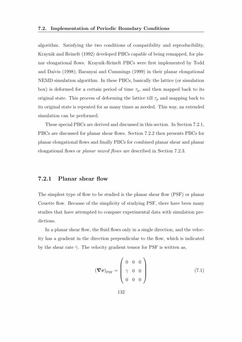
7.2. Implementation of Periodic Boundary Conditions
algorithm. Satisfying the two conditions of compatibility and reproducibility,
Kraynik and Reinelt (1992) developed PBCs capable of being remapped, for pla-
nar elongational flows. Kraynik-Reinelt PBCs were first implemented by Todd
and Daivis (1998); Baranyai and Cummings (1999) in their planar elongational
NEMD simulation algorithm. In these PBCs, basically the lattice (or simulation
box) is deformed for a certain period of time τp, and then mapped back to its
original state. This process of deforming the lattice till τp and mapping back to
its original state is repeated for as many times as needed. This way, an extended
simulation can be performed.
These special PBCs are derived and discussed in this section. In Section 7.2.1,
PBCs are discussed for planar shear flows. Section 7.2.2 then presents PBCs for
planar elongational flows and finally PBCs for combined planar shear and planar
elongational flows or planar mixed flows are described in Section 7.2.3.
7.2.1 Planar shear flow
The simplest type of flow to be studied is the planar shear flow (PSF) or planar
Couette flow. Because of the simplicity of studying PSF, there have been many
studies that have attempted to compare experimental data with simulation pre-
dictions.
In a planar shear flow, the fluid flows only in a single direction, and the veloc-
ity has a gradient in the direction perpendicular to the flow, which is indicated
by the shear rate γ. The velocity gradient tensor for PSF is written as,
(∇v)PSF =
0 0 0
γ 0 0
0 0 0
(7.1)
132

7.2. Implementation of Periodic Boundary Conditions
Though we have mentioned in Section 7.1 that the simulation box should de-
form with the flow, it is worth justifying this argument here by a visual picture.
Originally, the PBC for planar shear flow was developed by Lees and Edwards
(1972), in which they did not allow the lattice to deform but did allow it to move
in a specific manner. This is illustrated in Fig. 7.1, where red marks indicate
particles, the box in grey is the original simulation box, and other boxes are pe-
riodic images of the original box. First, we examine the case in which the lattice
is not allowed to move (as in equilibrium simulations). The top panel in Fig. 7.1
shows this case. It is clear that after being subjected to shear flow, there is no
periodicity in the lattice and hence this case is inconsistent with PBC. However,
as can be seen in the bottom panel, moving or sliding the lattice with the flow
in a specific manner maintains the periodicity in the lattice. This method is also
called the sliding brick method. In this method, the image box above the simula-
tion box is displaced by L2yγ∆t, and the image box below the simulation box is
displaced by −L2yγ∆t, where L2y is the height of the simulation box and ∆t is
the time step size. The advantage of this method is that the shape of each box
does not change and hence the lattice vectors are always orthonormal. However,
the major drawback of this method is the presence of non-aligned boundaries.
When these boxes or cells slide past each other, their cell neighbors change and
it is a burden in any algorithm to keep a track of all the neighbors of a cell with
time.
Hansen and Evans (1994) and Bhupathiraju et al. (1996) found it inefficient
to use the sliding brick method in a parallel computing environment. Therefore,
they implemented an efficient algorithm by modifying the sliding brick method
to the deforming brick method. In this method, instead of moving the cells, they
deformed the cell with time as shown in Fig. 7.2. The periodic boundary condi-
tion in this method works in the following two ways: (i) if particles move out of
133
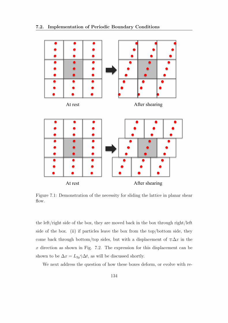
7.2. Implementation of Periodic Boundary Conditions
At rest After shearing
At rest After shearing
Figure 7.1: Demonstration of the necessity for sliding the lattice in planar shearflow.
the left/right side of the box, they are moved back in the box through right/left
side of the box. (ii) if particles leave the box from the top/bottom side, they
come back through bottom/top sides, but with a displacement of ∓∆x in the
x direction as shown in Fig. 7.2. The expression for this displacement can be
shown to be ∆x = L2yγ∆t, as will be discussed shortly.
We next address the question of how these boxes deform, or evolve with re-
134
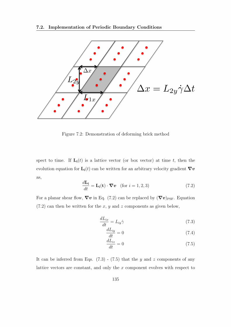
7.2. Implementation of Periodic Boundary Conditions
∆x
L1x
L2y
∆x = L2yγ∆t
Figure 7.2: Demonstration of deforming brick method
spect to time. If Li(t) is a lattice vector (or box vector) at time t, then the
evolution equation for Li(t) can be written for an arbitrary velocity gradient ∇v
as,dLi
dt= Li(t) ·∇v (for i = 1, 2, 3) (7.2)
For a planar shear flow, ∇v in Eq. (7.2) can be replaced by (∇v)PSF. Equation
(7.2) can then be written for the x, y and z components as given below,
dLixdt
= Liyγ (7.3)
dLiydt
= 0 (7.4)
dLizdt
= 0 (7.5)
It can be inferred from Eqs. (7.3) - (7.5) that the y and z components of any
lattice vectors are constant, and only the x component evolves with respect to
135

7.2. Implementation of Periodic Boundary Conditions
time. For a planar flow, L3x is also constant and the only remaining variables
are L1x and L2x that may change with time. Writing Eq. (7.3) for i = 1,
dL1x
dt= L1yγ (7.6)
Here, L1y can be considered to be 0 for convenience; this way the lattice will
always be aligned with the x-axis. As a result, L1x is constant, implying that
the top and bottom sides of the box are always constant and equal to L1x, as
depicted in Fig. 7.2. When Eq. (7.3) is written for i = 2,
dL2x
dt= L2yγ (7.7)
Recall that L2y is constant. Upon integrating Eq. (7.7), and considering an
initial condition that at time t = 0, L1 ⊥ L2, i.e., L2x(t = 0) = 0, we obtain,
L2x = L2yγt (7.8)
Based on these lattice vectors, the evolution of the lattice system is shown in
Fig. 7.3 for greater clarity. The simulation box is initially considered to be
a square in 2-D (or cube in 3-D), hence the angle between L1 and L2 is π/2
at t = 0. This angle, based on simple geometry, can be expressed in terms of
time as θs(t) = tan−1[L2y/L2x(t)] = tan−1[1/γt], where L2y is constant and L2x
increases with time as given by Eq. (7.8). It is obvious that as t→∞, θs → 0 or
L2x →∞. This situation is computationally very inefficient as it requires dealing
with very large numbers. Therefore, the simulation is not carried out for a very
long time but rather until the time at which θs = π/4, at which time, the box
is transformed back to its original square lattice shape (θs = π/2). In this way,
L2x never gets too large. The reason for choosing π/4 comes from the fact that
136

7.2. Implementation of Periodic Boundary Conditions
L1(0)
L2(0)
L1(t) = L1(0)
L2(t)
L1x
L2y
L2x(t)
θs(0) = π/2 θs(t) = tan−1
L2y
L2x(t)
Figure 7.3: Lattice evolution in planar shear flow (Reproduced from Todd andDaivis (2007))
at this angle all the deformed lattice points can be overlapped with the original
square lattice, as indicated by the black circles in Fig. 7.4. In this figure, the
initial lattice is depicted in grey, while the lattice at θs = 450 is indicated in red.
This also means that the lattice is reproducible at θs = π/4, and the time to reach
there is simply τp = 1/γ. A slight modification can be made to this process to
double the speed of the algorithm. In the modified form (Bhupathiraju et al.,
1996), the initial box is considered to have an angle of −π/4 and is allowed
to deform till θs = π/4. In this way, the transformations are carried out less
frequently. For this case, the evolution equation for L2x has a different form due
to a different initial condition (i.e., at t = 0, L2x = −L2y),
L2x = L2yγt− L2y (7.9)
The modified process is shown in Fig. 7.5. Here, the square lattice is indicated
in grey, while the initial lattice, which is oriented at −450, is shown in blue.
Upon imposing the shear flow, the blue lattice deforms and passes through a
stage, at time τp , where it overlaps with the square lattice. Continuing the
137

7.2. Implementation of Periodic Boundary Conditions
L2x(t)
+450
L2y
L1x
Figure 7.4: Lattice evolution in planar shear flow: 900 to 450 (Todd and Daivis,2007)
−450 +450
L1x(0)
L2y
L2x(0) = −L2y
Figure 7.5: Lattice reproducibility in planar shear flow: Blue indicates initiallattice, grey indicates lattice after time τp and red indicates lattice after time 2τp
138

7.2. Implementation of Periodic Boundary Conditions
deformation, at time 2τp the angle θs becomes +450 (red lattice) and then, as
discussed above, the red lattice is transformed back to the blue lattice. The
reason why this transformation is feasible is clear from Fig. 7.5; this is simply
because the lattice at +450 is reproducible to the lattice at −450. In other words,
the lattice points in these two stages (θs = −450 and + 450) overlap on top of
each other, as indicated by the black symbols in Fig. 7.5. This confirms the
reproducibility of lattices in planar shear flow, and also completes our discussion
on the PBC’s for planar shear flow.
7.2.2 Planar elongational flow
Elongational flow occurs in many industrial processes. It is generally difficult
to study this flow using computer simulations and experimental techniques. In
elongational flow, the fluid element is stretched exponentially with time, when
subjected to a constant elongational rate. Therefore, a sample of fluid quickly
becomes very thin and long as soon as elongational flow is imposed, and there
is a very short span of time in which to observe the phenomena of stretching.
Moreover, as discussed in Section 7.2.1, the simulation box needs to be deformed
to follow the motion of the fluid, resulting in an exponential increase or decrease
in the size of the simulation box. This situation is challenging because once a
side of the stretched box becomes less than twice the inter-particle interaction
range, the simulation has to cease. For carrying out indefinitely long simulations,
special periodic boundary conditions need to be developed for elongational flows.
A general velocity gradient for elongational, shear free and volume preserving
flows can be written as (Bird et al., 1987)
(∇v) =
ε 0 0
0 −ε(1 + bf)/2 0
0 0 −ε(1− bf)/2
(7.10)
139

7.2. Implementation of Periodic Boundary Conditions
where ε is the rate of elongation and bf determines the type of elongational flow.
For instance:
1. Uniaxial elongational flow occurs when bf = 0 and ε > 0
2. Biaxial elongational flow occurs when bf = 0 and ε < 0
3. Planar elongational flow occurs when bf = 1 and ε 6= 0
Kraynik and Reinelt (1992) showed that it is not possible to derive PBCs for
uniaxial and biaxial elongational flows that can be used for indefinite simula-
tion. However, they derived PBCs for planar elongational flows that satisfies
this criteria. This section discusses the periodic boundary conditions for planar
elongational flow proposed by Kraynik and Reinelt (1992).
In planar elongational flow (PEF), the fluid is stretched in one direction and
contracts in another direction with the same elongational rate ε. The velocity
gradient tensor for PEF is given by
(∇v)PEF =
ε 0 0
0 −ε 0
0 0 0
(7.11)
Here, the fluid is being stretched in the x direction and contracts in the y direc-
tion. Figure 7.6 illustrates a schematic of the deformation of a cubic simulation
box under planar elongational flow. Here, blue indicates the initial lattice and
red indicates a lattice after some time of elongation. Using this square lattice,
molecular dynamics simulations for elongational flow were first carried out by
Heyes (1985). Unfortunately, they were not able to simulate for an indefinitely
long time because at least one of the sides of the box becomes smaller than 2rc,
where rc is the cutoff radius of the inter-particle potential. If L02y is the length of
the simulation box in the contracting direction, then the maximum simulation
140
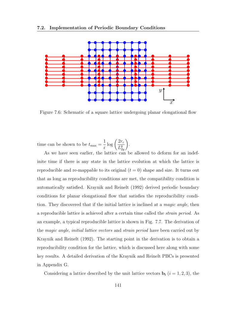
7.2. Implementation of Periodic Boundary Conditions
x
y
Figure 7.6: Schematic of a square lattice undergoing planar elongational flow
time can be shown to be tmax =1
εlog
(2rcL0
2y
).
As we have seen earlier, the lattice can be allowed to deform for an indef-
inite time if there is any state in the lattice evolution at which the lattice is
reproducible and re-mappable to its original (t = 0) shape and size. It turns out
that as long as reproducibility conditions are met, the compatibility condition is
automatically satisfied. Kraynik and Reinelt (1992) derived periodic boundary
conditions for planar elongational flow that satisfies the reproducibility condi-
tion. They discovered that if the initial lattice is inclined at a magic angle, then
a reproducible lattice is achieved after a certain time called the strain period. As
an example, a typical reproducible lattice is shown in Fig. 7.7. The derivation of
the magic angle, initial lattice vectors and strain period have been carried out by
Kraynik and Reinelt (1992). The starting point in the derivation is to obtain a
reproducibility condition for the lattice, which is discussed here along with some
key results. A detailed derivation of the Kraynik and Reinelt PBCs is presented
in Appendix G.
Considering a lattice described by the unit lattice vectors bi (i = 1, 2, 3), the
141
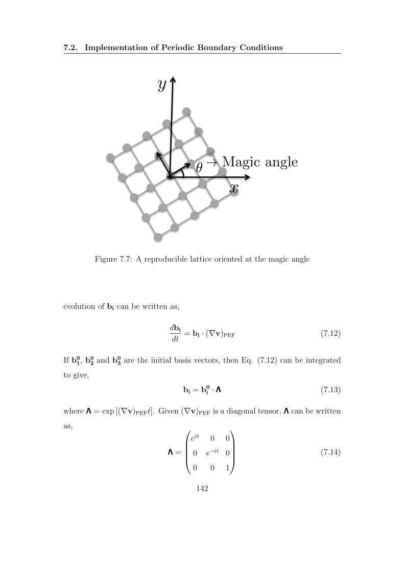
7.2. Implementation of Periodic Boundary Conditions
x
y
θ → Magic angleθ → Magic angle
Figure 7.7: A reproducible lattice oriented at the magic angle
evolution of bi can be written as,
dbi
dt= bi · (∇v)PEF (7.12)
If b01, b0
2 and b03 are the initial basis vectors, then Eq. (7.12) can be integrated
to give,
bi = b0i · Λ (7.13)
where Λ = exp [(∇v)PEFt]. Given (∇v)PEF is a diagonal tensor, Λ can be written
as,
Λ =
eεt 0 0
0 e−εt 0
0 0 1
(7.14)
142

7.2. Implementation of Periodic Boundary Conditions
Λ is also called the time evolution matrix. As Kraynik and Reinelt (1992) pointed
out, for a given Λ, a lattice is reproducible if and only if there exists integers Nij
such that,
bi = b0i · Λ = Ni1b
01 +Ni2b
02 +Ni3b
03 (7.15)
The justification of this reproducibility condition is explained in Appendix G.
The reproducibility condition can be framed in terms of an eigenvalue problem,
and the different results (such as the strain period τp and magic angle θ etc . . . )
can be interpreted in terms of eigenvalues as discussed in Appendix G. There
exist multiple solutions for the strain period and the magic angle. An example
of one such solution is θ ≈ 31.720 and τp = 0.9624/ε. This example is shown
Figure 7.8: Lattice reproducibility for planar elongational flow
schematically in Fig. 7.8, where the lattice in blue indicates the initial lattice
and the red lattice represents the lattice after τp. Clearly, the lattice points on
the red and the blue lattices overlap on top of each other (indicated by the big
blue circles), confirming the reproducibility. Once the magic angle θ is known,
143
7.2. Implementation of Periodic Boundary Conditions
the basis vectors of the initial lattice (b1,b2,b3) can be written as
b1 = (cos θ, sin θ, 0) (7.16)
b2 = (− sin θ, cos θ, 0) (7.17)
b3 = (0, 0, 1) (7.18)
The lattice based on these basis vectors is reproducible, and can be deformed till
τp. At this time (t = τp), the lattice is mapped back to its original shape and
size. This guarantees that the lattice is not deformed any more once t reaches
τp, which ensures that the compatibility condition is satisfied as well.
Having addressed issues regarding the initial lattice, magic angle and strain
period, the only remaining question to ask is: how do the lattices evolve or how
does a point in the lattice evolve? Following is a derivation for the evolution
of lattice points in PEF. If r is a position vector of a lattice point, then the
evolution equation for r can be written as
dr
dt= r · (∇v)PEF (7.19)
Using Eq. (7.11), the left hand side of the above equation can be written as
r · (∇v)PEF =(εrx, −εry, 0
)(7.20)
144

7.2. Implementation of Periodic Boundary Conditions
where rx and ry are the x and y components of r, respectively. Using Eqs. (7.19)
and (7.20), the differential equations for rx, ry and rz can be written as,
drxdt
= εrx
drydt
= −εrydrzdt
= 0
(7.21)
This set of equations can easily be integrated, if the initial conditions for each
component is known. Therefore, if r0x, r
0y and r0
z are the values of rx, ry and rz,
respectively, at time t = 0, then the expressions for rx, ry and rz are:
rx = r0x exp (εt)
rx = r0y exp (−εt)
rz = r0z = constant
(7.22)
Hence, the lattice point r evolves as r0x exp (εt), r0
y exp (−εt), r0z. In the simula-
tion algorithm, the x and y component of any lattice vector are evolved according
to Eq. (7.22). The lattice vectors Li are related to bi through Li = |Li|bi since
bi are the unit vectors in the direction of Li. It follows that if L1 is a lattice
vector in the direction of extension, then L1x will evolve as L01x exp (εt) and L1y
will evolve as L01y exp (−εt), where L0
1x and L01y are the values of L1x and L1y at
time t = 0. This completes our discussion of lattice evolution and the periodic
boundary conditions for planar elongational flow.
7.2.3 Planar mixed flow
There has been a significant amount of work on computer simulations of planar
shear and planar elongational flows because of their relative simplicity. However,
145

7.2. Implementation of Periodic Boundary Conditions
in many practical applications, a linear combination of planar shear and planar
elongational flows occur, which are denoted as planar mixed flows. An extended
molecular dynamics simulation of planar mixed flow was first carried out by Hunt
et al. (2010). With regard to polymer solutions undergoing mixed flow, simula-
tion studies have been carried out only in the dilute concentration limit by Woo
and Shaqfeh (2003); Dua and Cherayil (2003) and Hoffman and Shaqfeh (2007).
Since only a single chain is required for simulating dilute polymer solutions, there
is no need for reproducible periodic boundary conditions. However, in order to
simulate planar mixed flow of semidilute polymer solutions, this is essential. To
the best of our knowledge, there has been no attempt to simulate semidilute
polymer solutions under planar mixed flow conditions. In this thesis, we adopt
the reproducible periodic boundary conditions for planar mixed flow developed
by Hunt et al. (2010), and use it in a multi-chain Brownian dynamics simulation
algorithm for semidilute polymer solutions.
For planar mixed flow (PMF), the canonical form of the velocity gradient
tensor ∇v (Hunt et al., 2010) is given by,
(∇v)PMF =
ε 0 0
γ −ε 0
0 0 0
(7.23)
As discussed in Section 4.5.2, for the canonical form of the velocity gradient
tensor, the planar shear flow contribution is due to the velocity gradient in the
y-direction, and the contribution from planar elongational flow leads to extension
in the x-direction and contraction in the y-direction. In the canonical represen-
tation, the eigenvalues of (∇v)PMF are ε,−ε, 0, and a possible choice of the
corresponding eigenvectors is
(1,γ
2ε, 0
), (0, 1, 0) and (0, 0, 1). It is worth noting
that the eigenvalues of the velocity gradient tensor of the canonical PMF are
146

7.2. Implementation of Periodic Boundary Conditions
equivalent to those for PEF, where (∇v)PEF is already in a diagonal form. How-
ever, the eigenvectors corresponding to the eigenvalue ε are different for (∇v)PMF
and (∇v)PEF. For PEF, the eigenvector corresponding to ε is (1, 0, 0), which
leads to the fact that the extension axis and contraction axis are orthogonal.
In case of the canonical PMF, the eigenvector corresponding to ε is (1, γ/2ε,
0), resulting in a system where the extension axis and contraction axis are non-
orthogonal. The angle β between the extension axis and the contraction axis
depends on the ratio of γ to ε. The expression for β is displayed in Fig. 7.9 and
given below
β = cos−1
[γ√
γ2 + 4ε2
](7.24)
Note that, for the sake of simplicity, we will use the phrase PMF instead of
y
x
Contraction axis
Extension axis
β = cos−1
γ
γ2 + 42
Figure 7.9: Axis of extension and contraction in planar mixed flow
“canonical” PMF.
Since the eigenvalues of the velocity gradient tensor for PMF and PEF are
147

7.2. Implementation of Periodic Boundary Conditions
the same, the magic angle and strain period for PMF can be obtained in a sim-
ilar manner as in the case of PEF. However, the initial lattice configuration for
PMF is different from that of PEF because of the differences in the eigenvec-
tors discussed above. An important point made by Kraynik and Reinelt (1992)
in their derivation of PBCs for PEF is that (∇v)PEF can be replaced by any
diagonalizable constant matrix with real eigenvalues and zero trace. Following
this point, Hunt et al. (2010) realized that, in fact, (∇v)PMF is a diagonalizable
matrix as written below
ε 0 0
γ −ε 0
0 0 0
=
1 0 0
γ2ε
1 0
0 0 1
ε 0 0
0 −ε 0
0 0 0
1 0 0
− γ2ε
1 0
0 0 1
= T ·D · T−1 (7.25)
where T is a transformation matrix that consists of the eigenvectors of (∇v)PMF,
and the diagonal matrix D has the same component form as (∇v)PEF. The
Kraynik-Reinelt periodic boundary condition for PEF is written in terms of the
lattice evolution matrix Λ = exp (Dt). Similarly for PMF, as the velocity gradient
tensor (∇v)PMF is diagonalizable, we can write the lattice evolution matrix Λ′
as
Λ′ = exp ((∇v)PMFt) = exp (T ·D · T−1t) = T · exp (Dt) · T−1 (7.26)
As (∇v)PMF = T ·D · T−1 with D being a diagonal matrix, a new set of initial
basis vectors,
b0i′= b0
i · T−1 (for i = 1, 2, 3) (7.27)
exists in PMF, such that this new set is reproducible in the case of PMF (Hunt
et al., 2010). The tensor T−1, thus, can be understood as a mapping necessary
to make the PEF basis vectors b0i (in PEF) reproducible in the PMF. Similar to
148
7.2. Implementation of Periodic Boundary Conditions
Eqs. (7.13) and (7.15), an equation for the lattice reproducibility condition for
PMF can be written as
bi′ = b0
i′ · Λ′ (7.28)
where bi′ denotes the lattice vector at time τp (strain period). Using this rela-
tion, and substituting Λ′ form Eq. (7.26) in Eq. (7.28) leads to the following
simplification
bi′(t = τp) = b0
i′ · Λ′(τp)
= b0i · T−1 · T · exp (Dt) · T−1
= b0i · exp (Dt) · T−1
=[Ni1b
01 +Ni2b
02 +Ni3b
03
]· T−1 (see Eq. (7.15))
= Ni1b01 · T−1 +Ni2b
02 · T−1 +Ni3b
03 · T−1
= Ni1b01′+Ni2b
02′+Ni3b
03′
(7.29)
This equation for the reproducibility condition is identical to the one for PEF
(Eq. (7.15)), except that b0i is replaced by b0
i′. The vectors b0
1′, b0
2′and b0
3′can
be found easily since b01, b0
2 and b03 are known as discussed in Section 7.2.2. The
mapping of Eq. (7.27) is applied to b0i to obtain a reproducible lattice under
mixed flow as follows.
b01′= b0
1 · T−1
=(
cos θ sin θ 0)
1 0 0
− γ2ε
1 0
0 0 1
=
[(cos θ − γ
2εsin θ
), sin θ, 0
]
(7.30)
149

7.2. Implementation of Periodic Boundary Conditions
b02′= b0
2 · T−1
=(− sin θ cos θ 0
)
1 0 0
− γ2ε
1 0
0 0 1
=
[(− sin θ − γ
2εcos θ
), cos θ, 0
]
(7.31)
b03′= b0
3 · T−1
=(
0 0 1)
1 0 0
− γ2ε
1 0
0 0 1
= [0, 0, 1]
(7.32)
where θ is the magic angle, which is similar to that for PEF. In contrast to
PEF, where the basis lattice vectors are orthogonal, in the case of PMF, they
are non-orthogonal and not equal in length. If the elongational rate is high or the
shear rate is small, these lattice vectors becomes almost orthogonal and equal
in length. These basis lattice vectors are used as an initial lattice configuration
and the simulation is then run till the time approaches τp. The lattice is then
mapped back to its original state, and this way the simulation can be carried out
for extended period.
The question of how the lattices evolve in PMF can be addressed in a similar
manner as has been done for PEF in Section 7.2.2. The evolution equation for
a lattice point is shown in Eq. (7.19). The same equation can be used here but
with (∇v)PEF replaced by (∇v)PMF given by Eq. (7.23). The left hand side of
Eq. (7.19) for PMF becomes
r · (∇v)PMF =(εrx + γry, −εry, 0
)(7.33)
150

7.2. Implementation of Periodic Boundary Conditions
Equations (7.19) and (7.33) can be used to obtain the differential equations for
rx, ry and rz as,
drxdt
= (εrx + γry)
drydt
= −εrydrzdt
= 0
(7.34)
If r0x, r
0y and r0
z are considered to be the initial values of rx, ry and rz, respectively,
then these equations can be integrated and expressions for rx, ry and rz can be
found. For instance, ry can be found to be
ry(t) = r0y exp (−εt) (7.35)
and rz is simply a constant equal to r0z . The governing differential equation for
rx is a first order linear differential equation that can be integrated to give
rx = exp(εt)
[−
˙γr0y
2εexp(−2εt) + C
](7.36)
Using the initial condition for rx, C can be found to be r0x +
γ
2εr0y. As a result,
rx =γ
εr0y sinh(εt) + r0
x exp (εt) (7.37)
The lattice point r consequently evolves as γεr0y sinh(εt)+r0
x exp (εt), r0y exp (−εt),
r0z. In the simulation algorithm, the x and y components of any lattice vector
are evolved simply according to Eq. (7.22). For example, if L1 is a lattice vector
in the direction of extension, then L1x will evolve as γεL0
1y sinh(εt) + L01x exp (εt)
and L1y will evolve as L01y exp (−εt), where L0
1x and L01y are the values of L1x and
151

7.3. Modifications in Calculating the Ewald Summation in thePresence of Flow
L1y at time t = 0.
There is only one issue left to discuss regarding the implementation of PMF
in the simulation algorithm, and that is related to the compatibility condition.
As discussed earlier, the length of one of the sides of the simulation box decreases
with time. Kraynik and Reinelt (1992) showed that the reproducibility condi-
tion automatically guarantees the compatibility condition. In other words, they
showed that the distance D(τp) between any two lattice points at time τp is never
less than the minimum lattice spacing Dmin, such that the lattice points do not
overlap. In simulations, the cutoff radius of any inter-particle interaction poten-
tial is always chosen to be less than Dmin/2, and that assures the compatibility
condition is satisfied. The derivation of Dmin has been carried out by Hunt et al.
(2010), and here the detailed steps of the derivation are presented in Appendix
H. This completes our discussion of the periodic boundary conditions for planar
mixed flow.
7.3 Modifications in Calculating the Ewald Sum-
mation in the Presence of Flow
The Ewald summation method for hydrodynamic interactions has been presented
in Section 5.2 for a cubic simulation cell in the context of equilibrium simulations.
However, for far from equilibrium simulations, a cubic simulation cell cannot be
considered because the simulation cell continuously deforms to be consistent
with the imposed flow. A generalized Ewald sum method for a parallelepiped
simulation cell was first developed by Wheeler et al. (1997), who adapted it
for the Lees-Edwards periodic boundary condition. The same procedure can be
adopted for any flow geometry such as planar elongational or planar mixed flows.
Here, we briefly outline the important changes that need to be made in the real
152
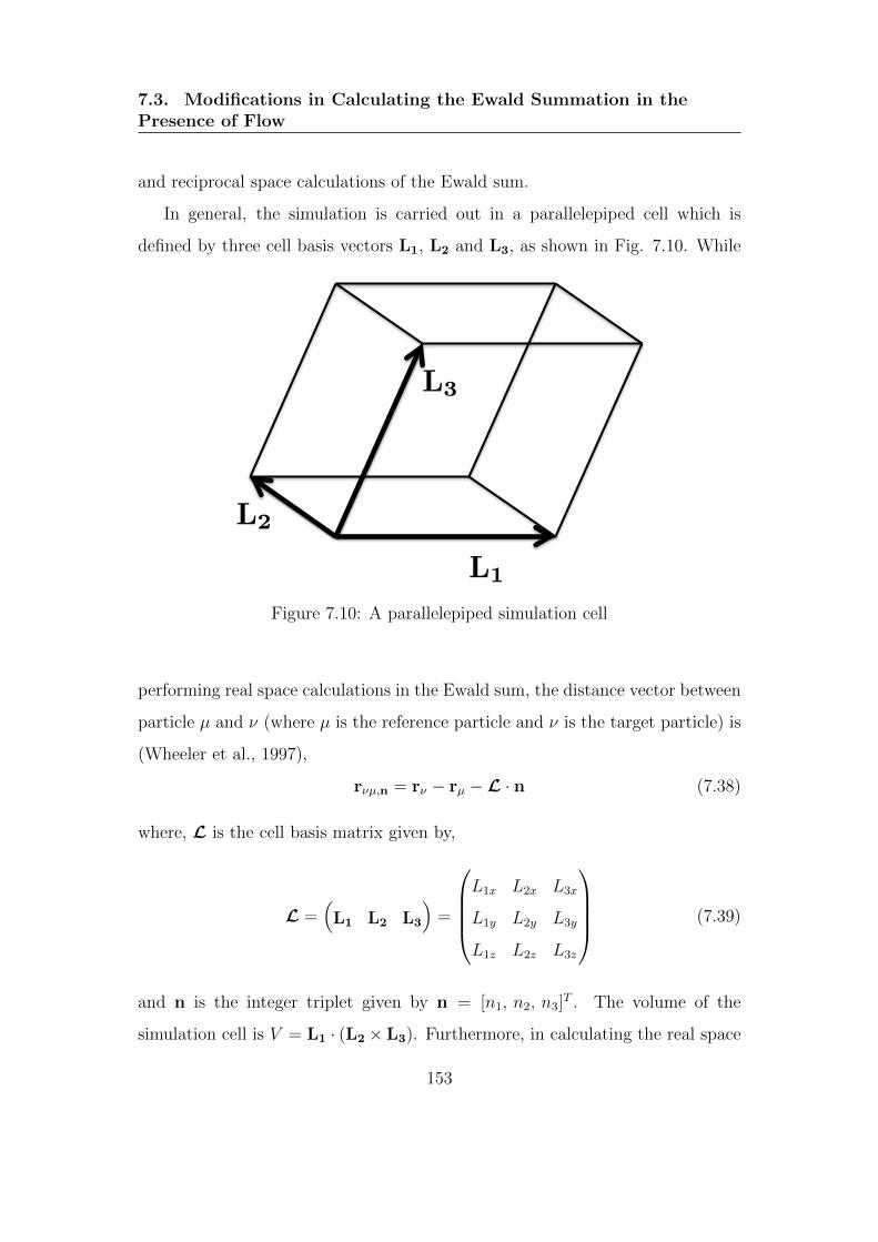
7.3. Modifications in Calculating the Ewald Summation in thePresence of Flow
and reciprocal space calculations of the Ewald sum.
In general, the simulation is carried out in a parallelepiped cell which is
defined by three cell basis vectors L1, L2 and L3, as shown in Fig. 7.10. While
L1
L2
L3
Figure 7.10: A parallelepiped simulation cell
performing real space calculations in the Ewald sum, the distance vector between
particle µ and ν (where µ is the reference particle and ν is the target particle) is
(Wheeler et al., 1997),
rνµ,n = rν − rµ −L · n (7.38)
where, L is the cell basis matrix given by,
L =(L1 L2 L3
)=
L1x L2x L3x
L1y L2y L3y
L1z L2z L3z
(7.39)
and n is the integer triplet given by n = [n1, n2, n3]T . The volume of the
simulation cell is V = L1 · (L2 × L3). Furthermore, in calculating the real space
153

7.3. Modifications in Calculating the Ewald Summation in thePresence of Flow
part of the sum, it is important to make sure that the magnitude of rνµ,n for any
pair µ and ν is always less than the real space cutoff radius rc. In equilibrium
simulations, once the cutoff radius is fixed, the number of neighboring cells or
the cell neighbor-list is fixed for a given cell. However, in flow simulations,
the implementation of the neighbor-list is much more complicated because the
number of neighboring cells for a given cell keeps changing as the cells deform
(Todd and Daivis, 1999).
In the reciprocal space part of the Ewald sum, the procedure remains the
same as for equilibrium simulations, except the way in which the wave-vectors
are calculated. For flow simulations, since the simulation cell is not a cube, the
wave-vectors depend on the lattice vector of the simulation cell. The wave-vectors
are generated through (Wheeler et al., 1997),
k = 2π(LT )−1 · n (7.40)
In flow simulations, the difficulty in calculating the reciprocal space sum arises
due to the fact that M(2)(k) (see Section 5.2.1) needs to be updated at each time
step, where as in the case of equilibrium simulations this term is calculated only
once in the beginning of the simulation, and then used in all the time steps.
In equilibrium simulations there are a few terms in both the real and the
reciprocal sums that are not updated at each time step but rather calculated in
the beginning and used for the rest of the simulation. However, this is not true
for flow simulations in which all the terms need to be updated at each time step.
Therefore, this problem leads to an increase in the CPU cost as compared to the
cost in equilibrium simulations.
154

7.4. Validation Studies
7.4 Validation Studies
The validation of the extended BD algorithm has been carried out at very low
concentrations, where the results of multi-chain BD can be compared with single-
chain BD simulations for dilute polymer solutions. Due to time constraints, we
have not carried out simulations with hydrodynamic interactions, but only with
excluded volume interactions. Nevertheless, this allows us to test various aspects
of the algorithm. This section presents some preliminary data on validation of
the BD algorithm for flow simulations.
7.4.1 Planar shear flow
The main aspects in the development of a BD algorithm for flow simulations are
the implementation of (i) a neighbor-list and (ii) periodic boundary conditions.
We first validate our algorithm for a case in which these two implementations are
unnecessary. This allows us to identify errors in the algorithm from sources other
than due to the neighbor-list and PBCs implementation. The neighbor-list and
PBCs do not play any role in the simulation when hydrodynamic and excluded
volume interactions are ignored. Such a case is well described by the Rouse model
for which analytical expressions for various properties are known. We switched
off HI and EV interactions and computed the dimensionless mean square end-
to-end distance 〈R2e〉 of chains consisting of 10 beads in the ultra dilute limit,
as a function of dimensionless shear rate γ, and compared with Rouse model
predictions given by (Bird et al., 1987)
〈R2e〉Rouse = 〈R2
e〉eq
[1 +
Nb (Nb + 1) (N2b + 1) γ2
45
](7.41)
where, it may be recalled that 〈R2e〉eq = 3(Nb− 1) is the mean square end-to-end
distance at equilibrium (Bird et al., 1987). Red symbols in Fig. 7.11 indicate the
155

7.4. Validation Studies
0 0.2 0.4 0.6 0.8 1101
102
103
104
!
!R2 e"
BD SimulationRouse Model
c/c! = 4.6 # 10!5
Nb = 10
Figure 7.11: Mean square end-to-end distance obtained by BD simulations com-pared with Rouse model predictions, for bead-spring chains with Nb = 10 beads.
results for 〈R2e〉 obtained by carrying out multi-chain BD simulations. The solid
line in the figure shows the Rouse model predictions for a 10 bead chain. Multi-
chain BD simulations were carried out by considering Nc = 30, c/c? = 4.6×10⁻⁵
and a time step size ∆t = 0.005.
In order to test the neighbor-list and PBCs implementations, we have carried
out multi-chain BD simulations of dumbbells (Nb = 2) in a ultra dilute system
with EV interactions between the beads. In this study, simulations were carried
out using z = 1.7, Nc = 10, c/c? = 6 × 10⁻¹² and ∆t = 0.005. A large number
of independent runs (in the range of 103 - 105) were performed to obtain better
statistics. Figure 7.12 shows the results for 〈R2e〉 and 〈R2
g〉 for a range of shear
156
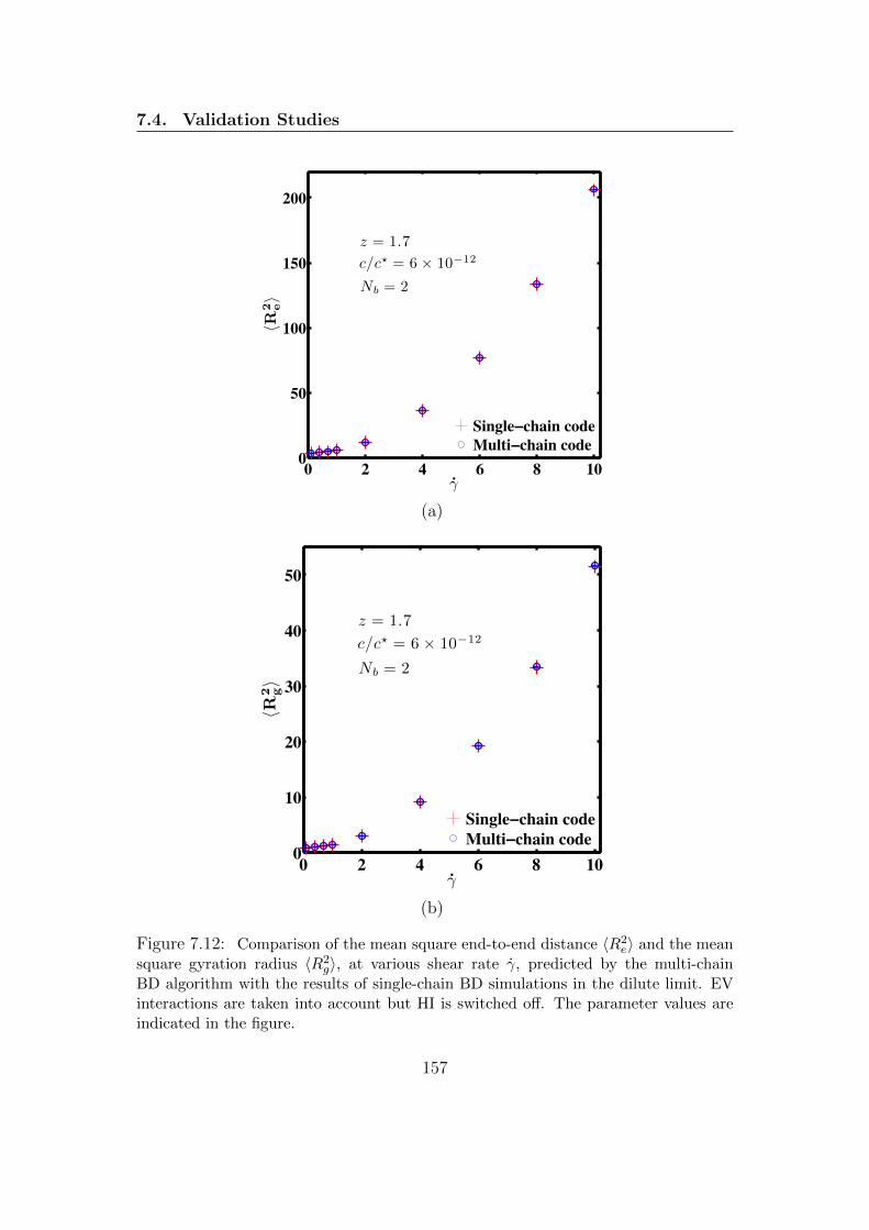
7.4. Validation Studies
0 2 4 6 8 100
50
100
150
200
!
!R2 e"
Single chain codeMulti chain code
z = 1.7
c/c! = 6 # 10!12
Nb = 2
(a)
0 2 4 6 8 100
10
20
30
40
50
!
!R2 g"
Single chain codeMulti chain code
z = 1.7
c/c! = 6 # 10!12
Nb = 2
(b)
Figure 7.12: Comparison of the mean square end-to-end distance 〈R2e〉 and the mean
square gyration radius 〈R2g〉, at various shear rate γ, predicted by the multi-chain
BD algorithm with the results of single-chain BD simulations in the dilute limit. EVinteractions are taken into account but HI is switched off. The parameter values areindicated in the figure.
157

7.4. Validation Studies
rates. These results are compared with the results obtained using single-chain
BD simulations (for which the neighbor-list and PBCs are not required). Clearly,
the agreement with single-chain simulations indicates our BD algorithm is valid.
We have also computed the viscosity η as a function of the shear rate γ and
compared the results with single-chain BD simulations. Here η is calculated using
Eq. (4.30), by considering χ = 0 and Γ = γ. Blue circles in Fig. 7.13 show the
multi-chain BD simulation results for the viscosity and the red plus symbols rep-
resent the data obtained by running single-chain BD simulations. Clearly, there
is agreement between the multi-chain and single-chain BD simulation results.
Also, shear thinning behavior can be observed in Fig. 7.13. At low shear rates,
excluded volume effects increase the size of polymer chains and hence increase
the viscosity. The decrease in viscosity with increasing γ is due to excluded vol-
ume interactions being switched off as the dumbbells undergo stretching in shear
flow.
Though HI was not considered in the validation of physical properties, a basic
check of the implementation of the Ewald sum for HI was carried out by compar-
ing the numerical value of the Ewald sum obtained using the planar shear flow
code at θs = 00 with that obtained using the equilibrium code for the same bead
configuration. We also calculated the Ewald sum at θs = 450 and −450, and
obtained results that matched with the equilibrium results. A more thorough
check will be carried out by evaluating dynamic properties in the future, with
the inclusion of HI.
7.4.2 Planar elongational flow
We now turn our attention to validation studies for the planar elongational flow
(PEF) case. Our implementation of the Ewald sum was checked by using a sim-
ilar approach to that for the case of PSF. We computed the Ewald sum for a
158

7.4. Validation Studies
2 4 6 8 101
1.02
1.04
1.06
!
"
Nb = 2, z = 1.7
Single-chain code(c/c! = 0)
Multi-chain code(c/c! = 6 ! 10!12)
Figure 7.13: Comparison of the viscosity η, at various γ, predicted by the multi-chain BD algorithm with the results of single-chain BD simulations in the dilutelimit
given bead configuration (i) in a simulation cell oriented at the magic angle of
θ = 31.720, which corresponds to the initial simulation setup, and (ii) in a simu-
lation cell at its maximum permissible deformed state, which occurs at the strain
period. Ewald sums in both the cases were found to be identical because in these
two cases the lattices are reproducible and periodic. This agreement establishes
the correct implementation of the modified Ewald sum in the context of PEF as
well. This study required calculating the Ewald sum at just one instant of time.
A more thorough check of physical property predictions will be carried out in
159

7.4. Validation Studies
the future with the inclusion of HI.
We have, however, computed physical properties in PEF with EV interac-
tions included. In PEF simulations, it turns out that as time progresses, the
numerical values of the x coordinates of beads increases due to elongation in the
x direction. As a result, after a long time, the numerical values are so high that
the simulation suffers from numerical instability. In order to illustrate the prob-
lem, an example of PEF viscosity η1 for FENE dumbbells with finite extensibility
parameter bp = 50 and for elongation rate ε = 0.3 is shown as a function of time
in Fig. 7.14. The correct value of η1 for the same parameters can be found by
carrying out single-chain BD simulations, and it is found to be 4.351 ± 0.002.
It is clear that the value of η1 reaches 4.35 very rapidly, however, after about
25 strain periods, a catastrophic change is observed. Eventually, η1 settles to a
wrong value. A similar numerical instability has been observed in NEMD sim-
ulations of PEF, however, the source of this instability has been attributed to
the lack of momentum conservation due to numerical round-off errors (Todd and
Daivis, 2000).
We have solved the instability problem with the following approach. After
each strain period, it is checked whether a chain is in close proximity of the
simulation box. In order to check this proximity, the following steps are used.
If rν,x, rν,y and rν,z are the coordinates of bead ν, then, if either |rν,x| > 2L1,
|rν,y| > 2L2, or |rν,z| > 2L3, the bead ν is considered to not be in the proximity of
the simulation box. Here, L1, L2 and L3 are the magnitudes of cell basis vectors
L1, L2 and L3, respectively. If all the beads of a chain are not in the proxim-
ity of the simulation box, then we abandon this chain, and begin to follow the
trajectory of the image of this chain that is in the proximity of the simulation
box. This does not affect in anyway the calculation of any of the properties,
since we are still tracking the trajectories of the same set of N unique particles
160
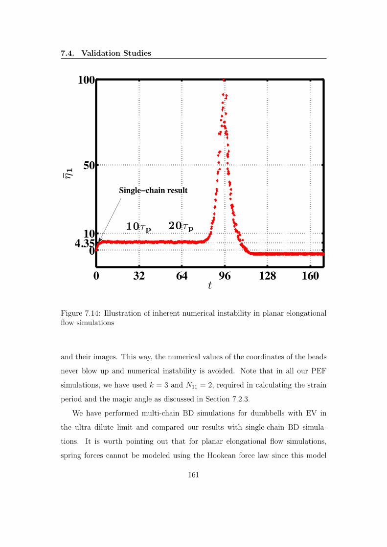
7.4. Validation Studies
0 32 64 96 128 160
04.3510
50
100
t
!1
10"p 20"p
Single chain result
Figure 7.14: Illustration of inherent numerical instability in planar elongationalflow simulations
and their images. This way, the numerical values of the coordinates of the beads
never blow up and numerical instability is avoided. Note that in all our PEF
simulations, we have used k = 3 and N11 = 2, required in calculating the strain
period and the magic angle as discussed in Section 7.2.3.
We have performed multi-chain BD simulations for dumbbells with EV in
the ultra dilute limit and compared our results with single-chain BD simula-
tions. It is worth pointing out that for planar elongational flow simulations,
spring forces cannot be modeled using the Hookean force law since this model
161

7.4. Validation Studies
10 1 1000
20
40
60
80
!
"1
Nb = 2, b = 50, z! = 0
Single-chain code
Multi-chain code
(a)
0.9 1 2 3
40
50
60
70
80
90
!
"1
Nb = 2, b = 50, z! = 10
Single-chain code
Multi-chain code
(b)
Figure 7.15: Comparison of η1, at various ε, predicted by the multi-chain BD algo-rithm with the results of single-chain BD simulations in the dilute limit: (a) for z? = 0and (b) for z? = 10.
162

7.5. Preliminary Results and Discussion for Planar Mixed Flows
allows the molecule to be extended indefinitely, which is clearly physically unre-
alistic. The finite extensibility of the polymer becomes important in situations
where a polymer molecule is likely to be close to full extension, such as in strong
shear or elongational flows. We use FENE springs to model the spring forces in
simulating planar elongational flow.
We have carried out multi-chain BD simulations to obtain the planar elon-
gational flow viscosity η1 for a range of ε, for z? = 0 and for z? = 10. Note that
z? = 10 corresponds to z = 10 ×√
2 = 14.142. We set the other parameter in
EV potential, d? to be equal to 1. Other than these parameters, we have used
Nc = 500, c/c? = 2×10⁻¹⁶ and the FENE parameter bp = 50. Simulation results
for z? = 0 and 10 are shown in Figs. 7.15 (a) and (b), respectively, obtained
by both multi-chain and single-chain simulations. Clearly, in both the cases, we
can see the agreement between the multi-chain and single-chain BD simulation
results for dilute solutions of FENE dumbbells.
This completes our discussion of validation studies for planar shear and pla-
nar elongational flow. Clearly, as the planar mixed flow is a linear combination of
planar shear and elongational flows, the algorithm developed here can be used to
predict various rheological properties of semidilute polymer solutions undergoing
planar mixed flow. Some preliminary results are presented in the next section.
7.5 Preliminary Results and Discussion for Pla-
nar Mixed Flows
The purpose of this section is to show that we have a working algorithm to
simulate semidilute polymer solutions at finite concentration, undergoing planar
mixed flow. In order to show this, we consider a very simple system of FENE
dumbbells (Nb = 2) at the overlap concentration (c = c?). With regard to
163

7.5. Preliminary Results and Discussion for Planar Mixed Flows
microscopic interactions, for reasons discussed in the previous section, we do
not account for hydrodynamic interactions in this study. However, we consider
excluded volume interactions, which allows us to capture some of the interesting
rheological behavior of polymer solutions at finite concentration in the mixed flow
geometry. Various results, obtained by running BD simulations with the FENE
parameter bp = 50, and for excluded volume interaction parameters z? = 10 and
d? = 1, are presented here. In discussing results for PMF, we have a choice
of using either the pair (Γ, χ), or (ε, γ) as variables with which to explore the
behavior of polymer solutions. Both give valuable insights. However, because of
time constraints, only the latter pair of variables has been examined here.
Prior to carrying out simulations for a finite concentration system, it is a
prerequisite to know the value of c?, which is defined as Nb/
[4π
3(R0
g)3
], where
R0g is the gyration radius for an isolated chain at equilibrium. We carry out
BD simulation for an ultra dilute system (as discussed in the previous section)
at equilibrium for Nb = 2, bp = 50, z? = 10 and d? = 1. Using a time step
size of 0.005, the value of R0g is found to be 1.2023 ± 0.0001, which is used to
calculate c? as 0.27473 ± 9 × 10⁻⁵. Using c = c?, BD simulations for PMF are
then carried out for a range of shear rates γ and elongation rates ε. For the
strain period and magic angle calculations, we use k = 3 and N11 = 2, which
results in a magic angle θ ∼= 31.720. For better statistical accuracy of the various
results, a large number of dumbbells (Nc = 500 − 1000), a sufficiently large
number of independent trajectories (in the range of 500 − 1000), and a long
enough simulation length (500 dimensionless time units) are considered in our
simulations.
Figure 7.16 (a) displays results for the mean square end-to-end distance 〈R2e〉
as a function of elongation rate ε at fixed values of shear rate γ. The coil-stretch
transition can be seen in Fig. 7.16 (a), where the dumbbells are coils for low ε,
164
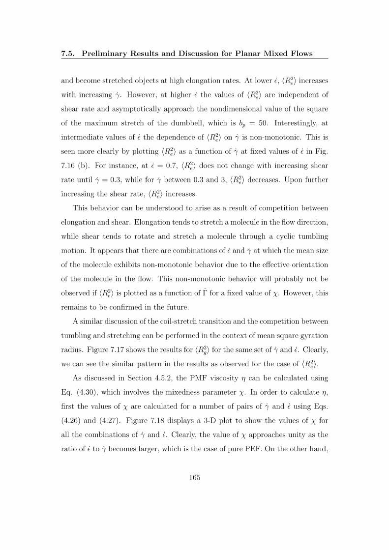
7.5. Preliminary Results and Discussion for Planar Mixed Flows
and become stretched objects at high elongation rates. At lower ε, 〈R2e〉 increases
with increasing γ. However, at higher ε the values of 〈R2e〉 are independent of
shear rate and asymptotically approach the nondimensional value of the square
of the maximum stretch of the dumbbell, which is bp = 50. Interestingly, at
intermediate values of ε the dependence of 〈R2e〉 on γ is non-monotonic. This is
seen more clearly by plotting 〈R2e〉 as a function of γ at fixed values of ε in Fig.
7.16 (b). For instance, at ε = 0.7, 〈R2e〉 does not change with increasing shear
rate until γ = 0.3, while for γ between 0.3 and 3, 〈R2e〉 decreases. Upon further
increasing the shear rate, 〈R2e〉 increases.
This behavior can be understood to arise as a result of competition between
elongation and shear. Elongation tends to stretch a molecule in the flow direction,
while shear tends to rotate and stretch a molecule through a cyclic tumbling
motion. It appears that there are combinations of ε and γ at which the mean size
of the molecule exhibits non-monotonic behavior due to the effective orientation
of the molecule in the flow. This non-monotonic behavior will probably not be
observed if 〈R2e〉 is plotted as a function of Γ for a fixed value of χ. However, this
remains to be confirmed in the future.
A similar discussion of the coil-stretch transition and the competition between
tumbling and stretching can be performed in the context of mean square gyration
radius. Figure 7.17 shows the results for 〈R2g〉 for the same set of γ and ε. Clearly,
we can see the similar pattern in the results as observed for the case of 〈R2e〉.
As discussed in Section 4.5.2, the PMF viscosity η can be calculated using
Eq. (4.30), which involves the mixedness parameter χ. In order to calculate η,
first the values of χ are calculated for a number of pairs of γ and ε using Eqs.
(4.26) and (4.27). Figure 7.18 displays a 3-D plot to show the values of χ for
all the combinations of γ and ε. Clearly, the value of χ approaches unity as the
ratio of ε to γ becomes larger, which is the case of pure PEF. On the other hand,
165
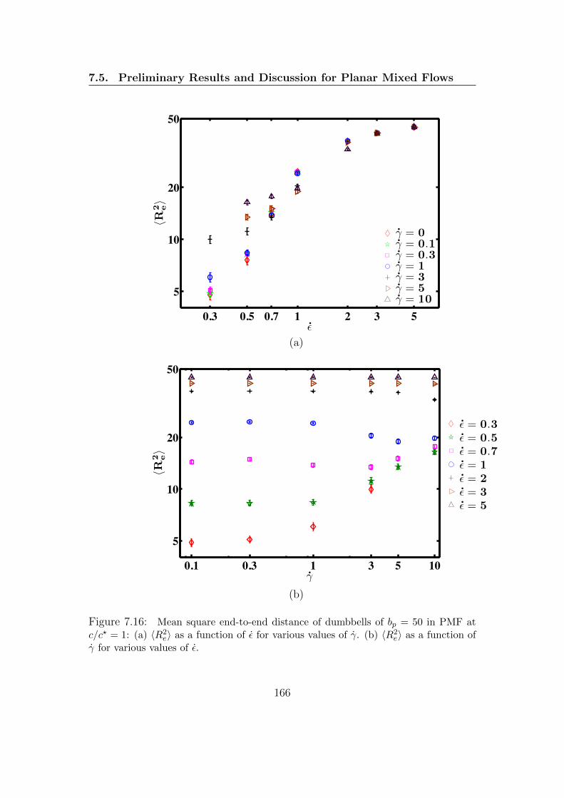
7.5. Preliminary Results and Discussion for Planar Mixed Flows
0.3 0.5 0.7 1 2 3 5
5
10
20
50
!
!R2 e"
" = 0" = 0.1" = 0.3" = 1" = 3" = 5" = 10
(a)
0.1 0.3 1 3 5 10
5
10
20
50
!
!R2 e"
" = 0.3" = 0.5" = 0.7" = 1" = 2" = 3" = 5
(b)
Figure 7.16: Mean square end-to-end distance of dumbbells of bp = 50 in PMF atc/c? = 1: (a) 〈R2
e〉 as a function of ε for various values of γ. (b) 〈R2e〉 as a function of
γ for various values of ε.
166

7.5. Preliminary Results and Discussion for Planar Mixed Flows
0.3 0.5 0.7 1 2 3 5100
101
!
!R2 g"
" = 0" = 0.1" = 0.3" = 1" = 3" = 5" = 10
(a)
0.1 0.3 1 3 5 10100
101
!
!R2 g"
" = 0.3" = 0.5" = 0.7" = 1" = 2" = 3" = 5
(b)
Figure 7.17: Mean square gyration radius of dumbbells of bp = 50 in PMF at c/c? = 1:(a) 〈R2
g〉 as a function of ε for various values of γ. (b) 〈R2g〉 as a function of γ for various
values of ε.
167
7.5. Preliminary Results and Discussion for Planar Mixed Flows
02
46
02
460
0.2
0.4
0.6
0.8
1
Shear rate !Elongational rate "
Mix
edness
para
mete
r#
0.1
0.2
0.3
0.4
0.5
0.6
0.7
0.8
0.9
Figure 7.18: Mixedness parameter χ as function of γ and ε
χ→ 0 asε
γ→ 0, which corresponds to pure PSF limit.
The PMF viscosity is then calculated using these values of χ for a number
of values of γ and ε. Figure 7.19 (a) shows the results for η as a function of ε
at fixed values of γ. Similar to the discussion in the context of Fig. 7.16, here
also we can see the PMF viscosity corresponds to the coiled state at low ε, while
it corresponds to the stretched state at high ε. It is worth pointing out that
the PEF viscosity η1 for FENE dumbbells in dilute solutions at high ε is given
analytically by (Bird et al., 1987)
η1 = 2bp(1−bp + 3
2bp
1
ε+ . . .) (7.42)
which, in the limit ε→∞, becomes η1 = 2bp = 100. Interestingly, Fig. 7.19 (a)
shows that the PMF viscosity η seems to be approaching this value for high ε,
irrespective of the shear rate. Note that for a given ε, the viscosity is lower as γ
168

7.6. Conclusions
increases. This can be attributed to shear thinning.
The shear-thinning phenomena can be observed in Fig. 7.19 (b), which is
a plot of η as function of γ for various values of ε. It is interesting to observe
that the shear-thinning sets in later when the elongational rate is higher. For
instance, for ε = 5, the shear-thinning starts at about γ = 1, while it sets in at
about γ = 0.3 for ε = 1. The phenomena of shear-thinning is related to the align-
ment of polymer chains. Tumbling brought about by shear favors alignment. For
higher ε/γ ratios, it appears that tumbling is hindered, and as a result alignment
is weaker.
This completes our discussion on the few preliminary results obtained for
semidilute polymer solutions of FENE dumbbells at overlap concentration un-
dergoing PMF. These results which appear physically meaningful, give us confi-
dence that the algorithm is correctly implemented, and paves the way to carry
out more detailed studies of PMF in the future.
7.6 Conclusions
The implementation of a variety of flows in the context of a BD simulation algo-
rithm for semidilute polymer solutions was presented in this chapter. Though,
a detailed simulation study was not carried out using the algorithm we have
developed, validation studies and some preliminary results show that this algo-
rithm can indeed be used to study planar mixed flows in detail in the future. In
summary,
1. Periodic boundary conditions for planar shear flow have been implemented
using the Lees Edwards periodic boundary condition (Lees and Edwards,
1972).
2. The Kraynik-Reinelt periodic boundary condition (Kraynik and Reinelt,
169
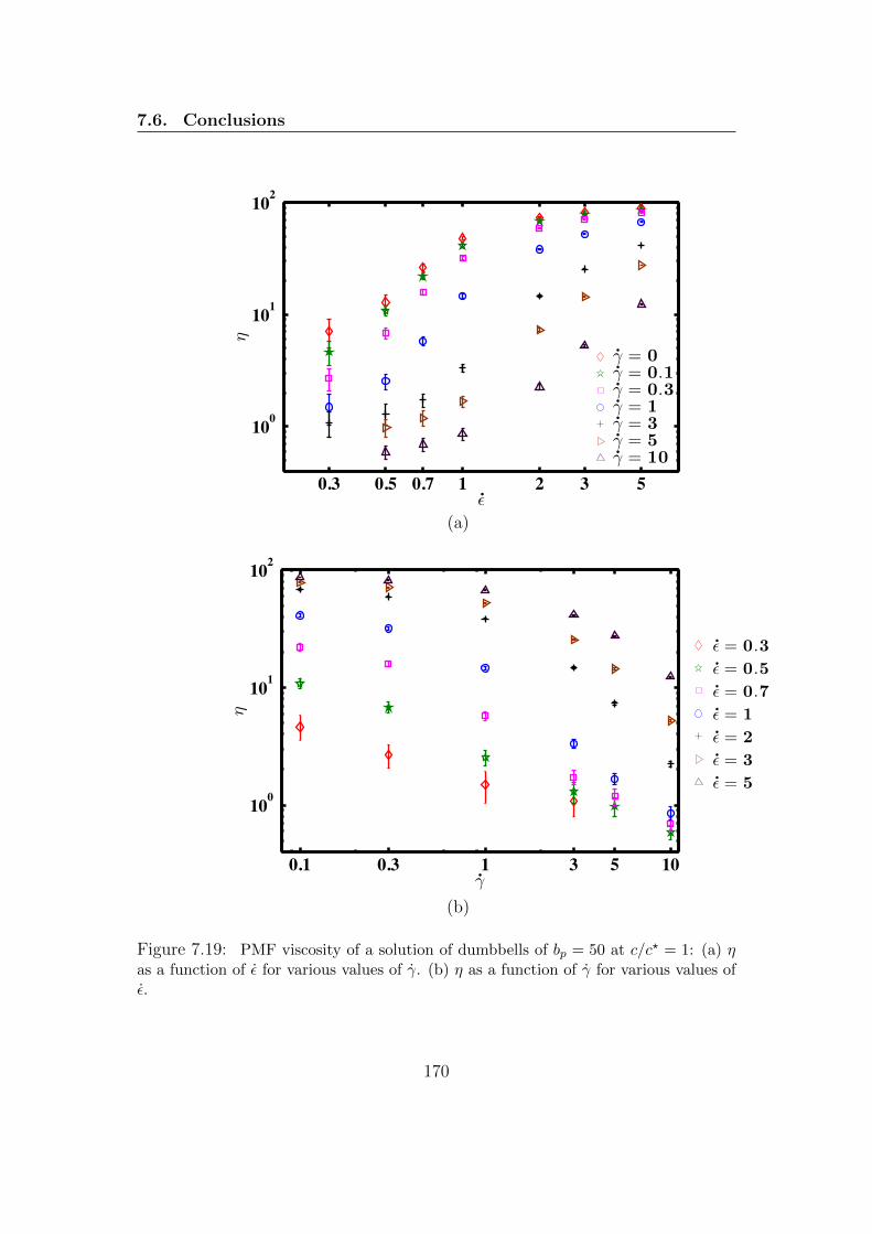
7.6. Conclusions
0.3 0.5 0.7 1 2 3 5
100
101
102
!
"
# = 0# = 0.1# = 0.3# = 1# = 3# = 5# = 10
(a)
0.1 0.3 1 3 5 10
100
101
102
!
"
# = 0.3
# = 0.5
# = 0.7
# = 1
# = 2
# = 3
# = 5
(b)
Figure 7.19: PMF viscosity of a solution of dumbbells of bp = 50 at c/c? = 1: (a) ηas a function of ε for various values of γ. (b) η as a function of γ for various values ofε.
170

7.6. Conclusions
1992) has been used to implement planar elongational flow. This PBC has
also been extended to the case of planar mixed flow, developed by Hunt
et al. (2010) in the context of NEMD simulations.
3. The calculation of the Ewald sum for hydrodynamics interactions has been
modified to account for a non-cubical simulation box.
4. Planar shear and planar elongational flows have been validated in the dilute
concentration regime by comparing results of the multi-chain code with the
results obtained from running single-chain BD simulations.
5. Some preliminary results have been obtained for FENE dumbbells at the
overlap concentration for a range of shear and elongational rates.
171

7.6. Conclusions
172
Chapter 8
Conclusions and Future Work
8.1 Conclusions
The broad objective of this work has been to understand the behavior of poly-
mer solutions in the semidilute regime at and far from equilibrium with the help
of Brownian dynamics simulations. In particular, we have focused greater at-
tention on understanding the concentration and solvent quality dependence of
various static and dynamic properties at equilibrium. With regard to far from
equilibrium systems, a BD algorithm for planar mixed flow, which is a linear
combination of shear and elongational flows, was developed for semidilute poly-
mer solutions. In particular, the following is a brief list of the key aspects of this
thesis:
1. Semidilute polymer solutions have largely been understood through scaling
theories, particularly in the limit of theta and good solvents. We have
developed a scaling theory (Chapter 3) that is valid in the entire double
crossover region of the phase diagram of polymer solutions.
2. Scaling theory has helped us arrive at the general conclusion that the
173
8.1. Conclusions
crossover scaling functions φR, φD and φη depend on the scaling variables
z and (c/c?). This can be tested either by experiments or computer simu-
lations. However, scaling theory does not reveal the specific forms of these
functions.
3. We have developed an optimized BD algorithm (Chapter 5) that is capa-
ble of (i) simulating semidilute polymer solutions with hydrodynamic and
excluded volume interactions, and (ii) controlling solvent quality across
the entire domain from theta to good solvents. We have also developed a
systematic procedure for obtaining universal predictions in the long-chain
limit.
4. With the help of the BD algorithm, we have shown the general validity of
the scaling predictions, and in particular, we have teased out the specific
dependence of the crossover scaling functions on z and (c/c?) (Chapter 6).
It appears that the dependence on (c/c?) is identical to the good solvent
limit, while the dependence on z comes in through an effective exponent.
It can be said that by these steps, a fairly complete understanding of the
static and dynamic behavior of semidilute solutions has been achieved at
equilibrium.
5. The challenge in the future is to study semidilute solutions far from equilib-
rium and to carry out a systematic comparison with experimental observa-
tions. Not much is currently understood of the behavior of semidilute poly-
mer solutions across a range of concentrations. With a view to facilitating
these studies in the future, we have extended the BD algorithm to describe
planar mixed flows (Chapter 7). The advantage of our implementation is
that it allows one to study the limit of planar shear and elongational flows
174

8.2. Future Work
and all the combinations in between. Preliminary results show that our
implementation is robust and agrees with earlier results where relevant.
8.2 Future Work
Some directions in which the current work can be taken further are listed below.
1. An improvement in the speed of the current BD algorithm is essential in
order to be able to tackle the large number of long polymer chains that are
required in order to study the universal behavior of semidilute solutions.
There is plenty of scope for improvement of the current BD algorithm.
Firstly, the algorithm is implemented based on a simple Euler integrator.
A semi-implicit predictor-corrector integrator may lead to an increased
time step, as observed previously for dilute polymer solutions. Secondly,
a fast Fourier transform technique can be used to make the calculation
of the Fourier space part of the Ewald sum much faster. This will lead
to an algorithm of computational complexity of O(N1.3 logN) (Sierou and
Brady, 2001; Banchio and Brady, 2003). Further, a Verlet table can be
implemented to make the evaluation of the real space part of the Ewald
sum more efficient. These improvements would make the current code
competitive with other mesoscopic simulation algorithms.
2. The scaling theory in the present work is restricted to polymer solutions
close to equilibrium. In the presence of flow, an additional scaling variable,
namely, the Weissenberg number determines the behavior of polymer so-
lutions. It is important to develop a scaling theory for flowing semidilute
polymer solutions since it would guide both experiments and simulations,
as demonstrated here at equilibrium. Clearly, the concept of a Pincus blob
(de Gennes, 1979; Rubinstein and Colby, 2003), that determines relevant
175

8.2. Future Work
length scales in the presence of flow would play an important role in such
a scaling theory.
3. There is currently very little that is known experimentally about the behav-
ior of semidilute solutions in flow, particularly across a range of molecular
weights, concentrations and temperatures, except for some early work by
Shaqfeh and co-workers (Hur et al., 2001). There is currently work in the
rheology lab at Monash where benchmark data on semidilute solutions of
DNA molecules is being acquired. The challenge for simulations would be
to obtain a parameter free comparison with this experimental data. Such a
comparison would establish that a predictive understanding of the behavior
of semidilute solutions has been attained.
176

Appendix A
Averaging Methods
We have used the ensemble averaging method to estimate static properties and
the sliding average method to estimate diffusivity. Details of both these averaging
methods are discussed below.
A.1 The Ensemble Averaging Method
Average values and error bars of static properties are conventionally estimated
based on the block averaging method (Rapaport, 2004). We tried the block
averaging method to calculate the various static properties but it turned out
that the block averaging method was not useful to us to obtain properties with
acceptable error estimates. Below is a brief discussion to show why the block
averaging method was unsuitable.
Consider a trajectory or time series of any property A containing Ns data
points, which are divided into nb blocks. Hence each block contains Ns/nb data
points. If Aij is the jth element in ith block for A, an average over block i can be
estimated as
Ai =1
(Ns/nb)
Ns/nb∑
j=1
Aij (A.1)
177

A.1. The Ensemble Averaging Method
Consequently, the block averaging method estimates the average value of A with
the expression
〈A〉 =1
nb
nb∑
i=1
Ai (A.2)
Note that the mean value of A is always the same, irrespective of the choice of nb
because the same data points are always used in the sum. However, the standard
deviation, which is obtained by computing the variance of the block averages,
depends on the choice of nb. For any nb, an estimate of the standard deviation
of the mean can be shown to be
σbA =
√√√√ 1
(nb − 1)
nb∑
i=1
Ai2 − 〈A〉2 (A.3)
Clearly, one can envisage that the choice of nb could affect the estimated value of
the standard deviation. In order to illustrate this argument, the Ornstein−Uhlenbeck
process (which is a stochastic process that describes the velocity of a massive
Brownian particle under the influence of friction) is used as a tool. This process
is also considered to be a modification of the random walk in continuous time, or
Wiener process. The equation below represents the Ornstein−Uhlenbeck (OU)
process
A(t+ ∆t) = A(t) + α [µ− A(t)] ∆t+ σ dWt (A.4)
where α > 0, µ and σ are OU parameters, ∆t is the time step and Wt denotes
the Wiener process. Using Eq. (A.4), with α = 0.9, µ = 0, ∆t = 0.01 and
σ = 1, the process A(t) is generated, of which a small snap shot is shown in
Fig. A.1 (a). The error analysis for A is carried out using the block averaging
method for different values of nb. As anticipated, Fig. A.1 (b) shows that for
a range of values of nb, σbA increases until a limiting value is reached, and this
178

A.1. The Ensemble Averaging Method
0 200 400 600 8001.5
1
0.5
0
0.5
1
1.5
t
A
(a)
100 101 102 103 1040.01
0.02
0.03
0.04
0.05
Ns/nb
!b A
(b)
Figure A.1: Demonstration of block averaging method using the Ornstein−Uhlenbeckprocess: (a) A typical trajectory in the Ornstein−Uhlenbeck process (b) The standarddeviation reaches a limiting value.
179
A.1. The Ensemble Averaging Method
value corresponds to the true standard deviation of the mean. If the number of
data points are not sufficient, the limiting value is not reached. The error for
small values of nb indicates poor statistics.
In our case, the calculation of error estimates for 〈Re2〉 and 〈Rg
2〉 using the
block averaging method failed because the standard deviation for both these
properties never reached their corresponding limiting values. An example is
shown in Fig. A.2 for the mean value and the standard deviation of 〈Re2〉,
denoted as σb〈R2e〉
, as a function of block size. The failure of using the block aver-
aging method for 〈Re2〉 and 〈Rg
2〉 stems from the fact that the current code is
not able to generate sufficiently long trajectories, which is mainly because of the
poor speed of the code and insufficient computational resources.
An alternative approach is used in this work to calculate the error estimates.
In this approach many trajectories for any static property A are generated si-
multaneously and the time average of each trajectory is calculated. Next, an
ensemble average of all these mean values is calculated, along with the standard
error of the ensemble average obtained in this process as shown below
〈A〉 =1
NsNT
NT∑
i=1
Ns∑
j=1
Aij (A.5)
where, Ns is the number of data points in a trajectory, NT is the number of
independent trajectories and Aij is the jth element in the ith trajectory. Also,
the standard deviation on the mean is then estimated using the expression given
below
σA =
√√√√ 1
(NsNT − 1)
NT∑
i=1
Ns∑
j=1
(Aij − 〈A〉)2 (A.6)
An example to calculate the mean value and the standard deviation of 〈Re2〉
180

A.1. The Ensemble Averaging Method
100 101 102 10328
30
32
34
36
38
40
42
44
Ns/nb
!R2 e"
(a)
100 101 102 103
100
101
Ns/nb
!b !R
2 e"
(b)
Figure A.2: Illustration of block averaging method to calculate the mean value andthe standard deviation of 〈Re
2〉: (a) the mean value along with the standard deviation(b) the standard deviation does not reach a limiting value.
181

A.2. The Sliding Average Method
using this approach is shown in Fig. A.3. As expected, the standard deviation
decreases by increasing NT , however, it does not reach a limiting value. In this
approach the length of simulation can be small (of the order of 10−70 relaxation
times) but the number of trajectories needs to be large to obtain highly accurate
results.
Comparing between Figs. A.2 (a) and A.3 (a), gives more confidence in the
mean value of 〈Re2〉 when an ensemble averaging method is used. We have used
the ensemble averaging method for estimating all the static properties.
A.2 The Sliding Average Method
In the sliding average method, the time series of any property is analyzed by
creating a series of averages of different subsets of the full time series. If the
number of data points in a time series are Ns and the size of a subset is denoted
by Nτ , then for a fixed Nτ , the mean-square-displacement MSD(τ), where τ =
Nτ∆t, for a multi-chain system is given by
MSD(τ) =kBT
ζ
1
Nc
Nc∑
i=1
1
Ns −Nτ
Ns−Nτ∑
j=1
⟨|ricm(j +Nτ )− ricm(j)|2
⟩(A.7)
Equation (A.7) is used to obtain MSD(τ) for Nτ = 1, 2, 3.....Ns. In other words,
we obtain the time series of MSD. Each stochastic trajectory (simulation run)
leads to a time series for the MSD. An ensemble average over all the trajectories
then gives the time series of the mean of the MSD (denoted here as MSDavg)
along with standard error. An example of MSDavg for some values of τ in the
interval 0 < τ < 400 is shown in Fig. A.4 for z = 0.7, c/c? = 1, Nb = 6, Nc =
46, Ns = 20000, where error bars on each data point is shown. Since the initial
MSDavg data represents transient short time diffusivity, while the data at large
182
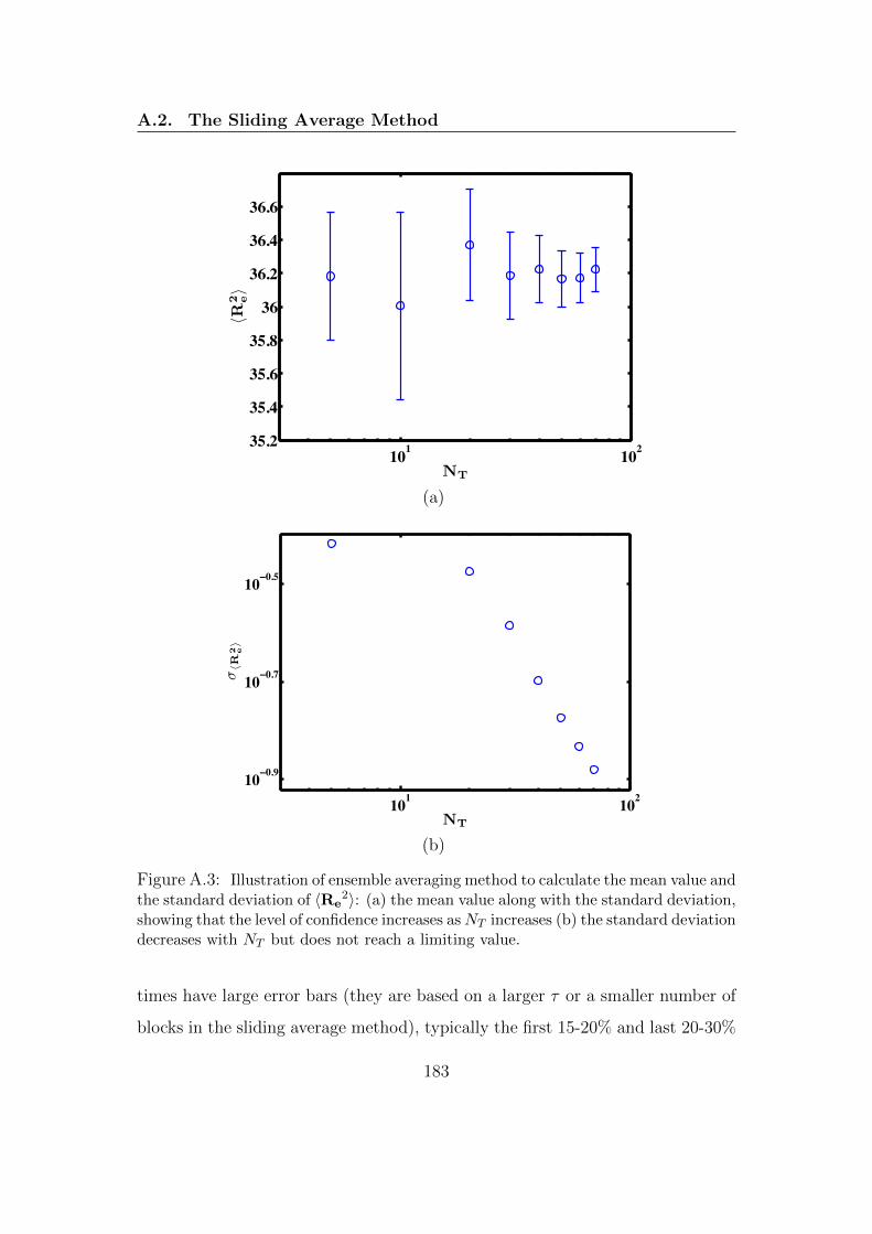
A.2. The Sliding Average Method
101 10235.2
35.4
35.6
35.8
36
36.2
36.4
36.6
NT
!R2 e"
(a)
101 10210 0.9
10 0.7
10 0.5
NT
!!R
2 e"
(b)
Figure A.3: Illustration of ensemble averaging method to calculate the mean value andthe standard deviation of 〈Re
2〉: (a) the mean value along with the standard deviation,showing that the level of confidence increases asNT increases (b) the standard deviationdecreases with NT but does not reach a limiting value.
times have large error bars (they are based on a larger τ or a smaller number of
blocks in the sliding average method), typically the first 15-20% and last 20-30%
183
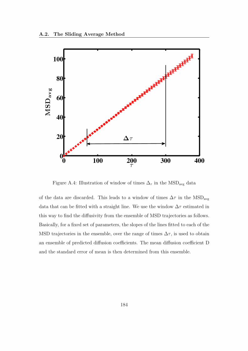
A.2. The Sliding Average Method
0 100 200 300 4000
20
40
60
80
100
!
MSD
avg
!!
Figure A.4: Illustration of window of times ∆τ in the MSDavg data
of the data are discarded. This leads to a window of times ∆τ in the MSDavg
data that can be fitted with a straight line. We use the window ∆τ estimated in
this way to find the diffusivity from the ensemble of MSD trajectories as follows.
Basically, for a fixed set of parameters, the slopes of the lines fitted to each of the
MSD trajectories in the ensemble, over the range of times ∆τ , is used to obtain
an ensemble of predicted diffusion coefficients. The mean diffusion coefficient D
and the standard error of mean is then determined from this ensemble.
184
Appendix B
Ewald Summation of
Rotne-Prager-Yamakawa
Mobility Tensor
Originally the Ewald summation method was developed for electrostatic interac-
tions, therefore, a quick introduction to this method is first discussed in the con-
text of electrostatic interactions. The remainder of this appendix then presents
the derivation of the Ewald sum for hydrodynamic interactions based on the
Rotne-Prager-Yamakawa mobility tensor.
B.1 Brief introduction to the Ewald Sum for
Electrostatic Interactions
In a system of particles, the inter-particle force is defined to be short ranged if
it decreases with distance faster than r−d where d is the dimensionality of the
system. In a system where there are long-range interactions such as Coulombic
185

B.1. Brief introduction to the Ewald Sum for ElectrostaticInteractions
interactions, and a large number of particles, it becomes crucial to avoid the
computing of all pair interactions, as otherwise the computational effort would
be proportional to the square of the number of particles. If the electrostatic
potential is truncated at a distance rc, then the contribution of the tail of the
potential u(r) is (in 3-D),
U tail =Nρ
2
∫ ∞
rc
dr u(r) 4π r2 (B.1)
where N is the number of particles and ρ is the number density. This equa-
tion shows that the tail correction to the potential energy diverges, unless u(r)
decays faster than r−3. This is why one cannot use a truncation procedure for
long-ranged Coulombic interactions. In order to solve the problem of having
to account for all the long-ranged interactions, the Ewald summation method is
used (Frenkel and Smit, 2002). Physically the Ewald method works by surround-
ing each point charge in the system by a charge distribution of equal magnitude
and opposite sign. This distribution is usually considered a Gaussian distribu-
tion, although this choice is arbitrary. The counter-charge screens the original
potential and thus making it short-ranged. This is then summed in real space.
Then a second imaginary charge distribution of opposite sign to the first (and of
the same sign as the point charges) is added to cancel out the screening charges.
We can call it the compensating charge distribution. As this screening distribu-
tion is a smooth function, its Fourier transform is rapidly convergent. Therefore,
this second term is summed in reciprocal space. One more term, which does
not involve any summation, takes care of undesired self-interactions. Details of
the Ewald summation formula for electrostatic interactions are not covered here.
However, the remaining sections of this appendix discuss the detailed derivation
of Ewald summation for hydrodynamic interactions which was originally carried
186
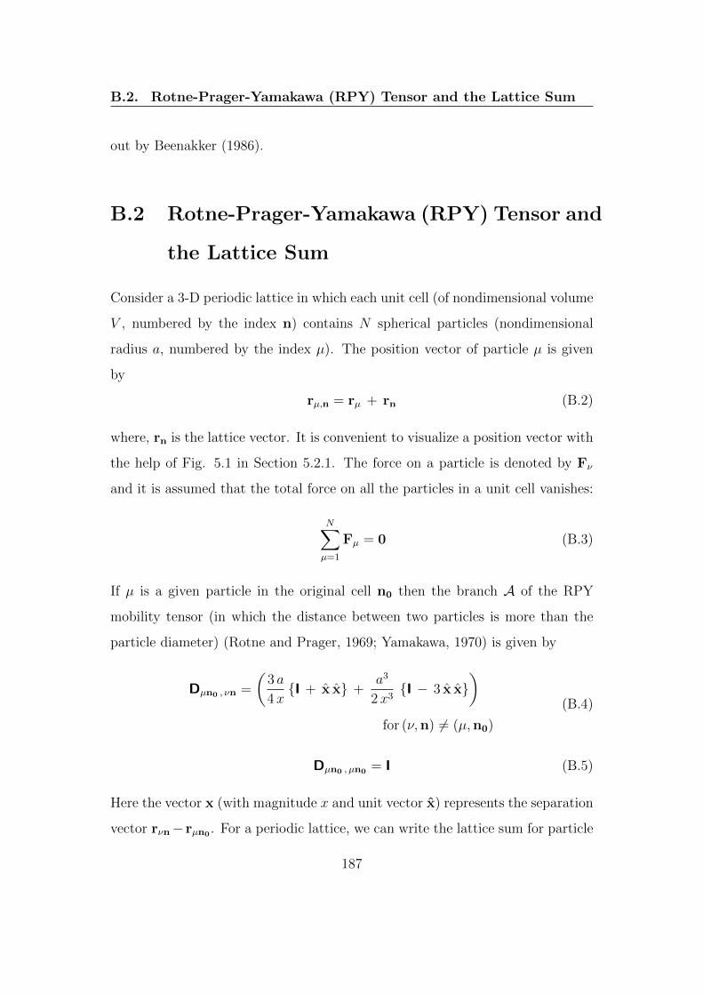
B.2. Rotne-Prager-Yamakawa (RPY) Tensor and the Lattice Sum
out by Beenakker (1986).
B.2 Rotne-Prager-Yamakawa (RPY) Tensor and
the Lattice Sum
Consider a 3-D periodic lattice in which each unit cell (of nondimensional volume
V , numbered by the index n) contains N spherical particles (nondimensional
radius a, numbered by the index µ). The position vector of particle µ is given
by
rµ,n = rµ + rn (B.2)
where, rn is the lattice vector. It is convenient to visualize a position vector with
the help of Fig. 5.1 in Section 5.2.1. The force on a particle is denoted by Fν
and it is assumed that the total force on all the particles in a unit cell vanishes:
N∑
µ=1
Fµ = 0 (B.3)
If µ is a given particle in the original cell n0 then the branch A of the RPY
mobility tensor (in which the distance between two particles is more than the
particle diameter) (Rotne and Prager, 1969; Yamakawa, 1970) is given by
Dµn0 , νn =
(3 a
4xI + x x +
a3
2x3I − 3 x x
)
for (ν,n) 6= (µ,n0)
(B.4)
Dµn0 , µn0 = I (B.5)
Here the vector x (with magnitude x and unit vector x) represents the separation
vector rνn− rµn0 . For a periodic lattice, we can write the lattice sum for particle
187
B.3. Derivation of the Ewald Sum of RPY Tensor
µ as
Sµ =N∑
ν=1
Dµν · Fν (B.6)
For simplicity, we have represented the sum∑
n
(∑Nν=1 Dµn0 , νn · Fν
)by the sum
∑Nν=1 Dµν · Fν in above equation to be consistent with Eq. (5.1), since both of
the sums are equivalent. In this appendix, these two forms of the sum will be
used interchangeably for convenience.
Because of the long-range of the RPY tensor, the sum in Eq. (B.6) converges
only slowly. Using the Ewald summation method, this sum can be written as two
fast converging sums. Note that the Ewald summation formula for the branch A(See Section 4.4) of the RPY mobility matrix will first be derived, as was done by
Beenakker (1986). A correction term to account for the presence of the branch
B (See Section 4.4) of the RPY tensor has already been derived in Section 5.2.2.
B.3 Derivation of the Ewald Sum of RPY Ten-
sor
Following Beenakker (1986), an alternative representation of the two-sphere RPY
tensor (Eq. (B.4)) is written as:
Dµn0,νn =
(3a
4+a3
4∇2
)(∇2I−∇∇) | rνn − rµn0 |
for (ν,n) 6= (µ,n0),
(B.7)
where ∇ = ∂/∂(rνn − rµn0). Now, exploiting the fact that the sum of the error
function and the complementary error function is 1, Eq. (B.7) can be written as
Dµn0 , νn = M(1)(rνn − rµn0) + M(2)(rνn − rµn0) ,
for (ν,n) 6= (µ,n0),(B.8)
188
B.3. Derivation of the Ewald Sum of RPY Tensor
where,
M(1)(r) =
(3 a
4+a3
4∇2
)(∇2 I − ∇∇) r erfc(αr) (B.9)
M(2)(r) =
(3a
4+a3
4∇2
)(∇2I−∇∇)r erf(αr) (B.10)
and α is an arbitrary parameter. Here, r is the magnitude of the vector r =
rνn − rµn0 . Upon substituting the decomposition Eq. (B.8) into Eq. (B.6), the
lattice sum becomes,
Sµ = Fµ +
[∑
n
′N∑
ν=1
(M(1)(rνn − rµn0) · Fν
)]−[M(2)(r = 0) · Fµ
]
+
[∑
n
N∑
ν=1
(M(2)(rνn − rµn0) · Fν
)],
(B.11)
The first summation on the right-hand side of Eq. (B.11) is rapidly converging.
The ′ over the sum indicates that the terms with self-interactions in the original
cell n0 are to be omitted. If the self-interactions are not excluded, then the
second summation on the right-hand side is perfectly continuous and periodic
and hence it converges rapidly on the reciprocal lattice. However, as the self-
interactions lead to spurious results, there is a requirement of a term to correct
this. The third term on the right-hand side compensates for self-interactions, and
is subtracted from the Ewald sum as shown in Eq. (B.11). The transformation
to reciprocal space is performed by means of the formula given by Nijboer and
de Wette (1957)∑
n
g(rn) =1
V
∞∑
λ=−∞
g(kλ) (B.12)
with the Fourier transform of a function g defined by
g(k) =
∫dr exp(ik · r) g(r) (B.13)
189

B.3. Derivation of the Ewald Sum of RPY Tensor
We may, therefore, write
∑
n
N∑
ν=1
M(2)(rνn − rνn0) · Fν =1
V
∑
λ
N∑
ν=1
(e−ikλ·(rν−rµ) M(2)(kλ) · Fν
)(B.14)
where terms with kλ = 0 are excluded in the sum in Eq. (B.14) by virtue of Eq.
(B.3). Now the main focus is on calculating M(1)(r), M(2)(k) and M(2)(r = 0).
B.3.1 Calculation of M(1)(r)
For the sake of simplicity, let us consider that 3a4
= A, a3
4= B and r erfc(αr) =
f(r) = f , then Eq. (B.9) can be written in index notation as
M(1)(r) =[(A+B∇2) (∇2I−∇∇)
]f
=[A (∂k
2δij − ∂i∂j)]f +
[B ∂k
2(∂k2δij − ∂i∂j)
]f
(B.15)
where, ∂k = ∂/∂xk. Now, each term of Eq. (B.15) can be calculated one by one:
∂i ∂j f(r) = ∂i
(f ′rjr
)
= f ′ ∂i
(rjr
)+rjrf ′′(rir
)
=f ′
rδij −
f ′
r2rjrir
+ f ′′rirjr2
= δij
f ′
r
+rirjr2
f ′′ − f ′
r
(B.16)
∂k2 δij f(r) = δij ∂k
(f ′rkr
)
= δij
rkrf ′′
rkr
+ f ′ ∂k
(rkr
)
= δij
f ′′ + 3
f ′
r− f ′
r2rkrkr
= δij
f ′′ +
2f ′
r
(B.17)
190

B.3. Derivation of the Ewald Sum of RPY Tensor
Subtracting Eq (B.16) from Eq (B.17) leads to
(∂k
2 δij − ∂i ∂j)f = δij
f ′′ +
f ′
r
+rirjr2
f ′
r− f ′′
(B.18)
which is the first part of Eq. (B.15). The second part of Eq. (B.15) requires the
second derivative of the left hand side of Eq. (B.18). Hence,
∂k2(∂k
2 δij − ∂i ∂j)f = ∂k
2
(δij
f ′′ +
f ′
r
+rirjr2
f ′
r− f ′′
)
= δij ∂k2
(f ′′ +
f ′
r
)+rirjr2
∂k2
(f ′
r− f ′′
)
+
(f ′
r− f ′′
)∂k
2(rirjr2
)(B.19)
The derivatives of each of the three terms on the right hand side of Eq. (B.19)
will be calculated one by one.
(i) Derivative in the first term on the right hand side of Eq. (B.19):
Let us consider that g1 = f ′′+ f ′
r. From Eq. (B.17), we know that ∂k
2(g) = g′′+ 2g′
r
for any function g(r). Therefore,
∂k2
(f ′′ +
f ′
r
)= ∂k
2 (g1)
= g1′′ +
2g1′
r
=
(f ′′′′ +
f ′′′
r− 2f ′′
r2+
2f ′
r3
)+
(2f ′′′
r+
2f ′′
r2− 2f ′
r3
)
= f ′′′′ +3f ′′′
r
(B.20)
191

B.3. Derivation of the Ewald Sum of RPY Tensor
(ii) Derivative in the second term on the right hand side of Eq. (B.19):
Let us consider that g2 = f ′
r− f ′′. From Eq. (B.17), it follows that,
∂k2
(f ′
r− f ′′
)= ∂k
2 (g2)
= g2′′ +
2g2′
r
=
(−f ′′′′ +
f ′′′
r− 2f ′′
r2+
2f ′
r3
)+
(−2f ′′′
r+
2f ′′
r2− 2f ′
r3
)
= −f ′′′′ − f ′′′
r
(B.21)
(iii) Derivative in the third term on the right hand side of Eq. (B.19):
∂k2(rirjr2
)= ∂k
(δki rjr2
+δkj rir2− ri rj
2
r3
rkr
)
=δki δkjr2
− 2 δki rjr3
rkr
+δkj δkir2
− 2 δkj rir3
rkr
− 6 ri rjr4
+8 ri rj rkr5
rkr− 2 rk
r4ri δkj −
2 rkr4
rj δki
=δijr2− 2 ri rj
r4+δijr2− 2 ri rj
r4− 6 ri rj
r4+
8 ri rjr4
− 2 rirjr4
− 2 ri rjr4
= δij
2
r2
− ri rj
r2
6
r2
(B.22)
Therefore, Eq. (B.19) now becomes,
∂k2(∂k
2 δij − ∂i ∂j)f = δij
f ′′′′ +
3 f ′′′
r
− ri rj
r2
f ′′′′ +
f ′′′
r
+
(f ′
r− f ′′
) (δij
2
r2
− ri rj
r2
6
r2
)
= δij
f ′′′′ +
3 f ′′′
r+
2 f ′
r3− 2 f ′′
r2
+ri rjr2
−f ′′′′ − f ′′′
r− 6 f ′
r3+
6 f ′′
r2
(B.23)
192

B.3. Derivation of the Ewald Sum of RPY Tensor
which can be used to obtain the second term on the right hand side of Eq. (B.15).
Hence, combining Eqs. (B.18) and (B.23), Eq. (B.15) can be written as
M(1)(r) = δij
Af ′′ +
Af ′
r
+ri rjr2
Af ′
r− Af ′′
+ δij
B f ′′′′ +
3B f ′′′
r+
2B f ′
r3− 2B f ′′
r2
+ri rjr2
−B f ′′′′ − B f ′′′
r+
6B f ′′
r2− 6B f ′
r3
= δij
Af ′′ +
Af ′
r+ B f ′′′′ +
3B f ′′′
r+
2B f ′
r3− 2B f ′′
r2
+ri rjr2
Af ′
r− Af ′′ − B f ′′′′ − B f ′′′
r− 6B f ′
r3+
6B f ′′
r2
(B.24)
Using the definition of f = r erfc(αr), we can evaluate the derivatives of f as
follows
f ′ = erfc(αr) − 2α r β (B.25)
f ′′ =(4α3 r2 − 4α
)β (B.26)
f ′′′ =(16α3 r − 8α5 r3
)β (B.27)
f ′′′′ =(16α7 r4 − 56α5 r2 + 16α3
)β (B.28)
193
B.3. Derivation of the Ewald Sum of RPY Tensor
where β = exp (−α2r2)√π
. Substitution of f ′, f ′′, f ′′′, f ′′′′, A and B into Eq. (B.24)
leads to
M(1)(r) = I
[3 aα3 r2 β − 3 aα β +
3 a
4rerfc(α r) − 3 aα β
2+ 4 a3 α7 r4 β
−14 a3 α5 r2 β + 4 a3 α3 β − 6 a3 α5 β − 6 a3 α5 r2 β + 12 a3 α3 β
+a3 erfc(α r)
2 r3− α a3 β
r2− 2 a3 α3 β +
2 a3 αβ
r2
]
+ r r
[3 a
4 rerfc(α r) − 3 aα β
2− 3 aα3 r2 β + 3 aα β
− 4 a3 α7 r4 β + 14 a3 α5 r2 β − 4 a3 α3 β + 2 a3 α5 r2 β − 4 a3 α3 β
− 3 a3
2 r3erfc(α r) +
3 a3 αβ
r2+ 6 a3 α3 β − 6 a3 αβ
r2
]
= I
[erfc(α r)
(3 a
4 r+
a3
2 r3
)+
exp (−α2 r2)√π
(3 aα3 r2 − 9 aα
2
+ 4 a3 α7 r4 − 20 a3 α5 r2 + 14 a3 α3 +a3 α
r2
)]
+ rr
[erfc(α r)
(3 a
4 r− 3 a3
2 r3
)+
exp (−α2 r2)√π
(3 aα
2− 3 aα3 r2
− 4 a3 α7 r4 + 16 a3 α5 r2 − 2 a3 α3 − 3 a3 α
r2
)]
(B.29)
where r is unit vector in the direction of r. This completes the derivation of
M(1)(r) required for the real space sum.
B.3.2 Calculation of M(2)(k)
To derive M(2)(k), the Fourier transform of M(2)(r) using Eq. (B.10) is per-
formed. Considering r erf(αr) = g(r) = g, we can write,
M(2)(k) =
∫dr exp (ik.r)
(3 a
4+a3
4∇2
) (∇2 I − ∇∇
)g (B.30)
194
B.3. Derivation of the Ewald Sum of RPY Tensor
Partial integration of Eq. (B.30) results in
M(2)(k) =
∫dr g
(3 a
4+a3
4∇2
) (∇2 I − ∇∇
)exp (ik.r) (B.31)
Note that the constant term obtained during partial integration is zero. Let us
now simplify(
3 a4
+ a3
4∇2)
(∇2 I − ∇∇) exp (ik.r),
(∇2 I − ∇∇
)exp (ik.r) = (∇ ·∇ I − ∇∇) exp (ik.r)
= (i k · i k I − i k i k) exp (ik.r)
=(−k2 I + k k
)exp (ik.r)
(B.32)
Hence,
(3 a
4+a3
4∇2
) (∇2 I − ∇∇
)exp (ik.r) =
3 a
4
(−k2 I + k k
)exp (ik · r)
+a3
4
(k4 I − k2 k k
)exp (ik · r)
= k2
3 a
4
(−I + k k
)+a3 k2
4
(I − k k
)exp (ik · r)
= −3 k2
4
(I − k k
) (a − a3 k2
3
)exp (ik · r)
(B.33)
where k is the unit vector. Inserting Eq. (B.33) in Eq. (B.31) gives,
M(2)(k) = −3 k2
4
(I − k k
) (a − a3 k2
3
)∫dr exp (ik · r) g (B.34)
The integral in Eq. (B.34) can be evaluated as follows. It is known that for a
spherical coordinate system dr = r2 sin θ dr dθ dφ and k · r = k r cos θ (Champ-
195

B.3. Derivation of the Ewald Sum of RPY Tensor
eney, 1973), where θ is the angle between the vectors k and r. We can write,
∫dr exp (ik · r) f =
∫ ∞
0
dr
∫ π
0
dθ
∫ 2π
0
dφ exp (ikr cos θ) r2 sin θ g
=
∫ ∞
0
dr
∫ π
0
dθ 2 π r2 sin θ g exp (ikr cos θ)
(B.35)
Considering cos θ = x,
∫dr exp (ik · r) f = −
∫ ∞
0
dr
∫ −1
+1
2π r2 dx g (cos (krx) + i sin (krx))
= −∫ ∞
0
dr2π r2
k rg (sin (−kr) − i cos (−kr) − sin (kr) + i cos (kr))
=
∫ ∞
0
4 π r2
ksin (kr) erf(αr) dr
= −4 π
k
∂2
∂k2
[∫ ∞
0
sin (kr) erf(αr) dr
]
=4π
k
∂2
∂k2
[exp (−k
2
4α2 )
k
]
=4π
k
∂
∂k
[exp
(−k2
4α2
) (1
k2+
1
2α2
)]
= −4 π
k
exp
(−k2
4α2
) (1
2 k α2+
k
4α4+
2
k3
)
(B.36)
Using this integral, Eq. (B.34) now becomes,
M(2)(k) =(
I − k k) (
a − a3 k2
3
)(3 π k) exp
(−k2
4α2
) (1
2 k α2+
k
4α4+
2
k3
)
=(
I − k k) (
a − a3 k2
3
)exp
(−k2
4α2
) (3π
2α2+
3π k2
4α4+
6π
k2
)
=(
I − k k) (
a − a3 k2
3
) (1 +
k2
4α2+
k4
8α4
)(6π
k2
)exp
(−k2
4α2
)
(B.37)
196

B.3. Derivation of the Ewald Sum of RPY Tensor
This completes the derivation of M(2)(k) required for the Fourier space sum.
Recall that in the derivation of M(2)(k) we have included the self interaction
between a smooth function (M(2)(r)) and a point force Fν located at ν. In the
following section, a compensating term M(2)(r = 0) is derived which takes care
of the self correction.
B.3.3 Calculation of M(2)(r = 0) (self-correction term)
In order to proceed, first an inverse Fourier transform of M(2)(k) is performed,
M(2)(r) =1
(2 π)3
∫ ∫ ∫M(2)(k) exp (ik · r) dk (B.38)
Or,
M(2)(r = 0) =1
(2 π)3
∫ ∫ ∫M(2)(k) dk
=1
(2 π)3
∫ ∞
0
∫ π
0
∫ 2π
0
M(2)(k) k2 sin δ dk dδ dη
=2π
(2 π)3
∫ ∞
0
dk
∫ π
0
dδ sin δ k2 M(2)(k)
=2
(2 π)2
∫ ∞
0
k2 M(2)(k) dk
(B.39)
Inserting M(2)(k) from Eq. (B.37) into Eq. (B.39) leads to
M(2)(r = 0) =3
π
∫ ∞
0
dk I
(a − a3 k2
3
) (1 +
k2
4α2+
k4
8α4
)exp
(−k2
4α2
)
− 3
π
∫ ∞
0
dk kk
(a − a3 k2
3
) (1 +
k2
4α2+
k4
8α4
)exp
(−k2
4α2
)
(B.40)
Note that the result of integrating a function of the dyadic product of a unit
vector with itself, over all space, must be isotropic. Therefore, Eq. (B.40) can
197
B.3. Derivation of the Ewald Sum of RPY Tensor
also be written as
M(2)(r = 0) = (I1 − I2) I (B.41)
where I1 and I2 are the scalar parts in the first and second terms on the right
hand side of Eq. (B.40) respectively. Both I1 and I2 are evaluated as follows:
Evaluation of I1:
I1 =3
π
∫ ∞
0
dk
(a − a3 k2
3
) (1 +
k2
4α2+
k4
8α4
)exp
(−k2
4α2
)
=3
π
[ −a12α2
4α3 (20 a2 α2 − 9)
√π erf
(k
2α
)
+a
12α2exp
(−k2
4α2
) 80 k a2 α4 + 12 k α2 (a2 k2 − 2) + k3 (a2 k2 − 3)
]∞
0
=aα√π
(9 − 20 a2 α2
)
(B.42)
Evaluation of I2:
I I2 =3
π
∫ ∞
0
dk kk
(a − a3 k2
3
) (1 +
k2
4α2+
k4
8α4
)(B.43)
× exp
(−k2
4α2
)
Since kk : I = kx2
+ ky2
+ kz2
= |k|2 = 1, a double dot product with I on both
sides of Eq. (B.43) is carried out to give
I : I I2 =3
π
∫ ∞
0
1 dk
(a − a3 k2
3
) (1 +
k2
4α2+
k4
8α4
)exp
(−k2
4α2
)(B.44)
198

B.3. Derivation of the Ewald Sum of RPY Tensor
The same integration result that was evaluated for the case of I1, can be used
here. Also, noting that I : I = 3, we obtain,
I2 =aα
3√π
(9 − 20 a2 α2) (B.45)
Using I1 and I2, Eq. (B.41) can be simplified to obtain M(2)(r = 0)
M(2)(r = 0) = (I1 − I2) I
= I
aα√π
(1 − 1
3
)(9− 20a2α2)
= I1√π
(6 aα − 40
3a3 α3
)(B.46)
Finally, using M(1)(r), M(2)(k) and M(2)(r = 0), the Ewald summation formula
for the branch A of RPY mobility tensor can be written (using Eq. (B.11)) as
follows:
Sµ =N∑
ν=1
Dµν · Fν =
(1 − 6 aα√
π+
40 a3 α3
3√π
)Fµ
︸ ︷︷ ︸Point force and self correction
+∞∑
n=0
′ N∑
ν=1
M(1)(rνn − rµn0) · Fν
︸ ︷︷ ︸Real space sum
+1
V
∑
λ
N∑
ν=1
M(2)(kλ) · Fν cos kλ · (rν − rµ)︸ ︷︷ ︸
Reciprocal space sum
(B.47)
Recall that the first sum on the right-hand side of Eq. (B.47) converges rapidly.
The ′ over the sum indicates that the terms with self interactions are to be
omitted. The second sum converges rapidly on the reciprocal lattice. The self-
correction appears in the first term along with the point force. The summations
199

B.3. Derivation of the Ewald Sum of RPY Tensor
in Eq. B.47 are carried out for all possible pairs of particles (|rνn − rµn0 | > 0),
however it should be used only for those pairs for which |rνn − rµn0 | > 2a. A
modified Ewald summation formula which accounts for the overlapping beads
is derived in Section (5.2.2). This modified formula involves an additional term
which is evaluated only in the original simulation cell, and in particular only for
overlapping beads. This additional term is discussed in the next section.
B.3.4 Derivation of the form of the additional term in
the modified Ewald sum
In this section, an expression for the tensor M∗ is derived, which makes up the
correction term shown in Section (5.2.2). From Eq. (5.1), the sum∑N
µ=1 Dνµ ·Fµ
for the two branches of the RPY tensor can be written as (where the overlapping
particles have been explicitly identified),
[N∑
µ=1
Dνµ · Fµ
]
A
=
[(1− 6aα√
π+
40a3 α3
3√π
)Fν
]
A+
N∗∑
µ=1µ 6=ν
M(1)(rνµ,n=0) · Fµ
A
+
[∑
n6=0
N∗∑
µ=1
M(1)(rνµ,n) · Fµ
]
A
+
[∑
n
N∑
µ=N∗+1
M(1)(rνµ,n) · Fµ
]
A
+
[∑
k 6=0
M(2)(k) ·
cos(k · rν)N∑
µ=1
cos(k · rµ)Fµ − sin(k · rν)N∑
µ=1
sin(k · rµ)Fµ
]
A
(B.48)
200
B.3. Derivation of the Ewald Sum of RPY Tensor
and
[N∑
µ=1
Dνµ · Fµ
]
B
=
[(1− 6aα√
π+
40a3 α3
3√π
)Fν
]
B+
N∗∑
µ=1µ6=ν
MB(1)(rνµ,n=0) · Fµ
+
[∑
n6=0
N∗∑
µ=1
M(1)(rνµ,n) · Fµ
]
B
+
[∑
n
N∑
µ=N∗+1
M(1)(rνµ,n) · Fµ
]
B
+
[∑
k 6=0
M(2)(k) ·
cos(k · rν)N∑
µ=1
cos(k · rµ)Fµ − sin(k · rν)N∑
µ=1
sin(k · rµ)Fµ
]
B
(B.49)
Subtracting Eq. (B.48) from (B.49) and noting that the first, third, fourth and
fifth terms in both the equations are the same, we can write,
[N∑
µ=1
Dνµ · Fµ
]
B
−[
N∑
µ=1
Dνµ · Fµ
]
A
=N∗∑
µ=1µ 6=ν
MB(1)(rνµ,n=0) · Fµ −
N∗∑
µ=1µ 6=ν
M(1)(rνµ,n=0) · Fµ
A
(B.50)
The right-hand side of Eq. (B.50) is the quantity∑N∗
µ=1µ6=ν
M?(rνµ,n=0) ·Fµ defined
in Eq. (5.6). The difference between the sums on the left hand side of Eq. (B.50)
can be calculated using explicit expressions of RPY functions given in Eqs. (4.3)
- (4.6). As a result,
M∗(x) = δ
[1− 1
2x3
(3x2
4+ 1
)2]
+ x x
[1
2x3
(3x2
4− 1
)2]
(B.51)
where x = r(νµ,n=0)/a and x is the unit vector in the direction of r(νµ,n=0).
201

B.3. Derivation of the Ewald Sum of RPY Tensor
202
Appendix C
Scaling of Computational Cost
with Chain Size
Asymptotic predictions in the long chain limit have been obtained for each state
point (z, c/c?) by extrapolating finite chain data accumulated for chain lengths
ranging from Nb = 6 to Nb = 20 as illustrated in Fig. 6.1. The use of this
rather limited range of Nb values is necessitated by the computational cost of
the Brownian dynamics simulation algorithm used here. As shown below, an
estimate of the computational cost of the algorithm can be derived by using
some simple scaling arguments, and the resulting expression can be verified by
comparison with the CPU time required in the current simulations.
The computational cost of carrying out an Euler integration of the governing
stochastic differential equation for a single time step has been shown in Chapter
5 to scale with system size as Nx, where x = 2.1. Recall that N = Nb×Nc is the
total number of beads in a cubic cell of edge length L, with Nc being the number
of bead-spring chains. Since typical simulations consist of runs extending over
several relaxation times τ1, followed by averaging over many independent runs,
it is necessary to find the dependence of τ1 on Nb in order to find the scaling of
203

the total CPU cost. This is done as follows for simulations carried out in the
semidilute regime C.
From Eq. (3.20), the requirement that L ≥ 2Re (where Re is the end-to-end
distance of a chain) in order to prevent chains from wrapping over themselves
leads to
L ∼ b( cc?
)−12
2ν−13ν−1
z2ν−1N1/2b (C.1)
The concentration of monomers in the simulation box is c = (NbNc)/L3. As a
result, from Eq. (C.1)
c ∼(Nc
b3
)( cc?
)32
2ν−13ν−1
z−3(2ν−1)N−1/2b (C.2)
Using Eqs. (3.6) and (2.10), the overlap concentration c? can be written in terms
of the solvent quality z as
c? ∼ b−3z−3(2ν−1)N−1/2b (C.3)
It follows from Eqs. (C.2) and (C.3) that Nc is independent of z, and related to
the scaled concentration through the relation
Nc ∼( cc?
)12
13ν−1
(C.4)
The number of chains in a simulation box is consequently constant when (c/c?)
is maintained constant.
The relaxation time of a macromolecule τ1 ∼ R2/D. From Eqs. (3.20) and
(3.23), this implies
τ1 ∼ τ0 (c/c?)2−3ν3ν−1 z3(2ν−1)N
3/2b (C.5)
where τ0 = ηsb3/kBT is the monomer relaxation time.
204
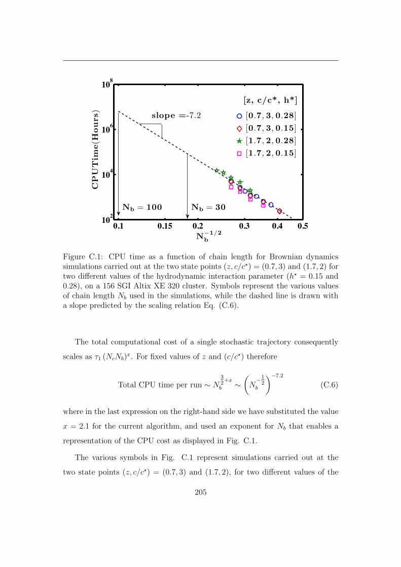
0.1 0.15 0.2 0.3 0.4 0.5102
104
106
108
N!1/2b
CP
UT
ime(H
ours)
[z, c/c*, h*]
[0.7, 3, 0.28]
[0.7, 3, 0.15]
[1.7, 2, 0.28]
[1.7, 2, 0.15]
Nb = 100 Nb = 30
slope =-7.2
Figure C.1: CPU time as a function of chain length for Brownian dynamicssimulations carried out at the two state points (z, c/c?) = (0.7, 3) and (1.7, 2) fortwo different values of the hydrodynamic interaction parameter (h? = 0.15 and0.28), on a 156 SGI Altix XE 320 cluster. Symbols represent the various valuesof chain length Nb used in the simulations, while the dashed line is drawn witha slope predicted by the scaling relation Eq. (C.6).
The total computational cost of a single stochastic trajectory consequently
scales as τ1 (NcNb)x. For fixed values of z and (c/c?) therefore
Total CPU time per run ∼ N32
+x
b ∼(N−1
2b
)−7.2
(C.6)
where in the last expression on the right-hand side we have substituted the value
x = 2.1 for the current algorithm, and used an exponent for Nb that enables a
representation of the CPU cost as displayed in Fig. C.1.
The various symbols in Fig. C.1 represent simulations carried out at the
two state points (z, c/c?) = (0.7, 3) and (1.7, 2), for two different values of the
205
hydrodynamic interaction parameter h?, on a 156 SGI Altix XE 320 cluster. The
simulations are identical to those used to display the ratio D/DZ in Fig. 6.1.
It is immediately apparent that the prediction in Eq. (C.6) for the scaling of
the total CPU time with chain size is obeyed closely by the present simulations,
independent of solvent quality and scaled concentration.
It is clearly desirable to add data for longer chains in order to improve the
accuracy of the asymptotic value obtained by extrapolation to the long chain
limit. Unfortunately, the additional CPU cost this would entail (which can be
estimated from the scaling of computational cost with chain size shown in Fig.
C.1) makes this highly infeasible. For instance, simulating a chain with Nb = 30
would require roughly O(104) CPU hours, while Nb = 100 would require roughly
O(106) CPU hours! Indeed, by including simulations for a chain with Nb = 30,
the CPU time for obtaining the static and dynamic properties of a semidilute
solution at a single state point (z, c/c?) = (3, 4) in the phase diagram is estimated
to increase from its current value of approximately 7×10⁴ hours to roughly 3×10⁵
hours.
206
Appendix D
Error in the Extrapolated Value
at Nb→∞
At each state point (z, c/c?) the mean value of D and the error in the mean,
for a set of finite size chains with Nb = 6, 8, ..., 20 is obtained as described in
Section 4.5.1 and Appendix A. Single chain BD simulations are used to compute
Dz for the same values of Nb and z, and then the mean and error-of-mean of
the ratio D/Dz is easily obtained . As described earlier, the asymptotic value of
D/Dz in the long-chain limit is obtained by plotting the data at finite Nb as a
function of N−1/2b , and extrapolating a straight line fit to the data, to the limit
Nb →∞. The fitting of the straight line, and the estimation of the error in the
extrapolated value is carried out here with the help of “Least-Squares Fitting”
numerical routines provided in the GNU Scientific Library (GSL). Essentially, the
GSL routine finds the least-squares fit by minimizing χ2, the weighted sum of
squared residuals, for the straight line model D/Dz = c0 + c1N−1/2b . The weights
are the inverse of the error at each data point. The fitting routine gsl fit wlinear
returns the best-fit parameters c0 and c1, along with a 2 × 2 covariance matrix
that measures the statistical errors on c0 and c1 resulting from the errors in
207

the data. The standard deviations of the best-fit parameters are then given
by the square root of the corresponding diagonal elements of the covariance
matrix. Particularly conveniently, the routine gsl fit linear est uses the best-fit
coefficients c0, c1 and their estimated covariance to compute the fitted function
and its standard deviation at any desired point. By using gsl fit linear est to
find the value of the fitted function and its error at N−1/2b = 0, we determine
both the infinite chain length limit value of D/Dz and its associated error. We
find the error bars on the extrapolated values to be very large because the GSL
routines account for the error on each data point and that results to a conservative
estimate of the error bar on the extrapolated value. Though the error bars on
the extrapolated results are large, a very good fit gives us the confidence that
the actual error bar on the extrapolated result is much smaller.
208
Appendix E
Running LB/MD Simulations
In the LB/MD method, a polymer chain is modeled as a bead-spring chain
consisting of Nb beads connected through Nb − 1 finitely extensible nonlinear
elastic (FENE) massless springs. The short-ranged excluded volume interactions
are accounted through a WCA potential given by,
UWCA = 4ε
(σ12
r12− σ6
r6
)+ ε, r ≤ 21/6σ (E.1)
and the FENE potential is given by,
UFENE = −kFENE q20
2ln
(1−
(r
q0
)2)
(E.2)
where r is the distance between a pair of beads, and σ and ε are the length
scale and the energy scale parameters of the WCA potential, respectively. In
Eq. (E.2), kFENE is the spring constant and q0 is the maximum extension of a
spring. In the LB/MD method, the natural unit system is based on the WCA
potential parameters, i.e., the length unit is σ, the energy unit is ε and the
time unit is considered to be τ , where τ =√mσ2/ε (where m is the mass of a
209

monomer). Conversely, in the BD method with FENE springs, the length unit is
lk =√kBT/kFENE, the energy unit is kBT and the time unit is τk = ζ/(4kFENE)
(where ζ is the bead friction coefficient). As the unit system is different in the
LB/MD and BD methods, in order to compare these two methods, it becomes a
necessary step to represent all the data in a common unit system. Pham et al.
(2009) have carried out the parameter mapping between these two methods in
detail. Here, their findings are briefly discussed.
Pham et al. (2009) make the point that the LB/MD method is based on an
inertial time scale while the BD method is based on a diffusive time scale. This
is relevant to the existence of a difference between the short-time and long-time
friction coefficients. The short-time friction coefficient is denoted by ζbare which
is an input parameter to the LB/MD method, where as the long-time friction
coefficient ζeff is identified with the BD bead friction coefficient ζ. Dunweg and
Ladd (2009) and Ahlrichs and Dunweg (1999) showed that ζbare and ζeff can be
related through1
ζeff
=1
ζbare
+1
gηsa′(E.3)
where, they showed that, g ≈ 25 if a′ is the LB lattice spacing. Pham et al. (2009)
point out that it is intrinsically impossible to run the two simulations with the
same unit system. As a result, they scaled all the parameters of LB/MD and
BD based on the LB/MD unit system. Firstly, we set l†σ = l‡lk and t†τ =
t‡τk, where the ‡ superscript denotes BD nondimensionalization, while † denotes
a nondimensionalization for LB/MD. It follows that kFENE can be written as
k†FENE(ε/σ2), resulting in lk =
√σ2kBT
εk†FENE
. Hence,
σ
lk=l‡
l†=
√k†FENEε
kBT(E.4)
210
Similarly using ζ = ζ†eff
√mε
σ2,
τ
τk=τ ‡
τ †=
4k†FENE
ζ†eff
(E.5)
Note that kBT/ε is the nondimensionalized temperature in LB/MD units, and is
an input parameter to the LB/MD method. Another BD parameter that needs
to be evaluated in terms of LB/MD parameters is the nondimensional bead
radius a‡. This parameter is related to the conventionally defined (Thurston
and Peterlin, 1967; Bird et al., 1987) hydrodynamic interaction parameter h? by
a‡ =√πh?. We can find,
a‡lk =ζeff
6πηs=ζ†effσ
6πηs(E.6)
which implies
a‡ =ζ†eff
6πη†
√k†FENEε
kBT(E.7)
In order to compare simulation results of these two methods, firstly, for given
values of Nb, Nc and c/c?, the LB/MD simulation is run using the LB/MD input
parameters k†FENE, kBT/ε, η† and ζ†bare. Secondly, Eqs. (E.3), (E.4), (E.5) and
(E.7) are used to calculate the values of corresponding BD parameters to run
the BD simulations. The choice of LB/MD simulation parameters made in this
study, as was in the case of Pham et al. (2009), are shown in the Table E.1.
Using these parameters the LB/MD simulation is carried out. An example of a
Tcl script (Example.tcl), and the command to execute the ESPResSo package are
given at the end of this appendix. After running this script file, particles trajec-
tories are stored in a text file (‘Trajectory.dat”), which can be post-processed to
obtain various physical properties. In order to run BD simulations, as mentioned
211

Nondimensional LB/MD simulation parameters Values
kBT/ε (Temperature) 1.2ρ† (Density) 0.864ν† = η†/ρ† (Kinematic viscosity) 2.8
a′† (Lattice spacing) 1
ζ†bare (Short-time friction coefficient) 20.8
k†FENE (Spring constant) 7
q†0 (Maximum extension of a spring) 2∆t† (Time step) 0.01
Table E.1: Choice of LB/MD simulation parameters
earlier, the BD parameters are first calculated. For example, if the box size in
LB/MD units is LLB, then in BD units the box size can be calculated using
Eq. (E.4) to be LBD = LLB
√k†FENEkBT/ε
. Similarly, if the time step in LB/MD
method is ∆tLB, then in BD the time step can be estimated using Eq. (E.5)
to be ∆tBD = ∆tLB(4k†FENE/ζ†eff). Once the results are obtained by running BD
simulations, they need to be interpreted in terms of LB/MD units in order to
make a proper comparison.
An example of tcl script to run ESPResSo
#########################################
Example.tcl
#########################################
set pi 3.1415926535
set verbose "yes"
set tcl_precision 12
#########################################
# System parameters
#########################################
# Following is a list of parameters used to define the system
# and also to define interaction parameters
set n_beads <insert value here> # Number of beads in a chain
212

set temp 1.2
set time_step 0.01 # Time step used in the main integrator
set skin 0.4
set n_chains <insert value here> # Number of chains
set bond_l 0.95
set min_dist 0.9
set cap_start 5
set n_total [expr $n_beads*$n_chains]
set fene_k 7.0 #FENE parameter
set box_l <insert value here> #Box size L
set ccs <insert value here> #c/c*
set fene_r 2.0 #FENE parameter
set lj_eps 1.0 #WCA parameter
set lj_sig 1.0 #WCA parameter
set lj_cut 1.122462048 #WCA parameter
set lj_shift 0.25 #WCA parameter
set lj_off 0.0 #WCA parameter
#########################################
# Lattice Boltzmann parameters
#########################################
set lb_dens 0.864 # Density
set lb_visc 2.8 # Kinematic viscosity
set lb_grid 1.0 # Lattice spacing
set lb_tau 0.02 # time step used equilibration process
set lb_zeta 20.8 # bare friction coefficient
set zeta_eff [expr 1/(1/$lb_zeta+1/(25.0*$lb_dens
*$lb_visc*$lb_grid))] # This one is similar to
BD friction coefficient
#########################################
# Integration parameters
#########################################
# All warm_* variables are used in Langevin warm up step
set warm_steps <insert value here> # Number of time steps
set warm_loops <insert value here> # Number of loops
# All diff_* variables are used in LB warp up step
set diff_time <insert value here> #Physical time for the diffusion process
set diff_steps [expr int($diff_time/$time_step)] # Number of time steps
# All n_* variables are used in the main integration step
set n_steps <insert value here> # Number of time steps
set n_loops <insert value here> # Number of loops
set data_collection_interval <insert value here> # Number of data points
213

after which the data will be entered in to output file
#########################################
# System identification
#########################################
set filename [format "Trajectory.dat" ] # Setting the name of output file
##########################################
# Procedures
##########################################
proc output args
global verbose
if $verbose == "yes"
set l [llength $args]
if $l == 1
puts [lindex $args 0]
elseif $l == 2
puts [lindex $args 0] [lindex $args 1]
else
puts [lindex $args 0] [lindex $args 1] [eval concat
[lrange $args 2 $l]]
proc write_positions dest
global n_total
for set np 0 $np < $n_total incr np
set pos [part $np print pos]
lappend xpos [lindex $pos 0]
lappend ypos [lindex $pos 1]
lappend zpos [lindex $pos 2]
puts $dest "[setmd time] $xpos"
puts $dest "[setmd time] $ypos"
puts $dest "[setmd time] $zpos"
#########################################
# Setup the system
#########################################
# Random number generator
#########################################
t_random seed 54919
#########################################
214

# Setting the simulation box
#########################################
setmd box_l $box_l $box_l $box_l
setmd periodic 1 1 1
cellsystem domain_decomposition -no_verlet_list
#########################################
# Setting Interactions (manual of Espresso can be see for the details)
#########################################
inter 0 FENE $fene_k $fene_r #FENE interaction
inter 0 0 lennard-jones $lj_eps $lj_sig $lj_cut $lj_shift $lj_off
#LJ or WCA interaction
#########################################
# Setting Polymer Chains (achieving SAW)
#########################################
polymer $n_chains $n_beads $bond_l type 0 0
bond 0 mode SAW 0.5 1000000
#########################################
# Integration
#########################################
setmd time_step $time_step
setmd skin $skin
#########################################
# Run the simulation
#########################################
# warmup with Langevin equation (part of equilibration)
#########################################
thermostat langevin $temp 0.5
set cap $cap_start
set act_min_dist [analyze mindist]
inter ljforcecap $cap
set i 1
while $i <= $warm_loops || $act_min_dist < $min_dist
integrate $warm_steps
set act_min_dist [analyze mindist]
set cap [expr $cap+10]
inter ljforcecap $cap
incr i
output ""
inter ljforcecap 0
galileiTransformParticles
215

invalidate_system
########################################
# warmup with Lattice Boltzmann (Diffusion process and part of equilibration)
########################################
thermostat off
lbfluid density $lb_dens viscosity $lb_visc agrid $lb_grid tau $lb_tau
lbfluid friction $lb_zeta
thermostat lb $temp
for set i 1 $i <= $warm_loops incr i
output -nonewline "\[Warmup $i/$warm_loops\]\r"; flush stdout
integrate $diff_steps
output ""
# Langevin and Lattice Boltzmann warm ups processes equilibrate the system
########################################
# Integration (This is he main integration step which is used to store
# particle trajectories and also to compare CPU time)
########################################
setmd time 0.0
set file [open "$filename" "w"]
write_positions $file
for set i 1 $i <= $n_loops incr i
output -nonewline "\[Loop $i/$n_loops\]\r"; flush stdout
for set j 1 $j <= $n_steps/$data_collection_interval
incr j
#integrate $n_steps
integrate $data_collection_interval
write_positions $file
#output ""
close $file
########################################
In order to execute this script file, ESPResSo must be installed and the
following command is used:
>> Espresso Example.tcl
216

Appendix F
Static Structure Factor
Calculations
As discussed in Chapter 3, in semidilute polymer solutions both hydrodynamic
and excluded volume interactions are screened on a length scale of ξc, which
denotes the size of a concentration blob. The information about the screening
length or the concentration driven crossover in semidilute polymer solutions is
reflected in the polymer structure factor (Huang et al., 2010). The aim of this
section is to compute the structure factor for a range of c/c? and z, and we then
hope to interpret the size of a concentration blob in terms of structure factor
results. The static structure factor of a polymer chain is given by
S(k) =1
Nb
∑
µν
〈exp (ik · rµν)〉 =1
Nb
∑
µν
⟨sin (krµν)
krµν
⟩(F.1)
where k is the scattering vector and k is the magnitude of k, also known as
wavenumber. The distance vector rµν connecting the beads µ and ν is an abbre-
viation for rν − rµ and rµν is the magnitude of rµν .
Scaling arguments can be used to show that the structure factor S(k) of a
217
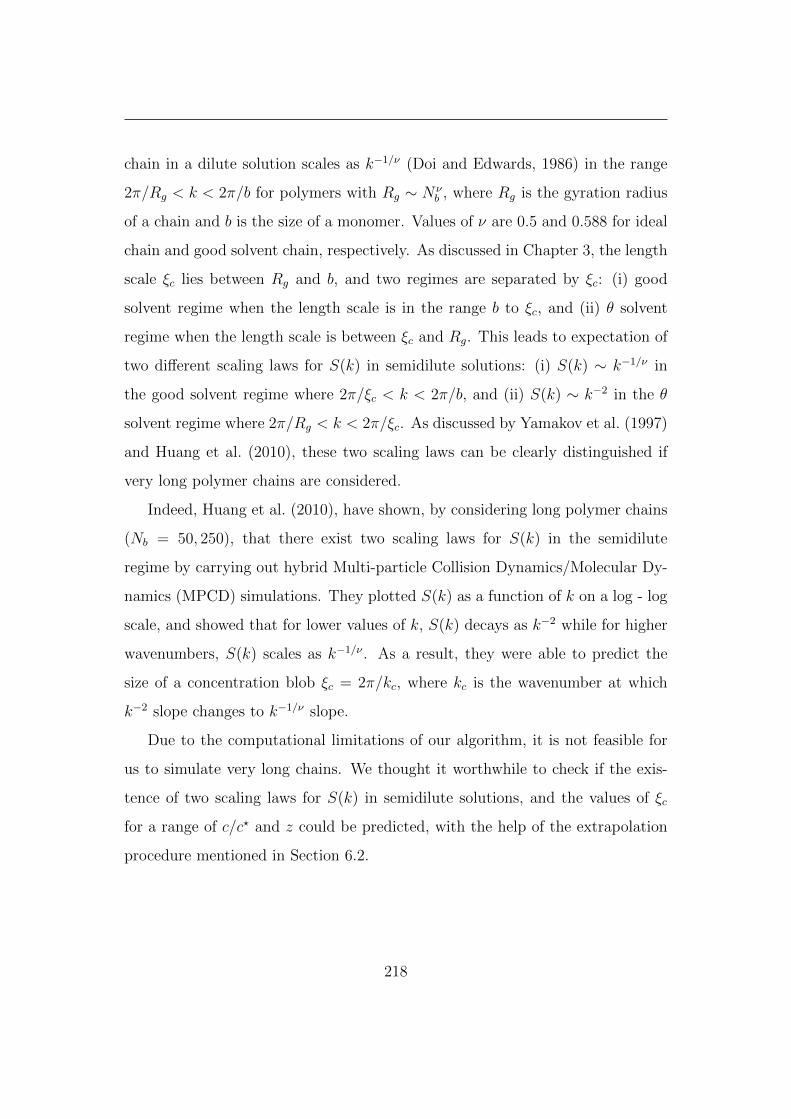
chain in a dilute solution scales as k−1/ν (Doi and Edwards, 1986) in the range
2π/Rg < k < 2π/b for polymers with Rg ∼ N νb , where Rg is the gyration radius
of a chain and b is the size of a monomer. Values of ν are 0.5 and 0.588 for ideal
chain and good solvent chain, respectively. As discussed in Chapter 3, the length
scale ξc lies between Rg and b, and two regimes are separated by ξc: (i) good
solvent regime when the length scale is in the range b to ξc, and (ii) θ solvent
regime when the length scale is between ξc and Rg. This leads to expectation of
two different scaling laws for S(k) in semidilute solutions: (i) S(k) ∼ k−1/ν in
the good solvent regime where 2π/ξc < k < 2π/b, and (ii) S(k) ∼ k−2 in the θ
solvent regime where 2π/Rg < k < 2π/ξc. As discussed by Yamakov et al. (1997)
and Huang et al. (2010), these two scaling laws can be clearly distinguished if
very long polymer chains are considered.
Indeed, Huang et al. (2010), have shown, by considering long polymer chains
(Nb = 50, 250), that there exist two scaling laws for S(k) in the semidilute
regime by carrying out hybrid Multi-particle Collision Dynamics/Molecular Dy-
namics (MPCD) simulations. They plotted S(k) as a function of k on a log - log
scale, and showed that for lower values of k, S(k) decays as k−2 while for higher
wavenumbers, S(k) scales as k−1/ν . As a result, they were able to predict the
size of a concentration blob ξc = 2π/kc, where kc is the wavenumber at which
k−2 slope changes to k−1/ν slope.
Due to the computational limitations of our algorithm, it is not feasible for
us to simulate very long chains. We thought it worthwhile to check if the exis-
tence of two scaling laws for S(k) in semidilute solutions, and the values of ξc
for a range of c/c? and z could be predicted, with the help of the extrapolation
procedure mentioned in Section 6.2.
218

F.1. Simulation results
F.1 Simulation results
As discussed in earlier sections, the behavior of semidilute polymer solutions is
captured in the asymptotic limit Nb → ∞ and only in this limit can the uni-
versal crossover scaling functions be verified. The same set of input simulation
parameters are considered here (see Table 6.1) that were used to obtain crossover
scaling functions φR, φD and φη. As a matter of fact, simulations are run only
once for a set of parameters and then all the properties (gyration radius, diffu-
sivity, structure factors) are calculated based on the beads’ trajectories in the
post-processing stage.
A similar extrapolation technique, as was used for other properties, is used
here. Extrapolation of the finite chain data to the limit Nb → ∞ is performed
in order to obtain the asymptotic result for static structure factor S(k). Though
the procedure to obtain extrapolated data is explained in Section 6.2, because
of a certain subtlety, it is important to discuss the procedure in the context of
structure factor calculations. This subtlety arises because rather than plotting
S(k) vs. k, we plot S(k)/Nb vs. kRg since it provides a wider window in the
range of k in which we are interested. In order to obtain the extrapolated data, it
is necessary to fix the value of kRg and calculate S(k)/Nb for each Nb. Note that
kRg can have different value for different Nb at a fixed value of k. Therefore, a
linear interpolation is used to obtain S(k)/Nb around a fixed value of kRg. Once
S(k)/Nb data is calculated for all Nb at a fixed value of kRg, S(k)/Nb is plotted
as a function of N−2b as shown in Fig. F.1. A straight line is fitted through
the data and finally the fitted line is used to evaluate S(k)/Nb at N−2b = 0 or
Nb = ∞. It is found, for this particular case, that the best extrapolation result
is obtained when a straight line is chosen, and when the x-axis is selected to be
N−2b . The selection of whether to choose a straight line or to choose a polynomial
of a certain order can be different at different values of kRg, based on which fits
219
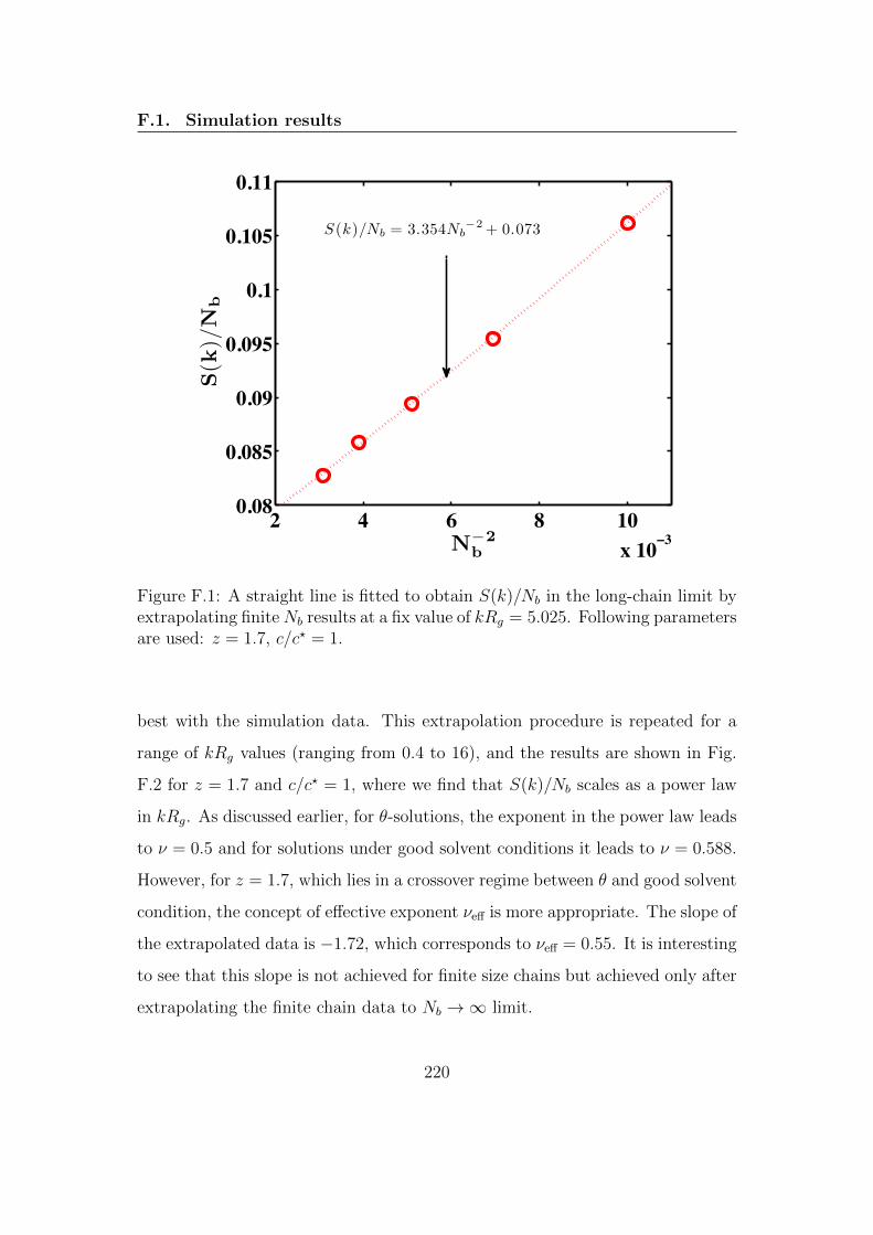
F.1. Simulation results
2 4 6 8 10x 10 3
0.08
0.085
0.09
0.095
0.1
0.105
0.11
N!2b
S(k
)/N
bS(k)/Nb = 3.354Nb
!2 + 0.073
Figure F.1: A straight line is fitted to obtain S(k)/Nb in the long-chain limit byextrapolating finiteNb results at a fix value of kRg = 5.025. Following parametersare used: z = 1.7, c/c? = 1.
best with the simulation data. This extrapolation procedure is repeated for a
range of kRg values (ranging from 0.4 to 16), and the results are shown in Fig.
F.2 for z = 1.7 and c/c? = 1, where we find that S(k)/Nb scales as a power law
in kRg. As discussed earlier, for θ-solutions, the exponent in the power law leads
to ν = 0.5 and for solutions under good solvent conditions it leads to ν = 0.588.
However, for z = 1.7, which lies in a crossover regime between θ and good solvent
condition, the concept of effective exponent νeff is more appropriate. The slope of
the extrapolated data is −1.72, which corresponds to νeff = 0.55. It is interesting
to see that this slope is not achieved for finite size chains but achieved only after
extrapolating the finite chain data to Nb →∞ limit.
220
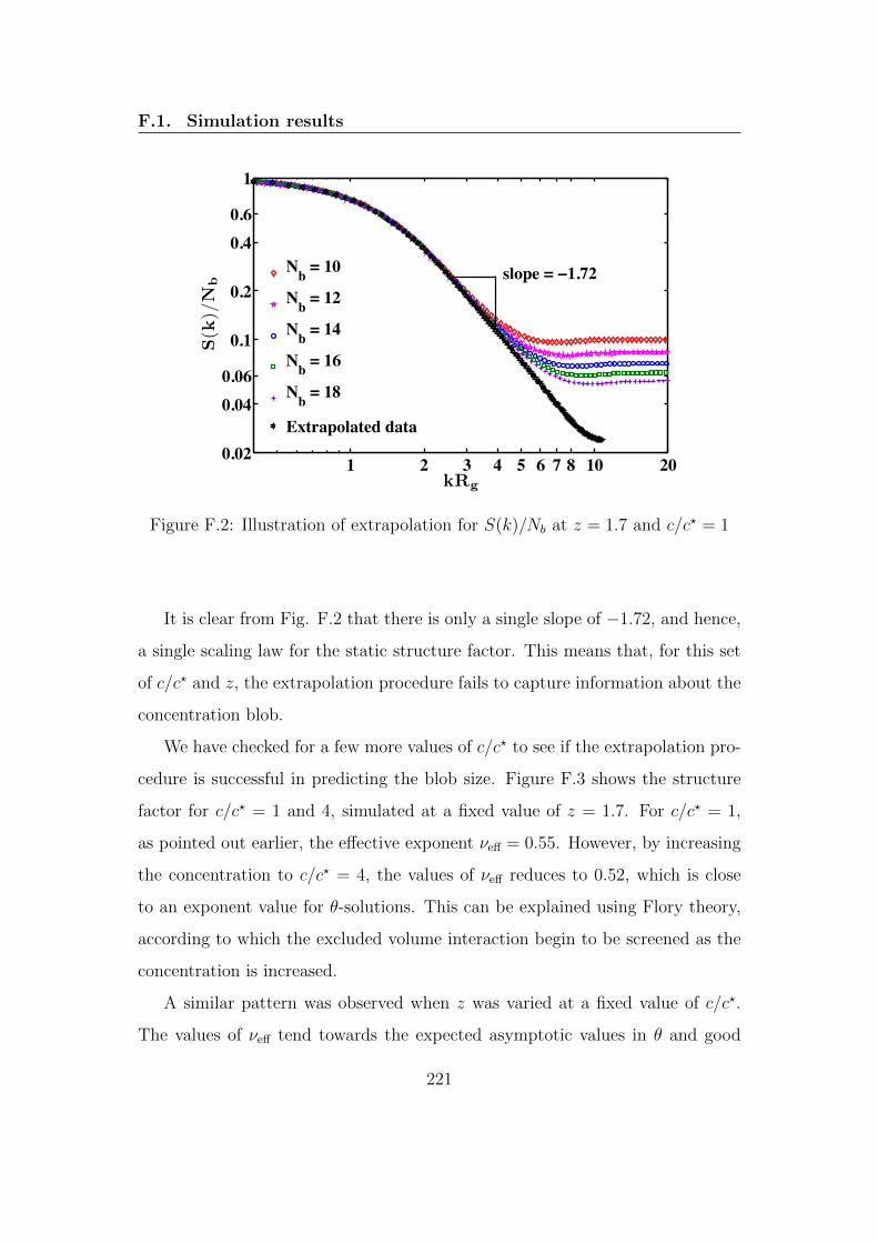
F.1. Simulation results
1 2 3 4 5 6 7 8 10 200.02
0.040.06
0.1
0.2
0.40.6
1
kRg
S(k
)/N
b
Nb = 10
Nb = 12
Nb = 14
Nb = 16
Nb = 18
Extrapolated data
slope = 1.72
Figure F.2: Illustration of extrapolation for S(k)/Nb at z = 1.7 and c/c? = 1
It is clear from Fig. F.2 that there is only a single slope of −1.72, and hence,
a single scaling law for the static structure factor. This means that, for this set
of c/c? and z, the extrapolation procedure fails to capture information about the
concentration blob.
We have checked for a few more values of c/c? to see if the extrapolation pro-
cedure is successful in predicting the blob size. Figure F.3 shows the structure
factor for c/c? = 1 and 4, simulated at a fixed value of z = 1.7. For c/c? = 1,
as pointed out earlier, the effective exponent νeff = 0.55. However, by increasing
the concentration to c/c? = 4, the values of νeff reduces to 0.52, which is close
to an exponent value for θ-solutions. This can be explained using Flory theory,
according to which the excluded volume interaction begin to be screened as the
concentration is increased.
A similar pattern was observed when z was varied at a fixed value of c/c?.
The values of νeff tend towards the expected asymptotic values in θ and good
221
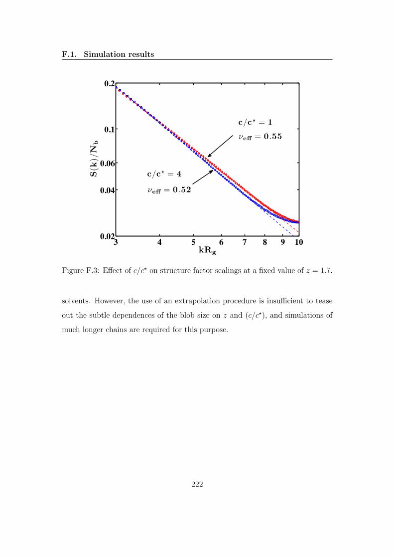
F.1. Simulation results
3 4 5 6 7 8 9 100.02
0.04
0.06
0.1
0.2
kRg
S(k
)/N
b
c/c! = 4
!e! = 0.52
!e! = 0.55
c/c! = 1
Figure F.3: Effect of c/c? on structure factor scalings at a fixed value of z = 1.7.
solvents. However, the use of an extrapolation procedure is insufficient to tease
out the subtle dependences of the blob size on z and (c/c?), and simulations of
much longer chains are required for this purpose.
222

Appendix G
Periodic Boundary Condition for
Planar Elongational Flow
G.1 Introduction
In this appendix, periodic boundary conditions (PBCs) are discussed for planar
elongational flows (PEF). The derivation of PBCs for PEF was first carried out
by Kraynik and Reinelt (1992). Here the intention is to elaborate many steps in
their derivation in detail. The key questions to be addressed in this appendix
are the following: (i) At what angle should the lattice be inclined initially? (ii)
What should the initial lattice vectors be? (iii) At what time should the lattice be
mapped back to its original configuration? The very first step in order to address
these questions is to recognize the condition for the reproducibility of a lattice.
A lattice is said to be reproducible with another lattice if the lattice points on
both the lattices coincide. The equations for the lattice reproducibility condition
leads to an eigenvalue problem, and the solution of the eigenvalue problem is
used to answer these three questions.
223

G.2. Condition for Reproducibility
G.2 Condition for ReproducibilityWe start by constructing an arbitrary 3-D lattice consisting of all the points Rn
through the expression,
Rn = n1b1 + n2b2 + n3b3 (G.1)
where b1, b2 and b3 are linearly independent basis vectors, and n = n1, n2, n3is a set of integer numbers. In order to be compatible with the elongational flow,
these basis vectors need to evolve suitably with respect to time. The evolution
of these basis lattice vectors can be written in terms of the following differential
equation,dbi
dt= bi · ∇u = bi ·D (G.2)
where ∇u or D is the flow gradient tensor. For planar elongational flows, it is
given by
D =
ε 0 0
0 ε 0
0 0 0
If b01, b0
2 and b03 are considered to be the initial basis vectors, then Eq. (G.2)
can be integrated to give,
bi = b0i · Λ (G.3)
where Λ = exp (Dt). As D is a diagonal tensor, Λ can be written as,
Λ =
eεt 0 0
0 e−εt 0
0 0 1
(G.4)
Λ is also called the time evolution matrix.
As pointed out by Kraynik and Reinelt (1992), for a given Λ, a lattice is
224
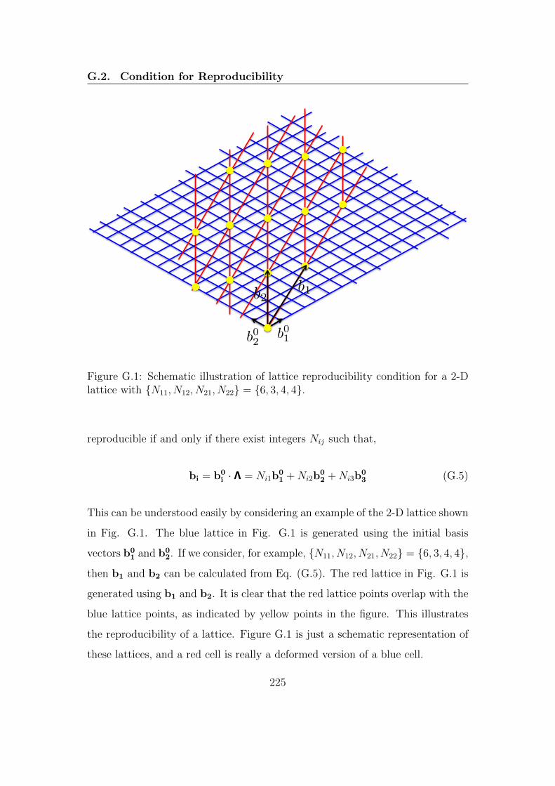
G.2. Condition for Reproducibility
b01b0
2
b2b1
Figure G.1: Schematic illustration of lattice reproducibility condition for a 2-Dlattice with N11, N12, N21, N22 = 6, 3, 4, 4.
reproducible if and only if there exist integers Nij such that,
bi = b0i · Λ = Ni1b
01 +Ni2b
02 +Ni3b
03 (G.5)
This can be understood easily by considering an example of the 2-D lattice shown
in Fig. G.1. The blue lattice in Fig. G.1 is generated using the initial basis
vectors b01 and b0
2. If we consider, for example, N11, N12, N21, N22 = 6, 3, 4, 4,then b1 and b2 can be calculated from Eq. (G.5). The red lattice in Fig. G.1 is
generated using b1 and b2. It is clear that the red lattice points overlap with the
blue lattice points, as indicated by yellow points in the figure. This illustrates
the reproducibility of a lattice. Figure G.1 is just a schematic representation of
these lattices, and a red cell is really a deformed version of a blue cell.
225

G.3. The Eigenvalue Problem
If we need to remap the lattice to its original configuration after a certain
time, we must make sure that the lattice remains periodic after the remapping.
Todd and Daivis (1998) and Baranyai and Cummings (1999) have shown that the
reproducibility of the lattice can be successfully utilized to ensure that periodic
boundary conditions are maintained throughout the simulation. We can obtain
a reproducible lattice only for a certain set of integers that satisfy Eq. (G.5),
and therefore, our problem now reduces to solving for such integers.
G.3 The Eigenvalue Problem
The reproducibility condition (Eq. (G.5)) can be turned into an eigenvalue prob-
lem, as discussed below. Equation (G.5) is first expanded in the form,
b01 · Λ = N11b
01 +N12b
02 +N13b
03 (G.6)
b02 · Λ = N21b
01 +N22b
02 +N23b
03 (G.7)
b03 · Λ = N31b
01 +N32b
02 +N33b
03 (G.8)
Since, Λ is a diagonal matrix or Λij = 0 for i 6= j, Eqs. (G.6), (G.7) and (G.8)
can be written in component form as,
Λ11b01,x = N11b
01,x +N12b
02,x +N13b
03,x (G.9)
Λ22b01,y = N11b
01,y +N12b
02,y +N13b
03,y (G.10)
Λ33b01,z = N11b
01,z +N12b
02,z +N13b
03,z, (G.11)
Λ11b02,x = N21b
01,x +N22b
02,x +N23b
03,x (G.12)
Λ22b02,y = N21b
01,y +N22b
02,y +N23b
03,y (G.13)
Λ33b02,z = N21b
01,z +N22b
02,z +N23b
03,z (G.14)
226

G.3. The Eigenvalue Problem
and
Λ11b03,x = N31b
01,x +N32b
02,x +N33b
03,x (G.15)
Λ22b03,y = N31b
01,y +N32b
02,y +N33b
03,y (G.16)
Λ33b03,z = N31b
01,z +N32b
02,z +N33b
03,z (G.17)
Considering all the x component equations in Eqs. (G.9), (G.12) and (G.15), we
can write the matrix equation,
Λ11
b01,x
b02,x
b03,x
=
N11 N12 N13
N21 N22 N23
N31 N32 N33
·
b01,x
b02,x
b03,x
(G.18)
Similarly, all the y components can be combined in a matrix equation,
Λ22
b01,y
b02,y
b03,y
=
N11 N12 N13
N21 N22 N23
N31 N32 N33
·
b01,y
b02,y
b03,y
(G.19)
and the z components equations can be represented by
Λ33
b01,z
b02,z
b03,z
=
N11 N12 N13
N21 N22 N23
N31 N32 N33
·
b01,z
b02,z
b03,z
(G.20)
Eqs. (G.18), (G.19) and (G.20) can be written in the general form
λj
b01,j
b02,j
b03,j
=
N11 N12 N13
N21 N22 N23
N31 N32 N33
·
b01,j
b02,j
b03,j
(G.21)
227

G.4. The Strain Period of the Lattice
where λj = Λjj = exp (Djjt), and j = 1, 2, 3 or x, y, z. If we consider cj to be a
column vector of components b01,j, b
02,j, b
03,j, then Eq. (G.21) can be written as,
λjI · cj = N · cj (G.22)
which can be expressed as the eigenvalue problem,
(N− λjI) · cj = 0 (G.23)
The solution of this eigenvalue problem leads to results for the strain period, the
magic angle and the initial lattice vectors.
G.4 The Strain Period of the Lattice
The strain period is obtained by first finding the eigenvalues of the N tensor.
In order to obtain the eigenvalues λj, Eq. (G.23) is solved to give the following
characteristic equation
λ3i − kλ2
i +mλi − l = 0 (G.24)
where,
k = N11 +N22 +N33 = tr(N),
m = N11N22 +N11N33 +N22N33 −N32N23 −N12N21 −N13N31
=1
2
[tr(N)2 − tr(NN)
],
and
l = N11N22N33−N11N32N23−N12N21N33 +N12N31N23 +N13N21N32−N13N31N22
= det(N).
We can evaluate k, l and m by making use of the fact that they are the invariants
of the matrix N, and λi (i = 1, 2, 3) are the eigenvalues of N.
228

G.4. The Strain Period of the Lattice
1.
k = tr(N) = λ1 + λ2 + λ3 (G.25)
2.
m =1
2
[tr(N)2 − tr(NN)
]= λ2λ3 + λ1λ3 + λ1λ2 (G.26)
Dividing the above equation by λ1 λ2 λ3 (= 1), leads to
m =1
λ1
+1
λ2
+1
λ3
(G.27)
3.
l = det(N) = λ1 λ2 λ3 (G.28)
For isochoric deformations, det(N) = 1, hence, l = 1.
If λ1 = φ, then for planar elongational flow, it follows from Eq. (G.4) that
λ2 = 1/φ and λ3 = 1. When these eigenvalues are inserted in Eq. (G.25) we get,
φ+1
φ+ 1 = k (G.29)
which is a quadratic equation for φ, with a solution
φ =(k − 1) +
√(k − 1)2 − 4
2= λ1 (G.30)
which is one of the roots of the quadratic equation. It can be easily shown that1
φ=
(k − 1)−√
(k − 1)2 − 4
2. As a result, the second root is simply 1/φ or λ2.
Note that from Eq. (G.27), and the known values of λ1, λ2 and λ3, it follows
that m = k.
For a discrete set of k, a discrete set of φ can be calculated. From Eq. (G.30)
it is clear that k cannot be less than 3. Since m = k, it follows that m ≥ 3. In
229

G.5. Magic Angle and Initial Lattice
the case of no deformation, the matrix Λ is a unit matrix, and for this trivial
case k = m = 3. We are interested in nontrivial cases in which the lattices are
deforming, i.e., we require integers k > 3 and m > 3 for which there exist lattices
that are reproducible and periodic. For k = 4, 5, 6, . . ., discrete values of φ can
be calculated, and at only these discrete values the lattice will exhibit periodic
planar elongational flow. Since φ = eεt, for a given ε, the times at which the
lattice will be periodic are t =log φ
ε.
Finding the information for strain period is useful but not complete. It is
also required to derive the initial lattice configuration with which the simulation
starts, for instance, the initial lattice vectors and the orientation of the lattice
(the magic angle). These can be achieved by finding out a suitable N matrix.
G.5 Magic Angle and Initial Lattice
In planar flows, the lattice in the direction perpendicular to the plane of flow
remains undeformed. As a result b3 = b03 at all times, and it is sufficient to
consider the 2-D lattice in the plane of flow. The 2-D lattice can be defined in
terms of (i) a, the ratio of the magnitudes of b2 to b1, and (ii) Φ, the angle
between b1 and b2, as shown in Fig. G.2. If θ is the angle at which the lattice
is initially oriented, then we can write the basis vectors as
b1 = (cos θ, sin θ) and b2 = (a cos (θ + Φ), a sin (θ + Φ)) (G.31)
Here, θ is the magic angle, and the derivation of it is discussed here. We start
with rewriting Eq. (G.23) for j = 1 and 2 as,
(N− λ1I) · c1 = 0 (G.32)
(N− λ2I) · c2 = 0 (G.33)
230

G.5. Magic Angle and Initial Lattice
Origin
θ
Φ b1
b2
|b2||b1| = a
Figure G.2: A general 2-D lattice with magic angle θ
For a 2-D system, Eq. (G.32) can be written as two set of equations. In this
case, λ1 = φ and c1 = (cos θ, a cos (θ + Φ)), and the two equations are
(N11 − φ) cos θ + aN12 cos (θ + Φ) = 0 (G.34)
N21 cos θ + a(N22 − φ) cos (θ + Φ) = 0 (G.35)
Similarly, for j = 2, λ2 = 1/φ and c2 = (sin θ, a sin (θ + Φ)), and the correspond-
ing two equations are
(N11 − 1/φ) sin θ + aN12 sin (θ + Φ) = 0 (G.36)
N21 sin θ + a(N22 − 1/φ) sin (θ + Φ) = 0 (G.37)
Note that for planar flows, N13 = N23 = N31 = N32 = 0, and N33 = 1. Equation
(G.34) can be solved to obtain an expression for θ in terms of a, Φ, φ, N11 and
N12,
θ = tan−1
[(N11 − φ) + aN12 cos Φ
aN12 sin Φ
](G.38)
Here φ can be calculated using Eq. (G.30), and a and Φ are also known for any
specific lattice. For instance, for a square lattice a = 1 and Φ = π/2, and for a
231

G.5. Magic Angle and Initial Lattice
hexagonal lattice a = 1 and Φ = π/3. Hence, the only unknowns in Eq. (G.38)
are N11 and N12. An expression for θ is also obtained from Eq. (G.36) as given
below,
θ = tan−1
[ −aN12 sin Φ
(N11 − 1/φ) + aN12 cos Φ
](G.39)
Now, Eqs. (G.38) and (G.39) can be equated to give
[(N11 − φ) + aN12 cos Φ] [(N11 − 1/φ) + aN12 cos Φ] =
− [aN12 sin Φ] [aN12 sin Φ](G.40)
Or,
N211 −N11 (φ+ 1/φ) + 2a cos ΦN11N12 + 1
−aN12 cos Φ (φ+ 1/φ) + a2N212 = 0
(G.41)
Note that for planar elongational flows, φ + (1/φ) is equal to N11 + N22 since
N33 = 1. Further, we can write
m = λ1 + λ2 + λ1λ2 = φ+ (1/φ) + 1 = N11N22 +N11 +N22 −N12N21,
or
N11N22 −N12N21 = λ1 λ2 = 1. As a result, Eq. (G.41) can be simplified to give,
−N21 + a cos Φ(N11 −N22) + a2N12 = 0 (G.42)
We define k = N11 + N22, and note that N11N22 − N12N21 = 1. This leads to
equations for N22 and N21 in terms of k, N11 and N12, as given below,
N22 = k −N11 (G.43)
N21 =N11(k −N11)− 1
N12
(G.44)
232
G.6. Step-by-Step Implementation for a Square Lattice
Note that k ≥ 2. Inserting N22 and N21 into Eq. (G.42) gives an equation in
terms of a, Φ, k, N11 and N12,
(N11 − k/2
)2
+ 2a cos Φ(N11 − k/2
)N12 + a2N2
12 = k2/4− 1 (G.45)
This is also an equation of ellipse centered at (k/2, 0). For a square lattice (a = 1,
Φ = π/2), Eq. (G.45) becomes an equation of circle,
(N11 − k/2
)2
+N212 = k2/4− 1 (G.46)
and Eq. (G.42) simplifies to N21 = N12. Equation (G.46) can be used to find an
expression for N12 in terms of k and N11 as,
N12 = ±√N11(k −N11)− 1 (G.47)
If, for a given N11, we find an integer value of N12, then we have found the
solution. As mentioned by Kraynik and Reinelt (1992), the negative root is
always considered in Eq. (G.47). It is conventional to simulate PEF with square
lattices, which we also do in this work.
G.6 Step-by-Step Implementation for a Square
Lattice
Finally, in order to implement all these steps in a computer program, we sum-
marize these results in a step-by-step procedure as follows:
1. First choose an integer value of k (k = 3, 4, 5, . . .).
233
G.6. Step-by-Step Implementation for a Square Lattice
2. Calculate the eigenvalue φ using the following expression
φ =k +
√k2 − 4
2(G.48)
3. Estimate the strain period τp using the expression τp = log (φ)/ε, where ε
is the elongational rate.
4. Select a positive integer value of N11 such that an integer value of N12 is
obtained using the following expression
N12 = −√N11(k −N11)− 1 (G.49)
5. Calculate the magic angle using the expression
θ = tan−1
[N11 − φN12
](G.50)
Note that this equation is a simplified form of Eq. (G.38) for a square
lattice.
Therefore, we know the initial lattice configuration and the time at which the
lattice should be deformed and mapped back to its original configuration.
234

Appendix H
Compatibility Condition in
Planar Mixed Flow
Since lattices evolve only in the xy plane for planar flows, one corner of the
simulation box can be set at the origin and r1(t), r2(t) and r3(t) can be considered
to be the other three corners, as shown in Fig. H.1. The lattice spacing D(t) is
in turn expressed as the modulus of the sum of the three vectors r1, r2 and r3
(which are three of the corners in the cell). As indicated by the black dashed
lines in Fig. H.1, the trajectories of any cell vectors can be used to derive the
minimum length in the direction of the cell vectors. Considering r = r1 +r2 +r3,
expressions for rx(t) and ry(t) for PMF are given in Eqs. (7.37) and (7.35)
respectively. Note that rx and ry are the x and y components of the vector r,
respectively. D(t) reaches its minimum value when,
d
dt(r(t) · r(t)) = 0 (H.1)
235
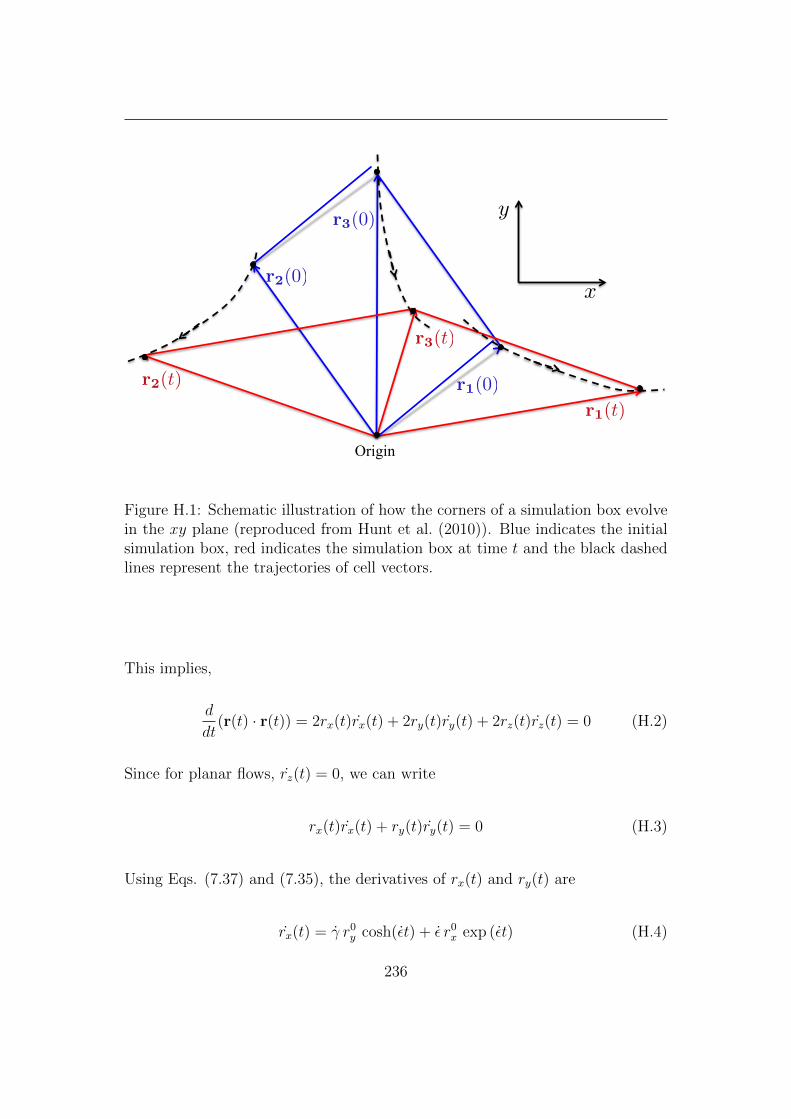
Origin
r1(0)
r2(0)
r3(0)
r1(t)
r2(t)
r3(t)
x
y
Figure H.1: Schematic illustration of how the corners of a simulation box evolvein the xy plane (reproduced from Hunt et al. (2010)). Blue indicates the initialsimulation box, red indicates the simulation box at time t and the black dashedlines represent the trajectories of cell vectors.
This implies,
d
dt(r(t) · r(t)) = 2rx(t)rx(t) + 2ry(t)ry(t) + 2rz(t)rz(t) = 0 (H.2)
Since for planar flows, rz(t) = 0, we can write
rx(t)rx(t) + ry(t)ry(t) = 0 (H.3)
Using Eqs. (7.37) and (7.35), the derivatives of rx(t) and ry(t) are
rx(t) = γ r0y cosh(εt) + ε r0
x exp (εt) (H.4)
236
and
ry(t) = −ε r0y exp (−εt) (H.5)
Putting together rx(t), ry(t), rx(t) and ry(t) in Eq. (H.3) leads to
[γ
εr0y sinh(εt) + r0
x exp (εt)
] [γ r0
y cosh(εt) + ε r0x exp (εt)
]
+[r0y exp (−εt)
] [−ε r0
y exp (−εt)]
= 0
(H.6)
Equation (H.6) can be simplified by using trigonometric formulas and also using
the definitions of sinh(x), cosh(x) in terms of exponentials exp (x), to give
exp (2εt)
[γ2 r0
y2
4ε+ γ r0
x r0y + εr0
x2
]= exp (−2εt)
[γ2 r0
y2
4ε+ ε r0
y2
](H.7)
Or,
exp (4εt) =γ2 r0
y2
+ 4ε2 r0y
2
γ2 r0y
2 + 4γ ε r0x r
0y + 4ε2 r0
x2 (H.8)
Denoting by tmin, the time at which the lattice spacing is a minimum, we can see
that,
tmin =1
4εlog
[γ2 r0
y2
+ 4ε2 r0y
2
γ2 r0y
2 + 4γ ε r0x r
0y + 4ε2 r0
x2
](H.9)
Therefore, the minimum lattice spacing Dmin can be found to be
Dmin =√r2x(tmin) + r2
y(tmin) (H.10)
Using Eqs. (7.35), (7.37), (H.9) and (H.10), the minimum lattice spacing can
be calculated, and hence a suitable cutoff radius rc can be chosen to ensure the
compatibility condition is satisfied.
237

238

Bibliography
Ahlrichs, P. and B. Dunweg, 1999: Simulation of a single polymer chain in solu-
tion by combining Lattice Boltzmann and molecular dynamics. J.Chem.Phys.,
111, 8225.
Ahlrichs, P., R. Everaers, and B. Duenweg, 2001: Screening of hydrodynamic
interactions in semidilute polymer solutions: A computer simulation study.
Phys.Rev. E, 64, 040501.
Allen, M. and D. Tildesley, 1990: Computer Simulations of Liquids. Oxford
Science, London.
Banchio, A. J. and J. F. Brady, 2003: Accelerated Stokesian dynamics: Brownian
motion. J. Chem. Phys., 118(22), 10323–10332.
Baranyai, A. and P. T. Cummings, 1995: Nonequilibrium molecular dynamics
study of shear and shear-free flows in simple fluids. J.Chem.Phys., 103(23),
10217–10225.
Baranyai, A. and P. T. Cummings, 1999: Steady state simulation of planar
elongation flow by nonequilibrium molecular dynamics. J.Chem.Phys., 110(1),
42–45.
Beenakker, C. W. J., 1986: Ewald sum of the Rotne-Prager tensor.
J.Chem.Phys., 85, 1581–1582.
239
Bibliography
Bhupathiraju, R., P. T. Cummings, and H. D. Cochran, 1996: An efficient
parallel algorithm for non-equilibrium molecular dynamics simulations of very
large systems in planar Couette flow. Mol.Phys., 88(6), 1665–1670.
Binder, K., 1995: Monte Carlo and Molecular Dynamics Simulations in Polymer
Science. Oxford University Press, USA.
Bird, R. B., C. F. Curtiss, R. C. Armstrong, and O. Hassager, 1987: Dynamics
of Polymeric Liquids, volume 2. John Wiley and Sons, New York.
Bixon, M., 1976: Polymer dynamics in solution. Annu. Rev. Phys. Chem., 27(1),
65–84.
Brady, J. F., R. J. Phillips, J. C. Lester, and G. Bossis, 1988: Dynamic simulation
of hydrodynamically interacting suspensions. J. Fluid.Mech., 195, 257–280.
Champeney, D. C., 1973: Fourier Transforms and Their Physical Applications.
Academic, New York.
Clisby, N., 2010: Accurate estimate of the critical exponent ν for self-avoiding
walks via a fast implementation of the pivot algorithm. Phys. Rev. Lett., 104,
055702.
Cloizeaux, J. and G. Jannink, 2010: Polymers in Solution: Their Modelling and
Structure. Oxford Classic Texts in the Physical Sciences. OUP Oxford.
Daivis, P. J., M. L. Matin, and B. D. Todd, 2003: Nonlinear shear and elonga-
tional rheology of model polymer melts by non-equilibrium molecular dynam-
ics. J. Non-Newtonian Fluid Mech., 111, 1–18.
Daivis, P. J. and D. N. Pinder, 1990: Application of the blob model to the
calculation of cooperative and self-diffusion coefficients in polymer solutions.
Macromolecules, 23(25), 5176–5181.
240

Bibliography
Daoud, M., J. P. Cotton, B. Farnoux, G. Jannink, G. Sarma, H. Benoit, C. Du-
plessix, C. Picot, and P. G. de Gennes, 1975: Solutions of flexible polymers.
neutron experiments and interpretation. Macromolecules, 8(6), 804–818.
de Gennes, P. G., 1976a: Dynamics of entangled polymer solutions. I. the Rouse
model. Macromolecules, 9(4), 587–593.
de Gennes, P. G., 1976b: Dynamics of entangled polymer solutions. II. inclusion
of hydrodynamic interactions. Macromolecules, 9, 594.
de Gennes, P. G., 1979: Scaling Concepts in Polymer Physics. Cornell University,
Ithaca, New York.
Deserno, M. and C. Holm, 1998: How to mesh up Ewald sums. i. a theoretical
and numerical comparison of various particle mesh routines. J.Chem.Phys.,
109, 7678.
Doi, M. and S. F. Edwards, 1986: The Theory of Polymer Dynamics. Clarendon
Press, Oxford, New York.
Dua, A. and B. J. Cherayil, 2003: Polymer dynamics in linear mixed flow.
J.Chem.Phys., 119(11), 5696–5700.
Dunweg, B. and A. J. C. Ladd, 2009: Lattice Boltzmann simulations of soft
matter systems. Adv. Polym. Sci., 221, 89.
Edwards, S. F. and M. Muthukumar, 1984: Brownian dynamics of polymer
solutions. Macromolecules, 17, 586.
Ewald, P., 1921: . Ann. Phys., 64, 253.
241
Bibliography
Ewen, B. and D. Richter, 1997: Neutron spin echo investigations on the segmen-
tal dynamics of polymers in melts, networks and solutions. Adv. Polym. Sci.,
134, 1–129.
Fincham, D., 1994: Optimization of the Ewald sum for large systems. Mol. Sim.,
13, 1.
Fixman, M., 1986: Construction of Langevin forces in the simulation of hydro-
dynamic interaction. Macromolecules, 19, 1204 – 1207.
Flory, P. J., 1953: Principles of Polymer Chemistry. Baker lectures 1948. Cornell
University Press.
Fredrickson, G. H. and E. Helfand, 1990: Collective dynamics of polymer solu-
tions. J.Chem.Phys., 93(3), 2048–2061.
Freed, K. F., 1987: Renormalization Group Theory of Macromolecules. Wiley,
New York.
Freed, K. F. and S. F. Edwards, 1974: Polymer viscosity in concentrated solu-
tions. J. Chem. Phys., 61(9), 3626–3633.
Frenkel, D. and B. Smit, 2002: Understanding Molecular Simulation. Academic
Press, London.
Fuller, G. and L. Leal, 1981: The effects of conformation-dependent friction and
internal viscosity on the dynamics of the nonlinear dumbbell model for a dilute
polymer solution. Journal of Non-Newtonian Fluid Mechanics, 8(3 - 4), 271 –
310.
Gompper, G., T. Ihle, D. Kroll, and R. Winkler, 2009: Multi-particle collision
dynamics: A particle-based mesoscale simulation approach to the hydrody-
namics of complex fluids. Adv. Polym. Sci., 221, 1–87.
242

Bibliography
Graessley, W. W., R. C. Hayward, and G. S. Grest, 1999: Excluded-volume
effects in polymer solutions. 2. comparison of experimental results with nu-
merical simulation data. Macromolecules, 32(10), 3510–3517.
Grest, G. S., B. Dunweg, and K. Kremer, 1989: Vectorized link cell fortran code
for molecular dynamics simulations for a large number of particles. Comput.
Phys. Commun., 55(3), 269 – 285.
Griebel, M., S. Knapek, and G. Zumbusch, 2007: Numerical Simulation in
Molecular Dynamics. Springer, Berlin, Heidelberg.
Grosberg, A. Y. and A. R. Khokhlov, 1994: Statistical physics of macromolecules.
AIP Press, New York.
Hansen, D. P. and D. J. Evans, 1994: A parallel algorithm for nonequilibrium
molecular dynamics simulation of shear flow on distributed memory machines.
Mol. Sim., 13(6), 375–393.
Hasimoto, M., 1959: On the periodic fundamental solutions of the Stokes equa-
tions and their applications to viscous flow past a cubic array of spheres. J.
Fluid Mech., 5, 317.
Hernandez-Ortiz, J. P., J. J. de Pablo, and M. D. Graham, 2007: Fast computa-
tion of many-particle hydrodynamic and electrostatic interactions in a confined
geometry. Phys. Rev. Lett., 98, 140602.
Heyes, D., 1985: Molecular dynamics simulations of extensional, shear and
unidirectional flow. Chem. Phys., 98(1), 15 – 27.
Hockney, R. W., S. P. Goel, and J. W. Eastwood, 1973: A 10000 particle
molecular dynamics model with long range forces. Chem. Phys. Lett., 21, 589.
243

Bibliography
Hoffman, B. D. and E. S. G. Shaqfeh, 2007: The dynamics of the coil-stretch
transition for long, flexible polymers in planar mixed flows. J. Rheol., 51(5),
947–969.
Hounkonnou, M. N., C. Pierleoni, and J.-P. Ryckaert, 1992: Liquid chlorine
in shear and elongational flows: A nonequilibrium molecular dynamics study.
J.Chem.Phys., 97(12), 9335–9344.
Huang, C. C., R. G. Winkler, G. Sutmann, and G. Gompper, 2010: Semidi-
lute polymer solutions at equilibrium and under shear flow. Macromolecules,
43(23), 10107–10116.
Hunt, T. A., S. Bernardi, and B. D. Todd, 2010: A new algorithm for extended
nonequilibrium molecular dynamics simulations of mixed flow. J.Chem.Phys.,
133(15), 154116.
Hur, J., E. S. G. Shaqfeh, H. P. Babcock, D. E. Smith, and S. Chu, 2001:
Dynamics of dilute and semidilute DNA solutions in the start-up of shear
flow. J. Rheol., 45, 421.
Jain, A., B. Dunweg, and J. R. Prakash, 2012: Dynamic crossover scaling in
polymer solutions. Phys. Rev. Lett., 109, 088302.
Jain, A., P. Sunthar, B. Dunweg, and J. R. Prakash, 2012: Optimization of a
Brownian-dynamics algorithm for semidilute polymer solutions. Phys. Rev. E,
85, 066703.
Jendrejack, R. M., M. D. Graham, and de Pablo J. J., 2000: Hydrodynamic
interactions in long-chain polymers: Application of the Chebyshev polynomial
approximation in stochastic simulations. J.Chem.Phys., 113, 2894.
244
Bibliography
Kapral, R., 2008: Multiparticle Collision Dynamics: Simulation of Complex
Systems on Mesoscales. 89–146.
Kirkwood, J. G. and J. Riseman, 1948: The intrinsic viscosities and diffusion
constants of flexible macromolecules in solution. J.Chem.Phys., 16(6), 565–
573.
Kozer, N., Y. Y. Kuttner, G. Haran, and G. Schreibe, 2007: Protein-protein
association in polymer solutions: From dilute to semidilute to concentrated.
Biophys. J ., 92, 2139–2149.
Kraynik, A. M. and D. A. Reinelt, 1992: Extensional motions of spatially periodic
lattices. Int. J. Multiphase Flow, 18, 1045.
Kroger, M., A. Alba-Perez, M. Laso, and H. C. Ottinger, 2000: Variance reduced
Brownian simulation of a bead-spring chain under steady shear flow considering
hydrodynamic interaction effects. J. Chem. Phys., 113, 4767–4773.
Kumar, K. S. and J. R. Prakash, 2003: Equilibrium swelling and universal ratios
in dilute polymer solutions: An exact Brownian dynamics simulations for a
delta function excluded volume potential. Macromolecules, 36(20), 7842–7856.
Ladd, A. J. C., R. Kekre, and J. E. Butler, 2009: Comparison of the static and
dynamic properties of a semiflexible polymer using Lattice Boltzmann and
Brownian-dynamics simulations. Phys. Rev. E, 80, 036704.
Larson, R., 1988: Constitutive Equations for Polymer Melts and Solutions.
Biotechnology Series. Butterworths (Canada) Limited.
Lees, A. W. and S. F. Edwards, 1972: The computer studies of transport pro-
cesses under extreme conditions. J. Phys. C: Solid State Phys., 5, 1921–1929.
245
Bibliography
Li, B., N. Madras, and A. D. Sokal, 1995: Critical exponents, hyperscaling, and
universal amplitude ratios for two- and three-dimensional self-avoiding walks.
J. Stat. Phys., 80(3-4), 661–754.
Luty, B., M. Davis, I. Tironi, and W. van Gunsteren, 1994: A comparison of
particle-particle, particle-mesh and Ewald methods for calculating electrostatic
interactions in periodic molecular systems. Mol. Sim., 14, 11–20.
Malevanets, A. and R. Kapral, 1999: Mesoscopic model for solvent dynamics. J.
Chem. Phys., 110(17), 8605–8613.
Mangenota, S., S. Kellera, and J. Radler, 2003: Transport of nucleosome core
particles in semidilute DNA solutions. Biophys. J ., 85, 1817–1825.
Marmonier, M. F. and L. Leger, 1985: Reptation and tube renewal in entangled
polymer solutions. Phys. Rev. Lett., 55, 1078–1081.
Miyaki, Y. and H. Fujita, 1981: Excluded-volume effects in dilute polymer
solutions. 11. tests of the two-parameter theory for radius of gyration and
intrinsic viscosity. Macromolecules, 14(3), 742–746.
Muller, M., K. Binder, and L. Schafer, 2000: Intra- and interchain correlations
in semidilute polymer solutions: Monte Carlo simulations and renormalization
group results. Macromolecules, 33(12), 4568–4580.
Muthukumar, M., 1984: Concentration dependent relaxation times of linear
polymers in dilute solutions. Macromolecules, 17(4), 971–973.
Muthukumar, M. and S. Edwards, 1982a: Screening concepts in polymer solution
dynamics. Polymer, 23(3), 345 – 348.
Muthukumar, M. and S. F. Edwards, 1982b: Extrapolation formulas for polymer
solution properties. J.Chem.Phys., 76(5), 2720–2730.
246
Bibliography
Muthukumar, M. and S. F. Edwards, 1983: Screening of hydrodynamic inter-
action in a solution of rodlike macromolecules. Macromolecules, 16(9), 1475–
1478.
Nijboer, B. R. A. and F. W. de Wette, 1957: On the calculation of lattice sums.
Physica., 23, 309–321.
Ottinger, H. C., 1989: Gaussian approximation for rouse chains with hydrody-
namic interaction. The Journal of Chemical Physics, 90(1), 463–473.
Ottinger, H. C., 1996: Stochastic Processes in Polymeric Fluids. Springer, Berlin.
Pan, S., D. A. Nguyen, P. Sunthar, T. Sridhar, and J. R. Prakash Universal
solvent quality crossover of the zero shear rate viscosity of semidilute DNA
solutions. 2011arXiv1112.3720P.
Perram, J., H. Peterson, and K. De Leeuw, 1988: An algorithm for the simulation
of condensed matter which grows as the 3/2 power of the number of particles.
Mol. Phys., 65, 875.
Pham, T. T., U. D. Schiller, J. R. Prakash, and B. Dunweg, 2009: Implicit and
explicit solvent models for the simulation of a single polymer chain in solution:
Lattice Boltzmann versus Brownian dynamics. J. Chem. Phys., 131, 164114.
Pouyet, G., F. Candau, and J. Dayantis, 1976: Sedimentation measurements on
polystyrene solutions in cyclohexane below the Flory theta temperature. Die
Makromolekulare Chemie, 177(10), 2973–2980.
Prabhakar, R., 2005: Predicting the rheological properties of dilute polymer so-
lutions using bead-spring models: Brownian dynamics simulations and closure
approximations. PhD thesis, Monash University.
247

Bibliography
Prabhakar, R. and J. R. Prakash, 2004: Multiplicative separation of the influ-
ences of excluded volume, hydrodynamic interactions and finite extensibility
on the rheological properties of dilute polymer solutions. J.Non-Newtonian
Fluid.Mech., 116, 163.
Prakash, J. R., 1999: The kinetic theory of dilute solutions of flexible polymers:
Hydrodynamic interaction. In Advances in flow and rheology of non-Newtonian
fluids, Siginer, D. A., Kee, D. D., and Chhabra, R. P., editors, Elsevier Science,
Rheology Series, Amsterdam, 467–517.
Prakash, J. R., 2001a: The influence of the range of excluded volume interactions
on the linear viscoelastic properties of dilute polymer solutions. Chem. Eng.
Sci., 56(19), 5555 – 5564.
Prakash, J. R., 2001b: Rouse chains with excluded volume interactions: Linear
viscoelasticity. Macromolecules, 34(10), 3396–3411.
Prakash, J. R., 2002: Rouse chains with excluded volume interactions in steady
simple shear flow. J. Rheol., 46(6), 1353–1380.
Prakash, J. R., 2009: Micro and macro in the dynamics of dilute polymer
solutions: Convergence of theory with experiment. Korea-Australia Rheology
Journal, 21(4), 245–268.
Prakash, J. R. and H. C. Ottinger, 1999: Viscometric functions for a dilute
solution of polymers in a good solvent. Macromolecules, 32(6), 2028–2043.
R. H. Colby, M. Rubinstein, and M. Daoud, 1994: Hydrodynamics of polymer
solutions via two-parameter scaling. J. Phys. II France, 4(8), 1299–1310.
Rapaport, D., 2004: The Art of Molecular Dynamics Simulation. Cambridge
University Press.
248

Bibliography
Richter, D., K. Binder, B. Ewen, and B. Stuehn, 1984: Screening of hydrody-
namic interactions in dense polymer solutions: a phenomenological theory and
neutron-scattering investigations. J. Phys. Chem., 88, 6618.
Rinn, B., K. Zahn, P. Maass, and G. Maret, 1999: Influence of hydrodynamic
interactions on the dynamics of long-range interacting colloidal particles. Eu-
rophys. Lett., 46(4), 537.
Rotne, J. and S. Prager, 1969: Variational treatment of hydrodynamic interac-
tion in polymers. J. Chem. Phys., 50, 4831–4837.
Rubinstein, M. and R. H. Colby, 2003: Polymer Physics. Oxford University
Press.
Schafer, L., 1999: Excluded Volume Effects in Polymer Solutions. Springer-
Verlag, Berlin.
Shiwa, Y., Y. Oono, and P. R. Baldwin, 1988: Dynamics of semidilute polymer
solutions: hydrodynamic screening. Macromolecules, 21(1), 208–214.
Sierou, A. and J. F. Brady, 2001: Accelerated Stokesian dynamics simulations.
J. Fluid Mech., 448, 115.
Smith, E. R., I. K. Snook, and W. V. Megen, 1987: Hydrodynamic interac-
tions in Brownian dynamics: 1. periodic boundary conditions for computer
simulations. Physica, 143A, 441–467.
Stoltz, C., 2006: Simulation of dilute polymer and polyelectrolyte solutions: Con-
centration effects. PhD thesis, The University of Wisconsin.
Stoltz, C., J. J. de Pablo, and M. D. Graham, 2006: Concentration dependence
of shear and extensional rheology of polymer simulations: Brownian dynamics
simulations. J.Rheol., 502, 137.
249
Bibliography
Sunthar, P. and J. R. Prakash, 2005: Parameter free prediction of DNA confor-
mations in elongational flow by successive fine graining. Macromolecules, 38,
617.
Sunthar, P. and J. R. Prakash, 2006: Dynamic scaling in dilute polymer solutions:
The importance of dynamic correlations. Europhys. Lett., 75, 77.
Thurston, G. B. and A. Peterlin, 1967: Influence of finite number of chain
segments, hydrodynamic interaction, and internal viscosity on intrinsic bire-
fringence and viscosity of polymer solutions in an oscillating laminar flow field.
J.Chem.Phys., 46(12), 4881–4885.
Todd, B. and P. J. Daivis, 1999: A new algorithm for unrestricted duration
nonequilibrium molecular dynamics simulations of planar elongational flow.
Comput. Phys. Commun., 117(3), 191 – 199.
Todd, B. D. and P. J. Daivis, 1998: Non-equilibrium molecular dynamics sim-
ulations of planar elongational flow with spatially and temporally periodic
boundary conditions. Phys. Rev. Lett., 81, 1118.
Todd, B. D. and P. J. Daivis, 2000: The stability of nonequilibrium molecular
dynamics simulations of elongational flows. The Journal of Chemical Physics,
112(1), 40–46.
Todd, B. D. and P. J. Daivis, 2007: Homogeneous non-equilibrium molecular
dynamics simulations of viscous flow: techniques and applications. Mol. Sim.,
33(3), 189–229.
Toukmaji, A. Y. and J. A. J. Board, 1996: Ewald summation techniques in
perspective: A survey. Comput. Phys. Commun., 95, 73–92.
250

Bibliography
W. Paul, K. Binder, D. W. Heermann, and K. Kremer, 1991: Crossover scaling
in semidilute polymer solutions: a Monte Carlo test. J. Phys. II France, 1(1),
37–60.
Wheeler, D. R., N. G. Fuller, and R. L. Rowley, 1997: Non-equilibrium molecular
dynamics simulation of the shear viscosity of liquid methanol: Adaptation of
the Ewald sum to Lees Edwards boundary conditions. Mol. Phys., 92, 55–62.
Wiltzius, P. and D. S. Cannell, 1986: Wave-vector dependence of the initial
decay rate of fluctuations in polymer solutions. Phys. Rev. Lett., 56, 61.
Wiltzius, P., H. R. Haller, D. S. Cannell, and D. W. Schaefer, 1984: Dynamics
of long-wavelength concentration fluctuations in solutions of linear polymers.
Phys. Rev. Lett., 53, 834–837.
Woo, N. J. and E. S. G. Shaqfeh, 2003: The configurational phase transitions
of flexible polymers in planar mixed flows near simple shear. J.Chem.Phys.,
119(5), 2908–2914.
Yamakawa, H., 1970: Transport properties of polymer chains in dilute solution:
Hydrodynamic interaction. J. Chem. Phys., 53(1), 436–443.
Yamakawa, H., 1971: Modern theory of polymer solutions. Harper’s chemistry
series. Harper & Row.
Yamakov, V., A. Milchev, and K. Binder, 1997: Inter-chain structure factors
of flexible polymers in solutions: A Monte Carlo investigation. J. Phys. II
France, 7(8), 1123–1139.
Zhang, K. J., M. E. Briggs, R. W. Gammon, J. V. Sengers, and J. F. Dou-
glas, 1999: Thermal and mass diffusion in a semidilute good solvent-polymer
solution. J. Chem. Phys., 111, 2270.
251

Bibliography
Zhou, T. and S. B. Chen, 2006: Computer simulations of diffusion and dynam-
ics of short-chain polyelectrolytes. The Journal of Chemical Physics, 124(3),
034904.
Zimm, B. H., 1956: Dynamics of polymer molecules in dilute solution: Viscoelas-
ticity, flow birefringence and dielectric loss. J.Chem.Phys., 24(2), 269–278.
252
Related Documents