UniversityofMaryland,CollegePark …Letw ∈{0,1}n beacharacteristicstring.LetF ⊢w1...wt be aforkforaprefixofw withs+k ≤t ≤n.Wesaythataslots isnotk-seŠledinF iftheforkcontainstwotinest

arX

iv:1

911.

1018

7v1

[cs

.CR

] 2

2 N

ov 2

019

e combinatorics of the longest-chain rule:

Linear consistency for proof-of-stake blockchains∗

Erica Blum1, Aggelos Kiayias2,5, Cristopher Moore3, Saadader4, and Alexander Russell4,5

1University of Maryland, College Park2University of Edinburgh

3Santa Fe Institute4University of Connecticut

5IOHK

November 25, 2019

Abstract

Blockchain data structures maintained via the longest-chain rule have emerged as a powerful algorithmic tool

for consensus algorithms. e technique—popularized by the Bitcoin protocol—has proven to be remarkably flexible

and now supports consensus algorithms in a wide variety of seings. Despite such broad applicability and adoption,

current analytic understanding of the technique is highly dependent on details of the protocol’s leader election

scheme. A particular challenge appears in the proof-of-stake seing, where existing analyses suffer from quadratic

dependence on suffix length.

We describe an axiomatic theory of blockchain dynamics that permits rigorous reasoning about the longest-

chain rule in quite general circumstances and establish bounds—optimal to within a constant—on the probability of

a consistency violation. is seles a critical open question in the proof-of-stake seing where we achieve linear

consistency for the first time.

Operationally, blockchain consensus protocols achieve consistency by instructing parties to remove a suffix of a

certain length from their local blockchain. While the analysis of Bitcoin guarantees consistency with error 2−k by

removing O(k) blocks, recent work on proof-of-stake (PoS) blockchains has suffered from quadratic dependence:

(PoS) blockchain protocols, exemplified by Ouroboros (Crypto 2017), Ouroboros Praos (Eurocrypt 2018) and Sleepy

Consensus (Asiacrypt 2017), can only establish that the length of this suffix should be Θ(k2). is consistency

guarantee is a fundamental design parameter for these systems, as the length of the suffix is a lower bound for the

time required to wait for transactions to sele. Whether this gap is an intrinsic limitation of PoS—due to issues

such as the “nothing-at-stake” problem—has been an urgent open question, as deployed PoS blockchains further

rely on consistency for protocol correctness: in particular, security of the protocol itself relies on this parameter.

Our general theory directly improves the required suffix length from Θ(k2) to Θ(k). us we show, for the first

time, how PoS protocols can match proof-of-work blockchain protocols for exponentially decreasing consistency

error.

Our analysis focuses on the articulation of a two-dimensional stochastic process that captures the features of in-

terest, an exact recursive closed form for the critical functional of the process, and tail bounds established for associ-

ated generating functions that dominate the failure events. Finally, the analysis provides an explicit polynomial-time

algorithm for exactly computing the exponentially-decaying error function which can directly inform practice.

∗Erica Blum’s workwas partly supported by financial assistance award 70NANB19H126 fromU.S. Department of Commerce, National Instituteof Standards and Technology. Aggelos Kiayias’ research was partly supported byH2020 Grant #780477, PRIViLEDGE. CristopherMoore’s researchwas partly supported by NSF grant BIGDATA-1838251. Alexander Russell’s work was partly supported by NSF Grant #1717432.

1

1 Introduction

A blockchain is a data structure consisting of a collection of data blocks placed in linear order. It further requires thateach block contains a collision-free hash of the previous block: thus blocks implicitly commit to the entire prefix ofthe blockchain preceding them. is elementary data structure has remarkable applications in distributed computing,and now appears as an essential component of consensus protocols in a wide variety of models and seings; thisnotably includes both the “permissionless” seing popularized by Bitcoin and the classic “permissioned” model.

Such consensus protocols call for players to collaboratively assemble a blockchain by repeatedly selecting playersto add blocks. Specifically, the protocol determines a stochastic process resembling a loery: each “leader” selectedby the loery is then responsible for broadcasting a new block. While the algorithmic details of this loery dependheavily on the protocol, the outcome can be privately determined and provides the winning player a proof of lead-ership that can be publicly demonstrated. Assuming that the expected wait time for some player to win the loeryis constant, the blockchain experiences steady growth when players follow the protocol.

Network infelicities, adversarial behavior, or the possibility that two players simultaneously win the loery canlead to disagreements among the players about the current blockchain. us protocols adopt a “chain selection rule”that determines how players should break ties among the various chains they observe on the network; ideally, thecombination of the chain selection rule and the loery should guarantee that the players’ blockchains agree, perhapswith the exception of a short suffix. e emblematic chain selection strategy among such systems is the longest-chainrule, which calls for players to adopt the longest chain among various contenders.

e first blockchain protocol was the core of the sensational Bitcoin system [18]; it adopted a loery mechanismbased on a cryptographic puzzle [7, 1]—also known as proof-of-work or PoW, for short—and a chain selection rulefavoring chains that represent more work. e system is particularly notable for its ability to survive in a permis-sionless seing—where players may freely join and depart—even when a portion of the players are actively aackingthe protocol. Unfortunately, the proof-of-work mechanism makes quite striking energy demands: the system cur-rently consumes as much electricity as a small country.1 is motivated the blockchain community to exploringalternative loery mechanisms, e.g., proof-of-stake (PoS) [3, 21, 13], proof of space [8, 20] and others [16]. eproof-of-stake mechanism is particularly aractive from the perspective of efficiency, as it makes no assumption ofexternal computational resources.

e fundamental consistency property—critical in all these blockchain systems—is common-prefix (cf. [9]). Itprecisely captures the intuition described above: by trimming a k-block suffix from the chain held by any honestplayer the resulting blockchain is a prefix of the blockchain possessed by any honest party at any future point of theexecution. A principal goal in the analysis of these systems is a to guarantee common prefix, for an appropriate valueof k, even if some of the players collude to disrupt the protocol. Common prefix is typically only shown to hold withhigh probability 1 − ε, where ε is an error term that is a function of k. e exact dependency of ε on k is criticallyimportant: it determines the length of the suffix that is to be removed from a blockchain in order to ensure thatthe remaining prefix will be retained at any future point of the execution. is directly imposes a lower bound onhow long one has to wait for information in the blockchain (such as a payment transaction) to “sele.” Additionally,many blockchain protocols internally rely on common prefix for correctness; thus the relationship between ε and kis critical to establishing the regime of correctness of the entire protocol.

A relatively straightforward lower bound for ε is ε ≥ exp(−αk) for some α > 0. is lower bound applies whenthere is a coalition of adversarial players of constant fraction, the case of primary interest in practice. e result is easyto infer from the analysis of [18], where a strategy is demonstrated that violates common prefix with such probability(this is referred to as a “double-spending” aack in that paper). e tightness of this bound is an important openproblem. For the special case of proof-of-work an upper bound of exp(−Ω(k)) was shown first in [9] and furtherverified in extended security models by [11, 24]. In the proof-of-stake seing, on the other hand, the tightness ofthe bound remains open. While recent proof-of-stake algorithms have been presented with rigorous analyses thatrival proof-of-work in many regards, they suffer from a quadratic relationship between k and log(ε). For example,the Ouroboros protocols [13, 6, 2], as well as Snow White [4], provide an upper bound on ε of exp(−Ω(

√k)); this

should be compared with ε = exp(−Θ(k)) for proof-of-work. e significant gap from the known lower bound

1See e.g., https://digiconomist.net/bitcoin-energy-consumption where it is reported that Bitcoin annual energyconsumption is on the order of at least 50 Twhr at the time of writing.

2

was aributed to a notable, general aack that distinguished PoS from PoW: Known as the nothing-at-stake problem,this refers to the ability of an adversarial coalition of players to strategically reuse a winning PoS loery to extendmultiple blockchains.

Our results. Our objective is to control the common-prefix error ε as tightly as possible while making minimalassumptions on the underlying blockchain protocol. We work in a general model formulated by a simple family ofblockchain axioms. e axioms themselves are easy to interpret and few in number. is permits us to abstract manyfeatures of the underlying blockchain protocol (e.g., the details of the leader-election process, the cryptographicsecurity of the relevant signature schemes and hash functions, and randomness generation), while still establishingresults that are strong enough to directly incorporate into existing specific analyses.

Our most interesting finding is a quite tight theory of common prefix that depends only on the schedule of partic-ipants certified to add a block. Under common assumptions about this schedule, we achieve the optimal relationshipε = exp(−Θ(k)). is directly improves the common prefix guarantees (and selement times) of existing proof-of-stake blockchains such as Snow White [4], Ouroboros [13], Ouroboros Praos [6], and Ouroboros Genesis [2].Specifically, this improves the scaling in the exponent from

√k to k and establishes a tight characterization for

ε = exp(−Θ(k)). (In fact, we even obtain reasonable control of the constants.) We remark that our assumptionsabout the schedule distribution can be weakened—without any effect on the final bounds—to apply to martingale-style distributions such as those that arise in the analysis of adaptive adversaries [6, 2].

Our new analysis offers an additional, but lower order, improvement for several of these blockchains. e existinganalysis of, e.g., Ouroboros Praos [6], required a union bound to be taken over the entire lifetime of the protocol inorder to rule out a common prefix violation at a particular point of time; thus such events were actually boundedabove by a function of the form T exp(−Ω(

√k)), where T is the lifetime of the protocol. While this event does

depend on the entire dynamics of the protocol, we show how to avoid this pessimistic tail bound to achieve a “singleshot” common prefix violation—at a particular time of interest—of form exp(−Θ(k)); this removes the dependenceon T .

From a technical perspective, we contrast the structure of our proofs with existing techniques for the PoW case.e PoW results find a direct connection between common-prefix and the behavior of a biased, one-dimensionalrandom walk. Interestingly, our results give a tight relationship between the general (e.g., PoS) case and a pair ofcoupled biased random walks. A major challenge in the analysis is to bound the behavior of this richer stochasticprocess. Our tools yield precise, explicit upper bounds on the probability of persistence violations that can be directlyapplied to tune the parameters of deployed PoS systems. See Appendix A where we record some concrete results ofthe general theory. e importance of these results in the practice of PoS blockchain systems cannot be overstated:they provide, for the first time, concrete error bounds for selement times for PoS blockchains that follow the longestchain rule.

Further analytic details. Our approach begins with the graph-theoretic framework of forks andmargin developedfor the analysis of the Ouroboros [13] protocol. (A fork is an abstraction of the protocol execution given the outcomesof the leader-election process.) We begin by generalizing the notion of margin to account for local, rather than global,features of a leader schedule, and provide an exact, recursive closed form for this new quantity (see Section 5). isproof identifies an optimal online adversary (i.e., a fork-building strategy whose current decisions do not dependon the future) for PoS blockchain algorithms with the remarkable property that the sequence of forks producedby this adversary simultaneously achieve the worst-case (slot) common-prefix violations associated with all slots(see Section 8). We then study the stochastic process generated when the characteristic string—a Boolean stringrepresenting the outcome of the leader election scheme—is given by a family of i.i.d. Bernoulli random variables. Inthis case, we identify a generating function that bounds the tail events off interest, and analytically upper bound thegrowth of the function. We then show how to extend the analysis to the seing where the characteristic string isdrawn from a martingale sequence. As it happens, this more general distribution arises naturally in the analyses ofPoS protocols that survive adaptive adversaries; e.g., Ouroboros Genesis [2]. We obtain the pleasing result that thecommon prefix error probability in the martingale case is no more than that in the i.i.d. Bernoulli case.

3

Direct consequences. Our results establish consistency bounds in a quite general seing—see below: In particular,they directly imply exp(−Θ(k)) consistency for the Sleepy consensus (SnowWhite) [21], Ouroboros [13], OuroborosPraos [6], and Ouroboros Genesis [2] blockchain protocols. (e Ouroboros Praos and Ouroboros Genesis analysesin fact directly relied on an earlier e-print version of the present article for their selement estimates.)

Related work. Blockchain protocol analysis in the PoW-seing was initiated in [9] and further improved in [24,11]. e established security bounds for consistency are linear in the security parameter. Sleepy consensus [21,eorem 13] provides a consistency bound of the form exp(−Ω(

√k)). Note that [21] is not a PoS protocol per se,

but it is possible to turn it into one (as was demonstrated in [4]). e analysis of the Ouroboros blockchain [13]achieves exp(−Ω(

√k)). We remark that the analyses of Ouroboros Praos [6] and Ouroboros Genesis [2] developed

significant new machinery for handling other challenges (e.g., adaptive adversaries, partial synchrony), but directlyreferred to a preliminary version of this article to conclude their guarantees of exp(−Ω(k)).

Our results complement the recent results of [5], which also considers longest-chain PoS protocols. [5] focuseson identifying dynamics unique to longest-chain PoS protocols. In particular, they show that longest-chain PoSprotocols that are predictable (i.e., for which some portion of the schedule of slot leaders is known ahead of time)are necessarily vulnerable to “predictable double-spends.” e conventional defense against such aacks is to waitfor the specified selement time to elapse before accepting a transaction, which (until now) has resulted in slowconfirmation times. As such, [5] raised the question of whether long confirmation times are a necessary evil inlongest-chain PoS blockchains. As double-spending aacks imply a consistency violation, our results show that PoSprotocols can safely decrease selement times to asymptotically match PoW protocols without sacrificing securityagainst double-spends.

Because we focus on the longest-chain rule, our analysis is not applicable to protocols like Algorand [15] which,in fact, offer selement in expected constant time without invoking blockchain reorganisation or forks; however,Algorand lacks the ability to operate in the “sleepy” [21] or “dynamic availability” [2] seing. In our combinatorialanalysis, synchronous operation is assumed against a rushing adversary; this is without loss of generality vis-a-visthe result of [6] where it was shown how to reduce the combinatorial analysis in the partially synchronous seingto the synchronous one. We note that a number of works have shown how to use a blockchain protocol to bootstrapa cryptographic protocol that can offer faster selement time under stronger assumptions than honest majority, e.g.,Hybrid Consensus [22] or underella [23]; our results are orthogonal and synergistic to those since they can beused to improve the selement time bounds of the blockchain protocol that operates as a fallback mechanism.

Outline. We begin in Section 2 by describing a simple general model for blockchain dynamics. Section 3 buildson this model to set down a number of basic definitions required for the proofs. e first part of the main proof isdescribed in Section 5, which develops a “relative” version of the theory of margin from [13]; most details are thenrelegated to Section 7 in order to move quickly to the consistency estimates in Section 6. In Section 8, we present anoptimal online adversary who can simultaneously maximize the relative margins for all prefixes of the characteristicstring. Finally, in Appendix A, we compute exact upper bounds on k-selement error probabilities for variousvalues of k and describe a simple O(k3)-time algorithm to compute these probabilities in general.

2 e blockchain axioms and the settlement security model

Typical blockchain consensus protocols call for each participant to maintain a blockchain; this is a data structurethat organizes transactions and other protocol metadata into an ordered historical record of “blocks.” A basic designgoal of these systems is to guarantee that participants’ blockchains always agree on a common prefix; the differingsuffixes of the chains held by various participants roughly correspond to the possible future states of the system. usthe major analytic challenge is to ensure that—despite evolving adversarial control of some of the participants—theportion of honest participants’ blockchains that might pairwise disagree is confined to a short suffix. is analysisin turn supports the fundamental guarantee of consistency for these algorithms, which asserts that data appearingdeep enough in the chain can be considered to be stable, or “seled.”

We adopt a discrete notion of time organized into a sequence of slots sl0, sl1, . . . and assume all protocol partic-ipants have the luxury of synchronized clocks that report the current slot number. As discussed above, the protocols

4

we consider rely on two algorithmic devices:

• A leader election mechanism, which randomly assigns to each time slot a set of “leaders” permied to post anew block in that slot.

• e longest-chain rule, which calls for the leader(s) of each slot to add a block to the end of the longestblockchain she has yet observed, and broadcast this new chain to other participants.

e Bitcoin protocol uses a proof-of-work mechanism to carry out leader election, which can be modeled using arandom oracle [9, 24, 11]. Proof-of-stake systems typically require more intricate leader election mechanisms; forexample, the Ouroboros protocol [13] uses a full multi-party private computation to distribute clean randomness,while SnowWhite [4], Algorand [15], and Ouroboros Praos [6] use hashing and a family of values determined on-the-fly. Despite these differences, all existing analyses show that the leader election mechanism suitably approximatesan ideal distribution, which is also the approach we will adopt for our analysis.

2.1 e blockchain axioms and forks

To simplify our analysis, we assume a synchronous communication network in the presence of a rushing adversary:in particular, any message broadcast by an honest participant at the beginning of a particular slot is received by theadversary first, who may decide strategically and individually for each recipient in the network whether to injectadditional messages and in what order all messages are to be delivered prior to the conclusion of the slot. (See §2.5below for comments on this network assumption.)

Given this, the behavior of the protocol when carried out by a group of honest participants (who follow theprotocol in the presence of an adversary who may only reorganize messages) is clear. Assuming that the system isinitialized with a common “genesis block” corresponding to sl0 and the leader election process in fact elects a singleleader per slot, the players observe a common, linearly growing blockchain:

0 1 2 . . .

Here node i represents the block broadcast by the leader of slot i and the arrows represent the direction of increasingtime. (Note that the requirement of a single leader per slot is important in this simple picture; it is possible for anetwork adversary to induce divergent views between the players by taking advantage of slots where more than asingle honest participant is elected a leader.)

e blockchain axioms: Informal discussion. e introduction of adversarial participants or multiple slotleaders complicates the family of possible blockchains that could emerge from this process. To explore this in thecontext of our protocols, we work with an abstract notion of a blockchain which ignores all internal structure. Weconsider a fixed assignment of leaders to time slots, and assume that the blockchain uses a proof mechanism toensure that any block labeled with slot slt was indeed produced by a leader of slot slt; this is guaranteed in practiceby appropriate use of a secure digital signature scheme.

Specifically, we treat a blockchain as a sequence of abstract blocks, each labeled with a slot number, so that:

A1. e blockchain begins with a fixed “genesis” block, assigned to slot sl0.

A2. e (slot) labels of the blocks are in strictly increasing order.

It is further convenient to introduce the structure of a directed graph on our presentation, where each block is treatedas a vertex; in light of the first two axioms above, a blockchain is a path beginning with a special “genesis” vertex,labeled 0, followed by vertices with strictly increasing labels that indicate which slot is associated with the block.

0 2 4 5 7 9

e protocols of interest call for honest players to add a single block during any slot. In particular:

5

A3. If a slot slt was assigned to a single honest player, then a single block is created—during the entire protocol—with the label slt.

Recall that blockchains are immutable in the sense that any block in the chain commits to the entire previous historyof the chain; this is achieved in practice by including with each block a collision-free hash of the previous block.ese properties imply that if a specific slot slt was assigned to a unique honest player, then any chain that includesthe unique block from slt must also include that block’s associated prefix in its entirety.

Aswe analyze the dynamics of blockchain algorithms, it is convenient tomaintain an entire family of blockchainsat once. As a maer of bookkeeping, when two blockchains agree on a common prefix, we can glue together theassociated paths to reflect this, as indicated below.

0 2 4 5

7 9

8 9

When we glue together many chains to form such a diagram, we call it a “fork”—the precise definition appears below.Observe that while these two blockchains agree through the vertex (block) labeled 5, they contain (distinct) verticeslabeled 9; this reflects two distinct blocks associated with slot 9 which, in light of the axiom above, must have beenproduced by an adversarial participant.

Finally, as we assume that messages from honest players are delivered without delay, we note a direct conse-quence of the longest chain rule:

A4. If two honestly generated blocks B1 and B2 are labeled with slots sl1 and sl2 for which sl1 < sl2, then thelength of the unique blockchain terminating at B1 is strictly less than the length of the unique blockchainterminating at B2.

Recall that the honest participant assigned to slot sl2 will be aware of the blockchain terminating at B1 that wasbroadcast by the honest player in slot sl1 as a result of synchronicity; according to the longest-chain rule, it musthave placed B2 on a chain that was at least this long. In contrast, not all participants are necessarily aware of allblocks generated by dishonest players, and indeed dishonest players may oen want to delay the delivery of anadversarial block to a participant or show one block to some participants and show a completely different block toothers.

Characteristic strings, forks, and the formal axioms. Note that with the axioms we have discussed above,whether or not a particular fork diagram (such as the one just above) corresponds to a valid execution of the protocoldepends on how the slots have been awarded to the parties by the leader election mechanism. We introduce thenotion of a “characteristic” string as a convenient means of representing information about slot leaders in a givenexecution.

Definition 1 (Characteristic string). Let sl1, . . . , sln be a sequence of slots. A characteristic string w is an element of0, 1n defined for a particular execution of a blockchain protocol so that

wt =

0 if slt was assigned to a single honest participant,

1 otherwise.

For two Boolean strings x and w, we write x ≺ w iff x is a strict prefix of w. Similarly, we write x w iff eitherx = w or x ≺ w. e empty string ε is a prefix to any string. With this discussion behind us, we set down the formalobject we use to reflect the various blockchains adopted by honest players during the execution of a blockchainprotocol. is definition formalizes the blockchains axioms discussed above.

Definition 2 (Fork; [13]). Let w ∈ 0, 1n and let H = i | wi = 0. A fork for the string w consists of a directedand rooted tree F = (V,E) with a labeling ℓ : V → 0, 1, . . . , n. We insist that each edge of F is directed away fromthe root vertex and further require that

6

(F1.) the root vertex r has label ℓ(r) = 0;

(F2.) the labels of vertices along any directed path are strictly increasing;

(F3.) each index i ∈ H is the label for exactly one vertex of F ;

(F4.) for any vertices i, j ∈ H , if i < j, then the depth of vertex i in F is strictly less than the depth of vertex j in F .

If F is a fork for the characteristic string w, we write F ⊢ w. Note that the conditions (F1.)–(F4.) are directanalogues of the axioms A1–A4 above. See Fig. 1 for an example fork. A final notational convention: If F ⊢ x andF ⊢ w, we say that F is a prefix of F , wrien F ⊑ F , if x w and F appears as a consistently-labeled subgraph ofF . (Specifically, each path of F appears, with identical labels, in F .)

w = 0

1

1

2

2

0

3

1

4

4

4

0

5

0

6

1

7

1

8

0

90

Figure 1: A fork F for the characteristic string w = 010100110; vertices appear with their labels and honest verticesare highlighted with double borders. Note that the depths of the (honest) vertices associated with the honest indicesof w are strictly increasing. Note, also, that this fork has two disjoint paths of maximum depth.

Let w be a characteristic string. e directed paths in the fork F ⊢ w originating from the root are called tines;these are abstract representations of blockchains. (Note that a tine might not terminate at a leaf of the fork.) Wenaturally extend the label function ℓ for tines: i.e., ℓ(t) , ℓ(v) where the tine t terminates at vertex v. e length ofa tine t is denoted by length(t).

Viable tines. e longest-chain rule dictates that honest players build on chains that are at least as long as allpreviously broadcast honest chains. It is convenient to distinguish such tines in the analysis: specifically, a tine t ofF is called viable if its length is at least the depth of any honest vertex v for which ℓ(v) ≤ ℓ(t). A tine t is viable atslot s if the portion of t appearing over slots 0, . . . , s has length at least that of any honest vertices labeled from thisset. (As noted, the properties (F3.) and (F4.) together imply that an honest observer at slot s will only adopt a viabletine.) e honest depth function d : H → [n] gives the depth of the (unique) vertex associated with an honest slot;by (F4.), d(·) is strictly increasing.

2.2 Settlement and the common prefix property

We are now ready to explore the power of an adversary in this seing who has corrupted a (perhaps evolving)coalition of the players. We focus on the possibility that such an adversary can blatantly confound consistency ofthe honest player’s blockchains. In particular, we consider the possibility that, at some time t, the adversary conspiresto produce two blockchains of maximum length that diverge prior to a previous slot s ≤ t; in this case honest playersadopting the longest-chain rule may clearly disagree about the history of the blockchain aer slot s. We call such acircumstance a selement violation.

To reflect this in our abstract language, let F ⊢ w be a fork corresponding to an execution with characteristicstring w. Such a selement violation induces two viable tines t1, t2 with the same length that diverge prior to aparticular slot of interest. We record this below.

Definition 3 (Selement with parameters s, k ∈ N). Let w ∈ 0, 1n be a characteristic string. Let F ⊢ w1 . . . wt bea fork for a prefix of w with s+ k ≤ t ≤ n. We say that a slot s is not k-seled in F if the fork contains two tines t1, t2

7

of maximum length that “diverge prior to s,” i.e., they either contain different vertices labeled with s, or one contains avertex labeled with s while the other does not. Note that such tines are viable by definition. Otherwise, slot s is k-seledin F . We say that a slot s is k-seled (for the characteristic string w) if it is k-seled in every fork F ⊢ w1, . . . wt, foreach t ≥ s+ k.

Common prefix. Selement violations are a convenient and intuitive proxy for the notion of common prefixdiscussed in the introduction. Indeed, as we show in Section 4, the two notions are equivalent, so we have theluxury of discussing selement violations which have the advantage of a more ready interpretation. Concretely, wewill simultaneously upper bound—using the same analytic techniques—the probability of selement violations andcommon prefix violations.

Recall that the common prefix property with parameter k asserts that, for any slot index s, if an honest observerat slot s+k adopts a blockchain C, the prefix C[0 : s]will be present in every honestly-held blockchain at or aer slots+ k. (Here, C[0 : s] denotes the prefix of the blockchain C containing only the blocks issued from slots 0, 1, . . . , s.)

We translate this property into the framework of forks. Consider a tine t of a fork F ⊢ w. e trimmed tine t⌈k isdefined as the portion of t labeled with slots 0, . . . , ℓ(t)− k. For two tines, we use the notation t1 t2 to indicatethat the tine t1 is a prefix of tine t2.

Definition 4 (Common Prefix Property with parameter k ∈ N). Let w be a characteristic string. A fork F ⊢ w

satisfies k-CPslot if, for all pairs (t1, t2) of viable tines F for which ℓ(t1) ≤ ℓ(t2), we have t⌈k1 t2. Otherwise, we say

that the tine-pair (t1, t2) is a witness to a k-CPslot violation. Finally, w satisfies k-CPslot if every fork F ⊢ w satisfies

k-CPslot.

If a string w does not possess the k-CPslot property, we say that w violates k-CPslot. Observe that we definedthe common prefix property in terms of deleting any blocks associated with the last k trailing slots from a localblockchain C. Traditionally (cf. [10]), this property has been defined in terms of deleting a suffix of (block-)lengthk from C. We denote the block-deletion-based version of the common prefix property as the k-CP property. Note,however, that a k-CP violation immediately implies a k-CPslot violation, so bounding the probability of a k-CPslot

violation is sufficient to rule out both events.

2.3 Adversarial attacks on settlement time; the settlement game

To clarify the relationship between forks and the chains at play in a canonical blockchain protocol, we define agame-based model below that explicitly describes the relationship between forks and executions. By design, theprobability that the adversary wins this game is at most the probability that a slot s is not k-seled. We remark thatwhile we focus on selement violations for clarity, one could equally well have designed the game around commonprefix violations.

Consider the (D, T ; s, k)-selement game, played between an adversary A and a challenger C with a leader elec-tion mechanism modeled by an ideal distribution D. Intuitively, the game should reflect the ability of the adversaryto achieve a selement violation; that is, to present two maximally-long viable blockchains to a future honest ob-server, thus forcing them to choose between two alternate histories which disagree on slot s. e challenger playsthe role(s) of the honest players during the protocol.

Note that in typical PoS seings the distribution D is determined by the combined stake held by the adversarialplayers, the leader election mechanism, and the dynamics of the protocol. e most common case (as seen in SnowWhite [21] and Ouroboros [13]) guarantees that the characteristic string w = w1 . . . wT is drawn from an i.i.d.distribution for which Pr[wi = 1] ≤ (1 − ǫ)/2; here the constant (1 − ǫ)/2 is directly related to the stake held bythe adversary. Seings involving adaptive adversaries (e.g., Ouroboros Praos [6] and Ouroboros Genesis [2]) yieldthe weaker martingale-type guarantee that Pr[wi = 1 | w1, . . . , wi−1] ≤ (1− ǫ)/2.

8

e (D, T ; s, k)-settlement game

1. A characteristic string w ∈ 0, 1T is drawn from D and provided to A. (is reflects the resultsof the leader election mechanism.)

2. Let A0 ⊢ ε denote the initial fork for the empty string ε consisting of a single node correspondingto the genesis block.

3. For each slot t = 1, . . . , T in increasing order:

(a) If wt = 0, this is an honest slot. In this case, the challenger is given the fork At−1 ⊢w1 . . . wt−1 and must determine a new fork Ft ⊢ w1 . . . wt by adding a single vertex (la-beled with t) to the end of a longest path inAt−1. (If there are ties,Amay choose which paththe challenger adopts.)

(b) If wt = 1, this is an adversarial slot. A may set Ft ⊢ w1 . . . wt to be an arbitrary fork forwhich At−1 ⊑ Ft.

(c) (Adversarial augmentation.) A determines an arbitrary fork At ⊢ w1 . . . , wt for which Ft ⊑At.

Recall that F ⊑ F ′ indicates that F ′ contains, as a consistently-labeled subgraph, the fork F .

A wins the selement game if slot s is not k-seled in some fork At (with t ≥ s+ k).

Definition 5. Let D be a distribution on 0, 1T . en define the (s, k)-selement insecurity of D to be

Ss,k[D] , max

APr[A wins the (D, T ; s, k)-selement game] ,

this maximum taken over all adversaries A.

Remarks. Observe that the adversarial augmentation step permits the adversary to “suddenly” inject new pathsin the fork between two honest players at adjacent slots; this corresponds to circumstances when the adversarychooses to deliver a new blockchain to an honest participant which may consist of an earlier honest chain withsome adversarial blocks appended to the end. Observe, additionally, that the behavior of the challenger in the gameis entirely deterministic, as it simply plays according to the longest-chain rule (even permiing the adversary tobreak ties). us the result of the game is entirely determined by the characteristic string w drawn from D and thechoices of the adversary A. We record the following immediate conclusion:

Lemma 1. Let s, k, T ∈ N. Let D be a distribution on 0, 1T . en

Ss,k[D] ≤ Pr

w∼D[slot s is not k-seled for w] .

In the subsequent sections, we will develop some further notation and tools to analyze this event. We will investi-gate two different families of distributions, those with i.i.d. coordinates and those with martingale-type conditioningguarantees. For T ∈ N and ǫ ∈ (0, 1), let Bǫ = (B1, . . . , Bn) denote the random variable taking values in 0, 1nso that the Bi are independent and Pr[Bi = 1] = (1− ǫ)/2; we let Bǫ denote the distribution on 0, 1n associatedwith Bǫ. When ǫ can be inferred from context, we simply write B and B.

We also study a more general family of distributions, defined next.

Definition 6 (ǫ-martingale condition). Let W = (W1, . . . ,Wn) be a random variable taking values in 0, 1n. Wesay that W satisfies the ǫ-martingale condition if for each t ∈ 1, . . . , n,

E[Wt |W1, · · · ,Wt−1] ≤ (1− ǫ)/2 .

Equivalently, Pr[Wt = 1 | W1, . . . ,Wt−1] ≤ (1 − ǫ)/2. e conditioning on the variablesW1, · · · ,Wt−1 is arbitraryin both cases; as a consequence, Pr[Wt = 1] ≤ (1 − ǫ)/2. As a maer of notation, we letW denote the distribution

9

associated with the random variable W . We use the term “ǫ-martingale condition” to qualify both a random variableand its distribution.

ere are seings, such as Genesis [2], where this martingale-type conditioning is important. Note that Bǫsatisfies the ǫ-martingale condition. Now we are ready to state our main theorem.

eorem 1 (Main theorem). Let ǫ ∈ (0, 1), s, k, T ∈ N. LetW and Bǫ be two distributions on 0, 1T where Bǫ isdefined above andW satisfies the ǫ-martingale condition. en

Ss,k[W ] ≤ S

s,k[Bǫ] ≤ exp(

−Ω(ǫ3(1 −O(ǫ))k))

.

(Here, the asymptotic notation hides constants that do not depend on ǫ or k.)

By techniques similar to the ones used to prove this result, we obtain the following theorem pertaining directlyto k-CPslot (and k-CP).

eorem2 (Main theorem; k-CP version). Let ǫ ∈ (0, 1) and T ∈ N. Letw ∈ 0, 1T be a random variable satisfyingthe ǫ-martingale condition. en

Pr[w violates k-CP] ≤ Pr[w violates k-CPslot] ≤ T · exp(

−Ω(ǫ3(1−O(ǫ))k))

.

e proofs of these theorems are presented in Section 6.5. Additionally, we provide a O(k3)-time algorithm forcomputing an explicit upper bound on these probabilities; cf. Appendix A.

2.4 Survey of the proofs of the main theorems

A central object in our combinatorial analysis is an “x-balanced fork” for a characteristic string w = xy. Such afork contains two distinct, maximum-length tines that are disjoint over y; see Definition 9 for details. A selementviolation for the slot |x| + 1 implies an x-balanced fork for the string xy; see Observation 1. In particular, for anydistribution on characteristic strings in 0, 1n and s+ k ≤ n,

Prw[slot s is not k-seled] ≤ Pr

w

there is a decomposition w = xyz anda fork F ⊢ xy, where |x| = s − 1 and|y| ≥ k + 1, so that F is x-balanced

.

(is is a variant of Lemma 5 from Section 6.5.)As promised above, common prefix violations can be handled the same way: we likewise establish (see Section 4;

eorem 3) that a common prefix violation implies that there exists a balanced fork for some prefix ofw. Specifically,for any distribution of characteristic strings,

Prw[w violates k-CPslot] ≤ Pr

w

[

there is a decomposition w = xyz anda fork F ⊢ xy, where |y| ≥ k + 1, sothat F is x-balanced

]

. (1)

Next, in Section 5, we give a recursive expression for the combinatorial quantity “relative margin,” wrien µx(y)(see Definition 13 in Section 3). We establish that, for an arbitrary decomposition of the characteristic string w = xy,the event “there is an x-balanced fork for xy” is equivalent to the event “the relative margin µx(y) is non-negative;”this is Fact 1. In Lemma 3, we develop an exact recursive presentation for µx(y); hence we can bound the probabilityof a common prefix violation (or a selement violation) by reasoning about the non-negativity of the relative marginand, in particular, without reasoning directly about forks.

In Section 6, we prove two bounds for the probability

Prw=xy|x|=s

[µx(y) ≥ 0] ,

for a fixed length s. e first bound pertains to the seing where w = xy is drawn from Bǫ. e second pertains toany distributionW satisfying the ǫ-martingale condition. For characteristic strings with distribution Bǫ, we identify

10

a random variable which stochastically dominates µx(y) and is amenable to exact analysis via generating functions;this yields the bound

Prw=xy

[µx(y) ≥ 0] ≤ exp(−Ω(|y|)) .

Notice that this bound does not depend on s, the length of x. e result for distributions satisfying the ǫ-martingalecondition then follows from stochastic dominance (Lemma 4). See Section 6 for details.

It immediately follows that an (s, k)-selement violation (or a k-CPslot violation) is a rare event for distributionsof interest. e multiplicative factor T in eorem 2 comes from a union bound taken over all prefixes of w.

2.5 Comments on the model

Analysis in the∆-synchronous setting. e security game above most naturally models a blockchain protocolover a synchronous network with immediate delivery (because each “honest” play of the challenger always buildson a fork that contains the fork generated by previous honest plays). However, the model can be easily adapted toprotocols in the∆-synchronous model adopted by the Snow White and Ouroboros Praos protocols and analyses. Inparticular, David et al. [6] developed a “∆-reduction” mapping on the space of characteristic strings that permitsanalyses of forks (and the related statistics of interest, cf. §3) in the∆-synchronous seing by a direct appeal to thesynchronous seing.

Public leader schedules. One aractive feature of this model is that it gives the adversary full information aboutthe future schedule of leaders. e analysis of some protocols indeed demand this (e.g., Ouroboros, Snow White).Other protocols—especially those designed to offer security against adaptive adversaries (Praos, Genesis)—in factcontrive to keep the leader schedule private. Of course, as our analysis is in the more difficult “full information”model, it applies to all of these systems.

Bootstrappingmulti-phase algorithms; stake shi. We remark that several existing proof-of-stake blockchainprotocols proceed in phases, each of which is obligated to generate the randomness (for leader election, say) forthe next phase based on the current stake distribution. e blockchain security properties of each phase are thenindividually analyzed—assuming clean randomness—which yields a recursive security argument; in this context thegame outlined above precisely reflects the single phase analysis.

3 Definitions

We rely on the elementary framework of forks and margin from Kiayias et al. [13]. We restate and briefly discuss thepertinent definitions below. With these basic notions behind us, we then define a new “relative” notion of margin,which will allow us to significantly improve the efficacy of these tools for reasoning about selement times.

Recall that for a given execution of the protocol, we record the result of the leader election process via a charac-teristic string w ∈ 0, 1T , defined such that wi = 0when a unique and honest party is assigned to slot i and wi = 1otherwise. A vertex of a fork is said to be honest if it is labeled with an index i such that wi = 0.

Definition 7 (Tines, length, and height). Let F ⊢ w be a fork for a characteristic string. A tine of F is a directed pathstarting from the root. For any tine t we define its length to be the number of edges in the path, and for any vertex vwe define its depth to be the length of the unique tine that ends at v. If a tine t1 is a strict prefix of another tine t2, wewrite t1 ≺ t2. Similarly, if t1 is a non-strict prefix of t2, we write t1 t2. e longest common prefix of two tines t1, t2is denoted by t1 ∩ t2. at is, ℓ(t1 ∩ t2) = maxℓ(u) : u t1 and u t2. e height of a fork (as usual for a tree)is the length of the longest tine, denoted height(F ).

Definition 8 (e ∼x relations). For two tines t1 and t2 of a fork F , we write t1 ∼ t2 when t1 and t2 share anedge; otherwise we write t1 ≁ t2. We generalize this equivalence relation to reflect whether tines share an edge over aparticular suffix of w: for w = xy we define t1 ∼x t2 if t1 and t2 share an edge that terminates at some node labeledwith an index in y; otherwise, we write t1 ≁x t2 (observe that in this case the paths share no vertex labeled by a slot

11

associated with y). We sometimes call such pairs of tines disjoint (or, if t1 ≁x t2 for a string w = xy, disjoint over y).Note that ∼ and ∼ε are the same relation.

e basic structure we use to use to reason about selement times is that of a “balanced fork.”

Definition 9 (Balanced fork; cf. “flat” in [13]). A fork F is balanced if it contains a pair of tines t1 and t2 for whicht1 ≁ t2 and length(t1) = length(t2) = height(F ). We define a relative notion of balance as follows: a fork F ⊢ xy isx-balanced if it contains a pair of tines t1 and t2 for which t1 6∼x t2 and length(t1) = length(t2) = height(F ).

us, balanced forks contain two completely disjoint, maximum-length tines, while x-balanced forks containtwo maximum-length tines that may share edges in x but must be disjoint over the rest of the string. See Figures 2and 3 for examples of balanced forks.

w = 0

1

1

2

0

3

1

4

0

5

1

6

0

Figure 2: A balanced fork

w = 0

1

0

2

0

3

1

4

0

5

1

6

0

Figure 3: An x-balanced fork, where x = 00

Balanced forks and settlement time. A fundamental question arising in typical blockchain seings is how todetermine selement time, the delay aer which the contents of a particular block of a blockchain can be consideredstable. e existence of a balanced fork is a precise indicator for “selement violations” in this sense. Specifically,consider a characteristic string xy and a transaction appearing in a block associated with the first slot of y (that is,slot |x| + 1). One clear violation of selement at this point of the execution is the existence of two chains—each ofmaximum length—which diverge prior to y; in particular, this indicates that there is an x-balanced fork F for xy. Letus record this observation below.

Observation 1. Let s, k ∈ N be given and let w be a characteristic string. Slot s is not k-seled for the characteristicstring w if there exist a decomposition w = xyz, where |x| = s− 1 and |y| ≥ k + 1, and an x-balanced fork for xy.

In fact, every k-CPslot violation produces a balanced fork as well; see eorem 3 in Section 4. In particular, toprovide a rigorous k-slot selement guarantee—which is to say that the transaction can be considered seled oncek slots have gone by—it suffices to show that with overwhelming probability in choice of the characteristic stringdetermined by the leader election process (of a full execution of the protocol), no such forks are possible. Specifically,if the protocol runs for a total of T time steps yielding the characteristics string w = xy (where w ∈ 0, 1T andthe transaction of interest appears in slot |x|+ 1 as above) then it suffices to ensure that there is no x-balanced fork

12

for xy, where y is an arbitrary prefix of y of length at least k+1; see Corollary 1 in Section 6. Note that for systemsadopting the longest chain rule, this condition must necessarily involve the entire future dynamics of the blockchain.We remark that our analysis below will in fact let us take T =∞.

Definition 10 (Closed fork). A fork F is closed if every leaf is honest. For convenience, we say the trivial fork is closed.

Closed forks have two nice properties that make them especially useful in reasoning about the view of honestparties. First, a closed fork must have a unique longest tine (since honest parties are aware of all previous honestblocks, and honest parties observe the longest chain rule). Second, recalling our description of the selement game,closed forks intuitively capture decision points for the adversary. e adversary can potentially show many tines tomany honest parties, but once an honest node has been placed on top of a tine, any adversarial blocks beneath it arepart of the public record and are visible to all honest parties. For these reasons, we will oen find it easier to reasonabout closed forks than arbitrary forks.

e next few definitions are the start of a general toolkit for reasoning about an adversary’s capacity to buildhighly diverging paths in forks, based on the underlying characteristic string.

Definition 11 (Gap, reserve, and reach). For a closed fork F ⊢ w and its unique longest tine t, we define the gap ofa tine t to be gap(t) = length(t) − length(t). Furthermore, we define the reserve of t, denoted reserve(t), to be thenumber of adversarial indices in w that appear aer the terminating vertex of t. More precisely, if v is the last vertex oft, then

reserve(t) = | i | wi = 1 and i > ℓ(v)| .ese quantities together define the reach of a tine: reach(t) = reserve(t)− gap(t).

e notion of reach can be intuitively understood as a measurement of the resources available to our adversaryin the selement game. Reserve tracks the number of slots in which the adversary has the right to issue new blocks.When reserve exceeds gap (or equivalently, when reach is nonnegative), such a tine could be extended—using asequence of dishonest blocks—until it is as long as the longest tine. Such a tine could be offered to an honest playerwho would prefer it over, e.g., the current longest tine in the fork. In contrast, a tine with negative reach is too farbehind to be directly useful to the adversary at that time.

Definition 12 (Maximum reach). For a closed fork F ⊢ w, we define ρ(F ) to be the largest reach aained by any tineof F , i.e.,

ρ(F ) = maxt

reach(t) .

Note that ρ(F ) is never negative (as the longest tine of any fork always has reach at least 0). We overload this notationto denote the maximum reach over all forks for a given characteristic string:

ρ(w) = maxF⊢w

F closed

[

maxt

reach(t)]

.

Definition 13 (Margin). e margin of a fork F ⊢ w, denoted µ(F ), is defined as

µ(F ) = maxt1≁t2

(

minreach(t1), reach(t2))

, (2)

where this maximum is extended over all pairs of disjoint tines of F ; thus margin reflects the “second best” reach obtainedover all disjoint tines. In order to study splits in the chain over particular portions of a string, we generalize this to definea “relative” notion of margin: If w = xy for two strings x and y and, as above, F ⊢ w, we define

µx(F ) = maxt1≁xt2

(

minreach(t1), reach(t2))

.

Note that µε(F ) = µ(F ).For convenience, we once again overload this notation to denote the margin of a string. µ(w) refers to the maximum

value of µ(F ) over all possible closed forks F for a characteristic string w:

µ(w) = maxF⊢w,F closed

µ(F ) .

13

Likewise, if w = xy for two strings x and y we define

µx(y) = maxF⊢w,F closed

µx(F ) .

Note that, at least informally, “second-best” tines are of natural interest to an adversary intent on the constructionof an x-balanced fork, which involves two (partially disjoint) long tines.

Balanced forks and relative margin. Kiayias et al. [13] showed that a balanced fork can be constructed for agiven characteristic string w if and only if there exists some closed F ⊢ w such that µ(F ) ≥ 0. We record a relativeversion of this theorem below, which will ultimately allow us to extend the analysis of [13] to more general class ofdisagreement and selement failures.

Fact 1. Let xy ∈ 0, 1n be a characteristic string. en there is an x-balanced fork F ⊢ xy if and only if µx(y) ≥ 0.

Proof. e proof is immediate from the definitions. We sketch the details for completeness.Suppose F is an x-balanced fork for xy. en F must contain a pair of tines t1 and t2 for which t1 6∼x t2 and

length(t1) = length(t2) = height(F ). We observe that (1) gap(ti) = 0 for both t1 and t2, and (2) reserve is alwaysa nonnegative quantity. Together with the definition of reach, these two facts immediately imply reach(ti) ≥ 0.Because t1 and t2 are edge-disjoint over y and minreach(t1), reach(t2) ≥ 0, we conclude that µx(y) ≥ 0, asdesired.

Suppose µx(y) ≥ 0. en there is some closed fork F for xy such that µx(F ) ≥ 0. By the definition of relativemargin, we know that F has two tines t1, t2 such that t1 ≁x t2 and reach(ti) ≥ 0. Recall that we define reach byreach(t) = reserve(t) − gap(t), and so in this case it follows that reserve(ti) − gap(ti) ≥ 0. us, an x-balancedfork F ′ ⊢ xy can be constructed from F by appending a path of gap(ti) adversarial vertices to each ti.

As indicated above, we can define the “forkability” of a characteristic string in terms of its margin.

Definition 14 (Forkable strings). A charactersitic string w is forkable if its margin is non-negative, i.e., µ(w) ≥ 0.Equivalently, w is forkable if there is a balanced fork for w.

Although this definition is not necessary for our presentation, it reflects the terminology of existing literature.

4 Common prefix violation and balanced forks

In this section, we show that a common prefix violation implies the existence of a balanced fork. is allows us tobound consistency errors by reasoning about balanced forks. In particular, inequality (1) is a direct consequence ofthe theorem below.

eorem 3. Let k, T ∈ N. Let w ∈ 0, 1T be a characteristic string which violates k-CPslot. en there exist adecomposition w = xyz and a fork F ⊢ xy, where |y| ≥ k + 1, so that F is x-balanced.

Proof. Recall that ℓ(t) is the slot index of the last vertex of tine t. Define A ,⋃

F⊢w AF where, for a given forkF ⊢ w, define

AF ,

(τ1, τ2) :τ1, τ2 are two viable tines in the fork F ,ℓ(τ1) ≤ ℓ(τ2), and the pair (τ1, τ2) is awitness to a k-CPslot violation

.

Define the slot divergence of two tines as divslot(τ1, τ2) , ℓ(τ1) − ℓ(τ1 ∩ τ2) where τ1 ∩ τ2 denotes the commonprefix of the tines τ1 and τ2. Recalling the definition of a k-CPslot violation, it is clear that

divslot(τ1, τ2) ≥ k + 1 for all (τ1, τ2) ∈ A . (3)

Notice that there must be a tine-pair (t1, t2) ∈ A which satisfies the following two conditions:

divslot(t1, t2) is maximal over A , and (4)

|ℓ(t2)− ℓ(t1)| is minimal among all tine-pairs in A for which (4) holds. (5)

e tines t1, t2 will play a special role in our proof; let F be a fork containing these tines.

14

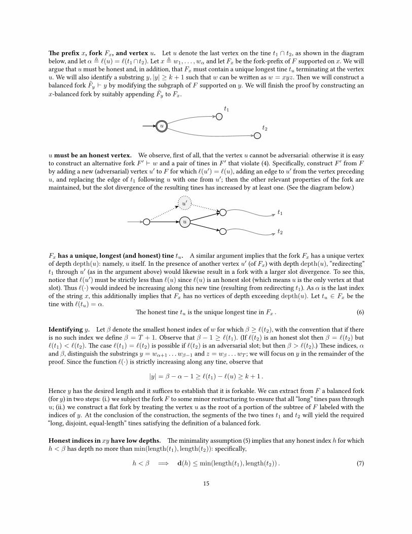
e prefix x, fork Fx, and vertex u. Let u denote the last vertex on the tine t1 ∩ t2, as shown in the diagrambelow, and let α , ℓ(u) = ℓ(t1∩ t2). Let x , w1, . . . , wα and let Fx be the fork-prefix of F supported on x. We willargue that umust be honest and, in addition, that Fx must contain a unique longest tine tu terminating at the vertexu. We will also identify a substring y, |y| ≥ k + 1 such that w can be wrien as w = xyz. en we will construct abalanced fork Fy ⊢ y by modifying the subgraph of F supported on y. We will finish the proof by constructing an

x-balanced fork by suitably appending Fy to Fx.

u

t1

t2

umust be an honest vertex. We observe, first of all, that the vertex u cannot be adversarial: otherwise it is easyto construct an alternative fork F ′ ⊢ w and a pair of tines in F ′ that violate (4). Specifically, construct F ′ from Fby adding a new (adversarial) vertex u′ to F for which ℓ(u′) = ℓ(u), adding an edge to u′ from the vertex precedingu, and replacing the edge of t1 following u with one from u′; then the other relevant properties of the fork aremaintained, but the slot divergence of the resulting tines has increased by at least one. (See the diagram below.)

u

u′

t1

t2

Fx has a unique, longest (and honest) tine tu. A similar argument implies that the fork Fx has a unique vertexof depth depth(u): namely, u itself. In the presence of another vertex u′ (of Fx) with depth depth(u), “redirecting”t1 through u′ (as in the argument above) would likewise result in a fork with a larger slot divergence. To see this,notice that ℓ(u′)must be strictly less than ℓ(u) since ℓ(u) is an honest slot (which means u is the only vertex at thatslot). us ℓ(·) would indeed be increasing along this new tine (resulting from redirecting t1). As α is the last indexof the string x, this additionally implies that Fx has no vertices of depth exceeding depth(u). Let tu ∈ Fx be thetine with ℓ(tu) = α.

e honest tine tu is the unique longest tine in Fx . (6)

Identifying y. Let β denote the smallest honest index of w for which β ≥ ℓ(t2), with the convention that if thereis no such index we define β = T + 1. Observe that β − 1 ≥ ℓ(t1). (If ℓ(t2) is an honest slot then β = ℓ(t2) butℓ(t1) < ℓ(t2). e case ℓ(t1) = ℓ(t2) is possible if ℓ(t2) is an adversarial slot; but then β > ℓ(t2).) ese indices, αand β, distinguish the substrings y = wα+1 . . . wβ−1 and z = wβ . . . wT ; we will focus on y in the remainder of theproof. Since the function ℓ(·) is strictly increasing along any tine, observe that

|y| = β − α− 1 ≥ ℓ(t1)− ℓ(u) ≥ k + 1 .

Hence y has the desired length and it suffices to establish that it is forkable. We can extract from F a balanced fork(for y) in two steps: (i.) we subject the forkF to some minor restructuring to ensure that all “long” tines pass throughu; (ii.) we construct a flat fork by treating the vertex u as the root of a portion of the subtree of F labeled with theindices of y. At the conclusion of the construction, the segments of the two tines t1 and t2 will yield the required“long, disjoint, equal-length” tines satisfying the definition of a balanced fork.

Honest indices in xy have low depths. eminimality assumption (5) implies that any honest index h for whichh < β has depth no more than min(length(t1), length(t2)): specifically,

h < β =⇒ d(h) ≤ min(length(t1), length(t2)) . (7)

15

To see this, consider an honest index h, h < β and a tine th for which ℓ(th) = h. Recall that t1 and t2 are viable andthat h < ℓ(t2). (If ℓ(t2) is honest, it is obvious. Otherwise, h < ℓ(t2) < β since ℓ(t2) is adversarial.) As t2 is viable,it follows immediately that d(h) = length(th) ≤ length(t2). Similarly, if h ≤ ℓ(t1) then d(h) ≤ length(t1) sincet1 is viable as well. e remaining case, i.e., when ℓ(t1) < h < ℓ(t2), can be ruled out by the argument below.

ere is no honest index between ℓ(t1) and ℓ(t2). We claim that

ere is no honest index h satisfying ℓ(t1) < h < ℓ(t2) . (8)

e claim above is trivially true if ℓ(t1) = ℓ(t2). Otherwise, suppose (toward a contradiction) that h is an honestindex satisfying ℓ(t1) < h < ℓ(t2). Let th be the (honest) tine at slot h. e tine-pair (t1, th) may or may not be inA. We will show that both cases lead to contradictions.

• If (t1, th) is inA and ℓ(t1∩ th) ≤ ℓ(u), divslot(t1, th) is at least divslot(t1, t2). In fact, due to (4), this inequalitymust be an equality. However, the assumption ℓ(t1) < h < ℓ(t2) contradicts (5).

• If (t1, th) is in A and ℓ(t1 ∩ th) > ℓ(u), it follows that divslot(th, t2) > divslot(t1, t2). As the laer quantity isat least k + 1, (th, t2) must be in A. e preceding inequality, however, contradicts (4).

• If (t1, th) 6∈ A, divslot(t1, th) is at most k. As divslot(t1, t2) is at least k + 1, th and t1 must share a vertexaer slot ℓ(u). Since ℓ(t1) < h < ℓ(t2) by assumption, divslot(th, t2) > divslot(t1, t2) ≥ k+1 and, as a result,(th, t2) ∈ A. However, the preceding strict inequality violates condition (4).

A fork F⊲u⊳ where all long tines go through u. In light of the remarks above, we observe that the fork Fmay be “pinched” at u to yield an essentially identical fork F⊲u⊳ ⊢ w with the exception that all tines of lengthexceeding depth(u) pass through the vertex u. Specifically, the fork F⊲u⊳ ⊢ w is defined to be the graph obtainedfrom F by changing every edge of F directed towards a vertex of depth depth(u) + 1 so that it originates from u.To see that the resulting tree is a well-defined fork, it suffices to check that ℓ(·) is still increasing along all tines ofF⊲u⊳. For this purpose, consider the effect of this pinching on an individual tine t terminating at a particular vertexv—it is replaced with a tine t⊲u⊳ defined so that:

• If length(t) ≤ depth(u), the tine t is unchanged: t⊲u⊳ = t.

• Otherwise, length(t) > depth(u) and t has a vertex v of depth depth(u) + 1; note that ℓ(v) > ℓ(u) becauseFx contains no vertices of depth exceeding depth(u). en t⊲u⊳ is defined to be the path given by the tineterminating at u, a (new) edge from u to v, and the suffix of t beginning at z. (As ℓ(v) > ℓ(u) this has theincreasing label property.)

us the tree F⊲u⊳ is a legal fork on the same vertex set; note that the depths of vertices in F and F⊲u⊳ areidentical.

Constructing a shallow fork Fy ⊢ y. By excising the tree rooted at u from this pinched fork F⊲u⊳, we mayextract a fork for the string wα+1 . . . wT . Specifically, consider the induced subgraph Fu⊳ of F⊲u⊳ given by thevertices u ∪ v | depth(v) > depth(u). By treating u as a root vertex and suitably defining the labels ℓu⊳ ofFu⊳ so that ℓu⊳(v) = ℓ(v)− ℓ(u), this subgraph has the defining properties of a fork for wα+1 . . . wT . In particular,considering that α is honest it follows that each honest index h > α has depth d(h) > length(u) and hence h labelsa vertex in Fu⊳. For a tine t of F⊲u⊳, we let tu⊳ denote the suffix of this tine beginning at u, which forms a tine inFu⊳. (If length(t) ≤ depth(u), we define tu⊳ to consist solely of the vertex u.) Note that t1

u⊳ and t2u⊳ share no

edges in the fork Fu⊳.Finally, let Fy denote the subtree obtained from Fu⊳ as the union of all tines tu⊳ of Fu⊳ so that all labels of tu⊳

are drawn from y (as it appears as a prefix of wα+1 . . . wT ), and

length(tu⊳) ≤ maxh≤|y|h honest

d(h) . (9)

It is immediate that Fy ⊢ y.

16

Two longest viable tines in Fy . Consider the tines t1u⊳ and t2

u⊳. As mentioned above, they share no edges inFu⊳ and hence the prefixes t1 and t2 (of t1

u⊳ and t2u⊳) appearing in Fy share no edges. We wish to show that

these prefixes have the maximal length in Fy , making Fy balanced, as desired. Let h be the largest honest index iny. Since the lengths of the tines in Fy are at most d(h), it suffices to show that the lengths of ti, i ∈ 1, 2 is at leastd(h).

is is immediate for the tine t1 since all labels of t1u⊳ are drawn from y and, considering (7), its depth is at least

that of all relevant honest vertices. As for t2, observe that if ℓ(t2) is not honest then β > ℓ(t2) so that, as with t1,the tine t2 is labeled by y so that the same argument, relying on (7), ensures that the length(t2) is at least the depthof all relevant honest vertices. If ℓ(t2) is honest, β = ℓ(t2), and the terminal vertex of t2

u⊳ does not appear in Fy

(as ℓ(t2u⊳) falls outside y). In this case, however, length(t2

u⊳) > d(h) for any honest index h of y. It follows thatlength(t2), which equals length(t2

u⊳)− 1, is at least the depth of any honest index of y, as desired. us we haveproved

t1 and t2 are two maximally long viable tines in Fy ⊢ y . (10)

Constructing a flat fork Fy ⊢ y. Let us identify the fork prefix Fy ⊑ Fy which is either identical to Fy or differs

from Fy in only one of the tines t1, t2. In particular, if length(t1) = length(t2), we set Fy = Fy . Otherwise, let tabe the longer of the two tines t1, t2; let tb be the shorter one. We modify Fy by deleting some trailing adversarial

nodes from ta until it has the same length as tb; we set Fy as the resulting fork and, in addition, set tb = tb and taas the tine aer trimming ta.

We claim that Fy is balanced. e claim is obvious if length(t1) = length(t2). Otherwise, thanks to (10), itremains to show that the longer tine, ta, has sufficiently many trailing adversarial nodes which, if deleted, yieldslength(t1) = length(t2). To that end, let hi be the index of the last honest vertex on ti ∈ Fy, i ∈ 1, 2.

Suppose length(t2) > length(t1). By (8), we also have length(t1) ≥ d(h2) and hence we can trim some ofthe trailing adversarial nodes from t2 to get the tine t2 whose length is the same as that of t1. Otherwise, supposelength(t1) > length(t2). Since t2 is a viable tine in F , we also have length(t2) ≥ d(h1). us we can trim someof the trailing adversarial nodes from t1 to have a tine t1 whose length is the same as that of t2. In any case, thequantitymin(length(t1), length(t2)) remains the same asmin(length(t1), length(t2)). us the fork Fy has at least

two tines, t1 and t2, that achieve the maximum length of all tines in Fy ; hence Fy is balanced.

An x-balanced fork F ⊑ F . Let us identify the root of the fork Fy with the vertex u of Fx and let F be the

resulting graph (aer “gluing” the root of Fy to u). By (6), it is easy to see that the fork F ⊑ F is indeed a valid fork

on the string xy. Moreover, F is x-balanced since Fy is balanced. e claim ineorem 3 follows immediately since|y| ≥ k + 1.

5 A simple recursive formulation of relative margin

A significant finding of Kiayias et al. [13] is that the margin of a characteristic string µ(w)—the maximum value ofa quantity taken over a (typically) exponentially-large family of forks—can be given a simple, mutually recursiveformulation with the associated quantity of reach ρ(w). Specifically, they prove the following lemma.

Lemma 2 ([13, Lemma 4.19]). ρ(ε) = 0 where ε is the empty string, and, for all nonempty strings w ∈ 0, 1∗,

ρ(w1) = ρ(w) + 1 , and ρ(w0) =

0 if ρ(w) = 0,

ρ(w) − 1 otherwise.(11)

Furthermore, margin satisfies the mutually recursive relationship µ(ε) = 0 and for all w ∈ 0, 1∗,

µ(w1) = µ(w) + 1 , and µ(w0) =

0 if ρ(w) > µ(w) = 0,

µ(w)− 1 otherwise.(12)

Additionally, there exists a closed fork F ⊢ w such that ρ(F ) = ρ(w) and µ(F ) = µ(w).

17

We prove an analogous recursive statement for relative margin, recorded below.

Lemma 3 (Relative margin). Given a fixed string x ∈ 0, 1*, µx(ε) = ρ(x) where ε is the empty string, and, for allnonempty strings w = xy ∈ 0, 1*,

µx(y1) = µx(y) + 1 , and µx(y0) =

0 if ρ(xy) > µx(y) = 0 ,

µx(y)− 1 otherwise.(13)

Additionally, there exists a closed fork F ⊢ xy such that ρ(F ) = ρ(xy) and µx(F ) = µx(y).

We delay the proof of Lemma 3 to Section 7, preferring to immediately focus on the application to selementtimes in Section 6.

Discussion. e proof of Lemma 3 shares many technical similarities with the proof of Lemma 2 given by Kiayiaset al. [13]. However, there is an important respect in which the proofs differ. Each of the proofs requires the definitionof a particular adversary (which, in effect, constructs a fork achieving the worst case reach and margin guaranteedby the lemma). e adversary constructed by [13] can create a balanced fork for w whenever µ(w) ≥ 0 (i.e., w is“forkable”). However, the adversary only focuses on the problem of producing disjoint tines over the entire string w(consistent with the definition of µ(·)). e “optimal online adversary,” developed in Section 8, uses a more sophis-ticated rule for extending chains (tines) of the fork. Notably, this adversary can simultaneously maximize relativemargin over all prefixes of the string.

6 General settlement guarantees and proof of main theorems

With the recursive formulation for relative margin in hand, we study the stochastic process that arises when thecharacteristic string w is chosen from a distribution satisfying the ǫ-martingale condition. Let us write w = xy(where the decomposition is arbitrary) and let E be the event that the relative margin µx(y) is non-negative. AsFact 1 and Observation 1 point out, this event has a direct bearing on the selement violation on w.

In this section, we prove two bounds on the probability of the event E. e first bound corresponds to thedistribution Bǫ whereas the second bound applies to any distribution that satisfies the ǫ-martingale condition. (Recallthat the distribution Bǫ, mentioned in eorem 1, satisfies the ǫ-martingale condition with equality.) Our expositionin this section culminates in the proofs of our main theorems.

We start with the following theorem which is a direct consequences of these bounds; see Section 6.1 for a proof.

eorem 4. Let T, k ∈ N. Let w ∈ 0, 1T be a random variable satisfying the ǫ-martingale condition. Consider thedecomposition w = xy, |y| = k. en

Prw=xy

[there is an x-balanced fork for xy] = Prw=xy

[µx(y) ≥ 0] ≤ exp(−Ω(k)) .

(e asymptotic notation hides constants that depend only on ǫ.)

Notice how the final bound does not depend on |x|. Indeed, as we show in Lemma 4, the reach of a Booleanstring x drawn from the distribution Bǫ converges to a fixed exponential distribution as |x| → ∞. is limitingdistribution “stochastically dominates” any distribution that satisfies the ǫ-martingale condition; see Section 6.2. efollowing corollary is immediate.

Corollary 1. Let T, s, k ∈ N. Let w ∈ 0, 1T be a random variable satisfying the ǫ-martingale condition. en

Prw

[

there is a decomposition w = xyz, where |x| =s− 1 and |y| ≥ k, so that µx(y) ≥ 0

]

≤ O(1) · exp(−Ω(k)) . (14)

Proof. Notice that eorem 4 works for any prefix x of the characteristic string w = xy. us we can fix the prefixx with length s − 1 and sum the bound in eorem 4 over all suffixes y with length at least k. is would give anupper bound to the le-hand side of our claim, the bound being

∑

t≥k exp(−Ω(t)) = O(1) · exp(−Ω(k)).

18

We obtain another imporant corollary by seing |x| = 0 and |y| = n in eorem 4.

Corollary 2. Let w ∈ 0, 1n be a random variable satisfying the ǫ-martingale condition. en

Pr[w is forkable] = Pr[µ(w) ≥ 0] ≤ exp(−Ω(n)) .us forkable strings are rare where “forkable” is defined in Definition 14. is result significantly strengthens

the exp(−Ω(√n)) bound obtained in eorem 4.13 of [13]. e improvement comes in two respects: first, Corol-lary 1 improves the exponent from

√n to n, and second, the characteristic string is allowed to be drawn from any

distribution satisfying the ǫ-martingale condition. For comparison, the characteristic string in eorem 4.13 of [13]has the distribution Bǫ, i.e., the bits were i.i.d. Bernoulli random variables with expectation (1− ǫ)/2.

6.1 Two bounds for non-negative relative margin

e main ingredients to proving eorem 4 are two bounds on the event that for a characteristic string xy, therelative margin µx(y) is non-negative.

Bound 1. Let x ∈ 0, 1m and y ∈ 0, 1k be independent random variables, each chosen according to Bǫ. en

Pr[µx(y) ≥ 0] ≤ exp(−ǫ3(1−O(ǫ))k/2) .

Bound 2. Let x ∈ 0, 1m and y ∈ 0, 1k be random variables (jointly) satisfying the ǫ-martingale condition withrespect to the ordering x1, . . . , xm, y1, . . . , yk . Let x

′ ∈ 0, 1m and y′ ∈ 0, 1k be independent random variables,each chosen independently according to Bǫ. en

Pr[µx(y) ≥ 0] ≤ Pr[µx′(y′) ≥ 0] ≤ exp(−ǫ3(1−O(ǫ))k/2) .

Proof of eorem 4. e equality is Fact 1 and the inequality is Bound 2.

6.2 A stochastically dominant prefix distribution

Stochastic dominance plays an important role in the arguments below. First of all, we observe that the distributionBǫ stochastically dominates any distribution satisfying the ǫ-martingale condition; this yields the first inequality ineorem 1. A more delicate application of stochastic dominance is used in order to achieving bounds, such as thoseof Section 6.1, that are independent of the length of x. is follows from the fact that reach(Bǫ) converges to aparticular, dominant distribution as its argument increases in length.

For notational convenience, we denote the probability distribution associated with a random variable using up-percase script leers; for example, the distribution of a random variable R is denoted by R. is usage should beclear from the context.

Definition 15 (Monotonicity and stochastic dominance). Let Ω be a set endowed with a partial order ≤. A subsetA ⊂ Ω is monotone if for all x ≤ y, x ∈ A implies y ∈ A. Let X and Y be random variables taking values in Ω. Wesay that X stochastically dominates Y , wrien Y X , if X (A) ≥ Y(A) for all monotone A ⊆ Ω. As a special case,when Ω = R, Y X if Pr[X ≥ Λ] ≥ Pr[Y ≥ Λ] for every Λ ∈ R. We extend this notion to probability distributionsin the natural way.

Observe that for any non-decreasing function u defined on Ω, Y X implies u(Y ) ≤ u(X). Finally, wenote that for real-valued random variables X , Y , and Z , if Y X and Z is independent of both X and Y , thenZ + Y Z +X .

Lemma 4. Suppose W = (W1, . . . ,Wn) ∈ 0, 1n satisfies the ǫ-martingale condition. Let ǫ ∈ (0, 1) and B =(B1, . . . , Bn) ∈ 0, 1n where each Bi is independent with expectation (1 − ǫ)/2. Let R∞ ∈ 0, 1, . . . be a randomvariable whose distributionR∞ is defined as

R∞(k) = Pr[R∞ = k] ,

(

2ǫ

1 + ǫ

)

·(

1− ǫ

1 + ǫ

)k

for k = 0, 1, 2, . . . . (15)

en ρ(W ) ρ(B) R∞.

19

Proof. We begin by observing that B stochastically dominates W . As a maer of notation, for any fixed valuesw1, . . . , wk ∈ 0, 1k, let

θ[w1, . . . , wk] = Pr[Wk+1 = 1 | Wi = wi, for i ≤ k] ≤ (1− ǫ)/2

and θ[ε] = Pr[W1 = 1] where ε is the empty string. en consider n uniform and independent real numbers(A1, . . . , An), each taking a value in the unit interval [0, 1]; we use these random variables to construct a monotonecoupling between W and B. Specifically, define β : [0, 1]n → 0, 1n by the rule β(α1, . . . , αn) = (b1, . . . , bn)where

bt =

1 if αt ≤ (1− ǫ)/2,

0 if αt > (1− ǫ)/2,

and define B = (B1, . . . , Bn) = β(A1, . . . , An); these Bis are independent zero-one Bernoulli random variableswith expectation (1−ǫ)/2. Likewise define the function ω : [0, 1]n → 0, 1n so that ω(α1, . . . , αn) = (w1, . . . , wn)where each wt is assigned by the iterative rule

wt+1 =

1 if α ≤ θ[w1, . . . , wt],

0 if α > θ[w1, . . . , wt],

and observe that the probability law of ω(A1, . . . , An) is precisely that of W = (W1, . . . ,Wn). For convenience,we simply identify the random variable W with ω(A1, . . . , An). Note that for any α = (α1, . . . , αn) and for eachi, the ith coordinates of β(α) and ω(α) satisfy ω(α)i ≤ β(α)i (which is to say that Wi ≤ Bi with probability 1).But this is equivalent to saying W B. (See [14, Lemma 22.5].) Now consider the following partial order ≤ onthe n-bit Boolean strings: for x, y ∈ 0, 1n, we write x ≤ y if and only if xi = 1 implies yi = 1, i ∈ [n]. Sinceρ is non-decreasing with respect to this partial order, we have ρ(ω(α)) ≤ ρ(β(α)) with probability 1 and henceρ(W ) ρ(B) as well.

To complete the proof, we now establish that ρ(B) R∞. We remark that the random variables ρ(B) (andR∞)have an immediate interpretation in terms of the Markov chain corresponding to a biased random walk on Z with a“reflecting boundary” at -1. Specifically, consider the Markov chain on 0, 1, . . . given by the transition diagram

0 1 2 . . .

where edges pointing right have probability (1 − ǫ)/2 and edges pointing le—including the loop at 0—have prob-ability (1 + ǫ)/2. Examining the recursive description of ρ(w), it is easy to confirm that the random variableρ(B1, . . . , Bn) is precisely given by the result of evolving the Markov chain above for n steps with all probabil-ity initially placed at 0. It is further easy to confirm that the distribution given by (15) above is stationary for thischain.

To establish stochastic dominance, it is convenient to work with the underlying distributions and consider walksof varying lengths: letRn : Z→ R denote the probability distribution given by ρ(B1, . . . , Bn); likewise defineR∞.For a distribution R on Z, we define [R]0 to denote the probability distribution obtained by shiing all probabilitymass on negative numbers to zero; that is, for x ∈ Z,

[R]0(x) =

R(x) if x > 0,∑

t≤0R(t) if x = 0,

0 if x < 0.

We observe that if A C then [A]0 [C]0 for any distributions A and C on Z. It will also be convenient tointroduce the shi operators: for a distribution R : Z → R and an integer k, we define SkR to be the distributiongiven by the rule SkR(x) = R(x − k). With these operators in place, we may write

Rt =

(

1− ǫ

2

)

S1Rt−1 +

(

1 + ǫ

2

)

[

S−1Rt−1

]

0,

20

with the understanding thatR0 is the distribution placing unit probability at 0. e proof now proceeds by induction.It is clear thatR0 R∞. Assuming thatRn R∞, we note that for any k

SkRn SkR∞ and, additionally, that [S−1Rn]0 [S−1R∞]0 .

Finally, it is clear that stochastic dominance respects convex combinations, in the sense that ifA1 C1 andA2 C2

then λA1 + (1− λ)A2 λC1 + (1− λ)C2 (for 0 ≤ λ ≤ 1). We conclude that

Rt+1 =

(

1− ǫ

2

)

S1Rt +

(

1 + ǫ

2

)

[

S−1Rt

]

0(

1− ǫ

2

)

S1R∞ +

(

1 + ǫ

2

)

[

S−1R∞

]

0.

By inspection, the right-hand side equalsR∞, as desired. Hence ρ(B) R∞.

Remark. In fact, the random variable ρ(B) actually converges to R∞ as n → ∞. is can be seen, for example,by solving for the stationary distribution of the Markov chain in the proof above. However, we will only require thedominance for our exposition. Importantly, since µx(ε) = ρ(x), and Pr[µx(y) ≥ 0] increases monotonically withan increase in Pr[µx(ε) ≥ r] for any r ≥ 0, it suffices to take |x| → ∞ when reasoning about an upper bound onPr[µx(y) ≥ 0].

6.3 Proof of Bound 1

Anticipating the proof, we make a few remarks about generating functions and stochastic dominance. We reservethe term generating function to refer to an “ordinary” generating function which represents a sequence a0, a1, . . .of non-negative real numbers by the formal power series A(Z) =

∑∞t=0 atZ

t. When A(1) =∑

t at = 1 we saythat the generating function is a probability generating function; in this case, the generating function A can naturallybe associated with the integer-valued random variable A for which Pr[A = k] = ak. If the probability generatingfunctions A and B are associated with the random variables A and B, it is easy to check that A ·B is the generatingfunction associated with the convolution A + B (where A and B are assumed to be independent). Translatingthe notion of stochastic dominance to the seing with generating functions, we say that the generating function A

stochastically dominates B if∑

t≤T at ≤∑

t≤T bt for all T ≥ 0; we write B A to denote this state of affairs. IfB1 A1 and B2 A2 then B1 ·B2 A1 ·A2 and αB1 + βB2 αA1 + βA2 (for any α, β ≥ 0). Moreover, if B A

then it can be checked that B(C) A(C) for any probability generating function C(Z), where we write A(C) todenote the composition A(C(Z)).

Finally, we remark that if A(Z) is a generating function which converges as a function of a complex Z for|Z| < R for some non-negative R,R is called the radius of convergence of A. It follows from [26, eorem 2.19] thatlimk→∞ akR

k = 0 and |ak| = O(R−k). In addition, if A is a probability generating function associated with therandom variable A then it follows that Pr[A ≥ T ] = O(R−T ).

We define p = (1 − ǫ)/2 and q = 1− p and as in the proof of Bound 2, consider the independent 0, 1-valuedrandom variables w1, w2, . . . where Pr[wt = 1] = p. We also define the associated ±1-valued random variablesWt = (−1)1+wt .

Although our actual interest is in the random variable µx(y) from (13) on a characteristic string w = xy, webegin by analyzing the case when |x| = 0.

Case 1: x is the empty string. In this case, the random variable µx(y) is identical to µ(w) from (12) with w = y.Our strategy is to study the probability generating function

L(Z) =

∞∑

t=0

ℓtZt

where ℓt = Pr[t is the last time µt = 0]. Controlling the decay of the coefficients ℓt suffices to give a bound on theprobability that w1 . . . wk is forkable because

Pr[w1 . . . wk is forkable] ≤ 1−k−1∑

t=0

ℓt =∞∑

t=k

ℓt .

21

It seems challenging to give a closed-form algebraic expression for the generating function L; our approach is todevelop a closed-form expression for a probability generating function L =

∑

t ℓtZt which stochastically dominates

L and apply the analytic properties of this closed form to bound the partial sums∑

t≥k ℓk . Observe that if L L

then the series L gives rise to an upper bound on the probability that w1 . . . wk is forkable as∑∞

t=k ℓt ≤∑∞

t=k ℓt.e coupled random variables ρt and µt are Markovian in the sense that values (ρs, µs) for s ≥ t are entirely

determined by (ρt, µt) and the subsequent values Wt+1, . . . of the underlying variables Wi. We organize the se-quence (ρ0, µ0), (ρ1, µ1), . . . into “epochs” punctuated by those times t for which ρt = µt = 0. With this in mind,we define M(Z) =

∑

mtZt to be the generating function for the first completion of such an epoch, corresponding

to the least t > 0 for which ρt = µt = 0. As we discuss below, M(Z) is not a probability generating function, butratherM(1) = 1− ǫ. It follows that

L(Z) =

(

1 + (1− ǫ) · M(Z)

M(1)+

(

(1− ǫ) · M(Z)

M(1)

)2

+ · · ·)

· ǫ

= (1 +M(Z) +M(Z)2 + · · · ) · ǫ=

ǫ

1−M(Z). (16)

e expression above represents the following geometric process: before the beginning of an epoch,we “ask”whetherthewalk is ever going to come back to zero. With probability ǫ, the answer is “no” andwe stop the process. Otherwise,i.e., with probability 1− ǫ, we commence an epoch which is guaranteed to finish; then we ask again.

Below we develop an analytic expression for a generating function M for whichM M and define L = ǫ/(1−M(Z)). We then proceed as outlined above, noting that L L and using the asymptotics of L to upper bound theprobability that a string is forkable.

In preparation for defining M, we set down two elementary generating functions for the “descent” and “ascent”stopping times. Treating the random variablesW1, . . . as defining a (negatively) biased random walk, define D to bethe generating function for the descent stopping time of the walk; this is the first time the random walk, starting at0, visits −1. e natural recursive formulation of the descent time yields a simple algebraic equation for the descentgenerating function, D(Z) = qZ + pZD(Z)2, and from this we may conclude

D(Z) =1−

√

1− 4pqZ2

2pZ.

We likewise consider the generating function A(Z) for the ascent stopping time, associated with the first time thewalk, starting at 0, visits 1: we have A(Z) = pZ + qZA(Z)2 and

A(Z) =1−

√

1− 4pqZ2

2qZ.

Note that while D is a probability generating function, the generating function A is not: according to the classical“gambler’s ruin” analysis [12], the probability that a negatively-biased random walk starting at 0 ever rises to 1 isexactly p/q; thus A(1) = p/q.

Returning to the generating function M above, we note that an epoch can have one of two “shapes”: in the firstcase, the epoch is given by a walk for whichW1 = 1 followed by a descent (so that ρ returns to zero); in the secondcase, the epoch is given by a walk for which W1 = −1, followed by an ascent (so that µ returns to zero), followedby the eventual return of ρ to 0. Considering that when ρt > 0 it will return to zero in the future almost surely, itfollows that the probability that such a biased random walk will complete an epoch is p + q(p/q) = 2p = 1 − ǫ,as mentioned in the discussion of (16) above. One technical difficulty arising in a complete analysis of M concernsthe second case discussed above: while the distribution of the smallest t > 0 for which µt = 0 is proportional to A

above, the distribution of the smallest subsequent time t′ for which ρt′ = 0 depends on the value t. More specifically,the distribution of the return time depends on the value of ρt. Considering that ρt ≤ t, however, this conditionaldistribution (of the return time of ρ to zero conditioned on t) is stochastically dominated by D

t, the time to descendt steps. is yields the following generating function M which, as described, stochastically dominatesM:

M(Z) = pZ · D(Z) + qZ · D(Z) · A(Z · D(Z)) .

22

It remains to establish a bound on the radius of convergence of L. Recall that if the radius of convergence ofL is exp(δ) it follows that Pr[w1 . . . wk is forkable] = O(exp(−δk)). A sufficient condition for convergence ofL(z) = ǫ/(1 − M(z)) at z is that that all generating functions appearing in the definition of M converge at z andthat the resulting value M(z) < 1.

e generating function D(z) (and A(z)) converges when the discriminant 1 − 4pqz2 is positive; equivalently|z| < 1/

√1− ǫ2 or |z| < 1 + ǫ2/2 + O(ǫ4). Considering M, it remains to determine when the second term,

qzD(z)A(zD(z)), converges; this is likewise determined by positivity of the discriminant, which is to say that

1− (1− ǫ2)

(

1−√

1− (1− ǫ2)z2

1− ǫ

)2

> 0 .

Equivalently,

|z| <√

1

1 + ǫ

(

2√1− ǫ2

− 1

1 + ǫ

)

= 1 + ǫ3/2 +O(ǫ4) .

Note that when the series pz ·D(z) converges, it converges to a value less than 1/2; the same is true of qz · A(z). Itfollows that for |z| = 1 + ǫ3/2 +O(ǫ4), |M(z)| < 1 and L(z) converges, as desired. We conclude that

Pr[w1 . . . wk is forkable] = exp(−ǫ3(1 +O(ǫ))k/2) . (17)

Case 2: x is non-empty. e relative margin before y begins is µx(ε). Recalling that µx(ε) = ρ(x) and condi-tioning on the event that ρ(x) = r, let us define the random variables µt for t = 0, 1, 2, · · · as follows: µ0 = ρ(x)and

Pr[µt = s] = Pr[µx(y) = s | ρ(x) = r and |y| = t] .

If the µ random walk makes the rth descent at some time t < n, then µt = 0 and the remainder of the walk isidentical to an (k − t)-step µ random walk which we have already analyzed. Hence we investigate the probabilitygenerating function

Br(Z) = D(Z)rL(Z) with coefficients b(r)t := Pr[t is the last time µt = 0 | µ0 = r]

where t = 0, 1, 2, · · · . Our interest lies in the quantity

bt := Pr[t is the last time µt = 0] =∑

r≥0

b(r)t Rm(r) ,

where the reach distribution Rm : Z→ [0, 1] associated with the random variable ρ(x), |x| = m is defined as

Rm(r) = Prx : |x|=m

[ρ(x) = r] . (18)

Let Rm(Z) be the probability generating function for the distribution Rm. Using Lemma 4 and Definition 15, wededuce thatRm R∞ for everym ≥ 0 sinceRm R∞. In addition, it is easy to check from (15) that the probabilitygenerating function forR∞ is in fact R∞(Z) = (1− β)/(1− βZ) where β := (1− ǫ)/(1+ ǫ). us the generatingfunction corresponding to the probabilities bt∞t=0 is

B(Z) =

∞∑

t=0

btZt =

∞∑

r=0

Rm(r)

∞∑

t=0

b(r)t Zt =

∞∑

r=0

Rm(r)Br(Z)

= L(Z)

∞∑

r=0

Rm(r)D(Z)r = L(Z) Rm(D(Z)) L(Z) R∞(D(Z))

=(1− β) L(Z)

1− βD(Z). (19)

23

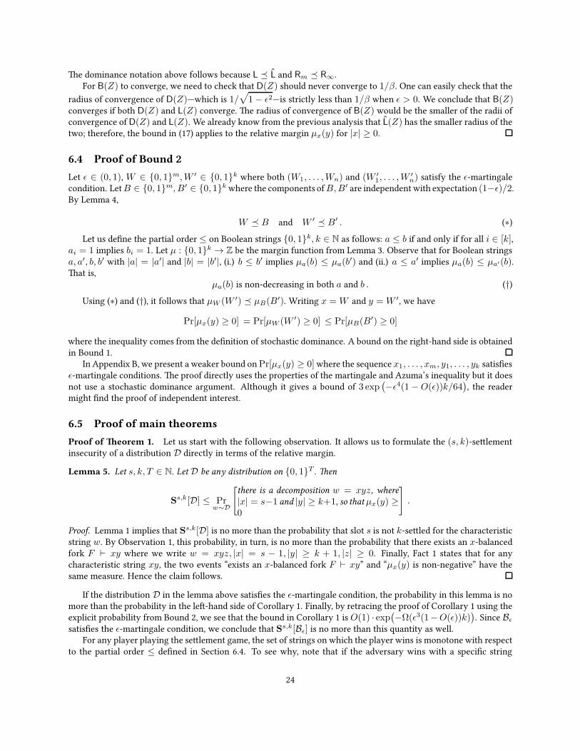
e dominance notation above follows because L L and Rm R∞.For B(Z) to converge, we need to check that D(Z) should never converge to 1/β. One can easily check that the

radius of convergence of D(Z)—which is 1/√

1− ǫ2—is strictly less than 1/β when ǫ > 0. We conclude that B(Z)converges if both D(Z) and L(Z) converge. e radius of convergence of B(Z) would be the smaller of the radii ofconvergence ofD(Z) and L(Z). We already know from the previous analysis that L(Z) has the smaller radius of thetwo; therefore, the bound in (17) applies to the relative margin µx(y) for |x| ≥ 0.

6.4 Proof of Bound 2

Let ǫ ∈ (0, 1), W ∈ 0, 1m,W ′ ∈ 0, 1k where both (W1, . . . ,Wn) and (W ′1, . . . ,W

′n) satisfy the ǫ-martingale

condition. LetB ∈ 0, 1m, B′ ∈ 0, 1k where the components ofB,B′ are independent with expectation (1−ǫ)/2.By Lemma 4,

W B and W ′ B′ . (∗)Let us define the partial order ≤ on Boolean strings 0, 1k, k ∈ N as follows: a ≤ b if and only if for all i ∈ [k],

ai = 1 implies bi = 1. Let µ : 0, 1k → Z be the margin function from Lemma 3. Observe that for Boolean stringsa, a′, b, b′ with |a| = |a′| and |b| = |b′|, (i.) b ≤ b′ implies µa(b) ≤ µa(b

′) and (ii.) a ≤ a′ implies µa(b) ≤ µa′(b).at is,

µa(b) is non-decreasing in both a and b . (†)Using (∗) and (†), it follows that µW (W ′) µB(B

′). Writing x = W and y = W ′, we have

Pr[µx(y) ≥ 0] = Pr[µW (W ′) ≥ 0] ≤ Pr[µB(B′) ≥ 0]

where the inequality comes from the definition of stochastic dominance. A bound on the right-hand side is obtainedin Bound 1.

In Appendix B, we present a weaker bound onPr[µx(y) ≥ 0]where the sequence x1, . . . , xm, y1, . . . , yk satisfiesǫ-martingale conditions. e proof directly uses the properties of the martingale and Azuma’s inequality but it doesnot use a stochastic dominance argument. Although it gives a bound of 3 exp

(

−ǫ4(1 −O(ǫ))k/64)

, the readermight find the proof of independent interest.

6.5 Proof of main theorems

Proof of eorem 1. Let us start with the following observation. It allows us to formulate the (s, k)-selementinsecurity of a distribution D directly in terms of the relative margin.

Lemma 5. Let s, k, T ∈ N. Let D be any distribution on 0, 1T . en

Ss,k[D] ≤ Pr

w∼D

[

there is a decomposition w = xyz, where|x| = s−1 and |y| ≥ k+1, so that µx(y) ≥0

]

.

Proof. Lemma 1 implies that Ss,k[D] is no more than the probability that slot s is not k-seled for the characteristicstring w. By Observation 1, this probability, in turn, is no more than the probability that there exists an x-balancedfork F ⊢ xy where we write w = xyz, |x| = s − 1, |y| ≥ k + 1, |z| ≥ 0. Finally, Fact 1 states that for anycharacteristic string xy, the two events “exists an x-balanced fork F ⊢ xy” and “µx(y) is non-negative” have thesame measure. Hence the claim follows.

If the distribution D in the lemma above satisfies the ǫ-martingale condition, the probability in this lemma is nomore than the probability in the le-hand side of Corollary 1. Finally, by retracing the proof of Corollary 1 using theexplicit probability from Bound 2, we see that the bound in Corollary 1 is O(1) · exp

(

−Ω(ǫ3(1−O(ǫ))k))

. Since Bǫsatisfies the ǫ-martingale condition, we conclude that Ss,k[Bǫ] is no more than this quantity as well.

For any player playing the selement game, the set of strings on which the player wins is monotone with respectto the partial order ≤ defined in Section 6.4. To see why, note that if the adversary wins with a specific string

24

w, he can certainly win with any string w′ where w ≤ w′. As Bǫ stochastically dominates W , it follows thatSs,k[W ] ≤ S

s,k[Bǫ].

Proof of eorem 2 For the first inequality, observe that if w violates k-CP, it must violate k-CPslot as well. Itremains to prove the second inequality. Let D be any distribution on 0, 1T . We can apply Fact 1 on the statementof eorem 3 to deduce that

Prw∼D

[w violates k-CPslot] ≤ Prw∼D

[

there is a decomposition w = xyz,where |y| ≥ k, so that µx(y) ≥ 0

]

.

By using a union bound over |x|, the above probability is at most

T−k+1∑

s=1

Prw

[

there is a decomposition w = xyz, where|x| = s− 1 and |y| ≥ k, so that µx(y) ≥ 0

]

.

Since w satisfies the ǫ-martingale condition, we can upper bound the probability inside the sum using Corollary 1.As we have seen in the proof of eorem 1, the bound in Corollary 1 is O(1) · exp

(

−Ω(ǫ3(1 −O(ǫ))k))

. It follows

that the sum above is at most T exp(

−Ω(ǫ3(1−O(ǫ))k))

.It remains to prove the recursive formulation of the relative margin from Section 5; we tackle it in the next

section.

7 Proof of the relative margin recurrence

We set the stage by formally defining fork prefixes.

Definition 16 (Fork prefixes). Let w, x ∈ 0, 1∗ so that x w. Let F, F ′ be two forks for x and w, respectively. Wesay that F is a prefix of F ′ if F is a consistently labeled subgraph of F ′. at is, all vertices and edges of F also appearin F ′ and the label of any vertex appearing in both F and F ′ is identical. We denote this relationship by F ⊑ F ′.

When speaking about a tine that appears in both F and F ′, we place the fork in the subscript of relevant properties,e.g., writing reachF , etc.

Observe that for any Boolean strings x and w, x w, one can extend (i.e., augment) a fork prefix F ⊢ x intoa larger fork F ′ ⊢ w so that F ⊑ F ′. A conservative extension is a minimal extension in that it consumes the leastamount of reserve (cf. Definition 11), leaving the remaining reserve to be used in future. Extensions and, in particular,conservative extensions play a critical role in the exposition that follows.

Definition 17 (Conservative extension of closed forks). Let w be a Boolean string, F a closed fork for w, and let s bean honest tine in F . Let F ′ be a closed fork for w0 so that F ⊑ F ′ and F ′ contains an honest tine σ, ℓ(σ) = |w| + 1.We say that F ′ is an extension of F or, equivalently, that σ is an extension of s, if s ≺ σ. If, in addition, length(σ) =height(F ) + 1, we call this extension a conservative extension.

Clearly, σ is the longest tine inF ′. Since σ is honest, it follows that length(σ) ≥ 1+height(F ) = 1+length(s)+gap(s). e root-to-leaf path in F ′ that ends at σ contains at least gap(s) adversarial vertices u ∈ F ′ so thatℓ(u) ∈ [ℓ(s) + 1, |w|] and u 6∈ F . If σ is a conservative extension, the number of such vertices is exactly gap(s) and,in particular, the height of F ′ is exactly one more than the height of F .

e main ingredients to proving Lemma 3 are a fork-building strategy for the string xy and Propositions 1and 2. Specifically, recall equation (13). e first proposition shows that the fork F ⊢ xy0 built by the said strategyachieves µx(F ) ≥ µx(y0) while the second proposition shows that this value, in fact, is the largest possible, i.e.,µx(y0) ≤ µx(y0). In addition, any fork-building strategy whose forks satisfy the premise of Proposition 1 can beused to prove Lemma 3.

25

7.1 A fork-building strategy to maximize x-relative margin

Any fork F ⊢ xy contains two tines tx, tρ so that reach(tρ) = ρ(F ), reachF (tx) = µx(F ), and the tines tx, tρ aredisjoint over the suffix y. We say that the tine-pair (tρ, tx) is a witness to µx(F ).

Let x, y ∈ 0, 1∗ and write w = xy. Recursively build closed forks F0, F1, . . . , F|w| where Fi ⊢ w1 . . . wi, i ≥ 1andF0 ⊢ ε is the trivial fork consisting of a single vertex corresponding to the genesis block. For i = 0, 1, . . . , |w|−1in increasing order, do as follows. Ifwi+1 = 1, setFi+1 ← Fi. Ifwi+1 = 0, setFi+1 ⊢ w0 as a conservative extensionof Fi ⊢ w so that σ ∈ Fi+1, ℓ(σ) = i + 1 is a conservative extension of a tine s ∈ Fi identified as follows. If Fi

contains no zero-reach tine, s is the unique longest tine in Fi. Otherwise, first identify a maximal-reach tine tρ ∈ Fi

as follows: if i ≥ |x|+1, tρ is a maximal-reach tine in Fi which belongs to a tine-pair witnessing µx(Fi); otherwise,tρ can be an arbitrary maximal-reach tine in Fi. Finally, s is the zero-reach tine in Fi that diverges earliest from tρ.If there are multiple candidates for s or tρ, break tie arbitrarily.

Proposition 1. Let x, y be arbitrary Boolean strings, |y| ≥ 1 and w = xy. Let F ⊢ w and F ′ ⊢ w0 be two closed forksbuilt by the strategy above so that F ⊑ F ′ and suppose, in addition, that ρ(F ) = ρ(xy) and µx(F ) = µx(y). enρ(F ′) = ρ(xy0) and µx(F

′) ≥ µx(y0).

7.2 Proof of Proposition 1

Before we proceed further, let us record two useful results related to conservative extensions and closed fork prefixes.

Claim 1 (A conservative extension has reach zero). Consider closed forks F ⊢ w,F ′ ⊢ w0 such that F ⊑ F ′. If atine t of F ′ is a conservative extension then reachF ′(t) = 0.

Proof. We have assumed that t is a conservative extension, so its terminal vertex must be the new honest node. Bydefinition, reachF ′(t) = reserveF ′(t) − gapF ′(t). Honest players will only place nodes at a depth strictly greaterthan all other honest nodes, so we infer that t is the longest tine of F ′, and so gapF ′(t) = 0. Moreover, we observethat there are no 1s occurring aer this point in the characteristic string, and so reserveF ′(t) = 0. Plugging thesevalues into our definition of reach we see that reachF ′(t) = 0− 0 = 0.

Claim 2 (Reach of non-extended tines). Consider a closed forkF ⊢ w and some closed fork F ′ ⊢ w0 such that F ⊑ F ′.If t ∈ F then reachF ′(t) ≤ reachF (t) − 1. e inequality becomes and equality if F ′ is obtained via a conservativeextension from F .

Proof. Definitionally, we know that reachF ′(t) = reserveF ′(t) − gapF ′(t). From F to F ′, the length of the longesttine increases by at least one, and the length of t does not change, so we observe that gapF ′(t) ≥ gapF (t) + 1with equality only for conservative extensions. e reserve of t does not change, because there are no new 1sin the characteristic string. erefore, reachF ′(t) = reserveF ′(t) − gapF ′(t) ≤ reserveF (t) − gapF (t) − 1 =reachF (t)− 1.

Assume the premise of Proposition 1. at is, F is a fork for xy so that ρ(F ) = ρ(xy), µx(F ) = µx(y), and thetine tρ identified by the fork-building strategy in Section 7.1 belongs to an F -tine-pair (tρ, tx) that witnesses µx(F ).To recap, this means reachF (tρ) = ρ(F ) = ρ(x), reachF (tx) = µx(F ) = µx(y), and the tines tρ, tx are disjointover y (i.e., ℓ(tρ ∩ tx) ≤ |x|). In addition, since σ ∈ F ′ is a conservative extension of s, we have reachF ′(σ) = 0.Finally, let S be the set of all zero-reach tines in F .

We will break this part of the proof into several cases based on the relative reach and margin of the fork.

Case 1: ρ(xy) > 0 and µx(y) = 0. We wish to show that ρ(F ′) = ρ(xy0) and µx(F′) ≥ 0. Since ρ(F ) > 0,

s 6= tρ and therefore, By (11) and Claim 2, us ρ(F ′) ≥ reachF ′(tρ) = reachF (tρ) − 1 = ρ(xy) − 1 = ρ(xy0).erefore, ρ(F ′) = ρ(xy0).

Since µx(y) = 0, tx is a candidate for being selected as s and hence ℓ(s∩ tρ) ≤ ℓ(tx ∩ tρ) ≤ |x|. us σ, tρ ∈ F ′

are disjoint over y0 and, therefore, µx(F′) ≥ reachF ′(σ) = 0.

26

Case 2: ρ(xy) = 0. We wish to show that ρ(F ′) = ρ(xy0) and µx(F′) ≥ µx(y) − 1. Since there is at least one

zero-reach tine, reachF (s) = 0 and, in addition, tρ ∈ S, |S| ≥ 1. Since reachF ′(σ) = 0 = ρ(xy0) by (11), σ hasthe maximal reach in F ′ and, in particular, ρ(F ′) = ρ(xy0). Depending on S and s, there are three possibilities.If s = tρ, this means S = tρ, tx’s F ′-reach is one less than its F -reach, and σ, tx are still disjoint over y0.Hence µx(F

′) ≥ reachF (tx) − 1 = µx(y) − 1. If s = tx, then tρ’s F′-reach is one less than its F -reach and

σ, tρ are disjoint over y0. Hence µx(F′) ≥ reachF (tρ) − 1 = ρ(xy) − 1 ≥ µx(y) − 1. Finally, suppose s 6= tρ

and s 6= tx. en µx(y) = reachF (tx) < 0 and, in addition, s (and σ) must share an edge with tρ somewhereover y since otherwise, we would have achieved µx(y) = 0. As a result, tx and σ must be disjoint over y0. Henceµx(F

′) ≥ reachF ′(tx) = reachF (tx)− 1 = µx(y)− 1.

Case 3: ρ(xy) > 0, µx(y) 6= 0. We wish to show that ρ(F ′) = ρ(xy0) and µx(F′) ≥ µx(y) − 1. In this case,

s 6= tρ and s 6= tx and therefore, reachF ′(ti) = reachF (ti) − 1 for i = 1, 2. e tines tρ, tx are still disjoint overy0. In addition, tρ will still have the maximal reach in F ′ since reachF ′(tρ) = ρ(xy)− 1 = ρ(xy0) by 11. erefore,ρ(F ′) = ρ(xy0) and, in addition, µx(F

′) ≥ reachF ′(tx) = reachF (tx)− 1 = µx(y)− 1.is complete the proof of Proposition 1.

7.3 Proof of Lemma 3

Let F be a closed fork for the characteristic string xy. Let tρ, tx ∈ F be the two tines that witness µx(F ), i.e.,reach(tρ) = ρ(F ), reachF (tx) = µx(F ), and tρ, tx are disjoint over y. Let t be the longest tine in F .

In the base case, where y = ε, we observe that any two tines of F are disjoint over y. Moreover, even a single tinetρ is disjoint with itself over ε. erefore, the relative margin µx(ε)must be greater than or equal to the reach of thetine t that achieves reach(t) = ρ(x). e relative margin must also be less than or equal to ρ(x), because that is, bydefinition, the maximum reach over all tines in all forks F ⊢ w. Puing these facts together, we have µx(ε) = ρ(x).

Moving beyond the base case, we will consider a pair of closed forks F ⊢ xy and F ′ ⊢ xyb such that F ⊑ F ′,x, y ∈ 0, 1∗, |y| ≥ 1, and b ∈ 0, 1. If b = 1, we have set F ′ = F . e reach of each tine increases by 1 from F toF ′ since the gap has not changed but the reserve has increased by one. erefore, µx(y1) = µx(y) + 1, as desired.

If b = 0, however, things are more nuanced. Consider the following proposition:

Proposition 2. Let x, y be arbitrary Boolean strings, |y| ≥ 1, and w = xy0. en µx(y0) ≤ 0 if ρ(xy) > µx(y) = 0,and µx(y0) ≤ µx(y)− 1 otherwise.

Recall that µx(F′) ≥ µx(y0) by Proposition 1. Combining this with Proposition 2 above, we conclude that

µx(F′) = µx(y0) and, in addition, that the fork F ′ actually achieves the maximum reach and the maximum relative

margin for the characteristic string xy0. It remains to prove Proposition 2.

Proof of Proposition 2. Suppose F ′ ⊢ xy0 is a closed fork such that ρ(xy0) = ρ(F ′) and µx(y0) = µx(F′). Let

tρ, tx ∈ F ′ to be a pair of tines disjoint over y in F ′ such that reachF ′(tρ) = ρ(F ′) and reachF ′(tx) = µx(F′) =

µx(y0). Let F ⊢ xy be the unique closed fork such that F ⊑ F ′. Note that while F ′ is an extension of F , it is notnecessarily a conservative extension.

Case 1: ρ(xy) > 0 and µx(y) = 0. We wish to show that µx(y0) ≤ 0. Suppose (toward a contradiction) thatµx(y0) > 0. en neither tρ or tx is a conservative extension because, as we proved in Claim 1, conservativeextensions have reach exactly 0. is means that tρ and tx existed in F , and had strictly greater reach in F than theydo presently in F ′ (by Claim 2). Because tρ and tx are disjoint over y0, they must also be disjoint over y; thereforethe µx(F ) must be at least minreachF (tρ), reachF (tx). Following this line of reasoning, we have 0 = µx(y) ≥mini∈1,2reachF (ti) > mini∈1,2reachF ′(ti) = µx(F

′) = µx(y0) > 0, a contradiction, as desired.

Case 2: ρ(xy) = 0. We wish to show that µx(y0) ≤ µx(y) − 1 or, equivalently, that µx(y0) < µx(y). First, weclaim that tρ must arise from an extension. Suppose, toward a contradiction, that tρ is not an extension, i.e., tρ ∈ F .e fact that tρ achieves the maximum reach in F ′ implies that tρ has non-negative reach since the longest honesttine always achieves reach 0. Furthermore, Claim 2 states that all tines other than the extended tine see their reach

27

decrease. erefore, tρ ∈ F must have had a strictly positive reach. But this contradicts the central assumption ofthe case, i.e., that ρ(xy) = 0. erefore, we conclude that tρ ∈ F ′, tρ 6∈ F , and, since F ′ differs from F by a singleextension, tx ∈ F .

Let s ∈ F be the tine-prefix of tρ ∈ F ′ so that tρ is an extension of s. Since reachF ′(tρ) = ρ(xy0) = 0 by (11),reachF (s) must be at least 0. Additionally, since ρ(xy) = 0, reachF (s) ≤ 0. Together, these statements tell usthat reachF (s) = 0. Restricting our view to F , we see that s and tx are disjoint over y and so it must be true thatminreachF (s), reachF (tx) ≤ µx(y). Because reachF (s) = 0 and reachF (tx) ≤ ρ(xy) = 0, we can simplify thatstatement to reachF (tx) ≤ µx(y). Finally, since tx ∈ F , Claim 2 tells us that reachF ′(tx) < reachF (tx). Takentogether, these two inequalities show that µx(y0) = reachF ′(tx) < reachF (tx) ≤ µx(y).

Case 3: ρ(xy) > 0, µx(y) 6= 0. We wish to show that µx(y0) ≤ µx(y)− 1 or, equivalently, that µx(y0) < µx(y).Note that by 11, ρ(xy0) = ρ(xy)− 1 ≥ 0. We will break this case into two sub-cases.

If both tρ, tx ∈ F . en tρ, tx ∈ F and, consequently,minreachF (tρ), reachF (tx) ≤ µx(y) since tρ and tx mustbe disjoint over y. Furthermore, by Claim 2, reachF ′(ti) < reachF (ti) for i ∈ 1, 2. erefore, µx(y0) =reachF ′(tx) = minreachF ′(tρ), reachF ′(tx) < minreachF (tρ), reachF (tx) ≤ µx(y), as desired.

If either tρ 6∈ F or tx 6∈ F . It must be true that reachF ′(tx) ≤ 0, because either tx is the extension (and thereforehas reach exactly 0) or tρ is the extension and we have reachF ′(tx) = µx(y0) ≤ ρ(xy0) = reachF ′(tρ) = 0.Recall that we have assumed µx(y) 6= 0. If µx(y) > 0, we are done: certainly µx(y0) ≤ 0 < µx(y). If,however, µx(y) < 0, there is more work to do. In this case, we claim that tx ∈ F , i.e., tx did not arisefrom an extension. To see why, consider the following: if tx arose from extension, then there must be somes ∈ F so that s ≺ tx and reachF (s) ≥ 0. Additionally, by our claim about non-extended tines, we seethat reachF (tρ) > reachF ′(tρ) = ρ(xy0) ≥ 0. erefore, µx(y) ≥ minreachF (tρ), reachF (s) ≥ 0,contradicting our assumption that µx(y) < 0. us tx ∈ F .

e only remaining scenario is the one in which µx(y) < 0 and tρ arises from an extension of some tines ∈ F, reachF (s) ≥ 0. In this scenario, tx cannot have been the extension (since there is only one). ByClaim 2, reachF (tx) > reachF ′(tx). Using a now-familiar line of reasoning, note that the two tines tx ands are disjoint over y and, therefore, µx(y) ≥ minreachF (s), reachF (tx). Since, µx(y) < 0 by assumptionand reachF (s) ≥ 0, it follows that µx(y) ≥ reachF (tx) > reachF ′(tx) = µx(y0), as desired.

is completes the proof of Lemma 3.

8 Canonical forks and an optimal online adversary

Let w be a characteristic string, wrien w = xy, and recall the online fork-building strategy from Section 7.1. InProposition 1, we showed that the fork produced by this strategy (for the string w) always contains a tine-pair(tρ, tx) that witnesses µx(y). In this section, we present an online fork-building strategy which produces a fork thatsimultaneously contains, for every prefix x w, a tine-pair that witnesses µx(y). ese forks are called canonicalforks, defined below.

Definition 18 (Canonical forks). Let w1 . . . wT ∈ 0, 1T . For n = 0, 1, . . . , T , a canonical fork Fn for w =w1 . . . wn is inductively defined as follows. If n = 0 then F0 is the trivial fork for the empty string; it consists of asingle (honest) vertex and no edge. If n ≥ 1, the following holds: Fn is a closed fork so that Fn−1 ⊑ Fn. Fn containsan honest tine τρ so that reach(τρ) = ρ(Fn) = ρ(w). For every decomposition w = xy, x ≺ w, Fn contains twohonest tines τx, τρx so that the tine-pair (τρx, τx) witnesses µx(Fn) = µx(y). e (possibly non-distinct) designatedtines τρ, τρx, τx, x ≺ w are called the witness tines.

Note that if one’s objective is to create a fork which contains many early-diverging tine-pairs witnessing largerelative margins, a canonical fork is the best one can hope for.

28

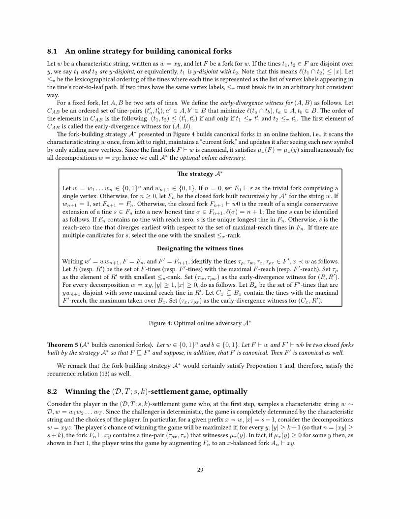
8.1 An online strategy for building canonical forks

Let w be a characteristic string, wrien as w = xy, and let F be a fork for w. If the tines t1, t2 ∈ F are disjoint overy, we say t1 and t2 are y-disjoint, or equivalently, t1 is y-disjoint with t2. Note that this means ℓ(t1 ∩ t2) ≤ |x|. Let≤π be the lexicographical ordering of the tines where each tine is represented as the list of vertex labels appearing inthe tine’s root-to-leaf path. If two tines have the same vertex labels, ≤π must break tie in an arbitrary but consistentway.

For a fixed fork, let A,B be two sets of tines. We define the early-divergence witness for (A,B) as follows. LetCAB be an ordered set of tine-pairs (t′a, t

′b), a

′ ∈ A, b′ ∈ B that minimize ℓ(ta ∩ tb), ta ∈ A, tb ∈ B. e order ofthe elements in CAB is the following: (t1, t2) ≤ (t′1, t

′2) if and only if t1 ≤π t′1 and t2 ≤π t′2. e first element of

CAB is called the early-divergence witness for (A,B).e fork-building strategy A∗ presented in Figure 4 builds canonical forks in an online fashion, i.e., it scans the

characteristic stringw once, from le to right, maintains a “current fork,” and updates it aer seeing each new symbolby only adding new vertices. Since the final fork F ⊢ w is canonical, it satisfies µx(F ) = µx(y) simultaeneously forall decompositions w = xy; hence we call A∗ the optimal online adversary.

e strategyA∗

Let w = w1 . . . wn ∈ 0, 1n and wn+1 ∈ 0, 1. If n = 0, set F0 ⊢ ε as the trivial fork comprising asingle vertex. Otherwise, for n ≥ 0, let Fn be the closed fork built recursively by A∗ for the string w. Ifwn+1 = 1, set Fn+1 = Fn. Otherwise, the closed fork Fn+1 ⊢ w0 is the result of a single conservativeextension of a tine s ∈ Fn into a new honest tine σ ∈ Fn+1, ℓ(σ) = n+ 1; e tine s can be identifiedas follows. If Fn contains no tine with reach zero, s is the unique longest tine in Fn. Otherwise, s is thereach-zero tine that diverges earliest with respect to the set of maximal-reach tines in Fn. If there aremultiple candidates for s, select the one with the smallest ≤π-rank.

Designating the witness tines

Writing w′ = wwn+1, F = Fn, and F′ = Fn+1, identify the tines τρ, τw, τx, τρx ∈ F ′, x ≺ w as follows.

Let R (resp. R′) be the set of F -tines (resp. F ′-tines) with the maximal F -reach (resp. F ′-reach). Set τρas the element of R′ with smallest ≤π-rank. Set (τw, τρw) as the early-divergence witness for (R,R′).For every decomposition w = xy, |y| ≥ 1, |x| ≥ 0, do as follows. Let Bx be the set of F ′-tines that areywn+1-disjoint with some maximal-reach tine in R′. Let Cx ⊆ Bx contain the tines with the maximalF ′-reach, the maximum taken over Bx. Set (τx, τρx) as the early-divergence witness for (Cx, R

′).

Figure 4: Optimal online adversary A∗

eorem 5 (A∗ builds canonical forks). Let w ∈ 0, 1n and b ∈ 0, 1. Let F ⊢ w and F ′ ⊢ wb be two closed forksbuilt by the strategy A∗ so that F ⊑ F ′ and suppose, in addition, that F is canonical. en F ′ is canonical as well.

We remark that the fork-building strategy A∗ would certainly satisfy Proposition 1 and, therefore, satisfy therecurrence relation (13) as well.

8.2 Winning the (D, T ; s, k)-settlement game, optimally

Consider the player in the (D, T ; s, k)-selement game who, at the first step, samples a characteristic string w ∼D, w = w1w2 . . . wT . Since the challenger is deterministic, the game is completely determined by the characteristicstring and the choices of the player. In particular, for a given prefix x ≺ w, |x| = s− 1, consider the decompositionsw = xyz. e player’s chance of winning the game will be maximized if, for every y, |y| ≥ k+1 (so that n = |xy| ≥s+ k), the fork Fn ⊢ xy contains a tine-pair (τρx, τx) that witnesses µx(y). In fact, if µx(y) ≥ 0 for some y then, asshown in Fact 1, the player wins the game by augmenting Fn to an x-balanced fork An ⊢ xy.

29

Note, in addition, that if Fn is canonical, the player can optimally play (D, T ; s, k)-selement games simultane-ously for every s ∈ [n−k]. at is, given a distributionD, a canonical fork Fn gives the player the largest probabilityof causing a selement violation at as many slots s ∈ [n− k] as possible, at once.

8.3 Proof of eorem 5

For convenience, let us record the following fact which compacts Claims 1 and 2.

Fact 2. Let F ⊢ w and F ′ ⊢ w0 be closed forks so that F ⊑ F ′ and F ′ differs from F by a single conservative extensionσ ∈ F ′, ℓ(σ) = |w| + 1. en reachF ′(t) = reachF (t)− 1 for every t ∈ F and, in addition, reachF ′(σ) = 0.

In the rest of the proof, we will frequently use the above fact along with Lemma 2 and Lemma 3, oen withoutan explicit reference.

By assumption, F is a canonical fork. us reachF (tρ) = ρ(w) and for every prefix x ≺ w, reachF (tx) = µx(y).Let w′ = wb and let τρ, τw, τρw, τx, τρx ∈ F ′, x ≺ w be the purported witness tines in F ′. Note that τx must be yb-disjoint with τρx by construction. Similarly, τw must bewn+1-disjoint with τρw since both cannot contain the uniquevertex from slot n+1. It is evident from the construction that ρ(F ′) = reachF ′(τρ) = reachF ′(τρw) = reachF ′(τρx)for x ≺ w. erefore, we wish to show that reachF ′(τρ) = ρ(wb), reachF ′(τw) = µw(b) and reachF ′(τx) = µx(yb)for x ≺ w.

If b = 1. In this case, F ′ = F and w′ = w1. Examining the rule for assigning τρ, τx, τρx, and τw , we see thatτρ = tρ, τw = tρ, τx = tx, and τρx = tρx for all x ≺ w. Since F ′ = F and b = 1, the F ′-reach of everyF -tine is one plus its F -reach. us for any x, x ≺ w, writing w′ = xy1, we have µx(y1) = 1 + µx(y) =1 + reachF (tx) = reachF ′(tx) = reachF ′(τx). Similarly, ρ(w1) = 1 + ρ(w) = reachF ′(tρ) = reachF ′(τρ).By construction, τw has the largest reach in F ; but this means reachF ′(τw) = reachF ′(tρ) = ρ(F ′) = ρ(w1)but, on the other hand, µw(1) = 1 + µw(ε) = 1 + ρ(w) = ρ(w1); hence reachF ′(τw) = µw(1).

If b = 0. e contingencies of this case are covered by Propositions 3, 4, and 5 below.

Proposition 3. Assume the premise of eorem 5 with b = 0. en F ′ contains a witness tine τρ so that reachF ′(τρ) =ρ(w0).

Proof. Recall that the tine σ ∈ F ′, ℓ(σ) = |w| + 1 is a conservative extension to a tine s ∈ F, reachF (s) = 0 sothat reachF ′(σ) = 0. Also recall that µz(ε) = ρ(z) for any characteristic string z. Finally, note that it suffices toshow that reachF ′(τρ) ≥ ρ(w0).

Suppose ρ(w) > 0. Using Fact 2, Lemma 3, and examining the rule for assigning τρ, we see that reachF ′(τρ) ≥reachF ′(tρ) = reachF (tρ) − 1 = ρ(w) − 1 = ρ(w0). On the other hand, if ρ(w) = 0 then ρ(w0) is zero as well. Itfollows that reachF ′(τρ) ≥ reachF ′(σ) = 0 = ρ(w0).

Proposition 4. Assume the premise of eorem 5 with b = 0. en F ′ contains a tine-pair (τρw , τw) that witnessesµw(0).

Proof. Recall that the tine σ ∈ F ′, ℓ(σ) = |w|+1 is a conservative extension to a tine s ∈ F, reachF (s) = 0 so thatreachF ′(σ) = 0. In addition, since F ′ contains a single vertex at slot |w|+ 1, τw and τρw are disjoint over the suffixwn+1 and, moreover, reachF ′(τρw) = ρ(F ′) = ρ(w0) by Proposition 3. Now consider the following contingenciesbased on ρ(w).

If ρ(w) > 0. us µw(0) = µw(ε)− 1 = ρ(w) − 1 = ρ(w0). ere are two mutually exclusive scenarios based onτρw and σ. If τρw = σ then, by construction, τw 6= σ (since ℓ(τρw , τw) ≤ |w|) and, in addition, reachF (τw) =ρ(w). is implies reachF ′(τw) = reachF (τw)− 1 = ρ(w)− 1 = µw(0). On the other hand, if τρw 6= σ thenτρw ∈ F . Since τw is the F -tine with the largest F ′-reach, it follows that reachF ′(τw) = reachF ′(τρw) =ρ(w0) = µw(0).

30

If ρ(w) = 0. Since ρ(F ) = ρ(w) = 0, Fact 2 tells us that every F -tine must have a negative reach in F ′. Since ρ(F ′)is non-negative, it must be the case that τρw = σ. We can reuse the argument from the subcase “τρw = σ” ofthe preceding case and conclude that reachF ′(τw) = µw(0).

Proposition 5. Assume the premise of eorem 5 with b = 0. Let x ≺ w and write w = xy. en F ′ contains atine-pair (τρx, τx) that witnesses µx(y0).

Proof. By construction, reachF ′(τx) = µx(F′) and, by the definition of relative margin, µx(F

′) ≤ µx(y0). In lightof (13), it suffices to show that reachF ′(τx) ≥ 0 if ρ(xy) > µx(y) = 0, and reachF ′(τx) ≥ µx(y)− 1 otherwise.

LetR be the set of F -tines with the maximal F -reach and letR′ be the set of F ′-tines with the maximal F ′-reach;thus τρx ∈ R′. We know that tx is y-disjoint with tρ in F . Consider the following mutually exclusive cases.

If ρ(w) > 0 and µx(y) = 0. In this case, µx(y0) = 0 using Lemma 3. Since reachF (s) = 0 < reachF (tρx) = ρ(w),it follows that s 6= tρx. In addition, observe that tρx must be in R′. By our choice of s, ℓ(s∩ tρx) ≤ ℓ(tx ∩ tρx)since reachF (tx) = µx(y) = 0 = reachF (s). Since tx is y-disjoint with tρx, so is s. Recall that reachF ′(τx) isthe largest among all tines that are y0-disjoint with τρx.

If τρx = tρx. us tx is y0-disjoint with τρx. Since ℓ(σ) = |w| + 1, σ must be y0-disjoint with tρx = τρx, itfollows that reachF ′(τx) ≥ reachF ′(σ) = 0 = µx(y0).

If τρx 6= tρx. is happens when ρ(w) = 1, ρ(w0) = 0, and tρx, σ ∈ R′. Note that |R′| ≥ 2 since bothσ, tρx ∈ R′ but σ 6= tρx. If there are two y0-disjoint tines r′1, r

′2 ∈ R′ then reachF ′(τx) ≥ 0 = µx(y0).

Otherwise, all tines r′ ∈ R′ share a vertex indexed by y. Since tx is y-disjoint with tρx, tx must bey-disjoint (and thus y0-disjoint) with every r′ ∈ R′ as well. Examining the rule for assigning τx, weconclude that τx = tx and, therefore, reachF ′(τx) = reachF ′(tx) = µx(y) = 0 = µx(y0).

If ρ(w) = 0. Let x ≺ w and note that µx(y0) = µx(y) − 1. Since ρ(w) = 0, reachF (s) = 0 all F -tines will havea negative reach in F ′; by Fact 2, σ is the only tine in F ′ with the maximal reach ρ(F ′) = ρ(w0) = 0, i.e.,τρx = τρ = σ. In addition, we must also have reachF (s) = 0, i.e., s ∈ R; we conclude that s has the smallest≤π rank among all members of R and, therefore, s = tρ. It follows that τx is y0-disjoint with s = tρ and,in particular, τx ∈ F . Considering tx, if it is y-disjoint with tρ then we must have τx = tx; in this case,reachF ′(τx) = reachF ′(tx) = reachF (tx) − 1 = µx(y) − 1 = µx(y0). Otherwise, ℓ(tx ∩ tρ) ≥ |x| + 1and there must be a tine tρx ∈ F that is y-disjoint with tx (and hence, with τρx). erefore, reachF ′(τx) ≥reachF ′(tρx) ≥ reachF ′(tx) = reachF (tx) − 1 = µx(y) − 1. Here, the first inequality follows from theconstruction of τx and the second one follows since tρx) has the maximal reach in F .

If ρ(w) > 0 and µx(y) 6= 0. ere can be two cases depending on whether s has zero reach in F .

If reachF (s) = 0. en s 6∈ tρx, tx. Observe that reachF ′(tρx) = reachF (tρx) − 1 = ρ(w) − 1 = ρ(w0).It follwos that tρx ∈ R′. Since tx is y0-disjoint with tρx ∈ R′ and, in addition, that τx has the largestreach among all tines that are y0-disjoint with some member of R′, we conclude that reachF ′(τx) ≥reachF ′(tx) = reachF (tx)− 1 = µx(y)− 1 = µx(y0).

If reachF (s) ≥ 1. In this case, s is the longest tine in F . Considering fork F ′, if some tine r′ ∈ R′ is y0-disjoint with tx then reachF ′(τx) ≥ reachF ′(tx) = reachF (tx)− 1 = µx(y)− 1 = µx(y0). Otherwise,ℓ(r′ ∩ tx) > |x| for every tine r′ ∈ R′, i.e., no maximal-reach F ′-tine is y0-disjoint with tx. Sinceℓ(tx, tρx) ≤ |x| by assumption and τρx ∈ R′, it follows that ℓ(τρx ∩ tρx) ≤ |x|, i.e., tρx is y0-disjointwith τρx. erefore, reachF ′(τx) ≥ reachF ′(tρx) = reachF (tρx)−1 = ρ(w)−1 ≥ µx(y)−1 = µx(y0).Here, the second inequality is true since µx(y) ≤ ρ(xy) = ρ(w).

31

is completes the proof of eorem 5.In regards to the canonical fork F ⊢ w produced by the strategy A∗ (see Figure 4), it is possible to maintain

witness tines τρ, τ′m ∈ F , for integers m = −|w|, . . . , |w|, so that for every prefix x ≺ w, the tine-pair (τρ, τ

′µx(y)

)

witnesses µx(y). In particular, a single maxmimal-reach tine τρ appears in every witness tine-pair. We omit futherdetails.

Acknowledgments

We are grateful to Shreyas Gandlur and BruceHajek (UIUC) for their suggestion about using the dominance argumentin the proof of Bound 2.

References

[1] Adam Back. Hashcash. hp://www.cypherspace.org/hashcash, 1997.

[2] Christian Badertscher, Peter Gazi, Aggelos Kiayias, Alexander Russell, and Vassilis Zikas. Ouroboros genesis:Composable proof-of-stake blockchains with dynamic availability. IACR Cryptology ePrint Archive, 2018:378,2018.

[3] Iddo Bentov, Ariel Gabizon, and Alex Mizrahi. Cryptocurrencies without proof of work. CoRR, abs/1406.5694,2014.

[4] Iddo Bentov, Rafael Pass, and Elaine Shi. Snow white: Provably secure proofs of stake. IACR Cryptology ePrintArchive, 2016:919, 2016.

[5] Jonah Brown-Cohen, Arvind Narayanan, Christos-Alexandros Psomas, and S. Mahew Weinberg. Formalbarriers to longest-chain proof-of-stake protocols. CoRR, abs/1809.06528, 2018.

[6] Bernardo David, Peter Gazi, Aggelos Kiayias, and Alexander Russell. Ouroboros praos: An adaptively-secure,semi-synchronous proof-of-stake blockchain. In Nielsen and Rijmen [19], pages 66–98.

[7] Cynthia Dwork and Moni Naor. Pricing via processing or combaing junk mail. In Ernest F. Brickell, editor,Advances in Cryptology – CRYPTO’92, volume 740 of Lecture Notes in Computer Science, pages 139–147, SantaBarbara, CA, USA, August 16–20, 1993. Springer, Heidelberg, Germany.

[8] Stefan Dziembowski, Sebastian Faust, Vladimir Kolmogorov, and Krzysztof Pietrzak. Proofs of space. In RosarioGennaro and Mahew J. B. Robshaw, editors, Advances in Cryptology – CRYPTO 2015, Part II, volume 9216of Lecture Notes in Computer Science, pages 585–605, Santa Barbara, CA, USA, August 16–20, 2015. Springer,Heidelberg, Germany.

[9] Juan A. Garay, Aggelos Kiayias, and Nikos Leonardos. e bitcoin backbone protocol: Analysis and applica-tions. In Elisabeth Oswald and Marc Fischlin, editors, Advances in Cryptology - EUROCRYPT 2015 - 34th AnnualInternational Conference on the eory and Applications of Cryptographic Techniques, Sofia, Bulgaria, April 26-30,2015, Proceedings, Part II, volume 9057 of Lecture Notes in Computer Science, pages 281–310. Springer, 2015.

[10] Juan A. Garay, Aggelos Kiayias, and Nikos Leonardos. e bitcoin backbone protocol with chains of variabledifficulty. In Jonathan Katz and Hovav Shacham, editors, Advances in Cryptology – CRYPTO 2017, Part I, vol-ume 10401 of Lecture Notes in Computer Science, pages 291–323, Santa Barbara, CA, USA, August 20–24, 2017.Springer, Heidelberg, Germany.

[11] Juan A. Garay, Aggelos Kiayias, and Nikos Leonardos. e bitcoin backbone protocol with chains of variabledifficulty. In Jonathan Katz and Hovav Shacham, editors, Advances in Cryptology - CRYPTO 2017 - 37th AnnualInternational Cryptology Conference, Santa Barbara, CA, USA, August 20-24, 2017, Proceedings, Part I, volume10401 of Lecture Notes in Computer Science, pages 291–323. Springer, 2017.

32

[12] Charles M. Grinstead and J. Laurie Snell. Introduction to Probability. American Mathematical Association, 1997.

[13] Aggelos Kiayias, Alexander Russell, Bernardo David, and Roman Oliynykov. Ouroboros: A provably secureproof-of-stake blockchain protocol. In Jonathan Katz and Hovav Shacham, editors, Advances in Cryptology -CRYPTO 2017 - 37th Annual International Cryptology Conference, volume 10401 of Lecture Notes in ComputerScience, pages 357–388. Springer, 2017.

[14] David A Levin, Yuval Peres, and Elizabeth L Wilmer. Markov chains and mixing times, volume 58. AmericanMathematical Society, 2009.

[15] Silvio Micali. ALGORAND: the efficient and democratic ledger. CoRR, abs/1607.01341, 2016.

[16] Tal Moran and Ilan Orlov. Proofs of space-time and rational proofs of storage. Cryptology ePrint Archive,Report 2016/035, 2016. http://eprint.iacr.org/2016/035.

[17] Rajeev Motwani and Prabhakar Raghavan. Randomized Algorithms. Cambridge University Press, New York,NY, USA, 1995.

[18] Satoshi Nakamoto. Bitcoin: A peer-to-peer electronic cash system. hp://bitcoin.org/bitcoin.pdf, 2008.

[19] Jesper Buus Nielsen and Vincent Rijmen, editors. Advances in Cryptology - EUROCRYPT 2018 - 37th AnnualInternational Conference on the eory and Applications of Cryptographic Techniques, Tel Aviv, Israel, April 29 -May 3, 2018 Proceedings, Part II, volume 10821 of Lecture Notes in Computer Science, 2018. Springer.

[20] Sunoo Park, Krzysztof Pietrzak, Albert Kwon, Joel Alwen, Georg Fuchsbauer, and Peter Gazi. Spacemint: Acryptocurrency based on proofs of space. IACR Cryptology ePrint Archive, 2015:528, 2015.

[21] Rafael Pass and Elaine Shi. e sleepy model of consensus. In Tsuyoshi Takagi and omas Peyrin, editors,Advances in Cryptology - ASIACRYPT 2017 - 23rd International Conference on the eory and Applications ofCryptology and Information Security, Hong Kong, China, December 3-7, 2017, Proceedings, Part II, volume 10625of Lecture Notes in Computer Science, pages 380–409. Springer, 2017.

[22] Rafael Pass and Elaine Shi. Hybrid consensus: Efficient consensus in the permissionless model. In Andrea W.Richa, editor, 31st International Symposium on Distributed Computing, DISC 2017, October 16-20, 2017, Vienna,Austria, volume 91 of LIPIcs, pages 39:1–39:16. Schloss Dagstuhl - Leibniz-Zentrum fuer Informatik, 2017.

[23] Rafael Pass and Elaine Shi. underella: Blockchains with optimistic instant confirmation. In Nielsen andRijmen [19], pages 3–33.

[24] Rafael Pass, Lior Seeman, and Abhi Shelat. Analysis of the blockchain protocol in asynchronous networks.In Jean-Sebastien Coron and Jesper Buus Nielsen, editors, Advances in Cryptology - EUROCRYPT 2017 - 36thAnnual International Conference on the eory and Applications of Cryptographic Techniques, Paris, France, April30 - May 4, 2017, Proceedings, Part II, volume 10211 of Lecture Notes in Computer Science, pages 643–673, 2017.

[25] Saad ader and Alexander Russell. C++ source code to compute selement error estimates.https://github.com/saad0105050/forkable-strings-code , 2018. Accessed: 2019-10-14.

[26] Herbert S Wilf. generatingfunctionology. AK Peters/CRC Press, 3 edition, 2005.

33

A Exact settlement probabilities

Let m, k ∈ N and ǫ ∈ (0, 1]. Let w be a characteristic string of length T = m + k such that the bits of w are i.i.d.Bernoulli with expectation α = (1 − ǫ)/2. Write w as w = xy where |x| = m, |y| = k. e recursive definition ofrelative margin (cf. Lemma 3) implies an algorithm for computing the probability Pr[µx(y) ≥ 0] in time poly(m, k).In typical circumstances, however, it is more interesting to establish an explicit upper bound onPr[µx(y) ≥ 0]where|x| → ∞; this corresponds to the case where the distribution of the initial reach ρ(x) is the dominant distributionR∞ in Lemma 4. Due to dominance, R∞(m) serves as an upper bound on ρ(x) for any finite m = |x|. For thispurpose, one can implicitly maintain a sequence of matrices (Mt) for t = 0, 1, 2, · · · , k such thatM0(r, r) = R∞(r)for all 0 ≤ r ≤ 2k and the invariant

Mt(r, s) = Pry∼B(t,α)

[ρ(xy) = r and µx(y) = s]

is satisfied for every integer t ∈ [1, k], r ∈ [0, 2k], and s ∈ [−2k, 2k]. Here,M(i, j) denotes the entry at the ith rowand jth column of the matrixM . Observe thatMt(r, s) can be computed solely from the neighboring cells ofMt−1,that is, from the values Mt−1(r ± 1, s± 1). Of course, only the transitions approved by the recursions in Lemma 2and Lemma 3 should be considered.

Finally, one can compute Pr[µx(y) ≥ 0] by summing Mk(r, s) for r, s ≥ 0. Table 1 contains these probabilitieswhere α ranges from 0.05 to 0.40 and k ranges from 50 to 1000. In addition, Figure 5 shows the base-10 logarithm ofthese probabilities. e points corresponding to a fixed α appear to form a straight line. is means the probabilitydecays exponentially in k, or equivalently, that the exponent depends linearly on k, as stipulated by Bound 1.

AC++ implementation of the above algorithm is publicly available at hps://github.com/saad0105050/forkable-strings-code[25].

Table 1: Exact probabilities Pr[µx(y) ≥ 0] where the bits of the characteristic string xy are i.i.d. Bernoulli withexpectation α. Each row of the table corresponds to a different k = |y|.

kα

0.05 0.10 0.15 0.20 0.25 0.30 0.35 0.40

50 5.37E-15 1.16E-09 1.02E-06 8.68E-05 1.96E-03 1.86E-02 9.36E-02 2.92E-01

100 1.23E-28 5.10E-18 3.52E-12 2.28E-08 1.03E-05 8.00E-04 1.72E-02 1.37E-01

150 2.83E-42 2.24E-26 1.22E-17 6.05E-12 5.54E-08 3.57E-05 3.30E-03 6.74E-02

200 6.49E-56 9.82E-35 4.21E-23 1.61E-15 2.98E-10 1.60E-06 6.40E-04 3.36E-02

250 1.49E-69 4.31E-43 1.46E-28 4.27E-19 1.61E-12 7.21E-08 1.25E-04 1.69E-02

300 3.42E-83 1.89E-51 5.05E-34 1.14E-22 8.67E-15 3.25E-09 2.44E-05 8.52E-03

350 7.84E-97 8.29E-60 1.75E-39 3.02E-26 4.67E-17 1.46E-10 4.78E-06 4.31E-03

400 1.80E-110 3.64E-68 6.06E-45 8.02E-30 2.52E-19 6.59E-12 9.37E-07 2.18E-03

450 4.13E-124 1.60E-76 2.10E-50 2.13E-33 1.36E-21 2.97E-13 1.84E-07 1.11E-03

500 9.47E-138 7.00E-85 7.26E-56 5.67E-37 7.32E-24 1.34E-14 3.60E-08 5.62E-04

550 2.17E-151 3.07E-93 2.51E-61 1.51E-40 3.95E-26 6.02E-16 7.05E-09 2.86E-04

600 4.98E-165 1.35E-101 8.70E-67 4.00E-44 2.13E-28 2.71E-17 1.38E-09 1.45E-04

650 1.14E-178 5.91E-110 3.01E-72 1.06E-47 1.15E-30 1.22E-18 2.71E-10 7.37E-05

700 2.62E-192 2.59E-118 1.04E-77 2.83E-51 6.19E-33 5.51E-20 5.31E-11 3.75E-05

750 6.02E-206 1.14E-126 3.61E-83 7.52E-55 3.33E-35 2.48E-21 1.04E-11 1.91E-05

800 1.38E-219 4.99E-135 1.25E-88 2.00E-58 1.80E-37 1.12E-22 2.04E-12 9.69E-06

850 3.17E-233 2.19E-143 4.33E-94 5.31E-62 9.69E-40 5.04E-24 4.00E-13 4.93E-06

900 7.27E-247 9.61E-152 1.50E-99 1.41E-65 5.23E-42 2.27E-25 7.84E-14 2.50E-06

950 1.67E-260 4.22E-160 5.19E-105 3.75E-69 2.82E-44 1.02E-26 1.54E-14 1.27E-06

1000 3.83E-274 1.85E-168 1.80E-110 9.98E-73 1.52E-46 4.61E-28 3.01E-15 6.48E-07

34

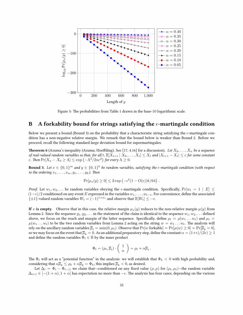
0 200 400 600 800 1,000−300

−200

−100

0

Length of y

log10Pr[µx(y)≥

0]

α = 0.40α = 0.35α = 0.30α = 0.25α = 0.20α = 0.15α = 0.10α = 0.05

Figure 5: e probabilities from Table 1 drawn in the base-10 logarithmic scale.

B A forkability bound for strings satisfying the ǫ-martingale condition

Below we present a bound (Bound 3) on the probability that a characteristic string satisfying the ǫ-martingale con-dition has a non-negative relative margin. We remark that the bound below is weaker than Bound 2. Before weproceed, recall the following standard large deviation bound for supermartingales.

eorem 6 (Azuma’s inequality (Azuma; Hoeffding). See [17, 4.16] for a discussion). LetX0, . . . , Xn be a sequenceof real-valued random variables so that, for all t, E[Xt+1 | X0, . . . , Xt] ≤ Xt and |Xt+1 −Xt| ≤ c for some constantc. en Pr[Xn −X0 ≥ Λ] ≤ exp

(

−Λ2/2nc2)

for every Λ ≥ 0.

Bound 3. Let x ∈ 0, 1m and y ∈ 0, 1k be random variables, satisfying the ǫ-martingale condition (with respectto the ordering x1, . . . , xm, y1, . . . , yk). en

Pr[µx(y) ≥ 0] ≤ 3 exp(

−ǫ4(1−O(ǫ))k/64)

.

Proof. Let w1, w2, . . . be random variables obeying the ǫ-martingale condition. Specifically, Pr[wt = 1 | E] ≤(1−ǫ)/2 conditioned on any eventE expressed in the variablesw1, . . . , wt−1. For convenience, define the associated±1-valued random variablesWt = (−1)1+wt and observe that E[Wt] ≤ −ǫ.

If x is empty. Observe that in this case, the relative margin µx(y) reduces to the non-relative margin µ(y) fromLemma 2. Since the sequence y1, y2, . . . in the statement of the claim is identical to the sequence w1, w2, . . . definedabove, we focus on the reach and margin of the laer sequence. Specifically, define ρt = ρ(w1 . . . wt) and µt =µ(w1 . . . wt) to be the two random variables from Lemma 2 acting on the string w = w1 . . . wt. e analysis willrely on the ancillary random variables µt = min(0, µt). Observe thatPr[w forkable] = Pr[µ(w) ≥ 0] = Pr[µk = 0],sowemay focus on the event thatµk = 0. As an additional preparatory step, define the constantα = (1+ǫ)/(2ǫ) ≥ 1and define the random variables Φt ∈ R by the inner product

Φt = (ρt, µt) ·(

1α

)

= ρt + αµt .

e Φt will act as a “potential function” in the analysis: we will establish that Φk < 0 with high probability and,considering that αµk ≤ ρk + αµk = Φk , this implies µk < 0, as desired.

Let ∆t = Φt − Φt−1; we claim that—conditioned on any fixed value (ρ, µ) for (ρt, µt)—the random variable∆t+1 ∈ [−(1 + α), 1 + α] has expectation no more than −ǫ. e analysis has four cases, depending on the various

35

regimes of ρ and µ from Lemma 2. When ρ > 0 and µ < 0, ρt+1 = ρ +Wt+1 and µt+1 = µ +Wt+1, where µ =max(0, µ); then∆t+1 = (1 + α)Wt+1 and E[∆t+1] ≤ −(1 + α)ǫ ≤ −ǫ. When ρ > 0 and µ ≥ 0, ρt+1 = ρ+Wt+1

but µt+1 = µ so that ∆t+1 = Wt+1 and E[∆t+1] ≤ −ǫ. Similarly, when ρ = 0 and µ < 0, µt+1 = µ+Wt+1 whileρt+1 = ρ+max(0,Wt+1); we may compute

E[∆t+1] ≤1− ǫ

2(1 + α)− 1 + ǫ

2α =

1− ǫ

2− ǫα =

1− ǫ

2− ǫ

(

1

ǫ· 1 + ǫ

2

)

= −ǫ .

Finally, when ρ = µ = 0 exactly one of the two random variables ρt+1 and µt+1 differs from zero: ifWt+1 = 1 then(ρt+1, µt+1) = (1, 0); likewise, if Wt+1 = −1 then (ρt+1, µt+1) = (0,−1). It follows that

E[∆t+1] ≤1− ǫ

2− 1 + ǫ

2α ≤ −ǫ .

us E[Φk] = E∑k

t=1 ∆t ≤ −ǫk. We wish to apply Azuma’s inequality to conclude that Pr[Φk ≥ 0] is exponen-tially small. For this purpose, we transform the random variables Φt to a related supermartingale by shiing them:specifically, define Φt = Φt + ǫt and ∆t = ∆t + ǫ so that Φt =

∑ti ∆t. en

E[Φt+1 | Φ1, . . . , Φt] = E[Φt+1 |W1, . . . ,Wt] ≤ Φt , ∆t ∈ [−(1 + α) + ǫ, 1 + α+ ǫ] ,

and Φk = Φk + ǫk. It follows from Azuma’s inequality that

Pr[w forkable] = Pr[µk = 0] ≤ Pr[Φk ≥ 0] = Pr[Φk ≥ ǫk]

≤ exp

(

− ǫ2k2

2k(1 + α+ ǫ)2

)

= exp

(

−(

2ǫ2

1 + 3ǫ+ 2ǫ2

)2

· k2

)

≤ exp

(

− 2ǫ4

1 + 35ǫ· k)

. (20)

If x is not empty. In this case, we go back to study the sequences x and y as in the statement of the claim.Recall the reach distribution (i.e., the distribution of the random variable ρ(x)) Rm : Z → [0, 1] from (18). Since

x = (x1, . . . , xm) satisfies the ǫ-martingale condition, Lemma 4 states thatRm R∞. We reserve the symbol µ(r)x

for the relative margin random walk µx which starts at a non-negative initial position r. us ρ(x) = µx(ǫ) = r,and

Pr[µx(y) ≥ 0] =∑

r≥0

Rm(r) Pr[µ(r)x (y) ≥ 0] ≤

∑

r≥0

R∞(r) Pr[µ(r)x (y) ≥ 0] (21)

since the sequence ( Pr[µ(r)x (y) ≥ 0] )∞r=0 is non-decreasing and Rm R∞. Fix a “large enough” positive integer

r∗ whose value will be assigned later in the analysis. Let us define the following events:

• Event Br : it occurs when r ∈ [0, r∗] and the µ(r)x walk is strictly positive on every prefix of y with length at

most k/2; and

• Event Cr,s: it occurs when r ∈ [0, r∗] and y is the smallest prefix of y of length s ∈ [r, k/2] such that µ(r)x (y) =

0. We say that y is a witnesses to the event Cr,s.

e right-hand side of (21) can be wrien as

∑

r>r∗

R∞(r) Pr[µ(r)x (y) ≥ 0] +

∑

r≤r∗

R∞(r) Pr[Br ] · Pr[

µ(r)x (y) ≥ 0 | Br

]

+∑

r≤r∗

R∞(r)

k/2∑

s=r

Pr[Cr,s] · Pr[µ(r)x (y) ≥ 0 | Cr,s] .

36

We observe that the probabilities Pr[µ(r)x (y) ≥ 0] and Pr[µ

(r)x (y) ≥ 0 | Br] are at most one. In addition, recall that

for two non-negative sequences (ai), (bi) of equal lengths, we have∑

aibi ≤ max bi if∑

ai ≤ 1. us (21) can besimplified as

Pr[µx(y) ≥ 0] ≤∑

r>r∗

R∞(r) +∑

r≤r∗

R∞(r) Pr[Br]

+∑

r≤r∗

R∞(r) maxr≤s≤k/2

Pr[µ(r)x (y) ≥ 0 | Cr,s]

≤∑

r>r∗

R∞(r) + maxr≤r∗

Pr[Br ] + maxr≤r∗

r≤s≤k/2

Pr[µ(r)x (y) ≥ 0 | Cr,s] . (22)

e first term in (22) is the right-tail of the distribution R∞. Using Lemma 4, this quantity is at most βr∗ whereβ := (1− ǫ)/(1 + ǫ). Furthermore, it can be easily checked that the above quantity is at most exp(−5ǫ/3).

e second term in (22) concerns the event Br and calls for more care. Define

S(r)k :=

k∑

t=0

Wt

where W0 = r and the random variables Wt are defined at the outset of this proof for t ≥ 1. We know that the

µ(r)x walk starts with ρ(x) = µ(x) = r ≥ 0. Since Br holds, both the margin µx(y) and the reach ρ(xy) remain

non-negative for all prefixes y of length t = 1, 2, · · · , k/2. ese two facts imply that the random variable µ(r)x (y)

is identical to the sum S(r)t for all prefixes y of length t = 1, 2, · · · , k/2.

To be precise,

Pr[Br] = Pr[S(r)t ≥ 0 for all t ≤ k/2] .

e laer probability is at most Pr[S(r)k/2 ≥ 0] because the event S

(r)k/2 ≥ 0 does not constrain the intermediate sums

S(r)t for t < k/2. Since Pr[S

(r)k/2 ≥ 0] increases monotonically in r, we conclude that the second term in (22) is at

most Pr[S(r∗)k/2 ≥ 0]. Now we are free to shi our focus from the relative margin walk to the sum of a martingale

sequence.

For notational clarity, let us write S := S(r∗)k/2 . Since the sequence (wt) obeys the ǫ-martingale condition, ES is

at most M := r∗ − kǫ/2. Let us set r∗ = W0 = kǫ/4. en ES is at most −kǫ/4 and Azuma’s inequality gives us

Pr[S ≥ 0] = Pr[(S − ES) ≥ kǫ/4] ≤ exp

(

− (kǫ/4)2

2(k/2) · 22)

= exp

(

−kǫ2

64

)

.

is is an upper bound on the second term in (22).e third term in (22) concerns the event Cr,s and it can be bounded using our existing analysis of the |x| = 0 case.

Specifically, suppose y = yzwhere y is a witness to the eventCr,s. Since theµ(r)x walk remains non-negative over the

entire string y, it follows that ρ(xy) = µ(xy) = 0 and as a consequence, theµxy walk on z is identical to theµwalk onz. Our analysis in the |x| = 0 case suggests thatPr[µ(z) ≥ 0] is atmostA(k−s, ǫ)where |z| = k−s andA(k, ǫ) is thebound in (20). SinceA(·, ǫ) decreases monotonically in the first argument,A(k−s, ǫ) is at mostA(k/2, ǫ). However,since the last quantity is independent of r, the third term in (22) is at most A(k/2, ǫ) = exp

(

−kǫ4/(1 + 35ǫ))

.Returning to (22) and using r∗ = kǫ/4, we get

Pr[µx(y) ≥ 0] ≤ exp

(

−5ǫ

3· kǫ4

)

+ exp

(

− 2ǫ4

1 + 35ǫ· n2

)

+ exp

(

−kǫ2

64

)

.

It is easy to check that the above quantity is at most 3 exp(

−kǫ4/(64 + 35ǫ))

= 3 exp(

−ǫ4(1 −O(ǫ))k/64)

.

37