University of Warwick institutional repository: · thesis deposit 2.1 I understand that under my registration at the University, I am required to deposit my thesis with the University

University of Warwick institutional repository: http://go.warwick.ac.uk/wrap

A Thesis Submitted for the Degree of PhD at the University of Warwick

http://go.warwick.ac.uk/wrap/57475

This thesis is made available online and is protected by original copyright.

Please scroll down to view the document itself.

Please refer to the repository record for this item for information to help you to cite it. Our policy information is available from the repository home page.

http://go.warwick.ac.uk/wrap

http://go.warwick.ac.uk/wrap/57475

www.warwick.ac.uk

AUTHOR: Gabor Szepesi DEGREE: Ph.D.

TITLE: Modelling of Turbulent Particle Transport in Finite-Beta and Multi-

ple Ion Species Plasma in Tokamaks

DATE OF DEPOSIT: . . . . . . . . . . . . . . . . . . . . . . . . . . . . . . . . .

I agree that this thesis shall be available in accordance with the regulationsgoverning the University of Warwick theses.

I agree that the summary of this thesis may be submitted for publication.I agree that the thesis may be photocopied (single copies for study purposes

only).Theses with no restriction on photocopying will also be made available to the British

Library for microfilming. The British Library may supply copies to individuals or libraries.subject to a statement from them that the copy is supplied for non-publishing purposes. Allcopies supplied by the British Library will carry the following statement:

“Attention is drawn to the fact that the copyright of this thesis rests withits author. This copy of the thesis has been supplied on the condition thatanyone who consults it is understood to recognise that its copyright rests withits author and that no quotation from the thesis and no information derivedfrom it may be published without the author’s written consent.”

AUTHOR’S SIGNATURE: . . . . . . . . . . . . . . . . . . . . . . . . . . . . . . . . . . . . . . . . . . . . . . . . . . . . . . .

USER’S DECLARATION

1. I undertake not to quote or make use of any information from this thesiswithout making acknowledgement to the author.

2. I further undertake to allow no-one else to use this thesis while it is in mycare.

DATE SIGNATURE ADDRESS

. . . . . . . . . . . . . . . . . . . . . . . . . . . . . . . . . . . . . . . . . . . . . . . . . . . . . . . . . . . . . . . . . . . . . . . . . . . . . . . . . .

. . . . . . . . . . . . . . . . . . . . . . . . . . . . . . . . . . . . . . . . . . . . . . . . . . . . . . . . . . . . . . . . . . . . . . . . . . . . . . . . . .

. . . . . . . . . . . . . . . . . . . . . . . . . . . . . . . . . . . . . . . . . . . . . . . . . . . . . . . . . . . . . . . . . . . . . . . . . . . . . . . . . .

. . . . . . . . . . . . . . . . . . . . . . . . . . . . . . . . . . . . . . . . . . . . . . . . . . . . . . . . . . . . . . . . . . . . . . . . . . . . . . . . . .

. . . . . . . . . . . . . . . . . . . . . . . . . . . . . . . . . . . . . . . . . . . . . . . . . . . . . . . . . . . . . . . . . . . . . . . . . . . . . . . . . .

JHG 05/2011

Library Declaration and Deposit Agreement

1. STUDENT DETAILS

Please complete the following:

Full name: …………………………………………………………………………………………….

University ID number: ………………………………………………………………………………

2. THESIS DEPOSIT

2.1 I understand that under my registration at the University, I am required to deposit my thesis with the University in BOTH hard copy and in digital format. The digital version should normally be saved as a single pdf file. 2.2 The hard copy will be housed in the University Library. The digital version will be deposited in the University’s Institutional Repository (WRAP). Unless otherwise indicated (see 2.3 below) this will be made openly accessible on the Internet and will be supplied to the British Library to be made available online via its Electronic Theses Online Service (EThOS) service. [At present, theses submitted for a Master’s degree by Research (MA, MSc, LLM, MS or MMedSci) are not being deposited in WRAP and not being made available via EthOS. This may change in future.] 2.3 In exceptional circumstances, the Chair of the Board of Graduate Studies may grant permission for an embargo to be placed on public access to the hard copy thesis for a limited period. It is also possible to apply separately for an embargo on the digital version. (Further information is available in the Guide to Examinations for Higher Degrees by Research.) 2.4 If you are depositing a thesis for a Master’s degree by Research, please complete section (a) below. For all other research degrees, please complete both sections (a) and (b) below:

(a) Hard Copy

I hereby deposit a hard copy of my thesis in the University Library to be made publicly available to readers (please delete as appropriate) EITHER immediately OR after an embargo period of ……….................... months/years as agreed by the Chair of the Board of Graduate Studies. I agree that my thesis may be photocopied. YES / NO (Please delete as appropriate)

(b) Digital Copy

I hereby deposit a digital copy of my thesis to be held in WRAP and made available via EThOS. Please choose one of the following options: EITHER My thesis can be made publicly available online. YES / NO (Please delete as appropriate)

OR My thesis can be made publicly available only after…..[date] (Please give date)

YES / NO (Please delete as appropriate)

OR My full thesis cannot be made publicly available online but I am submitting a separately identified additional, abridged version that can be made available online.

YES / NO (Please delete as appropriate)

OR My thesis cannot be made publicly available online. YES / NO (Please delete as appropriate)

MA

EGNS

IT A T

MOLEM

UN

IVERSITAS WARWICENSIS

Modelling of Turbulent Particle Transport in

Finite-Beta and Multiple Ion Species Plasma in

Tokamaks

by

Gabor Szepesi

Thesis

Submitted to the University of Warwick

for the degree of

Doctor of Philosophy

Department of Physics

March 2013

Contents

Acknowledgments iv

Declarations vi

Abstract vii

Abbreviations viii

Chapter 1 Introduction to Anomalous Transport in Tokamak Plas-

mas 1

1.1 Magnetic Confinement Fusion . . . . . . . . . . . . . . . . . . . . . . 1

1.2 Turbulent Transport in Tokamaks . . . . . . . . . . . . . . . . . . . 2

1.2.1 Drift Instabilities . . . . . . . . . . . . . . . . . . . . . . . . . 3

1.2.2 Modelling of Turbulent Transport in Tokamaks . . . . . . . . 4

1.3 Purpose of this Thesis . . . . . . . . . . . . . . . . . . . . . . . . . . 5

Chapter 2 Derivation of Gyrokinetic Equations for Finite-Beta Plas-

mas for GKW 6

2.1 Introduction . . . . . . . . . . . . . . . . . . . . . . . . . . . . . . . . 6

2.2 Motivation and Basic Mathematical Concept of Gyrokinetics . . . . 7

2.2.1 The Lie-transform Perturbation Method . . . . . . . . . . . . 8

2.2.2 Lagrangian Formalism and Lie-transform in Gyrokinetics . . 12

2.3 Derivation of the Fully Electro-magnetic Gyrokinetic Equations . . . 13

2.3.1 Notes on Ordering . . . . . . . . . . . . . . . . . . . . . . . . 14

2.3.2 Plasma Rotation . . . . . . . . . . . . . . . . . . . . . . . . . 15

2.3.3 Lagrangian in Guiding-centre Coordinates . . . . . . . . . . . 16

2.3.4 Lagrangian in Gyro-centre Coordinates . . . . . . . . . . . . 20

2.3.5 Gyrokinetic Vlasov-equation . . . . . . . . . . . . . . . . . . 27

2.3.6 Maxwell’s Equations in Gyro-centre Coordinates . . . . . . . 31

i

2.3.7 The GKW Particle Flux . . . . . . . . . . . . . . . . . . . . . 41

2.4 Summary of the Chapter . . . . . . . . . . . . . . . . . . . . . . . . . 44

Chapter 3 Gyrokinetic Analysis of Particle Transport in FTU-LLL

and High-Beta MAST Discharges 46

3.1 Analysis of FTU #30582 . . . . . . . . . . . . . . . . . . . . . . . . . 46

3.1.1 Experimental Features of FTU-LLL Discharges . . . . . . . . 46

3.1.2 Linear Gyrokinetic Analysis . . . . . . . . . . . . . . . . . . . 48

3.1.3 Non-linear Gyrokinetic Analysis . . . . . . . . . . . . . . . . 62

3.2 Analysis of MAST #24541 . . . . . . . . . . . . . . . . . . . . . . . 66

3.2.1 Experimental Features of MAST #24541 . . . . . . . . . . . 67

3.2.2 Linear Gyrokinetic Analysis . . . . . . . . . . . . . . . . . . . 68


Chapter 4 Derivation of a Fluid Model for Anomalous Particle Trans-

port in Low-Beta Multiple Ion Species Tokamak Plasma 79

4.1 Introduction . . . . . . . . . . . . . . . . . . . . . . . . . . . . . . . . 79

4.2 The Fluid Model . . . . . . . . . . . . . . . . . . . . . . . . . . . . . 81

4.2.1 Derivation of the Model Equations . . . . . . . . . . . . . . . 81

4.2.2 Derivation of the Dispersion Relation . . . . . . . . . . . . . 86

4.2.3 Quasi-linear Particle Flux . . . . . . . . . . . . . . . . . . . . 89

4.3 Limiting Cases . . . . . . . . . . . . . . . . . . . . . . . . . . . . . . 91

4.3.1 Two-fluid Model with Adiabatic Electrons . . . . . . . . . . . 91

4.3.2 Two-fluid Model with Non-adiabatic Electrons . . . . . . . . 95

4.3.3 Three-fluid Model with Adiabatic Electrons . . . . . . . . . . 96


Chapter 5 Multi-Fluid Particle Flux Analysis of Non-trace Impurity

Doped Tokamak Plasmas 103

5.1 Analysis of FTU #30582 . . . . . . . . . . . . . . . . . . . . . . . . . 103

5.1.1 The Density Ramp-up Phase . . . . . . . . . . . . . . . . . . 103

5.1.2 The Density Plateau Phase . . . . . . . . . . . . . . . . . . . 105

5.1.3 Separating the Ion Eigenmodes . . . . . . . . . . . . . . . . . 106

5.1.4 Reduced Impurity Density Gradient Case . . . . . . . . . . . 110

5.1.5 A MAST-like Case . . . . . . . . . . . . . . . . . . . . . . . . 111


Chapter 6 Conclusions 117

ii

Appendix A Integrals Involving Products of Bessel Functions 119

Appendix B Coefficients of the Dispersion Relation Polynomial 122

B.1 9th Degree Coefficients . . . . . . . . . . . . . . . . . . . . . . . . . . 122

B.2 4th Degree Coefficients . . . . . . . . . . . . . . . . . . . . . . . . . . 126

iii

Acknowledgments

I would like to say thanks to all the people who taught me during my life. Parents

and friends, teachers, coaches, colleagues and lecturers. Without them I would not

have been able to start my postgraduate studies and arrive to this point. Knowledge

is of great value, providing it is kindness, and I am deeply grateful to them.

I would like to express my special gratitude to my supervisors, Arthur Peeters

and Michele Romanelli. Although Arthur left the university before I could finish my

PhD, he provided excellent guidance during the first year and a half of my course. He

helped me with understanding the basic idea of gyrokinetic theory and the structure

of the gyrokinetic code GKW, of which he is the principal developer. His physical

sense and intuitive way of thinking has been, and will remain, an example to follow

during my scientific career.

Michele took over the role of my supervisor for the remaining two and a half

years while I stayed at Culham. During our many discussions he provided me with

crystal clear explanations and enlightening analogies of various physical topics, most

notably of transport theory. His sense of grasping the main point of a problem is

exemplary, it improved all my writings and I hope I have been able to learn some of

his skills. His guidance, optimism and encouragement was especially helpful when I

felt that my thesis was not going anywhere.

A big thanks goes to Fulvio Militello who sparing no time and effort, ex-

plained many subtleties of fluid theory to me. His theoretical knowledge and preci-

sion stands as yet another major example that I will remember and try to follow.

The gyrokinetic code I used for my work has been developed by the GKW

group, Yann Camenen, Francis Casson, William Hornsby and Andrew Snodin under

iv

the guidance of Arthur Peeters. They explained various parts of the code to me and

provided plenty of support with running it. Many thanks to all of them.

My thanks goes to the FTU and MAST teams, as well, who provided the

experimental data for my simulations.

I would also like to mention my good friends and fellow PhD students, Kornel

Jahn and David Wagner, with whom we discussed several issues that arose during

our studies.

I would like to express my respect and gratitude to Natia Sopromadze for

her encouragement and constant emotional support during my course, and for her

unique ability of making me smile even during my desperate periods.

My PhD course at the University of Warwick has been funded by the Engi-

neering and Physical Sciences Research Council.

This thesis was typeset with LATEX2ε1 by the author.

1LATEX2ε is an extension of LATEX. LATEX is a collection of macros for TEX. TEX is a trademarkof the American Mathematical Society. The style package warwickthesis was used.

v

Declarations

I hereby declare that this thesis has been completely written by me, and the material

presented in it is my work. Experimental data has been provided by the FTU and

MAST teams. All sources used for the results and discussions have been referenced.

The majority of the results in chapter 3 and chapter 5 has been published in Nuclear

Fusion [45]. The thesis has not been submitted for a degree at any other university.

vi

Abstract

Recent experimental results carried out on Frascati Tokamak Upgrade (FTU) with theuse of Liquid Lithium Limiter (LLL) show that the presence of lithium impurity can give rise toan improved particle confinement regime in which the main plasma constituents are transportedtowards the core whereas the impurity particles are driven outwards. The aim of our research wasto further investigate this process using gyrokinetic simulations with the GKW code to calculate theparticle flux in FTU-LLL discharges, and to provide a physical explanation of the above phenomenawith a simplified multi-fluid description. The fluctuations in the FTU tokamak are dominantlyelectro-static (ES), magnetic perturbations are expected to be important in high beta tokamakplasmas, such as those in the Mega Ampere Spherical Tokamak (MAST). The effects of impuritieson the electro-magnetic (EM) terms of turbulent particle transport are investigated in a typicalMAST H-mode discharge.

The first chapter of the thesis is dedicated to provide an understandable but thoroughintroduction to the gyrokinetic equation and the code GKW. It summarizes the concept of the Lie-transform perturbation method which forms the basis of the modern approach to gyrokinetics. Thegyrokinetic Vlasov–Maxwell system of equations including the full electro-magnetic perturbation isderived in the Lagrangian formalism in a rotating frame of reference. The simulation code GKWis briefly introduced and the calculation of the particle fluxes is explained.

In the second chapter the FTU-LLL and MAST experiments are introduced and the gy-rokinetic simulations of the two discharges are presented. It is shown that in an ES case the ITGdriven electron transport is significantly reduced at high lithium concentration. This is accom-panied by an ion flow separation in order to maintain quasi-neutrality, and an inward deuteriumpinch is obtained by a sufficiently high impurity density gradient. The EM terms are found to benegligible in the ion particle flux compared to the ExB contribution even at relatively high plasmabeta. However, the EM effects drive a strong non-adiabatic electron response and thus prevent theion flow separation in the analyzed cases.

The third chapter provides a detailed description of a multi-fluid model that is used to gaininsight into the diffusive, thermo-diffusive and pinch terms of the anomalous particle transport. Itis based on the collisionless Weiland model, however, the trapped electron collisions are introduced(Nilsson & Weiland, NF 1994) in order to capture the micro-stability properties of the gyrokineticsimulations. The model is compared with analytical and numerical results in the two-fluid, adiabaticelectron and large aspect ratio limits, showing good qualitative agreement.

In the fourth chapter the fluid analysis of the FTU-LLL discharge is presented. It is shownthat the inward deuterium pinch is achieved by a reduction of the diffusive term of the ITG drivenmain ion flux in presence of lithium impurities. The ITG mode responsible for the majority ofthe radial particle transport has been found to be the only unstable eigenmode rotating in theion diamagnetic direction. Eigenmodes associated with the deuterium and lithium temperaturegradients can be separately obtained when the Larmor-radius of the two ion species are moredistinct, in which case the effect of lithium on the main ion transport is reduced and the inwarddeuterium flux is weaker.

vii

Abbreviations

FTU Frascati Tokamak Upgrade

MAST Mega Ampere Spherical Tokamak

LLL Liquid Lithium Limiter

GKW GyroKinetics at Warwick

ITG Ion Temperature Gradient (Driven Mode)

ETG Electron Temperature Gradient (Driven Mode)

TEM Trapped Electron Mode

KBM Kinetic Ballooning Mode

ES Electro-static

EM Electro-magnetic

MCF Magnetic Confinement Fusion

ICF Inertial Confinement Fusion

NBI Neutral Beam Injection

viii

Chapter 1

Introduction to Anomalous

Transport in Tokamak Plasmas

1.1 Magnetic Confinement Fusion

From the peaked shape of the mean nuclear binding energy per nucleon as a function

of the atomic number, it is clear that nuclear energy can be potentially released either

by splitting large nuclei to parts or by fusing small ones together (see any textbook

on nuclear physics, for example [1]). While commercial reactors based on nuclear

fission have been in operation since the mid 20th century, using nuclear fusion for

controlled energy production has still not been achieved.

Any kind of fusion reaction is resisted by the Coulomb-force between the

two approaching nuclei of the same charge. In order to make fusion possible, the

fuel particles must be accelerated to sufficient speed to overcome this barrier. The

effective cross-section of a fusion reaction thus depends on the type as well as the

energy of the colliding particles. The reaction with the highest effective fusion cross

section at the lowest required energy is that between a deuterium and a tritium ion,

resulting in an energetic helium nucleus and a neutron [2]:

1D2 + 1T

3 → 2He4 + 0n

1

↓ ↓3.5MeV 17.6MeV

(1.1)

In any medium containing fusion fuel, a self-sustaining reaction will take

place when the energy deposited by the fusion products is larger than the energy

lost to the environment. This is the phenomenological condition of the so-called

ignition, and it has been quantified by the Lawson-criterion [3]. The fusion energy

1

production is proportional to the densities of the fuel ions, nf1 and nf2, whilst the

energy loss rate is estimated as the total stored energy divided by the time it takes

for this energy to be fully depleted (the energy confinement time). Since the total

energy is proportional to the sum fuel densities, this line of thought leads to the

inequalitynf1nf2nf1 + nf2

τE > C (1.2)

where τE is the energy confinement time and C is a constant determined by temper-

ature of the medium and the type of the fusion reaction considered. This estimate

does not take into account the external energy required for the initial heating, and

therefore it is not the condition for overall positive energy balance.

The inequality in equation 1.2 suggests that ignition in a fusion experiment

at a given temperature can be achieved by increasing either the density of the fuel

particles or the energy confinement time, and sets the direction of the two main

paths of fusion research. In inertial confinement fusion (ICF) a small solid D-T

pellet is imploded in an elaborate way by shooting high energy lasers at its surface.

The confinement time is relatively short as it is determined by the inertia of the

pellet material, hence the name of the method, but a very high particle density

can be achieved during the implosion. In contrast, in magnetic confinement fusion

(MCF) a relatively low density and high temperature plasma containing the fuel

ions is confined for an extended period of time using strong external magnetic fields.

The energy required for fusion reactions is provided by the thermal energy of the

particles, therefore this method is also called thermo-nuclear fusion.

Two main approaches to fusion-relevant experiments exist within MCF: the

tokamak and the stellarator concepts. Tokamaks are toroidal, axi-symmetric devices

in which the main toroidal magnetic field is generated by external coils [2] 1. The

poloidal magnetic field, required to balance the pressure gradient of the plasma, is

induced by driving toroidal plasma current. In stellarators both the toroidal and the

poloidal magnetic fields are generated by external coils, therefore there is no need

for driving plasma current. However, they require careful design and optimization.

The rest of this thesis focuses on particle transport in tokamaks.

1.2 Turbulent Transport in Tokamaks

The quality of the confinement in a tokamak is determined by the rate particles,

energy, momentum, or any physical quantity is transported across the confining

1The word tokamak is a Russian abbreviation, it stands for toroidal chamber with magneticcoils.

2

magnetic field. It is typically characterized by the confinement time, defined as

the time needed for a given quantity stored in the plasma to be exhausted to the

environment. On this bases one can talk about particle, energy, momentum, etc.

confinement times, respectively.

It is easy to understand that particle and energy confinement times play

a central role in determining the feasibility of a future fusion reactor. Not long

after the beginning of tokamak research it has been realized that confinement time

calculations based on collisional transport processes (classical transport) are severely

overestimated (see for example [4] and references therein). These estimates have

been improved by the inclusion of toroidal effects, giving rise to the so called neo-

classical transport theory [5], but they still could not explain the rapid heat loss

observed in experiments. The process leading to this unexpectedly high level of

transport was therefore labelled anomalous.

It is now commonly accepted that the source of anomalous transport arises

from plasma turbulence. By plasma turbulence we mean structured, small-scale

fluctuations of the quantities, such as the density of the plasma particles or the

electro-static potential. It is associated with the forming of turbulent eddies trans-

porting heat and particles across the confining magnetic field more effectively than

collisions. Eddies in tokamaks are small scale structures, typically a few ion Larmor-

radii across the confining magnetic field while are elongated in the direction parallel

to the magnetic field. The origin of these eddies is associated with the non-linear

saturation phase of different micro-instabilities of the plasma, most notably the

drift-like instabilities.

1.2.1 Drift Instabilities

There is a wide range of micro-instabilities that can occur in a tokamak plasma.

One practical way of categorizing these instabilities is by determining the source

of free energy required for their onset [6]. In every case, the free energy comes

from some kind of deviation from the perfect thermo-dynamical equilibrium. The

most important type of instabilities in terms of turbulent transport are those driven

unstable by the spatial gradients of density, temperature or velocity [7]. Since these

gradients give rise to diamagnetic drift currents in the plasma, these modes are

called drift-instabilities. Historically, it was believed that there is always available

free energy for this type of modes whenever the plasma occupies a finite volume of

space, hence they are also denoted as universal instabilities [6]. Although this is not

always the case, they are indeed commonly observed in typical tokamak conditions,

and believed to be the main reason for anomalous transport.

3

The simplest form of a drift-mode occurs in presence of finite density gradient.

In an ideal plasma with no dissipative effects, this mode is a wave propagating in

the diamagnetic direction of the species at the diamagnetic frequency. It is driven

unstable only if a dissipative mechanism, such as collisions or Landau-damping, is

present [2, 7], since in a collisionless plasma thermal equilibrium is maintained even

when the density is not uniform in space. In typical tokamak conditions the collision

frequency in the plasma core is sufficiently low that this mode remains sub-dominant.

The dominant instabilities driving turbulence in present day tokamaks are typically

the so called ion temperature gradient (ITG) driven, electron temperature gradient

(ETG) driven and trapped electron (TE) modes [8].

While TEM and ETG are responsible for the majority of electron particle and

heat transport in tokamaks, the cross-field ion particle transport is typically driven

by ITG and TE modes. ITG modes are drift modes coupled with ion sound modes

along the magnetic field lines, driven unstable by the ion temperature gradient

[9, 10, 11]. In tokamaks they develop two branches, the slab and the curvature

variety [2]. Both of these branches are characterized by wavelengths of the order

of the ion Larmor-radius (k⊥ρL,i ∼ 1), and modified ion diamagnetic frequencies

depending on the parallel ion transit frequency and the magnetic drift frequency,

respectively [2].

1.2.2 Modelling of Turbulent Transport in Tokamaks

Micro-instabilities are typically studied in the framework of gyrokinetic or multi-

fluid theory. It is important to capture the difference between the ion and elec-

tron response for the analysis of these modes, and therefore a single-fluid approach

(magneto-hydrodynamics) is not sufficient.

Gyrokinetic theory is based on a transformation of the Vlasov–Maxwell sys-

tem of equation in order to average out the rapid gyro-motion of the charged particles

around the equilibrium magnetic field [12]. It is therefore applicable whenever the

physical processes under investigation are characterized by much lower frequencies

than the Larmor-frequency, which is typically true for drift instabilities. A more

detailed introduction to gyrokinetic theory and a derivation of the fully electro-

magnetic gyrokinetic Vlasov–Maxwell system in a rotating frame of reference is

found in chapter 2.

Fluid theory is derived by taking moments of the kinetic equation in velocity

space. It is therefore applicable when the velocity distribution of the particles is

close to Maxwellian, and any physical processes related to a non-Maxwellian state

are expected to be weak. This is generally true in a strongly collisional plasma, in

4

which case the collisional fluid equations derived by Braginskii [13] are applicable.

Although in the core of a typical tokamak plasma the collision frequency is low and

the plasma can often be considered collisionless, the presence of strong magnetic field

provides sufficient organization of the particles and enables an asymptotic closure

of the fluid equations [14]. The fluid equations used in this thesis are based on a

Weiland-type diamagnetic closure [15], their derivation is detailed in chapter 4.

1.3 Purpose of this Thesis

The main focus of this thesis is to assess the effect of light impurities, most impor-

tantly lithium, on the turbulent particle transport in a tokamak plasma. The study

is motivated by the recent experimental observations on the Frascati Tokamak Up-

grade (FTU) [16] following the installation of a Liquid Lithium Limiter (LLL) [17]:

Discharges performed with LLL exhibit significantly increased particle confinement

properties and density peaking compared to the previous standard metallic limiter

scenarios [18, 19].

The presence of large lithium concentration can have several different ef-

fects on plasma performance, for example, it is known that lithium coating greatly

increases the deuterium retention capabilities of the plasma facing components

[20, 21, 22, 23, 24]. However, since impurity induced improved confinement has

been reported from various other tokamaks [25, 26, 27], it seems probable that a

large impurity concentration has a significant impact on plasma turbulence, and

hence on anomalous transport. This has been confirmed, for example, in [28] with

gyrokinetic simulations of a standard test case with helium impurities.

In this thesis a comprehensive particle transport analysis using gyrokinetic

and fluid methods of the FTU-LLL #30582 discharge is presented in chapters 3 and

5, respectively. Emphasis is laid on how the impurities change the radial turbulent

flux of the main plasma constituents, deuterium ions and electrons, and why are

light impurities, especially lithium, effective in this process.

The effects of impurities on particle transport are also studied in the Mega

Ampere Spherical Tokamak (MAST) [29]. Although electro-magnetic perturbations

in FTU are typically not significant due to the high toroidal magnetic field and

low plasma beta, they have to be taken into account when estimating the particle

transport in MAST. The gyrokinetic transport analysis of MAST #24541 is found

in the second part of chapter 3.

5

Chapter 2

Derivation of Gyrokinetic

Equations for Finite-Beta

Plasmas for GKW

2.1 Introduction

In this chapter the derivation of the gyrokinetic Vlasov–Maxwell system of equations

is presented. First, in section 2.2, the main motivation and the basic mathematical

concept of the gyrokinetic transformation based on the Lie-transform perturbation

method is outlined. A constructive derivation of the gyrokinetic equations is shown

in section 2.3. This calculation is based on the work by Dannert presented in his

thesis [30]. The main difference is that my derivation includes plasma rotation and is

formulated in a co-rotating frame of reference. The gyrokinetic Maxwell-equations

are shown in more detail, in particular the parallel component of Ampere’s law

where a minor correction of the equation is suggested.

The equations derived in this chapter are solved by the gyrokinetic code

GKW [31], and form the basis of the analysis described in the following chapter.

The parallel Ampere’s law has recently been implemented in the code and is required

for an accurate modelling of high beta discharges. Estimating the radial particle

transport in tokamaks is a crucial part of this thesis. Therefore, the calculation of

the radial particle flux, as performed in GKW, is introduced in section 2.3.7.

6

2.2 Motivation and Basic Mathematical Concept of Gy-

rokinetics

Modelling the turbulent processes in a tokamak plasma is a difficult task. Despite

the fact that the forces acting on individual plasma particles can be analytically

expressed, the solution of the equation of motion for every single particle is presently

impossible. However, in order to characterize the macroscopic behaviour of the

plasma, such detailed knowledge is not required. A statistical method, based on

describing the evolution of the distribution function of the particles both in real

and velocity space, is sufficient. The underlying theory is called the kinetic theory

and the equation governing the dynamics of the distribution function is the Vlasov-

equation (see any textbook on plasma physics, for example [32]):

∂f

∂t+ v · ∂f

∂x+ a · ∂f

∂v= 0 (2.1)

where f = f(x,v, t) is the distribution of the particles in the six-dimensional phase

space, x is the real spatial coordinate, v is the velocity space coordinate, t is time

and a is the acceleration of particles determined by the force acting on them. Bi-

nary interactions between particles can be included in this equation with a collision

operator on the right hand side. The study of collisions is in itself a complex theory,

and for the purpose of this introduction a collisionless case is considered.

Without collisions the particles are accelerated only by electromagnetic forces.

The electromagnetic fields are determined by the density and current of the plasma

through Maxwell’s equations, which are expressed as moments of the distribution

function. The acceleration is therefore a non-trivial function of the distribution

function and the third term on the left hand side becomes non-linear in f . This

means that the Vlasov-equation is a complicated integro-differential equation. And

the fact that it is six-dimensional (not counting the different species of the plasma),

makes its numerical treatment challenging.

Gyrokinetic theory is basically a method that enables the numerical solution

of the Vlasov-equation. The idea is based on the fact that one component of the

single particle motion in a magnetized plasma is always a gyration around the mag-

netic field lines. Although gyro-motion leads to fundamental physical phenomena,

such as drifts, and therefore strongly influences plasma turbulence, the exact knowl-

edge of where the particles reside on their respective gyro-orbits is not required for

estimating macroscopic plasma confinement and transport. The gyro-motion can

be averaged out and the orbiting particles replaced by an associated gyro-centre

7

that moves according to the particle drifts. The advantage of gyro-averaging is

twofold: first, in an appropriately chosen coordinate system (where the gyro-angle

is one of the coordinates), it reduces the dimensionality of the problem from six

to five. Second, the gyro-motion typically takes place on a much faster time scale

than the turbulent processes of interest. Therefore, once the gyro-averaging has

been performed, there is no need to resolve the particles’ rapid gyromotion, and a

significantly larger time-step can be applied in the numerical scheme.

In a stationary plasma with uniform magnetic field the projection of the

particle orbits onto the plane perpendicular to the magnetic field is a circle. Inte-

grating the particle motion along the gyro-orbit in this case is straightforward since

none of the quantities depend on the gyro-phase. However, turbulence in plasmas

is characterized by small scale and small amplitude fluctuations superimposed on

the quasi-stationary equilibrium. These fluctuations vary on the length scale of

the Larmor-radius and therefore they reintroduce the gyro-phase dependence to the

system. Although a direct averaging over the gyro-angle is still possible, in modern

gyrokinetic theory the averaging process is regarded as a phase space transforma-

tion. The basic idea is that the six-dimensional phase space manifold is mapped

onto itself in a way that the gyro-phase dependence of the fluctuations are asymp-

totically removed from the equations of motion up to a certain order [12]. A rigorous

mathematical treatment of the problem is based on the Lie-transform perturbation

method [33].

2.2.1 The Lie-transform Perturbation Method

The Lie transform perturbation method is a general way of treating small-amplitude

perturbations to arbitrary orders with near-identity, continuous mappings of man-

ifolds. The underlying idea is that the points of the manifold are infinitesimally

transported along a pre-defined vector field. The vector field can be pictured as a

breeze blowing the points of the manifold, like grains of sand1. This defines a map-

ping Φ of the manifold M onto itself generated by a vector field G: Φ :M →M .

Pull-back, push-forward

As a result of this mapping not only the points of the manifold are transported, the

functions (mapping of the manifold to the real numbers) and curves (mapping of the

real numbers to the manifold) change, as well. Figure 2.1 introduces two important

concepts arising from this: the pull-back and push-forward operators. For the sake

1Note, however, that unlike what generally happens when sand is blown by the wind, the move-ment of the grains must be small.

8

of generality we define a non-invertible mapping Φ between two manifolds M and

N . We assume that there exists a curve on the original manifold M represented by

the mapping γ : R →M . One possible definition of a vector space upon a manifold

is through finding equivalence classes of curves (for details see [34] or any textbook

on differential geometry). A vector space upon manifold M will be denoted by

T 1(M) indicating that the vectors lie in the local tangent plane to the manifold.

The upper index shows that this is a special, one times contravariant, case of a

general T pq tensor space. Note, that a vector space T 1(M) is not the same as one

particular vector field G generating the transform. Usually G ⊂ T 1(M). The curve

γ is therefore related to a vector at point x denoted with γ ∈ T 1(x). If we now

apply the mapping Φ, the points of curve γ ⊂ M are simply transported to N and

thus a curve Φ γ and an associated vector in Φ(x) naturally arise. The two-step

process of moving along the arrows γ and Φ can be substituted by a single mapping

from R directly to N . In other words, the curve γ and the vector γ are pushed

forward from manifold M to N by the mapping Φ. The push-forward operator

acting on the vector space is denoted by Φ∗ and the new vector by Φ∗γ. Note, that

this process does not work in the opposite direction: if a curve originally existed

on N it could not be pushed forward to M unless Φ was invertible. However, if a

function Ψ : N → R is defined on the target manifold N it can be pulled back to M .

Any point on N that is mapped to a certain real value by Ψ has an origin in M .

Thus, following the two-step process of moving along Φ and then Ψ can be replaced

by a single effective arrow from M to R Ψ Φ.For our present purpose, the application of Lie-transform method in gyroki-

netics, we have to consider an other mathematical object: functions mapping the

vectors on a manifold to the real numbers. These can also be thought of as elements

of the dual space of the original vector space and denoted as T1(M). If we replaceM

and N on figure 2.1 with T 1(M) and T 1(N), such a mapping will be analogous to

Ψ : N → R in the previous example. They are therefore pulled back from the vector

space upon the target manifold N to that upon M . The pull-back operator acting

on the dual space T1(N) will be denoted by Φ∗. The reason why we have to consider

this object is because in the Lagrangian formalism of the gyrokinetic transformation

the Lagrangian itself is represented by a differential one-form on the phase space.

A complete introduction to differential forms is beyond the scope of this thesis. We

simply state that differential one-forms are elements of the dual vector space upon

a manifold. We can therefore conclude, that when the gyrokinetic transformation is

applied, the Lagrangian will be transformed by the pull-back operator.

9

Figure 2.1: The pull-back and push-forward operators induced by a general continu-ous mapping Φ between two differentiable manifolds M and N . Since Φ is generallynot invertible, the existence of a mapping R → M induces a mapping R → N butnot the other way around. Similarly Ψ : N → R naturally leads to Ψ Φ :M → R.

Transformation of a one-form

Let us assume that the infinitesimal transport Φ on manifold M generated by the

vector field G can be expressed as a function of a small parameter ε. If we want

to calculate how a general covariant tensor field A ∈ Tq(M) changes due to the

transport, we have to compare it with its original state at the same point. In order

to do this, we have to pull the resulting tensor space back to the original manifold.

This operation is expressed by the Lie-derivative:

LGA =d

dε

∣∣∣∣0

Φ∗εA =⇒ (2.2)

Φ∗εA = A+ εLGA+O(ε2) ε≪ 1. (2.3)

Note, that the above formula is generally true if Φ∗ε, and therefore Φ, is differentiable.

Φ is usually assumed to be an exponential function of ε: Φ = eεG [35]. This means

that the pull-back operator can also be written as an exponential containing the

Lie-derivative. If the manifold M is such that Taylor-series converge (M is Cω class

[34]) then it can be approximated as

Φ∗ε = eεLG = 1 + εLG +

ε2

2!LGLG +O(ε3). (2.4)

Let Γ ∈ T1(M) an arbitrary one-form on M . If it was defined on N then

it could simply be pulled back to M by Φ∗. However, if we want to evaluate it on

10

the target manifold, we have to apply the inverse of the pull-back operator. The

inverse generally exists if Φ itself is invertible. This, together with the condition

on differentiability, requires Φ to be a diffeomorphism. In this particular case the

exponential form of Φ satisfies this condition and one can write

(Φ∗ε)

−1 = e−εLG = 1− εLG +ε2

2!LGLG +O(ε3) (2.5)

and the one-form on the target manifold as

Γ = (Φ∗ε)

−1Γ + dS (2.6)

where Γ ∈ T1(N). dS expresses gauge freedom, that is, we allow for a constant

additional term in the one-form. This is related to the motion being independent

up to an additive constant in the Lagrangian. Finally, the Lie-derivative of the one-

form in terms of the generating vector field can be calculated using the homotopy

formula [35]:

(LGΓ)i = Gj(∂Γi∂xj

− ∂Γj∂xi

)(2.7)

where xi are contravariant coordinates and Gi are the components of the generating

vector field.

Perturbations

So far we have expressed how an arbitrary one-form changes under an infinitesimal

transformation of the manifold. The reason why this is interesting from a practical

point of view is perturbations. Perturbations can be modelled by writing the one-

form as a sum of contributions of different orders:

Γ = Γ0 + εΓ1 + ε2Γ2 + . . . . (2.8)

A series of transformations associated to each of these terms can be introduced and

the overall inverse pull-back operator written as

(Φ∗ε)

−1 = . . . e−ε2LG2e−εLG1

= 1− εLG1 + ε2(1

2L2G1

− LG2

)+O(ε3)

11

where the second line is obtained by using equation 2.5 for each of the factors.

Finally, substituting to equation 2.6 and separating the orders lead to:

Γ0 = Γ0 + dS0

Γ1 = Γ1 − LGΓ0 + dS1

Γ2 = Γ2 − LG1Γ1 +

(1

2L2G1

− LG2

)Γ0 + dS2

...

This introduction shows how the perturbation method can be applied up to arbitrary

orders. In the present work perturbations only up to first order in an appropriate

small parameter will be considered. Choosing the zeroth order gauge function S0

to be zero and using the homotopy formula 2.7, the first order perturbation can be

finally expressed as

Γ0 = Γ0 (2.9)

Γ1,i = Γ1,i −Gj1

(∂Γ0,i

∂xj− ∂Γ0,j

∂xi

)+∂S1∂xi

. (2.10)

2.2.2 Lagrangian Formalism and Lie-transform in Gyrokinetics

In this work the derivation of the gyrokinetic equations in Lagrangian formalism is

presented. In general kinetic theory the Lagrangian is used to derive the equations

of motion through the Euler–Lagrange equations (2.52). The time derivatives of the

coordinates enter the Vlasov equation which is solved for the distribution function.

As mentioned in the introduction of the chapter, the Vlasov-equation is coupled

with Maxwell’s equations through the dependence of the electro-magnetic fields on

the distribution function. An analytical solution of the Vlasov–Maxwell system

is rarely possible, typically an iterative method outlined in figure 2.2 is used in

numerical schemes. In the first iteration an initial estimate of the electro-magnetic

fields is used for the calculations of the distribution function. Then, the fields are

updated by solving the Maxwell-equations are solved with the first approximation

of the distribution function. The process is continued until convergence is reached.

In the previous section (2.2.1) it was shown what happens to an arbitrary

differential one-form under an infinitesimal transformation of the manifold described

by a generating vector field. In gyrokinetics the aim is to find an appropriate trans-

formation of the six-dimensional phase space so that the gyro-angle dependence of

the perturbations are asymptotically removed from the Lagrangian. This is now an

12

Figure 2.2: Iterative solution of the Vlasov–Maxwell system in Lagrangian formal-ism.

inverse problem: the vector field generating the transport is not specified, its com-

ponents are derived based on prescribed conditions on the gyrokinetic Lagrangian.

If the new Lagrangian, the starting point of the graph on figure 2.2 is known,

why is it still needed to derive the generating vector field? The gyrokinetic La-

grangian leads to the equations of motion in the transformed coordinates and a

Vlasov-equation describing the evolution of the transformed gyrokinetic distribution

function. However, the electro-magnetic fields depend on the actual, untransformed

positions and velocities of the plasma particles. The transformed distribution func-

tion has to be pulled back to the original manifold in order to solve Maxwell’s

equations. The transformation rule, i.e. the components of the generating vector

field, must be derived in order to carry out this pull-back operation.

2.3 Derivation of the Fully Electro-magnetic Gyroki-

netic Equations

The derivation outlined here closely follows the structure of the calculation described

by Dannert in his thesis [30]. The major difference is that in this work the derivation

is performed in presence of finite plasma rotation in a co-rotating frame of reference.

The derivation of the gyrokinetic equations is carried out through a two-

step coordinate transformation method. The first step is a change of coordinates

performed in equilibrium without perturbations. The new coordinates are the so

13

called guiding-centre coordinates (and the manifold the guiding-centre phase space)

which are more suitable to describe the gyrating motion of the charged particles in

the stationary magnetic field. The derivation of the guiding-centre Lagrangian is

detailed in section 2.3.3.

The second step is performed when the perturbations are introduced. It is

based on the Lie-transform perturbation method and decouples the gyro-angle de-

pendence of the Lagrangian in the presence of small scale fluctuations. The trans-

formation takes us from the guiding-centre phase space to the so called gyro-centre

phase space. This process is explained in section 2.3.4.

Before proceeding to the derivation of the gyro-kinetic Lagrangian, the or-

dering assumptions are clarified in section 2.3.1 and the notation required for the

rotating frame of reference is introduced in section 2.3.2.

2.3.1 Notes on Ordering

It has been emphasized in the previous section that the Lie-transform method is

applicable for small perturbations. In the general theory this has been expressed by

the smallness of the parameter ε and the linear approximation of the exponential

transformation formulae. In gyrokinetic theory the aim is to decouple the effect

of small-scale, small amplitude fluctuations of the plasma in the Lagrangian. It

is therefore natural to choose either of these properties of the fluctuations as the

small parameter in this problem. These statements can be formalized by the usual

ordering assumptions applied in gyrokinetic theory [12]

|A1||A0|

∼ Φ1

Φ0∼ εδ ≪ 1 (2.11)

ρ∇B0

B0∼ ρ

∇E0

E0∼ ρ

LB∼ εB ≪ 1 (2.12)

k⊥ρ ∼ ε⊥ ∼ 1 (2.13)ω

ωL∼ εω ≪ 1 (2.14)

where A and Φ are the vector and scalar potentials, B and E are the magnetic

and electric fields, ω and k⊥ are the typical mode frequency and perpendicular

wavenumber, ρ and ωL are the Larmor-radius and Larmor-frequency. The equi-

librium quantities are denoted with 0 and the fluctuations with 1 subscript. The

above equations express that the fluctuations have a much smaller magnitude than

the corresponding equilibrium values, their typical time scale is much slower than

the Larmor-frequency, their characteristic length scale is of the order of the Larmor-

radius and it is typically much shorter than the equilibrium spatial variation scale.

14

The gyrokinetic equation as derived in this document is valid if these ordering as-

sumptions are true. The three different small parameters described here arise for

different physical reasons. However, the general practice is to assume that they are

of similar order and substitute them with one parameter. In this work the ratio

of the reference thermal Larmor-radius and the equilibrium magnetic length scale

ρ∗ = ρrefLB

=mrefvth,ref

eBref∼ εB ∼ εδ ∼ εω is chosen for this purpose, and the equations

are derived up to first order in this quantity.

2.3.2 Plasma Rotation

Turbulence in a rotating plasma can be conveniently described in a co-rotating frame

of reference. Although plasma rotation is outside the main scope of this thesis, for

the sake of generality the derivation of the gyrokinetic equations is shown in a

reference frame rigidly rotating with velocity u0. The plasma rotation is assumed

to be toroidal, its poloidal component is typically much smaller and neglected. The

reference frame is therefore chosen to rotate in the toroidal direction, and its velocity

can be expressed with a constant angular frequency in the form

u0 = Ω× x = R2Ω∇ϕ (2.15)

where ϕ is the toroidal angle and R∇ϕ is the unit vector in the toroidal direction

[36].

The rotation of the plasma in the laboratory frame is typically not a rigid

body rotation, it is characterized by a radial profile of angular velocity Ω(ψ). The

rotating frame is chosen in a way that its angular frequency Ω matches the plasma

rotation at a certain radial point: Ω = Ω(ψr). This method is suitable for local

gyrokinetic studies, since in the rotating frame on the surface labelled by ψr the

plasma rotation vanishes. However, a finite gradient of the rotation profile has to

be taken into account. The plasma rotation in the co-rotating frame of reference

will be denoted as ωϕ(ψ) = Ω(ψ)− Ω. The associated plasma rotation speed along

the magnetic field line in the co-rotating frame can be expressed as

u‖ =RBt

Bωϕ(ψ) (2.16)

where Bt is the toroidal component of the magnetic field [36].

15

2.3.3 Lagrangian in Guiding-centre Coordinates

The particle phase space consists of three real space and three velocity space com-

ponents: (x,v). A point in this space describes a particle at a certain position

travelling according to a certain velocity vector. The Lagrangian, or fundamental

one-form, of a particle with mass m and charge number Z in an electro-magnetic

field is written as

γ = γνdzν = (mv + ZeA(x)) · dx−

(1

2mv2 + ZeΦ(x)

)dt, (2.17)

where ν indexes the six coordinates, and summation over repeated indices is meant

[37]. A and Φ are the vector and scalar potentials, respectively. The first term,

multiplied by the differential of the spatial coordinates, is called the symplectic part

and the second is the Hamiltonian: H(x,v).

In order to write the Lagrangian in a rotating frame of reference, both the

velocity coordinates and the fields have to be modified according to the Lorentz-

transformation:

v → v + u0 E → E+ u0 ×B Φ → Φ+A · u0. (2.18)

Following the calculation outlined in [36] the Lagrangian becomes

γ = (mv +mu0 + ZeA(x)) · dx−(1

2mv2 + ZeΦ(x)− 1

2mu20

)dt. (2.19)

Let us introduce the guiding-centre phase space with the following coordinate

transformation:

X(x,v) = x− r = x− ρ(x,v)a(x,v) (2.20)

v‖(x,v) = v · b(x) (2.21)

µ(x,v) =mv2L(x)

2B(x)(2.22)

θ(x,v) = cos−1

(1

vL(x)(b(x)× v) · e1

). (2.23)

The new coordinates are the position of the centre of the particle’s gyro-orbit, or

guiding-centre X, the particle velocity parallel to the equilibrium magnetic field v‖,

the magnetic moment µ and the gyrophase θ. b(x) is the unit vector in the direction

of the equilibrium magnetic field and ρ(x,v)a(x,v) is the vector pointing from the

guiding-centre to the particle’s position. Its direction is determined by the unit

16

vector a and its length is the Larmor-radius

ρ(x,v) =mvL(x)

|Z|eB(x)(2.24)

where vL is the velocity of the gyro-motion, or Larmor-velocity. The absolute value of

the charge number is needed so the ion and electron Larmor-radii are both positive.

The fact that their gyration is in opposite direction is expressed by the vectorial

factor a. The unit vector a can be expressed in a local orthonormal basis as the

function of the gyro-angle:

a(θ) = e1 cos θ + e2 sin θ. (2.25)

The vectors b, e1 and e2 form a local righthanded Cartesian coordinate system at

the guiding-centre position.

The transformation of the one-form due to the change of coordinates can be

expressed as

Γη = γνdzν

dZη(2.26)

where Γη is a component of the guiding-centre fundamental one-form [37]. In order

to calculate these new components the transformation equations 2.20, 2.21, 2.22 and

2.23 have to be inverted in order to provide the old coordinates as functions of the

new ones: z(Z). It is clear that the direct transformation is uniquely determined

if the magnetic field is known at the particle’s position. However, when the inverse

is taken and particle coordinates are calculated, the particle position can not be

explicitly expressed due to the dependence of the Larmor-radius on x through the

magnetic field. The coordinates are therefore Taylor-expanded in space around the

guiding-centre location X:

x = X+ ρ(x)a(θ)

ρ(x) ≈ ρ(X) +

(∂ρ(x)

∂x

)

X

ρ(x)a(θ) +O((ρ(x)a(θ))2).

It can be shown that the first order correction in the Taylor-expansion containing

ρ ∂ρ∂x ∼ ρ2 leads to second order terms in ρ∗. It is thus sufficient to keep only

ρ(x) ≈ ρ(X) which gives

x(X, θ) ≈ X+ ρ(X)a(θ). (2.27)

Note that the Larmor radius ρ also depends on the velocity space coordinates v

17

in particle phase space, or the magnetic moment µ in guiding-centre phase space

through the formula ρ(X, µ) = 1Ze

√2µmB(X) . This dependence will not be explicitly

indicated unless greater clarity is called for.

The particle velocity is the sum of three contributions: the velocity along the

magnetic field, the gyration velocity and the drift velocities. It will be shown later

that the particle drifts are described by the motion of the guiding centre. Hence the

velocity in the guiding-centre frame can be written as

v = v‖b(x) + vL = v‖b(x) + ρ(x)a(θ)

Applying Taylor expansion again around X we obtain

v(X, v‖, µ, θ) ≈ v‖

[b(X) +

∂b(X)

∂X· a(θ)ρ(X, µ)

]+ ρ(X, µ)a(θ) (2.28)

The transformation formula (2.26) can now be applied to express the funda-

mental one-form in the new coordinates. The X component takes the form

ΓXi = γxjdxj

dXi+ γvj︸︷︷︸

0

dvj

dXi+ γt

dt

dXi︸︷︷︸0

.

The required derivative is

dxj

dXi= δji +

dρ(X)

dXiaj(θ)

which substituted into (2.26) gives

ΓXi = (mvj +mu0j + ZeAj(x))dxj

dXi

=(mv‖bj(x) +mρ(x)aj(θ) +mu0j + ZeAj(x)

)(δji +

dρ(X)

dXiaj(θ)

).

Expanding the quantities into Taylor-series around X and keeping terms up to first

order in ρ results

ΓXi = mv‖

[bi(X) +

∂bi(X)

∂Xkak(θ)ρ(X)

]+mρ(X)ai +mu0i

+Ze

[Ai(X) +

∂Ai(X)

∂Xkak(θ)ρ(X)

]+ (ZeAj(X) +mu0j)

dρ(X)

dXiaj(θ).

Note that a is perpendicular to both b and a and the term containing ρ ∂ρ∂X can be

18

neglected.

The gyro-averaging operator in guiding-centre phase space is simply an in-

tegral over the gyro-phase θ:

〈. . . 〉 = 1

2π

2π∫

0

. . . dθ. (2.29)

It follows from the definition of the vector a (equation 2.25) that first order terms

in a or a disappear under gyro-averaging. Hence the θ-integral yields

〈ΓXi〉 = mv‖bi(X) +mu0i + ZeAi(X). (2.30)

The remaining components are expressed in an analogous way. The parallel

velocity component according to equation 2.26 becomes

Γv‖ = γνdzν

dv‖= γxi

dxi

dv‖︸︷︷︸0

+ γvi︸︷︷︸0

dvi

dv‖= 0 (2.31)

meaning that this component remains zero in the guiding-centre approximation.

The µ-component takes the form

Γµ = γνdzν

dµ= γxi

dxi

dµ= (mvi +mu0i + ZeAi(x))

∂ρ(X, µ)

∂µai(θ)

=(mv‖bi(x) +mρ(x)ai(θ) +mu0i + ZeAi(x)

) ∂ρ(X, µ)∂µ

ai(θ)

=

[mu0i + Ze

(Ai(X) +

∂Ai(X)

∂Xkak(θ)ρ(X, µ)

)]∂ρ(X, µ)

∂µai(θ).

Since ∂ρ∂µ ∼ ρ

µ , the term containing ρ ∂ρ∂µ leads to second order terms in ρ∗ and

therefore it can be neglected. Finally, gyro-averaging gives

〈Γµ〉 = 0. (2.32)

Using relations a(θ) = ∂a(θ)∂θ θ and θ = ωL = ZeB

m , the gyration velocity can

be written as ρ(X)θ = Z|Z|vL(X). Since ∂ai

∂θ∂ai

∂θ = 1 (see equations 2.25 and 2.28) the

θ-component becomes

Γθ = γxidxi

dθ=⇒ 〈Γθ〉 = mρ(X)

Z

|Z|vL(X) =2µm

Ze. (2.33)

19

Time is not transformed thus the Hamiltonian part in guiding-centre coor-

dinates remains

〈Γt〉 = −(1

2mv2‖ + µB(X)− 1

2mu20 + ZeΦ(X)

). (2.34)

Using equations 2.30, 2.31, 2.32, 2.33 and 2.34 describing the components of

the fundamental one-form in guiding-centre coordinates we finally obtain

〈Γ〉 =(mv‖b(X) +mu0 + ZeA(X)

)· dX+

2µm

Zedθ

−(1

2mv2‖ + µB(X)− 1

2mu20 + ZeΦ(X)

)dt. (2.35)

The equations of motion can be derived from equation 2.35 with the Euler–Lagrange

equations (2.52). The results are the well known drifts of the guiding centre and

are not detailed here. However, it is important to note that as a consequence of

of the Lagrangian being independent of the gyro-phase θ, the magnetic moment µ

(the associated conjugate coordinate pair of θ) becomes an invariant of the motion:

µ = 0.

2.3.4 Lagrangian in Gyro-centre Coordinates

In this section the fluctuations are added to the guiding-centre Lagrangian, and a

transformation is derived that removes the gyro-phase dependence of the perturba-

tions up to first order in ρ∗. The derivation is based on a list of requirements on the

new Lagrangian and the transformation is defined in terms of the generating vector

field.

Perturbed guiding-centre one-form

Let us introduce small scale perturbations of the electromagnetic fields in the form

A = A0 +A1 Φ = Φ0 +Φ1.

The equilibrium electric field is typically assumed zero in a stationary plasma, but

it has to be kept in case of finite plasma rotation. According to the gyrokinetic

ordering the perturbations are first order in the typical small parameters used in

gyrokinetics: A1A0

∼ Φ1Φ0

∼ ρ∗. The perturbations appear in the particle phase space

20

Lagrangian as

γ = γ0 + γ1

γ0 = (mv +mu0 + ZeA0(x)) · dx−(1

2mv2 − 1

2mu20 + ZeΦ0(x)

)dt

γ1 = ZeA1(x) · dx− ZeΦ1(x)dt.

The total Lagrangian has to be transformed first to the guiding-centre and then to

gyro-centre phase space. The guiding-centre transformation of the equilibrium part

has been completed in section 2.3.3. The transformation of the perturbed part of the

Lagrangian γ1 is analogous to the calculation shown there. An important difference

arises from the fact that fluctuating quantities vary on a small length scale and

therefore Taylor expansion around the guiding-centre is not advantageous. Their

values have to be taken at the particle position which is a function of the gyro-angle

in guiding-centre coordinates.

The spatial components of the perturbed guiding-centre one-form are calcu-

lated as

Γ1,Xi = γ1,νdzν

dXi= ZeA1,j(x)

(δji +

dρ(X)

dXiaj(θ)

)

= ZeA1,i(x) + Zedρ(X)

dXiA1,j(x)a

j(θ)

≈ ZeA1,i(x).

The final approximation can be made because the second term contains ∂ρ∂xA1 ∼ ρ2

and therefore can be neglected. The parallel velocity component remains zero since

there are no terms added in the perturbed part

Γ1,v‖ = 0. (2.36)

The perturbed µ component is

Γ1,µ = ZeA1,j(x)ρ(X)

2µaj(θ) =

Z

|Z|1

vL(X, µ)A1(x) · a(θ), (2.37)

the θ component is

Γ1,θ = ZeA1,j(x)ρ(X)daj(θ)

dθ=

Z

|Z|2µ

vL(X, µ)A1(x) ·

da(θ)

dθ, (2.38)

21

and the Hamiltonian becomes

Γ1,t = −ZeΦ1(x). (2.39)

The perturbed part of the one-form in the guiding-centre phase space can be written

as

Γ1 = ZeA1(x) · dX+Z

|Z|A1(x) · a

vLdµ+

Z

|Z|2µ

vLA1(x) ·

da

dθdθ − ZeΦ1(x)dt. (2.40)

The complete guiding-centre Lagrangian including perturbations is the sum of equa-

tions 2.35 and 2.40.

Gyro-centre transformation

The aim is now to find a transformation that removes the gyro-angle dependence

introduced by the fluctuations from the Lagrangian. Since the perturbations are

first order in ρ∗, this one-form can be transformed into the gyro-centre phase space

according to equation 2.10. Note, that the transformation is an inverse pull-back

operator, which means that the new Lagrangian in the gyro-centre phase space is

expressed in guiding-centre coordinates (X, v‖, µ, θ) in order to allow the comparison

of the two one-forms. However, the transformation does give rise to a new set of

gyro-centre coordinates (X, v‖, µ, θ) which are not being used in the present section.

The gyro-centre Lagrangian will be distinguished from its guiding-centre counterpart

with an overbar Γ.

It is not obvious which vector field to use to generate a transformation that

removes the fluctuating quantities from the Lagrangian. Therefore, we do not per-

form a direct transformation. The vector field is derived based on a simple set of

requirements on the gyro-centre Lagrangian suggested by Dannert [30]:

G1,t = 0 → no transformation in time

Γ1,v‖ = 0 → no v‖ component

Γ1,µ = 0 → no µ component

Γ1,θ = 0 → no change in θ component

Γ1,X = Ze〈A1(x)〉 → the transformation leads to the gyro-average

Let us now apply equation 2.10 and the requirements above to express the

components of the generator vector field that provides the desired Lagrangian. As

it was mentioned in section 2.2.2, this can be considered as an inverse problem. The

22

equation for the µ component is written as

Γ1,µ =Z

|Z|A1(x) · a(θ)vL(X, µ)

+Gθ12m

Ze+∂S1∂µ

= 0 =⇒

Gθ1 = −Ze

2m

(Z

|Z|A1(x) · a(θ)vL(X, µ)

+∂S1∂µ

). (2.41)

The equation for the θ component gives

Γ1,θ =Z

|Z|mvL(X, µ)

B0(X)A1(x) ·

da(θ)

dθ−Gµ1

2m

Ze+∂S1∂θ

= 0 =⇒

Gµ1 =Ze

2m

(∂S1∂θ

+Z

|Z|mvL(X, µ)

B0(X)A1(x) ·

da(θ)

dθ

). (2.42)

The v‖ component leads to

Γ1,v‖ = GX

1 ·mb0 +∂S1∂v‖

= 0 =⇒

GX

1 · b0 = − 1

m

∂S1∂v‖

. (2.43)

The spatial components’ transformation can be written as

Γ1,X = ZeA1(x) + ZeGX

1 ×∇×(A0(X) +

m

Ze(v‖b0(X) + u0)

)

︸︷︷︸≡B∗

0(X)≡∇×A∗0(X)

+

mGv‖1 b0(X) +∇S1 = Ze〈A1(x)〉 =⇒

0 = Ze (A1(x)− 〈A1(x)〉)︸︷︷︸A1(x)

+ZeGX

1 ×B∗0(X)−mG

v‖1 b0(X) +∇S1(2.44)

where the notationB∗0(X) = ∇×

(A0(X) + m

Ze(v‖b0(X) + u0))has been introduced.

The scalar and vector potential perturbations are formally separated into a gyro-

averaged and an oscillating part:

A1 = A1 + 〈A1〉 (2.45)

Φ1 = Φ1 + 〈Φ1〉. (2.46)

In order to express the required component of the generating vector field, first we

take the scalar product of equation 2.44 with B∗0 to obtain G

v‖1 , then the vector

23

product with b0 to obtain GX1 .

Gv‖1 =

1

mB∗0‖(X)

(ZeA1(x) ·B∗

0(X) +∇S1 ·B∗0(X)

)(2.47)

GX

1 = − 1

B∗0‖(X)

(A1(x)× b0(X) +

1

m

∂S1∂v‖

B∗0(X) + Ze∇S1 × b0(X)

)(2.48)

where equation 2.43 and B∗0‖ = B∗

0 · b0 have been used. Finally, the transformation

of the Hamiltonian part yields

Γ1,t = −ZeΦ1(x) +GX

1 · (µ∇B0(X) + Ze∇Φ0(X)) +Gv‖1 mv‖ +Gµ1B0(X) +

∂S1∂t

= −ZeΦ1(x)−1

B∗0‖

(A1(x)× b0(X) +

1

m

∂S1∂v‖

B∗0(X) + Ze∇S1 × b0(X)

)·

(µ∇B0(X) + Ze∇Φ0(X)) +v‖

B0‖∗

(ZeA1(x) ·B∗

0(X) +∇S1 ·B∗0(X)

)+

Ze

2m

(∂S1∂θ

+Z

|Z|mvL(X, µ)

B0(X)A1(x) ·

da(θ)

dθ

)B0(X) +

∂S1∂t

.

Let us now take a closer look on the gauge transformation function S1 and

its derivatives. According to equations 2.13-2.14 the ordering of these derivatives is

as follows:

∂tS1 ∼ ωS1 ∼ εωωLS1 ∼ ρ∗ωLS1

∇‖S1 ∼ 1

LBS1 ∼

ρ∗ρS1

∇⊥S1 ∼ 1

ρS1

∂v‖S1 ∼ 1

vthS1

∂µS1 ∼ B0

TS1

∂θS1 ∼ 1.

Note that the characteristic length scale of the perturbations along the magnetic

field lines is of order LB and that the characteristic parallel velocity and Larmor-

speed is of order of the thermal velocity. Using the above assumptions and |B∗0| =∣∣∣B0 +

mv‖e ∇× b0

∣∣∣ ∼ B0 + ρ∗B0, the ordering of the terms containing S1 in the

24

gyro-centre Hamiltonian can be written as

B∗0

B∗0‖

1

m

∂S1∂v‖

· (µ∇B0 + Ze∇Φ0) ∼ ρ∗ωL

(1 +

ZeΦ0

µB0

)S1

1

B∗0‖

Ze∇S1 × b0 · (µ∇B0 + Ze∇Φ0) ∼ ρ∗ωL

(1 +

ZeΦ0

µB0

)S1

B∗0

B∗0‖

· ∇S1v‖ ∼v‖

ρεBS1 ∼ ρ∗ωLS1

Ze

2m

∂S1∂θ

B0 ∼ ωLS1

∂S1∂t

∼ ρ∗ωLS1

Note that ∇⊥S1 ·B0 = 0 and ∇‖S1 ×b0 = 0. Let us assume that the order of ZeΦ0µB0

is no larger than 1 (Φ0 is zero in a non-rotating plasma). Terms that are explicitly

second order in ρ∗ have been neglected. Since S1 is the first order gauge function,

ρ∗S1 gives rise to second order terms and therefore can be neglected, as well. The

only term that remains is the one containing the θ derivative of S1. Using the above

orderings and applying the decomposition in equation 2.46 gives

Γ1,t = −Ze(Φ1(x) + 〈Φ1(x)〉

)− 1

B∗0‖

A1(x)× b0(X) · (µ∇B0(X) + Ze∇Φ0(X))

+ωL∂S1∂θ

+v‖

B∗0‖

ZeA1(x) ·B∗0(X)

+Ze (〈A1(x) · vL(X, µ, θ)〉+ (A1(x) · vL(X, µ, θ))osc)

where vL(X, µ, θ) = vL(X, µ)∂a(θ)∂θ . The word ”osc” in superscript is the same as ,

it denotes the oscillating part of the quantity between the brackets.

In order to remove the oscillating quantities from the Lagrangian, the term

ωL∂S1∂θ has to cancel them all. This leads to the following equation for S1:

∂S1∂θ

=1

ωL

(ZeΦ1(x) +

1

B∗0‖

A1(x)× b0(X) · (µ∇B0(X) + Ze∇Φ0(X))−

v‖

B∗0‖

ZeA1(x) ·B∗0(X)− Ze (A1(x) · vL(X, µ, θ))

osc

).

25

As a result, the total gyro-centre Lagrangian becomes

Γ = Γ0 + Γ1 =(mv‖b0(X) +mu0 + ZeA0(X) + Ze〈A1(x)〉

)· dX+

2µm

Zedθ − (2.49)

(1

2m(v2‖ − u20

)+ µB0(X) + Ze (Φ0(X) + 〈Φ1(x)〉)− Ze〈A1(x) · vL(X, µ, θ)〉

)dt.

The oscillating quantities have thus been systematically removed from the gyro-

centre Lagrangian and added to the gauge function. The components of the gyro-

centre Lagrangian are again independent of the gyro-phase, and therefore the mag-

netic moment in the new phase space remains invariant during the particles’ motion.

Bessel functions

Gyro-averaging of the fluctuations can be performed in Fourier-space by separating

the quantities’ dependence on the gyro-centre position and the Larmor-radius vector:

〈A1(x)〉 = 〈A1(X+ r)〉 = 〈∫

A1(k)eik·(X+r)dk〉

=1

2π

∫ 2π

0

∫A1(k)e

ik·Xeik⊥ρ cos θdkdθ

=

∫A1(k)e

ik·X 1

2π

∫ 2π

0eik⊥ρ cos θdθ

︸︷︷︸J0(ρk⊥)

dk

=

∫J0(ρk⊥)A1(k)e

ik·Xdk = J0(λ)A1(X)

where the vector r is used in the sense of equation 2.20, and the direction of the basis

vector e1 has been aligned with the wavenumber vector so that k = e1k⊥ leading

to k · r = ρk⊥ cos θ. J0 is a zeroth order Bessel function of the first kind as defined

in [39]. Its argument becomes λ = iρ∇⊥ during the inverse Fourier transformation.

Gyro-averaging of the 〈A1 · vL〉 can be performed in a similar fashion, al-

though through some lengthy algebra. The detailed calculation can be found in

Appendix C of [30]. The gyro-averaging process eventually gives

〈Φ1(x)〉 = J0(λ)Φ1(X)

〈A1(x)〉 = J0(λ)A1(X)

Ze〈A1(x) · vL(X, µ, θ)〉 = −J1(λ)µB1‖(X)

where J1(z) = 2zJ1(z) is a modified first order Bessel function of the first kind.

26

Substituting the above expressions into the gyro-centre Lagrangian gives

Γ =(mv‖b0(X) + ZeA0(X) +mu0 + ZeJ0(λ)A1(X)

)· dX+

2µm

Zedθ −

(1

2m(v2‖ − u20

)+ Ze (Φ0(X) + J0(λ)Φ1(X)) + µ

(B0(X) + J1(λ)B1‖(X)

))dt

=(ZeA∗

0(X) + ZeA1(X))· dX+

2µm

Zedθ −

(1

2m(v2‖ − u20

)+ Ze

(Φ0(X) + Φ1(X)

)+ µ

(B0(X) + B1‖(X)

))dt (2.50)

where we used A∗0 = A0+

mZe(v‖b0+u0) again and introduced the shorter notations

J0(λ)Φ1 = Φ1, J0(λ)A1 = A1 and J1(λ)B1‖ = B1‖.

2.3.5 Gyrokinetic Vlasov-equation

The time evolution of the distribution function in the phase space is described by

the Vlasov equation. In particle phase space without collisions it can be written as

∂f

∂t+ x · ∂f

∂x+ v · ∂f

∂v= 0.

Since in gyro-centre phase space the gyro-phase is an ignorable coordinate and

the total time derivative of the gyro-centre magnetic moment is zero (see equation

(2.53)), the Vlasov equation takes the form

∂fgy∂t

+ X · ∂fgy∂X

+ v‖∂fgy∂v‖

= 0 (2.51)

where fgy is the distribution function of they gyro-centres instead of the particles.

In the remainder of this section the ”gy” underscript will be dropped for simplicity

and f will denote the gyro-centre distribution function unless otherwise stated.

Two important modifications have to be performed on equation 2.51: first,

the terms X and v‖ have to be expressed from the gyro-centre Lagrangian through

of the Euler–Lagrange equations, and second, the total distribution function f will

be decomposed into a sum of an equilibrium and a perturbation part: f = F + δf

where δfF ∼ εδ. The latter step is the so called delta-f approximation.

27

The Euler–Lagrange equations

According to Scott [37] the Euler–Lagrange equations can be written as

(∂γj∂zi

− ∂γi∂zj

)dzj

dt=∂H

∂zi+∂γi∂t. (2.52)

After substituting equation 2.50 the equations of motion are directly obtained as

mv‖b0 − ZeX×B∗0 − ZeX×

(∇× A1

)= (2.53)

−Ze∇(Φ0 + Φ1

)− Ze

d

dtA1

︸︷︷︸ZeE

−µ∇(B0 + B1‖

)+

1

2m∇u20

v‖ = b0 · X µ = 0 θ = ωL − Ze

m

∂

∂µ

(ZeA1 · X− ZeΦ1 − µB1‖

)

where the relation(∇A− (∇A)T

)· X = X × (∇ × A) has been applied. Using

equation 2.15 the last term in the first equation of 2.53 can be rewritten as 12m∇u20 =

mRΩ2∇R.By introducing the notation ∇× A1 = B1 and taking the cross product with

b0 the time evolution of the gyro-centre position X can be expressed as

X = b0v‖ +mv2‖

ZeB0(∇× b0)⊥ +

B1⊥

B0v‖ −

1

B0E× b0 +

µ

ZeB0∇(B0 + B1‖

)× b0 +

2mv‖

ZeB0Ω⊥ − mRΩ2

ZeB0∇R× b0

= b0v‖ + vB1⊥

+ vE×B0

+ v∇B1‖︸︷︷︸vχ

+vC + v∇B0 + vco + vcf︸︷︷︸vD

. (2.54)

To obtain equation 2.54 the Taylor expansion

1

B∗0‖ + B1‖

=1

B0

(1− m

ZeB0b0 · ∇ × (v‖b0 + u0)−

B1‖

B0+O(ρ2)

)

has been used and the terms were kept up to first order in ρ∗.

The subsequent terms in the first two lines of equation 2.54 denote streaming

along the equilibrium magnetic field (b0v‖), curvature drift (vC), streaming along

the perpendicular perturbed magnetic field (vB1⊥

), E × B drift in the total elec-

tric field (vE×B0

), and grad-B drifts in the gradients of the equilibrium as well as

the parallel perturbed magnetic fields (v∇B1‖and v∇B0), the Coriolis (vco) and

centrifugal (vcf) drifts, respectively.

28

Note that the motion along the parallel component of the perturbed magnetic

field is missing in equation 2.54, it would only appear in higher orders. The perpen-

dicular component of the perturbed vector potential A1⊥ is related to the parallel

perturbation of the magnetic field and it has been kept in E. However, according

to typical normalization assumptions in gyrokinetics (see for example [31]) one can

easily show that the time derivative of the vector potential is one order smaller

than the gradient of the electrostatic potential and therefore its contribution can be

neglected in the vE×B0velocity.

After dropping the vector potential term from vE×B0, the velocities due to

the perturbation of the fields can be written in a more compact form. Let us define

the quantity χ as

χ = Φ0 + Φ1︸︷︷︸Φ

−v‖A1‖ +µ

ZeB1‖

with which one can write

vχ =b×∇χB0

= vB1⊥

+ vE×B0

+ v∇B1‖.

The equation for v‖ is obtained by taking the scalar product of the first

equation of equation 2.53 with X:

v‖ =X

mv‖·(ZeE− µ∇(B0 + B1‖) +

1

2m∇u20

). (2.55)

By substituting the obtained drift velocities it can be shown that the acceleration of

the E×B0 velocity by the mirror force of the perturbed magnetic field µ∇B1‖ and

the acceleration of the ∇B1‖ × B0 velocity by the electric field cancel each other.

Noting that ∇Φ ⊥ ∇Φ×b0 and ∇B1‖ ⊥ ∇B1‖×b0, the equation of motion for the

parallel velocity becomes

v‖ =X

mv‖·(−µ∇B0 +

1

2m∇u20

)+

vD + vB1⊥

mv‖· (ZeE− µ∇B1‖). (2.56)

The delta-f approximation

Substituting equations 2.55 and 2.54 into the gyro-centre Vlasov equation 2.51 and

applying the delta-f approximation f = F + δf leads to

∂δf

∂t+ X · ∇δf − b0

m· (∇Φ0 −mRΩ2∇R+∇B0)

∂δf

∂v‖= −X · ∇F − v‖

∂F

∂v‖︸︷︷︸S

. (2.57)

29

Note that in equation 2.57 only the highest order term of v‖ has to be kept in v‖∂δf∂v‖

,

the contributions of B1‖ and Φ1 can be neglected.

The equilibrium distribution function is assumed to be a Maxwellian. In a

toroidally rotating plasma, a finite radial equilibrium electric field arises in order to

balance the centrifugal force (in the co-rotating frame). A combined energy term

associated with the kinetic energy of the rotation and the energy stored in the

equilibrium electric field has to be included in the Maxwellian. According to [36],

in the rotating frame this term can be written as

E = Ze〈Φ0〉 −1

2mω2

ϕ(R2 −R2

0)

where the angled brackets denote flux-surface averaging, ωϕ is the plasma rotation

frequency profile in the rotating frame as introduced in section 2.3.2, R is the local

major radius and R0 is an integration constant which can be chosen, for example,

as the major radius of the plasma or the flux surface average of the major radius

[38]. The Maxwellian is written as

F = FM =n0

(2πT/m)32

exp

(−

12m(v‖ − u‖)

2 + µB0 + ET

)= FM(X, v‖, µ) (2.58)

where n0 is the equilibrium particle density and u‖ is rotation speed of the plasma in

the rotating frame parallel to the magnetic field. In a local description, a reference

frame rotating with u‖ can be chosen in which case u‖ vanishes but its gradient has

to be taken into account. According to [36] the derivatives of the Maxwellian can

be expressed as

∇FM =

[∇n0n0

+

(12mv

2‖ + µB0 + E

T− 3

2

)∇TT

− µB0

T

∇B0

B0+

(mv‖RBt

BT+mΩ(R2 −R2

0)

)∇ωϕ

]FM

∂FM

∂v‖= −

mv‖

TFM

∂FM

∂µ= −B0

TFM (2.59)

where the ∇ωϕ terms in the gradient are coming from the derivatives of the u‖ and

E terms, respectively, and evaluated at zero rotation speed locally in the co-rotating

frame. Using equations 2.54, 2.55 and 2.59 it can be shown that the ∇B0 term in

−X · ∇FM cancels with X

mv‖µ∇B0

∂FM∂v‖

. In case of purely toroidal rotation ∇R ⊥ Ω,

and ∇R ⊥ ∇R× b0. Using these expression the source term can be finally written

30

as

S = − (vχ + vD) · ∇pFM −Zev‖

T

∂A1‖

∂tFM

−FM

T

(v‖b0 + vD + vB1⊥

)·(Ze∇Φ + µ∇B1‖

)

where ∇p means that only the ∇n, ∇T and ∇ωϕ terms of ∇FM are considered [31].

The term containing the time derivative of the perturbed vector potential is

computationally difficult to handle. Therefore a modified distribution function g is

defined as

g = δf +Zev‖

TA1‖FM. (2.60)

Note that g is not the non-adiabatic part of the distribution function, as it typically

appears in the literature. The perturbed part of the distribution function δf is

replaced with g in the first term of the left hand side of the Vlasov-equation 2.57,

and also in the second term where it is multiplied by vχ. In the remaining part

of the second term, where it is multiplied by b0v‖ + vD the original distribution

function is kept. It can be easily shown that as a result of this substitutions the

vB1⊥term in the source cancels out and the equation simplifies to

∂g

∂t+vχ ·∇g+

(v‖b0 + vD

)·∇δf− b0

m·(∇Φ0 −mRΩ2∇R+∇B0

) ∂δf∂v‖

= S (2.61)

with the source term being

S = − (vχ + vD) · ∇pFM +FM

T

(v‖b0 + vD

)·(−Ze∇Φ1 − µ∇B1‖

). (2.62)

This is the form of the Vlasov-equation currently implemented in the code GKW.

The normalized version of its terms is found in [31]. The effect of the magnetic

compression on the Vlasov-equation is that a new velocity term, v∇B1‖describing

the grad-B drift in the parallel perturbation of the magnetic field, and an associated

mirror force in the source term appear.

2.3.6 Maxwell’s Equations in Gyro-centre Coordinates

In order to obtain a self-consistent system of equations, the perturbed electro-

magnetic fields must be calculated with Maxwell’s equations. In typical fusion

plasmas the Gauss law is replaced by the quasi-neutrality condition. This expresses

that any deviation from neutrality can only happen at small length scales (within the

Debye-length) and on a time scale much shorter than that of the fluctuations. The

31

Figure 2.3: Idea of gyrokinetic Maxwell’s equations: The density and current ofparticles as well as the gyro-centre distribution function are expressed in guidingcentre phase space.

displacement current in Ampere’s law is also neglected due to the non-relativistic

time scale of the turbulence. With these assumptions the Maxwell-equations can be

written as

∑

sp

Zspensp = 0 ∇×E1 = −∂B1

∂t

∇ ·B1 = 0 ∇×B1 = µ0∑

sp

jsp.

These equations contain densities and currents of particles that can be ex-

pressed by taking the moments of the particle phase space distribution function.

The Vlasov equation, however, describes the evolution of the distribution function

in the gyro-centre phase space. The connection between them is recovered by ex-

pressing the particle moments with the guiding-centre distribution function and by

pulling back the gyro-centre distribution function to the guiding-centre phase space.

That is, Maxwell’s equations in gyrokinetic theory are written in the guiding-centre

phase space (see figure 2.3).

As a first step, the particle densities and currents of one species are expressed

with the guiding-centre distribution function:

n(x) =

∫f(x,v)dv =

B0

m

∫δ(X+ r− x)fgcdXdv‖dθdµ (2.63)

j‖ = Ze

∫v‖f(x,v)dv =

ZeB0

m

∫δ(X+ r− x)v‖fgcdXdv‖dθdµ (2.64)

j⊥ = Ze

∫vLf(x,v)dv =

ZeB0

m

∫δ(X+ r− x)vLfgcdXdv‖dθdµ(2.65)

where r is the vector pointing from the centre of the Larmor orbit to the particle’s

position. The B0m factor is the Jacobian. Formally, the delta function appears since

the change of coordinates affects the whole phase space while the integral goes only

32

Figure 2.4: The connection between the density of particles and density of guiding-centres.

over the velocity subspace. It guarantees that the spatial region taken into account

in the integral remains unchanged during the coordinate transformation. Physically,

this expresses a condition that all the particles that have a Larmor orbit crossing a

given point x in real space contribute to the particle density there (see figure 2.4).

The second step is to express the guiding-centre distribution function with

the gyro-centre one and write it into equations 2.63-2.65. Since the distribution

function is a regular function (or zero-form) on the manifold, it is transformed by

the pull-back operator:

fgc = Φ∗fgy = eεLG1fgy ≈ (1 + εLG1) fgy = fgy +Gν1∂fgy∂Zν

. (2.66)

Substituting the components of the generator vector field derived in section 2.3.4,

the expressions that connect the gyro-centre and guiding-centre distribution function

are directly obtained. The delta-f approximation is applied once again and the

equilibrium part of the gyro-centre distribution function fgy is assumed Maxwellian

(equation 2.58). Since the generator functions are already first order in ρ∗, in the

second part of equation 2.66 only the equilibrium distribution function FM must be

taken into account. Also, as ∇FM only contains first order terms in ρ∗ the term

33

GX1 · ∇FM can be dropped. The resulting transformation formula is

Gµ1∂FM

∂µ=

1

B0

(ZeΦ1 − Zev‖A1‖ − Ze

(A1 · vL

)+ ZevL |A1⊥|

) ∂FM

∂µ

=1

B0

(ZeΦ1 − Zev‖A1‖ − Ze〈A1 · vL〉

) ∂FM

∂µ

= − 1

T

(ZeΦ1 − Zev‖A1‖ + µB1‖

)FM

Gv‖1

∂FM

∂v‖= −Ze

v‖

TA1‖FM

fgc = fgy +Gµ1∂FM

∂µ+G

v‖1

∂FM

∂v‖= fgy −

FM

T

(ZeΦ1 − µB1‖

). (2.67)

The two correction terms appearing in equation 2.67 containing the fluctuations

of the electro-magnetic fields are the results of the pull-back transformation from

the gyro-centre to the guiding centre phase space. Physically, they describe the

polarization and magnetization effects of the fluctuations on the gyro-orbit [12].

Normalization

The field equations derived in the following sections will be normalized as detailed

in [31]. The definition of the normalized quantities is reiterated here for the sake of

completeness. A reference mass mref , density nref , temperature Tref , magnetic field

Bref and major radius Rref is chosen. These are then used to define the reference

thermal velocity Tref = 12mrefv

2th,ref and reference thermal Larmor radius ρref =

mrefvth,refeBref

. The normalized major radius and equilibrium magnetic field are simply

R = RrefRstN and B = BrefBN. For convenience, the small parameter ρ∗ is redefined

with the reference values as ρ∗ = ρrefRref

. The reference quantities are used to define

the dimensionless relative quantities

mR =m

mrefnR =

n

nrefTR,sp =

T

TrefvR =

vthvth,ref

. (2.68)

The fluctuating fields are normalized as

Φ1 = ρ∗Trefe

Φ1N A1‖ = BrefRrefρ2∗A1‖N B1‖ = ρ∗BrefB1‖N. (2.69)

34

The time and the angular rotation frequency are normalized using the reference

thermal velocity as

t =Rref

vth,reftN Ω =

vth,refRref

ΩN (2.70)

whereas the velocity space coordinates and the distribution functions are normalized

with the thermal velocity to maintain their species dependence:

v‖ = vthv‖N µ =mv2theBref

δf = ρ∗n

v3refδfN FM =

n

v3refFM,N. (2.71)

Finally, the parallel and perpendicular gradients of the equilibrium and the wavenum-

ber of the fluctuations are normalized, respectively, as

∇⊥ =1

Rref∇⊥N ∇‖ =

1

Rref∇‖N k =

kNρ∗. (2.72)

Gyrokinetic Poisson equation

The derivation of the gyrokinetic Maxwell-equations is now straightforward: the

distribution function transformed from gyro-centre to guiding-centre phase space

by equation 2.67 has to be substituted to the guiding-centre particle density and

current equations 2.63-2.65. Equation 2.63 takes the form

n(x) =B0

m

∫δ(X+ r− x)

(fgy(X)− FM

T

(ZeΦ1(X+ r)− B1‖(X)

))dXdv‖dθdµ

= n(x)− B0

m

∫δ(X+ r− x)

(ZeΦ1(X+ r)− µB1‖(X)

) FM

TdXdv‖dθdµ

where the density of gyro-centres n has been introduced. Note that the distribution

functions fgy depends on X as well as the velocity coordinates v‖, µ and θ. Here,

however, only the spatial dependence is indicated for the gyroaveraging. Writing

the oscillating part of the perturbed potential as Φ1(X + r) = Φ1(X + r) − Φ1(X)

and integrating the Φ1(X+ r) term yields

n(x) = n(x)− ZeΦ1(x)

Tn0(x)

+B0

m

∫δ(X+ r− x)

(ZeΦ1(X) + µB1‖(X)

) FM

TdXdv‖dθdµ

where n0 is the equilibrium particle density. The factor FMT changes on the equi-

librium length scale. Therefore, its weak spatial dependence has been neglected in

the previous step compared to the fast variation of the fluctuating Φ1. The integral

over X together with the delta function changes the arguments of the fields to x−r.

35

After integrating over θ this results


Tn0(x)

+2πB0

m

∫J0(λ)

(ZeΦ1(x) + µB1‖(x)

) FM

Tdv‖dµ

where λ2 = −ρ2∇2⊥. Performing the v‖ integral is straightforward as it is only the

Maxwellian that depends on it:

FM = FM(µ)e−m(v‖−u‖)

2

2T e−ET


Tn0(x)

+B0√T

(2π

m

) 32

e−ET

∫FM(µ)J0(λ)

(ZeΦ1(x) + µB1‖(x)

)dµ.

In order to evaluate the integrals of the Bessel functions, let us introduce the new

variable x = µBT , leading to λ2 = 2xb, b = −ρ2th∇2

⊥, where ρth is the thermal Larmor

radius. The two remaining integrals are of the form

∞∫

0

J20 (√2bx)e−xdx

∞∫

0

J0(√2bx)J1(

√2bx)

√xe−xdx.

For the details of evaluating these integrals see appendix A. The results are

e−bI0(b) e−b (I0(b)− I1(b)) ,

respectively, where In is the n-th order modified Bessel function of the first kind.

Using the notation Γn(b) = In(b)e−b, the expression for the particle density can be

written as


Tn0(x) + n0e

−ET

(Γ0(b)

ZeΦ1(x)

T+ (Γ0(b)− Γ1(b))

B1‖(x)

B0

).

The quasineutrality equation∑

sp Zspensp = 0 gives

∑

sp

Zspe

(1− e

−EspTsp Γ0(bsp)

)ZspeΦ1(x)n0,sp

Tsp=

∑

sp

Zspe

(nsp + e

−EspTsp (Γ0(bsp)− Γ1(bsp))

B1‖(x)n0,sp

B0

). (2.73)

In order to bring this equation to the form implemented in GKW, the mod-

36

ified distribution function g has to be applied. When substituting equation 2.60

into the definition of the gyro-centre density, it can be seen that the second term

provides zero contribution since it contains the product of FM, which is symmetric

in v‖, with v‖, which is antisymmetric:

n(x) =B0

m

∫δ(X+ r− x)fgy(X)dXdv‖dµdθ

=2πB0

m

∫J0(λ)

(g(x)− FM

Tv‖ZeA1‖

)dv‖dµ =

2πB0

m

∫J0(λ)g(x)dv‖dµ.

After Fourier-transforming and applying the normalizing expressions of sec-

tion 2.3.6, the gyrokinetic Poisson equation finally takes the form

∑

sp

ZspnR,sp

[2πBN

∫J0(k⊥ρsp)gN,spdv‖NdµN+

Zsp

TR,spΦ1N

(e

−EN,spTR,sp Γ0(bsp)− 1

)+B1‖N

BNe

−EN,spTR,sp (Γ0(bsp)− Γ1(bsp))

]= 0.(2.74)

Since the equation does not contain spatial derivatives of the fields and the distri-

bution function, and they are linear in every term, the Fourier transform simply

results in the Fourier components gN,sp(k), Φ1N(k) and B1‖N(k).

Equation for A1‖

The method to calculate the equation of the parallel perturbation of the vector

potential is analogous to that used for the Poisson-equation. The starting point

is the parallel component of Ampere’s law. It is first transformed into guiding-

centre coordinates, then the guiding-centre distribution function is expressed with

the pull-back of its gyro-centre counterpart.

The parallel component of Ampere’s law using Coulomb gauge ∇ · A1 = 0

can be written as

∇2A1‖ = µ0j1‖. (2.75)

The parallel perturbation of the current density is expressed with equation 2.64.

37

After applying equation 2.67 it takes the form

j1‖ =ZeB0

m

∫v‖δ(X+ r− x)

[fgy(X)− FM

T

(ZeΦ1(X+ r)− µB1‖(X)

)]dXdv‖dµdθ

=ZeB0

m

∫v‖δ(X+ r− x)fgy(X)dXdv‖dµdθ −

ZeB0

m

∫v‖FM(v‖)dv‖

︸︷︷︸0

∫(. . . )dXdµdθ

=2πZeB0

m

∫v‖J0(λ)fgy(x)dv‖dµ.

Substituting equation 2.60 gives

j1‖ =2πZeB0

m

∫v‖J0(λ)gdv‖dµ− 2πZeB0

m

∫v2‖J0(λ)

FM

TZeA1‖dv‖dµ.

In the second term the integral over v‖ can be performed by parts leading to

−B0Zem−2v−2

th

n0A1‖√2

e−ET

∫J20 (λ)e

−µB0T dµ

︸︷︷︸TB0

Γ0(b)

,

and so the total expression for j1‖ becomes

j1‖ =2πB0Ze

m

∫v‖J0(λ)gdv‖dµ− Zen0

me

−ET Γ0(b)A1‖.

Summing the above expression over the species, substituting into Ampere’s law,

Fourier transforming and applying the normalization equations yield

[k2⊥N + βref

∑

sp

Z2spnR,sp

mR,spe

−EN,spTR,sp Γ0(bsp)

]A1‖N =

2πBNβref∑

sp

ZspnR,spvR,sp

∫v‖NJ0(k⊥ρsp)gN,spdv‖NdµN (2.76)

where the reference plasma beta has been defined as

βref =2µ0nrefTref

B2ref

. (2.77)

38

Equation for B1‖

The perpendicular component of Ampere’s law can be written as

(∇×B1)⊥ =

(∂yB1‖ − ∂zB1y

∂zB1x − ∂xB1‖

)= µ0j1⊥

where z is the direction of the equilibrium magnetic field. The parallel gradients

of the perturbed quantities can be neglected since they are one order smaller than

perpendicular ones, giving

(∂yB1‖

−∂xB1‖

)= ∇⊥B1‖ × b = µ0j1⊥.

Taking the cross-product of the above equation with b from the left gives

µ0b× j1⊥ = b×∇⊥B1‖ × b = ∇⊥B1‖.

Using equation 2.65, assuming zero equilibrium current j0 = 0, summing over species

and dotting with k⊥ leads to

k⊥ · ∇⊥B1‖ = µ0B0e∑

sp

Zsp

msp

∫δ(X+ r− x)k⊥ · b× vL︸︷︷︸

vL·(k⊥×b)(fgy,sp −

(ZspeΦ1 − µB1‖

) FM

Tsp

)dXdv‖dµdθ

= µ0B0e∑

sp

Zsp

msp

[∫vL · (k⊥ × b(x))fgy,sp(x− r)dv‖dµdθ

+

∫vL · (k⊥ × b(x))

FM

Tsp

(ZspeΦ1(x− r) + µB1‖(x− r)

)dv‖dµdθ

].

Performing the θ-integral gives (for details see [30], Appendix C)

k⊥ · ∇⊥B1‖ = −2πµ0B0e∑

sp

Zsp

|Zsp|Zsp

msp

[vL

∫d3k

(2π)3

(ik2⊥(k⊥ × b · e1fgy,sp)−

ik1⊥(k⊥ × b · e2fgy,sp)) ρsp

2J1(k⊥ρsp)e

ik·rdv‖dµ+

vL

∫d3k

(2π)3ik2⊥

(k⊥ × b · e1

FM

Tsp

(Zspe

ˆΦ1 + µ ˆB1‖

))−

ik1⊥

(k⊥ × b · e2

FM

Tsp

(Zspe

ˆΦ1 + µ ˆB1‖

)) ρsp2J1(k⊥ρsp)e

ik·rdv‖dµ

].

39

It can be easily shown that k⊥ × b · e1 = k2⊥ and k⊥ × b · e2 = −k1⊥, where the

upper indices represent contravariant components. Fourier transforming both sides,

dividing by the perpendicular wavenumber and transforming back to real space

results

ik2⊥B1‖ = −2πB0eµ0∑

sp

Zsp

|Zsp|Zsp

msp

[vL

∫ik2⊥fgy,sp

ρsp2J1(k⊥ρsp)dv‖dµ +

vL

∫ik2⊥

(Zspe

ˆΦ1 + µ ˆB1‖

) FM

Tsp

ρsp2J1(k⊥ρsp)dv‖dµ

]

B1‖ = −2πB0µ0∑

sp

Zsp

|Zsp|1

msp

[∫µZsp

|Zsp|J1(λsp)fgy,spdv‖dµ

+

∫µ(ZspeJ0(λsp)Φ1 + µJ1(λsp)B1‖

) FM

Tsp

Zsp

|Zsp|J1(λsp)dv‖dµ

].

Here the upper index in k2⊥ means second power. The integral over v‖ is elementary

as again it only appears in the Maxwellian. Using equation 2.60 and evaluating the

integrals over µ according to equations A.8 in appendix A one obtains

B1‖ = −∑

sp

2µ0Tspn0,spB0

[πB2

0

mspn0,spTsp

∫µJ1(λsp)gspdv‖dµ+

e−ETsp (Γ0(bsp)− Γ1(bsp))

(ZspeΦ1

2Tsp+B1‖

B0

)].

Normalization and rearrangement of the terms after writing the fields in Fourier-

space yield

[1 +

∑

sp

βspe−EN,spTR,sp (Γ0(bsp)− Γ1(bsp))

]B1‖N =

−∑

sp

βsp

[2πB3

N

∫µN J1(k⊥ρsp)gN,spdv‖NdµN +

e−EN,spTR,sp (Γ0(bsp)− Γ1(bsp))

ZspBN

2TR,spΦ1N

]. (2.78)

Using the reference instead of the full value of the plasma beta (β = βrefβR =

βrefTR,spnR,sp

B2N

), the equation for the parallel magnetic perturbation can be finally

40

written as

[1 +

∑

sp

TR,spnR,spB2

N

βrefe−EN,spTR,sp (Γ0(bsp)− Γ1(bsp))

]B1‖N =

−∑

sp

βref

[2πBNTR,spnR,sp

∫µN J1(k⊥ρsp)gN,spdv‖NdµN

+ e−EN,spTR,sp (Γ0(bsp)− Γ1(bsp))

ZspnR,sp2BN

Φ1N

]. (2.79)

It can be seen that both the perpendicular (equation 2.76) and parallel (equa-

tion 2.78) components of the perturbed magnetic field depend strongly on the plasma

β. Indeed, it has been commonly observed in gyrokinetic simulations that in low

β plasmas the amplitude of the magnetic perturbations is much lower than that of

the fluctuating scalar potential. However, in high β plasmas magnetic perturbations

strongly impact mode stability and transport by destabilizing kinetic ballooning [40]

and micro-tearing [41] modes.

The correction suggested in equation 2.78 compared to the calculation by

Dannert in [30] is the missing 2b factor in the second term on the left hand side,

which is the direct consequence of equation A.8. High β simulations with GKW using

the corrected form of this equation have been successfully benchmarked against an

other gyrokinetic code, GS2 [42].

2.3.7 The GKW Particle Flux

The aim of this section is to introduce one of the GKW output data types, the

particle flux, that is extensively used in this work in the following chapters. The

calculation of the particle flux, as it is performed in GKW, is shown, as well as its

meaning in the linear and non-linear sense. It is also pointed out that the flux of

gyro-centres is equal to the flux of particles up to first order in ρ∗.

GKW

GyroKinetics@Warwick (GKW) [31] is a fully electromagnetic, flux tube, initial

value Eulerian code using delta-f approximation, including kinetic electrons, strong

rotation and collisional effects. It uses a linearized Fokker–Planck collision operator

consisting of pitch-angle scattering, energy scattering and friction terms, the exact

form of the operator is detailed in [43]. It solves the self-consistent Vlasov–Maxwell

system of equations 2.61, 2.62, 2.74, 2.76 and 2.79 in a normalized form. Being a

local, flux-tube code, the spatial domain of the simulation is an elongated, three

41

dimensional tube along an equilibrium magnetic field line on a particular flux sur-

face. The parallel dimension with respect to the magnetic field is described with a

finite differences method in real space, while the solution is Fourier-transformed in

the perpendicular plane. The extent of this domain largely depends on the char-

acteristic mode driving the turbulence. Typically, several tens of toroidal periods

along the field line in the parallel direction, and several tens of gyro-radii in the

perpendicular direction is required for sufficiently capture the mode dynamics. The

velocity space consisting of the parallel velocity and the magnetic moment are also

treated with a finite differences scheme.

Numerically, solving the Vlasov–Maxwell system can be regarded as an inho-

mogeneous eigenvalue problem with the eigenfunction being the discretized vector

of the combined distribution function and electro-magnetic fields, and the operator

being the complex gyrokinetic operator. As suggested in section 2.2.2, the system

is solved iteratively. GKW is highly parallelized in the parallel spatial and velocity

directions and its performance scales well up to a processor number of 103. The

details of the numerical methods and algorithms applied in the code are found in

[31].

Calculating the particle flux

The radial (ψ) particle flux due to the fluctuating electro-magnetic fields can be

written as

Γψpart(x) =

∫ (vE1×B0 + vB1⊥

+ v∇B1‖

)· ∇ψ(x)f(x,v)d3v

(2.80)

where the three velocities are the E × B, the magnetic flutter and the compres-

sional velocities, respectively, ∇ψ is the radial unit vector, and the curly brackets

denote flux surface averaging. The gyro-motion of the particles does not give a

contribution to the flux and it vanishes from the definition. Equation 2.80 is not

gyro-averaged, it is written in the particle phase space. However, GKW solves the

gyrokinetic equation to obtain the distribution function in the gyro-centre phase

space. Similar to the method applied in the derivation of the gyrokinetic Maxwell-

equations, this equation will be transformed into the guiding-centre phase space

and the guiding-centre distribution function will be expressed algebraically with the

gyro-centre distribution function using equation 2.67. For the sake of simplicity,

only the E × B term will be carried in the remainder of the derivation, which is

related to the fluctuating potential, and typically provides the largest contribution

to the flux.

42

Equation 2.80 in guiding-centre coordinates becomes

ΓψE×B(x) =

∫δ(X+ ρ− x)

−∇Φ1(X)× b

B0· ∇ψ(X)

fgc(X, v‖, µ, θ)B0

mdXdv‖dµdθ

. (2.81)

Substituting equation 2.67 into equation 2.81 gives

ΓψE×B(x) =

∫B0

m

−∇Φ1(X)× b

B0δ(X+ ρ− x) · ∇ψ(X)

(fGY(X, v‖, µ, θ)

−FM

T(Zeφ1(X+ ρ)− µB1‖(X))

)dXdv‖dµdθ

. (2.82)

The first term is the flux of gyro-centres driven by the fluctuating E×B velocity and

is the only term in this expression calculated in GKW . The two remaining terms are

related to the polarization and magnetization effects due to the fluctuating fields.

They are first order terms in ρ∗ and therefore kept in Maxwell’s equations. However,

in GKW the fields and the distribution function are represented as series of Fourier

modes in the perpendicular direction:

Φ1(X) =∑

m

Φ1,meik⊥,m·X =⇒ vE1×B =

∑

m

vmE1×Beik⊥,m·X (2.83)

where (.) denotes a complex Fourier-component of the associated quantity. There-

fore, each term in equation 2.82 is a product of two of such series. When performing

the flux surface average in equation 2.82, only terms consisting of Fourier compo-

nents in opposite phase give a non-zero contribution to the sum [31]. This implies

vE1×B · ∇ψfgy = 2∑

m

Re((vmE1×B)

∗ · ∇ψfmgy), (2.84)

where (.)∗ denotes complex conjugation. That is, a flux associated to each Fourier-

component can be defined. However, these are not the Fourier-components of the

total flux itself. Equation 2.84 is valid both with the gyro-averaged and the oscillat-

ing components of the fluctuating scalar potential since gyro-averaging is performed

along the independent θ coordinate. The real part of this expression is required

since the Fourier-components are generally complex whereas the physical quanti-

ties are real. Therefore, if there is no phase difference between the two quantities

combined in the sense of equation 2.84, the real part of this expression will vanish.

Consequently, the flux associated with the polarization term Φ1 in equation 2.82

43

is zero since its phase, with respect to the perpendicular Fourier-decomposition, is

the same as that of the gyro-averaged Φ1. The same exact cancellation cannot be

said about the magnetization term including B1‖. As shown by equation 2.79, one

term in the expression for the parallel magnetic perturbation is proportional to Φ1,

which therefore cancels in equation 2.82, but the other term is an integral over the

gyro-centre distribution function that generally gives a finite contribution to the

flux. This is caused by the fact that the partice gyro-orbits do not close on them-

selves in presence of magnetic compression. However, the magnetic perturbation

scales roughly linearly with the plasma β, which is typically small ( 10−2) in fusion

experiments. Even in high β discharges its value is about 10−1, hence the flux due

to the magnetic perturbations is at least an order of magnitude smaller than the

leading order gyro-centre flux due to the E ×B convection.

In a linear simulation the solution given by GKW is normalized after every

timestep against the sum of the mode amplitudes squared [31]. The normalizing

factors in two consecutive timesteps are then used to calculate the growth rate of

the mode but the time evolution is generally not kept. Convergence is reached when

the growth rate is stabilized and its change is smaller than a user defined limit. This

means that the eigenfunction and flux calculated by the code are also normalized

and they are associated with the fastest growing eigenmode of the system. The

magnitude of the flux therefore does not carry information about the saturated flux

level. It is proportional to the phase difference between the density and potential

fluctuations during the linear phase of the mode evolution, and its sign indicates

whether the flux is radially inward (negative) or outward (positive) [44]. In a non-

linear simulation the above normalization scheme is not applied. Both the perturbed

distribution function and velocities are calculated taking into account the full non-

linear Vlasov-equation. Their product is a second order term in ρ∗ providing a

physical radial flux on the transport time scale.

2.4 Summary of the Chapter

In this chapter the motivation and basic mathematical concept of the gyrokinetic

transformation has been outlined. Based on the work by Dannert [30], a construc-

tive derivation of the first order gyrokinetic Vlasov–Maxwell system using the Lie-

transform perturbation method in Lagrangian formalism including toroidal rotation

has been shown. The role of the parallel magnetic perturbations in gyrokinetic the-

ory has been identified: it gives rise to an additional magnetic drift velocity, and

leads to a magnetization term in the field equations. This magnetization term is

44

expected to give a non-zero correction to the radial gyro-centre flux, however, it is

presently neglected due to its close to linear scaling with the typically small plasma

β. The gyrokinetic equations derived here are solved by the GKW code and provide

the basis for the particle transport analysis in the following chapter.

45

Chapter 3

Gyrokinetic Analysis of Particle

Transport in FTU-LLL and

High-Beta MAST Discharges

3.1 Analysis of FTU #30582

In this section we apply the gyrokinetic framework introduced in the previous chap-

ter in order to understand the recent experimental observations on the Frascati

Tokamak Upgrade (FTU) following the installation of a Liquid Lithium Limiter

(LLL): discharges performed with LLL exhibit larger density peaking compared to

the previous standard metallic limiter scenarios [19].

One of the possible explanations for the increased density peaking in FTU-

LLL discharges is that the high concentration of lithium impurities alters the turbu-

lent mode spectrum and the phase difference between density and potential fluctu-

ations, and thus leads to an inward anomalous particle transport, in contrast with

the standard plasma operation (without LLL). In order to test this hypothesis a

local gyrokinetic analysis with the GKW code (Gyrokinetics@Warwick, [31]) of the

FTU-LLL discharge #30582 has been performed. Most of the results presented in

this section are published in [45].

3.1.1 Experimental Features of FTU-LLL Discharges

FTU is a medium size, fully metallic (stainless steel vacuum chamber), toroidal lim-

iter (molybdenum) tokamak [19], its typical operating parameters are summarized

in table 3.1. The most notable feature is the high toroidal magnetic field allowing

FTU to generate high density discharges.

46

FTU parameters Value Dim.

Plasma major radius 0.935 mPlasma minor radius 0.31 mMaximum plasma current 1.6 MAToroidal magnetic field 8 TToroidal field flat-top duration 1.5 s

Table 3.1: Typical parameters of the FTU tokamak. Data fromhttp://www.fusione.enea.it/FTU

FTU has been fitted with a Liquid Lithium Limiter (LLL) in the shadow of

the original molybdenum limiter. The main impact of employing a LLL on plasma

performance is twofold. First, the deuterium and light impurity retention capa-

bilities of the lithium coated walls are greatly increased, resulting in a reduced

deuterium recycling rate and a plasma containing only lithium impurities in large

concentration (measured by UV emission). Second, the lithium ions are being re-

moved from the plasma core during the discharge, and a Zeff ∼ 1 is typically ob-

served during most of the current plateau phase. At the same time a more peaked

electron and deuterium density profile occurs compared to standard metallic lim-

iter experiments [19]. Figure 3.1 shows a comparison of a typical metallic limiter

(#26671) and a LLL (#30583) discharge with otherwise similar parameters. The

time evolution of the plasma current (top), the core and edge electron density (mid-

dle) and deuterium gas injection rate (bottom) are plotted. The electron density

and temperature profiles are also indicated at two time instances. In the standard

limiter scenario the increase of the density profile is approximately uniform, and

the electron temperature becomes more peaked during the discharge. In contrast,

in the LLL case an increasingly peaked density profile is accompanied by slightly

reduced temperatures. The core electron density in the LLL discharge follows the

increasing gas fuelling rate, indicating electron and deuterium particle pinch from

the edge towards the core. The value of the fuelling rate is about three times as

much as in the metallic limiter case. This is required to balance the larger density

peaking and the increased deuterium retention of the walls.

The reference discharge selected for the analysis is FTU #30582. As it is

clear from figure 3.2, the features described in the previous paragraph in connection

with FTU #30583 are present, they are typical characteristics of FTU-LLL plasmas.

FTU #30582 is preferable for the analysis since it displays a more clearly separated

density ramp-up (up to ∼0.6s) and density plateau phases.

47

Figure 3.1: Comparison of the FTU #26671 (metallic limiter only, left) and FTU#30583 (LLL, right) discharges.

Since FTU is not fitted with a Neutral Beam Injection (NBI) system, the

plasma rotation is typically of the order of the diamagnetic velocity. At this rotation

speed centrifugal effects (implemented in GKW [38]) are not expected to affect the

main ion and light impurity transport, and are not included in the present analysis.

3.1.2 Linear Gyrokinetic Analysis

The micro-stability and turbulent transport properties of FTU #30582 are investi-

gated at two time instances: one during the transient ramp up phase of the discharge

at t = 0.3s characterized by Zeff =∑

s nsZ2s = 1.93 due to the high lithium concen-

tration (cLi = nLi/ne = 0.15), and one in the density plateau phase at t = 0.8s with

cLi = 0.01 and Zeff = 1.06. The input parameters of the simulations are reported

in table 3.2 [44]. The reference density is chosen to be the electron density, and

the reference temperature the ion temperature. The thermal velocity is defined as

vth =√2Ti/mi, and the reference Larmor radius is the ion thermal Larmor radius

on the magnetic axis: ρi = (mrefvth,ref)/(eBref). The linear simulations have been

performed using 264 points along the parallel direction covering 11 periods around

the torus, 10 points in magnetic moment and 36 points in parallel velocity space. A

non-shifted circular geometry described in [46] has been applied.

In the linear simulations both the parallel and perpendicular components

48

Figure 3.2: Experimental data from FTU #30582. Left: time traces of plasmacurrent (top), core and edge electron density (middle) and gas injection rate (bot-tom). Edge refers to r/a = 0.8 with a = 0.3 m. Right: electron density (top) andtemperature (bottom) profiles at t1 = 0.3s and t2 = 0.8s [44].

of the magnetic perturbations have been included. However, due to the strong

toroidal magnetic field, the plasma beta, defined as the ratio of the magnetic and

hydrodynamic pressures β = pB2/(2µ0)

, is expected to be low. The plasma beta is

related to the strength of the magnetic perturbations, as shown in section 2.3.6.

Indeed, the amplitude of the normalized magnetic perturbations is approximately

10−3-10−4 times of that of the electro-static perturbations. Consequently, when

calculating the particle flux according to equation 2.80, only the first term (the flux

associated with the fluctuating ExB velocity) is kept. The effect of high plasma beta

will be discussed in section 3.2 in connection with a MAST discharge analysis.

The Density Ramp-up Phase

The top left and right panels of figure 3.3 show the linear growth rate and real

frequency spectra of the bi-normal modes at the beginning of the discharge (t =

0.3s) for two different values of collision frequencies. Simulations performed with a

Lorentz-type collision operator (pitch angle scattering only, blue crosses) and the

full collision operator (pitch-angle scattering, energy scattering and friction terms,

cyan diamonds) are included. The collision frequencies are given in terms of the

49

n[1019m−3] T [keV] −a∇TT −a∇n

n

t = 0.3s

D+ 3.21 0.47 2.14 0.89

e− 6.03 0.57 3.07 0.89

Li3+ 0.94 0.47 2.14 0.89

Rref = 0.97m q = 2.76 s = 0.97 νii,N = 0.028

t = 0.8s

D+ 15.50 0.26 4.61 3.12

e− 15.95 0.24 4.94 3.12

Li3+ 0.15 0.26 4.61 3.12

Rref = 0.98m q = 2.36 s = 1.55 νii,N = 0.220

Table 3.2: Plasma parameters used in the gyrokinetic simulations of FTU #30582at r/a = 0.6, t1 = 0.3 s and t2 = 0.8 s. a = 0.3 m.

normalized ion-ion collision frequency νii,N in units of vth,ref/Rref . The collision

frequencies between the other species are calculated from νii,N within the code [31].

The reference value, as determined from the measured plasma parameters, is νii,N =

0.028 (solid), and the increased value is νii,N = 0.1 (dot dashed). Positive real

frequencies correspond to modes rotating in the ion diamagnetic direction.

If collisions are not included in the simulation (x-es), the spectrum is fully

dominated by trapped electron modes. When using a Lorentz-type collision oper-

ator (pitch angle scattering only, crosses), the spectrum contains both ITG (below

kθρi ≈ 1.4) and TE modes. Increasing collisionality with respect to the reference

value (dashed, crosses) weakly stabilizes ITG modes and destabilizes trapped elec-

tron modes. The latter observation is unexpected since TEM-s are typically sta-

bilized by increasing collisionality even with pitch-angle scattering only. A similar

behaviour is also observed at 1% lithium concentration (not shown). A peaked col-

lisionality scaling of linear growth rates has been reported in [47], but there the

increasing part of the γ(ν) function corresponds to significantly higher density gra-

dients than those in the present simulation. When using the full collision operator

(diamonds), it changes the ITG/TEM spectrum to an ITG only case via stabiliza-

tion of the TE modes. If the collision frequency is increased to νii,N = 0.1 (dashed,

diamonds), a uniform stabilizing effect across the whole spectrum is obtained. If the

collision frequency is further increased to the value of the t = 0.8s case (νii,N = 0.22)

50

the modes are completely stabilized (not shown). When the impurity concentra-

tion is reduced to cLi = 0.01 while keeping the full collision operator (dots), the

reference collision frequency slightly changes through the weak density dependence

of the Coulomb-logarithm (the change is less than 2%). However, the frequency

of the collisions with the two ion species is strongly affected: νsi increases while

νsI decreases due to the higher deuterium and lower impurity densities. The ef-

fective collision frequency of the species is proportional to the Zeff of the plasma.

The reduced Zeff means that stabilization through collisions becomes weaker, the

deuterium population less diluted, and the screening of the potential fluctuations

less effective [48]. These effects together cause the main ion ITG modes to grow

more unstable, the impurity ITG modes to disappear and the electron driven modes

to become dominant above kθρi ≈ 1.4 (as observed in [44] with Lorentz collision

operator).

The spectra of the corresponding quasi-linear deuterium and impurity fluxes

are shown on the bottom left and right panels of figure 3.3, respectively. The

ITG modes are found to drive an inward deuterium and outward lithium flux at

the reference impurity concentration cLi = 0.15, both with pitch-angle scattering

and the full collision operator, at both collision frequencies. The direction of the

particle transport remains the same even if the collision frequency is reduced to

about one third of the reference value to νii,N = 0.01 (not shown). However, at

the reduced impurity concentration of cLi = 0.01 the modes below kθρi ≈ 0.6 drive

the deuterium ions outward. These modes are expected to provide the majority of

the particle transport according to mixing length estimates and, consequently, to

reverse the direction of the deuterium flux. This result is only obtained when the

energy scattering and friction terms are taken into account in the collision operator

and therefore it was missed in [44]. Although the impact of these terms on the linear

fluxes are typically much smaller than that of the pitch-angle scattering operator,

in this case it is enough to change the sign of the fluxes that are close to zero. The

gyrokinetic simulations in the remainder of this thesis are performed using the full

collision operator unless otherwise stated.

A scan of the impurity concentration in the t = 0.3s case is shown on figure

3.4. With reducing impurity concentration the main ITG modes become gradually

more unstable, and the transition to the electron driven modes occurs at lower kθ

values. This trend is similar to as described in [44] with pitch-angle scattering only.

However, below a certain lithium concentration the low-k modes (below kθρi ≈ 0.5

at cLi = 0.1) drive an outward deuterium flux (bottom left). Inward deuterium

transport requires approximately cLi > 0.05 in this case. The outward impurity

51

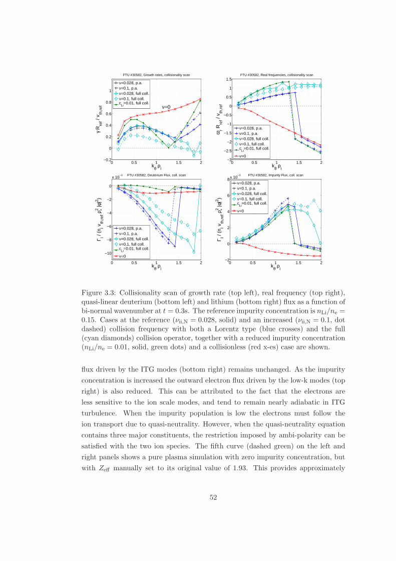
0 0.5 1 1.5 2−0.2

0

0.2

0.4

0.6

0.8

1

kθ ρi

γ R

ref /

v th,r

ef

FTU #30582, Growth rates, collisionality scan

ν=0.028, p.a.ν=0.1, p.a.ν=0.028, full coll.ν=0.1, full coll.c

Li=0.01, full coll.

ν=0

0 0.5 1 1.5 2−3

−2.5

−2

−1.5

−1

−0.5

0

0.5

1

1.5

kθ ρi

ωr R

ref /

v th,r

ef

FTU #30582, Real frequencies, collisionality scan


Li=0.01, full coll.

ν=0

0 0.5 1 1.5 2

−10

−8

−6

−4

−2

0

x 10−3

kθ ρi

Γ i / (n

i vth

,ref

ρ*2 |φ

|2 )

FTU #30582, Deuterium Flux, coll. scan


Li=0.01, full coll.

ν=0

0 0.5 1 1.5 2−2

0

2

4

6

8x 10−3

kθ ρi

Γ I / (n

I vth

,ref

ρ*2 |φ

|2 )

FTU #30582, Impurity Flux, coll. scan


Li=0.01, full coll.

ν=0

Figure 3.3: Collisionality scan of growth rate (top left), real frequency (top right),quasi-linear deuterium (bottom left) and lithium (bottom right) flux as a function ofbi-normal wavenumber at t = 0.3s. The reference impurity concentration is nLi/ne =0.15. Cases at the reference (νii,N = 0.028, solid) and an increased (νii,N = 0.1, dotdashed) collision frequency with both a Lorentz type (blue crosses) and the full(cyan diamonds) collision operator, together with a reduced impurity concentration(nLi/ne = 0.01, solid, green dots) and a collisionless (red x-es) case are shown.

flux driven by the ITG modes (bottom right) remains unchanged. As the impurity

concentration is increased the outward electron flux driven by the low-k modes (top

right) is also reduced. This can be attributed to the fact that the electrons are

less sensitive to the ion scale modes, and tend to remain nearly adiabatic in ITG

turbulence. When the impurity population is low the electrons must follow the

ion transport due to quasi-neutrality. However, when the quasi-neutrality equation

contains three major constituents, the restriction imposed by ambi-polarity can be

satisfied with the two ion species. The fifth curve (dashed green) on the left and

right panels shows a pure plasma simulation with zero impurity concentration, but

with Zeff manually set to its original value of 1.93. This provides approximately

52

0 0.5 1 1.5 2−0.2

0

0.2

0.4

0.6

0.8

1

kθ ρi

γ R

ref /

v th,r

ef

FTU #30582, Growth rates, cLi

scan

cLi

=0.15, ref.

cLi

=0.1

cLi

=0.05

cLi

=0.01

cLi

=0, Zeff

=1.93

0.2 0.4 0.6 0.8 1

0

10

20x 10−5

kθ ρi

Γ e / (n

e vth

,ref

ρ*2 |φ

|2 )

FTU #30582, Electron Flux, cLi

scan

cLi

=0.15, ref.

cLi

=0.1

cLi

=0.05

cLi

=0.01

cLi

=0, Zeff

=1.93

0 0.2 0.4 0.6 0.8 1

−14

−12

−10

−8

−6

−4

−2

0

2

x 10−4

kθ ρi

Γ i / (n

i vth

,ref

ρ*2 |φ

|2 )

FTU #30582, Deuterium Flux, cLi

scan

cLi

=0.15, ref.

cLi

=0.1

cLi

=0.05

cLi

=0.01

cLi

=0, Zeff

=1.93

0 0.2 0.4 0.6 0.8 1−1

0

1

2

3

4

5x 10−3

kθ ρi

Γ I / (n

I vth

,ref

ρ*2 |φ

|2 )

FTU #30582, Impurity Flux, cLi

scan

cLi

=0.15, ref.

cLi

=0.1

cLi

=0.05

cLi

=0.01

Figure 3.4: Lithium concentration scan of growth rate (top left), quasi-linear elec-tron (top right), deuterium (bottom left) and lithium (bottom right) flux as a func-tion of bi-normal wavenumber at t = 0.3s.

the same effective electron and ion collision frequencies as in the experimental case

(within 2% difference due to the change of the Coulomb logarithm). The growth

rates, frequencies and fluxes are nearly identical to the 1% impurity concentration

results, showing that the main impact of the lithium impurities is not a collisional

effect.

It has been pointed out by several authors (see for example [28, 49, 50])

that impurity transport is sensitive to the ion density gradient. In the previous

simulations the same positive density gradient value has been used for all three

species, that is, a centrally peaked impurity density profile has been assumed. How-

ever, experimentally the impurity profile is often found to be peaked towards the

edge. The effect of varying the lithium density gradient on the quasi-linear ion flux

is investigated in figure 3.5. The deuterium density gradient is kept at the refer-

ence value (Rref/Ln,D = 2.9), the electron density gradient has been adjusted in

order to maintain quasi-neutrality. The growth rates are slightly increased at lower

53

0 0.5 1 1.5 20

0.1

0.2

0.3

0.4

0.5

kθ ρi

γ R

ref/v

th,r

ef

FTU #30582, Growth rates, Rref

/Ln,Li

scan

R/Ln,Li

=2.9, ref.

R/Ln,Li

=2

R/Ln,Li

=1

R/Ln,Li

=0

R/Ln,Li

=−1

0 0.5 1 1.5 20

0.5

1

1.5

kθ ρi

ωr R

ref/v

th,r

ef

FTU #30582, Frequencies, Rref

/Ln,Li

scan

R/Ln,Li

=2.9, ref.

R/Ln,Li

=2

R/Ln,Li

=1

R/Ln,Li

=0

R/Ln,Li

=−1

0 0.5 1 1.5 2−10

−8

−6

−4

−2

0

2x 10−3

kθ ρi

Γ i / (n

i vth

,ref

ρ*2 |φ

|2 )

FTU #30582, Deuterium Flux, Rref

/Ln,Li

scan

R/Ln,Li

=2.9, ref.

R/Ln,Li

=2

R/Ln,Li

=1

R/Ln,Li

=0

R/Ln,Li

=−1

0 0.5 1 1.5 2−2

−1

0

1

2

3

4

5

6

7x 10−3

kθ ρi

Γ I / (n

I vth

,ref

ρ*2 |φ

|2 )

FTU #30582, Impurity Flux, Rref

/Ln,Li

scan

R/Ln,Li

=2.9, ref.

R/Ln,Li

=2

R/Ln,Li

=1

R/Ln,Li

=0

R/Ln,Li

=−1

Figure 3.5: Impurity density gradient scan of the growth rates (top left), frequencies(top right), quasi-linear deuterium (bottom left) and lithium (bottom right) flux asa functions of bi-normal wavenumber at t = 0.3s.

lithium gradients due to the stronger drive of the lithium component of the ITG

modes. An inward deuterium and outward impurity flux driven by the low-k modes

is observed only with the two largest values of the lithium density gradient, that is

Rref/Ln,Li = 2.9 and 2.0. However, the reduction of the impurity flux in the latter

case is already significant. At Rref/Ln,Li = 1 the flux driven by the modes below

kθρi ≈ 0.4 is reversed, expectedly leading to outward deuterium transport and core

lithium accumulation in the saturated phase.

An impurity density gradient scan of the quasi-linear ion flux at three dif-

ferent impurity concentrations at kθρi = 0.28 summarizes the above observations

(figure 3.6). Since the electron response to the low-k modes is expected to be close

to adiabatic in a highly contaminated plasma, the direction of the deuterium and

lithium transport is determined by the balance of the drive of their respective fluxes.

This drive strongly depends on the concentration and the density gradient of the

impurity species, while the impact of these parameters on the low-k ITG mode sta-

54

−1 0 1 2 3−5

0

5x 10−4

Rref

/ Ln,Li

Γ i / (n

i vth

,ref

ρ*2 |φ

|2 )

FTU #30582, Deuterium Flux, Rref

/Ln,Li

scan, kθ ρi=0.28

cLi

=0.15

cLi

=0.10

cLi

=0.05

−1 0 1 2 3−1

−0.5

0

0.5

1x 10−3

Rref

/ Ln,Li

Γ I / (n

I vth

,ref

ρ*2 |φ

|2 )

FTU #30582, Impurity Flux, Rref

/Ln,Li

scan, kθ ρi=0.28

cLi

=0.15

cLi

=0.10

cLi

=0.05

Figure 3.6: Impurity concentration and impurity density gradient scan of the quasi-linear deuterium (left) and lithium (right) fluxes at t = 0.3s and kθρi = 0.28.

bility is relatively weak. If the impurity concentration is sufficiently high and its

density profile sufficiently peaked, such as it is assumed during the density ramp-up

of this FTU-LLL discharge, then the outward drive of the impurity flux outweighs

that of the deuterium, and forces the main ions to be transported inward. This

observation is qualitatively consistent with the results of [28] obtained with helium

impurities in a standard test case.

The significance of the impurities being lithium ions is tested by a series of

simulations using different light impurity species (carbon, tritium, helium) while

keeping the deuterium concentration constant. A mixed deuterium-tritium-lithium

case is also investigated due to its potential relevance in future burning plasma

applications. The results are plotted in figure 3.7. The carbon (black circles) and

lithium (cyan diamonds) are the most effective among the selected impurity species

in reducing the quasi-linear electron flux and driving the deuterium flux inward.

However, under the current circumstances, the increase of the ion collisionality due

to 7% carbon concentration strongly stabilizes the modes. The helium impurity

(blue squares) and the mixed D-T-Li case exhibit similar behaviour, but the results

with 46% tritium (light green triangles) are close to the clear plasma simulations

(1% lithium, green dots), both of them driving an outward deuterium flux. If

the deuterium and impurity Larmor-radii are too close, they are expected to react

similarly to the main ion ITG modes, and thus to be unable to reduce the electron

transport and generate the deuterium pinch. Indeed, the quasi-linear tritium flux

in both the D-T and D-T-Li cases follow that of the deuterium, although in the

former case the flux is close to zero and only the three lowest k modes indicate an

outward transport. The dynamics of the deuterium and lithium ions are sufficiently

55

0 0.5 1 1.5 20

0.2

0.4

0.6

0.8

1

kθ ρi

γ R

ref /

v th,r

ef

FTU #30582, Growth rates, impurity scan

cLi

=0.15, ref.

cLi

=0.01

cC

=0.077

cHe

=0.23

cT=0.46

cT=0.16, c

Li=0.1

0.2 0.4 0.6 0.8 1

0

10

20x 10−5

kθ ρi

Γ e / (n

e vth

,ref

ρ*2 |φ

|2 )

FTU #30582, Electron Flux, impurity scan

cLi

=0.15, ref.

cLi

=0.01

cC

=0.077

cHe

=0.23

cT=0.46

cT=0.16 , c

Li=0.1

−0.2 0 0.2 0.4 0.6 0.8−20

−15

−10

−5

0

5x 10−4

kθ ρi

Γ i / (n

i vth

,ref

ρ*2 |φ

|2 )

FTU #30582, Deuterium Flux, impurity scan

cLi

=0.15, ref.

cLi

=0.01

cC

=0.077

cHe

=0.23

cT=0.46

cT=0.16, c

Li=0.1

0 0.2 0.4 0.6 0.8 1−4

−2

0

2

4

6

8

10x 10−3

kθ ρi

Γ I / (n

I vth

,ref

ρ*2 |φ

|2 )

FTU #30582, Impurity Flux, impurity scan

cLi

=0.15, ref.

cLi

=0.01

cC

=0.077

cHe

=0.23

cT=0.46

cT=0.16, c

Li=0.1

ΓT

Figure 3.7: Growth rate (top left), electron (top right), deuterium (bottom left)and impurity (bottom left) quasi-linear flux spectra as a function of the bi-normalwavenumber using different impurity species.

different for the ion flow separation to occur. However, the typical D-ITG length

scale is still sufficiently close to the lithium Larmor-radius that the lithium ions can

have a significant effect on the low-k ITG transport. Moreover, ZLi is low enough

that it does not have a major qualitative impact on mode stability and it does not

cause large radiative losses.

The dependence of the growth rates, real frequencies and ion particle flux on

the magnetic shear (s = rqdqdr , q is the safety factor) at t = 0.3s is presented in figure

3.8. Increasing magnetic shear in the range of s = 0.5−1.5 stabilizes the ITG modes,

also observed in more detailed studies on the impact of magnetic shear by Kinsey

et al. [51], Moradi at al. [52] and Nordman at al. [53]. However, it should be noted

that the actual effect of the magnetic shear strongly depends on the other plasma

parameters and its stabilizing effect should be considered on a case-to-case basis.

TEM-s are suppressed by the collisionality and they remain stable even at the lower

shear value. The phase difference between potential and ion density perturbations

56

0 0.5 1 1.5 2−0.1

0

0.1

0.2

0.3

0.4

kθ ρi

γ R

ref /

v th,r

ef

FTU #30582, Growth rates, magnetic shear scan

s=0.97, ref.s=0.5s=1.5

0 0.5 1 1.5 2−4

−3

−2

−1

0

1

2

kθ ρi

ωr R

ref /

v th,r

ef

FTU #30582, Real frequencies, magnetic shear scan

s=0.97, ref.s=0.5s=1.5

0 0.5 1 1.5 2−10

−8

−6

−4

−2

0

2x 10−3

kθ ρi

Γ i/ (n i v

th,r

ef ρ

*2 |φ|2 )

FTU #30582, Deuterium Flux, magnetic shear scan

s=0.97, ref.s=0.5s=1.5

0 0.5 1 1.5 20

1

2

3

4

5x 10−3

kθ ρi

Γ I / (n

I vth

,ref

ρ*2 |φ

|2 )

FTU #30582, Impurity Flux, magnetic shear scan

s=0.97, ref.s=0.5s=1.5

Figure 3.8: Magnetic shear s scan of growth rate (top left), real frequency (topright), quasi-linear deuterium (bottom left) and lithium (bottom right) flux as afunction of the bi-normal wavenumber at t = 0.3s.

depends weakly on the variation of the magnetic shear.

The Density Plateau Phase

At t = 0.3s the plasma is not in steady-state. It is characterized by finite radial

particle transport that, as it has been shown above, contributes to the dynamical

build-up of the deuterium density profile and the reduction of impurity concentra-

tion. At t = 0.8s the plasma is described by significantly larger deuterium and

electron density (and also temperature) gradients, reduced Zeff , and a slightly in-

creased magnetic shear. The reference collision frequency is approximately a factor

of eight higher (νii,N = 0.22) due to the lower temperature and higher density values,

leading to an increased effective collision frequency of the species despite the lower

Zeff .

The effect of increasing only the temperature or density gradients of all three

species from t = 0.3s to their corresponding values at t = 0.8s while keeping the other

57

parameters constant is shown in figure 3.9. The higher temperature gradients (blue

circles) provide a stronger drive for both ITG and TE modes, increasing the growth

rates across the whole spectrum. The transition between ion and electron modes

occur at approximately the same wavenumber value as in the t = 0.3s simulation

(dashed, cyan diamonds), and the fluxes maintain their directions compared to the

reference case. Increasing the density gradients only (yellow squares) is sufficient to

reverse the direction of the deuterium transport from inward to outward, according

to the expectations. However, the spectrum of modes exhibits a different nature

compared to the t = 0.3s case: the modes below kθρi ≈ 1.2 rotate in the electron

diamagnetic direction and their frequencies monotonically increase with the mode

number. If both density and temperature gradients are increased (red x-es) a similar

behaviour is found, but the real frequencies are shifted up and thus the transition

point from ion to electron direction is moved to kθρi ≈ 0.6, and the modes below this

value are further destabilized by the increased temperature gradient. As described

in [54], the spectra in these two latter cases consist of trapped electron modes that

are destabilized by the electron density gradient, and that obtain fluid-like character

at higher mode numbers. These observations are in contrast with the results of the

t = 0.8s case (solid, cyan diamonds). At t = 0.8s the modes are stabilized by the

increased collisionality. The unstable modes below kθρi ≈ 1 show the characteristics

of the ITG modes (positive real frequency) and drive an outward deuterium flux.

The microstability and particle transport properties of the t = 0.8s case can

be further approached by sequentially increasing the reference collision frequency

to νii,N = 0.2, decreasing the lithium concentration to cLi = 0.01 and electron

temperature to Te/Ti = 0.9, as shown on figure 3.10. The graphs indicate that the

high collisionality is essential in stabilizing the trapped electron modes but it is not,

on its own, sufficient to obtain the mode structure and fluxes as observed at the later

time stage. Only by reducing the lithium concentration (and thus decreasing the

effective collisionality) can an ITG dominated spectrum and outward deuterium flux

in the mid-k range (kθρi > 0.6) be reproduced. The high-k modes are stabilized by

the lower electron temperature, and the low-k ITG mode growth rates are reduced

by the increased magnetic shear (not shown), finally providing the spectrum of the

t = 0.8s case.

The impurity density scan at t = 0.8s, presented on figure 3.11, shows that

the reversal of the deuterium flux can be retained again with high lithium concen-

tration. However, the effect on the microstability is even more pronounced in this

case. Both at cLi = 0.1 and cLi = 0.15 the growth rate and frequency (top left and

right) spectra suggest the presence of three distinct modes rotating in the ion di-

58

0 0.5 1 1.5 2

−0.4

−0.2

0

0.2

0.4

0.6

0.8

1

kθ ρi

γ R

ref /

v th,r

ef

FTU #30582, Growth rates, gradients scan

t=0.3s, ref.R/L

T at t=0.8s

R/Ln at t=0.8s

R/Ln,T

at t=0.8s

t=0.8s

0 0.5 1 1.5 2−3

−2

−1

0

1

2

kθ ρi

ωr R

ref /

v th,r

ef

FTU #30582, Real frequencies, gradients scan

t=0.3s, ref.R/L

T at t=0.8s

R/Ln at t=0.8s

R/Ln,T

at t=0.8s

t−0.8s

0 0.5 1 1.5 2−10

−8

−6

−4

−2

0

2

4x 10−3

kθ ρi

Γ i / (n

i vth

,ref

ρ*2 |φ

|2 )

FTU #30582, Deuterium Flux, gradients scan

t=0.3s, ref.R/L

T at t=0.8s

R/Ln at t=0.8s

R/Ln,T

at t=0.8s

t=0.8s

0 0.5 1 1.5 2−0.005

0

0.005

0.01

0.015

0.02

0.025

kθ ρi

Γ I / (n

I vth

,ref

ρ*2 |φ

|2 )

FTU #30582, Impurity Flux, gradients scan

t=0.3s, ref.R/L

T at t=0.8s

R/Ln at t=0.8s

R/Ln,T

at t=0.8s

t=0.8s

Figure 3.9: Effect of increasing the gradients on the growth rate (top left), realfrequency (top right), quasi-linear deuterium (bottom left) and lithium (bottomright) flux as a function of the bi-normal wavenumber at t = 0.3s.

rection. The low-k peak can be associated with the D-ITG modes, the middle peak

between 0.5 < kθρi < 1.5 with Li-ITG modes, and above kθρi ≈ 1.5 with ion drift

modes. The stabilization of the D-ITG and destabilization of the ion drift modes is

attributed to the significantly increased effective collisionality. In both the cLi = 0.1

and cLi = 0.15 cases the Li-ITG modes are characterized by strong potential and

density phase difference and drive an inward deuterium flux. The ion drift modes

also drive an outward deuterium flow but their contribution is likely to be small in

the saturated phase due to their high kθ values.

Separation of Ion ITG Modes

The above results highlight the role of lithium impurities in ITG driven turbulent

transport. At t = 0.8s the impurity ITG modes can be distinguished from the

D-ITG, the former driving inward and the latter outward deuterium flux (figure

59

0 0.5 1 1.5 2

0

0.2

0.4

0.6

0.8

1

1.2

1.4

1.6

1.8

kθ ρi

γ R

ref /

v th,r

ef

FTU #30582, Growth rates

t=0.3, R/Ln,T

at t=0.8s, ref.ν=0.2ν=0.2, c

Li=0.01

ν=0.2, cLi

=0.01,T

e=0.9

t=0.8s

0 0.5 1 1.5 2−1

0

1

2

3

4

5

6

kθ ρi

ωr R

ref /

v th,r

ef

FTU #30582, Real frequencies

t=0.3s, R/Ln,T

at t=0.8s, ref.

ν=0.2ν=0.2, c

Li=0.01

ν=0.2, cLi

=0.01, Te=0.9

t=0.8s

0 0.5 1 1.5 2−12

−10

−8

−6

−4

−2

0

2

4

x 10−3

kθ ρi

Γ i / (n

i vth

,ref

ρ*2 |φ

|2 )

FTU #30582, Deuterium Flux

t=0.3s, R/Ln,T

at t=0.8s, ref.ν=0.2ν=0.2, c

Li=0.01

ν=0.2, cLi

=0.01,T

e=0.9

t=0.8s

0 0.5 1 1.5 20

0.005

0.01

0.015

0.02

0.025

0.03

kθ ρi

Γ I / (n

Iv th,r

ef ρ

*2 |φ|2 )

FTU #30582, Impurity Flux

t=0.3s, R/Ln,T

at t=0.8s, ref.

ν=0.2ν=0.2, c

Li=0.01

ν=0.2, cLi

=0.01, Te=0.9

t=0.8s

Figure 3.10: Approaching the t = 0.8s case (cyan diamonds) by increasing thegradients (red x-es), collisionality (green crosses), decreasing the lithium concentra-tion (yellow down triangle) and electron temperature (black up triangle) from theirrespective values at t = 0.3s.

3.11). At t = 0.3s D-ITG and Li-ITG modes are not as clearly separated in the

bi-normal wavenumber spectrum (figure 3.3), they are expected to be mixed ITG

modes sensitive to the temperature gradients of both ion species [44]. However, the

presence of the lithium ions changes the phase difference between the deuterium

density and potential fluctuations in a way that it produces an inward deuterium

flux (figure 3.4). This effect is different from the collisionality effect described in [55]:

Fable et al. showed that collisionality provides an outward contribution to the radial

deuterium flux in a plasma with trace impurities, whereas in the present case larger

lithium concentration leads to inward deuterium transport despite the increasing

collisionality. However, if the collisionality is sufficiently high, the reduction of the

impurity concentration towards the trace limit leads to outward main ion flux, in

agreement with [55].

The typical spatial scale of the impurity ITG modes can be separated from

60

0 0.5 1 1.5 2−0.1

−0.05

0

0.05

0.1

0.15

0.2

0.25

kθ ρi

γ R

ref /

v th,r

ef

FTU #30582, t=0.8s, Growth rates, cLi

scan

cLi

=0.01, ref.

cLi

=0.1

cLi

=0.15

0 0.5 1 1.5 2−1

0

1

2

3

4

kθ ρi

ωr R

ref /

v th,r

ef

FTU #30582, t=0.8s, Real frequencies, cLi

scan

cLi

=0.01, ref.

cLi

=0.1

cLi

=0.15

0 0.5 1 1.5 2−12

−10

−8

−6

−4

−2

0

2

4x 10−3

kθ ρi

Γ i / (n

i vth

,ref

ρ*2 |φ

|2 )

FTU #30582, t=0.8s, Deuterium Flux, cLi

scan

cLi

=0.01, ref.

cLi

=0.1

cLi

=0.15

0 0.5 1 1.5 20

0.005

0.01

0.015

0.02

0.025

0.03

0.035

kθ ρi

Γ I / (n

I vth

,ref

ρ*2 |φ

|2 )

FTU #30582, t=0.8s, Impurity Flux, cLi

scan

cLi

=0.01, ref.

cLi

=0.1

cLi

=0.15

Figure 3.11: Lithium concentration scan of growth rate (top left), real frequency(top right), quasi-linear deuterium (bottom left) and lithium (bottom right) flux asa function of bi-normal wavenumber at t = 0.8s.

those of the deuterium by reducing the impurity temperature, and thus their Larmor-

radius: ρLi/ρD = ZD/ZLi

√mLiTLi/(mDTD). Figure 3.12 shows the effect of chang-

ing the TLi/TD temperature ratio from 1 down to 0.5 (green circles) and 0.2 (blue

squares). At 50% reduced lithium temperature all ion modes are stabilized high-

lighting their mixed nature. The ion peak in the growth rate spectrum becomes

wider as the modes at higher kθ values are destabilized as a result of the smaller

lithium Larmor-radius. A further cooling of the impurity species almost completely

stabilizes the lithium modes due to their significantly increased collisionality. How-

ever, the peak of the lithium driven modes is now shifted even further away from

the main D-ITG region.

61

0 0.5 1 1.5 2−0.05

0

0.05

0.1

0.15

0.2

0.25

0.3

0.35

0.4

kθ ρi

γ R

ref /

v th,r

ef

FTU #30582, Growth rates, ρI scan

t=0.3s, ref.T

Li=0.5

TLi

=0.2

0 0.5 1 1.5 2

0

0.5

1

1.5

kθ ρi

ωr R

ref /

v th,r

ef

FTU #30582, Real frequencies, ρI scan

t=0.3s, ref.T

Li=0.5

TLi

=0.2

0 0.5 1 1.5 2−0.04

−0.03

−0.02

−0.01

0

0.01

kθ ρi

Γ i / (n

i vth

,ref

ρ*2 |φ

|2 )

FTU #30582, Deuterium Flux, ρI scan

t=0.3s, ref.T

Li=0.5

TLi

=0.2

0 0.5 1 1.5 20

0.005

0.01

0.015

0.02

0.025

0.03

kθ ρi

Γ I / (n

I vth

,ref

ρ*2 |φ

|2 )

FTU #30582, Impurity Flux, ρI scan

t=0.3s, ref.T

Li=0.5

TLi

=0.2

Figure 3.12: Effect of changing the impurity Larmor-radius on the growth rate (topleft), real frequency (top right), quasi-linear deuterium (bottom left) and lithium(bottom right) flux as a function of the bi-normal wavenumber at t = 0.3s.

3.1.3 Non-linear Gyrokinetic Analysis

A non-linear gyrokinetic study of the FTU #30582 discharge has been carried out

with GKW in order to support the linear gyrokinetic and fluid results. Figure 3.13

shows four electro-static simulations of the radial particle flux of the species driven

by the ITG modes as a function of time at t = 0.3s and r/a = 0.6. The top left panel

is the reference, it corresponds to the experimental lithium concentration cLi = 0.15,

while the top right panel to the reduced cLi = 0.01 impurity concentration. In both

cases the full collision operator has been adopted. The simulation of the reference

case has been performed with 21 bi-normal modes equally spaced up to kθρi = 1.6

and 83 radial modes, yielding a box size of ∼ 75ρi in both perpendicular directions.

In the reduced lithium case the maximum wavenumber has been decreased to kθρi =

1.4 in order to match the transition point from ITG to TEM in the corresponding

linear spectrum. The resolution along the remaining dimensions is 16 points per

62

0 50 100 150

−15

−10

−5

0

5

t vth,ref

/ Rref

Γ / (

n ref v

th,r

ef ρ

*2 )

FTU #30582, Non−linear ExB particle flux, r/a=0.6, t=0.3s, full coll.

D+

e−

Li3+

ΓD

= −6.60 ± 1.43

cLi

=0.15 ΓLi

= 2.78 ± 0.76

Γe = 1.73 ± 0.96

0 20 40 60 80 100 120 140

−2

0

2

4

6

8

10

12

14

16

FTU #30582, Non−linear ExB particle flux, r/a=0.6, t=0.3s, full coll.

t vth,ref

/ Rref

Γ / (

n ref v

th,r

ef ρ

*2 )

D+

e−

Li3+

Γe = 8.30 ±

2.59

ΓLi

= 0.25 ± 0.05 cLi

=0.01

ΓD

= 7.53 ± 2.44

0 20 40 60 80

−10

−5

0

5

10

15FTU #30582, Non−linear ExB particle flux, r/a=0.6, t=0.3s, ful coll.

t vth,ref

/ Rref

Γ / (

n ref v

th,r

ef ρ

*2 )

D+

e−

Li3+

ΓLi

= −2.70 ± 0.70

R/Ln,Li

= −1.0

Γe = −1.56 ± 0.73

ΓD

= 6.54 ± 2.48

0 50 100 150 200 250−25

−20

−15

−10

−5

0

5

10

t vth,ref

/ Rref

Γ / (

n ref v

th,r

ef ρ

*2 )

FTU #30582, Non−linear ExB particle flux, r/a=0.6, t=0.3s

D+

e−

Li3+ p.a. scattering only

ΓD

= −10.13 ± 3.07

Γe = −1.80 ± 0.62

ΓLi

= 2.78 ± 0.91

Figure 3.13: Non-linear simulation of the radial particle flux driven by ITG modesas a function of time in FTU #30582 at t = 0.3s and r/a = 0.6, using the fullcollision operator, with the experimental (cLi = 0.15, top left) and with reduced(cLi = 0.01, top right) lithium concentration. The experimental case with negativeimpurity density gradient Rref/Ln,Li = −1.0 and with pitch-angle scattering onlyare shown on the bottom left and right panels.

period in parallel direction, 10 points in magnetic moment and 48 points in parallel

velocity space. The fluxes are expressed in units of nrefvth,refρ2∗ ≈ 7.9 · 1018s−1m−2.

The reference case (top left) shows that the deuterium and lithium flux main-

tain their directions as predicted by the linear analysis. However, the electron

flux changes from inward to outward when progressing into the saturated phase.

This suggests that the electron flux is determined by the fast growing modes above

kθρi ≈ 0.5 in the linear phase (see figure 3.4, top right) but they are overtaken by the

low-k modes in the saturated phase. Therefore, quasi-linear methods for estimating

electron transport have to be employed with caution in this particular case.

The same non-linear simulation using pitch-angle scattering only (figure 3.13,

bottom right) gives approximately the same value for the lithium flux: 2.78± 0.91,

63

and values reduced by approximately the same number for both deuterium and

electron fluxes: −10.13 ± 3.07 and −1.80 ± 0.62, respectively. This reduction is

again in agreement with the expected outward contribution of the collisions [55].

The different direction of the simulated electron flux with the full collision operator

and pitch-angle scattering only is due to the fact that the electron transport is

near zero. In this case the additional outward component of the flux provided by

the energy scattering and friction terms is sufficient to change the direction of the

turbulent electron transport.

If the impurity density gradient is negative on the analysed flux surface (fig-

ure 3.13, bottom left), the ion species flow in the opposite radial direction compared

to the experimental case, as anticipated from the linear results (figure 3.6). The

electron flux also becomes negative due to the reduced electron density gradient

(Rref/Ln,e = 1.1).

When the lithium concentration is reduced to cLi = 0.01 (figure 3.13, top

right) both the deuterium and electron fluxes are outward and the lithium flux is

negligible. The value of the outward electron flux in this case (8.30±2.59) is almost

a factor of five larger than in the experimental case (1.73 ± 0.96). The deuterium

flux is thus reversed and the electron flux is significantly reduced by the high lithium

concentration, as suggested by figure 3.4 in the linear analysis. The heat flux of the

species (not shown) is also lower by approximately a factor of two at cLi = 0.15 than

at cLi = 0.01 which can be attributed to the stabilization of the ITG modes.

The electron flux can be estimated from the time evolution of the density

profile by solving the transport equation ∂tn(ψ) = −∇ψ ·Γ(ψ)+S(ψ), where ψ is the

radial coordinate. Calculating the fluxes for the transport equation with gyrokinetic

method at a reasonable radial resolution is a comuptationally expensive project and

it has not been done for this thesis. However, this calculation has been performed

with the JETTO [56] transport code using a fluid model to approximate the fluxes

and assuming the source term S to be zero. The results of this simulation have been

plotted in figure 3.14. The left panel shows the experimental electron flux profile

at t = 0.3s, and the right panel the time traces of the flux at r/a = 0.6. Since the

estimated electron flux is much larger than the simulated one in the reference case

(figure 3.13, top left), especially towards the edge, it suggests that there is significant

electron source in the plasma at this time. However, the simulated electron flux in

the reduced lithium concentration case is of the same magnitude as the estimated

one, and thus it would effectively counteract the source term. The lithium induced

electron flux reduction therefore seems to be an important factor in achieving a

highly peaked electron density profile. The time traces of the estimated electron flux

64

Figure 3.14: Estimate of the radial electron flux based on time evolution of themeasured electron density profile. Left: flux profile at t=0.3s. Right: time traces ofthe flux at r/a = 0.6.

(figure 3.14, right) show that the electron density increases until t = 0.6s, after which

an oscillation around zero occurs in the stady-state phase of the discharge. The ion

density profiles are not measured directly, the same analysis is not immediately

available. However, since the average Zeff of the plasma decreases to near unity

during the experiment, the deuterium profile must reach approximately the same

degree of peaking as the electrons.

Since FTU #30582 is an Ohmically heated discharge with relatively low

temperature and high magnetic field, the Ware-pinch is expected to contribute to

the total particle flux with a significant margin. The neoclassical particle transport

has been estimated with the Neoart code [57]. The turbulent electron flux predicted

by GKW in physical units is Γturbe ≈ 1.34 · 1019s−1m−2. The overall neoclassical

electron flux is calculated as Γneoe ≈ −0.87 · 1019s−1m−2 of which the flux due to the

Ware-pinch is ΓWaree ≈ −0.99 · 1019s−1m−2. The turbulent and neoclassical values

are thus comparable and the neoclassical contribution further reduces the electron

transport.

Peaking could also be caused by a larger electron source in the core orig-

inating from an increased number of lithium atoms. However, a crude estimate

of the neutral lithium penetration depth shows that lithium atoms can only travel

approximately 0.5 cm before ionization under plasma conditions at r/a = 0.6 and

t = 0.3s. The penetration depth is certainly larger near the edge, this result nonethe-

less suggests that the electron source term in the core is not significantly increased

by lithium atoms coming from the limiter during the density ramp-up phase of the

discharge. The estimate is based on the formula λiz = vn/(neσviz(Te)), where λiz

is the penetration depth, vn is the velocity of the neutrals and σviz(Te) is the tem-

65

MAST parameters Value Dim.

Plasma diameter 3 mPlasma volume 8 m3

Plasma current 1.3 MAToroidal magnetic field 0.6 TPulse length 1 s

Table 3.3: Typical parameters of the MAST tokamak. Data fromhttp://www.ccfe.ac.uk/MAST.aspx

perature dependent electron ionization coefficient [58]. The ionization coefficient for

lithium can be found in [59], in the range of Te ≈ 0.57 keV its value is approximately

σviz(Te) ≈ 5 · 10−14 m3/s. The neutral velocity for hydrogen atoms has been esti-

mated in [60] as vn ≈ 1.7 · 104 m/s by assuming Franck–Condon atoms. The same

value has been used for lithium which, albeit not accurate, provides a conservative

estimate for the penetration depth, since the lithium neutral velocity is expected to

be lower.

3.2 Analysis of MAST #24541

MAST is a medium size spherical tokamak located in Culham Science Centre, UK,

its characteristic parameters are summarized in table 3.3. Due to their compact

shapes, spherical tokamaks are capable of operating at much lower toroidal magnetic

field, and typically higher plasma beta, than the conventional tokamaks. The effects

of high plasma beta and finite magnetic perturbations on turbulent transport are

investigated with a series of gyrokinetic simulations of the MAST discharge #24541.

The role of light impurities in determining mode stability and transport in high-beta

plasmas is also discussed.

Plasma beta impacts the turbulence in two major ways. First, by enabling

magnetic perturbations it gives rise to magnetic flutter and fluctuating grad-B veloc-

ities, as introduced in chapter 2, and leads to electro-magnetic eigenmodes. Second,

it has an effect on the magnetic equilibrium: the Shafranov-shift α is proportional

to the radial derivative of beta, and therefore high-beta tokamak plasmas are char-

acterized by strongly shifted flux surfaces. This mainly affects the vertical drift

frequency and therefore has an impact of the response of the species. The circular,

non-shifted geometry, that has been applied in the previous section, is not a suffi-

cient approximation of the magnetic structure. The magnetic equilibrium required

66

Figure 3.15: Electron density (left) and temperature profiles (right) at t = 0.317sas a function of the square root of the normalized poloidal flux

√ψN. Blue points

indicate measurements on the inboard and red ones on the outboard side.

for the GKW simulations of this MAST discharge is calculated using the CHEASE

[61] Grad–Shafranov solver code. In this thesis only the first effect of high plasma

beta is investigated.

3.2.1 Experimental Features of MAST #24541

The discharge selected for the analysis is a typical ELMy H-mode MAST plasma

without any particular instability in the core causing additional complexity. The

plasma beta is moderate (βref ∼ 3.6% locally on the magnetic surface) but it is

sufficient to provide non-negligible magnetic perturbations. The radial electron

density and temperature profiles at t = 0.317s are indicated on figure 3.15 (figure

courtesy of Luca Garzotti), where the radial coordinate is the square root of the

normalized poloidal flux ψN. The profiles are flat in most of the core plasma, typical

to H-mode discharges, the gradient region is located outside√ψN ≈ 0.6.

The magnetic equilibrium has been reconstructed with the CHEASE code.

The input required for a CHEASE run consists of the coordinates of the last closed

flux surface, the pressure and the current (or q) profiles. These can be specified

numerically with the measured values, or with analytical formulae. In the present

case the measured coordinates of the last closed flux surface has been used, and the

profiles have been approximated by 8th degree polynomial expressions. The poloidal

cross section of the magnetic equilibrium as calculated by CHEASE is shown in

figure 3.16. As it has been mentioned above, the magnetic equilibrium is sensitive

to changes in plasma beta, and it should be consistently recalculated for simulations

scanning over different beta values. However, the analysis of the geometrical effects

67

0 0.2 0.4 0.6 0.8 1 1.2

−1

−0.5

0

0.5

1

R (m)

Z (

m)

MAST #24541, Flux Surfaces

Figure 3.16: Flux surfaces of MAST #24541 as reconstructed by the CHEASEequilibrium code.

on turbulence is not within the focus of this thesis, and the gyrokinetic simulations

have all been performed with the same equilibrium.

The discharge was heated by two beams of Neutral Beam Injection (NBI)

depositing PNBI ∼ 3.5MW heating power into the plasma. The toroidal rotation

velocity of the plasma caused by NBI heating is of the order of vtor ∼ 105 m/s

(profile shown on figure 3.17). Although plasma rotation is expected to have a

stabilising property on the ITG modes, the effect of rotation on the turbulence

is outside the main scope of this thesis and the simulations have been performed

assuming stationary plasma.

3.2.2 Linear Gyrokinetic Analysis

The simulations have been performed at t = 0.317s at the radial position of ψN = 0.8,

including carbon impurities. The relevant plasma parameters are listed in table 3.4.

Similar to the FTU analysis, the reference density is chosen to be the electron

density, and the reference temperature is the deuterium temperature.

The spectra of growth rates (top left), frequencies (top right), quasi-linear

deuterium and impurity flux (bottom left and right) are shown on figure 3.18 for

five different values of βref . The reference value, as calculated from the measured

quantities, is βref = 0.036. The points above kθρi ≈ 1 of the reference curve are

stable. The fluxes plotted here are driven by the fluctuating ExB velocity, corre-

68

800 900 1000 1100 1200 1300 14002

4

6

8

10

12

14

16x 104

r (mm)

vto

r (m

/s)

MAST #24541, Toroidal rotation velocity profile at t=0.315s

Figure 3.17: Measured toroidal rotation velocity profile of MAST #24541 at t =0.315s.

n[1019m−3] T [keV] −Rref∇TT −Rref∇n

n

t = 0.317s

D+ 2.52 0.58 7.85 2.09

e− 2.96 0.43 6.06 1.17

C6+ 0.073 0.58 7.85 -4.12

Bref = 0.56T Rref = 0.93m νii,N = 0.0088 Zeff = 1.74

Table 3.4: Plasma parameters of MAST #24541 at ψN = 0.8 and t = 0.317s.

sponding to the first term of equation 2.80. This is the only term present in an

electro-static simulations, and even in high beta electro-magnetic runs it remains

the dominant part in the total quasi-linear flux. The terms associated with the

perturbed magnetic flutter and grad-B drift velocities are still at least one order of

magnitude smaller, as shown on figure 3.20. The top left panel of figure 3.18 shows

a strongly increasing mode growth when βref is raised from 2% to 10%. The growth

rates of the βref = 0.02 and βref = 0.036 cases are similar below kθρi = 1. How-

ever, the frequency plots (top right panel) indicate that they are different modes.

At βref = 0.02 all the modes rotate in the ion diamagnetic direction, whereas at

βref = 0.036 the mode frequency changes sign at kθρi ≈ 0.4. At βref = 0.05 there is

69

0 0.5 1 1.5 2−0.5

0

0.5

1

1.5

2

2.5

kθ ρi

γ R

ref /

v th,r

ef

MAST #24541, Growth rates

βref

=0.02

βref

=0.036, ref.

βref

=0.05

βref

=0.1

0 0.5 1 1.5 2−10

−5

0

5

kθ ρi

ωr R

ref /

v th,r

ef

MAST #24541, Real Frequencies

βref

=0.02

βref

=0.036, ref.

βref

=0.05

βref

=0.1

0 0.5 1 1.5 2

0

2

4

6

8

10

x 10−4

kθ ρi

Γ i / (n

i vth

,ref

ρ*2 )

MAST #24541, Deuterium Flux

βref

=0.02

βref

=0.036, ref.

βref

=0.05

βref

=0.1

0 0.5 1 1.5 2

−8

−6

−4

−2

0

2

4

6

x 10−4

kθ ρi

Γ I / (n

I vth

,ref

ρ*2 )

MAST #24541, Impurity Flux

βref

=0.02

βref

=0.036, ref.

βref

=0.05

βref

=0.1

Figure 3.18: βref scan of growth rate (top left), real frequency (top right), quasi-linear ExB driven deuterium (bottom left) and carbon (bottom right) flux as afunction of the bi-normal wavenumber.

a narrow region in the spectrum where the modes rotate in the electron direction

at kθρi ≈ 0.3, and again above kθρi ≈ 1. At βref = 0.1 a similar transition occurs at

kθρi ≈ 1.9.

In order to elucidate this behaviour it is useful to take a look at the parallel

structure of the various modes, also called the parallel eigenfunctions, and how

they change with varying plasma beta. Figure 3.19 illustrates the linear electro-

static potential Φ and parallel vector potential A‖ responses of the most unstable

bi-normal modes (kθρi = 0.3−0.4) at three different beta values as a function of the

parallel coordinate s. The centre of the graphs (s = 0) is the outboard midplane

around which the modes are typically localized, and the values are normalized to

|Φ(s = 0)|. In three of the included cases (at βref = 0.036 and kθρi = 0.3, βref = 0.02

and kθρi = 0.4, βref = 0.05 and kθρi = 0.4) the real part of the electro-static

potential perturbation is an even function of the parallel coordinate accompanied

by an anti-symmetric (odd) vector-potential perturbation. These are characteristic

70

properties of the electro-static ITG, TEM and ETG modes, as well as the electro-

magnetic Kinetic Ballooning Modes (KBM) [40]. In the fourth case the shape of

the eigenmodes is the opposite: the scalar potential becomes odd and the vector

potential is approximately even, which is the signature of the electro-magnetic micro-

tearing mode (MTM) [41]. MTM-s are also typically more elongated along the

magnetic field lines than the ITG modes. It can be shown that the even shape

of the vector potential eigenfunction A‖(s) leads to tearing of the magnetic field

lines and generation of magnetic islands [41]. Therefore, the odd parallel Φ mode

structure is also sometimes referred to as tearing mode parity. Micro-tearing modes

are also distinguished from ITG modes by having negative real frequencies. In

conclusion, figure 3.19 shows that at βref = 0.036 the spectrum changes from ITG

mode to micro-tearing mode (insted of TEM/ETG) dominated regime at kθρi = 0.4.

Micro-tearing modes are commonly observed in MAST due to its relatively high beta

operation [41].

In figure 3.21 a more detailed βref scan of the fastest growing mode at kθρi =

0.4 is shown. At low plasma beta a typical ITG driven mode is observed. As βref

increases the mode is slightly stabilized, but at βref ≈ 0.04 the trend changes. As

the ITG mode becomes less unstable it eventually transitions into a micro-tearing

mode at βref ≈ 0.4. If the plasma beta is further increased the mode changes again

and turns into a kinetic kallooning mode characterized by growth rates strongly

increasing with βref [40]. In the reference case the plasma beta (βref = 0.036) is

close to the transition point of the fastest growing mode between the ITG and KBM

regimes. This is the point when the ion modes are the most stable and hence a micro-

tearing dominated spectrum occurs above kθρi ≈ 0.4, as observed on figure 3.18. At

lower beta (βref = 0.02) the ITG modes remain dominant across the spectrum up

to kθρi = 2. At βref = 0.05 the ITG mode stabilization is stronger and therefore

the transition point occurs at a lower wavenumber value, at kθρi ≈ 0.3. First a

narrow region of micro-tearing modes is observed followed by the destabilization of

KBM-s rotating in the ion diamagnetic direction. At the second transition point,

at kθρi ≈ 1, the spectrum becomes dominated by micro-tearing modes again as

KBM-s are stabilized at smaller length scales. In the highest beta case included in

this analysis at βref = 0.1 the modes obtain a KBM nature already at the lowest

wavenumber values, a change from KB to micro-tearing modes can be observed at

kθρi ≈ 1.9 due to the stronger drive of the kinetic ballooning modes.

The quasi-linear electro-static deuterium flux driven by the ITG modes (bot-

tom left, figure 3.18) align with each other at all four values of plasma beta, fol-

lowing the βref = 0.02 curve. The deuterium transport points outward, and the

71

−10 −5 0 5 10−0.4

−0.2

0

0.2

0.4

0.6

0.8

1

2 π s

Re(

Φ),

Re(

A||)

(a.u

.)

MAST #24541, Parallel eigenmode, βref

=0.036, kθ ρi=0.3

Re(Φ)Re(A

||)

−10 −5 0 5 10−1

−0.5

0

0.5

1

2 π s

Re(

Φ),

Re(

A||)

(a.u

.)

MAST #24541, Parallel eigenmode βref

=0.036, kθ ρi=0.4

Re(Φ)Re(A

||)

−10 −5 0 5 10−0.2

0

0.2

0.4

0.6

0.8

1

1.2

2 π s

Re(

Φ),

Re(

A||)

(a.u

.)


=0.02, kθ ρi=0.4

Re(Φ)Re(A

||)

−10 −5 0 5 10−0.2

0

0.2

0.4

0.6

0.8

1

1.2

2 π s

Re(

Φ),

Re(

A||)

(a.u

.)


=0.05, kθ ρi=0.4

Re(Φ)Re(A

||)

Figure 3.19: Parallel mode structure of the real part of the normalized electro-static(blue) and parallel vector potential (red) perturbations. Top left: βref = 0.036,kθρi = 0.3, Top right: βref = 0.036, kθρi = 0.4 (tearing parity), Bottom left: βref =0.02, kθρi = 0.4, Bottom right: βref = 0.05, kθρi = 0.4.

phase difference between the potential and density perturbations is reduced when

the modes transition to the micro-tearing (in the βref = 0.036 case) or to the KB (in

the βref = 0.05 and 0.1 cases) regime. The carbon flux (bottom fight, figure 3.18)

points inward in all four cases, and becomes reduced with increasing plasma beta

in the ITG driven regime. However, the KBM-s appear to generate stronger phase

difference when βref is increased.

The magnetic flutter component of the quasi-linear ion flux (top and bottom

left, figure 3.20) driven by the ITG modes (βref = 0.02, crosses) generates an outward

particle transport. When KBM-s appear due to the increasing plasma beta the linear

flux becomes less negative and eventually changes direction at βref = 0.1. The deu-

terium flux driven by the micro-tearing dominated modes both in the βref = 0.036

and βref = 0.05 cases provide an outward contribution. While the flux associated

with the magnetic flutter velocity is qualitatively similar for the two ion species, the

72

0 0.5 1 1.5 2−8

−6

−4

−2

0

2

4

6x 10−5

kθ ρi

Γ i / (n

i vth

,ref

ρ*2 )

MAST #24541, Deuterium flux driven by B1,⊥

0 0.5 1 1.5 2−1

0

1

2

3

4

5

6x 10−5

kθ ρi

Γ i / (n

i vth

,ref

ρ*2 )

MAST #24541, Deuterium flux driven by B1,||

0 0.5 1 1.5 2−3

−2

−1

0

1

2

3

4x 10−5

kθ ρi

Γ I / (n

I vth

,ref

ρ*2 )

MAST #24541, Impurity flux driven by B1,⊥

0 0.5 1 1.5 2−8

−6

−4

−2

0

2

4

6x 10−6

kθ ρi

Γ I / (n

I vth

,ref

ρ*2 )

MAST #24541, Impurity flux driven by B1,||

βref

=0.02

βref

=0.036, ref.

βref

=0.05

βref

=0.10

Figure 3.20: βref scan of deuterium (top) and carbon (bottom) flux driven by themagnetic flutter (left) and compressional grad-B drift (right) velocities as a functionof the bi-normal wavenumber.

0 0.02 0.04 0.06 0.08−1.5

−1

−0.5

0

0.5

1

1.5

2

2.5

3

βref

[ωr, γ

] Rre

f / v th

,ref

MAST #24541, Frequencies, βref

scan, kθ ρi=0.4

γω

r

0 0.02 0.04 0.06 0.08

−10

−8

−6

−4

−2

0

2

4

6

x 10−4

βref

Γ s / (n

s vth

,ref

ρ*2 )

MAST #24541, Particle Flux, βref

scan, kθ ρi=0.4

D+

e−

C6+

Figure 3.21: βref scan of the fastest growing mode at kθρi = 0.4. Left: growth rate(dashed, cross) and real frequency (solid, triangle), right: ExB driven quasi-linearparticle flux of deuterium (cross), electron (circle) and carbon (square) species.

73

flux due to magnetic compression (top and bottom right, 3.20) shows different be-

haviour: the ITG modes drive an outward deuterium and inward impurity transport

reinforcing, although only with a small margin, the electro-static fluxes. The KBM

driven deuterium transport is outward and increases with βref . The KBM driven

impurity transport is negligible at βref = 0.05 but grows positive as plasma beta is

further increased.

In the remaining part of this section the effect of light impurities on the

linear ITG and KB modes will be discussed. Since in the experimental case the

plasma beta (βref = 0.036) is close to the critical beta for the onset of the KB

modes (βref,C ≈ 0.04), the βref = 0.02 case has been selected for the ITG analysis.

The KBM-s are studied in the βref = 0.1 case.

Figure 3.22 shows the growth rate, electro-static quasi-linear electron, deu-

terium and impurity flux spectra in five different settings in the ITG dominated

regime (the reference curve is the βref = 0.02 case, crosses). Increasing the carbon

concentration from the original cC = nC/ne = 0.025 value (crosses) to cC = 0.05

(circles, Zeff = 2.5) destabilizes the Carbon-ITG modes around kθρi ∼ 1.5 and sta-

bilizes the the D-ITG peak, in a way analogous to the lithium effect in the FTU

analysis. The deuterium flux is only slightly affected by the increased carbon con-

centration. However, the inward impurity flux driven by the D-ITG modes has been

significantly decreased compared to the reference curve, and an outward transport

above kθρi ≈ 0.6 can be observed. If the carbon ions in the cC = 0.05 case are re-

placed by lithium while keeping the same deuterium dilution (cLi = 0.1, Zeff = 1.6,

squares), the modes are destabilized in a wide region around kθρi ≈ 1. The stabi-

lization of the D-ITG is less pronounced due to the lower Zeff . The impurity flux

is similar to that in the cC = 0.05 case, however, in the region where the lithium

affects the growth rate spectrum the deuterium flux is also strongly reduced. This

effect is not observed in presence of the heavier carbon impurity. In all five cases

the variation of the impurity concentration has a negligible effect on the electron

flux. This is explained by the fact that in typical tokamak conditions the electro-

magnetic fluctuations provide the main mechanism driving a non-adiabatic electron

response [62]. Already at βref = 0.02 the electron flux is not reduced by the presence

of impurities and therefore an ion flow separation, as observed in every cases of the

FTU analysis, does not necessarily occur.

The cases discussed so far are all characterized by a negative impurity den-

sity gradient, and an impurity flux driven inward by the low-k ITG modes. In the

remaining two cases in figure 3.22 the effect of a centrally peaked impurity density

profile (i.e. positive local density gradient) is tested. First, the density gradient of

74

0 0.5 1 1.5 2−0.1

0

0.1

0.2

0.3

0.4

kθ ρi

γ R

ref /

v th,r

ef

MAST #24541, Growth rates, βref

=0.02

βref

=0.02, ref.

cC

=0.05

cLi

=0.10

R/Ln,s

=2.1

R/Ln,s

=2.1, cC

=0.05

0 0.2 0.4 0.6 0.8 1−2

0

2

4

6

8

10x 10−4

kθ ρi

Γ e / (n

e vth

,ref

ρ*2 |φ

|2 )

MAST #24541, Electron Flux, βref

=0.02

βref

=0.02, ref.

cC

=0.05

cLi

=0.1

R/Ln,s

=2.1

R/Ln,s

=2.1, cC

=0.5

0 0.5 1 1.5 2

−4

−2

0

2

4

6

8

10

12

x 10−4

kθ ρi

Γ i / (n

i vth

,ref

ρ*2 |φ

|2 )

MAST #24541, Deuterium Flux, βref

=0.02

βref

=0.02, ref.

cC

=0.05

cLi

=0.10

R/Ln,s

=2.1

R/Ln,s

=2.1, cC

=0.05

0 0.5 1 1.5 2−2

−1.5

−1

−0.5

0

0.5

1

1.5x 10−3

kθ ρi

Γ I / (n

I vth

,ref

ρ*2 |φ

|2 )

MAST #24541, Impurity Flux, βref

=0.02

βref

=0.02, ref.

cC

=0.05

cLi

=0.10

R/Ln,s

=2.1

R/Ln,s

=2.1, cC

=0.05

Figure 3.22: Growth rate (top left), quasi-linear ExB driven electron (top right),deuterium (bottom left) and impurity (bottom right) flux as a function of bi-normalwavenumber in an ITG mode dominated spectrum. The reference beta is βref = 0.02(crosses), the reference carbon concentration is cC = 0.025.

the species is set uniformly to Rref/Ln,s = 2.1 (diamonds), that is the density gradi-

ent of the deuterium species in the experimental case. This causes the stabilization

of the ITG peak above kθρi ≈ 0.6. The deuterium flux is not strongly affected by

this change, but the carbon flux reverses its direction from inward to outward. How-

ever, this is not followed by an inversion of the deuterium transport, in contrast with

the results of the FTU analysis. Even when the carbon concentration is increased

to cC = 0.05 while keeping the density gradients of the species at Rref/Ln,s = 2.1

(triangles), although the outward impurity flux is enhanced, there is no significant

change in the deuterium flux.

The same analysis described above has been carried out for a KBM domi-

nated spectrum, at βref = 0.1. Figure 3.23 indicates that the KBM growth rates

and real frequencies are much less sensitive to the changes of the impurity species,

impurity concentration or impurity density gradient, they show the same trend in

75

0 0.5 1 1.5 20

0.5

1

1.5

2

2.5

3

kθ ρi

γ R

ref /

v th,r

ef

MAST #24541, Growth rates, βref

=0.1

βref

=0.1, ref.

cC

=0.05

cLi

=0.10

R/Ln,s

=2.1

R/Ln,s

=2.1, cC

=0.5

0 0.5 1 1.5 2−10

−5

0

5

kθ ρi

ωr R

ref /

v th,r

ef

MAST #24541, Real frequencies, βref

=0.1

βref

=0.1, ref.

cC

=0.05

cLi=0.10

R/Ln,s

=2.1

R/Ln,s

=2.1, cC

=0.05

0 0.5 1 1.5 2−1

0

1

2

3

4

5

6x 10−4

kθ ρi

Γ i / (n

i vth

,ref

ρ*2 )

MAST #24541, Deuterium flux, βref

=0.1

βref

=0.1

cC

=0.05

cLi

=0.10

R/Ln,s

=2.1

R/Ln,s

=2.1, cC

=0.05

0 0.5 1 1.5 2−10

−8

−6

−4

−2

0

2

x 10−4

kθ ρi

Γ I / (n

I vth

,ref

ρ*2 )

MAST #24541, Impurity flux, βref

=0.1

Figure 3.23: Growth rate (top left), real frequency (top right), quasi-linear ExBdriven deuterium (bottom left) and impurity (bottom right) flux as a function ofbi-normal wavenumber in an KBM dominated spectrum. The reference beta isβref = 0.1 (crosses), the reference carbon concentration is cC = 0.025.

all five cases. The transition point from KB to TE modes is slightly shifted towards

lower kθρi values by the increased Zeff , and towards higher kθρi by the modified im-

purity and electron density gradients. The KBM driven impurity flux also changes

direction in the two cases with positive impurity density gradients. Similarly to the

ITG analysis, this is not followed by a reversal of the deuterium transport.


In this chapter the gyrokinetic mode stability and particle transport analysis of two

discharges have been presented.

The first case is a liquid lithium limiter FTU discharge characterized by

increased density peaking and improved particle confinement compared to the typi-

cal standard metallic limiter experiments. Local gyrokinetic simulations performed

76

with GKW at mid radius during the density ramp-up phase show that the pres-

ence of a high concentration, centrally peaked lithium profile reverses the deuterium

flux from outward to inward. This reversal is not a result of higher collisionality,

since the increased Zeff leads to increased effective collision frequencies which are

expected to give an outward contribution to the particle transport. At the same

time, the lithium is transported radially outward resulting in the decontamination

of the plasma. In the reference case the electron flux remains outward even in the

presence of large lithium concentration, but it is significantly reduced due to the

fact that quasi-neutrality at the ion scales can be satisfied with the two ion species.

At the reduced level the turbulent electron flux becomes comparable to the inward

neoclassical electron flux dominated by the Ware-pinch term. The core electron

source is not expected to be strongly modified by the presence of lithium, therefore

the reduced electron transport leads to a more peaked electron density profile. An

other consequence of the low electron flux is that its direction becomes sensitive

to effects that modify transport. In this particular analysis, neglecting the energy

scattering and friction terms in the GKW collision operator was sufficient to drive

an inward electron flux. The build-up of the deuterium and electron profiles can, of

course, not go on forever. At a later time stage, in the density plateau phase, the

discharge is characterized by higher density gradients, low impurity concentration

and an outward flux of all three species. However, if the lithium concentration is

artificially increased, a reversal of the deuterium transport can be obtained again.

The effect of light impurities on particle transport has also been analysed in

the MAST #24541 discharge. MAST is a spherical tokamak characterized by much

lower toroidal magnetic field compared to FTU, significantly higher plasma beta

and strongly shaped flux surfaces. The main impurity species are carbon, and the

impurity density gradient is measured to be negative at the selected flux surface,

which is also in contrast with the FTU analysis. Simulations show that at low

plasma beta the turbulence is dominated by ITG modes, but the increasing beta

gives rise to a Kinetic Ballooning Mode (KBM) dominated regime. In simulations

of a non-rotating plasma micro-tearing modes can be observed at intermediate beta

values, between the ITG and KBM dominated regime. However, plasma rotation

is known to have a significant stabilizing property on ITG modes, while it does not

affect the micro-tearing instabilities. This is why in this analysis a micro-tearing

mode dominated regime, typically observed in MAST experiments [41], has not

been reproduced. Both in the ITG and KBM dominated cases the majority of the

flux is driven by the fluctuating ExB velocity, the electro-magnetic terms are at

least an order of magnitude smaller. The inward impurity transport can be reduced

77

by increasing impurity concentration, in the ITG driven case even a reversal can

be achieved in the kθ range where the impurity modes have a strong effect on the

modes. The direction of the impurity transport is sensitive to the sign of the density

gradient, a reversal from inward to outward in the whole spectrum is achieved with a

centrally peaked impurity density profile. However, this is not followed by deuterium

flux reversal in this case due the electro-magnetic perturbation driving a strong non-

adiabatic electron response. The described effects are similar but more pronounced

when carbon is replaced by lithium impurities.

78

Chapter 4

Derivation of a Fluid Model for

Anomalous Particle Transport

in Low-Beta Multiple Ion

Species Tokamak Plasma

4.1 Introduction

In this section a fluid model is introduced that, although lacks the small scale physics

present in a gyrokinetic calculation, captures the main aspects of the ion particle

transport and allows us to analyse the effects of impurities in more detail. Since

GKW is an initial value code, it only provides information about the fastest growing

eigenmode at every kθ value, while the fluid model describes all eigenmodes present

in the system. This is, of course, possible with gyrokinetic eigenvalue solvers, such as

QuaLiKiz [63] or GENE [64], we decided to use a fluid approach for its computational

effectiveness and intuitive results.

It has been pointed out by a number of authors that the effective particle

transport in magnetized fusion plasmas is determined by a delicate balance be-

tween several contributing factors [63, 65, 66, 67]. The particle flux can be formally

separated into a diffusive part explicitly proportional to the density gradient, a ther-

modiffusive part proportional to the temperature gradient, and a residual term often

called the particle pinch [65]. These contributions have been analysed in detail by

both quasi-linear fluid and gyrokinetic methods in terms of their dependences on

magnetic shear [51, 52, 53, 68], magnetic curvature [50, 65], collisionality [69, 70],

impurity concentration and charge number [28, 50, 52, 53, 71, 72], and whether the

79

dominant instability driving the small scale turbulence is an ion or electron mode

[55, 65, 73, 74]. In rotating plasmas an additional term, the rotodiffusion, is also

taken into account [75, 76]. Each of these terms are functions of essentially all the

plasma parameters and either of them can provide radially inward or outward con-

tributions to the flux depending on the circumstances. An other advantage of using

a fluid model is that, compared to gyrokinetic simulations, it provides a straightfor-

ward way of separating the flux into diffusion, thermodiffusion and particle pinch

terms and evaluate their roles independently.

In impurity transport studies a commonly applied technique is the so called

trace-impurity approximation. Under this assumption one may say that the amount

of impurity ions in the system is small enough that they can be omitted from the

quasi-neutrality equation. As it will be shown later, this method greatly simplifies

the dispersion relation and, moreover, leads to a linear relationship between the

impurity transport coefficients and impurity gradients [65]. While in many exper-

imental situations this approximation is indeed applicable, in a typical FTU-LLL

discharge the lithium concentration can reach values up to nLi/ne ≈ 15%. In such

scenarios the impurity species have a strong effect on the transport of the other

plasma constituents and must be fully taken into account in the quasi-neutrality

equation.

A multiple ion-species fluid model with adiabatic electrons for ITG modes

in toroidal geometry has been developed by Frojdh et al. [50]. They have shown

that the presence of impurities stabilize the main ITG modes in a wide range of the

parameter Ln/LB, the equilibrium density length scale over the magnetic curvature,

and that the particle flux driven by these modes is accordingly reduced. The direc-

tion of the radial transport of the two ion species is always in the opposite direction

due to ambi-polarity, and it is sensitive to the density gradients of both constituents.

Determining the direction of the ion transport in FTU-LLL discharges is a key el-

ement of this thesis, as well. However, as it has been observed in the gyrokinetic

analysis in chapter 3, as the impurity concentration is reduced significant electron

transport occurs. The ambi-polarity condition is relaxed and the two ion species

can move in the same direction. In order to include this effect into a fluid model a

non-adiabatic electron response is required.

In toroidal geometry the electron species are separated into trapped and

passing electron fractions depending on their particle orbits. Passing electrons are

commonly assumed adiabatic and the density response of the trapped electrons is

used to obtain finite electron transport. In a slab-like configuration, where there

is no trapping condition, a non-adiabatic electron response is achieved by either

80

keeping finite electron inertia, including electron collisions or electro-magnetic per-

turbations [62]. In order to keep the dispersion relation relatively simple three

non-adiabatic species, main and impurity ions and trapped electrons, and adiabatic

passing electrons will be included for modelling the FTU-LLL discharges.

Fluctuations in FTU plasmas are dominantly electro-static and therefore

magnetic perturbations will be neglected. This means that the model is not ap-

plicable for analysis of high-β experiments, such as those in MAST. A fluid model

for two plasma constituents including electro-magnetic fluctuations have been de-

veloped by Hein et al. [77]. Adding magnetic perturbations to the present model is

subject of future work.

As it was mentioned in chapter 3, one particular feature of FTU plasmas is

high collisionality due to their relatively low temperature and high density values.

Although our model is based on the collisionless Braginskii equations [13], collisions

are introduced for the trapped electrons according to Nilsson and Weiland [78].

The fluid closure applied is that of the Weiland model [15]: the energy balance

equation is closed by assuming diamagnetic heat flux. The final system is similar

to the one used by Moradi et al. [52] for impurity transport studies. The main

difference is the treatment of the Finite Larmor Radius (FLR) terms: as detailed

by Tardini in his doctoral thesis [79], they introduce a flute-mode equation between

potential and pressure fluctuations and thus confine the FLR terms to appear only

as corrections to the potential in the continuity equation. We do not introduce such

a simplification and, as it will be seen in the following sections, the FLR corrections

present themselves symmetrically in the potential, density, temperature and velocity

fluctuation terms. This has purely a formal importance, the effect of this separation

on the numerical results is negligible.

4.2 The Fluid Model

4.2.1 Derivation of the Model Equations

Our starting equations for the ions are the collisionless Braginskii equations. The

two ion species are described by the same set of equations and they will be denoted by

subscript s. The density fluctuation is obtained by solving the set of their continuity

(4.1), momentum balance (4.2) and energy balance equations (4.3):

∂ns∂t

+∇ · (nsvs) = 0 (4.1)

81

msnsdvs

dt+∇ps +∇ · πgvs − Zsens(E+ vs ×B) = 0 (4.2)

3

2

dpsdt

+5

2ps∇ · vs +∇ · q∗s = 0 (4.3)

where ddt = ( ∂∂t + vs · ∇) is the total time derivative, vs is the fluid velocity of the

species, ps is the scalar pressure, πgvs is the gyro-viscous part of the pressure tensor

(the other parts are collisional), and the heat flux in the energy balance equations

has been approximated by the diamagnetic heat flux q∗s (diamagnetic closure [15])

q∗s =5

2

psmsωc,s

b×∇Ts (4.4)

where ωc,s = ZseB/ms is the cyclotron frequency of the species. Magnetic pertur-

bations are neglected and we write E = −∇φ.A right-handed coordinate system of parallel (b), radial (r) and bi-normal

(y) vectors is used: b×r = y. The radial basis vector points from the central column

of the tokamak towards the low-field-side and the bi-normal base vector on the low-

field-side points downwards. The model is radially local, i.e. it is only applicable in

a narrow radial region in which the profiles and gradients can be considered constant

(similar to the flux tube nature of GKW).

The quantities are separated into equilibrium and fluctuating parts ns =

ns0 + ns1, and the equations are linearized for the fluctuations. Only parallel and

bi-normal fluctuations are considered. For simplicity, fluctuations in the radial di-

rection are neglected. This can be motivated by noting that radial potential fluctua-

tions would give rise to a bi-normal ExB velocity which would not contribute to the

radial transport. The solution of the equations is assumed to be of the Fourier-form:

ns1 = ns1e−iωt+ikyy+ik‖z. (4.5)

The perpendicular derivative of the fluctuations is ordered as ky ∼ 1/ρref while that

of the equilibrium is as ∇⊥ ∼ 1/Rref , where ρref = mrefvth,ref/(eBref) is the reference

Larmor radius (typically the main ion Larmor radius) and Rref is the reference

macroscopic length scale, often chosen as the minor or major radius of the tokamak.

In order for the fluid treatment to be adequate kyρref < 1 is required. The parallel

gradient of the fluctuations are taken to be k‖ ∼ 1/Rref and the parallel variation

of the equilibrium is neglected. The time scale of the fluctuations are considered

slow compared to the ion cyclotron frequency: ω ∼ ρ∗ωc,i, with ρ∗ = ρref/Rref ≪ 1

being the ratio of the reference Larmor radius and the reference length scale and

used as our ordering parameter. We also assume zero electric field and parallel flow

82

in equilibrium.

An iterative solution of the perpendicular component of momentum equation

(4.2) yields

vs =b×∇φB

+b×∇psZsensB

+b×∇ · πgvsZsensB

+1

ωc,sb× dvs

dt(4.6)

where the terms are the well known ExB velocity, diamagnetic drift, drift due to

the gyro-viscous force and the polarization drift, respectively.

Under the drift ordering assumption [11], the first two velocities are of order

O(ρ∗vth,ref) and the latter two are both O(ρ2∗vth,ref), where vth,ref is the reference

thermal velocity (typically the main ion thermal velocity). Note, however, that

both the continuity and energy balance equations contain the divergence of the

fluid velocity. In these terms the divergence of the polarization term will be the

same order as that of the ExB and diamagnetic contributions.

In the momentum equation the gyro-viscous cancellation is applied. The

conventional derivation shown in [80] is applicable in slab magnetic geometry and

at constant temperature, and expresses that the total diamagnetic contribution in

the polarization velocity is partially cancelled with the gyro-viscous force. In the

present study a different version of the cancellation suggested by Chang and Callen

[81] is applied. It does not require uniform temperature profile and therefore it is

more relevant for ITG modelling. The main difference between the two cases is that

in the latter result only the convective diamagnetic part of the polarization term

takes part in the cancellation:

nsmsv∗s · ∇⊥vs +∇ · πgvs = (∇+ 2b∇‖)χs +psωc,s

(b×∇)∇‖v‖s (4.7)

where χs is a higher order pressure correction and will be neglected in the remaining

of the derivation. The divergence of the polarization term after the cancellation is

∇ · vp,s = ∇⊥ · b

ωc,s×(∂

∂t+ vExB · ∇⊥

)vs −

psnsmsω2

c,s

∇2⊥∇‖v‖s. (4.8)

Note, that although this result also requires slab magnetic geometry, the variation

of the polarization velocity due to magnetic curvature is a higher order correction

and can be omitted. The divergence of the polarization velocity after linearizing

and Fourier transforming becomes

∇ · v1p,s = −iω1

2k2yρ

2th,s

(Zse

Tsφ1 +

ps1ps0

)+ ik‖

1

2k2yρ

2th,sv

1‖s (4.9)

83

where ρth,s is the thermal Larmor radius of the species.

The divergence term appearing in the continuity equation (4.1) can be re-

formulated with the vector calculus identity ∇ · (A×B) = B · ∇ ×A−A · ∇ ×B.

With this we can write

∇ · (nsvExB) = ∇ns ·b×∇φB

− ns∇BB

· b×∇φB

+ ns∇φ · ∇ × b

B

= vExB · ∇ns +Zse

Ts∇φ · Ts

ZseB

(b× ∇B

B+∇× b

)

= vExB · ∇ns +Zse

TsvD,s · ∇φ (4.10)

where the notation vD,s has been introduced for the magnetic drift velocity of the

species accounting for the grad-B and curvature drifts. Similarly for the diamagnetic

term of the divergence one obtains

∇ · (nsv∗s) =1

TsvD,s · ∇ps. (4.11)

After linearizing and substituting Fourier-mode solution for the fluctuations,

the continuity equation can be written as

ns,1ns0

(2ωD,s − ω − ω

1

2k2yρ

2th,s

)+Ts,1Ts0

(2ωD,s − ω

1

2k2yρ

2th,s

)+

Zse

Ts0φ1

(2ωD,s − ωn

∗s − ω1

2k2yρ

2th,s

)+ k‖v

1‖s

(1 +

1

2k2s ρ

2th,s

)= 0 (4.12)

where ps = nsTs has been used and the drift and diamagnetic frequencies have been

introduced:

2ωD,s = kyy · vD,s ωn∗s = − kyTs

ZseBLn,s. (4.13)

Here, Ln,s = − ns∇ns

is the density gradient length scale and the minus sign in 4.13

indicates that the ion diamagnetic velocity points in the negative bi-normal direc-

tion. Also note that only the ns0∇ · v1p,s term is kept as ∇ns0 · v1

p,s is higher order

in ρ∗.

The linear Fourier-transformed equation for the parallel velocity fluctuation

is

− ms

Tsωv1‖s + k‖

(ns1ns0

+Ts1Ts0

+Zse

Ts0φ1

)= 0. (4.14)

Similarly to the perpendicular wavenumber, the condition k‖ρref < 1 is required in

order for the fluid treatment to be adequate. In tokamaks the modes exhibit an

elongated structure along the magnetic field lines, and this condition is typically

84

satisfied.

In the energy equation (4.3) we substitute ∇·vs = − 1ns

(dnsdt +∇ns · vs

)from

the continuity equation 4.1 and keep only the leading order vExB and v∗s velocities

in the expression. The divergence of the diamagnetic heat flux can be written as

∇ · q∗s =5

2ns∇Ts · (vD,s − v∗s) . (4.15)

Note, that v∗s · ∇ps = 0 which removes the diamagnetic convective term and also

causes a cancellation between the diamagnetic term of the divergence of the heat flux

and the term containing∇ns ·v∗s. Linearization removes the parallel convective term

as there are no parallel equilibrium gradients. The linearized Fourier-transformed

energy equation takes the form

(10

3ωD,s − ω

)Ts1Ts0

+2

3ωns1ns0

− Zse

Tsφ1ω

n∗s

(ηs −

2

3

)= 0 (4.16)

where ηs = Ln,s/LT,s is the ratio of the density and temperature gradient length

scales.

These equations are the same as found in the thesis by Tardini [79] with the

difference that, while he introduces a flute mode equation between the potential

and pressure FLR terms, we keep them separated so they appear as a correction for

every fluctuating quantities.

The above equations can also be used to describe non-adiabatic passing elec-

tron response due to finite electron inertia [62] which allows the simulation of ETG

modes. However, the system is prone to numerical instabilities when solved for

the typical ITG driven long wavelength modes. This problem can be overcome by

assuming adiabatic passing electron response and including trapped electrons with

negligible bounce-averaged parallel motion.

Following the simplified model suggested by Nielsson and Weiland [78] colli-

sions of the trapped electron fraction is included in order to recover the dissipative

Trapped Electron Modes (TEM). The continuity and energy balance equations for

the trapped electrons neglecting electron FLR corrections can be expressed as

ns,1ns0

(2ωD,s − ω − iνth) +Ts,1Ts0

2ωD,s +Zse

Ts0φ1 (2ωD,s − ωn

∗s − iνthΓ) = 0 (4.17)

and

(10

3ωD,s − ω

)Ts1Ts0

+ns1ns0

(2

3ω − βiνth

)−Zse

Tsφ1

[ωn∗s

(ηs −

2

3

)+ βiνth

]= 0 (4.18)

85

where νth = νei/ǫ, ǫ = r/R the inverse aspect ratio, Γ = 1 + αηeωn∗e

ω−ωD,e+iνth. α ≈ 1 and

β ≈ 1.5 are factors determined in [78] in order to recover the strongly collisional

TEM dynamics using the simplified collision operator.

4.2.2 Derivation of the Dispersion Relation

The system of equations 4.12, 4.14 and 4.16 yields the density response of the species

as

ns1ns0

= −Zse

Ts0φ1

[2ωD,s − Cs

FLRω +Tsms

k2‖

ω(1 + Cs

FLR)

]×

[10

3ωD,s − ω + ωn

∗s

(ηs −

2

3

)]− 10

3ωD,sω

n∗s + ωn

∗sω

/

[2ωD,s − Cs

FLRω +Tsms

k2‖

ω(1 + Cs

FLR)

](10

3ωD,s −

5

3ω

)−

10

3ωD,sω + ω2

(4.19)

where 12k

2yρ

2th,s has been replaced with Cs

FLR. The expression can be split into

adiabatic and non-adiabatic parts to give

ns1ns0

= −Zse

Ts0φ1

1 +

[2ωD,s − Cs

FLRω +Tsms

k2‖

ω(1 + Cs

FLR)

]×

[2

3ω + ωn

∗s

(ηs −

2

3

)]+ (ω − ωn

∗s)

(10

3ωD,s − ω

)/

[2ωD,s − Cs

FLRω +Tsms

k2‖

ω(1 + Cs

FLR)

](10

3ωD,s −

5

3ω

)−

ω

(10

3ωD,s − ω

)(4.20)

showing that the main sources of non-adiabaticity is ηs and the difference between

the mode frequency and the diamagnetic frequency.

The effect of magnetic geometry is contained in the magnetic drift frequency

ωD. It is taken into account in a simplified way according to Hirose [82]: the

norms of the parallel and perpendicular differential operators are estimated by

taking the average of an ad-hoc strongly ballooning eigenfunction in the balloon-

ing space, resulting k‖ = 1/√

3(qR)2, k⊥ = ky√1 + (π2/3− 5/2)s2 replacing ky

in the FLR terms, ωD,s = −kyTs0(2/3 + 5/9s)/(ZseR) = −kyTs0λs/(ZseR) and

ωD,e = −kyTe0(1/4 + 2/3s)/(ZeeR) = −kyTe0λe/(ZeeR) in the ion and trapped

86

electron magnetic drift frequencies, respectively [68]. R is the tokamak major ra-

dius, q is the safety factor, s = r/q dq/dr is the magnetic shear.

The frequencies are normalized with the ion drift frequency taken at the

reference length scale Rref and at λi = 1: ωrefD,i = −kyTi0/(ZieRref). The factors

Fs =Ts0Ti0

ZiZs

are introduced appearing in theωD,s

ωD,iand ω∗s

ωD,iterms. The normalization

rules as outlined in section 2.3.6 are followed: ns0 = nrefnN,s, Ts0 = TrefTN,s, B =

BrefBN, ky = ky,N/ρ∗, and k‖ = k‖N/Rref is chosen. The notations Js =2Z2

i Ts,NBNk2‖N

T 2i,Nms,Nk

2y,N

appearing during the normalization of the parallel terms, and ωN = ω/ωrefD,i are also

introduced. The density response (equation 4.19) with these modifications becomes

ns1ns0

= −Zse

Ts0φ1

[2Fsλs

Rref

RωN − Cs

FLRω2N + Js(1 + Cs

FLR)

]×

[10

3Fsλs

Rref

R− ωN + Fs

Rref

Ln,s

(ηs −

2

3

)]− ωNFs

Rref

Ln,s

(10

3Fsλs

Rref

R− ωN

)/

[2Fsλs

Rref

RωN − Cs

FLRω2N + Js(1 + Cs

FLR)

]5

3

(2Fsλs

Rref

R− ωN

)−

ω2N

(10

3Fsλs

Rref

R− ωN

). (4.21)

Evaluating the brackets gives a third degree polynomial in ωN in both the numerator

and the denominator and the density response can be written in a compact form as

ns1ns0

= −Zse

Ts0φ1A3sω

3N +A2sω

2N +A1sωN +A0s

B3sω3N +B2sω2

N +B1sωN +B0s= −Zse

Ts0φ1PA,s

PB,s(4.22)

with the coefficients

A3s = CsFLR

A2s = −Fs

[(10

3CsFLR + 2

)λsRref

R+Rref

Ln,s

(ηs −

2

3

)CsFLR − Rref

Ln,s

]

A1s = 2F 2s

[10

3

Rref

Rλs +

Rref

Ln,s

(ηs −

7

3

)]Rref

Rλs − Js(1 + Cs

FLR)

A0s = FsJs(1 + CsFLR)

[10

3

Rref

Rλs +

Rref

Ln,s

(ηs −

2

3

)]

87

B3s =5

3CsFLR + 1

B2s = −10

3

Rref

RλsFs (2 + Cs

FLR)

B1s =5

3

[(Rref

Rλs

)2

4F 2s − Js(1 + Cs

FLR)

]

B0s =10

3

Rref

RFsλsJs(1 + Cs

FLR). (4.23)

Collisionless trapped electron response can be recovered by assuming Je = 0

and multiplying ne with the trapped electron fraction ft. The density response of

the collisional trapped electrons are derived in a straightforward way using equations

4.17 and 4.18. The resulting coefficients are

A3e = 0

A2e = FeRref

Ln,e− 2Feλe

Rref

R+ 2Ne

A1e =26

3F 2e

(Rref

Rλe

)2

+ F 2e λe

Rref

R

Rref

Ln,e

(2ηe −

17

3

)+N2

e −

FeλeRref

RNe

(19

3+ 2β

)+ Fe

Rref

Ln,eNe(1 + αηe)

A0e = 2FeλeRref

R

−10

3

(Rref

Rλe

)2

F 2e − F 2

e λeRref

R

Rref

Ln,e

(ηe −

7

3

)+ Feλe

Rref

RNe(5 + β)+

FeRref

Ln,eNe

[(1− 5

3α

)ηe −

7

3

]−N2

e

(5

3+ β

)

B3e = 1

B2e = −23

3FeRref

Rλe + 2Ne

B1e =40

3F 2e

(Rref

Rλe

)2

+ FeλeRref

RNe(2β − 11) +N2

e

B0e = 2FeλeRref

R

[−10

3F 2e

(Rref

Rλe

)2

+ FeλeRref

RNe(5− β) +N2

e

(β − 5

3

)](4.24)

where the notation Ne = − iǫ

(νei

Rrefvth,ref

)2ZiBNky,NTi,N

for the normalized collision fre-

quency has been introduced. Note, that it is not immediately evident that the

coefficients in 4.24 are equivalent to those in equation 4.23 in case of zero colli-

sion frequency. However, if Ne is set to zero, both polynomials can be divided by

ωN − FeRrefR and the previous result can be obtained.

The system of equations 4.12, 4.14 and 4.16 is closed by the quasi-neutrality

88

condition ∑

s

Zsns = 0. (4.25)

Substituting the density fluctuations of the species into equation 4.25 the dispersion

relation can be expressed as

∑

s

Z2s ns,NTs,N

A3sω3N +A2sω

2N +A1sωN +A0s

B3sω3N +B2sω2

N +B1sωN +B0s= 0. (4.26)

In order to obtain a dispersion relation in polynomial form equation 4.26 is multiplied

by the denominators of its terms. In case of adiabatic passing electron response and

in presence of trapped electrons this leads to a ninth degree polynomial, the roots of

which provide the frequencies and growth rates of the physical modes as a function of

the parameters and wavenumbers: ωN = ωN(ns, Ts, Rref/LT,s, Rref/LT,s,ms, Zs, B,R, ky, k‖).

Although it is straightforward to calculate, for the sake of completeness the coef-

ficients of this polynomial are given in appendix B.11. The dispersion relation is

evaluated numerically with the commercial Matlab mathematical software package.

4.2.3 Quasi-linear Particle Flux

The radial quasi-linear particle flux of the species is given by the formula

Γs,r = 〈ns1r · vs1〉 = 〈∞∑

l=−∞

nls1eikl·x

∞∑

m=−∞

r · vms1eikm·x〉

= 2Re

(∞∑

l=0

nls1(r · vls1)∗)

(4.27)

where the angled brackets mean flux-surface averaging, and the ∗ superscript indi-

cates complex conjugate. The same argument is applied here as described earlier in

section 2.3.7: since both the density and velocity fluctuations are expressed as series

of Fourier-components in space, when their product is taken, every term containing

different modes will be nullified by the averaging operator. However, when a mode

is multiplied by its complex conjugate pair, it will give a constant non-zero contri-

bution to the sum and thus to the flux-surface average [31], allowing to evaluate the

flux driven by individual modes Γks,r.

Substituting equation 4.22 and the leading order terms from equation 4.6

1The ten coefficients for the case with non-adiabatic passing electrons and no trapping can berecovered analogously.

89

yields

Γks,r = 2Re

−Zse

Ts0φk1ns0

A3sω3N +A2sω

2N +A1sωN +A0s

B3sω3N +B2sω2

N +B1sωN +B0s

(−ikyφk1B

)∗

= 2Im

Zse

Ts0ns0|φk1|2

kyB

A3sω3N +A2sω

2N +A1sωN +A0s

B3sω3N +B2sω2

N +B1sωN +B0s

. (4.28)

Note, that the diamagnetic velocity does not give a contribution to the flux. For-

mally, this is because it is proportional to the density fluctuation, there is no phase

difference between the two, and therefore the imaginary part of the flux surface

average of their product is zero. The physical reason is that the diamagnetic drift

is not an actual particle velocity, it only arises as a consequence of particle gyration

in finite background density gradient.

For estimating the magnitude of the potential perturbation the Weiland-

model [15] is applied and, assuming isotropic turbulence in the saturated phase, the

potential is written as |φk1| = γBk2y

. Although there exist more complex and accurate

saturation models [63], it has been shown by Wagner [83] that applying various

quasi-linear rules does not result in qualitatively different particle fluxes. Finally,

normalization leads to

Γks,r = Im

A3sω

3N +A2sω

2N +A1sωN +A0s

B3sω3N +B2sω2

N +B1sωN +B0s

Zsns,NTs,N

T 2i,N

Z2i

γ2Nky,NBN

nrefvth,refρ2∗. (4.29)

The particle flux can formally be split into terms explicitly proportional

to the normalized density and temperature gradients (Rref/Ln,s and Rref/LT,s) of

the species, and a residual term. These contributions are often called as diffusive,

thermo-diffusive and pinch terms, and the flux can be expressed as

Γks,r =ns,0Rref

(Dn,s

Rref

Ln,s+DT,s

Rref

LT,s+RrefVp,s

)(4.30)

where Dn,s is the diffusion coefficient, DT,s the thermo-diffusion coefficient and Vp,s

the pinch velocity [71]. Note, however, that this splitting is purely formal: due

to the complex dependence of the mode frequency on the plasma parameters, the

above coefficients depend on the gradients themselves, and in general the transport

can not be treated as a linear problem. Nonetheless, these terms provide useful

additional information about the main driving mechanisms of particle transport.

The flux can be further separated into terms containing the magnetic curvature and

those appearing even in slab geometry. In stationary plasmas with zero particle

90

flux, the thermo-diffusion and pinch coefficients are often expressed as

CT,s =DT,s

Dn,sCP,s =

RrefVp,sDn,s

.

The advantage of CT and CP is that their values are independent of the normal-

ization scheme applied in a linear simulation (typically in gyrokinetics). These

definitions will be used when comparing the fluid results with the literature.

4.3 Limiting Cases

In this section standard limiting cases of the fluid equations are considered and com-

pared with previous numerical and analytical results. The physical modes described

by the model in these cases are identified and the impact of the added features on

mode stability is estimated.

Three limiting cases are analysed: (i.) two-fluid model in slab geometry

with one ion species adiabatic electrons, (ii.) two-fluid model in slab geometry with

one ion species and non-adiabatic passing electrons and (iii.) three-fluid model in

toroidal geometry with two ion species, adiabatic electrons and no parallel dynamics.

All cases in this section are collisionless.

Adiabatic electron response can be achieved by setting the electron mass

and temperature fluctuation to zero in the parallel momentum equation. However,

applying this limit in the dispersion relation 4.26 is not sufficient as the full density

response contains terms from the energy and continuity equations, as well. One has

to set both the PA,s and PB,s polynomials of the electrons in equation 4.22 to unity:

A3e = A2e = A1e = 0, A0e = 1 and B3e = B2e = B1e = 0, B0e = 1. For the zero

impurity case nI,N = Rref/Ln,I = 0 as well as B3I = B2I = B1I = 0, B0I = 1 are

required2. In slab geometry Rref/R must be set to zero. Electron finite Larmor-

radius effects are typically neglected for ITG modelling which is obtained simply by

CeFLR = 0.

4.3.1 Two-fluid Model with Adiabatic Electrons

First, the simple two-fluid ITG model with adiabatic electrons in slab geometry with

uniform magnetic field is considered. This limit is detailed in [11]. The dispersion

relation is

ω

(ω +

TeTiωn∗i

)=Temik2‖

[5

3

TiTe

+ 1− ωn∗i

ω

(ηi −

2

3

)](4.31)

2The latter condition is needed because the 9th degree dispersion relation is derived by multi-plying equation 4.26 by its denominators.

91

which can be derived from the model equations (4.12, 4.14, 4.16 and 4.25) by ne-

glecting the toroidal and FLR terms, setting the impurity density to zero and cal-

culating the electron density response from the parallel momentum equation 4.14

assuming zero electron mass. It can be easily shown that, as a third degree poly-

nomial with real coefficients, it has either three real or one real and two complex

roots that are complex conjugates of each other, describing three distinct physical

modes. As a limiting case of our model, the dispersion relation is evaluated by

setting PA,e = PB,e = PB,I = 1 and zero impurity concentration.

The spectrum of real frequencies and growth rates of the three modes as a

function of the normalized bi-normal wavenumber ky,N = kyρref at k‖N = k‖Rref =

1.0, Te/Ti = 1.2, Rref/Ln,i = Rref/Ln,e = 4 and Rref/LT,i = Rref/LT,e = 9 is plotted

on the left panel of figure 4.1. The spectrum is calculated up to ky,N = 1 even though

the validity of the fluid description breaks down approaching ky,N ∼ 1. The right

panel shows a scan of the parallel wavenumber k‖ of the unstable mode (mode 3) at

ky,N = 0.4 with the same physical parameters. This graph shows good qualitative

agreement to the behaviour of the ITG mode described in [11] on page 161-162, and

mode 3 is therefore identified as the Ion Temperature Gradient driven eigenmode.

The real frequency of the ITG mode is negative due to the normalization applied

in the model, corresponding to the ion diamagnetic direction. The oscillating mode

(mode 1) is characterized by a frequency linear in ky and therefore proportional to

the electron diamagnetic frequency. The mode is identified as a modified electron

drift wave [11]. The stability criterion of the ITG mode when ω ∼ k‖Temi

≪ ωn∗i is

expected to be ηi >23 [11]. This can be easily expressed using equation 4.31 keeping

only the terms proportional to ωn∗s, and it is confirmed by a scan of Rref/LT,i at

ky,N = 0.4 and k‖N = 0.1 shown on figure 4.2.

If the parallel wavenumber, and together with it the mode frequency, is

increased, the stabilizing terms on the right hand side of equation 4.31 are becoming

more important. This leads to the shifting of the instability towards higher ky values.

The same effect can be obtained by increasing Ti/Te.

The FLR corrections do not increase the degree of the dispersion relation in

this case due to the fixed adiabatic response of the electrons. They have a weak

stabilizing effect on the ITG driven modes at ky,N < 1 (figure 4.3, left). Not shown

on this figure, but at the same time they limit the bi-normal wavenumber range

where the instability occurs to ky,N ∼ 1, whereas without the FLR correction the

mode stays unstable even at much higher ky,N values. This, of course, is just in

a mathematical sense as the fluid description becomes invalid as ky,N approaches

unity. The frequency of the electron drift mode is significantly reduced at high ky

92

0 0.2 0.4 0.6 0.8 1−2

−1

0

1

2

3

4Mode frequencies (black−) and growth rates (blue−−), adiabatic el., no FLR

ky ρ

i

[ωr, γ

] Rre

f/vre

f

mode 1mode 2mode 3

Te/Ti=1.2nI/ne=0Rref/Lne=4Rref/Lni=4Rref/LTe=9Rref/LTi=9Rref/R=0kpar=1

ωr: Black −

γ : Blue −−

0 0.5 1 1.5 2−1.5

−1

−0.5

0

0.5

k|| scan of ITG frequencies, adiabatic el., no FLR

k|| R

ref

[ωr, γ

] Rre

f/vre

f

ωr

γ

Te/Ti=1.2TI/Ti=1nI/ne=0Rref/Lne=4Rref/Lni=4Rref/LTe=9Rref/LTi=9Rref/R=0kyrho=0.4

Figure 4.1: Two-Fluid Model with Adiabatic Electrons. Left: Real frequency (black)and growth rate (blue) spectrum of the three physical modes as a function of thebi-normal wavenumber. Right: k‖ scan of mode 3 (ITG mode) at ky,N = 0.4.

0 2 4 6 8−0.08

−0.06

−0.04

−0.02

0

0.02

0.04

0.06

0.08

0.1

Rref

/LT.i

scan of ITG frequencies, adiabatic el., no FLR

Rref

/LT,i

[ωr, γ

] Rre

f/vre

f

ωr

γTe/Ti=1.2nI/ne=0Rref/Lne=4Rref/Lni=4Rref/LTe=9Rref/R=0kyrho=0.4kpar=0.1

ηi=0.65

Figure 4.2: Two-Fluid Model with Adiabatic Electrons. R/LT,i scan of the realfrequency (black) and growth rate (blue) of the ky,N = 0.4, k‖/R = 0.1 mode.

93

0 0.2 0.4 0.6 0.8 1−1.5

−1

−0.5

0

0.5

1

1.5

2Mode frequencies (black−) and growth rates (blue−−), adiabatic el.

ky ρ

i

[ωr, γ

] Rre

f/vre

f

mode 1

mode 2

mode 3


ωr: Black −

γ : Blue −−

0 0.2 0.4 0.6 0.8 1−2

−1.5

−1

−0.5

0

0.5

1

1.5Mode frequencies (black−) and growth rates (blue−−), adiabatic el.

ky ρ

i

[ωr, γ

] Rre

f/vre

f

mode 1

mode 2

mode 3


ωr: Black −

γ : Blue −−

Figure 4.3: Two-Fluid Model with Adiabatic Electrons. Real frequency (black)and growth rate (blue) spectrum of the three physical modes as a function of thebi-normal wavenumber with FLR corrections in slab (left) and toroidal (right) ge-ometry.

and the absolute value of unstable ITG mode frequency becomes linearly increasing,

commonly observed in gyro-kinetic simulations (see for example [44]).

Including curvature corrections in equation 4.21 also does not change the

degree of the dispersion relation. Qualitatively, the mode structure remains the

same but the occurrence of the unstable ITG modes is further limited in the bi-

normal wavenumber range (figure 4.3, right). A scan over the toroidicity parameter

of the ky,N = 0.4 mode at k‖ = 0 and λs = 1, shown on the left of figure 4.4, reveals

that the growth rate of a typical ITG mode increases with Rref/R, in accordance

with the expectation on the bad curvature side. The growth rate curve is also

in qualitative agreement with the results of Jarmen et al. [84] who obtained a

similar dependence in a circular tokamak geometry solving the eigenvalue problem

in ballooning space. In the simple case of λsRref/R = 1 with k‖ = 0 and no FLR

corrections the dispersion relation is quadratic and the stability criterion reduces to

the expression

(Rref

Ln,i

)2

− 4

[1 +

10

3

Ti,NTe,N

− 14

3

Ti,NTe,N

]Rref

Ln,i+ 4 +

160

9

(Ti,NTe,N

)2

< 8Ti,NTe,N

Rref

Ln,iηi (4.32)

giving ηi > 1.28 with Rref/Ln,i = 4 and Te,N/Ti,N = 1.2, confirmed by the right

panel of figure 4.4.

94

0 0.5 1 1.5 2−1.5

−1

−0.5

0

0.5

1

Rref

/R scan of ITG frequencies, adiabatic el.

Rref

/R

[ωr, γ

] Rre

f/vre

f

ωr

γ

Te/Ti=1.2nI/ne=0Rref/Lne=4Rref/Lni=4Rref/LTe=9Rref/LTi=9kyrho=0.4kpar=0

0 2 4 6 8−1.2

−1

−0.8

−0.6

−0.4

−0.2

0

0.2

0.4

0.6

Rref

/LT,i

scan of ITG frequencies, adiabatic el., no FLR

Rref

/LT,i

[ωr, γ

] Rre

f/vre

f

ωr

γ

Te/Ti=1.2nI/ne=0Rref/Lne=4Rref/Lni=4Rref/LTe=9Rref/R=1kyrho=0.4kpar=0

ηi=1.2

Figure 4.4: Two-Fluid Model with Adiabatic Electrons. Rref/R (left) and Rref/Ln,i

(right) scan of the real frequencies (black, solid) and growth rates (blue, dashed) ofmode 3 (ITG mode) at k‖ = 0.

4.3.2 Two-fluid Model with Non-adiabatic Electrons

The impact of turning on non-adiabatic electron response due to finite electron

inertia in the slab model with the same parameters as those for figure 4.1 is that

of completely stabilizing the bi-normal modes. The reason can be understood by

looking at the dispersion relation including both ion and electron dynamics in case

of no FLR and no toroidal effects. In this limit one obtains

A3s = 0, A2s = FsRref

Ln,s, A1s = −Js, A0s = FsJs

Rref

Ln,s

(ηs −

2

3

)

B3s = 1, B2s = 0, B1s = −5

3Js, B0,s = 0

leading to a fifth degree polynomial. However, the zeroth order term is zero and the

highest order coefficient RrefLn,i

−RrefLn,e

cancels due to quasi-neutrality leaving, effectively,

a third degree problem. Setting ni,N = ne,N, Zi = −Ze = 1 and realizing that

typically JiJe

∼ memi

TiTe

≪ 1 one can write

ωN

(ωN + τ

Rref

Ln,i(ηe + 1)

)=

5

3Ji

(τ + 1 +

τ

ωN

Rref

Ln,i(ηe − ηi)

)(4.33)

95

with τ = Te,N/Ti,N. Note, that τJi =Temi

k2‖

(ωmodD,i )2

. Using now the limit ω ∼ k‖Temi

≪ωn∗i again and assuming (ηe − ηi) ∼ 1 gives

ω2N =

5

3Jiηe − ηiηe + 1

(4.34)

leading to ηi > ηe as the instability criterion. If (ηe − ηi) ≪ 1 then the dispersion

relation is the first order expression

ωNτRref

Ln,i(ηe + 1) =

5

3Ji (τ + 1) (4.35)

which means the mode is always stable. This cancellation is the consequence of

the symmetry between the ion and electron dynamics. This limit, however, is not

typical in experimental conditions. The presence of trapped electrons, as additional

species, or impurity particles breaks the symmetry and gives rise to unstable modes

even when ηi = ηe.

Turning on the FLR terms maintains a similar stability criterion for the ITG

modes. Comparing the left panel of figure 4.5, showing the ITG spectrum with

non-adiabatic electrons response, with figure 4.3 shows that the stabilizing effect of

the electrons is still present despite the stronger drive for the ITG mode. In case of

ηe > ηi ETG modes appear at kyρi ≈ 10 (figure 4.5, right). The detailed analysis of

these modes is beyond the scope of this thesis.

4.3.3 Three-fluid Model with Adiabatic Electrons

The system describing two ion species in toroidal geometry with adiabatic electrons

and without parallel dynamics has been studied in detail by Frojdh et al. in [50].

The presence of impurity species leads to impurity ITG modes that, as it is shown

below, either co-exist or compete with the main ion ITG modes. In this work we are

investigating the effect of low-Z impurities on turbulence and therefore only fully

ionized particles will be considered (unless otherwise stated).

Figure 4.6 shows a case when two distinct ion ITG modes, associated with

deuterium and carbon species, are present. The relevant parameters are Rref/Ln,s =

4, Rref/LT,e = Rref/LT,I = 9, Rref/LT,i = 12, Te/Ti = 1.2, TI/Ti = 1.0, nI/ne =

0.05, Rref/R = 1 and k‖ = 0. The ky,N range of this plot has been extended up

to 2 as the fully ionized carbon ions have a Larmor-radius about 2.4 times smaller

than that of the deuterium. The right panel of the same figure shows the Rref/LT,i

scan of the main ion ITG and the Rref/LT,I scan of the impurity ITG mode at

ky,N = 0.4. Both modes present the expected dependence on ηs as observed in

96

0 0.2 0.4 0.6 0.8 1−2

−1

0

1

2

3

4Mode frequencies (black−) and growth rates (blue−−), non−adiabatic el.

ky ρ

i

[ωr, γ

] Rre

f/vre

f

mode 1mode 2mode 3mode 4


ωr: Black −

γ : Blue −−

0 10 20 30 40 50 60−40

−20

0

20

40

60

80

100Mode frequencies (black−) and growth rates (blue−−), non−adiabatic el., full FLR

ky ρ

i

[ωr, γ

] Rre

f/vre

f


ωr: Black −

γ : Blue −−

Figure 4.5: Two-Fluid Model with Non-Adiabatic Electrons. Real frequency (black)and growth rate (blue) spectrum of the ITG (left) and ETG (right) modes as afunction of the bi-normal wavenumber with non-adiabatic electron response andFLR corrections in slab geometry.

section 4.3.1 in figure 4.2. A similar bi-normal mode spectrum can be achieved

with the same physical parameters using neon impurities. Figure 4.7 shows that

with a lower main ion concentration, either due to higher Z impurity species or

larger amount of impurity particles, the threshold of the main ITG branch is shifted

towards higher temperature gradients. This plot is in good qualitative agreement

with figure 2 of [50].

When lithium impurities are used the frequency spectrum of the bi-normal

modes with the same physical parameters (4.8, left) shows a qualitatively different

picture. In this case only one unstable mode is obtained at any bi-normal wavenum-

ber value, but, between ky,N ∼ 1.0 − 1.5, a secondary branch of unstable modes

appears driven by the impurity temperature gradient. Although these modes are

not, strictly speaking, within the regime of interest of our model (kyρth,i < 1), the

structural difference compared to the spectra obtained with higher Z impurities

within the same limit is peculiar.

In order to give an analytical explanation for this behaviour one would have

to treat a fourth degree problem, any further reduction would mean that the model

can not describe two unstable modes simultaneously. This, in general, can be quite

demanding and is beyond the scope of the present work. However, deriving the

coefficients of dispersion relation without FLR corrections (appendix B.2) shows

that only two quantities are significantly affected when different impurity species

97

0 0.5 1 1.5 2−5

−4

−3

−2

−1

0


ky ρ

i

[ωr, γ

] Rre

f/vre

f

Te/Ti=1.2TI/Ti=1nI/ne=0.05ZI=6Rref/Lne=4Rref/Lni=4Rref/LnI=4Rref/LTe=9Rref/LTi=12Rref/LTI=9Rref/R=1kpar=0

ωr: Black −

γ : Blue −−

0 5 10 15−1

−0.8

−0.6

−0.4

−0.2

0

0.2

0.4

0.6

0.8

Rref

/LT,s

scan of ITG frequencies, adiabatic el.

Rref

/LT,s

[ωr, γ

] Rre

f/vre

f

Te/Ti=1.2TI/Ti=1nI/ne=0.05ZI=6Rref/Lne=4Rref/Lni=4Rref/LnI=4Rref/LTe=9Rref/R=1kyrho=0.4kpar=0

Rref

/LT,i

scan, Rref

/LT,I

=9

ωr: Black −

γ : Blue −−

Rref

/LT,I

scan, R

ref/L

T,i=9

Figure 4.6: Left: Real frequency (black) and growth rate (blue) spectrum of the ITGmodes as a function of the bi-normal wavenumber with carbon impurity, FLR correc-tions and adiabatic electrons in toroidal geometry. Right: Rref/LT,i and Rref/LT,I

scans of the two ITG modes at ky,N = 0.4.

0 5 10 15−1

−0.5

0

0.5

Rref

/LT,i

and Rref

/LT,I

scan of ITG frequencies, adiabatic el.

Rref

/LT,s

[ωr, γ

] Rre

f/vre

f

Rref

/LT,I

scan, Rref

/LT,i

=9

Rref

/LT,i

scan, Rref

/LT,I

=9

ωr: Black −

γ : Blue −−


0 5 10 150

0.1

0.2

0.3

0.4

0.5

0.6

0.7

0.8

Rref

/LT,i

and Rref

/LT,I

scan of ITG growth rates, adiabatic el.

Rref

/LT,s

γ R

ref/v

ref

Solid: Main ion ITG,R

ref/L

T,i scan,

Rref

/LT,I

=9

Dashed: Impurity ITG,R

ref/L

T,I scan,

Rref

/LT,i

=9

Te/Ti=1.2TI/Ti=1ZI=10Rref/Lne=4Rref/Lni=4Rref/LnI=4Rref/LTe=9Rref/R=1kyrho=0.4kpar=0

nI/n

e=0.1 −−> 0.4

Figure 4.7: Rref/LT,i and Rref/LT,I scans of growth rates and frequencies of the twoITG modes at ky,N = 0.4 with neon impurities at nI/ne = 0.05 (left) and growthrates at four different values of nI/ne = 0.01, 0.02, 0.03, 0.04 (right).

98

0 0.5 1 1.5 2−6

−5

−4

−3

−2

−1

0


ky ρ

i

[ωr, γ

] Rre

f/vre

f


ωr: Black −

γ : Blue −−

0 5 10 150

0.1

0.2

0.3

0.4

0.5

0.6

0.7

0.8

Rref

/LT,i

and Rref

/LT,I

scan of ITG growth rates, adiabatic el.

Rref

/LT,s

γ R

ref/v

ref

Rref

/LT,I

=4

Rref

/LT,I

=8

Rref

/LT,I

=12

Rref

/LT,i

=4

Rref

/LT,i

=6

Rref

/LT,i

=8


Rref

/LT,i

scan: −R

ref/L

T,I scan: −−

Figure 4.8: Left: Real frequency (black) and growth rate (blue) spectrum of the ITGmodes as a function of the bi-normal wavenumber with lithium impurity, FLR cor-rections and adiabatic electrons in toroidal geometry. Right: Rref/LT,i and Rref/LT,I

scans of the ITG modes at ky,N = 0.5 and ky,N = 1.3.

are included in the system: the main ion density (through quasi-neutrality) and

FI = (TI/Ti)(Zi/ZI). The FLR terms would also change but their contribution is

small at low ky values and the present phenomenon occurs without them, as well.

Using heavier impurities while keeping the same impurity concentration means that

the effective charge number (Zeff = Z2i ni+Z

2I nI) increases. This can also be achieved

by a larger amount of lighter impurities. In our present example, increasing nLi in

order to maintain the Zeff value obtained by 5% carbon concentration does not

change the qualitative features of the spectrum of figure 4.8. However, decreasing

the lithium temperature to TLi/Ti = 0.3 increases the value of FI and compensates

for the difference due to the smaller ZLi. With the reduced impurity temperature

the two ITG modes co-exist again at low ky,N values and a spectrum much similar

to that in figure 4.6 is produced. Accordingly, if the temperature of carbon species

(or any higher Z impurities) is sufficiently increased, a spectrum similar to that in

figure 4.8 is obtained.

In the case when there is only one instability, the mode is a mixture of main

and impurity ITG-s. The two mechanisms compete with each other, and the one

with the stronger drive dominates. This behaviour is shown on the right panel of

figure 4.8: If the impurity temperature gradient is low, the Rref/LT,i scan gives the

previously observed dependence of the main ITG growth rates. Similarly, when the

main ion temperature gradient is low, the Rref/LT,I scan reveals that the same bi-

99

normal mode is driven unstable by the impurity temperature gradient. In this case

the secondary instability branch, observed on the left panel only at ky,N ∼ 1.0− 1.5

above the main ITG modes, appears at a wide range of the bi-normal spectrum,

much the same as the impurity mode in figure 4.6 without the dominant mode.

Above Rref/LT,i ∼ 8 increasing the impurity temperature gradient has only a weak

effect on the growth rates but between 0 < Rref/LT,i < 5 the impurities clearly

play an important role in destabilizing the modes. The impurity ITG-s (dashed)

are more sensitive to the main ion temperature gradient. Increasing Rref/LT,i from

4 to 8 the mode almost completely loses its dependence on Rref/LT,I.

These findings suggest that the reason for this qualitative difference is related

to the ratio of the Larmor-radii of the main and impurity ions and the typical length

scale of their associated ITG modes. In case of lithium impurities at TLi/Ti = 1.0

this ratio is relatively small, ρi/ρLi ∼ 1.7, and the two species are expected to

show similar dynamics. Fluctuations, represented by the imposed bi-normal Fourier-

modes, that have a spatial extent similar to the deuterium Larmor radius will also

be perceived by the lithium ions and, within the framework of this model, only

one unstable eigenmode appears. When the difference between the Larmor-radii of

the two ion species is larger either due to higher ZI (ρi/ρC ∼ 2.4) or lower TI/Ti

(ρi/ρLi ∼ 1.7√Ti/TI), the fluctuations typically driving main ion ITG modes will

not affect the impurities, and vica versa. In this case two distinct unstable modes

exist with the impurity mode being sub-dominant at kyρi < 1.

The quasi-linear radial particle flux corresponding to this limit will always

exhibit the ambi-polarity of the two ion species due to the adiabatic electron re-

sponse. Figure 4.9 shows the flux as a function of the bi-normal wavenumber driven

by the two unstable modes in presence of carbon impurities. The spectrum is not

peaked, the lowest ky mode gives the largest contribution to the particle flux. When

both the deuterium and carbon density profiles are centrally peaked (positive den-

sity gradients, left) both ITG modes drive an outward impurity, and consequently,

an inward deuterium flux. If the impurity density profile is peaked on the outside

(negative density gradient), then the direction of the D-ITG flux reverses, in accor-

dance with the results of [50]. The impurity ITG modes still drive the particles in

the inward direction but their effect is subdominant compared to the D-ITG modes.


In this chapter a Weiland-type fluid model has been introduced that captures the

main aspects of the particle transport properties of the FTU Liquid Lithium Limiter

100

0 0.5 1 1.5 2−20

−15

−10

−5

0

5Radial Particle Flux, red: D+, blue: e−, green: impurity

ky ρ

i

Γ r,s

k /

(nre

f vre

f ρ*2 )

D−ITGC−ITG


0 0.5 1 1.5 2−5

0

5

10

15


ky ρ

i

Γ r,s

k /

(nre

f vre

f ρ*2 )

D−ITGC−ITG

Te/Ti=1.2TI/Ti=1nI/ne=0.05ZI=6Rref/Lne=4Rref/Lni=6Rref/LnI=−0.67Rref/LTe=9Rref/LTi=12Rref/LTI=9Rref/R=1kpar=0

Figure 4.9: Radial particle flux spectrum of the deuterium (red), impurity ion(green) and electron (blue) species as a function of the bi-normal wavenumber drivenby the main ion (circles) and impurity (squares) ITG modes, with centrally peaked(left) and reversed (right) impurity density profile.

discharges. For this purpose, two non-trace impurity species and non-adiabatic elec-

tron response are required. The non-adiabatic electron dynamics can be provided

either by a trapped electron fraction in toroidal geometry or finite passing electron

inertia. Electron collisions are included in order to stabilize trapped electron modes

and obtain an ITG dominated turbulent regime. The dispersion relation obtained

from the model is written in a polynomial form and its roots are evaluated numer-

ically. The quasi-linear particle flux is calculated using Weiland’s model for the

saturated electrostatic potential [15].

In order to check the validity of the model, three simple limiting cases have

been presented. The first case, with one ion species and adiabatic electrons in slab

geometry, is the simplest case when ITG modes can be excited. The dispersion

relation can be evaluated analytically when the mode frequency is sufficiently low,

and the numerical results show good agreement with the theoretical formula. In

the second case non-adiabatic passing electron response was included. Although

this model can capture ETG modes, since we are aiming to study ITG mode driven

transport, it is not relevant for the present work. However, it provides a useful

analytical benchmark against the numerical results. The third case, with two non-

trace ion species in toroidal geometry without parallel dynamics, is a comparison

with the work of Frojdh et al. in [50]. It is shown that two separate eigenmodes,

associated with the deuterium and impurity ITGmodes, are present when the typical

101

spatial scale of the two ion modes are sufficiently far from each other. In a lithium

doped plasma with thermal equilibrium between the two ion species, only one mixed

ITG mode exists. Its growth rate is dominated by the mode with the stronger drive

and therefore it is sensitive to the temperature gradient of both ion species. The ion

particle flux is ambi-polar and, in agreement with the results of [50], its direction is

determined by the sign of the impurity density gradient.

The above cases provide a baseline of benchmarks of the model and its nu-

merical implementation. The effect of trapped electrons, electron collisions and

magnetic geometry will be investigated in the following chapter in relation with the

analysis of the experimental cases.

102

Chapter 5

Multi-Fluid Particle Flux

Analysis of Non-trace Impurity

Doped Tokamak Plasmas

The local gyrokinetic transport analysis of the FTU #30582 discharge presented in

chapter 3 is repeated here using the quasi-linear fluid model introduced in chapter

4. Emphasis is placed on separating the unstable eigenmodes of the system, and

identifying the role of the diffusion, thermodiffusion and pinch terms of the ion

particle flux under the different cases. The main results of this chapter have been

published in [45].

5.1 Analysis of FTU #30582

5.1.1 The Density Ramp-up Phase

The spectra of growth rates of the two most unstable modes and the total particle

flux of the deuterium, trapped electron and lithium species as functions of the bi-

normal wavenumber ky are plotted on the top left and right panels of figure 5.1,

respectively. The remaining eigenmodes are completely stable and omitted from

the graph. The deuterium and lithium fluxes driven by the ITG modes split into

diffusive, thermo-diffusive and pinch terms are shown on the bottom left and right

panels. The slab (solid) and curvature driven (dashed) terms are also indicated

separately. The plasma parameters at t = 0.3s have been used (table 3.2). Although

the electron flux is not expected to be accurately captured by a quasi-linear model,

for the sake of completeness it is also included in the total flux plot.

The modes of the lower-k peak in the growth rate spectrum located between

103

0.1 < kyρi < 1.2 rotate in the ion diamagnetic direction and they are associated

with ITG modes. The real frequency of the other eigenmode has the opposite sign,

indicating TE modes. Compared with the linear gyrokinetic simulation of the same

case (figure 3.3), one can see that the maxima of the ITG growth rates are in close

agreement, but the TE modes are predicted to be much more unstable by the fluid

calculation. They become the most unstable eigenmode at kyρi ≈ 0.7 in the fluid

model, while they do not appear in the corresponding gyrokinetic spectrum below

kθρi = 2. The deuterium flux driven by the ITG mode is directed inward across the

whole spectrum except for the longest wavelength mode included in the analysis, at

kyρi = 0.1. These observations suggest that the effect of collisionality in the fluid

model is underestimated at high, and overestimated at low ky values due to the 1/ky

scaling of the collision operator.

Although a precise quantitative agreement between the fluid and gyrokinetic

results are not expected, the ratio of the deuterium and lithium fluxes in the linear

gyrokinetic, non-linear gyrokinetic and quasi-linear fluid calculations at the fastest

growing mode, at kyρi = 0.4, are all between -0.5 and -0.3. The coefficient CT,σ =

DT,σ/Dn,σ, as calculated from the fluid model, takes a value between approximately

-0.28 and -0.43 for deuterium ions in the region 0.3 < kθρi < 0.5, where the largest

flux is observed. These values are similar to those found in [85] for a metallic limiter

FTU scenario.

If the collision frequency is sufficiently low, TEM-s become the dominant

mode, but the ITG driven deuterium flux remains to be directed inward (collisionless

case shown in figure 5.2). An ITG dominated spectrum driving inward deuterium

flux can be obtained at low collisionality by manually reducing the trapped electron

fraction, showing that the deuterium pinch is not caused by collisions.

The effect of reducing the lithium concentration of the plasma to cLi = 0.01

at the t = 0.3s case while keeping the reference νe,N = 0.049 collision frequency is

shown on figure 5.3. The ITG modes become more unstable but occupy a narrower

region in the bi-normal spectrum, similarly to the gyrokinetic results (figure 3.4).

The TE modes are also more unstable reflecting the effect of the impurity screening

on the electron driven modes [48]. The distribution of the deuterium particle flux

driven by the ITG modes between the various channels (bottom left panel) shows

a similar picture as in the reference cLi = 0.15 case. However, the slab diffusive

component stays dominant in a wider region of the kθ space resulting in a strong

outward particle transport up until kθρi ≈ 0.5 and a weak inward flux above.

104

0 0.5 1 1.5 20

0.1

0.2

0.3

0.4

0.5

0.6

0.7Growth rates of the two most unstable modes

ky ρ

i

γ R

ref/v

ref

TEM

ITGTe/Ti=1.2TI/Ti=1nI/ne=0.15ZI=3ft=0.55nue=0.049shat=1q=2.76Rref/Lne=3Rref/Lni=3Rref/LnI=3Rref/LTe=10Rref/LTi=7Rref/LTI=7Rref/R=1kpar=0.20918

0 0.2 0.4 0.6 0.8 1−4

−2

0

2

4

6

8

10


ky ρ

i

Γ r,s

k /

(nre

f vre

f ρ*2 )

ITG, DITG, eITG, LiTEM, DTEM, eTEM, Li

0 0.2 0.4 0.6 0.8 1−20

−10

0

10

20

30Ion Radial Particle Flux per Driving Mechanism

ky ρ

i

Γ r,i

k /

(nre

f vre

f ρ*2 )

diff., slabdiff., curv.thermod., slabthermod., curv.pinch, slabpinch, curv.

0 0.2 0.4 0.6 0.8 1−4

−2

0

2

4

6Impurity Radial Particle Flux per Driving Mechanism

ky ρ

i

Γ r,I

k /

(nre

f vre

f ρ*2 )

diff., slabdiff, curv.thermod., slabthermod., curv.pinch, slabpinch, curv.

Figure 5.1: Fluid analysis at t = 0.3s with the reference cLi = 0.15 lithium con-centration. Growth rates of the two most unstable modes (ITG and TEM, topleft), total flux of the species driven by ITG and TE modes (top right), deuterium(bottom left) and lithium (bottom right) particle flux by slab (solid) and curvature(dashed) terms of the diffusive (black), thermo-diffusive (cyan) and pinch (yellow)contributions driven by ITG modes as a function of the bi-normal wavenumber.

5.1.2 The Density Plateau Phase

The fluid analysis of the t = 0.8s case with the experimental parameters (figure 5.4)

shows that the fastest growing eigenmode is associated with ITG modes below kyρi ≈0.6. This case is characterized by strong collisionality (νe,N = 0.46) that stabilizes

TEM-s and destabilizes drift modes rotating in the ion diamagnetic direction. Ion

drift modes have also been observed in the gyrokinetic analysis (figure 3.11) but,

in contrast with the fluid results, they are completely stable. However, due to

the inverse scaling of the flux with the bi-normal wavenumber according to the

mixing length theory, these modes are expected to contribute little to the overall

particle transport. Electron and deuterium fluxes are similar due to the low lithium

concentration, both of them are dominated by the outward slab diffusive term.

105

0 0.5 1 1.5 2−1

0

1

2

3

4Mode frequencies (black−) and growth rates (blue−−)

ky ρ

i

[ωr, γ

] Rre

f/vre

f

Te/Ti=1.2TI/Ti=1nI/ne=0.15ZI=3ft=0.55nuei=0shat=1q=2.76Rref/Lne=3Rref/Lni=3Rref/LnI=3Rref/LTe=10Rref/LTi=7Rref/LTI=7Rref/R=1kpar=0.20918

TEM

ITG

ωr: Black −

γ : Blue −−

0 0.2 0.4 0.6 0.8 1−10

0

10

20

30


ky ρ

i

Γ r,s

k /

(nre

f vre

f ρ*2 )

TEM, DTEM, eTEM, LiITG, DITG, eITG, Li

Figure 5.2: Fluid analysis at t = 0.3s without collisions. Growth rates (dashed) andreal frequencies (solid) of the two most unstable modes (ITG and TEM, left) andthe total particle flux of the species driven by ITG and TE modes (right).

If the high lithium concentration (cLi = 0.15) is artificially restored in the t =

0.8s case, it again causes a deuterium pinch similarly to the gyrokinetic result (figure

3.11). The low-k ITG modes are slightly stabilized allowing the TEM-s to become

the most unstable eigenmodes below kyρi ≈ 0.5. However, the majority of the flux

remains to be driven by the ITG modes. In contrast with the previous fluid results,

the slab diffusion term of the quasi-linear deuterium flux is now inward in most

of the bi-normal spectrum, and the main outward drive comes from the curvature

diffusion term. The thermo-diffusion and pinch terms of the low-k modes, however,

provide a strong inward contribution and produce an overall inward deuterium flux.

The distribution of the impurity flux between the various channels are the same as

in the experimental case, but the magnitude is, of course, significantly larger due to

the higher lithium concentration.

5.1.3 Separating the Ion Eigenmodes

In all of the previous cases only a single unstable eigenmode rotating in the ion

diamagnetic direction has been observed at low wavenumbers (below kyρi ≈ 0.5).

The expected deuterium and lithium ITG modes did not appear separately, they

generated one mixed deuterium-lithium ITGmode. In the linear gyrokinetic analysis

the D-ITG and Li-ITG dominated modes have been separated in the bi-normal

spectrum by decreasing the relative impurity temperature and thus their Larmor-

radius. The same idea is used with the fluid model: The t = 0.3s case with a reduced

lithium and deuterium temperature ratio TLi/TD = 0.5 is plotted on figure 5.6. The

106

0 0.5 1 1.5 20

0.2

0.4

0.6

0.8

1Growth rates of the two most unstable modes

ky ρ

i

γ R

ref/v

ref

ITGTEM

Te/Ti=1.2TI/Ti=1nI/ne=0.01ZI=3ft=0.55nue=0.049shat=1q=2.76Rref/Lne=3Rref/Lni=3Rref/LnI=3Rref/LTe=10Rref/LTi=7Rref/LTI=7Rref/R=1kpar=0.20918

0 0.2 0.4 0.6 0.8 1−5

0

5

10

15

20

25


ky ρ

i

Γ r,s

k /

(nre

f vre

f ρ*2 )


0 0.2 0.4 0.6 0.8 1−50

0

50


ky ρ

i

Γ r,i

k /

(nre

f vre

f ρ*2 )


0 0.2 0.4 0.6 0.8 1−0.4

−0.2

0

0.2

0.4

0.6Impurity Radial Particle Flux per Driving Mechanism

ky ρ

i

Γ r,I

k /

(nre

f vre

f ρ*2 )

diff., slabdiff., curv.thermod., slabthermod., curv.pinch, slabpinch. curv.

Figure 5.3: Fluid analysis at t = 0.3s with reduced cLi = 0.01 lithium concentration.Growth rates of the two most unstable modes (ITG and TEM, top left), total flux ofthe species driven by ITG and TE modes (top right), deuterium (bottom left) andlithium (bottom right) particle flux by slab (solid) and curvature (dashed) terms ofthe diffusive (black), thermo-diffusive (cyan) and pinch (yellow) contributions drivenby ITG modes as a function of the bi-normal wavenumber.

growth rate spectrum (top left) shows three unstable eigenmodes, two of which

rotate in the ion diamagnetic and one in the electron diamagnetic direction below

kyρi ≈ 0.5, associated with D-ITG, Li-ITG and TE modes, respectively. At higher

wavenumber values the D-ITG modes become stable and the third most unstable

eigenmode becomes an electron drift mode. If compared with the gyrokinetic results

on figure 3.12, it can be seen that the deuterium and lithium ITG growth rates

follow a similar pattern in the two models: the D-ITG maximum is located around

kyρi ≈ 0.4 and the Li-ITG modes are peaked around kyρi ≈ 1 in both cases. The

growth rates in the fluid calculation are slightly overestimated, probably due to the

fact that only electron collisions are included, and the fluid model also predicts the

presence of fast growing TE modes above kyρi ≈ 0.5 missing from the gyrokinetic

107

0 0.5 1 1.5 20

0.1

0.2

0.3

0.4

0.5

0.6


ky ρ

i

γ R

ref/v

ref

ion driftmode

Te/Ti=0.9TI/Ti=1nI/ne=0.01ZI=3ft=0.55nue=0.46shat=1.5q=2.36Rref/Lne=10Rref/Lni=10Rref/LnI=10Rref/LTe=16Rref/LTi=15Rref/LTI=15Rref/R=1kpar=0.24464

ITG

TEM

0 0.2 0.4 0.6 0.8 1

0

2

4

6

8

10

12

14

16

Radial Particle Flux, red: D+, blue: e−, green: impurity

ky ρ

i

Γ r,s

k /

(nre

f vre

f ρ*2 )


0 0.2 0.4 0.6 0.8 1−20

−10

0

10

20

30

40

50


ky ρ

i

Γ r,i

k /

(nre

f vre

f ρ*2 )


0 0.2 0.4 0.6 0.8 1

−0.4

−0.2

0

0.2

0.4

0.6

0.8

1

Impurity Radial Particle Flux per Driving Mechanism

ky ρ

i

Γ r,I

k /

(nre

f vre

f ρ*2 )


Figure 5.4: Fluid analysis at t = 0.8s with the reference cLi = 0.01 lithium con-centration. Growth rates of the two most unstable modes (ITG and TEM, topleft), total flux of the species driven by ITG and TE modes (top right), deuterium(bottom left) and lithium (bottom right) particle flux by slab (solid) and curvature(dashed) terms of the diffusive (black), thermo-diffusive (cyan) and pinch (yellow)contributions driven by ITG modes as a function of the bi-normal wavenumber.

spectrum. The total deuterium flux, as shown on the top right panel, driven by

both ITG eigenmodes modes is still inward between 0.2 < kyρi < 0.6, but the

pinch is less pronounced than in the experimental case (figure 5.1). The bottom left

and right panels show the deuterium flux distributed among the different channels,

driven by the D-ITG and Li-ITG eigenmodes, respectively. The D-ITG modes

produce a deuterium flux determined by the balance of the outward slab diffusive

and inward slab thermo-diffusive and curvature pinch terms. The deuterium flux

driven by the Li-ITG modes resemble in structure the t = 0.8s case with increased

lithium concentration (figure 5.5): the slab diffusion and curvature pinch terms are

directed inward while the curvature diffusion is outward. This indicates that the

ITG eigenmode in figure 5.5 is indeed an Li-ITG dominated mode, as suggested

108

0 0.5 1 1.5 20

0.1

0.2

0.3

0.4

0.5

0.6


ky ρ

i

γ R

ref/v

ref

Te/Ti=0.9TI/Ti=1nI/ne=0.15ZI=3ft=0.55nue=0.46shat=1.5q=2.36Rref/Lne=10Rref/Lni=10Rref/LnI=10Rref/LTe=16Rref/LTi=15Rref/LTI=15Rref/R=1kpar=0.24464

ion driftmode

ITG

TEM

0 0.2 0.4 0.6 0.8 1−20

−15

−10

−5

0

5


ky ρ

i

Γ r,s

k /

(nre

f vre

f ρ*2 )

mode 1, Dmode 1, emode 1, Limode 2, Dmode 2, emode 2, Li

0 0.2 0.4 0.6 0.8 1

−30

−20

−10

0

10

20

Ion Radial Particle Flux per Driving Mechanism

ky ρ

i

Γ r,i

k /

(nre

f vre

f ρ*2 )


0 0.2 0.4 0.6 0.8 1−10

−5

0

5

10


ky ρ

i

Γ r,I

k /

(nre

f vre

f ρ*2 )


Figure 5.5: Fluid analysis at t = 0.8s with increased cLi = 0.15 lithium concentra-tion. Growth rates of the two most unstable modes (ITG and TEM, top left), totalflux of the species driven by ITG and TE modes (top right), deuterium (bottomleft) and lithium (bottom right) particle flux by slab (solid) and curvature (dashed)terms of the diffusive (black), thermo-diffusive (cyan) and pinch (yellow) contribu-tions driven by ITG modes as a function of the bi-normal wavenumber.

by the gyrokinetic results in figure 3.11. The lithium-ITG modes, whether or not

distinguished from the D-ITG as a separate eigenmode, generate a phase difference

between deuterium density and potential fluctuation in a way that it drives an inward

flux. The lithium transport driven by both ITG modes is similar as observed in the

previous cases.

The same effect can be achieved when the lithium impurities are replaced by

carbon while keeping the same deuterium concentration (figure 5.7). The TE and

electron drift modes appear to be more stable compared to the lithium case (figure

5.6) due to higher Zeff = 3.25, but the two ITG eigenmodes show similar behaviour

in terms of both stability and transport.

109

0 0.5 1 1.5 20

0.1

0.2

0.3

0.4

0.5

0.6

0.7Growth rates of the three most unstable modes

ky ρ

i

γ R

ref/v

ref

TEM

D−ITG

Te/Ti=1.2TI/Ti=0.5nI/ne=0.15ZI=3ft=0.55nue=0.049shat=1q=2.76Rref/Lne=3Rref/Lni=3Rref/LnI=3Rref/LTe=10Rref/LTi=7Rref/LTI=7Rref/R=1kpar=0.20918Li−ITG

el. driftmode

0 0.2 0.4 0.6 0.8 1−2

0

2

4

6

8

10


ky ρ

i

Γ r,s

k /

(nre

f vre

f ρ*2 )

D−ITG, DD−ITG, eD−ITG, LiLi−ITG, DLi−ITG, eLi−ITG, Li

0 0.2 0.4 0.6 0.8 1−20

−10

0

10

20


ky ρ

i

Γ r,i

k /

(nre

f vre

f ρ*2 )


0 0.2 0.4 0.6 0.8 1−2

−1.5

−1

−0.5

0

0.5

1

1.5

2Deuterium Particle Flux per Driving Mechanism

ky ρ

i

Γ r,i

k /

(nre

f vre

f ρ*2 )


Figure 5.6: Fluid analysis at t = 0.3s with decreased TLi/TD = 0.5. Growth rates ofthe three most unstable modes (top left), total flux of the species driven by D-ITGand Li-ITG modes (top right), deuterium particle flux by slab (solid) and curvature(dashed) terms of the diffusive (black), thermo-diffusive (cyan) and pinch (yellow)contributions driven by D-ITG (bottom left) and Li-ITG (bottom right) modes asa function of the bi-normal wavenumber.

5.1.4 Reduced Impurity Density Gradient Case

The effect of the centrally peaked impurity density gradient is tested also in the fluid

calculation. Figures 5.8 and 5.9 show plots with reduced but positive (Rref/Ln,Li =

1) and with negative (Rref/Ln,Li = −1) lithium density gradient. In both cases

the diffusive part (both slab and curvature) of the impurity flux (bottom right)

changes approximately proportionally with the prescribed density gradient, that is,

the lithium behaves as if it was present only in trace amounts. The change in the

other components of the impurity flux is small. Consequently, the overall outward

flux of the lithium ions becomes reduced at Rref/Ln,Li = 1, then turns inward at

Rref/Ln,Li = −1, which is qualitatively consistent with the gyrokinetic results (figure

3.6). The deuterium flux reacts with an increased diffusive and thermo-diffusive

110

0 0.5 1 1.5 20

0.1

0.2

0.3

0.4

0.5Growth rates (blue−−) of the three most unstable modes

ky ρ

i

γ R

ref/v

ref

D−ITG

C−ITG

Te/Ti=1.2TI/Ti=1nI/ne=0.075ZI=6ft=0.55nue=0.071shat=1q=2.76Rref/Lne=3Rref/Lni=3Rref/LnI=3Rref/LTe=10Rref/LTi=7Rref/LTI=7Rref/R=1kpar=0.20918

el. driftmode

TEM

0 0.2 0.4 0.6 0.8 1−2

0

2

4

6

8

10


ky ρ

i

Γ r,s

k /

(nre

f vre

f ρ*2 )

D−ITG, DD−ITG, eD−ITG, CC−ITG, DC−ITG, eC−ITG, C

0 0.2 0.4 0.6 0.8 1−20

−10

0

10

20


ky ρ

i

Γ r,i

k /

(nre

f vre

f ρ*2 )


0 0.2 0.4 0.6 0.8 1−2

−1.5

−1

−0.5

0

0.5

1

1.5

2Deuterium Particle Flux per Driving Mechanism

ky ρ

i

Γ r,i

k /

(nre

f vre

f ρ*2 )


Figure 5.7: Fluid analysis at t = 0.3s with carbon impurities at constant deuteriumdilution. Growth rates of the two most unstable modes (ITG and TEM, top left),total flux of the species driven by D-ITG and C-ITG modes (top right), deuteriumparticle flux by slab (solid) and curvature (dashed) terms of the diffusive (black),thermo-diffusive (cyan) and pinch (yellow) contributions driven by D-ITG (bottomleft) and C-ITG (bottom right) modes as a function of the bi-normal wavenumber.

drive, while the pinch terms remain similar to the reference case. However, the

curvature diffusive and thermo-diffusive parts still cancel, and the increase of the

slab diffusive term is larger than that of the slab thermo-diffusion, leading to an

overall outward deuterium flux.

5.1.5 A MAST-like Case

Although the fluid model does not contain all the physics required for the accurate

modelling of particle transport in MAST, in this section the model is applied to

analyse a MAST-like case. That is, we are still looking at an electro-static, circular

plasma but the physical parameters are taken from the gyrokinetic analysis of the

MAST discharge #24541 (table 3.4). Figure 5.10 shows the reference case with 5%

111

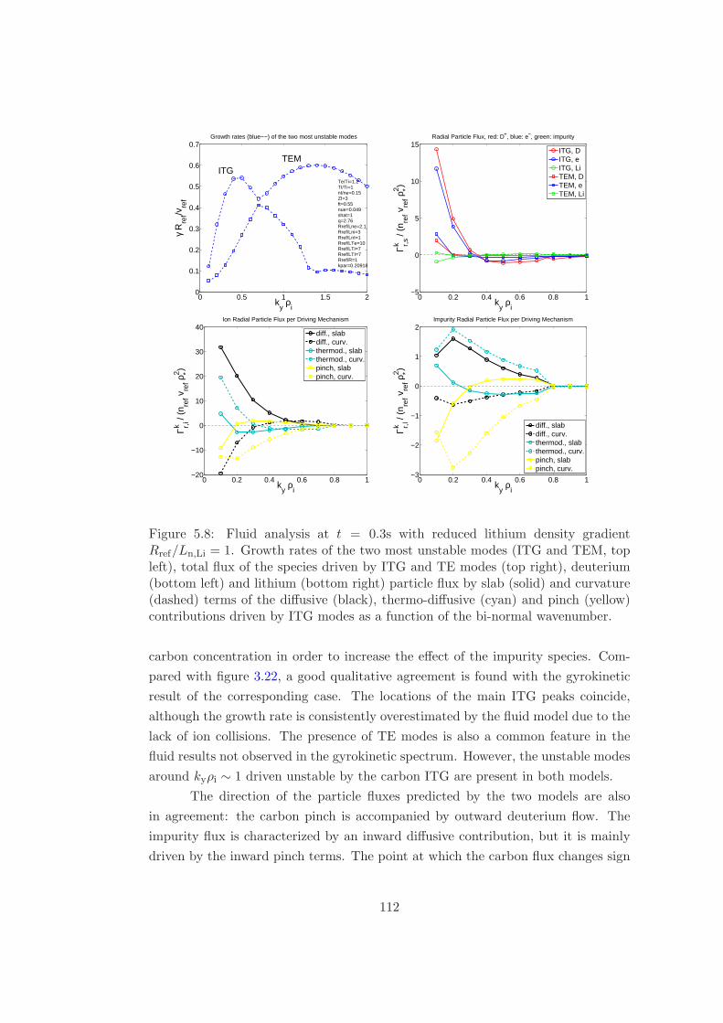
0 0.5 1 1.5 20

0.1

0.2

0.3

0.4

0.5

0.6

0.7Growth rates (blue−−) of the two most unstable modes

ky ρ

i

γ R

ref/v

ref

Te/Ti=1.2TI/Ti=1nI/ne=0.15ZI=3ft=0.55nue=0.049shat=1q=2.76Rref/Lne=2.1Rref/Lni=3Rref/LnI=1Rref/LTe=10Rref/LTi=7Rref/LTI=7Rref/R=1kpar=0.20918

ITGTEM

0 0.2 0.4 0.6 0.8 1−5

0

5

10


ky ρ

i

Γ r,s

k /

(nre

f vre

f ρ*2 )


0 0.2 0.4 0.6 0.8 1−20

−10

0

10

20

30


ky ρ

i

Γ r,i

k /

(nre

f vre

f ρ*2 )


0 0.2 0.4 0.6 0.8 1−3

−2

−1

0

1


ky ρ

i

Γ r,I

k /

(nre

f vre

f ρ*2 )


Figure 5.8: Fluid analysis at t = 0.3s with reduced lithium density gradientRref/Ln,Li = 1. Growth rates of the two most unstable modes (ITG and TEM, topleft), total flux of the species driven by ITG and TE modes (top right), deuterium(bottom left) and lithium (bottom right) particle flux by slab (solid) and curvature(dashed) terms of the diffusive (black), thermo-diffusive (cyan) and pinch (yellow)contributions driven by ITG modes as a function of the bi-normal wavenumber.

carbon concentration in order to increase the effect of the impurity species. Com-

pared with figure 3.22, a good qualitative agreement is found with the gyrokinetic

result of the corresponding case. The locations of the main ITG peaks coincide,

although the growth rate is consistently overestimated by the fluid model due to the

lack of ion collisions. The presence of TE modes is also a common feature in the

fluid results not observed in the gyrokinetic spectrum. However, the unstable modes

around kyρi ∼ 1 driven unstable by the carbon ITG are present in both models.

The direction of the particle fluxes predicted by the two models are also

in agreement: the carbon pinch is accompanied by outward deuterium flow. The

impurity flux is characterized by an inward diffusive contribution, but it is mainly

driven by the inward pinch terms. The point at which the carbon flux changes sign

112

0 0.5 1 1.5 20

0.1

0.2

0.3

0.4

0.5

0.6


ky ρ

i

γ R

ref/v

ref

TEMITG

Te/Ti=1.2TI/Ti=1nI/ne=0.15ZI=3ft=0.55nue=0.049shat=1q=2.76Rref/Lne=1.2Rref/Lni=3Rref/LnI=−1Rref/LTe=10Rref/LTi=7Rref/LTI=7Rref/R=1kpar=0.20918

0 0.2 0.4 0.6 0.8 1−5

0

5

10

15


ky ρ

i

Γ r,s

k /

(nre

f vre

f ρ*2 )


0 0.2 0.4 0.6 0.8 1−30

−20

−10

0

10

20

30


ky ρ

i

Γ r,i

k /

(nre

f vre

f ρ*2 )


0 0.2 0.4 0.6 0.8 1−3

−2

−1

0

1


ky ρ

i

Γ r,I

k /

(nre

f vre

f ρ*2 )


Figure 5.9: Fluid analysis at t = 0.3s with negative lithium density gradientRref/Ln,Li = −1. Growth rates of the two most unstable modes (ITG and TEM, topleft), total flux of the species driven by ITG and TE modes (top right), deuterium(bottom left) and lithium (bottom right) particle flux by slab (solid) and curvature(dashed) terms of the diffusive (black), thermo-diffusive (cyan) and pinch (yellow)contributions driven by ITG modes as a function of the bi-normal wavenumber.

from negative to positive is kyρi ≈ 0.4 in both cases.

If the carbon density gradient is set to positive, i.e. a centrally peaked profile

is assumed (figure 5.11), the main difference again occurs in the impurity diffusive

term: both the slab and curvature diffusion changes approximately proportionally

with the carbon density gradient, driving the impurities more towards the edge.

However, in contrast with the lithium case, the effect of carbon ions on the deuterium

flux is weak, and the outward deuterium flow remains.

113

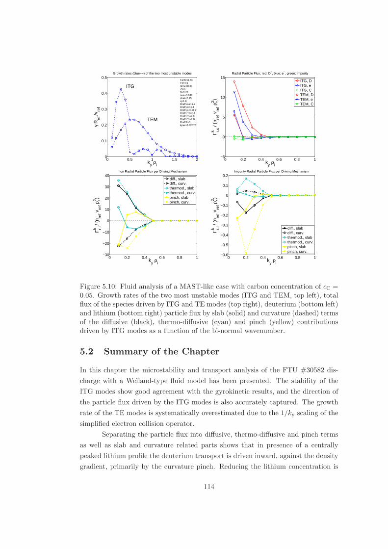
0 0.5 1 1.5 20

0.1

0.2

0.3

0.4


ky ρ

i

γ R

ref/v

ref

TEM

ITGTe/Ti=0.73TI/Ti=1nI/ne=0.05ZI=6ft=0.78nue=0.049shat=2.15q=1.8Rref/Lne=1.2Rref/Lni=2.1Rref/LnI=−0.9Rref/LTe=6.1Rref/LTi=7.8Rref/LTI=7.8Rref/R=1kpar=0.32075

0 0.2 0.4 0.6 0.8 1−5

0

5

10


ky ρ

i

Γ r,s

k /

(nre

f vre

f ρ*2 )

ITG, DITG, eITG, CTEM, DTEM, eTEM, C

0 0.2 0.4 0.6 0.8 1−30

−20

−10

0

10

20

30


ky ρ

i

Γ r,i

k /

(nre

f vre

f ρ*2 )


0 0.2 0.4 0.6 0.8 1−0.6

−0.5

−0.4

−0.3

−0.2

−0.1

0

0.1


ky ρ

i

Γ r,I

k /

(nre

f vre

f ρ*2 )


Figure 5.10: Fluid analysis of a MAST-like case with carbon concentration of cC =0.05. Growth rates of the two most unstable modes (ITG and TEM, top left), totalflux of the species driven by ITG and TE modes (top right), deuterium (bottom left)and lithium (bottom right) particle flux by slab (solid) and curvature (dashed) termsof the diffusive (black), thermo-diffusive (cyan) and pinch (yellow) contributionsdriven by ITG modes as a function of the bi-normal wavenumber.


In this chapter the microstability and transport analysis of the FTU #30582 dis-

charge with a Weiland-type fluid model has been presented. The stability of the

ITG modes show good agreement with the gyrokinetic results, and the direction of

the particle flux driven by the ITG modes is also accurately captured. The growth

rate of the TE modes is systematically overestimated due to the 1/ky scaling of the

simplified electron collision operator.

Separating the particle flux into diffusive, thermo-diffusive and pinch terms

as well as slab and curvature related parts shows that in presence of a centrally

peaked lithium profile the deuterium transport is driven inward, against the density

gradient, primarily by the curvature pinch. Reducing the lithium concentration is

114

0 0.5 1 1.5 20

0.1

0.2

0.3

0.4


ky ρ

i

γ R

ref/v

ref

Te/Ti=0.73TI/Ti=1nI/ne=0.05ZI=6ft=0.78nue=0.049shat=2.15q=1.8Rref/Lne=2.1Rref/Lni=2.1Rref/LnI=2.1Rref/LTe=6.1Rref/LTi=7.8Rref/LTI=7.8Rref/R=1kpar=0.32075

TEM

ITG

0 0.2 0.4 0.6 0.8 1−5

0

5

10


ky ρ

i

Γ r,s

k /

(nre

f vre

f ρ*2 )

ITG, DITG, eITG, CTEM, DTEM, eTEM, C

0 0.2 0.4 0.6 0.8 1−30

−20

−10

0

10

20

30


ky ρ

i

Γ r,i

k /

(nre

f vre

f ρ*2 )


0 0.2 0.4 0.6 0.8 1−0.6

−0.4

−0.2

0

0.2


ky ρ

i

Γ r,I

k /

(nre

f vre

f ρ*2 )


Figure 5.11: Fluid analysis of a MAST-like case with carbon concentration of cC =0.05 and a centrally peaked impurity density profile. Growth rates of the two mostunstable modes (ITG and TEM, top left), total flux of the species driven by ITGand TE modes (top right), deuterium (bottom left) and lithium (bottom right)particle flux by slab (solid) and curvature (dashed) terms of the diffusive (black),thermo-diffusive (cyan) and pinch (yellow) contributions driven by ITG modes as afunction of the bi-normal wavenumber.

accompanied by a relative increase of the outward slab diffusive contribution to the

deuterium transport.

Despite its high concentration in the density ramp-up phase, the lithium has

been found to act like trace impurity species when varying its density gradient value.

That is, the diffusive part of the lithium flux (both slab and curvature) changes pro-

portionally with Rref/Ln,Li, while the other components are weakly affected. When

reducing the lithium density gradient, and thus its outward flux, the deuterium flux

reacts by a relative increase of the diffusive transport again.

Two separate eigenmodes for the deuterium-ITG and lithium-ITG modes

could be obtained when the relative impurity temperature, and thus the lithium

Larmor-radius, has been reduced. In this case the overall outward lithium and the

115

inward deuterium flux have both been found less pronounced. The same effect is

observed when the lithium is replaced by carbon impurities. The detailed analysis

of the particle transport shows that when the lithium-ITG eigenmode appears it

is characterized by inward deuterium slab diffusive and outward curvature diffusive

terms, in contrast with the typical pattern of the deuterium-ITG eigenmodes. Even

when the two ITG eigenmodes are not separated, and appear as a mixed eigenmode,

the effect of the impurities on the deuterium flux is analogous: the slab diffusive

term is reduced.

The analysis of a MAST-like case shows that the main features of the ITG

growth rates and fluxes, as obtained with gyrokinetic simulations, can be captured

with the fluid model despite its obvious shortcomings in accurately modelling geo-

metrical and electro-magnetic effects. This indicates that the observed separation of

the ion flow is not strongly influenced by these mechanisms, it is mostly determined

by the densities, temperatures and gradients of the species.

116

Chapter 6

Conclusions

In this thesis the particle transport properties of light impurity seeded core tokamak

plasmas have been investigated. The main motivation of this work was provided by

the Liquid Lithium Limiter experiments in the FTU tokamak, in which a signifi-

cantly improved electron density peaking was consistently observed. Analysis of a

low-beta FTU-LLL discharge and a high-beta MAST discharge has been presented

in order to assess the electro-magnetic effects on particle transport.

A local gyrokinetic analysis of an FTU-LLL discharge during the density

ramp-up and density plateau phases in the high gradient region of the plasma core

(approximately mid-radius) has been performed. The simulations confirm that the

large lithium concentration has a major impact on the linear spectrum of the tur-

bulence and the associated anomalous particle transport. In a mainly electro-static,

ITG dominated turbulence the electron response remains close to adiabatic. The

electron flux thus becomes small compared to the ion fluxes, enabling the ions to

flow in opposite direction in order to maintain quasi-neutrality. This has not been

observed when tritium was used instead of lithium, due to the similar dynamics

of the deuterium and tritium species. However, with any other impurities heavier

than tritium the ion flow separation occurs. In order to obtain an inward deuterium

(and/or tritium) transport, the outward drive of the impurity flux must be stronger

than that of the main ion species. This can be achieved by sufficiently high impurity

concentration and density gradient, which conditions are satisfied during the density

ramp-up phase of the analysed FTU-LLL discharge.

These features of the turbulent particle transport in a lithiated FTU plasma

indicate a better confinement of the deuterium and electron species, improved even

further by the relatively strong Ware-pinch contribution. Since the turbulent trans-

port is likely to be quenched deeper in the core plasma due to the weaker drive of

the drift-instabilities, the reduced electron flux is expected to lead to a more peaked

117

density profile. However, since the gyrokinetic analysis is local, no quantitative

prediction regarding the profile evolution of the species can be made.

Gyrokinetic simulations of an H-mode MAST discharge have also been per-

formed in order to provide inter-machine comparison of the effect of impurities, and

to assess the role of magnetic perturbations on particle transport. Although both

an inward and outward impurity flux has been observed in the simulations both

in ITG and KBM dominated turbulence depending mainly on the direction of the

impurity density gradient, this has not been followed by an ion flow separation as

in the FTU analysis. The deuterium flux has consistently been found to be inward.

This is attributed to the fact that, although the electro-magnetic perturbations pro-

vide negligible contribution to the ion transport, they drive a strong non-adiabatic

electron response.

The fluid analysis of the FTU-LLL experiment provided information regard-

ing the distribution of the particle transport between the diffusive, thermo-diffusive

and pinch channels. It has been found that the lithium behaves as trace species

despite its high concentration in the plasma. That is, the diffusive part of the

lithium transport changes approximately proportionally with the lithium density

gradient, while the other contributions to the flux remain unaffected by the changes

in Rref/Ln,Li. In every case when an inward deuterium flux is enforced by an out-

ward lithium transport, it is mainly the outward diffusive term of the deuterium flux

that responds by taking a reduced value. In the reference case only one unstable

eigenmode is found rotating in the ion diamagnetic direction. However, separate

deuterium-ITG and lithium-ITG eigenmodes can be obtained by decreasing the rel-

ative lithium temperature and thus separating the typical spatial scale of the two

modes from each other. A similar splitting of the modes is achieved with carbon im-

purities. When the Larmor-radii of the two ion species are further apart, the impact

of the impurities on the main ion transport is weaker. However, the impurity-ITG

mode still drives an inward deuterium flux and it is characterized by an inward slab

diffusive contribution.

The described mechanism driving inward deuterium transport during the

ramp-up phase of the discharge is not a collisional effect. It has been observed in

simulations with reduced collisionality, and not been observed in clean plasma with

increased Zeff to model the effect of higher collisionality. Furthermore, collisions

provide an outward contribution in and ITG driven turbulent flux for all the species.

This indicates that light impurity seeding during the startup of a discharge might

lead to improved deuterium and tritium density peaking also in higher temperature

tokamak experiments.

118

Appendix A

Integrals Involving Products of

Bessel Functions

The following three types of integrals involving products of Bessel functions, expo-

nential and algebraic terms appear in the derivation of the gyrocentre Maxwell’s

equations:

1.

∞∫

0

J20 (λ)e

−µB0T dµ (A.1)

2.

∞∫

0

µJ0(λ)J1(λ)e−

µB0T dµ (A.2)

3.

∞∫

0

µ2J21 (λ)e

−µB0T dµ (A.3)

where J1(λ) = 2λJ1(λ). In all three cases the new variable x = µB0

T is introduced

according to Dannert [30], which also leads to λ =√2xb where b = −ρ2th∇2

⊥. The

Jacobian is simply TB0

and the integrals can be written as

1.T

B0

∞∫

0

J20 (√2xb)e−xdx

2.T 2

B20

2√2b

∞∫

0

√xJ0(

√2xb)J1(

√2xb)e−xdx

3.T 3

B30

2

b

∞∫

0

xJ21 (λ)e

−µB0T dx.

119

The first integral can be solved using the formula 6.615 on page 710 of [86]:

∞∫

0

e−αxJν(2β√x)Jnu(2γ

√x)dx =

1

αIν

(2βγ

α

)e−

β2+γ2

α2

which immedately gives

1.T

B0

∞∫

0

J20 (√2xb)e−xdx = I0(b)e

−b.

In the two remaining integrals let us use the new variable y =√2bx. The Jacobian

is yb and therefore it leads to

2.T 2

B20

2√2b

∞∫

0

√xJ0(

√2xb)J1(

√2xb)e−xdx =

T 2

B20

1

b2

∞∫

0

y2J0(y)J1(y)e−hy2dy

3.T 3

B30

2

b

∞∫

0

xJ21 (λ)e

−µB0T dµ =

T 3

B30

1

b3

∞∫

0

y3J21 (y)e

−hy2dy

where h = 12b was used in the exponentials.

The second integral (leaving the prefactors for now) can be further written

as

∞∫

0

y2J0(y)J1(y)e−hy2dy =

∂

∂h

−

∞∫

0

e−hy2J0(y)J1(y)

dy

=1

2

∂

∂h

∞∫

0

e−hy2 d

dy

(J20 (y)

) dy

=1

2

∂

∂h

[J20 (y)e

−hy2]∞0︸︷︷︸

1

+2h

∞∫

0

J20 (y)ye

−hy2dy

where the relation dJ0(y)dy = −J1(y) was applied (see [39]). The integral can be found

in [87] on page 395 and it gives

∞∫

0

yJ20 (y)e

−hy2dy =1

2he−

12h I0

(1

2h

). (A.4)

120

Taking the derivative with respect to h and using the identity dI0(z)dz = I1(z) results

∞∫

0

y2J0(y)J1(y)e−hy2dy =

1

4h2e−

12h

(I0

(1

2h

)− I1

(1

2h

))

= b2e−b (I0(b)− I1(b)) . (A.5)

And with the prefactors:

2.

∞∫

0

µJ0(λ)J1(λ)e−

µB0T dµ =

T 2

B20

e−b (I0(b)− I1(b)) . (A.6)

The third integral (without the prefactors) is integrated by parts first to get

∞∫

0

y3J21 (y)e

−hy2dy = − 1

2h

∞∫

0

(−2hy)e−hy2y2J1(y)dy

= − 1

2h

[e−hy

2y2J2

1 (y)]∞0︸︷︷︸

0

−2

∞∫

0

e−hy2

(yJ2

1 (y) + y2J1(y)dJ1(y)

dy

) .

Using the relation dJ1(y)dy = J0(y)− 1

yJ1(y) (see [39]) two of the terms cancel out and

the integral simplifies to

∞∫

0

y3J21 (y)e

−hy2dy =1

h

∞∫

0

y2J0(y)J1(y)e−hy2dy.

Using equation (A.5) the third integral can be written as

∞∫

0

y3J21 (y)e

−hy2dy = 2b3e−b (I0(b)− I1(b)) (A.7)

and with prefactors:

3.

∞∫

0

µ2J21 (λ)e

−µB0T dµ =

T 3

B30

2e−b (I0(b)− I1(b)) . (A.8)

121

Appendix B

Coefficients of the Dispersion

Relation Polynomial

B.1 9th Degree Coefficients

c9 =Z2i ni,NTi,N

(A3iB3IB3e) +Z2I nI,NTI,N

(A3IB3iB3e) +

Z2ene,NftTe,N

(A3eB3IB3i) +Z2ene,N(1− ft)

Te,N(B3eB3IB3i)

c8 =Z2i ni,NTi,N

(A3iB3IB2e +A3iB2IB3e +A2iB3IB3e) +

Z2I nI,NTI,N

(A3IB3iB2e +A3IB2iB3e +A2IB3iB3e) +

Z2ene,NftTe,N

(A3eB3IB2i +A3eB2IB3i +A2eB3IB3i) +

Z2ene,N(1− ft)

Te,N(B3eB3IB2i +B3eB2IB3i +B2eB3IB3i)

122

c7 =Z2i ni,NTi,N

(A3iB3IB1e +A3iB1IB3e +A1iB3IB3e +A3iB2IB2e +A2iB3IB2e +A2iB2IB3e) +

Z2I nI,NTI,N

(A3IB3iB1e +A3IB1iB3e +A1IB3iB3e +A3IB2iB2e +A2IB3iB2e +A2IB2iB3e) +

Z2ene,NftTe,N

(A3eB3IB1i +A3eB1IB3i +A1eB3IB3i +A3eB2IB2i +A2eB3IB2i +A2eB2IB3i) +

Z2ene,N(1− ft)

Te,N(B3eB3IB1i +B3eB1IB3i +B1eB3IB3i +B3eB2IB2i +B2eB3IB2i +B2eB2IB3i)

c6 =Z2i ni,NTi,N

(A3iB3IB0e +A3iB0IB3e +A0iB3IB3e +A3iB2IB1e +A3iB1IB2e +

A2iB3IB1e +A1iB3IB2e +A2iB1IB3e +A1iB2IB3e +A2iB2IB2e) +

Z2I nI,NTI,N

(A3IB3iB0e +A3IB0iB3e +A0IB3iB3e +A3IB2iB1e +A3IB1iB2e +

A2IB3iB1e +A1IB3iB2e +A2IB1iB3e +A1IB2iB3e +A2IB2iB2e) +

Z2ene,NftTe,N

(A3eB3IB0i +A3eB0IB3i +A0eB3IB3i +A3eB2IB1i +A3eB1IB2i +

A2eB3IB1i +A1eB3IB2i +A2eB1IB3i +A1eB2IB3i +A2eB2IB2i) +

Z2ene,N(1− ft)

Te,N(B3eB3IB0i +B3eB0IB3i +B0eB3IB3i +B3eB2IB1i +B3eB1IB2i +

B2eB3IB1i +B1eB3IB2i +B2eB1IB3i +B1eB2IB3i +B2eB2IB2i)

c5 =Z2i ni,NTi,N

(A3iB2IB0e +A3iB0IB2e +A2iB3IB0e +A0iB3IB2e +A2iB0IB3e +A0iB2IB3e +

A3iB1IB1e +A1iB3IB1e +A1iB1IB3e +A2iB2IB1e +A2iB1IB2e +A1iB2IB2e) +

Z2I nI,NTI,N

(A3IB2iB0e +A3IB0iB2e +A2IB3iB0e +A0IB3iB2e +A2IB0iB3e +A0IB2iB3e +

A3IB1iB1e +A1IB3iB1e +A1IB1iB3e +A2IB2iB1e +A2IB1iB2e +A1IB2iB2e) +

Z2ene,NftTe,N

(A3eB2IB0i +A3eB0IB2i +A2eB3IB0i +A0eB3IB2i +A2eB0IB3i +A0eB2IB3i +

A3eB1IB1i +A1eB3IB1i +A1eB1IB3i +A2eB2IB1i +A2eB1IB2i +A1eB2IB2i) +

Z2ene,N(1− ft)

Te,N(B3eB2IB0i +B3eB0IB2i +B2eB3IB0i +B0eB3IB2i +B2eB0IB3i +B0eB2IB3i +

B3eB1IB1i +B1eB3IB1i +B1eB1IB3i +B2eB2IB1i +B2eB1IB2i +B1eB2IB2i)

123

c4 =Z2i ni,NTi,N

(A3iB1IB0e +A3iB0IB1e +A1iB3IB0e +A0iB3IB1e +A1iB0IB3e +A0iB1IB3e +

A2iB1IB1e +A1iB2IB1e +A1iB1IB2e +A2iB2IB0e +A2iB0IB2e +A0iB2IB2e) +

Z2I nI,NTI,N

(A3IB1iB0e +A3IB0iB1e +A1IB3iB0e +A0IB3iB1e +A1IB0iB3e +A0IB1iB3e +

A2IB1iB1e +A1IB2iB1e +A1IB1iB2e +A2IB2iB0e +A2IB0iB2e +A0IB2iB2e) +

Z2ene,NftTe,N

(A3eB1IB0i +A3eB0IB1i +A1eB3IB0i +A0eB3IB1i +A1eB0IB3i +A0eB1IB3i +

A2eB1IB1i +A1eB2IB1i +A1eB1IB2i +A2eB2IB0i +A2eB0IB2i +A0eB2IB2i) +

Z2ene,N(1− ft)

Te,N(B3eB1IB0i +B3eB0IB1i +B1eB3IB0i +B0eB3IB1i +B1eB0IB3i +B0eB1IB3i +

B2eB1IB1i +B1eB2IB1i +B1eB1IB2i +B2eB2IB0i +B2eB0IB2i +B0eB2IB2i)

c3 =Z2i ni,NTi,N

(A3iB0IB0e +A0iB3IB0e +A0iB0IB3e +A2iB1IB0e +A1iB2IB0e +

A2iB0IB1e +A1iB0IB2e +A0iB2IB1e +A0iB1IB2e +A1iB1IB1e) +

Z2I nI,NTI,N

(A3IB0iB0e +A0IB3iB0e +A0IB0iB3e +A2IB1iB0e +A1IB2iB0e +

A2IB0iB1e +A1IB0iB2e +A0IB2iB1e +A0IB1iB2e +A1IB1iB1e) +

Z2ene,NftTe,N

(A3eB0IB0i +A0eB3IB0i +A0eB0IB3i +A2eB1IB0i +A1eB2IB0i +

A2eB0IB1i +A1eB0IB2i +A0eB2IB1i +A0eB1IB2i +A1eB1IB1i) +

Z2ene,N(1− ft)

Te,N(B3eB0IB0i +B0eB3IB0i +B0eB0IB3i +B2eB1IB0i +B1eB2IB0i +

B2eB0IB1i +B1eB0IB2i +B0eB2IB1i +B0eB1IB2i +B1eB1IB1i)

c2 =Z2i ni,NTi,N

(A2iB0IB0e +A0iB2IB0e +A0iB0IB2e +A1iB1IB0e +A1iB0IB1e +A0iB1IB1e) +

Z2I nI,NTI,N

(A2IB0iB0e +A0IB2iB0e +A0IB0iB2e +A1IB1iB0e +A1IB0iB1e +A0IB1iB1e) +

Z2ene,NftTe,N

(A2eB0IB0i +A0eB2IB0i +A0eB0IB2i +A1eB1IB0i +A1eB0IB1i +A0eB1IB1i) +

Z2ene,N(1− ft)

Te,N(B2eB0IB0i +B0eB2IB0i +B0eB0IB2i +B1eB1IB0i +B1eB0IB1i +B0eB1IB1i)

124

c1 =Z2i ni,NTi,N

(A1iB0IB0e +A0iB1IB0e +A0iB0IB1e) +

Z2I nI,NTI,N

(A1IB0iB0e +A0IB1iB0e +A0IB0iB1e) +

Z2ene,NftTe,N

(A1eB0IB0i +A0eB1IB0i +A0eB0IB1i) +

Z2ene,N(1− ft)

Te,N(B1eB0IB0i +B0eB1IB0i +B0eB0IB1i)

c0 =Z2i ni,NTi,N

(A0iB0IB0e) +Z2I nI,NTI,N

(A0IB0iB0e) +

Z2ene,NftTe,N

(A0eB0IB0i) +Z2ene,N(1− ft)

Te,N(B0eB0IB0i)

125

B.2 4th Degree Coefficients

c4 =Z2e

Te,0

c3 =Z2i

Ti,0

ni,0ne,0

−Fi

(2− Rref

Ln,i

)+Z2I

TI,0

nI,0ne,0

−FI

(2− Rref

Ln,I

)+Z2e

Te

−20

3(Fi + FI)

c2 =Z2i

Ti,0

ni,0ne,0

2F 2

i

[10

3+Rref

Ln,i

(ηi −

7

3

)]+

20

3FiFI

(2− Rref

Ln,i

)+

Z2I

TI,0

nI,0ne,0

2F 2

I

[10

3+Rref

Ln,I

(ηI −

7

3

)]+

20

3FiFI

(2− Rref

Ln,I

)+

Z2e

Te

20

3

F 2i + F 2

I +20

3FiFI

c1 =Z2i

Ti,0

ni,0ne,0

−20

3FiF

2I

(2− Rref

Ln,i

)− 40

3F 2i FI

[10

3+Rref

Ln,i

(ηi −

7

3

)]+

Z2I

TI,0

nI,0ne,0

−20

3FIF

2i

(2− Rref

Ln,I

)− 40

3F 2I Fi

[10

3+Rref

Ln,I

(ηI −

7

3

)]+

Z2e

Te

−400

9

(FiF

2I + FIF

2i

)

c0 =Z2i

Ti,0

ni,0ne,0

40

3F 2i F

2I

[10

3+Rref

Ln,i

(ηi −

7

3

)]+

Z2I

TI,0

nI,0ne,0

40

3F 2i F

2I

[10

3+Rref

Ln,I

(ηI −

7

3

)]+

Z2e

Te

400

9F 2i F

2I

126

Bibliography

[1] C.M.H. Smith, A Textbook of Nuclear Physics, p 223 (Pergamon, Oxford, 1965)

[2] J. Wesson, Tokamaks, p4 (Clarendon Press, Oxford, 1987)

[3] J. D. Lawson, Proceedings of the Physical Society B, 70, 6 (1957)

[4] H.P. Furth, Nucl. Fusion 15, 487 (1975)

[5] P. Helander, D.J. Sigmar, Collisional Transport in Magnetized Plasmas (Cam-

bridge University Press 2002)

[6] B. Lehnert, Plasma Physics 9, 301 (1967)

[7] W. Horton, Rev. Mod. Phys. 71 735 (1999)

[8] E.J. Doyle et al., Nucl. Fusion 47, S18-S127 (2007)

[9] B. Coppi, M.N. Rosenbluth, R.Z. Sagdeev, Phys. Fluids 10, 582 (1967)

[10] S.C. Cowley, R.M. Kulsrud, R. Sudan, Phys. Fluids B 3, 2767 (1991)

[11] R.D. Hazeltine, F.L. Waelbroeck, The Framework of Plasma Phyiscs (Perseus

Book, 1998)

[12] A.J. Brizard, T.S. Hahm, Rev. Mod. Phys. 79, 421 (2007)

[13] S.I. Braginskii, Chapter 3, Reviews of Plasma Physics, Vol. 1 (Consultants

Bureau, New York, 1965)

[14] R.D. Hazeltine, J.D. Meiss, Plasma Confinement (Courier Dover Publications,

2003)

[15] J. Weiland et al., Nucl. Fusion 29, 10 (1989)

[16] C. Gormezano et al., Fusion Sci. Technol. 45, no. 3 (2004)

127

[17] M.L. Apicella et al., J. Nucl. Materials 363-365, 1346 (2007)

[18] A. Tuccillo et al., Nucl. Fusion 49, 104013 (2009)

[19] G. Mazzitelli et al. (including G. Szepesi), Nucl. Fusion 51, 073006 (2011)

[20] V. Evitkin et al., Fusion Eng. Des. 56-57, 363 (2001)

[21] R. Majeski et al., Phys. Rev. Letters 97, 075002 (2006)

[22] D. K. Mansfield et al., Phys. Plasmas 3, 1892 (1996)

[23] D. A. Gates et al., Nucl. Fusion 49, 104016 (2009)

[24] R. Maingi et al., Phys. Rev. Letters 103, 075001 (2009)

[25] M. Murakami et al., Nucl. Fusion 41, 317 (2001)

[26] G.R. McKee et al., Phys. Plasmas 7, 1870 (2000)

[27] R.R. Weynants, Nucl. Fusion 39, 1637 (1999)

[28] C. Estrada-Mila et al., Phys. Plasmas 12, 022305 (2005)

[29] A. Darke et al., MAST: a mega ampere spherical tokamak, Proc. 18th Sympo-

sium on Fusion Technology (1994)

[30] T. Dannert: Gyrokinetische Simulation von Plasmaturbulenz mit gefangenen

Teilchen und Elektromagnetischen Effekten (Doctoral Thesis, Technische Uni-

versitat Munchen, 2005)

[31] A.G. Peeters et al. (including G. Szepesi), Comput. Phys. Commun. 180, 2650

(2009)

[32] P.M. Bellan, Fundamentals of Plasma Physics (Cambridge University Press,

2006)

[33] R.G. Littlejohn, Phys. Fluids 24, 1730 (1981)

[34] M. Fecko Differential Geometry and Lie Groups for Physicists (Cambridge Uni-

versity Press, 2006)

[35] R.G. Littlejohn, J. Math. Phys. 23, 742 (1982)

[36] A.G. Peeters et al., Phys. Plasmas 16, 042310 (2009)

128

[37] B. Scott: Introduction to Gyrokinetic Field Theory (Lecture notes, GOTiT

course at IPP Garching, 2008 November)

[38] F.J. Casson et al. (including G. Szepesi), Phys. Plasmas 17, 102305 (2010)

[39] M. Abramowitz, I.A. Stegun, eds., Handbook of Mathematical Functions with

Formulas, Graphs, and Mathematical Tables, (New York: Dover Publications,

1972)

[40] F. Jenko, W. Dorland, Plasma Phys. Control. Fusion 43, A141 (2001)

[41] D J Applegate et al., Plasma Phys. Control. Fusion 49, 1113 (2007)

[42] M. Kotschenreuther, G. Rewoldt, and M. W. Tang, Comput. Phys. Commun.

88, 128 (1995)

[43] C. Karney, Comp. Phys. Rep. 4 183, (1986)

[44] M. Romanelli, et al. (including G. Szepesi), Nucl. Fusion 51, 103008 (2011)

[45] G. Szepesi et al., Nucl. Fusion 53, 033007 (2013)

[46] X. Lapillone et al., Phys. Plasmas 16, 032308 (2009)

[47] M. Romanelli et al., Phys. Plasmas 14, 082305 (2007)

[48] M. Reshko, C.M. Roach, Plasma Phys. Control. Fusion 50, 115002 (2008)

[49] B. Coppi et al., Phys. Fluids 19, 1144 (1976)

[50] M. Frojdh et al., Nucl. Fusion 31, 419 (1992)

[51] J.E. Kinsey et al., Phys. Plasmas 13, 022305 (2006)

[52] S. Moradi et al., Phys. Plasmas 17, 012101 (2010)

[53] H Nordman et al., Phys. Plasmas 14, 052303 (2007)

[54] B. Coppi et al., Phys. Fluids 2, 2322 (1990)

[55] E. Fable et al., Plasma Phys. Control. Fusion 52, 015007 (2010)

[56] G. Cenacchi, A. Taroni, Rapporto ENEA RT/TIB 88, 5 (1988)

[57] A.G. Peeters, Phys. Plasmas 7, 268 (2000)

[58] P.C. Stangeby, The Plasma Boundary of Magnetic Fusion Devices (Taylor &

Francis, 2000)

129

[59] K.L. Bell et al., J. Phys. Chem. Ref. Data 12, 891 (1983)

[60] F. Militello, W. Fundamenski, Plasma Phys. Control. Fusion 53, 095002 (2011)

[61] H. Lutjens et al., Comput. Phys. Commun. 97, 219 (1996)

[62] F. Militello, W. Fundamenski, Plasma Phys. Control. Fusion 53, 095002 (2011)

[63] C. Bourdelle et al., Phys. Plasmas 14, 112501 (2007)

[64] F. Jenko et al., Phys. Plasmas 7, 1904 (2000)

[65] C. Angioni et al., Plasma Phys. Control. Fusion 51, 124017 (2009)

[66] C. Bourdelle et al., Plasma Phys. Control. Fusion 47, A317 (2005)

[67] X. Garbet et al., Phys. Rev. Letters 91, 035001-1 (2003)

[68] H Nordman et al., Plasma Phys. Control. Fusion 49, 985 (2007)

[69] C. Angioni et al., Phys. Plasmas 12, 112310 (2005)

[70] C. Angioni et al., Phys. Rev. Letters 90, 205003 (2003)

[71] C. Angioni, A.G. Peeters, Phys. Rev. Letters 96, 095003 (2006)

[72] A. Skyman et al., Phys. Plasmas 19, 032313 (2012)

[73] M. Frojdh, A. Jarmen, Nucl. Fusion 35, 575 (1995)

[74] C. Angioni et al., Plasma Phys. Control. Fusion 49, 2027 (2007)

[75] Y. Camenen et al., Phys. Rev. Lett. 102, 125001 (2009)

[76] C. Angioni et al., Nucl. Fusion 51, 023006 (2011)

[77] T. Hein, C. Angioni, Phys. Plasmas 17, 012307 (2010)

[78] J. Nilsson, J. Weiland, Nucl. Fusion 34, 803 (1994)

[79] G. Tardini: Validation of Theory Based Transport Models in Tokamak Plasmas

(Doctoral Thesis, Technische Universtat Munchen, 2003)

[80] R.D. Hazeltine, J.D. Meiss, Phys. Rep. 121, No. 1 (1985)

[81] Z. Chang, J.D. Callen, Phys. Fluids B 4, 1766 (1992)

[82] A. Hirose, Phys. Fluids B 5, 230 (1993)

130

[83] D. Wagner at al., Plasma Phys. Control. Fusion 54, 085018 (2012)

[84] A. Jarmen et al., Nucl. Fusion 27, 941 (1987)

[85] M. Romanelli et al., Plasma Phys. Control. Fusion 49, 935 (2007)

[86] I.S. Gradshteyn, I.M. Ryzhik: Table of Integrals, Series, and Products (Aca-

demic Press, 1965)

[87] E.T. Whittaker, G.N. Watson, A Course of Modern Analysis (Cambridge Uni-

versity Press, 4th edition, 1927)

131

University of Warwick institutional repository: · thesis deposit 2.1 I understand that under my registration at the University, I am required to deposit my thesis with the University

Documents