University of Southern Queensland Faculty of Engineering and Surveying Feasibility Assessment of Low Cost Stereo Computer Vision in Clay Target Shooting Coaching. A dissertation submitted by Oliver J Anderson In fulfilment of the requirements of Bachelor of Engineering (Honours) Mechatronic Major October 2015

Welcome message from author
This document is posted to help you gain knowledge. Please leave a comment to let me know what you think about it! Share it to your friends and learn new things together.
Transcript

University of Southern Queensland
Faculty of Engineering and Surveying
Feasibility Assessment of Low Cost Stereo Computer
Vision in Clay Target Shooting Coaching.
A dissertation submitted by
Oliver J Anderson
In fulfilment of the requirements of
Bachelor of Engineering (Honours)
Mechatronic Major
October 2015

Abstract
Clay target shooting is a sport that has been slow to adopt new technology to
help automate and improve coaching. Currently gun mounted cameras and
shooting simulators are available but these are prohibitively expensive for
most shooters. This project aims to determine if a lower cost alternative can be
created to provide feedback to new shooters about the distance they missed
the target using low cost stereo computer vision.
Initially an investigation was undertaken into the use of web cameras and
GoPro action cameras for suitability to create a stereo vision system to track
the shooter aim and the target position. The focus of this assessment was the
camera resolution, frame rate and ability to be synchronized. The assessment
found that these consumer-grade cameras all have high resolutions but no
ability to be synchronized. Of these cameras the GoPro cameras could record in
high definition at much higher frame rates then the web cameras and therefore
were selected for the field trials.
Field trials to test the accuracy of the low cost stereo vision system were
performed in three phases; “static”, “dynamic” and “vs coaches”. The static trials
were designed to find a baseline accuracy where the effect of frame
synchronization errors could be reduced. The dynamic trials were performed
to test the system on moving targets and to try and compensate for the
synchronization errors. Finally the system was trialed against the judgement of
three experienced human judges to test its reliability against the current
coaching method.
Matlab scripts were written to process the stereo images that were recorded as
part of the field trials. Using colour thresholding and a custom filter that was

created as part of this project, markers on the gun and the clay target were able
to be segmented from the background in the trials. Using these positions the
real world coordinates were able to be calculated and the aim of the gun vs
target location estimated.
The outcome of the trials showed that low cost computer vision can have good
accuracy in estimation of gun aim in a static scene. When movement was
introduced to the trials the synchronization errors of the cameras resulted in
large positional errors. The final outcome of the project determined that low
cost stereo computer vision is far less reliable and accurate than human
coaches and is not at this time feasible to be used in clay target coaching.

University of Southern Queensland
Faculty of Health, Engineering and Sciences
ENG4111/ENG4112 Research Project
Limitations of Use
The Council of the University of Southern Queensland, its Faculty of Health,
Engineering & Sciences, and the staff of the University of Southern Queensland,
do not accept any responsibility for the truth, accuracy or completeness of
material contained within or associated with this dissertation.
Persons using all or any part of this material do so at their own risk, and not at
the risk of the Council of the University of Southern Queensland, its Faculty of
Health, Engineering & Sciences or the staff of the University of Southern
Queensland.
This dissertation reports an educational exercise and has no purpose or
validity beyond this exercise. The sole purpose of the course pair entitled
“Research Project” is to contribute to the overall education within the student’s
chosen degree program. This document, the associated hardware, software,
drawings, and other material set out in the associated appendices should not
be used for any other purpose: if they are so used, it is entirely at the risk of the
user.

University of Southern Queensland
Faculty of Health, Engineering and Sciences
ENG4111/ENG4112 Research Project
Certification of Dissertation
I certify that the ideas, designs and experimental work, results, analyses and
conclusions set out in this dissertation are entirely my own effort, except where
otherwise indicated and acknowledged.
I further certify that the work is original and has not been previously submitted for
assessment in any other course or institution, except where specifically stated.
Oliver Anderson
0050106236

Acknowledgments
There are many people who were generous with their time throughout this
project. Dr. Tobias Low where my emails never stayed unanswered in his inbox
for too long, enabling me to get back to work after being stuck on an issue. Ian
Collison and Brisbane Sporting Clays who made the club facilities available on
days not normally open for shooting. Chris Worland who helped me setup and
record most of the field trials and listened to more talk about machine vision
than he cared for.
Finally I would like to acknowledge the contribution of my wife, Emma
Anderson, without her patience and understanding this entire degree would
not have been possible.

Table of Contents .......................................................................................................................... 1
Introduction ............................................................................................................................ 1
1.1 Background ............................................................................................................... 1
1.2 Project Aim ................................................................................................................ 3
1.3 Research Objectives ............................................................................................... 4
.......................................................................................................................... 6
Literature Review ................................................................................................................. 6
2.1 Computer Vision in Sport Coaching .................................................................. 6
2.2 Technology in Clay Target Shooting Coaching ............................................. 7
2.3 Stereo Camera Calibration .................................................................................. 8
2.4 Object Detection Methods .................................................................................. 10
2.4.1 Object Detection Using Target Colour ................................................................. 11
2.4.2 Object Detection Using Target Motion ................................................................ 12
2.5 Positional Measurement Using Stereo Computer Vision ........................ 14
2.6 Accuracy of Positional Measurement Using Low Cost Stereo Vision .. 15
2.7 Low Cost Camera Synchronization ................................................................. 16
2.8 Shotgun Projectile Motion ................................................................................. 17
2.8.1 Shot Velocity ................................................................................................................... 17
2.8.2 Pattern Spread ............................................................................................................... 20
....................................................................................................................... 21
Methodology ......................................................................................................................... 21
3.1 Project Methodology ............................................................................................ 21
3.2 Task Analysis .......................................................................................................... 22
3.2.1 Determination of Low Cost Camera Equipment for Tracking Moving
Objects. ............................................................................................................................................. 22
3.2.2 Stereo Camera Mounting and Baseline Distance Assessment. .................. 22
3.2.3 Develop Stereo Camera Calibration Routine. ................................................... 22

3.2.4 Develop Functions to Identify and Measure the Position of Target and
Gun Markers ................................................................................................................................... 23
3.2.5 Develop Function to Calculate the Accuracy of a Shot Taken at a Moving
Target. 23
3.2.6 Conduct Trial of Computer Program vs the Human Judges and Evaluate
Results. ............................................................................................................................................. 24
3.2.7 Optimize Matlab Program and Repeat Step 6 if the Original Results are
Unsatisfactory................................................................................................................................ 24
3.3 Project Consequential Effects ........................................................................... 24
3.3.1 Sustainability ................................................................................................................. 24
3.3.2 Ethics ................................................................................................................................. 25
3.4 Risk Assessment .................................................................................................... 25
3.4.1 Risks Identified ............................................................................................................. 26
3.5 Project Timeline .................................................................................................... 26
....................................................................................................................... 27
Stereo Platform Development ........................................................................................ 27
4.1 Camera Selection ................................................................................................... 27
4.1.1 Camera Properties Comparison ............................................................................. 27
4.1.2 Camera Synchronization ........................................................................................... 30
4.2 Camera Mounting .................................................................................................. 33
4.2.1 Initial Design .................................................................................................................. 33
4.2.2 Final Design .................................................................................................................... 35
4.3 Camera Calibration .............................................................................................. 35
4.3.1 Prepare images.............................................................................................................. 36
4.3.2 Add Images ..................................................................................................................... 38
4.3.3 Calibrate ........................................................................................................................... 38
4.3.4 Evaluate and Improve ................................................................................................ 39
4.3.5 Export ................................................................................................................................ 40
....................................................................................................................... 41
Static Target Accuracy ....................................................................................................... 41
5.1 Static Scene Capture ............................................................................................. 41
5.1.1 Target Mounting and Shot Pattern Feedback ................................................... 41

5.1.2 Field Trial Layout ......................................................................................................... 43
5.1.3 Gun Marker Colour ...................................................................................................... 44
5.1.4 Gun Marker Positioning ............................................................................................. 44
5.1.5 Initial Attempts ............................................................................................................. 45
5.2 Static Trial Stereo Image Processing ............................................................. 45
5.2.1 Image Selection ............................................................................................................. 45
5.2.2 Colour Thresholding ................................................................................................... 46
5.2.3 Noise Filtering ............................................................................................................... 49
5.2.4 Blob Detection ............................................................................................................... 49
5.2.5 Create Point Cloud from Scene ............................................................................... 50
5.2.6 Real World Coordinates ............................................................................................ 51
5.2.7 Calculation of the Aim and Accuracy .................................................................... 52
5.3 Results....................................................................................................................... 53
....................................................................................................................... 56
Dynamic Target Accuracy ................................................................................................ 56
6.1 Dynamic Scene Capture ...................................................................................... 56
6.1.1 Field Trial Layout ......................................................................................................... 56
6.1.2 Gun Marker Colour ...................................................................................................... 58
6.1.3 Gun Marker Positioning ............................................................................................. 58
6.2 Use of Existing Code ............................................................................................. 58
6.3 Moving Target Tracking ..................................................................................... 59
6.3.1 Matlab Foreground Detector ................................................................................... 59
6.3.2 Custom Background Subtraction Filter............................................................... 61
6.4 Prediction of Target Position ........................................................................... 63
6.4.1 Predicted Target Path ................................................................................................. 63
6.4.2 Target Velocity .............................................................................................................. 64
6.4.3 Shot Cloud Flight Time ............................................................................................... 64
6.5 Estimation of Frame Synchronization ........................................................... 64
6.6 Initial Results ......................................................................................................... 65
6.6.1 Target Z Distance.......................................................................................................... 66
6.6.2 Calculated Accuracy .................................................................................................... 67
6.7 Program Accuracy Improvement .................................................................... 69

6.8 Results....................................................................................................................... 72
6.8.1 Target Z Distance.......................................................................................................... 72
6.8.2 Calculated Accuracy .................................................................................................... 73
....................................................................................................................... 76
Results and Discussion ...................................................................................................... 76
7.1 Final Testing ........................................................................................................... 76
7.2 Results....................................................................................................................... 78
7.3 Concept Feasibility ............................................................................................... 81
7.4 Future work ............................................................................................................ 82
7.4.1 More Robust Target Segmentation Filter ........................................................... 82
7.4.2 Investigate Other Means of Measuring Shooter Aim ..................................... 83
7.4.3 Better Interpolation of The Gun Markers and Target Position. ................ 83
7.4.4 Reduce the Manual User Input ............................................................................... 83
List of References ....................................................................................................... 85
Appendix A Project Specification ......................................................................... 91
Appendix B Project Timeline ................................................................................. 93
Appendix C Results from Camera Synchronization Trials .......................... 94
Appendix D Results from Static Trials................................................................ 96
Appendix E Results from Dynamic Trials vs Human Judges ..................... 101
Appendix F Arduino Source Code Listings ...................................................... 106
Appendix G Matlab Source Code Listings ........................................................ 110
List of Figures
Figure 1.1 Earliest known illustration of competitive shotgun shooting
(Sporting Magazine 1793). .................................................................................................... 1
Figure 1.2 Skeet field layout which was used for target throw angles in the field
trials (Redrawn from Australian Clay Target Association 2014). .......................... 3
Figure 2.1 Process of adaptive background subtraction (Zhang & Ding 2012)
....................................................................................................................................................... 13
Figure 2.2 An example of background subtraction with a natural background
causing background movement artifacts and the result of using a de-noising
process after background subtraction(Desa & Salih 2004). .................................. 13
Figure 2.3 Diagram showing a stereo camera setup and how the disparities
between the images can be used to give an objects location (Reproduced from
Kang et al. 2008). .................................................................................................................... 14
Figure 2.4 Empirical test data vs the fitted mathematical function. ................... 19
Figure 2.5 Time vs Distance for empirical test data vs fitted mathematical
function. ..................................................................................................................................... 20
Figure 4.1 Comparison between Logitech C920(left) and Microsoft LifeCam
Studio(right) images. ............................................................................................................ 29
Figure 4.2 Comparison between GoPro images at various frame rates from
30fps to 240fps. ....................................................................................................................... 29
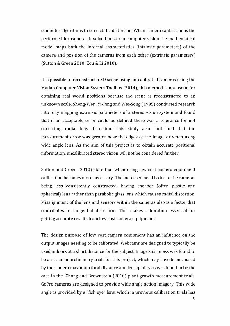
Figure 4.3 Result of synchronization trial 1 with two GoPro’s recording at 30fps
using a circuit controlled by Arduino to light a series of LED’s............................ 32
Figure 4.4 Initial design for camera mounting apparatus. ..................................... 34
Figure 4.5 Final camera mounting design .................................................................... 35
Figure 4.6 Sample of calibration images from dynamic trials .............................. 37
Figure 4.7 Accepted calibration pattern positions from the initial dynamic
trials. ............................................................................................................................................ 39
Figure 4.8 Reprojection errors from accepted calibration image pairs from the
initial dynamic trials. ............................................................................................................ 39
Figure 5.1 Image showing part of the scene from static test 1. ............................ 42
Figure 5.2 Backing board from Static test 1 with the actual vs calculated aim
result. .......................................................................................................................................... 42

Figure 5.3 Layout of the scene used during the static trials .................................. 43
Figure 5.4 RGB segmentation of the scene from Static Trial 1 showing the
threshold limits from the Matlab Color Thresholder App ...................................... 47
Figure 5.5 Visual representation of the three colour channels in the HSV colour
space (Image Processing Toolbox 2014). ..................................................................... 47
Figure 5.6 HSV segmentation of the scene from Static Trial 1 showing the
threshold limits from the Matlab Color Thresholder App ...................................... 48
Figure 5.7 Point cloud from Static Trial 1 plotted in 3D rotated to show the
noise in depth measurement of the gun. ....................................................................... 51
Figure 5.8 Point cloud around gun showing with the gun markers highlighted
....................................................................................................................................................... 51
Figure 5.9 schematic of the pixels used to get the average real world position
of the gun markers and the target. .................................................................................. 52
Figure 5.10 Collated results from the static trials showing the distribution of
calculated aim for the three methods used. ................................................................. 54
Figure 6.1 Layout of the scene used during the dynamic trials ............................ 57
Figure 6.2 Comparison of gun marker colour captured in static and dynamic
trials. ............................................................................................................................................ 57
Figure 6.3 Frame 4 of the test images with bounding boxes around areas that
were segmented as foreground. The red circle shows the target location. ..... 60
Figure 6.4 Frame 5 of the test images with bounding boxes around areas that
were segmented as foreground. The red circle shows the target location. ..... 60
Figure 6.5 Flow chart showing the background subtraction process created for
this project. ............................................................................................................................... 62
Figure 6.6 The stages the image sequences go through as part of
GetTargetLoc.m. From left to right – original pixels, subtracted and thresholded
pixels, pixels after noise filtering. .................................................................................... 62
Figure 6.7 Camera synchronization test circuit set to illuminate 10 LEDs in
1/60s showing the left camera leads the right in this trial by 0.2 frames. ...... 65
Figure 6.8 z distance the target was measured at the moment of firing vs the
frame synchronization. ........................................................................................................ 66
Figure 6.9 Modified diagram from figure 2.3 giving a showing the positional
errors created by frame synchronization errors. ...................................................... 67
Figure 6.10 Calculated miss distance vs approximate shot cloud location
around target. .......................................................................................................................... 68
Figure 6.11 Point cloud from Dynamic Trial 1 showing the calculated aim vs
predicted target location. The target positions from the images are in red
circles, the predicted position as a red filled circle and the projected aim as a
green line. .................................................................................................................................. 69
Figure 6.12 z distance the target was measured at the moment of firing with
the use of pixel interpolation vs the frame synchronization. ................................ 73
Figure 6.13 Point cloud from Dynamic Trial 1 showing a result when the target
positions are interpolated to be closer to the shooter. The target positions from
the images are in red circles, the predicted position as a red filled circle and the
projected aim as a green line. ............................................................................................ 74
Figure 6.14 Point cloud from Dynamic Trial 5 showing a result when the target
positions are interpolated to be further from the shooter. The target positions
from the images are in red circles, the predicted position as a red filled circle
and the projected aim as a green line. ............................................................................ 74
Figure 6.15 Calculated miss distances with target position interpolated based
on frame synchronization vs approximate shot cloud location around target.
....................................................................................................................................................... 75
Figure 7.1 Scene from the trials vs human judges with the judges standing in
the locations that they would normally be to coach a new shooter. .................. 77
Figure 7.2 Calculated aim for final trials 1,4,5,6 where the judges all said the
shooter hit the target with the middle of his shot cloud. ........................................ 79

List of Tables
Table 4.1 Comparison of Camera Specifications ........................................................ 28
Table 4.2 Summary of results from synchronization testing of stereo Microsoft
LifeCam Studio webcams. ................................................................................................... 31
Table 4.3 Summary of results from synchronization testing of stereo GoPro
Hero3 Black Edition Cameras. ........................................................................................... 32
Table 5.1 Average error for each of the methods of aim calculation ................. 54
Table 6.1 Movement in blob centroids in the x direction measured in pixels
between each of the frames from the right camera in dynamic trial 1. ............ 70

1
Introduction
1.1 Background
Shotgun shooting as a competitive sport dates back more than 200 years, with
its origins based in entertainment for English aristocracy. The earliest
documented competition can be found in the Sporting Magazine (1793) where
the competition, shooting etiquette, dimensions of the layout and live pigeon
traps were described in detail.
Figure 1.1 Earliest known illustration of competitive shotgun shooting (Sporting Magazine 1793).

2
Shooting trapped birds for sport has been banned in most western countries
including the United Kingdom and Australia, which gave rise to modern clay
target shooting (also known as “clay pigeon shooting”). Modern Clay target
shooting still shares much terminology with its ancestor including the targets
are often referred to as pigeons, the machine that throws the target is referred
to as the trap, throwing a target is referred to “releasing a bird” from the trap,
and to request a target to be released the shooter calls “pull” which comes from
pulling a string to open the pigeon trap. Even though today most shotgun
shooters have never shot a trapped bird, the sport retains these traditions.
With the rise in popularity of clay target shooting comes the challenge of
teaching a large number of new shooters. Typically when a new shooter starts
they are coached on their stance and after each shot given feedback on how
they should alter their lead for the next shot. This method is successful if the
shooter isn’t feeling too overwhelmed with all the things they are being told
and if the coach is giving accurate feedback. With the large number of new
shooters, experienced shooters are in high demand and are often trying to
coach while they are also shooting a round of targets, which leads to
distraction. Distracted coaching leads to vague feedback and slower progress
for new shooters.
For the purpose of this project, targets trajectories were designed to
approximate those thrown from the low house in an American skeet
competition when the shooter is located on station 2 (
Figure 1.2). The skeet targets are thrown from a mechanical thrower across in
front of the shooters at around 22 m/s (National Skeet Shooting Association
2015), which requires the shooter to lead the target in order to hit it. The
distance the target is required to be led changes with its position within its
flight path and the ammunition that is being used. Previous experience guides
the shooter on the lead required for each shot.

3
Ce
nte
r Lin
e
36.8m
High Tower Target
Flight Path
19.2
m
Low Tower Target
Flight Path
Low Tower High Tower
Station 2
Figure 1.2 Skeet field layout which was used for target throw angles in the field trials (Redrawn from Australian Clay Target Association 2014).
The typical method of coaching clay target shooting has changed very little
since the sport began. In order to provide feedback an experienced shooter,
watches for a small plastic piece of the shotgun shell, called a “wad”, as it flies
through the air, trailing the pellets.
Typically verbal feedback is given describing the shot as “over”, “under”,
“behind” or “in front” with an approximate distance. This feedback is difficult
to visualize for the new shooter, it is unlikely to be anything more than
moderately helpful, to someone who is already overwhelmed by the new skill.
1.2 Project Aim
The benefits of an automated tool to give accurate feedback after a missed
target has been an idea that the author has considered for many years. This
dissertation aims to determine the feasibility of computer vision using low cost
“off-the-shelf” (OTS) camera equipment to give feedback to a clay target
shooter as a coaching tool.

4
Completion of this project needed design effort in two parts that work together
and provide the feedback. Hardware to capture the stereo imagery and a
software component to process the images then feedback shooters accuracy.
As this study focuses on feasibility of use, there is no requirement for real-time
processing of the images or a commercialized solution.
1.3 Research Objectives
To be feasible, the system should have comparable accuracy to experienced
clay target coaches and show that with further effort, a commercialized version
could be made some time in the future. If these objectives can be met the
system will be shown to be feasible.
To test the feasibility, the project can be split into the following key tasks:
Carry out a review of literature that is relevant to low cost stereo
computer vision technology in clay target coaching and shotgun
ballistics;
Select, trial and compare a range of low cost cameras that could be used
in stereo-vision;
Write program to perform stereo camera calibration. Analyse the
results of the calibration to determine inaccuracies and other factors
that may affect the outcome of the testing;
Design and perform static trials to establish measurement accuracy in a
static situation including the positon of a target and a shooters aim;
Design and perform dynamic trials gathering and using data from live
shooting to determine the distance the shooter misses;
Perform dynamic testing against experienced coaches to be able to
compare the results of the computer vision to the current method of
miss estimation.

5
Investigation of the following tasks will be dependent on available time:
Optimize the image processing program from coach feedback;
Create external circuitry to sense the gun shot and give a visual
indication of when the gun was fired between the frames and camera
synchronization at the moment of firing;
Re-run trials of experienced coach’s vs computer vision system to judge
system accuracy improvements.
Once these steps are complete the use of low cost stereo computer vision
should have similar or better accuracy then human judges if it is to be feasibly
adopted for use. If the system has less reliability or accuracy then the judges it
will not be found to be a currently feasible.

6
Literature Review
The primary areas that have been researched for this project are: computer
vision techniques relevant to coaching clay target shooting, technology already
in use in shooting coaching, and shotgun ballistics.
2.1 Computer Vision in Sport Coaching
Technology has become a huge influence in sport as sports people look to gain
an advantage over their opponents. Computer vision, motion capture and
resultant models of the motion of athletes have become common in many
sports including rowing, weight lifting, golf, tennis (Luo 2013). Computer
vision and motion capture has given well documented positive improvements
in sporting performance (Fothergill, Harle & Holden 2008; Luo 2013; Tamura,
Maruyama & Shima 2014).
Animation is the industry where the technological envelope has been pushed
in motion capture. Animation traditionally has been able to do this because
lighting can be precisely controlled, extra weight carried on an actor is
tolerable and large budgets are common. When using motion capture to track
the motion of an athlete minimal extra weight should be worn on the subject.
Another factor that makes this more difficult is the effect of variable lighting
when outdoors. These restrictions typically limit sports tracking to two
methods; markerless and passive marker motion capture.
Employing teams of motion capture experts is currently too expensive to be
adopted by small clubs or individuals. As the required quality of the technology
7
that is required to perform the analysis becomes cheaper researchers have
been experimenting with low cost options for athlete feedback that could be
implemented by clubs. An example of this is the use of a Microsoft Kinect
camera to capture the motion of a novice baseball pitcher to give automated
feedback(Tamura, Maruyama & Shima 2014). This system, whilst being low
cost, provided large improvements in pitching technique for the subjects.
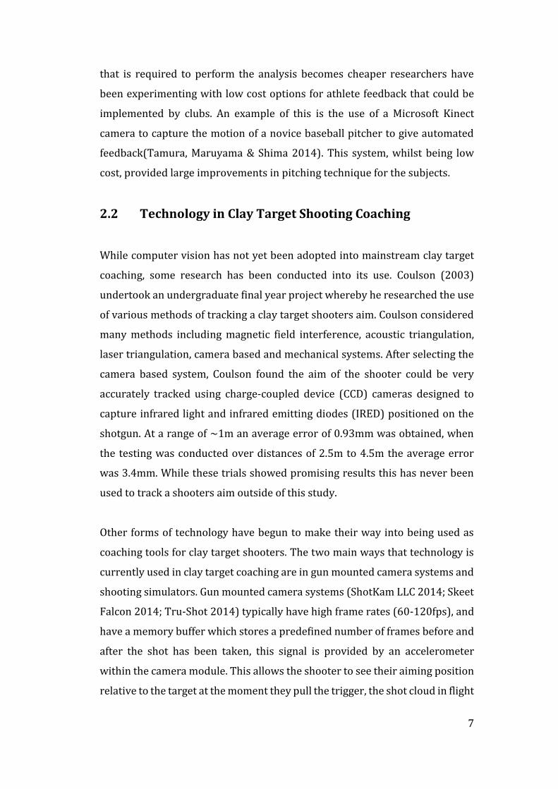
2.2 Technology in Clay Target Shooting Coaching
While computer vision has not yet been adopted into mainstream clay target
coaching, some research has been conducted into its use. Coulson (2003)
undertook an undergraduate final year project whereby he researched the use
of various methods of tracking a clay target shooters aim. Coulson considered
many methods including magnetic field interference, acoustic triangulation,
laser triangulation, camera based and mechanical systems. After selecting the
camera based system, Coulson found the aim of the shooter could be very
accurately tracked using charge-coupled device (CCD) cameras designed to
capture infrared light and infrared emitting diodes (IRED) positioned on the
shotgun. At a range of ~1m an average error of 0.93mm was obtained, when
the testing was conducted over distances of 2.5m to 4.5m the average error
was 3.4mm. While these trials showed promising results this has never been
used to track a shooters aim outside of this study.
Other forms of technology have begun to make their way into being used as
coaching tools for clay target shooters. The two main ways that technology is
currently used in clay target coaching are in gun mounted camera systems and
shooting simulators. Gun mounted camera systems (ShotKam LLC 2014; Skeet
Falcon 2014; Tru-Shot 2014) typically have high frame rates (60-120fps), and
have a memory buffer which stores a predefined number of frames before and
after the shot has been taken, this signal is provided by an accelerometer
within the camera module. This allows the shooter to see their aiming position
relative to the target at the moment they pull the trigger, the shot cloud in flight

8
and a replay the moment of impact to see if it hit cleanly or if the
top/bottom/front/back was more smashed to give shooter feedback. These
systems are good for experienced shooters or shooters being coached by an
experienced shooters as they require knowledge of lead distances to give
useful feedback.
Simulated shooting environments have been used in clay target coaching. The
methods of aim tracking and simulated environment vary with each system.
The ST-2 Shooting simulator (Marksman Training Systems AB 2014) projects
a 2D scene onto a large screen and uses a combination of gun mounted
accelerometers and forward facing camera to give the aim of the gun to the
simulated environment that is detailed in the US Patent 5991043 (Andersson
& Ahlen 1999). This has the advantage of being able to use your own gun and
automated feedback about shooter accuracy. The extra weight of the camera,
accelerometer and a cable for data transmission would affect the ability to
swing the gun. ShotPro 2000 (TROJAN Aviation 2000) uses a modified shotgun
cartridges which are used in the gun to project a laser beam onto the screen
which is picked up by a camera to determine the gun aim at the moment of
firing. This is similar to the much lower budget system DryFire (Wordcraft
International 2014) which projects a laser spot onto a wall and the camera
picks up a laser beam projected from a modified shotgun cartridge at the
moment of firing. All of these systems use a 2D targeting surface which while
does not accurately represent the actual shooting, these systems have all been
used by shooters and claim to provide good shooter improvements.
2.3 Stereo Camera Calibration
The calibration of camera equipment is something that has been studied for
many years. In the 1950’s through to 1970’s much of the effort was around the
calibration of expensive film based camera equipment used in aerial mapping
(Clarke & Fryer 1998). Now as the use of digital photography has become the
norm, the majority of the research on camera calibration has turned to using
9
computer algorithms to correct the distortion. When camera calibration is the
performed for cameras involved in stereo computer vision the mathematical
model maps both the internal characteristics (intrinsic parameters) of the
camera and position of the cameras from each other (extrinsic parameters)
(Sutton & Green 2010; Zou & Li 2010).
It is possible to reconstruct a 3D scene using un-calibrated cameras using the
Matlab Computer Vision System Toolbox (2014), this method is not useful for
obtaining real world positions because the scene is reconstructed to an
unknown scale. Sheng-Wen, Yi-Ping and Wei-Song (1995) conducted research
into only mapping extrinsic parameters of a stereo vision system and found
that if an acceptable error could be defined there was a tolerance for not
correcting radial lens distortion. This study also confirmed that the
measurement error was greater near the edges of the image or when using
wide angle lens. As the aim of this project is to obtain accurate positional
information, uncalibrated stereo vision will not be considered further.
Sutton and Green (2010) state that when using low cost camera equipment
calibration becomes more necessary. The increased need is due to the cameras
being less consistently constructed, having cheaper (often plastic and
spherical) lens rather than parabolic glass lens which causes radial distortion.
Misalignment of the lens and sensors within the cameras also is a factor that
contributes to tangential distortion. This makes calibration essential for
getting accurate results from low cost camera equipment.
The design purpose of low cost camera equipment has an influence on the
output images needing to be calibrated. Webcams are designed to typically be
used indoors at a short distance for the subject. Image sharpness was found to
be an issue in preliminary trials for this project, which may have been caused
by the camera maximum focal distance and lens quality as was found to be the
case in the Chong and Brownstein (2010) plant growth measurement trials.
GoPro cameras are designed to provide wide angle action imagery. This wide
angle is provided by a “fish eye” lens, which in previous calibration trials has

10
been shown to have a very large amount of radial distortion (Rahman &
Krouglicof 2012; Shah & Aggarwal 1996; Shi, Niu & Wang 2013). While both
low cost camera systems present their own set of challenges, each have also
showed that accurate measurements are able to be made after calibration.
The process of finding the mathematical calibration model using a computer
has been made easier by algorithms having been written that take multiple
images with predefined patterns and compute the distortion values. The
algorithms that compute the parameters have been described in many papers
including Heikkila and Silven (1996); Meng and Hu (2003); Rahman and
Krouglicof (2012); Shah and Aggarwal (1996); Wang et al. (2008), these
methods of calibration have been tested and shown to give accurate calibration
results. The camera calibration toolbox in Matlab uses a printed checkerboard
pattern to calibrate camera’s (Computer Vision System Toolbox 2014). This
toolbox has been used with webcams, gopro cameras and higher cost cameras
providing excellent results (Fetic, Juric & Osmankovic 2012; Lü, Wang & Shen
2013; Page et al. 2008; Poh & Poh 2005; Schmidt & Rzhanov 2012; Shi, Niu &
Wang 2013; Sutton & Green 2010; Zou & Li 2010). Matlab provides the user
friendly workflow and accurate interface to calculate the camera parameters
to use in image rectification.
2.4 Object Detection Methods
Measuring the position of a target across multiple frames and determining the
targets position, direction and velocity is common in computer vision
applications. As the trial software will be written in Matlab, the research into
object detection and tracking will focus on methods that are available within
the Matlab Computer Vision toolbox and Image Processing toolbox (Computer
Vision System Toolbox 2014; Image Processing Toolbox 2014).
In this project there are three key points of interest that will be searched for,
they are; the two visual markers on the gun and the clay target. The Matlab

11
Suite contains many functions that will assist in identifying these points, in the
sections below we will look at some of the features that will be able to be used.
2.4.1 Object Detection Using Target Colour
To track the shooters aim markers will be placed on the gun as per the previous
research completed on shotgun aim tracking (Coulson 2003), using a form of
motion capture with markers on the gun. The markers for the gun in study can
be made a colour that contrasts the background to achieve a similar effect as
the infrared markers used by Coulson. The clay targets that have been selected
to be used in this trial will be florescent orange as this will help them to
contrast the background and will not need additional markers added.
This method of image segmentation can be performed on an image in any
colour space but typically an image is converted from RGB (Red, Green Blue)
to HSV (Hue, Saturation, Value) colour space to isolate the colour component
of each pixel and simplify the computation to reduce search time(Liu et al.
2012). Yang et al. (2012) describes the process of the segmentation as the
process of converting the image to binary by checking each pixel against a
threshold and converting the pixel to a 1 if it is above the value and 0 if it is less.
This has been used for purposes such as skin tone identification (Kramberger
2005), for motion capture marker tracking (Ofli et al. 2007) and automated air
hockey and table tennis interception machines (Kawempy, Ragavan & Khoo
Boon 2011; Liu et al. 2013; Zhang, Xu & Tan 2010), which show that it is an
effective method of isolating the regions of interest when that area of interest
has a contrasting colour from the back ground.
The Matlab Color Thresholder App allows the user to segment an image based
on pixel colours (Image Processing Toolbox 2014) and work on an image in
various colour spaces to isolate the relevant features. Once a workflow has
been defined it can be included into the main Matlab program to be a part of an
automated process. The Matlab Image Processing Toolbox Users Guide shows
many examples of the colour segmentation using these processes the gun

12
markers and clay target should be able to be segmented form the background
image.
2.4.2 Object Detection Using Target Motion
Measuring the position of an object through multiple sequential frames is a
common task in stereo computer vision. Once the target object is isolated from
the back ground the targets position and velocity can be determined. When the
object to be tracked is moving and the back ground is relatively static, such as
tracking an air hockey puck on moving on a table, background subtraction has
been shown to be an effective process to segment the object from the
background (Kawempy, Ragavan & Khoo Boon 2011).
Early background subtraction processes compared one frame with a static
model that had been built during the initialization process. More recently
researchers have focused on background modelling that adapts the
background to eliminate artifacts caused by changes in lighting and slight
background movement(Stauffer & Grimson 1999). Adaptive/Dynamic
background modelling help with reducing the artifacts caused by changes in
lighting, repositioning of the camera and background movements (Desa & Salih
2004; Stauffer & Grimson 1999; Yin et al. 2013; Zhang & Ding 2012). Figure 2.1
shows the process where background adaptation occurs through an in build
feedback path within the algorithm. This model averages the background
across many images to give a model that is close to the current scene.
Commonly there are two ways that the foreground is determined through
background subtraction. The two methods differ in the way that they regard
the pixels for comparison; the first method the pixels are considered
individually without considering the influence of the others around them and
Gaussian Mixture Method (GMM), which is the most common considers the
clusters of pixels and their interactions to get a more reliable result (Yin et al.
2013). Other methods have been considered but are not widely adopted.

13
Pre-
treatment
Moving
object
detection
Input image
Tracking
moving
objects
After -
Processing
Updated
Background
Image
Figure 2.1 Process of adaptive background subtraction (Zhang & Ding 2012)
Experimental results from show that the results of the background subtraction
can be noisy due to artifacts from slight movements in the background or slight
lighting changes (Desa & Salih 2004; Zhang & Ding 2012). Figure 2.2 shows that
images with artifacts causes by minor disturbances in lighting or background
movement can have a filter applied to de-noise the output ready for further
processing.
Figure 2.2 An example of background subtraction with a natural background causing background movement artifacts and the result of using a de-noising process after background subtraction(Desa & Salih 2004).

14
The Matlab Computer Vision toolbox supports background subtraction with
adaptive background modelling. Using the vision.ForegroundDetector object
the background and foreground can be segmented using GMM. Once this is
completed for an image much of the erroneous data has been removed making
the next operations on the images less computationally expensive because the
areas that are not of interest have been excluded.
2.5 Positional Measurement Using Stereo Computer Vision
The use of stereo imagery to obtain measurements and find an object’s real
world position is a fundamental goal of machine vision. Camera calibration and
object detection methods exist so that the position or size of the correct object
can be accurately measured. Now after many years of development software
packages such as OpenCV (OpenCV 2015) and Matlab (Computer Vision
System Toolbox 2014) provide prebuilt computer vision tools to streamline
the process.
yz
x
Reference Coordinates
x
y
x
y
Object Position
P(x,y,z)
Right Camera
Plane
Left Camera
Plane
Left Camera
Lens Center
Right Camera
Lens Center
Left Camera
Optical Axis
Right Camera
Optical Axis
Focal Length
Baseline Distance
Figure 2.3 Diagram showing a stereo camera setup and how the disparities between the images can be used to give an objects location (Reproduced from Kang et al. 2008).

15
Using the rectified images and extrinsic parameters of the cameras the real
world position of an object can be computed by examining where that object
appears in pictures taken simultaneously. Figure 2.3 shows a schematic which
is of how the position of the object in the images is used to find its real world
position. (Kang et al. 2008; Liu & Chen 2009; Lü, Wang & Shen 2013) explain
this process in their conference papers and discuss the use of the disparity
mapping to use trigonometry to obtain very accurate measurements of real
world position.
2.6 Accuracy of Positional Measurement Using Low Cost
Stereo Vision
For the real world position of the object to be as accurate as possible many
factors need to be controlled to provide an accurate outcome.
The theoretical accuracy of these measurements depends on the resolution of
the camera and the baseline distance the cameras are positioned from each
other (Kang et al. 2008; Liu et al. 2013; Lü, Wang & Shen 2013). With a wider
baseline or larger camera resolution, the disparity between the images is
greater and more pixels are crossed per unit of length providing higher
precision of measurement. This is shown diagrammatically in Figure 2.3.
Camera synchronization is a factor that contributes to the accuracy of
positional measurement of an object in motion. If the cameras are out of sync
the object will move between when the first can second camera capture the
images and the disparities will be inaccurate(Bazargani, Omidi & Talebi 2012).
Typically stereo vision camera use cameras that are triggered by external clock
pulse to keep them synchronized (Liu et al. 2013) but low cost camera
equipment such as webcams are not designed to allow this.
From the various studies that have been reviewed the accuracy of the
measurement using low cost camera equipment has been promising.
16
Accuracies of ±0.5% (Pohanka, Pribula & Fischer 2010)to ±2.31% (Kang et al.
2008) error rates have been found. While these studies focus on much shorter
distances (<1m) with baseline distances of 10-15cm, Liu and Chen (2009)
measures distances out to 7.5m finding a 3.79% error using a 15cm baseline.
Accuracy to this margin of error could be improved, as Liu and Chen (2009)
proposed that much of this error was due to image matching errors and slight
inaccuracies of the baseline distance.
2.7 Low Cost Camera Synchronization
To be able to accurately measure the position of a moving object, the images
used need to be synchronized. Time delays caused by asynchronous stereo
images causes large errors in the positional measurement in fast moving
objects (Alouani & Rice 1994). The time delay between the images results in
the object moving between the moments the images are captured and the
disparity between the two images being incorrect.
Synchronization of low cost camera equipment is difficult to achieve and due
to this research has been conducted into algorithms that correct for errors in
asynchronous stereovision. In a research paper by Chung-Cheng et al. (2009)
it was found that depth estimation for vehicle hazard detection could be
achieved using an asynchronous stereovision system, this study focused on the
searching module of the algorithm and looking for features to match in
adjacent line to reduce matching error. This paper doesn’t propose a solution
to the depth mapping error due to out of sync images.
Bazargani, Omidi and Talebi (2012) proposed a solution to reduce the disparity
error caused by asynchronous stereovision. In this solution an adaptive
kalman filter was proposed that models the objects movement within each
image plain and compensates for the delay in timing by effectively
interpolating the position of the object. This was shown to provide a much
more accurate calculation that object position than unfiltered images.

17
In previous USQ undergraduate project completed by Cox (2011) tested the
used of low cost stereo vision using webcams. This project use two basic
webcams were calibrated and were able to be used to accurately reconstruct a
scene and obtain a depth map. As part of this project only static scenes where
analysed so synchronization issues where not encountered or considered.
2.8 Shotgun Projectile Motion
As part of modelling the accuracy of a shooter, to determine the distance that
the centre of their shot was from the target a mathematical description of the
velocity of the shot must be obtained. This formula will be the basis of the
calculation of the distance the shooter’s aim should have been leading target at
the moment of firing.
2.8.1 Shot Velocity
Information is readily available about the characteristics of rifle ammunition
throughout its flight. Large manufacturers provide online ballistics calculators
to assist rifle shooters to get estimations of the projectiles velocity, drop, wind
drift and impact energy at various distances down range(Federal Premium
Ammunition 2015a; Winchester 2015a). This data is relatively easily
calculated once the parameters for the air the projectile passes through and the
projectile shape and weight are entered into a computational fluid dynamics
(CFD) model (Davidson, Thomson & Birkbeck 2002). Determining the behavior
of the projectiles in a shot cloud is made more difficult by the interaction of the
projectiles while in flight and the deformation of the spheres caused by the
forces in the barrel(Compton, Radmore & Giblin 1997).
The muzzle velocity of all common commercially available shotgun shells are
advertised on the packaging and the manufactures website (Bronzewing
Ammunition 2013; Federal Premium Ammunition 2015b; Winchester 2015b).

18
As part of this study Winchester was asked if they could provide test data from
some of their commonly available cartridges as their cartridges could be used
and test data would be available to base the formula for the ballistics
calculation but they declined as they regard this information as their
intellectual property (Wilson 2015). An Australian shotgun shell
manufacturer, Bronzewing was able to provide their SAAMI test data for their
“Trap” target shotgun shells in sizes 7-1/2, 8 and 9 (Gibson 2015). Bronzewing
ammunition will be used in the dynamic testing in this project, so the empirical
test data from the shells being sued can be compared to the mathematical
model ensure the calculated flight times are as close as accurate as possible.
Empirical test data that has been collected in many past studies and is available
to shooters. Publications such as The Modern Shotgun: Volume II: The
Cartridge (Burrard 1955) has tables for most common shot sizes and through
common choke sizes at various distances. This gives most shooters all the
information that they need without complex calculations.
Mathematical models for the ballistics of shot clouds have been obtained from
Burrard (1955), Chugh (1982) and Compton, Radmore and Giblin (1997) each
of these use a ballistics coefficient that is dependent on the shot properties and
environmental factors. Both of these models claim it accurately match
empirical test data for a range of shot sizes and shot material densities but on
inspection both of these papers are missing key data to create a useful model
from their research. The research paper published by Chugh (1982) is vague
about units for the input parameters and as a result no model has been able to
made that matches the empirical test data obtained through Bronzewing or
Burrard (1955). Compton, Radmore and Giblin (1997) is an investigation and
statistical analysis of the behavior of a shot cloud and the formulas used
contain a “random force” which leads to a normal distribution of results when
modelled.
To obtain a simple function that can be used in estimating flight time of a shot
cloud for this project. Matlab can be used to fit a function to the empirical test

19
data from Burrard (1955). Figure 2.4 shows the empirical test data compared
to the quadratic function (Equation 2.1) function in fitted
v = 0.1179x2 − 21.5831x + 1205.5 (2.1)
where
v is velocity (𝑓𝑡/𝑠−1)
x is displacement (Yards)
The function provided by fitting the Burrard test data also closely fits the
Bronzewing test data, so this method will be able to be used to get a function
of time vs distance.
Figure 2.4 Empirical test data vs the fitted mathematical function.
After converting the distances in the test data, the function that can be obtained
from Burrard (1955) for the relationship between distance and time is can be
seen in Figure 2.5 where the plotted line is the function
t = (62.08 × 10−6)x2 + (1.833 × 10⁻³)x + 3.132 × 10⁻³. (2.2)

20
where
t is time (s)
x is displacement (m)
Figure 2.5 Time vs Distance for empirical test data vs fitted mathematical function.
2.8.2 Pattern Spread
The interaction of the pellets within a shot cloud is highly complex and research has
shown it expand in diameter with time/distance within a range of values. Many
researchers such Compton (1996) and Compton, Radmore and Giblin (1997) have
used statistical averages to produce models of the diameter of a shot cloud over
time/distance. This information would be helpful for predicting hit or missed targets,
as this study is measuring the centre of the pattern vs centre of the target the shot
cloud diameter will not be considered further.

21
Methodology
This chapter documents the approach that was taken to develop, execute and
evaluate the use of low cost computer vision equipment to provide feedback in
clay target coaching. This chapter contains the project methodology, a
summary of the project risks, and project timeline.
3.1 Project Methodology
To be able to fulfil the objectives outlined in section 1.3, the project was broken
down into 7 main sub tasks:
1) Determination of low cost camera equipment suitability for tracking
fast moving objects.
2) Stereo webcam mounting and baseline distance assessment.
3) Stereo camera calibration routine.
4) Identify and measure the position of clay target and gun markers.
5) Calculate the accuracy of a shot taken by a shooter.
6) Conduct trial of computer program vs the human judges and evaluate
results.
7) Optimize Matlab program

22
3.2 Task Analysis
3.2.1 Determination of Low Cost Camera Equipment for Tracking
Moving Objects.
This stage of the project will involve comparing stereo webcams against the
more expensive option of stereo GoPro cameras. Criteria for this comparison
are camera synchronization, resolution, and frame rate. After the testing is
complete the appropriate camera equipment will be selected and used in all
subsequent steps.
3.2.2 Stereo Camera Mounting and Baseline Distance Assessment.
As part of this phase of the project an appropriate baseline distance will be
determined for the camera mounting. The distance between the cameras will
be maximized to increase accuracy but close enough the pixel disparities are
not be too great to be matched.
Design of the camera mounting apparatus will optimize the stability of the
cameras to avoid vibration and movement caused by the wind or other
environmental factors. The apparatus should rigidly mount both cameras, in
positions that can be repeated so the testing is similar in all the trials.
3.2.3 Stereo Camera Calibration Routine.
Camera calibration is crucial to the accuracy and therefore the success of this
project. The workflow for this is based around the procedure from the Matlab
Stereo Calibration documentation with specific details further defined where
relevant to the project.
To ensure accurate results the calibration process will be completed each time
the camera apparatus is assembled. This process will also be repeated if the
cameras are moved in any way that could affect the extrinsic parameters.

23
3.2.4 Identify and Measure the Position of Target and Gun Markers
The initial field trials will be kept as simple as possible with the target being
mounted at a fixed point, reducing errors due to camera synchronization as
much as possible. To do this the static target and gun markers will be
segmented from the background based on their colour. Once their position is
found within the images it will be used to calculate their real world position.
To get feedback on the accuracy of the static targets will be mounted on a
backing material that will show the where the shot hit the target. The post and
target position will be moved to various positions along the flight path of the
clay target, with the height varied to simulate different target locations.
3.2.5 Calculate the Accuracy of a Shot Taken at a Moving Target.
This phase of the project will involve recording the target being shot in real
time and building a program to estimate the accuracy. Many trials were
recorded but only the 10 most accurate shots will used in the program
development. From these 10 trials a program will be developed to estimate the
distance the centre of the shot cloud is from the target as it passes.
Accuracy feedback will be given in “x” and “y” distances from the centre of the
target to the centre of the shot cloud as it passes the target. Camera
synchronization will measure in each recording to determine its effect on the
accuracy and if poor synchronization could compensated for within the
software.

24
3.2.6 Conduct Trial of Computer Program vs the Human Judges and
Evaluate Results.
The final step to prove the feasibility of the project will be a trial of the
computer vs three experienced coaches from the Brisbane Sporting Clays Club.
Each of the judges will stand in the normal position to coach a new shooter, and
will record the distance they estimate the centre of the shot cloud passes the
target.
The trial will run for 10 targets, and none of the judges will compare notes on
the distances they observe. If a coach was is unsure of the result, none will be
recorded to eliminate guessing. Once the trial is complete the results from the
human coaches will be compared to the Matlab results. The accuracy of the
system and feasibility of low cost stereo computer vision will be determined
by the criteria set out in Section 1.3 of this report.
3.2.7 Optimize Matlab Program
As time permitted and methods were identified, the Matlab script was modified
to optimize its accuracy and step 6 was be repeated to get a more accurate
result.
3.3 Project Consequential Effects
3.3.1 Sustainability
The stereovision system that will be built as part of this project will have
negligible safety, environmental, social or economic impacts. Energy
consumption by the camera or computer will only be in line with what is
consumed in a small home office as no extra external lighting is required for
filming as the testing are conducted outside.

25
The trial phase of this project involves shooting at clay targets with a shotgun.
This has an environmental impact as lead shot is a pollutant and the shotgun
cartridges go to landfill. Avoidance of using lead shot isn’t feasible so the
number of shots taken in testing will be minimized wherever possible to
reduce pollution as per the Engineers Australia guidelines (Engineers Australia
2015).
3.3.2 Ethics
As an engineering project may present situations where professional
judgement is required, ethics must be a consideration in the planning of this
project. Engineers Australia provide a Code of Ethics (Engineers Australia
2010) that will be used to guide decisions made throughout the project
completion process. The code relates to demonstrating integrity, practicing
competently, exercising leadership and promoting sustainability. By using the
code of ethics the project outcome will benefit the community.
3.4 Risk Assessment
As part of the planning phase of this project a risk assessment has been
performed in alignment with the Work Cover (2011) guidelines. The risks that
have been assessed for this project have been categorized into two main
groups. The first group of risks are around personal and process safety. As part
of the risk assessment process, controls have been put in place make the
residual risk to as low as reasonably practicable.

26
3.4.1 Risks Identified
The two main safety hazards for this project are related to the use of guns while
performing testing tasks and the chance of hand or eye injury when setting up
tests.
1. Hand and eye injuries: To minimize the chance of a hand or eye injury
occurring gloves will be worn at all times when setting up field trials and
glasses will be worn at all times when at BSC as per their safety policy.
2. Gun injuries: The hazards that are related to gun use have only been able
to have their risk level reduced to medium due to the extreme
consequence if an incident does occur. The likelihood of this hazard
occurring is extremely low as the safety procedures and attitude to safety
around the BSC is excellent.
3.5 Project Timeline
The project schedule for this project is located in Appendix B.

27
Stereo Platform Development
This stage of the project involved comparing web cameras against the more
expensive GoPro action camera. From this comparison a decision was made
about the most appropriate cameras to be used in all subsequent steps. The
selection was primarily based on frame synchronization, frame rate and
resolution.
If the use of this technology is found to be feasible and real time processing will
be needed in the future for a commercialized design. Both of these camera
options have the ability to be linked with a computer for real time processing
through either USB or WIFI.
4.1 Camera Selection
Three camera models were considered for this project. They are the Logitech
C920 webcam, the Microsoft LifeCam Studio webcam, and the GoPro Hero3
Black Edition Action camera (GoPro). The first two webcams are top of the
range current models, whereas the GoPro is an older model that was released
in 2012. The GoPro is now able to be purchased second hand, bringing its price
down closer to the selected webcams.
4.1.1 Camera Properties Comparison
As a reference point in the comparison, the Bumblebee 2 stereo vision camera
from Point Grey was used. Point Grey are a market leader in digital cameras for

28
industrial and scientific applications, and the Bumblebee 2 is their lower cost,
purpose designed stereo vision camera.
Table 4.1 shows a comparison of some of the key features of the low cost
cameras compared to the Bumblebee 2 from Point Grey. From this comparison,
the low cost consumer cameras have the advantage in nearly every
specification with the exception of the shutter type. Having a global shutter is
important when accurately capturing images of fast moving objects, as the
entire image is captured at the same instant, rather than sequentially.
Table 4.1 Comparison of Camera Specifications
C920 LifeCam Hero3 Bumblebee 2
Price $119.00 * $99.00 *
RRP $539.95 (2012) Ebay $270 - $340 (2015) USD$2395 ^
Max Resolution/ Frame rate
1920 x 1080/ 30fps
1920 x 1080/ 30fps
4096 x 2160/ 15fps
1032 x 776/ 20fps
Max Frame Rate/ Resolution
30fps/ 1920 x 1080
30fps/ 1920 x 1080
240fps/ 848 x 480
20fps/ 1032 x 776
Shutter Type Rolling Rolling Rolling Global
Field of view 78o 75o W:176o,M:127o,
N:90o 43o
Focus Auto/ Software set
Auto/ Software set Fixed fixed
*Officeworks 15/12/14
^Choi (2015)
The Bumblebee 2 has image sensors securely mounted so they will not move
relatively to each other if the cameras are bumped. While this can be an
advantage as it reduces the need for camera calibration, it gives no flexibility
with baseline distance.
In preliminary trials, the Logitech C920 was found to have poor image
sharpness at distances >5m in bright lighting conditions. Figure 4.1 shows the
results of a test of both webcams in similar lighting conditions in an outdoor

29
scene. The LifeCam has superior image sharpness and the colours on the
Logitech appear to be washed out in bright light. As the Microsoft LifeCam
Studio also has a lower purchase cost, it will be selected for the synchronization
trials.
Figure 4.1 Comparison between Logitech C920(left) and Microsoft LifeCam Studio(right) images.
Figure 4.2 Comparison between GoPro images at various frame rates from 30fps to 240fps.

30
In preliminary camera trials the GoPro was found to have a reduction in colour
intensity at frame rates higher than 60fps. This is demonstrated in Figure 4.2,
where colored markers have been added to the forestock of a shotgun and held
up for the camera. This footage also showed a reduction in brightness of the
clay targets in the thrower in the background at the higher frame rates.
4.1.2 Camera Synchronization
The Bumblebee from Point Grey uses a system where an external clock signal
is generated, driving both cameras simultaneously, keeping them perfectly
synchronized. When the cameras are synchronized in this way they are defined
as being “genlocked” or “generator locked”. This section investigates if this
level of synchronization can be achieved from these consumer video grade
cameras.
Webcam Synchronization Testing
The literature review for this project gave several examples of stereo webcams
being used to capture video with OpenCV. As the image processing for this
project has been completed in Matlab the video for synchronization testing was
initially captured using the Matlab Image Acquisition Toolbox.
The performance of stereo video acquisition with two webcams using the
Matlab Image Acquisition Toolbox was found to be very poor, and inadequate
for the project needs. The fastest frame rate that was able to be achieved when
recording through Matlab was ~3fps, with 0.11s delay between frames. By
recording outside of Matlab, both of the cameras are were able to record at
their full rated speed of 30fps, with a maximum time between frames of
0.01667 seconds, which is half the period of the frame rate.
To judge the synchronization error of the stereo system a circuit was created
to illuminate 10 LEDs sequentially then turn them off in the same order. The
LED board from this circuit is shown in Figure 4.3, and the second red LED from

31
the left is lit so the circuit set to 30fps mode. These modes change the frequency
the LEDs progression through their sequence, in 30fps mode the LEDs change
condition every 1/300 of a second. This board also has buttons to change mode
and start/stop the flashing. Full details of the code to run this board can be
found in Appendix F.
. Table 4.2 shows a summary of the results of synchronization testing of stereo
Microsoft LifeCam Studio webcams. Results of synchronization trials showed
the delay between frame acquisitions for stereo webcams to have a high
degrees of variation which is to be expected with two separate cameras being
started manually. The full results from these trials is available in Appendix C.
Table 4.2 Summary of results from synchronization testing of stereo Microsoft LifeCam Studio webcams.
Min delay Max Delay Average Delay
Frame Rate Frames/Seconds Frames/Seconds Frames/Seconds
30fps 1.1 f 0.037 s 35.3 f 1.177 s 6.3 f 0.210 s
The delay between starting times varied quite a lot, which was contributed to
the attention of the user starting the cameras. This delay could be reduced if
required and made to be more consistent for the field trials. Alternatively an
additional circuit could be built to flash LEDs, enabling frames to be matched
in post processing.
GoPro Synchronization Testing
The GoPro cameras came with built in Wi-Fi capability that allows
communication with a remote control. The Wi-Fi remote allows multiple
cameras to be started and stopped wirelessly with a single button press, which
is convenient for field trials when trying to ensure the cameras are not bumped
after the calibration process is complete. Anecdotal evidence was found on
online forums, with some users suggesting that they have achieved good
synchronization between GoPro cameras using the Wi-Fi remote, some even
suggested genlocked quality synchronization.
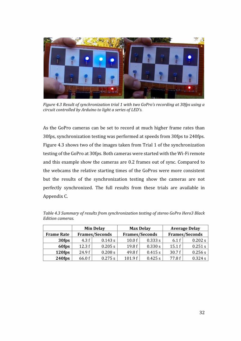
32
Figure 4.3 Result of synchronization trial 1 with two GoPro’s recording at 30fps using a circuit controlled by Arduino to light a series of LED’s.
As the GoPro cameras can be set to record at much higher frame rates than
30fps, synchronization testing was performed at speeds from 30fps to 240fps.
Figure 4.3 shows two of the images taken from Trial 1 of the synchronization
testing of the GoPro at 30fps. Both cameras were started with the Wi-Fi remote
and this example show the cameras are 0.2 frames out of sync. Compared to
the webcams the relative starting times of the GoPros were more consistent
but the results of the synchronization testing show the cameras are not
perfectly synchronized. The full results from these trials are available in
Appendix C.
Table 4.3 Summary of results from synchronization testing of stereo GoPro Hero3 Black Edition cameras.
Min Delay Max Delay Average Delay
Frame Rate Frames/Seconds Frames/Seconds Frames/Seconds
30fps 4.3 f 0.143 s 10.0 f 0.333 s 6.1 f 0.202 s
60fps 12.3 f 0.205 s 19.8 f 0.330 s 15.1 f 0.251 s
120fps 24.9 f 0.208 s 49.8 f 0.415 s 30.7 f 0.256 s
240fps 66.0 f 0.275 s 101.9 f 0.425 s 77.8 f 0.324 s

33
Conclusion
After the completion of the camera comparison and the synchronization
testing, the GoPro system was selected to be used in all future parts of this
project. The GoPro cameras can:
Record in the same resolution as the webcams at twice the frame rate,
resulting in the same number of pixel locations with half the maximum
frame timing error.
The GoPros also have the advantage of using a WiFi remote to start and
stop which reduced the possibility of effecting the calibration.
The WiFi remote is also a convenient way to control the cameras without
help from an assistant.
4.2 Camera Mounting
The camera mount design for this project was an iterative process. The initial
design was created and then, as software limitations were discovered
throughout the calibration process and initial attempts to conduct the static
trials failed, the design was modified.
4.2.1 Initial Design
The initial design for the camera mounting apparatus was based around the
principal explained by Kang et al. (2008) and in Figure 2.3; that having a wider
baseline distance gives more accurate positional results. The other factor that
was to be considered was that the cameras must be securely mounted to
ensure they would not move or the mounting material would not flex and effect
the extrinsic parameters.
With this in mind the baseline distance was maximized to what could be
reasonably transported and would keep the cameras rigidly mounted. A length
of 25x25x2mm Aluminum extrusion was mounted on a builders saw horse

34
with brackets at either end to hold the cameras in position with a baseline
distance of ~1200mm, which was the maximum that could be easily
transported. As per Figure 4.4 rubber bands were used to ensure that the
cameras could not move once they were in position.
While this design was found to be structurally sound, and was used to record
the first two attempts at static trials, no useable video was captured with that
camera configuration. When a disparity map was created from the images of
the scene it was discovered that Matlab will only match disparities of less than
64 pixels. This limitation within Matlab resulted disparity matched no closer
than 60m from the cameras.
With a baseline distance of 1200mm objects such as a shooter at around 4m
from the cameras had a pixel disparity of ~225 pixels and objects at around
15m such as the target, had a pixel disparity of ~90 pixels. This resulted in no
useable video from this attempt at static trials with this initial camera
configuration.
Figure 4.4 Initial design for camera mounting apparatus.

35
4.2.2 Final Design
The final design for the camera mounting apparatus is depicted in Figure 4.5.
By reducing the baseline distance between the cameras, smaller disparities
would be seen in the images overcoming the Matlab limitations. The new
smaller aluminum extrusion was able to be mounted on a camera tripod
making it easier to handle and transport. With the experience gained from the
initial design, it was concluded that the aluminum brackets that held the
cameras were not necessary. The rubber coating on the bottom of the GoPros
and with rubber bands holding them down was adequately secure. The
selected baseline distance for the trials was ~180mm as this has the cameras
as wide as they can be while having some safety factor in the pixel disparities
to ensure all of the important regions will have mappable disparities.
Figure 4.5 Final camera mounting design
4.3 Camera Calibration
During the literature review phase, reliable camera calibration was identified
as being vital to the accuracy of the field trials. To ensure the reliability of the
results, a calibration procedure was developed. This process was followed

36
each time the camera apparatus is assembled or the cameras were moved in a
way that could affect the extrinsic parameters.
The Matlab stereo camera calibration workflow was used as a starting point
for the development of the calibration process for this project. The six main
steps of prepare images, add images, calibrate, evaluate, improve, and export,
were used as a framework and expanded to make the process work
functionally for this project.
4.3.1 Prepare images
The preparation process for capturing calibration images was broken down
into three steps;
Prepare test pattern
Capture images
Pre-process images.
Test Pattern Preparation
Fetic, Juric and Osmankovic (2012) and Coulson (2003) detailed best practices
to attain optimal measurement accuracy using machine vision in their papers
on the topic.
Calibration images should be captured across the entire area that
measurements are to be taken.
In each calibration image as much as possible of the frame should be
covered by the calibration pattern, with full frame coverage in the series
of images.
To ensure accurate pixel mapping the calibration pattern should also be
mounted on a rigid backing to ensure it remains flat.
To enable measurements to be taken accurately at distances greater than 10m
a calibration pattern measuring 1170mm by 780mm was printed on A0 paper

37
and fixed to a sheet of MDF measuring 1200mm by 900mm and 16mm thick.
This ensured accuracy of the calibration pattern and ensured rigidity, as shown
in Figure 4.6.
Figure 4.6 Sample of calibration images from dynamic trials
Capture Images
The first attempt to capture calibration images was completed using the
GoPro’s still camera mode at 5 megapixel, as this was the closest resolution to
the resolution the trials were to be recorded in. It was later discovered that the
camera calibration output gives the intrinsic parameters of each camera as a
pixel map. This pixel map is used to transform the image and move each pixel
to its rectified position, to do this the calibration images must be the same
resolution as the trial recordings. To ensure that there was no camera
movement between calibration and trial recording the calibration images were
recorded in video at 60fps.
To ensure that the calibration images could be synchronized, an Arduino based
circuit was placed on the ground in front of the cameras. This allowed it to be
included in the bottom of the frame while it ran the code details in Appendix F
called “Calibration_flasher”. The purpose of this program is to flash some LEDs
with a period of 1.5s, which would allow images to be paired.
38
Pre-Process Images
Once the calibration video was captured the preprocessing of images contained
two-steps;
split the video into individual frames
select synchronized pairs for processing.
A Matlab routine was developed called SingleImSplit.m (Appendix G) to read
the videos, and write a series of .png files. The resultant images could then be
manually sorted and paired.
4.3.2 Add Images
The use of the Matlab Stereo Calibration App was found to be the best method
of finding calibration parameters. Using a manually coded script in Matlab was
less flexible and did not save any processing time. By adding around 50 stereo
pairs, good frame coverage with the calibration pattern after some of the pairs
had been rejected.
4.3.3 Calibrate
Calibration computing the skew and tangential distortion using two
coefficients was found to give the best calibration results for the GoPro images.
Using three coefficients gave the rectified images extreme distortion and was
unusable, even though the reprojection errors were computed to be smaller by
around 20%.
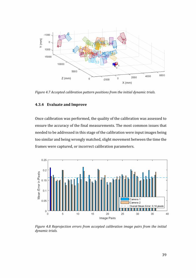
39
Figure 4.7 Accepted calibration pattern positions from the initial dynamic trials.
4.3.4 Evaluate and Improve
Once calibration was performed, the quality of the calibration was assessed to
ensure the accuracy of the final measurements. The most common issues that
needed to be addressed in this stage of the calibration were input images being
too similar and being wrongly matched, slight movement between the time the
frames were captured, or incorrect calibration parameters.
Figure 4.8 Reprojection errors from accepted calibration image pairs from the initial dynamic trials.

40
Accuracy was assessed by viewing the rectified images and ensuring they were
free from distortion. When inaccuracies were identified, the actions taken were
to remove image pairs with mean reprojection errors greater than 0.25 pixels,
removing image pairs causing matching errors, and ensuring calibrations
parameters were correct as per section 4.3.3. Figure 4.8 shows the results from
the camera calibration used in the initial dynamic trials.
4.3.5 Export
The camera calibration parameters were then saved as a .mat file to be loaded
by static and dynamic trial processing routines. This saved a large amount of
time over exporting the code as a function and have the camera parameters
recomputed each time they needed to be used.

41
Static Target Accuracy
As part of assessing the accuracy of low cost camera equipment in the
application of clay target coaching, getting an understanding of the impact of
the asynchronization is essential. To reduce the error cause by the random
delay between frame capture, testing was performed in a static scene to avoid
movement between frames.
5.1 Static Scene Capture
The static shooting scene was designed to approximate the shooting angles and
distances that would be seen on a skeet layout as per
Figure 1.2. Markers were added to the gun as per the passive marker motion
capture system discussed in the literature review.
5.1.1 Target Mounting and Shot Pattern Feedback
When setting up the scene so that movement could be minimized, a clay target
was mounted on a post with a backing of cardboard as can be seen in Figure
5.1. This not only held the target without movement but as seen in Figure 5.2
showed the exact location of the centre of the shot cloud as it hit the target.
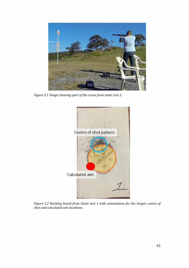
42
Figure 5.1 Image showing part of the scene from static test 1.
Figure 5.2 Backing board from Static test 1 with annotations for the target, centre of shot and calculated aim locations.
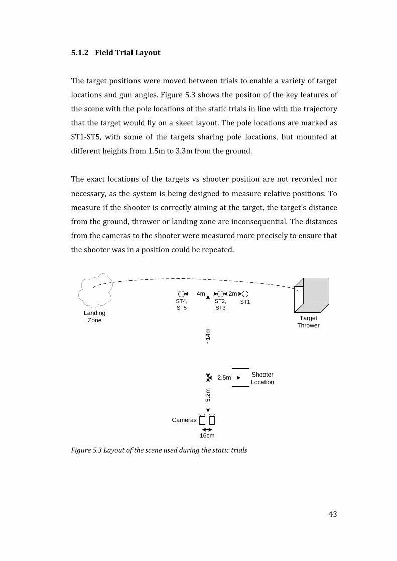
43
5.1.2 Field Trial Layout
The target positions were moved between trials to enable a variety of target
locations and gun angles. Figure 5.3 shows the positon of the key features of
the scene with the pole locations of the static trials in line with the trajectory
that the target would fly on a skeet layout. The pole locations are marked as
ST1-ST5, with some of the targets sharing pole locations, but mounted at
different heights from 1.5m to 3.3m from the ground.
The exact locations of the targets vs shooter position are not recorded nor
necessary, as the system is being designed to measure relative positions. To
measure if the shooter is correctly aiming at the target, the target’s distance
from the ground, thrower or landing zone are inconsequential. The distances
from the cameras to the shooter were measured more precisely to ensure that
the shooter was in a position could be repeated.
~1
4m
5.2
m
2.5m
16cm
Shooter
Location
Landing
Zone Target
Thrower
ST1ST2,
ST3
ST4,
ST5
4m 2m
Cameras
Figure 5.3 Layout of the scene used during the static trials

44
5.1.3 Gun Marker Colour
The colour of the markers on the gun were selected based on a colour that
would be unlikely to be found in the background of the image. This allowed for
easier segmentation of the image and more reliable results. High visibility
florescent orange was selected as the marker colour in earlier trials as there
are many self-adhesive products available. QuikStik self-adhesive labels from
Esselte were found to be the right size to be put onto the gun as they were as
wide is the barrels and were a good contrast against the background.
When the final static trials were recorded a new product was selected to enable
the markers on the gun to be different colours which would ensure that none
of the pixels were incorrectly matched between the two markers. Florescent
orange and pink duct tape was sourced for this purpose as both colours are not
normally seen in a shooting background and are very near each other on the
HSV colour spectrum.
5.1.4 Gun Marker Positioning
Inaccurate positioning of the markers on the gun was identified as an area that
could negatively affect the accuracy of the outcome of the trials. To ensure
consistency between the static and dynamic trials the gun markers were
aligned using the top of the upper barrel of the shotgun. Using the barrel as an
alignment tool allowed for consistent application of the stickers and maximum
accuracy.
As seen in Figure 5.1 the gun markers were positioned as far apart on the gun
as possible while still being able to be placed accurately. The “barrel marker”,
as it is referred to within the code was placed at the very end of the barrel, and
the “stock marker” was placed on the hinge between the barrels and the stock.
This resulted in the centres of the markers being 725mm apart, providing the
maximum accuracy that could be attained.
45
5.1.5 Initial Attempts
The initial attempts to capture usable images failed due to following an
incorrect image capture procedure. The learnings from these failed attempts
formed the basis for the image capture procedure used for the rest of the
project.
Key learnings from the failed trials were:
Calibration image resolution: As discussed in section 4.3.1, the first
attempt to capture usable images failed due to the calibration images
being taken in a different resolution to the trial images. This was rectified
by the calibration being captured in video and split into still images for
all subsequent trials.
Baseline distance: As discussed in section 4.2, the baseline distance
used in the second attempt to record the images for the static trials
caused pixel disparities of up to ~225 pixels on critical points on the
shooter. Theoretically, larger baseline distances are desirable as it gives
greater accuracy, but Matlab will only search for disparities up to 64
pixels. This would have been an issue in the first attempted static trials if
the calibration resolution had allowed the disparity mapping to take
place.
5.2 Static Trial Stereo Image Processing
5.2.1 Image Selection
Video captured as part of the field trials was saved as .mp4 format, which is
standard for GoPro cameras. The first step in frame selection from the videos
is processing them using the Matlab script SingleImSplit.m (Appendix G),
which separates the individual frames into .png files.

46
Selecting matching images from the folders of .png stills was completed
manually and done using a “gunshot minus two” system. As part of the scene
setup, an Arduino based gunshot sensing circuit was placed within view of the
cameras to give a visual reference of the moment of firing. The images that
were matched and used in processing were two frames previous to the first
frame that showed the LED’s of the gunshot sensing circuit were illuminated.
The source code for this program named Gunshot_sensor_circuit can be found
in Appendix F.
5.2.2 Colour Thresholding
As the markers on the gun and the target were uniquely colored against the
background, the only segmentation technique that was required to process the
static trials was colour thresholding. Initially, segmentation attempts were
conducted on the images in the RGB colour space.
Using the RGB colour space separated the image into three colour channels,
with each channel representing the red, green or blue in each pixel. RGB is the
most common way that images are displayed, saved or worked on. Figure 5.4
shows the thresholding outcome of RGB segmentation on the image from
Figure 5.1, with the upper and lower thresholds for each channel set at:
Red: 62-164
Green: 11-88
Blue: 24-58
These values were found to be the smallest range of values for each channel
where the points of interest were still visible. Figure 5.4 shows that using RGB
segmentation, and trying to isolate the orange and pink markers against a
natural background such as the one show in Figure 5.1 is difficult and
unreliable. This segmentation showed a large amount of noise with many of
the segmented noise blobs being larger than the markers and target.

47
Figure 5.4 RGB segmentation of the scene from Static Trial 1 showing the threshold limits from the Matlab Color Thresholder App
To segment the image in a different colour space the image must be converted
through a mathematical transformation. The HSV colour space is very
commonly used in machine vision as it can be easier the segment than RGB.
Within Matlab converting from RGB to HSV is easily completed using the
rgb2hsv() command. After the image is transformed each of the values in the
colour channels can be visualized as per the graphic is Figure 5.5.
Figure 5.5 Visual representation of the three colour channels in the HSV colour space (Image Processing Toolbox 2014).

48
Using the HSV colour space for the image thresholding allowed the colour
portion of the image to be isolated. As the markers and the target are a similar
colour the background is easily segmented out. The thresholds on the other
channels were adjusted to reduce the remaining noise while trying to keep the
thresholds on these channels as wide as possible. Having the saturation and
value channel thresholds wide helped to ensure the key points were not
segmented out if the scene lighting changed.
Segmentation threshold values were selected with the Matlab Color
Thresholder App using only the left image from Static Trial 1(Figure 5.1). These
values were found to be very reliable and did not need to be altered when
processing any of the other static trial image pairs. Figure 5.6 shows the
segmentation result of processing the image show in Figure 5.1 with the colour
threshold values used for the static trials:
Hue: 0.86-0.10 (this parameter is circular)
Saturation: 0.59-1.00
Value: 0.12-1.00
Figure 5.6 HSV segmentation of the scene from Static Trial 1 showing the threshold limits from the Matlab Color Thresholder App
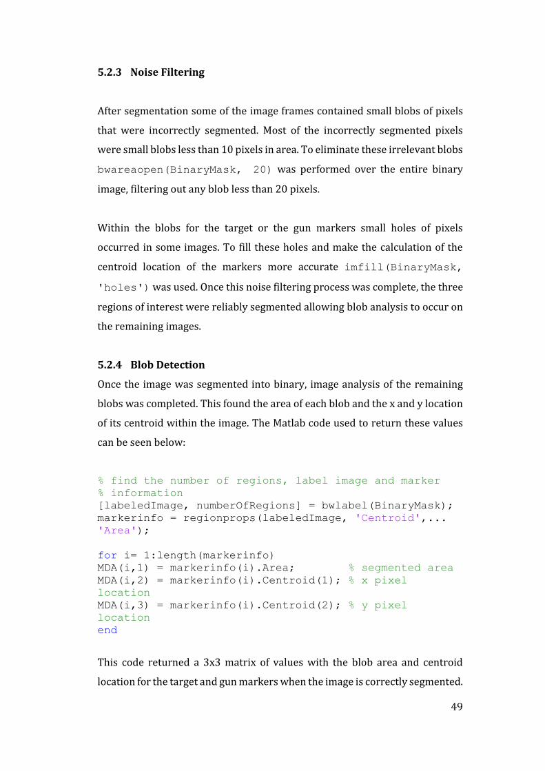
49
5.2.3 Noise Filtering
After segmentation some of the image frames contained small blobs of pixels
that were incorrectly segmented. Most of the incorrectly segmented pixels
were small blobs less than 10 pixels in area. To eliminate these irrelevant blobs
bwareaopen(BinaryMask, 20) was performed over the entire binary
image, filtering out any blob less than 20 pixels.
Within the blobs for the target or the gun markers small holes of pixels
occurred in some images. To fill these holes and make the calculation of the
centroid location of the markers more accurate imfill(BinaryMask,
'holes') was used. Once this noise filtering process was complete, the three
regions of interest were reliably segmented allowing blob analysis to occur on
the remaining images.
5.2.4 Blob Detection
Once the image was segmented into binary, image analysis of the remaining
blobs was completed. This found the area of each blob and the x and y location
of its centroid within the image. The Matlab code used to return these values
can be seen below:
% find the number of regions, label image and marker
% information
[labeledImage, numberOfRegions] = bwlabel(BinaryMask);
markerinfo = regionprops(labeledImage, 'Centroid',...
'Area');
for i= 1:length(markerinfo)
MDA(i,1) = markerinfo(i).Area; % segmented area
MDA(i,2) = markerinfo(i).Centroid(1); % x pixel
location
MDA(i,3) = markerinfo(i).Centroid(2); % y pixel
location
end
This code returned a 3x3 matrix of values with the blob area and centroid
location for the target and gun markers when the image is correctly segmented.

50
The area value was planned to be used to further exclude blobs of certain sizes
if the image segmentation was not reliable. The centroid locations of these
blobs were used with the point cloud that was generated to get the real world
coordinates for the segmented points.
5.2.5 Create Point Cloud from Scene
To enable the measurement of the shooting scene a point cloud was created.
Once the left and right images were rectified the disparities between the
images were mapped giving a depth map of the scene. Using the disparity map
and the camera parameters, a point cloud was created from every pixel where
a stereo match was found.
To create the point cloud the reconstructScene() command was used
then pixels with real world coordinates outside of the range of x, y and z
distances that encompassed the shooter and the target were eliminated to
reduce the noise and speed up processing.
When the point clouds from each trial were viewed by plotting them in 3D,
some noise was seen in the depth values. An example of this can be seen in
Figure 5.7 which depicts the point cloud rotated so we are viewing the scene
from above. This figure shows the positional values of all the pixels from Figure
5.1. The depth values can be seen to be arranged in steps away from the
camera.
When zooming in on area around the gun in the point cloud in Figure 5.8, the
individual x, y and z values for the pixels can be seen. The area along the length
of the gun shows the depth is not distributed in a smooth linear gradient, rather
pixels are seen to be grouped in places with no variance in z distance.

51
Figure 5.7 Point cloud from Static Trial 1 plotted in 3D rotated to show the noise in depth measurement of the gun.
Figure 5.8 Point cloud of gun area with the gun markers highlighted
5.2.6 Real World Coordinates
Due to the observed noise in the real world pixel locations and stepped nature
of the depth values, it was hypothesized that averaging the pixel locations in a
small area may give a more reliable positional result. To do this an average of
the pixel’s real world coordinates around the gun markers and target centroids
were taken.
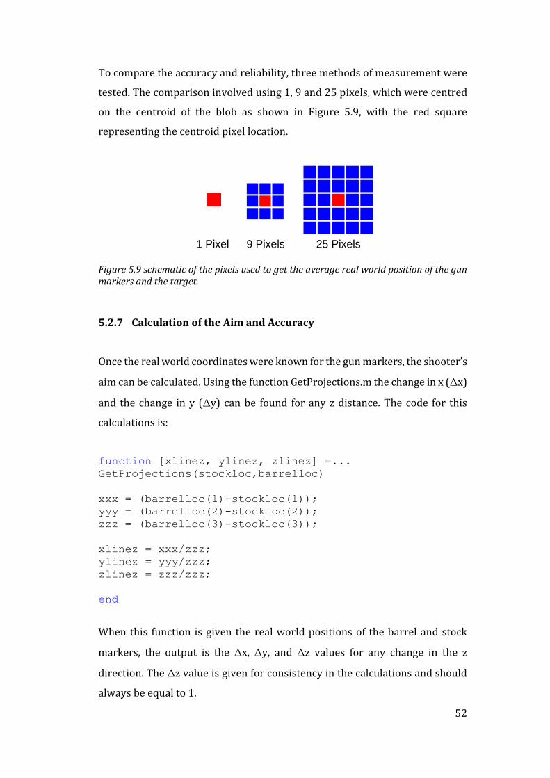
52
To compare the accuracy and reliability, three methods of measurement were
tested. The comparison involved using 1, 9 and 25 pixels, which were centred
on the centroid of the blob as shown in Figure 5.9, with the red square
representing the centroid pixel location.
1 Pixel 9 Pixels 25 Pixels
Figure 5.9 schematic of the pixels used to get the average real world position of the gun markers and the target.
5.2.7 Calculation of the Aim and Accuracy
Once the real world coordinates were known for the gun markers, the shooter’s
aim can be calculated. Using the function GetProjections.m the change in x (Δx)
and the change in y (Δy) can be found for any z distance. The code for this
calculations is:
function [xlinez, ylinez, zlinez] =...
GetProjections(stockloc,barrelloc)
xxx = (barrelloc(1)-stockloc(1));
yyy = (barrelloc(2)-stockloc(2));
zzz = (barrelloc(3)-stockloc(3));
xlinez = xxx/zzz;
ylinez = yyy/zzz;
zlinez = zzz/zzz;
end
When this function is given the real world positions of the barrel and stock
markers, the output is the Δx, Δy, and Δz values for any change in the z
direction. The Δz value is given for consistency in the calculations and should
always be equal to 1.

53
Once the Δx, Δy values were calculated, they were used to create a function of
a line that represented the path of the centre of the shot cloud. As the shot
distance and flight time were short, gravity was neglected allowing the path to
be approximated as a straight line. This line function was then used to calculate
the minimum distance that the centre of the shot cloud travelled past the
target, giving the x and y distances for shooter feedback.
5.3 Results
By using cardboard backing behind the targets in the static trials, the actual
centre of the shot cloud was preserved in a reliable and accurate way. With the
actual centre of the shot cloud recorded, the determination of the accuracy of
the calculated aim was made possible and gave the results credibility.
Appendix D shows the complete results of each of the five static trials. These
results show the actual centre of the shot, the target location and the position
of the calculated aim with each of the three methods. The outcome of the trials
demonstrated that the aim measurement is quite accurate in the y direction,
and generally all three methods show similar magnitude of error in the x
direction.
When the results, are collated in Figure 5.10 (refer to Appendix D for full
results), the calculated aim points were distributed in a band across the x plane.
The distribution calculated aim results visually shows no clear winner for
which method is the most accurate.

54
Figure 5.10 Collated results from the static trials showing the distribution of calculated aim for the three methods used.
Table 5.1 Average error for each of the methods of aim calculation
Method Average Error
Centroid 209 mm
9 Pixels 238 mm 25 Pixels 254 mm
When the error values for each method were averaged (refer Table 5.1), the
centroid pixel method has the lowest error. This value could be seen as a good
indication of accuracy except this method also has the data point with the
largest x error -484mm as seen in Figure 5.10. Due to this further investigation
is needed to select the method based on accuracy but also reliability.
The data point with the largest error when viewed in isolation gives the
impression that the results from the centroid method may have a tendency to
be inconsistent. Though when this data point is compared directly to the other
results from the same trial in Figure D.6 in Appendix D, it can be seen that the
others from Static Trial 3 are scattered almost as far left. When the individual
pixels are looked at in a similar way to the visualization in Figure 5.8 the z
55
values for these pixels show more noise and are not neatly planar. This could
suggest their being some slight errors in the stereo matching or some
movement occurred between the time these frames were captured. This
implies that the cause of this large error may be common to all three methods
and not only the centroid method of aim calculation.
The results from other trials showed that on occasions two methods of aim
were on one side of the centre and one showing an error on the opposite side
of the target. In these cases, it was assumed that the one outlier on the opposite
side is unreliable, as it is the only one that disagrees with the majority. The
results from Static Trial 2 show that the 9 pixel average predicting a miss of
391mm to the right when the others are predicting 242mm and 368mm to the
left. This quite large variance can be traced to a large amount of z distance noise
in the area around the barrel marker of the gun. The results from Static Trial 4
were also caused by noise in the barrel marker area this time causing the 25
pixel average to have a large variance from the other results.
From this investigation, the method selected to be used in the dynamic trials
was the centroid method of aim prediction. This result disproves the earlier
hypothesis that by averaging the pixels around the centroid of the markers a
more reliable result could be achieved. The averaging process was found to
include more noisy pixels into the measurement, which gave a reduction in
accurate and reliability.
The results of the static trials showed that the low cost computer vision
measurements can be very accurate in a static scene. Accuracy of prediction of
+/- 200mm-250mm would match the authors expectations of what a human
judge would be able to predict over a shot distance of 14m-15m. If this accuracy
could be attained in a dynamic scene, using low cost stereo computer vision
could be feasible to build a coaching feedback system.

56
Dynamic Target Accuracy
Using the results of the static trials as a baseline accuracy, dynamic testing was
performed in an attempt to build a system with similar accuracy to be used in
a comparison to the results of human judges. The impact of camera
asynchronization needed to be investigated and understood before the error
could be improved.
This chapter will document the development and testing process that was used
to create the program to test the accuracy of the camera equipment on a
moving target.
6.1 Dynamic Scene Capture
The shooting layout was designed similarly to the static trials, with the
exception of the shooter standing on the other side of the camera. This change
was made due to the sun position during the static trials casting a shadow on
the gun markers, making them harder to segment. The shooter and layout
continue to approximate the skeet layout as seen in
Figure 1.2 except the camera viewing angle is from a different position.
6.1.1 Field Trial Layout
The location and scene setup for the dynamic trials was similar to the static
trials. The targets were thrown along a path that was parallel to the target
locations of the static targets, to maintain as much consistency as possible. The
trial layout for this testing can be seen in Figure 6.1.

57
~1
4m
4.5
m
2.5m
16cm
Shooter
Location
Landing
Zone Target
Thrower
Cameras
Figure 6.1 Layout of the scene used during the dynamic trials
The decision to change the shooter/camera positions was made as a results of
the gun markers being in the shade in the original position in the scene layout.
As seen in Figure 6.2 when the gun makers are in the direct sun light the colours
are seen by the cameras much more brightly than in previous trials. The
markers in the dynamic trials were able to be segmented with less noise to be
filtered out.
Figure 6.2 Comparison of gun marker colour captured in static and dynamic trials.
58
6.1.2 Gun Marker Colour
As per the final static testing florescent orange and pink duct tape was used for
gun markers. Refer to section 5.1.3 for further information.
6.1.3 Gun Marker Positioning
As per the static trials the gun markers were positioned as far as reasonably
practicable. Refer to section 5.1.4 for further information.
6.2 Use of Existing Code
Much of the code to create dynamicprocess.m was taken directly or modified
from staticprocess.m.
The code for importation and rectification of the images was able to be used
with very little modification other than saving the imported files into a cell
arrays for the left and right cameras. Similarly much of the image processing
for finding gun markers and getting real world coordinates across multiple
image pairs was able to be done in a loop with the output being saved into a
multidimensional array for later use.
The majority of the new work that was done to enable this stage of the project
to be completed was around tracking and segmenting the moving target. Once
its position was found, its predicted position needed to be calculated. To do
this, the shot cloud flight time and the target speed and velocity needed to be
derived. In the following section additional detail of this functionality will be
discussed.
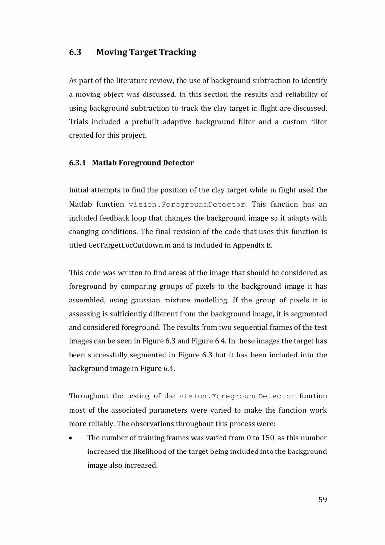
59
6.3 Moving Target Tracking
As part of the literature review, the use of background subtraction to identify
a moving object was discussed. In this section the results and reliability of
using background subtraction to track the clay target in flight are discussed.
Trials included a prebuilt adaptive background filter and a custom filter
created for this project.
6.3.1 Matlab Foreground Detector
Initial attempts to find the position of the clay target while in flight used the
Matlab function vision.ForegroundDetector. This function has an
included feedback loop that changes the background image so it adapts with
changing conditions. The final revision of the code that uses this function is
titled GetTargetLocCutdown.m and is included in Appendix E.
This code was written to find areas of the image that should be considered as
foreground by comparing groups of pixels to the background image it has
assembled, using gaussian mixture modelling. If the group of pixels it is
assessing is sufficiently different from the background image, it is segmented
and considered foreground. The results from two sequential frames of the test
images can be seen in Figure 6.3 and Figure 6.4. In these images the target has
been successfully segmented in Figure 6.3 but it has been included into the
background image in Figure 6.4.
Throughout the testing of the vision.ForegroundDetector function
most of the associated parameters were varied to make the function work
more reliably. The observations throughout this process were:
The number of training frames was varied from 0 to 150, as this number
increased the likelihood of the target being included into the background
image also increased.
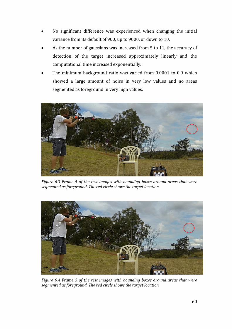
60
No significant difference was experienced when changing the initial
variance from its default of 900, up to 9000, or down to 10.
As the number of gaussians was increased from 5 to 11, the accuracy of
detection of the target increased approximately linearly and the
computational time increased exponentially.
The minimum background ratio was varied from 0.0001 to 0.9 which
showed a large amount of noise in very low values and no areas
segmented as foreground in very high values.
Figure 6.3 Frame 4 of the test images with bounding boxes around areas that were segmented as foreground. The red circle shows the target location.
Figure 6.4 Frame 5 of the test images with bounding boxes around areas that were segmented as foreground. The red circle shows the target location.
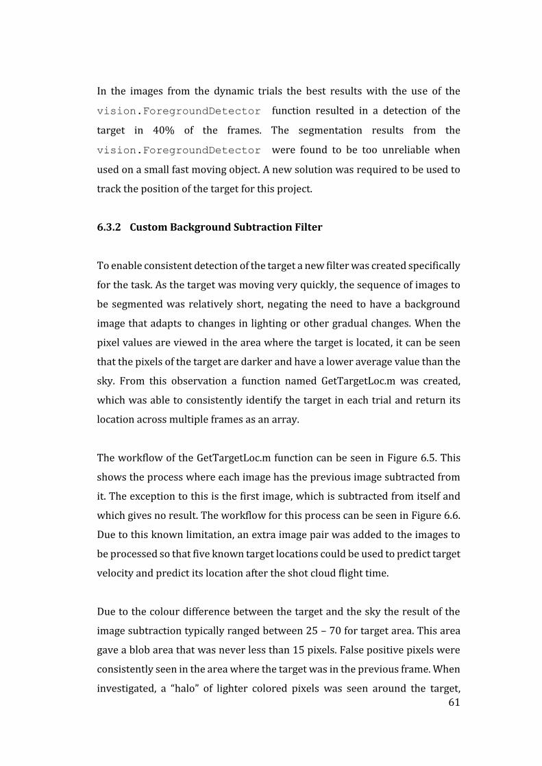
61
In the images from the dynamic trials the best results with the use of the
vision.ForegroundDetector function resulted in a detection of the
target in 40% of the frames. The segmentation results from the
vision.ForegroundDetector were found to be too unreliable when
used on a small fast moving object. A new solution was required to be used to
track the position of the target for this project.
6.3.2 Custom Background Subtraction Filter
To enable consistent detection of the target a new filter was created specifically
for the task. As the target was moving very quickly, the sequence of images to
be segmented was relatively short, negating the need to have a background
image that adapts to changes in lighting or other gradual changes. When the
pixel values are viewed in the area where the target is located, it can be seen
that the pixels of the target are darker and have a lower average value than the
sky. From this observation a function named GetTargetLoc.m was created,
which was able to consistently identify the target in each trial and return its
location across multiple frames as an array.
The workflow of the GetTargetLoc.m function can be seen in Figure 6.5. This
shows the process where each image has the previous image subtracted from
it. The exception to this is the first image, which is subtracted from itself and
which gives no result. The workflow for this process can be seen in Figure 6.6.
Due to this known limitation, an extra image pair was added to the images to
be processed so that five known target locations could be used to predict target
velocity and predict its location after the shot cloud flight time.
Due to the colour difference between the target and the sky the result of the
image subtraction typically ranged between 25 – 70 for target area. This area
gave a blob area that was never less than 15 pixels. False positive pixels were
consistently seen in the area where the target was in the previous frame. When
investigated, a “halo” of lighter colored pixels was seen around the target,

62
which caused pixel values of up to 35 after image subtraction. As these noise
blobs never occurred with a size greater than 6 pixels a noise filter was able to
be applied that segmented out any blobs less than 11 pixels.
Input:
Cell Array
of Images
Current Background =
Frame 1
Current Frame =
Frame(i)
Output =
Current background -
Current frame
Loop Count
i = 1
Output Binary =
Output > threshold
Blob analysis:
Centroid and Area
Found and saved
Current Background =
Current Frame
If Blob area
> 11
Save Centroid
location
If i = number of
images
Output:
Array of target
centroid locations
Figure 6.5 Flow chart showing the background subtraction process created for this project.
Figure 6.6 The stages the image sequences go through as part of GetTargetLoc.m. From left to right – original pixels, subtracted and thresholded pixels, pixels after noise filtering.

63
The computation resources to complete these operations were reduced by
restricting the search area to only the pixels that could contain the target.
Another technique to save computational time was the use of high level
operations on the entire matrix rather than embedded loops or using complex
operations. Using this new filter was an efficient solution to segmentation of
the target from the background and was able to identify the target in all of the
dynamic trials.
6.4 Prediction of Target Position
To estimate the “miss distance”, a prediction of the target position when the
shot cloud was to intersect it needed to be made. The calculation of the position
of the target involved three variables, the predicted target path, the target
velocity and the shot cloud flight time.
6.4.1 Predicted Target Path
The predicted target path was calculated using the calculated position of the
target across the previous image pairs. All of the dynamic trials used an input
of 6 image pairs, which resulted in an output of five target positions. Using the
known targets positions, curve fitting equations for the targets position with
respect to time in the x, y and z directions were calculated.
The days selected to perform the initial and final dynamic trials were relatively
wind free to make the segmentation of the target easier against the natural
background. With low wind the influence of wind on the target was neglected
in the calculations. The forces assumed to be acting on the target once in flight
were gravity and lift due to the shape of the target. From this the equations for
the x and z directions were made to be first order with the y direction being
second order to create a parabolic flight path.

64
6.4.2 Target Velocity
The target velocity was taken as an average over the distance travelled across
all of the target positions. As the camera frame rate was known, the velocity
was an easy calculation. The distance travelled by the target was in the number
of frames divided by the time taken. Deceleration due to drag was neglected as
the decrease in velocity was expected to be negligible over the short simulation
time.
6.4.3 Shot Cloud Flight Time
Equation 2.2 in Section 2.8.1 was derived from empirical test data gives a flight
time of a shot cloud in seconds where the cartridge used has size 8 shot and a
muzzle velocity of 1200fps. To estimate the shot cloud flight time, the distance
from the shooter to the target at the moment before the trigger was pulled can
be used. To ensure shot ballistics replicate the test data, the shotgun cartridges
used in all trials match the shot size and muzzle velocity from this original data.
The shot cloud flight time was used with the target velocity and flight path to
predict the target position at the anticipated moment of impact. Variance in the
targets distance from the shooter over the flight time was neglected as the
target was flying approximately in the negative x direction. The shot cloud
velocity being far greater than the rate this distance was changing would mean
that the errors created would have been very small.
6.5 Estimation of Frame Synchronization
As camera synchronization was identified as an issue for the stereo GoPro
cameras in Section 4.1.2 the synchronization test circuit was setup in the field
of view of the cameras throughout the dynamic testing process.

65
To get frame synchronization estimates from each of the trials the
synchronization circuit was set to cycle 10 LEDs in 1/60s, which was the period
of the time between camera frames. This gave feedback about the
synchronization of the cameras to 1/600s, which assisted in determining the
impact of camera synchronization on aim estimation.
Left Camera Right Camera
Figure 6.7 Camera synchronization test circuit set to illuminate 10 LEDs in 1/60s showing the left camera leads the right in this trial by 0.2 frames.
The code for the synchronization circuit can be found in Appendix D in and
program named “FieldTrials_Flasher”. The use of this circuit can be seen in
Figure 6.7 from Dynamic Trial 2, where the left camera only saw one LED
illuminated and the right saw 3 LEDs illuminated therefore the left image was
taken approximately 2/600 s before the right. This system was used in all field
trials and feedback from this was incorporated into the dynamic trials code to
improve performance.
6.6 Initial Results
The initial dynamic trials comprise of 28 shots taken at targets and the 10 with
the cleanest strike when reviewed were used get results. As the strike of the
target by the shot cloud was very clean it can be assumed that the centre of the
shot cloud was close to the centre of the target at the time of impact.

66
6.6.1 Target Z Distance
Using the geometry of the shooting scene, as shown in Figure 6.1 it can be seen
that the z distance from the cameras varies very little across its flight path as
its path is predominantly in the negative x direction. The elevation change of
the target is measured in the y direction so it should not have a large impact on
the z distance. From this, the calculated target z distances can be plotted
against the frame synchronization, as per Figure 6.8, to show the impact
asyncronisation on the target position in the initial dynamic trials.
The approximate z distance in Figure 6.1 is ~18.5m from the cameras to the
target path, with calculated distances ranging between 10.50m to 29.73m or a
total range of 19.23m. These errors correlate very well with the frame
observed frame synchronization taken from the LED counts in the images. This
can be explained using Figure 6.9. In this graphic the target has moved in the
time between when the frames are captured resulting in a large error in z
distance calculation.
Figure 6.8 z distance the target was measured at the moment of firing vs the frame synchronization.

67
Figure 6.9 Modified diagram from figure 2.3 giving a showing the positional errors created by frame synchronization errors.
Errors in calculated positions of moving objects are also created in the x and y
directions due to frame asynchronization. These errors have a smaller
magnitude but will have larger effect on the aim accuracy of the gun because a
small error in x or y direction creates a larger aim angle error than z direction
errors due to the gun being primarily pointed in the z direction.
6.6.2 Calculated Accuracy
The results from the initial dynamic trials were calculated without any attempt
to correct for frame synchronization errors. As the trials selected for
processing all had good hits on the target it was assumed that the target was
within the diameter, of the shot cloud, at that distance. Figure 6.10 shows the
calculated aim vs a circle representing the approximate shot cloud diameter at
15m. If these results are compared to the results from the static trials in Figure
yz
x
Reference Coordinates
x
y
x
y
Measured
P(x,y,z)
Right Camera
Plane
Left Camera
Plane
Left Camera Right Camera Baseline Distance
Object Path
P(x,y,z) @ t(1) P(x,y,z) @ t(0)

68
5.10, where the maximum calculated error was less than 0.5m, the impact of
frame synchronization significant.
Figure 6.10 Calculated miss distance vs approximate shot cloud location around target.
When the point cloud of each trial is looked at, the effect of the z distance
calculation errors on the estimated shot cloud flight time can be seen. In the
point cloud shown in Figure 6.11 from Dynamic Trial 1 the frame sync error of
0.1 frame caused the calculated z depth of ~22.5m. The distance error has then
resulted in the an error of the predicted distance that the target will fly after
the shot was taken due to an increase in shot cloud flight time from 46.6ms @
14m to 78.7ms @ 22.5m, which results in the target having a predicted position
too far along its path. This is of course has the opposite effect when the target
is calculated to be closer than in reality but due to the trigonometry of the z
distance calculation, a frame error that creates a larger disparity, and therefore
a shorter z distance, will have a smaller magnitude error than the an error that
reduces the disparity by the same number of pixels.

69
Figure 6.11 Point cloud from Dynamic Trial 1 showing the calculated aim vs predicted target location. The target positions from the images are in red circles, the predicted position as a red filled circle and the projected aim as a green line.
The results from the initial dynamic trials were less accurate than would be
expected from a human judge. Giving new shooters feedback with errors of
over 2m at a shot distance of 14m would be counterproductive to their learning
as their shot cloud diameter from their shot were less than 1m. If the new
shooter followed the correction provided from the feedback it would result in
the shooter missing the target entirely. Due to this an attempt to improve the
programs accuracy will be discussed in section 6.7.
6.7 Program Accuracy Improvement
To improve the accuracy of the system, and to correct for the incorrect
disparities at the key points created by the frame delay, a method of moving
the pixels at the key points in the images was devised. To do this the pixel
positions were interpolated based on the key point’s movement between the
frames and the measured frame delay from the synchronization test circuit.

70
Initially a study was completed on assessing what the pixel disparity errors
would be based on the frame delay. To do this, the position of the markers and
target where taken from a sample of image sequences used in the initial
dynamic trials to determine the distance in pixels that the marker moved in the
x direction was found. The results of this assessment varied very little between
the trials as the target was thrown along a similar path with the shooter in the
same location. Table 6.1 shows the results of this assessment for the right
camera from Dynamic Trial 4, showing the large variance in the number of
pixels each marker moves between frames.
Table 6.1 Movement in blob centroids in the x direction measured in pixels between each of the frames from the right camera in dynamic trial 1.
Barrel Marker Stock Marker Target
Frame 1 - - -
Frame 2 -1.2323 -3.5642 -
Frame 3 -0.6312 -3.5850 18
Frame 4 -0.8341 -3.3649 19
Frame 5 -0.5845 -3.7240 18
Frame 6 -0.5388 -3.7945 18
From this assessment it was found that interpolating the pixel locations for the
gun markers within the images would be impractical. The gun markers
movement was very small and as the pixels can only be moved in integer
quantities, the resolution would be too coarse.
Each of the dynamic trial, used six image pairs to get the results Due to the
filtering process to get the target location this left 4/6 images to assess the
movement. As the variance in the results was not large, it was assumed that the
interpolation could be applied to the second frame as well. The movement of
the target between the frames in all of the image sequences sampled was
between 18-22 pixels. This was found to be enough so that the pixels around
the target could have their position interpolated to attempt to correct the
disparity error.
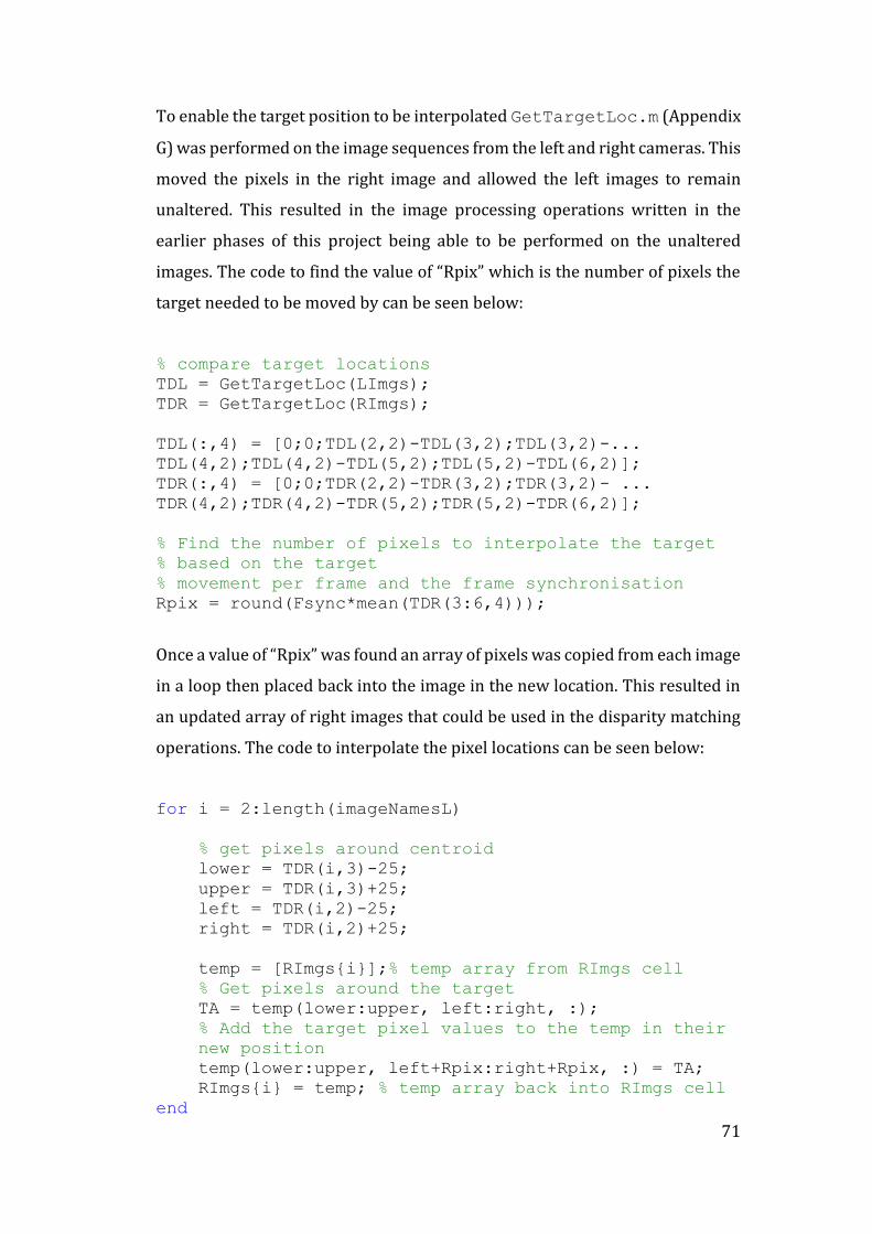
71
To enable the target position to be interpolated GetTargetLoc.m (Appendix
G) was performed on the image sequences from the left and right cameras. This
moved the pixels in the right image and allowed the left images to remain
unaltered. This resulted in the image processing operations written in the
earlier phases of this project being able to be performed on the unaltered
images. The code to find the value of “Rpix” which is the number of pixels the
target needed to be moved by can be seen below:
% compare target locations
TDL = GetTargetLoc(LImgs);
TDR = GetTargetLoc(RImgs);
TDL(:,4) = [0;0;TDL(2,2)-TDL(3,2);TDL(3,2)-...
TDL(4,2);TDL(4,2)-TDL(5,2);TDL(5,2)-TDL(6,2)];
TDR(:,4) = [0;0;TDR(2,2)-TDR(3,2);TDR(3,2)- ...
TDR(4,2);TDR(4,2)-TDR(5,2);TDR(5,2)-TDR(6,2)];
% Find the number of pixels to interpolate the target
% based on the target
% movement per frame and the frame synchronisation
Rpix = round(Fsync*mean(TDR(3:6,4)));
Once a value of “Rpix” was found an array of pixels was copied from each image
in a loop then placed back into the image in the new location. This resulted in
an updated array of right images that could be used in the disparity matching
operations. The code to interpolate the pixel locations can be seen below:
for i = 2:length(imageNamesL)
% get pixels around centroid
lower = TDR(i,3)-25;
upper = TDR(i,3)+25;
left = TDR(i,2)-25;
right = TDR(i,2)+25;
temp = [RImgs{i}];% temp array from RImgs cell
% Get pixels around the target
TA = temp(lower:upper, left:right, :);
% Add the target pixel values to the temp in their
new position
temp(lower:upper, left+Rpix:right+Rpix, :) = TA;
RImgs{i} = temp; % temp array back into RImgs cell
end
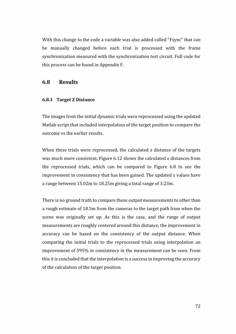
72
With this change to the code a variable was also added called “Fsync” that can
be manually changed before each trial is processed with the frame
synchronization measured with the synchronization test circuit. Full code for
this process can be found in Appendix F.
6.8 Results
6.8.1 Target Z Distance
The images from the initial dynamic trials were reprocessed using the updated
Matlab script that included interpolation of the target position to compare the
outcome vs the earlier results.
When these trials were reprocessed, the calculated z distance of the targets
was much more consistent. Figure 6.12 shows the calculated z distances from
the reprocessed trials, which can be compared to Figure 6.8 to see the
improvement in consistency that has been gained. The updated z values have
a range between 15.02m to 18.25m giving a total range of 3.23m.
There is no ground truth to compare these output measurements to other than
a rough estimate of 18.5m from the cameras to the target path from when the
scene was originally set up. As this is the case, and the range of output
measurements are roughly centered around this distance, the improvement in
accuracy can be based on the consistency of the output distance. When
comparing the initial trials to the reprocessed trials using interpolation an
improvement of 595% in consistency in the measurement can be seen. From
this it is concluded that the interpolation is a success in improving the accuracy
of the calculation of the target position.

73
Figure 6.12 z distance the target was measured at the moment of firing with the use of pixel interpolation vs the frame synchronization.
6.8.2 Calculated Accuracy
After the results from the initial dynamic trials were reprocessed with the
interpolation of the target pixels, the results of the accuracy became worse. The
direction that the aim was predicted against the target showed a good
correlation to the frame synchronization. This can be explained due to the z
distance error of the gun not being corrected, which results in the position of
the marker at the end of the barrel being calculated incorrectly.
To look at the impact of this error the point clouds of the first and fifth dynamic
trials can be compared. When the images were captured for Dynamic Trial 1,
the left camera was 0.1 frames behind the right camera causing the targets to
be calculated as further away from the shooter. Once the interpolation of the
pixel positions is complete the shooter appears to be shooting to the left of the
target. In Dynamic Trial 5 the left camera was 0.3 frames in front of the right
camera causing the target positons to be moved further away with the
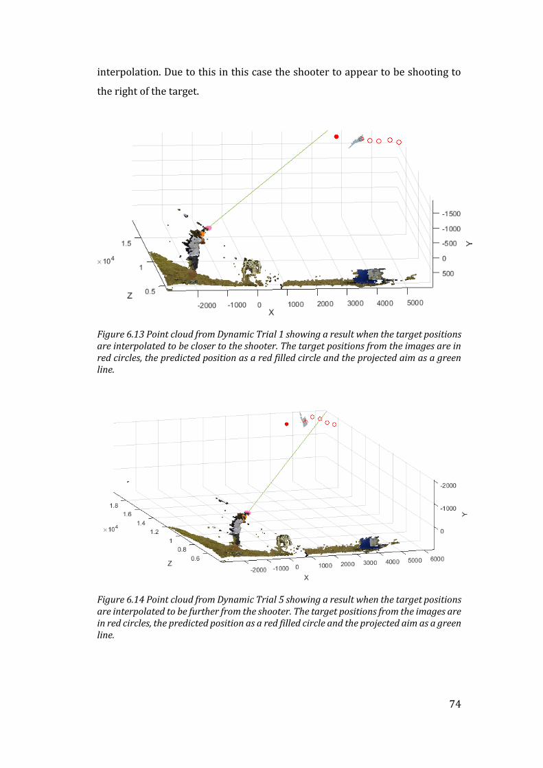
74
interpolation. Due to this in this case the shooter to appear to be shooting to
the right of the target.
Figure 6.13 Point cloud from Dynamic Trial 1 showing a result when the target positions are interpolated to be closer to the shooter. The target positions from the images are in red circles, the predicted position as a red filled circle and the projected aim as a green line.
Figure 6.14 Point cloud from Dynamic Trial 5 showing a result when the target positions are interpolated to be further from the shooter. The target positions from the images are in red circles, the predicted position as a red filled circle and the projected aim as a green line.
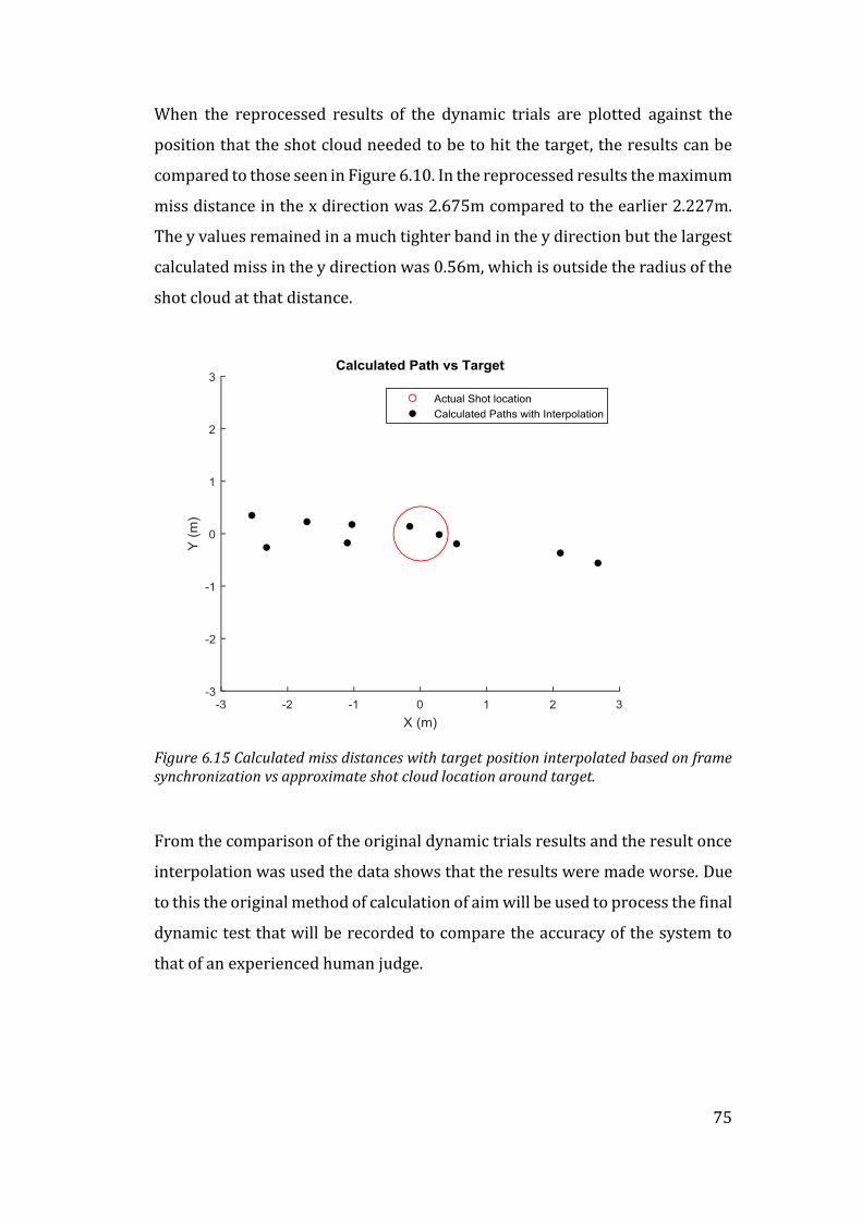
75
When the reprocessed results of the dynamic trials are plotted against the
position that the shot cloud needed to be to hit the target, the results can be
compared to those seen in Figure 6.10. In the reprocessed results the maximum
miss distance in the x direction was 2.675m compared to the earlier 2.227m.
The y values remained in a much tighter band in the y direction but the largest
calculated miss in the y direction was 0.56m, which is outside the radius of the
shot cloud at that distance.
Figure 6.15 Calculated miss distances with target position interpolated based on frame synchronization vs approximate shot cloud location around target.
From the comparison of the original dynamic trials results and the result once
interpolation was used the data shows that the results were made worse. Due
to this the original method of calculation of aim will be used to process the final
dynamic test that will be recorded to compare the accuracy of the system to
that of an experienced human judge.

76
Results and Discussion
This chapter documents the final testing of the low cost stereo computer vision
system against three experienced human judges. From these trials the
feasibility of using this technology to provide feedback to clay target shooters
was determined.
7.1 Final Testing
The final series of trials were performed to test the accuracy of the system
compared to human judges, the existing coaching method. To feasibly provide
feedback to clay target shooters the system would need to have equivalent or
better accuracy than the human judges.
The recording procedure and scene layout for this phase of the project were
implemented as per the earlier dynamic trials. This ensured no additional
variable were introduced into the workflow, and to enable for the earlier
dynamic results to be verified.
The interpolation of the target position was not used in the computer aim
calculation. This decision was due to the results from the dynamic trails
showing less accurate results after the interpolation of the target position, as
the aim of the shooter was not able to be interpolated. The goal of the final
testing was to have comparable accuracy to the judges, and using the original
method gave the system the best chance.

77
Throughout the trials the three coaches were asked to stand in the normal
observation position they would stand if they were looking to coach a new
shooter. As can be seen in Figure 7.1 the three coaches all selected quite
different observation positions. When asked about their positions, the coach
with ear muffs in the back of the scene and the coach with the red shirt directly
behind the shooter said that this position is where they could best see the
wadding flying through the air. The third coach said that standing back and to
the right of a right handed shooter allowed him to best see the shooters stance
to correct any issues and still be behind the shooter enough to see the wadding
in flight.
The coach who stood behind and to the right felt that correcting the issues in
the shooters stance and gun motion was potentially more important than
giving feedback about miss distances. Giving stance feedback is beyond the
scope of this project but research into correcting baseball pitcher actions was
discussed in section 2.1 of this report and could be potentially completed in the
future.
Figure 7.1 Scene from the trials vs human judges with the judges standing in the locations that they would normally be to coach a new shooter.

78
During discussion after the trials, all three judges commented that in most
cases where the target was hit very cleanly, no feedback would have been given
by them to the shooter. In cases such as this they would have just told the
shooter it was a good shot and told them to repeat those actions again to try
and become more consistent.
7.2 Results
To ensure the results were not influenced by having a shooter who knew the
system well, a new less experience shooter was used for the final testing. He
was given instruction to hit most of the targets but to also miss some. The full
results of the final testing are shown in Appendix E with a plot that compared
the feedback of each judge with the calculated result. As shown in Figure 7.2,
the human judges are much more consistent in their feedback and have
comparable accuracy to the results from the static trials.
Figure 7.2 Summary of results of the trials against human judges showing the spread of the Matlab results compared to the judges.

79
The results from Trials 1, 4, 5 and 6 (Figures E.1, E.4, E.5, E.6) all show the
coaches believe the shooter hit the target within 0.2m of the centre of the shot
cloud. Figure 7.3 shows the calculated aim for these trials plotted against the
target location. These results are consistent with the results from the initial
dynamic trials in the way they are spread up to 2m to the left. These results
confirm the results from the earlier trials and demonstrate that the spread of
results wasn’t due to poor trial selection used as test images.
Figure 7.3 Calculated aim for final trials 1,4,5,6 where the judges all said the shooter hit the target with the middle of his shot cloud.
The results from Trial 3 and Trial 9 show the calculated result to be within the
range of the judges. If these results were seen in isolation it would appear that
the system had comparable accuracy to the judges. If these results are viewed
neglecting the influence of frame synchronization, it appears that some of the
results even by luck are near the judges feedback.

80
Figure 7.4 Results for Trial 3 & 9 showing the calculated aim to be within the coaches error margin
An investigation into the frame synchronization of these trials showed that in
Trial 9 the cameras were synchronized to within 0.1 of a frame and Trial 3 the
left camera was 0.1 frames behind the right camera. With the information from
the static trials, and the results of these two trials the conclusion could be made
that with correct frame synchronization a comparable accuracy to human
judges could be attained. This conclusion would need to be confirmed as future
work as a sample size of two is not enough evidence to be certain that this
result is repeatable.
In all of the results from the initial dynamic trials and the trials vs judges, the y
distance is reasonably close to the expected value. The results from Trial 2 as
seen in Figure E.2 confirm the systems accuracy in y direction calculation as
this is the only trial where the reference was above or below the target and the
calculated y position approximately matches the judges.

81
Overall the computer vision accuracy results were as expected from the initial
dynamic trials, with calculated aim values up to 2 m in the negative x direction
from the actuals. The feedback provided by the coaches was reasonably
consistent between the three. A key conclusion from these trials with human
judges is that better accuracy is required from the computer system to match
a human coach. These results have shown that it would be very difficult to
create a system using low cost computer vision with the required accuracy.
7.3 Concept Feasibility
The results of the dynamic testing in this project show that the use of low cost
computer vision is far less accurate than the human judges when the target is
moving quickly across in front of the cameras. The inability to adequately
synchronize the low cost cameras creates large positional errors which have
not been able to be corrected as part of this project. It is therefore concluded
that it is not feasible, at this time, to use low cost stereo computer vision to
provide coaching feedback to clay target shooters. The calculated feedback has
shown to be inconsistent, and will often direct the shooter to change their aim
in amounts and directions that would make their shooting worse rather than
better.
Interpolation of the position of the target showed a marked improvement in
the positional error of the target in the dynamic trials. From this it could be
assumed that if sub pixel interpolation of all of the markers were feasible and
the frame synchronization could be estimated more accurately, then the
complete system could be made to be more accurate.
This project showed that the gun markers and the target could be reliably
segmented. It may be possible to use these functions to find the centroids of
the gun markers and target across a sequence of frames, then by using these
positions, interpolate new points based in the frame synchronization to
fractions of a pixel. The new points would be an approximation of the positions
of the centroids in synchronized frames. With these points the trigonometric

82
functions as described in Figure 2.3 and the paper by Kang et al. (2008) could
be used to find the real world positions. This would speed up processing time
as point clouds would not need to be generated for each image pair and would
have the potential to interpolate the gun markers the very small distances
required. If interpolation of the markers by values less than 1 pixel can be
achieved, using low cost asynchronous cameras has the potential to be feasible
at some time in the future.
7.4 Future work
While this project showed that the use of low cost stereo computer vision is
not currently capable of providing reliable and accurate shooter feedback, it
has also shown that there is potential with further work to improve the results
to the point where it may be feasible. This section will discuss the areas where
further work could be conducted to improve the project outcome.
7.4.1 More Robust Target Segmentation Filter
All of the trials for this project were designed to have the clay target against a
background of sky. As such the filter was only created to work reliably in that
situation. A more robust filter could be created that would work with other
backgrounds.
The concept that would be used for this filter would create an adaptive
background image from a rolling previous 3+ frame block. The previous frames
would have all of their pixels values averaged then each pixel from the initial
frames would be compared to the average value for its location and the high
and low outliers would be removed.

83
7.4.2 Investigate Other Means of Measuring Shooter Aim
An option that could be investigated is the use of an accelerometer and/or a
gyroscope to provide the aim direction. This system could be made cheaply
enough that multiple shooters could have them attached to their shotguns
when shooting in a group. The users could switch then share the same stereo
vision setup on a skeet layout used for tracking the target.
7.4.3 Better Interpolation of the Gun Markers and Target Position.
As discussed in Section 7.3 there is potential for stereo vision to provide more
accurate shooter feedback if the interpolation can be improved. To achieve this
the circuit that tests the synchronization of the frames would need more LED’s.
Alternatively a sequence of LED’s representing a binary number could be
incremented a number of values in the time between the image frames. The
number could be automatically decoded from the LED pattern and subtracted
to indicate the frame synchronization.
Once better estimation of the synchronization is established, the points that
represent the locations of the markers can be more accurately interpolated to
give a more reliable output. Using the method discussed in Section 7.3,
processing time would be reduced and the impact of stereo matching errors
would be negated.
7.4.4 Reduce the Manual User Input
If the accuracy of the aim prediction using low cost stereo computer vision was
improved to the point where it reliably produced accurate results comparable
to a human coach, some additional areas could be improved to get the product
closer to being marketable. These are:
Manual processing of images to find image pairs could be automated
using visual markers.
84
The frame synchronization could be estimated automatically using
pattern recognition or similar from the LED pattern or count.
Code the project so it operates more closely to real time. It is unnecessary
to do all the processing between frames but it could trigger a process
after the gun shot has been taken. This would provide the shooter with a
result almost immediately after the shot was taken.
A self-calibration routine could be used so that when deployed, the user
would not need to take images of a checkerboard to calibrate the system.
They would be able to simply move the cameras around and use the scene
to calibrate the cameras.

85
List of References
Alouani, AT & Rice, TR 1994, 'On asynchronous data fusion', in Proceedings of the Annual Southeastern Symposium on System Theory: proceedings of theProceedings of the Annual Southeastern Symposium on System Theory pp. 143-6, <http://www.scopus.com/inward/record.url?eid=2-s2.0-0028755097&partnerID=40&md5=f2441f651f23e6e43339ef3f66af958d>. Andersson, T & Ahlen, H 1999, Impact position marker for ordinary or simulated shooting, US Patent 5991043. Australian Clay Target Association 2014, 'Skeet Rules', <http://www.claytarget.com.au/component/docman/doc_download/4410-2014-skeet-shooting-rules> Bazargani, H, Omidi, E & Talebi, HA 2012, 'Adaptive Extended Kalman Filter for asynchronous shuttering error of stereo vision localization', in Robotics and Biomimetics (ROBIO), 2012 IEEE International Conference on: proceedings of theRobotics and Biomimetics (ROBIO), 2012 IEEE International Conference on pp. 2254-9. Bronzewing Ammunition 2013, Competition Loads, Bronzewing Ammunition Yenda, New South Wales, viewed 5 February 2015, <http://bronzewing.net/?page_id=7>. Burrard, G 1955, The Modern Shotgun: Volume II: The Cartridge, Herbert Jenkins, London. Choi, J 2015, RE: Point Grey Request For Quote, Email Communication, Point Greg, Richmond BC, Canada. Chong, AK & Brownstein, G 2010, 'A technique for improving webcam precision in biological plant measurement', Photogrammetric Record, vol. 25, pp. 180-96, viewed 23 October 2014, EBSCOhost, a9h. Chugh, OP 1982, 'Maximum range of pellets fired from a shotgun', Forensic Science International, vol. 10, no. 3, pp. 223-30, viewed 10 October 2014, Scopus. Chung-Cheng, C, Wen-Chung, C, Min-Yu, K & Yuh-Jiun, L 2009, 'Asynchronous stereo vision system for front-vehicle detection', in Acoustics, Speech and Signal Processing, 2009. ICASSP 2009. IEEE International Conference on: proceedings of theAcoustics, Speech and Signal Processing, 2009. ICASSP 2009. IEEE International Conference on pp. 965-8.

86
Clarke, TA & Fryer, JG 1998, 'The development of camera calibration methods and models', Photogrammetric Record, vol. 16, no. 91, pp. 51-66, Scopus. Compton, D 1996, 'An Experimental And Theoretical Investigation Of Shot Cloud Ballistics', PhD thesis, University of London, London. Compton, DJ, Radmore, PM & Giblin, RA 1997, 'A stochastic model of the dynamics of an ensemble of spheres', Proceedings of the Royal Society of London. Series A: Mathematical, Physical and Engineering Sciences, vol. 453, no. 1963, pp. 1717-31, viewed 25 October 2014. Computer Vision System Toolbox 2014, MathWorks, Natick, Massachusetts, viewed 16 October 2014, <http://au.mathworks.com/help/vision/index.html>. Coulson, S 2003, 'Real Time Positioning and Motion Tracking for Simulated Clay Pigeon Shooting Environments', Undergraduate Project Report, Imperial College, London. Cox, A 2011, 'Stereo vision for webcams', Undergraduate Dissertation, University of Southern Queensland, Toowoomba. Davidson, R, Thomson, RD & Birkbeck, AE 2002, 'Computational modelling of the shot pattern of a sporting shotgun', Journal of Sports Engineering, vol. 5, no. 1, pp. 33-42. Desa, SM & Salih, QA 2004, 'Image subtraction for real time moving object extraction', in Computer Graphics, Imaging and Visualization, 2004. CGIV 2004. Proceedings. International Conference on: proceedings of theComputer Graphics, Imaging and Visualization, 2004. CGIV 2004. Proceedings. International Conference on pp. 41-5. Engineers Australia 2010, 28 July 2010, 'Code of Ethics', <https://www.engineersaustralia.org.au//sites/default/files/shado/About%20Us/Overview/Governance/codeofethics2010.pdf> Engineers Australia 2015, Sustainability Resources, Barton, Australian Captial Territory, viewed 15 February 2015, <https://www.engineersaustralia.org.au/environmental-college/sustainability-resources>. Federal Premium Ammunition 2015a, Federal Premium Ballistics Calculator, Federal Premium Anoka, Minnesota, viewed 5 February 2015, <https://www.federalpremium.com/ballistics_calculator/>. Federal Premium Ammunition 2015b, Shotshell Ammunition, Federal Premium Anoka, Minnesota, viewed 5 February 2015, <https://www.federalpremium.com/products/shotshell.aspx>.

87
Fetic, A, Juric, D & Osmankovic, D 2012, 'The procedure of a camera calibration using Camera Calibration Toolbox for MATLAB', in MIPRO, 2012 Proceedings of the 35th International Convention: proceedings of theMIPRO, 2012 Proceedings of the 35th International Convention pp. 1752-7. Fothergill, S, Harle, R & Holden, S 2008, 'Modeling the model athlete: Automatic coaching of rowing technique', Proceedings of the Artificial Intelligence in Bioinformatics, University of Cambridge, Cambridgeshire, pp. 372-81. Gibson, S 2015, Email, 18 February. Heikkila, J & Silven, O 1996, 'Calibration procedure for short focal length off-the-shelf CCD cameras', in Pattern Recognition, 1996., Proceedings of the 13th International Conference on: proceedings of thePattern Recognition, 1996., Proceedings of the 13th International Conference on pp. 166-70 vol.1. Image Processing Toolbox 2014, MathWorks, Natick, Massachusetts, viewed 25 October 2014, <http://au.mathworks.com/help/releases/R2015a/pdf_doc/images/images_tb.pdf>. Kang, MJ, Lee, CH, Kim, JH & Huh, UY 2008, 'Distance and velocity measurement of moving object using stereo vision system', 2008 International Conference on Control, Automation and Systems, ICCAS, Seoul, South Korea, pp. 2181-4. Kawempy, I, Ragavan, SV & Khoo Boon, H 2011, 'Intelligent system for intercepting moving objects', Advances in Intelligent Computational Systems, IEEE, Kerala, India, pp. 792-7. Kramberger, I 2005, 'Real-time skin feature identification in a time-sequential video stream', Optical Engineering, vol. 44, no. 4, pp. 047201--10. Liu, H, Li, Z, Wang, B, Zhou, Y & Zhang, Q 2013, 'Table tennis robot with stereo vision and humanoid manipulator II: Visual measurement of motion-blurred ball', 2013 International Conference on Robotics and Biomimetics, IEEE Computer Society, Shenzhen, China, pp. 2430-5. Liu, Z & Chen, T 2009, 'Distance measurement system based on binocular stereo vision', 1st IITA International Joint Conference on Artificial Intelligence, JCAI, Hainan Island, China, pp. 456-9. Liu, Z, Chen, W, Zou, Y & Hu, C 2012, 'Regions of interest extraction based on HSV color space', in IEEE International Conference on Industrial Informatics (INDIN): proceedings of theIEEE International Conference on Industrial Informatics (INDIN) pp. 481-5, <http://www.scopus.com/inward/record.url?eid=2-s2.0-84868245619&partnerID=40&md5=16fd131dbf4ba1cc416f3ec23e89158c>.

88
Lü, C, Wang, X & Shen, Y 2013, 'A stereo vision measurement system Based on OpenCV', Proceedings of the 2013 6th International Congress on Image and Signal Processing, CISP 2013, Beijing, China, pp. 718-22. Luo, Q 2013, 'Research on motion capture instruments in sports', in Applied Mechanics and Materials: proceedings of theApplied Mechanics and Materials pp. 151-5, <http://www.scopus.com/inward/record.url?eid=2-s2.0-84883153123&partnerID=40&md5=4abc3cf59344e045eb65b1608be48a7e>. Marksman Training Systems AB 2014, ST-2 Shooting simulator, Stockholm, Sweden, viewed 10 December 2014, <http://www.marksman.se/eng_home/eng_home.htm>. Meng, X & Hu, Z 2003, 'A new easy camera calibration technique based on circular points', Pattern Recognition, vol. 36, no. 5, pp. 1155-64. National Skeet Shooting Association 2015, Use of Radar Gun for Setting Skeet Targets, viewed 30 April 2015, <http://www.nssa-nsca.org/wp-content/uploads/2010/07/radargunuse.pdf>. Ofli, F, Demir, Y, Erzin, E, Yemez, Y & Tekalp, AM 2007, 'Multicamera audio-visual analysis of dance figures', in Proceedings of the 2007 IEEE International Conference on Multimedia and Expo, ICME 2007: proceedings of theProceedings of the 2007 IEEE International Conference on Multimedia and Expo, ICME 2007 pp. 1703-6, <http://www.scopus.com/inward/record.url?eid=2-s2.0-46449111503&partnerID=40&md5=11bbfd07e573f49339306cd0bff4b6ff>. OpenCV 2015, itseez, Nizhny Novgorod, Russia, viewed 19 October 2014, <http://opencv.org/>. Page, A, Moreno, R, Candelas, P & Belmar, F 2008, 'The accuracy of webcams in 2D motion analysis: sources of error and their control', European Journal of Physics, vol. 29, no. 4, p. 857. Poh, CH & Poh, CK 2005, 'An effective data acquisition system using image processing', in Proceedings of SPIE - The International Society for Optical Engineering: proceedings of theProceedings of SPIE - The International Society for Optical Engineering <http://www.scopus.com/inward/record.url?eid=2-s2.0-33645095728&partnerID=40&md5=6381f8b70c2f8e2a30d9afabc48b69fb>. Pohanka, J, Pribula, O & Fischer, J 2010, 'An embedded stereovision system: Aspects of measurement precision', Proceedings of the 12th Biennial Baltic Electronics Conference, Prague, Czech Republic, pp. 157-60. Rahman, T & Krouglicof, N 2012, 'An efficient camera calibration technique offering robustness and accuracy over a wide range of lens distortion', IEEE Transactions on Image Processing, vol. 21, no. 2, pp. 626-37, Scopus.

89
Schmidt, VE & Rzhanov, Y 2012, 'Measurement of micro-bathymetry with a GOPRO underwater stereo camera pair', OCEANS 2012: Harnessing the Power of the Ocean, Institute of Electrical and Electronics Engineers, Virginia Beach, Virginia. Shah, S & Aggarwal, JK 1996, 'Intrinsic parameter calibration procedure for a (high-distortion) fish-eye lens camera with distortion model and accuracy estimation*', Pattern Recognition, vol. 29, no. 11, pp. 1775-88. Sheng-Wen, S, Yi-Ping, H & Wei-Song, L 1995, 'When should we consider lens distortion in camera calibration', Pattern Recognition, vol. 28, no. 3, pp. 447-61. Shi, J, Niu, Y & Wang, Q 2013, Multi-Camera System Based Driver Behavior Analysis Final Report, Winter 2013, The University Of Pennsylvania, Pennsylvania, viewed 19 October 2014, <http://utc.ices.cmu.edu/utc/Penn%20Reports%202013/Shi%20Final%20Report.pdf>. ShotKam LLC 2014, http://www.shotkam.com/, United States of America, viewed 29 March 2015. Skeet Falcon 2014, HKKW Innovations, Holzkirchen, Germany viewed 30 September 2014, <http://skeetfalcon.de/>. Sporting Magazine 1793, 'Pigeon Shooting', vol. Volume 1, pp. 251-3. Stauffer, C & Grimson, WEL 1999, 'Adaptive background mixture models for real-time tracking', Proceedings of the 1999 IEEE Computer Society Conference on Computer Vision and Pattern Recognition, IEEE, Los Alamitos, California, United States, pp. 246-52. Sutton, D & Green, R 2010, 'Evaluation of real time stereo vision system using web cameras', Proceedings of 25th International Conference Image and Vision Computing, Queenstown, New Zealand. Tamura, Y, Maruyama, T & Shima, T 2014, 'Analysis and feedback of baseball pitching form with use of Kinect', in Workshop Proceedings of the 22nd International Conference on Computers in Education, ICCE 2014: proceedings of theWorkshop Proceedings of the 22nd International Conference on Computers in Education, ICCE 2014 pp. 820-5, <http://www.scopus.com/inward/record.url?eid=2-s2.0-84924015334&partnerID=40&md5=377bf4fa99fd8e34b057d45a0500832a>. TROJAN Aviation 2000, ShotPro 2000, Kjeller, Norway, viewed 19 December 2014, <http://www.trojansim.com/index.html>.

90
Tru-Shot 2014, Tru-Shot, Taunton, England, viewed 16 August 2014, <http://tru-shot.com/>. Wang, J, Shi, F, Zhang, J & Liu, Y 2008, 'A new calibration model of camera lens distortion', Pattern Recognition, vol. 41, no. 2, pp. 607-15. Wilson, D 2015, Email, Winchester, 16 February. Winchester 2015a, Winchester’s Ballistics Calculator, Olin Corporation East Alton, Illinois, viewed 5 February 2015, <http://www.winchester.com/learning-center/ballistics-calculator/Pages/ballistics-calculator.aspx>. Winchester 2015b, Choose your Ammo, Olin Corporation East Alton, Illinois, viewed 5 February 2015, <http://www.winchester.com/choose-your-ammo/Pages/Choose-Your-Ammo.aspx#2_vTrap_vShotgun_v12>. Wordcraft International 2014, DryFire Target Simulator, Derby, United Kingdom, viewed 19 December 2014, <http://dryfire.com/>. Work Cover, How to manage work health and safety risks, 2011, DoJaA General, Brisbane, <https://www.worksafe.qld.gov.au/__data/assets/pdf_file/0003/58170/how-to-manage-whs-risks-cop-2011.pdf>. Yang, HY, Wang, XY, Wang, QY & Zhang, XJ 2012, 'LS-SVM based image segmentation using color and texture information', Journal of Visual Communication and Image Representation, vol. 23, no. 7, pp. 1095-112, viewed 16 October 2014, Scopus. Yin, H, Yang, H, Su, H & Zhang, C 2013, 'Dynamic background subtraction based on appearance and motion pattern', 2013 IEEE International Conference on Multimedia and Expo Workshops, ICMEW 2013, San Jose, California. Zhang, R & Ding, J 2012, 'Object Tracking and Detecting Based on Adaptive Background Subtraction', Procedia Engineering, vol. 29, no. 0, pp. 1351-5. Zhang, Z, Xu, D & Tan, M 2010, 'Visual measurement and prediction of ball trajectory for table tennis Robot', IEEE Transactions on Instrumentation and Measurement, vol. 59, no. 12, pp. 3195-205, viewed 16 October 2014, Scopus, item: 5454397. Zou, L & Li, Y 2010, 'A method of stereo vision matching based on OpenCV', 2010 International Conference on Audio, Language and Image Processing, Proceedings, ICALIP, Shanghai, China, pp. 185-90.

91
Appendix A Project Specification

92

93
Appendix B Project Timeline
DecNovOctSepAugJulJunMayAprMarFebJanDecNovOct
20152014
Sep
Start-up Phase
Preliminary Equipment Trials
Professional Practice 1
Compile Research Proposal
Literature Review
Gather Equipment & Check compatibility
Finalise Project Specification
Project Execution
Stereo camera mounting and baseline distance assessment
Develop Stereo camera calibration routine
Determination of low cost camera suitability
Develop Matlab routines to identify gun markers and clay target
Develop Matlab routines to measure position of markers and
clay target
Record shooting in real time
Develop routines to estimate shooter accuracy
Conduct trial of computer program vs human judges
Optimize Matlab program and repeat the computer vs human
judges trial
1
2
3
Documentation of Progress
Prepare Preliminary Report
Prepare Partial Dissertation
Prepare Presentation for PP 2
Professional Practice 2
4
Finalise Dissertation
Dissertation Submission
Perform static trials
5
6
7
8
9
10
11
12
13
14
15
16
17
18
19
20
21
22
# Task
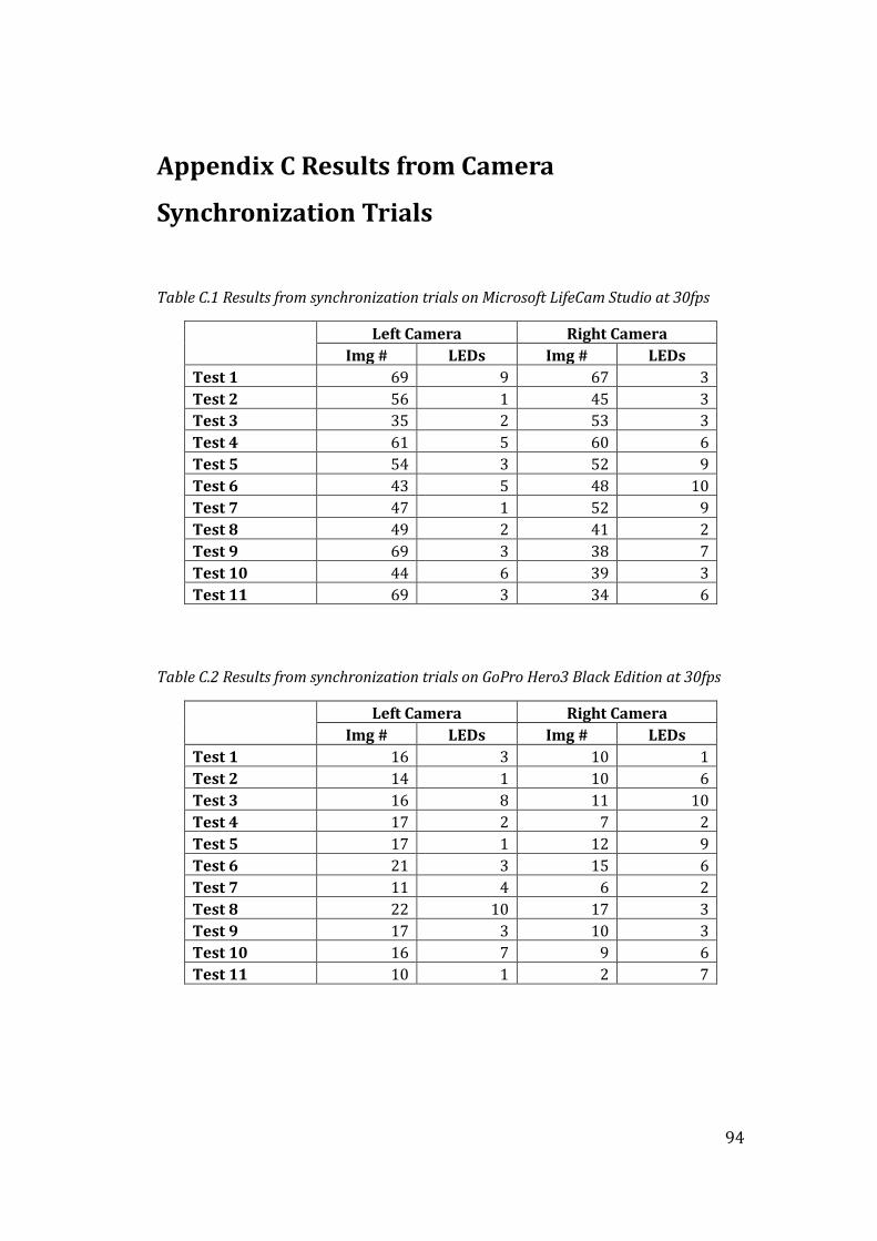
94
Appendix C Results from Camera
Synchronization Trials
Table C.1 Results from synchronization trials on Microsoft LifeCam Studio at 30fps
Left Camera Right Camera
Img # LEDs Img # LEDs
Test 1 69 9 67 3
Test 2 56 1 45 3
Test 3 35 2 53 3
Test 4 61 5 60 6
Test 5 54 3 52 9
Test 6 43 5 48 10
Test 7 47 1 52 9
Test 8 49 2 41 2
Test 9 69 3 38 7
Test 10 44 6 39 3
Test 11 69 3 34 6
Table C.2 Results from synchronization trials on GoPro Hero3 Black Edition at 30fps
Left Camera Right Camera
Img # LEDs Img # LEDs
Test 1 16 3 10 1
Test 2 14 1 10 6
Test 3 16 8 11 10
Test 4 17 2 7 2
Test 5 17 1 12 9
Test 6 21 3 15 6
Test 7 11 4 6 2
Test 8 22 10 17 3
Test 9 17 3 10 3
Test 10 16 7 9 6
Test 11 10 1 2 7

95
Table C.3 Results from synchronization trials on GoPro Hero3 Black Edition at 60fps
Left Camera Right Camera
Img # LEDs Img # LEDs
Test 1 39 10 21 8
Test 2 31 1 17 1
Test 3 39 2 24 10
Test 4 43 2 24 10
Test 5 44 2 29 8
Test 6 53 6 40 1
Test 7 43 9 30 2
Test 8 42 3 28 6
Test 9 37 10 24 9
Test 10 58 7 42 2
Test 11 46 6 34 9
Table C.4 Results from synchronization trials on GoPro Hero3 Black Edition at 120fps
Left Camera Right Camera
Img # LEDs Img # LEDs
Test 1 77 7 45 1
Test 2 91 8 41 6
Test 3 128 6 100 7
Test 4 110 10 83 4
Test 5 83 1 59 10
Test 6 99 7 72 7
Test 7 73 8 42 1
Test 8 70 7 37 3
Test 9 120 10 92 1
Test 10 74 2 45 8
Test 11 81 4 53 1
Table C.5 Results from synchronization trials on GoPro Hero3 Black Edition at 240fps
Left Camera Right Camera
Img # LEDs Img # LEDs
Test 1 198 9 114 1
Test 2 204 2 102 1
Test 3 274 2 202 9
Test 4 255 7 171 2
Test 5 216 4 150 4
Test 6 259 7 190 7
Test 7 190 3 117 6
Test 8 201 1 123 2
Test 9 261 5 189 7
Test 10 222 10 144 7
Test 11 205 3 133 5

96
Appendix D Results from Static Trials
Figure D.1 Results from Static Trial 1
Outline of target
Centre of shot pattern
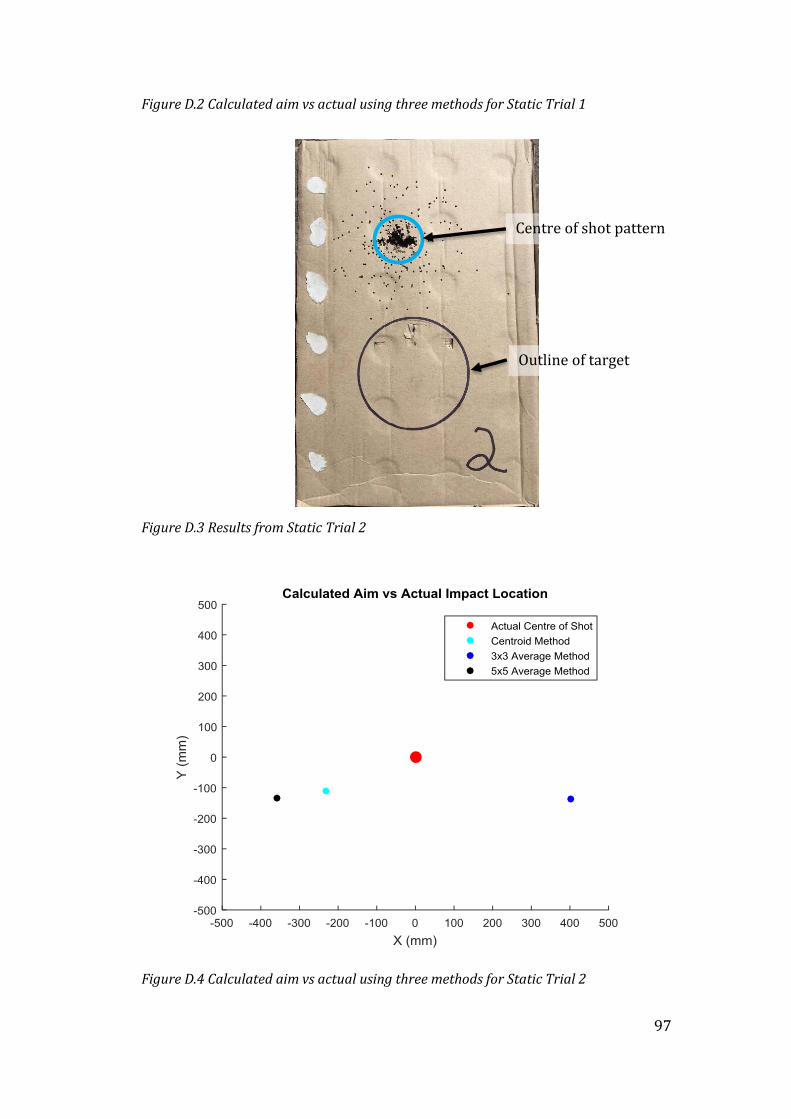
97
Figure D.2 Calculated aim vs actual using three methods for Static Trial 1
Figure D.3 Results from Static Trial 2
Figure D.4 Calculated aim vs actual using three methods for Static Trial 2
Centre of shot pattern
Outline of target
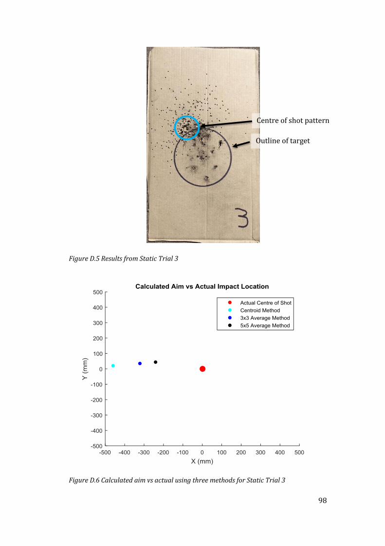
98
Figure D.5 Results from Static Trial 3
Figure D.6 Calculated aim vs actual using three methods for Static Trial 3
Centre of shot pattern
Outline of target

99
Figure D.7 Results from Static Trial 4
Figure D.8 Calculated aim vs actual using three methods for Static Trial 4
Centre of shot pattern
Outline of target

100
Figure D.9 Results from Static Trial 5
Figure D.10 Calculated aim vs actual using three methods for Static Trial 5
Centre of shot pattern
Outline of target

101
Appendix E Results from Dynamic Trials vs
Human Judges
Figure D.1 Calculated aim vs Judges Feedback for Human Judge Trial 1
Figure D.2 Calculated aim vs Judges Feedback for Human Judge Trial 2

102
Figure D.3 Calculated aim vs Judges Feedback for Human Judge Trial 3
Figure D.4 Calculated aim vs Judges Feedback for Human Judge Trial 4

103
Figure D.5 Calculated aim vs Judges Feedback for Human Judge Trial 5
Figure D.6 Calculated aim vs Judges Feedback for Human Judge Trial 6

104
Figure D.7 Calculated aim vs Judges Feedback for Human Judge Trial 7
Figure D.8 Calculated aim vs Judges Feedback for Human Judge Trial 8

105
Figure D.9 Calculated aim vs Judges Feedback for Human Judge Trial 9
Figure D.10 Calculated aim vs Judges Feedback for Human Judge Trial 10

106
Appendix F Arduino Source Code Listings
//----------------------------------------------------------
// Josh Anderson 2015
// Gunshot_sensor_circuit program for Arduino Uno
// Uses a microphone board attached to pin A0
// to light LED's attached to pin 13 for 1s
//----------------------------------------------------------
// Arduino pin numbers
const int DO_pin = 2;
const int AO_pin = 0;
int sound = 0;
int led1 = 13;
int smax = 0;
void setup() {
pinMode(DO_pin, INPUT);
pinMode(led1, OUTPUT);
}
void loop() {
if (sound > 50)
{
digitalWrite(led1, HIGH);
delay(1000);
}
if (sound < 50)
{
digitalWrite(led1, LOW);
}
sound = analogRead(AO_pin);
}
//-----------------------------------------------------------------------
---
// Josh Anderson 2015
// FieldTrials_Flasher program for Arduino Mega
// Flashes a sequence of 10 LED's at speeds
// matching 10 times the camera frame rate
//-----------------------------------------------------------------------
---
int modenumber = 1;
int LED1 = 11;
int LED2 = 10;
int LED3 = 9;
int LED4 = 8;
int LED5 = 5;
int LED6 = 4;
int LED7 = 3;
int LED8 = 2;
int LED9 = 1;
int LED10 = 0;
int mLED1 = 31;

107
int mLED2 = 33;
int mLED3 = 35;
int mLED4 = 37;
int mLED5 = 39;
int gobut = 6;
int freqbut = 7;
void setup()
{
// put your setup code here, to run once:
pinMode(mLED1, OUTPUT); // mode LED1 signal
pinMode(mLED2, OUTPUT); // mode LED2 signal
pinMode(mLED3, OUTPUT); // mode LED3 signal
pinMode(mLED4, OUTPUT); // mode LED4 signal
pinMode(LED1, OUTPUT); // LED1
pinMode(LED2, OUTPUT); // LED2
pinMode(LED3, OUTPUT); // LED3
pinMode(LED4, OUTPUT); // LED4
pinMode(LED5, OUTPUT); // LED5
pinMode(LED6, OUTPUT); // LED6
pinMode(LED7, OUTPUT); // LED7
pinMode(LED8, OUTPUT); // LED8
pinMode(LED9, OUTPUT); // LED9
pinMode(LED10, OUTPUT); // LED10
pinMode(freqbut, INPUT); //Go Button
pinMode(gobut, INPUT); //Change Freq Button
}
void flash() // this is where the sequence of LEDs will flash
{
int dtime = 1;
switch(modenumber)
{
case 1: //Test mode - ~1 fps
dtime = 30000; // delay = 30 mS
break;
case 2: //30 fps mode
dtime = 3333; //delay= 3.33 mS
break;
case 3: //60 fps mode
dtime = 1667; //delay= 1.67 mS
break;
case 4: //120 fps mode
dtime = 833; //delay= 0.83 mS
break;
case 5: //240 fps mode
dtime = 417; //delay= 0.42 mS
break;
}
digitalWrite(LED1, HIGH); // turn the LED on
delayMicroseconds(dtime); // wait for a variable time
digitalWrite(LED2, HIGH); // turn the LED on
delayMicroseconds(dtime); // wait for a variable time
digitalWrite(LED3, HIGH); // turn the LED on
delayMicroseconds(dtime); // wait for a variable time
digitalWrite(LED4, HIGH); // turn the LED on
delayMicroseconds(dtime); // wait for a variable time
digitalWrite(LED5, HIGH); // turn the LED on
delayMicroseconds(dtime); // wait for a variable time
digitalWrite(LED6, HIGH); // turn the LED on
delayMicroseconds(dtime); // wait for a variable time
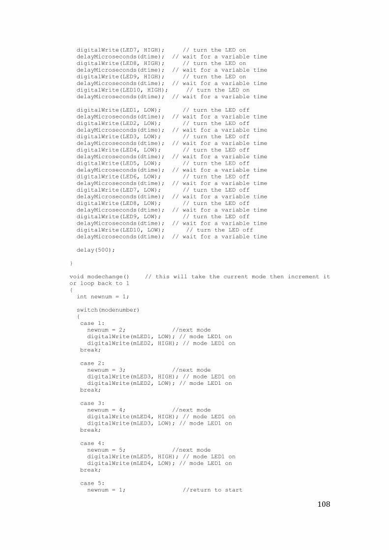
108
digitalWrite(LED7, HIGH); // turn the LED on
delayMicroseconds(dtime); // wait for a variable time
digitalWrite(LED8, HIGH); // turn the LED on
delayMicroseconds(dtime); // wait for a variable time
digitalWrite(LED9, HIGH); // turn the LED on
delayMicroseconds(dtime); // wait for a variable time
digitalWrite(LED10, HIGH); // turn the LED on
delayMicroseconds(dtime); // wait for a variable time
digitalWrite(LED1, LOW); // turn the LED off
delayMicroseconds(dtime); // wait for a variable time
digitalWrite(LED2, LOW); // turn the LED off
delayMicroseconds(dtime); // wait for a variable time
digitalWrite(LED3, LOW); // turn the LED off
delayMicroseconds(dtime); // wait for a variable time
digitalWrite(LED4, LOW); // turn the LED off
delayMicroseconds(dtime); // wait for a variable time
digitalWrite(LED5, LOW); // turn the LED off
delayMicroseconds(dtime); // wait for a variable time
digitalWrite(LED6, LOW); // turn the LED off
delayMicroseconds(dtime); // wait for a variable time
digitalWrite(LED7, LOW); // turn the LED off
delayMicroseconds(dtime); // wait for a variable time
digitalWrite(LED8, LOW); // turn the LED off
delayMicroseconds(dtime); // wait for a variable time
digitalWrite(LED9, LOW); // turn the LED off
delayMicroseconds(dtime); // wait for a variable time
digitalWrite(LED10, LOW); // turn the LED off
delayMicroseconds(dtime); // wait for a variable time
delay(500);
}
void modechange() // this will take the current mode then increment it
or loop back to 1
{
int newnum = 1;
switch(modenumber)
{
case 1:
newnum = 2; //next mode
digitalWrite(mLED1, LOW); // mode LED1 on
digitalWrite(mLED2, HIGH); // mode LED1 on
break;
case 2:
newnum = 3; //next mode
digitalWrite(mLED3, HIGH); // mode LED1 on
digitalWrite(mLED2, LOW); // mode LED1 on
break;
case 3:
newnum = 4; //next mode
digitalWrite(mLED4, HIGH); // mode LED1 on
digitalWrite(mLED3, LOW); // mode LED1 on
break;
case 4:
newnum = 5; //next mode
digitalWrite(mLED5, HIGH); // mode LED1 on
digitalWrite(mLED4, LOW); // mode LED1 on
break;
case 5:
newnum = 1; //return to start

109
digitalWrite(mLED5, LOW); // mode LED1 on
digitalWrite(mLED1, HIGH); // mode LED1 on
break;
}
delay(750);
modenumber = newnum;
}
void loop()
{
char butgo = 1;
char butfreq = 1;
char mmm = 0;
while(2>1)
{
butgo = digitalRead(gobut); //read go button pin
butfreq = digitalRead(freqbut); //read go button pin
if(butgo == HIGH)
{
delay(700);
butgo = digitalRead(gobut); //read go button pin
while(butgo == LOW)
{
butgo = digitalRead(gobut); //read go button pin
flash();
}
//delay(500);
}
if(butfreq == HIGH)
{
modechange();
}
}
}
//-----------------------------------------------------------------------
---
// Josh Anderson 2015
// Calibration_flasher for Arduino Uno
// Uses flashes LED's attached to pin 13 for 0.75s
// so image pairs can be identified for calibration
//-----------------------------------------------------------------------
---
void setup()
{
pinMode(13, OUTPUT);
}
void loop()
{
digitalWrite(13, HIGH); // turn the LED off
delay(750);
digitalWrite(13, LOW); // turn the LED off
delay(750);
}

110
Appendix G Matlab Source Code Listings
% ERP2015 - Feasibility Assessment of Low Cost Stereo Computer Vision
% in Clay Target Shooting Coaching.
%
% Josh Anderson - 0050106236
%
% SingleImSplit.m
%
% Program to split input video from GoPro Cameras into images
% to be used in calibration or accuracy trials
%
clear all; % clear all previous variables
clc; % clear all previous dialog
firstnumber = 3291; % First file number
numoffiles = 28; % Number of files in folder
folderpath = 'E:\Gopro\20150820 - dynamic trials\Trials\';
% make directory name to save images
mkdirname = strcat(folderpath,'Images\');
% which camera is used?
cameraside = 'L';
vidii = 1;
% Main loop to convert each file
for j = 1 : numoffiles
% Set filename - needed because one camera has filenames
% larger than the other
if firstnumber > 999
name1 = 'GOPR';
else
name1 = 'GOPR0';
end
strvidii = int2str(vidii);
fname = int2str(firstnumber);
fname = strcat(name1,fname);
videoname = strcat(folderpath,fname,'.MP4');
foldername = strcat(mkdirname,cameraside,strvidii,'\');
%read video into GPVideo variable
GPVideo = VideoReader(videoname);
%make directory to save images
mkdir(foldername)
% Loop to create still images
imgii = 1;
while hasFrame(GPVideo)
img = readFrame(GPVideo);
strii = int2str(imgii);
filename =
strcat(foldername,cameraside,strvidii,'_',strii,'.png');

111
imwrite(img,filename); % Write img to a PNG file
disp(filename)
imgii=imgii+1;
end
firstnumber = firstnumber + 1;
vidii = vidii + 1;
end
disp('Video Split Complete')
% ERP2015 - Feasibility Assessment of Low Cost Stereo Computer Vision
% in Clay Target Shooting Coaching.
%
% Josh Anderson - 0050106236
%
% staticprocess.m
%
% This is the program developed to measure the accuracy of using GoPro
% camera images to judge the accuracy of a shooters aim when the target
and
% shooter are static to get a baseline accuracy, trying to minimise the
% influence of errors in synchronisation.
%
% Easily identifiable coloured markers are attached to the gun and the
% target used is florescent orange type to help with segmentation.
%
% This program was used to process images taken during the static trials
on
% 29 Sept 2015 at the Brisbane Sporting Clays Club.
%%
clc; % clear all previous dialog
clear; % clear variables
TrialNumber = 1; % to be changed to process each trial
folderpath = 'C:\Users\Owner\Documents\MATLAB\Project\Images\Static\';
% If the stereo calibration parameter doesnt exist load stereoParams
i = exist('stereoParams','var');
if i == 0
load('stereoParamsStaticTrials.mat');
end
Lnum = strcat('L');
Rnum = strcat('R');
% Load image names
imageNamesL = dir(fullfile(folderpath,Lnum,'*.png'));
imageNamesL = {imageNamesL.name}';
imageNamesR = dir(fullfile(folderpath,Rnum,'*.png'));
imageNamesR = {imageNamesR.name}';
% Load images
imleft=imread(fullfile(folderpath,Lnum,imageNamesL{TrialNumber}));
imright=imread(fullfile(folderpath,Rnum,imageNamesR{TrialNumber}));
%%
% Use calibration data and selected images to reconstruct the scene in 3D
% to enable measurements of key points
% use images and calibration data to return point cloud

112
% Limit Scene Bounds
maxX = 5; % Max distance left of left camera axis (meters)
minX = -8; % Max distance right of left camera axis
(meters)
maxY = 1; % Max distance below left camera axis (meters)
minY = -4; % Max distance above left camera axis (meters)
maxZ = 16; % Max distance from left camera axis (meters)
minZ = 4; % Min distance from left camera axis (meters)
% Rectify Images using stereo calibration
[imleft_rec,imright_rec] = rectifyStereoImages(imleft,imright,...
stereoParams);
% Create disparity map from the recifies images
disparityMap = disparity(rgb2gray(imleft_rec), rgb2gray(imright_rec),...
'BlockSize', 9);
% Create point cloud in meters.
point3D = reconstructScene(disparityMap, stereoParams);
point3D = point3D / 1000;
% Plot points within the bounds given.
% get the x, y, z values for the pixels from point3D
xx = point3D(:, :, 1);
yy = point3D(:, :, 2);
zz = point3D(:, :, 3);
% Eliminate the pixels that are outside the bounds
xdisp = xx;
xdisp(xx < minX | xx > maxX) = NaN;
ydisp = yy;
ydisp(yy < minY | yy > maxY) = NaN;
zdisp = zz;
zdisp(zz < minZ | zz > maxZ) = NaN;
% add the new x, y, z values to the matrix to be displayed
point3Ddisp = point3D;
point3Ddisp(:,:,1) = xdisp;
point3Ddisp(:,:,2) = ydisp;
point3Ddisp(:,:,3) = zdisp;
%%
% Use color thresholds to segment the left image and return target
locations
% Convert RGB image to HSV color space
imleft_rec_hsv = rgb2hsv(imleft_rec);
% Define thresholds for channel 1 based on histogram settings
channel1Min1 = 0.860;
channel1Max1 = 1.000;
% Define thresholds for channel 1 based on histogram settings
channel1Min2 = 0.000;
channel1Max2 = 0.100;
% Define thresholds for channel 2 based on histogram settings
channel2Min = 0.590;
channel2Max = 1.000;
% Define thresholds for channel 3 based on histogram settings
channel3Min = 0.120;
channel3Max = 1.000;
113
% Seperate the three colour channels
hue=imleft_rec_hsv(:,:,1);
sat=imleft_rec_hsv(:,:,2);
val=imleft_rec_hsv(:,:,3);
% Segment the three channels based on colour thresholds
binaryH1 = hue >= channel1Min1 & hue <= channel1Max1;
binaryH2 = hue >= channel1Min2 & hue <= channel1Max2;
binaryS = sat >= channel2Min & sat <= channel2Max;
binaryV = val >= channel3Min & val <= channel3Max;
% Combine the mask that has been created for each channel
binaryH = binaryH1 | binaryH2; % OR the hue binaries together
BinaryMask = binaryH & binaryS & binaryV; % AND the binaries
% Filter out small blobs.
BinaryMask = bwareaopen(BinaryMask, 20);
% Fill holes
BinaryMask = imfill(BinaryMask, 'holes');
% find the number of regions, label image and marker information
[labeledImage, numberOfRegions] = bwlabel(BinaryMask);
markerinfo = regionprops(labeledImage, 'Centroid', 'Area');
for i= 1:length(markerinfo)
MDA(i,1) = markerinfo(i).Area; % segmented area
MDA(i,2) = markerinfo(i).Centroid(1); % x pixel location
MDA(i,3) = markerinfo(i).Centroid(2); % y pixel location
end
%%
% Use Point cloud and target pixel locations to get target real world
% coordinates
% set number of pixels around centroid to average
agsize = 1;
ag = (agsize*2+1)^2;
for i = 1:size(MDA,1)
% get an average of the real world pixels coordinates around the centroid
% of each ROI and return them to be plotted and used to calculate
accuracy
M3DA(i,1) = MDA(i,1);
xtemp = point3Ddisp(round(MDA(i,3))-agsize:round(MDA(i,3))+agsize,...
round(MDA(i,2))-agsize:round(MDA(i,2))+agsize,1);
xtemp = nanmean(xtemp);
M3DA(i,2) = nanmean(xtemp);
ytemp = point3Ddisp(round(MDA(i,3))-agsize:round(MDA(i,3))+agsize,...
round(MDA(i,2))-agsize:round(MDA(i,2))+agsize,2);
ytemp = nanmean(ytemp);
M3DA(i,3) = nanmean(ytemp);
ztemp = point3Ddisp(round(MDA(i,3))-agsize:round(MDA(i,3))+agsize,...
round(MDA(i,2))-agsize:round(MDA(i,2))+agsize,3);
ztemp = nanmean(ztemp);
M3DA(i,4) = nanmean(ztemp);
% get real world locations taken from centroid of blob
M3DAcent(i,1) = MDA(i,1);
M3DAcent(i,2:4) = point3Ddisp(round(MDA(i,3)),...
round(MDA(i,2)),:);
end
114
% If there are 3 blobs, use their z distance to identify the target,
stock
% and barrel markers
if size(MDA,1)==3
% Assign positions to the target, stock and barrel marker variables using
% average coordinates
for i = 1:3
if M3DA(i,4)== min(M3DA(:,4))
stockloc = M3DA(i,2:4);
elseif M3DA(i,4)== median(M3DA(:,4))
barrelloc = M3DA(i,2:4);
else
targetloc = M3DA(i,2:4);
end
end
% Assign positions to the target, stock and barrel marker variables using
% centroid coordinates
for i = 1:3
if M3DAcent(i,4)== min(M3DAcent(:,4))
stockloccent = M3DAcent(i,2:4);
elseif M3DAcent(i,4)== median(M3DAcent(:,4))
barrelloccent = M3DAcent(i,2:4);
else
targetloccent = M3DAcent(i,2:4);
end
end
else
% This is a basic trouble shooting error trap that is not needed after
the
% first image pairs were processed. All subsequent pairs process
% sucessfully
disp('Incorrect number of blobs identified from colour thresholds')
disp('review thresholding limits.')
end
% create an array with positions spaced at 1cm for the length of the gun
% to the target +2.5m
linez = [0:0.01:(targetloc(3)-stockloc(3))+2.5];
% Use GetProjections function to get dx and dy as the z distance changes
[xlinez, ylinez, zlinez] = GetProjections(stockloc,barrelloc);
[xlinezcent, ylinezcent, zlinezcent] =...
GetProjections(stockloccent,barrelloccent);
% Plot the point cloud with the POI's and calculated aim plotted for
% visual confirmation of accuracy results
figure('name','Point Cloud from images','numbertitle','off')
showPointCloud(point3Ddisp, imleft_rec, 'VerticalAxis', 'Y',...
'VerticalAxisDir', 'Down' )
xlabel('X'); ylabel('Y'); zlabel('Z');
hold on;
% Plot POI's from averaged locations
scatter3(targetloc(1),targetloc(2),targetloc(3),'o','r','filled');
scatter3(barrelloc(1),barrelloc(2),barrelloc(3),'o','r','filled');
scatter3(stockloc(1),stockloc(2),stockloc(3),'o','r','filled')
% Plot POI's from centroid locations
scatter3(targetloccent(1),targetloccent(2),targetloccent(3),'o','c','fill
ed');
scatter3(barrelloccent(1),barrelloccent(2),barrelloccent(3),'o','c','fill
ed');
scatter3(stockloccent(1),stockloccent(2),stockloccent(3),'o','c','filled'
)

115
% Plot aim each directions as lines
plot3(stockloc(1)+(xlinez*linez),stockloc(2)+(ylinez*linez),...
stockloc(3)+zlinez*linez)
plot3(stockloccent(1)+(xlinezcent*linez),stockloccent(2)+...
(ylinezcent*linez), stockloccent(3)+zlinezcent*linez)
hold off;
% Calulate the accuracy miss distance using the blobs centroids using the
% GetDisntance function
FlightPath = [stockloc(1)+(xlinez*linez);stockloc(2)+(ylinez*linez);...
stockloc(3)+zlinez*linez];
[xdist, ydist] = GetDistance(FlightPath,targetloc);
% Calulate the accuracy miss distance using an average of the cells
%around the blobs centroids using the GetDisntance function
FlightPath = [stockloccent(1)+(xlinezcent*linez);...
stockloccent(2)+(ylinezcent*linez);
stockloccent(3)+zlinezcent*linez];
[xdistcent, ydistcent] = GetDistance(FlightPath,targetloc);
%%
% Display the calculated miss distances
fprintf('By defining the miss distance axes from the perspective of the')
fprintf('shooter as positive y as being\n')
fprintf('in the up direction and the positive x direction in the right')
fprintf(' direction\n\n')
fprintf('The calculated miss distance taken from only the blob
centroids')
fprintf(' is:\n\n')
fprintf(' x: %.3f mm and y: %.3f mm.\n\n',...
xdistcent*1000,ydistcent*1000)
fprintf('The calculated miss distance taken from average of the')
fprintf(' %.0f pixel locations around the blob''s centroid is:\n\n',ag)
fprintf(' x: %.3f mm and y: %.3f mm.\n', xdist*1000,ydist*1000)
% ERP2015 - Feasibility Assessment of Low Cost Stereo Computer Vision
% in Clay Target Shooting Coaching.
%
% Josh Anderson - 0050106236
%
% GetProjections.m
%
% takes the stock and barrel marker loactions and returns x and y
gradients
% as z distance changes
%
% This function is use in staticprocess.m and dynamicprocess.m
function [xlinez, ylinez, zlinez] = GetProjections(stockloc,barrelloc)
xxx = (barrelloc(1)-stockloc(1));
yyy = (barrelloc(2)-stockloc(2));
zzz = (barrelloc(3)-stockloc(3));
xlinez = xxx/zzz;
ylinez = yyy/zzz;
zlinez = zzz/zzz;
end

116
% ERP2015 - Feasibility Assessment of Low Cost Stereo Computer Vision
% in Clay Target Shooting Coaching.
%
% Josh Anderson - 0050106236
%
% GetDistance.m
%
% This program takes the a valiable that describes the flightpath of the
% shotcloud and approximates the closest distance the centre of the shot
% flew past the target.
%
% the result is the approximate x and y distances from the target in a
% plane approximately perpendicular to the view of the shooter.
%
% This function is use in staticprocess.m and dynamicprocess.m
function [xdist, ydist] = GetDistance(FlightPath,targetloc)
temp = 10000; % Large starting value
for i = 1:size(FlightPath,2)
% Get the distance from the target
ax = ((FlightPath(1,i)-targetloc(1))^2);
ay = ((FlightPath(2,i)-targetloc(2))^2);
az = ((FlightPath(3,i)-targetloc(3))^2);
a = sqrt((ax)+(ay)+(az));
% get distance in each direction from the target
dirx = (targetloc(1)-FlightPath(1,i));
diry = (targetloc(2)-FlightPath(2,i));
% if this is the closest the shot has been to the target save
% the x and y distances
if a < temp
temp = a;
xdist =dirx;
ydist =diry;
end
end
end
% ERP2015 - Feasibility Assessment of Low Cost Stereo Computer Vision
% in Clay Target Shooting Coaching.
%
% Josh Anderson - 0050106236
%
% dynamicprocess.m
%
% This is an updated version of dynamicprocess.m, to get the
% same functionality as the previous version set Fsync to 0 (zero).
%
% This program is takes a series of 6 image pair and using the measured
% frame synchronisation calculates a the distance the shooter missed the
% target by in the x and y directions from the perspective of the
shooter.
%
% Using frame synchronisation as a parameter to interpolate the target
% position within the image frames has shown a marked improvement in
% measurement accuracy. This accuracy is both improved in z distance
% measurement and shooter aim prediction.
%

117
%%
%clc; % clear all previous dialog
TrialNumber = 1; % to be changed to process each trial
% value to indicate the camera sync = If (-) left trials right, If (+)
right trials left
Fsync = -0.1; % decimal value between -0.5 and 0.5
folderpath = 'E:\Gopro\20150820 - dynamic trials\ToProcess\';
Lnum = strcat('L',int2str(TrialNumber));
Rnum = strcat('R',int2str(TrialNumber));
% If stereoParams doesnt exist load it
i = exist('stereoParams','var');
if i == 0
load('stereoParamsDyn.mat');
end
% Load image names
imageNamesL = dir(fullfile(folderpath,Lnum,'*.png'));
imageNamesL = {imageNamesL.name}';
imageNamesR = dir(fullfile(folderpath,Rnum,'*.png'));
imageNamesR = {imageNamesR.name}';
% If statement to decide whether or not to proceed based in number of
input
% images
if length(imageNamesL) == 0
disp('Cant find the required pictures')
elseif length(imageNamesL)==length(imageNamesR)
% Load images, rectify and make a cell array's to store the recified
% image sequences
for i=1:length(imageNamesL)
% Load images
LI=imread(fullfile(folderpath,Lnum,imageNamesL{i}));
RI=imread(fullfile(folderpath,Rnum,imageNamesR{i}));
% Rectify and save
[LImgs{i},RImgs{i}] = rectifyStereoImages(LI,RI, stereoParams);
end
%%
%Interpolate target position
% compare target locations
TDL = GetTargetLoc(LImgs);
TDR = GetTargetLoc(RImgs);
TDL(:,4) = [0;0;TDL(2,2)-TDL(3,2);TDL(3,2)-TDL(4,2);TDL(4,2)-
TDL(5,2);TDL(5,2)-TDL(6,2)];
TDR(:,4) = [0;0;TDR(2,2)-TDR(3,2);TDR(3,2)-TDR(4,2);TDR(4,2)-
TDR(5,2);TDR(5,2)-TDR(6,2)];
% Find the number of pixels to interpolate the target based on the target
% movement per frame and the frame syncronisation
Rpix = round(Fsync*mean(TDR(3:6,4)));
for i = 2:length(imageNamesL)
% get pixels around centroid
118
lower = TDR(i,3)-25;
upper = TDR(i,3)+25;
left = TDR(i,2)-25;
right = TDR(i,2)+25;
temp = [RImgs{i}]; % temp array
TA = temp(lower:upper, left:right, :);
temp(lower:upper, left+Rpix:right+Rpix, :) = TA;
RImgs{i} = temp;
% newRImgs{i} = temp;
end
%%
% MDA array column order
%(Pink Area, Pink X, Pink Y, Orange Area, Orange X, Orange Y)
MDA = GetGunLoc(LImgs);
% get point cloud and point of interest locations
% RL columns (Target X,Y,Z; Pink X,Y,Z; Orange X,Y,Z)
RL = GetRealLoc(LImgs,RImgs,TDL,MDA,stereoParams);
% calculate the distance the target was missed by
[xdist, ydist] = GetMissDist(RL, LImgs, RImgs, stereoParams);
% Display a message with the miss distances to the user
aaa=strcat('The miss distance for trial',{' '},num2str(TrialNumber),...
{' '},'is x:',char(round(xdist)),{' '},'mm and y:',...
char(round(ydist)),{' '},'mm.');
disp(aaa)
else
disp('number of images in left and right folder is different')
end
% ERP2015 - Feasibility Assessment of Low Cost Stereo Computer Vision
% in Clay Target Shooting Coaching.
%
% Josh Anderson - 0050106236
%
% GetTargetLoc.m
%
% This function takes a cell array of sequential images and uses
background
% subtraction to find the clay target in the images. This filter is only
% applied to the area of the image frame that is expected to contain the
% target to reduce processing time.
%
% The output of this function is an array of blob area, x and y position
% for the target is each frame.
%
% This function is use in dynamicprocess.m
function TD = GetTargetLoc(LImgs)
% blob size constraints
minsize = 11;
maxsize = 100;
% Define blob area object
blobarea = vision.BlobAnalysis(...
'CentroidOutputPort', false, 'AreaOutputPort', true, ...
'BoundingBoxOutputPort', false, ...
'MinimumBlobAreaSource', 'Property', 'MinimumBlobArea',
minsize,...
'MaximumBlobAreaSource', 'Property', 'MaximumBlobArea',maxsize);
119
% Define blob centroid object
blobcent = vision.BlobAnalysis(...
'CentroidOutputPort', true, 'AreaOutputPort', false, ...
'BoundingBoxOutputPort', false, ...
'MinimumBlobAreaSource', 'Property', 'MinimumBlobArea',
minsize,...
'MaximumBlobAreaSource', 'Property', 'MaximumBlobArea',maxsize);
% Read first frame to use as initial background image
frame = LImgs{1};
targarea2 = frame(350:500,1100:1900);
% loop and save target centroid location and area for each frame
for i = 2:length(LImgs)
frame = LImgs{i};
% Reduce search area to improve performance
targarea1 = frame(350:500,1100:1900);
% Pixel difference threshold is 15
output = (targarea2-targarea1)> 15;
% Current frame becomes background frame
targarea2 = targarea1;
% Get blob information and save it
cent = step(blobcent, output);
cent(1) = cent(1)+1100;
cent(2) = cent(2)+350;
area = step(blobarea, output);
TrackerArray(i,:)=[area, cent];
end
TD = TrackerArray;
% ERP2015 - Feasibility Assessment of Low Cost Stereo Computer Vision
% in Clay Target Shooting Coaching.
%
% Josh Anderson - 0050106236
%
% GetGunLoc.m
%
% This function takes a cell array of sequential images and uses colour
% thresholding to find the markers on a shooters gun to calculate the
aim.
% The images are conterted in to the HSV colour space during this process
% as it was found to be more reliable.
%
% The ouptut of this fuction is an array of locations of the gun markers
% in the form: [Pink Area, Pink X, Pink Y, Orange Area, Orange X, Orange
Y]
%
% This function is use in dynamicprocess.m
function [MDA] = GetGunLoc(LImgs)
% Define thresholds for orange marker
% Channel 1
channel1MinO = 0.000;
channel1MaxO = 0.100;
% Channel 2

120
channel2MinO = 0.600;
channel2MaxO = 1.000;
% Channel 3
channel3MinO = 0.600;
channel3MaxO = 1.000;
% Define thresholds for Pink marker
% Channel 1
channel1MinP = 0.900;
channel1MaxP = 1.000;
% Channel 2
channel2MinP = 0.350;
channel2MaxP = 1.000;
% Channel 3
channel3MinP = 0.350;
channel3MaxP = 1.000;
for i = 1:length(LImgs)
% Convert RGB image to HSV color space
LImgs_hsv_LG = rgb2hsv(LImgs{i});
% Reduce search area to improve performance
LImgs_hsv = LImgs_hsv_LG(250:550,400:950,:);
% Seperate the three colour channels
hue=LImgs_hsv(:,:,1);
sat=LImgs_hsv(:,:,2);
val=LImgs_hsv(:,:,3);
% Segment the three channels based on orange marker thresholds
binaryH = hue >= channel1MinO & hue <= channel1MaxO;
binaryS = sat >= channel2MinO & sat <= channel2MaxO;
binaryV = val >= channel3MinO & val <= channel3MaxO;
% Combine the mask that has been created for each channel
BinaryMaskO = binaryH & binaryS & binaryV;
% Segment the three channels based on orange marker thresholds
binaryH = hue >= channel1MinP & hue <= channel1MaxP;
binaryS = sat >= channel2MinP & sat <= channel2MaxP;
binaryV = val >= channel3MinP & val <= channel3MaxP;
% Combine the mask that has been created for each channel
BinaryMaskP = binaryH & binaryS & binaryV;
% Filter out small blobs.
BinaryMaskP = bwareaopen(BinaryMaskP, 20);
BinaryMaskO = bwareaopen(BinaryMaskO, 20);
% Fill holes
BinaryMaskP = imfill(BinaryMaskP, 'holes');
BinaryMaskO = imfill(BinaryMaskO, 'holes');
% Get blob information for each marker
[labeledImageP, numberOfRegionsP] = bwlabel(BinaryMaskP);
[labeledImageO, numberOfRegionsO] = bwlabel(BinaryMaskO);
markerinfoP = regionprops(labeledImageP, 'Centroid', 'Area');
markerinfoO = regionprops(labeledImageO, 'Centroid', 'Area');
MDA(i,1) = markerinfoP(1).Area; % Pink segmented area
MDA(i,2) = markerinfoP(1).Centroid(1)+400; % Pink x pixel location
MDA(i,3) = markerinfoP(1).Centroid(2)+250; % Pink y pixel location
MDA(i,4) = markerinfoO(1).Area; % Orange segmented area
MDA(i,5) = markerinfoO(1).Centroid(1)+400; % Orange x pixel location
MDA(i,6) = markerinfoO(1).Centroid(2)+250; % Orange y pixel location

121
end
% ERP2015 - Feasibility Assessment of Low Cost Stereo Computer Vision
% in Clay Target Shooting Coaching.
%
% Josh Anderson - 0050106236
%
% GetRealLoc.m
%
% This function takes a two cell arrays of sequential image pairs, arrays
% of target and gun marker locations and the camera parameters data that
% was created during calibration.
%
% The function then creates a point cloud from the image pairs and find
the
% real world coordinates of the points of interest
%
% The ouptut of this fuction is an array of locations of the points of
% interest in the form: (Target X,Y,Z; Pink X,Y,Z; Orange X,Y,Z).
%
% This function is use in dynamicprocess.m
function RL = GetRealLoc(LImgs,RImgs,TD,MDA,stereoParams)
for i = 1:length(LImgs)
% Create disparity map from the recified images
disparityMap = disparity(rgb2gray(LImgs{i}),
rgb2gray(RImgs{i}),'BlockSize', 9);
% Create point cloud in millimeters.
point3D = reconstructScene(disparityMap, stereoParams);
%point3D = point3D / 1000;
% if there is a value for the target location find its real world
% coordinates. Target X,Y,Z, Time
if (TD(i,3)>1)&&(TD(i,2)>1)
RL(i,1:3,1) = point3D(round(TD(i,3)),round(TD(i,2)),:);
RL(i,4,1)=(i-length(LImgs))*(1/60);
end
% if the is a valid value for the or Pink marker
% Pink X,Y,Z, Time
if (MDA(i,2)>1)&&(MDA(i,3)>1)
RL(i,1:3,2) = point3D(round(MDA(i,3)),round(MDA(i,2)),:);
RL(i,4,2)=(i-length(LImgs))*(1/60);
end
% if the is a valid value for the or Pink marker
% Orange X,Y,Z, Time
if (MDA(i,5)>1)&&(MDA(i,6)>1)
RL(i,1:3,3) = point3D(round(MDA(i,6)),round(MDA(i,5)),:);
RL(i,4,3)=(i-length(LImgs))*(1/60);
end
end
RL=vpa(RL);
end

122
% ERP2015 - Feasibility Assessment of Low Cost Stereo Computer Vision
% in Clay Target Shooting Coaching.
%
% Josh Anderson - 0050106236
%
% GetRealLoc.m
%
% This function takes a two cell arrays of sequential image pairs, the
% arrays of real world locations and the camera parameters finds the
% distance that the centre of the aim was from the predicted target
% location.
%
% A plot of the scene is then plotted, with the relevant points plotted
and
% the predicted aim drawn as a line from the shooter to the target.
%
% The output of this function is an two variables named xdist and ydist
% containing the predicted miss quantities in millimetres. The other
output
% is a plot of the 3D point cloud for visual validation of the result.
%
% This function is use in dynamicprocess.m
function [xdist, ydist] = GetMissDist(RL, LImgs, RImgs, stereoParams)
i = length(RL);
% calculate the distance from the pink marker at the end of the barrel to
% the target in millimeters
FlightDist = sqrt((RL(i,1,1)-RL(i,1,2))^2+(RL(i,2,1)-
RL(i,2,2))^2+(RL(i,3,1)-RL(i,3,2))^2);
% Calculate shot flight time from emperical test data
% from 'The Modern Shotgun: Volume II: The Cartridge' (Burrard 1955)
FightTime = FlightDist*FlightDist*6.2085e-11+FlightDist*1.8333e-
06+0.0031;
% Find target location at the time that shot would have travelled that
% distance
% Target x location
% first order polyfit becuase the target should be flying in a straight
% line in this direction
tx = polyfit(RL(2:end,4,1)',RL(2:end,1,1)',1);
TX = FightTime*tx(1)+tx(2);
% Target y location
% second order polyfit due to effects of gravity
ty = polyfit(RL(2:end,4,1)',RL(2:end,2,1)',2);
TY = FightTime*FightTime*ty(1)+FightTime*ty(2)+ty(3);
% Target z location
% first order polyfit becuase the target should be flying in a straight
% line in this direction
tz = polyfit(RL(2:end,4,1)',RL(2:end,3,1)',1);
TZ = FightTime*tz(1)+tz(2);
% Draw line representing shot cloud flight path
lnz = [0:1000:(TZ-RL(i,3,2))+2000];
[xlinez, ylinez, zlinez] = GetProjections(RL(i,1:3,3),RL(i,1:3,2));
% Calculate the miss distance in meters
FlightPath = [RL(i,1,3)+(xlinez*lnz); RL(i,2,3)+(ylinez*lnz);
RL(i,3,3)+zlinez*lnz];
[xdist, ydist] = GetDistance(FlightPath,RL(i,1:3,1));

123
%%
% Create disparity map from the recifies images
disparityMap = disparity(rgb2gray(LImgs{i}),
rgb2gray(RImgs{i}),'BlockSize', 9);
% Create point cloud in millimeters.
point3D = reconstructScene(disparityMap, stereoParams);
%point3D = point3D / 1000;
% Limit Scene Bounds
maxX = 8000; % Max distance left of left camera axis
(meters)
minX = -3000; % Max distance right of left camera axis
(meters)
maxY = 1000; % Max distance below left camera axis
(meters)
minY = -4000; % Max distance above left camera axis
(meters)
maxZ = 26000; % Max distance from left camera axis
(meters)
minZ = 4000; % Min distance from left camera axis
(meters)
% Plot points within the bounds given.
% get the x, y, z values for the pixels from point3D
xx = point3D(:, :, 1);
yy = point3D(:, :, 2);
zz = point3D(:, :, 3);
% Eliminate the pixels that are outside the bounds
xdisp = xx;
xdisp(xx < minX | xx > maxX) = NaN;
ydisp = yy;
ydisp(yy < minY | yy > maxY) = NaN;
zdisp = zz;
zdisp(zz < minZ | zz > maxZ) = NaN;
% add the new x, y, z values to the matrix to be displayed
point3Ddisp = point3D;
point3Ddisp(:,:,1) = xdisp;
point3Ddisp(:,:,2) = ydisp;
point3Ddisp(:,:,3) = zdisp;
% Plot the points
% iptsetpref('ImshowBorder','tight');
figure('name','Point Cloud from images','numbertitle','off')
showPointCloud(point3Ddisp, LImgs{i}, 'VerticalAxis', 'Y',...
'VerticalAxisDir', 'Down' )
xlabel('X');
ylabel('Y');
zlabel('Z');
% set(gca,'position',[0 0 1 1],'units','normalized')
hold on
% Draw markers for target locations
scatter3(RL(2:end,1,1),RL(2:end,2,1),RL(2:end,3,1),'o','r');
% Draw pink marker locations
scatter3(RL(:,1,2),RL(:,2,2),RL(:,3,2),'o','filled','MarkerFaceColor',[1
.5 .75]);
% Draw orange markers
scatter3(RL(:,1,3),RL(:,2,3),RL(:,3,3),'o','filled','MarkerFaceColor',[1
.5 0]);
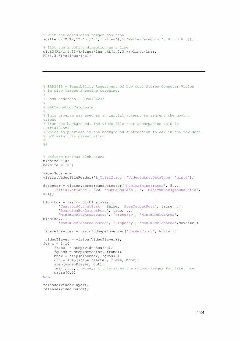
124
% Plot the calculated target position
scatter3(TX,TY,TZ,'o','r','filled');%,'MarkerFaceColor',[0.5 0 0.5]);
% Plot the shooting direction as a line
plot3(RL(i,1,3)+(xlinez*lnz),RL(i,2,3)+(ylinez*lnz),
RL(i,3,3)+zlinez*lnz);
% ERP2015 - Feasibility Assessment of Low Cost Stereo Computer Vision
% in Clay Target Shooting Coaching.
%
% Josh Anderson - 0050106236
%
% GetTargetLocCutdown.m
%
% This program was used as an initial attempt to segment the moving
target
% from the background. The video file that accompanies this is
L_Trial2.avi
% which is provided in the background_subtraction folder in the raw data
% DVD with this dissertation
%
%%
% defines min/max blob sizes
minsize = 8;
maxsize = 100;
videoSource =
vision.VideoFileReader('L_Trial2.avi','VideoOutputDataType','uint8');
detector = vision.ForegroundDetector('NumTrainingFrames', 5,...
'InitialVariance', 200, 'NumGaussians', 8, 'MinimumBackgroundRatio',
0.1);
blobbbox = vision.BlobAnalysis(...
'CentroidOutputPort', false, 'AreaOutputPort', false, ...
'BoundingBoxOutputPort', true, ...
'MinimumBlobAreaSource', 'Property', 'MinimumBlobArea',
minsize,...
'MaximumBlobAreaSource', 'Property', 'MaximumBlobArea',maxsize);
shapeInserter = vision.ShapeInserter('BorderColor','White');
videoPlayer = vision.VideoPlayer();
for i = 1:10
frame = step(videoSource);
fgMask = step(detector, frame);
bbox = step(blobbbox, fgMask);
out = step(shapeInserter, frame, bbox);
step(videoPlayer, out);
ims(:,:,:,i) = out; % this saves the output images for later use
pause(0.5)
end
release(videoPlayer);
release(videoSource);
Related Documents